This excerpt from

Foundations of Statistical Natural Language Processing.Christopher D. Manning and Hinrich Schütze.© 1999 The MIT Press.

is provided in screen-viewable form for personal use only by membersof MIT CogNet.

Unauthorized use or dissemination of this information is expresslyforbidden.

If you have any questions about this material, please contactcognetadmin@cognet.mit.edu.

p

i i

9 Markov Models

Hidden Markov Models (HMMs) have been the mainstay of the sta-tistical modeling used in modern speech recognition systems. Despitetheir limitations, variants of HMMs are still the most widely used tech-nique in that domain, and are generally regarded as the most successful.In this chapter we will develop the basic theory of HMMs, touch on theirapplications, and conclude with some pointers on extending the basicHMM model and engineering practical implementations.

An HMM is nothing more than a probabilistic function of a Markov pro-HMM

cess. We have already seen an example of Markov processes in the n-grammodels of chapters 2 and 6. Markov processes/chains/models were firstMarkov model

developed by Andrei A. Markov (a student of Chebyshev). Their first usewas actually for a linguistic purpose – modeling the letter sequences inworks of Russian literature (Markov 1913) – but Markov models were thendeveloped as a general statistical tool. We will refer to vanilla Markovmodels as Visible Markov Models (VMMs) when we want to be careful toVisible Markov

Models distinguish them from HMMs.We have placed this chapter at the beginning of the “grammar” part of

the book because working on the order of words in sentences is a startat understanding their syntax. We will see that this is what a VMM does.HMMs operate at a higher level of abstraction by postulating additional“hidden” structure, and that allows us to look at the order of categoriesof words. After developing the theory of HMMs in this chapter, we look atthe application of HMMs to part-of-speech tagging. The last two chaptersin this part then deal with the probabilistic formalization of core notionsof grammar like phrase structure.

p

i i

318 9 Markov Models

9.1 Markov Models

Often we want to consider a sequence (perhaps through time) of randomvariables that aren’t independent, but rather the value of each variabledepends on previous elements in the sequence. For many such systems,it seems reasonable to assume that all we need to predict the future ran-dom variables is the value of the present random variable, and we don’tneed to know the values of all the past random variables in the sequence.For example, if the random variables measure the number of books inthe university library, then, knowing how many books were in the librarytoday might be an adequate predictor of how many books there will be to-morrow, and we don’t really need to additionally know how many booksthe library had last week, let alone last year. That is, future elements ofthe sequence are conditionally independent of past elements, given thepresent element.

Suppose X = (X1, . . . , XT ) is a sequence of random variables takingvalues in some finite set S = {s1, . . . , sN}, the state space. Then the MarkovMarkov assumption

Properties are:

Limited Horizon:

P(Xt+1 = sk|X1, . . . , Xt) = P(Xt+1 = sk|Xt)(9.1)

Time invariant (stationary):

= P(X2 = sk|X1)(9.2)

X is then said to be a Markov chain, or to have the Markov property.One can describe a Markov chain by a stochastic transition matrix A:

aij = P(Xt+1 = sj|Xt = si)(9.3)

Here, aij ≥ 0,∀i, j and∑Nj=1 aij = 1,∀i.

Additionally one needs to specify Π, the probabilities of different initialstates for the Markov chain:

πi = P(X1 = si)(9.4)

Here,∑Ni=1πi = 1. The need for this vector can be avoided by specifying

that the Markov model always starts off in a certain extra initial state, s0,and then using transitions from that state contained within the matrix Ato specify the probabilities that used to be recorded in Π.

p

i i

9.1 Markov Models 319

h a p

e t i

start

1.00.4 0.3

0.4

0.60.3

0.60.4

1.0

1.0

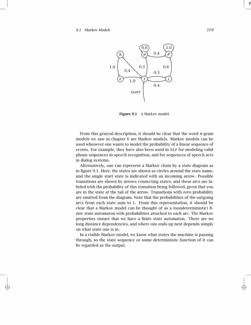
Figure 9.1 A Markov model.

From this general description, it should be clear that the word n-grammodels we saw in chapter 6 are Markov models. Markov models can beused whenever one wants to model the probability of a linear sequence ofevents. For example, they have also been used in NLP for modeling validphone sequences in speech recognition, and for sequences of speech actsin dialog systems.

Alternatively, one can represent a Markov chain by a state diagram asin figure 9.1. Here, the states are shown as circles around the state name,and the single start state is indicated with an incoming arrow. Possibletransitions are shown by arrows connecting states, and these arcs are la-beled with the probability of this transition being followed, given that youare in the state at the tail of the arrow. Transitions with zero probabilityare omitted from the diagram. Note that the probabilities of the outgoingarcs from each state sum to 1. From this representation, it should beclear that a Markov model can be thought of as a (nondeterministic) fi-nite state automaton with probabilities attached to each arc. The Markovproperties ensure that we have a finite state automaton. There are nolong distance dependencies, and where one ends up next depends simplyon what state one is in.

In a visible Markov model, we know what states the machine is passingthrough, so the state sequence or some deterministic function of it canbe regarded as the output.

p

i i

320 9 Markov Models

The probability of a sequence of states (that is, a sequence of randomvariables) X1, . . . , XT is easily calculated for a Markov chain. We find thatwe need merely calculate the product of the probabilities that occur onthe arcs or in the stochastic matrix:

P(X1, . . . , XT ) = P(X1)P(X2|X1)P(X3|X1, X2) · · · P(XT |X1, . . . , XT−1)

= P(X1)P(X2|X1)P(X3|X2) · · · P(XT |XT−1)

= πX1

T−1∏t=1

aXtXt+1

So, using the Markov model in figure 9.1, we have:

P(t, i, p) = P(X1 = t)P(X2 = i|X1 = t)P(X3 = p|X2 = i)= 1.0× 0.3× 0.6

= 0.18

Note that what is important is whether we can encode a process as aMarkov process, not whether we most naturally do. For example, recallthe n-gram word models that we saw in chapter 6. One might think that,for n ≥ 3, such a model is not a Markov model because it violates theLimited Horizon condition – we are looking a little into earlier history.But we can reformulate any n-gram model as a visible Markov model bysimply encoding the appropriate amount of history into the state space(states are then (n − 1)-grams, for example (was, walking, down) wouldbe a state in a fourgram model). In general, any fixed finite amount ofhistory can always be encoded in this way by simply elaborating the statespace as a crossproduct of multiple previous states. In such cases, wesometimes talk of an mth order Markov model, where m is the numberof previous states that we are using to predict the next state. Note, thus,that an n-gram model is equivalent to an (n− 1)th order Markov model.

Exercise 9.1 [«]

Build a Markov Model similar to figure 9.1 for one of the types of phone numbersin table 4.2.

9.2 Hidden Markov Models

In an HMM, you don’t know the state sequence that the model passesthrough, but only some probabilistic function of it.

p

i i

9.2 Hidden Markov Models 321

ColaPref.

Iced TeaPref.

0.3

0.5

start

0.50.7

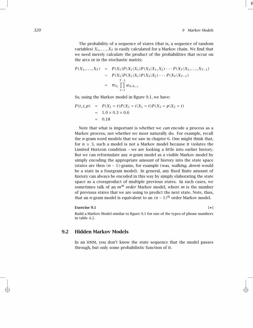
Figure 9.2 The crazy soft drink machine, showing the states of the machineand the state transition probabilities.

Example 1: Suppose you have a crazy soft drink machine: it can be intwo states, cola preferring (CP) and iced tea preferring (IP), but it switchesbetween them randomly after each purchase, as shown in figure 9.2.

Now, if, when you put in your coin, the machine always put out a colaif it was in the cola preferring state and an iced tea when it was in theiced tea preferring state, then we would have a visible Markov model. Butinstead, it only has a tendency to do this. So we need symbol emissionemission

probability probabilities for the observations:

P(Ot = k|Xt = si, Xt+1 = sj) = bijkFor this machine, the output is actually independent of sj , and so can bedescribed by the following probability matrix:

(9.5) Output probability given From state

cola iced tea lemonade(ice_t) (lem)

CP 0.6 0.1 0.3IP 0.1 0.7 0.2

What is the probability of seeing the output sequence {lem, ice_t} if themachine always starts off in the cola preferring state?

Solution: We need to consider all paths that might be taken through theHMM, and then to sum over them. We know that the machine starts instate CP. There are then four possibilities depending on which of thetwo states the machine is in at the other two time instants. So the total

p

i i

322 9 Markov Models

probability is:

0.7× 0.3× 0.7× 0.1+ 0.7× 0.3× 0.3× 0.1 +0.3× 0.3× 0.5× 0.7+ 0.3× 0.3× 0.5× 0.7 = 0.084

Exercise 9.2 [«]

What is the probability of seeing the output sequence {col,lem} if the machinealways starts off in the ice tea preferring state?

9.2.1 Why use HMMs?

HMMs are useful when one can think of underlying events probabilisti-cally generating surface events. One widespread use of this is tagging– assigning parts of speech (or other classifiers) to the words in a text.We think of there being an underlying Markov chain of parts of speechfrom which the actual words of the text are generated. Such models arediscussed in chapter 10.

When this general model is suitable, the further reason that HMMs arevery useful is that they are one of a class of models for which there existefficient methods of training through use of the Expectation Maximiza-tion (EM) algorithm. Given plenty of data that we assume to be generatedby some HMM – where the model architecture is fixed but not the proba-bilities on the arcs – this algorithm allows us to automatically learn themodel parameters that best account for the observed data.

Another simple illustration of how we can use HMMs is in generatingparameters for linear interpolation of n-gram models. We discussed inchapter 6 that one way to estimate the probability of a sentence:

P(Sue drank her beer before the meal arrived)

was with an n-gram model, such as a trigram model, but that just usingan n-gram model with fixed n tended to suffer because of data sparse-ness. Recall from section 6.3.1 that one idea of how to smooth n-gramestimates was to use linear interpolation of n-gram estimates for variouslinear

interpolation n, for example:

P li(wn|wn−1, wn−2) = λ1P1(wn)+ λ2P2(wn|wn−1)+ λ3P3(wn|wn−1, wn−2)

This way we would get some idea of how likely a particular word was,even if our coverage of trigrams is sparse. The question, then, is howto set the parameters λi . While we could make reasonable guesses as to

p

i i

9.2 Hidden Markov Models 323

λ1ab wbw1

wawb λ2ab wbw2

λ3ab wbwM

ε : λ1

ε : λ2

ε : λ3

w1:P1(w1)

w 2:P

1 (w 2)

w M:P

1 (w M)

w1 :P2(w

1 |wb )

w2:P2(w2|wb)

w M:P

2 (w M|w b)

w1 :P 3(w

1 |wa ,w

b )

w2 :P3(w

2 |wa ,w

b )

wM :P3(wM |wa,wb)

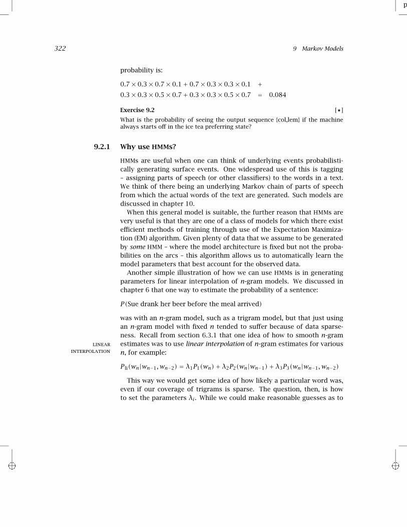
Figure 9.3 A section of an HMM for a linearly interpolated language model. Thenotation o : p on arcs means that this transition is made with probability p, andthat an o is output when this transition is made (with probability 1).

what parameter values to use (and we know that together they must obeythe stochastic constraint

∑i λi = 1), it seems that we should be able to

find the optimal values automatically. And, indeed, we can (Jelinek 1990).The key insight is that we can build an HMM with hidden states that

represent the choice of whether to use the unigram, bigram, or trigramprobabilities. The HMM training algorithm will determine the optimalweight to give to the arcs entering each of these hidden states, whichin turn represents the amount of the probability mass that should bedetermined by each n-gram model via setting the parameters λi above.

Concretely, we build an HMM with four states for each word pair, onefor the basic word pair, and three representing each choice of n-grammodel for calculating the next transition. A fragment of the HMM isshown in figure 9.3. Note how this HMM assigns the same probabilities asthe earlier equation: there are three ways for wc to follow wawb and thetotal probability of seeing wc next is then the sum of each of the n-gramprobabilities that adorn the arcs multiplied by the corresponding param-eter λi . The HMM training algorithm that we develop in this chapter can

p

i i

324 9 Markov Models

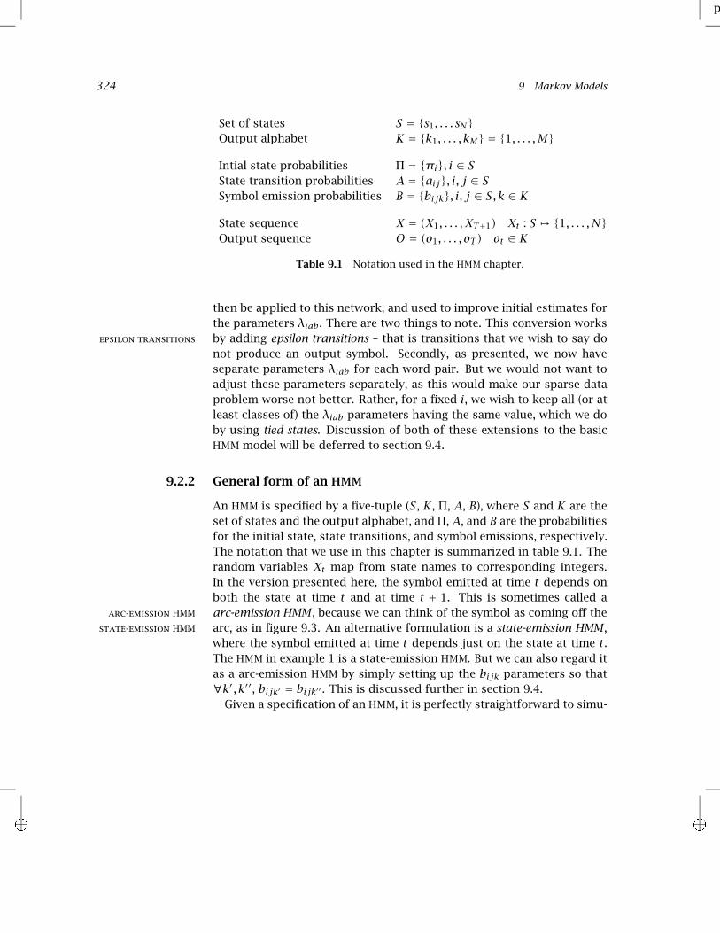
Set of states S = {s1, . . . sN}Output alphabet K = {k1, . . . , kM} = {1, . . . ,M}

Intial state probabilities Π = {πi}, i ∈ SState transition probabilities A = {aij}, i, j ∈ SSymbol emission probabilities B = {bijk}, i, j ∈ S, k ∈ K

State sequence X = (X1, . . . , XT+1) Xt : S , {1, . . . , N}Output sequence O = (o1, . . . , oT ) ot ∈ K

Table 9.1 Notation used in the HMM chapter.

then be applied to this network, and used to improve initial estimates forthe parameters λiab. There are two things to note. This conversion worksby adding epsilon transitions – that is transitions that we wish to say doepsilon transitions

not produce an output symbol. Secondly, as presented, we now haveseparate parameters λiab for each word pair. But we would not want toadjust these parameters separately, as this would make our sparse dataproblem worse not better. Rather, for a fixed i, we wish to keep all (or atleast classes of) the λiab parameters having the same value, which we doby using tied states. Discussion of both of these extensions to the basicHMM model will be deferred to section 9.4.

9.2.2 General form of an HMM

An HMM is specified by a five-tuple (S, K, Π, A, B), where S and K are theset of states and the output alphabet, and Π, A, and B are the probabilitiesfor the initial state, state transitions, and symbol emissions, respectively.The notation that we use in this chapter is summarized in table 9.1. Therandom variables Xt map from state names to corresponding integers.In the version presented here, the symbol emitted at time t depends onboth the state at time t and at time t + 1. This is sometimes called aarc-emission HMM , because we can think of the symbol as coming off thearc-emission HMM

arc, as in figure 9.3. An alternative formulation is a state-emission HMM ,state-emission HMM

where the symbol emitted at time t depends just on the state at time t .The HMM in example 1 is a state-emission HMM. But we can also regard itas a arc-emission HMM by simply setting up the bijk parameters so that∀k′, k′′, bijk′ = bijk′′ . This is discussed further in section 9.4.

Given a specification of an HMM, it is perfectly straightforward to simu-

p

i i

9.3 The Three Fundamental Questions for HMMs 325

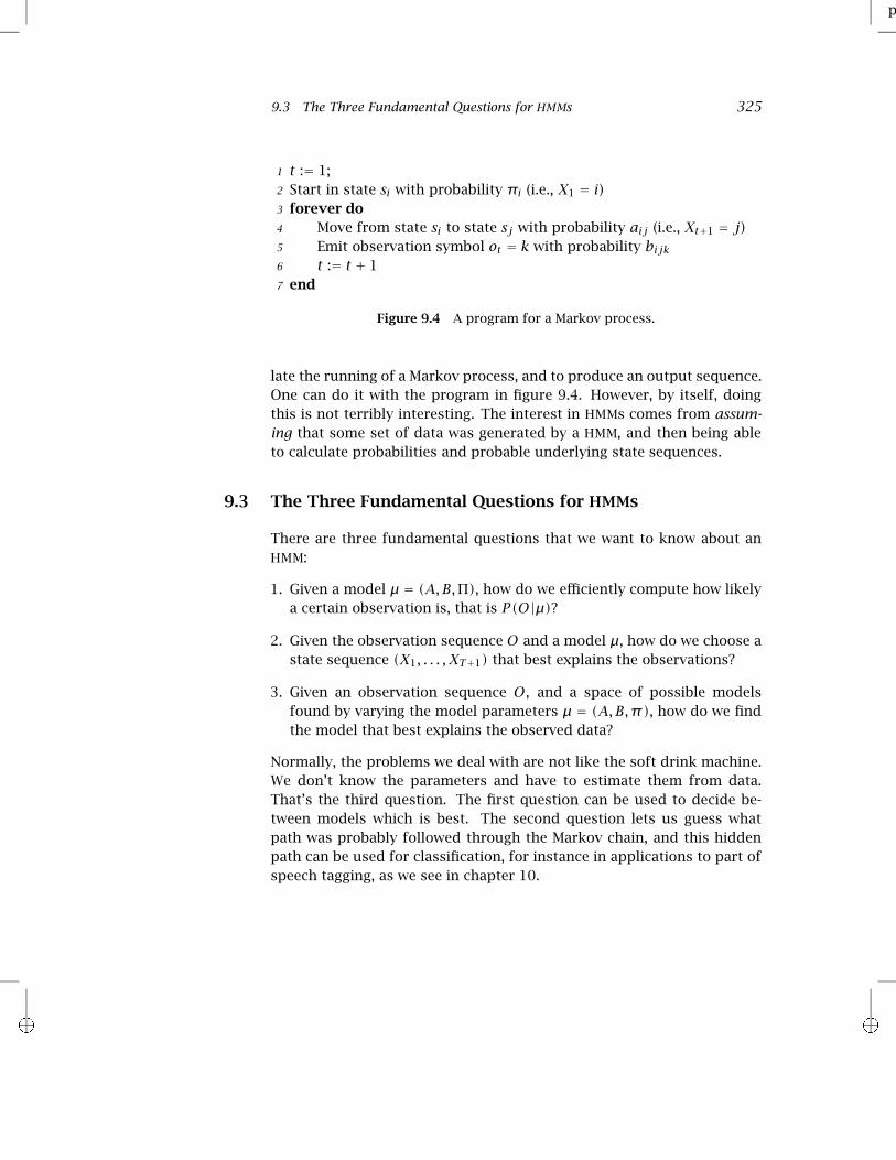
1 t := 1;2 Start in state si with probability πi (i.e., X1 = i)3 forever do4 Move from state si to state sj with probability aij (i.e., Xt+1 = j)5 Emit observation symbol ot = k with probability bijk6 t := t + 17 end

Figure 9.4 A program for a Markov process.

late the running of a Markov process, and to produce an output sequence.One can do it with the program in figure 9.4. However, by itself, doingthis is not terribly interesting. The interest in HMMs comes from assum-ing that some set of data was generated by a HMM, and then being ableto calculate probabilities and probable underlying state sequences.

9.3 The Three Fundamental Questions for HMMs

There are three fundamental questions that we want to know about anHMM:

1. Given a model µ = (A, B,Π), how do we efficiently compute how likelya certain observation is, that is P(O|µ)?

2. Given the observation sequence O and a model µ, how do we choose astate sequence (X1, . . . , XT+1) that best explains the observations?

3. Given an observation sequence O, and a space of possible modelsfound by varying the model parameters µ = (A, B,π), how do we findthe model that best explains the observed data?

Normally, the problems we deal with are not like the soft drink machine.We don’t know the parameters and have to estimate them from data.That’s the third question. The first question can be used to decide be-tween models which is best. The second question lets us guess whatpath was probably followed through the Markov chain, and this hiddenpath can be used for classification, for instance in applications to part ofspeech tagging, as we see in chapter 10.

p

i i

326 9 Markov Models

9.3.1 Finding the probability of an observation

Given the observation sequence O = (o1, . . . , oT ) and a model µ =(A, B,Π), we wish to know how to efficiently compute P(O|µ) – the prob-ability of the observation given the model. This process is often referredto as decoding.decoding

For any state sequence X = (X1, . . . , XT+1),

P(O|X,µ) =T∏t=1

P(ot|Xt,Xt+1, µ)(9.6)

= bX1X2o1bX2X3o2 · · ·bXTXT+1oT

and,

P(X|µ) = πX1aX1X2aX2X3 · · ·aXTXT+1(9.7)

Now,

P(O,X|µ) = P(O|X,µ)P(X|µ)(9.8)

Therefore,

P(O|µ) =∑XP(O|X,µ)P(X|µ)(9.9)

=∑

X1···XT+1

πX1

T∏t=1

aXtXt+1bXtXt+1ot

This derivation is quite straightforward. It is what we did in exam-ple 1 to work out the probability of an observation sequence. We simplysummed the probability of the observation occurring according to eachpossible state sequence. But, unfortunately, direct evaluation of the re-sulting expression is hopelessly inefficient. For the general case (whereone can start in any state, and move to any other at each step), the calcu-lation requires (2T + 1) ·NT+1 multiplications.

Exercise 9.3 [«]

Confirm this claim.

The secret to avoiding this complexity is the general technique of dy-dynamic

programming namic programming or memoization by which we remember partial re-memoization

sults rather than recomputing them. This general concept crops up inmany other places in computational linguistics, such as chart parsing,

p

i i

9.3 The Three Fundamental Questions for HMMs 327

and in computer science more generally (see (Cormen et al. 1990: ch. 16)for a general introduction). For algorithms such as HMMs, the dynamicprogramming problem is generally described in terms of trellises (alsotrellis

called lattices). Here, we make a square array of states versus time, andlattice

compute the probabilities of being at each state at each time in termsof the probabilities for being in each state at the preceding time instant.This is all best seen in pictures – see figures 9.5 and 9.6. A trellis canrecord the probability of all initial subpaths of the HMM that end in a cer-tain state at a certain time. The probability of longer subpaths can thenbe worked out in terms of one shorter subpaths.

The forward procedure

The form of caching that is indicated in these diagrams is called the for-forward procedure

ward procedure. We describe it in terms of forward variables:

αi(t) = P(o1o2 · · ·ot−1, Xt = i|µ)(9.10)

The forward variable αi(t) is stored at (si, t) in the trellis and expressesthe total probability of ending up in state si at time t (given that the obser-vations o1 · · ·ot−1 were seen). It is calculated by summing probabilitiesfor all incoming arcs at a trellis node. We calculate the forward variablesin the trellis left to right using the following procedure:

1. Initialization

αi(1) = πi, 1 ≤ i ≤ N

2. Induction

αj(t + 1) =N∑i=1

αi(t)aijbijot , 1 ≤ t ≤ T,1 ≤ j ≤ N

3. Total

P(O|µ) =N∑i=1

αi(T + 1)

This is a much cheaper algorithm that requires only 2N2T multiplica-tions.

p

i i

328 9 Markov Models

s1

s2

State 3

sN

1 2 3Time, t

T + 1

Figure 9.5 Trellis algorithms. The trellis is a square array of states versustimes. A node at (si, t) can store information about state sequences which in-clude Xt = i. The lines show the connections between nodes. Here we have afully interconnected HMM where one can move from any state to any other ateach step.

The backward procedure

It should be clear that we do not need to cache results working forwardthrough time like this, but rather that we could also work backward. Thebackward procedure computes backward variables which are the totalbackward

procedure probability of seeing the rest of the observation sequence given that wewere in state si at time t . The real reason for introducing this less intu-itive calculation, though, is because use of a combination of forward andbackward probabilities is vital for solving the third problem of parameter

p

i i

9.3 The Three Fundamental Questions for HMMs 329

s1α1(t)

s2α2(t)

s3α3(t)

sjαj(t + 1)

sNαN(t)

t t + 1

a1j b

1jot

a2j b

2jot

a3jb3jot

a NjbNjot

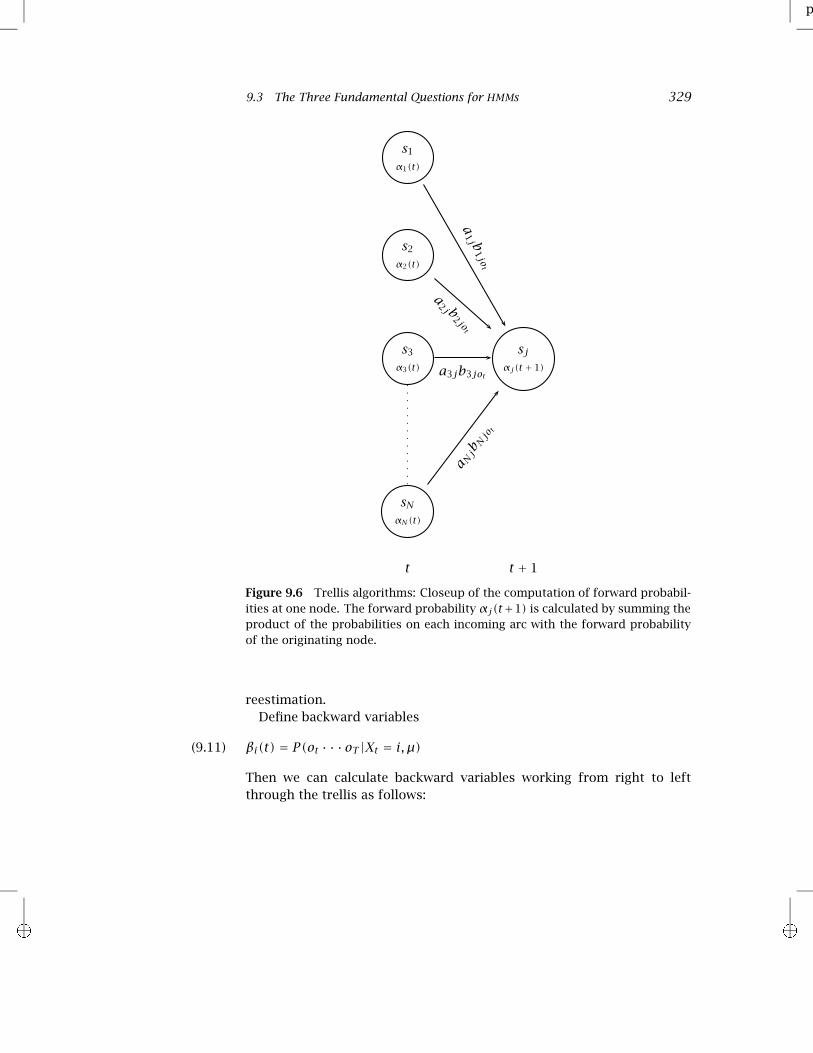
Figure 9.6 Trellis algorithms: Closeup of the computation of forward probabil-ities at one node. The forward probability αj(t+1) is calculated by summing theproduct of the probabilities on each incoming arc with the forward probabilityof the originating node.

reestimation.Define backward variables

βi(t) = P(ot · · ·oT |Xt = i, µ)(9.11)

Then we can calculate backward variables working from right to leftthrough the trellis as follows:

p

i i

330 9 Markov Models

Outputlem ice_t cola

Time (t): 1 2 3 4αCP(t) 1.0 0.21 0.0462 0.021294αIP(t) 0.0 0.09 0.0378 0.010206

P(o1 · · ·ot−1) 1.0 0.3 0.084 0.0315βCP(t) 0.0315 0.045 0.6 1.0βIP (t) 0.029 0.245 0.1 1.0

P(o1 · · ·oT ) 0.0315γCP(t) 1.0 0.3 0.88 0.676γIP (t) 0.0 0.7 0.12 0.324

Xt CP IP CP CPδCP(t) 1.0 0.21 0.0315 0.019404δIP (t) 0.0 0.09 0.0315 0.008316ψCP(t) CP IP CPψIP(t) CP IP CP

Xt CP IP CP CPP(X) 0.019404

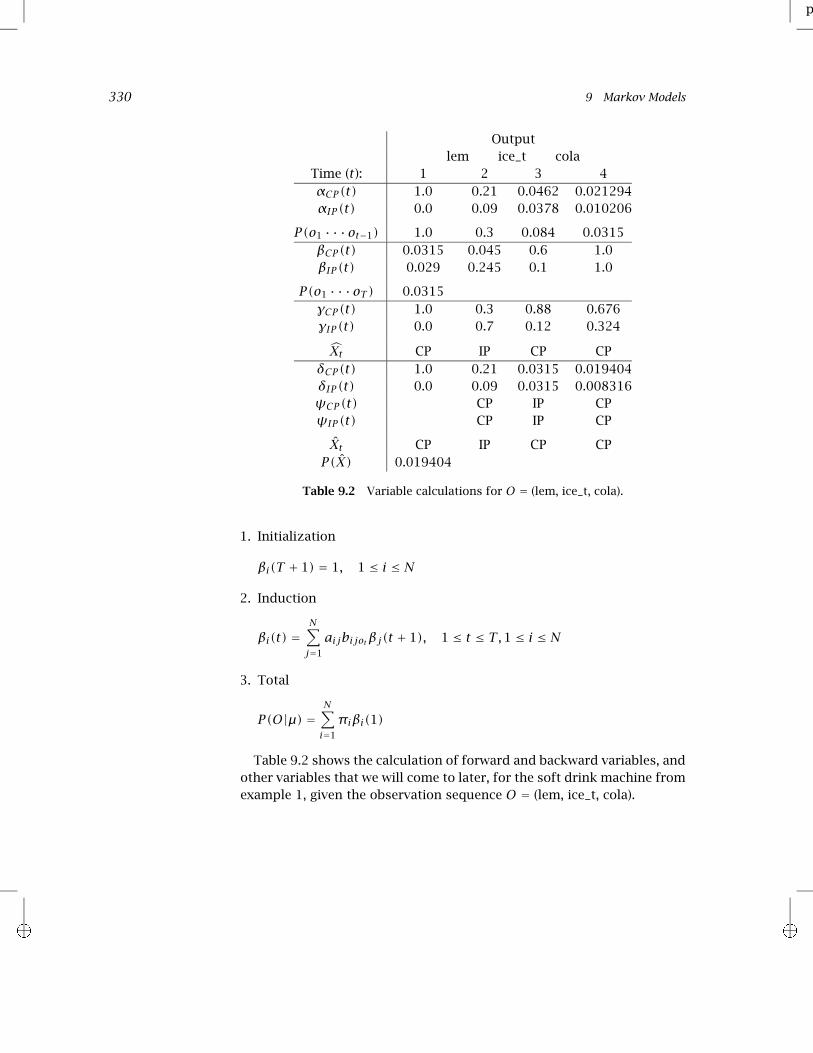
Table 9.2 Variable calculations for O = (lem, ice_t, cola).

1. Initialization

βi(T + 1) = 1, 1 ≤ i ≤ N

2. Induction

βi(t) =N∑j=1

aijbijotβj(t + 1), 1 ≤ t ≤ T,1 ≤ i ≤ N

3. Total

P(O|µ) =N∑i=1

πiβi(1)

Table 9.2 shows the calculation of forward and backward variables, andother variables that we will come to later, for the soft drink machine fromexample 1, given the observation sequence O = (lem, ice_t, cola).

p

i i

9.3 The Three Fundamental Questions for HMMs 331

Combining them

More generally, in fact, we can use any combination of forward and back-ward caching to work out the probability of an observation sequence.Observe that:

P(O,Xt = i|µ) = P(o1 · · ·oT ,Xt = i|µ)= P(o1 · · ·ot−1, Xt = i, ot · · ·oT |µ)= P(o1 · · ·ot−1, Xt = i|µ)

×P(ot · · ·oT |o1 · · ·ot−1, Xt = i, µ)= P(o1 · · ·ot−1, Xt = i|µ)P(ot · · ·oT |Xt = i, µ)= αi(t)βi(t)

Therefore:

P(O|µ) =N∑i=1

αi(t)βi(t), 1 ≤ t ≤ T + 1(9.12)

The previous equations were special cases of this one.

9.3.2 Finding the best state sequence

The second problem was worded somewhat vaguely as “finding the statesequence that best explains the observations.” That is because there ismore than one way to think about doing this. One way to proceed wouldbe to choose the states individually. That is, for each t , 1 ≤ t ≤ T + 1, wewould find Xt that maximizes P(Xt|O,µ).

Let

γi(t) = P(Xt = i|O,µ)(9.13)

= P(Xt = i,O|µ)P(O|µ)

= αi(t)βi(t)∑Nj=1αj(t)βj(t)

The individually most likely state Xt is:

Xt = arg max1≤i≤N

γi(t), 1 ≤ t ≤ T + 1(9.14)

This quantity maximizes the expected number of states that will beguessed correctly. However, it may yield a quite unlikely state sequence.

p

i i

332 9 Markov Models

Therefore, this is not the method that is normally used, but rather theViterbi algorithm, which efficiently computes the most likely state se-quence.

Viterbi algorithm

Commonly we want to find the most likely complete path, that is:

arg maxX

P(X|O,µ)

To do this, it is sufficient to maximize for a fixed O:

arg maxX

P(X,O|µ)

An efficient trellis algorithm for computing this path is the Viterbi al-Viterbi algorithm

gorithm. Define:

δj(t) = maxX1···Xt−1

P(X1 · · ·Xt−1, o1 · · ·ot−1, Xt = j|µ)This variable stores for each point in the trellis the probability of the mostprobable path that leads to that node. The corresponding variable ψj(t)then records the node of the incoming arc that led to this most probablepath. Using dynamic programming, we calculate the most probable paththrough the whole trellis as follows:

1. Initialization

δj(1) = πj, 1 ≤ j ≤ N2. Induction

δj(t + 1) = max1≤i≤N

δi(t)aijbijot , 1 ≤ j ≤ N

Store backtrace

ψj(t + 1) = arg max1≤i≤N

δi(t)aijbijot ,1 ≤ j ≤ N

3. Termination and path readout (by backtracking). The most likely statesequence is worked out from the right backwards:

XT+1 = arg max1≤i≤N

δi(T + 1)

Xt = ψXt+1(t + 1)

P(X) = max1≤i≤N

δi(T + 1)

p

i i

9.3 The Three Fundamental Questions for HMMs 333

In these calculations, one may get ties. We assume that in that case onepath is chosen randomly. In practical applications, people commonlywant to work out not only the best state sequence but the n-best se-quences or a graph of likely paths. In order to do this people often storethe m < n best previous states at a node.

Table 9.2 above shows the computation of the most likely states andstate sequence under both these interpretations – for this example, theyprove to be identical.

9.3.3 The third problem: Parameter estimation

Given a certain observation sequence, we want to find the values of themodel parameters µ = (A, B,π) which best explain what we observed.Using Maximum Likelihood Estimation, that means we want to find thevalues that maximize P(O|µ):

arg maxµ

P(Otraining|µ)(9.15)

There is no known analytic method to choose µ to maximize P(O|µ). Butwe can locally maximize it by an iterative hill-climbing algorithm. Thisalgorithm is the Baum-Welch or Forward-Backward algorithm, which is aForward-Backward

algorithm special case of the Expectation Maximization method which we will coverEM algorithm in greater generality in section 14.2.2. It works like this. We don’t know

what the model is, but we can work out the probability of the observa-tion sequence using some (perhaps randomly chosen) model. Looking atthat calculation, we can see which state transitions and symbol emissionswere probably used the most. By increasing the probability of those, wecan choose a revised model which gives a higher probability to the ob-servation sequence. This maximization process is often referred to astraining the model and is performed on training data.training

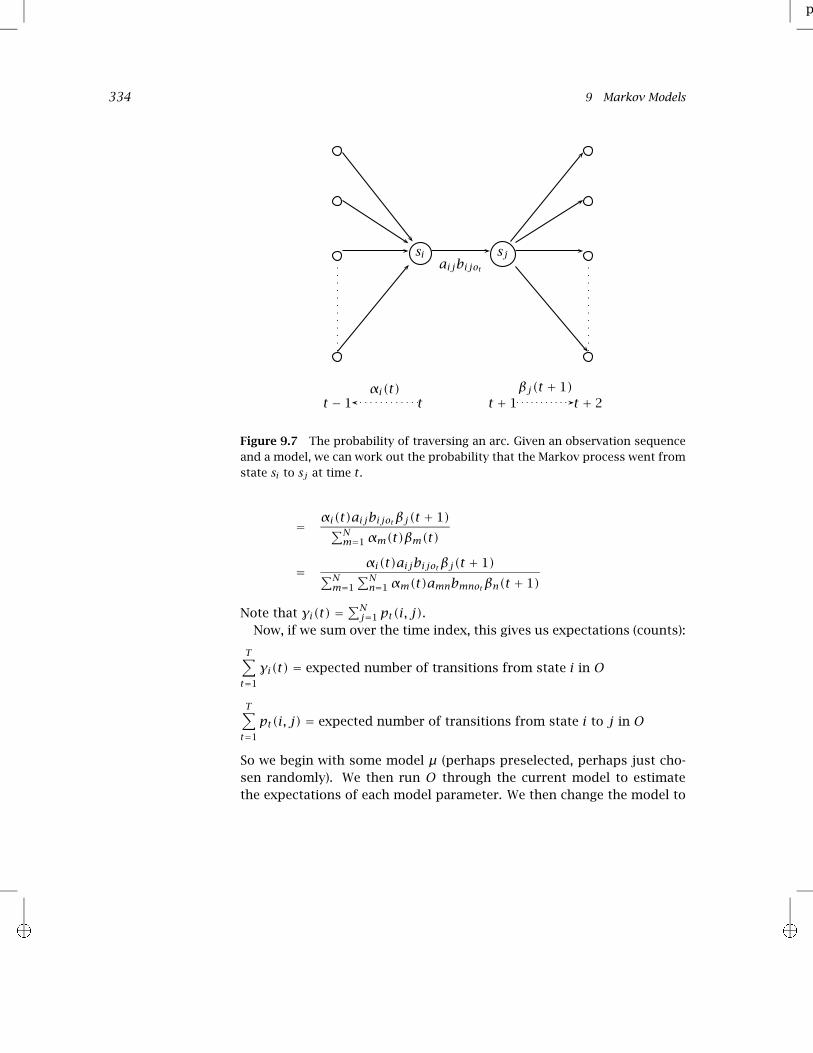
training data Define pt(i, j),1 ≤ t ≤ T,1 ≤ i, j ≤ N as shown below. This is the prob-ability of traversing a certain arc at time t given observation sequence O;see figure 9.7.

pt(i, j) = P(Xt = i, Xt+1 = j|O,µ)(9.16)

= P(Xt = i, Xt+1 = j,O|µ)P(O|µ)

p

i i

334 9 Markov Models

si sj

t − 1 t t + 1 t + 2

aijbijot

αi(t) βj(t + 1)

Figure 9.7 The probability of traversing an arc. Given an observation sequenceand a model, we can work out the probability that the Markov process went fromstate si to sj at time t .

= αi(t)aijbijotβj(t + 1)∑Nm=1αm(t)βm(t)

= αi(t)aijbijotβj(t + 1)∑Nm=1

∑Nn=1αm(t)amnbmnotβn(t + 1)

Note that γi(t) =∑Nj=1 pt(i, j).

Now, if we sum over the time index, this gives us expectations (counts):

T∑t=1

γi(t) = expected number of transitions from state i in O

T∑t=1

pt(i, j) = expected number of transitions from state i to j in O

So we begin with some model µ (perhaps preselected, perhaps just cho-sen randomly). We then run O through the current model to estimatethe expectations of each model parameter. We then change the model to

p

i i

9.3 The Three Fundamental Questions for HMMs 335

maximize the values of the paths that are used a lot (while still respect-ing the stochastic constraints). We then repeat this process, hoping toconverge on optimal values for the model parameters µ.

The reestimation formulas are as follows:

πi = expected frequency in state i at time t = 1(9.17)

= γi(1)

aij = expected number of transitions from state i to jexpected number of transitions from state i

(9.18)

=∑Tt=1 pt(i, j)∑Tt=1 γi(t)

bijk = expected number of transitions from i to j with k observedexpected number of transitions from i to j

(9.19)

=∑{t :ot=k,1≤t≤T} pt(i, j)∑T

t=1 pt(i, j)

Thus, from µ = (A, B,Π), we derive µ = (A, B, Π). Further, as proved byBaum, we have that:

P(O|µ) ≥ P(O|µ)

This is a general property of the EM algorithm (see section 14.2.2). There-fore, iterating through a number of rounds of parameter reestimationwill improve our model. Normally one continues reestimating the pa-rameters until results are no longer improving significantly. This processof parameter reestimation does not guarantee that we will find the bestmodel, however, because the reestimation process may get stuck in a lo-local maximum

cal maximum (or even possibly just at a saddle point). In most problemsof interest, the likelihood function is a complex nonlinear surface andthere are many local maxima. Nevertheless, Baum-Welch reestimation isusually effective for HMMs.

To end this section, let us consider reestimating the parameters of thecrazy soft drink machine HMM using the Baum-Welch algorithm. If we letthe initial model be the model that we have been using so far, then train-ing on the observation sequence (lem, ice_t, cola) will yield the followingvalues for pt(i, j):

p

i i

336 9 Markov Models

(9.20) Time (and j)1 2 3CP IP γ1 CP IP γ2 CP IP γ3

i CP 0.3 0.7 1.0 0.28 0.02 0.3 0.616 0.264 0.88IP 0.0 0.0 0.0 0.6 0.1 0.7 0.06 0.06 0.12

and so the parameters will be reestimated as follows:

Original ReestimatedΠ CP 1.0 1.0

IP 0.0 0.0

CP IP CP IPA CP 0.7 0.3 0.5486 0.4514

IP 0.5 0.5 0.8049 0.1951

cola ice_t lem cola ice_t lemB CP 0.6 0.1 0.3 0.4037 0.1376 0.4587

IP 0.1 0.7 0.2 0.1363 0.8537 0.0

Exercise 9.4 [«]

If one continued running the Baum-Welch algorithm on this HMM and this train-ing sequence, what value would each parameter reach in the limit? Why?

The reason why the Baum-Welch algorithm is performing so strangely hereshould be apparent: the training sequence is far too short to accurately rep-resent the behavior of the crazy soft drink machine.

Exercise 9.5 [«]

Note that the parameter that is zero in Π stays zero. Is that a chance occurrence?What would be the value of the parameter that becomes zero in B if we did an-other iteration of Baum-Welch reestimation? What generalization can one makeabout Baum-Welch reestimation of zero parameters?

9.4 HMMs: Implementation, Properties, and Variants

9.4.1 Implementation

Beyond the theory discussed above, there are a number of practical is-sues in the implementation of HMMs. Care has to be taken to make theimplementation of HMM tagging efficient and accurate. The most obviousissue is that the probabilities we are calculating consist of keeping onmultiplying together very small numbers. Such calculations will rapidly

p

i i

9.4 HMMs: Implementation, Properties, and Variants 337

underflow the range of floating point numbers on a computer (even if youstore them as ‘double’!).

The Viterbi algorithm only involves multiplications and choosing thelargest element. Thus we can perform the entire Viterbi algorithm work-ing with logarithms. This not only solves the problem with floating pointunderflow, but it also speeds up the computation, since additions aremuch quicker than multiplications. In practice, a speedy implementa-tion of the Viterbi algorithm is particularly important because this is theruntime algorithm, whereas training can usually proceed slowly offline.

However, in the Forward-Backward algorithm as well, something stillhas to be done to prevent floating point underflow. The need to performsummations makes it difficult to use logs. A common solution is to em-ploy auxiliary scaling coefficients, whose values grow with the time t soscaling

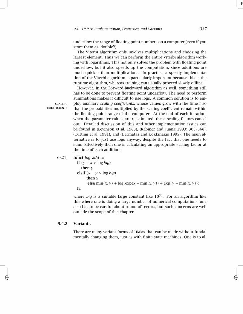
coefficients that the probabilities multiplied by the scaling coefficient remain withinthe floating point range of the computer. At the end of each iteration,when the parameter values are reestimated, these scaling factors cancelout. Detailed discussion of this and other implementation issues canbe found in (Levinson et al. 1983), (Rabiner and Juang 1993: 365–368),(Cutting et al. 1991), and (Dermatas and Kokkinakis 1995). The main al-ternative is to just use logs anyway, despite the fact that one needs tosum. Effectively then one is calculating an appropriate scaling factor atthe time of each addition:

(9.21) funct log_add ≡if (y − x > log big)

then yelsif (x− y > log big)

then xelse min(x, y)+ log(exp(x−min(x, y))+ exp(y −min(x, y)))

fi.

where big is a suitable large constant like 1030. For an algorithm likethis where one is doing a large number of numerical computations, onealso has to be careful about round-off errors, but such concerns are welloutside the scope of this chapter.

9.4.2 Variants

There are many variant forms of HMMs that can be made without funda-mentally changing them, just as with finite state machines. One is to al-

p

i i

338 9 Markov Models

low some arc transitions to occur without emitting any symbol, so-calledepsilon or null transitions (Bahl et al. 1983). Another commonly used vari-epsilon transitions

null transitions ant is to make the output distribution dependent just on a single state,rather than on the two states at both ends of an arc as you traverse anarc, as was effectively the case with the soft drink machine. Under thismodel one can view the output as a function of the state chosen, ratherthan of the arc traversed. The model where outputs are a function ofthe state has actually been used more often in Statistical NLP, becauseit corresponds naturally to a part of speech tagging model, as we see inchapter 10. Indeed, some people will probably consider us perverse forhaving presented the arc-emission model in this chapter. But we chosethe arc-emission model because it is trivial to simulate the state-emissionmodel using it, whereas doing the reverse is much more difficult. As sug-gested above, one does not need to think of the simpler model as havingthe outputs coming off the states, rather one can view the outputs as stillcoming off the arcs, but that the output distributions happen to be thesame for all arcs that start at a certain node (or that end at a certain node,if one prefers).

This suggests a general strategy. A problem with HMM models is thelarge number of parameters that need to be estimated to define themodel, and it may not be possible to estimate them all accurately if notmuch data is available. A straightforward strategy for dealing with thissituation is to introduce assumptions that probability distributions oncertain arcs or at certain states are the same as each other. This is re-ferred to as parameter tying, and one thus gets tied states or tied arcs.parameter tying

tied states

tied arcs

Another possibility for reducing the number of parameters of the modelis to decide that certain things are impossible (i.e., they have probabilityzero), and thus to introduce structural zeroes into the model. Makingsome things impossible adds a lot of structure to the model, and socan greatly improve the performance of the parameter reestimation al-gorithm, but is only appropriate in some circumstances.

9.4.3 Multiple input observations

We have presented the algorithms for a single input sequence. How doesone train over multiple inputs? For the kind of HMM we have been as-suming, where every state is connected to every other state (with a non-zero transition probability) – what is sometimes called an ergodic modelergodic model

– there is a simple solution: we simply concatenate all the observation

p

i i

9.5 Further Reading 339

sequences and train on them as one long input. The only real disadvan-tage to this is that we do not get sufficient data to be able to reestimatethe initial probabilities πi successfully. However, often people use HMM

models that are not fully connected. For example, people sometimes usea feed forward model where there is an ordered set of states and one canfeed forward model

only proceed at each time instant to the same or a higher numbered state.If the HMM is not fully connected – it contains structural zeroes – or ifwe do want to be able to reestimate the initial probabilities, then we needto extend the reestimation formulae to work with a sequence of inputs.Provided that we assume that the inputs are independent, this is straight-forward. We will not present the formulas here, but we do present theanalogous formulas for the PCFG case in section 11.3.4.

9.4.4 Initialization of parameter values

The reestimation process only guarantees that we will find a local max-imum. If we would rather find the global maximum, one approach is totry to start the HMM in a region of the parameter space that is near theglobal maximum. One can do this by trying to roughly estimate good val-ues for the parameters, rather than setting them randomly. In practice,good initial estimates for the output parameters B = {bijk} turn out to beparticularly important, while random initial estimates for the parametersA and Π are normally satisfactory.

9.5 Further Reading

The Viterbi algorithm was first described in (Viterbi 1967). The mathe-matical theory behind Hidden Markov Models was developed by Baumand his colleagues in the late sixties and early seventies (Baum et al.1970), and advocated for use in speech recognition in lectures by JackFerguson from the Institute for Defense Analyses. It was applied tospeech processing in the 1970s by Baker at CMU (Baker 1975), and byJelinek and colleagues at IBM (Jelinek et al. 1975; Jelinek 1976), and thenlater found its way at IBM and elsewhere into use for other kinds of lan-guage modeling, such as part of speech tagging.

There are many good references on HMM algorithms (within the contextof speech recognition), including (Levinson et al. 1983; Knill and Young1997; Jelinek 1997). Particularly well-known are (Rabiner 1989; Rabiner

p

i i

340 9 Markov Models

and Juang 1993). They consider continuous HMMs (where the output isreal valued) as well as the discrete HMMs we have considered here, con-tain information on applications of HMMs to speech recognition and mayalso be consulted for fairly comprehensive references on the develop-ment and the use of HMMs. Our presentation of HMMs is however mostclosely based on that of Paul (1990).

Within the chapter, we have assumed a fixed HMM architecture, andhave just gone about learning optimal parameters for the HMM withinthat architecture. However, what size and shape of HMM should onechoose for a new problem? Sometimes the nature of the problem de-termines the architecture, as in the applications of HMMs to tagging thatwe discuss in the next chapter. For circumstances when this is not thecase, there has been some work on learning an appropriate HMM struc-ture on the principle of trying to find the most compact HMM that canadequately describe the data (Stolcke and Omohundro 1993).

HMMs are widely used to analyze gene sequences in bioinformatics. Seefor instance (Baldi and Brunak 1998; Durbin et al. 1998). As linguists, wefind it a little hard to take seriously problems over an alphabet of foursymbols, but bioinformatics is a well-funded domain to which you canapply your new skills in Hidden Markov Modeling!

This excerpt from

Foundations of Statistical Natural Language Processing.Christopher D. Manning and Hinrich Schütze.© 1999 The MIT Press.

is provided in screen-viewable form for personal use only by membersof MIT CogNet.

Unauthorized use or dissemination of this information is expresslyforbidden.

If you have any questions about this material, please contactcognetadmin@cognet.mit.edu.