Four Essays in Economic Theory

Inaugural-Dissertationzur Erlangung des Grades eines Doktors

der Wirtschafts- und Gesellschaftswissenschaftendurch die

Rechts- und Staatswissenschaftliche Fakultätder Rheinischen Friedrich-Wilhelms-Universität

Bonn

vorgelegt vonDeniz Dizdar

aus Daun

2013

Dekan: Prof. Dr. Klaus SandmannErstreferent: Prof. Dr. Benny MoldovanuZweitreferent: Prof. Dr. Dezsö Szalay

Tag der mündlichen Prüfung: 13.06.2013

Diese Dissertation ist auf dem Hochschulschriftenserver der ULB Bonn (http://hss.ulb.uni-bonn.de/diss_online) elektronisch publiziert.

Acknowledgements

I am particularly grateful to my supervisor Benny Moldovanu, who kindled myinterest in economic theory via a course on matching markets at the time when I wasstudying mathematics at the University of Bonn. I would like to thank him for guidance,encouragement and support, which have all been invaluable throughout the past fewyears, and also for countless inspiring conversations.

I want to thank Alex Gershkov, both for his interest in the material of Chapter 3of this thesis and for the many enjoyable hours of discussions with him and BennyMoldovanu during our joint work on the dynamic knapsack problem. In addition, Ibenefited a lot from discussions with Thomas Gall, Daniel Krähmer, Matthias Lang,Konrad Mierendorff and Dezsö Szalay, and I would like to express my gratitude for theirinsightful comments and for their interest in my work. I also owe special thanks to DezsöSzalay for agreeing without hesitance to be the second referee of this thesis.

I had a great time and many interesting conversations with numerous doctoral studentsof the Bonn Graduate School of Economics, as well as with postdocs and professorsat the Department of Economics. They are too many to name all of them here, but Iwould like to mention at least my fellow doctoral students Rafael Aigner, Benjamin Born,Andreas Esser, Alexandra Peter, Johannes Pfeifer, Christian Seel, Christoph Wagnerand Florian Zimmermann, and my colleagues at the Chair of Microeconomics, DennisGärtner, Nicolas Klein, Frank Rosar, Nora Szech and Alex Westkamp.

The Bonn Graduate School of Economics provides a superb environment for doctoralresearch. This thriving and lively academic institution would be unthinkable without thetireless efforts of Urs Schweizer. Silke Kinzig and Pamela Mertens also manage the affairsof the BGSE very well, and I would like to thank them for providing unbureaucratic

iii

help whenever it is needed. Moreover, I gratefully acknowledge financial support by theGerman Science Foundation, which I received first through a scholarship of the BGSEand more recently by means of a position at SFB TR 15.Finally, I am grateful to my friends, my parents, my brother and to Anastasiya, for

having helped me to stay motivated whenever I was trapped in a dead end with myresearch - and for much more. Thank you!

iv

Contents

Introduction 1

1 Investments and matching with multi-dimensional attributes 71.1 Introduction . . . . . . . . . . . . . . . . . . . . . . . . . . . . . . . . . . 8

1.1.1 Related literature . . . . . . . . . . . . . . . . . . . . . . . . . . . 121.2 Model . . . . . . . . . . . . . . . . . . . . . . . . . . . . . . . . . . . . . 16

1.2.1 Agent populations, costs, and match surplus . . . . . . . . . . . . 161.2.2 The transferable utility assignment game . . . . . . . . . . . . . . 171.2.3 Ex-post contracting equilibria . . . . . . . . . . . . . . . . . . . . 20

1.3 Ex-ante contracting equilibria . . . . . . . . . . . . . . . . . . . . . . . . 221.4 Efficient ex-post contracting equilibria . . . . . . . . . . . . . . . . . . . 221.5 Inefficient equilibria . . . . . . . . . . . . . . . . . . . . . . . . . . . . . . 23

1.5.1 Two kinds of inefficiency: mismatch and inefficiency of joint in-vestments . . . . . . . . . . . . . . . . . . . . . . . . . . . . . . . 231.5.1.1 Technological multiplicity and inefficiency of joint invest-

ments . . . . . . . . . . . . . . . . . . . . . . . . . . . . 241.5.1.2 The “constrained efficiency” property . . . . . . . . . . . 25

1.5.2 Preparation: the basic module for examples . . . . . . . . . . . . 261.5.3 A multi-dimensional model without technological multiplicity . . 27

1.5.3.1 An example of mismatch inefficiency . . . . . . . . . . . 281.5.3.2 The limits of mismatch: a simple example . . . . . . . . 291.5.3.3 The limits of mismatch continued: a fully multi-dimensional

case . . . . . . . . . . . . . . . . . . . . . . . . . . . . . 30

v

Contents

1.5.4 Technological multiplicity and severe coordination failures . . . . 311.5.5 Simultaneous under- and over-investment: the case of missing

middle sectors . . . . . . . . . . . . . . . . . . . . . . . . . . . . . 331.6 Appendix for Chapter 1 . . . . . . . . . . . . . . . . . . . . . . . . . . . 35

2 Surplus division and efficient matching 512.1 Introduction . . . . . . . . . . . . . . . . . . . . . . . . . . . . . . . . . . 512.2 The matching model . . . . . . . . . . . . . . . . . . . . . . . . . . . . . 57

2.2.1 Sharing rules . . . . . . . . . . . . . . . . . . . . . . . . . . . . . 582.2.2 Mechanisms . . . . . . . . . . . . . . . . . . . . . . . . . . . . . . 58

2.3 The main results . . . . . . . . . . . . . . . . . . . . . . . . . . . . . . . 592.4 Conclusion . . . . . . . . . . . . . . . . . . . . . . . . . . . . . . . . . . . 622.5 Appendix for Chapter 2 . . . . . . . . . . . . . . . . . . . . . . . . . . . 62

3 On the optimality of small research tournaments 713.1 Introduction . . . . . . . . . . . . . . . . . . . . . . . . . . . . . . . . . . 713.2 Optimal tournament size under complete information . . . . . . . . . . . 75

3.2.1 The model and some known results . . . . . . . . . . . . . . . . . 753.2.2 A sharp bound for general asymmetric cost structures . . . . . . . 77

3.3 Incomplete information, (FM)’s contestant selection auction, and optimaltournament size . . . . . . . . . . . . . . . . . . . . . . . . . . . . . . . . 81

3.4 Appendix for Chapter 3 . . . . . . . . . . . . . . . . . . . . . . . . . . . 85

4 Revenue maximization in the dynamic knapsack problem 934.1 Introduction . . . . . . . . . . . . . . . . . . . . . . . . . . . . . . . . . . 93

4.1.1 Outline and preview of results . . . . . . . . . . . . . . . . . . . . 954.2 The model . . . . . . . . . . . . . . . . . . . . . . . . . . . . . . . . . . . 974.3 Incentive compatible policies . . . . . . . . . . . . . . . . . . . . . . . . . 984.4 Dynamic revenue maximization . . . . . . . . . . . . . . . . . . . . . . . 99

4.4.1 The hazard rate stochastic ordering . . . . . . . . . . . . . . . . . 1024.4.2 The role of concavity . . . . . . . . . . . . . . . . . . . . . . . . . 103

4.5 Asymptotically optimal and time-independent pricing . . . . . . . . . . . 1054.5.1 The deterministic problem . . . . . . . . . . . . . . . . . . . . . . 1064.5.2 A simple policy for the stochastic problem . . . . . . . . . . . . . 109

vi

Contents

4.6 Appendix for Chapter 4 . . . . . . . . . . . . . . . . . . . . . . . . . . . 110

Bibliography 127

vii

Introduction

This thesis comprises four essays that belong to different strands of the theoreticaleconomic literature. Both Chapter 1 and Chapter 2 contribute to the study of two-sided one-to-one matching, or assignment, markets with quasi-linear utility and multi-dimensional heterogeneity. Chapter 1 investigates the efficiency of two-sided investmentsin large (continuum) two-sided economies in which matching and bargaining take place inan endogenously determined market without frictions after all agents have made costly,sunk investments. Chapter 2 scrutinizes a novel two-sided matching model with a finitenumber of agents and two-sided private information about exogenously given attributes.Chapter 3 is a note on the optimal size of fixed-prize research tournaments that seeksto fill two important gaps in an influential paper by Fullerton and McAfee (1999), andChapter 4 studies the impact of incomplete information on the problem of maximizingrevenue in a dynamic version of the knapsack problem, which is a classical combinatorialresource allocation problem with numerous economic applications.

Chapter 2 is based on joint work with Benny Moldovanu, and Chapter 4 is joint workwith Alex Gershkov and Benny Moldovanu that has been published (in a slightly differentversion) as a paper in 2011 (Dizdar, Gershkov and Moldovanu, 2011). For this reason, Iuse the pronoun “we” in these chapters, whereas I use “I” in Chapter 1 and in Chapter 3.The analysis of assignment markets with quasi-linear utility has been pioneered by

Shapley and Shubik (1971). The basic setting is as follows: there are several heterogeneousagents on each side of the market, e.g. workers and firms, or buyers and sellers, whoare characterized by attributes that jointly determine the match value/surplus of eachpotential partnership (or trade). Monetary transfers among agents are possible. In theirfamous study, Shapley and Shubik characterized the outcomes of transferable utility

1

Introduction

assignment games - assignment economies of the kind just described, in which attributesare exogenously given, and in which matching and bargaining take place under completeinformation and without any other frictions.Many papers have varied or extended special cases of the basic assignment game

framework, e.g. to investigate effects on prices and matching patterns introduced byprivate information (in auction or double auction settings, say) or search frictions, orto analyze investment incentives and the efficiency of market outcomes in situations inwhich attributes, rather than being exogenously given, result from costly investmentsmade by the agents. Much (though not all) of the related literature has built on oneparticular version of the Shapley-Shubik model that was popularized by Becker (1973).1

In this kind of model, all agents are completely described by a one-dimensional attribute,representing for example the skill or education of a worker or the quality of the physicalcapital of a firm. Moreover, attributes satisfy a strong form of complementarity. Theserestrictive assumptions have strong implications for agents’ preferences that are often nottenable (in particular, positive assortative matching is implied in the frictionless model).A common motivation for the research of Chapters 1 and 2 is to add to the under-

standing of the economics of assignment markets in which agents on both sides of themarket are heterogeneous with respect to several relevant characteristics. Therefore, thepresent work is based on the general Shapley-Shubik model and on parts of the moreadvanced mathematical literature on optimal transport.Previous research has noted that in many two-sided economies, agents must make

costly investments in physical or human capital before they meet potential partners:agents compete for partners only “ex-post”, in a market that is endogenously determinedby all agents’ (sunk) investments (Acemoglu, 1996; Cole, Mailath and Postlewaite, 2001a).Chapter 1 studies the efficiency of two-sided investments and matching in large economies,when agents are characterized by multi-dimensional cost/ability types and must decideabout investments in multi-dimensional attributes. To this end, I extend the seminalmodel of Cole, Mailath and Postlewaite (in particular, I maintain the assumptions ofcomplete information and of frictionless ex-post markets), who assumed supermodularmatch surplus and ordered marginal cost types, to allow for general continuum assignmentgames. First, I show that there always is an “ex-post contracting” equilibrium (agents

1In addition, linear versions of the Shapley-Shubik model also play a prominent role in applications toauctions and double auctions.

2

must not have an incentive to deviate from their investment, given correct anticipationof the post-investment market; see Chapter 1 for the formal definition) that supportsex-ante efficient investment and matching. Hence, the main efficiency result of Cole,Mailath and Postlewaite does not hinge on the single-crossing properties entailed by theBecker framework. The main part of Chapter 1 aims at an in-depth study of the complexinterplay of technology and ex-ante heterogeneity that determines whether inefficientequilibria exist as well, or whether these are necessarily ruled out by sufficiently richattribute markets. I identify a certain form of multiplicity in the technology as themain source of potential coordination failures. Mismatch of agents due to inefficientspecialization (which is impossible in Becker-type models) may occur even without suchmultiplicity, but there are very strong trends towards ex-ante efficiency in these cases. Ialso illustrate (in a case with multiplicity) that, in contrast to examples given by Cole,Mailath and Postlewaite, it is possible that even arbitrarily high ex-ante heterogeneitydoes not suffice to rule out inefficiency. The analysis proceeds by means of a combinationof general lemmas and several rather involved examples, one of which uses some advancedresults from optimal transport theory.If attributes are private information, then match surplus becomes informationally

interdependent. In Chapter 2, we study such situations of two-sided private information:a finite number of agents with exogenously given, privately known attributes need tobe matched to form productive relationships. We ask whether there are standardizedrules for dividing ex-post realized surplus within matched pairs that are compatible withinformation revelation leading, for each realization of attributes in the economy, to anefficient matching. Maybe surprisingly, we find that for multi-dimensional, complementaryattributes, the only robust rules that are compatible with efficient match formationin this sense are those that divide the surplus in each match according to the samefixed proportion, independently of the attributes of the pair’s members. Such fixed-proportion rules are observed in widely differing circumstances. We interpret our resultas highlighting a desirable feature distinguishing such contracts that has previously goneunnoticed, and which complements other rationales that have been given in the literature,based for example on moral hazard or risk-sharing arguments.

Fullerton and McAfee (1999) studied how to design a fixed-prize research tournamentin cases where firms/suppliers are heterogeneous with respect to their research costs andwhere the research technology is stochastic. They focused on how cost asymmetries affect

3

Introduction

two major issues for the designer (who wants to procure a high quality innovation at lowcost): how many contestants should be admitted? How should these be selected from theset of available candidates when costs are private information prior to the tournament?The note in Chapter 3 analyzes two open problems with regard to the optimal numberof contestants. One problem pertains to the case where costs are common knowledge,the procurer can select participants by charging non-discriminatory entry fees, and noartificial restrictions on asymmetries are imposed. My result generally supports arrangingtournaments with the two most efficient firms only, but it also identifies instances ofasymmetry for which admitting more contestants is profitable for the procurer. Moreimportantly, I provide a rigorous analysis of optimal tournament size for a case wherecosts are private information of ex-ante symmetric firms before the tournament. Fullertonand McAfee showed that an all-pay entry auction should then be used to select the mostefficient firms from the pool of candidates and to raise money to finance parts of theprize (entry fees, as well as standard discriminatory-price and uniform-price auctions mayfail as selection mechanisms). I discuss the procurer’s problem of stimulating a givenexpected aggregate research effort at lowest expected total cost by choosing tournamentsize optimally, and I derive a closed form solution for the case where marginal costsare uniformly distributed on [0, c]. The result strongly favors the smallest possibletournament with only two participants.

Chapter 4 analyzes maximization of revenue in the dynamic and stochastic knapsackproblem where a given capacity needs to be allocated by a given deadline to sequentiallyarriving, impatient agents. Each agent is described by a two-dimensional type that reflectshis capacity requirement and his willingness to pay per unit of capacity. Types are privateinformation and result from i.i.d. draws. We first characterize all implementable policiesthat are relevant for the purpose of revenue maximization. A simple characterizationof these policies is available (despite two-dimensional private information) since utilityfunctions have a special form. Then we solve the revenue maximization problem forthe special case where there is private information about per-unit values, but capacityneeds are observable. After that we derive two sets of additional conditions on thejoint distribution of values and weights under which the revenue maximizing policy forthe case with observable weights is implementable, and thus optimal also for the casewith two-dimensional private information. We also construct a simple policy for whichper-unit prices vary with requested weight but not with time, and we prove that it is

4

asymptotically revenue maximizing when available capacity and time to the deadlineboth go to infinity. This highlights the importance of nonlinear as opposed to dynamicpricing.

5

Chapter 1

Investments and matching withmulti-dimensional attributes

This chapter studies the role of multi-dimensional heterogeneity for the efficiency oftwo-sided investments in large two-sided economies. Heterogeneous agents characterizedby multi-dimensional cost/ability types first make sunk investments in multi-dimensionalattributes, with which they then compete for partners in a frictionless market withtransferable utility. The Kantorovich duality theorem of optimal transport is used toextend the seminal model of Cole, Mailath and Postlewaite (2001a) (CMP) from one-dimensional attributes, supermodular match surplus and ordered marginal cost types (the“1-d supermodular framework”) to general continuum assignment games. There always isan ex-post contracting equilibrium that supports ex-ante efficient investment and matching.Hence, the main efficiency result of (CMP) does not hinge on single-crossing conditions. Acomplex interplay of ex-ante heterogeneity and technology determines whether endogenousattribute markets are necessarily rich enough to rule out inefficient equilibria. Unlikein the 1-d supermodular framework, mismatch of agents due to inefficient specializationmay occur. This can happen even if the technology does not feature a kind of multiplicitythat is shown to be necessary for inefficient equilibria in the model of (CMP). However,outside options in the endogenous attribute market strongly tend to rule out inefficientinvestments in this case. The geometric characterization of efficient matchings and otherresults from the theory of optimal transport are shown to be useful tools for studyingsuch effects. If the technology features multiplicity, then severe coordination failuresinvolving mismatch and/or jointly inefficient investments are often possible. Finally, an

7

Chapter 1

example with simultaneous under- and over-investment shows that, unlike in the examplesof (CMP), even extreme ex-ante differentiation of types may not suffice to eliminateinefficient equilibria.

1.1 Introduction

Many investments in physical and human capital must be made before economic agentscompete for complementary partners. For example, individuals make substantial humancapital investments before they try to find a job, and firms acquire physical capitalbefore they hire workers (Acemoglu, 1996; Cole, Mailath and Postlewaite, 2001a, 2001b).Similarly, sellers may need to invest in features of their product prior to contractingwith buyers. These may, in turn, invest to prepare for optimal usage of the product. Inboth cases, two-sided investments have a strong impact on how productive or profitablepotential future relationships can be. However, buyers and sellers (firms and workers)can not contract ex-ante and coordinate their choices directly: at the time investmentsmust be made, the parties have not met each other yet.What are agents’ incentives to invest in view of the subsequent competition for part-

ners?1 When does future competition trigger efficient two-sided investments, effectivelyeliminating hold-up problems and coordination failures? Which relationships are formedand how are the profits or productive surpluses shared among partners? These andrelated questions have been studied both for small, finite and for very large, continuumtwo-sided economies. In two seminal papers, Cole, Mailath and Postlewaite (2001a,2001b) examined the case of frictionless (core) bargaining ex-post. In their continuummodel (Cole, Mailath and Postlewaite, 2001a, henceforth (CMP)), an equilibrium with ef-ficient investment and matching always exists, but coordination failures may still happen.Other important contributions analyzed the role of search frictions (Acemoglu, 1996) andthe impact of non-transferable utility (Peters and Siow, 2002).2 In all these papers, het-erogeneous agents from both sides of a two-sided economy first make costly investments

1In the classical hold-up problem due to incomplete contracts, parties are in a relationship when theyinvest, and the degree to which investments are relationship-specific is determined by exogenousoutside options (e.g. Williamson, 1985). Here, like in the more closely related literature that isdiscussed below, the specificity of any investment is endogenously determined by the investmentsof all other agents, as well as by properties of the market in which agents compete (see e.g. Cole,Mailath and Postlewaite 2001a, 2001b).

2See below for a brief summary of results and of further related literature.

8

1.1 Introduction

in a simultaneous and non-cooperative manner. They thereby acquire attributes withwhich they then compete for partners, pair off and share a match surplus that dependson the attributes of both parties. Equilibrium requires in particular that agents mustnot have a profitable deviation at the investment stage. Quasi-linear utility, completeinformation and a deterministic technology, which turns investments into attributes andmatched attributes into match surplus, also belong to the common framework.The present study is motivated by two central observations. First, investments (and

attributes that result from investment) determining match surplus are inherently multi-dimensional in most interesting applications. This is important since it implies that, inmarked contrast to the situation studied in most of the literature, agents’ preferencesover potential partners are usually not fully aligned, or even ordered by standard single-crossing conditions. In particular, investing in multi-dimensional attributes may entailsignificant specialization: having chosen a particular investment, one may be a suitablepartner for some agents but not for others, even if the investment was “high-level”. Thesecond observation is that agents are typically very heterogeneous with respect to theircost of acquiring the multi-dimensional attributes. As a simple example, some agent mayhave low costs for investing in communication and social skills while he has high costsfor investing in mathematical skills - but it may be the other way round for anotheragent from the same side of the market.

In this chapter, I study the implications that multi-dimensional attributes and multi-dimensional cost/ability types have for the efficiency of two-sided investments, in amodel that generalizes the one of (CMP). In particular, I do neither assume that grossmatch surplus is a strictly supermodular function of buyers’ and sellers’ one-dimensionalinvestment levels (strategic complementarity), nor that the heterogeneous agents can becompletely ordered in terms of marginal cost of investment.3 In short, I use the generalcontinuous assignment game framework (Shapley and Shubik, 1971; Gretzky, Ostroyand Zame, 1992, 1999) and methods from the closely related mathematical theory ofoptimal transport (Villani, 2009; Chiappori, McCann and Nesheim, 2010), instead of theBecker (1973) framework of assortative matching. Consequently, the model allows forthe representation of general preference relations both before and after investment.Here is a brief preview of the main results. First, there always is an equilibrium in

3Such assumptions à la Becker (1973) have been made by a vast majority of papers that study two-sidedmatching with quasi-linear utility, and these assumptions have then been adapted by the relatedliterature that includes an ex-ante investment stage.

9

Chapter 1

which all agents invest and match efficiently. Second, unlike in the “1-d supermodularframework” à la (CMP), equilibria featuring a mismatch of buyers and sellers due toinefficient specialization may exist. This is possible even if the economy’s net technologydoes not feature a certain kind of multiplicity that turns out to be necessary for inefficiencyin the 1-d supermodular framework. Third, however, without technological multiplicity,outside options in the endogenous attribute market strongly tend to trigger deviationsin any hypothesized inefficient equilibrium, so that investments and matching are oftenforced to be ex-ante efficient. In marked contrast, severe coordination failures involvingmismatch and/or jointly inefficient investments in equilibrium partnerships may easilyoccur when the technology features multiplicity. A very high degree of heterogeneityof ex-ante populations is usually needed to rule out such coordination failures, viasufficiently rich attribute markets. In fact, unlike in the under-/over-investment examplesof (CMP), even arbitrarily high ex-ante differentiation may be insufficient. This is truealso within the 1-d supermodular framework.The basic two-stage model is as in (CMP): after all agents have non-cooperatively

made their investments, second-stage bargaining leads to a core solution (equivalently,a competitive equilibrium) of the frictionless continuum transferable utility assignmentgame that corresponds to the given gross match surplus function and to the populationsof attributes that result from investment. In equilibrium, every agent correctly anticipatesthe investments of all others, the outcome of the second-stage equilibrium matchingmarket (i.e. allocation and prices/payoffs for existing attributes) and the effect of anydeviation from his own equilibrium investment. Given this, agents must not have anincentive for a unilateral deviation. (CMP) called this an ex-post contracting equilibrium,and I will follow their nomenclature.

I employ a fundamental theorem from the theory of optimal transport, adapted fromVillani (2009), to formalize ex-post contracting equilibrium for general assignment games.Compared to the economic literature on assignment games which has primarily beenconcerned with Walrasian prices/core utilities, the optimal transport result sheds alot of additional light on the structure of efficient matchings/Walrasian allocations.4

This is important for studying coordination failures in the second part of this chapter.5

Moreover, the approach also serves to resolve some technical issues with the continuum

4See Section 1.2.2.5For the first part of the chapter, one could also build on Gretzky, Ostroy and Zame (1992, 1999).

10

1.1 Introduction

model that have been discussed at considerable length in (CMP).Virtually any ex-ante stable and feasible bargaining outcome, i.e. pair of efficient

matching and core sharing of net surplus in the hypothetical assignment game in whichagents can match and write complete contracts prior to investment, can be achievedin ex-post contracting equilibrium.6 Hence, the main result about the existence ofan ex-post contracting equilibrium that is ex-ante efficient (Proposition 3 in (CMP)),does not hinge on the Spence-Mirrlees single-crossing conditions which are implied bysupermodular match surplus and ordered marginal costs.7 This is remarkable since thenice explicit proof of (CMP) heavily used single-crossing conditions. Intuitively, with acontinuum of buyers and sellers all agents have “essentially perfect substitutes” (Cole,Mailath and Postlewaite, 2001b, pg. 1), and no single individual can affect the marketpayoffs of others.8 Transferable utility (TU) and frictionless matching eliminate theremaining potential sources of hold-up, and it turns out that this is sufficient to guaranteethe existence of an efficient ex-post contracting equilibrium, regardless of additionalstructural assumptions about the technology or about the ex-ante populations.9

(CMP) gave examples of additional equilibria in which parts of both populationsunder-invest (over-invest). However, these coordination failures are very special: due tosupermodular match surplus and ordered marginal costs, matching is always positivelyassortative in equilibrium, both ex-post (in investment levels) and ex-ante (in marginalcost types). Even though some buyers and sellers form matches with investments thatare not jointly efficient, there never is any mismatch from an ex-ante perspective.To organize the analysis of general ex-post contracting equilibria, I first note that

(because of no hold-up) any agent’s equilibrium investment maximizes net match surplus,given the investment of his equilibrium partner. In other words, for all equilibriummatches, investments must form a Nash equilibrium of a hypothetical “full appropriationgame”. Multiplicity of Nash equilibria of these games corresponds to a multiplicity inthe economy’s technology. In this case, (generically) only one of the Nash equilibriumprofiles maximizes net surplus for the pair. In the framework of (CMP), coordination

6This holds true under a very mild technical condition.7The standard formulation of this well known condition may be found for instance in Milgrom andShannon (1994).

8For details, see Cole, Mailath and Postlewaite (2001b), (CMP), Section 1.2.3, and also the discussionof Makowski (2004) below.

9Often, though not always, there is a (essentially) unique ex-ante stable and feasible bargainingoutcome, see also footnote 28.

11

Chapter 1

failures are possible only if such multiplicity in the technology exists (see Proposition1.5). In contrast, with multi-dimensional cost types and attributes, coordination failuresinvolving inefficient specialization and a mismatch of buyers and sellers may happeneven if there is no multiplicity in the technology (see Section 1.5.3.1).In any case, whether a candidate for an inefficient equilibrium unravels or not is

determined by whether the induced attribute market triggers a deviation by some agent(who is better off if he changes his investment and proposes a match with an existingattribute from the other side, given prices for existing attributes). This in turn dependson the exogenous ex-ante heterogeneity. (CMP) used these insights to show that theirinefficient equilibria unravel when the ex-ante heterogeneity is sufficiently large.

Once one leaves the 1-d supermodular framework, it is not a priori clear any more whomatches with whom in equilibrium. Still, I will argue that in cases without multiplicity inthe technology, outside options strongly discipline equilibrium investment and matchingtowards ex-ante efficiency. To illustrate this in a rigorous way, I analyze one particulartruly multi-dimensional model in Section 1.5.3. I derive a set of conditions on ex-anteheterogeneity which imply that any equilibrium that features a pure, smooth matchingof buyers and sellers is ex-ante optimal. This part of the paper uses the geometriccharacterization of efficient matchings that is implied by the fundamental theorem ofoptimal transport, along with a more advanced regularity result, applied to the classicalcase of bilinear surplus.If technological multiplicity is an issue, then coordination failures may easily occur

even for highly differentiated ex-ante populations (as in the examples of (CMP)). Multi-dimensionality adds at least two aggravating factors then: the basic possibility ofmismatch substantially weakens unraveling effects, and whether all inefficient candidateequilibria are eliminated depends heavily on the full type distributions rather than just ontheir supports. Finally, I show that even extreme ex-ante heterogeneity may be insufficientto guarantee that the attribute market is rich enough to rule out coordination failures.The example, in which under- and over-investment occur simultaneously, also adds tothe picture of the most interesting inefficiencies in the 1-d supermodular framework.

1.1.1 Related literature

The most closely related paper (CMP) has already been discussed above. In the caseof finitely many buyers and sellers, an efficient ex-post contracting equilibrium that is

12

1.1 Introduction

robust with respect to specifications of the off-equilibrium (core) bargaining outcomeexists whenever a, non-generic, “double-overlap” condition is satisfied (Cole, Mailathand Postlewaite, 2001b). Generically, full ex-ante efficiency may be achieved only ifoff-equilibrium outcomes punish deviations, which requires unreasonable sensitivity towhether the deviating agent is a buyer or a seller. A particular and limited form ofmismatch is sometimes possible due to the allocative externality that a single agent canexert on others by “taking away a better partner” through an aggressive investment.This additional form of coordination failure was first identified by Felli and Roberts(2001).10 Makowski (2004) analyzed a continuum model with general assignment gamesin which single agents are - and expect to be - pivotal for aggregate market outcomeswhenever the endogenous attribute economy has a non-singleton core. He showed thatresults similar to those of Cole, Mailath and Postlewaite (2001b) hold in this case: inparticular, hold-up and Felli-Roberts type inefficiencies are possible. I prefer to follow(CMP) and assume that a single agent is not - and does not expect to be - pivotalfor aggregate market outcomes in a very large economy. For example, in contrast toMakowski’s model, such assumptions are in principle consistent with the introduction ofsmall amounts of uncertainty, e.g. in the form of a small “probability of death” betweeninvestment and market participation.11 Moreover, the main focus of the present chapteris on whether outside options in endogenous markets necessarily rule out coordinationfailures - a question that Makowski does not study.

For a particular form of non-transferable utility (NTU, fifty-fifty sharing of an additivematch surplus), ordered cost types and continuum populations, Peters and Siow (2002)showed that there is an equilibrium that is ex-ante efficient. Acemoglu (1996) formalizedthe hold-up problem associated with search frictions in the second-stage matchingmarket. He also demonstrated how such frictions and a resulting “pecuniary externality”(Acemoglu, 1996, pg. 1) may explain social increasing returns in human (and physical)capital accumulation, in a model without technological externalities. Mailath, Postlewaiteand Samuelson (2012a, 2012b) introduced another friction, namely that sellers can notobserve buyers’ attributes and may only use uniform pricing. They studied the impact

10They studied the interplay of hold-up and coordination failure when double-overlap does not hold,and when buyers bid for sellers in a particular non-cooperative game.

11See Gall, Legros, and Newman (2012) and Bhaskar and Hopkins (2011) for models with a noisyinvestment technology. Gall, Legros and Newman also obtained a result of “over-investment at thetop, under-investment at the bottom”(compare the result of Section 1.5.5), albeit for very differentreasons, in a model with non-transferable utility.

13

Chapter 1

that premuneration values have for the efficiency of investments in this case. Except forMakowski (2004), all of the above papers assume one-dimensional investments and somekind of single-crossing.

The transferable utility assignment game with exogenously given attributes has receivedconsiderable attention in the economics literature. In their seminal paper on the “housingmarket” with finitely many buyers and sellers, Shapley and Shubik (1971) proved thatthe core of the assignment game is equivalent to the set of Walrasian equilibria, and tothe solutions of a linear program. More precisely, “solutions to the linear programmingproblem [of maximizing aggregate surplus, D. D.] are Walrasian allocations, and solutionsto the dual linear programming problem are core utilities and correspond to Walrasianprices”, as Gretzky, Ostroy and Zame (1999, pg. 66) succinctly put it. In addition, coreutilities are stable and feasible surplus shares for two-sided matching.

Gretzky, Ostroy and Zame (1992) (henceforth (GOZa)) extended these equivalences tothe continuum model, for which the heterogeneous populations of buyers and sellers aredescribed by non-negative Borel measures on the spaces of possible attributes. Gretzky,Ostroy and Zame (1999) (henceforth (GOZb)) identified several equivalent conditionsfor perfect competitiveness of an assignment economy with continuous match surplus(as is the case in this chapter), in the sense that individuals (in the continuum model,infinitesimal individuals) are unable to manipulate prices in their favor. Among theseequivalent conditions are that the core is a singleton, that all agents fully appropriatetheir marginal products, and that the social gains function (i.e. the optimal value of thelinear program) is differentiable with respect to the population measure. (GOZb) showedthat perfect competition is a generic property for continuum assignment economieswith continuous match surplus,12 and that most large finite assignment economies are“approximately perfectly competitive”.

The linear program associated with the transferable utility assignment game, i.e. theoptimal transport problem, is also the subject of study of an extensive mathematicalliterature. An excellent reference is the book by Villani (2009). It surveys a multitude ofresults, including the fundamental duality theorem about the existence and structure ofoptimal transports that I use in this chapter. More advanced topics include sufficientconditions for uniqueness of optimal transports/ Walrasian allocations ((GOZb) were

12Intuitively, the existence of a long side and a short side of the market as well as “overlaps” of matchedagent types are generic and pin down core utilities uniquely.

14

1.1 Introduction

concerned with uniqueness of prices) and for pure optimal assignments (i.e. each type ofagent is matched to exactly one type of agent from the other side), a delicate regularitytheory,13 and many other things.Chiappori, McCann and Nesheim (2010) related the optimal transport problem to

hedonic pricing and to stable matching.14 Using advanced techniques, they establishedsufficient conditions for uniqueness and purity of an optimal matching (including ageneralized single-crossing condition), as well as a weaker condition that is sufficient foruniqueness. They also stated a condition that implies that derivatives of core utilities areunique, thereby complementing the results of (GOZb). Figalli, Kim and McCann (2011)used advanced techniques from the regularity theory for optimal transport problems toprovide necessary and sufficient conditions for monopolistic screening to be a convexprogram. This substantial achievement sheds light on important earlier contributions tomulti-dimensional monopolistic screening, such as Rochet and Chone (1998).Some less closely related papers analyzed how heterogeneous agents compete for

partners through costly signals in the assortative framework. In Hoppe, Moldovanu andSela (2009), investments are wasteful and may be used to signal private information aboutcharacteristics that determine match surplus (which is shared fifty-fifty). They studiedhow the heterogeneity of (finite or infinite) agent populations determines the amount ofwasteful signalling. Among other things, they identified conditions such that randommatching is welfare superior to assortative matching based on costly signalling. Hopkins(2012) studied a model in which investments signal private information about productivecharacteristics but also contribute to match surplus (i.e. they are only partially wasteful).His main results nicely identify comparative statics effects associated with changes inthe populations, both under NTU and under TU.

The plan of the chapter is as follows: Section 1.2 explains the primitives of the model,the structure of market outcomes, and the two-stage equilibrium concept. Section 1.3lays out the efficiency benchmark. Section 1.4 contains the result about existence of anex-ante efficient equilibrium. Section 1.5 studies the interplay of technology and ex-anteheterogeneity of types that determines whether coordination failures may happen, and ifso, what they look like. All proofs may be found in Section 1.6.

13I use a classical regularity result in Section 1.5.3.3.14Their work is partly inspired by two earlier papers by Ekeland (2005, 2010), who used a convex

programming approach.

15

Chapter 1

1.2 Model

1.2.1 Agent populations, costs, and match surplus

There is a continuum of buyers and sellers. All agents have quasi-linear utility functionsand utility is transferable in the form of monetary payments. At an ex-ante stage t = 0,all buyers and sellers simultaneously and non-cooperatively choose costly investments.Agents may be heterogeneous with respect to costs. Formally, a buyer of type b ∈ B whoinvests into an attribute x ∈ X incurs a cost c(x, b). Similarly, a seller of type s ∈ S caninvest into an attribute y ∈ Y at cost d(y, s). B, S, X and Y are compact metric spaces(metrics and induced topologies are suppressed in the notation),15 and c : X ×B → R+

and d : Y × S → R+ are continuous functions.If a buyer with attribute x and a seller with attribute y match, they generate gross

match surplus v(x, y). The function v : X × Y → R+ is continuous, and unmatchedagents obtain zero surplus.16

The continuum populations of buyers and sellers are described by Borel probabilitymeasures µ on B and ν on S.17 The “generic” case with a long side and a short side ofthe market (that is, more buyers than sellers or vice versa) is easily included by adding(topologically isolated) “dummy” types on the short side. Dummy types b∅ ∈ B ands∅ ∈ S always choose dummy investments x∅ ∈ X and y∅ ∈ Y at zero cost. x∅ and y∅are assumed to be prohibitively costly for all b 6= b∅, s 6= s∅, so that no real agent everchooses them. The assumption that unmatched agents create no surplus translates intov(x∅, ·) ≡ 0 and v(·, y∅) ≡ 0.

15The basic theory of optimal transport has been developed for general Polish spaces, and some resultscould be obtained in that setting. Such a gain in generality seems to be of very minor economicimportance but would require additional technical assumptions. Thus, I stick to compact metrictype- and attribute spaces.

16This latter assumption is made merely for simplicity. A model in which it may be a socially valuableoption to leave some agents unmatched even though potential partners are still available is ultimatelyequivalent.

17I use normalized measures which is common in optimal transport. (GOZa) and (GOZb) use non-negative Borel measures, which is useful for analyzing the “social gains function” that plays a keyrole in their work.

16

1.2 Model

1.2.2 The transferable utility assignment game

The two-sided market in which agents compete for partners at the ex-post staget = 1, given the attributes that result from sunk investments, is modeled as a continuumtransferable utility assignment game. The basic data are two population measures ofattributes, µ on X and ν on Y , along with the gross match surplus function v.18 I focuson the linear programming formulation of the assignment game. Proposition 1.1 below,which is adapted from Theorem 5.10 of Villani (2009) suggests a natural definition of astable and feasible bargaining outcome for a given assignment game, as a pair of i) anefficient matching/coupling (a primal solution) and ii) a stable and feasible (pointwise,for all matches that are formed) sharing of match surplus (a dual solution). Giventhe equivalences established by (GOZa) (compare Section 1.1.1), these solutions alsocorrespond to Walrasian equilibria and to pairs of efficient allocations and core utilities.The exposition of material in this section is deliberately concise. For additional details,Chapters 4 and 5 of Villani (2009) and potentially also (GOZa) and (GOZb) should beconsulted.The feasible allocations (i.e. matchings of attributes) are the so-called couplings of

µ and ν, i.e. the measures π on X × Y with marginal measures µ and ν.19 I writeΠ(µ, ν) for the set of all these couplings. Thus, the linear program of finding an efficientmatching/ a Walrasian allocation is to find a π ∈ Π(µ, ν) that attains

supπ′∈Π(µ,ν)

∫X×Y

v dπ′.

The dual linear program is to minimize aggregate payoffs among all attribute payofffunctions that satisfy a pointwise stability requirement (but no feasibility, there isno matching in the dual problem): find functions ψ ∈ L1(µ) and φ ∈ L1(ν) fromthe constraint set specified below (the constraint qualification must hold for a pair ofrepresentatives from the L1-equivalence classes) which attain

inf{(ψ′,φ′)∈L1(µ)×L1(ν)| φ′(y)+ψ′(x)≥v(x,y) for all (x,y)∈Supp(µ)×Supp(ν)}

(∫Yφ′ dν +

∫Xψ′ dµ

).

18Since v is continuous, the framework is equivalent to that of (GOZb) and of Section 3.5 in (GOZa).19Note that since match surplus is non-negative and unmatched agents create zero surplus, there is no

need to explicitly consider the possibility that agents remain unmatched. Those agents who matchwith a dummy type are of course de facto unmatched.

17

Chapter 1

Note that the measure supports Supp(µ) and Supp(ν) describe the sets of existingattributes, i.e. attributes for which there are agents with that attribute.20 Whensearching for optimal stable payoffs, one may restrict attention to functions ψ that arev-convex as defined below and set φ := ψv, the so-called v-transform of ψ.

Definition 1.1. A function ψ : Supp(µ)→ R is called v-convex (w.r.t. the sets Supp(µ)and Supp(ν)) if there is a function ζ: Supp(ν)→ R ∪ {+∞} such that

ψ(x) = supy∈Supp(ν)

(v(x, y)− ζ(y)

)=: ζv(x).

In this case, ψv(y) := supx∈Supp(µ)

(v(x, y)− ψ(x)

)is called the v-transform of ψ, and

the v-subdifferential of ψ, ∂vψ is defined as

∂vψ :={

(x, y) ∈ Supp(µ)× Supp(ν)| ψv(y) + ψ(x) = v(x, y)}.

Remark 1.1. i) A function ψ : Supp(µ) → R is v-convex if and only if ψ = (ψv)v

(Proposition 5.8 in Villani (2009)).21

ii) ψ and φ = ψv are pinned down for all x ∈ Supp(µ) and y ∈ Supp(ν), not justalmost surely.iii) The relation ψ(x) = supy∈Supp(ν)

(v(x, y)− φ(y)

)reflects price-taking behavior of

a single buyer. Given payoffs φ for existing seller attributes, a buyer with attribute xcan claim the gross match surplus net of the seller’s payoff in any relationship, and hemay optimize over all y ∈ Supp(ν) (an analogous remark applies for sellers).iv) Since v is continuous and Supp(µ) and Supp(ν) are compact, any v-convex function

is continuous and so is its v-transform.22 In particular, v-subdifferentials are closed.v) The v-subdifferential ∂vψ is precisely the set of (x, y) for which the payoffs (ψ, φ)

are not only stable but also feasible, and hence may truly be interpreted as surplus sharesfor the given pair.

Definition 1.2. A set A ⊂ X × Y is called v-cyclically monotone if for all K ∈ N,

20More precisely, for any x ∈ Supp(µ), every neighborhood of attributes containing x has strictlypositive mass.

21This is a generalization of the usual Legendre duality for convex functions.22The proofs of these claims are straightforward. They also follow immediately from the proof of

Theorem 6 in (GOZa) who “v-convexify” a given dual solution to extract a continuous representativein the same L1-equivalence class.

18

1.2 Model

(x1, y1), ..., (xK , yK) ∈ A and yK+1 = y1, it holds that

K∑i=1

v(xi, yi) ≥K∑i=1

v(xi, yi+1).

It is easy to see that the v-subdifferential ∂vψ of a v-convex ψ is a v-cyclicallymonotone set. The following proposition is adapted from the fundamental Theorem 5.10on Kantorovich duality in Villani (2009). It has two parts. The first part assures theexistence of both primal and dual solutions (note that “sup” has turned into “max” and“inf” has turned into “min” in the equation below) and the equality of optimal values.The second part makes a statement about the structure of all optimal primal and dualsolutions: couplings concentrated on v-cyclically monotone sets are optimal, and thesupport of any optimal coupling is contained in the v-subdifferential of any optimalbuyer payoff function.

Proposition 1.1. It holds

maxπ∈Π(µ,ν)

∫X×Y

v dπ = min{ψ|ψ is v−convex w.r.t. Supp(µ) andSupp(ν)}

(∫Yψv dν +

∫Xψ dµ

).

If π ∈ Π(µ, ν) is concentrated on a v-cyclically monotone set then it is optimal. Moreover,there is a closed set Γ ⊂ Supp(µ)× Supp(ν) such that

π is optimal in the primal problem if and only if Supp(π) ⊂ Γ,

a v-convex ψ is optimal in the dual problem if and only if Γ ⊂ ∂vψ.

Thus, the dual solutions (attribute payoffs, prices, core utilities) are defined for allexisting attributes and constitute a stable sharing of surplus that is (pointwise!) feasiblefor all matches that are part of an optimal coupling.23 One may therefore define stableand feasible bargaining outcomes of a given transferable utility assignment game asfollows.

Definition 1.3. A stable and feasible bargaining outcome for the assignment game(µ, ν, v) is a pair (π, ψ), such that π ∈ Π(µ, ν) is an optimal solution for the primal linear23(CMP) had to invest some effort to deal with functions that are defined only almost surely and to define

feasibility appropriately, even in the special assortative framework. Proposition 1.1 immediatelyresolves such issues.

19

Chapter 1

program, and the v-convex function ψ is an optimal solution for the dual linear program.

Proposition 1.1 ensures the existence of a stable and feasible bargaining outcome.

Remark 1.2. The fact that the support of any optimal coupling is a v-cyclically monotoneset hints at the fundamental connection between optimal transport and multi-dimensionalmonopolistic screening and mechanism design, which underlies the recent work of Figalli,Kim and McCann (2011).

1.2.3 Ex-post contracting equilibria

Agents’ non-cooperative equilibrium investments at t = 0 will be described by mea-surable functions β : B × S → X and σ : B × S → Y , along with a “pre-assignment”π ∈ Π(µ, ν) of buyers and sellers. The push-forwards (i.e. the image measures) β#π andσ#π then describe the resulting populations of attributes. I allow here for the possibilitythat an agent’s investment depends explicitly both on his own type and on the type ofagent from the other side that he plans to match with. This is needed to include casesin which agents of the same type make different investments, which often happens forinstance when type spaces are discrete and, accordingly, there are continua of agents ofthe same type. However, in many cases it is possible to describe equilibrium investmentsby measurable functions β : B → X and σ : S → Y .24 Attribute populations are givenby β#µ and σ#ν then,25 and one may effectively drop π from the description.26

I call a tuple (β, σ, π) an investment profile, and I impose an innocuous regularitycondition that corresponds to the “no isolated points” condition of (CMP).

Definition 1.4. An investment profile (β, σ, π) is said to be regular if it holds for all(b, s) ∈ Supp(π) that β(b, s) ∈ Supp(β#π) and σ(b, s) ∈ Supp(σ#π).

For a regular investment profile, there are no buyers and no sellers whose attributesget lost in the description (β#π, σ#π, v) of the attribute assignment game. Moreover,24(CMP) considered a special case of this. In their model, B = S = [0, 1], µ = ν = U [0, 1], X = Y = R+,

and β and σ are “well-behaved”, i.e. strictly increasing with finitely many discontinuities, Lipschitzon intervals of continuity points, and without isolated values.

25If β : B → X is measurable, then β(b, s) := β(b) is product measurable, and β#π = β#µ for anycoupling π ∈ Π(µ, ν).

26The literature on optimal transport has found important combinations of generalized single-crossingconditions for match surplus and mild conditions on type distributions that jointly ensure “pure”optimal matchings, see e.g. Villani (2009), Chiappori, McCann, and Nesheim (2010).

20

1.2 Model

there are infinitely many “equivalent” outside options for each agent’s investment.27

I follow (CMP) then and assume that a deviation by a single agent does not affect thepayoff of any agent other than himself: given a stable and feasible bargaining outcome(π, ψ) for (β#π, σ#π, v), a buyer who chooses attribute x ∈ X (following a deviation thismay be any attribute in X) can get a gross payoff of

rB(x) = supy∈Supp(σ#π)

(v(x, y)− ψv(y)

).

Since ψv is continuous, the same is true for rB (by the Maximum Theorem), andrB(x) = ψ(x) holds for all x ∈ Supp(β#π). Similarly, sellers with attribute y ∈ Y obtain

rS(y) = supx∈Supp(β#π)

(v(x, y)− ψ(x)

),

which coincides with ψv(y) on Supp(σ#π).

Definition 1.5. An ex-post contracting equilibrium is a tuple ((β, σ, π), (π, ψ)), where(β, σ, π) is a regular investment profile and (π, ψ) is a stable and feasible bargainingoutcome for (β#π, σ#π, v), such that it holds for all (b, s) ∈ Supp(π) that

ψ(β(b, s))− c(β(b, s), b) = supx∈X

(rB(x)− c(x, b)) =: rB(b),

andψv(σ(b, s))− d(σ(b, s), s) = sup

y∈Y(rS(y)− d(y, s)) =: rS(s).

The equilibrium net payoff functions rB and rS are continuous (by the MaximumTheorem again).

27In the Appendix, I show that β(Supp(π)) and σ(Supp(π)) are contained and dense in Supp(β#π)and Supp(σ#π) (Lemma 1.5). As a consequence, the fact that β(Supp(π)) and σ(Supp(π)) are notnecessarily closed or even merely measurable does not cause problems, and one may use the stableand feasible bargaining outcomes for (β#π, σ#π, v) as defined in Section 1.2.2 to formulate agents’investment problems. Compare also Lemma 1.6 which formally shows how to complete a “stableand feasible bargaining outcome with respect to the sets β(Supp(π)) and σ(Supp(π))”.

21

Chapter 1

1.3 Ex-ante contracting equilibria

Just as in (CMP), the hypothetical case in which agents can match and bargainwithout frictions at t = 0 and write binding contracts provides the ex-ante efficiencybenchmark. Define

h(x, y|b, s) := v(x, y)− c(x, b)− d(y, s).

The net match surplus that a buyer of type b and a seller of type s can generate is

w(b, s) := maxx∈X,y∈Y

h(x, y|b, s). (1.1)

Jointly optimal investments (x∗(b, s), y∗(b, s)) maximizing h(·, ·|b, s) exist for all (b, s) ∈B × S since X and Y are compact, and since v, c and d are continuous. These solutionsneed not be unique. By the Maximum Theorem, w is continuous. Applying Proposition1.1 to (µ, ν, w) thus yields the existence of an ex-ante stable and feasible bargainingoutcome (π∗, ψ∗), along with a closed set Γ ⊂ B × S that contains the support of anyex-ante optimal coupling, and which is contained in the w-subdifferential of any optimalw-convex buyer net payoff function.

Definition 1.6. An ex-ante contracting equilibrium for (µ, ν, w) is a tuple((π∗, ψ∗), (x∗, y∗)), such that (π∗, ψ∗) is a stable and feasible bargaining outcome for(µ, ν, w), and (x∗(b, s), y∗(b, s)) is a solution to (1.1) for all (b, s) ∈ Supp(π∗).

Let me recall two immediate consequences for future reference. For any ex-ante stableand feasible bargaining outcome (π∗, ψ∗), it holds

(ψ∗)w(s) + ψ∗(b) = w(b, s) for all (b, s) ∈ Supp(π∗)(ψ∗)w(s) + ψ∗(b) ≥ w(b, s) for all b ∈ Supp(µ), s ∈ Supp(ν).

(1.2)

1.4 Efficient ex-post contracting equilibria

Theorem 1.1 below shows that any ex-ante stable and feasible bargaining outcomecan be achieved in ex-post contracting equilibrium, provided that a very mild technical

22

1.5 Inefficient equilibria

condition is satisfied.28 Consequently, the main efficiency result of (CMP) does not hingeon supermodularity of match surplus and cost functions, which imply ordered preferencesand assortative matching. This is particularly remarkable since single-crossing conditionstook center stage in the proof of (CMP).By the Maximum Theorem, the solution correspondence for the problem (1.1) is

upper-hemicontinuous (and hence a measurable selection always exists). Any ex-antestable and feasible bargaining outcome (π∗, ψ∗) that satisfies the following mild conditioncan be achieved as an ex-post contracting equilibrium.

Condition 1.1. There is a selection (β∗, σ∗) from the solution correspondence for (1.1)such that (β∗, σ∗, π∗) is a regular investment profile.

Theorem 1.1. Let (π∗, ψ∗) be an ex-ante stable and feasible bargaining outcome for(µ, ν, w) that satisfies Condition 1.1, and let (β∗, σ∗) be the corresponding selection. Thenthe regular investment profile (β∗, σ∗, π∗) is part of an ex-post contracting equilibrium((β∗, σ∗, π∗), (π∗, ψ∗)) with π∗ = (β∗, σ∗)#π

∗.29

1.5 Inefficient equilibria

1.5.1 Two kinds of inefficiency: mismatch and inefficiency ofjoint investments

A pair of equilibrium investment profile and equilibrium coupling of attributes iscompatible with at least one interpretation as an induced coupling of buyers and sellers.For example, if investments are given by injective maps from types to attributes, then

28One might ask when ex-ante stable and feasible bargaining outcomes are unique. This (very delicate)question about uniqueness of primal and dual solutions of the optimal transport problem is notpeculiar to the two-stage model of this chapter which aims at analyzing the equilibrium investmentsof agents who subsequently enter a large and frictionless two-sided market. The question has ofcourse been studied previously. For instance, (GOZb) have shown that for a given continuous matchsurplus function w and generic population measures µ and ν, dual solutions are unique. On theother hand, a substantial amount of research in optimal transport has been devoted to establishingsufficient conditions for unique, or more often unique and pure, optimal couplings.

29Remember that investments do not depend explicitly on the pre-assignment π∗ whenever this couplingis pure! Still, π∗ is needed to describe the coupling of attributes (β∗, σ∗)#π

∗ that supports theex-ante efficient matching of agents.

23

Chapter 1

the interpretation is unique.30

It is useful to distinguish two kinds of inefficiency that are conceptually different. First,agents might prepare for the wrong partners and opt for an inefficient specializationfor that reason. I will say that an ex-post contracting equilibrium exhibits mismatchinefficiency if it is not compatible with any ex-ante optimal coupling of buyers andsellers. Secondly, for a given coupling of buyers and sellers that is compatible with theequilibrium, it might be that some agents match with attributes that are not jointlyoptimal (i.e. the attributes do not maximize (1.1)). I will call this inefficiency of jointinvestments. In particular, an equilibrium is ex-ante efficient if and only if it has thefollowing two properties (like the equilibrium constructed in Theorem 1.1): it does notexhibit mismatch inefficiency, and there is a compatible ex-ante optimal coupling ofbuyers and sellers for which there is no inefficiency of joint investments.To avoid repetition, I would like to refer the reader to Section 1.1 for a preview of

the analysis and results of this section. Sections 1.5.1.1 - 1.5.2 should be viewed aspreparatory, while Sections 1.5.3 - 1.5.5 contain the main examples and results. Let mestress again though that in (CMP) mismatch is impossible: due to one-dimensional typesand attributes and single-crossing conditions, every equilibrium is compatible with thepositively assortative coupling of buyer types and seller types, and this coupling is ex-ante optimal. The examples of under-investment (over-investment) are characterized byinefficiency of joint investments for types with low (high) costs. Moreover, these equilibriaalways cease to exist when the ex-ante populations are sufficiently heterogeneous, sincethe (endogenous) attribute populations are then necessarily so rich that some agentwants to deviate.

1.5.1.1 Technological multiplicity and inefficiency of joint investments

As an expression of “no hold-up”, any agent’s equilibrium investment must maximizenet match surplus, conditional on the attribute of his equilibrium partner.

Lemma 1.1. In an ex-post contracting equilibrium ((β, σ, π), (π, ψ)), any (β(b, s′), y) ∈Supp(π), where (b, s′) ∈ Supp(π), satisfies β(b, s′) ∈ argmaxx∈X (v(x, y)− c(x, b)).Similarly, for any (b′, s) ∈ Supp(π) and any (x, σ(b′, s)) ∈ Supp(π), it holds that

30On the other hand, if buyers of different types choose the same attribute and if this type of attribute ismatched with investments that stem from different seller types, then the interpretation as a couplingof buyers and sellers is non-unique.

24

1.5 Inefficient equilibria

σ(b′, s) ∈ argmaxy∈Y (v(x, y)− d(y, s)).

In particular, the investments of a buyer b and a seller s who match in equilibriummust form a Nash equilibrium of a hypothetical complete information game between band s with strategy spaces X and Y and payoffs v(x, y)− c(x, b) and v(x, y)− d(y, s). Iwill refer to this game as a “full appropriation” (FA) game between b and s.

Corollary 1.1. If (β(b, s′), σ(b′, s)) ∈ Supp(π) for some (b, s′), (b′, s) ∈ Supp(π), then(β(b, s′), σ(b′, s)) is a Nash equilibrium (NE) of the FA game between b and s.

Jointly optimal investments always form a Nash equilibrium of the FA game betweenb and s. When FA games have more than one pure strategy NE (in accordance with thedeterministic investment functions β and σ, I consider only pure strategy NE withoutfurther mentioning it), this corresponds to a multiplicity in the economy’s technology.Such multiplicity is a necessary condition for inefficiency of joint investments:

Corollary 1.2. Assume that for all b ∈ Supp(µ), s ∈ Supp(ν), the FA game betweenb and s has a unique NE (which then coincides with the unique pair (x∗(b, s), y∗(b, s))of jointly optimal investments). Then there is no inefficiency of joint investments inex-post contracting equilibrium.

In particular, without technological multiplicity, ex-post contracting equilibria areex-ante efficient in the framework of (CMP). In the Appendix, I prove the claims madeso far about that framework under Assumption 1.1 below, which slightly generalizes thebasic model of (CMP) in three respects: no smoothness is assumed, costs need not beconvex in attribute choice, and types need not be uniformly distributed on intervals.

Assumption 1.1. Let X, Y,B, S ⊂ R+, and assume that v is strictly supermodular in(x, y), c is strictly submodular in (x, b), and d is strictly submodular in (y, s).31

1.5.1.2 The “constrained efficiency” property

(CMP) observed a useful indirect “constrained efficiency” property that quickly followsfrom the definition of ex-post contracting equilibrium: if there is a pair of agents thatwould ex-ante block the equilibrium outcome, then no attribute they could use for

31See e.g. Milgrom and Roberts (1990) or Topkis (1998) for formal definitions of these very well-knownconcepts.

25

Chapter 1

blocking may exist in the equilibrium attribute market. Lemma 1.2 below rephrases theresult in the current notation. A short proof is included in Section 1.6.

Lemma 1.2 (Lemma 2 of (CMP)). Let ((β, σ, π), (π, ψ)) be an ex-post contractingequilibrium. Suppose that there are b ∈ Supp(µ), s ∈ Supp(ν) and (x, y) ∈ X × Y suchthat h(x, y|b, s) > rB(b) + rS(s). Then, x /∈ Supp(β#π) and y /∈ Supp(σ#π).

1.5.2 Preparation: the basic module for examples

(CMP) constructed their examples in a piecewise manner from two different supermodu-lar surplus functions. This approach can fruitfully be pushed further. I will systematicallyuse a certain one-dimensional basic module that satisfies Assumption 1.1 to constructexamples (which, apart from those in Section 1.5.5, do not satisfy Assumption 1.1). Forthe basic module, let 0 < α < 2, γ > 0, f(z) = γzα for z ∈ R+, and set v(x, y) := f(xy)for x, y ∈ R+. This defines a strictly supermodular gross match surplus. Costs are givenby c(x, b) = x4/b2 and d(y, s) = y4/s2 for b, s ∈ R++. Symmetry is just a trick to keepthe analysis reasonably tractable. None of the effects that I illustrate in the followingsections depends on symmetry assumptions.For all (b, s), there is a trivial NE of the FA game, namely (x, y) = (0, 0). However,

this stationary point, which is not even a local maximizer of h(x, y|b, s), should be viewedas the only unpleasant feature of an otherwise very convenient example.Therefore, throughout Section 1.5, I will focus on non-trivial equilibria, in which agents

who get a (non-dummy) match partner do not make zero investments. Hence, equilibriathat arise only because of the pathological stationary point of the basic module will beignored!32

Non-trivial NE attributes in the basic module are unique for all (b, s) and coincidewith the jointly optimal investments:

x∗(b, s) = (γα4 )

14−2α b

4−α8−4α s

α8−4α

y∗(b, s) = (γα4 )1

4−2α s4−α

8−4α bα

8−4α .(1.3)

Net match surplus isw(b, s) = κ(α, γ)(bs)

α2−α , (1.4)

32Eliminating the trivial NE explicitly by modifying the functions is possible but this would make thesubsequent analysis a lot messier, which is not worth the effort.

26

1.5 Inefficient equilibria

whereκ(α, γ) = γ

22−α

(α

4

) α2−α

(1− α

2

). (1.5)

The maximal surplus net of own costs that seller s can attain when he matches withan investment that buyer b makes for seller s′ is

maxy∈Y

(γ(x∗(b, s′)y)α − y4

s2

)= b

α2−α s

2α4−α (s′)

α2(4−α)(2−α)γ

22−α

(α

4

) α2−α

(1− α

4

). (1.6)

If x∗(b, s′) is an equilibrium investment of buyer b then, the net payoff for seller s fromthe above investment and match, after leaving the equilibrium market gross payoff tobuyer b, is

maxy∈Y

(v(x∗(b, s′), y)− d(y, s))− c(x∗(b, s′), b)− rB(b). (1.7)

Symmetric formulae apply for buyers.

1.5.3 A multi-dimensional model without technologicalmultiplicity

In the model of this section, buyers and sellers have multi-dimensional cost types,and they can invest in multi-dimensional attributes. The technology does not featuremultiplicity, so that inefficiency of joint investments is impossible: non-trivial NE of FAgames are unique. The goal is to shed light on the extent to which mismatch may occurin this situation. Is it possible that agents invest for the wrong partners in equilibrium?Or do the resulting attribute markets necessarily violate Definition 1.5 (or, alternatively,Lemma 1.2), so that only the ex-ante efficient equilibrium survives? The tentativelesson from the analysis below is the following: mismatch is possible in principle andmay sometimes occur, but with heterogeneous, differentiated ex-ante populations, theattribute markets that result from mismatch inefficient situations often necessarily causedeviations, so that matching and equilibrium are forced to be ex-ante efficient.

Here is the model: the supports of non-dummy buyer types b = (b1, b2) and seller typess = (s1, s2) are contained in R2

+−{0}, and agents can invest in attributes x = (x1, x2) ∈R2

+ and y = (y1, y2) ∈ R2+. Match surplus is bilinear: v(x, y) = x1y1 + x2y2. This form

has been used in many papers on screening and mechanism design, and with regard tooptimal transport, it corresponds to the classical case of quadratic transportation cost.

27

Chapter 1

Costs are c(x, b) = x41b2

1+ x4

2b2

2and d(y, s) = y4

1s2

1+ y4

2s2

2. Hence, surplus and costs are additively

separable in the two dimensions, and the specification corresponds to setting γ = α = 1in the basic module of Section 1.5.2, for both dimensions. The model is constructedsuch that net surplus is also bilinear. It holds w(b, s) = 1

8(b1s1 + b2s2), according to (1.4)and (1.5). From (1.6) it follows that maxy∈Y (v(x∗(b, s′), y)− d(y, s)) = ∑2

i=1316s

23i (s′i)

13 bi.

Moreover, c(x∗(b, s), b) = d(y∗(b, s), s) = 116(b1s1 + b2s2).

I allow that one type parameter of an agent is equal to zero, meaning that anystrictly positive investment in the corresponding dimension is infinitely costly (and that,consequently, the agent makes zero investments in that dimension). This assumptionis not fully in line with the general model of Section 1.2.1 but it does not cause anyproblems. It merely serves to avoid unnecessary ε-arguments in Sections 1.5.3.1 and1.5.3.2. The examples of Sections 1.5.3.1 and 1.5.3.2 are still close to the one-dimensionalsupermodular framework. The analysis in Section 1.5.3.3 is substantially more involvedand uses Proposition 1.1.

1.5.3.1 An example of mismatch inefficiency

In this example, sellers (workers) are generalists who can invest in both dimensions.There are only two possible types, high and low, which are completely ordered. Moreover,sellers are on the long side of the market. Formally, ν = aHδ(sH ,sH)+(1−aH)δ(sL,sL), where0 < sL < sH and 0 < aH < 1. It is easy to derive the unique ex-ante optimal couplingthen, irrespectively of the distribution of buyer types. Indeed, w((b1, b2), (s1, s1)) =18(b1 + b2)s1, so that s1 and b1 + b2 are sufficient statistics to determine net match surplus.Since w is strictly supermodular in these sufficient statistics, the unique ex-ante optimalcoupling is positively assortative with respect to them.

There are two types/sectors of specialized buyers (employers): with a slight abuse ofnotation (namely, (b1, b2) does not denote a generic buyer type here), let µ = a1δ(b1,0) +a2δ(0,b2) + (1− a1− a2)δb∅ , where 0 < a1, a2, b1, b2 and a1 + a2 < 1. To make the probleminteresting, sector 1 is more productive ex-ante, i.e. b1 > b2, and not all buyers can gethigh type sellers, i.e. aH < a1 + a2. The ex-ante efficient equilibrium constructed inTheorem 1.1 always exists. What about other, mismatch inefficient equilibria?Case aH > a2: there is exactly one additional, mismatch inefficient equilibrium if and

28

1.5 Inefficient equilibria

only ifb2

b1≥ 1− sL

sHand 3

2b2

b1≥

1− sLsH

1− ( sLsH

) 23.

Otherwise, only the ex-ante efficient equilibrium exists.In the mismatch inefficient equilibrium, all (0, b2)-buyers match with (sH , sH)-sellers,

and sector 1 attracts both high and low type sellers. Both conditions put lower boundson the ratio b2

b1. The first one is a participation constraint for (0, b2)-buyers. Given the

payoff they have to leave to (sH , sH)-sellers, it must be weakly profitable for them toinvest and enter the market. The second condition makes sure that low-type sellers donot want to deviate and match with x∗((0, b2), (sH , sH))-attributes, given the payoff thatmust be left to buyers from sector 2. The first condition is the more stringent one forsmall values of sL

sH(in which case (sH , sH)-sellers capture a lot of surplus), while it is the

other way round for sLsH

close to one.Case aH < a2: there is exactly one additional, mismatch inefficient equilibrium if and

only if

23b2

b1≥

(sHsL

) 23 − 1

sHsL− 1 .

Otherwise, only the ex-ante efficient equilibrium exists.In the mismatch inefficient equilibrium, all (sH , sH)-sellers are “depleted” by (0, b2)-

buyers. The lower bound on b2b1

makes sure that (sH , sH)-sellers do not wish to deviateand match with x∗((b1, 0), (sL, sL))-attributes. It is most stringent if sH

sLis close to 1,

in which case the investments made by the more productive sector of buyers are verysuitable also for (sH , sH)-sellers.

1.5.3.2 The limits of mismatch: a simple example

The example of this section is a variation of the previous one. The population ofgeneralist sellers is more differentiated now: ν is concentrated on {(s1, s1)|sL ≤ s1 ≤ sH},where sL < sH . For simplicity, I assume that ν has a bounded density, uniformly boundedaway from zero, with respect to Lebesgue measure on that interval.Buyers again belong to one of two specialized sectors. Formally, µ is compactly

supported in R++ × {0} ∪ {0} ×R++ ∪ {b∅}. I assume that µ restricted to R++ × {0}and {0} × R++ also has interval support, with a density as above. In particular, bothsectors are heterogeneous and it need not be the case that one sector is uniformly more

29

Chapter 1

productive than the other one. It turns out that the only non-trivial ex-post contractingequilibrium is the ex-ante optimal one. The diversity of seller types and their ability todeviate to the other sector suffices to rule out any mismatch inefficient situation.

1.5.3.3 The limits of mismatch continued: a fully multi-dimensional case

The ex-ante populations in this example are of a form for which the regularity theoryfor optimal transport (for bilinear surplus, recall that w(b, s) = 1

8(b1s1 + b2s2)) makessure that the unique ex-ante optimal matching is deterministic and smooth.

Assumption 1.2. Supp(µ), Supp(ν) ⊂ R2++ are closures of bounded, open and uniformly

convex sets with smooth boundaries. Moreover, both measures are absolutely continuouswith respect to Lebesgue measure, with smooth densities bounded from above and belowon the supports.

Theorem 12.50 and Theorem 10.28 of Villani (2009) yield:

Proposition 1.2. Under the conditions of Assumption 1.2, the ex-ante assignmentgame has a, up to an additive constant unique, (w-) convex dual solution ψ∗ which issmooth. Moreover, the unique ex-ante optimal coupling π∗ is given by a smooth bijectionT ∗ : Supp(µ)→ Supp(ν) satisfying 1

8T∗(b) = ∇ψ∗(b).

I will show that under very mild additional assumptions on the supports, any smoothand deterministic matching/coupling of buyers and sellers that is compatible with anarbitrary ex-post contracting equilibrium is necessarily ex-ante optimal. In this sense,the differentiated ex-ante populations and the rich endogenous attribute markets leaveno room for mismatch!The idea of proof is as follows: I first note that whenever a coupling of buyers and

sellers that is induced by an ex-post contracting equilibrium is locally given by a smoothmap T , then T corresponds to the gradient of the equilibrium buyer net payoff function,∇rB(b) = 1

8T (b). Then, I use a local version of the fact that both buyers and sellers mustnot have incentives to change investments and match with other equilibrium attributesfrom the other side. This yields bounds both on DT (b) = 8Hess rB(b) (the Hessian) andon the inverse of this matrix. Taken together, these bounds force Hess rB to be positivesemi-definite under mild assumptions on the type supports. It then follows that rB isconvex, so that the coupling associated with T is concentrated on the subdifferential of

30

1.5 Inefficient equilibria

a convex function. This is a w-cyclically monotone set, and hence T is ex-ante optimalby Proposition 1.1.

Theorem 1.2. Let Assumption 1.2 hold, and assume that(s1b1b2s2

+ s2b2b1s1

)< 32 for all

b ∈ Supp(µ), s ∈ Supp(ν). Let T : Supp(µ) → Supp(ν) be a smooth one-to-one ontodeterministic coupling of buyers and sellers that is compatible with an ex-post contractingequilibrium. Then T is ex-ante efficient.

The rest of this section contains the sequence of preliminary results leading to Theorem1.2. Throughout, η will denote a direction: η ∈ R2 and |η| = 1. Moreover, T always standsfor a deterministic, one-to-one onto, coupling of buyers and sellers that is compatiblewith an ex-post contracting equilibrium. Finally, · denotes the standard inner producton R2.

Lemma 1.3. Let T be smooth in a neighborhood of b ∈ Supp(µ). Then it holds for alladmissible directions η:

18T (b) · η = lim

t→0

rB(b+ tη)− rB(b)t

.

Corollary 1.3. Let T be smooth on an open set U ⊂ Supp(µ). Then rB is smooth onU and satisfies ∇rB(b) = 1

8T (b) for all b ∈ U .

Proposition 1.3. Let T be smooth on an open set U ⊂ Supp(µ) and b ∈ U . Then, forT (b) and the symmetric, non-singular linear map DT (b) = 8Hess rB(b) it holds: both

3DT (b) + T (b)1

b10

0 T (b)2b2

and 3DT (b)−1 + b1

T (b)10

0 b2T (b)2

are positive semi-definite.

Proposition 1.4. Let T be smooth on an open set U ⊂ Supp(µ). For b ∈ U , if(T (b)1b1

b2T (b)2

+ T (b)2b2

b1T (b)1

)< 32, then DT (b) = 8Hess rB(b) is positive semi-definite.

1.5.4 Technological multiplicity and severe coordinationfailures

The under- and over-investment examples of (CMP) show that severe coordinationfailures may be possible when technological multiplicity is an issue for the given popu-lations. The simple example of this section illustrates how this problem is aggravated

31

Chapter 1

outside of the one-dimensional supermodular framework. Coordination failures then typ-ically involve mismatch, which makes it less likely that the endogenous markets containattributes that destroy the inefficient equilibrium. In particular, whether coordinationfailures are ruled out or not depends in a complex way on the full ex-ante populations(not just on supports as in (CMP)), and there may well be mismatch inefficient equilibria,potentially without any inefficiency of joint investments, even for rich, differentiatedpopulations.

The example combines the one of Section 1.5.3.2 with an under-investment example àla (CMP). Population measures are as in Section 1.5.3.2, with support {(s1, s1)|sL ≤ s1 ≤sH} (sL < sH) for ν, {(0, b2)|b2,L ≤ b2 ≤ b2,H} (b2,L < b2,H) for the sector 2 populationof buyers, and {(b1, 0)|b1,L ≤ b1 ≤ b1,H} (b1,L < b1,H) for the sector 1 population ofbuyers. Moreover, the technology for sector 1 remains unchanged. In sector 2 however,match surplus has an additional regime of complementarity for high attributes: v(x, y) =x1y1 + max(f1, f2)(x2y2), where f1(z) = z and f2(z) = 1

2z32 . Lemma 1.9 in Section 1.6

shows that the match surplus for sector 2 is strictly supermodular.33 If the technology forsector 2 were globally given by f1, then the unique non-trivial NE of the FA game between(0, b2) and (s1, s1) would be (x, y) =

((0, 1

2b342 s

141

),(

0, 12b

142 s

341

)), yielding net surplus

18b2s1. The corresponding expressions for f2 are (x, y) =

((0, 3

16b542 s

341

),(

0, 316b

342 s

541

))and κ

(32 ,

12

)(b2s1)3 = 33

215 (b2s1)3. Hence, couples with b2s1 <26

332

=: τ are better off withthe f1-technology, and couples with b2s1 > τ are better off with the f2-technology. Thetrue technology for sector 2 is defined via f1 for x2y2 < z12 = 4 and via f2 for x2y2 > 4.Still, the identified attributes are the jointly efficient choices for all b2 and s1, sincex2y2 = 1

4b2s1 and x2y2 = 32

28 (b2s1)2 evaluated at the indifference couples b2s1 = τ areequal to 24

332< 4 and 24

3 > 4 respectively.Consider now a situation in which ex-ante efficiency requires that high cost investments

are made in sector 2. This is the case iff (0, b2,H) is matched to a (s∗1, s∗1) satisfyingb2,Hs

∗1 > τ in the ex-ante efficient equilibrium. As a side remark, note that since there is

no 1-d sufficient statistic in which net surplus is supermodular (in contrast to Section1.5.3.2), the problem of finding the ex-ante optimal coupling is actually non-local anddifficult, with potentially very complicated solutions.34 However, for the present purposes,

33As (CMP) noted, the piecewise construction matters only for analytical convenience. One couldsmooth out kinks without affecting any results.

34I briefly illustrate this difficulty by spelling out the 2-cycle condition in the Appendix.

32

1.5 Inefficient equilibria

it is not necessary to solve the ex-ante assignment problem explicitly.If all sector 2 couples invest according to the low technology regime (which is inefficient

by assumption), then the analysis of Section 1.5.3.2 implies that (0, b2,H) is matched tothe seller (s1,q, s1,q) who satisfies ν({(s1, s1)|s1 ≥ s1,q}) = q, for q = µ({b|b1 + b2 ≥ b2,H}).This inefficient situation (in which efficient investment opportunities in sector 2 aremissed, and some high type sellers invest for sector 1 while they should invest for sector 2)is ruled out if and only if the low regime investments made by (0, b2,H) and (s1,q, s1,q) aresufficiently high to trigger an upward deviation by at least one of the two parties. This inturn depends crucially on q, and hence on sector 1 of the buyer population. Note finallythat if the inefficient equilibrium survives, it exhibits inefficiency of joint investments ifb2,Hs1,q > τ , while all agents make jointly efficient investments if b2,Hs1,q ≤ τ .

1.5.5 Simultaneous under- and over-investment: the case ofmissing middle sectors

In this section, I show that, in contrast to the examples of (CMP) and to the examplesgiven so far in this chapter, even extreme ex-ante heterogeneity may be insufficient torule out inefficient equilibria. To this end, I return to the 1-d supermodular frameworkto construct examples with simultaneous under- and over-investment. Combined withthe results of (CMP), the current section yields a comprehensive picture of the mostinteresting coordination failures in the 1-d supermodular framework. In the examples,“lower middle” types under-invest and bunch with low types who invest efficiently, while“upper middle” types over-invest and bunch with high types who invest efficiently. Inparticular, the attribute economy lacks an efficient middle sector. As in (CMP), there isno bunching in a literal sense since attributes are fully differentiated. It should rather beunderstood as bunching in the same connected component of the attribute economy.I employ the construction of Lemma 1.9, as well as the notation introduced there.

v has three different regimes of complementarity, i.e. K = 3, z12 < z23 and v(x, y) =(maxi=1,...,3 fi) (xy). Population measures are absolutely continuous with respect toLebesgue measure, have interval support, and - for simplicity - they are symmetric, i.e.µ = ν. I denote the interval support by I ⊂ R++. By Corollary 1.4 in Section 1.6, b ismatched to s = b in any ex-post contracting equilibrium.

If surplus were globally given by fi(xy) (i ∈ {1, 2, 3}) rather than v, then the non-trivial

33

Chapter 1

NE of the FA game for (b, b) would be unique and given by

x∗i (b, b) = y∗i (b, b) =(γiαi

4

) 14−2αi

b1

2−αi . (1.8)

The net surplus that the couple (b, b) would generate according to fi is wi(b) = κib2αi

2−αi ,where κi = κ(αi, γi). For i < j, wj crosses wi exactly once in R++ and this crossing isfrom below (like for the functions fi, fj). The type at which this crossing occurs is

bij =(κiκj

) 12αj/(2−αj)−2αi/(2−αi)

=(κiκj

) (2−αi)(2−αj)4(αj−αi)

.

I write xiij for the attributes that the indifference types bij would use under fi, andxjij for those attributes they would use under fj. These are given by

xiij = z12ij

(αi4

) 14−2αi

(αi4

) αi2−αi (2− αi)(

αj4

) αj2−αj (2− αj)

2−αj

4(αj−αi)

,

and

xjij = z12ij

(αj4

) 14−2αj

(αi4

) αi2−αi (2− αi)(

αj4

) αj2−αj (2− αj)

2−αi

4(αj−αi)

.

Thus, xiij and xjij depend on γi, γj only through γi/γj , and moreover, xjij/xiij dependsonly on αi and αj. It follows that

xjijxiij

=(αj4

) 14−2αj

(αi4

)− 14−2αi

(αi4

) αi2−αi (2− αi)(

αj4

) αj2−αj (2− αj)

14

=(αj(2− αi)αi(2− αj)

) 14

.

This ratio is greater than one (since 0 < αi < αj < 2), so that there is an upwardjump in attribute choice where the indifferent types would like to switch from the fi tothe fj surplus function.If parameters are such that b12 < b23, then f1 would be the best surplus function for

b < b12, f2 would be best for b12 < b < b23, and f3 would be best for b23 < b.However, the true gross surplus function is v with its three different regimes. The

34

1.6 Appendix for Chapter 1

above comparison of net surplus from optimal choices for globally valid f1, f2 and f3 issufficient to find the ex-ante efficient ex-post contracting equilibrium if and only if the“jump attributes” actually lie in the valid regimes. Formally, this requires

x2112 < z12 < x2

212 < x2223 < z23 < x2

323. (1.9)

If b12 < b13 < b23, it is clear from (1.8) that x112 < x113, x212 < x223 and x313 < x323. Ishow next that the following two conditions may simultaneously be satisfied:a) (1.9) holdsb) the jump from x113 to x313 (which is not part of the efficient equilibrium!) is also

between valid regimes, that is x2113 < z12 and z23 < x2

313.Indeed, as an example, let α1 = 0.1, α2 = 0.6, α3 = 1.6, γ1 = 1, γ2 = 1.5 and γ3 = 1.

Then z12 = 4/9, z23 = 3/2, b12 ≈ 1.5823, b13 ≈ 1.8908, b23 ≈ 1.9266 and jump attributesfor all three possible jumps lie in the valid regimes: x2

112 ≈ 0.2326, x2113 ≈ 0.2806,

x2212 ≈ 0.6637, x2

223 ≈ 0.8793, x2313 ≈ 2.4459 and x2

323 ≈ 2.6863.In the Appendix, I show that for the above parameters and any symmetric populations

with interval support I and b13 ∈ I, the inefficient outcome in which types b < b13

make investments β(b) = σ(b) =(γ1α1b2

4

) 14−2α1 and types b > b13 make investments

β(b) = σ(b) =(γ3α3b2

4

) 14−2α3 can be sustained as an ex-post contracting equilibrium with

symmetric payoffs ψ(x) = φ(x) = v(x, x)/2 on cl(β(I)) = cl(σ(I)) (cl(·) denotes theclosure of a set).

1.6 Appendix for Chapter 1

The next lemma shows that the sets of existing buyer and seller types, Supp(µ) andSupp(ν), may equivalently be described by Supp(π) for any π ∈ Π(µ, ν).

Lemma 1.4. Let PB(b, s) = b and PS(b, s) = s be the coordinate projections. For anyπ ∈ Π(µ, ν) it holds Supp(µ) = PB(Supp(π)) and Supp(ν) = PS(Supp(π)).

Proof of Lemma 1.4. I prove the claim for µ only and first show PB(Supp(π)) ⊂ Supp(µ).So take any (b, s) ∈ Supp(π). Then, for any open neighborhood U of b, π(U × S) > 0and hence µ(U) > 0. Thus, b ∈ Supp(µ).I next prove the slightly less trivial inclusion Supp(µ) ⊂ PB(Supp(π)). Assume to

the contrary that there is some b ∈ Supp(µ) that is not contained in PB(Supp(π)). The

35

Chapter 1

latter assumption implies that for all s ∈ S there are open neighborhoods Us ⊂ B ofb and Vs ⊂ S of s such that π(Us × Vs) = 0. Since S is compact, the open cover{Vs}s∈S of S contains a finite subcover {Vs1 , ..., Vsk}. Moreover, U := ⋂k

i=1 Usi is anopen neighborhood of b and U × S ⊂ ⋃k

i=1 Usi × Vsi . This leads to the contradiction0 < µ(U) = π(U × S) ≤ π(⋃ki=1 Usi × Vsi) = 0.

Lemma 1.5. Let (β, σ, π) be a regular investment profile. Then β(Supp(π)) is densein Supp(β#π), σ(Supp(π)) is dense in Supp(σ#π), and (β, σ)(Supp(π)) is dense inSupp((β, σ)#π).

Proof of Lemma 1.5. I prove the claim for β(Supp(π)). Assume to the contrary that thereis a point x ∈ Supp(β#π) and an open neighborhood U of x such that U∩β(Supp(π)) = ∅.Then β#π(U) > 0 (by definition of the support) and on the other hand β#π(U c) ≥π(Supp(π)) = 1. Contradiction.

Lemma 1.6. Let (β, σ, π) be a regular investment profile. Let ψ : β(Supp(π))→ R bev-convex with respect to the (not necessarily closed) sets β(Supp(π)) and σ(Supp(π)),let ψv be its v-transform, and let π ∈ Π(β#π, σ#π) be such that ψv(y) + ψ(x) = v(x, y)on a dense subset of Supp(π). Then there is a unique extension of (ψ, ψv) to a v-dualpair with respect to the compact metric spaces Supp(β#π) and Supp(σ#π), and withthis extension (π, ψ) becomes a stable and feasible bargaining outcome in the sense ofDefinition 1.3.

Proof of Lemma 1.6. First define for all y ∈ Supp(σ#π),

φ0(y) := supx∈β(Supp(π))

(v(x, y)− ψ(x)).

By definition, φ0 coincides with ψv on the set σ(Supp(π)) ⊂ Supp(σ#π), which is adense subset by Lemma 1.5. Next, set for all x ∈ Supp(β#π),

ψ1(x) := supy∈Supp(σ#π)

(v(x, y)− φ0(y)),

and finally for all y ∈ Supp(σ#π),

φ1(y) := supx∈Supp(β#π)

(v(x, y)− ψ1(x)).

36

1.6 Appendix for Chapter 1

By definition, ψ1 is a v-convex function with respect to the compact metric spacesSupp(β#π) and Supp(σ#π), and φ1 is its v-transform. Observe that ψ1 coincides with ψon β(Supp(π)) and that φ1 coincides with ψv on σ(Supp(π)). Indeed, for any x = β(b, s)with (b, s) ∈ Supp(π), the set of real numbers used to define the supremum ψ(x) iscontained in the one used to define ψ1(x). Assume then for the sake of deriving acontradiction that ψ1(β(b, s)) > ψ(β(b, s)). Then there must be some y ∈ Supp(σ#π),such that v(β(b, s), y) > ψ(β(b, s)) + φ0(y) and hence in particular v(β(b, s), y) >

ψ(β(b, s))+v(β(b, s), y)−ψ(β(b, s)), which yields a contradiction. A completely analogousargument shows that φ1(σ(b, s)) = ψv(σ(b, s)) for all (b, s) ∈ Supp(π). So ψ(x) := ψ1(x)and ψv(y) := φ1(y) are well-defined (and unique) extensions to a v-dual pair with respectto Supp(β#π) and Supp(σ#π).

Since, for the extended ψ, ∂vψ is closed, it follows that Supp(π) ⊂ ∂vψ. Hence (π, ψ)is a stable and feasible bargaining outcome.

Proof of Theorem 1.1. By assumption, it holds for all b ∈ B, s ∈ S that

v(β∗(b, s), σ∗(b, s))− c(β∗(b, s), b)− d(σ∗(b, s), s) = w(b, s),

and moreover (β∗, σ∗, π∗) is a regular investment profile. The measure π∗ := (β∗, σ∗)#π∗

couples β∗#π∗ and σ∗#π∗, and it is intuitively quite clear that this must be an optimalcoupling. Indeed, from a social planner’s point of view, and modulo technical details,the problem of finding an ex-ante optimal coupling with corresponding mutually optimalinvestments is equivalent to a two-stage optimization problem where he must first decideon investments for all agents and then match the two resulting populations optimally.I next construct the v-convex buyer payoff function ψ∗ that will be the other part

of the stable and feasible bargaining outcome in the ex-post contracting equilibrium.Optimality of π∗ will be proven along the way.35 For any x for which there is some(b, s) ∈ Supp(π∗) such that x = β∗(b, s), set

ψ∗(x) := ψ∗(b) + c(x, b).

35It should be kept in mind that there may be other stable and feasible bargaining outcomes for(β∗

#π∗, σ∗

#π∗, v). These other outcomes are incompatible with (two-stage) ex-post contracting

equilibrium however.

37

Chapter 1

This is well-defined. Indeed, take any other (b′, s′) ∈ Supp(π∗) with x = β∗(b′, s′).Since ψ∗ is a w-convex dual solution, it holds Supp(π∗) ⊂ ∂wψ

∗. Thus v(x, σ∗(b, s))−c(x, b)− d(σ∗(b, s), s) = w(b, s) = (ψ∗)w(s) + ψ∗(b). Moreover, v(x, σ∗(b, s))− c(x, b′)−d(σ∗(b, s), s) ≤ w(b′, s) ≤ (ψ∗)w(s) + ψ∗(b′), where the first inequality follows fromthe definition of w and the second follows from (1.2). This implies c(x, b) − c(x, b′) ≤ψ∗(b′)− ψ∗(b), and hence ψ∗(b) + c(x, b) ≤ ψ∗(b′) + c(x, b′). Reversing roles in the aboveargument shows that ψ∗(x) is well-defined.Similarly, for any y for which there is some (b, s) ∈ Supp(π∗) such that y = σ∗(b, s),

φ∗(y) := (ψ∗)w(s) + d(y, s)

is well-defined. ψ∗(x) and φ∗(y) are the gross payoffs that agents get in their ex-anteefficient matches if the net payoffs are ψ∗ and (ψ∗)w respectively.

From the equality in (1.2) and from the definitions of ψ∗ and φ∗ it follows that for all(b, s) ∈ Supp(π∗),

v(β∗(b, s), σ∗(b, s)) = w(b, s) + c(β∗(b, s), b) + d(σ∗(b, s), s)

= ψ∗(b) + (ψ∗)w(s) + c(β∗(b, s), b) + d(σ∗(b, s), s)

= ψ∗(β∗(b, s)) + φ∗(σ∗(b, s)). (1.10)

Moreover, the inequality in (1.2) implies for any x = β∗(b, s) and y = σ∗(b′, s′) with(b, s), (b′, s′) ∈ Supp(π∗),

ψ∗(x) + φ∗(y) = ψ∗(b) + c(x, b) + (ψ∗)w(s′) + d(y, s′)

≥ w(b, s′) + c(x, b) + d(y, s′) ≥ v(x, y). (1.11)

(1.10) and (1.11) imply that with respect to the sets β∗(Supp(π∗)) and σ∗(Supp(π∗)),ψ∗ is a v-convex function, and φ∗ is its v-transform. Furthermore (by (1.10)), theset (β∗, σ∗)(Supp(π∗)), which by Lemma 1.5 is dense in Supp(π∗), is contained in thev-subdifferential of ψ∗. Completing ψ∗ as in Lemma 1.6 yields the stable and feasiblebargaining outcome (π∗, ψ∗) for (β∗#π∗, σ∗#π∗, v).It remains to be shown that no agent has an incentive to deviate. So assume that

there is a buyer of type b ∈ Supp(µ) for whom it is profitable to deviate. Then there

38

1.6 Appendix for Chapter 1

must be some x ∈ X such that

supy∈Supp(σ∗#π∗)

(v(x, y)− (ψ∗)v(y)

)− c(x, b) > ψ∗(b),

and hence there is some y ∈ Supp(σ∗#π∗) for which

v(x, y)− (ψ∗)v(y)− c(x, b) > ψ∗(b).

Since σ∗(Supp(π∗)) is dense in Supp(σ∗#π∗) and by continuity of v and (ψ∗)v, it followsthat there is some (b′, s′) ∈ Supp(π∗) such that

v(x, σ∗(b′, s′))− (ψ∗)w(s′)− d(σ∗(b′, s′), s′)− c(x, b) > ψ∗(b).

Hence in particular w(b, s′) > (ψ∗)w(s′)+ψ∗(b), which contradicts (1.2). The argumentfor sellers is analogous.

Proof of Lemma 1.1. Assume to the contrary that there is some x such that v(x, y)−c(x, b) > v(β(b, s′), y) − c(β(b, s′), b). (β(b, s′), y) ∈ Supp(π) implies ψ(β(b, s′)) =v(β(b, s′), y)− ψv(y). Hence

ψ(β(b, s′))− c(β(b, s′), b) = v(β(b, s′), y)− ψv(y)− c(β(b, s′), b)

< v(x, y)− ψv(y)− c(x, b) ≤ rB(b),

which contradicts the assumption that β(b, s′) is an equilibrium choice of buyer b. Theproof for sellers is analogous.

Proof of Lemma 1.2. Assume to the contrary that x ∈ Supp(β#π). Then, from thedefinition of rS, and by assumption,

rS(s) + ψ(x)− c(x, b) ≥ v(x, y)− ψ(x)− d(y, s) + ψ(x)− c(x, b) > rB(b) + rS(s).

Hence ψ(x)− c(x, b) > rB(b), a contradiction (formally, ψ(x) = v(x, y′)− ψv(y′) forsome y′ ∈ Supp(σ#π) matched with x under π and this leads to a contradiction to thedefinition of rB). The proof for y /∈ Supp(σ#π) is analogous.

39

Chapter 1

Basic facts about the 1-d supermodular model

As is well known, strict supermodularity of v forces optimal couplings to be positivelyassortative for any attribute economy. The Kantorovich duality theorem can be used fora very short proof.

Lemma 1.7. Let Assumption 1.1 hold. Then, for any attribute economy (µ, ν, v), theunique optimal coupling is the positively assortative one.

Proof of Lemma 1.7. By Kantorovich duality, the support of any optimal coupling π is av-cyclically monotone set. In particular, for any (x, y), (x′, y′) ∈ Supp(π) with x > x′, itholds v(x, y)+v(x′, y′) ≥ v(x, y′)+v(x′, y) and hence v(x, y)−v(x′, y) ≥ v(x, y′)−v(x′, y′).Since v has strictly increasing differences, it follows that y ≥ y′.

Lemma 1.8. Let Assumption 1.1 hold. Then, in any ex-post contracting equilibrium,attribute choices are non-decreasing with respect to agents’ own type.

Proof of Lemma 1.8. From Definition 1.5, β(b, s) ∈ argmaxx∈X(rB(x) − c(x, b)). Theobjective is strictly supermodular in (x, b). By Theorem 2.8.4 from Topkis (1998), allselections from the solution correspondence are non-decreasing in b. The argument forsellers is analogous.

Corollary 1.4. Let Assumption 1.1 hold. Then every ex-post contracting equilibrium((β, σ, π), (π, ψ)) is compatible with the positively assortative coupling of buyers andsellers.

Note that the positively assortative coupling may of course feature matching buyers ofthe same type to different seller types, and vice versa, whenever the distributions haveatoms. This does not matter for the result.

Proposition 1.5. Let Assumption 1.1 hold and assume that Corollary 1.2 applies. Thenevery ex-post contracting equilibrium is ex-ante efficient.

Proof of Proposition 1.5. By Corollary 1.4, buyer and seller types can ex-post be in-terpreted to be coupled in the same way (positively assortative) in any equilibrium.In particular, this is true for the ex-ante efficient equilibrium that was constructedin Section 1.4 (note that, by (upper hemi-) continuity, Condition 1.1 is automaticallysatisfied if (x∗(b, s), y∗(b, s)) is unique for all (b, s)). By Corollary 1.2, all agents makejointly optimal investments for their equilibrium partnership in every ex-post contractingequilibrium. This proves the claim.

40

1.6 Appendix for Chapter 1

Formulae and proofs for the basic module

NE of the FA game for (b, s) necessarily are stationary points of h(x, y|b, s) = γ(xy)α−x4

b2 − y4

s2 . By behavior of this objective function on the main diagonal x = y for small x,as well as by the asymptotic behavior as x→∞ or y →∞, there is an interior globalmaximum. Necessary first order conditions are

γαxα−1yα = 4

b2x3

γαxαyα−1 = 4s2y

3⇒

y = ( 4γαb2 )1/αx(4−α)/α

x = ( 4γαs2 )1/αy(4−α)/α.

Plugging in yields a unique stationary point apart from (0, 0), given byx

(4−α)2/α2−1 = (γαs2

4 )1/α(γαb2

4 )(4−α)/α2

y(4−α)2/α2−1 = (γαb2

4 )1/α(γαs2

4 )(4−α)/α2.⇒

x = (γα4 )1/(4−2α)b(4−α)/(8−4α)sα/(8−4α)

y = (γα4 )1/(4−2α)s(4−α)/(8−4α)bα/(8−4α).

This proves (1.3). Net match surplus is

w(b, s) = γ(x∗(b, s)y∗(b, s))α − x∗(b, s)4

b2 − y∗(b, s)4

s2

= γ(γα

4

) α2−α

(bs)α

2−α − 1b2

(γα

4

) 22−α

b4−α2−α s

α2−α − 1

s2

(γα

4

) 22−α

s4−α2−α b

α2−α

= κ(α, γ)(bs)α

2−α ,

where

κ(α, γ) = γ2

2−α

((α

4

) α2−α− 2

(α

4

) 22−α

)= γ

22−α

(α

4

) α2−α

(1− α

2

).

This proves (1.4) and (1.5).

Now, let x = x∗(b, s′). To derive (1.6), note that from the first order condition it

41

Chapter 1

follows that y =(γαs2

4

) 14−α x

α4−α . Hence

γ(xy)α − y4

s2 = γx4α

4−α

(γα

4

) α4−α

s2α

4−α − 1s2

(γαs2

4

) 44−α

x4α

4−α

= s2α

4−α

((γα

4

) 14−2α

b4−α

8−4α (s′)α

8−4α

) 4α4−α

(γ(γα

4

) α4−α−(γα

4

) 44−α

)

= bα

2−α s2α

4−α (s′)α2

(4−α)(2−α)γ2

2−α

(α

4

) α2−α

(1− α

4

).

For s = s′, this coincides with w(b, s) + c(x∗(b, s), b).

Lemma 1.9. Let K ∈ N, 0 < α1 < ... < αK < 2, γ1, ..., γK > 0 and fi(z) = γizαi for

i = 1, ..., K. For i < j, there is a unique zij ∈ R++ in which fj crosses fi (from below).zij is given by

zij =(γiγj

) 1αj−αi

.

Consider parameter constellations for which z12 < z23 < ... < z(K−1)K. In this case,(maxi=1,...,K fi) (xy) defines a strictly supermodular function in (x, y) ∈ R2

+.

Proof of Lemma 1.9. Note that f1(xy) is strictly increasing and strictly supermodularin (x, y), and that (maxi=1,...,K fi) (xy) = g(f1(xy)) for the strictly increasing, convexfunction

g(t) =

t for t ≤ γ1z

α112

γ−αi/α11 γit

αi/α1 for γ1zα1(i−1)i < t ≤ γ1z

α1i(i+1), i = 2, ..., K − 1

γ−αK/α11 γKt

αK/α1 for t > γ1zα1(K−1)K .

The claim thus follows, e.g from an adaptation of Lemma 2.6.4 in Topkis (1998).

Proofs for Section 1.5.3.1

Note first that it is not possible that (sL, sL)-sellers are matched while some (sH , sH)-sellers remain unmatched. This follows immediately from (1.6) and (1.7) (the net returnfrom making zero investments and staying unmatched is zero for both types of seller).

42

1.6 Appendix for Chapter 1

Case aH > a2: some (sH , sH)-sellers must match with (b1, 0)-buyers then. Theequilibrium is not compatible with the ex-ante optimal coupling if and only if some((0, b2), (sH , sH))-couples and ((b1, 0), (sL, sL))-couples exist as well, in any compatiblecoupling. In particular, by uniqueness of non-trivial NE of the FA games, rB(0, b2) +rS(sH , sH) = 1

8b2sH and rB(b1, 0) + rS(sL, sL) = 18b1sL. Thus rB(0, b2) + rS(sL, sL) +

rB(b1, 0) + rS(sH , sH) < 18b2sL + 1

8b1sH (by strict supermodularity). If ((0, b2), (sL, sL))-couples existed as well, then all attributes needed for efficient matches would exist inthe attribute market, and at least one of the couples ((0, b2), (sL, sL)), ((b1, 0), (sH , sH))would violate Lemma 1.2.

Hence, the only candidate for an inefficient ex-post contracting equilibrium is the onein which only ((0, b2), (sH , sH))-, ((b1, 0), (sH , sH))- and ((b1, 0), (sL, sL))-couples exist.As sellers are on the long side, some (sL, sL)-types remain unmatched and make zeroinvestments, so that rS(sL, sL) = 0. Thus, rB(b1, 0) = 1

8b1sL, rS(sH , sH) = 18b1(sH − sL)

and rB(0, b2) = 18b2sH − rS(sH , sH). In particular, neither (b1, 0) nor (sH , sH) have

profitable deviations. The remaining equilibrium conditions are that (0, b2)-types do notwant to deviate to zero investments, i.e. rB(0, b2) ≥ 0 (there is only one suitable attributeto match with for them in the candidate equilibrium, the one chosen by (sH , sH)-typesfor sector 2), and that (sL, sL)-types can not get a strictly positive net return frominvesting to match with x∗((0, b2), (sH , sH)). According to (1.6) and (1.7), the lattercondition is equivalent to

316b2s

23Ls

13H −

116b2sH − rB(0, b2) ≤ 0.

Plugging in rB(0, b2) and rearranging terms yields

32b2

b1≥

1− sLsH

1− ( sLsH

) 23.

Finally, rB(0, b2) ≥ 0 may be rewritten as b2b1≥ 1− sL

sH.

Case aH < a2: as before, inefficiency requires the existence of both ((0, b2), (sH , sH))-and ((b1, 0), (sL, sL))-couples. Some ((0, b2), (sL, sL))-couples necessarily exist as well.As in the previous case, the existence of ((b1, 0), (sH , sH))-couples would then contra-dict Lemma 1.2. So, the only possibility is that all (sH , sH)-sellers are depleted bysector 2. It follows that rS(sL, sL) = 0, rB(0, b2) = 1

8b2sL, rS(sH , sH) = 18b2(sH − sL)

43

Chapter 1

and rB(b1, 0) = 18b1sL. Buyers and (sL, sL)-sellers have no profitable deviations. The

remaining equilibrium condition for (sH , sH) is

18b2 (sH − sL) ≥ 3

16b1 s23Hs

13L −

316b1 sL,

which may be rewritten as

23b2

b1≥

(sHsL

) 23 − 1

sHsL− 1 .

Proofs for Section 1.5.3.2

Assume that there is an ex-post contracting equilibrium that is not ex-ante efficient.So, in any compatible matching of buyers and sellers there exist (s′1, s′1), (s′′1, s′′1) withs′1 < s′′1 and b′, b′′ with |b′| > |b′′| such that (b′, s′) and (b′′, s′′) match (with their jointlyefficient investments). Equilibrium matching is positively assortative within each sector(according to Corollary 1.4), so that b′ and b′′ must be from different sectors. W.l.o.g.b′ = (b′1, 0), b′′ = (0, b′′2). Define open right-neighborhoods Rε(s1) := {t1|s1 < t1 < s1 + ε},and

s1 := inf{s1 ≥ s′1|for all ε > 0 there are t1 ∈ Rε(s1) with investments y∗((0, ·), (t1, t1))}.

The set used to define the infimum is non-empty since (s′′1, s′′1) makes investmenty∗((0, b′′2), (s′′1, s′′1)), ν is absolutely continuous w.r.t. Lebesgue measure and investmentprofiles are regular (Definition 1.4). Hence, s1 exists and satisfies s′1 ≤ s1 ≤ s′′1. Ifs1 > s′1, then every left-neighborhood of s1 contains sellers investing for sector 1. Ifs1 = s′1, then (s1, s1) invests for sector 1 by assumption. In either case, regularity(and completion) implies that there are suitable attributes for (s1, s1) in both sec-tors: there are (b1, 0), b1 ≥ b′1 and (0, b2), b2 ≤ b′′2 (in particular b2 < b1) such thatx∗((0, b2), (s1, s1)), x∗((b1, 0), (s1, s1)) ∈ Supp(β#π). (s1, s1) must be indifferent betweenthe two corresponding equilibrium matches. This implies rS(s1, s1) = 1

8 b1s1− rB(b1, 0) =18 b2s1 − rB(0, b2). By construction, there are buyers from sector 2 just above b2 whoinvest for seller types just above s1 and vice versa. I will show now that these sellertypes can profitably deviate to match with x∗((b1, 0), (s1, s1)). This will be the desired

44

1.6 Appendix for Chapter 1

contradiction. Indeed, rS must be right-differentiable at s1 with derivative 18 b2. However,

if s1 > s1 invests for and matches with x∗((b1, 0), (s1, s1)), this type can claim

316 b1s

231 s

131 −

116 b1s1 − rB(b1, 0) = 3

16 b1s231 s

131 −

316 b1s1 + rS(s1, s1).

The leading order term in the expansion of the first two terms on the right hand side(around s1) is 1

8 b1(s1 − s1). This contradicts the conclusion about the derivative of rSobtained from sector 2 (since b2 < b1).

Proofs for Section 1.5.3.3

Proof of Lemma 1.3. I show lim supt→0,t>0rB(b+tη)−rB(b)

t≤ 1

8T (b) · η andlim inft→0,t>0

rB(b+tη)−rB(b)t

≥ 18T (b) · η. Assume to the contrary that

lim supt→0,t>0rB(b+tη)−rB(b)

t> 1

8T (b) · η. Then there is an a > 18T (b) · η and a monotone

decreasing sequence (tn) with limn→∞ tn = 0 such that rB(b+tnη) ≥ rB(b)+tna. Considerthe sellers T (b+ tnη) then. Net payoffs must satisfy

rS(T (b+ tnη)) = 18(b+ tnη) · T (b+ tnη)− rB(b+ tnη)

≤ 18(b+ tnη) · T (b+ tnη)− rB(b)− tna

= rs(T (b)) + tn(18b ·DT (b)η + 1

8T (b) · η − a) + o(tn).

On the other hand, when T (b+ tnη) invests optimally to match with x∗(b, T (b)) hegets:

2∑i=1

316T (b+ tnη)

23i T (b)

13i bi −

116b · T (b)− rB(b)

=2∑i=1

( 316

(T (b)

23i + 2

3T (b)−13

i tn(DT (b)η)i)T (b)

13i bi −

316biT (b)i

)+ rS(T (b)) + o(tn)

= rS(T (b)) + 18tnb ·DT (b)η + o(tn).

It follows that for small tn, T (b + tnη) has a profitable deviation. This contradictsequilibrium. Thus, lim supt→0,t>0

rB(b+tη)−rB(b)t

≤ 18T (b) · η. lim inft→0,t>0

rB(b+tη)−rB(b)t

≥

45

Chapter 1

18T (b) · η may be shown by an analogous argument, this time using deviations bybuyers.

Proof of Corollary 1.3. At b ∈ U derivatives in all directions η exist and are given by18T (b) · η (Lemma 1.3). These are smooth on U since T is smooth. Hence rB is smoothon U and satisfies ∇rB = 1

8T .

Proof of Proposition 1.3. Given b ∈ U , an arbitrary direction η and t > 0, considerbuyers b+ tη and b. Ex-post contracting equilibrium requires in particular that b+ tη

does not want to deviate from his match with T (b + tη) and invest (optimally) fory∗(b, T (b)) instead. Moreover, T (b + tη) must not want to deviate and match withx∗(b, T (b)). The two resulting conditions are:

2∑i=1

316(bi + tηi)

23 b

13i T (b)i ≤ rB(b+ tη) + 1

2rB(b) + 32rS(T (b)), (1.12)

and

2∑i=1

316T (b+ tη)

23i T (b)

13i bi ≤ rS(T (b+ tη)) + 1

2rS(T (b)) + 32rB(b). (1.13)

I next derive the second order approximations of the left and right hand side of (1.12),using the following identities:

(bi + tηi)23 = b

23i + 2

3b− 1

3i tηi −

19b− 4

3i t2η2

i + o(t2),

T (b+ tη) = T (b) + tDT (b)η + t2

2 D2T (b)(η, η) + o(t2).

2∑i=1

316(bi + tηi)

23 b

13i T (b)i =

2∑i=1

316

(b

23i + 2

3b− 1

3i tηi −

19b− 4

3i t2η2

i

)b

13i T (b)i + o(t2)

= 316b · T (b) + t

18η · T (b)− t2 1

48

2∑i=1

T (b)ibi

η2i + o(t2).

46

1.6 Appendix for Chapter 1

rB(b+ tη) + 12rB(b) + 3

2rS(T (b)) = 316b · T (b) + rB(b+ tη)− rB(b)

= 316b · T (b) + t

18η · T (b) + t2

116η ·DT (b)η + o(t2).

Thus, inequality (1.12) turns into

t2η ·

3DT (b) + T (b)1

b10

0 T (b)2b2

η + o(t2) ≥ o(t2).

Letting t→ 0 shows that 3DT (b) + T (b)1

b10

0 T (b)2b2

must be positive semi-definite.

The second claim follows by symmetry (or from explicitly spelling out the second orderapproximation of (1.13)).

Proof of Proposition 1.4. Since DT (b) = 8Hess rB(b) is symmetric, there is a basis ofR2 consisting of orthonormal (w.r.t. the standard inner product) eigenvectors. SinceDT (b) is non-singular, all eigenvalues differ from zero. For the purpose of deriving acontradiction, assume thatDT (b) has an eigenvalue λ < 0, with corresponding eigenvectorη. From the first result in Proposition 1.3 it follows that 3λ+ η2

1T (b)1b1

+ (1− η21)T (b)2

b2≥

0, i.e. η21T (b)1b1

+ (1 − η21)T (b)2

b2≥ 3|λ|. The second result of Proposition 1.3 implies

3λ−1 + η21

b1T (b)1

+ (1− η21) b2T (b)2

≥ 0, i.e. η21

b1T (b)1

+ (1− η21) b2T (b)2

≥ 3|λ| = 9

3|λ| . It follows

9 ≤(η2

1T (b)1

b1+ (1− η2

1)T (b)2

b2

)(η2

1b1

T (b)1+ (1− η2

1) b2

T (b)2

)

≤ 1 + η21(1− η2

1)(T (b)1

b1

b2

T (b)2+ T (b)2

b2

b1

T (b)1

).

Since η21(1− η2

1) ≤ 14 this requires 32 ≤

(T (b)1b1

b2T (b)2

+ T (b)2b2

b1T (b)1

). Contradiction.

Proof of Theorem 1.2. Since Supp(µ) is the closure of an open convex set, Proposition1.4 implies that T is the gradient of a convex function on Supp(µ). This implies that thecoupling πT associated with T is concentrated on a w-cyclically monotone set. Hence,by Proposition 1.1, it is ex-ante optimal.

47

Chapter 1

Supplement for Section 1.5.4

For s′1 < s′′1, (b1, 0) and (0, b2) with b2s′′1 > τ , the expression that must be analyzed to

verify 2-cycle monotonicity is

w((0, b2), (s′′1, s′′1)) + w((b1, 0), (s′1, s′1))− w((0, b2), (s′1, s′1))− w((b1, 0), (s′′1, s′′1)).

Two cases should be distinguished. If s′1 ≥ τb2, then

w((0, b2), (s′′1, s′′1)) + w((b1, 0), (s′1, s′1))− w((0, b2), (s′1, s′1))− w((b1, 0), (s′′1, s′′1))

=∫ s′′1

s′1

κ(3

2 ,12

)3b3

2t2 − κ(1, 1)b1 dt >

∫ s′′1

s′1

3κ(1, 1)b2 − κ(1, 1)b1 dt.

The inequality holds since b2t > τ , so that κ(

32 ,

12

)b3

2t3 > κ(1, 1)b2t. In particular,

matching (0, b2) to the higher seller type is definitely in line with 2-cycle monotonicity if3b2 ≥ b1. If s′1 < τ

b2however, an additional term with a potentially opposite sign occurs.

w((0, b2), (s′′1, s′′1)) + w((b1, 0), (s′1, s′1))− w((0, b2), (s′1, s′1))− w((b1, 0), (s′′1, s′′1))

=∫ s′′1

τ/b2κ(3

2 ,12

)3b3

2t2 − κ(1, 1)b1 dt+

∫ τ/b2

s′1

κ(1, 1)(b2 − b1)dt.

Proofs for Section 1.5.5

xiij =(γiαi

4

) 14−2αi

(κiκj

) 2−αj4(αj−αi)

= γ1

4−2αi+

2−αj2(2−αi)(αj−αi)

i γ− 1

2(αj−αi)j

(αi4

) 14−2αi

(αi4

) αi2−αi (2− αi)(

αj4

) αj2−αj (2− αj)

2−αj

4(αj−αi)

=(γiγj

) 12(αj−αi)

(αi4

) 14−2αi

(αi4

) αi2−αi (2− αi)(

αj4

) αj2−αj (2− αj)

2−αj

4(αj−αi)

= z12ij

(αi4

) 14−2αi

(αi4

) αi2−αi (2− αi)(

αj4

) αj2−αj (2− αj)

2−αj

4(αj−αi)

.

48

1.6 Appendix for Chapter 1

A similar computation yields

xjij =(γjαj

4

) 14−2αj

(κiκj

) 2−αi4(αj−αi)

= γ1

2(αj−αi)i γ

14−2αj

− 2−αi2(2−αj)(αj−αi)

j

(αj4

) 14−2αj

(αi4

) αi2−αi (2− αi)(

αj4

) αj2−αj (2− αj)

2−αi

4(αj−αi)

= z12ij

(αj4

) 14−2αj

(αi4

) αi2−αi (2− αi)(

αj4

) αj2−αj (2− αj)

2−αi

4(αj−αi)

.

It is straightforward to check that ψ is a v-convex function with respect to the setscl(β(I)) and cl(σ(I)) = cl(β(I)), that φ is its transform, and that the deterministiccoupling of the symmetric attribute measures given by the identity mapping is supportedin ∂vψ. This yields a stable and feasible bargaining outcome for the attribute economy.

Given φ, buyer type b13 is indifferent between the option (choose x = x113, match withy = x113) and the option (choose x = x313, match with y = x313). Indeed, net payoffsfrom this are γ1x

2α1113/2− c(x113, b13) = w1(b13)/2 and γ3x

2α3313/2− c(x313, b13) = w3(b13)/2

which are equal by definition of b13. I show next that these are indeed the optimal choicesfor buyer type b13. Note that for a given y, the conditionally optimal x(y, b13) solves

maxx∈R+

(v(x, y)− v(y, y)

2 − c(x, b13)),

where

v(x, y) =

γ1(xy)α1 for x ≤ z12/y

γ2(xy)α2 for z12/y ≤ x ≤ z23/y

γ3(xy)α3 for z23/y ≤ x.

Let y ≤ x113. Then, x(y, b13) ≤ x113. Indeed,

∂

∂x

(γi(xy)αi − x4

b213

)= γiαiy

αixαi−1 − 4x3

b213

is strictly positive for x <(γiαiy

αib213

4

) 14−αi and strictly negative for x >

(γiαiy

αib213

4

) 14−αi .

49

Chapter 1

For y ≤ x113, this zero is less than or equal to(γiαix

αi113b

213

4

) 14−αi , which for i = 1 equals

x113. For i = 2,(γ2α2x

α2113b

213

4

) 14−α2 = 0.8385 < z12/x113 = 0.8391, so that the derivative

is negative on the entire second part of the domain. Similarly,(γ3α3x

α3113b

213

4

) 14−α3 =

0.7599 < z23/x113. It follows that maxx∈R+,y≤x113

(v(x, y)− v(y,y)

2 − c(x, b13))is attained

in the domain of definition of v where it coincides with f1, the first order conditionthen yields y = x and thus (maximizing γ1x2α1

2 − c(x, b13)) x = y = x113. A com-pletely analogous reasoning applies for y ≥ x313 (I omit the details), showing thatmaxx∈R+,y≥x313

(v(x, y)− v(y,y)

2 − c(x, b13))is attained at x = y = x313.

Therefore, buyer type b13 is indifferent between his two optimal choices (choose x113,match with y = x113) and (choose x313, match with y = x313). Note next that thebuyer objective function v(x, y)− v(y,y)

2 − c(x, b) is supermodular in (x, y) on the latticeR+ × cl(β(I)) and has increasing differences in ((x, y), b). By Theorem 2.8.1 of Topkis(1998), the solution correspondence is increasing w.r.t. b in the usual set order (seeTopkis 1998, Chapter 2.4). Hence, for b < b13 there must be an optimum in the domainwhere v is defined via f1. First order conditions lead to y = x, thus to maximizationof γ1x

2α1/2 − c(x, b) and hence to x = β(b). The argument for buyer types b > b13 isanalogous. Since the entire argument applies to sellers as well, this concludes the proof.Q.E.D.

50

Chapter 2

Surplus division and efficientmatching

We study a two-sided matching model with a finite number of agents who are charac-terized by privately known, multi-dimensional attributes that jointly determine the matchsurplus of each potential partnership. Utility functions are quasi-linear, and monetarytransfers among agents are feasible. We ask the following question: what divisions ofsurplus within matched pairs are compatible with information revelation leading to theformation of an efficient (surplus-maximizing) matching? Our main result shows that theonly robust rules compatible with efficient matching are those that divide realized surplusin a fixed proportion, independently of the attributes of the pair’s members. In otherwords, to enable efficient match formation, it is necessary that each agent expects toget the same fixed percentage of surplus in every conceivable match. A more permissiveresult is obtained for one-dimensional attributes and supermodular value functions.

2.1 Introduction

We study a two-sided one-to-one matching (or assignment) market with a finite numberof privately informed agents that need to be matched to form productive relationships.For ease of reference, we call the two sides of the market “workers” and “employers”.Agents are characterized by multi-dimensional attributes which determine the matchvalue / surplus potentially created by each employer-worker pair. Attributes are privateinformation, and our model is a incomplete information version of the famous assignment

51

Chapter 2

game due to Shapley and Shubik (1971). In particular, for each pair, match surplus isinformationally interdependent, a natural feature in the context of matching models.

We consider situations in which the ex-post realized match surplus in every partnershipis divided according to some standardized contract or “sharing rule”. For instance, sucha sharing rule might result from specifying claims to various components of joint surplus(or fixed shares of these). If partners’ attributes are ex-post verifiable, the rule mightalso determine shares directly as a function of these attributes. The implied divisionof surplus determines agents’ utilities in every possible matching, net of additionalmonetary transfers that are decided upon when workers and employers compete forpartners under incomplete information, i.e. in the match formation phase. We askthe following question: can we characterize standardized divisions of surplus that arecompatible with information revelation leading, for each realization of attributes inthe economy, to an efficient matching? Our main result shows that in settings withmulti-dimensional, complementary attributes, the only sharing rules that may induceefficient match formation are those that divide the surplus in each match according to afixed proportion, independently of the attributes of the pair’s members. Thus, to enableefficient matching it is necessary and sufficient that all workers expect to get the samefixed percentage of surplus in every conceivable match, and the same thing must hold foremployers! More flexibility is possible when attributes are one-dimensional and matchsurplus is supermodular. Efficient matching is then compatible with any division thatleaves each partner with a fraction of the surplus that is also supermodular.

The equilibrium notion used here is the ex-post equilibrium. This is a generalization ofequilibrium in dominant strategies appropriate for settings with interdependent values,and it embodies a notion of no regret: chosen actions must be considered optimal evenafter the private information of others is revealed. Ex-post equilibrium is a belief-freenotion, and our results do not depend in any way on the distribution of attributes in thepopulation.1

An interesting illustration for a fixed-proportion rule is offered by the German lawgoverning the sharing of profit among a public sector employer and an employee arisingfrom the employee’s invention activity. The law differentiates between universities andall other public institutions.2 Outside universities - where, presumably, the probability

1See also Bergemann and Morris (2005) for the tight connections between ex-post equilibria and“robust design”.

2Practically all German universities are public.

52

2.1 Introduction

of an employee making a job-related discovery is either nil or very low - the law allowsany ex-ante negotiated contract governing profit sharing (see §40-1 in BundesgesetzblattIII, 422-1 ). In marked contrast, independently of circumstances, any university and anyresearcher working there must divide the profit from the researcher’s invention accordingto a fixed 30%-70% rule, with the employee getting the 30% share (see §42-4). Therigidity of this “no-exception” rule is additionally underlined by an explicit mention thatall feasible arrangements under §40-1 are not applicable within universities (see §42-5).

The occurrence of inflexible, fixed-proportion rules for sharing ex-post surplus - sharesdo not vary with attributes and are not the object of negotiation - is a recurrent themein several interesting literatures that try to explain this somewhat puzzling phenomenon.For example, Newbery and Stiglitz (1979) and Allen (1985), among many others, notedthat sharecropping contracts in many rural economies involve shares of around onehalf for landlord and tenant. This percentage division is observed in widely differingcircumstances and has persisted in many places for a considerable length of time.3

Another example is the commenda, a rudimentary form of company that formed for theduration of a single shipping mission in medieval Venice (for more details and impacton Venice’s extraordinary economic expansion see Acemoglu and Robinson, 2012). Acommenda involved two partners, one who stayed at home, and one who accompanied thecargo. Only two types of contracts were possible: either the sedentary partner provided100% of the capital and received 75% of the profits, or he provided 67% of the capitaland received 50% of the profits.

Our study is at the intersection of several important strands of the economic literature.We briefly review below some related papers from each of these strands, emphasizingboth the existing relations to our work and the present novel aspects.1. Matching: An overwhelming majority of studies within the large body of work

on two-sided markets has assumed either complete information or private values models,that is, models where agents’ preferences only depend on signals available to them atthe time of the decision, but not on signals privately available to others. This holdsfor both the Gale-Shapley (1962) type of models with ordinal preferences, and for thebranch studying variants and applications (to auctions and double auctions, say) of theassignment model with quasi-linear preferences due to Shapley and Shubik (1971).

3For example, Chao (1983) noted that a fixed 50-50 ratio was prevalent in China for more than 2000years. The French and Italian words for “sharecropping” literally mean “50-50 split”.

53

Chapter 2

In the Gale-Shapley model, one-sided serial dictatorship where women, say, sequentiallychoose partners according to their preferences leads to a Pareto-optimal matching.Difficulties occur when the stronger stability requirement is invoked: a standard resultis that no stable matching can be implemented in dominant strategies if both sidesof the market are privately informed (see Roth and Sotomayor, 1990). Chakraborty,Citanna and Ostrovsky (2010) showed that stability may fail even in a one-sided privateinformation model if preferences on one side of the market (colleges, say) depend oninformation available to agents on the same side of the market.Becker (1973) has popularized a special case of the complete information Shapley-

Shubik model where agents have one-dimensional attributes, and where the match valueis a supermodular function of these attributes. In particular, agents are completelyordered according to their marginal productivity, and efficient matching is assortative. Iftwo-sided incomplete information is introduced in the Becker model one immediatelyobtains interdependent values, i.e., agents’ preferences also depend on signals availableto others. But, somewhat surprisingly, there are only very few such models: most of theliterature has assumed either complete information, or one-sided private information(which yields private values), or a continuum of types (so that aggregate uncertaintydisappears). An exception is Hoppe, Moldovanu and Sela (2009) who analyzed a two-sided matching model with a finite number of privately informed agents, characterizedby complementary one-dimensional attributes. In their model match surplus is dividedin a fixed proportion, and they showed that efficient, assortative matching can arise asone of the equilibria of a bilateral signaling game. This finding is consistent with theresults of the present chapter.Another strand using Becker’s specification and complete information has combined

matching with ex-ante investment: before matching, agents undertake costly investmentsthat affect their attributes and hence, ultimately, their match values. In two recent studiesin this vein, Mailath, Postlewaite and Samuelson (2012a, 2012b) focused on the role ofwhat they call “premuneration values”, i.e., the surplus accruing to agents from matching,net of additional monetary transfers. They detailed how these values are affected by thespecification of property rights.4 Under personalized pricing - that must finely dependon the attributes of the matched pairs - an equilibrium which entails efficient investment

4They also noted that in certain circumstances it may be difficult to adjust premuneration values dueto legal restrictions, prevailing social norms, or non-contractible components of match value.

54

2.1 Introduction

and matching always exists in large (continuum) markets, no matter how surplus isshared.5 In contrast, when personalized pricing is not feasible, premuneration valuesaffect both the incentives to invest and final payoffs, and under-investment typicallyoccurs.2. Property rights: Our study is also related to the large literature analyzing the

effects of the ex-ante allocation of property rights on bargaining outcomes, followingCoase (1960). Traditionally, this literature has not placed the bargaining agents inan explicit market context. The interplay between private information and ex-anteproperty rights in private value settings was emphasized by Myerson-Satterthwaite (1983)and Cramton-Gibbons-Klemperer (1987) in a buyer-seller framework and a partnershipdissolution model, respectively. Fieseler, Kittsteiner and Moldovanu (2003) offered aunified treatment that allows for interdependent values and encompasses both the aboveprivate values models and Akerlof’s (1970) market for lemons. In all these papers, agentshave one-dimensional types and a value maximizing allocation can be implemented viastandard Clarke-Groves-Vickrey schemes. Whenever inefficiencies for certain allocationsof property rights occur, these stem from the inability to design budget-balanced andindividually rational transfers that sustain the value maximizing allocation.6 Brusco,Lopomo, Robinson and Viswanathan (2007) and Gärtner and Schmutzler (2009) lookedat mergers with interdependent values, a setting which is more related to the presentstudy.7 They focused on the difficulties that privately known stand-alone values pose fordesigning combinations of property rights and budget-balanced and individually rationaltransfers that lead to value maximizing mergers.

In marked contrast to all the above papers, our present analysis completely abstractsfrom budget-balancedness and individual rationality. In our setting, stand-alone valuesare known and forming a match between two agents is always better than leaving themas singles, but who is matched to whom is crucial for allocative efficiency. The fixed-proportion sharing rules are dictated here by the mere requirement of value maximizationtogether with incentive compatibility.

5Thus, as in Cole, Mailath and Postlewaite (2001a), market competition eliminates hold-up problems.6With several buyers and sellers, the Myerson-Satterthwaite model becomes a one-dimensional, linearincomplete information version of the Shapley-Shubik assignment game. Only in the limit, whenthe market gets very large, one can reconcile, via almost efficient double-auctions, incentives forinformation revelation with budget-balancedness and individual rationality.

7However, at most one match is formed in these models, and private information consists of, or can bereduced to, one-dimensional types.

55

Chapter 2

3. Multi-dimensional attributes and mechanism design: The prevalent as-sumption that agents can be described by a single trait such as skill, technology, wealth,or education is often not tenable. Workers, for example, have very diverse job-relevantcharacteristics, which are only partially correlated. Tinbergen (1956) pioneered theanalysis of labor markets where jobs and workers are described by several characteristics.The study of complete information assignment models with a continuum of traders andmulti-dimensional attributes has been pioneered by Gretsky, Ostroy and Zame (1992,1999). Chapter 1 of this thesis generalizes the matching cum ex-ante investment modeldue to Cole, Mailath and Postlewaite (2001a) along this line.The present combination of multi-dimensional attributes, private information and

interdependent values is usually detrimental to efficient implementation. In fact, Jehiel,Meyer-ter-Vehn, Moldovanu and Zame (2006) have shown that, generically, only trivialsocial choice functions - where the outcome does not depend on the agents’ privateinformation - can be ex-post implemented when values are interdependent and typesare multi-dimensional. Jehiel and Moldovanu (2001) have shown that, generically, theefficient allocation cannot be implemented even if the weaker Bayes-Nash equilibriumconcept is used.Our present insight can be reconciled with those general negative results by noting

that the two-sided matching model is not generic. In particular, we assume here thatmatch surplus has the same functional form for all pairs (as a function of the respectiveattributes), and that the match surplus of any pair depends neither on how agentsoutside that pair match, nor on what their attributes are. These features are naturalfor the matching model but are “non-generic”. Moreover, fixed-proportion sharing canbe interpreted as using some limited amount of ex-post information (for each pair, thesurplus realized by that pair) to determine final payoffs, and it is known that suchfeatures may potentially aid implementation (see Mezzetti, 2004 and Remark 2.1 below).The sufficiency of fixed-proportion sharing for incentive compatibility is related to

the presence of individual utilities that admit a cardinal alignment with social welfare:aggregate surplus becomes a cardinal potential, as defined by Jehiel, Meyer-ter-Vehnand Moldovanu (2008).8 By proving necessity of fixed-proportion rules,9 we identify

8They presented several non-generic cases where ex-post implementation is possible. See also Bikhchan-dani (2006) for other such cases, e.g. certain auction settings.

9There is some minor additional flexibility if the rule is not required to be independent of whetheremployers or workers are on the long side of the market, see Theorem 2.1.

56

2.2 The matching model

a class of interesting settings for which efficient implementation is possible only ifsocial welfare is a cardinal potential. Our result is also reminiscent of Roberts’ (1979)characterization of dominant strategy implementation in private values settings, butboth technical assumptions and proof are very different here. The analysis of the specialcase with one-dimensional types and supermodular match surplus is based on an elegantcharacterization result due to Bergemann and Välimäki (2002), who generalized previousinsights due to Jehiel and Moldovanu (2001) and Dasgupta and Maskin (2000).Finally, in a recent contribution, Che, Kim and Kojima (2012) have shown that

efficiency is not compatible with incentive compatibility in a one-sided assignment modelwhere agents’ values over objects are allowed to depend on information of other agents.Their signals are one-dimensional but inefficiency occurs there because of the assumedlack of monetary transfers.

The chapter is organized as follows: in Section 2.2 we present the matching model. InSection 2.3 we state our results, both for the multi-dimensional case and for the specialcase of one-dimensional attributes and supermodular surplus. Section 2.4 concludes. Allproofs are in the Appendix.

2.2 The matching model

There are I employers and J workers. Each employer ei (i ∈ I = {1, ..., I}) privatelyknows his type xi ∈ X, and each worker wj (j ∈ J = {1, ..., J}) privately knows his typeyj ∈ Y . The supports of agents’ possible types, X and Y , are open connected subsets ofEuclidean space Rn for some n ∈ N. If an employer of type x and a worker of type y forma match, they subsequently create a match surplus of v(x, y), where v : X × Y → R+ iscontinuously differentiable. Unmatched agents create zero surplus, and all agents havequasi-linear utilities.

The set of alternativesM consists of all possible one-to-one matchings of employers andworkers. If I ≤ J , these are the injective maps m : I → J . A matching m ∈M will becalled efficient for a type profile (x1, ..., xI , y1, ..., yJ) if and only if it maximizes aggregatesurplus um′(x1, ..., xI , y1, ..., yJ) = ∑I

i=1 v(xi, ym′(i)) among all m′ ∈ M. Analogousdefinitions apply for the case J ≤ I. Efficient matchings can be obtained as the solutionsof a finite linear program (Shapley and Shubik, 1971).

57

Chapter 2

2.2.1 Sharing rules

A sharing rule specifies a standardized division of match surplus. As noted in Section2.1, such a division might result from defining claims to (fixed shares of) different compo-nents of joint surplus (whose relative contribution to full match surplus may depend on at-tributes), or, if partners’ attributes are ex-post verifiable, shares may be defined as a func-tion of both attributes. We introduce the following notation: if ei and wj are matched inm ∈M, then employer ei’s share of surplus is veim(x1, ..., xI , y1, ..., yJ) = γ(xi, yj)v(xi, yj),and worker wj’s share is vwjm (x1, ..., xI , y1, ..., yJ) = (1 − γ(xi, yj))v(xi, yj), where weassume that γ : X × Y → R is continuously differentiable.10 If ei remains unmatched inm we have veim(x1, ..., xI , y1, ..., yJ) = 0 (similarly, vwjm (x1, ..., xI , y1, ..., yJ) = 0 if wj staysunmatched). Note that, for each realization of attributes, the set of value-maximizingmatchings does not depend on γ. It will follow easily that, for efficient matching tobe implementable, it is necessary that γ is [0, 1]-valued (to provide strict incentives fortruth-telling, it is necessary that γ is (0, 1)-valued).

Together with a sharing rule, the previously described matching model gives rise to anatural social choice setting with interdependent values. Every agent attaches a valueto each possible alternative, i.e. to matchings of employers and workers. This valuedepends both on the agent’s own type and on the type of the partner, but not on theprivate information of other agents. Moreover, this value does not depend on how otheragents match. Thus, there are no allocative externalities, and there are no informationalexternalities across matched pairs.

2.2.2 Mechanisms

By the Revelation Principle, we may restrict attention to direct revelation mechanismswhere truthful reporting by all agents forms an ex-post equilibrium. A direct revelationmechanism (mechanism hereafter) is given by functions Ψ : XI×Y J →M, tei : XI×Y J

→ R and twj : XI × Y J → R, for all i ∈ I, j ∈ J . Ψ selects a feasible matching as afunction of reports, tei is the monetary transfer to employer ei, and twj is the monetarytransfer to worker wj, as functions of reports.Truth-telling is an ex-post equilibrium if for all employers ei, for all workers wj, and

10In principle, one might allow that shares depend on the identities of the partners. Given thatmatch surplus is determined by productive attributes only, this would not be conducive to efficientimplementation. This intuition may easily be formalized using the techniques from the Appendix.

58

2.3 The main results

for all type profiles p = (x1, ..., xI , y1, ..., yJ), p′ = (x1, ..., x′i, ..., xI , y1, ..., yJ) and p′′ =

(x1, ..., xI , y1, ..., y′′j , ..., yJ) it holds that

veiΨ(p)(p) + tei(p) ≥ veiΨ(p′)(p) + tei(p′)

vwjΨ(p)(p) + twj(p) ≥ v

wjΨ(p′′)(p) + twj(p′′).

2.3 The main results

We now turn to our main question: which sharing rules, if any, are compatiblewith information revelation leading to an efficient matching? In other words, usingthe mechanism design terminology, we ask for which induced utility functions we canimplement the value-maximizing social choice function in ex-post equilibrium.For our main results we need an assumption known as the twist condition in the

mathematical literature on optimal transport (see Villani, 2009). This is a multi-dimensional generalization of the well-known Spence-Mirrlees condition. While in optimaltransport - where measures of agents are matched - the condition is invoked in orderto ensure that the optimal transport, corresponding here to the efficient matching, isunique and deterministic, we use it for quite different, technical reasons (see the lemmasin Section 2.5).

Condition 2.1. i) For all x ∈ X, the continuous mapping from Y to Rn given byy 7→ (∇Xv)(x, y) is injective.ii) For all y ∈ Y , the continuous mapping from X to Rn given by x 7→ (∇Y v)(x, y) is

injective.

Match surplus functions that fulfill Condition 2.1 model many interesting comple-mentarities between multi-dimensional types of workers and employers. In particular,v is not additively separable with respect to x and y, so that the precise allocation ofmatch partners really matters for efficiency.11 As a simple example consider the bilinearmatch surplus: v(x, y) = x · y, where · denotes the standard inner product on Rn. Then(∇Xv)(x, y) = y and (∇Y v)(x, y) = x, and Condition 2.1 is satisfied.11Note for instance that if v is additively separable and I = J , then all matchings are efficient, and

hence the efficient matching can trivially be implemented, no matter what γ is. This stands in sharpcontrast to the result of Theorem 2.1.

59

Chapter 2

We can now state the central results concerning the necessity and sufficiency offixed-proportion sharing:

Theorem 2.1. Let n ≥ 2, I, J ≥ 2, and assume that Condition 2.1 is satisfied. Thenthe following are equivalent:i) The efficient matching is implementable in ex-post equilibrium.ii) There is a constant λ0 ∈ [0, 1] and functions g : X → R and h : Y → R such that

for all x ∈ X, y ∈ Y it holds that

(γv)(x, y) = λ0v(x, y) + g(x) + h(y),

and, moreover, h is constant if I < J , and g is constant if I > J .

Corollary 2.1. The only sharing rules that can implement the efficient matching irre-spective of whether employers or workers are on the short side of the market are of theform (γv)(x, y) = λ0v(x, y) + c, where λ0 ∈ [0, 1] and c is a constant.

It is easy to show that under the conditions of Theorem 2.1 ii), it is possible to alignall agents’ utilities with aggregate surplus (via appropriate Clark-Groves-Vickrey typetransfers). When the part of the share that is proportional to match surplus is strictlypositive for both sides of the market (i.e. λ0 ∈ (0, 1)), then a strict cardinal alignment ispossible: in this case, aggregate surplus is a cardinal potential for the individual utilities(Jehiel, Meyer-ter-Vehn and Moldovanu, 2008).

Proving that Theorem 2.1 ii) is necessary for efficient implementation is much moredifficult. The heart of our proof is concerned with situations with two agents on eachside, and it exploits the implications of incentive compatibility on the part of employersfor varying worker type profiles. Condition 2.1 ensures that the subset of types for whichboth feasible matchings are efficient is a well-behaved manifold. As mentioned earlier, ourresult is reminiscent of Roberts’ (1979) Theorem that shows (under some relatively strongtechnical conditions) that any dominant-strategy implementable social choice functionmust maximize a weighted sum of individual utilities plus some alternative-specificconstants. Both present assumptions and proof are quite different from Roberts’.12

12Our main technical result is derived by varying a social choice setting with only two alternatives(Roberts studied a single setting with at least three alternatives), surplus may take here generalfunctional forms, and type spaces are arbitrary connected open sets (Roberts has linear utilities andneeds an unbounded type space).

60

2.3 The main results

Remark 2.1. Mezzetti (2004) has shown that efficiency is always (that is, in our context,for any given γ) attainable with two-stage “generalized Groves” mechanisms where afinal allocation is chosen at stage one, and where, subsequently, monetary transfers thatdepend on the realized ex-post utilities of all agents at that allocation are executed atstage two.13 In particular, such mechanisms would require ex-post transfers across allexisting partnerships, contingent on the previously realized surplus in each of these pairs.We think that using ex-post information (whether reported or verifiable) to this extent issomewhat unrealistic in the present environment. For example, group manipulations bypartners should be an issue for any mechanism that imposes ex-post transfers across pairs.Our fixed-proportion sharing also needs ex-post information, but uses it in a much morelimited way to divide surplus within pairs. In particular, there are no contingent paymentsbetween pairs or to/from a potential matchmaker after partnerships have formed.

Our second main result deals with the special case where agents’ attributes are one-dimensional. If n = 1, then Condition 2.1 implies that y 7→ (∂xv)(x, y) is either strictlyincreasing or strictly decreasing. Consequently, v either has strictly increasing differencesor strictly decreasing differences in (x, y).14 That is, v is either strictly supermodular orstrictly submodular. This is the classical one-dimensional assortative/anti-assortativeframework à la Becker (1973). We treat here the supermodular case. The submodularone is analogous.

In the one-dimensional supermodular case we find that the class of sharing rules thatis compatible with efficient matching is larger, and strictly contains the class of constantrules obtained above.

Theorem 2.2. Let n = 1, I, J ≥ 2 and assume that v is strictly supermodular. Then,the efficient matching is implementable in ex-post equilibrium if and only if both γv and(1− γ)v are supermodular.

We derive Theorem 2.2 by applying a characterization result due to Bergemann andVälimäki (2002). These authors have provided a necessary as well as a set of sufficientconditions for efficient ex-post implementation for one-dimensional types. The logic ofour proof is as follows. We first verify that monotonicity in the sense of Definition 4 ofBergemann and Välimäki is satisfied for strictly supermodular match surplus. This is the13The generalized Groves mechanism has the problem that it does not provide strict incentives for

truthful reporting of ex-post utilities.14See also Topkis (1998).

61

Chapter 2

first part of their set of sufficient conditions (Proposition 3). Then, we show that theirnecessary condition (Proposition 1) implies that γv and (1− γ)v must be supermodular.Finally, we show that the second part of the sufficient conditions is satisfied as well if γvand (1− γ)v are supermodular.

2.4 Conclusion

We have introduced a novel two-sided matching model with a finite number of agents,two-sided incomplete information, interdependent values, and multi-dimensional at-tributes. We have shown that fixed-proportion sharing rules are the only ones conducivefor efficiency in this setting. While our present result is agnostic about the preferredproportion, augmenting our model with, say, a particular ex-ante investment gamewill introduce new, additional forces that can be used to differentiate between variousconstant sharing rules.

2.5 Appendix for Chapter 2

We prepare the proof of Theorem 2.1 by a sequence of lemmas. The key step isLemma 2.4 below. It will be very useful to introduce a cross-difference (two-cycle) linearoperator F , which acts on functions f : X × Y → R. The operator Ff has argumentsx1 ∈ X1 = X, x2 ∈ X2 = X, y1 ∈ Y 1 = Y and y2 ∈ Y 2 = Y , and it is defined asfollows:15

Ff (x1, x2, y1, y2) := f(x1, y1) + f(x2, y2)− f(x1, y2)− f(x2, y1).

We also define the sets

A := {(x1, x2, y1, y2) ∈ X ×X × Y × Y |Fv(x1, x2, y1, y2) = 0},

andA0 := {(x1, x2, y1, y2) ∈ A|∇Fv(x1, x2, y1, y2) 6= 0},

15We choose superscripts here because x1 is already reserved for the type of employer e1, and so on.

62

2.5 Appendix for Chapter 2

where

∇Fv(x1, x2, y1, y2) = (∇X1Fv,∇X2Fv,∇Y 1Fv,∇Y 2Fv)(x1, x2, y1, y2).

Whenever x1 6= x2 or y1 6= y2, Condition 2.1 implies that ∇Fv(x1, x2, y1, y2) 6= 0. Thisis repeatedly used below.

Lemma 2.1. Let n ∈ N, I = J = 2, and let Condition 2.1 be satisfied. If theefficient matching is ex-post implementable, then the following implications hold for all(x1, x2, y1, y2):

Fv(x1, x2, y1, y2) ≥ (≤) 0⇒ Fγv(x1, x2, y1, y2) ≥ (≤) 0, (2.1)

Fv(x1, x2, y1, y2) ≥ (≤) 0⇒ F(1−γ)v(x1, x2, y1, y2) ≥ (≤) 0. (2.2)

Proof of Lemma 2.1. There are only two alternative matchings, m1 = ((e1, w1), (e2, w2))and m2 = ((e1, w2), (e2, w1)). Since the efficient matching is ex-post implementable,the taxation principle for ex-post implementation implies that there must be “transfer”functions te1

m1(x2, y1, y2) and te1m2(x2, y1, y2) for employer e1 such that

Fv(x1, x2, y1, y2) > (<) 0⇒ (2.3)

(γv)(x1, y1) + te1m1(x2, y1, y2) ≥ (≤) (γv)(x1, y2) + te1

m2(x2, y1, y2).

For y1 6= y2, we have (∇X1Fv)(x2, x2, y1, y2) = (∇Xv)(x2, y1)− (∇Xv)(x2, y2) 6= 0 byCondition 2.1. Hence, in every neighborhood of x1 = x2, there are x′1 and x′′1 such thatFv(x′1, x2, y1, y2) > 0 and Fv(x′′1, x2, y1, y2) < 0. Since γv is continuous, relation (2.3) pinsdown the difference of transfers as:

te1m1(x2, y1, y2)− te1

m2(x2, y1, y2) = (γv)(x2, y2)− (γv)(x2, y1).

Plugging this back into (2.3) yields for all (x1, x2, y1, y2) with y1 6= y2:

Fv(x1, x2, y1, y2) > (<) 0⇒ Fγv(x1, x2, y1, y2) ≥ (≤) 0. (2.4)

As Fv(x1, x2, y, y) = Fγv(x1, x2, y, y) = 0, relation (2.4) holds for all (x1, x2, y1, y2).However, every neighborhood of any (x1, x2, y1, y2) ∈ A contains both points at which

63

Chapter 2

Fv is strictly positive and points at which Fv is strictly negative. Whenever x1 6= x2 ory1 6= y2, this follows immediately from ∇Fv(x1, x2, y1, y2) 6= 0. Otherwise, if x1 = x2 andy1 = y2, one may perturb x2 by an arbitrarily small amount to some x′2 (staying in Asince y1 = y2) and apply the argument to (x1, x

′2, y1, y2).

Using continuity of γv, (2.4) may thus be strengthened to (2.1). A completely analogousargument applies for worker w1 and yields (2.2).

To prove Theorem 2.1, we only need local versions of (2.1) and (2.2) at profiles wherethe efficient matching changes. These are available for general I, J ≥ 2:

Lemma 2.2. Let n ∈ N, I, J ≥ 2 and let Condition 2.1 be satisfied. If the effi-cient matching is ex-post implementable, then for all (x1, x2, y1, y2) ∈ A, there is anopen neighborhood U(x1,x2,y1,y2) ⊂ X × X × Y × Y of (x1, x2, y1, y2) such that for all(x′1, x′2, y′1, y′2) ∈ U(x1,x2,y1,y2):

Fv(x′1, x′2, y′1, y′2) ≥ (≤) 0⇒ Fγv(x′1, x′2, y′1, y′2) ≥ (≤) 0, (2.5)

Fv(x′1, x′2, y′1, y′2) ≥ (≤) 0⇒ F(1−γ)v(x′1, x′2, y′1, y′2) ≥ (≤) 0. (2.6)

Proof of Lemma 2.2. Given (x1, x2, y1, y2) ∈ A, fix the types of all other employers andworkers (xi for i 6= 1, 2, yj for j 6= 1, 2) such that there is an open neighborhood U(x1,x2,y1,y2)

of (x1, x2, y1, y2) with the following property: for all (x′1, x′2, y′1, y′2) ∈ U(x1,x2,y1,y2), theefficient matching for the profile (x′1, x′2, x3, ..., xI , y

′1, y′2, y3, ..., yJ) either matches e1 to

w1 and e2 to w2, or e1 to w2 and e2 to w1 (depending on the sign of Fv(x′1, x′2, y′1, y′2)).From here on, the proof parallels the one of Lemma 2.1.

Lemma 2.2 has the immediate consequence that on A0, the gradients of Fv, Fγv andF(1−γ)v must all point in the same direction:

Lemma 2.3. Let n ∈ N, I, J ≥ 2 and let Condition 2.1 be satisfied. If the efficientmatching is ex-post implementable, then there is a unique function λ : A0 → [0, 1]satisfying

∇Fγv(x1, x2, y1, y2) = λ(x1, x2, y1, y2)∇Fv(x1, x2, y1, y2) (2.7)

for all (x1, x2, y1, y2) ∈ A0.

64

2.5 Appendix for Chapter 2

Proof of Lemma 2.3. Since∇Fv(x1, x2, y1, y2) 6= 0 for all (x1, x2, y1, y2) ∈ A0, (2.5) yieldsa unique λ(x1, x2, y1, y2) ≥ 0 with

∇Fγv(x1, x2, y1, y2) = λ(x1, x2, y1, y2)∇Fv(x1, x2, y1, y2).

Moreover, ∇F(1−γ)v(x1, x2, y1, y2) = (1 − λ(x1, x2, y1, y2))∇Fv(x1, x2, y1, y2) and (2.6)therefore implies λ(x1, x2, y1, y2) ∈ [0, 1].

The crucial step in the proof follows now. It shows that for n ≥ 2 the function λ mustbe constant. This constant corresponds then to a particular fixed-proportion sharingrule.

Lemma 2.4. Let n ≥ 2, I, J ≥ 2 and let Condition 2.1 be satisfied. Then the functionλ from Lemma 2.3 must be constant: there is a λ0 ∈ [0, 1] such that λ ≡ λ0.

Proof of Lemma 2.4. Let us spell out the system of equations (2.7):

(∇Xγv)(x1, y1)− (∇Xγv)(x1, y2) = λ(x1, x2, y1, y2)((∇Xv)(x1, y1)− (∇Xv)(x1, y2))

(∇Xγv)(x2, y2)− (∇Xγv)(x2, y1) = λ(x1, x2, y1, y2)((∇Xv)(x2, y2)− (∇Xv)(x2, y1))

(∇Y γv)(x1, y1)− (∇Y γv)(x2, y1) = λ(x1, x2, y1, y2)((∇Y v)(x1, y1)− (∇Y v)(x2, y1))

(∇Y γv)(x2, y2)− (∇Y γv)(x1, y2) = λ(x1, x2, y1, y2)((∇Y v)(x2, y2)− (∇Y v)(x1, y2)).

(2.8)

Given any (x1, x2, y1, y2) ∈ A0, one obtains the same system of equations at (x2, x1, y1, y2)∈ A0, albeit for λ(x2, x1, y1, y2). Thus, the function λ is symmetric with respect to x1

and x2. Similarly, it is symmetric with respect to y1 and y2. Next, for given x1 ∈ X andy1 6= y2, the vectors in the first equation of (2.8) (with (∇Xv)(x1, y1)− (∇Xv)(x1, y2) 6= 0on the right hand side) do not depend on how (x1, y1, y2) is completed by x2 to yield afull profile that lies in A0. Consequently, λ(x1, x2, y1, y2) = λ(x1, x1, y1, y2) for all thesepossible choices.We next show that for a given x1, λ does in fact not depend on y1 and y2 as long

as y1 6= y2. To this end, start with any x1 ∈ X and y1 6= y2. We will show that for ally′2 6= y1 it holds

λ(x1, x1, y1, y2) = λ(x1, x1, y1, y′2). (2.9)

65

Chapter 2

Then, by symmetry of λ, λ(x1, x1, y1, y2) = λ(x1, x1, y′2, y1), and repeating the argument

will yield that λ is indeed independent of y1 and y2 as long as y1 6= y2.So, let us prove (2.9). Using the first equation of (2.8), we have:

λ(x1, x1, y1, y2)((∇Xv)(x1, y1)− (∇Xv)(x1, y2))

= ((∇Xγv)(x1, y1)− (∇Xγv)(x1, y′2)) + ((∇Xγv)(x1, y

′2)− (∇Xγv)(x1, y2))

= λ(x1, x1, y1, y′2)((∇Xv)(x1, y1)− (∇Xv)(x1, y

′2))

+ λ(x1, x1, y′2, y2)((∇Xv)(x1, y

′2)− (∇Xv)(x1, y2)).

It follows that

(λ(x1, x1, y1, y′2)− λ(x1, x1, y1, y2)) ((∇Xv)(x1, y1)− (∇Xv)(x1, y

′2))

+ (λ(x1, x1, y′2, y2)− λ(x1, x1, y1, y2)) ((∇Xv)(x1, y

′2)− (∇Xv)(x1, y2))

= 0. (2.10)

Two cases must now be distinguished.Case 1: (∇Xv)(x1, y1)− (∇Xv)(x1, y

′2) and (∇Xv)(x1, y

′2)− (∇Xv)(x1, y2) are linearly

independent. Then, it follows from (2.10) that λ(x1, x1, y1, y′2) = λ(x1, x1, y1, y2).

Case 2: (∇Xv)(x1, y1)− (∇Xv)(x1, y′2) and (∇Xv)(x1, y

′2)− (∇Xv)(x1, y2) are linearly

dependent. In this case, pick some y′′2 ∈ Y such that (∇Xv)(x1, y1)− (∇Xv)(x1, y′′2) and

(∇Xv)(x1, y′′2) − (∇Xv)(x1, y2) are linearly independent. This is always possible since

(∇Xv)(x1, ·) maps open neighborhoods of y1 one-to-one into Rn, and since for n ≥ 2,there is no one-to-one continuous mapping from an open set in Rn to the real line R.16

From Case 1, we obtain λ(x1, x1, y1, y′′2) = λ(x1, x1, y1, y2). Since (∇Xv)(x1, y1) −

(∇Xv)(x1, y′2) and (∇Xv)(x1, y

′2)− (∇Xv)(x1, y

′′2) are also linearly independent, we then

get λ(x1, x1, y1, y′2) = λ(x1, x1, y1, y

′′2), and hence (2.9) follows.

The third equation of (2.8) may be now used in an analogous way to show that for agiven y1, λ(x1, x2, y1, y1) does not depend on x1 and x2, as long as x1 6= x2.The final ingredient is the following observation: for every (x1, x1, y1, y2) ∈ A0, there

is a x2 6= x1 with (x1, x2, y1, y2) ∈ A0. Indeed, (∇X2Fv)(x1, x1, y1, y2) 6= 0, so that theset of x2 for which (x1, x2, y1, y2) ∈ A0 is given locally (in a neighborhood of x2 = x1) by

16This is a special case of Brouwer’s (1911) classical dimension preservation result: for k < m, there isno one-to-one, continuous function from a non-empty open set U of Rm into Rk.

66

2.5 Appendix for Chapter 2

a differentiable manifold of dimension n− 1. Since n ≥ 2, this manifold must containpoints other than x1. A similar argument applies to (x1, x2, y1, y1) ∈ A0.To conclude the proof, we show that λ is constant on {(x1, x2, y1, y2) ∈ A0|x1 6=

x2 and y1 6= y2}. This set is non-empty by the previous observation (and we have alreadyseen that λ(x1, x2, y1, y2) = λ(x1, x1, y1, y2) and λ(x1, x2, y1, y2) = λ(x1, x2, y1, y1), sothat λ is constant on all of A0 then). Given any (x1, x2, y1, y2), (x′1, x′2, y′1, y′2) ∈ A0 withx1 6= x2, y1 6= y2, x′1 6= x′2 and y′1 6= y′2, we have:

λ(x1, x2, y1, y2) = λ(x1, x1, y1, y2) = λ(x1, x1, y′1, y′2)

= λ(x1, x′′2, y′1, y′2) = λ(x1, x

′′2, y′1, y′1)

= λ(x′1, x′2, y′1, y′1) = λ(x′1, x′2, y′1, y′2),

where x′′2 6= x1 is any feasible profile completion for (x1, y′1, y′2).

We are now finally ready to prove Theorem 2.1.

Proof of Theorem 2.1. ii)⇒ i): Consider the case I ≤ J . As in the proof of Lemma 2.1,we make use of the “taxation principle” for ex-post implementation. For employer ei,and matching m ∈ M define teim(x−i, y1, ..., yJ) := λ0

∑l 6=i v(xl, ym(l)) − h(ym(i)). Then,

(γv)(xi, ym(i)) + teim(x−i, y1, ..., yJ) = λ0∑Il=1 v(xl, ym(l)) + g(xi), so that it is optimal for

ei to select a matching that maximizes aggregate welfare. Note that strict incentives fortruth-telling can be provided only if λ0 > 0. For worker wj, define

twjm (x1, ..., xI , y−j) := (1− λ0)∑

k∈m(I),k 6=jv(xm−1(k), yk)

+g(xm−1(j))1j∈m(I) − h(yj)1j /∈m(I).

Here, 1j∈m(I) = 1 if j ∈ m(I), and 1j∈m(I) = 0 otherwise. Note that if I = J , thenj ∈ m(I) for all possible matchings m, so that the final (yj-dependent) term alwaysvanishes. If I < J , then h is constant by assumption, and the transfer does not dependon yj. It follows that if wj is matched in m, his utility is ((1 − γ)v)(xm−1(j), yj) +twjm (x1, ..., xI , y−j) = (1− λ0)∑k∈m(I) v(xm−1(k), yk)− h(yj). Otherwise, his utility is justtwjm (x1, ..., xI , y−j) = (1−λ0)∑k∈m(I) v(xm−1(k), yk)−h(yj). Hence, it is optimal for wj toselect a matching that maximizes aggregate welfare, and strict incentives for truth-tellingcan be provided only if λ0 < 1. This proves i) for I ≤ J . The proof for the case I ≥ J is

67

Chapter 2

completely analogous.i) ⇒ ii): By Lemma 2.4, there is a λ0 ∈ [0, 1] such that for all x ∈ X, y1, y2 ∈ Y with

y1 6= y2 it holds (the profile may be completed to lie in A0, e.g. by x′ = x):

(∇Xγv)(x, y1)− (∇Xγv)(x, y2) = λ0((∇Xv)(x, y1)− (∇Xv)(x, y2)).

Integrating along any path from x2 to x1 (X is open and connected in Rn, hencepath-connected) yields Fγv(x1, x2, y1, y2) = λ0Fv(x1, x2, y1, y2). Hence, by linearity of theoperator F , we obtain that F(γ−λ0)v ≡ 0. A function of two variables has vanishing crossdifferences if and only if it is additively separable, so that we can write (γv)(x, y) =λ0v(x, y) + g(x) + h(y). This concludes the proof for the case where I = J .

It remains to prove that h must be constant if I < J (the proof that g must be constantwhen I > J is analogous). Given y1 ∈ Y , Condition 2.1 implies that (∇Y v)(·, y1) vanishesat most in one point. Pick then any x1 ∈ X with (∇Y v)(x1, y1) 6= 0. Set y2 = y1 andcomplete the type profile for (i 6= 1, j 6= 1, 2) such that, for an open neighborhoodU of (y1, y1), the efficient matching changes only with respect to the partner of e1 :either w1 is matched to e1 and w2 remains unmatched, or w2 is matched to e1 and w1

remains unmatched. For (y′1, y′2) ∈ U , it follows that v(x1, y′1)− v(x1, y

′2) ≥ (≤) 0 implies

((1− γ)v)(x1, y′1)− ((1− γ)v)(x1, y

′2) ≥ (≤) 0. Hence, there is a µ(x1, y1) ≥ 0 such that

(1− λ0)(∇Y v)(x1, y1)− (∇Y h)(y1) = µ(x1, y1)(∇Y v)(x1, y1).

In other words, (∇Y h)(y1) and (∇Y v)(x1, y1) are linearly dependent. Finally, let x1

vary and note that, by Condition 2.1, the image of (∇Y v)(·, y1) cannot be concentratedon a line (recall footnote 16). Thus, we obtain that (∇Y h)(y1) = 0. Since y1 was arbitraryand Y is connected, it follows that the function h must constant.

Proof of Theorem 2.2. Let I ≤ J (the proof for I ≥ J is analogous). Consider some i ∈ Iand a given, fixed type profile for all other agents (x−i, y1, ..., yJ). Given any such typeprofile, we re-order the workers and employers other than i such that x(1) ≥ ... ≥ x(I−1)

and y(1) ≥ ... ≥ y(J).We now verify the monotonicity condition identified by Bergemann and Välimäki.17

17We only verify it for type profiles for which all these inequalities are strict. When some types coincide,it is still straightforward to verify monotonicity but we do not spell out the more cumbersome casedistinctions here.

68

2.5 Appendix for Chapter 2

This requires that the set of types of agent i for which a particular social alternative isefficient forms an interval. Let then mk, k = 1, ..., I denote the matching that matchesx(l) to y(l) for l = 1, ..., k − 1, xi to y(k) and x(l) to y(l+1) for l = k, ..., I − 1. Then, fork = 2, ..., I − 1 it holds that the set

{xi ∈ X|umk(x1, ..., xI , y1, .., yJ) ≥ um(x1, ..., xI , y1, .., yJ) ,∀m ∈M}

is simply [x(k), x(k−1)]. For k = I the set is (inf X, x(I−1)], and for k = 1 it is[x(1), supX). Monotonicity for workers j is verified in the same way.

Next, the necessary condition of Bergemann and Välimäki, spelled out for our matchingmodel, requires that at all “switching points” xi = x(k−1) where the efficient allocationchanges, it also holds that

∂

∂xi((γv)(xi, y(k−1))− (γv)(xi, y(k))) ≥ 0.

Given xi and y′ > y we can always complete these to a full type profile such thatxi is a change point at which the efficient match for xi switches from y to y′. Hence∂∂x

((γv)(x, y′) − (γv)(x, y)) ≥ 0 for all x and y′ > y. So, γv must have increasingdifferences, i.e. it is supermodular. Since ∂

∂xi((γv)(xi, y(k−1)) − (γv)(xi, y(k))) ≥ 0 is

satisfied for all xi ∈ X (not just at switching points!), the second part of the sufficientconditions of Bergemann and Välimäki is satisfied. The argument for workers (yieldingsupermodularity of (1− γ)v) is analogous. This completes the proof.

69

Chapter 3

On the optimality of small researchtournaments

I study two open problems with regard to the optimal number of participants in theresearch tournament model of Fullerton and McAfee (1999), in which firms are asymmet-ric with respect to their marginal effort cost. I derive a sharp bound for the possible costinefficiency associated with a tournament of size 2, if costs are common knowledge andthe procurer can charge non-discriminatory entry fees. The analysis generally supportsarranging a small tournament with the two most efficient firms, but it also identifiessome notable exceptions. If costs are private information of ex-ante symmetric firmsprior to the tournament, Fullerton and McAfee’s contestant selection auction has to beused to select the most efficient candidates, and to raise money in advance. I discussthe procurer’s problem of stimulating a given expected aggregate research effort at lowestexpected total cost by choosing the optimal tournament size. A closed form solution isderived for the case where marginal costs are uniformly distributed on [0, c]. The resultstrongly favors the smallest possible tournament with two participants.

3.1 Introduction

Research tournaments, or contests, are widely used as mechanisms to procure innova-tions. They may mitigate many of the problems that plague traditional procurementcontracts in this case, such as non-verifiable quality of the innovation, or difficulties tomonitor and verify the efforts and costs of suppliers. Properly designed contests suc-

71

Chapter 3

cessfully foster competition between potential suppliers, while requiring relatively littleinformation on the part of the procurer.1 In an influential paper, Fullerton and McAfee(1999) (henceforth (FM)) studied how to design a fixed-prize research tournament whenfirms/suppliers are heterogenous (or asymmetric) with respect to their cost of exertingresearch effort, and when the research technology is stochastic. (FM) focused on howasymmetries affect the answers to two major design questions for the procurer: howmany participants should be admitted to the tournament? How should contestants beselected from a pool of n candidates when costs are private information prior to thetournament? The purpose of this chapter is to address two open questions with regardto the optimal number of contestants. One problem concerns the complete informationcase, while the other, more fundamental one deals with the case of private information.Both problems arise naturally from the work of (FM), and my analysis builds on theirmodel and results. I therefore summarize these before explaining the open problems andthe results that I obtain.(FM) provided a complete characterization of firms’ equilibrium research efforts and

expected profits in a fixed-prize tournament with prize P , when the stochastic researchtechnology is of the “independent draws” type (leading to a standard Tullock successfunction, see also Baye and Hoppe, 2003), and when the heterogeneous effort costs of allm participants are common knowledge. Having more firms in the tournament increasesaggregate research effort (which determines the distribution of the quality of the bestinnovation) but decreases equilibrium profits and hence firms’ valuations for enteringthe tournament. Taking this tradeoff into account, the procurer’s optimization probleminvolves stimulating given levels of aggregate research effort at the lowest possible totalcost. For the case where the procurer can set non-discriminatory entry fees, (FM) deriveda condition on the structure of heterogeneity which ensures that it is optimal to host avery small tournament with the two most efficient firms only.2 These are selected bysetting an appropriate entry fee.Even if one has a clear idea what the optimal number of participants is, another key

issue arises when effort costs are private information before the tournament: how canone make sure that the most efficient firms enter? (FM) advocated the use of an all-pay

1See for instance Che and Gale (2003) and Fullerton and McAfee (1999) for very readable accountsof some of the most appealing features of contests and tournaments. These papers also provide anumber of interesting examples.

2The condition is sufficient even if duplication of fixed costs plays no role.

72

3.1 Introduction

entry auction with a small interim prize (the “contestant selection auction”), in whichfirms bid for participation in the final tournament (with prize P and m participants).They analyzed a setup of incomplete information with ex-ante symmetric firms whoseactual types, i.e. their marginal costs of conducting research, are drawn from a commonand commonly known distribution. Firms’ types are private information prior to entry.However, in case a firm is admitted, it learns about the costs of its (small numberof) competitors, so that the research tournament with asymmetric firms and completeinformation can be used as a building block for the analysis. (FM) identified conditionson the distribution of types under which standard discriminatory-price and uniform-priceentry auctions do not possess an efficient symmetric equilibrium, i.e. an equilibrium thatalways selects the candidates with the lowest costs. In this sense, these auctions mayfail as selection mechanisms. The authors nicely demonstrated that, in sharp contrast,the contestant selection auction is much more likely to have an efficient equilibrium. Inparticular, this is always the case when types are independent.

I now describe the two open problems. First, while the sufficient condition for optimalityof m = 2 in the complete information model is not implausible, there are also manyinteresting cases in which it is violated. In particular, this often happens when firms’costs are drawn from a common distribution as described above. I therefore drop thecondition entirely. Instead, I derive a sharp bound for the loss that may possibly occur -compared to the optimal tournament size - if entry is restricted to only two firms. I alsoillustrate the meaningfulness of the numerical value of this bound. The analysis confirmsthat setting m = 2 is a good idea in many cases. However, it also provides an intuitiveanswer as to when admitting more contestants may be particularly beneficial. Roughlyspeaking, this is the case if a) there is a substantial but not too extreme cost asymmetrybetween the two most efficient firms and b) there are other firms which are (almost) asefficient as the second best firm.

Second and importantly, it is not clear why picking a tournament size of m = 2 shouldbe a good idea, or even optimal, when firms’ costs are private information. In thiscase, setting optimal entry fees is infeasible: the contestant selection auction has to beused to select participants efficiently and to collect money before the tournament, inthe form of all-pay bids. Both (FM)’s sufficient condition and the loss analysis carriedout in Section 3.2.2 of this chapter rely on complete information, and in particular onthe procurer’s ability to set optimal non-discriminatory entry fees. Therefore, I further

73

Chapter 3

investigate the incomplete information model that was used by (FM) to argue in favorof the contestant selection auction. I discuss the expression that must be analyzed for adesigner’s objective of “procuring” a given expected aggregate effort at lowest expectedtotal cost and find a closed form solution for the important special case in which marginalcosts are uniformly distributed on [0, c] (see Section 3.3 for additional motivation). Thisexercise turns out to be fairly involved but still analytically tractable (see the proof ofTheorem 3.3). The results strongly support setting m = 2.

A comprehensive review of the literature on the optimal design of contests would gowell beyond the scope of this chapter. Still, let me mention some related papers. Thesealso provide further references and point out connections with several important strandsof the economic literature, such as the literature on labor tournaments following Lazearand Rosen (1981), and the large body of work on all-pay auctions under either completeor incomplete information. Very closely related to (FM) is a seminal contributionfor the case of symmetric firms by Taylor (1995), who also found that limiting thenumber of contestants is beneficial. Fullerton, Linster, McKee, and Slate (2002) andSchöttner (2008) compared fixed-prize tournaments to first-price auctions (firms bida combination of quality and price after having conducted research) in two differentmodels with stochastic research technology and symmetric firms. Che and Gale (2003)studied a model with deterministic technology, complete information and (possibly)asymmetric firms. They showed that inviting the two most efficient firms to participatein a first-price auction (handicapping the better firm by a maximum allowable price)is optimal within a much broader class of possible contests. In a model with a givennumber of ex-ante symmetric participants, deterministic technology and privately knowncost types, Moldovanu and Sela (2001) demonstrated that it may be better to awardmultiple prizes rather than just a single one if the cost function is convex. However, asingle prize is better for concave or linear costs (as is the case here).

The chapter is organized as follows. Section 3.2.1 describes (FM)’s complete informationtournament model with asymmetric firms, introduces notation, and collects the knownresults that are needed later on. Section 3.2.2 studies the complete information modelwithout the sufficient condition of (FM). In particular, the sharp bound mentioned aboveis developed. Section 3.3 contains the analysis and results for the incomplete informationmodel, in which the contestant selection auction is used to determine participants. Allproofs that are not in the main text may be found in Section 3.4.

74

3.2 Optimal tournament size under complete information

3.2 Optimal tournament size under completeinformation

3.2.1 The model and some known results

In this section, I present the basic complete information tournament model, as wellas the results from (FM) that will be used.3 I adopt their notation so as to facilitate acomparative reading.Risk-neutral firms j = 1, ..., n (n ≥ 2) have costs for making an effort zj ∈ R+ when

they take part in a simultaneous-move research tournament with m participants andprize P > 0. Costs are given by γ + cjzj (where γ ≥ 0 and cj > 0) if zj > 0, andby 0 if zj = 0.4 If firm j exerts effort zj, it produces an innovation of random qualityxj ∈ [0, x], whose c.d.f. is given as F zj(xj). This simple stochastic research technologycorresponds to a continuous version of modeling independent draws from the distributionF , which is assumed to be absolutely continuous with respect to Lebesgue measure. Firms’research activities are independent, so that FZ is the distribution function of the winningquality, where Z = ∑

j zj is the aggregate effort. In this model, winning probabilities aredetermined by a standard Tullock success function. That is, the probability that firmj produces the highest quality and wins the tournament (and hence the prize P ) is zj

Z.

Each others’ costs are common knowledge among the m participants.(FM) showed the following: if M denotes the set of contestants (|M | ≤ m) who choose

strictly positive effort in equilibrium, then for each i ∈M , effort zi and expected profitπi before substracting γ are given by

zi = P (|M | − 1)∑j∈M cj

[1− ci(|M | − 1)∑

j∈M cj

],

πi = P

[1− ci(|M | − 1)∑

j∈M cj

]2

.

If γ > 0, the additional constraint πi ≥ γ must be satisfied for all i ∈M . (FM) showedthat there is a unique set of lowest-cost contestants who choose strictly positive effortin equilibrium if γ = 0 (which is the case that I consider below). There may be some

3For more details, their paper should be consulted.4The fixed cost γ ≥ 0 is incurred only if zj > 0.

75

Chapter 3

ambiguity if γ > 0. However, even in that case one may essentially restrict attention tothe equilibrium in which only (a γ-dependent number of) lowest-cost contestants activelyparticipate.5 For convenience, and following (FM), I label all n firms such that marginalcosts are ordered: c1 ≤ c2 ≤ ... ≤ cn.

It is intuitive, and confirmed by the model, that high fixed costs are a strong reason forhaving a small number of participants. To enhance a clear analysis of the consequencesof asymmetries in marginal costs for the optimal size of the tournament, I eliminate thiseffect and set γ = 0. Note that

Z =∑i∈M

zi = P (|M | − 1)∑j∈M cj

, (3.1)

and that it is profitable for firm m to be in a tournament with 1, ...,m− 1 if and onlyif

(m− 1)cm∑mj=1 cj

< 1. (3.2)

This is condition (5) in (FM). It is straightforward to see that the left hand side of(3.2) is strictly increasing in m as long as it is smaller than 1, and that if 2 ≤ m ≤ n

is the maximal number such that (3.2) is satisfied for all m ≤ m, then the condition isviolated for all k with n ≥ k > m (compare (FM)).

For a given P , varying the number of participants from 2 up to m goes along withincreasing total effort. Indeed, let m + 1 ≤ m, so that (3.2) implies cm+1 <

∑m+1j=1 cj

m

which is also equivalent to cm+1 <

∑m

j=1 cj

m−1 . For the comparison of total efforts with m+ 1and m contestants this yields

Pm∑m+1j=1 cj

>Pm

mm−1

∑mj=1 cj

= P (m− 1)∑mj=1 cj

.

On the other hand, firms’ equilibrium profits decrease with more participants, whichdiminishes the procurer’s ability to collect money in advance, through entry fees or entryauctions, that may be used to partly finance the prize.

As (FM) noted, with complete information the procurer can charge a non-discriminatory

5See Lemma 1 in (FM).

76

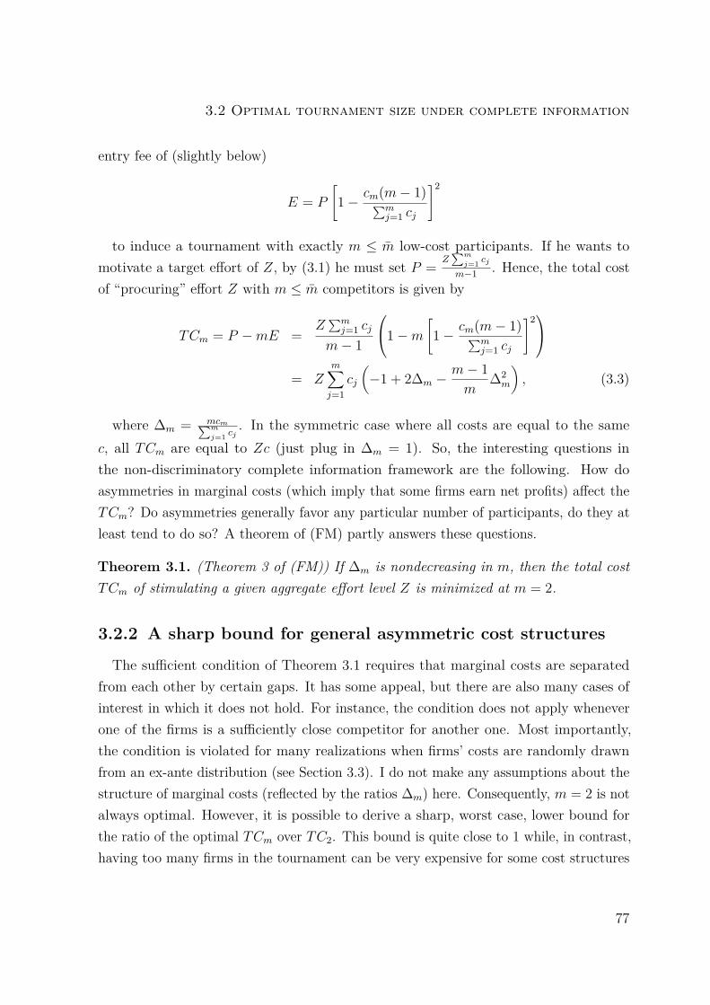
3.2 Optimal tournament size under complete information

entry fee of (slightly below)

E = P

[1− cm(m− 1)∑m

j=1 cj

]2

to induce a tournament with exactly m ≤ m low-cost participants. If he wants tomotivate a target effort of Z, by (3.1) he must set P = Z

∑m

j=1 cj

m−1 . Hence, the total costof “procuring” effort Z with m ≤ m competitors is given by

TCm = P −mE =Z∑mj=1 cj

m− 1

1−m[1− cm(m− 1)∑m

j=1 cj

]2

= Zm∑j=1

cj

(−1 + 2∆m −

m− 1m

∆2m

), (3.3)

where ∆m = mcm∑m

j=1 cj. In the symmetric case where all costs are equal to the same

c, all TCm are equal to Zc (just plug in ∆m = 1). So, the interesting questions inthe non-discriminatory complete information framework are the following. How doasymmetries in marginal costs (which imply that some firms earn net profits) affect theTCm? Do asymmetries generally favor any particular number of participants, do they atleast tend to do so? A theorem of (FM) partly answers these questions.

Theorem 3.1. (Theorem 3 of (FM)) If ∆m is nondecreasing in m, then the total costTCm of stimulating a given aggregate effort level Z is minimized at m = 2.

3.2.2 A sharp bound for general asymmetric cost structures

The sufficient condition of Theorem 3.1 requires that marginal costs are separatedfrom each other by certain gaps. It has some appeal, but there are also many cases ofinterest in which it does not hold. For instance, the condition does not apply wheneverone of the firms is a sufficiently close competitor for another one. Most importantly,the condition is violated for many realizations when firms’ costs are randomly drawnfrom an ex-ante distribution (see Section 3.3). I do not make any assumptions about thestructure of marginal costs (reflected by the ratios ∆m) here. Consequently, m = 2 is notalways optimal. However, it is possible to derive a sharp, worst case, lower bound forthe ratio of the optimal TCm over TC2. This bound is quite close to 1 while, in contrast,having too many firms in the tournament can be very expensive for some cost structures

77

Chapter 3

(see Example 3.1 for an illustration). In this sense, hosting a tournament with the twomost efficient firms is generally not a bad idea.6 However, the analysis also yields thefollowing insights as by-products. First, it is better to have more than two contestantswhenever there exist close competitors for firm 2. Secondly, increasing the number ofparticipants can be really profitable only for intermediate degrees of asymmetry betweenfirms 1 and 2, and the effect is maximal for ∆2 =

√2 (see Remark 3.1).

Theorem 3.2. It holds

infn≥2, 0<c1≤...≤cn, 1≤m<m

TCm+1

TC2= inf

∆2∈[1,2)

1

2[2(1−

√12

)−(√

12∆2 −

√1

∆2

)2]= 1

4(1−

√12

) ≈ 0.85. (3.4)

To prove Theorem 3.2, I first rewrite formula (3.3) in a form that is more suitable forexamining the ratios TCm+1

TC2, m > m ≥ 1.

TCm+1 = Zm+1∑j=1

cj

(−1 + 2∆m+1 −

m

m+ 1 ∆2m+1

)

= Z(m+ 1)cm+1

∆m+1

2(

1−√

m

m+ 1

)∆m+1 −

(√m

m+ 1∆m+1 − 1)2

= Z(m+ 1)cm+1

2(

1−√

m

m+ 1

)−(√

m

m+ 1∆m+1 −√

1∆m+1

)2 .This yields for m > m ≥ 1,

TCm+1

TC2= (m+ 1)cm+1

2c2

[2(1−

√mm+1

)−(√

mm+1∆m+1 −

√1

∆m+1

)2]

[2(1−

√12

)−(√

12∆2 −

√1

∆2

)2]

= m∏j=2

αj

(m+ 1)[2(1−

√mm+1

)−(√

mm+1∆m+1 −

√1

∆m+1

)2]

2[2(1−

√12

)−(√

12∆2 −

√1

∆2

)2] .

(3.5)6The argument is reinforced by the observations that the bound is developed for the case γ = 0, andthat there may be important additional costs related to conducting the tournament (evaluation, etc.)that lie beyond the framework of the model.

78

3.2 Optimal tournament size under complete information

Here αj := cj+1cj

, and an empty product is equal to 1 by convention. By the orderingof costs, ∆m+1 ≥ 1. On the other hand, m

m+1∆m+1 < 1 is necessary for firm m + 1 toenter and to exert positive effort (i.e., for m < m). The following lemma establishes astraightforward recursive formula for ∆m, as well as a necessary and sufficient conditionfor the implication (m ≤ m⇒ m+ 1 ≤ m) in terms of the sequence of marginal costs.

Lemma 3.1. i) It holds

∆m+1 = (m+ 1)cm+1

mcm + ∆m cm+1∆m.

ii) If m−1m

∆m < 1, then

m

m+ 1 ∆m+1 < 1 ⇔ cm+1 <(m− 1m

∆m

)−1cm.

Consequently, each structure of marginal costs that may lead to a situation in whichm+ 1 firms participate in equilibrium is characterized by a sequence of αj satisfying

αj ∈

1,(j − 1j

∆j

)−1 for j = 2, ...,m.

This is all information that is available a priori for studying how small the expression(3.5) may get for arbitrary sequences of marginal costs (that do not satisfy an additionalmonotonicity property like in Theorem 3.1). At first glance, it thus seems rather difficultto find a sharp lower bound for the ratio (3.5). The next observation drastically simplifiesthis task.

Lemma 3.2. Consider any 2 ≤ m ≤ m. If it holds in addition that cm+1 = cm, thenTCm+1 ≤ TCm, i.e. it is weakly better to have a tournament with m+ 1 rather than mparticipants. The inequality is strict unless ∆m = 1.

Lemma 3.2 enables the following proof of Theorem 3.2.

Proof of Theorem 3.2. Lemma 3.2 shows that for any situation in which a tournamentwith m > 2 firms is better than one with 2, one may construct a case in which total costsare even lower with m + 1 firms (by adding another firm whose marginal cost equalsthat of firm m).

79

Chapter 3

Returning to the expression for the ratio of total costs (3.5), mm+1∆m+1 ∈

[mm+1 , 1

)and

∆−1m+1 ∈

(mm+1 , 1

]imply

(√m

m+ 1∆m+1 −√

1∆m+1

)2

= O( 1m2

).

This follows from√x = 1 + 1

2(x− 1) +O((x− 1)2) as x→ 1, which furthermore yields

1−√

m

m+ 1 = 12(m+ 1) +O

( 1m2

).

Hence, asymptotically only the latter term determines the numerator in (3.5). Fora given ∆2 ∈ [1, 2), one may thus reach convergence to the infimum of (3.5) over alladmissible cost structures by setting αj = 1 for all j ≥ 2. The infimum is given by

limm→∞

2(m+ 1)(1−

√mm+1

)2[2(1−

√12

)−(√

12∆2 −

√1

∆2

)2] = 1

2[2(1−

√12

)−(√

12∆2 −

√1

∆2

)2] .

This expression is minimized at ∆2 =√

2 with value 14(

1−√

12

) .Remark 3.1. As indicated above, the proof yields some additional insights: whether itcan be really profitable to allow entry of more than two firms depends crucially on thethe asymmetry between the two strongest firms. In the extremal cases of equal strength(∆2 = 1) and drastic superiority of firm 1 (∆2 → 2), m = 2 is always optimal. Indeed,in these cases the denominator of the ratio (3.5) is equal to 1. The closer the asymmetryis to the geometric mean of these extremes, the more profitable it may be to allow formore contestants to increase competition, but only if there are other firms which are(almost) as strong as firm 2.

To conclude this section, I construct an ad hoc example which shows that the costinefficiency from having too many firms in the tournament may be significantly higherthan the one associated with the worst case bound of Theorem 3.2.

Example 3.1. Consider ∆j = 1 + j−2m−1

1m

for j = 2, ...,m + 1, and for m = 5.7 ThenTC6TC2≈ 1.38.

7For a fully rigorous argument, ∆m+1 has to be slightly below m+1m .

80

3.3 Incomplete information, (FM)’s contestant selection auction, andoptimal tournament size

3.3 Incomplete information, (FM)’s contestantselection auction, and optimal tournament size

In this section, I study the optimal number of participants for the model of incompleteinformation with ex-ante symmetric firms that was used by (FM) to argue in favor ofthe contestant selection auction. The crucial observation, which seems to have goneunnoticed in (FM), is that a separate and more involved analysis is needed for thatpurpose. Both Theorem 3.1 and the results of Section 3.2.2 have been obtained assumingcomplete information and the use of non-discriminatory entry fees. Therefore, theseresults are not applicable (even though they are useful to guide intuition).The type of each firm, i.e. its marginal cost, is drawn ex-ante from a common and

commonly known distribution H with support [c, c] ⊂ R+ and density h. Types areprivate information prior to the tournament. However, they become common knowledgeamong the selected contestants before effort choices are made, so that efforts and profitscan be computed as in Section 3.2.1. (FM) showed that the contestant selection auction,an all-pay entry auction with a small interim prize for entry, performs well in selectingthe most efficient contestants under incomplete information. In contrast, entry fees,uniform-price auctions and discriminatory-price auctions may perform very poorly (seealso Section 3.1). In particular, for independent types the contestant selection auctionalways has a symmetric equilibrium with a bidding function that is strictly decreasing inmarginal cost (Theorem 5 of (FM)). Moreover, for every P and m, the expected totalcost of conducting the tournament, which takes the revenue from the pre-tournamentauction into account, is then formally equivalent to the expression that would arise foran efficient uniform-price auction (Theorem 6 of (FM)). To be precise about the latterpoint, let hn−m,n denote the density of the m+ 1st - lowest out of n independent drawsfrom H. Moreover, let ψ(c, c) denote the conditional expected profit of a firm of type cwhich enters the tournament as the weakest one of m contestants, and which happensto have the same cost as the mth-strongest out of all remaining n− 1 candidates (the“marginal” firm).8 Lemma 3.3 below follows easily from Theorem 6 of (FM).9

8ψ(c, c) is the usual candidate for equilibrium bidding in a uniform-price auction.9For completeness, a proof is included in Section 3.4. The reason is that (FM) presented their resultsin a slightly different model, in which firms/agents are characterized by an ability parameter w. wand c are related by w = 1

c .

81

Chapter 3

Lemma 3.3. With independent types, the expected total cost of conducting a tournamentwith prize P , when the m participants are determined by means of (FM)’s contestantselection auction, is

P −m∫ c

cψ(c, c)hn−m,n(c) dc. (3.6)

For the rest of this chapter, it will be convenient to drop the assumption that c1,...,cm−1

are ordered. Spelling out ψ(c, c) explicitly for γ = 0, one finds (compare (FM), wherethe “max” was forgotten):

ψ(c, c) =∫ c

c...∫ c

cP max

(1− c(m− 1)

c+∑m−1j=1 cj

, 0)2 m−1∏

j=1

h(cj)H(c) dc1...dcm−1. (3.7)

Absent further (and necessarily special) assumptions about the procurer’s utility as afunction of i) the quality of the winning innovation, and ii) monetary costs, the mostnatural and interesting optimization problem is the following, which is analogous to theone in the complete information case: “procure” a given expected effort Z at the lowestpossible expected total cost. Remember from (3.1) that the relationship between prizeP , total equilibrium effort Z = ∑

j∈M zj (where M is the set of firms that make strictlypositive effort) and marginal costs is Z = P (|M |−1)∑

j∈M cj. Thus, to target an expected effort of

Z with m participants, the procurer must set

P = Z

En

[|M |−1∑j∈M cj

∣∣∣∣ |M | ≤ m] .

The conditional expectation in the denominator is the expected total effort made bythe m lowest cost firms (which are selected by the all-pay auction) in a tournament withprize 1. The subscript n indicates the dependence of this expression on the total numberof firms. Plugging ψ(c, c) and the relationship for P into (3.6), one obtains an expression

82

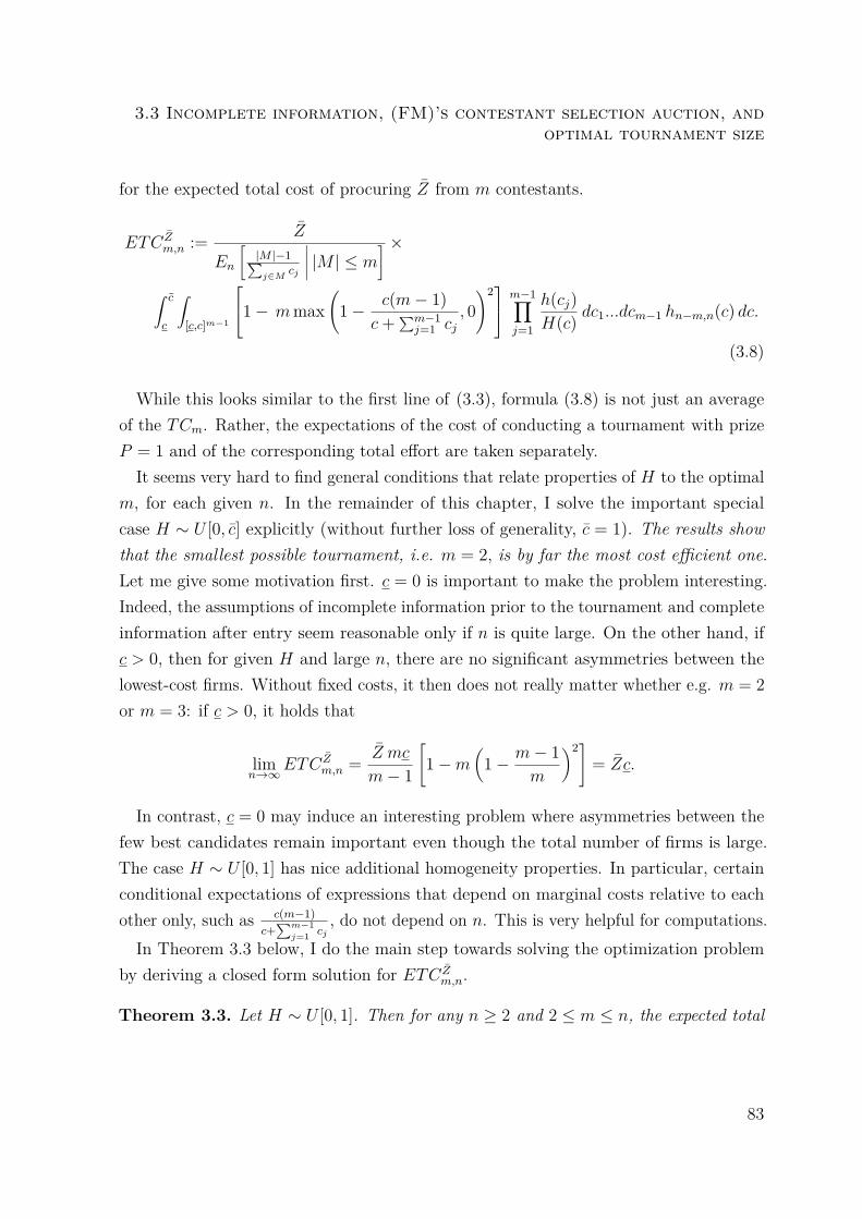
3.3 Incomplete information, (FM)’s contestant selection auction, andoptimal tournament size

for the expected total cost of procuring Z from m contestants.

ETCZm,n := Z

En

[|M |−1∑j∈M cj

∣∣∣∣ |M | ≤ m] ×

∫ c

c

∫[c,c]m−1

1− mmax(

1− c(m− 1)c+∑m−1

j=1 cj, 0)2 m−1∏

j=1

h(cj)H(c) dc1...dcm−1 hn−m,n(c) dc.

(3.8)

While this looks similar to the first line of (3.3), formula (3.8) is not just an averageof the TCm. Rather, the expectations of the cost of conducting a tournament with prizeP = 1 and of the corresponding total effort are taken separately.

It seems very hard to find general conditions that relate properties of H to the optimalm, for each given n. In the remainder of this chapter, I solve the important specialcase H ∼ U [0, c] explicitly (without further loss of generality, c = 1). The results showthat the smallest possible tournament, i.e. m = 2, is by far the most cost efficient one.Let me give some motivation first. c = 0 is important to make the problem interesting.Indeed, the assumptions of incomplete information prior to the tournament and completeinformation after entry seem reasonable only if n is quite large. On the other hand, ifc > 0, then for given H and large n, there are no significant asymmetries between thelowest-cost firms. Without fixed costs, it then does not really matter whether e.g. m = 2or m = 3: if c > 0, it holds that

limn→∞

ETCZm,n = Z mc

m− 1

[1−m

(1− m− 1

m

)2]= Zc.

In contrast, c = 0 may induce an interesting problem where asymmetries between thefew best candidates remain important even though the total number of firms is large.The case H ∼ U [0, 1] has nice additional homogeneity properties. In particular, certainconditional expectations of expressions that depend on marginal costs relative to eachother only, such as c(m−1)

c+∑m−1

j=1 cj, do not depend on n. This is very helpful for computations.

In Theorem 3.3 below, I do the main step towards solving the optimization problemby deriving a closed form solution for ETCZ

m,n.

Theorem 3.3. Let H ∼ U [0, 1]. Then for any n ≥ 2 and 2 ≤ m ≤ n, the expected total

83

Chapter 3

m κm ln 2 +∑mj=3

βj(j−1)!

nZETCZ

m,n

2 0.113706 0.693147 1.114613 0.012558 0.716395 1.343294 0.001373 0.718123 1.384875 0.000142 0.718268 1.391256 0.000014 0.718281 1.39210

Table 3.1: Expected money raised per contestant for P = 1, normalized aggregateexpected effort for P = 1, and normalized expected total cost, for m = 2, ..., 6.

cost for stimulating expected effort Z in a tournament with m participants is

ETCZm,n = Z

n

1−mκmln 2 +∑m

j=3βj

(j−1)!

,

where κ2 = 32 − 2 ln 2, and for m ≥ 3

κm = 1(m− 2)!

[(ln(m− 1)− lnm)

((m− 2)mm−3 − 2(m− 1)mm−2 +mm

)]

+ 1(m− 2)!

m−4∑j=0

(m− 2

m− 3− j −2(m− 1)m− 2− j + m

m− 1− j

)mj

+ 1

(m− 2)!

[(2− 3

2m)mm−3 +mm−1

],

and

βm = (m− 1)−mm−2(ln(m− 1)− lnm)−

m−3∑j=0

mj

m− 2− j

+(m− 2)

(m− 1)m−2(ln(m− 2)− ln(m− 1)) +m−3∑j=0

(m− 1)jm− 2− j

.Theorem 3.3 settles the question about the optimal number of contestants for the

case H ∼ U [0, 1]. It reveals that two contestants are optimal because the decrease inexpected money raised by the entry auction that goes along with increasing tournamentsize strongly dominates the positive effect of increasing aggregate effort. This is shownin Table 3.1 for m = 2, ..., 6. Note in particular the big jump in expected costs fromm = 2 to m = 3.

84

3.4 Appendix for Chapter 3

3.4 Appendix for Chapter 3

Proof of Lemma 3.1. To establish i), note that

1∆m+1

=∑m+1j=1 cj

(m+ 1)cm+1= 1

∆m

mcm(m+ 1)cm+1

+ 1m+ 1 = mcm + ∆m cm+1

(m+ 1)cm+1∆m

.

ii) By i), we have

m

m+ 1 ∆m+1 < 1 ⇔ mcm+1∆m < mcm + ∆m cm+1 ⇔ (m− 1)cm+1∆m < mcm

⇔ cm+1 <m

m− 1∆−1m cm.

Proof of Lemma 3.2. From the technical appendix of (FM) it follows that

TCm+1 − TCm = Zm+1∑j=1

cj

[(∆m+1 −∆m)

(2− m

m+ 1∆m+1 −m− 1m

∆m

)]

+ Zm+1∑j=1

cj

[∆m+1

m+ 1(∆m − 1)(

1− m− 1m

∆m

)].

The factor multiplied with Z ∑m+1j=1 cj has been split into two additive parts merely

due to limitations of space. I examine this factor for the case cm+1 = cm, which by

85

Chapter 3

Lemma 3.1 implies ∆m+1 = (m+1)∆m

m+∆m. This yields

(∆m+1 −∆m)(

2− m

m+ 1∆m+1 −m− 1m

∆m

)+ ∆m+1

m+ 1(∆m − 1)(

1− m− 1m

∆m

)=

((m+ 1)∆m

m+ ∆m

−∆m

)(2− m∆m

m+ ∆m

− m− 1m

∆m

)

+ ∆m

m+ ∆m

(∆m − 1)(

1− m− 1m

∆m

)

= ∆m(1−∆m)m+ ∆m

2(m+ ∆m)−m∆m − m−1m

∆m(m+ ∆m)m+ ∆m

+(∆m − 1)

(∆m − m−1

m∆2m

)m+ ∆m

= ∆m − 1(m+ ∆m)2

[(m+ ∆m)

(∆m −

m− 1m

∆2m

)−∆m

(2m+ (3− 2m)∆m −

m− 1m

∆2m

)]= ∆m − 1

(m+ ∆m)2

[m∆m + ∆2

m − (m− 1)∆2m − 2m∆m − (3− 2m)∆2

m

]= ∆m − 1

(m+ ∆m)2

[(m− 1)∆2

m −m∆m

]= ∆m(∆m − 1)

(m+ ∆m)2 [(m− 1)∆m −m]

Note that (m− 1)∆m −m < 0 by assumption. The other factor is ≥ 0, and equalityholds only in the boundary case ∆m = 1. This proves the claim.

Calculations for Example 3.1. Note that ∆2 = 1 and ∆m+1 = m+1m

. (3.5) implies

TC6

TC2= 5∏j=2

αj

6(1−

√56

) (1 +

√56

)2(1−

√12

) (1 +

√12

) =5∏j=2

αj.

From Lemma 3.1,

∆j+1 = (j + 1)cj+1

jcj + ∆j cj+1∆j = ∆j

j(j+1)αj + ∆j

j+1

,

which yields after a few steps

αj = j∆j+1

∆j(j + 1−∆j+1) .

86

3.4 Appendix for Chapter 3

For the current example, this implies α2 = 2(1+ 120 )

3−(1+ 120 ) = 14

13 . Similarly, α3 = 220203 , α4 =

920847 , α5 = 25

23 and thusTC6

TC2=

5∏j=2

αj ≈ 1.38.

Proof of Lemma 3.3. In (FM), [w, w] (or [w,+∞)) denotes the support of the distributionof an ability type, with c.d.f. H and density h. hm+1,n is the density of the m + 1st-highest draw out of n independent draws from H, and ψ(w,w) is the analog of ψ(c, c).According to Theorem 6 of (FM) then, with independent types, the expected total cost ofconducting a tournament with m contestants when these are selected by the contestantselection auction is

P −m∫ w

wψ(w,w) hm+1,n(w)dw. (3.9)

Set w := 1c, w := 1

c, and w = 1

cin between. Define ψ(w,w) via ψ(w,w) := ψ( 1

w, 1w

).Since dc = − 1

w2 dw, and since increasing c means decreasing w, it holds that h(w) =−h(c) dc

dw= 1

w2 h( 1w

). Moreover, H(w) = 1−H(

1w

).

From the general formula for order statistics, it follows that

hm+1,n(w) = n!(n−m− 1)!m! H(w)n−m−1

(1− H(w)

)mh(w)

= n!m! (n−m− 1)! H

( 1w

)m (1−H

( 1w

))n−m−1 h(

1w

)w2

=hn−m,n( 1

w)

w2 .

Hence, expression (3.9) becomes

P −m∫ w

wψ( 1w,

1w

) hn−m,n(

1w

)w2 dw = P −m

∫ c

cψ(c, c)hn−m,n(c) dc.

Proof of Theorem 3.3. Observe that h(cj)H(c) = 1

c. Let volk(A) denote the k-dimensional

Hausdorff measure of set A. Making use of the Coarea formula for the mapping(c1, ...cm−1) 7→

∑m−1j=1 cj, I find for the crucial term in the second factor of ETCZ

m,n

87

Chapter 3

in (3.8), for m ≥ 3:

∫[0,c]m−1

max(

1− c(m− 1)c+∑m−1

j=1 cj, 0)2 1

cm−1 dc1...dcm−1

= 1cm−1

∫ (m−1)c

(m−2)c

(1− (m− 1)c

c+ a

)2

volm−2

m−1∑j=1

cj = a

∩ [0, c]m−1

√1

m− 1 da

= 1cm−1

∫ c

0

(1− (m− 1)c

mc− a

)2

volm−2

m−1∑j=1

cj = (m− 1)c− a

∩ [0, c]m−1

√1

m− 1 da

= 1cm−1

∫ c

0

(c− amc− a

)2volm−2

m−1∑j=1

cj = a

∩ [0, c]m−1

√1

m− 1 da

= 1cm−1

∫ c

0

(c− amc− a

)2 √m− 1

(m− 2)!√

2m−2(√

2a)m−2

√1

m− 1 da

= 1cm−1(m− 2)!

∫ c

0

(c2am−2 − 2cam−1 + am

(mc− a)2

)da. (3.10)

For the step from line 3 to 4, symmetry with respect to the corners of [0, c]m−1 wasinvoked. In the second but last step, I plugged in a well known formula for the volumeof a simplex of unit side length.

Expression (3.10) shows that a formula for integrals of the form∫ c0

ak

(b−a)2 da for k ≥ 1and b > c is needed. Integrating by parts once,

∫ c

0

ak

(b− a)2 da = ck

b− c− k

∫ c

0

ak−1

b− ada.

Noting that ak−1 = ak−1 − bk−1 + bk−1 = (a − b)(∑k−2

j=0 ak−2−j bj

)+ bk−1 (with the

convention that sums running from j = 0 to −1 are zero), it is straightforward toestablish

∫ c

0

ak

(b− a)2 da = ck

b− c+ kbk−1(ln(b− c)− ln b) +

k−2∑j=0

k bjck−1−j

k − 1− j .

After plugging in and collecting terms, which I omit here for the sake of brevity,

88

3.4 Appendix for Chapter 3

equation (3.10) turns into:

∫[0,c]m−1

max(

1− c(m− 1)c+∑m−1

j=1 cj, 0)2 1

cm−1 dc1...dcm−1

= 1(m− 2)!

[(ln(m− 1)− lnm)

((m− 2)mm−3 − 2(m− 1)mm−2 +mm

)]

+ 1(m− 2)!

m−4∑j=0

(m− 2

m− 3− j −2(m− 1)m− 2− j + m

m− 1− j

)mj

+ 1

(m− 2)!

[(2− 3

2m)mm−3 +mm−1

]= κm.

This expression does not depend on c or n, so that κm is also the expected moneyraised per contestant in the entry auction (for P = 1), irrespectively of n. A separatecalculation is necessary for κ2.

κ2 =∫ c

0

(1− c

c+ c1

)2 1cdc1 = 1

c

∫ c

0

(c1

c+ c1

)2dc1

= 1c

[− c2 +

∫ c

0

2c1

c+ c1dc1

]= −1

2 + 2c

[c ln(2c)−

∫ c

0ln(c+ c1) dc1

]= −1

2 + 2c

[c ln(2c)− 2c ln(2c) + c+ c ln c]

= 32 + 2(ln c− ln(2c)) = 3

2 − 2 ln 2.

Concerning the terms γm,n := En

[|M |−1∑j∈M cj

∣∣∣∣ |M | ≤ m], a separate calculation is again

needed for m = 2.

γ2,n = En

[|M | − 1∑j∈M cj

∣∣∣∣ |M | ≤ 2]

=∫ 1

0

∫ c

0

1c+ c1

1cdc1 hn−1,n(c) dc

=∫ 1

0

∫ c

0

1c+ c1

dc1 n(n− 1)(1− c)n−2 dc

= (ln 2)n(n− 1)∫ 1

0(1− c)n−2 dc = n ln 2.

While it is practically impossible to compute the terms for higher m directly, theymay be computed recursively. Indeed, allowing for an additional contestant has an effecton aggregate equilibrium effort only in those cases where the cost of the new firm is lowenough in the sense of inequality (3.2). Also, in all these relevant cases, if the new firm

89

Chapter 3

is not allowed to participate, then all the lower cost firms make positive effort becauseof the monotonicity of the right hand side of (3.2) that was mentioned in Section 3.2.1.I use the equivalent formulation of (3.2) which was also mentioned in Section 3.2.1 todescribe the domain of integration. Consequently, for m ≥ 3,

γm,n − γm−1,n

=∫ 1

0

hn−m+1,n(c)cm−1

∫[0,c]m−1

(m− 1

c+∑m−1j=1 cj

− m− 2∑m−1j=1 cj

)I{(m−2)c<

∑m−1j=1 cj}

dc1...dcm−1 dc.

The inner integral may again be computed by using the Coarea formula and the littlesymmetry trick:

∫[0,c]m−1

(m− 1

c+∑m−1j=1 cj

− m− 2∑m−1j=1 cj

)I{(m−2)c<

∑m−1j=1 cj}

dc1...dcm−1

=∫ (m−1)c

(m−2)c

(m− 1c+ a

− m− 2a

)volm−2

m−1∑j=1

cj = a

∩ [0, c]m−1

√1

m− 1 da

=∫ c

0

(m− 1mc− a

− m− 2(m− 1)c− a

)volm−2

m−1∑j=1

cj = a

∩ [0, c]m−1

√1

m− 1 da

=∫ c

0

(m− 1mc− a

− m− 2(m− 1)c− a

) √m− 1

(m− 2)!am−2

√1

m− 1 da

= 1(m− 2)!

∫ c

0

((m− 1) am−2

mc− a− (m− 2) am−2

(m− 1)c− a

)da.

Now,

∫ c

0

((m− 1) am−2

mc− a− (m− 2) am−2

(m− 1)c− a

)da

= (m− 1)−(mc)m−2(ln(m− 1)− lnm)−

m−3∑j=0

mj

m− 2− j cm−2

+ (m− 2)

((m− 1)c)m−2(ln(m− 2)− ln(m− 1)) +m−3∑j=0

(m− 1)jm− 2− j c

m−2

= cm−2βm.

90

3.4 Appendix for Chapter 3

Hence,

γm,n − γm−1,n =∫ 1

0

hn−m+1,n(c)cm−1

1(m− 2)!c

m−2 βm dc

= βm1

(m− 2)!

∫ 1

0

n!(n−m)! (m− 1)!(1− c)

n−m cm−2 dc

= βm1

(m− 2)!n!

(n−m)! (m− 1)!(m− 2)!(n−m)!

(n− 1)!= n

(m− 1)! βm.

This shows

γm,n = n

ln 2 +m∑j=3

βj(j − 1)!

.Q.E.D.

91

Chapter 4

Revenue maximization in thedynamic knapsack problem

We analyze maximization of revenue in the dynamic and stochastic knapsack problemwhere a given capacity needs to be allocated by a given deadline to sequentially arrivingagents. Each agent is described by a two-dimensional type that reflects his capacityrequirement and his willingness to pay per unit of capacity. Types are private information.We first characterize implementable policies. Then we solve the revenue maximizationproblem for the special case where there is private information about per-unit values, butcapacity needs are observable. After that we derive two sets of additional conditions onthe joint distribution of values and weights under which the revenue maximizing policyfor the case with observable weights is implementable, and thus optimal also for thecase with two-dimensional private information. In particular, we investigate the role ofconcave continuation revenues for implementation. We also construct a simple policy forwhich per-unit prices vary with requested weight but not with time, and we prove that itis asymptotically revenue maximizing when available capacity and time to the deadlineboth go to infinity. This highlights the importance of nonlinear as opposed to dynamicpricing.

4.1 Introduction

The knapsack problem is a classical combinatorial optimization problem with numerouspractical applications: several objects with given, known capacity needs (or weights) and

93

Chapter 4

given, known values must be packed into a “knapsack” of given capacity to maximize thetotal value of the included objects. In the dynamic and stochastic version (see Ross andTsang, 1989), objects sequentially arrive over time and their weight-value combinationis stochastic but becomes known to the designer at arrival times. Objects cannot berecalled later, so it must be decided upon arrival whether an object is included or not.Several applications that come to mind are logistic decisions in the freight transportationindustry, the allocation of fixed capacities in the travel and leisure industries (e.g., airlines,trains, hotels, rental cars), the allocation of fixed equipment or personnel in a givenperiod of time, the allocation of fixed budgets to investment opportunities that appearsequentially, and the allocation of dated advertising space on web portals.In the present study, we add incomplete information to the dynamic and stochastic

setting. In this way, we obtain a dynamic monopolistic screening problem: there isa finite number of periods, and at each period a request for capacity arrives from anagent who is impatient and privately informed about both his valuation per unit ofcapacity and the needed capacity.1 Each agent derives positive utility if he gets theneeded capacity (or more), and zero utility otherwise. The designer accepts or rejectsthe requests so as to maximize the revenue obtained from the allocation.

The dynamic and stochastic knapsack problem with complete information about valuesand requests was analyzed by Papastavrou, Rajagopalan and Kleywegt (1996) and byKleywegt and Papastavrou (2001). These authors characterized optimal policies in termsof weight-dependent value thresholds. Kincaid and Darling (1963) and Gallego and VanRyzin (1994) examined a setting that can be reinterpreted as having (one-dimensional)incomplete information about values, but in their frameworks all requests have the sameknown weight.2 In particular, Gallego and Van Ryzin showed that optimal expectedrevenue is concave in capacity in the case of equal weights. Kleywegt and Papastavrougave examples showing that total value is not necessarily globally concave in capacityif the weight requests are heterogeneous, and they provided a sufficient condition forthis structural property to hold. Gallego and Van Ryzin also showed that the optimalpolicy, which exhibits complicated time dynamics, can often be replaced by a simpletime-independent policy without much loss: the simple policy performs asymptoticallyoptimal as the number of periods and the units to be sold go to infinity. Finally, Gershkov

1Our results are easily extended to the setting where arrivals are stochastic and/or time is continuous.2We refer the reader to the book by Talluri and Van Ryzin (2004) for references to the large literatureon revenue (or yield) management that adopts variations on these models.

94

4.1 Introduction

and Moldovanu (2009) generalized the Gallego-Van Ryzin model to incorporate objectswith the same weight but with several qualities that are equally ranked by all agents,independently of their types (which are also one-dimensional).

Problems of multi-dimensional mechanism design are usually complex and difficult tosolve: the main problem is that incentive compatibility - which in the one-dimensional caseoften reduces to a monotonicity constraint - imposes, besides a monotonicity requirement,an integrability constraint that is not easily included in maximization problems (seee.g. Rochet, 1985; Armstrong, 1996; Jehiel, Moldovanu and Stacchetti, 1999; and thesurvey of Rochet and Stole, 2003). Our implementation problem is special thoughbecause utilities have a special form and useful deviations in the weight dimension canonly be one-sided (upward). This feature allows a less cumbersome characterization ofimplementable policies that can be embedded in the dynamic analysis under certainconditions on the joint distribution of values and weights of the arriving agents. Othermulti-dimensional mechanism design problems with restricted deviations in one or moredimensions were studied for example by Blackorby and Szalay (2007), Che and Gale(2000), Iyengar and Kumar (2008), Kittsteiner and Moldovanu (2005), and Pai and Vohra(2009).

4.1.1 Outline and preview of results

We first characterize implementable policies, as explained above. Then, we solve therevenue maximization problem for the case where there is private information aboutper-unit values, but weights are observable. We will sometimes refer to this as therelaxed problem. Under a standard monotonicity assumption on virtual values, thisis the virtual value analog of the problem solved by Papastavrou, Rajagopalan andKleywegt (1996). The resulting optimal policy is Markovian and deterministic, and ithas a threshold property with respect to virtual values. It is important to emphasizethat this policy need not be implementable for the case where both values and weightsare unobservable, unless additional conditions are imposed. Our main results in Section4.4 are therefore concerned with the implementability of the relaxed optimal solution:we derive two different sets of additional conditions on the joint distribution of valuesand weights under which the revenue maximizing policy for the case with observableweights is implementable, and thus optimal also for the case with two-dimensional privateinformation. The first set of conditions - which is satisfied in a variety of intuitive settings

95

Chapter 4

- features a hazard rate ordering that expresses a form of positive correlation betweenweights and values. It ensures that the incentive constraint in the capacity dimension isnever binding. Related conditions can be found in previous work on multi-dimensionalmechanism design with restricted deviations mentioned above, e.g. in the papers ofPai and Vohra (2009), Iyengar and Kumar (2008), or Blackorby and Szalay (2007).More interestingly, we also draw a connection between incentive compatibility and thestructural property of concavity of revenue in capacity. Concavity of optimal expectedrevenue in the relaxed problem creates a tendency to set higher virtual value thresholdsfor higher capacity requests. It is then less attractive for agents to overstate theircapacity needs, which facilitates the implementation of the relaxed solution by relaxingthe incentive constraints. We quantify this relation in our second set of additionalconditions: concavity of revenue combined with a (substantial) weakening of the hazardrate order imply implementability of the relaxed solution. For completeness, we alsobriefly translate to our model the sufficient condition for concavity of revenue due toPapastavrou, Rajagopalan and Kleywegt so as to obtain a condition on the model’sprimitives.

The last part of this chapter contains another main result. We construct - for generaldistributions of weights and values - a time-independent, nonlinear price schedule whichis asymptotically revenue maximizing when the available capacity and the time to thedeadline both go to infinity, and when weights are observable. This extends an asymptoticresult by Gallego and van Ryzin (1994) (for a detailed discussion, see Section 4.5) andsuggests that complicated dynamic pricing may not be that important for revenuemaximization if the distribution of agents’ types is known. Our result emphasizes thoughthat nonlinear pricing remains asymptotically important in dynamic settings. As anice link to the first part of the paper, the constructed price schedule turns out to beimplementable for the case with two-dimensional private information if the weakenedhazard rate condition employed in our discussion of concavity is satisfied. Since pricesare time-independent, the policy is also immune to strategic buyer arrivals (which we donot model explicitly here). We also point out that a policy that varies with time butnot with requested weight (whose asymptotic optimality in the complete informationcase was established by Lin, Lu and Yao, 2008) is usually not optimal under incompleteinformation.

The chapter is organized as follows. In Section 4.2 we present the dynamic model and

96

4.2 The model

the informational assumptions about values and weights. In Section 4.3 we characterizeincentive compatible allocation policies. In Section 4.4 we focus on dynamic revenuemaximization. We first characterize the revenue maximizing policy for the relaxedproblem. We then offer two results that exhibit conditions under which the above policyis incentive compatible, and thus optimal also for the case where both values and weightsare private information. Section 4.5 contains the asymptotic analysis. All proofs are inthe Appendix.

4.2 The model

The designer has a “knapsack” of given capacity C ∈ R that he wants to allocate in arevenue-maximizing way to several agents in at most T <∞ periods. In each period,an impatient agent arrives with a demand for capacity characterized by a weight (orquantity request) w, and by a per-unit value v.3 While the realization of the randomvector (w, v) is private information to the arriving agent, its distribution is assumed tobe common knowledge and given by the joint cumulative distribution function F (w, v),with continuously differentiable density f(w, v) > 0, defined on [0,∞)2. w, v and wv allhave finite expected value. Demands are independent across different periods.4

In each period, the designer decides on a capacity to be allocated to the arriving agent(possibly none) and on a monetary payment. Type (w, v)’s utility is given by wv − p ifat price p he is allocated a capacity w′ ≥ w and by −p if he is assigned an insufficientcapacity w′ < w. Each agent observes the remaining capacity of the designer.5 Finally,we assume that for all w, the conditional virtual value functions v(v, w) := v − 1−F (v|w)

f(v|w)

are unbounded as a function of v and strictly monotone increasing with ∂∂vv(v, w) > 0

for all (w, v).

3It is an easy extension to assume that the arrival probability per period is given by p < 1.4As pointed out by a referee, the results of Sections 4.3 and 4.4 apply also, with the obvious modifications,if types in different periods are independent but not necessarily drawn from identical distributions.

5Alternatively, we can assume that each agent observes the entire history of the previous allocations.These assumptions are innocuous in the following sense: when we analyze revenue maximization inSection 4.4, we first solve for the optimal policy in the relaxed problem with observable weight typesw. We then provide conditions for when this relaxed solution is implementable. Since in the caseof observable weight requests, the designer cannot gain by hiding the available capacity, he cannotincrease expected revenue by hiding the remaining capacity in the original problem.

97

Chapter 4

4.3 Incentive compatible policies

To characterize the revenue maximizing scheme, we may restrict attention, withoutloss of generality, to direct mechanisms where every agent, upon arrival, reports a type(w, v) and the mechanism then specifies an allocation and a payment. In this section,we characterize incentive compatibility for a class of allocation policies that necessarilycontains the revenue-maximizing one. The schemes we develop also have an obviousand immediate interpretation as indirect mechanisms, where the designer sets menus ofper-unit prices that depend on time and on the remaining capacity.

An allocation rule is called deterministic and Markovian if, at any period t = 1, ..., Tand for any possible type of agent arriving at t, it uses a non-random allocation rule thatdepends only on the arrival time t, on the declared type of the arriving agent, and oncapacity that is still available, denoted by c. The restriction to these policies is innocuousas shown in Section 4.4.For the purpose of revenue maximization, we can assume without loss of generality

that a deterministic Markovian allocation rule for time t with remaining capacity c hasthe form αct : [0,+∞)2 → {1, 0} where 1 (0) means that the reported capacity demandw is satisfied (not satisfied). Indeed, it never makes sense to allocate an insufficientquantity 0 < w′ < w because individually rational agents are not willing to pay for this.Alternatively, allocating more capacity than the reported demand is useless as well: suchallocations do not further increase agents’ utility while they may decrease continuationrevenues for the designer. Finally, note that all feasible allocation rules αct must satisfyαct(w, v) = 0 for all w > c. qct : [0,+∞)2 → R will denote a payment rule associated withsuch a αct .

Proposition 4.1. A feasible, deterministic, Markovian allocation rule {αct}t,c is imple-mentable if and only if for every t and every c it satisfies the following two conditions.6

i) For all (w, v), v′ ≥ v : αct(w, v) = 1 ⇒ αct(w, v′) = 1.

ii) The function wpct(w) is non-decreasing in w, where pct(w) = inf{v|αct(w, v) = 1}.7

6Here, we use “implementable” in the standard sense from the mechanism design literature. Anallocation rule is implementable if we can associate to it a payment rule such that any agent finds itoptimal to truthfully reveal her type when faced with the combined allocation-payment scheme.

7We set pct(w) =∞ if the set {v|αc

t(w, v) = 1} is empty.

98

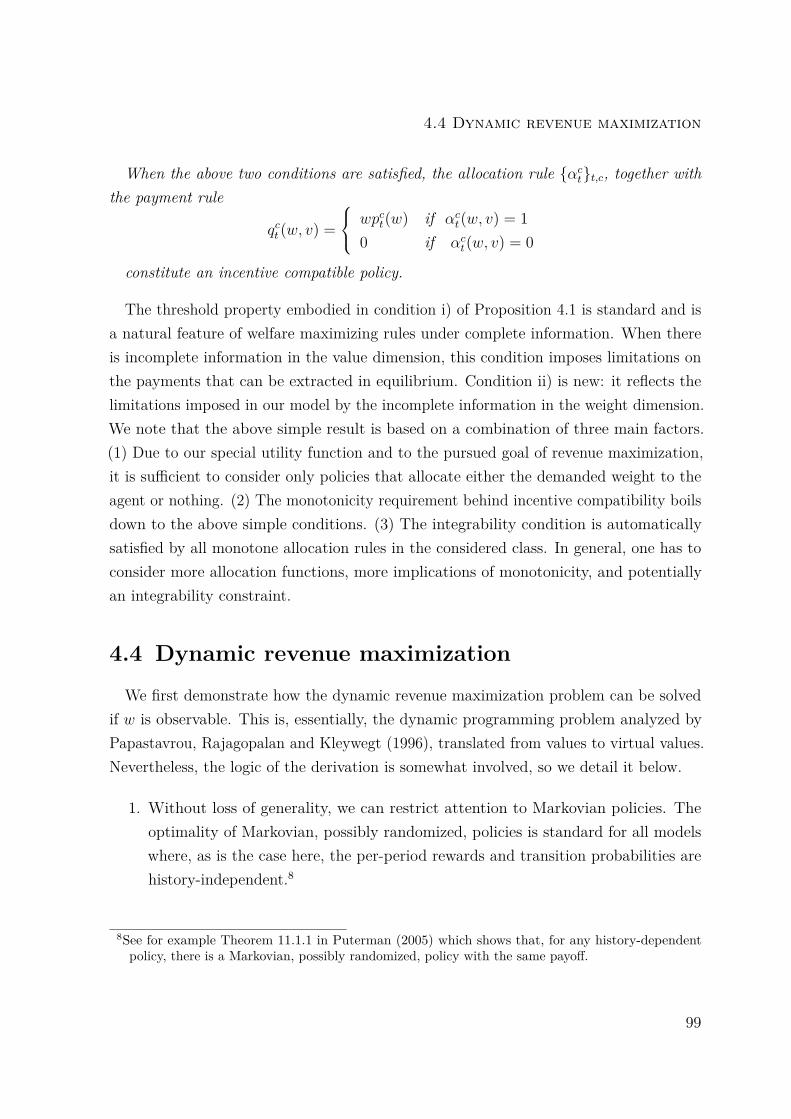
4.4 Dynamic revenue maximization

When the above two conditions are satisfied, the allocation rule {αct}t,c, together withthe payment rule

qct (w, v) =

wpct(w) if αct(w, v) = 10 if αct(w, v) = 0

constitute an incentive compatible policy.

The threshold property embodied in condition i) of Proposition 4.1 is standard and isa natural feature of welfare maximizing rules under complete information. When thereis incomplete information in the value dimension, this condition imposes limitations onthe payments that can be extracted in equilibrium. Condition ii) is new: it reflects thelimitations imposed in our model by the incomplete information in the weight dimension.We note that the above simple result is based on a combination of three main factors.(1) Due to our special utility function and to the pursued goal of revenue maximization,it is sufficient to consider only policies that allocate either the demanded weight to theagent or nothing. (2) The monotonicity requirement behind incentive compatibility boilsdown to the above simple conditions. (3) The integrability condition is automaticallysatisfied by all monotone allocation rules in the considered class. In general, one has toconsider more allocation functions, more implications of monotonicity, and potentiallyan integrability constraint.

4.4 Dynamic revenue maximization

We first demonstrate how the dynamic revenue maximization problem can be solvedif w is observable. This is, essentially, the dynamic programming problem analyzed byPapastavrou, Rajagopalan and Kleywegt (1996), translated from values to virtual values.Nevertheless, the logic of the derivation is somewhat involved, so we detail it below.

1. Without loss of generality, we can restrict attention to Markovian policies. Theoptimality of Markovian, possibly randomized, policies is standard for all modelswhere, as is the case here, the per-period rewards and transition probabilities arehistory-independent.8

8See for example Theorem 11.1.1 in Puterman (2005) which shows that, for any history-dependentpolicy, there is a Markovian, possibly randomized, policy with the same payoff.

99

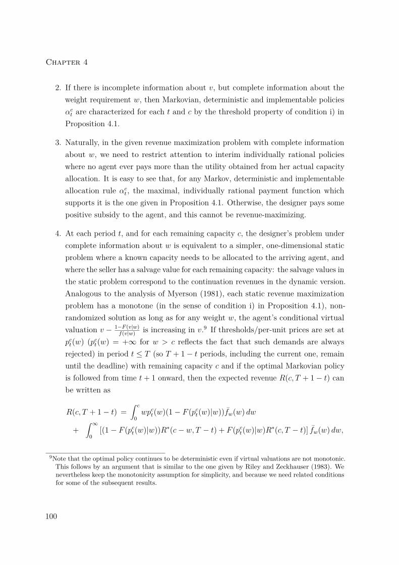
Chapter 4

2. If there is incomplete information about v, but complete information about theweight requirement w, then Markovian, deterministic and implementable policiesαct are characterized for each t and c by the threshold property of condition i) inProposition 4.1.

3. Naturally, in the given revenue maximization problem with complete informationabout w, we need to restrict attention to interim individually rational policieswhere no agent ever pays more than the utility obtained from her actual capacityallocation. It is easy to see that, for any Markov, deterministic and implementableallocation rule αct , the maximal, individually rational payment function whichsupports it is the one given in Proposition 4.1. Otherwise, the designer pays somepositive subsidy to the agent, and this cannot be revenue-maximizing.

4. At each period t, and for each remaining capacity c, the designer’s problem undercomplete information about w is equivalent to a simpler, one-dimensional staticproblem where a known capacity needs to be allocated to the arriving agent, andwhere the seller has a salvage value for each remaining capacity: the salvage values inthe static problem correspond to the continuation revenues in the dynamic version.Analogous to the analysis of Myerson (1981), each static revenue maximizationproblem has a monotone (in the sense of condition i) in Proposition 4.1), non-randomized solution as long as for any weight w, the agent’s conditional virtualvaluation v − 1−F (v|w)

f(v|w) is increasing in v.9 If thresholds/per-unit prices are set atpct(w) (pct(w) = +∞ for w > c reflects the fact that such demands are alwaysrejected) in period t ≤ T (so T + 1− t periods, including the current one, remainuntil the deadline) with remaining capacity c and if the optimal Markovian policyis followed from time t+ 1 onward, then the expected revenue R(c, T + 1− t) canbe written as

R(c, T + 1− t) =∫ c

0wpct(w)(1− F (pct(w)|w))fw(w) dw

+∫ ∞

0[(1− F (pct(w)|w))R∗(c− w, T − t) + F (pct(w)|w)R∗(c, T − t)] fw(w) dw,

9Note that the optimal policy continues to be deterministic even if virtual valuations are not monotonic.This follows by an argument that is similar to the one given by Riley and Zeckhauser (1983). Wenevertheless keep the monotonicity assumption for simplicity, and because we need related conditionsfor some of the subsequent results.

100

4.4 Dynamic revenue maximization

where fw denotes the marginal density in w, and where R∗ denotes optimal expectedrevenues, with R∗(c, 0) = 0 for all c. The revenue maximizing unit prices willbe called pct(w) from now on. For w ≤ c, they are determined by the first-orderconditions

w

(pct(w)− 1− F (pct(w)|w)

f(pct(w)|w)

)= R∗(c, T − t)−R∗(c− w, T − t).10

5. By backward induction, and by the above reasoning, the seller has a Markov,non-randomized optimal policy in the dynamic problem with complete informationabout w. Note also that, by a simple duplication argument, R∗(c, T + 1− t) mustbe monotone non-decreasing in c.

If the above solution to the relaxed problem satisfies the incentive compatibilityconstraint in the weight dimension, i.e. if wpct(w) happens to be monotone as requiredby condition ii) of Proposition 4.1, then the associated allocation where αct(w, v) = 1if and only if v ≥ pct(w) is also implementable in the original problem with incompleteinformation about both v and w. It then constitutes the revenue maximizing schemethat we are after. The next example illustrates that condition ii) of Proposition 4.1 canbe binding.

Example 4.1. Assume that T = 1. The distribution of the agents’ types is given bythe following stochastic process. First, the weight request w is realized according toan exponential distribution with parameter λ. Next, the per-unit value of the agent issampled from the following distribution

F (v|w) =

1− e−λv if w > w∗

1− e−λv if w ≤ w∗

where λ > λ and w∗ ∈ (0, c).In this case, for an observable weight request, the seller charges the take-it-or-leave-it

offer of 1λ( 1λ) per unit if the weight request is smaller than or equal to (larger than) w∗.

10Note that by our assumption of unbounded conditional virtual values, which is a mild assumption fordistributions with unbounded support, these first-order conditions always admit a solution and mustbe satisfied at the optimum.

101

Chapter 4

This implies that

wpct(w) =

wλ

if c ≥ w > w∗

wλ

if w ≤ w∗

and, therefore, wpct(w) is not monotone.

4.4.1 The hazard rate stochastic ordering

A simple sufficient condition that guarantees implementability of the relaxed solutionis a particular stochastic ordering of the conditional distributions of per-unit values: theconditional distribution given a higher weight should be (weakly) statistically higher inthe hazard rate order than the conditional distribution given a lower weight. This issimilar to conditions found in static frameworks by Pai and Vohra (2009), Iyengar andKumar (2008), or Blackorby and Szalay (2007).

Theorem 4.1. For each c, t, and w, let pct(w) denote the solution to the problem ofmaximizing expected revenue under complete information about w, determined recursivelyby the Bellman equation

w

(pct(w)− 1− F (pct(w)|w)

f(pct(w)|w)

)= R∗(c, T − t)−R∗(c− w, T − t). (4.1)

Assume that the following conditions hold.

i) For any w, the conditional hazard rate f(v|w)1−F (v|w) is non-decreasing in v.11

ii) For any w′ ≥ w, and for any v, f(v|w)1−F (v|w) ≥

f(v|w′)1−F (v|w′) .

Then, wpct(w) is non-decreasing in w, and, consequently, the underlying allocationwhere αct(w, v) = 1 if and only if v ≥ pct(w) is implementable. In particular, (4.1)characterizes the revenue maximizing scheme under incomplete information about bothvalues and weights.

An important special case for which the conditions of Theorem 4.1 hold is where thedistribution of per-unit values is independent of the distribution of weights and has anincreasing hazard rate.

11Note that this condition already implies the needed monotonicity in v of the conditional virtual valuefor all w.

102

4.4 Dynamic revenue maximization

4.4.2 The role of concavity

A major result for the case where capacity comes in discrete units, and where allweights are equal is that optimal expected revenue is concave in capacity.12 This is a veryintuitive property since it says that additional capacity is more valuable to the designerwhen capacity itself is scarce. Due to the more complicated combinatorial nature ofthe knapsack problem with heterogeneous weights, concavity need not generally hold(see Papastavrou, Rajagopalan and Kleywegt, 1996, for examples where concavity ofexpected welfare in the framework with complete information fails). When concavitydoes hold, the optimal per-unit virtual value thresholds for the relaxed problem increasewith weight, which facilitates implementation for the case of two-dimensional privateinformation.Our main result in this subsection identifies a condition on the distribution of types

that, together with concavity of the expected revenue in the remaining capacity, ensuresthat for each t and c, wpct(w) is increasing.

Theorem 4.2. Assume the following conditions.

i) The expected revenue R∗(c, T + 1− t) is a concave function of c for all times t.

ii) For any w ≤ w′, v − 1−F (v|w)f(v|w) ≥

vww′− 1−F ( vw

w′ |w′)

f( vww′ |w

′) .

For each c, t, and w, let pct(w) denote the solution to the problem of maximizing expectedrevenue under complete information about w, determined recursively by (4.1). Thenwpct(w) is non-decreasing in w, and hence the underlying allocation where αct(w, v) = 1if and only if v ≥ pct(w) is implementable. In particular, (4.1) characterizes the revenuemaximizing scheme under incomplete information about both values and weights.

Remark 4.1. The sufficient conditions for implementability used in Theorem 4.1 are,taken together, stronger than condition ii) in Theorem 4.2. To see this, assume that forany w, the conditional hazard rate f(v|w)

1−F (v|w) is increasing in v, and that for any w′ ≥ w

and for all v, f(v|w)1−F (v|w) ≥

f(v|w′)1−F (v|w′) . This yields:

v − 1− F (v|w)f(v|w) ≥ vw

w′−

1− F (vww′|w)

f(vww′|w) ≥ vw

w′−

1− F (vww′|w′)

f(vww′|w′) ,

12See Gallego and van Ryzin (1994) for a continuous time framework with Poisson arrivals and Bitranand Mondschein (1997) for a discrete time setting.

103

Chapter 4

where the first inequality follows by the monotonicity of the hazard rate, and the secondfollows by the stochastic order assumption. Note also that condition ii) of Theorem 4.2will play an important role for implementability of the asymptotically optimal policy thatwe construct in Section 4.5.

We next modify a result of Papastavrou, Rajagopalan and Kleywegt (1996) so as toidentify conditions on the joint distribution F (w, v) that imply concavity of expectedrevenue with respect to c for all periods, as required by Theorem 4.2.13 It is convenientto introduce the joint distribution of weight and total valuation u = vw, which wedenote by G(w, u) with density g(w, u). By means of a transformation of variables, thedensities f and g are related by wg(w,wv) = f(w, v). In particular, marginal densitiesin w coincide, i.e.

fw(w) =∫ ∞

0f(w, v) dv =

∫ ∞0

g(w, u) du = gw(w).

Under our assumptions, the virtual total value is increasing in u with strictly positivederivative for any given w. This follows from the identity

u(u,w) := u− 1−G(u|w)g(u|w) = wv − 1− F (v|w)

f(v|w)/w = wv(v, w).

We write u−1(u, w) for the inverse of u(u,w) with respect to u and define a distributionG(u, w) by both G(u|w) := G(u−1(u, w)|w) for all w and ¯gw(w) := gw(w). On the levelof v, this corresponds to F (v|w) = F (v−1(v, w)|w) and ¯

fw(w) = fw(w).

Theorem 4.3. Assume that the conditional distribution G(w|u) is concave in w for allu, that both g(w|u) and d

dwg(w|u) are bounded, and that the total virtual value u has a

finite mean. Then, in the revenue maximization problem where the designer has completeinformation about w, the expected revenue R∗(c, T + 1− t) is concave as a function of cfor all times t.

Example 4.2. A simple setting where the conditions of Theorem 4.2 are satisfied whilethose of Theorem 4.1 are violated is obtained as follows. Assume that G(w, u) is such13In the Appendix we also provide an elementary proof of the result of Papastavrou, Rajagopalan

and Kleywegt, since a proof is neither contained in the above-mentioned paper nor in the relatedone by Kleywegt and Papastavrou (2001). Moreover, we were unable to find a general result fromfinite horizon stochastic dynamic programming that ensures concavity of expected value in the statevariable c, which is only a part of the relevant state description.

104

4.5 Asymptotically optimal and time-independent pricing

that u and w are independent, the hazard rate gu(u)1−Gu(u) is non-decreasing, and Gw is

concave.14 Then condition i) of Theorem 4.2 is satisfied according to Theorem 4.3because the G(w|u) are concave. Consider then w < w′. By independence of u and w, wehave w′v(vw

w′, w′) = u(vw,w′) = u(vw,w) = wv(v, w) and hence v(v, w) = w′

wv(vw

w′, w′).

As w′

w> 1, this implies condition ii) of Theorem 4.2 in the relevant domain where

virtual values are non-negative. However, as we show now, condition ii) of Theorem4.1, i.e. the hazard rate ordering, is violated. Indeed, the equation we have just derivedimplies also that f(v|w)

1−F (v|w) = ww′

f( vww′ |w

′)1−F ( vw

w′ |w′) . But the conditional hazard rates of F are non-

decreasing (because Gu has non-decreasing hazard rate) and ww′< 1, so that f(v|w)

1−F (v|w) =ww′

f( vww′ |w

′)1−F ( vw

w′ |w′) <

f(v|w′)1−F (v|w′) , which contradicts the hazard rate ordering of Theorem 4.1.

4.5 Asymptotically optimal and time-independentpricing

The optimal policy identified above requires price adjustments in every period and forany quantity request w. These dynamics are arguably too complicated to be appliedin practice. Gallego and van Ryzin (1994) used an asymptotic argument to showthat the theoretical gain from optimal dynamic pricing compared to a suitably chosen,time-independent policy is usually small in the setting with unit demands. Our maintheorem in this section extends their result to the dynamic knapsack problem withgeneral distribution of types. We construct a static nonlinear price schedule that usesthe existing correlations between w and v, and we show that it is asymptotically optimalif both capacity and time horizon go to infinity.While the basic strategy of the proof follows the suggestion made by Gallego and

van Ryzin, there are several major differences. In fact, in Section 5 of their paper theseauthors also considered the case of heterogeneous capacity demands. However, theyassumed that weights and values are independent and, most importantly, their optimalitybenchmark does not even allow per-unit prices to depend on weight requests. But, as wesaw above, such weight dependency is a general property of the dynamically optimalsolution, even if w and v are independent. We therefore take our solution of the relaxedproblem as the optimality benchmark, and we also consider general type distributions F .

14We also assume that the other mild technical conditions of Theorem 4.3 are satisfied.

105

Chapter 4

As above, we start by focusing on the case of observable weights. We then show thatcondition ii) of Theorem 4.2 is a sufficient condition for implementability for the casewith two-dimensional private information.

Like Gallego and van Ryzin, we first solve a simpler, suitably chosen deterministicmaximization problem. The revenue obtained in the solution to that problem providesan upper bound for the optimal expected revenue of the stochastic problem, and thesolution itself suggests the use of per-unit prices that depend on weight requests, but thatare constant in time. We next show that the derived policy is asymptotically optimalalso in the original stochastic problem where both capacity and time go to infinity: theratio of expected revenue from following the considered policy over expected revenuefrom the optimal Markovian policy converges to one. Moreover, there are various waysto quantify this ratio for moderately large capacities and time horizons.Let us first recall some assumptions and introduce further notation. The marginal

density fw(w) and the conditional densities f(v|w) pin down the distribution of (inde-pendent) arriving types (wt, vt)Tt=1. Given w, the demanded per-unit price p and theprobability λw of a request being accepted are related by λw(p) = 1−F (p|w). Let pw(λ)be the inverse of λ, and note that this is well defined on (0, 1]. Because of monotonicityof conditional virtual values, the instantaneous (expected) per-unit revenue functionsrw(λ) := λ pw(λ) are strictly concave, and each one attains a unique interior maximum.Indeed, pw(λ) = F (·|w)−1(1− λ) and hence

d

dλrw(λ) = pw(λ)− λ 1

f(pw(λ)|w) = pw(λ)− 1− F (pw(λ)|w)f(pw(λ)|w) = v(pw(λ), w),

d2

dλ2 rw(λ) = −

(∂

∂vv

)(pw(λ), w) 1

f(pw(λ)|w) < 0.

Consequently, rw is strictly concave, strictly increasing up to the λw,∗ that satisfiesv(pw(λw,∗), w) = 0, and strictly decreasing from there on.

4.5.1 The deterministic problem

We now formulate an auxiliary deterministic problem that closely resembles the relaxedstochastic problem. Let Cap : (0,∞)→ (0,∞) , w 7→ Cap(w) be a measurable function.

106

4.5 Asymptotically optimal and time-independent pricing

Consider the problem:

maxCap(·)

∫ ∞0

max(λwt )t=1,...,T

(T∑t=1

rw(λwt ))wfw(w) dw, (4.2)

subject to

T∑t=1

λwt wfw(w) ≤ Cap(w) a.s. and∫ ∞

0Cap(w) dw ≤ C. (4.3)

In words, we analyze a problem where the following statements are true.

1. The capacity C needs to be divided into capacities Cap(w), one for each w.

2. In each w subproblem, a deterministic quantity request of wfw(w) arrives in eachperiod, and λwt determines a share (not a probability!) of this request that isaccepted and sold at per-unit price pw(λwt ).

3. In each subproblem, the allocated capacity over time cannot exceed Cap(w), andtotal allocated capacity in all subproblems

∫∞0 Cap(w) dw cannot exceed C.

4. The designer’s goal is to maximize total revenue. We call the revenue at thesolution Rd(C, T ).

As rw is strictly concave and increasing up to λw,∗, it is straightforward to verify that,given a choice Cap(w), the solution to the w subproblem

max(λwt )t=1,...,T

(T∑t=1

rw(λwt ))wfw(w) such that

T∑t=1

λwt wfw(w) ≤ Cap(w)

is given by

λwt ≡ λw,d :=

λw,∗ if λw,∗ ≤ Cap(w)

Twfw(w)Cap(w)Twfw(w) else.

(4.4)

Accordingly, the revenue in the w subproblem is rw(λw,d)Twfw(w).

Proposition 4.2. The solution to the deterministic problem given by (4.2) and (4.3) ischaracterized by

107

Chapter 4

i) v(pw(λw,d), w) = β(C, T ) = const,

ii) λwt = λw,d = Cap(w)Twfw(w) ,

iii)∫∞0 Cap(w) dw = min(C, T

∫∞0 λw,∗wfw(w) dw).

To get an intuition for the above result, observe that the marginal increase of theoptimal revenue for the w subproblem from marginally increasing Cap(w) is

(d

dλrw)(

Cap(w)Twfw(w)

)= v(pw(λw,d), w) if λw,∗ > Cap(w)

Twfw(w),

and 0 otherwise. Proposition 4.2 says that, optimally, the capacity should be split insuch a way that the marginal revenue from increasing Cap(w) is the same for all w.Actually solving the problem amounts to the simple static exercise of determining theconstant β(C, T ) in accordance with the integral feasibility constraint.The above construction is justified by the following two-step argument: on the one

hand, we show in Theorem 4.4 below that the optimal revenue in the deterministicproblem, Rd(C, T ), bounds from above the optimal revenue in the original stochastic case.On the other hand, as we show in Section 4.5.2, the optimal solution of the deterministicproblem serves to define a simple time-independent policy that in the stochastic problemcaptures revenues RTI(C, T ) such that RTI(C,T )

Rd(C,T ) converges to 1 as C and T go to infinity.Combining these two points yields the kind of asymptotic optimality result we want toestablish.

Since we assume here that weights are observable, a Markovian policy α for the originalstochastic problem is characterized by the acceptance probabilities λwtt [ct] contingent oncurrent time t, remaining capacity ct, and weight request wt. Expected revenue frompolicy α at the beginning of period t (i.e. when there are (T − t+ 1) periods left) withremaining capacity ct is given by

Rα(ct, T − t+ 1) = Eα

[T∑s=t

ws pws(λwss [cs]) I{vs≥pws (λwss [cs])}

]

such thatT∑s=t

ws I{vs≥pws (λwss [cs])} ≤ ct.

Here, the constraint must hold almost surely when following α. As before, we writeR∗(ct, T − t+ 1) for the optimal revenue, i.e. the supremum of expected revenues taken

108

4.5 Asymptotically optimal and time-independent pricing

over all feasible Markovian policies α.

Theorem 4.4. For any capacity C and deadline T , it holds that R∗(C, T ) ≤ Rd(C, T ).

4.5.2 A simple policy for the stochastic problem

Having established the upper bound of Theorem 4.4, we proceed with the second partof our two-step argument outlined in the preceding section. We use the optimal solutionof the deterministic problem to define a w-contingent yet time-independent policy αTIfor the stochastic case as follows.

1. Given C and T , solve the deterministic problem to obtain β(C, T ), λw,d and thuspw,d := pw(λw,d) = v−1(β(C, T ), w).

2. In the stochastic problem charge these weight-contingent prices pw,d for the entiretime horizon, provided that the quantity request does not exceed the remainingcapacity. Else, charge a price equal to +∞ (i.e., reject the request).

Note that under condition ii) of Theorem 4.2, the time-independent policy αTI isalso implementable if weights are not observable! Indeed, setting all virtual valuationthresholds equal to a constant is like setting them optimally for linear and hence concavesalvage values.

We now determine how well the time-independent policy constructed above performscompared to the optimal Markovian policy. Recall that we do this by comparing itsexpected revenue, RTI(C, T ), with the optimal revenue in the deterministic problem,Rd(C, T ), which, as we know by Theorem 4.4, provides an upper bound for the optimalrevenue in the stochastic problem, R∗(C, T ).

Theorem 4.5. i) For any joint distribution of values and weights

limC,T→∞,C

T=const

RTI(C, T )Rd(C, T ) = 1.

ii) Assume that w and v are independent. Then

RTI(C, T )Rd(C, T ) ≥

1 −

√E[w2]/E[w]

2√

min(C, λ∗E[w]T )

.

109

Chapter 4

In particular, limmin(C,T )→∞RTI(C,T )Rd(C,T ) = 1.

We have chosen to focus on these two general limit results, but various other quan-titative results could be proven by similar techniques at the expense of slightly moretechnical effort and possibly some further assumptions on the distribution F . This shouldbe clear from the proof in the Appendix. Since the policy αTI is stationary, it does notgenerate incentives to postpone arrivals even in a more complex model where buyers arepatient and can choose their arrival time.

Remark 4.2. In a complete information knapsack model, Lin, Lu and Yao (2008)studied policies that start by accepting only high value requests and then switch over toaccepting also lower values as time goes by. They established asymptotic optimality ofsuch policies (with carefully chosen switch-over times) as available capacity and timego to infinity. In other words, their prices are time-dependent but do not conditionon the weight request. It is easy to show that, in our incomplete information model,such policies are in general suboptimal. Consider first a one-period example where theseller has capacity 2, and where the arriving agent has either a weight request of 1 or2 (equally likely). If the weight request is 1(2), the agent’s per-unit value distributesuniformly between 0 and 1 (between 1 and 2). The optimal mechanism in this case isas follows: if the buyer requests one unit, the seller sells it for a price of 0.5, and ifthe buyer requests two units, the seller sells each unit at a price of 1. Note that thispolicy is implementable since the requested per-unit price is monotonically increasing inthe weight request. The expected revenue is 9

8 . If, however, the seller is forced to sellall units at the same per-unit price without conditioning on the weight request, he willcharge the price of 1 for each unit, yielding an expected revenue of 1, and thus loose 1

8

versus the optimal policy. Now replicate this problem so that there are T periods andcapacity C=2T. Then, the expected revenue from the optimal mechanism is 9

8T , while theexpected revenue from the constrained mechanism is only T. Obviously, the constrainedmechanism is not asymptotically optimal.

4.6 Appendix for Chapter 4

Proof of Proposition 4.1. =⇒. So assume that conditions i) and ii) are satisfied anddefine for any t, c,

110

4.6 Appendix for Chapter 4

qct (w, v) =

wpct(w) if αct(w, v) = 1

0 if αct(w, v) = 0.

Consider then an arrival of type (w, v) in period t with remaining capacity c. There aretwo cases.a) αct(w, v) = 1. In particular, v ≥ pct(w). Then, truth-telling yields utility w(v −

pct(w)) ≥ 0. Assume that the agent reports instead (w, v). If αct(w, v) = 0, then theagent’s utility is zero and the deviation is not profitable. Assume then that αct(w, v) = 1.By the form of the utility function, a report of w < w is never profitable. But, forw ≥ w, the agent’s utility is wv − wpct(w) ≤ w(v − pct(w)), where we used condition ii).Therefore, such a deviation is also not profitable.

b) αct(w, v) = 0. In particular, v ≤ pct(w). Truth-telling yields here utility of zero.Assume that the agent reports instead (w, v). If αct(w, v) = 0, then the agent’s utilityremains zero, and the deviation is not profitable. Assume then that αct(w, v) = 1. By theform of the utility function, a report of w < w is never profitable. Thus, consider thecase where w ≥ w. In this case, the agent’s utility is wv − wpct(w) ≤ w(v − pct(w)) ≤ 0,where we used condition ii). Therefore, such a deviation is also not profitable.

⇐=. Consider now an implementable, deterministic and Markovian allocation policy{αct}t,c. Assume first, by contradiction, that condition i) is not satisfied. Then, there exist(w, v) and (w, v′) such that v′ > v, αct(w, v) = 1 and αct(w, v′) = 0. We obtain the chainof inequalities wv′ − qct (w, v) > wv − qct (w, v) ≥ −qct (w, v′) where the second inequalityfollows by incentive compatibility for type (w, v). This shows that a deviation to areport (w, v) is profitable for type (w, v′), a contradiction to implementability. Therefore,condition i) must hold.In particular, note that for any two types who have the same weight request, (w, v)

and (w, v′), if both are accepted, i.e. αct(w, v) = αct(w, v′) = 1, the payment must be thesame (otherwise the type which needs to make the higher payment would deviate andreport the other type). Denote this payment by rct (w). Note also that any two types(w, v) and (w′, v′) such that αct(w, v) = αct(w′, v′) = 0 must also make the same payment(otherwise the type that needs to make the higher payment would deviate and reportthe other type) and denote this payment by s.Assume now, by contradiction, that condition ii) does not hold. Then there exist

w and w′ such that w′ > w but w′pct(w′) < wpct(w). In particular, w′pct(w′) < ∞, and

111

Chapter 4

therefore pct(w′) <∞.Assume first that pct(w) < ∞. We have w′pct(w′) − rct (w′) = wpct(w) − rct (w) = −s

because, by incentive compatibility, both types (w, pct(w)) and (w′, pct(w′)) must beindifferent between getting their request and not getting it. Since by assumptionw′pct(w′) < wpct(w), we obtain that rct (w′) < rct (w). Consider now a type (w, v) for whichv > pct(w). By reporting truthfully, this type gets utility wv−rct (w), while by deviating to(w′, v) he gets utility wv−rct (w′) > wv−rct (w), a contradiction to incentive compatibility.

Assume now that pct(w) is infinite, and therefore wpct(w) is infinite. Consider a type(w′, v) where v > pct(w′). The utility of this type is w′v−rct (w′) > w′pct(w′)−rct (w′) = −s.In particular, rct (w′) must be finite. By reporting truthfully, a type (w, v) gets utility−s , while by deviating to a report of (w′, v) he gets wv − rct (w′). For v large enough,we obtain wv − rct (w′) > −s, a contradiction to implementability.

Thus, condition ii) must hold and, in particular, the payment rct (w) is monotonic inw.

Proof of Theorem 4.1. Let w < w′. We need to show that wpct(w) − w′pct(w′) ≤ 0. Ifpct(w) ≤ pct(w′), the result is clear. Assume then that pct(w) > pct(w′). We obtain thefollowing chain of inequalities:

w

(1− F (pct(w)|w)f(pct(w)|w)

)− w′

(1− F (pct(w′)|w′)f(pct(w′)|w′)

)

≤ w′(

1− F (pct(w)|w)f(pct(w)|w) − 1− F (pct(w′)|w′)

f(pct(w′)|w′)

)

≤ w′(

1− F (pct(w′)|w)f(pct(w′)|w) − 1− F (pct(w′)|w′)

f(pct(w′)|w′)

)≤ 0,

where the second inequality follows by the monotonicity of the hazard rate and thethird follows by the hazard rate ordering condition.Since R∗(c− w, T − t) is monotonically decreasing in w, we obtain that

w

(pct(w)− 1− F (pct(w)|w)

f(pct(w)|w)

)≤ w′

(pct(w′)−

1− F (pct(w′)|w′)f(pct(w′)|w′)

)⇔

wpct(w)− w′pct(w′) ≤ w

(1− F (pct(w)|w)f(pct(w)|w)

)− w′

(1− F (pct(w′)|w′)f(pct(w′)|w′)

)≤ 0,

where the last inequality follows by the derivation above. Hence wpct(w)− w′pct(w′) ≤ 0

112

4.6 Appendix for Chapter 4

as desired.

Proof of Theorem 4.2. For any concave function φ, and for any x < y < z in its domain,the well known “Three Chord Lemma” asserts that

φ(y)− φ(x)y − x

≥ φ(z)− φ(x)z − x

≥ φ(z)− φ(y)z − y

.

Consider then w < w′ and let x = c−w′ < y = c−w < z = c. For the case of a concaverevenue, the lemma then yields

R∗(c− w, T − t)−R∗(c− w′, T − t)w′ − w

≥ R∗(c, T − t)−R∗(c− w′, T − t)w′

≥ R∗(c, T − t)−R∗(c− w, T − t)w

.

We obtain in particular

pct(w′)−1− F (pct(w′)|w′)f(pct(w′)|w′)

= R∗(c, T − t)−R∗(c− w′, T − t)w′

≥ R∗(c, T − t)−R∗(c− w, T − t)w

= pct(w)− 1− F (pct(w)|w)f(pct(w)|w) ,

which yields

pct(w′)−1− F (pct(w′)|w′)f(pct(w′)|w′)

≥ pct(w)− 1− F (pct(w)|w)f(pct(w)|w) ≥ w

w′pct(w)−

1− F ( ww′pct(w)|w′)

f( ww′pct(w)|w′)

where the last inequality follows by the condition in the statement of the Theorem.Since virtual values are increasing, this yields pct(w′) ≥ w

w′pct(w)⇔ w′pct(w′) ≥ wpct(w) as

desired.

For the proof of Theorem 4.3, we first need a lemma on maximization of expectedwelfare under complete information. The result appears (without proof) in Papastavrou,Rajagopalan and Kleywegt (1996).

Lemma 4.1. Assume that the total value u has finite mean, and that both g(w|u) andddwg(w|u) are bounded and continuous. Consider the allocation policy that maximizes

expected welfare under complete information (i.e., upon arrival the agent’s type is revealedto the designer). If G(w|u) is concave in w for all u, then the optimal expected welfare,

113

Chapter 4

denoted U ct , is twice continuously differentiable and concave in the remaining capacity c

for all periods t ≤ T .

Proof of Lemma 4.1. Note that, for notational convenience throughout this proof, weindex optimal expected welfare by the current time t and not by periods remaining todeadline. By standard arguments, the optimal policy for this unconstrained dynamicoptimization problem is deterministic and Markovian, and U c

t is non-decreasing inremaining capacity c by a simple strategy duplication argument. Moreover, the optimalpolicy can be characterized by weight thresholds wct (u) ≤ c : If c remains at time t anda request whose acceptance would generate value u arrives, then it is accepted if andonly if w ≤ wct (u). If U c

t+1 ≥ u, then the weight threshold must satisfy the indifferencecondition

u = U ct+1 − U

c−wct (u)t+1 . (4.5)

Otherwise, we have wct (u) = c.We now prove the lemma by backward induction. At time t = T , i.e. in the deadlineperiod, it holds that

U cT =

∫ ∞0

G(c|u)u gu(u) du.

This is concave in c because all G(c|u) are concave by assumption, because u gu(u)is positive, and because the distribution of u has a finite mean. Since both g(w|u) andddwg(w|u) are bounded and continuous, U c

T is also twice continuously differentiable.Suppose now that the lemma has been proven down to time t+ 1. The optimal expectedwelfare at t provided that capacity c remains may be written as

U ct =

∫ ∞0

[uG(wct (u)|u) +

∫ wct (u)

0U c−wt+1 g(w|u) dw + (1−G(wct (u)|u))U c

t+1

]gu(u) du.

(4.6)We proceed to show concavity with respect to c of the term in brackets, for all u.

This in turn implies concavity of U ct and hence, with a short additional argument for

differentiability, is sufficient to conclude the induction step. We distinguish the casesu > U c

t+1 for which the indifference condition (4.5) does not hold, and u ≤ U ct+1 for

which it does. For both cases, we demonstrate that the second derivative (one-sided ifnecessary) of the bracket term with respect to c is non-positive, and thus establish globalconcavity.Case 1: u > U c

t+1. The bracket term becomes uG(c|u) +∫ c0 U

c−wt+1 g(w|u) dw + (1 −

114

4.6 Appendix for Chapter 4

G(c|u))U ct+1. By continuity of U c

t+1, this representation also holds in a small intervalaround c. We find

d

dc

[uG(c|u) +

∫ c

0U c−wt+1 g(w|u) dw + (1−G(c|u))U c

t+1

]= ug(c|u) +

∫ c

0

d

dcU c−wt+1 g(w|u) dw + U0

t+1 g(c|u)

−g(c|u)U ct+1 + (1−G(c|u)) d

dcU ct+1

= (u− U ct+1)g(c|u) +

∫ c

0

d

dcU c−wt+1 g(w|u) dw + (1−G(c|u)) d

dcU ct+1

and

d2

dc2

[uG(c|u) +

∫ c

0U c−wt+1 g(w|u) dw + (1−G(c|u))U c

t+1

]= (u− U c

t+1)g′(c|u)− g(c|u) ddcU ct+1 +

∫ c

0

d2

dc2Uc−wt+1 g(w|u) dw

+ d

dwUwt+1

∣∣∣w=0

g(c|u)− g(c|u) ddcU ct+1 + (1−G(c|u)) d

2

dc2Uct+1. (4.7)

The last term is non-positive by the concavity of U ct+1, the first term is non-positive

because u > U ct+1 and because G(c|u) has a non-increasing density by assumption. In

addition, g(c|u) ddcU ct+1 is non-negative, and hence (4.7) is bounded from above by

∫ c

0

d2

dc2Uc−wt+1 g(w|u) dw + g(c|u)

(d

dwUwt+1

∣∣∣w=0− d

dcU ct+1

).

But∫ c

0d2

dc2Uc−wt+1 g(w|u) dw may be bounded from above by g(c|u)

∫ c0

d2

dc2Uc−wt+1 dw because

of the decreasing density and because d2

dc2Uc−wt+1 ≤ 0. Thus,

d2

dc2

[uG(c|u) +

∫ c

0U c−wt+1 g(w|u) dw + (1−G(c|u))U c

t+1

]≤ g(c|u)

[∫ c

0

d2

dc2Uc−wt+1 dw + d

dwUwt+1

∣∣∣w=0− d

dcU ct+1

]

= g(c|u)[∫ c

0

d2

dw2Uc−wt+1 dw + d

dwUwt+1

∣∣∣w=0− d

dcU ct+1

]= 0. (4.8)

Case 2: u ≤ U ct+1 . Here u = U c

t+1 − Uc−wct (u)t+1 . Consequently, the bracket term in

115

Chapter 4

(4.6) becomes

U ct+1 − U

c−wct (u)t+1 G(wct (u)|u) +

∫ wct (u)

0U c−wt+1 g(w|u) dw. (4.9)

Before computing its first and second derivatives, we differentiate the identity u =U ct+1−U

c−wct (u)t+1 to obtain an expression for d

dcwct (u) (derivative from the right if u = U c

t+1):

0 = d

dcU ct+1 −

d

dwUwt+1

∣∣∣w=c−wct (u)

(1− d

dcwct (u)

).

Since indeed ddwUwt+1 > 0 in our setup with strictly positive densities, this implies

d

dcwct (u) =

ddwUwt+1

∣∣∣w=c−wct (u)

− ddcU ct+1

ddwUwt+1

∣∣∣w=c−wct (u)

. (4.10)

By concavity of U ct+1, its derivative is non-increasing and hence the identity (4.10)

yields in particular ddcwct (u) ≥ 0. We now compute the derivatives of (4.9):

d

dc

[U ct+1 − U

c−wct (u)t+1 G(wct (u)|u) +

∫ wct (u)

0U c−wt+1 g(w|u) dw

]

= d

dcU ct+1 −

d

dwUwt+1

∣∣∣w=c−wct (u)

(1− d

dcwct (u)

)G(wct (u)|u)

−U c−wct (u)t+1 g(wct (u)|u) d

dcwct (u)

+Uc−wct (u)t+1 g(wct (u)|u) d

dcwct (u) +

∫ wct (u)

0

d

dcU c−wt+1 g(w|u) dw

(4.10)= d

dcU ct+1 −

d

dcU ct+1G(wct (u)|u) +

∫ wct (u)

0

d

dcU c−wt+1 g(w|u) dw

= d

dcU ct+1(1−G(wct (u)|u)) +

∫ wct (u)

0

d

dcU c−wt+1 g(w|u) dw.

116

4.6 Appendix for Chapter 4

Thus,

d2

dc2

[U ct+1 − U

c−wct (u)t+1 G(wct (u)|u) +

∫ wct (u)

0U c−wt+1 g(w|u) dw

]

= d2

dc2Uct+1(1−G(wct (u)|u))− d

dcU ct+1 g(wct (u)|u) d

dcwct (u)

+ d

dwUwt+1

∣∣∣w=c−wct (u)

g(wct (u)|u) ddcwct (u) +

∫ wct (u)

0

d2

dc2Uc−wt+1 g(w|u) dw

≤ g(wct (u)|u) ddcwct (u)

(d

dwUwt+1

∣∣∣w=c−wct (u)

− d

dcU ct+1

)+∫ wct (u)

0

d2

dw2Uc−wt+1 g(w|u) dw.

For the final inequality we used concavity of U ct+1, as well as d2

dc2Uc−wt+1 = d2

dw2Uc−wt+1 .

Noting that (4.10) implies that ddcwct (u) ≤ 1 and once more using concavity of U c

t+1, wemay bound the first term from above. Since g(w|u) is non-increasing in w, we can alsobound the second term to obtain

d2

dc2

[U ct+1 − U

c−wct (u)t+1 G(wct (u)|u) +

∫ wct (u)

0U c−wt+1 g(w|u) dw

](4.11)

≤ g(wct (u)|u)(d

dwUwt+1

∣∣∣w=c−wct (u)

− d

dcU ct+1 +

∫ wct (u)

0

d2

dw2Uc−wt+1 dw

)= 0.

Taken together, (4.8) and (4.11) establish concavity of the integrand in (4.6) withrespect to c. This implies that U c

t is concave. Having a second look at the computationsjust performed reveals that the integrand in (4.6) has a kink in the second derivativeat u = U c

t+1. However, this event has measure zero for any given c, so that we also getthat U c

t is twice continuously differentiable. This completes the induction step.

Proof of Theorem 4.3. The main idea of the proof is to translate the problem of maxi-mizing revenue when w is observable into the problem of maximizing welfare with respectto virtual values (rather than values) and to use Lemma 4.1 then.To begin with, note that there is a dual way to describe the policy that maximizes

expected welfare under complete information. In the proof of Lemma 4.1, we characterizedit by optimal weight thresholds wct (u). Alternatively, given any requested quantity w ≤ c,we may set a valuation per unit threshold vct (w). Requests above this valuation areaccepted, those below are not. Such optimal thresholds are characterized by the Bellman-type condition

wvct (w) = U ct+1 − U c−w

t+1 .

117

Chapter 4

Thus, using vct (w) = +∞ for w > c, one way to write optimal expected welfare undercomplete information is

U ct =

∫ c

0w∫ ∞vct (w)

vf(v|w) dv fw(w) dw

+∫ ∞

0

[(1− F (vct (w)|w))U c−w

t+1 + F (vct (w)|w)U ct+1

]fw(w) dw. (4.12)

In contrast, the optimal expected revenue with complete information about w butincomplete information about v satisfies

R∗(c, T + 1− t) =∫ c

0w pct(w) (1− F (pct(w)|w)) fw(w) dw (4.13)

+∫ ∞

0[(1− F (pct(w)|w))R∗(c− w, T − t) + F (pct(w)|w)R∗(c, T − t)] fw(w) dw,

where pct(w) are the per-unit prices from (4.1). We rephrase this in terms of F , whosedefinition required monotonicity of virtual values. Setting vct (w) := v(pct(w), w) we haveon the one hand

F (pct(w)|w) = F (vct (w)|w).

On the other hand,

pct(w) (1− F (pct(w)|w)) =∫ ∞pct (w)

[v f(v|w)− (1− F (v|w))] dv

=∫ ∞pct (w)

v(v, w) f(v(v, w)|w) ddvv(v, w) dv

=∫ ∞vct (w)

v f(v|w) dv.

Plugging this and the identities for the marginal densities in w into (4.13), we obtain:

R∗(c, T + 1− t) =∫ c

0w∫ ∞vct (w)

vf(v|w) dv ¯fw(w) dw

+∫ ∞

0

[(1− F (vct (w)|w))R∗(c− w, T − t) + F (vct (w)|w)R∗(c, T − t)

] ¯fw(w) dw.

Comparing this with (4.12), it follows that maximizing expected revenue when w isobservable is equivalent to maximizing expected welfare with respect to the distributionof weight and conditional virtual valuation (note the identical zero boundary values atT + 1). Invoking Lemma 4.1 applied to G, we see that R∗(c, T + 1− t) is concave with

118

4.6 Appendix for Chapter 4

respect to c for all t (note that the fact that the support of virtual valuations containsalso negative numbers does not matter for the argument of Lemma 4.1).

Proof of Proposition 4.2. The proposition is an immediate consequence of the charac-terization (4.4) of optimal solutions for the w subproblems given Cap(w), and of astraightforward variational argument ensuring that marginal revenues from marginalincrease of Cap(w) must be constant almost surely in w.

Proof of Theorem 4.4. We need to distinguish two cases.

Case 1: Assume that C > T∫∞

0 λw,∗wfw(w) dw. In this case, β(C, T ) = 0 andRd(C, T ) = T

∫∞0 rw(λw,∗)wfw(w) dw. We also know that R∗(C, T ) ≤ R∗(+∞, T ), where

R∗(+∞, T ) denotes the optimal expected revenue from a stochastic problem without anycapacity constraint. But for such a problem, the optimal Markovian policy maximizes ateach period the instantaneous expected revenue upon observing wt, wt rwt(λ). That is,the optimal policy sets λwtt [+∞] = λw,∗. Thus,

R∗(C, T ) ≤ R∗(+∞, T ) = T∫ ∞

0wrw(λw,∗)fw(w) dw = Rd(C, T ).

Case 2: Assume now that C ≤ T∫∞

0 λw,∗wfw(w) dw. For µ ≥ 0, consider theunconstrained maximization problem

maxCap(·)

[∫ ∞0

rw(

Cap(w)Twfw(w)

)Twfw(w) dw + µ

(C −

∫ ∞0

Cap(w) dw)].

The Euler-Lagrange equation is(ddλrw) (

Cap(w)Twfw(w)

)= µ. Hence, if we write Rd(C, T, µ)

for the optimal value of the above problem and if we let µ = β(C, T ), where β(C, T ) isthe constant from Proposition 4.2, then the solution equals the one of the constraineddeterministic problem. In particular

∫∞0 Cap(w) dw = C, and Rd(C, T, β(C, T )) =

Rd(C, T ) .Recall that for the stochastic problem and for any Markovian policy α we have

Rα(C, T ) = Eα

[T∑t=1

wt pwt(λwtt [ct]) I{vt≥pwt (λwtt [ct])}

],

119

Chapter 4

and define

Rα(C, T, β(C, T )) = Rα(C, T ) + β(C, T )(C − Eα

[T∑t=1

wt I{vt≥pwt (λwtt [ct])}

]).

Since for any policy α that is admissible in the original problem, it holds that

T∑t=1

wt I{vt≥pwt (λwtt [ct])} ≤ C a.s.,

we have Rα(C, T ) ≤ Rα(C, T, β(C, T )). We show below that, for arbitrary α (whichmay or may not satisfy the capacity constraint), it holds that

Rα(C, T, β(C, T )) ≤ Rd(C, T, β(C, T )). (4.14)

This yields, for any α that is admissible in the original problem,

Rα(C, T ) ≤ Rα(C, T, β(C, T )) ≤ Rd(C, T, β(C, T )) = Rd(C, T ).

Taking the supremum over α then concludes the proof for the second case.It remains to prove (4.14). The argument uses the filtration {Ft}Tt=1 of σ-algebras that

contain information prior to time t (in particular the value of ct) and, in addition, the

120

4.6 Appendix for Chapter 4

currently observed wt.

Rα(C, T, β(C, T )) = Eα

[T∑t=1

wt (pwt(λwtt [ct])− β(C, T )) I{vt≥pwt (λwtt [ct])}

]+ β(C, T )C

= Eα

[T∑t=1

Eα[wt (pwt(λwtt [ct])− β(C, T )) I{vt≥pwt (λwtt [ct])}|Ft

]]+ β(C, T )C

= Eα

[T∑t=1

wt (pwt(λwtt [ct])− β(C, T ))Eα[I{vt≥pwt (λwtt [ct])}|Ft

]]+ β(C, T )C

= Eα

[T∑t=1

wt (rwt(λwtt [ct])− β(C, T )λwtt [ct])]

+ β(C, T )C

≤ Eα

[T∑t=1

wt(rwt(λwt,d)− β(C, T )λwt,d

)]+ β(C, T )C

= E(wt)Tt=1

[T∑t=1

wt(rwt(λwt,d)− β(C, T )λwt,d

)]+ β(C, T )C

= T∫ ∞

0(rw(λw,d)− β(C, T )λw,d)wfw(w) dw + β(C, T )C = Rd(C, T, β(C, T )).

For the inequality, we have used that λw,d maximizes rw(λ)− β(C, T )λ.

For the proof of Theorem 4.5, we first need a lemma.

Lemma 4.2. Let RTI(C, T ) be the expected revenue obtained form the stationary policyαTI . Let (wt, vt)Tt=1 be an independent copy of the process (wt, vt)Tt=1. Then

i)

RTI(C, T ) = E(wt)Tt=1

[T∑t=1

rwt(λwt,d)wt(

1− P[t−1∑s=1

wsI{vs≥pws,d}> C − wt

])],

ii)

RTI(C, T )Rd(C, T ) ≥ 1−

∑Tt=1

∫∞0 rw(λw,d)w

(min

(1, (t−1)σ2

d

((T−t+1)µd−w)2

)I1 + I2

)fw(w) dw

T∫∞

0 rw(λw,d)wfw(w) dw.

where µd := min(C,T∫∞

0 λw,∗wfw(w) dw)T

, I1 := I{w≤(T−t+1)µd}, I2 := I{w>(T−t+1)µd}, andσ2d := E[w2I{v≥pw,d}]− µ2

d =∫∞

0 w2λw,dfw(w) dw − µ2d.

121

Chapter 4

Proof of Lemma 4.2. RTI(C, T ) may be written as

RTI(C, T ) = E(wt,vt)Tt=1

T∑t=1

pwt,dwt I{vt≥pwt,d} I{∑t−1

s=1 wsI{vs≥pws,d}≤C−wt

}= E(wt)Tt=1

[T∑t=1

rwt(λwt,d)wt]

−E(wt,vt)Tt=1

T∑t=1

pwt,dwt I{vt≥pwt,d} I{∑t−1

s=1 wsI{vs≥pws,d}>C−wt

} .To simplify the second term, we use the fact that vt and (ws, vs)t−1

s=1 are independentconditional on wt.

E(wt,vt)Tt=1

T∑t=1

pwt,dwt I{vt≥pwt,d} I{∑t−1

s=1 ws I{vs≥pws,d}>C−wt

}= E(wt,vt)Tt=1

T∑t=1

E

pwt,dwt I{vt≥pwt,d} I{∑t−1s=1 ws I{vs≥pws,d}

>C−wt} |wt

= E(wt,vt)Tt=1

T∑t=1

pwt,dwtE[I{vt≥pwt,d}|wt

]E

I{∑t−1s=1 ws I{vs≥pws,d}

>C−wt} |wt

= E(wt,vt)Tt=1

[T∑t=1

pwt,dwt λwt,d P

[t−1∑s=1

ws I{vs≥pws,d}> C − wt

]]

= E(wt)Tt=1

[T∑t=1

rwt(λwt,d)wt P[t−1∑s=1

ws I{vs≥pws,d}> C − wt

]].

This establishes i). Recall that Rd(C, T ) = T∫∞0 rw(λw,d)wfw(w) dw then. Observe

furthermore that λw,d depends on C and T only through the ratio Ceff

T, where Ceff =

min(C, T∫∞

0 λw,∗wfw(w) dw), via E[wI{v≥pw,d}] =∫∞

0 wλw,dfw(w) dw = Ceff

T= µd.

Observe first that

P

[t−1∑s=1

ws I{vs≥pws,d}> C − wt

]≤ P

[t−1∑s=1

ws I{vs≥pws,d}> Tµd − wt

]

= P

[t−1∑s=1

ws I{vs≥pws,d}− (t− 1)µd > (T − t+ 1)µd − wt

].

We trivially bound the last expression by 1 if (T − t+ 1)µd − wt ≤ 0, and otherwise

122

4.6 Appendix for Chapter 4

use Chebychev’s inequality to deduce

P

[t−1∑s=1

ws I{vs≥pws,d}− (t− 1)µd > (T − t+ 1)µd − wt

]

≤ P

(t−1∑s=1

ws I{vs≥pws,d}− (t− 1)µd

)2

> ((T − t+ 1)µd − wt)2

≤E

[(∑t−1s=1 ws I{vs≥pws,d}

− (t− 1)µd)2]

((T − t+ 1)µd − wt)2 = (t− 1)σ2d

((T − t+ 1)µd − wt)2 .

As we are bounding a probability, we can replace this estimate by the trivial bound 1again whenever this is better, i.e. if wt is smaller than but close to (T − t+ 1)µd. Thus,

E(wt,vt)Tt=1

[T∑t=1

pwt,dwt I{vt≥pwt,d} I{∑t−1

s=1 ws I{vs≥pws,d}>C−wt}

]

≤T∑t=1

∫ ∞0

rw(λw,d)w(

min(

1, (t− 1)σ2d

((T − t+ 1)µd − w)2

)I1 + I2

)fw(w) dw.

Finally, dividing by Rd(C, T ) yields ii).

Proof of Theorem 4.5. We first prove i). I1 and I2 are defined as in Lemma 4.2, and thestarting point for the proof is estimate ii) from that lemma.Note that rw(λw,d)wfw(w) is an integrable upper bound for

rw(λw,d)w(

min(

1, (t− 1)σ2d

((T − t+ 1)µd − w)2

)I1 + I2

)fw(w).

Moreover, for fixed w, for arbitrary η ∈ (0, 1) and for t ≤ ηT we have w < (1− η)Tµdeventually as T,C →∞, C

T= const. Moreover,

(t− 1)σ2d

((T − t+ 1)µd − w)2 ≤ηTσ2

d

((1− η)Tµd − w)2 → 0, as T →∞.

The Dominated Convergence Theorem implies then that

∫ ∞0

rw(λw,d)w(

min(

1, (t− 1)σ2d

((T − t+ 1)µd − w)2

)I1 + I2

)fw(w) dw → 0,

123

Chapter 4

in the considered limit, for arbitrary η ∈ (0, 1) and for t ≤ ηT . Consequently, also theterm that is subtracted in estimate ii) of Lemma 4.2 converges to zero. This proves i).We now prove ii). A straightforward application of the proof by Gallego and Van

Ryzin is possible for this last part. For completeness, we spell it out. If w and v areindependent, all the λw,d for different w coincide, as do the λw,∗. Call them λd and λ∗,respectively. We then have

RTI(C, T ) = p(λd)E[min

(C,

T∑t=1

wt I{vt≥p(λd)}

)]

= p(λd)E T∑t=1

wt I{vt≥p(λd)} −(

T∑t=1

wt I{vt≥p(λd)} − C

)+ .We use now the following estimate for E[(X − k)+], where X is a random variable

with mean m and variance σ2 and where k is a constant:

E[(X − k)+] ≤

√σ2 + (k −m)2 − (k −m)

2 .

Note that by independence

E

[T∑t=1

wt I{vt≥p(λd)}

]= E[w]Tλd,

V ar

[T∑t=1

wt I{vt≥p(λd)}

]= T

(E[(w I{v≥p(λd)})2]− E[w]2(λd)2

)= T

(E[w2]λd − E[w]2(λd)2

).

If λ∗TE[w] > C and hence if λd = CTE[w] this yields

RTI(C, T ) ≥ Rd(C, T )− p(λd)

√TE[w2]λd

2 = Rd(C, T )1−

√E[w2]/E[w]

2√C

.If λ∗TE[w] ≤ C and hence if λd = λ∗, then C ≥ E

[∑Tt=1wt I{vt≥p(λd)}

], so that

124

4.6 Appendix for Chapter 4

E[(∑T

t=1wt I{vt≥p(λd)} − C)+]≤√σ2

2 . Thus,

RTI(C, T ) ≥ Rd(C, T )− p(λ∗)

√λ∗TE(w2)

2 = Rd(C, T )1−

√E[w2]/E[w]

2√λ∗E(w)T

.Hence, we can conclude that

RTI(C, T )Rd(C, T ) ≥

1−

√E[w2]/E[w]

2√

min(C, Tλ∗E[w]))

.

125

Bibliography

[1] Acemoglu, D. (1996): “A Microfoundation for Social Increasing Returns in HumanCapital Accumulation,” Quarterly Journal of Economics 111, 779-804.

[2] Acemoglu, D., and J. A. Robinson: Why Nations Fail, Crown Publishers, New York,2012.

[3] Akerlof, G. A. (1970): “The Market for “Lemons”: Quality Uncertainty and theMarket Mechanism,” Quarterly Journal of Economics 84, 488-500.

[4] Allen, F. (1985): “On the Fixed Nature of Sharecropping Contracts,” The EconomicJournal 95, 30-48.

[5] Armstrong, M. (1996): “Multiproduct Nonlinear Pricing,” Econometrica 64, 51-75.

[6] Baye, M. R., and H. C. Hoppe (2003): “The Strategic Equivalence of Rent-Seeking,Innovation, and Patent-Race Games,” Games and Economic Behavior 44, 217-226.

[7] Becker, G. S. (1973): “A Theory of Marriage: Part 1,” Journal of Political Economy81, 813-846.

[8] Bergemann, D., and S. Morris (2005): “Robust Mechanism Design,” Econometrica73, 1771-1813.

[9] Bergemann, D., and J. Välimäki (2002): “Information Acquisition and EfficientMechanism Design,” Econometrica 70, 1007-1033.

127

Bibliography

[10] Bhaskar, V., and E. Hopkins (2011): “Marriage as a Rat Race: Noisy Pre-MaritalInvestments with Assortative Matching,” Unpublished working paper, University ofEdinburgh.

[11] Bikhchandani, S. (2006): “Ex post implementation in environments with privategoods,” Theoretical Economics 1, 369-393.

[12] Bitran, G. R., and S. V. Mondschein (1997): “Periodic Pricing of Seasonal Productsin Retailing,” Management Science 43, 64-79.

[13] Blackorby, C., and D. Szalay (2007): “Multidimensional Screening, Affiliation, andFull Separation,” Warwick Economic Research Paper 802, Department of Economics,University of Warwick.

[14] Brouwer, L. E. J. (1911): “Beweis der Invarianz der Dimensionzahl,” MathematischeAnnalen 70, 161-165.

[15] Brusco, S., G. Lopomo, D. T. Robinson, and S. Viswanathan (2007): “EfficientMechanisms For Mergers And Acquisitions,” International Economic Review 48,995-1035.

[16] Chakraborty, A., A. Citanna, and M. Ostrovsky (2010): “Two-sided matching withinterdependent values,” Journal of Economic Theory 145, 85-105.

[17] Chao, K. (1983): “Tenure Systems in Traditional China,” Economic Developmentand Cultural Change 31, 295-314.

[18] Che, Y.-K., and I. Gale (2000): “The Optimal Mechanism for Selling to a Budget-Constrained Buyer,” Journal of Economic Theory 92, 198-233.

[19] Che, Y.-K., and I. Gale (2003): “Optimal Design of Research Contests,” AmericanEconomic Review 93, 646-671.

[20] Che, Y.-K., J. Kim, and F. Kojima (2012): “Efficient Assignment with Interdepen-dent Values,” Working paper, Columbia University.

[21] Chiappori, P.-A., R. J. McCann, and L. P. Nesheim (2010): “Hedonic price equilibria,stable matching, and optimal transport: equivalence, topology, and uniqueness,”Economic Theory 42, 317-354.

128

Bibliography

[22] Coase, R. H. (1960): “The Problem of Social Cost,” Journal of Law and Economics3, 1-44.

[23] Cole, H. L., G. J. Mailath, and A. Postlewaite (2001a): “Efficient Non-ContractibleInvestments in Large Economies,” Journal of Economic Theory 101, 333-373.

[24] Cole, H. L., G. J. Mailath, and A. Postlewaite (2001b): “Efficient Non-ContractibleInvestments in Finite Economies,” Advances in Theoretical Economics 1, Iss. 1,Article 2.

[25] Cramton, P., R. Gibbons, and P. Klemperer (1987): “Dissolving a PartnershipEfficiently,” Econometrica 55, 615-632.

[26] Dasgupta, P., and E. Maskin (2000): “Efficient Auctions,” Quarterly Journal ofEconomics 115, 341-388.

[27] Dizdar, D., A. Gershkov, and B. Moldovanu (2011): “Revenue maximization in thedynamic knapsack problem,” Theoretical Economics 6, 157-184.

[28] Ekeland, I. (2005): “An optimal matching problem,” ESAIM: Control, Optimisation,and Calculus of Variations 11, 57-71.

[29] Ekeland, I. (2010): “Existence, uniqueness and efficiency of equilibrium in hedonicmarkets with multidimensional types,” Economic Theory 42, 275-315.

[30] Felli, L., and K. Roberts (2001): “Does Competition Solve the Hold-Up Problem?”Theoretical Economics Discussion Paper TE/01/414, STICERD, London School ofEconomics.

[31] Fieseler, K., T. Kittsteiner, and B. Moldovanu (2003): “Partnerships, lemons andefficient trade,” Journal of Economic Theory 113, 223-234.

[32] Figalli, A., Y.-H. Kim, and R. J. McCann (2011): “When is multidimensionalscreening a convex program?” Journal of Economic Theory 146, 454-478.

[33] Fullerton, R. L., B. G. Linster, M. McKee, and S. Slate (2002): “Using Auctions toReward Tournament Winners: Theory and Experimental Investigations,” The RandJournal of Economics 33, 62-84.

129

Bibliography

[34] Fullerton, R. L., and R. P. McAfee (1999): “Auctioning Entry into Tournaments,”Journal of Political Economy 107, 573-605.

[35] Gärtner, D. L., and A. Schmutzler (2009): “Merger negotiations and ex-post regret,”Journal of Economic Theory 144, 1636-1664.

[36] Gale, D., and L. S. Shapley (1962): “College Admissions and the Stability ofMarriage,” American Mathematical Monthly 69, 9-15.

[37] Gall, T., P. Legros, and A. F. Newman (2012): “Mismatch, Rematch, and Invest-ment,” Unpublished working paper, University of Bonn.

[38] Gallego, G., and G. Van Ryzin (1994): “Optimal Dynamic Pricing of Inventorieswith Stochastic Demand over Finite Horizons,” Management Science 40, 999-1020.

[39] Gershkov, A., and B. Moldovanu (2009): “Dynamic Revenue Maximization with Het-erogenous Objects: A Mechanism Design Approach,” American Economic Journal:Microeconomics 1, 168-198.

[40] “Gesetz über Arbeitnehmererfindungen,” Bundesgesetzblatt Teil III,Gliederungsnummer 422-1, 25.07.1957, (German Law about Employees’ In-ventions, last amended 2009).

[41] Gretzky, N. E., J. M. Ostroy, and W. R. Zame (1992): “The nonatomic assignmentmodel,” Economic Theory 2, 103-127.

[42] Gretzky, N. E., J. M. Ostroy, and W. R. Zame (1999): “Perfect Competition in theContinuous Assignment Model,” Journal of Economic Theory 88, 60-118.

[43] Hopkins, E. (2012): “Job Market Signaling Of Relative Position, Or Becker MarriedTo Spence,” Journal of the European Economic Association 10, 290-322.

[44] Hoppe, H. C., B. Moldovanu, and A. Sela (2009): “The Theory of AssortativeMatching Based on Costly Signals,” Review of Economic Studies 76, 253-281.

[45] Iyengar, G., and A. Kumar (2008): “Optimal procurement mechanisms for divisiblegoods with capacitated suppliers,” Review of Economic Design 12, 129-154.

130

Bibliography

[46] Jehiel, P., M. Meyer-ter-Vehn, and B. Moldovanu (2008): “Ex-post implementationand preference aggregation via potentials,” Economic Theory 37, 469-490.

[47] Jehiel, P., M. Meyer-ter-Vehn, B. Moldovanu, and W. R. Zame (2006): “The LimitsOf Ex Post Implementation,” Econometrica 74, 585-610.

[48] Jehiel, P., and B. Moldovanu (2001): “Efficient Design with Interdependent Valua-tions,” Econometrica 69, 1237-1259.

[49] Jehiel, P., B. Moldovanu, and E. Stacchetti (1999): “Multidimensional MechanismDesign for Auctions with Externalities,” Journal of Economic Theory 85, 258-293.

[50] Kincaid, W. M., and D. A. Darling (1963): “An inventory pricing problem,” Journalof Mathematical Analysis and Applications 7, 183-208.

[51] Kittsteiner, T., and B. Moldovanu (2005): “Priority Auctions and Queue Disciplinesthat Depend on Processing Time,” Management Science 51, 236-248.

[52] Kleywegt, A. J., and J. D. Papastavrou (2001): “The Dynamic and StochasticKnapsack Problem with Random Sized Items,” Operations Research 49, 26-41.

[53] Lazear, E. P., and S. Rosen (1981): “Rank-order tournaments as optimum laborcontracts,” Journal of Political Economy 89, 841-864.

[54] Lin, G. Y., Y. Lu, and D. D. Yao (2008): “The Stochastic Knapsack Revisited:Switch-Over Policies and Dynamic Pricing,” Operations Research 56, 945-957.

[55] Mailath, G. J., A. Postlewaite, and L. Samuelson (2012a): “Pricing and Investmentsin Matching Markets,” Unpublished working paper, University of Pennsylvania.

[56] Mailath, G. J., A. Postlewaite, and L. Samuelson (2012b): “Premuneration Valuesand Investments in Matching Markets,” Unpublished working paper, University ofPennsylvania.

[57] Makowski, L. (2004): “Pre-Contractual Investment Without The Fear Of Holdups:The Perfect Competition Connection,” Unpublished working paper, University ofCalifornia, Davis.

131

Bibliography

[58] Mezzetti, C. (2004): “Mechanism Design with Interdependent Valuations: Effi-ciency,” Econometrica 72, 1617-1626.

[59] Milgrom, P., and J. Roberts (1990): “Rationalizability, Learning, and Equilibriumin Games with Strategic Complementarities,” Econometrica 58, 1255-1277.

[60] Milgrom, P., and C. Shannon (1994): “Monotone Comparative Statics,” Economet-rica 62, 157-180.

[61] Moldovanu, B., and A. Sela (2001): “The Optimal Allocation of Prizes in Contests,”American Economic Review 91, 542-558.

[62] Myerson, R. B. (1981): “Optimal Auction Design,” Mathematics of OperationsResearch 6, 58-73.

[63] Myerson, R. B., and M. A. Satterthwaite (1983): “Efficient Mechanisms for BilateralTrading,” Journal of Economic Theory 29, 265-281.

[64] Newbery, D. M. G., and J. E. Stiglitz (1979): “Sharecropping, risk sharing andthe importance of imperfect information,” in Risk, Uncertainty and AgriculturalDevelopment, Roumasset, J. A., Broussard, J. M. and I. Singh (eds.), AgriculturalDevelopment Council, New York.

[65] Pai, M., and R. Vohra (2009): “Optimal Dynamic Auctions,” Unpublished paper,Kellogg School of Management, Northwestern University.

[66] Papastavrou, J. D., S. Rajagopalan, and A. J. Kleywegt (1996): “The Dynamic andStochastic Knapsack Problem with Deadlines,” Management Science 42, 1706-1718.

[67] Peters, M., and A. Siow (2002): “Competing Premarital Investments,” Journal ofPolitical Economy 110, 592-608.

[68] Puterman, M. L.: Markov Decision Processes, Wiley, Hoboken, New Jersey, 2005.

[69] Riley, J., and R. Zeckhauser (1983): “Optimal Selling Strategies: When to Haggle,When to Hold Firm,” Quarterly Journal of Economics 98, 267-289.

[70] Roberts, K. (1979): “The Characterization of Implementable Choice Rules,” inAggregation and Revelation of Preferences, Laffont, J.-J. (ed.), 321-349, NorthHolland.

132

Bibliography

[71] Rochet, J.-C. (1985): “The taxation principle and multitime Hamilton-Jacobiequations,” Journal of Mathematical Economics 14, 113-128.

[72] Rochet, J.-C., and P. Choné (1998): “Ironing, Sweeping, and MultidimensionalScreening,” Econometrica 66, 783-826.

[73] Rochet, J.-C., and L. A. Stole (2003): “The Economics of Multidimensional Screen-ing,” in Advances in Economics and Econometrics, Theory and Applications, EighthWorld Congress Vol. I, Dewatripont, M., L. P. Hansen, and S. J. Turnovsky (eds.),150-197, Cambridge University Press, Cambridge.

[74] Ross, K. W., and D. H. K. Tsang (1989): “The Stochastic Knapsack Problem,”IEEE Transactions on Communications 37, 740-747.

[75] Roth, A. E., and M. A. Sotomayor: Two-Sided Matching: A Study in Game-Theoretic Modeling and Analysis, Cambridge University Press, Cambridge, 1990.

[76] Schöttner, A. (2008): “Fixed-prize tournaments versus first-price auctions in inno-vation contests,” Economic Theory 35, 57-71.

[77] Shapley, L. S., and M. Shubik (1971): “The Assignment Game I: The Core,”International Journal of Game Theory 1, 111-130.

[78] Talluri, K. T., and G. Van Ryzin: The Theory and Practice of Revenue Management,Springer, New York, 2004.

[79] Taylor, C. R. (1995): “Digging for Golden Carrots: An Analysis of ResearchTournaments,” American Economic Review 85, 872-890.

[80] Tinbergen, J. (1956): “On the Theory of Income Distribution,” WeltwirtschaftlichesArchiv 77, 155-175.

[81] Topkis, D. M.: Supermodularity and Complementarity, Princeton University Press,Princeton, 1998.

[82] Villani, C.: Optimal Transport, Old And New, Grundlehren der mathematischenWissenschaften, Vol. 338, Springer-Verlag, Berlin, 2009.

[83] Williamson, O. E.: The Economic Institutions of Capitalism, Free Press, New York,1985.

133