fourier analysis of the 2d screened poisson equation for...

Fourier Analysis of the 2D Screened PoissonEquation for Gradient Domain Problems

Pravin Bhat1 Brian Curless1 Michael Cohen1,2 C. Lawrence Zitnick2

1University of Washington 2Microsoft Research

Abstract. We analyze the problem of reconstructing a 2D function thatapproximates a set of desired gradients and a data term. The combineddata and gradient terms enable operations like modifying the gradientsof an image while staying close to the original image. Starting with avariational formulation, we arrive at the “screened Poisson equation”known in physics. Analysis of this equation in the Fourier domain leadsto a direct, exact, and efficient solution to the problem. Further analysisreveals the structure of the spatial filters that solve the 2D screenedPoisson equation and shows gradient scaling to be a well-defined sharpenfilter that generalizes Laplacian sharpening, which itself can be mappedto gradient domain filtering. Results using a DCT-based screened Poissonsolver are demonstrated on several applications including image blendingfor panoramas, image sharpening, and de-blocking of compressed images.

1 Introduction

Accurately and efficiently recovering a depth map or an image from gradientshas become a common problem in computer vision and computer graphics. Inphotometric stereo, for instance, one measures gradients (normals) to the sur-face and then “integrates” them to recover a depth map. In gradient domaincompositing applications, one combines the gradients of multiple images andthen solves for the underlying image most compatible with those gradients. Inboth cases, the problem is over-constrained; in general, no function exists whosegradients match the input gradients. The goal then is to project to the nearestfunction whose gradients approximate the inputs. A common approach is to em-ploy a least squares metric and integrate over the domain, leading to a Poissonequation. This equation may be solved using, e.g., multigrid methods [1], fastmarching methods [2], or so-called fast Poisson solvers [3].

In many applications the use of fast Poisson solvers based on the Fast FourierTransform (FFT) are overlooked. This is due in part to the fact that fast Poissonsolvers are restricted in the class of problems they can handle; e.g., spatiallyvarying weights are not supported. Further, more complex approaches such asmultigrid methods are perceived to be much faster.

In this paper, we expand the set of gradient domain problems that maybe solved directly and exactly in the Fourier domain by including a data termthat the reconstructed function must also approximate. This extra term enablesoperations like modifying the gradients of an image while staying close to the

2 ECCV-08 Bhat et al.

original image or combining independently measured depth maps and normals.We pose the problem in a variational framework and arrive at a modification tothe Poisson equation, a result that corresponds to a 2D version of the “screenedPoisson equation” known in physics [4].

Additional analysis reveals the structure of the spatial filters used to solvethe 2D screened Poisson equation. Further, we show that uniformly scaling thegradients in an image, which intuitively ought to sharpen it, does in fact pre-cisely correspond to a linear sharpen filter. This filter generalizes the standardLaplacian subtraction filter, which we show can also be interpreted in the samevariational framework. In that framework, we show that, unlike Laplacian sub-traction, gradient scaling includes a penalty term for large gradients.

We demonstrate results using an FFT-based screened Poisson solver for a setof image operations including image blending for panoramas, image sharpening,and de-blocking of compressed images. The FFT approach is direct and exact,unlike efficient least squares solvers which are typically iterated to within someerror tolerance [5, 6]. Though not quite as fast as the fastest solvers, the perfor-mance does scale well, and the implementation is very simple given commonlyavailable libraries.

The paper is organized as follows: Section 2 describes previous work. Next inSection 3 we formulate the problem using a variational framework. In Section 4we map our variational approach to the Fourier domain followed by a mappingto the spatial domain in Section 5; in these sections, we also analyze gradient-based sharpen filters. A description of our FFT-based screened Poisson solver ispresented in Section 6 with results in Section 7. We conclude our paper with adiscussion in Section 8.

2 Related work

Gradient domain problems that map to Poisson equations can arise in numer-ous scenarios in vision and graphics. Simchony et al. [7] describe a number ofsuch scenarios in vision including shape-from-shading, the lightness problem,and optical flow. The problem of integrability of normals, in addition to shape-from-shading, is important in photometric stereo [8] and Helmholtz stereo [9]. Incomputer graphics, gradient domain methods have become an essential tool inthe image processing toolbox. Examples include tone-mapping of high dynamicrange images [10], Poisson image editing [11], and digital photomontage [12].

The introduction of a data function term is less common, though it is a nat-ural extension and is getting increasing attention. An early example is given byHorn for shape-from-shading, in the form of a term that minimizes the differencebetween the reflectance map and image irradiance, along with the surface gra-dient [13]. Several papers combine depth information with normals to improvedepth map reconstruction [14–16]. Lischinski et al. [17] apply strokes as data con-straints for gradient-based scattered data interpolation. More recently, Bhat etal. [18] have introduced a variety of image operations based on gradients anddata images to enable new image and video processing filters like saliency sharp-ening, suppressing block artifacts in compressed images, and non-photorealistic

ECCV-08 Screened Poisson 3

rendering. All of these methods take a linear (weighted or unweighted) leastsquares approach to representing and solving their problems. Agrawal et al. [19]explore a wide space of formulations (some of them non-linear) for surface re-construction that includes the possibility of a data term. Agrawal’s thesis [20] isan excellent survey of surface reconstruction techniques from gradients. In thispaper, we analyze the gradients plus data term using a formulation that corre-sponds to unweighted least squares, but analyze it in the Fourier domain anddevelop a corresponding fast solver.

Linear least squares techniques are among the most common approaches tosolving problems described above. Szeliski [21] provides a nice summary of theseapproaches. A particular advantage of these approaches is their flexibility inmodeling irregularly shaped domains and spatially varying weights. Agarwala [5]develops a quad-tree based solution for gradient domain compositing with uni-form weights. A number of problems have a regular domain and uniform weights.Additional solvers include the fast marching method for integrating surface nor-mals, introduced by Ho et al. [2] and the streaming multigrid method of Kazhdanand Hoppe [6]. Frankot and Chellapa [22] approached the same problem using aFourier basis, and others have adopted cosine basis for their particular boundaryconditions [22][23]. These latter approaches fall into the category of fast Poissonsolvers [3]. We follow this Fourier approach to the problem of gradient domainintegration that includes a data term.

We also note that Weiss [24] provides a method for computing a discretespatial filter that minimizes squared differences between filtered versions of animage and corresponding inputs. Our analysis focuses on the continuous problem,specifically variational and Fourier analysis of the screened Poisson equation.

3 Variational formulation

In this section, we describe the standard gradient integration problem and itsPoisson solution and then expand this result to include a data function term.

The problem of computing a function f(x, y) whose gradient ∇f(x, y) is asclose as possible to a given gradient field g(x, y) is commonly solved by mini-mizing the following objective:∫ ∫

‖∇f − g‖2 dx dy. (1)

Note that g is a vector-valued function that is generally not a gradient derivedfrom another function. (If g were derived from another function, then the optimalf would be that other function, up to an unknown constant offset.)

It is well-known that, by applying the Euler-Lagrange equation, the optimalf satisfies the following Poisson equation:

∇2f = ∇ · g, (2)

which can be expanded as fxx + fyy = gxx + gy

y , where g = (gx, gy). Subscriptsin x and y correspond to partial derivatives with respect to those variables. We


have superscripted gx and gy to denote the elements of g rather than subscriptthem, which would incorrectly suggest they are partial derivatives of the samefunction.

We now expand the objective beyond the standard formulation. In particular,we additionally require f(x, y) to be as close as possible to some data functionu(x, y). The objective function to minimize now becomes:∫ ∫

λd(f − u)2 + ‖∇f − g‖2 dx dy, (3)

where λd is a constant that controls the trade-off between the fidelity of f to thedata function versus the input gradient field.

To solve for the function f that minimizes this integral, we first isolate theintegrand:

L = λd(f − u)2 + ‖∇f − g‖2 = λd(f − u)2 + (fx − gx)2 + (fy − gy)2. (4)

The function f that minimizes this integral satisfies the Euler-Lagrange equation:

∂L

∂f− ∂

∂x

∂L

∂fx− ∂

∂y

∂L

∂fy= 0. (5)

Substituting and differentiating, we then have:

2λd(f − u)− 2(fxx − gxx)− 2(fyy − gy

y) = 0. (6)

Rearranging gives us:

λdf − (fxx + fyy) = λdu− (gxx + gy

y) (7)

or equivalently:λdf −∇2f = λdu−∇ · g. (8)

The left-hand side of this equation is a screened Poisson equation, typically stud-ied in three dimensions in physics [4]. Our analysis will be in 2D. As expected,setting λd = 0 nullifies the data term and gives us the Poisson equation.

4 Fourier solution

In this section we analyze the 2D screened Poisson equation the Fourier do-main. As with fast Poisson solvers, we can solve the screened Poisson equation(Equation 8) by taking its Fourier transform. First, we adopt the (sx, sy) spatialfrequency notation of Bracewell [25] and recall that for a given function h andits Fourier transform, F{h} = H, we have F{hx} = i2πsxH, F{hy} = i2πsyH,F{hxx} = −4π2s2

xH, and F{hyy} = −4π2s2yH.

Simply transforming the left and right sides of Equation 7 gives us:

λdF + 4π2s2xF + 4π2s2

yF = λdU − i2πsxGx − i2πsyGy, (9)


where F , U , Gx, and Gy are the Fourier transforms of f , u, gx, and gy respec-tively. Solving for F , we find:

F =λdU − i2πsxGx − i2πsyGy

λd + 4π2(s2

x + s2y

) . (10)

We can interpret this equation as combining, in the numerator, the data func-tion with “sharpened” versions (after taking derivatives) of the gradient fieldcomponents, and then low-pass filtering the result with the denominator, whichtends to dampen high frequencies.

Note that when λd = 0, Equation 10 simplifies to the well-known fast Poissonsolver result:

F =−i2πsxGx − i2πsyGy

4π2(s2

x + s2y

) . (11)

This solution, however, is undefined at sx = sy = 0, corresponding to anunknown DC term (constant offset) which must be supplied. Thus, there existsa null space of solutions, and the operation is not strictly invertible. This obser-vation is evident by examining the objective in Equation 1, which is invariant toconstant offsets to f . This situation does not arise, however, when a data termis present λd > 0, in which case we find F (0, 0) = U(0, 0).

4.1 Image sharpening through gradient amplification

The previous section showed how gradient domain functionals that can be writ-ten in the form given by Equation 3 can be solved in the Fourier domain. Itturns out that many interesting image processing filters can be written quiteintuitively in this form, as will be discussed in Section 7.

In this section, we explore one intuitive example: sharpening an image byscaling up its gradients. Consider taking an image u and sharpening it by boost-ing its gradients ∇u by a constant factor cs. Clearly, if one simply required anoutput image with scaled gradients, a simple (and optimal) solution would beto scale the image intensities by cs. But, in addition to possibly pushing theintensities out of displayable range, this output image has drifted substantiallyfrom the intensities of the input image.

Instead, we can formulate an objective that trades off fidelity to the imageagainst fidelity to the amplified gradients:∫ ∫

λd(f − u)2 + ‖∇f − cs∇u‖2 dx dy. (12)

This objective function is equivalent to the one in Equation 3, where we nowhave g = cs∇u. The Euler-Lagrange solution is then:

λdf −∇2f = λdu− cs∇2u. (13)

Similarly, the Fourier domain versions of gradient functions become: Gx =i2πsxU and Gy = i2πsyU . Substituting into Equation 10, we obtain:

F =

[λd + 4π2cs

(s2

x + s2y

)λd + 4π2

(s2

x + s2y

) ]U =

[1 + 4π2(cs/λd)

(s2

x + s2y

)1 + 4π2(1/λd)

(s2

x + s2y

) ]U. (14)


0 0.2 0.4 0.6 0.8 1.01

10

20

30

40

Laplacian subtractionGradient amplification

sx

c = 20 s

A (s , 0)xLS

A (s , 0)xGA

0 0.5 1 1.5 2 2.5 30

1

2

3

4

5

K (x)0

x

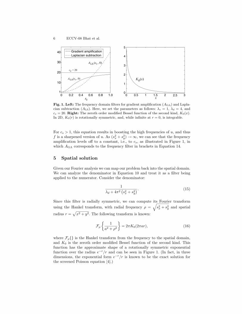
Fig. 1. Left: The frequency domain filters for gradient amplification (AGA) and Lapla-cian subtraction (ALS). Here, we set the parameters as follows: λs = 1, λd = 4, andcs = 20. Right: The zeroth order modified Bessel function of the second kind, K0(x).In 2D, K0(r) is rotationally symmetric, and, while infinite at r = 0, is integrable.

For cs > 1, this equation results in boosting the high frequencies of u, and thusf is a sharpened version of u. As (s2

x + s2y) →∞, we can see that the frequency

amplification levels off to a constant, i.e., to cs, as illustrated in Figure 1, inwhich AGA corresponds to the frequency filter in brackets in Equation 14.

5 Spatial solution

Given our Fourier analysis we can map our problem back into the spatial domain.We can analyze the denominator in Equation 10 and treat it as a filter beingapplied to the numerator. Consider the denominator:

1λd + 4π2

(s2

x + s2y

) . (15)

Since this filter is radially symmetric, we can compute its Fourier transformusing the Hankel transform, with radial frequency ρ =

√s2

x + s2y and spatial

radius r =√

x2 + y2. The following transform is known:

Fρ

{1

a2 + ρ2

}= 2πK0(2πar), (16)

where Fρ{} is the Hankel transform from the frequency to the spatial domain,and K0 is the zeroth order modified Bessel function of the second kind. Thisfunction has the approximate shape of a rotationally symmetric exponentialfunction over the radius e−r/r and can be seen in Figure 1. (In fact, in threedimensions, the exponential form e−r/r is known to be the exact solution forthe screened Poisson equation [4].)


With some simple algebraic manipulations, we arrive at:

Fρ

{1

λd + 4π2(s2

x + s2y

)}=

12π

K0(2π√

λdr) =12π

K0(2π√

λd(x2 + y2)).

(17)The numerator in Equation 10 corresponds to λdu−gx

x−gyy in the spatial domain,

and so the final result is the following convolution:

f =12π

K0(2π√

λd(x2 + y2)) ∗ (λdu− gxx − gy

y). (18)

Thus, we see that f can be obtained by subtracting the divergence of the gradientfield from the input image u, and then blurring the result with the K0 filter. Notethat as λd increases, the support of this filter becomes smaller; i.e., a strongerdata term shrinks the support of the blurring filter.

5.1 Spatial domain sharpening

Here we determine the spatial domain filter associated with gradient amplifi-cation. Starting with Equation 14, we can decompose the frequency filter asfollows:

λd + 4π2cs

(s2

x + s2y

)λd + 4π2

(s2

x + s2y

) = cs −λd(cs − 1)

λd + 4π2(s2

x + s2y

) . (19)

The inverse Fourier transform of the first term is a scaled Dirac delta function,and the second term follows from Equation 17, giving us:

Fρ

{λd + 4π2cs

(s2

x + s2y

)λd + 4π2

(s2

x + s2y

) }= csδ(x, y)− λd(cs − 1)

2πK0(2π

√λd(x2 + y2)).

(20)Convolving this with the data function then gives:

f(x, y) = csu(x, y)− λd(cs − 1)2π

K0(2π√

λd(x2 + y2)) ∗ u(x, y). (21)

Note that when amplifying gradients, cs > 1, so the operation amounts to blur-ring the image with the K0() filter and subtracting it from the original image.

5.2 Relationship to Laplacian subtraction sharpening

In this section, we relate sharpening by gradient amplification to the more con-ventional sharpening by Laplacian subtraction. First, we return to the Fourierdomain, define another constant λs = cs/λd, and re-write Equation 14 as:

F =

[1 + 4π2λs

(s2

x + s2y

)1 + 4π2(1/λd)

(s2

x + s2y

)]U = AGAU. (22)

If we then let λd →∞ while holding λs constant, we arrive at:

F =[1 + 4π2λs

(s2

x + s2y

)]U = ALSU. (23)


This equation is precisely the Fourier transform of a commonly known sharpenfilter (the Laplacian subtraction filter):

f = u− λs∇2u. (24)

Thus, the gradient domain sharpen filter subsumes another common sharpenfilter. At the same time, unlike this common sharpen filter, our new filter has anadditional parameter to control the amount of high frequency gain. As mentionedabove, the parameter cs controls the maximum frequency amplification.

It is interesting to note, as justified in Appendix A, that the Laplacian sub-traction filter can also be interpreted in a variational framework. In particular,it minimizes the following:∫ ∫

(f − u)2 − 2λs∇f · ∇u dx dy. (25)

In words, the desired function f must trade off being close to the input image uagainst maximizing the dot product between∇f and∇u. The second part of thisobjective favors f with large gradients aligned with the input image gradients.

Furthermore, one can take the objective for gradient sharpening (Equa-tion 12) and show that minimizing it is equivalent to minimizing the followingobjective: ∫ ∫

(f − u)2 − 2λs∇f · ∇u +1λd‖∇f‖2 dx dy. (26)

This objective has almost the same form as the Laplacian subtraction objec-tive, augmented with a penalty on gradient magnitudes. This observation givessome intuition for the difference between the two sharpen filters in the frequencydomain; while the Laplacian subtraction filter amplifies high frequencies with-out bound, the gradient amplification filter rolls off to a constant due to theadditional penalty on large gradients (Figure 1).

6 Discrete solution

The Fourier method provides a direct solution to the screened Poisson equation(Equation 8). In practice, we operate on sampled representations and solve theproblem with discrete derivatives and the discrete Fourier transform (DFT).

In particular, we can first re-write Equation 7 as:

λdf − (dx ∗ dx ∗ f + dy ∗ dy ∗ f) = λdu− (dx ∗ gx + dy ∗ gy), (27)

where dx and dy are discrete derivative filters in the x and y directions respec-tively and f , u, gx, and gy are sampled versions of their continuous counterpartsfrom Section 4. Typical choices for these discrete derivatives are forward, back-ward, or central differences. Taking the DFT of this equation gives us:

λdF − D2xF − D2

yF = λdU − DxGx − DyGy, (28)


where capitalization indicates having taken the DFT of a given discrete function.Rearranging, we arrive at:

F =λdU − DxGx − DyGy

λd − D2x − D2

y

=H

λd − D2x − D2

y

, (29)

where, for efficiency, H is computed as the DFT of h = λdu− dx ∗ gx − dy ∗ gy.In practice, using the DFT is problematic, as it implicitly assumes the input

sequence is periodic, placing the left boundary next to the right, and top nextto bottom, before filtering. Instead, we employ the discrete cosine transform(DCT), which implicitly performs reflections across boundaries before tiling theplane periodically. We note that switching to a cosine basis has been exploredby other researchers [22][23] and corresponds to Neumann boundary conditions.

A few implementation details follow. We compute the input gradients in gx

and gy using backward differences, while the derivative filters dx and dy areimplemented as forward differences when computing h. Using backward thenforward differences for derivatives also means that the derivative terms in thedenominator of Equation 29 correspond to the DCT of the standard discrete 2DLaplacian. Because this filter has extremely local support in the spatial domain,we can compute its transform efficiently using the brute force DCT and withoutexplicitly storing it.

We employ type-I DCTs using the FFTW library [26]. A single forwardtransform is needed to transform h to H. A single reverse transform is neededto compute f from F . For color images, this process is repeated for each colorchannel independently. The FFTW library can compute transforms in place inmemory with single precision floating point arithmetic; therefore the maximumamount of memory required by our solver at any given time is four bytes for eachpixel in the image. The FFTW library computes each transform in O(n log n)time, where n is the number of pixels in the image.

7 Applications and results

In this section, we demonstrate the practical utility of our Fourier domain anal-ysis of gradient domain problems. We start with several examples in imageprocessing and then compare performance to several state-of-the-art methodscurrently used to solve one of these applications.

7.1 Gradient domain filters and applications

The de-blocking filter proposed by Bhat et al. [18] suppresses blocking artifactsseen in highly compressed images by selectively attenuating gradients that lieacross macro-block boundaries. The modified gradients are integrated to obtaina de-blocked image, while a data term ensures the result does not drift too farfrom the compressed image. See Figures 2e,2f for an example.

The saliency sharpening filter [18] builds on the gradient amplification sharp-ening filter presented in Section 4.1 in order to sharpen large scale features in an


(a) Input image (b) Sharpening (c) Saliency sharpening

(d) Image abstraction (e) Compressed image (f) De-blocking filter

Fig. 2. Image processing with data and gradient terms using the FFT solver. Sub-figures (b,c,d) show the application of various image enhancement filters on the inputimage (a). Note that the blockiness in (b) arises from sharpening JPEG compressionartifacts present in the original image. Sub-figure (f) shows the de-blocking filter appliedto a compressed image (e).

image without amplifying the noise or background clutter. This filter works byusing an edge detector to detect large scale edges in the image and then selec-tively amplifying only those gradients that lie across large edges. Figures 2b,2ccompare uniform gradient scaling to saliency sharpening.

The image abstraction filter defined by Bhat et al. [18] operates by suppress-ing small scale textures in an image. Similar to the saliency sharpening filtering,this filter uses an edge detector to determine which gradients give rise to salientfeatures in an image. Then it selectively attenuates the non-salient gradients,thus abstracting away fine texture and noise from the input image (Figure 2d).

In gradient domain compositing applications [12], one combines the gradientsof multiple images and then solves for the underlying image most compatible withthose gradients. When no data function is used these applications can also besolved using regular Poisson solvers. Our method supports both types of gradientdomain compositing applications – those with or without a data function.

7.2 Comparison to gradient-only methods

We now compare the performance of our method on a gradient domain com-positing application (no data term) to several state-of-the-art methods. Theapplication here concerns seamless image stitching to create large panoramicimages. Agarwala [5] presented a method specialized for this application by re-lying on the solution to the Poisson equation being smooth in most regionsof the domain. He compared the performance of his method (QT) to that ofa preconditioned conjugate gradient solver using two different preconditioners


Size Time (s) Memory (MB)

Dataset (MP) FS QT SM HB LHAB FS QT SM HB LHAB

St. Emilion 10 31 9 NA 3639 160 40 24 NA 362 1044Beynac 12 22 8 17 3357 177 48 16 190 435 1252Rainier 23 79 14 33 6446 268 92 27 110 620 1790Sedona 36 85 29 NA NA NA 144 52 NA NA NAEdinburgh 51 187 122 79 NA NA 204 123 123 NA NACrag 68 172 78 NA NA NA 272 96 112 NA NARedRock 88 270 118 118 NA NA 352 112 NA NA NA

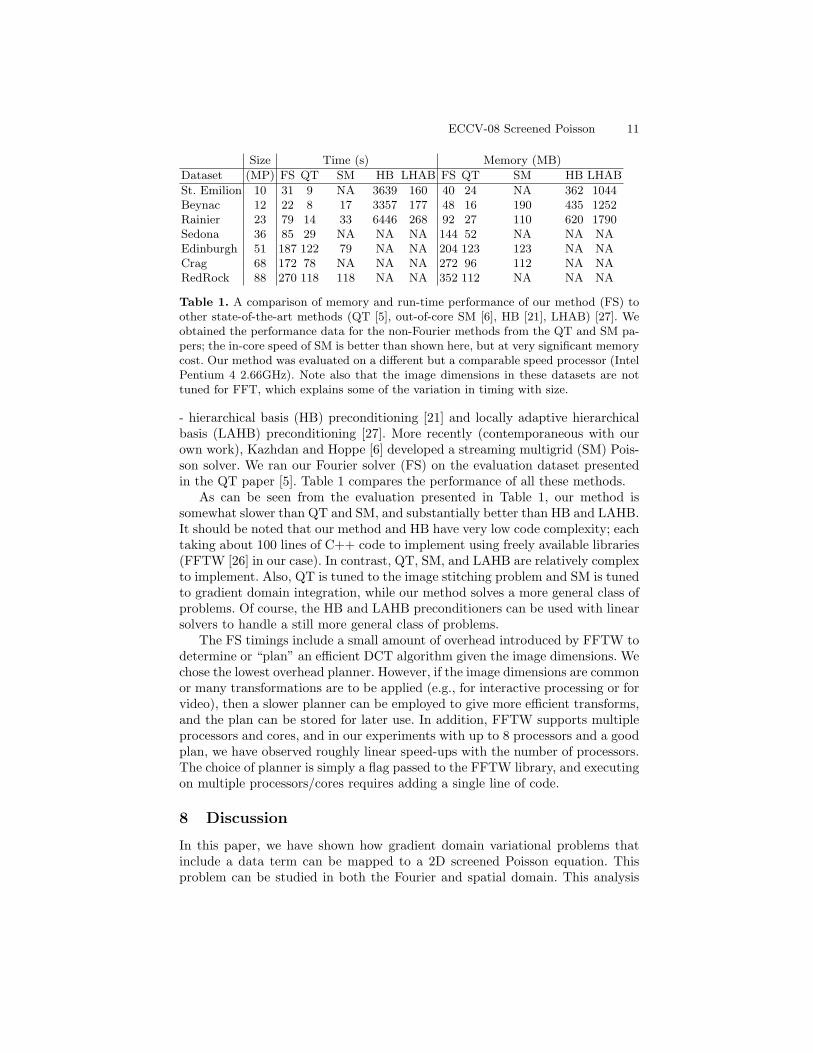
Table 1. A comparison of memory and run-time performance of our method (FS) toother state-of-the-art methods (QT [5], out-of-core SM [6], HB [21], LHAB) [27]. Weobtained the performance data for the non-Fourier methods from the QT and SM pa-pers; the in-core speed of SM is better than shown here, but at very significant memorycost. Our method was evaluated on a different but a comparable speed processor (IntelPentium 4 2.66GHz). Note also that the image dimensions in these datasets are nottuned for FFT, which explains some of the variation in timing with size.

- hierarchical basis (HB) preconditioning [21] and locally adaptive hierarchicalbasis (LAHB) preconditioning [27]. More recently (contemporaneous with ourown work), Kazhdan and Hoppe [6] developed a streaming multigrid (SM) Pois-son solver. We ran our Fourier solver (FS) on the evaluation dataset presentedin the QT paper [5]. Table 1 compares the performance of all these methods.

As can be seen from the evaluation presented in Table 1, our method issomewhat slower than QT and SM, and substantially better than HB and LAHB.It should be noted that our method and HB have very low code complexity; eachtaking about 100 lines of C++ code to implement using freely available libraries(FFTW [26] in our case). In contrast, QT, SM, and LAHB are relatively complexto implement. Also, QT is tuned to the image stitching problem and SM is tunedto gradient domain integration, while our method solves a more general class ofproblems. Of course, the HB and LAHB preconditioners can be used with linearsolvers to handle a still more general class of problems.

The FS timings include a small amount of overhead introduced by FFTW todetermine or “plan” an efficient DCT algorithm given the image dimensions. Wechose the lowest overhead planner. However, if the image dimensions are commonor many transformations are to be applied (e.g., for interactive processing or forvideo), then a slower planner can be employed to give more efficient transforms,and the plan can be stored for later use. In addition, FFTW supports multipleprocessors and cores, and in our experiments with up to 8 processors and a goodplan, we have observed roughly linear speed-ups with the number of processors.The choice of planner is simply a flag passed to the FFTW library, and executingon multiple processors/cores requires adding a single line of code.

8 Discussion

In this paper, we have shown how gradient domain variational problems thatinclude a data term can be mapped to a 2D screened Poisson equation. Thisproblem can be studied in both the Fourier and spatial domain. This analysis


gives insights into how gradient amplification corresponds to a linear sharpenfilter and can be related to a standard Laplacian subtraction filter. Moreover, weshow that this screened Poisson equation can be solved directly and efficientlyusing DCT’s. By handling a data term, we are able to demonstrate a number ofuseful applications in image processing. We also note that the DCT formulationis extremely simple to implement with standard, optimized FFT libraries withmulti-processor support.

The primary limitation of this approach is the inability to handle spatiallyvarying weights on the gradient and data term constraints. Analysis shows thatinserting such weighting into the variational formulation results in product termsthat become convolutions in the frequency domain. In addition, we require com-plete, regular domains. Still, a number of applications can operate with con-stant weights over regular domains, or may potentially be initialized with anunweighted solution over a regular domain using our DCT solver to speed con-vergence of a more general solver.

Acknowledgments

We thank Sameer Agarwal and Eli Shechtman for helpful discussions that gen-eralized our initial results on gradient domain filtering. Sameer also identifiedthe connection to the screened Poisson equation. This work was supported byMicrosoft, Adobe, the University of Washington Animation Research Labs, andan NVIDIA fellowship.

A Variational formulation of Laplacian subtraction

In Section 4.1, we showed that gradient amplification has a variational formula-tion that maps to a sharpen filter. Here we show that a more common sharpenfilter – Laplacian subtraction (Equation 24) – can arise from another variationalformulation. Consider the following objective to minimize:∫ ∫

(f − u)2 − 2λs∇f · ∇u dx dy. (30)

We can isolate and expand the integrand:

LLS = (f − u)2 − 2λsfxux − 2λsfyuy. (31)

Applying the Euler-Lagrange equation, the minimizing function must satisfy:

2(f − u)− 2λsuxx − 2λsuyy = 0. (32)

Rearranging gives us:

f = u− λs(uxx + uyy) = u− λs∇ · u. (33)

which is exactly the sharpen filter based on Laplacian subtraction.


Note that we do not claim that the form of the objective function (Equa-tion 30) is unique. Indeed, adding other functions that do not include f or itsderivatives to the integrand LLS will yield the same result. Rather, it illustratesone objective function that has intuitive meeting and does lead to the Laplaciansubtraction filter.

It is also instructive to relate the integrand LLS to the integrand in gradientamplification:

LGA = λd(f − u)2 + ‖∇f − cs∇u‖2 (34)= λd(f − u)2 + (fx − csux)2 + (fy − csuy)2. (35)

We can divide this integrand by λd, because it does not affect the minimumsolution. Doing so and expanding gives us:

LGA = (f − u)2 +1λd

f2x − 2

cs

λdfxux +

c2s

λdu2

x +1λd

f2y − 2

cs

λdfyuy +

c2s

λdu2

y. (36)

We can drop the terms that do not depend on f or its derivatives, since againthese do not affect the solution. Thus, we can omit c2

s

λdu2

x and c2s

λdu2

y. After alsosubstituting λs = cs/λd, we arrive at:

LGA = (f − u)2 +1λd

f2x − 2λsfxux +

1λd

f2y − 2λsfyuy (37)

= (f − u)2 − 2λs∇f · ∇u +1λd‖∇f‖2. (38)

We can now see that the gradient amplification integrand can be related to theLaplacian subtraction integrand very simply:

LGA = LLS +1λd‖∇f‖2. (39)

Again, as λd → ∞ while holding λs constant, the gradient amplification inte-grand becomes the Laplacian subtraction integrand.

References

1. Trottenberg, U., Oosterlee, C.W., Schller, A.: Multigrid. Academic Press (2000)2. Ho, J., Lim, J., Yang, M., Kriegman, D.: Integrating surface normal vectors using

fast marching method. In: European Conference on Computer Vision. (2006) III:239–250

3. Strang, G.: Introduction to Applied Mathematics. Wellesley-Cambridge Press(1986)

4. Fetter, A.L., Walecka, J.D.: Theoretical Mechanics of Particles and Continua.Courier Dover (2003)

5. Agarwala, A.: Efficient gradient-domain compositing using quadtrees. ACM Trans.Graph. 26 (2007) 94:1–94:5

6. Kazhdan, M., Hoppe, H.: Streaming multigrid for gradient-domain operations onlarge images. ACM Transactions on Graphics (Proc. of ACM SIGGRAPH 2008,to appear) (2008)


7. Simchony, T., Chellappa, R., Shao, M.: Direct analytical methods for solvingpoisson equations in computer vision problems. Pattern Analysis and MachineIntelligence, IEEE Transactions on 12 (May 1990) 435–446

8. Horn, B.: Robot Vision. MIT Press (1986)9. Zickler, T.E., Belhumeur, P.N., Kriegman, D.J.: Helmholtz stereopsis: Exploiting

reciprocity for surface reconstruction. Int. J. Comput. Vision 49 (2002) 215–22710. Fattal, R., Lischinski, D., Werman, M.: Gradient domain high dynamic range

compression. In: SIGGRAPH ’02: Proceedings of the 29th annual conference onComputer graphics and interactive techniques, New York, NY, USA, ACM Press(2002) 249–256

11. Perez, P., Gangnet, M., Blake, A.: Poisson image editing. In: SIGGRAPH ’03:ACM SIGGRAPH 2003 Papers, New York, NY, USA, ACM Press (2003) 313–318

12. Agarwala, A., Dontcheva, M., Agrawala, M., Drucker, S., Colburn, A., Curless, B.,Salesin, D., Cohen, M.: Interactive digital photomontage. ACM Trans. Graph. 23(2004) 294–302

13. Horn, B.K.P.: Height and gradient from shading. Int. J. Comput. Vision 5 (1990)37–75

14. Horovitz, I., Kiryati, N.: Depth from gradient fields and control points: bias cor-rection in photometric stereo. Image Vision Comput. 22 (2004) 681–694

15. Nehab, D., Rusinkiewicz, S., Davis, J., Ramamoorthi, R.: Efficiently combiningpositions and normals for precise 3d geometry. ACM Trans. Graph. 24 (2005)536–543

16. Ng, H., Wu, T., Tang, C.: Surface-from-gradients with incomplete data for singleview modeling. In: International Conference on Computer Vision. (2007) 1–8

17. Lischinski, D., Farbman, Z., Uyttendaele, M., Szeliski, R.: Interactive local adjust-ment of tonal values. In: SIGGRAPH ’06: ACM SIGGRAPH 2006 Papers, NewYork, NY, USA, ACM Press (2006) 646–653

18. Bhat, P., Zitnick, L., Cohen, M., Curless, B.: A perceptually-motivatedoptimization-framework for image and video processing. Technical Report UW-CSE-08-06-02, University of Washington (2008)

19. Agrawal, A.K., Raskar, R., Chellappa, R.: What is the range of surface reconstruc-tions from a gradient field? In: ECCV (1). (2006) 578–591

20. Agrawal, A.: Scene Analysis under Variable Illumination using Gradient DomainMethods. PhD thesis, University of Maryland (2006)

21. Szeliski, R.: Fast surface interpolation using hierarchical basis functions. IEEETrans. Pattern Anal. Mach. Intell. 12 (1990) 513–528

22. Frankot, R.T., Chellappa, R.: A method for enforcing integrability in shape fromshading algorithms. IEEE Trans. Pattern Anal. Mach. Intell. 10 (1988) 439–451

23. Georghiades, A.S., Belhumeur, P.N., Kriegman, D.J.: From few to many: Illumi-nation cone models for face recognition under variable lighting and pose. IEEETransactions on Pattern Analysis and Machine Intelligence 23 (2001) 643–660

24. Weiss, Y.: Deriving intrinsic images from image sequences. In: International Con-ference on Computer Vision. (2001) II: 68–75

25. Bracewell, R.: The Fourier Transform and Its Applications. second edn. Mcgraw-Hill (1986)

26. Frigo, M., Johnson, S.G.: FFTW for version 3.0 (2003)27. Szeliski, R.: Locally adapted hierarchical basis preconditioning. In: SIGGRAPH

’06: ACM SIGGRAPH 2006 Papers, New York, NY, USA, ACM Press (2006)1135–1143

fourier analysis of the 2d screened poisson equation for...

Documents