Lehrstuhl für Bildverarbeitung

Institute of Imaging & Computer Vision

Fourier, Block and Lapped Transforms

Til AachInstitute of Imaging and Computer Vision

RWTH Aachen University, 52056 Aachen, Germanytel: +49 241 80 27860, fax: +49 241 80 22200

web: www.lfb.rwth-aachen.de

in: Advances in Imaging and Electron Physics. See also BibTEX entry below.

BibTEX:

@inproceedings{AAC03a,

author = {Til Aach},

title = {Fourier, Block and Lapped Transforms},

booktitle = {Advances in Imaging and Electron Physics},

volume = {128},

editor = {P. W. Hawkes},

publisher = {Academic Press},

address = {San Diego},

year = {2003},

pages = {1-52}}

Copyright (c) Elsevier Inc. All rights reserved. This material is presented to ensure timely disseminationof scholarly and technical work. Copyright and all rights therein are retained by the authors or byother copyright holders. All persons copying this information are expected to adhere to the terms andconstraints invoked by each author’s copyright. These works may not be reposted without the explicitpermission of the copyright holder.

document created on: December 15, 2006created from file: aiepaachcover.tex

cover page automatically created with CoverPage.sty

(available at your favourite CTAN mirror)

Fourier, Block and Lapped Transforms

Til AachInstitute for Signal Processing, University of LubeckRatzeburger Allee 160, D-23538 Lubeck, Germany

Tel. +49 451 3909556, Fax: +49 451 3909555aach@isip.mu-luebeck.de

Contents

1 Introduction: Why transform signals anyway? 2

2 Linear System Theory and Fourier Transforms 3

2.1 Continuous-Time Signals and Systems . . . . . . . . . . . . . . . . . . . . . . . . . . . . . 3

2.2 Discrete-Time Signals and Systems . . . . . . . . . . . . . . . . . . . . . . . . . . . . . . . 5

2.3 The Discrete Fourier Transform and Block Transforms . . . . . . . . . . . . . . . . . . . . 6

3 Transform Coding 8

3.1 The Role of Transforms: Constrained Source Coding . . . . . . . . . . . . . . . . . . . . . 8

3.2 Transform Efficiency . . . . . . . . . . . . . . . . . . . . . . . . . . . . . . . . . . . . . . . 9

3.3 Transform Coding Performance . . . . . . . . . . . . . . . . . . . . . . . . . . . . . . . . . 14

4 Two-Dimensional Transforms 15

5 Lapped Transforms 16

5.1 Block Diagonal Transforms . . . . . . . . . . . . . . . . . . . . . . . . . . . . . . . . . . . 16

5.2 Extension to Lapped Transforms . . . . . . . . . . . . . . . . . . . . . . . . . . . . . . . . 17

5.3 The Lapped Orthogonal Transform . . . . . . . . . . . . . . . . . . . . . . . . . . . . . . . 18

5.4 The Modulated Lapped Transform . . . . . . . . . . . . . . . . . . . . . . . . . . . . . . . 19

5.5 Extensions . . . . . . . . . . . . . . . . . . . . . . . . . . . . . . . . . . . . . . . . . . . . . 21

6 Image Restoration and Enhancement 23

7 Discussion 23

8 Appendix A 24

9 Appendix B 24

10 Appendix C 25

11 Appendix D 26

12 Acknowledgement 27

1

1 Introduction: Why transform signals anyway?

The Fourier transform and its related discrete transforms are of key importance in both theory andpractice of signal and image processing. In the theory of continuous-time systems and signals, theFourier transform allows to describe both signal and system properties and the relation between sys-tem input and output signals in the frequency domain [Ziemer et al., 1989, Luke, 1999]. Fourier-optical systems based on the diffraction of coherent light are a direct practical realization of the two-dimensional continuous Fourier transform [Papoulis, 1968, Bamler, 1989]. The discrete-time Fouriertransform (DTFT) describes properties of discrete-time signals and systems. While the DTFT as-signs frequency-continuous and periodic spectra to discrete-time signals, the discrete Fourier transform(DFT) represents a discrete-time signal of finite length by a finite number discrete-frequency coefficients[Oppenheim and Schafer, 1998, Proakis and Manolakis, 1996, Luke, 1999]. The DFT thus permits tocompute spectral respresentations numerically. The DFT and other discrete transforms related to it, likethe discrete cosine transform (DCT), are also of great practical importance for the implementations ofsignal and image processing systems, since efficient algorithms for their computations exist, e.g. in theform of the fast Fourier transform (FFT).

However, while continuous-time Fourier analysis generally considers the entire time axis from minus infin-ity to plus infinity, the DFT is only defined for signals of finite duration. Conceptually, the finite-durationsignals are formed by taking single periods from originally periodic signals. Consequently, enhancementand transform coding of, for instance, speech, are based on the spectral analysis of short time intervalsof the speech waveform [Lim and Oppenheim, 1979, Ephraim and Malah, 1984, van Compernolle, 1992,Cappe, 1994, Aach and Kunz, 1998]. The length of the time intervals depends on the nature of thesignals, viz. short-time stationarity. Similarly, transform coding [Clarke, 1985] or frequency-domain en-hancement [Lim, 1980, Aach and Kunz, 1996b, Aach and Kunz, 1996a, Aach and Kunz, 2000] of imagesrequire spectral analysis of rectangular blocks of finite extent in order to take into account short-spacestationarity. Such processing by block transforms often generates audible or visible artifacts at blockboundaries. While in some applications, these artifacts may be mitigated using overlapping blocks[Lim and Oppenheim, 1979, Lim, 1980, Ephraim and Malah, 1984, Cappe, 1994, van Compernolle, 1992,Aach and Kunz, 1996b, Aach and Kunz, 1998, Aach, 2000], this is not practical in applications like trans-form coding, where overlapping blocks would inflate the data volume. Transform coders therefore punchout adjacent blocks from the incoming continuous data stream, and encode these individually. To illus-trate the block artifacts, Fig. 1 shows an image reconstructed after encoding by the JPEG algorithm,which uses a blockwise DCT [Rabbani and Jones, 1991].

Lapped transforms aim at reducing or even eliminating block artifacts by the use of overlapping basisfunctions, which extend over more than one block. The purpose of this chapter is to provide a self-contained introduction into lapped transforms. Our approach is to develop lapped transforms fromstandard block transforms as a starting point. To introduce the topic of signal transforms, we willfirst summarize the development from the Fourier transform of continuous-time signals to the DFT.An in-depth treatment can be found in many texts on digital signal processing and system theory, e.g.[Ziemer et al., 1989, Oppenheim and Schafer, 1998, Luke, 1999]. In section 3, we discuss the relevanceof orthogonal block transforms for transform coding, which depends on the covariance structure of thesignals. Section 4 deals with two-dimensional block transforms.

Orthogonal block transforms map a given number of signal samples contained in each block into anidentical number of transform coefficients. Each signal block can hence be perfectly reconstructed fromits transform coefficients by an inverse transform. In contrast to block transforms, the basis functionsof lapped transforms discussed in section 5 extend into neighbouring blocks. The number of transformcoefficients generated is then lower than the number of signal samples covered by the basis functions.Signal blocks can therefore not be perfectly reconstructed from their individual transform coefficients.However, if the transform meets a set of extended orthogonality conditions, the original signal is perfectlyreconstructed by superimposing the overlapping, imperfectly reconstructed signal blocks. Two types oflapped transforms will be exposed, the lapped orthogonal transform (LOT) and the modulated lappedtransform (MLT). We then discuss extensions of these transforms before concluding with some examplescomparing the use of block and lapped transforms in image restoration and enhancement.

2

2 Linear System Theory and Fourier Transforms

2.1 Continuous-Time Signals and Systems

Let s(t) denote a real signal, with t being the independent continuous-time variable. Our aim is todescribe the transmission of signals through one or more systems, where a system is regarded as a blackbox which maps an input signal s(t) into the output signal g(t) by a mapping M , i.e. g(t) = M(s(t)).Restricting ourselves here to the class of linear time-invariant (LTI) systems, we require the systems tocomply with the following conditions:

Linearity: A linear system reacts to any weighted combination of K input signals si(t), i = 1, . . . K,with the same weighted combination of output signals gi(t) = M(si(t)):

M

(K∑

i=1

aisi(t)

)=

K∑i=1

aiM(si(t)) =K∑

i=1

aigi(t) , (1)

where ai, i = 1, . . . ,K denote the weighting factors.

Time invariance: A time-invariant system reacts to an arbitrary delay of the input signal with acorrespondingly delayed, but otherwise unchanged output signal:

M(s(t)) = g(t) ⇒ M(s(t− τ)) = g(t− τ) , (2)

where τ is the delay.

An LTI system is completely characterized by the response to the Dirac delta impulse δ(t). Denotingthe so-called impulse response by h(t), we have h(t) = M(δ(t)). The Dirac impulse δ(t) is a distributiondefined by the integral equation

s(t) =∫ ∞

−∞s(τ)δ(t− τ)dτ , (3)

which essentially represents a signal s(t) by an infinite series of Dirac impulses delayed by τ and weightedby s(τ). Since an LTI system reacts to the signal s(t) by the same weighted combination of delayedimpulse responses h(t), it suffices to replace δ(t − τ) in Equation (3) by h(t − τ) to obtain the outputg(t):

g(t) =∫ ∞

−∞s(τ)h(t− τ)dτ . (4)

This relationship is known as the so-called convolution, and abbreviated by g(t) = s(t) ∗ h(t). Theconvolution is commutative, we may therefore interchange input signal and impulse response, and equallywrite g(t) = h(t) ∗ s(t).

Let us now consider the system reaction to the complex exponential seig(t) of frequency f (or radianfrequency ω = 2πf) given by

seig(t) = ej2πft , (5)

where j =√−1. From g(t) = h(t) ∗ seig(t), we obtain

g(t) = ej2πft ·∫ ∞

−∞h(τ)e−j2πfτdτ = seig(t) ·H(f) , (6)

where 1

H(f) =∫ ∞

−∞h(t)e−j2πftdt . (7)

Hence, the input signal is only weighted by the generally complex weighting factor H(f), but otherwisereproduced unchanged, and called an eigenfunction of LTI systems. The relationship between h(t) andH(f) is the Fourier transform, and denoted by h(t) ◦−•H(f). If known for all frequencies, H(f) is calledthe spectrum of the signal h(t), or the transfer function of the LTI system. Equation (7) essentially is an

1In the following, we assume the Fourier integrals to exist. For h(t) piecewise continuous, a sufficient condition is∫∞−∞ |h(τ)|dτ < ∞.

3

inner product or correlation between h(t) and the complex exponential of frequency f . The signal h(t)can be recovered from its spectrum H(f) by the inverse Fourier transform

h(t) =∫ ∞

−∞H(f)ej2πftdf , (8)

which is a weighted superposition of complex exponentials. (This integral reconstructs discontinuities ofh(t) by the average between left and right limit.) Evidently, an LTI system can also be fully describedby its transfer function H(f). When applied to a signal s(t), the Fourier transform S(f) is called thespectrum of s(t). It specifies the weights and phases of the complex exponentials contributing to s(t) inthe inverse Fourier transform according to

s(t) ◦−• S(f) ⇒ s(t) =∫ ∞

−∞S(f)ej2πftdf . (9)

The Fourier transform allows to describe the transfer of a signal s(t) over an LTI system in the frequencydomain. According to Equation (6), the LTI system reacts to ej2πft by H(f) · ej2πft. Equation (9)represents the system input s(t) as a weighted superposition of complex exponentials. Because of linearity,the output signal g(t) is given by an identical weighted superposition of system reactions H(f) · ej2πft:

g(t) =∫ ∞

−∞S(f)H(f)ej2πftdf . (10)

Denoting the spectrum of g(t) by G(f), the inverse Fourier transform yields

g(t) ◦−•G(f) ⇒ g(t) =∫ ∞

−∞G(f)ej2πftdf . (11)

Comparing Equations (10) and (11), we obtain G(f) = H(f)S(f), i.e. the spectrum of the output signalis given by the product of the spectrum of the input signal and the transfer function of the LTI system.

The Fourier transform as given by Equations (7) and (8) thus provides insight into the frequency contentof signals, and transfer properties of LTI systems. Relating a continuous-time signal to a spectrum whichis a function of a continuous frequency variable, this version of the Fourier transform is, however, notsuited for numerical evaluation by computer or digital signal processing systems. Still, realization of acontinuous Fourier analyzer is possible, for instance by optical systems [Papoulis, 1968, Bamler, 1989].

2.2 Discrete-Time Signals and Systems

Let us now consider a discrete-time signal s(n), where the independent variable may only take integervalues, i.e. n = 0,±1,±2, . . .. Essentially, s(n) is an ordered sequence of numbers stored e.g. in thememory of a computer, or coming from an A/D-converter. A discrete-time system maps the input signals(n) into the output signal g(n) by the mapping g(n) = M(s(n)). As in the continuous-time case, weregard only linear time-invariant systems obeying the following conditions:

Linearity:

M

(K∑

i=1

aisi(n)

)=

K∑i=1

aiM(si(n)) =K∑

i=1

aigi(n) , (12)

for arbitrary input signals si(n) and weighting factors ai, i = 1, . . . ,K.

Time invariance:M(s(n)) = g(n) ⇒ M(s(n−m)) = g(n−m) , (13)

where m is an integer delay.

In the discrete-time case, the Dirac delta impulse is replaced by the unit impulse δ(n) which is definedby

δ(n) ={

1 for n = 00 else . (14)

4

A discrete-time signal s(n) can then be composed of a sum of weighted and shifted unit impulses accordingto

s(n) =∞∑

m=−∞s(m)δ(n−m) . (15)

To determine the system response g(n), it then suffices to know its impulse response h(n) = M(δ(n)).Because of linearity and time invariance, the output signal is given by the following superposition ofweighted and shifted impulse responses:

g(n) =∞∑

m=−∞s(m)h(n−m) . (16)

This operation is called the discrete-time convolution, and denoted by g(n) = s(n) ∗ h(n). Like itscontinuous-time counterpart, the discrete-time convolution is commutative.

The eigenfunctions of discrete-time LTI systems are discrete-time complex exponentials given by

seig(n) = ej2πfn . (17)

Note that the frequency variable f is still continuous. Passing seig(n) through our LTI system yields theoutput signal

g(n) = ej2πfn ·∞∑

m=−∞h(m)e−j2πfm = seig(n) ·HDT (f) , (18)

where

HDT (f) =∞∑

n=−∞h(n)e−j2πfn (19)

is the discrete-time Fourier transform (DTFT) of h(n), which can be regarded as the transfer function ofthe LTI system, or the spectrum of the signal h(n). We denote this relation by h(n)◦−•HDT (f). Clearly,the spectrum of a discrete-time signal is periodic over f . Indeed, s(n) can be regarded as the Fourierseries representation of HDT (f). To reconstruct h(n) from its spectrum, it therefore suffices to considera single period of HDT (f):

h(n) ◦−•HDT (f) ⇒ h(n) =∫ 1

2

− 12

HDT (f)ej2πfndf . (20)

As in the continuous-time case, it is straightforward to show that the spectrum of an output signal ofan LTI system is the product of the spectrum of the input signal and the transfer function of the LTIsystem:

g(n) = s(n) ∗ h(n) ◦−•GDT (f) = SDT (f) ·HDT (f) . (21)

While the discrete-time convolution in Equation (16) can be implemented on digital signal processingsystems, the spectral-domain relations are of less practical value, since they depend on a continuousfrequency variable.

2.3 The Discrete Fourier Transform and Block Transforms

Let us now consider a finite-duration signal s(n), n = 0, . . . , N − 1 comprising N samples. Seekinga spectral-domain representation for s(n) by N frequency coefficients SDFT (k), k = 0, . . . , N − 1, westart from its DTFT SDT (f), which is a sum over N components. SDT (f) is periodic with period 1,and therefore fully specified by one period, for instance 0 ≤ f < 1. Seeking to represent the N -samplesequence s(n) by N discrete frequency coefficients, we take N equally spaced samples from one period ofSDT (f), 0 ≤ f < 1, thus obtaining the discrete Fourier transform (DFT) of s(n) by

SDFT (k) = SDT

(k

N

)=

N−1∑n=0

s(n)e−j 2πN kn , k = 0, . . . , N − 1 . (22)

5

The finite-duration signal s(n) can be recovered from its DFT SDFT (k) by the inverse DFT (see AppendixA)

s(n) ◦−• SDFT (k) ⇒ s(n) =1N

N−1∑k=0

SDFT (k)ej 2πN kn , n = 0, . . . , N − 1 . (23)

The DFT hence represents a finite-duration discrete-time signal s(n) of N coefficients by N discretespectral coefficients SDFT (k), and is therefore perfectly suited for numerical implementation. In general,the frequency coefficients are complex, offering 2N degrees of freedom. However, for real s(n), the DFTobeys the symmetry condition SDFT (k) = S∗DFT (N − k), what reduces the degrees of freedom to N .

Since the DFT applies to finite-length signals, samples of signals of long duration must be collectedinto successive segments or blocks of finite length, which are then subjected to the DFT. Transformslike the DFT are therefore termed block transforms. The block length is, on the one hand, limited bypractical considerations, like available memory and performance of the DSP system. More important,however, is the influence of statistical signal properties on the block length: the notion of power spectrum,for instance, is meaningful only for (wide sense) stationary random signals. Real data, like speech orimages, are stationary only over short time intervals and blocks of rather small extent, respectively.Applications of spectral analysis, like power spectrum estimation by block transforms or block transformcoding therefore only make sense when applied to reasonably short and small segments. In the JPEGstill image compression standard, images are processed in blocks of 8×8 pixels. Speech can be consideredstationary for intervals in the order of 10ms - 50 ms. When sampled at 8 KHz, this translates into blockswith 64 - 256 samples.

Linear block transforms are conveniently expressed as matrix operations. Grouping the signal sampless(n), n = 0, . . . , N − 1 into a column vector s = [s(0), s(1), . . . , s(N − 1)]T , and the frequency coefficientsinto a vector S = [SDFT (0), SDFT (1), . . . , SDFT (N − 1)]T , Equation (22) can be written as

S = W · s, with W = [W]kn , (24)

where W is the square N ×N transform matrix with entry

Wkn = e−j 2πN kn (25)

in the k + 1-th row and n + 1-th column. The inverse transform in Equation (23) can be expressed by

s =1N

(W∗)T · S . (26)

Thus,(W∗)T ·W = N · I , (27)

where I is the identity matrix. The DFT transform matrix is hence unitary up to a factor N , or, in otherwords, the DFT basis functions are orthogonal.

We have derived the DFT by sampling the first period of the DTFT of a signal of length N with a samplingperiod 1/N . What are the consequences of this frequency-domain sampling operation? Comparing theFourier transform S(f) of a continuous-time signal s(t) according to Equation (7) to the DTFT inEquation (19), we see that replacing a continuous-time signal by discrete equally spaced samples withsampling period one leads to a periodic spectrum with period one in the DTFT of Equation (19). Also,the Fourier transform and its inverse in Equation (8) are almost identical in structure. Apart froma sign change in the exponent, the signal s(t) and its spectrum S(f) are simply interchanged, as arethe time and frequency variables t and f . Therefore, like time-domain sampling leads to a periodicspectrum, frequency-domain sampling of the periodic spectrum leads to a periodic discrete signal sp(n)by periodically repeating s(n) with a period which is the inverse of the sampling period in the frequencydomain. Since the frequency-domain sampling period in Equation (22) is 1/N , the periodic signal sp(n)is given by

sp(n) =∞∑

r=−∞s(n + rN) . (28)

Hence, the DFT represents one period of a periodic discrete-time signal by one period of its discrete-frequency periodic spectrum. Both the “actually” transformed signal and its spectrum are therefore

6

periodic. This implicit, underlying periodicity must not be overlooked when applying the DFT. Oneconsequence is the occurrence of spurious high-frequency artifacts in the DFT spectrum, which aregenerated when the block-end signal coefficients s(0) and s(N − 1) differ strongly. The periodicallyrepeated signal sp(n) then exhibits abrupt transitions, which “leak” spectral energy into high-frequencyspectral coefficients. To illustrate this effect, Fig. 2 shows the signal s(n) = cos(4πn/64), n = 0, . . . , 63and its DFT spectrum. Since two periods of the cosine fit perfectly into the analysis interval, periodicrepetition of s(n) generates a smooth signal. As expected, the DFT spectrum exhibits two “clean” peaksat k = 2 and k = 62. This is vastly different in Fig. 3: The frequency of the cosine is slightly increasedsuch that now 2.5 periods fit into the data interval, with s(n) = cos(5πn/64), n = 0, . . . , 63. Periodicrepetition generates transitions from almost −1 to 1 between block-end samples. The effect of thesetransitions is evident in the DFT spectrum, which is now spread over all frequency coefficients.

This example also illustrates one important application of block transforms: As Fig. 2 shows, a blocktransform may concentrate the signal energy into only a few number of spectral coefficients. This propertyis essential for data compression by transform coding. From Fig. 3, however, it becomes clear that theDFT is probably not the optimal transform for this purpose, due to problems caused by discontinuitiesat the block ends. In the next section, we examine transform coding in more detail. We will see that,though better transforms than the DFT exist for transform coders, artifacts caused by block boundariespersist. This will be the main motivation for the development and use of lapped transforms.

Various fast and highly efficient algorithms are available for the computation of the DFT and its inverse(“fast Fourier transform”, FFT). These are widely used in applications like power spectrum estimation,fast convolution, adaptive filtering, noise reduction and signal enhancement, as well as in many others.Some of these applications require the use of overlapping segments, others the use of segments which aresubjected to a smooth window function such that discontinuities at block ends are reduced or eliminated[Oppenheim and Schafer, 1998, Ziemer et al., 1989, Chapter 11].

3 Transform Coding

3.1 The Role of Transforms: Constrained Source Coding

The aim of source coding or data compression is to represent discrete signals s(n) with only a small ex-pected number of bits per sample (the socalled bit rate), with either no distortion (lossless compression),or as low distortion as possible for a given rate (lossy compression). Since we try to optimize the trade-offbetween distortion and rate on the average, we regard signals as random which we describe by theirstatistical properties. The essential step in source coding is quantization [Goyal, 2001, p.12]. A straight-forward approach is so-called pulse code modulation (PCM), where each sample is quantized individuallyat a fixed number of bits, e.g. eight bits for grey level images. Most signals representing meaningfulinformation, however, exhibit strong statistical dependencies between signal samples. In images, for in-stance, the grey levels of neighbouring pixels tend to be similar. To take such dependencies into account,possibly large sets of adjacent samples should be quantized together. Unfortunately, this unconstrainedapproach leads to practical problems even for relatively small groups of samples [Goyal, 2001].

In transform coding, the signals or images are first decomposed into adjacent blocks or vectors of N inputsamples each. Each block is then individually transformed such that the statistical dependencies betweenthe samples are reduced, or even eliminated [Clarke, 1985, Zelinski and Noll, 1977, Goyal, 2001]. Also, thesignal energy which generally is evenly distributed over all signal samples s(n) should be repacked into onlya few transform coefficients. The transform coefficients S(k) can then be quantized individually (scalarquantization). Each quantizer output consists of an index i(k) of the quantization interval into whichthe corresponding transform coefficient falls. These indices are then coded, e.g. by a fixed length code oran entropy code. The decoder then first reconverts the incoming bitstream into the quantization indices,and then replaces the quantization index i(k) for each transform coefficient S(k) by the centroid V (i(k))of the indexed quantization interval, which serves as approximation, or better, estimate, S(k) = V (i(k))of S(k). The relation between the indices i(k) and the centroids V (i(k)) is stored in a look-up tablecalled a codebook. An inverse transform then calculates the reconstructed signal s(n). The principle ofa transform codec is shown in Fig. 4. Clearly, due to quantization, the compression technique is lossy.The distortion caused by uniform scalar quantization is discussed in Appendix B. Optimizing a transform

7

codec needs to address choosing an optimal transform and optimal scalar quantization of the transformcoefficients. Since the optimization is thus constrained by the architecture outlined in Fig. 4, we speakof constrained source coding.

Practical transform codecs employ linear unitary or orthogonal transforms. Linear transforms explicitlyinfluence linear statistical dependencies, that is, correlations. In the next section, we therefore first discussunitary transforms subject to the criteria decorrelation and energy concentration. We then show that theoptimal transform with respect to these criteria is also optimal with respect to the reconstruction errorsincurred at given rates.

3.2 Transform Efficiency

Modelling the signal s(n) as wide-sense stationary over n = 0, . . . , N − 1, the mean value is constantfor all samples. Without loss of generality, we assume that the mean is zero, if necessary by havingfirst subtracted a potential non-zero mean from the data. The autocovariance function (ACF) is thengiven by cs(n) = E (s(m)s(m + n)), where E denotes expectation, and the (constant) variance σ2 ofs(n) is σ2 = cs(0). The ACF can be normalized by cs(n) = σ2 · ps(n), with ps(0) = 1, and |ps(n)| ≤ 1.Alternatively, covariances can be expressed by the covariance matrix Cs [Fukunaga, 1972, Therrien, 1989],which is an N ×N -matrix defined by

Cs = E[ssT]

= σ2 ·

1 ps(1) ps(2) . . . ps(N − 1)

ps(1) 1 ps(1) . . . ps(N − 2)...

ps(N − 1) ps(N − 2) ps(n− 3) . . . 1

. (29)

The entry in the n + 1-th row and k + 1-th column of Cs is thus given by cs(|n − k|). The covariancematrix of a wide-sense stationary signal vector is evidently a positive semidefinite and symmetric Toeplitzmatrix [Therrien, 1989, Makhoul, 1981, Akansu and Haddad, 2001], indeed, Cs is symmetric about bothmain diagonals (persymmetric) [Unser, 1984]. We transform the signal vector s into the coefficient vectorS = A · s by a linear, unitary transform. The transform is described by an N × N matrix A, withA−1 = AH , where the superscript H denotes conjugate transpose (cf. Equation (27)). For instance, Acould be a unitary DFT defined by A = 1/

√N ·W, with W given by Equation (25). A unitary transform

preserves Euclidean lengths:

||S||22 = SHS = sT ·AHA · s = sT · I · s = ||s||22 , (30)

where sH = sT , since s is real. The covariance matrix CS of the transform coefficients can then bederived to

CS = E[SSH

]= AE

[ssT]AH = ACsAH , (31)

and also det(CS) = det(Cs). Furthermore, the sum of the variances of the signal and transform coeffi-cients are identical:

N · σ2 = tr (Cs) = tr (CS) =N−1∑k=0

σ2S(k) , (32)

where tr(C) is the trace of matrix C. In general, the non-diagonal entries of Cs differ more or lessstrongly from zero, reflecting correlations between the signal samples s(n). We now seek a unitarytransform matrix A, which decorrelates as much as possible the input data. Hence, we seek a transformmatrix such that the covariance matrix CS of the transform coefficients is diagonal or nearly diagonal[Fukunaga, 1972, Therrien, 1989, Clarke, 1985, Goyal, 2001]. At the same time, we seek to optimallyconcentrate the signal energy into only a few dominant transform coefficients. The decorrelation efficiencyηd can be measured by comparing the sums of absolute non-diagonal matrix entries before and aftertransformation by [Akansu and Haddad, 2001, p. 33]

ηd = 1−∑

k,l,k 6=l |[CS ]kl|∑m,n,m6=n |[Cs]mn|

. (33)

8

Energy concentration can be evaluated by the relative energy contribution of the L < N transformcoefficients with lowest energy to the total energy. Ordering the variances of the transform coefficientsby rank to σ2

S(0) > σ2S(1) > . . . σ2

S(N − 1), such a measure is

DBR(L) =∑N−1

k=L σ2S(k)∑N−1

k=0 σ2S(k)

=∑N−1

k=L σ2S(k)

tr (CS), (34)

which is sometimes referred to as the basis restriction error [Jain, 1979, Unser, 1984,Akansu and Haddad, 2001]. Denoting the rows of A by N -component row vectors aT

k , k = 0, . . . , N − 1,we obtain for the variances σ2

S(k) by evaluating Equation (31) for the entries along the main diagonal

σ2S(k) = aT

k Csa∗k . (35)

Minimizing the basis restriction error subject to the real constraint aTk · a∗l = δ(k − l) is equivalent to

minimizing the functional

J =N−1∑k=L

[aT

k Csa∗k − λk(aTk a∗k − 1)

], (36)

with Langrangian multipliers λk, and where we have taken into account that the denominator in Equation(34) is invariant under a unitary transform. It can straightforwardly be shown that J is minimized bythe normalized eigenvectors uk, k = 0, . . . , N − 1 of the data covariance matrix Cs [Therrien, 1992, p.50, p. 694], [Therrien, 1989, Akansu and Haddad, 2001]. The eigenvectors fulfill

Csuk = λkuk . (37)

Since Cs is symmetric and positive semidefinite, its eigenvalues λk are real and non-negative. Its eigen-vectors are orthogonal, and, since the eigenvalues are real, the eigenvectors can always be found such thattheir elements are real (Cs also has complex eigenvectors, obtained by multiplying the real eigenvectorsby a non-zero complex factor). The unitary transform matrix A is given by

A =

uT

0

uT1...

uTN−1

. (38)

This transform is called the Karhunen-Loeve transform (KLT) [Fukunaga, 1972, Therrien, 1989]. Thevariances of the transform coefficients are given by the eigenvalues λk, since from Equation (35)

σ2S(k) = uT

k Csuk = uTk λkuk = λk , (39)

where we have considered only real eigenvectors. Also, since the eigenvectors are orthogonal, we have forthe non-diagonal entries of the covariance matrix CS

[CS ]kl = uTk Csul = uT

k λlul = 0 for k 6= l . (40)

Hence, CS is a diagonal matrix, and the transform coefficients are perfectly decorrelated. We constrainthe eigenvectors to be real, and order them in Equation (38) by rank of their eigenvalues. Up to signof the eigenvectors, the KLT then is the unique unitary transform which minimizes the basis restrictionerror and perfectly diagonalizes the covariance matrix if the eigenvalues are all distinct. Also, invokingHadamard’s inequality which states that the determinant of any symmetric, positive semi-definite matrixis less than or equal to the product of its diagonal elements, we obtain an additional measure for energyconcentration: we find that the determinant of a covariance matrix is always less or equal to the productover all variances, i.e.

det [Cs] = det [CS ] ≤N−1∏k=0

σS(k)2 . (41)

If CS was obtained by the KLT, we have equality:

det [Cs] = det [CS ] =N−1∏k=0

λk =N−1∏k=0

σS(k)2 . (42)

9

Hence, the KLT minimizes the geometric mean of the variances to [Zelinski and Noll, 1977, Goyal, 2001]

σ2GM =

[N−1∏k=0

σS(k)2]1/N

=

[N−1∏k=0

λk

]1/N

. (43)

As we will see later on, this measure is directly related to the distortion of a transform coder as a functionof the rate.

Though thus optimal in theory, the KLT has two drawbacks: First, it depends on the covariance structureof the data. Secondly, there is no general fast algorithm for computation of the KLT. Fortunately, aswe will see below, the KLT is in practice well approximated by sinusoidal tranforms like the DCT andlapped transforms. Let us first examine how the DFT is related to the KLT. Rewriting the covariancematrix in Equation (29) to

Cs =

c(0) c(1) c(2) . . . c(N − 1)c(1) c(0) c(1) . . . c(N − 2)

...c(N − 1) c(N − 2) c(N − 3) . . . c(0)

= toeplitz[c0, c1, . . . , cN−2, cN−1] , (44)

we form another symmetric Toeplitz matrix by

Ds = toeplitz[c0, cN−1, cN−2, . . . , c1] =

c(0) c(N − 1) c(N − 2) . . . c(1)

c(N − 1) c(0) c(N − 1) . . . c(2)...

c(1) c(2) c(3) . . . c(0)

. (45)

Similar to the decomposition of a signal s(n) into the sum s(n) = se(n) + so(n) of an even signalse(n) = 0.5[s(n) + s(−n)] and an odd signal so(n) = 0.5[s(n)− s(−n)], we can decompose the covariancematrix Cs into the sum of a circulant and a skew circulant matrix [Unser, 1984]. The circulant matrix iscalculated by

E =12

[Cs + Ds] = toeplitz[e0, e1, . . . , eN−1] , (46)

and the skew circulant by

O =12

[Cs −Ds] = toeplitz[o0, o1, . . . , oN−1] . (47)

Evidently, e0 = c0 and o0 = 0. The entries ei and oi, i = 1, . . . , N − 1 are related to the ci by

ei =12

[ci + cN−i] = eN−i and oi =12

[ci − cN−i] = −oN−i , (48)

and the covariance matrix Cs is the sum

Cs = E + O . (49)

A shown in [Unser, 1984, sec. 4], [Therrien, 1992, sec. 4.7.2], [Akansu and Haddad, 2001, p.43], the basisfunctions of the unitary DFT form complex eigenvectors uk of the circulant matrix E. Denoting theelements of uk by uk(n), we thus have

uk(n) =1√N

exp{±j

2π

Nkn

}. (50)

Similarly, the basis vectors of a related transform called the discrete odd Fourier transform are eigenvectorsof O. The eigenvalues of E are then given by the DFT of its first row:

λEk =

N−1∑n=0

en · exp{±j

2π

Nkn

}, k = 0, . . . , N − 1 . (51)

10

Because of the symmetry en = eN−n, n = 1, . . . , N−1, the DFT is real and symmetric, that is λEk = λE

N−k,k = 1, . . . , N−1. Therefore, eigenvectors with real elements can also be found for E, like real or imaginarypart of Equation (50). The DFT can be simplified to

λEk =

N−1∑n=0

en cos(

2π

Nkn

). (52)

Recalling from Equation (29) that the elements of a covariance matrix are given by the samples of theACF, and regarding E as a valid covariance matrix, the eigenvalues λE

k can also be interpreted as powerspectral coefficients.

Although we have thus found fast KLTs for circulant and skew circulant matrices, this does not generallysolve for the KLT of the sum. We therefore analyze now a specific parametric covariance model, whichis often used as an elementary approximation of the short-time behaviour of s(n). Let w(n) denotezero-mean white noise with variance σ2

w, which is stationary by definition. Its ACF is cw(n) = σ2w · δ(n),

and its covariance matrix is the N × N -diagonal matrix Cw = diag[σ2w, σ2

w, . . . , σ2w]. We model s(n) as

the output of a first-order recursive LTI system with input w(n), s(n) then is also stationary and obeyss(n) = ρs(n− 1) + w(n), with |ρ| < 1. Transfer function HDT (f) and impulse response h(n) of the LTIsystem are

HDT (f) =1

1− ρe−j2πf•−◦ h(n) = ε(n)ρn , (53)

where ε(n) is the unit step sequence, i.e. ε(n) = 1 for n ≥ 0, and zero otherwise. The ACF of thisfirst-order autoregressive (AR(1)) or Markov-I process is

cs(n) = σ2sρ|n| , with σ2

s =σ2

w

1− ρ2. (54)

The covariance matrix Cs then is

Cs = σ2s · toeplitz

[1, ρ, ρ2, . . . , ρN−1

]. (55)

The correlation between samples of s(n) decays exponentially with their distance, and ρ isthe correlation between directly adjacent samples. Practically, approximation of the short-time and short-space behaviour of speech and image signals, respectively, leads to ρ pos-itive and close to one [Ahmed et al., 1974, Clarke and Tech, 1981, Clarke, 1985, Malvar, 1992b,Goyal, 2001, Akansu and Haddad, 2001]. The eigenvectors of the covariance matrix are sinusoids[Ray and Driver, 1970] (see also [Clarke and Tech, 1981], [Akansu and Haddad, 2001, p.36]) the frequen-cies of which are not equally spaced on the unit circle. No fast algorithm for computing this KLT exists.Fortunately, as shown numerically in [Ahmed et al., 1974], the KLT for an AR(1)-process with ρ suffi-ciently large is well approximated by the discrete cosine transform. Element n of basis vector k of theDCT is defined as

ak(n) =

√

1N for k = 0√2N cos

(2n+12N kπ

)for k = 1, . . . , N − 1

, n = 0, . . . , N − 1 . (56)

For a visual comparison, Figs. 5 and 6 depict the KLT basis functions for ρ = 0.91, N = 8 and theDCT basis vectors. Later, Clarke proved analytically that the KLT of an AR(1)-process approachesthe DCT as ρ approaches one [Clarke and Tech, 1981]. Moreover, the DCT of an N -point signal vectorcan be regarded as the 2N -point DFT of the concatenation s(n) and the mirrored signal s(2N − 1− n)[Clarke and Tech, 1981], [Lim, 1990, p.148]. Periodic repetition of the concatenated signal is not afflictedwith discontinuities between the periods, thus avoiding the spreading of spectral energy caused by theDFT leakage artifacts [Lim, 1990, p.645]. More details are given in Appendix C.

Fig. 5 also illustrates symmetry properties of the KLT: evidently, half of the eigenvectors are invariantto reversing the order of their elements, they are called (even) symmetric. For these vectors, we haveui = Jui, where J denotes the N × N counter identity matrix (or reverse operator), with ones alongthe second diagonal and zero elsewhere. For the other half, we have have ui = −Jui, these vectorsare skew symmetric. In fact, for persymmetric matrices C with distinct eigenvalues and N even, half

11

of the eigenvectors are symmetric, while the other half is skew symmetric [Cantoni and Butler, 1976,Makhoul, 1981, Unser, 1984, Akansu and Haddad, 2001]. The same symmetry properties hold for theDCT basis vectors, half of which are symmetric, while the other half is skew symmetric. We will needthis property for the construction of lapped transforms.

Let us summarize the results of this section:

� The covariance matrix of a wide-sense stationary random signal is a persymmetric Toeplitz matrix.

� The orthogonal linear transform generating perfectly decorrelated transform coefficients from awide-sense stationary signal is the KLT, which is unique except for a sign in the eigenvectors if theeigenvectors are constrained to have only real elements. For an even number N of samples, half ofthe eigenvectors are symmetric, while the other half is skew symmetric. Also, the KLT maximizesenergy concentration as measured by the basis restriction error, and minimizes the geometric meanof the transform coefficient variances.

� The covariance matrix of a wide-sense stationary process can be decomposed into the sum of acirculant and a skew circulant matrix. A KLT of the circulant matrix is the DFT.

� Real data can often be regarded as a first order autoregressive (AR(1), or Markov-I) process withrelatively high adjacent-sample correlation. A KLT for this model is well approximated by theDCT. As the adjacent-sample correlation approaches one, this KLT approaches the DCT.

For the AR(1)-process with ρ = 0.91 and N = 8, the decorrelation efficiency of the DCT is ηd = 98, 05%(for the KLT, ηd = 100% by design). The basis restriction errors are given in Table 1.

3.3 Transform Coding Performance

In this section, we show how to optimally distribute an allowable maximum bit rate to the transformcoefficients in Fig. 4 such that the average distortion is minimized, and quantify the distortion. Since aunitary transform preserves Euclidean length, it is straightforward to show that the distortion introducedby quantization in the transform domain is the same as the mean square error of the reconstructed sig-nal [Huang and Schultheiss, 1963, Zelinski and Noll, 1977]. Denoting the quantized transform coefficientvector by S, and the reconstructed signal vector by s, the average distortion is (cf. Equation (30))

D =1N

E[(S− S)H(S− S)

]=

1N

E[(s− s)T (s− s)

]. (57)

For sufficiently fine quantization, it is shown in Appendix B, Equation (119), that the distortion D(k) ofthe k-th transform coefficient depends on the allocated bit rate R(k) by

D(k) = γ(k) · σ2S(k) · 2−2R(k) . (58)

The required bit rate for a given maximum distortion then is

R(k) =12

log2 [γ(k)] +12

log2

[σ2

S(k)D(k)

]. (59)

The parameters γ(k) depend on the distribution of the coefficients, and the type of quantization. As-suming a Gaussian signal, the transform coefficients are also Gaussian. (Transform coefficients perfectlydecorrelated by a KLT are then also statistically independent). The γ(k) are then all identical, and therate simplifies to

R(k) =12

log2 [γ] +12

log2

[σ2

S(k)D(k)

]. (60)

Minimizing the average distortion

D =1N

N−1∑k=0

D(k) (61)

12

subject to a fixed average rate

R =1N

N−1∑k=0

R(k) (62)

yields that all transform coefficients have to be quantized with the same distortion D(k) = D, k =0, . . . , N − 1. The optimum bit rate for the k-th transform coefficient is

R(k) = R +12

log2

[σ2

S(k)σ2

GM

], (63)

where σ2GM is the geometric mean of the transform coefficient variances introduced in Equation (43).

(Potential negative rates for low-variance coefficients may be clipped, see e.g. [Zelinski and Noll, 1977,Goyal, 2001]). Inserting this result into Equation (58), and with D(k) = D, we obtain for the distortionas a function of rate given optimal bit allocation

D = γ · 2−2R · σ2GM . (64)

As we saw above, the σ2GM is minimized by the KLT, hence, the KLT is the transform minimizing the

distortion under optimal bit allocation. To quantify the performance of a transform coder, the optimaltransform coding distortion is compared to the distortion DPCM of PCM. In the latter, the transformmatrix can formally be set to the identity matrix. Then, the transform coefficients are identical to thesignal samples, and the coefficient variances are identical to the signal variance σ2. We thus obtain forthe transform coding gain

GTC =σ2

σ2GM

=1N

∑N−1k=0 σ2

S(k)σ2

GM

, (65)

where the rightmost identity follows form the energy preservation property of unitary transforms. Foran AR(1)-process with ρ = 0.91 and N = 8, the transform coding gains of DCT and KLT are 4.6334(6.66dB) and 4.668 (6.69dB), respectively. Evidently, the DCT is a very good approximation to the KLT.Experiments show that this result holds also for covariance matrices estimated from real speech or imagedata [Zelinski and Noll, 1977, Malvar, 1992b, Clarke, 1985, Akansu and Haddad, 2001].

4 Two-Dimensional Transforms

So far, we have considered only 1D-signals and their transformations. In this section, we generalize to2D-signals. Let s(m,n) denote a real signal defined over the 2D-block m,n = 0, . . . N − 1, and S(k, l) thetransform coefficients for k, l = 0, . . . N − 1. (Without loss of generality, the restriction to square blockssimplifies notation). Signal samples and transform coefficients can be regarded as N ×N -matrices s andS, respectively. The basis vectors ak = [ak(0), . . . , ak(N − 1)]T , k = 0, . . . , N − 1, are then replaced bybasis matrices bkl = [bkl]mn. The transform coefficients are calculated by

S(k, l) =N−1∑m=0

N−1∑n=0

s(m,n)bkl(m,n) . (66)

With a 4D-transform tensor T, this can be expressed as [Malvar, 1992b, p.22]

S = Ts, with T = [T]klmn = [bkl(m,n)] . (67)

Alternatively, we can order the signal samples row by row into a N2-dimensional column vector sv as

sv = [s(0, 0), s(0, 1), . . . , s(0, N − 1), s(1, 0), . . . , s(N − 1, N − 1)]T . (68)

Similarly, a transform coefficient vector Sv can be formed. Ordering the entries bkl(m,n) in an appropriateorder in a N2×N2-matrix B, we can express the 2D-transform as a product of a matrix with a vector as

Sv = Bsv . (69)

Clearly, for real signals and transforms, this product requires O(N4) multiplications and additions.

13

In practice, however, so-called separable 2D-transforms are used almost exclusively. The entries bkl(m,n)of the (k +1), (l +1)-th basis matrix of a separable transform are calculated from 1D-basis vector entriesby bkl(m,n) = ak(m)al(n). For the unitary 2D-DFT, this yields

bkl(m,n) =1N

e−j 2πN (km+ln) , (70)

and for the 2D-DCT, we obtain

bkl(m,n) =

1N for k = l = 0√

2N cos

(2m+12N kπ

)for l = 0, k = 1, . . . , N − 1√

2N cos

(2n+12N lπ

)for k = 0, l = 1, . . . , N − 1

2N cos

(2m+12N kπ

)cos(

2n+12N lπ

)for k, l = 1, . . . , N − 1

, m, n = 0, . . . , N − 1 . (71)

The matrix B in Equation (69) can then be written as the Kronecker product of the N × N -transformmatrix A for a 1D-signal of length N with itself:

B = A⊗A =

a00A a01A . . . a0N−1A...

aN−10A aN−11A . . . aN−1N−1A

. (72)

In the tensor notation of Equation (67), the transform simplifies to the product of three N ×N -matricesas

S = AsAT , (73)

where the multiplication from the right by AT is a transform of the rows of s, while the multiplicationfrom the left by A transforms the columns. The 2D-transform can hence be realized by a 1D-transformalong each row of the signal block followed by a 1D-transform along each column of the result, or viceversa. Evidently, the number of multiplications and additions needed by Equation (73) is O(N3), downfrom O(N4) for the non-separable transforms, if no fast algorithms are used.

As an illustration, Fig. 7 depicts the real part of a basis matrix for the DFT computed from Equation(70) and a basis matrix for the DCT according to Equation (71). A comparison shows that in the caseof a real transform, separability comes at a price: while the DFT basis matrix exhibits an unambiguousorientation, this is not the case for the DCT, which consists of two cosine waves with different orientations.The separable 2D-DFT is therefore unambiguously orientation-selective, while the separable 2D-DCTbasis matrices are sensitive to two different orientations. Unambiguous orientation selectivity is desiredin applications like adaptive enhancement of oriented structures, like lines and edges. More on this topiccan be found in section 5.5, and in [Kunz and Aach, 1999, Aach and Kunz, 2000, Aach and Kunz, 1996a].

In the following, we will consider only separable transforms. Since these can always be implemented asa sequence of 1D-transforms, we will return to the 1D-notation for the remainder of this paper.

5 Lapped Transforms

5.1 Block Diagonal Transforms

In the preceding discussion, it was sufficient to express the transform operations with respect to singleblocks. The development of lapped transforms will require the joint consideration of several neighbouringblocks. Denoting the m + 1-th block by sm = [s(mN), s(mN + 1), . . . , s(mN + N − 1)]T , a signal st

consisting of M blocks can be written as sTt = [s0, s1, . . . , sM−1]. Similarly, with Sm = Asm being the

transform coefficients for the m + 1-th block and stacking these, we obtain

St =

S0

S1

...

...SM−1

=

. . . 0A

AA

0. . .

·

s0

s1

...

...sM−1

= T · st , (74)

14

where the matrix T = diag(A, . . . ,A) is block-diagonal. The inverse transform is given by

st = TT St = diag(AT , . . . ,AT ) , (75)

where we have assumed a real transform. Evidently, orthogonality of the blockwise transform can alsobe expressed as orthogonality of the transform matrix T.

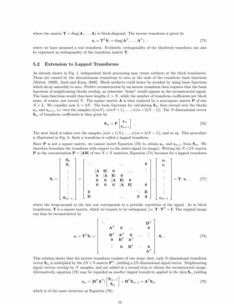
5.2 Extension to Lapped Transforms

As already shown in Fig. 1, independent block processing may create artifacts at the block boundaries.These are caused by the discontinuous transitions to zero at the ends of the transform basis functions[Malvar, 1992b, Aach and Kunz, 2000]. Block artifacts could hence be avoided by using basis functionswhich decay smoothly to zero. Perfect reconstruction by an inverse transform then requires that the basisfunctions of neighbouring blocks overlap, as otherwise “holes” would appear in the reconstructed signal.The basis functions would thus have lengths L > N , while the number of transform coefficients per blockmust, of course, not exceed N . The square matrix A is then replaced by a non-square matrix P of sizeN × L. We consider now L = 2N . The basis functions for calculating Sm then extend over the blockssm and sm+1, i.e. over the samples [s(mN), s(mN + 1), . . . , s((m + 2)N − 1)]. The N -dimensional vectorSm of transform coefficients is then given by

Sm = P[

sm

sm+1

]. (76)

The next block is taken over the samples [s(m + 1)N), . . . , s((m + 3)N − 1)], and so on. This procedureis illustrated in Fig. 8. Such a transform is called a lapped transform.

Since P is not a square matrix, we cannot invert Equation (76) to obtain sm and sm+1 from Sm. Wetherefore formulate the transform with respect to the entire signal (or image). Writing the N×2N -matrixP as the concatenation P = [AB] of two N ×N matrices, Equation (74) becomes for a lapped transform

St =

S0

S1

...

...

...

...SM−1

=

. . . . . . 0

[A B] 0 . . ....

0 [A B] 00 0 [A B] 00 0 0 [A B] 0

0. . . B

B . . . 0 A

·

s0

s1

...

...

...

...sM−1

= T · st , (77)

where the wrap-around in the last row corresponds to a periodic repetition of the signal. As in blocktransforms, T is a square matrix, which we require to be orthogonal, i.e. T ·TT = I. The original imagecan thus be reconstructed by

st = TT St =

. . . BT

AT 0 . . . 0

BT AT 0 . . ....

0 BT AT

... 0 BT . . . 0AT

· St . (78)

This relation shows that the inverse transform consists of two steps: first, each N -dimensional transformvector Sm is multiplied by the 2N×N -matrix PT , yielding a 2N -dimensional signal vector. Neighbouringsignal vectors overlap by N samples, and are added in a second step to obtain the reconstructed image.Alternatively, equation (78) may be regarded as another lapped transform applied to the data St, yielding

sm = [BT AT ][Sm−1

Sm

]= BT Sm−1 + AT Sm (79)

which is of the same structure as Equation (76).

15

5.3 The Lapped Orthogonal Transform

The matrix product T ·TT yields a block tridiagonal matrix, with entries P ·PT along the main diagonal,entries A·BT along the diagonal immediately to the left, and entries B·AT along the diagonal immediatelyto the right. From the orthogonality condition T · TT = I, the necessary and sufficient conditions onP = [AB] therefore are

P ·PT = A ·AT + B ·BT = I and A ·BT = B ·AT = 0 . (80)

For T · TT = I, we can equivalently write TT · T = I, from which an alternative formulation of thenecessary and sufficient condition can be derived:

AT ·A + BT ·B = I and AT ·B = BT ·A = 0 . (81)

We may also approach the orthogonality conditions by rewriting Equation (76) to

Sm = P[

sm

sm+1

]= [AB]

[sm

sm+1

](82)

Inserting this into Equation (79), we obtain

sm = BT Asm−1 + AT Bsm+1 +(AT A + BT B

)sm . (83)

This equality holds with condition (81).

The first condition in Equation (80) states that the rows of P, i.e. the transform basis functions, mustbe orthogonal, while the second condition requires the overlapping parts of the basis functions to beorthogonal as well. A transform complying with Equation (80) is called a lapped orthogonal transform(LOT). Invoking the shift matrix V defined as

V =[

0 I0 0

], (84)

where 0 and I are of size N ×N , conditions (80) can be more compactly written as

PVmPT = δ(m)I, ,m = 0, 1 . (85)

Extending the above considerations towards lapped transforms with basis functions of lengths L = KN ,K = 2, 3, . . ., the matrix P then has size N × L, and condition (85) becomes [Malvar and Staelin, 1989,Malvar, 1992b]

PVmPT = δ(m)I, ,m = 0, 1, 2, . . . ,K − 1 , (86)

where the identity matrix in the shift matrix V is now of order (K − 1)N . Of course, for K = 1 thisnotation includes traditional non-overlapping block transforms as a special case.

If P0 is a valid LOT matrix, it can be used to generate more valid LOT matrices P by P = Z ·P0, whereZ is an orthogonal N ×N matrix. P will then also comply with condition (86), since

PVmPT = ZP0VmPT0 ZT = Zδ(m)IZT = δ(m)I . (87)

In the following, we construct a valid LOT of order N with basis functions of length L = 2N . Toobtain a transform which can be realized by a fast algorithm, the initial matrix P0 is constructed fromthe unitary DCT basis functions of lengths N . As we have seen in section 3.2, half of the DCT basisfunctions are even symmetric, while the other half is odd. Stacking the even basis functions row-wiseinto the N

2 ×N matrix De, and the odd ones into the matrix Do, a valid LOT matrix is [Malvar, 1992a,Akansu and Wadas, 1992, Akansu and Haddad, 2001]

P0 =12

[De −Do (De −Do)JDe −Do −(De −Do)J

], (88)

where J is the counter identity matrix (or reverse operator) already used in section 3.2. The matrix P0 isof size N×2N , where, similar to KLT and DCT, the basis functions in the first N

2 rows are even, while the

16

other N2 basis functions are odd. It satisfies condition (86), but it will not optimize the transform coding

gain of e.g. an AR(1)-process. Hence, for a given covariance model Cs, the orthogonal square matrix Zis determined such that its rows are identical to the eigenvectors of the covariance matrix P0CsPT

0 . TheLOT ZP0 thus consists of two steps, first a transform by P0 followed by another transform by Z. Thecovariance matrix CS = ZP0CsPT

0 ZT then is diagonal. Note, however, that the LOT does not preservethe determinant of the covariance matrix. Fig. 9 shows the basis functions for N = 8 and L = 16 ascomputed for an AR(1) process with ρ = 0.91. The coding gain of this LOT is 5.06 (7.05dB).

The fast implementation of this transform reflects its two-step structure [Malvar, 1992b]: the matrix P0

is realized using an N -point DCT, which is followed by a series of plane rotations used to approximateZ [Akansu and Haddad, 2001, Akansu and Wadas, 1992]. The numerical values of the basis functions ofthe approximate LOT can be found for ρ = 0.95 in [Malvar, 1992b, p. 171].

5.4 The Modulated Lapped Transform

The above LOT was derived by an eigenvector analysis, leading to basis functions with even or oddsymmetry. An alternative approach is motivated by the close relationship between maximally decimatedfilter banks on the one hand and block and lapped transforms on the other [Akansu and Haddad, 2001,p. 4], [Malvar, 1992b]. In filter banks, the filters are often realized by a lowpass prototype shifted toN different frequency channels by modulation. In the context of lapped transforms, this leads to theso-called modulated lapped transform if the filter length L is equal to 2N . For longer filters (or basisfunctions), this transform is referred to as the extended lapped transform (ELT).

For L = 2N , the basis functions are formed by a cosine modulated window function h(n), leading to theN × 2N transform matrix P with entries

[P]kn = h(n) ·√

2N

cos[(

n +N + 1

2

)(k +

12

)π

N

], (89)

for k = 0, . . . , N − 1, and n = 0, . . . , 2N − 1. The window h(n) obeys

h(n) = ± sin[(

n +12

)π

2N

]. (90)

These basis functions are shown in Fig. 10. Evidently, they are not symmetric any more. Still, thehalf-sine window ensures a continuous transition towards zero at the ends of the basis functions. In thefollowing, we will show that this choice of basis functions complies with the orthogonality conditions (81).

The window function obeys the conditions

h2(n) + h2(n + N) = 1 (91)

andh(n) = h(2N − 1− n) . (92)

Arranging the window samples into two diagonal N ×N matrices H0 and H1, we obtain

H0 = diag[h(0), h(1), . . . , h(N − 1)]H1 = diag[h(N), h(N + 1), . . . , h(2N − 1)]

= diag[h(N − 1), h(N − 2), . . . , h(0)] = JH0J (93)

where JH0J reverses both rows and columns of H0. The modulating cosines are arranged into the N×Nmatrices Q0 and Q1, yielding

[Q0]kn =

√2N

cos[(

n +N + 1

2

)(k +

12

)π

N

], k, n = 0, . . . , N − 1 (94)

and

[Q1]kn =

√2N

cos[(

n + N +N + 1

2

)(k +

12

)π

N

], k, n = 0, . . . , N − 1 (95)

17

Expressing the transformation matrix P as the concatenation P = [AB], we get

A = Q0H0 , and B = Q1H1 . (96)

For Q0 and Q1, the conditionsQT

0 Q1 = QT1 Q0 = 0 , (97)

QT0 Q0 = Q0QT

0 = I− J (98)

andQT

1 Q1 = Q1QT1 = I + J (99)

hold (see Appendix D). Inserting these into condition (81), we obtain

AT B = H0QT0 Q1H1 = 0 (100)

and

AT A + BT B = H0QT0 Q0H0 + H1QT

1 Q1H1

= H0 [I− J]H0 + H1 [I + J]H1

= H20 + H2

1 −H0JH0 + H1JH1 = I (101)

since H20 + H2

1 = I and H0JH0 = H1JH1. This shows that the MLT complies with the orthogonalityconditions for the LOT. For the AR(1)-model with ρ = 0.91, the MLT transform coding gain is 5.15(7.12dB).

5.5 Extensions

In this section, we discuss three extensions of the MLT and the LOT by introducing additional basisfunctions which are in a certain sense complementary to the already existing ones.

In the MLT, reconstruction from the transform vector Sm = P[sTmsT

m+1]T only leads to[

sm

sm+1

]= PT Sm =

[AT

BT

][AB]

[sm

sm+1

]. (102)

With Equations (96), (98) and (99), we obtain[AT

BT

][AB] =

[AT A AT BBT A BT B

]=[

H0(I− J)H0 00 H1(I + J)H1

](103)

where 0 is of size N × N . This matrix is evidently not diagonal, thus mixing coefficients from sm withdifferent time indices into one coefficient of the reconstructed vector sm, and similarly for sm+1. Inanalogy to frequency-domain aliasing, where higher frequencies are mapped back onto lower ones duringdownsampling, this phenomenon is called time-domain aliasing. Since the MLT perfectly reconstructsthe entire signal st by adding the overlapping signals obtained by individual inverse transforms, time-domain aliasing in the reconstruction from Sm is hence cancelled from reconstructions from Sm−1 andSm+1 (time-domain aliasing cancellation, TDAC). This observation holds if the transform vectors Si areleft unchanged. Frequency-domain processing of the transform coefficients unbalances the time-domainaliasing components contained in the si, thus resulting in uncancelled time-domain aliasing in the re-constructed signal. In general, these uncancelled aliasing components are the larger, the stronger thetransform coefficients are changed during processing. Keeping uncancelled aliasing below an acceptablethreshold hence restricts how strongly the transform coefficients can be processed. As an example, acous-tic echo cancellation using the MLT is mentioned in [Malvar, 1999], where the occurrence of uncancelledaliasing limits the maximum echo reduction to no more than 10dB.

In [Malvar, 1999], the MLT is therefore extended by replacing the real basis functions by complex onesdefined as

[P]kn = h(n) ·√

2N

exp{−j

(n +

N + 12

)(k +

12

)π

N

}. (104)

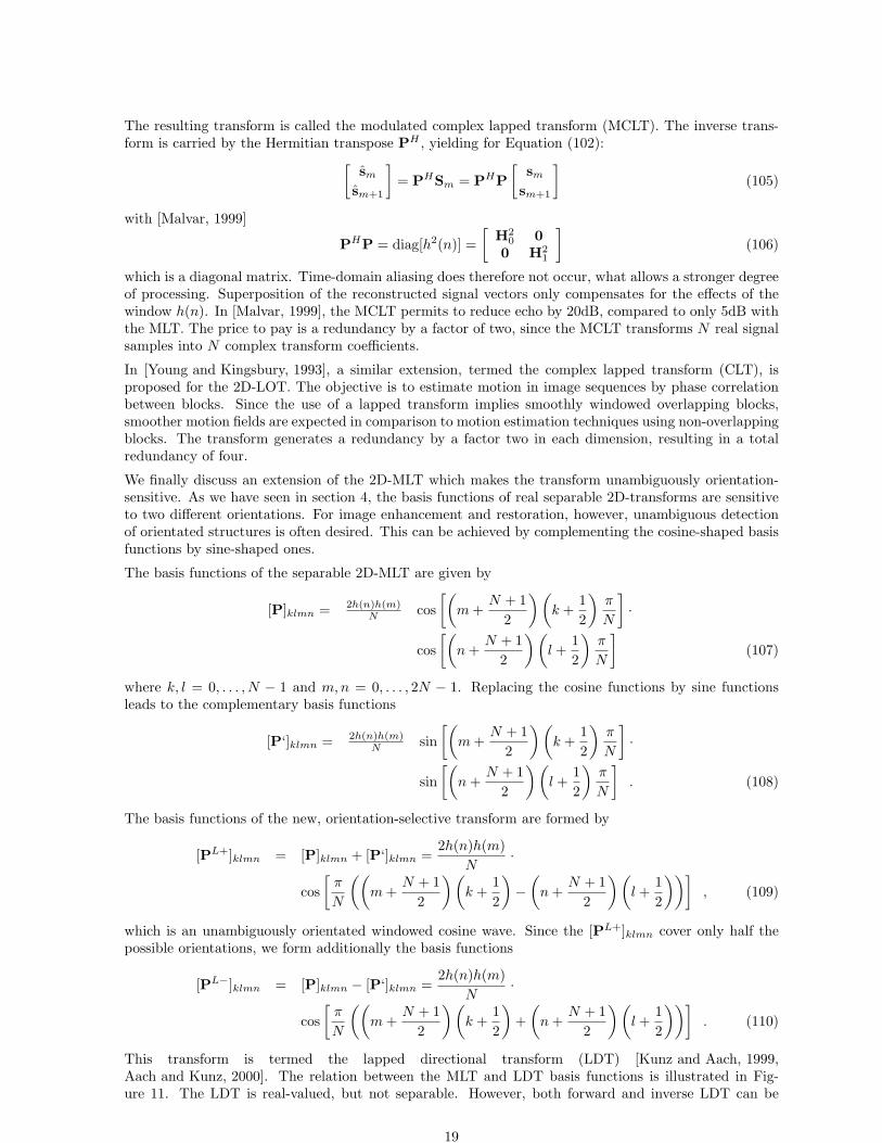
18

The resulting transform is called the modulated complex lapped transform (MCLT). The inverse trans-form is carried by the Hermitian transpose PH , yielding for Equation (102):[

sm

sm+1

]= PHSm = PHP

[sm

sm+1

](105)

with [Malvar, 1999]

PHP = diag[h2(n)] =[

H20 0

0 H21

](106)

which is a diagonal matrix. Time-domain aliasing does therefore not occur, what allows a stronger degreeof processing. Superposition of the reconstructed signal vectors only compensates for the effects of thewindow h(n). In [Malvar, 1999], the MCLT permits to reduce echo by 20dB, compared to only 5dB withthe MLT. The price to pay is a redundancy by a factor of two, since the MCLT transforms N real signalsamples into N complex transform coefficients.

In [Young and Kingsbury, 1993], a similar extension, termed the complex lapped transform (CLT), isproposed for the 2D-LOT. The objective is to estimate motion in image sequences by phase correlationbetween blocks. Since the use of a lapped transform implies smoothly windowed overlapping blocks,smoother motion fields are expected in comparison to motion estimation techniques using non-overlappingblocks. The transform generates a redundancy by a factor two in each dimension, resulting in a totalredundancy of four.

We finally discuss an extension of the 2D-MLT which makes the transform unambiguously orientation-sensitive. As we have seen in section 4, the basis functions of real separable 2D-transforms are sensitiveto two different orientations. For image enhancement and restoration, however, unambiguous detectionof orientated structures is often desired. This can be achieved by complementing the cosine-shaped basisfunctions by sine-shaped ones.

The basis functions of the separable 2D-MLT are given by

[P]klmn = 2h(n)h(m)N cos

[(m +

N + 12

)(k +

12

)π

N

]·

cos[(

n +N + 1

2

)(l +

12

)π

N

](107)

where k, l = 0, . . . , N − 1 and m,n = 0, . . . , 2N − 1. Replacing the cosine functions by sine functionsleads to the complementary basis functions

[P‘]klmn = 2h(n)h(m)N sin

[(m +

N + 12

)(k +

12

)π

N

]·

sin[(

n +N + 1

2

)(l +

12

)π

N

]. (108)

The basis functions of the new, orientation-selective transform are formed by

[PL+]klmn = [P]klmn + [P‘]klmn =2h(n)h(m)

N·

cos[

π

N

((m +

N + 12

)(k +

12

)−(

n +N + 1

2

)(l +

12

))], (109)

which is an unambiguously orientated windowed cosine wave. Since the [PL+]klmn cover only half thepossible orientations, we form additionally the basis functions

[PL−]klmn = [P]klmn − [P‘]klmn =2h(n)h(m)

N·

cos[

π

N

((m +

N + 12

)(k +

12

)+(

n +N + 1

2

)(l +

12

))]. (110)

This transform is termed the lapped directional transform (LDT) [Kunz and Aach, 1999,Aach and Kunz, 2000]. The relation between the MLT and LDT basis functions is illustrated in Fig-ure 11. The LDT is real-valued, but not separable. However, both forward and inverse LDT can be

19

computed from the separable fast MLTs in Equations (107) and (108). The LDT generates a redundancyby a factor of only two, and was successfully used for anisotropic image restoration and enhancement in[Kunz and Aach, 1999, Aach and Kunz, 2000]. In a combined image restoration, enhancement and com-pression framework, the processed LDT coefficients can be reconverted into the coefficients of the MLTand the complementary MLT by a simple butterfly. Using only the MLT coefficients for compressioneliminates the redundancy problem [Aach and Kunz, 2000].

6 Image Restoration and Enhancement

In this section, we compare the block FFT and the LDT within a framework for anisotropic noise reductionby a nonlinear spectral domain filter. The noisy input image is first decomposed into blocks of size 32×32pixels, which are then transformed by the FFT or the LDT. The observed noisy transform coefficients arethen attenuated depending on their observed signal-to-noise ratio: the more the magnitude of a coefficientexceeds a corresponding noise estimate, the lower it is attenuated. Since directional image informationleads to spectral energy concentration, which can unambiguously be detected in both FFT and LDT(but not in real separable transforms, like DCT, LOT and MLT), coefficients contributing to orientedlines and edges can be identified and more carefully treated than other ones. These algorithms arediscussed in detail in [Aach and Kunz, 2000, Aach, 2000, Kunz and Aach, 1999, Aach and Kunz, 1996a,Aach and Kunz, 1998]. Figure 12 shows an original image and its noisy version (white Gaussian noise,peak signal-to-noise-ratio 20.2 dB). The processed images are given in Figure 13. Evidently, processingby the FFT without block overlap reduces the noise level visibly, but the rather strong processing causesthe block raster to appear. (In [Aach and Kunz, 1996b, Aach and Kunz, 1996a], we have therefore usedoverlapping blocks, inflating the processed data volume by a factor four.) The LDT-based processingresult reduces noise approximately as much as the FFT-based approach, viz. by about 6 dB, withoutcausing block artifacts. Enlargements of both processing results are given in Fig. 14.

7 Discussion

In this chapter, we have summarized the development of lapped transforms. We started with thecontinuous-time and discrete-time Fourier transforms of time-dependent signals with infinite duration.These transforms were viewed as a decomposition of the signals into frequency-selective basis functions,or eigenfunctions of LTI systems. With the discrete Fourier transform which decomposes a finite-lengthsignal block into a set of orthogonal basis functions, a transform could be expressed as a multiplicationof the signal vector by a unitary matrix, i.e. viewed as a rotation of coordinate axes. We have then ana-lyzed the effects of unitary transforms of the covariance structure of random signals, and found optimaltransforms with respect to decorrelation and energy concentration. While these optimal transforms aresignal-dependent and cannot be calculated fast, we showed that Fourier-like fixed transforms, in particu-lar the DCT, are practically good approximations to the optimal transforms. The downside of blockwiseprocessing are the blocking artifacts introduced by independent spectral-domain processing the blocks.To alleviate the blocking effects, we have then turned to finite-length transforms with overlapping basisfunctions. The transform matrix for a single block then is not square anymore, inverse transforms ofsingle blocks do therefore not exist. Under extended orthogonality conditions, however, it was shownthat the original signal can be reconstructed from non-perfectly reconstructed individual blocks by over-lapping and adding. Two types of lapped transforms were discussed, the lapped orthogonal transformand the modulated lapped transform, where we have focussed on a 2:1 overlap. For the LOT, a feasiblerectangular matrix obeying the extended orthogonality conditions was first constructed using DCT basisfunctions. This matrix was optimized by multiplication with an orthogonal square matrix derived from aneigenvector analysis. The MLT did not need an eigenvector analysis, rather, it was based on modulatedfilter banks. We did not delve deeper into the relation between block transforms and filter banks. Sufficeit to mention that a block transform can be viewed as a uniform critically sampled filter bank, wherethe filter length is equal to the number of subbands. Similarly, a lapped transform can be regarded as auniform and critically sampled filter bank with filter length equal to e.g. twice the number of subbands.

We then have discussed extensions of both the LOT and the MLT in speech and image processing.These extensions are based on the additional use of complementary basis functions, thus introducing

20

redundancy. We have concluded with an exemplary comparison of block and lapped transforms in imageprocessing.

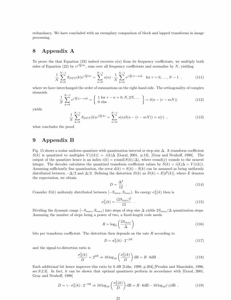
8 Appendix A

To prove the that Equation (23) indeed recovers s(n) from its frequency coefficients, we multiply bothsides of Equation (22) by ej 2π

N kr, sum over all frequency coefficients and normalize by N , yielding

1N

N−1∑k=0

SDFT (k)ej 2πN kr =

N−1∑n=0

s(n) · 1N

N−1∑k=0

ej 2πN (r−n)k for r = 0, . . . , N − 1 , (111)

where we have interchanged the order of summations on the right-hand side. The orthogonality of complexsinusoids

1N

N−1∑k=0

ej 2πN (r−n)k =

{1 for r − n = 0, N, 2N, . . .0 else

}= δ(n− (r −mN)) (112)

yields1N

N−1∑k=0

SDFT (k)ej 2πN kr =

N−1∑n=0

s(n)δ(n− (r −mN)) = s(r) , (113)

what concludes the proof.

9 Appendix B

Fig. 15 shows a scalar uniform quantizer with quantization interval or step size ∆. A transform coefficientS(k) is quantized to multiples V (i(k)) = i(k)∆ [Goyal, 2001, p.13], [Gray and Neuhoff, 1998]. Theoutput of the quantizer hence is an index i(k) = round(S(k)/∆), where round(x) rounds to the nearestinteger. The decoder calculates the quantized transform coefficient values by S(k) = i(k)∆ = V (i(k)).Assuming sufficiently fine quantization, the error d(k) = S(k)− S(k) can be assumed as being uniformlydistributed between −∆/2 and ∆/2. Defining the distortion D(k) as D(k) = E[d2(k)], where E denotesthe expectation, we obtain

D =∆2

12. (114)

Consider S(k) uniformly distributed between [−Smax, Smax). Its energy σ2S(k) then is

σ2S(k) =

(2Smax)2

12. (115)

Dividing the dynamic range [−Smax, Smax) into steps of step size ∆ yields 2Smax/∆ quantization steps.Assuming the number of steps being a power of two, a fixed-length code needs

R = log2

(2Smax

∆

)(116)

bits per transform coefficient. The distortion then depends on the rate R according to

D = σ2S(k) · 2−2R (117)

and the signal-to-distortion ratio is

σ2S(k)D

= 22R ⇒ 10 log10

(σ2

S(k)D

)dB = R · 6dB . (118)

Each additional bit hence improves this ratio by 6 dB [Luke, 1999, p.204],[Proakis and Manolakis, 1996,sec.9.2.3]. In fact, it can be shown that optimal quantizers perform in accordance with [Goyal, 2001,Gray and Neuhoff, 1998]

D = γ · σ2S(k) · 2−2R ⇒ 10 log10

(σ2

S(k)D

)dB = R · 6dB− 10 log10(γ)dB , (119)

21

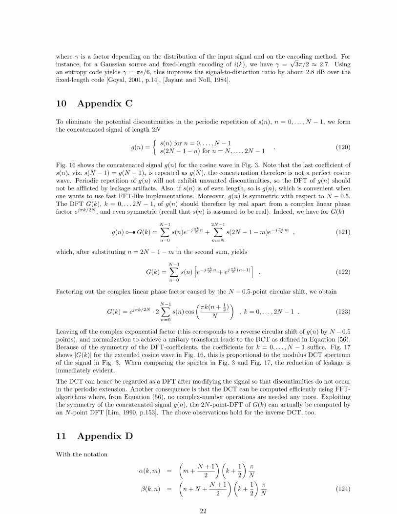
where γ is a factor depending on the distribution of the input signal and on the encoding method. Forinstance, for a Gaussian source and fixed-length encoding of i(k), we have γ =

√3π/2 ≈ 2.7. Using

an entropy code yields γ = πe/6, this improves the signal-to-distortion ratio by about 2.8 dB over thefixed-length code [Goyal, 2001, p.14], [Jayant and Noll, 1984].

10 Appendix C

To eliminate the potential discontinuities in the periodic repetition of s(n), n = 0, . . . , N − 1, we formthe concatenated signal of length 2N

g(n) ={

s(n) for n = 0, . . . , N − 1s(2N − 1− n) for n = N, . . . , 2N − 1 . (120)

Fig. 16 shows the concatenated signal g(n) for the cosine wave in Fig. 3. Note that the last coefficient ofs(n), viz. s(N − 1) = g(N − 1), is repeated as g(N), the concatenation therefore is not a perfect cosinewave. Periodic repetition of g(n) will not exhibit unwanted discontinuities, so the DFT of g(n) shouldnot be afflicted by leakage artifacts. Also, if s(n) is of even length, so is g(n), which is convenient whenone wants to use fast FFT-like implementations. Moreover, g(n) is symmetric with respect to N − 0.5.The DFT G(k), k = 0, . . . 2N − 1, of g(n) should therefore by real apart from a complex linear phasefactor ejπk/2N , and even symmetric (recall that s(n) is assumed to be real). Indeed, we have for G(k)

g(n) ◦−•G(k) =N−1∑n=0

s(n)e−j πkN n +

2N−1∑m=N

s(2N − 1−m)e−j πkN m , (121)

which, after substituting n = 2N − 1−m in the second sum, yields

G(k) =N−1∑n=0

s(n)[e−j πk

N n + ej πkN (n+1)

]. (122)

Factoring out the complex linear phase factor caused by the N − 0.5-point circular shift, we obtain

G(k) = ejπk/2N · 2N−1∑n=0

s(n) cos(

πk(n + 12 )

N

), k = 0, . . . , 2N − 1 . (123)

Leaving off the complex exponential factor (this corresponds to a reverse circular shift of g(n) by N −0.5points), and normalization to achieve a unitary transform leads to the DCT as defined in Equation (56).Because of the symmetry of the DFT-coefficients, the coefficients for k = 0, . . . , N − 1 suffice. Fig. 17shows |G(k)| for the extended cosine wave in Fig. 16, this is proportional to the modulus DCT spectrumof the signal in Fig. 3. When comparing the spectra in Fig. 3 and Fig. 17, the reduction of leakage isimmediately evident.

The DCT can hence be regarded as a DFT after modifying the signal so that discontinuities do not occurin the periodic extension. Another consequence is that the DCT can be computed efficiently using FFT-algorithms where, from Equation (56), no complex-number operations are needed any more. Exploitingthe symmetry of the concatenated signal g(n), the 2N -point-DFT of G(k) can actually be computed byan N -point DFT [Lim, 1990, p.153]. The above observations hold for the inverse DCT, too.

11 Appendix D

With the notation

α(k, m) =(

m +N + 1

2

)(k +

12

)π

N

β(k, n) =(

n + N +N + 1

2

)(k +

12

)π

N(124)

22

we have for the m + 1, n + 1-th element of QT0 Q1

[QT0 Q1]mn =

2N

N−1∑k=0

cos α(k, m) cos β(k, n)

=1N

N−1∑k=0

[cos (α(k, m) + β(k, n)) + cos (α(k, m)− β(k, n))] (125)

With

γ(k) = α(k, m) + β(k, n) = (m + n + 1)(

k +12

)π

N+ π (126)

and 0 < m + n + 1 < 2N , the sum∑N−1

k=0 cos γ(k) extends over i periods if m + n + 1 = 2i is an evennumber, and is thus zero. For m + n + 1 = 2i + 1 odd, the sequence of cos γ(k), k = 0, . . . , N − 1, is anodd sequence, and again sums to zero. Similarly, the sum over the cos (α(k, m)− β(k, n)) is zero, whatproves Equation (97).

The entries of QT0 Q0 are

[QT0 Q0]mn =

2N

N−1∑k=0

cos α(k, m) cos α(k, n)

=1N

N−1∑k=0

[cos (α(k, m)− α(k, n)) + cos (α(k, m) + α(k, n))] (127)

whereN−1∑k=0

cos (α(k, m)− α(k, n)) ={

0 for m 6= nN for m = n

(128)

andN−1∑k=0

cos (α(k, m) + α(k, n)) ={

0 for m + n 6= N − 1−N for m + n = N − 1 (129)

from which Equation (98) follows. The proof of Equation (99) is similar.

12 Acknowledgement

The author is grateful to Cicero Mota, formerly with the University of Amazonas, Brazil, and now withthe University of Lubeck, and to Dietmar Kunz, Cologne University of Applied Sciences, for fruitfuldiscussions.

References

[Aach, 2000] Aach, T. (2000). Transform-based denoising and enhancement in medical x-ray imaging. InGabbouj, M. and Kuosmanen, P., editors, European Signal Processing Conference, pages 1085–1088,Tampere, Finland. EURASIP.

[Aach and Kunz, 1996a] Aach, T. and Kunz, D. (1996a). Anisotropic spectral magnitude estimationfilters for noise reduction and image enhancement. In Proceedings ICIP-96, pages 335–338, Lausanne,Switzerland. IEEE.

[Aach and Kunz, 1996b] Aach, T. and Kunz, D. (1996b). Spectral estimation filters for noise reductionin x-ray fluoroscopy imaging. In Ramponi, G., Sicuranza, G. L., Carrato, S., and Marsi, S., editors,Proceedings EUSIPCO-96, pages 571–574, Trieste, Italy. Edizioni LINT Trieste.

23

[Aach and Kunz, 1998] Aach, T. and Kunz, D. (1998). Spectral amplitude estimation-based x-ray imagerestoration: An extension of a speech enhancement approach. In Theodoridis, S., Pitas, I., Stouraitis,A., and Kalouptsidis, N., editors, Proceedings EUSIPCO-98, pages 323–326, Patras. Typorama.

[Aach and Kunz, 2000] Aach, T. and Kunz, D. (2000). A lapped directional transform for spectral imageanalysis and its application to restoration and enhancement. Signal Processing, 80(11):2347–2364.

[Ahmed et al., 1974] Ahmed, N., Natarajan, T., and Rao, K. R. (1974). Discrete cosine transform. IEEETransactions on Computers, 23:90–93.

[Akansu and Haddad, 2001] Akansu, A. N. and Haddad, R. A. (2001). Multiresolution Signal Decompo-sition. Academic Press, Boston.

[Akansu and Wadas, 1992] Akansu, A. N. and Wadas, F. E. (1992). On lapped orthogonal transforms.IEEE Transactions on Signal Processing, 40(2):439–443.

[Bamler, 1989] Bamler, R. (1989). Mehrdimensionale lineare Systeme. Springer Verlag, Berlin.

[Cantoni and Butler, 1976] Cantoni, A. and Butler, P. (1976). Properties of the eigenvectors of persym-metric matrices with applications to communication theory. IEEE Transactions on Communications,24(8):804–809.

[Cappe, 1994] Cappe, O. (1994). Elimination of the musical noise phenomenon with the Ephraim andMalah noise suppressor. IEEE Transactions on Speech and Audio Processing, 2(2):345–349.

[Clarke, 1985] Clarke, R. J. (1985). Transform Coding of Images. Academic Press, London.

[Clarke and Tech, 1981] Clarke, R. J. and Tech, B. (1981). Relation between the carhunen loeve andcosine transform. IEEE Proc., 128(6):359–360.

[Ephraim and Malah, 1984] Ephraim, Y. and Malah, D. (1984). Speech enhancement using a minimummean-square error short-time spectral amplitude estimator. IEEE Transactions on Acoustics, Speech,and Signal Processing, 32(6):1109–1121.

[Fukunaga, 1972] Fukunaga, K. (1972). Introduction to Statistical Pattern Recognition. Academic Press,New York.

[Goyal, 2001] Goyal, V. K. (2001). Theoretical foundations of transform coding. IEEE Signal ProcessingMagazine, September:9–21.

[Gray and Neuhoff, 1998] Gray, R. M. and Neuhoff, D. L. (1998). Quantization. IEEE Transactions onInformation Theory, 44:2325–2383.

[Huang and Schultheiss, 1963] Huang, J. and Schultheiss, P. (1963). Block quantization of correlatedGaussian random variables. IEEE Transactions on Communication Systems, 11:289–296.

[Jain, 1979] Jain, A. K. (1979). A sinusoidal family of unitary transforms. IEEE Transactions on PatternAnalysis and Machine Intelligence, 1(4):356–365.

[Jayant and Noll, 1984] Jayant, N. S. and Noll, P. (1984). Digital Coding of Waveforms. Prentice Hall,Englewood Cliffs, NJ.

[Kunz and Aach, 1999] Kunz, D. and Aach, T. (1999). Lapped directional transform: A new transformfor spectral image analysis. In Proceedings ICASSP-99, pages 3433–3436, Phoenix, AZ. IEEE.

[Lim, 1980] Lim, J. S. (1980). Image restoration by short space spectral subtraction. IEEE Transactionson Acoustics, Speech, and Signal Processing, 28(2):191–197.

[Lim, 1990] Lim, J. S. (1990). Two-Dimensional Signal and Image Processing. Prentice-Hall, EnglewoodCliffs.

[Lim and Oppenheim, 1979] Lim, J. S. and Oppenheim, A. V. (1979). Enhancement and bandwidthcompression of noisy speech. Proceedings of the IEEE, 67(12):1586–1604.

24

[Luke, 1999] Luke, H. D. (1999). Signalubertragung. Springer Verlag, Berlin, Heidelberg, New York.

[Makhoul, 1981] Makhoul, J. (1981). On the eigenvectors of symmetric Toeplitz matrices. IEEE Trans-actions on Acoustics, Speech, and Signal Processing, 29(4):868–872.

[Malvar, 1999] Malvar, H. (1999). A modulated complex lapped transform and its application to audioprocessing. In Proceedings ICASSP-99, pages 1421–1424, Phoenix, AZ. IEEE.

[Malvar, 1992a] Malvar, H. S. (1992a). Extended lapped transforms: Properties, applications, and fastalgorithms. IEEE Transactions on Signal Processing, 40(11):2703–2714.

[Malvar, 1992b] Malvar, H. S. (1992b). Signal Processing with Lapped Transforms. Artech House, Nor-wood, MA.

[Malvar and Staelin, 1989] Malvar, H. S. and Staelin, D. H. (1989). The LOT: Transform coding withoutblocking effects. IEEE Transactions on Acoustics, Speech, and Signal Processing, 37(4):553–559.

[Oppenheim and Schafer, 1998] Oppenheim, A. V. and Schafer, R. W. (1998). Discrete-Time SignalProcessing. Prentice Hall, Englewood Cliffs, NJ.

[Papoulis, 1968] Papoulis, A. (1968). Systems and Transforms with Applications in Optics. McGraw Hill,New York.

[Proakis and Manolakis, 1996] Proakis, J. G. and Manolakis, D. G. (1996). Digital Signal Processing.Prentice Hall, Upper Saddle River, NJ.

[Rabbani and Jones, 1991] Rabbani, M. and Jones, P. W. (1991). Digital Image Compression Techniques.SPIE Optical Engineering Press, Bellingham.

[Ray and Driver, 1970] Ray, W. D. and Driver, R. M. (1970). Further decomposition of the Karhunen-Loeve series representation of a stationary random process. IEEE Transactions on Information Theory,16(4):845–850.

[Therrien, 1989] Therrien, C. W. (1989). Decision, Estimation, and Classification. John Wiley, NewYork.

[Therrien, 1992] Therrien, C. W. (1992). Discrete Random Signals and Statistical Signal Processing.Prentice-Hall, Englewood Cliffs.

[Unser, 1984] Unser, M. (1984). On the approximation of the discrete Karhunen-Loeve Transform forstationary processes. Signal Processing, 7:231–249.

[van Compernolle, 1992] van Compernolle, D. (1992). DSP techniques for speech enhancement. In SpeechProcessing in Adverse Conditions, pages 21–30, Cannes-Mandelieu, 10.-13. November.

[Young and Kingsbury, 1993] Young, R. W. and Kingsbury, N. G. (1993). Frequency-domain motionestimation using a complex lapped transform. IEEE Transactions on Image Processing, 2(1):2–17.

[Zelinski and Noll, 1977] Zelinski, R. and Noll, P. (1977). Adaptive transform coding of speech signals.IEEE Transactions on Acoustics, Speech, and Signal Processing, ASSP–25(4):299–309.

[Ziemer et al., 1989] Ziemer, R. E., Tranter, W. H., and Fannin, D. R. (1989). Signals and Systems:Continuous and Discrete. Macmillan Publishing Company, New York.

25

L 0 1 2 3 4 5 6 7KLT 100 20.5 8.9 5.2 3.3 2.1 1.3 0.61DCT 100 20.7 9.1 5.2 3.3 2.2 1.3 0.61

Table 1: Basis restriction error in percent for KLT and DCT.

Figure 1: Left: Portion of size 361 × 390 pixels of the ’Marcel’ image, eight bits per pixel. Right:Reconstruction after JPEG compression at about 0.2 bits per pixel.

26

Figure 2: Left: Source signal s(n) = cos(4πn/64) for n = 0, . . . , 63. Right: Modulus DFT spectrumSDFT (k) of s(n) for k = 0, . . . , 63. Since periodic repetition of s(n) does not create discontinuities, theDFT spectrum exhibits the expected two peaks.

Figure 3: Left: Source signal s(n) = cos(5πn/64) for n = 0, . . . , 63. Right: Modulus DFT spectrumSDFT (k) of s(n) for k = 0, . . . , 63. Periodic repetition of s(n) results in strong discontinuities betweenthe periods, causing the spreading of signal energy over all frequency coefficients.

27

Figure 4: Block diagram of a transform coder and decoder. The signal vector s is first transformed intothe transform coefficient vector S = As. The transform coefficients are quantized. The quantizationindices i(k) are encoded into codewords and multiplexed into the bitstream which is transmitted over thechannel. The decoder first demultiplexes the bitstream into the codewords, which are then reconvertedinto the quantization indices i(k). The decoded quantization indices are used to access the codebooks,yielding the quantized transform coefficient values S(k) = V (i(k)). These are subjected to an inversetransform to obtain the reconstructed signal vector s = A−1S.

Figure 5: Numerically computed KLT basis vectors of an AR(1)-process for ρ = 0.91 and N = 8.

28

Figure 6: Basis vectors of the unitary DCT for N = 8. Up to a sign, the similarity to the KLT basisvectors in Fig. 5 is evident.

Figure 7: Left: Real part of a basis matrix of the 2D-DFT for N = 16, k = l = 2. Right: 2D-DCT basismatrix for N = 16, k = l = 4.

29

Figure 8: Formation of signal blocks sm and transform vectors Sm in a lapped transform with basisfunctions of length L = 2N .

Figure 9: Basis functions of the LOT for N = 8 and L = 16. The computation of the basis functions isbased on an AR(1) signal model with ρ = 0.91. The functions are sorted from left to right and top tobottom in descending order of the eigenvalues of P0CsPT

0 .

30

Figure 10: Basis functions of the MLT for N = 8 and L = 16. The frequency index k increases from leftto right and top to bottom.

31

a) b)

c) d)

Figure 11: Example 2D-MLT and LDT basis functions for N = 8, and k = 3, l = 2: a) MLT, b) MLT′,c) LDT (sum), d) LDT (difference).

Figure 12: Left: Original image ’Marcel’. Right: Noisy version with a PSNR of 20.2 dB.

32

Figure 13: Left: Processing result for the noisy ’Marcel’ image using the block FFT with no overlap.The blocking effect is evident. Right: Processing result for the noisy ’Marcel’ image using the LDT. Thenoise reduction performance is almost identical to the FFT-based algorithm, but the blocking effect hasdisappeared.

Figure 14: Enlarged versions of the FFT-processed (left) and LDT-processed (right) noisy ’Marcel’ image.

33

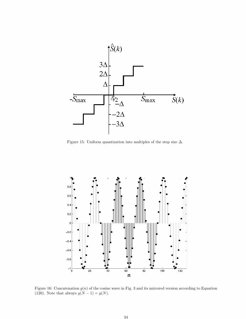
Figure 15: Uniform quantization into multiples of the step size ∆.

Figure 16: Concatenation g(n) of the cosine wave in Fig. 3 and its mirrored version according to Equation(120). Note that always g(N − 1) = g(N).

34

Figure 17: Modulus DFT of the extended cosine in Fig. 16, for k = 0, . . . , N−1 = 63, what is proportionalto the DCT of the cosine wave in Fig. 3. Note the improved concentration of spectral energy with respectto the DFT spectrum in Fig. 3.

35