Fourier spectral methods for fractional-in-spacereaction-diffusion equations

by

Alfonso Bueno-Orovio

David Kay

Kevin Burrage

OCCAM Preprint Number 12/50

Fourier spectral methods for fractional-in-space

reaction-diffusion equations

Alfonso Bueno-Orovioa,b,∗, David Kayb, Kevin Burrageb,c

aOxford Centre for Collaborative Applied Mathematics, University of Oxford,

Oxford OX1 3LB, United KingdombComputational Biology Group, Department of Computer Science, University of Oxford,

Oxford OX1 3QD, United KingdomcSchool of Mathematical Sciences, Queensland University of Technology,

Brisbane 4001, Australia

Abstract

Fractional differential equations are becoming increasingly used as a power-ful modelling approach for understanding the many aspects of nonlocality andspatial heterogeneity. However, the numerical approximation of these modelsis computationally demanding and imposes a number of computational con-straints. In this paper, we introduce Fourier spectral methods as an attractiveand easy-to-code alternative for the integration of fractional-in-space reaction-diffusion equations. The main advantages of the proposed schemes is that theyyield a fully diagonal representation of the fractional operator, with increasedaccuracy and efficiency when compared to low-order counterparts, and a com-pletely straightforward extension to two and three spatial dimensions. Ourapproach is show-cased by solving several problems of practical interest, in-cluding the fractional Allen–Cahn, FitzHugh–Nagumo and Gray–Scott models,together with an analysis of the properties of these systems in terms of thefractional power of the underlying Laplacian operator.

Keywords: Fractional calculus, fractional Laplacian, spectral methods,reaction-diffusion equations2010 MSC: 35R11, 65M70, 34L10, 65T50, 35K57

1. Introduction

Fractional differential equations are becoming increasingly used as a mod-elling tool for diffusive processes associated with sub-diffusion (fractional intime), super-diffusion (fractional in space) or both, and have a long history in,

∗Corresponding authorEmail addresses: alfonso.bueno@maths.ox.ac.uk (Alfonso Bueno-Orovio),

david.kay@cs.ox.ac.uk (David Kay), kevin.burrage@cs.ox.ac.uk (Kevin Burrage)

Preprint submitted to Journal of Computational Physics June 7, 2012

for example, physics, finance, mathematical biology and hydrology. In water re-sources, fractional models have been used to describe chemical and contaminanttransport in heterogeneous aquifers [1, 2, 3]. In finance, they have been usedbecause of the relationship with certain option pricing mechanisms and heavytailed stochastic processes [4]. More recently, fractional models of the Bloch–Torrey equation have been used in magnetic resonance [5]. In this paper wewill only consider super-diffusion effects (space-fractional models) in spatiallyextended structures, such as those possessing spatial connectivity, where themovement of particles may thus be facilitated within a certain scale.

In this context, the spatial complexity of the environment imposes geometricconstraints on the transport processes on all length scales, which can be inter-preted as temporal correlations on all time scales. Non-homogeneities of themedium may fundamentally alter the laws of Markov diffusion, leading to longrange fluxes, and non-Gaussian, heavy tailed profiles [6, 7], and these motionsmay no longer obey Fick’s Law [8]. It is in this setting that fractional modelscan offer insights that traditional approaches do not offer.

A space-fractional diffusion equation can be derived by replacing Fick’s Lawfor the flux V (the rate at which mass is transported through an unit area againstthe concentration gradient) by its fractional counterpart (cf. Meerschaert et al.[9]):

V = −K∇βu, 0 < β ≤ 1, (1)

where K is the conductivity or diffusion tensor, and ∇β =(

∂β

∂xβ ,∂β

∂yβ ,∂β

∂zβ

)T

is

the Riemann–Louiville fractional gradient, where

∂β

∂xβu(x, y, z) =

1

Γ(1− β)

∂

∂x

∫ x

0

u(s, y, z)

(x− s)βds, (2)

with similar expressions for ∂β

∂yβ and ∂β

∂zβ [10]. The fractional Fick’s Law (1)naturally implies spatial and temporal nonlocality, and can be derived fromrigorous approaches using spatial averaging theorems and measurable functions[11]. Combining this with a conservation of mass equation for the concentrationof particles u(x, t)

∂tu = −∇ · V, (3)

finally leads to∂tu = −∇ · (−K∇βu). (4)

Equivalently, in the isotropic setting [12] the space fractional reaction-diffusionequation can be written as

∂tu = −K(−∆)α/2u+ f(u, t), 1 < α ≤ 2, (5)

where (−∆)α/2 is the fractional Laplacian operator.A standard approach for solving problems of the form (5) is to apply a finite

difference, finite element or finite volume discretisation of the fractional oper-ator, and then use a semi-implicit Euler formulation for the time evolution of

2

the solution. This requires the solution of a linear system of equations at eachtime step, whose left-hand-side matrix has a fractional power. Various authorssuch as Meerschaert et al. [13], Roop [14], Ilic et al., [15], Liu et al. [16] andPang et al. [17] have considered the numerical solution of such problems usingvarious discretisations, but most of these approaches either do not scale wellor their scalability has not been demonstrated. Very recently, two approacheshave been developed that use Krylov approaches [18] or fast numerical integra-tion in conjunction with effective preconditioners [19] –see Section 2.1 for moredetails– that allow for problems in two or three spatial dimensions to be tack-led. However, even these latter approaches do not scale perfectly as the spatialdimension increases to three and their effectiveness still depends on the meshdiscretisation.

In this paper we introduce Fourier spectral methods as an efficient alterna-tive approach to solving fractional reaction-diffusion problems in the form of(5). The main advantage of this approach is that it gives a full diagonal repre-sentation of the fractional operator, being able to achieve spectral convergenceregardless of the fractional power in the problem. An additional advantage isthat the application to two and three spatial dimensions is essentially the sameas the one dimensional problem.

The outline of the paper is as follows. In Section 2 we discuss different nu-merical methods for the solution of problems with non-local diffusion processes.Section 3 gives the main elements of our spectral approach and presents someconvergence analysis for different types of initial and boundary conditions. InSection 4 we present the applicability of these ideas to a number of importantproblems, involving metastability (the Allen–Cahn equation), excitable media(the FitzHugh–Nagumo model) and pattern formation in two and three dimen-sional space (the Gray–Scott model). Finally, Section 5 offers some conclusionsand thoughts for future work.

2. Numerical approaches for fractional diffusion

Several numerical approaches have been suggested in the literature to over-come the nonlocal restrictions of space fractional operators. A brief survey ofsuch methods is presented in this section.

2.1. Finite element methods

The main advantage of using a finite element approach is the flexibility themethod offers. In particular, the ability to model complex geometries and toimprove approximations by using adaptive local refinement. The main hurdle toovercome is the non-local nature of the fractional operator and thus a straightapplication of finite elements would lead to large dense matrices. Even theconstruction off such matrices presents difficulties, especially in efficiency, see,for example, [14].

One choice is to truncate the kernel, so that local interactions are only con-sidered. When using this approach it is not a trivial exercise to obtain reliable

3

approximations. Furthermore, to obtain optimal convergence would requirethe radius of truncation to increase, leading back to the original dense matrixstructure. A second choice is to produce the standard discrete finite elementLaplacian operator, A, and use a partial diagonalisation of this matrix. Thisapproach will suffer from the same issues as the first one. Finally, in the caseof the fractional Laplacian, take the matrix representation, A, of the Laplacianand raise it to the desired fractional power. An alternative approach to thelatter method, known as the Matrix Transfer Technique (MTT), is to computethe direct product of the function of a matrix times a vector. This avoids raisingthe matrix A to the fractional power, thus retaining the sparse structure of thefinite element approximation of the operator. Yang et al. [18] have solved thetime-space fractional diffusion equation in two spatial dimensions with homoge-neous Dirichlet boundary conditions using the MTT either by a preconditionedLanczos (symmetric) or a M-Lanczos (non-symmetric) technique. Recently,Burrage et al. [19] have developed a robust, efficient MTT approach that canbe equally applicable to fractional-in-space problems in two or three spatialdimensions on structured and unstructured grids. They considered three tech-niques: the contour integral method, Extended Krylov subspace methods, andthe pre-assigned poles and interpolation nodes method, and found precondition-ers that allow almost mesh independent convergence and which thus scale tosolving three dimensional problems.

2.2. Finite difference methods

Finite differences are typically defined on well structured grids. In the caseof the fractional operator two approaches may be taken. The first is to apply thefractional power to the finite difference Laplacian matrix using the techniquesmentioned above. Alternatively a finite difference formula on tensor grids usinga shifted Grunwald discretisation may be applied [13, 15, 16, 20]. When appliedin two and three space dimensions this approach leads to relatively sparse,well structured, positive definite matrices. The solution of these linear systemscan be approximated efficiently using a combination of multigrid and conjugategradient methods, see [17, 21]. As well as relying on having simple geometries,finite difference approximations are not capable of exploiting solutions with highregularity.

2.3. Spectral methods

Despite their higher order of convergence when compared to low order sten-cils and being in nature nonlocal, little use has been done of spectral methodsfor the solution of fractional-in-space equations. Li and Xu [22] have considereda spectral approach for the weak solution of the space-time fractional diffu-sion equation. Khader [23] proposes a Chebyshev Galerkin method for thediscretisation of the fractional diffusion equation where the spatial derivativesare considered in the Caputo sense, similar to the results of Li and Xu [24]for the time-fractional diffusion equation. Hanert [25] also has considered theuse of a Chebyshev spectral element method for the numerical solution of the

4

fractional Riemann–Louiville advection-diffusion equation for tracer transport.However, all previous works were restricted to one-dimensional simulations, andto our knowledge there is no rigorous study on the application of Fourier spec-tral methods to fractional-in-space reaction-diffusion equations. This will be themain contribution of this paper. We will show that fractional-in-space reaction-diffusion equations, with simple geometries and boundary conditions, can besolved efficiently and accurately using this approach.

3. Fourier spectral method for fractional diffusion

Spectral decomposition plays a central role in the interpretation of the frac-tional Laplacian – see [15] and [20]. Suppose the Laplacian (−∆) has a com-plete set of orthonormal eigenfunctions {ϕj} satisfying standard boundary con-ditions on a bounded region D ⊂ R

d, with corresponding eigenvalues λj , i.e.,(−∆)ϕj = λjϕj on D, and let

Uα :=

u =

∞∑

j=0

ujϕj , uj = 〈u, ϕj〉,

∞∑

j=0

|uj |2|λj |

α/2 < ∞, 1 < α ≤ 2

. (6)

Then, for any u ∈ Uα, it holds

(−∆)α/2u =

∞∑

j=0

ujλα/2j ϕj . (7)

Therefore, (−∆)α/2 has the same interpretation as (−∆) in terms of its spectraldecomposition. Furthermore, the former result suggests that a spectral approachmay be feasible for solving problems in the form of (5).

3.1. Space discretisation

In order to present the bases of the method, let us consider for simplicity theone-dimensional space fractional heat equation in the absence of source term

∂tu = −K(−∆)α/2u, (8)

subject to u(x, 0) = u0(x) and any of the standard homogeneous boundaryconditions in x ∈ [a, b]. By using (6)-(7), we can easily derive the analyticalsolution of (8) as

u(x, t) =

∞∑

j=0

uj(t)ϕj(x) =

∞∑

j=0

uj(0)e−Kλ

α/2j t ϕj(x), (9)

with uj(0) = 〈u0(x), ϕj(x)〉. Eigenfunctions and eigenvalues will depend on the

specified boundary conditions: λj =(

(j+1)πL

)2

, ϕj =√

2L sin

(

(j+1)π(x−a)L

)

for

5

Code 1: Fractional heat equation (homogeneous Dirichlet boundary conditions).

1 function u = f r a c t i o n a l h e a t d i r i c h l e t (L ,Nx,K, alpha , t )2 lambda = ( ( ( 1 :Nx)∗pi/L ) . ˆ 2 ) . ˆ ( alpha /2 ) ; % Eigenva lues

3 dx = L/(Nx+1); x = −L/2+(1:Nx)∗dx ; % Mesh genera t ion

4 k = 25 ; u = exp(−k∗x .ˆ2./(1−x . ˆ 2 ) ) ; % I n i t i a l cond i t i on

5 u = i d s t (exp(−K∗ lambda∗ t ) . ∗ dst (u ) ) ; % Spec t r a l s o l u t i o n

Code 2: Fractional heat equation (homogeneous Neumann boundary conditions).

1 function u = frac t i ona l heat neumann (L ,Nx,K, alpha , t )2 lambda = ( ( ( 0 :Nx−1)∗pi/L ) . ˆ 2 ) . ˆ ( alpha /2 ) ; % Eigenva lues

3 dx = L/Nx ; x = −L/2+(0:Nx−1)∗dx+dx /2 ; % Mesh genera t ion

4 k = 25 ; u = tanh ( k∗x . / sqrt(1−x . ˆ 2 ) ) ; % I n i t i a l cond i t i on

5 u = id c t (exp(−K∗ lambda∗ t ) . ∗ dct (u ) ) ; % Spec t r a l s o l u t i o n

homogeneous Dirichlet; λj =(

jπL

)2, ϕj =

√

2L cos

(

jπ(x−a)L

)

for homogeneous

Neumann; and λj =(

2πjL

)2, ϕj = ei

2πjL (x−a) for periodic ones, where L = b− a.

Fourier spectral methods represent the truncated series expansion of (9)when a finite number of orthonormal trigonometric eigenfunctions {ϕj} (equalto the number of discretisation points) are considered

u(x, t) ≈

N−1∑

j=0

uj(t)ϕj(x) =

N−1∑

j=0

uj(0)e−Kλ

α/2j t ϕj(x). (10)

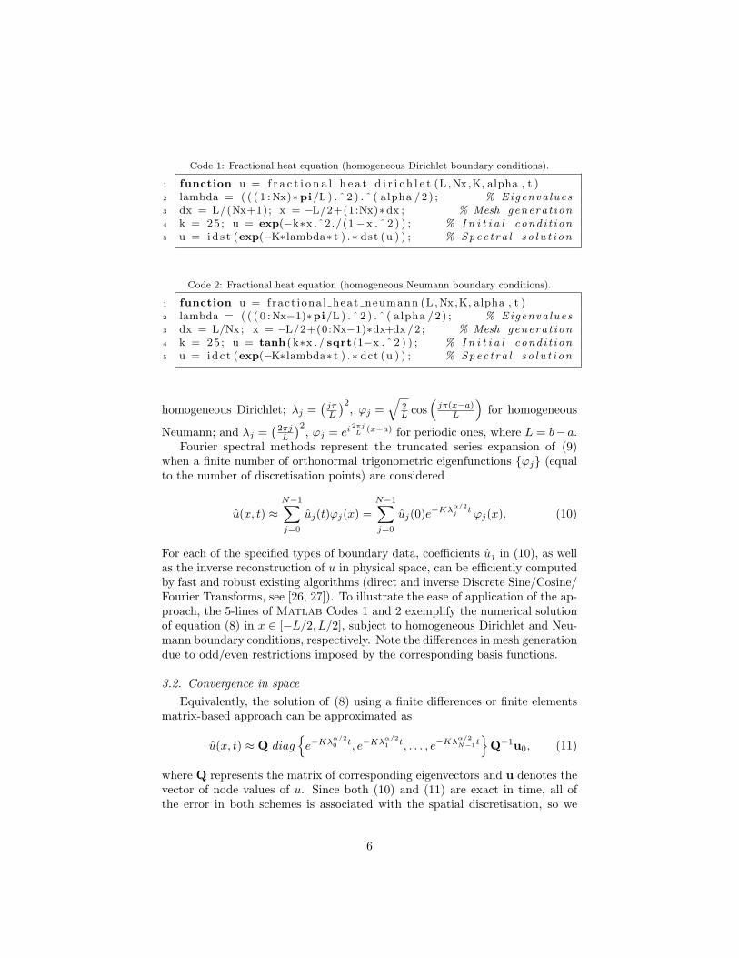
For each of the specified types of boundary data, coefficients uj in (10), as wellas the inverse reconstruction of u in physical space, can be efficiently computedby fast and robust existing algorithms (direct and inverse Discrete Sine/Cosine/Fourier Transforms, see [26, 27]). To illustrate the ease of application of the ap-proach, the 5-lines of Matlab Codes 1 and 2 exemplify the numerical solutionof equation (8) in x ∈ [−L/2, L/2], subject to homogeneous Dirichlet and Neu-mann boundary conditions, respectively. Note the differences in mesh generationdue to odd/even restrictions imposed by the corresponding basis functions.

3.2. Convergence in space

Equivalently, the solution of (8) using a finite differences or finite elementsmatrix-based approach can be approximated as

u(x, t) ≈ Q diag{

e−Kλα/20

t, e−Kλα/21

t, . . . , e−Kλα/2N−1

t}

Q−1u0, (11)

where Q represents the matrix of corresponding eigenvectors and u denotes thevector of node values of u. Since both (10) and (11) are exact in time, all ofthe error in both schemes is associated with the spatial discretisation, so we

6

(a) u0(x) = e−k

x2

1−x2 (b) u0(x) = tanh

(

kx√1−x2

)

(c) Evolution of initial data

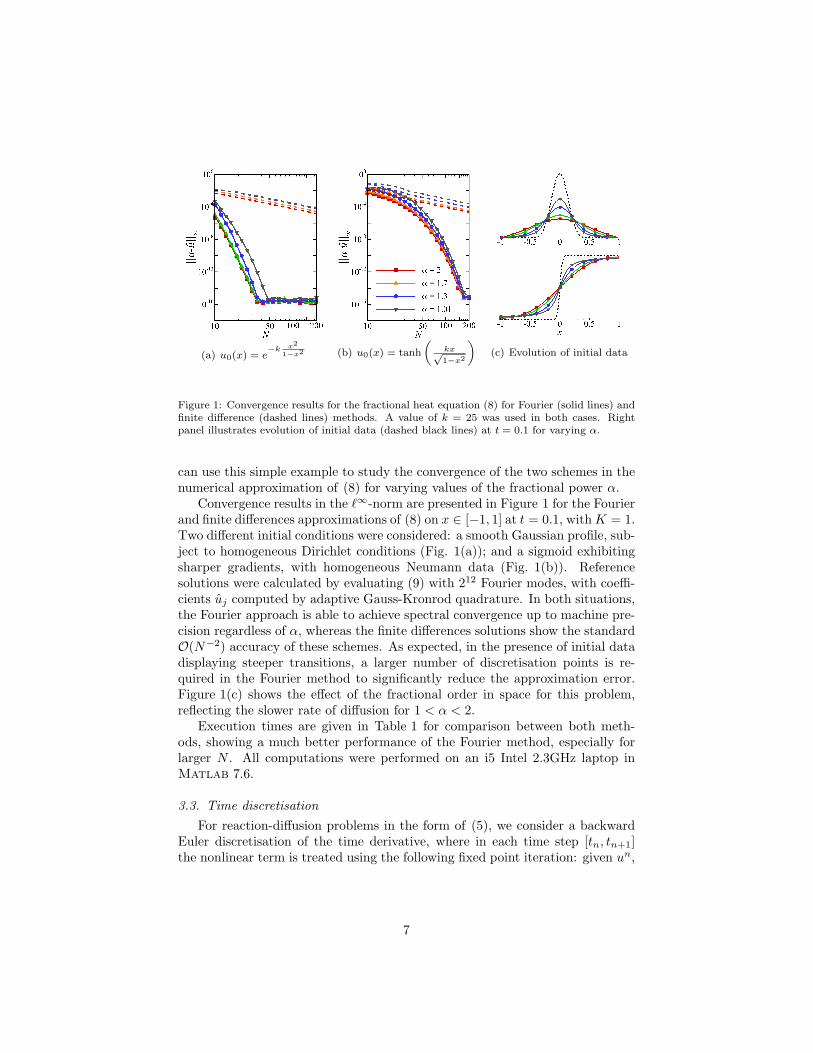
Figure 1: Convergence results for the fractional heat equation (8) for Fourier (solid lines) andfinite difference (dashed lines) methods. A value of k = 25 was used in both cases. Rightpanel illustrates evolution of initial data (dashed black lines) at t = 0.1 for varying α.

can use this simple example to study the convergence of the two schemes in thenumerical approximation of (8) for varying values of the fractional power α.

Convergence results in the ℓ∞-norm are presented in Figure 1 for the Fourierand finite differences approximations of (8) on x ∈ [−1, 1] at t = 0.1, withK = 1.Two different initial conditions were considered: a smooth Gaussian profile, sub-ject to homogeneous Dirichlet conditions (Fig. 1(a)); and a sigmoid exhibitingsharper gradients, with homogeneous Neumann data (Fig. 1(b)). Referencesolutions were calculated by evaluating (9) with 212 Fourier modes, with coeffi-cients uj computed by adaptive Gauss-Kronrod quadrature. In both situations,the Fourier approach is able to achieve spectral convergence up to machine pre-cision regardless of α, whereas the finite differences solutions show the standardO(N−2) accuracy of these schemes. As expected, in the presence of initial datadisplaying steeper transitions, a larger number of discretisation points is re-quired in the Fourier method to significantly reduce the approximation error.Figure 1(c) shows the effect of the fractional order in space for this problem,reflecting the slower rate of diffusion for 1 < α < 2.

Execution times are given in Table 1 for comparison between both meth-ods, showing a much better performance of the Fourier method, especially forlarger N . All computations were performed on an i5 Intel 2.3GHz laptop inMatlab 7.6.

3.3. Time discretisation

For reaction-diffusion problems in the form of (5), we consider a backwardEuler discretisation of the time derivative, where in each time step [tn, tn+1]the nonlinear term is treated using the following fixed point iteration: given un,

7

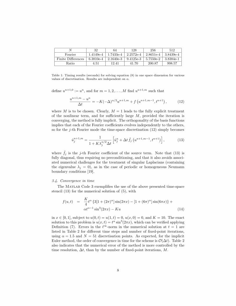
N 32 64 128 256 512

Fourier 1.4149e-4 1.7433e-4 2.2572e-4 2.8651e-4 3.8439e-4

Finite Differences 6.3810e-4 2.1640e-3 9.4125e-3 5.7550e-2 3.8384e-1

Ratio 4.51 12.41 41.70 200.87 998.57

Table 1: Timing results (seconds) for solving equation (8) in one space dimension for variousvalues of discretisation. Results are independent on α.

define un+1,0 := un, and for m = 1, 2, . . . ,M find un+1,m such that

un+1,m − un

∆t= −K(−∆)α/2un+1,m + f

(

un+1,m−1, tn+1)

, (12)

where M is to be chosen. Clearly, M = 1 leads to the fully explicit treatmentof the nonlinear term, and for sufficiently large M , provided the iteration isconverging, the method is fully implicit. The orthogonality of the basis functionsimplies that each of the Fourier coefficients evolves independently to the others,so for the j-th Fourier mode the time-space discretisation (12) simply becomes

un+1,mj =

1

1 +Kλα/2j ∆t

[

unj +∆t fj

(

un+1,m−1, tn+1)

]

, (13)

where fj is the j-th Fourier coefficient of the source term. Note that (13) isfully diagonal, thus requiring no preconditioning, and that it also avoids associ-ated numerical challenges for the treatment of singular Laplacians (containingthe eigenvalue λj = 0), as in the case of periodic or homogeneous Neumannboundary conditions [19].

3.4. Convergence in time

The Matlab Code 3 exemplifies the use of the above presented time-spacestencil (13) for the numerical solution of (5), with

f(u, t) =K

4tα {3[1 + (2π)α] sin(2πx)− [1 + (6π)α] sin(6πx)}+

αtα−1 sin3(2πx)−Ku (14)

in x ∈ [0, 1], subject to u(0, t) = u(1, t) = 0, u(x, 0) = 0, and K = 10. The exactsolution to this problem is u(x, t) = tα sin3(2πx), which can be verified applyingDefinition (7). Errors in the ℓ∞-norm in the numerical solution at t = 1 arelisted in Table 2 for different time steps and number of fixed-point iterations,using α = 1.5 and N = 51 discretisation points. As expected, for the implicitEuler method, the order of convergence in time for the scheme is O(∆t). Table 2also indicates that the numerical error of the method is more controlled by thetime resolution, ∆t, than by the number of fixed-point iterations, M .

8

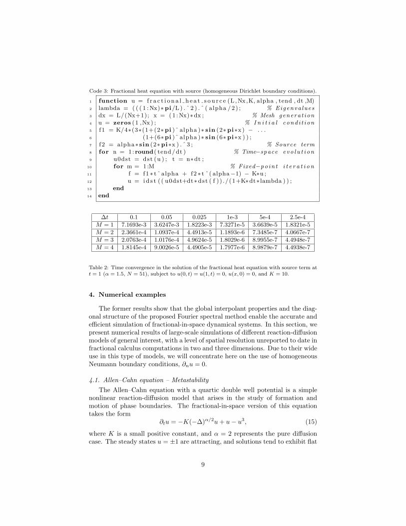
Code 3: Fractional heat equation with source (homogeneous Dirichlet boundary conditions).

1 function u = f r a c t i o n a l h e a t s o u r c e (L ,Nx,K, alpha , tend , dt ,M)2 lambda = ( ( ( 1 :Nx)∗pi/L ) . ˆ 2 ) . ˆ ( alpha /2 ) ; % Eigenva lues

3 dx = L/(Nx+1); x = ( 1 :Nx)∗dx ; % Mesh genera t ion

4 u = zeros (1 ,Nx ) ; % I n i t i a l cond i t i on

5 f 1 = K/4∗(3∗(1+(2∗pi )ˆ alpha )∗ sin (2∗pi∗x ) − . . .6 (1+(6∗pi )ˆ alpha )∗ sin (6∗pi∗x ) ) ;7 f 2 = alpha ∗ sin (2∗pi∗x ) . ˆ 3 ; % Source term

8 for n = 1 : round( tend/dt ) % Time−space e v o l u t i on

9 u0dst = dst (u ) ; t = n∗dt ;10 for m = 1 :M % Fixed−po in t i t e r a t i o n

11 f = f1 ∗ t ˆ alpha + f2 ∗ t ˆ( alpha−1) − K∗u ;12 u = i d s t ( ( u0dst+dt∗dst ( f ) ) ./ (1+K∗dt∗ lambda ) ) ;13 end

14 end

∆t 0.1 0.05 0.025 1e-3 5e-4 2.5e-4

M = 1 7.1693e-3 3.6247e-3 1.8223e-3 7.3271e-5 3.6639e-5 1.8321e-5

M = 2 2.3661e-4 1.0937e-4 4.4913e-5 1.1893e-6 7.3485e-7 4.0667e-7

M = 3 2.0763e-4 1.0176e-4 4.9624e-5 1.8029e-6 8.9955e-7 4.4948e-7

M = 4 1.8145e-4 9.0026e-5 4.4905e-5 1.7977e-6 8.9879e-7 4.4938e-7

Table 2: Time convergence in the solution of the fractional heat equation with source term att = 1 (α = 1.5, N = 51), subject to u(0, t) = u(1, t) = 0, u(x, 0) = 0, and K = 10.

4. Numerical examples

The former results show that the global interpolant properties and the diag-onal structure of the proposed Fourier spectral method enable the accurate andefficient simulation of fractional-in-space dynamical systems. In this section, wepresent numerical results of large-scale simulations of different reaction-diffusionmodels of general interest, with a level of spatial resolution unreported to date infractional calculus computations in two and three dimensions. Due to their wideuse in this type of models, we will concentrate here on the use of homogeneousNeumann boundary conditions, ∂nu = 0.

4.1. Allen–Cahn equation – Metastability

The Allen–Cahn equation with a quartic double well potential is a simplenonlinear reaction-diffusion model that arises in the study of formation andmotion of phase boundaries. The fractional-in-space version of this equationtakes the form

∂tu = −K(−∆)α/2u+ u− u3, (15)

where K is a small positive constant, and α = 2 represents the pure diffusioncase. The steady states u = ±1 are attracting, and solutions tend to exhibit flat

9

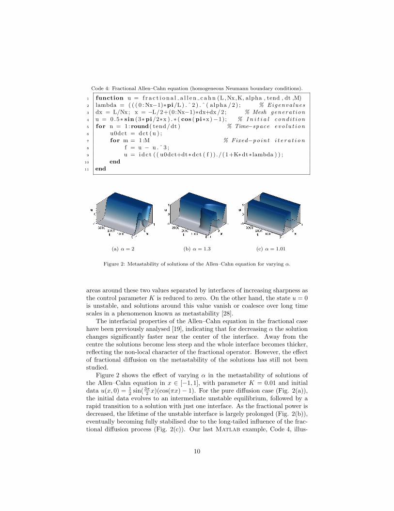
Code 4: Fractional Allen–Cahn equation (homogeneous Neumann boundary conditions).

1 function u = f r a c t i o n a l a l l e n c a h n (L ,Nx,K, alpha , tend , dt ,M)2 lambda = ( ( ( 0 :Nx−1)∗pi/L ) . ˆ 2 ) . ˆ ( alpha /2 ) ; % Eigenva lues

3 dx = L/Nx ; x = −L/2+(0:Nx−1)∗dx+dx /2 ; % Mesh genera t ion

4 u = 0.5∗ sin (3∗pi /2∗x ) . ∗ ( cos (pi∗x)−1); % I n i t i a l cond i t i on

5 for n = 1 : round( tend/dt ) % Time−space e v o l u t i on

6 u0dct = dct (u ) ;7 for m = 1 :M % Fixed−po in t i t e r a t i o n

8 f = u − u . ˆ 3 ;9 u = id c t ( ( u0dct+dt∗dct ( f ) ) ./ (1+K∗dt∗ lambda ) ) ;

10 end

11 end

(a) α = 2 (b) α = 1.3 (c) α = 1.01

Figure 2: Metastability of solutions of the Allen–Cahn equation for varying α.

areas around these two values separated by interfaces of increasing sharpness asthe control parameter K is reduced to zero. On the other hand, the state u = 0is unstable, and solutions around this value vanish or coalesce over long timescales in a phenomenon known as metastability [28].

The interfacial properties of the Allen–Cahn equation in the fractional casehave been previously analysed [19], indicating that for decreasing α the solutionchanges significantly faster near the center of the interface. Away from thecentre the solutions become less steep and the whole interface becomes thicker,reflecting the non-local character of the fractional operator. However, the effectof fractional diffusion on the metastability of the solutions has still not beenstudied.

Figure 2 shows the effect of varying α in the metastability of solutions ofthe Allen–Cahn equation in x ∈ [−1, 1], with parameter K = 0.01 and initialdata u(x, 0) = 1

2 sin(3π2 x)(cos(πx)− 1). For the pure diffusion case (Fig. 2(a)),

the initial data evolves to an intermediate unstable equilibrium, followed by arapid transition to a solution with just one interface. As the fractional power isdecreased, the lifetime of the unstable interface is largely prolonged (Fig. 2(b)),eventually becoming fully stabilised due to the long-tailed influence of the frac-tional diffusion process (Fig. 2(c)). Our last Matlab example, Code 4, illus-

10

trates the solution of the fractional-in-space Allen–Cahn equation using theproposed Fourier method.

4.2. FitzHugh–Nagumo model – Excitable media

The FitzHugh Nagumo model represents one of the simplest models forthe study of excitable media [29, 30]. The propagation of the transmembranepotential in the nerve axon is modeled by a diffusion equation with a cubic non-linear reaction term, whereas the recovery of the slow variable is represented bya single ordinary differential equation in the form

∂tu = −Ku(−∆)α/2u+ u(1− u)(u− a)− v(16)

∂tv = ǫ(βu− γv − δ)

where we consider the following choice of model parameters, a = 0.1, ǫ = 0.01,β = 0.5, γ = 1, δ = 0, which is known to generate stable patterns in thesystem in the form of reentrant spiral waves. In our simulations, the trivial state(u, v) = (0, 0) was perturbed by setting the lower-left quarter of the domain tou = 1 and the upper half part to v = 0.1, which allows the initial condition tocurve and rotate clockwise generating the spiral pattern. The domain is takento be [0, 2.5]2, discretised using N = 256 points in each spatial coordinate, witha diffusion coefficient Ku = 10−4.

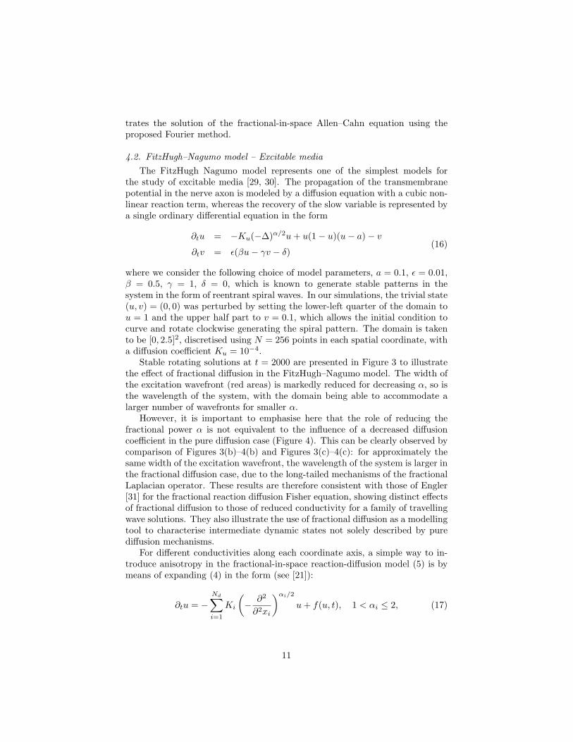
Stable rotating solutions at t = 2000 are presented in Figure 3 to illustratethe effect of fractional diffusion in the FitzHugh–Nagumo model. The width ofthe excitation wavefront (red areas) is markedly reduced for decreasing α, so isthe wavelength of the system, with the domain being able to accommodate alarger number of wavefronts for smaller α.

However, it is important to emphasise here that the role of reducing thefractional power α is not equivalent to the influence of a decreased diffusioncoefficient in the pure diffusion case (Figure 4). This can be clearly observed bycomparison of Figures 3(b)–4(b) and Figures 3(c)–4(c): for approximately thesame width of the excitation wavefront, the wavelength of the system is larger inthe fractional diffusion case, due to the long-tailed mechanisms of the fractionalLaplacian operator. These results are therefore consistent with those of Engler[31] for the fractional reaction diffusion Fisher equation, showing distinct effectsof fractional diffusion to those of reduced conductivity for a family of travellingwave solutions. They also illustrate the use of fractional diffusion as a modellingtool to characterise intermediate dynamic states not solely described by purediffusion mechanisms.

For different conductivities along each coordinate axis, a simple way to in-troduce anisotropy in the fractional-in-space reaction-diffusion model (5) is bymeans of expanding (4) in the form (see [21]):

∂tu = −

Nd∑

i=1

Ki

(

−∂2

∂2xi

)αi/2

u+ f(u, t), 1 < αi ≤ 2, (17)

11

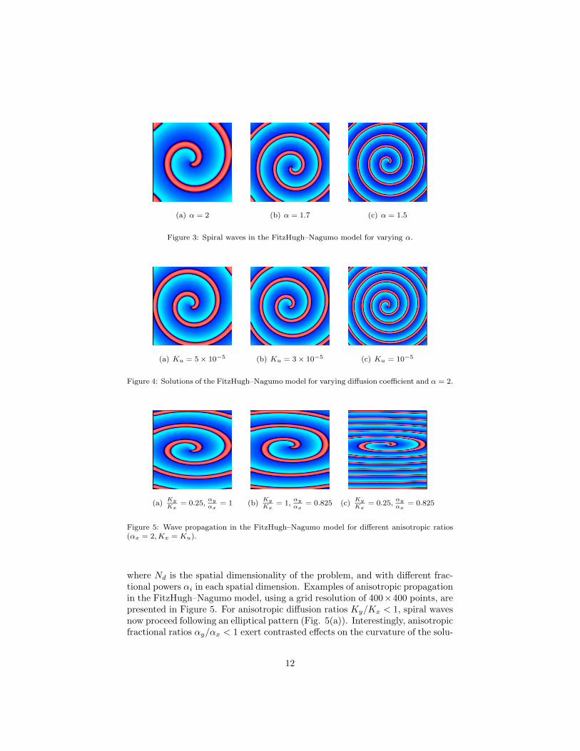
(a) α = 2 (b) α = 1.7 (c) α = 1.5

Figure 3: Spiral waves in the FitzHugh–Nagumo model for varying α.

(a) Ku = 5× 10−5 (b) Ku = 3× 10−5 (c) Ku = 10−5

Figure 4: Solutions of the FitzHugh–Nagumo model for varying diffusion coefficient and α = 2.

(a)Ky

Kx= 0.25,

αy

αx= 1 (b)

Ky

Kx= 1,

αy

αx= 0.825 (c)

Ky

Kx= 0.25,

αy

αx= 0.825

Figure 5: Wave propagation in the FitzHugh–Nagumo model for different anisotropic ratios(αx = 2,Kx = Ku).

where Nd is the spatial dimensionality of the problem, and with different frac-tional powers αi in each spatial dimension. Examples of anisotropic propagationin the FitzHugh–Nagumo model, using a grid resolution of 400×400 points, arepresented in Figure 5. For anisotropic diffusion ratios Ky/Kx < 1, spiral wavesnow proceed following an elliptical pattern (Fig. 5(a)). Interestingly, anisotropicfractional ratios αy/αx < 1 exert contrasted effects on the curvature of the solu-

12

tions (Fig. 5(b)), reflecting distinct super-diffusion scales in each of the spatialdimensions of the system. The combination of the two sources of anisotropyyield a mixed effect of the two independent contributions (Fig. 5(c)), also fur-ther reducing the wavelength of the system, in agreement with the previousresults illustrated by Figures 3 and 4.

4.3. Gray–Scott model – Morphogenesis

The extension of the Fourier stencil to systems of reaction-diffusion equationsis as well straightforward. We consider the fractional version of the Gray–Scottmodel [32, 33]

∂tu = −Ku(−∆)α/2u− uv2 + F (1− u)(18)

∂tv = −Kv(−∆)α/2v + uv2 − (F + κ)v,

whereKu,Kv, F and κ are positive constants. For a ratio of diffusion coefficientsKu/Kv > 1, the model is known to generate different mechanisms of patternformation depending on the values of the feed, F , and depletion, κ, rates. Herewe select Ku = 2 × 10−5, Ku/Kv = 2, F = 0.03, and vary κ in a range inwhich the standard diffusion model is known to exhibit interesting dynamics[34]. The domain of interest is taken to be [0, 1]2, discretised using N = 400points in each spatial coordinate. Initially, the entire system was placed in thetrivial state (u, v) = (1, 0), and a 32×32 mesh point area located symmetricallyabout the centre of the grid was perturbed to (u, v) = (1/2, 1/4). The initialdisturbance then propagates outward from the central square until the entiregrid is affected by the initial perturbation.

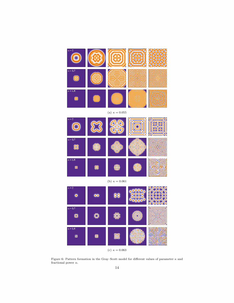
Figure 6 summarizes the effects of fractional diffusion in the Gray–Scottmodel. For κ = 0.055 (Fig. 6(a)), the model with standard diffusion (α = 2) isknown to organize in a steady state field of negative solitons. A reduction inthe fractional order of the diffusive process (α = 1.7) produces a decrease in thevelocity of propagation of the initial perturbation, and a much finer granulationin the size of the structures of the final steady state field. For smaller values ofthe fractional power (α = 1.5), a new process of nucleation of structures in thecentre and in the boundaries of the domain is observed, that then grow outwarduntil the entire domain reaches its final steady state configuration.

For κ = 0.061 (Fig. 6(b)), the original model produces a wavefront propa-gation partially driven by curvature, and a final steady state pattern showingthe presence of filaments. The curvature driven mechanisms are increased bythe diffusive effects of the fractional Laplacian operator, yielding a final fieldformed by much thiner filaments, and steady state patterns totally different tothose generated by standard diffusion.

Finally, the Gray–Scott model exhibits mitosis for κ = 0.063 under condi-tions of normal diffusion (Fig. 6(c)). However, the replication pattern is com-pletely altered when the fractional order of the model is decreased, as shown inthis Figure for α = 1.7. In fact, further reductions of the fractional power, asshown for α = 1.5, produce dynamical states where solitons and filaments may

13

(a) κ = 0.055

(b) κ = 0.061

(c) κ = 0.063

Figure 6: Pattern formation in the Gray–Scott model for different values of parameter κ andfractional power α.

14

(a) α = 2

(b) α = 1.5

Figure 7: Isosurfaces u = 0.65 for the Gray–Scott model for κ = 0.061.

coexist, the latter slowing self-dividing into the former until the whole domainis filled by a soliton-like pattern.

4.4. Gray–Scott model – Patterns in Three Dimensional Space

Numerical simulation of the Gray–Scott model in three spatial dimensionsrepresents an even more interesting scenario where more exotic patterns mayarise. For the parameter regime where wavefront motion is partially driven bycurvature (κ = 0.061), and for two different α, Figure 7 illustrates the three di-mensional propagation of the initial perturbation before the interaction of thesolution with the domain boundaries. As can be clearly appreciated, the smoothgrowing of lobes in the presence of normal diffusion (Fig. 7(a)) is replaced bymore intriguing patterns in the fractional diffusion case (Fig. 7(b)). For im-provement of visualization results, the domain size is [0, 1]3 in Fig. 7(a), and[0.25, 0.75]3 in Fig. 7(b).

5. Conclusions

In this paper, Fourier spectral methods have been introduced as an attractiveand easy-to-code alternative for the integration of fractional-in-space reaction-diffusion equations. These methods offer several advantages over traditionalalternatives. Since the operator is non-local, the benefits of using a basis withlocally supported elements are destroyed. Hence, the use of an orthogonal, with

15

respect to the operator, non-local basis is preferable and will give rise to a fullydiagonal representation of the fractional operator, thus avoiding the solution oflarge systems of equations or the use of matrix transfer techniques. In terms ofaccuracy and efficiency, Fourier methods have been proven to be not only advan-tageous relative to memory requirements (number of discretisation points) whencompared to low-order schemes, but also computationally efficient in executiontimes. Furthermore, the use of established discrete fast Fourier transforms en-sures efficiency, makes immediate the implementation of appropriate boundaryconditions, and allows the extension of the stencil to two and three dimensionsin a completely straightforward manner.

Simulation results of the fractional-in-space Allen–Cahn, FitzHugh–Nagumoand in particular Gray–Scott models show that such problems can have verydifferent dynamics to standard diffusion, and as such represent a powerful mod-elling approach for understanding the many aspects of heterogeneity.

Despite their higher order of convergence, the biggest drawback of spectralmethods is their inability to handle irregularly shaped domains, since the domainof interest must be simple enough to allow the use of an appropriate series ofpolynomial or trigonometric basis functions in where to expand the global high-order interpolants. However, recent work in combining spectral methods withdomain embedding techniques has allowed the extension of these methods toirregular domains [27, 35, 36, 37, 38]. The use of these techniques may constitutea suitable approach for extending our results in the fractional-in-space settingto irregular shape geometries.

The applications presented in this paper also have illustrated that Fourierspectral methods can easily handle anisotropy when this is constant through-out the entire integration domain. For spatially-dependent conductivities, therepresentation of the fractional operator in Fourier space would be the convolu-tion of the Fourier coefficients of such conductivities and those of the fractionalLaplacian, thus losing the diagonal structure of the operator and requiring thesolution of full systems of equations. However, due to the smaller number ofdegrees of freedom required by Fourier methods to achieve a given accuracy,they could still be competitive when compared to low order schemes. On theother hand, the use of spectral differentiation matrices [28, 39], in combinationwith the matrix transfer technique, could also be helpful in order to overcomethese limitations.

Finally, an additional advantage of finite element and finite difference meth-ods is their ability to accommodate adaptive mesh refinement for non-smoothsolutions. Rather than the use of mesh refinement algorithms, the easiest wayto incorporate spatial adaptivity in spectral methods seems to be by meansof the so-called moving mesh techniques, also known as r-adaptivity [40, 41].The implementation of these techniques for fractional-in-space reaction-diffusionequations may also constitute another of our future lines of research.

16

Acknowledgments

This publication is based on work supported by Award No. KUK-C1-013-04,made by King Abdullah University of Science and Technology (KAUST).

References

[1] E. E. Adams, L. W. Gelhar, Field study of dispersion in a heterogeneousaquifer: 2. Spatial moment analysis, Water Resources Res. 28 (1992) 3293–3307.

[2] D. A. Benson, S. Wheatcraft, M. M. Meerschaert, Application of a frac-tional advection-dispersion equation, Water Resources Res. 36 (2000) 1403–1412.

[3] M. M. Meerschaert, D. A. Benson, S. W. Wheatcraft, Subordinatedadvection-dispersion equation for contaminant transport, Water ResourceRes. 37 (2001) 1543–1550.

[4] E. Scalas, R. Gorenflo, F. Mainardi, Fractional calculus and continuoustime finance, Physica A 284 (2000) 376–384.

[5] R. L. Magin, O. Abdullah, D. Baleanu, X. J. Zhou, Anomalous diffusion ex-pressed through fractional order differential operators in the Bloch–Torreyequation, J. of Mag. Res. 190 (2008) 255–270.

[6] P. Becker-Kern, M. M. Meerschaert, H. P. Scheffler, Limit theorem forcontinuous time random walks with two time scales, J. App. Prob. 41 (2004)455–466.

[7] R. Metzler, J. Klafter, The random walk’s guide to anomalous diffusion: Afractional dynamics approach, Phys. Rep. 339 (2000) 1–77.

[8] Y. Zhang, D. A. Benson, D. M. Reeves, Time and space nonlocalities un-derlying fractional-derivative models: Distinction and literature review offield applications, Adv. in Water Res. 32 (2009) 561–581.

[9] M. M. Meerschaert, J. Mortensenb, S. W. Wheatcraft, Fractional vectorcalculus for fractional advection-dispersion, Physica A 367 (2006) 181–190.

[10] M. Riesz, L’integrale de Riemann-Liouville et le probleme de Cauchy, ActaMathematica 81 (1949) 1–222.

[11] J. P. Bouchaud, A. Georges, Anomalous diffusion in disordered media:Statistical mechanisms, models and physical applications, Phy. Rep. 195(1990) 127–293.

[12] I. Turner, M. Ilic, P. Perr, The use of fractional-in-space diffusion equationsfor describing microscale diffusion in porous media, in: 11th InternationalDrying Conference, Magdeburg, Germany, 2010.

17

[13] M. M. Meerschaert, C. Tadjeran, Finite difference approximations for two-sided space-fractional partial differential equations, App. Num. Math 56(2006) 80–90.

[14] J. Roop, Computational aspects of FEM approximations of fractional ad-vection dispersion equations on bounded domains on R2, J. Comp. Appl.Math. 193 (2005) 243–268.

[15] M. Ilic, F. Liu, I. Turner, V. Anh, Numerical approximation of a fractional-in-space diffusion equation, I. Frac. Calc. and App. Anal. 8 (2005) 323–341.

[16] F. Liu, P. Zhuang, V. Anh, I. Turner, K. Burrage, Stability and conver-gence of the finite difference method for the space-time fractional advection-diffusion equation, App. Num. and Comp. 91 (2007) 12–20.

[17] H.-K. Pang, H.-W. Sun, Multigrid method for fractional diffusion, J. Comp.Phys. 231 (2012) 693–703.

[18] Q. Yang, I. Turner, F. Liu, M. Ilic, Novel numerical methods for solvingthe time-space fractional diffusion equation in 2D, SIAM J. Sci. Comp. 33(2011) 1159–1180.

[19] K. Burrage, N. Hale, D. Kay, An efficient implicit FEM scheme forfractional-in-space reaction-diffusion equations.

[20] Q. Yang, F. Liu, I. Turner, Numerical methods for fractional partial differ-ential equations with Riesz space fractional derivatives, App. Num. Mod.34 (2010) 200–218.

[21] K. Burrage, D. Kay, Efficient numerical solvers for fractional diffusion, InReview.

[22] X. Li, C. Xu, Existence and uniqueness of the weak solution of the space-time fractional diffusion equation and a spectral method approximation,Commun. Comput. Phys. 8 (2010) 1016–1051.

[23] M. M. Khader, On the numerical solutions for the fractional diffusion equa-tion, Commun. Nonlinear Sci. Numer. Simulat. 16 (2010) 2535–2542.

[24] X. Li, C. Xu, A space-time spectral method for the time fractional diffusionequation, SIAM J. Numer. Anal. 47 (2009) 2108–2131.

[25] E. Hanert, A comparison of three eulerian numerical methods for fractional-order transport models, Environ. Fluid Mech. 10 (2010) 7–20.

[26] W. L. Briggs, V. E. Henson, The DFT: an owner’s manual for the discreteFourier transform, SIAM, Philadelphia, 2000.

[27] A. Bueno-Orovio, V. M. Perez-Garcıa, Spectral smoothed boundary meth-ods: The role of external boundary conditions, Numer. Meth. Part. Differ.Equ. 22 (2006) 435–448.

18

[28] L. N. Trefethen, Spectral methods in Matlab, SIAM, Philadelphia, 2000.

[29] R. FitzHugh, Impulses and physiological states in theoretical models ofnerve membranes, Biophys. J. 1 (1961) 445–466.

[30] J. Nagumo, S. Animoto, S. Yoshizawa, An active pulse transmission linesimulating nerve axon, Proc. Inst. Radio Engineers 50 (1962) 2061–2070.

[31] H. Engler, On the speed of spread for fractional reaction-diffusion equa-tions, Int. J. Diff. Eqn.doi:10.1155/2010/315421.

[32] P. Gray, S. K. Scott, Autocatalytic reactions in the isothermal, continuousstirred tank reactor: isolas and other forms of multistability, Chem. Eng.Sci. 38 (1983) 29–43.

[33] P. Gray, S. K. Scott, Sustained oscillations and other exotic patterns ofbehavior in isothermal reactions, J. Phys. Chem. 89 (1985) 22–32.

[34] J. E. Pearson, Complex patterns in a simple system, Science 261 (1993)189–192.

[35] A. Bueno-Orovio, Fourier embedded domain methods: periodic and C∞

extension of a function defined on an irregular region to a rectangle viaconvolution with Gaussian kernels, App. Math. Comp. 183 (2006) 813–818.

[36] A. Bueno-Orovio, V. M. Perez-Garcıa, F. H. Fenton, Spectral methods forpartial differential equations in irregular domains: The spectral smoothedboundary method, SIAM J. Sci. Comput. 28 (2006) 886–900.

[37] S. H. Lui, Spectral domain embedding for elliptic PDEs in complex do-mains, J. Comput. Appl. Math. 225 (2009) 541–557.

[38] F. Sabetghadam, S. Sharafatmandjoor, F. Norouzi, Fourier spectral embed-ded boundary solution of the Poisson’s and Laplace equations with Dirichletboundary conditions, J. Comput. Phys. 228 (2009) 55–74.

[39] J. A. C. Weideman, S. C. Reddy, A matlab differentiation matrix suite,ACM Trans. Math. Softw. 26 (2000) 465–519.

[40] W. M. Feng, P. Yu, S. Y. Hu, Z. K. Liu, Q. Du, L. Q. Chen, Spectral imple-mentation of an adaptive moving mesh method for phase-field equations,J. Comput. Phys. 220 (2006) 498–510.

[41] L. S. Mulholland, W. Z. Huang, D. M. Sloan, Pseudospectral solution ofnear-singular problems using numerical coordinate transformations basedon adaptivity, SIAM J. Sci. Comput. 19 (1998) 1261–1289.

19

RECENT REPORTS

12/26 Age related changes in speed and mechanism of adult skeletal

muscle stem cell migration

Collins-Hooper

Woolley

Dyson

Patel

Potter

Baker

Gaffney

Maini

Dash

Patel

12/27 The interplay between tissue growth and scaffold degradation in

engineered tissue constructs

ODea

Osborne

El Haj

Byrne

Waters

12/28 Non-linear effects on Turing patterns: time oscillations and

chaos.

Aragon

Barrio

Woolley

Baker

Maini

12/29 Colorectal Cancer Through Simulation and Experiment Kershaw

Byrne

Gavaghan

Osborne

12/30 A theoretical investigation of the effect of proliferation and adhe-

sion on monoclonal conversion in the colonic crypt

Mirams

Fletcher

Maini

Byrne

12/31 Convergent evolution of spiny mollusk shells points to elastic en-

ergy minimum

Chirat

Moulton

Shipman

Goriely

12/32 Three-dimensional oblique water-entry problems at small dead-

rise angles

Moore

Howison

Ockendon

Oliver

12/33 Second weak order explicit stabilized methods for stiff stochastic

differential equations

Abdulle

Vilmart

Zygalakis

12/34 The sensitivity of Graphene ‘Snap-through’ to substrate geometry Wagner

Vella

12/35 The physics of frost heave and ice-lens growth Peppin

Style

12/36 Finite Element Simulation of Dynamic Wetting Flows as an Inter-

face Formation Process

Sprittles

Shikhmurzaev

12/37 The Dynamics of Liquid Drops and their Interaction with Solids of

Varying Wettabilities

Sprittles

Shikhmurzaev

12/40 A Branch and Bound Algorithm for the Global Optimization of

Hessian Lipschitz Continuous Functions

Fowkes

Gould

Farmer

12/41 The Orthogonal Gradients Method: a Radial Basis Functions

Method for Solving Partial Differential Equations on Arbitrary Sur-

faces

Piret

12/42 Squeeze-Film Flow in the Presence of a Thin Porous Bed, with

Application to the Human Knee Joint

Knox

Wilson

Duffy

McKee

12/43 Gravity-driven draining of a thin rivulet with constant width down

a slowly varying substrate

Paterson

Wilson

Duffy

12/44 The ‘Sticky Elastica’: Delamination blisters beyond small defor-

mations

Wagner

Vella

12/45 Stochastic models of intracellular transport Bressloff

Newby

12/46 The effects of noise on binocular rivalry waves: a stochastic neu-

ral field model

Webber

Bressloff

12/47 An Ensemble Bayesian Filter for State Estimation Farmer

12/48 Simulation of cell movement through evolving environment: a fic-

titious domain approach

Seguis

Burrage

Erban

Kay

12/49 The Mathematics of Liquid Crystals: Analysis, Computation and

Applications

Majumdar

Copies of these, and any other OCCAM reports can be obtained from:

Oxford Centre for Collaborative Applied Mathematics

Mathematical Institute

24 - 29 St Giles’

Oxford

OX1 3LBEngland

www.maths.ox.ac.uk/occam