fourth progress report - national park service
TRANSCRIPT
National Park Service U.S. Department of the Interior
Natural Resource Stewardship and Science
Alaskan National Park Glaciers - Status and Trends Fourth Progress Report Natural Resource Data Series NPS/AKRO/NRDS—2014/607

ON THE COVER Bering Glacier, in the foreground, drains the massive Bagley Icefield in Wrangell-St. Elias National Park and Preserve. Mt. Logan is visible in the far distance. July 21, 2011. Photograph by: JT Thomas
Alaskan National Park Glaciers - Status and Trends Fourth Progress Report Natural Resource Data Series NPS/AKRO/NRDS—2014/607
Anthony Arendt, Chris Larsen Geophysical Institute University of Alaska Fairbanks 903 Koyukuk Drive Fairbanks, AK 99775 Michael Loso Environmental Science Dept Alaska Pacific University 4101 University Drive Anchorage, AK 99508 Nate Murphy, Justin Rich Geophysical Institute University of Alaska Fairbanks 903 Koyukuk Drive Fairbanks, AK 99775
January 2014 U.S. Department of the Interior National Park Service Natural Resource Stewardship and Science Fort Collins, Colorado

The National Park Service, Natural Resource Stewardship and Science office in Fort Collins, Colorado, publishes a range of reports that address natural resource topics. These reports are of interest and applicability to a broad audience in the National Park Service and others in natural resource management, including scientists, conservation and environmental constituencies, and the public.
The Natural Resource Data Series is intended for the timely release of basic data sets and data summaries. Care has been taken to assure accuracy of raw data values, but a thorough analysis and interpretation of the data has not been completed. Consequently, the initial analyses of data in this report are provisional and subject to change.
All manuscripts in the series receive the appropriate level of peer review to ensure that the information is scientifically credible, technically accurate, appropriately written for the intended audience, and designed and published in a professional manner. This report received informal peer review by subject-matter experts who were not directly involved in the collection, analysis, or reporting of the data.
Views, statements, findings, conclusions, recommendations, and data in this report do not necessarily reflect views and policies of the National Park Service, U.S. Department of the Interior. Mention of trade names or commercial products does not constitute endorsement or recommendation for use by the U.S. Government.
This report is available from the Natural Resource Publications Management website (http://www.nature.nps.gov/publications/nrpm/). To receive this report in a format optimized for screen readers, please email [email protected].
Please cite this publication as:
Arendt, A., C. Larsen, M. Loso, N. Murphy, and J. Rich. 2014. Alaskan National Park glaciers - status and trends: Fourth progress report. Natural Resource Data Series NPS/AKRO/NRDS—2014/607. National Park Service, Fort Collins, Colorado.
NPS 953/123451, January 2014
ii

Contents Page
Figures............................................................................................................................................. v
Tables ............................................................................................................................................. xi
Executive Summary ..................................................................................................................... xiii
Acknowledgments......................................................................................................................... xv
Introduction ..................................................................................................................................... 1
Project Overview ..................................................................................................................... 1
Project Deliverables and Timeline ........................................................................................... 1
Scope of Progress Report 4 ...................................................................................................... 2
Study Areas ..................................................................................................................................... 5
Kenai Fjords National Park ................................................................................................. 5
Wrangell-St. Elias National Park and Preserve .................................................................. 7
Methods-Mapping ........................................................................................................................... 9
Data .......................................................................................................................................... 9
Analysis ................................................................................................................................... 9
Methods-Elevation Change ........................................................................................................... 13
Data ........................................................................................................................................ 13
Analysis ................................................................................................................................. 13
Methods-Focus Glaciers ............................................................................................................... 17
Focus Glacier Selection ......................................................................................................... 17
Summary of Field Efforts ...................................................................................................... 17
Results-Mapping ........................................................................................................................... 21
Kenai Fjords NP .................................................................................................................... 21
Wrangell-St. Elias NP&P ...................................................................................................... 23
iii

Contents (continued) Page
Results-Elevation Change ............................................................................................................. 29
Kenai Fjords NP .................................................................................................................... 29
Wrangell-St. Elias NP&P ...................................................................................................... 32
Results-Focus Glaciers.................................................................................................................. 33
Data Collection ...................................................................................................................... 33
Report Design ........................................................................................................................ 33
Discussion ..................................................................................................................................... 39
Preliminary Highlights ........................................................................................................... 39
Literature Cited ............................................................................................................................. 41
Appendix A: Data Sources for Mapping-Map Date ..................................................................... 43
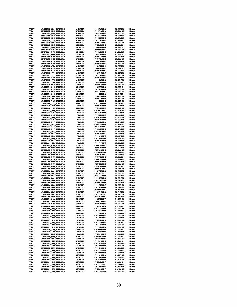
Appendix B: Data Sources for Mapping-Modern ......................................................................... 47
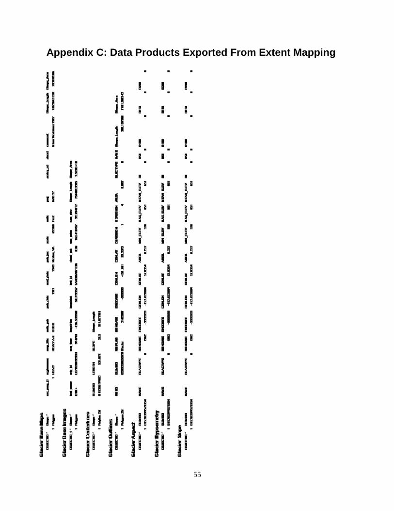
Appendix C: Data Products Exported From Extent Mapping ...................................................... 55
Appendix D: Close-up Maps of Glacier Extent Changes ............................................................. 57
Appendix E: Elevation and Volume Change Analyses ................................................................ 63
iv

Figures Page
Figure 1. Kenai Fjords National Park. Blue polygons are map date glacier coverage ................... 6
Figure 2. Wrangell-St. Elias National Park and Preserve ............................................................... 8
Figure 3. Workflow for the generation of glacier inventory data for NPS glaciers...................... 10
Figure 4. Aerial oblique imagery (from the south viewing Tokositna and Ruth Glaciers, Denali NP&P) demonstrating generation of glacier inventory data for NPS glaciers. ......................................................................................................................................... 12
Figure 5. Existing laser altimetry profiles (red lines) in Kenai Fjords NP (upper panel) and Wrangell-St. Elias NP&P (lower panel) as of January 2011 ................................................. 16
Figure 6. Overview of focus glacier locations (red dots) .............................................................. 18
Figure 7. Changes in glacier area between map date and modern in Kenai Fjords NP ................ 22
Figure 8. Histograms of changes in number of individual glaciers by area-weighted mean elevation (left) and area (right) in Kenai Fjords NP between map date (1950-1951) and modern (2005-2007). ................................................................................................... 23
Figure 9. Total area of glacier-covered terrain in Kenai Fjords NP by elevation between map date (1950-1951) and modern (2005-2007). ........................................................... 23
Figure 10. Changes in glacier area between map date and modern in Wrangell-St. Elias NP&P ................................................................................................................................... 25
Figure 11. Histograms of changes in number of individual glaciers by area-weighted mean elevation (left) and area (right) in Wrangell-St. Elias NP&P between map date (1948-1973) and modern (2006-2011).......................................................................................... 26
Figure 12. Total area of glacier-covered terrain in Wrangell-St. Elias NP&P by elevation between map date (1948-1973) and modern (2006-2011). ........................................... 27
Figure 13. Glacier-wide mass balance rates (m/yr) for 11 glaciers from Kenai Fjords NP between 1994 and 2007 .......................................................................................................... 30
Figure 14. Annual rate of ice thickness change, by elevation, for selected glaciers in Kenai Fjords National Park. .......................................................................................................... 31
Figure 15. Glacier-wide mass balance rates (m/yr) for five glaciers from Wrangell-St. Elias NP&P between 2000 and 2012 ............................................................................................ 32
v

Figures (continued) Page
Figure 16. Glacier outlines and terminus positions collected for Exit Glacier, Kenai Fjords NP ...................................................................................................................................... 36
Figure 17. Map page style mockup of interpretive report. ........................................................... 37
Figure 18. Photo style mockup of interpretive report ................................................................... 38
Figure D1. Close-up of northeastern Kenai Fjords NP glaciers. .................................................. 57
Figure D2. Close-up of southwestern Kenai Fjords NP glaciers. ................................................. 58
Figure D3. Close-up of Wrangell Mountains glaciers in northwestern Wrangell-St. Elias NP&P. .................................................................................................................................. 59
Figure D4. Close-up of coastal glaciers in southwestern Wrangell-St. Elias NP&P. ................... 60
Figure D5. Close-up of Malaspina Glacier in southern Wrangell-St. Elias NP&P. ..................... 61
Figure E1. Details of calculated elevation changes by elevation (upper panel) and the area altitude distribution (lower panel) for Aialik Glacier ............................................................ 64
Figure E2. Details of calculated elevation changes by elevation (upper panel) and the area altitude distribution (lower panel) for Aialik Glacier. ........................................................... 65
Figure E3. Details of calculated elevation changes by elevation (upper panel) and the area altitude distribution (lower panel) for Aialik Glacier. ........................................................... 66
Figure E4. Details of calculated elevation changes by elevation (upper panel) and the area altitude distribution (lower panel) for Bear Glacier .............................................................. 68
Figure E5. Details of calculated elevation changes by elevation (upper panel) and the area altitude distribution (lower panel) for Bear Glacier. ............................................................. 69
Figure E6. Details of calculated elevation changes by elevation (upper panel) and the area altitude distribution (lower panel) for Bear Glacier .............................................................. 70
Figure E7. Details of calculated elevation changes by elevation (upper panel) and the area altitude distribution (lower panel) for Chernof Glacier ........................................................ 72
Figure E8. Details of calculated elevation changes by elevation (upper panel) and the area altitude distribution (lower panel) for Chernof Glacier. ....................................................... 73
vi

Figures (continued) Page
Figure E9. Details of calculated elevation changes by elevation (upper panel) and the area altitude distribution (lower panel) for Chernof Glacier ........................................................ 74
Figure E10. Details of calculated elevation changes by elevation (upper panel) and the area altitude distribution (lower panel) for Dinglestadt Glacier ............................................. 76
Figure E11. Details of calculated elevation changes by elevation (upper panel) and the area altitude distribution (lower panel) for Dinglestadt Glacier ............................................. 77
Figure E12. Details of calculated elevation changes by elevation (upper panel) and the area altitude distribution (lower panel) for Dinglestadt Glacier ............................................. 78
Figure E13. Details of calculated elevation changes by elevation (upper panel) and the area altitude distribution (lower panel) for Exit Glacier ......................................................... 80
Figure E14. Details of calculated elevation changes by elevation (upper panel) and the area altitude distribution (lower panel) for Exit Glacier. ........................................................ 81
Figure E15. Details of calculated elevation changes by elevation (upper panel) and the area altitude distribution (lower panel) for Exit Glacier. ........................................................ 82
Figure E16. Details of calculated elevation changes by elevation (upper panel) and the area altitude distribution (lower panel) for Exit Glacier ......................................................... 83
Figure E17. Details of calculated elevation changes by elevation (upper panel) and the area altitude distribution (lower panel) for “Harris Glacier” (see text for alternate names) ........................................................................................................................................... 85
Figure E18. Details of calculated elevation changes by elevation (upper panel) and the area altitude distribution (lower panel) for “Harris Glacier” (see text for alternate names). .......................................................................................................................................... 86
Figure E19. Details of calculated elevation changes by elevation (upper panel) and the area altitude distribution (lower panel) for “Harris Glacier” (see text for alternate names) ........................................................................................................................................... 87
Figure E20. Details of calculated elevation changes by elevation (upper panel) and the area altitude distribution (lower panel) for Holgate Glacier. .................................................. 89
Figure E21. Details of calculated elevation changes by elevation (upper panel) and the area altitude distribution (lower panel) for Holgate Glacier ................................................... 90
Figure E22. Details of calculated elevation changes by elevation (upper panel) and the area altitude distribution (lower panel) for Holgate Glacier. .................................................. 91
vii

Figures (continued) Page
Figure E23. Details of calculated elevation changes by elevation (upper panel) and the area altitude distribution (lower panel) for Kachemak Glacier ............................................... 93
Figure E24. Details of calculated elevation changes by elevation (upper panel) and the area altitude distribution (lower panel) for Kachemak Glacier ............................................... 94
Figure E25. Details of calculated elevation changes by elevation (upper panel) and the area altitude distribution (lower panel) for Kachemak Glacier. .............................................. 95
Figure E26. Details of calculated elevation changes by elevation (upper panel) and the area altitude distribution (lower panel) for McCarty Glacier ................................................. 97
Figure E27. Details of calculated elevation changes by elevation (upper panel) and the area altitude distribution (lower panel) for McCarty Glacier ................................................. 98
Figure E28. Details of calculated elevation changes by elevation (upper panel) and the area altitude distribution (lower panel) for McCarty Glacier ................................................. 99
Figure E29. Details of calculated elevation changes by elevation (upper panel) and the area altitude distribution (lower panel) for Northwestern Glacier ........................................ 101
Figure E30. Details of calculated elevation changes by elevation (upper panel) and the area altitude distribution (lower panel) for Northwestern Glacier ........................................ 102
Figure E31. Details of calculated elevation changes by elevation (upper panel) and the area altitude distribution (lower panel) for Northwestern Glacier ........................................ 103
Figure E32. Details of calculated elevation changes by elevation (upper panel) and the area altitude distribution (lower panel) for Skilak Glacier ................................................... 105
Figure E33. Details of calculated elevation changes by elevation (upper panel) and the area altitude distribution (lower panel) for Skilak Glacier. .................................................. 106
Figure E34. Details of calculated elevation changes by elevation (upper panel) and the area altitude distribution (lower panel) for Skilak Glacier ................................................... 107
Figure E35. Details of calculated elevation changes by elevation (upper panel) and the area altitude distribution (lower panel) for Tustumena Glacier ............................................ 109
Figure E36. Details of calculated elevation changes by elevation (upper panel) and the area altitude distribution (lower panel) for Tustumena Glacier ............................................ 110
Figure E37. Details of calculated elevation changes by elevation (upper panel) and the area altitude distribution (lower panel) for Tustumena Glacier ............................................ 111
viii

Figures (continued) Page
Figure E38. Details of calculated elevation changes by elevation (upper panel) and the area altitude distribution (lower panel) for Guyot Glacier .................................................... 113
Figure E39. Details of calculated elevation changes by elevation (upper panel) and the area altitude distribution (lower panel) for Guyot Glacier. ................................................... 114
Figure E40. Details of calculated elevation changes by elevation (upper panel) and the area altitude distribution (lower panel) for Guyot Glacier. ................................................... 115
Figure E41. Details of calculated elevation changes by elevation (upper panel) and the area altitude distribution (lower panel) for Hubbard Glacier ................................................ 117
Figure E42. Details of calculated elevation changes by elevation (upper panel) and the area altitude distribution (lower panel) for Hubbard Glacier ................................................ 118
Figure E43. Details of calculated elevation changes by elevation (upper panel) and the area altitude distribution (lower panel) for Hubbard Glacier ................................................ 119
Figure E44. Details of calculated elevation changes by elevation (upper panel) and the area altitude distribution (lower panel) for Kennicott Glacier .............................................. 121
Figure E45. Details of calculated elevation changes by elevation (upper panel) and the area altitude distribution (lower panel) for Nabesna Glacier ................................................ 123
Figure E46. Details of calculated elevation changes by elevation (upper panel) and the area altitude distribution (lower panel) for Yahtse Glacier. .................................................. 125
Figure E47. Details of calculated elevation changes by elevation (upper panel) and the area altitude distribution (lower panel) for Yahtse Glacier. .................................................. 126
Figure E48. Details of calculated elevation changes by elevation (upper panel) and the area altitude distribution (lower panel) for Yahtse Glacier ................................................... 127
Figure E49. Details of calculated elevation changes by elevation (upper panel) and the area altitude distribution (lower panel) for Yahtse Glacier. .................................................. 128
ix


Tables Page
Table 1. Overall scope of project by component: Principal Investigator, glacier coverage, and types of analyses. ..................................................................................................... 1
Table 2. Schedule for project tasks and deliverables. .................................................................... 3
Table 3. Date of laser altimetry flights for glaciers located in Kenai Fjords NP (rows 1-2) and Wrangell-St. Elias NP&P (row 3). ................................................................................. 15
Table 4. Focus glaciers for each of Alaska’s 9 glaciated park units. ............................................ 19
Table 5. Summary statistics for glaciers in Kenai Fjords NP. ...................................................... 21
Table 6. Summary statistics for glaciers in Wrangell-St. Elias NP&P. ........................................ 26
Table 7. Glacier outlines collected for use in the focus glacier component of the interpretive report.......................................................................................................................... 34
xi


Executive Summary This is the fourth progress report for a multi-year study of glaciers in Alaskan national parks. The project will be completed in December 2013. Here we present results from mapping of all glacier extents and from measurements of surface elevation change for some glaciers in Kenai Fjords National Park (NP) and Wrangell-St. Elias National Park and Preserve (NP&P). With the exception of some surface elevation analyses in Wrangell-St. Elias NP&P, we have accomplished all tasks on schedule for this deliverable. Significant results include the following:
• Glaciers in Kenai Fjords NP (including portions of the Harding Icefield outside the park boundary) increased in number by 25%, from 297 to 498 between the two mapping periods (nominally 1950-51 to 2005-07).
• Glacier cover in Kenai Fjords NP decreased 11% over the same period, from 2603 to 2323 km2. This was accomplished mainly through terminus retreat of the larger glaciers.
• Glaciers in Wrangell-St. Elias NP (including substantial contiguous ice cover in adjacent Canada) also increased in number over the mapping period, from 5421 to 5816. The mapping period in Wrangells is more broadly defined: 1948-1973 to 2006-2011.
• Wrangell-St. Elias is the most heavily glaciated park unit, with 38,198 km2 of ice (again, including Canada) in recent satellite imagery, down 5% from the map date interval. Ice loss was heavily influenced by a few large glaciers in Icy Bay and the Bering Glacier.
• In both park units, it was mostly very small (<1 km2) glaciers that increased in number. We attribute this mostly to the effect of better resolution imagery and more detailed mapping, rather than creation of new ice.
• Using laser altimetry, we measured and analyzed 37 distinct intervals of elevation change among twelve glaciers in Kenai Fjords NP and 13 distinct intervals among five glaciers in Wrangell-St. Elias NP&P. Additional glaciers in Wrangell-St. Elias have been measured, but analyses are not complete and will be presented in a subsequent report.
• Glaciers in Kenai Fjords NP all lost volume over the 1994 (or 1996) to 2007 period, but there is some evidence that most of this loss occurred after 2001. We are uncertain of this latter interpretation, which may be an artifact of a deep snowpack in 2001.
• Two large interior land-terminating glaciers in Wrangell-St. Elias showed similar thinning rates, with glacier-wide average rates of under 0.5 m/yr after 2000. Coastal and tidewater glaciers were more variable over time, including some gain in mass by Guyot and Yahtse Glaciers between 2009 and 2012.
• We visited and photographed glaciers in Denali, Katmai, and Lake Clark NP&Ps in summer 2011. Sample interpretive themes for their focus glaciers are presented herein.
xiii

• Collection of existing data, published reports, and photographs for the focus glacier component of the project is essentially complete, and an artist is contracted to do design and layout for the ~200 page interpretive report. A sample layout is included here.
xiv
Acknowledgments We acknowledge the advice and contributions of our NPS collaborators Bruce Giffen, Guy Adema, Rob Burrows, Chuck Lindsay, Dave Schirokauer, and Denny Capps. We also thank all the many scientists whose work has helped build the foundation upon which this project is built, including in particular Austin Johnson, Greg Wiles, Game McGimsey, Christina Neal, Cathy Connor, Chris Fastie, Simon Pendleton, John Clague, Roman Motyka, David Barclay, Tim Bartholomaus, and Robert McNabb.
xv

Introduction Project Overview Basic information on the extent of glaciers and how they are responding to climatic changes in Alaska NPS units is lacking. Because glaciers are a central component of the visitor experience for many Alaskan parks, because the complicated relationship between glaciers, humans, and the climate system constitutes a significant interpretive challenge for NPS staff, and because glacier changes affect hydrology, wildlife, vegetation, and infrastructure, this project was initiated to document the status and recent trends in extent of glaciers throughout the nine glaciated park units in Alaska. The work will also be of substantial interest to scientists who recognize recent changes in Alaskan glaciers, including their collective contribution to sea level rise, as both globally significant and under-studied.
Of Alaska’s 15 national parks, preserves, and monuments, nine contain or adjoin glaciers: Aniakchak (ANIA), Denali (DENA), Gates of the Arctic (GAAR), Glacier Bay (GLBA), Katmai (KATM), Kenai Fjords (KEFJ), Klondike Gold Rush (KLGO), Lake Clark (LACL), and Wrangell-St. Elias (WRST). Under this project, status and trends of glaciers within (or in isolated cases—adjacent to) these park units will be assessed in three primary ways: changes in extent (area) for all glaciers, changes in glacier volume for all glaciers with available laser altimetry, and an interpretive-style description of glacier and landscape change for 1-3 “focus glaciers” per park unit. These components of the project, summarized in Table 1, are described in more detail in the methods section of this report.
Table 1. Overall scope of project by component: Principal Investigator, glacier coverage, and types of analyses.
Project Deliverables and Timeline The results of our work will be presented in two written products: a technical report and an interpretive report. Dr. Loso has primary responsibility for the content of both publications – including layout and design.
The technical report, published internally as a Natural Resource Technical Report, will be a comprehensive technical document prepared to thoroughly document the data sources, methodology, and results of the project, to analyze those results, and to discuss the implications of those analyses. The technical report will be accompanied by a permanent electronic archive of
1

geographic and statistical data and is intended to serve a specialized audience interested in working directly with the project’s datasets. It will therefore be complete, lengthy, and cumbersome to read for scientists interested primarily in the project’s findings and implications. All audiences will find a comprehensive, but more accessible, discussion of the project’s results and implications in the interpretive report, discussed below.
The interpretive report will be a non-technical document suitable for glaciologists, park interpretation specialists, park managers, and park visitors with no particular background in science or glaciology. The document will be comprehensive and thorough, however, and is envisioned as graphics and photo-intensive, content rich, and accessibly written. Content will be prepared to fit in a publication similar to an existing model: (Winkler 2000, A Geologic Guide to Wrangell-St. Elias National Park and Preserve, Alaska). Content will include a comprehensive literature review, and also detailed—but accessible—summaries of the key data sources, methodologies, and findings of the technical report. We will utilize the “focus glaciers” as a primary narrative tool to describe status and trends in NPS glaciers.
Separately from these primary publications, the principal investigators—in collaboration with other research associates and NPS staff, as appropriate and willing—will publish the research results of most broad and compelling scientific interest in a more concise form in one or more peer-reviewed journals (e.g. Journal of Glaciology). These articles are not considered project deliverables. Interpretive summaries may also be produced based on region-wide and/or park-by-park themes. These 2 page (front and back) summaries, published internally by NPS, would summarize the most broad and compelling findings of scientific interest.
The project was initiated with a kickoff meeting held October 11, 2010 and is scheduled for completion December 15, 2013. Interim project tasks and deliverables are summarized in Table 2, and are subject to modification in each year’s annual meeting and task agreement.
Scope of Progress Report 4 This is the final of four progress reports due biannually during the first two years of the project (Table 2). These reports are meant to be technical in nature and park-centered. They may contain some analysis on parks with completed data products, and in other cases may simply present data products that remain incomplete. Parks scheduled for presentation in this report are Kenai Fjords and Wrangell-St. Elias (extent mapping and volume change). Volume change analyses for Wrangell-St. Elias are not complete at the time of this report, however, and only some are included. All remaining WRST analyses will be presented as part of the final report.
Because it was our first substantive written communication to the project sponsors, the first progress report placed considerable emphasis on defining the project and our approach to it. In subsequent progress reports, including this one, we focus our efforts on presentation of data products. Much of the text in the introduction and methods is appropriated from previous reports and has only minor changes.
2

Table 2. Schedule for project tasks and deliverables. Report is under the direction of Loso, but relies substantially on timely contribution by all collaborators.
3


Study Areas Alaska is the largest and most heavily glaciated of the fifty United States. With an area of 1,530,693 km2, approximately 5% of the land area is covered by glacial ice (Post and Meier, 1980). Roughly 18,500 km2 of the state’s glaciers (~25%) are on lands administered by the National Park Service. Statewide, NPS administers 15 national parks, preserves, monuments, and national historical parks; glaciers occur in (or adjacent to, in the case of Klondike Gold Rush) 9 of those units:
• Aniakchak National Monument and Preserve • Denali National Park & Preserve • Gates of the Arctic National Park & Preserve • Glacier Bay National Park & Preserve • Katmai National Park & Preserve • Kenai Fjords National Park • Klondike Gold Rush National Historic Park • Lake Clark National Park & Preserve • Wrangell-St. Elias National Park & Preserve
This progress report focuses on two of those units: Kenai Fjords (Figure 1) and Wrangell-St. Elias (Figure 2). Overview maps of park and modern glacier boundaries for each unit are presented here, and we describe them in more detail below.
Kenai Fjords National Park Kenai Fjords National Park (Figure 1) was established in 1980 by the Alaska National Interest Lands Conservation Act (ANILCA) to preserve fjord and rainforest ecosystems, the Harding Icefield, and marine and terrestrial wildlife. The park includes 2711 km2 of terrain along the southeastern Kenai Peninsula, and is dominated in map view by the ~750 km2 Harding Icefield, its distributary glaciers, and convoluted fjord systems on the park’s southern marine margin. The topography of the park is almost completely mountainous, with elevations ranging from sea level to 1996 m on the Harding Icefield. Though largely wilderness, the park is accessible by road from the city of Seward, about 150 km south of Anchorage. The popular park access road terminates at Exit Glacier—an outlet of the Harding Icefield and one of the most visited glaciers in Alaska. The climate of Kenai Fjords is cool and wet. At sea level on the coastal side of the park in Seward, the average January low temperature is -6° C and the average July high is 17° C, with an average total annual precipitation of 168 cm. Precipitation is much higher on the Harding Icefield and diminishes rapidly on the leeward side of the mountains northwest of the park. In the most recent imagery, there are 498 glaciers in and adjacent to the park (as shown in Figure 1), ranging from small glaciers less than 1 km2 to the Tustumena Glacier at 393 km2. Average glacier area is 4.7 km2. Within the park boundary, glaciers range from 59° 25’ to 60° 16’ N and from 149° 32’ to 150° 59’ W.
5

Figure 1. Kenai Fjords National Park. Blue polygons are map date glacier coverage. Park boundaries in green.
6

Wrangell-St. Elias National Park and Preserve Wrangell-St. Elias National Park and Preserve (Figure 2) is the largest NPS unit in Alaska and the nation, at 53,371 km2. It was first designated a National Monument in 1978, but ANILCA expanded the boundaries when creating the park and Preserve in 1980. The park and preserve contains 3815 km2 of wilderness, and along with Canada’s adjacent Kluane National Park comprises the largest protected wilderness in the world, outside Antarctica. The massive glaciers of the park and preserve were specifically cited by Congress in the ANILCA legislation, and indeed these glaciers constitute the largest contiguous nonpolar icefield on the planet. The park has low visitation, due largely to its location far from urban centers and its wilderness character, but it does have relatively good road access from adjacent highways and from two gravel roads that penetrate the interior of the park. The park spans several mountain ranges, including essentially all of the Wrangell Mountains and portions of the Chugach and St. Elias Mountains. Nine of the 16 highest peaks in North America lie within the park boundary; the highest is Mt. St. Elias at 5489 m. Given the park’s size, it is difficult to adequately summarize either the geography or the climate. Coastal regions are cool and wet, while the northern portion of the park has a very continental climate. Coastal Yakutat has an average January low of -7.44° C, a July high of 15.2° C, and an annual average total precipitation of 384 cm. In comparison, Slana at the northcentral edge of the park has a January low of -25.6° C, a July high of 20.6° C, and annual average total precipitation of only 37 cm. Glacier coverage within the park/Preserve boundaries ranges from 59° 43’ to 62° 23’ N and from 139° 4’ to 144° 52’ W, but consistent with recent practice in many glacier mapping projects we include the full extent of the icefields as they extend eastwards into Canada and also into the Bering Icefield region to the southwest (Figure 2). Within this broader region, recent imagery indicates that there are a staggering 5816 glaciers; the largest is Malaspina Glacier at 4601 km2.
7

Figure 2. Wrangell-St. Elias National Park and Preserve. Blue polygons are modern glacier coverage. Park boundaries in green.
8
Methods-Mapping Data The mapping component of this project aims to delineate the outlines of all glaciers in all Alaskan parks for two time intervals: mid-20th century (based mainly upon USGS topographic mapping from that time period, typically available as Digital Raster Graphics or “DRGs”) and the early 2000s (based upon latest available satellite imagery). For simplicity, we commonly refer to these time intervals as “map date” and “modern.” Topographic map coverage is based on photography that ranges from 1948 to 1973 (and as late as 2012 for some Canadian glaciers not covered by USGS maps), with some later revisions. Post-2000 (mostly 2005-2010 with some 2011) satellite data for this phase of the project are from a combination of Ikonos, Landsat ETM+, and SPOT4 imagery. Detailed source information for mapping presented in this report is presented in Appendices A and B.
Analysis Map date glacier outlines are derived directly, without editing, from DRGs. Glacier boundaries from that time period reflect the interpretations of individual cartographers, and for consistency our map date shapefiles are not corrected even in cases where we disagree with the original interpretation.
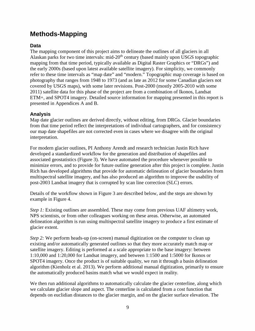
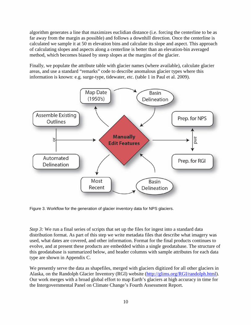
For modern glacier outlines, PI Anthony Arendt and research technician Justin Rich have developed a standardized workflow for the generation and distribution of shapefiles and associated geostatistics (Figure 3). We have automated the procedure whenever possible to minimize errors, and to provide for future outline generation after this project is complete. Justin Rich has developed algorithms that provide for automatic delineation of glacier boundaries from multispectral satellite imagery, and has also produced an algorithm to improve the usability of post-2003 Landsat imagery that is corrupted by scan line correction (SLC) errors.
Details of the workflow shown in Figure 3 are described below, and the steps are shown by example in Figure 4.
Step 1: Existing outlines are assembled. These may come from previous UAF altimetry work, NPS scientists, or from other colleagues working on these areas. Otherwise, an automated delineation algorithm is run using multispectral satellite imagery to produce a first estimate of glacier extent.
Step 2: We perform heads-up (on-screen) manual digitization on the computer to clean up existing and/or automatically generated outlines so that they more accurately match map or satellite imagery. Editing is performed at a scale appropriate to the base imagery: between 1:10,000 and 1:20,000 for Landsat imagery, and between 1:1500 and 1:5000 for Ikonos or SPOT4 imagery. Once the product is of suitable quality, we run it through a basin delineation algorithm (Kienholz et al. 2013). We perform additional manual digitization, primarily to ensure the automatically produced basins match what we would expect in reality.
We then run additional algorithms to automatically calculate the glacier centerline, along which we calculate glacier slope and aspect. The centerline is calculated from a cost function that depends on euclidian distances to the glacier margin, and on the glacier surface elevation. The
9
algorithm generates a line that maximizes euclidian distance (i.e. forcing the centerline to be as far away from the margin as possible) and follows a downhill direction. Once the centerline is calculated we sample it at 50 m elevation bins and calculate its slope and aspect. This approach of calculating slopes and aspects along a centerline is better than an elevation-bin averaged method, which becomes biased by steep slopes at the margins of the glacier.
Finally, we populate the attribute table with glacier names (where available), calculate glacier areas, and use a standard “remarks” code to describe anomalous glacier types where this information is known: e.g. surge-type, tidewater, etc. (table 1 in Paul et al. 2009).
Figure 3. Workflow for the generation of glacier inventory data for NPS glaciers.
Step 3: We run a final series of scripts that set up the files for ingest into a standard data distribution format. As part of this step we write metadata files that describe what imagery was used, what dates are covered, and other information. Format for the final products continues to evolve, and at present these products are embedded within a single geodatabase. The structure of this geodatabase is summarized below, and header columns with sample attributes for each data type are shown in Appendix C.
We presently serve the data as shapefiles, merged with glaciers digitized for all other glaciers in Alaska, on the Randolph Glacier Inventory (RGI) website (http://glims.org/RGI/randolph.html). Our work merges with a broad global effort to map Earth’s glaciers at high accuracy in time for the Intergovernmental Panel on Climate Change’s Fourth Assessment Report.
10

• Glacier Base Maps – polygons depicting all topographic map sources for map date outlines.
• Glacier Base Images – polygons depicting all imagery sources for modern outlines. • Glacier Centerlines – polylines depicting centerlines of all map date and modern
glaciers, as derived by an automated algorithm. • Glacier Outlines – polygons depicting outlines of all map date and modern glaciers, as
derived by the processes described in step 2, above. Identical outlines are currently presented in two forms: Lat/Long with WGS 1984 datum, and Albers Projection with NAD 1983 datum.
• Glacier Aspect – table of glacier aspects presented in 50 meter elevation bins. • Glacier Hypsometry – table of glacier areas presented in 50 meter elevation bins. • Glacier Slope – table of glacier slopes presented in 50 meter elevation bins.
Every glacier is identified throughout the database by a standardized GLIMS ID, and the geodatabase structure described above collectively summarizes each glacier (both map date and modern) with the following attributes:
• Outline and centerline • Map or imagery source for outline/centerline • Date of map/imagery source • Name (if available) • Centroid latitude and longitude • Length and overall slope of centerline • Glacier area (km2) • Min, max, and area-weighted mean glacier elevations • Hypsometry data, presented as glacier areas within 50 m elevation bins • Glacier surface aspects and slopes, averaged within 50 m elevation bins • Glacier types
Note that glacier volumes are no longer calculated or presented in the geodatabase, reflecting our view that area/volume scaling (as done in previous progress reports and summarized by Bahr 1997) is not a sufficiently robust technique for calculation of volume changes over time.
11
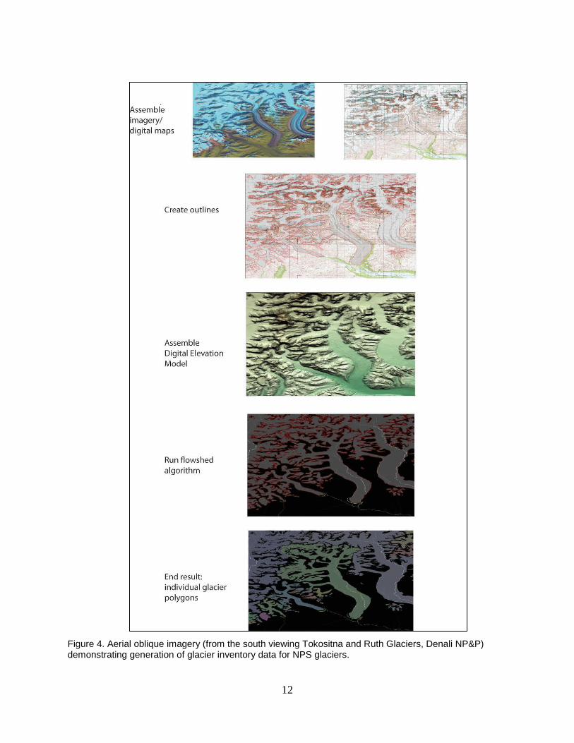
Figure 4. Aerial oblique imagery (from the south viewing Tokositna and Ruth Glaciers, Denali NP&P) demonstrating generation of glacier inventory data for NPS glaciers.
12

Methods-Elevation Change The elevation change component of this project aims to characterize changes in surface elevations of all glaciers (within glaciated Alaskan parks) that have existing laser point data from two or more time intervals since this work commenced in the mid-1990s. No new laser altimetry data will be acquired under the scope of this project. Existing laser altimetry profiles (as of January 2011) for KEFJ and WRST are shown in Figure 5 and Table 3. As noted in the introduction, some analyses from Wrangell-St. Elias NP&P were not completed in time for this progress report—only those presented here are labeled in Figure 5.
Data Elevation change estimates are based upon laser point data acquired from aircraft at discrete time intervals. Laser point data has been acquired with three different systems since data collection began in 1995, including two different laser profilers before 2009 and a scanning laser system since then. The laser profilers have been described in previous publications (Arendt et al. 2002; Echelmeyer et al. 1996; Sapiano et al. 1998). The data acquired during those earlier missions have been reprocessed with the same methods as post-2009 scanning laser system data, which was acquired with a Riegl LMS-Q240i that has a sampling rate of 10,000 points per second, an angular range of 60 degrees, and a wavelength of 900 nm. The average spacing of laser returns both along and perpendicular to the flight path at an optimal height above the glacier of 500 m is approximately 1 m x 1 m with a swath width of 500 – 600 m. The aircraft is oriented using an inertial navigation system (INS) and global position system (GPS) unit. The INS is an Oxford Technical Solutions Inertial+ unit that has a positioning accuracy of 2 cm, a velocity accuracy of 0.05 km/h RMS, and an update rate of 100 Hz. The GPS receiver is a Trimble R7 that records data at 5 Hz and has an accuracy of 1 cm horizontal and 2 cm vertical in ideal kinematic surveying conditions.
To translate laser point data to estimates of volume change, we require digital elevation models (DEMs) and glacier outlines for measured glaciers. The DEM is derived from the National Elevation Database (NED), a USGS product derived from diverse source data that generally (in Alaska) reflect elevations from the most recent topographic map at 2-arc-second (~60 m) grid spacing. Outlines and surface areas of each glacier are based upon “modern” glacier outlines developed elsewhere in this project.
Analysis The workflow for calculation of elevation changes and derived volume changes follows these steps:
Step 1: Glacier surface elevations are derived from laser point data by integrating the GPS-based position of the aircraft on its flight path over a glacier, airplane orientation data from an onboard INS, and laser point return positions relative to the airplane. The combination of these data determines the position in 3-dimensional space of the laser point returns from the glacier surface.
The points are referenced in ITRF00 and coordinates are projected to WGS84, with a coordinate accuracy in x, y, and z position of +/- 30 cm. Elevation data are recorded as height above ellipsoid.
13

Step 2: Glacier surface elevation profiles from different years can then be differenced to find the cumulative thickness change (dz, meters) over that time interval. Division by the time elapsed (dt, years) gives the rate of thickness change ∆z (m/yr). This is determined with slightly different methods depending on whether data from the laser profiler (1995 – 2009) or laser scanner (2010 – 2011) are being used.
Step 3a: For laser profiler to laser profiler differencing, points that are located within 10 m of each other in the x-y plane are selected as common points between the different years. If more than one point is located within that 10 m grid, then the mode of the elevation is used for each grid point. These common points are then used in the determination of ∆z. Since there are data points recorded only along the flight track at nadir with the laser profiler it is critical that these earlier flight paths were repeated as accurately as possible to obtain a large number of common points. Sometimes the flights were not repeated closely enough to provide extensive elevation change, and dz plots using this data typically exhibit many fewer points than comparable plots based on the laser scanning system (described below in step 3b). This limits the robustness of the interpolated line that is fit to the data, especially if there is variability within the data.
Step 3b: For laser scanner to laser profiler differencing, a grid is made of the laser scanner swath at a resolution of 10 m. Elevation values in this grid are based upon the mode of all the points within each of the grid cells, which helps to filter out laser returns from crevasse bottoms. Then, the coordinates from each point in the old profile are used to extract an elevation from this grid (for all laser profiler points that fall within the new LiDAR swath extents). This laser scanner elevation is differenced with the laser profiler elevation at that point, giving the change in elevation. The same idea is used for laser scanner to laser scanner comparisons, but instead of using every point from the older laser scanner swath, an average value on a 10 m x 10 m is calculated out of the old swath, then the value for that point location is also extracted from the newer laser scanner grid.
Step 4: The complete series of ∆z measurements at specific elevations along the glacier flight line is plotted as the median of a smoothing window with a typical width of twelve data points from the bottom to the top of the glacier. Plotted confidence intervals are based upon the interquartile range of the moving window. At both the lower and upper elevation limits of the glacier, ∆z is forced to zero and the confidence interval is presented as an average of the interquartile ranges calculated along the entire profile.
Step 5: The NED-based DEM is used to develop an area-altitude distribution (AAD) for the glacier in 30 m elevation bins. Volume change is found by performing a numerical integration wherein the binned ∆z line is multiplied by the binned AAD.
To facilitate comparison of volume changes among glaciers of different sizes, we convert volume changes to glacier-wide mass balance rates (�̇�𝐵), adhering to terminology in the Glossary of Mass Balance Terms (Cogley et al. 2011). The mass change is calculated assuming that the lost (or gained) volume was composed entirely of ice, e.g. Sorge’s law (Bader, 1954). The mass change can then be converted to water equivalent (w.e.) by assuming a constant ice density of 900 kg/m3, and the mass change presented as Gt/yr. Glacier-wide mass balance rate is then just mass change divided by glacier surface area.
14

Table 3. Date of laser altimetry flights for glaciers located in Kenai Fjords NP (rows 1-2) and Wrangell-St. Elias NP&P (row 3). Glacier types are land terminating (L), lake calving (LK), and tidewater (T).
15

Figure 5. Existing laser altimetry profiles (red lines) in Kenai Fjords NP (upper panel) and Wrangell-St. Elias NP&P (lower panel) as of January 2011. Modern glacier outlines in blue; only glaciers analyzed in this report are labeled.
16

Methods-Focus Glaciers The focus glacier component of this project aims to provide additional information about a small subset of glaciers in each glaciated Alaskan park for the purpose of demonstrating the potentially unique ways in which A) glaciers change in response to climate and other forcings, and B) landscapes respond to glacier change. The focus glacier portion of the final report will include a narrative description of each glacier and a collection of photos, maps, figures, and other graphical information. In comparison with the other components of this project, which are directed clearly towards generating and analyzing new or existing data, the focus glacier component is focused more on interpretation and synthesis. No new data will be acquired, but collection of existing materials is a central task for the PI Michael Loso. For each glacier, this collection of materials will ultimately be presented as a “vignette” in the final document. A sample vignette was presented in the Second Progress Report.
Focus Glacier Selection The final list of focus glaciers is included below (Table 4) and mapped in Figure 6. The focus glaciers are not intended to be statistically representative of Alaskan glaciers as a whole, but rather were selected to collectively represent the diversity of glacier types and climatic responses evident statewide. Additional supporting criteria for inclusion in the list were a rich history of visitation/ documentation and public accessibility. Since October 2010, the list evolved some under the advice and guidance of NPS staff, particularly including NPS unit resource staff and regional I&M staff. No changes have occurred since the Second Progress Report.
Summary of Field Efforts In the summer of 2011, PI Loso visited several NPS units to collect existing resource materials and develop first-hand familiarity with some of the focus glaciers. Results of these efforts were summarized in the Second Progress Report. No additional fieldwork has occurred, or is expected under the scope of this project.
In the past year, most focus glacier work has focused on two objectives: 1) collection of existing data and published reports to facilitate vignette writing, and 2) design of the interpretive report. We report progress on these two objectives in the results of this paper.
17

Figure 6. Overview of focus glacier locations (red dots). Green polygons are NPS unit outlines.
18

Table 4. Focus glaciers for each of Alaska’s 9 glaciated park units. “Snapshot” briefly denotes unique aspects of each glacier. PI Loso has personal knowledge of “visited” glaciers. Quality of historic record will largely dictate scope of each glacier’s narrative. Note that Turquoise Glacier (LACL) and Fourpeaked Glacier (KATM) have been removed from this list due to lack of available information.
19


Results-Mapping Maps of glacier outlines, with associated geostatistics, were completed for all glaciers in KEFJ and WRST. In both parks, modern outlines are based mostly upon high-quality imagery (entirely Ikonos in Kenai Fjords, with some additional SPOT4 and Landsat ETM+ data in Wrangells) and we do not anticipate significant further refinements of these outlines. The full datasets upon which these results are based will be delivered in electronic format when the project is finalized, but NPS investigators may contact the mapping team (Arendt and Rich) if they wish to obtain preliminary data in advance of that time. The analysis presented here is focused on basic metrics of glacier change, but we ultimately plan a more robust analysis of the geostatistical component of the datasets (e.g. Bolch et al. 2010). Note that statistics presented here for both parks include glaciers that are outside the park boundaries. In the final reporting for this project, we will include these contiguous glaciers in the database but exclude them from statistical analyses. Additional, higher resolution maps of glacier change are presented in Appendix D.
Kenai Fjords NP Mapped outlines for glaciers in and around Kenai Fjords NP are shown in Figure 7 and summarized in Table 5. In total, KEFJ and surrounding areas had 397 glaciers mapped on the DRGs (1950-1951) and 25% more in modern satellite imagery (2005-2007). In that same time, total glacier area nonetheless decreased 11% from 2603 km2 to 2323 km2. These overall changes are summarized on a per-glacier basis in Figure 8. Small and medium sized glaciers (~< 2 km2) were more common in modern mapping, whereas larger glaciers showed little change in abundance (right panel). Ranking glaciers by mean elevation we see that the lowest and highest elevation glaciers were the least changed in abundance, while glaciers with a moderate mean elevation were more numerous in modern imagery (left panel). There is weak evidence for loss of the very lowest elevation glaciers over the same time period. This pattern is also reflected by Figure 9, which shows change in total glacier coverage (rather than individual glaciers) as a function of elevation. Ice at the modal elevation (1250-1300 m) diminished most noticeably, with the least proportional change at the upper elevations.
Table 5. Summary statistics for glaciers in Kenai Fjords NP. Statistics include glaciers outside the park, as shown in Figures 1 and 7.
We interpret these changes as primarily reflecting two processes. Growth in numbers of small glaciers is probably a reflection of more advanced mapping techniques with high resolution imagery. Loss of overall glacier area, however, appears to be a real reflection of terminus retreat that is conspicuously apparent on most large glaciers of the region (Figure 7, Appendix D).
21
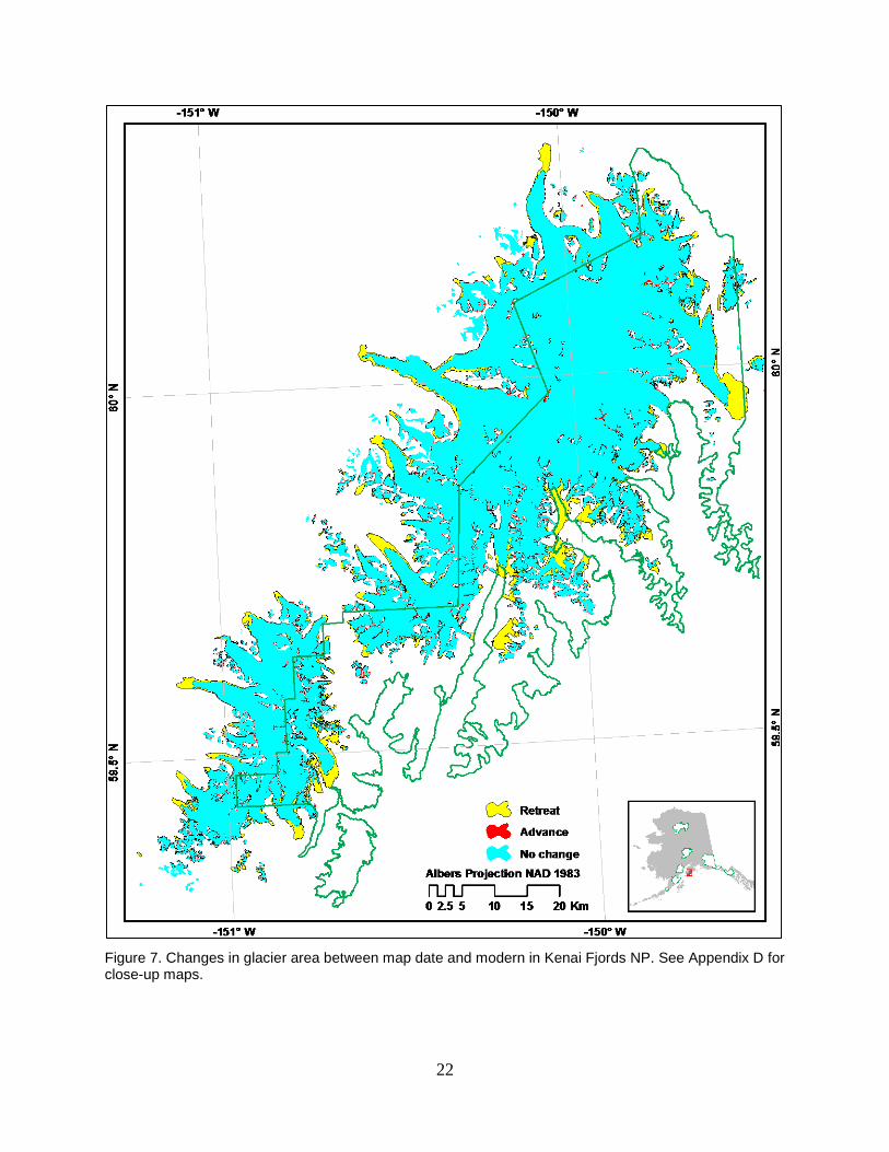
Figure 7. Changes in glacier area between map date and modern in Kenai Fjords NP. See Appendix D for close-up maps.
22

Figure 8. Histograms of changes in number of individual glaciers by area-weighted mean elevation (left) and area (right) in Kenai Fjords NP between map date (1950-1951) and modern (2005-2007).
Figure 9. Total area of glacier-covered terrain in Kenai Fjords NP by elevation between map date (1950-1951) and modern (2005-2007).
Wrangell-St. Elias NP&P Mapped outlines for glaciers in and around Wrangell-St. Elias NP&P are shown in Figure 10 and summarized in Table 6. Here, a substantial amount of Canadian ice is included in our calculations, as the large icefields on either side of the border are completely contiguous. Map
Map date
Modern
23

date photography is from a broad range of years, including 1948-1973 in the United States (where we focus) and as recent as 2012 in Canada. Acquisition dates of satellite imagery for modern outlines ranged from 2006-2011. Within that loosely defined period of change, the WRST population of glaciers grew 7% from 5421 to 5816, while simultaneously losing 5% of its
24

Figure 10. Changes in glacier area between map date and modern in Wrangell-St. Elias NP&P. See Appendix D for close-up maps.
25

total glacier area. We emphasize that the relatively small percentage loss translates to a large area for this heavily glaciated region—our mapping shows that over 2000 km2 of ice were lost between the map date and modern periods. The right panel of Figure 11 shows that the modest increase in the number of individual glaciers was mostly due to the mapping of very small glaciers (<<1 km2). Categorizing glaciers by their mean elevations (left panel), it is apparent that low elevation glaciers diminished in abundance while glaciers in middle to higher elevations (~> 1000 m mean elevation) generally increased. Figure 12 summarizes park-wide changes in ice-covered area, and shows that ice loss was concentrated between ~500 m and the modal elevation of ~1900 m, with little change at higher elevations.
Table 6. Summary statistics for glaciers in Wrangell-St. Elias NP&P. Statistics include glaciers outside the park, as shown in Figures 2 and 10.
As at Kenai Fjords, it appears likely that the “new” small glaciers were likely present but undetected in the DRGs, and that the increase in glacier numbers is an artifact of enhanced mapping techniques. Nonetheless, total glacier-covered area did decrease, and can be attributed primarily to generalized terminus retreat, mainly by large glaciers in the Wrangell Mountains, by the Bering Glacier, and by glaciers in Icy Bay.
Figure 11. Histograms of changes in number of individual glaciers by area-weighted mean elevation (left) and area (right) in Wrangell-St. Elias NP&P between map date (1948-1973) and modern (2006-2011).
Map date Modern
Map date Modern
26

Figure 12. Total area of glacier-covered terrain in Wrangell-St. Elias NP&P by elevation between map date (1948-1973) and modern (2006-2011).
Map date Modern
27


Results-Elevation Change We have completed analysis of surface elevation changes and inferred volume changes for twelve glaciers in Kenai Fjords NP and five glaciers in Wrangell-St. Elias NP (Table 3). Analyses of remaining profiles from WRST will be presented in the final progress report. Change for each glacier was measured over intervals that range from one to fifteen years. Below, we present and summarize overall results from each park unit. Complete results of these analyses are presented in narrative and graphic form in Appendix E.
Kenai Fjords NP Glacier-wide balance rates, which average annual volume losses across the surface area of a given glacier, are summarized for Kenai Fjords in Figure 13. The most conspicuous trend is that most of the Harding Icefield glaciers show an increase in surface elevation/glacier volume for the early period of measurement (1994/6 – 2001), with the only exceptions being Aialik and Chernof (no change) and Holgate, Skilak, and Tustumena (very slightly negative change). All glaciers measured, including the latter exceptions, were markedly more negative in the latter period (2001 – 2007), and every glacier lost elevation/volume when averaged over the entire period of measurement. Volume losses are summarized as a function of elevation in Figure 14, which confirms that Bear, Chernof, and Tustumena Glaciers have the most negative balances over the decade-plus of measurement.
We cannot yet say with certainty whether this early period elevation gain reflects actual changes in ice volume (as we would assume under Sorge’s law), or alternatively, whether it is a reflection of anomalously deep snowpack during the 2001 measurement. The latter seems possible, particularly because A) measurements were made slightly earlier in the melt season in 2001 (May 17-19 compared with late-May or early-June measurements in other years), and B) winter accumulation at nearby Wolverine Glacier was higher than usual when measured in spring of that year (Van Beusekom 2010). We will continue to investigate this surprising result before drawing firm conclusions in our final report, but for now we can tentatively conclude that since 1994/1996 most Harding Icefield glaciers lost volume at average rates between 0 and 2 meters/year, but perhaps at a much more rapid pace in recent years than in the earliest part of that interval.
We also note that the records from two glaciers, Harris Glacier and Northwestern Glacier, are very poor with only a limited elevation range of these glaciers sampled. The estimated values for these glaciers are extremely rough. We include them in this progress report to provide a record of the data, but due to the poor quality they are not intended for publication or use beyond this progress report. Due to weather and scheduling constraints, the Harding Icefield has not been flown since 2007, which means that, at the moment, there are no scanning LiDAR data for the Kenai Fjords region.
29

Figure 13. Glacier-wide mass balance rates (m/yr) for 11 glaciers from Kenai Fjords NP between 1994 and 2007. Rates are averaged over the period spanned by each bar. See Appendix E and text for complete details, including confidence intervals that are excluded here for clarity.
30
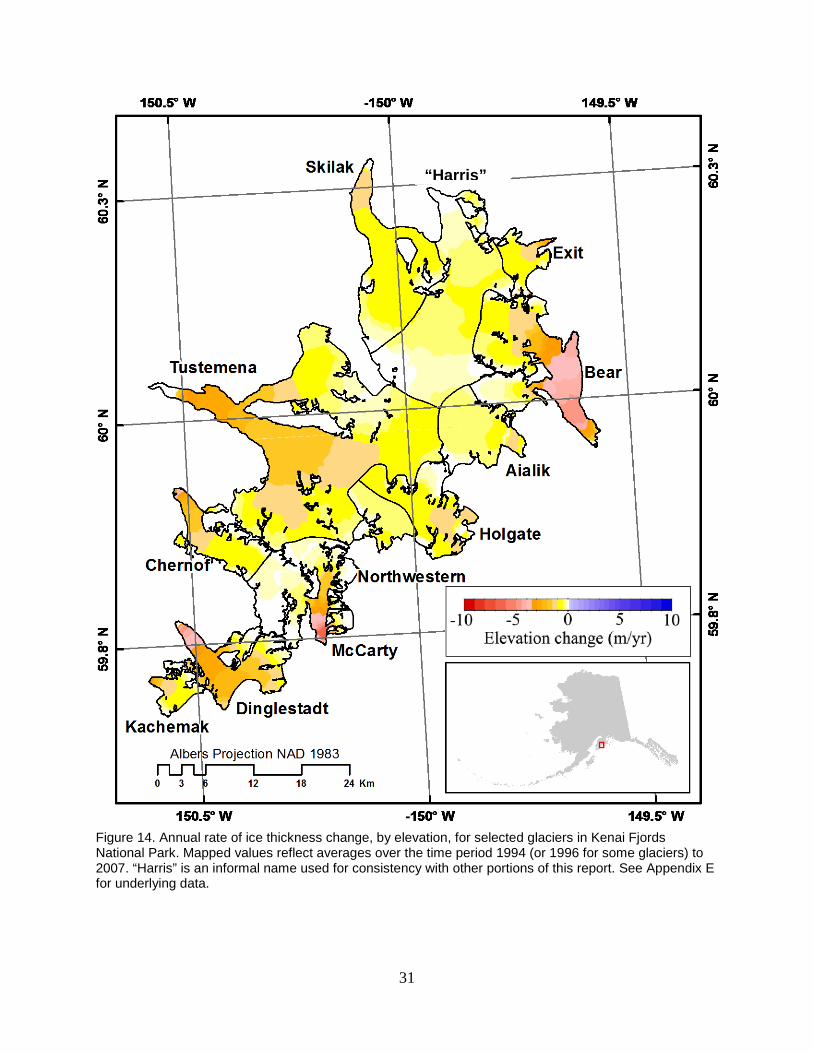
Figure 14. Annual rate of ice thickness change, by elevation, for selected glaciers in Kenai Fjords National Park. Mapped values reflect averages over the time period 1994 (or 1996 for some glaciers) to 2007. “Harris” is an informal name used for consistency with other portions of this report. See Appendix E for underlying data.
“Harris”
31

Wrangell-St. Elias NP&P As discussed previously, analyses of volume change from WRST are not complete, and we include in this report only preliminary data from five glaciers: Guyot and Yahtse (Icy Bay), Hubbard (Yakutat Bay), and Kennicott / Nabesna (interior). Because these glaciers were flown more recently (2010 to 2012) than Kenai Fjords glaciers, their most recent data was collected using the laser scanning system and consequently has higher point density. Dynamics of the coastal glaciers in this dataset, however, are in general more complicated and we keep our interpretation of the data at a minimum until analysis of WRST is complete. Mapped elevation changes will be presented at that time. Some basic trends can be noted here, as shown in Figure 15 (with details in Appendix E). The two interior, land-terminating glaciers in the dataset (Kennicott and Nabesna) both exhibit minor thinning and volume loss of just under 0.5 m/yr between 2000 and 2007. Guyot, a land-terminating but near-tidewater glacier, lost volume between 2007 and 2010 but gained volume from 2010-2012. Yahtse similarly changed from negative change between 2006 and 2010 to volume gain after 2010. Hubbard has been more or less neutral since 2001, with some evidence for volume gain at the earliest interval of measurement between 2000 and 2001.
Figure 15. Glacier-wide mass balance rates (m/yr) for five glaciers from Wrangell-St. Elias NP&P between 2000 and 2012. Rates are annual averages for the period spanned by each bar. See Appendix E and text for complete details, including confidence intervals that are excluded here for clarity.
32

Results-Focus Glaciers In the past year, most focus glacier work has focused on two objectives: 1) collection of existing data and published reports to facilitate vignette writing, and 2) design of the interpretive report. We report progress on these two objectives here.
Data Collection Collection of existing datasets is nearly complete, and has focused on glacier outlines to supplement the map date and modern outlines assembled by Anthony Arendt and Justin Rich. Availability of existing outlines is the primary constraint on this endeavor, but many focus glaciers have been studied by others, and we have experienced great generosity on the part of other scientists who are very willing to share their published work, work in progress, and general insights. Standouts include Exit Glacier (51 outlines) and Muir Glacier (over 200 outlines!). We summarize the collected outlines (with a few modest additional remaining steps outlined in red font) in Table 7. A rough example of the wealth of available data is shown in Figure 16, which depicts collected outlines for Exit Glacier. We will continue to explore the best graphic format for depicting such high-resolution change data, and will test this format in a scheduled publication of results from this project in Alaska Park Science. The deadline for submission of this article is May 1. In any case, we remind readers that few glaciers are so well documented.
Report Design Design of the interpretive report is underway in collaboration with Fresh Art & Design, a firm based in Anchorage Alaska. Inger Deede is the lead designer on this project, and is responsible for development of a style guide for the interpretive report and will later do the actual layout.
Inger Deede Fresh Art and Design www.freshartanddesign.com 525 W 3rd Ave #409 Anchorage AK 99501 (907) 360-7062 [email protected]
The scope of this agreement currently calls for layout in a “perfect bind” style that allows maps and photos to spread uninterrupted across two pages of the report when opened flat. Design of the style guide is ongoing, but to give some flavor of the expected product we include here two ‘mock-up’ page layouts. Note that text/photo/map contents in the mock-ups are meaningless, and these are mainly meant to display the designer’s current thoughts. See Figures 17 and 18.
33

Table 7. Glacier outlines collected for use in the focus glacier component of the interpretive report. Table is organized by park and by focus glacier, and continues on the next page. “map and sat outlines” refers to data created for this project—all other outlines are existing data. Red font indicates a task still underway.
34

35

Figure 16. Glacier outlines and terminus positions collected for Exit Glacier, Kenai Fjords NP. These data do not include the map date and modern outlines assembled by our team, and have not been carefully vetted at this time. Graphic presentation of these outlines will be more carefully explored at the time of final publication. Data courtesy of Deb Kurtz (NPS), Greg Wiles, and Bruce Giffen (NPS).
36

37
Figure 17. Map page style mockup of interpretive report.

38
Figure 18. Photo style mockup of interpretive report
Discussion Preliminary Highlights The data presented here are preliminary, but serve well to document our approach to, and progress on, this project. Some of the details of our analytical techniques are still evolving, but the general presentation has now been vetted in several meetings and three prior progress reports. Accordingly, the language and structure of this progress report is largely similar to the previous one and our focus here has been on documenting new datasets. The following trends and conclusions emerge from this preliminary work.
• Glaciers in Kenai Fjords NP (including portions of the Harding Icefield outside the park boundary) increased in number by 25%, from 297 to 498 between the two mapping periods (nominally 1950-51 to 2005-07).
• Glacier cover in Kenai Fjords NP decreased 11% over the same period, from 2603 to 2323 km2. This was accomplished mainly through terminus retreat of the larger glaciers.
• Glaciers in Wrangell-St. Elias NP (including substantial contiguous ice cover in adjacent Canada) also increased in number over the mapping period, from 5421 to 5816. The mapping period in Wrangells is more broadly defined: 1948-1973 to 2006-2011.
• Wrangell-St. Elias is the most heavily glaciated park unit, with 38,198 km2 of ice (again, including Canada) in recent satellite imagery, down 5% from the map date interval. Ice loss was heavily influenced by a few large glaciers in Icy Bay and the Bering Glacier.
• In both park units, it was mostly very small (<1 km2) glaciers that increased in number. We attribute this mostly to the effect of better resolution imagery and more detailed mapping, rather than creation of new ice.
• Using laser altimetry, we measured and analyzed 37 distinct intervals of elevation change among twelve glaciers in Kenai Fjords NP and 13 distinct intervals among five glaciers in Wrangell-St. Elias NP&P. Additional glaciers in Wrangell-St. Elias have been measured, but analyses are not complete and will be presented in a subsequent report.
• Glaciers in Kenai Fjords NP all lost volume over the 1994 (or 1996) to 2007 period, but there is some evidence that most of this loss occurred after 2001. We are uncertain of this latter interpretation, which may be an artifact of a deep snowpack in 2001.
• Two large interior land-terminating glaciers in Wrangell-St. Elias showed similar volume loss of under 0.5 m/yr after 2000. Coastal and tidewater glaciers were more variable over time, including some gain in mass by Guyot and Yahtse Glaciers between 2009 and 2012.
• We visited and photographed glaciers in Denali, Katmai, and Lake Clark NP&Ps in summer 2011. Sample interpretive themes for their focus glaciers are presented herein.
39

• Collection of existing data, published reports, and photographs for the focus glacier component of the project is essentially complete, and an artist is contracted to do design and layout for the ~200 page interpretive report. A sample layout is included here.
40

Literature Cited Arendt AA, Echelmeyer KA, Harrison WD, Lingle CS, Valentine VB (2002) Rapid wastage of
Alaska glaciers and their contribution to rising sea level. Science 297: 382-386
Bader H, 1954. Sorge’s Law of densification of snow on high polar glaciers. Journal of Glaciology 2: 319–323.
Bahr DB, Meier MF, Peckham SD (1997) The physical basis of glacier volume-area scaling. Journal of Geophysical Research 102: 20355-20362
Bolch T, Menounos B, Wheate R (2010) Landsat-based inventory of glaciers in western Canada, 1985-2005. Remote Sensing of Environment 114: 127-137
Cogley, JG, Hock R, Rasmussen LA, Arendt AA, Bauder A, Braithwaite RJ, Jansson P, Kaser G, Moller M, Nicholson L, and Zemp M. 2011. Glossary of Glacier Mass Balance and Related Terms. IHP-VII Technical Documents in Hydrology No. 86. Paris: UNESCO-IHP.
Echelmeyer KA, Harrison WD, Larsen CF, Sapiano J, Mitc hell JE, DeMallie J, Rabus B, Adalgeirsdottir G, Sombardier L (1996) Airborne surface profiling of glaciers: a case-study in Alaska. Journal of Glaciology 42: 538-547
Kienholz C, Hock R, Arendt AA (2013). A new semi-automatic approach for dividing glacier complexes into individual glaciers. Journal of Glaciology 59(217): 913–925. doi:10.3189/2013JoG12J138
Paul F, Barry RG, Cogley JG, Frey H, Haeberli W, Ohmura A, Ommanney CSL, Raup B, Rivera A, Zemp M (2009) Recommendations for the compilation of glacier inventory data from digital sources. Annals of Glaciology 50: 119-126
Post A, Meier MF (1980) A preliminary inventory of Alaskan glaciers, in World Glacier Inventory Workshop, 17–22 September 1987, Reideralp, Switzerland, Proceedings: International Association of Hydrological Sciences (IAHS) Publication No. 126, p. 45–47
Sapiano JJ, Harrison WD, Echelmeyer KA (1998) Elevation, volume and terminus changes of nine glaciers in North America. Journal of Glaciology 39: 582-590
Van Beusekom AE, O’Neel SR, March RS, Sass LC, Cox LH (2010) Re-analysis of Alaskan benchmark glacier mass-balance data using the index method. USGS Scientific Investigations Report 2010-5247, 14 pp.
Winkler GR, MacKevett EM Jr., Plafker G, Richter DH, Rosenkrans DS, Schmoll HR (2000) A geologic guide to Wrangell-St. Elias National Park and Preserve, Alaska. USGS Professional Paper 1616, 166 pp.
41


Appendix A: Data Sources for Mapping-Map Date
43

44

45

46

Appendix B: Data Sources for Mapping-Modern
47

48

49
50

51

52

53

54
Appendix C: Data Products Exported From Extent Mapping
55


Appendix D: Close-up Maps of Glacier Extent Changes
Figure D1. Close-up of northeastern Kenai Fjords NP glaciers.
57

Figure D2. Close-up of southwestern Kenai Fjords NP glaciers.
58

Figure D3. Close-up of Wrangell Mountains glaciers in northwestern Wrangell-St. Elias NP&P.
59

Figure D4. Close-up of coastal glaciers in southwestern Wrangell-St. Elias NP&P.
60

Figure D5. Close-up of Malaspina Glacier in southern Wrangell-St. Elias NP&P.
61

Appendix E: Elevation and Volume Change Analyses Narrative summaries of elevation changes for individual glaciers during discrete time intervals are followed by plots of all summarized data.
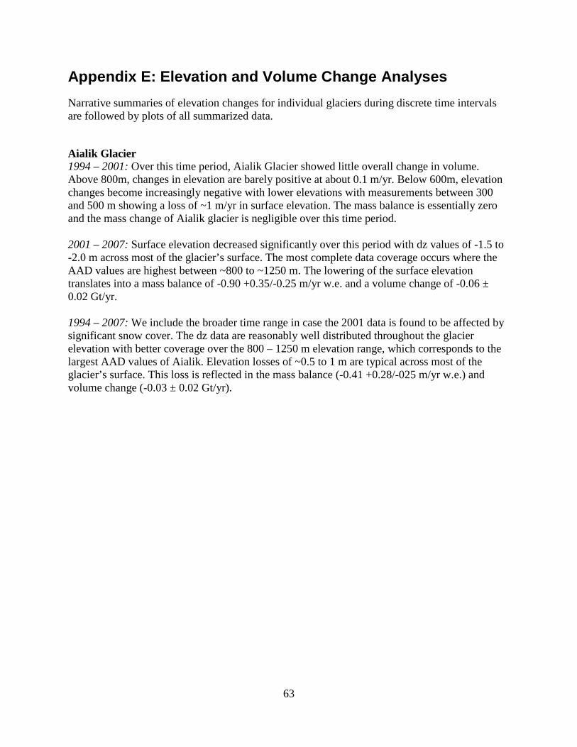
Aialik Glacier 1994 – 2001: Over this time period, Aialik Glacier showed little overall change in volume. Above 800m, changes in elevation are barely positive at about 0.1 m/yr. Below 600m, elevation changes become increasingly negative with lower elevations with measurements between 300 and 500 m showing a loss of ~1 m/yr in surface elevation. The mass balance is essentially zero and the mass change of Aialik glacier is negligible over this time period. 2001 – 2007: Surface elevation decreased significantly over this period with dz values of -1.5 to -2.0 m across most of the glacier’s surface. The most complete data coverage occurs where the AAD values are highest between ~800 to ~1250 m. The lowering of the surface elevation translates into a mass balance of -0.90 +0.35/-0.25 m/yr w.e. and a volume change of -0.06 ± 0.02 Gt/yr. 1994 – 2007: We include the broader time range in case the 2001 data is found to be affected by significant snow cover. The dz data are reasonably well distributed throughout the glacier elevation with better coverage over the 800 – 1250 m elevation range, which corresponds to the largest AAD values of Aialik. Elevation losses of ~0.5 to 1 m are typical across most of the glacier’s surface. This loss is reflected in the mass balance (-0.41 +0.28/-025 m/yr w.e.) and volume change (-0.03 ± 0.02 Gt/yr).
63
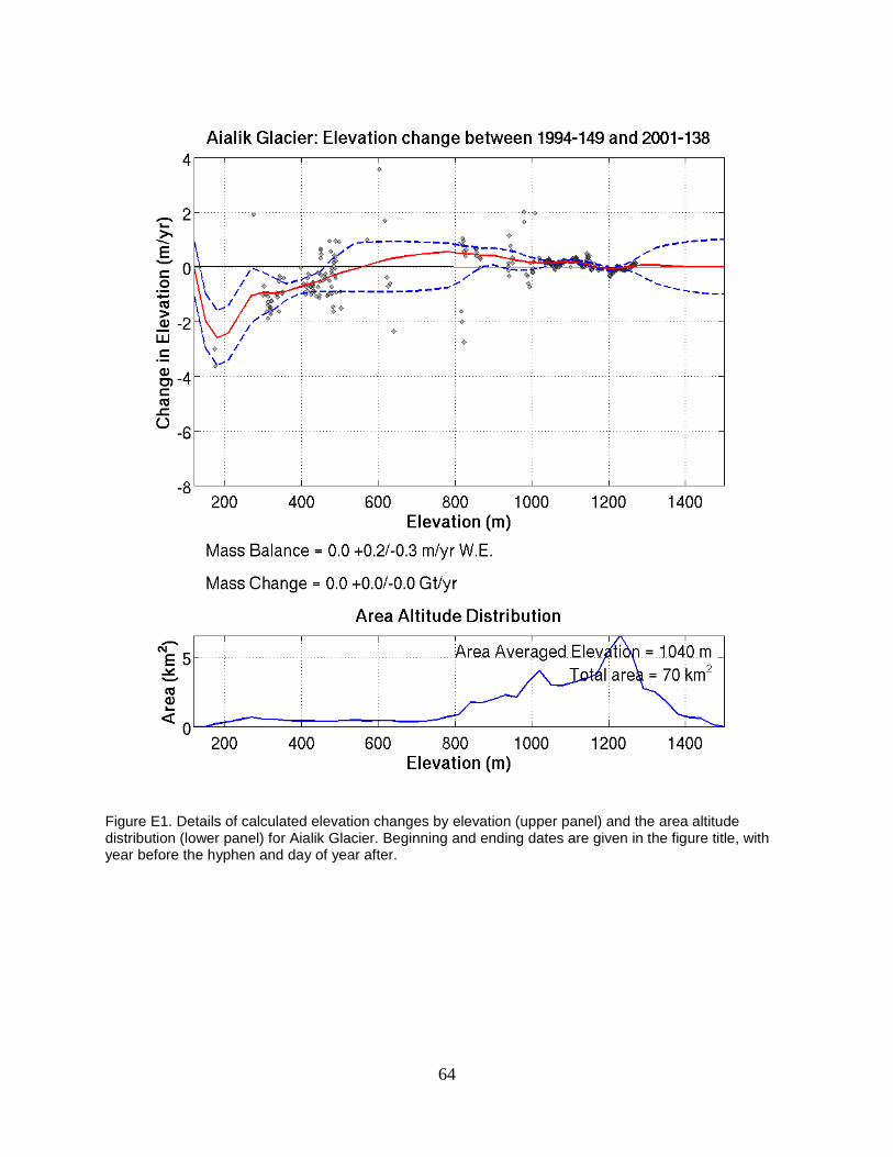
Figure E1. Details of calculated elevation changes by elevation (upper panel) and the area altitude distribution (lower panel) for Aialik Glacier. Beginning and ending dates are given in the figure title, with year before the hyphen and day of year after.
64
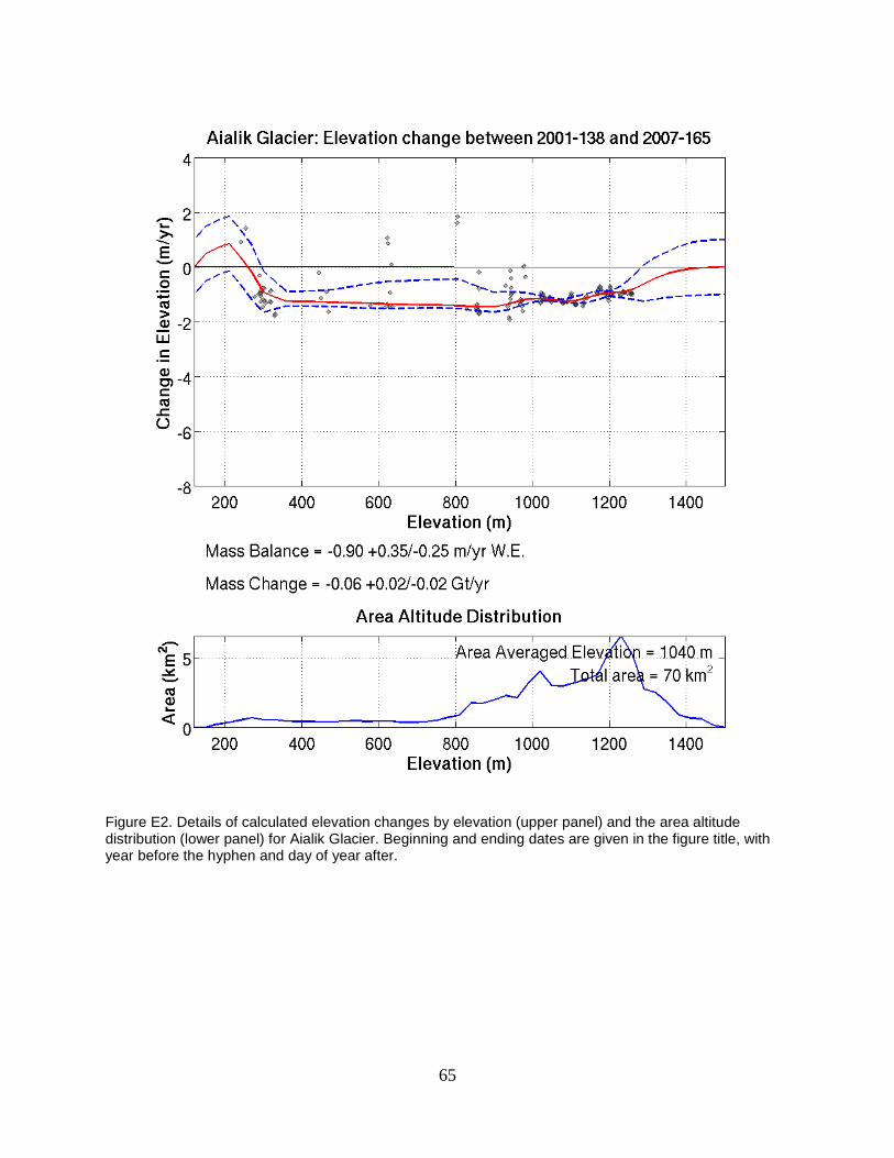
Figure E2. Details of calculated elevation changes by elevation (upper panel) and the area altitude distribution (lower panel) for Aialik Glacier. Beginning and ending dates are given in the figure title, with year before the hyphen and day of year after.
65

Figure E3. Details of calculated elevation changes by elevation (upper panel) and the area altitude distribution (lower panel) for Aialik Glacier. Beginning and ending dates are given in the figure title, with year before the hyphen and day of year after.
66
Bear Glacier 1994 – 2001: At higher elevations (>800 m), the surface elevation decreased by only ~0.2 m/yr between 1994 and 2001. Below 800 m, however, the elevation changes become increasingly negative down to ~ -4 m/yr at 100 m. Data is sparse in some elevation ranges, but where data are present they show a consistent picture of the dz increasingly negative at lower elevations. Overall, Bear shows negative mass balance (-1.14 +0.38/-0.65 m/yr w.e.) and change (-0.16 ± 0.09 Gt/yr). 2001 – 2007: The trend of elevation loss observed from 1994 to 2001 continues at greater pace during this period with loss rates nearly twice the values seen in the 1994 to 2001 data. Similar to the previous period, there are significant gaps in the measurement points available, but where data exists it shows a coherent picture of elevation losses increasing down glacier. The glacier-wide mass balance and change are double those of the previous period at -2.28 +0.62/-0.49 m/yr w.e. and -0.33 ± 0.07 Gt/yr. 1994 – 2007: Data coverage is quite good up to ~1100 m on Bear Glacier between 1994 and 2007. The data are relatively continuous with little variation in dz values for a given elevation. The mass balance is significantly negative at -1.62 +0.42/-0.33 m/yr w.e. and the mass loss is also significant at -0.23 ± 0.05 Gt/yr.
67

Figure E4. Details of calculated elevation changes by elevation (upper panel) and the area altitude distribution (lower panel) for Bear Glacier. Beginning and ending dates are given in the figure title, with year before the hyphen and day of year after.
68

Figure E5. Details of calculated elevation changes by elevation (upper panel) and the area altitude distribution (lower panel) for Bear Glacier. Beginning and ending dates are given in the figure title, with year before the hyphen and day of year after.
69

Figure E6. Details of calculated elevation changes by elevation (upper panel) and the area altitude distribution (lower panel) for Bear Glacier. Beginning and ending dates are given in the figure title, with year before the hyphen and day of year after.
70
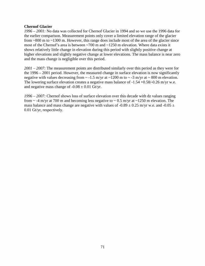
Chernof Glacier 1996 – 2001: No data was collected for Chernof Glacier in 1994 and so we use the 1996 data for the earlier comparison. Measurement points only cover a limited elevation range of the glacier from ~800 m to ~1300 m. However, this range does include most of the area of the glacier since most of the Chernof’s area is between ~700 m and ~1250 m elevation. Where data exists it shows relatively little change in elevation during this period with slightly positive change at higher elevations and slightly negative change at lower elevations. The mass balance is near zero and the mass change is negligible over this period. 2001 – 2007: The measurement points are distributed similarly over this period as they were for the 1996 – 2001 period. However, the measured change in surface elevation is now significantly negative with values decreasing from ~ -1.5 m/yr at ~1200 m to ~ -3 m/yr at ~ 800 m elevation. The lowering surface elevation creates a negative mass balance of -1.54 +0.58/-0.26 m/yr w.e. and negative mass change of -0.08 ± 0.01 Gt/yr. 1996 – 2007: Chernof shows loss of surface elevation over this decade with dz values ranging from ~ -4 m/yr at 700 m and becoming less negative to ~ 0.5 m/yr at ~1250 m elevation. The mass balance and mass change are negative with values of -0.89 ± 0.25 m/yr w.e. and -0.05 ± 0.01 Gt/yr, respectively.
71

Figure E7. Details of calculated elevation changes by elevation (upper panel) and the area altitude distribution (lower panel) for Chernof Glacier. Beginning and ending dates are given in the figure title, with year before the hyphen and day of year after.
72

Figure E8. Details of calculated elevation changes by elevation (upper panel) and the area altitude distribution (lower panel) for Chernof Glacier. Beginning and ending dates are given in the figure title, with year before the hyphen and day of year after.
73

Figure E9. Details of calculated elevation changes by elevation (upper panel) and the area altitude distribution (lower panel) for Chernof Glacier. Beginning and ending dates are given in the figure title, with year before the hyphen and day of year after.
74

Dinglestadt Glacier 1996 – 2001: The data are reasonably spread from near the terminus of the glacier at 400 m up to 1200 m. This misses the upper reaches of Dinglestadt. dz values are negative from 400 m to 800 m, but become increasingly positive above this to the upper limit of coverage at 1200 m. With more area above 800 m, the overall mass balance is slightly positive at 0.1 ± 0.3 m/yr w.e. and the mass change is negligible. 2001 – 2007: Data coverage is reasonable with regularly spaced measurement points from 400 m to 1200 m elevation. The upper reaches of the glacier are missed, but based on the trend of elevation change in the data it appears that the modeled curve of elevation is a reasonable approximation where data is unavailable. The glacier surface lowered by ~ 5 m/yr near the toe of the glacier at ~ 400 m with the elevation loss decreasing up the glacier to the highest available data that shows a loss of ~ -1 m/yr at 1200 m. Dinglestadt shows significant loss of mass during this period with a mass balance of -1.53 ± 0.35 m/yr w.e. and mass loss of -0.11 ± 0.02 Gt/yr. 1996 – 2007: Data coverage for this longer time period is similar to the two shorter contained within this period. Over this decade, Dinglestadt experienced negative mass balance (-0.70 ± 0.14 m/yr w.e.) and mass loss (-0.05 ± 0.01 Gt/yr).
75
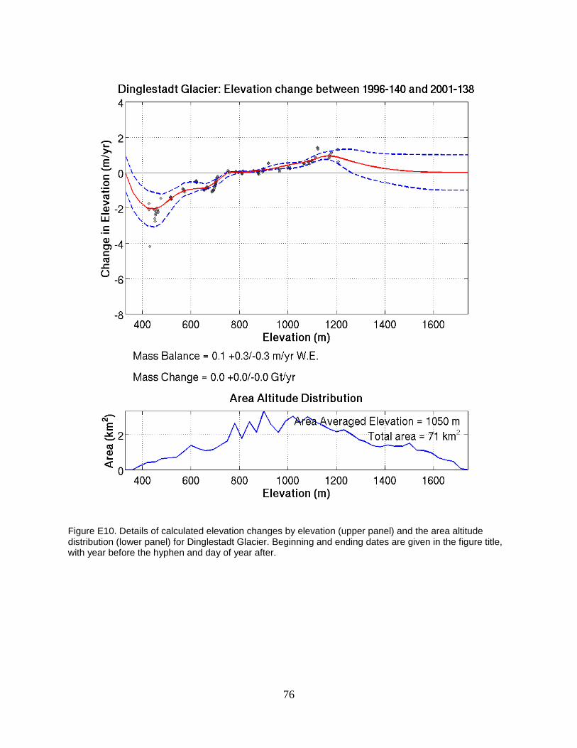
Figure E10. Details of calculated elevation changes by elevation (upper panel) and the area altitude distribution (lower panel) for Dinglestadt Glacier. Beginning and ending dates are given in the figure title, with year before the hyphen and day of year after.
76

Figure E11. Details of calculated elevation changes by elevation (upper panel) and the area altitude distribution (lower panel) for Dinglestadt Glacier. Beginning and ending dates are given in the figure title, with year before the hyphen and day of year after.
77
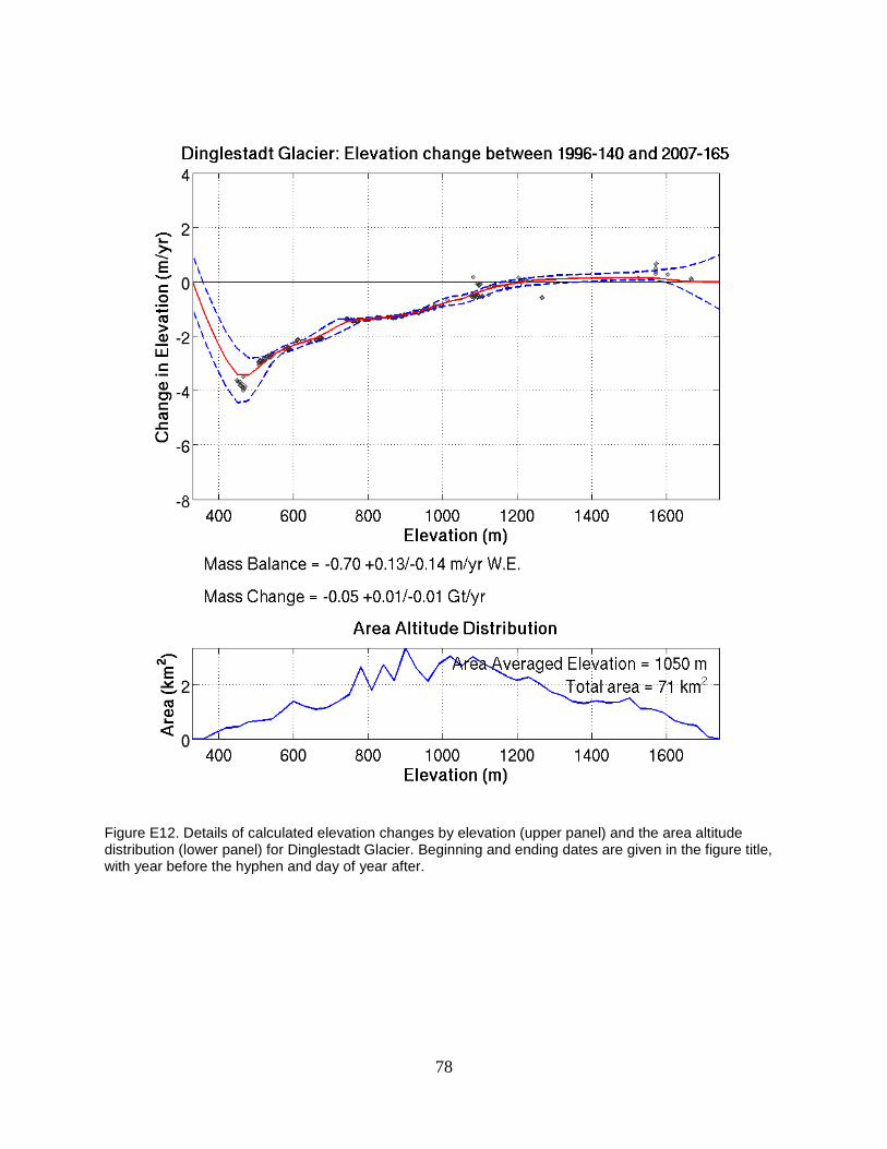
Figure E12. Details of calculated elevation changes by elevation (upper panel) and the area altitude distribution (lower panel) for Dinglestadt Glacier. Beginning and ending dates are given in the figure title, with year before the hyphen and day of year after.
78
Exit Glacier 1994 – 2001: The data coverage on Exit for this period is very good, but does not include any of the glacier about ~1150 m. Data does cover the elevations with the highest AAD values between 1000 and 1150 m. Much of Exit glacier shows negative surface elevation changes over this period with values ranging from -2 m/yr at the terminus to zero at 1100 m. Above 1100 m the elevation change appears to trend positive. Mass balance is slightly negative at -0.2 ± 0.2 m/yr w.e. and the mass change is negligible. 1999 – 2001: The elevation changes of Exit during this period are strongly positive with values > 1.5 m/yr for the bulk of the area of Exit Glacier. It is not clear at this point whether this represents a real change in elevation or whether heavy snowfall or other factors are creating misleading data. However, if accurate, these data show a strong positive mass balance (1.12 +0.46/-0.38 m/yr w.e.) and mass change (0.03 ± 0.01 Gt/yr). 2001 – 2007: Where the elevation changes were measured as positive from 1999 to 2001, they are consistently negative during this later period. The data do not cover the uppermost reaches of the glacier (>1200 m) and there is a large gap from 300 to 600 m, but there are numerous and consistent data between 600 and ~1200 m that show a typical elevation loss of ~ 2 m/yr. These elevation losses suggest a negative mass balance (-1.21 ± 0.27 m/yr w.e.) of similar magnitude to the positive mass balance in the previous period. Similarly, the mass change is negative (-0.03 ± 0.01 Gt/yr) and of equal magnitude to the positive mass change in the previous time period. 1994 – 2007: Data coverage is good between 700 and 1100 m, but non-existent above this range and spotty below. However, this does cover most of the area of Exit glacier and so the glacier-wide mass balance (-0.68 ± 0.25 m/yr w.e.) and mass change (-0.02 ± 0.01 Gt/yr) both reasonable estimates.
79
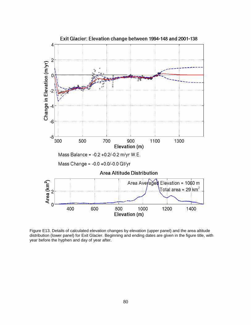
Figure E13. Details of calculated elevation changes by elevation (upper panel) and the area altitude distribution (lower panel) for Exit Glacier. Beginning and ending dates are given in the figure title, with year before the hyphen and day of year after.
80

Figure E14. Details of calculated elevation changes by elevation (upper panel) and the area altitude distribution (lower panel) for Exit Glacier. Beginning and ending dates are given in the figure title, with year before the hyphen and day of year after.
81

Figure E15. Details of calculated elevation changes by elevation (upper panel) and the area altitude distribution (lower panel) for Exit Glacier. Beginning and ending dates are given in the figure title, with year before the hyphen and day of year after.
82

Figure E16. Details of calculated elevation changes by elevation (upper panel) and the area altitude distribution (lower panel) for Exit Glacier. Beginning and ending dates are given in the figure title, with year before the hyphen and day of year after.
83

Harris Glacier Note that this glacier, informally named “Harris” by the technician generating these results, is not commonly known by this name. We retain the usage for this report only to maintain internal consistency. Other, more common informal names for this glacier in usage in the region are “Jap Glacier” or “Glacier A.” 1996 – 2001: Data for the elevation change of Harris Glacier is extremely limited in its elevation range, but does cover the highest values of the area altitude distribution from 1150 m to 1350 m elevation. The quality of coverage is low. Where data exist they show a positive change in elevation of ~ 1 m/yr for the glacier with subtle indications that this may increase in the upper reaches of the glacier and decrease down glacier from where measurements are available. Due to the lack of measurements, the range of uncertainty is greater than the value for both the mass balance (0.6 ± 0.8 m/yr w.e.) and mass change (0.1 ± 0.02 Gt/yr). 2001 – 2007: Similar to the previous period, the data are concentrated between 1150 and 1350 m elevation on the glacier. They show negative changes in elevation with values typically around –1 m/yr. The mass balance is negative at -0.95 ± 0.63 m/yr w.e. and the mass change is also negative at -0.20 ± 0.13 Gt/yr over this period. 1996 – 2007: Data coverage is extremely limited. While a poor estimate, the calculated mass balance is -0.2 + 0.4/-0.7 m/yr w.e. and the mass change is negligible.
84

Figure E17. Details of calculated elevation changes by elevation (upper panel) and the area altitude distribution (lower panel) for “Harris Glacier” (see text for alternate names). Beginning and ending dates are given in the figure title, with year before the hyphen and day of year after.
85

Figure E18. Details of calculated elevation changes by elevation (upper panel) and the area altitude distribution (lower panel) for “Harris Glacier” (see text for alternate names). Beginning and ending dates are given in the figure title, with year before the hyphen and day of year after.
86
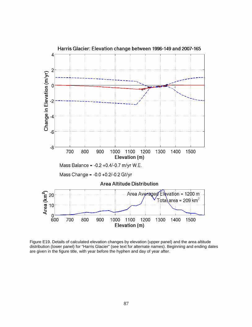
Figure E19. Details of calculated elevation changes by elevation (upper panel) and the area altitude distribution (lower panel) for “Harris Glacier” (see text for alternate names). Beginning and ending dates are given in the figure title, with year before the hyphen and day of year after.
87

Holgate Glacier 1994 – 2001: The elevation range of available data is limited to 600 to 1000 m elevation. While this covers most of the area of the glacier, it does miss the uppermost regions of Holgate. Elevation changes during this period for Holgate are slightly negative with values between ~ -0.2 to ~ -0.5 m/yr. The small negative change combined with the large areas of the glacier that remain unmeasured create significant uncertainty in the mass balance (-0.2 ± 0.4 m/yr w.e.). The small change in elevation and small size of the glacier lead to negligible mass change. 2001 – 2007: The distribution of data with respect to elevation is similar to that of the 1994 – 2001 comparison. However, the elevation changes are more negative than the previous period, creating a more negative mass balance (-0.96 ± 0.37 m/yr w.e.) and mass change (-0.08 ± 0.03 Gt/yr). 1994 – 2007: Data coverage is reasonable below 1100 m, but Holgate has significant area above 1100 m and so much of the elevation change is not sampled. For what is measured, we calculate a mass balance of -0.57 ± 0.30 m/yr w.e. and a mass change of -0.04 ± 0.02 Gt/yr.
88
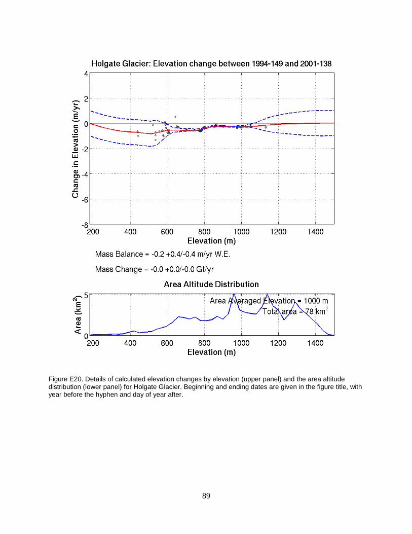
Figure E20. Details of calculated elevation changes by elevation (upper panel) and the area altitude distribution (lower panel) for Holgate Glacier. Beginning and ending dates are given in the figure title, with year before the hyphen and day of year after.
89

Figure E21. Details of calculated elevation changes by elevation (upper panel) and the area altitude distribution (lower panel) for Holgate Glacier. Beginning and ending dates are given in the figure title, with year before the hyphen and day of year after.
90
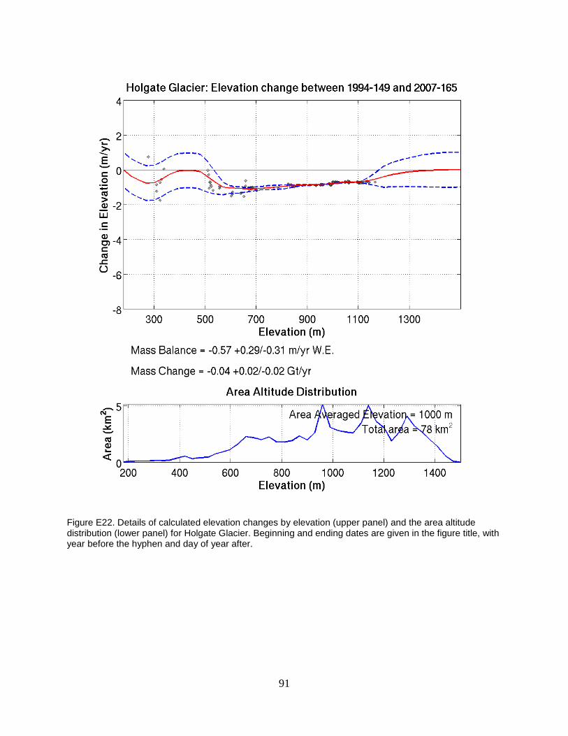
Figure E22. Details of calculated elevation changes by elevation (upper panel) and the area altitude distribution (lower panel) for Holgate Glacier. Beginning and ending dates are given in the figure title, with year before the hyphen and day of year after.
91

Kachemak Glacier 1996 – 2001: The flight paths of 1996 and 2001 only overlap in the bottom half of Kachemak Glacier, leaving the upper half unsampled. The lowest section of Kachemak shows elevation loss over this period with a maximum loss of ~ 2 m/yr at the toe and losses lessening to zero at 800 m. Above 800 m the elevation change is increasingly positive to ~ 0.8 m/yr at 1000 m, which is the upper limit of the available measurements. Based on the trends of other glaciers on the Harding Icefield during this period, it is likely that the increasingly positive elevation change continued into the unmeasured upper reaches of the glacier. Based on the available measurements, we see a slightly positive mass balance (0.2 ± 0.4 m/yr w.e.), but a negligible mass change (0.0 Gt/yr) due to the small size of Kachemak and only slight elevation change. 2001 – 2007: The available data are also limited during this period, but where coverage exists it shows significant negative changes in the surface elevation with typical values of -2 m/yr. The mass balance and mass change are both negative with values of -1.40 ± 0.50 m/yr w.e. and -0.03 ± 0.01 Gt/yr, respectively. 1996 – 2007: The elevation range covered in this period is similar to the two shorter measurement periods of Kachemak, but data is overall generally sparser within the covered elevation range. The estimated mass balance was negative (-0.67 ± 0.41 m/yr w.e.) during this time and the mass change was slightly negative, but essentially negligible over this period at -0.01 ± 0.01 Gt/yr.
92

Figure E23. Details of calculated elevation changes by elevation (upper panel) and the area altitude distribution (lower panel) for Kachemak Glacier. Beginning and ending dates are given in the figure title, with year before the hyphen and day of year after.
93

Figure E24. Details of calculated elevation changes by elevation (upper panel) and the area altitude distribution (lower panel) for Kachemak Glacier. Beginning and ending dates are given in the figure title, with year before the hyphen and day of year after.
94

Figure E25. Details of calculated elevation changes by elevation (upper panel) and the area altitude distribution (lower panel) for Kachemak Glacier. Beginning and ending dates are given in the figure title, with year before the hyphen and day of year after.
95

McCarty Glacier 1996 – 2001: The coverage of McCarty over this period is sufficient to provide a coherent picture of the elevation changes across the majority of the glacier. Elevation changes are generally positive above ~450 m elevation, with typical values of ~1 m/yr and ranging from zero to just under 2 m/yr. Below 450 m, the elevation changes are strongly negative reaching values as low as -6 m/yr, but relatively little area of the glacier is below this elevation range and so the mass balance overall remains positive, but with significant negative uncertainty (0.4 +0.3/-0.7 m/yr w.e.) and the mass change is negligible (0.0 ± 0.1 Gt/yr). 2001 – 2007: All of the measured elevations of McCarty show negative elevation changes over this period ranging from -1 m/yr at 1200 m elevation to -12 m/yr at the base of the glacier. The mass balance is negative (-1.25 +0.53/-1.01) and the mass change is also negative (-0.14 ± 0.11 Gt/yr). 1996 – 2007: Data coverage is similar for this decade compared to the two shorter periods contained within. The mass balance is negative (-0.5 +0.6/-0.4 m/yr w.e.) and the mass change is slightly negative (-0.06 ± 0.05 Gt/yr). However, uncertainties for both values are large due to the lack of coverage above ~1300 m.
96

Figure E26. Details of calculated elevation changes by elevation (upper panel) and the area altitude distribution (lower panel) for McCarty Glacier. Beginning and ending dates are given in the figure title, with year before the hyphen and day of year after.
97

Figure E27. Details of calculated elevation changes by elevation (upper panel) and the area altitude distribution (lower panel) for McCarty Glacier. Beginning and ending dates are given in the figure title, with year before the hyphen and day of year after.
98

Figure E28. Details of calculated elevation changes by elevation (upper panel) and the area altitude distribution (lower panel) for McCarty Glacier. Beginning and ending dates are given in the figure title, with year before the hyphen and day of year after.
99

Northwestern Glacier 1996 – 2001: Data are limited for Northwestern over this period, but do cover the elevation range with the largest areas of the glacier. Due to the poor coverage of this data, it is not intended for use beyond this progress report. However, even where there is coverage the data are relatively sparse and show significant spread beyond the 1 m/yr values that are typical between ~850 and 1100 m elevation. The calculated mass balance and mass change are likely not accurate. 2001 – 2007: Data are even sparser for Northwestern during this period than the previous measurement period. 1996 – 2007: Data coverage is extremely limited. The estimate mass balance and mass change are likely not accurate.
100

Figure E29. Details of calculated elevation changes by elevation (upper panel) and the area altitude distribution (lower panel) for Northwestern Glacier. Beginning and ending dates are given in the figure title, with year before the hyphen and day of year after.
101

Figure E30. Details of calculated elevation changes by elevation (upper panel) and the area altitude distribution (lower panel) for Northwestern Glacier. Beginning and ending dates are given in the figure title, with year before the hyphen and day of year after.
102

Figure E31. Details of calculated elevation changes by elevation (upper panel) and the area altitude distribution (lower panel) for Northwestern Glacier. Beginning and ending dates are given in the figure title, with year before the hyphen and day of year after.
103

Skilak Glacier 1994 – 2001: The data coverage for Skilak is quite good with fairly continuous coverage from 500m to 1200 m elevation and includes most of the area of the glacier. The elevation change is only slightly negative with values between zero and ~ 0.5 m/yr over most of the measured elevation range. The mass balance is slightly negative at -0.32 +0.13/-0.19 m/yr w.e. The mass change is also slightly negative at -0.04 ± 0.02 Gt/yr. 2001 – 2007: The data coverage remains strong for Skilak over this period. Elevation changes are relatively constant over the glacier, but have become more negative compared to those of 1994 – 2001 with values around -2 m/yr. The more negative changes in elevation cause more negative estimates of the mass balance (-1.19 +0.24/-0.26 m/yr w.e.) and mass change (-0.14 ± 0.03 Gt/yr). 1994 – 2007: Skilak shows fairly constant elevation change over these 13 years, similar to the sub-periods from 1994 – 2001 and 2001 – 2007. Elevation changed by ~ -1 m/yr for most of the measured elevations of the glacier. The mass balance is negative, -0.65 ± 0.26 m/yr w.e., and the mass change is also negative, -0.08 ± 0.03 Gt/yr.
104

Figure E32. Details of calculated elevation changes by elevation (upper panel) and the area altitude distribution (lower panel) for Skilak Glacier. Beginning and ending dates are given in the figure title, with year before the hyphen and day of year after.
105

Figure E33. Details of calculated elevation changes by elevation (upper panel) and the area altitude distribution (lower panel) for Skilak Glacier. Beginning and ending dates are given in the figure title, with year before the hyphen and day of year after.
106

Figure E34. Details of calculated elevation changes by elevation (upper panel) and the area altitude distribution (lower panel) for Skilak Glacier. Beginning and ending dates are given in the figure title, with year before the hyphen and day of year after.
107

Tustumena Glacier 1994 – 2001: The data coverage of Tustumena is likely the best of all the glaciers in the Harding Icefield with continuous and dense coverage from the base to the uppermost reaches of the glacier. Elevations changes are near zero above 1300 m, but are increasingly negative moving down the glacier from 1300 m with a maximum negative change of about -2 m/yr at the base of the glacier. The mass balance is negative, but not strongly so at -0.46 +0.18/-0.11 m/yr w.e., but the large size of the glacier (384 km2) leads to a noticeable negative mass change of -0.18 ± 0.04 Gt/yr. 2001 – 2007: The data coverage for this period is also quite strong, but does miss the uppermost reaches of Tustumena. However, based on the similar patterns of change for both the 1994 – 2001 and 2001 – 2007 periods, it is reasonable to assume that the model of the surface elevation change is relatively accurate where data coverage is absent. The elevation changes are more strongly negative compared to the 1994 – 2001 changes with negative changes observed for all measured elevations. The negative elevation change grows moving down the glacier from a value of ~ -1 m/yr at 1400 m elevation to ~ -4 m/yr at the base of the glacier (~200 m). The mass balance and mass change are both more negative over this period compared to the 1994 – 2001 comparison, with values of -1.34 ± 0.30 m/yr w.e. and -0.51 ± 0.12 Gt/yr, respectively. 1994 – 2007: Data coverage remains strong for the broader period from 1994 to 2007. The mass balance and change are averages of the two sub-periods at -0.86 ± 0.07 m/yr w.e. and -0.33 ± 0.03 Gt/yr, respectively.
108
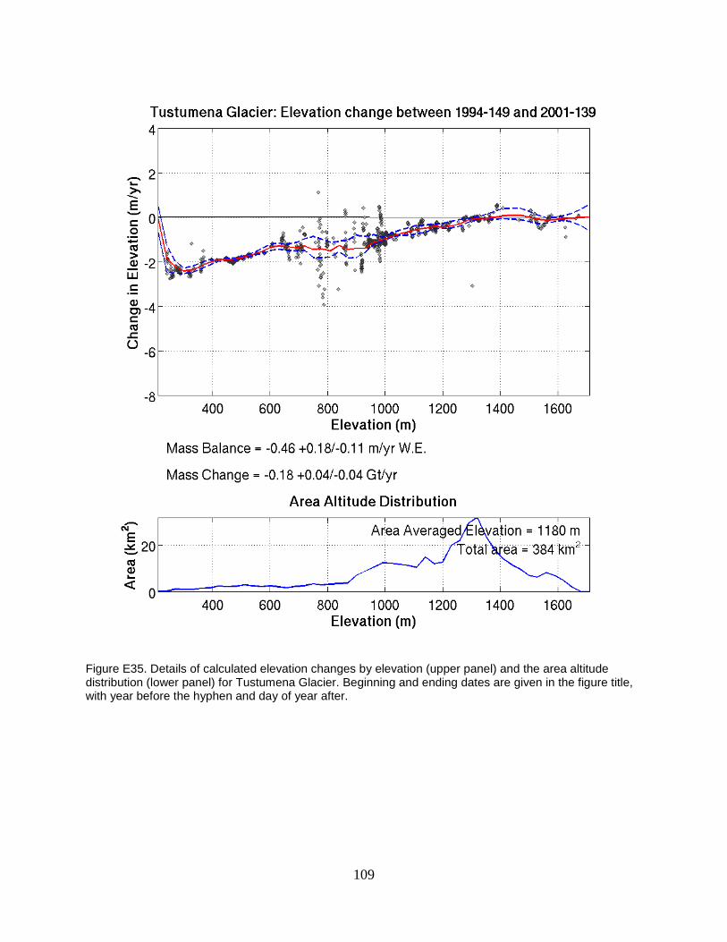
Figure E35. Details of calculated elevation changes by elevation (upper panel) and the area altitude distribution (lower panel) for Tustumena Glacier. Beginning and ending dates are given in the figure title, with year before the hyphen and day of year after.
109

Figure E36. Details of calculated elevation changes by elevation (upper panel) and the area altitude distribution (lower panel) for Tustumena Glacier. Beginning and ending dates are given in the figure title, with year before the hyphen and day of year after.
110

Figure E37. Details of calculated elevation changes by elevation (upper panel) and the area altitude distribution (lower panel) for Tustumena Glacier. Beginning and ending dates are given in the figure title, with year before the hyphen and day of year after.
111

Guyot Glacier 2007 – 2012: There is significant spread in the elevation change data for this period, but the dz data are consistent enough to provide a reasonable estimate of surface elevation changes. The glacier is not sampled above 1600 m and so a reasonable area of the glacier remains unsampled. The mass balance estimate is slightly positive, but essentially insignificant due to the large uncertainty (0.2 ± 0.6 m/yr w.e.) and the mass change is negligible.
112

Figure E38. Details of calculated elevation changes by elevation (upper panel) and the area altitude distribution (lower panel) for Guyot Glacier. Beginning and ending dates are given in the figure title, with year before the hyphen and day of year after.
113

Figure E39. Details of calculated elevation changes by elevation (upper panel) and the area altitude distribution (lower panel) for Guyot Glacier. Beginning and ending dates are given in the figure title, with year before the hyphen and day of year after.
114

Figure E40. Details of calculated elevation changes by elevation (upper panel) and the area altitude distribution (lower panel) for Guyot Glacier. Beginning and ending dates are given in the figure title, with year before the hyphen and day of year after.
115

Hubbard Glacier 2001 – 2007: The glacier is unsampled above ~2200 m and dz values show significant spreading below this elevation. This leads to large uncertainties in the mass balance (0.1 +0.4/-0.3 m/yr w.e.) and mass change (0.2 ± 0.8 Gt/yr). 2007 – 2012: Despite the inclusion of the LiDAR system, the results are relatively similar to those of 2001 – 2007 with large uncertainties in the mass balance (0.1 +0.4/-0.7 m/yr w.e.) and mass change (0.3 ± 1.8 Gt/yr).
116
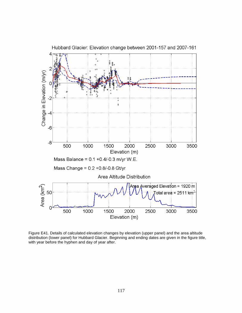
Figure E41. Details of calculated elevation changes by elevation (upper panel) and the area altitude distribution (lower panel) for Hubbard Glacier. Beginning and ending dates are given in the figure title, with year before the hyphen and day of year after.
117
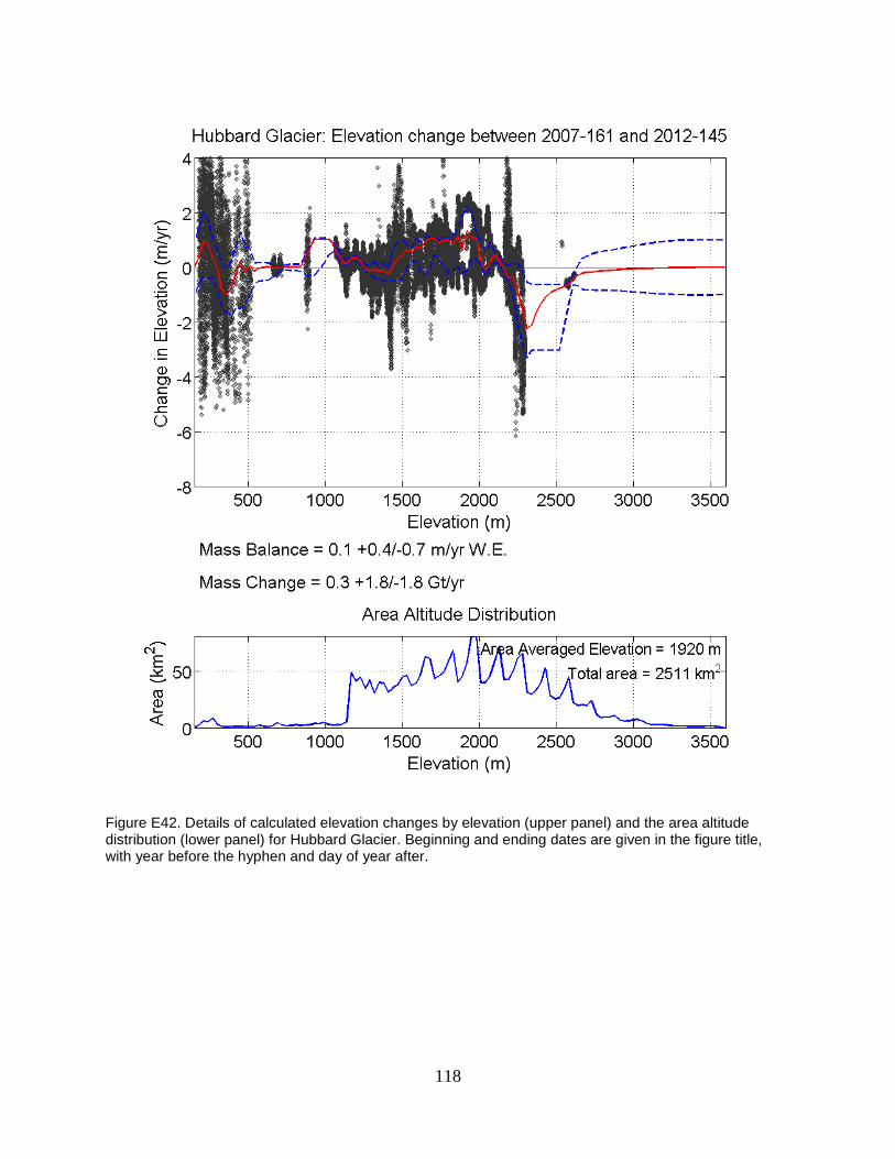
Figure E42. Details of calculated elevation changes by elevation (upper panel) and the area altitude distribution (lower panel) for Hubbard Glacier. Beginning and ending dates are given in the figure title, with year before the hyphen and day of year after.
118
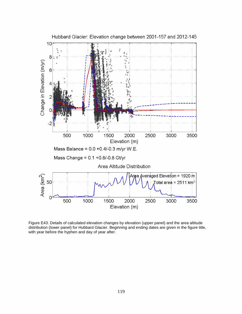
Figure E43. Details of calculated elevation changes by elevation (upper panel) and the area altitude distribution (lower panel) for Hubbard Glacier. Beginning and ending dates are given in the figure title, with year before the hyphen and day of year after.
119

Kennicott Glacier 2000 – 2007: No comparison points exist above ~2500 m elevation, which excludes about 30% of the glacier. Coverage below 2500 m is reasonable and shows elevation losses ranging from -3 m at the toe to near zero at 2500 m. The mass balance is negative, but with large uncertainties (-0.4 ± 0.5 m/yr w.e.). The mass change is negligible.
120

Figure E44. Details of calculated elevation changes by elevation (upper panel) and the area altitude distribution (lower panel) for Kennicott Glacier. Beginning and ending dates are given in the figure title, with year before the hyphen and day of year after.
121

Nabesna Glacier 2000 – 2007: Data coverage is quite good for Nabesna over this period. There is relatively little area above the upper limit of the data at 2600 m. Nabesna showed decreasing surface elevation over this period with values ranging from about -2 m/yr at the toe to zero at 2500 m. The mass balance and change are both negative with values of -0.42 ± 0.24 m/yr w.e. and -0.42 ± 0.23 Gt/yr, respectively.
122

Figure E45. Details of calculated elevation changes by elevation (upper panel) and the area altitude distribution (lower panel) for Nabesna Glacier. Beginning and ending dates are given in the figure title, with year before the hyphen and day of year after.
123

Yahtse Glacier There are multiple periods of measurement for Yahtse Glacier. We summarize the periods together since the trends and data quality are relatively consistent throughout all measurement periods. From 2006 to 2012, Yahtse consistently shows increases in surface elevation and positive mass balances. From 2006 – 2012 the mass balance was positive (0.2 +0.2/-0.1 m/yr w.e.) with mass balance increasing through the measured years with the highest value of 1.17 +0.37/-0.32 m/yr w.e. from 2010 to 2012. Similarly, the mass changes are consistently positive throughout the measurement periods with an overall value of 0.12 ± 0.10 Gt/yr from 2006 to 2012 and the highest value (0.90 ± 0.24 Gt/yr) observed from 2010 to 2012.
124
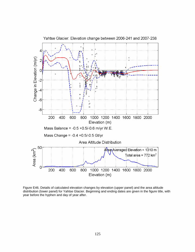
Figure E46. Details of calculated elevation changes by elevation (upper panel) and the area altitude distribution (lower panel) for Yahtse Glacier. Beginning and ending dates are given in the figure title, with year before the hyphen and day of year after.
125

Figure E47. Details of calculated elevation changes by elevation (upper panel) and the area altitude distribution (lower panel) for Yahtse Glacier. Beginning and ending dates are given in the figure title, with year before the hyphen and day of year after.
126
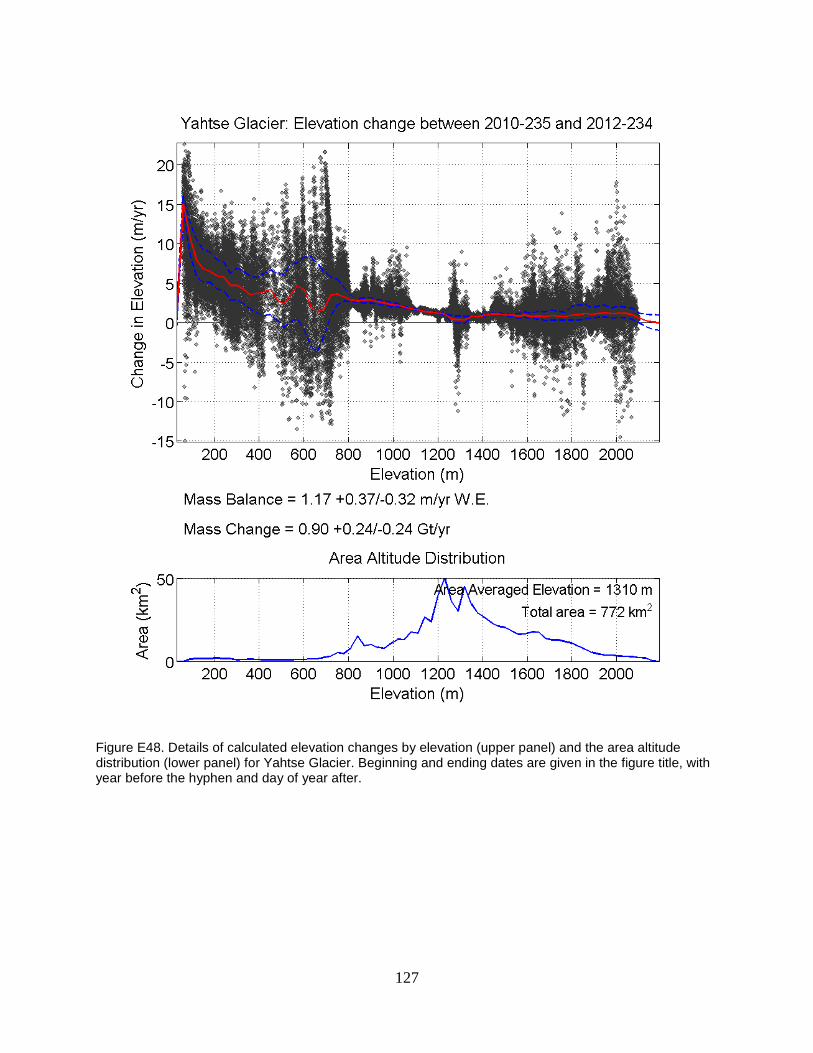
Figure E48. Details of calculated elevation changes by elevation (upper panel) and the area altitude distribution (lower panel) for Yahtse Glacier. Beginning and ending dates are given in the figure title, with year before the hyphen and day of year after.
127

Figure E49. Details of calculated elevation changes by elevation (upper panel) and the area altitude distribution (lower panel) for Yahtse Glacier. Beginning and ending dates are given in the figure title, with year before the hyphen and day of year after.
128

The Department of the Interior protects and manages the nation’s natural resources and cultural heritage; provides scientific and other information about those resources; and honors its special responsibilities to American Indians, Alaska Natives, and affiliated Island Communities. NPS 953/123451, January 2014

National Park Service U.S. Department of the Interior
Natural Resource Stewardship and Science 1201 Oakridge Drive, Suite 150 Fort Collins, CO 80525 www.nature.nps.gov
EXPERIENCE YOUR AMERICA TM