fpga implementation of graph cut method …etd.lib.metu.edu.tr/upload/12612556/index.pdf · fpga...
TRANSCRIPT

FPGA IMPLEMENTATION OF GRAPH CUT METHOD FOR REAL TIME STEREO MATCHING
A THESIS SUBMITTED TO THE GRADUATE SCHOOL OF NATURAL AND APPLIED SCIENCES
OF MIDDLE EAST TECHNICAL UNIVERSITY
BY
HAVVA SAĞLIK ÖZSARAÇ
IN PARTIAL FULFILLMENT OF THE REQUIREMENTS FOR
THE DEGREE OF MASTER OF SCIENCE IN
ELECTRICAL AND ELECTRONICS ENGINEERING
SEPTEMBER 2010

Approval of the thesis:
FPGA IMPLEMENTATION OF GRAPH CUT METHOD FOR REAL TIME STEREO MATCHING
submitted by HAVVA SAĞLIK ÖZSARAÇ in partial fulfillment of the requirements for the degree of Master of Science in Electrical and Electronics Engineering Department, Middle East Technical University by,
Prof. Dr. Canan ÖZGEN ________________ Dean, Graduate School of Natural and Applied Sciences
Prof. Dr. İsmet ERKMEN ________________ Head of Department, Electrical and Electronics Engineering
Prof. Dr. Zafer ÜNVER ________________ Supervisor, Electrical and Electronics Eng. Dept., METU Assist. Prof. Dr. İlkay ULUSOY ________________ Co-Supervisor, Electrical and Electronics Eng. Dept., METU
Examining Committee Members:
Prof. Dr. Gözde BOZDAĞI AKAR ________________ Electrical and Electronics Engineering Dept., METU
Prof. Dr. Zafer ÜNVER ________________ Electrical and Electronics Engineering Dept., METU
Assist. Prof. Dr. İlkay ULUSOY ________________ Electrical and Electronics Engineering Dept., METU
Assoc. Prof. Dr. Tolga ÇİLOĞLU ________________ Electrical and Electronics Engineering Dept., METU Enes ERDİN M.Sc. ________________ Digital Electronic Design Group, TÜBİTAK-SAGE
Date: September 15, 2010

iii
I hereby declare that all information in this document has been obtained and presented in accordance with academic rules and ethical conduct. I also declare that, as required by these rules and conduct, I have fully cited and referenced all material and results that are not original to this work.
Name, Last Name : Havva SAĞLIK ÖZSARAÇ
Signature :

iv
ABSTRACT
FPGA IMPLEMENTATION OF GRAPH CUT METHOD
FOR REAL TIME STEREO MATCHING
Sağlık Özsaraç, Havva
M.S., Department of Electrical and Electronics Engineering
Supervisor : Prof. Dr. Zafer Ünver
Co-supervisor : Assist. Prof. Dr. İlkay Ulusoy
September 2010, 74 pages
The present graph cut methods cannot be used directly for real time stereo matching
applications because of their recursive structure. Graph cut method is modified to
change its recursive structure so that making it suitable for real time FPGA (Field
Programmable Gate Array) implementation.
The modified method is firstly tested by MATLAB on several data sets, and the
results are compared with those of previous studies. Although the disparity results
of the modified method are not better than other methods’, computation time
performance is better. Secondly, the FPGA simulation is performed using real data
sets. Finally, the modified method is implemented in FPGA with two PAL cameras
at 25 Hz. The computation time of the implementation is 40 ms which is suitable for
real time applications.
Keywords: Real Time Stereo Matching, Graph Cut, FPGA

v
ÖZ
GERÇEK ZAMANLI STEREO EŞLEME İÇİN
ÇİZGE KESME YÖNTEMİNİN FPGA UYGULAMASI
Sağlık Özsaraç, Havva
Yüksek Lisans, Elektrik ve Elektronik Mühendisliği Bölümü
Tez Yöneticisi : Prof. Dr. Zafer Ünver
Ortak Tez Yöneticisi : Yrd. Doç. Dr. İlkay Ulusoy
Eylül 2010, 74 sayfa
Günümüz çizge kesme yöntemleri özyinelemeli bir yapıya sahip olduğundan
doğrudan gerçek zamanlı stereo eşleme uygulamalarında kullanılamazlar. Çizge
kesme yönteminin özyineli yapısı, gerçek zamanlı FPGA(Alan Programlanabilir
Kapı Dizisi) uygulamasına uygun olabilmesi için değiştirilmi ştir.
Değiştirilen çizge kesme yöntemi, önce MATLAB ile çeşitli veri kümeleri üzerinde
test edilmiş ve sonuçlar önceki çalışmalar ile karşılaştırılmıştır. Önerilen metodun
derinlik sonuçları diğer yöntemlerinkinden iyi olmamasına rağmen hesaplama
zaman performansı daha yüksektir. Doğru sonuçlar elde edildikten sonra FPGA
benzetimi gerçek veri kümeleri ile gerçekleştirilmi ştir. Son olarak, bu yeni yöntem
2 adet 25 Hz PAL kamera ile FPGA üzerinde gerçeklenmiştir. Uygulamanın
hesaplama zamanı gerçek zamanlı uygulamalar için uygun olan 40 ms’dir.
Anahtar Kelimeler: Gerçek Zamanlı Stereo Eşleme, Çizge Kesme, FPGA (Alan
Programlanabilir Kapı Dizisi)

vi
To My Husband,
To My Family…

vii
ACKNOWLEDGEMENTS
Firstly, I would like to express my sincere thanks to my supervisors Prof. Dr. Zafer
ÜNVER and Assist. Prof. Dr. İlkay ULUSOY, for their supports, friendly attitude
and encouragement at each stage of this thesis study.
I would like to thank to TÜBİTAK-SAGE (The Scientific and Technological
Research Council of Turkey – Defense Industries Research and Development
Institute) for the support given throughout this study.
I would like to forward my appreciation to all colleagues for their continuous
encouragement.
I would like to present my thanks to Örsan AYTEKİN for sharing his knowledge.
I would like to thanks to my parents, Yılmaz SAĞLIK and Hadiye SAĞLIK and my
sister Hale SAĞLIK for their support and unlimited love.
Lastly, special thanks to my husband, İsmail ÖZSARAÇ for all his support,
guidance, sharing his knowledge and help in implementation and for showing great
patience during my thesis.

viii
TABLE OF CONTENTS
ABSTRACT .............................................................................................................. iv
ÖZ...............................................................................................................................v
ACKNOWLEDGEMENTS ..................................................................................... vii
TABLE OF CONTENTS ........................................................................................ viii
LIST OF TABLES ..................................................................................................... x
LIST OF FIGURES .................................................................................................. xi
CHAPTERS
1. INTRODUCTION ................................................................................................. 1
1.1 Definition of the Stereo Matching Problem ..................................................... 1
1.2 Stereo Matching Methods ................................................................................ 3
1.3 Stereo Matching by Graph Cut Method ........................................................... 5
1.4 Objective of the Thesis..................................................................................... 6
1.5 Organization of the Thesis ............................................................................... 7
2. GRAPH CUT THEORY IN STEREO MATCHING ............................................ 8
2.1 Graph Construction in Stereo Matching Applications ..................................... 8
2.2 Minimum Cut Calculation Methods............................................................... 13

ix
2.3 Modified Graph Cut Method .......................................................................... 14
2.3.1 Basic Stereo Energy Calculation ............................................................... 15
2.3.2 Modified Minimum Energy Calculation Method ..................................... 17
3. IMPLEMENTATION OF THE NEW METHOD ............................................... 20
3.1 Computer Based Implementation in MATLAB ............................................. 20
3.2 Real Time Implementation in FPGA ............................................................. 24
3.2.1 The Hardware Description ........................................................................ 24
3.2.2 Real Time Implementation ........................................................................ 25
4. SIMULATION AND IMPLEMENTATION RESULTS .................................... 39
4.1 MATLAB Implementation Results ................................................................ 41
4.2 FPGA Implementation Results ...................................................................... 47
4.2.1 Simulation Results .................................................................................... 47
4.2.2 Hardware Results ...................................................................................... 50
5. CONCLUSIONS AND FUTURE WORK .......................................................... 57
5.1 Conclusions .................................................................................................... 57
5.2 Future Work ................................................................................................... 59
REFERENCES ......................................................................................................... 61
APPENDICES
A. GRAPH CUT METHODS................................................................................65
x
LIST OF TABLES
TABLES
Table 1: Comparisons of the previous stereo matching methods and proposed
method for Tsukuba image pairs. ............................................................................. 47
Table 2: FPGA resource utilization ......................................................................... 50
Table 3: The performance comparison of previous real time studies and proposed
method. ..................................................................................................................... 51
Table 4: Augmented path algorithm ........................................................................ 67
Table 5: Push-Relabel Algorithm ............................................................................ 70
Table 6: βα − swap algorithm ............................................................................... 73
Table 7: α-expansion algorithm ............................................................................... 74

xi
LIST OF FIGURES
FIGURES
Figure 1: The parallel camera localization [11]. ........................................................ 2
Figure 2: 2D stereo camera localization..................................................................... 3
Figure 3: Stereo matching graph (R is the maximum disparity range). ..................... 9
Figure 4: The matching pixel P(x, y) and its neighbor pixels. ................................. 11
Figure 5: The functional graph of neighborhood interaction function [3]. .............. 11
Figure 6: The functional graph of multiplying term [3]. .......................................... 12
Figure 7: Implementation of the modified graph cut method. ................................. 14
Figure 8: Matching pixel P(x,y) and its neighbors. .................................................. 15
Figure 9: The structure for matching energy calculation. ........................................ 16
Figure 10: Cut on the constructed graph. ................................................................. 18
Figure 11: The flow chart of proposed minimum cut calculation method. .............. 19
Figure 12: The block diagram of Computer Based Implementation........................ 21
Figure 13: The block diagram of Basic Energy Calculation Module. ..................... 22
Figure 14: The block diagram of Graph Cut Implementation Module. ................... 23
Figure 15: Hardware structure. ................................................................................ 25

xii
Figure 16 : The general structure of the FPGA blocks. ........................................... 26
Figure 17: The detailed structure of Stereo Matching Block. .................................. 28
Figure 18: Frame timing signals. ............................................................................. 28
Figure 19: Basic Energy Calculation Block. ............................................................ 29
Figure 20: Sub-Pixel Intensity Calculation Block. .................................................. 30
Figure 21: Usage of sub-pixel buffers. ..................................................................... 30
Figure 22: Cost Energy Calculation Block. ............................................................. 31
Figure 23: Edata Calculation Block. ........................................................................ 32
Figure 24 : The Comparison Block. ......................................................................... 33
Figure 25: The Structure of Graph Cut Implementation Block. .............................. 34
Figure 26: The structure of GC Main Controller Block. .......................................... 35
Figure 27: The structure of Smooth1 Energy Calculation Block. ............................ 35
Figure 28: The structure of Smooth2 Energy Calculation Block ............................. 36
Figure 29: The structure of Smooth3 Energy Calculation Block. ............................ 37
Figure 30: The structure of GC Cost Calculation Block. ......................................... 38
Figure 31: The structure of Comparison Block........................................................ 38
Figure 32: Middlebury data pairs and their ground truths ...................................... 40
Figure 33: The Middlebury comparison regions. .................................................... 41
Figure 34: The effect of umax values on disparity errors. ......................................... 43
xiii
Figure 35: Basic energy calculation module minimum matching energy disparity
results . ..................................................................................................................... 43
Figure 36: Extensions at object boundaries by increasing umax values on Tsukuba
image. ....................................................................................................................... 44
Figure 37: Disparity results of proposed method for different umax values. ............. 45
Figure 38: Evaluated disparity results using Middlebury stereo pairs. .................... 46
Figure 39: The simulation environment ................................................................... 48
Figure 40: Simulation screens of the control signals. .............................................. 48
Figure 41: A part of the simulation screen of the design. ........................................ 49
Figure 42: Comparison of MATLAB and VHDL simulation results on Tsukuba
image. ....................................................................................................................... 49
Figure 43: FPGA design environment. .................................................................... 51
Figure 44: The real time FPGA implementation results. ......................................... 53
Figure 45: The signal tap screen of the design. ........................................................ 55
Figure 46: The distorted image. ............................................................................... 56
Figure 47: The example of minimum cut on residual graph. ................................... 68
Figure 48: Gαβ structure. ........................................................................................... 71
Figure 49: The possible cuts on constructed Gαβ for pixels p and q. ....................... 72
Figure 50: Constructed graph for α-expansion. ....................................................... 74

1
CHAPTER 1
INTRODUCTION
Stereo analysis is an important topic in computer vision due to its usage in many
areas like 3D vision, 3D reconstruction, 3D object detection and robotic
applications such as navigation, path planning, mapping and localization [9, 10]. In
stereo analysis multiple cameras can be used to calculate 3D information. However,
in most of the applications, only two cameras are used which provide the right and
left images that can be used to simulate the human vision system.
The main problem of stereo analysis is stereo matching which can be stated as
finding corresponding pixels on the right and left images. The stereo matching
problem is defined in Section 1.1. Section 1.2 and 1.3 explain the stereo matching
methods. The objective of the thesis study is given in Section 1.4, and the
organization of the thesis is provided in Section 1.5.
1.1 Definition of the Stereo Matching Problem
The stereo matching problem can be defined as finding depth information of the
objects in the image. In the solution process, the right and left images are captured
by using specially localized cameras. Then the depths are calculated according to
some pixel intensity similarities and constraints.
Consider the cameras and an object shown in Figure 1.

2
Figure 1: The parallel camera localization [11].
b is the baseline between the two cameras, and the focal length of the cameras is
denoted by fc. (XL, YL, ZL ) and (XR, YR, ZR ) are the coordinate systems for the left
and right cameras, respectively. PL is the projection of this object onto the left
camera and PR is the projection onto the right camera. PL and PR are located on the
epipolar line which may have different vertical coordinates on the left and right
images; however, the camera locations can be arranged to make the epipolar line
have the same vertical coordinate on both images [11].
Disparity is the absolute horizontal coordinate difference between the
corresponding pixels (PL, PR) on the left and right images. The disparity of object
P(x,y,z) is defined as (xL-xR). In stereo matching, the main goal is to calculate
disparity values of the pixels in an image.
The camera localization shown in Figure 2 is used to derive the depth calculation
formula.

3
Figure 2: 2D stereo camera localization.
Since x
z
x
f
L
c = and bx
z
x
f
R
c
−= , the depth, z, of the object P(x,y,z) follows as
RL
c
xx
bfz
−= * (1-1)
In equation (1-1), the disparity (xL-xR) is inversely proportional with the depth of the
object. Since the focal length, fc, of the cameras and the distance, b, between the
cameras are given, the disparity is the only unknown value for the depth calculation.
There are different stereo matching methods to calculate disparity of the pixels on
the image. Section 1.2 gives the main features of these methods.
1.2 Stereo Matching Methods
Stereo matching algorithms can be put into three groups [12]: pixel-based, region-
based and feature-based. These algorithms have different approaches to calculate
the disparity information.

4
In pixel-based methods [13], the correlation data of the pixels on the right and left
images is used to compute disparity. Since pixel-based algorithms use all pixels in
the image, they can produce dense disparity maps. These algorithms can be
examined under two subtitles: local methods and global methods.
Local pixel-based methods try to calculate the disparity values by comparing the
pixel intensities in a finite window whose size can vary according to the approach
of the algorithm. A reference window on the right or the left image is selected and
every pixel in this window is compared with every pixel in the other image window.
The total difference of the compared pixels is used to calculate the matching cost by
different techniques: Squared Intensity Differences (SD) [14, 15], Absolute
Intensity Differences (AD), and Sum of Absolute Differences (SAD) [12].
Global pixel-based methods differ from the local methods in terms of matching cost
calculation. Local methods are not interested in finding the minimum matching cost
for the whole image. Since global methods try to reach the minimum matching cost
by using some optimization techniques, they give better results than local matching
algorithms [22]. Dynamic-Programming [16], Belief Propagation [17], and Graph
Cut [1, 2, 3, 7] methods are the most studied global pixel-based methods.
Region-based stereo matching methods [18] calculate the disparity by using the
regions on the right and left images. Firstly, the images are divided into sub regions
by using some segmentation techniques, and these regions are compared. According
to the comparison results, the disparity value of the pixels in the same region is
determined. Therefore, region-based algorithms generate dense disparity maps like
pixel-based method.
Feature-based stereo matching methods use some specific information in the images
like edges and corners. Firstly, some feature detection algorithms [19, 20, 21] are
used to find the special features in the images, and then a matching process is
applied to find the same features in both images. Since the matching process is used

5
only for the pixels which have special features, only these pixels are assigned to
disparity values. Therefore, feature-based methods produce sparse disparity maps.
1.3 Stereo Matching by Graph Cut Method
In robotic applications, many different tasks like camera calibration, video
correction, video stabilization, 3D analysis, path planning and communication
should be done sequentially in a certain amount of time. Since total implementation
time is limited, each task has a very strict time constraint.
Stereo matching is the first step of 3D analysis, and it should also be completed in a
certain amount of time. For a real time PAL standard video, this duration is around
40 ms. Recall that human visual system can detect latencies greater than 150 ms
[23]. Therefore, if the stereo matching processing time increases, there can be
discontinuities between the following frames. This can result wrong decisions and
actions in the robot control system.
Recent studies show that in stereo matching, graph cut method (GC) has a good
performance when compared with other algorithms [22]. Even though, GC is not
suitable for real time applications, because of its iterative structure, which will be
explained in Appendices, there are new studies to implement this algorithm in real
time; but the results do not satisfy the real time constraints yet [24, 3, 25].
Kolmogorov and Zabih implement α-expansion move method in [24]. They applied
their method to 384x288 size Tsukuba image. The image is processed by 450 MHz
Ultra SPARC II processor. Disparity range is 16 for the selected image, and the
calculation time is 69 seconds. This shows that for a 384x288 size image, 1,769,472
disparities can be checked within 69 seconds. Disparity estimation results are good,
but their method can not be used in real time applications because of the limitations

6
given in [23]. {The α-expansion move method will be explained in detail in
Appendices.}
Zureiki, Devy and Chatila implement reduce graph method to decrease the
calculation time [3]. They reduce the total number of possible disparities by using a
stereo matching method like SAD, construct a graph using these disparity values
and use the push-relabel method. They applied the method to image sets having the
resolutions of 434x380 and 217x190. The disparities are calculated by 3 GHz
Pentium4 processor with 512 MB of RAM. The complete graph approach for
434x380 size images can not be implemented because of memory explosion, while
the reduced graph method calculates the disparities in 15-50 seconds. For 217x190
images, the complete graph approach takes 150 seconds, while the reduced graph
method takes 4 seconds for 4 disparity range and 5 seconds for 5 disparity range.
This shows that for a 217x190 size image, 164,920 disparities can be checked
within 4 seconds. However, they have not succeeded to run the algorithm in real
time yet. {The push-relabel method will be explained in Appendices.}
Vineet and Narayanan implement the push-relabel algorithm on the Nvidia GTX
280 Graphic Processing Unit (GPU) [25]. The real time implementation is possible
only if 2 disparities are looked for. For example the calculation time of a 640x480
size image with 2 disparities is 30-40 ms. This shows that for this image 614,400
disparities can be checked within 30-40 ms. The time performance is the best
among the recent studies; but since only 2 disparities are used, the implementation
is close to image segmentation rather than stereo matching.
1.4 Objective of the Thesis
Since the graph cut algorithm in stereo matching can not be implemented in real
time yet, a modified graph cut method is suggested in this thesis study to decrease
the calculation time. General purpose computer (C and MATLAB) and special

7
purpose hardware (GPU) are used in previous studies. Even though GPU
performance is better than that of general purpose computers, it can not be used for
parallel processing applications to increase speed performance. In this thesis, FPGA
is chosen due to its parallel processing capability which is the basic difference
between the FPGAs and GPUs. Also ASICs can be used for parallel processing
applications, but they can not be reconfigured. On the contrary, FPGAs can be
reconfigured easily for the updates in algorithms. The detailed information about
the hardware structure will be explained in Section 0.
The proposed method can complete stereo analysis of 576x768 size images with 80
disparity range in 40 ms in an Altera Cyclone III FPGA. This shows that
35,389,440 disparities can be checked within 40 ms. The right and left videos are
captured by 2 PAL cameras and processed in FPGA, and the result of the algorithm
is displayed on DVI monitor. These steps can be done in real time.
The disparity estimation results of the modified method is not better than the graph
cut implementations of previous studies; but the calculation time is much better
even for 80 disparity range. The disparity results of the modified graph cut method
are compared with the previous studies’ listed in [22]. The results are worse than
that of the best resultant graph cut stereo matching method [24]; however, the time
performance of the modified method is about thousand times faster. These
comparisons will be given in Section 4.2.2 in detail.
1.5 Organization of the Thesis
Chapter 2 is devoted to the theory behind the graph cut method in stereo matching
and the modified graph cut method which is implemented in this thesis. Chapter 3
includes the details of implementation of the modified graph cut method. Chapter 4
discusses the results and performance comparisons of the implementation. The
conclusions and possible future work are presented in Chapter 5.

8
CHAPTER 2
2 GRAPH CUT THEORY IN STEREO MATCHING
Graph cut method (GC) is used in different image processing applications such as
segmentation and stereo matching. The common property of these applications is
their requirement for energy minimization.
In stereo matching, GC, a pixel-based global method, is used to calculate minimum
matching cost energy. Minimum cost calculation is done by different methods in
GC. Since these methods are not suitable for real time applications, a modified
method is proposed which has a non-recursive structure.
In the following, first the construction of a graph for stereo matching is given. Then,
existent GC methods will be presented. Finally, the modified graph cut method
which is implemented in this study is discussed.
2.1 Graph Construction in Stereo Matching Applications
A graph is composed of vertices which are connected by edges. Row-column
structure is used to construct a stereo matching graph as shown in Figure 3. There is
a row of edges for every pixel on an image line and a column of edges for each
disparity value. Vertices are located at graph row-column intersection points, and
they represent the possible disparity values. In addition to vertices on graph rows,
two special vertices are added: s and t. The source vertex, s, is located at the
beginning side of the graph, and the sink vertex, t, is located at the end side of the
graph.

9
There are two types of edges between the vertices: t-links and n-links. t-links
connect the neighbor vertices on the same graph row, and these links represent the
matching cost energy for the related disparity value. n-links connect the neighbor
vertices at different graph rows, and they hold the smoothness energies between the
connected vertices (disparities). Matching cost energy and smoothness energy will
be explained in detail in the following sections.
Figure 3: Stereo matching graph (R is the maximum disparity range).
In Figure 3, tx(d) represents a t-link where x shows the horizontal coordinate of the
pixel on the image line and d shows the disparity value. n(x1,x2)(D1,D2) represents an
n-link where x1 and x2 show the horizontal coordinates of upper and lower pixels,
respectively, D1 is the disparity value of x1 at vertex dk and D2 is the disparity value
of x2 at vertex dk-1.

10
There are two main types of energies in global stereo matching applications:
matching cost and smoothness. The energy structure is a function of the assigned
disparity values or labels denoted by f. The energy functions Edata(f) and Esmooth(f)
represent the matching cost and the smoothness energies, respectively. In stereo
matching, the goal is to find optimum labels , f, to minimize the total energy E (f)
which is the sum of Edata(f) and Esmooth(f) .
Edata(f) is related with the pixel intensity values. The square of the intensity
difference between the matching pixel on the left image and the corresponding pixel
on the right image is used to calculate Edata(f). This calculation is done for all
possible disparity values in the disparity range.
∑∈
=Pp
ppdata fDfE )()(
Dp(fp) = ( Il(p) - Ir(q) )2 where fp=xp-xq (2-1)
In the above expression, P is the compared pixel set on the right and left images, p
is the matching pixel in the left image, and q is the corresponding pixel in the right
image. I l(p) and Ir(q) are the intensities of pixels p and q, respectively. fp is the
label(disparity) value of the pixel p; xp and xq are the horizontal coordinates of the
pixels p and q, respectively.
Esmooth(f) is related with the labeling of the matching pixel and its neighbors. Three
neighbors are considered for Esmooth(f) calculation. The matching pixel located at
(x,y) and its neighbors are shown in Figure 4.
Esmooth(f) is calculated according to the smoothness constraint which states that the
disparity values of the pixels in the same object region should be the same, while
the disparity values of the pixels at the boundaries should be different. The pixels
which are in the same region have similar intensity values, but at the boundaries

11
pixels have different intensity values. Therefore, Esmooth(f) has two components:
intensity and labeling.
Figure 4: The matching pixel P(x, y) and its neighbor pixels.
{ }{ }∑
∈
∗=Nqp
qpqpsmooth ffVufE,
, ),()( (2-2)
In equation (2-2), N is the neighbor pixel set and V(fp,fq) is the neighborhood
interaction function [3] which checks the neighbor pixels for the assigned labels. If
p and q have different labels, this function gives high penalties. V(fp,fq) is equal to
the absolute difference of the neighbor pixels’ labels (disparity values):
V(fp,fq) = |fp-fq|. fp and fq are the assigned labels to the matching pixel and its
neighbor pixel, respectively. The functional graph of neighborhood interaction
function is shown in Figure 5.
),( qp ffV
|| qp ff −0
Figure 5: The functional graph of neighborhood interaction function [3].

12
If the neighbor pixels are in the same region, the neighborhood interaction function
prevents to assign different labels to these pixels. This is the necessary check for
proper labeling in the same region. The neighbor pixels should have different labels
at the boundaries; and the multiplying term u{p,q} is used to correct the
neighborhood interaction function error for these pixels. The multiplying term is a
decreasing function with increasing intensity difference:
u{p,q} = umax * (1- |I1-I2| / 255). umax value is the controllable variable which is
determined after the functional tests. I1 and I2 are the intensity values of the
neighbor pixels. At the boundaries, if the difference between the intensity values of
the neighboring pixels goes to 255 (the upper boundary of the intensity values for 8
bit representation), this term goes to zero. Since the neighborhood interaction
function gives high penalties at the boundaries, the multiplying term gives lower
values and balances the smoothness energy. The functional graph of the
multiplying term is shown in Figure 6.
{ }qpu ,
|| qp II −
maxu
Figure 6: The functional graph of multiplying term [3].
After the construction of the graph, the minimum energy can be computed by the
cut calculation. Cut can be defined as the collection of edges which hold the
matching cost energies (t-links) or the smoothness energies (n-links). It is assumed
that the minimum cut has the minimum total energy. There are two different
methods for computing the minimum cut: maximum flow and swap method. These

13
methods are given in Section 2.2. The modified graph cut method which is
implemented in this study is described in Section 2.3.
2.2 Minimum Cut Calculation Methods
The main aim is to find the minimum energy value on the constructed graph. There
are different methods in previous studies for minimum cut calculation. These
methods search the minimum energy among all possible disparity combinations, so
they require a recursive structure.
In these methods, energy value is calculated for a disparity combination, then
another energy value for a different combination is obtained. If the new energy
value is smaller than the previous one, new disparity combination is assigned to
pixels. These steps are done for all possible disparity combinations in the
determined range.
Maximum flow method assumes the graph as a water pipe net which lets the
maximum amount of water flow from the source to the sink. In a pipe net, the
maximum flow amount is determined by the narrowest pipes. The pipes represent
the links of the graph. Therefore, the cost values of the pipes are the energy values
and the narrowest ones hold the minimum energy. Since minimum energy
represents the minimum cut, maximum flow amount is equal to the minimum cut of
the graph.
Swap methods check possible disparity combinations for the neighbor pixels
recursively. They assign different labels (disparities) to the pixels and compare the
resultant energy values with the previous ones. According to the comparisons of the
resultant energy values, swap methods determine the final labeling. The methods
are explained in detail in Appendices.

14
In the proposed method, the main goal is to change the structure of the standard
graph cut method to non-recursive for real time applications. The minimum energy
of the matching pixel is calculated and added previously calculated pixels energy
value so the minimum energy is not calculated repeatedly for all possible
disparities. All possible disparities are contributed to each pixel’s energy value
calculations not whole minimum energy calculation in the constructed graph. In the
following section the modified minimum cut calculation method will be explained.
2.3 Modified Graph Cut Method
Graph cut methods can generate accurate disparity maps but recursive calculations
are necessary to find the minimum matching cost energy to determine the correct
disparity values. Because of their recursive structure, their calculation time is too
long to be used in real time applications, e.g., a robot control system. The modified
graph cut method is proposed to reduce the calculation time.
The proposed method is implemented by two main functional blocks shown in
Figure 7.
Figure 7: Implementation of the modified graph cut method.
The basic stereo energy calculation block computes the stereo matching energies by
using a local method which uses linearly interpolated pixels [7]. It sends the
calculated matching energy values and minimum energy disparity value to the
graph cut implementation block which calculates the disparity map of the whole
image. The detailed information of the first block is given in Section 2.3.1, and the
second block is discussed in Section 2.3.2.

15
2.3.1 Basic Stereo Energy Calculation
The matching costs are calculated by linear interpolation which is done between the
neighbor pixels. In the proposed method, both horizontal neighbors and vertical
neighbors contribute to the energy calculation so that 3 lines are used for the
calculation of total energy. Smoothness energy is calculated not only for epipolar
line (horizontal) neighbors but also for upper and lower neighbors of matching
pixel. The matching pixel, its neighbors and interpolated pixels (sub-pixels) are
shown in Figure 8.
The method reduces the possible errors which results from the sampling noise [8].
By using the sub-pixel values the matching will be less sensitive to the sampling
through the image.
Figure 8: Matching pixel P(x,y) and its neighbors.
The sub-pixel intensity values given below are the intensity averages of the
matching pixel and its neighbors.
I(x,(y-0.5))= 0.5* ( I (x,y)+ I (x,(y-1))) (2-3)
I (x,(y+0.5))= 0.5* ( I (x,y)+ I (x,(y+1)) ) (2-4)
I ((x-0.5),y)= 0.5* ( I (x,y)+ I ((x-1),y) ) (2-5) I ((x+0.5),y)=0.5* ( I (x,y)+ I (x+1),y) ) (2-6)

16
I(x,(y-0.5)), I (x,(y+0.5)), I ((x-0.5),y) and I ((x+0.5),y) are the intensity values for the pixels
P(x,y-0.5), P(x,y+0.5), P(x-0.5,y), and P(x+0.5,y) , respectively.
In the matching energy calculation, a pixel pair from the disparity range is taken,
the sub-pixel values for both are computed, and finally, the intensity differences of
the matching pixels and their sub-pixels are calculated. The basic structure of the
method is shown in Figure 9.
Figure 9: The structure for matching energy calculation.
The matching pixel’s and its sub-pixels’ cost calculations are given in the following
equations.
cost(x,y)=|IR(x,y)-IL(x,y)| (2-7) cost(x,(y+0,5))=|IR(x,(y+0,5))-IL(x,(y+0,5))| (2-8) cost(x,(y-0,5))=|IR(x,(y-0,5))-IL(x,(y-0,5))| (2-9) cost((x+0,5),y)=|IR((x+0,5),y)-IL((x+0,5),y)| (2-10) cost((x-0,5),y)=|IR((x-0,5),y)-IL((x-0,5),y)| (2-11)
The total matching cost value is calculated by adding all cost values:
E_data_basic(x,y)= cost(x,y)+cost(x,(y+0,5))+cost(x,(y-0,5))+ cost((x+0,5),y)+ cost((x-0,5),y). (2-12)

17
The total matching cost energy is calculated for all possible disparity values. The
matching pixel is selected and its matching cost energies are calculated for each
possible disparity value. The minimum of them is also found. Then, the minimum
energy disparity value and (R+1) different matching cost energies are sent to the
graph cut implementation module.
2.3.2 Modified Minimum Energy Calculation Method
As explained in Section 2.1, n-links are computed by equation (2-2). The functional
graphs (Figure 5 and Figure 6) are used for the computation of neighborhood
interaction function and multiplying term of smoothness structure. The resultant
formulation of smoothness energy for the modified method is given as,
Esmooth(I1, I2, f1, f2)= C *(1- |I1-I2| / 255) * |f1-f2| (2-13)
In the above equation, I1 and I2 are the intensity values of the matching pixel and its
neighbor pixel, respectively, and C is the umax value. In addition, f1 and f2 are the
label values (disparity values) of matching pixel and its neighbor pixel,
respectively. The n-links notation (see Section 2.1) of the smoothness energy
structure is,
n (P(x-1,y), P(x,y))(fP(x-1), fP(x,y)) = Esmooth(IP(x-1,y), IP(x,y), fP(x-1,y), fP(x,y)) (2-14)
After calculating all necessary t-links and n-links, the graph is ready for the
minimum cut calculation. The minimum cut is calculated for each pixel and then
combined with the previously calculated ones in the implementation. Figure 10
shows the possible cut on the constructed graph.
In Figure 10, Current Cut Index is the starting point of the cut on the graph and it is
assumed that d2 is the computed disparity value for pixel P(x-1,y).
C1, C2, C3, .., CR, CR+1 are the possible cuts for the pixel P(x,y). The cut calculation

18
block computes (R+1) different possible cut energies for P(x,y). The cut energy
includes the link energies which intersects with Cn on the graph and the smoothness
term between P(x,y) and P(x,y+1), P(x,y-1). In equation (2-15), the general cut
energy formula EPi is given.
Figure 10: Cut on the constructed graph.
( )
( )( ))1,(),()1,(),(
)1,(),()1,(),(
,,,
,,,
++
−−
∀
+
+
−−= ∑
yxPyxPyxPyxPsmooth
yxPyxPyxPyxPsmooth
pPi
ffIIE
ffIIE
linksnandlinkstpaththeonlinktheofvaluesEnergyE
(2-15)
Here, fP(x,y-1) is the calculated disparity value for P(x,y-1). Since it is on the previous
line, this value has been already calculated. fP(x,y+1) is the disparity value of P(x,y+1)
which has not been calculated yet. The output information of basic energy
calculation (BEC) module can be used for fP(x,y+1). The BEC module gives (R+1)
energy values and the calculated disparity value of the minimum of these energy
values. Therefore, the calculated BEC disparity value is used for fP(x,y+1) in the
smoothness calculation.
For P(x,y), there are R+1 different cut energies (EPi) which are shown in Figure 10.
The next step is the comparison step for the calculation of minimum EPi. After that,
the corresponding disparity for minimum EPi is assigned to the calculated disparity

19
for P(x,y). This disparity value will be the current cut index of the calculation step
of P(x+1,y). The whole method is summarized in Figure 11:
Is k=M? (k is
the vertical pixel
coordinate)
YES
NO
End of algorithm
Initialize
current cut
index and
Energy
Is j=N? (j is the
horizontal pixel
coordinate)
Calculate
EPi
NO
Is i=R+1? (i is the
number of the
current disparity
number)
NO
YES
YESj++
k++
If
Epi<Energy
YES
Energy=Epi
Current path index=i
i++NO
Figure 11: The flow chart of proposed minimum cut calculation method.
20
CHAPTER 3
3 IMPLEMENTATION OF THE NEW METHOD
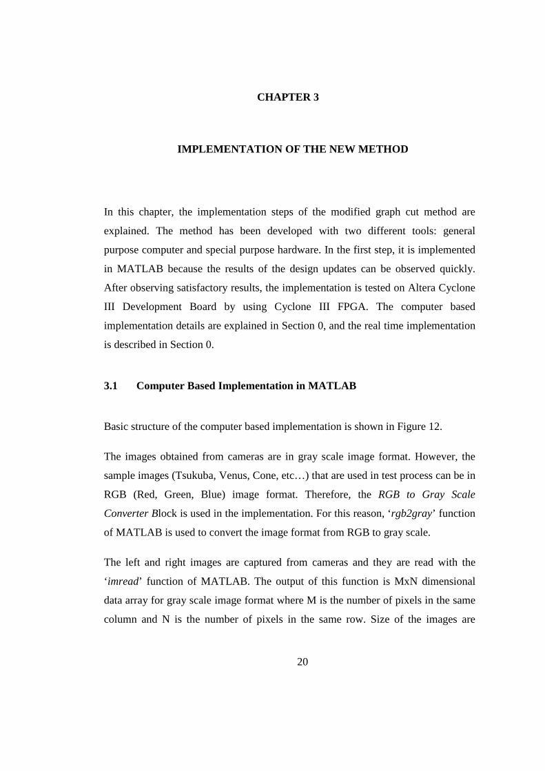
In this chapter, the implementation steps of the modified graph cut method are
explained. The method has been developed with two different tools: general
purpose computer and special purpose hardware. In the first step, it is implemented
in MATLAB because the results of the design updates can be observed quickly.
After observing satisfactory results, the implementation is tested on Altera Cyclone
III Development Board by using Cyclone III FPGA. The computer based
implementation details are explained in Section 0, and the real time implementation
is described in Section 0.
3.1 Computer Based Implementation in MATLAB
Basic structure of the computer based implementation is shown in Figure 12.
The images obtained from cameras are in gray scale image format. However, the
sample images (Tsukuba, Venus, Cone, etc…) that are used in test process can be in
RGB (Red, Green, Blue) image format. Therefore, the RGB to Gray Scale
Converter Block is used in the implementation. For this reason, ‘rgb2gray’ function
of MATLAB is used to convert the image format from RGB to gray scale.
The left and right images are captured from cameras and they are read with the
‘ imread’ function of MATLAB. The output of this function is MxN dimensional
data array for gray scale image format where M is the number of pixels in the same
column and N is the number of pixels in the same row. Size of the images are

21
determined and sent to the following blocks. The left and right MxN dimensional
images are converted to 1xN dimensional arrays, because energy calculation is done
with pixels located on the same line. Basic Energy Calculation Module takes the
left and right 1xN dimensional images with the image sizes and produces the
disparity energies for all disparities in the range (R). The detailed block diagram of
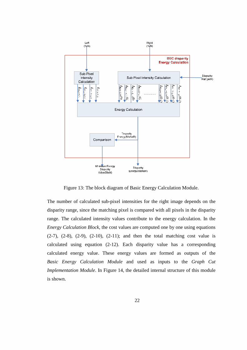
the Basic Energy Calculation Module is shown in Figure 13.
Figure 12: The block diagram of Computer Based Implementation.
The 1xN dimensional left and right arrays enter the Sub-pixel Intensity Calculation
Block where the intensity values of the sub-pixels are calculated by the equations
(2-3), (2-4), (2-5), (2-6). The number of calculated sub-pixel intensities for the left
image is four, since the matching pixel is selected from this image (see Figure 9).
22
Figure 13: The block diagram of Basic Energy Calculation Module.
The number of calculated sub-pixel intensities for the right image depends on the
disparity range, since the matching pixel is compared with all pixels in the disparity
range. The calculated intensity values contribute to the energy calculation. In the
Energy Calculation Block, the cost values are computed one by one using equations
(2-7), (2-8), (2-9), (2-10), (2-11); and then the total matching cost value is
calculated using equation (2-12). Each disparity value has a corresponding
calculated energy value. These energy values are formed as outputs of the
Basic Energy Calculation Module and used as inputs to the Graph Cut
Implementation Module. In Figure 14, the detailed internal structure of this module
is shown.

23
Figure 14: The block diagram of Graph Cut Implementation Module.
The Graph Cut Implementation Module is the main calculation and comparison
module of the proposed method. The links of the graph structure and the minimum
disparity energy are computed in this module. At the last step, the disparity map is
formed and the disparity image is shown on the screen.
After the 1xN dimensional left arrays enter the Graph Cut Implementation Module,
the smoothness energies are calculated according to equation (2-2). The relation
between the matching pixel and its neighbor which is located on the same line (y) is
calculated in the Smoothness Calculation-1 Block. In Figure 8, these neighbor
pixels are displayed as P(x-1,y) and P(x,y). Left image line pixel value, current
disparity value and umax1 are necessary inputs to calculate the smoothness energy-1.
The relation between the matching pixel and its upper neighbor (y-1) is calculated
in the Smoothness Calculation-2 Block. In Figure 8, this neighbor pixel is displayed
as P(x,y-1). The left image y-coordinate line pixel value, the left image

24
(y-1)-coordinate line pixel value, the calculated disparity value of the upper line
pixel and umax2 are necessary inputs to calculate the smoothness energy-2.
The relation between the matching pixel and its lower neighbor (y+1) is calculated
in the Smoothness Calculation-3 Block. In Figure 8, this neighbor pixel is displayed
as P(x,y+1). The left image y-coordinate line pixel value, the left image
(y+1)-coordinate line pixel value, the minimum energy disparity value which is
calculated in the Basic Energy Calculation Module and umax3 are necessary inputs to
calculate the smoothness energy-3.
The calculated smoothness energy-1, smoothness energy-2, smoothness energy-3
and disparity energies are inputs to the Summation Block where the cost energies
are calculated as in equation (2-15). The energy disparity indexes (0, 1,…, R) and
their total cost energies are sent to the Comparison Block.
In the Comparison Block, the minimum disparity energy is found by comparing all
cost energies. The disparity values which have the minimum energies of pixels form
the disparity map of corresponding images. This disparity map is sent to the Write
Image Block to be shown on the screen.
3.2 Real Time Implementation in FPGA
3.2.1 The Hardware Description
The hardware is composed of three cards. The main processing card is
Altera Cyclone III Development Board which includes Cyclone III EP3C120 FPGA
and DDR2-SDRAM memories. FPGA is used for the video processing application
and DDR2-SDRAM memories are used for frame buffering. Other cards are
Bitec HSMC (High Speed Mezzanine Card) daughter cards that are plugged to the
main board. HSMC Quad Video is used to capture the right and left analog videos.

25
This card contains a video decoder that digitizes the analog video and sends to the
FPGA. HSMC DVI is used to display outputs of the processing block on the
monitor. The general hardware structure is shown in Figure 15.
Figure 15: Hardware structure.
3.2.2 Real Time Implementation
The necessary signals, hardware blocks and pipelining for the real time
implementation of the proposed method are described in this section. The general
structure of the FPGA blocks is shown in Figure 16. All these blocks are coded in
VHDL (Very high speed integrated circuit Hardware Description Language). For
stereo matching application two cameras are used providing PAL video at 25Hz.
The videos are captured by the video decoder on the HSMC Quad Video and sent to
the Video Input Block in FPGA. This block makes the necessary decomposition of

26
the video signals and outputs the active pixels in the video frame. In this block also
YCbCr to Y decomposition is done. Cb and Cr are the chrominance (color) part of
the video and Y is the luminance (intensity) part. The Stereo Matching Block uses
only the intensity values for the calculations.
Video Input
Analog
video read
YCbCr to Y
converter
Video Input
Analog
video read
YCbCr to Y
converter
DDR2-SDRAM
interface
DDR2-SDRAM
Right
buffer1
Right
buffer2
Left buffer1
Left buffer2
DDR2-SDRAM
interface
Video read
Video read
Stereo
Matching
DDR2-SDRAM
interface
DDR2-SDRAM
interface
Disparity
buffer
Video
output
FPGA
Right
Video
Left
Video
DVI
Figure 16 : The general structure of the FPGA blocks.
The captured video frames are written to the DDR2 SDRAM memory by
DDR-SDRAM Interface Block. In this memory, there are two frame buffers for each
of the left and right video. This double buffering is used to eliminate the frame
latencies between the video frames. The right and left camera power up timings
may be different and there can be frame latencies between the left and right frames.
These latencies may result in faulty calculations in the Stereo Matching Block.

27
The Video Read block reads the right and left video frame buffers which contains
the last incoming video frames. Then, these video frames are sent to the Stereo
Matching Block which process on the video frames and calculates the disparity
values. The calculated disparity values are written to DDR2 SDRAM for the Video
Output Block. Finally, the Video Output Block reads the disparity values from the
memory and sends to the HSMC DVI to display on the monitor.
The main block of this real time implementation is Stereo Matching. The proposed
modified graph cut method is realized in this block. The detailed structure of this
block is shown in Figure 17. The Stereo Matching Block is composed of two main
blocks: Basic Energy Calculation and Graph Cut Implementation. The Basic
Energy Calculation Block computes the matching cost energies for every disparity
value in the range. These matching energies are used by the Graph Cut
Implementation Block to compute GC disparity value of the related pixel.
The video lines are written to the FIFO’s (First In First Out) by using the frame
timing signals. The general description of the frame timing signals is shown in
Figure 18. The frame valid signal indicates a new video frame, the line valid signal
shows the change of the video lines and the pixel valid signal is used to capture the
active pixels in the video line.
The received video lines (Right and Left) are firstly written to the Plus Line FIFO’s
(Right and Left). Then the pixel data in Plus Line FIFO is transferred to the Line
FIFO when a new active video line starts and the pixel data in the Line FIFO is
written to the Minus Line FIFO. After the three active video lines, the Plus Line
FIFO contains line(y+1), the Line FIFO contains line(y) and the Minus Line FIFO
holds line(y-1). Since all the necessary lines are ready, the Basic Energy
Calculation Block can start to calculate the matching cost energies. The structure of
the Basic Energy Calculation Block is shown in Figure 19.

28
Left plus fifo
read signal
Right plus fifo
read signal
Left plus fifo
data(7..0)
Right plus fifo
data(7..0)
Figure 17: The detailed structure of Stereo Matching Block.
Figure 18: Frame timing signals.
The FIFO Control Interface controls the FIFO signals to arrange the read/write
sequences between the FIFO’s. It sends the pixel data to the Arithmetic Calculation
Block for the calculations of the matching cost energies of each disparity value. The
Arithmetic Calculation Block contains two sub-blocks. The first block calculates the

29
sub pixel intensity values, and the second block computes the cost energies using
these values. The structure for sub-pixel intensity calculation is shown in Figure 20. Pixel Valid
Line Valid
Frame Valid
Figure 19: Basic Energy Calculation Block.
The sub-pixel intensity values are calculated with the matching pixel P(x,y) and its
neighbors. Firstly the matching pixel and its neighbor pixel intensity values are
added. Then sum is divided by two to get the average. In Figure 20, the Right Shift
Operator is used for the division by two. The left image is the reference image, so
the matching pixel values for the right image are calculated. Since the
implementation works in a pipeline order, the calculated sub-pixel values can be
used for the next matching cost energy calculation. The previous sub-pixel values in
the buffers are kept and used for the next calculation. Figure 21 shows the main idea
of sub-pixel buffer usage. In this figure R(x) and L(x) represent the right and left
image pixels, respectively, and dx is used for the calculated disparity.

30
+Right Pixel(x,y)
Right Shift
operator
x minus right
buffer0
Arithmetic calculation 1
x minus right
buffer1
x minus right
buffer79Right Pixel(x-1,y)
x right pre
buffer0
x right pre
buffer1
x right
buffer0
x right
buffer1
x right
buffer79
+Right Pixel(x,y)
Right Shift
operator
x plus right
buffer0
x plus right
buffer1
x plus right
buffer79Right Pixel(x+1,y)
+Right Pixel(x,y)
Right Shift
operator
y minus right
buffer0
y minus right
buffer1
y minus right
buffer79Right Pixel(x,y-1)
+Right Pixel(x,y)
Right Shift
operator
y plus right
buffer0
y plus right
buffer1
y plus right
buffer79Right Pixel(x,y+1)
+Left Pixel(x,y)
Right Shift
operator
x minus left
bufferLeft Pixel(x-1,y)
x left pre
buffer0
x left pre
buffer1
x left
buffer
+Left Pixel(x,y)
Right Shift
operator
x plus left
bufferLeft Pixel(x+1,y)
+Left Pixel(x,y)
Right Shift
operator
y minus left
bufferLeft Pixel(x,y-1)
+Left Pixel(x,y)
Right Shift
operator
y plus left
bufferLeft Pixel(x,y+1)
IR(x,y-0.5 )(0) IR(x,y-0.5 )(1) IR(x,y-0.5 )(79)
IL(x,y-0.5 )
IL(x,y+0.5 )
IL(x-0.5,y )
IL(x+0.5,y )
IL(x,y )
IR(x,y )(0) IR(x,y )(1) IR(x,y )(79)
IR(x-0.5,y )(0) IR(x-0.5,y)(1) IR(x-0.5,y)(79)
IR(x+0.5,y )(0) IR(x+0.5,y)(1) IR(x+0.5,y)(79)
IR(x,y+0.5 )(0) IR(x,y+0.5 )(1) IR(x,y+0.5 )(79)
Figure 20: Sub-Pixel Intensity Calculation Block.
R(x-79) R(x-78) R(x-1) R(x)
L(x)
R(x-78) R(x-77) R(x) R(x+1)
L(x+1)
P(x,y)
P(x+1,y)
d0d1d78d79
d0d1d78d79
Figure 21: Usage of sub-pixel buffers.

31
Having the sub-pixel intensity values, the matching cost energies are calculated by
the second block in Arithmetic Calculation. The general structure for the Cost
Energy Calculation is shown in Figure 22.
Absolute
difference
x minus left
buffer
Cost0 (x-0.5,y)
Absolute
difference
x minus right
buffer0
x minus right
buffer79
Absolute
difference
Cost0 (x,y-0.5) y minus right
buffer0
y minus left
buffer
Absolute
difference
y minus right
buffer79
Absolute
difference
Cost0 (x,y+0.5)
y plus left
bufferAbsolute
difference
y plus right
buffer0
y plus right
buffer79
Absolute
difference x right buffer0
Absolute
difference x right buffer79
x left buffer
Cost0 (x,y)
Arithmetic Calculation 2
Cost79 (x-0.5,y)
Absolute
difference
x plus left
buffer
Cost0 (x+0.5,y)
Absolute
difference
x plus right
buffer0
x plus right
buffer79
Cost79 (x+0.5,y)
Cost79 (x,y-0.5) Cost79 (x,y)
Cost79 (x,y+0.5)
Figure 22: Cost Energy Calculation Block.
The matching cost energies of the matching pixel and sub-pixels are sent to the
Edata Calculation block. In this block, matching cost energies are added and the
total cost energies for the disparities are calculated. Figure 23 shows the general
structure of Edata Calculation block.

32
Figure 23: Edata Calculation Block.
The calculated Edata values are compared in Comparison Block to find the
disparity value with minimum cost energy. This block computes the minimum
energy in 3 stages. There are sub-blocks that can compare 5 values at the same time.
So, 80 cost energies compared and 16 values are obtained. 15 of these values are
compared and 3 values are obtained. In the last stage, these 3 values and the
16th value from the previous stage are compared, and the disparity value with the
minimum cost energy is calculated. The Comparison Block is shown in Figure 24.

33
Figure 24 : The Comparison Block.
The calculated Edata values of each disparity, matching pixel value and its BEC
disparity value are transferred to the GC implementation Block which calculates the
disparity values as explained in Section 2.3.2. The detailed structure of this block is
shown in Figure 25.
The Edata values are transferred from the BEC to the GC module with valid signal.
By using this valid signal, these energies are written to the internal FIFO’s of GC
Implementation Block. The GC Main Controller Block reads Edata values from the
internal FIFO’s during the GC cost energy calculation.
The main process of GC implementation is controlled by the GC Main Controller
Block. All FIFO read/write operations are arranged and the GC disparity results are

34
calculated by this main controller block. The structure of the GC Main Controller
Block is shown in Figure 26.
Figure 25: The Structure of Graph Cut Implementation Block.
The Smooth1 Energy Calculation Block reads from the line FIFO to calculate the
neighboring relation energy between pixels P(x,y) and P((x-1),y). In this block,
equation (2-13) is implemented. The term “C*|fp-fq|” is calculated in the Smooth1
Look-up Table. In this implementation, the term umax1 is used instead of C and k is
used instead of |fp-fq|. The k*umax1 terms are computed for all the disparity values in
the range and transferred to the Smooth1 Energy Calculation Block. The structure of
this block is shown in Figure 27.

35
Figure 26: The structure of GC Main Controller Block.
Figure 27: The structure of Smooth1 Energy Calculation Block.

36
The data read from the line FIFO is saved as Ip pixel value. In addition, this Ip pixel
value is copied to the Iq pixel value to be used as the (x-1)th pixel intensity value
for the next smooth1 calculation. The absolute difference between the Ip and Iq
values are calculated and transferred to the Multipliers Block. k*umax1 values are
multiplied with |Ip-Iq| value in this block, and the results are sent to the Absolute
Differences Block. This block computes the |k*umax1-k*umax1*|Ip-Iq|| values and
transfers the results to the 8-bit Right Shift Operator Block which is used to divide
the inputs by 256. After division, Smooth1-Energy Results are ready for cost energy
calculation.
The Smooth2 Energy Calculation Block and the Smooth3 Energy Calculation Block
calculate the energy values in parallel with the Smooth1 Energy Calculation Block.
All the smooth energies become ready for the calculation of cost energies at the
same time. The structure of the Smooth2 Calculation Block is shown in Figure 28.
Figure 28: The structure of Smooth2 Energy Calculation Block
The structure of Smooth2 Calculation block is similar to the structure of Smooth1
Calculation block. One of the difference is smooth1 is related with the neighboring
relation between P(x,y) and P((x-1),y) but smooth2 is related with the neighboring
37
relation between P(x,y) and P(x,y-1). The other difference is the look-up tables. In
addition, smooth2 reads pixel data from Line and Minus Line FIFO’s.
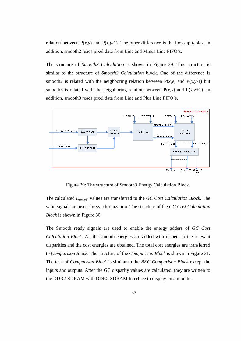
The structure of Smooth3 Calculation is shown in Figure 29. This structure is
similar to the structure of Smooth2 Calculation block. One of the difference is
smooth2 is related with the neighboring relation between P(x,y) and P(x,y-1) but
smooth3 is related with the neighboring relation between P(x,y) and P(x,y+1). In
addition, smooth3 reads pixel data from Line and Plus Line FIFO’s.
Figure 29: The structure of Smooth3 Energy Calculation Block.
The calculated Esmooth values are transferred to the GC Cost Calculation Block. The
valid signals are used for synchronization. The structure of the GC Cost Calculation
Block is shown in Figure 30.
The Smooth ready signals are used to enable the energy adders of GC Cost
Calculation Block. All the smooth energies are added with respect to the relevant
disparities and the cost energies are obtained. The total cost energies are transferred
to Comparison Block. The structure of the Comparison Block is shown in Figure 31.
The task of Comparison Block is similar to the BEC Comparison Block except the
inputs and outputs. After the GC disparity values are calculated, they are written to
the DDR2-SDRAM with DDR2-SDRAM Interface to display on a monitor.

38
Figure 30: The structure of GC Cost Calculation Block.
Figure 31: The structure of Comparison Block.

39
CHAPTER 4
4 SIMULATION AND IMPLEMENTATION RESULTS
This chapter discusses the disparity results of MATLAB and FPGA
implementations of the proposed method. The MATLAB implementation and
FPGA simulation results are evaluated by Middlebury Stereo pairs which are
Tsukuba, Venus, Teddy, and Cones. FPGA implementation results are evaluated by
dedicated hardware.
The MATLAB and FPGA simulation results are compared with the ground truth of
Middlebury stereo pairs. The ground truth contains the accurate pixel disparity
results. The Middlebury stereo pairs and their ground truths are given in Figure 32.
In the evaluation process, the percentage of bad pixels, which are the differences
between evaluated method and ground truth, is calculated:
∑∈∈
>−=MyNx
dGRN
yxdyxdP
B )),(),((1 δ (4-1)
In this equation, PN is the total number of pixels in the image, dR(x,y) and dG(x,y)
are the calculated and the ground truth disparity values, respectively, for pixel (x,y).
δd is the disparity error tolerance which is taken as 1 in the evaluations.
The Middlebury comparisons are performed in three ways. In the first comparison,
all pixel disparity values are compared; in the second one, non-occluded pixel
disparities are evaluated; and discontinuity pixel disparities are measured in the last
one. On the contrary to the occluded region pixels, in non-occluded regions, pixels
are visible in both images, so every matching pixel in one image has the

40
corresponding pixel in the other image. Discontinuity occurs on the boundaries of
the regions in the image. Namely, discontinuity pixels are neighbor pixels which get
different disparities. The original image, its ground truth, occluded/non-occluded
and depth discontinuity regions are given in Figure 33.
Figure 32: Middlebury data pairs and their ground truths.
(a) Tsukuba, (b) Venus, (c) Teddy, (d) Cones.

41
(a) (b)
(c) (d)
Figure 33: The Middlebury comparison regions. (a) Original image; (b) Ground
truth disparity map; (c) Occluded regions(black), Non-occluded regions(white);
(d) Discontinuity regions (white).
According to these evaluation criteria, MATLAB implementation results are
discussed in Section 4.1, and FPGA implementation results are given in Section 4.2.
4.1 MATLAB Implementation Results
MATLAB implementation details are given in Chapter 3. In these implementation
steps, the only controllable parameters are umax1, umax2, and umax3 which are used in
smoothness calculation blocks. The variation in umax values affects the disparity
results of proposed method.

42
The proposed method uses the umax values for the relations between the neighbour
pixels P(x,y), P(x-1,y), P(x,y+1) and P(x,y-1). The disparity values of P(x-1,y),
P(x,y+1), and P(x,y-1) affect the graph cut result of P(x,y). P(x-1,y) and P(x,y-1)
disparity values are calculated by graph cut, on the other hand P(x,y+1) disparity
value is generated by basic energy calculation module where matching cost energies
are calculated. Firstly, all three umax variables are assigned to the same value and the
disparity results are evaluated for the image pairs Tsukuba, Venus, Teddy and
Cones. The percentage of bad pixels versus umax values are given in Figure 34.
Small umax values result in high percentage of bad pixels, because smoothness terms
give lower contribution to the total energy than matching cost term in minimum cut
calculation. Therefore, the neighbouring relations between the pixels are neglected.
When umax values are increased, smoothness terms become dominant in the total
energy and neighbouring relations affect the minimum energy calculation. Then, the
all and non-occluded pixel disparity errors decrease. On the other hand, since the
graph cut module uses matching cost energies from basic energy calculation
module, discontinuity pixel error is changing according to the basic energy
calculation module results.
In basic energy calculation module, if the matching costs are calculated correctly at
the discontinuity points, graph cut implementation module finds the correct
disparity values. Therefore, the discontinuity pixel error decreases in the case of
Venus, Teddy and Cones images. However, if the calculated matching cost energies
are incorrect, the minimum energies can not be calculated correctly at the
boundaries. Then, the discontinuity pixel error increases as in the case of Tsukuba
image.
In Figure 35, the disparity results of basic energy calculation module are given.
These results are obtained by the minimum matching cost energy disparities. In
Tsukuba image, the calculated minimum energy disparities are not correct at some

43
of object boundaries. Therefore, some deformations are observed at these
boundaries as shown in Figure 36.
Figure 34: The effect of umax values on disparity errors. (a) Tsukuba image pairs,
(b) Venus image pairs, (c) Teddy image pairs, (d) Cones image pairs.
Figure 35: Basic energy calculation module minimum matching energy disparity
results (a) Tsukuba, (b) Venus, (c) Teddy, (d) Cones.
44
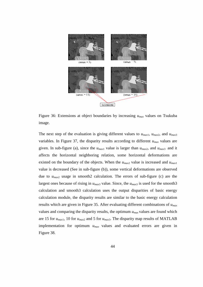
Figure 36: Extensions at object boundaries by increasing umax values on Tsukuba
image.
The next step of the evaluation is giving different values to umax1, umax2, and umax3
variables. In Figure 37, the disparity results according to different umax values are
given. In sub-figure (a), since the umax1 value is larger than umax2, and umax3 and it
affects the horizontal neighboring relation, some horizontal deformations are
existed on the boundary of the objects. When the umax2 value is increased and umax1
value is decreased (See in sub-figure (b)), some vertical deformations are observed
due to umax2 usage in smooth2 calculation. The errors of sub-figure (c) are the
largest ones because of rising in umax3 value. Since, the umax3 is used for the smooth3
calculation and smooth3 calculation uses the output disparities of basic energy
calculation module, the disparity results are similar to the basic energy calculation
results which are given in Figure 35. After evaluating different combinations of umax
values and comparing the disparity results, the optimum umax values are found which
are 15 for umax1, 10 for umax2 and 5 for umax3. The disparity map results of MATLAB
implementation for optimum umax values and evaluated errors are given in
Figure 38.

45
Figure 37: Disparity results of proposed method for different umax values.

46
Figure 38: Evaluated disparity results using Middlebury stereo pairs. (a) Ground
truths, (b) Disparity results of the best resultant graph cut method in Middlebury,
(c) Disparity results of the proposed method and the percentage of bad pixels
related with these results.
The MATLAB implementation results are compared with previous methods for
Tsukuba image pairs. Although the error rate of the proposed method is larger than
other methods, time performance is much better. The comparisons of different
methods are given in Table 1.

47
Table 1: Comparisons of the previous stereo matching methods and proposed
method for Tsukuba image pairs.
Percentage of bad pixels
Tool Computation
Time References All
pixel
Non-
occluded Discontinuity
Methods
Dynamic
Programming 5.04% 4.12% 12.0% CPU 1.0s [30]
Graph Cut
Method 2.01% 1.19% 6.24% CPU 69.8s [2]
SSD+min filter 7.22% 5.08% 24.1% CPU 1.1s [13]
Proposed
Method 7.08% 5.09% 18.2% FPGA 40ms This study
4.2 FPGA Implementation Results
In this section, the FPGA implementation results are evaluated. In Section 4.2.1, the
simulation results are given, and the real time hardware results are presented
in Section 4.2.2 .
4.2.1 Simulation Results
The simulation of the proposed FPGA implementation is done
by Modelsim-Altera 6.5b tool. The functional behavior of the proposed VHDL code
is simulated. Since all the FPGA blocks are operating on the real hardware, the
simulation outputs provide information about the hardware performance.
During the simulation, Tsukuba image is used. This image is converted to text file
because Modelsim can read text files as an input. Then, the pixel intensity values of
the right and left image are sent to the VHDL code (GC implementation module)
for the simulation of disparity calculation. Finally, disparity results of the

48
simulation are written to a text file and then converted to the disparity image. The
simulation environment is shown in Figure 39.
Figure 39: The simulation environment
Throughout the simulation, all necessary signals and data are examined with respect
to timing and accuracy. In FPGA hierarchy, some blocks need other blocks’ output
at certain time which is called pipeline processing. If these outputs arrive late or
early, all real time flow can be broken. Therefore, the simulation provides valuable
information about the flow in an FPGA. With this information, the VHDL code is
updated and the problems are solved.
In Figure 40, the simulation screen for frame start and graph cut disparity result is
shown. This simulation shows the synchronization of the signals with each other
and pixel clock. Figure 41 gives a part of the simulation for the whole FPGA
design.
Figure 40: Simulation screens of the control signals.

49
Figure 41: A part of the simulation screen of the design.
The VHDL simulation generates the disparity results of Tsukuba image. The results
of the VHDL simulation and MATLAB are compared which is shown in Figure 42.
There are some differences between the results. VHDL simulation results are worse
at some boundary points. The extensions are increased. Since MATLAB uses
double floating point in calculations, its accuracy is better. On the other hand,
FPGA implementation uses fix point in calculations which decrease the accuracy.
Therefore, the error in VHDL simulation is greater than the MATLAB results.
Figure 42: Comparison of MATLAB and VHDL simulation results on Tsukuba
image.

50
4.2.2 Hardware Results
VHDL codes are written by Altera Quartus-II software tool which has a free license
version for the academic studies. All VHDL blocks are connected in a top block
with their schematic representation which is very helpful for the user to debug and
analyze the whole flow. Figure 43 shows the schematic representation of the
implemented blocks in FPGA design environment.
The FPGA consist of logic elements, embedded memory bits and multipliers. Logic
elements are used for realization of the VHDL codes. In addition, these elements
make the necessary connections between the internal blocks. The data is stored in
embedded memories and the multipliers are used for the arithmetic calculations.
Table 2 shows the total dedicated FPGA resources and the usage summary of the
proposed method.
Table 2: FPGA resource utilization
FPGA Resources Available Used Logic Element 119,088 66,123 Memory(bits) 3,981,312 1,901,632
Multiplier(9x9) 576 480
FPGA implementations of stereo matching are realized in previous studies which
use local methods. The performance of the proposed method and the other FPGA
implementations are given at Table 3.
According to Table 3, the hardware uses different types of FPGA’s. The
performance of the real-time stereo system is directly related with the FPGA type,
because each FPGA has its own maximum clock frequency, logic element and
embedded multipliers. Therefore, image resolution, maximum disparity range and
frame rate are depend on the FPGA type.

51
Figure 43: FPGA design environment.
Table 3: The performance comparison of previous real time studies and proposed
method.
Hardware Image
Resolution Disparity
Range Method
Frame per
second References
4 x Virtex-2 256x360 20
Local Weighted Phase Correlation
(Pixel-based, Local)
30 [26]
Virtex-4 640x480 64 Census
(Pixel-based, Local)
60 [27]
Virtex-2 640x480 128 SAD
(Pixel-based, Local)
60 [28]
Virtex-2 640x480 64 SAD
(Pixel-based, Local)
30 [29]
Cyclone III 720x576 80 Modified Graph Cut (Pixel-based, Local & Global)
25 This Study

52
In Figure 44, the FPGA real time implementation results are shown. These results
are captured from DVI monitor with a camera at the running time. Different objects
are used for the evaluation of the real-time system. These objects are located at
different positions and their depths are observed by the brightness on the results.
The higher brightness means that the objects are closer to the camera, whereas the
objects which are far away results lower brightness.
Some problems are encountered during the hardware implementation of the
proposed method which is related with the cameras and connections. When frames
are computed sequentially in FPGA, some distortions are occurred on disparity
map. There are two reasons for these distortions: the camera intensity variation and
camera lens optical distortion. The pixel intensity values are not similar in
sequential frames for similar scene. In Figure 45, the signal tap which is the debug
screen of the Quartus is shown. This debug tool is used to monitor the signals in an
FPGA when implementation is running. Pixel intensity variation is observed at
P(100,200). In this representation 100 is the value of pixel counter and 200 is the
value of line counter. The left pixel intensity changes from 95 to 100 and right pixel
intensity changes between 60 and 76. These variations result in distortions on the
sequential disparity frames.
The camera lenses cause the optical distortion which is larger at the lens boundaries
and smaller at the centre. Optical distortion disturbs the epipolar line geometry
which prevents accurate matching of the corresponding pixels in the right and left
image. The optical distortion of the camera lens can be seen on the top of the
library in Figure 46.
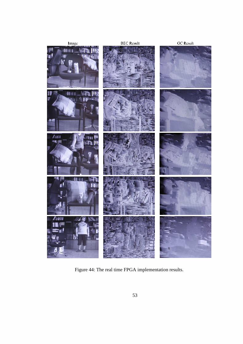
53
Figure 44: The real time FPGA implementation results.

54
Figure 44: Continuation.

55
Figure 45: The signal tap screen of the design.

56
Figure 46: The distorted image.

57
CHAPTER 5
5 CONCLUSIONS AND FUTURE WORK
5.1 Conclusions
In this thesis, a modified graph cut method for stereo matching is proposed. The
modification is such that the real time implementation is possible. The method is
firstly developed in MATLAB, and then realized in dedicated hardware with FPGA
to achieve the real time constraints.
The literature survey of different stereo matching methods is presented and their
advantages and disadvantages are summarized. Stereo matching methods can be put
into three groups: pixel-based, region based and feature based. Pixel-based methods
which include local and global methods are mostly used in literature. Local methods
like SAD and SD require less computational time compared with global methods,
but their accuracy is worse. On the other hand, global methods can generate
accurate stereo results, but their computation time is long.
The main aim of the proposed method is to turn the recursive structure of the
standard graph cut method (a global method) into a non-recursive structure. There
are two basic differences between the standard graph cut method and the proposed
method, namely, the computation structure and the required image lines. The
standard graph cut method is recursive, because all possible disparity combinations
are checked repeatedly. On the other hand, the proposed method is implemented in
non-recursive structure; all possible disparities are checked only for the matching
pixel and the disparity result is added to the previously calculated ones. Another
basic difference is the required line numbers of the computation. In the proposed

58
method, three lines are necessary for the implementation of the neighboring
relations whereas the standard graph cut method needs only the epipolar line. The
upper and lower line neighbors are critical for the smoothness calculation in the
proposed method.
The proposed method is implemented in two main blocks: basic energy calculation
and graph cut. In the first block, the matching cost energy values are calculated. In
the graph cut implementation block, the graph structure is constructed with
calculated matching cost energies, and the minimum cut is found according to some
smoothness constraints for neighbor pixels.
Firstly, the modified graph cut method is implemented by MATLAB. The
MATLAB results show that the smoothness constraints directly affect the disparity
results. Using different smoothness variables (umax values) generates different
disparity results. In the evaluation, firstly, all smoothness variables are kept same
and the results are compared with well known data sets from Middlebury. Using the
same value for all smoothness variables increases the percentage of bad pixel errors;
because each smoothness variable is used in smoothness calculation of different
neighbor pixels. To control the effects of smoothness, different values are assigned
to these variables. When the neighboring relation variable between the pixels P(x,y)
and P(x,y-1) is given a larger value than the others, vertical deformations are
observed in the disparity map. On the other hand, when the smoothness variable
between the pixels P(x,y) and P(x-1,y) is increased, the error at the boundaries also
increases in the horizontal direction. The last controllable smoothness variable is
between the pixels P(x,y) and P(x,y+1). When this variable is increased, the total
percentage of bad pixel errors becomes larger than the other variable combinations.
Since the disparity results of Basic Energy Calculation Module, which are mostly
incorrect, are used in this smoothness calculation, the disparity results of Graph Cut
Implementation Module are incorrect and the resultant disparity map is similar to
the output disparity map of Basic Energy Calculation Module. After evaluating

59
different smoothness variable combinations, the optimum one is obtained and used
in the FPGA implementation.
Secondly, the proposed method is implemented in a pipeline structure in FPGA. In
this structure, the VHDL blocks are connected to each other sequentially so that a
real time flow is possible. VHDL codes of the design are simulated by Modelsim
tool of Altera. The data flow is examined with respect to the real time constraints,
and the disparity results are compared with the MATLAB results. Some differences
are observed between the MATLAB and FPGA results which are mainly occurred
at boundary points. These differences are related with the used number formats.
For the real time implementation, Altera Cyclone III FPGA is used. videos, Two
PAL cameras are used for the right and left videos. The total computation time of
the FPGA graph cut implementation for 80 disparity stereo matching is 40 ms
which is suitable for real time applications. The FPGA implementation results are
displayed on a DVI monitor.
5.2 Future Work
The proposed method’s computation time (40 ms) and the disparity range (80) are
encouraging values for stereo matching applications. However, the labeling result of
the method can be improved by new additions on the basic energy calculation and
graph cut parts. The graph cut part, which uses the output of the basic energy
calculation block, can generate more accurate disparity results if the outputs of the
basic energy calculation part can be improved. Different local methods or their
fusion can be used for the basic energy calculation.
The Graph Cut Module needs some parameters for the calculation. In FPGA
implementation, these parameters are embedded into the code. The main board does
not have a serial communication interface. A serial communication interface like

60
RS-232 can be added to the main board and the parameters can be updated during
the run time.
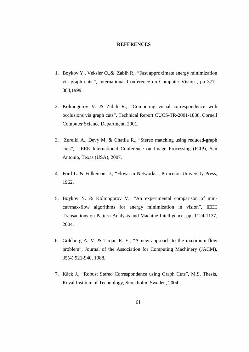
61
6 REFERENCES
1. Boykov Y., Veksler O.,& Zabih R., “Fast approximate energy minimization
via graph cuts.”, International Conference on Computer Vision , pp 377–
384,1999.
2. Kolmogorov V. & Zabih R., “Computing visual correspondence with
occlusions via graph cuts”, Technical Report CUCS-TR-2001-1838, Cornell
Computer Science Department, 2001.
3. Zureiki A., Devy M. & Chatila R., “Stereo matching using reduced-graph
cuts”, IEEE International Conference on Image Processing (ICIP), San
Antonio, Texas (USA), 2007.
4. Ford L. & Fulkerson D., “Flows in Networks”, Princeton University Press,
1962.
5. Boykov Y. & Kolmogorov V., “An experimental comparison of min-
cut/max-flow algorithms for energy minimization in vision”, IEEE
Transactions on Pattern Analysis and Machine Intelligence, pp. 1124-1137,
2004.
6. Goldberg A. V. & Tarjan R. E., “A new approach to the maximum-flow
problem”, Journal of the Association for Computing Machinery (JACM),
35(4):921-940, 1988.
7. Käck J., “Robust Stereo Correspondence using Graph Cuts”, M.S. Thesis,
Royal Institute of Technology, Stockholm, Sweden, 2004.

62
8. Birchfield S. and Tomasi C., “A Pixel Dissimilarity Measure That Is
Insensitive to Image Sampling”, PAMI, Vol. 20, No. 4, 1998
9. Ude A. and Dillmann R., “Vision-Based Robot Path Planning”, Advances in
Robot Kinematics and Computational Geometry, pp. 505-512, 1994.
10. Se S., Lowe D. and Little J., “Vision-based Mobile Robot Localization And
Mapping using Scale-Invariant Features”, Proceedings of the IEEE
International Conference on Robotics & Automation (ICRA), pp. 2051-
2058, Seoul, Korea, 2001.
11. Wang J. H., Hsieh R. F., and Chiu H. C., “A Progressive Constraint Search
Approach for Disparity Matching in Stereo Vision”, Proceedings of the
National Science Council- Part A, vol.23, no.6, pp 789-798, 1999.
12. Bilgin A., “Selection and Fusion of Multiple Stereo Algorithms for Accurate
Disparity Segmentation”, M.S. Thesis, METU, 2008.
13. Scharstein D., Szeliski R., “A taxonomy and evaluation of dense two-frame
stereo correspondence algorithms”, Intl. J. Comp. Vis., 47(1): 7–42, 2002.
14. Matthies L., Szeliski R., and Kanade T., “Kalman Filter-Based Algorithms
for Estimating Depth from Image Sequences”, International Journal of
Computer Vision, 3:209–236, 1989.
15. Hannah M. J., “Computer Matching of Areas in Stereo Images”, PhD thesis,
Stanford University,1974.

63
16. Cox I. J., Hingorani S. L., Rao S. B., Maggs B. M., “A maximum likelihood
stereo algorithm”, Computer Vision and Image Understanding, 63(3):542–
567, 1996.
17. Sun J., Zheng N. N., Shum H. Y., "Stereo Matching Using Belief
Propagation", IEEE Transactions on Pattern Analysis and Machine
Intelligence, vol. 25, no. 7, pp. 787-800, Jul., 2003.
18. Cohen L., Vinet L., Sander P.T., Gagalowicz A., “Hierarchical region based
stereo matching”, Computer Vision and Pattern Recognition, Proceedings
CVPR '89., IEEE Computer Society Conference, pp. 416-421, 1989.
19. Canny J., “A Computational Approach To Edge Detection”, IEEE Trans.
Pattern Analysis and Machine Intelligence, 8:679-714, 1986.
20. Wang H., Brady M., “Real-time corner detection algorithm for motion
estimation”, Image and Vision Computing, 13(9): 695-703, 1995.
21. Lee Y.S., Koo H.S., Jeong C.S., “A straight line detection using principal
component analysis”, Pattern Recognition Letters 27(14): 1744-1754, 2006.
22. http://vision.middlebury.edu/stereo, last accessed date: 22.07.2010.
23. Thorpe S., Fize D. & Marlot C., ”Speed of processing in the human visual
system”, Nature, Vol.381, No.6582, pp. 520-522, 1996.
24. Zabih R. & Kolmogorov V., “Graph Cut algorithms for Binocular stereo
with occlusions”, In Mathematical Models in Computer Vision: The
Handbook, 2005.

64
25. Vineet V. & Narayanan P.J. “Cuda Cuts : Fast Graph Cuts on the GPU”,
CVPR Workshop on Visual Computer Vision on GPUs, 2008
26. Darabiha A., Rose J., & MacLean W. J. “Video-Rate Stereo Depth
Measurement on Programmable Hardware”, IEEE Trans. Computer Vision
and Pattern Recognition, 1063-6919/03, 2003.
27. Jin S., Cho J., Pham X. D., Lee K. M., Park S. K., Kim M. & Jeon W. J.
“FPGA Design and Implementation of a Real-Time Stereo Vision System”,
IEEE Trans. Circuits and Systems for Video Technology, Vol. 20, No. 1,
2010.
28. Han D. & Hwang D.-H. “A Novel Stereo Matching Method for Wide
Disparity Range Detection”, International Conference on Image Analysis
and Recognition (ICIAR), pp. 643-650, 2005.
29. Yunde J., Zhang X., Li M., & An L. “A Miniature Stereo Vision Machine
(MSVM-III) for Dense Disparity Mapping”, International Conference on
Pattern Recognition (ICPR), 1051-4651/04, 2004.

65
7 APPENDIX A
GRAPH CUT METHODS
Maximum Flow Method
Suppose that G(V,E) is a directed graph where V shows the vertices and E shows the
edges. In addition to V and E, two new concepts which are capacity and flow of the
graph edges are used in maximum flow method.
Let (u,v) ∈ E and c(u,v) be the positive capacity of (u,v). It represents the maximum
amount of flow that can pass through an edge. We assume that if (u,v)∉E than
c(u,v)=0. f(u,v) is the flow representation of the (u,v). It is a real function,
f:VxV→R which must satisfy the following constraints for all (u,v):
1. Capacity constraint: The flow along an edge can be lower than its capacity.
),(),( vucvuf < (A-1)
2. Skew symmetry constraint: The flow from u to v must be the opposite of the
flow from v to u.
),(),( uvfvuf −= (A-2)
3. Flow conservation constraint: The sum of input and output flows of each
edge can be equal except for s(source) and t(sink).
0),( =∑∈Vv
vuf (A-3)
Notice that f(u,v) is a net flow from u to v. For example, there is a flow of 4 units
from u to v, and a flow of 3 units from v to u, we have f(u,v)=1 and f(v,u)=-1.

66
Maximum flow method is used to find the maximum amount that can flow on a
constructed graph. Because maximum flow amount is determined by the edges that
have lower capacities. Therefore, the maximum value of an s-t flow is equal to the
minimum capacity of an s-t cut according to the theorem of Ford & Fulkerson [4].
In literature, two basic maximum flow algorithms are found. The first is augmented
path algorithm which is developed by Ford & Fulkerson and the second is the push-
relabel algorithm.
Augmented Path Algorithm
Augmented path algorithm was introduced by Ford & Fulkerson [4] for the
minimum cut calculation. Boykov & Kolmogorov [5] implemented this algorithm
in stereo matching.
The first step of augmented path algorithm is the construction of residual graph. A
residual graph Gr(V,E) differs from the original in edge capacities. The capacities
cr(u,v) are changed in the following way[5]:
If f(u,v)<c(u,v) then (u,v)∈E and cr(u,v)=c(u,v)-f(u,v),
If f(u,v)≥0 then (v,u)∈E and cr(v,u)=f(u,v).
Therefore residual graph Gr(V,E) has duplicate edges with capacities cr(u,v) and
cr(v,u).
An augmented path which is represented by (u1, u2, ..., uk) is a path on the residual
graph from source to sink. In this context, u1 is the source and uk is the sink of the
residual graph. The important property of an augmented path is cr(ui, ui+1)>0.
The aim of this algorithm is to find the maximum flow (minimum cut) of the graph
and this is done by removing augmenting paths in the residual graph.

67
Algorithm starts with constructing the residual graph. The second step is to find the
augmented paths on the graph and then finally to remove these augmented paths
with iterations. The detailed version of this algorithm is explained in Table 4.
Table 4: Augmented path algorithm
Algorithm steps Description
1 Construct a residual graph Gr
2 Find an augmented path a on Gr
3 Calculate capacity of augmented path: )),(:),(min()( avuvucac rf ∈=
4
For each (u,v) Є a
),(),(
)(),(),(
vufuvf
acvufvuf f
←
+←
5 Update Gr
6 Is there an augmented path on Gr? YES → Return step-2 NO → Go to step-7
7 Finish
After the residual graph is updated with no augmented path, the minimum cut can
be calculated by finding the vertices which are reachable and non-reachable from
the source. The edges between the reachable and non-reachable vertices give the
minimum cut path. In Figure 47, the updated residual graph and the minimum cut
are shown, in this figure, the red vertices are non-reachable and blue ones are
reachable vertices.

68
s
tMin cut
Figure 47: The example of minimum cut on residual graph.
Push Relabel Algorithm
Firstly, Goldberg [6] proposed Push-relabel algorithm for the maximum flow
computation. After that Zureiki, Devy & Chatila [3] used this algorithm for stereo
correspondence problem.
The main idea of the algorithm is to find the maximum flow of the graph G(V,E) by
some operations on the graph. We should define new concepts which are height and
preflow to understand the process of the algorithm.
Height (u) is the number of total vertices between the vertex u and the t(sink). The
assumptions are,
Height(s)=V (Total number of the vertices),
Height(t)=0.
Preflow is the similar to the flow concept. The only difference is that input flow
should be larger than the output flow of the vertex. P(u,v) is the preflow
representation of the (u,v). It is a real function, P:VxV→R+ which must satisfy the
following constraints for all (u,v):

69
1. Capacity constraint: The preflow along an edge can be lower and equal to its
capacity:
EvuvucvuP ∈∀≤ ),(),,(),( (A-4) 2. Skew symmetry constraint: The preflow from u to v must be the opposite of
the preflow from v to u:
EvuuvPvuP ∈∀−= ),(),,(),( (A-5) 3. Let e(u) is the excess of vertex u. It is the difference between the input flow
and output flow of u:
}{sVuvuPuvPueEvuEuv
−∈∀≥−= ∑∑∈∈
,0),(),()(),(),(
(A-6)
Two operations are used to find maximum flow which are push and relabel.
Push operation:
If you want to push a flow from vertex u to vertex v, you can send a part of excess
flow from u to v, but following three conditions must be satisfied:
1. e(u)>0: The input flow is bigger than output flow
2. c(u,v)-f(u,v)>0 : Available capacity from u to v.
3. Height(u)>Height(v) : The distance between u and t(sink) is larger than the
distance between v and t(sink).
After these three conditions are satisfied, the amount of min(e(u), c(u,v)-f(u,v))
flow can send.
Relabel operation:
If you want to relabel a vertex u, you can increase its height until it is bigger than at
least one of the vertices which have available capacity. The necessary conditions
are:

70
1. e(u)>0: There must be an excess in the relabeling vertex u
2. Height(u)≤Height(v) ∀ v, such that: There are not any lower or equal
height vertices connected to vertex u.
After these two conditions are satisfied, the height of vertex u can increase until at
least one lowest height vertex is found.
Algorithm starts with constructing graph G(V,E). The second step is to find the
vertex which has positive excess. After that, do push operation or relabel operation
on that vertex. When there is not any positive excess vertex on the graph, the
algorithm stops. The edges that carry the maximum flow will be minimum cut
edges.
The detailed version of this algorithm is explained in Table 5.
Table 5: Push-Relabel Algorithm
Algorithm steps Description
1 Construct a graph G(V,E)
2 Find a vertex with 0)( >ue on G(V,E)
3 Is )()( vHeightuHeight > ? YES → Go to step-4 NO → Go to step-5
4 Do relabel operation
5 Do push operation
6 Is there a vertex with 0)( >ue on G(V,E)? YES → Return step-2 NO → Go to step-7
7 Finish

71
Swap-Expansion Method
Swap-Expansion methods try to find the minimum match energy by changing the
pixel’s disparity values (labels). These algorithms start with an arbitrary labeling
and change the disparities until they reach optimum labeling. Swap-expansion
algorithm is discussed under two titles by Boykov, Veksler & Zabih [1].
α-β Swap Method
In α−β swap method, initial labels x’s are given to all pixels in the defined partition
P. x is selected from the disparity range, and this range includes α and β. The
objective is to find the correct labels x’ to reach minimum matching energy for the
partition P.
The constructed graph Gαβ is shown in Figure 48 [1]. The source and the sink which
are explained in the Section 2.1 are assigned to possible labels α and β. The
connection between the disparity vertices and the labels α, β is made with t-links.
As explained in section 2.1, these links hold the matching energy. n-links are used
to connect vertices which are belong to neighbor pixels and show the smoothness
energy. This graph representation is different from the defined in section 2.1,
because this graph is used to check only two possible disparity while the other one
checks all possible disparities.
),( qpn
αqt
βpt
αpt
Figure 48: Gαβ structure.

72
The basic idea of this method is to try all possible disparity pairs until the optimum
labeling is reached. The labeling is done according to the cut on the constructed
graph. Cut is found by using the energy values of the links. There are many possible
energy values to be compared to calculate the cut path. Finding the minimum
energy cut means to assign the disparity value. If cut passes through tpα, pixel p
remains its old disparity value α but if cut passes through tpβ, pixel p is assigned to
new disparity value β. The label of pixel p swaps from α to β.
),( qpn
αpt
βpt
αqt
βqt
),( qpn
αpt
βpt
αqt
βqt
),( qpn
αpt
βpt
αqt
βqt
),( qpn
αpt
βpt
αqt
βqt
Figure 49: The possible cuts on constructed Gαβ for pixels p and q.
As shown in Figure 49, cut determines the disparity values for the pixels. For
instance, Cut1 passes through tpα, tq
α => the disparity values of p and q are α. Cut2
passes through tpβ, tq
β => the disparity values of p and q are β. Cut3 passes through
tpα, n(p,q), tq
β => the disparity value of p is α and q is β. Since cut3 path passes
through the n-link between the neighbor pixels p and q, the disparities of these
neighbor pixels is changed. Finally, Cut4 passes through tpβ, n(p,q) , tq
α => the
disparity value of p is β and q is α.
Algorithm starts with constructing graph Gαβ. The second step is to determine the
initial labeling x and calculate the energy values with these labels. After that α, β
swap is done and new matching energy value is calculated with these new labels. If
Enew is lower than the previous energy, convert x label to new labels x’. When all
labels are tested, the algorithm stops.

73
The detailed version of this algorithm is explained in Table 6.
Table 6: βα − swap algorithm
Algorithm steps
Description
1 Construct a graph Gαβ
2 Start with initial labeling x
3 Are all labels tested? YES → Go to step-8 NO → Go to step-4
4 For each pairs of labels (α,β)
5 Do α-β swap operation (resultant label x’)
6 Calculate E(x’)
7
Is E(x’)<E(x)? YES → Determine x=x’ Update Gαβ Return step-3 NO → Return step-3
8 Finish
α Expansion Method
Similar to α-β swap method, α-expansion starts with an initial labeling x. This
labeling has matching cost energy EX. Then with one α-expansion of x, EX is tried to
be minimized according to the initial labeling [1].
In α-expansion method an auxiliary vertex is defined between the pixel vertices
which have different labels. The reason of adding new vertex is to decrease the cost
value of the link between the neighbor pixels which have different labels. The
auxiliary vertex assumed to be labeled with α. Figure 50 shows the constructed
graph with auxiliary node.

74
),( apn
αqt
,αpt
αpt
),( qan
,αat
Figure 50: Constructed graph for α-expansion.
In this method every possible labels in the range is checked for pixel p. Then
according to the new labeling, matching cost energy EX is calculated and compared
with the previous one. If the new energy value is less than the previous one, pixel p
is assigned to new label, otherwise the other label is assigned. This process
continues until all labels are checked for pixel p. The algorithm steps are given in
Table 7 .
Table 7: α-expansion algorithm
Algorithm steps
Description
1 Construct a graph Gαά
2 Start with initial labeling x
3 Are all labels tested? YES → Go to step-8 NO → Go to step-4
4 For every labels (α) Set pixel label to α (resultant label x’)
5 Calculate E(x’)
6
Is E(x’)<E(x)? YES → Determine x=x’ Update Gαά Return step-3 NO → Return step-3
8 Finish