fractal - internet archive
TRANSCRIPT

FRACTALGEOMETRYMathematical Foundationsand Applications
Fractal Geometry: Mathematical Foundations and Application. Second Edition Kenneth Falconer 2003 John Wiley & Sons, Ltd ISBNs: 0-470-84861-8 (HB); 0-470-84862-6 (PB)

FRACTALGEOMETRYMathematical Foundationsand Applications
Second Edition
Kenneth FalconerUniversity of St Andrews, UK

Copyright 2003 John Wiley & Sons Ltd, The Atrium, Southern Gate, Chichester,West Sussex PO19 8SQ, England
Telephone (+44) 1243 779777
Email (for orders and customer service enquiries): [email protected] our Home Page on www.wileyeurope.com or www.wiley.com
All Rights Reserved. No part of this publication may be reproduced, stored in a retrieval system ortransmitted in any form or by any means, electronic, mechanical, photocopying, recording,scanning or otherwise, except under the terms of the Copyright, Designs and Patents Act 1988 orunder the terms of a licence issued by the Copyright Licensing Agency Ltd, 90 Tottenham CourtRoad, London W1T 4LP, UK, without the permission in writing of the Publisher. Requests to thePublisher should be addressed to the Permissions Department, John Wiley & Sons Ltd, TheAtrium, Southern Gate, Chichester, West Sussex PO19 8SQ, England, or emailed [email protected], or faxed to (+44) 1243 770620.
This publication is designed to provide accurate and authoritative information in regard to thesubject matter covered. It is sold on the understanding that the Publisher is not engaged inrendering professional services. If professional advice or other expert assistance is required, theservices of a competent professional should be sought.
Other Wiley Editorial Offices
John Wiley & Sons Inc., 111 River Street, Hoboken, NJ 07030, USA
Jossey-Bass, 989 Market Street, San Francisco, CA 94103-1741, USA
Wiley-VCH Verlag GmbH, Boschstr. 12, D-69469 Weinheim, Germany
John Wiley & Sons Australia Ltd, 33 Park Road, Milton, Queensland 4064, Australia
John Wiley & Sons (Asia) Pte Ltd, 2 Clementi Loop #02-01, Jin Xing Distripark, Singapore 129809
John Wiley & Sons Canada Ltd, 22 Worcester Road, Etobicoke, Ontario, Canada M9W 1L1
Wiley also publishes its books in a variety of electronic formats. Some content that appearsin print may not be available in electronic books.
British Library Cataloguing in Publication Data
A catalogue record for this book is available from the British Library
ISBN 0-470-84861-8 (Cloth)ISBN 0-470-84862-6 (Paper)
Typeset in 10/12pt Times by Laserwords Private Limited, Chennai, IndiaPrinted and bound in Great Britain by TJ International, Padstow, CornwallThis book is printed on acid-free paper responsibly manufactured from sustainable forestryin which at least two trees are planted for each one used for paper production.
Contents
Preface ix
Preface to the second edition xiii
Course suggestions xv
Introduction xvii
Notes and references xxvii
PART I FOUNDATIONS 1
Chapter 1 Mathematical background . . . . . . . . . . . . . . . . . . . . . . . . . . . . . . . 3
1.1 Basic set theory . . . . . . . . . . . . . . . . . . . . . . . . . . . . . . . . . . . 31.2 Functions and limits . . . . . . . . . . . . . . . . . . . . . . . . . . . . . . . . . 61.3 Measures and mass distributions . . . . . . . . . . . . . . . . . . . . . . . . 111.4 Notes on probability theory . . . . . . . . . . . . . . . . . . . . . . . . . . . . 171.5 Notes and references . . . . . . . . . . . . . . . . . . . . . . . . . . . . . . . . 24
Exercises . . . . . . . . . . . . . . . . . . . . . . . . . . . . . . . . . . . . . . . . 25
Chapter 2 Hausdorff measure and dimension . . . . . . . . . . . . . . . . . . . . . . . . . 27
2.1 Hausdorff measure . . . . . . . . . . . . . . . . . . . . . . . . . . . . . . . . . 272.2 Hausdorff dimension . . . . . . . . . . . . . . . . . . . . . . . . . . . . . . . . 312.3 Calculation of Hausdorff dimension—simple examples . . . . . . . . . . . 34
*2.4 Equivalent definitions of Hausdorff dimension . . . . . . . . . . . . . . . . . 35*2.5 Finer definitions of dimension . . . . . . . . . . . . . . . . . . . . . . . . . . . 36
2.6 Notes and references . . . . . . . . . . . . . . . . . . . . . . . . . . . . . . . . 37Exercises . . . . . . . . . . . . . . . . . . . . . . . . . . . . . . . . . . . . . . . . 37
Chapter 3 Alternative definitions of dimension . . . . . . . . . . . . . . . . . . . . . . . 39
3.1 Box-counting dimensions . . . . . . . . . . . . . . . . . . . . . . . . . . . . . 413.2 Properties and problems of box-counting dimension . . . . . . . . . . . . 47
v
vi Contents
*3.3 Modified box-counting dimensions . . . . . . . . . . . . . . . . . . . . . . . 49*3.4 Packing measures and dimensions . . . . . . . . . . . . . . . . . . . . . . . 503.5 Some other definitions of dimension . . . . . . . . . . . . . . . . . . . . . . . 533.6 Notes and references . . . . . . . . . . . . . . . . . . . . . . . . . . . . . . . . 57
Exercises . . . . . . . . . . . . . . . . . . . . . . . . . . . . . . . . . . . . . . . . 57
Chapter 4 Techniques for calculating dimensions . . . . . . . . . . . . . . . . . . . . . 59
4.1 Basic methods . . . . . . . . . . . . . . . . . . . . . . . . . . . . . . . . . . . . 594.2 Subsets of finite measure . . . . . . . . . . . . . . . . . . . . . . . . . . . . . 684.3 Potential theoretic methods . . . . . . . . . . . . . . . . . . . . . . . . . . . . 70
*4.4 Fourier transform methods . . . . . . . . . . . . . . . . . . . . . . . . . . . . . 734.5 Notes and references . . . . . . . . . . . . . . . . . . . . . . . . . . . . . . . . 74
Exercises . . . . . . . . . . . . . . . . . . . . . . . . . . . . . . . . . . . . . . . . 74
Chapter 5 Local structure of fractals . . . . . . . . . . . . . . . . . . . . . . . . . . . . . . . 76
5.1 Densities . . . . . . . . . . . . . . . . . . . . . . . . . . . . . . . . . . . . . . . . 765.2 Structure of 1-sets . . . . . . . . . . . . . . . . . . . . . . . . . . . . . . . . . . 805.3 Tangents to s-sets . . . . . . . . . . . . . . . . . . . . . . . . . . . . . . . . . . 845.4 Notes and references . . . . . . . . . . . . . . . . . . . . . . . . . . . . . . . . 89
Exercises . . . . . . . . . . . . . . . . . . . . . . . . . . . . . . . . . . . . . . . . 89
Chapter 6 Projections of fractals . . . . . . . . . . . . . . . . . . . . . . . . . . . . . . . . . . 90
6.1 Projections of arbitrary sets . . . . . . . . . . . . . . . . . . . . . . . . . . . . 906.2 Projections of s-sets of integral dimension . . . . . . . . . . . . . . . . . . . 936.3 Projections of arbitrary sets of integral dimension . . . . . . . . . . . . . . 956.4 Notes and references . . . . . . . . . . . . . . . . . . . . . . . . . . . . . . . . 97
Exercises . . . . . . . . . . . . . . . . . . . . . . . . . . . . . . . . . . . . . . . . 97
Chapter 7 Products of fractals . . . . . . . . . . . . . . . . . . . . . . . . . . . . . . . . . . . . 99
7.1 Product formulae . . . . . . . . . . . . . . . . . . . . . . . . . . . . . . . . . . . 997.2 Notes and references . . . . . . . . . . . . . . . . . . . . . . . . . . . . . . . . 107
Exercises . . . . . . . . . . . . . . . . . . . . . . . . . . . . . . . . . . . . . . . . 107
Chapter 8 Intersections of fractals . . . . . . . . . . . . . . . . . . . . . . . . . . . . . . . . . 109
8.1 Intersection formulae for fractals . . . . . . . . . . . . . . . . . . . . . . . . 110*8.2 Sets with large intersection . . . . . . . . . . . . . . . . . . . . . . . . . . . . 1138.3 Notes and references . . . . . . . . . . . . . . . . . . . . . . . . . . . . . . . . 118
Exercises . . . . . . . . . . . . . . . . . . . . . . . . . . . . . . . . . . . . . . . . 119
PART II APPLICATIONS AND EXAMPLES 121
Chapter 9 Iterated function systems—self-similar and self-affine sets . . . . 123
9.1 Iterated function systems . . . . . . . . . . . . . . . . . . . . . . . . . . . . . 1239.2 Dimensions of self-similar sets . . . . . . . . . . . . . . . . . . . . . . . . . . 128
vii
9.3 Some variations . . . . . . . . . . . . . . . . . . . . . . . . . . . . . . . . . . . 1359.4 Self-affine sets . . . . . . . . . . . . . . . . . . . . . . . . . . . . . . . . . . . . 1399.5 Applications to encoding images . . . . . . . . . . . . . . . . . . . . . . . . . 1459.6 Notes and references . . . . . . . . . . . . . . . . . . . . . . . . . . . . . . . . 148
Exercises . . . . . . . . . . . . . . . . . . . . . . . . . . . . . . . . . . . . . . . . 149
Chapter 10 Examples from number theory . . . . . . . . . . . . . . . . . . . . . . . . . . . . 151
10.1 Distribution of digits of numbers . . . . . . . . . . . . . . . . . . . . . . . . . 15110.2 Continued fractions . . . . . . . . . . . . . . . . . . . . . . . . . . . . . . . . . 15310.3 Diophantine approximation . . . . . . . . . . . . . . . . . . . . . . . . . . . . 15410.4 Notes and references . . . . . . . . . . . . . . . . . . . . . . . . . . . . . . . . 158
Exercises . . . . . . . . . . . . . . . . . . . . . . . . . . . . . . . . . . . . . . . . 158
Chapter 11 Graphs of functions . . . . . . . . . . . . . . . . . . . . . . . . . . . . . . . . . . . . . 160
11.1 Dimensions of graphs . . . . . . . . . . . . . . . . . . . . . . . . . . . . . . . . 160*11.2 Autocorrelation of fractal functions . . . . . . . . . . . . . . . . . . . . . . . 16911.3 Notes and references . . . . . . . . . . . . . . . . . . . . . . . . . . . . . . . . 173
Exercises . . . . . . . . . . . . . . . . . . . . . . . . . . . . . . . . . . . . . . . . 173
Chapter 12 Examples from pure mathematics . . . . . . . . . . . . . . . . . . . . . . . . . 176
12.1 Duality and the Kakeya problem . . . . . . . . . . . . . . . . . . . . . . . . . 17612.2 Vitushkin’s conjecture . . . . . . . . . . . . . . . . . . . . . . . . . . . . . . . 17912.3 Convex functions . . . . . . . . . . . . . . . . . . . . . . . . . . . . . . . . . . . 18112.4 Groups and rings of fractional dimension . . . . . . . . . . . . . . . . . . . . 18212.5 Notes and references . . . . . . . . . . . . . . . . . . . . . . . . . . . . . . . . 184
Exercises . . . . . . . . . . . . . . . . . . . . . . . . . . . . . . . . . . . . . . . . 185
Chapter 13 Dynamical systems . . . . . . . . . . . . . . . . . . . . . . . . . . . . . . . . . . . . . 186
13.1 Repellers and iterated function systems . . . . . . . . . . . . . . . . . . . . 18713.2 The logistic map . . . . . . . . . . . . . . . . . . . . . . . . . . . . . . . . . . . 18913.3 Stretching and folding transformations . . . . . . . . . . . . . . . . . . . . . 19313.4 The solenoid . . . . . . . . . . . . . . . . . . . . . . . . . . . . . . . . . . . . . . 19813.5 Continuous dynamical systems . . . . . . . . . . . . . . . . . . . . . . . . . . 201
*13.6 Small divisor theory . . . . . . . . . . . . . . . . . . . . . . . . . . . . . . . . . 205*13.7 Liapounov exponents and entropies . . . . . . . . . . . . . . . . . . . . . . . 20813.8 Notes and references . . . . . . . . . . . . . . . . . . . . . . . . . . . . . . . . 211
Exercises . . . . . . . . . . . . . . . . . . . . . . . . . . . . . . . . . . . . . . . . 212
Chapter 14 Iteration of complex functions—Julia sets . . . . . . . . . . . . . . . . . . 215
14.1 General theory of Julia sets . . . . . . . . . . . . . . . . . . . . . . . . . . . . 21514.2 Quadratic functions—the Mandelbrot set . . . . . . . . . . . . . . . . . . . 22314.3 Julia sets of quadratic functions . . . . . . . . . . . . . . . . . . . . . . . . . 22714.4 Characterization of quasi-circles by dimension . . . . . . . . . . . . . . . . 23514.5 Newton’s method for solving polynomial equations . . . . . . . . . . . . . 23714.6 Notes and references . . . . . . . . . . . . . . . . . . . . . . . . . . . . . . . . 241
Exercises . . . . . . . . . . . . . . . . . . . . . . . . . . . . . . . . . . . . . . . . 242

viii Contents
Chapter 15 Random fractals . . . . . . . . . . . . . . . . . . . . . . . . . . . . . . . . . . . . . . . 244
15.1 A random Cantor set . . . . . . . . . . . . . . . . . . . . . . . . . . . . . . . . . 24615.2 Fractal percolation . . . . . . . . . . . . . . . . . . . . . . . . . . . . . . . . . . 25115.3 Notes and references . . . . . . . . . . . . . . . . . . . . . . . . . . . . . . . . 255
Exercises . . . . . . . . . . . . . . . . . . . . . . . . . . . . . . . . . . . . . . . . 256
Chapter 16 Brownian motion and Brownian surfaces . . . . . . . . . . . . . . . . . . . 258
16.1 Brownian motion . . . . . . . . . . . . . . . . . . . . . . . . . . . . . . . . . . . 25816.2 Fractional Brownian motion . . . . . . . . . . . . . . . . . . . . . . . . . . . . 26716.3 Levy stable processes . . . . . . . . . . . . . . . . . . . . . . . . . . . . . . . 27116.4 Fractional Brownian surfaces . . . . . . . . . . . . . . . . . . . . . . . . . . . 27316.5 Notes and references . . . . . . . . . . . . . . . . . . . . . . . . . . . . . . . . 275
Exercises . . . . . . . . . . . . . . . . . . . . . . . . . . . . . . . . . . . . . . . . 276
Chapter 17 Multifractal measures . . . . . . . . . . . . . . . . . . . . . . . . . . . . . . . . . . 277
17.1 Coarse multifractal analysis . . . . . . . . . . . . . . . . . . . . . . . . . . . . 27817.2 Fine multifractal analysis . . . . . . . . . . . . . . . . . . . . . . . . . . . . . . 28317.3 Self-similar multifractals . . . . . . . . . . . . . . . . . . . . . . . . . . . . . . 28617.4 Notes and references . . . . . . . . . . . . . . . . . . . . . . . . . . . . . . . . 296
Exercises . . . . . . . . . . . . . . . . . . . . . . . . . . . . . . . . . . . . . . . . 296
Chapter 18 Physical applications . . . . . . . . . . . . . . . . . . . . . . . . . . . . . . . . . . . 298
18.1 Fractal growth . . . . . . . . . . . . . . . . . . . . . . . . . . . . . . . . . . . . 30018.2 Singularities of electrostatic and gravitational potentials . . . . . . . . . . 30618.3 Fluid dynamics and turbulence . . . . . . . . . . . . . . . . . . . . . . . . . . 30718.4 Fractal antennas . . . . . . . . . . . . . . . . . . . . . . . . . . . . . . . . . . . 30918.5 Fractals in finance . . . . . . . . . . . . . . . . . . . . . . . . . . . . . . . . . . 31118.6 Notes and references . . . . . . . . . . . . . . . . . . . . . . . . . . . . . . . . 315
Exercises . . . . . . . . . . . . . . . . . . . . . . . . . . . . . . . . . . . . . . . . 316
References . . . . . . . . . . . . . . . . . . . . . . . . . . . . . . . . . . . . . . . . . . . 317
Index . . . . . . . . . . . . . . . . . . . . . . . . . . . . . . . . . . . . . . . . . . . . . . . . 329

Preface
I am frequently asked questions such as ‘What are fractals?’, ‘What is fractaldimension?’, ‘How can one find the dimension of a fractal and what does ittell us anyway?’ or ‘How can mathematics be applied to fractals?’ This bookendeavours to answer some of these questions.
The main aim of the book is to provide a treatment of the mathematics asso-ciated with fractals and dimensions at a level which is reasonably accessible tothose who encounter fractals in mathematics or science. Although basically amathematics book, it attempts to provide an intuitive as well as a mathematicalinsight into the subject.
The book falls naturally into two parts. Part I is concerned with the generaltheory of fractals and their geometry. Firstly, various notions of dimension andmethods for their calculation are introduced. Then geometrical properties of frac-tals are investigated in much the same way as one might study the geometry ofclassical figures such as circles or ellipses: locally a circle may be approximatedby a line segment, the projection or ‘shadow’ of a circle is generally an ellipse,a circle typically intersects a straight line segment in two points (if at all), andso on. There are fractal analogues of such properties, usually with dimensionplaying a key role. Thus we consider, for example, the local form of fractals,and projections and intersections of fractals.
Part II of the book contains examples of fractals, to which the theory of thefirst part may be applied, drawn from a wide variety of areas of mathematicsand physics. Topics include self-similar and self-affine sets, graphs of functions,examples from number theory and pure mathematics, dynamical systems, Juliasets, random fractals and some physical applications.
There are many diagrams in the text and frequent illustrative examples. Com-puter drawings of a variety of fractals are included, and it is hoped that enoughinformation is provided to enable readers with a knowledge of programming toproduce further drawings for themselves.
It is hoped that the book will be a useful reference for researchers, providingan accessible development of the mathematics underlying fractals and showinghow it may be applied in particular cases. The book covers a wide variety ofmathematical ideas that may be related to fractals, and, particularly in Part II,
ix

x Preface
provides a flavour of what is available rather than exploring any one subjectin too much detail. The selection of topics is to some extent at the author’swhim—there are certainly some important applications that are not included.Some of the material dates back to early in the twentieth century whilst some isvery recent.
Notes and references are provided at the end of each chapter. The referencesare by no means exhaustive, indeed complete references on the variety of topicscovered would fill a large volume. However, it is hoped that enough informationis included to enable those who wish to do so to pursue any topic further.
It would be possible to use the book as a basis for a course on the mathe-matics of fractals, at postgraduate or, perhaps, final-year undergraduate level, andexercises are included at the end of each chapter to facilitate this. Harder sectionsand proofs are marked with an asterisk, and may be omitted without interruptingthe development.
An effort has been made to keep the mathematics to a level that can be under-stood by a mathematics or physics graduate, and, for the most part, by a diligentfinal-year undergraduate. In particular, measure theoretic ideas have been kept toa minimum, and the reader is encouraged to think of measures as ‘mass distribu-tions’ on sets. Provided that it is accepted that measures with certain (intuitivelyalmost obvious) properties exist, there is little need for technical measure theoryin our development.
Results are always stated precisely to avoid the confusion which would other-wise result. Our approach is generally rigorous, but some of the harder or moretechnical proofs are either just sketched or omitted altogether. (However, a fewharder proofs that are not available in that form elsewhere have been included, inparticular those on sets with large intersection and on random fractals.) Suitablediagrams can be a help in understanding the proofs, many of which are of ageometric nature. Some diagrams are included in the book; the reader may findit helpful to draw others.
Chapter 1 begins with a rapid survey of some basic mathematical conceptsand notation, for example, from the theory of sets and functions, that are usedthroughout the book. It also includes an introductory section on measure theoryand mass distributions which, it is hoped, will be found adequate. The sectionon probability theory may be helpful for the chapters on random fractals andBrownian motion.
With the wide variety of topics covered it is impossible to be entirely consistentin use of notation and inevitably there sometimes has to be a compromise betweenconsistency within the book and standard usage.
In the last few years fractals have become enormously popular as an art form,with the advent of computer graphics, and as a model of a wide variety of physicalphenomena. Whilst it is possible in some ways to appreciate fractals with little orno knowledge of their mathematics, an understanding of the mathematics that canbe applied to such a diversity of objects certainly enhances one’s appreciation.The phrase ‘the beauty of fractals’ is often heard—it is the author’s belief thatmuch of their beauty is to be found in their mathematics.
Preface xi
It is a pleasure to acknowledge those who have assisted in the preparationof this book. Philip Drazin and Geoffrey Grimmett provided helpful commentson parts of the manuscript. Peter Shiarly gave valuable help with the computerdrawings and Aidan Foss produced some diagrams. I am indebted to CharlotteFarmer, Jackie Cowling and Stuart Gale of John Wiley and Sons for overseeingthe production of the book.
Special thanks are due to David Marsh—not only did he make many usefulcomments on the manuscript and produce many of the computer pictures, but healso typed the entire manuscript in a most expert way.
Finally, I would like to thank my wife Isobel for her support and encourage-ment, which extended to reading various drafts of the book.
Kenneth J. FalconerBristol, April 1989
Preface to the second edition
It is thirteen years since Fractal Geometry—Mathematical Foundations and Appli-cations was first published. In the meantime, the mathematics and applications offractals have advanced enormously, with an ever-widening interest in the subjectat all levels. The book was originally written for those working in mathematicsand science who wished to know more about fractal mathematics. Over the pastfew years, with changing interests and approaches to mathematics teaching, manyuniversities have introduced undergraduate and postgraduate courses on fractalgeometry, and a considerable number have been based on parts of this book.
Thus, this new edition has two main aims. First, it indicates some recent devel-opments in the subject, with updated notes and suggestions for further reading.Secondly, more attention is given to the needs of students using the book as acourse text, with extra details to help understanding, along with the inclusion offurther exercises.
Parts of the book have been rewritten. In particular, multifractal theory hasadvanced considerably since the first edition was published, so the chapter on‘Multifractal Measures’ has been completely rewritten. The notes and referenceshave been updated. Numerous minor changes, corrections and additions havebeen incorporated, and some of the notation and terminology has been changed toconform with what has become standard usage. Many of the diagrams have beenreplaced to take advantage of the more sophisticated computer technology nowavailable. Where possible, the numbering of sections, equations and figures hasbeen left as in the first edition, so that earlier references to the book remain valid.
Further exercises have been added at the end of the chapters. Solutions to theseexercises and additional supplementary material may be found on the world wideweb at
http://www.wileyeurope.com/fractalIn 1997 a sequel, Techniques in Fractal Geometry, was published, presenting
a variety of techniques and ideas current in fractal research. Readers wishingto study fractal mathematics beyond the bounds of this book may find thesequel helpful.
I am most grateful to all who have made constructive suggestions on the text. Inparticular I am indebted to Carmen Fernandez, Gwyneth Stallard and Alex Cain
xiii

xiv Preface to the second edition
for help with this revision. I am also very grateful for the continuing supportgiven to the book by the staff of John Wiley & Sons, and in particular to RobCalver and Lucy Bryan, for overseeing the production of this second edition andJohn O’Connor and Louise Page for the cover design.
Kenneth J. FalconerSt Andrews, January 2003

Course suggestions
There is far too much material in this book for a standard length course onfractal geometry. Depending on the emphasis required, appropriate sections maybe selected as a basis for an undergraduate or postgraduate course.
A course for mathematics students could be based on the following sections.
(a) Mathematical background1.1 Basic set theory; 1.2 Functions and limits; 1.3 Measures and massdistributions.
(b) Box-counting dimensions3.1 Box-counting dimensions; 3.2 Properties of box-counting dimensions.
(c) Hausdorff measures and dimension2.1 Hausdorff measure; 2.2 Hausdorff dimension; 2.3 Calculation of Haus-dorff dimension; 4.1 Basic methods of calculating dimensions.
(d) Iterated function systems9.1 Iterated function systems; 9.2 Dimensions of self-similar sets; 9.3 Somevariations; 10.2 Continued fraction examples.
(e) Graphs of functions11.1 Dimensions of graphs, the Weierstrass function and self-affine graphs.
(f) Dynamical systems13.1 Repellers and iterated function systems; 13.2 The logistic map.
(g) Iteration of complex functions14.1 Sketch of general theory of Julia sets; 14.2 The Mandelbrot set; 14.3Julia sets of quadratic functions.
xv
Introduction
In the past, mathematics has been concerned largely with sets and functions towhich the methods of classical calculus can be applied. Sets or functions thatare not sufficiently smooth or regular have tended to be ignored as ‘pathological’and not worthy of study. Certainly, they were regarded as individual curiositiesand only rarely were thought of as a class to which a general theory might beapplicable.
In recent years this attitude has changed. It has been realized that a great dealcan be said, and is worth saying, about the mathematics of non-smooth objects.Moreover, irregular sets provide a much better representation of many naturalphenomena than do the figures of classical geometry. Fractal geometry providesa general framework for the study of such irregular sets.
We begin by looking briefly at a number of simple examples of fractals, andnote some of their features.
The middle third Cantor set is one of the best known and most easily con-structed fractals; nevertheless it displays many typical fractal characteristics. Itis constructed from a unit interval by a sequence of deletion operations; seefigure 0.1. Let E0 be the interval [0, 1]. (Recall that [a, b] denotes the set of realnumbers x such that a � x � b.) Let E1 be the set obtained by deleting the mid-dle third of E0, so that E1 consists of the two intervals [0, 1
3 ] and [ 23 , 1]. Deleting
the middle thirds of these intervals gives E2; thus E2 comprises the four intervals[0, 1
9 ], [ 29 , 1
3 ], [ 23 , 7
9 ], [ 89 , 1]. We continue in this way, with Ek obtained by delet-
ing the middle third of each interval in Ek−1. Thus Ek consists of 2k intervalseach of length 3−k. The middle third Cantor set F consists of the numbers thatare in Ek for all k ; mathematically, F is the intersection
⋂∞k=0 Ek. The Cantor
set F may be thought of as the limit of the sequence of sets Ek as k tends toinfinity. It is obviously impossible to draw the set F itself, with its infinitesimaldetail, so ‘pictures of F ’ tend to be pictures of one of the Ek, which are a goodapproximation to F when k is reasonably large; see figure 0.1.
At first glance it might appear that we have removed so much of the interval[0, 1] during the construction of F , that nothing remains. In fact, F is an infinite(and indeed uncountable) set, which contains infinitely many numbers in everyneighbourhood of each of its points. The middle third Cantor set F consists
xvii

xviii Introduction
0 1 E0E1E2E3E4E5
FFL FR
13
23
...
Figure 0.1 Construction of the middle third Cantor set F , by repeated removal of themiddle third of intervals. Note that FL and FR, the left and right parts of F , are copiesof F scaled by a factor 1
3
precisely of those numbers in [0, 1] whose base-3 expansion does not containthe digit 1, i.e. all numbers a13−1 + a23−2 + a33−3 + · · · with ai = 0 or 2 foreach i. To see this, note that to get E1 from E0 we remove those numbers witha1 = 1, to get E2 from E1 we remove those numbers with a2 = 1, and so on.
We list some of the features of the middle third Cantor set F ; as we shall see,similar features are found in many fractals.
(i) F is self-similar. It is clear that the part of F in the interval [0, 13 ] and the
part of F in [ 23 , 1] are both geometrically similar to F , scaled by a factor
13 . Again, the parts of F in each of the four intervals of E2 are similar toF but scaled by a factor 1
9 , and so on. The Cantor set contains copies ofitself at many different scales.
(ii) The set F has a ‘fine structure’; that is, it contains detail at arbitrarilysmall scales. The more we enlarge the picture of the Cantor set, the moregaps become apparent to the eye.
(iii) Although F has an intricate detailed structure, the actual definition of F
is very straightforward.(iv) F is obtained by a recursive procedure. Our construction consisted of
repeatedly removing the middle thirds of intervals. Successive steps giveincreasingly good approximations Ek to the set F .
(v) The geometry of F is not easily described in classical terms: it is not thelocus of the points that satisfy some simple geometric condition, nor is itthe set of solutions of any simple equation.
(vi) It is awkward to describe the local geometry of F —near each of its pointsare a large number of other points, separated by gaps of varying lengths.
(vii) Although F is in some ways quite a large set (it is uncountably infinite),its size is not quantified by the usual measures such as length—by anyreasonable definition F has length zero.
Our second example, the von Koch curve, will also be familiar to many readers;see figure 0.2. We let E0 be a line segment of unit length. The set E1 consists ofthe four segments obtained by removing the middle third of E0 and replacing it

Introduction xix
E0
E1
E2
F
E3
(a)
(b)
Figure 0.2 (a) Construction of the von Koch curve F . At each stage, the middle third ofeach interval is replaced by the other two sides of an equilateral triangle. (b) Three vonKoch curves fitted together to form a snowflake curve
by the other two sides of the equilateral triangle based on the removed segment.We construct E2 by applying the same procedure to each of the segments in E1,and so on. Thus Ek comes from replacing the middle third of each straight linesegment of Ek−1 by the other two sides of an equilateral triangle. When k is
xx Introduction
large, the curves Ek−1 and Ek differ only in fine detail and as k tends to infinity,the sequence of polygonal curves Ek approaches a limiting curve F , called thevon Koch curve.
The von Koch curve has features in many ways similar to those listed forthe middle third Cantor set. It is made up of four ‘quarters’ each similar to thewhole, but scaled by a factor 1
3 . The fine structure is reflected in the irregularitiesat all scales; nevertheless, this intricate structure stems from a basically simpleconstruction. Whilst it is reasonable to call F a curve, it is much too irregularto have tangents in the classical sense. A simple calculation shows that Ek is oflength
(43
)k; letting k tend to infinity implies that F has infinite length. On the
other hand, F occupies zero area in the plane, so neither length nor area providesa very useful description of the size of F.
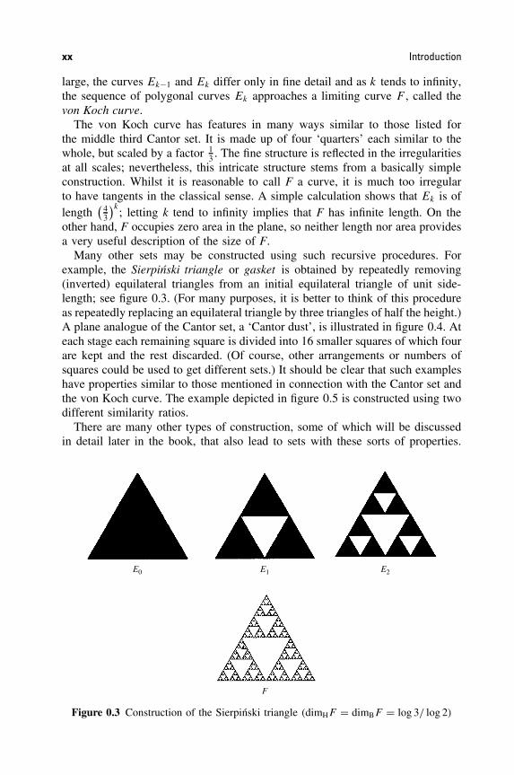
Many other sets may be constructed using such recursive procedures. Forexample, the Sierpinski triangle or gasket is obtained by repeatedly removing(inverted) equilateral triangles from an initial equilateral triangle of unit side-length; see figure 0.3. (For many purposes, it is better to think of this procedureas repeatedly replacing an equilateral triangle by three triangles of half the height.)A plane analogue of the Cantor set, a ‘Cantor dust’, is illustrated in figure 0.4. Ateach stage each remaining square is divided into 16 smaller squares of which fourare kept and the rest discarded. (Of course, other arrangements or numbers ofsquares could be used to get different sets.) It should be clear that such exampleshave properties similar to those mentioned in connection with the Cantor set andthe von Koch curve. The example depicted in figure 0.5 is constructed using twodifferent similarity ratios.
There are many other types of construction, some of which will be discussedin detail later in the book, that also lead to sets with these sorts of properties.
E0 E1
F
E2
Figure 0.3 Construction of the Sierpinski triangle (dimHF = dimBF = log 3/ log 2)

Introduction xxi
E0 E1
F
E2
Figure 0.4 Construction of a ‘Cantor dust’ (dimHF = dimBF = 1)
E0 E1
F
E2
Figure 0.5 Construction of a self-similar fractal with two different similarity ratios
xxii Introduction
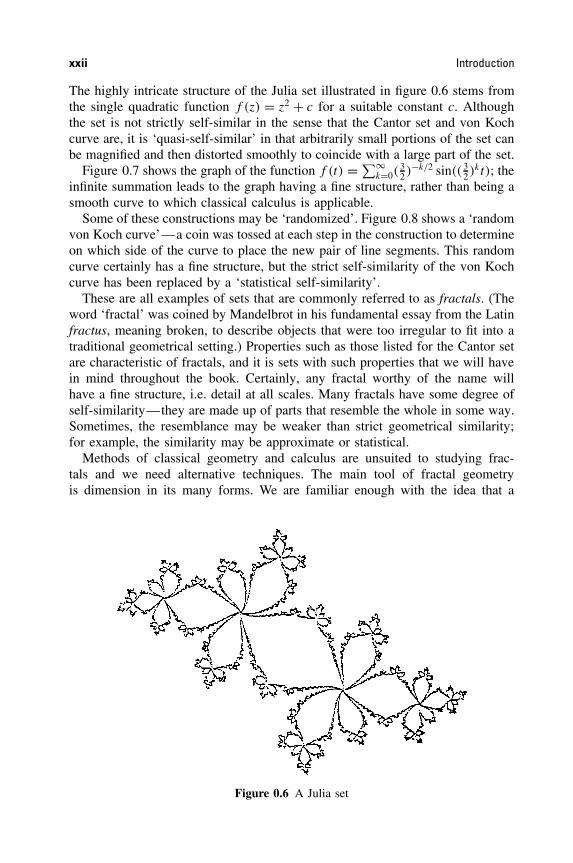
The highly intricate structure of the Julia set illustrated in figure 0.6 stems fromthe single quadratic function f (z) = z2 + c for a suitable constant c. Althoughthe set is not strictly self-similar in the sense that the Cantor set and von Kochcurve are, it is ‘quasi-self-similar’ in that arbitrarily small portions of the set canbe magnified and then distorted smoothly to coincide with a large part of the set.
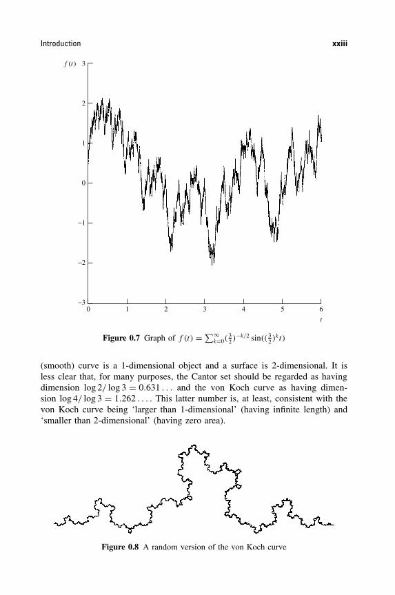
Figure 0.7 shows the graph of the function f (t) = ∑∞k=0(
32 )−k/2 sin(( 3
2 )kt); theinfinite summation leads to the graph having a fine structure, rather than being asmooth curve to which classical calculus is applicable.
Some of these constructions may be ‘randomized’. Figure 0.8 shows a ‘randomvon Koch curve’—a coin was tossed at each step in the construction to determineon which side of the curve to place the new pair of line segments. This randomcurve certainly has a fine structure, but the strict self-similarity of the von Kochcurve has been replaced by a ‘statistical self-similarity’.
These are all examples of sets that are commonly referred to as fractals. (Theword ‘fractal’ was coined by Mandelbrot in his fundamental essay from the Latinfractus, meaning broken, to describe objects that were too irregular to fit into atraditional geometrical setting.) Properties such as those listed for the Cantor setare characteristic of fractals, and it is sets with such properties that we will havein mind throughout the book. Certainly, any fractal worthy of the name willhave a fine structure, i.e. detail at all scales. Many fractals have some degree ofself-similarity—they are made up of parts that resemble the whole in some way.Sometimes, the resemblance may be weaker than strict geometrical similarity;for example, the similarity may be approximate or statistical.
Methods of classical geometry and calculus are unsuited to studying frac-tals and we need alternative techniques. The main tool of fractal geometryis dimension in its many forms. We are familiar enough with the idea that a
Figure 0.6 A Julia set
Introduction xxiii
3f (t )
2
1
0
−1
−2
−30 1 2 3 4 5 6
t
Figure 0.7 Graph of f (t) = ∑∞k=0(
32 )−k/2 sin(( 3
2 )kt)
(smooth) curve is a 1-dimensional object and a surface is 2-dimensional. It isless clear that, for many purposes, the Cantor set should be regarded as havingdimension log 2/ log 3 = 0.631 . . . and the von Koch curve as having dimen-sion log 4/ log 3 = 1.262 . . . . This latter number is, at least, consistent with thevon Koch curve being ‘larger than 1-dimensional’ (having infinite length) and‘smaller than 2-dimensional’ (having zero area).
Figure 0.8 A random version of the von Koch curve

xxiv Introduction
(a)
(b)
(c)
(d )
Figure 0.9 Division of certain sets into four parts. The parts are similar to the whole withratios: 1
4 for line segment (a); 12 for square (b); 1
9 for middle third Cantor set (c); 13 for
von Koch curve (d )
The following argument gives one (rather crude) interpretation of the meaningof these ‘dimensions’ indicating how they reflect scaling properties and self-similarity. As figure 0.9 indicates, a line segment is made up of four copies ofitself, scaled by a factor 1
4 . The segment has dimension − log 4/ log 14 = 1. A
square, however, is made up of four copies of itself scaled by a factor 12 (i.e.
with half the side length) and has dimension − log 4/ log 12 = 2. In the same way,
the von Koch curve is made up of four copies of itself scaled by a factor 13 , and
has dimension − log 4/ log 13 = log 4/ log 3, and the Cantor set may be regarded
as comprising four copies of itself scaled by a factor 19 and having dimension
− log 4/ log 19 = log 2/ log 3. In general, a set made up of m copies of itself scaled
by a factor r might be thought of as having dimension − log m/ log r . The numberobtained in this way is usually referred to as the similarity dimension of the set.
Unfortunately, similarity dimension is meaningful only for a relatively smallclass of strictly self-similar sets. Nevertheless, there are other definitions ofdimension that are much more widely applicable. For example, Hausdorff dimen-sion and the box-counting dimensions may be defined for any sets, and, inthese four examples, may be shown to equal the similarity dimension. The earlychapters of the book are concerned with the definition and properties of Hausdorffand other dimensions, along with methods for their calculation. Very roughly, adimension provides a description of how much space a set fills. It is a measure ofthe prominence of the irregularities of a set when viewed at very small scales. Adimension contains much information about the geometrical properties of a set.
A word of warning is appropriate at this point. It is possible to define the‘dimension’ of a set in many ways, some satisfactory and others less so. Itis important to realize that different definitions may give different values of

Introduction xxv
dimension for the same set, and may also have very different properties. Incon-sistent usage has sometimes led to considerable confusion. In particular, warninglights flash in my mind (as in the minds of other mathematicians) whenever theterm ‘fractal dimension’ is seen. Though some authors attach a precise meaningto this, I have known others interpret it inconsistently in a single piece of work.The reader should always be aware of the definition in use in any discussion.
In his original essay, Mandelbrot defined a fractal to be a set with Haus-dorff dimension strictly greater than its topological dimension. (The topologicaldimension of a set is always an integer and is 0 if it is totally disconnected, 1 ifeach point has arbitrarily small neighbourhoods with boundary of dimension 0,and so on.) This definition proved to be unsatisfactory in that it excluded a num-ber of sets that clearly ought to be regarded as fractals. Various other definitionshave been proposed, but they all seem to have this same drawback.
My personal feeling is that the definition of a ‘fractal’ should be regarded inthe same way as a biologist regards the definition of ‘life’. There is no hard andfast definition, but just a list of properties characteristic of a living thing, suchas the ability to reproduce or to move or to exist to some extent independentlyof the environment. Most living things have most of the characteristics on thelist, though there are living objects that are exceptions to each of them. In thesame way, it seems best to regard a fractal as a set that has properties suchas those listed below, rather than to look for a precise definition which willalmost certainly exclude some interesting cases. From the mathematician’s pointof view, this approach is no bad thing. It is difficult to avoid developing propertiesof dimension other than in a way that applies to ‘fractal’ and ‘non-fractal’ setsalike. For ‘non-fractals’, however, such properties are of little interest—they aregenerally almost obvious and could be obtained more easily by other methods.
When we refer to a set F as a fractal, therefore, we will typically have thefollowing in mind.
(i) F has a fine structure, i.e. detail on arbitrarily small scales.(ii) F is too irregular to be described in traditional geometrical language, both
locally and globally.(iii) Often F has some form of self-similarity, perhaps approximate or statis-
tical.(iv) Usually, the ‘fractal dimension’ of F (defined in some way) is greater
than its topological dimension.(v) In most cases of interest F is defined in a very simple way, perhaps
recursively.
What can we say about the geometry of as diverse a class of objects as frac-tals? Classical geometry gives us a clue. In Part I of this book we study certainanalogues of familiar geometrical properties in the fractal situation. The orthog-onal projection, or ‘shadow’ of a circle in space onto a plane is, in general, anellipse. The fractal projection theorems tell us about the ‘shadows’ of a fractal.For many purposes, a tangent provides a good local approximation to a circle.

xxvi Introduction
Though fractals do tend not to have tangents in any sense, it is often possi-ble to say a surprising amount about their local form. Two circles in the planein ‘general position’ either intersect in two points or not at all (we regard thecase of mutual tangents as ‘exceptional’). Using dimension, we can make sim-ilar statements about the intersection of fractals. Moving a circle perpendicularto its plane sweeps out a cylinder, with properties that are related to those ofthe original circle. Similar, and indeed more general, constructions are possiblewith fractals.
Although classical geometry is of considerable intrinsic interest, it is also calledupon widely in other areas of mathematics. For example, circles or parabolaeoccur as the solution curves of certain differential equations, and a knowledge ofthe geometrical properties of such curves aids our understanding of the differentialequations. In the same way, the general theory of fractal geometry can be appliedto the many branches of mathematics in which fractals occur. Various examplesof this are given in Part II of the book.
Historically, interest in geometry has been stimulated by its applications tonature. The ellipse assumed importance as the shape of planetary orbits, as didthe sphere as the shape of the earth. The geometry of the ellipse and sphere canbe applied to these physical situations. Of course, orbits are not quite elliptical,and the earth is not actually spherical, but for many purposes, such as the pre-diction of planetary motion or the study of the earth’s gravitational field, theseapproximations may be perfectly adequate.
A similar situation pertains with fractals. A glance at the recent physics liter-ature shows the variety of natural objects that are described as fractals—cloudboundaries, topographical surfaces, coastlines, turbulence in fluids, and so on.None of these are actual fractals—their fractal features disappear if they areviewed at sufficiently small scales. Nevertheless, over certain ranges of scalethey appear very much like fractals, and at such scales may usefully be regardedas such. The distinction between ‘natural fractals’ and the mathematical ‘frac-tal sets’ that might be used to describe them was emphasized in Mandelbrot’soriginal essay, but this distinction seems to have become somewhat blurred.There are no true fractals in nature. (There are no true straight lines or cir-cles either!)
If the mathematics of fractal geometry is to be really worthwhile, then itshould be applicable to physical situations. Considerable progress is being madein this direction and some examples are given towards the end of this book.Although there are natural phenomena that have been explained in terms of fractalmathematics (Brownian motion is a good example), many applications tend tobe descriptive rather than predictive. Much of the basic mathematics used in thestudy of fractals is not particularly new, though much recent mathematics hasbeen specifically geared to fractals. For further progress to be made, developmentand application of appropriate mathematics remain a high priority.
Introduction xxvii
Notes and references
Unlike the rest of the book, which consists of fairly solid mathematics, thisintroduction contains some of the author’s opinions and prejudices, which maywell not be shared by other workers on fractals. Caveat emptor!
The foundational treatise on fractals, which may be appreciated at many levels,is the scientific, philosophical and pictorial essay of Mandelbrot (1982) (devel-oped from the original 1975 version), containing a great diversity of natural andmathematical examples. This essay has been the inspiration for much of the workthat has been done on fractals.
Many other books have been written on diverse aspects of fractals, and theseare cited at the end of the appropriate chapters. Here we mention a selection with abroad coverage. Introductory treatments include Schroeder (1991), Moon (1992),Kaye (1994), Addison (1997) and Lesmoir-Gordon, Rood and Edney (2000).The volume by Peitgen, Jurgens and Saupe (1992) is profusely illustrated withdiagrams and examples, and the essays collated by Frame and Mandelbrot (2002)address the role of fractals in mathematics and science education.
The books by Edgar (1990, 1998), Peitgen, Jurgens and Saupe (1992) and LeMehaute (1991) provide basic mathematical treatments. Falconer (1985a), Mat-tila (1995), Federer (1996) and Morgan (2000) concentrate on geometric measuretheory, Rogers (1998) addresses the general theory of Hausdorff measures, andWicks (1991) approaches the subject from the standpoint of non-standard anal-ysis. Books with a computational emphasis include Peitgen and Saupe (1988),Devaney and Keen (1989), Hoggar (1992) and Pickover (1998). The sequel tothis book, Falconer (1997), contains more advanced mathematical techniques forstudying fractals.
Much of interest may be found in proceedings of conferences on fractal mathe-matics, for example in the volumes edited by Cherbit (1991), Evertsz, Peitgen andVoss (1995) and Novak (1998, 2000). The proceedings edited by Bandt, Graf andZahle (1995, 2000) concern fractals and probability, those by Levy Vehel, Luttonand Tricot (1997), Dekking, Levy Vehel, Lutton and Tricot (1999) address engi-neering applications. Mandelbrot’s ‘Selecta’ (1997, 1999, 2002) present a widerange of papers with commentaries which provide a fascinating insight into thedevelopment and current state of fractal mathematics and science. Edgar (1993)brings together a collection of classic papers on fractal mathematics.
Papers on fractals appear in many journals; in particular the journal Fractalscovers a wide range of theory and applications.

Part I
FOUNDATIONS
Fractal Geometry: Mathematical Foundations and Application. Second Edition Kenneth Falconer 2003 John Wiley & Sons, Ltd ISBNs: 0-470-84861-8 (HB); 0-470-84862-6 (PB)

Chapter 1 Mathematical background
This chapter reviews some of the basic mathematical ideas and notation that willbe used throughout the book. Sections 1.1 on set theory and 1.2 on functions arerather concise; readers unfamiliar with this type of material are advised to consulta more detailed text on mathematical analysis. Measures and mass distributionsplay an important part in the theory of fractals. A treatment adequate for ourneeds is given in Section 1.3. By asking the reader to take on trust the existenceof certain measures, we can avoid many of the technical difficulties usuallyassociated with measure theory. Some notes on probability theory are given inSection 1.4; an understanding of this is needed in Chapters 15 and 16.
1.1 Basic set theory
In this section we recall some basic notions from set theory and point set topology.We generally work in n-dimensional Euclidean space, �n, where �1 = � is
just the set of real numbers or the ‘real line’, and �2 is the (Euclidean) plane.Points in �n will generally be denoted by lower case letters x, y, etc., and we willoccasionally use the coordinate form x = (x1, . . . , xn), y = (y1, . . . , yn). Addi-tion and scalar multiplication are defined in the usual manner, so that x + y =(x1 + y1, . . . , xn + yn) and λx = (λx1, . . . , λxn), where λ is a real scalar. We usethe usual Euclidean distance or metric on �n. So if x, y are points of �n, the dis-tance between them is |x − y| = (∑n
i=1 |xi − yi |2)1/2
. In particular, we have thetriangle inequality |x + y| � |x| + |y|, the reverse triangle inequality |x − y| �∣∣∣|x| − |y|
∣∣∣, and the metric triangle inequality |x − y| � |x − z| + |z − y|, for all
x, y, z ∈ �n.Sets, which will generally be subsets of �n, are denoted by capital letters E,
F , U , etc. In the usual way, x ∈ E means that the point x belongs to the set E,and E ⊂ F means that E is a subset of the set F . We write {x : condition} forthe set of x for which ‘condition’ is true. Certain frequently occurring sets have aspecial notation. The empty set, which contains no elements, is written as Ø. Theintegers are denoted by � and the rational numbers by �. We use a superscript+ to denote the positive elements of a set; thus �+ are the positive real numbers,
Fractal Geometry: Mathematical Foundations and Application. Second Edition Kenneth Falconer 2003 John Wiley & Sons, Ltd ISBNs: 0-470-84861-8 (HB); 0-470-84862-6 (PB)
3
4 Mathematical background
and �+ are the positive integers. Occasionally we refer to the complex numbers�, which for many purposes may be identified with the plane �2, with x1 + ix2
corresponding to the point (x1, x2).The closed ball of centre x and radius r is defined by B(x, r) = {y : |y − x|
� r}. Similarly the open ball is Bo(x, r) = {y : |y − x| < r}. Thus the closedball contains its bounding sphere, but the open ball does not. Of course in �2 aball is a disc and in �1 a ball is just an interval. If a < b we write [a, b] for theclosed interval {x : a � x � b} and (a, b) for the open interval {x : a < x < b}.Similarly [a, b) denotes the half-open interval {x : a � x < b}, etc.
The coordinate cube of side 2r and centre x = (x1, . . . , xn) is the set {y =(y1, . . . , yn) : |yi − xi | � r for all i = 1, . . . , n}. (A cube in �2 is just a squareand in �1 is an interval.)
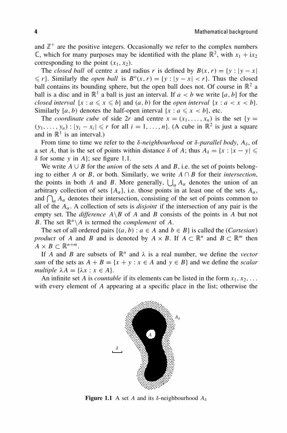
From time to time we refer to the δ-neighbourhood or δ-parallel body, Aδ , ofa set A, that is the set of points within distance δ of A; thus Aδ = {x : |x − y| �δ for some y in A}; see figure 1.1.
We write A ∪ B for the union of the sets A and B, i.e. the set of points belong-ing to either A or B, or both. Similarly, we write A ∩ B for their intersection,the points in both A and B. More generally,
⋃α Aα denotes the union of an
arbitrary collection of sets {Aα}, i.e. those points in at least one of the sets Aα ,and
⋂α Aα denotes their intersection, consisting of the set of points common to
all of the Aα . A collection of sets is disjoint if the intersection of any pair is theempty set. The difference A\B of A and B consists of the points in A but notB. The set �n\A is termed the complement of A.
The set of all ordered pairs {(a, b) : a ∈ A and b ∈ B} is called the (Cartesian)product of A and B and is denoted by A × B. If A ⊂ �n and B ⊂ �m thenA × B ⊂ �n+m.
If A and B are subsets of �n and λ is a real number, we define the vectorsum of the sets as A + B = {x + y : x ∈ A and y ∈ B} and we define the scalarmultiple λA = {λx : x ∈ A}.
An infinite set A is countable if its elements can be listed in the form x1, x2, . . .
with every element of A appearing at a specific place in the list; otherwise the
d
Ad
A
Figure 1.1 A set A and its δ-neighbourhood Aδ
Basic set theory 5
set is uncountable. The sets � and � are countable but � is uncountable. Notethat a countable union of countable sets is countable.
If A is any non-empty set of real numbers then the supremum sup A is theleast number m such that x � m for every x in A, or is ∞ if no such numberexists. Similarly, the infimum inf A is the greatest number m such that m � x forall x in A, or is −∞. Intuitively the supremum and infimum are thought of as themaximum and minimum of the set, though it is important to realize that sup A
and inf A need not be members of the set A itself. For example, sup(0, 1) = 1,but 1 /∈ (0, 1). We write supx∈B( ) for the supremum of the quantity in brackets,which may depend on x, as x ranges over the set B.
We define the diameter |A| of a (non-empty) subset of �n as the greatestdistance apart of pairs of points in A. Thus |A| = sup{|x − y| : x, y ∈ A}. In �n
a ball of radius r has diameter 2r , and a cube of side length δ has diameter δ√
n.A set A is bounded if it has finite diameter, or, equivalently, if A is containedin some (sufficiently large) ball.
Convergence of sequences is defined in the usual way. A sequence {xk} in�n converges to a point x of �n as k → ∞ if, given ε > 0, there exists anumber K such that |xk − x| < ε whenever k > K , that is if |xk − x| convergesto 0. The number x is called the limit of the sequence, and we write xk → x orlimk→∞ xk = x.
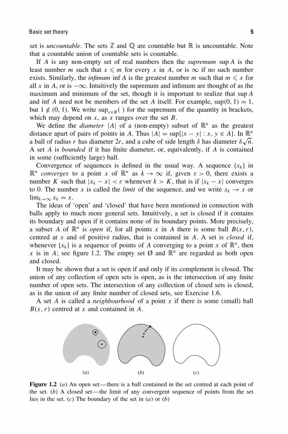
The ideas of ‘open’ and ‘closed’ that have been mentioned in connection withballs apply to much more general sets. Intuitively, a set is closed if it containsits boundary and open if it contains none of its boundary points. More precisely,a subset A of �n is open if, for all points x in A there is some ball B(x, r),centred at x and of positive radius, that is contained in A. A set is closed if,whenever {xk} is a sequence of points of A converging to a point x of �n, thenx is in A; see figure 1.2. The empty set Ø and �n are regarded as both openand closed.
It may be shown that a set is open if and only if its complement is closed. Theunion of any collection of open sets is open, as is the intersection of any finitenumber of open sets. The intersection of any collection of closed sets is closed,as is the union of any finite number of closed sets, see Exercise 1.6.
A set A is called a neighbourhood of a point x if there is some (small) ballB(x, r) centred at x and contained in A.
(a) (b) (c)
Figure 1.2 (a) An open set—there is a ball contained in the set centred at each point ofthe set. (b) A closed set—the limit of any convergent sequence of points from the setlies in the set. (c) The boundary of the set in (a) or (b)

6 Mathematical background
The intersection of all the closed sets containing a set A is called the closureof A, written A. The union of all the open sets contained in A is the interiorint(A) of A. The closure of A is thought of as the smallest closed set containingA, and the interior as the largest open set contained in A. The boundary ∂A of A
is given by ∂A = A\int(A), thus x ∈ ∂A if and only if the ball B(x, r) intersectsboth A and its complement for all r > 0.
A set B is a dense subset of A if B ⊂ A ⊂ B, i.e. if there are points of B
arbitrarily close to each point of A.A set A is compact if any collection of open sets which covers A (i.e. with
union containing A) has a finite subcollection which also covers A. Technically,compactness is an extremely useful property that enables infinite sets of condi-tions to be reduced to finitely many. However, as far as most of this book isconcerned, it is enough to take the definition of a compact subset of �n as onethat is both closed and bounded.
The intersection of any collection of compact sets is compact. It may be shownthat if A1 ⊃ A2 ⊃ · · · is a decreasing sequence of compact sets then the intersec-tion
⋂∞i=1 Ai is non-empty, see Exercise 1.7. Moreover, if
⋂∞i=1 Ai is contained
in V for some open set V , then the finite intersection⋂k
i=1 Ai is contained in V
for some k.A subset A of �n is connected if there do not exist open sets U and V such that
U ∪ V contains A with A ∩ U and A ∩ V disjoint and non-empty. Intuitively,we think of a set A as connected if it consists of just one ‘piece’. The largestconnected subset of A containing a point x is called the connected componentof x. The set A is totally disconnected if the connected component of each pointconsists of just that point. This will certainly be so if for every pair of points x
and y in A we can find disjoint open sets U and V such that x ∈ U, y ∈ V andA ⊂ U ∪ V .
There is one further class of set that must be mentioned though its precisedefinition is indirect and should not concern the reader unduly. The class of Borelsets is the smallest collection of subsets of �n with the following properties:
(a) every open set and every closed set is a Borel set;(b) the union of every finite or countable collection of Borel sets is a Borel
set, and the intersection of every finite or countable collection of Borelsets is a Borel set.
Throughout this book, virtually all of the subsets of �n that will be of anyinterest to us will be Borel sets. Any set that can be constructed using a sequenceof countable unions or intersections starting with the open sets or closed sets willcertainly be Borel. The reader will not go far wrong in work of the sort describedin this book by assuming that all the sets encountered are Borel sets.
1.2 Functions and limits
Let X and Y be any sets. A mapping, function or transformation f from X to Y
is a rule or formula that associates a point f (x) of Y with each point x of X.
Functions and limits 7
We write f : X → Y to denote this situation; X is called the domain of f andY is called the codomain. If A is any subset of X we write f (A) for the imageof A, given by {f (x) : x ∈ A}. If B is a subset of Y , we write f −1(B) for theinverse image or pre-image of B, i.e. the set {x ∈ X : f (x) ∈ B}; note that inthis context the inverse image of a single point can contain many points.
A function f : X → Y is called an injection or a one-to-one function iff (x) = f (y) whenever x = y, i.e. different elements of X are mapped to dif-ferent elements of Y . The function is called a surjection or an onto functionif, for every y in Y , there is an element x in X with f (x) = y, i.e. every ele-ment of Y is the image of some point in X. A function that is both an injectionand a surjection is called a bijection or one-to-one correspondence between X
and Y . If f : X → Y is a bijection then we may define the inverse functionf −1 : Y → X by taking f −1(y) as the unique element of X such that f (x) = y.In this situation, f −1(f (x)) = x for x in X and f (f −1(y)) = y for y in Y .
The composition of the functions f : X → Y and g : Y → Z is the func-tion g◦f : X → Z given by (g◦f )(x) = g(f (x)). This definition extends to thecomposition of any finite number of functions in the obvious way.
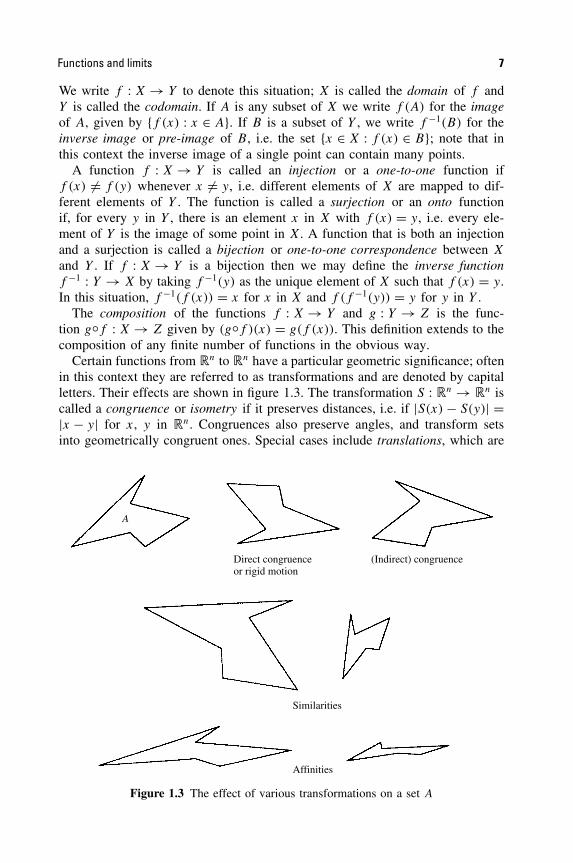
Certain functions from �n to �n have a particular geometric significance; oftenin this context they are referred to as transformations and are denoted by capitalletters. Their effects are shown in figure 1.3. The transformation S : �n → �n iscalled a congruence or isometry if it preserves distances, i.e. if |S(x) − S(y)| =|x − y| for x, y in �n. Congruences also preserve angles, and transform setsinto geometrically congruent ones. Special cases include translations, which are
A
Direct congruenceor rigid motion
(Indirect) congruence
Similarities
Affinities
Figure 1.3 The effect of various transformations on a set A

8 Mathematical background
of the form S(x) = x + a and have the effect of shifting points parallel to thevector a, rotations which have a centre a such that |S(x) − a| = |x − a| for allx (for convenience we also regard the identity transformation given by I (x) = x
as a rotation) and reflections which map points to their mirror images in some(n − 1)-dimensional plane. A congruence that may be achieved by a combinationof a rotation and a translation, i.e. does not involve reflection, is called a rigidmotion or direct congruence. A transformation S : �n → �n is a similarity ofratio or scale c > 0 if |S(x) − S(y)| = c|x − y| for all x, y in �n. A similaritytransforms sets into geometrically similar ones with all lengths multiplied by thefactor c.
A transformation T : �n → �n is linear if T (x + y) = T (x) + T (y) andT (λx) = λT (x) for all x, y ∈ �n and λ ∈ �; linear transformations may berepresented by matrices in the usual way. Such a linear transformation is non-singular if T (x) = 0 if and only if x = 0. If S : �n → �n is of the formS(x) = T (x) + a, where T is a non-singular linear transformation and a is apoint in �n, then S is called an affine transformation or an affinity. An affinitymay be thought of as a shearing transformation; its contracting or expanding effectneed not be the same in every direction. However, if T is orthonormal, then S
is a congruence, and if T is a scalar multiple or an orthonormal transformationthen T is a similarity.
It is worth pointing out that such classes of transformation form groups undercomposition of mappings. For example, the composition of two translations is atranslation, the identity transformation is trivially a translation, and the inverse ofa translation is a translation. Finally, the associative law S◦(T ◦U) = (S◦T )◦Uholds for all translations S, T , U . Similar group properties hold for the congru-ences, the rigid motions, the similarities and the affinities.
A function f : X → Y is called a Holder function of exponent α if
|f (x) − f (y)| � c|x − y|α (x, y ∈ X)
for some constant c � 0. The function f is called a Lipschitz function if α maybe taken to be equal to 1, that is if
|f (x) − f (y)| � c|x − y| (x, y ∈ X)
and a bi-Lipschitz function if
c1|x − y| � |f (x) − f (y)| � c2|x − y| (x, y ∈ X)
for 0 < c1 � c2 < ∞, in which case both f and f −1 : f (X) → X are Lipschitzfunctions.
We next remind readers of the basic ideas of limits and continuity of functions.Let X and Y be subsets of �n and �m respectively, let f : X → Y be a function,and let a be a point of X. We say that f (x) has limit y (or tends to y, or convergesto y) as x tends to a, if, given ε > 0, there exists δ > 0 such that |f (x) − y| < ε
for all x ∈ X with |x − a| < δ. We denote this by writing f (x) → y as x → a
Functions and limits 9
or by limx→a f (x) = y. For a function f : X → � we say that f (x) tends toinfinity (written f (x) → ∞) as x → a if, given M , there exists δ > 0 such thatf (x) > M whenever |x − a| < δ. The definition of f (x) → −∞ is similar.
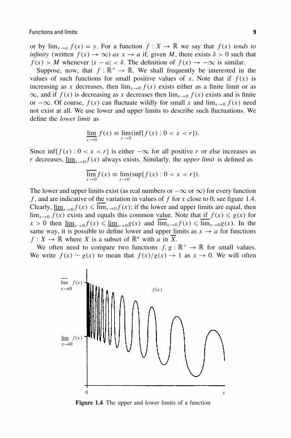
Suppose, now, that f : �+ → �. We shall frequently be interested in thevalues of such functions for small positive values of x. Note that if f (x) isincreasing as x decreases, then limx→0 f (x) exists either as a finite limit or as∞, and if f (x) is decreasing as x decreases then limx→0 f (x) exists and is finiteor −∞. Of course, f (x) can fluctuate wildly for small x and limx→0 f (x) neednot exist at all. We use lower and upper limits to describe such fluctuations. Wedefine the lower limit as
limx→0
f (x) ≡ limr→0
(inf{f (x) : 0 < x < r}).
Since inf{f (x) : 0 < x < r} is either −∞ for all positive r or else increases asr decreases, limx→0f (x) always exists. Similarly, the upper limit is defined as
limx→0
f (x) ≡ limr→0
(sup{f (x) : 0 < x < r}).
The lower and upper limits exist (as real numbers or −∞ or ∞) for every functionf , and are indicative of the variation in values of f for x close to 0; see figure 1.4.Clearly, limx→0f (x) � limx→0f (x); if the lower and upper limits are equal, thenlimx→0 f (x) exists and equals this common value. Note that if f (x) � g(x) forx > 0 then limx→0f (x) � limx→0g(x) and limx→0f (x) � limx→0g(x). In thesame way, it is possible to define lower and upper limits as x → a for functionsf : X → � where X is a subset of �n with a in X.
We often need to compare two functions f, g : �+ → � for small values.We write f (x) ∼ g(x) to mean that f (x)/g(x) → 1 as x → 0. We will often
f (x )f (x )
f (x )
0 x
limx→0
limx→0
Figure 1.4 The upper and lower limits of a function

10 Mathematical background
have that f (x) ∼ xs ; in other words that f obeys an approximate power law ofexponent s when x is small. We use the notation f (x) g(x) more loosely, tomean that f (x) and g(x) are approximately equal in some sense, to be specifiedin the particular circumstances.
Recall that function f : X → Y is continuous at a point a of X if f (x) → f (a)
as x → a, and is continuous on X if it is continuous at all points of X. Inparticular, Lipschitz and Holder mappings are continuous. If f : X → Y is acontinuous bijection with continuous inverse f −1 : Y → X then f is called ahomeomorphism, and X and Y are termed homeomorphic sets. Congruences,similarities and affine transformations on �n are examples of homeomorphisms.
The function f : � → � is differentiable at x with the number f ′(x) as deriva-tive if
limh→0
f (x + h) − f (x)
h= f ′(x).
In particular, the mean value theorem applies: given a < b and f differentiableon [a, b] there exists c with a < c < b such that
f (b) − f (a)
b − a= f ′(c)
(intuitively, any chord of the graph of f is parallel to the slope of f at some inter-mediate point). A function f is continuously differentiable if f ′(x) is continuousin x.
More generally, if f : �n → �n, we say that f is differentiable at x withderivative the linear mapping f ′(x) : �n → �n if
lim|h|→0
|f (x + h) − f (x) − f ′(x)h||h| = 0.
Occasionally, we shall be interested in the convergence of a sequence offunctions fk : X → Y where X and Y are subsets of Euclidean spaces. Wesay that functions fk converge pointwise to a function f : X → Y if fk(x) → f (x)
as k → ∞ for each x in X. We say that the convergence is uniform ifsupx∈X |fk(x) − f (x)| → 0 as k → ∞. Uniform convergence is a rather strongerproperty than pointwise convergence; the rate at which the limit is approachedis uniform across X. If the functions fk are continuous and converge uniformlyto f , then f is continuous.
Finally, we remark that logarithms will always be to base e. Recall that, fora, b > 0, we have that log ab = log a + log b, and that log ac = c log a for realnumbers c. The identity ac = bc log a/ log b will often be used. The logarithm is theinverse of the exponential function, so that elog x = x, for x > 0, and log ey = y
for y ∈ �.

Measures and mass distributions 11
1.3 Measures and mass distributions
Anyone studying the mathematics of fractals will not get far before encounteringmeasures in some form or other. Many people are put off by the seeminglytechnical nature of measure theory—often unnecessarily so, since for most fractalapplications only a few basic ideas are needed. Moreover, these ideas are oftenalready familiar in the guise of the mass or charge distributions encountered inbasic physics.
We need only be concerned with measures on subsets of �n. Basically ameasure is just a way of ascribing a numerical ‘size’ to sets, such that if a setis decomposed into a finite or countable number of pieces in a reasonable way,then the size of the whole is the sum of the sizes of the pieces.
We call µ a measure on �n if µ assigns a non-negative number, possibly ∞,to each subset of �n such that:
(a) µ(Ø) = 0; (1.1)(b) µ(A) � µ(B) if A ⊂ B; (1.2)(c) if A1, A2, . . . is a countable (or finite) sequence of sets then
µ
( ∞⋃
i=1
Ai
)
�∞∑
i=1
µ(Ai) (1.3)
with equality in (1.3), i.e.
µ
( ∞⋃
i=1
Ai
)
=∞∑
i=1
µ(Ai), (1.4)
if the Ai are disjoint Borel sets.We call µ(A) the measure of the set A, and think of µ(A) as the size of A
measured in some way. Condition (a) says that the empty set has zero measure,condition (b) says ‘the larger the set, the larger the measure’ and (c) says that ifa set is a union of a countable number of pieces (which may overlap) then thesum of the measure of the pieces is at least equal to the measure of the whole.If a set is decomposed into a countable number of disjoint Borel sets then thetotal measure of the pieces equals the measure of the whole.
Technical note. For the measures that we shall encounter, (1.4) generally holdsfor a much wider class of sets than just the Borel sets, in particular for allimages of Borel sets under continuous functions. However, for reasons that neednot concern us here, we cannot in general require that (1.4) holds for everycountable collection of disjoint sets Ai . The reader who is familiar with measuretheory will realize that our definition of a measure on �n is the definition ofwhat would normally be termed ‘an outer measure on �n for which the Borelsets are measurable’. However, to save frequent referral to ‘measurable sets’ it
12 Mathematical background
is convenient to have µ(A) defined for every set A, and, since we are usuallyinterested in measures of Borel sets, it is enough to have (1.4) holding for Borelsets rather than for a larger class. If µ is defined and satisfies (1.1)–(1.4) forthe Borel sets, the definition of µ may be extended to an outer measure on allsets in such a way that (1.1)–(1.3) hold, so our definition is consistent with theusual one.
If A ⊃ B then A may be expressed as a disjoint union A = B ∪ (A\B), so itis immediate from (1.4) that, if A and B are Borel sets,
µ(A\B) = µ(A) − µ(B). (1.5)
Similarly, if A1 ⊂ A2 ⊂ · · · is an increasing sequence of Borel sets then
limi→∞ µ(Ai) = µ
( ∞⋃
i=1
Ai
)
. (1.6)
To see this, note that⋃∞
i=1 Ai = A1 ∪ (A2\A1) ∪ (A3\A2) ∪ . . ., with this uniondisjoint, so that
µ
( ∞⋃
i=1
Ai
)
= µ(A1) +∞∑
i=1
(µ(Ai+1) − µ(Ai))
= µ(A1) + limk→∞
k∑
i=1
(µ(Ai+1) − µ(Ai))
= limk→∞
µ(Ak).
More generally, it can be shown that if, for δ > 0, Aδ are Borel sets that areincreasing as δ decreases, i.e. Aδ′ ⊂ Aδ for 0 < δ < δ′, then
limδ→0
µ(Aδ) = µ
(⋃
δ>0
Aδ
)
. (1.7)
We think of the support of a measure as the set on which the measure isconcentrated. Formally, the support of µ, written spt µ, is the smallest closed setX such that µ(�n\X) = 0. The support of a measure is always closed and x isin the support if and only if µ(B(x, r)) > 0 for all positive radii r . We say thatµ is a measure on a set A if A contains the support of µ.
A measure on a bounded subset of �n for which 0 < µ(�n) < ∞ will becalled a mass distribution, and we think of µ(A) as the mass of the set A. Weoften think of this intuitively: we take a finite mass and spread it in some wayacross a set X to get a mass distribution on X; the conditions for a measure willthen be satisfied.
Measures and mass distributions 13
We give some examples of measures and mass distributions. In general, weomit the proofs that measures with the stated properties exist. Much of technicalmeasure theory concerns the existence of such measures, but, as far as applica-tions go, their existence is intuitively reasonable, and can be taken on trust.
Example 1.1. The counting measure
For each subset A of �n let µ(A) be the number of points in A if A is finite,and ∞ otherwise. Then µ is a measure on �n.
Example 1.2. Point mass
Let a be a point in �n and define µ(A) to be 1 if A contains a, and 0 otherwise.Then µ is a mass distribution, thought of as a point mass concentrated at a.
Example 1.3. Lebesgue measure on �
Lebesgue measure L1 extends the idea of ‘length’ to a large collection of sub-sets of � that includes the Borel sets. For open and closed intervals, we takeL1(a, b) = L1[a, b] = b − a. If A = ⋃
i[ai, bi] is a finite or countable union ofdisjoint intervals, we let L1(A) = ∑
(bi − ai) be the length of A thought of as thesum of the length of the intervals. This leads us to the definition of the Lebesguemeasure L1(A) of an arbitrary set A. We define
L1(A) = inf
{ ∞∑
i=1
(bi − ai) : A ⊂∞⋃
i=1
[ai, bi]
}
,
that is, we look at all coverings of A by countable collections of intervals, andtake the smallest total interval length possible. It is not hard to see that (1.1)–(1.3)hold; it is rather harder to show that (1.4) holds for disjoint Borel sets Ai , andwe avoid this question here. (In fact, (1.4) holds for a much larger class of setsthan the Borel sets, ‘the Lebesgue measurable sets’, but not for all subsets of �.)Lebesgue measure on � is generally thought of as ‘length’, and we often writelength (A) for L1(A) when we wish to emphasize this intuitive meaning.
Example 1.4. Lebesgue measure on �n
If A = {(x1, . . . , xn) ∈ �n : ai � xi � bi} is a ‘coordinate parallelepiped’ in �n,the n-dimensional volume of A is given by
voln(A) = (b1 − a1)(b2 − a2) · · · (bn − an).
(Of course, vol1 is length, as in Example 1.3, vol2 is area and vol3 is the usual 3-dimensional volume.) Then n-dimensional Lebesgue measure Ln may be thought
14 Mathematical background
of as the extension of n-dimensional volume to a large class of sets. Just as inExample 1.3, we obtain a measure on �n by defining
Ln(A) = inf
{ ∞∑
i=1
voln(Ai) : A ⊂∞⋃
i=1
Ai
}
where the infimum is taken over all coverings of A by coordinate parallelepipedsAi . We get that Ln(A) = voln(A) if A is a coordinate parallelepiped or, indeed,any set for which the volume can be determined by the usual rules of mensuration.Again, to aid intuition, we sometimes write area (A) in place of L2(A), vol(A)for L3(A) and voln(A) for Ln(A).
Sometimes, we need to define ‘k-dimensional’ volume on a k-dimensionalplane X in �n; this may be done by identifying X with �k and using Lk onsubsets of X in the obvious way.
Example 1.5. Uniform mass distribution on a line segment
Let L be a line segment of unit length in the plane. Define µ(A) = L1(L ∩ A)
i.e. the ‘length’ of intersection of A with L. Then µ is a mass distribution withsupport L, since µ(A) = 0 if A ∩ L = Ø. We may think of µ as unit mass spreadevenly along the line segment L.
Example 1.6. Restriction of a measure
Let µ be a measure on �n and E a Borel subset of �n. We may define a measureν on �n, called the restriction of µ to E, by ν(A) = µ(E ∩ A) for every set A.Then ν is a measure on �n with support contained in E.
As far as this book is concerned, the most important measures we shall meet arethe s-dimensional Hausdorff measures Hs on subsets of �n, where 0 � s � n.These measures, which are introduced in Section 2.1, are a generalization ofLebesgue measures to dimensions that are not necessarily integral.
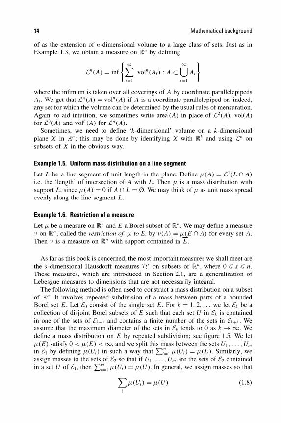
The following method is often used to construct a mass distribution on a subsetof �n. It involves repeated subdivision of a mass between parts of a boundedBorel set E. Let E0 consist of the single set E. For k = 1, 2, . . . we let Ek be acollection of disjoint Borel subsets of E such that each set U in Ek is containedin one of the sets of Ek−1 and contains a finite number of the sets in Ek+1. Weassume that the maximum diameter of the sets in Ek tends to 0 as k → ∞. Wedefine a mass distribution on E by repeated subdivision; see figure 1.5. We letµ(E) satisfy 0 < µ(E) < ∞, and we split this mass between the sets U1, . . . , Um
in E1 by defining µ(Ui) in such a way that∑m
i=1 µ(Ui) = µ(E). Similarly, weassign masses to the sets of E2 so that if U1, . . . , Um are the sets of E2 containedin a set U of E1, then
∑mi=1 µ(Ui) = µ(U). In general, we assign masses so that
∑
i
µ(Ui) = µ(U) (1.8)

Measures and mass distributions 15
U
E0
E1
E2U1 U2
Figure 1.5 Steps in the construction of a mass distribution µ by repeated subdivision.The mass on the sets of Ek is divided between the sets of Ek+1; so, for example,µ(U) = µ(U1) + µ(U2)
for each set U of Ek, where the {Ui} are the disjoint sets in Ek+1 contained in U .For each k, we let Ek be the union of the sets in Ek, and we define µ(A) = 0 forall A with A ∩ Ek = Ø.
Let E denote the collection of sets that belong to Ek for some k together withthe subsets of �n\Ek. The above procedure defines the mass µ(A) of every set A
in E, and it should seem reasonable that, by building up sets from the sets in E, itspecifies enough about the distribution of the mass µ across E to determine µ(A)
for any (Borel) set A. This is indeed the case, as the following proposition states.
Proposition 1.7
Let µ be defined on a collection of sets E as above. Then the definition of µ
may be extended to all subsets of �n so that µ becomes a measure. The value ofµ(A) is uniquely determined if A is a Borel set. The support of µ is contained in⋂∞
k=1 Ek .
Note on Proof. If A is any subset of �n, let
µ(A) = inf
{∑
i
µ(Ui) : A ⊂⋃
i
Ui and Ui ∈ E}
. (1.9)
16 Mathematical background
(Thus we take the smallest value we can of∑∞
i=1 µ(Ui) where the sets Ui are inE and cover A; we have already defined µ(Ui) for such Ui .) It is not difficult tosee that if A is one of the sets in E, then (1.9) reduces to the mass µ(A) specifiedin the construction. The complete proof that µ satisfies all the conditions of ameasure and that its values on the sets of E determine its values on the Borelsets is quite involved, and need not concern us here. Since µ(�n\Ek) = 0, wehave µ(A) = 0 if A is an open set that does not intersect Ek for some k, so thesupport of µ is in Ek for all k. �
Example 1.8Let Ek denote the collection of ‘binary intervals’ of length 2−k of the form[r2−k, (r + 1)2−k) where 0 � r � 2k − 1. If we take µ[r2−k, (r + 1)2−k) = 2−k
in the above construction, we get that µ is Lebesgue measure on [0, 1].
Note on calculation. Clearly, if I is an interval in Ek of length 2−k and I1, I2 arethe two subintervals of I in Ek+1 of length 2−k−1, we have µ(I) = µ(I1) + µ(I2)
which is (1.8). By Proposition 1.7 µ extends to a mass distribution on [0, 1]. Wehave µ(I) = length (I ) for I in E, and it may be shown that this implies that µ
coincides with Lebesgue measure on any set. �
We say that a property holds for almost all x, or almost everywhere (withrespect to a measure µ) if the set for which the property fails has µ-measurezero. For example, we might say that almost all real numbers are irrational withrespect to Lebesgue measure. The rational numbers � are countable; they maybe listed as x1, x2, . . ., say, so that L1(�) = ∑∞
i=1 L1{xi} = 0.Although we shall usually be interested in measures in their own right, we
shall sometimes need to integrate functions with respect to measures. There aretechnical difficulties concerning which functions can be integrated. We may getaround these difficulties by assuming that, for f : D → � a function defined ona Borel subset D of �n, the set f −1(−∞, a] = {x ∈ D : f (x) � a} is a Borelset for all real numbers a. A very large class of functions satisfies this condition,including all continuous functions (for which f −1(−∞, a] is closed and thereforea Borel set). We make the assumption throughout this book that all functions tobe integrated satisfy this condition; certainly this is true of functions that arelikely to be encountered in practice.
To define integration we first suppose that f : D → � is a simple function,i.e. one that takes only finitely many values a1, . . . , ak. We define the integralwith respect to the measure µ of a non-negative simple function f as
∫f dµ =
k∑
i=1
aiµ{x : f (x) = ai}.
The integral of more general functions is defined using approximation by simplefunctions. If f : D → � is a non-negative function, we define its integral as
∫f dµ = sup
{∫g dµ : g is simple, 0 � g � f
}.

Notes on probability theory 17
To complete the definition, if f takes both positive and negative values, welet f+(x) = max{f (x), 0} and f−(x) = max{−f (x), 0}, so that f = f+ − f−,and define ∫
f dµ =∫
f+dµ −∫
f− dµ
provided that∫
f+ dµ and∫
f− dµ are both finite.All the usual properties hold for integrals, for example,
∫(f + g)dµ =
∫f dµ +
∫g dµ
and ∫λf dµ = λ
∫f dµ
if λ is a scalar. We also have the monotone convergence theorem, that iffk : D → � is an increasing sequence of non-negative functions converging(pointwise) to f , then
limk→∞
∫fkdµ =
∫f dµ.
If A is a Borel subset of D, we define integration over the set A by
∫
A
f dµ =∫
f χAdµ
where χA : �n → � is the ‘indicator function’ such that χA(x) = 1 if x is in A
and χA(x) = 0 otherwise.Note that, if f (x) � 0 and
∫f dµ = 0, then f (x) = 0 for µ-almost all x.
As usual, integration is denoted in various ways, such as∫
f dµ,∫
f or∫f (x)dµ(x), depending on the emphasis required. When µ is n-dimensional
Lebesgue measure Ln, we usually write∫
f dx or∫
f (x)dx in place of∫
f dLn.On a couple of occasions we shall need to use Egoroff’s theorem. Let D be
a Borel subset of �n and µ a measure with µ(D) < ∞. Let f1, f2, . . . and f
be functions from D to � such that fk(x) → f (x) for each x in D. Egoroff’stheorem states that for any δ > 0, there is a Borel subset E of D such thatµ(D\E) < δ and such that the sequence {fk} converges uniformly to f on E,i.e. with supx∈E |fk(x) − f (x)| → 0 as k → ∞. For the measures that we shallbe concerned with, it may be shown that we can always take the set E tobe compact.
1.4 Notes on probability theory
For an understanding of some of the later chapters of the book, a basic knowledgeof probability theory is necessary. We give a brief survey of the concepts needed.
18 Mathematical background
Probability theory starts with the idea of an experiment or trial ; that is, anaction whose outcome is, for all practical purposes, not predetermined. Mathe-matically, such an experiment is described by a probability space, which has threecomponents: the set of all possible outcomes of the experiment, the list of all theevents that may occur as consequences of the experiment, and an assessment oflikelihood of these events. For example, if a die is thrown, the possible outcomesare {1, 2, 3, 4, 5, 6}, the list of events includes ‘a 3 is thrown’, ‘an even numberis thrown’, and ‘at least a 4 is thrown’. For a ‘fair die’ it may be reasonable toassess the six possible outcomes as equally likely.
The set of all possible outcomes of an experiment is called the sample space,denoted by �. Questions of interest concerning the outcome of an experimentcan always be phrased in terms of subsets of �; in the above example ‘is anodd number thrown?’ asks ‘is the outcome in the subset {1, 3, 5}?’ Associat-ing events dependent on the outcome of the experiment with subsets of � inthis way, it is natural to think of the union A ∪ B as ‘either A or B occurs’,the intersection A ∩ B as ‘both A and B occur’, and the complement �\A asthe event ‘A does not occur’, for any events A and B. In general, there is acollection F of subsets of � that particularly interest us, which we call events.In the example of the die, F would normally be the collection of all subsetsof �, but in more complicated situations a relatively small collection of sub-sets might be relevant. Usually, F satisfies certain conditions; for example, ifthe occurrence of an event interests us, then so does its non-occurrence, soif A is in F, we would expect the complement �\A also to be in F. Wecall a (non-empty) collection F of subsets of the sample space � an eventspace if
�\A ∈ F whenever A ∈ F (1.10)
and∞⋃
i=1
Ai ∈ F whenever Ai ∈ F (1 � i < ∞). (1.11)
It follows from these conditions that Ø and � are in F, and that A\B and⋂∞i=1 Ai are in F whenever A, B and Ai are in F. As far as our applications
are concerned, we do not, in general, specify F precisely—this avoids technicaldifficulties connected with the existence of suitable event spaces.
Next, we associate probabilities with the events of F, with P(A) thought of asthe probability, or likelihood, that the event A occurs. We call P a probabilityor probability measure if P assigns a number P(A) to each A in F, such that thefollowing conditions hold:
0 � P(A) � 1 for all A ∈ F (1.12)
P(Ø) = 0 and P(�) = 1 (1.13)
Notes on probability theory 19
and, if A1, A2, . . . are disjoint events in F,
P
( ∞⋃
i=1
Ai
)
=∞∑
i=1
P(Ai). (1.14)
It should seem natural for any definition of probability to satisfy these conditions.We call a triple (�,F, P) a probability space if F is an event space of subsets
of � and P is a probability measure defined on the sets of F.For the die-throwing experiment we might have � = {1, 2, 3, 4, 5, 6} with the
event space consisting of all subsets of �, and with P(A) = 16 × number of ele-
ments in A. This describes the ‘fair die’ situation with each outcome equallylikely.
Often, � is an infinite set. For example we might have � = [0, 1] and thinkof a random number drawn from [0, 1] with the probability of the number in aset A as P(A) = length (A). Here the event space might be the Borel subsets of[0, 1].
The resemblance of the definition of probability to the definition of a measurein (1.1)–(1.4) and the use of the term probability measure is no coincidence. Prob-abilities and measures may be put into the same context, with � correspondingto �n and with the event space corresponding to the Borel sets.
In our applications later on in the book, we shall be particularly interested inevents (on rather large sample spaces) that are virtually certain to occur. We saythat an event A occurs with probability 1 or almost surely if P(A) = 1.
Sometimes, we may possess partial information about the outcome of an exper-iment; for example, we might be told that the number showing on the die is even.This leads us to reassess the probabilities of the various events. If A and B are inF with P(B) > 0, the conditional probability of A given B, denoted by P(A|B),is defined by
P(A|B) = P(A ∩ B)
P(B). (1.15)
This is thought of as the probability of A given that the event B is known tooccur; as would be expected P(B|B) = 1. It is easy to show that (�,F, P′) is aprobability space, where P′(A) = P(A|B). We also have the partition formula: ifB1, B2, . . . are disjoint events with
⋃i Bi = � and P(Bi) > 0 for all i, then, for
an event A,P(A) =
∑
i
P(A|Bi)P(Bi). (1.16)
In the case of the ‘fair die’ experiment, if B1 is the event ‘an even number isthrown’, B2 is ‘an odd number is thrown’ and A is ‘at least 4 is thrown’, then
P(A|B1) = P(4 or 6 is thrown)/P(2, 4 or 6 is thrown) = 26/ 3
6 = 23 .
P(A|B2) = P(5 is thrown)/P(1, 3 or 5 is thrown) = 16/ 3
6 = 13
from which (1.16) is easily verified.
20 Mathematical background
We think of two events as independent if the occurrence of one does not affectthe probability that the other occurs, i.e. if P(A|B) = P(A) and P(B|A) = P(B).Using (1.15), we are led to make the definition that two events A and B in aprobability space are independent if
P(A ∩ B) = P(A)P(B). (1.17)
More generally, an arbitrary collection of events is independent if for every finitesubcollection {Ak : k ∈ J } we have
P
(⋂
k∈J
Ak
)
=∏
k∈J
P(Ak). (1.18)
In the die example, it is easy to see that ‘a throw of at least 5’ and ‘an evennumber is thrown’ are independent events, but ‘a throw of at least 4’ and ‘aneven number is thrown’ are not.
The idea of a random variable and its expectation (or average or mean) isfundamental to probability theory. Essentially, a random variable X is a real-valued function on a sample space. In the die example, X might represent thescore on the die. Alternatively it might represent the reward for throwing aparticular number, for example X(ω) = 0 if ω = 1, 2, 3, or 4, X(5) = 1 andX(6) = 2. The outcome of an experiment determines a value of the randomvariable. The expectation of the random variable is the average of these valuesweighted according to the likelihood of each outcome.
The precise definition of a random variable requires a little care. We say that X
is a random variable on a probability space (�,F, P) if X : � → � is a functionsuch that X−1((−∞, a]) is an event in F for each real number a; in other words,the set of ω in � with X(ω) � a is in the event space. This condition is equivalentto saying that X−1(E) is in F for any Borel set E. In particular, for any such E theprobability that the random variable X takes a value in E, i.e. P({ω : X(ω) ∈ E}),is defined. It may be shown that P({ω : X(ω) ∈ E}) is determined for all Borelsets E from a knowledge of P({ω : X(ω) � a}) for each real number a. Note thatit is usual to abbreviate expressions such as P({ω : X(ω) ∈ E}) to P(X ∈ E).
It is not difficult to show that if X and Y are random variables on (�,F, P)
and λ is a real number, then X + Y,X − Y, XY and λX are all random variables(these are defined in the obvious way, for example (X + Y )(ω) = X(ω) + Y (ω)
for each ω ∈ �). Moreover, if X1, X2, . . . is a sequence of random variables withXk(ω) increasing and bounded for each ω, then limk→∞ Xk is a random variable.
A collection of random variables {Xk} is independent if, for any Borel setsEk, the events {(X ∈ Ek)} are independent in the sense of (1.18); that is if, forevery finite set of indices J ,
P(Xk ∈ Ek for all k ∈ J ) =∏
k∈J
P(Xk ∈ Ek).
Notes on probability theory 21
Intuitively, X and Y are independent if the probability of Y taking any par-ticular value is unaffected by a knowledge of the value of X. Consider theprobability space representing two successive throws of a die, with sample space{(x, y) : x, y = 1, 2, . . . , 6} and probability measure P defined by P{(x, y)} = 1
36for each pair (x, y). If X and Y are the random variables given by the scoreson successive throws, then X and Y are independent, modelling the assumptionthat one throw does not affect the other. However, X and X + Y are not inde-pendent—this reflects that the bigger the score for the first throw, the greater thechance of a high total score.
The formal definition of the expectation of a random variable is analogousto the definition of the integral of a function; indeed, expectation is really theintegral of the random variable with respect to the probability measure. Let X bea random variable on a probability space (�,F, P). First suppose that X(ω) � 0for all ω in � and that X takes only finitely many values x1, . . . , xk; we call sucha random variable simple. We define the expectation, mean or average E(X) ofX as
E(X) =k∑
i=1
xiP(X = xi). (1.19)
The expectation of an arbitrary random variable is defined using approximationby simple random variables. Thus for a non-negative random variable X
E(X) = sup{E(Y ) : Y is a simple random variable
with 0 � Y (ω) � X(ω) for all ω ∈ �}.Lastly, if X takes both positive and negative values, we let X+ = max{X, 0} andX− = max{−X, 0}, so that X = X+ − X−, and define
E(X) = E(X+) − E(X−)
provided that both E(X+) < ∞ and E(X−) < ∞.The random variable X representing the score of a fair die is a simple random
variable, since X(ω) takes just the values 1, . . . , 6. Thus
E(X) =6∑
i=1
i × 16 = 3 1
2 .
Expectation satisfies certain basic properties, analogous to those for the inte-gral. If X1, X2, . . . are random variables then
E(X1 + X2) = E(X1) + E(X2)
and, more generally,
E
(k∑
i=1
Xi
)
=k∑
i=1
E(Xi).
22 Mathematical background
If λ is a constantE(λX) = λE(X)
and if the sequence of non-negative random variables X1, X2, . . . is increasingwith X = limk→∞ Xk a (finite) random variable, then
limk→∞ E(Xk) = E(X).
Provided that X1 and X2 are independent, we also have
E(X1X2) = E(X1)E(X2).
Thus if Xi represents that kth throw of a fair die in a sequence of throws,the expectation of the sum of the first k throws is E(X1 + · · · + Xk) = E(X1) +· · · + E(Xk) = 3 1
2 × k.We define the conditional expectation E(X|B) of X given an event B with
P(B) > 0 in a similar way, but starting with
E(X|B) =k∑
i=1
xiP(X = xi |B) (1.20)
in place of (1.19). We get a partition formula resembling (1.16)
E(X) =∑
i
E(X|Bi)P(Bi) (1.21)
where B1, B2, . . . are disjoint events with⋃
i Bi = � and P(Bi) > 0.It is often useful to have an indication of the fluctuation of a random variable
across a sample space. Thus we introduce the variance of the random variableX as
var(X) = E((X − E(X))2)
= E(X2) − E(X)2
by a simple calculation. Using the properties of expectation, we get
var(λX) = λ2 var(X)
for any real number λ, and
var(X + Y ) = var(X) + var(Y )
provided that X and Y are independent.
Notes on probability theory 23
If the probability distribution of a random variable is given by an integral, i.e.
P(X � x) =∫ x
−∞f (u)du (1.22)
the function f is called the probability density function for X. It may be shownfrom the definition of expectation that
E(X) =∫ ∞
−∞uf (u)du
and
E(X2) =∫ ∞
−∞u2f (u)du
which allows var(X) = E(X2) − E(X)2 to be calculated.Note that the density function tells us about the distribution of the random
variable X without reference to the underlying probability space, which, formany purposes, is irrelevant. We may express the probability that X belongs toany Borel set E in terms of the density function as
P(X ∈ E) =∫
E
f (u)du.
We say that a random variable X has uniform distribution on the interval[a, b] if
P(X � x) = 1
b − a
∫ x
a
du (a < x < b). (1.23)
Thus the probability of X lying in a subinterval of [a, b] is proportional to thelength of the interval. In this case, we get that E(X) = 1
2 (a + b) and var(X) =1
12 (b − a)2.A random variable X has normal or Gaussian distribution of mean m and
variance σ 2 if
P(X � x) = 1
σ√
2π
∫ x
−∞exp
(−(u − m)2
2σ 2
)du. (1.24)
It may be verified by integration that E(X) = m and var(X) = σ 2. If X1 and X2
are independent normally distributed random variables of means m1 and m2 andvariances σ 2
1 and σ 22 respectively, then X1 + X2 is normal with mean m1 + m2
and variance σ 21 + σ 2
2 , and λX1 is normal with mean λm1 and variance λ2σ 21 , for
any real number λ.If we throw a fair die a large number of times, we might expect the average
score thrown to be very close to 3 12 , the expectation or mean outcome of each
throw. Moreover, the larger the number of throws, the closer the average should
24 Mathematical background
be to the mean. This ‘law of averages’ is made precise as the strong law oflarge numbers.
Let (�,F, P) be a probability space. Let X1,X2, . . . be random variables thatare independent and that have identical distribution (i.e. for every set E, P(Xi ∈ E)
is the same for all i), with expectation m and variance σ 2, both assumed finite.For each k we may form the random variable Sk = X1 + · · · + Xk , so that therandom variable (1/k)Sk is the average of the first k trials. The strong law oflarge numbers states that, with probability 1,
limk→∞
1
kSk = m. (1.25)
We can also say a surprising amount about the distribution of the randomvariable Sk when k is large. It may be shown that Sk has approximately thenormal distribution with mean km and variance kσ 2. This is the content of thecentral limit theorem, which states that, for every real number x,
P(
Sk − km
σ√
k� x
)→
∫ x
−∞1√2π
exp(− 12u2)du as k → ∞. (1.26)
An important aspect of the normal distribution now becomes clear—it is the formof distribution approached by sums of a large number of independent identicallydistributed random variables.
We may apply these results to the experiment consisting of an infinite sequenceof die throws. Let � be the set of all infinite sequences {ω = (ω1, ω2, . . .) :ωi = 1, 2, . . . , 6} (we think of ωi as the outcome of the kth throw). It is possibleto define an event space F and probability measure P in such a way that for anygiven k and sequence ω1, . . . , ωk (ωi = 1, 2, . . . , 6), the event ‘the first k throwsare ω1, . . . , ωk’ is in F and has probability ( 1
6 )−k . Let Xk be the random variablegiven by the outcome of the kth throw, so that Xk(ω) = ωk . It is easy to seethat the Xk are independent and identically distributed, with mean m = 3 1
2 andvariance 2 11
12 . The strong law of large numbers tells us that, with probability 1, theaverage of the first k throws, Sk/k converges to 3 1
2 as k tends to infinity, and thecentral limit theorem tells us that, when k is large, the sum Sk is approximatelynormally distributed, with mean 3 1
2 × k and variance 2 1112 × k. Thus if we repeat
the experiment of throwing k dice a large number of times, the sum of the k
throws will have a distribution close to the normal distribution, in the senseof (1.26).
1.5 Notes and references
The material outlined in this chapter is covered at various levels of sophisticationin numerous undergraduate mathematical texts. Almost any book on mathematicalanalysis, for example Rudin (1964) or Apostol (1974), contains the basic theoryof sets and functions. A thorough treatment of measure and probability theory
Exercises 25
may be found in Kingman and Taylor (1966), Billingsley (1995) and Edgar(1998). For probability theory, the book by Grimmett and Stirzaker (1992) maybe found helpful.
Exercises
The following exercises do no more than emphasize some of the many facts that havebeen mentioned in this chapter.
1.1 Verify that for x, y, z ∈ �n, (i) |x + y| � |x| + |y|, (ii) |x − y| �∣∣∣|x| − |y|
∣∣∣,
(iii) |x − y| � |x − z| + |z − y|.1.2 Show from the definition of δ-neighbourhood that Aδ+δ′ = (Aδ)δ′ .
1.3 Show that a (non-empty) set is bounded if and only if it is contained in some ballB(0, r) with centre the origin.
1.4 Determine which of the following sets are open and which are closed. In eachcase determine the interior and closure of the set. (i) A non-empty finite set A,(ii) the interval (0, 1), (iii) the interval [0, 1], (iv) the interval [0, 1), (v) the set{0, 1, 1
2 , 13 , 1
4 , . . .}.1.5 Show that the middle third Cantor set, figure 0.1, is compact and totally discon-
nected. What is its interior, closure and boundary?
1.6 Show that the union of any collection of open subsets of �n is open and that theintersection of any finite collection of open sets is open. Show that a subset of �n
is closed if and only if its complement is open and hence deduce the correspondingresult for unions and intersections of closed sets.
1.7 Show that if A1 ⊃ A2 ⊃ · · · is a decreasing sequence of non-empty compact subsetsof �n then
⋂∞k=1 Ak is a non-empty compact set.
1.8 Show that the half-open interval {x ∈ � : 0 � x < 1} is a Borel subset of �.
1.9 Let F be the set of numbers in [0, 1] whose decimal expansions contain the digit 5infinitely many times. Show that F is a Borel set.
1.10 Show that the coordinate transformation of the plane
(x1x2
)�→
(c cos θ −c sin θc sin θ c cos θ
)(x1x2
)+
(a1a2
)
is a similarity of ratio c, and describe the transformation geometrically.
1.11 Find limx→0f (x) and limx→0f (x) where f : �+ → � is given by: (i) sin(x);(ii) sin(1/x); (iii) x2 + (3 + x) sin(1/x).
1.12 Let f, g : [0, 1] → � be Lipschitz functions. Show that the functions defined on[0, 1] by f (x) + g(x) and f (x)g(x) are also Lipschitz.
1.13 Let f : � → � be differentiable with |f ′(x)| � c for all x. Show, using the meanvalue theorem, that f is a Lipschitz function.
1.14 Show that every Lipschitz function f : � → � is continuous.
1.15 Let f : � → � be given by f (x) = x2 + x. Find (i) f −1(2), (ii) f −1(−2),(iii) f −1([2, 6]).

26 Mathematical background
1.16 Show that f (x) = x2 is Lipschitz on [0, 2], bi-Lipschitz on [1, 2], and not Lipschitzon �.
1.17 Show that if E is a compact subset of �n and f : E → �n is continuous, then f (E)
is compact.
1.18 Let A1, A2, . . ., be a decreasing sequence of Borel subsets of �n and let A =⋂∞k=1 Ak . If µ is a measure on �n with µ(A1) < ∞, show using (1.6) that µ(Ak) →
µ(A) as k → ∞.
1.19 Show that the point mass concentrated at a (see Example 1.2) is a measure.
1.20 Show how to define a mass distribution on the middle third Cantor set, figure 0.1,in as uniform a way as possible.
1.21 Verify that Lebesgue measure satisfies (1.1), (1.2) and (1.3).
1.22 Let f : [0, 1] → � be a continuous function. For A a subset of �2 define µ(A) =L{x : (x, f (x)) ∈ A}, where L is Lebesgue measure. Show that µ is a mass distri-bution on �2 supported by the graph of f .
1.23 Let D be a Borel subset of �n and let µ be a measure on D with µ(D) < ∞. Letfk : D → � be a sequence of functions such that fk(x) → f (x) for all x in D.Prove Egoroff’s theorem: that given ε > 0 there exists a Borel subset A of D withµ(D\A) < ε such that fk(x) converges to f (x) uniformly for x in A.
1.24 Prove that if µ is a measure on D and f : D → � satisfies f (x) � 0 for all x inD and
∫D
f dµ = 0 then f (x) = 0 for µ-almost all x.
1.25 If X is a random variable show that E((X − E(X))2) = E(X2) − E(X)2 (these num-bers equalling the variance of X).
1.26 Verify that if X has the uniform distribution on [a, b] (see (1.23)) then E(X) =12 (a + b) and var(X) = (b − a)2/12.
1.27 Let A1, A2, . . . be a sequence of independent events in some probability space suchthat P(Ak) = p for all k, where 0 < p < 1. Let Nk be the random variable definedby taking Nk(ω) to equal the number of i with 1 � i � k for which ω ∈ Ai . Usethe strong law of large numbers to show that, with probability 1, Nk/k → p ask → ∞. Deduce that the proportion of successes in a sequence of independent trialsconverges to the probability of success of each trial.
1.28 A fair die is thrown 6000 times. Use the central limit theorem to estimate theprobability that at least 1050 sixes are thrown. (A numerical method will be neededif the integral obtained is to be evaluated.)
Chapter 2 Hausdorff measureand dimension
The notion of dimension is central to fractal geometry. Roughly, dimension indi-cates how much space a set occupies near to each of its points. Of the wide varietyof ‘fractal dimensions’ in use, the definition of Hausdorff, based on a construc-tion of Caratheodory, is the oldest and probably the most important. Hausdorffdimension has the advantage of being defined for any set, and is mathematicallyconvenient, as it is based on measures, which are relatively easy to manipulate.A major disadvantage is that in many cases it is hard to calculate or to estimateby computational methods. However, for an understanding of the mathematicsof fractals, familiarity with Hausdorff measure and dimension is essential.
2.1 Hausdorff measure
Recall that if U is any non-empty subset of n-dimensional Euclidean space, �n,the diameter of U is defined as |U | = sup{|x − y| : x, y ∈ U }, i.e. the greatestdistance apart of any pair of points in U . If {Ui} is a countable (or finite) collectionof sets of diameter at most δ that cover F , i.e. F ⊂ ⋃∞
i=1 Ui with 0 � |Ui | � δ
for each i, we say that {Ui} is a δ-cover of F .Suppose that F is a subset of �n and s is a non-negative number. For any
δ > 0 we define
Hsδ(F ) = inf
{ ∞∑
i=1
|Ui|s : {Ui} is a δ-cover of F
}
. (2.1)
Thus we look at all covers of F by sets of diameter at most δ and seek to minimizethe sum of the sth powers of the diameters (figure 2.1). As δ decreases, the classof permissible covers of F in (2.1) is reduced. Therefore, the infimum Hs
δ(F )
increases, and so approaches a limit as δ → 0. We write
Hs(F ) = limδ→0
Hsδ(F ). (2.2)
27
Fractal Geometry: Mathematical Foundations and Application. Second Edition Kenneth Falconer 2003 John Wiley & Sons, Ltd ISBNs: 0-470-84861-8 (HB); 0-470-84862-6 (PB)

28 Hausdorff measure and dimension
F
d
Figure 2.1 A set F and two possible δ-covers for F . The infimum of �|Ui |s over allsuch δ-covers {Ui} gives Hs
δ(F )
This limit exists for any subset F of �n, though the limiting value can be(and usually is) 0 or ∞. We call Hs(F ) the s-dimensional Hausdorff measureof F .
With a certain amount of effort, Hs may be shown to be a measure; seesection 1.3. It is straightforward to show that Hs(Ø) = 0, that if E is con-tained in F then Hs(E) � Hs(F ), and that if {Fi} is any countable collection ofsets, then
Hs
( ∞⋃
i=1
Fi
)
�∞∑
i=1
Hs(Fi). (2.3)
It is rather harder to show that there is equality in (2.3) if the {Fi} are disjointBorel sets.
Hausdorff measures generalize the familiar ideas of length, area, volume,etc. It may be shown that, for subsets of �n, n-dimensional Hausdorff mea-sure is, to within a constant multiple, just n-dimensional Lebesgue measure,i.e. the usual n-dimensional volume. More precisely, if F is a Borel subset of�n, then
Hn(F ) = c−1n voln(F ) (2.4)
where cn is the volume of an n-dimensional ball of diameter 1, so that cn =πn/2/2n(n/2)! if n is even and cn = π(n−1)/2((n − 1)/2)!/n! if n is odd. Similarly,

Hausdorff measure 29
Length × l
Area × l2
Hs × ls
Figure 2.2 Scaling sets by a factor λ increases length by a factor λ, area by a factor λ2,and s-dimensional Hausdorff measure by a factor λs
for ‘nice’ lower-dimensional subsets of �n, we have that H0(F ) is the numberof points in F ; H1(F ) gives the length of a smooth curve F ; H2(F ) = (4/π) ×area (F ) if F is a smooth surface; H3(F ) = (6/π) × vol(F ); and Hm(F ) =c−1m × volm(F ) if F is a smooth m-dimensional submanifold of �n (i.e. an m-
dimensional surface in the classical sense).The scaling properties of length, area and volume are well known. On magni-
fication by a factor λ, the length of a curve is multiplied by λ, the area of a planeregion is multiplied by λ2 and the volume of a 3-dimensional object is multipliedby λ3. As might be anticipated, s-dimensional Hausdorff measure scales witha factor λs (figure 2.2). Such scaling properties are fundamental to the theoryof fractals.
Scaling property 2.1
Let S be a similarity transformation of scale factor λ > 0. If F ⊂ �n, then
Hs(S(F )) = λsHs(F ). (2.5)

30 Hausdorff measure and dimension
Proof. If {Ui} is a δ-cover of F then {S(Ui)} is a λδ-cover of S(F ), so
�|S(Ui)|s = λs�|Ui|s
soHs
λδ(S(F )) � λsHsδ(F )
on taking the infimum. Letting δ → 0 gives that Hs(S(F )) � λsHs(F ). ReplacingS by S−1, and so λ by 1/λ, and F by S(F ) gives the opposite inequality required.
�
A similar argument gives the following basic estimate of the effect of moregeneral transformations on the Hausdorff measures of sets.
Proposition 2.2
Let F ⊂ �n and f : F → �m be a mapping such that
|f (x) − f (y)| � c|x − y|α (x, y ∈ F) (2.6)
for constants c > 0 and α > 0. Then for each s
Hs/α(f (F )) � cs/αHs(F ). (2.7)
Proof. If {Ui} is a δ-cover of F , then, since |f (F ∩ Ui)| � c|F ∩ Ui |α � c|Ui |α , itfollows that {f (F ∩ Ui)} is an ε-cover of f (F ), where ε = cδα . Thus∑
i |f (F ∩ Ui)|s/α � cs/α∑
i |Ui|s , so that Hs/αε (f (F )) � cs/αHs
δ(F ). As δ → 0,so ε → 0, giving (2.7). �
Condition (2.6) is known as a Holder condition of exponent α; such a conditionimplies that f is continuous. Particularly important is the case α = 1, i.e.
|f (x) − f (y)| � c|x − y| (x, y ∈ F) (2.8)
when f is called a Lipschitz mapping, and
Hs(f (F )) � csHs(F ). (2.9)
In particular (2.9) holds for any differentiable function with bounded derivative;such a function is necessarily Lipschitz as a consequence of the mean valuetheorem. If f is an isometry, i.e. |f (x) − f (y)| = |x − y|, then Hs(f (F )) =Hs(F ). Thus, Hausdorff measures are translation invariant (i.e. Hs(F + z) =Hs(F ), where F + z = {x + z : x ∈ F }), and rotation invariant, as wouldcertainly be expected.

Hausdorff dimension 31
2.2 Hausdorff dimension
Returning to equation (2.1) it is clear that for any given set F ⊂ �n and δ < 1,Hs
δ(F ) is non-increasing with s, so by (2.2) Hs(F ) is also non-increasing. Infact, rather more is true: if t > s and {Ui} is a δ-cover of F we have
∑
i
|Ui |t �∑
i
|Ui|t−s |Ui |s � δt−s∑
i
|Ui |s (2.10)
so, taking infima, Htδ(F ) � δt−sHs
δ(F ). Letting δ → 0 we see that if Hs(F ) < ∞then Ht (F ) = 0 for t > s. Thus a graph of Hs(F ) against s (figure 2.3) showsthat there is a critical value of s at which Hs(F ) ‘jumps’ from ∞ to 0. Thiscritical value is called the Hausdorff dimension of F , and written dimHF ; it isdefined for any set F ⊂ �n. (Note that some authors refer to Hausdorff dimensionas Hausdorff–Besicovitch dimension.) Formally
dimHF = inf{s � 0 : Hs(F ) = 0} = sup{s : Hs(F ) = ∞} (2.11)
(taking the supremum of the empty set to be 0), so that
Hs(F ) ={∞ if 0 � s < dimHF
0 if s > dimHF.(2.12)
If s = dimHF , then Hs(F ) may be zero or infinite, or may satisfy
0 < Hs(F ) < ∞.
Hs (F )
∞
00 dimH F n
s
Figure 2.3 Graph of Hs (F ) against s for a set F . The Hausdorff dimension is the valueof s at which the ‘jump’ from ∞ to 0 occurs

32 Hausdorff measure and dimension
A Borel set satisfying this last condition is called an s-set. Mathematically,s-sets are by far the most convenient sets to study, and fortunately they occursurprisingly often.
For a very simple example, let F be a flat disc of unit radius in �3. Fromfamiliar properties of length, area and volume, H1(F ) = length (F ) = ∞,0 < H2(F ) = (4/π) × area (F ) = 4 < ∞ and H3(F ) = (6/π) × vol(F ) = 0.Thus dimHF = 2, with Hs(F ) = ∞ if s < 2 and Hs(F ) = 0 if s > 2.
Hausdorff dimension satisfies the following properties (which might well beexpected to hold for any reasonable definition of dimension).
Monotonicity. If E ⊂ F then dimHE � dimHF . This is immediate from themeasure property that Hs(E) � Hs(F ) for each s.
Countable stability. If F1, F2, . . . is a (countable) sequence of sets thendimH
⋃∞i=1 Fi = sup1�i<∞{dimHFi}. Certainly, dimH
⋃∞i=1 Fi � dimHFj for each
j from the monotonicity property. On the other hand, if s > dimHFi for all i,then Hs(Fi) = 0, so that Hs(
⋃∞i=1 Fi) = 0, giving the opposite inequality.
Countable sets. If F is countable then dimHF = 0. For if Fi is a single point,H0(Fi) = 1 and dimHFi = 0, so by countable stability dimH
⋃∞i=1 Fi = 0.
Open sets. If F ⊂ �n is open, then dimHF = n. For since F contains a ball ofpositive n-dimensional volume, dimHF � n, but since F is contained in countablymany balls, dimHF � n using countable stability and monotonicity.
Smooth sets. If F is a smooth (i.e. continuously differentiable) m-dimensionalsubmanifold (i.e. m-dimensional surface) of �n then dimHF = m. In particu-lar smooth curves have dimension 1 and smooth surfaces have dimension 2.Essentially, this may be deduced from the relationship between Hausdorff andLebesgue measures, see also Exercise 2.7.
The transformation properties of Hausdorff dimension follow immediatelyfrom the corresponding ones for Hausdorff measures given in Proposition 2.2.
Proposition 2.3
Let F ⊂ �n and suppose that f : F → �m satisfies a Holder condition
|f (x) − f (y)| � c|x − y|α (x, y ∈ F).
Then dimHf (F ) � (1/α)dimHF .
Proof. If s > dimHF then by Proposition 2.2 Hs/α(f (F )) � cs/αHs(F ) = 0,implying that dimHf (F ) � s/α for all s > dimHF . �
Corollary 2.4
(a) If f : F → �m is a Lipschitz transformation (see (2.8)) then dimHf (F ) �dimHF .
(b) If f : F → �m is a bi-Lipschitz transformation, i.e.
Hausdorff dimension 33
c1|x − y| � |f (x) − f (y)| � c2|x − y| (x, y ∈ F) (2.13)
where 0 < c1 � c2 < ∞, then dimHf (F ) = dimHF .
Proof. Part (a) follows from Proposition 2.3 taking α = 1. Applying this to f −1 :f (F ) → F gives the other inequality required for (b). �
This corollary reveals a fundamental property of Hausdorff dimension: Haus-dorff dimension is invariant under bi-Lipschitz transformations. Thus if two setshave different dimensions there cannot be a bi-Lipschitz mapping from one ontothe other. This is reminiscent of the situation in topology where various ‘invari-ants’ (such as homotopy or homology groups) are set up to distinguish betweensets that are not homeomorphic: if the topological invariants of two sets differthen there cannot be a homeomorphism (continuous one-to-one mapping withcontinuous inverse) between the two sets.
In topology two sets are regarded as ‘the same’ if there is a homeomor-phism between them. One approach to fractal geometry is to regard two setsas ‘the same’ if there is a bi-Lipschitz mapping between them. Just as topo-logical invariants are used to distinguish between non-homeomorphic sets, wemay seek parameters, including dimension, to distinguish between sets that arenot bi-Lipschitz equivalent. Since bi-Lipschitz transformations (2.13) are neces-sarily homeomorphisms, topological parameters provide a start in this direction,and Hausdorff dimension (and other definitions of dimension) provide furtherdistinguishing characteristics between fractals.
In general, the dimension of a set alone tells us little about its topologicalproperties. However, any set of dimension less than 1 is necessarily so sparseas to be totally disconnected; that is, no two of its points lie in the same con-nected component.
Proposition 2.5
A set F ⊂ �n with dimHF < 1 is totally disconnected.
Proof. Let x and y be distinct points of F . Define a mapping f : �n → [0,∞)
by f (z) = |z − x|. Since f does not increase distances, as |f (z) − f (w)| =∣∣∣|z − x| − |w − x|
∣∣∣ � |(z − x) − (w − x)| = |z − w|, we have from Corollary
2.4(a) that dimHf (F ) � dimHF < 1. Thus f (F ) is a subset of � of H1-measureor length zero, and so has a dense complement. Choosing r with r /∈ f (F ) and0 < r < f (y) it follows that
F = {z ∈ F : |z − x| < r} ∪ {z ∈ F : |z − x| > r}.
Thus F is contained in two disjoint open sets with x in one set and y in theother, so that x and y lie in different connected components of F . �

34 Hausdorff measure and dimension
2.3 Calculation of Hausdorff dimension—simple examples
This section indicates how to calculate the Hausdorff dimension of some simplefractals such as some of those mentioned in the Introduction. Other methods willbe encountered throughout the book. It is important to note that most dimensioncalculations involve an upper estimate and a lower estimate, which are hopefullyequal. Each of these estimates usually involves a geometric observation followedby a calculation.
Example 2.6
Let F be the Cantor dust constructed from the unit square as in figure 0.4. (Ateach stage of the construction the squares are divided into 16 squares with aquarter of the side length, of which the same pattern of four squares is retained.)Then 1 � H1(F ) � √
2, so dimHF = 1.
Calculation. Observe that Ek, the kth stage of the construction, consists of 4k
squares of side 4−k and thus of diameter 4−k√
2. Taking the squares of Ek as aδ-cover of F where δ = 4−k
√2, we get an estimate H1
δ(F ) � 4k4−k√
2 for theinfimum in (2.1). As k → ∞ so δ → 0 giving H1(F ) � √
2.For the lower estimate, let proj denote orthogonal projection onto the x-axis.
Orthogonal projection does not increase distances, i.e. |proj x − proj y| � |x − y|if x, y ∈ �2, so proj is a Lipschitz mapping. By virtue of the construction of F ,the projection or ‘shadow’ of F on the x-axis, proj F , is the unit interval [0, 1].Using (2.9)
1 = length [0, 1] = H1([0, 1]) = H1(proj F) � H1(F ). �
Note that the same argument and result hold for a set obtained by repeateddivision of squares into m2 squares of side length 1/m of which one square ineach column is retained.
This trick of using orthogonal projection to get a lower estimate of Hausdorffmeasure only works in special circumstances and is not the basis of a moregeneral method. Usually we need to work rather harder!
Example 2.7
Let F be the middle third Cantor set (see figure 0.1). If s = log 2/ log 3 =0.6309 . . . then dimHF = s and 1
2 � Hs(F ) � 1.
Heuristic calculation. The Cantor set F splits into a left part FL = F ∩ [0, 13 ] and
a right part FR = F ∩ [ 23 , 1]. Clearly both parts are geometrically similar to F
but scaled by a ratio 13 , and F = FL ∪ FR with this union disjoint. Thus for any s
Hs(F ) = Hs(FL) + Hs(FR) = ( 13 )sHs(F ) + ( 1
3 )sHs(F )
Equivalent definitions of Hausdorff dimension 35
by the scaling property 2.1 of Hausdorff measures. Assuming that at the criticalvalue s = dimHF we have 0 < Hs(F ) < ∞ (a big assumption, but one that canbe justified) we may divide by Hs(F ) to get 1 = 2( 1
3 )s or s = log 2/ log 3.
Rigorous calculation. We call the intervals that make up the sets Ek in the con-struction of F level-k intervals. Thus Ek consists of 2k level-k intervals each oflength 3−k .
Taking the intervals of Ek as a 3−k-cover of F gives that Hs3−k (F ) � 2k3−ks
= 1 if s = log 2/ log 3. Letting k → ∞ gives Hs(F ) � 1.To prove that Hs(F ) � 1
2 we show that
∑|Ui |s � 1
2 = 3−s (2.14)
for any cover {Ui} of F . Clearly, it is enough to assume that the {Ui} are intervals,and by expanding them slightly and using the compactness of F , we need onlyverify (2.14) if {Ui} is a finite collection of closed subintervals of [0, 1]. For eachUi , let k be the integer such that
3−(k+1) � |Ui | < 3−k. (2.15)
Then Ui can intersect at most one level-k interval since the separation of theselevel-k intervals is at least 3−k. If j � k then, by construction, Ui intersectsat most 2j−k = 2j 3−sk � 2j 3s |Ui |s level-j intervals of Ej , using (2.15). If wechoose j large enough so that 3−(j+1) � |Ui | for all Ui , then, since the {Ui}intersect all 2j basic intervals of length 3−j , counting intervals gives 2j �∑
i 2j 3s |Ui |s , which reduces to (2.14). �
With extra effort, the calculation can be adapted to show that Hs(F ) = 1.It is already becoming apparent that calculation of Hausdorff measures and
dimensions can be a little involved, even for simple sets. Usually it is the lowerestimate that is awkward to obtain.
The ‘heuristic’ method of calculation used in Example 2.7 gives the rightanswer for the dimension of many self-similar sets. For example, the von Kochcurve is made up of four copies of itself scaled by a factor 1
3 , and hence hasdimension log 4/ log 3. More generally, if F = ⋃m
i=1 Fi , where each Fi is geo-metrically similar to F but scaled by a factor ci then, provided that the Fi
do not overlap ‘too much’, the heuristic argument gives dimHF as the num-ber s satisfying
∑mi=1 cs
i = 1. The validity of this formula is discussed fully inChapter 9.
*2.4 Equivalent definitions of Hausdorff dimension
It is worth pointing out that there are other classes of covering set that definemeasures leading to Hausdorff dimension. For example, we could use coverings
36 Hausdorff measure and dimension
by spherical balls: letting
Bsδ(F ) = inf{�|Bi|s : {Bi} is a δ-cover of F by balls} (2.16)
we obtain a measure Bs(F ) = limδ→0 Bsδ(F ) and a ‘dimension’ at which Bs(F )
jumps from ∞ to 0. Clearly Hsδ(F ) � Bs
δ(F ) since any δ-cover of F by ballsis a permissible covering in the definition of Hs
δ . Also, if {Ui} is a δ-cover ofF , then {Bi} is a 2δ-cover, where, for each i, Bi is chosen to be some ballcontaining Ui and of radius |Ui | � δ. Thus �|Bi|s � �(2|Ui|)s = 2s�|Ui|s , andtaking infima gives Bs
2δ(F ) � 2sHsδ(F ). Letting δ → 0 it follows that Hs(F ) �
Bs(F ) � 2sHs(F ). In particular, this implies that the values of s at which Hs
and Bs jump from ∞ to 0 are the same, so that the dimensions defined by thetwo measures are equal.
It is easy to check that we get the same values for Hausdorff measure anddimension if in (2.1) we use δ-covers of just open sets or just closed sets. More-over, if F is compact, then, by expanding the covering sets slightly to opensets, and taking a finite subcover, we get the same value of Hs(F ) if we merelyconsider δ-covers by finite collections of sets.
Net measures are another useful variant. For the sake of simplicity let F
be a subset of the interval [0, 1). A binary interval is an interval of the form[r2−k, (r + 1)2−k) where k = 0, 1, 2, . . . and r = 0, 1, . . . , 2k − 1. We define
Msδ(F ) = inf{�|Ui|s : {Ui} is a δ-cover of F by binary intervals} (2.17)
leading to the net measures
Ms(F ) = limδ→0
Msδ(F ). (2.18)
Since any interval U ⊂ [0, 1) is contained in two consecutive binary intervalseach of length at most 2|U | we see, in just the same way as for the measureBs , that
Hs(F ) � Ms(F ) � 2s+1Hs(F ). (2.19)
It follows that the value of s at which Ms(F ) jumps from ∞ to 0 equals the Haus-dorff dimension of F , i.e. both definitions of measure give the same dimension.
For certain purposes net measures are much more convenient than Hausdorffmeasures. This is because two binary intervals are either disjoint or one of themis contained in the other, allowing any cover of binary intervals to be reduced toa cover of disjoint binary intervals.
*2.5 Finer definitions of dimension
It is sometimes desirable to have a sharper indication of dimension than just anumber. To achieve this let h : �+ → �+ be a function that is increasing and
Exercises 37
continuous, which we call a dimension function or gauge function. Analogouslyto (2.1) we define
Hhδ (F ) = inf{�h(|Ui|) : {Ui} is a δ-cover of F } (2.20)
for F a subset of �n. This leads to a measure, taking Hh(F ) = limδ→0 Hhδ (F ).
(If h(t) = t s this is the usual definition of s-dimensional Hausdorff measure.) Ifh and g are dimension functions such that h(t)/g(t) → 0 as t → 0 then, by anargument similar to (2.10), we get that Hh(F ) = 0 whenever Hg(F ) < ∞. Thuspartitioning the dimension functions into those for which Hh is finite and thosefor which it is infinite gives a more precise indication of the ‘dimension’ of F
than just the number dimHF .An important example of this is Brownian motion in �3 (see Chapter 16
for further details). It may be shown that (with probability 1) a Brownian pathhas Hausdorff dimension 2 but with H2-measure equal to 0. More refined cal-culations show that such a path has positive and finite Hh-measure, whereh(t) = t2 log log(1/t). Although Brownian paths have dimension 2, the dimen-sion is, in a sense, logarithmically smaller than 2.
2.6 Notes and references
The idea of defining measures using covers of sets was introduced byCaratheodory (1914). Hausdorff (1919) used this method to define the measuresthat now bear his name, and showed that the middle third Cantor set has positiveand finite measure of dimension log 2/ log 3. Properties of Hausdorff measureshave been developed ever since, not least by Besicovitch and his students.
Technical aspects of Hausdorff measures and dimensions are discussed in rathermore detail in Falconer (1985a), and in greater generality in the books of Rogers(1998), Federer (1996) and Mattila (1995). Merzenich and Staiger (1994) relateHausdorff dimension to formal languages and automata theory.
Exercises
2.1 Verify that the value of Hs (F ) is unaltered if, in (2.1), we only consider δ-coversby sets {Ui} that are all closed.
2.2 Show that H0(F ) equals the number of points in the set F .
2.3 Verify from the definition that Hs(Ø) = 0, that Hs (E) ⊂ Hs (F ) if E ⊂ F , and thatHs (
⋃∞i=1 Fi) �
∑∞i=1 Hs(Fi).
2.4 Let F be the closed interval [0, 1]. Show that Hs (F ) = ∞ if 0 � s < 1, thatHs (F ) = 0 if s > 1, and that 0 < H1(F ) < ∞.
2.5 Let f : � → � be a differentiable function with continuous derivative. Show thatdimHf (F ) � dimHF for any set F . (Consider the case of F bounded first and showthat f is Lipschitz on F .)

38 Hausdorff measure and dimension
2.6 Let f : � → � be the function f (x) = x2, and let F be any subset of �. Show thatdimHf (F ) = dimHF .
2.7 Let f : [0, 1] → � be a Lipschitz function. Writing graph f = {(x, f (x)) : 0 � x
� 1}, show that dimHgraph f = 1. Note, in particular, that this is true if f is con-tinuously differentiable, see Exercise 1.13.
2.8 What is the Hausdorff dimension of the sets {0, 1, 2, 3, . . .} and {0, 1, 12 , 1
3 , 14 , . . .}
in �?
2.9 Let F be the set consisting of the numbers between 0 and 1 whose decimal expan-sions do not contain the digit 5. Use a ‘heuristic’ argument to show that dimHF =log 9/ log 10. Can you prove this by a rigorous argument? Generalize this result.
2.10 Let F consist of the points (x, y) ∈ �2 such that the decimal expansions of nei-ther x or y contain the digit 5. Use a ‘heuristic’ argument to show that dimHF =2 log 9/ log 10.
2.11 Use a ‘heuristic’ argument to show that the Hausdorff dimension of the set depictedin figure 0.5 is given by the solution of the equation 4( 1
4 )s + ( 12 )s = 1. By solving
a quadratic equation in ( 12 )s , find an explicit expression for s.
2.12 Let F be the set of real numbers with base-3 expansion bmbm−1 · · · b1 · a1a2 · · · withnone of the digits bi or ai equal to 1. (Thus F is constructed by a Cantor-like processextending outwards as well as inwards.) What is the Hausdorff dimension of F ?
2.13 What is the Hausdorff dimension of the set of numbers x with base-3 expansion0 · a1a2 · · · for which there is a positive integer k (which may depend on x) suchthat ai �= 1 for all i � k?
2.14 Let F be the middle-λ Cantor set (obtained by removing a proportion 0 < λ < 1from the middle of intervals). Use a ‘heuristic argument’ to show that dimHF =log 2/ log(2/(1 − λ)). Now let E = F × F ⊂ �2. Show in the same way thatdimHE = 2 log 2/ log(2/(1 − λ)).
2.15 Show that there is a totally disconnected subset of the plane of Hausdorff dimensions for every 0 � s � 2. (Modify the construction of the Cantor dust in figure 0.4.)
2.16 Let S be the unit circle in the plane, with points on S parameterized by the angle θ
subtended at the centre with a fixed axis, so that θ1 and θ2 represent the same point ifand only if θ1 and θ2 differ by a multiple of 2π , in the usual way. Let F = {θ ∈ S :0 � 3kθ � π(mod 2π) for all k = 1, 2, . . .}. Show that dimHF = log 2/ log 3.
2.17 Show that if h and g are dimension functions such that h(t)/g(t) → 0 as t → 0then Hh(F ) = 0 whenever Hg(F ) < ∞.
Chapter 3 Alternative definitionsof dimension
Hausdorff dimension, discussed in the last chapter, is the principal definition ofdimension that we shall work with. However, other definitions are in widespreaduse, and it is appropriate to examine some of these and their inter-relationship. Notall definitions are generally applicable—some only describe particular classes ofset, such as curves.
Fundamental to most definitions of dimension is the idea of ‘measurement atscale δ’. For each δ, we measure a set in a way that ignores irregularities of sizeless than δ, and we see how these measurements behave as δ → 0. For example,if F is a plane curve, then our measurement, Mδ(F ), might be the number ofsteps required by a pair of dividers set at length δ to traverse F . A dimension ofF is then determined by the power law (if any) obeyed by Mδ(F ) as δ → 0. If
Mδ(F ) ∼ cδ−s (3.1)
for constants c and s, we might say that F has ‘divider dimension’ s, with c
regarded as the ‘s-dimensional length’ of F . Taking logarithms
log Mδ(F ) � log c − s log δ (3.2)
in the sense that the difference of the two sides tends to 0 with δ, and
s = limδ→0
log Mδ(F )
− log δ. (3.3)
These formulae are appealing for computational or experimental purposes, since s
can be estimated as minus the gradient of a log–log graph plotted over a suitablerange of δ; see figure 3.1. Of course, for real phenomena, we can only workwith a finite range of δ; theory and experiment diverge before an atomic scale is
39
Fractal Geometry: Mathematical Foundations and Application. Second Edition Kenneth Falconer 2003 John Wiley & Sons, Ltd ISBNs: 0-470-84861-8 (HB); 0-470-84862-6 (PB)

40 Alternative definitions of dimension
log d
log Md (F )
log c
Figure 3.1 Empirical estimation of a dimension of a set F , on the power-law assumptionMδ(F ) ∼ cδ−s
reached. For example, if F is the coastline of Britain, plotting a log–log graphfor δ between 20 m and 200 km gives the divider dimension of F about 1.2.
There may be no exact power law for Mδ(F ), and the closest we can get to(3.3) are the lower and upper limits.
For the value of s given by (3.1) to behave like a dimension, the method ofmeasurement needs to scale with the set, so that doubling the size of F and atthe same time doubling the scale at which measurement takes place does notaffect the answer; that is, we require Mδ(δF ) = M1(F ) for all δ. If we modifyour example and redefine Mδ(F ) to be the sum of the divider step lengths thenMδ(F ) is homogeneous of degree 1, i.e. Mδ(δF ) = δ1M1(F ) for δ > 0, and thismust be taken into account when defining the dimension. In general, if Mδ(F ) ishomogeneous of degree d , that is Mδ(δF ) = δdM1(F ), then a power law of theform Mδ(F ) ∼ cδd−s corresponds to a dimension s.
There are no hard and fast rules for deciding whether a quantity may reasonablybe regarded as a dimension. There are many definitions that do not fit exactly intothe above, rather simplified, scenario. The factors that determine the acceptabilityof a definition of a dimension are recognized largely by experience and intuition.In general one looks for some sort of scaling behaviour, a naturalness of thedefinition in the particular context and properties typical of dimensions such asthose discussed below.
A word of warning: as we shall see, apparently similar definitions of dimen-sion can have widely differing properties. It should not be assumed that differentdefinitions give the same value of dimension, even for ‘nice’ sets. Such assump-tions have led to major misconceptions and confusion in the past. It is necessaryto derive the properties of any ‘dimension’ from its definition. The properties ofHausdorff dimension (on which we shall largely concentrate in the later chaptersof this book) do not necessarily all hold for other definitions.
Box-counting dimensions 41
What are the desirable properties of a ‘dimension’? Those derived in the lastchapter for Hausdorff dimension are fairly typical.
Monotonicity. If E ⊂ F then dimHE � dimHF .Stability. dimH(E ∪ F) = max(dimHE, dimHF).Countable stability. dimH
(⋃∞i=1 Fi
) = sup1�i<∞ dimHFi .Geometric invariance. dimHf (F ) = dimHF if f is a transformation of �n
such as a translation, rotation, similarity or affinity.Lipschitz invariance. dimHf (F ) = dimHF if f is a bi-Lipschitz transforma-
tion.Countable sets. dimHF = 0 if F is finite or countable.Open sets. If F is an open subset of �n then dimHF = n.Smooth manifolds. dimHF = m if F is a smooth m-dimensional manifold
(curve, surface, etc.).All definitions of dimension are monotonic, most are stable, but, as we shall
see, some common definitions fail to exhibit countable stability and may havecountable sets of positive dimension. All the usual dimensions are Lipschitzinvariant, and, therefore, geometrically invariant. The ‘open sets’ and ‘smoothmanifolds’ properties ensure that the dimension is an extension of the classi-cal definition. Note that different definitions of dimension can provide differentinformation about which sets are Lipschitz equivalent.
3.1 Box-counting dimensions
Box-counting or box dimension is one of the most widely used dimensions.Its popularity is largely due to its relative ease of mathematical calculation andempirical estimation. The definition goes back at least to the 1930s and it has beenvariously termed Kolmogorov entropy, entropy dimension, capacity dimension (aterm best avoided in view of potential theoretic associations), metric dimension,logarithmic density and information dimension. We shall always refer to box orbox-counting dimension to avoid confusion.
Let F be any non-empty bounded subset of �n and let Nδ(F ) be the smallestnumber of sets of diameter at most δ which can cover F . The lower and upperbox-counting dimensions of F respectively are defined as
dimBF = limδ→0
log Nδ(F )
− log δ(3.4)
dimBF = limδ→0
log Nδ(F )
− log δ. (3.5)
If these are equal we refer to the common value as the box-counting dimensionor box dimension of F
dimBF = limδ→0
log Nδ(F )
− log δ. (3.6)
42 Alternative definitions of dimension
Here, and throughout the book, we assume that δ > 0 is sufficiently small toensure that − log δ and similar quantities are strictly positive. To avoid problemswith ‘log 0’ or ‘log ∞’ we generally consider box dimension only for non-emptybounded sets. In developing the general theory of box dimensions we assumethat sets considered are non-empty and bounded.
There are several equivalent definitions of box dimension that are sometimesmore convenient to use. Consider the collection of cubes in the δ-coordinatemesh of �n, i.e. cubes of the form
[m1δ, (m1 + 1)δ] × · · · × [mnδ, (mn + 1)δ]
where m1, . . . , mn are integers. (Recall that a ‘cube’ is an interval in �1 and asquare in �2.) Let N ′
δ(F ) be the number of δ-mesh cubes that intersect F . Theyobviously provide a collection of N ′
δ(F ) sets of diameter δ√
n that cover F , so
Nδ√
n(F ) � N ′δ(F ).
If δ√
n < 1 thenlog Nδ
√n(F )
− log(δ√
n)� log N ′
δ(F )
− log√
n − log δ
so taking limits as δ → 0
dimBF � limδ→0
log N ′δ(F )
− log δ(3.7)
and
dimBF � limδ→0
log N ′δ(F )
− log δ. (3.8)
On the other hand, any set of diameter at most δ is contained in 3n mesh cubesof side δ (by choosing a cube containing some point of the set together with itsneighbouring cubes). Thus
N ′δ(F ) � 3nNδ(F )
and taking logarithms and limits as δ → 0 leads to the opposite inequalities to(3.7) and (3.8). Hence to find the box dimensions (3.4)–(3.6), we can equallywell take Nδ(F ) to be the number of mesh cubes of side δ that intersect F .
This version of the definitions is widely used empirically. To find the box dimen-sion of a plane set F we draw a mesh of squares or boxes of side δ and count the num-ber Nδ(F ) that overlap the set for various small δ (hence the name ‘box-counting’).The dimension is the logarithmic rate at which Nδ(F ) increases as δ → 0, and maybe estimated by the gradient of the graph of log Nδ(F ) against − log δ.
This definition gives an interpretation of the meaning of box dimension. Thenumber of mesh cubes of side δ that intersect a set is an indication of how spreadout or irregular the set is when examined at scale δ. The dimension reflects howrapidly the irregularities develop as δ → 0.

Box-counting dimensions 43
Another frequently used definition of box dimension is obtained by takingNδ(F ) in (3.4)–(3.6) to be the smallest number of arbitrary cubes of side δ
required to cover F . The equivalence of this definition follows as in the meshcube case, noting that any cube of side δ has diameter δ
√n, and that any set of
diameter of at most δ is contained in a cube of side δ.Similarly, we get exactly the same values if in (3.4)–(3.6) we take Nδ(F ) as
the smallest number of closed balls of radius δ that cover F .A less obviously equivalent formulation of box dimension has the largest
number of disjoint balls of radius δ with centres in F . Let this number be N ′δ(F ),
and let B1, . . . , BN ′δ(F ) be disjoint balls centred in F and of radius δ. If x belongs
to F then x must be within distance δ of one of the Bi , otherwise the ball of centrex and radius δ can be added to form a larger collection of disjoint balls. Thus theN ′
δ(F ) balls concentric with the Bi but of radius 2δ (diameter 4δ) cover F , giving
N4δ(F ) � N ′δ(F ). (3.9)
Suppose also that B1, . . . , BN ′δ(F ) are disjoint balls of radii δ with centres in F .
Let U1, . . . , Uk be any collection of sets of diameter at most δ which cover F .Since the Uj must cover the centres of the Bi , each Bi must contain at least oneof the Uj . As the Bi are disjoint there are at least as many Uj as Bi . Hence
N ′δ(F ) � Nδ(F ). (3.10)
Taking logarithms and limits of (3.9) and (3.10) shows that the values of (3.4)–(3.6) are unaltered if Nδ(F ) is replaced by this N ′
δ(F ).These various definitions are summarized below and in figure 3.2.
Equivalent definitions 3.1
The lower and upper box-counting dimensions of a subset F of �n are given by
dimBF = limδ→0
log Nδ(F )
− log δ(3.11)
dimBF = limδ→0
log Nδ(F )
− log δ(3.12)
and the box-counting dimension of F by
dimBF = limδ→0
log Nδ(F )
− log δ(3.13)
(if this limit exists), where Nδ(F ) is any of the following :
(i) the smallest number of closed balls of radius δ that cover F ;(ii) the smallest number of cubes of side δ that cover F ;
(iii) the number of δ-mesh cubes that intersect F ;(iv) the smallest number of sets of diameter at most δ that cover F ;(v) the largest number of disjoint balls of radius δ with centres in F.
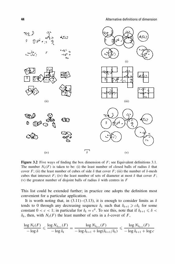
44 Alternative definitions of dimension
F
(i)
(ii) (iii)
(iv) (v)d
Figure 3.2 Five ways of finding the box dimension of F ; see Equivalent definitions 3.1.The number Nδ(F ) is taken to be: (i) the least number of closed balls of radius δ thatcover F ; (ii) the least number of cubes of side δ that cover F ; (iii) the number of δ-meshcubes that intersect F ; (iv) the least number of sets of diameter at most δ that cover F ;(v) the greatest number of disjoint balls of radius δ with centres in F
This list could be extended further; in practice one adopts the definition mostconvenient for a particular application.
It is worth noting that, in (3.11)–(3.13), it is enough to consider limits as δ
tends to 0 through any decreasing sequence δk such that δk+1 � cδk for someconstant 0 < c < 1; in particular for δk = ck. To see this, note that if δk+1 � δ <
δk, then, with Nδ(F ) the least number of sets in a δ-cover of F ,
log Nδ(F )
− log δ� log Nδk+1(F )
− log δk
= log Nδk+1(F )
− log δk+1 + log(δk+1/δk)� log Nδk+1(F )
− log δk+1 + log c

Box-counting dimensions 45
and so
limδ→0
log Nδ(F )
− log δ� lim
k→∞log Nδk
(F )
− log δk
. (3.14)
The opposite inequality is trivial; the case of lower limits may be dealt with inthe same way.
There is an equivalent definition of box dimension of a rather different formthat is worth mentioning. Recall that the δ-neighbourhood Fδ of a subset F of�n is
Fδ = {x ∈ �n : |x − y| � δ for some y ∈ F } (3.15)
i.e. the set of points within distance δ of F . We consider the rate at which then-dimensional volume of Fδ shrinks as δ → 0. In �3, if F is a single pointthen Fδ is a ball with vol(Fδ) = 4
3πδ3, if F is a segment of length l then Fδ is‘sausage-like’ with vol(Fδ) ∼ πlδ2, and if F is a flat set of area a then Fδ isessentially a thickening of F with vol(Fδ) ∼ 2aδ. In each case, vol(Fδ) ∼ cδ3−s
where the integer s is the dimension of F , so that exponent of δ is indicative ofthe dimension. The coefficient c of δ3−s , known as the Minkowski content of F ,is a measure of the length, area or volume of the set as appropriate.
This idea extends to fractional dimensions. If F is a subset of �n and, for somes, voln(Fδ)/δ
n−s tends to a positive finite limit as δ → 0 where voln denotes n-dimensional volume, then it makes sense to regard F as s-dimensional. Thelimiting value is called the s-dimensional content of F —a concept of slightlyrestricted use since it is not necessarily additive on disjoint subsets, i.e. is not ameasure. Even if this limit does not exist, we may be able to extract the criticalexponent of δ and this turns out to be related to the box dimension.
Proposition 3.2
If F is a subset of �n, then
dimBF = n − limδ→0
log voln(Fδ)
log δ
dimBF = n − limδ→0
log voln(Fδ)
log δ
where Fδ is the δ-neighbourhood of F.
Proof. If F can be covered by Nδ(F ) balls of radius δ < 1 then Fδ can be coveredby the concentric balls of radius 2δ. Hence
voln(Fδ) � Nδ(F )cn(2δ)n
46 Alternative definitions of dimension
where cn is the volume of the unit ball in �n. Taking logarithms,
log voln(Fδ)
− log δ� log 2ncn + n log δ + log Nδ(F )
− log δ,
so
limδ→0
log voln(Fδ)
− log δ� −n + dimBF (3.16)
with a similar inequality for the upper limits. On the other hand if there areNδ(F ) disjoint balls of radius δ with centres in F , then by adding their volumes,
Nδ(F )cnδn � voln(Fδ).
Taking logarithms and letting δ → 0 gives the opposite inequality to (3.16), usingEquivalent definition 3.1(v). �
In the context of Proposition 3.2, box dimension is sometimes referred to asMinkowski dimension or Minkowski–Bouligand dimension.
It is important to understand the relationship between box-counting dimensionand Hausdorff dimension. If F can be covered by Nδ(F ) sets of diameter δ, then,from definition (2.1),
Hsδ(F ) � Nδ(F )δs.
If 1 < Hs(F ) = limδ→0 Hsδ(F ) then log Nδ(F ) + s log δ > 0 if δ is sufficiently
small. Thus s � limδ→0 log Nδ(F )/− log δ so
dimHF � dimBF � dimBF (3.17)
for every F ⊂ �n. We do not in general get equality here. Although Hausdorffand box dimensions are equal for many ‘reasonably regular’ sets, there are plentyof examples where this inequality is strict.
Roughly speaking (3.6) says that Nδ(F ) � δ−s for small δ, where s = dimBF .More precisely, it says that
Nδ(F )δs → ∞ if s < dimBF
andNδ(F )δs → 0 if s > dimBF.
But
Nδ(F )δs = inf
{∑
i
δs : {Ui} is a (finite) δ-cover of F
}
,
Properties and problems of box-counting dimension 47
which should be compared with
Hsδ(F ) = inf
{∑
i
|Ui |s : {Ui} is a δ-cover of F
}
,
which occurs in the definitions of Hausdorff measure and dimension. In calculat-ing Hausdorff dimension, we assign different weights |Ui|s to the covering setsUi , whereas for the box dimensions we use the same weight δs for each coveringset. Box dimensions may be thought of as indicating the efficiency with whicha set may be covered by small sets of equal size, whereas Hausdorff dimensioninvolves coverings by sets of small but perhaps widely varying size.
There is a temptation to introduce the quantity v(F ) = limδ→0Nδ(F )δs , butthis does not give a measure on subsets of �n. As we shall see, one consequenceof this is that box dimensions have a number of unfortunate properties, and canbe awkward to handle mathematically.
Since box dimensions are determined by coverings by sets of equal size theytend to be easier to calculate than Hausdorff dimensions. Just as with Hausdorffdimension, calculations of box dimension usually involve finding a lower boundand an upper bound separately, each bound depending on a geometric observationfollowed by an algebraic estimate.
Example 3.3
Let F be the middle third Cantor set (figure 0.1). Then dimBF = dimBF =log 2/ log 3.
Calculation. The obvious covering by the 2k level-k intervals of Ek of length 3−k
gives that Nδ(F ) � 2k if 3−k < δ � 3−k+1. From (3.5)
dimBF = limδ→0
log Nδ(F )
− log δ� lim
k→∞log 2k
log 3k−1= log 2
log 3.
On the other hand, any interval of length δ with 3−k−1 � δ < 3−k intersects atmost one of the level-k intervals of length 3−k used in the construction of F .There are 2k such intervals so at least 2k intervals of length δ are required tocover F . Hence Nδ(F ) � 2k leading to dimBF � log 2/ log 3. �
Thus, at least for the Cantor set, dimHF = dimBF .
3.2 Properties and problems of box-counting dimension
The following elementary properties of box dimension mirror those of Hausdorffdimension, and may be verified in much the same way.
48 Alternative definitions of dimension
(i) A smooth m-dimensional submanifold of �n has dimBF = m.(ii) dimB and dimB are monotonic.
(iii) dimB is finitely stable, i.e.
dimB(E ∪ F) = max {dimBE, dimBF };the corresponding identity does not hold for dimB.
(iv) dimB and dimB are bi-Lipschitz invariant. This is so because, if |f (x) −f (y)| � c|x − y| and F can be covered by Nδ(F ) sets of diameter at mostδ, then the Nδ(F ) images of these sets under f form a cover of f (F )
by sets of diameter at most cδ, thus dimBf (F ) � dimBF . Similarly, boxdimensions behave just like Hausdorff dimensions under bi-Lipschitz andHolder transformations.
We now start to encounter the disadvantages of box-counting dimension. Thenext proposition is at first appealing, but has undesirable consequences.
Proposition 3.4
Let F denote the closure of F (i.e. the smallest closed subset of �n containingF ). Then
dimBF = dimBF
anddimBF = dimBF.
Proof. Let B1, . . . , Bk be a finite collection of closed balls of radii δ. If the closedset
⋃ki=1 Bi contains F , it also contains F . Hence the smallest number of closed
balls of radius δ that cover F equals the smallest number required to cover thelarger set F . The result follows. �
An immediate consequence of this is that if F is a dense subset of an openregion of �n then dimBF = dimBF = n. For example, let F be the (countable) setof rational numbers between 0 and 1. Then F is the entire interval [0, 1], so thatdimBF = dimBF = 1. Thus countable sets can have non-zero box dimension.Moreover, the box-counting dimension of each rational number regarded as aone-point set is clearly zero, but the countable union of these singleton setshas dimension 1. Consequently, it is not generally true that dimB
⋃∞i=1 Fi =
supi dimBFi .This severely limits the usefulness of box dimension—introducing a small, i.e.
countable, set of points can play havoc with the dimension. We might hope to sal-vage something by restricting attention to closed sets, but difficulties still remain.
Example 3.5
F = {0, 1, 12 , 1
3 , . . .} is a compact set with dimBF = 12 .
Modified box-counting dimensions 49
Calculation. Let 0 < δ < 12 and let k be the integer satisfying 1/(k − 1)k > δ �
1/k(k + 1). If |U | � δ, then U can cover at most one of the points {1, 12 , . . . , 1/k}
since 1/(k − 1) − 1/k = 1/(k − 1)k > δ. Thus at least k sets of diameter δ arerequired to cover F , so Nδ(F ) � k giving
log Nδ(F )
− log δ� log k
log k(k + 1).
Letting δ → 0 so k → ∞ gives dimBF � 12 . On the other hand, if 1
2 > δ > 0,take k such that 1/(k − 1)k > δ � 1/k(k + 1). Then (k + 1) intervals of lengthδ cover [0, 1/k], leaving k − 1 points of F which can be covered by anotherk − 1 intervals. Thus Nδ(F ) � 2k, so
log Nδ(F )
− log δ� log(2k)
log k(k − 1)
givingdimBF � 1
2 . �
No-one would regard this set, with all but one of its points isolated, as a fractal,yet it has large box dimension.
Nevertheless, as well as being convenient in practice, box dimensions are veryuseful in theory. If, as often happens, it can be shown that a set has equal boxand Hausdorff dimensions, the interplay between these definitions can be usedto powerful effect.
*3.3 Modified box-counting dimensions
There are ways of overcoming the difficulties of box dimension outlined in thelast section. However, they may not at first seem appealing since they re-introduceall the difficulties of calculation associated with Hausdorff dimension and more.
For F a subset of �n we can try to decompose F into a countable number ofpieces F1, F2, . . . in such a way that the largest piece has as small a dimensionas possible. This idea leads to the following modified box-counting dimensions:
dimMBF = inf
{
supi
dimBFi : F ⊂∞⋃
i=1
Fi
}
(3.18)
dimMBF = inf
{
supi
dimBFi : F ⊂∞⋃
i=1
Fi
}
. (3.19)
(In both cases the infimum is over all possible countable covers {Fi} of F .)Clearly dimMBF � dimBF and dimMBF � dimBF . However, we now have that
50 Alternative definitions of dimension
dimMBF = dimMBF = 0 if F is countable—just take the Fi to be one-point sets.Moreover, for any subset F of �n,
0 � dimHF � dimMBF � dimMBF � dimBF � n. (3.20)
It is easy to see that dimMB and dimMB recover all the desirable properties ofa dimension, but they can be hard to calculate. However, there is a useful testfor compact sets to have equal box and modified box dimensions. It applies tosets that might be described as ‘dimensionally homogeneous’.
Proposition 3.6
Let F ⊂ �n be compact. Suppose that
dimB(F ∩ V ) = dimBF (3.21)
for all open sets V that intersect F. Then dimBF = dimMBF . A similar resultholds for lower box-counting dimensions.
Proof. Let F ⊂ ⋃∞i=1 Fi with each Fi closed. A version of Baire’s category theo-
rem (which may be found in any text on basic general topology, and which wequote without proof) states that there is an index i and an open set V ⊂ �n suchthat F ∩ V ⊂ Fi . For this i, dimBFi = dimBF . Using (3.19) and Proposition 3.4
dimMBF = inf
{
sup dimBFi : F ⊂∞⋃
i=1
Fi where the Fi are closed sets
}
� dimBF.
The opposite inequality is contained in (3.20). A similar argument deals withthe lower dimensions. �
For an application, let F be a compact set with a high degree of self-similarity,for instance the middle third Cantor set or von Koch curve. If V is any open setthat intersects F , then F ∩ V contains a geometrically similar copy of F whichmust have upper box dimension equal to that of F , so that (3.21) holds, leadingto equal box and modified box dimensions.
*3.4 Packing measures and dimensions
Unlike Hausdorff dimension, neither the box dimensions or modified box dimen-sions are defined in terms of measures, and this can present difficulties in theirtheoretical development. Nevertheless, the circle of ideas in the last section maybe completed in a way that is, at least mathematically, elegant. Recall that Haus-dorff dimension may be defined using economical coverings by small balls (2.16)

Packing measures and dimensions 51
whilst dimB may be defined using economical coverings by small balls of equalradius (Equivalent definition 3.1(i)). On the other hand dimB may be thought ofas a dimension that depends on packings by disjoint balls of equal radius thatare as dense as possible (Equivalent definition 3.1(v)). Coverings and packingsplay a dual role in many areas of mathematics and it is therefore natural to try tolook for a dimension that is defined in terms of dense packings by disjoint ballsof differing small radii.
We try to follow the pattern of definition of Hausdorff measure and dimension.For s � 0 and δ > 0, let
P sδ (F ) = sup
{∑
i
|Bi|s : {Bi} is a collection of disjoint balls of radii at
most δ with centres in F
}
. (3.22)
Since P sδ (F ) decreases with δ, the limit
P s0 (F ) = lim
δ→0P s
δ (F ) (3.23)
exists. At this point we meet the problems encountered with box-counting dimen-sions. By considering countable dense sets it is easy to see that P s
0 (F ) is not ameasure. Hence we modify the definition to
P s (F ) = inf
{∑
i
P s0 (Fi) : F ⊂
∞⋃
i=1
Fi
}
. (3.24)
It may be shown that P s (F ) is a measure on �n, known as the s-dimensionalpacking measure. We may define the packing dimension in the natural way:
dimPF = sup{s : P s(F ) = ∞} = inf{s : P s(F ) = 0}. (3.25)
The underlying measure structure immediately implies monotonicity: thatdimPE � dimPF if E ⊂ F . Moreover, for a countable collection of sets {Fi},
dimP
( ∞⋃
i=1
Fi
)
= supi
dimPFi, (3.26)
since if s > dimPFi for all i, then P s(⋃
i Fi) �∑
i P s(Fi) = 0 implyingdimP
(⋃i Fi
)� s.
We now investigate the relationship of packing dimension with other definitionsof dimension and verify the surprising fact that packing dimension is just the sameas the modified upper box dimension.
52 Alternative definitions of dimension
Lemma 3.7
dimPF � dimBF. (3.27)
Proof. If dimPF = 0, the result is obvious. Otherwise choose any t and s with0 < t < s < dimPF . Then P s(F ) = ∞, so P s
0 (F ) = ∞. Thus, given 0 < δ � 1,there are disjoint balls {Bi}, of radii at most δ with centres in F , such that1 < �∞
i=1|Bi|s . Suppose that, for each k, exactly nk of these balls satisfy 2−k−1 <
|Bi| � 2−k; then
1 <
∞∑
k=0
nk2−ks . (3.28)
There must be some k with nk > 2kt (1 − 2t−s), otherwise the sum in (3.28) isat most �∞
k=02kt−ks(1 − 2t−s) = 1, by summing the geometric series. These nk
balls all contain balls of radii 2−k−2 � δ centred in F . Hence if Nδ(F ) denotesthe greatest number of disjoint balls of radius δ with centres in F , then
N2−k−2(F )(2−k−2)t � nk(2−k−2)t > 2−2t (1 − 2t−s)
where 2−k−2 < δ. It follows that limδ→0Nδ(F )δt > 0, so that dimBF � t
using Equivalent definition 3.1(v). This is true for any 0 < t < dimPF so(3.27) follows. �
Proposition 3.8
If F ⊂ �n then dimPF = dimMBF .
Proof. If F ⊂ ⋃∞i=1 Fi then, by (3.26) and (3.27),
dimPF � supi
dimPFi � supi
dimBFi.
Definition (3.19) now gives that dimPF � dimMBF .Conversely, if s > dimPF then P s(F ) = 0, so that F ⊂ ⋃
i Fi for a collectionof sets Fi with P s
0 (Fi) < ∞ for each i, by (3.24). Hence, for each i, if δ is smallenough, then P s
δ (Fi) < ∞, so by (3.22) Nδ(Fi)δs is bounded as δ → 0, where
Nδ(Fi) is the largest number of disjoint balls of radius δ with centres in Fi . ByEquivalent definition 3.1(v) dimBFi � s for each i, giving that dimMBF � s by(3.19), as required. �
We have established the following relations:
dimHF � dimMBF � dimMBF = dimPF � dimBF. (3.29)
Suitable examples show that none of the inequalities can be replaced by equality.
Some other definitions of dimension 53
As with Hausdorff dimension, packing dimension permits the use of powerfulmeasure theoretic techniques in its study. The introduction of packing measures(remarkably some 60 years after Hausdorff measures) has led to a greater under-standing of the geometric measure theory of fractals, with packing measuresbehaving in a way that is ‘dual’ to Hausdorff measures in many respects. Indeedcorresponding results for Hausdorff and packing measures are often presentedside by side. Nevertheless, one cannot pretend that packing measures and dimen-sions are easy to work with or to calculate; the extra step (3.24) in their definitionmakes them more awkward to use than the Hausdorff analogues.
This situation is improved slightly by the equality of packing dimension andthe modified upper box dimension. It is improved considerably for compact setswith ‘local’ dimension constant throughout—a situation that occurs frequentlyin practice, in particular in sets with some kind of self-similarity.
Corollary 3.9
Let F ⊂ �n be compact and such that
dimB(F ∩ V ) = dimBF (3.30)
for all open sets V that intersect F. Then dimPF = dimBF .
Proof. This is immediate from Propositions 3.6 and 3.8. �
The nicest case, of course, is of fractals with equal Hausdorff and upper boxdimensions, in which case equality holds throughout (3.29)—we shall see manysuch examples later on. However, even the much weaker condition dimHF =dimPF , though sometimes hard to prove, eases analysis of F .
3.5 Some other definitions of dimension
A wide variety of other definitions of dimension have been introduced, many ofthem only of limited applicability, but nonetheless useful in their context.
The special form of curves gives rise to the several definitions of dimension.We define a curve or Jordan curve C to be the image of an interval [a, b] under acontinuous bijection f : [a, b] → �n. (Thus, we restrict attention to curves thatare non-self-intersecting.) If C is a curve and δ > 0, we define Mδ(C) to be themaximum number of points x0, x1, . . . , xm, on the curve C, in that order, suchthat |xk − xk−1| = δ for k = 1, 2, . . . , m. Thus (Mδ(C) − 1)δ may be thought ofas the ‘length’ of the curve C measured using a pair of dividers with points setat a distance δ apart. The divider dimension is defined as
limδ→0
log Mδ(C)
− log δ(3.31)

54 Alternative definitions of dimension
assuming the limit exists (otherwise we may define upper and lower dividerdimensions using upper and lower limits). It is easy to see that the divider dimen-sion of a curve is at least equal to the box dimension (assuming that they bothexist) and in simple self-similar examples, such as the von Koch curve, theyare equal. The assertion that the coastline of Britain has dimension 1.2 is usu-ally made with the divider dimension in mind—this empirical value comes fromestimating the ratio in (3.31) for values of δ between about 20 m and 200 km.
A variant of Hausdorff dimension may be defined for curves by using intervalsof the curves themselves as covering sets. Thus we look at inf
{∑mi=1 |f [ti−1, ti]|s
}
where the infimum is over all dissections a = t0 < t1 < · · · < tm = b such thatthe diameters |f ([ti−1, ti])| are all at most δ. We let δ tend to 0 and deem the valueof s at which this limit jumps from ∞ to 0 to be the dimension. For self-similarexamples such as the von Koch curve, this equals the Hausdorff dimension, butfor ‘squeezed’ curves, such as graphs of certain functions (see Chapter 11) wemay get a somewhat larger value.
Sometimes, we are interested in the dimension of a fractal F that is the bound-ary of a set A. We can define the box dimension of F in the usual way, butsometimes it is useful to take special account of the distinction between A andits complement. Thus the following variation of the ‘s-dimensional content’ def-inition of box dimension, in which we take the volume of the set of pointswithin distance δ of F that are contained in A is sometimes useful. We definethe one-sided dimension of the boundary F of a set A in �n as
n − limδ→0
log voln(Fδ ∩ A)
log δ(3.32)
where Fδ is the δ-neighbourhood of F (compare Proposition 3.2). This definitionhas applications to the surface physics of solids where it is the volume veryclose to the surface that is important and also to partial differential equations indomains with fractal boundaries.
It is sometimes possible to define dimension in terms of the complement of aset. Suppose F is obtained by removal of a sequence of intervals I1, I2, . . . from,say, the unit interval [0, 1], as, for example, in the Cantor set construction. Wemay define a dimension as the number s0 such that the series
∞∑
j=1
|Ij |s converges if s < s0 and diverges if s > s0; (3.33)
the number s0 is called the critical exponent of the series. For the middle thirdCantor set, this series is
∑∞k=1 2k−13−ks , giving s0 = log 2/ log 3, equal to the
Hausdorff and box dimensions in this case. In general, s0 equals the upper boxdimension of F .
Dimension prints provide an interesting variation on Hausdorff dimension ofa rather different nature. Dimension prints may be thought of as a sort of ‘fin-gerprint’ that enables sets with differing characteristics to be distinguished, even

Some other definitions of dimension 55
though they may have the same Hausdorff dimension. In particular they reflectnon-isotropic features of a set.
We restrict attention to subsets of the plane, in which case the dimension printwill also be planar. The definition of dimension prints is very similar to thatof Hausdorff dimension but coverings by rectangles are used with side lengthsreplacing diameters. Let U be a rectangle (the sides need not be parallel to thecoordinate axes) and let a(U) � b(U) be the lengths of the sides of U . Let s, t
be non-negative numbers. For F a subset of �2, let
Hs,tδ (F ) = inf
{∑
i
a(Ui)sb(Ui)
t : {Ui} is a δ-cover of F by rectangles
}
.
In the usual way, we get measures of ‘Hausdorff type’, Hs,t , by letting δ → 0:
Hs,t (F ) = limδ→0
Hs,tδ (F ).
(Note that Hs,0 is just a minor variant of s-dimensional Hausdorff measure whereonly rectangles are allowed in the δ-covers.) The dimension print, print F , of F
is defined to be the set of non-negative pairs (s, t) for which Hs,t (F ) > 0.Using standard properties of measures, it is easy to see that we have mono-
tonicityprint F1 ⊂ print F2 if F1 ⊂ F2 (3.34)
and countable stability
( ∞⋃
i=1
Fi
)
=∞⋃
i=1
print Fi. (3.35)
Moreover, if (s, t) is a point in print F and (s ′, t ′) satisfies
s ′ + t ′ � s + t
t ′ � t (3.36)
then (s ′, t ′) is also in print F .Unfortunately, dimension prints are not particularly easy to calculate. We dis-
play a few known examples in figure 3.3. Notice that the Hausdorff dimensionof a set is given by the point where the edge of its print intersects the x-axis.
Dimension prints are a useful and appealing extension of the idea of Haus-dorff dimension. Notice how the prints in the last two cases distinguish betweentwo sets of Hausdorff (or box) dimension 1 1
2 , one of which is dust-like, theother stratified.
One disadvantage of dimension prints defined in this way is that they are notLipschitz invariants. The straight line segment and smooth convex curve are bi-Lipschitz equivalent, but their prints are different. In the latter case the dimension
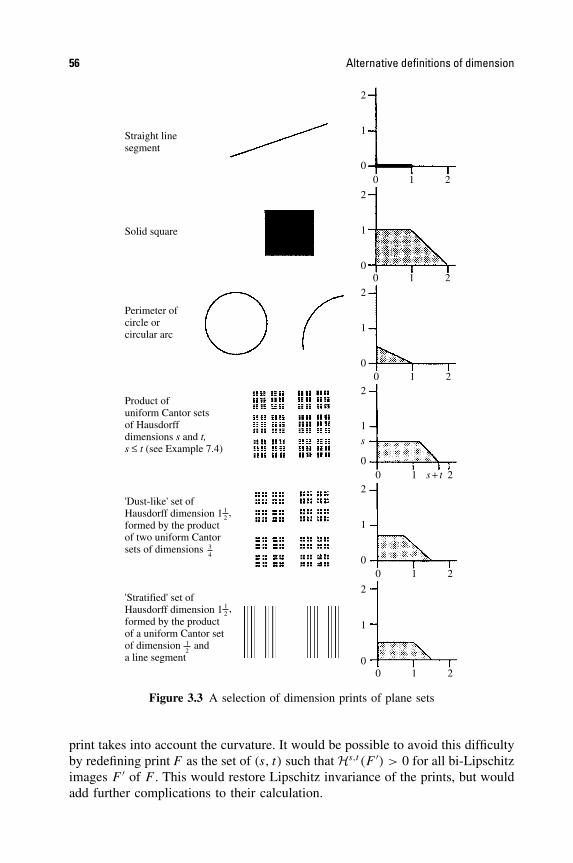
56 Alternative definitions of dimension
2
1
00 1 2
0 1 2
0 1 2
0 1 s + t 2
0 1 2
0 1 2
2
1
0
2
1
0
2
1
s
0
2
1
0
2
1
0
Straight linesegment
Solid square
Perimeter ofcircle orcircular arc
Product ofuniform Cantor setsof Hausdorffdimensions s and t,s ≤ t (see Example 7.4)
'Dust-like' set ofHausdorff dimension 1formed by the productof two uniform Cantorsets of dimensions 3
4
12,
12,
'Stratified' set ofHausdorff dimension 1formed by the productof a uniform Cantor setof dimension anda line segment
12
Figure 3.3 A selection of dimension prints of plane sets
print takes into account the curvature. It would be possible to avoid this difficultyby redefining print F as the set of (s, t) such that Hs,t (F ′) > 0 for all bi-Lipschitzimages F ′ of F . This would restore Lipschitz invariance of the prints, but wouldadd further complications to their calculation.
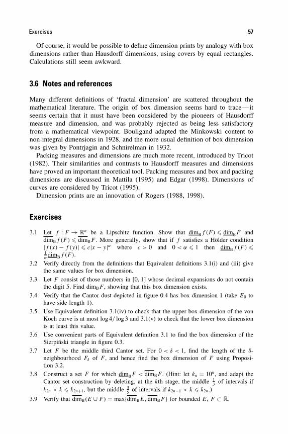
Exercises 57
Of course, it would be possible to define dimension prints by analogy with boxdimensions rather than Hausdorff dimensions, using covers by equal rectangles.Calculations still seem awkward.
3.6 Notes and references
Many different definitions of ‘fractal dimension’ are scattered throughout themathematical literature. The origin of box dimension seems hard to trace—itseems certain that it must have been considered by the pioneers of Hausdorffmeasure and dimension, and was probably rejected as being less satisfactoryfrom a mathematical viewpoint. Bouligand adapted the Minkowski content tonon-integral dimensions in 1928, and the more usual definition of box dimensionwas given by Pontrjagin and Schnirelman in 1932.
Packing measures and dimensions are much more recent, introduced by Tricot(1982). Their similarities and contrasts to Hausdorff measures and dimensionshave proved an important theoretical tool. Packing measures and box and packingdimensions are discussed in Mattila (1995) and Edgar (1998). Dimensions ofcurves are considered by Tricot (1995).
Dimension prints are an innovation of Rogers (1988, 1998).
Exercises
3.1 Let f : F → �n be a Lipschitz function. Show that dimBf (F ) � dimBF anddimBf (F ) � dimBF . More generally, show that if f satisfies a Holder condition|f (x) − f (y)| � c|x − y|α where c > 0 and 0 < α � 1 then dimBf (F ) �1α
dimBf (F ).
3.2 Verify directly from the definitions that Equivalent definitions 3.1(i) and (iii) givethe same values for box dimension.
3.3 Let F consist of those numbers in [0, 1] whose decimal expansions do not containthe digit 5. Find dimBF , showing that this box dimension exists.
3.4 Verify that the Cantor dust depicted in figure 0.4 has box dimension 1 (take E0 tohave side length 1).
3.5 Use Equivalent definition 3.1(iv) to check that the upper box dimension of the vonKoch curve is at most log 4/ log 3 and 3.1(v) to check that the lower box dimensionis at least this value.
3.6 Use convenient parts of Equivalent definition 3.1 to find the box dimension of theSierpinski triangle in figure 0.3.
3.7 Let F be the middle third Cantor set. For 0 < δ < 1, find the length of the δ-neighbourhood Fδ of F , and hence find the box dimension of F using Proposi-tion 3.2.
3.8 Construct a set F for which dimBF < dimBF . (Hint: let kn = 10n, and adapt theCantor set construction by deleting, at the kth stage, the middle 1
3 of intervals ifk2n < k � k2n+1, but the middle 3
5 of intervals if k2n−1 < k � k2n.)
3.9 Verify that dimB(E ∪ F) = max{dimBE, dimBF } for bounded E, F ⊂ �.
58 Alternative definitions of dimension
3.10 Find subsets E and F of � such that dimB(E ∪ F) > max{dimBE, dimBF }. (Hint:consider two sets of the form indicated in Exercise 3.8.)
3.11 What are the Hausdorff and box dimensions of the set{0, 1, 1
4 , 19 , 1
16 , . . .}?
3.12 Find two disjoint Borel subsets E and F of � such that P s0 (E ∪ F) �= P s
0 (E) +P s
0 (F ).
3.13 What is the packing dimension of the von Koch curve?
3.14 Find the divider dimension (3.31) of the von Koch curve.
3.15 Show that the divider dimension (3.31) of a curve is greater than or equal to its boxdimension, assuming that they both exist.
3.16 Let 0 < λ < 1 and let F be the ‘middle λ Cantor set’ obtained by repeated removalof the middle proportion λ from intervals. Show that the dimension of F definedby (3.33) in terms of removed intervals equals the Hausdorff and box dimensionsof F .
3.17 Verify properties (3.34)–(3.36) of dimension prints. Given an example of a set witha non-convex dimension print.

Chapter 4 Techniques for calculatingdimensions
A direct attempt at calculating the dimensions, in particular the Hausdorff dimen-sion, of almost any set will convince the reader of the practical limitations ofworking from the definitions. Rigorous dimension calculations often involvepages of complicated manipulations and estimates that provide little intuitiveenlightenment.
In this chapter we bring together some of the basic techniques that are availablefor dimension calculations. Other methods, that are applicable in more specificcases, will be found throughout the book.
4.1 Basic methods
As a general rule, we get upper bounds for Hausdorff measures and dimensions byfinding effective coverings by small sets, and lower bounds by putting measuresor mass distributions on the set. For most fractals ‘obvious’ upper estimates ofdimension may be obtained using natural coverings by small sets.
Proposition 4.1
Suppose F can be covered by nk sets of diameter at most δk with δk → 0 ask → ∞. Then
dimHF � dimBF � limk→∞
log nk
− log δk
.
Moreover, if nkδsk remains bounded as k → ∞, then Hs(F ) < ∞. If δk → 0
but δk+1 � cδk for some 0 < c < 1, then
dimBF � limk→∞
log nk
− log δk
.
Proof. The inequalities for the box-counting dimension are immediate from thedefinitions and the remark at (3.14). That dimHF � dimBF is in (3.17), and if
59
Fractal Geometry: Mathematical Foundations and Application. Second Edition Kenneth Falconer 2003 John Wiley & Sons, Ltd ISBNs: 0-470-84861-8 (HB); 0-470-84862-6 (PB)

60 Techniques for calculating dimensions
nkδsk is bounded then Hs
δk(F ) � nkδ
sk , so Hs
δk(F ) tends to a finite limit Hs(F ) as
k → ∞. �
Thus, as we have seen already (Example 2.7), in the case of the middle thirdCantor set the natural coverings by 2k intervals of length 3−k give dimHF �dimBF � dimBF � log 2/ log 3.
Surprisingly often, the ‘obvious’ upper bound for the Hausdorff dimensionof a set turns out to be the actual value. However, demonstrating this can bedifficult. To obtain an upper bound it is enough to evaluate sums of the form∑ |Ui |s for specific coverings {Ui} of F , whereas for a lower bound we mustshow that
∑ |Ui|s is greater than some positive constant for all δ-coverings of F .Clearly an enormous number of such coverings are available. In particular, whenworking with Hausdorff dimension as opposed to box dimension, considerationmust be given to covers where some of the Ui are very small and others haverelatively large diameter—this prohibits sweeping estimates for
∑ |Ui |s such asthose available for upper bounds.
One way of getting around these difficulties is to show that no individual setU can cover too much of F compared with its size measured as |U |s . Then if{Ui} covers the whole of F the sum
∑ |Ui |s cannot be too small. The usual wayto do this is to concentrate a suitable mass distribution µ on F and compare themass µ(U) covered by U with |U |s for each U . (Recall that a mass distributionon F is a measure with support contained in F such that 0 < µ(F) < ∞, seeSection 1.3.)
Mass distribution principle 4.2
Let µ be a mass distribution on F and suppose that for some s there are numbersc > 0 and ε > 0 such that
µ(U) � c|U |s (4.1)
for all sets U with |U | � ε. Then Hs(F ) � µ(F )/c and
s � dimHF � dimBF � dimBF.
Proof. If {Ui} is any cover of F then
0 < µ(F) � µ
(⋃
i
Ui
)
�∑
i
µ(Ui) � c∑
i
|Ui |s (4.2)
using properties of a measure and (4.1).Taking infima, Hs
δ(F ) � µ(F )/c if δ is small enough, so Hs(F ) � µ(F )/c.Since µ(F ) > 0 we get dimHF � s. �
Notice that the conclusion Hs(F ) � µ(F )/c remains true if µ is a mass dis-tribution on �n and F is any subset.

Basic methods 61
The Mass distribution principle 4.2 gives a quick lower estimate for the Haus-dorff dimension of the middle third Cantor set F (figure 0.1). Let µ be the naturalmass distribution on F , so that each of the 2k kth level intervals of length 3−k
in Ek in the construction of F carry a mass 2−k . (We imagine that we start withunit mass on E0 and repeatedly divide the mass on each interval of Ek betweenits two subintervals in Ek+1; see Proposition 1.7.) Let U be a set with |U | < 1and let k be the integer such that 3−(k+1) � |U | < 3−k. Then U can intersect atmost one of the intervals of Ek, so
µ(U) � 2−k = (3log 2/ log 3)−k = (3−k)log 2/ log 3 � (3|U |)log 2/ log 3
and hence Hlog 2/ log 3(F ) � 3− log 2/ log 3 = 12 by the mass distribution principle,
giving dimHF � log 2/ log 3.
Example 4.3
Let F1 = F × [0, 1] ⊂ �2 be the product of the middle third Cantor set F and theunit interval. Then, setting s = 1 + log 2/ log 3, we have dimBF1 = dimHF1 = s,with 0 < Hs(F1) < ∞.
Calculation. For each k, there is a covering of F by 2k intervals of length 3−k. Acolumn of 3k squares of side 3−k (diameter 3−k
√2) covers the part of F1 above each
such interval, so taking these all together, F1 may be covered by 2k3k squares ofside 3−k. Thus Hs
3−k√
2(F1) � 3k2k(3−k√
2)s = (3 · 2 · 3−1−log 2/ log 3)k2s/2 = 2s/2,
so Hs(F1) � 2s/2 and dimHF1 � dimBF1 � dimBF1 � s.We define a mass distribution µ on F1 by taking the natural mass distribution
on F described above (each kth level interval of F of side 3−k having mass2−k) and ‘spreading it’ uniformly along the intervals above F . Thus if U is arectangle, with sides parallel to the coordinate axes, of height h � 1, above a kthlevel interval of F , then µ(U) = h2−k. Any set U is contained in a square ofside |U | with sides parallel to the coordinate axes. If 3−(k+1) � |U | < 3−k thenU lies above at most one kth level interval of F of side 3−k, so
µ(U) � |U |2−k � |U |3−k log 2/ log 3 � |U |(3|U |)log 2/ log 3 = 3log 2/ log 3|U |s = 2|U |s .
By the Mass distribution principle 4.2, Hs(F1) > 12 . �
Note that the method of Examples 4.2 and 4.3 extends to a wide variety ofself-similar sets. Indeed, Theorem 9.3 may be regarded as a generalization of thiscalculation.
Notice that in this example the dimension of the product of two sets equals thesum of the dimensions of the sets. We study this in greater depth in Chapter 7.
The following general construction of a subset of � may be thought of as ageneralization of the Cantor set construction. Let [0, 1] = E0 ⊃ E1 ⊃ E2 ⊃ . . .
be a decreasing sequence of sets, with each Ek a union of a finite number of
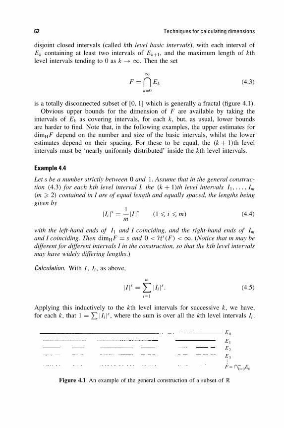
62 Techniques for calculating dimensions
disjoint closed intervals (called kth level basic intervals), with each interval ofEk containing at least two intervals of Ek+1, and the maximum length of kthlevel intervals tending to 0 as k → ∞. Then the set
F =∞⋂
k=0
Ek (4.3)
is a totally disconnected subset of [0, 1] which is generally a fractal (figure 4.1).Obvious upper bounds for the dimension of F are available by taking the
intervals of Ek as covering intervals, for each k, but, as usual, lower boundsare harder to find. Note that, in the following examples, the upper estimates fordimHF depend on the number and size of the basic intervals, whilst the lowerestimates depend on their spacing. For these to be equal, the (k + 1)th levelintervals must be ‘nearly uniformly distributed’ inside the kth level intervals.
Example 4.4
Let s be a number strictly between 0 and 1. Assume that in the general construc-tion (4.3) for each kth level interval I, the (k + 1)th level intervals I1, . . . , Im
(m � 2) contained in I are of equal length and equally spaced, the lengths beinggiven by
|Ii|s = 1
m|I |s (1 � i � m) (4.4)
with the left-hand ends of I1 and I coinciding, and the right-hand ends of Im
and I coinciding. Then dimHF = s and 0 < Hs(F ) < ∞. (Notice that m may bedifferent for different intervals I in the construction, so that the kth level intervalsmay have widely differing lengths.)
Calculation. With I , Ii , as above,
|I |s =m∑
i=1
|Ii |s . (4.5)
Applying this inductively to the kth level intervals for successive k, we have,for each k, that 1 = ∑ |Ii |s , where the sum is over all the kth level intervals Ii .
E0
E1
E2
E3···F = ∩ Ekk=0
∞
Figure 4.1 An example of the general construction of a subset of �

Basic methods 63
The kth level intervals cover F ; since the maximum interval length tends to 0 ask → ∞, we have Hs
δ(F ) � 1 for sufficiently small δ, giving Hs(F ) � 1.Now distribute a mass µ on F in such a way that µ(I) = |I |s whenever I
is any level k interval. Thus, starting with unit mass on [0, 1] we divide thisequally between each level 1 interval, the mass on each of these intervals beingdivided equally between each level 2 subinterval, and so on; see Proposition 1.7.Equation (4.5) ensures that we get a mass distribution on F with µ(I) = |I |sfor every basic interval. We estimate µ(U) for an interval U with endpoints inF . Let I be the smallest basic interval that contains U ; suppose that I is a kthlevel interval, and let Ii, . . . , Im be the (k + 1)th level intervals contained in I .Then U intersects a number j � 2 of the Ii , otherwise U would be contained ina smaller basic interval. The spacing between consecutive Ii is
(|I | − m|Ii |)/(m − 1) = |I |(1 − m|Ii|/|I |)/(m − 1)
= |I |(1 − m1−1/s)/(m − 1)
� cs |I |/m
using (4.4) and that m � 2 and 0 < s < 1, where cs = (1 − 21−1/s). Thus
|U | � j − 1
mcs |I | � j
2mcs |I |.
By (4.4)
µ(U) � jµ(Ii) = j |Ii |s = j
m|I |s
� 2sc−ss
(j
m
)1−s
|U |s � 2sc−ss |U |s. (4.6)
This is true for any interval U with endpoints in F , and so for any set U (byapplying (4.6) to the smallest interval containing U ∩ F ). By the Mass distribu-tion principle 4.2, Hs(F ) > 0. �
A more careful estimate of µ(U) in Example 4.4 leads to Hs(F ) = 1.We call the sets obtained when m is kept constant throughout the construction
of Example 4.4 uniform Cantor sets ; see figure 4.2. These provide a naturalgeneralization of the middle third Cantor set.
Example 4.5. Uniform Cantor sets
Let m � 2 be an integer and 0 < r < 1/m. Let F be the set obtained by theconstruction in which each basic interval I is replaced by m equally spaced subin-tervals of lengths r|I |, the ends of I coinciding with the ends of the extreme subin-tervals. Then dimHF = dimBF = log m/− log r , and 0 < Hlog m/− log r (F ) < ∞.
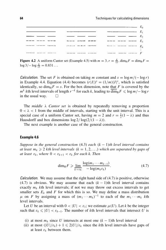
64 Techniques for calculating dimensions
E0
E1
E2
E3
E4
F
···
Figure 4.2 A uniform Cantor set (Example 4.5) with m = 3, r = 415 , dimHF = dimBF =
log 3/− log 415 = 0.831 . . .
Calculation. The set F is obtained on taking m constant and s = log m/(− log r)
in Example 4.4. Equation (4.4) becomes (r|I |)s = (1/m)|I |s , which is satisfiedidentically, so dimHF = s. For the box dimension, note that F is covered by themk kth level intervals of length r−k for each k, leading to dimBF � log m/− log r
in the usual way. �
The middle λ Cantor set is obtained by repeatedly removing a proportion0 < λ < 1 from the middle of intervals, starting with the unit interval. This is aspecial case of a uniform Cantor set, having m = 2 and r = 1
2 (1 − λ) and thusHausdorff and box dimensions log 2/ log(2/(1 − λ)).
The next example is another case of the general construction.
Example 4.6
Suppose in the general construction (4.3) each (k − 1)th level interval containsat least mk � 2 kth level intervals (k = 1, 2, . . .) which are separated by gaps ofat least εk , where 0 < εk+1 < εk for each k. Then
dimHF � limk→∞
log(m1 · · ·mk−1)
− log(mkεk). (4.7)
Calculation. We may assume that the right hand side of (4.7) is positive, otherwise(4.7) is obvious. We may assume that each (k − 1)th level interval containsexactly mk kth level intervals; if not we may throw out excess intervals to getsmaller sets Ek and F for which this is so. We may define a mass distributionµ on F by assigning a mass of (m1 · · · mk)
−1 to each of the m1 · · ·mk kthlevel intervals.
Let U be an interval with 0 < |U | < ε1; we estimate µ(U). Let k be the integersuch that εk � |U | < εk−1. The number of kth level intervals that intersect U is
(i) at most mk since U intersects at most one (k − 1)th level interval(ii) at most (|U |/εk) + 1 � 2|U |/εk since the kth level intervals have gaps of
at least εk between them.
Basic methods 65
Each kth level interval supports mass (m1 · · · mk)−1 so that
µ(U) � (m1 · · · mk)−1 min{2|U |/εk,mk}
� (m1 · · · mk)−1(2|U |/εk)
sm1−sk
for every 0 � s � 1.Hence
µ(U)
|U |s � 2s
(m1 · · ·mk−1)mskε
sk
.
Ifs < lim
k→∞log(m1 · · · mk−1)/− log(mkεk)
then (m1 · · · mk−1)mskε
sk > 1 for large k, so µ(U) � 2s |U |s , and dimHF � s by
Principle 4.2, giving (4.7). �
Now suppose that in Example 4.6 the kth level intervals are all of length δk ,and that each (k − 1)th level interval contains exactly mk kth level intervals,which are ‘roughly equally spaced’ in the sense that mkεk � cδk−1, where c > 0is a constant. Then (4.7) becomes
dimHF � limk→∞
log(m1 · · · mk−1)
− log c − log δk−1= lim
k→∞log(m1 · · · mk−1)
− log δk−1.
But Ek−1 comprises m1 · · · mk−1 intervals of length δk−1, so this expression equalsthe upper bound for dimHF given by Proposition 4.1. Thus in the situation wherethe intervals are well spaced, we get equality in (4.7).
Examples of the following form occur in number theory; see Section 10.3.
Example 4.7
Fix 0 < s < 1 and let n0, n1, n2, . . . be a rapidly increasing sequence of integers,say nk+1 � max {nk
k, 4n1/s
k } for each k. For each k let Hk ⊂ � consist of equallyspaced equal intervals of lengths n
−1/s
k with the midpoints of consecutive intervalsdistance n−1
k apart. Then writing F = ⋂∞k=1 Hk , we have dimHF = s.
Calculation. Since F ⊂ Hk for each k, the set F ∩ [0, 1] is contained in at mostnk + 1 intervals of length n
−1/s
k , so Proposition 4.1 gives dimH(F ∩ [0, 1]) �limk→∞ log(nk + 1)/− log n
−1/s
k = s. Similarly, dimH(F ∩ [n, n + 1]) � s forall n ∈ �, so dimHF � s as a countable union of such sets.
Now let E0 = [0, 1] and, for k � 1, let Ek consist of the intervals of Hk thatare completely contained in Ek−1. Then each interval I of Ek−1 contains at leastnk|I | − 2 � nkn
−1/s
k−1 − 2 � 2 intervals of Ek, which are separated by gaps of at
66 Techniques for calculating dimensions
least n−1k − n
−1/s
k � 12n−1
k if k is large enough. Using Example 4.6, and notingthat setting mk = nkn
−1/s
k−1 rather than mk = nkn−1/s
k−1 − 2 does not affect the limit,
dimH(F ∩ [0, 1]) � dimH
∞⋂
k=1
Ek � limk→∞
log((n1 · · · nk−2)1−1/snk−1)
− log(nkn−1/s
k−112n−1
k )
= limk→∞
log(n1 · · · nk−2)1−1/s + log nk−1
log 2 + (log nk−1)/s.
Provided that nk is sufficiently rapidly increasing, the terms in log nk−1 in thenumerator and denominator of this expression are dominant, so that dimHF �dimH(F ∩ [0, 1]) � s, as required. �
Although the Mass distribution principle 4.2 is based on a simple idea, wehave seen that it can be very useful in finding Hausdorff and box dimensions.We now develop some important variations of the method.
It is enough for condition (4.1) to hold just for sufficiently small balls centredat each point of F . This is expressed in Proposition 4.9(a). Although mass dis-tribution methods for upper bounds are required far less frequently, we includepart (b) because it is, in a sense, dual to (a). Note that density expressions, suchas limr→0 µ(B(x, r))/rs play a major role in the study of local properties offractals—see Chapter 5. (Recall that B(x, r) is the closed ball of centre x andradius r .)
We require the following covering lemma in the proof of Proposition 4.9(b).
Covering lemma 4.8
Let C be a family of balls contained in some bounded region of �n. Then thereis a (finite or countable) disjoint subcollection {Bi} such that
⋃
B∈CB ⊂
⋃
i
Bi (4.8)
where Bi is the closed ball concentric with Bi and of four times the radius.
Proof. For simplicity, we give the proof when C is a finite family; the basic ideais the same in the general case. We select the {Bi} inductively. Let B1 be aball in C of maximum radius. Suppose that B1, . . . , Bk−1 have been chosen. Wetake Bk to be the largest ball in C (or one of the largest) that does not intersectB1, . . . , Bk−1. The process terminates when no such ball remains. Clearly theballs selected are disjoint; we must check that (4.8) holds. If B ∈ C, then eitherB = Bi for some i, or B intersects one of the Bi with |Bi | � |B|; if this werenot the case, then B would have been chosen instead of the first ball Bk with|Bk| < |B|. Either way, B ⊂ Bi , so we have (4.8). (It is easy to see that the

Basic methods 67
result remains true taking Bi as the ball concentric with Bi and of 3 + ε timesthe radius, for any ε > 0; if C is finite we may take ε = 0.) �
Proposition 4.9
Let µ be a mass distribution on �n, let F ⊂ �n be a Borel set and let 0 < c < ∞be a constant.
(a) If limr→0µ(B(x, r))/rs < c for all x ∈ F then Hs(F ) � µ(F )/c
(b) If limr→0µ(B(x, r))/rs > c for all x ∈ F then Hs(F ) � 2sµ(�n)/c.
Proof
(a) For each δ > 0 let
Fδ = {x ∈ F : µ(B(x, r)) < crs for all 0 < r � δ}.
Let {Ui} be a δ-cover of F and thus of Fδ . For each Ui containing a pointx of Fδ , the ball B with centre x and radius |Ui | certainly contains Ui . Bydefinition of Fδ ,
µ(Ui) � µ(B) < c|Ui|s
so that
µ(Fδ) �∑
i
{µ(Ui) : Ui intersects Fδ} � c∑
i
|Ui |s .
Since {Ui} is any δ-cover of F , it follows that µ(Fδ)�cHsδ(F )�cHs(F ).
But Fδ increases to F as δ decreases to 0, so µ(F ) � cHs(F ) by (1.7).(b) For simplicity, we prove a weaker version of (b) with 2s replaced by 8s ,
but the basic idea is similar. Suppose first that F is bounded. Fix δ > 0and let C be the collection of balls
{B(x, r) : x ∈ F, 0 < r � δ and µ(B(x, r)) > crs}.
Then by the hypothesis of (b) F ⊂ ⋃B∈C B. Applying the Covering
lemma 4.8 to the collection C, there is a sequence of disjoint balls Bi ∈ Csuch that
⋃B∈C B ⊂ ⋃
i Bi where Bi is the ball concentric with Bi but offour times the radius. Thus {Bi} is an 8δ-cover of F , so
Hs8δ(F ) �
∑
i
|Bi|s � 4s∑
i
|Bi|s
� 8sc−1∑
i
µ(Bi) � 8sc−1µ(�n).

68 Techniques for calculating dimensions
Letting δ → 0, we get Hs(F ) � 8sc−1µ(�n) < ∞. Finally, if F is un-bounded and Hs(F ) > 8sc−1µ(�n), the Hs-measure of some boundedsubset of F will also exceed this value, contrary to the above. �
Note that it is immediate from Proposition 4.9 that if limr→0 log µ(B(x, r))/
log r = s for all x ∈ F then dimHF = s.Applications of Proposition 4.9 will occur throughout the book.We conclude this section by a reminder that these calculations can be used
in conjunction with the basic properties of dimensions discussed in Chapters 2and 3. For example, since f (x) = x2 is Lipschitz on [0, 1] and bi-Lipschitz on[ 2
3 , 1], it follows that dimH{x2 : x ∈ C} = dimHf (C) = log 2/ log 3, where C isthe middle third Cantor set.
4.2 Subsets of finite measure
This section may seem out of place in a chapter about finding dimensions. How-ever, Theorem 4.10 is required for the important potential theoretic methodsdeveloped in the following section. Sets of infinite measure can be awkward towork with, and reducing them to sets of positive finite measure can be a veryuseful simplification.
Theorem 4.10 guarantees that any (Borel) set F with Hs(F ) = ∞ contains asubset E with 0 < Hs(E) < ∞ (i.e. with E an s-set). At first, this might seemobvious—just shave pieces off F until what remains has positive finite measure.Unfortunately it is not quite this simple—it is possible to jump from infinitemeasure to zero measure without passing through any intermediate value. Statingthis in mathematical terms, it is possible to have a decreasing sequence of setsE1 ⊃ E2 ⊃ . . . with Hs(Ek) = ∞ for all k, but with Hs(
⋂∞k=1 Ek) = 0. (For a
simple example, take Ek = [0, 1/k] ⊂ � and 0 < s < 1.) To prove the theoremwe need to look rather more closely at the structure of Hausdorff measures.Readers mainly concerned with applications may prefer to omit the proof!
Theorem 4.10
Let F be a Borel subset of �n with 0 < Hs(F ) � ∞. Then there is a compactset E ⊂ F such that 0 < Hs(E) < ∞.
∗Sketch of proof. The complete proof of this is complicated. We indicate the ideasinvolved in the case where F is a compact subset of [0, 1) ⊂ � and 0 < s < 1.
We work with the net measures Ms which are defined in (2.17)–(2.18) usingthe binary intervals [r2−k, (r + 1)2−k) and are related to Hausdorff measure by(2.19). We define inductively a decreasing sequence E0 ⊃ E1 ⊃ E2 ⊃ . . . of com-pact subsets of F . Let E0 = F . For k � 0 we define Ek+1 by specifying itsintersection with each binary interval I of length 2−k. If Ms
2−(k+1) (Ek ∩ I ) � 2−sk
we let Ek+1 ∩ I = Ek ∩ I . Then
Ms2−(k+1) (Ek+1 ∩ I ) = Ms
2−k (Ek ∩ I ) (4.9)
Subsets of finite measure 69
since using I itself as a covering interval in calculating Ms2−k gives an esti-
mate at least as large as using shorter binary intervals. On the other hand, ifMs
2−(k+1) (Ek+1 ∩ I ) > 2−sk we take Ek+1 ∩ I to be a compact subset of Ek ∩ I
with Ms2−(k+1) (Ek+1 ∩ I ) = 2−sk . Such a subset exists since Ms
2−(k+1) (Ek ∩ I ∩[0, u]) is finite and continuous in u. (This is why we need to work with the Ms
δ
rather than Ms .) Since Ms2−k (Ek ∩ I ) = 2−sk , (4.9) again holds. Summing (4.9)
over all binary intervals of length 2−k we get
Ms2−(k+1) (Ek+1) = Ms
2−k (Ek). (4.10)
Repeated application of (4.10) gives Ms2−k (Ek) = Ms
1(E0) for all k. Let E bethe compact set
⋂∞k=0 Ek. Taking the limit as k → ∞ gives Ms (E) = Ms
1(E0)
(this step needs some justification). The covering of E0 = F by the singleinterval [0, 1) gives Ms(E) = Ms
1(E0) � 1. Since Ms(E0) � Hs(E0) > 0 wehave Ms
2−k (E0) > 0 if k is large enough. Thus either Ms (E) = Ms1(E0) � 2−ks ,
or Ms1(E0) < 2−ks in which case Ms(E) = Ms
1(E0) = Ms2−k (E0) > 0. Thus
0 < Ms(E) < ∞, and the theorem follows from (2.19). �
A number of results, for example those in Chapter 5, apply only to s-sets,i.e. sets with 0 < Hs(F ) < ∞. One way of approaching s-dimensional sets withHs(F ) = ∞ is to use Theorem 4.10 to extract a subset of positive finite measure,to study its properties as an s-set, and then to interpret these properties in thecontext of the larger set F . Similarly, if 0 < s < t , any set F of Hausdorffdimension t has Hs(F ) = ∞ and so contains an s-set.
The following proposition which follows from Proposition 4.9, leads to anextension of Theorem 4.10.
Proposition 4.11
Let F be a Borel set satisfying 0 < Hs(F ) < ∞. There is a constant b and acompact set E ⊂ F with Hs(E) > 0 such that
Hs(E ∩ B(x, r)) � brs (4.11)
for all x ∈ �n and r > 0.
Proof. In Proposition 4.9(b) take µ as the restriction of Hs to F , i.e. µ(A) =Hs(F ∩ A). Then, if
F1 ={x ∈ �n : lim
r→0Hs(F ∩ B(x, r))/rs > 21+s
}
it follows that Hs(F1)�2s2−(1+s)µ(F ) = 12Hs(F ). Thus Hs(F\F1)� 1
2Hs(F )
> 0, so if E1 = F\F1 thenHs(E1) > 0 and limr→0Hs(F ∩ B(x, r))/rs � 21+s forx ∈ E1. By Egoroff’s theorem (see also Section 1.3) it follows that there is a com-pact set E ⊂ E1 with Hs(E) > 0 and a number r0 > 0 such that

70 Techniques for calculating dimensions
Hs(F ∩ B(x, r))/rs � 22+s for all x ∈ E and all 0 < r � r0. However, wehave that Hs(F ∩ B(x, r))/rs � Hs(F )/rs
0 if r � r0 so (4.11) holds for allr > 0. �
Corollary 4.12
Let F be a Borel subset of �n with 0 < Hs(F ) � ∞. Then there is a compactset E ⊂ F such that 0 < Hs(E) < ∞ and a constant b such that
Hs(E ∩ B(x, r)) � brs
for all x ∈ �n and r > 0.
Proof. Theorem 4.10 provides us with a compact subset F1 of F of positive finitemeasure, and applying Proposition 4.11 to F1 gives the result. �
Corollary 4.12, which may be regarded as a converse of the Mass distributionprinciple 4.2, is often called ‘Frostman’s lemma’.
4.3 Potential theoretic methods
In this section we introduce a technique for calculating Hausdorff dimensionsthat is widely used both in theory and in practice. This replaces the need forestimating the mass of a large number of small sets, as in the Mass distributionprinciple, by a single check for the convergence of a certain integral.
The ideas of potential and energy will be familiar to readers with a knowledgeof gravitation or electrostatics. For s � 0 the s-potential at a point x of �n dueto the mass distribution µ on �n is defined as
φs(x) =∫
dµ(y)
|x − y|s . (4.12)
(If we are working in �3 and s = 1 then this is essentially the familiar Newtoniangravitational potential.) The s-energy of µ is
Is(µ) =∫
φs(x)dµ(x) =∫∫
dµ(x)dµ(y)
|x − y|s . (4.13)
The following theorem relates Hausdorff dimension to seemingly unconnectedpotential theoretic ideas. Particularly useful is part (a): if there is a mass distri-bution on a set F which has finite s-energy, then F has dimension at least s.
Theorem 4.13
Let F be a subset of �n.
(a) If there is a mass distribution µ on F with Is(µ) < ∞ then Hs(F ) = ∞and dimHF � s.
Potential theoretic methods 71
(b) If F is a Borel set with Hs(F ) > 0 then there exists a mass distribution µ
on F with It (µ) < ∞ for all 0 < t < s.
Proof(a) Suppose that Is(µ) < ∞ for some mass distribution µ with support con-
tained in F . Define
F1 ={x ∈ F : lim
r→0µ(B(x, r))/rs > 0
}.
If x ∈ F1 we may find ε > 0 and a sequence of numbers {ri} decreasing to0 such that µ(B(x, ri)) � εrs
i . Since µ({x}) = 0 (otherwise Is(µ) = ∞)it follows from the continuity of µ that, by taking qi (0 < qi < ri) smallenough, we get µ(Ai) � 1
4εrsi (i = 1, 2, . . .), where Ai is the annulus
B(x, ri)\B(x, qi). Taking subsequences if necessary, we may assume thatri+1 < qi for all i, so that the Ai are disjoint annuli centred on x. Hencefor all x ∈ F1
φs(x) =∫
dµ(y)
|x − y|s �∞∑
i=1
∫
Ai
dµ(y)
|x − y|s
�∞∑
i=1
14εrs
i r−si = ∞
since |x − y|−s � r−si on Ai . But Is(µ) = ∫
φs(x)dµ(x) < ∞, soφs(x) < ∞ for µ-almost all x. We conclude that µ(F1) = 0. Sincelimr→0µ(B(x, r))/rs = 0 if x ∈ F\F1, Proposition 4.9(a) tells us that,for all c > 0, we have
Hs(F ) � Hs(F\F1) � µ(F\F1)/c � (µ(F ) − µ(F1))/c = µ(F )/c.
Hence Hs(F ) = ∞.(b) Suppose that Hs(F ) > 0. We use Hs to construct a mass distribution µ
on F with It (µ) < ∞ for every t < s.By Corollary 4.12 there exist a compact set E ⊂ F with 0 < Hs(E) <
∞ and a constant b such that
Hs(E ∩ B(x, r)) � brs
for all x ∈ �n and r > 0. Let µ be the restriction of Hs to E, so thatµ(A) = Hs(E ∩ A); then µ is a mass distribution on F . Fix x ∈ �n
and write
m(r) = µ(B(x, r)) = Hs(E ∩ B(x, r)) � brs. (4.14)
72 Techniques for calculating dimensions
Then, if 0 < t < s
φt (x) =∫
|x−y|�1
dµ(y)
|x − y|t +∫
|x−y|>1
dµ(y)
|x − y|t
�∫ 1
0r−tdm(r) + µ(�n)
= [r−tm(r)]10+ + t
∫ 1
0r−(t+1)m(r)dr + µ(�n)
� b + bt
∫ 1
0rs−t−1dr + µ(�n)
= b
(1 + t
s − t
)+ Hs(F ) = c,
say, after integrating by parts and using (4.14). Thus φt(x) � c for allx ∈ �n, so that It (µ) = ∫
φt (x)dµ(x) � cµ(�n) < ∞. �
Important applications of Theorem 4.13 will be given later in the book, forexample, in the proof of the projection theorems in Chapter 6 and in the deter-mination of the dimension of Brownian paths in Chapter 16. The theorem is oftenused to find the dimension of fractals Fθ which depend on a parameter θ . Theremay be a natural way to define a mass distribution µθ on Fθ for each θ . If wecan show, that for some s,
∫Is(µθ )dθ =
∫∫∫dµθ(x)dµθ(y)dθ
|x − y|s < ∞,
then Is(µθ ) < ∞ for almost all θ , so that dimHFθ � s for almost all θ .Readers familiar with potential theory will have encountered the definition of
the s-capacity of a set F :
Cs(F ) = supµ
{1/Is(µ) : µ is a mass distribution on F with µ(F ) = 1}
(with the convention that 1/∞ = 0). Thus another way of expressing Theo-rem 4.13 is
dimHF = inf{s � 0 : Cs(F ) = 0} = sup{s � 0 : Cs(F ) > 0}.
Whilst this is reminiscent of the definition (2.11) of Hausdorff dimension in termsof Hausdorff measures, it should be noted that capacities behave very differentlyfrom measures. In particular, they are not generally additive.
Fourier transform methods 73
*4.4 Fourier transform methods
In this section, we do no more than indicate that Fourier transforms can be apowerful tool for analysing dimensions.
The n-dimensional Fourier transforms of an integrable function f and a massdistribution µ on �n are defined by
f (u) =∫
�n
f (x) exp(ix · u)dx (u ∈ �n) (4.15)
µ(u) =∫
�n
exp(ix · u)dµ(x) (u ∈ �n) (4.16)
where x · u represents the usual scalar product. (Fourier transformation extendsto a much wider class of function using the theory of distributions.)
The s-potential (4.12) of a mass distribution µ is just the convolution
φs(x) = (| · |−s ∗ µ)(x) ≡∫
|x − y|−sdµ(y).
Formally, the transform of |x|−s may be shown to be c|u|s−n, where c dependson n and s, so the convolution theorem, which states that the transform of theconvolution of two functions equals the product of the transforms of the func-tions, gives
φs(u) = c|u|s−nµ(u).
Parseval’s theorem tells us that∫
φs(x)dµ(x) = (2π)n∫
φs(u)µ(u)du
where the bar denotes complex conjugation, so
Is(µ) = (2π)nc
∫|u|s−n|µ(u)|2du. (4.17)
This expression for Is(µ), which may be established rather more rigorously, issometimes a convenient way of expressing the energy (4.13) required in Theo-rem 4.13. Thus if there is a mass distribution µ on a set F for which the integral(4.17) is finite, then dimHF � s. In particular, if
|µ(u)| � b|u|−t/2 (4.18)
for some constant b, then, noting that, by (4.16), |µ(u)| � µ(�n) for all u, wehave from (4.17) that
Is(µ) � c1
∫
|u|�1|u|s−ndu + c2
∫
|u|>1|u|s−n|u|−tdu

74 Techniques for calculating dimensions
which is finite if 0 < s < t . Thus if (4.18) holds, any set F which supports µ hasHausdorff dimension at least t . The greatest value of t for which there is a massdistribution µ on F satisfying (4.18) is sometimes called the Fourier dimensionof F , which never exceeds the Hausdorff dimension.
4.5 Notes and references
Many papers are devoted to calculating dimensions of various classes of fractal,for example the papers of Eggleston (1952), Beardon (1965) and Peyriere (1977)discuss fairly general constructions.
The potential theoretic approach was, essentially, due to Frostman (1935);see Taylor (1961), Hayman and Kennedy (1976), Carleson (1967) or Kahane(1985) for more recent accounts. For an introduction to Fourier transforms seePapoulis (1962).
The work on subsets of finite measure originates from Besicovitch (1952)and a very general treatment is given in Rogers (1998). Complete proofs ofTheorem 4.10 may be found in Falconer (1985a) and Mattila (1995).
Subsets of finite positive packing measure are investigated by Joyce andPreiss (1995).
Exercises
4.1 What is the Hausdorff dimension of the ‘Cantor tartan’ given by {(x, y) ∈ �2 :either x ∈ F or y ∈ F } where F is the middle third Cantor set?
4.2 Use the mass distribution principle and a natural upper bound to show that the set ofnumbers in [0, 1] containing only even digits has Hausdorff dimension log 5/ log 10.
4.3 Use the mass distribution method to show that the ‘Cantor dust’ depicted in figure 0.4has Hausdorff dimension 1. (Hint: note that, taking the square E0 to have side 1,any two squares in the set Ek of the construction are separated by a distance of atleast 4−k .)
4.4 Fix 0 < λ � 12 , and let F be the set of real numbers
F ={ ∞∑
k=1
akλk : ak = 0 or 1 for k = 1, 2, . . .
}
.
Find the Hausdorff and box dimensions of F .
4.5 What is the Hausdorff dimension of F × F ⊂ �2, where F is the middle thirdCantor set?
4.6 Let F be the middle third Cantor set. What is the Hausdorff dimension of the planeset given by {(x, y) ∈ �2 : x ∈ F and 0 � y � x2}?
4.7 Use a mass distribution method to obtain the result of Example 4.5 directly ratherthan via Example 4.4.
Exercises 75
4.8 Show that every number x � 0 may be expressed in the form
x = m + a2
2!+ a3
3!+ · · ·
where m � 0 is an integer and ak is an integer with 0 � ak � k − 1 for each k. LetF = {x � 0 : m = 0 and ak is even for k = 2, 3, . . .}. Find dimHF .
4.9 Show that there is a compact subset F of [0, 1] of Hausdorff dimension 1 butwith H1(F ) = 0. (Hint: try a ‘Cantor set’ construction, but reduce the proportion ofintervals removed at each stage.)
4.10 Deduce from Theorem 4.10 that if F is a Borel subset of �n with Hs (F ) = ∞ andc is a positive number, then there is a Borel subset E of F with Hs (E) = c.
4.11 Let µ be the natural mass distribution on the middle third Cantor set F (see afterPrinciple 4.2). Estimate the s-energy of µ for s < log 2/ log 3 and deduce fromTheorem 4.13 that dimHF � log 2/ log 3.
Chapter 5 Local structure of fractals
Classical calculus involves finding local approximations to curves and surfacesby tangent lines and planes. Viewed on a large scale the neighbourhood of apoint on a smooth curve appears close to a line segment. Can we say anythingabout the local structure of as diverse a class of objects as fractals? Surprisingly,the answer in many cases is yes. We can go some way to establishing the formof fractals in a neighbourhood of a general point. In particular, we can study theconcentration of fractals about typical points; in other words, their local densities,and the directional distribution of fractals around points including the questionof whether tangents exist. A knowledge of the local form of a fractal is usefulboth in developing theory and in applications.
In order to realize the power of Hausdorff measures, it is necessary torestrict attention to s-sets, i.e. Borel sets of Hausdorff dimension s with positivefinite s-dimensional Hausdorff measure. (More generally, it is possible to workwith s-sets of positive finite Hh-measure for some dimension function h;see Section 2.5—we do not consider this generalization here.) This is not sorestrictive as it first appears. Many fractals encountered in practice are s-sets,but even if Hs(F ) = ∞ then, by Theorem 4.10, F has subsets that are s-setsto which this theory can be applied. Alternatively, it sometimes happens that aset F of dimension s is a countable union of s-sets, and the properties of thesecomponent sets can often be transferred to F .
The material outlined in this chapter lies at the heart of geometric measuretheory, a subject where rigorous proofs are often intricate and difficult. We omitthe harder proofs here; it is hoped that those included will be found instructiveand will give the flavour of the subject. We generally restrict attention to subsetsof the plane—the higher-dimensional analogues, though valid, are often an orderof magnitude harder.
5.1 Densities
Let F be a subset of the plane. The density of F at x is
limr→0
area (F ∩ B(x, r))
area (B(x, r))= lim
r→0
area (F ∩ B(x, r))
πr2(5.1)
76
Fractal Geometry: Mathematical Foundations and Application. Second Edition Kenneth Falconer 2003 John Wiley & Sons, Ltd ISBNs: 0-470-84861-8 (HB); 0-470-84862-6 (PB)

Densities 77
where B(x, r) is the closed disc of radius r and centre x. The classical Lebesguedensity theorem tells us that, for a Borel set F , this limit exists and equals 1when x ∈ F and 0 when x /∈ F , except for a set of x of area 0. In other words,for a typical point x of F , small discs centred at x are almost entirely filled byF , but if x is outside F then small discs centred at x generally contain very littleof F ; see figure 5.1.
Similarly, if F is a smooth curve in the plane and x is a point of F (other thanan endpoint), then F ∩ B(x, r) is close to a diameter of B(x, r) for small r and
limr→0
length (F ∩ B(x, r))
2r= 1.
If x /∈ F then this limit is clearly 0.Density theorems such as these tell us how much of the set F , in the sense of
area or length, is concentrated near x. In the same way it is natural to investigatedensities of fractals—if F has dimension s, how does the s-dimensional Haus-dorff measure of F ∩ B(x, r) behave as r → 0? We look at this question whenF is an s-set in �2 with 0 < s < 2 (0-sets are just finite sets of points, and thereis little to say, and H2 is essentially area, so if s = 2 we are in the Lebesguedensity situation (5.1)).
We define the lower and upper densities of an s-set F at a point x ∈ �n as
Ds(F, x) = limr→0
Hs(F ∩ B(x, r))
(2r)s(5.2)
and
Ds(F, x) = lim
r→0
Hs(F ∩ B(x, r))
(2r)s(5.3)
x
y
F
x
Figure 5.1 The Lebesgue density theorem. The point x is in F , and area (F ∩ B(x, r))/area (B(x, r)) is close to 1 if r is small. The point y is outside F , and area (F ∩ B(y, r))/area (B(y, r)) is close to 0 if r is small

78 Local structure of fractals
respectively (note that |B(x, r)| = 2r). If Ds(F, x) = Ds(F, x) we say that the
density of F at x exists and we write Ds(F, x) for the common value.A point x at which Ds(F, x) = D
s(F, x) = 1 is called a regular point of F ,
otherwise x is an irregular point. An s-set is termed regular if Hs-almost all ofits points (i.e. all of its points except for a set of Hs-measure 0) are regular, andirregular if Hs-almost all of its points are irregular. (Here ‘irregular’ does notmean ‘not regular’!) As we shall see, a fundamental result is that an s-set F mustbe irregular unless s is an integer. However, if s is integral an s-set decomposesinto a regular and an irregular part. Roughly speaking, a regular 1-set consists ofportions of rectifiable curves of finite length, whereas an irregular 1-set is totallydisconnected and dust-like, and typically of fractal form.
By definition, a regular set is one for which the direct analogue of the Lebesguedensity theorem holds. However, even the densities of irregular sets cannotbehave too erratically.
Proposition 5.1
Let F be an s-set in �n. Then
(a) Ds(F, x) = Ds(F, x) = 0 for Hs-almost all x /∈ F
(b) 2−s � Ds(F, x) � 1 for Hs-almost all x ∈ F .
Partial proof
(a) If F is closed and x /∈ F , then B(x, r) ∩ F = Ø if r is small enough.Hence limr→0 Hs(F ∩ B(x, r))/(2r)s = 0. If F is not closed the proof isa little more involved and we omit it here.
(b) This follows quickly from Proposition 4.9(a) by taking µ as the restrictionof Hs to F , i.e. µ(A) = Hs(F ∩ A): if
F1 ={x ∈ F : D
s(F, x) = lim
r→0
Hs(F ∩ B(x, r))
(2r)s< 2−sc
}
then Hs(F1) � Hs(F )/c � Hs(F1)/c. If 0 < c < 1 this is only possible ifHs(F1) = 0; thus for almost all x ∈ F we have D
s(F, x) � 2−s . The upper
bound follows in essentially the same way using Proposition 4.9(b). �
Note that an immediate consequence of Proposition 5.1(b) is that an irregularset has a lower density which is strictly less than 1 almost everywhere.
We will sometimes need to relate the densities of a set to those of certainsubsets. Let F be an s-set and let E be a Borel subset of F . Then
Hs(F ∩ B(x, r))
(2r)s= Hs(E ∩ B(x, r))
(2r)s+ Hs((F\E) ∩ B(x, r))
(2r)s.
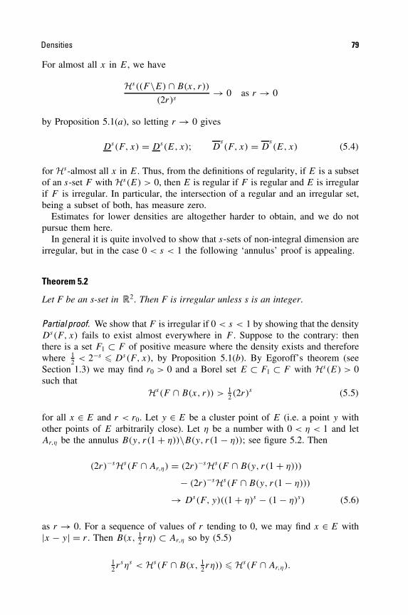
Densities 79
For almost all x in E, we have
Hs((F\E) ∩ B(x, r))
(2r)s→ 0 as r → 0
by Proposition 5.1(a), so letting r → 0 gives
Ds(F, x) = Ds(E, x); Ds(F, x) = D
s(E, x) (5.4)
for Hs-almost all x in E. Thus, from the definitions of regularity, if E is a subsetof an s-set F with Hs(E) > 0, then E is regular if F is regular and E is irregularif F is irregular. In particular, the intersection of a regular and an irregular set,being a subset of both, has measure zero.
Estimates for lower densities are altogether harder to obtain, and we do notpursue them here.
In general it is quite involved to show that s-sets of non-integral dimension areirregular, but in the case 0 < s < 1 the following ‘annulus’ proof is appealing.
Theorem 5.2
Let F be an s-set in �2. Then F is irregular unless s is an integer.
Partial proof. We show that F is irregular if 0 < s < 1 by showing that the densityDs(F, x) fails to exist almost everywhere in F . Suppose to the contrary: thenthere is a set F1 ⊂ F of positive measure where the density exists and thereforewhere 1
2 < 2−s � Ds(F, x), by Proposition 5.1(b). By Egoroff’s theorem (seeSection 1.3) we may find r0 > 0 and a Borel set E ⊂ F1 ⊂ F with Hs(E) > 0such that
Hs(F ∩ B(x, r)) > 12 (2r)s (5.5)
for all x ∈ E and r < r0. Let y ∈ E be a cluster point of E (i.e. a point y withother points of E arbitrarily close). Let η be a number with 0 < η < 1 and letAr,η be the annulus B(y, r(1 + η))\B(y, r(1 − η)); see figure 5.2. Then
(2r)−sHs(F ∩ Ar,η) = (2r)−sHs(F ∩ B(y, r(1 + η)))
− (2r)−sHs(F ∩ B(y, r(1 − η)))
→ Ds(F, y)((1 + η)s − (1 − η)s) (5.6)
as r → 0. For a sequence of values of r tending to 0, we may find x ∈ E with|x − y| = r . Then B(x, 1
2rη) ⊂ Ar,η so by (5.5)
12rsηs < Hs(F ∩ B(x, 1
2 rη)) � Hs(F ∩ Ar,η).
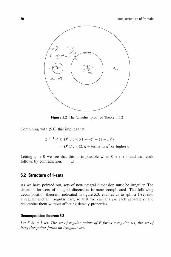
80 Local structure of fractals
Ar,h+ +y
E
B(x, rh/2)
Figure 5.2 The ‘annulus’ proof of Theorem 5.2
Combining with (5.6) this implies that
2−s−1ηs � Ds(F, y)((1 + η)s − (1 − η)s)
= Ds(F, y)(2sη + terms in η2 or higher).
Letting η → 0 we see that this is impossible when 0 < s < 1 and the resultfollows by contradiction. �
5.2 Structure of 1-sets
As we have pointed out, sets of non-integral dimension must be irregular. Thesituation for sets of integral dimension is more complicated. The followingdecomposition theorem, indicated in figure 5.3, enables us to split a 1-set intoa regular and an irregular part, so that we can analyse each separately, andrecombine them without affecting density properties.
Decomposition theorem 5.3
Let F be a 1-set. The set of regular points of F forms a regular set, the set ofirregular points forms an irregular set.
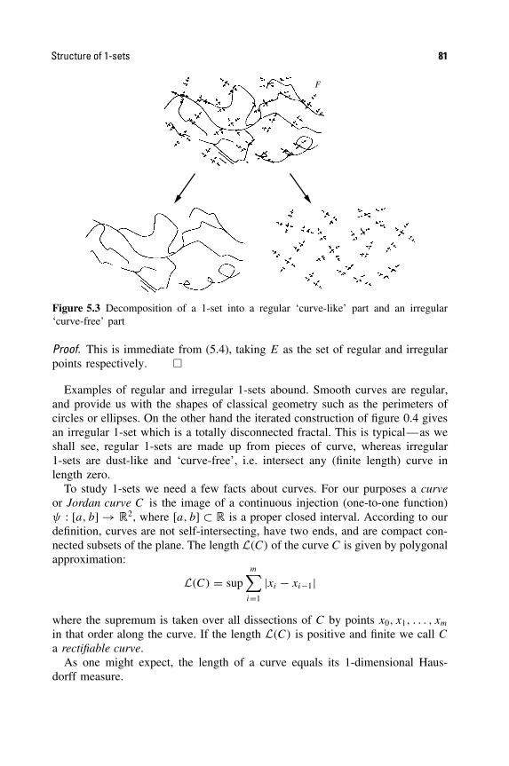
Structure of 1-sets 81
F
Figure 5.3 Decomposition of a 1-set into a regular ‘curve-like’ part and an irregular‘curve-free’ part
Proof. This is immediate from (5.4), taking E as the set of regular and irregularpoints respectively. �
Examples of regular and irregular 1-sets abound. Smooth curves are regular,and provide us with the shapes of classical geometry such as the perimeters ofcircles or ellipses. On the other hand the iterated construction of figure 0.4 givesan irregular 1-set which is a totally disconnected fractal. This is typical—as weshall see, regular 1-sets are made up from pieces of curve, whereas irregular1-sets are dust-like and ‘curve-free’, i.e. intersect any (finite length) curve inlength zero.
To study 1-sets we need a few facts about curves. For our purposes a curveor Jordan curve C is the image of a continuous injection (one-to-one function)ψ : [a, b] → �2, where [a, b] ⊂ � is a proper closed interval. According to ourdefinition, curves are not self-intersecting, have two ends, and are compact con-nected subsets of the plane. The length L(C) of the curve C is given by polygonalapproximation:
L(C) = supm∑
i=1
|xi − xi−1|
where the supremum is taken over all dissections of C by points x0, x1, . . . , xm
in that order along the curve. If the length L(C) is positive and finite we call C
a rectifiable curve.As one might expect, the length of a curve equals its 1-dimensional Haus-
dorff measure.
82 Local structure of fractals
Lemma 5.4
If C is a rectifiable curve then H1(C) = L(C).
Proof. For x, y ∈ C, let Cx,y denote that part of C between x and y. Since orthog-onal projection onto the line through x and y does not increase distances, (2.9)gives H1(Cx,y) � H1[x, y] = |x − y|, where [x, y] is the straight-line segmentjoining x to y. Hence for any dissection x0, x1, . . . , xm of C,
m∑
i=1
|xi − xi−1| �m∑
i=1
H1(Cxi ,xi−1) � H1(C)
so that L(C) � H1(C). On the other hand, let f : [0,L(C)] → C be the mappingthat takes t to the point on C at distance t along the curve from one of its ends.Clearly |f (t) − f (u)| � |t − u| for 0 � t, u � L(C), that is f is Lipschitz andH1(C) � H1[0,L(C)] = L(C) by (2.9) as required. �
It is straightforward to show that rectifiable curves are regular.
Lemma 5.5
A rectifiable curve is a regular 1-set.
Proof. If C is rectifiable, L(C) < ∞, and since C has distinct endpoints p and q,we get L(C) � |p − q| > 0. By Lemma 5.4, 0 < H1(C) < ∞, so C is a 1-set.
A point x of C that is not an endpoint, divides C into two parts Cp,x andCx,q . If r is sufficiently small, then moving away from x along the curve Cx,q
we reach a first point y on C with |x − y| = r . Then Cx,y ⊂ B(x, r) and
r = |x − y| � L(Cx,y) = H1(Cx,y) � H1(Cx,q ∩ B(x, r)).
Similarly, r � H1(Cp,x ∩ B(x, r)), so, adding, 2r � H1(C ∩ B(x, r)), if r issmall enough. Thus
D1(C, x) = limr→0
H1(C ∩ B(x, r))
2r� 1.
By Proposition 5.1(b) D1(C, x) � D1(C, x) � 1, so D1(C, x) exists and equals
1 for all x ∈ C other than the two endpoints, so C is regular. �
Other regular sets are easily constructed. By (5.4), subsets of regular sets, andunions of regular sets should also be regular. With this in mind we define a 1-setto be curve-like if it is contained in a countable union of rectifiable curves.
Proposition 5.6
A curve-like 1-set is a regular 1-set.
Structure of 1-sets 83
Proof. If F is a curve-like 1-set then F ⊂ ⋃∞i=1 Ci where the Ci are rectifiable
curves. For each i and H1-almost all x ∈ F ∩ Ci we have, using Lemma 5.5 andequation (5.4),
1 = D1(Ci, x) = D1(F ∩ Ci, x) � D1(F, x)
and hence 1 � D1(F, x) for almost all x ∈ F . But for almost all x ∈ F wehave D1(F, x) � D
1(F, x) � 1 by Proposition 5.1, so D1(F, x) = 1 almost
everywhere, and F is regular. �
It is natural to introduce a complementary definition: a 1-set is called curve-freeif its intersection with every rectifiable curve has H1-measure-zero.
Proposition 5.7
An irregular 1-set is curve-free.
Proof. If F is irregular and C is a rectifiable curve then F ∩ C is a subset ofboth a regular and an irregular set, so has zero H1-measure. �
These two propositions begin to suggest that regular and irregular sets might becharacterized as curve-like and curve-free respectively. This is indeed the case,but it is far from easy to prove. The crux of the matter is the following lower-density estimate, which depends on an intricate investigation of the properties ofcurves and connected sets and some ingenious geometrical arguments.
Proposition 5.8
Let F be a curve-free 1-set in �2. Then D1(F, x) � 34 at almost all x ∈ F .
Proof. Omitted. �
Assuming this proposition, a complete characterization of regular and irregularsets is relatively easy.
Theorem 5.9
(a) A 1-set in �2 is irregular if and only if it is curve-free.(b) A 1-set in �2 is regular if and only if it is the union of a curve-like set and
a set of H1-measure zero.
Proof
(a) A curve-free set must be irregular by Proposition 5.8. Proposition 5.7 pro-vides the converse implication.
(b) By Proposition 5.6 a curve-like set is regular, and adding in a set ofmeasure zero does not affect densities or, therefore, regularity.

84 Local structure of fractals
If F is regular, then any Borel subset E of positive measure is regular withD1(E, x) = 1 for almost all x ∈ E. By Proposition 5.8 the set E cannotbe curve-free, so some rectifiable curve intersects E in a set of positivelength. We use this fact to define inductively a sequence of rectifiablecurves {Ci}. We choose C1 to cover a reasonably large part of F , say
H1(F ∩ C1) � 12 sup {H1(F ∩ C) : C is rectifiable} > 0.
If C1, . . . , Ck have been selected and Fk = F\⋃ki=1 Ci has positive mea-
sure, let Ck+1 be a rectifiable curve for which
H1(Fk ∩ Ck+1) � 12 sup {H1(Fk ∩ C) : C is rectifiable} > 0. (5.7)
If the process terminates then for some k the curves C1, . . . , Ck coveralmost all of F and F is curve-like. Otherwise,
∞ > H1(F ) �∑
k
H1(Fk ∩ Ck+1)
since the Fk ∩ Ck+1 are disjoint, so that H1(Fk ∩ Ck+1) → 0 as k → ∞.If H1(F\ ⋃∞
i=1 Ci) > 0 there is a rectifiable curve C such that H1((F\⋃∞i=1 Ci) ∩ C) = d for some d > 0. But H1(Fk ∩ Ck+1) < 1
2d for somek, so, according to (5.7), C would have been selected in preference toCk+1. Hence H1(F\⋃∞
i=1 Ci) = 0, and F consists of the curve-like setF ∩ ⋃∞
i=1 Ci together with F\⋃∞i=1 Ci , which is of measure zero. �
Thus regular 1-sets are essentially unions of subsets of rectifiable curves, butirregular 1-sets contain no pieces of rectifiable curves at all. This dichotomy isremarkable in that the definition of regularity is purely in terms of densities andmakes no reference to curves. Propositions 5.6 and 5.8 provide a further contrast.Almost everywhere, a regular set has lower density 1, whereas an irregular sethas lower density at most 3
4 . Thus in any 1-set F the set of points for which34 < D1(F, x) < 1 has H1-measure zero.
Regular 1-sets may be connected but, like sets of dimension less than 1, irreg-ular 1-sets must be totally disconnected. We know at least that distinct pointscannot be joined by a rectifiable curve in an irregular set, and further investigationshows that no two points can lie in the same connected component.
Further differences between regular and irregular sets include the existence oftangents (see Section 5.3) and projection properties (see Chapter 6). In all theseways, the classes of regular and irregular 1-sets are distanced from each other.For the special case of 1-sets, it would make sense mathematically to definefractals to be those sets which are irregular.
5.3 Tangents to s-sets
Suppose that a smooth curve C has a tangent (in the classical sense) at x. Thismeans that close to x the set C is concentrated in two diametrically opposite

Tangents to s-sets 85
directions. What can be said about the directional distribution of an s-set about atypical point? Is there a meaningful definition of a tangent to an s-set, and whendo such tangents exist?
Any generalization of the definition of tangents should reflect the local direc-tional distribution of sets of positive measure—for sets of the complexity thatwe have in mind, there is no hope of a definition involving all nearby points;we must be content with a condition on almost all points. We say that an s-setF in �n has a tangent at x in direction θ (θ a unit vector) if
Ds(F, x) > 0 (5.8)
and, for every angle ϕ > 0,
limr→0
r−sHs(F ∩ (B(x, r)\S(x, θ , ϕ))) = 0 (5.9)
where S(x, θ , ϕ) is the double sector with vertex x, consisting of those y suchthat the line segment [x, y] makes an angle at most ϕ with θ or −θ ; see figure 5.4.Thus, for a tangent in direction θ , (5.8) requires that a significant part of F liesnear x, of which, by (5.9), a negligible amount close to x lies outside any doublesector S(x, θ , ϕ); see figure 5.5.
We first discuss tangents to regular 1-sets in the plane, a situation not farremoved from the classical calculus of curves.
Proposition 5.10
A rectifiable curve C has a tangent at almost all of its points.
Proof. By Lemma 5.5 the upper density D1(C, x) = 1 > 0 for almost all x ∈
C. We may reparametrize the defining function of C by arc length, so that
q
jj
x
Figure 5.4 The double sector S(x, θ , ϕ)
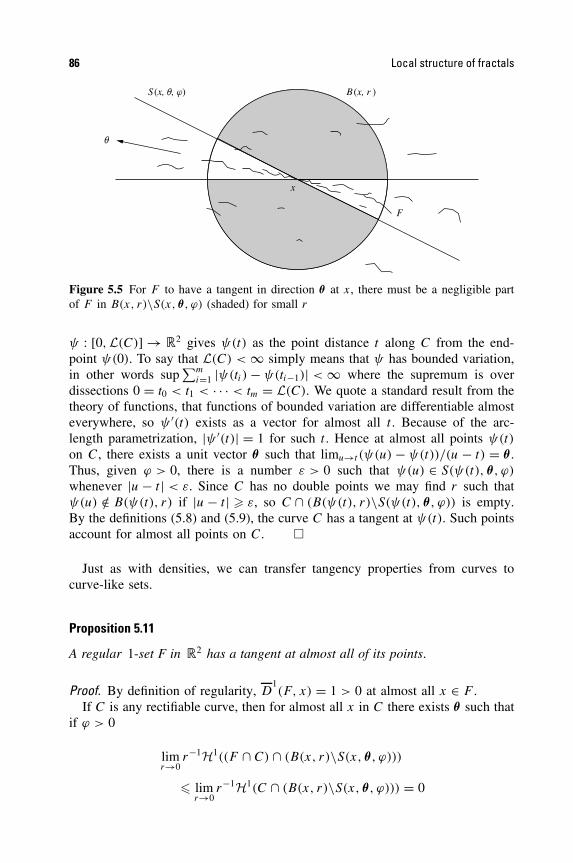
86 Local structure of fractals
S(x, q, j) B(x, r )
F
x
q
Figure 5.5 For F to have a tangent in direction θ at x, there must be a negligible partof F in B(x, r)\S(x, θ , ϕ) (shaded) for small r
ψ : [0,L(C)] → �2 gives ψ(t) as the point distance t along C from the end-point ψ(0). To say that L(C) < ∞ simply means that ψ has bounded variation,in other words sup
∑mi=1 |ψ(ti) − ψ(ti−1)| < ∞ where the supremum is over
dissections 0 = t0 < t1 < · · · < tm = L(C). We quote a standard result from thetheory of functions, that functions of bounded variation are differentiable almosteverywhere, so ψ ′(t) exists as a vector for almost all t . Because of the arc-length parametrization, |ψ ′(t)| = 1 for such t . Hence at almost all points ψ(t)
on C, there exists a unit vector θ such that limu→t (ψ(u) − ψ(t))/(u − t) = θ .Thus, given ϕ > 0, there is a number ε > 0 such that ψ(u) ∈ S(ψ(t), θ , ϕ)
whenever |u − t | < ε. Since C has no double points we may find r such thatψ(u) /∈ B(ψ(t), r) if |u − t | � ε, so C ∩ (B(ψ(t), r)\S(ψ(t), θ , ϕ)) is empty.By the definitions (5.8) and (5.9), the curve C has a tangent at ψ(t). Such pointsaccount for almost all points on C. �
Just as with densities, we can transfer tangency properties from curves tocurve-like sets.
Proposition 5.11
A regular 1-set F in �2 has a tangent at almost all of its points.
Proof. By definition of regularity, D1(F, x) = 1 > 0 at almost all x ∈ F .
If C is any rectifiable curve, then for almost all x in C there exists θ such thatif ϕ > 0
limr→0
r−1H1((F ∩ C) ∩ (B(x, r)\S(x, θ , ϕ)))
� limr→0
r−1H1(C ∩ (B(x, r)\S(x, θ , ϕ))) = 0
Tangents to s-sets 87
by Proposition 5.10. Moreover
limr→0
r−1H1((F\C) ∩ (B(x, r)\S(x, θ , ϕ)))
� limr→0
r−1H1((F\C) ∩ B(x, r)) = 0
for almost all x ∈ C by Property 5.1(a). Adding these inequalities
limr→0
r−1H1(F ∩ (B(x, r)\S(x, θ , ϕ))) = 0
for almost all x ∈ C and so for almost all x ∈ F ∩ C. Since a countable collectionof such curves covers almost all of F , the result follows. �
In contrast to regular sets, irregular 1-sets do not generally support tangents.
Proposition 5.12
At almost all points of an irregular 1-set, no tangent exists.
Proof. The proof, which depends on the characterization of irregular sets as curve-free sets, is too involved to include here. �
We turn now to s-sets in �2 for non-integral s, which, as we have seen,are necessarily irregular. For 0 < s < 1 tangency questions are not particularlyinteresting, since any set contained in a smooth curve will automatically satisfy(5.9) with θ the direction of the tangent to the curve at x. For example, the middlethird Cantor set F regarded as a subset of the plane is a (log 2/ log 3)-set thatsatisfies (5.8) and (5.9) for all x in F and ϕ > 0, where θ is a vector pointingalong the set. On the other hand, if F , say, is a Cartesian product of two uniformCantor sets, each formed by repeated removal of a proportion α > 1
2 from thecentre of intervals, then a little calculation (see Chapter 7) shows that F is ans-set with s = 2 log 2/ log(2/(1 − α)) < 1 with no tangents at any of its points.
It is at least plausible that s-sets in �2 with 1 < s < 2 do not have tan-gents—such sets are so large that they radiate in many directions from a typicalpoint, so that (5.9) cannot hold. This is made precise in the following proposition.
Proposition 5.12
If F is an s-set in �2 with 1 < s < 2, then at almost all points of F, no tan-gent exists.
Proof. For r0 > 0 let
E = {y ∈ F : Hs(F ∩ B(y, r)) < 2(2r)s for all r < r0}. (5.10)

88 Local structure of fractals
For each x ∈ E, each unit vector θ and each angle ϕ with 0 < ϕ < 12π , we
estimate how much of E lies in B(x, r) ∩ S(x, θ , ϕ). For r < r0/20 and i =1, 2, . . . let Ai be the intersection of the annulus and the double sector given by
Ai = (B(x, irϕ)\B(x, (i − 1)rϕ)) ∩ S(x, θ , ϕ).
Then B(x, r) ∩ S(x, θ , ϕ) ⊂ ⋃mi=1 Ai ∪ {x} for some integer m < 2/ϕ. Each Ai
comprises two parts, both of diameter at most 10rϕ < r0, so applying (5.10) tothe parts that contain points of E, and summing,
Hs(E ∩ B(x, r) ∩ S(x, θ , ϕ)) � 2m2(20rϕ)s � (4ϕ−1)2(20rϕ)s
so that(2r)−sHs(E ∩ B(x, r) ∩ S(x, θ , ϕ)) � 8.10sϕs−1 (5.11)
if r < r0/20.Now, almost all x ∈ E satisfy D
s(F\E, x) = 0 by Proposition 5.1(a). Decom-
posing F ∩ B(x, r) into three parts we get
Hs(F ∩ B(x, r)) = Hs((F\E) ∩ B(x, r)) + Hs(E ∩ B(x, r) ∩ S(x, θ , ϕ))
+ Hs(E ∩ (B(x, r)\S(x, θ , ϕ))).
Dividing by (2r)s and taking upper limits as r → 0,
Ds(F, x) � 0 + 8.10sϕs−1 + lim
r→0(2r)−sHs(F ∩ (B(x, r)\S(x, θ , ϕ)))
for almost all x ∈ E, using (5.11). Choosing ϕ sufficiently small, it follows thatfor all θ (5.8) and (5.9) cannot both hold, so no tangent exists at such x. Tocomplete the proof, we note that almost all x ∈ F belong to the set E defined in(5.10) for some r0 > 0, by Proposition 5.1(b). �
The results of this chapter begin to provide a local picture of fractals thatare s-sets. By taking these methods rather further, it is possible to obtain muchmore precise estimates of densities and also of the directional distributions ofs-sets about typical points. For example, it may be shown that if s > 1, almostevery line through Hs-almost every point of an s-set F intersects F in a set ofdimension s − 1.
Recently, packing measures (see Section 3.4) have been employed in the studyof local properties, and it has been shown that regularity of a set correspondsclosely to the equality of its packing measure and (slightly modified) Haus-dorff measure.
These ideas extend, albeit with considerable effort, to higher dimensions. Reg-ular s-sets in �n may be defined using densities and, again, s-sets can only beregular if s is an integer. Regular s-sets have tangents almost everywhere, and are
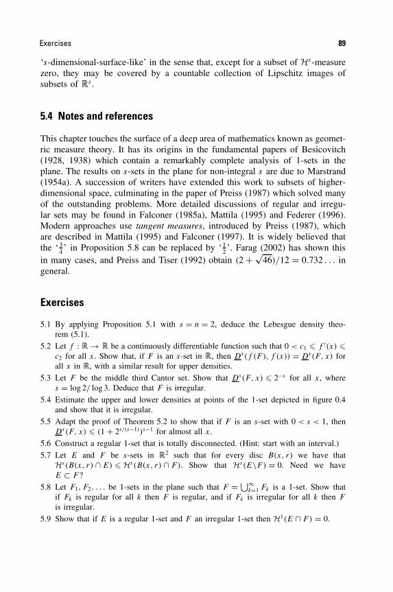
Exercises 89
‘s-dimensional-surface-like’ in the sense that, except for a subset of Hs-measurezero, they may be covered by a countable collection of Lipschitz images ofsubsets of �s .
5.4 Notes and references
This chapter touches the surface of a deep area of mathematics known as geomet-ric measure theory. It has its origins in the fundamental papers of Besicovitch(1928, 1938) which contain a remarkably complete analysis of 1-sets in theplane. The results on s-sets in the plane for non-integral s are due to Marstrand(1954a). A succession of writers have extended this work to subsets of higher-dimensional space, culminating in the paper of Preiss (1987) which solved manyof the outstanding problems. More detailed discussions of regular and irregu-lar sets may be found in Falconer (1985a), Mattila (1995) and Federer (1996).Modern approaches use tangent measures, introduced by Preiss (1987), whichare described in Mattila (1995) and Falconer (1997). It is widely believed thatthe ‘ 3
4 ’ in Proposition 5.8 can be replaced by ‘ 12 ’. Farag (2002) has shown this
in many cases, and Preiss and Tiser (1992) obtain (2 + √46)/12 = 0.732 . . . in
general.
Exercises
5.1 By applying Proposition 5.1 with s = n = 2, deduce the Lebesgue density theo-rem (5.1).
5.2 Let f : � → � be a continuously differentiable function such that 0 < c1 � f ′(x) �c2 for all x. Show that, if F is an s-set in �, then Ds(f (F ), f (x)) = Ds(F, x) forall x in �, with a similar result for upper densities.
5.3 Let F be the middle third Cantor set. Show that Ds(F, x) � 2−s for all x, wheres = log 2/ log 3. Deduce that F is irregular.
5.4 Estimate the upper and lower densities at points of the 1-set depicted in figure 0.4and show that it is irregular.
5.5 Adapt the proof of Theorem 5.2 to show that if F is an s-set with 0 < s < 1, thenDs(F, x) � (1 + 2s/(s−1))s−1 for almost all x.
5.6 Construct a regular 1-set that is totally disconnected. (Hint: start with an interval.)
5.7 Let E and F be s-sets in �2 such that for every disc B(x, r) we have thatHs (B(x, r) ∩ E) � Hs (B(x, r) ∩ F). Show that Hs(E\F) = 0. Need we haveE ⊂ F ?
5.8 Let F1, F2, . . . be 1-sets in the plane such that F = ⋃∞k=1 Fk is a 1-set. Show that
if Fk is regular for all k then F is regular, and if Fk is irregular for all k then F
is irregular.
5.9 Show that if E is a regular 1-set and F an irregular 1-set then H1(E ∩ F) = 0.

Chapter 6 Projections of fractals
In this chapter we consider the orthogonal projection or ‘shadow’ of fractals in �n
onto lower-dimensional subspaces. A smooth (1-dimensional) curve in �3 gener-ally has a (1-dimensional) curve as its shadow on a plane, but a (2-dimensional)surface or (3-dimensional) solid object generally has a 2-dimensional shadow, asin the upper part of figure 6.1. We examine analogues of this for fractals. Intui-tively, one would expect a set F in �3 to have plane projections of dimension2 if dimHF > 2 and of dimension dimHF if dimHF < 2, as in the lower partof figure 6.1. Roughly speaking this is correct, but a precise formulation of theprojection properties requires some care.
We prove the projection theorems in the simplest case, for projection of subsetsof the plane onto lines, and then state the higher-dimensional analogues.
6.1 Projections of arbitrary sets
Let Lθ be the line through the origin of �2 that makes an angle θ with thehorizontal axis. We denote orthogonal projection onto Lθ by projθ , so that if F isa subset of �2, then projθF is the projection of F onto Lθ ; see figure 6.2. Clearly,|projθx − projθy| � |x − y| if x, y ∈ �2, i.e. projθ is a Lipschitz mapping. Thus
dimH(projθF ) � min{dimHF, 1} (6.1)
for any F and θ , by Corollary 2.4(a). (As projθF is a subset of the line Lθ ,its dimension cannot be more than 1.) The interesting question is whether theopposite inequality is valid. The projection theorems tell us that this is so foralmost all θ ∈ [0, π); that is, the exceptional values of θ for which inequality(6.1) is strict form a set of zero length (1-dimensional Lebesgue measure).
Projection theorem 6.1
Let F ⊂ �2 be a Borel set.
(a) If dimHF � 1 then dimH(projθF ) = dimHF for almost all θ ∈ [0, π).(b) If dimHF > 1 then projθF has positive length (as a subset of Lθ ) and so
has dimension 1 for almost all θ ∈ [0, π).
90
Fractal Geometry: Mathematical Foundations and Application. Second Edition Kenneth Falconer 2003 John Wiley & Sons, Ltd ISBNs: 0-470-84861-8 (HB); 0-470-84862-6 (PB)

Projections of arbitrary sets 91
F1 F2
Figure 6.1 Top: projections of classical sets onto a plane—a curve ‘typically’ has pro-jection of dimension 1, but the surface and cube have projections of dimension 2 andof positive area. Bottom: projections of fractal sets onto a plane. If dimHF1 < 1 anddimHF2 > 1 then ‘typically’ the projection of F1 has dimension equal to dimHF1 (andzero area) and the projection of F2 has dimension 2 and positive area
q
F
L q
proj qF
Figure 6.2 Projection of a set F onto a line Lθ
92 Projections of fractals
Proof. We give a proof that uses the potential theoretic characterization of Haus-dorff dimension in a very effective way. If s < dimHF � 1 then by Theo-rem 4.13(b) there exists a mass distribution µ on (a compact subset of) F with0 < µ(F) < ∞ and ∫
F
∫
F
dµ(x)dµ(y)
|x − y|s < ∞. (6.2)
For each θ we ‘project’ the mass distribution µ onto the line Lθ to get a massdistribution µθ on projθF . Thus µθ is defined by the requirement that
µθ([a, b]) = µ{x : a � x · θ � b}
for each interval [a, b], or equivalently,
∫ ∞
−∞f (t)dµθ(t) =
∫
F
f (x · θ)dµ(x)
for each non-negative function f . (Here θ is the unit vector in the direction θ ,with x identified with its position vector and x · θ the usual scalar product.) Then
∫ π
0
[∫ ∞
−∞
∫ ∞
−∞dµθ(u)dµθ(v)
|u − v|s]
dθ =∫ π
0
[∫
F
∫
F
dµ(x)dµ(y)
|x · θ − y · θ |s]
dθ
=∫ π
0
[∫
F
∫
F
dµ(x)dµ(y)
|(x − y) · θ |s]
dθ
=∫ π
0
dθ
|τ · θ |s∫
F
∫
F
dµ(x)dµ(y)
|x − y|s (6.3)
for any fixed unit vector τ . (Note that the integral of |(x − y) · θ |−s with respectto θ depends only on |x − y|.) If s < 1 then (6.3) is finite by virtue of (6.2)and that ∫ π
0
dθ
|τ · θ |s =∫ π
0
dθ
| cos(τ − θ)|s < ∞.
Hence ∫
F
∫
F
dµθ(u)dµθ(v)
|u − v|s < ∞
for almost all θ ∈ [0, π). By Theorem 4.13(a) the existence of such a massdistribution µθ on projθF implies that dimH(projθF ) � s. This is true for alls < dimHF , so part (a) of the result follows.
The proof of (b) follows similar lines, though Fourier transforms need to beintroduced to show that the projections have positive length. �
These projection theorems generalize to higher dimensions in the natural way.Let Gn,k be the set of k-dimensional subspaces or ‘k-planes through the origin’ in

Projections of s-sets of integral dimension 93
�n. These subspaces are naturally parametrized by k(n − k) coordinates (‘gen-eralized direction cosines’) so that we may refer to ‘almost all’ subspaces in aconsistent way in terms of k(n − k)-dimensional Lebesgue measure. We writeproj� for orthogonal projection onto the k-plane �.
Theorem 6.2. Higher-dimensional projection theorem
Let F ⊂ �n be a Borel set.
(a) If dimHF � k then dimH(proj�F) = dimHF for almost all � ∈ Gn,k
(b) If dimHF > k then proj�F has positive k-dimensional measure and so hasdimension k for almost all � ∈ Gn,k .
Proof. The proof of Theorem 6.1 extends to higher dimensions without diffi-culty. �
Thus if F is a subset of �3, the plane projections of F are, in general, ofdimension min{2, dimHF }. This result has important practical implications. Wecan estimate the dimension of an object in space by estimating the dimensionof a photograph taken from a random direction. Provided this is less than 2,it may be assumed to equal the dimension of the object. Such a reduction canmake dimension estimates of spatial objects tractable—box-counting methodsare difficult to apply in 3 dimensions but can be applied with reasonable successin the plane.
6.2 Projections of s-sets of integral dimension
If a subset F of �2 has Hausdorff dimension exactly 1, then Theorem 6.1 tells usthat the projections of F onto almost every Lθ have dimension 1. However, in thiscritical case, no information is given as to whether these projections have zero orpositive length. In the special case where F is a 1-set, i.e. with 0 < Hs(F ) < ∞,an analysis is possible. Recall from Theorem 5.3 that a 1-set may be decomposedinto a regular curve-like part and an irregular dust-like part. The following twotheorems provide another sharp contrast between these types of set.
Theorem 6.3
Let F be a regular 1-set in �2. Then projθF has positive length except for atmost one θ ∈ [0, π).
Sketch of proof. By Theorem 5.9(b) it is enough to prove the result if F is a subsetof positive length of a rectifiable curve C. Using the Lebesgue density theoremto approximate to such an F by short continuous subcurves of C, essentially allwe need to consider is the case when F is itself a rectifiable curve C1 joining

94 Projections of fractals
distinct points x and y. But clearly, the projection onto Lθ of such a curve is aninterval of positive length, except possibly for the one value of θ for which Lθ
is perpendicular to the straight line through x and y. �
(In general projθF will have positive length for all θ ; there is an exceptionalvalue of θ only if F is contained in a set of parallel line segments.)
Theorem 6.4
Let F be an irregular 1-set in �2. Then projθF has length zero for almost allθ ∈ [0, π).
Proof. The proof is complicated, depending on the intricate density and angulardensity structure of irregular sets. We omit it! �
These theorems may be combined in several ways.
Corollary 6.5
Let F be a 1-set in �2. If the regular part of F has H1-measure zero, then projθFhas length zero for almost all θ ; otherwise it has positive length for all but atmost one value of θ .
The following characterization of irregular sets is also useful.
Corollary 6.6
A 1-set in �2 is irregular if and only if it has projections of zero length in at leasttwo directions.
Example 6.7
The Cantor dust F of figure 0.4 is an irregular 1-set.
Calculation. In Example 2.6 we showed that F is a 1-set. It is easy to see that theprojections of F onto lines Lθ with tan θ = 1
2 and tan θ = −2 have zero length(look at the first few iterations), so F is irregular by Corollary 6.6. �
The results of this section have been stated for sets for which 0 < H1(F ) < ∞,which is rather a strong property for 1-dimensional sets to have, although onewhich occurs surprisingly often. However, the theorems can be applied rathermore widely. If F is any set that intersects some rectifiable curve in a set ofpositive length, so that F contains a regular subset, then projθF has positivelength for almost all θ . Again, if F is a σ -finite irregular set, i.e. one which maybe expressed as a countable union of irregular 1-sets each of finite measure, thenprojθF has zero length for almost all θ ; this follows by taking countable unionsof the projections of these component 1-sets.

Projections of arbitrary sets of integral dimension 95
For the record, we state the higher-dimensional analogue of Theorems 6.3 and6.4, though the proofs are even more complicated than in the plane case.
Theorem 6.8
Let F be a k-set in �n, where k is an integer.
(a) If F is regular then proj�F has positive k-dimensional measure for almostall � ∈ Gn,k .
(b) If F is irregular then proj�F has zero k-dimensional measure for almostall � ∈ Gn,k .
6.3 Projections of arbitrary sets of integral dimension
The theorems of the last section, although mathematically elegant and sophisti-cated, do not provide a complete answer to the question of whether projectionsof plane sets onto lines have zero or positive length. A subset F of �2 of Haus-dorff dimension 1 need not be a 1-set or even be of σ -finite H1-measure (i.e. acountable union of sets of finite H1-measure). Moreover there need not be anydimension function h (see Section 2.5) for which 0 < Hh(F ) < ∞, in whichcase mathematical analysis is extremely difficult. What can be said about theprojections of such sets? The surprising answer is that, by working in this ratherdelicate zone of sets of Hausdorff dimension 1 but of non-σ -finite H1-measure,we can construct sets with projections more or less what we please. For example,there is a set F in �2 such that projθF contains an interval of length 1 for almostall θ with 0 � θ < 1
2π but with projθF of length zero for 12π � θ < π . More
generally, we have the following result which says that there exist sets for whichthe projections in almost all directions are, to within length zero, anything thatwe care to prescribe. The measurability condition in square brackets is includedfor completeness, but is best ignored by non-specialists!
Theorem 6.9
Let Gθ be a subset of Lθ for each θ ∈ [0, π) [such that the set⋃
0�θ<π Gθ isplane Lebesgue measurable]. Then there exists a Borel set F ⊂ �2 such that
(a) projθF ⊃ Gθ for all θ , and(b) length (projθF\Gθ) = 0 for almost all θ .
In particular, for almost all θ , the set of points of Lθ belonging to either Gθ orprojθF , but not both, has zero length.
Idea of proof. Without going into much detail, we indicate the basic building blockfor such sets, which has been termed the ‘iterated Venetian blind’ construction.This is shown in figure 6.3. Let E be a line segment of length λ. Let ε be a
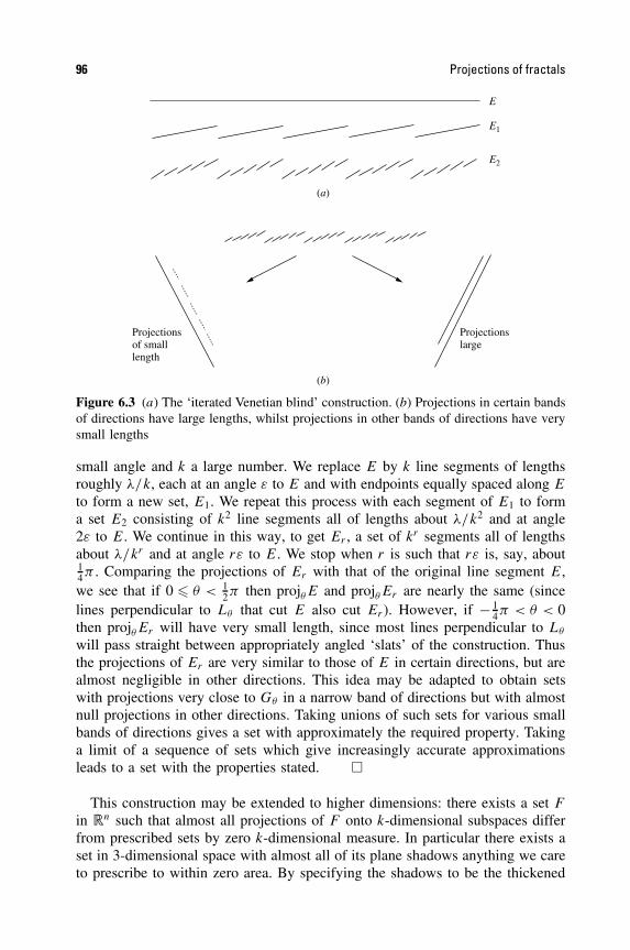
96 Projections of fractals
(a)
Projectionsof smalllength
Projectionslarge
(b)
E
E1
E2
Figure 6.3 (a) The ‘iterated Venetian blind’ construction. (b) Projections in certain bandsof directions have large lengths, whilst projections in other bands of directions have verysmall lengths
small angle and k a large number. We replace E by k line segments of lengthsroughly λ/k, each at an angle ε to E and with endpoints equally spaced along E
to form a new set, E1. We repeat this process with each segment of E1 to forma set E2 consisting of k2 line segments all of lengths about λ/k2 and at angle2ε to E. We continue in this way, to get Er , a set of kr segments all of lengthsabout λ/kr and at angle rε to E. We stop when r is such that rε is, say, about14π . Comparing the projections of Er with that of the original line segment E,we see that if 0 � θ < 1
2π then projθE and projθEr are nearly the same (sincelines perpendicular to Lθ that cut E also cut Er). However, if − 1
4π < θ < 0then projθEr will have very small length, since most lines perpendicular to Lθ
will pass straight between appropriately angled ‘slats’ of the construction. Thusthe projections of Er are very similar to those of E in certain directions, but arealmost negligible in other directions. This idea may be adapted to obtain setswith projections very close to Gθ in a narrow band of directions but with almostnull projections in other directions. Taking unions of such sets for various smallbands of directions gives a set with approximately the required property. Takinga limit of a sequence of sets which give increasingly accurate approximationsleads to a set with the properties stated. �
This construction may be extended to higher dimensions: there exists a set F
in �n such that almost all projections of F onto k-dimensional subspaces differfrom prescribed sets by zero k-dimensional measure. In particular there exists aset in 3-dimensional space with almost all of its plane shadows anything we careto prescribe to within zero area. By specifying the shadows to be the thickened

Exercises 97
Set of dimension 2
Shadow that changes as the sun moves round to give differentprojections
Figure 6.4 A digital sundial
digits of the time when the sun is shining from a perpendicular direction, weobtain, at least in theory, a digital sundial; see figure 6.4. As the sun movesacross the sky we get different projections of the set. The notion of a digitalsundial was introduced to provide an intuitive view of this result, rather than as afeasible method of chronography, but, amazingly, working digital sundials haverecently been manufactured, albeit depending on a different principle!
6.4 Notes and references
A geometric proof of the projection theorems for arbitrary subsets of the planewas given by Marstrand (1954a); the potential theoretic proof was due to Kauf-man (1968). Mattila (1975) obtained various generalizations including extensionsto higher dimensions. The projection results for regular and irregular 1-sets inthe plane are, surprisingly, rather older, dating back to Besicovitch (1939), withthe analogous results for s-sets in �n in the mammoth paper of Federer (1947).More detailed accounts of the projection theorems are in Falconer (1985a) andMattila (1995). Projection results for box and packing dimensions are more sub-tle, see Falconer and Howroyd (1997) and Howroyd (2001). A dual version ofTheorem 6.9 was given by Davies (1952) and a direct proof, with the higher-dimensional generalizations, by Falconer (1986a).
Exercises
6.1 Let E = F × F ⊂ �2 where F is the middle λ Cantor set. (E has Hausdorff dimen-sion 2 log 2/ log(2/(1 − λ)), see Examples 4.5 and 7.6.) What is dimHprojθE (a) fora typical θ and (b) for θ = 0 and θ = π/2?

98 Projections of fractals
6.2 Let E be the ‘circular Cantor set’ given in complex number form by E = {e2πiϕ :ϕ ∈ F } where F is the middle third Cantor set. What is dimHprojθE for each θ?
6.3 For 0 < s < 1, give an example of an s-set F in �2 such that projθF is an s-set forall θ .
6.4 Let E and F be subsets of � with Hausdorff dimension strictly between 0 and1. You are given that the subset E × F of �2 has Hausdorff dimension at leastdimHE + dimHF (see Chapter 7). Show that the projections of E × F onto thecoordinate axes are always ‘exceptional’ as far Projection theorem 6.1 is concerned.
6.5 Show that dimHprojθF � dimHF − 1 for all F ⊂ �2 and all θ .
6.6 Let F be an irregular 1-set in the plane. Deduce from Theorem 6.4 that F is totallydisconnected.
6.7 Let F be a connected subset of �2 containing more than one point. Show that projθFhas positive length for all except possibly one value of θ . (Thus the projectiontheorems in the plane are only really of interest for sets that are not connected.)
6.8 Let E and F be subsets of �. Show that, for almost all real numbersλ, dimH(E + λF) = min{1, dimH(E × F)}, where E + λF denotes the set of realnumbers {x + λy : x ∈ E, y ∈ F }.
6.9 Show that the conclusion of Theorem 6.4 remains true if F is a countable union ofirregular 1-sets.
6.10 Let E and F be any subsets of � of length (1-dimensional Lebesgue measure)0. Show that any rectifiable curve in �2 intersects the product E × F in a set oflength 0.
6.11 If F is a set and x is a point in �2, the projection of F at x, denoted by projxF , isdefined as the set of θ in [0, 2π) such that the half-line emanating from x in directionθ intersects F . Let L be a line. Show that if dimHF � 1 then dimHprojxF = dimHF
for almost all x on L (in the sense of Lebesgue measure) and if dimHF > 1 thenprojxF has positive length for almost all x on L. (Hint: consider a sphere tangentialto the plane and a transformation that maps a point x on the plane to the point onthe sphere intersected by the line joining x to the centre of the sphere.)
6.12 Let F ⊂ �2. Show that for all θ , dimB projθF � dimBF , dimB projθF � dimBF
and dimP projθF � dimPF . Show that dimP projθF = dimPF for almost all θ ifdimPF = dimHF .

Chapter 7 Products of fractals
One way of constructing ‘new fractals from old’ is by forming Cartesian products.Indeed, many fractals that occur in practice, for example as attractors of certaindynamical systems, are products or, at least, are locally product-like. In thischapter we develop dimension formulae for products.
7.1 Product formulae
Recall that if E is a subset of �n and F is a subset of �m, the Cartesian product,or just product, E × F is defined as the set of points with first coordinate in E
and second coordinate in F , i.e.
E × F = {(x, y) ∈ �n+m : x ∈ E, y ∈ F }. (7.1)
Thus if E is a unit interval in �, and F is a unit interval in �2, then E × F isa unit square in �3 (figure 7.1). Again, if F is the middle third Cantor set, thenF × F is the ‘Cantor product’ (figure 7.2) consisting of those points in the planewith both coordinates in F .
In the first example above it is obvious that
dim(E × F) = dimE + dimF
using the classical definition of dimension. This holds more generally, in the‘smooth’ situation, where E and F are smooth curves, surfaces or higher-dimen-sional manifolds. Unfortunately, this equation is not always valid for ‘fractal’dimensions. For Hausdorff dimensions the best general result possible is aninequality dimH(E × F) � dimHE + dimHF . Nevertheless, as we shall see, inmany situations equality does hold.
The proof of the product rule uses the Hausdorff measures on E and F todefine a mass distribution µ on E × F . Density bounds on E and F lead toestimates for µ suitable for a mass distribution method.
99
Fractal Geometry: Mathematical Foundations and Application. Second Edition Kenneth Falconer 2003 John Wiley & Sons, Ltd ISBNs: 0-470-84861-8 (HB); 0-470-84862-6 (PB)

100 Products of fractals
E × F
E
F2
E × F
E
F
Figure 7.1 The Cartesian product of a unit interval in � and a unit interval in �2
Proposition 7.1
If E ⊂ �n, F ⊂ �m are Borel sets with Hs(E),Ht (F ) < ∞, then
Hs+t (E × F) � cHs(E)Ht (F ) (7.2)
where c > 0 depends only on s and t.
Proof. For simplicity we assume that E,F ⊂ �, so that E × F ⊂ �2; the generalproof is almost identical. If either Hs(E) or Ht (F ) is zero, then (7.2) is trivial,
Figure 7.2 The product F × F , where F is the middle third Cantor set. In this case,dimHF × F = 2 dimHF = 2 log 2/ log 3
Product formulae 101
so suppose that E is an s-set and F is a t-set, i.e. 0 < Hs(E),Ht (F ) < ∞. Wemay define a mass distribution µ on E × F by utilizing the ‘product measure’of Hs and Ht . Thus if I, J ⊂ �, we define µ on the ‘rectangle’ I × J by
µ(I × J ) = Hs(E ∩ I )Ht (F ∩ J ). (7.3)
It may be shown that this defines a mass distribution µ on E × F with µ(�2) =Hs(E)Ht (F ).
By the density estimate Proposition 5.1(b) we have that
limr→0
Hs(E ∩ B(x, r))(2r)−s � 1 (7.4)
for Hs-almost all x ∈ E and
limr→0
Ht (F ∩ B(y, r))(2r)−t � 1 (7.5)
for Ht -almost all y ∈ F . (Of course, since we are concerned with subsets of �,the ‘ball’ B(x, r) is just the interval of length 2r with midpoint x.) From thedefinition of µ, both (7.4) and (7.5) hold for µ-almost all (x, y) in E × F . Sincethe disc B((x, y), r) is contained in the square B(x, r) × B(y, r) we have that
µ(B((x, y), r)) � µ(B(x, r) × B(y, r)) = Hs(E ∩ B(x, r))Ht (F ∩ B(y, r))
soµ(B((x, y), r))
(2r)s+t� Hs(E ∩ B(x, r))
(2r)s
Ht (F ∩ B(y, r))
(2r)t.
It follows, using (7.4) and (7.5), that limr→0 µ(B((x, y), r))(2r)−(s+t) � 1 forµ-almost all (x, y) ∈ E × F . By Proposition 4.9(a)
Hs(E × F) � 2−(s+t)µ(E × F) = 2−(s+t)Hs(E)Ht (F ). �
Product formula 7.2
If E ⊂ �n, F ⊂ �m are Borel sets then
dimH(E × F) � dimHE + dimHF. (7.6)
Proof. If s, t are any numbers with s < dimHE and t < dimHF , then Hs(E) =Ht (F ) = ∞. Theorem 4.10 implies that there are Borel sets E0 ⊂ E and F0 ⊂ F
with 0 < Hs(E0),Ht (F0) < ∞. By Proposition 7.1 Hs+t (E× F)�Hs+t (E0 ×F0)�cHs(E0)Ht (F0) > 0. Hence dimH(E × F) � s + t . By choosing s and t
arbitrarily close to dimHE and dimHF , (7.6) follows. �
Proposition 7.1 and Formula 7.2 are in fact valid for arbitrary (non-Borel) sets.
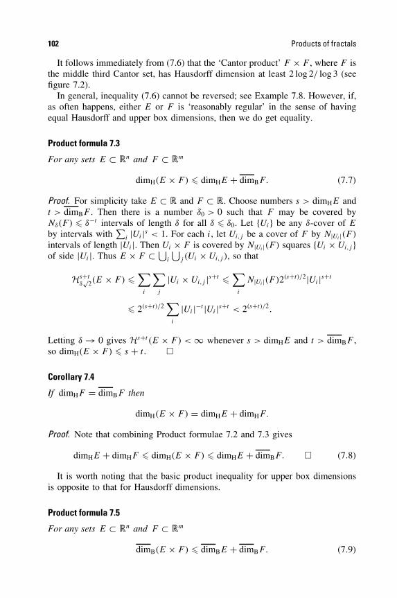
102 Products of fractals
It follows immediately from (7.6) that the ‘Cantor product’ F × F , where F isthe middle third Cantor set, has Hausdorff dimension at least 2 log 2/ log 3 (seefigure 7.2).
In general, inequality (7.6) cannot be reversed; see Example 7.8. However, if,as often happens, either E or F is ‘reasonably regular’ in the sense of havingequal Hausdorff and upper box dimensions, then we do get equality.
Product formula 7.3
For any sets E ⊂ �n and F ⊂ �m
dimH(E × F) � dimHE + dimBF. (7.7)
Proof. For simplicity take E ⊂ � and F ⊂ �. Choose numbers s > dimHE andt > dimBF . Then there is a number δ0 > 0 such that F may be covered byNδ(F ) � δ−t intervals of length δ for all δ � δ0. Let {Ui} be any δ-cover of E
by intervals with∑
i |Ui |s < 1. For each i, let Ui,j be a cover of F by N|Ui |(F )
intervals of length |Ui|. Then Ui × F is covered by N|Ui |(F ) squares {Ui × Ui,j }of side |Ui |. Thus E × F ⊂ ⋃
i
⋃j (Ui × Ui,j ), so that
Hs+tδ√
2(E × F) �∑
i
∑
j
|Ui × Ui,j |s+t �∑
i
N|Ui |(F )2(s+t)/2|Ui |s+t
� 2(s+t)/2∑
i
|Ui |−t |Ui |s+t < 2(s+t)/2.
Letting δ → 0 gives Hs+t (E × F) < ∞ whenever s > dimHE and t > dimBF ,so dimH(E × F) � s + t . �
Corollary 7.4
If dimHF = dimBF then
dimH(E × F) = dimHE + dimHF.
Proof. Note that combining Product formulae 7.2 and 7.3 gives
dimHE + dimHF � dimH(E × F) � dimHE + dimBF. � (7.8)
It is worth noting that the basic product inequality for upper box dimensionsis opposite to that for Hausdorff dimensions.
Product formula 7.5
For any sets E ⊂ �n and F ⊂ �m
dimB(E × F) � dimBE + dimBF. (7.9)

Product formulae 103
Proof. This is left as Exercise 7.5. The idea is just as in Formula 7.3—note that ifE and F can be covered by Nδ(E) and Nδ(F ) intervals of side δ, then E × F iscovered by the Nδ(E)Nδ(F ) squares formed by products of these intervals. �
Example 7.6. Product with uniform Cantor sets
Let E, F be subsets of � with F a uniform Cantor set (see Example 4.5). ThendimH(E × F) = dimHE + dimHF .
Calculation. Example 4.5 shows that uniform Cantor sets have equal Hausdorffand upper box dimensions, so the result follows from Corollary 7.4. �
Thus the ‘Cantor product’ of the middle third Cantor set with itself has Haus-dorff and box dimensions exactly 2 log 2/ log 3. Similarly, if E is a subset of �and F is a straight line segment, then dimH(E × F) = dimHE + 1.
Many fractals encountered in practice are not actually products, but are locallyproduct-like. For example, the Henon attractor (see (13.5)) looks locally like aproduct of a line segment and a Cantor-like set F . More precisely, there aresmooth bijections from [0, 1] × F to small neighbourhoods of the attractor. Suchsets may be analysed as the image of a product under a suitable Lipschitz trans-formation.
Example 7.7
The ‘Cantor target’ is the plane set given in polar coordinates by F ′ = {(r, θ) :r ∈ F, 0 � θ � 2π} where F is the middle third Cantor set; see figure 7.3. ThendimHF ′ = 1 + log 2/ log 3.
Calculation. Let f : �2 → �2 be given by f (x, y) = (x cos y, x sin y). It is easyto see that f is a Lipschitz mapping and F ′ = f (F × [0, 2π]). Thus
dimHF ′ = dimHf (F × [0, 2π]) � dimH(F × [0, 2π])
= dimHF + dimH[0, 2π] = (log 2/ log 3) + 1
by Corollary 2.4(a) and Example 7.6. On the other hand, if we restrict f to[ 2
3 , 1] × [0, π] then f is a bi-Lipschitz function on this domain. Since F ′ ⊃f ((F ∩ [ 2
3 , 1]) × [0, π]) we have
dimHF ′ � dimHf ((F ∩ [ 23 , 1]) × [0, π])
= dimH((F ∩ [ 23 , 1]) × [0, π])
= dimH(F ∩ [ 23 , 1]) + dimH[0, π]
= (log 2/ log 3) + 1
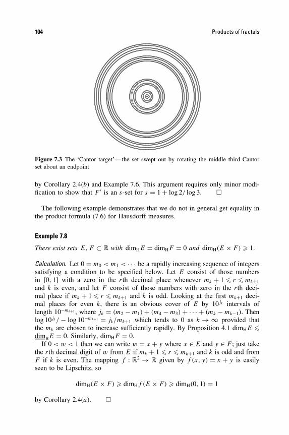
104 Products of fractals
Figure 7.3 The ‘Cantor target’—the set swept out by rotating the middle third Cantorset about an endpoint
by Corollary 2.4(b) and Example 7.6. This argument requires only minor modi-fication to show that F ′ is an s-set for s = 1 + log 2/ log 3. �
The following example demonstrates that we do not in general get equality inthe product formula (7.6) for Hausdorff measures.
Example 7.8
There exist sets E,F ⊂ � with dimHE = dimHF = 0 and dimH(E × F) � 1.
Calculation. Let 0 = m0 < m1 < · · · be a rapidly increasing sequence of integerssatisfying a condition to be specified below. Let E consist of those numbersin [0, 1] with a zero in the rth decimal place whenever mk + 1 � r � mk+1
and k is even, and let F consist of those numbers with zero in the rth deci-mal place if mk + 1 � r � mk+1 and k is odd. Looking at the first mk+1 deci-mal places for even k, there is an obvious cover of E by 10jk intervals oflength 10−mk+1 , where jk = (m2 − m1) + (m4 − m3) + · · · + (mk − mk−1). Thenlog 10jk / − log 10−mk+1 = jk/mk+1 which tends to 0 as k → ∞ provided thatthe mk are chosen to increase sufficiently rapidly. By Proposition 4.1 dimHE �dimBE = 0. Similarly, dimHF = 0.
If 0 < w < 1 then we can write w = x + y where x ∈ E and y ∈ F ; just takethe rth decimal digit of w from E if mk + 1 � r � mk+1 and k is odd and fromF if k is even. The mapping f : �2 → � given by f (x, y) = x + y is easilyseen to be Lipschitz, so
dimH(E × F) � dimHf (E × F) � dimH(0, 1) = 1
by Corollary 2.4(a). �

Product formulae 105
A useful generalization of the product formula relates the dimension of a setto the dimensions of parallel sections. We work in the (x, y)-plane and let Lx
denote the line parallel to the y-axis through the point (x, 0).
Proposition 7.9
Let F be a Borel subset of �2. If 1 � s � 2 then
∫ ∞
−∞Hs−1(F ∩ Lx)dx � Hs(F ). (7.10)
Proof. Given ε > 0, let {Ui} be a δ-cover of F such that
∑
i
|Ui|s � Hsδ(F ) + ε.
Each Ui is contained in a square Si of side |Ui| with sides parallel to the coor-dinate axes.
Let χi be the indicator function of Si (i.e. χi(x, y) = 1 if (x, y) ∈ Si andχi(x, y) = 0 if (x, y) /∈ Si). For each x, the sets {Si ∩ Lx} form a δ-cover ofF ∩ Lx , so
Hs−1δ (F ∩ Lx) �
∑
i
|Si ∩ Lx |s−1
=∑
i
|Ui |s−2|Si ∩ Lx |
=∑
i
|Ui |s−2∫
χi(x, y)dy.
Hence
∫Hs−1
δ (F ∩ Lx)dx �∑
i
|Ui|s−2∫∫
χi(x, y)dxdy
=∑
i
|Ui |s
� Hsδ(F ) + ε.
Since ε > 0 is arbitrary,∫ Hs−1
δ (F ∩ Lx)dx � Hsδ(F ). Letting δ → 0 gives
(7.10). �

106 Products of fractals
Corollary 7.10
Let F be a Borel subset of �2. Then, for almost all x (in the sense of 1-dimensionalLebesgue measure), dimH(F ∩ Lx) � max{0, dimHF − 1}.Proof. Take s > dimHF , so that Hs(F ) = 0. If s > 1, formula (7.10) givesHs−1(F ∩ Lx) = 0 and so dimH(F ∩ Lx) � s − 1, for almost all x. �
We state, without proof, a further useful generalization.
Proposition 7.11
Let F be any subset of �2, and let E be any subset of the x-axis. Suppose thatthere is a constant c such that Ht (F ∩ Lx) � c for all x ∈ E. Then
Hs+t (F ) � bcHs(E) (7.11)
where b > 0 depends only on s and t.
This result may be phrased in terms of dimensions.
Corollary 7.12
Let F be any subset of �2, and let E be a subset of the x-axis. If dimH(F ∩ Lx) � t
for all x ∈ E, then dimHF � t + dimHE.
The obvious higher-dimensional analogues of these results are all valid.The following illustration of Proposition 7.9 is an example of a self-affine set,
a class of sets which will be discussed in more detail in Section 9.4.
Example 7.13. A self-affine set
Let F be the set with iterated construction indicated in figure 7.4. (At the kth stageeach rectangle of Ek is replaced with an affine copy of the rectangles in E1. Thusthe contraction is greater in the ‘y’ direction than in the ‘x’ direction, with thewidth to height ratio of the rectangles in Ek tending to infinity as k → ∞.) ThendimHF = dimBF = 1 1
2 .
Calculation. Ek consists of 6k rectangles of size 3−k × 4−k. Each of these rect-angles may be covered by at most (4/3)k + 1 squares of side 4−k, by dividingthe rectangles using a series of vertical cuts. Hence Ek may be covered by6k × 2 × 4k × 3−k = 2 × 8k squares of diameter 4−k
√2. In the usual way this
gives dimHF � dimBF � 1 12 .
On the other hand, except for x of the form j3−k where j and k are integers, wehave that Ek ∩ Lx consists of 2k intervals of length 4−k. A standard applicationof the mass distribution method shows that H1/2(Ek ∩ Lx) � 1
2 for each such x.By Proposition 7.9, H3/2(F ) � 1
2 . Hence dimHF = dimBF = 1 12 . �

Exercises 107
E0 E1
F
E2
Figure 7.4 Construction of a self-affine set, dimHF = 1 12
7.2 Notes and references
Versions of the basic product formula date from Besicovitch and Moran (1945). Avery general result, proved using net measures, was given by Marstrand (1954b).For packing dimensions of products, see Tricot (1982) and Howroyd (1996).
Exercises
7.1 Show that for every set F ⊂ [0, 1], we have dimH(F × [0, 1]) = 1 + dimHF .
7.2 Let Fλ denote the middle λ Cantor set (see Example 4.5). What are the box andHausdorff dimensions of Fλ × Fµ for 0 < λ, µ < 1?
7.3 Let F be any subset of [0, ∞) and let F ′ be the ‘target’ in �2 given in polarcoordinates by {(r, θ) : r ∈ F, 0 � θ < 2π}. Show that dimHF ′ = 1 + dimHF .
7.4 Show that there is a subset F of �2 of Hausdorff dimension 2 with projections ontoboth coordinate axes of length 0. (Hint: see Exercise 4.9.) Deduce that any 1-setcontained in F is irregular, and that any rectifiable curve intersects F in a set oflength 0.
7.5 Derive Product formula 7.5.
7.6 What are the Hausdorff and box dimensions of the plane set {(x, y) ∈ �2 : x + y ∈F and x − y ∈ F }, where F is the middle third Cantor set?
7.7 Let F ⊂ � have equal Hausdorff and upper box dimensions. Let D be theset {x − y : x, y ∈ F }, known as the difference set of F . Show that dimHD �min{1, 2dimHF }. (Hint: consider the set F × F .)
7.8 Sketch the plane set {(x, y) : y − x2 ∈ F } where F is the middle third Cantor set,and find its Hausdorff and box dimensions.
7.9 Let Lx be as in Proposition 7.9. Let F be a subset of �2 and let Es = {x ∈ � :dimH(F ∩ Lx) � s} for 0 � s � 1. Show that dimHF � sup0�s�1{s + dimHEs}.

108 Products of fractals
7.10 Divide the unit square E0 into a three column, five row array of rectangles of sides 13
and 15 , and let E1 be a set obtained by choosing some four of the five rectangles from
each column. Let F be the self-affine set formed by repeatedly replacing rectanglesby affine copies of E1 (compare Example 7.13). Adapt the method of Example 7.13to show that dimHF = 1 + log 4/ log 5.
7.11 Modify the construction of the previous exercise so that E1 contains four rectanglesfrom each of the first and third columns but none from the middle column. Showthat dimHF = log 2/ log 3 + log 4/ log 5.
Chapter 8 Intersections of fractals
The intersection of two fractals is often a fractal; it is natural to try to relate thedimension of this intersection to that of the original sets. It is immediately appar-ent that we can say almost nothing in the general case. For if F is bounded, thereis a congruent copy F1 of F such that dimH(F ∩ F1) = dimHF (takeF1 = F) and another congruent copy with dimH(F ∩ F1) = Ø (take F and F1
disjoint). However, we can say rather more provided we consider the intersectionof F and a congruent copy in a ‘typical’ relative position.
To illustrate this, let F and F1 be unit line segments in the plane. Then F ∩ F1
can be a line segment, but only in the exceptional situation when F and F1 arecollinear. If F and F1 cross at an angle, then F ∩ F1 is a single point, but nowF ∩ F1 remains a single point if F1 is replaced by a nearby congruent copy.Thus, whilst ‘in general’ F ∩ F1 contains at most one point, this situation occurs‘frequently’.
We can make this rather more precise. Recall that a rigid motion or directcongruence transformation σ of the plane transforms any set E to a congruentcopy σ(E) without reflection. The rigid motions may be parametrized by threecoordinates (x, y, θ) where the origin is transformed to (x, y) and θ is the angleof rotation. Such a parametrization provides a natural measure on the space ofrigid motions, with the measure of a set A of rigid motions given by the 3-dimensional Lebesgue measure of the (x, y, θ) parametrizing the motions in A.For example, the set of all rigid motions which map the origin to a point of therectangle [1, 2] × [0, 3] has measure 1 × 3 × 2π .
In the example with F a unit line segment, the set of transformations σ forwhich F ∩ σ(F ) is a line segment has measure 0. However, F ∩ σ(F ) is a singlepoint for a set of transformations of positive measure, in fact a set of measure 4.
Similar ideas hold in higher dimensions. In �3, ‘typically’, two surfaces inter-sect in a curve, a surface and a curve intersect in a point and two curves aredisjoint. In �n, if smooth manifolds E and F intersect at all, then ‘in general’they intersect in a submanifold of dimension max{0, dim E + dim F − n}. Moreprecisely, if dim E + dim F − n > 0 then dim (E ∩ σ(F )) = dim E + dim F − n
for a set of rigid motions σ of positive measure, and is 0 for almost all otherσ . (Of course, σ is now measured using the 1
2n(n + 1) parameters required tospecify a rigid transformation of �n.)
109
Fractal Geometry: Mathematical Foundations and Application. Second Edition Kenneth Falconer 2003 John Wiley & Sons, Ltd ISBNs: 0-470-84861-8 (HB); 0-470-84862-6 (PB)
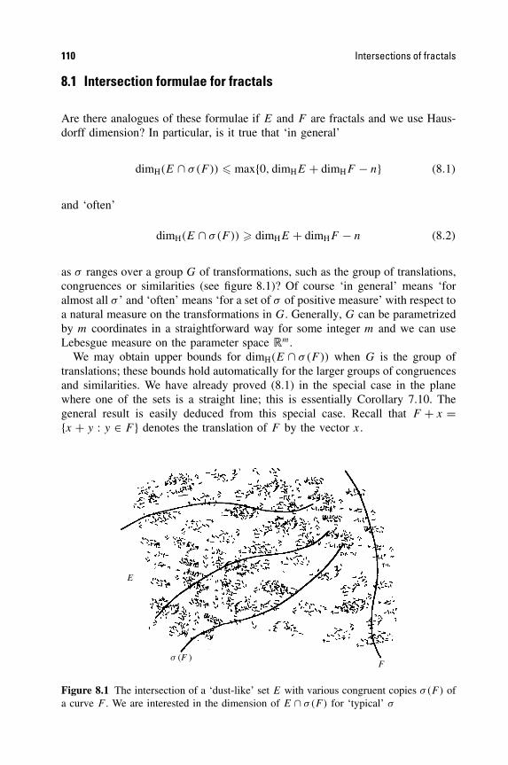
110 Intersections of fractals
8.1 Intersection formulae for fractals
Are there analogues of these formulae if E and F are fractals and we use Haus-dorff dimension? In particular, is it true that ‘in general’
dimH(E ∩ σ(F )) � max{0, dimHE + dimHF − n} (8.1)
and ‘often’
dimH(E ∩ σ(F )) � dimHE + dimHF − n (8.2)
as σ ranges over a group G of transformations, such as the group of translations,congruences or similarities (see figure 8.1)? Of course ‘in general’ means ‘foralmost all σ ’ and ‘often’ means ‘for a set of σ of positive measure’ with respect toa natural measure on the transformations in G. Generally, G can be parametrizedby m coordinates in a straightforward way for some integer m and we can useLebesgue measure on the parameter space �m.
We may obtain upper bounds for dimH(E ∩ σ(F )) when G is the group oftranslations; these bounds hold automatically for the larger groups of congruencesand similarities. We have already proved (8.1) in the special case in the planewhere one of the sets is a straight line; this is essentially Corollary 7.10. Thegeneral result is easily deduced from this special case. Recall that F + x ={x + y : y ∈ F } denotes the translation of F by the vector x.
E
Fs (F )
Figure 8.1 The intersection of a ‘dust-like’ set E with various congruent copies σ(F ) ofa curve F . We are interested in the dimension of E ∩ σ(F ) for ‘typical’ σ

Intersection formulae for fractals 111
Theorem 8.1
If E, F are Borel subsets of �n then
dimH(E ∩ (F + x)) � max{0, dimH(E × F) − n} (8.3)
for almost all x ∈ �n.
Proof. We prove this when n = 1; the proof for n > 1 is similar, using a higher-dimensional analogue of Corollary 7.10. Let Lc be the line in the (x, y)-plane withequation x = y + c. Assuming that dimH(E × F) > 1, it follows from Corollary7.10 (rotating the lines through 45◦ and changing notation slightly) that
dimH((E × F) ∩ Lc) � dimH(E × F) − 1 (8.4)
for almost all c ∈ �. But a point (x, x − c) ∈ (E × F) ∩ Lc if and only ifx ∈ E ∩ (F + c). Thus, for each c, the projection onto the x-axis of (E × F) ∩ Lc
is the set E ∩ (F + c). In particular, dimH(E ∩ (F + c)) = dimH((E × F) ∩ Lc),so the result follows from (8.4). �
Theorem 8.1 is some way from (8.1), but examples show that it is the bestthat we can hope to achieve, even if the group of translations is replaced by thegroup of all rigid motions. Unfortunately, inequality (7.6) is the opposite to whatwould be needed to deduce (8.1) from (8.3). Nevertheless, in many instances,we do have dimH(E × F) = dimHE + dimHF ; for example, if dimHF = dimBF ;see Corollary 7.4. Under such circumstances we recover (8.1), with σ(F ) as thetranslate F + x.
Lower bounds for dimH(E ∩ σ(F )) of the form (8.2) are rather harder toobtain. The main known results are contained in the following theorem.
Theorem 8.2
Let E,F ⊂ �n be Borel sets, and let G be a group of transformations on �n.Then
dimH(E ∩ σ(F )) � dimHE + dimHF − n (8.5)
for a set of motions σ ∈ G of positive measure in the following cases:
(a) G is the group of similarities and E and F are arbitrary sets(b) G is the group of rigid motions, E is arbitrary and F is a rectifiable curve,
surface, or manifold.(c) G is the group of rigid motions and E and F are arbitrary, with either
dimHE > 12 (n + 1) or dimHF > 1
2 (n + 1).
*Outline of proof. The proof uses the potential theoretic methods of Section 4.3. Inmany ways, the argument resembles that of Projection theorem 6.1, but varioustechnical difficulties make it much more complicated.

112 Intersections of fractals
Briefly, if s < dimHE and t < dimHF , there are mass distributions µ on E andν on F with the energies Is(µ) and It (ν) both finite. If ν happened to be absolutelycontinuous with respect to n-dimensional Lebesgue measure, i.e. if there were afunction f such that ν(A) = ∫
Af (x)dx for each set A, then it would be natural
to define a mass distribution ησ on E ∩ σ(F ) by ησ (A) = ∫A
f (σ−1(x))dµ(x).If we could show that Is+t−n(ησ ) < ∞ for almost all σ , Theorem 4.13(a) wouldimply that dimH(E ∩ σ(F )) � s + t − n if ησ (�n) > 0. Unfortunately, when F
is a fractal, ν is supported by a set of zero n-dimensional volume, so is anythingbut absolutely continuous. To get around this difficulty, we can approximate ν byabsolutely continuous mass distributions νδ supported by the δ-neighbourhood ofF . Then, if νδ(A) = ∫
Afδ(x)dx and ησ,δ = ∫
Afδ(σ
−1(x))dµ(x), we can estimateIs+t−n(ησ,δ) and take the limit as δ → 0. Simplifying the integral
∫Is+t−n(ησ,δ)dσ
isolates a term
ϕδ(w) =∫
G0
∫
�n
νδ(y)νδ(y + σ(w))dydσ
where integration with respect to σ is now over the subgroup G0 of F whichfixes the origin. Provided that
ϕδ(w) � constant|w|t−n (8.6)
for all w and δ, it may be shown that∫
Is+t−n(ησ,δ)dσ < c < ∞, where c is inde-pendent of δ. Letting δ → 0, the measures ησ,δ ‘converge’ to measures ησ on E ∩σ(F ), where
∫Is+t−n(ησ ) dσ < c. Thus Is+t−n(ησ ) < ∞ for almost all σ , so, by
Theorem 4.13(a), dimH(E ∩ σ(F )) � s + t − n whenever ησ (E ∩ σ(F )) > 0,which happens on a set of positive measure.
It may be shown that (8.6) holds if It (ν) < ∞ in the cases (a), (b) and (c)listed. This is relatively easy to show for (a) and (b). Case (c) is more awkward,requiring Fourier transform theory. �
The condition that dimHE or dimHF > 12 (n + 1) in case (c) is a curious con-
sequence of the use of Fourier transforms. It is not known whether the theoremremains valid for the group of congruences if n � 2 and 1
2n < dimHE, dimHF �12 (n + 1).
Example 8.3
Let F ⊂ � be the middle third Cantor set. For λ, x ∈ � write λF + x = {λy +x : y ∈ F }. Then dimH(F ∩ (F + x)) � 2(log 2/ log 3) − 1 for almost all x ∈�, and dimH(F ∩ (λF + x)) = 2(log 2/ log 3) − 1 for a set of (x, λ) ∈ �2 ofpositive plane Lebesgue measure.
Calculation. We showed in Example 7.6 that dimH(F × F) = 2(log 2/ log 3), sothe stated dimensions follow from Theorems 8.1 and 8.2(a). �
Sets with large intersection 113
The box and packing dimensions of intersections of sets can behave veryirregularly, with the dimensions of intersections often being ‘unexpectedly small’,see Exercise 8.7.
*8.2 Sets with large intersection
We have seen that (8.1) need not always hold; in this section we examine a classof sets for which it fails dramatically. We construct a large class Cs of subsetsof � of Hausdorff dimension at least s with the property that the intersection ofany countable collection of sets in Cs still has dimension at least s. Sets of thistype occur naturally in number theory; see Section 10.3.
The class Cs is defined in terms of the sums (2.1) used in the definition ofHausdorff measures. For any subset F of � we define
Hs∞(F ) = inf
{ ∞∑
i=1
|Ui |s :∞⋃
i=1
Ui is any cover of F
}
.
Thus Hs∞(F ) is defined using covers of F without any diameter restriction. Thisensures that Hs∞(I ) is finite if I is a bounded interval, which would not be thecase if we used Hs . It is easy to see that Hs∞(F1 ∪ F2) � Hs∞(F1) + Hs∞(F2)
and that Hs∞(F1) � Hs∞(F2) if F1 ⊂ F2.Recall that limk→∞Ek = ⋂∞
i=1
⋃∞k=i Ek is the set of points that belong to
infinitely many Ek; such sets are termed lim sup sets. Let 0 < s < 1 and let[a, b] ⊂ � be a proper closed interval. We say that a subset F of [a, b] is amember of the class Cs[a, b] if
F ⊃ limk→∞Ek (8.7)
where {Ek} is a sequence of subsets of [a, b], such that
(i) each Ek is a finite union of disjoint closed intervals, and
(ii) limk→∞ Hs∞(I ∩ Ek) = |I |s (8.8)
for every bounded closed interval I .
(Of course, we always have Hs∞(I ∩ Ek) � |I |s .) We define Cs(−∞, ∞) by say-ing that F is in Cs (−∞,∞) if F ∩ I ∈ Cs[a, b] for every bounded interval [a, b].The results below extend easily from Cs[a, b] to Cs(−∞,∞).
As an example of the sets we have in mind, we might take Ek = {x :|x − p/k| < k−3 for some integer p}, so that F = limk→∞Ek consists of thenumbers which satisfy the inequality |x − p/k| < k−3 for some p for infinitelymany positive integers k. As we shall see, F ∈ C1/3(−∞, ∞).
Any set in Cs[a, b] must be dense in [a, b]; for if F is in Cs[a, b] and I is aclosed interval, then I ∩ Ek1 contains a closed interval I1 if k1 is large enough,by (8.8). Similarly, I1 ∩ Ek2 contains a closed interval I2 for some k2 > k1.
114 Intersections of fractals
Proceeding in this way, we get a sequence of closed intervals I ⊃ I1 ⊃ I2 ⊃ · · ·with Ir ⊂ Ekr
for each r . Thus the non-empty set⋂∞
r=1 Ir is contained in infinitelymany Ek, so is contained in F ∩ I .
By Proposition 3.4 any set in Cs[a, b] has box-counting dimension 1. Wenow show that these sets have Hausdorff dimension at least s. Moreover theintersection of any countable collection of sets in Cs[a, b] is also in Cs[a, b]and so has dimension at least s. Furthermore f (F ) is in Cs[f (a), f (b)] if F
is in Cs[a, b], for a large class of functions f . The proofs below are somewhattechnical and might well be omitted on a first reading. We require the followinglemma which extends (8.8) to unions of closed intervals and which is the key tothese properties.
Lemma 8.4
Let {Ek} be a sequence of closed subsets of � such that
limk→∞Hs
∞(I ∩ Ek) = |I |s (8.9)
for every bounded closed interval I. Then, if A is a bounded set made up of a finiteunion of closed intervals,
limk→∞
Hs∞(A ∩ Ek) = Hs
∞(A). (8.10)
Proof. Suppose that A consists of m disjoint intervals with minimum separationd > 0. Given ε > 0 we may, using (8.9), choose kε such that if k � kε
Hs∞(I ∩ Ek) > (1 − ε)|I |s (8.11)
whenever |I | � εd and I ⊂ A. (Since Hs∞(Ek ∩ I ) varies continuously with I
in the obvious sense, we may find a kε such that (8.11) holds simultaneouslyfor all such I .) To estimate Hs∞(A ∩ Ek) let {Ui} be a cover of A ∩ Ek. Wemay assume that this cover is finite, since A ∩ Ek is compact (see Section 2.4)and also that the Ui are closed intervals with endpoints in A, which are disjointexcept possibly at endpoints. We divide the sets Ui into two batches according towhether |Ui | � d or |Ui | < d . The set A \ ⋃
|Ui |�d Ui consists of disjoint intervalsV1, . . . , Vr where r � m, and
A ⊂⋃
|Ui |�d
Ui ∪⋃
j
Vj . (8.12)
Observe that any Ui with |Ui | < d is contained in an interval of A, and so inone of the Vj . For each j the sets Ui contained in Vj cover Vj ∩ Ek, so
∑
{i:Ui⊂Vj }|Ui |s � Hs
∞(Vj ∩ Ek) > (1 − ε)|Vj |s
Sets with large intersection 115
if |Vj | � εd , by (8.11). Hence
∑
i
|Ui |s �∑
|Ui |�d
|Ui |s +∑
|Vj |�εd
∑
Ui⊂Vj
|Ui |s �∑
|Ui |�d
|Ui |s +∑
|Vj |�εd
(1 − ε)|Vj |s . (8.13)
From (8.12)
Hs∞(A) �
∑
|Ui |�d
|Ui |s +∑
|Vj |�εd
|Vj |s +∑
|Vj |<εd
|Vj |s �∑
|Ui |�d
|Ui |s +∑
|Vj |�εd
|Vj |s + (εd)sm.
Combining with (8.13) we see that
Hs∞(A) � (1 − ε)−1
∑
i
|Ui|s + (εd)sm
for any cover {Ui} of A ∩ Ek. Thus
Hs∞(A) � (1 − ε)−1Hs
∞(A ∩ Ek) + (εd)sm
if k � kε, which implies (8.10). �
Repeated application of this Lemma now gives the dimension estimate werequire.
Proposition 8.5
If F ∈ Cs[a, b] then Hs(F ) > 0, and in particular dimHF � s.
Proof. For simplicity of notation assume that [a, b] = [0, 1]. Suppose limk→∞Ek
⊂ F ⊂ ⋃i Ui where the Ui are open sets. Taking I = [0, 1] in (8.8) we may
find a number k1 such that Hs∞(Ek1) > 12 . Since Ek1 is a finite union of closed
intervals, Lemma 8.4 implies there is a number k2 > k1 such that Hs∞(Ek1 ∩ Ek2)
> 12 . Proceeding in this way, we get a sequence k1 < k2 < · · · such that
Hs∞(Ek1 ∩ · · · ∩ Ekr) > 1
2 for all r . We have⋂∞
i=1 Eki⊂ F ⊂ ⋃
i Ui ; since Ek1 ∩· · · ∩ Ekr
is a decreasing sequence of compact (i.e. closed and bounded) sets and⋃i Ui is open, there is an integer r such that Ek1 ∩ · · · ∩ Ekr
⊂ ⋃i Ui . It follows
that∑
i |Ui|s � Hs∞(Ek1 ∩ · · · ∩ Ekr) > 1
2 for every cover of F by open sets, soHs(F ) � 1
2 . �
Proposition 8.6
Let Fj ∈ Cs[a, b] for j = 1, 2, . . . . Then⋂∞
j=1 Fj ∈ Cs[a, b].
116 Intersections of fractals
Proof. For each j there is a sequence of sets Ej,k , each a finite union of closedintervals, such that Fj ⊃ limk→∞Ej,k , where limk→∞ Hs∞(I ∩ Ej,k) = Hs∞(I )
for every interval I . By Lemma 8.4
limk→∞Hs
∞(A ∩ Ej,k) = Hs∞(A) (8.14)
for any finite union of closed intervals A. There are countably many intervals[c, d] ⊂ [a, b] with c and d both rational: let I1, I2, . . . be an enumeration of allsuch intervals.
For each r we define a set Gr as follows. Using (8.14) we may choose k1 � r
large enough to make
Hs∞(Im ∩ E1,k1) > Hs
∞(Im) − 1/r
simultaneously for m = 1, . . . , r . Using (8.14) again, taking A = Im ∩ E1,k1 , wemay find k2 � r such that
Hs∞(Im ∩ E1,k1 ∩ E2,k2) > Hs
∞(Im) − 1/r
for m = 1, . . . , r . Continuing in this way, we get k1, . . . , kr � r such that
Hs∞
(
Im ∩r⋂
j=1
Ej,kj
)
> Hs∞(Im) − 1/r (8.15)
for all m = 1, . . . , r . For each r , let Gr be the finite union of closed intervals
Gr =r⋂
j=1
Ej,kj. (8.16)
Let I ⊂ [a, b] be any closed interval. Given ε > 0, there is an interval Im ⊂I such that Hs∞(Im) > Hs∞(I ) − ε/2. If r � m and r > 2/ε, (8.15) gives thatHs∞(I ∩ Gr) � Hs∞(Im ∩ Gr) > Hs∞(Im) − 1/r > Hs∞(I ) − ε, so
limr→∞Hs
∞(I ∩ Gr) = Hs∞(I ).
Let j be any positive integer. If r > j and x ∈ Gr , then x ∈ Ej,kj, by (8.16). Thus
if x ∈ limr→∞Gr , then x ∈ Ej,kjfor infinitely many kj , so x ∈ limi→∞Ej,i ⊂ Fj .
Hence limr→∞Gr ⊂ Fj for each j , so⋂∞
i=1 Fi ∈ Cs[a, b]. �
Corollary 8.7
Let Fj ∈ Cs[a, b] for j = 1, 2, . . . . Then dimH⋂∞
j=1 Fj � s.

Sets with large intersection 117
Proof. This is immediate from Propositions 8.5 and 8.6. �
Clearly, if F is in Cs (−∞,∞) then so is the translate F + x. Hence, given a setF in Cs(−∞, ∞) and a sequence of numbers x1, x2, . . ., we have
⋂∞i=1(F + xi)
a member of Cs(−∞, ∞), so that this intersection has dimension at least s. Thesame idea may be applied using more general transformations of F .
Proposition 8.8
Let f : [a, b] → � be a mapping with a continuous derivative such that |f ′(x)| > c
for some constant c > 0. If F ∈ Cs[a, b], then f (F ) ∈ Cs[f (a), f (b)].
Proof. This may be proved in the same sort of way as Proposition 8.4. We omitthe (rather tedious) details. �
In a typical Cs set the Ek are made up of intervals which have lengths andspacings tending to 0 as k → ∞.
Example 8.9
Fix α > 2. Let Ek = {x : |x − p/k| � k−α for some integer p}, so that Ek isa union of equally spaced intervals of length 2k−α. Then F = limk→∞Ek is amember of Cs(−∞, ∞) for all s < 1/α.
Proof. Take 0 < s < 1/α and a bounded closed interval I . We must show that
limk→∞Hs
∞(I ∩ Ek) = |I |s . (8.17)
The interval I contains m complete intervals of Ek, each of length 2k−α, wherem � k|I | − 2. Let µ be the mass distribution on I ∩ Ek obtained by distributinga mass 1/m uniformly across each complete interval of Ek contained in I . Toestimate Hs∞(I ∩ Ek), let U be a set in a covering of I ∩ Ek; we may assumethat U is a closed interval and that the ends of U are points of I ∩ Ek. Then U
intersects at most k|U | + 2 intervals of I ∩ Ek. If 1/2k � |U | � |I | then
µ(U) � (k|U | + 2)/m � (k|U | + 2)/(k|I | − 2) = (|U | + 2k−1)/(|I | − 2k−1)
= |U |s(|U |1−s + 2k−1|U |−s)/(|I | − 2k−1)
� |U |s(|U |1−s + 2s+1ks−1)/(|I | − 2k−1)
= |U |s|I |s
(|U |1−s |I |s−1 + 2s+1ks−1|I |s−1)
(1 − 2k−1|I |−1)
� |U |s|I |s
(1 + 2s+1ks−1|I |s−1)
(1 − 2k−1|I |−1). (8.18)
118 Intersections of fractals
On the other hand, if k is large enough and |U | < 1/2k, then U can intersect justone interval of Ek so |U | � 2k−α , since the endpoints of U are in Ek. A massof 1/m is distributed evenly across this interval of length 2k−α , so
µ(U) � |U |/(2k−αm) = |U |s |U |1−s/(2k−αm) � |U |s(2k−α)1−s/(2k−α(k|I | − 2))
� |U |s2−sksα−1/(|I | − 2k−1). (8.19)
With I and ε > 0 given, then, provided k is sufficiently large,
µ(U) � (1 + ε)|U |s/|I |s
for all covering intervals U , using (8.18) and (8.19). Hence if I ∩ Ek ⊂ ⋃i Ui
then1 = µ(I ∩ Ek) �
∑
i
µ(Ui) � (1 + ε)|I |−s∑
i
|Ui |s
so Hs∞(I ∩ Ek) � |I |s/(1 + ε), from which (8.17) follows. �
In this example, F belongs to Cs(−∞,∞) if s < 1/α, so dimHF � 1/α, byProposition 8.5. Moreover, it is clear that the translate F + x is in Cs(−∞, ∞) forany real number x, so by Proposition 8.6
⋂∞i=1(F + xi) belongs to Cs(−∞, ∞)
for any countable set x1, x2, . . ., implying that dimH⋂∞
i=1 (F + xi) � 1/α. Moregenerally, f (F ) is in Cs(−∞, ∞) for all ‘reasonable’ functions f by Proposition8.8, and this generates a large stock of Cs sets, countable intersections of whichalso have dimension at least 1/α.
In Section 10.3 we shall indicate how Example 8.9 may be improved to give F
in Cs(−∞, ∞) for all s < 2/α, with corresponding consequences for dimensions.
8.3 Notes and references
The study of intersections of sets as they are moved relative to one another is partof a subject known as integral geometry. A full account in the classical setting isgiven by Santalo (1976). The main references for the fractal intersection formulaof Section 8.1 are Kahane (1986) and Mattila (1984, 1985, 1995).
For the strange properties of packing dimension of intersections of sets, seeFalconer, Jarvenpaa and Mattila (1999) and Csornyei (2001).
There are several definitions of classes of sets with large intersections, suchas those given by Baker and Schmidt (1970) and Falconer (1985b). An impor-tant class of ‘ubiquitous’ systems of sets was introduced by Dodson, Rynneand Vickers (1990), see also Bernik and Dodson (1999), and their ‘Ubiquitytheorem’ provides a powerful technique for finding dimensions of lim sup sets.Rynne (1992) compares different definitions of large intersection classes. Fal-coner (1994) gives a general theory of large intersection sets and also considerstheir packing dimensions.

Exercises 119
Exercises
8.1 Let E and F be rectifiable curves in �2 and let σ be a rigid motion. Prove Poincare’sformula of classical integral geometry
4 × length (E) length (F ) =∫
(number of points in (E ∩ σ(F )))dσ
where integration is with respect to the natural measure on the set of rigid motions.(Hint: show this first when E and F are line segments, then for polygons, and obtainthe general result by approximation.)
8.2 Show that if a curve C bounds a (compact) convex set in the plane, then the lengthof C is given by
1
2
∫ 2π
θ=0length (projθC)dθ.
(Hint: take E as C and F as a long line segment in the result of Exercise 8.1.)
8.3 In the plane, let E be the product of two middle third Cantor sets and let F be (i) acircle, (ii) the von Koch curve and (iii) a congruent copy of E. In each case, what canbe said about the Hausdorff dimension of E ∩ σ(F ) for congruence transformationsσ?
8.4 Show that the conclusion of Theorem 8.1 may be extended to give that E ∩ (F + x)
is empty for almost all x if dimH(E × F) < n.
8.5 By taking E as a suitable set dense in a region of �2 and F as a unit line segment,show that (8.5) fails if Hausdorff dimension is replaced by box dimensions, even forthe group of similarities.
8.6 Let 1 < s < 2. Construct a plane s-set F in the unit disc B such that if E is anystraight line segment of length 2 that intersects the interior of B then E ∩ F is an(s − 1)-set.
8.7 Let E be the set of parallel line segments
E = {(0, 0)} ∪∞⋃
n=1
{(x, n−1/2) : 0 � x � n−1/2}.
Show that dimBE � 4/3, but that dimB(L ∩ E) = 0 for all lines L that do not passthrough the origin. (Hint: see Example 3.5.)
8.8 Let Ek be the set of real numbers with base-3 expansion m · a1a2 · · · such that ak = 0or 2. Show that F = limk→∞Ek is in class Cs(−∞,∞) for all 0 < s < 1. (Note that F
is the set of numbers with infinitely many base-3 digits different from 1.) Deduce thatdimHF = 1 and that dimH(
⋂∞i=1(F + xi)) = 1 for any countable sequence x1, x2, . . . .

Part II
APPLICATIONS ANDEXAMPLES
Fractal Geometry: Mathematical Foundations and Application. Second Edition Kenneth Falconer 2003 John Wiley & Sons, Ltd ISBNs: 0-470-84861-8 (HB); 0-470-84862-6 (PB)
Chapter 9 Iterated functionsystems—self-similarand self-affine sets
9.1 Iterated function systems
Many fractals are made up of parts that are, in some way, similar to the whole.For example, the middle third Cantor set is the union of two similar copies ofitself, and the von Koch curve is made up of four similar copies. These self-similarities are not only properties of the fractals: they may actually be used todefine them. Iterated function systems do this in a unified way and, moreover,often lead to a simple way of finding dimensions.
Let D be a closed subset of �n, often D = �n. A mapping S : D → D iscalled a contraction on D if there is a number c with 0 < c < 1 such that|S(x) − S(y)| � c|x − y| for all x, y ∈ D. Clearly any contraction is continuous.If equality holds, i.e. if |S(x) − S(y)| = c|x − y|, then S transforms sets intogeometrically similar sets, and we call S a contracting similarity.
A finite family of contractions {S1, S2, . . . , Sm}, with m � 2, is called an iter-ated function system or IFS. We call a non-empty compact subset F of D anattractor (or invariant set) for the IFS if
F =m⋃
i=1
Si(F ).
The fundamental property of an iterated function system is that it determines aunique attractor, which is usually a fractal. For a simple example, take F to bethe middle third Cantor set. Let S1, S2 : � → � be given by
S1(x) = 13x; S2(x) = 1
3x + 23 .
Then S1(F ) and S2(F ) are just the left and right ‘halves’ of F , so that F =S1(F ) ∪ S2(F ); thus F is an attractor of the IFS consisting of the contractions{S1, S2}, the two mappings, which represent the basic self-similarities of theCantor set.
123
Fractal Geometry: Mathematical Foundations and Application. Second Edition Kenneth Falconer 2003 John Wiley & Sons, Ltd ISBNs: 0-470-84861-8 (HB); 0-470-84862-6 (PB)

124 Iterated function systems—self-similar and self-affine sets
Bd
B
Ad
A
Figure 9.1 The Hausdorff distance between the sets A and B is the least δ > 0 such thatthe δ-neighbourhood Aδ of A contains B and the δ-neighbourhood Bδ of B contains A
We shall prove the fundamental property that an IFS has a unique (non-emptycompact, i.e. closed and bounded) attractor. This means, for example, that themiddle third Cantor set is completely specified as the attractor of the mappings{S1, S2} given above.
To this end, we define a metric or distance d between subsets of D. Let S denotethe class of all non-empty compact subsets of D. Recall that the δ-neighbourhoodof a set A is the set of points within distance δ of A, i.e. Aδ = {x ∈ D : |x − a| �δ for some a ∈ A}. We make S into a metric space by defining the distancebetween two sets A and B to be the least δ such that the δ-neighbourhood of A
contains B and vice versa:
d(A, B) = inf{δ : A ⊂ Bδ and B ⊂ Aδ}(see figure 9.1). A simple check shows that d is a metric or distance function, thatis, satisfies the three requirements (i) d(A, B) � 0 with equality if and only if A =B, (ii) d(A,B) = d(B,A), (iii) d(A, B) � d(A, C) + d(C, B) for all A, B,C ∈S. The metric d is known as the Hausdorff metric on S. In particular, if d(A, B)
is small, then A and B are close to each other as sets.We give two proofs of the fundamental result on IFSs. The first depends on
Banach’s contraction mapping theorem, and the second is direct and elementary.
Theorem 9.1
Consider the iterated function system given by the contractions {S1, . . . , Sm} onD ⊂ �n, so that
|Si(x) − Si(y)| � ci |x − y| (x, y) ∈ D (9.1)
with ci < 1 for each i. Then there is a unique attractor F, i.e. a non-empty compactset such that
F =m⋃
i=1
Si(F ). (9.2)

Iterated function systems 125
Moreover, if we define a transformation S on the class S of non-empty compactsets by
S(E) =m⋃
i=1
Si(E) (9.3)
for E ∈ S, and write Sk for the kth iterate of S (so S0(E) = E and Sk(E) =S(Sk−1(E)) for k � 1), then
F =∞⋂
k=0
Sk(E) (9.4)
for every set E ∈ S such that Si(E) ⊂ E for all i.
First proof. Note that sets in S are transformed by S into other sets of S. IfA, B ∈ S then
d(S(A), S(B)) = d
(m⋃
i=1
Si(A),
m⋃
i=1
Si(B)
)
� max1�i�m
d(Si(A), Si(B))
using the definition of the metric d and noting that if the δ-neighbourhood(Si(A))δ contains Si(B) for all i then (
⋃mi=1 Si(A))δ contains
⋃mi=1 Si(B), and
vice versa. By (9.1)
d(S(A), S(B)) � ( max1�i�m
ci)d(A, B). (9.5)
It may be shown that d is a complete metric on S, that is every Cauchy sequenceof sets in S is convergent to a set in S. Since 0 < max1�i�m ci < 1, (9.5) states thatS is a contraction on the complete metric space (S, d). By Banach’s contractionmapping theorem, S has a unique fixed point, that is there is a unique set F ∈ Ssuch that S(F ) = F , which is (9.2), and moreover Sk(E) → F as k → ∞. Inparticular, if Si(E) ⊂ E for all i then S(E) ⊂ E, so that Sk(E) is a decreasingsequence of non-empty compact sets containing F with intersection
⋂∞k=0 Sk(E)
which must equal F . �
Second proof. Let E be any set in S such that Si(E) ⊂ E for all i; for exampleE = D ∩ B(0, r) will do provided r is sufficiently large. Then Sk(E) ⊂ Sk−1(E),so that Sk(E) is a decreasing sequence of non-empty compact sets, which nec-essarily have non-empty compact intersection F = ⋂∞
k=1 Sk(E). Since Sk(E) isa decreasing sequence of sets, it follows that S(F ) = F , so F satisfies (9.2) andis an attractor of the IFS.
To see that the attractor is unique, we derive (9.5) exactly as in the first proof.Suppose A and B are both attractors, so that S(A) = A and S(B) = B. Since 0 <
max1�i�m ci < 1 it follows from (9.5) that d(A, B) = 0, implying A = B. �
126 Iterated function systems—self-similar and self-affine sets
There are two main problems that arise in connection with iterated functionsystems. The first problem is to represent or ‘code’ a given set as the attractorof some IFS, and the second is to ‘decode’ the IFS by displaying its attractor.In both cases, we may wish to go on to analyse the structure and dimensions ofthe attractor, and the IFS can be a great aid in doing this.
Finding an IFS that has a given F as its unique attractor can often be doneby inspection, at least if F is self-similar or self-affine. For example, the Cantordust (figure 0.4) is easily seen to be the attractor of the four similarities whichgive the basic self-similarities of the set:
S1(x, y) = ( 14x, 1
4y + 12 ), S2(x, y) = ( 1
4x + 14 , 1
4y),
S3(x, y) = ( 14x + 1
2 , 14y + 3
4 ), S4(x, y) = ( 14x + 3
4 , 14y + 1
4 ).
In general it may not be possible to find an IFS with a given set as attractor, butwe can normally find one with an attractor that is a close approximation to therequired set. This question of representing general objects by IFSs is consideredin Section 9.5.
The transformation S introduced in Theorem 9.1 is the key to computing theattractor of an IFS; indeed (9.4) already provides a method for doing so. Infact, the sequence of iterates Sk(E) converges to the attractor F for any ini-tial set E in S, in the sense that d(Sk(E), F ) → 0. This follows since (9.5)implies that d(S(E), F ) = d(S(E), S(F )) � cd(E,F ), so that d(Sk(E), F ) �ckd(E, F ), where c = max1�i�m ci < 1. Thus the Sk(E) provide increasinglygood approximations to F . If F is a fractal, these approximations are sometimescalled pre-fractals for F .
For each k
Sk(E) =⋃
Ik
Si1◦ · · · ◦Sik (E) =
⋃
Ik
Si1(Si2(· · · (Sik (E)) · · ·)) (9.6)
where the union is over the set Ik of all k-term sequences (i1, . . . , ik) with1 � ij � m; see figure 9.2. (Recall that Si1
◦ · · · ◦Sik denotes the composition ofmappings, so that (Si1
◦ · · · ◦Sik )(x) = Si1(Si2(· · · (Sik (x)) · · ·)).) If Si(E) is con-tained in E for each i and x is a point of F , it follows from (9.4) that there isa (not necessarily unique) sequence (i1, i2, . . .) such that x ∈ Si1
◦ · · · ◦Sik (E) forall k. This sequence provides a natural coding for x, with
x = xi1,i2,... =∞⋂
k=1
Si1◦ · · · ◦Sik (E), (9.7)
so that F = ⋃{xi1,i2,...}.This expression for xi1,i2,... is independent of E provided that Si(E) is contained
in E for all i.

Iterated function systems 127
S1(S1(E ))
S1(E )
E
S2(E )
S1(S2(E ))S2(S1(E ))
S2(S2(E ))
Figure 9.2 Construction of the attractor F for contractions S1 and S2 which map the largeellipse E onto the ellipses S1(E) and S2(E). The sets Sk(E) = ⋃
ii=1,2 Si1◦ · · · ◦ Sik (E)
give increasingly good approximations to F
Notice that if the union in (9.2) is disjoint then F must be totally disconnected(provided the Si are injections), since if xi1,i2,... �= xi ′1,i
′2,...
we may find k suchthat (i1, . . . , ik) �= (i′1, . . . , i
′k) so that the disjoint closed sets Si1
◦ · · · ◦Sik (F ) andSi ′1
◦ · · · ◦Si ′k(F ) disconnect the two points.
Again this may be illustrated by S1(x) = 13x, S2(x) = 1
3x + 23 and F the Cantor
set. If E = [0, 1] then Sk(E) = Ek, the set of 2k basic intervals of length 3−k
obtained at the kth stage of the usual Cantor set construction; see figure 0.1.Moreover, xi1,i2,... is the point of the Cantor set with base-3 expansion 0 · a1a2 . . . ,where ak = 0 if ik = 1 and ak = 2 if ik = 2. The pre-fractals Sk(E) providethe usual construction of many fractals for a suitably chosen initial set E; theSi1
◦ · · · ◦Sik (E) are called the level-k sets of the construction.This theory provides us with two methods for computer drawing of IFS attrac-
tors in the plane, as indicated in figure 9.3. For the first method, take any initialset E (such as a square) and draw the kth approximation Sk(E) to F given by(9.6) for a suitable value of k. The set Sk(E) is made up of mk small sets—eitherthese can be drawn in full, or a representative point of each can be plotted. IfE can be chosen as a line segment in such a way that S1(E), . . . , Sm(E) joinup to form a polygonal curve with endpoints the same as those of E, then thesequence of polygonal curves Sk(E) provides increasingly good approximationsto the fractal curve F . Taking E as the initial interval in the von Koch curveconstruction is an example of this, with Sk(E) just the kth step of the construc-tion (Ek in figure 0.2). Careful recursive programming is helpful when usingthis method.

128 Iterated function systems—self-similar and self-affine sets
S1(E )
E
F
S2(E )
S3(E )
(a)
(b)
Figure 9.3 Two ways of computer drawing the attractor F of the IFS consisting of thethree affine transformations S1, S2 and S3 which map the square onto the rectangles.In method (a) the 3k parallelograms Si1(Si2 (· · · (Sik (E)) · · ·)) for ij = 1, 2, 3 are drawn(k = 6 here). In method (b) the sequence of points xk is plotted by choosing Sik at randomfrom S1, S2 and S3 for successive k and letting xk = Sik (xk−1)
For the second method, take x0 as any initial point, select a contraction Si1
from S1, . . . , Sm at random, and let x1 = Si1(x0). Continue in this way, choos-ing Sik from S1, . . . , Sm at random (with equal probability, say) and lettingxk = Sik (xk−1) for k = 1, 2, . . . . For large enough k, the points xk will be indis-tinguishably close to F , with xk close to Sik
◦ · · · ◦Si1(F ), so the sequence {xk}will appear randomly distributed across F . A plot of the sequence {xk} from,say, the hundredth term onwards may give a good impression of F . (It is a con-sequence of ergodic theory that, with probability 1, this sequence of points willfill F , in a manner that approximates a certain measure on F .)
9.2 Dimensions of self-similar sets
One of the advantages of using an iterated function system is that the dimension ofthe attractor is often relatively easy to calculate or estimate in terms of the definingcontractions. In this section we discuss the case where S1, . . . , Sm : �n → �n aresimilarities, i.e. with
|Si(x) − Si(y)| = ci |x − y| (x, y ∈ �n) (9.8)
where 0 < ci < 1 (ci is called the ratio of Si). Thus each Si transforms sub-sets of �n into geometrically similar sets. The attractor of such a collection ofsimilarities is called a (strictly) self-similar set, being a union of a number of

Dimensions of self-similar sets 129
smaller similar copies of itself. Standard examples include the middle third Can-tor set, the Sierpinski triangle and the von Koch curve, see figures 0.1–0.5. Weshow that, under certain conditions, a self-similar set F has Hausdorff and boxdimensions equal to the value of s satisfying
m∑
i=1
csi = 1 (9.9)
and further that F has positive and finite Hs-measure. A calculation similar to the‘heuristic calculation’ of Example 2.7 indicates that the value given by (9.9) is atleast plausible. If F = ⋃m
i=1 Si(F ) with the union ‘nearly disjoint’, we have that
Hs(F ) =m∑
i=1
Hs(Si(F )) =m∑
i=1
csiHs(F ) (9.10)
using (9.8) and Scaling property 2.1. On the assumption that 0 < Hs(F ) < ∞ atthe ‘jump’ value s = dimHF , we get that s satisfies (9.9).
For this argument to give the right answer, we require a condition that ensuresthat the components Si(F ) of F do no overlap ‘too much’. We say that the Si
satisfy the open set condition if there exists a non-empty bounded open set V
such that
V ⊃m⋃
i=1
Si(V ) (9.11)
with the union disjoint. (In the middle third Cantor set example, the open setcondition holds for S1 and S2 with V as the open interval (0, 1).) We show that,provided that the similarities Si satisfy the open set condition, the Hausdorffdimension of the attractor is given by (9.9).
We require the following geometrical result.
Lemma 9.2
Let {Vi} be a collection of disjoint open subsets of �n such that each Vi containsa ball of radius a1r and is contained in a ball of radius a2r . Then any ball B ofradius r intersects at most (1 + 2a2)
na−n1 of the closures V i .
Proof. If V i meets B, then V i is contained in the ball concentric with B ofradius (1 + 2a2)r . Suppose that q of the sets V i intersect B. Then, summing thevolumes of the corresponding interior balls of radii a1r , it follows that q(a1r)
n �(1 + 2a2)
nrn, giving the stated bound for q. �
The derivation of the lower bound in the following theorem is a little awk-ward. The reader may find it helpful to follow through the proof with the

130 Iterated function systems—self-similar and self-affine sets
middle third Cantor set in mind, or by referring to the ‘general example’ offigure 9.2. Alternatively, the proof of Proposition 9.7 covers the case when thesets S1(F ), . . . , Sm(F ) are disjoint, and is rather simpler.
Theorem 9.3
Suppose that the open set condition (9.11) holds for the similarities Si on �n withratios 0 < ci < 1 for 1 � i � m. If F is the attractor of the IFS {S1, . . . , Sm},that is
F =m⋃
i=1
Si(F ), (9.12)
then dimHF = dimBF = s, where s is given by
m∑
i=1
csi = 1. (9.13)
Moreover, for this value of s, 0 < Hs(F ) < ∞.
Proof. Let s satisfy (9.13). LetIk denote the set of all k-term sequences (i1, . . . , ik)
with 1 � ij � m. For any set A and (i1, . . . , ik) ∈ Ik we write Ai1,...,ik =Si1
◦ . . . ◦Sik (A). It follows, by using (9.12) repeatedly, that
F =⋃
Ik
Fi1,...,ik .
We check that these covers of F provide a suitable upper estimate for the Haus-dorff measure. Since the mapping Si1
◦ · · · ◦Sik is a similarity of ratio ci1 · · · cik ,then
∑
Ik
|Fi1,...,ik |s =∑
Ik
(ci1 · · · cik )s |F |s =
(∑
i1
csi1
)
· · ·(
∑
ik
csik
)
|F |s = |F |s
(9.14)
by (9.13). For any δ > 0, we may choose k such that |Fi1,...,ik | � (maxi ci)k|F | �
δ, so Hsδ(F ) � |F |s and hence Hs(F ) � |F |s .
The lower bound is more awkward. Let I be the set of all infinite sequences I ={(i1, i2, . . .) : 1 � ij � m}, and let Ii1,...,ik = {(i1, . . . , ik, qk+1, . . .) : 1 � qj � m}be the ‘cylinder’ consisting of those sequences in I with initial terms (i1, . . . , ik).We may put a mass distribution µ on I such that µ(Ii1,...,ik ) = (ci1 · · · cik )
s . Since(ci1 · · · cik )
s = ∑mi=1(ci1 · · · cik ci)
s , i.e. µ(Ii1,...,ik ) = ∑mi=1 µ(Ii1,...,ik,i ), it follows
that µ is indeed a mass distribution on subsets of I with µ(I) = 1. Wemay transfer µ to a mass distribution µ on F in a natural way by definingµ(A) = µ{(i1, i2, . . .) : xi1,i2,... ∈ A} for subsets A of F . (Recall that xi1,i2,... =

Dimensions of self-similar sets 131
⋂∞k=1 Fi1,...,ik .) Thus the µ-mass of a set is the µ-mass of the corresponding
sequences. It is easily checked that µ(F ) = 1.We show that µ satisfies the conditions of the Mass distribution principle 4.2.
Let V be the open set of (9.11). Since V ⊃ S(V ) = ⋃mi=1 Si(V ), the decreas-
ing sequence of iterates Sk(V ) converges to F ; see (9.4). In particular V ⊃ F
and V i1,...,ik ⊃ Fi1,...,ik for each finite sequence (i1, . . . , ik). Let B be any ball ofradius r < 1. We estimate µ(B) by considering the sets Vi1,...,ik with diameterscomparable with that of B and with closures intersecting F ∩ B.
We curtail each infinite sequence (i1, i2, . . .) ∈ I after the first term ik for which(
min1�i�m
ci
)r � ci1ci2 · · · cik � r (9.15)
and let Q denote the finite set of all (finite) sequences obtained in this way.Then for every infinite sequence (i1, i2, . . .) ∈ I there is exactly one value of k
with (i1, . . . , ik) ∈ Q. Since V1, . . . , Vm are disjoint, so are Vi1,...,ik ,1, . . . , Vi1,...,ik ,m
for each (i1, . . . , ik). Using this in a nested way, it follows that the collectionof open sets {Vi1,...,ik : (i1, . . . , ik) ∈ Q} is disjoint. Similarly F ⊂ ⋃
Q Fi1,...,ik ⊂⋃Q V i1,...,ik .We choose a1 and a2 so that V contains a ball of radius a1 and is contained in
a ball of radius a2. Then, for all (i1, . . . , ik) ∈ Q, the set Vi1,...,ik contains a ballof radius ci1 · · · cika1 and therefore one of radius (mini ci)a1r , and is containedin a ball of radius ci1 · · · cika2 and hence in a ball of radius a2r . Let Q1 denotethose sequences (i1, . . . , ik) in Q such that B intersects V i1,...,ik . By Lemma 9.2there are at most q = (1 + 2a2)
na−n1 (mini ci)
−n sequences in Q1. Then
µ(B) = µ(F ∩ B) = µ{(i1, i2, . . .) : xi1,i2,... ∈ F ∩ B}
� µ
{⋃
Q1
Ii1,...,ik
}
since, if xi1,i2,... ∈ F ∩ B ⊂ ⋃Q1
V i1,...,ik , then there is an integer k such that(i1, . . . , ik) ∈ Q1. Thus
µ(B) �∑
Q1
µ(Ii1,...,ik )
=∑
Q1
(ci1 · · · cik )s �
∑
Q1
rs � rsq
using (9.15). Since any set U is contained in a ball of radius |U |, we haveµ(U) � |U |sq, so the Mass distribution principle 4.2 gives Hs(F ) � q−1 > 0,and dimHF = s.
If Q is any set of finite sequences such that for every (i1, i2, . . .) ∈ I thereis exactly one integer k with (i1, . . . , ik) ∈ Q, it follows inductively from (9.13)that
∑Q(ci1ci2 · · · cik )
s = 1. Thus, if Q is chosen as in (9.15), Q contains at

132 Iterated function systems—self-similar and self-affine sets
most (mini ci)−sr−s sequences. For each sequence (i1, . . . , ik) ∈ Q we have
|V i1,...,ik | = ci1 · · · cik |V | � r|V |, so F may be covered by (mini ci)−sr−s sets
of diameter r|V | for each r < 1. It follows from Equivalent definition 3.1(iv)that dimBF � s; noting that s = dimHF � dimBF � dimBF � s, using (3.17),completes the proof. �
If the open set condition is not assumed in Theorem 9.3, it may be shown thatwe still have dimHF = dimBF though this value may be less than s.
Theorem 9.3 enables us to find the dimension of many self-similar fractals.
Example 9.4. Sierpinski triangle
The Sierpinski triangle or gasket F is constructed from an equilateral triangle byrepeatedly removing inverted equilateral triangles; see figure 0.3. Then dimHF =dimBF = log 3/ log 2.
Calculation. The set F is the attractor of the three obvious similarities of ratios12 which map the triangle E0 onto the triangles of E1. The open set conditionholds, taking V as the interior of E0. Thus, by Theorem 9.3, dimHF = dimBF =log 3/ log 2, which is the solution of 3( 1
2 )s = ∑31(
12 )s = 1. �
The next example involves similarity transformations of more than one ratio.
Generator
E1
E2
E3
E4
E5~ F
Figure 9.4 Construction of a modified von Koch curve—see Example 9.5
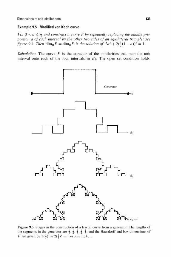
Dimensions of self-similar sets 133
Example 9.5. Modified von Koch curve
Fix 0 < a � 13 and construct a curve F by repeatedly replacing the middle pro-
portion a of each interval by the other two sides of an equilateral triangle; seefigure 9.4. Then dimHF = dimBF is the solution of 2as + 2( 1
2 (1 − a))s = 1.
Calculation. The curve F is the attractor of the similarities that map the unitinterval onto each of the four intervals in E1. The open set condition holds,
Generator
E1
E2
E3
E4 ~− F
Figure 9.5 Stages in the construction of a fractal curve from a generator. The lengths ofthe segments in the generator are 1
3 , 14 , 1
3 , 14 , 1
3 , and the Hausdorff and box dimensions ofF are given by 3( 1
3 )s + 2( 14 )s = 1 or s = 1.34 . . .
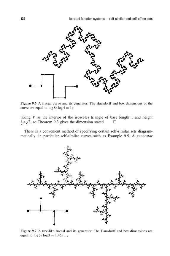
134 Iterated function systems—self-similar and self-affine sets
Figure 9.6 A fractal curve and its generator. The Hausdorff and box dimensions of thecurve are equal to log 8/ log 4 = 1 1
2
taking V as the interior of the isosceles triangle of base length 1 and height12a
√3, so Theorem 9.3 gives the dimension stated. �
There is a convenient method of specifying certain self-similar sets diagram-matically, in particular self-similar curves such as Example 9.5. A generator
Figure 9.7 A tree-like fractal and its generator. The Hausdorff and box dimensions areequal to log 5/ log 3 = 1.465 . . .
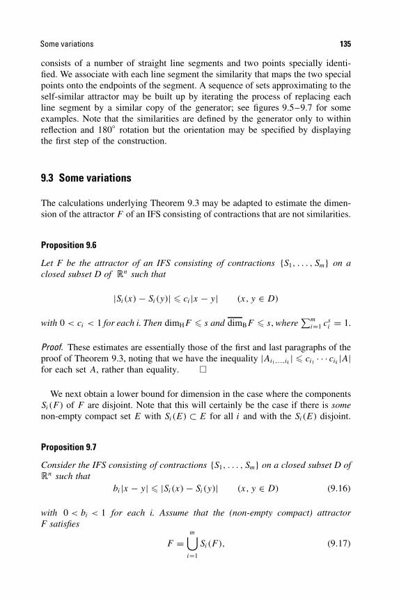
Some variations 135
consists of a number of straight line segments and two points specially identi-fied. We associate with each line segment the similarity that maps the two specialpoints onto the endpoints of the segment. A sequence of sets approximating to theself-similar attractor may be built up by iterating the process of replacing eachline segment by a similar copy of the generator; see figures 9.5–9.7 for someexamples. Note that the similarities are defined by the generator only to withinreflection and 180◦ rotation but the orientation may be specified by displayingthe first step of the construction.
9.3 Some variations
The calculations underlying Theorem 9.3 may be adapted to estimate the dimen-sion of the attractor F of an IFS consisting of contractions that are not similarities.
Proposition 9.6
Let F be the attractor of an IFS consisting of contractions {S1, . . . , Sm} on aclosed subset D of �n such that
|Si(x) − Si(y)| � ci |x − y| (x, y ∈ D)
with 0 < ci < 1 for each i. Then dimHF � s and dimBF � s, where∑m
i=1 csi = 1.
Proof. These estimates are essentially those of the first and last paragraphs of theproof of Theorem 9.3, noting that we have the inequality |Ai1,...,ik | � ci1 · · · cik |A|for each set A, rather than equality. �
We next obtain a lower bound for dimension in the case where the componentsSi(F ) of F are disjoint. Note that this will certainly be the case if there is somenon-empty compact set E with Si(E) ⊂ E for all i and with the Si(E) disjoint.
Proposition 9.7
Consider the IFS consisting of contractions {S1, . . . , Sm} on a closed subset D of�n such that
bi |x − y| � |Si(x) − Si(y)| (x, y ∈ D) (9.16)
with 0 < bi < 1 for each i. Assume that the (non-empty compact) attractorF satisfies
F =m⋃
i=1
Si(F ), (9.17)
136 Iterated function systems—self-similar and self-affine sets
with this union disjoint. Then F is totally disconnected and dimHF � s where
m∑
i=1
bsi = 1. (9.18)
Proof. Let d > 0 be the minimum distance between any pair of the disjoint com-pact sets S1(F ), . . . , Sm(F ), i.e. d = mini �=j inf{|x − y| : x ∈ Si(F ), y ∈ Sj (F )}.Let Fi1,...,ik = Si1
◦ · · · ◦Sik (F ) and define µ by µ(Fii,...ik ) = (bi1 · · · bik )s . Since
m∑
i=1
µ(Fi1,...,ik,i ) =m∑
i=1
(bi1 · · · bikbi)s
= (bi1 · · · bik )s = µ(Fi1,...,ik )
= µ
(k⋃
i=1
Fi1,...,ik ,i
)
it follows that µ defines a mass distribution on F with µ(F ) = 1.If x ∈ F , there is a unique infinite sequence i1, i2, . . . such that x ∈ Fi1,...,ik for
each k. For 0 < r < d let k be the least integer such that
bi1 · · · bikd � r < bi1 · · · bik−1d.
If i′1, . . . , i′k is distinct from i1, . . . , ik , the sets Fi1,...,ik and Fi ′1,...,i
′k
are disjoint andseparated by a gap of at least bi1 · · · bik−1d > r . (To see this, note that if j is theleast integer such that ij �= i′j then Fij ,...,ik ⊂ Fij and Fi ′
j,...,i ′
k⊂ Fi ′
jare separated
by d , so Fi1,...,ik and Fi ′1,...,i′k
are separated by at least bi1 · · · bij−1d .) It follows thatF ∩ B(x, r) ⊂ Fi1,...,ik so
µ(F ∩ B(x, r)) � µ(Fi1,...,ik ) = (bi1 . . . bik )s � d−srs .
If U intersects F , then U ⊂ B(x, r) for some x ∈ F with r = |U |. Thus µ(U) �d−s |U |s , so by the Mass distribution principle 4.2 Hs(F ) > 0 and dimHF � s.
The separation indicated above implies that F is totally disconnected. �
Example 9.8. ‘Non-linear’ Cantor set
Let D =[
12 (1 + √
3), (1 + √3)
]and let S1, S2 : D → D be given by
S1(x) = 1 + 1/x, S2(x) = 2 + 1/x. Then 0.44 < dimHF � dimBF � dimBF <
0.66 where F is the attractor of {S1, S2}. (This example arises in connection withnumber theory ; see Section 10.2.)
Calculation. We note that S1(D) =[
12 (1 + √
3),√
3]
and S2(D) =[
12 (3 + √
3) ,
1 + √3]
so we can use Propositions 9.6 and 9.7 to estimate dimHF . By
Some variations 137
the mean value theorem (see Section 1.2) if x, y ∈ D are distinct points then(Si(x) − Si(y))/(x − y) = S ′
i (zi) for some zi ∈ D. Thus for i = 1, 2,
infx∈D
|S ′i (x)| � |Si(x) − Si(y)|
|x − y| � supx∈D
|S ′i (x)|.
Since S ′1(x) = S ′
2(x) = −1/x2 it follows that
12 (2 − √
3) = (1 + √3)−2 � |Si(x) − Si(y)|
|x − y| � ( 12 (1 + √
3))−2 = 2(2 − √3)
for both i = 1 and i = 2. According to Propositions 9.6 and 9.7 lower andupper bounds for the dimensions are given by the solutions of 2( 1
2 (2 −√3))s = 1 and 2(2(2 − √
3))s = 1 which are s = log 2/ log(2(2 + √3)) = 0.34
and log 2/ log( 12 (2 + √
3)) = 1.11 respectively.For a subset of the real line, an upper bound greater than 1 is not of much
interest. One way of getting better estimates is to note that F is also the attractorof the four mappings on [0, 1]
Si◦Sj = i + 1/(j + 1/x) = i + x/(jx + 1) (i, j = 1, 2).
By calculating derivatives and using the mean-value theorem as before, weget that
(Si◦Sj )′(x) = (jx + 1)−2
so
(j (1 + √3) + 1)−2|x − y| � |Si◦Sj (x) − Si◦Sj (y)| � ( 1
2j (1 + √3) + 1)−2|x − y|.
Lower and upper bounds for the dimensions are now given by the solutionsof 2(2 + √
3)−2s + 2(3 + 2√
3)−2s = 1 and 2( 12 (3 + √
3))−2s + 2(2 + √3)−2s =
1, giving 0.44 < dimHF < 0.66, a considerable improvement on the previousestimates. In fact dimHF = 0.531, a value that may be obtained by looking atyet higher-order iterates of the Si . �
*[The rest of this subsection may be omitted.]
The technique used in Example 9.8 to improve the dimension estimates isoften useful for attractors of transformations that are not strict similarities. IfF is the attractor for the IFS {S1, . . . , Sm} on D then F is also the attractorfor the IFS consisting of the mk transformations {Si1
◦ · · · ◦Sik } for each k. Ifthe Si are, say, twice differentiable on an open set containing F , it may beshown that when k is large, the contractions Si1
◦ · · · ◦Sik are in a sense, closeto similarities on D. In particular, for transformations on a subset D of �, ifb = infx∈D |(Si1
◦ · · · ◦Sik )′(x)| and c = supx∈D |(Si1
◦ · · · ◦Sik )′(x)|, then
b|x − y| � |Si1◦ · · · ◦Sik (x) − Si1
◦ · · · ◦Sik (y)| � c|x − y| (x, y ∈ D)

138 Iterated function systems—self-similar and self-affine sets
If k is large then b/c will be close to 1, and applying Propositions 9.6 and 9.7to the mk transformations Si1
◦ · · · ◦Sik gives good upper and lower estimates forthe dimensions of F .
We may take this further. If the Si are twice differentiable on a subset D of �,
|Si1◦ · · · ◦Sik (x) − Si1
◦ · · · ◦Sik (y)||x − y| ∼ |(Si1
◦ · · · ◦Sik )′(w)|
for large k, where x, y and w are any points of D. The composition of mappingsSi1
◦ · · · ◦Sik is close to a similarity on D, so by comparison with Theorem 9.3we would expect the dimension of the attractor F to be close to the value of s
for which ∑
Ik
|(Si1◦ · · · ◦Sik )
′(w)|s = 1 (9.19)
where the sum is over the set Ik of all k-term sequences. This expectation moti-vates the following theorem.
Theorem 9.9
Let V ⊂ � be an open interval. Let S1, . . . , Sm be contractions on V that aretwice differentiable on V with a � |S ′
i (w)| � c for all i and w ∈ V , where 0 <
a � c < 1 are constants. Suppose that the Si satisfy the open set condition (9.11)with open set V. Then the limit
limk→∞
∑
Ik
|(Si1◦ · · · ◦Sik )
′(w)|s
1/k
= ϕ(s) (9.20)
exists for each s > 0, is independent of w ∈ V , and is decreasing in s. If F isthe attractor of {S1, . . . , Sm} then dimHF = dimBF is the solution of ϕ(s) = 1,and F is an s-set, i.e. 0 < Hs(F ) < ∞ for this value of s.
Note on Proof. The main difficulty is to show that the limit (9.20) exists—thisdepends on the differentiability condition on the Si . Given this, the argumentoutlined above may be used to show that the value of s satisfying (9.19) is agood approximation to the dimension when k is large; letting k → ∞ then givesthe result.
Similar ideas, but involving the rate of convergence to the limit in (9.20), areneeded to show that 0 < Hs(F ) < ∞. �
There are higher-dimensional analogues of Theorem 9.9. Suppose that the con-tractions S1, . . . , Sm on a domain D in the complex plane are complex analyticmappings. Then the Si are conformal, or in other words are locally like similaritytransformations, contracting at the same rate in every direction. We have
Si(z) = Si(z0) + S ′i (z0)(z − z0) + terms in (z − z0)
2 and higher powers
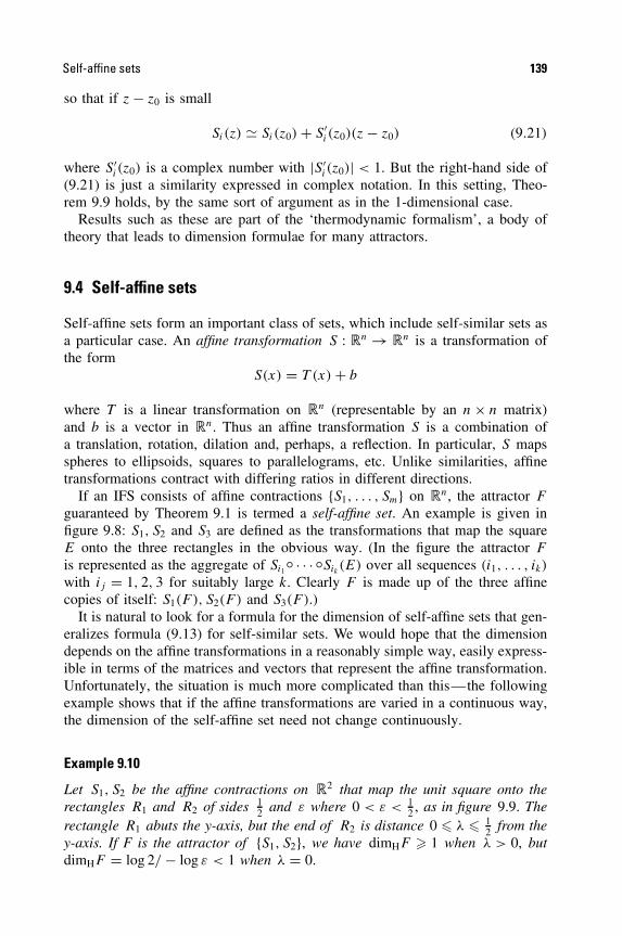
Self-affine sets 139
so that if z − z0 is small
Si(z) Si(z0) + S ′i (z0)(z − z0) (9.21)
where S ′i (z0) is a complex number with |S ′
i (z0)| < 1. But the right-hand side of(9.21) is just a similarity expressed in complex notation. In this setting, Theo-rem 9.9 holds, by the same sort of argument as in the 1-dimensional case.
Results such as these are part of the ‘thermodynamic formalism’, a body oftheory that leads to dimension formulae for many attractors.
9.4 Self-affine sets
Self-affine sets form an important class of sets, which include self-similar sets asa particular case. An affine transformation S : �n → �n is a transformation ofthe form
S(x) = T (x) + b
where T is a linear transformation on �n (representable by an n × n matrix)and b is a vector in �n. Thus an affine transformation S is a combination ofa translation, rotation, dilation and, perhaps, a reflection. In particular, S mapsspheres to ellipsoids, squares to parallelograms, etc. Unlike similarities, affinetransformations contract with differing ratios in different directions.
If an IFS consists of affine contractions {S1, . . . , Sm} on �n, the attractor F
guaranteed by Theorem 9.1 is termed a self-affine set. An example is given infigure 9.8: S1, S2 and S3 are defined as the transformations that map the squareE onto the three rectangles in the obvious way. (In the figure the attractor F
is represented as the aggregate of Si1◦ · · · ◦Sik (E) over all sequences (i1, . . . , ik)
with ij = 1, 2, 3 for suitably large k. Clearly F is made up of the three affinecopies of itself: S1(F ), S2(F ) and S3(F ).)
It is natural to look for a formula for the dimension of self-affine sets that gen-eralizes formula (9.13) for self-similar sets. We would hope that the dimensiondepends on the affine transformations in a reasonably simple way, easily express-ible in terms of the matrices and vectors that represent the affine transformation.Unfortunately, the situation is much more complicated than this—the followingexample shows that if the affine transformations are varied in a continuous way,the dimension of the self-affine set need not change continuously.
Example 9.10
Let S1, S2 be the affine contractions on �2 that map the unit square onto therectangles R1 and R2 of sides 1
2 and ε where 0 < ε < 12 , as in figure 9.9. The
rectangle R1 abuts the y-axis, but the end of R2 is distance 0 � λ � 12 from the
y-axis. If F is the attractor of {S1, S2}, we have dimHF � 1 when λ > 0, butdimHF = log 2/ − log ε < 1 when λ = 0.
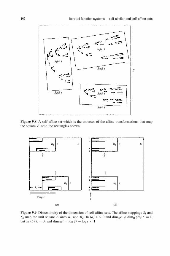
140 Iterated function systems—self-similar and self-affine sets
S1(F )
S1(E )
S2(F )
S3(F )
S2(E )
S3(E )
E
Figure 9.8 A self-affine set which is the attractor of the affine transformations that mapthe square E onto the rectangles shown
R1 E ER1
R2 e eR2
12
12
12
12
λ
Proj F
(a) (b)
e e
F
Figure 9.9 Discontinuity of the dimension of self-affine sets. The affine mappings S1 andS2 map the unit square E onto R1 and R2. In (a) λ > 0 and dimHF � dimH proj F = 1,but in (b) λ = 0, and dimHF = log 2/ − log ε < 1

Self-affine sets 141
Calculation. Suppose λ > 0 (figure 9.9(a)). Then the kth stage of the constructionEk = ⋃
Si1◦ · · · ◦Sik (E) consists of 2k rectangles of sides 2−k and εk with the
projection of Ek onto the x-axis, proj Ek, containing the interval [0, 2λ]. SinceF = ⋂∞
i=1 Ek it follows that proj F contains the interval [0, 2λ]. (Another wayof seeing this is by noting that proj F is the attractor of S1, S2 : � → � given byS1(x) = 1
2x, S2(x) = 12x + λ, which has as attractor the interval [0, 2λ].) Thus
dimHF � dimHproj F = dimH[0, 2λ] = 1.If λ = 0, the situation changes (figure 9.9(b)). Ek consists of 2k rectangles of
sides 2−k and εk which all have their left-hand ends abutting the y-axis, withEk contained in the strip {(x, y) : 0 � x � 2−k}. Letting k → ∞ we see thatF is a uniform Cantor set contained in the y-axis, which may be obtained byrepeatedly removing a proportion 1 − 2ε from the centre of each interval. ThusdimHF = log 2/ − log ε < 1 (see Example 4.5). �
With such discontinuous behaviour, which becomes even worse for moreinvolved sets of affine transformations, it is likely to be difficult to obtain ageneral expression for the dimension of self-affine sets. However, one situationwhich has been completely analysed is the self-affine set obtained by the follow-ing recursive construction; a specific case is illustrated in figures 9.10 and 9.11.
Example 9.11
Let the unit square E0 be divided into a p × q array of rectangles of sides 1/p
and 1/q where p and q are positive integers with p < q. Select a subcollection ofthese rectangles to form E1, and let Nj denote the number of rectangles selectedfrom the jth column for 1 � j � p; see figure 9.10. Iterate this construction inthe usual way, with each rectangle replaced by an affine copy of E1, and let Fbe the limiting set obtained. Then
dimHF = log
p∑
j=1
Nlog p/ log q
j
1
log p
and
dimBF = log p1
log p+ log
1
p1
p∑
j=1
Nj
1
log q
where p1 is the number of columns containing at least one rectangle of E1.
Calculation. Omitted. �
Notice in this example that the dimension depends not only on the number ofrectangles selected at each stage, but also on their relative positions. MoreoverdimHF and dimBF are not, in general, equal.
*[The rest of this subsection may be omitted.]

142 Iterated function systems—self-similar and self-affine sets
N1 Np
1/q
1/p
• • •
Figure 9.10 Data for the self-affine set of Example 9.11. The affine transformations mapthe square onto selected 1/p × 1/q rectangles from the p × q array
The above example is rather specific in that the affine transformations areall translates of each other. Obtaining a dimension formula for general self-affine sets is an intractable problem. We briefly outline an approach which leadsto an expression for the dimension of the attractor of the affine contractionsSi(x) = Ti(x) + bi(1 � i � m) for almost all sequences of vectors b1, . . . , bm.
Let T : �n → �n be a linear mapping that is contracting and non-singular.The singular values 1 > α1 � α2 � · · · � αn > 0 of T may be defined in twoways: they are the lengths of the principal semi-axes of the ellipsoid T (B) where
E0 E1
F
E2
Figure 9.11 Construction of a self-affine set of the type considered in Example 9.11.Such sets may have different Hausdorff and box dimensions

Self-affine sets 143
B is the unit ball in �n, and they are the positive square roots of the eigenvaluesof T ∗T , where T ∗ is the adjoint of T . Thus the singular values reflect the con-tractive effect of T in different directions. For 0 � s � n we define the singularvalue function
ϕs(T ) = α1α2 · · ·αr−1αs−r+1r (9.22)
where r is the integer for which r − 1 < s � r . Then ϕs(T ) is continuous andstrictly decreasing in s. Moreover, for fixed s, ϕs may be shown to be submul-tiplicative, i.e.
ϕs(T U) � ϕs(T )ϕs(U)
for any linear mappings T and U . We introduce the kth level sums �sk ≡∑
Ikϕs(Ti1
◦ · · · ◦Tik ) where Ik denotes the set of all k-term sequences (i1, . . . , ik)
with 1 � ij � m. For fixed s
�sk+q =
∑
Ik+q
ϕs(Ti1◦ · · · ◦Tik+q
)
�∑
Ik+q
ϕs(Ti1◦ · · · ◦Tik )ϕ
s(Tik+1◦ · · · ◦Tik+q
)
=
∑
Ik
ϕs(Ti1◦ · · · ◦Tik )
∑
Iq
ϕs(Ti1◦ · · · ◦Tiq )
= �sk�
sq
i.e. the sequence �sk is submultiplicative in k. By a standard property of submul-
tiplicative sequences, (�sk)
1/k converges to a number �s∞ as k → ∞. Since ϕs isdecreasing in s, so is �s∞. Provided that �n∞ � 1, there is a unique s, which wedenote by d(T1, . . . , Tm), such that 1 = �s∞ = limk→∞
(∑Ik
ϕs(Ti1◦ · · · ◦Tik )
)1/k.
Equivalently
d(T1, . . . , Tm) = inf
{
s :∞∑
k=1
∑
Ik
ϕs(Ti1◦ · · · ◦Tik ) < ∞
}
. (9.23)
Theorem 9.12
Let T1, . . . , Tm be linear contractions and let y1, . . . , ym ∈ �n be vectors. If F isthe self-affine set satisfying
F =m⋃
i=1
(Ti(F ) + yi)
then dimHF = dimBF � d(T1, . . . , Tm). If |Ti(x) − Ti(y)| � c|x − y| for all iwhere 0 < c < 1
2 , then equality holds for almost all (y1, . . . , ym) ∈ �nm in thesense of nm-dimensional Lebesgue measure.

144 Iterated function systems—self-similar and self-affine sets
Figure 9.12 Each of the fractals depicted above is the attractor of the set of transforma-tions that map the square onto the three rectangles. The affine transformations for eachfractal differ only by translations, so by Theorem 9.12 the three fractals all have the samedimension (unless we have been very unlucky in our positioning!). A computation givesthis common value of Hausdorff and box dimension as about 1.42
Partial proof. We show that dimHF � d(T1, . . . , Tm) for all y1, . . . , ym. WriteSi for the contracting affine transformation Si(x) = Ti(x) + yi . Let B be alarge ball so that Si(B) ⊂ B for all i. Given δ > 0 we may choose k largeenough to get |Si1
◦ · · · ◦Sik (B)| < δ for every k-term sequence (i1, . . . , ik) ∈ Ik.By (9.6) F ⊂ ⋃
IkSi1
◦ · · · ◦Sik (B). But Si1◦ · · · ◦Sik (B) is a translate of the
ellipsoid Ti1◦ · · · ◦Tik (B) which has principal axes of lengths α1|B|, . . . , αn|B|,
where α1, . . . , αn are the singular values of Ti1◦ · · · ◦Tik . Thus Si1
◦ · · · ◦Sik (B) iscontained in a rectangular parallelepiped P of side lengths α1|B|, . . . , αn|B|. If0 � s � n and r is the least integer greater than or equal to s, we may divide P
into at most
(2α1
αr
)(2α2
αr
)· · ·
(2αr−1
αr
)� 2nα1 · · · αr−1α
1−rr

Applications to encoding images 145
cubes of side αr |B| < δ. Hence Si1◦ · · · ◦Sik (B) may be covered by a collection
of cubes Ui with |Ui | < δ√
n such that
∑
i
|Ui|s � 2nα1 · · · αr−1α1−rr αs
r |B|s
� 2n|B|sϕs(Ti1◦ · · · ◦Tik ).
Taking such a cover of Si1◦ · · · ◦Sik (B) for each (i1, . . . , ik) ∈ Ik it follows that
Hsδ√
n(F ) � 2n|B|s∑
Ik
ϕs(Ti1◦ · · · ◦Tik ).
But k → ∞ as δ → 0, so by (9.23), Hs(F ) = 0 if s > d(T1, . . . , Tm). ThusdimHF � d(T1, . . . , Tm).
The lower estimate for dimHF may be obtained using the potential theoretictechniques of Section 4.3. We omit the somewhat involved details. �
One consequence of this theorem is that, unless we have been unfortunateenough to hit on an exceptional set of parameters, the fractals in figure 9.12 allhave the same dimension, estimated at about 1.42.
9.5 Applications to encoding images
In this chapter, we have seen how a small number of contractions can deter-mine objects of a highly intricate fractal structure. This has applications to datacompression—if a complicated picture can be encoded by a small amount ofinformation, then the picture can be transmitted or stored very efficiently.
It is desirable to know which objects can be represented as, or approximatedby, attractors of an iterated function system, and also how to find contractions thatlead to a good representation of a given object. Clearly, the possibilities using,say, three or four transformations are limited by the small number of parametersat our disposal. Such sets are also likely to have a highly repetitive structure.
However, a little experimentation drawing self-affine sets on a computer (seeend of Section 9.1) can produce surprisingly good pictures of naturally occurringobjects such as ferns, grasses, trees, clouds, etc. The fern and tree in figure 9.13are the attractors of just four and six affine transformations, respectively. Self-similarity and self-affinity are indeed present in nature.
The following theorem, sometimes known as the collage theorem, gives anidea of how good an approximation a set is to the attractor of an IFS.
Theorem 9.13
Let {S1, . . . , Sm} be an IFS and suppose that |Si(x) − Si(y)| � c|x − y| forall x, y ∈ �n and all i, where c < 1. Let E ⊂ �n be any non-empty compact
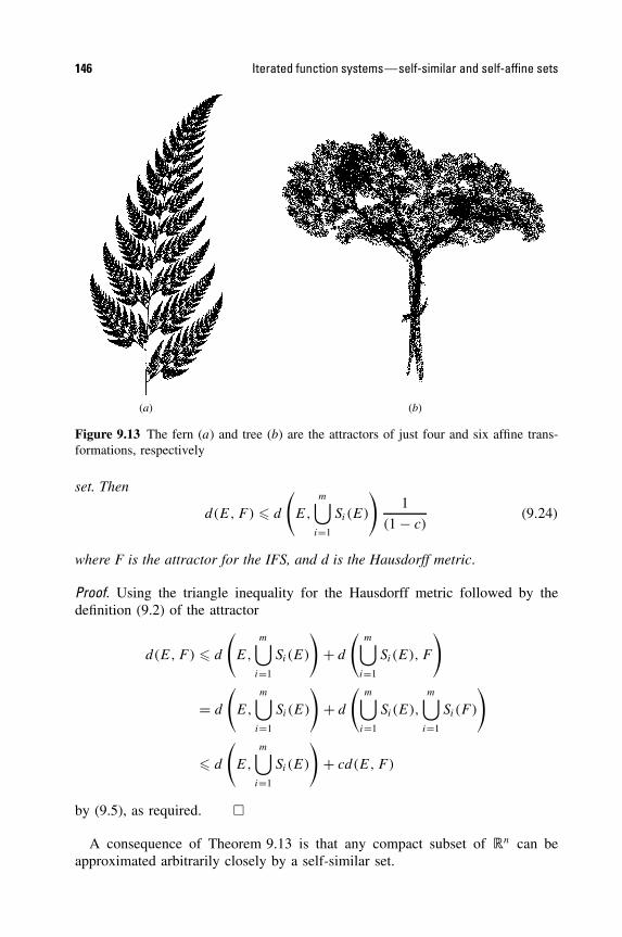
146 Iterated function systems—self-similar and self-affine sets
(a) (b)
Figure 9.13 The fern (a) and tree (b) are the attractors of just four and six affine trans-formations, respectively
set. Then
d(E,F ) � d
(
E,
m⋃
i=1
Si(E)
)1
(1 − c)(9.24)
where F is the attractor for the IFS, and d is the Hausdorff metric.
Proof. Using the triangle inequality for the Hausdorff metric followed by thedefinition (9.2) of the attractor
d(E,F ) � d
(
E,
m⋃
i=1
Si(E)
)
+ d
(m⋃
i=1
Si(E), F
)
= d
(
E,
m⋃
i=1
Si(E)
)
+ d
(m⋃
i=1
Si(E),
m⋃
i=1
Si(F )
)
� d
(
E,
m⋃
i=1
Si(E)
)
+ cd(E, F )
by (9.5), as required. �
A consequence of Theorem 9.13 is that any compact subset of �n can beapproximated arbitrarily closely by a self-similar set.
Applications to encoding images 147
Corollary 9.14
Let E be a non-empty compact subset of �n. Given δ > 0 there exist contractingsimilarities S1, . . . , Sm with attractor F satisfying d(E,F ) < δ.
Proof. Let B1, . . . , Bm be a collection of balls that cover E and which havecentres in E and radii at most 1
4δ. Then E ⊂ ⋃mi=1 Bi ⊂ Eδ/4, where Eδ/4 is
the 14δ-neighbourhood of E. For each i, let Si be any contracting similarity
of ratio less than 12 that maps E into Bi . Then Si(E) ⊂ Bi ⊂ (Si(E))δ/2, so
(⋃m
i=1 Si(E)) ⊂ Eδ/4 and E ⊂ ⋃mi=1(Si(E))δ/2. By definition of the Hausdorff
metric, d(E,⋃m
i=1 Si(E)) � 12δ. It follows from (9.24) that d(E,F ) < δ where
F is the attractor. �
The approximation by the IFS attractor given by the above proof is rathercoarse—it is likely to yield a very large number of contractions that take littleaccount of the fine structure of E. A rather more subtle approach is required toobtain convincing images with a small number of transformations. One methodwhich often gives good results is to draw a rough outline of the object andthen cover it, as closely as possible, by a number of smaller similar (or affine)copies. The similarities (or affinities) thus determined may be used to compute anattractor which may be compared with the object being modelled. Theorem 9.13guarantees that the attractor will be a good approximation if the union of thesmaller copies is close to the object. A trial and error process allows modificationand improvements to the picture.
More complex objects may be built up by superposition of the invariant setsof several different sets of transformations.
Ideally, it would be desirable to have a ‘camera’ which could be pointed at anobject to produce a ‘photograph’ consisting of a specified number of affine trans-formations whose attractor is a good approximation to the object. Obviously, thetechnical problems involved are considerable. One approach is to scan the objectto estimate various geometric parameters, and use these to impose restrictions onthe transformations.
For example, for a ‘natural fractal’ such as a fern, we might estimate the dimen-sion by a box-counting method. The assumption that the similarities or affinitiessought must provide an attractor of this dimension gives, at least theoretical,restrictions on the possible set of contractions, using results such as Theorem 9.3or 9.12. In practice, however, such information is rather hard to utilize, and wecertainly need many further parameters for it to be of much use.
Very often, attractors in the plane that provide good pictures of physical objectswill have positive area, so will not be fractals in the usual sense. Nevertheless,such sets may well be bounded by fractal curves, a feature that adds realism topictures of natural objects. However, fractal properties of boundaries of invariantsets seem hard to analyse.
These ideas may be extended to provide shaded or coloured images, byassigning a probability pi to each of the contractions Si , where 0 < pi < 1 and∑m
i=1 pi = 1. Without going into details, these data define a mass distribution
148 Iterated function systems—self-similar and self-affine sets
µ on the attractor F such that µ(A) = ∑mi=1 piµ(S−1
i (A)), and the set may beshaded, or even coloured, according to the local density of µ.
This leads to the following modification of the second method of drawingattractors mentioned at the end of Section 9.1. Let x0 be any initial point. Wechoose Sj1 from S1, · · · , Sm at random in such a way that the probability ofchoosing Si is pi , and let x1 = Sj1(x0). We continue in this way, so that xk =Sjk
(xk−1) where Sjkequals Si with probability pi . Plotting the sequence {xk}
(after omitting the first 100 terms, say) gives a rendering of the attractor F , butin such a way that a proportion pi1 · · · piq of the points tends to lie in the partSi1
◦ · · · ◦Siq (F ) for each i1, . . . , iq . This variable point density provides a directshading of F . Alternatively, the colour of a point of F can be determined bysome rule, which depends on the number of {xk} falling close to each point. Thecomputer artist may care to experiment with the endless possibilities that thismethod provides—certainly, some very impressive colour pictures have beenproduced using relatively few transformations.
It is perhaps appropriate to end this section with some of the ‘pros and cons’of representing images using iterated function systems. By utilizing the self-similarity and repetition in nature, and, indeed, in man-made objects, the methodoften enables scenes to be described by a small number (perhaps fewer than100) of contractions and probabilities in an effective manner. This represents anenormous compression of information compared, for example, with that requiredto detail the colour in each square of a fine mesh. The corresponding disadvan-tage is that there is a high correlation between different parts of the picture—themethod is excellent for giving an overall picture of a tree, but is no use if theexact arrangement of the leaves on different branches is important. Given a set ofaffine contractions, reproduction of the image is computationally straightforward,is well-suited to parallel computation, and is stable—small changes in the con-tractions lead to small changes in the attractor. The contractions define the imageat arbitrarily small scales, and it is easy to produce a close-up of a small region.At present, the main disadvantage of the method is the difficulty of obtaining aset of contractions to represent a given object or picture.
9.6 Notes and references
The first systematic account of what are now known as iterated function sys-tems is that of Hutchinson (1981), though similar ideas were around earlier. Thederivation of the formula for the dimension of self-similar sets was essentiallygiven by Moran (1946). Computer pictures of self-similar sets and attractors ofother IFSs are widespread, the works of Mandelbrot (1982), Dekking (1982),Peitgen, Jurgens and Saupe (1992) and Barnsley (1993) contain many interestingand beautiful examples.
For details of the thermodynamic formalism and material relating to Theo-rem 9.9, see Ruelle (1983), Bedford (1991), Beck and Schlogl (1993), Falconer(1997) and Pesin (1997).
Exercises 149
A discussion of self-affine sets is given by Mandelbrot (1986) and a surveyon their dimension properties by Peres and Solomyak (2000). Full details ofExample 9.11 are given by McMullen (1984) and of Theorem 9.12 by Falconer(1988) and Solomyak (1998).
These ideas have been extended in many directions: for example, for IFSs withinfinitely many transformations see Mauldin and Urbanski (1996, 1999), and forgraph directed constructions see Mauldin and Williams (1988).
Applications to image compression and encoding are described by Barnsley(1993), Barnsley and Hurd (1993) and Fisher (1995).
Exercises9.1 Verify that the Hausdorff metric satisfies the conditions for a metric.
9.2 Find a pair of similarity transformations on � for which the interval [0, 1] is theattractor. Now find infinitely many such pairs of transformations.
9.3 Find sets of (i) four and (ii) three similarity transformations on � for which themiddle third Cantor set is the attractor. Check that (9.13) has solution log 2/ log 3in each case.
9.4 Write down (using matrix notation) the four basic similarity transformations thatdefine the von Koch curve (figure 0.2). Find an open set for which the open setcondition holds and deduce from Theorem 9.3 that the von Koch curve does indeedhave box and Hausdorff dimension of log 4/ log 3.
9.5 Find an IFS for the set depicted in figure 0.5 and deduce that it has Hausdorff andbox dimensions given by 4( 1
4 )s + ( 12 )s = 1.
9.6 Sketch the first few steps in the construction of a self-similar set with generator. What are the Hausdorff and box dimensions of this fractal? (The stem of
the T is one quarter of the total length of the top.)
9.7 Let F be the set obtained by a Cantor-type construction in which each interval isreplaced by two intervals, one of a quarter of the length at the left-hand end, and oneof half the length at the right-hand end. Thus E0 is the interval [0, 1], E1 consistsof the intervals [0, 1
4 ] and [ 12 , 1], etc. Find an IFS with attractor F , and thus find the
Hausdorff and box dimensions of F .
9.8 Describe the attractors of the following IFSs on �.
(i) S1(x) = 14 x, S2(x) = 1
4 x + 34 ;
(ii) S1(x) = 12 x, S2(x) = 1
2 x + 12 ;
(iii) S1(x) = 23 x, S2(x) = 2
3 x + 13 .
9.9 Divide the unit square E0 into p2 squares of side 1/p in the obvious way and choosesome m of these squares to form E1. Let Si(1 � i � m) be similarity transformationsthat map E0 onto each of these squares. Show that the attractor F of the IFS sodefined has dimHF = dimBF = log m/ log p.
9.10 Let S1, S2 : [0, 1] → [0, 1] be given by S1(x) = x/(2 + x) and S2(x) = 2/(2 + x).Show that the attractor F of this IFS satisfies 0.52 < dimHF < 0.81.
9.11 Show that any self-similar set F satisfying the conditions of Theorem 9.3 has c1 �D(F, x) � D(F, x) � c2 for all x ∈ F , where c1 and c2 are positive constants. (Seeequations (5.2) and (5.3) for the definition of the densities.)

150 Iterated function systems—self-similar and self-affine sets
9.12 Let S1, . . . , Sm be bi-Lipschitz contractions on a subset D of �n and let F be theattractor satisfying (9.2). Show that, if V is any open set intersecting F , then F
and F ∩ V have equal Hausdorff, equal upper box and equal lower box dimensions.Deduce from Corollary 3.9 that dimPF = dimBF .
9.13 Verify the Hausdorff dimension formula in Example 9.11 in the cases (a) whereNj = N for 1 � j � p and (b) where Nj = N or 0 for 1 � j � p, where N is aninteger with 1 < N < q. (Hint: see Example 7.13.)
9.14 Find the Hausdorff and box dimensions of the set in figure 9.11.
9.15 Write a computer program to draw self-similar sets in the plane, given a generatorof the set.
9.16 Write a computer program to draw the attractor of a given collection of contractionsof a plane region (see the end of Section 9.1). Examine the attractors of similarities,affinities and try some non-linear transformations. If you are feeling really enter-prising, you might write a program to estimate the dimension of these sets using abox-counting method.

Chapter 10 Examples from numbertheory
Fractals can often be defined in number theoretic terms; for instance, the middlethird Cantor set consists of the numbers between 0 and 1 which have a base-3expansion containing only the digits 0 and 2. We examine three classes of fractalsthat occur in classical number theory—these examples serve to illustrate someof the ideas encountered earlier in the book.
10.1 Distribution of digits of numbers
In this section we consider base-m expansions of real numbers, where m � 2is a fixed integer. Let p0, p1, . . . , pm−1 be ‘proportions’ summing to 1, so that0 < pi < 1 and
∑m−1i=0 pi = 1. Let F(p0, . . . , pm−1) be the set of numbers x in
[0, 1) with base-m expansions containing the digits 0, 1, . . . , m − 1 in proportionsp0, . . . , pm−1 respectively. More precisely, if nj (x|k) denotes the number of timesthe digit j occurs in the first k places of the base-m expansion of x, then
F(p0, . . . , pm−1) = {x ∈ [0, 1) : limk→∞ nj (x|k)/k = pj for all j = 0, . . . , m − 1}.
(10.1)
Thus we think of F( 13 , 2
3 ) as the set of numbers with ‘two thirds’ of their base-2digits being 1 and the rest being 0.
It is well-known that almost all numbers (in the sense of Lebesgue measure) arenormal to all bases; that is, they have base-m expansions containing equal pro-portions of the digits 0, 1, . . . , m − 1 for all m. In our notation, F(m−1, . . . , m−1)
has Lebesgue measure 1, and therefore dimension 1, for all m. Paradoxically, nospecific example of a number that is normal to all bases has ever been exhibited.We may use Hausdorff dimension to describe the size of the sets F(p0, . . . , pm−1)
when the pj are not all equal. (Such sets are dense in [0, 1) so have box dimen-sion 1.)
A mass distribution technique is used in the following proof—the mass dis-tribution occurs naturally as a probability measure. Note that we adopt the usualconvention that 0 × log 0 = 0.
151
Fractal Geometry: Mathematical Foundations and Application. Second Edition Kenneth Falconer 2003 John Wiley & Sons, Ltd ISBNs: 0-470-84861-8 (HB); 0-470-84862-6 (PB)

152 Examples from number theory
Proposition 10.1
With F = F(p0, . . . , pm−1) as above,
dimHF = − 1
log m
m−1∑
i=0
pi log pi.
Proof. The proof is best thought of probabilistically. We imagine that base-mnumbers x = 0.i1i2 . . . are selected at random in such a way that the kth digit iktakes the value j with probability pj , independently for each k. Thus we take[0, 1) as our sample space and define a probability measure P on subsets of [0, 1)
such that if Ii1,...,ik is the kth level basic interval containing the numbers withbase-m expansion beginning 0.i1 · · · ik then the probability of a number being inthis interval is
P(Ii1,...,ik ) = pi1 · · · pik . (10.2)
Given j , the events ‘the kth digit of x is a j ’ are independent for k = 1, 2, . . . .A consequence of the strong law of large numbers (see Exercise 1.27) is that,with probability 1, the proportion of occurrences of an event in a number ofrepeated independent trials tends to the probability of the event occurring. Thus,with probability 1,
1
knj (x|k) = 1
k(number of occurrences of j in the first k digits) → pj
as k → ∞ for all j . Hence P(F ) = 1. We write Ik(x) = Ii1,...,ik for the kth levelinterval (of length m−k) to which x belongs. For a fixed y, the probability thatx ∈ Ik(y) is given by
log P(Ik(y)) = n0(y|k) log p0 + · · · + nm−1(y|k) log pm−1
by taking logarithms of (10.2). If y ∈ F then nj (y|k)/k → pj as k → ∞ foreach j , so
1
klog
P(Ik(y))
|Ik(y)|s = 1
klog P(Ik(y)) − 1
klog m−ks
→m−1∑
i=0
pi log pi + s log m.
Hence, for all y in F , the ‘interval density’
limk→∞
P(Ik(y))
|Ik(y)|s ={
0 if s < θ
∞ if s > θ
where
θ = − 1
log m
m−1∑
i=0
pi log pi.

Continued fractions 153
We are now virtually in the situation of Proposition 4.9. The same results hold andmay be proved in the same way, if the ‘spherical densities’ limr→0 µ(B(x, r))/rs
are replaced by these interval densities. Thus Hs(F ) = ∞ if s < θ and Hs(F ) =0 if s > θ , as required. �
10.2 Continued fractions
Instead of defining sets of numbers in terms of base-m expansions, we mayuse continued fraction expansions. Any number x that is not an integer may bewritten as
x = a0 + 1/x1
where a0 is an integer and x1 > 1. Similarly, if x1 is not an integer, then
x1 = a1 + 1/x2
with x2 > 1, sox = a0 + 1/(a1 + 1/x2).
Proceeding in this way,
x = a0 + 1/(a1 + 1/(a2 + 1/(· · · + 1/(ak−1 + 1/xk))))
for each k, provided that at no stage is xk an integer. We call the sequence ofintegers a0, a1, a2, . . . the partial quotients of x, and write
x = a0 + 1
a1+1
a2+1
a3 + · · ·for the continued fraction expansion of x. This expansion terminates if and onlyif x is rational, otherwise taking a finite number of terms,
a0 + 1/(a1 + 1/(a2 + 1/(· · · + 1/ak)))
provides a sequence of rational approximations to x which converge to x as k →∞. (Continued fractions are, in fact, closely allied to the theory of Diophantineapproximation; see Section 10.3.)
Examples of continued fractions include
√2 = 1 + 1
2+1
2+1
2 + · · ·√
3 = 1 + 1
1+1
2+1
1+1
2 + · · · .
More generally, any quadratic surd (i.e. root of a quadratic equation with integercoefficients) has eventually periodic partial quotients.

154 Examples from number theory
Sets of numbers defined by conditions on their partial quotients may be thoughtof as fractal attractors of certain iterated function systems, as the followingexample illustrates.
Example 10.2
Let F be the set of positive real numbers x with non-terminating continued fractionexpressions which have all partial quotients equal to 1 or 2. Then F is a fractalwith 0.44 < dimHF < 0.66.
Proof. It is easy to see that F is closed (since its complement is open) andbounded (since F ⊂ [1, 3]). Moreover, x ∈ F precisely when x = 1 + 1/y orx = 2 + 1/y with y ∈ F . Letting S1(x) = 1 + 1/x and S2(x) = 2 + 1/x, it fol-lows that F = S1(F ) ∪ S2(F ); in other words, F is the attractor of the iteratedfunction system {S1, S2} in the sense of (9.2). In fact F is just the set analysedin Example 9.8 which we showed to have Hausdorff dimension between 0.44and 0.66. �
Computational methods have been developed that enable dimensions of setsdefined in terms of continued fraction expansions to be found very accurately.The set F of Example 10.2 has Hausdorff dimension 0.531280506 . . . .
Obviously, varying the conditions on the partial quotients will lead to otherfractals that are the attractors of certain transformations.
10.3 Diophantine approximation
How closely can a given irrational number x be approximated by a rational p/qwith denominator q no larger than q0? Diophantine approximation is the study ofsuch problems, which can crop up in quite practical situations (see Section 13.6).A classical theorem of Dirichlet (see Exercise 10.8) states that for every realnumber x, there are infinitely many positive integers q such that
∣∣∣∣x − p
q
∣∣∣∣ � 1
q2
for some integer p; such p/q are ‘good’ rational approximations to x. Equiva-lently,
||qx|| � q−1
for infinitely many q, where ||y|| = minm∈� |y − m| denotes the distance from y
to the nearest integer.There are variations on Dirichlet’s result that apply to almost all numbers x.
It may be shown that if ψ(q) is a decreasing function of q with 0 � ψ(q) then
||qx|| � ψ(q) (10.3)

Diophantine approximation 155
is satisfied by infinitely many q for almost all x or almost no x (in the sense of1-dimensional Lebesgue measure) according to whether
∑∞q=1 ψ(q) diverges or
converges. In the latter case, the set of x for which (10.3) does have infinitelymany solutions not only has Lebesgue measure 0, but is often a fractal.
We speak of a number x such that
||qx|| � q1−α (10.4)
for infinitely many positive integers q as being α-well approximable. It is naturalto ask how large this set of numbers is when α > 2, and, indeed, whether suchirrational numbers exist at all. We prove Jarnık’s theorem, that the set of α-wellapproximable numbers has Hausdorff dimension 2/α.
It is almost immediate from Example 4.7 (check!) that the set of α-well approx-imable numbers has dimension at least 1/α. An extra subtlety is required to obtaina value of 2/α. The idea is as follows. Let Gq be the set of x ∈ [0, 1] satisfying(10.4). A factorization argument shows that, if n is large and p1, p2 are primeswith n < p1, p2 � 2n, then Gp1 and Gp2 are disjoint (except for points very closeto 0 or 1). Thus the set
Hn =⋃
p primen<p�2n
Gp
consists of, roughly,∑
n<p�2n 1/p � n2/ log n reasonably regularly spaced inter-vals of lengths at least 2(2n)−α . We then show that if nk is a rapidly increasingsequence, the intersection
⋂∞k=1 Hnk
has dimension at least 2/α, and note thatany number in this intersection lies in infinitely many Gp and so is α-wellapproximable.
Jarnık’s theorem 10.3
Suppose α > 2. Let F be the set of real numbers x ∈ [0, 1] for which the inequal-ity
||qx|| � q1−α (10.5)
is satisfied by infinitely many positive integers q. Then dimHF = 2/α.
∗Proof. For each q let Gq denote the set of x ∈ [0, 1] satisfying (10.5). Then Gq
consists of q − 1 intervals of length 2q−α and two ‘end’ intervals of length q−α .Clearly, F ⊂ ⋃∞
q=k Gq for each k, so taking the intervals of Gq for q � k asa cover of F gives that Hs
δ(F ) �∑∞
q=k(q + 1)(2q−α)s if 2k−α � δ. If s > 2/α
the series∑∞
q=1(q + 1)(2q−α)s converges, so limk→∞∑∞
q=k(q + 1)(2q−α)s = 0and Hs(F ) = 0. Hence dimHF � 2/α.
Let G′q be the set of x ∈ (q−α, 1 − q−α) satisfying (10.5), so that G′
q is just Gq
with the end intervals removed. Let n be a positive integer, and suppose p1 andp2 are prime numbers satisfying n < p1 < p2 � 2n. We show that G′
p1and G′
p2

156 Examples from number theory
are disjoint and reasonably well separated. For if 1 � r1 < p1 and 1 � r2 < p2,then p1r2 = p2r1 since p1 and p2 are prime. Thus
∣∣∣∣r1
p1− r2
p2
∣∣∣∣ = 1
p1p2|p2r1 − p1r2| � 1
p1p2� 1
4n2
that is, the distance between the centres of any pairs of intervals from G′p1
andG′
p2is at least 1/4n2. Since these intervals have lengths at most 2n−α , the distance
between any point of G′p1
and any point of G′p2
is at least 14n−2 − 2n−α � 1
8n−2
provided that n � n0 for some sufficiently large n0. For such n the set
Hn =⋃
p primen<p�2n
G′p
is a disjoint union of the intervals in the G′p, so Hn is made up of intervals of
lengths at least (2n)−α which are separated by gaps of lengths at least 18n−2.
If I ⊂ [0, 1] is any interval with 3/|I | < n < p � 2n then at least p|I |/3 �n|I |/3 of the intervals of G′
p are completely contained in I . A version of theprime number theorem states that the number of primes between 2 and n isasymptotically n/ log n, so there are at least n/(2 log n) primes in the range(n, 2n] if n � n1, for some large n1 � n0. Thus at least
n2|I |6 log n
(10.6)
intervals of Hn are contained in I provided that n � n1 and |I | � 3/n.To complete the proof, we use Example 4.6. With n1 as above, let nk =
max{nkk−1, 3 × 2ana
k−1}, for k = 2, 3, . . ., where a > α is an integer. Let E0 =[0, 1] and for k = 1, 2, . . . let Ek consist of those intervals of Hnk
that are com-pletely contained in Ek−1. The intervals of Ek are of lengths at least (2nk)
−α andare separated by gaps of at least εk = 1
8n−2k . Using (10.6), each interval of Ek−1
contains at least mk intervals of Ek, where
mk = n2k(2nk−1)
−α
6 log nk
= cn2kn
−αk−1
log nk
if k � 2, where c = 2−α/6. (We take m1 = 1.) By (4.7)
dimH
( ∞⋂
k=1
Ek
)
� limk→∞
log[ck−2n−α1 (n2 · · · nk−2)
2−αn2k−1(log n2)
−1 · · · (log nk−1)−1]
− log[cn−αk−1(8 log nk)
−1]

Diophantine approximation 157
= limk→∞
log[ck−2n−α1 (n2 · · ·nk−2)
2−α(log n2)−1 · · · (log nk−1)
−1] + 2 log nk−1
− log(c/8) + log k(log nk−1) + α log nk−1
= 2/α
since the dominant terms in numerator and denominator are those in log nk−1.(Note that log nk = k log nk−1 so log nk = ck! for k sufficiently large.) If x ∈Ek ⊂ Hnk
for all k, then x lies in infinitely many of the G′p and so x ∈ F . Hence
dimHF � 2/α. �
*[The rest of this section may be omitted.]
Obviously, the set F of Jarnık’s theorem is dense in [0, 1], with dimH(F ∩ I ) =2/α for any interval I . However, considerably more than this is true, F is a ‘setof large intersection’ of the type discussed in Section 8.2, and this has somesurprising consequences. For the definition of Cs , in the following proposition,see (8.7) and (8.8).
Proposition 10.4
Suppose α > 2. If F is the set of positive numbers such that ||qx|| � q1−α forinfinitely many q, then F ∈ Cs[0, ∞) for all s < 2/α.
Note on proof. This follows the proof of Jarnık’s Theorem 10.3 up to the def-inition of Hn. Then a combination of the method of Example 8.9 and primenumber theorem estimates are used to show that limn→∞ Hs∞(I ∩ Hn) = Hs∞(I ).Slightly different methods are required to estimate the number of intervals ofHn that can intersect a covering interval U , depending on whether |I | < 1/n or|I | � 1/n. �
The first deduction from Proposition 10.4 is that dimHF = 2/α, which weknow already from Jarnık’s Theorem. However, Proposition 8.8 tells us thatsmooth bijective images of F are also in Cs . Thus if s < 2/α then f (F ∩ [a, b])is in Cs[f (a), f (b)] for any continuously differentiable function f : [a, b] → �with |f ′(x)| > c > 0. Taking the functions given by fm(x) = x1/m we have thatfm(F ) ∩ [1, 2] is in Cs[1, 2] for s < 2/α. It follows from Proposition 8.6 that⋂∞
m=1 fm(F ) ∩ [1, 2] is in Cs[1, 2], so
dimH
( ∞⋂
m=1
fm(F )
)
= 2/α.
Butfm(F ) = {x : ||qxm|| � q1−α for infinitely many q}
so we have shown that the set of x for which all positive integral powers areα-well-approximable has Hausdorff dimension 2/α.
Clearly, many variations are possible using different sequences of functions fm.

158 Examples from number theory
10.4 Notes and references
There are many introductory books on number theory, of which the classic byHardy and Wright (1979) is hard to beat.
The dimensional analysis of the distribution of base-m digits is given inBillingsley (1978). Continued fractions are discussed in most basic texts in num-ber theory. Rogers (1998) and Bumby (1985) discuss dimensional aspects, andMauldin and Urbanski (1999) consider them in the context of IFSs with infinitelymany mappings. Hensley (1996) has calculated the Hausdorff dimension of var-ious sets of numbers defined by continued fractions to many decimal places.
Full accounts of Diophantine approximation are to be found in the books ofCassels (1957) and Schmidt (1980). Various proofs of Jarnık’s theorem havebeen given by Jarnık (1931), Besicovitch (1934), Eggleston (1952) and Kaufman(1981). The book by Bernik and Dodson (1999) discusses many dimensionalaspects of Diophantine approximation.
Some novel relations between fractals and number theory may be found inLapidus and van Frankenhuysen (2000).
Exercises
10.1 Find an IFS of similarities on � with attractor F consisting of those numbers in[0, 1] whose decimal expansions contain only even digits. Show that dimHF =log 5/ log 10.
10.2 Show that the set F(p0, . . . , pm−1) in (10.1) is the attractor of a set of m similaritytransformations in the sense of (9.2). (It is not, of course, compact.)
10.3 Find the Hausdorff dimension of the set of numbers whose base-3 expansionshave ‘twice as many 2s as 1s’ (i.e. those x such that 2 limk→∞ n1(x|k)/k =limk→∞ n2(x|k)/k with both these limits existing).
10.4 Find the continued fraction representations of (i) 41/9 and (ii)√
5.
10.5 What number has continued fraction representation
1 + 1
1+1
1+1
1 + · · ·?
10.6 Use the continued fraction representation of√
2 (with partial quotients 1, 2, 2,2, . . .) to obtain some good rational approximations to
√2. (In fact, the number
obtained by curtailing a partial fraction at the kth partial quotient gives the bestrational approximation by any number with equal or smaller denominator.)
10.7 Find an iterated function system whose attractor is the set of positive numbers withinfinite continued fraction expansions that have partial quotients containing onlythe digits 2 and 3. Thus obtain estimates for the Hausdorff and box dimensions ofthis set.
10.8 Let x be a real number and Q a positive integer. By considering the set of numbers{rx(mod1) : r = 0, 1, . . . ,Q}, prove Dirichlet’s theorem: i.e. that there is an integerq with 0 � q � Q such that ||qx|| � Q−1. Deduce that there are infinitely manypositive integers q such that ||qx|| � q−1.
Exercises 159
10.9 Let n and d be positive integers. Show that if the Diophantine equation xn − dyn = 1has infinitely many solutions (x, y) with x and y positive integers, then d1/n mustbe n-well-approximable.
10.10 Fix α > 3, let F be the set of (x, y) in �2 such that ||qx|| � q1−α and ||qy|| � q1−α
are satisfied simultaneously for infinitely many positive integers q. Show, in asimilar way to the first part of the proof of Theorem 10.3, that dimHF � 3/α. (Infact, it may be shown, using a generalization of the remainder of the proof, thatdimHF = 3/α.)
10.11 Show that the set of real numbers x, such that (x + m)2 is α-well-approximablefor all integers m, has Hausdorff dimension 2/α.
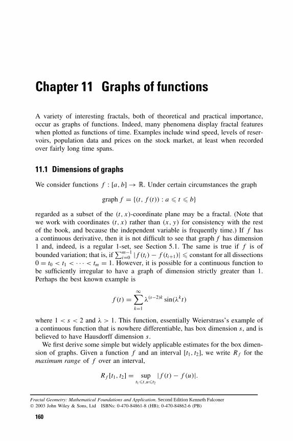
Chapter 11 Graphs of functions
A variety of interesting fractals, both of theoretical and practical importance,occur as graphs of functions. Indeed, many phenomena display fractal featureswhen plotted as functions of time. Examples include wind speed, levels of reser-voirs, population data and prices on the stock market, at least when recordedover fairly long time spans.
11.1 Dimensions of graphs
We consider functions f : [a, b] → �. Under certain circumstances the graph
graph f = {(t, f (t)) : a � t � b}regarded as a subset of the (t, x)-coordinate plane may be a fractal. (Note thatwe work with coordinates (t, x) rather than (x, y) for consistency with the restof the book, and because the independent variable is frequently time.) If f hasa continuous derivative, then it is not difficult to see that graph f has dimension1 and, indeed, is a regular 1-set, see Section 5.1. The same is true if f is ofbounded variation; that is, if
∑m−1i=0 |f (ti) − f (ti+1)| � constant for all dissections
0 = t0 < t1 < · · · < tm = 1. However, it is possible for a continuous function tobe sufficiently irregular to have a graph of dimension strictly greater than 1.Perhaps the best known example is
f (t) =∞∑
k=1
λ(s−2)k sin(λkt)
where 1 < s < 2 and λ > 1. This function, essentially Weierstrass’s example ofa continuous function that is nowhere differentiable, has box dimension s, and isbelieved to have Hausdorff dimension s.
We first derive some simple but widely applicable estimates for the box dimen-sion of graphs. Given a function f and an interval [t1, t2], we write Rf for themaximum range of f over an interval,
Rf [t1, t2] = supt1�t,u�t2
|f (t) − f (u)|.
160
Fractal Geometry: Mathematical Foundations and Application. Second Edition Kenneth Falconer 2003 John Wiley & Sons, Ltd ISBNs: 0-470-84861-8 (HB); 0-470-84862-6 (PB)

Dimensions of graphs 161
Proposition 11.1
Let f : [0, 1] → � be continuous. Suppose that 0 < δ < 1, and m is the leastinteger greater than or equal to 1/δ. Then, if Nδ is the number of squares of theδ-mesh that intersect graph f ,
δ−1m−1∑
i=0
Rf [iδ, (i + 1)δ] � Nδ � 2m + δ−1m−1∑
i=0
Rf [iδ, (i + 1)δ]. (11.1)
Proof. The number of mesh squares of side δ in the column above the interval[iδ, (i + 1)δ] that intersect graph f is at least Rf [iδ, (i + 1)δ]/δ and at most 2 +Rf [iδ, (i + 1)δ]/δ, using that f is continuous. Summing over all such intervalsgives (11.1). This is illustrated in figure 11.1. �
This proposition may be applied immediately to functions satisfying aHolder condition.
Corollary 11.2
Let f : [0, 1] → � be a continuous function.
(a) Suppose|f (t) − f (u)| � c|t − u|2−s (0 � t, u � 1) (11.2)
where c > 0 and 1 � s � 2. Then Hs(graph f ) < ∞ and dimH graph f �dimB graph f � dimB graph f � s. This remains true provided (11.2) holdswhen |t − u| < δ for some δ > 0.
x
x = f (t)
td
Figure 11.1 The number of δ-mesh squares in a column above an interval of width δ
that intersect graph f is approximately the range of f over that interval divided by δ.Summing these numbers gives estimates for the box dimension of graph f
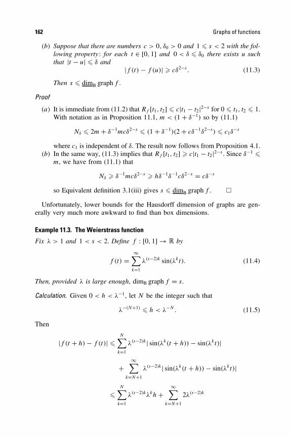
162 Graphs of functions
(b) Suppose that there are numbers c > 0, δ0 > 0 and 1 � s < 2 with the fol-lowing property : for each t ∈ [0, 1] and 0 < δ � δ0 there exists u suchthat |t − u| � δ and
|f (t) − f (u)| � cδ2−s . (11.3)
Then s � dimB graph f .
Proof
(a) It is immediate from (11.2) that Rf [t1, t2] � c|t1 − t2|2−s for 0 � t1, t2 � 1.With notation as in Proposition 11.1, m < (1 + δ−1) so by (11.1)
Nδ � 2m + δ−1mcδ2−s � (1 + δ−1)(2 + cδ−1δ2−s) � c1δ−s
where c1 is independent of δ. The result now follows from Proposition 4.1.(b) In the same way, (11.3) implies that Rf [t1, t2] � c|t1 − t2|2−s . Since δ−1 �
m, we have from (11.1) that
Nδ � δ−1mcδ2−s � hδ−1δ−1cδ2−s = cδ−s
so Equivalent definition 3.1(iii) gives s � dimB graph f . �
Unfortunately, lower bounds for the Hausdorff dimension of graphs are gen-erally very much more awkward to find than box dimensions.
Example 11.3. The Weierstrass function
Fix λ > 1 and 1 < s < 2. Define f : [0, 1] → � by
f (t) =∞∑
k=1
λ(s−2)k sin(λkt). (11.4)
Then, provided λ is large enough, dimB graph f = s.
Calculation. Given 0 < h < λ−1, let N be the integer such that
λ−(N+1) � h < λ−N . (11.5)
Then
|f (t + h) − f (t)| �N∑
k=1
λ(s−2)k| sin(λk(t + h)) − sin(λkt)|
+∞∑
k=N+1
λ(s−2)k| sin(λk(t + h)) − sin(λkt)|
�N∑
k=1
λ(s−2)kλkh +∞∑
k=N+1
2λ(s−2)k
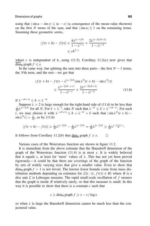
Dimensions of graphs 163
using that | sin u − sin v| � |u − v| (a consequence of the mean-value theorem)on the first N terms of the sum, and that | sin u| � 1 on the remaining terms.Summing these geometric series,
|f (t + h) − f (t)| � hλ(s−1)N
1 − λ1−s+ 2λ(s−2)(N+1)
1 − λs−2
� ch2−s
where c is independent of h, using (11.5). Corollary 11.2(a) now gives thatdimB graph f � s.
In the same way, but splitting the sum into three parts—the first N − 1 terms,the N th term, and the rest—we get that
|f (t + h) − f (t) − λ(s−2)N (sin λN(t + h) − sin λNt)|
� λ(s−2)N−s+1
1 − λ1−s+ 2λ(s−2)(N+1)
1 − λs−2(11.6)
if λ−(N+1) � h < λ−N .Suppose λ > 2 is large enough for the right-hand side of (11.6) to be less than
120λ(s−2)N for all N . For δ < λ−1, take N such that λ−N � δ < λ−(N−1). For eacht , we may choose h with λ−(N+1) � h < λ−N < δ such that | sin λN(t + h) −sin λNt | > 1
10 , so by (11.6)
|f (t + h) − f (t)| � 110λ(s−2)N − 1
20λ(s−2)N = 120λ(s−2)N � 1
20λs−2δ2−s .
It follows from Corollary 11.2(b) that dimB graph f � s. �
Various cases of the Weierstrass function are shown in figure 11.2.It is immediate from the above estimate that the Hausdorff dimension of the
graph of the Weierstrass function (11.4) is at most s. It is widely believedthat it equals s, at least for ‘most’ values of λ. This has not yet been provedrigorously—it could be that there are coverings of the graph of the functionby sets of widely varying sizes that give a smaller value. Even to show thatdimH graph f > 1 is not trivial. The known lower bounds come from mass dis-tribution methods depending on estimates for L{t : (t, f (t)) ∈ B} where B is adisc and L is Lebesgue measure. The rapid small-scale oscillation of f ensuresthat the graph is inside B relatively rarely, so that this measure is small. In thisway it is possible to show that there is a constant c such that
s � dimH graph f � s − c/ log λ
so when λ is large the Hausdorff dimension cannot be much less than the con-jectured value.
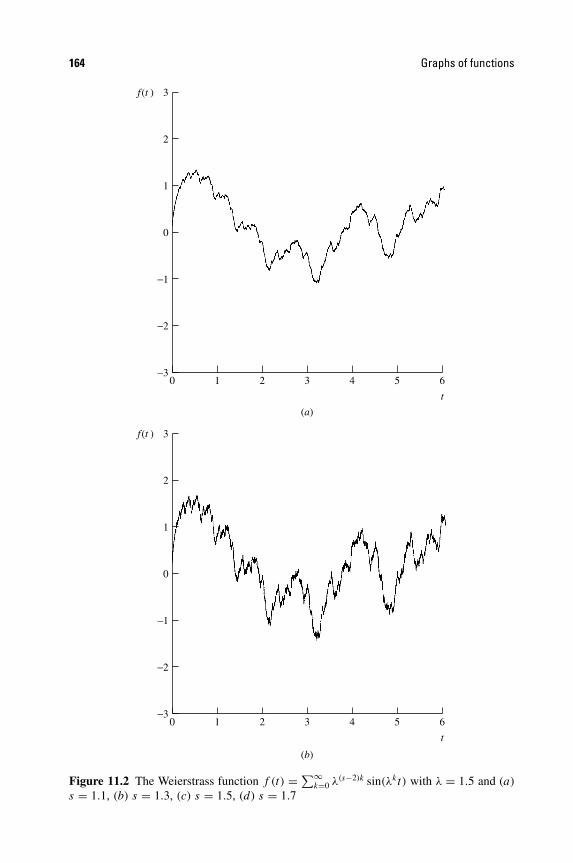
164 Graphs of functions
3
2
1
0
−1
−2
−30 1 2 3 4 5 6
t
3
2
1
0
−1
−2
−30 1 2 3
(a)
(b)
4 5 6
t
f (t )
f (t )
Figure 11.2 The Weierstrass function f (t) = ∑∞k=0 λ(s−2)k sin(λkt) with λ = 1.5 and (a)
s = 1.1, (b) s = 1.3, (c) s = 1.5, (d) s = 1.7
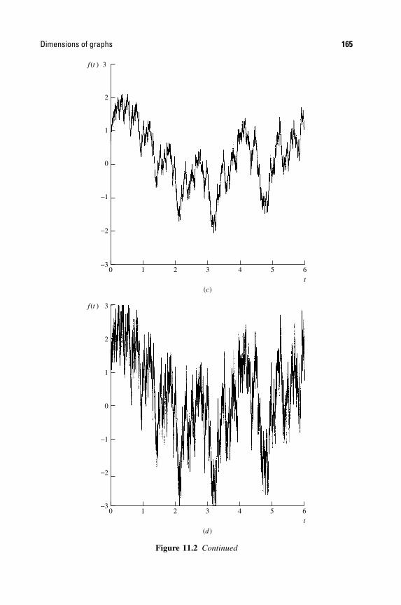
Dimensions of graphs 165
3
2
1
0
−1
−2
−30 1 2 3 4 5 6
t
3f (t )
2
1
0
−1
−2
−30 1 2 3
(c)
(d )
4 5 6t
f (t )
Figure 11.2 Continued

166 Graphs of functions
The Weierstrass function (11.4) is representative of a much wider class offunctions to which these methods apply. If g is a suitable periodic function, asimilar method can often show that
f (t) =∞∑
k=1
λ(s−2)kg(λkt) (11.7)
has dimB graph f = s. At first such functions seem rather contrived, but theiroccurrence as repellers in certain dynamical systems (see Exercise 13.9) givesthem a new significance.
In Section 9.4 we saw that self-affine sets defined by iterated function systemsare often fractals; by a suitable choice of affine transformations, they can alsobe graphs of functions. Let {Si, . . . , Sm} be affine transformations represented inmatrix notation with respect to (t, x) coordinates by
Si
[t
x
]=
[1/m 0ai ci
] [t
x
]+
[(i − 1)/m
bi
]. (11.8)
that isSi(t, x) = (t/m + (i − 1)/m, ait + cix + bi).
Thus the Si transform vertical lines to vertical lines, with the vertical strip 0 �t � 1 mapped onto the strip (i − 1)/m � t � i/m. We suppose that
1/m < ci < 1 (11.9)
so that contraction in the t direction is stronger than in the x direction.Let p1 = (0, b1/(1 − c1)) and pm = (1, (am + bm)/(1 − cm)) be the fixed
points of S1 and Sm. We assume that the matrix entries have been chosen so that
Si(pm) = Si+1(p1) (1 � i � m − 1) (11.10)
so that the segments [Si(p1), Si(pm)] join up to form a polygonal curve E1. Toavoid trivial cases, we assume that the points S1(p1), . . . , Sm(p1), pm are not allcollinear. The attractor F of the iterated function system {Si, . . . , Sm} (see (9.2))may be constructed by repeatedly replacing line segments by affine images ofthe ‘generator’ E1; see figures 11.3 and 11.4. Condition (11.10) ensures that thesegments join up with the result that F is the graph of some continuous functionf : [0, 1] → �. Note that these conditions do not necessarily imply that the Si
are contractions with respect to Euclidean distance. However, it is possible toredefine distance in the (x, t) plane in such a way that the Si become contractions,and in this context the IFS theory guarantees a unique attractor.
Example 11.4. Self-affine curves
Let F = graph f be the self-affine curve described above. Then dimBF = 1 +log(c1 + · · · + cm)/ log m.

Dimensions of graphs 167
E3
E2
E1
E0
q1 q2
p
p1 p2
Figure 11.3 Stages in the construction of a self-affine curve F . The affine transforma-tions S1 and S2 map the generating triangle p1pp2 onto the triangles p1q1p and pq2p2,respectively, and transform vertical lines to vertical lines. The rising sequence of polyg-onal curves E0, E1, . . . are given by Ek+1 = S1(Ek) ∪ S2(Ek) and provide increasinglygood approximations to F (shown in figure 11.4(a) for this case)
Calculation. Let Ti be the ‘linear part’ of Si , represented by the matrix
[1/m 0ai ci
].
Let Ii1,...,ik be the interval of the t-axis consisting of those t with base-m expansionbeginning 0.i′1 · · · i′k where i′j = ij − 1. Then the part of F above Ii1,...,ik is theaffine image Si1
◦ · · · ◦Sik (F ), which is a translate of Ti1◦ · · · ◦ Tik (F ). The matrix
representing Ti1◦ · · · ◦ Tik is easily seen by induction to be
[m−k 0
m1−kai1 + m2−kci1ai2 + · · · + ci1ci2 · · · cik−1aik ci1ci2 · · · cik
].
This is a shear transformation, contracting vertical lines by a factor ci1ci2 · · · cik .Observe that the bottom left-hand entry is bounded by
|m1−ka + m2−kci1a + · · · + ci1 · · · cik−1a|� ((mc)1−k + (mc)2−k + · · · + 1)ci1 · · · cik−1a
� rci1 · · · cik−1
where a = max |ai |, c = min{ci} > 1/m and r = a/(1 − (mc)−1) from summingthe geometric series. Thus the image Ti1
◦ · · · ◦ Tik (F ) is contained in a rectangleof height (r + h)ci1 · · · cik where h is the height of F . On the other hand, ifq1, q2, q3 are three non-collinear points chosen from S1(p1), . . . , Sm(p1), pm,then Ti1
◦ · · · ◦ Tik (F ) contains the points Ti1◦ · · · ◦ Tik (qj )(j = 1, 2, 3). The height
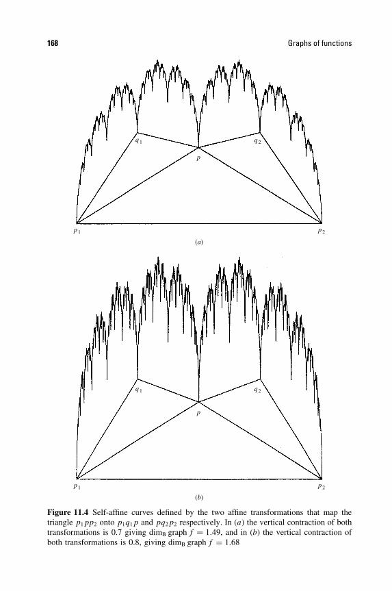
168 Graphs of functions
q1 q2
q1 q2
p
p
p1 p2
(a)
p1 p2
(b)
Figure 11.4 Self-affine curves defined by the two affine transformations that map thetriangle p1pp2 onto p1q1p and pq2p2 respectively. In (a) the vertical contraction of bothtransformations is 0.7 giving dimB graph f = 1.49, and in (b) the vertical contraction ofboth transformations is 0.8, giving dimB graph f = 1.68
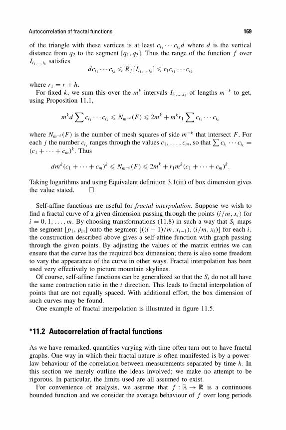
Autocorrelation of fractal functions 169
of the triangle with these vertices is at least ci1 · · · cikd where d is the verticaldistance from q2 to the segment [q1, q3]. Thus the range of the function f overIi1,...,ik satisfies
dci1 · · · cik � Rf [Ii1,...,ik ] � r1ci1 · · · cik
where r1 = r + h.For fixed k, we sum this over the mk intervals Ii1,...,ik of lengths m−k to get,
using Proposition 11.1,
mkd∑
ci1 · · · cik � Nm−k (F ) � 2mk + mkr1
∑ci1 · · · cik
where Nm−k (F ) is the number of mesh squares of side m−k that intersect F . Foreach j the number cij ranges through the values c1, . . . , cm, so that
∑ci1 · · · cik =
(c1 + · · · + cm)k. Thus
dmk(c1 + · · · + cm)k � Nm−k (F ) � 2mk + r1mk(c1 + · · · + cm)k.
Taking logarithms and using Equivalent definition 3.1(iii) of box dimension givesthe value stated. �
Self-affine functions are useful for fractal interpolation. Suppose we wish tofind a fractal curve of a given dimension passing through the points (i/m, xi) fori = 0, 1, . . . , m. By choosing transformations (11.8) in such a way that Si mapsthe segment [p1, pm] onto the segment [((i − 1)/m, xi−1), (i/m, xi)] for each i,the construction described above gives a self-affine function with graph passingthrough the given points. By adjusting the values of the matrix entries we canensure that the curve has the required box dimension; there is also some freedomto vary the appearance of the curve in other ways. Fractal interpolation has beenused very effectively to picture mountain skylines.
Of course, self-affine functions can be generalized so that the Si do not all havethe same contraction ratio in the t direction. This leads to fractal interpolation ofpoints that are not equally spaced. With additional effort, the box dimension ofsuch curves may be found.
One example of fractal interpolation is illustrated in figure 11.5.
∗11.2 Autocorrelation of fractal functions
As we have remarked, quantities varying with time often turn out to have fractalgraphs. One way in which their fractal nature is often manifested is by a power-law behaviour of the correlation between measurements separated by time h. Inthis section we merely outline the ideas involved; we make no attempt to berigorous. In particular, the limits used are all assumed to exist.
For convenience of analysis, we assume that f : � → � is a continuousbounded function and we consider the average behaviour of f over long periods

170 Graphs of functions
(a) (b)
(c) (d)
Figure 11.5 Fractal interpolation on the northern and southern halves of a map of South-West England, using the vertices of the polygon in figure (a) as data points. The dimen-sions of the self-affine curves fitted to these data points are (b) 1.1, (c) 1.2 and (d) 1.3
[−T , T ]. (Similar ideas hold if f is just defined on [0,∞), or on a finite interval,by extending f to � in a periodic manner). We write f for the average value off , i.e.
f = limT →∞
1
2T
∫ T
−T
f (t)dt.
A measure of the correlation between f at times separated by h is provided bythe autocorrelation function
C(h) = limT →∞
1
2T
∫ T
−T
(f (t + h) − f )(f (t) − f )dt (11.11)
= limT →∞
1
2T
∫ T
−T
f (t + h)f (t)dt − (f )2. (11.12)
From (11.11) we see that C(h) is positive if f (t + h) − f and f (t) − f tend tohave the same sign, and is negative if they tend to have opposite signs. If thereis no correlation, C(h) = 0. Since
∫(f (t + h) − f (t))2dt =
∫f (t + h)2dt +
∫f (t)2dt − 2
∫f (t + h)f (t)dt

Autocorrelation of fractal functions 171
we have
C(h) = f 2 − (f )2 − 1
2lim
T →∞1
2T
∫ T
−T
(f (t + h) − f (t))2dt
= C(0) − 1
2lim
T →∞1
2T
∫ T
−T
(f (t + h) − f (t))2dt (11.13)
where
f 2 = limT →∞
1
2T
∫ T
−T
f (t)2dt
is the mean square of f , assumed to be positive and finite. With C(h) in the form(11.13) we can infer a plausible relationship between the autocorrelation functionof f and the dimension of graph f . The clue is in Corollary 11.2. Suppose that f
is a function satisfying (11.2) and also satisfying (11.3) in a ‘reasonably uniformway’. Then, there are constants c1 and c2 such that
c1h4−2s � 1
2T
∫ T
−T
(f (t + h) − f (t))2dt � c2h4−2s (11.14)
for small h. Obviously, this is not directly equivalent to (11.2) and (11.3), but inmany reasonably ‘time-homogeneous’ situations, the conditions do correspond.Thus if the autocorrelation function of f satisfies
C(0) − C(h) � ch4−2s
for small h, it is reasonable to expect the box dimension of graph f to equal s.The autocorrelation function is closely connected with the power spectrum of
f , defined by
S(ω) = limT →∞
1
2T
∣∣∣∣
∫ T
−T
f (t)eitωdt
∣∣∣∣
2
. (11.15)
For functions with any degree of long-term regularity, S(ω) is likely to exist.The power spectrum reflects the strength of the frequency ω in the harmonicdecomposition of f .
We show that the power spectrum is the Fourier transform of the autocorrelationfunction. By working with f (t) − f we may assume that f has zero mean. LetfT (t) be given by f (t) if |t | � T and be 0 otherwise, and define
CT (h) = 1
2T
∫ ∞
−∞fT (t + h)fT (t)dt
= 1
2Tf −
T ∗ fT (−h)
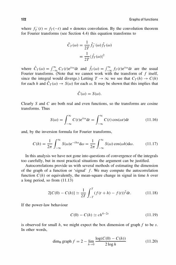
172 Graphs of functions
where f −T (t) = fT (−t) and ∗ denotes convolution. By the convolution theorem
for Fourier transforms (see Section 4.4) this equation transforms to
CT (ω) = 1
2Tf −
T (ω)fT (ω)
= 1
2T|fT (ω)|2
where CT (ω) = ∫ ∞−∞ CT (t)eitωdt and fT (ω) = ∫ ∞
−∞ fT (t)eitωdt are the usualFourier transforms. (Note that we cannot work with the transform of f itself,since the integral would diverge.) Letting T → ∞ we see that CT (h) → C(h)
for each h and CT (ω) → S(ω) for each ω. It may be shown that this implies that
C(ω) = S(ω).
Clearly S and C are both real and even functions, so the transforms are cosinetransforms. Thus
S(ω) =∫ ∞
−∞C(t)eitωdt =
∫ ∞
−∞C(t) cos(ωt)dt (11.16)
and, by the inversion formula for Fourier transforms,
C(h) = 1
2π
∫ ∞
−∞S(ω)e−ihωdω = 1
2π
∫ ∞
−∞S(ω) cos(ωh)dω. (11.17)
In this analysis we have not gone into questions of convergence of the integralstoo carefully, but in most practical situations the argument can be justified.
Autocorrelations provide us with several methods of estimating the dimensionof the graph of a function or ‘signal’ f . We may compute the autocorrelationfunction C(h) or equivalently, the mean-square change in signal in time h overa long period, so from (11.13)
2[C(0) − C(h)] � 1
2T
∫ T
−T
(f (t + h) − f (t))2dt. (11.18)
If the power-law behaviour
C(0) − C(h) � ch4−2s (11.19)
is observed for small h, we might expect the box dimension of graph f to be s.In other words,
dimB graph f = 2 − limh→0
log(C(0) − C(h))
2 log h(11.20)

Exercises 173
if this limit exists. We might then seek functions with graphs known to havethis dimension, such as those of Examples 11.3 and 11.4 or the fractional Brow-nian functions of Section 16.2 to provide simulations of signals with similarcharacteristics.
Alternatively, we can work from the power spectrum S(ω) and use (11.17) tofind the autocorrelation function. We need to know about C(0) − C(h) for smallh; typically this depends on the behaviour of its transform S(ω) when ω is large.The situation of greatest interest is when the power spectrum obeys a power lawS(ω) ∼ c/ωα for large ω, in which case
C(0) − C(h) ∼ bhα−1 (11.21)
for small h, for some constant b. To see this formally note that from (11.17)
π(C(0) − C(h)) =∫ ∞
0S(ω)(1 − cos(ωh))dω = 2
∫ ∞
0S(ω) sin2
(12ωh
)dω
and taking S(ω) = ω−α gives
12π(C(0) − C(h)) =
∫ ∞
0ω−α sin2 1
2ωh dω = hα−1∫ ∞
0u−α sin2 1
2u du
having substituted u = ωh. It may be shown that (11.21) also holds if S isany sufficiently smooth function such that S(ω) ∼ cω−α as ω → ∞. Comparing(11.19) and (11.21) suggests that graph f has box dimension s where 4 − 2s =α − 1, or s = 1
2 (5 − α). Thus it is reasonable to expect a signal with a 1/ωα
power spectrum to have a graph of dimension 12 (5 − α) for 1 < α < 3.
In practice, curves of dimension 12 (5 − α) often provide good simulations and
display similar characteristics to signals observed to have 1/ωα power spectra.
11.3 Notes and references
The dimension of fractal graphs was first studied by Besicovitch and Ursell(1937). For more recent work on Weierstrass-type curves see Berry and Lewis(1980), Mauldin and Williams (1986b) and Hunt (1998). Self-affine curves arethe theme of a book by Massopust (1994), and self-affine curves are discussed inBedford (1989). The theory of autocorrelation functions is given in most bookson time series analysis, for example Papoulis (1962).
Exercises
11.1 Verify that if f : [0, 1] → � has a continuous derivative then graph f is a regular1-set, see Section 5.1.
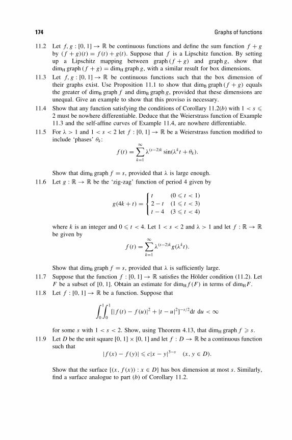
174 Graphs of functions
11.2 Let f, g : [0, 1] → � be continuous functions and define the sum function f + g
by (f + g)(t) = f (t) + g(t). Suppose that f is a Lipschitz function. By settingup a Lipschitz mapping between graph (f + g) and graph g, show thatdimH graph (f + g) = dimH graph g, with a similar result for box dimensions.
11.3 Let f, g : [0, 1] → � be continuous functions such that the box dimension oftheir graphs exist. Use Proposition 11.1 to show that dimB graph (f + g) equalsthe greater of dimB graph f and dimB graph g, provided that these dimensions areunequal. Give an example to show that this proviso is necessary.
11.4 Show that any function satisfying the conditions of Corollary 11.2(b) with 1 < s �2 must be nowhere differentiable. Deduce that the Weierstrass function of Example11.3 and the self-affine curves of Example 11.4, are nowhere differentiable.
11.5 For λ > 1 and 1 < s < 2 let f : [0, 1] → � be a Weierstrass function modified toinclude ‘phases’ θk :
f (t) =∞∑
k=1
λ(s−2)k sin(λkt + θk).
Show that dimB graph f = s, provided that λ is large enough.
11.6 Let g : � → � be the ‘zig-zag’ function of period 4 given by
g(4k + t) =
t (0 � t < 1)
2 − t (1 � t < 3)
t − 4 (3 � t < 4)
where k is an integer and 0 � t < 4. Let 1 < s < 2 and λ > 1 and let f : � → �be given by
f (t) =∞∑
k=1
λ(s−2)kg(λkt).
Show that dimB graph f = s, provided that λ is sufficiently large.
11.7 Suppose that the function f : [0, 1] → � satisfies the Holder condition (11.2). LetF be a subset of [0, 1]. Obtain an estimate for dimHf (F ) in terms of dimHF .
11.8 Let f : [0, 1] → � be a function. Suppose that
∫ 1
0
∫ 1
0[|f (t) − f (u)|2 + |t − u|2]−s/2dt du < ∞
for some s with 1 < s < 2. Show, using Theorem 4.13, that dimH graph f � s.
11.9 Let D be the unit square [0, 1] × [0, 1] and let f : D → � be a continuous functionsuch that
|f (x) − f (y)| � c|x − y|3−s (x, y ∈ D).
Show that the surface {(x, f (x)) : x ∈ D} has box dimension at most s. Similarly,find a surface analogue to part (b) of Corollary 11.2.
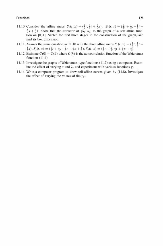
Exercises 175
11.10 Consider the affine maps S1(t, x) = ( 12 t, 1
4 t + 56x), S2(t, x) = ( 1
2 t + 12 ,− 1
4 t +56x + 1
4 ). Show that the attractor of {S1, S2} is the graph of a self-affine func-tion on [0, 1]. Sketch the first three stages in the construction of the graph, andfind its box dimension.
11.11 Answer the same question as 11.10 with the three affine maps S1(t, x) = ( 13 t, 1
3 t +12x), S2(t, x) = ( 1
3 t + 13 ,− 2
3 t + 12 x + 1
3 ), S3(t, x) = ( 13 t + 2
3 , 13 t + 1
2 x − 13 ).
11.12 Estimate C(0) − C(h) where C(h) is the autocorrelation function of the Weierstrassfunction (11.4).
11.13 Investigate the graphs of Weierstrass-type functions (11.7) using a computer. Exam-ine the effect of varying s and λ, and experiment with various functions g.
11.14 Write a computer program to draw self-affine curves given by (11.8). Investigatethe effect of varying the values of the ci .

Chapter 12 Examples from puremathematics
Fractal constructions have provided counterexamples, and sometimes solutions,to a variety of problems where more regular constructions have failed. In thischapter we look at several simple but elegant instances from differing areas ofpure mathematics.
12.1 Duality and the Kakeya problem
The method of duality converts sets of points in the plane to sets of lines andmay be used to create new fractals from old. The techniques can be applied toconstruct sets with particular properties; for example, to construct a plane set ofzero area that contains a line running in every direction.
For each point (a, b) of �2, we let L(a, b) denote the set of points on theline y = a + bx, see figure 12.1. If F is any subset of �2 we define the lineset L(F ) to be the union of the lines corresponding to the points of F , i.e.L(F ) = ⋃{L(a, b) : (a, b) ∈ F }. Writing Lc for the vertical line x = c, we have
L(a, b) ∩ Lc = (c, a + bc) = (c, (a, b)·(1, c)),
where ‘·’ is the usual scalar product in �2; thus for a subset F of �2
L(F ) ∩ Lc = {(c, (a, b)·(1, c)) : (a, b) ∈ F }.
Taking a scalar product with the vector (1, c) may be interpreted geometricallyas projecting onto the line in the direction of (1, c) and stretching by a factor(1 + c2)1/2. Thus the set L(F ) ∩ Lc is a similar copy of projθF scaled by (1 +c2)1/2, where projθ denotes orthogonal projection onto the line through the originat angle θ to the x-axis, where c = tan θ . In particular,
dimH(L(F ) ∩ Lc) = dimH(projθF ) (12.1)
176
Fractal Geometry: Mathematical Foundations and Application. Second Edition Kenneth Falconer 2003 John Wiley & Sons, Ltd ISBNs: 0-470-84861-8 (HB); 0-470-84862-6 (PB)
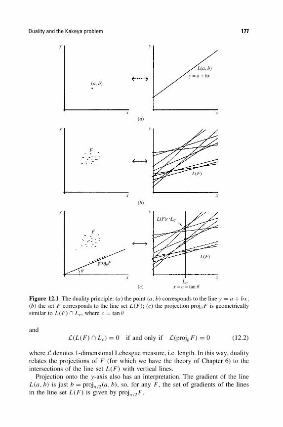
Duality and the Kakeya problem 177
y
x
y
x
(a, b)
F
F
L(F)
L(a, b)
y = a + bx
(a)
y
x
y
x
(b)
y
x
y
x
(c)
L(F)∩Lc
L(F)
Lcx = c = tan q
q
projqF
Figure 12.1 The duality principle: (a) the point (a, b) corresponds to the line y = a + bx;(b) the set F corresponds to the line set L(F); (c) the projection projθF is geometricallysimilar to L(F) ∩ Lc, where c = tan θ
andL(L(F ) ∩ Lc) = 0 if and only if L(projθF ) = 0 (12.2)
where L denotes 1-dimensional Lebesgue measure, i.e. length. In this way, dualityrelates the projections of F (for which we have the theory of Chapter 6) to theintersections of the line set L(F ) with vertical lines.
Projection onto the y-axis also has an interpretation. The gradient of the lineL(a, b) is just b = projπ/2(a, b), so, for any F , the set of gradients of the linesin the line set L(F ) is given by projπ/2F .
178 Examples from pure mathematics
If F is a fractal its line set L(F ) often has a fractal structure, albeit a highlyfibrous one. (In fact, L(F ) need not be a Borel set if F is Borel, though it will beif F is compact. We ignore the minor technical difficulties that this introduces.)We have the following dimensional relationship.
Proposition 12.1
Let L(F ) be the line set of a Borel set F ⊂ �2. Then
(a) dimHL(F ) � min{2, 1 + dimHF }, and(b) if F is a 1-set then area(L(F )) = 0 if and only if F is irregular.
Proof.(a) By the Projection theorem 6.1, dimH(projθF ) = min{1, dimHF } for almost
all θ ∈ [0, π), so from (12.1) dimH(L(F ) ∩ Lc) = min{1, dimHF } foralmost all −∞ < c < ∞. Part (a) now follows from Corollary 7.10.
(b) Let F be a 1-set. Corollary 6.5 tells us that if F is irregular thenL(projθF ) = 0 for almost all θ , otherwise L(projθF ) > 0 for almost all θ .Using (12.2) we get the dual statement that if F is irregular then L(L(F ) ∩Lc) = 0 for almost all c, otherwise L(L(F ) ∩ Lc) > 0 for almost all c.Since area(L(F )) = ∫ ∞
−∞ L(L(F ) ∩ Lc)dc, part (b) follows. �
In 1917 Kakeya posed the problem of finding the plane set of least areainside which a unit line segment could be reversed, i.e. manoeuvred continu-ously without leaving the set to reach its original position but rotated through180◦. Essentially, this problem reduces to that of finding the smallest region thatcontains a unit line segment in every direction; certainly any set in which a seg-ment can be reversed must have this property. By 1928 Besicovitch had founda surprising construction of a set of arbitrarily small area inside which a unitsegment could be reversed. Only many years later did he realize that the methodof duality gave a short and elegant solution to the problem.
Proposition 12.2
There is a plane set of zero area which contains a line in every direction. AnyBorel set with this property must have Hausdorff dimension 2.
Proof. Let F be any irregular 1-set such that the projection of F onto the y-axis,projπ/2F , contains the interval [0, 1]. (The set of figure 0.4, see Examples 2.6 and6.7, certainly meets this requirement.) Since F is irregular, L(F ) has zero area,by Proposition 12.1(b). However, since [0, 1] ⊂ projπ/2F , the set L(F ) containslines that cut the x-axis at all angles between 0 and π/4. Taking L(F ), togetherwith copies rotated through π/4, π/2 and 3π/4, gives a set of area 0 containinga line in every direction.
Vitushkin’s conjecture 179
For the second part, suppose that E contains a line in every direction. If
F = {(a, b) : L(a, b) ⊂ E}
then projπ/2F is the entire y-axis. Projection does not increase dimension (see(6.1)), so dimHF � 1. By Proposition 12.1(a) dimHL(F ) = 2; since L(F ) ⊂ E
it follows that dimHE = 2. �
A set in �n that contains a line segment in every direction is called a Besicov-itch set. Proposition 12.2 shows that Besicovitch sets exist in �2, and taking aproduct with �n−2 gives a Besicovitch set in �n. A long-standing conjecture isthat every Besicovitch set in �n has dimension n; we have shown this if n = 2.
Sets of this type have important applications in functional analysis. For asimple example, let g : �2 → � and write G(θ, t) for the integral of g alongthe line making angle θ with the x-axis and perpendicular distance t from theorigin. Let F be a set of zero area containing a line in every direction, and letg(x, y) = 1 if (x, y) is a point of F and g(x, y) = 0 otherwise. It is clear thatG(θ, t) is not continuous in t for any fixed value of θ . This example becomessignificant when contrasted with the 3-dimensional situation. If g : D → � is abounded function on a bounded domain D in �3, and G(θ, t) is the integral ofg over the plane perpendicular to the unit vector θ and perpendicular distance t
from the origin, it may be shown that G(θ, t) must be continuous in t for almostall unit vectors θ .
The Besicovitch construction may be thought of as a packing of lines in alldirections into a set of area zero. Similar problems may be considered for pack-ings of other collections of curves. For example, there are sets of zero area thatcontain the circumference of a circle of every radius, see Exercises 12.1 and12.2. However, every set that contains some circle circumference centred at eachpoint in the plane necessarily has positive area.
12.2 Vitushkin’s conjecture
A long-standing conjecture of Vitushkin in complex potential theory was dis-proved using a fractal construction. For geometrical purposes we identify thecomplex plane � with the Euclidean plane �2.
Let F be a compact subset of �. We say that F is a removable set if, givenany bounded open domain V containing F and any bounded analytic (i.e. differ-entiable in the complex sense) function f on the complement V \F , then f hasan analytic extension to the whole of V . Thus the functions that are bounded andanalytic on V are essentially the same as those that are bounded and analytic onV \F ; removing F makes no difference.
The problem of providing a geometrical characterization of removable setsdates back many years. The removability, or otherwise, of F has now been
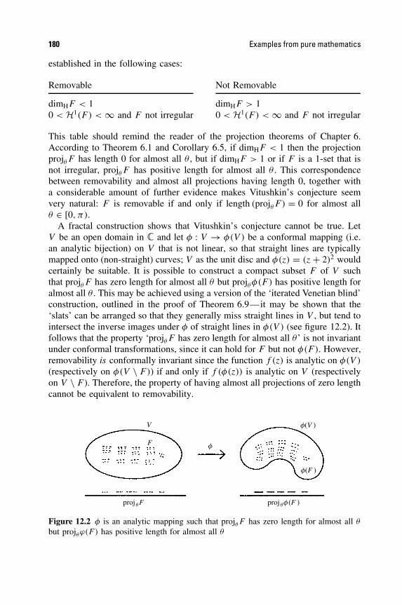
180 Examples from pure mathematics
established in the following cases:
Removable Not Removable
dimHF < 1 dimHF > 10 < H1(F ) < ∞ and F not irregular 0 < H1(F ) < ∞ and F not irregular
This table should remind the reader of the projection theorems of Chapter 6.According to Theorem 6.1 and Corollary 6.5, if dimHF < 1 then the projectionprojθF has length 0 for almost all θ , but if dimHF > 1 or if F is a 1-set that isnot irregular, projθF has positive length for almost all θ . This correspondencebetween removability and almost all projections having length 0, together witha considerable amount of further evidence makes Vitushkin’s conjecture seemvery natural: F is removable if and only if length (projθF ) = 0 for almost allθ ∈ [0, π).
A fractal construction shows that Vitushkin’s conjecture cannot be true. LetV be an open domain in � and let φ : V → φ(V ) be a conformal mapping (i.e.an analytic bijection) on V that is not linear, so that straight lines are typicallymapped onto (non-straight) curves; V as the unit disc and φ(z) = (z + 2)2 wouldcertainly be suitable. It is possible to construct a compact subset F of V suchthat projθF has zero length for almost all θ but projθφ(F ) has positive length foralmost all θ . This may be achieved using a version of the ‘iterated Venetian blind’construction, outlined in the proof of Theorem 6.9—it may be shown that the‘slats’ can be arranged so that they generally miss straight lines in V , but tend tointersect the inverse images under φ of straight lines in φ(V ) (see figure 12.2). Itfollows that the property ‘projθF has zero length for almost all θ ’ is not invariantunder conformal transformations, since it can hold for F but not φ(F ). However,removability is conformally invariant since the function f (z) is analytic on φ(V )
(respectively on φ(V \ F)) if and only if f (φ(z)) is analytic on V (respectivelyon V \ F ). Therefore, the property of having almost all projections of zero lengthcannot be equivalent to removability.
V
F
proj qF proj qf (F )
f(F )
f(V )
f
Figure 12.2 φ is an analytic mapping such that projθF has zero length for almost all θ
but projθϕ(F ) has positive length for almost all θ

Convex functions 181
One of the curious features of this particular argument is that it leaves us nonethe wiser as to whether sets with almost all projections of zero length must beremovable or vice versa. All we can deduce is that both cannot be true.
Subsequently, a non-removable set with almost all projections of zero lengthwas obtained using an iterated construction.
12.3 Convex functions
A continuous function f : �2 → � is convex if
f (λx + (1 − λ)y) � λf (x) + (1 − λ)f (y)
for all x, y ∈ �2 and 0 � λ � 1. Geometrically, if S = {(x, f (x)) : x ∈ �2} isthe surface in �3 representing the graph of f , then f is convex if the line segmentjoining any two points of S lies in or above S.
A convex function f need not be particularly smooth—there may be pointswhere f is not differentiable. However, convexity implies that the set of such‘singular’ points cannot be too big, in the sense of dimension. Note that if f isnot differentiable at x then the surface S supports more than one tangent plane at(x, f (x)). Also notice that if P1 and P2 are distinct tangent planes at (x, f (x))
then there is a continuum of tangent planes through this point, namely thoseplanes ‘between P1 and P2’ that contain the line P1 ∩ P2.
Theorem 12.3
Let f : �2 → � be a convex function. Then the set of points at which f is not dif-ferentiable is contained in a countable union of rectifiable curves, so in particularhas Hausdorff dimension at most 1.
Proof. Without loss of generality, we may assume that the minimum value off is strictly positive. Let S be the surface given by the graph of f and letg : �2 → S be the ‘nearest point’ mapping, so that if x ∈ �2 then g(x) is thatpoint of S for which the distance |g(x) − x| is least, see figure 12.3. Convexityof f guarantees that this point is unique. If x, y ∈ �2 then the angles of the(possibly skew) quadrilateral x, g(x), g(y), y at g(x) and g(y) must both be atleast π/2; otherwise the segment (g(x), g(y)) will contain a point on or aboveS that is nearer to x or y. It follows that g is distance decreasing, i.e.
|g(x) − g(y)| � |x − y| (x, y ∈ �2). (12.3)
If f fails to be differentiable at x, then S supports more than one tangent planeat (x, f (x)). Thus g−1(x, f (x)), the subset of the coordinate plane �2 mapped
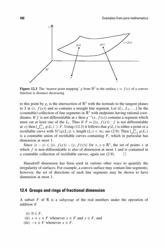
182 Examples from pure mathematics
z
z = f (x)g(x) g(y)
xy
2
Figure 12.3 The ‘nearest point mapping’ g from �2 to the surface z = f (x) of a convexfunction is distance decreasing
to this point by g, is the intersection of �2 with the normals to the tangent planesto S at (x, f (x)) and so contains a straight line segment. Let {L1, L2, . . .} be the(countable) collection of line segments in �2 with endpoints having rational coor-dinates. If f is not differentiable at x then g−1(x, f (x)) contains a segment whichmust cut at least one of the Li . Thus if F = {(x, f (x)) : f is not differentiableat x} then
⋃∞i=1 g(Li) ⊃ F . Using (12.3) it follows that g(Li) is either a point or a
rectifiable curve with H1(g(Li)) � length (Li) < ∞; see (2.9). Then⋃∞
i=1 g(Li)
is a countable union of rectifiable curves containing F , which in particular hasdimension at most 1.
Since |x − y| � |(x, f (x)) − (y, f (y))| for x, y ∈ �2, the set of points x atwhich f is non-differentiable is also of dimension at most 1 and is contained ina countable collection of rectifiable curves; again see (2.9). �
Hausdorff dimension has been used in various other ways to quantify theirregularity of surfaces. For example, a convex surface may contain line segments;however, the set of directions of such line segments may be shown to havedimension at most 1.
12.4 Groups and rings of fractional dimension
A subset F of � is a subgroup of the real numbers under the operation ofaddition if
(i) 0 ∈ F ,(ii) x + y ∈ F whenever x ∈ F and y ∈ F , and
(iii) −x ∈ F whenever x ∈ F .

Groups and rings of fractional dimension 183
The set F is a subring of � under addition and multiplication if, also,
(iv) xy ∈ F whenever x ∈ F and y ∈ F .
There are many simple examples of such structures: the integers, the rationalsand the set of numbers {r + s
√2 : r, s ∈ �} are all subrings (and therefore sub-
groups) of �. These examples are countable sets and therefore have Hausdorffdimension 0. Do there exist subgroups and subrings of � of Hausdorff dimensions if 0 < s < 1?
It is relatively easy to modify the earlier Example 4.7 to obtain a subgroup ofany given dimension.
Example 12.4
Fix 0 < s < 1. Let n0, n1, n2, . . . be a rapidly increasing sequence of integers,say with nk+1 � max{nk
k, 4n1/s
k } for each k. For r = 1, 2, . . . let
Fr = {x ∈ � : |x − p/nk| � rn−1/s
k for some integer p, for all k}and let F = ⋃∞
r=1 Fr . Then dimHF = s, and F is a subgroup of � under addition.
Calculation. Fr is essentially the set of Example 4.7, so dimHFr = s for all r
(it is easy to see that the value of r does not affect the dimension). Taking acountable union, dimHF = s.
Clearly 0 ∈ F1 ⊂ F . If x, y ∈ F then x, y ∈ Fr for some r , noting that Fr ′ ⊂Fr if r � r ′. Thus, for each k, there are integers p, q such that
|x − p/nk| � rn−1/s
k |y − q/nk| � rn−1/s
k .
Adding,|x + y − (p + q)/nk| � 2rn
−1/s
k
so x + y ∈ F2r ⊂ F . Clearly, if x ∈ Fr then −x ∈ Fr , so F satisfies conditions(i)–(iii) above. �
Subrings are rather harder to analyse. One geometrical approach depends onestimating the dimension of the set of distances realized by a plane set. If E isa subset of �2, we define the distance set of E by
D(E) = {|x − y| : x, y ∈ E} ⊂ �.
Theorem 12.5
Let E ⊂ �2 be a Borel set. Then
dimHD(E) � min{1, dimHE − 12 }. (12.4)

184 Examples from pure mathematics
Note on proof. The potential theoretic proof of this theorem is a little complicated.Fourier transforms and the convolution theorem are used to examine the circleswith centres in E that intersect E. It is unlikely that (12.4) is the best inequalitypossible. �
Assuming this theorem, it is not difficult to obtain a partial solution to thesubrings problem.
Theorem 12.6
Let F be a subring of � under addition and multiplication. If F is a Borel setthen either dimHF = 0 or F = �.
Partial proof. We use a geometrical method to show there are no subrings ofdimension between 1
2 and 1. Using (x, y) coordinates in �2, if (x1, y1), (x2, y2) ∈F × F ⊂ �2, then |(x1, y1) − (x2, y2)|2 = (x1 − x2)
2 + (y1 − y2)2 ∈ F , since F
is a subring. Thus, if D2(F × F) denotes the set of squares of distances betweenpoints of F × F , we have D2(F × F) ⊂ F . Since the mapping t → t2 preservesHausdorff dimension (see Exercise 2.6) we have
dimHF � dimHD2(F × F) = dimHD(F × F)
� min{1, dimH(F × F) − 12 }
� min{1, 2dimHF − 12 }
using Theorem 12.5 and Product formula 7.2. This inequality is satisfied if andonly if dimHF = 1 or dimHF � 1
2 . �
12.5 Notes and references
More detailed accounts of the Kakeya problem and its variants are given in Besi-covitch (1963), Cunningham (1974) and Falconer (1985a) and the dual approachwas introduced by Besicovitch (1964). For recent surveys see Wolff (1999) andKatz and Tao (2000). The book by Stein (1993) includes applications of Kakeyasets to functional and harmonic analysis.
For discussions on Vitushkin’s conjecture, see Mattila (1995), Murai (1988)and David (1999). The construction outlined is due to Mattila (1986) and thenon-removable set with projections of lengths zero is due to Jones and Murai(1988). David (1999) showed that irregular 1-sets are removable.
For general information on convex geometry see Gruber and Wills (1993). Theresult given here is due to Anderson and Klee (1952). For other results involvingHausdorff dimension and convexity, see Dalla and Larman (1980) and the surveyof Schneider (1993).

Exercises 185
Examples of groups of fractional dimension were given by Erdos and Volk-mann (1966) who raised the question of dimensions of rings. Falconer (1985c)used Fourier transform methods to show that Borel rings could not have dimen-sion between 1
2 and 1, see also Mattila (1995). The complete proof of Theo-rem 12.6 is due to Edgar and Miller (2003).
Exercises
12.1 Construct a plane set of zero area that contains a line at every perpendicular dis-tance from the origin between 0 and 1. (Hint: consider the image of the set F inProposition 12.2 under the transformation (a, b) → (a(1 + b2)1/2, b).)
12.2 By transforming the set obtained in the previous exercise by the mapping given inpolar coordinates by (r, θ) → (1/r, θ), show that there exists a plane set of zeroarea that contains a circle of radius r for all r > 0.
12.3 Show that there is a subset of the plane of area 0 that contains a different straightline through every point on the x-axis.
12.4 Let A be a (Borel) subset of [0, π). Let F be a subset of the plane that contains aline running in direction θ for every θ ∈ A. Show that dimHF � 1 + dimHA.
12.5 Dualize Theorem 6.9 to show that any Borel set of finite area a may be completelycovered by a collection of straight lines of total area a.
12.6 Show that if a compact subset F of � supports a mass distribution µ such thatf (z) = ∫F (z − w)−1dµ(w) is bounded then F is not removable in the sense ofSection 12.2. Show that this is the case if 1 < dimHF � 2. (Hint: see the proof ofTheorem 4.13(b).)
12.7 Show that every finite set is removable. Show that the unit circle is not removable.
12.8 Let f : � → � be a convex function. Show that the set of points at which f isnot differentiable is finite or countable.
12.9 Find a convex f : �2 → � such that the set of points of non-differentiability hasHausdorff dimension 1. Find a (non-convex) f : �2 → � such that the set of pointsof non-differentiability has Hausdorff dimension 2.
12.10 Show that any subgroup of � under addition has box dimension 0 or 1.
12.11 Show that, for all 0 < s < 2, there is a subgroup of �2 under vector addition withHausdorff dimension 2. (Hint: consider a product of subgroups of �.)

Chapter 13 Dynamical systems
Dynamical systems continue to be intensively studied, both from theoretical andapplied viewpoints. The availability of powerful computers has allowed numeri-cal investigation to complement theoretical analysis. Moreover, ‘topological’methods for studying the qualitative behaviour of systems augment the moretraditional quantitative approach. The subject is stimulated by an increasinglydiverse range of applications—dynamical systems are now used to model phe-nomena in biology, geography, economics and internet traffic as well as in thetraditional disciplines of engineering and physics. Volumes have been writtenon dynamical systems and chaos. We make no attempt to provide a generalaccount, which would require excursions into ergodic theory, bifurcation theoryand many other areas, but we illustrate various ways in which fractals can occurin dynamical systems.
Let D be a subset of �n (often �n itself), and let f : D → D be a continuousmapping. As usual, f k denotes the kth iterate of f , so that f 0(x) = x, f 1(x) =f (x), f 2(x) = f (f (x)), etc. Clearly f k(x) is in D for all k if x is a pointof D. Typically, x, f (x), f 2(x), . . . are the values of some quantity at times0, 1, 2, . . . . Thus the value at time k + 1 is given in terms of the value at time k
by the function f . For example, f k(x) might represent the size after k years ofa biological population or the value of an investment subject to certain interestand tax conditions.
An iterative scheme {f k} is called a discrete dynamical system. We are inter-ested in the behaviour of the sequence of iterates, or orbits, {f k(x)}∞k=1 for variousinitial points x ∈ D, particularly for large k. For example, if f (x) = cos x, thesequence f k(x) converges to 0.739 . . . as k → ∞ for any initial x: try repeatedlypressing the cosine button on a calculator and see! Sometimes the distributionof iterates appears almost random. Alternatively, f k(x) may converge to a fixedpoint w, i.e. a point of D with f (w) = w. More generally, f k(x) may convergeto an orbit of period-p points {w, f (w), . . . , f p−1(w)}, where p is the least posi-tive integer with f p(w) = w, in the sense that |f k(x) − f k(w)| → 0 as k → ∞.Sometimes, however, f k(x) may appear to move about at random, but alwaysremaining close to a certain set, which may be a fractal. In this chapter weexamine several ways in which such ‘fractal attractors’ or ‘strange attractors’can occur.
186
Fractal Geometry: Mathematical Foundations and Application. Second Edition Kenneth Falconer 2003 John Wiley & Sons, Ltd ISBNs: 0-470-84861-8 (HB); 0-470-84862-6 (PB)
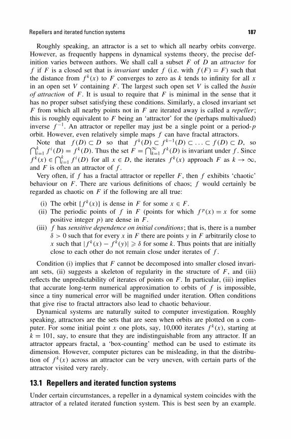
Repellers and iterated function systems 187
Roughly speaking, an attractor is a set to which all nearby orbits converge.However, as frequently happens in dynamical systems theory, the precise def-inition varies between authors. We shall call a subset F of D an attractor forf if F is a closed set that is invariant under f (i.e. with f (F ) = F ) such thatthe distance from f k(x) to F converges to zero as k tends to infinity for all x
in an open set V containing F . The largest such open set V is called the basinof attraction of F . It is usual to require that F is minimal in the sense that ithas no proper subset satisfying these conditions. Similarly, a closed invariant setF from which all nearby points not in F are iterated away is called a repeller ;this is roughly equivalent to F being an ‘attractor’ for the (perhaps multivalued)inverse f −1. An attractor or repeller may just be a single point or a period-porbit. However, even relatively simple maps f can have fractal attractors.
Note that f (D) ⊂ D so that f k(D) ⊂ f k−1(D) ⊂ . . . ⊂ f (D) ⊂ D, so⋂ki=1 f i(D) = f k(D). Thus the set F = ⋂∞
k=1 f k(D) is invariant under f . Sincef k(x) ∈ ⋂k
i=1 f i(D) for all x ∈ D, the iterates f k(x) approach F as k → ∞,and F is often an attractor of f .
Very often, if f has a fractal attractor or repeller F , then f exhibits ‘chaotic’behaviour on F . There are various definitions of chaos; f would certainly beregarded as chaotic on F if the following are all true:
(i) The orbit {f k(x)} is dense in F for some x ∈ F .(ii) The periodic points of f in F (points for which f p(x) = x for some
positive integer p) are dense in F .(iii) f has sensitive dependence on initial conditions; that is, there is a number
δ > 0 such that for every x in F there are points y in F arbitrarily close tox such that |f k(x) − f k(y)| � δ for some k. Thus points that are initiallyclose to each other do not remain close under iterates of f .
Condition (i) implies that F cannot be decomposed into smaller closed invari-ant sets, (ii) suggests a skeleton of regularity in the structure of F , and (iii)reflects the unpredictability of iterates of points on F . In particular, (iii) impliesthat accurate long-term numerical approximation to orbits of f is impossible,since a tiny numerical error will be magnified under iteration. Often conditionsthat give rise to fractal attractors also lead to chaotic behaviour.
Dynamical systems are naturally suited to computer investigation. Roughlyspeaking, attractors are the sets that are seen when orbits are plotted on a com-puter. For some initial point x one plots, say, 10,000 iterates f k(x), starting atk = 101, say, to ensure that they are indistinguishable from any attractor. If anattractor appears fractal, a ‘box-counting’ method can be used to estimate itsdimension. However, computer pictures can be misleading, in that the distribu-tion of f k(x) across an attractor can be very uneven, with certain parts of theattractor visited very rarely.
13.1 Repellers and iterated function systemsUnder certain circumstances, a repeller in a dynamical system coincides with theattractor of a related iterated function system. This is best seen by an example.
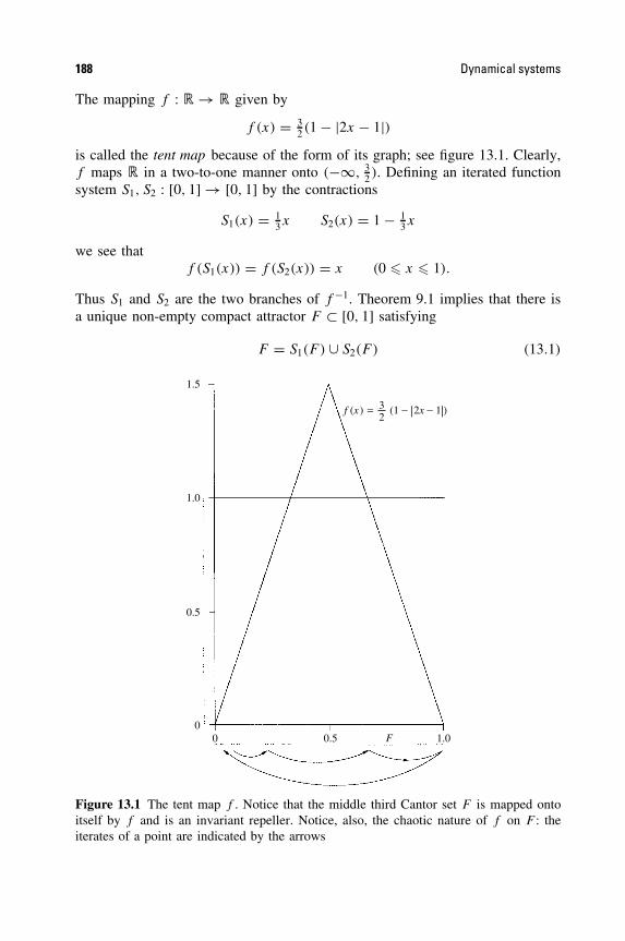
188 Dynamical systems
The mapping f : � → � given by
f (x) = 32 (1 − |2x − 1|)
is called the tent map because of the form of its graph; see figure 13.1. Clearly,f maps � in a two-to-one manner onto (−∞, 3
2 ). Defining an iterated functionsystem S1, S2 : [0, 1] → [0, 1] by the contractions
S1(x) = 13x S2(x) = 1 − 1
3x
we see thatf (S1(x)) = f (S2(x)) = x (0 � x � 1).
Thus S1 and S2 are the two branches of f −1. Theorem 9.1 implies that there isa unique non-empty compact attractor F ⊂ [0, 1] satisfying
F = S1(F ) ∪ S2(F ) (13.1)
1.5
1.0
0.5
00 0.5 1.0
f (x) = (1 − |2x − 1|)32
F
Figure 13.1 The tent map f . Notice that the middle third Cantor set F is mapped ontoitself by f and is an invariant repeller. Notice, also, the chaotic nature of f on F : theiterates of a point are indicated by the arrows

The logistic map 189
which is given by F = ⋂∞k=0 Sk([0, 1]) (writing S(E) = S1(E) ∪ S2(E) for any
set E). Clearly the attractor F is the middle third Cantor set, with Hausdorff andbox dimensions log 2/ log 3.
It follows from (13.1) that f (F ) = F . To see that F is a repeller, observethat if x < 0 then f (x) = 3x, so f k(x) = 3kx → −∞ as k → ∞. If x > 1then f (x) < 0 and again f k(x) → −∞. If x ∈ [0, 1]\F then for some k, wehave x /∈ Sk[0, 1] = ∪{Si1
◦ · · · ◦Sik [0, 1] : ij = 1, 2} so f k(x) /∈ [0, 1], and againf k(x) → −∞ as k → ∞. All points outside F are iterated to −∞ so F isa repeller.
With the notation of Section 9.1, the chaotic nature of f on F is readilyapparent. Denoting the points of F by xi1,i2,... with ij = 1, 2, as in (9.7),|xi1,i2,... − xi ′1,i
′2,...
| � 3−k if i1 = i′1, . . . , ik = i′k . Since xi1,i2,... = Si1(xi2,i3,...), itfollows that f (xi1,i2,...) = xi2,i3,.... Suppose that (i1, i2, . . .) is an infinite sequencewith every finite sequence of 1s and 2s appearing as a consecutive block of terms;for example,
(1, 2, 1,1, 1,2, 2,1, 2,2, 1,1,1, 1,1,2, . . .)
where the spacing is just to indicate the form of the sequence. For each pointxi ′1,i
′2,...
in F and each integer q, we may find k such that (i′1, i′2, . . . , i
′q) =
(ik+1, . . . , ik+q). Then |xik+1,ik+2,... − xi ′1,i′2,...
| < 3−q , so the iterates f k(xi1,i2,...) =xik+1,ik+2,... come arbitrarily close to each point of F for suitable large k, sothat f has dense orbits in F . Similarly, since xi1,...,ik ,i1,...,ik ,i1,... is a periodicpoint of period k, the periodic points of f are dense in F . The iterates havesensitive dependence on initial conditions, since f k(xi1,...,ik ,1,...) ∈ [0, 1
3 ] butf k(xi1,...,ik,2,...) ∈ [ 2
3 , 1]. We conclude that F is a chaotic repeller for f . (Thestudy of f by its effect on points of F represented by sequences (i1, i2, . . .) isknown as symbolic dynamics.)
In exactly the same way, the attractors of general iterated function systemscorrespond to repellers of functions. If S1, . . . , Sm is a set of bijective contractionson a domain D with attractor F such that S1(F ), . . . , Sm(F ) are disjoint, then F
is a repeller for any mapping f such that f (x) = S−1i (x) when x is near Si(F ).
Again, by examining the effect of f on the point xi1,i2,..., it may be shown thatf acts chaotically on F . Indeed, for many dynamical systems f , it is possibleto decompose the domain D into parts (called a Markov partition) such that thebranches of f −1 on each part look rather like an iterated function system. SeeTheorem 14.15 for an example in the complex plane.
13.2 The logistic map
The logistic map f : � → � is given by
fλ(x) = λx(1 − x) (13.2)

190 Dynamical systems
where λ is a positive constant. This mapping was introduced to model the popu-lation development of certain species—if the (normalized) population is x at theend of a given year, it is assumed to be fλ(x) at the end of the following year.Nowadays the logistic map is studied intensively as an archetypal 1-dimensionaldynamical system. We content ourselves here with an analysis when λ is large,and a brief discussion when λ is small.
For λ > 2 + √5 = 4.236 . . . we get a nonlinear version of the tent map
repeller of Section 13.1. Write a = 12 −
√14 − 1/λ and 1 − a = 1
2 +√
14 − 1/λ
for the roots of fλ(x) = 1. Each of the intervals [0, a] and [1 − a, 1] is mappedbijectively onto [0, 1] by fλ. The mappings S1 : [0, 1] → [0, a] and S2 : [0, 1] →[1 − a, 1] given by
S1(x) = 12 −
√14 − x/λ S2(x) = 1
2 +√
14 − x/λ
are the values of the inverse f −1λ in [0, a] and [1 − a, 1], with fλ(S1(x)) =
fλ(S2(x)) = x for each x in [0, 1]. For i = 1, 2 we have
|S ′i (x)| = 1
2λ( 1
4 − x/λ)−1/2
so1
λ� |S ′
i (x)| � 1
2λ( 1
4 − 1/λ)−1/2 = 12 (λ2/4 − λ)−1/2
if 0 � x � 1. By the mean-value theorem
1
λ|x − y| � |Si(x) − Si(y)| � 1
2 (λ2/4 − λ)−1/2|x − y| (0 � x, y � 1).
(13.3)
Thus, if λ > 2 + √5 the mappings S1 and S2 are contractions on [0, 1], so by The-
orem 9.1 the iterated function system {S1, S2} has a unique (non-empty compact)attractor F ⊂ [0, 1] satisfying
F = S1(F ) ∪ S2(F ),
and it follows that fλ(F ) = F . Since this union is disjoint, F is totally dis-connected. In exactly the same way as for the tent map, F is a repeller, withf k
λ (x) → −∞ if x /∈ F , and f is chaotic on F .To estimate the dimension of F we proceed as in Example 9.8. Using Propo-
sitions 9.6 and 9.7 it follows from (13.3) that
log 2
log λ� dimHF � dimBF � dimBF � log 2
log(λ(1 − 4/λ)1/2).
Thus, if λ is large, the dimension of F is close to log 2/ log λ.
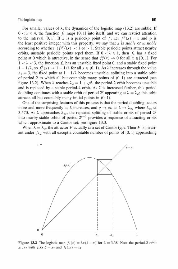
The logistic map 191
For smaller values of λ, the dynamics of the logistic map (13.2) are subtle. If0 < λ � 4, the function fλ maps [0, 1] into itself, and we can restrict attentionto the interval [0, 1]. If x is a period-p point of f , i.e. f p(x) = x and p isthe least positive integer with this property, we say that x is stable or unstableaccording to whether |(f p)′(x)| < 1 or > 1. Stable periodic points attract nearbyorbits, unstable periodic points repel them. If 0 < λ � 1, then fλ has a fixedpoint at 0 which is attractive, in the sense that f k
λ (x) → 0 for all x ∈ [0, 1]. For1 < λ < 3, the function fλ has an unstable fixed point 0, and a stable fixed point1 − 1/λ, so f k
λ (x) → 1 − 1/λ for all x ∈ (0, 1). As λ increases through the valueλ1 = 3, the fixed point at 1 − 1/λ becomes unstable, splitting into a stable orbitof period 2 to which all but countably many points of (0, 1) are attracted (seefigure 13.2). When λ reaches λ2 = 1 + √
6, the period-2 orbit becomes unstableand is replaced by a stable period-4 orbit. As λ is increased further, this perioddoubling continues with a stable orbit of period 2q appearing at λ = λq ; this orbitattracts all but countably many initial points in (0, 1).
One of the surprising features of this process is that the period doubling occursmore and more frequently as λ increases, and q → ∞ as λ → λ∞ where λ∞ 3.570. As λ approaches λ∞, the repeated splitting of stable orbits of period 2q
into nearby stable orbits of period 2q+1 provides a sequence of attracting orbitswhich approximate to a Cantor set; see figure 13.3.
When λ = λ∞ the attractor F actually is a set of Cantor type. Then F is invari-ant under fλ∞ with all except a countable number of points of [0, 1] approaching
fl(x )
y = x
0
1
0 x1 x2 1
Figure 13.2 The logistic map fλ(x) = λx(1 − x) for λ = 3.38. Note the period-2 orbitx1, x2 with fλ(x1) = x2 and fλ(x2) = x1
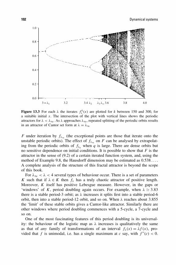
192 Dynamical systems
0.0
3 = l1 l2 l3 l∞3.2 3.4 3.6 3.8 4.0
0.2
0.4
0.6
0.8
1.0
Figure 13.3 For each λ the iterates f kλ (x) are plotted for k between 150 and 300, for
a suitable initial x. The intersection of the plot with vertical lines shows the periodicattractors for λ < λ∞. As λ approaches λ∞, repeated splitting of the periodic orbits resultsin an attractor of Cantor set form at λ = λ∞
F under iteration by fλ∞ (the exceptional points are those that iterate onto theunstable periodic orbits). The effect of fλ∞ on F can be analysed by extrapolat-ing from the periodic orbits of fλq
when q is large. There are dense orbits butno sensitive dependence on initial conditions. It is possible to show that F is theattractor in the sense of (9.2) of a certain iterated function system, and, using themethod of Example 9.8, the Hausdorff dimension may be estimated as 0.538 . . . .A complete analysis of the structure of this fractal attractor is beyond the scopeof this book.
For λ∞ < λ < 4 several types of behaviour occur. There is a set of parametersK such that if λ ∈ K then fλ has a truly chaotic attractor of positive length.Moreover, K itself has positive Lebesgue measure. However, in the gaps or‘windows’ of K , period doubling again occurs. For example, when λ 3.83there is a stable period-3 orbit; as λ increases it splits first into a stable period-6orbit, then into a stable period-12 orbit, and so on. When λ reaches about 3.855the ‘limit’ of these stable orbits gives a Cantor-like attractor. Similarly there areother windows where period doubling commences with a 5-cycle, a 7-cycle andso on.
One of the most fascinating features of this period doubling is its universal-ity: the behaviour of the logistic map as λ increases is qualitatively the sameas that of any family of transformations of an interval fλ(x) = λf (x), pro-vided that f is unimodal, i.e. has a single maximum at c say, with f ′′(c) < 0.
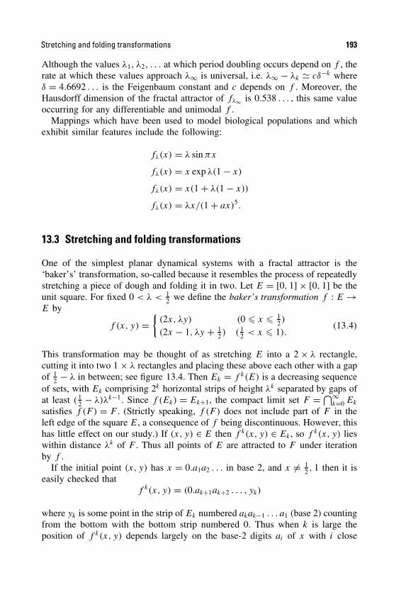
Stretching and folding transformations 193
Although the values λ1, λ2, . . . at which period doubling occurs depend on f , therate at which these values approach λ∞ is universal, i.e. λ∞ − λk cδ−k whereδ = 4.6692 . . . is the Feigenbaum constant and c depends on f . Moreover, theHausdorff dimension of the fractal attractor of fλ∞ is 0.538 . . . , this same valueoccurring for any differentiable and unimodal f .
Mappings which have been used to model biological populations and whichexhibit similar features include the following:
fλ(x) = λ sin πx
fλ(x) = x exp λ(1 − x)
fλ(x) = x(1 + λ(1 − x))
fλ(x) = λx/(1 + ax)5.
13.3 Stretching and folding transformations
One of the simplest planar dynamical systems with a fractal attractor is the‘baker’s’ transformation, so-called because it resembles the process of repeatedlystretching a piece of dough and folding it in two. Let E = [0, 1] × [0, 1] be theunit square. For fixed 0 < λ < 1
2 we define the baker’s transformation f : E →E by
f (x, y) ={
(2x, λy) (0 � x � 12 )
(2x − 1, λy + 12 ) ( 1
2 < x � 1).(13.4)
This transformation may be thought of as stretching E into a 2 × λ rectangle,cutting it into two 1 × λ rectangles and placing these above each other with a gapof 1
2 − λ in between; see figure 13.4. Then Ek = f k(E) is a decreasing sequenceof sets, with Ek comprising 2k horizontal strips of height λk separated by gaps ofat least ( 1
2 − λ)λk−1. Since f (Ek) = Ek+1, the compact limit set F = ⋂∞k=0 Ek
satisfies f (F ) = F . (Strictly speaking, f (F ) does not include part of F in theleft edge of the square E, a consequence of f being discontinuous. However, thishas little effect on our study.) If (x, y) ∈ E then f k(x, y) ∈ Ek, so f k(x, y) lieswithin distance λk of F . Thus all points of E are attracted to F under iterationby f .
If the initial point (x, y) has x = 0.a1a2 . . . in base 2, and x = 12 , 1 then it is
easily checked thatf k(x, y) = (0.ak+1ak+2 . . . , yk)
where yk is some point in the strip of Ek numbered akak−1 . . . a1 (base 2) countingfrom the bottom with the bottom strip numbered 0. Thus when k is large theposition of f k(x, y) depends largely on the base-2 digits ai of x with i close
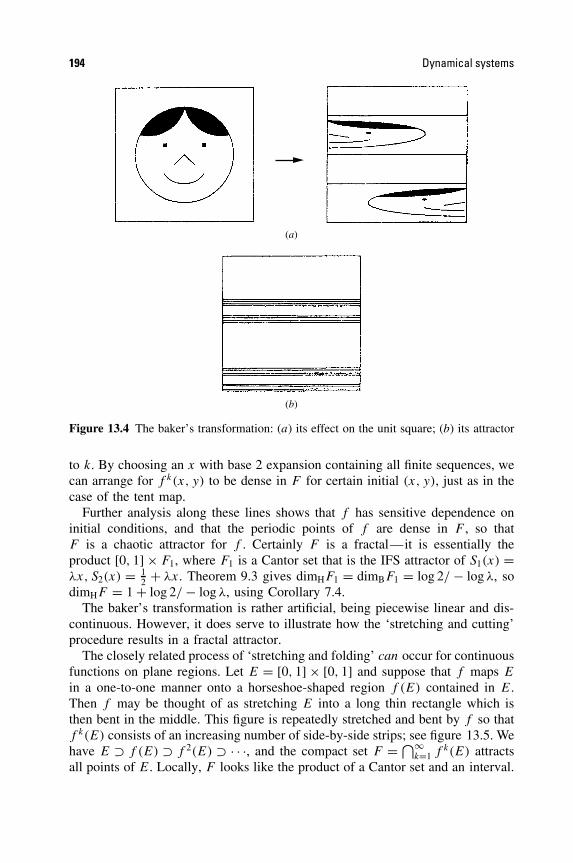
194 Dynamical systems
(a)
(b)
Figure 13.4 The baker’s transformation: (a) its effect on the unit square; (b) its attractor
to k. By choosing an x with base 2 expansion containing all finite sequences, wecan arrange for f k(x, y) to be dense in F for certain initial (x, y), just as in thecase of the tent map.
Further analysis along these lines shows that f has sensitive dependence oninitial conditions, and that the periodic points of f are dense in F , so thatF is a chaotic attractor for f . Certainly F is a fractal—it is essentially theproduct [0, 1] × F1, where F1 is a Cantor set that is the IFS attractor of S1(x) =λx, S2(x) = 1
2 + λx. Theorem 9.3 gives dimHF1 = dimBF1 = log 2/ − log λ, sodimHF = 1 + log 2/ − log λ, using Corollary 7.4.
The baker’s transformation is rather artificial, being piecewise linear and dis-continuous. However, it does serve to illustrate how the ‘stretching and cutting’procedure results in a fractal attractor.
The closely related process of ‘stretching and folding’ can occur for continuousfunctions on plane regions. Let E = [0, 1] × [0, 1] and suppose that f maps E
in a one-to-one manner onto a horseshoe-shaped region f (E) contained in E.Then f may be thought of as stretching E into a long thin rectangle which isthen bent in the middle. This figure is repeatedly stretched and bent by f so thatf k(E) consists of an increasing number of side-by-side strips; see figure 13.5. Wehave E ⊃ f (E) ⊃ f 2(E) ⊃ · · ·, and the compact set F = ⋂∞
k=1 f k(E) attractsall points of E. Locally, F looks like the product of a Cantor set and an interval.

Stretching and folding transformations 195
A variation on this construction gives a transformation with rather differentcharacteristics; see figure 13.6. If D is a plane domain containing the unit squareE and f : D → D is such that f (E) is a horseshoe with ‘ends’ and ‘arch’ lyingin a part of D outside E that is never iterated back into E, then almost all points ofthe square E (in the sense of plane measure) are eventually iterated outside E byf . If f k(x, y) ∈ E for all positive k, then (x, y) ∈ ⋂∞
k=1 f −k(E). With f suitablydefined, f −1(E) consists of two horizontal bars across E, so
⋂∞k=1 f −k(E) is the
product of [0, 1] and a Cantor set. The set F = ⋂∞k=−∞ f k(E) = ⋂∞
k=0 f k(E) ∩⋂∞k=1 f −k(E) is compact and invariant for f , and is the product of two Cantor
sets. However, F is not an attractor, since points arbitrarily close to F are iteratedoutside E.
(a)
(b)
c d
Ef (E)
f (E) f 2(E) f 3(E)
b
b′ a′ d ′ c′
a
Figure 13.5 A horseshoe map. (a) The square E is transformed, by stretching and bend-ing, to the horseshoe f (E), with a, b, c, d mapped to a′, b′, c′, d ′, respectively. (b) Theiterates of E under f form a set that is locally a product of a line segment and aCantor set

196 Dynamical systems
(a)
(b)
c d
Ef (E)
b
b′ a′ d ′ c′
a
f −k(E)k = 1∞⊃ f k(E)
k = 0∞⊃ f k(t) ∩ F =
k = 0∞⊃ f −k(E)
k = 1∞⊃
Figure 13.6 An alternative horseshoe map. (a) The square E is transformed so that the‘arch’ and ‘ends’ of f (E) lie outside E. (b) The sets
⋂∞k=1 f −k(E) and
⋂∞k=0 f k(E)
are both products of a Cantor set and a unit interval. Their intersection F is an unstableinvariant set for f
A specific example of a ‘stretching and folding’ transformation is the Henonmap f : �2 → �2
f (x, y) = (y + 1 − ax2, bx) (13.5)
where a and b are constants. (The values a = 1.4 and b = 0.3 are usually chosenfor study. For these values there is a quadrilateral D for which f (D) ⊂ D towhich we can restrict attention.) This mapping has Jacobian −b for all (x, y),so it contracts area at a constant rate throughout �2; to within a linear changeof coordinates, (13.5) is the most general quadratic mapping with this property.The transformation (13.5) may be decomposed into an (area-preserving) bend, acontraction, and a reflection, the net effect being ‘horseshoe-like’; see figure 13.7.This leads us to expect f to have a fractal attractor, and this is borne out bycomputer pictures, figure 13.8. Detailed pictures show banding indicative of aset that is locally the product of a line segment and a Cantor-like set. Numerical
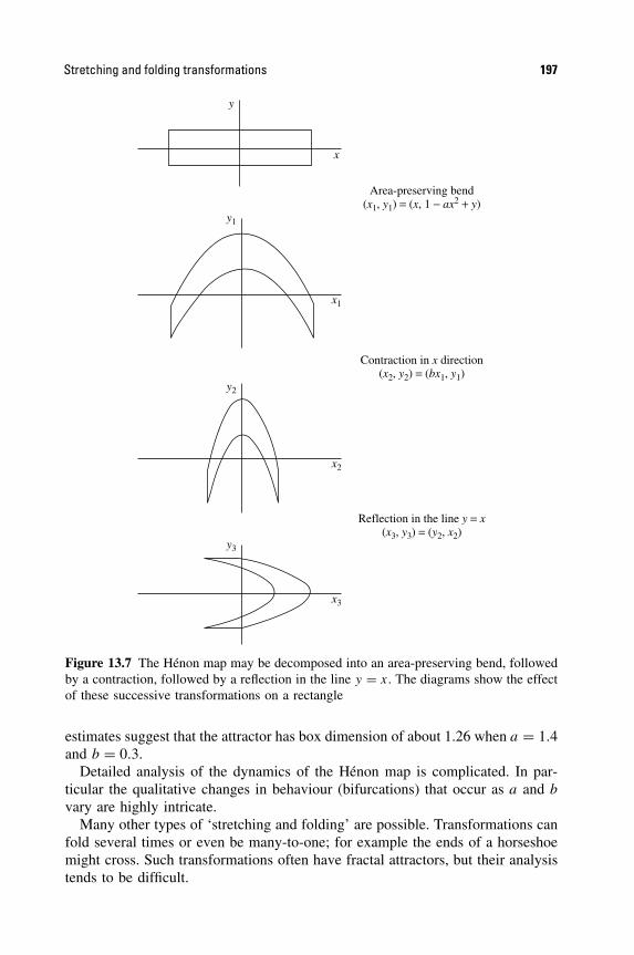
Stretching and folding transformations 197
y
y1
y2
y3
x
x1
x2
x3
Area-preserving bend(x1, y1) = (x, 1 − ax2 + y)
Contraction in x direction(x2, y2) = (bx1, y1)
Reflection in the line y = x(x3, y3) = (y2, x2)
Figure 13.7 The Henon map may be decomposed into an area-preserving bend, followedby a contraction, followed by a reflection in the line y = x. The diagrams show the effectof these successive transformations on a rectangle
estimates suggest that the attractor has box dimension of about 1.26 when a = 1.4and b = 0.3.
Detailed analysis of the dynamics of the Henon map is complicated. In par-ticular the qualitative changes in behaviour (bifurcations) that occur as a and b
vary are highly intricate.Many other types of ‘stretching and folding’ are possible. Transformations can
fold several times or even be many-to-one; for example the ends of a horseshoemight cross. Such transformations often have fractal attractors, but their analysistends to be difficult.

198 Dynamical systems
0.5
0 0.5−0.5−1.0 1.0
−0.5
Figure 13.8 Iterates of a point under the Henon map (13.5) showing the form of theattractor. Banding is apparent in the enlarged portion in the inset
13.4 The solenoid
Our next example is of a transformation of a 3-dimensional region—a solid torus.If a unit disc B is rotated through 360◦ about an axis L in the plane of, but notintersecting, B, a solid torus D is swept out. The torus D may be thought of asthe product of the circle C, of radius r > 1, obtained by rotating the centre of B
around L, and B. This gives a convenient parametrization of D as
{(φ, w) ∈ C × B : 0 � φ < 2π, |w| � 1}
where the angle φ specifies a point on C, and where w is a position vectorrelative to the centre of B; see figure 13.9.
Fix 0 < a < 14 and define f : D → D by
f (φ, w) = (2φ(mod 2π), aw + 12 φ) (13.6)

The solenoid 199
w
B
D
f
L
Figure 13.9 Parametrization of the torus D
where φ is the unit vector in B at angle φ to the outwards axis. Then f mapsD onto a solid tube of radius a that traverses D twice, see figure 13.10. Notethat (φ, w) and (φ + π,w) are mapped to points in the same ‘slice’ of D, that isthe same half-plane bounded by L. The second iterate f 2(D) is a tube of radiusa2 going round f (D) twice, so around D four times; f 3(D) traverses D eighttimes, etc. The intersection F = ⋂∞
k=1 f k(D) is highly fibrous—locally it lookslike a bundle of line segments that cut any cross section of D in a Cantor-likeset. The set F , called a solenoid, is invariant under f , and attracts all pointsof D.
We may find the dimension of F by routine methods. Let Pφ be the half-plane bounded by L and cutting C at φ. Observe that f k(C) is a smoothclosed curve traversing the torus 2k times, with total length at most 2kc wherec is independent of k (f k(C) cannot oscillate too wildly—the angle betweenevery curve f k(C) and every half-plane Pφ has a positive lower bound). Theset f k(D) is a ‘fattening’ of the curve f k(C) to a tube of radius ak, so itmay be covered by a collection of balls of radius 2ak spaced at intervals ofak along f k(C). Clearly, 2 × 2kca−k balls will suffice, so applying Proposi-tion 4.1 in the usual way we get dimHF � dimBF � s and Hs(F ) < ∞ fors = 1 + log 2/ − log a.
To get a lower estimate for the dimension, we examine the sections F ∩ Pφ foreach φ. The set f (D) ∩ Pφ consists of two discs of radius a situated diametricallyopposite each other with centres 1
2 apart inside D ∩ Pφ . Each of these discscontains two discs of f 2(D) ∩ Pφ of radius a2 and with centres 1
2a apart, and soon. We may place a mass distribution µ on F ∩ Pφ in such a way that each ofthe 2k discs of f k(D) ∩ Pφ has mass 2−k . If U ⊂ Pφ satisfies
ak( 12 − 2a) � |U | < ak−1( 1
2 − 2a)
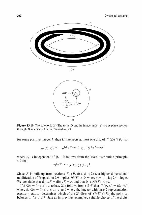
200 Dynamical systems
f(D )
f (D )
f 2(D )
D
D
(a)
(b)
Figure 13.10 The solenoid. (a) The torus D and its image under f . (b) A plane sectionthrough D intersects F in a Cantor-like set
for some positive integer k, then U intersects at most one disc of f k(D) ∩ Pφ , so
µ(U) � 2−k = ak(log 2/−log a) � c1|U |log 2/−log a
where c1 is independent of |U |. It follows from the Mass distribution principle4.2 that
Hlog 2/−log a(F ∩ Pφ) � c−11 .
Since F is built up from sections F ∩ Pφ (0 � φ < 2π), a higher-dimensionalmodification of Proposition 7.9 implies Hs(F ) > 0, where s = 1 + log 2/ − log a.We conclude that dimHF = dimBF = s, and that 0 < Hs(F ) < ∞.
If φ/2π = 0 · a1a2 . . . to base 2, it follows from (13.6) that f k(φ, w) = (φk, vk)
where φk/2π = 0 · ak+1ak+2 . . . and where the integer with base-2 representationakak−1 · · · ak−d+1 determines which of the 2d discs of f d(D) ∩ Pφk
the point vk
belongs to for d � k. Just as in previous examples, suitable choice of the digits
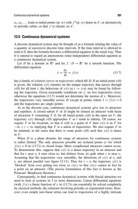
Continuous dynamical systems 201
a1, a2, . . . leads to initial points (φ, w) with f k(φ, w) dense in F , or alternativelyto periodic orbits, so that f is chaotic on F .
13.5 Continuous dynamical systems
A discrete dynamical system may be thought of as a formula relating the value ofa quantity at successive discrete time intervals. If the time interval is allowed totend to 0, then the formula becomes a differential equation in the usual way. Thusit is natural to regard an autonomous (time-independent) differential equation asa continuous dynamical system.
Let D be a domain in �n and let f : D → �n be a smooth function. Thedifferential equation
x = dx
dt= f (x) (13.7)
has a family of solution curves or trajectories which fill D. If an initial point x(0)is given, the solution x(t) remains on the unique trajectory that passes throughx(0) for all time t ; the behaviour of x(t) as t → ±∞ may be found by follow-ing the trajectory. Given reasonable conditions on f , no two trajectories cross;otherwise the equations (13.7) would not determine the motion of x. Moreover,the trajectories vary smoothly across D except at points where x = f (x) = 0and the trajectories are single points.
As in the discrete case, continuous dynamical systems give rise to attractorsand repellers. A closed subset F of D might be termed an attractor with basinof attraction V containing F if, for all initial points x(0) in the open set V , thetrajectory x(t) through x(0) approaches F as t tends to infinity. Of course, werequire F to be invariant, so that if x(0) is a point of F then x(t) is in F for−∞ < t < ∞ implying that F is a union of trajectories. We also require F tobe minimal, in the sense that there is some point x(0) such that x(t) is densein F .
When D is a plane domain, the range of attractors for continuous systemsis rather limited. The only attractors possible are isolated points (x for whichf (x) = 0 in (13.7)) or closed loops. More complicated attractors cannot occur.To demonstrate this, suppose that x(t) is a dense trajectory in an attractor andthat for t near t2 it runs close to, but distinct from, its path when t is near t1.Assuming that the trajectories vary smoothly, the directions of x(t) at t1 andt2 are almost parallel (see figure 13.11). Thus for t > t2 the trajectory x(t) is‘blocked’ from ever getting too close to x(t1) so that x(t1) cannot in fact bea point on an attractor. (The precise formulation of this fact is known as thePoincare–Bendixson theorem.)
Consequently, to find continuous dynamical systems with fractal attractors weneed to look at systems in 3 or more dimensions. Linear differential equations(with f (x) a linear function of x in (13.7)) can essentially be solved completelyby classical methods, the solutions involving periodic or exponential terms. How-ever, even simple non-linear terms can lead to trajectories of a highly intricate
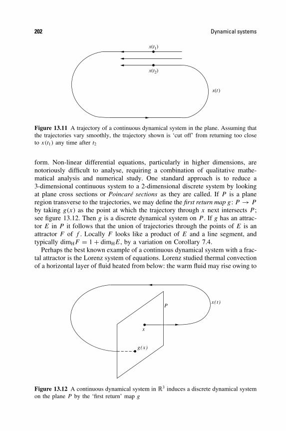
202 Dynamical systems
x(t1)
x(t2)
x(t )
Figure 13.11 A trajectory of a continuous dynamical system in the plane. Assuming thatthe trajectories vary smoothly, the trajectory shown is ‘cut off’ from returning too closeto x(t1) any time after t2
form. Non-linear differential equations, particularly in higher dimensions, arenotoriously difficult to analyse, requiring a combination of qualitative mathe-matical analysis and numerical study. One standard approach is to reduce a3-dimensional continuous system to a 2-dimensional discrete system by lookingat plane cross sections or Poincare sections as they are called. If P is a planeregion transverse to the trajectories, we may define the first return map g : P → P
by taking g(x) as the point at which the trajectory through x next intersects P ;see figure 13.12. Then g is a discrete dynamical system on P . If g has an attrac-tor E in P it follows that the union of trajectories through the points of E is anattractor F of f . Locally F looks like a product of E and a line segment, andtypically dimHF = 1 + dimHE, by a variation on Corollary 7.4.
Perhaps the best known example of a continuous dynamical system with a frac-tal attractor is the Lorenz system of equations. Lorenz studied thermal convectionof a horizontal layer of fluid heated from below: the warm fluid may rise owing to
x
g(x)
x( t )P
Figure 13.12 A continuous dynamical system in �3 induces a discrete dynamical systemon the plane P by the ‘first return’ map g

Continuous dynamical systems 203
Cool upper boundary
Warm lower boundary
Figure 13.13 The Lorenz equations describe the behaviour of one of the rotating cylin-drical rolls of heat-conducting viscous fluid
its buoyancy and circulate in cylindrical rolls. Under certain conditions these cellsare a series of parallel rotating cylindrical rolls; see figure 13.13. Lorenz used thecontinuity equation and Navier–Stokes equations from fluid dynamics, togetherwith the heat conduction equation to describe the behaviour of one of these rolls.A series of approximations and simplifications lead to the Lorenz equations
x = σ(y − x)
y = rx − y − xz (13.8)
z = xy − bz.
The term x represents the rate of rotation of the cylinder, z represents thedeviation from a linear vertical temperature gradient, and y corresponds to thedifference in temperature at opposite sides of the cylinder. The constant σ isthe Prandtl number of the air (the Prandtl number involves the viscosity andthermal conductivity), b depends on the width-to-height ratio of the layer, and r
is a control parameter representing the fixed temperature difference between thebottom and top of the system. The non-linearity in the second and third equationsresults from the non-linearity of the equations of flow.
Working in (x, y, z)-space, the first thing to notice is that the system (13.8)contracts volumes at a constant rate. The differences in velocity between pairsof opposite faces of a small coordinate box of side δ are approximatelyδ(∂x/∂x), δ(∂y/∂y), δ(∂z/∂z), so the rate of change of volume of the boxis δ3((∂x/∂x) + (∂y/∂y) + (∂z/∂z)) = −(σ + b + 1)δ3 < 0. Nevertheless, withσ = 10, b = 8
3 , r = 28 (the values usually chosen for study) the trajectories areconcentrated onto an attractor of a highly complex form. This Lorenz attractorconsists of two ‘discs’ each made up of spiralling trajectories (figure 13.14).Certain trajectories leave each of the discs almost perpendicularly and flow intothe other disc. If a trajectory x(t) is computed, the following behaviour is typical.As t increases, x(t) circles around one of the discs a number of times and then‘flips’ over to the other disc. After a few loops round this second disc, it flipsback to the original disc. This pattern continues, with an apparently randomnumber of circuits before leaving each disc. The motion seems to be chaotic; inparticular points that are initially close together soon have completely different

204 Dynamical systems
Figure 13.14 A view of the Lorenz attractor for σ = 10, b = 83 , r = 28. Note the
spiralling round the two discs and the ‘jumps’ from one disc to the other
patterns of residence in the two discs of the attractor. One interpretation of thissensitive dependence on initial conditions is that long-term weather predictionis impossible.
The Lorenz attractor appears to be a fractal with numerical estimates suggestinga dimension of 2.06 when σ = 10, b = 8
3 , r = 28.Other systems of differential equations also have fractal attractors. The
equations
x = −y − z
y = x + ay
z = b + z(x − c)
were studied by Rossler. Fixing suitable b and c, the nature of the attractorchanges as a is varied. When a is small the attractor is a simple closed curve,but on increasing a this splits into a double loop, then a quadruple loop, and soon. Thus a type of period doubling takes place, and when a reaches a criticalvalue there is a fractal attractor in the form of a band (figure 13.15). The bandhas a twist in it, rather like a Mobius strip.
Figure 13.15 A view of the Rossler band attractor for a = 0.173, b = 0.4, c = 8.5. Notethe banding, suggestive of a set that is locally the product of a Cantor set and a line segment

Small divisor theory 205
To a large extent, each continuous dynamical system must be studied individ-ually; there is little general theory available. Attractors of continuous systems arewell suited to computer study, and mathematicians are frequently challenged toexplain ‘strange’ attractors that are observed on computer screens.
*13.6 Small divisor theory
There are a number of important dynamical systems dependent on a parameterω, which are, in some sense, stable provided that ω is ‘not too close to a rationalnumber’, in other words if ω is badly approximable in the sense of Section 10.3.By Jarnık’s theorem 10.3 the well-approximable numbers form fractal sets, sothe stable parameters lie in sets with fractal complement.
The following simple example indicates how badly approximable parameterscan result in stable systems.
Let C be the infinite cylinder of unit radius {(θ, y) : 0 � θ < 2π, −∞ < y <
∞}. Fix ω ∈ � and define a discrete dynamical system f : C → C by
f (θ, y) = (θ + 2πω(mod 2π), y). (13.9)
Clearly, f just rotates points on the cylinder through an angle 2πω, and thecircles y = constant are invariant under f . It is natural to ask if these invariantcurves are stable—if the transformation (13.9) is perturbed slightly, will thecylinder still be covered by a family of invariant closed curves (figure 13.16)?
q
(a) (b)
y
Figure 13.16 (a) Invariant circles for the mapping f (θ, y) = (θ + 2πω(mod 2π), y).(b) If ω is not ‘too rational’, a small perturbation of the mapping to f (θ, y) = (θ +2πω(mod 2π), y + g(θ)) distorts the circles to a family of smooth invariant curves
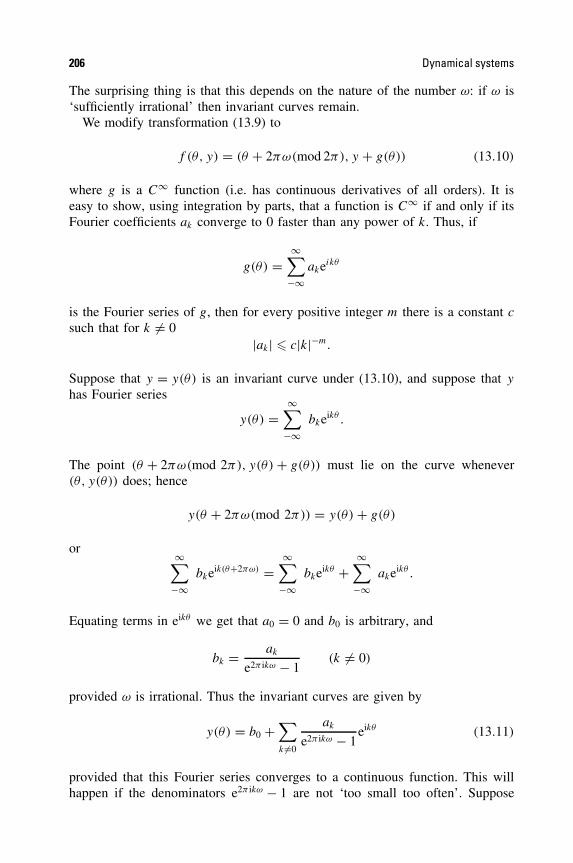
206 Dynamical systems
The surprising thing is that this depends on the nature of the number ω: if ω is‘sufficiently irrational’ then invariant curves remain.
We modify transformation (13.9) to
f (θ, y) = (θ + 2πω(mod 2π), y + g(θ)) (13.10)
where g is a C∞ function (i.e. has continuous derivatives of all orders). It iseasy to show, using integration by parts, that a function is C∞ if and only if itsFourier coefficients ak converge to 0 faster than any power of k. Thus, if
g(θ) =∞∑
−∞akeikθ
is the Fourier series of g, then for every positive integer m there is a constant c
such that for k = 0|ak| � c|k|−m.
Suppose that y = y(θ) is an invariant curve under (13.10), and suppose that y
has Fourier series
y(θ) =∞∑
−∞bkeikθ .
The point (θ + 2πω(mod 2π), y(θ) + g(θ)) must lie on the curve whenever(θ, y(θ)) does; hence
y(θ + 2πω(mod 2π)) = y(θ) + g(θ)
or ∞∑
−∞bkeik(θ+2πω) =
∞∑
−∞bkeikθ +
∞∑
−∞akeikθ .
Equating terms in eikθ we get that a0 = 0 and b0 is arbitrary, and
bk = ak
e2π ikω − 1(k = 0)
provided ω is irrational. Thus the invariant curves are given by
y(θ) = b0 +∑
k =0
ak
e2π ikω − 1eikθ (13.11)
provided that this Fourier series converges to a continuous function. This willhappen if the denominators e2π ikω − 1 are not ‘too small too often’. Suppose
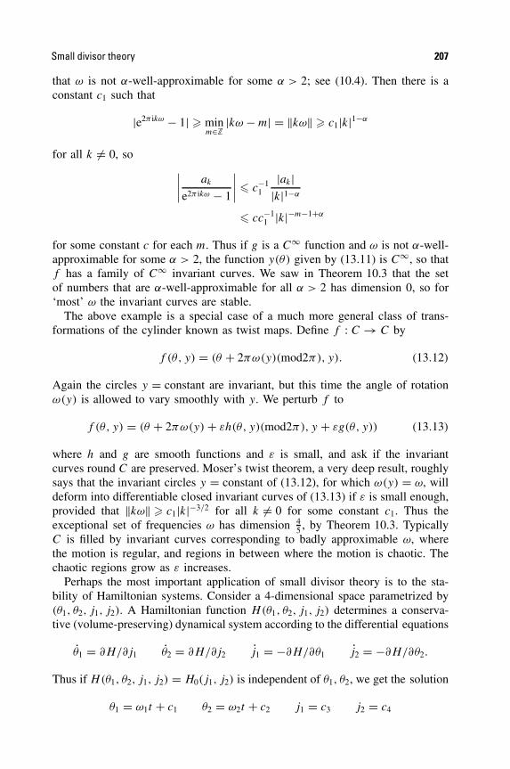
Small divisor theory 207
that ω is not α-well-approximable for some α > 2; see (10.4). Then there is aconstant c1 such that
|e2π ikω − 1| � minm∈�
|kω − m| = ||kω|| � c1|k|1−α
for all k = 0, so∣∣∣∣
ak
e2π ikω − 1
∣∣∣∣ � c−11
|ak||k|1−α
� cc−11 |k|−m−1+α
for some constant c for each m. Thus if g is a C∞ function and ω is not α-well-approximable for some α > 2, the function y(θ) given by (13.11) is C∞, so thatf has a family of C∞ invariant curves. We saw in Theorem 10.3 that the setof numbers that are α-well-approximable for all α > 2 has dimension 0, so for‘most’ ω the invariant curves are stable.
The above example is a special case of a much more general class of trans-formations of the cylinder known as twist maps. Define f : C → C by
f (θ, y) = (θ + 2πω(y)(mod2π), y). (13.12)
Again the circles y = constant are invariant, but this time the angle of rotationω(y) is allowed to vary smoothly with y. We perturb f to
f (θ, y) = (θ + 2πω(y) + εh(θ, y)(mod2π), y + εg(θ, y)) (13.13)
where h and g are smooth functions and ε is small, and ask if the invariantcurves round C are preserved. Moser’s twist theorem, a very deep result, roughlysays that the invariant circles y = constant of (13.12), for which ω(y) = ω, willdeform into differentiable closed invariant curves of (13.13) if ε is small enough,provided that ||kω|| � c1|k|−3/2 for all k = 0 for some constant c1. Thus theexceptional set of frequencies ω has dimension 4
5 , by Theorem 10.3. TypicallyC is filled by invariant curves corresponding to badly approximable ω, wherethe motion is regular, and regions in between where the motion is chaotic. Thechaotic regions grow as ε increases.
Perhaps the most important application of small divisor theory is to the sta-bility of Hamiltonian systems. Consider a 4-dimensional space parametrized by(θ1, θ2, j1, j2). A Hamiltonian function H(θ1, θ2, j1, j2) determines a conserva-tive (volume-preserving) dynamical system according to the differential equations
θ1 = ∂H/∂j1 θ2 = ∂H/∂j2 j1 = −∂H/∂θ1 j2 = −∂H/∂θ2.
Thus if H(θ1, θ2, j1, j2) = H0(j1, j2) is independent of θ1, θ2, we get the solution
θ1 = ω1t + c1 θ2 = ω2t + c2 j1 = c3 j2 = c4
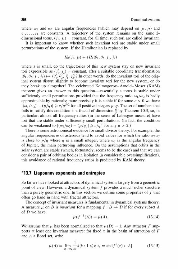
208 Dynamical systems
where ω1 and ω2 are angular frequencies (which may depend on j1, j2) andc1, . . . , c4 are constants. A trajectory of the system remains on the same 2-dimensional torus, (j1, j2) = constant, for all time; such tori are called invariant.
It is important to know whether such invariant tori are stable under smallperturbations of the system. If the Hamiltonian is replaced by
H0(j1, j2) + εH1(θ1, θ2, j1, j2)
where ε is small, do the trajectories of this new system stay on new invarianttori expressible as (j ′
1, j′2) = constant, after a suitable coordinate transformation
(θ1, θ2, j1, j2) → (θ ′1, θ
′2, j
′1, j
′2)? In other words, do the invariant tori of the orig-
inal system distort slightly to become invariant tori for the new system, or dothey break up altogether? The celebrated Kolmogorov–Arnold–Moser (KAM)theorem gives an answer to this question—essentially a torus is stable undersufficiently small perturbations provided that the frequency ratio ω1/ω2 is badlyapproximable by rationals; more precisely it is stable if for some c > 0 we have|(ω1/ω2) − (p/q)| � c/q5/2 for all positive integers p, q. The set of numbers thatfails to satisfy this condition is a fractal of dimension 4
5 by Theorem 10.3, so, inparticular, almost all frequency ratios (in the sense of Lebesgue measure) havetori that are stable under sufficiently small perturbations. (In fact, the conditioncan be weakened to |(ω1/ω2) − (p/q)| � c/qα for any α > 2.)
There is some astronomical evidence for small divisor theory. For example, theangular frequencies ω of asteroids tend to avoid values for which the ratio ω/ωJ
is close to p/q where q is a small integer, where ωJ is the angular frequencyof Jupiter, the main perturbing influence. On the assumptions that orbits in thesolar system are stable (which, fortunately, seems to be the case) and that we canconsider a pair of orbiting bodies in isolation (a considerable oversimplification),this avoidance of rational frequency ratios is predicted by KAM theory.
*13.7 Liapounov exponents and entropies
So far we have looked at attractors of dynamical systems largely from a geometricpoint of view. However, a dynamical system f provides a much richer structurethan a purely geometric one. In this section we outline some properties of f thatoften go hand in hand with fractal attractors.
The concept of invariant measures is fundamental in dynamical systems theory.A measure µ on D is invariant for a mapping f : D → D if for every subset A
of D we haveµ(f −1(A)) = µ(A). (13.14)
We assume that µ has been normalized so that µ(D) = 1. Any attractor F sup-ports at least one invariant measure: for fixed x in the basin of attraction of F
and A a Borel set, write
µ(A) = limm→∞
1
m#{k : 1 � k � m andf k(x) ∈ A} (13.15)

Liapounov exponents and entropies 209
for the proportion of iterates in A. It may be shown using ergodic theory thatthis limit exists and is the same for µ-almost all points in the basin of attractionunder very general circumstances. Clearly, µ(A ∪ B) = µ(A) + µ(B) if A andB are disjoint, and f k(x) ∈ A if and only if f k−1(x) ∈ f −1(A), giving (13.14).The measure (13.15) is concentrated on the set of points to which f k(x) comesarbitrarily close infinitely often; thus µ is supported by an attractor of f . Themeasure µ(A) reflects the proportion of the iterates that lie in A, and may bethought of as the distribution that is seen when a large number of iterates f k(x)
are plotted on a computer screen. The intensity of the measure can vary widelyacross the attractor A; this variation is often analysed using multifractal analysis(see Chapter 17). As far as the size of an attractor is concerned, it is often thedimension of the set occupied by the invariant measure µ that is relevant, ratherthan the entire attractor. With this in mind, we define the Hausdorff dimensionof a measure µ for which µ(D) = 1 as
dimHµ = inf{dimHE : E is a Borel set with µ(E) > 0}. (13.16)
If µ is supported by F then clearly dimHµ � dimHF , but we may have strictinequality; see Exercise 13.10. However, if there are numbers s > 0 and c > 0such that for every set U
µ(U) � c|U |s (13.17)
then the Mass distribution principle 4.2 implies that for each set E with 0 < µ(E)
we have Hs(E) � µ(E)/c > 0, so that dimHE � s. Hence if (13.17) holds then
dimHµ � s. (13.18)
Once f is equipped with an invariant measure µ several other dynamicalconstants may be defined. For simplicity, we assume that D is a domain in �2
and f : D → D is differentiable. The derivative (f k)′(x) is a linear mapping on�2; we write ak(x) and bk(x) for the lengths of the major and minor semi-axesof the ellipse (f k)′(x)(B) where B is the unit ball. Thus the image under f k ofa small ball of radius r and centre x approximates to an ellipse with semi-axesof lengths rak(x) and rbk(x). We define the Liapounov exponents as the averagelogarithmic rate of growth with k of these semi-axes:
λ1(x) = limk→∞
1
klog ak(x) λ2(x) = lim
k→∞1
klog bk(x). (13.19)
Techniques from ergodic theory show that if µ is invariant for f , these exponentsexist and have the same values λ1, λ2 for µ-almost all x. Hence in a system withan invariant measure, we refer to λ1 and λ2 as the Liapounov exponents of thesystem. The Liapounov exponents represent the ‘average’ rates of expansion off . If B is a disc of small radius r , then f k(B) will ‘typically’ be close to anellipse with semi-axes of lengths reλ1k and reλ2k; see figure 13.17.
A related dynamical idea is the entropy of a mapping f : D → D. Write
V (x, ε, k) = {y ∈ D : |f i(x) − f i(y)| < ε for 0 � i � k} (13.20)
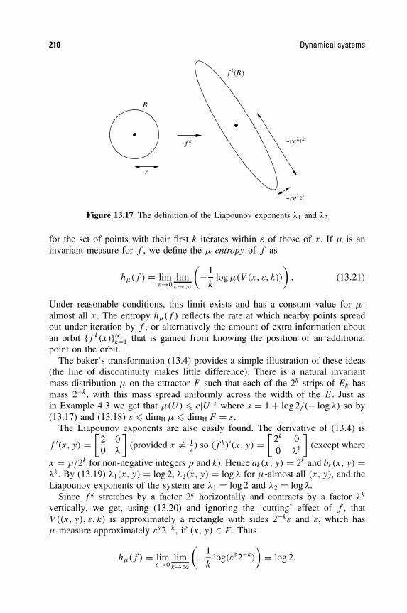
210 Dynamical systems
r
~rel1k
~rel2k
f k
f k(B )
B
Figure 13.17 The definition of the Liapounov exponents λ1 and λ2
for the set of points with their first k iterates within ε of those of x. If µ is aninvariant measure for f , we define the µ-entropy of f as
hµ(f ) = limε→0
limk→∞
(−1
klog µ(V (x, ε, k))
). (13.21)
Under reasonable conditions, this limit exists and has a constant value for µ-almost all x. The entropy hµ(f ) reflects the rate at which nearby points spreadout under iteration by f , or alternatively the amount of extra information aboutan orbit {f k(x)}∞k=1 that is gained from knowing the position of an additionalpoint on the orbit.
The baker’s transformation (13.4) provides a simple illustration of these ideas(the line of discontinuity makes little difference). There is a natural invariantmass distribution µ on the attractor F such that each of the 2k strips of Ek hasmass 2−k, with this mass spread uniformly across the width of the E. Just asin Example 4.3 we get that µ(U) � c|U |s where s = 1 + log 2/(− log λ) so by(13.17) and (13.18) s � dimH µ � dimH F = s.
The Liapounov exponents are also easily found. The derivative of (13.4) is
f ′(x, y) =[
2 00 λ
](provided x = 1
2 ) so (f k)′(x, y) =[
2k 00 λk
](except where
x = p/2k for non-negative integers p and k). Hence ak(x, y) = 2k and bk(x, y) =λk. By (13.19) λ1(x, y) = log 2, λ2(x, y) = log λ for µ-almost all (x, y), and theLiapounov exponents of the system are λ1 = log 2 and λ2 = log λ.
Since f k stretches by a factor 2k horizontally and contracts by a factor λk
vertically, we get, using (13.20) and ignoring the ‘cutting’ effect of f , thatV ((x, y), ε, k) is approximately a rectangle with sides 2−kε and ε, which hasµ-measure approximately εs2−k, if (x, y) ∈ F . Thus
hµ(f ) = limε→0
limk→∞
(−1
klog(εs2−k)
)= log 2.
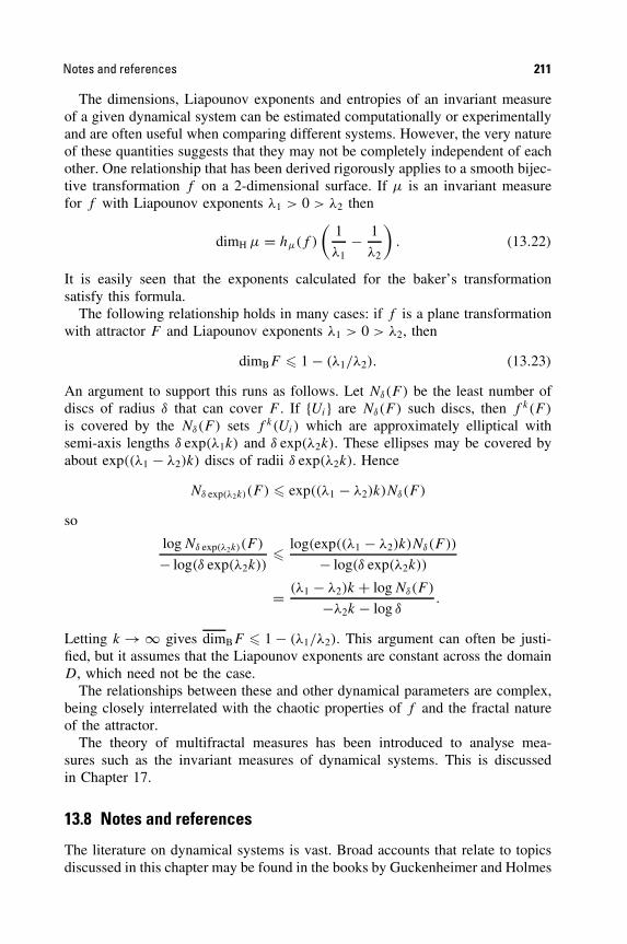
Notes and references 211
The dimensions, Liapounov exponents and entropies of an invariant measureof a given dynamical system can be estimated computationally or experimentallyand are often useful when comparing different systems. However, the very natureof these quantities suggests that they may not be completely independent of eachother. One relationship that has been derived rigorously applies to a smooth bijec-tive transformation f on a 2-dimensional surface. If µ is an invariant measurefor f with Liapounov exponents λ1 > 0 > λ2 then
dimH µ = hµ(f )
(1
λ1− 1
λ2
). (13.22)
It is easily seen that the exponents calculated for the baker’s transformationsatisfy this formula.
The following relationship holds in many cases: if f is a plane transformationwith attractor F and Liapounov exponents λ1 > 0 > λ2, then
dimBF � 1 − (λ1/λ2). (13.23)
An argument to support this runs as follows. Let Nδ(F ) be the least number ofdiscs of radius δ that can cover F . If {Ui} are Nδ(F ) such discs, then f k(F )
is covered by the Nδ(F ) sets f k(Ui) which are approximately elliptical withsemi-axis lengths δ exp(λ1k) and δ exp(λ2k). These ellipses may be covered byabout exp((λ1 − λ2)k) discs of radii δ exp(λ2k). Hence
Nδ exp(λ2k)(F ) � exp((λ1 − λ2)k)Nδ(F )
so
log Nδ exp(λ2k)(F )
− log(δ exp(λ2k))� log(exp((λ1 − λ2)k)Nδ(F ))
− log(δ exp(λ2k))
= (λ1 − λ2)k + log Nδ(F )
−λ2k − log δ.
Letting k → ∞ gives dimBF � 1 − (λ1/λ2). This argument can often be justi-fied, but it assumes that the Liapounov exponents are constant across the domainD, which need not be the case.
The relationships between these and other dynamical parameters are complex,being closely interrelated with the chaotic properties of f and the fractal natureof the attractor.
The theory of multifractal measures has been introduced to analyse mea-sures such as the invariant measures of dynamical systems. This is discussedin Chapter 17.
13.8 Notes and references
The literature on dynamical systems is vast. Broad accounts that relate to topicsdiscussed in this chapter may be found in the books by Guckenheimer and Holmes

212 Dynamical systems
(1993), Schuster (1984), Thompson and Stewart (1986), Devaney (1989), Haleand Kocak (1991), Peitgen, Jurgens and Saupe (1992), Drazin (1992) and Katokand Hasselblatt (1995). More computational approaches are given by Stuart andHumphries (1996) and Nusse and Yorke (1998). The collections of papers editedby Cvitanovic (1989), Holden (1986), Bedford and Swift (1988) and Ledrappier,Lewowicz and Newhouse (1996) highlight a variety of related aspects.
For more details on symbolic dynamics, see Bedford, Keane and Series (1991),Lind and Marcus (1995) and Pesin (1997). For accounts of the logistic map, seeMay (1976), and most of the books mentioned above. The horseshoe attractor wasintroduced in the fundamental paper by Smale (1967) and the Henon attractor inHenon and Pomeau (1976). The book by Sparrow (1982) contains a full accountof the Lorenz equations.
The main theory and applications of small divisor theory are brought togetherin the collected papers on Hamiltonian dynamical systems edited by MacKayand Meiss (1987). For results relating Liapounov exponents to dimensions, seethe papers by Young (1982), Frederickson, Kaplan, Yorke and Yorke (1983), thepapers in Mayer-Kress (1986), and the books by Temam (1997) and Pesin (1997).
Exercises
13.1 Find a fractal invariant set F for the ‘tent-like’ map f : � → � given by f (x) =2(1 − |2x − 1|). Show that F is a repeller for f and that f is chaotic on F . Whatis dimHF ?
13.2 Let f : � → � be given by
f (x) ={
5x (x � 1)10 − 5x (1 < x < 2)5x − 10 (x � 2)
Determine an IFS S1, S2, S3 : [0, 5] → [0, 5] such that f (Si(x)) = x for each i.Show that the attractor F of this IFS is a repeller for f , and determine the Hausdorffand box dimension of F .
13.3 Let fλ : [0, 1] → � be given by fλ(x) = λ sin πx. Show that for λ sufficientlylarge, fλ has a repeller F , in the sense that if x /∈ F then f k
λ (x) /∈ [0, 1] for somepositive integer k. Find an IFS which has F as its attractor, and thus estimatedimHF for large λ (see Example 9.8).
13.4 Investigate the iterates f kλ (x) of x in [0, 1] under the logistic mapping (13.2) for
various values of λ and initial points x. Show that if the sequence of iteratesconverges then it converges either to 0 or to 1 − 1/λ. Show that if λ = 1
2 then,for all x in (0, 1), the iterates converge to 0, but that if λ = 2 they converge to12 . Show that if λ = 4, then there are infinitely many values of x in (0, 1) suchthat f k
λ (x) converges to 0, infinitely many x in (0, 1) for which f kλ (x) converges
to 34 , and infinitely many x in (0, 1) for which f k
λ (x) does not converge. Use aprogrammable calculator or computer to investigate the behaviour of the orbits forother values of λ. Investigate other transformations listed at the end of Section 13.2in a similar way.
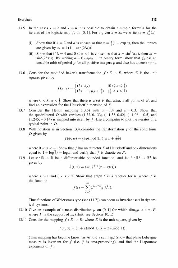
Exercises 213
13.5 In the cases λ = 2 and λ = 4 it is possible to obtain a simple formula for theiterates of the logistic map fλ on [0, 1]. For a given x = x0 we write xk = f k
λ (x).
(i) Show that if λ = 2 and a is chosen so that x = 12 (1 − exp a), then the iterates
are given by xk = 12 (1 − exp(2ka)).
(ii) Show that if λ = 4 and 0 � a < 1 is chosen so that x = sin2(πa), then xk =sin2(2kπa). By writing a = 0 · a1a2 . . . in binary form, show that f4 has anunstable orbit of period p for all positive integers p and also has a dense orbit.
13.6 Consider the modified baker’s transformation f : E → E, where E is the unitsquare, given by
f (x, y) ={
(2x, λy) (0 � x � 12 )
(2x − 1, µy + 12 ) ( 1
2 < x � 1)
where 0 < λ, µ < 12 . Show that there is a set F that attracts all points of E, and
find an expression for the Hausdorff dimension of F .
13.7 Consider the Henon mapping (13.5) with a = 1.4 and b = 0.3. Show thatthe quadrilateral D with vertices (1.32, 0.133), (−1.33, 0.42), (−1.06,−0.5) and(1.245,−0.14) is mapped into itself by f . Use a computer to plot the iterates of atypical point in D.
13.8 With notation as in Section 13.4 consider the transformation f of the solid torusD given by
f (φ,w) = (3φ(mod 2π), aw + 12 φ)
where 0 < a < 110 . Show that f has an attractor F of Hausdorff and box dimensions
equal to 1 + log 3/ − log a, and verify that f is chaotic on F .
13.9 Let g : � → � be a differentiable bounded function, and let h : �2 → �2 begiven by
h(t, x) = (λt, λ2−s(x − g(t)))
where λ > 1 and 0 < s < 2. Show that graph f is a repeller for h, where f isthe function
f (t) =∞∑
k=0
λ(s−2)kg(λkt).
Thus functions of Weierstrass type (see (11.7)) can occur as invariant sets in dynam-ical systems.
13.10 Give an example of a mass distribution µ on [0, 1] for which dimHµ < dimHF ,where F is the support of µ. (Hint: see Section 10.1.)
13.11 Consider the mapping f : E → E, where E is the unit square, given by
f (x, y) = (x + y(mod 1), x + 2y(mod 1)).
(This mapping has become known as Arnold’s cat map.) Show that plane Lebesguemeasure is invariant for f (i.e. f is area-preserving), and find the Liapounovexponents of f .

214 Dynamical systems
13.12 Write a computer program that plots the orbits of a point x under iteration bya mapping of a region in the plane. Use it to study the attractors of the baker’stransformation, the Henon mapping and experiment with other functions.
13.13 Write a computer program to draw trajectories of the Lorenz equations (13.8). Seehow the trajectories change as σ, r and b are varied. Do a similar study for theRossler equations.

Chapter 14 Iteration of complexfunctions—Julia sets
Julia sets provide a most striking illustration of how an apparently simple pro-cess can lead to highly intricate sets. Functions on the complex plane � assimple as f (z) = z2 + c, with c a constant, can give rise to fractals of an exoticappearance—look ahead to figure 14.7.
Julia sets arise in connection with the iteration of a function of a complexvariable f , so are related to the dynamical systems discussed in the previouschapter—in general a Julia set is a dynamical repeller. However, by specializingto functions that are analytic on the complex plane (i.e. differentiable in the sensethat f ′(z) = limw→0(f (z + w) − f (z))/w exists as a complex number, wherez, w ∈ �) we can use the powerful techniques of complex variable theory toobtain much more detailed information about the structure of such repelling sets.
14.1 General theory of Julia sets
For convenience of exposition, we take f : � → � to be a polynomial of degreen � 2 with complex coefficients, f (z) = anz
n + an−1zn−1 + · · · + a0. Note that
with minor modifications the theory remains true if f is a rational functionf (z) = p(z)/q(z) (where p, q are polynomials) on the extended complex plane� ∪ {∞}, and much of it holds if f is any meromorphic function (that is, afunction that is analytic on � except at isolated poles).
As usual we write f k for the k-fold composition f ◦ · · · ◦f of the function f ,so that f k(w) is the kth iterate f (f (· · · (f (w)) · · ·)) of w.
Julia sets are defined in terms of the behaviour of the iterates f k(z) for largek. First, we define the filled-in Julia set of the polynomial f ,
K(f ) = {z ∈ � : f k(z) �→ ∞}.
The Julia set of f is the boundary of the filled-in Julia set, J (f ) = ∂K(f ). (Wewrite K for K(f ) and J for J (f ) when the function is clear.) Thus z ∈ J (f )
215
Fractal Geometry: Mathematical Foundations and Application. Second Edition Kenneth Falconer 2003 John Wiley & Sons, Ltd ISBNs: 0-470-84861-8 (HB); 0-470-84862-6 (PB)

216 Iteration of complex functions—Julia sets
if in every neighbourhood of z there are points w and v with f k(w) → ∞ andf k(v) �→ ∞.
The complement of the Julia set is called the Fatou set or stable set F(f ). Thischapter investigates the geometry and structure of the Julia sets of polynomials;in particular J is usually a fractal.
For the simplest example, let f (z) = z2, so that f k(z) = z2k
. Clearly f k(z) → 0as k → ∞ if |z| < 1 and f k(z) → ∞ if |z| > 1, but with f k(z) remaining on thecircle |z| = 1 for all k if |z| = 1. Thus, the filled-in Julia set k is the unit disc|z| � 1, and the Julia set J is its boundary, the unit circle, |z| = 1. The Julia set J
is the boundary between the sets of points which iterate to 0 and ∞. Of course, inthis special case J is not a fractal.
Suppose that we modify this example slightly, taking f (z) = z2 + c where c
is a small complex number. It is easy to see that we still have f k(z) → w if z
is small, where w is the fixed point of f close to 0, and that f k(z) → ∞ if z islarge. Again, the Julia set is the boundary between these two types of behaviour,but it turns out that now J is a fractal curve; see figure 14.1.
We shall need some terminology about fixed and periodic points of f . Recallthat if f (w) = w we call w a fixed point of f , and if f p(w) = w for some integerp � 1 we call w a periodic point of f ; the least such p is called the period ofw. We call w, f (w), . . . , f p(w) a period p orbit. Let w be a periodic point ofperiod p, with (f p)′(w) = λ, where the prime denotes complex differentiation.The point w is called attractive if 0 � |λ| < 1, in which case nearby points areattracted to the orbit under iteration by f , and repelling if |λ| > 1, in which casepoints close to the orbit move away. The study of sequences f k(z) for variousinitial z is known as complex dynamics. The position of z relative to the Julia setJ (f ) is a key to this behaviour.
0 w
J J
(a) (b)
Figure 14.1 (a) The Julia set of f (z) = z2 is the circle |z| = 1, with the iterates f k(z) → 0if z is inside J , and |f k(z)| → ∞ if z is outside J . (b) If f is perturbed to the functionf (z) = z2 + c for small c this picture distorts slightly, with a curve J separating thosepoints z for which f k(z) converges to the fixed point w of f near 0 from those points z
with |f k(z)| → ∞. The curve J is now a fractal
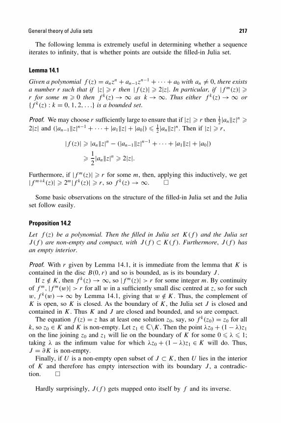
General theory of Julia sets 217
The following lemma is extremely useful in determining whether a sequenceiterates to infinity, that is whether points are outside the filled-in Julia set.
Lemma 14.1
Given a polynomial f (z) = anzn + an−1z
n−1 + · · · + a0 with an �= 0, there existsa number r such that if |z| � r then |f (z)| � 2|z|. In particular, if |f m(z)| �r for some m � 0 then f k(z) → ∞ as k → ∞. Thus either f k(z) → ∞ or{f k(z) : k = 0, 1, 2, . . .} is a bounded set.
Proof. We may choose r sufficiently large to ensure that if |z| � r then 12 |an||z|n �
2|z| and (|an−1||z|n−1 + · · · + |a1||z| + |a0|) � 12 |an||z|n. Then if |z| � r ,
|f (z)| � |an||z|n − (|an−1||z|n−1 + · · · + |a1||z| + |a0|)� 1
2|an||z|n � 2|z|.
Furthermore, if |f m(z)| � r for some m, then, applying this inductively, we get|f m+k(z)| � 2m|f k(z)| � r , so f k(z) → ∞. �
Some basic observations on the structure of the filled-in Julia set and the Juliaset follow easily.
Proposition 14.2
Let f (z) be a polynomial. Then the filled in Julia set K(f ) and the Julia setJ (f ) are non-empty and compact, with J (f ) ⊂ K(f ). Furthermore, J (f ) hasan empty interior.
Proof. With r given by Lemma 14.1, it is immediate from the lemma that K iscontained in the disc B(0, r) and so is bounded, as is its boundary J .
If z /∈ K , then f k(z) → ∞, so |f m(z)| > r for some integer m. By continuityof f m, |f m(w)| > r for all w in a sufficiently small disc centred at z, so for suchw, f k(w) → ∞ by Lemma 14.1, giving that w /∈ K . Thus, the complement ofK is open, so K is closed. As the boundary of K , the Julia set J is closed andcontained in K . Thus K and J are closed and bounded, and so are compact.
The equation f (z) = z has at least one solution z0, say, so f k(z0) = z0 for allk, so z0 ∈ K and K is non-empty. Let z1 ∈ �\K . Then the point λz0 + (1 − λ)z1
on the line joining z0 and z1 will lie on the boundary of K for some 0 � λ � 1;taking λ as the infimum value for which λz0 + (1 − λ)z1 ∈ K will do. Thus,J = ∂K is non-empty.
Finally, if U is a non-empty open subset of J ⊂ K , then U lies in the interiorof K and therefore has empty intersection with its boundary J , a contradic-tion. �
Hardly surprisingly, J (f ) gets mapped onto itself by f and its inverse.

218 Iteration of complex functions—Julia sets
Proposition 14.3
The Julia set J = J (f ) of f is forward and backward invariant under f, i.e. J =f (J ) = f −1(J ).
Proof. Let z ∈ J . Then f k(z) �→ ∞, and we may find wn → z with f k(wn) →∞ as k → ∞ for all n. Thus, f k(f (z)) �→ ∞ and f k(f (wn)) → ∞, where bycontinuity of f , f (wn) can be chosen as close as we like to f (z). Thus f (z) ∈ J ,so f (J ) ⊂ J which also implies J ⊂ f −1(f (J )) ⊂ f −1(J ).
Similarly, with z and wn as above, if f (z0) = z then we may find vn → z0 withf (vn) = wn, by the mapping properties of polynomials on �. Hence, f k(z0) =f k−1(z) �→ ∞ and f k(vn) = f k−1(wn) → ∞ as k → ∞, so z0 ∈ J . Thus,f −1(J ) ⊂ J which implies J = f (f −1(J )) ⊂ f (J ). �
Proposition 14.4
J (f p) = J (f ) for every positive integer p.
Proof. It follows from Lemma 14.1 that f k(z) → ∞ if and only if (f p)k(z) =f kp(z) → ∞. Thus f and f p have identical filled-in Julia sets and so identicalJulia sets. �
To develop the theory of Julia sets much further, we cannot avoid introducingsome technical tools from complex variable theory, in particular normal familiesof analytic functions and Montel’s theorem.
[∗Readers who wish to omit the quite technical arguments involving complexvariable theory should skip to Summary 14.12.]
Let U be an open subset of �, and let gk : U → �, k = 1, 2, . . . be a familyof complex analytic functions (i.e. functions differentiable on U in the complexsense). The family {gk} is said to be normal on U if every sequence of func-tions selected from {gk} has a subsequence which converges uniformly on everycompact subset of U , either to a bounded analytic function or to ∞. Notice thatby standard complex variable theory, this means that the subsequence convergeseither to a finite analytic function or to ∞ on each connected component ofU . In the former case, the derivatives of the subsequence must converge to thederivative of the limit function. The family {gk} is normal at the point w of U ifthere is some open subset V of U containing w such that {gk} is a normal familyon V . Observe that this is equivalent to there being a neighbourhood V of w onwhich every sequence {gk} has a subsequence convergent to a bounded analyticfunction or to ∞.
The key result which we will use repeatedly in our development of Julia setsis the remarkable theorem of Montel, which asserts that non-normal families offunctions take virtually all complex values.
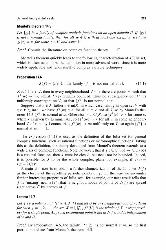
General theory of Julia sets 219
Montel’s theorem 14.5
Let {gk} be a family of complex analytic functions on an open domain U. If {gk}is not a normal family, then for all w ∈ � with at most one exception we havegk(z) = w for some z ∈ U and some k.
Proof. Consult the literature on complex function theory. �
Montel’s theorem quickly leads to the following characterization of a Julia set,which is often taken to be the definition in more advanced work, since it is morewidely applicable and lends itself to complex variable techniques.
Proposition 14.6
J (f ) = {z ∈ � : the family {f k} is not normal at z}. (14.1)
Proof. If z ∈ J , then in every neighbourhood V of z there are points w such thatf k(w) → ∞, whilst f k(z) remains bounded. Thus no subsequence of {f k} isuniformly convergent on V , so that {f k} is not normal at z.
Suppose that z /∈ J . Either z ∈ intK , in which case, taking an open set V withz ∈ V ⊂ intK , we have f k(w) ∈ K for all w ∈ V and all k, so by Montel’s the-orem 14.5 {f k} is normal at w. Otherwise, z ∈ �\K , so |f k(z)| > r for some k,where r is given by Lemma 14.1, so |f k(w)| > r for all w in some neighbour-hood V of z, so by Lemma 14.1, f k(w) → ∞ uniformly on V , so again {f k} isnormal at w. �
The expression (14.1) is used as the definition of the Julia set for generalcomplex functions, such as rational functions or meromorphic functions. Takingthis as the definition, the theory developed from Montel’s theorem extends to awide class of complex functions. Note, however, that if f : � ∪ {∞} → � ∪ {∞}is a rational function, then J must be closed, but need not be bounded. Indeed,it is possible for J to be the whole complex plane; for example, if f (z) =((z − 2)/z)2.
A main aim now is to obtain a further characterization of the Julia set J (f )
as the closure of the repelling periodic points of f . On the way we encounterfurther interesting properties of Julia sets; for example, our next result tells thatf is ‘mixing’ near J (f ), that is neighbourhoods of points of J (f ) are spreadright across � by iterates of f .
Lemma 14.7
Let f be a polynomial, let w ∈ J (f ) and let U be any neighbourhood of w. Thenfor each j = 1, 2, . . ., the set W ≡ ⋃∞
k=j f k(U) is the whole of �, except possi-bly for a single point. Any such exceptional point is not in J (f ), and is independentof w and U.
Proof. By Proposition 14.6, the family {f k}∞k=j is not normal at w, so the firstpart is immediate from Montel’s theorem 14.5.

220 Iteration of complex functions—Julia sets
Suppose v /∈ W . If f (z) = v, then, since f (W) ⊂ W , it follows that z /∈ W .As �\W consists of at most one point, then z = v. Hence f is a polynomial ofdegree n such that the only solution of f (z) − v = 0 is v, which implies thatf (z) − v = c(z − v)n for some constant c.
If z is sufficiently close to v, then f k(z) − v → 0 as k → ∞, convergencebeing uniform on, say, {z : |z − v| < (2c)−1/(n−1)}. Thus {f k} is normal at v, sothe exceptional point v /∈ J (f ). Clearly v only depends on the polynomial f . (Infact, if W omits a point v of �, then J (f ) is the circle with centre v and radiusc−1/(n−1).) �
The following corollary is the basis of many computer pictures of Julia sets;see Section 14.3.
Corollary 14.8
(a) The following holds for all z ∈ � with at most one exception: if U is anopen set intersecting J (f ) then f −k(z) intersects U for infinitely manyvalues of k.
(b) If z ∈ J (f ) then J (f ) is the closure of⋃∞
k=1 f −k(z).
Proof.
(a) Provided z is not the exceptional point of Lemma 14.7, z ∈ f k(U), andthus f −k(z) intersects U , for infinitely many k.
(b) If z ∈ J (f ) then f −k(z) ⊂ J (f ), by Proposition 14.3, so that⋃∞
k=1 f −k(z)
and, therefore, its closure is contained in the closed set J (f ). On the otherhand, if U is an open set containing z ∈ J (f ), then f −k(z) intersects U
for some k, by part (a); z cannot be the exceptional point by Lemma 14.7,so z is in the closure of
⋃∞k=1 f −k(z). �
Proposition 14.9
J (f ) is a perfect set (i.e. closed and with no isolated points) and is thereforeuncountable.
Proof. Let v ∈ J (f ) and let U be a neighbourhood of v. We must show that U
contains other points of J (f ). We consider three cases separately.
(i) v is not a fixed or periodic point of f . By Corollary 14.8(b) and Proposi-tion 14.3, U contains a point of f −k(v) ⊂ J (f ) for some k � 1, and thispoint must be different from v.
(ii) f (v) = v. If f (z) = v has no solution other than v, then, just as in theproof of Lemma 14.7, v /∈ J (f ). Thus, there exists w �= v with f (w) = v.By Corollary 14.8(b), U contains a point u of f −k(w) = f −k−1(v) forsome k � 1. Any such u is in J (f ) by backward invariance and is distinctfrom v, since f k(v) = v �= w = f k(u).

General theory of Julia sets 221
(iii) f p(v) = v for some p > 1. By Proposition 14.4, J (f ) = J (f p), so byapplying (ii) to f p we see that U contains points of J (f p) = J (f ) otherthan v.
Thus J (f ) has no isolated points; since it is closed, it is perfect. Finally, everyperfect set is uncountable, see Exercise 14.1. �
We can now prove the main result of this section, that the Julia set J (f ) isthe closure of the repelling periodic points of f .
Theorem 14.10
If f is a polynomial, J (f ) is the closure of the repelling periodic points of f.
Proof. Let w be a repelling periodic point of f of period p, so w is a repellingfixed point of g = f p. Suppose that {gk} is normal at w; then w has an openneighbourhood V on which a subsequence {gki } converges to a finite analyticfunction g0 (it cannot converge to ∞ since gk(w) = w for all k). By a standardresult from complex analysis, the derivatives also converge, (gki )′(z) → g′
0(z) ifz ∈ V . However, by the chain rule, |(gki )′(w)| = |(g′(w))ki | → ∞ since w is arepelling fixed point and |g′(w)| > 1. This contradicts the finiteness of g′
0(w), so{gk} cannot be normal at w. Thus w ∈ J (g) = J (f p) = J (f ), by Proposition14.4. Since J (f ) is closed, it follows that the closure of the repelling periodicpoints is in J (f ).
Let E = {w ∈ J (f ) such that there exists v �= w with f (v) = w and f ′(v) �= 0}.Suppose that w ∈ E. Then there is an open neighbourhood V of w on which wemay find a local analytic inverse f −1 : V → �\V so that f −1(w) = v �= w (justchoose values of f −1(z) in a continuous manner). Define a family of analyticfunctions {hk} on V by
hk(z) = (f k(z) − z)
(f −1(z) − z).
Let U be any open neighbourhood of w with U ⊂ V . Since w ∈ J (f ) the family{f k} and thus, from the definition, the family {hk} is not normal on U . ByMontel’s theorem 14.5, hk(z) must take either the value 0 or 1 for some k andz ∈ U . In the first case f k(z) = z for some z ∈ U ; in the second case f k(z) =f −1(z) so f k+1(z) = z for some z ∈ U . Thus U contains a periodic point of f ,so w is in the closure of the repelling periodic points for all w ∈ E.
Since f is a polynomial, E contains all of J (f ) except for a finite number ofpoints. Since J (f ) contains no isolated points, by Proposition 14.9, J (f ) ⊂ E
is a subset of the closure of the repelling periodic points. �
If w is an attractive fixed point of f , we write
A(w) = {z ∈ � : f k(z) → w as k → ∞} (14.2)
222 Iteration of complex functions—Julia sets
for the basin of attraction of w. We define the basin of attraction of infinity,A(∞), in the same way. Since w is attractive, there is an open set V containingw in A(w) (if w = ∞, we may take {z : |z| > r}, for sufficiently large r). Thisimplies that A(w) is open, since if f k(z) ∈ V for some k, then z ∈ f −k(V ),which is open. The following characterization of J as the boundary of any basinof attraction is extremely useful in determining Julia sets. Recall the notation ∂A
for the boundary of the set A.
Lemma 14.11
Let w be an attractive fixed point of f. Then ∂A(w) = J (f ). The same is true ifw = ∞.
Proof. If z ∈ J (f ) then f k(z) ∈ J (f ) for all k so cannot converge to an attractivefixed point, and z /∈ A(w). However, if U is any neighbourhood of z, the setf k(U) contains points of A(w) for some k by Lemma 14.7, so there are pointsarbitrarily close to z that iterate to w. Thus z ∈ A(w) and so z ∈ ∂A(w).
Suppose z ∈ ∂A(w) but z /∈ J (f ). Then z has a connected open neighbourhoodV on which {f k} has a subsequence convergent either to an analytic function orto ∞. The subsequence converges to w on V ∩ A(w), which is open and non-empty, and therefore on V , since an analytic function is constant on a connectedset if it is constant on any open subset. All points of V are mapped into A(w)
by iterates of f , so V ⊂ A(w), contradicting that z ∈ ∂A(w). �
For an example of this lemma, recall the case f (z) = z2. The Julia set is theunit circle, which is the boundary of both A(0) and A(∞).
We collect together the main points of this section.
Summary 14.12
The Julia set J (f ) of the polynomial f is the boundary of the set of points z ∈ �such that f k(z) → ∞. It is an uncountable non-empty compact set containingno isolated points and is invariant under f and f −1, and J (f ) = J (f p) for eachpositive integer p. If z ∈ J (f ), then J (f ) is the closure of
⋃∞k=1 f −k(z). The
Julia set is the boundary of the basin of attraction of each attractive fixed pointof f, including ∞, and is the closure of the repelling periodic points of f.
Proof. This collects together the results of this section. �
It is possible to discover a great deal more about the dynamics of f on the Juliaset. It may be shown that ‘f acts chaotically on J ’ (see Chapter 13). Periodicpoints of f are dense in J but, on the other hand, J contains points z with iteratesf k(z) that are dense in J . Moreover, f has ‘sensitive dependence on initialconditions’ on J ; thus |f k(z) − f k(w)| will be large for certain k regardless ofhow close z, w ∈ J are, making accurate computation of iterates impossible.

Quadratic functions—the Mandelbrot set 223
14.2 Quadratic functions—the Mandelbrot set
We now specialize to the case of quadratic functions on �. We study Julia setsof polynomials of the form
fc(z) = z2 + c. (14.3)
This is not as restrictive as it first appears: if h(z) = αz + β (α �= 0) then
h−1(fc(h(z))) = (α2z2 + 2αβz + β2 + c − β)/α.
By choosing appropriate values of α, β and c we can make this expression intoany quadratic function f that we please. Then h−1◦fc◦h = f , so h−1◦f k
c◦h = f k
for all k. This means that the sequence of iterates {f k(z)} of a point z under f
is just the image under h−1 of the sequence of iterates {f kc (h(z))} of the point
h(z) under fc. The mapping h transforms the dynamical picture of f to that offc. In particular, f k(z) → ∞ if and only if f k
c (z) → ∞; thus the Julia set of f
is the image under h−1 of the Julia set of fc.The transformation h is called a conjugacy between f and fc. Any quadratic
function is conjugate to fc for some c, so by studying the Julia sets of fc forc ∈ � we effectively study the Julia sets of all quadratic polynomials. Sinceh is a similarity transformation, the Julia set of any quadratic polynomial isgeometrically similar to that of fc for some c ∈ �.
It should be borne in mind throughout this section that f −1c (z) takes two distinct
values ±(z − c)1/2, called the two branches of f −1c (z), except when z = c. Thus
if U is a small open set with c /∈ U , then the pre-image f −1c (U) has two parts,
both of which are mapped bijectively and smoothly by fc onto U .We define the Mandelbrot set M to be the set of parameters c for which the
Julia set of fc is connected
M = {c ∈ � : J (fc) is connected}. (14.4)
At first, M appears to relate to one rather specific property of J (fc). In fact, aswe shall see, M contains an enormous amount of information about the structureof Julia sets.
The definition (14.4) is awkward for computational purposes. We derive anequivalent definition that is much more useful for determining whether a param-eter c lies in M and for investigating the extraordinarily intricate form of M; seefigure 14.2: we show that c ∈ M if and only if f k
c (0) �→ ∞.To do this, we first need to know a little about the effect of the transformation
fc on smooth curves. For brevity, we term a smooth (i.e. differentiable), closed,simple (i.e. non-self-intersecting) curve in the complex plane a loop. We referto the parts of � inside and outside such a curve as the interior and exteriorof the loop. A figure of eight is a smooth closed curve with a single point ofself-intersection.
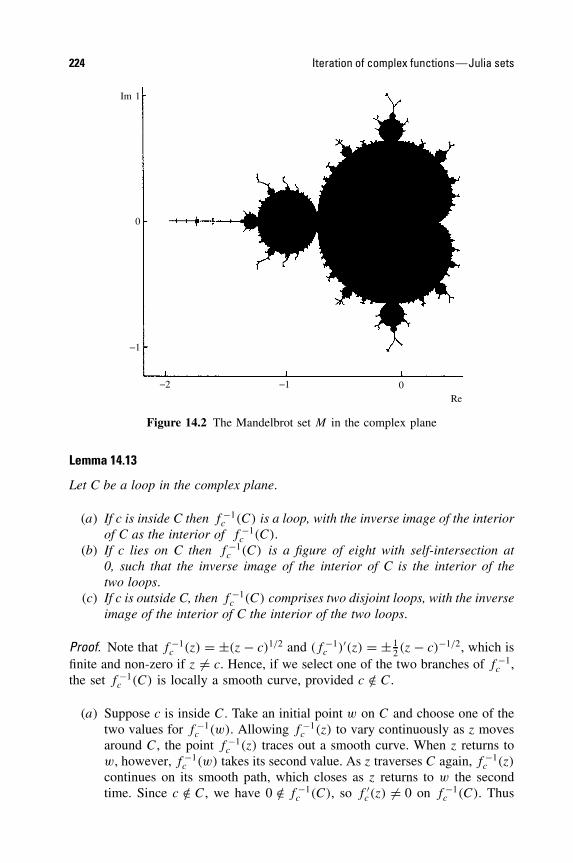
224 Iteration of complex functions—Julia sets
1Im
0
−1
−2 −1 0Re
Figure 14.2 The Mandelbrot set M in the complex plane
Lemma 14.13
Let C be a loop in the complex plane.
(a) If c is inside C then f −1c (C) is a loop, with the inverse image of the interior
of C as the interior of f −1c (C).
(b) If c lies on C then f −1c (C) is a figure of eight with self-intersection at
0, such that the inverse image of the interior of C is the interior of thetwo loops.
(c) If c is outside C, then f −1c (C) comprises two disjoint loops, with the inverse
image of the interior of C the interior of the two loops.
Proof. Note that f −1c (z) = ±(z − c)1/2 and (f −1
c )′(z) = ± 12 (z − c)−1/2, which is
finite and non-zero if z �= c. Hence, if we select one of the two branches of f −1c ,
the set f −1c (C) is locally a smooth curve, provided c /∈ C.
(a) Suppose c is inside C. Take an initial point w on C and choose one of thetwo values for f −1
c (w). Allowing f −1c (z) to vary continuously as z moves
around C, the point f −1c (z) traces out a smooth curve. When z returns to
w, however, f −1c (w) takes its second value. As z traverses C again, f −1
c (z)
continues on its smooth path, which closes as z returns to w the secondtime. Since c /∈ C, we have 0 /∈ f −1
c (C), so f ′c(z) �= 0 on f −1
c (C). Thus

Quadratic functions—the Mandelbrot set 225
fc is locally a smooth bijective transformation near points on f −1c (C). In
particular z ∈ f −1c (C) cannot be a point of self-intersection of f −1
c (C),otherwise fc(z) would be at a self-intersection of C, so f −1(C) is a loop.
Since fc is a continuous function that maps the loop f −1c (C) and no
other points onto the loop C, the polynomial fc must map the interior andexterior of f −1
c (C) into the interior and exterior of C respectively. Hencef −1
c maps the interior of C to the interior of f −1c (C).
(b) This is proved in a similar way to (a), noting that if C0 is a smooth pieceof curve through c, then f −1
c (C0) consists of two smooth pieces of curvethrough 0 which cross at right angles, providing the self-intersection of thefigure of eight.
(c) This is similar to (a), noting that this time, f −1c (z) can only pick up one
of the two values as z moves around C, so we get two loops. �
We now prove the ‘fundamental theorem of the Mandelbrot set’ which givesan alternative characterization in terms of iterates of fc.
Theorem 14.14
M = {c ∈ � : {f kc (0)}k�1 is bounded} (14.5)
= {c ∈ � : f kc (0) �→ ∞ as k → ∞}. (14.6)
Proof. By Lemma 14.1 it is clear that f kc (0) �→ ∞ if and only if {f k
c (0)} isbounded, so (14.5) and (14.6) are equal.
(a) We first show that if {f kc (0)} is bounded then J (fc) is connected. Let
C be a large circle in � such that all the points {f kc (0)} lie inside C,
such that f −1c (C) is interior to C and such that points outside C iterate
to ∞ under f kc . Since c = fc(0) is inside C, Lemma 14.13(a) gives that
f −1c (C) is a loop contained in the interior of C. Also, fc(c) = f 2
c (0) isinside C and f −1
c maps the exterior of C onto the exterior of f −1c (C), so
c is inside f −1c (C). Applying Lemma 14.13(a) again, f −2
c (C) is a loopcontained in the interior of f −1
c (C). Proceeding in this way, we see that{f −k
c (C)} consists of a sequence of loops, each containing the next in itsinterior (figure 14.3(a)). Let K denote the closed set of points that are onor inside the loops f −k
c (C) for all k. If z ∈ �\K some iterate f kc (z) lies
outside C and so f kc (z) → ∞. Thus
A(∞) = {z : f kc (z) → ∞ as k → ∞} = �\K
so K is the filled in Julia set of fc. By Lemma 14.11 J (fc) is the boundaryof �\K which is, of course, the same as the boundary of K . But K is theintersection of a decreasing sequence of closed simply connected sets (i.e.sets that are connected and have connected complement), so, by a simple

226 Iteration of complex functions—Julia sets
c
C
fc−1(C )
fc−2(C )
C
J
fc−1(C )
fc−2(C )
0
K
(a)
(b)
fc−p(C )
0
Figure 14.3 Inverse iterates of a circle c under fc, illustrating the two parts of the proofof Theorem 14.14: (a) c = −0.3 + 0.3i; (b) c = −0.9 + 0.5i
Julia sets of quadratic functions 227
topological argument, K is simply connected and therefore has connectedboundary. Thus J (fc) is connected.
(b) The proof that J (fc) is not connected if {f kc (0)} is unbounded is fairly
similar. Let C be a large circle such that f −1c (C) is inside C, such that
all points outside C iterate to ∞, and such that for some p, the pointf
p−1c (c) = f
pc (0) ∈ C with f k
c (0) inside or outside C according as towhether k is less than or greater than p. Just as in the first part of theproof, we construct a series of loops {f −k
c (C)}, each containing the nextin its interior (figure 14.3(b)). However, the argument breaks down whenwe get to the loop f
1−pc (C), since c ∈ f
1−pc (C) and Lemma 14.13(a) does
not apply. By Lemma 14.13(b) we get that E ≡ f −p(C) is a figure of eightinside the loop f
1−pc (C), with fc mapping the interior of each half of E
onto the interior of f1−pc (C). The Julia set J (fc) must lie in the interior
of the loops of E, since other points iterate to infinity. Since J (fc) isinvariant under f −1
c , parts of it must be contained in each of the loops ofE. Thus this figure of eight E disconnects J (fc). In fact, if we now applyLemma 14.13(c) in the same way, it is easy to see that J (fc) is totallydisconnected. �
The reason for considering iterates of the origin in (14.5) and (14.6) is that theorigin is the critical point of fc for each c, i.e. the point for which f ′
c(z) = 0. Thecritical points are the points where fc fails to be a local bijection—a propertythat was crucial in distinguishing the two cases in the proof of Theorem 14.14and which is crucial in analysing the dynamics of any polynomial or meromor-phic function.
The equivalent definition of M provided by (14.5) is the basis of computerpictures of the Mandelbrot set. Choose numbers r > 2 and k0 of the order of 100,say. For each c compute successive terms of the sequence {f k
c (0)} until either|f k
c (0)| � r , in which case c is deemed to be outside M , noting Exercise 14.12,or k = k0, in which case we take c ∈ M . Repeating this process for values of c
across a region enables a picture of M to be drawn. Often colours are assignedto the complement of M according to the first integer k such that |f k
c (0)| � r .Pictures of the Mandelbrot set (see figure 14.2) suggest that it has a highly
complicated form. It has certain obvious features: a main cardioid to which aseries of prominent circular ‘buds’ are attached. Each of these buds is surroundedby further buds, and so on. However, this is not all. In addition, fine, branched‘hairs’ grow outwards from the buds, and these hairs carry miniature copies ofthe entire Mandelbrot set along their length. The Mandelbrot set is connected,and its boundary has Hausdorff dimension 2, a reflection on its intricacy.
14.3 Julia sets of quadratic functions
In this section we will see a little of how the structure of the Julia set J (fc)
changes as the parameter c varies across the complex plane. In particular, the

228 Iteration of complex functions—Julia sets
significance of the various parts of the Mandelbrot set will start to becomeapparent.
The attractive periodic points of fc are crucial to the form of J (fc). It maybe shown (see Exercise 14.17) that if w �= ∞ is an attractive periodic point of apolynomial f then there is a critical point z (a point with f ′(z) = 0) such thatf k(z) is attracted to the periodic orbit containing w. Since the only critical pointof fc is 0, fc can have at most one attractive periodic orbit. Moreover, if c /∈ M
then, by Theorem 14.14, f kc (0) → ∞, so fc can have no attractive periodic orbit.
It is conjectured that the set of c for which fc has an attractive periodic orbitfills the interior of M .
It is natural to categorize fc by the period p of the (finite) attractive orbit, ifany; the values of c corresponding to different p may be identified as differentregions of the Mandelbrot set M .
To begin with, suppose c lies outside M , so fc has no attractive periodic points.By definition, J (fc) is not connected. In fact, J (fc) must be totally disconnectedand expressible as the disjoint union J = S1(J ) ∪ S2(J ), where S1 and S2 arethe two branches of f −1
c on J . This means that J is the attractor of the IFS{S1, S2}, see (9.2). Basically, this follows from the second half of the proof ofTheorem 14.14—we get that fc maps the interior of each loop of a figure of eightE onto a region D containing E. The mappings S1 and S2 may be taken as therestrictions of f −1
c to the interior of each loop. Since S1(J ) and S2(J ) are interiorto the two halves of E, they are disjoint, so J must be totally disconnected; seeremarks after (9.7).
We look at this situation in more detail when c is large enough to allow somesimplifications to be made.
Theorem 14.15
Suppose |c| > 14 (5 + 2
√6) = 2.475 . . . . Then J (fc) is totally disconnected, and
is the attractor (in the sense of (9.2)) of the contractions given by the two branchesof f −1
c (z) = ±(z − c)1/2 for z near J. When |c| is large
dimBJ (fc) = dimHJ (fc) 2 log 2/ log 4|c|.
Proof. Let C be the circle |z| = |c| and D its interior |z| < |c|. Then
f −1c (C) = {(c eiθ − c)1/2 : 0 � θ � 4π}
which is a figure of eight with self-intersection point at 0, with the loops on eitherside of a straight line through the origin (see Lemma 14.13 and figure 14.4).Since |c| > 2 we have f −1
c (C) ⊂ D since if |z| > |c| then |fc(z)| � |z2| − |c| �|c|2 − |c| > |c|. The interior of each of the loops of f −1
c (C) is mapped by fc in abijective manner onto D. If we define S1, S2 : D → D as the branches of f −1
c (z)
inside each loop, then S1(D) and S2(D) are the interiors of the two loops.

Julia sets of quadratic functions 229
S2(V )
S1(V )f −1(C )
0
VC
D
Figure 14.4 Proof of Theorem 14.15
Let V be the disc {z : |z| < |2c|1/2}. We have chosen the radius of V so thatV just contains f −1
c (C), so S1(D), S2(D) ⊂ V ⊂ D. Hence S1(V ), S2(V ) ⊂ V
with S1(V ) and S2(V ) disjoint. We have, for i = 1, 2,
|Si(z1) − Si(z2)| = |(z1 − c)1/2 − (z2 − c)1/2| = |z1 − z2||(z1 − c)1/2 + (z2 − c)1/2| .
Hence, if z1, z2 ∈ V , taking least and greatest values,
12 (|c| + |2c|1/2)−1/2 � |Si(z1) − Si(z2)|
|z1 − z2| � 12 (|c| − |2c|1/2)−1/2. (14.7)
The upper bound is less than 1 if |c| > 14 (5 + 2
√6), in which case S1 and S2
are contractions on the disc V . By Theorem 9.1 there is a unique non-emptycompact attractor F ⊂ V satisfying
S1(F ) ∪ S2(F ) = F. (14.8)
Since S1(V ) and S2(V ) are disjoint, so are S1(F ) and S2(F ), implying that F istotally disconnected.
Of course, F is none other than the Julia set J = J (fc). One way to see this isto note that, since V contains at least one point z of J (for example, a repellingfixed point of fc), we have J = closure (
⋃∞k=1 f −k
c (z)) ⊂ V , since f −kc (V ) ⊂ V .
Using further results from Summary 14.12, J is a non-empty compact subset of

230 Iteration of complex functions—Julia sets
V satisfying J = f −1c (J ) or, equivalently, J = S1(J ) ∪ S2(J ). Thus J = F , the
unique non-empty compact set satisfying (14.8).Finally, we estimate the dimension of J (fc) = F . By Propositions 9.6 and
9.7 and (14.7), lower and upper bounds for dimHJ (fc) are provided by thesolutions of 2
(12 (|c| ± |2c|1/2)−1/2
)s = 1, i.e. by s = 2 log 2/ log 4(|c| ± |2c|1/2),which gives the stated asymptotic estimate. �
We next turn to the case where c is small. We know that if c = 0 then J (fc) isthe unit circle. If c is small and z is small enough, then f k
c (z) → w as k → ∞,where w is the attractive fixed point 1
2
(1 − √
1 − 4c)
close to 0. On the otherhand, f k
c (z) → ∞ if z is large. It is not unreasonable to expect the circle to‘distort’ into a simple closed curve (i.e. having no points of self-intersection)separating these two types of behaviour as c moves away from 0.
In fact, this is the case provided that fc retains an attractive fixed point, i.e.if |f ′
c(z)| < 1 at one of the roots of fc(z) = z. Simple algebra shows that thishappens if c lies inside the cardioid z = 1
2 eiθ(1 − 1
2 eiθ)
(0 � θ � 2π)—this isthe main cardioid of the Mandelbrot set, see Exercise 14.15.
For convenience, we treat the case of |c| < 14 , but the proof is easily modified
if fc has any attractive fixed point.
Theorem 14.16
If |c| < 14 then J (fc) is a simple closed curve.
Proof. Let C0 be the curve |z| = 12 , which encloses both c and the attractive fixed
point w of fc. Then by direct calculation the inverse image f −1c (C0) is a loop
C1 surrounding C0. We may fill the annular region A1 between C0 and C1 by acontinuum of curves, which we call ‘trajectories’, which leave C0 and reach C1
perpendicularly; see figure 14.5(a). For each θ let ψ1(θ) be the point on C1 atthe end of the trajectory leaving C0 at ψ0(θ) = 1
2 eiθ . The inverse image f −1c (A1)
is an annular region A2 with outer boundary the loop C2 = f −1c (C1) and inner
boundary C1, with fc mapping A2 onto A1 in a two-to-one manner. The inverseimage of the trajectories joining C0 to C1 provides a family of trajectories joiningC1 to C2. Let ψ2(θ) be the point on C2 at the end of the trajectory leaving C1 atψ1(θ). We continue in this way to get a sequence of loops Ck, each surroundingits predecessor, and families of trajectories joining the points ψk(θ) on Ck toψk+1(θ) on Ck+1 for each k.
As k → ∞, the curves Ck approach the boundary of the basin of attraction ofw; by Lemma 14.11 this boundary is just the Julia set J (fc). Since |f ′
c(z)| > γ
for some γ > 1 outside C1, it follows that f −1c is contracting near J . Thus the
length of the trajectory joining ψk(θ) to ψk+1(θ) converges to 0 at a geometric rateas k → ∞. Consequently ψk(θ) converges uniformly to a continuous functionψ(θ) as k → ∞, and J is the closed curve given by ψ(θ) (0 � θ � 2π).
It remains to show that ψ represents a simple curve. Suppose that ψ(θ1) =ψ(θ2). Let D be the region bounded by C0 and the two trajectories joining

Julia sets of quadratic functions 231
Trajectories
0
A3 A2 A1
C0
C0D
C1 C2
J
J
y0(q)
y(q1) = y(q2)
y1(q)
y(q)
y2(q)
y0(q2)
y0(q1)
(a)
(b)
Figure 14.5 Proof of Theorem 14.16
ψ0(θ1) and ψ0(θ2) to this common point. The boundary of D remains boundedunder iterates of fc, so by the maximum modulus theorem (that the modulus ofan analytic function takes its maximum on the boundary point of a region) D
remains bounded under iteration of f . Thus D is a subset of the filled-in Juliaset, so the interior of D cannot contain any points of J . Thus the situation offigure 14.5(b) cannot occur, so that ψ(θ) = ψ(θ1) = ψ(θ2) for all θ between θ1
and θ2. It follows that ψ(θ) has no point of self-intersection. �
By an extension of this argument, if c is in the main cardioid of M , then J (fc)
is a simple closed curve; such curves are sometimes referred to as quasi-circles.Of course, J (fc) will be a fractal curve if c > 0. It may be shown that, for smallc, its dimension is given by
s = dimBJ (fc) = dimHJ (fc) = 1 + |c|24 log 2
+ terms in |c|3 and higher powers.
(14.9)

232 Iteration of complex functions—Julia sets
Moreover, 0 < Hs (J ) < ∞, with dimBJ (fc) = dimHJ (fc) given by a real ana-lytic function of c.
The next case to consider is when fc has an attractive periodic orbit of period2. By a straightforward calculation this occurs if |c + 1| < 1
4 ; that is, if z lies inthe prominent circular disc of M abutting the cardioid, see Exercise 14.16.
Since f 2c is a polynomial of degree 4, fc has two fixed points and two period-
2 points. Let w1 and w2 be the points of the attractive period-2 orbit. It maybe shown, as in the proof of Theorem 14.16, that the basin of attraction for wi
(i.e. {z : f 2kc (z) → wi as k → ∞}) includes a region bounded by a simple closed
curve Ci surrounding wi , for i = 1, 2. By Lemma 14.11 and Proposition 14.4,Ci ⊂ J (f 2
c ) = J (fc). The curves Ci are mapped onto themselves in a two-to-onefashion by f 2
c , which implies that there is a fixed point of f 2c on each Ci . The
period-2 points are strictly inside the Ci , so there is a fixed point of fc on eachCi ; since the Ci are mapped onto each other by fc, the only possibility is for C1
and C2 to touch at one of the fixed points of fc. The inverse function f −1c is two-
valued on C1. One of the inverse images is C2 (which encloses w2). However,the other branch of f −1
c (C1) is a further simple closed curve enclosing the secondvalue of f −1
c (w1). We may continue to take inverse images in this way to findthat J (fc) is made up of infinitely many simple closed curves which enclose thepre-images of w1 and w2 of all orders and touch each other in pairs at ‘pinchpoints’—see figure 14.7(c). Thus we get fractal Julia sets that are topologicallymuch more complicated than in the previous cases.
It is possible to use such ideas to analyse the case when fc has an attractiveperiodic orbit of period p > 2. The immediate neighbourhoods of the period-ppoints that are drawn into the attractive orbits are bounded by simple closedcurves which touch each other at a common point. The Julia set consists of thesefractal curves together with all their pre-images under f k.
A variety of examples are shown in figures 14.6 and 14.7. The ‘buds’ on theMandelbrot set corresponding to attractive orbits of period p are indicated infigure 14.8.
The Julia sets J (fc) that are most intricate, and are mathematically hardest toanalyse are at the ‘exceptional’ values of c on the boundary of M . If c is on theboundary of the cardioid or a bud of M , then fc has an indifferent periodic point(where |(f p)′(w)| = 1). If c is at a ‘neck’ where a bud touches a parent region,then J (fc) includes a series of ‘tendrils’ joining its boundary to the indifferentperiodic points. For c elsewhere on the boundary of the cardioid the Julia setmay contain ‘Siegel discs’. The Julia set J (fc) consists of infinitely many curvesbounding open regions, with fc mapping each region into a ‘larger’ one, untilthe region containing the fixed point is reached. Inside this Siegel disc, fc rotatespoints on invariant loops around the fixed point.
There are still further possibilities. If c is on one of the ‘hairs’ of M then J (fc)
may be a dendrite, i.e. of tree-like form. This occurs if an iterate of the criticalpoint 0 is periodic, i.e. if f k
c (0) = fk+qc (0) for positive integers k and q.
We have mentioned that there are miniature copies of M located in the hairsof M . If c belongs to one of these, then J (fc) will be of dendrite form, but with

Julia sets of quadratic functions 233
Figure 14.6 Julia sets J (fc) for c at various points in the Mandelbrot set. The Julia setsare displayed in more detail in figure 14.7
small copies of the Julia set from the corresponding value of c in the main partof M inserted at the ‘vertices’ of the dendrite.
A good way to explore the structure of Julia sets and, indeed, the Julia setsof other functions, is using a computer. There are two usual methods of drawingJulia sets, based on properties that we have discussed.
For the first method, we choose a repelling periodic point z. For suitable k, wemay compute the set of inverse images Jk = f −k(z). By Corollary 14.8(b) these2k points are in J , and should fill J as k becomes large. A difficulty with picturingJ in this way is that the points of Jk need not be uniformly distributed acrossJ —they may tend to cluster in some parts of J and be sparse in other parts.Consequently, even with k quite large, parts of J can be missed altogether. (Thistends to happen for fc with c close to the boundary of M .) There are variousways of getting around this difficulty. For instance, with J0 = {z}, instead oftaking Jk = f −1(Jk−1) for each k, we can choose a subset Jk of f −1(Jk−1) byignoring all but one of the points in every ‘small’ cluster. This ensures that weare working with a reasonably well distributed set of points of J at each step ofthe iteration, and also reduces the calculation involved.
A second method is to test individual points to see if they are close to theJulia set. Suppose, for example, that f has two or more attractive fixed points
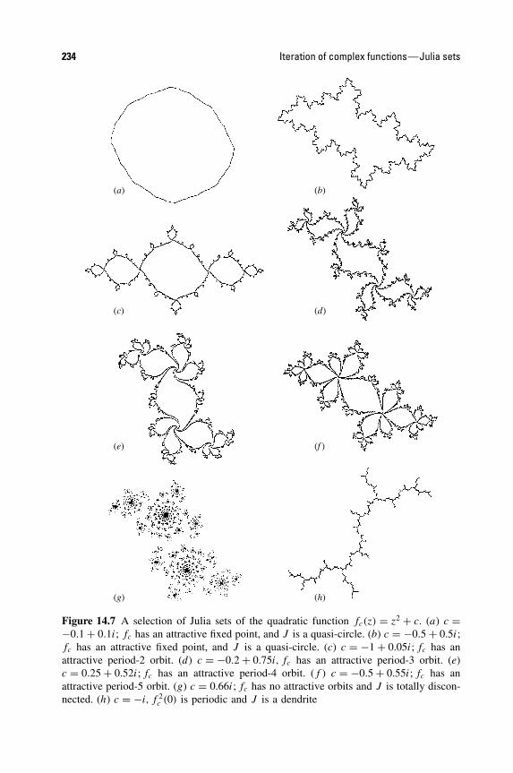
234 Iteration of complex functions—Julia sets
(a) (b)
(c) (d)
(e) (f )
(g) (h)
Figure 14.7 A selection of Julia sets of the quadratic function fc(z) = z2 + c. (a) c =−0.1 + 0.1i; fc has an attractive fixed point, and J is a quasi-circle. (b) c = −0.5 + 0.5i;fc has an attractive fixed point, and J is a quasi-circle. (c) c = −1 + 0.05i; fc has anattractive period-2 orbit. (d) c = −0.2 + 0.75i, fc has an attractive period-3 orbit. (e)c = 0.25 + 0.52i; fc has an attractive period-4 orbit. (f ) c = −0.5 + 0.55i; fc has anattractive period-5 orbit. (g) c = 0.66i; fc has no attractive orbits and J is totally discon-nected. (h) c = −i, f 2
c (0) is periodic and J is a dendrite
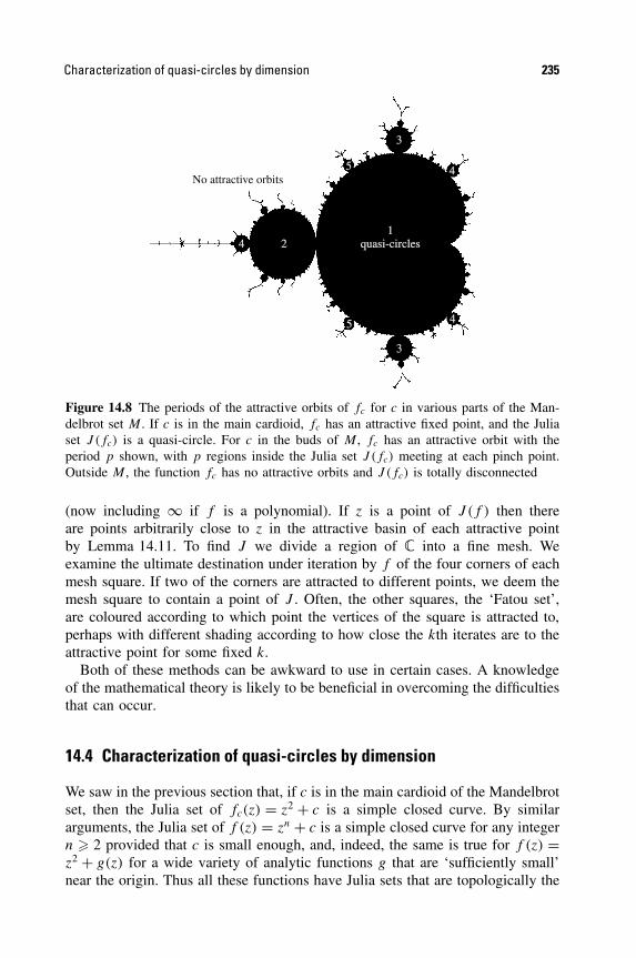
Characterization of quasi-circles by dimension 235
No attractive orbits
1quasi-circles2
3
3
5
5
4
4
4
Figure 14.8 The periods of the attractive orbits of fc for c in various parts of the Man-delbrot set M . If c is in the main cardioid, fc has an attractive fixed point, and the Juliaset J (fc) is a quasi-circle. For c in the buds of M , fc has an attractive orbit with theperiod p shown, with p regions inside the Julia set J (fc) meeting at each pinch point.Outside M , the function fc has no attractive orbits and J (fc) is totally disconnected
(now including ∞ if f is a polynomial). If z is a point of J (f ) then thereare points arbitrarily close to z in the attractive basin of each attractive pointby Lemma 14.11. To find J we divide a region of � into a fine mesh. Weexamine the ultimate destination under iteration by f of the four corners of eachmesh square. If two of the corners are attracted to different points, we deem themesh square to contain a point of J . Often, the other squares, the ‘Fatou set’,are coloured according to which point the vertices of the square is attracted to,perhaps with different shading according to how close the kth iterates are to theattractive point for some fixed k.
Both of these methods can be awkward to use in certain cases. A knowledgeof the mathematical theory is likely to be beneficial in overcoming the difficultiesthat can occur.
14.4 Characterization of quasi-circles by dimension
We saw in the previous section that, if c is in the main cardioid of the Mandelbrotset, then the Julia set of fc(z) = z2 + c is a simple closed curve. By similararguments, the Julia set of f (z) = zn + c is a simple closed curve for any integern � 2 provided that c is small enough, and, indeed, the same is true for f (z) =z2 + g(z) for a wide variety of analytic functions g that are ‘sufficiently small’near the origin. Thus all these functions have Julia sets that are topologically the

236 Iteration of complex functions—Julia sets
same—they are all homeomorphic to a circle. The surprising thing is that theyare essentially the same as fractals, in other words are bi-Lipschitz equivalent,if and only if they have the same Hausdorff dimension. Of course, if two setshave different dimensions they cannot be bi-Lipschitz equivalent (Corollary 2.4).However, in this particular situation the converse is also true.
We term a set F a quasi-self-similar circle or quasi-circle if the followingconditions are satisfied:
(i) F is homeomorphic to a circle (i.e. F is a simple closed curve).(ii) 0 < Hs(F ) < ∞ where s = dimHF .
(iii) There are constants a, b, r > 0 such that for any subset U of F with|U | � r there is a mapping ϕ : U → F such that
a|x − y| � |U ||ϕ(x) − ϕ(y)| � b|x − y| (x, y ∈ F). (14.10)
The ‘quasi-self-similar’ condition (iii) says that arbitrarily small parts of F are‘roughly similar’ to a large part of F .
The following theorem depends on using s-dimensional Hausdorff measure tomeasure ‘distance’ round a quasi-circle.
Theorem 14.17
Quasi-circles E and F are bi-Lipschitz equivalent if and only if dimHE = dimHF .
Sketch of proof. If there is a bi-Lipschitz mapping between E and F thendimHE = dimHF by Corollary 2.4(b).
Suppose that dimHE = dimHF . Let E(x, y) be the ‘arc’ of E between pointsx, y ∈ E, taken in the clockwise sense, with a similar notation for arcs of F .Conditions (ii) and (iii) imply that Hs(E(x, y)) is continuous in x, y ∈ E and ispositive if x �= y. We claim that there are constants c1, c2 > 0 such that
c1 � Hs(E(x, y))
|x − y|s � c2 (14.11)
whenever E(x, y) is the ‘shorter’ arc, i.e. Hs(E(x, y)) � Hs(E(y, x)). Assumethat ε > 0 is sufficiently small. If |x − y| � ε then (14.11) is true by a continuityargument for suitable constants. If |x − y| < ε there is a mapping ϕ : E(x, y) →E satisfying (14.10) such that |ϕ(x) − ϕ(y)| � ε. Inequalities (14.10), (2.8) and(2.9) imply that the ratio (14.11) changes by a bounded amount if x and y arereplaced by ϕ(x) and ϕ(y), so (14.11) holds for suitable c1 and c2 for all x, y ∈ E.
Now choose base points p ∈ E, q ∈ F . Set γ = Hs(E)/Hs(F ) and defineψ : E → F by taking ψ(x) to be the point of F such that
Hs(E(p, x)) = γHs(F (q, ψ(x)))
(see figure 14.9). Then ψ is a continuous bijection, and also
Hs(E(x, y)) = γHs (F (ψ(x), ψ(y))) (x, y ∈ E).

Newton’s method for solving polynomial equations 237
E F
E (p, x)
p
x
y
y(x )
q = y(p)
= g Hs(E(p, x ))
Hs(F(q, y(x )))
Figure 14.9 Setting up a bi-Lipschitz mapping ψ between two quasi-circles of Hausdorffdimension s
Using (14.11) together with similar inequalities for arcs of F , this gives
c3 � |ψ(x) − ψ(y)||x − y| � c4
if x �= y, so that ψ is bi-Lipschitz, as required. �
Corollary 14.18
Suppose that the Julia sets J1 and J2 of the polynomials f1 and f2 are simpleclosed curves. Suppose that fi is strictly repelling on Ji (i.e. |f ′
i (z)| > 1 for i =1, 2). Then J1 and J2 are bi-Lipschitz equivalent if and only if dimHJ1 = dimHJ2.
Proof. It may be shown that if a polynomial f is strictly repelling on its Julia setJ then 0 < Hs(J ) < ∞, where s = dimHJ . Moreover, given a subset U of J , wemay choose k so that f k(U) has diameter comparable with that of J itself, and(14.10) holds taking ϕ = f k (this reflects the quasi-self-similarity of J ). Thus J1
and J2 are quasi-circles to which Theorem 14.17 may be applied. �
14.5 Newton’s method for solving polynomial equations
Anyone who has done any numerical analysis will have found roots of equationsusing Newton’s method. Let p(x) be a function with continuous derivative.If f (x) = x − p(x)/p′(x) then the iterates f k(x) converge to a solution ofp(x) = 0 provided that p′(x) �= 0 at the solution and that the initial value of x ischosen appropriately. Cayley suggested investigating the method in the complexplane, and in particular which initial points of � iterate to which zero of p.
238 Iteration of complex functions—Julia sets
Let p : � → � be a polynomial with complex coefficients, and form the ratio-nal function f : � ∪ {∞} → � ∪ {∞}
f (z) = z − p(z)/p′(z). (14.12)
Then the fixed points of f , given by p(z)/p′(z) = 0, are the zeros of p togetherwith ∞. Differentiating, we find that
f ′(z) = p(z)p′′(z)/p′(z)2 (14.13)
so a zero z of p is a superattractive fixed point of f , i.e. f ′(z) = 0, providedthat p′(z) �= 0. If |z| is large, f (z) ∼ z(1 − 1/n), where n is the degree of p, so∞ is a repelling point of f . As usual, we write
A(w) = {z : f k(z) → w} (14.14)
for the basin of attraction of the zero w, i.e. the set of initial points whichconverge to w under Newton iteration. Since the zeros are attractive, the basinA(w) includes an open region containing w. We shall see, however, that A(w)
can be remarkably complicated further away from w.The theory of Julia sets developed for polynomials in Section 14.1 is almost
the same for a rational function, provided that the point ∞ is included in thenatural way. The main differences are that if f is a rational function J (f ) neednot be bounded (though it must be closed) and it is possible for J (f ) to haveinterior points, in which case J (f ) = � ∪ {∞}. However, Lemma 14.11 remainstrue, so that J (f ) is the boundary of A(w) for each attractive fixed point w. ThusJ (f ) is likely to be important when analysing the domains of attraction of theroots in Newton’s method.
A straightforward case is the quadratic polynomial
p(z) = z2 − c (c �= 0)
with zeros ± √c (as before, more general quadratic polynomials can be reduced
to this form by a conjugacy). Newton’s formula (14.12) becomes
f (z) = (z2 + c)/2z.
Thusf (z) ± √
c = (z ± √c)2/2z
sof (z) + √
c
f (z) − √c
=(
z + √c
z − √c
)2
. (14.15)
It follows immediately that if |z + √c|/|z − √
c| < 1 then |f k(z) + √c|/
|f k(z) − √c| → 0 and also f k(z) → −√
c as k → ∞, and similarly if
Newton’s method for solving polynomial equations 239
|z + √c|/|z − √
c| > 1 then f k(z) → √c. The Julia set J (f ) is the line |z + √
c|= |z − √
c| (the perpendicular bisector of −√c and
√c) and A(−√
c) andA(
√c) are the half-planes on either side. (Letting h(z) = (z + √
c)/(z − √c)
in (14.15) gives f (z) = h−1(h(z))2, so that f is conjugate to, and therefore hassimilar dynamics to, the mapping g(z) = z2.) In this case the situation is veryregular—any initial point is iterated by f to the nearest zero of p.
The quadratic example might lead us to hope that the domains of attractionunder Newton iteration of the zeros of any polynomial are reasonably regular.However, for higher-order polynomials the situation is fundamentally different.Lemma 14.11 (which holds for rational functions, including Newton functionsof polynomials) provides a hint that something very strange happens. If p haszeros z1, . . . , zn with p′(zi) �= 0, Lemma 14.11 tells us that the Julia set of f isthe boundary of the domain of the attraction of every zero:
J (f ) = ∂A(z1) = · · · = ∂A(zn).
A point on the boundary of any one of the domains of attraction must be on theboundary of all of them; since J (f ) is uncountable, there are a great many suchmultiple boundary points. An attempt to visualize three or more disjoint sets withthis property will convince the reader that they must be very complicated indeed.
Let us look at a specific example. The cubic polynomial
p(z) = z3 − 1
has zeros 1, ei2π/3, ei4π/3, and Newton function
f (z) = 2z3 + 1
3z2.
The transformation ρ(z) = z ei2π/3 is a rotation of 120◦ about the origin. It iseasily checked that f (ρ(z)) = ρ(f (z)), in other words ρ is a conjugacy of f
to itself. It follows that a rotation of 120◦ about the origin maps A(w) ontoA(w ei2π/3) for each of the three zeros w, so that the Julia set has threefold sym-metry about the origin. (Of course, these symmetries would be expected fromthe symmetric disposition of the three zeros of p.) If z is real then f k(z) remainsreal for all k, and, by elementary arguments, f k(z) converges to 1 except forcountably many real z. Thus A(1) contains the real axis except for a countablenumber of points, and, by symmetry, A(ei2π/3) and A(ei4π/3) contain the linesthrough the origin making 120◦ and 240◦ to the real axis, again except for count-ably many points. We also know that each A(w) contains an open region roundw, that any point on the boundary of one of the A(w) is on the boundary ofall three, and that there are uncountably many such ‘triple points’. Most peo-ple require the insight of a computer drawing to resolve this almost paradoxicalsituation, see figure 14.10.
The domain A(1) is shown in black in figure 14.10(b); note that the basinsof attraction of the other two zeros, obtained by rotation of 120◦ and 240◦, key

240 Iteration of complex functions—Julia sets
ei2p /3
ei4p /3
1
(a)
(b)
Figure 14.10 Newton’s method for p(z) = z3 − 1. The Julia set for the Newton functionf (z) = (2z3 + 1)/3z2 is shown in (a), and the domain of attraction of the zero z = 1 isshown in black in (b)
Notes and references 241
into the picture in a natural way. The Julia set shown in figure 14.10(a) is theboundary of the three basins and is made up of three ‘chains’ leading away fromthe origin. These fractal chains have a fine structure—arbitrarily close to eachpoint of J (f ) is a ‘slightly distorted’ copy of the picture at the origin with sixcomponents of the A(w) meeting at a point. This reflects Corollary 14.8(b), againvalid for rational functions: J (f ) is the closure of
⋃∞k=1 f −k(0), so that if z is
in J (f ) then there is a point w arbitrarily close to z, and an integer k, suchthat f k(w) = 0. But f k is locally a conformal mapping, so that the local inverse(f k)−1 maps a neighbourhood of 0 to an ‘almost similar’ neighbourhood of w.The Julia set J (f ) exhibits quasi-self-similarity.
This, of course, is just the beginning. The domains of attraction of the zerosof other polynomials of degree 3 or more and, indeed, other analytic functions,may be investigated using a combination of theory and computer graphics. Thisleads to a wealth of sets of a highly intricate form which raise many intriguingmathematical questions.
In this chapter we have touched on what is a complicated and fascinating areaof mathematics in which fractals play a fundamental role. It is an area in whichcomputer experiments often lead the way with mathematical theory trying to keepup. The variations are endless—we can investigate the Julia set of higher-orderpolynomials and of other analytic functions such as exp z, as well as invariantsets of non-analytic transformations of the plane. With the advent of high qualitycolour computer graphics, these ideas have become the basis of much computerart. A single function of simple form can lead to highly intricate yet regularpictures—often very beautiful, sometimes almost weird.
14.6 Notes and references
Much of the basic theory of iteration of complex functions was developed by Julia(1918) and Fatou (1919). For many years the subject lay almost dormant, untilcomputer graphics was sufficiently advanced to reveal the intricate form of Juliasets. Recently, there has been an extraordinary interest in the subject, and drawingJulia sets and the Mandelbrot set on computers has become a popular activity,with the incredibly beautiful and intricate pictures that are easily produced.
For an account of basic complex variable theory, see Ahlfors (1979). Thebooks by Peitgen and Richter (1986), Becker and Dorfler (1989) and Peitgen,Jurgens and Saupe (1992) provide well-illustrated accounts of complex iteration.Other recommended accounts of complex dynamics include Blanchard (1984),Saupe (1987), Devaney (1989), Beardon (1991), Carleson and Gamelin (1993),McMullen (1994) and Milnor (1999). Mandelbrot (1980) introduced the set bear-ing his name; the fundamental Theorem 14.14 is given by Brolin (1965). A col-lection of papers on topics related to the Mandelbrot set was edited by Tan (2000).
The formula (14.9) for the dimension of J (fc) is due to Ruelle (1982), andextensions are given by Collet, Dobbertin and Moussa (1992) and Abenda,
242 Iteration of complex functions—Julia sets
Moussa and Osbaldestin (1999). For details of the characterization of quasi-circles by dimension, see Falconer and Marsh (1989). Fractals associated withNewton’s method are discussed in Peitgen and Richter (1986), Peitgen, Saupeand von Haeseler (1984) and Curry, Garnett and Sullivan (1983).
Exercises
Throughout these exercises we write fc(z) = z2 + c.
14.1 Show that every perfect set E (i.e. every set that is closed and has no isolatedpoints) is uncountable. (Hint: Construct a ‘Cantor-like’ set inside E.) Deduce thatJ (fc) is uncountable for all c.
14.2 Describe the Julia set of f (z) = z2 + 4z + 2. (Hint: Write z1 = z + 2.)
14.3 Let f (z) = z2 + 2iz + b. By considering the mapping h(z) = z + i, show that theJulia set of f is connected if and only if b + 1 + i ∈ M .
14.4 Let |c| � 14 . Show that if |z| � 1
2 then |fc(z)| � 12 . Deduce that B(0, 1
4 ) ⊂ K(fc).Also show that if |z| � 2 then |fc(z)| � 3
2 |z|. Deduce that K(fc) ⊂ B(0, 2). Whatdoes this tell us about the location of J (fc)?
14.5 Let f (z) = z2 − 2. Find a repelling fixed point of f . Deduce from Corollary 14.8that J (f ) is a subset of the real interval [−2, 2]. Use Theorem 14.14 to deducethat J (f ) is connected, and hence that it is the interval [−2, 2].
14.6 Show that the Julia set J (fc) is symmetric about the origin (that is z ∈ J (fc) ifand only if −z ∈ J (fc)).
14.7 Show that if c is real with c > 14 then z /∈ J (fc) for all real numbers z. Deduce,
using Exercise 14.6, that if c > 14 then J (fc) is not connected, and so c /∈ M .
14.8 Show that if c is a non-real number with |c| < 14 and w = 1
2 (1 + (1 − 4c)−1/2) isthe repelling fixed point of fc(z) = z2 + c then f ′
c(w) is not real. Deduce that thesimple closed curve that forms the Julia set J (fc) cannot have a tangent at w.Hence deduce that the curve contains no differentiable arcs.
14.9 Show that if |c| � 14 and |z| � 1
2 then |fc(z)| � 12 . Deduce that B(0, 1
4 ) ⊂ M .
14.10 Show that if |c + 1| � 120 and |z| � 1
10 then |fc(fc(z))| � 110 . Deduce that
B(−1, 120 ) ⊂ M .
14.11 Show that if ε > 0 and if |z| � max(2 + ε, |c|) then |fc(z)| � |z|(1 + ε). Deducethat if |c| > 2 then c /∈ M .
14.12 Use Exercise 14.11 to show that M = {c : |f kc (0)| > 2 for some k}.
14.13 Show that if |c| < 1 then the Julia set of f (z) = z3 + 3z is a simple closed curve.
14.14 Obtain an estimate for the dimension of the Julia set of f (z) = z3 + c when |c|is large.
14.15 Show that fc has an attractive fixed point precisely when c lies inside the maincardioid of the Mandelbrot set given by z = 1
2 eiθ(1 − 1
2 eiθ)
for 0 � θ � 2π .
14.16 Show that f 2c (z) − z = (z2 − z + c)(z2 + z + c + 1). Deduce that f has an attrac-
tive period-2 point just when |c + 1| < 14 (the large disc in M).
14.17 Show that if w is an attractive fixed point of fc then the attractive basin A(w) mustcontain the point c. (Hint: Show that otherwise there is an open neighbourhoodof w on which the inverse iterates f −k of f can be uniquely defined and form

Exercises 243
a normal family, which is impossible since w is a repelling fixed point of f −1.)Deduce that fc can have at most one attractive fixed point. Generalize this to showthat if w is an attractive fixed point of any polynomial f then A(w) contains apoint f (z) for some z with f ′(z) = 0.
14.18 Let f be a quadratic polynomial. Show by applying Exercise 14.17 to f p forpositive integers p, that f can have at most one attractive periodic orbit.
14.19 Write a computer program to draw Julia sets of functions (see the end ofSection 14.3). Try it out first on quadratic functions, then experiment with otherpolynomials and rational functions, and then other functions such as exp z.
14.20 Use a computer to investigate the domains of attraction for the zeros of some otherpolynomials under Newton’s method iteration; for example for p(z) = z4 − 1 orp(z) = z3 − z.
Chapter 15 Random fractals
Many of the fractal constructions that have been encountered in this book haverandom analogues. For example, in the von Koch curve construction, each timewe replace the middle third of an interval by the other two sides of an equilateraltriangle, we might toss a coin to determine whether to position the new part‘above’ or ‘below’ the removed segment. After a few steps, we get a ratherirregular looking curve which nevertheless retains certain of the characteristicsof the von Koch curve; see figure 15.1.
The middle third Cantor set construction may be randomized in several ways,as in figure 15.2. Each time we divide a segment into three parts we could, insteadof always removing the middle segment, throw a die to decide which parts toremove. Alternatively, we might choose the interval lengths at each stage of theconstruction at random, so that at the kth stage we are left with 2k intervals ofdiffering lengths, resulting in a rather irregular looking fractal.
Whilst such ‘random fractals’ do not have the self-similarity of their non-random counterparts, their non-uniform appearance is often rather closer to nat-ural phenomena such as coastlines, topographical surfaces or cloud boundaries.Indeed, random fractal constructions are the basis of many impressive computer-drawn landscapes or skyscapes.
Most fractals discussed in this book involve a sequence of approximationsEk, each obtained from its predecessor by modification in increasingly finedetail, with a fractal F as a limiting set. A random fractal worthy of thename should display randomness at all scales, so it is appropriate to introducea random element at each stage of the construction. By relating the size ofthe random variations to the scale, we can arrange for the fractal to be statis-tically self-similar in the sense that enlargements of small parts have the samestatistical distribution as the whole set. This compares with (non-random) self-similar sets (see Chapter 9) where enlargements of small parts are identical tothe whole.
In order to describe fractal constructions involving infinitely many randomsteps with precision, we must use the language of probability theory, a briefsurvey of which is given in Section 1.4.
244
Fractal Geometry: Mathematical Foundations and Application. Second Edition Kenneth Falconer 2003 John Wiley & Sons, Ltd ISBNs: 0-470-84861-8 (HB); 0-470-84862-6 (PB)
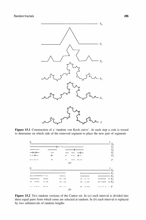
Random fractals 245
E0
F
E1
E2
E3
E4
Figure 15.1 Construction of a ‘random von Koch curve’. At each step a coin is tossedto determine on which side of the removed segment to place the new pair of segments
0 1E0E1E2E3E4
F(a)
0 1E0E1E2E3E4
F(b)
Figure 15.2 Two random versions of the Cantor set. In (a) each interval is divided intothree equal parts from which some are selected at random. In (b) each interval is replacedby two subintervals of random lengths

246 Random fractals
15.1 A random Cantor set
We give a detailed analysis of a specific statistically self-similar construction.It resembles that of the middle third Cantor set, except that the lengths of theintervals at each stage are random. This analysis extends to much more generalrandom fractals.
Intuitively, we consider a construction F = ⋂∞k=1 Ek, where [0, 1] = E0 ⊃
E1 ⊃ · · · is a decreasing sequence of closed sets, with Ek a union of 2k disjointclosed kth level basic intervals. We assume that each kth level interval I containstwo (k + 1)th level intervals IL and IR, abutting the left- and right-hand ends of I
respectively. The lengths of the intervals are random, and we impose statisticalself-similarity by the requirement that the length ratios |IL|/|I | have independentand identical probability distribution for every basic interval I of the construction,and similarly for the ratios |IR|/|I |. This ‘random Cantor set’ F is statisticallyself-similar, in that the distribution of the set F ∩ I is the same as that of F , butscaled by a factor |I |, for each I .
We describe this random construction in probabilistic terms. Let a, b be con-stants with 0 < a � b < 1
2 . We let � denote the class of all decreasing sequencesof sets [0, 1] = E0 ⊃ E1 ⊃ E2 ⊃ · · · satisfying the following conditions. The setEk comprises 2k disjoint closed intervals Ii1,...,ik indexed by i1, . . . , ik , whereij = 1 or 2 (1 � j � k); see figure 15.3. The interval Ii1,...,ik of Ek contains thetwo intervals Ii1,...,ik,1 and Ii1,...,ik,2 of Ek+1, with the left-hand ends of Ii1,...,ik
and Ii1,...,ik ,1 and the right-hand ends of Ii1,...,ik and Ii1,...,ik,2 coinciding. We writeCi1,...,ik = |Ii1,...,ik |/|Ii1,...,ik−1 |, and suppose that a � Ci1,...,ik � b for all i1, . . . , ik.We thus define the random Cantor set F = ⋂∞
k=1 Ek.
0
I1
I1, 1
I1, 1, 1 I1, 1, 2 I1, 2, 1 I1, 2, 2 I2, 1, 1 I2, 1, 2 I2, 2, 1 I2, 2, 2
I1, 2 I2, 1 I2, 2
I2
1
E4
E3
E2
E1
F
E0
•
••
Figure 15.3 Construction of the random Cantor set analysed in Theorem 15.1. The lengthratios |Ii1,...,ik,1|/|Ii1,...,ik | have the same statistical distribution for each i1, . . . , ik , andsimilarly for |Ii1,...,ik ,2|/|Ii1,...,ik |
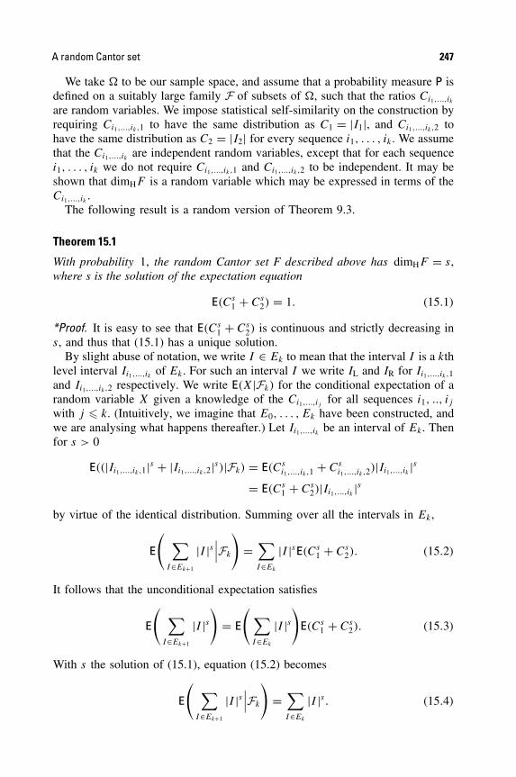
A random Cantor set 247
We take � to be our sample space, and assume that a probability measure P isdefined on a suitably large family F of subsets of �, such that the ratios Ci1,...,ik
are random variables. We impose statistical self-similarity on the construction byrequiring Ci1,...,ik,1 to have the same distribution as C1 = |I1|, and Ci1,...,ik,2 tohave the same distribution as C2 = |I2| for every sequence i1, . . . , ik . We assumethat the Ci1,...,ik are independent random variables, except that for each sequencei1, . . . , ik we do not require Ci1,...,ik ,1 and Ci1,...,ik,2 to be independent. It may beshown that dimHF is a random variable which may be expressed in terms of theCi1,...,ik .
The following result is a random version of Theorem 9.3.
Theorem 15.1
With probability 1, the random Cantor set F described above has dimHF = s,where s is the solution of the expectation equation
E(Cs1 + Cs
2) = 1. (15.1)
*Proof. It is easy to see that E(Cs1 + Cs
2) is continuous and strictly decreasing ins, and thus that (15.1) has a unique solution.
By slight abuse of notation, we write I ∈ Ek to mean that the interval I is a kthlevel interval Ii1,...,ik of Ek. For such an interval I we write IL and IR for Ii1,...,ik,1
and Ii1,...,ik,2 respectively. We write E(X|Fk) for the conditional expectation of arandom variable X given a knowledge of the Ci1,...,ij for all sequences i1, .., ijwith j � k. (Intuitively, we imagine that E0, . . . , Ek have been constructed, andwe are analysing what happens thereafter.) Let Ii1,...,ik be an interval of Ek. Thenfor s > 0
E((|Ii1,...,ik ,1|s + |Ii1,...,ik ,2|s)|Fk) = E(Csi1,...,ik,1 + Cs
i1,...,ik ,2)|Ii1,...,ik |s= E(Cs
1 + Cs2)|Ii1,...,ik |s
by virtue of the identical distribution. Summing over all the intervals in Ek,
E
(∑
I∈Ek+1
|I |s∣∣∣Fk
)
=∑
I∈Ek
|I |sE(Cs1 + Cs
2). (15.2)
It follows that the unconditional expectation satisfies
E
(∑
I∈Ek+1
|I |s)
= E
(∑
I∈Ek
|I |s)
E(Cs1 + Cs
2). (15.3)
With s the solution of (15.1), equation (15.2) becomes
E
(∑
I∈Ek+1
|I |s∣∣∣Fk
)
=∑
I∈Ek
|I |s . (15.4)
248 Random fractals
Readers familiar with probability theory will recognize (15.4) as saying that thesequence of random variables
Xk =∑
I∈Ek
|I |s (15.5)
is a martingale with respect to Fk . Moreover, a routine calculation, see Exercise15.7, shows that it is an L2-bounded martingale, that is there is a number c suchthat E(X2
k) � c for all k. The crucial fact for our purposes, which we ask otherreaders to take on trust, is that, in this situation, Xk converges with probability1 as k → ∞ to a random variable X such that E(X) = E(X0) = E(1s) = 1. Inparticular 0 � X < ∞ with probability 1, and X = 0 with probability q < 1.But X = 0 if and only if
∑I∈Ek∩I1
|I |s and∑
I∈Ek∩I2|I |s both converge to 0 as
k → ∞, where I1 and I2 are the intervals of E1, and this happens with probabilityq2, by virtue of the self-similarity of the construction. Hence q = q2, so q = 0,and we conclude that 0 < X < ∞ with probability 1. In particular, this impliesthat with probability 1 there are (random) numbers M1, M2 such that
0 < M1 � Xk =∑
I∈Ek
|I |s � M2 < ∞ (15.6)
for all k. We have |I | � 2−k for all I ∈ Ek, so, Hsδ(F ) �
∑I∈Ek
|I |s � M2 ifk � − log δ/ log 2, giving Hs(F ) � M2. Thus dimHF � s with probability 1.
We use the potential theoretic method of Section 4.3 to derive the almost surelower bound for dimHF . To do this we introduce a random mass distribution µ onthe random set F . Let s satisfy (15.1). For I ∈ Ek let µ(I) be the random variable
µ(I) = limj→∞
{∑|J |s : J ∈ Ej and J ⊂ I
}.
As with (15.5) this limit exists, and 0 < µ(I) < ∞ with probability 1. Further-more, if I ∈ Ek,
E(µ(I)|Fk) = |I |s . (15.7)
If I ∈ Ek then µ(I) = µ(IL) + µ(IR) so µ is additive on the kth level sets for allk, and so, µ extends to a mass distribution with support contained in
⋂∞k=0 Ek =
F , see Proposition 1.7. (We ignore measure theoretic questions connected withthe definition of µ.)
We fix 0 < t < s and estimate the expectation of the t-energy of µ. If x, y ∈ F ,there is a greatest integer k such that x and y belong to a common kth levelinterval; denote this interval by x ∧ y. If I is a kth level interval, its (k + 1)thlevel subintervals IL and IR are separated by a gap of at least d|I |, where d =1 − 2b. Thus
∫∫
x∧y=I
|x − y|−tdµ(x)dµ(y) = 2∫
x∈IL
∫
y∈IR
|x − y|−tdµ(x)dµ(y)
� 2d−t |I |−tµ(IL)µ(IR).
A random Cantor set 249
If I ∈ Ek,
E(∫∫
x∧y=I
|x − y|−tdµ(x)dµ(y)
∣∣∣Fk+1
)
� 2d−t |I |−tE(µ(IL)|Fk+1)E(µ(IR)|Fk+1)
� 2d−t |I |−t |IL|s |IR|s� 2d−t |I |2s−t
using (15.7). Using a variation of (1.21) this gives an inequality for the uncon-ditional expectation
E(∫∫
x∧y=I
|x − y|−tdµ(x)dµ(y)
)� 2d−tE(|I |2s−t ).
Summing over I ∈ Ek,
E
(∑
I∈Ek
∫∫
x∧y=I
|x − y|−tdµ(x)dµ(y)
)
� 2d−tE
(∑
I∈Ek
|I |2s−t
)
= 2d−tλk
where λ = E(C2s−t1 + C2s−t
2 ) < 1, using (15.3) repeatedly. Then
E(∫
F
∫
F
|x − y|−tdµ(x)dµ(y)
)= E
( ∞∑
k=0
∑
I∈Ek
∫∫
x∧y=I
|x − y|−tdµ(x)dµ(y)
)
� 2d−t
∞∑
k=0
λk < ∞,
so that the t-energy of µ is finite, with probability 1. As we have noted,0 < µ(F) = µ([0, 1]) < ∞ with probability 1, so dimHF � t by Theo-rem 4.13(a). �
Note that the proof of Theorem 15.1 is typical of many random models, inthat the key to both upper and lower estimates is the estimation of the momentsE( ∑
I∈Ek|I |t) for certain t .
This theorem and proof generalize in many directions. Each interval in Ek
might give rise to a random number of intervals of random lengths in Ek+1. Ofcourse, the construction generalizes to �n, and the separation condition betweendifferent component intervals can be relaxed, provided some sort of ‘open setcondition’ (see (9.11)) is satisfied. The following construction is a full randomanalogue of the sets discussed in Section 9.2.
Let V be an open subset of �n with closure V , let m � 2 be an integer, andlet 0 < b < 1. We take � to be the class of all decreasing sequences V = E0 ⊃

250 Random fractals
E1 ⊃ E2 ⊃ · · · of closed sets satisfying the following conditions. The set Ek is aunion of the mk closed sets V i1,...,ik where ij = 1, . . . , m (1 � j � k) and Vi1,...,ik
is either similar to V or is the empty set.We assume that, for each i1, . . . , ik , the set Vi1,...,ik contains Vi1,...,ik ,i (1 � i � m)
and that these sets are disjoint; this is, essentially, equivalent to the open setcondition. If Vi1,...,ik is non-empty, we write Ci1,...,ik = |Vi1,...,ik |/|Vi1,...,ik−1 | for thesimilarity ratio between successive sets and we take Ci1,...,ik = 0 if Vi1,...,ik is theempty set. We define the random self-similar set F = ⋂∞
k=0 Ek.Let P be a probability measure on a family of subsets of � such that the Ci1,...,ik
are random variables. Suppose that given Ci1,...,ik > 0, i.e. given that Vi1,...,ik isnon-empty, Ci1,...,ik ,i has identical distribution to Ci for each sequence i1, . . . , ikand for 1 � i � m. We assume that the Ci1,...,ik are independent, except that,for each sequence i1, . . . , ik , the random variables Ci1,...,ik ,1, . . . , Ci1,...,ik ,m neednot be independent. This defines a self-similar probability distribution on theconstructions in �. We write N for the (random) number of the C1, . . . , Ck thatare positive; that is, the number of the sets V1, . . . , Vk that are non-empty.
Theorem 15.2
The random set F described above has probability q of being empty, where t = q
is the smallest non-negative solution to the polynomial equation
f (t) ≡m∑
j=0
P(N = j)tj = t. (15.8)
With probability 1 − q the set F has Hausdorff and box dimensions given by thesolution s of
E
(m∑
j=0
Csi
)
= 1. (15.9)
*Note on proof. Basically, this is a combination of the probabilistic argument ofTheorem 15.1 and the geometric argument of Theorem 9.3. Note that, if there isa positive probability that N = 0, then there is a positive probability that E1 = Øand therefore that F = Ø. This ‘extinction’ occurs if each of the basic sets inE1 becomes extinct. By the self-similarity of the process, the probability q0 ofthis happening is f (q0), so q0 = f (q0). If q is the least non-negative solutionof f (q) = q, then, using that f is increasing, an inductive argument showsthat P(Ek = Ø) = f (P(Ek−1 = Ø)) � f (q) = q for all k, so that q0 � q. Thusq0 = q.
Observe that F has probability 0 of being empty, i.e. q = 0, if and only if N �1 with probability 1. It is also not hard to show that F is empty with probability1, i.e. q = 1, if and only if either E(N) < 1 or E(N) = 1 and P(N = 1) < 1.(These extinction probabilities are closely related to the theory of branchingprocesses.) �

Fractal percolation 251
Example 15.3. Random von Koch curve
Let C be a random variable with uniform distribution on the interval (0, 13 ). Let
E0 be a unit line segment in �2. We form E1 by removing a proportion C fromthe middle of E0 and replacing it by the other two sides of an equilateral trianglebased on the removed interval. We repeat this for each of the four segments inE1 independently and continue in this way to get a limiting curve F. Then withprobability 1, dimHF = dimBF = 1.144 . . . .
Calculation. This is a special case of Theorem 15.2. The set V may be taken asthe isosceles triangle based on E0 and of height 1
6
√3. At each stage, a segment
of length L is replaced by four segments of lengths 12 (1 − C)L, CL, CL and
12 (1 − C)L, so we have m = 4 and C1 = C4 = 1
2 (1 − C) and C2 = C3 = C.Since C is uniformly distributed on (0, 1
3 ), expression (15.9) becomes
1 = E(2( 1
2 (1 − C))s + 2Cs) =
∫ 1/3
03 × 2[
(12 (1 − c)
)s + cs] dc
ors + 1 = 12 × 2−(s+1) − 6 × 3−(s+1)
giving the dimension stated. �
15.2 Fractal percolation
Random fractals can have complicated topological structure, for example they canbe highly multiply connected. We consider topological aspects of a statisticallyself-similar construction known as ‘fractal percolation’. In particular, this exhibitsa ‘phase transition’, where the topological structure changes dramatically whena continuously varying parameter increases through a critical value.
Let p be a number with 0 < p < 1. We divide the unit square E0 into 9squares of side 1
3 in the obvious way. We select a subset of these squares toform E1 in such a way that each square has independent probability p of beingselected. Similarly, each square of E1 is divided into 9 squares of side 1
9 , andeach of these has independent probability p of being chosen to be a square ofE2. We continue in this way, so that Ek is a random collection of kth levelsquares of side 3−k . This procedure, which depends on the parameter p, definesa random fractal Fp = ⋂∞
k=0 Ek; see figures 15.4 and 15.5. (It is not difficult todescribe this construction in precise probabilistic terms; for example, by takingthe possible nested sequences of squares Ek as the sample space.)
Proposition 15.4
Given p, let t = q be the least positive solution of the equation
t = (pt + 1 − p)9.

252 Random fractals
Then Fp is empty with probability q. If p � 19 then q = 1. If 1
9 < p < 1 then0 < q < 1 and, with probability 1 − q, dimHFp = dimBFp = log 9p/ log 3.
Proof. Let N be the (random) number of squares in E1. Then P(N = j) =(9j
)pj(1 − p)9−j , where
(n
r
)= n!
r!(n − r)!is the binomial coefficient, so the
probability that Fp = Ø is, by (15.8), the smallest positive solution of
t =9∑
j=0
(9j
)pj(1 − p)9−j tj = (pt + 1 − p)9.
Each square of E1 has side 13 , so (15.9) becomes
1 = E
(N∑
j=0
Csi
)
= E
(N∑
j=0
3−s
)
= 3−sE(N) = 3−s9p
(each of the nine squares of side 13 is selected with probability p, so the expected
number chosen is 9p). Thus by Theorem 15.2, the almost sure dimension of Fp,given it is non-empty, is log 9p/ log 3. �
We now discuss briefly the qualitative way in which the random set Fp changesas p increases from 0 to 1. We have already noted that Fp is almost surely empty
E0 E1
E2 E3
Figure 15.4 Steps in the construction of the random fractal discussed in Section 15.2with p = 0.6. The fractal obtained is shown in figure 15.5(a)

Fractal percolation 253
(a)
(b)
Figure 15.5 Random fractals realized by the percolation process discussed in Section 15.2with (a) p = 0.6 and (b) p = 0.8
254 Random fractals
if 0 < p � 19 . If 1
9 < p < 13 we have, with probability 1, that either Fp = Ø or
dimHFp = log 9p/ log 3 < 1, so by Proposition 2.5 Fp is totally disconnected. Atthe other extreme, if p is close to 1, it is plausible that such a high proportion ofthe squares are retained at each stage of the construction that Fp will connect theleft and right sides of the square E0; when this happens we say that percolationoccurs between the sides. We show that this is the case at least if p is very closeto 1; the ridiculous bound 0.999 obtained can certainly be reduced considerably.
Proposition 15.5
Suppose that 0.999 < p < 1. Then there is a positive probability (in fact biggerthan 0.9999) that the random fractal Fp joins the left and right sides of E0.
*Proof. The proof depends on the observation that if I1 and I2 are abutting squaresin Ek and both I1 and I2 contain either 8 or 9 subsquares of Ek+1, then there isa subsquare in I1 and one in I2 that abut, so that the squares of Ek+1 in I1 andI2 form a connected unit.
We say that a square of Ek is full if it contains either 8 or 9 squares of Ek+1.We say that a square of Ek is 2-full if it contains 8 or 9 full squares of Ek+1,and, inductively, that a square of Ek is m-full if it contains either 8 or 9 squaresof Ek+1 that are (m − 1)-full. By the above remark, if E0 is m-full, then oppositesides of E0 are joined by a sequence of abutting squares of Em.
The square E0 is m-full (m � 1) if either
(a) E1 contains 9 squares all of which are (m − 1)-full, or(b) E1 contains 9 squares of which 8 are (m − 1)-full, or(c) E1 contains 8 squares all of which are (m − 1)-full.
Thus, if pm is the probability that E0 is m-full, we get, summing the proba-bilities of these three alternatives using (1.16), and using the self-similarity ofthe process,
pm = p9p9m−1 + p99p8
m−1(1 − pm−1) + 9p8(1 − p)p8m−1
= 9p8p8m−1 − 8p9p9
m−1 (15.10)
if m � 2. Furthermore, p1 = p9 + 9p8(1 − p) = 9p8 − 8p9, so we have a dis-crete dynamical system defined by pm = f (pm−1) for m � 1, where p0 = 1 and
f (t) = 9p8t8 − 8p9t9. (15.11)
Suppose that p = 0.999. Then (15.11) becomes
f (t) = 8.928 2515t8 − 7.928 2874t9
Notes and references 255
and a little calculation shows that t0 = 0.999 9613 is a fixed point of f whichis stable in the sense that 0 < f (t) − t0 � 1
2 (t − t0) if t0 < t � 1. It follows thatpm is decreasing and converges to t0 as m → ∞, so there is a probability t0 > 0that E0 is m-full for all m. When this happens, opposite sides of E0 are joinedby a sequence of squares in Em for each m, so the intersection F = ⋂∞
k=0 Ek
joins opposite sides of E0. Thus, there is a positive probability of percolationoccurring if p = 0.999, and consequently for larger values of p. �
We have seen that if 0 < p < 13 then, with probability 1, Fp is empty or totally
disconnected. On the other hand, if p > 0.999 then there is a high probability ofpercolation. The next theorem states that one or other of these situations pertainsfor each value of p.
Theorem 15.6
There is a critical number pc with 0.333 < pc < 0.999 such that if 0 < p < pc
then Fp is totally disconnected with probability 1, but if pc < p < 1 then thereis positive probability that Fp connects the left and right sides of E0.
Idea of proof. Suppose p is such that there is a positive probability of Fp notbeing totally disconnected. Then there is positive probability of some two distinctpoints of F being joined by a path in F . This implies that there is a positiveprobability of the path passing through opposite sides of one of the squares in Ek
for some k; by virtue of the statistical self-similarity of the construction, thereis a positive probability of a path crossing E0 from left to right. Clearly, if Fp
has probability 1 of being totally disconnected, the same is true of Fp′ if p′ < p.Thus the critical probability pc is the supremum of those p such that Fp is totallydisconnected, and has the properties stated. �
Experiment suggests that 0.7 < pc < 0.8.The change in form of Fp as p increases through pc is even more dramatic
than Theorem 15.6 suggests. Let F ′p be a random set obtained by tiling the
plane with independent random copies of Fp. If p < pc then, almost surely, F ′p
is totally disconnected. However, if p � pc then, with probability 1, F ′p has a
single unbounded connected component. Thus as p increases through pc there isa ‘phase transition’ as the isolated points of F ′
p suddenly coalesce to form whatis basically a single unit. The idea underlying the proof of this is that, if p > pc,then given that parts of F ′
p lie in two disjoint discs of unit radius, there is apositive probability of them being joined by a path in F ′
p. There are infinitelymany such discs in an unbounded component of F ′
p, so if F ′p had two unbounded
components, there would be probability 1 of them being joined.
15.3 Notes and references
Various versions of the random fractal constructions of the type discussedin Section 15.1 are presented in Mandelbrot (1974, 1982), Kahane (1974),
256 Random fractals
Peyriere (1974), Falconer (1986b), Mauldin and Williams (1986a), Graf(1987), Graf, Mauldin and Williams (1988), Olsen (1994) and Hutchinson andRuschendorf (2000).
An interesting construction for fractals by random deletion was introduced byMandelbrot (1972); see also Kahane (1985), Zahle (1984) and Falconer (1997).For other applications of probability to fractals, see Stoyan and Stoyan (1994)and Falconer (1997).
The fractal percolation model was suggested by Mandelbrot (1974). Chayes,Chayes and Durrett (1988) analysed the phase transition in detail, and Dekkingand Meester (1990) highlighted other phase transitions of the model. Chayes(1995) gives a clear survey on fractal percolation and its generalizations.
Much has been written on ‘discrete’ percolation, where points are selected atrandom from a large square mesh (see Kesten (1982) and Grimmett (1999)), andthere are many relationships between this and the fractal case.
Exercises
15.1 Find the almost sure Hausdorff dimension of the random Cantor set constructedby removing the middle third of each interval with probability 1
2 and the middletwo-thirds of the interval with probability 1
2 at each step of the construction.
15.2 Consider the following random version of the von Koch construction. We start witha unit segment. With probability 1
2 we replace the middle third of the segment by theother two sides of the (upwards pointing) equilateral triangle, and with probability 1
2we remove the middle third altogether. We repeat this procedure with the segmentsthat remain, in the usual way. Show that, with probability 1, this random fractal hasHausdorff dimension 1.
15.3 Show that the random von Koch curve depicted in figure 15.1 always has Hausdorffdimension s = log 4/ log 3 and, indeed, is an s-set. (This is not typical of randomconstructions.)
15.4 Let 0 < p < 1. We may randomize the construction of the Sierpinski gasket(figure 0.3) by selecting each of the three equilateral subtriangles independentlywith probability p at each step. (Thus we have a percolation process based onthe Sierpinski gasket.) Show that if p � 2
3 then the limiting set F is empty withprobability 1, but if 2
3 < p < 1 then there is a positive probability that F is non-empty. Find an expression for this probability, and show that, given F is non-empty,dimHF = log 3p/ log 2 with probability 1.
15.5 For the random Sierpinski gasket described in Exercise 15.4 show that F is totallydisconnected with probability 1 for every p < 1. (We regard two triangles as beingjoined if they touch at a vertex.)
15.6 Consider the random Cantor set analysed in Theorem 15.1. With Hs∞(F ) denotingthe infimum of the sums in (2.1) over arbitrary coverings of F , show that
Hs∞(F ) = min{1,Hs
∞(F ∩ I1) + Hs∞(F ∩ I2)}
where s is the solution of (15.1). Use statistical self-similarity to deduce that, unlessP(Cs
1 + Cs2 = 1) = 1, then, almost surely, Hs∞(F ) = 0, and thus Hs (F ) = 0.
Exercises 257
15.7 Show that the martingale Xk given by (15.5) is L2-bounded, that is E(X2k ) � m for
all k, for some number m. (Hint: Show that E(X2k+1|Fk) � X2
k + aγ k where γ =E(C2s
1 + C2s2 ) < 1 and a is a constant, and then take unconditional expectations.)
15.8 Consider the fractal percolation model F constructed with selection probabilityp, where pc < p < 1. Show that with probability 1, either F = Ø or F containsinfinitely many non-trivial connected components. (Here non-trivial means contain-ing at least two distinct points.)
Chapter 16 Brownian motion andBrownian surfaces
In 1827 the botanist R. Brown noticed that minute particles suspended in a liquidmoved on highly irregular trails. This, and a similar phenomenon for smoke par-ticles in air, was explained ultimately as resulting from molecular bombardmentof the particles. Einstein published a mathematical study of this motion, whicheventually led to Perrin’s Nobel Prize-winning calculation of Avogadro’s number.
In 1923 Wiener proposed a rigorous mathematical model that exhibited randombehaviour similar to that observed in Brownian motion. The paths described bythis ‘Wiener process’ in 3-dimensional space are so irregular as to have Hausdorffdimension equal to 2. This is a good example of a natural phenomenon with afractal appearance that can be explained by a simple mathematical model.
A trail may be described by a function f : � → �n where f (t) is the positionof a particle at time t . We can study f from two differing viewpoints. Eitherwe can think of the trail or image f ([t1, t2]) = {f (t) : t1 � t � t2} as a subsetof �n with t regarded merely as a parameter, or we can consider the graph off , graph f = {(t, f (t)) : t1 � t � t2} ⊂ �n+1, as a record of the variation of f
with time. Brownian trails and their graphs are, in general, fractals.In this chapter, our aim is to define a probability measure on a space of func-
tions, such that the trails likely to occur resemble observed Brownian motion.We begin by investigating the fractal form of classical Brownian motion, andthen we examine some variants that have been used to model a wide varietyof phenomena, including polymer chains, stock market prices and topographi-cal surfaces.
16.1 Brownian motion
We first define Brownian motion in one dimension, and then extend the definitionto the higher-dimensional cases.
To motivate the definition, let us consider a particle performing a random walkon the real line. Suppose at small time intervals τ the particle jumps a small dis-tance δ, randomly to the left or to the right. (This might be a reasonable descrip-tion of a particle undergoing random molecular bombardment in one dimension.)
258
Fractal Geometry: Mathematical Foundations and Application. Second Edition Kenneth Falconer 2003 John Wiley & Sons, Ltd ISBNs: 0-470-84861-8 (HB); 0-470-84862-6 (PB)

Brownian motion 259
Let Xτ (t) denote the position of the particle at time t . Then, given the positionXτ (kτ) at time kτ , the position Xτ((k + 1)τ ) at time (k + 1)τ is equally likelyto be Xτ(kτ) + δ or Xτ(kτ) − δ. Assuming that the particle starts at the origin attime 0, then for t > 0, the position at time t is described by the random variable
Xτ(t) = δ(Y1 + · · · + Y�t/τ�)
where Y1, Y2, . . . are independent random variables, each having probability 12
of equalling 1 and probability 12 of equalling −1. Here �t/τ� denotes the largest
integer less than or equal to t/τ . We normalize the step length by setting δ = √τ
so thatXτ (t) = √
τ(Y1 + · · · + Y�t/τ�). (16.1)
The central limit theorem (see (1.26)) tells us that, for fixed t , if τ is smallthen the distribution of the random variable Xτ (t) is approximately normal withmean 0 and variance τ�t/τ� � t , since the Yi have mean 0 and variance 1. In thesame way, if t and h are fixed, and τ is sufficiently small, then Xτ (t + h) − Xτ (t)
is approximately normal with mean 0 and variance h. We also note that,if 0 � t1 � t2 � · · · � t2m, then the increments Xτ(t2) − Xτ(t1), Xτ (t4) −Xτ (t3), . . . , Xτ (t2m) − Xτ(t2m−1) are independent random variables. We defineBrownian motion with the limit of the random walk Xτ (t) as τ → 0 in mind.
Let (�,F, P) be a probability space. For our purposes we call X a randomprocess or random function from [0,∞) to � if X(t) is a random variable foreach t with 0 � t < ∞. Sometimes, we consider random functions on a finiteinterval [t1, t2] instead, in which case the development is similar. (In the formaldefinition of a random process there is an additional ‘measurability’ condition,which need not concern us here.) Of course, we think of X as defining a samplefunction t �→ X(ω, t) for each point ω in the sample space �. Thus we think ofthe points of � as parametrizing the functions X : [0, ∞) → �, and we think ofP as a probability measure on this class of functions.
We define Brownian motion or the Wiener process to be a random process X
such that:
(BM) (i) with probability 1, X(0) = 0 (i.e. the process starts at the origin)and X(t) is a continuous function of t ;
(ii) for all t � 0 and h > 0 the increment X(t + h) − X(t) is normallydistributed with mean 0 and variance h, thus
P(X(t + h) − X(t) � x) = (2πh)−1/2∫ x
−∞exp
(−u2
2h
)du;
(16.2)
(iii) if 0 � t1 � t2 � · · · � t2m, the increments X(t2) − X(t1), X(t4) −X(t2), . . . , X(t2m) − X(t2m−1) are independent.
Note that it is immediate from (i) and (ii) that X(t) is itself normally distributedwith mean 0 and variance t for each t . Observe that the increments of X arestationary ; that is, X(t + h) − X(t) has distribution independent of t .
260 Brownian motion and Brownian surfaces
The first question that arises is whether there actually is a random functionsatisfying the conditions (BM). It is quite hard to show that Brownian motiondoes exist, and we do not do so here. The proof uses the special propertiesof the normal distribution. For example, given that X(t2) − X(t1) and X(t3) −X(t2) are independent and normal with means 0 and variances t2 − t1 and t3 −t2 respectively, the sum X(t3) − X(t1) is necessarily normal with mean 0 andvariance t3 − t1; see (1.24) et seq. This is essential for the definition (BM) to beself-consistent. It should at least seem plausible that a continuous process X(t)
satisfying (BM) exists, if only as a limit of the random walks Xτ (t) as τ → 0.Instead of proving existence, we mention three methods of simulating Brow-
nian sample functions, for example with a computer. Each method can, in fact,be used as a basis for existence proofs. The first method uses the random walkapproximation (16.1). Values of 1 or −1 are assigned by ‘coin tossing’ to Yi
for 1 � i � m, where m is large, and Xτ(t) is plotted accordingly. If τ is smallcompared with t , then this gives an accurate approximation to a Brownian samplefunction.
The ‘random midpoint displacement’ method may be used to obtain a samplefunction X : [0, 1] → �. We define the values of X(k2−j ) where 0 � k � 2j byinduction on j . We set X(0) = 0 and choose X(1) at random from a normaldistribution with mean 0 and variance 1. Next we select X( 1
2 ) from a normaldistribution with mean 1
2 (X(0) + X(1)) and variance 12 . At the next step X( 1
4 )
and X( 34 ) are chosen, and so on. At the j th stage the values X(k2−j ) for odd k
are chosen independently from a normal distribution with mean 12 (X((k − 1)2−j )
+ X((k + 1)2−j )) and variance 2−j . This procedure determines X(t) at all binarypoints t = k2−j . Assuming that X is continuous, then X is completely deter-mined. It may be shown, using properties of normal distributions, that the func-tions thus generated have the distribution given by (BM).
Brownian motion on [0, π] has a Fourier series representation
X(t) = 1√π
C0t +√
2
π
∞∑
k=1
Ck
sin kt
k
where the Ck have independent normal distributions of mean 0 and variance 1.Choosing the Ck at random and curtailing the series gives an approximation toa sample function. The graph of a Brownian sample function is in figure 16.1.
It is easy to extend the definition of Brownian motion from � to �n: we justdefine Brownian motion on �n so that the coordinate components are indepen-dent 1-dimensional Brownian motions. Thus X : [0,∞) → �n given by X(t) =(X1(t), . . . , Xn(t)) is an n-dimensional Brownian motion on some probabilityspace if the random process Xi(t) is a 1-dimensional Brownian motion for eachi, and X1(t1), . . . , Xn(tn) are independent for all sets of times t1, . . . , tn. A sampletrail of Brownian motion in �2 is shown in figure 16.2.
By definition, the projection of X(t) onto each of the coordinate axes is a1-dimensional Brownian motion. However, the coordinate axes are not special

Brownian motion 261
0.8
0.6
0.4
0.2
0.2 0.4 0.6 0.8 10
−0.4
−0.2
Figure 16.1 Graph of a realization of Brownian motion
in this respect: n-dimensional Brownian motion is isotropic; that is, it has thesame characteristics in every direction. To see this, consider, for convenience, thecase of 2-dimensional Brownian motion X(t) = (X1(t), X2(t)). The projectionof X(t) onto the line Lθ at angle θ through the origin is X1(t) cos θ + X2(t) sin θ .For t � 0 and h > 0 the random variables X1(t + h) − X1(t) and X2(t + h) −X2(t) are independent and normally distributed with means 0 and variances h.Thus the increments of the projection onto Lθ , given by
(X1(t + h) − X1(t)) cos θ + (X2(t + h) − X2(t)) sin θ,
are normally distributed with mean 0 and variance h cos2 θ + h sin2 θ = h; see(1.24) et seq. In a similar way, the increments of the projection are independent,so the projection of X(t) onto Lθ is 1-dimensional Brownian motion, for allangles θ .
Figure 16.2 A simulation of a Brownian trail in �2

262 Brownian motion and Brownian surfaces
If γ > 0, replacing h by γh and x by γ 1/2x does not alter the value of theright-hand side of (16.2) (by substituting u1 = uγ −1/2 in the integral). Thus
P(Xi(t + h) − Xi(t) � xi) = P(Xi(γ t + γh) − Xi(γ t) � γ 1/2xi)
for all xi . It follows that X(t) and γ −1/2X(γ t) have the same distribution. Thuschanging the temporal scale by a factor γ and the spatial scale by a factor γ 1/2
gives a process indistinguishable from the original so we term Brownian motionX(t) and its graph statistically self-affine. But we call Brownian trails statisticallyself-similar, in that the spatial distribution of the trails {X(t) : 0 � t � T } and{X(t) : 0 � t � γT } are indistinguishable except for a scale factor of γ 1/2.
Suppose that X(t) = (X1(t), . . . , Xn(t)) is n-dimensional Brownian motion.Since Xi(t + h) − Xi(t) has independent normal distribution for each i, it followsfrom (16.2) that if [ai, bi] are intervals, then
P(Xi(t + h) − Xi(t) ∈ [ai, bi]) = (2πh)−1/2∫ bi
ai
exp
(− x2
i
2h
)dxi.
Hence if E is the coordinate parallelepiped [a1, b1] × · · · × [an, bn]
P(X(t + h) − X(t) ∈ E) =n∏
i=1
[(2πh)−1/2
∫ bi
ai
exp
(− x2
i
2h
)dxi
]
= (2πh)−n/2∫
E
exp
(−|x|2
2h
)dx (16.3)
where x = (x1, . . . , xn). By approximating sets by unions of such parallelepipeds,it follows that (16.3) holds for any Borel set E. Thus, taking E as the ball B(0, ρ),and converting into polar coordinates,
P(|X(t + h) − X(t)| � ρ) = ch−n/2∫ ρ
r=0rn−1 exp
(− r2
2h
)dr (16.4)
where c = 2π−n/2an with an the (n − 1)-dimensional area of the surface ofB(0, 1).
A fundamental property of a Brownian motion is that, with probability 1, thesample functions satisfy a Holder condition of exponent λ for each λ < 1
2 .
Proposition 16.1
Suppose 0 < λ < 12 . With probability 1 the Brownian sample function
X : [0, 1] → �n satisfies
|X(t + h) − X(t)| � b|h|λ (|h| < H0) (16.5)
for some H0 > 0, where b depends only on λ.

Brownian motion 263
Proof. For h > 0 we have, by (16.4),
P(|X(t + h) − X(t)| > hλ) = ch−n/2∫ ∞
hλ
rn−1 exp
(−r2
2h
)dr
= c
∫ ∞
hλ−1/2un−1 exp
(−u2
2
)du
� c1
∫ ∞
hλ−1/2exp(−u)du
= c1 exp(−hλ−1/2)
� c2h−2 (16.6)
after a substitution u = rh−1/2 and some sweeping estimates, where c1 and c2 donot depend on h or t . Taking [t, t + h] as the binary intervals [(m − 1)2−j , m2−j ]we have
P(|X((m − 1)2−j ) − X(m2−j )| > 2−jλ for some j � k and 1 � m � 2j )
� c2
∞∑
j=k
2j 2−2j
= c22−k+1.
Thus with probability 1 there is an integer K such that
|X((m − 1)2−j ) − X(m2−j )| � 2−jλ (16.7)
for all j > K and 1 � m � 2j . If h < H0 = 2−K the interval [t, t + h] may,except possibly for the endpoints, be expressed as a countable union of contiguousbinary intervals of the form [(m − 1)2−j , m2−j ] with 2−j � h and with no morethan two intervals of any one length. (Take all the binary intervals in [t, t + h]not contained in any other such intervals.) Then, using the continuity of X, if k
is the least integer with 2−k � h,
|X(t) − X(t + h)| � 2∞∑
j=k
2−jλ = 2−kλ2
(1 − 2−λ)� 2hλ
(1 − 2−λ). �
Theorem 16.2
With probability 1, a Brownian trail in �n(n � 2) has Hausdorff dimension andbox dimension equal to 2.
Proof. For every λ < 12 , X : [0, 1] → �n satisfies a Holder condition (16.5) with
probability 1, so by Proposition 2.3, dimHX([0, 1]) � (1/λ) dimH [0, 1] < 1/λ,
264 Brownian motion and Brownian surfaces
with a similar inequality for box dimensions. Thus, almost surely, Browniantrails have dimension at most 2.
For the lower bound we use the potential theoretic method. Take 1 < s < 2.For given t and h let p(ρ) denote the expression in (16.4). Taking the expectation,it follows that
E(|X(t + h) − X(t)|−s ) =∫ ∞
0r−sdp(r)
= ch−n/2∫ ∞
0r−s+n−1 exp
(−r2
2h
)dr
= 12ch−s/2
∫ ∞
0w(n−s−2)/2 exp
(−w
2
)dw
= c1h−s/2 (16.8)
after substituting w = r2/h, where c1 is independent of h and t . Then
E(∫ 1
0
∫ 1
0|X(t) − X(u)|−sdt du
)=
∫ 1
0
∫ 1
0E(|X(t) − X(u)|−s )dt du
=∫ 1
0
∫ 1
0c1|t − u|−s/2dt du
< ∞ (16.9)
since s < 2. There is a natural way of defining a mass distribution µf on atrail f , with the mass of a set equal to the time the trail spends in the set,i.e. µf (A) = L{t : 0 � t � 1 and f (t) ∈ A} where L is Lebesgue measure. Then∫
g(x)dµf (x) = ∫ 10 g(f (t))dt for any function g, so (16.9) becomes
E(∫∫
|x − y|−sdµX(x)dµX(y)
)< ∞.
Hence if s < 2 then∫∫ |x − y|−sdµX(x)dµX(y) < ∞ with probability 1, where
µX is a mass distribution on X(t), so dimHX([0, 1]) � s by Theorem 4.13(a).�
In fact, with probability 1, Brownian trails in �n(n � 2) have 2-dimensionalHausdorff measure 0. More delicate arguments involving the finer definitionsof dimension given in Section 2.5 show that, with probability 1, the trailsX([0, 1]) have positive finite measure with respect to the function h(t) =t2 log(1/t) log log log(1/t), if n = 2, and with respect to h(t) = t2 log log(1/t),if n � 3. In this sense, Brownian trails have a dimension that is ‘logarithmicallysmaller’ than 2.
An obvious qualitative question about Brownian trails is whether they aresimple curves, or whether they are self-intersecting. Given a function f , we

Brownian motion 265
say that x is a point of multiplicity k if f (t) = x for k distinct values of t .Dimensional methods may be used to determine whether Brownian functionshave multiple points.
Theorem 16.3
With probability 1, a Brownian sample function X : [0, ∞) → �n has multiplepoints as follows:n = 2: there are points of multiplicity k for every positive integer k ;n = 3: there are double points but no triple points;n � 4: there are no multiple points.
Idea of proof. One approach is to use the intersection theorems of Chapter 8.For the case n = 3, suppose that dimH(X([0, 1]) ∩ X([2, 3])) < 1 with prob-ability 1. Using isotropy and scaling of Brownian motion it is not difficultto see that this implies that dimH(X([0, 1]) ∩ σ(X([2, 3]))) < 1 with proba-bility 1 for any similarity transformation σ . It follows that, with probability1, dimH(X([0, 1]) ∩ σ(X([2, 3]))) < 1 for almost all similarities σ . Since, byTheorem 16.2, dimH X([0, 1]) = dimBX([0, 1]) = 2 with probability 1, this con-tradicts Theorem 8.2(a), and we conclude that dimH(X([0, 1]) ∩ X([2, 3])) = 1with positive probability p, say. Using the statistical self-similarity of X(t) itfollows that dimH(X([t, t + δ]) ∩ X([t + 2δ, t + 3δ])) = 1 with probability p forevery t and δ, so, since the increments are independent, the set of double pointshas Hausdorff dimension 1 with probability 1.
Similar techniques may be used to prove the other results. �
The derivation of the almost sure dimension of Brownian graphs is similar tothat for Brownian trails.
Theorem 16.4
With probability 1, the graph of a Brownian sample function X : [0, 1] → � hasHausdorff and box dimension 1 1
2 .
Proof. From the Holder condition (16.5) and Corollary 11.2(a) it is clear that,with probability 1, graph X has Hausdorff dimension and upper box dimensionat most 2 − λ for every λ < 1
2 , so has dimensions at most 1 12 . For the lower
estimate, as in the proof of Theorem 16.2,
E((|X(t + h) − X(t)|2 + h2)−s/2) =∫ ∞
0(r2 + h2)−s/2dp(r)
= ch−1/2∫ ∞
0(r2 + h2)−s/2 exp
(−r2
2h
)dr
= 12c
∫ ∞
0(wh + h2)−s/2w−1/2 exp
(−w
2
)dw

266 Brownian motion and Brownian surfaces
� 12c
∫ h
0(h2)−s/2w−1/2dw
+ 12c
∫ ∞
h
(wh)−s/2w−1/2dw
� c1h1/2−s
on splitting the range of integration and estimating the integral in two ways.We may lift Lebesgue measure from the t-axis to get a mass distribution µf onthe graph of a function f given by µf (A) = L{t : 0 � t � 1 and (t, f (t)) ∈ A}.Using Pythagoras’ Theorem,
E(∫∫
|x − y|−sdµX(x)dµX(y)
)
=∫ 1
0
∫ 1
0E((|X(t) − X(u)|2 + |t − u|2)−s/2)dt du
�∫ 1
0
∫ 1
0c1|t − u|1/2−sdt du
< ∞if s < 1 1
2 . With probability 1, the mass distribution µX on graph X is posi-tive and finite and has finite s-energy, so Theorem 4.13(a) gives dimHgraph X
� 1 12 . �
Since, with probability 1, the graph of X over any interval has dimension 1 12 ,
it is immediate that Brownian functions, though continuous, are not continu-ously differentiable. In fact, with probability 1, a Brownian function is nowheredifferentiable.
As with Brownian trails, Brownian graphs have dimension logarithmicallysmaller than 1 1
2 : with probability 1, the graph of X over the range [0, 1] haspositive finite measure with respect to the function h(t) = t3/2 log log(1/t).
The sets of times at which a Brownian sample function takes particular valuesare often of interest. If f : [0, 1] → � is a function, we define the level setsf −1(c) = {t : f (t) = c} for each value of c. The level sets are, essentially, theintersections of the graph of f with lines parallel to the t-axis.
Proposition 16.5
With probability 1, a Brownian sample function X : [0, 1] → � satisfiesdimHX−1(c) � 1
2 for almost all c (in the sense of 1-dimensional Lebesguemeasure). Moreover, for any given c, dimHX−1(c) = 1
2 with positive probability.
Note on proof. With probability 1, we must have dimHX−1(c) = dimH((graph X)∩Lc) � 1
2 for almost all c, where Lc is the line y = c; otherwise Corollary 7.10would imply that dimH graph X > 1 1
2 , contradicting Theorem 16.4.

Fractional Brownian motion 267
It is much harder to show that dimHX−1(c) = 12 with positive probability. The
argument is not unlike that indicated for the proof of Theorem 8.2. �
16.2 Fractional Brownian motion
Brownian motion, although of central theoretical importance, is, for many pur-poses, too restrictive. The graph of a Brownian sample function has dimension 1 1
2almost surely but random functions with graphs of other dimensions are requiredfor a variety of modelling purposes.
Brownian motion X : [0, ∞) → � is a Gaussian process. This means that for0 � t1 � t2 � · · · � tm and scalars λ1, . . . , λm, the random variable λ1X(t1) +· · · + λmX(tm) is normal (we say that (X(t1), . . . , X(tm)) is multivariate normal ).In fact Brownian motion is the unique probability distribution on functions whichhas independent increments that are stationary and of finite variance. To obtainsample functions with different characteristics it is necessary to relax one or moreof these conditions.
There are two usual variations. Fractional Brownian motion has incrementswhich are normally distributed but no longer independent. Levy processes, onthe other hand, dispense with the normal distribution condition and this can leadto discontinuous functions. For simplicity, we just discuss these processes inthe 1-dimensional case; analogous processes may be defined taking values inn-dimensional space.
Fractional Brownian motion of index-α (0 < α < 1) is defined to be a Gaussianprocess X : [0,∞) → � on some probability space such that:
(FBM) (i) with probability 1, X(t) is continuous and X(0) = 0;(ii) for every t � 0 and h > 0 the increment X(t + h) − X(t) has
the normal distribution with mean zero and variance h2α , so that
P(X(t + h) − X(t) � x) = (2π)−1/2h−α
∫ x
−∞exp(−u2/2h2α)du.
(16.10)
It may be shown that, for 0 < α < 1, a process satisfying (FBM) exists.Figure 16.3 shows graphs of fractional Brownian motion for various α.
It is implicit in the above definition that the increments X(t + h) − X(t) arestationary; that is, they have probability distribution independent of t . How-ever, the distribution of functions specified by (FBM) cannot have independentincrements except in the Brownian case of α = 1
2 . By conditions (i) and (ii),E(X(t)2) = t2α and
E((X(t + h) − X(t))2) = h2α
from whichE(X(t)X(t + h)) = 1
2 [t2α + (t + h)2α − h2α]

268 Brownian motion and Brownian surfaces
so that
E(X(t)(X(t + h) − X(t))) = 12 [(t + h)2α − t2α − h2α] (16.11)
which is non-zero if α �= 12 . Hence E((X(t) − X(0))(X(t + h) − X(t))) is posi-
tive or negative according to whether α > 12 or α < 1
2 . Thus, the increments arenot independent—if α > 1
2 then X(t) − X(0) and X(t + h) − X(t) tend to be ofthe same sign, so that X(t) tends to increase in the future if it has had an increas-ing history. Similarly, if α < 1
2 then X(t) − X(0) and X(t + h) − X(t) tend tobe of opposite sign. Note also that (16.10) implies that the process is self-affine,that is the scaled paths γ −αX(γ t) have the same statistical distribution as X(t)
for γ > 0.The almost sure dimension of fractional Brownian graphs may be determined
in a similar way to the strict Brownian case.
Proposition 16.6
Suppose 0 < λ < α. With probability 1, an index-α Brownian sample functionX : [0, 1] → � satisfies
|X(t + h) − X(t)| � b|h|λ (16.12)
if |h| < H0, for some H0 > 0 and b > 0.
Note on proof. Provided that λ < 12 , the proof goes through as in Proposition
16.1, using (16.10) instead of (16.4). However, if α > λ � 12 this leads to an
estimate c2h1/2−α in place of (16.6) and rather more sophisticated techniques
from probability theory are required to show that the Holder condition (16.12) isvalid uniformly for all t . �
Theorem 16.7
With probability 1 the graph of an index-α Brownian sample function X : [0, 1] →� has Hausdorff and box dimensions 2 − α.
Proof. Corollary 11.2(a) together with the Holder condition (16.12) show thatthe dimension is almost surely at most 2 − α. The lower bound is obtained as inTheorem 16.4 using the probability distribution (16.10). �
The autocorrelation theory discussed in Section 11.2 may be applied to frac-tional Brownian functions. It is convenient to assume that X is defined for alltime, i.e. X : (−∞, ∞) → �. This requires only trivial modification to the defi-nition (FBM). Since the variance E(|X(t + h) − X(t)|2) tends to infinity with h,we have
limT →∞ E
(1
2T
∫ T
−T
X(t)2dt
)= ∞

Fractional Brownian motion 269
3210
−1−2−3
6
4
2
0−2
−4
−610
5
0
−5
−10
20
10
605040302010
0
0
−10
−20
0 50 100 150 200 250
a = 0.1
a = 0.3
a = 0.5
a = 0.7
a = 0.9
Figure 16.3 Realizations of index-α fractional Brownian for α = 0.1, 0.3, 0.5, 0.7, 0.9
so the sample functions tend to have an infinite mean square. Nevertheless,
E(
1
2T
∫ T
−T
(X(t + h) − X(t))2dt
)= 1
2T
∫ T
−T
E(X(t + h) − X(t))2dt = h2α
It may be deduced that ‘on average’ the sample functions satisfy
1
2T
∫ T
−T
(X(t + h) − X(t))2dt � ch2α
270 Brownian motion and Brownian surfaces
and, according to (11.18) and (11.19), this does indeed correspond to a graph ofdimension 2 − α. Taking this parallel further, we might expect X(t) to have apower spectrum (11.15) approximately 1/ω1+2α .
Simulation of fractional Brownian motion is much more awkward than Brow-nian motion, because the increments are not independent. However, with moderncomputing power, exact simulation is possible. To get a realization of index-αfractional Brownian motion X at points t1, . . . , tk , we recall that the covariancesof X are given by the covariance matrix
Ai,j = E(X(ti )X(tj )) = 12 (|ti |2α + |tj |2α − |ti − tj |2α).
Then, if M is a matrix such that MMT = A, where T denotes transpose, andV = (V1, . . . , Vk) is a vector of independent random variables with normal dis-tribution of mean 0 and variance 1, X = X(ti) = MV has the distribution ofindex-α fractional Brownian motion at the points ti . To see this we check thecovariances, using matrix notation:
E(X(ti )X(tj )) = E(XXT ) = E(MV (MV )T )
= E(MV V T MT ) = ME(V V T )MT = MIMT = A.
Thus, by drawing a sequence of independent normally distributed random num-bers for the Vi , the product X = MV gives a realization of index-α fractionalBrownian motion. Finding a matrix M such that A has ‘Choleski decomposi-tion’ A = MMT is computationally intensive if k is large, and there are variousnumerical approaches to facilitate this.
An alternative method of constructing functions with characteristics similarto index-α Brownian functions is to randomize the Weierstrass function (11.4).Consider the random function
X(t) =∞∑
k=1
Ckλ−αk sin (λkt + Ak) (16.13)
where λ > 1 and where the Ck are independent random variables with the normaldistribution of zero mean and variance one, and the ‘phases’ Ak are independent,each having the uniform distribution on [0, 2π). Clearly E(X(t + h) − X(t)) = 0.Furthermore, using the formula for the difference of two sines,
E(X(t + h) − X(t))2 = E
( ∞∑
k=1
Ckλ−αk2 sin ( 1
2λkh) cos (λk(t + 12h) + Ak)
)2
= 2∞∑
k=1
λ−2αk sin2 ( 12λkh)
Levy stable processes 271
using that E(CkCj ) = 1 or 0 according as to whether k = j or not, and that themean of cos2(a + Ak) is 1
2 . Choosing N so that λ−(N+1) � h < λ−N , gives
E(X(t + h) − X(t))2 � 12
N∑
k=1
λ−2αkλ2kh2 + 2∞∑
k=N+1
λ−2αk
� cλ−2αN
� ch2α
in the sense that 0 < c1 � E(X(t + h) − X(t))2/h2α � c2 < ∞ for h < 1. Thus(16.13) has certain statistical characteristics resembling index-α fractional Brow-nian motion, and provides a usable method for drawing random graphs of variousdimensions. Such functions are often used in fractal modelling. A value ofα = 0.8, corresponding to a graph of dimension 1.2, is about right for a ‘mountainskyline’.
As might be expected, the level sets of index-α Brownian sample functionsare typically of dimension 1 − α. Proposition 16.5 generalizes to give that,with probability 1, dimHX−1(c) � 1 − α for almost all c, and that, for givenc, dimHX−1(c) = 1 − α with positive probability.
A further generalization of fractional Brownian motion is multifractionalBrownian motion, which looks and behaves like index-α(t) fractional Brownianmotion close to t , where α : [0, ∞) → (0, 1) is a given continuous function.
16.3 Levy stable processes
An alternative generalization of Brownian motion gives the Levy stable processes.A Levy process is a random function X : [0, ∞) → � such that the incrementsX(t + h) − X(t) are stationary, i.e. with distribution depending only on h, andindependent, i.e. with X(t2) − X(t1), . . . , X(t2m) − X(t2m−1) independent if 0 �t1 � t2 · · · � t2m. However, except in very special cases such as Brownian motion,Levy processes have infinite variance and are discontinuous with probability 1.A Levy process is stable if a self-affinity condition holds, that is γ −1/αX(γ t)
and X(t) have the same distribution for all γ > 0, and some α.It is not, in general, possible to specify the probability distribution of stable
processes directly. Fourier transforms are usually used to define such distribu-tions, and analysis of the dimensions of graphs and trails of stable processesrequires Fourier transform methods.
The probability distribution of a random variable Y may be specified by itscharacteristic function, i.e. the Fourier transform E(exp(iuY )) for u ∈ �. Todefine a stable process, we take a suitable function ψ : � → � and require thatthe increments X(t + h) − X(t) satisfy
E(exp(iu(X(t + h) − X(t)))) = exp(−hψ(u)) (16.14)
with X(t2) − X(t1), . . . , X(t2m) − X(t2m−1) independent if 0 � t1 � t2 � · · · �t2m. Clearly the increments are stationary. This definition is, at least, consistent
272 Brownian motion and Brownian surfaces
in the following sense. If t1 < t2 < t3, then, taking expectations and usingindependence,
E(exp(iu(X(t3) − X(t1)))) = E(exp iu((X(t3) − X(t2)) + (X(t2) − X(t1))))
= E(exp iu(X(t3) − X(t2)))E(exp iu(X(t2) − X(t1)))
= exp(−(t3 − t2)ψ(u)) exp(−(t2 − t1)ψ(u))
= exp(−(t3 − t1)ψ(u)).
It may be shown that, for suitable ψ , stable processes do exist.Taking ψ(u) = c|u|α with 0 < α � 2, gives the stable symmetric process of
index-α. Replacing h by γh and u by γ −1/αu leaves the right-hand side of(16.14) unaltered, and it follows that γ −1/αX(γ t) has the same statistical dis-tribution as X(t) so such processes are self-affine. The case α = 2 is standardBrownian motion.
Theorem 16.8
With probability 1, the graph of the stable symmetric process of index-α hasHausdorff and box dimension max{1, 2 − 1/α}.Partial proof. We show that dimH graph X � dimB graph X � max{1, 2 − 1/α}.Write Rf [t1, t2] = sup{|f (t) − f (u)| : t1 � t, u � t2} for the maximum range ofa function f over the interval [t1, t2]. By virtue of the self-affinity of the processX, for any t and 0 < δ < 1
E(RX[t, t + δ]) = δ1/αE(RX[0, 1]).
If Nδ squares of the δ-coordinate mesh are intersected by graph X, it followsfrom Proposition 11.1 that
E(Nδ) � 2m + δ−1m−1∑
i=0
E(RX[iδ, (i + 1)δ])
= 2m + mδ−1δ1/αE(RX[0, 1])
where m is the least integer greater than or equal to 1/δ, so m � 2/δ. It maybe shown, and is at least plausible, that E(RX[0, 1]) < ∞, so there is a con-stant c such that E(Nδδ
β) � c for all small δ, where β = max{1, 2 − 1/α}. ThenE(Nδδ
β+ε) � cδε if ε > 0, so that
E
( ∞∑
k=1
N2−k (2−k)β+ε
)
� c
∞∑
k=1
(2−k)ε < ∞.
It follows that, with probability 1,∑∞
k=1 N2−k (2−k)β−ε < ∞. In particular,Nδδ
β−ε → 0 as δ = 2−k → 0, so dimB graph X � β with probability 1 usingProposition 4.1. �

Fractional Brownian surfaces 273
If α < 1 then almost surely dimHgraph X = 1, the smallest dimension pos-sible for the graph of any function on [0, 1]. This reflects the fact that thesample functions consist of ‘jumps’, with infinitely many jumps in everypositive time interval, though many such jumps are very small. The imageof X, that is {X(t) : 0 � t � 1}, has dimension α with probability 1, whichis indicative of the distribution of the jumps. It may be shown that the prob-ability of there being k jumps of absolute value at least a in the interval[t, t + h] is (ha−α)k exp(−ha−α)/k!, corresponding to a Poisson distributionof mean ha−α.
If 1 < α < 2 the stable symmetric process combines a ‘continuous’ componentand a ‘jump’ component.
16.4 Fractional Brownian surfaces
We end this chapter with a brief discussion of fractional Brownian surfaces whichhave been used very effectively in creating computer-generated landscapes.
We replace the time variable t by coordinates (x, y) so the random variableX(x, y) may be thought of as the height of a surface at the point (x, y).
For 0 < α < 1 we define an index-α fractional Brownian function X : �2 → �to be a Gaussian random function such that:
(FBS) (i) with probability 1, X(0, 0) = 0, and X(x, y) is a continuous func-tion of (x, y);
(ii) for (x, y), (h, k) ∈ �2 the height increments X(x + h, y + k) −X(x, y) have the normal distribution with mean zero and variance(h2 + k2)α = |(h, k)|2α , thus
P(X(x + h, y + k) − X(x, y) � z)
= (2π)−1/2(h2 + k2)−α/2∫ z
−∞exp
( −r2
2(h2 + k2)α
)dr. (16.15)
Some effort is required to demonstrate the existence of a process satisfying theseconditions. The correlations between the random variables X(x, y) at differentpoints are quite involved.
We term {(x, y, X(x, y)) : (x, y) ∈ �2)} an index-α fractional Brownian sur-face. Some sample surfaces are depicted in figure 16.4.
Comparing (16.15) with the distribution (16.10) we see that the graph obtainedby intersecting X(x, y) with any vertical plane is that of a 1-dimensional index-αBrownian function (after adding a constant to ensure X(0) = 0). We can oftengain information about surfaces by considering such vertical sections.
Theorem 16.9
With probability 1, an index-α Brownian sample surface has Hausdorff and boxdimensions equal to 3 − α.

274 Brownian motion and Brownian surfaces
(a)
(b)
Figure 16.4 Index-α fractional Brownian surfaces: (a) α = 0.5, dimension = 2.5;(b) α = 0.8, dimension = 2.2

Notes and references 275
Proof. Using similar methods to Propositions 16.1 and 16.6, it may be shownthat if λ < α then, with probability 1, an index-α Brownian function X : [0, 1] ×[0, 1] → � satisfies
|X(x + h, y + k) − X(x, y)| � b(h2 + k2)λ/2 = b|(h, k)|λ
provided that (h, k) is sufficiently small. The analogue of Corollary 11.2(a) for afunction of two variables (see Exercise 11.9) then gives 3 − λ as an upper boundfor the upper box dimension of the surface.
If we fix x0, then X(x0, y) − X(x0, 0) is an index-α Brownian function on[0, 1], so by Theorem 16.7 X(x0, y) has graph of Hausdorff dimension 2 − α
with probability 1. Thus, with probability 1, the graph of X(x0, y) has dimension2 − α for almost all 0 � x0 � 1. But these graphs are just parallel sections of thesurface given by X, so, by the obvious analogue of Corollary 7.10 in �3, thesurface has Hausdorff dimension at least (2 − α) + 1. �
The level sets X−1(c) = {(x, y) : X(x, y) = c} are the contours of the randomsurface. Proposition 16.5 extends to index-α surfaces. It may be shown that, withprobability 1, dimHX−1(c) � 2 − α for almost all c (in the sense of 1-dimensionalmeasure), and that dimHX−1(c) = 2 − α with positive probability. Thus the con-tours of index-α surfaces have, in general, dimension 2 − α.
The problems of generating sample surfaces for index-α Brownian functionsare considerable, and we do not go into details here. However, we remark thatan analogue of (16.13) for index-α surfaces is
X(x, y) =∞∑
k=1
Ckλ−αk sin (λk(x cos Bk + y sin Bk) + Ak)
where the Ck are independent with normal distribution of mean zero and vari-ance 1, and the Ak and Bk are independent with uniform distribution on [0, 2π).Such functions provide one possible approach to computer generation of ran-dom surfaces.
The ideas in this chapter may be extended in many directions and combinedin many ways. Fractional Brownian motion and stable processes may be definedfrom �n to �m for any n, m and there are many other variations. Questionsof level sets, multiple points, intersections with fixed sets, the images X(F)
for various fractals F , etc. arise in all these situations. Analysis of such prob-lems often requires sophisticated probabilistic techniques alongside a variety ofgeometrical arguments.
16.5 Notes and references
The probabilistic basis of Brownian motion is described in the books by Karlinand Taylor (1975, 1981), Billingsley (1995) and Rogers and Williams (2000).
Fractional Brownian motion was introduced by Mandelbrot and Van Ness(1968); see the papers in Mandelbrot (2002). The books by Adler (1981), Kahane
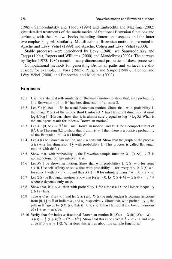
276 Brownian motion and Brownian surfaces
(1985), Samorodnitsky and Taqqu (1994) and Embrechts and Maejima (2002)give detailed treatments of the mathematics of fractional Brownian functions andsurfaces, with the first two books including dimensional aspects and the lattertwo emphasizing self-similarity. Multifractional Brownian motion is presented inAyache and Levy Vehel (1999) and Ayache, Cohen and Levy Vehel (2000).
Stable processes were introduced by Levy (1948); see Samorodnitsky andTaqqu (1994), Rogers and Williams (2000) and Mandelbrot (2002). The surveysby Taylor (1973, 1986) mention many dimensional properties of these processes.
Computational methods for generating Brownian paths and surfaces are dis-cussed, for example, in Voss (1985), Peitgen and Saupe (1988), Falconer andLevy Vehel (2000) and Embrechts and Maejima (2002).
Exercises
16.1 Use the statistical self-similarity of Brownian motion to show that, with probability1, a Brownian trail in �3 has box dimension of at most 2.
16.2 Let X : [0, ∞) → �3 be usual Brownian motion. Show that, with probability 1,the image X(F) of the middle third Cantor set F has Hausdorff dimension at mostlog 4/ log 3. (Harder: show that it is almost surely equal to log 4/ log 3.) What isthe analogous result for index-α Brownian motion?
16.3 Let X : [0,∞) → �3 be usual Brownian motion, and let F be a compact subset of�3. Use Theorem 8.2 to show that if dimHF > 1 then there is a positive probabilityof the Brownian trail X(t) hitting F .
16.4 Let X(t) be Brownian motion, and c a constant. Show that the graph of the processX(t) + ct has dimension 1 1
2 with probability 1. (This process is called Brownianmotion with drift.)
16.5 Show that, with probability 1, the Brownian sample function X : [0,∞) → � isnot monotonic on any interval [t, u].
16.6 Let X(t) be Brownian motion. Show that with probability 1, X(t) = 0 for somet > 0. Use self-affinity to show that with probability 1, for every a > 0, X(t) = 0for some t with 0 < t < a, and thus X(t) = 0 for infinitely many t with 0 < t < a.
16.7 Let X(t) be Brownian motion. Show that for q > 0, E(|X(t + h) − X(t)|q) = c|h|qwhere c depends only on q.
16.8 Show that, if λ > α, then with probability 1 for almost all t the Holder inequality(16.12) fails.
16.9 Take 12 � α1 � α2 < 1 and let X1(t) and X2(t) be independent Brownian functions
from [0, 1] to � of indices α1 and α2 respectively. Show that, with probability 1, thepath in �2 given by {(X1(t), X2(t)) : 0 � t � 1} has Hausdorff and box dimensionsof (1 + α2 − α1)/α2.
16.10 Verify that for index-α fractional Brownian motion E((X(t) − X(0))(X(t + h) −X(t)) = 1
2 [(t + h)2α − t2α − h2α]. Show that this is positive if 12 < α < 1 and neg-
ative if 0 < α < 1/2. What does this tell us about the sample functions?

Chapter 17 Multifractal measures
A mass distribution µ may be spread over a region in such a way that theconcentration of mass is highly irregular. Indeed, the set of points where thelocal mass concentration obeys an index α power law, say µ(B(x, r)) � rα forsmall r , may determine a different fractal for different values of α. Thus, awhole range of fractals may arise from a single measure, and we may examinethe structure of these fractals and their inter-relationship. A measure µ with sucha rich structure is called a multifractal measure or just a multifractal. As withfractals, a precise definition of ‘multifractal’ tends to be avoided.
Multifractal measures have been observed in many physical situations, forexample in fluid turbulence, rainfall distribution, mass distribution across theuniverse, viscous fingering, neural networks, share prices, and in many otherphenomena.
An important class of multifractal occurs in dynamical systems, see Sec-tion 13.7. If f : D → D is a mapping on a domain D, we can define a ‘residencemeasure’ by
µ(A) = limm→∞
1
m#{k : 1 � k � m andf k(x) ∈ A}
for subsets A of D, where x ∈ D is some initial point. Thus, µ(A) represents theproportion of time that the iterates of x spend in A. We have seen that the supportof µ is often an attractor of f and may be a fractal. However, the non-uniformityof µ across the attractor may highlight further dynamical structure which can berecorded and analysed using multifractal theory.
Many ideas related to fractals have counterparts in multifractals, for exampleprojection of multifractal measures onto a line or plane may be considered inan analogous manner to projection of fractals, though the calculations can beconsiderably more awkward.
There are two basic approaches to multifractal analysis: fine theory, where weexamine the structure and dimensions of the fractals that arise themselves, andcoarse theory, where we consider the irregularities of distribution of the measureof balls of small but positive radius r and then take a limit as r → 0. In manyways, fine multifractal analysis parallels finding the Hausdorff dimension of sets,
277
Fractal Geometry: Mathematical Foundations and Application. Second Edition Kenneth Falconer 2003 John Wiley & Sons, Ltd ISBNs: 0-470-84861-8 (HB); 0-470-84862-6 (PB)

278 Multifractal measures
whilst coarse theory is related to box-counting dimension. The coarse approach isusually more practicable when it comes to analysing physical examples or com-puter experiments, but the fine theory may be more convenient for mathematicalanalysis. There are many parallels between the fine and the coarse approaches,and for many measures both approaches lead to the same ‘multifractal spectra’.
We outline coarse and fine multifractal theory, and then consider the specialcase of self-similar measures in more detail, both to illustrate the theory and todemonstrate central ideas such as Legendre transformation.
Throughout our discussion, we refer to the following example of a self-similarmultifractal measure on a Cantor set. Just as the middle third Cantor set illustratesmany features of fractal mathematics, this self-similar measure supported by theCantor set is typical of a large class of multifractal measures.
Example 17.1
Let p1, p2 > 0 be given, with p1 + p2 = 1. We construct a measure µ on themiddle third Cantor set F = ∩∞
k=0Ek by repeated subdivision. (Here Ek comprisesthe 2k kth level intervals of length 3−k in the usual Cantor set construction seefigure 0.1.) Assign the left interval of E1 mass p1 and the right interval mass p2.Divide the mass on each interval of E1 between its two subintervals of E2 inthe ratio p1 : p2. Continue in this way, so that the mass on each interval of Ek
is divided in ratio p1 : p2 between its two subintervals of Ek+1. This defines amass distribution on F, see Proposition 1.7.
It is easily seen that if I is a kth level interval of Ek then µ(I) = pr1p
k−r2 where,
in constructing I , a left-hand interval is taken r times and a right-hand intervalk − r times. If p1 �= p2 and k is large, the masses of the kth level intervals willvary considerably, see figure 17.1, and this is a manifestation of multifractality.
17.1 Coarse multifractal analysis
Coarse multifractal analysis of a measure µ on �n with 0 < µ(�n) < ∞ is akinto box-counting dimension, in that we count the number of mesh cubes C forwhich µ(C) is roughly rα . (Recall that the r-mesh cubes in �n are the cubes of theform [m1r, (m1 + 1)r] × · · · × [mnr, (mn + 1)r] where m1, . . . , mn are integers.)For µ a finite measure on �n and α � 0 we write
Nr(α) = #{r-mesh cubes C with µ(C) � rα}, (17.1)
and define the coarse multifractal spectrum or coarse singularity spectrum ofµ as
fC(α) = limε→0
limr→0
log+(Nr(α + ε) − Nr(α − ε))
− log r(17.2)

Coarse multifractal analysis 279
0 1E0
E1
E2
E3
E4
•••
Figure 17.1 Construction of the self-similar measure described in Example 17.1. Themass on each interval of Ek in the construction of the Cantor set, indicated by the areaof the rectangle, is divided in the ratio p1 : p2 (in this case 1
3 : 23 ) between the two
subintervals of Ek+1. Continuing this process yields a self-similar measure on the Cantorset
if the double limit exists. (We write log+ x ≡ max{0, log x}, which ensures fC(α)
� 0.) Definition (17.2) implies that if η > 0, and ε > 0 is small enough, then
r−fC(α)+η � Nr(α + ε) − Nr(α − ε) � r−fC(α)−η (17.3)
for all sufficiently small r . Roughly speaking −fC(α) is the power law exponentfor the number of r-mesh cubes C such that µ(C) � rα . Note that fC(α) is notthe box dimension of the set of x such that µ(C(x, r)) � rα as r → 0 whereC(x, r) is the r-mesh cube containing x; the coarse spectrum provides a globaloverview of the fluctuations of µ at scale r , but gives no information about thelimiting behaviour of µ at any point.

280 Multifractal measures
To allow for the possibility of the limit (17.2) not existing, we define the lowerand the upper coarse multifractal spectra of µ by
fC(α) = lim
ε→0limr→0
log+(Nr(α + ε) − Nr(α − ε))
− log r(17.4)
and
f C(α) = limε→0
limr→0log+(Nr(α + ε) − Nr(α − ε))
− log r(17.5)
for α � 0.It is usually awkward to calculate the coarse multifractal spectrum fC directly.
Continuation of Example 17.1. In this example, the set Ek is made up of 2k intervals
of length 3−k, and for each r , a number
(k
r
)of these have mass pr
1pk−r2 , where
(k
r
)is the usual binomial coefficient. Thus, assuming without loss of generality
that 0 < p1 < 12 , we have
N3−k (α) =m∑
r=0
(k
r
),
where m is the largest integer such that
pm1 pk−m
2 � 3−kα, i.e. m � k(log p2 + α log 3)
log p2 − log p1.
It is now possible, but tedious, to estimate N3−k (α) and thus examine its powerlaw exponent. However, we shortly encounter a better approach. �
Next, we introduce moment sums: for q ∈ � and r > 0 the qth power momentsum of µ is given by
Mr(q) =∑
Mr
µ(C)q, (17.6)
where the sum is over the set Mr of r-mesh cubes C for which µ(C) > 0.(There is a problem of stability for negative q: if a cube C just clips the edgeof spt µ, then µ(C)q can be very large. There are ways around this difficulty,for example by restricting the sums to cubes with a central portion intersectingspt µ, but we do not pursue this here.) We identify the power law behaviour ofMr(q) by defining
β(q) = limr→0
log Mr(q)
− log r, (17.7)
assuming this limit exists.

Coarse multifractal analysis 281
It is hardly surprising that these moment sums are related to the Nr(α). Using(17.1), it follows that if q � 0 and α � 0
Mr(q) =∑
Mr
µ(C)q � rqαNr(α), (17.8)
and if q < 0
Mr(q) =∑
Mr
µ(C)q � rqα#{r-mesh cubes with 0 < µ(C) � rα}. (17.9)
These inequalities lead to a useful relationship between fc(α) and β(q) interms of Legendre transformation. The Legendre transform fL of β is definedfor α � 0 by
fL(α) = inf−∞<q<∞{β(q) + αq}, (17.10)
provided this is finite. There is a useful geometrical interpretation of the Legendretransform. For those α for which the graph of β has under it a line of support Lα
of slope −α, the Legendre transform of β is given by the value of the interceptof Lα with the vertical axis, see figure 17.2.
It is easy to see that the coarse spectrum is bounded above by the Legendretransform of β.
Proposition 17.2Let µ be a finite measure on �n, and assume that the limit in (17.7) exists. Thenfor all α � 0,
fC(α) � f C(α) � fL(α) (17.11)
where fL is the Legendre transform of β.
b(q) curve
b(q) (q, b(q))
q
q
f (a) = b (q) + aq
La
b
tan−1a
Figure 17.2 The Legendre transform of β(q) is f (α), the intersection of the tangent Lα
of slope −α with the β-axis
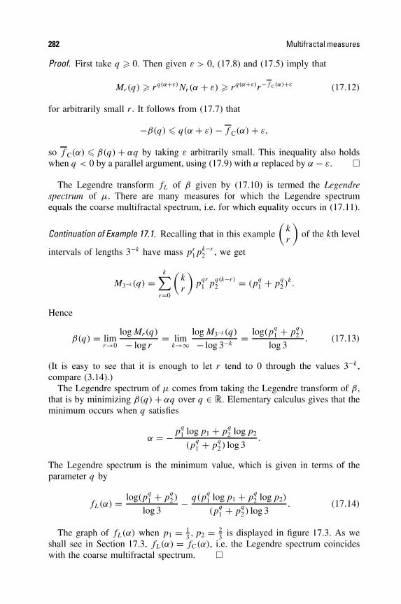
282 Multifractal measures
Proof. First take q � 0. Then given ε > 0, (17.8) and (17.5) imply that
Mr(q) � rq(α+ε)Nr(α + ε) � rq(α+ε)r−f C(α)+ε (17.12)
for arbitrarily small r . It follows from (17.7) that
−β(q) � q(α + ε) − f C(α) + ε,
so f C(α) � β(q) + αq by taking ε arbitrarily small. This inequality also holdswhen q < 0 by a parallel argument, using (17.9) with α replaced by α − ε. �
The Legendre transform fL of β given by (17.10) is termed the Legendrespectrum of µ. There are many measures for which the Legendre spectrumequals the coarse multifractal spectrum, i.e. for which equality occurs in (17.11).
Continuation of Example 17.1. Recalling that in this example
(k
r
)of the kth level
intervals of lengths 3−k have mass pr1p
k−r2 , we get
M3−k (q) =k∑
r=0
(k
r
)p
qr
1 pq(k−r)
2 = (pq
1 + pq
2 )k.
Hence
β(q) = limr→0
log Mr(q)
− log r= lim
k→∞log M3−k (q)
− log 3−k= log(p
q
1 + pq
2 )
log 3. (17.13)
(It is easy to see that it is enough to let r tend to 0 through the values 3−k,compare (3.14).)
The Legendre spectrum of µ comes from taking the Legendre transform of β,that is by minimizing β(q) + αq over q ∈ �. Elementary calculus gives that theminimum occurs when q satisfies
α = −pq
1 log p1 + pq
2 log p2
(pq
1 + pq
2 ) log 3.
The Legendre spectrum is the minimum value, which is given in terms of theparameter q by
fL(α) = log(pq
1 + pq
2 )
log 3− q(p
q
1 log p1 + pq
2 log p2)
(pq
1 + pq
2 ) log 3. (17.14)
The graph of fL(α) when p1 = 13 , p2 = 2
3 is displayed in figure 17.3. As weshall see in Section 17.3, fL(α) = fC(α), i.e. the Legendre spectrum coincideswith the coarse multifractal spectrum. �

Fine multifractal analysis 283
log 2/log 3
fL(a) 0.8
0.6
0.4
0.2
00 0.2 0.4 0.6 0.8 1.0
a
q = 4
q = 2 q = −2
q = −4
q = 1
q = 0
Figure 17.3 The multifractal spectrum of Example 17.1 with p1 = 13 , p2 = 2
3
In practical situations, multifractal spectra are often awkward to estimate andwork with. One might hope to compute the coarse spectrum fC by ‘box-counting’.For instance, if µ is a residence measure on the attractor of a dynamical system inthe plane, a count of the proportion of the iterates of an initial point that lie in eachr-mesh square C might be used to estimate the number of squares for which αi �log µ(C)/ log r < αi+1, where 0 � α1 < · · · < αk . Examining this ‘histogram’for various r enables the power law behaviour of Nr(α + ε) − Nr(α + ε) to bestudied and f (α) to be estimated. However, this histogram method tends to becomputationally slow and awkward.
In general, it is more satisfactory to use the method of moments for experimen-tal determination of a multifractal spectrum. Thus, for a range of q, the momentsums (17.6) are estimated for various small r and the power law behaviourexamined to estimate β(q) using (17.7). Legendre transformation of β gives aLegendre spectrum of µ, and this is often taken to be the coarse spectrum. Themethod of moments is usually more numerically manageable than the histogrammethod.
17.2 Fine multifractal analysis
Fine multifractal analysis looks directly at the fractals determined by the localintensity of a measure. Let µ be a measure on �n with 0 < µ(�n) < ∞. Wedefine the local dimension or Holder exponent of µ at x by
dimlocµ(x) = limr→0
log µ(B(x, r))
log r, (17.15)

284 Multifractal measures
provided this limit exists. (More generally, one can work with upper and lowerlocal limits leading to upper and lower local dimensions, but we do not pursuethis here.) We study the sets of points x ∈ �n where the local dimension takesparticular values. For α � 0 we define
Fα = {x ∈ �n : dimlocµ(x) = α}=
{x ∈ �n : lim
r→0
log µ(B(x, r))
log r= α
}. (17.16)
Thus, Fα comprises those points where the local dimension exists and equals α.In fine multifractal analysis we aim to find the dimensions of Fα for a range
of α. In most examples of interest Fα is dense in the support of µ so dimBFα =dimBFα = dimB(spt µ) (and similarly for upper box dimensions) by Proposition3.4, so box-counting dimensions are of little use in discriminating between the Fα.Thus, we concentrate on the fine (Hausdorff) multifractal spectrum or singularityspectrum of µ defined by
fH(α) = dimHFα. (17.17)
(We do not consider here the fine packing spectrum which has a similar definitionusing packing dimension.)
Clearly, 0 � fH(α) � dimH(sptµ) for all α � 0, and it follows from Proposi-tion 4.9(b) that
0 � fH(α) � α. (17.18)
Continuation of Example 17.1. We may code the points x of the Cantor set F as(i1, i2, . . .) in the usual way, with ik = 1 if x is in the left sub-interval at the kthstage of the Cantor set construction, and ik = 2 if x is in the right sub-interval.Then, writing nj (x|k), j = 1, 2, for the number of occurrences of j in the first k
terms of the sequence coding x, we have µ(B(x, 3−k)) = pn1(x|k)1 p
n2(x|k)2 , so that
logµ(B(x, 3−k))
log 3−k= −1
log 3
(n1(x|k)
klog p1 + n2(x|k)
klog p2
).
Thus, if nj (x|k)/k → αj , j = 1, 2, then x ∈ Fα where α = −(α1 log p1 +α2 log p2)/ log 3. In this instance, we could now calculate fH(α) = dimHFα asin Proposition 10.1, and this gives a parametric expression equivalent to (17.14).We defer a formal calculation until the next section, where it will be done in amore general context. �
Just as the Hausdorff dimension of a set is never more than its box dimension,there is a basic inequality between the fine and coarse spectra.

Fine multifractal analysis 285
Lemma 17.3
Let µ be a finite measure on �n. Then
fH(α) � fC(α) � f C(α) (17.19)
for all α � 0.
Proof. The right-hand inequality of (17.19) is obvious. We prove the left-handinequality in the case where µ is a measure on �; the proof is similar for n � 2except that measures of balls and cubes have to be compared instead of measuresof intervals.
For fixed α � 0 write for brevity f ≡ fH(α) = dimHFα; we may assumef > 0. Given 0 < ε < f then Hf −ε(Fα) = ∞. By (17.16) there is a setF 0
α ⊂ Fα with Hf −ε(F 0α ) > 1 and a number c0 > 0 such that
3rα+ε � µ(B(x, r)) < 2ε−αrα−ε (17.20)
for all x ∈ F 0α and all 0 < r � c0, using Egoroff’s theorem. We may choose δ
with 0 < δ � 12c0 such that Hf −ε
δ (F 0α ) � 1.
For each r � δ we consider r-mesh intervals (of the form [mr, (m + 1)r] withm ∈ �) that intersect F 0
α . Such an interval I contains a point x of F 0α , with
B(x, r) ⊂ I ∪ IL ∪ IR ⊂ B(x, 2r),
where IL and IR are the r-mesh intervals immediately to the left and right of I .By (17.20)
3rα+ε � µ(B(x, r)) � µ(I ∪ IL ∪ IR) � µ(B(x, 2r)) < rα−ε,
so thatrα+ε � µ(I0) < rα−ε, (17.21)
where I0 is one of I , IL and IR . By definition of Hf −ε
δ there are at leastrε−fHf −ε
δ (F 0α ) � rε−f distinct r-mesh intervals that intersect F 0
α , so there are atleast 1
3 rε−f distinct r-mesh intervals I0 that satisfy (17.21) (note that two inter-vals I separated by 2r or more give rise to different intervals I0). We concludethat for r � δ
Nr(α + ε) − Nr(α − ε) � 13rε−f ,
so from (17.4) fC(α) � f − ε; as this is true for all positive ε we conclude
fC(α) � f = fH(α). �

286 Multifractal measures
Just as many fractals we have encountered have equal box and Hausdorffdimensions, many common multifractal measures have equal coarse and finespectra, that is, equality in (17.19). In the next section, we shall show that thisis the case for self-similar measures.
By setting up Hausdorff-type measures tailored for multifractal purposes, wecan define a quantity β(q) playing a similar role in the fine theory to that of (17.7)in the coarse theory. The Legendre transform of this β(q) gives an upper boundfor the fine multifractal spectrum, and again in many cases gives the actual value.
17.3 Self-similar multifractals
In this section we calculate the fine multifractal spectrum of a self-similar measureon �, of which Example 17.1 is a specific case. Not only are self-similar measuresimportant in their own right, but also the methods to be described adapt to manyother classes of measures.
We consider a self-similar measure µ supported on a self-similar subset F
of �. Let S1, . . . , Sm : � → � be contracting similarities with ratios c1, . . . , cm.As in Chapter 9, the iterated function system {S1, . . . , Sm} has a (unique non-empty compact) attractor F ⊂ �. We assume that a strong separation conditionholds, that is there is a closed interval I such that Si(I ) ⊂ I for all i, andSi(I ) ∩ Sj (I ) = Ø whenever i �= j .
As in Chapter 9, we index the intervals in the natural construction of F bythe finite sequences Ik = {(i1, . . . , ik) : 1 � i � m}, writing i = (i1, . . . , ik) for atypical sequence of Ik. Thus
Ii = Ii1,...,ik = Si1◦ · · · ◦Sik (I ). (17.22)
For convenience, we assume that |I | = 1, so for i = (i1, i2, . . . , ik) ∈ Ik we have
|Ii| = ci ≡ ci1ci2 · · · cik . (17.23)
We define a self-similar measure µ with support F by repeated subdivision.Let p1, . . . , pm be ‘probabilities’ or ‘mass ratios’, that is pi > 0 for all i and∑m
i=1 pi = 1. Repeatedly dividing the mass on intervals Ii1,...,ik between subin-tervals Ii1,...,ik,1, . . . , Ii1,...,ik ,m in the ratios p1 : · · · : pm defines a measure µ onF , see Proposition 1.7. Thus
µ(Ii1,i2,...,ik ) = pi ≡ pi1pi2 · · · pik . (17.24)
It is easy to see that µ is a self-similar measure, in the sense that
µ(A) =m∑
i=1
piµ(S−1i (A)) (17.25)
for all sets A.
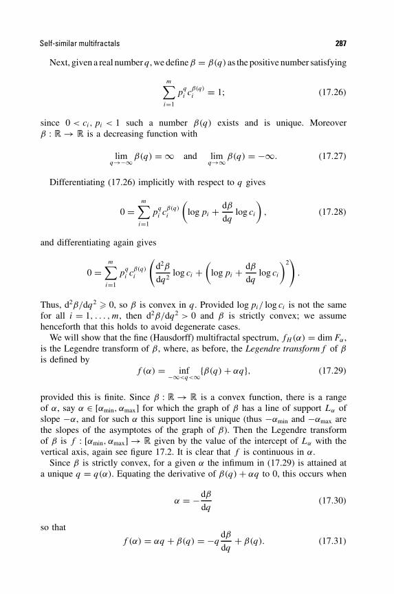
Self-similar multifractals 287
Next, given a real number q, we define β = β(q) as the positive number satisfying
m∑
i=1
pq
i cβ(q)
i = 1; (17.26)
since 0 < ci, pi < 1 such a number β(q) exists and is unique. Moreoverβ : � → � is a decreasing function with
limq→−∞ β(q) = ∞ and lim
q→∞ β(q) = −∞. (17.27)
Differentiating (17.26) implicitly with respect to q gives
0 =m∑
i=1
pq
i cβ(q)
i
(log pi + dβ
dqlog ci
), (17.28)
and differentiating again gives
0 =m∑
i=1
pq
i cβ(q)
i
(d2β
dq2log ci +
(log pi + dβ
dqlog ci
)2)
.
Thus, d2β/dq2 � 0, so β is convex in q. Provided log pi/ log ci is not the samefor all i = 1, . . . , m, then d2β/dq2 > 0 and β is strictly convex; we assumehenceforth that this holds to avoid degenerate cases.
We will show that the fine (Hausdorff) multifractal spectrum, fH (α) = dim Fα ,is the Legendre transform of β, where, as before, the Legendre transform f of β
is defined byf (α) = inf−∞<q<∞{β(q) + αq}, (17.29)
provided this is finite. Since β : � → � is a convex function, there is a rangeof α, say α ∈ [αmin, αmax] for which the graph of β has a line of support Lα ofslope −α, and for such α this support line is unique (thus −αmin and −αmax arethe slopes of the asymptotes of the graph of β). Then the Legendre transformof β is f : [αmin, αmax] → � given by the value of the intercept of Lα with thevertical axis, again see figure 17.2. It is clear that f is continuous in α.
Since β is strictly convex, for a given α the infimum in (17.29) is attained ata unique q = q(α). Equating the derivative of β(q) + αq to 0, this occurs when
α = −dβ
dq(17.30)
so that
f (α) = αq + β(q) = −qdβ
dq+ β(q). (17.31)

288 Multifractal measures
Note that if any one of q ∈ �, β ∈ � and α ∈ (αmin, αmax) is given, the other twoare determined by (17.26), (17.30) and (17.31). Using (17.30) and rearranging(17.28) gives
α =∑m
i=1 pq
i cβ
i log pi∑m
i=1 pq
i cβ
i log ci
. (17.32)
On inspecting this expression, we see that
αmin = min1�i�m
log pi/ log ci and αmax = max1�i�m
log pi/ log ci (17.33)
which correspond to q approaching ∞ and −∞, respectively.Provided that the numbers {log pi/ log ci}mi=1 are all different, f (αmin) =
f (αmax) = 0, see Exercise 17.8.Differentiating (17.31) with respect to α and using (17.30),
df
dα= α
dq
dα+ q + dβ
dq
dq
dα= q. (17.34)
Since q decreases as α increases, it follows that f is a concave function of α.Some values of q are of special interest, see figure 17.4. If q = 0 then β(q) =
dimHF = dimH(sptµ), comparing (17.26) and the dimension formula for self-similar sets (9.13). Moreover, by (17.34), q = 0 corresponds to the maximum off (α); hence, dimHF = dimH(spt µ) = maxα f (α).
When q = 1 (17.26) implies β(q) = 0 so f (α) = α by (17.31). Moreover,df (α)/dα = q = 1, so that the f (α) curve lies under the line f = α and touchesit just at the point corresponding to q = 1. It will follow later that α(1) =f (α(1)) = dimHµ, where
dimHµ = inf{dimHE : E is a Borel set with µ(E) > 0} (17.35)
is the Hausdorff dimension of the measure µ. Thus the dimension of µ is thedimension of a set on which a significant part of µ is concentrated.
We can now state the main result on the fine multifractal spectrum of aself-similar measure, that the Hausdorff multifractal spectrum is given by theLegendre transform (17.29) of β(q) given by (17.26).
Theorem 17.4
Let µ be a self-similar measure as above and let
Fα = {x ∈ �n : dimlocµ(x) = α}.If α /∈ [αmin, αmax] then Fα = Ø, and if α ∈ [αmin, αmax] then
fH (α) ≡ dimHFα = f (α), (17.36)
where f is the Legendre transform of β(q).
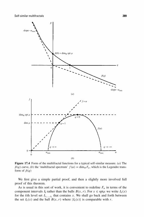
Self-similar multifractals 289
(a)
10
slope−amax
slope−amin
amin amax a
b(0) = dimH spt m
dimH spt m
dim m q = 1
q → ∞ q → −∞
q = 0
f = a
0
0
f
b(q)
f(a)
q
b
(b)
Figure 17.4 Form of the multifractal functions for a typical self-similar measure. (a) Theβ(q) curve, (b) the ‘multifractal spectrum’ f (α) = dimH Fα , which is the Legendre trans-form of β(q)
We first give a simple partial proof, and then a slightly more involved fullproof of this theorem.
As is usual in this sort of work, it is convenient to redefine Fα in terms of thecomponent intervals Ii rather than the balls B(x, r). For x ∈ sptµ we write Ik(x)
for the kth level set Ii1,...,ik that contains x. We shall go back and forth betweenthe set Ik(x) and the ball B(x, r) where |Ik(x)| is comparable with r .
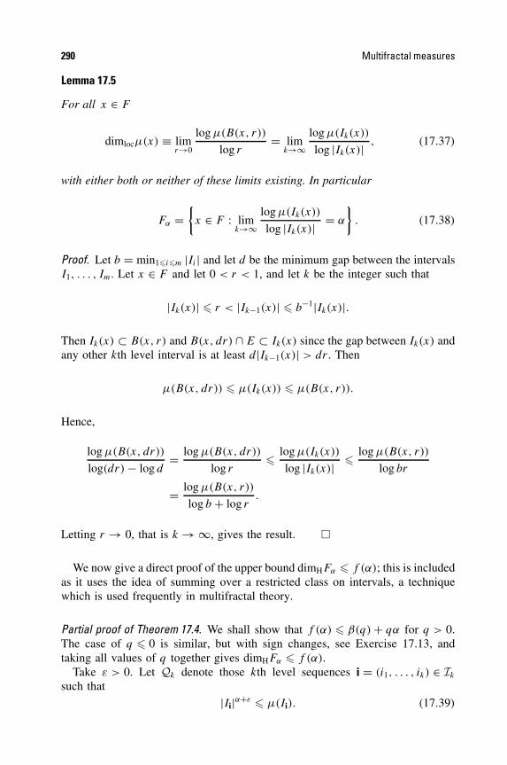
290 Multifractal measures
Lemma 17.5
For all x ∈ F
dimlocµ(x) ≡ limr→0
log µ(B(x, r))
log r= lim
k→∞log µ(Ik(x))
log |Ik(x)| , (17.37)
with either both or neither of these limits existing. In particular
Fα ={x ∈ F : lim
k→∞log µ(Ik(x))
log |Ik(x)| = α
}. (17.38)
Proof. Let b = min1�i�m |Ii| and let d be the minimum gap between the intervalsI1, . . . , Im. Let x ∈ F and let 0 < r < 1, and let k be the integer such that
|Ik(x)| � r < |Ik−1(x)| � b−1|Ik(x)|.
Then Ik(x) ⊂ B(x, r) and B(x, dr) ∩ E ⊂ Ik(x) since the gap between Ik(x) andany other kth level interval is at least d|Ik−1(x)| > dr . Then
µ(B(x, dr)) � µ(Ik(x)) � µ(B(x, r)).
Hence,
log µ(B(x, dr))
log(dr) − log d= log µ(B(x, dr))
log r� log µ(Ik(x))
log |Ik(x)| � log µ(B(x, r))
log br
= log µ(B(x, r))
log b + log r.
Letting r → 0, that is k → ∞, gives the result. �
We now give a direct proof of the upper bound dimHFα � f (α); this is includedas it uses the idea of summing over a restricted class on intervals, a techniquewhich is used frequently in multifractal theory.
Partial proof of Theorem 17.4. We shall show that f (α) � β(q) + qα for q > 0.The case of q � 0 is similar, but with sign changes, see Exercise 17.13, andtaking all values of q together gives dimHFα � f (α).
Take ε > 0. Let Qk denote those kth level sequences i = (i1, . . . , ik) ∈ Ik
such that|Ii|α+ε � µ(Ii). (17.39)
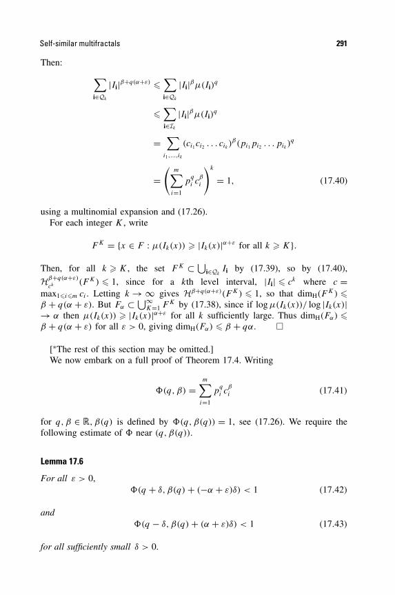
Self-similar multifractals 291
Then:
∑
i∈Qk
|Ii|β+q(α+ε) �∑
i∈Qk
|Ii|βµ(Ii)q
�∑
i∈Ik
|Ii|βµ(Ii)q
=∑
i1,...,ik
(ci1ci2 . . . cik )β(pi1pi2 . . . pik )
q
=(
m∑
i=1
pq
i cβ
i
)k
= 1, (17.40)
using a multinomial expansion and (17.26).For each integer K , write
F K = {x ∈ F : µ(Ik(x)) � |Ik(x)|α+ε for all k � K}.
Then, for all k � K , the set F K ⊂ ⋃i∈Qk
Ii by (17.39), so by (17.40),
Hβ+q(α+ε)
ck (F K) � 1, since for a kth level interval, |Ii| � ck where c =max1�i�m ci . Letting k → ∞ gives Hβ+q(α+ε)(F K) � 1, so that dimH(F K) �β + q(α + ε). But Fα ⊂ ⋃∞
K=1 F K by (17.38), since if log µ(Ik(x))/ log |Ik(x)|→ α then µ(Ik(x)) � |Ik(x)|α+ε for all k sufficiently large. Thus dimH(Fα) �β + q(α + ε) for all ε > 0, giving dimH(Fα) � β + qα. �
[∗The rest of this section may be omitted.]We now embark on a full proof of Theorem 17.4. Writing
�(q, β) =m∑
i=1
pq
i cβ
i (17.41)
for q, β ∈ �, β(q) is defined by �(q, β(q)) = 1, see (17.26). We require thefollowing estimate of � near (q, β(q)).
Lemma 17.6
For all ε > 0,�(q + δ, β(q) + (−α + ε)δ) < 1 (17.42)
and�(q − δ, β(q) + (α + ε)δ) < 1 (17.43)
for all sufficiently small δ > 0.

292 Multifractal measures
Proof. Recalling that dβ/dq = −α, expansion about q gives
β(q + δ) = β(q) − αδ + O(δ2) < β(q) + (−α + ε)δ
if δ is small enough. Since �(q + δ, β(q + δ)) = 1 and � is decreasing inits second argument, (17.42) follows. Inequality (17.43) is derived in a similarway. �
To prove Theorem 17.4, for each α we concentrate a measure ν on Fα andexamine the power law behaviour of ν(B(x, r)) as r → 0, so that we can useProposition 4.9 to find the dimension of Fα . Given q ∈ � and β = β(q), (17.26)enables us to define a probability measure ν on sptµ by repeated subdivisionsuch that
ν(Ii1,...,ik ) = (pi1pi2 · · · pik )q(ci1ci2 · · · cik )
β, (17.44)
for each (i1, . . . , ik), and extending this to a measure on F in the usual way.Together with (17.23) and (17.24) this gives three ways of quantifying the Ii:
|Ii| = ci, µ(Ii) = pi, ν(Ii) = pq
i cβ
i (17.45)
for all i = (i1, . . . , ik).The following proposition contains the crux of the multifractal spectrum cal-
culation.
Proposition 17.7
With q, β, α and f as above, and with ν determined by (17.44),
(a) ν(Fα) = 1,(b) for all x ∈ Fα we have log ν(B(x, r))/ log r → f (α) as r → 0.
Proof. Let ε > 0 be given. Then for all δ > 0
ν{x : µ(Ik(x)) � |Ik(x)|α−ε} = ν{x : 1 � µ(Ik(x))δ |Ik(x)|(ε−α)δ}
�∫
µ(Ik(x))δ |Ik(x)|(ε−α)δdν(x)
=∑
i∈Ik
µ(Ii)δ|Ii|(ε−α)δν(Ii)
=∑
i∈Ik
pq+δ
i cβ+(ε−α)δ
i
=(
m∑
i=1
pq+δ
i cβ+(ε−α)δ
i
)k
= [�(q + δ, β + (ε − α)δ)]k,

Self-similar multifractals 293
where � is given by (17.41), using (17.45) and a multinomial expansion. Choos-ing δ small enough and using (17.42) gives that
ν{x : µ(Ik(x)) � |Ik(x)|α−ε} � γ k (17.46)
where γ < 1 is independent of k. Thus
ν{x : µ(Ik(x)) � |Ik(x)|α−ε for some k � K} �∞∑
k=K
γ k � γ K/(1 − γ ).
It follows that for ν-almost all x we have
limk→∞
log µ(Ik(x))
log |Ik(x)| � α − ε.
This is true for all ε > 0, so we get the left-hand inequality of
α � limk→∞
log µ(Ik(x))
log |Ik(x)| � limk→∞
log µ(Ik(x))
log |Ik(x)| � α.
The right-hand inequality follows in the same way, using (17.43) in estimatingν{x : µ(Ik(I )) � |Ik(x)|α+ε}. From (17.37) we conclude that for ν-almost all x
dimlocµ(x) = limk→∞
log µ(Ik(x))
log |Ik(x)| = α
and it follows that ν(Fα) = ν(F ) = 1.For (b) note that from (17.45)
log ν(Ik(x))
log |Ik(x)| = qlog µ(Ik(x))
log |Ik(x)| + βlog |Ik(x)|log |Ik(x)| , (17.47)
so for all x ∈ Fαlog ν(Ik(x))
log |Ik(x)| → qα + β = f (17.48)
as k → ∞, using (17.31). Part (b) follows, applying (17.37) with ν replacingµ. �
Our main Theorem 17.4 on the multifractal spectrum of self-similar measuresnow follows easily.
Proof of Theorem 17.4. From (17.45)
log µ(Ii)
log |Ii| =∑k
j=1 log pij∑k
j=1 log cij

294 Multifractal measures
where i = (i1, . . . , ik), so by (17.33) log µ(Ii)/ log |Ii| ∈ [αmin, αmax] for all i.Thus the only possible limit points of log µ(Ii)/ log |Ii|, and so by (17.37) oflog B(x, r)/ log r , are in [αmin, αmax]. In particular, Fα = Ø if α /∈ [αmin, αmax].
If α ∈ (αmin, αmax) then by Proposition 17.7 there exists a measure ν concen-trated on Fα with limr→0 log ν(B(x, r))/ log r = f (α) for all x ∈ Fα , so (17.36)follows from Proposition 4.9. For the cases α = αmin and α = αmax, see Exercise17.14. �
Thus, for a self-similar measure, the dimension of Fα may be calculated bytaking the Legendre transform of β(q) given by (17.26).
The dimensions of spt µ and of the measure µ, see (17.35), may easily befound from the multifractal spectrum.
Proposition 17.8
Let µ be a self-similar measure as above. Regarding α = α(q) as a function of q,
(a) f (α) takes its maximum when α = α(0), with f (α(0)) = dimHsptµ.(b) f (α(1)) = α(1) = dimHµ.
Proof. Part (a) and that f (α(1)) = α(1) were noted as a consequence of (17.34).For the dimension of the measure µ, if q = 1 then β = 0 from (17.26), so by(17.44) the measure ν is identical to µ. By Proposition 17.7 µ(Fα(1)) = 1 anddimlocµ(x) = f (α(1)) for all x ∈ Fα(1), so by Proposition 4.9, dimHE = f (α(1))
for all E with µ(E) > 0. Thus (b) follows from the definition of the dimensionof a measure (17.35). �
Next we show that the coarse spectrum of a self-similar measure is also equalto f (α), the Legendre transform of β.
Proposition 17.9
Let µ be a self-similar measure on � as above. Then
fC(α) = f C(α) = fH(α) = f (α) (17.49)
for all α = α(q) for which q � 0.
Proof. We first note that by Theorem 17.4 and Lemma 17.3 we have f (α) =fH(α) � f
C(α) � f C(α), where the coarse spectra are given by (17.4) and (17.5).
To prove the opposite inequality, let d be the minimum separation of Ii and Ij
for i �= j , and write a = 2/d . Given r < a−1, let Q be the set of all sequencesi = (i1, . . . , ik) ∈ Ik such that |Ii1,...,ik | � ar but |Ii1,...,ik−1 | > ar . Then
abr < |Ii| = ci � ar (17.50)
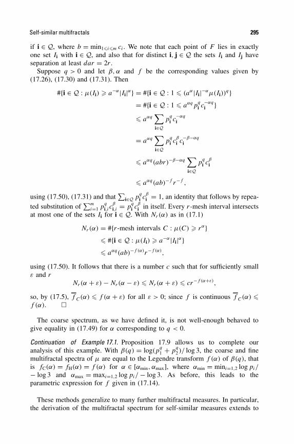
Self-similar multifractals 295
if i ∈ Q, where b = min1�i�m ci . We note that each point of F lies in exactlyone set Ii with i ∈ Q, and also that for distinct i, j ∈ Q the sets Ii and Ij haveseparation at least dar = 2r .
Suppose q > 0 and let β, α and f be the corresponding values given by(17.26), (17.30) and (17.31). Then
#{i ∈ Q : µ(Ii) � a−α|Ii|α} = #{i ∈ Q : 1 � (aα|Ii|−αµ(Ii))q}
= #{i ∈ Q : 1 � aαqpq
i c−αq
i }� aαq
∑
i∈Qp
q
i c−αq
i
= aαq∑
i∈Qp
q
i cβ
i c−β−αq
i
� aαq(abr)−β−αq∑
i∈Qp
q
i cβ
i
� aαq(ab)−f r−f ,
using (17.50), (17.31) and that∑
i∈Q pq
i cβ
i = 1, an identity that follows by repea-ted substitution of
∑mi=1 p
q
i,icβ
i,i = pq
i cβ
i in itself. Every r-mesh interval intersectsat most one of the sets Ii for i ∈ Q. With Nr(α) as in (17.1)
Nr(α) = #{r-mesh intervals C : µ(C) � rα}� #{i ∈ Q : µ(Ii) � a−α|Ii|α}� aαq(ab)−f (α)r−f (α),
using (17.50). It follows that there is a number c such that for sufficiently smallε and r
Nr(α + ε) − Nr(α − ε) � Nr(α + ε) � cr−f (α+ε),
so, by (17.5), f C(α) � f (α + ε) for all ε > 0; since f is continuous f C(α) �f (α). �
The coarse spectrum, as we have defined it, is not well-enough behaved togive equality in (17.49) for α corresponding to q < 0.
Continuation of Example 17.1. Proposition 17.9 allows us to complete ouranalysis of this example. With β(q) = log(p
q
1 + pq
2 )/ log 3, the coarse and finemultifractal spectra of µ are equal to the Legendre transform f (α) of β(q), thatis fC(α) = fH(α) = f (α) for α ∈ [αmin, αmax], where αmin = mini=1,2 log pi/
− log 3 and αmax = maxi=1,2 log pi/ − log 3. As before, this leads to theparametric expression for f given in (17.14).
These methods generalize to many further multifractal measures. In particular,the derivation of the multifractal spectrum for self-similar measures extends to

296 Multifractal measures
self-similar measures on �n without difficulty, and the separation condition onthe intervals Si(I ) can be weakened to the open set condition.
17.4 Notes and references
A great deal has been written on multifractals, and multifractal spectra have beencalculated for many specific measures. We mention a small selection of referenceswhere further details may be found.
The idea of studying measures from a fractal viewpoint is implicit in Mandel-brot’s essay (1982); see also Mandelbrot (1974). Legendre transformation wasintroduced into multifractal analysis in Frisch and Parisi (1985) and Halsey et al.(1986). Various approaches at a fairly basic level are given by Evertsz and Man-delbrot (1992), Falconer (1997), Feder (1988), McCauley (1993) and Tel (1988).Mandelbrot’s ‘Selecta’ (1999) includes reprints of many papers, as well as a wide-ranging survey and a comprehensive bibliography on multifractals. The book byHarte (2001) gives a substantial treatment of the theory with many references,and in particular addresses statistical estimation of spectra.
Measure theoretic approaches to multifractal theory, including use of measuresof Hausdorff type and the relationships between different types of spectra, aregiven by Brown, Michon and Peyriere (1992), Olsen (1995) and Pesin (1997).A careful treatment of the coarse theory is given by Riedi (1995).
Self-similar measures are analysed by Cawley and Mauldin (1992), and Edgarand Mauldin (1992) and Olsen (1994) extend this to graph-directed construc-tions of measures. For self-similar multifractals with infinitely many similarities,see Mandelbrot and Riedi (1995) and Mauldin and Urbanski (1996). Extensionsto random self-similar measures are considered by Mandelbrot (1974), Kahaneand Peyriere (1976) and Olsen (1994), to self-conformal measures and weakerseparation conditions by Patzschke (1997), and to vector-valued multifractalsby Falconer and O’Neil (1996). McCauley (1993), Simpelaere (1994) and Pesin(1997) consider multifractal measures that occur in dynamical systems. Jaffard(1997) discusses the local form of functions from a multifractal viewpoint.
There are many other interesting aspects of multifractal behaviour, such as theinterpretation of negative dimensions, see Mandelbrot (1991), and the geometricalproperties of multifractals, such as their behaviour under projections, intersectionsor products, see Olsen (2000).
Exercises
17.1 Find the Legendre transform of β(q) = e−q .
17.2 Let µ1, µ2 be finite measures on �n with disjoint supports, and define ν = µ1 + µ2.Show that f ν
H(α) = max{f 1H(α), f 2
H(α)} where f νH, f 1
H and f 2H are the Hausdorff
spectra of ν, µ1 and µ2. Deduce that fH(α) need not be concave over the range ofα for which it does not vanish.

Exercises 297
17.3 Let µ be a finite measure on �n and let g : �n → �n be a bi-Lipschitz function.Define the image measure ν on �n by ν(A) = µ(g−1(A)). Show that the localdimensions dimlocµ(x) and dimlocν(g(x)) are equal when either exists. Hence showthat fH(α) given by (17.17) is the same for both ν and µ.
17.4 Let µ be a self-similar measure supported by the ‘middle half’ Cantor set, so c1 =c2 = 1
4 , with the mass repeatedly divided between the left and right parts in the ratiop1 : p2, where p1 + p2 = 1 and p1 < p2. Show that β(q) = log(p
q
1 + pq
2 )/ log 4,and hence find α and f in terms of the parameter q.
17.5 Let µ be the measure on the middle half Cantor set of Exercise 17.4. For q � 0estimate the moment sums (17.6). [Hint: consider the case where r = 4−k first.]Hence show that β(q) given by (17.7) coincides with that defined by that stated inExercise 17.4.
17.6 Let µ be a self-similar measure constructed by repeated subdivision of the supportin the ratios c1 = 1
2 and c2 = 14 and of the measure in ratios p1 and p2. Obtain an
explicit formula for β(q).
17.7 Let µ be the measure of Example 17.1, with β given by (17.13). Show that β(q) −β(−q) = q log(p1p2)/ log 3. Hence show the multifractal spectrum f (α) given bythe Legendre transform (17.10) is symmetrical about α = − log(p1p2)/2 log 3, thatis f (α) = f (− log(p1p2)/ log 3 − α).
17.8 Let µ be the measure of Example 17.1, with 0 < p1 < p2 < 1 and β given by(17.13). Show that for large q, β(q) = q log p2/ log 3 + o(1) and obtain a similarexpression for q large negative. (Here o(1) means a function of q that tends to 0 asq → ∞.) Deduce that the asymptotes of the graph of β(q) pass through the origin,that αmin = − log p2/ log 3, αmax = − log p1/ log 3 and that f (αmin) = f (αmax) =0.
17.9 For the self-similar measures discussed in Section 17.3, show that d2f/dα2 < 0for αmin < α < αmax; thus the f (α) curve is strictly concave.
17.10 With β defined by (17.26), show that β(q) � 1 − q if 0 < q � 1 andβ(q) � 1 − q if q � 1. (Hint: recall Holder’s inequality:
∑mi=1 aibi �
(∑mi=1 a
p
i
)1/p ( ∑mi=1 b
p′i
)1/p′, where 1 < p < ∞ and 1/p + 1/p′ = 1.)
17.11 Let µ be a finite measure on �2 and let proj denote projection onto a givenline L. Define the projection of µ onto L by (proj µ)(A) = µ{x ∈ �2 : proj x ∈A} for A ⊂ L. For x ∈ �2, show that limr→0 log((proj µ)(BL(proj x, r)))/ log r �limr→0 log µ(B(x, r))/ log r , where BL(y, r) is the interval within L of centre y
and length 2r .
17.12 Adapt the ‘Partial proof of Theorem 17.4’ to show that dimHFα � β(q) + qα forthe case of α corresponding to q < 0. (Hint: consider
∑ |I |β+q(α−ε) for intervalsI with µ(I) � |I |α−ε .)
17.13 Extend the ‘Partial proof of Theorem 17.4’ to show that, for α corresponding toq > 0,
dimH{x ∈ F : limk→∞
log µ(Ik(x))/ log |Ik(x)| � α} � f (α).
17.14 Prove (17.36) when α = αmin. (Hint: take α close to αmin, and note that Propo-sition 17.7 remains true with (b) replaced by ‘for all x such that log µ(B(x, r))/
log r � α we have limr→0 log ν(B(x, r))/ log r � f (α)’.)
Chapter 18 Physical applications
Cloud boundaries, mountain skylines, coastlines, forked lightning, . . .; these, andmany other natural objects have a form much better described in fractal terms thanby the straight lines and smooth curves of classical geometry. Fractal mathematicsought, therefore, to be well suited to modelling and making predictions aboutsuch phenomena.
There are, however, considerable difficulties in applying the mathematics offractal geometry to real-life examples. We might estimate the box dimension of,say, the coastline of Britain by counting the number Nδ of mesh squares of side δ
intersected by the coastline. For a range of δ between 20 m and 200 km the graphof log Nδ against − log δ is closely matched by a straight line of slope about 1.2.Thus the power law Nδ � constant × δ−1.2 is valid for such δ and it makes senseto say that the coastline has dimension 1.2 over this range of scales. However,as δ gets smaller, this power law first becomes inaccurate and then meaningless.Similarly, with other physical examples, estimates of dimension using boxes ofside δ inevitably break down well before a molecular scale is reached.
The theory of fractals studied in Part I of this book depends on taking lim-its as δ → 0, which cannot be achieved in reality. There are no true fractalsin nature—for that matter, there are no inextensible strings or frictionless pul-leys either!
Nevertheless, it should be possible to apply the mathematical theory of ‘exact’fractals to the ‘approximate’ fractals of nature, and this has been achieved con-vincingly in many situations. This is analogous to the well established use ofclassical geometry in science—for example, regarding the earth as sphericalprovides a good enough approximation for many calculations involving its grav-itational field.
Perhaps the most convincing example of a physical phenomenon with a fractalmodel is that of Brownian motion; see Chapter 16. The underlying physicalassumption, that a particle subject to random molecular bombardment moves withincrements distributed according to a normal distribution, leads to the conclusionthat the particle trail has dimension 2. This can be checked experimentally usingbox-counting methods. The motion can also be simulated on a computer, byplotting a trail formed by a large number of small random increments. Thedimension of such computer realizations can also be estimated by box counting.
298
Fractal Geometry: Mathematical Foundations and Application. Second Edition Kenneth Falconer 2003 John Wiley & Sons, Ltd ISBNs: 0-470-84861-8 (HB); 0-470-84862-6 (PB)
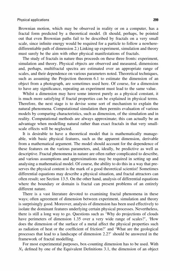
Physical applications 299
Brownian motion, which may be observed in reality or on a computer, has afractal form predicted by a theoretical model. (It should, perhaps, be pointedout that even Brownian paths fail to be described by fractals on a very smallscale, since infinite energy would be required for a particle to follow a nowhere-differentiable path of dimension 2.) Linking up experiment, simulation and theorymust surely be the aim with other physical manifestations of fractals.
The study of fractals in nature thus proceeds on these three fronts: experiment,simulation and theory. Physical objects are observed and measured, dimensionsand, perhaps, multifractal spectra are estimated over an appropriate range ofscales, and their dependence on various parameters noted. Theoretical techniques,such as assuming the Projection theorem 6.1 to estimate the dimension of anobject from a photograph, are sometimes used here. Of course, for a dimensionto have any significance, repeating an experiment must lead to the same value.
Whilst a dimension may have some interest purely as a physical constant, itis much more satisfying if fractal properties can be explained in physical terms.Therefore, the next stage is to devise some sort of mechanism to explain thenatural phenomena. Computational simulation then permits evaluation of variousmodels by comparing characteristics, such as dimension, of the simulation and inreality. Computational methods are always approximate; this can actually be anadvantage when modelling natural rather than exact fractals in that very small-scale effects will be neglected.
It is desirable to have a theoretical model that is mathematically manage-able, with basic physical features, such as the apparent dimension, derivablefrom a mathematical argument. The model should account for the dependence ofthese features on the various parameters, and, ideally, be predictive as well asdescriptive. Fractal phenomena in nature are often rather complicated to describe,and various assumptions and approximations may be required in setting up andanalysing a mathematical model. Of course, the ability to do this in a way that pre-serves the physical content is the mark of a good theoretical scientist! Sometimesdifferential equations may describe a physical situation, and fractal attractors canoften result; see Section 13.5. On the other hand, analysis of differential equationswhere the boundary or domain is fractal can present problems of an entirelydifferent nature.
There is a vast literature devoted to examining fractal phenomena in theseways; often agreement of dimension between experiment, simulation and theoryis surprisingly good. Moreover, analysis of dimension has been used effectively toisolate the dominant features underlying certain physical processes. Nevertheless,there is still a long way to go. Questions such as ‘Why do projections of cloudshave perimeters of dimension 1.35 over a very wide range of scales?’, ‘Howdoes the dimension of the surface of a metal affect the physical properties suchas radiation of heat or the coefficient of friction?’ and ‘What are the geologicalprocesses that lead to a landscape of dimension 2.2?’ should be answered in theframework of fractal modelling.
For most experimental purposes, box-counting dimension has to be used. WithNδ defined by one of the Equivalent Definitions 3.1, the dimension of an object

300 Physical applications
is usually found by estimating the gradient of a graph of log Nδ against − log δ.We often wish to estimate the dimension of a theoretical exact fractal F bybox counting on a physical approximation E. To do this, boxes that are largecompared with the accuracy of the approximation must be used. More precisely,if d(E,F ) � ε where d denotes Hausdorff distance, and Nδ(E) and Nδ(F ) arethe number of balls of radius δ required to cover the sets, it is easy to see that
Nδ+ε(E) � Nδ(F ) � Nδ−ε(E)
for δ > ε, and this may be taken into account when estimating dimHF fromlog–log plots of measurements of E. It is also worth remembering, as wehave indicated in various instances throughout the book, that there are oftentheoretical reasons for supposing that exact fractals have equal box and Haus-dorff dimensions.
Sometimes other quantities are more convenient to measure than dimension.For example, in the case of a time-dependent signal, the autocorrelation func-tion (see Section 11.2) might be measured, with equation (11.20) providing anindication of the dimension.
We now examine in more detail some specific physical examples where fractalanalysis can aid understanding of physical processes.
18.1 Fractal growth
Many natural objects grow in an apparently fractal form, with branches repeatedlysplitting and begetting smaller side branches. When viewed at appropriate scales,certain trees, root systems and plants (in particular more primitive ones such aslichens, mosses and seaweeds) appear as fractals. Forked patterns of lightningor other electrical discharges, and the ‘viscous fingering’ that occurs when wateris injected into a viscous liquid such as oil also have a branched fractal form.During electrolysis of copper sulphate solution, the copper deposit at the cathodegrows in a fractal pattern.
The biological laws that govern plant growth are far too complex to be used asa basis for a mathematical model. However, other phenomena may be modelledby relatively simple growth laws and we examine some of these.
A simple experiment demonstrates fractal growth by electrolysis of coppersulphate (CuSO4); see figure 18.1. The bottom of a circular dish is covered witha little copper sulphate solution. A copper cathode is suspended in the centre ofthe dish and a strip of copper is curved around the edge of the dish to form ananode. If a potential of a few volts is applied between the electrodes, then, aftera few minutes, a deposit of copper starts to form around the cathode. After halfan hour or so the copper deposit will have extended into fractal fingers severalinches long.
The mechanism for this electrolysis is as follows. In solution, the copper sul-phate splits into copper Cu2+ ions and sulphate SO4
2− ions which drift around
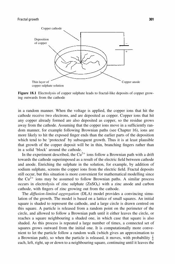
Fractal growth 301
Copper cathode
Depositionof copper
Thin layer ofcopper sulphate solution
Copper anode
−
+
Figure 18.1 Electrolysis of copper sulphate leads to fractal-like deposits of copper grow-ing outwards from the cathode
in a random manner. When the voltage is applied, the copper ions that hit thecathode receive two electrons, and are deposited as copper. Copper ions that hitany copper already formed are also deposited as copper, so the residue growsaway from the cathode. Assuming that the copper ions move in a sufficiently ran-dom manner, for example following Brownian paths (see Chapter 16), ions aremore likely to hit the exposed finger ends than the earlier parts of the depositionwhich tend to be ‘protected’ by subsequent growth. Thus it is at least plausiblethat growth of the copper deposit will be in thin, branching fingers rather thanin a solid ‘block’ around the cathode.
In the experiment described, the Cu2+ ions follow a Brownian path with a drifttowards the cathode superimposed as a result of the electric field between cathodeand anode. Enriching the sulphate in the solution, for example, by addition ofsodium sulphate, screens the copper ions from the electric field. Fractal depositsstill occur, but this situation is more convenient for mathematical modelling sincethe Cu2+ ions may be assumed to follow Brownian paths. A similar processoccurs in electrolysis of zinc sulphate (ZnSO4) with a zinc anode and carboncathode, with fingers of zinc growing out from the cathode.
The diffusion-limited aggregation (DLA) model provides a convincing simu-lation of the growth. The model is based on a lattice of small squares. An initialsquare is shaded to represent the cathode, and a large circle is drawn centred onthis square. A particle is released from a random point on the perimeter of thecircle, and allowed to follow a Brownian path until it either leaves the circle, orreaches a square neighbouring a shaded one, in which case that square is alsoshaded. As this process is repeated a large number of times, a connected set ofsquares grows outward from the initial one. It is computationally more conve-nient to let the particle follow a random walk (which gives an approximation toa Brownian path), so when the particle is released, it moves, with probability 1
4each, left, right, up or down to a neighbouring square, continuing until it leaves the
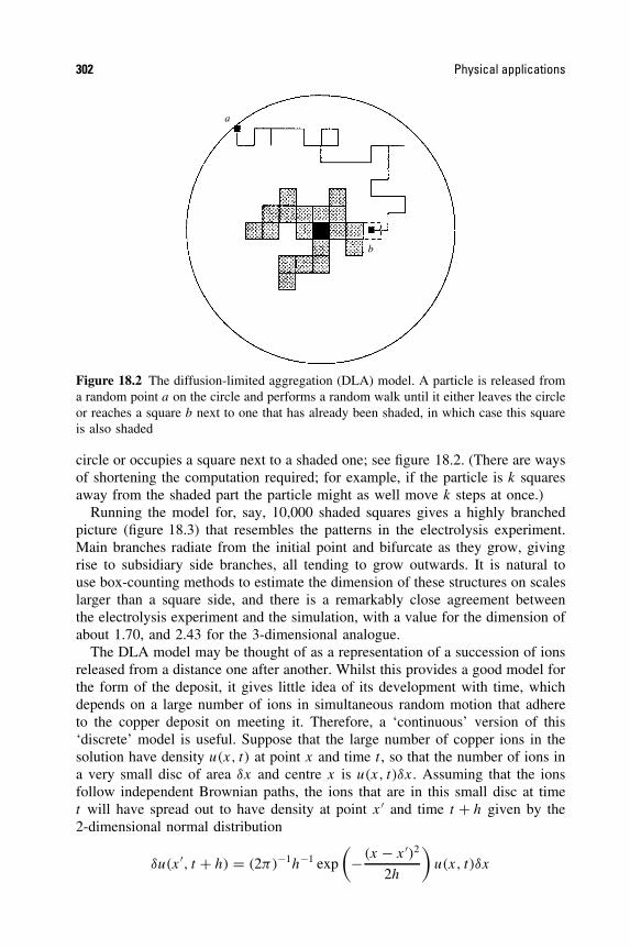
302 Physical applications
a
b
Figure 18.2 The diffusion-limited aggregation (DLA) model. A particle is released froma random point a on the circle and performs a random walk until it either leaves the circleor reaches a square b next to one that has already been shaded, in which case this squareis also shaded
circle or occupies a square next to a shaded one; see figure 18.2. (There are waysof shortening the computation required; for example, if the particle is k squaresaway from the shaded part the particle might as well move k steps at once.)
Running the model for, say, 10,000 shaded squares gives a highly branchedpicture (figure 18.3) that resembles the patterns in the electrolysis experiment.Main branches radiate from the initial point and bifurcate as they grow, givingrise to subsidiary side branches, all tending to grow outwards. It is natural touse box-counting methods to estimate the dimension of these structures on scaleslarger than a square side, and there is a remarkably close agreement betweenthe electrolysis experiment and the simulation, with a value for the dimension ofabout 1.70, and 2.43 for the 3-dimensional analogue.
The DLA model may be thought of as a representation of a succession of ionsreleased from a distance one after another. Whilst this provides a good model forthe form of the deposit, it gives little idea of its development with time, whichdepends on a large number of ions in simultaneous random motion that adhereto the copper deposit on meeting it. Therefore, a ‘continuous’ version of this‘discrete’ model is useful. Suppose that the large number of copper ions in thesolution have density u(x, t) at point x and time t , so that the number of ions ina very small disc of area δx and centre x is u(x, t)δx. Assuming that the ionsfollow independent Brownian paths, the ions that are in this small disc at timet will have spread out to have density at point x ′ and time t + h given by the2-dimensional normal distribution
δu(x ′, t + h) = (2π)−1h−1 exp
(− (x − x ′)2
2h
)u(x, t)δx

Fractal growth 303
Figure 18.3 A computer realization of diffusion-limited aggregation. The square wasdivided into a 700 × 700 mesh from which 16,000 squares were selected using themethod described
(see (16.3)) and so
u(x ′, t + h) = (2π)−1h−1∫
exp
(− (x − x ′)2
2h
)u(x, t)dx
where integration is across the fluid region. This assumes that h is small relativeto the distance of x ′ from the deposit and the boundary, so that the effect ofthe introduction or removal of ions can be neglected. Differentiating under theintegral sign with respect to x ′ and h gives
∂u/∂t = 12∇2u (18.1)
as the differential equation governing the change of the ion density in the solution.This is the well known diffusion equation or heat equation in two dimensions.
We need to specify the boundary conditions for this differential equation. At theouter boundary, say a circle of radius r0, ions are supplied at a constant rate, so
u = u0 on |x| = r0. (18.2)
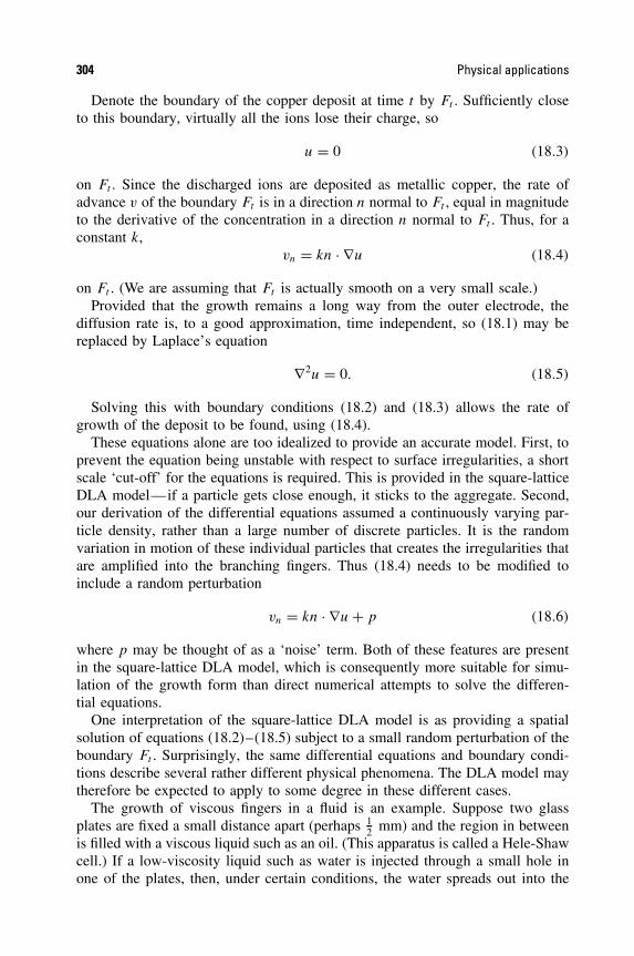
304 Physical applications
Denote the boundary of the copper deposit at time t by Ft . Sufficiently closeto this boundary, virtually all the ions lose their charge, so
u = 0 (18.3)
on Ft . Since the discharged ions are deposited as metallic copper, the rate ofadvance v of the boundary Ft is in a direction n normal to Ft , equal in magnitudeto the derivative of the concentration in a direction n normal to Ft . Thus, for aconstant k,
vn = kn · ∇u (18.4)
on Ft . (We are assuming that Ft is actually smooth on a very small scale.)Provided that the growth remains a long way from the outer electrode, the
diffusion rate is, to a good approximation, time independent, so (18.1) may bereplaced by Laplace’s equation
∇2u = 0. (18.5)
Solving this with boundary conditions (18.2) and (18.3) allows the rate ofgrowth of the deposit to be found, using (18.4).
These equations alone are too idealized to provide an accurate model. First, toprevent the equation being unstable with respect to surface irregularities, a shortscale ‘cut-off’ for the equations is required. This is provided in the square-latticeDLA model—if a particle gets close enough, it sticks to the aggregate. Second,our derivation of the differential equations assumed a continuously varying par-ticle density, rather than a large number of discrete particles. It is the randomvariation in motion of these individual particles that creates the irregularities thatare amplified into the branching fingers. Thus (18.4) needs to be modified toinclude a random perturbation
vn = kn · ∇u + p (18.6)
where p may be thought of as a ‘noise’ term. Both of these features are presentin the square-lattice DLA model, which is consequently more suitable for simu-lation of the growth form than direct numerical attempts to solve the differen-tial equations.
One interpretation of the square-lattice DLA model is as providing a spatialsolution of equations (18.2)–(18.5) subject to a small random perturbation of theboundary Ft . Surprisingly, the same differential equations and boundary condi-tions describe several rather different physical phenomena. The DLA model maytherefore be expected to apply to some degree in these different cases.
The growth of viscous fingers in a fluid is an example. Suppose two glassplates are fixed a small distance apart (perhaps 1
2 mm) and the region in betweenis filled with a viscous liquid such as an oil. (This apparatus is called a Hele-Shawcell.) If a low-viscosity liquid such as water is injected through a small hole inone of the plates, then, under certain conditions, the water spreads out into the
Fractal growth 305
oil in thin highly branched fingers. The patterns resemble closely the deposits ofcopper in the electrolysis experiment.
Lubrication theory tells us that in this situation the velocity of flow v of theoil is proportional to the pressure gradient.
v = −c∇p (18.7)
where p(x) is the pressure at a point x in the oil. The oil is assumed incom-pressible, so the velocity has zero divergence ∇ · v = 0, giving
∇2p = 0
throughout the oil. If the viscosity of the water is negligible compared with thatof the oil, then the pressure throughout the water is effectively constant. Thuswe have the boundary conditions
p(x) = p0
at the fluid interface, andp(x) = 0
at a large distance r0 from the point of injection. Thus the pressure differenceu(x) = p0 − p(x) satisfies the differential equation (18.5) and boundary con-ditions (18.2) and (18.3) of the electrolysis example. Furthermore, at the fluidinterface, the pressure gradient in the oil is normal to the boundary (since thepressure is constant on the boundary), so (18.4) gives the rate of advance of theboundary, vn = −kn · ∇p, with short-range cut-off provided by surface tensioneffects. The pressure is analogous to the ion density in the electrolysis example.
It is perhaps, therefore, not surprising that under certain conditions the viscousfingers resemble the patterns produced by the square-lattice DLA model. Whilstthe element of randomness inherent in the electrolysis example is lacking, irreg-ularities in the interface are nevertheless amplified to give the fingering effect.
A very similar situation pertains for fluid flow through a porous medium—(18.7) is Darcy’s law governing such flow. Fractal fingering can also occur inthis situation.
Electrical discharge in a gas provides a further example. The electrostaticpotential u satisfies Laplace’s equation ∇2u = 0 away from the ionized regionof discharge. The ionized path conducts well enough to be regarded as being atconstant potential, so u satisfies the same boundary conditions as in the viscousfingering example. The (questionable) assumption that the rate of breakdown isproportional to the electric field gives equation (18.4). This is another examplewith similar differential equations, for which the square-mesh DLA model pro-vides a realistic picture.
Under suitable experimental conditions, the growth patterns in electrolysis, vis-cous fingering and electrical discharge have a dimension of about 1.7 when esti-mated over a suitable range of scales. This coincides with the value obtained from

306 Physical applications
computer studies of square-mesh DLA. Although the theoretical explanations ofsuch phenomena are not always entirely satisfactory, the universality of thisdimension is very striking.
18.2 Singularities of electrostatic and gravitational potentials
The electrostatic potential at a point x due to a charge distribution µ or thegravitational potential due to a mass distribution µ in �3 is given by
φ(x) =∫
dµ(y)
|x − y| . (18.8)
We show that the dimension of the singularity set of the potential, i.e. the set ofx for which φ(x) = ∞, cannot be too large.
Proposition 18.1
Let µ be a mass distribution of bounded support on �3. Suppose that the potential(18.8) has singularity set F = {x : φ(x) = ∞}. Then dimHF � 1.
Proof. Suppose s > 1. Let x ∈ �3 and write m(r) = µ(B(x, r)) for r > 0. Sup-pose that there are numbers a > 0, c > 0 such that m(r) � crs for all 0 < r �a. Then
φ(x) =∫
|x−y|�a
dµ(x)
|x − y| +∫
|x−y|>a
dµ(x)
|x − y|
�∫ a
r=0
dm(r)
r+
∫
|x−y|>a
dµ(x)
a
� [r−1m(r)]a0 +∫ a
0r−2m(r)dr + a−1µ(�3)
� c(1 + (s − 1)−1)as−1 + a−1µ(�3) < ∞,
after integrating by parts. So, if x ∈ F , we must have that limr→∞(µ(B(x, r))/rs)
� c for all c > 0. It follows from Proposition 4.9(b) that Hs(F ) = 0 for s > 1, asrequired. �
Often µ is expressible in terms of a ‘density function’ f , so that µ(A) =∫A
f (x)dx for Borel sets A, and (18.8) becomes
φ(x) =∫
f (y)
|x − y|dy. (18.9)
Given certain conditions on f , for example if∫ |f (x)|pdx < ∞ for some p > 1,
similar methods can be used to place further bounds on the dimension of thesingularity set, see Exercise 18.5.
Fluid dynamics and turbulence 307
It is easily verified that, if f is a sufficiently smooth function, then (18.9) isthe solution of Poisson’s equation
∇2φ = −4πf
satisfying φ(x) → 0 as |x| → ∞. For a general integrable function f the poten-tial φ need not be differentiable. Nevertheless (18.9) may be regarded as a weaksolution of Poisson’s equation in a sense that can be made precise using thetheory of distributions. This technique extends, in a non-trivial way, to givebounds for the dimension of the singularity sets of weak solutions of other partialdifferential equations.
18.3 Fluid dynamics and turbulence
Despite many years of intense study, turbulence in fluids is still not fully under-stood. Slowly moving fluids tend to flow in a smooth unbroken manner, whichis described accurately by the Navier–Stokes equations—the fundamental dif-ferential equations of fluid dynamics. Such smooth flow is termed laminar. Athigher speeds, the flow often becomes turbulent, with the fluid particles followingconvoluted paths of rapidly varying velocity with eddies and irregularities at allscales. Readers will no doubt be familiar with the change from laminar to turbu-lent flow as a tap is turned from low to full. Although the exact form of turbulentflow is irregular and unpredictable, its overall features are consistently present.
There is no uniformly accepted definition of turbulent flow—this has theadvantage that it can reasonably be identified with any convenient ‘singular fea-ture’ of a flow description. We consider a model in which turbulence is manifestedby a significant local generation of heat due to viscosity, i.e. ‘fluid friction’, atpoints of intense activity.
At reasonably small scales, turbulence may be regarded as isotropic, i.e. direc-tion independent. Our intuitive understanding of isotropic turbulence stems largelyfrom the qualitative approach of Kolmogorov rather than from an analysis of dif-ferential equations. Kolmogorov’s model is based on the idea that kinetic energyis introduced into a fluid on a large scale, such as by stirring. However, kineticenergy can only be dissipated (in the form of heat) on very small scales where theeffect of viscosity becomes important. At intermediate scales dissipation can beneglected. If there are circulating eddies on all scales, then energy is transferredby the motion of the fluid through a sequence of eddies of decreasing size, until itreaches the small eddies at which dissipation occurs. If, as Kolmogorov assumed,the fluid region is filled by eddies of all scales, then dissipation of energy as heatshould occur uniformly throughout the fluid.
Let ε(x) be the rate of dissipation per unit volume at the point x, so that theheat generated in a small volume δV around x in time δt is ε(x)δV δt . Then, onthe assumption of uniform dissipation
ε(x) = ε for all x in D
308 Physical applications
where ε is the rate of input of energy into the fluid region D, which is assumedto have unit volume.
Although such ‘homogeneous’ turbulence is appealing in its simplicity, itis not supported by experimental observations. Measurements using a hot-wireanemometer show that in a turbulent fluid the rate of dissipation differs greatly indifferent parts of the fluid. This is the phenomenon of intermittency. Dissipationis high in some regions and very low in others, whereas the Kolmogorov modelrequires it to be constant. This variation can be quantified using correlation func-tions. For a small vector h the correlation of dissipation rates between pointsdistance h apart is given by
〈ε(x)ε(x + h)〉 (18.10)
where angle brackets denote the average over all x in D. If dissipation were con-stant we would have 〈ε(x)ε(x + h)〉 = ε2. However, experiment indicates that
〈ε(x)ε(x + h)〉 � ε2|h|−d (18.11)
for a value of d between 0.4 and 0.5.The Kolmogorov model can be modified to explain the intermittency by assum-
ing that, instead of the eddies at each scale filling space, the eddies fill asuccessively smaller proportion of space as their size decreases. Kinetic energyis introduced into the largest eddy and passed through eddies of decreasing sizeuntil it is dissipated at the smallest scale. Now, however, the energy and dissi-pation are concentrated on a small part of the fluid. The cascade of eddies maybe visualized as the first k stages Ei of the construction of a self-similar fractalF (see Chapter 9) where k is quite large, with dissipation occurring across thekth stage Ek. For convenience, we assume that each kth level basic set of Ei isreplaced by a constant number of sets of equal size to form Ei+1.
If A is a subset of D, we define µ(A) = ∫A
ε(x)dx as the total rate of dis-sipation of energy in the set A; thus µ(D) = ε, the rate of energy input. Thenµ has the properties of a mass distribution on D. Moreover, if we assume thatthe rate of dissipation in each component of Ei is divided equally between theequal-sized subcomponents in Ei+1, we have, as a simple consequence of F
being self-similar of Hausdorff or box dimension s, that
c1εrs � µ(B(x, r)) � c2εr
s
if x ∈ F and 0 < r < r0, where c1 and c2 are positive constants (see Exercise9.11). These inequalities hold for the limit F as the size of the dissipation eddiestends to 0, but also for the physical approximation Ek, provided that r is largerthan the dissipation scale. Then
∫
|h|�r
〈ε(x)ε(x + h)〉dh =∫
x∈D
∫
|h|�r
ε(x)ε(x + h)dhdx
=∫
x∈D
ε(x)µ(B(x, r))dx
=∫
x∈Ek
ε(x)µ(B(x, r))dx
Fractal antennas 309
since dissipation is concentrated on Ek, so
c1ε2rs �
∫
|h|�r
〈ε(x)ε(x + h)〉dh � c2ε2rs . (18.12)
This may be achieved if the correlation satisfies a power law
〈ε(x)ε(x + h)〉 � ε2|h|s−3
for then the integral in (18.12) becomes
4π
∫ r
t=0ε2t s−3t2dt = 4πε2rs/s.
Comparison with (18.11) suggests that s = 3 − d , so the hypothesis of ‘fractallyhomogeneous turbulence’, that dissipation is concentrated on an approximatefractal of dimension between 2.5 and 2.6, is consistent with experimental results.
It is natural to seek theoretical reasons for the turbulent region to have afractal form. One possible explanation is in terms of the vortex tubes in the fluid.According to Kelvin’s circulation theorem, such tubes are preserved throughoutthe motion, at least in the approximation of inviscid flow. However, the vortextubes are stretched by the fluid motion, and become long and thin. Repeatedfolding is necessary to accommodate this length, so the tubes might assume anapproximate fractal form not unlike the horseshoe example in figure 13.5.
The behaviour of a (viscous) fluid should be predicted by the Navier–Stokesequation
∂u
∂t+ (u · ∇)u − ν∇2u + ∇p = f (18.13)
where u is the velocity, p is the pressure, ν is viscosity and f is the appliedforce density. Deducing the existence of fractal regions of activity from theNavier–Stokes equation is far from easy. Nevertheless, the method indicated inSection 18.2 may be generalized beyond recognition to demonstrate rigorouslythat, for example, the set on which a solution u(x, t) of (18.13) fails to be boundedfor all t has dimension at most 2 1
2 . Thus it is possible to show from the equationsof fluid flow that certain types of ‘intense activity’ must be concentrated on setsof small dimension.
18.4 Fractal antennas
A remarkable application of fractals is their use as antennas in high frequencyradio and in particular in mobile telephones. There are two advantages of usingfractals. First, the ‘space-filling’ nature of some fractals, such as variations onthe von Koch curve, allow a high response fractal antenna to be fitted into arelatively small space. Secondly, depending on their geometry, antennas can be

310 Physical applications
multiband with resonant frequencies reflecting the self-similarities of the fractal,or alternatively can have frequency independent response, for example in thecase of certain random fractal antennas.
Electrodynamics, and in particular the behaviour of radio waves, is governedby Maxwell’s equations. Assume a time dependence of the electromagnetic quan-tities proportional to eiωt , where ω is the frequency, so that the electric field atthe point x is eiωtE(x) and the magnetic field is eiωtH(x). Then Maxwell’s ‘curl’equations in a vacuum reduce to
∇ × E = −iωµH
∇ × H = iωεE,
where ε is the permittivity and µ the permeability of space. It is immediate thatthese equations are invariant under the pair of transformations
x → λx and ω → ω/λ,
for every (positive or negative) scalar λ, with both sides of the equations multi-plied by 1/λ under the transformations.
If the antenna has a similar form when scaled by a factor λ, the boundaryconditions for Maxwell’s equations are similar under this scaling, so the radiationproperties might be expected to behave in a similar manner when the frequencyis scaled by 1/λ, that is when the wavelength is scaled by λ.
This is borne out in the Sierpinski dipole, a practical instance of a fractalantenna, see figure 18.4. In one realization, two Sierpinski triangles are etched on
(a) (b)
(c)
Figure 18.4 Fractal antennas, showing feed lines. (a) Sierpinski dipole, (b) random treeantenna, (c) von Koch dipole

Fractals in finance 311
a printed circuit board, vertex to vertex (a fractal ‘bow-tie’), with the vertices fedby a two-wire transmission line from a transmitter or receiver. The fundamentalfrequency of the antenna corresponds to a wavelength comparable to the overalldiameter of the Sierpinski triangle. Sharp peaks are observed in the antennaresponse at 1, 1
2 , 14 , 1
8 and 116 times this wavelength, these ratios corresponding to
the fundamental similarity ratios of the triangle, bearing out the above argument.At each of these resonances the current density is concentrated on the pair ofsimilar copies of the Sierpinski triangle nearest to the feed point and at theappropriate scale. Varying the construction parameters of the Sierpinski triangleleads to antennas with other sequences of bands.
Random fractals can be used to construct antennas suitable for a continuousrange of frequencies. For example, tree antennas, which are statistical self-similarat all scales (such as those generated by electrochemical deposition of the formof figure 18.3), give a relatively constant response across a range of frequen-cies. These compare well with traditional antennas designed for a continuousfrequency band.
18.5 Fractals in finance
Examination of graphs of share prices, exchange rates, etc., suggests some sortof self-affine scaling, that is for a number 0 < α < 1, if X(t) is the share priceat time t then the increment X(γ t) − X(γ t0) has similar overall form to theincrement γ α(X(t) − X(t0)) for a range of t > t0 and γ > 0. This suggests thata statistically self-affine process or even a deterministic self-affine function mightbe appropriate for modelling prices. Moreover, the self-affinity assumption hasmany consequences for features of the process modelled.
Because of its central place in stochastic processes, Brownian motion (seeSection 16.1) is the most natural statistically self-affine model to try. Togetherwith its variants, it is the basis for many financial models.
Let X be Brownian motion on [0,∞); we might think of a realization of X(t)
as the price, or perhaps the logarithm of the price, of some stock at time t . Acrucial feature of Brownian motion is the martingale or independent incrementproperty: given the process up to time t , the expected value of X(t + h) is justX(t), for all h > 0, reflecting that the future value of the stock is unpredictable,with a profit as likely as a loss.
If we now take X to be index-α fractional Brownian motion (Section 16.2),the increments are no longer independent, but are correlated, i.e. E((X(t) −X(0))(X(t + h) − X(t))) > 0 or < 0, according to whether α > 1
2 or α < 12 .
Moreover, if α > 12 the process has long range dependence, that is, for fixed
small h, the covariances of the increments
E((X(h) − X(0))(X(t + h) − X(t))) = 1
2[(t + h)2α + (t − h)2α − 2t2α]
� α(2α − 1)t2α−2h2

312 Physical applications
die away slowly as t increases, in the sense that∑∞
k=0 E((X(h) − X(0))(X(k + h)
− X(k))) ∼ ∑∞k=0 k2α−2 diverges. An interpretation might be that if, for some
α > 12 , index-α fractional Brownian motion provides a reasonable model of prices
then we may make inference on the future behaviour of share prices by studyingpast variations.
Many further variants are possible, for example taking cX(t) + at where X isindex-α fractional Brownian motion and a and c are positive constants, adds a‘drift’ to the process, with an underlying upward trend of rate a. Given financialdata over a range of t , statistical methods may be used to estimate appropriatevalues of α, a and c.
At first sight, realizations of Brownian motion appear qualitatively similar toshare prices or exchange rates, but a more careful examination shows markeddifferences, see figure 18.5(a) and (c). Brownian motion does not exhibit thesudden jumps and periods of intense activity, or ‘volatility’, observed in prices.This is exemplified by considering increments: for fixed small h > 0, the incre-ment X(t + h) − X(t) regarded as a function of t appears as a ‘noise’ of fairlyconstant amplitude if X is Brownian motion, figure 18.6(a), whereas for stockprices it has very marked sharp peaks and dips rising above the ambient noiselevel, corresponding to price jumps, figure 18.6(c).
One way this might arise is if X has a multifractal structure as a function,that is with a relatively small set of times t where the local fluctuations areexceptionally large. This may be made precise in terms of the dimensions ofthe sets
Ea ={t : lim inf
h→0
log |X(t + h) − X(t)|log |h| = a
};
thus, Ea comprises those t at which the Holder exponent of X is a, an analogueof (17.16) for functions. There are several ways of modelling these more extremefluctuations. A self-affine curve (Section 11.1) with a ‘generator’ that has severaldifferent gradients, has fluctuating Holder exponents and can yield graphs withmany of the features of share prices.
A more sophisticated approach uses multifractal time. The underlying idea isthat prices follow Brownian or fractional Brownian motion, but with respect torescaled or ‘warped’ time called trading time T (t). Thus, when the market isvolatile a short period in real time t is stretched to a long period of trading timeT , whilst at inactive periods, a long t period corresponds to a short T period,figures 18.5(b) and 18.6(b).
Let µ be a measure on �+, typically a multifractal measure. For t � 0 wedefine the trading time T (t) = µ[0, t] = ∫ t
0 dµ. Writing Bα for index-α Brownianmotion, we set X(t) = Bα(T (t)). Given T , then X(t) is a zero mean Gaussianprocess with variance of increments given by
E(X(t + h) − X(t))2 = E(Bα(T (t + h)) − Bα(T (t)))2
= |T (t + h) − T (t)|2α = µ[t, t + h]2α ∼ |h|2γ α (18.14)
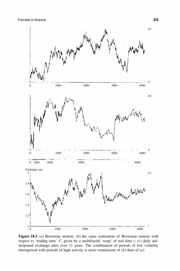
Fractals in finance 313
0 1000
Exchange rate
2000
(a)
(b)
(c)
T
T
t3000 4000
0 1000 2000 3000 4000
0 1000 2000 3000 4000
0 1000 2000 3000 4000
1
1.2
1.4
1.6
1.8
2
Figure 18.5 (a) Brownian motion, (b) the same realization of Brownian motion withrespect to ‘trading time’ T , given by a multifractal ‘warp’ of real time t , (c) daily dol-lar/pound exchange rates over 11 years. The combination of periods of low volatilityinterspersed with periods of high activity is more reminiscent of (b) than of (a)

314 Physical applications
10
8
6
4
2
0
−8
−6
−4
−2
0 500 1000 1500 2000
10
8
6
4
2
0
−8
−6
−4
−2
0 500 1000 1500 20006
4
2
0
−12
−10
−8
−6
−4
−2
0 500 1000 1500 2000
Figure 18.6 (a) Increments of Brownian motion; (b) increments of Brownian motion‘warped’ by multifractal time; (c) real data: increments of a stock price over period of5 1
2 years. The character of (c) is closer to (b) than to (a)
if t ∈ Fγ , where
Fγ ={t : lim
h→0
log µ[t, t + h]
log h= γ
}
is the set of times where µ has a local dimension γ . Thus, the volatility of X
at t depends on the local dimension of µ at t , and so the distribution of times
Notes and references 315
of high and low activity in the share prices depends on the multifractal structureof µ. If we develop the model to make µ a random multifractal measure, thetrading time T becomes a random process, so that the times of high and lowactivity are random.
Statistical methods may be applied to real price data to estimate α and themultifractal spectrum required for µ, which may be related to the ‘multifractalspectrum of X’ given by dimHEα .
Fractality is a crucial feature in mathematical modelling of finance. Here wehave just indicated some simple models; more sophisticated techniques includestochastic differential equations, where the fractal nature of the process is aconsequence of the modelling assumptions.
18.6 Notes and references
The literature on applications of fractals is enormous. A wide variety of applicationsare described in the books by Mandelbrot (1982), Feder (1988), Hastings and Sugi-hara (1993), Crilly, Earnshaw and Jones (1993), Gouyet (1996) and Meakin (1998).General conference proceedings include those edited by Shlesinger, Mandelbrotand Rubin (1984), Pietronero and Tosatti (1986), Pietronero (1989), Aharony andFeder (1990), Fleischmann, Tildesley and Ball (1990), Takayasu (1990), Cherbit(1991) and Novak (1998, 2000).
For fractal growth and DLA, refer to Stanley and Ostrowsky (1986, 1988),Feder (1988) and Vicsek (1989).
For an introduction to the ideas of turbulence, see Leslie (1973). The homoge-neous model of Kolmogorov (1941) was adapted to the fractally homogeneousmodel by Mandelbrot (1974); see also Frisch, Sulem and Nelkin (1978). Collec-tions of papers relevant to fractal aspects of turbulence include Temam (1976) andBarenblatt, Iooss and Joseph (1983). The books by Temam (1983, 1997) discussesthe dimension of sets related to solutions of the Navier–Stokes equation.
For discussion of fractal antennas, see Puente, Romeu, Rous and Cardama(1997), Jaggard (1997) and Hohlfeld and Cohen (1999).
Fractals in finance are discussed in the book by Peters (1994) and in Man-delbrot’s (1997) ‘Selecta’ and the many references therein; multifractal time ispresented in Mandelbrot (1997) and Goncalves and Riedi (1999).
There are many books on other applications. For geophysics see Scholz andMandelbrot (1989), Xie (1993) and Turcotte (1997), and for fractal river basinssee Rodrıguez-Iturbe and Rinaldo (1997). Applications to chemistry may be foundin Avinir (1989), to astronomy in Heck and Perdang (1991), to molecular bio-physics in Dewey (1997), to physiology and medicine in West (1990) and toengineering in Levy Vehel, Lutton and Tricot (1997) and Dekking, Levy Vehel,Lutton and Tricot (1999). Surface growth is discussed by Barabsi and Stan-ley (1995), and multifractal aspects of rainfall are considered by Lovejoy andSchertzer (1995).

316 Physical applications
Exercises
18.1 Suppose that the DLA square-lattice model is run for a large number of very smallsquares. Suppose that the set obtained is an approximate fractal of dimension s.What power law would you expect the number of shaded squares within distance r
of the initial square to obey? Assuming that during the process squares tend to beadded to parts of the set further away from the initial square, how would you expectthe ‘radius’ of the growth after k squares have been added to depend on k?
18.2 Let m(t) be the mass of copper that has been deposited and r(t) be the ‘radius’ of thecopper deposit after time t in the electrolysis experiment described in Section 18.1.It may be shown that the current flowing, and thus, by Faraday’s law, the rate ofmass deposition, is proportional to r(t). On the assumption that the growth formsan approximate fractal of dimension s, so that m(t) ∼ cr(t)s , give an argument tosuggest that r(t) ∼ c1t
1/(s−1).
18.3 Verify that u(x, t) in the DLA model satisfies the partial differential equation (18.1).
18.4 Verify that the potential in (18.9) satisfies Poisson’s equation if, say, f is a twicecontinuously differentiable function with f (x) = 0 for all sufficiently large x.
18.5 Show that, if f (x) = 0 for all sufficiently large x and∫ |f (x)|2 dx < ∞, then the
singularity set of φ, given by (18.9), is empty.
18.6 Show that the argument leading to (18.12) can be adapted to the case when, say, D
is the unit cube in �3 and F is the product of the Cantor dust of figure 0.4 and aunit line segment L. (Dissipation is assumed to occur on the set Ek × L, where Ek
is the kth stage in the construction of the Cantor dust for some large k.)
18.7 For a fractal antenna made from a wire in the shape of a von Koch curve, if thefundamental frequency is ω, what are the higher resonant frequencies?
18.8 Generalize (18.14) to show that E(|X(t + h) − X(t)|q) ∼ |h|qγ for t ∈ Fγ (seeExercise 16.7).

References
Abenda S, Moussa P. and Osbaldestin A. H. (1999) Multifractal dimensions and thermo-dynamical description of nearly-circular Julia sets, Nonlinearity, 12, 19–40.
Addison P. S. (1997) Fractals and Chaos—An Illustrated Course, Institute of PhysicsPublishing, Bristol.
Adler R. J. (1981) The Geometry of Random Fields, Wiley, New York.
Aharony A. and Feder J. (1990) Fractals in Physics, North-Holland, Amsterdam.
Ahlfors L. V. (1979) Complex Analysis, McGraw-Hill, New York.
Anderson R. D. and Klee V. L. (1952) Convex functions and upper semi-continuous func-tions, Duke Math. J., 19, 349–357.
Apostol T. M. (1974) Mathematical Analysis, 2nd edition, Addison-Wesley, Reading, MA.
Avnir D. (Ed.) (1989) The Fractal Approach to Heterogeneous Chemistry, Wiley, NewYork.
Ayache A. and Levy Vehel J. (1999) Generalized multifractional Brownian motion: def-inition and preliminary results, in Fractals: Theory and applications in engineering,17–32. Springer, London.
Ayache A., Cohen S. and Levy Vehel J. (2000) The covariance structure of multifractionalBrownian motion, with application to long range dependence, ICASSP, June 2000.
Baker A. and Schmidt W. M. (1970) Diophantine approximation and Hausdorff dimen-sion, Proc. Lond. Math. Soc. (3), 21, 1–11.
Bandt C., Graf S. and Zahle M. (Eds.) (1995) Fractal Geometry and Stochastics. Progressin Probability, 37, Birkhauser, Basel.
Bandt C., Graf S. and Zahle M. (Eds.) (2000) Fractal Geometry and Stochastics, II. Prog-ress in Probability, 46, Birkhauser, Basel.
Barabsi A.-L. and Stanley H. E. (1995) Fractal Concepts in Surface Growth, CambridgeUniversity Press, Cambridge.
Barenblatt G. I., Iooss G. and Joseph D. D. (Eds) (1983) Nonlinear Dynamics and Tur-bulence, Pitman, London.
Barnsley M. F. (1993) Fractals Everywhere, 2nd ed., Academic Press, Boston.
317
Fractal Geometry: Mathematical Foundations and Application. Second Edition Kenneth Falconer 2003 John Wiley & Sons, Ltd ISBNs: 0-470-84861-8 (HB); 0-470-84862-6 (PB)

318 References
Barnsley M. F. and Hurd L. P. (1993) Fractal Image Compression, A. K. Peters, Welles-ley.
Beardon A. F. (1965) On the Hausdorff dimension of general Cantor sets, Proc. Camb.Phil. Soc., 61, 679–694.
Beardon A. F. (1991) Iteration of Rational Functions, Springer, New York.
Beck C. and Schlogl F. (1993) Thermodynamics of Chaotic Systems, Cambridge Univer-sity Press, Cambridge.
Becker K.-H. and Dorfler M. (1989) Dynamical Systems and Fractals, Cambridge Uni-versity Press, Cambridge.
Bedford T. J. (1989) The box dimension of self-affine graphs and repellers, Nonlinearity,2, 53–71.
Bedford T. (1991) Applications of dynamical systems theory to fractals, in Fractal Analy-sis and Geometry, (Belair and Dubuc, S., Eds.), Kluwer, Dordrecht.
Bedford T., Keane M. and Series C. (1991) Ergodic Theory, Symbolic Dynamics andHyperbolic Spaces, Oxford University Press, Oxford.
Bedford T. J. and Swift J. (Eds) (1988) New Directions in Dynamical Systems, CambridgeUniversity Press, Cambridge.
Bernik V. I. and Dodson M. M. (1999) Metric Diophantine Approximation on Manifolds,Cambridge University Press, Cambridge.
Berry M. V. and Lewis Z. V. (1980) On the Weierstrass–Mandelbrot fractal function,Proc. R. Soc. London, A 370, 459–484.
Besicovitch A. S. (1928) On the fundamental geometrical properties of linearly measur-able plane sets of points, Math. Annalen, 98, 422–464.
Besicovitch A. S. (1934) Sets of fractional dimensions IV: On rational approximation toreal numbers, J. Lond. Math. Soc., 9, 126–131.
Besicovitch A. S. (1938) On the fundamental geometric properties of linearly measurableplane sets of points II, Math. Annalen, 115, 296–329.
Besicovitch A. S. (1939) On the fundamental geometric properties of linearly measurableplane sets of points III, Math. Annalen, 116, 349–357.
Besicovitch A. S. (1952) On existence of subsets of finite measure of sets of infinitemeasure, Indag. Math., 14, 339–344.
Besicovitch A. S. (1963) The Kakeya problem, Am. Math. Monthly, 70, 697–706.
Besicovitch A. S. (1964) On fundamental geometric properties of plane line sets, J. Lond.Math. Soc., 39, 441–448.
Besicovitch A. S. and Moran P. A. P. (1945) The measure of product and cylinder sets,J. Lond. Math. Soc., 20, 110–120.
Besicovitch A. S. and Ursell H. D. (1937) Sets of fractional dimensions, V: On dimen-sional numbers of some continuous curves, J. Lond. Math. Soc., 12, 18–25.
Billingsley P. (1978) Ergodic Theory and Information, Krieger, New York.
Billingsley P. (1995) Probability and Measure, 3rd ed. Wiley, New York.
Blanchard P. (1984) Complex analytic dynamics on the Riemann sphere, Bull. Am. Math.Soc., 11, 85–141.
Bouligand G. (1928) Ensembles impropres et nombre dimensionnel, Bull. Sciences Mathe-matiques, II-52, 320–334, 361–376.

References 319
Brolin H. (1965) Invariant sets under iteration of rational functions, Arkiv Math., 6,103–144.
Brown G., Michon G. and Peyriere J. (1992) On the multifractal analysis of measures, J.Stat. Phys., 66, 775–790.
Bumby R. T. (1985) Hausdorff dimension of sets arising in number theory, in NumberTheory, New York 1983–84. Seminar (Lecture Notes in Mathematics, 1135), pp. 1–8.Springer, New York.
Caratheodory C. (1914) Uber das lineare Mass von Punktmengen–eine Verallgemeinerungdas Langenbegriffs, Nach. Ges. Wiss. Gottingen, pp. 406–426.
Carleson A. (1967) Selected Problems on Exceptional Sets, Van Nostrand, Princeton, NJ.
Carleson L. and Gamelin T. W. (1993) Complex Dynamics, Springer-Verlag, New York.
Cassels J. W. S. (1957) An Introduction to Diophantine Approximation, Cambridge Uni-versity Press, Cambridge.
Cawley R. and Mauldin R. D. (1992) Multifractal decomposition of Moran fractals, Adv.Math., 92, 196–236.
Chayes J. T., Chayes L. and Durrett R. (1988) Connectivity of Mandelbrot’s percolationprocess, Prob. Theor. Related Fields, 77, 307–324.
Chayes L. (1995) Aspects of the fractal percolation process, in Fractal Geometry andStochastics, 113–143. Progr. Probab., 37, Birkhauser, Basel.
Cherbit G. (Ed.) (1991) Fractals: Non-integral dimensions and applications, Wiley, Chich-ester.
Collet P., Dobbertin R. and Moussa P. (1992) Multifractal analysis of nearly circular Juliaset and thermodynamical formalism, Ann. Inst. H. Poincare Phys. Theor., 56, 91–122.
Crilly A. J., Earnshaw R. A. and Jones H. (Eds.) (1993) Applications of Fractals andChaos . The Shape of Things, Springer-Verlag, Berlin.
Csornyei M. (2001) On planar sets with prescribed packing dimensions of line sections,Math. Proc. Cambridge Philos. Soc., 130, 523–539.
Cunningham F. (1974) Three Kakeya problems, Am. Math. Monthly, 81, 589–592.
Curry J., Garnett L. and Sullivan D. (1983) On the iteration of rational functions: com-puter experiments with Newton’s method, Commun. Math. Phys., 91, 267–277.
Cvitanovic P. (Ed.) (1989) Universality in Chaos, 2nd ed. Adam Hilger, Bristol.
Dalla L. and Larman D. G. (1980) Convex bodies with almost all k-dimensional sectionspolytopes, Math. Proc. Camb. Phil. Soc., 88, 395–401.
David G. (1999) Analytic capacity, Caldern-Zygmund operators, and rectifiability, Publ.Mat. 43, 3–25.
Davies R. O. (1952) On accessibility of plane sets and differentiation of functions of tworeal variables, Proc. Camb. Phil. Soc., 48, 215–232.
Dekking F. M. (1982) Recurrent sets, Adv. Math., 44, 78–104.
Dekking F., Levy Vehel J., Lutton E. and Tricot C. (Eds.) (1999) Fractals: Theory andApplications in Engineering, Springer-Verlag, London.
Dekking F. M. and Meester R. W. J. (1990) On the structure of Mandelbrot’s percolationprocess and other random Cantor sets, J. Statist. Phys. 58, 1109–1126.
Devaney R. L. (1989) Introduction to Chaotic Dynamic Systems, Benjamin Cummings,Menlo Park, CA.
320 References
Devaney R. L. and Keen L. (1989) Chaos and Fractals: The Mathematics Behind theComputer Graphics, American Mathematical Society, Providence.
Dewey T. G. (1997) Fractals in Molecular Biophysics, Oxford University Press, NewYork.
Dodson M. M., Rynne B. P. and Vickers J. A. G. (1990) Diophantine approximation anda lower bound for Hausdorff dimension, Mathematika, 37, 59–73.
Drazin P. G. (1992) Nonlinear Systems, Cambridge University Press, Cambridge.
Edgar G. A. (1990) Measure, Topology, and Fractal Geometry, Springer-Verlag, NewYork.
Edgar G. A. (1993) Classics on Fractals, Addison-Wesley, Menlo Park.
Edgar G. A. (1998) Integral, Probability, and Fractal Measures, Springer-Verlag, NewYork.
Edgar G. A. and Mauldin R. D. (1992) Multifractal decompositions of digraph recursivefractals. Proc. London Math. Soc. (3), 65, 604–628.
Edgar G. A. and Miller C. (2003) Borel subrings of the reals, Proc. Am. Math. Soc., 131,1121–1129.
Eggleston H. G. (1952) Sets of fractional dimension which occur in some problems ofnumber theory, Proc. Lond. Math. Soc. (2), 54, 42–93.
Embrechts P. and Maejima M. (2002) Selfsimilar Processes, Princeton University Press,Princeton.
Erdos P. and Volkmann B. (1966) Additive Gruppen mit vorgegebener HausdorffscherDimension, J. reine angew. Math., 221, 203–208.
Evertsz C. J. G. and Mandelbrot B. B. (1992) Multifractal measures. Appendix B inChaos and Fractals (Peitgen, H.-O., Jurgens, H. and Saupe, D. Eds.), Springer-Verlag,New York.
Evertsz C. J. G., Peitgen H.-O. and Voss R. F. (Eds.) (1995) Fractal Geometry and Analy-sis: Papers from the Symposium in Honor of Benoit Mandelbrot, World Scientific, RiverEdge.
Falconer K. J. (1985a) The Geometry of Fractal Sets, Cambridge University Press, Cam-bridge.
Falconer K. J. (1985b) Classes of sets with large intersection, Mathematika, 32, 191–205.
Falconer K. J. (1985c) The Hausdorff dimension of distance sets, Mathematika, 32,206–212.
Falconer K. J. (1986a) Sets with prescribed projections and Nikodym sets, Proc. Lond.Math. Soc. (3), 53, 48–64.
Falconer K. J. (1986b) Random fractals, Math. Proc. Camb. Phil. Soc., 100, 559–582.
Falconer K. J. (1988) The Hausdorff dimension of self-affine fractals, Math. Proc. Camb.Phil. Soc., 103, 339–350.
Falconer K. J. (1994) Sets with large intersection properties, J. London Math. Soc. (2),49, 267–280.
Falconer K. J. (1997) Techniques in Fractal Geometry, John Wiley, Chichester.
Falconer K. J. and Howroyd J. D. (1997) Packing dimensions of projections and dimen-sion profiles, Math. Proc. Cambridge Philos. Soc., 121, 269–286.
Falconer K. J., Jarvenpaa M. and Mattila P. (1999) Examples illustrating the instabilityof packing dimensions of sections, Real Anal. Exchange, 25, 629–640.

References 321
Falconer K. J. and Levy Vehel J. (2000) Horizons of fractional Brownian surfaces. Proc.Royal Soc. London A, 456, 2153–2178.
Falconer K. J. and Marsh D. T. (1989) Classification of quasi-circles by Hausdorff dimen-sion, Nonlinearity, 2, 489–493.
Falconer K. J. and O’Neil T. C. (1996) Vector-valued multifractal measures, Proc. RoyalSoc. London A, 452, 1–26.
Farag H. (2002) On the 12 -problem of Besicovitch: quasi-arcs do not contain sharp saw-
teeth, Rev. Mat. Iberoamericana, 18, 17–40.
Fatou P. (1919) Sur les equations fonctionelles, Bull. Soc. Math. France, 47, 161–271.
Feder J. (1988) Fractals, Plenum Press, New York.
Federer H. (1947) The (ϕ, k) rectifiable subsets of n-space, Trans. Am. Math. Soc., 62,114–192.
Federer H. (1996) Geometric Measure Theory, Springer, New York.
Fisher G. (1995) Fractal Image Compression: Theory and Applications, Springer-Verlag,New York.
Fleischmann M., Tildesley D. J. and Ball R. C. (Eds.) (1990) Fractals in the NaturalSciences, Princeton University Press, Princeton.
Frame M. L. and Mandelbrot B. B. (2002) Fractals, Graphics and Mathematical Educa-tion, Mathematical Association of America, Washington.
Frederickson P., Kaplan J., Yorke E. and Yorke J. (1983) The Lyapunov dimension ofstrange attractors, J. Diff. Eq., 49, 185–207.
Frisch U. and Parisi G. (1985) Fully developed turbulence and intermittency. In Turbu-lence and Predictability of Geophysical Flows and Climate Dynamics (eds. M. Ghil,R. Benzi and G. Parisi), pp. 84–88, North-Holland, Amsterdam.
Frisch U., Sulem P.-L. and Nelkin M. (1978) A simple dynamical model of fully devel-oped turbulence, J. Fluid Mech., 87, 719–736.
Frostman O. (1935) Potential d’equilibre et capacite des ensembles avec quelques appli-cations a la theorie des fonctions, Meddel. Lunds Univ. Math. Sem., 3, 1–118.
Goncalves P. and Riedi R. (1999) Wavelet analysis of fractional Brownian motion inmultifractal time, Proc. 17th Colloq. GRETSI, Vannes, France.
Gouyet J.-F. (1996) Physics and Fractal Structures, Springer-Verlag, New York.
Graf S. (1987) Statistically self-similar fractals, Prob. Theor. Related Fields, 74, 357–392.
Graf S., Mauldin R. D. and Williams S. C. (1988) The exact Hausdorff dimension inrandom recursive constructions, Mem. Am. Math. Soc., 71, no. 381.
Grimmett G. R. (1999) Percolation, 2nd ed. Springer, New York.
Grimmett G. R. and Stirzaker D. R. (1992) Probability and Random Processes, 2nd ed.Clarendon Press, Oxford.
Gruber P. M. and Wills J. M. (Eds.) (1993) Handbook of Convex Geometry, Vol. A, B.,North-Holland, Amsterdam.
Guckenheimer J. and Holmes P. (1983) Nonlinear Oscillations, Dynamical Systems andBifurcations of Vector Fields, Springer, New York.
Hale J. K. and Kocak H. (1991) Dynamics and Bifurcations, Springer-Verlag, New York.
Halsey T. C., Jensen M. H., Kadanoff L. P., Procaccia I. and Shraiman B. I. (1986) Frac-tal measures and their singularities: the characterization of strange sets, Phys. Rev. A(3) 33, 1141–1151.
322 References
Hardy G. H. and Wright E. M. (1979) An Introduction to the Theory of Numbers, 5thedition, Cambridge University Press, Cambridge.
Harte D. (2001) Multifractals, Theory and Applications, Chapman & Hall/CRC, BocaRaton.
Hastings H. M. and Sugihara G. (1993) Fractals. A User’s Guide for the Natural Sciences,Oxford University Press, New York.
Hausdorff F. (1919) Dimension und ausseres Mass, Math. Annalen, 79, 157–179.
Hayman W. K. and Kennedy P. B. (1976) Subharmonic Functions, Volume 1, AcademicPress, New York.
Heck A. and Perdang J. M. (Eds.) (1991) Applying Fractals in Astronomy, Springer-Verlag, Berlin.
Henon M. and Pomeau Y. (1976) Two strange attractors with a simple structure, in Tur-bulence and the Navier–Stokes Equations (Lecture Notes in Mathematics, 565), (Ed.R. Temam), pp. 29–68, Springer, New York.
Hensley D. (1996) A polynomial time algorithm for the Hausdorff dimension of continuedfraction Cantor sets, J. Number Theory, 58, 9–45.
Hoggar S. G. (1992) Mathematics for Computer Graphics, Cambridge University Press,Cambridge.
Hohlfeld R. G. and Cohen N. (1999) Self-similarity and the geometric requirements forfrequency independence in antennae, Fractals, 7, 79–84.
Holden A. V. (1986) Chaos, Manchester University Press, Manchester.
Howroyd J. D. (1996) On Hausdorff and packing dimensions of product spaces, Math.Proc. Cambridge Philos. Soc., 119, 715–727.
Howroyd J. D. (2001) Box and packing dimensions of projections and dimension profiles,Math. Proc. Cambridge Philos. Soc., 130, 135–160.
Hunt B. R. (1998) The Hausdorff dimension of graphs of Weierstrass functions, Proc.Amer. Math. Soc., 126, 791–800.
Hutchinson J. E. (1981) Fractals and self-similarity, Indiana Univ. Math. J., 30, 713–747.
Hutchinson J. E. and Ruschendorf L. (2000) Random fractals and probability metrics,Adv. in Appl. Probab. 32, 925–947.
Jaffard S. (1997) Multifractal formalism for functions I, II, SIAM J. Math. An., 28,944–970, 971–998.
Jaggard D. L. (1997) Fractal electrodynamics: from super antennas to superlattices, inFractals in Engineering, Springer-Verlag, New York, 204–221.
Jarnık V. (1931) Uber die simultanen diophantischen Approximationen, Math. Zeit., 33,505–543.
Jones P. W. and Murai T. (1988) Positive analytic capacity but zero Buffon needle prob-ability, Pacific J. Math., 133, 99–114.
Joyce H. and Preiss D. (1995) On the existence of subsets of finite positive packingmeasure, Mathematika, 42, 15–24.
Julia G. (1918) Sur l’iteration des fonctions rationnelles, J. Math. Pure Appl., Ser. 7, 4,47–245.
Kahane J.-P. (1974) Sur le modele de turbulence de Benoit Mandelbrot, C. R. Acad. Sci.Paris, 278A, 621–623.

References 323
Kahane J.-P. (1985) Some Random Series of Functions, 2nd edition, Cambridge UniversityPress, Cambridge.
Kahane J.-P. (1986) Sur la dimensions des intersections, in Aspects of Mathematics andits Applications (Ed. J. A. Barroso), pp. 419–430, North-Holland, Amsterdam.
Kahane J.-P. and Peyriere J. (1976) Sur certaines martingales de Benoit Mandelbrot, Adv.Math. 22, 131–145.
Karlin S. and Taylor H. M. (1975) A First Course in Stochastic Processes, AcademicPress, New York.
Karlin S. and Taylor H. M. (1981) A Second Course in Stochastic Processes, AcademicPress, New York.
Katok A. and Hasselblatt B. (1995) Introduction to the Modern Theory of DynamicalSystems, Cambridge University Press, Cambridge.
Katz N. and Tao T. (2000) Recent progress on the Kakeya conjecture, PublicacionsMatematiques, Proc. 6th Int. Conf. on Harmonic Analysis and P.D.E.s, Barcelona,161–180.
Kaufman R. (1968) On the Hausdorff dimension of projections, Mathematika, 15,153–155.
Kaufman R. (1981) On the theorem of Jarnık and Besicovitch, Acta Arithmetica, 39,265–267.
Kaye B. H. (1994) A Random Walk Through Fractal Dimensions, 2nd Ed, VCH Verlags-gesellschaft, Weinheim.
Kesten H. (1982) Percolation Theory for Mathematicians, Birkhauser, Boston, MA.
Kingman J. F. C. and Taylor S. J. (1966). Introduction to Measure and Probability, Cam-bridge University Press, Cambridge.
Kolmogorov A. N. (1941) Local structure of turbulence in an incompressible liquid forvery large Reynolds numbers, C.R. Acad. Sci. USSR, 30, 299–303.
Lapidus M. L. and van Frankenhuysen M. (2000) Fractal Geometry and Number Theo-ry. Complex Dimensions of Fractal Strings and Zeros of Zeta Functions, Birkhauser,Boston.
Ledrappier F., Lewowicz J. and Newhouse S. (Eds.) (1996) International Conference onDynamical Systems. A Tribute to Ricardo Ma, Longman, Harlow.
Le Mehaute A. (1991) Fractal Geometries: Theory and Applications, CRC Press, BocaRaton.
Leslie D. C. (1973) Developments in the Theory of Turbulence, Clarendon Press, Oxford.
Lesmoir-Gordon N., Rood W. B. and Edney R. (2000) Introducing Fractal Geometry,Totem.
Levy P. (1948) Processus Stochastiques et Mouvement Brownian, 2nd ed. 1965, Gauthier-Villars, Paris.
Levy Vehel J., Lutton E. and Tricot C. (1997) Fractals in Engineering, Springer-Verlag,New York.
Lind D. and Marcus B. (1995) An Introduction to Symbolic Dynamics and Coding, Cam-bridge University Press, Cambridge.
Lovejoy S. (1982) Area perimeter relation for rain and cloud areas, Science, 216, 185–187.
Lovejoy S. and Schertzer D. (1995) Multifractals and rain, in New Uncertainty Conceptsin Hydrology and Hydrological Modelling, 62–103, Cambridge University Press.

324 References
McCauley J. L. (1993) Chaos, Dynamics and Fractals, Cambridge University Press, Cam-bridge.
MacKay R. S. and Meiss J. D. (Eds) (1987) Hamiltonian Dynamical Systems, AdamHilger, Bristol.
McMullen C. (1984) The Hausdorff dimension of general Sierpinski carpets, NagoyaMath. J., 96, 1–9.
McMullen C. T. (1994) Complex Dynamics and Renormalization, Princeton UniversityPress, Princeton.
Mandelbrot B. B. (1972) Renewal sets and random cutouts, Z. Warsch Verw. Geb., 22,145–157.
Mandelbrot B. B. (1974) Intermittent turbulence in self-similar cascades: divergence ofhigh moments and dimension of the carrier, J. Fluid Mech., 62, 331–358.
Mandelbrot B. B. (1980) Fractal aspects of the iteration of z → λz(1 − z) for complexλ, z, Ann. N. Y. Acad. Sci., 357, 249–259.
Mandelbrot B. B. (1982) The Fractal Geometry of Nature, Freeman, San Francisco.
Mandelbrot B. B. (1986) Self-affine fractal sets, in Fractals in Physics (Eds L. Pietroneroand E. Tosatti), North-Holland, Amsterdam.
Mandelbrot B. B. (1991) Random multifractals: negative dimensions and the resultinglimitations of the thermodynamic formalism, Proc. Roy. Soc. London, A434, 79–88.
Mandelbrot B. B. (1997) Fractals and Scaling in Finance: Discontinuity, Concentration,Risk, Springer-Verlag, New York.
Mandelbrot B. B. (1999) Multifractals and 1/f Noise: Wild Self-affinity in Physics,Springer-Verlag, New York.
Mandelbrot B. B. (2002) Gaussian Self-affinity and Fractals. Globality, the Earth, 1/fNoise, and R/S, Springer-Verlag, New York.
Mandelbrot B. B. and Riedi R. (1995) Multifractal formalism for infinite multinomialmeasures, Adv. App. Math., 16, 132–150.
Mandelbrot B. B. and Van Ness J. W. (1968) Fractional Brownian motions, fractionalnoises and applications, SIAM Rev., 10, 422–437.
Marstrand J. M. (1954a) Some fundamental geometrical properties of plane sets of frac-tional dimensions. Proc. Lond. Math. Soc. (3), 4, 257–302.
Marstrand J. M. (1954b) The dimension of Cartesian product sets, Proc. Camb. Phil. Soc.,50, 198–202.
Massopust P. R. (1994) Fractal Functions, Fractal Surfaces, and Wavelets, AcademicPress, San Diego.
Mattila P. (1975) Hausdorff dimension, orthogonal projections and intersections withplanes, Ann. Acad. Sci. Fennicae, A 1, 227–244.
Mattila P. (1984) Hausdorff dimension and capacities of intersections of sets in n-space,Acta Math., 152, 77–105.
Mattila P. (1985) On the Hausdorff dimension and capacities of intersections, Mathe-matika, 32, 213–217.
Mattila P. (1986) Smooth maps, null-sets for integral geometric measures and analyticcapacity, Ann. Math., 123, 303–309.
Mattila P. (1995) Geometry of Sets and Measures in Euclidean Spaces, Cambridge Uni-versity Press, Cambridge.
References 325
Mauldin R. D. and Urbanski M. (1996) Dimensions and measures in infinite iterated func-tion systems, Proc. Lond. Math. Soc. (3), 73, 105–154.
Mauldin R. D. and Urbanski M. (1999) Conformal iterated function systems withapplications to the geometry of continued fractions, Trans. Amer. Math. Soc., 351,4995–5025.
Mauldin R. D. and Williams S. C. (1986a) Random recursive constructions: asymptoticgeometric and topological properties, Trans. Am. Math. Soc., 295, 325–346.
Mauldin R. D. and Williams S. C. (1986b) On the Hausdorff dimension of some graphs,Trans. Am. Math. Soc., 298, 793–803.
Mauldin R. D. and Williams S. C. (1988) Hausdorff dimension in graph directed con-structions, Trans. Amer. Math. Soc, 309, 811–829.
May R. M. (1976) Simple mathematical models with very complicated dynamics, Nature,261, 459–467.
Mayer-Kress G. (Ed.) (1986) Dimensions and Entropies in Chaotic Dynamical Systems,Springer-Verlag, Berlin.
Meakin P. (1998) Fractals, Scaling and Growth Far from Equilibrium, Cambridge Uni-versity Press, Cambridge, 55.
Merzenich W. and Staiger L. (1994) Fractals, dimension, and formal languages, RAIROInformatique thorique et Applications, 28, 361–386.
Milnor J. (1999) Dynamics in One Complex Variable, Introductory Lectures, Friedr. Vie-weg and Sohn, Braunschweig.
Moon F. C. (1992) Chaotic and Fractal Dynamics, Wiley, New York.
Moran P. A. P. (1946) Additive functions of intervals and Hausdorff measure, Proc.Camb. Phil. Soc., 42, 15–23.
Morgan F. (2000) Geometric Measure Theory. A Beginner’s Guide, Academic Press, SanDiego.
Murai T. (1988) A real variable method for the Cauchy transform, and analytic capacity,Lecture Notes in Mathematics, 1307, Springer-Verlag, Berlin.
Novak M. M. (Ed.) (1998) Fractals and Beyond, World Scientific, Singapore.
Novak M. M. (Ed.) (2000) Paradigms of Complexity, World Scientific, Singapore.
Nusse H. E. and Yorke J. A. (1998) Dynamics: Numerical Explorations, Springer-Verlag,New York.
Olsen L. (1994) Random Geometrically Graph Directed Self-similar Multifractals, Long-man, Harlow.
Olsen L. (1995) A multifractal formalism, Adv. Math., 116, 82–196.
Olsen L. (2000) Multifractal geometry, in Fractal Geometry and Stochastics, II, 3–37,Progr. Probab., 46, Birkhauser, Basel.
Papoulis A. (1962) The Fourier Integral and its Applications, McGraw-Hill, New York.
Patzschke N. (1997) Self-conformal multifractal measures, Adv. Appl. Math. 19, 486–513.
Peitgen H.-O., Jurgens H. and Saupe D. (1992) Chaos and Fractals, Springer-Verlag, NewYork.
Peitgen H.-O. and Richter P. H. (1986) The Beauty of Fractals, Springer, Berlin.
Peitgen H.-O. and Saupe D. (Eds) (1988) The Science of Fractal Images, Springer, NewYork.
326 References
Peitgen H.-O., Saupe D. and von Haeseler F. (1984) Cayley’s problem and Julia sets,Math. Intelligencer, 6, 11–20.
Peres Y. and Solomyak B. (2000) Problems on self-similar sets and self-affine sets: anupdate, in Fractal Geometry and Stochastics II, 95–106, Progr. Probab., 46, Birkhauser,Basel.
Pesin Y. (1997), Dimension Theory in Dynamical Systems, University of Chicago Press,Chicago.
Peters E. E. (1994) Fractal Market Analysis: Applying Chaos Theory to Investment andEconomics, Wiley, New York.
Peyriere J. (1974) Turbulence et dimension de Hausdorff, C.R. Acad. Sci. Paris, 278A,567–569.
Peyriere J. (1977) Calculs de dimensions de Hausdorff, Duke Math. J., 44, 591–601.
Pickover C. A. (Ed.) (1998) Chaos and Fractals. A Computer Graphical Journey, Elsevier,Amsterdam.
Pietronero L. (Ed.) (1989) Fractals, Plenum Press, New York.
Pietronero L. and Tosatti E. (Eds) (1986) Fractals in Physics, North-Holland, Amsterdam.
Pontrjagin L. and Schnirelman L. (1932) Sur une propriete metrique de la dimension,Ann. Math., 33, 156–162.
Preiss D. (1987) Geometry of measures in Rn: distribution, rectifiability and densities,Ann. Math., 125, 537–641.
Preiss D. and Tiser J. (1992) On Besicovitch’s 12 -problem, J. London Math. Soc. (2), 45,
279–287.
Puente C., Romeu J., Rous R. and Cardama A. (1997) Multiband fractal antennas andarrays, in Fractals in Engineering, Springer-Verlag, New York, 221–236.
Riedi R. (1995) An improved multifractal formalism and self-similar measures, J. Math.Anal. Appl., 189, 462–490.
Rodriguez-Iturbe I. and Rinaldo A. (1997) Fractal River Basins, Cambridge UniversityPress, Cambridge.
Rogers L. C. G. and Williams D. (2000) Diffusions, Markov Processes and Martingales,Volume 1: Foundations, 2nd ed., Cambridge University Press, Cambridge.
Rogers C. A. (1988) Dimension prints, Mathematika, 35, 1–27.
Rogers C. A. (1998) Hausdorff Measures, 2nd ed. Cambridge University Press, Cam-bridge.
Rudin W. (1964) Principles of Mathematical Analysis, McGraw-Hill, New York.
Ruelle D. (1980) Strange attractors, Math. Intelligencer, 2, 126–137.
Ruelle D. (1982) Repellers for real analytic maps, Ergod. Theor. Dyn. Syst., 2, 99–108.
Ruelle D. (1983) Bowen’s formula for the Hausdorff dimension of self-similar sets, inScaling and Self-similarity in Physics (Progress in Physics, 7 ) Birkhauser, Boston,MA.
Rynne B. P. (1992) Regular and ubiquitous systems, and Ms∞-dense sequences, Mathe-matika 39, 234–243.
Samorodnitsky G. and Taqqu M. S. (1994) Stable Non-Gaussian Random Processes,Chapman & Hall/CRC, Boca Raton.
Santalo L. A. (1976) Integral Geometry and Geometric Probability, Addison-Wesley,Reading, Massachusetts.

References 327
Saupe D. (1987) Efficient computation of Julia sets and their fractal dimension, Physica,28D, 358–370.
Schmidt W. M. (1980) Diophantine Approximation (Lecture Notes in Mathematics, 785).Springer, Berlin.
Schneider R. (1993) Convex surfaces, curvature and surface area measures, in Handbookof Convex Geometry, Vol. A, 273–299, North-Holland, Amsterdam.
Scholz C. H. and Mandelbrot B. B. (Eds) (1989) Fractals in Geophysics, Birkhauser,Boston, MA.
Schroeder M. (1991) Fractals, Chaos, Power Laws, W. H. Freeman, New York.
Schuster H. G. (1984) Deterministic Chaos—An Introduction, Physik Verlag, Weinheim.
Shlesinger M. F., Mandelbrot B. B. and Rubin R. J. (Eds) (1984) Proceedings of theGaithersburg Symposium on Fractals in the Natural Sciences , J. Stat. Phys., 36 (specialissue) 519–921.
Simpelaere D. (1994) Dimension spectrum of Axiom A diffeomorphisms I,II, J. Stat.Phys., 76, 1329–1358, 1359–1375.
Smale S. (1967) Differentiable dynamical systems, Bull. Am. Math. Soc., 73, 747–817.
Solomyak B. (1998) Measure and dimension for some fractal families, Math. Proc. Cam-bridge Philos. Soc., 124, 531–546.
Sparrow C. (1982) The Lorenz Equations: Bifurcations, Chaos, and Strange Attractors,Springer, New York.
Stanley H. E. and Ostrowsky N. (Eds.) (1986) On Growth and Form, Martinus Nijhoff,Dordrecht.
Stanley H. E. and Ostrowsky N. (Eds.) (1988) Random Fluctuations and Pattern Growth,Kluwer Academic, Dordrecht.
Stein E. M. (1993) Harmonic Analysis: Real-variable Methods, Orthogonality, and Oscil-latory Integrals, Princeton University Press, Princeton.
Stoyan D. and Stoyan H. (1994) Fractals, Random Shapes and Point Fields, Wiley, Chich-ester.
Stuart A. M. and Humphries A. R. (1996) Dynamical Systems and Numerical Analysis,Cambridge University Press, Cambridge.
Takayasu H. (1990) Fractals in the Physical Sciences, Manchester University Press, Man-chester.
Tan L. (Ed.) (2000) The Mandelbrot Set, Theme and Variations, London Math. Soc. Lec-ture Notes, 274, Cambridge University Press, Cambridge.
Taylor S. J. (1961) On the connection between Hausdorff measures and generalized capac-ities, Proc. Camb. Phil. Soc., 57, 524–531.
Taylor S. J. (1973) Sample path properties of processes with stationary independentincrements, in Stochastic Analysis (Eds D. G. Kendall and E. F. Harding), pp. 387–414.Wiley, New York.
Taylor S. J. (1986) The measure theory of random fractals, Math. Proc. Camb. Phil. Soc.,100, 383–406.
Tel T. (1988) Fractals and multifractals, Zeit. Naturforsch., 43A, 1154–1174.
Temam R. (Ed.) (1976) Turbulence and the Navier–Stokes Equations, Lecture Notes inMathematics 565, Springer, New York.

328 References
Temam R. (1983) Navier–Stokes Equations and Non-linear Functional Analysis, Societyfor Industrial and Applied Mathematics, Philadelphia, PA.
Temam R. (1997) Infinite-dimensional Dynamical Systems in Mechanics and Physics, 2nded., Springer-Verlag, New York.
Thompson J. M. T. and Stewart H. B. (1986) Nonlinear Dynamics and Chaos, Wiley,Chichester.
Tricot C. (1982) Two definitions of fractional dimension, Math. Proc. Camb. Phil. Soc.,91, 54–74.
Tricot C. (1995) Curves and Fractal Dimension, Springer-Verlag, New York.
Turcotte D. L. (1997) Fractals and Chaos in Geology and Geophysics, Cambridge Uni-versity Press, Cambridge.
Vicsek T. (1992) Fractal Growth Phenomena, 2nd ed., World Scientific, River Edge.
Voss R. F. (1985) Random fractal forgeries, in Fundamental Algorithms in ComputerGraphics (Ed. R. A. Earnshaw), pp. 805–835. Springer, Berlin.
West B. J. (1990) Fractal Physiology and Chaos in Medicine, World Scientific, Teaneck.
Wicks K. R. (1991) Fractals and Hyperspaces, Lecture Notes in Mathematics 1492,Springer-Verlag.
Wolff T. (1999) Recent work connected with the Kakeya problem, in Prospects in Math-ematics, 129–162, Amer. Math. Soc., Providence.
Xie H. (1993) Fractals in Rock Mechanics, A. A. Balkema, Rotterdam.
Young L.-S. (1982) Dimension, entropies and Lyapunov exponents, Ergod. Theor. Dyn.Syst., 2, 109–124.
Zahle U. (1984) Random fractals generated by random cutouts, Math. Nachr., 116, 27–52.
Index
Page numbers in bold type refer to definitions, those in italics refer to Figures
affine transformation 8, 139affinity 7, 8almost all 16, 85almost everywhere 16almost surely 19analytic function 138, 180, 215antennas 309–311, 310arc, dimension print 56area 14
scaling of 29Arnold’s cat map 213astronomical evidence, for small divisors
208attractive orbit 228attractive point 216, 222attractor 123, 123–128, 127, 139, 140,
187in continuous dynamical system
201–205in discrete dynamical system 187,
189, 192, 194autocorrelation 169–173, 268autocorrelation function 170average 21Avogadro’s number 258
baker’s transformation 193, 193–194,194, 210, 211
ball 4Banach’s contraction mapping theorem
124, 125basic interval 35, 62, 127, 152
basin of attraction 187, 201, 222,238–241
Besicovitch construction 178, 179Besicovitch set 179bifurcation diagram 192bijection 7, 236bi-Lipschitz equivalence 236bi-Lipschitz function 8, 103bi-Lipschitz transformation 32, 33, 41binary interval 16, 36Borel set(s) 6
and duality 178and intersections 111measure on 11–12and products 100, 101, 105, 106and projections 90, 93and subrings 183–184and subsets of finite measure 68, 69,
70boundary 5, 6bounded set 5, 114bounded variation 86box counting 283, 298box(-counting) dimension 41, 41–47,
43, 44Brownian motion 263, 265fractional Brownian motion 268fractional Brownian surface 273and growth 299–300and Hausdorff dimension 46, 60Levy stable process 272limitations 48
329
Fractal Geometry: Mathematical Foundations and Application. Second Edition Kenneth Falconer 2003 John Wiley & Sons, Ltd ISBNs: 0-470-84861-8 (HB); 0-470-84862-6 (PB)
330 Index
box(-counting) dimension (continued )modified 49, 49–50problems 48–49properties 47–48ways of finding 44, 47
branch 223branching process theory 250Brownian graph 266Brownian motion 37, 258–267, 259,
261, 298, 299, 311–315Fourier series representation 260fractional 173, 267, 267–271, 269,
275index-α fractional 267, 267–271, 269,
311multifractional 271n-dimensional 260
Brownian sample function 259, 261, 262graph 265–266index-α fractional 273multiple points 265
Brownian surface, fractional 273–275Brownian trail(s) 258, 261, 262,
264–265
Cantor dust xx, xxi, 94, 126calculation of Hausdorff dimension 34construction of xxi , 34
‘Cantor product’ 99, 100, 102, 103Cantor set
as attractor 189, 192, 194construction of 61–62dimension of xxiii, 34–35, 47middle λ 64middle third xvii, xviii, xviii , 34–35,
47, 60, 61, 63–64, 87, 99, 100,112, 123–124, 127, 129, 188, 189
non-linear 136–137, 154random 245–246, 246–250, 256uniform 63–64, 64, 103, 141see also main entry: middle third
Cantor set‘Cantor target’ 103–104, 104(s-)capacity 72capacity dimension 41Cartesian product 4, 87, 99, 100cat map 213Cauchy sequence 125central limit theorem 24, 259chaos 189chaotic attractor 189, 192chaotic repeller 189characteristic function 271Choleski decomposition 270
circle perimeter, dimension print 56class Cs 113, 113–118, 157
member 113closed ball 4, 66closed interval 4closed loop, as attractor 201closed set 5, 5, 114, 201closure of set 6cloud boundaries 244, 298coarse multifractal spectrum 278–279
lower 280upper 280
coastline(s) 54, 244, 298codomain 7collage theorem 145compact set 6, 48complement of a set 4complete metric 125complex dynamics 216composition of functions 7computer drawings 127–128, 128,
145–148, 196, 227, 232, 233, 234,239, 240, 244, 260, 269, 270–271,275
conditional expectation 22conditional probability 19conformal mapping 138–139, 180, 241congruence(s) 7, 7, 112
direct 8conjugacy 223connected component 6connected set 6content
Minkowski 45s-dimensional 45
continued fraction(s) 153–154examples 153
continued fraction expansion 153continuity equation 203continuous dynamical systems 201–205continuous function 10continuously differentiable function 10contours 275contracting similarity 123contraction 123contraction mapping theorem 124, 125convergence 8
pointwise 10of sequence 5uniform 10, 17
convex function 181, 181–182, 287convex surface 182convolution theorem 73, 172coordinate cube 4
Index 331
copper sulphate, electrolysis of300–301, 302–304
correlation 169–173, 268, 311countable set 4, 32, 41countable stability
of dimension print 55of Hausdorff dimension 32, 41
counting measure 13covariance matrix 270cover of a set 27, 28, 30, 35–36
see also (δ-)covercovering lemma 66–67critical exponent 54critical point 227, 228cross section 202cube 4, 42cubic polynomial, Newton’s method for
239–241, 240curve 53, 81
fractal 133–134Jordan 53, 81rectifiable 81, 81–84, 85–86,
181–182curve-free set 81, 83, 83–84curve-like set 81, 82–83, 83–84
Darcy’s law 305data compression 145–148decomposition of 1-sets 80–81, 81(delta-)/(δ-)cover 27, 28, 30, 36(delta-)/(δ-)neighbourhood 4, 4, 45, 112,
124(delta-)/(δ-)parallel body 4dendrite 232dense set 6density 76, 76–80, 84, 88, 152
lower 77, 84upper 77
density function 306derivative 10diameter of subset 5, 27difference of sets 4differentiability 10, 137–138, 160, 182
continuous 10diffusion equation 303diffusion limited aggregation (DLA)
model 301–306, 302, 303digital sundial 96–97, 97dimension xxii–xxv, xxiv
alternative definitions 39–58approximations to 299, 305of attractors and repellers 186–201box(-counting) 41, 41–50, 43, 44, 60,
263, 265, 268, 272, 273, 299–300
calculation of 34–35, 59–75,128–135
of Cantor set xxiiicapacity 41characterization of quasi-circles by
235–237divider 39, 53–54entropy 41experimental estimation of 39–40,
299–300finer definitions 36–37Fourier 74of graphs of functions 160–169, 161Hausdorff xxiv, 27, 31, 31–33,
35–36, 40, 54, 70, 92Hausdorff–Besicovitch 31Hausdorff dimension of a measure
209, 288information 41of intersections 109–118local 283lower box(-counting) 41, 43of a measure 288metric 41Minkowski(–Bouligand) 46modified box-counting 49, 49–50one-sided 54packing 50–53, 51of products 99–107of projections 90–97of random sets 246–251, 259–275of self-affine sets 106–107, 139–144,
166–169of self-similar sets xxiv, 128–135similarity xxivtopological xxvupper box(-counting) 41, 43of von Koch curve xxiiiof (α-)well approximable number 155
dimension function 37dimension print 54–57, 55, 56
disadvantages 55–56examples 56
dimensionally homogeneous set 50Diophantine approximation 153,
154–157, 205direct congruence 8Dirichlet’s theorem 154discrete dynamical system 186, 186–201disjoint binary intervals 36disjoint collection of sets 4distance set 183
332 Index
distributionGaussian 23multidimensional normal 262normal 23, 260uniform 23
distribution of digits 151–153divider dimension 39, 53–54domain 7double sector 85duality method 176–179, 177‘dust-like’ set 110dynamical systems 186–212
continuous 201–205discrete 186, 186–201
dynamics, complex 216
eddies 308Egoroff’s theorem 17, 79electrical discharge in gas 305electrodynamics 310electrolysis 300–301, 301, 302–304electrostatic potential 70, 305, 306–307(s-)energy 70entropy 209–211, 210entropy dimension 41ergodic theory 128, 209Euclidean distance or metric 3Euclidean space 3event 18
independence of 20event space 18exchange rate variation 311, 313expectation 21
conditional 22expectation equation 247, 250experiment (probabilistic) 18experimental approach to fractals 39–40,
299–300exterior, of loop 223extinction probability 250
Fatou set 216, 235Feigenbaum constant 193figure of eight 223, 228filled-in Julia set 215finance 186, 311–315fine (Hausdorff) multifractal spectrum
284fine multifractal analysis 277, 283–286first return map 202, 202fixed point 125, 186, 216fluid dynamics 277, 307–309forked lightning 298, 300
Fourier dimension 74Fourier series 206Fourier transform 73, 92
methods using 73–74, 112, 171–173,260, 271
fractal, definition xxii, xxvfractal curve 133–134 , 216fractal growth 300–306fractal interpolation 169, 170fractal percolation 251–255fractally homogeneous turbulence 309fractional Brownian motion 173, 267,
269, 267–271fractional Brownian surface(s) 273–275fractions, continued 153–154Frostman’s lemma 70full square 254function(s) 6, 6–7
continuous 10convex 181, 181–182
functional analysis 179
gauge function 37Gaussian distribution 23Gaussian process 267general construction 61–62, 62generator 134–135
examples 132, 133, 134geometric invariance 41geometric measure theory 53, 76graphs of functions 160, 160–169, 258,
266, 267gravitational potential 70, 306–307group(s) of fractional dimension
182–184group of transformations 8, 110, 111growth 300–306
Hamiltonian 207–208Hamiltonian systems, stability of
207–208, 212Hamilton’s equations 207Hausdorff–Besicovitch dimension 31Hausdorff dimension xxiv, 27, 31, 31–33,
31, 54of attractor 192, 193and box(-counting) dimension 46, 60Brownian motion 263, 265calculating 70–72, 92equivalent definitions 35–36fractional Brownian motion 268fractional Brownian surface 273Levy stable process 272

Index 333
of a measure 209, 288and packing dimension 53and projections 90–93properties 32of self-affine set 140–144, 140, 144
Hausdorff distance 124, 124Hausdorff measure 14, 27–30, 28
and intersections 113and packing measure 53and product rule 99and quasi-circle 236
Hausdorff metric 124, 124, 145, 300heat equation 303Hele–Shaw cell 304Henon attractor/map 103, 196–197, 197,
198, 212, 213heuristic calculation(s) 34–35, 129histogram method, for multifractal
spectrum 279, 283Holder condition 30, 32, 262, 265, 268Holder exponent 283, 312Holder function 8, 10, 30, 161Holder’s inequality 297homeomorphism 10, 33homogeneous turbulence 308horseshoe map 194–195, 195, 196, 212
image 7, 258, 275image encoding 145–148in general 109, 110independence
of events 20of random variables 20
independent increment 259, 268, 311index-α fractional Brownian function
273index-α fractional Brownian motion 267,
267–271, 269, 311–312index-α fractional Brownian surface
273, 274infimum 5information dimension 41injection 7integral 16–17integral geometry 118interior 6
of loop 223intermittency 308interpolation 169, 170intersection formulae 110–113intersection(s) 4, 109–118, 110,
265–266, 275large 113–118, 157
interval 4
interval density 152invariance
geometric 41Lipschitz 41, 48
invariant curves 205, 207invariant measure 208, 208–211invariant set 123, 123–129, 187, 218invariant tori 208inverse function 7inverse image 7investment calculations 186irregular point 78irregular set 78, 79–80, 94
examples xxi , 81, 180isolated point, as attractor 201isometry 7, 30isotropic 261isotropic turbulence 307iterated construction(s) 95–96, 96,
180–181iterated function system (IFS) 123,
123–128advantages 128attractor for 123, 123–129, 146–148,
194, 228and repellers 187–189variations 135–139
iterated Venetian blind construction95–96, 96, 180
iteration 186–201, 215–242
Jarnık’s theorem 155–157, 205, 207Jordan curve 53, 81Julia set xxii, 215, 215–242, 219, 233,
234
Kakeya problem 176–179Koch curve see von Koch curveKolmogorov–Arnold–Moser (KAM)
theorem 208Kolmogorov entropy 41Kolmogorov model of turbulence
307–309
laminar flow 307landscapes 273Laplace’s equation 304, 305law of averages 23–24Lebesgue density theorem 77, 77, 93Lebesgue measure 13, 16, 112, 192, 264
n-dimensional 13, 17, 28, 112, 143,266
Legendre spectrum 282
334 Index
Legendre transform 281, 281, 282, 287length 13, 81
scaling of 29level set 266, 275level-k interval 35, 62, 152level-k set 127Levy process 267, 271–273Levy stable process 271, 271–273Liapounov exponents 208–211, 209,
210, 212limit 8–9
lower 9of sequence 5upper 9
lim sup sets 113line segment
dimension print 56uniform mass distribution on 14
line set 176, 176–179linear transformation 8Lipschitz equivalence 236Lipschitz function 8, 10, 30, 103Lipschitz invariance 41, 48, 55, 56Lipschitz transformation 30, 32, 34local dimension 283local product 103, 196, 202local structure of fractals 76–89logarithmic density 41logarithms 10logistic map 189–193, 191, 192, 212long range dependence 311loop 223, 224–225
closed 201Lorenz attractor 203–204, 204Lorenz equations 202–203lower box(-counting) dimension 41lower coarse multifractal spectrum 280lower density 77, 84lower limit 9lubrication theory 305
Mandelbrot, Benoit xxii, xxvMandelbrot set 223, 223–227, 224, 230,
233, 235mapping(s) 6, 8Markov partition 189martingale 248, 311mass distribution 11, 12, 277
construction by repeated subdivision14–15, 15
and distribution of digits 151–152and product rule 99, 101uniform, on line segment 14
mass distribution principle 60, 60–61,131, 200
maximum modulus theorem 231maximum range 160Maxwell’s equations 310mean 21mean-value theorem 10, 137, 190measure(s) 11, 11–17
counting 13Hausdorff 14, 27–30, 28, 53, 99, 113Hausdorff dimension of 209, 288invariant 208, 208–211Lebesgue 13, 16, 28, 112, 192multifractal 211, 277–296n-dimensional Lebesgue 13, 17, 112,
143net 36, 68packing 50–53, 51, 88probability 19restriction of 14self-similar 278, 279, 280, 286on a set 11σ -finite 95tangent 89
r-mesh cube 42, 278method of moments, for multifractal
spectrum 280–281, 283metric dimension 41middle λ Cantor set 64middle third Cantor set xvii, xviii
as attractor 189box(-counting) dimension 47construction of xviii , 127features xviii, 123generalization of 63–64Hausdorff dimension 34–35, 60, 61in intersections 112product 99, 100and repellers 188, 189and self-similarity 123, 124, 129and tangents 87
Minkowski content 45Minkowski(-Bouligand) dimension 46modified box(-counting) dimension 49,
49–50upper, and packing dimension 51–52
modified von Koch curve 132, 133–134moment sum 280, 281monotonicity
of box(-)counting dimension 48of dimension print 55of Hausdorff dimension 32, 41of packing dimension 51
Montel’s theorem 218–219, 221
Index 335
Moser’s twist theorem 207mountain skyline 271, 298multifractal(s) 211, 277–296
coarse analysis 277, 278–283fine analysis 277, 283–286self-similar 286–296
multifractal spectrum 277–286, 283,289, 292–294, 315
multifractal time 312, 313, 314multifractional Brownian motion 271multiple points 265, 275multivariate normal variable(s) 267
natural fractals xxvi, 146, 147, 298–300natural logarithms 10Navier–Stokes equations 203, 307, 309‘nearest point mapping’ 181, 182neighbourhood 4, 5, 45
see also (delta-)/(δ-)neighbourhoodnet measure 36, 68neural networks 277Newton’s method 237–241non-linear Cantor set 136–137, 154non-removable set 180, 181non-singular transformation 8normal distribution 23, 260normal family 218, 218–219
at a point 218normal numbers 151number theory 151–158
often 110one-sided dimension 54one-to-one correspondence 7one-to-one function 7onto function 7open ball 4open interval 4, 138open set 5, 5, 32, 41, 187open set condition 129, 130–134, 249orbit 186, 189, 216, 228orthogonal projection xxv, 34, 90–97, 91,
176, 177
packing dimension 50–53, 51, 284and modified upper box dimension
51–52packing measure 50–53, 51, 88
and Hausdorff measure 53parallel body 4Parseval’s theorem 73partial quotient 153percolation 251–255, 252, 253, 254
perfect set 220, 242period 216period doubling 191–193period-p orbit 216, 232, 235period-p point 186, 191periodic orbit 228, 232periodic point 216, 221phase transition 251physical applications xxvi, 298–316pinch point 232plane cross section 202plant growth 300Poincare–Bendixson theorem 201, 202Poincare section 202point mass 13pointwise convergence 10Poisson’s equation 307polynomials, Newton’s method for
237–241population dynamics 186, 190, 193porous medium, flow through 305(s-)potential 70potential theoretic methods 70–72, 92,
111, 248–249power spectrum 171, 270Prandtl number 203pre-fractal(s) 126, 127pre-image 7probability 18
conditional 19probability density function 23probability measure 18, 19probability space 19probability theory 17–24product 99
Cartesian 4, 87, 99, 100product formula 99–107projection(s) 90–97, 91
of arbitrary sets 90–93of arbitrary sets of integral dimension
95–97of s-sets of integral dimension 93–95
projection theorems 90–93, 180Pythagoras’s theorem 266
quadratic functions 223–235quadratic polynomial, Newton’s method
for 238–239quasi-circle(s) 231, 235–237, 236
radio antennas 309–311rainfall distribution 277random Cantor set 245, 246, 246–250,
256

336 Index
random fractal(s) 244–256random function 259, 260, 270random mid-point displacement method
260random process 259random variable 20
independence of 20–21simple 21
random von Koch curve xxii, xxiii , 245,251, 256
random walk 258–259range, maximum 160ratio of contraction 128rational function 238rectifiable curve 81, 81–84, 181–182
tangent 85–86reflection 8regular point 78regular set 78, 80–89, 93–94
examples 81tangent 86–87
removable set 179, 179–181repeller 187, 187–189, 215repelling point 216, 233
closure of 221reservoir level variations 160residence measure 208–209, 277, 283restriction of a measure 14rigid motion 8, 109, 111ring(s) of fractional dimension 182–184Rossler band 204, 204rotation 8
sample function 259, 262, 265sample space 18scalar multiple 4scaling property 29, 29sections, parallel 105sector, double 85self-affine curve 166–169, 168, 312
construction of 166, 167self-affine set 106–107, 107, 139,
139–145as attractor 139, 140, 142, 144, 146construction of 107, 142
self-similar fractal, with two differentsimilarity ratios xxi
self-similar measure 280, 286, 294construction of 278, 279multifractal spectrum 288, 293–296
self-similar multifractals xxiv, 286–296self-similar set xxiv, 128–135, 128
similarity dimension xxiv
see also middle third Cantor set;Sierpinski gasket; von Koch curve
self-similarity xxiisensitive dependence on initial conditions
187, 194, 222s-set 32, 69, 76
0-set 771-set 80–84, 86–87, 93–94tangent to 84–88, 85
set theory 3–6share prices 160, 258, 277, 311–315Siegel disc 232Sierpinski dipole 310–311Sierpinski gasket or triangle xx, xx, 129,
132, 256(sigma-)/σ -finite measure 95similarity 7, 8, 29, 111, 128similarity dimension xxivsimple closed curve 230, 235simple function 16simple random variable 21simulation 299singular value(s) 142singular value function 143singularity set 306singularity spectrum 284small divisor theory 205–208smooth manifold 41smooth set 32snowflake curve xixsolenoid 198–201, 199, 200solid square, dimension print 56solution curves 201stability 41, 48
countable 32, 41, 55stable point 191stable process 271, 271–273, 275stable set 216stable symmetric process 272, 273stationary increments 259, 267, 271statistically self-affine set 262, 268, 311statistically self-similar set 244, 246,
251, 262, 268stock market prices 160, 258, 277,
311–315strange attractor 186, 205stretching and folding or cutting
transformations 193–197, 210strong law of large numbers 24, 152subgroup 182, 183submanifold 29, 48submultiplicative sequence 143subring 183, 183–184
examples 183
Index 337
subset of finite measure 68–70sundial, digital 96–97, 97superattractive point 238support of a measure 12supremum 5surface, convex 182surjection 7symbolic dynamics 189, 212
tangent xxv–xxvi, 84–89, 85, 86tangent measure 89tangent plane 182tendril 232tends to 8tends to infinity 9tent map 188, 188–189, 188tent map repeller 188, 189, 190thermal convection 202topological dimension xxvtorus 198–201totally disconnected set(s) 6, 33, 81, 84,
136, 228, 255trading time 312trail 258, 262, 264trajectories 201–202transformation(s) 6, 7–8
effects on a set 7group of 110, 111linear 8stretching and folding or cutting
193–198, 210translations 7–8tree antenna 310, 311trial 18turbulence 307–309
fractally homogeneous 309homogeneous 308isotropic 307
turbulent flow 307twist map 207
ubiquity theorem 118uncountable set 5uniform Cantor set 63–64, 64, 103uniform convergence 10uniform distribution 23union of sets 4unstable point 191upper box(-counting) dimension 41upper coarse multifractal spectrum 280upper density of s-set 77upper limit 9
variance 22vector sum of sets 4‘Venetian blind’ construction, iterated
95–96, 96, 180viscous fingering 277, 300, 304–305Vitushkin’s conjecture 179–181volume 14, 45–46
scaling of 29von Koch curve xviii–xx, xix
construction of xix , 127–128dimension of xxiiifeatures xx, 35, 123modified 132, 133–134random xxii, xxiii , 245, 251, 256as self-similar set 123, 129
von Koch dipole 310von Koch snowflake xixvortex tubes 309
weak solution 307weather prediction 204Weierstrass function xxiii, 160, 162–166,
164–165random 270
(α-)well approximable number(s) 155,155–157, 205, 207
Wiener process 258, 259