Fractals and dynamical chaos

in a random 2D Lorentz gas with sinks

I. Claus,1 P. Gaspard,1 and H. van Beijeren2

1 Center for Nonlinear Phenomena and Complex Systems, Faculte des Sciences,Universite Libre de Bruxelles, Campus Plaine, Code Postal 231,

B-1050 Brussels, Belgium2 Institute for Theoretical Physics, Utrecht University,

Leuvenlaan 4, 3584 CE Utrecht, The Netherlands

Abstract

Two-dimensional random Lorentz gases with absorbing traps are considered inwhich a moving point particle undergoes elastic collisions on hard disks and an-nihilates when reaching a trap. In systems of finite spatial extension, the asymp-totic decay of the survival probability is exponential and characterized by an escaperate γ, which can be related to the average positive Lyapunov exponent and to thedimension of the fractal repeller of the system. For infinite systems, the survivalprobability obeys a stretched exponential law of the form P (c, t) ∼ exp(−Ct1/2).The transition between the two regimes is studied and we show that, for a giventrap density, the non-integer dimension of the fractal repeller increases with the sys-tem size to finally reach the integer dimension of the phase space. Nevertheless, therepeller remains fractal. We determine the special scaling properties of this fractal.

Key words: Microscopic chaos, escape, repeller.PACS: 05.45.Df, 05.60.-k

1 Introduction

Many recent works have been devoted to the problem of diffusion in the pres-ence of static absorbing traps, or sinks. In such models, the diffusing particlescan be seen as modeling some active chemical species or some kind of excita-tion. The trapping then consists in a reaction with another chemical speciesleading to a non-reactive product, or in an excitation trapping converting theenergy to some other form [1]. The important quantity to study is the survivalprobability P (c, t), i.e., the probability for a diffusing particle to survive in thesystem at time t for a trap concentration c. In the case of randomly distributed

Preprint submitted to Elsevier Science 23 September 2003

traps, in a system of infinite spatial extension, the survival probability P (c, t)of the diffusing particles obeys asymptotically a stretched exponential law ofthe form [2,3]

P (c, t) ∼ exp[−Ad u

2/(d+2) td/(d+2)], (1)

where d is the dimension of the system, c is the concentration of static traps,u = − ln(1− c) and Ad is a constant depending on the dimension and on thegeometry of the system. This behavior is due to the existence with a non-vanishing probability of very large trap-free regions in which particles cansurvive for a very long time [3].

The stretched exponential law (1) has been much studied in stochastic sys-tems although, until now, no study of this phenomenon has been carried outin deterministic chaotic systems. Such a study is of special interest in deter-ministic chaotic systems where the trapping process is characterized not onlyby the behavior of the survival probability but also by the fractal set of allthe trajectories that never meet a trap. This set is defined in the phase spaceof the deterministic system and is referred to as a fractal repeller [4,5].

The fractal repeller associated with the deterministic chaotic diffusion in thepresence of periodically distributed traps or sinks has been studied in a pre-vious paper [6]. The system studied there was a two-dimensional periodicLorentz gas: a point particle undergoes elastic collisions on hard disks fixed inthe plane and forming a regular triangular lattice. Some of these disks, form-ing a regular superlattice over the disk lattice, play the role of traps: when thepoint particle collides on one of them, it is annihilated. In this case, since thesize of trap-free regions is bounded, the decay is exponential, characterized byan escape rate γ, so

P (c, t) ∼ e−γt. (2)

The dynamics is chaotic and the repeller has a non-integer fractal dimension.

The purpose of the present paper is to introduce a model for the stretchedexponential law (1) which is based on a deterministic dynamics in order to beable to investigate the deterministic features of the process and, especially, theproperties of the associated fractal repeller. We might suspect that the fractaldimension of the repeller is integer and equal to the phase space dimensionDH = 3 since, in a random system of infinite spatial extension, the survivalprobability (1) decays more slowly than the exponential (2). However, if thedimension is integer, a finer characterization of the repeller is required and wemight even wonder if the repeller is still a fractal.

2

In order to find a solution to this puzzle, we first apply the escape-rate for-malism to finite two-dimensional random Lorentz gases. We confirm that, insuch systems, the asymptotic decay is exponential and that the correspond-ing escape rate can be related to the positive Lyapunov exponent and to thefractal dimension of the fractal repeller.

We next consider infinite 2D random Lorentz gases. Thanks to our fast event-driven numerical algorithm and appropriate simulation method, we are ableto extend the study of the survival probability to these deterministic chaoticsystems.

Finally, we study the transition from finite to infinite 2D random Lorentzgases, which then allows us to determine the evolution of the scaling prop-erties of the fractal repeller when the system size increases and to solve theaformentioned puzzle.

The paper is organized as follows. Section 2 is devoted to finite two-dimensionalrandom Lorentz gases with sinks. The asymptotic decay is shown to be ex-ponential, described by an escape rate γ. Moreover, we show that this openchaotic system is characterized by the existence of a fractal repeller. In theseopen systems, the average Lyapunov exponent and the fractal dimensions ofthe repeller are calculated with a non-equilibrium probability measure. Thevalidity of the relation (2) is confirmed for these finite size systems. The caseof infinite two-dimensional random Lorentz gases is presented in section 3.Thanks to our appropriate simulation method, the stretched exponential decayis observed for the first time in a deterministic chaotic system. The transitionfrom finite systems with exponential decay to infinite ones obeying stretchedexponential laws is studied in section 4. For a given concentration of traps, theHausdorff dimension of the repeller is shown to increase with system size, tofinally reach an integer value equal to the dimension of phase space, as it wouldbe the case for a closed system. We show that, nevertheless, the repeller re-mains fractal in the infinite-size limit and that it is no longer characterized bya simple power-law scaling as the classical fractals but by a more complicatedscaling. Conclusions are drawn in section 5.

2 The two-dimensional random Lorentz gas of finite spatial exten-sion

2.1 Description of the model

The 2D random Lorentz gas consists of a point particle colliding elasticallyon randomly and uniformly distributed non-overlapping hard disks fixed in

3

the plane. In finite (or periodic) geometry we will require in addition thatthe horizon is finite, i.e., that the point particle, starting from any initialcondition, collides on a disk after a finite time. Under these conditions thesystem is diffusive, with a well-defined diffusion coefficient. Some disks arechosen to be sinks: when the point particle collides on one of them, it isabsorbed, according to the following reaction scheme:

X + inert disk ↔ X + inert disk , (3)

X + sink → ∅ + sink . (4)

In practice, we consider a square unit cell of size L× L. In this cell, nd disksof unit radius are placed randomly in the following way. The disks are firstplaced periodically, on a square or triangular lattice. A random velocity of unitmagnitude is assigned to each of them, and the system is evolved as a hardball system during a relaxation time Trelax. The configuration is then frozenand ns disks are randomly chosen to be sinks. Each disk has the probability cto be a sink, independently of the others, so ns is always close to cnd. Threeexamples of such unit cells are shown in Fig. 1.

The motion of the point particle in the system is defined under periodic bound-ary conditions. The collisions on the disks are elastic so that the energy of thesystem is conserved. The magnitude of the point particle velocity is thereforea constant, fixed here to one. The particle velocity can be specified by a uniquecoordinate, for example the angle ψ between the velocity and the x-axis. Itsposition is specified by two coordinates {x, y}. The three phase-space variablesof the point particle are therefore Γ = {x, y, ψ}.

2.2 Escape and fractal repeller

2.2.1 Asymptotic behavior

To study the asymptotic time behavior in such a system, we define the survivalprobability P (c, t), which is the probability for a point particle to be still inthe system at time t, for a sink concentration c now taken to be exactly ns/nd.For finite systems in fact this survival probability depends on the positionsof the scatterers as well as on the distribution of the traps, but as systemsize increases the fluctuations of P (c, t) around its average value will becomeincreasingly smaller. Suppose the long time behavior of P (c, t) can be writtenin the form

P (c, t) ∼ exp[−C tα(t)

]. (5)

4

In the case of an exponential decay, α would be equal to 1, and for the stretchedexponential behavior we expect to hold asymptotically in two dimensions, itwould be equal to 0.5. This may be generalized into a time dependent α(t)defined as [8]

α(t) =d

d ln tln[− lnP (c, t)]. (6)

This quantity, obtained numerically, is plotted versus time in Fig. 2.

The first graph, in Fig. 2a, represents the values of α for the disk configurationrepresented in Fig. 1a, but with only 4 traps, corresponding to a trap densityc ≈ 0.05. An average has been taken over 10 different trap configurations.Figure 2b (respectively 2c) presents the results obtained for the disk configu-ration of Fig. 1b (respectively 1c), with 5 (respectively 6) traps, correspondingto c ≈ 0.05. In all three cases, we observe that, after a transient, α slowly tendsto 1 [7].

The escape rate characterizing the exponential decay may be obtained asfollows [4–6]. Let us take N0 initial conditions randomly distributed in thephase space of variables Γ = (x, y, ψ) according to some initial measure ν0.After a time t, only a number Nt of particles will remain in the system. Thisnumber will decrease monotonically with t. The set of particles remaining inthe random Lorentz gas at time t consists of those colliding on a trap, andtherefore escaping, at an escape time T (Γ0), which is larger than t:

Υ(t) = {Γ0 : t < T (Γ0)}. (7)

The decay of the number of particles is expected to be asymptotically expo-nential due to the finite size of the system. The escape rate is thus definedas

γ = limt→+∞

−1

tlnNt

N0

= limt→+∞

−1

tln ν0[Υ(t)]. (8)

The escape rate is a characteristic quantity of the system, independent of thechoice of the initial measure ν0 as long as this latter is smooth enough. Theescape rate is easily accessible by numerical computations, as shown in Fig. 3.The logarithm of the survival probability is plotted versus time in Fig. 3 forthe disk and trap configurations presented in Figs. 1a and c. The behavior isclearly exponential after a short transient. The slopes of the curves give escaperates of γ = 0.025 and γ = 0.017 respectively.

5

2.2.2 Fractal repeller and nonequilibrium probability measure

A two-dimensional random Lorentz gas of finite spatial extension with trapsis an open system, obeying an asymptotically exponential decay. Moreover,its dynamics is chaotic. It can therefore be studied by the methods devel-oped in Refs. [4–6], in order to relate its microscopic chaotic dynamics to itsmacroscopic exponential decay.

An important property of such a system is the existence of a fractal repeller.For a typical initial condition Γ0, the particle will collide on a trap and es-cape after a finite escape time T (Γ0). The same will happen if we follow thetrajectory in the negative time direction. Although a forward and a back-ward escape time exist for almost all trajectories, there do exist trajectoriesthat never collide on a sink and remain trapped forever in the Lorentz gas inboth time directions. They can be both periodic and non-periodic. Becauseof the defocusing character of the collisions on the disks, these non-collidingtrajectories are unstable and form a fractal set of zero Lebesgue measure inphase space: this set is called the fractal repeller F . It is a typical feature ofchaotic-scattering processes.

Evidence of the fractal character of this repeller is given by the forward escapetime T (Γ0) as a function of the initial condition, as shown in Fig. 4. Thisfunction is finite for almost all initial conditions since the particle typicallycollides with a sink after a finite time. However, it is infinite for trajectoriestrapped on the fractal repeller. These trajectories start from initial points onthe stable manifold (in the forward direction) of a trajectory that is trapped inboth time directions. The infinities of the escape-time function thus establisha fractal set formed by the stable manifold of the fractal repeller, Ws(Fn).

Fig. 4b-d shows this escape time as a function of the initial position, given byan angle θ0 around the disk marked by a star in Fig. 4a. The velocity is chosennormal to this disk. Due to the random distribution of disks, the fractal setis not quasi self-similar, as it was the case in Ref. [6]. However, Figs. 4c-dshow that a fine structure of escape windows exists at smaller and smallerscale. The characteristics of this structure, such as correlation functions andthe distribution of sizes of empty windows, may be expected to show self-similarity on small length scales.

The fractal repeller is the support of an invariant probability measure whichcan be constructed by considering statistical averages over all the trajectorieswhich have not yet escaped during a time interval [−T/2,+T/2] and, there-after, taking the limit T → ∞. In this limit the trajectories which do notescape during [0,+T/2] have initial conditions on the stable manifold of therepeller, Ws(F). On the other hand, the initial conditions of the trajectorieswhich, in the reverse time direction do not escape during [0,−T/2] approach

6

the unstable manifold, Wu(F). In the limit T →∞, imposing no escape overthe whole interval [−T/2,+T/2] selects trajectories which approach closer andcloser the repeller, given by the intersection Ws(F) ∩ Wu(F) = F . Statisticalaverages over these selected trajectories define an invariant measure havingthe fractal repeller for support.

In systems with time-reversal symmetric collision dynamics, such as the presentone, statistical averages calculated over the aforementioned invariant measureare equivalent to statistical averages over a conditionally invariant measuredefined by selecting the trajectories which do not escape during [0,+T/2]only and taking the limit T → ∞. This conditionally invariant measure hasbeen constructed in Refs. [4–6] and we report the reader to these papers forfurther detail. Let us here add that, in the limit of low densities of sinks, thesystem tends to the closed finite Lorentz gas, whereupon the invariant andthe conditionally invariant measures reduce to the microcanonical equilibriummeasure. In this limit, the escape process stops and the fractal repeller fillsthe whole phase space.

2.2.3 Average Lyapunov exponent of the repeller

The positive Lyapunov of the repeller can be calculated by averaging over theNT particles still in the system after time T according to

λ = limT→∞

limN0→∞

1

T

1

NT

NT∑j=1

ln ΛT (Γ(j)0 ), (9)

where ΛT at time T is the stretching factor of an initial perturbation on thetrajectory Γ

(j)0 of surviving particles [4–6]. The average (9) is equivalent to an

average based on the aforementioned conditional invariant measure as shownin Refs. [4,5].

Numerically, the positive Lyapunov exponent is obtained as the average slopeof the logarithm of the stretching factor as a function of time according to Eq.(9). This is illustrated in Figs. 5a and 6a, for the disk and trap configurationsdepicted respectively in Figs. 1a and 1c. The average Lyapunov exponentrespectively equals λ = 0.75 and λ = 1.67.

2.2.4 Fractal dimensions of the repeller

Important characteristics of the fractal properties of a repeller are its gen-eralized fractal dimensions. Repellers most often are multifractals, with non-trivial generalized fractal dimensions Dq [10]. Here the embedding dimensionof the repeller is three, since we are working in a 3-dimensional phase space.

7

Therefore, the fractal dimensions of the repeller must satisfy the inequality0 ≤ Dq < 3. Instead of calculating directly the dimensions Dq of the fractalrepeller of the full flow we will consider a set of so-called partial fractal dimen-sions dq defined for the intersection of the stable manifold of the repeller Fwith a line L across this stable manifold. Like F this mostly is a multifractalset. Obviously the values of dq must be between 0 and 1. Because the system istime-reversal symmetric the partial dimension in the stable direction is equalto the one in the unstable direction. The direction of the flow contributes apartial dimension equal to unity. Hence for given q, the dimension Dq is relatedto the partial dimension dq by Dq = 2dq + 1.

In the present paper, we focus on the fractal dimensions for q = 0 and q = 1.For q = 0, we have the Hausdorff dimension commonly defined by

dH = d0 = limε→0

− lnN(ε)

ln ε, (10)

where N(ε) is the number of intervals Ij of equal size ε, required to coverthe fractal f defined on a line. For q = 1, we find the so-called informationdimension

dI = d1 = limε→0

1

ln ε

Nl∑j=1

pj(ε) ln pj(ε) , (11)

where pj(ε) = µ(Ij ∩ f ) is the probability weight of the interval Ij of size ε.Here, µ denotes the probability measure describing the distribution of pointsin the fractal set f . The Hausdorff and information codimensions are definedrespectively as cH = 1− dH and cI = 1− dI .

For fractal repellers of an open hyperbolic system, a relation exists between thepartial information codimension cI , the (largest) positive Lyapunov exponentλ, and the escape rate γ [4–6]

γ = λ cI . (12)

To a good approximation the information codimension can be replaced by theHausdorff codimension [4,5]. This last dimension may be calculated with theaid of a numerical algorithm developed by the group of Maryland [4,5,11].The basic idea of this algorithm is to consider an ensemble of pairs of initialconditions, separated by ε, along the line L defined above. A pair is said tobe uncertain if there is a discontinuity of the escape-time function betweenboth initial conditions. On the other hand, when the pair is certain, the initialconditions belong to an interval of continuity of this function. An estimation ofthe fraction of uncertain pairs may be obtained in the following way: typically

8

for an uncertain pair the time after which the pair becomes uncertain coincideswith the time that the distance between the points becomes of order unity.This time may thus be estimated as tu = (1/λ) ln(1/ε). Since trajectoriesescape at the rate γ, the fraction of uncertain pairs would be proportional toexp(−γtu) ∼ εγ/λ = εcI . However, such an estimation needs to be refined totake into account the multifractal character of the repeller and the possibilitythat cI 6= cH due to local fluctuations of the Lyapunov exponents. A refinedestimation of the fraction of uncertain pairs given in the Appendix A for thesimple case of a piecewise-linear one-dimensional map shows that

f(ε) ∼ εcH , (13)

as proved for the general case in Ref. [11]. We notice that, to leading or-der in the sink density c, the Hausdorff codimension equals the informationcodimension [6].

In the case of the Lorentz gas, discontinuities in the escape-time functionare not very practical to calculate numerically. Instead one may calculate thefraction of pairs that do not collide with exactly the same sequence of disksuntil escape from the system. For small ε this will behave in precisely the sameway as the fraction of uncertain pairs, because it is determined by the samecriterion of reaching a distance of order unity between both trajectories of apair before escaping. The details of the algorithm used here are described inRefs. [4,5].

In Figs. 5b and 6b, the logarithm of the fraction of uncertain pairs (in factpairs with different collision sequences before escape) is plotted as a function ofthe logarithm of the small ε separating the two initial conditions of a pair, forthe systems defined respectively by the unit cells depicted in Figs 1a and 1c.After a transient regime, the linear behavior confirms the power-law predictionof Eq. (13) . The slope gives a value of the Hausdorff codimension equal tocH = 0.034 and cH = 0.01 respectively.

For both configurations, the value of the product λcH is in good agreementwith the value of the corresponding escape rate: λcH = 0.025 = γ in theformer case and λcH = 0.017 = γ in the latter. Since cH = cI to leading orderin the sink density c, this confirms the validity of the relation (12) for randomLorentz gases of finite spatial extension. This expression connects directly twoquantities characterizing the microscopic chaotic dynamics of the Lorentz gas,the average Lyapunov exponent λ and the Hausdorff codimension cH of thefractal repeller, and a quantity describing the macroscopic transport behaviorof this open system, the escape rate γ.

9

3 The two-dimensional random Lorentz gas of infinite spatial ex-tension

3.1 Description of the model and simulation method

We now consider a two-dimensional random Lorentz gas of infinite spatialextension. This supposes that the sinks are randomly distributed among aninfinite number of disks. As a consequence, the density of larger and largertrap-free regions decays exponentially with their volume but does not vanish.A suitable method is needed to simulate this situation. It cannot be done withthe simple method presented in the previous section: if, in a possibly large,but in practice always finite system, the nature of the disks is fixed a priori,the size of the largest trap-free region is determined. Trap-free regions of a sizethat is very rare for the given system size in practice just will not be observed.However, a certain probability c to be a sink can be assigned to each disk [8,7].This leads to an average over the different possible sink configurations, as aresult of which the probabilities for finding large trap-free regions will attainjust the proper values.

Let us define the corresponding configuration-averaged survival probabilityP (c, t), where c may be interpreted alternatively as the average concentrationof sinks. The time evolution of P (c, t) is given by

P (c, t) =∑n

(1− c)n p(n, t) = 〈(1− c)nt〉 (14)

where n = nt is the number of different disks on which the point particle hascollided during the time t and p(n, t) is the probability that this number isequal to n. 〈. . .〉 is an ensemble average. (1− c) is the probability that a diskis not a sink, so that (1− c)n is the probability that none of the disks met attime t is a sink, in other words the probability that the point particle survives.

To compute the probability p(n, t) to meet n different disks in a time t, apurely deterministic simulation is used. The two-dimensional random Lorentzgas in which the point particle diffuses is defined as in the previous section,by a square unit cell of size L× L. Periodic boundary conditions are applied.However, an index is associated with each square cell, allowing us to knowwhich one is currently visited. This is necessary to distinguish one disk fromits copies in the other cells. Indeed, if the point particle meets a disk and,later, one of its copies, this should be considered as collisions with differentdisks. In other words, although the scatterers are located on a periodic lattice,be it one with a very large unit cell of random filling, the distribution of trapshas no periodicity whatsoever.

10

3.2 Theoretical predictions and simulation results

The asymptotic time dependence of the survival probability P (c, t) is expectedto be of the form (1) [2,3,8,12]. For checking this dependence in our system,the easiest method using the idea of Eq. (14) is a direct simulation, in whichp(n, t) is estimated as an average over a large number of uniformly distributedinitial conditions. The system considered here has as unit cell the one depictedin Fig. 1c, of size 25× 25 and with 127 disks. The number of initial conditionsis of the order of 108.

We present our data following a procedure proposed by Barkema et al. in Ref.[12]. At short times and small concentrations, Eq. (14) can be approximatedby [13]

P (c, t) = 〈(1− c)nt〉 ' (1− c)〈nt〉. (15)

This is the so-called Rosenstock approximation. In two dimensions, 〈n〉 scalesas 4πρDt/ ln t, with ρ the average density of scatterers. We therefore expecta time dependence of the survival probability of the form:

− ln [P (c, t)]∼ 4πρDut/ ln t at short times and small concentrations,

− ln [P (c, t)]∼ (ut)1/2 asymptotically, (16)

with again u = − ln(1 − c). An efficient way to visualize the crossover fromone regime to the other is to plot − ln [P (c, t)] / ln t as a function of

√ut/ ln t

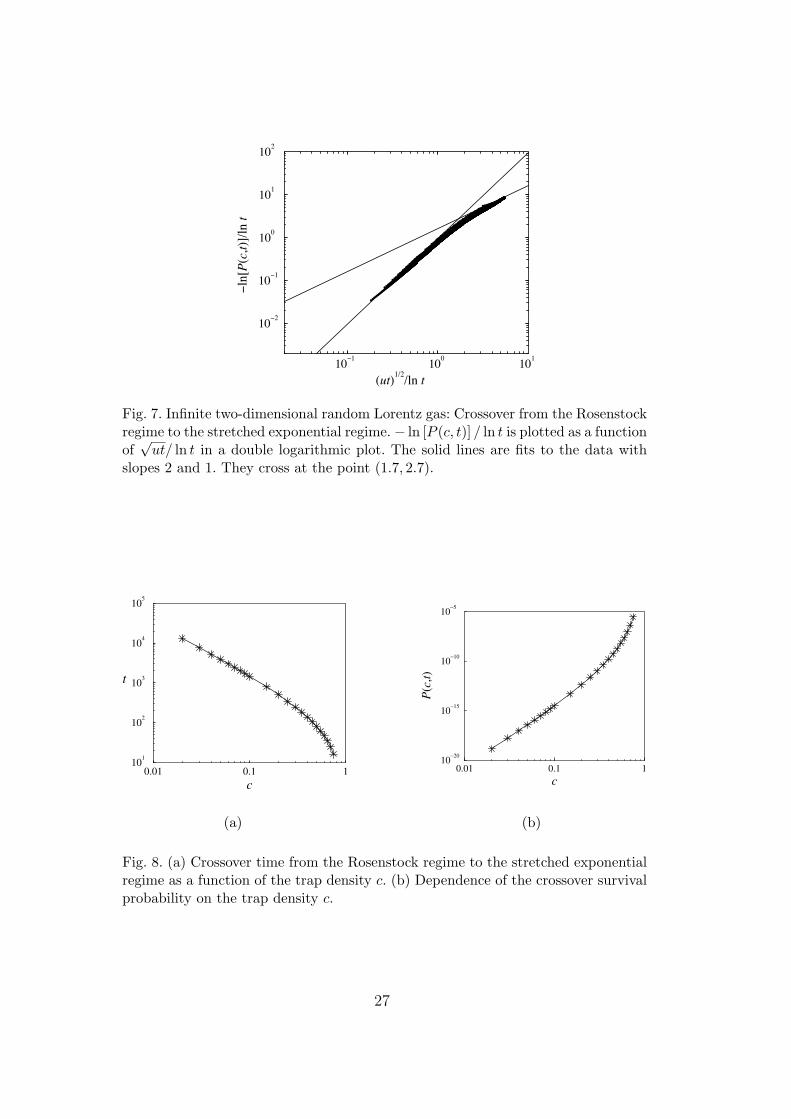
[12,14]. In the Rosenstock regime, we expect a quadratic dependence, whilethe stretched exponential regime should produce a linear behavior. The resultsare represented in Fig. 7 in a double-logarithmic plot. The data collapse forvalues of c taken in the range [0.01, . . . , 0.09, 0.1, . . . 0.9]. The crossover froma slope 2 to a slope 1 is clear.

The intersection point of the two linear fits gives an estimation of the crossovertime from the Rosenstock regime to another regime which ends with theDonsker-Varadhan asymptotics. Using this as reference point, we obtain thedependence on the trap density c of the crossover time and of the crossoversurvival probability [12], as presented in Figs. 8a and b respectively. These re-sults show that the crossover occurs at shorter and shorter times and at largerand larger probabilities as the trap density increases. We observe that thecrossover probability changes from O(10−20) to O(10−5) as the trap densityonly varies from O(10−2) to O(1).

A comment is here in order. The extensive numerical simulations of Ref. [15]show that the Donsker-Varadhan behavior is approached only very gradually.

11

It is known to provide an exact asymptote for the logarithm of P (c, t) includingthe prefactor of (ut)1/2. If one inserts the relevant values of the parametersone find this asymptote in Fig. 7 about 20% above the asymptote obtainedfrom the data fit. Given the limited time range over which our numerical datawere obtained we may conclude that their behavior is fully compatible withthe one observed for stochastic systems in Ref. [15].

4 Transition from finite to infinite random systems

We have considered finite random Lorentz gases with exponential behaviorand infinite ones with stretched exponential behavior. How does the transitionbetween these two regimes evolve with increasing system size L? And whathappens to the fractal repeller?

To answer these questions, let us first briefly sketch the arguments of Grass-berger and Procaccia for the infinite case [3]. They consider diffusing particlesdistributed according to a density ρc(r, t). The average density nc(r, t) is de-fined as

nc(r, t) = 〈ρc(r, t)〉s (17)

where 〈...〉s is an average over all the realizations of trap distributions orequivalently over all choices of the origin from which all particles start diffusinginitially. A perfectly absorbing sphere of large radius R centered at the originis added to the system. The value of the new density n′c(r, t) obtained in thepresence of this sphere is necessarily smaller than nc(r, t)

nc(r, t) ≥ n′c(r, t). (18)

n′c(r, t) depends on the distribution of traps inside the sphere. If {S} ={S1, S2, . . . , Sk} are the positions of the traps in the sphere, we have

nc(r, t) ≥ n′c(r, t) =∑{S}

n′c(r, t|{S}) P ({S}). (19)

The sum of the right-hand side can be bounded from below by consideringonly one term, corresponding to the situation of a sphere free of traps:

nc(r, t) > n′c(r, t|{S} = 0) P (0). (20)

A random distribution of sinks corresponds to a Poisson distribution. The

12

probability of finding k traps in a volume v is given by

Pk =Nk

k!exp(−N) (21)

with average value N = nsv, where ns is the average density of sinks. The prob-ability to have no trap in the sphere is thus given by P (0) = exp(−C ns R

d),where d is the dimension of the system and C the volume of the unit ball ind dimensions.

On the other hand, n′c(r, t|{S} = 0) is obtained as solution of a diffusionequation of coefficient D0 with absorbing boundary conditions on the borderof a sphere of radius |r| = R. Such a solution is known to decay asymptoticallyas the exponential exp(−κd

D0

R2 t), where κd is a constant depending on thedimensionality of the system.

Therefore, Eq. (20) becomes

nc(r, t) > n′c(r, t|{S} = 0)P (0) ∼ exp(−κd

D0

R2t− CnsR

d). (22)

The right-hand side may be maximized as a function of R, with R between 0and +∞ in an infinite system. This gives us an optimal value for R

R =(

2κd

dC

D0

ns

t)1/(d+2)

= α t1/(d+2). (23)

Inserting this result in Eq. (22), one obtains

nc(r, t) > exp[−βtd/(d+2)

]. (24)

Let us now consider a finite system of linear size 2L with a fixed configuration

of traps. As long as R = αt1/d+2 �(

ln Lns

)1/d, the optimal value of R is found

in a fraction of the volume described by (21) and the stretched exponentialbehavior is observed. However, for longer times, the maximal value of R isproportional to l0 ≈ (lnL/ns)

1/d. Inserting R = l0 in Eq. (22) leads to an

exponential decay of the form exp(−κd

D0

l20t). As L increases, the time t∗ at

which the transition occurs increases.

A logarithmic dependence of t∗ on L in two dimensions has been proven inRef. [7].

We now want to study the properties of the repeller. As a preparation, let usfirst consider the simple one-dimensional map with escape represented in Fig.

13

9. Starting from the full unit interval at time zero one finds after k discretetime steps an approximate forward repeller consisting of Nk = 2k pieces ofsizes εk = (1/3)k. The number of pieces is equal to the exponential of theKolmogorov-Sinai entropy times time, Nk = exp(hKSk), and the linear size ofthese pieces is given by εk = exp(−λk) with the Lyapunov exponent λ = ln 3.This last equality can be intuitively understood as follows: as time goes on, newstructures appear on the repeller on smaller and smaller scales. Therefore, longtimes correspond to small spatial scales. The total length Lk of the repeller attime step k is the product of Nk and εk. It decreases exponentially with timeas

Lk = Nk εk = exp(hKSk) exp(−λk) = exp(−γk), (25)

where γ = λ− hKS is the escape rate.

The fractal (Hausdorff) dimension of the repeller is thus given by the well-known result

DH = limε→0

lnN(ε)

ln(

1ε

) =hKS

λ=

ln 2

ln 3, (26)

in the illustrative example of Fig. 9. On the other hand, we know that thefraction of uncertain pairs f(ε), as defined for the Maryland algorithm, isproportional to the size ε to the power CH , with CH the codimension of therepeller. From this we obtain

f(ε) ∼ εCH ∼ ε1−DH ∼ ε

εDH∼ εN(ε). (27)

Let us now imagine a one-dimensional system in which the escape would obeya stretched exponential law. In this case, the remaining length of the repellerat time k would obey

Lk = Nk εk = exp(−c k1/2). (28)

¿From the relation ε = exp(−k λ), we can express the time as k = 1λ

ln 1ε. We

get

N(ε) =Lk

ε=

exp(−c k1/2)

ε=

1

εexp

[−c

(1

λln

1

ε

)1/2]. (29)

14

¿From Eq. (27), we have

f(ε) ∼ εN(ε) ∼ exp

[−c

(1

λln

1

ε

)1/2]. (30)

This dependence of the fraction of uncertain pairs on ε for a system withstretched exponential behavior can be tested numerically for the two-dimensio-nal infinite random Lorentz gas, with the help of the Maryland algorithm.The algorithm has to be slighty modified to simulate an infinite system. Asmentioned before, the absorbing or non-absorbing nature of the disks is notfixed a priori, but each disk has a probability c to be a sink. At each collision ona disk, the separation of the pair of particles considered is tested. If separationoccurs, the fraction of uncertain pairs is increased by (1− c)n, where n is thenumber of different disks that the pair has met before separating, so (1 −c)n is the probability that the particles have not escaped before separating.Simultaneously, the fraction of escaped pairs is increased by [1 − (1 − c)n].In Fig. 10a, the logarithm of the fraction of uncertain pairs, log10 f(ε), isplotted as a function of the logarithm of the distance between the two initialconditions of the pair, log10 ε. In order to check that this curve can be fitted bythe expression (30), we plot in Fig. 10b log[− log10 f(ε)] versus log(− log10 ε).We obtain a linear behavior with slope 1

2, in excellent agreement with Eq.

(30).

In the case of a system of finite spatial extension but with high density ofdisks, as represented in Fig. 1c, we see in Fig. 3b that the transient behaviorpersists until t ' 50. According to the relation ε = exp(tλ), this correspondsto log10 ε ' −34. This is consistent with the deviation from the linear curvewhich is observed in Fig. 6b for large values of ε.

In two-dimensional systems like the Lorentz gases we consider here, the codi-mension appearing in the relation f(ε) ∼ εcH is a partial codimension, asso-ciated with a partial dimension dH . The total dimension is given by DH =1 + 2dH . The total number of small three-dimensional pieces needed to coverthe fractal repeller is given by

N(ε) ∼ 1

ε

[f(ε)

ε

]2

∼ 1

ε3exp

[−2c

(1

λln

1

ε

)1/2]. (31)

This type of dependence of N(ε) on the size ε leads to an integer value of theHausdorff dimension DH . Indeed,

DH = limε→0

lnN(ε)

ln(

1ε

) = 3− limε→0

2c

(1

λ

1

ln 1ε

) 12

= 3. (32)

15

This dimension does not contain the information concerning the correction tothe power law dependence appearing in Eq. (31). We notice that correctionsto a power law also appear for Brownian motion in the plane [16]. In this case,the dependence essentially would take the form

N(ε) ∼ 1

ε2

1

ln ln 1ε

(33)

leading to the integer Hausdorff dimension DH = 2.

When the size L of a finite system with fixed traps increases, the time duringwhich stretched exponential behavior is observed increases likewise, and therange of ε over which the fraction of uncertain pairs deviates from a power-lawbehavior in ε. Correspondingly, as seen from Fig. 10, the slope in the linearregime of log10 f(ε) versus log10 ε becomes smaller and smaller, i.e., the partialHausdorff codimension of the repeller will be smaller. This means that withincreasing L the Hausdorff dimension of the repeller progressively increasestowards the asymptotic value DH = 3. The same holds for the informationdimension, as in the dominant regions the trap density approaches zero andwe saw before that both dimensions approach each other in this limit.

In the case of the two-dimensional random Lorentz gas of infinite spatial ex-tension, the integer value DH = 3 of the dimension of the fractal repeller canbe understood by intuitive arguments. Indeed, this dimension corresponds tothe case of a closed system, without escape. In an infinite system, for a giventime t, there exists with a finite probability a region free of traps of size

R =(

2κd

dCD0

nst)1/(d+2)

. The point particles in this region behave as particles ina closed system until they escape through the “boundary” at R. As time goeson, larger and larger trap-free regions have to be considered. Even if theirdensity decays exponentially with their size, it does not vanish, so that theseregions give the dominant contribution to the measure of the repeller.

Our results show that the repeller is indeed a fractal object in spite of itsinteger dimension DH = 3. This fractality is characterized by the complicatedscaling behavior of the fraction (30) of uncertain pairs or of the number (31)of pieces needed to cover the fractal. These theoretical predictions are nicelyconfirmed by our numerical results.

5 Conclusions

We have studied in this paper several types of two-dimensional random Lorentzgases with sinks.

16

The first model considered is a two-dimensional random Lorentz gas withsinks, of finite spatial extension. In this system, the sinks are randomly dis-tributed among the disks. Due to the finite size of the system, the size ofthe largest trap-free region is bounded. Therefore, the decay of the number ofparticles is asymptotically exponential. For this open system, we have shownthe existence of a fractal repeller formed by the trajectories that never escapefrom the system. Using a non-equilibrium measure on the repeller, we havecharacterized its chaotic and fractal properties. We have obtained the escaperate γ, the positive Lyapunov exponent λ, and the fractal dimensions of therepeller. A relation between γ, λ, and the Hausdorff codimension cH of thefractal repeller has been numerically tested in the limit of low sink densi-ties. This relation establishes a link between the macroscopic decay and theunderlying microscopic chaos.

The second case considered is the two-dimensional random Lorentz gas withsinks, of infinite spatial extension. This situation can be simulated by givingto each disk a certain probability to be a sink, while distinguishing betweendifferent periodic images of the same disk. This leads to an average over thedifferent sink configurations. The decay of the survival probability asymptot-ically obeys the stretched exponential law (1). Here this behavior has beenstudied numerically for the first time in a deterministic chaotic system.

For a dense 2D random Lorentz gas of finite size L, the transient stretchedexponential regime persists during a time fixed in first approximation by thetypical size of the largest trap-free region in the system [see Eq. (23)]. As Lincreases, the transient regime is observed for longer and longer times. Simul-taneously, the dimension of the repeller increases, reaching the integer valueDH = 3 in the infinite-size limit. We have here been able to show that therepeller remains fractal in the limit and to answer the puzzle mentioned in theintroduction by finding the nontrivial scaling property of this plain fractal. Itsfractal property can be characterized equivalently by the fraction of uncertainpairs of trajectories starting from initial conditions separated by ε or by thenumber of cells of size ε needed to cover the fractal. Both scaling functionsshow a correction to a simple power law proving that the repeller remainsfractal. The correction depends on the Lyapunov exponent as well as on theexponent 1/2 of the stretched exponential law (1) in d = 2. This nontrivialscaling is remarkably confirmed by our numerical results.

In conclusion, we have been able to show that, in a random deterministicchaotic system of infinite spatial extension with sinks, the repeller composedof all the trajectories that never meet a sink is a plain fractal with specialscaling properties related to the stretched exponential decay of the survivalprobability.

17

Acknowledgments

The authors thank Professor G. Nicolis for support and encouragement inthis research. IC and PG are supported financially by the National Fund forScientific Research (F. N. R. S. Belgium). H.v.B. also acknowledges supportby the Mathematical physics program of FOM and NWO/GBE.

A Direct proof that the uncertainty exponent is the Hausdorffcodimension

Let us consider the piecewise-linear one-dimensional map:

xn+1 ={

Λ0xn 0 < xn < AΛ1(1− xn) A < xn < 1

(A.1)

We assign the symbol ω = 0 to the interval [0, A] and the symbol ω = 1 tothe interval [A, 1].

If Λ0,Λ1 > 2, almost all the trajectories escape after a finite number of itera-tions. The subinterval Iω0ω1...ωn−1 is defined as the set of initial conditions forthe trajectories which escape in n iterations and successively visit the intervalscorresponding to the symbolic sequence ω0ω1...ωn−1. These subintervals forma partition of the unit interval [0, 1]:

∪ω0ω1...ωn−1Iω0ω1...ωn−1 = [0, 1] (A.2)

The length of the subinterval Iω0ω1...ωn−1 is

`ω0ω1...ωn−1 =K

Λω0Λω1 ...Λωn−1

(A.3)

Since the sum of lengths should be equal to one

∞∑n=1

∑ω0ω1...ωn−1

`ω0ω1...ωn−1 = 1 (A.4)

the constant K is given by

K =1− Λ−1

0 − Λ−11

Λ−10 + Λ−1

1

(A.5)

18

and the previously introduced constant A can now be fixed to the value:

A =1 +K

Λ0

. (A.6)

A pair is uncertain if it falls in a subinterval which is smaller than ε. Therefore,the fraction of uncertain pairs is equal to

f(ε) =∞∑

n=1

∑ω0ω1...ωn−1

`ω0ω1...ωn−1

∣∣∣`ω0ω1...ωn−1<ε

. (A.7)

The sum can be reordered in terms of the numbers n0 (resp. n1) of symbol0 (resp. 1) in the symbolic sequence ω0ω1...ωn−1. We have that n0 + n1 = n.The fraction of uncertain pairs becomes

f(ε) =∞∑

n0=0

∞∑n1=0

(n0 + n1)!

n0! n1!

K

Λn00 Λn1

1

∣∣∣n0 ln Λ0+n1 ln Λ1>ln(K/ε)

. (A.8)

We use the steepest-descent method for this double sum. The domain of sum-mation is the set of pairs of non-negative integers (n0, n1) above the straightline n0 ln Λ0 + n1 ln Λ1 = ln(K/ε) in the plane (n0, n1). The function to besummed decreases exponentially to zero as the exponents n0 and n1 tend toinfinity above the straight line. Therefore, the sum will be dominated by themaximum of the function on the straight line. If we introduce the alternativevariables

x0 ≡n0

ln(K/ε)and x1 ≡

n1

ln(K/ε)(A.9)

we thus find

f(ε) ∼ ε(K

ε

)D

∼ ε1−D (A.10)

with

D = x0 lnx0 + x1

x0

+ x1 lnx0 + x1

x1

(A.11)

and the constraint

x0 ln Λ0 + x1 ln Λ1 = 1. (A.12)

19

The maximum of the function is given by the steepest-descent condition

dD

dx0

= lnx0 + x1

x0

+dx1

dx0

lnx0 + x1

x1

= 0. (A.13)

With the constraint (A.12), we find that the steepest-descent condition reducesto

ln Λ1 lnx0 + x1

x0

= ln Λ0 lnx0 + x1

x1

. (A.14)

We now show that the exponent D is equal to the Hausdorff dimension. Inthe present piecewise-linear map, the Hausdorff dimension of the repeller mustsatisfy by definition the following condition

1

ΛD0

+1

ΛD1

= 1. (A.15)

Let us show that it is indeed the case. For this purpose, we first express thequantity D in terms of x0 and x1 by Eq. (A.11). Then, we use the steepest-descent condition (A.14) and, thereafter, the constraint (A.12). The calcula-tions are the following:

1

ΛD0

+1

ΛD1

= e−x0 ln

x0+x1x0

ln Λ0−x1 lnx0+x1

x1ln Λ0

+e−x0 ln

x0+x1x0

ln Λ1−x1 lnx0+x1

x1ln Λ1 (A.16)

= e−(x0 ln Λ0+x1 ln Λ1) ln

x0+x1x0 + e

−(x0 ln Λ0+x1 ln Λ1) lnx0+x1

x1 (A.17)

= e− ln

x0+x1x0 + e

− lnx0+x1

x1 = 1 (A.18)

Q.E.D.

The previous calculation provides a direct proof that the uncertainty exponentof the Maryland algorithm is the Hausdorff codimension in a piecewise-linearmap with two branches. Consequently, the uncertainty exponent should beexpected to differ from the information codimension on general multifractalrepellers. Indeed, by using the example (A.1), we have numerically observedthat the uncertainty exponent agrees with the Hausdorff codimension butdiffers from the information codimension if Λ0 6= Λ1.

The direct proof presented here can be extended to piecewise-linear one-dimensional maps with more than two branches. In the case of m branches,there would be m variables ni or xi and (m − 1) steepest-descent conditionssuch as (A.13) because of the constraint that the maximum point belongs to

20

the hyperplane∑m

i=1 ni ln Λi = ln(K/ε). Otherwise, a Lagrange multiplier maybe introduced, to deal with this constraint in the search of the maximum. Inthe general case, the argument of Ref. [11] provides the proof.

References

[1] S. Havlin and D. Ben-Avraham, Adv. Phys. 36, 696 (1987), and referencestherein.

[2] M. Donsker and S. R. S. Varadhan, Commun. Pure Appl. Math. 28, 525 (1975);32, 721 (1979).

[3] P. Grassberger and I. Procaccia, J. Chem. Phys. 77, 6281 (1982).

[4] P. Gaspard and F. Baras, Phys. Rev. E 51, 28 (1995).

[5] P. Gaspard, Chaos, Scattering, and Statistical Mechanics (CambridgeUniversity Press, Cambridge UK, 1998).

[6] I. Claus and P. Gaspard, Phys. Rev. E 63, 036227 (2001).

[7] A. Bunde, S. Havlin, J. Klafter, G. Graff, and A. Shehter, Phys. Rev. Lett. 78,3338 (1997).

[8] J. K. Anlauf, Phys. Rev. Lett. 52, 1845 (1984).

[9] Ya. G. Sinai, Russian Math. Surveys 25, 137 (1970).

[10] T. C. Hasley, M. H. Jensen, L. P. Kadanoff, I. Procaccia, and B. I. Shraiman,Phys. Rev. A 33, 1141 (1986).

[11] S. W. McDonald, C. Grebogi, E. Ott, and J. A. Yorke, Physica D 17, 125(1988).

[12] G. T. Barkema, P. Biswas, and H. van Beijeren, Phys. Rev. Lett. 87, 170601(2001)

[13] H. B. Rosenstock, J. Math. Phys. 11, 487 (1970); J. W. Haus and K. W. Kehr,Phys. Rep. 150, 263 (1987).

[14] According to the recent Ref. [15], improved agreement with the asymptoticformulas can be obtained by including non-leading corrections.

[15] V. Mehra and P. Grassberger, Physica D 168, 244 (2002).

[16] B. Mandelbrot, The Fractal Geometry of Nature (W. H. Freeman, New York,1977).

21

(a) (b) (c)

Fig. 1. Typical unit cell of a finite two-dimensional random Lorentz gas: (a) L = 25,nd = 72, ns = 9; (b) L = 25, nd = 88, ns = 7; (c) L = 25, nd = 127, ns = 23. Thefilled disks are the sinks.

22

0 100 200 300

t

0.3

0.4

0.5

0.6

0.7

0.8

0.9

1

1.1

1.2

α(t)

(a)

0 100 200 300

t

0.3

0.4

0.5

0.6

0.7

0.8

0.9

1

1.1

1.2

α(t)

(b)

0 100 200 300

t

0.3

0.4

0.5

0.6

0.7

0.8

0.9

1

1.1

1.2

α(t)

(c)

Fig. 2. Two-dimensional random Lorentz gas of finite spatial extension; Effectiveexponent α plotted versus time, for a trap density c ≈ 0.05: (a) in the case of thedisk configuration represented in Fig. 1a, but with ns = 4 traps; (b) in the case ofthe disk configuration represented in Fig. 1b, but with ns = 5 traps; (c) in the caseof the disk configuration represented in Fig. 1c, but with ns = 6 traps.

23

0 100 200 300

t

0

2

4

6

8

10

−ln

P(c

,t)

γ=0.025

(a)

0 100 200 300 400

t

0

2

4

6

8

10

−ln

P(c

,t)

γ=0.017

(b)

Fig. 3. Two-dimensional random Lorentz gas of finite spatial extension; Logarithm ofthe survival probability as a function of time: (a) for the disk and trap configurationrepresented in Fig. 1a, (b) for the disk and trap configuration represented in Fig.1c. After a transient time the behavior is exponential and the slope of the curvegives the value of the escape rate γ.

24

(a)

0 π/3 2π/3 π 4π/3 5π/3 2π

θ

0

20

40

60

80

100

Esc

ape

tim

e

(b)

2π/3 5π/6 π

θ

0

20

40

60

80

100

Esc

ape

tim

e

(c)

5π/6 11π/12 π

θ

0

20

40

60

80

100

Esc

ape

tim

e

(d)

Fig. 4. Escape time as a function of the initial position: (a) The initial positions aretaken at a varying angle θ around the disk marked by a star; the initial velocityis always normal to the disk. Escape time for (b) θ ∈ [0, 2π]; (c) θ ∈ [2π/3, π]; (d)θ ∈ [5π/6, π].

25

0 50 100 150

t

40

60

80

100

120

140

160<

ln

Λt >

λ=0.75

(a)

−150 −100 −50 0

log10

ε

−5

−4

−3

−2

−1

0

log

10f(

ε)

cH=0.034

(b)

Fig. 5. Two-dimensional random Lorentz gas of finite spatial extension defined bythe unit cell represented in Fig. 1a: (a) Average of the logarithm of the stretchingfactors, as a function of time t. The slope gives the average Lyapunov exponentλ = 0.75. (b) Maryland algorithm: the logarithm of the fraction of uncertain pairsas a function of the logarithm of the difference ε between the two initial conditions ofthe same pair. The slope gives the Hausdorff codimension cH = 0.034. The productλcH = 0.025 is in good agreement with the value of γ, obtained from Fig. 3a.

0 50 100 150

t

0

100

200

300

< l

n Λ

t >

λ=1.67

(a)

−150 −100 −50 0

log10

ε

−2.5

−2

−1.5

−1

−0.5

0

log

10f(

ε)

cH=0.01

(b)

Fig. 6. Two-dimensional random Lorentz gas of finite spatial extension defined bythe unit cell represented in Fig. 1c: (a) Average of the logarithm of the stretchingfactors, as a function of time t. The slope gives the average Lyapunov exponentλ = 1.67. (b) Maryland algorithm: the logarithm of the fraction of uncertain pairsas a function of the logarithm of the difference ε between the two initial conditionsof the same pair. The slope gives the Hausdorff codimension cH = 0.01. The productλcH = 0.017 is in good agreement with the value of γ, obtained from Fig. 3b.

26

10−1

100

101

(ut)1/2

/ln t

10−2

10−1

100

101

102

−ln

[P(c

,t)]

/ln

t

Fig. 7. Infinite two-dimensional random Lorentz gas: Crossover from the Rosenstockregime to the stretched exponential regime.− ln [P (c, t)] / ln t is plotted as a functionof√

ut/ ln t in a double logarithmic plot. The solid lines are fits to the data withslopes 2 and 1. They cross at the point (1.7, 2.7).

0.01 0.1 1

c

101

102

103

104

105

t

(a)

0.01 0.1 1

c

10−20

10−15

10−10

10−5

P(c

,t)

(b)

Fig. 8. (a) Crossover time from the Rosenstock regime to the stretched exponentialregime as a function of the trap density c. (b) Dependence of the crossover survivalprobability on the trap density c.

27

0 1/3 2/3 1

Fig. 9. One-dimensional map with escape.

28

−150 −100 −50 0

log10

ε

−10

−8

−6

−4

−2

0

log

10f(

ε)

(a)

0 2 4 6

log(−log10

ε)

0

1

2

3

log[−

log

10

f(ε)]

(b)

Fig. 10. Maryland algorithm in the case of a random Lorentz gas of infinite spa-tial extension: the system considered is represented in Fig. 1b, with a sink densityc = 0.6. (a) The logarithm of the fraction of uncertain pairs is plotted as a func-tion of the logarithm of the difference ε between the two initial conditions of thesame pair. (b) Logarithmic representation of the same quantities, confirming thedependence predicted by Eq. (30).

29