fractional actioncosmology: somedark energy models in

arX

iv:1

107.

0541

v2 [

phys

ics.

gen-

ph]

21

Sep

2011

Fractional Action Cosmology: Some Dark Energy Models in Emergent,

Logamediate and Intermediate Scenarios of the Universe

Ujjal Debnath,1, ∗ Surajit Chattopadhyay,2, † and Mubasher Jamil3, ‡

1Department of Mathematics, Bengal Engineering and Science University, Shibpur, Howrah-711 103, India.

2Department of Computer Application (Mathematics Section),

Pailan College of Management and Technology, Bengal Pailan Park, Kolkata-700 104, India.

3Center for Advanced Mathematics and Physics (CAMP),

National University of Sciences and Technology (NUST), H-12, Islamabad, Pakistan.

Abstract

In the framework of Fractional Action Cosmology, we have reconstructed the scalar po-

tentials and scalar fields, namely, quintessence, phantom, tachyon, k-essence, DBI-essence,

Hessence, dilaton field and Yang-Mills field. To get more physical picture of the variation

of the scalar field and potential with time, we express scale factor in emergent, logamediate

and intermediate scenarios, under which the Universe expands differently.

∗Electronic address: [email protected] , [email protected]†Electronic address: surajit˙[email protected], [email protected]‡Electronic address: [email protected] , [email protected]

http://arxiv.org/abs/1107.0541v2

mailto:[email protected] , [email protected]

mailto:[email protected], [email protected]

mailto:[email protected] , [email protected]

2

I. INTRODUCTION

Fractional action cosmology (FAC) is based on the principles and formalism of the fractional calculus applied

to cosmology. The fractional derivative and fractional integrals are the main tools in fractional calculus, where

the order of differentiation or integration is not an integer. The fractional calculus is immensely useful in various

branches of mathematics, physics and engineering [1]. In doing FAC, one can proceed in two different ways

[2]: the first one is quite easy as one has to replace the partial derivatives in the Einstein field equations with

the corresponding fractional derivatives; the second technique involves deriving the field equations and geodesic

equations from a more fundamental way, namely starting with the principle of least action and replacing the usual

integral with a fractional integral. This later technique is more useful in giving extra features of the FAC [3]:

Rami introduced the FAC by introducing the fractional time integral,

S = − m

2Γ(ξ)

∫

xµxνgµν(x)(t− τ)ξ−1dτ. (Ia)

Here Γ(ξ) =∫∞0 tξ−1e−tdt is the Gamma function, 0 < ξ ≤ 1, 0 < τ < t, m = constant and xµ = dxµ

dτ. The

variation yields an extra term in the field equations which he termed as ‘variable gravitational constant G’.

Moreover, when the weight function in the fractional time integral is replaced with a sinusoidal function, then the

solution of the corresponding field equations yield a variable cosmological constant and an oscillatory scale factor

[4]

S =m

2

∫ τ

0xµxνgµν(x)e

−χ sin(βt)dt, (Ib)

where χ = 0 reduces to the standard action. In [5], the authors extended the previous study by working out with

a general weight function:

S =m

2

τ∫

0

gµν(x)xµxνµ(χ, t)dt, (Ic)

Several examples were studied and cosmological parameters were calculated in there. An interesting feature of

FAC is that it yields an expanding Universe whose scale factor goes like power law form or exponential form

depending on the choice of the weight function. Hence cosmic acceleration can be modeled in FAC.

Reconstruction of potentials has been done by several authors in various cases. Capozziello et al [8] considered

scalar-tensor theories and reconstruct their potential and coupling by demanding a background ΛCDM cosmol-

ogy. In the framework of phantom quintessence cosmology, [9] used the Noether Symmetry Approach to obtain

general exact solutions for the cosmological equations.In this paper, we are going to reconstruct the potentials

and scalar fields, namely, quintessence, phantom, tachyonic, k-essence, DBI-essence, Hessence, dilaton field and

Yang-Mills field. Such reconstructions have been studied previously in other gravitational setups [6]. To get more

3

physical insight into the model, we express scale factor in three useful forms [7] namely emergent, logamediate

and intermediate scenarios, under which the Universe expands differently. Such expansion scenarios are consistent

with the observations with some restrictions on their parameters [7].

II. FRACTIONAL ACTION COSMOLOGICAL MODEL

For a FRW spacetime, the line element is

ds2 = −dt2 + a2(t)

[

dr2

1− kr2+ r2(dθ2 + sin2 θdφ2)

]

, (1)

where a(t) is the scale factor and k (= 0,±1) is the curvature scalar. We consider the Universe contains normal

matter and dark energy. From Eq. (Ia), the Einstein equations for the space-time given by equation (1) are [3]

H2 +2(ξ − 1)

T1H +

k

a2=

8πG

3ρ, (2)

H − (ξ − 1)

T1H − k

a2= −4πG(ρ + p), (3)

where T1 = t− τ , ρ = (ρm + ρφ) and p = (pm + pφ). Here ρm and pm are the energy density and pressure of the

normal matter connected by the equation of state

pm = wmρm , − 1 ≤ wm ≤ 1 (4)

and ρφ and pφ are the energy density and pressure due to the dark energy.

Now consider there is an interaction between normal matter and dark energy. Dark energy interacting with

dark matter is a promising model to alleviate the cosmic coincidence problem. In Ref. [10], the authors studied the

signature of such interaction on large scale cosmic microwave background (CMB) temperature anisotropies. Based

on the detail analysis in perturbation equations of dark energy and dark matter when they are in interaction,

they found that the large scale CMB, especially the late Integrated Sachs Wolfe effect, is a useful tool to measure

the coupling between dark sectors. It was deduced that in the 1σ range, the constrained coupling between dark

sectors can solve the coincidence problem. In Ref. [11], a general formalism to study the growth of dark matter

perturbations when dark energy perturbations and interactions between dark sectors were presented. They showed

that the dynamical stability on the growth of structure depends on the form of coupling between dark sectors.

Moreover due to the influence of the interaction, the growth index can differ from the value without interaction

by an amount up to the observational sensibility, which provides an opportunity to probe the interaction between

dark sectors through future observations on the growth of structure.

Due to this interaction, the normal matter and dark energy are not separately conserved. The energy conser-

vation equations for normal matter and dark energy are

ρm + 3H(pm + ρm) = −3δHρm, (5)

4

and

ρφ + 3H(pφ + ρφ) = 3δHρm, (6)

where H = a/a is the Hubble parameter.

From equation (5) we have the expression for energy density of matter as

ρm = ρ0a−3(1+wm+δ), (7)

where ρ0 is the integration constant.

III. EMERGENT, LOGAMEDIATE AND INTERMEDIATE SCENARIOS

•Emergent Scenario: For emergent Universe, the scale factor can be chosen as [26]

a(T1) = a0(

λ+ eµT1

)n(8)

where a0, µ, λ and n are positive constants. (1) a0 > 0 for the scale factor a to be positive; (2) λ > 0, to avoid

any singularity at finite time (big-rip); (3) a > 0 or n > 0 for expanding model of the Universe; (4) a < 0 and

n < 0 implies big bang singularity at t = −∞.

So the Hubble parameter and its derivatives are given by

H =nµeµT1

(λ+ eµT1), H =

nλµ2eµT1

(λ+ eµT1)2, H =

nλµ3eµT1(λ− eµT1)

(λ+ eµT1)3(9)

Here H and H are both positive, but H changes sign at T1 = 1µlogλ. Thus H, H and H all tend to zero as

t → −∞. On the other hand as t → ∞ the solution gives asymptotically a de Sitter Universe.

•Logamediate Scenario: Consider a particular form of Logamediate Scenario, where the form of the scale

factor a(t) is defined as [7]

a(T1) = eA(lnT1)α , (10)

where Aα > 0 and α > 1. When α = 1, this model reduces to power-law form. The logamediate form is motivated

by considering a class of possible cosmological solutions with indefinite expansion which result from imposing weak

general conditions on the cosmological model. Barrow has found in their model, the observational ranges of the

parameters are as follows: 1.5 × 10−92 ≤ A ≤ 2.1 × 10−2 and 2 ≤ α ≤ 50. The Hubble parameter H = aaand its

derivative become,

H =Aα

T1(lnT1)

α−1 , H =Aα

T 21

(lnT1)α−2(α− 1− lnT1) (11)

5

•Intermediate Scenario: Consider a particular form of Intermediate Scenario, where the scale factor a(t) of

the Friedmann universe is described as [7],

a(t) = eBTβ1 , (12)

where Bβ > 0, B > 0 and 0 < β < 1. Here the expansion of Universe is faster than Power-Law form, where the

scale factor is given as, a(T1) = T n1 , where n > 1 is a constant. Also, the expansion of the Universe is slower for

Standard de-Sitter Scenario where β = 1. The Hubble parameter H = aaand its derivative become,

H = BβT β−11 , H = Bβ(β − 1)T β−2

1 (13)

IV. VARIOUS CANDIDATES OF DARK ENERGY MODELS

A. Quintessence or Phantom field

Quintessence is described by an ordinary time dependent and homogeneous scalar field φ which is minimally

coupled to gravity, but with a particular potential V (φ) that leads to the accelerating Universe. The action for

quintessence is given by [27]

S =

∫

d4x√−g

[

−1

2gij∂iφ∂jφ− V (φ)

]

.

The energy momentum tensor of the field is:

Tij = − 2√−g

δS

δgij,

which gives

Tij = ∂iφ∂jφ− gij

[

1

2gkl∂kφ∂lφ+ V (φ)

]

.

The energy density and pressure of the quintessence scalar field φ are as follows

ρφ = −T 00 =

1

2φ2 + V (φ),

pφ = T ii =

1

2φ2 − V (φ).

The EoS parameter for the quintessence scalar field is given by

ωφ =pφρφ

=φ2 − 2V (φ)

φ2 + 2V (φ).

For ωφ < −1/3, we find that the Universe accelerates when φ2 < V (φ).

6

The energy density and the pressure of the quintessence (phantom field) can be represented by the minimally

coupled spatially homogeneous and time dependent scalar field φ having positive (negative) kinetic energy term

given by

ρφ =ǫ

2φ2 + V (φ) (14)

and

pφ =ǫ

2φ2 − V (φ) (15)

where V (φ) is the relevant potential for the scalar field φ, ǫ = +1 represents quintessence while ǫ = −1 refers to

phantom field.

Scalar field models of phantom energy indicate that it can behave as a long range repulsive force [12]. Moreover

the phantom energy has few characteristics different from normal matter, for instance, the energy density ρ(t) of

the phantom field increases with the expansion of the Universe; it can be used as a source to form and stabilize

traversable wormholes [14–17]; the phantom energy can disrupt all gravitationally bound structures i.e from

galaxies to black holes [18–23]; it can produce infinite expansion of the Universe in a finite time thus causing the

‘big rip’ [24].

From above equations, we get

φ2 = −(1 + wm)

ǫρm +

1

4πǫG

[

−H +(ξ − 1)

T1H +

k

a2

]

, (16)

and

V =(wm − 1)

2ρm +

1

8πG

[

H + 3H2 +5(ξ − 1)

T1H +

2k

a2.

]

(17)

• For emergent scenario, we get the expressions for φ and V as

φ =

∫

√

√

√

√−(1 + wm)ρ0a−3(1+wm+δ)0

ǫ (λ+ eµT1)3n(1+wm+δ)+

1

4πǫG

{

− nλµ2eµT1

(λ+ eµT1)2+

(ξ − 1)nµeµT1

T1(λ+ eµT1)+

k a−20

(λ+ eµT1)2n

}

dT1, (18)

and

V =(wm − 1)ρ0a

−3(1+wm+δ)0

2 (λ+ eµT1)3n(1+wm+δ)+

1

8πG

{

nµ2eµT1(λ+ 3neµT1)

(λ+ eµT1)2+

5(ξ − 1)nµeµT1

T1(λ+ eµT1)+

2k a−20

(λ+ eµT1)2n

}

. (19)

• For logamediate scenario, we get the expressions for φ and V as

φ =

∫

√

−(1 + wm)ρ0ǫ

e−3A(1+wm+δ)(ln T1)α +1

4πǫG

{

Aα

T 21

(ln T1)α−2(1− α+ ξ lnT1) + k e−2A(ln T1)α}

dT1 (20)

7

0.00 0.02 0.04 0.06 0.08 0.10 0.12 0.140.00

0.02

0.04

0.06

0.08

0.10

Φ

V

2.0 2.2 2.4 2.6 2.8 3.0 3.2 3.4

0.1

0.2

0.3

0.4

0.5

0.6

0.7

0.8

Φ

V

Fig.1 Fig.2

0.15 0.20 0.25 0.300.28

0.30

0.32

0.34

0.36

0.38

0.40

Φ

V

Fig.3

Figs.1-3 show the variations of V against quintessence or phantom field φ in the emergent, logamediate and intermediate

scenarios respectively. Solid, dash and dotted lines represent k = −1,+1, 0 respectively. Blue and red lines represent

quintessence field (ǫ = +1) and phantom field (ǫ = −1) respectively.

and

V =(wm − 1)ρ0

2e−3A(1+wm+δ)(ln T1)α+

1

8πG

[

Aα

T 21

(lnT1)α−2{α− 1 + (5ξ − 6) ln T1 + 3Aα(ln T1)

α}+ 2k e−2A(lnT1)α]

.

(21)

• For intermediate scenario, we get the expressions for φ and V as

φ =

∫

√

−(1 + wm)ρ0ǫ

e−3B(1+wm+δ)Tβ1 +

1

4πǫG

{

Bβ(ξ − β)T β−21 + k e−2BT

β1

}

dT1, (22)

and

V =(wm − 1)ρ0

2e−3B(1+wm+δ)Tβ

1 +1

8πG

[

BβT β−21 (5ξ + β + 3BβT β

1 ) + 2k e−2BTβ1

]

. (23)

In figures 1, 2 and 3, we have plotted the potentials against the scalar fields for the quintessence and phantom

fields in emergent, logamediate and intermediate scenarios of the universe respectively in fractional action cosmol-

ogy. It has been observed in figure 1 that after gradual decay, the potential starts increasing with scalar field for

8

quintessence as well as phantom field models of dark energy in the emergent scenario of the universe irrespective of

its type of curvature. On the contrary, when logamediate scenario is considered, the figure 2 exhibits a continuous

decay in the potential V with increase in the scalar field φ. A different behavior is observed in figure 3 that depicts

the behavior of the potential V against scalar field φ in the case of intermediate scenario of the universe. The

blue lines in this figure show a continuous decay in V with increase in φ for quintessence model. However, the red

lines exhibit an increasing pattern of V with scalar field φ.

B. Tachyonic field

A rolling tachyon has an interesting equation of state whose state parameter smoothly interpolates between

−1 and 0 [28]. Thus, tachyon can be realized as a suitable candidate for the inflation at high energy [29] as well

as a source of dark energy depending on the form of the tachyon potential [30]. Therefore it becomes meaningful

to reconstruct tachyon potential V (φ) from some dark energy models. An action for tachyon scalar φ is given by

Born-Infeld like action

S = −∫

d4x√−gV (φ)

√

1− gij∂iφ∂jφ (24)

where V (φ) is the tachyon potential. Energy-momentum tensor components for tachyon scalar φ are obtained as

Tij = V (φ)

[

∂iφ∂jφ√

1− gij∂iφ∂jφ+ gij

√

1− gkl∂kφ∂lφ

]

(25)

The energy density ρφ pressure pφ due to the tachyonic field φ have the expressions

ρφ =V (φ)

√

1− ǫφ2

, (26)

pφ = −V (φ)

√

1− ǫφ2, (27)

where V (φ) is the relevant potential for the tachyonic field φ. It is to be seen thatpφρφ

= −1 + ǫφ2 > −1 or < −1

accordingly as normal tachyon (ǫ = +1) or phantom tachyon (ǫ = −1).

From above, we get

φ2 =

[

−(1 + wm)

ǫρm +

1

4πǫG

{

−H +(ξ − 1)

T1H +

k

a2

}]

9

×[

−ρm +3

8πG

{

H2 +2(ξ − 1)

T1H +

k

a2

}]−1

(28)

and

V =

[

wmρm +1

8πG

{

2H + 3H2 +4(ξ − 1)

T1H +

k

a2

}]1

2

×[

−ρm +3

8πG

{

H2 +2(ξ − 1)

T1H +

k

a2

}]1

2

(29)


φ =

∫

[

−(1 + wm)ρ0a−3(1+wm+δ)0

ǫ (λ+ eµT1)3n(1+wm+δ)

+1

4πǫG

{

− nλµ2eµT1

(λ+ eµT1)2 +

(ξ − 1)nµeµT1

T1(λ+ eµT1)+

k a−20

(λ+ eµT1)2n

}]1

2

×[

− ρ0a−3(1+wm+δ)0

(λ+ eµT1)3n(1+wm+δ)+

3

8πG

{

n2µ2e2µT1

(λ+ eµT1)2+

2(ξ − 1)nµeµt

T1(λ+ eµT1)+

k a−20

(λ+ eµT1)2n

}]− 1

2

dT1 (30)

and

V =

[

wmρ0a−3(1+wm+δ)0


1

8πG

{

nµ2eµT1(2λ+ 3neµT1)

(λ+ eµT1)2+

4(ξ − 1)nµeµT1

T1(λ+ eµT1)+

k a−20

(λ+ eµT1)2n

}]1

2

×[

− ρ0a−3(1+wm+δ)0


3

8πG

{

n2µ2e2µT1

(λ+ eµT1)2+

2(ξ − 1)nµeµT1

T1(λ+ eµT1)+

k a−20

(λ+ eµT1)2n

}]1

2

. (31)


φ =

∫[

−(1 + wm)ρ0ǫ

e−3A(1+wm+δ)(ln T1)α +1

4πǫG

{

Aα

T 21

(ln T1)α−2(1− α+ ξ lnT1) + k e−2A(ln T1)α

}]1

2

×[

−ρ0 e−3A(1+wm+δ)(ln T1)α +3

8πG

{

Aα

T 21

(ln T1)α−1{Aα(ln T1)

α−1 + 2(ξ − 1)}+ k e−2A(lnT1)α}]− 1

2

dT1 (32)

and

V =

[

−ρ0 e−3A(1+wm+δ)(ln T1)α +3

8πG

{

Aα

T 21

(lnT1)α−1{Aα(ln T1)

α−1 + 2(ξ − 1)}+ k e−2A(lnT1)α}]

1

2

×[

wmρ0 e−3A(1+wm+δ)(ln T1)α +1

8πG

{

Aα

t2(lnT1)

α−2{2(α − 1) + 2(ξ − 3) ln t+ 3Aα(ln T1)α}+ k e−2A(lnT1)α

}]1

2

(33)


φ =

∫[

−(1 +wm)ρ0ǫ

e−3B(1+wm+δ)Tβ1 +

1

4πǫG

{


β1

}

]1

2

10

0.0 0.1 0.2 0.3 0.4

0.1

0.2

0.3

0.4

0.5

0.6

Φ

V

0.00 0.05 0.10 0.15 0.20 0.25 0.300.00

0.05

0.10

0.15

Φ

V

Fig.4 Fig.5

0.12 0.14 0.16 0.18 0.20

0.75

0.80

0.85

0.90

Φ

V

Fig.6

Figs.4-6 show the variations of V against tachyonic field φ in the emergent, logamediate and intermediate scenarios

respectively. Solid, dash and dotted lines represent k = −1,+1, 0 respectively. Blue and red lines represent normal

tachyonic field (ǫ = +1) and phantom tachyonic field (ǫ = −1) respectively.

×[

−ρ0 e−3B(1+wm+δ)Tβ1 +

3

8πG

{

BβT β−21 (2(ξ − 1) +BβT β

1 ) + k e−2BTβ1

}

]− 1

2

dT1 (34)

and

V =

[

−ρ0 e−3B(1+wm+δ)Tβ1 +

3

8πG

{

BβT β−21 (2(ξ − 1) +BβT β

1 ) + k e−2BTβ1

}

]1

2

11

×[

wmρ0 e−3B(1+wm+δ)Tβ1 +

1

8πG

{

BβT β−21 (2(2ξ + β − 3) + 3BβT β

1 ) + k e−2BTβ1

}

]1

2

. (35)

In figure 4, the V -φ plot for normal tachyon and phantom tachyon models of dark energy is presented for

emergent scenario of the universe. Potential of normal tachyon exhibits decaying pattern. However, it shows

increasing pattern for phantom tachyonic field φ. It happens irrespective of the curvature of the universe. In the

logamediate scenario (figure 5) the potentials for normal tachyon and phantom tachyon exhibit increasing and

decreasing behavior respectively with increase in the scalar field φ. From figure 6 we see a continuous decay in

the potential for normal tachyonic field in the intermediate scenario. However, in this scenario, the behavior of

the potential varies with the curvature of the universe characterized by interacting phantom tachyonic field. For

k = −1, 1, the potential increases with phantom tachyonic field and for k = 0, it decays after increasing initially.

C. k-essence

In the kinetically driven scalar field theory, we have non-canonical kinetic energy term with no potential.

Scalars, modelling this theory, are popularly known as k-essence. Motivated by Born-Infeld action of String

Theory, it was used as a source to explain the mechanism for producing the late time acceleration of the universe.

This model is given by the action [31]

S =

∫

d4x√−gL(φ, X), (36)

with

L(φ, X) = K(φ)X + L(φ)X2, (37)

ignoring higher order terms of

X =1

2gij∂iφ∂j φ. (38)

Using the following transformations, φ =∫

dφ√

|L(φ)|/K(φ), X = |L|KX and V (φ) = K2/|L| , the action can be

rewritten as

S =

∫

d4x√−gV (φ)L(X), (39)

with

L(X) = X −X2. (40)

From the action, the energy-momentum tensor components can be written as

Tij = V (φ)[ dLdX

∂iφ∂jφ− gijL]

. (41)

12

The energy density and pressure of k-essence scalar field φ are given by

ρk = V (φ)(−X + 3X2), (42)

and

pk = V (φ)(−X +X2), (43)

where φ is the scalar field having kinetic energy X = 12 φ

2 and V (φ) is the k-essence potential.

From above, we get

φ2 =

[

2(wm − 1)ρm +1

2πG

{

H + 3H2 +5(ξ − 1)

T1H +

2k

a2

}]

×[

(3wm − 1)ρm +3

4πG

{

H + 2H2 +3(ξ − 1)

T1H +

k

a2

}]−1

, (44)

and

V =

[

(3wm − 1)ρm +3

4πG

{

H + 2H2 +3(ξ − 1)

T1H +

k

a2

}]2

×[

2(wm − 1)ρm +1

2πG

{

H + 3H2 +5(ξ − 1)

T1H +

2k

a2

}]−1

. (45)

• For emergent scenario, we have

φ =

∫

[

2(wm − 1)ρ0a−3(1+wm+δ)0


1

2πG

{


(λ+ eµT1)2+

5(ξ − 1)nµeµT1

T1(λ+ eµT1)+

2k a−20

(λ+ eµT1)2n

}]1

2

×[

(3wm − 1)ρ0a−3(1+wm+δ)0


3

4πG

{


(λ+ eµT1)2+

3(ξ − 1)nµeµT1

T1(λ+ eµT1)+

k a−20

(λ+ eµT1)2n

}]− 1

2

dt. (46)

and

V =

[

(3wm − 1)ρ0a−3(1+wm+δ)0

(λ+ eµT1)3n(1+wm+δ)

+3

4πG

{


(λ+ eµT1)2 +

3(ξ − 1)nµeµT1

T1(λ+ eµT1)+

k a−20

(λ+ eµT1)2n

}]2

×[

2(wm − 1)ρ0a−3(1+wm+δ)0


1

2πG

{


(λ+ eµT1)2+

5(ξ − 1)nµeµT1

T1(λ+ eµT1)+

2k a−20

(λ+ eµT1)2n

}]−1

. (47)

13


φ =

∫[

2(wm − 1)ρ0 e−3A(1+wm+δ)(ln T1)α +1

2πG

{

Aα

T 21

(lnT1)α−2(α− 1 + (5ξ − 6) ln T1 + 3Aα(ln T1)

α) + 2k e−2A(lnT1)α}]

1

2

×[

(3wm − 1)ρ0 e−3A(1+wm+δ)(ln T1)α +3

4πG

{

Aα

T 21

(ln T1)α−2(α− 1 + (3ξ − 4) ln T1 + 2Aα(ln T1)

α) + k e−2A(lnT1)α}]− 1

2

dT1

(48)

and

V =

[

(3wm − 1)ρ0 e−3A(1+wm+δ)(ln T1)α +3

4πG

{

Aα

T 21

(lnT1)α−2(α− 1 + (3ξ − 4) ln T1 + 2Aα(ln T1)

α) + k e−2A(lnT1)α}]2

×[

2(wm − 1)ρ0 e−3A(1+wm+δ)(ln T1)α +1

2πG

{

Aα

T 21

(ln T1)α−2(α− 1 + (5ξ − 6) ln T1 + 3Aα(ln T1)

α) + 2k e−2A(ln T1)α}]−1

(49)


φ =

∫[

2(wm − 1)ρ0 e−3B(1+wm+δ)Tβ1 +

1

2πG

{

Bβ(5ξ + β − 6 + 3BβT β1 )T

β−21 + 2k e−2BT

β1

}

]1

2

×[

(3wm − 1)ρ0 e−3B(1+wm+δ)Tβ1 +

3

4πG

{

Bβ(3ξ + β − 4 + 2BβT β1 )T

β−21 + k e−2BT

β1

}

]− 1

2

dT1, (50)

and

V =

[

(3wm − 1)ρ0 e−3B(1+wm+δ)Tβ1 +

3

4πG

{

Bβ(3ξ + β − 4 + 2BβT β1 )T

β−21 + k e−2BT

β1

}

]2

×[

2(wm − 1)ρ0 e−3B(1+wm+δ)Tβ1 +

1

2πG

{

Bβ(5ξ + β − 6 + 3BβT β1 )T

β−21 + 2k e−2BT

β1

}

]−1

. (51)

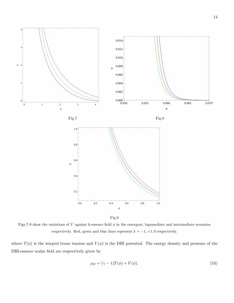
From figures 7, 8 and 9 we see that for interacting k-essence the potential V always decreases with increase in

the scalar field φ in all of the three scenarios and it happens for open, closed and flat universes.

D. DBI-essence

Consider that the dark energy scalar field is a Dirac-Born-Infeld (DBI) scalar field. In this case, the action of

the field be written as [33]

SD = −∫

d4xa3(t)

T (φ)

√

1− φ2

T (φ)+ V (φ)− T (φ)

, (52)

14

0 1 2 3 4

0

1

2

3

4

Φ

V

0.050 0.055 0.060 0.065 0.0700.000

0.002

0.004

0.006

0.008

0.010

0.012

0.014

ΦV

Fig.7 Fig.8

0.0 0.2 0.4 0.6 0.8 1.0

0.2

0.4

0.6

0.8

1.0

Φ

V

Fig.9

Figs.7-9 show the variations of V against k-essence field φ in the emergent, logamediate and intermediate scenarios

respectively. Red, green and blue lines represent k = −1,+1, 0 respectively.

where T (φ) is the warped brane tension and V (φ) is the DBI potential. The energy density and pressure of the

DBI-essence scalar field are respectively given by

ρD = (γ − 1)T (φ) + V (φ), (53)

15

and

pD =γ − 1

γT (φ)− V (φ), (54)

where γ is given by

γ =1

√

1− φ2

T (φ)

. (55)

Now we consider here particular case γ = constant. In this case, for simplicity, we assume T (φ) = T0φ2

(T0 > 1). So we have γ =√

T0

T0−1 . In this case the expressions for φ, T (φ) and V (φ) are given by

φ2 =

√

T0 − 1

T0

[

−(1 + wm)ρm +1

4πG

(

−H +ξ − 1

T1H +

k

a2

)]

. (56)

T =√

T0(T0 − 1)

[

−(1 + wm)ρm +1

4πG

(

−H +ξ − 1

tH +

k

a2

)]

. (57)

and

V =[(

T0 −√

T0(T0 − 1))

(1 + wm)− wm

]

ρm − 1

8πG

[(

1− T0 +√

T0(T0 − 1))

H + 3H2

+2(

T0 −√

T0(T0 − 1) + 2) ξ − 1

T1H +

(

2T0 − 2√

T0(T0 − 1) + 1) k

a2

]

. (58)

• For emergent scenario, we get the expressions for φ, T and V as

φ =

(

T0 − 1

T0

)1

4

∫

[

−(1 + wm)ρ0a−3(1+wm+δ)0


1

4πG

{

− nλµ2eµT1

(λ+ eµT1)2+

(ξ − 1)nµeµT1

T1(λ+ eµT1)+

k a−20

(λ+ eµT1)2n

}]1

2

dT1

(59)

T =√

T0(T0 − 1)

[

−(1 + wm)ρ0a−3(1+wm+δ)0


1

4πG

{

− nλµ2eµT1

(λ+ eµT1)2+

(ξ − 1)nµeµt

T1(λ+ eµT1)+

k a−20

(λ+ eµT1)2n

}]

(60)

and

V =[(

T0 −√

T0(T0 − 1))

(1 + wm)− wm

] ρ0a−3(1+wm+δ)0

(λ+ eµT1)3n(1+wm+δ)− 1

8πG

[

(

1− T0 +√

T0(T0 − 1)) nλµ2eµT1

(λ+ eµT1)2

+3n2µ2e2µT1

(λ+ eµT1)2+ 2

(

T0 −√

T0(T0 − 1) + 2) (ξ − 1)

T1

nµeµT1

(λ+ eµT1)+

(

2T0 − 2√

T0(T0 − 1) + 1) k a−2

0

(λ+ eµT1)2n

]

. (61)

16

• For logamediate scenario, we get the expressions for φ, T and V as

φ =

(

T0 − 1

T0

)1

4

∫[

−(1 + wm)ρ0 e−3A(1+wm+δ)(ln T1)α +1

4πG

{

Aα

T 21

(lnT1)α−2(1− α+ ξ lnT1) + k e−2A(lnT1)α

}]1

2

dT1

(62)

T =√

T0(T0 − 1)

[

−(1 + wm)ρ0 e−3A(1+wm+δ)(ln T1)α +1

4πG

{

Aα

T 21

(lnT1)α−2(1− α+ ξ lnT1) + k e−2A(lnT1)α

}]

,

(63)

and

V =[(

T0 −√

T0(T0 − 1))

(1 + wm)− wm

]

ρ0 e−3A(1+wm+δ)(ln T1)α − 1

8πG

[

2(

T0 −√

T0(T0 − 1) + 2) (ξ − 1)Aα

T 21

(lnT1)α−1

+3A2α2

T 21

(ln T1)2α−2 +

(

1− T0 +√

T0(T0 − 1)) Aα

T 21

(lnT1)α−2(α− 1− lnT1) +

(

2T0 − 2√

T0(T0 − 1) + 1)

k e−2A(ln T1)α]

.

(64)

• For intermediate scenario, we get the expressions for φ, T and V as

φ =

(

T0 − 1

T0

)1

4

∫[

−(1 + wm)ρ0 e−3B(1+wm+δ)Tβ1 +

1

4πG

{


β1

}

]1

2

dT1. (65)

T =√

T0(T0 − 1)

[

−(1 + wm)ρ0 e−3B(1+wm+δ)Tβ1 +

1

4πG

{


β1

}

]

(66)

and

V =[(

T0 −√

T0(T0 − 1))

(1 + wm)− wm

]

ρ0 e−3B(1+wm+δ)Tβ1 − 1

8πG

[(

1− T0 +√

T0(T0 − 1))

Bβ(β − 1)T β−21

+3B2β2T 2β−21 + 2

(

T0 −√

T0(T0 − 1) + 2) (ξ − 1)

T1BβT β−1

1 +(

2T0 − 2√

T0(T0 − 1) + 1)

k e−2BTβ1

]

(67)

When we consider an interacting DBI-essence dark energy, we get decaying pattern in the V -φ plot for emergent

and intermediate scenarios in the figures 10 and 12. However, from figure 11 we see an increasing plot of V -φ for

for interacting DBI-essence in the logamediate scenario.

E. Hessence

Wei et al [32] proposed a novel non-canonical complex scalar field named “hessence” which plays the role of

quintom. In the hessence model the so-called internal motion θ where θ is the internal degree of freedom of

17

0.20 0.25 0.30 0.35 0.40 0.450.65

0.70

0.75

0.80

0.85

Φ

V

7.50 7.55 7.60 7.65 7.70

0.10

0.15

0.20

0.25

0.30

Φ

V

Fig.10 Fig.11

0.5 0.6 0.7 0.8 0.9 1.0

1.3

1.4

1.5

1.6

1.7

1.8

Φ

V

Fig.12

Figs.10-12 show the variations of V against DBI field φ in the emergent, logamediate and intermediate scenarios

respectively. Solid, dash and dotted lines represent k = −1,+1, 0 respectively.

hessence plays a phantom like role and the phantom divide transitions is also possible. The Lagrangian density

of the hessence is given by

Lh =1

2[(∂µφ)

2 − φ2(∂µθ)2]− V (φ). (68)

The pressure and energy density for the hessence model are given by

ph =1

2(φ2 − φ2θ2)− V (φ), (69)

18

and

ρh =1

2(φ2 − φ2θ2) + V (φ), (70)

with

Q = a3φ2θ = constant, (71)

where Q is the total conserved charge, φ is the hessence scalar field and V is the corresponding potential.

From above we get,

φ2 − Q2

a6φ2= −(1 + wm)ρm +

1

4πG

(

−H +ξ − 1

T1H +

k

a2

)

, (72)

and

V =1

2(wm − 1)ρm +

1

8πG

(

H + 3H2 +5(ξ − 1)

T1H +

2k

a2

)

. (73)


φ2 − Q2

a60 (λ+ eµT1)6n

φ2= −(1 +wm)ρ0a

−3(1+wm+δ)0

(λ+ eµT1)3n(1+wm+δ)

+1

4πG

{

− nλµ2eµT1

(λ+ eµT1)2 +

(ξ − 1)nµeµt

T1(λ+ eµT1)+

k a−20

(λ+ eµT1)2n

}

,

(74)

and

V =(wm − 1)ρ0a

−3(1+wm+δ)0

2 (λ+ eµT1)3n(1+wm+δ)+

1

8πG

{


(λ+ eµT1)2+

5(ξ − 1)nµeµT1

T1(λ+ eµT1)+

2k a−20

(λ+ eµT1)2n

}

. (75)


φ2 − Q2e−6A(ln T1)α

φ2= −(1 + wm)ρ0 e−3A(1+wm+δ)(ln T1)α +

1

4πG

{

Aα

T 21

(ln T1)α−2(1− α+ ξ lnT1) + k e−2A(ln T1)α

}

(76)

and

V =(wm − 1)ρ0

2e−3A(1+wm+δ)(ln T1)α+

1

8πG

[

Aα

T 21

(lnT1)α−2{α− 1 + (5ξ − 6) ln T1 + 3Aα(ln T1)

α}+ 2k e−2A(lnT1)α]

.

(77)


φ2 − Q2e−6BTβ1

φ2= −(1 +wm)ρ0 e−3B(1+wm+δ)Tβ

1 +1

4πG

{


β1

}

, (78)

and

V =(wm − 1)ρ0

2e−3B(1+wm+δ)Tβ

1 +1

8πG

[

BβT β−21 (5ξ + β + 3BβT β

1 ) + 2k e−2BTβ1

]

. (79)

19

0.6 0.7 0.8 0.9 1.0 1.1 1.20.2

0.3

0.4

0.5

0.6

Φ

V

3.0 3.5 4.0 4.5 5.0 5.5 6.00.0

0.5

1.0

1.5

2.0

Φ

V

Fig.13 Fig.14

0.0 0.5 1.0 1.5

0.0

0.5

1.0

1.5

Φ

V

Fig.15

Figs.13-15 show the variations of V against hessence field φ in the emergent, logamediate and intermediate scenarios


For interacting hessence dark energy, figure 13 shows increase in the potential with scalar field and figures 14

and 15 show decay in the potential with scalar field. This means the potential for interacting hessence increases

in the emergent universe and decays in logamediate and intermediate scenarios.

F. Dilaton Field

The energy density and pressure of the dilaton dark energy model are given by [27]

ρd = −X + 3CeλφX2, (80)

and

pd = −X +CeλφX2, (81)

20

where φ is the dilaton scalar field having kinetic energy X = 12 φ

2, λ is the characteristic length which governs all

non-gravitational interactions of the dilaton and C is a positive constant.

We get,

φ =

∫[

1

2(3wm − 1)ρm +

3

8πG

(

H + 2H2 +3(ξ − 1)

T1H +

k

a2

)]1

2

dT1. (82)


φ =

∫

[

(3wm − 1)ρ0a−3(1+wm+δ)0

2 (λ+ eµT1)3n(1+wm+δ)

+3

8πG

{


(λ+ eµT1)2 +

3(ξ − 1)nµeµT1

T1(λ+ eµT1)+

k a−20

(λ+ eµT1)2n

}]1

2

dT1.

(83)

• For logamediate scenario, we get

φ =

∫[

3

8πG

{

Aα

T 21

(lnT1)α−2(α− 1 + (3ξ − 4) ln T1 + 2Aα(ln T1)

α) + k e−2A(ln T1)α}

+1

2(3wm − 1)ρ0 e−3A(1+wm+δ)(ln T1)α

]1

2

dT1 (84)

• For intermediate scenario, we get

φ =

∫[

1

2(3wm − 1)ρ0 e−3B(1+wm+δ)Tβ

1 +3

8πG

{

Bβ(3ξ + β − 4 + 2BβT β1 )T

β−21 + k e−2BT

β1

}

]1

2

dT1. (85)

For interacting dilaton field, the scalar field φ always increases with cosmic time T1 irrespective of the scenario

of the universe we consider. This is displayed in figures 16, 17 and 18 for emergent, logamediate and intermediate

scenarios respectively.

G. Yangs-Mills Dark Energy

Recent studies suggest that Yang-Mills field can be considered as a useful candidate to describe the dark energy

as in the normal scalar models the connection of field to particle physics models has not been clear so far and

the weak energy condition cannot be violated by the field. In the effective Yang Mills Condensate (YMC) dark

energy model, the effective Yang-Mills field Lagrangian is given by [34],

LY MC

=1

2bF (ln

∣

∣

∣

∣

F

K2

∣

∣

∣

∣

− 1), (86)

21

0.0 0.5 1.0 1.5 2.00.0

0.2

0.4

0.6

0.8

t

Φ

0.1 0.2 0.3 0.4 0.5 0.6 0.7 0.88.0

8.5

9.0

9.5

10.0

t

Φ

Fig.16 Fig.17

0.0 0.5 1.0 1.5 2.00

2

4

6

8

t

Φ

Fig.18

Figs.16-18 show the variations of dilaton field φ against time T1 in the emergent, logamediate and intermediate scenarios


where K is the re-normalization scale of dimension of squared mass, F plays the role of the order parameter of

the YMC where F is given by, F = −12F

aµνF

aµν = E2 −B2. The pure electric case we have, B = 0 i.e.F = E2.

From the above Lagrangian we can derive the energy density and the pressure of the YMC in the flat FRW

spacetime as

ρy =1

2(y + 1)bE2, (87)

and

py =1

6(y − 3)bE2, (88)

where y is defined as,

y = ln

∣

∣

∣

∣

E2

K2

∣

∣

∣

∣

. (89)

22

We get,

E2 =

[

1

2b(3wm − 1)ρm +

3

8πGb

(

H + 2H2 +3(ξ − 1)

T1H +

k

a2

)]

. (90)


E2 =

[

(3wm − 1)ρ0a−3(1+wm+δ)0

2b (λ+ eµT1)3n(1+wm+δ)+

3

8πbG

{


(λ+ eµT1)2+

3(ξ − 1)nµeµT1

T1(λ+ eµT1)+

k a−20

(λ+ eµT1)2n

}]

. (91)

• For logamediate scenario, we get

E2 =

[

3

8πbG

{

Aα

T 21

(lnT1)α−2(α− 1 + (3ξ − 4) ln T1 + 2Aα(ln T1)

α) + k e−2A(lnT1)α}

+1

2b(3wm − 1)ρ0 e−3A(1+wm+δ)(ln T1)α

]

. (92)

• For intermediate scenario, we get

E2 =

[

1

2b(3wm − 1)ρ0 e−3B(1+wm+δ)Tβ

1 +3

8πbG

{

Bβ(3ξ + β − 4 + 2BβT β1 )T

β−21 + k e−2BT

β1

}

]

. (93)

When we consider Yang-Mills dark energy, we find that E2 is always increasing with cosmic time T1. This is

displayed in figures 19, 20 and 21 for emergent, logamediate and intermediate scenarios respectively.

V. CONCLUSION

This paper is dedicated to the study of reconstruction of scalar fields and their potentials in a newly developed

model of Fractional Action Cosmology by Rami [3]. The fields that we used are quintessence, phantom, tachyonic,

k-essence, DBI-essence, Hessence, dilaton field and Yang-Mills field. We assumed that these fields interact with the

matter. These fields are various options to model dark energy which is varying in density and pressure, so called

variable dark energy. Different field models possess various advantages and disadvantages. The reconstruction

of the field potential involves solving the Friedmann equations in the FAC model with the standard energy

densities and pressures of the fields, thereby solving for the field and the potential. For simplicity, we expressed

these complicated expressions explicitly in time dependent form. We plotted these expressions in various figures

throughout the paper.

In plotting the figures for various scenarios, we choose the following values: Emergent scenario: ξ = .6, n = 4,

λ = 8,µ = .4, a0 = .7, G = 1 (all DE models); Logamediate: ξ = .6, α = 3, A = 5, G = 1 (all DE models);

23

1.0 1.5 2.0 2.5 3.0 3.5 4.00.6

0.7

0.8

0.9

1.0

t

E2

1.5 2.0 2.5 3.0 3.5 4.00.0

0.2

0.4

0.6

0.8

1.0

1.2

t

E2

Fig.19 Fig.20

1.0 1.5 2.0 2.5 3.0 3.5 4.00.92

0.94

0.96

0.98

1.00

t

E2

Fig.21

Figs.19-21 show the variations of E2 against time T1 in the emergent, logamediate and intermediate scenarios respectively.

Red, green and blue lines represent k = −1,+1, 0 respectively.

Intermediate: ξ = .6, β = .4, B = 2, G = 1 (all DE models). Moreover in all cases δ = .05, wm = .01. In

figures 1 to 3, we show the variations of V against φ in the emergent, logamediate and intermediate scenarios

respectively for phantom and quintessence field. In the first two cases, the potential function is a decreasing

function of the field. For the quintessence field, the potential is almost constant while for the phantom field, the

potential increases for different field values. Figures (4-6) show the variations of V against φ in the emergent,

logamediate and intermediate scenarios respectively for the tachyonic field. In figure 4, the V -φ plot for normal

tachyon and phantom tachyon models of dark energy is presented for emergent scenario of the universe. Potential

of normal tachyon exhibits decaying pattern. However, it shows increasing pattern for phantom tachyonic field

φ. It happens irrespective of the curvature of the universe. In the logamediate scenario (figure 5) the potentials

for normal tachyon and phantom tachyon exhibit increasing and decreasing behavior respectively with increase

in the scalar field φ. From figure 6 we see a continuous decay in the potential for normal tachyonic field in

the intermediate scenario. However, in this scenario, the behavior of the potential varies with the curvature of

24

the universe characterized by interacting phantom tachyonic field. For k = −1, 1, the potential increases with

phantom tachyonic field and for k = 0, it decays after increasing initially.

Similarly figures (7-9) show the reconstructed potentials for the k-essence field. We have seen that for interacting

k-essence the potential V always decreases with increase in the scalar field φ in all of the three scenarios and it

happens for open, closed and flat universes. When we consider an interacting DBI-essence dark energy, we get

decaying pattern in the V -φ plot for emergent and intermediate scenarios in the figures 10 and 12. However,

from figure 11 we see an increasing plot of V -φ for for interacting DBI-essence in the logamediate scenario. For

interacting hessence dark energy, figures 13 shows increase in the potential with scalar field and figures 14 and 15

show decay in the potential with scalar field. This means the potential for interacting hessence increases in the

emergent universe and decays in logamediate and intermediate scenarios. Figures (16-18) discuss the dilaton field

while figures (19-21) show the behavior of the Yang-Mills field in the FAC. For interacting dilaton field, the scalar

field φ always increases with cosmic time T1 irrespective of the scenario of the universe and when we consider

Yang-Mills dark energy, we find that E2 in always increasing with cosmic time T1.

[1] I. Podlubny, An Introduction to Fractional Derivatives, Fractional Differential Equations, to methods of their solution

and some of their Applications, (Academic Press, New York, 1999);

R. Hilfer, Editor, Applications of Fractional Calculus in Physics, (World Scientific Publishing, Singapore, 2000)

[2] M. Robert, arXiv:0909.1171 [gr-qc];

V. K. Shchigolev, arXiv:1011.3304v1 [gr-qc].

[3] R.A. EL.Nabulsi, Romm. Rep. Phys. 59 (2007) 763;

R.A. EL.Nabulsi, Fizika B 19 (2010) 103.

[4] R.A. EL.Nabulsi, Commun. Theor. Phys 54 (2010) 16.

[5] M. Jamil, D. Momeni, M.A. Rashid, arXiv:1106.2974

[6] M. U. Farooq, M. Jamil, U Debnath, arXiv:1104.3983;

U. Debnath, M. Jamil, arXiv:1102.1632;

K. Karami, M. S. Khaledian, M. Jamil, Phys. Scr. 83 (2011) 025901;

M. R. Setare, M. Jamil, Europhys. Lett.92 (2010) 49003;

A. Sheykhi, M. Jamil, Phys. Lett. B 694 (2011) 284;

M. Jamil, K. Karami, A. Sheykhi, arXiv:1005.0123;

M. U. Farooq, M.A. Rashid, M. Jamil, Int. J. Theor. Phys. 49 (2010) 2278;

M. Jamil, A. Sheykhi, M. U. Farooq, Int. J. Mod. Phys. D 19 (2010) 1831;

M. R. Setare, E. N. Saridakis, Phys. Lett. B 670 (2008) 1.

[7] J. D. Barrow, N. J. Nunes, Phys. Rev. D 76 (2007) 043501;

C. Campuzano et al, Phys. Rev. D 80 (2009) 123531;

http://arxiv.org/abs/0909.1171






25

B. C. Paul, P. Thakur, S. Ghose, arXiv:1004.4256;

G. F.R. Ellis, J. Murugan, C. G. Tsagas, Class. Quant. Grav. 21 (2004) 233;

R. B. Laughlin, Int. J. Mod. Phys. A 18 (2003) 831;

P. B. Khatua, U. Debnath, Int. J. Theor. Phys. 50 (2011) 799.

[8] S. Capozziello, S. Nesseris, L. Perivolaropoulos, JCAP 0712 (2007) 009.

[9] S. Capozziello, E. Piedipalumbo, C. Rubano, P. Scudellaro, Phys. Rev. D 80 (2009) 104030.

[10] J-H. He, B. Wang, P. Zhang, Phys. Rev. D 80 (2009) 063530.

[11] J-H. He, B. Wang, Y.P. Jing, JCAP 0907 (2009) 030.

[12] L. Amendola, Phys. Rev. Lett. 93 (2004) 181102.

[13] K.A. Bronikov, Acta Phys. Polon. B 4 (1973) 251.

[14] H.G. Ellis, J. Math. Phys. 14 (1973) 104.

[15] C.A. Picon, Phys. Rev. D 65 (2002) 104010.

[16] F. Rahaman et al, Phys. Scr. 76 (2007) 56.

[17] P.K. Kuhfittig, Class. Quantum Grav. 23 (2006) 5853.

[18] E. Babichev et al, Phys. Rev. Lett. 93 (2004) 021102.

[19] S. Nesseris and L. Perivolaropoulos, Phys. Rev. D 70 (2004) 123529.

[20] D.F. Mota and C. van de Bruck, Astron. Astrophs. 421 (2004) 71.

[21] D.F. Mota and J.D. Barrow, Mon. Not. Roy. Astron. Soc. 358 (2005) 601.

[22] E. Babichev, S. Chernov, V. Dokuchaev and Y. Eroshenko, arXiv:0806.0916[gr-qc].

[23] E. Babichev, S. Chernov, V. Dokuchaev and Y. Eroshenko, Phys. Rev. D 78 (2008) 104027.

[24] R. R. Caldwell et al, Phys. Rev. Lett. 91 (2003) 071301.

[25] L. Xu, JCAP 09 (2009) 016.

[26] S. Chattopadhyay, U. Debnath, arXiv:1102.0707v1 [physics.gen-ph];

S. Mukherjee, B. C. Paul, N. K. Dadhich, S. D. Maharaj and A. Beesham (2006) Class. Quantum Grav. 23 6927.

[27] E.J. Copeland, M. Sami, S. Tsujikawa, Int. J. Mod. Phys. D 15, 1753 (2006).

[28] G. W. Gibbons, Phys. Lett. B 537 (2002) 1.

[29] A. Mazumdar, S. Panda and A. Perez-Lorenzana, Nucl. Phys. B 614, 101 (2001);

A. Feinstein, Phys. Rev. D 66, 063511 (2002);

Y. S. Piao, R. G. Cai, X. M. Zhang and Y. Z. Zhang, Phys. Rev. D 66, 121301 (2002).

[30] T. Padmanabhan, Phys. Rev. D 66, 021301 (2002);

J.S. Bagla, H.K.Jassal, T. Padmanabhan, Phys. Rev. D 67 (2003) 063504;

Z. K. Guo and Y. Z. Zhang, JCAP 0408, 010 (2004);

E. J. Copeland, M. R. Garousi, M. Sami and S. Tsujikawa, Phys. Rev. D 71, 043003 (2005).

[31] Armendariz-Picon C., Damour T., Mukhanov V.F., Phys. Lett. B 458, 209 (1999);

Armendariz-Picon C., Mukhanov V.F., Steinhardt P.J., Phys. Rev. D 63, 103510 (2001);

Armendariz-Picon C., Mukhanov V.F., Steinhardt P.J., Phys. Rev. Lett. 85, 4438 (2000);

Chiba T., Okabe T., Yamaguchi M., Phys. Rev. D 62, 023511 (2000);




26

R. Myrzakulov, arXiv:1011.4337;

R. Myrzakulov, arXiv:1008.4486

[32] H. Wei, R-G Cai, D-F Zeng, Class. Quant. Grav.22 (2005) 3189;

H. Wei, R.-G. Cai, Phys. Rev. D 72 (2005) 123507.

[33] Yi-Fu Cai, J. B. Dent, D. A. Easson, Phys. Rev. D 83 (2011) 101301;

S. Chattopadhyay, U. Debnath, Int. J. Mod. Phys. A 25 (2010) 5557;

S. Chattopadhyay, U. Debnath, arXiv:1006.2226;

C. Ahn, C. Kim, E. V. Linder, Phys. Rev. D 80 (2009) 123016.

[34] Y. Zhang, T. Y. Xia and W. Zhao, Class. Quant. Grav. 24 3309 (2007);

T. Y. Xia and Y. Zhang, Phys. Lett. B 656 19 (2007);

M. Tong, Y. Zhang and T. Xia, Int. J. Mod. Phys. D 18 797 (2009).




fractional actioncosmology: somedark energy models in

Documents