frames in finite-dimensional inner product spaces · pdf fileframes in finite-dimensional...

1

VIETNAM NATIONAL UNIVERSITY

UNIVERSITY OF SCIENCE

FACULTY OF MATHEMATICS, MECHANICS AND INFORMATICS

Hoang Dinh Linh

FRAMES IN FINITE-DIMENSIONAL INNERPRODUCT SPACES

Undergraduate Thesis

Undergraduate Advanced Program in Mathematics

Thesis advisor: PhD. Dang Anh Tuan

Hanoi - 2013

Contents

Contents 1

Introduction 2

1 Frames in Finite-dimensional Inner Product Spaces 41.1 Some basic facts about frames . . . . . . . . . . . . . . . . . . . . . . 41.2 Frames in Cn . . . . . . . . . . . . . . . . . . . . . . . . . . . . . . . . 201.3 The discrete Fourier transform . . . . . . . . . . . . . . . . . . . . . 291.4 Pseudo-inverses and the singular value decomposition . . . . . . . . 331.5 Finite-dimensional function spaces . . . . . . . . . . . . . . . . . . . 41

Conclusion 51

References 52

1

Introduction

One of the important concepts in the study of vector spaces is the concepts of abasis for the vectors spaces, which allows every vector to be uniquely representedas a linear combination of the basis elements. However, the linear independenceproperty for a basis is restrictive; sometimes it is impossible to find vector whichboth fulfill the basis requirements and also satisfy external condition demandedby applied problems. For such purpose, we need to look for more flexible type ofspanning sets.

Frames are such tools which provide these alternatives. They not only havegreat variety for use in applications, but also have a rich theory from a pureanalysis point of view. A frame for a vector space equipped with an inner prod-uct also allows each element in the space to be written as a linear combination ofthe elements in the frame, but linear independence between the frame elementsis not required. Intuitively, one can think about a frame as a basis to whichone has added more elements. The theory for frames and bases has developedrapidly in recent years because of its role as a mathematical tool in signal andimage processing.

Let’s say you want to send a signal across some kind of communication sys-tem, perhaps by talking on wireless phone or sending a photo to your friend overthe internet. We think that signal as a vector in a vector space. The way it gettransmitted is as a sequence of coefficients which represent the signal in termof a spanning set. If that spanning set is an orthonormal basis, then comput-ing those coefficients just involves finding some inner product of vectors, whicha computer can accomplish very quickly. As a result, there is not a significanttime delay in sending your voice or the photograph. This is a good feature fora communication system to have, so orthonormal bases are used a lot in suchsituation.

2

CONTENTS

Orthogonality is a very restrictive property, though. What if one of the coeffi-cients representing a vector gets lost in transmission? That piece of informationcannot be reconstructed. It is lost. Perhaps, we’d like our system to have someredundancy, so that if one piece gets lost, the information can be pieced togetherfrom what does get through. This is where frames come in.

By using a frame instead of an orthonormal basis, we do give up the unique-ness of coefficients and orthogonality of the vectors. However, these propertiesare supperfluous. If you are sending your side of a phone conversation or a photo,what matter is quickly computing a working set of expansion coefficients, notwhether those coefficients are unique. In fact, in some setting the linear inde-pendence and orthogonality restrictions inhibit the use of orthonormal bases.Frame can be constructed with a wider variety of characteristics, and can thusbe tailored to match the needs of a particular system.

This thesis will introduce the concept of a frame for a finite-dimensionalHilbert space. We begin with the characteristics of frames. The first section dis-cusses some basic facts about frames, giving a standard definition of a frame.Then proceed in the latter to understood a litter bit about what frames are?,and how to construct a frames in finite-dimensional spaces. From that, thinkingabout the connection between frames in finite-dimensional vector spaces and theinfinite-dimensional constructions.

Most of contents of the thesis come from the book "An Introduction toFrames and Riesz Bases", written by Prof. Ole Christensen. Moreover, I haveused some results of Prof. Ingrid Daubechies in [2] and some results of Prof.Nguyễn Hữu Việt Hưng in [3].

3

CHAPTER 1

Frames in Finite-dimensional Inner

Product Spaces

1.1 Some basic facts about frames

Let V be a finite-dimensional vector space, equipped with an inner product〈., .〉

Definition 1.1 [1] A countable family of elements { fk}k∈I in V is a frame for Vif there exist constants A, B > 0 such that

A‖ f ‖2 ≤ ∑k∈I|〈 f , fk〉|2 ≤ B‖ f ‖2 , ∀ f ∈ V. (1.1)

• A , B are called frame bounds, and they are not unique! Indeed, we canchoose A′ = A

2 , B′ = B + 1 as other frame bounds.

• The frame are normalized if ‖ fk‖ = 1 , ∀k ∈ I.

• In the finite-dimensional space, { fk}k∈I can be having infinitely many ele-ments by adding infinitely many zero elements to the given frame.

Now, we will only consider finite families { fk}k∈I , I finite. Then, the upperframe condition is automatically satisfied by Cauchy-Schwartz’s inequality

m

∑k=1|〈 f , fk〉|2 ≤

m

∑k=1‖ fk‖2‖ f ‖2 , ∀ f ∈ V. (1.2)

4

1.1. Some basic facts about frames

For all f ∈ V, we are easily to prove that

|〈 f , fk〉|2 ≤ ‖ fk‖2‖ f ‖2 , ∀k ∈ {1, 2, 3, ..., m}. (1.3)

Indeed, for each k ∈ {1, 2, ..., m} ; f , fk ∈ V.If f = 0 then

|〈 f , fk〉| = |〈0, fk〉| = 0 = ‖ f ‖2‖ fk‖2.

So, the result holds automatically.Now assume f 6= 0, for any λ ∈ C we have:

0 ≤ ‖ fk + λ f ‖2 = 〈 fk + λ f , fk + λ f 〉. (1.4)

Expanding the right side

0 ≤ 〈 fk, fk〉+ λ〈 fk, f 〉+ λ〈 f , fk〉+ |λ|2〈 f , f 〉= ‖ fk‖2 + λ〈 fk, f 〉+ λ〈 f , fk〉+ |λ|2‖ f ‖2.

Now select

λ = −〈 fk, f 〉‖ f ‖2 .

Substituting this into preceding expression yields

0 ≤ ‖ fk‖2 − 2|〈 f , fk〉|2‖ f ‖2 +

|〈 f , fk〉|2‖ f ‖4 ‖ f ‖2

= ‖ fk‖2 − |〈 f , fk〉|2‖ f ‖2 .

which yields

|〈 f , fk〉|2 ≤ ‖ f ‖2‖ fk‖2.

Thus, we can choose the upper frame bound B =m∑

k=1‖ fk‖2.

Recall the Lemma about a vector spaces decomposition.

Definition 1.2 Let W is a subspace of a finite-dimensional vector space V. Then

W⊥ = {α ∈ V|α ⊥W, i.e.,〈α, β〉 = 0, ∀β ∈W} (1.5)

is said to be orthogonal complement of W in V.

5


We have the following lemma:

Lemma 1.3 [3] Let W be a subspace of finite-dimensional vector space V. Then(W⊥)⊥ = W , and V can be decomposed as V = W ⊕⊥W⊥.

PROOF Let (e1, e2, ..., em) be an orthogonal basis of W, and extend it to be a basis(e1, e2, ..., em, αm+1, ..., αn) of V. Applying Schmidt’s orthogonalization process tothis basis. Then we obtain an orthogonal basis (e1, e2, ..., em, em+1, ..., en) for V.The vectors em+1, ..., en are orthogonal to each element in (e1, e2, ..., em) , then theyare orthogonal to W. So, em+1, ..., en ∈W⊥.Let α ∈W then 〈α, β〉 = 0, ∀β ∈W⊥.So, α ∈ (W⊥)⊥. Therefore, W ⊂ (W⊥)⊥.In addition, if α is an arbitrary vector in (W⊥)⊥ ⊆ V then

α = a1e1 + a2e2 + ... + anen.

Since em+1, ..., en ∈W⊥ then

0 = 〈α, ej〉 = a1〈e1, ej〉+ a2〈e2, ej〉+ ... + an〈en, ej〉 == aj〈ej, ej〉 ∀j = m + 1, n.

Then, am+1 = am+2 = ... = an = 0.So, α represents linearly in (e1, ..., em).Therefore, α ∈W. Thus, (W⊥)⊥ ⊂W.Hence, (W⊥)⊥ = W.Finally, we will prove that W ∩W⊥ = {0}.Indeed, if α ∈W ∩W⊥ then ‖α‖2 = 〈α, α〉 = 0. Thus α = 0.In conclusion,

V = span(e1, e2, ..., em)⊕⊥ span(em+1, ..., en) = W ⊕⊥W⊥

.

In order for the lower condition to be satisfied, if and only if span{ fk}mf=1 = V.

Then we have the following theorem:

Theorem 1.4 [1] A family of elements { fk}mk=1 in V is a frame for V if and only

if span{ fk}mk=1 = V.

6


PROOF :If span{ fk}m

f=1 = V then we consider the following mapping:

φ :V −→ R

f 7−→m

∑k=1|〈 f , fk〉|2.

Firstly, we will prove that there exist A, B > 0 such that

A‖ f ‖2 ≤ ∑k∈I|〈 f , fk〉|2 ≤ B‖ f ‖2 , ∀ f ∈ V, ‖ f ‖ = 1. (1.6)

Take B =m∑

k=1| fk|2 then (1.6) holds automatically by (1.2). So, we only need to

show the existence of A.For any f , g ∈ V, we have:

|φ( f )− φ(g)| = |m

∑k=1

(|〈 f , fk〉|2 − |〈g, fk〉|2)|

= |m

∑k=1

(|〈 f , fk〉| − |〈g, fk〉|)(|〈 f , fk〉|+ |〈g, fk〉|)|

≤m

∑k=1|〈 f − g, fk〉|(‖ f ‖‖ fk‖+ ‖g‖‖ fk‖)

≤m

∑k=1‖ f − g‖(‖ f ‖+ ‖g‖)‖ fk‖2

= ‖ f − g‖(‖ f ‖+ ‖g‖)m

∑k=1‖ fk‖2.

Then, φ( f ) tends to φ(g) as f tends to g. So, φ is continuous.Moreover, the set { f ∈ V| ‖ f ‖ = 1} ,the unit sphere in finite-dimensional spaceV, is compact. By using Weierstrass’s theorem, we know that φ( f ) has a mini-mum on the unit sphere.Choose A = min

‖ f ‖=1φ( f ), we will prove that φ( f ) > 0 when ‖ f ‖ = 1, then A > 0.

Suppose the contrary that φ( f ) = 0 for some f ∈ V, ‖ f ‖ = 1. We have:

φ( f ) =m

∑k=1|〈 f , fk〉|2 = 0.

It implies that

|〈 f , fk〉| = 0, ∀k = {1, 2, ..., n}.

7


Besides, f ∈ V = span{ fk}mk=1 then ∃{αk}m

k=1 : f =m∑

k=1αk fk and

1 = ‖ f ‖2

= 〈 f , f 〉 = 〈 f ,m

∑k=1

αk fk〉

=m

∑k=1

αk〈 f , fk〉 = 0.

It is impossible!Thus, φ( f ) > 0 , ∀ f ∈ V when ‖ f ‖ = 1. Then for A > 0, we have

m

∑k=1|〈 f , fk〉|2 ≥ A = A‖ f ‖2 , ∀ f ∈ V, ‖ f ‖ = 1.

So the lower bound could be chosen as A = min‖ f ‖=1

φ( f ) > 0.

Indeed, if f = 0 then

0 =m

∑k=1|〈 f , fk〉|2 = A‖ f ‖2

If f 6= 0, we can choose f ′ = f‖ f ‖ then ‖ f ′‖ = 1.

Apply the above result then

m

∑k=1|〈 f ′, fk〉|2 ≥ A

equivalent to

m

∑k=1|〈 f‖ f ‖ , fk〉|2 ≥ A.

Hence,

m

∑k=1|〈 f , fk〉|2 ≥ A‖ f ‖2 , ∀ f ∈ V.

Conversely, we claim that if { fk}mk=1 is a frame for V then span{ fk}m

k=1 = V.Indeed, we suppose the contrary that { fk}m

k=1 is a frame for V but span{ fk}mk=1 $

V.Denote W = span{ fk}m

k=1 $ V. Then there exists f ∈ V but f /∈ W, i.e.,we canwrite f = g + h where g ∈W⊥ \ {0} and h ∈W (by Lemma 1.3).

8


So, g is orthogonal to span{ fk}mk=1.

It implies thatm∑

k=1|〈g, fk〉|2 = 0. By the definition of frame, g = 0. Contradiction!

Hence, span{ fk}mk=1 = V.

Remark 1.5

• A frame might contain more elements than needed to be a basic of V sincespan{ fk}m

k=1 = V. In particular, if { fk}mk=1 is a frame for V and {gk}n

k=1 isan arbitrary finite collection of vectors in V, then { fk}m

k=1⋃{gk}n

k=1 is alsoa frame for V. Because span{{ fk}m

k=1⋃{gk}n

k=1} = span{ fk}mk=1 = V.

• A frame which is not a basis is said to be overcomplete or redundant.

Example 1.6

V = R3 , f1 =

100

, f2 =

010

, f3 =

001

, f4 =

111

.

For all f ∈ R3, f=

abc

for a, b, c ∈ R, we have:

a2 + b2 + c2 ≤4

∑k=1|〈 f , fk〉|2 = a2 + b2 + c2 + (a + b + c)2 ≤ 4(a2 + b2 + c2).

So { fk}3k=1 is a frame for R3 but not a basis of R3.

Now, we consider a vector space V equipped with a frame { fk}mk=1 and define

a linear mapping

T : Cm −→ V,

{ck}mk=1 7−→

m

∑k=1

ck fk.

T is called pre-frame operator (or synthesis operator).The adjoint operator is given by

T∗ :V −→ Cm,

f 7−→ {〈 f , fk〉}mk=1.

9


Indeed, we have

〈T{ck}mk=1, f 〉 = 〈

m

∑k=1

ck fk, f 〉 =m

∑k=1

ck〈 fk, f 〉

=m

∑k=1

ck〈 f , fk〉 = 〈ck, 〈 f , fk〉〉

= 〈ck, T∗ f 〉.

T∗ is called analysis operator.By composing T with its adjoint,T∗, we obtain frame operator

S :V T◦T∗−−−→ V,

f 7−→m

∑k=1〈 f , fk〉 fk.

So, we have 〈S f , f 〉 =m∑

k=1|〈 f , fk〉|2 and

A‖ f ‖2 ≤ 〈S f , f 〉 ≤ B‖ f ‖2 , ∀ f ∈ V. (1.7)

Thus, the lower frame condition can be consider as ”lower bound” of S and theupper frame bound can be consider as ”upper bound” of S.

Definition 1.7 A frame { fk}mk=1 is tight if we can choose A = B in the Definition

1.1, i.e.,

m

∑k=1|〈 f , fk〉|2 = A‖ f ‖2 , ∀ f ∈ V. (1.8)

Proposition 1.8 [1] Assume that { fk}mk=1 is a tight frame for V with frame

bound A. Then S = AId ( Id is the identity operator on V), and

f =1A

m

∑k=1〈 f , fk〉 fk , ∀ f ∈ V. (1.9)

In order to prove our proposition, we first prove the following lemma.

Lemma 1.9 [1] Let H be a Hilbert space. Consider U : H −→ H be a boundedoperator, and assume that 〈Ux, x〉 = 0 for all x ∈ H. Then the following holds:

10


(i) If H is a complex Hilbert space, then U = 0.

(ii) If H is a real Hilbert space and U is self-adjoint, then U = 0.

PROOF :

(i) If H is a complex Hilbert space then we have:

4〈Ux, y〉 = 〈U(x + y), x + y〉 − 〈U(x− y), x− y〉+ i〈U(x + iy), x + iy〉−

− i〈U(x− iy), x− iy〉, ∀x, y ∈ H. (1.10)

In detail, we have:

〈U(x + y), x + y〉 = 〈Ux, x〉+ 〈Ux, y〉+ 〈Uy, x〉+ 〈Uy, y〉,〈U(x− y), x− y〉 = 〈Ux, x〉 − 〈Ux, y〉 − 〈Uy, x〉+ 〈Uy, y〉,i〈U(x + iy), x + iy〉 = i〈Ux, x〉 − i2〈Ux, y〉+ i2〈Uy, x〉 − i3〈Uy, y〉,i〈U(x− iy), x− iy〉 = i〈Ux, x〉+ i2〈Ux, y〉 − i2〈Uy, x〉 − i3〈Uy, y〉.

Then we obtain (1.10) by a direct calculation.Since 〈Ux, x〉 = 0, ∀x ∈ H then 〈Ux, y〉 = 0, ∀x, y ∈ H by using (1.10).That means U = 0.

(ii) If H is a real Hilbert space and U is self adjoint then let {ek}∞k=1 be an

orthonormal basis for H. For arbitrary j, k ∈N, we have:

0 = 〈U({ek + ej), ek + ej〉 = 〈Uek, ej〉+ 〈Uej, ek〉= 〈Uek, ej〉+ 〈ej, Uek〉 = 2〈Uek, ej〉.

It implies U = 0.

Now, we’re going to prove Proposition 1.8.

PROOF Let U = S− AId, we have:

〈Ux, y〉 = 〈(S− AId)x, y〉 = 〈Sx, y〉 − A〈Idx, y〉= 〈x, Sy〉 − A〈x, Idy〉= 〈x, (S− AId)y〉 = 〈x, Uy〉.

11


Therefore, U is self adjoint. Applying Lemma 1.9, we get

S− AId = 0 , i.e., S = AId,

then

S f = A f , ∀ f ∈ V.

Thus

f =1A

S f =1A

m

∑k=1〈 f , fk〉 fk , ∀ f ∈ V.

Lemma 1.10 Let V, W be finite-dimensional vector spaces, equipped with innerproducts 〈., .〉V, respectively 〈., .〉W . Assume that dim V = n, dim W = m.Given a linear operator T : V −→ W, the adjoint operator T∗ : W −→ V. Then thevector space KerT and ImT∗ are subspace of V, and KerT = ImT∗⊥.In particular,the linear map T induces orthogonal decomposition of V and (via T∗ of W) givenby

V = KerT ⊕⊥ ImT∗

W = KerT∗ ⊕⊥ ImT

PROOF Let v ∈ KerT, then Tv = 0.For any u ∈W, we have: 0 = 〈Tv, u〉W = 〈v, T∗u〉V. So v ∈ ImT∗⊥.Thus KerT ⊆ ImT∗⊥.For v ∈ ImT∗⊥, we have: 〈v, T∗u〉V = 0, ∀u ∈W.It is equivalent to

〈Tv, u〉W = 0, ∀u ∈W.

Choose u = Tv ∈W, then ‖Tv‖2 = 0.Therefore, Tv = 0 then v ∈ KerT. Thus, KerT = ImT∗⊥.Similarly, we have KerT∗ = ImT⊥. Applying Lemma 1.3 we have

V = KerT ⊕⊥ ImT∗

W = KerT∗ ⊕⊥ ImT.

12


An interpretation of (1.9) is that if { fk}mk=1 is a tight frame and we want to

express f ∈ V as a linear combination f =m∑

k=1ck fk, we can simply define gk =

1A fk

and take ck = 〈 f , gk〉. Formula (1.9) is similar to the representation

f =m

∑k=1〈 f , ek〉ek (1.11)

via an orthonormal basis {ek}mk=1: the only difference is the factor 1

A in (1.9).For general frames we now prove that we still have a representation of each

f ∈ V of the form f =m∑

k=1〈 f , gk〉 fk for an appropriate choice of {gk}m

k=1. The

obtained theorem is one of the most important results about frames, and (1.12)is called the frame decomposition:

Theorem 1.11 [1] Let { fk}mk=1 be a frame for V with frame operator S. Then

(i) S is invertible and self-adjoint.

(ii) Every f ∈ V can be represented as

f =m

∑k=1〈 f , S−1 fk〉 fk =

m

∑k=1〈 f , fk〉S−1 fk. (1.12)

(iii) If f ∈ V also has the representation f =m∑

k=1ck fk for some scalar coefficients

{ck}mk=1, then

m

∑k=1|ck|2 =

m

∑k=1|〈 f , S−1 fk〉|2 +

m

∑k=1|c− 〈 f , S−1 fk〉|2. (1.13)

PROOF (i) We have S = T ◦ T∗ is self-adjoint. Now, we prove that S is bijective.Indeed, let f ∈ V and assume that S f = 0 then

0 = 〈S f , f 〉 =m

∑k=1|〈 f , fk〉|2 ≥ A‖ f ‖2.

Therefore, f = 0 then S is injective.Moreover, since V =span{ fk}m

k=1 then T is surjective i.e.,for f ∈ V there exists {gk}m

k=1 ∈ Cm such that T{gk}mk=1 = f .

Rewrite

{gk}mk=1 = {gk}

mk=1 + {hk}m

k=1,

13


where {gk}mk=1 ∈ KerT⊥ and {hk}m

k=1 ∈ KerT.Then

f = T{gk}mk=1 = T{gk}

mk=1 + T{hk}m

k=1 = T{gk}mk=1.

By lemma 1.10, we have (KerT)⊥ = ImT∗.Therefore, for f ∈ V there exists {gk}m

k=1 ∈ ImT∗ such that T{gk}mk=1 = f .

So, V ⊂ T(ImT∗) = Im(TT∗) = ImS.Thus, S is surjective. Hence, S is invertible.

(ii) For any u, v ∈ V , S is self-adjoint then

〈S−1u, v〉 = 〈S−1u, S ◦ S−1v〉 = 〈S ◦ S−1u, S−1v〉 = 〈u, S−1v〉.

So S−1 is also self-adjoint. Therefore,

f = S ◦ S−1 f =m

∑k=1〈S−1 f , fk〉 fk =

m

∑k=1〈 f , S−1 fk〉 fk.

Moreover,

f = S−1 ◦ S f = S−1(m

∑k=1〈 f , fk〉 fk) =

m

∑k=1〈 f , fk〉S−1 fk.

(iii) We can write

{ck}mk=1 = {ck}m

k=1 − {〈 f , S−1 fk〉}mk=1 + {〈 f , S−1 fk〉}m

k=1.

Sincem

∑k=1

(ck − 〈 f , S−1 fk〉

)fk =

m

∑k=1

ck fk −m

∑k=1〈 f , S−1 fk〉 fk = 0.

then {{ck}m

k=1 − {〈 f , S−1 fk〉}mk=1 ∈ KerT = ImT∗⊥,

{〈 f , S−1 fk〉}mk=1 = {〈S−1 f , fk〉}m

k=1 ∈ ImT∗.

Thus, by Pythagoras’s Theorem, we get

m

∑k=1|ck|2 =

m

∑k=1|〈 f , S−1 fk〉|2 +

m

∑k=1|c− 〈 f , S−1 fk〉|2.

14


Remark 1.12

• Every frame in a finite-dimensional space contain a subfamily which is abasic. Because span{ fk}m

k=1 = V.

• If { fk}mk=1 is a frame but not a basis. Then there exist {dk}m

k=1 non-zero

sequence such thatm∑

k=1dk fk = 0 and

f =m

∑k=1〈 f , S−1 fk〉 fk +

m

∑k=1

dk fk =m

∑k=1

(〈 f , S−1 fk〉+ dk ) fk.

It implies that f has many representations.

• Theorem 1.11 shows that {〈 f , S−1 fk〉}mk=1 has minimal `2-norm among all

sequences {ck}mk=1 for which f =

m∑

k=1ck fk.

The numbers 〈 f , S−1 fk〉 , k = 1, 2, 3, ..., m, are called frame coefficients.

• {S−1 fk}mk=1 is also a frame for V because span{S−1 fk}m

k=1 = V. It is calledthe canonical dual of { fk}m

k=1. Theorem 1.11 gives some special informationin case { fk}m

k=1 is a basis:

Proposition 1.13 [1] Assume that { fk}mk=1 is a basis for V. Then there exist a

unique family {gk}mk=1 in V such that

f =m

∑k=1〈 f , gk〉 fk , ∀ f ∈ V. (1.14)

In term of the frame operator, {gk}mk=1 = {S−1 fk}m

k=1. Furthermore, 〈 f j, gk〉 = δjk.

PROOF The existence of {gk}mk=1 follow from Theorem 1.11. Now, we suppose

that there exist {g′k}mk=1 satisfying

f =m

∑k=1〈 f , g′k〉 fk =

m

∑k=1〈 f , gk〉 fk.

Then,m∑

k=1〈 f , g′k − gk〉 fk = 0.

Since { fk}mk=1 is a basis for V then 〈 f , g′k − gk〉 = 0 , ∀ f ∈ V.

Therefore, g′k = gk , ∀k = 1, 2, ..., m or {gk}mk=1 is unique!

15


Moreover, since { fk}mk=1 is a basis and f j =

m∑

k=1〈 f j, gk〉 fk

then

{〈 f j, gk〉 = 1 if j = k〈 f j, gk〉 = 0 if j 6= k

or 〈 f j, gk〉 = δjk.

We can give an intuitive explanation of why frames are important in signaltransmission. Assume that we want to transmit the signal f belonging to avector space V from a transmitter A to a receiver R. If both A and R haveknowledge of a frame { fk}m

k=1 for V, this can be done if A transmits the framecoefficients {〈 f , S−1 fk〉}m

k=1; based on knowledge of these numbers, the receiverR can reconstruct the signal f using the frame decomposition. Now assume thatR receives a noisy signal, meaning a perturbation {〈 f , S−1 fk〉 + ck}m

k=1 of thecorrect frame coefficients. Based on the received coefficients, R will claim thatthe transmitted signal was

m

∑k=1

(〈 f , S−1 fk〉+ ck) fk =m

∑k=1

(〈 f , S−1 fk〉) fk +m

∑k=1

ck fk

= f +m

∑k=1

ck fk.

This differs from the correct signal f by the noisem∑

k=1ck fk. If { fk}m

k=1 is over-

complete, the pre-frame operator T{ck}mk=1 =

m∑

k=1ck fk has a non- trivial kernel,

implying that parts of the noise contribution might add up to zero and can-cel. This will never happen if { fk}m

k=1 is an orthonormal basis! In that case

‖m∑

k=1ck fk‖2 =

m∑

k=1|ck|2, so each noise contribution will make the reconstruction

worse.We have already seen that for given f ∈ V, the frame coefficients {〈 f , S−1 fk〉}m

k=1

have minimal `2-norm among all sequences {ck}mk=1 for which f =

m∑

k=1ck fk. We

can also choose to minimize the norm in other space than `2, we now show theexistence of coefficients minimizing the `1-norm.

Theorem 1.14 [1] Let { fk}mk=1 be a frame for a finite-dimensional vector space

V. Given f ∈ V, there exist coefficients {dk}mk=1 in Cm such that f =

m∑

k=1dk fk and

m

∑k=1|dk| = inf{

m

∑k=1|ck| : f =

m

∑k=1

ck fk}. (1.15)

16


PROOF Fix f ∈ V, it’s clear that we can choose a set of coefficients {ck}mk=1 such

that f =m∑

k=1ck fk.

Let

r :=m

∑k=1|ck|,

and

M := {{dk}mk=1 ∈ Cm,

m

∑k=1|dk| ≤ r ; k = 1, 2, ..., m}.

M is closed and bounded in finite-dimensional space Cm, so M is compact. Thenthe following closed set

N = {{dk}mk=1 ∈ M| f =

m

∑k=1

dk fk}

is also compact.Consider

φ : C −→ R,

{dk}mk=1 7−→

m

∑k=1|dk|.

We have

|φ({ck}mk=1)− φ({dk}m

k=1)| =m

∑k=1|(|ck| − |dk|)|

≤m

∑k=1|ck − dk| = φ({ck}m

k=1 − {dk}mk=1).

So, φ({ck}mk=1) tends to φ({dk}m

k=1) as {ck}mk=1 → {dk}m

k=1.Thus, φ is continuous.Applying Weierstrass’s theorem, we get φ has minimum on N. In other words,

there exist coefficients {dk}mk=1 in Cm such that f =

m∑

k=1dk fk and

m

∑k=1|dk| = inf{

m

∑k=1|ck| : f =

m

∑k=1

ck fk}.

17


There are some important differences between Theorem 1.11 and Theorem1.14. In Theorem 1.11 we find the sequence minimizing the `2-norm of the co-efficients in the expansion of f explicity; it is unique, and it depends linearly onf . On the other hand, Theorem 1.14 only gives the existence of an `1-minimizer,and it may not be unique.

Example 1.15

Let {ek}2k=1 be an orthonormal basis for two-dimensional vector space V with

〈., .〉.Let

f1 = e1 , f2 = e1 − e2 , f3 = e1 + e2.

Then { fk}3k=1 is a frame for V. Indeed, for f ∈ V, f can be represent as

f = c1e1 + c2e2 , for some scalar c1, c2 ∈ R.

We have

3

∑k=1|〈 f , fk〉|2 = |c1|2 + |c1 − c2|2 + |c1 + c2|2

= 3c21 + 2c2

2.

So,

2‖ f ‖2 ≤3

∑k=1|〈 f , fk〉|2 ≤ 3‖ f ‖2 , ∀ f ∈ V.

Assume f =3∑

k=1dk fk then

{d1 + d2 + d3 = c1

−d2 + d3 = c2.

This equation system has at least 2 solutions {dk}3k=1 that minimizing

3∑

k=1|dk|.

Indeed, take f = e1 then {d1+ d2 + d3 = 1− d2 + d3 = 0.

18


So, we can choose {d1 = 1

d2 = d3 = 0,

or

d1 = d2 = d3 =13

,

then both cases get3

∑k=1|dk| = 1.

Even if the minimizer is unique, it may not depend linearly on f .

Example 1.16

Let {e1, e2} be the canonical orthonormal basis for C2 and consider the frame{ fk}3

k=1 = {e1, e2, e1 + e2}.Then

{c(1)k }3k=1 = {1, 0, 0},

{c(2)k }3k=1 = {0, 1, 0},

minimize the `1-norm in the representation of e1 and e2, respectively.

Clearly, e1 + e2 =3∑

k=1(c(1)k + c(2)k ) fk but {c(1)k + c(2)k }

3k=1 not minimizing the `1-norm

among all sequences representing e1 + e2.

Theorem 1.17 [1] Let { fk}mk=1 be a frame for a subspace W of the vector space V.

Then the orthogonal projection of V onto W is given by

P f =m

∑k=1〈 f , S−1 fk〉 fk , f ∈ V. (1.16)

PROOF It is enough to proof that if we define P by (1.16) then

P f =

{f for f ∈W

0 for f ∈W⊥.

Because of Theorem 1.11, P f = f for f ∈W. Moreover, S is a bijection on W thenS−1 fk ∈W. It implies P f = 0 for f ∈W⊥.

19

1.2. Frames in Cn

1.2 Frames in Cn

The natural examples of finite-dimensional vector space are

Rn = {(c1, c2, ..., cn)|ci ∈ R, i = 1, 2, ..., n},

and

Cn = {(c1, c2, ..., cn)|ci ∈ C, i = 1, 2, ..., n}.

The latter is equipped with the inner product

〈{ck}nk=1, {dk}n

k=1〉 =n

∑k=1

ckdk,

and the associated norm

‖{ck}nk=1‖ = (

n

∑k=1|ck|2)

12 .

From elementary linear algebra, we know many equivalent conditions for aset of vectors to constitute a basis for Cn. Let us list the most important charac-terizations:

Theorem 1.18 [1] Consider n vectors in Cn and write them as columns in ann× n

Λ =

λ11 λ12 ... λ1n

λ21 λ22 ... λ2n

...λn1 λn2 ... λnn

then the following are equivalent:

(i) The columns in Λ (i.e., the given vectors) constitute a basis for Cn.

(ii) The rows in Λ constitute a basis for Cn.

(iii) The determinant of Λ is non-zero.

(iv) Λ is invertible.

(v) Λ defines an injective mapping on Cn.

20

1.2. Frames in Cn

(vi) Λ defines a surjective mapping on Cn.

(vii) The columns in Λ are linearly independent.

(viii) Λ has rank equal to n.

PROOF (vii)↔ (i)↔ (iii)If the columns in Λ are linearly independent then it is maximal linearly inde-pendent. So, it constitute a basis for Cn.If the columns in Λ are linearly dependent then the determinant of Λ should bezero.Assume the columns in Λ are linearly independent then it constitute a basis forCn.Denote:e = (e1, e2, ..., en) be the canonical basis for Cn

α1, α2, ..., αn is the column vectors in Λand, Λn(Cn)∗ be the set of all alternative n-linear in Cn.So,

det Λ =dete(α1, α2, ..., αn) where αj =n∑

i=1λijei.

Therefore, det = dete constitute a basis for Λn(Cn)∗. We get

detα = cdet , (c ∈ C).

Thus

c det(α1, α2, ..., αn) =detα(α1, α2, ..., αn) = det In = 1.

Hence,

det Λ = det(α1, α2, ..., αn) 6= 0.

(iii)↔ (ii)We have

det Λ = det ΛT, ∀Λ ∈M(n× n, C).

Then det ΛT 6= 0, it is equivalent to the columns of ΛT constitute a basis for Cn

as the above proof.

21

1.2. Frames in Cn

Therefore, the rows of Λ constitute a basis for Cn.(iii)↔ (iv)Suppose Λ define a homomorphism f : Cn −→ Cn. Then we have to prove that fis an isomorphism if det Λ 6= 0.Assume that a = (a1, a2, ..., an) is a basis for Cn. Then

( f (a1) f (a2) ... f (an)) = (a1 a2 ... n)Λ.

We have

det Λ = det( f ) = det( f (a1) f (a2) ... f (an)) = det( f (a1) f (a2) ... f (an))det Idn

= det( f (a1) f (a2) ... f (an))deta(a1, a2, ..., n)

=deta (f(a1) f (a2) ... f (an))det Λ.

Note that, f is an isomorphism if and only if ( f (a1), f (a2), ..., f (an)) is linearlyindependent.This equivalent to (α1, α2, ..., αn) are linearly independent, or det Λ = det( f ) 6= 0.(iv)↔ (v)↔ (vi)Λ is invertible means that Λ defines a bijective mapping on Cn. Since Cn is finitethen Λ also defines an injective and a surjective mapping on Cn.(viii)↔ (vi)The rank of Λ should be the dimension of its range ImΛ. So, it must be n.

Recall that the rank of matrix E is defines as the dimension of its range ImE.Now, we turn to a discussion of frames for Cn. Note that we consequently identifyoperator A : Cn → Cm , with their matrix representations with respect to thecanonical bases in Cn and Cm.In case { fk}m

k=1 is a frame for Cn, the pre-frame operator T maps Cm onto Cn, andits matrix with respect to the canonical bases in Cn and Cm is

T =

| | ... |f1 f2 ... fn

| | ... |

i.e., the m× n matrix having the vectors fk as columns.Since m vectors can at most span an m-dimensional space then we necessarilyhave m ≥ n when { fk}m

k=1 is a frame for Cn, i.e., the matrix T has at least asmany columns as rows.

22

1.2. Frames in Cn

Theorem 1.19 [1] Let { fk}mk=1 be a frame for Cn. Then the vectors fk can be

consider as first n coordinates of some vectors gk in Cm consituting a basis for Cm.If { fk}m

k=1 is a tight frame then the vectors fk are the first n coordinates of somevector gk in Cm constituting an orthogonal basis for Cm.

PROOF Since { fk}mk=1 be an arbitrary frame for Cn then

Cn = span{ fk}mk=1.

Therefore, m ≥ n.Now, consider the pre-frame operator

T : Cm → Cn,

{ck}mk=1 7→

m

∑k=1

ck fk

corresponding to the matrix

T =

| | ... |f1 f2 ... fn

| | ... |

.

Then the adjoint operator

F : Cn → Cm,

x 7→ {〈x, fk〉}mk=1

corresponding to

F =

− f1 −− f2 −

...− fn −

.

We claim that F is injective. Indeed, if Fx = 0 then

0 = ‖Fx‖2 =m

∑k=1|〈x, fk〉|2.

Therefore, |〈x, fk〉| = 0 for all k = 1, m.In addition, span{ fk}m

k=1 = Cn. Hence we get x = 0.

23

1.2. Frames in Cn

For x = (x1, x2, ..., xn)T ∈ Cn

Fx =

f11 f12 ... f1n

f21 f22 ... f2n

...fm1 fm2 ... fmn

x1

x2

...xn

=

n∑

i=1f1ixi

n∑

i=1f2ixi

...n∑

i=1fmixi

=

〈x, f1〉〈x, f2〉

...〈x, fm〉

.

Now, we extend F to a bijection F of Cm onto Cm.Let {ek}m

k=1 be the canonical basis for Cm and {αk}mk=n+1 be the orthogonal basis

for ImF⊥ in Cm. Then the operator F corresponding to the matrix

F =

f11 f12 ... f1n α1

n+1 α1n+2 ... α1

m

f21 f22 ... f2n α2n+1 α2

n+2 ... α2m

... ...fm1 fm2 ... fmn αm

n+1 αmn+2 ... αm

m

is surjective.Indeed, since span{ f•k}n

k=1 = ImF , and

span{αk}mk=n+1 = ImF⊥.

then the columns of F spans Cm.Hence, the columns of F constitute a basis for Cm.

Applying Theorem 1.18, the rows of F constitute a basis for Cm. That meansfk can be consider as the first n coordinates of some vectors gk in Cm constitutinga basis for Cm.If { fk}m

k=1 is a tight frame then rewrite

f =1A

m

∑k=1〈 f , fk〉 fk

or S = AId. So,

〈TT∗ei, ej〉 = Aδij, ∀i, j = 1, 2, ..., m.

Thus, the n rows in the matrix

T =

| | ... |f1 f2 ... fn

| | ... |

24

1.2. Frames in Cn

are orthogonal.By adding m − n rows, we can extend the matrix for T to an m × n matrix inwhich the rows are orthogonal.Therefore, the columns are orthogonal.

From Theorem 1.19 we can construct a frame or a tight frame of Cn by takinga basis or an orthogonal basis of Cm, m > n, respectively. Then by taking first ncoordinates, we have a frame, or a tight frame.

Example 1.20

Consider 111−1

,

11−1

1

,

1−1

11

,

−1

111

in C4.

By Theorem 1.19, 111

,

11−1

,

1−1

1

,

−111

is a tight frame for C3 with frame bound A = 4.

For a given m× n matrix Λ the following proposition gives a condition for therows constituting a frame for Cn .

Proposition 1.21 [1] For an m× n matrix

Λ =

λ11 λ12 ... λ1n

λ21 λ22 ... λ2n

...λm1 λm2 ... λmn

The following are equivalent:

(i) There exists a constant A > 0 such that

An

∑k=1|ck|2 ≤ ‖Λ{ck}n

k=1‖2 for all {ck}n

k=1 ∈ Cn.

25

1.2. Frames in Cn

(ii) The columns in Λ constitute a basis for their span in Cm.

(iii) The rows in Λ constitute a frame for Cn.

PROOF (i)↔ (ii)Denote the columns in Λ by g1, g2, ..., gn ; gi ∈ Cm. Then (i) is equivalent to

An

∑k=1|ck|2 ≤ ‖

n

∑k=1

ckgk‖2.

So, by Theorem 1.4 {gk}nk=1 being a frame for their span. Moreover, {gk}n

k=1are linearly independent. Indeed, suppose that there exist {αk}n

k=1 and at leastαi 6= 0 such that

n

∑k=1

αkgk = 0.

Then

An

∑k=1|ck|2 = 0

implies αk = 0 , ∀k = 1, n.Therefore, {gk}n

k=1 being a basis for their span.(i)↔ (iii)Now, denote the rows in Λ by f1, f2, ..., fm ; fi ∈ Cn. Then (i) is equivalent to

An

∑k=1|ck|2 ≤

n

∑k=1|〈 fk,

c1

c2

...cn

〉|2.

It is equivalent to { fk}mk=1 should be a frame for Cn by Theorem 1.4.

As an illustration of Proposition 1.21 , consider

Λ =

1 00 11 0

.

26

1.2. Frames in Cn

It is clear that the rows

(10

),

(01

),

(10

)constitute a frame for C2.

The columns

101

,

010

constitute a basis for their span in C3 , but their

span is only two-dimensional subspace of C3.

Corollary 1.22 [1] Let Λ be an m× n matrix. Denote the columns by g1, g2, ..., gn

and the rows by f1, f2, ..., fm. Given A, B > 0, the vectors { fk}mk=1 constitute a frame

for Cn with bounds A, B if and only if

An

∑k=1|ck|2 ≤ ‖

n

∑k=1

ckgk‖2 ≤ Bn

∑k=1|ck|2, {ck}n

k=1 ∈ Cn. (1.17)

PROOF We have (1.17) is equivalent to

An

∑k=1|ck|2 ≤

n

∑k=1|〈 fk,

c1

c2

...cn

〉|2 ≤ Bn

∑k=1|ck|2, {ck}n

k=1 ∈ Cn.

Therefore, the vectors { fk}mk=1 constitute a frame for Cn with bounds A, B.

Example 1.23

Consider0

1√3√23

,

0

− 1√3√23

,

010

,

−√

56

01√6

,

√

56

01√6

in C3. (1.18)

Corresponding to these vectors we consider matrix

Λ =

0 1√3

√2√3

0 −1√3

√2√3

0 1 0√5√6

0 1√6

−√

5√6

0 1√6

.

27

1.2. Frames in Cn

We can check that the column {gk}3k=1 are normalized orthogonal in C5 with

length√

53 .

Therefore,

‖3

∑k=1

ckgk‖2 =53

3

∑k=1|ck|2.

for all c1, c2, c3 in C. By Corollary 1.22 we conclude that the vectors define by(1.18) constitute a tight frame for C3 with frame bound 5

3For later use we state a special case of Corollary 1.22:

Corollary 1.24 [1] Let Λ be an m× n matrix. Then the following are equivalent:

(i) Λ∗Λ = Idn×n , in which Idn×n is the n× n identity matrix.

(ii) The columns g1, g2, ..., gn in Λ constitute an orthonormal system in Cm.

(iii) The rows f1, f2, ..., fm in Λ constitute a tight frame for Cn with frame boundequal to 1.

PROOF Let g1, g2, ..., gn be the columns of Λ. Then

Λ∗Λ = Idn×n

equivalent to− f1 −− f2 −

...− fn −

| | ... |

f1 f2 ... fn

| | ... |

=

1 0 · · · 00 1 · · · 0... 0 . . . ...0 · · · 1

.

Thus, {|gi|2 = 1 , ∀i = 1, n,〈gi, gj〉 = 0 , ∀i 6= j.

Hence, g1, g2, ..., gn constitute an orthonormal system in Cm.Applying the Proposition 1.21 and Corollary 1.22, then

‖n

∑k=1

ckgk‖2 =n

∑k=1|ck|2.

Consequently, f1, f2, ..., fm is a tight frame for Cn with frame bound equal to 1.

28

1.3. The discrete Fourier transform

Example 1.25

Consider

Λ =

0 1√5

√2√5

0 −1√5

√2√5

0√

3√5

01√2

0 1√10

−1√2

0 1√10

then

Λ∗ =

0 0 0 1√

2−1√

21√5

−1√5

√3√5

0 0√

2√5

√2√5

0 1√10

1√10

.

We can check

Λ∗Λ =

1 · · · 0... . . . ...

0 · · · 1

.

Thus, the columns in Λ constitute an orthonormal system in C5.The rows in Λ constitute a tight frame for C3 with frame bound equal 1.

1.3 The discrete Fourier transform

When working with frames and bases in Cn, one has to be particularly carefulwith the meaning of the notation. For example: fk, gk be vectors in Cn ; ck bescalars. In order to avoid confusion, we will change the notation slightly.Define vectors ek in Cn by

ek(j) =1√n

e2πi(j−1) k−1n , j = 1, n. (1.19)

29


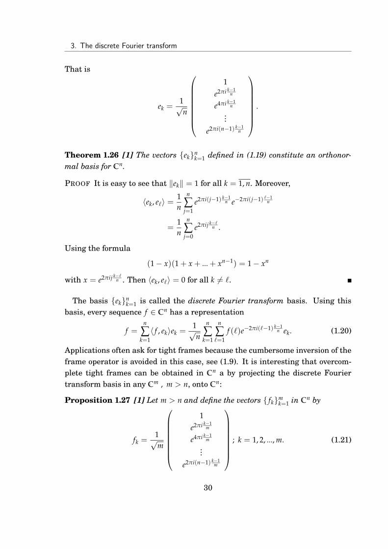
That is

ek =1√n

1e2πi k−1

n

e4πi k−1n

...e2πi(n−1) k−1

n

.

Theorem 1.26 [1] The vectors {ek}nk=1 defined in (1.19) constitute an orthonor-

mal basis for Cn.

PROOF It is easy to see that ‖ek‖ = 1 for all k = 1, n. Moreover,

〈ek, e`〉 =1n

n

∑j=1

e2πi(j−1) k−1n e−2πi(j−1) `−1

n

=1n

n

∑j=0

e2πij k−`n .

Using the formula

(1− x)(1 + x + ... + xn−1) = 1− xn

with x = e2πij k−`n . Then 〈ek, e`〉 = 0 for all k 6= `.

The basis {ek}nk=1 is called the discrete Fourier transform basis. Using this

basis, every sequence f ∈ Cn has a representation

f =n

∑k=1〈 f , ek〉ek =

1√n

n

∑k=1

n

∑`=1

f (`)e−2πi(`−1) k−1n ek. (1.20)

Applications often ask for tight frames because the cumbersome inversion of theframe operator is avoided in this case, see (1.9). It is interesting that overcom-plete tight frames can be obtained in Cn a by projecting the discrete Fouriertransform basis in any Cm , m > n, onto Cn:

Proposition 1.27 [1] Let m > n and define the vectors { fk}mk=1 in Cn by

fk =1√m

1e2πi k−1

m

e4πi k−1m

...e2πi(n−1) k−1

m

; k = 1, 2, ..., m. (1.21)

30


Then { fk}mk=1 is a tight overcomplete frame for Cn with frame bound equal to 1

and ‖ fk‖ =√ n

m for all k.

PROOF Applying Theorem 1.26 , one has { fk}mk=1 constitute an orthonormal ba-

sis for Cm with

fk =1√m

1e2πi k−1

m

e4πi k−1m

...e2πi(m−1) k−1

m

; k = 1, 2, ..., m. (1.22)

Applying the Corollary 1.24 , { fk}mk=1 constitute a tight frame bound for Cn with

frame bound equal to 1.In addition, ‖ fk‖ =

√ nm for all k = 1, m.

It is important to notice that all the vectors fk in Proposition 1.27 have thesame norm. If needed, we can therefore normalize them while keeping a tightframe; we only have to adjust the frame bound accordingly.

Corollary 1.28 [1] For any m > n , there exists a tight frame in Cn consisting ofm normalized vectors.

Example 1.29

The discrete Fourier transform basis in C4 consists of the vectors

12

1111

,12

1i−1

i

,12

1−1

1−1

,12

1−i−1

i

.

Via Proposition 1.27 , the vectors

12

111

,12

1i−1

,12

1−1

1

,12

1−i−1

.

constitute a tight frame in C3.One advantage of an overcomplete frame compared to a basis is that the frame

property might be kept if an element is removed. However, even for frames it can

31


happen that the remaining set is no longer a frame, for example if the removedelement is orthogonal to the rest of the frame elements. Unfortunately this canbe the case no matter how large the number of frame elements is, i.e., no matterhow redundant the frame is! If we have information on the lower frame boundand the norm of the frame elements we can provide a criterion for how manyelements we can (at least) remove:

Proposition 1.30 [1] Let { fk}mk=1 be a normalized frame for Cn with lower bound

frame bound A > 1. Then for any index set I ⊂ {1, 2, ..., m} with |I| < A, thefamily { fk}k/∈I is a frame for Cn with lower frame bound A− |I|.

PROOF Given f ∈ Cn ,

∑k∈I|〈 f , fk〉|2 ≤ ∑

k∈I‖ fk‖2‖ f ‖2 = |I|‖ f ‖2.

Thus,

∑k/∈I|〈 f , fk〉|2 ≥ (A− |I|)‖ f ‖2.

Since A− |I| > 0 then we can choose (A− |I|) as a lower frame bound of { fk}mk=1

Considering an arbitrary frame { fk}mk=1 for Cn, the maximal number of ele-

ments one can hope to remove while keeping the frame property is m − n. Ifwe want to be able to remove m − n arbitrary elements it is not enough to as-sume that { fk}m

k=1 is a normalized tight frame. Concerning the stability againstremoval of vectors, the frames obtained in Proposition 1.27 behave well: m− narbitrary elements can be removed:

Proposition 1.31 [1] Consider the frame { fk}mk=1 for Cn define as (1.21). Any

subset containing at least n elements of this frame forms a frame for Cn.

PROOF Consider an arbitrary subset {k1, f2, ..., kn} ⊆ {1, 2, ..., m}.Placing the vectors { fki}

ni=1 as rows in an n× n matrix and letting z := e

2πim , then

− fk1 −− fk2 −

...− fkn −

=1√m

1 zk1−1 · · · z(k1−1)(n−1)

1 zk2−1 · · · z(k2−1)(n−1)

· · ·1 zkn−1 · · · z(kn−1)(n−1)

.

32

1.4. Pseudo-inverses and the singular value decomposition

This is Vandermode matrix with determinant

det =1

mn2

∏i 6=j

(zki−1 − zkj−1) 6= 0. (1.23)

Hence, { fki}ni=1 is a basis for Cn.

From Proposition 1.31 , we have another way to construct a frame for Cn. Indetail, taking any at least n elements of the frame { fk}m

k=1 define as (1.21), wewill obtain a frame for Cn.

1.4 Pseudo-inverses and the singular valuedecomposition

Given m× n matrix E, consider it as a linear mapping

E : Cn −→ Cm.

E is not necessary injective, but by restricting E to orthogonal complement of thekernel KerE, we obtain an injective linear mapping

E : (KerE)⊥ −→ Cm.

Indeed, if Ex = 0 then x = 0 because KerE⋂(KerE)⊥ = {0}. So, E is injective.

We see that ImE = ImE then

˜E : (KerE)⊥ −→ ImE

has inverse and its inverse

( ˜E)−1 : ImE −→ (KerE)⊥.

Extend ˜E−1 to E† : Cm −→ Cn by defining

E†(y + z) = ˜E−1y if y ∈ ImE , z ∈ (ImE)⊥. (1.24)

So,

EE†x = x for all x ∈ ImE.

33


The operator E† is called pseudo-inverse of E.From the construction and Lemma 1.10, we have:

KerE† = ImE⊥ = KerE∗ (1.25)

ImE† = KerE⊥ = ImE∗. (1.26)

Indeed, if x ∈ (ImE)⊥ then E†x = 0 by (1.24). So, x ∈ KerE†.Thus (ImE)⊥ ⊆ KerE†.If x ∈ KerE† then 0 = E†x = ˜E−1y, for which x = y + z , y ∈ ImE, z ∈ (ImE)⊥.Since ˜E−1 is bijective then y = 0. Therefore, x = z ∈ (ImE)⊥.Thus, KerE† ⊆ (ImE)⊥.In conclusion, we obtain

KerE† = ImE⊥ = KerE∗.

Similarly, we have

ImE† = KerE⊥ = ImE∗.

We note two characterizations of the pseudo-inverse:

Proposition 1.32 [1] Let E be an m× n matrix. Then

(i) E† is the unique n × m matrix for which EE† is the orthogonal projectiononto ImE and E†E is the orthogonal projection onto ImE†.

(ii) E† is the unique n×m matrix for which EE† and E†E are self-adjoint and

EE†E = E , E†EE† = E†.

PROOF Assume that EE† is the orthogonal projection onto ImE then EE†E = Eand EE†x = 0 , ∀x ∈ (ImE)⊥. Therefore, (ImEE†)⊥ = KerEE† , i.e., EE† is self-adjoint.Similarly, we have E†E is self-adjoint and E†EE† = E†.Suppose EE† is self-adjoint and EE†E = E. Then, we have

(EE†)2 = EE†EE† = EE†.

So, EE† is a projection onto ImEE†. Since EE† is self-adjoint then

(ImEE†)⊥ = KerEE†, i.e., EE†(x) = 0 , ∀x ∈ (ImEE†)⊥.

34


Therefore, EE† is the orthogonal projection onto ImEE†.Moreover, EE†E = E then ImE = ImEE†E ⊆ ImEE† ⊆ ImE.Hence, ImEE† = ImE.That means EE† is the orthogonal projection onto ImE.Similar for E†E, E†E is the orthogonal projection onto ImE†.

Now, we have to prove that E† in Proposition 1.32 is exact E† in the above con-struction.

PROOF Assume E† as in the construction, if y ∈ ImE then EE†y = y.If y ∈ (ImE)⊥ = KerE† then EE†y = 0.Therefore, EE† is the orthogonal projection onto ImE.In addition, if y ∈ (ImE†)⊥ = KerE then E†Ey = 0.If y ∈ ImE† then y = E†x for some x. So,

E†Ey = E†EE†x = E†x− E†(Id− EE†)x

= E†x = y,

here Id− EE† is the orthogonal projection onto (ImE)⊥ = KerE†.Thus, E†Ey = ImE†.Hence, E†E is the orthogonal projection onto ImE†.Conversely, suppose E† is defined as in Proposition 1.32. From (ii)

E∗ = (EE†E)∗ = (E†E)∗E∗ = E†EE∗

because E†E is self-adjoint.Therefore,

(KerE)⊥ = ImE∗ ⊆ ImE†.

Now, take y ∈ ImE then ∃x ∈ (KerE)⊥ such that y = Ex. Then,

E†y = E†Ex = x = ( ˜E)−1Ex = ( ˜E)−1y.

If z ∈ (ImE)⊥ then EE†z = 0 by (i) ,and E†z = E†EE†z = 0 by (ii).

The pseudo-inverse gives the solution to an important minimization problem:

35


Theorem 1.33 [1] Let E be an m× n matrix. Given y ∈ ImE. Then the equationEx = y has a unique solution of minimal norm, namely x = E†y.

PROOF We have: EE†y = y for y ∈ ImE. So, E†y is a solution to the equationEx = y.Thus, the general solution x = E†y + z , where z ∈ KerE and y ∈ (KerE)⊥.Hence, ‖x‖2 = ‖E†y‖2 + ‖z‖2 ≥ ‖E†y‖2. It occurs when z = 0.

For computational purposes it is important to notice that the pseudo-inversecan be found using the singular value decomposition of E. We begin with alemma.

Lemma 1.34 [1] Let E be an m × n matrix with rank r ≥ 1. Then there existconstants σ1, σ2, ..., σr > 0 ,and orthonormal bases {uk}r

k=1 for ImE and {vk}rk=1

for ImE∗ such that

Evk = σkuk for k = 1, r. (1.27)

PROOF We have:

E∗E : Cn −→ Cn

is self-adjoint.Then there exists an orthonormal basis {vk}n

k=1 for Cn consisting of eigenvectorsfor E∗E.Let {λk}n

k=1 denote the corresponding eigenvalues. Then

λk = λk‖vk‖2

= 〈E∗Evk, vk〉 = ‖Evk‖2 ≥ 0 , ∀k = 1, n.

Thus,

r = dimImE = dimImE∗. (1.28)

Since

(ImE)⊥ = KerE∗

36


then

ImE∗ = ImE∗E = span{E∗Evk}nk=1

= span{λkvk}nk=1.

Therefore, the rank equal to the number of non-zero eigenvalues.Assume that we can order {vk}r

k=1 such that {vk}rk=1 corresponds to the non-zero

eigenvalues.Since

ImE∗ = span{λkvk}rk=1

then {vk}rk=1 is an orthonormal basis for ImE∗.

For k > r ,

‖Evk‖2 = 〈E∗Evk, vk〉 = 0.

Then Evk = 0 , ∀k > r.Define

uk :=1√λk

Evk , k = 1, 2, ..., r. (1.29)

Therefore, we obtain {uk}rk=1 spans ImE.

Hence,

σk =√

λk , k = 1, 2, ..., r.

Lemma 1.34 leads to the singular value decomposition of E:

Theorem 1.35 [1] Every m× n matrix E with rank r ≥ 1 has a decomposition:

E = U

(D 00 0

)V∗ (1.30)

where U is a unitary m×m matrix ,V is a unitary n× n matrix ,

and

(D 00 0

)is an m× n block matrix in which D is an r× r diagonal matrix

with positive entries σ1, σ2, ..., σr in the diagonal.

37


PROOF Let {vk}nk=1 be the orthonormal basis for Cn ordered such that {vk}r

k=1 isthe orthogonal basis for ImE∗.Let V be n× n matrix having the vector {vk}n

k=1 as columns:

V =

| | ... |v1 v2 ... vn

| | ... |

.

Extend the orthonormal basis {uk}rk=1 for ImE to the orthonormal basis {uk}m

k=1for Cm and let

U =

| | ... |u1 u2 ... um

| | ... |

.

Finally, let D be the r× r diagonal matrix with positive entries σ1, σ2, ..., σr in thediagonal.Since {

Evk = 0 for k > r,Evk = σkuk for k = 1, r

then

EV = (σ1u1 σ2u2 ... σrur 0 ... 0)

= U

(D 00 0

). (1.31)

Multiplying (1.31) with V∗ from the right, then

E = U

(D 00 0

)V∗.

The numbers σ1, ..., σr are called singular values of E; the proof of Lemma 1.34shows that they are the square roots of the positive eigenvalues for E∗E.

Corollary 1.36 [1] With the notation in Theorem 1.35, the pseudo-inverse of E isgiven by

E† = V

(D−1 0

0 0

)U∗ (1.32)

38


where

(D−1 0

0 0

)is an m× n block matrix in which D−1 is an r × r diagonal

matrix with positive entries σ−11 , σ−1

2 , ..., σ−1r in the diagonal.

PROOF We check that the matrix E† defined by (1.38) satisfies the requirementsin Proposition 1.32. First, via (1.30),

EE† = U

(D 00 0

)V∗V

(D−1 0

0 0

)U∗

= U

(Id 00 0

)U∗,

which shows that EE† is self-adjoint.Furthermore,

EE†E = U

(Id 00 0

)U∗U

(D 00 0

)V∗

= E.

Similarly, we can verify that E†E is self-adjoint and E†EE† = E†.

Let us return to the setting where { fk}mk=1 is a frame for Cn with pre-frame

operator T : Cm −→ Cn. The calculation of the frame coefficients amounts tofinding T†:

Theorem 1.37 [1] Let { fk}mk=1 be a frame for Cn, with pre-frame operator T and

frame operator S. Then

T† f = {〈 f , S−1 fk〉}mk=1 , ∀ f ∈ Cm. (1.33)

PROOF Let f ∈ Cn. Expressed in terms of the pre-frame operator T, the equa-

tion f =m∑

k=1ck fk means that T{ck}m

k=1 = f , f ∈ Cm.

By Theorem 1.33 , the equation

T{ck}mk=1 = f

39


has a unique solution of minimal norm {ck}mk=1 = T† f .

Applying Theorem 1.11 , we have:

ck = 〈 f , S−1k〉 , ∀k = 1, m.

Therefore,

T† f = {〈 f , S−1 fk〉}mk=1 , ∀ f ∈ Cm.

One interpretation of Theorem 1.37 is that when { fk}mk=1 is a frame for Cn, the

matrix T† is obtained by replacing the complex conjugate of the vectors in thecanonical dual frame {S−1 f }m

k=1 as rows in an m× n matrix:

T† =

− S−1 f1 −− S−1 f2 −

...− S−1 fm −

.

The singular value decomposition gives a natural way to obtain coefficients

{ck}mk=1 such that f =

m∑

k=1ck fk. Let { fk}m

k=1 be an overcomplete frame for Cn.

Since T is surjective, its rank equals n, and the singular value decomposition ofT is

T = U(D 0)V∗.

Note that since T is an n × m matrix, (D 0) is now an n × m matrix; U is ann× n matrix, and V is an m× n matrix. Given any (m− n)× n matrix F, we have

TV

(D−1

F

)U∗ f = U(D 0)V∗V

(D−1

F

)U∗ f

= UIU∗ f

= f .

This means that we can use the coefficients

{ck}mk=1 = V

(D−1

F

)U∗ f (1.34)

40

1.5. Finite-dimensional function spaces

for the reconstruction of f . As noted already in Theorem 1.11 the choice F = 0is optimal in the sense that the `2-norm of the coefficients is minimized, but forother purposes other choices might be preferable. The matrix

V

(D†

F

)U∗ (1.35)

is frequently called a generalized inverse of T.

1.5 Finite-dimensional function spaces

Given a, b ∈ R with a < b, let C[a, b] denote the set of continuous functions f :[a, b] −→ C. We equip C[a, b] with the supremums-norm

‖ f ‖∞ = supx∈[a,b]

| f (x)|.

The Weierstrass’s Approximation Theorem say that every f ∈ C[a, b] can be ap-proximated arbitrarily well by a polynomial:

Theorem 1.38 [1] Let f ∈ C[a, b]. Given ε > 0, there exists a polynomial

P(x) =n

∑k=0

ckxk

such that

‖ f (x)− P(x)‖∞ ≤ ε for all x ∈ [a, b]. (1.36)

PROOF Let t = a + x(b− a) for t ∈ [a, b], then x ∈ [0, 1].We will show that the polynomial

Bk(x) = Bk f (x) =k

∑p=0

Cpk f (

pk)xp(1− x)k−p (1.37)

converges to f for all x ∈ [0, 1].Indeed, remark

(x + y)k =k

∑p=0

Cpk xpyk−p. (1.38)

41


Taking the derivative (1.38) and multiplying x to both sides

kx(x + y)k−1 =k

∑p=0

pCpk xpyk−p. (1.39)

Taking the derivative twice (1.38) and multiplying x2 to both sides

k(k− 1)x2(x + y)k−2 =k

∑p=0

p(p− 1)Cpk xpyk−p. (1.40)

Let y := 1− x, rp(x) = Cpk xpyk−p, then

k

∑p=0

rp(x) = 1 ,k

∑p=0

prp(x) = kx ,k

∑p=0

p(p− 1)rp(x) = k(k− 1)x2.

Therefore,

k

∑p=0

(p− kx)2rp(x) =k

∑p=0

p2rp(x)− 2kxk

∑p=0

prp(x) + k2x2k

∑p=0

rp(x)

= [kx + (k− 1)kx2]− 2kx + k2x2

= kx(1− x).

Now, let

M = max|x|≤1| f (x)|. (1.41)

Given ε > 0, since f ∈ C[a, b] then

∃δ > 0 such that |x− y| < δ yields | f (x)− f (y)| < ε , ∀x, y ∈ [a, b]. (1.42)

Consider

f (x)−Bk(x) = f (x)−k

∑p=0

Cpk f (

pk)xp(1− x)k−p

=k

∑p=0

f (x)rp(x)−k

∑p=0

Cpk f (

pk)xp(1− x)k−p

=k

∑p=0

( f (x)− f (pk))rp(x).

42


Thus,

f (x)−Bk(x) = ∑{p|| pk−x|<δ}

( f (x)− f (pk))rp(x) + ∑

{p|| pk−x|≥δ}( f (x)− f (

pk))rp(x).

(1.43)

Since rp(x) ≥ 0 and

| f (x)− f (pk)| < ε

2when| p

k− x| < δ

then

| ∑{p|| pk−x|<δ}

( f (x)− f (pk))rp(x)| ≤ ε

2

k

∑p=0

rp(x) =ε

2.

Moreover,

| ∑{p|| pk−x|≥δ}

( f (x)− f (pk))rp(x)| ≤ 2M ∑

{p|| pk−x|≥δ}rp(x)

≤ 2Mk

∑p=0

((p− kx)

kδ)2rp(x)

=2Mk2δ2 kx(1− x)

≤ M2kδ2 .

Hence, for k ≥ Mεδ2

| f (x)−Bk(x)| = | ∑{p|| pk−x|<δ}

( f (x)− f (pk))rp(x) + ∑

{p|| pk−x|≥δ}( f (x)− f (

pk))rp(x)|

≤ | ∑{p|| pk−x|<δ}

( f (x)− f (pk))rp(x)|+ | ∑

{p|| pk−x|≥δ}( f (x)− f (

pk))rp(x)|

≤ ε

2+

ε

2= ε.

In conclusion,

‖ f (x)−Bk(x)‖∞ = sup|x|≤1| f (x)−Bk(x)| < ε.

It is essential for the conclusion that [a, b] is a finite and closed interval. Theorem1.38 will be fail if [a, b] replaced by an open interval or unbounded interval.

43


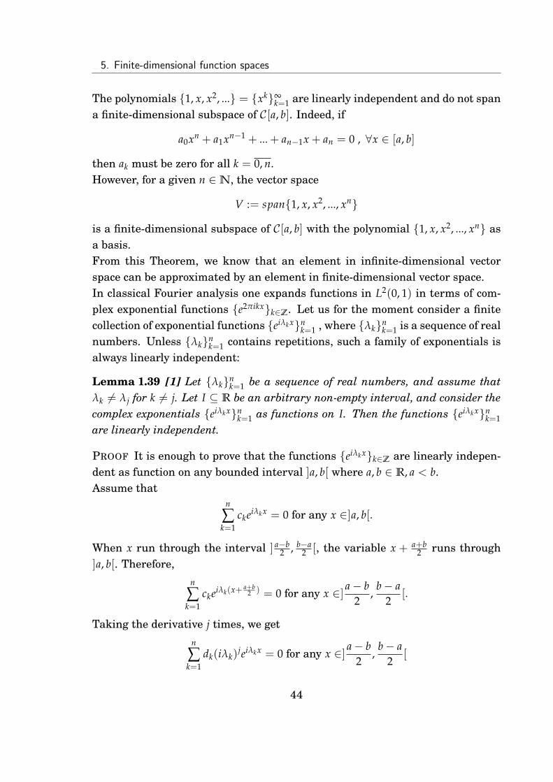
The polynomials {1, x, x2, ...} = {xk}∞k=1 are linearly independent and do not span

a finite-dimensional subspace of C[a, b]. Indeed, if

a0xn + a1xn−1 + ... + an−1x + an = 0 , ∀x ∈ [a, b]

then ak must be zero for all k = 0, n.However, for a given n ∈N, the vector space

V := span{1, x, x2, ..., xn}

is a finite-dimensional subspace of C[a, b] with the polynomial {1, x, x2, ..., xn} asa basis.From this Theorem, we know that an element in infinite-dimensional vectorspace can be approximated by an element in finite-dimensional vector space.In classical Fourier analysis one expands functions in L2(0, 1) in terms of com-plex exponential functions {e2πikx}k∈Z. Let us for the moment consider a finitecollection of exponential functions {eiλkx}n

k=1 , where {λk}nk=1 is a sequence of real

numbers. Unless {λk}nk=1 contains repetitions, such a family of exponentials is

always linearly independent:

Lemma 1.39 [1] Let {λk}nk=1 be a sequence of real numbers, and assume that

λk 6= λj for k 6= j. Let I ⊆ R be an arbitrary non-empty interval, and consider thecomplex exponentials {eiλkx}n

k=1 as functions on I. Then the functions {eiλkx}nk=1

are linearly independent.

PROOF It is enough to prove that the functions {eiλkx}k∈Z are linearly indepen-dent as function on any bounded interval ]a, b[ where a, b ∈ R, a < b.Assume that

n

∑k=1

ckeiλkx = 0 for any x ∈]a, b[.

When x run through the interval ] a−b2 , b−a

2 [, the variable x + a+b2 runs through

]a, b[. Therefore,n

∑k=1

ckeiλk(x+ a+b2 ) = 0 for any x ∈] a− b

2,

b− a2

[.

Taking the derivative j times, we getn

∑k=1

dk(iλk)jeiλkx = 0 for any x ∈] a− b

2,

b− a2

[

44


where dk := ckeiλka+b

2 .Letting x = 0 then

1 1 · · · 1λ1

1 λ12 · · · λ1

n

· · ·λn−1

1 λn−12 · · · λn−1

n

d1

d2...

dn

=

00...0

.

Besides

A =

1 1 · · · 1

λ11 λ1

2 · · · λ1n

· · ·λn−1

1 λn−12 · · · λn−1

n

is Vandermonde matrix with determinant

det A = ∏i>j

(λi − λj) 6= 0.

So, d1 = d2 = ... = dn = 0.Thus, c1 = c2 = ... = cn = 0.Hence, {eiλkx}k∈Z are linearly independent.

In words, Lemma 1.39 means that complex exponentials do not give natural ex-amples of frame in finite-dimensional spaces: if λk 6= λj for k 6= j, then thecomplex exponentials {eiλkx}n

k=1 form a basis for their span in L2(I) for any in-terval I of finite length, and not overcomplete system. We can not obtain over-completeness by adding extra exponentials (except by repeating some of the λ

-values)-this will just enlarge the space.Specially, as an important case we now consider the case where λk = 2. A func-tion f which is a finite combination of the type

f (x) =N2

∑k=N1

cke2πikx for some ck ∈ C; N1, N2 ∈ Z; N2 ≥ N1 (1.44)

is called a trigonometric polynomial. Trigonometric polynomial correspond topartial sums in Fourier series. A trigonometric polynomial f can also be writtenas a linear combination of functions sin(2πx), cos(2πx), in general with complexcoefficients. It will be useful later to note that if f is real-valued and coefficientsck in (1.44) are real, then f is linear combination of functions cos(2πx) alone:

45


Lemma 1.40 [1] Assume that the trigonometric polynomial in (1.44) is real-valued and that ck ∈ R, then

f (x) =N2

∑k=N1

ck cos(2πkx). (1.45)

PROOF We have:

f (x) =N2

∑k=N1

cke2πikx

=N2

∑k=N1

ck(cos 2πkx + i sin 2πkx).

Since f is real-valued then

f (x) =N2

∑k=N1

ck cos(2πkx).

Note that we need the assumption that ck ∈ R: for example, the function

f (x) =12i

eπix − 12i

e−πix = sin x,

is real-valued, but does not have the form (1.45).Moreover, we mention that a positive-valued triogonometric polynomial has asquare root, which is again a triogonometric polynomial:

Lemma 1.41 [1] Let f be a positive-valued triogonometric polynomial of the form

f (x) =N2

∑k=N1

ck cos(2πkx) , ck ∈ R.

Then there exists a triogonometric polynomial

g(x) =N

∑k=0

dke2πikx with dk ∈ R, (1.46)

such that

|g(x)|2 = f (x) , ∀x ∈ R. (1.47)

46


PROOF We can write f (x) =M∑

m=0am cos(mx) with am ∈ R.

Moreover, we have

cos(nx) = 2 cos(n− 1)x cos x + cos(n− 2)x , ∀n ≥ 2 , n ∈ R. (1.48)

So, cos(mx) can be rewritten as a polynomial of degree m of cos x.Therefore, f (x) = p f (cos x), where p f is a polynomial of degree M with realcoefficients. This polynomial can be factored,

p f (c) = αM

∏j=1

(c− cj),

where the zeros cj of p f appear either in complex duplets cj, cj, or in real singlets.We can also write

f (x) = eiMxPf (e−ix), (1.49)

where Pf is a polynomial of degree 2M. For |z| = 1, we have

Pf (z) = zMαM

∏j=1

(z + z−1

2− cj) = α

M

∏j=1

(12− cjz +

12

z2). (1.50)

Indeed, we have

Pf (e−ix) = e−iMxαM

∏j=1

(e−ix + eix

2− cj).

Therefore,

eiMxPf (e−ix) = αM

∏j=1

(e−ix + eix

2− cj)

= αM

∏j=1

(cos x− cj)

= p f (cos x) = f (x).

If cj is real, then the zeros of 12 − cjz + 1

2 z2 are cj ±√

c2j − 1.

For |cj| ≥ 1, these are two real zeros (degenerate if cj = ±1) of the form rj, r−1j .

For |cj| < 1, the two zeros are complex conjugate and of absolute value 1, i.e.,they are of the form eiαj , e−iαj . Then αj,−αj be the zeros of f (x), or

f (x) = ((x− αj)(x + αj))nQ(x). (1.51)

47


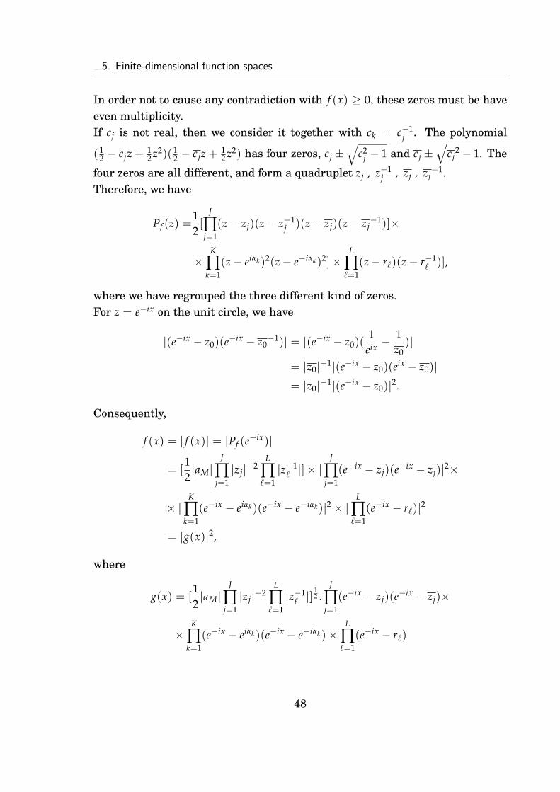
In order not to cause any contradiction with f (x) ≥ 0, these zeros must be haveeven multiplicity.If cj is not real, then we consider it together with ck = c−1

j . The polynomial

(12 − cjz + 1

2 z2)(12 − cjz + 1

2 z2) has four zeros, cj ±√

c2j − 1 and cj ±

√cj

2 − 1. The

four zeros are all different, and form a quadruplet zj , z−1j , zj , zj

−1.Therefore, we have

Pf (z) =12[

J

∏j=1

(z− zj)(z− z−1j )(z− zj)(z− zj

−1)]×

×K

∏k=1

(z− eiαk)2(z− e−iαk)2]×L

∏`=1

(z− r`)(z− r−1` )],

where we have regrouped the three different kind of zeros.For z = e−ix on the unit circle, we have

|(e−ix − z0)(e−ix − z0−1)| = |(e−ix − z0)(

1eix −

1z0)|

= |z0|−1|(e−ix − z0)(eix − z0)|= |z0|−1|(e−ix − z0)|2.

Consequently,

f (x) = | f (x)| = |Pf (e−ix)|

= [12|aM|

J

∏j=1|zj|−2

L

∏`=1|z−1` |]× |

J

∏j=1

(e−ix − zj)(e−ix − zj)|2×

× |K

∏k=1

(e−ix − eiαk)(e−ix − e−iαk)|2 × |L

∏`=1

(e−ix − r`)|2

= |g(x)|2,

where

g(x) = [12|aM|

J

∏j=1|zj|−2

L

∏`=1|z−1` |]

12 .

J

∏j=1

(e−ix − zj)(e−ix − zj)×

×K

∏k=1

(e−ix − eiαk)(e−ix − e−iαk)×L

∏`=1

(e−ix − r`)

48


= [12|aM|

J

∏j=1|zj|−2

L

∏`=1|z−1` |]

12 ×

J

∏j=1

(e−2ix − 2e−ixRezj + |zj|2)×

×K

∏k=1

(e−2ix − 2e−ix cos αk + 1)]×L

∏`=1

(e−ix − r`)

is clear a triogonometric polynomial of order M with real coefficients.

Example 1.42

Consider f (x) = 1 + cos 2x.We find g(x) = d0 + d1eix + d2ei2x satisfies |g(x)|2 = f (x). We have

|g(x)|2 = |d0 + d1 cos x + d2 cos 2x + i(d1 sin x + d2 sin 2x)|2

= (d0 + d1 cos x + d2 cos 2x)2 + (d1 sin x + d2 sin 2x)2

= d20 + d2

1 + d22 + 2(d0d1 + d1d2) cos x + 2d0d2 cos 2x = 1 + cos 2x.

Therefore, d2

0 + d21 + d2

2 = 12(d0d1 + d1d2) = 0

2d0d2 = 1

Thus, {d1 = 0

d0 = d2 = ± 1√2

Hence,

g(x) = ± 1√2(1 + ei2x).

Remark 1.43

1. This proof is constructive. It use factorization of a polynomial of degreeM, however, which has to be done numerically and may lead to problemsif M is large and some zeros are closed together. Note that in this proofwe need to factor a polynomial of degree only M, unlike some procedureswhich factor directly Pf , a polynomial of degree 2M.

49


2. This procedure of ”extracting the square root” is also called spectral factor-ization in the engineering literature.

3. The polynomial g(x) is not unique! For M odd, for instance, Pf may havequadruplets of complex zeros, and 1 pair of real zeros. In each quadrupletwe can choose either zj, zj to make up g(x), or z−1

j , z−1j ; for each duplet we

can choose either r` or r−1` . This make already for 2

M+12 different choices for

g(x). Moreover, we can always multiply g(x) with einx, n arbitrary in Z.

Example 1.44

Consider f (x) = 1 + cos x.We calculate directly g(x) = d0 + d1eix for which |g(x)|2 = f (x).Then we obtain g(x) = ± 1√

2(1 + eix).

Moreover, we can choose g′(x) = ± 1√2(eix + ei2x) also satisfy |g′(x)|2 = f (x).

Note that by definition, the function g(x) in (1.46) is complex-valued, unless f isconstant. Actually, despite the fact that f is assumed to be positive, there mightnot exist a positive trigonometric polynomial g satisfying (1.47).

50

Conclusion

The thesis can be fully understood with an elementary knowledge of linearalgebra. This presents basic results in finite-dimensional vector spaces with aninner product.

Section 1.1 contains the basic properties of frames. For example, it is provedthat every set of vectors { fk}m

k=1 in a vector space with an inner product is aframe for span{ fk}m

k=1. We have proved the existence of coefficients minimizingthe `2-norm of the coefficients in a frame expansion and showed how a frame fora subspace lead to a formula for the orthogonal projection onto the subspace.

In Section 1.2 and Section 1.3, we have considered frames on Cn; in particu-lar, we’ve proved how we can obtain an overcomplete frame by a projection of abasis for a larger space. We also proved that the vectors{ fk}m

k=1 is a frame for Cn

can be considered as the first n coordinates of some vectors in Cm constitutinga basis for Cm, and that the frame property for { fk}m

k=1 is equivalent to certainproperties for the m× n matrix having the vectors fk as rows.

In Section 1.4 we have proved that the canonical coefficients from the frameexpansion arise naturally by considering the pseudo-inverse of the pre-frame op-erator, and we showed how to find it in term of the singular value decomposition.Finally, in Section 1.5 we connected frames in finite-dimensional vector spaceswith the infinite-dimensional constructions which we expect study latter.

51

References

[1] Christensen, O. An Introduction to Frames and Riesz Bases, Birkhauser Ver-lag, 2003.

[2] Daubechies, I. Lectures on Wavelets. SIAM, Philadelphia, 1992.

[3] N. H. V. Hưng, Đại Số Tuyến Tính, NXB ĐHQGHN, 2001.

52

frames in finite-dimensional inner product spaces · pdf fileframes in finite-dimensional...

Documents