Journal of the Mechanics and Physics of Solids 115 (2018) 230–247

Contents lists available at ScienceDirect

Journal of the Mechanics and Physics of Solids

journal homepage: www.elsevier.com/locate/jmps

Transient response of nonlinear polymer networks: A kinetic

theory

Franck J. Vernerey

Department of Mechanical Engineering, Program of Materials Science and Engineering, University of Colorado, Boulder, USA

a r t i c l e i n f o

Article history:

Received 27 November 2017

Revised 9 February 2018

Accepted 27 February 2018

Available online 7 March 2018

a b s t r a c t

Dynamic networks are found in a majority of natural materials, but also in engineering

materials, such as entangled polymers and physically cross-linked gels. Owing to their

transient bond dynamics, these networks display a rich class of behaviors, from elastic-

ity, rheology, self-healing, or growth. Although classical theories in rheology and mechanics

have enabled us to characterize these materials, there is still a gap in our understanding on

how individuals (i.e., the mechanics of each building blocks and its connection with others)

affect the emerging response of the network. In this work, we introduce an alternative way

to think about these networks from a statistical point of view. More specifically, a network

is seen as a collection of individual polymer chains connected by weak bonds that can

associate and dissociate over time. From the knowledge of these individual chains (elas-

ticity, transient attachment, and detachment events), we construct a statistical description

of the population and derive an evolution equation of their distribution based on applied

deformation and their local interactions. We specifically concentrate on nonlinear elastic

response that follows from the strain stiffening response of individual chains of finite size.

Upon appropriate averaging operations and using a mean field approximation, we show

that the distribution can be replaced by a so-called chain distribution tensor that is used to

determine important macroscopic measures such as stress, energy storage and dissipation

in the network. Prediction of the kinetic theory are then explored against known exper-

imental measurement of polymer responses under uniaxial loading. It is found that even

under the simplest assumptions of force-independent chain kinetics, the model is able to

reproduce complex time-dependent behaviors of rubber and self-healing supramolecular

polymers.

© 2018 Elsevier Ltd. All rights reserved.

1. Introduction

Most polymers display a time-dependent behavior in the form of complex coupling between elasticity and flow. De-

pending on the polymer type, these effects may result from polymer chain diffusion and friction (non-entangled polymers),

chain entanglement and reptation (entangled polymers) or the detachment and reforming of weak cross-links (polymers

with physical bonds). These mechanisms eventually yield a rich spectrum of macroscopic responses such as viscoelasticity,

visco-plasticity ( Watanabe, 1999 ) or even elastic-fluidity ( Denn, 1990 ). Natural materials often depends on these physics to

achieve key functions of life. Dynamic polymers are indeed ubiquitous in nature due to their capacity to remain solid and

provide mechanical strength while keeping their ability to flow, reorganize and self-repair. In the plant and fungi kingdom,

E-mail address: franck.vernerey@colorado.edu

https://doi.org/10.1016/j.jmps.2018.02.018

0022-5096/© 2018 Elsevier Ltd. All rights reserved.

F.J. Vernerey / Journal of the Mechanics and Physics of Solids 115 (2018) 230–247 231

dynamic polymers are used as the structural material that makes cell walls ( Proseus et al., 1999 ) and their ability to se-

lectively control their rheology in order to either temporarily bend towards a light source (elastic deformation) or grow

in size and shape (inelastic deformation). In the animal kingdom, dynamic polymers are also the main chemical engine

to generate motion; muscle cells are made of acto-myosin assemblies, which are made of unidirectional actin filaments

on which tethers (small myosin filaments) are able to walk as powered by ATP ( Vernerey and Akalp, 2016 ). The periodic

attachment and detachments of myosin on actin, together with the power stroke, generates an overall contraction of the

polymer ( Joanny and Prost, 2009; Murrell et al., 2015; Vernerey and Farsad, 2011 ). Almost all soft tissues, including neurons

( Tang-Schomer et al., 2010 ), skin ( Evans et al., 2013 ) or fibrin networks ( Purohit et al., 2011 ) display dynamic responses as

required for growth ( Vernerey, 2016 ), self-repair, and adaptation. Synthetic (or supramolecular) polymers, that mimic their

biological counterparts have recently been introduced to replicate functions such as self-healing ( Roy et al., 2015 ), shape

memory ( Wang and Xie, 2010 ) , and toughness amplification ( Kong et al., 2003 ). Typically, these networks are formed from

chains that interact via non-covalent cross-links such as hydrogen bonds ( Wang and Xie, 2010 ), linkage with metal-ligand

interactions ( Grindy et al., 2015 ), or physical entanglements and dangling chains that display fast mobility ( de Gennes and

Leger, 1982 ). A theoretical framework has yet to be developed to link chain dynamics to the emerging elastic and rheological

behavior of these materials.

The dynamics of chain detachment, reattachment, entanglements, and diffusion have been extensively studied in the

physics community in the past few decades ( de Gennes, 1979; Rubinstein and Colby, 2003 ). These theoretical insights have

however not been fully translated to advancements in continuum models of viscoelasticity. Most existing models, from

the simple linear Maxwell or Kelvin-Voigt models ( Drozdov, 1999 ) to the more sophisticated nonlinear viscoelastic mod-

els ( Wineman, 2009 ) are either phenomenological or inspired – but not derived – from the underlying mechanisms. On

the one hand, derivations following classical continuum mechanics have led macroscopic constitutive relation based on the

multiplicative decomposition of the deformation gradient into elastic and inelastic components ( Simo, 1987 ). These formu-

lations are usually attractive for numerical implementation and experimental fitting, but suffer from a lack of connection

with the material’s structure. On the other hand, a second class of models has been inspired by mechanisms such as chain

entanglement dynamics ( Bergstrom and Boyce, 1998 ), or built from molecular dynamics simulations ( Li et al., 2016 ). In the

case of rubber for instance, stress relaxation has been described by the detachment and reattachment of chains as they

reptate along a tube representing the presence of the surrounding network. This tube model, originally proposed by De-

Gennes ( de Gennes and Leger, 1982 ) has now inspired a number of constitutive relations of rubber-like materials that have

successfully reproduced complex visco-elastic responses at large strains. A more complete description of these models, with

appropriate references is given in Zhou et al. (2018) . These models are however still based on the spring and dashpot view

of the polymer structure and it is arguable whether they can provide a direct bridge between structure, mechanisms and

macroscopic response. Another difficulty in modeling visco-elasticity is the lack of a common natural reference configura-

tion for all chains, due to the relaxation processes enabled by chain detachment. To accommodate this feature, approaches

were developed in which the physical state of a material point was characterized by several, yet distinct reference con-

figurations ( Rajagopal and Srinivasa, 2004 ). Mathematically, these formulations led to estimations of the stress, either as

a solution of time-dependent differential equations (for instance, the upper convected Maxwell equation) or by mean of

convoluted integrals that contains information about the history of material’s deformation from an initial time ( Long et al.,

2013 ). Although these models are capable of incorporating the kinetics of dynamic bonds, they are still subjected to the

following limitation. First, deriving a solution may be challenging and costly due to the large number of internal variables

required to store chain populations and their respective natural configurations. Second, as they still rely on continuum level

elasticity models (Neo-Hookean, Arruda-Boyce, or Gent model) ( Arruda and Boyce, 1993 ), it is still difficult to incorporate

molecular mechanisms such as entanglement and chain diffusion into these frameworks. To address these shortcomings, we

have recently introduced a statistical framework in which the physical state of a dynamic polymer is represented by the

distribution φ( r ) of the length and direction of chain end-to-end vector r ( Vernerey et al., 2017 ). An evolution equation was

presented for this distribution, providing a means to understand the changes in chain configuration within the polymer as a

result of deformation and chain kinetics. Under the assumption of Gaussian chain statistics (linear theory), the Cauchy stress

and energy dissipation could be derived from the knowledge of the second moment of the distribution, or chain distribution

tensor. Furthermore, this tensor also provides important information regarding the average stretch of the chains and their

reorientation in time. A key limitation of the theory was the assumption of Gaussian statistics, limiting the range of the

theory to long-chain polymer subjected to small to moderate deformation.

We propose here to generalize the theory to nonlinear Langevin chain dynamics ( Treloar, 1975 ). Because the chain non-

linearity does not yield a simple relation between stress and distribution, we invoke the so-called mean field approximation

to construct a macroscopic model that keeps, in spirit, the simplicity of our earlier linear model. Eventually, the formulation

consists of (a) an evolution equation for the distribution tensor and (b) an expression for the stored elastic energy, dissipa-

tion, and stress that depends on this tensor. Interestingly, this model provides a new form of the eight-chain Arruda–Boyce

model ( Arruda and Boyce, 1993 ) that naturally incorporates viscoelastic effects. To illustrate the model’s prediction, we then

consider simple examples of material models for which the rate of attachment and detachment are independent of stress.

We use these examples to model for cyclic compression of rubber and tensile tests of physically cross-linked polymers for

which numerous experimental data are available in the literature.

232 F.J. Vernerey / Journal of the Mechanics and Physics of Solids 115 (2018) 230–247

Table 1

Meaning and dimensions of mathematical symbols used in the manuscript.

Symbol Meaning Unit

b Length of a chain’s segment m

C Total chain density mol/m

3

c, c d Density of the attached chains, density of the detached chains mol/m

3

D The energy dissipation of chains J/s

f Probability density function of the end-to-end distance of chains 1/m

3

k a Association rate of active chains that are detached 1/s

k d Dissociation rate of active chains that are attached 1/s

k B Boltzmann constant

L , L −1 Langevin function and its inverse

N Number of segments in a polymer chain

p Lagrange multiplier that enforces incompressibility Pa

r End-to-end vector of a chain m

r End-to-end distance of a chain m

s Entropy of a chain J/K

T Absolute temperature K

X Lagrangian reference coordinate m

x Lagrangian current coordinate m

λ Stretch of end-to-end vector of a chain

λ Stretch ratio of a chain

λ Mean stretch ratio of chains in the network

μ Chain distribution tensor

μs Chain distribution tensor of permanent network

φ Distribution function of chain’s end-to-end vector 1/m

6

σ Cauchy stress tensor Pa

2. A statistical description of dynamic networks

In this work, we consider a network of polymer chains that are attached at their ends by cross-links. These cross-links are

characterized as strong if they are not able to detach under moderate forces, while they are considered weak if they are able

to periodically detach and re-attach under the action of applied forces and/or thermal fluctuations. In general, covalent or

chemical bonds belong to the first category, while physical bonds belong to the second category. The latter may, for instance,

consist of physical entanglements in polymer with higher molecular weight ( de Gennes and Leger, 1982 ), hydrogen bonds

or ionic bonds as found in a number of biopolymers such as alginates ( Lee and Mooney, 2012 ). Next, we provide a statistical

mechanics approach to describe the mechanical behavior of these polymers. For clarity, we included a description of the

mathematical symbols used in the paper in Table 1 .

2.1. Statistical mechanics of a polymer network

We consider a solid polymer contained at time t in a domain � in which the locations of material points are described

by their Lagrangian coordinate X = X i e i in a cartesian coordinate system with unit basis vectors e i (i = 1 , 2 , 3) . After defor-

mation, the motion of these points is described by a mapping function χ that maps the reference to the current coordinates

according to x = χ( x , t) . From a physical point of view, a material point is representative of the underlying polymer net-

work with total chain density C ( X , t ). When the network is dynamic, this population can be split into two contributions: (a)

a population of attached chains, with density c ( X , t ) that actively contribute to the overall mechanics of the network and

(b) a population of detached chains, with density c d ( X , t ) that are not physically connected to the network. In this study,

we assume that these two populations interact in a way that attached chains can detach periodically, while detached chains

can reattach at given rates. For the sake of simplicity, we consider that detached chains are not able to diffuse through

the network. Indeed, in this case, the total concentration at any point remains constant and c( X , t) + c d ( X , t) = C( X , t) . This

assumption may be relaxed in further studies as it may play an important role in the phenomenon of crack-healing for

instance ( Stukalin et al., 2013 ).

The elastic response of a polymer network depends on the deformation and elasticity of its chains. In other words, a

fairly accurate knowledge of its mechanical state can be gained by knowing the configurational state, or end-to-end vector

r of any single chain in the network. Due to the excessively large number of chains in a polymer, it is preferable to express

this knowledge in terms of a statistical distribution φ( X , r , t ) which tells us the number of chains whose configuration is

comprised between r and r + d r in an elementary volume dV centered about a point with reference coordinate X ( Fig. 1 ).

For convenience, this distribution can be decomposed into the density c ( X , t ) of connected chains, and a probability density

function f ( X , r , t ) as follows:

φ( X , r , t) = c( X , t) f ( X , r , t) (1)

F.J. Vernerey / Journal of the Mechanics and Physics of Solids 115 (2018) 230–247 233

Fig. 1. (a) Cross-linked polymer network and illustration of the physical configuration r of a single chain. The chain is assumed to be made of a number N

of small segment (Kuhn segments) with length b . (b) Statistically, the chain population can be described by the distribution φ( x , r , t ), for which we show

an example in one-dimension.

∫

where c( X , t) = φ( X , r , t) d�r and the integral is taken over all chain configurations (represented by the configuration

space �r = { r | r ∈ R

3 } as follows: ∫ ·d �r =

∫ 2 π

0

∫ π

0

(∫ Nb

0

·r 2 d r )

sin θd θd ω. (2)

To obtain this integral, the end-to-end vector was represented by its direction (angles θ and ω in spherical coordinates)

and magnitude r = | r | (or end-to-end distance). As it is normalized, the function f is to be interpreted as the probability of

finding an attached chain whose configuration is comprised between r and r + d r .

Based on this statistical description, let us now assess the deformation energy stored in the network. In this context,

Kuhn and Grun (1946) estimated the entropy of a chain by idealizing them as a series of jointed segments undergoing a

random walk (freely jointed chain model). A chain’s entropy was then expressed in terms of its contour length Nb in the

form Treloar (1975) :

s (r) = −k B N

(r

Nb β +

β

sinh β

)+ s 0 where β = L

−1 ( r/Nb ) (3)

where N is the number of Kuhn segments, b is the length of the segment, k B is Boltzmann’s constant, s 0 is a constant, and

L

−1 is the inverse Langevin function, with L (β) = coth (β) − 1 /β . For convenience, this expression can be rewritten in terms

of the stretch ratio λ = r/r 0 = r/ √

N b and the end-to-end vector can be normalized as follows:

λ =

r

r 0 =

1 √

N b r and hence, λ = | λ| . (4)

The entropy (3) can thus be rewritten in terms of the ratio λ/ √

N . We note that (3) expresses the fact that the entropy

decreases nonlinearly with the chain stretch ratio and that it is more sensitive to short chains than longer ones. In other

words, stretching a chain comes at the cost of a thermodynamic force (or tension) t , that can be expressed in terms of a

potential function ψ = −T s such that:

t(λ) =

∂ψ

∂r = − T √

N b

∂s

∂λ=

k B T

b L

−1

(λ√

N

)(5)

where T is the absolute temperature. Furthermore, if the chain distribution is known, it is now possible to estimate the

elastic energy in the network (per unit volume) by integrating ψ( r ) over all configurations. Doing so, the energy density

function � per unit reference volume is written:

� = c〈 ψ〉 where 〈•〉 =

∫ f ( λ, t) • d�λ (6)

is the average of an arbitrary field

• in the chain’s configuration space �λ = { λ| λ ∈ R

3 } . Note that we omitted the spatial

argument X to lighten the notation. In the general case, however, both the probability density function and the stored elastic

energy are functions of location X .

2.2. Macroscopic energy functional

It is often preferable to define the stored elastic energy such that it vanishes when the material is in its relaxed (or stress-

free) state. To assess whether (6) satisfies this requirement, one first needs to express the chain distribution corresponding

to this macrostate. From the idealized free jointed chain model, one can use classical statistical mechanics ( Treloar, 1975 ) to

234 F.J. Vernerey / Journal of the Mechanics and Physics of Solids 115 (2018) 230–247

show that, when force free, the average end-to-end distance of a single chain is related to the number N and length b of

Kuhn segments by r 0 =

√

N b. Further assuming that at a length-scale that is much larger than individual chains, the network

is random and isotropic, the stress-free chain distribution can be expressed as a normal distribution f 0 with a zero mean

and a standard deviation

√

N b/ 3 in each of the three spatial directions. We write ( Treloar, 1975 ):

f 0 ( λ) =

(3

2 πNb 2

) 3 2

exp

(−3 λ · λ

2

). (7)

In this case, the deformation energy of the network when it is stress-free becomes:

�0 = c〈 ψ〉 0 where 〈•〉 0 =

∫ f 0 ( λ) • d�λ. (8)

Since this expression for �0 does not vanish in the polymer’s relaxed state, the energy potential can be redefined as the

difference between the elastic energy in the current and relaxed state as follows:

�� = � − �0 = c [ 〈 ψ 〉 − 〈 ψ 〉 0 ] + p �ν

ν. (9)

Note that we introduced the Lagrange multiplier p to enforce the material’s incompressibility. In other words, the specific

volume ν of a polymer particle does not change in time and remains equal to its initial value ν0 (i.e. �ν = ν − ν0 = 0) . We

will see in the remainder of this manuscript that the knowledge of this energy functional at all time is enough to describe

the mechanical response of the network.

2.3. Transient networks

The evaluation of the deformation energy (9) requires the knowledge of two quantities: the concentration c ( t ) and the

probability function f ( λ, t ) of active chains. To evaluate these quantities, one needs to determine how the deformation of

chains evolves in time as a function of applied deformation and their potential detachment and reattachment from the

network in time. In this study, we assume that cross-links are dynamic entities that can periodically detach and reattach

to the surrounding network under thermal fluctuation ( Fig. 2 ). The change in the distribution of attached chains thus arises

from the interplay between three physical processes:

1. The change in chain stretch that results from distorting the network at a rate set by the macroscopic velocity gradient

L = ∇ � v , where v is the macroscopic velocity field, � is the tensor product, and ∇ the differential operator. Under

the assumption of affine deformation ( Bergstrom and Boyce, 2001 ), the relation between the chains’ stretch rate ˙ λ and

velocity gradient can be found to be ˙ λ = L λ (the derivation is shown in Vernerey et al., 2017 ).

2. The attachment of new chains to the network with association rate k a occuring in a near force-free state since these

chains are inactive before the association event. It can therefore be assumed that chains attach in a random configuration

that follows the stress-free probability function f 0 defined in (7) .

3. The detachment of attached chains in their stretched configuration with dissociation rate k d .

Based on these mechanisms, we have shown in a previous study ( Vernerey et al., 2017 ) that the distribution φ( λ, t ) is

the solution of the equation:

Dφ

Dt = −L :

(∇φ � λ)

+ k a c d f 0 − k d φ (10)

where ∇φ = ∂ φ/∂ λ and D / Dt is the material time derivative. This equation is reminiscent of Boltzmann equation for gas

dynamics ( Villani, 2002 ). In other words, the formulation may be seen as a kinetic theory , in contrast to the static the-

ory developed for rubber elasticity ( Treloar, 1975 ). Eq. (10) can be solved for the distribution φ( λ, t ) subjected to initial

Fig. 2. Illustration of the evolution equation for the chain distribution. Deformation has the effect of stretching the distribution without affecting its overall

area; chain detachment tends to decrease the distribution while chain attachment in a relaxed state tends to bring back the distribution near its stress-free

form φ0 = c f 0 .

F.J. Vernerey / Journal of the Mechanics and Physics of Solids 115 (2018) 230–247 235

condition φ( λ, 0) and boundary conditions φ → 0 as λ→ ∞ . Under the assumption that individual chains do not diffuse

through the polymer, an evolution equation for the total concentration C follows from the standard conservation equation

( Holzapfel, 20 0 0 ):

DC

Dt + C tr( L ) = 0 . (11)

Two important observations can be made. First, when the polymer is incompressible ( tr( L ) = 0 ), Eq. (11) implies that the

total chain concentration C remains constant. Second, Eq. (10) implicitly depends on the total concentration with the term

c d = C − c where the concentration of attached chain is computed from the integral c =

∫ φ d�r . An implication is that

Eqs. (10) and (11) consist of a coupled system of integro-differential equations for the distribution φ and the concentration

c d . We further note that if the detachment rate k d is independent of chain stretch λ, this system is decoupled from the

mechanical response of a single chain. In other words, the rate at which the network evolves will be the same regardless of

its level of deformation. In contrast, when k d becomes a function of stretch, the system becomes coupled with deformation

and we may see, for instance, an acceleration of chain detachment with stress. Such stress-dependent relaxation behaviors

have indeed been observed in polymers with physical cross-links ( Nam et al., 2016; Webber and Shull, 2004 ). In this situ-

ation, the dependency of the detachment rate on force can be determined in the context of Kramer’s reaction rate theory

( Hanggi et al., 1990 ), for which an exponential increase of k d with chain force t would be predicted. These considerations

are however not the object of the present study, and a force-independent k d is assumed in the following derivations.

3. Mean field approximation

For most practical problems, deriving a solution for Eqs. (10) and (11) can be a challenging and time-consuming task

(if numerical methods are to be employed). While this may be unavoidable when the chain distribution is non-Gaussian,

in this study, we are interested in a class of problems where the chain population remains close to Gaussian in time. This

situation is typically encountered when the chain kinetics are independent, or weakly dependent on force. In this case, we

can obtain an approachable macroscopic kinetic theory for dynamic polymers, that reduces the above integro-differential

equation to a significantly simpler ordinary tensorial differential equation. For this, we use a mean field approximation in

which the distribution of the chain population is represented by a single chain whose overall deformation is represented by

the so-called chain distribution tensor.

3.1. The chain distribution tensor and mean field approximation

The first step in constructing the mean field approximation is to introduce a macroscopic quantity that is able to capture,

in an average sense, the nature of the active chain distribution f ( λ, t ). We have previously shown ( Vernerey et al., 2017 ) that

a good candidate is the average μ of the tensor product ˜ μ = 3 λ � λ:

μ = 〈 ̃ μ〉 = 3 〈 λ � λ〉 (12)

From its definition, the tensor μ is represented by a symmetric second order chain distribution tensor that represents in an

average sense, the directions and magnitude of chain stretch. More specifically, the mean chain stretch is found as:

λ̄ =

√

tr( μ)

3

(13)

while the stretch directions are aligned with the principal directions of μ. As a consequence, μ provides useful infor-

mation about the evolution of the chain orientations during the network deformation and relaxation as discussed in

Vernerey et al. (2017) . It can also be shown that when the network is stress-free, the distribution f 0 ( λ) is expressed by

(7) and the distribution tensor becomes:

μ0 = 3 〈 λ � λ〉 0 = I . (14)

Using (14) , it follows that when the network is stress-free, the chains are distributed in an isotropic fashion and the mean

chain stretch ratio becomes λ̄0 = 1 , as expected. To construct the mean field approximation, we then we postulate that the

average of a function g ( m ) over the entire chain population satisfies:

〈 g( ̃ μ) 〉 =

∫ f ( ̃ μ) g( ̃ μ) d� ˜ μ ≈ g( μ) . (15)

It is clear that this approximation is only accurate if both the chain distribution and the function g to be approximated

satisfy certain requirements. We show in Appendix B that the approximation is exact either if the function g is linear or if

the probability density function f is equal to the Dirac δ−function f ( ̃ μ) = δ(μ − ˜ μ) . To evaluate the error made in approx-

imation (15) , we explored two quantities: ( a ) the standard deviation s of the probability density function f that expresses

its deviation from the δ−function, and ( b ) a coefficient κ that expresses the deviation of the function g from linearity, by

representing its second derivative at point ˜ μ = μ. In this case, we find that the error e is proportional to the product (see

Appendix A ):

e ∝ κs (16)

236 F.J. Vernerey / Journal of the Mechanics and Physics of Solids 115 (2018) 230–247

Fig. 3. Graphical illustration of the validity of the mean field approximation. The approximation is accurate when the function g is quasi-linear in the range

spanned by the distribution φ (left). It becomes inaccurate otherwise, as shown in the right panels. Mathematically, these concepts are expressed in terms

of an error in the approximation shown in (16) .

In other words, the approximation (15) loses its accuracy when the two following conditions occur simultaneously (a) the

function g becomes strongly nonlinear in the region near the value ˜ μ − μ and (b) the probability function f is character-

ized by a wide dispersion around its mean. A graphical explanation of these concepts is presented in Fig. 3 while their

consequences will be discussed in the context of the polymer deformation in the subsequent sections.

3.2. Evolution of the chain distribution tensor

To estimate the time evolution of the tensor μ, one can multiply (10) by the tensor λ�λ and integrate over the chain

configuration space �λ to find:

D

Dt (c μ) = k a (C − c) I − k d μ + c( L μ) + c( L μ) T (17)

Note that assuming material’s incompressibility, the equation was simplified by enforcing tr( L ) = 0 and the fact that the

quantity C remains constant in time (as a result of (11) ). Eq. (17) is a tensorial, macroscopic representation of (10) and

enables us to swap the three-dimensional probability density function f ( λ, t ) by the symmetric tensor μ( t ). An equation for

the concentration can also be derived by integrating (10) over the chain configurational space in order to find:

Dc

Dt = k a (C − c) − k d c. (18)

The two weakly coupled Eqs. (17) and (18) describe the evolution of the active concentration c and their state of stretch as

provided by the tensor μ. They provide sufficient information to characterize the change in the network structure over time

and assess its overall effect on the network’s mechanical properties as seen next.

3.3. Deformation energy, dissipation and the stress tensor

The link between the molecular scale and the emerging polymer response can be established by expressing macroscopic

measures such as the Cauchy stress σ and energy dissipation D in terms of the chain distribution tensor (or alternatively

by the mean chain stretch λ̄). For the sake of simplicity, let us consider an iso-thermal process and evaluate the change in

the deformation energy as the polymer undergoes a small deformation, characterized by the velocity gradient L , during a

small time interval. The general case, including changes in temperature, was described in a former study ( Vernerey et al.,

2017 ). For iso-thermal conditions, the second principle of thermodynamic states that the energy dissipation D is equal to

the difference between the work done by internal forces and the change in deformation energy as:

D = σ : L − � ˙ � ≥ 0 (19)

where σ is the Cauchy stress. As seen in (19) , the second principle is enforced by the fact that D must remain positive at all

times. To proceed further, one can use (9) to estimate the rate of change in deformation energy � ˙ � . Using the mean field

F.J. Vernerey / Journal of the Mechanics and Physics of Solids 115 (2018) 230–247 237

approximation (15) , we show in Appendix A that this quantity can be expressed as:

� ˙ � =

[c

3 ̄λ

dψ

d ̄λμ − c

3

dψ

d ̄λ(1) I + p I

]: L − ck d

[ψ( ̄λ) − ψ

0 ]. (20)

Now identifying the terms with (19) leads us to the energy dissipation:

D = ck d [ψ( ̄λ) − ψ

0 ]

(21)

and the true stress tensor σ:

σ =

c

3

[1

λ̄

dψ

d ̄λμ − dψ

d ̄λ(1) I

]+ p I . (22)

Further using the fact that d �/d λ = t √

N b where t is the chain force defined in (5) , the stress can be rewritten:

σ =

cb √

N

3

[t( ̄λ)

λ̄μ − t(1) I

]+ p I . (23)

A few comments must now be made on the validity of the mean field approximation used to derive the above expressions.

Following the derivation shown in Appendix B (and particularly Eqs. (51) and (53) ), it is found that the approximation is

accurate if:

• the chain distribution is characterized by an arbitrary dispersion around its mean and the term d ψ/d ( tr ̃ μ) is constant or

varies weakly with ˜ μ. The approximation is exact for long polymer chains that obey Gaussian statistics where the term

d ψ/d ( tr ̃ μ) is constant. • The function d ψ/d ( tr ̃ μ) is strongly nonlinear and the chain distribution is characterized by a narrow dispersion around

its mean. This assumption is verified for instance when polymer chains have a short but uniform length, such as consid-

ered in the derivation of the Arruda–Boyce 8-chain model.

From these two observations, the approximation may therefore become inaccurate in the case of the large deformations

of polymers with shorter chains (pronounced nonlinear response) that is combined with a highly diverse range of chain

deformation. The latter case can result for instance from the detachment and reattachment of chains in their stress-free

configuration during the deformation process. In this case, the evolution equation ( Eq. (10) ) for the full distribution must

be solved, resulting in a significant increase in computation cost. Nevertheless, we show in the example section that the

mean field approximation can provide an accurate description of the combined nonlinear elasticity and viscous relaxation

in a variety of situations.

Additional observations can be made regarding expressions (21) and (22) . First of all, the positivity of the dissipation

implies that the energy release rate k d ψ( ̄λ) arising from bond detachment must be larger than the energy gain from reat-

taching bond in their relaxed state. This gives the following condition on the rate of detachment:

ψ( ̄λ) ≥ ψ

0 (24)

This condition is usually true for a hyper elastic material. Regarding the stress expression (22) , we observe that in contrast

to a majority of models for viscoelastic solids, the stress is a function of the chain distribution tensor, rather than the

deformation gradient F . This implies that the mechanical response of the material does not require a prior knowledge of a

reference configuration. Instead, the evolution of the distribution tensor in terms of the rate of deformation implicitly resets

the stress-free (or natural) configuration over time. This significantly simplifies the mathematical formulation and does not

impose any limit on the magnitude of the deformation. As a corollary of the above remark, this formulation does not require

the knowledge of the material’s prior history, that often materializes via the computation of convoluted integrals ( Long et al.,

2013 ). Instead, the information is stored though the knowledge of the physical state of its microstructure, as described with

the chain distribution tensor. Time integrals are then replaced by the evolution Eq. (17) .

For practical purposes, let us now derive exact and approximate expressions of the stored elastic energy and the stress

tensor when the chain elasticity follows the Langevin model. For this, we substitute the potential ψ = −T s (where s is given

in (3) ) into the energy expression (9) to find:

�� = ckT N

[λ̄β − β0 √

N

+ ln

β sinh (β0 )

β0 sinh (β)

]+ p�V (25)

where β = L

−1 (λ̄/

√

N

)and β0 = L

−1 (1 /

√

N

). Because this expression does not lend a simple expression in terms of the

chain distribution tensor, one can use the series expansion of the inverse Langevin function described on Treloar (1975) to

obtain the simpler polynomial form:

�� = ckT

{

1

2

( tr( μ) − 3 ) +

1

20 N

(tr( μ) 2 − 9

)+

11

1050 N

2

(tr( μ) 3 − 27

)+ . . .

}

+ p�V. (26)

Note that above polynomial approximations is not unique and more accurate functions can be used when very large polymer

chains are considered (see Kroger, 2015 , for instance). Similarly for the stress, using the expression for the chain force in

238 F.J. Vernerey / Journal of the Mechanics and Physics of Solids 115 (2018) 230–247

(5) enables us to derive a closed form expression for σ as:

σ =

ck B T √

N

3

[1

λ̄L

−1

(λ̄√

N

)μ − L

−1

(1 √

N

)I

]+ p I . (27)

And again, using the approximate Langevin function, Eq. (27) can be estimated as:

σ = ck B T

[

( μ − I ) +

6

10 N

(tr( μ)

3

μ − I

)+

594

1050 N

2

( (tr( μ)

3

)2

μ − I

) ]

+ p I . (28)

In the limit where the chain length is very large ( N → ∞ ), the higher order terms asymptotically converges to 0, and the

theory degenerates to its linear form derived in Vernerey et al. (2017) . For finite chain length, however, we see that the

magnitude of the stress increases nonlinearly with the trace of the chain distribution tensor λ̄ = tr( μ) / 3 while its principal

directions are set by those of μ. Interestingly, for a permanent network, the solution of (17) is μs = J F T F where J = det( F ) .

Substituting this into the energy and stress expressions leads to the eight-chain model of Arruda and Boyce (1993) . In other

words, the kinetic theory generalizes the Arruda–Boyce model to the case of visco-elastic polymers. The polymer rheology

is captured by (17) , while its elasticity is captured by the elastic energy (26) .

We also note that the evolution Eq. (17) only contains one time scale that arise, depending on the loading conditions from

combined effects of the chain lifetimes 1/ k d and 1/ k a . This means that the response of the polymer will also be characterized

by a single relaxation time. In contrast, most real polymer networks contain a diversity of chain lengths and relaxation times.

To account for this, the proposed model may be extended by considering a real network as a parallel assembly of single

networks, each characterized by their own chain length and relaxation dynamics. Networks are therefore represented by

their representative chain distribution tensor μI and concentration c I where I = 1 , . . . , M indicates the index of the network

among a total of M others. In this case, their evolution follows from Eqs. (18) and (17) , where the rates k a and k d are replaced

by rates k I a and k I d

representing the dynamical behavior of network I . The stress σ I in each network is then captured by

Eq. (28) , subjected to a chain length N

I characterizing the Ith network. Thanks to the assumption of parallel networks, the

total stress σ in the multiple-network polymer can be found with the additive decomposition:

σ =

M ∑

I=1

σ I . (29)

We note that this decomposition is based on the assumption that all chains within the network undergo the same ex-

tension during deformation. This may not be accurate for a polydiverse chain length distribution, and other assumptions

based on equal forces between chains may also be invoked as discussed in Verron and Gros (2017) . The implication of such

assumption on the form of the kinetic theory is left for future studies.

4. Model predictions

In this section, we explore the predictions of the kinetic theory regarding the mechanical behavior of dynamic polymers

under simple uniaxial loading. Our objective is not to derive accurate constitutive relations for a specific polymer, but rather

illustrate the kinetic model in its simplest form and assess its predictive capabilities in the light of existing experimental

measurements. Our first example will thus explore the response prediction of chloroprene rubber loaded with carbon black

particles under compression as studied by Bergstrom and Boyce (1998) , while the second example will consider a physical

network of poly(vinyl alcohol) (PVA) chains ( Long et al., 2014 ).

4.1. Uniaxial loading of a transient polymer network

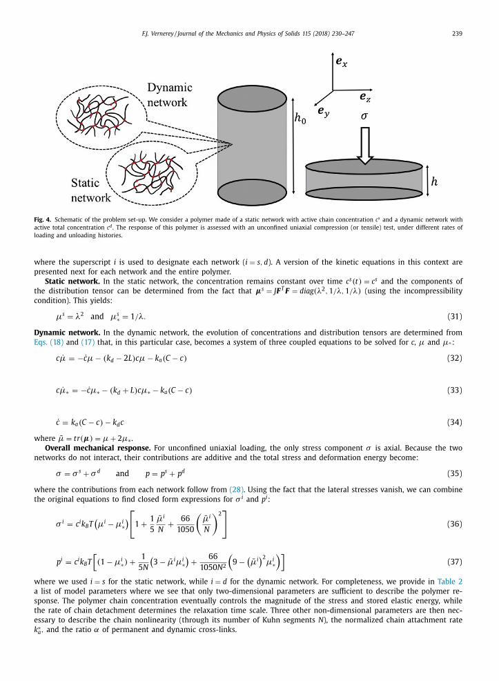
Both of the aforementioned polymers may be idealized by a structure made of two networks characterized by the same

uniform chain length N but different in their dynamic properties ( Fig. 4 ). The first, with total chain concentration C s is

taken to be static (i.e. the rate constants vanish) with distribution tensor μs . The second, with total concentration C d = C,

is dynamic with association and dissociation constant k a and k d . Their structural evolution can therefore be described by

the concentration c = c d of active chains and the associated chain distribution μ = μd . To model unconfined uniaxial loading

conditions, we then consider a cylindrical specimen of original height h 0 and radius r 0 , that is deformed into a configuration

with height and radius h and r , respectively. This system is associated with a coordinate system { e x , e y , e z } with the x-axis

pointing in the long axis of the cylinder. To be consistent with experimental measurements reported in Bergstrom and

Boyce (1998) , the uniaxial stress σ = σx and deformation ε = εx are taken to be:

σ = F / (π r 2 ) and ε = log (λ) (30)

where λ = h/h 0 is the stretch ratio. Loading is performed at constant rate ˙ h , or alternatively, at constant change in the

stretch ratio, characterized by ˙ λ =

˙ h /h 0 . The corresponding velocity gradient in the longitudinal and lateral direction are

thus L =

˙ λ/λ and L ∗ = − ˙ λ/ 2 λ, respectively, where we used the incompressibility condition L + 2 L ∗ = 0 . Furthermore, due to

the problem’s symmetry, the chain distribution tensors only contains diagonal components μi = μi x and μ(i )

∗ = μ(i ) y = μ(i )

z ,

F.J. Vernerey / Journal of the Mechanics and Physics of Solids 115 (2018) 230–247 239

Fig. 4. Schematic of the problem set-up. We consider a polymer made of a static network with active chain concentration c s and a dynamic network with

active total concentration c d . The response of this polymer is assessed with an unconfined uniaxial compression (or tensile) test, under different rates of

loading and unloading histories.

where the superscript i is used to designate each network ( i = s, d). A version of the kinetic equations in this context are

presented next for each network and the entire polymer.

Static network. In the static network, the concentration remains constant over time c s (t) = c s and the components of

the distribution tensor can be determined from the fact that μs = J F T F = diag(λ2 , 1 /λ, 1 /λ) (using the incompressibility

condition). This yields:

μs = λ2 and μs ∗ = 1 /λ. (31)

Dynamic network. In the dynamic network, the evolution of concentrations and distribution tensors are determined from

Eqs. (18) and (17) that, in this particular case, becomes a system of three coupled equations to be solved for c, μ and μ∗ :

c ˙ μ = − ˙ c μ − ( k d − 2 L ) cμ − k a ( C − c ) (32)

c ˙ μ∗ = − ˙ c μ∗ − ( k d + L ) cμ∗ − k a ( C − c ) (33)

˙ c = k a ( C − c ) − k d c (34)

where μ̄ = tr( μ) = μ + 2 μ∗.

Overall mechanical response. For unconfined uniaxial loading, the only stress component σ is axial. Because the two

networks do not interact, their contributions are additive and the total stress and deformation energy become:

σ = σ s + σ d and p = p s + p d (35)

where the contributions from each network follow from (28) . Using the fact that the lateral stresses vanish, we can combine

the original equations to find closed form expressions for σ i and p i :

σ i = c i k B T (μi − μi

∗)[

1 +

1

5

μ̄i

N

+

66

1050

(μ̄i

N

)2 ]

(36)

p i = c i k B T

[ (1 − μi

∗) +

1

5 N

(3 − μ̄i μi

∗)

+

66

1050 N

2

(9 −

(μ̄i

)2 μi

∗

)] (37)

where we used i = s for the static network, while i = d for the dynamic network. For completeness, we provide in Table 2

a list of model parameters where we see that only two-dimensional parameters are sufficient to describe the polymer re-

sponse. The polymer chain concentration eventually controls the magnitude of the stress and stored elastic energy, while

the rate of chain detachment determines the relaxation time scale. Three other non-dimensional parameters are then nec-

essary to describe the chain nonlinearity (through its number of Kuhn segments N ), the normalized chain attachment rate

k ∗a , and the ratio α of permanent and dynamic cross-links.

240 F.J. Vernerey / Journal of the Mechanics and Physics of Solids 115 (2018) 230–247

Table 2

Material parameters for a permanent/dynamic double network with nonlinear

chain elasticity.

Type Symbol Meaning Unit

Dimensional C Total chain concentration mole/volume

k d Detachment rate 1/time

Non-dimensional N Chain length no unit

k ∗a = k a /k d Attachment rate no unit

α = c s /c t Permanent chain fraction no unit

Fig. 5. Cyclic compressive response of rubber under constant loading rate ˙ λ/k d = 1 / 25 . (a) Experimental data from Bergstrom and Boyce (1998) with model

comparison. (b) and (c) Predicted time evolution of the chain stretch λ̄ = tr(μ) / 3 and normalized stress σ i / c i k B T for the static network SN (dashed lines),

dynamic network DN (semi-dashed lined), and their average TN (solid line). (d) Predicted normalized stress-strain response by the kinetic theory. Again, the

response is decomposed according to its static SN, dynamic DN, and total TN contributions. Note that the stresses and strains are shown here as positive

in compression.

4.2. Cyclic compression of elastomers

In this example, we consider the uniaxial compression of a Chloroprene rubber loaded with carbon black particles as

studied in Bergstrom and Boyce (1998) . The viscoelastic properties of these elastomers arise from the disruption of en-

tanglements and reptation of long polymer chains during deformation. In other words, an entangled chain may appear as

mechanically active at short times, since entanglements may themselves be viewed as physical cross-links. However, as the

chain is stretched, over time it will dissociate from the entanglement and evolve towards a more relaxed configuration. This

new configuration may also contain entanglements, and this event may therefore be interpreted as an attachment event.

Such molecular mechanisms have been captured by the reptation theory of de Gennes (1979) , in which the lifetime τ of

a physical link was found to scale with the square of chain length. The rate of detachment may therefore be seen as the

inverse of this lifetime, i.e., k a = k d = 1 /τ . We assume here that these rates are independent of time, chain stretch and poly-

mer deformation. Finally, experiments show that this rubber shows a relatively strong hysteresis response during a cycle

but tend to relax to the same equilibrium state, regardless of the relaxation dynamic. This observation indicates that the

material possesses a purely elastic component, which is interpreted as the presence of a static (or permanent) network, in

addition to a dynamic one.

In Fig. 5 , we present results that describe the compression and release of the rubber at constant strain rate characterized

by the Weissenberg number W =

˙ λ/k d = 1 / 25 ( Fig. 4 a). In order for the model to capture experimental trends, we used the

ratio of permanent chains to be α = 15% and a rate of chain attachment k ∗a = 1 , i.e., the rate of attachment and detachment

occur at the same time scale. These parameters were determined by manually fitting the shape of the experimental stress-

strain curves. The total chain concentration was further evaluated as C = 10 −3 mole/cm

3 to obtain a good experimental

match regarding the magnitude of stresses. Although we did not observe a significant effect of chain length, we chose

F.J. Vernerey / Journal of the Mechanics and Physics of Solids 115 (2018) 230–247 241

Fig. 6. Repeated cyclic loading under constant loading rate ˙ λ/k d = 1 / 25 with increasing amplitude. (a) Experimental data from Bergstrom and

Boyce (1998) with model comparison. (b) and (c) Predicted time evolution of the chain stretch λ̄ = tr(μ) / 3 and normalized stress σ i / c i k B T for the static

network SN (dashed lines), dynamic network DN (semi-dashed lined), and their average TN (solid line). (d) Predicted normalized stress-strain response by

the kinetic theory. Again, the response is decomposed according to its static SN, dynamic DN, and total TN contributions. Note that the stresses and strains

are shown here as positive in compression.

N = 30 for all computations. For illustration purposes, we show in Fig. 4 the separate contributions from static, permanent,

and total network response. In this context, Fig. 5 b shows that the average end-to-end distance increases significantly with

deformation in the permanent network while the chains are barely stretched in the dynamic network due to their ability

to relax faster than they are stretched. Eventually, the average chain length, defined as λ = ( c s λs + cλs ) / ( c s + c ) remains in

between its dynamic and static value. A key difference between the dynamic and static networks can be seen in the stress

response ( Fig. 4 c). Indeed, while the static network displays a purely elastic response (i.e., the stress is a monotonic function

of applied deformation), its dynamic counterpart displays a behavior that can be assimilated to a viscous fluid (i.e., the

stress is related to the strain rate). This fluid-like response is particularly pronounced due to high rate of chain turn-over

compared to the applied strain rate. Consequences of these mechanisms on the stress-strain response are shown in Fig. 5 d.

It is clear that the network’s stiffness is controlled by the elastic network, while its hysteresis response and overall energy

dissipation is purely due to its dynamic counterpart.

We next explore a situation in which the rubber specimen is subjected to multiple loading cycles with increasing ampli-

tude ( Fig. 6 a). Experimental tests indicate that the rubber’s mechanical response is repeatable and thus, no permanent dam-

age appears in the network as a result of deformation. We show in Fig. 6 d that this behavior can be reproduced by the dual-

network model. As observed in the previous example, the average chain stretch remains low in the dynamic network and

the effect of the nonlinearity in the chain response is only felt in the elastic network. The good agreement between model

and experiment can be attributed to the fact that the transient response arises primary from the chain dynamic, rather than

an irreversible reconfiguration that would occur in the case of damage as observed in the Mullins effect ( Cantournet et al.,

2009 ).

Our last example considers the compression of the same rubber material, but under a more complex loading history as

shown in Fig. 7 a ( Bergstrom and Boyce, 1998 ). In this example, the loading is periodically ceased during a small interval

during a single cycle, giving some time for the dynamic polymer to relax. In Fig. 7 b and c, we see that the deformation of

chains in the elastic network follow the imposed deformation, while those in the dynamic network display a exponential

stress-relaxation when the deformation remains constant. This simple response leads to an apparently complex stress-strain

behavior of the material, which can accurately be reproduced by the model ( Fig. 7 d). On a final note, although we showed

that a model with constant dissociation rates can successfully reproduce the above experimental trends, it is still limited

in capturing the effect of loading rate. Indeed, for a single time scale, the temporal response of the polymer is only depen-

dent on the Weissenberg number W =

˙ λ/k d , a prediction that is not in agreement with trends presented in Bergstrom and

Boyce (1998) . This issue may be explained by the fact that rubbers possess a large variety of chain lengths within their

molecular structure, each one of them characterized by a different relaxation time (in agreement with reptation theory).

242 F.J. Vernerey / Journal of the Mechanics and Physics of Solids 115 (2018) 230–247

Fig. 7. Cyclic loading with stages of stress relaxation under constant loading rate ˙ λ/k d = 1 / 25 . (a) Experimental data from Bergstrom and Boyce (1998) with

model comparison. (b) and (c) Predicted time evolution of the chain stretch λ̄ = tr(μ) / 3 and normalized stress σ i / c i k B T for the static network SN (dashed

lines), dynamic network DN (semi-dashed lined), and their average TN (solid line). (d) Predicted normalized stress-strain response by the kinetic theory.

Again, the response is decomposed according to its static SN, dynamic DN, and total TN contributions. Note that the stresses and strains are shown here

as positive in compression.

Short chains will display fast dynamics while long chains will react slowly. This polydiversity can be addressed by consider-

ing families of networks represented by a chain length distribution, each represented by different chain dynamics k d . In this

case, small chains will only respond to fast loading rates, while long chains will respond quasi-elastically. When slow load-

ing is considered, however, all (dynamic) chains will be able to relax. As a consequence, a nonlinear relationship between

loading rate and relaxation behavior should be observed in accordance to experimental observations. Other micromecha-

nisms may also be invoked to explain the complex strain-rate dependence of natural rubber, notably the stress-induced

crystallization and melting of the polymer network ( Rault et al., 2006 ). Such studies are however beyond the scope of this

paper.

4.3. Uniaxial tension of double network dynamic gel

In the second example, we consider a cyclic tensile test of a self-healing double network gel investigated in

Long et al. (2014) . The network is made of poly(vinyl alcohol) (PVA) chains with both chemical cross-links and transient

physical bonds between the chains and borate ions ( Narita et al., 2013 ). Long et al. investigated the polymer response by

subjecting it to a series of a cyclic tensile tests during which the deformation rates were varied between the loading and

unloading stages. The resulting hysteresis response was then interpreted as a signature of the polymer’s strain dependent

energy dissipation. Furthermore, the complete reattachment of physical cross-links in time indicated the perfect self-healing

potential of the network. Since this network is more uniform than the rubber considered above, we also expect the assump-

tion of the single relaxation time set by k d to be more realistic. To obtain a material behavior that is close to experimental

measurements ( Long et al., 2014 ), we used the following parameters: N = 30 , k ∗a = 1 , k d = 0 . 3 s −1 and α = c s /c t = 0 . 1 . Fig. 8

reproduces experimental results and shows the model predictions when the loading strain rate is 0.3 s −1 while the unload-

ing strain rate is 0.1,0.01 and 0.001, respectively. We see that when unloading occurs quickly (0.1 s −1 ), most chains do not

have time to detach, and therefore deform elastically. In this case, the model therefore predicts that the average chain stretch

λ̄ remains close to the stretch of the specimen ( Fig. 8 b). When the unloading rate decreases, however, chain turnover yields

a significant drop in the average chain stretch λ̄, compared to the overall stretch λ. This phenomenon eventually yields

stress relaxation and a rise in energy dissipation during unloading, which can be assessed by the area enclosed by the load-

ing and unloading curves in Fig. 8 d. Predicted trends are in line with experimental observations, although a better fit may

be obtained by introducing a more accurate model for chain detachment k d = k d ( ̄λ) (see for instance Long et al., 2014 ).

F.J. Vernerey / Journal of the Mechanics and Physics of Solids 115 (2018) 230–247 243

Fig. 8. Cyclic loading of the PVA double network with a loading rate 0.3 s −1 and unloading rates 0.1 s −1 , 0.01 s −1 and 0.001 s −1 , respectively. (a) Ex-

perimental data from Long et al. (2014) . (b) Predicted time evolution of the chain stretch λ̄ = tr(μ) / 3 (thick lines) compared with the average stretch of

the sample (thin lines) for unloading rates 0.1 s −1 and 0.01 s −1 . (c) Predicted nominal stress P / ck B T for unloading rates 0.1 s −1 and 0.01 s −1 . (d) Predicted

stress-strain response by the kinetic theory, to be compared with (a).

Fig. 9. Cyclic loading of the PVA double network with a loading rate 0.01 s −1 and unloading rates 0.1 s −1 , 0.01 s −1 and 0.001 s −1 , respectively. (a)

Experimental data from Long et al. (2014) . (b) Predicted time evolution of the chain stretch λ̄ = tr(μ) / 3 (thick lines) compared with the average stretch of

the sample (thin lines) for unloading rates 0.1 s −1 and 0.01 s −1 . (c) Predicted nominal stress P / ck B T for unloading rates 0.1 s −1 and 0.01 s −1 . (d) Predicted

stress-strain response by the kinetic theory, to be compared with (a).

244 F.J. Vernerey / Journal of the Mechanics and Physics of Solids 115 (2018) 230–247

The final test considers a similar experiment in which the rate of loading is reduced from 0.3 s −1 to 0.01 s −1 . In this case,

chain kinetics are relatively fast compared to the loading rate and this results in a situation where chain stretch λ̄ remains

low compared to the applied loading deformation λ ( Fig. 9 b). The unloading material response is significantly different

according to the strain rate. For fast unloading, we observe a temporary rise in chain stretch and a stress that quickly

becomes compressive before the network gradually returns to its stress-free state. This is due to the fast elastic response

of the networks as the applied loading switches from positive to negative. In contrast, for slower unloading rate, chains

have time to relax during the deformation and a smooth drop in chain stretch occurs. The consequence on the stress-strain

response can be seen in Fig. 9 d; fast unloading results in a residual strain when P = 0 as most of the network had no time

to reorganize after the end of the loading state. Slow loading does give enough time for chains to relax, only yielding a

negligible residual deformation as P = 0 . Overall, we see that even for the simplistic situation of constant chain kinetics,

the model is able to capture the underlying physical mechanisms occurring at the molecular level and further predicts the

associated mechanical response of the material.

5. Summary and concluding remarks

In summary, we have introduced a kinetic theory based on statistical mechanics, that aims to provide a connection be-

tween molecular mechanisms and the emerging (macroscopic) behavior of dynamic polymers. This is done by representing

the physical state of a dynamic network via the statistical distribution of the chain according to their end-to-end vector.

The kinetic theory is based on two pillars. The first is the evolution Eq. (10) for the distribution in terms of macroscopic

deformation and molecular processes. In short, the equation states that changes in the chain population arises from three

mechanisms: the distortion of chains due to the application of a macroscopic deformation, the attachment of new chains

in a stress-free configuration, and the detachment of chains in their current configuration. This equation, which closely re-

sembles the Boltzmann equation in gas dynamics, has deep implications regarding the network evolution resulting from

deformation and kinetics of attachment and detachment events. The second pillar of the kinetic theory resides in the con-

nection between the chain distribution and macroscopic quantities such as the stress, the stored elastic energy, and energy

dissipation. These relationships appear in Eqs. (22) , (9) and (21) of this manuscript, respectively. In particular, the tensor

μ provides a description of both the average end-to-end vector (related to the trace of μ) and the average stretch direc-

tions (principal directions of μ). We have shown in examples that when combined with (10) , the material response displays

stress-relaxation and self-healing characteristics shared by different classes of dynamic polymers.

An advantage of the kinetic theory is in the formulation of constitutive relations, where the elastic and viscous response

of the polymer are clearly separated. On the one hand, the polymer elasticity is entirely described by the elasticity of its

chains, which could be nonlinear for short-chain polymers undergoing large deformation. On the other hand, the rheology of

the polymer is given by the rate of chain attachment and detachment, k d and k d , respectively. In the simplest case considered

in this study, these rates are constant, and rheology is entirely decoupled from elasticity. We saw, however, that chain

stretch is largely dependent on strain rate. For low strain rates, chain turn-over dominates and the material response is

mostly viscous. For high strain rates (as the Weissenberg number goes to 1), the chains do not have time to detach and the

material response is dominated by chain elasticity. In other words, the nonlinear chain response is important to consider

in two situations: (a) for a static network that only responds elastically and (b) for a dynamic network under high strain

rate. A richer spectrum of behavior could however be obtained by coupling the rate k d with chain deformation (or force).

In this case, there is a direct coupling between elasticity and stress relaxation; elasticity controls the stretch of the chains,

which in turn affects their detachment rates. This produces a feed-back loop in which a lower fraction of attached chain

(resulting from a rise in k d ) can further increase they deformation under constant force. Depending on the polymer, bond

kinetics are driven by the temporary interactions between polymer chains, e.g., entanglements in polymer melts or lightly

cross-linked networks. Potentially, one can prescribe physics-based models to describe the kinetics of disentanglements and

re-entanglements by taking advantage of the established knowledge in a vast literature on the dynamics of polymer chains

( Doi and Edwards, 1988; de Gennes and Leger, 1982 ) or molecular dynamic simulations ( Yang et al., 2015 ). In entangled

polymers, chain dynamics are driven by reptation, which involves the diffusion of long chains constrained between slip-

rings. In bio-polymers such as alginate and agarose ( Lee and Mooney, 2012 ), the probability of bond breaking is a function

of force on the chains. For small strains, the chain force remains below a critical value and the chains do not detach and

the network behaves elastically. Above the critical force, the bonds yield in a stochastic manner with an average life time

that decreases with force. These behaviors are responsible for the visco-plasticity observed in those physically cross-linked

gels. Improvement of the theory may further concentrate on several items. First, the theory assumes affine deformation of

the chains, which in some case may not be representative of the network deformation. In this context, we may consider the

existence of nonaffine networks as recently discussed by Davidson and Goulbourne (2013) , or the concept of equal forces in

polymer chains ( Verron and Gros, 2017 ). Future effort s will also concentrate on establishing a strong connection between the

rates k d and k a to underlying mechanisms at the level of individual molecular chains. This will include, for instance, adding

the effect of force on chain dissociation using Kramers’s reaction theory ( Hanggi et al., 1990 ). The consideration of multiple

relaxation mechanisms, each characterized by their specific time scale may also be included via additional dissociation terms

(different k d ’s) in (10) .

This approach, due to its generality, can be extended to describe a number of molecular processes occurring in poly-

mers and hydrogels ( Akalp et al., 2015 ). This may include, for instance, the energy dissipation responsible for the enhanced

F.J. Vernerey / Journal of the Mechanics and Physics of Solids 115 (2018) 230–247 245

toughness and self-healing capacity of physically cross-link polymers or the degradation of cross-links ( Akalp et al., 2016;

Dhote et al., 2013; Skaalure et al., 2016 ). In biological materials, this theory can also prove useful to describe the mechanics

of growth and tissue remodeling ( Sridhar et al., 2017; Vernerey and Farsad, 2014 ), both of which often depends on the inter-

play between elastic deformation and deposition of new material in different configurations ( Vernerey, 2016 ). Finally, since

the theory predicts the evolution of the chain distribution during deformation, it may be used to provide new insights onto

the mechanisms responsible for the rheology of materials at the macroscale. This can prove to be a useful tool to formulate

new hypotheses for molecular mechanisms and test their macroscopic outcomes.

Aknowledgments

The author acknowledges the support of the National Science Foundation under the NSF CAREER award 1350090. Re-

search reported in this publication was also partially supported by the National Institute of Arthritis and Musculoskeletal

and Skin Diseases of the National Institutes of Health under Award Number 1R01AR065441. The content is solely the re-

sponsibility of the authors and does not necessarily represent the official views of the National Institutes of Health.

Appendix A

In this appendix, we aim to quantify the error made by the mean field appoximation of Eq. (15) :

〈 g( ̃ μ) 〉 =

∫ f ( ̃ μ) g( ̃ μ) d� ˜ μ ≈ g(μ) . (38)

where f ( ̃ μ) and g( ̃ μ) are the probability density function and an arbitrary function of the local variable ˜ μ, while μ is the

mean of ˜ μ, defined as:

μ = 〈 ̃ μ〉 (39)

The probability density function further verifies:

〈 1 〉 = 1 and 〈 ( ̃ μ − ˜ μ) 2 〉 = s 2 (40)

where s is the standard deviation. To estimate the error e , let us take a Taylor series expansion of the function g around the

mean ˜ μ = μ. We write:

g( ̃ μ) = g(μ) + b( ̃ μ − μ) + κ( ̃ μ − μ) 2 + O

(( ̃ μ − μ) 3

)(41)

Now assessing the average of the above expansion, using (39) and (40) leads to:

〈 g( ̃ μ) 〉 = g(μ) + κs + h.o.t (42)

where the last abreviation stands for “higher order terms” and the terms κ is interpreted as the curvature of the function g

at ˜ μ = μ. Comparing with (38) , we see that a first order approximation of the error e = 〈 g( ̃ μ) 〉 − g(μ) is given by:

e = κs (43)

Appendix B

We first express the change in stored energy (9) over time as:

˙ �(t) =

∫ ( ˙ φψ) d� (44)

where the change in chain distribution follows from (10) is:

˙ φ = −L : (∇φ � λ

)+ k a ( C − c ) f 0 − k d φ. (45)

We therefore obtain:

˙ �(t) = k a (C − c) 〈 ψ〉 0 − k d c〈 ψ〉 − L i j

∫ (dφ

dλi

λ j ψ

)d�. (46)

Applying the divergence theorem and using the fact that tr( L ) = 0 for an incompressible polymer, the change in elastic

energy becomes:

˙ �(t) = k a (C − c) 〈 ψ〉 0 − k d c〈 ψ〉 + c〈∇ψ � λ〉 : L . (47)

Now using the chain rule:

∇ψ =

dψ

d λ=

dψ

dλ

dλ

d λ=

1

λ

dψ

dλλ (48)

246 F.J. Vernerey / Journal of the Mechanics and Physics of Solids 115 (2018) 230–247

we can write:

˙ �(t) = k a (C − c) 〈 ψ〉 0 − ck d 〈 ψ〉 + c

⟨1

λ

dψ

dλλ � λ

⟩: L , (49)

˙ �0 (t) = k a (C − c) 〈 ψ〉 0 − ck d 〈 ψ〉 0 + c

⟨1

λ

dψ

dλλ � λ

⟩0

: L . (50)

Now, applying the mean field approximation, we write:

〈 1

λ

dψ

dλλ � λ〉 =

1

λ̄

dψ

d ̄λ〈 λ � λ〉 =

1

3 ̄λ

dψ

d ̄λμ, (51)

〈 1

λ

dψ

dλλ � λ〉 0 =

dψ

d ̄λ(1) 〈 λ � λ〉 0 =

1

3

dψ

d ̄λ(1) I , (52)

A discussion regarding the validity of the above approximations is provided in the paragraph following Eq. (22) . For this, it

is useful to note that in approximation (51) , the function g (corresponding to that introduced in Eq. (15) ) is written:

g( ̃ μ) =

1

λ

dψ

dλλ � λ = 6

dψ

d( tr ̃ μ) ˜ μ (53)

Finally using the above expressions, the difference � ˙ � becomes:

� ˙ �(t) =

[c

3 ̄λ

dψ

d ̄λμ − c

3

dψ

d ̄λ(1) I + p I

]: L − ck d

[ψ( ̄λ) − ψ

0 ]. (54)

Supplementary material

Supplementary material associated with this article can be found, in the online version, at 10.1016/j.jmps.2018.02.018

References

Akalp, U., Bryant, S., J. Vernerey, F., 2016. Tuning tissue growth with scaffold degradation in enzyme-sensitive hydrogels: a mathematical model. Soft Matter

12 (36), 7505–7520. doi: 10.1039/C6SM00583G . Akalp, U., Chu, S., Skaalure, S., Bryant, S., Doostan, A., Vernerey, F., 2015. Determination of the polymer-solvent interaction parameter for PEG hydrogels in

water: application of a self learning algorithm. Polymer 66, 135–147. doi: 10.1016/j.polymer.2015.04.030 . Arruda, E., Boyce, M., 1993. A three-dimensional constitutive model for the large stretch behavior of rubber elastic materials. J. Mech. Phys. Solids 41 (2),

389–412. doi: 10.1016/0 022-5096(93)90 013-6 .

Bergstrom, J.S., Boyce, M.C., 1998. Constitutive modeling of the large strain time-dependent behavior of elastomers. J. Mech. Phys. Solids 46 (5), 931–954.doi: 10.1016/S0 022-5096(97)0 0 075-6 .

Bergstrom, J.S., Boyce, M.C., 2001. Deformation of elastomeric networks: relation between molecular level deformation and classical statistical mechanicsmodels of rubber elasticity. Macromolecules 34 (3), 614–626. doi: 10.1021/ma0 0 07942 .

Cantournet, S., Desmorat, R., Besson, J., 2009. Mullins effect and cyclic stress softening of filled elastomers by internal sliding and friction thermodynamicsmodel. Int. J. Solids Struct. 46 (11), 2255–2264. doi: 10.1016/j.ijsolstr.2008.12.025 .

Davidson, J., Goulbourne, N.C., 2013. A nonaffine network model for elastomers undergoing finite deformations. J. Mech. Phys. Solids 61 (8), 1784–1797.

doi: 10.1016/j.jmps.2013.03.009 . Denn, M.M., 1990. Issues in viscoelastic fluid mechanics. Annu. Rev. Fluid Mech. 22 (1), 13–32. doi: 10.1146/annurev.fl.22.010190.0 0 0305 .

Dhote, V., Skaalure, S., Akalp, U., Roberts, J., Bryant, S., Vernerey, F., 2013. On the role of hydrogel structure and degradation in controlling the transport ofcell-secreted matrix molecules for engineered cartilage. J. Mech. Behav. Biomed. Mater. 19, 61–74. doi: 10.1016/j.jmbbm.2012.10.016 .

Doi, M. , Edwards, S.F. , 1988. The Theory of Polymer Dynamics. Clarendon Press . Google-Books-ID: dMzGyWs3GKcC Drozdov, A.D., 1999. A constitutive model in finite thermoviscoelasticity based on the concept of transient networks. Acta Mech. 133 (1–4), 13–37. doi: 10.

10 07/BF011790 08 .

Evans, N., Oreffo, R.C., Healy, E., Thurner, P., Man, Y., 2013. Epithelial mechanobiology, skin wound healing, and the stem cell niche. J. Mech. Behav. Biomed.Mater. 28, 397–409. doi: 10.1016/j.jmbbm.2013.04.023 .

de Gennes, P. , 1979. Scaling Concepts in Polymer Physics. Cornell University Press, Ithaca, NY . de Gennes, P., Leger, L., 1982. Dynamics of entangled polymer chains. Annu. Rev. Phys. Chem. 33 (1), 49–61. doi: 10.1146/annurev.pc.33.10 0182.0 0 0405 .

Grindy, S., Learsch, R., Mozhdehi, D., Cheng, J., Barrett, D., Guan, Z., Messersmith, P., Holten-Andersen, N., 2015. Control of hierarchical polymer mechanicswith bioinspired metal-coordination dynamics. Nat. Mater. 14 (12), 1210–1216. doi: 10.1038/nmat4401 .

Hanggi, P., Talkner, P., Borkovec, M., 1990. Reaction-rate theory: fifty years after kramers. Rev. Mod. Phys. 62 (2), 251–341. doi: 10.1103/RevModPhys.62.251 .

Holzapfel, G.A. , 20 0 0. Nonlinear Solid Mechanics: A Continuum Approach for Engineering. Wiley . Joanny, J., Prost, J., 2009. Active gels as a description of the actin-myosin cytoskeleton. HFSP J. 3 (2), 94–104. doi: 10.2976/1.3054712 .

Kong, H., Wong, E., Mooney, D., 2003. Independent control of rigidity and toughness of polymeric hydrogels. Macromolecules 36 (12), 4582–4588. doi: 10.1021/ma034137w .

Kroger, M., 2015. Simple, admissible, and accurate approximants of the inverse Langevin and Brillouin functions, relevant for strong polymer deformationsand flows. J. Nonnewton. Fluid Mech. 223 (Supplement C), 77–87. doi: 10.1016/j.jnnfm.2015.05.007 .

Kuhn, W., Grun, F., 1946. Statistical behavior of the single chain molecule and its relation to the statistical behavior of assemblies consisting of many chain

molecules. J. Polym. Sci. 1 (3), 183–199. doi: 10.10 02/pol.1946.120 010306 . Lee, K., Mooney, D.J., 2012. Alginate: properties and biomedical applications. Prog. Polym. Sci. 37 (1), 106–126. doi: 10.1016/j.progpolymsci.2011.06.003 .

Li, Y., Tang, S., Kroger, M., Liu, W., 2016. Molecular simulation guided constitutive modeling on finite strain viscoelasticity of elastomers. J. Mech. Phys.Solids 88 (Supplement C), 204–226. doi: 10.1016/j.jmps.2015.12.007 .

Long, R., Mayumi, K., Creton, C., Narita, T., Hui, C., 2014. Time dependent behavior of a dual cross-link self-healing gel: theory and experiments. Macro-molecules 47 (20), 7243–7250. doi: 10.1021/ma501290h .

F.J. Vernerey / Journal of the Mechanics and Physics of Solids 115 (2018) 230–247 247

Long, R., Qi, H., Dunn, M., 2013. Modeling the mechanics of covalently adaptable polymer networks with temperature-dependent bond exchange reactions.Soft Matter 9 (15), 4083–4096. doi: 10.1039/C3SM27945F .

Murrell, M., Oakes, P., Lenz, M., Gardel, M., 2015. Forcing cells into shape: the mechanics of actomyosin contractility. Nat. Rev. Mol. Cell Biol. 16 (8), 4 86–4 98.doi: 10.1038/nrm4012 .

Nam, S., Hu, K., Butte, M., Chaudhuri, O., 2016. Strain-enhanced stress relaxation impacts nonlinear elasticity in collagen gels. Proc. Natl. Acad. Sci. U.S.A.113 (20), 5492–5497. doi: 10.1073/pnas.1523906113 .

Narita, T., Mayumi, K., Ducouret, G., Hebraud, P., 2013. Viscoelastic properties of poly(vinyl alcohol) hydrogels having permanent and transient cross-links

studied by microrheology, classical rheometry, and dynamic light scattering. Macromolecules 46 (10), 4174–4183. doi: 10.1021/ma40 060 0f . Proseus, T. , Ortega, J. , Boyer, J. , 1999. Separating growth from elastic deformation during cell enlargement. Plant Physiol. 119 (2), 775–784 .

Purohit, P., Litvinov, R., Brown, A., Discher, D., Weisel, J., 2011. Protein unfolding accounts for the unusual mechanical behavior of fibrin networks. ActaBiomater. 7 (6), 2374–2383. doi: 10.1016/j.actbio.2011.02.026 .

Rajagopal, K.R., Srinivasa, A.R., 2004. On the thermomechanics of materials that have multiple natural configurations Part i: viscoelasticity and classicalplasticity. Zeitschrift für angewandte Mathematik und Physik ZAMP 55 (5), 861–893. doi: 10.10 07/s0 0 033-0 04-4019-6 .

Rault, J. , Marchal, J. , Judeinstein, P. , Albouy, P. , 2006. Stress-induced crystallization and reinforcement in filled natural rubbers: 2h nmr study. Macro-molecules 39 (24), 8356–8368 .

Roy, N., Bruchmann, B., Lehn, J., 2015. Dynamers: dynamic polymers as self-healing materials. Chem. Soc. Rev. 44 (11), 3786–3807. doi: 10.1039/c5cs00194c .

Rubinstein, M. , Colby, R. , 2003. Polymer Physics. OUP Oxford . Google-Books-ID: RHksknEQYsYC. Simo, J. , 1987. On a fully three-dimensional finite-strain viscoelastic damage model: formulation and computational aspects. Comput. Methods Appl. Mech.

Eng. 60, 153–173 . Skaalure, S., Akalp, U., Vernerey, F., Bryant, S., 2016. Tuning reaction and diffusion mediated degradation of enzyme-sensitive hydrogels. Adv. Healthc. Mater.

5 (4), 432–438. doi: 10.1002/adhm.201500728 . Sridhar, S., Schneider, M., Chu, S., de Roucy, G., Bryant, S., Vernerey, F., 2017. Heterogeneity is key to hydrogel-based cartilage tissue regeneration. Soft Matter

13 (28), 4 841–4 855. doi: 10.1039/C7SM00423K .

Stukalin, E.B., Cai, L., Kumar, N., Leibler, L., Rubinstein, M., 2013. Self-healing of unentangled polymer networks with reversible bonds. Macromolecules 46(18), 7525–7541. doi: 10.1021/ma401111n .

Tang-Schomer, M.D., Patel, A.R., Baas, P.W., Smith, D., 2010. Mechanical breaking of microtubules in axons during dynamic stretch injury underlies delayedelasticity, microtubule disassembly, and axon degeneration. FASEB J. 24 (5), 1401–1410. doi: 10.1096/fj.09-142844 .

Treloar, L.R.G. , 1975. The Physics of Rubber Elasticity. Oxford University press . Vernerey, F., 2016. A mixture approach to investigate interstitial growth in engineering scaffolds. Biomech. Model. Mechanobiol. 15 (2), 259–278. doi: 10.

1007/s10237-015-0684-y .

Vernerey, F., Akalp, U., 2016. Role of catch bonds in actomyosin mechanics and cell mechanosensitivity. Physical Review E 94 (1), 012403. doi: 10.1103/PhysRevE.94.012403 .

Vernerey, F., Farsad, M., 2011. A constrained mixture approach to mechano-sensing and force generation in contractile cells. J. Mech. Behav. Biomed. Mater.4 (8), 1683–1699. doi: 10.1016/j.jmbbm.2011.05.022 .

Vernerey, F., Farsad, M., 2014. A mathematical model of the coupled mechanisms of cell adhesion, contraction and spreading. J. Math. Biol. 68 (4), 989–1022.doi: 10.10 07/s0 0285- 013- 0656- 8 .

Vernerey, F.J., Long, R., Brighenti, R., 2017. A statistically-based continuum theory for polymers with transient networks. J. Mech. Phys. Solids 107, 1–20.

doi: 10.1016/j.jmps.2017.05.016 . Verron, E., Gros, A., 2017. An equal force theory for network models of soft materials with arbitrary molecular weight distribution. J. Mech. Phys. Solids 106

(Supplement C), 176–190. doi: 10.1016/j.jmps.2017.05.018 . Villani, C., 2002. A review of mathematical topics in collisional kinetic theory. Handbook Math. Fluid Dyn. 1, 71–74. doi: 10.1016/S1874-5792(02)80 0 04-0 .

Wang, R., Xie, T., 2010. Shape memory- and hydrogen bonding-based strong reversible adhesive system. Langmuir 26 (5), 2999–3002. doi: 10.1021/la9046403 .

Watanabe, H., 1999. Viscoelasticity and dynamics of entangled polymers. Prog. Polym. Sci. 24 (9), 1253–1403. doi: 10.1016/S0 079-670 0(99)0 0 029-5 .

Webber, R.E., Shull, K.R., 2004. Strain dependence of the viscoelastic properties of alginate hydrogels. Macromolecules 37 (16), 6153–6160. doi: 10.1021/ma049274n .

Wineman, A., 2009. Nonlinear viscoelastic solids: a review. Math. Mech. Solids 14 (3), 300–366. doi: 10.1177/1081286509103660 . Yang, H., Yu, K., Mu, X., Shi, X., Wei, Y., Guo, Y., Qi, H.J., 2015. A molecular dynamics study of bond exchange reactions in covalent adaptable networks. Soft

Matter 11 (31), 6305–6317. doi: 10.1039/C5SM00942A . Zhou, J. , Jiang, L. , Khayat, R. , 2018. A micro–macro constitutive model for finite-deformation viscoelasticity of elastomers with nonlinear viscosity. J. Mech.

Phys. Solids 110, 137–154 .