PNNL-19418, Vol.1 Rev.2

Prepared for the U.S. Department of Energy under Contract DE-AC05-76RL01830

FRAPCON-4.0: A Computer Code for the Calculation of Steady-State, Thermal-Mechanical Behavior of Oxide Fuel Rods for High Burnup

September 2015

KJ Geelhood WG Luscher PA Raynaud IE Porter

PNNL-19418, Vol.1 Rev.2

FRAPCON-4.0: A Computer Code for the Calculation of Steady-State, Thermal-Mechanical Behavior of Oxide Fuel Rods for High Burnup KJ Geelhood WG Luscher PA Raynaud IE Porter September 2015 Prepared for Division of System Analysis Office of Nuclear Regulatory Research U.S. Nuclear Regulatory Commission Washington DC 20555-0001 Pacific Northwest National Laboratory Richland, Washington 99352

iii

Abstract

FRAPCON is a Fortran 90 computer code that calculates the steady-state response of light-water reactor fuel rods during long-term burnup. The code calculates the temperature, pressure, and deformation of a fuel rod as functions of time-dependent fuel rod power and coolant boundary conditions. The phenomena modeled by the code include: 1) heat conduction through the fuel and cladding to the coolant; 2) cladding elastic and plastic deformation; 3) fuel-cladding mechanical interaction; 4) fission gas release from the fuel and rod internal pressure; and 5) cladding oxidation. The code contains necessary material properties, water properties, and heat-transfer correlations. FRAPCON is programmed for use on Windows-based computers, but the source code may be compiled on any computer with a Fortran 90 compiler.

The FRAPCON code is designed to perform steady-state fuel rod calculations and to generate initial conditions for transient fuel rod analysis by the FRAPTRAN computer code.

This document describes FRAPCON-4.0, which is the latest version of FRAPCON, released September 2015.

v

Foreword

Computer codes related to fuel performance have played an important role in the work of the U.S. Nuclear Regulatory Commission (NRC) since the agency’s inception in 1975. Formal requirements for fuel performance analysis appear in several of the agency’s regulatory guides and regulations, including those related to emergency core cooling system evaluation models, as set forth in Appendix K to Title 10, Part 50, of the Code of Federal Regulations (10 CFR Part 50), “Domestic Licensing of Production and Utilization Facilities.”

This document describes the latest version of NRC’s steady state fuel performance code, FRAPCON-4.0. This code provides the ability to accurately calculate the long-term burnup response of a single light-water reactor fuel rod, accomplishing a key objective of the NRC’s reactor safety research program. The FRAPCON code serves as an independent audit tool in NRC’s review of industry fuel performance codes and industry analyses that demonstrate a given fuel design application meeting specified acceptable design limits in U.S. NRC Standard Review Plan Section 4.2 (U.S. NRC 2007). FRAPCON is also a companion code to the FRAPTRAN code (Geelhood et al. 2015b) developed to calculate the response of a fuel rod under transient conditions.

The latest version of FRAPCON has been changed to modernize the FORTRAN language to the most recent standards. Other updates include, an update to plenum temperature model, update to gas properties, the inclusion of the ANS-5.4 (2011) Standard Fission Product Release Model, the ability to model spent fuel storage using the DATING creep models, the ability to use the ANS-5.1 decay heat model to calculate heating after shutdown, and the ability to specify axial coolant conditions. Various “Developer” options have been added to allow the user to change various model parameters for sensitivity studies. Hardwired material properties have also been removed and placed in material specific modules.

vii

Executive Summary

The fuel performance code, FRAPCON, has been developed for the U.S. Nuclear Regulatory Commission by Pacific Northwest National Laboratory for calculating steady-state fuel behavior at high burnup (up to rod-average burnup of 62 gigawatt-days per metric ton of uranium, depending on application). The code has been significantly modified since the release of FRAPCON-3 v1.0 in 1997. This document is Volume 1 of a two-volume series that describes the current version, FRAPCON-4.0 Volume 1 contains: 1) code limitations and structure; 2) fuel performance model summaries; and 3) code input instructions and features to aid the user. Volume 2 (Geelhood and Luscher 2015a) provides a code assessment based on comparisons of code predictions to integral performance data up to high burnup.

The FRAPCON code is designed to perform steady-state fuel rod calculations and generate initial input conditions for FRAPTRAN for transient analyses. The code uses a single-channel coolant enthalpy rise model. The code also uses a finite difference heat conduction model, similar to RELAP5 and FRAPTRAN, which uses a variable mesh spacing to accommodate the power peaking at the pellet edge that occurs in high-burnup fuel.

FRAPCON-4.0 has been validated for boiling-water reactors, pressurized reactors, and heavy-water reactors. The fuels that have been validated are uranium dioxide (UO2), mixed oxide fuel ((U,Pu)O2), urania-gadolinia (UO2-Gd2O3), and UO2 with zirconium diboride (ZrB2) coatings. The cladding types that have been validated are Zircaloy-2, Zircaloy-4, M5, ZIRLO, and Optimized ZIRLO. FRAPCON-4.0 can predict fuel and cladding temperature, rod internal pressure, fission gas release, cladding axial and hoop strain, and cladding corrosion and hydriding. The code uses an updated version of the MATPRO material properties package (Hagrman et al. 1981) as described in a separate material properties handbook (Luscher and Geelhood 2014) that has been updated for high-burnup conditions and advanced cladding alloys.

ix

Acronyms and Abbreviations

°C degrees Celsius ANS American Nuclear Society BOL beginning of life BWR boiling-water reactor cal/mol calorie(s) per mole cm2 square centimeter(s) cm3 cubic centimeter(s) EM evaluation models FEA finite element analysis g gram(s) Gd gadolinium GWd/MTU gigawatt-days per metric ton of uranium He helium HWR heavy-water reactor IFBA integral fuel burnable absorber J joule(s) K Kelvin kg kilogram(s) kW kilowatt(s) LHGR linear heat generation rate LWR light-water reactor m meter(s) m2 square meter(s) m3 cubic meter(s) MLI mean linear intercept MOX mixed oxide fuel, (U, Pu)O2 MPa megapascal(s) n neutron(s) NFI Nuclear Fuels Industries NRC U.S. Nuclear Regulatory Commission Pa pascal(s) PNNL Pacific Northwest National Laboratory ppm parts per million psi pounds per square inch Pu plutonium PWR pressurized-water reactor

x

RXA re-crystallized annealed s second(s) SHF surface heat flux SRA stress relief annealed TD theoretical density U uranium UO2 uranium dioxide UO2-Gd2O3 urania-gadolinia W watt(s) µm micrometer(s)

xi

Contents

Abstract ........................................................................................................................................................ iii Foreword ....................................................................................................................................................... v Executive Summary .................................................................................................................................... vii Acronyms and Abbreviations ...................................................................................................................... ix 1.0 Introduction ....................................................................................................................................... 1.1

1.1 Objectives of the FRAPCON Series ......................................................................................... 1.1 1.2 Limitations of FRAPCON-4.0 .................................................................................................. 1.2 1.3 Report Outline and Relation to Other Reports .......................................................................... 1.3

2.0 General Modeling Descriptions ......................................................................................................... 2.1 2.1 FRAPCON-4.0 Solution Scheme .............................................................................................. 2.1 2.2 Coupling of Thermal and Mechanical Models .......................................................................... 2.2 2.3 Fuel Rod Thermal Response ..................................................................................................... 2.3

2.3.1 Coolant Conditions ......................................................................................................... 2.5 2.3.2 Fuel Rod Surface Temperature....................................................................................... 2.6 2.3.3 Cladding Temperature Gradient ..................................................................................... 2.8 2.3.4 Fuel-Cladding Gap Temperature Gradient ..................................................................... 2.8 2.3.5 Fuel Pellet Heat Conduction Model ............................................................................. 2.10 2.3.6 Plenum Gas Temperature ............................................................................................. 2.21 2.3.7 Stored Energy ............................................................................................................... 2.23

2.4 Fuel Rod Mechanical Response .............................................................................................. 2.23 2.4.1 The FRACAS-I Model ................................................................................................. 2.23

2.5 Fission Gas Release and Fuel Rod Internal Gas Pressure Response ....................................... 2.55 2.5.1 Fuel Rod Internal Gas Pressure .................................................................................... 2.56 2.5.2 Fission Gas Production ................................................................................................. 2.57 2.5.3 Fuel Rod Gas Release .................................................................................................. 2.57 2.5.4 Nitrogen Release .......................................................................................................... 2.68 2.5.5 Helium Production and Release ................................................................................... 2.69 2.5.6 Fuel Rod Void Volumes ............................................................................................... 2.72

2.6 Waterside Corrosion and Hydrogen Pickup ............................................................................ 2.73 2.6.1 PWR and BWR Waterside Corrosion Models ............................................................. 2.73 2.6.2 Hydrogen Pickup Fraction ........................................................................................... 2.76

3.0 General Code Description ................................................................................................................. 3.1 3.1 Code Structure and Solution Routine ........................................................................................ 3.1

3.1.1 Code Structure ................................................................................................................ 3.1 3.1.2 Solution Scheme ............................................................................................................. 3.1

3.2 Code Results .............................................................................................................................. 3.6

xii

3.2.1 Fuel Rod Response ......................................................................................................... 3.6 3.2.2 Plot Package ................................................................................................................... 3.7 3.2.3 FRAPTRAN Initialization .............................................................................................. 3.7

3.3 Features of FRAPCON-4.0 ....................................................................................................... 3.7 3.3.1 Code Solution ................................................................................................................. 3.7 3.3.2 Excel Input Generator .................................................................................................... 3.7 3.3.3 Uncertainty Analysis ...................................................................................................... 3.7 3.3.4 Refabrication Capability .............................................................................................. 3.10 3.3.5 Spent Fuel Modeling .................................................................................................... 3.10 3.3.6 Developer Options ........................................................................................................ 3.11

4.0 References ......................................................................................................................................... 4.1 Appendix A – Input Instructions for the FRAPCON-4.0 Code ................................................................ A.1 Appendix B – Instruction for Using Excel Plot Routine for FRAPCON...................................................B.1

xiii

Figures

Figure 2.1. Simplified FRAPCON-4.0 Flowchart .................................................................................... 2.2 Figure 2.2. Flow Chart of the Fuel and Cladding Temperature Calculation ............................................. 2.4 Figure 2.3. Schematic of the Fuel Rod Temperature Distribution ............................................................ 2.5 Figure 2.4. Mesh Point Layout................................................................................................................ 2.12 Figure 2.5. Typical Mesh Points ............................................................................................................. 2.12 Figure 2.6. Boundary Mesh Points.......................................................................................................... 2.13 Figure 2.7. Typical Isothermal Stress-Strain Curve ................................................................................ 2.25 Figure 2.8. Schematic of the Method of Successive Elastic Solutions ................................................... 2.29 Figure 2.9. Cladding Creep Strain as a Function of Time and Hoop Stress for 630°F and Flux=1018 n/m²/s

for (a) SRA Zircaloy and (b) RXA Zircaloy .................................................................................... 2.34 Figure 2.10. Fuel Rod Geometry and Coordinates ................................................................................. 2.38

Figure 2.11. Calculation of Effective Stress se from dεP ........................................................................ 2.40 Figure 2.12. Idealized Stress-Strain Behavior ........................................................................................ 2.45 Figure 2.13. Computing Stress ................................................................................................................ 2.47 Figure 2.14. Predicted vs. Measured Yield Stress from the PNNL Database (293K≤T≤755K),

0≤Φ≤14x1025 n/m2, 0≤Hex≤850 ppm ............................................................................................... 2.51 Figure 2.15. Interpellet Void Volume ..................................................................................................... 2.53 Figure 2.16. Power and Burnup Dependence of the FRAPCON-4.0 Relocation Model with the Old

Relocation Model (v3.4) Shown for Reference ............................................................................... 2.55 Figure 2.17. Modeling the Pellet High Burnup Rim Structure in FRAPFGR ........................................ 2.65 Figure 3.1. FRAPCON-4.0 Flowchart ...................................................................................................... 3.2 Figure 3.2. Calling Sequence for FRAPCON-4.0 Subroutines ................................................................. 3.3

xiv

Tables

Table 1.1. Roadmap to Documentation of Models and Properties in NRC Fuel Performance Codes, FRAPCON-4.0 and FRAPTRAN-2.0 ................................................................................................ 1.4

Table 2.1. Fission and Capture Cross Sections Used in FRAPCON-4.0 ................................................ 2.18 Table 2.2. Summary of FRACAS-I Governing Equations ..................................................................... 2.27 Table 2.3. Parameters for FRAPCON-4.0 Creep Equation for SRA and RXA Cladding ...................... 2.32 Table 2.4. Decay Constants and Precursor Coefficients for Noble Gases and Iodines with half-life < 6 h2.59 Table 2.5. Decay Constants and Precursor Coefficients for Noble Gases and Iodines with 6 h < half-life

< 60 days .......................................................................................................................................... 2.59 Table 2.6. Fitting Parameters for Helium Production in MOX ............................................................... 2.70 Table 3.2. Initialization and Finalization Subroutines .............................................................................. 3.4 Table 3.3. Subroutines in the Time-Step Loop ......................................................................................... 3.4 Table 3.4. Subroutines in the Gas-Release Loop ...................................................................................... 3.5 Table 3.5. Subroutines in the Axial-Node Loop ....................................................................................... 3.5 Table 3.6. Subroutines in the Gap Conductance Loop.............................................................................. 3.6 Table 3.7. Input Variables for Uncertainty Analysis in FRAPCON-4.0................................................... 3.9 No table of figures entries found.

1.1

1.0 Introduction

1.1 Objectives of the FRAPCON Series

The ability to accurately calculate the performance of light-water reactor (LWR) fuel rods under long-term burnup conditions is a major objective of the reactor safety research program being conducted by the U.S. Nuclear Regulatory Commission (NRC). To achieve this objective, the NRC has sponsored an extensive program of analytical computer code development, as well as both in-pile and out-of-pile experiments to benchmark and assess the analytical code capabilities. The computer code developed to calculate the long-term burnup response of a single fuel rod is FRAPCON. This report describes FRAPCON-4.0, a major new release of the FRAPCON series.

FRAPCON is an analytical tool that calculates LWR fuel rod behavior when power and boundary condition changes are sufficiently slow for the term “steady-state” to apply. This includes situations such as long periods at constant power and slow power ramps that are typical of normal power reactor operations. The code calculates the variation with time of all significant fuel rod variables, including fuel and cladding temperatures, cladding hoop strain, cladding oxidation, hydriding, fuel irradiation swelling, fuel densification, fission gas release, and rod internal gas pressure. In addition, the code is designed to generate initial conditions for transient fuel rod analysis by FRAPTRAN, the companion transient fuel rod analysis code.

FRAPCON uses fuel, cladding, and gas material properties from MAPTRO that have been recently updated to include burnup-dependent properties and properties for advanced zirconium-based cladding alloys. These properties are documented elsewhere (Luscher and Geelhood 2014). The only material properties not included in the updated MATPRO document are fission gas release, cladding corrosion, and cladding hydrogen pickup, and these properties are described in this document. The material properties in FRAPCON-3 are contained in modular subroutines that define material properties for temperatures ranging from room temperatures to temperatures above melting and for rod-average burnup levels between 0 and 62 gigawatt-days per metric ton of uranium (GWd/MTU). Each subroutine defines only a single material property. For example, FRAPCON-3 contains subroutines defining fuel thermal conductivity as a function of fuel temperature, fuel density, and burnup; fuel thermal expansion as a function of fuel temperature; and the cladding stress-strain relation as a function of cladding temperature, strain rate, cold work, hydride content, and fast neutron fluence.

The FRAPCON-3 code was developed at Pacific Northwest National Laboratory (PNNL). FRAPCON-3 v1.0 was released first (Berna et al. 1997). Since then, eight updated versions have been released: FRAPCON-3 v1.1, FRAPCON-3 v1.2, FRAPCON-3 v1.3, FRAPCON-3 v1.3a, FRAPCON-3.2, FRAPCON-3.3, FRAPCON-3.4, and FRAPCON-3.5. Following a major code rewrite, FRAPCON-4.0 was released

FRAPCON-4.0 represents a major advancement in the modernization of the FORTRAN language that the code has been written in. All subroutines are incorporated into modules, and archaic syntaxes have been removed. Variables are no longer placed in commons. As with past versions of FRAPCON, the code has been simplified by removing extra input parameters and model selection features that cannot easily be measured and have a large impact on results. Also, reasonable default values are set for some parameters. The only model options available to the standard user are in the selection of the mechanical model and in the selection of the fission gas release model. There are additional options in a separate “developer” block that allow a more experienced use to change some model parameters to observe the sensitivity of these parameters on results.

1.2

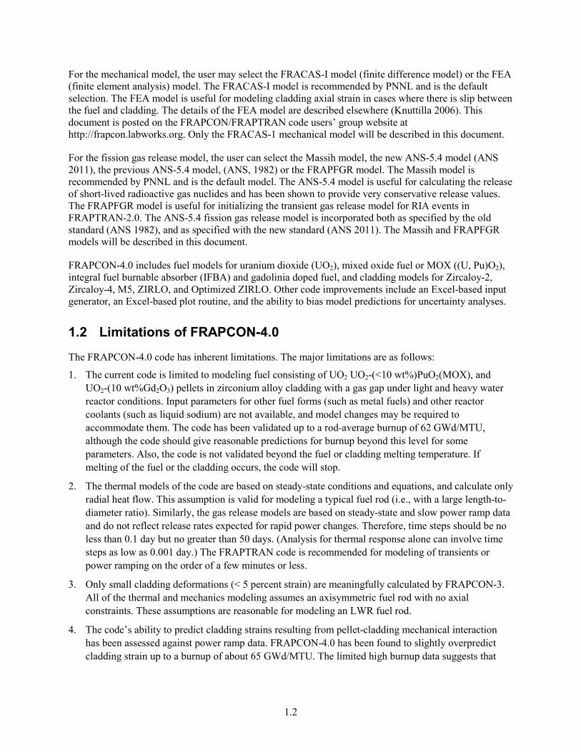
For the mechanical model, the user may select the FRACAS-I model (finite difference model) or the FEA (finite element analysis) model. The FRACAS-I model is recommended by PNNL and is the default selection. The FEA model is useful for modeling cladding axial strain in cases where there is slip between the fuel and cladding. The details of the FEA model are described elsewhere (Knuttilla 2006). This document is posted on the FRAPCON/FRAPTRAN code users’ group website at http://frapcon.labworks.org. Only the FRACAS-1 mechanical model will be described in this document.

For the fission gas release model, the user can select the Massih model, the new ANS-5.4 model (ANS 2011), the previous ANS-5.4 model, (ANS, 1982) or the FRAPFGR model. The Massih model is recommended by PNNL and is the default model. The ANS-5.4 model is useful for calculating the release of short-lived radioactive gas nuclides and has been shown to provide very conservative release values. The FRAPFGR model is useful for initializing the transient gas release model for RIA events in FRAPTRAN-2.0. The ANS-5.4 fission gas release model is incorporated both as specified by the old standard (ANS 1982), and as specified with the new standard (ANS 2011). The Massih and FRAPFGR models will be described in this document.

FRAPCON-4.0 includes fuel models for uranium dioxide (UO2), mixed oxide fuel or MOX ((U, Pu)O2), integral fuel burnable absorber (IFBA) and gadolinia doped fuel, and cladding models for Zircaloy-2, Zircaloy-4, M5, ZIRLO, and Optimized ZIRLO. Other code improvements include an Excel-based input generator, an Excel-based plot routine, and the ability to bias model predictions for uncertainty analyses.

1.2 Limitations of FRAPCON-4.0

The FRAPCON-4.0 code has inherent limitations. The major limitations are as follows:

1. The current code is limited to modeling fuel consisting of UO2 UO2-(<10 wt%)PuO2(MOX), and UO2-(10 wt%Gd2O3) pellets in zirconium alloy cladding with a gas gap under light and heavy water reactor conditions. Input parameters for other fuel forms (such as metal fuels) and other reactor coolants (such as liquid sodium) are not available, and model changes may be required to accommodate them. The code has been validated up to a rod-average burnup of 62 GWd/MTU, although the code should give reasonable predictions for burnup beyond this level for some parameters. Also, the code is not validated beyond the fuel or cladding melting temperature. If melting of the fuel or the cladding occurs, the code will stop.

2. The thermal models of the code are based on steady-state conditions and equations, and calculate only radial heat flow. This assumption is valid for modeling a typical fuel rod (i.e., with a large length-to-diameter ratio). Similarly, the gas release models are based on steady-state and slow power ramp data and do not reflect release rates expected for rapid power changes. Therefore, time steps should be no less than 0.1 day but no greater than 50 days. (Analysis for thermal response alone can involve time steps as low as 0.001 day.) The FRAPTRAN code is recommended for modeling of transients or power ramping on the order of a few minutes or less.

3. Only small cladding deformations (< 5 percent strain) are meaningfully calculated by FRAPCON-3. All of the thermal and mechanics modeling assumes an axisymmetric fuel rod with no axial constraints. These assumptions are reasonable for modeling an LWR fuel rod.

4. The code’s ability to predict cladding strains resulting from pellet-cladding mechanical interaction has been assessed against power ramp data. FRAPCON-4.0 has been found to slightly overpredict cladding strain up to a burnup of about 65 GWd/MTU. The limited high burnup data suggests that

1.3

FRAPCON-3 may underpredict the cladding strain during power ramps at very high burnup (i.e., > 65 GWd/MTU) for hold times greater than 30 minutes.

1.3 Report Outline and Relation to Other Reports

Section 2 and Section 3 of this report deal with the modeling concepts and the code description, respectively. The material properties for fuel, gas, and cladding are fully documented in a separate report (Luscher and Geelhood 2014). Instructions for creating an input file are discussed in Appendix A. The reader is cautioned that, although the thermal and mechanical models are described separately, they actually are highly interrelated. Section 2.2 is included to outline these interrelationships.

This report does not present an assessment of the code performance with respect to in-reactor data. Critical comparisons with experimental data from well-characterized, instrumented test rods are presented in Volume 2 of this series, titled “FRAPCON-4.0 Integral Assessment” (Geelhood et al 2015a).

The full documentation of the steady-state and transient fuel performance codes is described in three documents. The basic fuel, cladding, and gas material properties used in FRAPCON-4.0 and FRAPTRAN-2.0 are described in the material properties handbook (Luscher and Geelhood 2014). The FRAPCON-4.0 code structure and behavioral models are described in the FRAPCON-4.0 code description document (this document). The FRAPTRAN-2.0 code structure and behavioral models are described in the FRAPTRAN-2.0 code description document (Geelhood et al. 2014).

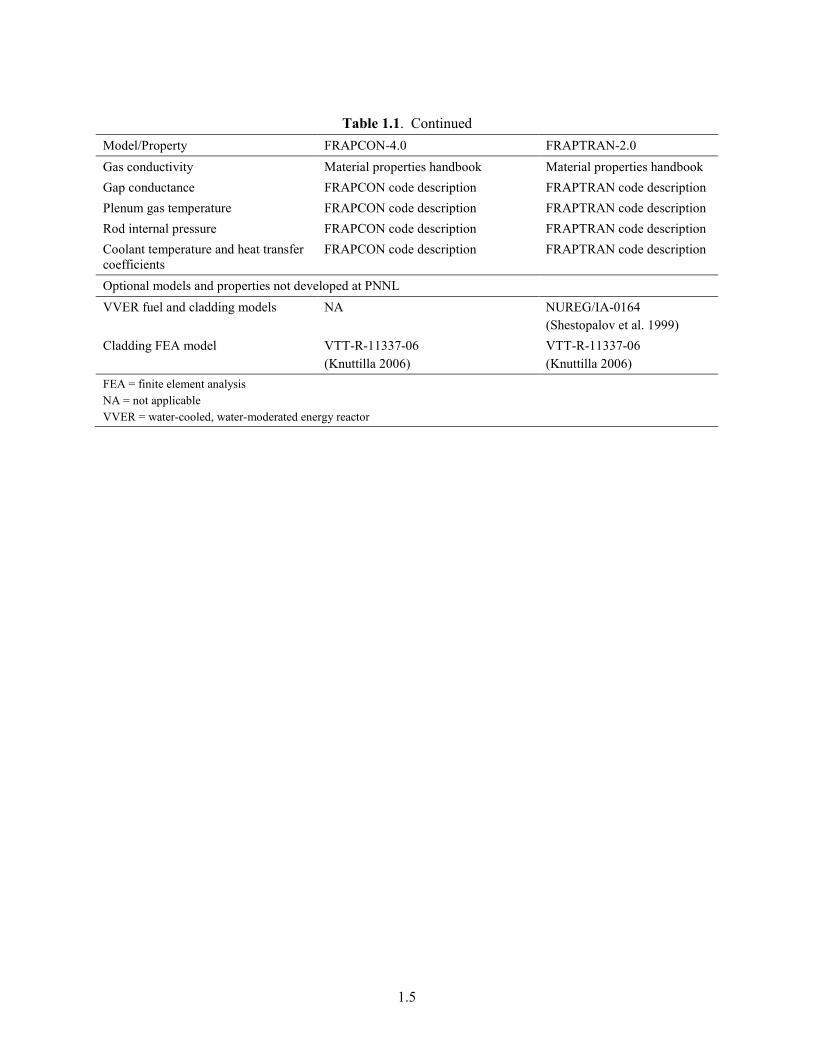
Table 1.1 shows where each specific material property and model used in the NRC fuel performance codes are documented.

1.4

Table 1.1. Roadmap to Documentation of Models and Properties in NRC Fuel Performance Codes, FRAPCON-4.0 and FRAPTRAN-2.0

Model/Property FRAPCON-4.0 FRAPTRAN-2.0 Fuel thermal conductivity Material properties handbook Material properties handbook Fuel thermal expansion Material properties handbook Material properties handbook Fuel melting temperature Material properties handbook Material properties handbook Fuel specific heat Material properties handbook material properties handbook Fuel enthalpy Material properties handbook material properties handbook Fuel emissivity Material properties handbook Material properties handbook Fuel densification Material properties handbook NA Fuel solid swelling Material properties handbook NA Fuel gaseous swelling Material properties handbook NA Fission gas release FRAPCON code description FRAPTRAN code description Fuel relocation FRAPCON code description FRAPTRAN code description Fuel grain growth FRAPCON code description NA High burnup rim model FRAPCON code description NA Nitrogen release FRAPCON code description NA Helium release FRAPCON code description NA Radial power profile FRAPCON code description NA (input parameter) Stored energy FRAPCON code description FRAPTRAN code description Decay heat model NA FRAPTRAN code description Fuel and cladding temperature solution

FRAPCON code description FRAPTRAN code description

Cladding thermal conductivity Material properties handbook Material properties handbook Cladding thermal expansion Material properties handbook Material properties handbook Cladding elastic modulus Material properties handbook Material properties handbook Cladding creep model Material properties handbook NA Cladding specific heat Material properties handbook Material properties handbook Cladding emissivity Material properties handbook Material properties handbook Cladding axial growth Material properties handbook NA Cladding Meyer hardness Material properties handbook Material properties handbook Cladding annealing FRAPCON code description FRAPTRAN code description Cladding yield stress and plastic deformation

FRAPCON code description FRAPTRAN code description

Cladding failure criteria NA FRAPTRAN code description Cladding waterside corrosion FRAPCON code description NA (input parameter) Cladding hydrogen pickup FRAPCON code description NA (input parameter) Cladding high temperature oxidation NA FRAPTRAN code description Cladding ballooning model NA FRAPTRAN code description Cladding mechanical deformation FRAPCON code description FRAPTRAN code description Oxide thermal conductivity Material properties handbook Material Properties Handbook Crud thermal conductivity FRAPCON code description NA

1.5

Table 1.1. Continued

Model/Property FRAPCON-4.0 FRAPTRAN-2.0 Gas conductivity Material properties handbook Material properties handbook Gap conductance FRAPCON code description FRAPTRAN code description Plenum gas temperature FRAPCON code description FRAPTRAN code description Rod internal pressure FRAPCON code description FRAPTRAN code description Coolant temperature and heat transfer coefficients

FRAPCON code description FRAPTRAN code description

Optional models and properties not developed at PNNL VVER fuel and cladding models NA NUREG/IA-0164

(Shestopalov et al. 1999) Cladding FEA model VTT-R-11337-06

(Knuttilla 2006) VTT-R-11337-06 (Knuttilla 2006)

FEA = finite element analysis NA = not applicable VVER = water-cooled, water-moderated energy reactor

2.1

2.0 General Modeling Descriptions

2.1 FRAPCON-4.0 Solution Scheme

The FRAPCON-4.0 code iteratively calculates the interrelated effects of fuel and cladding temperature, rod internal gas pressure, fuel and cladding deformation, release of fission product gases, fuel swelling and densification, cladding thermal expansion and irradiation-induced growth, cladding corrosion and hydriding, and crud deposition for a given buildup rate as functions of time and fuel-rod-specific power.

The calculated procedure is illustrated in Figure 2.1, a simplified flowchart of FRAPCON-4.0. (A detailed flowchart is provided in Section 3.) The calculation begins by processing input data. Next, the initial fuel rod state is determined through a self-initialization calculation. Time is advanced according to the input-specified time-step size, a steady-state solution is performed, and the new fuel rod state is determined. The new fuel rod state provides the initial state conditions for the next time step. The calculations are cycled in this manner for the user-specified number of time steps.

The solution for each time step consists of 1) calculating the temperature of the fuel and the cladding; 2) calculating fuel and cladding deformation; and 3) calculating the fission product generation and release, void volume, and fuel rod internal gas pressure. Each calculation is made in a separate subcode. As shown in Figure 2.1, the fuel rod response for each time step is determined by repeated cycling through two nested loops of iterative calculations until the fuel-cladding gap temperature difference and internal gas pressure converge.

For the FRACAS-I (Bohn et al. 1977) mechanical model, the fuel temperature and deformation are alternately calculated in the inner loop. On the first cycle through this loop for each time step, the gap conductance is computed using the fuel-cladding gap size from the previous time step. Then the fuel rod temperature distribution is computed. This temperature distribution feeds the deformation calculation by influencing the fuel and cladding thermal expansions and the cladding stress-strain relation. An updated fuel-cladding gap size is calculated and used in the gap conductance calculation on the next cycle through the inner loop. The cyclic process through the inner loop is repeated until two successive cycles calculate essentially the same temperature distribution.

The outer loop of calculations is cycled in a manner similar to that of the inner loop, but with the amount of internal gas being determined during each iteration. The calculation alternates between the fuel rod void volume-gas pressure calculation and the fuel rod temperature-deformation calculation. On the first cycle through the outer loop for each time step, the gas pressure from the previous time step is used. For each cycle through the outer loop, the number of gas moles is calculated and the updated gas pressure computed and fed back to the deformation and temperature calculations (the inner loop). The calculations are cycled until two successive cycles calculate essentially the same gas pressure, and then a new power-time step is begun.

2.2

Figure 2.1. Simplified FRAPCON-4.0 Flowchart

2.2 Coupling of Thermal and Mechanical Models

The close coupling of the thermal modeling and mechanical modeling is the result of the existence of the fuel-cladding gap. As the fuel temperature increases, the extreme stresses resulting from the large temperature gradients in the fuel cause the fuel to crack and relocate. Cracks can be circumferential or radial, but are predominantly radial. Void space, which is originally in the fuel-cladding gap, is relocated into the fuel as fragments of fuel move outwardly into the fuel-cladding gap.

As the fuel becomes hotter, the fuel expands, filling some of the voids within the fuel. However, asperities do not align exactly, thereby causing the fuel diameter to appear larger and the fuel to interact with the cladding at a lower power than that expected due to normal expansion (or contraction) mechanisms, including thermal expansion, swelling, and densification. FRACAS-I has been modified to allow 50 percent of the original fuel surface relocation to be recovered due to fuel swelling before hard contact is established between the fuel and the cladding.

2.3

The modeling of the cracked and relocated fuel, both thermally and mechanically, requires accounting for changed fuel-cladding gap size (and hence gap conductance) and the changed fuel pellet diameter as the fuel interacts with the cladding. The fuel surface relocation provides a new fuel-cladding gap size for calculating gap conductance and mechanical interactions. Also considered is the shift of voids from the fuel-cladding gap into cracks in the fuel pellet (and the resultant pressure change due to higher temperature in the cracks) and the feedback into the mechanics and thermal calculations.

FRACAS-I uses the relocated fuel-cladding gap size for the thermal calculations and makes partial use of the fuel surface relocation in the mechanics calculation (i.e., when 50 percent of the relocation is recovered, the code assumes the pellet to be a rigid structure, and, therefore, hard contact is assumed between the fuel and cladding).

2.3 Fuel Rod Thermal Response

The temperature distribution throughout the fuel and the cladding is calculated at each axial node. A simplified flowchart of the temperature distribution solution is shown in Figure 2.2. A schematic of the temperature distribution at an arbitrary axial node is shown in Figure 2.3.

The models used in the fuel rod temperature calculations assume a cylindrical fuel pellet located symmetrically within a cylindrical fuel rod surrounded by coolant. User-supplied boundary conditions (coolant inlet temperature, coolant channel equivalent heated diameter, and time coolant mass flux) and the user-supplied axial linear heat generation rate are used to calculate the coolant bulk temperature, Tb, using a single-channel coolant enthalpy rise model. A film temperature rise, ∆Tf, is then calculated from the coolant to the surface of the fuel rod through any crud layer which may exist. The cladding inside surface temperature, Tci, is found by calculating the temperature rise across the zirconium oxide and the cladding using Fourier’s law. The temperature rise to the fuel surface is determined from an annular gap conductance model, thereby establishing the fuel surface temperatures, Tfs. Finally, the temperature distribution in the fuel is calculated, accounting for fuel cracking effects using the fuel surface temperature and assumed symmetry at the centerline as boundary conditions.

The models used in the temperature calculations involve assumptions and limitations. The most important are as follows:

1. Heat conduction in the axial direction is considered negligible relative to radial heat conduction and is ignored due to the large length-to-diameter ratio.

2. Heat conduction in the azimuthal direction is ignored (axisymmetric analysis).

3. Constant boundary conditions are maintained during each time step.

4. Steady-state heat flow is assumed.

5. The fuel rod is a right circular cylinder surrounded by water coolant.

2.4

Figure 2.2. Flow Chart of the Fuel and Cladding Temperature Calculation

2.5

Figure 2.3. Schematic of the Fuel Rod Temperature Distribution

2.3.1 Coolant Conditions

FRAPCON-4.0 calculates bulk coolant temperatures assuming a single, closed coolant channel according to

∫

+=

z

fpinb dz

GACzqDTzT

0

0 )(")()( p

(2.1) where Tb(z) = bulk coolant temperature at elevation z on the rod axis (K) Tin = inlet coolant temperature (K) q"(z) = rod surface heat flux at elevation z on the rod axis (W/m2) Cp = heat capacity of the coolant (J/kg-K) G = coolant mass flux (kg/s-m2) Af = coolant channel flow area (m2) Do = outside cladding diameter (m)

2.6

Coolant heat capacity for water is calculated using the following relationships:

51039.2 ×=pC for Tb(z) < 544K

)]4.979)(8.1(1073.71[1039.2 45 −×+×= − zTC bp for 544K <= Tb(z) < 583K (2.2)

)]1031)(8.1(1095.21[1039.2 35 −×+×= − zTC bp for Tb(z) >= 583K

Coolant channel hydraulic diameter is calculated from rod pitch and diameter using the following relationship:

0

20

2

40.4

D

DPD

pit

e p

p

−

(2.3) where Ppit = rod-to-rod pitch (m) Do = outside cladding diameter (m)

2.3.2 Fuel Rod Surface Temperature

The cladding surface temperature at axial elevation z is taken as the minimum value of

Tw(z) = Tb(z) + ∆Tf (z) + ∆Tcr(z) + ∆Tox(z) (2.4)

Tw(z) = Tsat + ∆TJL + ∆Tox(z) (2.5)

where Tb(z) = bulk coolant temperature at elevation z on the rod axis (K) Tw(z) = rod surface temperature at elevation z on the rod axis (K) ∆Tf (z) = forced convection film temperature drop at elevation z on the rod axis (K) ∆Tcr(z) = crud temperature drop at elevation z on the rod axis (K) ∆Tox(z) = oxide layer temperature drop at elevation z Tsat = coolant saturation temperature (K) ∆TJL = nucleate boiling temperature drop at elevation z on the rod axis (K), determined by

the Jens-Lottes correlation (Jens and Lottes 1951)

The choice of the minimum value is a simple means of deciding whether heat is transferred from the cladding surface to the coolant by forced convection or nucleate boiling. It also provides a smooth numerical transition from forced convection to nucleate boiling, thereby avoiding convergence problems. For forced-convection heat transfer, the temperature drop across the coolant film layer at the rod surface is based on

ff hzqzT /)(")( =∆ (2.6)

2.7

where hf is the Dittus-Boelter (Dittus and Boelter 1930) film conductance given by

4.08.0 PrRe023.0

=

ef D

kh (2.7)

where hf = conductance (W/m2-K) k = thermal conductivity of the coolant (W/m-K) De = coolant channel heated diameter (m) Re = Reynolds number (dimensionless) Pr = Prandtl number (dimensionless)

The temperature drop across the crud is given by

cr

crcr k

zqzTδ

)(")( =∆ (2.8)

where δcr = crud thickness (m) kcr = crud thermal conductivity, 0.8648 (W/m-K)

For nucleate boiling heat transfer, the temperature drop across the coolant film layer at the rod surface is based on the Jens-Lottes (Jens and Lottes 1951) formulation:

)102.6/(25.06 6

/]10/)("[60)( ×=∆ PJL ezqzT (2.9)

where P = system bulk coolant pressure (Pa)

It is assumed that the crud does not offer any resistance to heat flow during nucleate boiling; therefore, no temperature drop due to crud is calculated. The coolant is assumed to boil through the crud blanket.

The temperature drop across the zirconium oxide layer at elevation z on the rod axis is determined by

ox

oxox k

zzqzT

)()(")(

δ=∆

(2.10) where ∆Tox(z) = oxide temperature drop at elevation z on the rod axis (K) δox(z) = oxide thickness at elevation z on the rod axis (m) kox = oxide thermal conductivity (W/m−K)

2.8

2.3.3 Cladding Temperature Gradient

The cladding temperature drop for each axial location is calculated according to the following expression for steady-state heat transfer through a cylinder with uniform thermal conductivity:

ciooc krrrzqT /)/ln()("=∆ (2.11) where ∆Tc = cladding temperature drop (K) ro = cladding outside radius (m) ri = cladding inside radius (m) kc = temperature and material dependent thermal conductivity of the cladding (W/m-K)

2.3.4 Fuel-Cladding Gap Temperature Gradient

The fuel-cladding gap temperature drop is calculated using the fuel rod surface heat flux at elevation z and the fuel-cladding gap conductance. The fuel-cladding gap conductance is the sum of three components: the conductance due to radiation, the conduction through the gas, and the conduction through regions of solid-solid contact. The equations and models for each of these components are presented in the following sections.

h

zqTgap)("

=∆ (2.12)

where h = hr + hgas + hsolid q"(z) = rod surface heat flux at elevation z on the rod axis (W/m2) hr = conductance due to radiation (W/m2-K) hgas = conductance of the gas gap (W/m2-K) hsolid = conductance due to fuel-cladding contact (W/m2-K)

2.3.4.1 Radiant Heat Transfer

The net radiant heat transfer of heat from the fuel to the cladding is the infinite-cylinder, gray body form as derived for high-aspect-ratio small gaps from the general radiant heat transfer equation by Kreith (1964) and others:

Net surface heat flux (SHF) = ( )44cifs TTF −s (2.13)

where F = )]1/1)(/(/[1 −+ ccifsf erre s = Stefan-Boltzman constant = 5.6697E-8 (W/m2-K4) ef = fuel emissivity ec = cladding emissivity Tci = fuel surface temperature (K)

2.9

Tfs = cladding inner surface temperature (K) rfs = fuel outer surface radius (m) rci = cladding inner surface radius (m)

The conductance due to radiation, hr (W/m2-K), is defined by

hr(Tfs - Tci) = SHF (2.14) Combining Equations (2.13) and (2.14) and dividing by (Tfs - Tci) gives

]][[ 22cifscifsr TTTTFh ++= s (2.15)

2.3.4.2 Conduction through the Interfacial Gas

The form of the conductance due to conductive heat transfer through the gas in the fuel-cladding gap, hgas (W/m2-K), is that applied to small annular gaps:

x

kh gas

gas ∆= (2.16)

where kgas = gas thermal conductivity (W/m-K) ∆x = total effective gap width (m)

∆x = deff + 1.8(gf + gc) - b + d (2.17) where d = value from FRACAS for open fuel-cladding gap size (m) deff = exp (-0.00125P) (Rf+ Rc) for closed fuel-cladding gaps (m), = (Rf+ Rc) for open fuel-cladding gaps (m) P = fuel-cladding interfacial pressure (kg/cm2) R+ Rc = cladding plus fuel surface roughness (m) (gf + gc) = temperature jump distances at fuel and cladding surfaces, respectively (m) b = 1.397x10-6 (m)

The quantity (gf + gc) is calculated from the GAPCON-2 (Beyer et al. 1975) model and is

=+

∑ iiigas

gasgascf MfaP

TkAgg

/1)( (2.18)

where A = 0.0137 (value of 2.23 in coding includes the 1.8 factor from Equation 2.17) kgas = gas conductivity (W/m-K) Pgas = gas pressure (Pa) Tgas = average gas temperature (K)

2.10

ai = accommodation coefficient of i-th gas component Mi = gram-molecular weight of i-th gas component (g moles) fi = mole fraction of i-th gas component

2.3.4.3 Conduction through Points of Contact

The contact conductance model is a modification of the Mikic-Todreas (Tondreas and Jacobs 1973) model that preserves the roughness, conductivity, and pressure dependencies while providing a best estimate for the range of contact conductances measured by Garnier and Begej (1979). The FRACAS-I model uses expressions for hsolid that depend on both the fuel-cladding interfacial pressure and the microscopic roughness, R, as follows:

RE

RPKh multrelm

solid4166.0

= , if Prel > 0.003

RE

Kh m

solid00125.0

= , if 0.003 > Prel > 9x10-6 (2.19)

RE

PKh relm

solid

5.04166.0= , if Prel < 9x10-6

where Prel = ratio of interfacial pressure to cladding Meyer hardness (approximately 680 MPa) Km = geometric mean conductivity (W/m-K) = 2Kf Kc/(Kf + Kc) R = 22

cf RR + (m), where Rf and Rc are the roughnesses of the fuel and cladding (m)

Rmult = 333.3 Prel, if Prel ≤ 0.0087 = 2.9 , if Prel > 0.0087 Kc = cladding thermal conductivity (W/m-K) Kf = fuel thermal conductivity (W/m-K) E = exp[5.738 - 0.528 ln(3.937 × 107 Rf)]

The above comes from a fit to Ross and Stoute (1962) data plus that by Rapier et al. (1963) using the Todreas (Tondreas and Jacobs 1973) model. The contact conductance model provides a relatively smooth transition between the open and closed gap conductance that helps to eliminate non-convergence in the code caused by oscillating between an open and closed gap situation.

2.3.5 Fuel Pellet Heat Conduction Model

This section describes the steady-state fuel pellet heat conduction model. The model is developed based on the finite difference heat conduction models used in RELAP5 and FRAPTRAN. First, an overview of the fuel pellet heat conduction model used in FRAPCON-4.0 is provided. Next, the requirements for the fuel pellet heat conduction model are given. The development of the finite difference approach begins in Section 2.3.5.1, and subsequent sections provide specific applications of the steady-state heat conduction equation that will lead to the final form of the heat conduction model.

2.11

A schematic of a representative temperature distribution at an arbitrary axial node is shown in Figure 2.3. The fuel surface temperature, Tfs, is used as one of the boundary conditions to feed into the finite difference heat conduction model. The new finite difference model calculates the temperature profile in the fuel pellet and has fine mesh capabilities at the fuel surface that will handle fuel pellets with burnup to 75 GWd/MTU.

2.3.5.1 The Finite Difference Approach

Finite differences will be used to calculate the temperature distribution in the fuel region. Variable mesh spacing will be used, and the spatial dependence of the internal heat source is allowed to vary over each mesh interval.

The steady-state integral form of the heat conduction equation is

∫∫∫∫∫ =•∇

VS

dVxSdsnxTxTk )()(),(

(2.20) where k = thermal conductivity (W/m-K) s = surface of the control volume (m2) n = the surface normal unit vector S = internal heat source (W/m3) T = temperature (K) V = control volume (m3) x = the space coordinates (m)

The following assumptions were made to develop this heat conduction model:

• fixed geometry

• symmetrical geometry

• negligible heat conduction in the axial direction

• negligible heat conduction in the azimuthal direction

• steady-state

• mesh point averaged thermal conductivity (discussed in the following sections)

Two boundary conditions are needed to calculate the temperature profile in the fuel. The boundary

conditions are the symmetry condition, 00

=∂∂

=xxT

, at the center of the fuel pellet and a prescribed

temperature at the surface of the fuel.

2.3.5.2 Mesh Point Layout

Figure 2.4 illustrates the placement of mesh points at which temperatures are to be calculated. The mesh point spacing is positive in the radial direction. The first mesh point is placed at the fuel centerline or at the inner annular surface of the fuel. Variable mesh spacing is used to determine the placement of interior

2.12

mesh points. The mesh placement does not provide constant volume nodes, but is consistent with the radial power and burnup distribution model, TUBRNP (Lassman et al. 1994; and Lassman et al. 1998), developed at the Institute for Transuranium Elements, Karlsruhe, incorporated in FRAPCON. This scheme places more nodes near the surface of the pellet to account for the rim effects. The last mesh point is placed on the surface of the fuel.

Figure 2.4. Mesh Point Layout

Figure 2.5 represents three typical mesh points. The subscripts are space indexes indicating the mesh point number; and l and r (if present) designate quantities to the left and right, respectively, of the mesh point. The δ’s indicate mesh point spacing. Between mesh points, the thermal conductivity, k, and the source term, S, are assumed spatially constant; but klm is not necessarily equal to krm and similarly for S.

Figure 2.5. Typical Mesh Points

To obtain the spatial-difference approximation for the m-th interior mesh point, a form of Equation (2.20) applicable to radial heat conduction in cylindrical coordinates is applied to the volume and surfaces indicated by the dashed line shown in Figure 2.5. To obtain the spatial difference approximation at the boundaries, Equation (2.20) is applied to the volumes and interior surfaces indicated by the dashed lines shown in Figure 2.6.

2.13

Figure 2.6. Boundary Mesh Points

The spatial finite-difference approximations use approximate expressions for the space and volume factors and simple differences for the gradient terms. To condense the expressions defining the numerical approximations, the following quantities are defined.

−=

422 lm

mlmv

lm xδδ

pδ,

−=

422 rm

mrmv

rm xδδ

pδ

−=

22 lm

mlm

slm x

δδ

pδ,

−=

22 rm

mrm

srm x

δδ

pδ (2.21)

mbm xpδ 2=

The superscripts, v and s, refer to volume and surface-gradient weights. The bmδ is a surface weight used

at exterior boundaries and in heat-transfer-rate equations.

2.3.5.3 Difference Approximation at Internal Mesh Points

The first term of Equation (2.20) for the surfaces of Figure 2.5 is approximated by

srmrmmm

slmlmmm

s

kTTkTTdsnxTxTk δδ )()()(),( 11 +− −+−≈•∇∫∫

(2.22)

Note that the volume in Figure 2.5 is divided into two sub-volumes by the interface line. When the surface integrals of these sub-volumes are added, the surface integrals along the common interface cancel because of the continuity of heat flow.

The source term in Equation (2.20) is represented by

)()( xPQPxS f= (2.23) where Pf = the axial power factor that relates P to a particular axial node P = the power function derived from the linear heat generation rate

2.14

Q(x) = the radial position dependent function (as determined by the TUBRNP model and subroutine)

The value of Q(x) is assumed constant over a mesh interval, but each interval can have a different value. The third term of Equation (2.20) is then approximated as

)(),( v

rmrmvlmlmf

V

QQPPdVtxS δδ +≈∫∫∫ (2.24)

Gathering the approximations of terms in Equation (2.20), the basic difference equation for the m-th mesh point is

)()()( 11vrmrm

vlmlmf

srmrmmm

slmlmmm QQPPkTTkTT δδδδ +=−+− +− (2.25)

Writing Equation (2.25) in abbreviated form, the difference approximation for the m-th interior mesh point is

mmmmmmm dTcTbTa =++ +− 11 (2.26)

)( slmlmm ka δ−= (2.27)

mmm cab −−= (2.28)

)( srmrmm kc δ−= (2.29)

)( vrmrm

vlmlmfm QQPPd δδ += (2.30)

2.3.5.4 Difference Approximation at Boundaries

To obtain the difference approximations for the mesh points at the boundaries, Equation (2.20) is applied to the volumes of Figure 2.6. The first boundary condition evaluated is the symmetry condition,

00

=∂∂

=xxT

. The symmetry condition is applied at mesh point 1. The first term of Equation (2.20) is

approximated by

srlrl

s

TTkdsnxTxTk δ)()(),( 12 −=•∇∫∫

(2.31)

The complete basic expression for mesh point 1 (located at the symmetry boundary) becomes

vrlrlf

srlrl QtPPTTk δδ )()( 12 =− (2.32)

2.15

Thus, for the symmetry boundary

12111 dTcTb =+ (2.33)

11 cb −= (2.34)

srlrlkc δ−=1 (2.35)

vrlrlf QPPd δ)(1 = (2.36)

For the fuel surface boundary at mesh point M, a known fuel surface temperature is applied, giving

MMMMM dTbTa =+−1 (2.37)

0=Ma (2.38)

1=Mb (2.39)

fsMfsM TdTd == (2.40)

2.3.5.5 Radial Power Profile

The radial power profile within a fuel pellet is a function of fuel type, reactor type, and burnup. FRAPCON-4.0 uses the TUBRNP (Lassman et al. 1994; and Lassman et al. 1998) model to calculate the radial power profile in UO2 and MOX under LWR and heavy-water reactor (HWR) conditions as a function of burnup.

The TUBRNP model is not currently able to calculate the radial power profile of urania-gadolinia (UO2-Gd2O3) fuel. For this fuel type, FRAPCON-4.0 interpolates from look-up tables for LWR and HWR conditions while the gadolinium (Gd) isotopes with high cross section are burning out. After these high-cross-section Gd isotopes have burnt out, FRAPCON-4.0 uses the radial power profiles calculated using TUBRNP. The look-up tables were created using the neutronics code, WIMS, for a standard fuel design at various Gd2O3 loadings under LWR and HWR conditions.

The neutron flux distribution (r) within the fuel pellet is described in TUBRNP by the solution of one-group, one-dimensional diffusion theory applied to cylindrical fuel:

)()( 0 rCIr κφ = (2.41)

for solid pellets, and

+= )(

)()(

)()( 001

010 rK

rKrI

rICr κκκ

κφ (2.42)

for annular pellets

2.16

where

Da /Σ=κ , ∑=Σk

iiaa N,s , totss N

Ds3

13

1=

Σ=

and I,K = modified Bessel functions C = a constant sa, ss = absorption and scattering cross sections N = pellet-average atom concentration r0 = the pellet outer radius i = subscript indicating all U and Pu isotopes

The evolution of average uranium and plutonium isotope concentrations in the fuel through time can be described as a coupled set of differential equations, which are coupled because the loss of one isotope by neutron capture leads in some cases to some production of the next higher isotope. These equations are summarized as follows:

φs 235235,

235 NdtNd

a−= (2.43)

φs 238238,

238 NdtNd

a−= (2.44)

φsφs 11,, −−+−= jjcjja

j NNdtNd

(2.45) where j = 239Pu, 240Pu, 241Pu, and 242Pu sa, sc = absorption and capture cross sections

Because, in fuel performance codes, the linear heat generation rate (LHGR) and time step duration are input values, the burnup increment for the time step is prescribed and can be related to the flux, the fission cross sections, and the concentrations of fissile isotopes. Thus, flux-time increment, dt, can be replaced by the burnup increment, dbu, via the relation

∑=

′′′=

kkkf

fuelfuel

dtNdtqdbu φsρα

ρ ,

(2.46)

2.17

where q''' = volumetric heat generation rate ρfuel = fuel density

sf = fission cross section

α = a conversion constant

Furthermore, the distribution of plutonium production is described by an empirical function, f(r), the parameters for which are to be selected based on code-data comparisons on plutonium concentrations as a function of burnup. Thus, the equations for isotope distribution N(r) become

ArN

dburdN

a )()(

235235,235 s−=

(2.47)

ArfN

dburdN

a )()(

238238,238 s−=

(2.48)

ANArN

dburdN

ca 238238,239239,239 )(

)(ss +−=

(2.49)

ANArN

dburdN

jjcjjaj

11,, )()(

−−+−= ss (2.50)

where, in this case, j = 240Pu, 241Pu, and 242Pu,

∑

=

iiif

fuel

NA

,

8815.0sα

ρ

( )3)(exp1)( 21p

out rrpprf −−+=

and p1, p2, and p3 are empirically determined constants.

In FRAPCON-4.0, the following values are used: p1 = 3.45 (for LWR), p1 = 2.21 (for HWR) p2 = 3.0 (for LWR and HWR) p3 = 0.45 (for LWR and HWR)

The function f(r) is constrained to have a volume-averaged value of 1.0.

The fission and capture cross sections are different for LWR conditions and HWR conditions due to the difference in neutron spectrum in these reactors. The fission and capture cross sections (sf and sc, respectively) used in FRAPCON-4.0 are listed in Table 2.1. The absorption cross section (sa) is the sum of the fission cross section and the capture cross section.

2.18

Table 2.1. Fission and Capture Cross Sections Used in FRAPCON-4.0

Isotope

LWR HWR

sf (barns) sc (barns) sf (barns) sc (barns) 235U 41.5 9.7 107.9 22.3 238U 0.00 0.78 0.00 1.16 239Pu 105 58.6 239.18 125.36 240Pu 0.584 100 0.304 127.26 241Pu 120 50 296.95 122.41 242Pu 0.458 80 0.191 91.30

The local power density, )(rq ′′′ , which is needed for the thermal analysis, is proportional to the neutron flux and the macroscopic cross section for fission,

∑∝′′′

jjjf Nrq φs ,)(

(2.51) where j = 235U, 238U, 239Pu, 240Pu, 241Pu, and 242Pu

Equation (2.51) can be used to obtain a normalized radial power profile across the pellet. This normalized radial power profile is used as Q(x) in Equation (2.23).

At the end of each time step, the isotope concentrations are updated based on the burnup increment, using the above equations. These equations are solved and the concentrations evaluated at every input radial boundary. Because the flux and plutonium deposition distribution functions are prescribed, and the solutions are carried out at ring boundaries, the solution is independent of the radial nodalization scheme; it is also quite stable with respect to time-step size, within the limits dictated by other processes, such as cladding creep and fission gas release.

2.3.5.6 Thermal Conductivity and Iteration Procedures

The thermal conductivity, k, is considered a function of temperature and burnup.

The fuel thermal conductivity model in FRAPCON-4.0 is based on the expression developed by the Nuclear Fuels Industries (NFI) model (Ohira and Itagaki 1997) with modifications. This model applies to UO2 and UO2-Gd2O3 fuel pellets at 95% of theoretical density (TD).

( )

−+

−−+++⋅+=

TF

TE

ThBugBuBufBTgadaAK

exp

)()()04.0exp(9.01)(1

2

95

(2.52)

2.19

where K95 = thermal conductivity for 95% TD fuel (W/m-K) T = temperature (K) Bu = burnup (GWd/MTU) f(Bu) = effect of fission products in crystal matrix (solution) f(Bu) = 0.00187•Bu (2.53) g(Bu) = effect of irradiation defects g(Bu) = 0.038•Bu0.28 (2.54) h(T) = temperature dependence of annealing on irradiation defects

TQeTh /3961

1)( −+= (2.55)

Q = temperature dependence parameter (“Q/R”) = 6380 K A = 0.0452 (m-K/W) a = constant = 1.1599 gad = weight fraction of gadolinia B = 2.46E-4 (m-K/W/K) E = 3.5E9 (W-K/m) F = 16361 (K)

As applied in FRAPCON-4.0, the above model is adjusted for as-fabricated fuel density (in fraction of TD) using the Lucuta recommendation for spherical-shaped pores (Lucuta et al. 1996), as follows:

Kd = 1.0789*K95*[d/{1.0 + 0.5(1-d)}] (2.56) where d = density (fraction of TD) K95 = as-given conductivity (reported to apply at 95% TD)

The factor 1.0789 adjusts the conductivity back to that for 100% TD material.

For MOX fuel ((UO2, Pu)O2), the same equation as shown in Equation (2.52) is used with A and B replaced by functions of the oxygen to metal ratio and several other fitting coefficients changed as follows:

( )

−+

−−+++⋅+=

TD

TC

ThBugBuBufTxBgadaxAK MOX

exp

)()()04.0exp(9.01)()()(1

2

)(95

(2.57) where K95(MOX) = thermal conductivity for 95% TD MOX fuel (W/m-K) x = 2.00 – O/M (i.e., oxygen-to-metal ratio) A(x) = 2.85x + 0.035 (m-K/W) B(x) = (2.86 - 7.15x)*1E-4 (m/W) C = 1.5E9 (W-K/m) D = 13,520 (K)

2.20

All others are as previously defined.

As with the formula for UO2 conductivity, the MOX conductivity can be adjusted for different pellet densities using Equation (2.56).

These thermal properties are obtained for each interval by using the average of the mesh point temperatures bounding the interval.

1,

1, 2 −

− =

+

= mrmm

ml kTT

kk (2.58)

1,

1, 2 +

+ =

+

= mlmm

mr kTT

kk (2.59)

Prior to the calculation of the temperature distribution in the fuel pellet, this model uses assumed thermal conductivity values based on an estimated temperature profile. The existing FRAPCON-4.0 gap conductance iteration scheme (Figure 2.2) will be used to converge on temperature and thermal conductivity in the fuel.

2.3.5.7 The Finite Difference Temperature Calculation

The difference approximation for the mesh points [Equations (2.26), (2.33), and (2.37)] lead to a tri-diagonal set of M simultaneous linear equations.

••

=

••

•••••

−−−−−

M

M

M

M

MM

MMM

dd

dd

TT

TT

bacba

cbacb

1

2

1

1

2

1

1111

222

11

(2.60)

Rows 1 and M correspond to the fuel centerline and fuel surface mesh points, respectively, and rows 2 through M-1 correspond to the interior mesh points. The coefficient matrix would normally be symmetric, but is not because of the right boundary condition that specifies the fuel surface temperature. The corresponding off-diagonal element is zero in the last row. The solution to the above equation is obtained by

1

11 b

cE = and 1

11 b

dF = (2.61)

1−−

=jjj

jj Eab

cE

1

1

−

−

−

−=

jjj

jjjj Eab

FacF for j = 2, 3,..., M-1 (2.62)

2.21

1

1

−

−

−−

=MMM

MMMM Eab

Fadg (2.63)

jjjj FgEg +−= +1 for j = M-1, M-2,..., 3, 2, 1 (2.64)

jj gT = for all j (2.65)

Equations (2.61) through (2.65) were derived by applying the rules for Gaussian elimination. This method of solution introduces little roundoff error, if the off-diagonal elements are negative and the diagonal is greater than the sum of the magnitudes of the off-diagonal elements. From the form of the difference equations for a fuel pellet, these conditions are satisfied for any values of the mesh point spacing, and thermal conductivity.

2.3.6 Plenum Gas Temperature

The plenum gas temperature is calculated based on energy transfer between the top of the pellet stack and the plenum gas, between the coolant channel and the plenum gas, and between the spring and the plenum gas. A discussion of these contributions follows.

Natural convection from the top of the fuel stack is calculated based on heat transfer coefficients from McAdams (1954) for laminar or turbulent natural convection from flat plates.

The heat transfer coefficient is calculated from

DkNuhp =

(2.66) where hp = the heat transfer coefficient from the top of the pellet stack to the plenum gas

(W/m2-K) Nu = Nusselt number D = inside diameter of the cladding of the top node (m) k = conductivity of the plenum gas (W/m-K)

The Nusselt number is calculated using

mGrCNu Pr)(= (2.67)

where Gr = the Grashof number Pr = the Prandtl number

and for

GrPr ≤ 2.0x107, C = 0.54 and m = 0.25,

2.22

or

GrPr > 2.0x107, C = 0.14 and m = 0.33.

The overall effective conductivity from the coolant to the plenum is defined as the inverse of the sum of the individual heat flow resistances. The three resistances are a) the resistance across the inside surface film, b) the resistance across the cladding, and c) the resistance across the outside surface film. The overall conductivity is therefore found as

DBoclad

i

o

f

c

hTDkDD

Dh

U

)0.1(0.2

ln0.2

0.1

∆++

+

=

α (2.68) where Uc = overall effective conductivity from the coolant to the plenum gas (W/m-K) D = hot-state inside cladding diameter (m) hf = cladding inside surface film coefficient (W/m2-K) Do = cold-state outside cladding diameter (m) Di = cold-state inside cladding diameter (m) kclad = temperature- and material-dependent thermal conductivity of the cladding

(W/m-K) α = coefficient of thermal expansion of the cladding (1/K) ∆T = temperature difference between cladding average temperature and datum

temperature for thermal expansion (K) hDB = heat transfer coefficient between the coolant and the cladding (W/m2-K)

Gamma heating in the hold down spring is calculated assuming a volumetric heating rate of 3.76 W/m3 for every W/m2 of rod average heat flux. The expression is

ssp VqQ "76.3 = (2.69) where Qsp = energy generated in the spring due to gamma heating (W) "q = average heat flux of the rod (W/m2) Vs = volume of the spring (m3)

The plenum temperature is approximated from

4

42

2

2

2

DhDV

U

DhTTDV

UQT

ppc

ppaBLKp

csp

plen p

p

+

++=

(2.70)

2.23

where Tplen = plenum temperature (K) Vp = volume of the plenum (m3) TBLK = bulk coolant temperature at the top axial node (K) Tpa = temperature associated with the insulator or top pellet (K)

2.3.7 Stored Energy

The stored energy in the fuel rod is calculated by summing the energy of each pellet ring calculated at the

ring temperature. The expression for stored energy is m

dTTCmE

I

i

T

Kpi

s

i

∑ ∫== 1 298

)(

(2.71) where Es = stored energy (J/kg) mi = mass of ring segment i (kg) Ti = temperature of ring segment i (K) Cp(T) = specific heat evaluated at temperature T (J/kg-K) m = total mass of the axial node (kg) I = number of annular rings

The stored energy is calculated for each axial node.

2.4 Fuel Rod Mechanical Response

An accurate calculation of fuel and cladding deformation is necessary in any fuel rod response analysis because the heat transfer coefficient across the fuel-cladding gap is a function of both the effective fuel-cladding gap size and the fuel-cladding interfacial pressure. In addition, an accurate calculation of stresses in the cladding is needed to accurately calculate the strain and the onset of cladding failure (and subsequent release of fission products). This section describes the default mechanical model, FRACAS-I. The optional cladding FEA model is described elsewhere (Knutilla 2006)

2.4.1 The FRACAS-I Model

The FRACAS-I model is available for the calculation of the small displacement deformation of the fuel and cladding. The simplified model, FRACAS-I, neglects the stress-induced deformation of the fuel, and is called the “rigid pellet model.”

In analyzing the deformation of fuel rods, two physical situations are envisioned. The first situation occurs when the fuel and cladding are not in contact. Here the problem of a cylindrical shell (the cladding) with specified internal and external pressures and a specified cladding temperature distribution must be solved. This situation is called the “open gap” regime.

2.24

The second situation envisioned is when the fuel (considerably hotter than the cladding) has expanded so as to be in contact with the cladding. Further heating (thermal expansion) of the fuel “drives” the cladding outward. This situation is called the “closed gap” regime. In addition, this closed gap can occur due to fuel swelling, relocation, and the creep of the cladding onto the fuel due to a high coolant pressure.

The deformation analysis in FRAPCON-4.0 consists of a small deformation analysis that includes stresses, strains, and displacements in the fuel and cladding for the entire fuel rod. This analysis is based on the assumption that the cladding retains its cylindrical shape during deformation, and includes the effects of the following:

• fuel thermal expansion, swelling, densification, and relocation

• cladding thermal expansion, creep, and plasticity

• fission gas and external coolant pressures

As part of the small displacement analysis, the applicable local deformation regime (open gap, or closed gap) is determined. Finally, an analysis is performed to determine cladding stresses and strains.

In Section 2.4.1.1, the general theory of plastic analysis is outlined and the method of solution used in the FRACAS-I model is presented. This method of solution is used in the rigid pellet model. In Section 2.4.1.2, the equations for the rigid pellet model are described.

2.4.1.1 General Theory and Method of Solution

The general theory of plastic analysis and the method of solution are used in the rigid pellet model.

General Considerations in Elastic-Plastic Analysis

Problems involving elastic-plastic deformation and multiaxial stress states involve aspects that do not require consideration in a uniaxial problem. In the following discussion, an attempt is made to briefly outline the structure of incremental plasticity and to outline the method of successive substitutions (also called the method of successive elastic solutions) (Mendelson 1968), which has been used successfully in treating multiaxial elastic-plastic problems. The method can be used for any problem for which a solution based on elasticity can be obtained. This method is used in the rigid pellet model.

In a problem involving only uniaxial stress, s1, the strain, ε1, is related to the stress by an experimentally determined stress-strain curve as shown in Figure 2.7 (including the elastic strains and plastic strains, but without thermal expansion strains) so Hooke’s law is taken as

∫++= dT

EP αε

sε 1

11

(2.72)

where P1ε is the plastic strain and E is the modulus of elasticity. The onset of yielding occurs at the yield

stress, which can be determined directly from Figure 2.7. Given a load (stress) history, the resulting deformation can be determined in a simple manner. The increase of yield stress with work-hardening is easily computed directly from Figure 2.7.

In a problem involving multiaxial states of stress, as with a fuel rod, the situation is not as clear. In such a problem, a method of relating the onset of plastic deformation to the results of a uniaxial test is required, and further, when plastic deformation occurs, some means is needed for determining how much plastic

2.25

deformation has occurred and how that deformation is distributed among the individual components of strain. These two complications are taken into account by use of the so-called “yield function” and “flow rule,” respectively.

A wealth of experimental evidence exists on the onset of yielding in a multiaxial stress state. Most of this evidence supports the von Mises yield criterion, which asserts that yielding occurs when the stress state is such that

( ) ( ) ( )[ ] 2213

232

2215.0 ysssssss =−+−+− (2.73)

where the si values (i = 1, 2, and 3) are the principle stresses, and sy is the yield stress as determined in a uniaxial stress-strain test. The square root of the left side of this equation is referred to as the “effective stress,” se, and this effective stress is one commonly used type of yield function.

To determine how the yield stress changes with permanent deformation, the yield stress is hypothesized to be a function of the equivalent plastic strain, εP. An increment of equivalent plastic strain is determined at each load step, and εP is defined as the sum of all increments incurred:

Figure 2.7. Typical Isothermal Stress-Strain Curve

∑∆

= pp dεε (2.74)

Each increment of effective plastic strain is related to the individual plastic strain components by

2.26

2

1213

232

221 ])()()[(

32 ppppppp ddddddd εεεεεεε −+−+−=

(2.75)

where the Pidε (i = 1, 2, and 3) are the plastic strain components in principle coordinates. Experimental

results indicate that at pressures on the order of the yield stress, plastic deformation occurs with no change in volume, which implies that

0321 =++ ppp ddd εεε (2.76)

Therefore, in a uniaxial test with s1=s, s2=s3= 0, the plastic strain increments are

ppp ddd 12

132 εεε −== (2.77)

Therefore, in a uniaxial test, Equations (2.73) and (2.75) reduce to

yss = (2.78)

pp dd 1εε = (2.79)

Thus, when the assumption is made that the yield stress is a function of the total effective plastic strain (called the “strain-hardening hypothesis”), the functional relationship between yield stress and plastic strain can be taken directly from a uniaxial stress-strain curve by virtue of Equations (2.78) and (2.79).

The relationship between the magnitudes of the plastic strain increments and the effective plastic strain increment is provided by the Prandtl-Reuss flow rule:

ie

pp

i Sddsεε

23

+ i = 1, 2, 3 (2.80)

where the Si values are the deviatoric stress components (in principal coordinates) defined by

)( 32131 ssss ++−= iiS i = 1, 2, 3 (2.81)

Equation (2.80) embodies the fundamental observation of plastic deformation; that is, plastic strain increments are proportional to the deviatoric stresses. The constant of proportionality is determined by the choice of the yield function. Direct substitution shows that Equations (2.73), (2.75), (2.80), and (2.81) are consistent with one another.

Once the plastic strain increments have been determined for a given load step, the total strains are determined from a generalized form of Hooke’s law given by

∫++++−= dTd

Epp

1113211 )}({1 αεεssνsε

2.27

∫++++−= dTd

Epp

2223122 )}({1 αεεssνsε (2.82)

∫++++−= dTd

Epp

3331233 )}({1 αεεssνsε

in which p1ε , p

2ε , p3ε are the total plastic strain components at the end of the previous load increment and

where E and ν are the modulus of elasticity and Poisson’s ratio, respectively, obtained from the material properties handbook (Luscher and Geelhood 2014).

The remaining continuum field equations of equilibrium, strain displacement, and strain compatibility are unchanged. The complete set of governing equations is presented in Table 2.2, written in terms of rectangular Cartesian coordinates and employing the usual indicial notation in which a repeated Latin index implies summation. This set of equations is augmented by an experimentally determined uniaxial stress-strain relation.

Table 2.2. Summary of FRACAS-I Governing Equations

Equilibrium sji,j + ρfi = 0

where s = stress tensor ρ = mass density

fi = components of body force per unit mass

Stress strain p

ijp

ijkkijijij ddTEE

εεαsνδsνε ++

−−

+= ∫

1

Compatibility

εij,kl + εkl,ij - εik,jl - εjl,ik = 0

Definitions used in plasticity

ijije SS23∆

=s

kkijijS ss31

−=∆

Prandtl-Reuss flow rule

ije

pp

ij Sddsεε

23

=

2.28

The Method of Solution—When the problem under consideration is statically determinate so that stresses can be found from equilibrium conditions alone, the resulting plastic deformation can be determined directly. However, when the problem is statically indeterminate and the stresses and deformation must be found simultaneously, the full set of plasticity equations proves to be quite formidable, even in the case of simple loadings and geometries.

One numerical procedure which has been used with considerable success is the method of successive substitutions. This method can be applied to any problem for which an elastic solution can be obtained, either in closed form or numerically. A full discussion of this technique, including a number of technologically useful examples, is contained in Knuutila (2006).

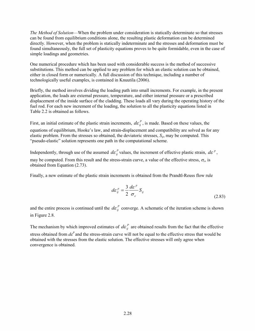
Briefly, the method involves dividing the loading path into small increments. For example, in the present application, the loads are external pressure, temperature, and either internal pressure or a prescribed displacement of the inside surface of the cladding. These loads all vary during the operating history of the fuel rod. For each new increment of the loading, the solution to all the plasticity equations listed in Table 2.2 is obtained as follows.

First, an initial estimate of the plastic strain increments, Pijdε , is made. Based on these values, the

equations of equilibrium, Hooke’s law, and strain-displacement and compatibility are solved as for any elastic problem. From the stresses so obtained, the deviatoric stresses, Sij, may be computed. This “pseudo-elastic” solution represents one path in the computational scheme.

Independently, through use of the assumed Pijdε values, the increment of effective plastic strain, pdε ,

may be computed. From this result and the stress-strain curve, a value of the effective stress, se, is obtained from Equation (2.73).

Finally, a new estimate of the plastic strain increments is obtained from the Prandtl-Reuss flow rule

ij

e

pp

ij Sddsεε

23

= (2.83)

and the entire process is continued until the Pijdε converge. A schematic of the iteration scheme is shown

in Figure 2.8.

The mechanism by which improved estimates of Pijdε are obtained results from the fact that the effective

stress obtained from dεP and the stress-strain curve will not be equal to the effective stress that would be

obtained with the stresses from the elastic solution. The effective stresses will only agree when convergence is obtained.

2.29

Figure 2.8. Schematic of the Method of Successive Elastic Solutions

The question of convergence is one that cannot, in general, be answered a priori. However, convergence can be shown to be obtained for sufficiently small load increments. Experience has shown that this technique is suitable for both steady-state and transient fuel rod analyses.

Extension to Creep

The method of solution described for the time-independent plasticity calculations can also be used for time-dependent creep calculations. In this context, the term “creep” refers to any time-dependent constant volume permanent deformation. Creep is a stress-driven process and is usually highly dependent on temperature.

The only change required to extend the method of successive elastic solutions to allow consideration of creep is to rewrite the Prandtl-Reuss flow rule [Equation (2.80)] as

( )m

c

e

cc tVStd

ssss

sεε 321

11 95.1

++∆+

∆=

( )m

c

e

cc tVStd

ssss

sεε 321

23 95.1

++∆+

∆=

(2.84)

( )m

c

e

cc tVStd

ssss

sεε 321

33 95.1

++∆+

∆=

The first term on the right-hand side of each of these equations computes the constant volume creep strain, whereas the second term in each equation computes the permanent change in volume. To use this form of the flow rule, two additional material property correlations must be available. The first is a

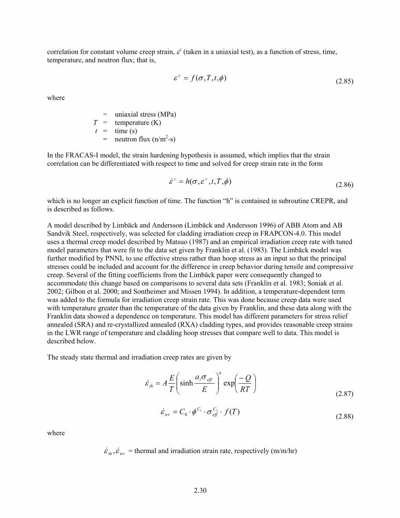
2.30

correlation for constant volume creep strain, εc (taken in a uniaxial test), as a function of stress, time, temperature, and neutron flux; that is,

),,,( φsε tTfc = (2.85) where = uniaxial stress (MPa) T = temperature (K) t = time (s) = neutron flux (n/m2-s)

In the FRACAS-I model, the strain hardening hypothesis is assumed, which implies that the strain correlation can be differentiated with respect to time and solved for creep strain rate in the form

),,,,( φεsε Tth cc = (2.86)

which is no longer an explicit function of time. The function “h” is contained in subroutine CREPR, and is described as follows.

A model described by Limbäck and Andersson (Limbäck and Andersson 1996) of ABB Atom and AB Sandvik Steel, respectively, was selected for cladding irradiation creep in FRAPCON-4.0. This model uses a thermal creep model described by Matsuo (1987) and an empirical irradiation creep rate with tuned model parameters that were fit to the data set given by Franklin et al. (1983). The Limbäck model was further modified by PNNL to use effective stress rather than hoop stress as an input so that the principal stresses could be included and account for the difference in creep behavior during tensile and compressive creep. Several of the fitting coefficients from the Limbäck paper were consequently changed to accommodate this change based on comparisons to several data sets (Franklin et al. 1983; Soniak et al. 2002; Gilbon et al. 2000; and Sontheimer and Missen 1994). In addition, a temperature-dependent term was added to the formula for irradiation creep strain rate. This was done because creep data were used with temperature greater than the temperature of the data given by Franklin, and these data along with the Franklin data showed a dependence on temperature. This model has different parameters for stress relief annealed (SRA) and re-crystallized annealed (RXA) cladding types, and provides reasonable creep strains in the LWR range of temperature and cladding hoop stresses that compare well to data. This model is described below.

The steady state thermal and irradiation creep rates are given by

−

=

RTQ

Ea

TEA

neffi

th expsinhs

ε (2.87)

)(210 TfC C

effC

irr ⋅⋅⋅= sφε (2.88) where irrth εε , = thermal and irradiation strain rate, respectively (m/m/hr)

2.31

These rates are added together, so

irrthirrth εεε +=+ (2.89)

The saturated primary hoop strain is given by

( ) 05.2109.0 )35500tanh(20216.0 −++ ⋅−⋅= irrthirrth

sp εεε

(2.90)

The total thermal strain is given by

( )( ) tt irrthirrthspH ⋅+⋅⋅−−= ++ εεεε 52exp1 (2.91)

In FRAPCON-4.0, strain rate is used. Taking the derivative with respect to time of the expression above gives

( ) irrthirrth

irrthsp

H tt

+++ +⋅⋅−

⋅

⋅⋅= εε

εεε

52exp

2

5221

21

(2.92) where T = temperature (K) t = time (hours) seff = effective stress (MPa) φ = fast neutron flux (n/m²-s)

The first term in Equation 2.92 represents the primary creep. It has been observed that following significant changes in stress or stress reversals, the primary creep is best related to the change in effective stress and the direction of the change in hoop stress (Geelhood 2013). In FRAPCON-4.0 the first term in Equation 2.92 is calculated based on the time since the last significant stress change (> 5MPa) using the change in effective stress and in the direction of the change in hoop stress.

Table 2.3 lists the parameters used in these equations for SRA and RXA cladding types. These parameters are those recommended by Limbäck and Andersson (Limbäck and Andersson 1996), with the exception of the “A” parameter and the “f(T)” parameter, that were modified by PNNL.

2.32

Table 2.3. Parameters for FRAPCON-4.0 Creep Equation for SRA and RXA Cladding

Parameter Units Values for SRA Cladding Values for RXA Cladding A K/MPa/hr 1.08E9 5.47E8 E MPA 1.149-59.9*T ai MPa-1 650{1-0.56[1-exp(-1.4E-27*Φ1.3)]}

Φ = fast neutron fluence (n/cm²) n unitless 2.0 3.5 Q kJ/mole 201 R kJ/mol-K 0.008314 C0 (n/m²-s)-C1

MPa-C2 4.0985E-24 1.87473E-24

C1 unitless 0.85 C2 unitless 1.0 f(T) unitless T<570K 0.7283

570<T<625K -7.0237+0.0136T T>625K 1.4763

0.7994 -3.18562+0.00699132T 1.1840

The effective stress in the cladding is found using the principal stresses at the mid-wall radius using the thick wall formula as follows:

( )

220

2

2222

i

iooiooii

r rrr

PPrrrPrP

−

−+−

=s (2.93)

( )

220

2

2222

i

iooiooii

t rrr

PPrrrPrP

−

−−−

=s (2.94)

220

22

i

ooiil rr

rPrP−−

=s (2.95)

where Pi = inner pressure Po = outer pressure ri = inner radius ro = outer radius r = radius within tube sr = radial stress st = tangential stress sl = longitudinal stress

The effective stress, seff, is then given by

2.33

( ) ( ) ( )( )22221

lrrttleff sssssss −+−+−= (2.96)

The correlations above are developed for SRA and RXA Zircaloy-4 and Zircaloy-2. For M5, the correlation for RXA Zircaloy is used. For ZIRLO and Optimized ZIRLO, the correlation for SRA Zircaloy reduced by a factor of 0.8 is used (Sabol et al. 1994). The steady-state creep coefficient remains the same as for the previous code version, FRAPCON-3.4, however, the primary creep has been changed as described above.

A plot of the resulting creep strain is shown as a function of time and effective stress for representative flux and temperature values in Figure 2.9.

2.34

(a)

(b)

Figure 2.9. Cladding Creep Strain as a Function of Time and Hoop Stress for 630°F and Flux=1018 n/m²/s for (a) SRA Zircaloy and (b) RXA Zircaloy

The second additional correlation required is a relationship between the rate of permanent volumetric strain and the applied loads; that is,

),,,( availmc VtTgV s= (2.97)

0.00%

0.50%

1.00%

1.50%

2.00%

2.50%

3.00%

0 200 400 600 800 1000

Time, days

Accu

mul

ated

Cre

epst

rain

, %

5000 psi 10000 psi 15000 psi

0.00%

0.20%

0.40%

0.60%

0.80%

1.00%

1.20%

0 200 400 600 800 1000

Time, days

Accu

mul

ated

Cre

epst

rain

, %

5000 psi 10000 psi 15000 psi

2.35

where sm = (s1+s2+s3)/3 the mean stress (MPa) T = temperature (K) t = time (s) Vavail = measure of maximum permanent volumetric change possible

The permanent volumetric strain increment dVc is related to the creep strain increments by the equation

cccc ddddV 321 εεε ++= (2.98)

As previously noted, the FRACAS-I model is the default model available for analyzing the small deformation of the fuel and cladding. The model considers the fuel pellets to be essentially rigid and to deform due to thermal expansion, swelling, and densification only. Thus, in the rigid pellet model, the displacement of the fuel is calculated independently of the deformation of the cladding. This rigid pellet analysis is performed with the FRACAS-I subcode.

2.4.1.2 Rigid Pellet Cladding Deformation Model

FRACAS-I consists of a cladding deformation model and a fuel deformation model. If the fuel-cladding gap is closed, the fuel deformation model will apply a driving force to the cladding deformation model. The cladding deformation model, however, never influences the fuel deformation model.

The cladding deformation model in FRACAS-I is based on the following assumptions:

• Incremental theory of plasticity.

• Prandtl-Reuss flow rule.

• Isotropic work-hardening.

• Thick wall cladding (thick wall approximation formula is used to calculate stress at midwall.

• If fuel and cladding are in contact, no axial slippage occurs at fuel cladding interface.

• Bending strains and stresses in cladding are negligible.

• Axisymmetric loading and deformation of cladding.

The fuel deformation model in FRACAS-I is based on the following assumptions:

• Thermal expansion, swelling, and densification are the only sources for fuel deformation.

• No resistance to expansion of fuel.

• No creep deformation of fuel.

• Isotropic fuel properties.

The cladding and fuel deformation models in FRACAS-I are described below.

Cladding Deformation Model

The rigid pellet cladding deformation subcode (FRACAS-I) consists of four sets of models, each used independently.

2.36

Deformation and stresses in the cladding in the open gap regime are computed using a model which considers a thick wall cylindrical shell with specified internal and external pressures and a prescribed uniform temperature.

Calculations for the closed gap regime are made using a model which considers a cylindrical shell with prescribed external pressure and a prescribed radial displacement of the cladding inside surface. The prescribed displacement is obtained from the fuel expansion models (including swelling) described later in this section. Further, since no slippage is assumed when the fuel and cladding are in contact, the axial expansion of the fuel is transmitted directly to the cladding, and hence, the change in axial strain in the shell is also prescribed.

The decision whether the fuel-cladding gap is open or closed is made by considering the relative movement of the cladding inside surface and the fuel outside surface. At the completion of the FRACAS-I analysis, either a new fuel-cladding gap size or a new fuel-cladding interfacial pressure and the elastic-plastic cladding stresses and strains are obtained.

Two additional models are used to compute changes in yield stress with work-hardening, given a uniaxial stress-strain curve. This stress-strain curve is obtained from the updated MATPRO properties. The first model computes the effective total strain and new effective plastic strain, given a value of effective stress and the effective plastic strain at the end of the last loading increment. The second model computes the effective stress, given an increment of plastic strain and the effective plastic strain at the end of the last loading increment. Depending on the work-hardened value of yield stress, loading can be either elastic or plastic, and unloading is constrained to occur elastically. (Isotropic work-hardening is assumed in these calculations.) These four sets of models are described below.

The determination of whether or not the fuel is in contact with the cladding is made by comparing the radial displacement (delta change) of the fuel surface (ur

fuel) with the radial displacement (delta change) that would occur in the cladding (ur

clad) due to the prescribed external (coolant) pressure and the prescribed internal (fission and fill gas) pressure. The free radial displacement of the cladding is obtained using Equation (2-82). The following expression is used to determine if fuel-cladding contact has occurred:

δ+≥ cladr

fuelr uu (2.99)

where δ = as-fabricated fuel-cladding gap size (m)

If Equation (2-99) is satisfied, the fuel is in contact with the cladding. The loading history enters into this decision by virtue of the permanent plastic cladding strains which are applied to the as-fabricated geometry. These plastic strains, and total effective plastic strain, εP, are retained for use in subsequent calculations.

If the fuel and cladding displacements are such that Equation (2.99) is not satisfied, the fuel-cladding gap has not closed during the current step and the solution obtained by the open gap solution is appropriate. The current value of the fuel-cladding gap size is then computed and is used in the temperature calculations. The plastic strain values may be changed in the solution if additional plastic straining has occurred.

If Equation (2.99) is satisfied, however, fuel and cladding contact has occurred during the current loading increment. At the contact interface, radial continuity requires that

2.37

δ−= fuelr

cladlr uu (2.100)

while in the axial direction the assumption is made that no slippage occurs between the fuel and the cladding. This state is referred to as “lockup.”

Note that only the additional strain which occurs in the fuel after lockup has occurred is transferred to the cladding. Thus, if clad

oz ,ε is the axial strain in the cladding just prior to contact, and fueloz ,ε is the

corresponding axial strain in the fuel, then the no-slippage condition in the axial direction becomes

fueloz

fuelz

cladoz

cladz ,, εεεε −=− (2.101)

The values of the “prestrains”, fueloz ,ε and clad

oz ,ε , are set equal to the values of the strains that existed in the fuel and cladding at the time of fuel-cladding gap closure and are stored and used in the cladding sequence of calculations. The values are updated at the end of any load increment during which the fuel-cladding gap is closed.

After cladru and clad

zε have been computed, they are used in a calculation which considers a cylindrical shell with prescribed axial strain, external pressure, and prescribed radial displacement of the inside surface. After the solution is obtained, a value of the fuel-cladding interfacial pressure is computed along with new plastic strains and stresses.

The open gap modeling considers a cylindrical shell loaded by both internal and external pressures. Axisymmetric loading and deformation are assumed. Loading is also restricted to being uniform in the axial direction, and no bending is considered. The geometry and coordinates are shown in Figure 2.10. The displacements of the midplane of the shell are u and w in the radial and axial directions, respectively.

2.38

Figure 2.10. Fuel Rod Geometry and Coordinates

For this case, the equilibrium equations are identically satisfied by the thick wall approximation below.

t

PrPr ooii −=θs (2.102)

22

22

io

ooiiz rr

PrPr−−

=s (2.103)

where sq = hoop stress (MPa) sz = axial stress (MPa) ri = inside radius of cladding (m) ro = outside radius of cladding (m) Pi = fuel rod internal gas pressure (MPa) Po = coolant pressure (MPa) t = cladding thickness (m)

For membrane shell theory, the strains are related to the midplane displacements by

zw

z ∂∂

=ε (2.104)

2.39

ru

=θε (2.105)

where r is the radius of the midplane. Strain across the thickness of the shell is allowed. In shell theory, since the radial stress can be neglected, and since the hoop stress, sq, and axial stress, sz, are uniform across the thickness when bending is not considered, the radial strain is due only to the Poisson effect and is uniform across the thickness. (Normally, radial strains are not considered in a shell theory, but plastic radial strains must be included when plastic deformations are considered.)

The stress-strain relations are written in incremental form as

∫+++−=T

T

PPz dTd

E0

}{1θθθθθ αεενssε (2.106)

∫+++−=T

Tz

Pz

Pzzz dTd

E0

}{1 αεενssε θ (2.107)

∫++++−=T

Tr

Pr

Przr dTd

E0

}{ αεεssνε θ (2.108)

where To = strain-free reference temperature (K) α = coefficient of thermal expansion T = current average cladding temperature (K) E = modulus of elasticity ν = Poisson’s ratio

The terms Pθε , P

zε , and Prε are the plastic strains at the end of the last load increment, and Pd θε , P

zdε ,

and Prdε are the additional plastic strain increments which occur due to the new load increment.

The magnitude of the additional plastic strain increments is determined by the effective stress and the Prandtl-Reuss flow rule, expressed as

21

])()()[(2

1 222θθ sssss ++−= zze (2.109)

ie

pp

i Sddsεε

23

= for i = r, θ, z (2.110)

)(31

ziiS sss θ +−= for i = r, θ, z (2.111)

2.40

The solution of the open gap case proceeds as follows. At the end of the last load increment the plastic strain components, P

θε , Pzε , and P

rε are known. Also the total effective plastic strain, εP, is known.

The loading is now incremented with the prescribed values of Pi, Po, and T. The new stresses can be determined from Equations (2.102) and (2.103), and a new value of effective stress is obtained from Equation (2.109).

The increment of effective plastic strain, dεP, which results from the current increment of loading, can now be determined from the uniaxial stress-strain curve at the new value of se, as shown in Figure 2.11. (The new elastic loading curve depends on the value of εP

old.)

Figure 2.11. Calculation of Effective Stress se from dεP

Once dεP is determined, the individual plastic strain components are found from Equation (2.110), and the total strain components are obtained from Equations (2.106) through (2.108).

The displacement of the inside surface of the shell must be determined so that a new fuel-cladding gap width can be computed. The radial displacement of the inside surface is given by

ritrru εεθ 2

)( −= (2.112)

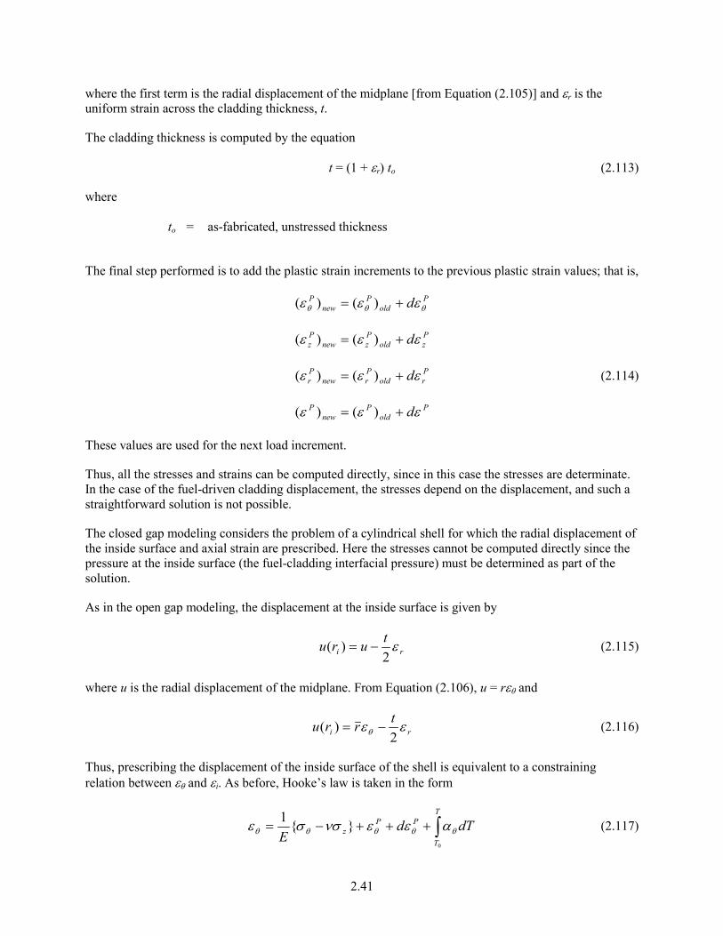
2.41

where the first term is the radial displacement of the midplane [from Equation (2.105)] and εr is the uniform strain across the cladding thickness, t.

The cladding thickness is computed by the equation

t = (1 + εr) to (2.113)

where to = as-fabricated, unstressed thickness

The final step performed is to add the plastic strain increments to the previous plastic strain values; that is,

P

oldP

newP d θθθ εεε += )()(

Pzold

Pznew

Pz dεεε += )()(

Prold

Prnew

Pr dεεε += )()( (2.114)

Pold

Pnew

P dεεε += )()(

These values are used for the next load increment.

Thus, all the stresses and strains can be computed directly, since in this case the stresses are determinate. In the case of the fuel-driven cladding displacement, the stresses depend on the displacement, and such a straightforward solution is not possible.

The closed gap modeling considers the problem of a cylindrical shell for which the radial displacement of the inside surface and axial strain are prescribed. Here the stresses cannot be computed directly since the pressure at the inside surface (the fuel-cladding interfacial pressure) must be determined as part of the solution.

As in the open gap modeling, the displacement at the inside surface is given by

rituru ε2

)( −= (2.115)

where u is the radial displacement of the midplane. From Equation (2.106), u = rεθ and

ritrru εεθ 2

)( −= (2.116)

Thus, prescribing the displacement of the inside surface of the shell is equivalent to a constraining relation between εθ and εi. As before, Hooke’s law is taken in the form

∫+++−=T

T

PPz dTd

E0

}{1θθθθθ αεενssε (2.117)

2.42

∫+++−=T

Tz

Pz

Pzzz dTd

E0

}{1 αεενssε θ (2.118)

∫++++−=T

Tr

Pr

Przr dTd

E0

}{ αεεssνε θ (2.119)

Use of Equations (2.116) and (2.119) in Equation (2.117) results in a relation between the stresses sθ and sz, and the prescribed displacement u(ri):

−+

+

=

++−

+++ ∫∫

z

T

T

PPT

T

Pr

Pr

i

rt

rt

E

dTddTdrr

ru

sνsν

αεεαεε

θ

θθ

122

11

21

21)(

00 (2.120)

Equations (2.118) and (2.120) are now a pair of simultaneous algebraic equations for the stresses sθ and sz, which may be written as

=

2

1

2221

1211

BB

AAAA

zss θ (2.121)

where

A11 = rt

21 ν

+

A12 =

−1

2rtν

A21 = - ν A22 = 1

B1 =

++−

+++ ∫∫T

T

PPT

T

Pr

Pr

i dTdEdTdr

Etrru

E00

4)(

αεεαεε θθ

B2 =

++− ∫

T

T

Pz

Pzz dTdEE

0

αεεε

Then the stresses can be written explicitly as

21122211

122221

AAAAABAB

−−

=θs (2.122)

21122211

211112

AAAAABAB

z −−

=s (2.123)

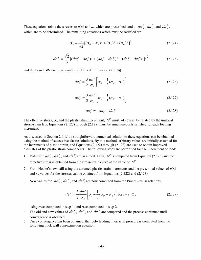
2.43

These equations relate the stresses to u(ri) and εz, which are prescribed, and to Pd θε , Pzdε , and P

rdε , which are to be determined. The remaining equations which must be satisfied are

21

])()()[(2

1 222θθ sssss ++−= zze (2.124)

21222 ])()()[(

32 p

rpz

pz

pppr

p ddddddd εεεεεεε θθ −+−+−= (2.125)

and the Prandtl-Reuss flow equations [defined in Equation (2.110)]

+−= )(

31

23

ze

pp dd sss

sεε θθθ (2.126)

+−= )(

31

23

zze

ppz

dd ssssεε θ (2.127)

pz

ppr ddd εεε θ −−= (2.128)

The effective stress, se, and the plastic strain increment, dεP, must, of course, be related by the uniaxial stress-strain law. Equations (2.122) through (2.128) must be simultaneously satisfied for each loading increment.

As discussed in Section 2.4.1.1, a straightforward numerical solution to these equations can be obtained using the method of successive elastic solutions. By this method, arbitrary values are initially assumed for the increments of plastic strain, and Equations (2.122) through (2.128) are used to obtain improved estimates of the plastic strain components. The following steps are performed for each increment of load:

1. Values of Pd θε , Pzdε , and P

rdε are assumed. Then, dεP is computed from Equation (2.125) and the

effective stress is obtained from the stress-strain curve at the value of dεP.

2. From Hooke’s law, still using the assumed plastic strain increments and the prescribed values of u(ri) and εz, values for the stresses can be obtained from Equations (2.122) and (2.123).

3. New values for Pd θε , Pzdε , and P

rdε are now computed from the Prandtl-Reuss relations,

+−= )(

31

23

zie

pp

idd ssssεε θ for i = r, θ, z (2.129)

using se as computed in step 1, and si as computed in step 2. 4. The old and new values of Pd θε , P

zdε , and Prdε are compared and the process continued until

convergence is obtained. 5. Once convergence has been obtained, the fuel-cladding interfacial pressure is computed from the

following thick wall approximation equation.

2.44

i

oo

rPrt

P+

= θsint (2.130)

When steps 1 through 5 have been accomplished, the solution is complete, provided that the fuel-cladding interface pressure is not less than the local gas pressure.

However, due to unequal amounts of plastic straining in the hoop and axial directions upon unloading, the fuel-cladding interfacial pressure as obtained in step 5 is often less than the gas pressure even though the fuel-cladding gap has not opened. When this situation occurs, the frictional “locking” (which is assumed to constrain the cladding axial deformation to equal the fuel axial deformation) no longer exists. The axial strain and stress adjust themselves so that the fuel-cladding interfacial pressure equals the gas pressure, at which point the axial strain is again “locked.” Thus, upon further unloading, the axial strain and the hoop and axial stresses continually readjust themselves to maintain the fuel-cladding interfacial pressure equal to the gas pressure until the fuel-cladding gap opens. Since the unloading occurs elastically, a solution for this portion of the fuel-cladding interaction problem can be obtained directly as discussed below.

Since the external pressure and the fuel-cladding interfacial pressure are known, the hoop stress is obtained from Equation (2-130) as

t

PrPr ooi −= int

θs (2.131)

From Equation (2.116), the following expression can be written:

r

tu rfuel

r εδεθ

2+−

= (2.132)

Substitution of εθ and εr, as given by Equations (2.117) and (2.119), into Equation (2.132) results in an explicit equation for sz:

( ) ( ) )(2

)2

( iPr

Pzi rEuddTEtddTrEtrr −+−+++= ∫∫ εαεαsνsν θθ (2.133)

in which sθ is known from Equation (2.20). With sz and sθ known, the strains may be computed from Hooke’s law, Equation (2.117) through (2.119). This set of equations is automatically invoked whenever Pint is computed to be less than the local gas pressure.

As in the open gap modeling, the last step is to set the plastic strain components and total effective strain equal to their new values by adding in the computed increments P

idε and Pdε .

The stress-strain modeling is used to relate stress and plastic strain, taking into consideration the direction of loading and the previous plastic deformation. A typical stress-strain curve is shown in Figure 2.12. This curve presents the results of a uniaxial stress-strain experiment and may be interpreted beyond initial yield as the focus of work-hardened yield stresses. The equation of the curve is provided by the updated MATPRO properties at each temperature given in Section 2.4.1.3.

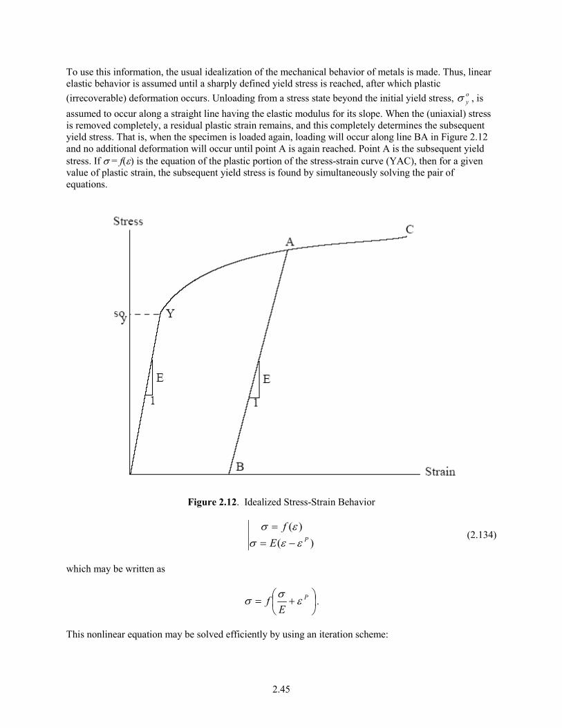
2.45

To use this information, the usual idealization of the mechanical behavior of metals is made. Thus, linear elastic behavior is assumed until a sharply defined yield stress is reached, after which plastic (irrecoverable) deformation occurs. Unloading from a stress state beyond the initial yield stress, o

ys , is assumed to occur along a straight line having the elastic modulus for its slope. When the (uniaxial) stress is removed completely, a residual plastic strain remains, and this completely determines the subsequent yield stress. That is, when the specimen is loaded again, loading will occur along line BA in Figure 2.12 and no additional deformation will occur until point A is again reached. Point A is the subsequent yield stress. If s = f(ε) is the equation of the plastic portion of the stress-strain curve (YAC), then for a given value of plastic strain, the subsequent yield stress is found by simultaneously solving the pair of equations.

Figure 2.12. Idealized Stress-Strain Behavior

)(

)(PE

fεεs

εs−=

= (2.134)

which may be written as

+= P

Ef εss .

This nonlinear equation may be solved efficiently by using an iteration scheme:

2.46

+=+ P

mm

Ef εss 1 m = 0, 1, 2… (2.135)

The initial iterate, sm, is arbitrary, and without loss of generality, is taken as 34.5 MPa. For any monotonically, increasing stress-plastic strain relation, the iteration scheme in Equation (2.135) will converge uniformly and absolutely.

The computations of the stress-strain modeling are described below. The first computes strain as a function of plastic strain, temperature, and stress. The second computes stress as a function of plastic strain, temperature, and plastic strain increments.

Values of plastic strain, εP, temperature, and stress are used as follows:

1. For a given temperature, s= f(ε) is obtained from the updated MATPRO properties given in Section 2.1.4.3.

2. The yield stress sy for given εP is obtained from Equation (2.135).

3. For a given value of stress, s,

if s ≤ sy, Pold

Pnew

P

Eεε

εsε

=

+= (2.136)

if s > sy,

Pold

Pnew

P

Pnew

dE

f

εεε

sεε

sε

−=

−=

= )(

(2.137)

where E is computed using the correlation in the material properties handbook (Luscher and Geelhood 2014).

Values of plastic strain, εP, temperature, and plastic strain increment, dεP, are used as follows:

1. For a given temperature, s = f(ε) is obtained from the updated MATPRO properties given in Section 2.1.4.3.

2. The yield stress sy for given εP is obtained from Equation (2.135).

3. Given dεP (see Figure 2.13).

PPold

Pnew dεεε += (2.138)

2.47

Figure 2.13. Computing Stress

Since dεP > 0, the new value of stress and strain must lie on the plastic portion of the stress-strain curve s = f(ε). So, s and ε are obtained by performing a simultaneous solution, as before.

2.4.1.3 Updated MATPRO Cladding Mechanical Properties Models

The cladding mechanical property correlations remain unchanged from FRAPCON-3.3. The mechanical properties of fuel rod Zircaloy cladding are known to change with irradiation because of damage induced from the fast neutron fluence. The changes are similar to cold-working the material because dislocation tangles are created that tend to both strengthen and harden the cladding while decreasing the ductility. In addition to the fast fluence effects, the presence of excess hydrogen in the Zircaloy, in the form of hydrides, may also affect the mechanical properties.

An analysis of recent data from mechanical testing of irradiated Zircaloy was conducted as part of the development work for FRAPCON and revised equations for use in MATPRO routines were then generated. The revised MATPRO routines have also been incorporated in FRAPTRAN. The following summarizes the revised mechanical property equations.

2.48

Three MATPRO models have been modified to account for the high fast neutron fluence levels, temperature, and strain rate. Those models are a) the strength coefficient in CKMN, b) the strain hardening exponent in CKMN, and c) the strain rate exponent in CKMN. Strength Coefficient, K

The strength coefficient, K, has been modified from MATPRO and is a function of temperature, fast neutron fluence, cold work, and alloy composition. The strength coefficient has not been found to be a function of hydrogen concentration. The fluence dependency, K(Φ), has been modified from MATPRO to better fit the high burnup data. The models for the strength coefficients of Zircaloy-2 and Zircaloy-4 are given below.

)(/))()(1()( ZryKKCWKTKK Φ++⋅= where K = strength coefficient, Pa 32359 72752.11028185.31054859.41017628.1)( TTTTK ⋅+×−×+×=

T<750K

××= 2

66 108500027.2exp10522488.2)(

TTK 750K<T<1090K

TTK 58 104345448.110841376039.1)( ×−×= 1090K<T<1255K 332147 1033.7107579.310685.610330.4)( TTTTK −×−×+×−×= 1255K<T<2100K CWCWK ⋅= 546.0)( ),()10464.11464.0()( 25 TCWfK Φ×+−=Φ − Φ< 0.1x1025 n/m² Φ×=Φ −2610928.2)(K 0.1x1025n/m²<Φ< 2x1025 n/m² Φ×+=Φ −27106618.253236.0)(K 2x1025 n/m²<Φ<12x1025 n/m²

110

550exp,1min)20exp(25.2),( +

−

⋅⋅−=TCWTCWf

In the above equations: K(Zry) = 1 for Zircaloy-4 K(Zry) = 1.305 for Zircaloy-2 T = temperature (K) CW = cold work (unitless ratio of areas) (valid from 0 to 0.75) Φ = fast neutron fluence (n/m²) (E > 1MeV)

The effective cold work and fast neutron fluence used to calculate the strength coefficient, K, can be reduced by annealing if the time and/or temperature are high enough. FRAPCON-4.0 uses the MATPRO model, CANEAL, to calculate the effective cold work and fast neutron fluence at each time step using the following equations.

×−×+−= −

−− 6

18

125

11033.2exp))(102.21(504.1exp

TtCWCW iii φ

2.49

1

20

8

236

20

101035.5exp)(1049.2

10

−

− +

×−×

=

i

i

Tt

φ

φ

where CWi-1, and CWi = the effective cold work for strength coefficient at the start and end of the time

step, respectively (unitless ratio of areas) φI , and φi-1 = effective fast neutron fluence for strength coefficient at the start and end of the

time step, respectively (n/m2) t = time step size (s) T = cladding temperature (K) Strain-Hardening Exponent, n

The strain-hardening exponent, n, has been modified from MATPRO to better fit the high burnup data and is a function of temperature, fast neutron fluence, and alloy composition. The strain hardening exponent has not been found to be a function of hydrogen concentration. The models for the strain hardening exponents of Zircaloy-2 and Zircaloy-4 are given below.

)(/)()( ZrynnTnn Φ⋅= where n = strain hardening exponent 11405.0)( =Tn T<419.4K 3102632 10588.910992.110165.110490.9)( TTTTn −−−− ×+×−×+×−= 419.4K<T<1099.0772K TTn 4105.222655119.0)( −×+−= 1099.0772K<T<1600K 17344880.0)( =Tn T>1600K Φ×+=Φ −251048.0321.1)(n Φ< 0.1x1025 n/m² Φ×+=Φ −2510096.0369.1)(n 0.1x1025 n/m²<Φ< 2x1025 n/m² Φ×+=Φ −2510008727.05435.1)(n 2x1025 n/m²<Φ<7.5x1025 n/m² 608953.1)( =Φn Φ>7.5x1025 n/m²

In the above equations n(Zry) = 1 for Zircaloy-4 n(Zry) = 1.6 for Zircaloy-2 T = temperature (K) Φ = fast neutron fluence (n/m²) (E > 1MeV)

The effective fast neutron fluence used to calculate the strain-hardening exponent, n, can be reduced by annealing if the time or temperature, or both, are high enough. FRAPCON-4.0 uses the MATPRO model, CANEAL, to calculate the effective fast neutron fluence at each time step using the following equation.

2.50

1

20

8

236

20

101035.5exp)(1049.2

10

−

− +

×−×

=

i

i

Tt

φ

φ

where φi, and φi-1 = effective fast neutron fluence for strain hardening exponent at the start and end of

the time step, respectively (n/m2) t = time step size (s) T = cladding temperature (K) Strain Rate Exponent

The strain rate exponent, m, has been modified from MATPRO to better fit the high burnup data and is given by a function of temperature only as described in the equation below.

Error! Objects cannot be created from editing field codes. T<750K

Error! Objects cannot be created from editing field codes. 750K<T<800K

Error! Objects cannot be created from editing field codes. T>800K where m = strain rate exponent T = temperature (K)

The impact of the strain rate exponent on yield stress is to increase the yield strength with increasing strain rate, but the effect is not large. For example, increasing the strain rate from 1×10-4/s to 1.0/s will increase the yield strength by about 15 percent. Assembled Model

Tensile strength, yield strength, and strain are calculated using the same relationships in MATPRO’s CMLIMT subroutine with slight modifications. The true ultimate strength is calculated using

nep

m

K +−

= εεs 310

(2.139)

where σ = true ultimate strength (MPa) K = strength coefficient (MPa) ε = strain rate (unitless) m = strain rate sensitivity constant from MATPRO (unitless) εp+e = true strain at maximum load (unitless) n = strain hardening exponent (unitless)

2.51

This is a change in the original MATPRO model in that the true strain at maximum load in the original model was set equal to the strain hardening exponent. This change was made to better fit the ultimate tensile strength data.

The CMLIMT subroutine equations predicting true yield strength and true strain at yield remain unchanged.

This model is applicable over the following ranges with an uncertainty (standard deviation) on yield and tensile strength of approximately 17 percent relative. A plot of predicted vs. measured yield stress is shown in Figure 2.14. Further data comparisons are shown in Geelhood et al. (2008). cladding temperature: 560 to 700K oxide corrosion thickness: 0 to 100 μm excess hydrogen level: 0 to 650 ppm strain rate: 10-4 to 10-5 s-1 fast neutron fluence: 0 to 12×1025 n/m2 Zircaloy: cold work and stress relieved

Figure 2.14. Predicted vs. Measured Yield Stress from the PNNL Database (293K≤T≤755K),

0≤Φ≤14x1025 n/m2, 0≤Hex≤850 ppm

Rigid Pellet Fuel Deformation in FRACAS-I

This section describes the analytical models used to compute fuel deformation in FRACAS-I. Models are available to calculate length change and fuel radial displacement. Relocation is also considered in FRACAS-I and is also discussed in this section. The effect of relocation is included in the thermal response; however, no hard contact between the fuel and cladding (and therefore no mechanical interaction) is allowed until the other fuel expansion components (swelling and thermal expansion)

0

200

400

600

800

1000

1200

0 200 400 600 800 1000 1200

Measured Yield Stress, MPa

Pred

icte

d Yi

eld

Stre

ss, M

Pa

Axial Tests Burst Tests ANL Axial Tests

2.52

recover 50 percent of the original relocated pellet radius. Therefore, the rigid pellet for mechanical analyses, and that also controls contact conductance, includes 50 percent of the original relocated pellet radius as well as the other pellet expansion components.

The assumptions made with respect to fuel deformation in FRACAS-I are that no pellet deformation is induced by fuel-cladding contact stress or thermal stress and that free-ring thermal expansion applies. Each individual fuel ring is assumed to expand without restraint from any other ring, and the total expansion is the sum of the individual expansions.

Radial Deformation

Radial deformation of the pellet due to thermal expansion, irradiation swelling, and densification is calculated with a free-ring expansion model. The governing equation for this model is

∑=

++−+∆=N

i

di

sirefiTiH TTrR

i1

)(1[ εεα (2.140)

where RH = hot-pellet radius (m)

iTα = coefficient of thermal expansion of the i-th radial temperature (1/K) Ti = average temperature of i-th radial ring (K) Tref = reference temperature (K) ∆ri = width of i-th radial ring (m) N = number of annular rings s

iε = swelling strain (positive)

sdε = densification strain (negative)

The fuel densification and solid fuel swelling models are briefly discussed. The densification asymptotically approaches the (input) ultimate density change, typically over a local (node-average) burnup of approximately 5 GWd/MTU. Solid fuel swelling is considered only as the athermal swelling associated with solid fission product accumulation. It is linear with local (node-average) burnup, and starts following a burnup of 6 GWd/MTU (delayed for swelling into as-fabricated porosity). It then accumulates per time step at a rate equal to 0.062 volume percent per GWd/MTU up to 80 GWd/MTU and 0.086 volume percent per GWd/MTU beyond 80 GWd/MTU (Luscher and Geelhood 2014).

A gasesous swelling model is included in FRAPCON-4.0. The FRAPCON-4.0 model is based on data from Mogensen (Mogensen 1985) and was developed after ramp test results suggested gaseous swelling may influence permanent cladding hoop strain in high burnup rods. The linear strain is given as a function of temperature over the ranges given in the following equations. These models are phased in between 40 and 50 GWd/MTU by applying a factor that varies linearly between 0 and 1 at 40 and 50 GWd/MTU, respectively.

25 1037.41055.4 −− ×−×=∆ Tll (960° < T < 1370°C)

25 1040.71005.4 −− ×+×−=∆ Tll (1370° < T < 1832°C)

2.53

Axial Deformation

Axial deformation of the total fuel stack takes into account the thermal, densification, and swelling strains at each axial node. The calculation proceeds differently for flat-ended versus dished-pellets as described below.

For flat-ended pellets, the volume-averaged ring axial deformation is calculated for each axial node, and these are summed to find the total stack deformation assuming isotropic behavior. The ring deformations account for thermal, densification, and swelling strains specific to each ring.

For dished pellets, the axial deformation of the “maximum ring” (the ring with the maximum deformed length) per node is found, and these “maximum ring” deformations are summed to find the total deformation. Typically, the “maximum ring” is the innermost ring on the dish shoulder because the deformation of the rings within the dish does not fill the dish volume, as illustrated in Figure 2.15.

Figure 2.15. Interpellet Void Volume

Fuel Relocation

Fuel pellet center temperatures measured at beginning of life (BOL) in instrumented test rods have repeatedly been found to be lower than values predicted by thermal performance computer programs when the predicted fuel-cladding gap in operation is calculated based only on fuel and cladding thermal expansion (Lanning 1982). It has long been concluded, based on microscopic examination of fuel cross sections (Galbraith 1973; Cunningham and Beyer 1984), that fuel pellet cracking promotes an outward

2.54

relocation of the pellet fragments that causes additional gap closure. This process begins at BOL and quickly reaches equilibrium. Oguma (1983) characterized this approach to equilibrium based on his analysis of BOL test rod elongation data from Halden instrumented test assemblies.

The fuel pellet cracking that promotes relocation is predominantly radial; however, some circumferential components to these crack patterns exist, and these components could alter the fuel thermal conductivity. Thus, cracking and relocation will to some degree increase the thermal resistance in the pellet while reducing the thermal resistance of the pellet-cladding gap by reducing its effective size. The relocation model implicitly includes any crack effects on heat transfer because the model is based on fuel centerline temperature data.

The best estimate pellet relocation model developed for GT2R2 (Cunningham and Beyer 1984), has been altered for use in FRAPCON in conjunction with the FRACAS-I mechanical model. The original GT2R2 relocation model was altered to provide a best estimate prediction of fuel temperatures for FRAPCON and was included in FRAPCON-3.0 to 3.4. This GT2R2 model is a function of LHGR and burnup that is similar to Oguma’s model, but less complex in form. Because of under-prediction of the centerline temperatures during the first ramp to power noted in the assessment of FRAPCON-3.4, a new model was developed and included in FRAPCON-3.5. The gap closure at beginning of life was fit to the first ramp to power data. Due to the excellent centerline temperature predictions throughout life the FRAPCON-3.4 pellet relocation model beyond 5 GWd/MTU was retained. Data from IFA-677.1 which contained very stable pellets that exhibited little to no densification was available showing stack elongation (which is proportional to fuel temperature) as a function of power for ramps to power at 0.1, 0.6, 4, and 5 GWd/MTU (Thérache 2005). These data demonstrated that the increase in relocation from 0 to 5 GWd/MTU appears to follow a logarithmic trend. Therefore, a logarithmic function was adopted to model the relocation between 0 and 5 GWd/MTU.

The gap closure due to relocation as a fraction of the as-fabricated pellet-cladding gap is given by

055.0/ =∆ GG for burnup less than 0.0937 GWd/MTU

( )( )( )burnuprelocrelocGG ln2447.05795.0,min055.0/ +⋅+=∆ (2.141) for burnup greater than 0.0937 GWd/MTU where ∆G/G = fraction of as fabricated gap closure due to pellet relocation (fraction)

>≤≤−+

<=

40445.04020200/)20(345.0

20345.0

PPP

Preloc

P = local power, kW/ft burnup = local burnup, GWd/MTU

A plot of this model (subroutine GTRLOC) as a function of burnup and LHGR is shown in Figure 2.16. Also shown for reference is the previous relocation model.

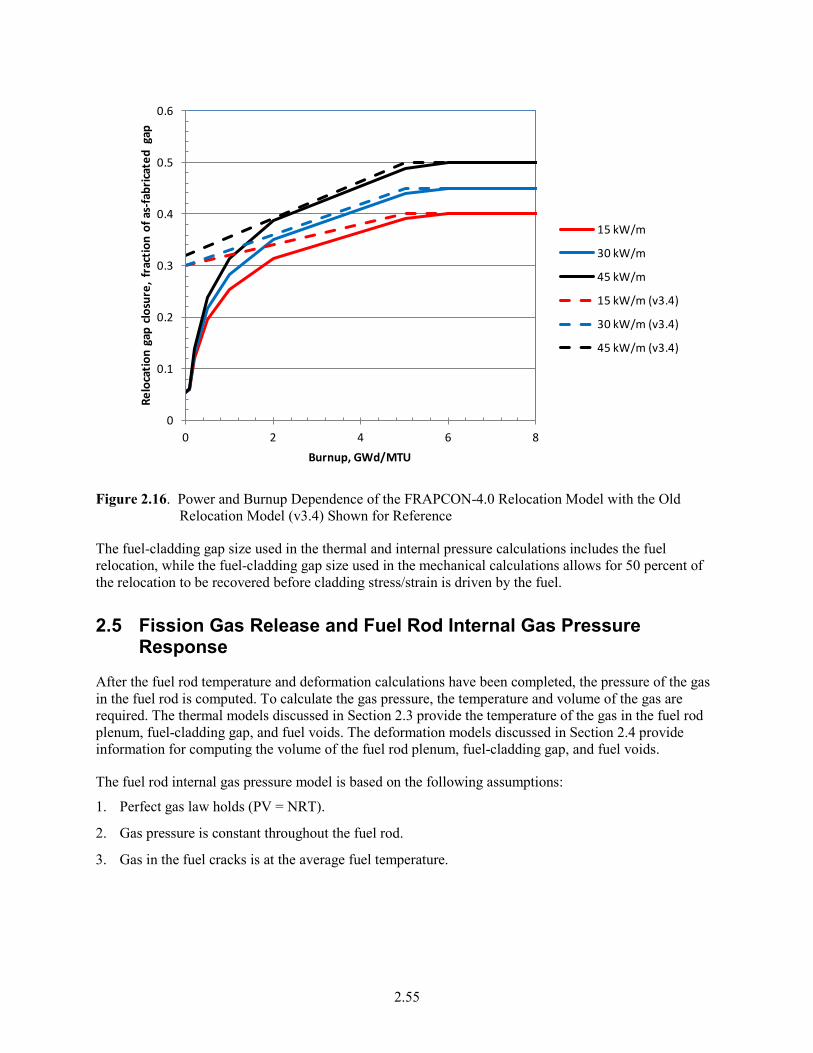
2.55

Figure 2.16. Power and Burnup Dependence of the FRAPCON-4.0 Relocation Model with the Old

Relocation Model (v3.4) Shown for Reference

The fuel-cladding gap size used in the thermal and internal pressure calculations includes the fuel relocation, while the fuel-cladding gap size used in the mechanical calculations allows for 50 percent of the relocation to be recovered before cladding stress/strain is driven by the fuel.

2.5 Fission Gas Release and Fuel Rod Internal Gas Pressure Response

After the fuel rod temperature and deformation calculations have been completed, the pressure of the gas in the fuel rod is computed. To calculate the gas pressure, the temperature and volume of the gas are required. The thermal models discussed in Section 2.3 provide the temperature of the gas in the fuel rod plenum, fuel-cladding gap, and fuel voids. The deformation models discussed in Section 2.4 provide information for computing the volume of the fuel rod plenum, fuel-cladding gap, and fuel voids.

The fuel rod internal gas pressure model is based on the following assumptions:

1. Perfect gas law holds (PV = NRT).

2. Gas pressure is constant throughout the fuel rod.

3. Gas in the fuel cracks is at the average fuel temperature.

0

0.1

0.2

0.3

0.4

0.5

0.6

0 2 4 6 8

Relo

catio

n ga

p clo

sure

, fra

ctio

n of

as-

fabr

icate

d ga

p

Burnup, GWd/MTU

15 kW/m

30 kW/m

45 kW/m

15 kW/m (v3.4)

30 kW/m (v3.4)

45 kW/m (v3.4)

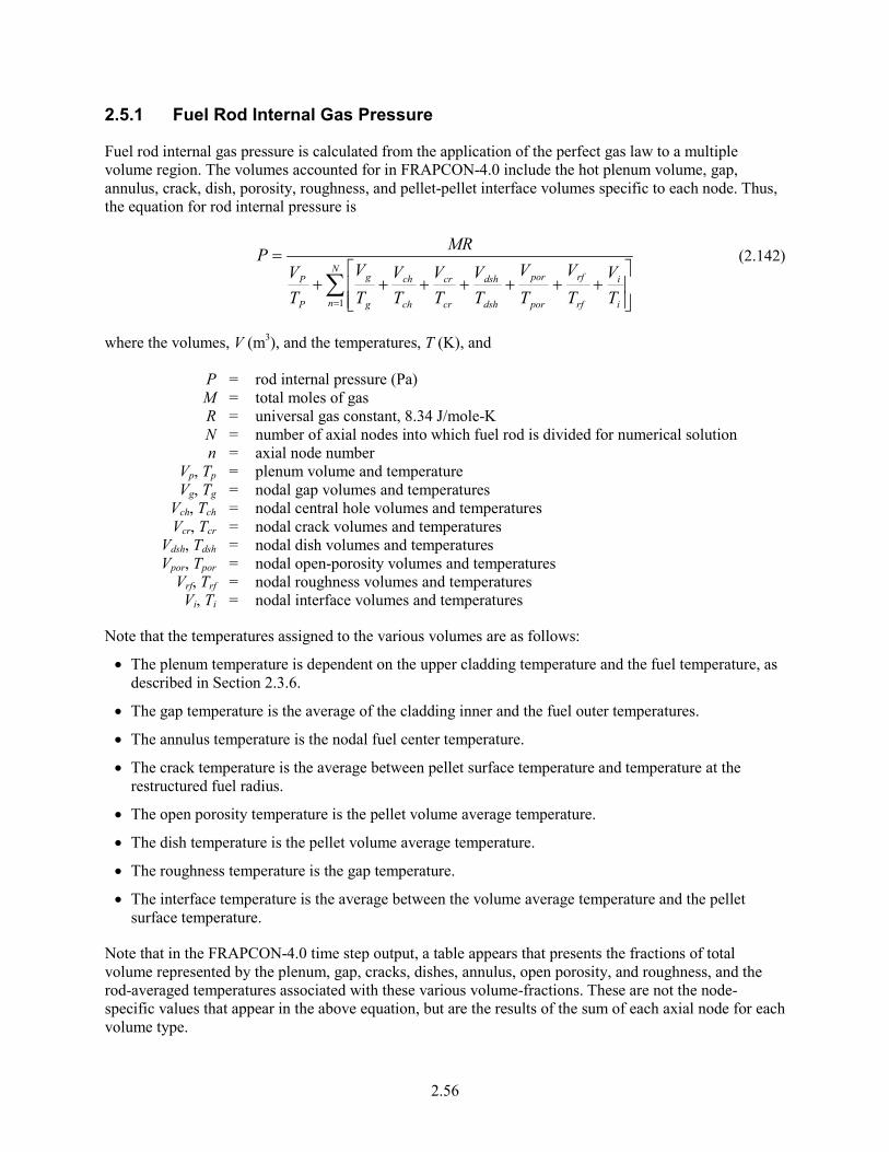
2.56

2.5.1 Fuel Rod Internal Gas Pressure

Fuel rod internal gas pressure is calculated from the application of the perfect gas law to a multiple volume region. The volumes accounted for in FRAPCON-4.0 include the hot plenum volume, gap, annulus, crack, dish, porosity, roughness, and pellet-pellet interface volumes specific to each node. Thus, the equation for rod internal pressure is

∑=

+++++++

=N

n i

i

rf

rf

por

por

dsh

dsh

cr

cr

ch

ch

g

g

P

P

TV

TV

TV

TV

TV

TV

TV

TV

MRP

1

(2.142)

where the volumes, V (m3), and the temperatures, T (K), and P = rod internal pressure (Pa) M = total moles of gas R = universal gas constant, 8.34 J/mole-K N = number of axial nodes into which fuel rod is divided for numerical solution n = axial node number Vp, Tp = plenum volume and temperature Vg, Tg = nodal gap volumes and temperatures Vch, Tch = nodal central hole volumes and temperatures Vcr, Tcr = nodal crack volumes and temperatures Vdsh, Tdsh = nodal dish volumes and temperatures Vpor, Tpor = nodal open-porosity volumes and temperatures Vrf, Trf = nodal roughness volumes and temperatures Vi, Ti = nodal interface volumes and temperatures

Note that the temperatures assigned to the various volumes are as follows:

• The plenum temperature is dependent on the upper cladding temperature and the fuel temperature, as described in Section 2.3.6.

• The gap temperature is the average of the cladding inner and the fuel outer temperatures.

• The annulus temperature is the nodal fuel center temperature.

• The crack temperature is the average between pellet surface temperature and temperature at the restructured fuel radius.

• The open porosity temperature is the pellet volume average temperature.

• The dish temperature is the pellet volume average temperature.

• The roughness temperature is the gap temperature.

• The interface temperature is the average between the volume average temperature and the pellet surface temperature.

Note that in the FRAPCON-4.0 time step output, a table appears that presents the fractions of total volume represented by the plenum, gap, cracks, dishes, annulus, open porosity, and roughness, and the rod-averaged temperatures associated with these various volume-fractions. These are not the node-specific values that appear in the above equation, but are the results of the sum of each axial node for each volume type.

2.57

The gas pressure calculation, therefore, requires information on the gas inventory, void volumes, and the void temperatures, which is provided by the following supportive models.

2.5.2 Fission Gas Production

Given production rates for the major diffusing gases, the burnup-dependent total fission gas generated at axial elevation z is calculated as

)(100

)()()( xenonheliumkryptonv

PRPRPRA

zVFzBUzGPT ++= (2.143)

where GPT(z) = total fission gas produced at z (mole) BU(z) = burnup at z (fission/cm3) VF(z) = fuel volume (cm3) Av = Avogadro’s number PR = fission gas production rate (atoms/100 fissions) for krypton, xenon, and helium

All the fission gas produced, however, is not released. A portion is trapped in the fuel and a portion is released to the fuel-cladding gap volume. Only the released portion is used to calculate the rod internal gas pressure. The gas release fraction is calculated as discussed in the following sections.

2.5.3 Fuel Rod Gas Release

Gas release models in FRAPCON-4.0 account for not only fission gas release (krypton, xenon, and helium) but also nitrogen release. The nitrogen is released from the fuel lattice, where it is trapped during the fuel fabrication process. Fission gas release in FRAPCON-4.0 includes four model options: ANS-5.4 (1982) (Rausch and Panisko 1979); ANS-5.4(2008); the modified Forsberg and Massih model (Forsberg and Massih 1985), modified at PNNL; and the FRAPFGR model developed at PNNL. All four of these release models are based on earlier formulations for diffusion from a sphere by Booth (1957) and are discussed below.

The user can select the Massih model, either ANS-5.4 model, or the FRAPFGR model. The Massih model is recommended by PNNL and is set as the default model. The ANS-5.4 model is useful for calculating the release of short-lived radioactive gas nuclides but is known to provide very conservative values for release. The FRAPFGR model is useful for initializing the transient gas release model in FRAPTRAN-2.0. However, neither the ANS-5.4 model nor the FRAPFGR model predicts stable fission gas release as well as the Massih model does. For this reason, PNNL recommends the Massih model for best-estimate calculation of stable fission gas release.

2.5.3.1 ANS-5.4 (1982) Gas Release Model

The ANS-5.4 (ANS, 1982) fractional fission gas release is calculated as a function of time and radial fuel temperature and axial burnup. The fuel is divided into radial and axial nodes according to the old 1982 American Nuclear Society (ANS) standard. A user requirement is that the time step sizes be such that the burnup increments do not exceed 2 GWd/MTU.

2.58

The modeling is divided into two main sections, one for release of stable isotopes and the other for release of short-lived isotopes. There are high- and low-temperature models for both the stable and radioactive fission products. The release is calculated using both the high-temperature and the low-temperature models, and the larger release value is used. Time steps should not exceed 50 days.

The ANS-5.4 fission gas release model (ANS 1982) is incorporated as specified by the standard and will not be described in this document. A revised ANS-5.4 fission gas release model has been recently approved as a standard (ANS 2011). The 1982 model is not currently an approved standard and provides a very conservative prediction of release in the FRAPCON-3.5 code, while the revised model provides a less conservative prediction even at the 95/95 upper bound. The 1982 model is retained in FRAPCON-4.0 for compliance with various regulations. The new ANS-5.4 standard (ANS 2011) is also available and is described below.

2.5.3.2 ANS-5.4 (2011) Gas Release Model The new ANS-5.4 standard was approved in 2011 and it provides a methodology for determining the radioactive releases from fuel rods, and to determine radiological consequences of postulated accidents. The model is based on the assumption that no significant power transient will occur, such as reactivity insertion accidents (RIAs). This model includes volatile and gaseous fission products of primary importance such as krypton, xenon, iodine, and cesium. The largest contributor to the equivalent dose to individuals is generally I-131, which is included in the model. The radioactive gaseous and volatile fission products are divided into two categories: (1) short-lived radioactive nuclides with half life < 1 year and (2) long-lived radioactive nuclides with half-life > 1 year. This distinction is particularly important when considering diffusion processes that proceed slowly as compared to the decay time for the nuclides under consideration. The model presented in the ANS 5.4 2011 standard is applicable to short lived nuclides; a further distinction is applied in the standard for nuclides with half life smaller than six hours, and nuclides with half lives greater than six hours but smaller than sixty days. The first incarnation of the ANS-5.4 standard was first implemented in 1982 and it was originally based on the Booth diffusion model. The model coefficients were determined rom the measured release data for xenon and krypton. Because of the lack of data for I-131, the diffusion coefficient for this nuclide was assumed to be a factor of seven higher than the one used for xenon and krypton. However, in the last twenty-five years, fuel experiments in test reactors have been performed and measured data have been used to validate the standard at higher burnups. Based on this data it was also concluded that the prediction for I-131 was overly conservative. The fission gas release model from ANS 5.4 2011 (ANS 2011) implements the model described in the standard and it calculates the release-to-birth ratio (R/B), or the so-called “gap release” for short-lived and long-lived nuclides, as defined by the standard. The nuclides considered by the model are listed in Table 2.4 and Table 2.5, together with their respective decay constants and the precursor coefficients for radioactive nuclides. The nuclides are categorized as short lived if their half-life is less than six hours, while they are considered long lived, if their half-life is greater than six hours but less than sixty days. It should be noted that Table 1 in (ANS 2011) does not contain all the nuclides mentioned in the text of the document. Due to this issue, it was necessary to obtain the complete nuclide list and associated physical parameters from (Turbull and Beyer 2011)

2.59

Table 2.4. Decay Constants and Precursor Coefficients for Noble Gases and Iodines with half-life < 6 h

Nuclide Precursor Coefficient (α) Decay Constant (sec-1)

Type of Nuclide

Xe-135m 23.5 7.55E-4 Short Lived Xe-137 1.07 3.02E-3 Short Lived Xe-138 1.0 8.19E-4 Short Lived Xe-139 1.0 1.75E-2 Short Lived Kr-85m 1.31 4.30E-5 Short Lived Kr-87 1.25 1.52E-4 Short Lived Kr-88 1.03 6.78E-5 Short Lived Kr-89 1.21 3.35E-3 Short Lived Kr-90 1.11 2.15E-2 Short Lived I-132 137 8.44E-5 Short Lived I-134 4.4 2.20E-4 Short Lived

Table 2.5. Decay Constants and Precursor Coefficients for Noble Gases and Iodines with 6 h < half-life < 60 days

Nuclide Precursor Coefficient (α) Decay Constant (sec-1)

Type of Nuclide

Xe-133 1.25 1.53E-6 Long Lived Xe-135 1.85 2.21E-5 Long Lived I-131 1.0 9.98E-7 Long Lived I-133 1.21 9.26E-6 Long Lived

The subroutine computes mainly two terms:

• Real Array: RB_axial (15, na), where na is the number of axial meshes defined for the fuel rod • Real Array: RB_rod (15, nt), where nt represents the number of time steps considered for the

problem RB_axial represents the axial distribution of the gap release for the fifteen nuclides listed in Table 2.4and Table 2.5 for the current time step. RB_rod contains the accumulated gap release for each nuclide at each time step for the entire fuel rod. Note that the model requires a number of axial meshes greater or equal to 11, in order to accurately predict the fission gas release.

2.5.3.3 Modified Forsberg-Massih Model

The original Forsberg-Massih model begins with a solution of the gas diffusion equation for constant production and properties in a spherical grain:

)(),()( ttrCtDdtdC

r β+∆= (2.144)

where C = gas concentration β = gas production

∆r =

+

drd

rdrd 2

2

2

2.60

D = diffusion constant t = time

with boundary conditions C(r,0) = 0 C(a,t) = 0

Forsberg and Massih attempt to solve the equation for the case where there is re-solution of gas on the grain surface, which changes the outer boundary condition to

D

tNtbtaC2

)()(),( λ= (2.145)

where N = surface gas concentration λ = resolution layer depth a = hypothetical grain radius b = resolution rate

They make use of a four-term approximation to the integration kernel, K, where

∫∫ −=τ

ττβττp0

0000

2 )()(),(4 dKdrtrCr e

a

(2.146)

and

Deββ = (2.147)

Dt=τ (2.148) and

∑∞

=

−

=1

2

2

22

3exp

8n n

an

aK

τp

p (2.149)

Low-Temperature Fission Gas Release Model at High Burnup

The modified Forsberg-Massih model is used to calculate fission gas release unless the low-temperature fission gas release model predicts a higher value for fission gas release. The low-temperature fission gas release model is defined as

CBUF +×= −5107 (2.150) where

2.61

F = fission gas release fraction BU = local burnup in GWd/MTU C = 0; for BU ≤ 40 GWd/MTU = 0.01(BU-40)/10; for burnup > 40 GWd/MTU and F ≤ 0.05

Grain Boundary Accumulation and Re-Solution

The final solution for a given time step, without re-solution and with constant production rate during the step, can be written as

∫

−−

+=∆2

1

000221 )()(exp)(τ

τ

τττττ dqaB

AGfG nnnnn (2.151)

∑=

∆=∆4

1nnGG (2.152)

∆G = change in gas concentration in fuel grain

∫∑ −+=∆2

1

00021 )()()(τ

τ

τττττ dqfunctAGfG nnnB (2.153)

∆GB = change in gas concentration on grain boundaries

1))((

exp 202 −

−−

=a

Bf n

nττ

(2.154)

fn = fission gas production fraction remaining in the grain from the previous time step where q is determined from

tfunctB

Afqa

n n

nn ∆=

∆+

− ∑

=

βτ )(4

1

2 (2.155)

where

funct (∆τ) = ∫ −2

1

)( 02

τ

τ

τττ dfunct

funct (∆τ) =

−

−

−

202

202 36 2

1

aaττττ

p if τ < 0.1

funct (∆τ) =

−−− 2

0222 exp61

aττ

pp

if t > 0.1

2.62

An and Bn are constants given by Massih.

22 43 aKaKp

−=

233 Ka

K =

∑=

−=+

4

123 exp1

n

nn a

BAK

τ, n = 1, 2, 3, 4

In modifying the original model, we have chosen to introduce re-solution by defining the partition of the gas arriving at the boundary each time step as follows:

∆ Re-solved Gas BGF

F∆

+=

1 (2.156)

F

GG BB +

∆=∆

1 (2.157)

where F = FITMULT[1.84 x 10-14 x GRN/(3 x D)] GRN = grain radius (m) D = diffusion constant (m2/s) FITMULT = an empirical multiplier on the term in brackets that is the original Massih equation

for the resolution rate (FITMULT = 300)

It should be noted that, although F is unitless in Massih’s derivation, it does not represent the fraction of retained gas.

Diffusion Constant

The diffusion constant in the original Forsberg-Massih model is defined over three temperature ranges, as follows:

)/6614exp(1009.1 17 TD −×= − , T > 1650K

)/22884exp(1014.2 13 TD −×= − , 1381 < T < 1650K

)/9508exp(1051.1 17 TD −×= − , T < 1381K

D = diffusion constant (m2/s)

In the FRAPCON-4.0 subroutine, MASSIH, only the mid-range diffusion constant (number 2 above), is generally used, and the activation energy term (Q/R) is 22884 * 1.15. If the modified constant from MASSIH is less than the low-range Massih diffusion constant (number 3 above), the latter is used. The high-temperature diffusion constant (number 1 above) is not used. Above 1850K, the diffusion constant calculated at 1850K is used.

2.63

A burnup enhancement factor multiplies the mid-range diffusion constant (number 2 above) and has the

form 4021

100−BURNUP

, where BURNUP = burnup in GWd/MTU with a maximum value of 20000 for this enhancement factor. A factor of 12 is applied to the burnup-enhanced diffusion constant as a final step.

Gas Release

The gas is accumulated at the grain boundary until a saturation concentration is achieved, at which time the grain boundary gas is released. The saturation area density of gas is given by

+

= ext

B

cS P

rTKVrF

N γθ

θ 2)(sin3

)(42 (2.158)

where Ns = saturation concentration, atoms/m2

θ = dihedral half-angle = 50° KB = Boltzman constant γ = surface tension = 0.6 (J/m2) Vc = critical area coverage fraction = 0.25 r = bubble radius = 0.5 microns F(θ) = 1 - 1.5 cos(θ) + 0.5 cos3(θ) Pext = external pressure on bubbles = gas pressure (Pa)

The final modification to the original model was to release both the grain boundary and the re-solved gas whenever the saturation condition is achieved and the grain boundary gas is released.

To summarize, optimized parameters have been applied based on comparisons to selected steady-state and transient data:

The activation energy (Q/R) = 1.15*22884. = 29060 (high temperature diffusion).

The resolution parameter = 300 x 1.84E-14 = 1.47E-12.

Burnup enhancement factor on diffusion constant = 100(BURNUP-21)/40

Multiplier on the diffusion constant = 12.0 (applied after all other modifications).

2.5.3.4 FRAPFGR Model

The FRAPFGR model has been developed at PNNL to initialize the transient release model in FRAPTRAN that is used to calculate fission gas release during fast transients such as a reactivity initiated accident. Because of this, it is important that the FRAPFGR model predict not only the steady state gas release, but also the amount of gas that remains within the grains and the amount of gas that is currently residing on the grain boundaries for each axial and radial node. The grain boundary gas is released during a fast transient due to cracking along the grain boundaries. To do this, gas release data as well as electron probe microanalysis (EPMA) and X-ray fluorescence (XRF) data have been used to validate that the model can accurately predict these parameters.

2.64

The basic layout of the FRAPFGR model is similar to the modified Massih model with the following differences.

Grain Growth Model

The FRAPFGR model accepts an input grain size that can be specified in the input. The default value for this is 10 micrometers (µm) using the mean linear intercept (MLI) method. The subcode uses a grain growth model proposed by Khoruzhii et al. (1999) given by

−−=

iraaaK

dtda 111

max

(2.159)

where

dtda = grain radius growth rate (µm/hour)

−

×=T

K 32100exp1024.5 7

T = temperature (K) a = grain size (µm)

−

×=T

a 7620exp1023.2 3max

−

⋅

⋅=

TTFair

5620exp5.326140050

F = fission rate, MW/tU

Equation (2.159) is solved by dividing the current time step into 100 steps and solving assuming constant rates within each sub-step.

High Burnup Rim Thickness and Porosity

The high burnup rim that is observed in the outer edge of high burnup pellets can be characterized in terms of sub-micron grains and high porosity. These two items are modeled in the FRAPFGR model. The size of the high burnup rim has been measured by optical microscopy (Manzel and Walker 2002) and is modeled using the equation

427.4610439.1 BUtrim−×= (2.160)

where trim = thickness of high burnup rim (µm) BU = pellet average burnup (GWd/MTU)

Figure 2.17 shows how the high burnup structure is modeled in FRAPFGR. The calculated value of ttim sets a thickness on the pellet surface that is entirely restructured grains. The grain size (MLI) for these grains is set at 0.15µm. The next region, which has a width also set by trim, is composed of a mixture of

2.65

restructured grains and non-restructured grains. The fraction of restructured grains decreases linearly to zero across this thickness of this region. If the temperature in a given axial node is greater than 1000°C, then no restructured grains are assumed to form.

Figure 2.17. Modeling the Pellet High Burnup Rim Structure in FRAPFGR

In addition to the restructured grains, there is also a porosity increase within the high burnup rim. The porosity is modeled based on a fit to observations on high burnup fuel (Spino et al. 1996; Une et al. 2001; and Manzel and Walker 2000). This model is given by

621.45)ln(283.11 −= localBUP if BUlocal > 57 GWd/MTU (2.161)

0=P if BUlocal < 57 GWd/MTU where P = porosity increase in high burnup rim structure (fraction theoretical density) BUlocal = local radial node burnup, GWd/MTU

This porosity is subtracted off the input theoretical density, which is used to calculate the production in each radial node. Therefore, as the porosity in the rim increases, the power production in the outer radial nodes is slightly decreased due to increase porosity.

Diffusion Constant

The diffusion constant used in FRAPFGR is given by

231015.1)( −×=TD T < 675K

trim trim

Fraction, restructured grains

0

1

Pellet Center Pellet Edge

2.66

)/9508exp(1051.1)( 17 TTD −×= − 675K < T < 1381K

)/22884exp(1014.2)( 13 TTD −×= − 1381K < T < 1650K (2.162)

)/34879exp(1014433.7)( 10 TTD −×= − 1650K < T < 1850K

181063.4)( −×=TD T > 1850K where D = diffusion constant (m²/s) T = temperature (K)

The diffusion constant is modified for the effects of burnup using the formula in Equation (2.163).

For non-restructured grains

⋅+=

−

12)12,min(1010)(),( 40

)0,21max( BuTDBuTDBu

(2.163)

up to a maximum adjustment of 49.81

For restructure grains, there is no burnup adjustment. where D(T,Bu) = diffusion constant adjusted for burnup (m2/s) D(T) = temperature dependent diffusion constant given by Equation (2-162) (m2/s) Bu = local radial node burnup (GWd/MTU)

The diffusion constant is also modified for the effects of low power using an error function

)3(5.15.2

),(),,(−−

=Powerf

BuTDPowBuTD (2.164)

where D(T, Bu, Pow) = diffusion constant adjusted for burnup and power (m2/s) D(T, Bu) = diffusion constant adjusted for burnup given by Equation (2-163) (m2/s) Pow = local radial node power (kW/ft)

Gas Release

Gas release calculations are performed separately for restructured grains and non-restructured grains. For those nodes that contain both restructured and non-restructured grains, the releases from each are combined based on the relative amount of each type of grain.

2.67

For the restructured grains, it is assumed that, because the grains are so small, all the gas produced in the grain will diffuse out to the grain boundary. Therefore, the only gas that will remain in these grains at the end of the time step is the gas that is re-solved back into the grains.

The gas re-solved back into the grain is given by the resolution factor from Massih (Forsberg and Massih 1985). The gas that is in the grain for a given time step, i, is given by

f

fGBGG ii += − 11 (2.165)

where GG = gas in grains (moles/m3) GB = gas on grain boundaries (moles/m3)

D

af3

1084.1 14−×= (2.166)

where a = grain radius (0.075×10-6 m for restructured grains) D = diffusion constant (m2/s)

For the non-restructured grains, the same formulas as those in MASSIH are used to calculate diffusion from the grains except that the release is reduced to account for resolution during the calculation of release. The following terms are changed as follows.

From Equation (2.153), the following term is changed:

resolterm

GfGf nn

nn∑∑ →

)()( 1

1

ττ (2.167)

From Equation (2.155), the following term is changed:

resolterm

functB

Af

functB

Af n n

nn

n n

nn

∆+

−

→

∆+

−

∑∑ =

=

)()(

4

14

1

ττ (2.168)

where )00282.0exp(14009.0,1max( Tresolterm = T < 1528.77K Tresolterm 0082.0976.22,1max( −= T > 1528.77K T = temperature (K)

In order for gas to be released from the grain boundaries, the saturation concentration must be reached. The saturation concentration is given by

2.68

a

Ngs s

23

= (2.169)

where gs = grain boundary saturation concentration (moles/m3) Ns = saturation area density given in Equation (2-146) (moles/m2) a = grain radius (m)

When the grain boundary gas concentration for a given radial node exceeds the saturation value for the first time, all the gas on the grain boundary except 65 percent of the saturation value is released. From then on for that radial node, any gas above 65 percent of the saturation values is released.

As discussed, for radial nodes that contain some restructured grains and some non-restructured grains, the released gas is calculated as

)1()( 22

21 erestructurrelerestructurrelreltot −∆+∆=∆ (2.170)

where ∆reltot = total release from a radial node (moles/m3) ∆rel1 = release from restructured grains in a radial node (moles/m3) ∆rel2 = release from non- restructured grains in a radial node (moles/m3) restructure = fraction of restructured grains in radial node

As with the MASSIH model, an athermal release term of 1 percent for every 10 GWd/MTU beyond 40 GWd/MTU is added on if the predicted release is less than 5 percent to account for the observed gas release from rods with very low power at high burnup.

2.5.4 Nitrogen Release

The release of nitrogen initially present in fuel material from fabrication occurs as a result of a diffusion transport mechanism. The release of nitrogen affects the rod internal pressure and the gas conductivity. The model proposed by Booth (1957) is used, given the following assumptions:

1. The initial concentration of diffusing substance, C, is uniform throughout a sphere of radius, a.

2. Transport of material does not occur from the external phase (gaseous nitrogen) back into the initial carrier medium.

The governing equation is

⋅

∂∂

=∂∂ )(2

2

rCr

DtCr (2.171)

where r = radial location (m) C = concentration of diffusing substance t = time (s) D = diffusion coefficient (m2/s)

2.69

with C = 0.0, when r = a C = C, when t = 0

By applying a series solution method, the fractional release of the diffusing substance (nitrogen) can be approximated based on the value of B:

ta

DB N

22 2p= (2.172)

where

22

aDN = temperature-dependent diffusion coefficient for nitrogen divided by the effective

diffusion radius squared (s-1) t = time from the start of diffusion (s)

Then, when B > 1, the fraction of nitrogen released as of time, t, equals

)exp(61 22BFN −−=

p (2.173)

and, when B < 1,

ta

Dt

aD

F NNN 2

5.0

222

23/6 −

= p (2.174)

From the experimental data of Ferrari (1963, 1964)

=

TaDN

9869.133400exp73.12

2 (2.175)

where T = temperature (K)

2.5.5 Helium Production and Release

Helium is produced at different rates in UO2 and MOX. The release of helium affects the rod internal pressure and the gas conductivity.

For UO2, helium production is given by

gasprodSAtQHeprod ⋅⋅⋅×= −1810297.1 (2.176)

2.70

where Heprod = helium produced for a given axial node (moles) Q = surface heat flux (W/m2) t = time (s) SA = axial node surface area (m2) gasprod = number of fission gas atoms produced per 100 fissions (default value = 31)

For MOX, a formula has been developed as a function of Pu concentration and burnup:

))(())(( 212

21 BUBPuBBUAPuAHeprod +++= (2.177) where Heprod = helium produced for a given axial node (moles) BU = node burnup (GWd/MTU)

Table 2.4 shows the fitting parameters that should be used for reactor-grade plutonium and weapons-grade plutonium.

Table 2.6. Fitting Parameters for Helium Production in MOX

Reactor-Grade Plutonium Weapons-Grade Plutonium A1 1.5350x10-4 -2.4360x10-4

A2 2.1490x10-3 3.6059x10-3

B1 -2.9080x10-3 3.3790x10-3

B2 9.7223x10-2 5.3658x10-2

The above equations calculate the amount of helium produced as a function of time. In order to calculate the helium released to the void volume, an approach similar to the approach for nitrogen release is used. By applying a series solution method, the fractional release of the diffusing substance (helium) can be approximated based on the value of B:

ta

DB He

22p= (2.178)

where

2aDHe = temperature dependent diffusion coefficient for helium divided by the effective

diffusion radius squared (s-1) t = time from the start of diffusion (s)

If t ≤ 1/(p2DHe/a2) then the fraction of helium released, FHe, as of time, t, equals

2.71

2

5.0

2 23

4a

tDa

tDF HeHe

He −

=

p (2.179)

If this fraction is greater than 0.57, then, when B < 1, the fraction of helium released as of time, t, equals

B

BFHe)653644.0)exp(607927.0(1 −−

+= (2.180)

and, when B >1,

1=HeF (2.181)

102 10452847.0 −×=

aDHe if T ≤ 873 K (2.182)

−

××= −

TaDHe 1

16731

986.1104exp1028.0

45

2 if T > 873 K (2.183)

Some fuel designs use a thin layer of ZrB2 applied to the surface of the pellets to act as an integral fuel burnable absorber (IFBA). The use of such coatings produces a large amount of helium. The following empirical correlation was fit to results from Monte Carlo N-Particle (MCNP), a neutron transport code, for helium production from IFBA liners.

)10)(()10)(( 212

21 BBIFBABBAIFBAAHeprod +++−= (2.184) where Heprod = helium production (atoms He/cm³-s) IFBA = percent of fuel rods in a core containing IFBA liners (percent) (valid only between

10 and 50 percent) B10 = boron-10 enrichment (percent) (valid from 0 to 90 percent) A1 = 6.23309x10-9 A2 = 7.02006x10-7 B1 = -1.35675x10-7 B2 = 3.1506x10-4

It can be seen from Equation (2.184) that the helium production rate is a function of the number of IFBA rods in a core and the boron-10 enrichment. Helium is produced as the boron-10 burns out until there is no more boron-10 in the liners. The rate of boron-10 depletion is equal to the helium production rate. The depletion of boron-10 is calculated in the code and the boron-10 enrichment, B10 in Equation (2.184), at the end of the time step is used to calculate the helium production for the next time step.

It is assumed in the code that all helium produced in the ZrB2 coatings is released directly to the rod-free volume.

2.72

2.5.6 Fuel Rod Void Volumes

Void volumes computed by FRAPCON-4.0 include the pellet dishing, pellet chamfers, the fuel-cladding gap, the crack, the plenum, the open porosity, and the roughness volume. These are calculated as indicated below.

2.5.6.1 Pellet Dish and Chamfer Volumes

The volume between pellets is calculated and included as part of the overall volume in the internal gas pressure model. The interpellet volume is calculated at each time step based on hot-pellet geometries. Figure 2.15 shows 1) a cold-pellet interface configuration for the case where the pellets are dished and 2) an exaggerated hot-pellet interface configuration. The void volume available for internal fill gas is defined by the cross-hatched areas (a and b in the figure). The dish volume is that portion of the hot interpellet volume that is within the dishes, excluding the volume of any central hole. The chamfer volume is included in the portion of the hot interpellet volume that is outside the dishes.

2.5.6.2 Interface Volume

The pellet-pellet interface volume is calculated as the difference between the hot interpellet volume and the dish volume.

2.5.6.3 Fuel-Cladding Gap Volume

The fuel-cladding gap volume is calculated by considering the area between two concentric cylinders. The outer cylinder is assumed to have a diameter equal to the diameter of the cladding inside surface based on plastic deformation. The inside cylinder is assumed to have a diameter equal to the diameter of the relocated fuel pellets.

2.5.6.4 Fuel Crack Volume

As the fuel expands, extensive cracking occurs due to the high thermally induced stresses, resulting in a relocated fuel surface. The crack volume is computed as

Vc= Vg- Veg - VTX (2.185) where Vc = fuel crack volume per unit length (m2) Veg = fuel volume per unit length defined by expanded radial nodes, including the

thermal expansion, swelling, and densification (m2) VTX = the computed fuel-cladding gap volume per unit length based on the relocated fuel

surface (m2) Vg = the volume per unit length within the thermally expanded cladding (m2)

2.5.6.5 Plenum Volume

The plenum volume is calculated from geometry considerations of the thermally expanded cladding and the thermal expansion, densification, and swelling of the fuel. The volume of the hold-down spring is considered.

2.73

2.5.6.6 Open Porosity Volume

A portion of the initial fabrication porosity is open to free gas flow, which is given by the expressions

Vpor = 0.0 when Gden ≥ 94.0 (2.186)

Vpor = 1.97 x 10-8 (94.0 - Gden) when 91.25 < Gden< 94.0 (2.187)

31028

4

10497.21043.1

818.31077.2

denden

denpor

GG

GV−−

−

×+×−

−×= when Gden < 91.25 (2.188)

where Vpor = porosity volume per unit length (m2) Gden = DEN - 1.25 DEN = fuel density (percent of theoretical density)

It should be noted that most commercially fabricated fuel today has little open porosity.

2.5.6.7 Roughness Volume

The roughness of the surface of the fuel and cladding results in a small void volume accounted for by

f

Prough V

DV p51027.5 −×= (2.189)

where Vrough = roughness volume per unit length (m2) DP = initial pellet diameter (m) Vf = geometric fuel volume per unit length (m2)

The gas pressure response resulting from the above models feeds back into the mechanical and temperature response models in the iteration scheme.

2.5.6.8 Central Hole Volume

The central hole volume is calculated by considering the area of the central hole (if present), the length of the axial node, and the length of the central hole.

2.6 Waterside Corrosion and Hydrogen Pickup

2.6.1 PWR and BWR Waterside Corrosion Models

For Zircaloy-4 under pressurized-water reactor (PWR) conditions, a cubic rate law for corrosion-layer thickness as a function of time is applied until a transition thickness of 2.0 microns is attained (Garzarolli et al. 1982):

2.74

−

=1

12

3

exp)(RT

QsA

dtsd (2.190)

In FRAPCON-4.0, this equation is integrated without regard to the feedback between oxide layer thickness and oxide metal interface temperature to obtain

( )31

311

1

11 exp3

+−

−

= ++ iii sttRT

QAs (2.191)

where i, i+1 = refers to (ends of) previous and current time step s = oxide thickness (m) A = 6.3x109 (m3/day) Q1 = 32289 (cal/mol) R = 1.98 (cal/mol-K) T1 = metal-oxide interface temperature (K) t = time (days)

After the transition thickness is attained, a flux-dependent linear rate law is applied, with the rate constant being an Arrhenius function of oxide-metal interface temperature:

{ }

−Φ+=

1

20 exp)(

RTQMUC

dtds P (2.192)

Because there is significant feedback between oxide-layer thickness and oxide-metal interface temperature, the oxide thickness is converted to weight gain, and the approximate integral solution from Garzarolli et al. (1982) is used. This solution has the form

1

1222

022

2

2

1 )("

expexp"1ln"

−

++

−

∆

−−+∆=∆ ii

o

i

oo

oii tt

RTwqQ

RTQk

RTqQ

qQRT

wwλ

γλ

γγ

λ (2.193)

Weight gain can be converted to thickness using the following formula:

100

γws ∆= (2.194)

2.75

where i, i+1 = refers to (ends of) previous and current time step s = oxide thickness (m) ∆w = weight gain (g/cm2) R = 1.98 (cal/mol-K) To = oxide-to-water interface temperature (K) λ = oxide thermal conductivity (W/cm-K) γ = 0.6789 (cm3/g) Q2 = 27354 (cal/mol) q" = heat flux (W/cm2) k0 = 11863+3.5x104(1.91x10-15Φ)0.24 (g/(cm2-day)) Φ = fast neutron flux (E>1 MeV) (n/cm2/s) t = time (days)

For M5 under PWR conditions, the same equations are used with the following changes.

• Q1 = 27446 (cal/mol)

• Q2 = 29816 (cal/mol)

• Transition thickness at 7 µm

For ZIRLO and Optimized ZIRLO under PWR conditions, the same equations are used with the following changes.

• Q2 = 27080 (cal/mol) for ZIRLO

• Q2 = 27354 (cal/mol) for Optimized ZIRLO

• Above the transition thickness if the oxide thickness is less than 80 µm then use 2*∆wi in the second term of Equation (2.193) and then divide that term by 2 as shown below.

1

1222

022

2

2

1 )(2"

expexp"1ln"2

1−

++

−

∆

−−+∆=∆ ii

o

i

oo

oii tt

RTwqQ

RTQk

RTqQ

qQRT

wwλ

γλ

γγ

λ (2.195)

For Zircaloy-2 under boiling-water reactor (BWR) conditions, a flux-dependent linear rate law is applied, with the rate constant being an Arrhenius function of oxide-metal interface temperature:

+

−=

11

exp"1expRTQCq

RTQK

dtds

(2.196)

Because there is significant feedback between oxide-layer thickness and oxide-metal interface temperature, the oxide thickness is converted to weight gain, and the approximate integral solution from Garzarolli et al. (1982) is used. This solution has the form

")(

)("

expexp"1ln"

1

1

122

2

1

qttCk

ttRT

wQqRT

QkRT

QqQq

RTww

ii

iio

i

oo

oii

−+

−

∆

−−+∆=∆

+

−

++ λγ

λγ

γλ

(2.197)

2.76

Weight gain can be converted to thickness using the following formula:

100

γws ∆= (2.198)

where i, i+1 = refers to (ends of) previous and current time step s = oxide thickness (m) ∆w = weight gain (g/cm2) R = 1.98 (cal/mol-K) To = oxide-to-water interface temperature (K) λ = oxide thermal conductivity (W/cm-K) γ = 0.6789 (cm3/g) Q = 27350 (cal/mol) q" = heat flux (W/cm2) k = 11800 (g/(cm2-day)) Φ = fast neutron flux (E>1 MeV) (n/cm2/s) C = 2.5x10-16 (m2/W) t = time (days)

To achieve numerical stability, the rate equation is integrated across each time step and applied to calculated corrosion layer increments per time step, which are accumulated to calculate cumulative layer thickness as a function of axial position (axial node) along the rod.

2.6.2 Hydrogen Pickup Fraction

The fraction of the hydrogen liberated by the metal-water corrosion reaction that is absorbed locally by the cladding is called the pickup fraction. For PWR conditions, a constant hydrogen pickup fraction has been found to be applicable. For Zircaloy-4, a pickup fraction of 0.15 is used. For M5, a pickup fraction of 0.10 is used. For ZIRLO and Optimized ZIRLO, a pickup fraction of 0.175 is used (Geelhood and Beyer 2011).

For BWR conditions, a constant hydrogen pickup fraction does not fit the observed hydrogen concentration data. Therefore, FRAPCON-4.0 uses a burnup-dependent hydrogen concentration model (Geelhood and Beyer 2008). For Zircaloy-2 prior to 1998 (when the vendors did not have tight control over concentration and second-phase precipitate particle size), the following equations are used

BUBU

H conc 316.01

3.1exp8.47 +

+−

= if BU < 50 GWd/MTU (2.199)

( ))20(117.0exp9.28 −+= BUH conc if BU > 50 GWd/MTU (2.200)

For modern Zircaloy-2 since 1998 (when the vendors have had tight control over concentration and second phase precipitate particle size), the following equation is used

( ))20(117.0exp8.22 −+= BUH conc (2.201)

2.77

where Hconc = hydrogen concentration (ppm) BU = local burnup (GWd/MTU)

3.1

3.0 General Code Description

3.1 Code Structure and Solution Routine

FRAPCON-4.0 is a large and complex code that contains over 200 subroutines. This section discusses the code structure, solution scheme, and the major subroutines involved in the solution scheme.

3.1.1 Code Structure

The FRAPCON-4.0 subroutines have been grouped into modules that perform a common function. These modules contain variables that can be passed to other modules as well as the appropriate subroutines and function. All variables are explicitly declared and arrays are dynamically dimensioned for the current problem.

3.1.2 Solution Scheme

Figure 3.1 shows a flowchart of FRAPCON-4.0 beginning with case setup, following through the convergence loops, and ending with output. Each major section of this sequence will be discussed, together with the subroutines involved. To aid this discussion, Figure 3.2 presents an abbreviated outline of the main subprogram, FRAPCON, arranged in the same order as the flowchart. Major subroutines appear in the figure as do the major Fortran loops.

The first portion of the flowchart has to do with case setup and initialization. This includes reading the input data, the dynamic dimensioning procedure, initializing variables, and an initial problem description output. The subroutines listed in Table 3.2 are involved in the setup and initialization.

3.2

Figure 3.1. FRAPCON-4.0 Flowchart

3.3

Figure 3.2. Calling Sequence for FRAPCON-4.0 Subroutines

3.4

Table 3.1. Initialization and Finalization Subroutines

Subroutine Description SETUP Reads the data input pertaining to the problem size requirements. POINTR Performs the dynamic dimensioning procedure. INITIAL Reads the remaining problem description input and initializes the variables. TURBIN Calculates The Initial Concentrations Of U-235,U-238,Pu-239,Pu-240,Pu-241 and

Pu-242. PRINT1 Generates the output, reflecting the initial conditions and specifications of the fuel

rod, and lists the proposed power history. AXHEF Calculates the initial axial power profile as it affects the axial regions of the fuel rod

and also any varying axial power profile changes. GRAFINI Writes the header of the plot file. PRINT2 Writes the calculation summary at the end of the run.

Next, the code enters the first of four major loops in the Fortran coding, the time-step loop. The time-step loop encompasses virtually all of the remainder of the FRAPCON-4.0 code. In each execution of the time-step loop, the code solves for the thermal and mechanical equilibrium of the fuel rod at a new point along the rod power versus time history input by the user. Those subroutines, which are executed only once per time step, are listed in Table 3.3.

Table 3.2. Subroutines in the Time-Step Loop

Subroutine Description AXHEF2 Calculates the axial power shape factors for all axial nodes for the current time step if

there has been a refabrication requested. CANEAL Calculates the change in effective fluence and effective cold work during a time step. STORE Stores variable values as necessary to account for history dependency. CCREEP The cladding creep portion of the FRACAS-I mechanics model (the subroutine calls

FCMI, which in turn calls CLADF that calls CREPR where the creep rate model is located).

MECH Main subroutine for the finite element model: calculates the mechanical response of the fuel rod with the finite element method, if selected.

PRINT2 Generates output for the code that presents converged values for all of the axial nodes for both thermal and mechanical solutions.

GRAFOUT Writes data to the plot file. RESTFS Writes data to the restart file.

Three additional loops exist in the code. The next loop encountered within the time-step loop is the gas-release loop. This loop is cycled until the value for calculated rod internal gas pressure (dependent on temperature, volume, and fission gas release) converges. Subroutines called from within this loop are listed in Table 3.4.

3.5

Table 3.3. Subroutines in the Gas-Release Loop

Subroutine Description TOTGAS Calculates the cumulative gas release of fission gas, helium, and nitrogen for the

entire rod, as well as the total moles of gas and mole fractions. PLNT Calculates the current plenum gas temperature and volume. GSPRES Calculates the rod internal gas pressure.

The next inner loop in the coding is the axial-node loop. For every pass through the gas-release loop, the axial-node loop sequences through each of the axial regions defined by the input. The subroutines controlled by this loop are listed in Table 3.5.

Table 3.4. Subroutines in the Axial-Node Loop

Subroutine Description BURNUP Calculates the local fuel burnup. GASPRO Calculates the fission gas production. COOLT Calculates the coolant temperature. FLMDRP Calculates the temperature drop from the cladding surface to the coolant. CORROS Calculates the corrosion on the cladding surface. CLADRP Calculates the temperature drop from the cladding inside surface to the cladding

outside surface. TUBRNP Calculates the radial power and burnup distribution. VOLUME Calculates the void volumes including plenum, crack, dish, chamfers, gap, and open

porosity. MASSIH Calculates fission gas release based on Forsberg and Massih solution to the booth

diffusion problem.

The innermost loop is the gap conductance loop. This loop iterates on each axial node until thermal equilibrium in the radial direction is achieved. Thermal equilibrium is signified by a converged value for the calculated temperature drop from the fuel outer surface to the cladding inner surface. The subroutines listed in Table 3.6 comprise the gap conductance loop.

3.6

Table 3.5. Subroutines in the Gap Conductance Loop

Subroutine Description TMPSUB Calculates the radial temperature distribution through the fuel. FUELTP Solves the equations for the radial heat balance. FEXPAN Fuel thermal expansion routine. SWELL Calculates fuel swelling and fuel densification. FRACAS This subroutine calculates the new position of the cladding due to deflection caused

by internal gas pressure changes. MECH Main subroutine for the finite element model: calculates the mechanical response of

the fuel rod with the finite element method, if selected. NEWGAP Calculates the new fuel-cladding gap size (used with the FRACAS mechanics model

only). CONDUC Calculates new values for the gap conductance and the fuel-cladding gap temperature

drop. GAPRS Computes gap conductance accounting for radiation heat transfer across gas gap and

gap thickness change.

At the completion of all the time steps, and before returning to the driver package, a final call to PRINT2 is made. This call prints a summary table for the entire power history of the rod.

3.2 Code Results

FRAPCON-4.0 generates fuel rod response information as a function of fuel rod fabrication information, boundary conditions, and power history. This information is provided to the user as printed output and as plots (optional). The capability also exists to supply this information for steady-state initialization of the FRAPTRAN computer code. The information provided to the transient fuel rod analysis code consists of permanent burnup effects, such as cladding creepdown, fuel swelling, fuel densification, normalized radial power and burnup profiles, and fission gas inventory in the fuel matrix and the fuel rod void volume. This section presents the important response parameters, the plotting package, and information on the FRAPCON link with FRAPTRAN.

3.2.1 Fuel Rod Response

FRAPCON provides the calculated fuel rod thermal, mechanical, and pressure response data. The results are presented in three forms: an axial-region printout, a power-time step printout, and a summary-page printout.

The axial-region printout presents local information on power, time, time step, and burnup. Also presented are rod radial-temperature distribution, coolant temperature, cladding stresses and strains (both recoverable and permanent), gap conductance, fuel-cladding interfacial pressure, and coolant film heat-transfer information for each axial node.

The power-time step printout presents rod burnup, void volumes and associated temperatures, mole fractions of constituent gases and release fractions, total moles of rod gas, and rod gas pressure. Also, this printout presents stresses, strains, temperatures, and stored energy for each axial node.

3.7

The summary page printout presents time-dependent information about the hot axial node. This includes temperatures of the cladding, fuel-cladding gap, and fuel; fuel-cladding interfacial pressure; cladding stress and strain; fuel outside diameter; gap conductance and gas pressure; Zircaloy oxide thickness; and hydrogen uptake.

3.2.2 Plot Package

The input instructions, Appendix A, identify the option to specify a file (FILE66) for graphics data output. This file is designed to be read by a PNNL-developed routine that works with Excel software. The file name needs to be specified in the input file as FILE66. When using the Excel input generator, this is done automatically. The Excel plot routine will be provided along with the FRAPCON-4.0 code to users. The user instructions for the Excel plot routine are shown in Appendix B.

3.2.3 FRAPTRAN Initialization

FRAPCON-4.0 contains subroutine RESTFS, which, when the flag NTAPE is set to 1, stores sets of history-dependent information for each power-time step. This information is stored on unit TAPE1 and is for FRAPTRAN initialization. This gives the user the ability to model the fuel rod initial conditions following steady-state operation accumulating significant burnup before a transient excursion.

3.3 Features of FRAPCON-4.0

FRAPCON-4.0 has been designed with special features to aid the user. These features include options for the code solution, an Excel input file generator, and options for uncertainty analysis.

3.3.1 Code Solution

FRAPCON-4.0 has been dynamically dimensioned so that a minimum of core storage is required for any given fuel modeling process. Parameters that are a function of the problem size are dimensioned to the exact size required by the axial and radial nodalization and the number of power-time steps. The user can set the core size based on the number of axial and radial nodes and the number of time steps.

3.3.2 Excel Input Generator

The input to FRAPCON-4.0 is a text file with variables described in Appendix A input through namelist format. It has been found that the manual creation of such an input file can be a time consuming process, can be subject to errors (particularly unit errors), and can be difficult for a new user to learn how to set up.

To assist with all these issues, an Excel Input Generator has been created. In this file, users fill in the requested information with different units available in dropdown boxes. The Excel Input Generator then creates the text file with the required units that FRAPCON-4.0 reads as input. The Excel Input Generator is available for download on the FRAPCON-/FRAPTRAN Code Users’ Group webpage. The instructions for using the Excel Input Generator are shown in Appendix A.

3.3.3 Uncertainty Analysis

One use fuel performance codes is running bounding design calculations. To do this, the models in the fuel performance code and the fuel rod design inputs must be biased up or down based on their

3.8

uncertainty levels. Since FRAPCON-4.0 is a best-estimate fuel performance code, it had not previously been possible to perform these studies on the effect of model uncertainties without changing the code. To facilitate these studies, standard deviations for the models in FRAPCON-4.0 that are known to most impact the outputs of regulatory interest have been calculated based on the available data. These standard deviations have been hardwired into the code, and new input variables have been added that allow the user to select the level of uncertainty to apply (e.g., +1s or -1.6s).

The FRAPCON-4.0 models selected to allow for a bounding design calculation were those expected to have a significant impact on outputs of regulatory interest such as rod internal pressure, fuel centerline temperature, and cladding strain. A sample sensitivity study was performed for a typical PWR and BWR rod (Geelhood et al. 2009) and based on the results of this study; eight models were identified as necessary in a bounding design calculation in FRAPCON-4.0. The eight models selected are

• fuel thermal conductivity

• fuel thermal expansion

• fission gas release

• fuel swelling

• irradiation creep

• cladding thermal expansion

• cladding corrosion

• cladding hydrogen pickup

These models may be biased through the use of the appropriate input variables in Appendix A. Table 3.7 lists the input variables used to bias the models and the built-in standard deviations. This table also identifies if an absolute or relative standard deviation is used.

3.9

Table 3.6. Input Variables for Uncertainty Analysis in FRAPCON-4.0

Input Variable (multiplier) Model Applied to Material Standard Deviation Relative Absolute sigftc Fuel thermal

conductivity UO2 8.8% X

sigftex Fuel thermal expansion

UO2 10.3% X

sigfgr Fission gas release UO2 100% on diffusion coefficient

X

sigswell Fuel swelling UO2, UO2-Gd2O3 0.08% ∆V/V per 10 GWd/MTU <80

GWd/MTU 0.16% ∆V/V per 10

GWd/MTU >80 GWd/MTU

X

sigcreep Cladding creep SRA 14.5% X RXA 21.6% X

siggro Cladding axial growth

Zircaloy-2 20.3% X Zircaloy-4 22.3% X

ZIRLO™ and Optimized ZIRLO™

0.05% Strain X

M5™ 18.6% X sigcor Cladding corrosion Zircaloy-2 7.6 µm X

Zircaloy-4 15.3 µm X ZIRLO™ and

Optimized ZIRLO™

15 µm X

M5™ 5 µm X sigh2 Cladding hydrogen

pickup Zircaloy-2 prior to

1998 10 ppm, <45 GWd/MTU 54 ppm, >50 GWd/MTU

X

Zircaloy-2 since to 1998

13 ppm, <45 GWd/MTU 60 ppm, >50 GWd/MTU

X

Zircaloy-4 94 ppm X ZIRLO™ and

Optimized ZIRLO™

110ppm X

M5™ 23 ppm X

3.10

3.3.4 Refabrication Capability

The capability to model a rod that has been refabricated following some period of irradiation and then further irradiated has been added in FRAPCON-4.0. The further irradiation of a segment of a full length rod with new plenum size and fill gas pressure may be accomplished with no restart file, simply through input variable selection.

This capability improves the ability of FRAPCON-4.0 to model power ramp tests and Halden instrumented fuel assembly irradiations that have been taken from sections of full length commercial rods and refabricated into short length rod segments for irradiation in test reactors such as Halden.

Appendix A describes the new input variables that have been added to the $frpcon namelist that the user can use to model refabrication.

In order to use these options to effectively model refabrication, the user may wish to take advantage of the ability in FRAPCON-3.5 to use variable length axial nodes to obtain the exact refabrication length and axial location. Additionally, the fill gas pressure, fgpavrefab, will be the pressure given the temperature and void volume predicted for the time step specified in irefab. If refabrication is performed at room temperature, it is recommended to add an extra time step with no power and room temperature surface conditions as this time step is used to accurately predict the number of gas moles put into the refabricated rod.

The code has been changed in the axial node loops to loop from jmin to jmax, rather than from node 1 to node X, where X is the number of axial nodes. In this way, the code can change the values of jmin and jmax at different time steps, to simulate the refabrication. At the time of refabrication, those variables that are changed following refabrication (plenum length and spring dimensions) are set to their new values. A new value of total stack length is calculated based on the nodes that are selected. The input axial power profiles are re-normalized over the remaining axial nodes.

The calculation of rod average burnup is repeated over the new rod length. Both the helium and fission gas inventory and release calculations are reset to calculate the fraction of helium and fission gas that is released following the refabrication. Following refabrication, the helium and fission gas release fractions will be the fraction of the total gas produced over the entire irradiation, but will not include gas released prior to refabrication. The coolant inlet temperature is fed into the boundary condition for the lowest axial node rather than node 1. The input refabricated pressure and gas mixture are imposed on the rod at this time.

Prior to the information related to the first timestep of the refabrication, FRAPCON-4.0 prints a summary of the refabrication. Following this table, a summary of the renormalized axial power profiles is given. After this information the output proceeds as normal, but only outputs information for the axial nodes included in the refabricated rod. After the information about each node is output, the time step summary is given. This summary only shows the axial nodes included in the refabricated rod. In the Excel plotter the information given for each axial node under the 1-D data tab is shown only for those axial nodes in the refabricated rod after the time step where the refabrication was specified. The other axial nodes show values of 0 after the time of refabrication.

3.3.5 Spent Fuel Modeling

The capability to model spent fuel during dry storage has been added in FRAPCON-4.0. This capability is provided by the DATING subcode.

3.11

Additional functionality to model the fuel after discharge was added outside of the dating subcode. These modifications allow the user to continue to use the FRAPCON solution scheme, with the ability to turn off oxidation after a given amount of time, add additional fuel swelling and to model additional gas release. The additional gas release is automatically modeled as Helium and can be used to alter the internal rod pressure and therefore stress on the cladding. Both the additional fuel swelling and additional gas release are input for each timestep.

The ability to model the average decay heat over a timestep was also implemented in FRAPCON-4.0. The decay heat is calculated using the ANS-5.1-2004 Draft Standard. The decay power is calculated for various sub-timesteps within the user supplied timestep (ProblemTime(it) – ProblemTime(it-1)). An average power is then calculated by summing the fraction of the power at each decay step relative to the total time modeled. The decay power takes into account the fraction of power coming from isotopes U-235, U-238, Pu-239 and Pu-241. These values are obtained from the TUBRNP subcode. In order to use this functionality during timestep it, qmpy(it) needs to be input as a negative value (i.e. qmpy(5) = -1.0). The user is able to model multiple decay periods, to mimic typical reactor shutdowns, as well as model multiple timesteps with a decay period, to allow for modeling spent fuel.

3.3.6 Developer Options

A new set of “developer” options have been added to allow the user more flexibility to analyze sensitivities that modeling parameters may have on results. It is cautioned that these options are turned off (not used) when performing the integral assessment. Therefore, any results obtained using these options should be perceived cautiously and understood that they may be outside of the bounds of the capability of the FRAPCON code.

A developer option that can have a significant impact on results is the ability to model gamma-ray heating. This option deposits a fraction of the energy directly into the coolant rather than depositing all of the energy into the fuel. Note that FRAPCON was developed and assessed under the assumption of no gamma heating. A detailed assessment of the impact this may have on results under typical reactor conditions can be found in reference documents. (Porter and Knight, 2014).

There are several developer options related to altering the FRAPCON default models. The user can select between several different fuel relocation models. The default model is the FRAPCON-3.5 model, which is the default in FRAPCON-4.0 as well. The second model is the model from FRAPCON-3.4, details of which can be found in the FRAPCON-3.4 code description. Two additional options include turning relocation off completely, and using a user-supplied value for relocation. The user supplied value is a fraction of the as-fabricated gap thickness, multiplied by a burnup factor. The burnup factor goes from 0 to 1 between 0 and 10 GWd/MTU. A similar option is to manipulate the relocation recovery fraction. By default, FRAPCON assumes that 50% of the relocation is added to the pellet as permanent relocation. Therefore, the other 50% must be recovered by additional fuel swelling and cladding creepdown before hard contact between the fuel and cladding occurs.

A new developer option includes the ability to manipulate the gap conductance via a gap conductance multiplier. This may allow for sensitivity studies to the gap conductance on fuel temperatures. The user also now has the ability to completely turn off the cladding oxidation and hydriding calculations.

For material property modification, the user can set a constant cladding elastic modulus. This may be beneficial when analyzing more rigid claddings than Zircaloy.

There are additional developer options relating to FRAPCON-to-FRAPCON restart capabilities, but these are not currently working in FRAPCON-4.0.

4.1

4.0 References

American Nuclear Society (ANS). 1982. “Method for Calculating the Fractional Release of Volatile Fission Products from Oxide Fuel.” ANS5.4 of the Standards Committee of the American Nuclear Society, ANSI/ANS-5.4-1982.

American Nuclear Society (ANS). 2011. “Method for Calculating the Fractional Release of Volatile Fission Products from Oxide Fuel.” ANS5.4 of the Standards Committee of the American Nuclear Society, ANSI/ANS-5.4-2011.

Berna GA, CE Beyer, KL Davis, and DD Lanning. 1997. FRAPCON-3: A Computer Code for the Calculation of Steady-State, Thermal-Mechanical Behavior of Oxide Fuel Rods for High Burnup. NUREG/CR-6534, Vol. 2, PNNL-11513, Vol. 2, Pacific Northwest National Laboratory, Richland, WA.

Beyer CE, CR Hann, DD Lanning, FE Panisko, and LJ Parchen. 1975. GAPCONTHERMAL-2: A Computer Program for Calculating the Thermal Behavior of an Oxide Fuel Rod. BNWL-1898, Battelle Northwest Laboratory, Richland, WA.

Bohn MP. 1977. FRACAS: A Subcode for the Analysis of Fuel Pellet-Cladding Mechanical Interaction. TREE-NUREG-1028, EG&E Idaho, Inc., Idaho National Engineering Laboratory, Idaho Falls, ID.

Booth AH. 1957. A Method of Calculating Fission Gas Diffusion from UO2 Fuel and Its Application to the X-2 Loop Test. AECL-496, CRDC-721, Atomic Energy of Canada, Ltd., Chalk River Project, Chalk River, Ontario.

Cunningham ME and CE Beyer. 1984. GT2R2: An Updated Version of GAPCONTHERMAL-2. NUREG/CR-3907, PNL-5178, Pacific Northwest Laboratory, Richland, WA.

Dittus F and LMK Boelter. 1930. “Heat Transfer in Automobile Radiators of the Tubular Type.” University of California Publications in Engineering 2(13):443−461.

Ferrari HM. 1963. “Nitrogen Release from UO2 Pellets at Elevated Temperatures.” Nuclear Science and Engineering 17(4):503−512.

Ferrari HM. 1964. “Diffusion of Nitrogen in Uranium Dioxide.” Journal of Nuclear Materials 12(2):142−144.

Forsberg K and AR Massih. 1985. “Diffusion Theory of Fission Gas Migration in Irradiated Nuclear Fuel UO2.” Journal of Nuclear Materials 135:140–148.

Franklin DG, GE Lucas, and AL Bement. 1983. Creep of Zirconium Alloys in Nuclear Reactors. ASTM STP 815, American Society for Testing and Materials, West Conshohocken, PA.

Galbraith KP. 1973. Pellet-Cladding Gap Closure from Pellet Cracking Data and Analysis. XN-73-17, Siemens Power Corporation (Formerly Exxon Nuclear), Richland, WA.

Garzarolli F, W Jung, H Shoenfeld, AM Garde, GW Parray, and PG Smerd. 1982. Review of PWR Fuel Rod Waterside Corrosion Behavior. EPRI NP-2789, Project 1250 Final Report, Electric Power Research Institute, Palo Alto, CA.

4.2

Garnier JE and S Begej. 1979. Ex-Reactor Determination of Thermal Gap and Contact Conductance Between Uranium Dioxide: Zircaloy-4 Interfaces; Stage I: Low Gas Pressure. NUREG/CR-0330, PNL-2696, Pacific Northwest Laboratory, Richland, WA.

Geelhood KJ and CE Beyer. 2011. “Hydrogen Pickup Modeling for Zircaloy-2, Zircaloy-4, M5™, and ZIRLO™.” In Proceedings of the 2011 Water Reactor Fuel Performance Meeting, September 11-14, 2011, Chengdu, China.

Geelhood KJ, CE Beyer, and WG Luscher. 2008. PNNL Stress/Strain Correlation for Zircaloy. PNNL-17700, Pacific Northwest National Laboratory, Richland, WA.

Geelhood KJ, WG Luscher, CE Beyer, DJ Senor, ME Cunningham, DD Lanning, and HE Adkins. 2009. Predictive Bias and Sensitivity in NRC Fuel Performance Codes. NUREG/CR-7001, PNNL-17644, Pacific Northwest National Laboratory, Richland, WA.

Geelhood KJ. 2013. “Implementing Primary Creep Calculations during Stress Changes and Reversals in the Fuel Performance Code FRAPCON-3.” In Proceedings of the 2013 Light Water Reactor Fuel Performance Meeting, September 15-19, 2013.

Geelhood KJ and WG Luscher. 2015a. FRAPCON-4.0 Integral Assessment. PNNL-19418 Vol. 2 Rev. 2, Pacific Northwest National Laboratory, Richland, WA.

Geelhood KJ, WG Luscher, and JM Cuta. 2015b FRAPTRAN-2.0: A Computer Code for the Transient Analysis of Oxide Fuel Rods. PNNL-19400, Vol. 1 Rev. 2, Pacific Northwest National Laboratory, Richland, WA.

Gilbon D, A Soniak, S Doriot, and JP Mardon. 2000. “Irradiation Creep and Growth Behavior, and Microstructural Evolution of Advanced Zr-Base Alloys.” Zirconium in the Nuclear Industry: Twelfth International Symposium, ASTM-STP-1354, Ed. GP Sabol and GD Moan, American Society of Testing and Materials, West Conshohocken, PA, pp. 51−73.

Hagrman DL, GA Reymann, and GE Mason. 1981. A Handbook of Materials Properties for Use in the Analysis of Light Water Reactor Fuel Rod Behavior. MATPRO Version 11 (Revision 2). NUREG/CR-0479 (TREE-1280), prepared by EG&G Idaho, Inc., Idaho Falls, Idaho for the U.S. Nuclear Regulatory Commission, Washington, D.C.

Jens WH and PA Lottes. 1951. Analysis of Heat Transfer, Burnout, Pressure Drop, and Density Data for High-Pressure Water. ANL-4627, Argonne National Laboratory, Argonne, IL.

Khorushii OV, SYu Kourtchatov, and VV Likhanskii. 1999. “New model of equiaxed grain growth in irradiated UO2.” Journal of Nuclear Materials 265:112−116.

Knuutila A. 2006. Improvements on FRAPCON-3/FRAPTRAN Mechanical Modeling. VTT-R-11337-06. VTT, Finland.

Kreith F. 1964. Principles of Heat Transfer, 8th Edition, Scranton: International Book Company.

Lanning DD. 1982. “The Possible Impact of Fuel Pellet Cracking on Inferred Gap Conductance and Stored Energy.” Nuclear Technology 56:565−574.

4.3

Lassman K, C O’Carrol, J VanderLaar, and CT Walker. 1994. “The Radial Distribution of Plutonium in High Burnup UO2 Fuels.” Journal of Nuclear Materials 28:223−231.

Lassman K, CT Walker, and J van de Laar. 1998. “Extension of the TRANSURANUS Burnup Model to Heavy Water Reactor Conditions.” Journal of Nuclear Materials 255:222−233.

Limbäck M and T Andersson. 1996. “A Model for Analysis of the Effect of Final Annealing on the In- and Out-of-Reactor Creep Behavior of Zircaloy Cladding.” Zirconium in the Nuclear Industry: Eleventh International Symposium, ASTM STP 1295, ER Bradley and GP Sabol, Eds., American Society for Testing and Materials, West Conshohocken, PA, pp. 448−468.

Lucuta PG, HS Matzke, and IJ Hastings. 1996. “A Pragmatic Approach to Modeling Thermal Conductivity of Irradiated UO2 Fuel: Review and Recommendations.” Journal of Nuclear Materials 232:166−180.

Luscher WG KJ Geelhood and IE Porter. 2015. Material Property Correlations: Comparisons between FRAPCON-3.5, FRAPTRAN-1.5, and MATPRO. PNNL-19417 Rev.2, Pacific Northwest National Laboratory, Richland, WA.

Manzel R and CT Walker. 2000. “High Burnup Fuel Microstructure and Its Effect on Fuel Rod Performance.” LWR Fuel Performance Meeting, Park City, UT.

Manzel R and CT Walker. 2002. “EPMA and SEM of fuel samples from PWR rods with an average burn-up of around 100 MWd/kgHM.” Journal of Nuclear Materials 301:170−182.

Matsuo Y. 1987. “Thermal Creep of Zircaloy-4 Cladding under Internal Pressure.” Journal of Nuclear Science and Technology 24(2):111−119.

McAdams WH. 1954. Heat Transmission. 34th Edition, New York: McGraw-Hill Book Company, Inc.

Mendelson A. 1968. Plasticity: Theory and Applications. New York: The MacMillan Company.

Mogensen M, CT Walker, ILF Ray, and M Coquerelle. 1985. “Local Fission Gas Release and Swelling in Water Reactor Fuel during Slow Power Transients.” Journal of Nuclear Materials 131:162-171.

Oguma M. 1983. “Cracking and Relocation Behavior of Nuclear Fuel Pellets During Rise to Power.” Nucl. Eng. Design 76:35−45.

Ohira K and N Itagaki. 1997. “Thermal Conductivity Measurements of High Burnup UO2 Pellets and Benchmark Calculation of Fuel Center Temperature.” In Proceedings of the ANS International Topical Meeting on LWR Fuel Performance, pp. 541−549. March 2−6, 1997, Portland, OR.

Porter, IE and TW Knight. “Fuel Performance Assessment when Modeling Gamma Heating During Steady-State and Transient Scenarios.” In Proceedings of ICAPP 2014. April 6-9, 2014.

Rapier AC, TM Jones, and JE McIntosh. 1963. “The Thermal Conductance of Uranium Dioxide/Stainless Steel Interfaces.” International Journal of Heat Mass Transfer 6:397−416.

Rausch WN and F .Panisko. 1979. ANS54: A Computer Subroutine for Predicting Fission Gas Release. NUREG/CR-1213, PNL-3077, Pacific Northwest Laboratory, Richland, WA.

4.4

Ross AM and RL Stoute. 1962. Heat Transfer Coefficients Between UO2 and Zircaloy-2. CRFD-1075, AECL-1552, Atomic Energy of Canada, Limited.

Sabol GP, RJ Comstock, RA Weiner, P Larouere, and RN Stanutz. 1994. “In-Reactor Corrosion Performance of ZIRLO™ and Zircaloy-4,” Zirconium in the Nuclear Industry: Tenth International Symposium, ASTM STP 1245, A.M. Garde and E.R. Bradley, Eds. American Society for Testing and Materials, Philadelphia, PA, pp. 724−744.

Shestopalov A, K Lioutov, L Yegorova, G Abyshov, and K Mikitiouk. 1999. Modification of USNRC’s FRAP-T6 Fuel Rod Transient Code for High Burnup VVER Fuel. NUREG/IA-0164, U.S. Nuclear Regulatory Commission, Washington, D.C.

Soniak A, N L’Hullier, J-P Mardon, V Rebeyrolle, P Boffioux, and C Bernaudat. 2002. “Irradiation Creep Behavior of Zr-Base Alloys.” Zirconium in the Nuclear Industry: Thirteenth International Symposium, ASTM STP 1423, GD Moan and P Rudling, Eds. ASTM International, West Conshohocken, PA, pp.837−862.

Sontheimer F and KL Nissen. 1994. “Evaluation of the Stress Reversal Creep Experiment IFA-585 in the HBWR and the Lift-Off Experiment ROPE-1 in the R2 Studsvik using the Siemens/KWU Clad Creep Model.” Enlarged HPG Meeting on High Burn-up Fuel Performance, Safety and Reliability and Degradation of In-Core Materials and Water Chemistry Effect and Man-Machine Systems Research, HPR-345/28.

Spino J, K Vennix, and M Coquerelle. 1996. “Detailed characterization of the rim microstructure on PWR fuels in the burn-up range 40-67 GWd/tM.” Journal of Nuclear Materials 231:179−190.

Thérache B. 2005. The High Initial Rating Test, IFA-677.1: Results after First Cycle of Irradiation. HWR-819, OECD Halden Reactor Project, Halden, Norway.

Todreas N and G Jacobs. 1973. “Thermal Contact Conductance of Reactor Fuel Elements.” Nuclear Science and Engineering 50:283. Turnbull, J. A. and C. E. Beyer, 2010. Background and Derivation of ANS-5.4 Standard Fission Product Release Model, NUREG/CR-7003, Office of Nuclear Regulatory Research, U.S. NRC.

Une K, K Nogita, T Shiratori, and K Hayashi. 2001. “Rim structure formation of isothermally irradiated UO2 fuel discs.” Journal of Nuclear Materials 288:20−28.

U.S. Nuclear Regulatory Commission. 2007. Standard Review Plan for the Review of Safety Analysis Reports for Nuclear Power Plants: LWR Edition: Section 4.2: Fuel System Design, Revision 3. NUREG-0800, U.S. Nuclear Regulatory Commission, Washington, D.C.

Appendix A –

Input Instructions for the FRAPCON-4.0 Code

A.1

Appendix A

Input Instructions for the FRAPCON-4.0 Code

Input Structure

The NAMELIST input is divided into five sections: case control integers (in $FRPCN); case design and operation descriptors (real and integer variables) located in ($FRPCON); plutonium isotopic distributions (in $FRPMOX), Spent fuel modeling options ($SpentFuel), and developer options to change model parameters ($DEVELOPER). The variables in the first group must be separated by commas and placed between the statement $FRPCN and $END. Similarly, the variables in the second, third, fourth, and fifth groups must be placed between $FRPCON and $END, between $FRPMOX and $END, between $SpentFuel and $END, and between $DEVELOPER and $END, respectively.

Before the NAMELIST input, the following lines must be included in the input file: FILE05='nullfile', STATUS='UNKNOWN', FORM='FORMATTED',

CARRIAGE CONTROL='NONE'

This line sets up a file called “nullfile” which is needed by FRAPCON-3.5.

FILE06=’file.out', STATUS='UNKNOWN', CARRIAGE CONTROL='LIST'

This line specifies the name of the output file. In this case the output file would be called “file.out.”

FILE66='file.plot', STATUS='UNKNOWN', FORM='FORMATTED',

CARRIAGE CONTROL='LIST'

This line is needed if a plot output file is being created. (see definition of variable NPLOT) In this case the plot file would be called “file.plot.”

FILE22=’file.restart',

STATUS='UNKNOWN'

This line is needed if a FRAPTRAN restart file is being created (see definition of variable NTAPE). In this case the restart file would be called “file.restart.”

The above four lines should not exceed 72 spaces, and if they do, continue on the next line with no continuation symbols needed. /**********************************************************************

The line seen above, which is preceded by the character “/”, tells the code that the lines specifying files are complete.

The line immediately after this line is reserved for the case description that will be displayed in the page headers in the output. Up to 72 characters can be inserted here to describe the case.

A.2

After this line the NAMELIST input can be entered. In the above section any line with a “*” in column 1 is considered a comment and will not be read by the code. An example case input is given in Section 2 below.

The following tables describe the input variables to FRAPCON-4.0. Unless otherwise noted in the Limitations/Default value column, the variables should be placed in the $frpcon data input block.

Input Variables Specifying Rod Design Rod Size

Variable Name (type) Description

Units British/SI Limitations/Default Value

dco (R)

Cladding outer diameter inches / meters Required Input

thkcld (R)

Cladding wall thickness inches / meters Required Input

thkgap (R)

Pellet-cladding as-fabricated radial gap thickness inches / meters Required Input

totl (R)

The total (active) fuel column length feet / meters Required Input

cpl (R)

Cold plenum length inches / meters Required Input

(R) = real, (I) = integer Spring Dimensions

Variable Name (type) Description

Units British/SI Limitations/Default Value

dspg (R)

Outer diameter of plenum spring inches / meters Required Input (dgpg should be less than the clad inner diameter)

dspgw (R)

Diameter of the plenum spring wire

inches / meters Required Input

vs (R)

Number of turns in the plenum spring

Dimensionless Required Input

(R) = real, (I) = integer

A.3

Input Variables Specifying Pellet Fabrication Pellet Shape

Variable Name (type) Description

Units British/SI Limitations/Default Value

hplt (R)

Height (length) of each pellet inches / meters Required Input

rc (R)

The inner pellet radius May input one value for entire pellet stack or input values as an array for each axial node starting at the bottom.

inches / meters Default = 0.0

hdish (R)

Height (depth) of pellet dish, assumed to be a spherical indentation

inches / meters Default = 0.0

dishsd (R)

Pellet end-dish shoulder width (outer radius of fuel pellet minus radius of dish)

inches / meters Default = 0.0

chmfrh (R)

Chamfer height inches / meters Default = 0.0

chmfrw (R)

Chamfer width inches / meters Default = 0.0

(R) = real, (I) = integer Pellet Isotopics

Variable Name (type) Description

Units British/SI Limitations/Default Value

enrch (R)

Fuel pellet U-235 enrichment May input one value for entire pellet stack or input values as an array for each axial node starting at the bottom.

Atom % U-235 in total U

Required Input

imox (I)

Index for modeling MOX: 0 = UO2 fuel >0 = mixed oxide fuel 1 = use Duriez/Ronchi/NFI Mod thermal conductivity correlation 2 = use Halden thermal conductivity correlation (if imox>0, must include comp and namelist $FRPMOX)

Dimensionless Default = 0

comp (R)

Weight percent of plutonia in fuel (Must specify if imox>0) May input one value for entire pellet stack or input values as an array for each axial node starting at the bottom.

Weight percent Default = 0.0

moxtype (I)

Type of Pu used in MOX moxtype = 1 reactor grade moxtype = 2 weapons grade

Dimensionless Default = 1 (namelist frpmox)

A.4

Variable Name (type) Description

Units British/SI Limitations/Default Value

enrpu39 (R)

Fuel pellet Pu-239 content Atom % Pu-239 in total Pu

Default = 0.0 (namelist frpmox)

enrpu40 (R)

Fuel pellet Pu-240 content Atom % Pu-240 in total Pu

Default = 0.0 (namelist frpmox)

enrpu41 (R)

Fuel pellet Pu-241 content Atom % Pu-241 in total Pu

Default = 0.0 (namelist frpmox)

enrpu42 (R)

Fuel pellet Pu-242 content Atom % Pu-242 in total Pu

Default = 0.0 (namelist frpmox)

fotmtl (R)

Oxygen-to-metal atomic ratio in the oxide fuel pellet

Dimensionless Default = 2.0 (If MOX fuel is selected, fotmtl should be less than 2.0.)

gadoln (R)

Weight fraction of gadolinia in urania-gadolinia fuel pellets May input one value for entire pellet stack or input values as an array for each axial node starting at the bottom.

Dimensionless Default = 0.0

ifba (R)

Percent of IFBA rods in the core % Default = 0.0

b10 (R)

Boron-10 enrichment in ZrB2 Atom % Default = 0.0

zrb2thick (R)

ZrB2 layer thickness on pellets inches, meters Default = 0.0

zrb2den (R)

Percent theoretical density of ZrB2 TD=6.08 g/cm³

% theoretical density

Default = 90.0

ppmh2o (R)

Parts per million by weight of moisture in the as-fabricated pellets

ppm Default = 0.0

ppmn2 (R)

Parts per million by weight of nitrogen in the as-fabricated pellets

ppm Default = 0.0

(R) = real, (I) = integer Pellet Fabrication

Variable Name (type) Description

Units British/SI Limitations/Default Value

den (R)

As-fabricated apparent fuel density % of theoretical density

Required Input (Theoretical density taken as 10.96 g/cm3)

deng (R)

Open porosity fraction for pellets % of theoretical density

Default = 0.0

roughf (R)

The fuel pellet surface arithmetic mean roughness, peak-to-average

inches / meters Default = 7.87×10-5 in / 2.0×10-6 m

A.5

Variable Name (type) Description

Units British/SI Limitations/Default Value

rsntr (R)

The increase in pellet density expected during in-reactor operation (determined from a standard re-sintering test per NUREG-0085 and Regulatory Guide 1.126) PNNL recommends 0.1 kg/m³ for UO2-Gd2O3 fuel

kg/m3 Required Input

tsint (R)

Temperature at which pellets were sintered

°F / K Default = 2911° F

(R) = real, (I) = integer

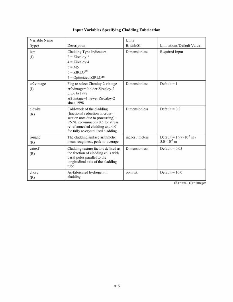
A.6

Input Variables Specifying Cladding Fabrication

Variable Name (type) Description

Units British/SI Limitations/Default Value

icm (I)

Cladding Type Indicator: 2 = Zircaloy 2 4 = Zircaloy 4 5 = M5 6 = ZIRLOTM

7 = Optimized ZIRLO™

Dimensionless Required Input

zr2vintage (I)

Flag to select Zircaloy-2 vintage zr2vintage= 0 older Zircaloy-2 prior to 1998 zr2vintage=1 newer Zircaloy-2 since 1998

Dimensionless Default = 1

cldwks (R)

Cold-work of the cladding (fractional reduction in cross-section area due to processing). PNNL recommends 0.5 for stress relief annealed cladding and 0.0 for fully re-crystallized cladding.

Dimensionless Default = 0.2

roughc (R)

The cladding surface arithmetic mean roughness, peak-to-average

inches / meters Default = 1.97×10-5 in / 5.0×10-7 m

catexf (R)

Cladding texture factor; defined as the fraction of cladding cells with basal poles parallel to the longitudinal axis of the cladding tube

Dimensionless Default = 0.05

chorg (R)

As-fabricated hydrogen in cladding

ppm wt. Default = 10.0

(R) = real, (I) = integer

A.7

Input Variables Specifying Rod Fill Conditions

Variable Name (type) Description

Units British/SI Limitations/Default Value

fgpav (R)

Initial fill gas pressure (taken to be at room temperature)

psia / Pa Required Input

idxgas (I)

Initial fill gas type indictator: 1 = helium 2 = air 3 = nitrogen 4 = fission gas 5 = argon 6 = user-specified mix, using the amfxx variables amfair, etc.

Dimensionless Default = 1

amfair (R)

Mole fraction of air; use only if idxgas = 6.

Mole Fraction Default = 0.0

amfarg (R)

Mole fraction of argon; use only if idxgas = 6.

Mole Fraction Default = 0.0

amffg (R)

Mole fraction of fission gas; use only if idxgas = 6 and if amfxe and amfkry = 0.0.

Mole Fraction Default = 0.0

amfhe (R)

Mole fraction of helium; use only idxgas = 6.

Mole Fraction Default = 0.0 (note default on idxgas = 1 initializes pure He)

amfh2 (R)

Mole fraction of hydrogen; use only if idxgas = 6.

Mole Fraction Default = 0.0

amfh2o (R)

Mole fraction of water vapor; use only if idxgas = 6.

Mole Fraction Default = 0.0

amfkry (R)

Mole fraction of krypton; use only if idxgas = 6.

Mole Fraction

Default = 0.0

amfn2 (R)

Mole fraction of nitrogen; use only if idxgas = 6.

Mole Fraction Default = 0.0

amfxe (R)

Mole fraction of xenon; use only if idxgas = 6.

Mole Fraction Default = 0.0

(R) = real, (I) = integer

A.8

Input Variables Specifying Reactor Conditions

Variable Name (type) Description

Units British/SI Limitations/Default Value

iplant (I)

Signal for which type of reactor: -2 = PWR -3 = BWR -4 = HBWR

Dimensionless Default = -2

nsp (I)

Signal for time-dependent input arrays for p2, tw, and go: If nsp = 0, single values for these three variables will be used for all time steps. If nsp = 1, a value for each variable for each time step must be input.

Dimensionless Required Input

p2(IT) (R)

Coolant system pressure. Must be input for each time step if nsp = 1.

psia / Pa Required Input

tw(IT) (R)

Coolant inlet temperature. Enter a value for every time step if nsp =1.

°F / K Required Input

go(IT) (R)

Mass flux of coolant around fuel rod. Input a value for each time step if nsp = 1. Note that go input may have to be adjusted to yield both desired coolant and desired cladding surface temperatures. Concurrent adjustment of pitch may also be required.

lb/hr-ft2 / kg/s-m2

Required Input

pitch (R)

Center-to-center distance between rods in a square array

inches / meters Required Input (Must be greater than dco)

icor (I)

Index for Crud Model: icor = 0 or 1 yields constant crud thickness; 0.0 mil crud as default; input crdt as constant thickness. Maximum temperature rise permitted across this layer is 20 ºF. icor = 2 yields time-dependent crud; growth rate is crdtr, starting from zero crud layer. There is no limit to the temperature rise across the crud when icor=2. The conductivity of the layer is 0.5 Btu/hr/ft-ΕF.

Dimensionless Default = 0

crdt (R)

Initial thickness of crud layer on cladding outside surface

mils/meters Default = 0.0

crdtr (R)

Rate of crud accumulation (used if icor = 2)

mils/hr / meters/s Default = 0.0

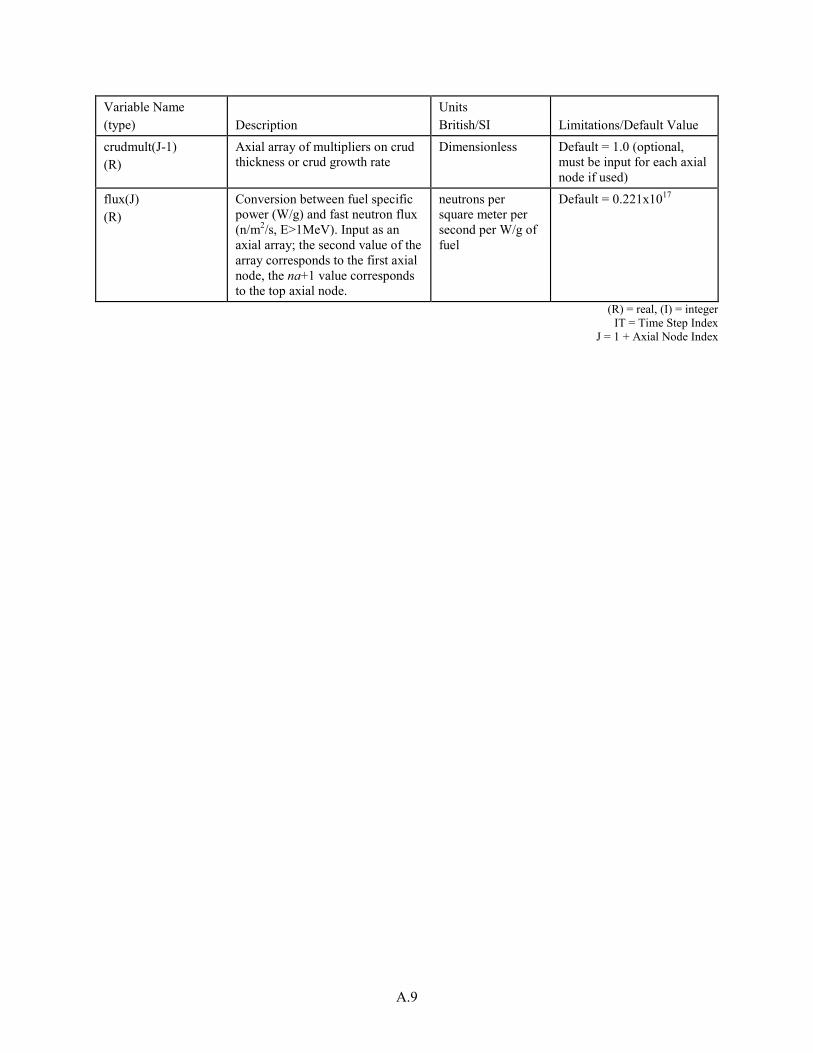
A.9

Variable Name (type) Description

Units British/SI Limitations/Default Value

crudmult(J-1) (R)

Axial array of multipliers on crud thickness or crud growth rate

Dimensionless Default = 1.0 (optional, must be input for each axial node if used)

flux(J) (R)

Conversion between fuel specific power (W/g) and fast neutron flux (n/m2/s, E>1MeV). Input as an axial array; the second value of the array corresponds to the first axial node, the na+1 value corresponds to the top axial node.

neutrons per square meter per second per W/g of fuel

Default = 0.221x1017

(R) = real, (I) = integer IT = Time Step Index

J = 1 + Axial Node Index

A.10

Input Variables Specifying Power History

Variable Name (type) Description

Units British/SI Limitations/Default Value

im (I)

Number of time steps Dimensionless Greater than 1 Required Input (namelist frpcn)

ProblemTime(IT) (R)

Cumulative time at the end of each time step. Note: Time steps greater than 50 days are not recommended. If steady-state operation is being modeled, use time steps greater than 1 day. Time steps less than 1 day should only be used when modeling a fast power ramp.

days Required Input

qmpy(IT) (R)

The linear heat generation rate at each time step. This equals the rod-average value if iq = 0 and the peak value if iq = 1. Note: Changes in local LHGR of greater than 1.5 kw/ft per time step are not recommended. Size qmpy accordingly.

kW/ft / kW/m Required Input

DecayModel (I)

Decay heat model to use. Currently only one model is implemented, and is the default model. 1 – ANS-5.1 (2005) Standard When a negative value of qmpy is found, the code will look at the previous value of qmpy and calculate an average power over the problem time

Dimensionless Default Value = 1

fpdcay (R)

Multiplicative factor applied to power given by decay heat model

Dimensionless Default Value = 1.0.

(R) = real, (I) = integer IT = Time Step Index

A.11

Input Variables Specifying Axial Power Profile

Variable Name (type) Description

Units British/SI Limitations/Default Value

iq (I)

Indicator for axial power shape: 0 = User-input power shapes, with qmpy = rod-average powers and power shapes defined by qf,x, and fa = 1.0. 1 = Chopped-cosine shape, with fa = Peak-to-average ratio and qmpy = peak power (use na=odd in order to have an axial node corresponding to the input peak power).

Dimensionless Required Input

x(N) (R)

The elevations in each qf, x array defining a power shape. Note the first value should be 0.0 and the last value must = totl.

feet / meters Required Input if iq=0 .

qf(N) (R)

The ratio of the linear power at the x(N) elevation to the axially-averaged value for the M-th power shape. The number of QF, X pairs for the Mth power shape is defined by jn(M). The code will automatically normalize to an average value of 1.0.

Dimensionless Required Input if iq = 0

jn(M) (I)

The number of qf, x value pairs for each axial power shape; required input if iq = 0. Input in the same sequence as the qf and x arrays.

Dimensionless Required Input if iq=0

jst(IT) (I)

The sequential number of the power shape to be used for each time step. One value of jst is required per time step if iq = 0.

Dimensionless Required Input if iq=0

fa (R)

Peak-to-average power ratio for cosine-type axial power distribution ( = 1.0, unless iq = 1; see description of iq).

Dimensionless Required Input

(R) = real, (I) = integer N = Axial Node Index for Input Power Profile

M = Power Shape Number, IT = Time Step Index

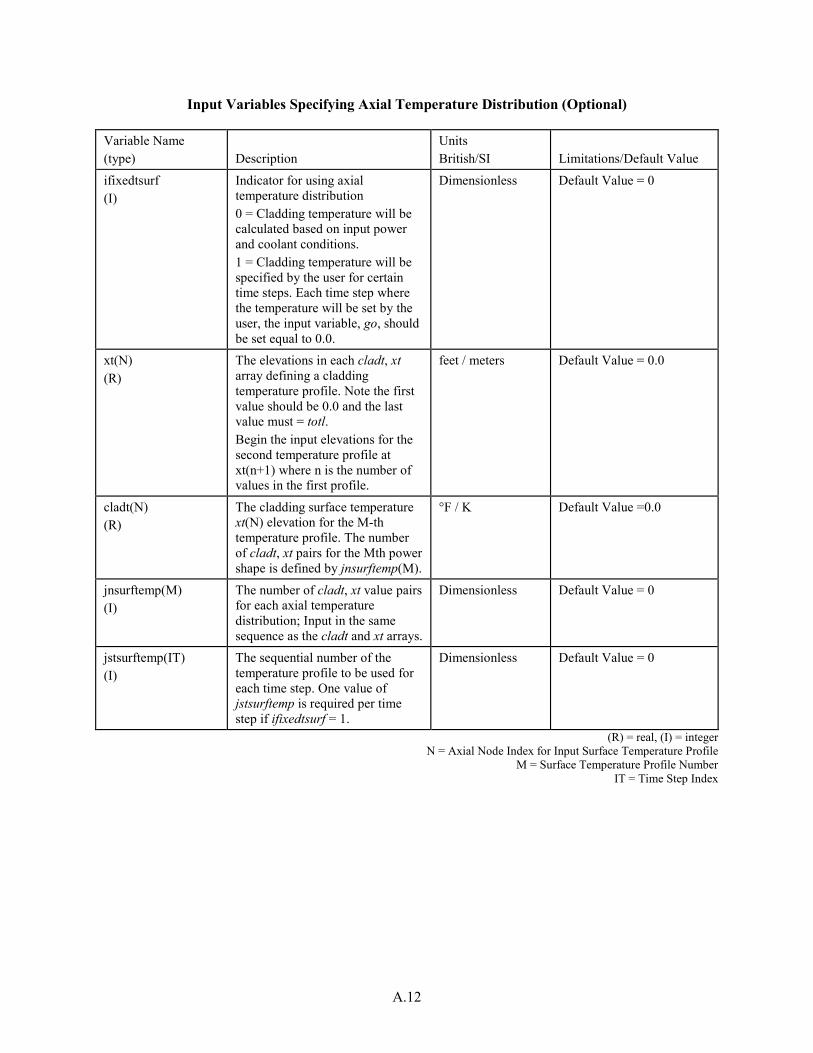
A.12

Input Variables Specifying Axial Temperature Distribution (Optional)

Variable Name (type) Description

Units British/SI Limitations/Default Value

ifixedtsurf (I)

Indicator for using axial temperature distribution 0 = Cladding temperature will be calculated based on input power and coolant conditions. 1 = Cladding temperature will be specified by the user for certain time steps. Each time step where the temperature will be set by the user, the input variable, go, should be set equal to 0.0.

Dimensionless Default Value = 0

xt(N) (R)

The elevations in each cladt, xt array defining a cladding temperature profile. Note the first value should be 0.0 and the last value must = totl. Begin the input elevations for the second temperature profile at xt(n+1) where n is the number of values in the first profile.

feet / meters Default Value = 0.0

cladt(N) (R)

The cladding surface temperature xt(N) elevation for the M-th temperature profile. The number of cladt, xt pairs for the Mth power shape is defined by jnsurftemp(M).

°F / K Default Value =0.0

jnsurftemp(M) (I)

The number of cladt, xt value pairs for each axial temperature distribution; Input in the same sequence as the cladt and xt arrays.

Dimensionless Default Value = 0

jstsurftemp(IT) (I)

The sequential number of the temperature profile to be used for each time step. One value of jstsurftemp is required per time step if ifixedtsurf = 1.

Dimensionless Default Value = 0

(R) = real, (I) = integer N = Axial Node Index for Input Surface Temperature Profile

M = Surface Temperature Profile Number IT = Time Step Index

A.13

Input Variables Specifying Fixed coolant Temperature and Pressure (Optional)

Variable Name (type) Description

Units British/SI Limitations/Default Value

ifixedcoolt (I)

Indicator for using axial coolant temperature distribution. 0 = Coolant temperature will be calculated based on coolant enthalpy rise model. 1 = Coolant temperature will be specified by the user at each time step.

Dimensionless Default Value = 0

zcool(N) (R)

The elevations in each coolt, Tcoolant array defining a coolant temperature profile. Note the first value should be 0.0 and the last value must = totl. Max # of elevations = na + 1

Feet/meters Default value = 0.0.

Tcoolant(N*im) (R)

Bulk coolant temperatures prescribed at each node zcoolt (N) for each time step(im). If the # of coolant temperature / time pairs is < im, then the last supplied value will be used for the remaining time steps for that node. Enter all coolant values (1 to im) for each node before proceeding to the next node.

°F/K Must be > 0.0

ifixedcoolp (I)

Indicator for using axial coolant pressure distribution. 0 = Coolant pressure will be based on user input value and constant at all axial nodes. 1 = Coolant pressure will be specified by the user at each time step.

Dimensionless Default Value = 0

Pcoolant(N*im) (R)

Bulk coolant pressures prescribed at each node zcoolt (N) for each time step(im). If the # of coolant pressure / time pairs is < im, then the last supplied value will be used for the remaining time steps for that node. Enter all coolant values (1 to im) for each node before proceeding to the next node. The same height (zcool) is used for both coolant temperature and pressure

psia/Pa Must be > 0.0

(R) = real, (I) = integer

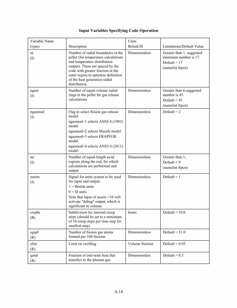
A.14

Input Variables Specifying Code Operation

Variable Name (type) Description

Units British/SI Limitations/Default Value

nr (I)

Number of radial boundaries in the pellet (for temperature calculations and temperature distribution output). These are spaced by the code with greater fraction in the outer region to optimize definition of the heat generation radial distribution.

Dimensionless Greater than 1, suggested minimum number is 17. Default = 17 (namelist frpcn)

ngasr (I)

Number of equal-volume radial rings in the pellet for gas release calculations

Dimensionless Greater than 6,suggested number is 45. Default = 45 (namelist frpcn)

ngasmod (I)

Flag to select fission gas release model ngasmod=1 selects ANS5.4 (1982) model ngasmod=2 selects Massih model ngasmod=3 selects FRAPFGR model ngasmod=4 selects ANS5.4 (2011) model

Dimensionless Default = 2

na (I)

Number of equal-length axial regions along the rod, for which calculations are performed and output

Dimensionless Greater than 1, Default = 9 (namelist frpcn)

nunits (I)

Signal for units system to be used for input and output: 1 = British units 0 = SI units Note that input of nunits >10 will activate "debug" output, which is significant in volume.

Dimensionless Default = 1

crephr (R)

Subdivision for internal creep steps (should be set to a minimum of 10 creep steps per time step for smallest step)

hours Default = 10.0

sgapf (R)

Number of fission gas atoms formed per 100 fissions

Dimensionless Default = 31.0

slim (R)

Limit on swelling Volume fraction Default = 0.05

qend (R)

Fraction of end-node heat that transfers to the plenum gas

Dimensionless Default = 0.3

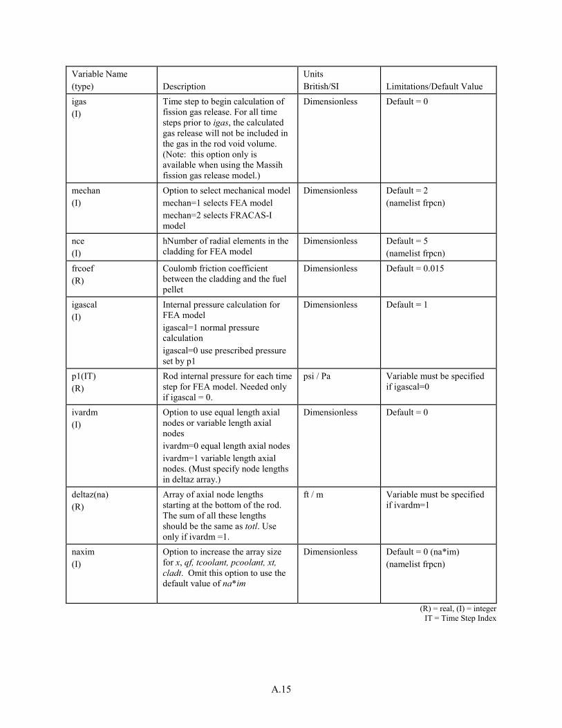
A.15

Variable Name (type) Description

Units British/SI Limitations/Default Value

igas (I)

Time step to begin calculation of fission gas release. For all time steps prior to igas, the calculated gas release will not be included in the gas in the rod void volume. (Note: this option only is available when using the Massih fission gas release model.)

Dimensionless Default = 0

mechan (I)

Option to select mechanical model mechan=1 selects FEA model mechan=2 selects FRACAS-I model

Dimensionless Default = 2 (namelist frpcn)

nce (I)

hNumber of radial elements in the cladding for FEA model

Dimensionless Default = 5 (namelist frpcn)

frcoef (R)

Coulomb friction coefficient between the cladding and the fuel pellet

Dimensionless Default = 0.015

igascal (I)

Internal pressure calculation for FEA model igascal=1 normal pressure calculation igascal=0 use prescribed pressure set by p1

Dimensionless Default = 1

p1(IT) (R)

Rod internal pressure for each time step for FEA model. Needed only if igascal = 0.

psi / Pa Variable must be specified if igascal=0

ivardm (I)

Option to use equal length axial nodes or variable length axial nodes ivardm=0 equal length axial nodes ivardm=1 variable length axial nodes. (Must specify node lengths in deltaz array.)

Dimensionless Default = 0

deltaz(na) (R)

Array of axial node lengths starting at the bottom of the rod. The sum of all these lengths should be the same as totl. Use only if ivardm =1.

ft / m Variable must be specified if ivardm=1

naxim (I)

Option to increase the array size for x, qf, tcoolant, pcoolant, xt, cladt. Omit this option to use the default value of na*im

Dimensionless Default = 0 (na*im) (namelist frpcn)

(R) = real, (I) = integer IT = Time Step Index

A.16

Model Uncertainty Variables for Sensitivity Analysis

Variable Name (type) Description

Units British/SI Limitations/Default Value

sigftc (R)

Bias on fuel thermal conductivity model. sigftc = 1 biases model up 1s, sigftc = -1.5 biases model down 1.5s.

Dimensionless Default = 0

sigftex (R)

Bias on fuel thermal expansion model. sigftex = 1 biases model up 1s, sigftex = -1.5 biases model down 1.5s.

Dimensionless Default = 0

sigfgr (R)

Bias on fission gas release model. sigfgr=1 biases model up 1s, sigfgr = -1.5 biases model down 1.5s.

Dimensionless Default = 0

sigswell (R)

Bias on fuel swelling model. sigswell=1 biases model up 1s, sigswell = -1.5 biases model down 1.5s.

Dimensionless Default = 0

sigcreep (R)

Bias on cladding creep model. sigcreep=1 biases model up 1s, sigcreep=-1.5 biases model down 1.5s.

Dimensionless Default = 0

siggro (R)

Bias on cladding axial growth model. siggro=1 biases model up 1s, siggro=-1.5 biases model down 1.5s.

Dimensionless Default = 0

sigcor (R)

Bias on cladding corrosion model. sigcor=1 biases model up 1s, sigcor=-1.5 biases model down 1.5s.

Dimensionless Default = 0

sigh2 (R)

Bias on cladding hydrogen pickup model. sigh2=1 biases model up 1s, sigh2=-1.5 biases model down 1.5s.

Dimensionless Default = 0

(R) = real, (I) = integer

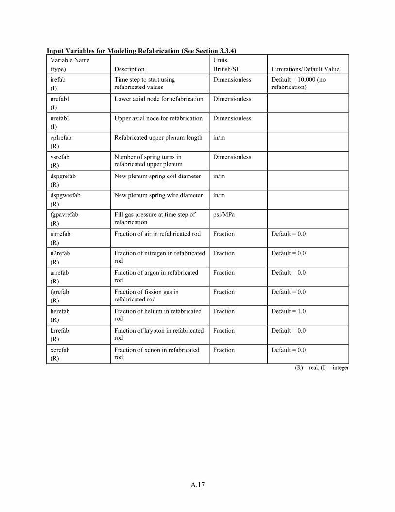
A.17

Input Variables for Modeling Refabrication (See Section 3.3.4) Variable Name (type) Description

Units British/SI Limitations/Default Value

irefab (I)

Time step to start using refabricated values

Dimensionless Default = 10,000 (no refabrication)

nrefab1 (I)

Lower axial node for refabrication Dimensionless

nrefab2 (I)

Upper axial node for refabrication Dimensionless

cplrefab (R)

Refabricated upper plenum length in/m

vsrefab (R)

Number of spring turns in refabricated upper plenum

Dimensionless

dspgrefab (R)

New plenum spring coil diameter in/m

dspgwrefab (R)

New plenum spring wire diameter in/m

fgpavrefab (R)

Fill gas pressure at time step of refabrication

psi/MPa

airrefab (R)

Fraction of air in refabricated rod Fraction Default = 0.0

n2refab (R)

Fraction of nitrogen in refabricated rod

Fraction Default = 0.0

arrefab (R)

Fraction of argon in refabricated rod

Fraction Default = 0.0

fgrefab (R)

Fraction of fission gas in refabricated rod

Fraction Default = 0.0

herefab (R)

Fraction of helium in refabricated rod

Fraction Default = 1.0

krrefab (R)

Fraction of krypton in refabricated rod

Fraction Default = 0.0

xerefab (R)

Fraction of xenon in refabricated rod

Fraction Default = 0.0

(R) = real, (I) = integer

A.18

Input Variables for Use of DATING Creep Model for Spent Fuel Storage Variable Name

(type) Description Units

(British/SI) Default

value/notes idatingcreep (I)

= 0 – do not model creep in dry cask storage following reactor operation = 1 – model creep in spent fuel using conservative creep and conservative Monkman-Grant = 2 – model creep in spent fuel using conservative creep and best estimate Monkman-Grant = 3 – model creep using best estimate creep and best estimate Monkman-Grant

unitless default = 0 (namelist SpentFuel)

ncreephist (I)

Temperature/pressure history for spent fuel storage = 1 – helium decay curve (good for 35 GWd/MTU) = 2 – nitrogen decay curve (good for 35 GWd/MTU) = 3 – input temperature history. Profile will be normalized to start at FRAPCON predicted EOL temperature. = 4 – input temperature and rod hoop stress history

unitless default = 1 if ncreephist = 3 or 4, input ncreeptab, creeptabtime, creeptabtemp, and creeptabstress (namelist SpentFuel)

creeptime (R)

Time in storage years/years default = 0.0 (namelist SpentFuel)

creeppooltime (R)

Time since discharge from reactor (time spent in fuel pool prior to dry storage)

years/years default = 5.0 (should not be less than 5 years) (namelist SpentFuel)

ncreepstep (I)

Number of output time steps unitless default = 1 (namelist SpentFuel)

ncreeptab (I)

Number of entries in user defined temperature and rod internal pressure histories

unitless default = 1 Required if ncreephist = 3 or 4 (namelist SpentFuel)

creeptabtime(IT) (R)

Time in storage from reactor discharge for user defined temperature and rod internal pressure histories

years/years default = 0.0 Required if ncreephist = 3 or 4 (namelist SpentFuel)

A.19

Variable Name (type)

Description Units (British/SI)

Default value/notes

creeptabtemp(IT) (R)

User defined temperature history °F/°C default = 0.0 Required if ncreephist = 3 or 4 (namelist SpentFuel)

creeptabstress(IT) (R)

User defined midwall hoop stress history

psi/MPa default = 0.0 Required if ncreephist = 4 (namelist SpentFuel)

stopox (R)

Indicator for when to stop the oxide calculation (days). This value should correspond to the ProblemTime value when the fuel is out of the pool. If it does not line up exactly with a ProblemTime value, the oxidation calculation will stop when the value for stopox > ProblemTime(it). Values for oxidation layer thickness & hydrogen uptake from the coolant will remain the same value as the last time step before oxidation was turned off.

days Default Value = 1.0e10 (namelist SpentFuel)

addswell (it) (R)

Additional volumetric swelling. Enter as a volumetric strain value. Must enter 1 value for every time step specified in ProblemTime. Values will be used at current time step only and do not compound with previous time step’s value.

Dimensionless

Default value = 0.0 (namelist SpentFuel)

addgmles (it) (R)

Additional gram moles of gas added to the rod internal gas pressure calculation. Must enter 1 value for every time step specified in ProblemTime. Values will be used at current time step only and do not compound with previous time step’s value.

Dimensionless Default value = 0.0.

(R) = real, (I) = integer

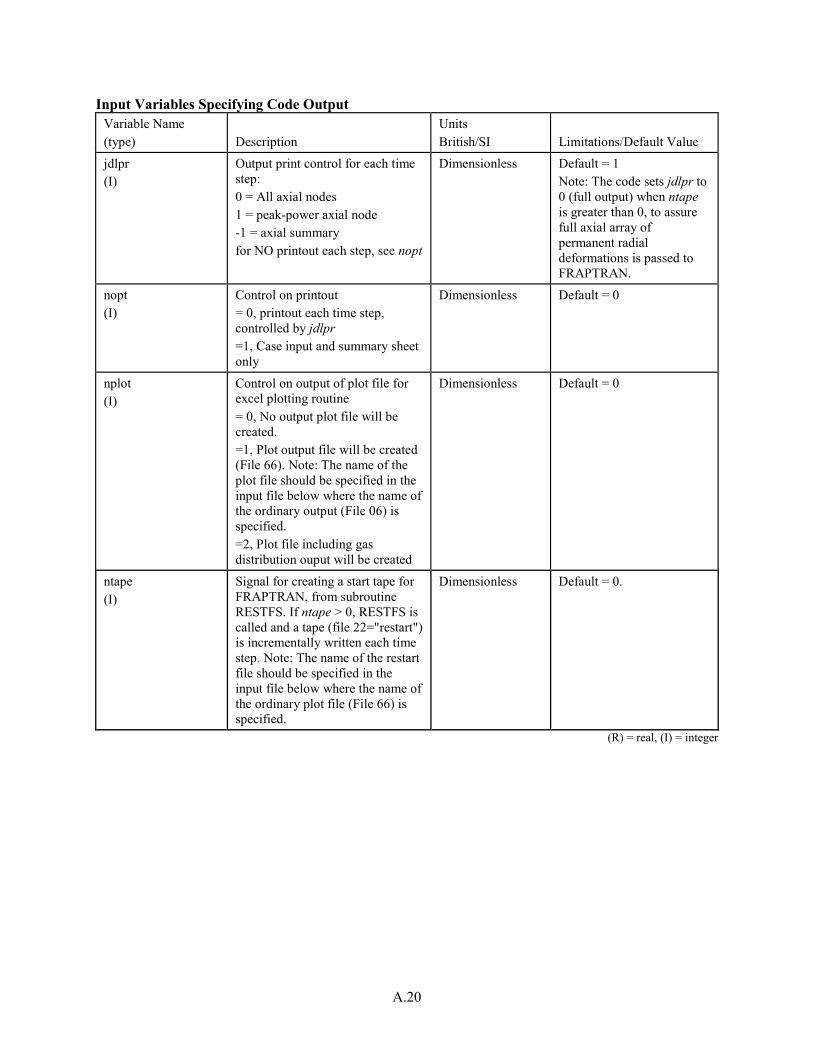
A.20

Input Variables Specifying Code Output Variable Name (type) Description

Units British/SI Limitations/Default Value

jdlpr (I)

Output print control for each time step: 0 = All axial nodes 1 = peak-power axial node -1 = axial summary for NO printout each step, see nopt

Dimensionless Default = 1 Note: The code sets jdlpr to 0 (full output) when ntape is greater than 0, to assure full axial array of permanent radial deformations is passed to FRAPTRAN.

nopt (I)

Control on printout = 0, printout each time step, controlled by jdlpr =1, Case input and summary sheet only

Dimensionless Default = 0

nplot (I)

Control on output of plot file for excel plotting routine = 0, No output plot file will be created. =1, Plot output file will be created (File 66). Note: The name of the plot file should be specified in the input file below where the name of the ordinary output (File 06) is specified. =2, Plot file including gas distribution ouput will be created

Dimensionless Default = 0

ntape (I)

Signal for creating a start tape for FRAPTRAN, from subroutine RESTFS. If ntape > 0, RESTFS is called and a tape (file 22="restart") is incrementally written each time step. Note: The name of the restart file should be specified in the input file below where the name of the ordinary plot file (File 66) is specified.

Dimensionless Default = 0.

(R) = real, (I) = integer

A.21

Input Variables for Developer Options (These inputs can be used to make fundamental changes to the models in FRAPCON-4.0 and therefore

the results of using these options are not validated) All variables are in namelist DEVELOPER

Variable Name (type)

Description Units (British/SI)

Default value/notes

calcoxide (L)

Flag to specify whether or not to calculate oxidation. If set to .false., no cladding oxidation will occur and the hydrogen intake into the cladding will also be turned off.

unitless Default value = .true.

gaphtcmult (R)

Gap conductance multiplier

unitless Default Value = 1.0. Must be > 0.

modheat (R)

Moderator heating fraction. Specifies the fraction of input linear heat generation rate to be deposited directly into the coolant. To use default values based on plant type, set modheat = -1.

fraction Default value = 0.0. Default values if modheat=-1 are: PWR: 0.026 BWR:0.035 HWR:0.084

cladelmod (R)

Cladding elastic modulus Pa Default = -1.0 (not used). Must be > 0.0 to use

relocmodel (Character)

Relocation model options. The available relocation models are: ‘FRAPCON-3.5’ (Default) ‘FRAPCON-3.4’ ‘OFF’ ‘USER’

N/A Default = ‘FRAPCON-3.5’

fuelreloc (R)

Fuel relocation fraction of as-fabricated gap. Fuel relocation fraction will ramp from 0.0 to fuelreloc over 10 GWd/MTU burnup. This value is only used when relocmodel = ‘USER’

fraction Default = -1.0 (not used). Must be 0.0 to 1.0 to use

gaprecov (R)

Fraction of relocated fuel allowed to recover before hard contact occurs. This fraction will be added to the fuel surface as permanent deformation.

fraction Default = 0.5

TimeIntegration (I)

Flag to specify the time/power integration technique. This increases the number of timesteps (im) performed in the calculation while only printing the timesteps specified by input flag ProblemTime. 0 = Off (Default), 1 = Linear Interpolation, 2 = Histogram. If > 0, must insert value for newtimestep

N/A Default = 0

A.22

Variable Name (type)

Description Units (British/SI)

Default value/notes

newtimestep (R)

New timestep value to use for FRAPCON calculation when performing a time-step reduction (TimeIntegration > 0)

days Must be > 0.0

RestartTime (R)

Problem time (s) to use for a restart calculation. Problem time of < 0 will default to the last calculation time

Seconds If < 0, will use last restart time.

nfrttr (I)

Indicator for printing data needed for TRACE using the NRC Internal Auto Input Generator. Set nfrttr = 1 to turn on.

unitless Default Value = 0

nread (I)

Signal to start up from a restart tape (File 13). The value of nread is the time step to start from. Note: User must switch the restart-write tape file number from 12 to 13 to make it a restart-read tape. Note: The restart functionality does NOT work with FRAPCON-4.0.

Dimensionless Default = 0

nrestr (I)

Signal for writing a restart tape for FRAPCON. If nrestr not equal to 0, subroutine TAPEGEN generates a restart tape (file 12) at each time step. Note that the restart tape does not currently contain complete restart information for the fission gas release models.

Dimensionless Default = 0

(R) = real, (I) = integer, (L)=Logical

A.23

Example Case with MOX Fuel *********************************************************************** * frapcon, steady-state fuel rod analysis code * *---------------------------------------------------------------------- * * * * CASE DESCRIPTION: MOX example rod * * * *UNIT FILE DESCRIPTION * *---- -----------------------------------------------Output: * * Output : * * 6 STANDARD PRINTER OUTPUT * * * * Scratch: * * 5 SCRATCH INPUT FILE FROM ECH01 * * * * Input: FRAPCON INPUT FILE (UNIT 55) * * * *********************************************************************** * GOESINS: FILE05='nullfile', STATUS='UNKNOWN', FORM='FORMATTED', CARRIAGE CONTROL='NONE' * * GOESOUTS: FILE06='MOXexample.out', STATUS='UNKNOWN', CARRIAGE CONTROL='LIST' FILE66='MOXexample.plot', STATUS='UNKNOWN', FORM='FORMATTED', CARRIAGE CONTROL='LIST' /********************************************************************** MOX Example Rod $frpcn im=50, na=4, ngasr = 45, $end $frpcon cpl = 2., crdt = 0.0, thkcld = 0.0224, thkgap = 0.0033, dco = 0.374, pitch = 0.5,nplot=1, rc = 0.0453, fotmtl = 1.997,dishsd=0.06488, den = 94.43, dspg = 0.3,fa = 1., dspgw = 0.03, enrch = 0.229, fgpav = 382, hdish = 0.011, hplt = 0.5, icm = 4, imox = 1, comp = 5.945, idxgas = 1, iplant =-2, iq = 0, jdlpr = 0, jn = 5,5, totl = 1.31, roughc = 3.94e-5, roughf = 7.9e-5, vs = 10.0, nunits = 1, rsntr = 52., nsp = 1, p2(1) = 44*2250., p2(45) = 6*2352, tw(1) = 44*570, tw(45) = 6*590 go(1) = 50*2.0e6, jst = 44*1, 6*2 qf(1) = 1.0, 1.0, 1.0, 1.0, 1.0 x(1) = 0.0, 0.3275, 0.6650, 0.9925, 1.31 qf(6) = 0.9, 1.0, 1.1, 1.0, 0.9 x(6) = 0.0, 0.3275, 0.6650, 0.9925, 1.31 ProblemTime= 0.1, 0.2, 0.3, 0.4, 0.5, 0.6, 30., 60., 90., 120., 150., 180., 210., 240., 270.,

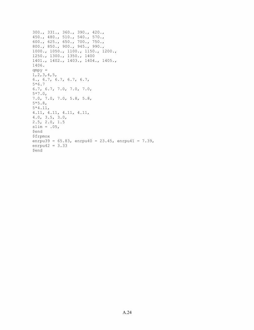
A.24

300., 331., 360., 390., 420., 450., 480., 510., 540., 570., 600., 625., 650., 700., 750., 800., 850., 900., 945., 990., 1000., 1050., 1100., 1150., 1200., 1250., 1300., 1350., 1400 1401., 1402., 1403., 1404., 1405., 1406. qmpy = 1,2,3,4,5, 6., 6.7, 6.7, 6.7, 6.7, 5*6.7 6.7, 6.7, 7.0, 7.0, 7.0, 5*7.0, 7.0, 7.0, 7.0, 5.8, 5.8, 5*5.8, 5*4.11, 4.11, 4.11, 4.11, 4.11, 4.0, 3.5, 3.0, 2.5, 2.0, 1.5 slim = .05, $end $frpmox enrpu39 = 65.83, enrpu40 = 23.45, enrpu41 = 7.39, enrpu42 = 3.33 $end

A.25

Input Variables Arranged Alphabetically and by Input Block $frpcn input block

Variable Name Page Number im A.10 mechan A.15 na A.14 nce A.15 ngasr A.14 nr A.14 naxim A.15

$frpmox input block

Variable Name Page Number enrpu39 A.4 enrpu40 A.4 enrpu41 A.4 enrpu42 A.4 moxtype A.3

A.26

$frpcon input block Variable Name Page Number Variable Name Page Number

airrefab A.17 fgpavrefab A.17 amfair A.7 fgrefab A.17 amfarg A.7 flux A.9 amffg A.7 fotmtl A.4 amfh2 A.7 fpdcay A.10 amfh2o A.7 frcoef A.15 amfhe A.7 gadoln A.4 amfkry A.7 go A.8 amfn2 A.7 hdish A.3 amfxe A.7 herefab A.17 arrefab A.17 hplt A.3 b10 A.4 icm A.6 catexf A.6 icor A.8 chmfrh A.3 idxgas A.7 chmfrw A.3 ifba A.4 chorg A.6 ifixedcoolp A.13 cladt A.12 ifixedcoolt A.13 cldwks A.6 ifixedtsurf A.12 comp A.3 igas A.15 cpl A.2 igascal A.15 cplrefab A.17 imox A.3 crdt A.8 iplant A.8 crdtr A.8 iq A.11 crephr A.14 irefab A.17 crudmult A.9 ivardm A.15 dco A.2 jdlpr A.20 decaymodel A.10 jn A.11 deltaz A.15 jnsurftemp A.12 den A.4 jst A.11 deng A.4 jstsurftemp A.12 dishd A.3 krrefab A.17 dspg A.2 n2refab A.17 dspgrefab A.17 ngasmod A.14 dspgw A.2 nopt A.20 dspgwrefab A.17 nplot A.20 enrch A.3 nrefab1 A.17 fa A.11 nrefab2 A.17 fgpav A.7 nsp A.8

A.27

Variable Name Page Number Variable Name Page Number ntape A.20 siggro A.16 nunits A.14 sigh2 A.16 p1 A.15 sigswell A.16 p2 A.8 sgapf A.14 pcoolant A.13 slim A.14 pitch A.8 tcoolant A.13 ppmh2o A.4 thkcld A.2 ppmn2 A.4 thkgap A.2 ProblemTime A.10 totl A.2 qend A.14 tsint A.5 qf A.11 tw A.8 qmpy A.10 vs A.2 rc A.3 vsrefab A.17 roughc A.6 x A.11 roughf A.4 xerefab A.17 rsntr A.5 xt A.12 sigcor A.16 zcool A.13 sigcreep A.16 zr2vintage A.6 sigfgr A.16 zrb2den A.4 sigftc A.16 zrb2thick A.4 sigftex A.16

$spent fuel input block

Variable Name Page Number addgmles A.19 addswell A.19 creeppooltime A.18 creeptabstress A.19 creeptabtemp A.19 creeptabtime A.18 creeptime A.18 idatingcreep A.18 ncreephist A.18 ncreepstep A.18 ncreeptab A.18 stopox A.19

A.28

$developer input block Variable Name Page Number

calcoxide A.21 cladelmod A.21 fuelreloc A.21 gaphtcmult A.21 gaprecov A.21 modheat A.21 newtimestep A.22 nfrttr A.22 nread A.22 nrestr A.22 relocmodel A.21 RestartTime A.22 TimeIntegration A.21

A.29

FRAPCON Auto Input Instructions

1. Open the file FRAPCON-4.0 AIG.xlsm. 2. If you would like to save the excel file, click file/save as to save as a different name. 3. In the “Input” worksheet, fill out all the values in red and blue for the specific case you are

creating. a. Values shown in red are required input. b. Values shown in blue are not required and are often left as the default value shown. c. Units shown in red or blue can be changed using the drop down boxes.

d. If you want to use generic dimensions, select the assembly type under “Select Auto

Inputs” and then click “Populate Auto Inputs”

4. In the “Power History” worksheet, fill out the columns of Time or Burnup, Power, and power

shape number to be used for each time step.

Time/Burnup Power Axial Power Shape Number

5. In the “Axial Power Profiles” worksheet, fill out the number of shapes to use for the run and the

axial profile vs. elevation for each shape. The input shape will automatically be normalized to an average value of 1.0 in FRAPCON.

6. In the “Coolant Conditions” worksheet, select constant or time dependent coolant conditions, and fill out the appropriate table.

7. Depending on advanced selections that are made, you may fill out tabs “Axial Variations,” “Refabrication,” “Axial Temp Profiles,” “Axial Coolant Conditions,” “Spent Fuel,” and “Developer,”. These tabs are marked in blue as they are not typically required.

8. In the “FRAPCON Input” worksheet, click on the button “Write Input.” The FRAPCON input file will be created in that Excel sheet.

9. Click on the button “Create File” to create a file in the directory and file name specified in the “Input Worksheet.”

A.30

Appendix B –

Instruction for Using Excel Plot Routine for FRAPCON

B.1

Appendix B

Instruction for Using Excel Plot Routine for FRAPCON

FRAPCON can create a separate plot file that can be read by an Excel plotting routine.

In the FRAPCON input file, add the variable nplot=1or nplot=2 (for extra gas distribution information) under $frpcon.

In the FRAPCON input file, add the plot file output name (unit=66) after the frapcon file output name (unit=6).

Run FRAPCON with the modified input file.

Open the Excel file FRAPlot.xlsm.

A warning will likely appear either as a pop-up window or as a warning bar above the spreadsheet formula field. Click ‘Enable Macros’ (or ‘Enable Content’ depending on the excel version) to enable the plotting macros.

Go to the “Data” tab to plot global variables for your calculation.

B.2

Type the name of the plot output file in cell B4 as indicated. There are 3 options to do this:

1. If the plot file is in the same folder as the plotter, you can check the box labeled ‘Plot file is in same directory as plotter’, and type the file name (example: filename.plot) without its path in cell B4, then press enter and click ‘Load Plot File’.

2. If the plot file is in a different folder from the plotter, make sure the ‘Plot file is in same directory as plotter’ box is unchecked, and type the file name including its path in cell B4, then press enter and click ‘Load Plot File’.

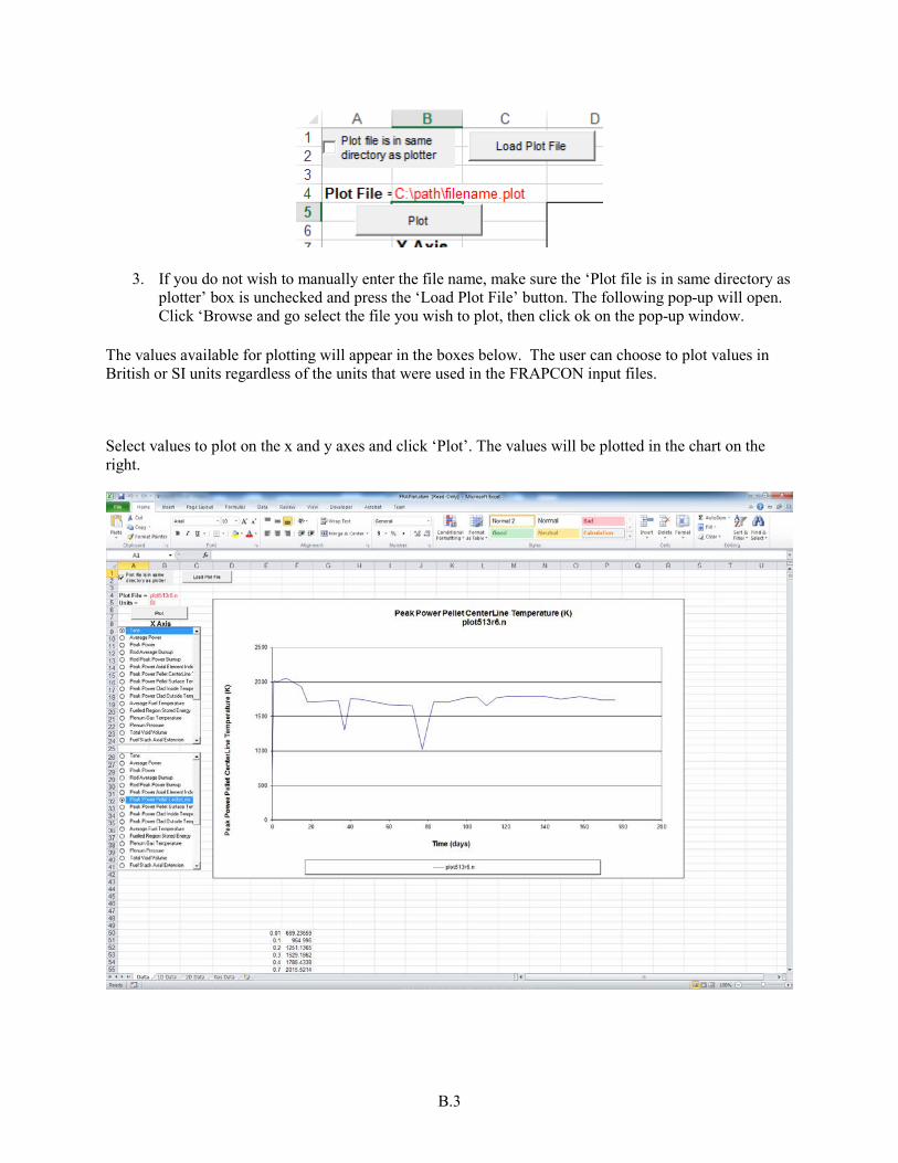
B.3

3. If you do not wish to manually enter the file name, make sure the ‘Plot file is in same directory as plotter’ box is unchecked and press the ‘Load Plot File’ button. The following pop-up will open. Click ‘Browse and go select the file you wish to plot, then click ok on the pop-up window.

The values available for plotting will appear in the boxes below. The user can choose to plot values in British or SI units regardless of the units that were used in the FRAPCON input files.

Select values to plot on the x and y axes and click ‘Plot’. The values will be plotted in the chart on the right.

B.4

The tabs at the bottom of the sheet apply to other data that can be plotted.

Click on them to go to the different data to be plotted.

The tab, “1D data,” contains data for each axial node plotted as a function of time.

Select the value to be plotted. Click ‘Nodal Plot’ to plot this value for each axial node.

Click ‘Axial Plot’ to plot the axial profile of a chosen parameter at a chosen time. By default, the plot will be for the last time step of the calculation. If you wish to plot the axial profile at a different time, check ‘User-specified time for axial plot (default last time step)’ and type in the desired time in cell C44, then click ‘Nodal Plot’ or ‘Axial Plot’. If you want the Y axis to be scaled from the minimum to the maximum value of your plotted data, check the ‘Fit Max Extents’ box and click ‘Nodal Plot’ or ‘Axial Plot’ to re-plot your data set.

B.5

The tab, “2D data,” contains a 3-D plot of the fuel rod temperatures at a given time step.

Select ‘Fuel Rod Mesh Temperatures’. Click ‘2D Plot’ to plot the temperatures at each axial and radial node at a given time step. The default time step is the last time step of the calculation. If you wish to plot the mesh temperatures at a different time, check ‘User-specified time for 2D plot (default last time step)’ and type in the desired time in cell B15, then click ‘2D Plot’. If you want the Y axis to be scaled from the minimum to the maximum value of your mesh temperatures, check the ‘Fit Max Extents’ box and click ‘2D Plot’ to re-plot your data set.

B.6

The same procedure can be used to plot value in the Gas Data if the correct input flag (nplot=2) was selected

When you are finished, close the Excel file without saving, or if you want to save some graphs, use the “Save as” function to avoid overwriting the initial plot file.