Free Surface Penetration of Inverted Right CircularCones at Low Froude Number

Samuel R. Koski

Thesis submitted to the Faculty of the

Virginia Polytechnic Institute and State University

in partial fulfillment of the requirements for the degree of

Masters of Science

in

Mechanical Engineering

Sunghwan Jung, Chair

Weiwei Deng

Jon Yagla

January 10, 2017

Blacksburg, Virginia

Keywords: boundary element method, free surface penetration, interfacial flow, water

entry, Laplace’s equation

Free Surface Penetration of Inverted Right Circular Cones at Low

Froude Number

Samuel R. Koski

ABSTRACT

This study is focused on the impact of inverted right circular cones over multiple deadrise

angles on an air water interface at low Froude number (Fr ≈ 10-70). In this flow regime it is

known that an air cavity is formed aft of a body as it travels into a liquid. Previous studies

have confirmed that the depth of the projectile at the collapse of this cavity follows a power

law ∝ Fr1/2 for disks, whereas for right cylinders or the impact of spheres on soft sand, the

depth at cavity seal is ∝ Fr1/3. Experiments were conducted at these Froude numbers with

0.02 m radius cones over multiple deadrise angles. High speed video was taken as well as

a measurement of the drag force over the depth of travel for each case. A numerical model

has been developed based on a boundary element method, and matching the conditions of

the experiments, we study the temporal dynamics of the cavity and the forces exerted on

the cone from impact on the liquid interface to cavity collapse.

Free Surface Penetration of Inverted Right Circular Cones at Low

Froude Number

Samuel R. Koski

GENERAL AUDIENCE ABSTRACT

In this thesis the impact of inverted cones on a liquid surface is studied. It is known that

with the right combination of velocity, geometry, and surface treatment, a cavity of air

can be formed behind an impacting body and extended for a considerable distance. Other

investigators have shown that the time and depth of the cone when this cavity collapses

and seals follows a different power law for flat objects such as disks, then it does for slender

objects such as cylinders. Intuitively it can be expected that a more slender body will have

less drag and that the streamlined shape will not push the fluid out of it’s way at impact to

the same extent as a more blunt body, therefore forming a smaller cavity behind it. With a

smaller initial cavity, the time and depth of it’s eventual collapse can be expected to be less

than that of a much more blunt object, such as a flat disk.

To study this, a numerical model has been developed to simulate cones with the same base

radius but different angles impacting on a liquid surface over a range of velocities, showing

how the seal depth, time at cavity seal, and drag forces change. In order to ensure the

numerical model is accurate, it is compared with experimental data including high speed

video and measurements made of the force with time.

It is expected that the results will fall inside the power law exponents reported by other

authors for very blunt objects such as disks on one end of the spectrum, and long slender

cylinders on the other. Furthermore, we expect that the drag force exerted on the cones will

become lower as the L/D of the cone is increased.

ACKNOWLEDGMENTS

I’d like to thank Cathy Hill for her help, guidance, and encouragement all of these years.

She was instrumental in my efforts at Virginia Tech from the start, and there is no question

I would not have finished without her.

I consider myself especially privileged to have been advised by each member of my commit-

tee. It was both a deep honor and humbling experience to have had Dr. Sunghwan (Sunny)

Jung as my committee chair. I’d like to thank him for sharing his experience, knowledge,

and guidance, and expect it will have a lasting impact on my career and continuing edu-

cation. Dr. Weiwei Deng played an important role on my committee and I thank him for

taking the time to share his insight and for stepping in at such a critical time. I’d like to

thank my friend and mentor of 10 years, Dr. Jon Yagla. Due to his uncanny ability to break

problems down to almost any level, he has guided me through efforts ranging from basic

woodworking to complex mathematics. This combined with his profound bank of knowledge

and experience has unquestionably shaped me into the engineer I am today.

I’d like to thank Dr. Pavlos Vlachos for his seemingly unlimited patience and for opening

up the opportunity to pursue graduate studies at Virginia Tech. His contribution to this

work and my overall success are greatly appreciated.

Finally, I’d like to thank my family, especially my wife Sharon, and my children Lily and

Ryan. The sacrifices you’ve made, particularly in the last month or two, cannot be over-

stated. After I’ve had a few months of sleep, I look forward to spending as much time as

possible together.

iv

CONTENTS

Acknowledgments iv

List of Figures vi

List of Tables vii

Nomenclature viii

1. Free surface penetration of inverted right circular cones at low Froude

number 1

1.1. Introduction 2

1.2. Experimental set-up 3

1.3. Mathematical formulation 4

1.4. Numerical method 7

1.4.1. Boundary element method (BEM) 7

1.4.2. Initial conditions 8

1.4.3. Time integration 10

1.5. Experimental and numerical results 12

1.5.1. Dynamics of the fluid interface 12

1.5.2. Depth and time at cavity seal 14

1.5.3. Drag force 16

1.6. Conclusions 18

1.6.1. Future work 20

1.7. References 21

2. Appendix A - Algorithms 23

2.1. Main Script 23

2.2. Functions 31

v

LIST OF FIGURES

1 Experimental set-up. . . . . . . . . . . . . . . . . . . . . . . . . . . . . . . . . . . . . . . . . . . . . . . . . . 4

2 Axisymmetric domain definitions. . . . . . . . . . . . . . . . . . . . . . . . . . . . . . . . . . . . . . . 5

3 Image processing sequence where (a) is the raw image from the high speed

video, (b) is the image converted to binary, and (c) is fluid interface after

extraction. . . . . . . . . . . . . . . . . . . . . . . . . . . . . . . . . . . . . . . . . . . . . . . . . . . . . . . . . . . 10

4 Steps for numerical solution. . . . . . . . . . . . . . . . . . . . . . . . . . . . . . . . . . . . . . . . . . . 11

5 Cavity development for the 77.5o cone (column a), 60o cone (column b),

and 45o cone (column c) dropped from Hexp=60 cm. The cones are shown at

depthsHz/R0=5, Hz/R0=10, and just prior to cavity seal, whereHz/R0=20.72

for the 45o cone, Hz/R0=18 for the 60o cone, and Hz/R0=14.66 for the 77.5o

cone. . . . . . . . . . . . . . . . . . . . . . . . . . . . . . . . . . . . . . . . . . . . . . . . . . . . . . . . . . . . . . . . 13

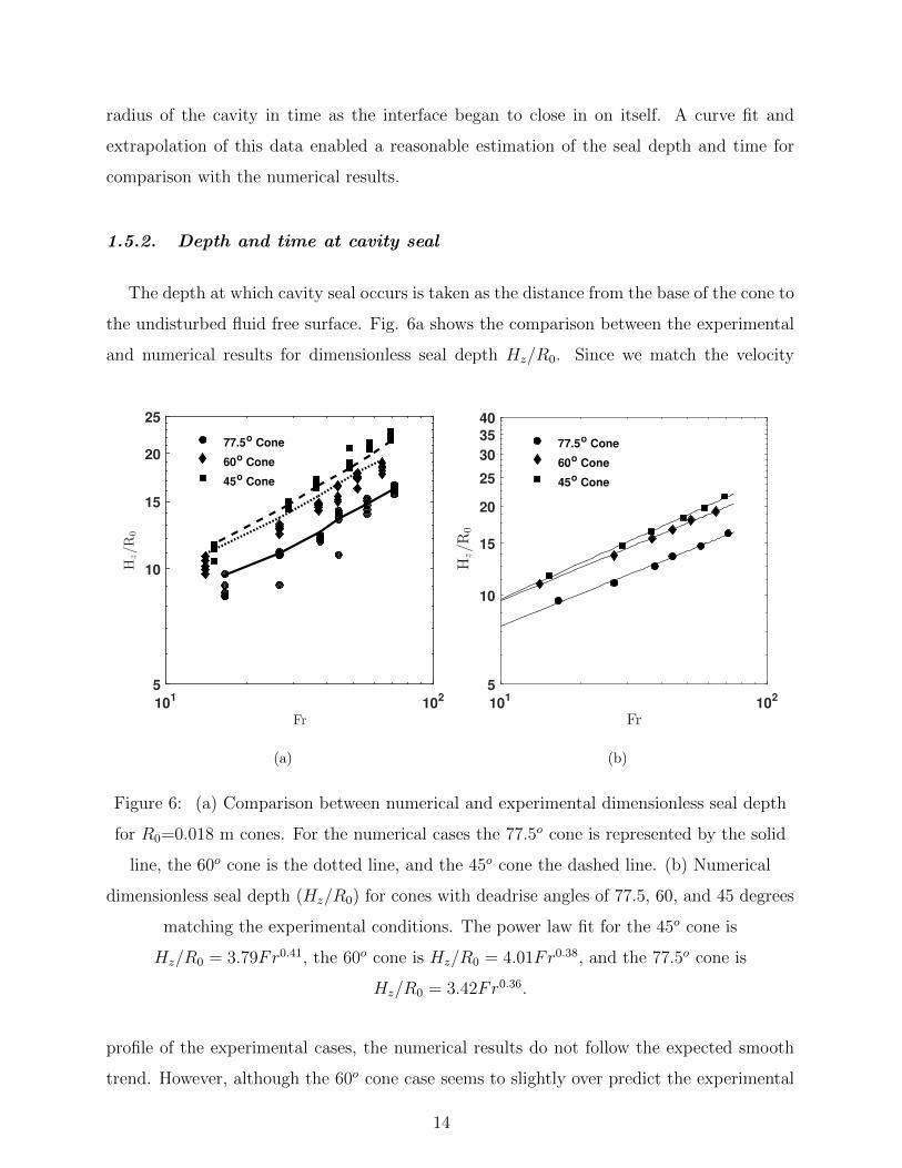
6 (a) Comparison between numerical and experimental dimensionless seal depth

for R0=0.018 m cones. For the numerical cases the 77.5o cone is represented

by the solid line, the 60o cone is the dotted line, and the 45o cone the dashed

line. (b) Numerical dimensionless seal depth (Hz/R0) for cones with deadrise

angles of 77.5, 60, and 45 degrees matching the experimental conditions. The

power law fit for the 45o cone is Hz/R0 = 3.79Fr0.41, the 60o cone is Hz/R0 =

4.01Fr0.38, and the 77.5o cone is Hz/R0 = 3.42Fr0.36. . . . . . . . . . . . . . . . . . . . . . 14

7 Comparison between numerical (solid line) and experimental (◦) dimension-

less time to seal (T ) for R0=0.02 m cones with deadrise angles of 77.5, 60,

and 45 degrees and Froude numbers (Fr = V 20 /gR0) ranging from ≈10-70. . . 15

8 Comparison of normalized force F = F/(π2ρR2

0V20 cot β) with time T =

t/(Hcone/V0) for all experimental cases and numerical runs for the 60o dead-

rise angle cone. The numerical data is represented by the smooth lines,

colored to match the corresponding experimental data . . . . . . . . . . . . . . . . . . . . 16

9 Cd plotted against σwe for all of the cones and Froude numbers, as well as the

approximate data for a disk from Glasheen and McMahon1 . . . . . . . . . . . . . . . . 18

10 77.5o cone drag coefficient with water entry cavitation number (σwe) for all

Froude numbers corresponding to the cone drop heights of 10-60 cm used in

the experiments. . . . . . . . . . . . . . . . . . . . . . . . . . . . . . . . . . . . . . . . . . . . . . . . . . . . . 19

vi

LIST OF TABLES

1 Numerical vs experimental RMSE . . . . . . . . . . . . . . . . . . . . . . . . . . . . . . . . . . . . . 17

vii

NOMENCLATURE

Fr = Froude number

V0 = Impact velocity

g = Standard gravity

R0 = Radius of the cone

Hseal = Depth of the base of the cone below the undisturbed free surface at cavity seal

Hexp = Height of the cone tip above the free surface prior to release

Hz = Depth of the base of the cone below the undisturbed free surface

β = Deadrise angle

V = Velocity of the cone

Re = Reynolds number

ν = Kinematic viscosity

φ = Velocity potential

δ = Dirac delta

P = Pressure

Pa = Ambient air pressure

ρ = Fluid density

γ = Interfacial tension

K = Curvature

s = Arc length

Fγ = Force contribution due to interfacial tension

F = Total drag force on the cone

4t = Time step

Rc = Radius of the cone at the fluid contact line as the cone enters the fluid

Ht = Height of the cone tip below the undisturbed free surface

n = Unit normal vector

T = Dimensionless time

F = Dimensionless force

Cd = Drag coefficient

σwe = Water entry cavitation number

α = Dimensionless acceleration

aavg = Mean acceleration

viii

1. FREE SURFACE PENETRATION OF INVERTED RIGHT CIRCULAR

CONES AT LOW FROUDE NUMBER

Samuel Koski,1 Sunghwan Jung,2 Pavlos Vlachos,3 Jon Yagla,4 Austin Mituniewicz,2

and Brian Chang2

1)Department of Mechanical Engineering, Virginia Tech, Blacksburg,

VA 24061

2)Department of Engineering Science and Mechanics, Virginia Tech, Blacksburg,

VA 24061

3)Department of Mechanical Engineering, Perdue University, West Lafayette,

IN 47907

4)Consultant to the Naval Surface Warfare Center - Code E41, Dahlgren,

VA 22448

In this paper, we study the impact of inverted right circular cones over multiple

deadrise angles on an air water interface at low Froude number (Fr ≈ 10-70). In

this flow regime it is known that an air cavity is formed aft of a body as it travels

into a liquid. Previous studies have confirmed that the depth of the projectile at

the collapse of this cavity follows a power law ∝ Fr1/2 for disks, whereas for right

cylinders or the impact of spheres on soft sand, the depth at cavity seal is ∝ Fr1/3.

Experiments were conducted at these Froude numbers with 0.02 m radius cones over

multiple deadrise angles. High speed video was taken as well as a measurement of

the drag force over the depth of travel for each case. A numerical model has been

developed based on a boundary element method, and matching the conditions of the

experiments, we study the temporal dynamics of the cavity and the forces exerted

on the cone from impact on the liquid interface to cavity collapse.

PACS numbers: 02.60.Lj, 02.60.-x, 47.11.-j, 47.55.N-+

1

1.1. Introduction

Free surface penetration is a multiphase flow phenomenon whereby a solid body is

translated through a gas penetrating a liquid. Divers or seaplane floats impacting a fluid

surface2,3, plunge-diving seabirds4, and water striders5 or basilisk lizards6 running on water

include examples in this class of problem. Classical work by Worthington7 showed that

for a given surface treatment, body geometry, and impact velocity a “basket splash” and

transient cavity can be maintained as a sphere travels from air into fluids such as water,

petroleum, and glycerin.

For projectiles with sharp corners such as disks and cones, the point at which the fluid

separates from the body at impact is well defined and much less dependent on the surface

treatment. Glasheen and McMahon1 performed an experimental study with disks ranging

in radius from 0.01-0.03 m and Froude numbers Fr = V02/gR0 from 1-80, where V0 is

the initial velocity, R0 the radius, and g is the acceleration due to gravity. Accounting

for hydrostatic pressure, a projectile weight which matched the average drag force enabled

experimentation conducted with a steady average velocity, providing for a more direct com-

parison with steady-state numerical and experimental results. From this, it was shown that

the non-dimensional depth at seal was related to the square-root of the Froude number as

Hseal/R0 = 2.30Fr0.5. They also found that the time to seal was nearly independent of

velocity, and related to the square root of the radius as 0.73R00.5.

Multiple investigators have since confirmed these findings numerically and experimentally8–10.

Experimentation and modeling conducted by Lohse et al.11 included the impact of spheres

on extremely fine aerated sand, where the depth at seal was found instead to be ∝ Fr1/3.

This work was extended by Duclaux et al.10 where experimentation and analytical modeling

was conducted confirming both of these power laws, with the depth at seal for spheres

∝ Fr1/2 and cylinders ∝ Fr1/3.

In this article, we investigate the effect that cone deadrise angle has on the cavity interface

dynamics, including pinch off time and depth, interface position, and the drag force on the

cone at low Froude number (Fr ≈ 10 − 70). We set out to show that as a result of the

differing angles, the seal depth falls inside the range ∝ Fr1/n where 2 < n < 3. To carry

this out, assumptions must be made about the relative importance of governing parameters.

At the impact velocities under consideration, the dynamic pressures that initially push the

2

fluid radially outward are quickly overcome and dominated by hydrostatic pressure as the

cavity wall behind the cone is extended and begins to collapse. As a result, forces due to

gravity and interfacial tension have a marked effect on the cavity development and cannot

be neglected. This was shown by Gaudet9 to be particularly important at very low Froude

number, where the fluid initially has minimal outward motion at impact and begins to

collapse almost immediately thereafter.

With these considerations in mind, we develop a boundary element scheme similar to Oguz

and Prosperetti12 and Gaudet9 which numerically simulates the evolution of the cavity in

time. The results of controlled experiments, including measurements of force, are then

compared and expanded with this model to gain insight into the cavity dynamics.

In §II we will discuss the experimental setup, and the mathematical formulation is covered

in §III followed by the numerical method in §IV. A comparison will then be made in §Vbetween the experimental and numerical results, including the position of the interface, time

and depth at cavity seal, and the drag force exerted on the surface of the cone. Finally, we

discuss the results and draw conclusions and recommendations in §VI.

1.2. Experimental set-up

Experiments have been conducted with 0.02 m fixed radius (R0) cones at deadrise angles

(β) of 45, 60, and 77.5 degrees. A sketch of the experimental setup is provided as Fig. 1.

The supporting structure around the water tank was constructed of aluminum t-slot beams.

Low friction sliding supports were mounted onto each of the vertical beams and onto each

of these an end of the horizontal cross member was secured. Force measurements were

made using an Omegadyne LCM105-10 load cell securely mounted at the center of the cross

member. The data was collected at 1000 samples/second with a National Instruments DAQ

after passing though a signal amplifier. A 3.18 mm radius stainless steel rod was threaded

into the load cell on one end and into a cone on the other. Experiments were conducted with

the tip of the cone located at a height Hexp=10-60 cm above the surface of the water. This

was achieved by securing a line to the sliding cross bar assembly and lifting it into place by

means of a pulley. Upon release, the cone was free to fall vertically to the fluid interface,

impacting at an instantaneous velocity V0 ≈√

2gHexp. Unlike the steady experiments of

Glasheen and McMahon1, and the decelerating cases studied by Duclaux et al.10, the cones

3

Figure 1: Experimental set-up.

for these experiments continue to accelerate an average of 2-5 m/s2 from impact to cavity

seal (≈ 0.1 s). Shadowgraphs were taken with a high speed IDT Motionxtra N3 camera

at 1000 frames per second with a shutter speed of 63 µs. The images were captured at a

resolution of 408×1248 pixels. The cone impacted the fluid interface at the center of the

tank, so that the camera captured the event as the cone crossed the fluid air interface from

below the surface. Although this recorded the temporal cavity dynamics below the free

surface well, the effects that occurred above it could not be recorded since, when looking at

the interface from inside the fluid, light was reflected off the air water interface.

1.3. Mathematical formulation

We set out to calculate the transient cavity dynamics encompassing the configuration

and conditions of the experiments. The axisymmetric region displayed in Fig. 2 defines the

coordinate system and domain. A cone with a deadrise angle β impacts the fluid interface

vertically along the z axis with a velocity V (t). The bottom and far field boundaries are

4

r

V(t)z

Cs

n Fi

Fb

Bb

Axis

Figure 2: Axisymmetric domain definitions.

positioned sufficiently far away that they have a negligible influence on the flow. At the

impact velocities under evaluation, the Reynolds number Re = R0V0/ν is on the order 104

or higher, so that the fluid is considered both inviscid and incompressible. It is assumed

also that the flow is irrotational, which means a velocity potential φ(r,z,t) exists inside the

fluid volume satisfying Laplace’s equation

52φ = 0. (1)

Since our interest lies exclusively on the dynamics occurring on the boundary, a boundary

integral method is ideally suited for the problem. To carry this out, we employ the Green’s

function of Laplace’s equation given by

52G(x,x0) + δ(x− x0) = 0, (2)

where

|x− x0| =√

(x− x0)2 + (y − y0)2 + (z − z0)2 (3)

is the distance of a field point x from the singular or source point x0. The fundamental

solution of Laplace’s equation in the absence of boundaries is known to be13

G(x,x0) =1

4π|x− x0|. (4)

5

Referring to Fig. 2, we see that the solution domain of interest is rotationally symmetric

about the z axis and thus integrate Eq. 4 from 0 to 2π, which yields

G (ξ, ξ0) =F (k)

π√

(z − z0)2 − (r + r0)2, (5)

representing the value of a function at ξ due to a point source at ξ0 in an infinite domain.

Here, F (k) is the complete elliptic integral of the first kind

F (k) =

∫ 2π

1

dη√1− k2 cos2 η

, (6)

where η is a dummy variable of integration and

k2 =4rr0

(z − z0)2 + (r + r0)2. (7)

For a bounded domain, we find after substitution of Eq. 2 into Green’s second identity, an

integral equation for the solution of Laplace’s equation by integrating over a control volume

V bounded by a surface S = Cs ∪ Fi ∪ Fb ∪Bb to be∫S

−G (ξ, ξ0)n · 5φ (ξ) + φ (ξ)n · 5G (ξ, ξ0) ds = λφ (ξ0) , (8)

where s is the arc length along S. Integration of δ(x − x0) is by definition a Heaviside

function from which

λ =

1 if ξ0 lies inside V

1/2 if ξ0 lies on S

0 if ξ0 lies outside V .

(9)

The unsteady Bernoulli equation given by

P − Pa = −ρ(gHz +

∂φ

∂t+

1

2| 5 φ|2

), (10)

provides a means by which the pressure (P ) inside the fluid volume can be determined, where

Pa is the ambient air pressure, Hz is the depth from the base of the cone to the undisturbed

free surface, and ρ is the fluid density. Recalling that the Young-Laplace equation4P = γK

relates the pressure difference across the fluid interface (Fi) to the mean curvature and

interfacial tension, we recast Eq. 10 to find the Lagrangian time rate of change of the

velocity potential as

∂φ

∂t

∣∣∣∣Fi

=1

2| 5 φ|2 − gHz −

γK

ρ, (11)

6

where γ is the interfacial tension and the mean curvature

K =zr − rz

(r2 + z2)3/2− z

r (r2 + z2)1/2(12)

with the dots denoting differentiation with respect to arc length.

For the calculation of drag, the force contribution due to interfacial tension acting at the

edge of the cone is determined to be

Fγ = 2πR0γ cos (θ) , (13)

where θ is the angle of the interface from the z axis on the edge of the cone located at R0.

The fluid pressure acting at the wetted cone surface is found by integration of Eq. 10 in

polar coordinates from r=0 to R0, so that the total drag force is given by

F = Acρ

(1

2Vn

2 − β∫ R0

r=0

(∂φ

∂t− 1

2

(∂φ

∂s

)2

− gHz

)rdr

)+2πR0γ cos (θ) , (14)

where Ac is the wetted area of the cone, and ∂φ/∂s is the tangential velocity of the fluid

at the cone surface. Recalling that the unknown velocity potential on the cone surface is

calculated in time by Eq. 8, the definition of a material derivative can be used to find

∂φ

∂t=Dφ

Dt−V(t) · 5φ (15)

assuming Dφ/Dt ∼= 4φ/4t.

1.4. Numerical method

1.4.1. Boundary element method (BEM)

In order to solve Eq. 8 numerically, the boundary S is approximated by nodes (z1, r1),(z2, r2)

. . . . . . (zN+1, rN+1), joined by straight line elements Ek with k = 1, 2, . . . , N . Assuming con-

stant φ = φk and ∂φ/∂n = Vk at the center of each element Eq. 8 can be written

λφ(z0, r0) =N∑k=1

−αk(z0, r0)Vk + φkψk(z0, r0), (16)

where

αk(z0, r0) =

∫Ek

G (ξ, ξ0) ds (17)

7

and

ψk(z0, r0) =

∫Ek

n · 5G (ξ, ξ0) ds. (18)

Recalling that our interest lies only on the boundary, we set λ = 1/2 so that Eq. 16 can be

written

1

2φj =

N∑k=1

φkψjk − Vkαjk, (19)

where the index j represents the evaluation node (z0, r0) on a boundary element. In order to

solve Eq. 19 numerically we write it in the form Ax=b, where the known values are stored

in the matrix A and vector b in order to calculate the unknown values represented by the

vector x

N∑k=1

Ajkxk =N∑k=1

bjk. (20)

To construct the A matrix and b vector, the line integrals for Eq. 17 and 18 are computed

with a 20 point Gaussian quadrature. For our problem either φk is known on the fluid

interface or Vk is known on the surface of the cone in Eq. 19. So that on an element where

φk is known and Vk is unknown, Ajk = −αk(zk, rk) and bjk = −φkψk(zk, rk) if j 6= k and

bjk = −φkψk(zk, rk) + 1/2φj if j = k. Alternately when Vk is known and φk is unknown,

Ajk = ψk(zk, rk) if j 6= k or ψk(zk, rk)− 1/2 if j = k, and bjk = Vkαk(zk, rk).

1.4.2. Initial conditions

We start our calculation with the cone surface fully wetted, where the initial shape of the

free surface and depth of the cone are determined by Wagner’s method2. The depth of the

cone tip below the undisturbed free surface Ht is first found by14

Ht =πRc tan β

4, (21)

where Rc is the radius of the cone at the fluid contact line. Setting Rc = R0, the fully

submerged depth is determined and the initial interface profile is calculated by15

ζ(r, t0) =rHt

R0

arcsin

(R0

r

)−Ht, for r > R0. (22)

8

Experiments were conducted for cones with deadrise angles of 45, 60 and 77.5 degrees

dropped from 10-60 cm heights in increments of 10 cm. For each drop height 5 experi-

ments were conducted with high speed video taken as well as measurements made of the

drag force exerted on the cone. The mean of the velocity was taken of all 5 samples for

a given drop height, and a quadratic fit of this was used as input into the numerical code

for V (t). In order to make a quantitative comparison of the experimental and numerical

cases, post processing of the high speed video data was carried out using the image pro-

cessing toolbox available in the technical computing software MATLAB16,17. Each of the

video frames were saved as .tiff files, which could be directly read into MATLAB. Once

loaded, an image was converted to binary using the im2bw function, as shown in Fig. 3.

The result of this was an image where the region at the cavity interface was represented by

ones (white) and the remaining pixels were given a value of zero (black). With the image

converted to binary, extraction of the interface was carried out using the bwtraceboundary

function. Prior to a series of experiments, an image was taken with the high speed camera

of a ruler, allowing for scaling of the extracted interface from pixels to a spatial unit. Due

to the fact that our simulations start with the cone fully submerged, the correct start time

is determined from the experimental data by fitting a curve to the average cone depth with

time. Differentiation of this provides an equation for V (t), and the time at Ht is then used

as input into this equation to determine the initial velocity for the calculation. At this time

the velocity potential is set to φ = 0 on the fluid interface, and the velocity ∂φ/∂n = V0 · nat the cone surface, where n is the unit normal pointing out of the fluid volume.

Adequate nodal spacing is important for proper resolution of the interface, particularly in

the early stages of the solution when the position of the fluid interface is rapidly evolv-

ing. The arc length spacing of the nodes (4s) is set at the beginning of the simulation

and held constant until its completion. We have found it to be important that the same

arc length spacing on both the cone surface and interface also be maintained throughout

the calculation18 (4s/R0=0.02). However, the far field boundaries have little effect on the

flow, and hence are sparsely populated with nodes, which has the added benefit of reducing

computational expense.

9

(a) (b) (c)

Figure 3: Image processing sequence where (a) is the raw image from the high speed video,

(b) is the image converted to binary, and (c) is fluid interface after extraction.

1.4.3. Time integration

Fig. 4 is included to illustrate the general process used to carry out a numerical sim-

ulation. By means of Eq. 20, we use the initial conditions on the boundary to find the

unknown velocity potential at the cone surface and the normal velocity on the fluid inter-

face at the center of each element. To advance the solution in time, the position of the cone

is determined by V (t)∆t. The advancement of the interface, and the calculation of Eq. 11

are carried out by means of a 4th order Runge-Kutta method.

At each iteration, the position of the nodes are changed by some spatial distance depending

on the local fluid velocity and time step. As a result, it is necessary to add and redistribute

nodes as the solution advances to ensure the interface is properly resolved. Although the

nodal spacing is maintained throughout the calculation, the first node on the interface next

to the cone is alternately placed at arc length 4s and 1/2 4s every time step, following the

10

Start

Set initial conditions

Solve BEM for unknownφ and Vn

Advance nodal positionsand the velocity potential

Calculate drag force

Redistribute nodeson the interface

Advance time (t+△t)and set V(t)

Calculationcomplete?

Stop

yes

no

Figure 4: Steps for numerical solution.

work of Oguz and Prosperetti12. This has the advantage of smoothing the interface while

preventing the growth of artificial instabilities.

The fluid interface is represented by parametric splines in order to determine the nodal

positions and velocity potential during the redistribution process. Oguz and Prosperetti12,

Gaudet9, and Dommermuth and Yue19 all represented the fluid interface by parametric cu-

bic splines. In regions of evolving curvature, such as where the fluid heaves upward near

the cone edge at initial impact and where deep seal occurs, standard cubic splines often

impose an exaggerated curvature on the interface, the extent of which is a function of nodal

resolution and the local curvature. Besides effecting the estimation of the interface position

with time, the presence of irregularities on the fluid interface introduce numerical noise when

differentiating with respect to arc length. To counter this, we use the monotone piece-wise

11

cubic by Fritsch and Carlson20 who suggested that unlike other spline types, “the curve

produced contains no extraneous bumps or wiggles, which makes it more readily acceptable

to scientists and engineers.”

1.5. Experimental and numerical results

In this section we make a comparison between the results of our numerical simulations

and experiments, including the position of the interface, time and depth at cavity seal, and

the drag force exerted on the surface of the cone.

1.5.1. Dynamics of the fluid interface

Fig. 5 shows results for a selection of the 60 cm drop height experiments, where the

numerically calculated interface position is overlaid on images for each of the cone deadrise

angles at dimensionless times Hz/R0=5, Hz/R0=10, and just prior to cavity seal. It can be

seen from this that upon impact on the air water interface, the water is accelerated radially

outward from the edge of the cone. This produces an air cavity aft of the cone with a radius

that is a function of the cone angle and impact velocity. As the cone moves further into

the fluid, the wall of the cavity becomes less affected by the cone, and hydrostatic pressure

begins to push it radially inward. The differences in cavity development for each of the

cones is clearly seen by this, where the higher deadrise angle cones are less able to push the

fluid radially outward and hence produce a cavity which has less volume. The numerical

results match the location of the interface in time very nicely for these cases. However,

near the fluid free surface there is some localized difference due to the splash, which is not

accounted for numerically. This clearly has little effect on the overall development of the

cavity interface. The error associated with this becomes larger with drop height and lower

cone deadrise angle, so that the images shown in column c of Fig. 5 represent the worst case

out of all the experiments conducted.

Considering the cases shown in images at cavity seal in Fig. 5, it is clear that the time

of complete cavity closure and hence the depth of the cone at pinching was not directly

measurable due to the presence of the rod pushing the cone into the fluid. Using the

interface position extracted from the high speed video, we were able to track the minimum

12

Hz/R

0=5

Hz/R

0=10

Cavityseal

a b c

Figure 5: Cavity development for the 77.5o cone (column a), 60o cone (column b), and 45o

cone (column c) dropped from Hexp=60 cm. The cones are shown at depths Hz/R0=5,

Hz/R0=10, and just prior to cavity seal, where Hz/R0=20.72 for the 45o cone, Hz/R0=18

for the 60o cone, and Hz/R0=14.66 for the 77.5o cone.

13

radius of the cavity in time as the interface began to close in on itself. A curve fit and

extrapolation of this data enabled a reasonable estimation of the seal depth and time for

comparison with the numerical results.

1.5.2. Depth and time at cavity seal

The depth at which cavity seal occurs is taken as the distance from the base of the cone to

the undisturbed fluid free surface. Fig. 6a shows the comparison between the experimental

and numerical results for dimensionless seal depth Hz/R0. Since we match the velocity

Fr10

110

2

Hz/R

0

5

10

15

20

25

77.5o Cone

60o Cone

45o Cone

(a)

101

102

Fr

5

10

15

20

25

30

35

40

Hz/R

0

77.5o Cone

60o Cone

45o Cone

(b)

Figure 6: (a) Comparison between numerical and experimental dimensionless seal depth

for R0=0.018 m cones. For the numerical cases the 77.5o cone is represented by the solid

line, the 60o cone is the dotted line, and the 45o cone the dashed line. (b) Numerical

dimensionless seal depth (Hz/R0) for cones with deadrise angles of 77.5, 60, and 45 degrees

matching the experimental conditions. The power law fit for the 45o cone is

Hz/R0 = 3.79Fr0.41, the 60o cone is Hz/R0 = 4.01Fr0.38, and the 77.5o cone is

Hz/R0 = 3.42Fr0.36.

profile of the experimental cases, the numerical results do not follow the expected smooth

trend. However, although the 60o cone case seems to slightly over predict the experimental

14

101

102

Fr

100

101

102

T

77.5o Cone

60o Cone

45o Cone

Figure 7: Comparison between numerical (solid line) and experimental (◦) dimensionless

time to seal (T ) for R0=0.02 m cones with deadrise angles of 77.5, 60, and 45 degrees and

Froude numbers (Fr = V 20 /gR0) ranging from ≈10-70.

data, the comparison between the numerical and experimental results are quite good. In

Fig. 6b a plot of the numerical data corresponding to the experimental cases with power

law fits is included. Here we see that for the 45o cone Hz/R0 = 3.79Fr0.41, the 60o cone

Hz/R0 = 4.01Fr0.38, and the 77.5o cone Hz/R0 = 3.42Fr0.36. Which confirms that as the

deadrise angle and hence the L/D is decreased for a fixed radius cone (e.g. it becomes

more blunt), the fluid has a greater radial momentum at the separation point, and hence

the interface dynamics approach that of the disks studied by Glasheen and McMahon1 and

Gaudet9, where the depth at seal was ∝ Fr0.5. Conversely, as the deadrise angle is increased,

the fluid experiences less radial motion at the edge of the cone and hence the cavity wall

is more quickly overcome by hydrostatic pressure, thereby producing a more rapid cavity

closure.

This is verified by the corresponding time to seal, normalized by T = t/(Hcone/V0) shown

in Fig. 7 for each of the cones. As expected, the magnitude of T increases with cone

angle, however it is notable that, unlike the seal depth, the dimensionless time to seal is

15

approximated by a power law fit ∝ Fr0.5 regardless of cone angle.

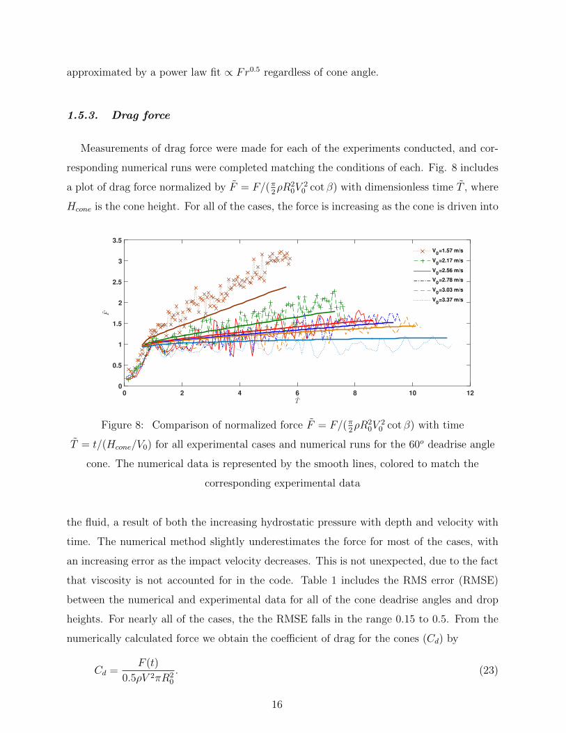
1.5.3. Drag force

Measurements of drag force were made for each of the experiments conducted, and cor-

responding numerical runs were completed matching the conditions of each. Fig. 8 includes

a plot of drag force normalized by F = F/(π2ρR2

0V20 cot β) with dimensionless time T , where

Hcone is the cone height. For all of the cases, the force is increasing as the cone is driven into

T

0 2 4 6 8 10 12

F

0

0.5

1

1.5

2

2.5

3

3.5

V0=1.57 m/s

V0=2.17 m/s

V0=2.56 m/s

V0=2.78 m/s

V0=3.03 m/s

V0=3.37 m/s

Figure 8: Comparison of normalized force F = F/(π2ρR2

0V20 cot β) with time

T = t/(Hcone/V0) for all experimental cases and numerical runs for the 60o deadrise angle

cone. The numerical data is represented by the smooth lines, colored to match the

corresponding experimental data

the fluid, a result of both the increasing hydrostatic pressure with depth and velocity with

time. The numerical method slightly underestimates the force for most of the cases, with

an increasing error as the impact velocity decreases. This is not unexpected, due to the fact

that viscosity is not accounted for in the code. Table 1 includes the RMS error (RMSE)

between the numerical and experimental data for all of the cone deadrise angles and drop

heights. For nearly all of the cases, the the RMSE falls in the range 0.15 to 0.5. From the

numerically calculated force we obtain the coefficient of drag for the cones (Cd) by

Cd =F (t)

0.5ρV 2πR20

. (23)

16

TABLE 1: Numerical vs experimental RMSE

RMS error RMS error RMS error

Hexp(cm) 77.5o cone 60o cone 45o cone

10 1.20 0.51 0.55

20 0.67 0.23 0.41

30 0.48 0.21 0.5

40 0.41 0.18 0.39

50 0.54 0.17 0.44

60 0.78 0.21 0.39

Glasheen and McMahon1 related this to the water entry cavitation number given by

σwe =g|Hz(t)|0.5V (t)2

, (24)

which by taking into account the changing depth and velocity with time, is a ratio between

hydrostatic and dynamic pressure. In their work, they found a linear relationship between

the two which was later confirmed by Gaudet9. Since they were interested in studying disks

with a near constant velocity, they only reported data that had dimensionless acceleration

(α) less than 0.015 given as

α =aavgR0

V 2rms

, (25)

where aavg is the mean acceleration. For our cones, α ranges from ≈ 5×10−3 for the highest

impact velocity cases to ≈0.03 for the lowest. Despite this we also see a linear relationship

for all of the cone angles and drop heights studied as shown in Fig. 9. In this case, the

slope of the line through a set of data decreases as the deadrise angle is increased, so that

for the 77.5 degree cone Cd is decreasing with σwe and the 45 degree cone is increasing. It

is therefore reasonable to assume that as the deadrise angle continues to decrease the slope

will continue to increase, approaching the plotted data from Glasheen and McMahon1 for a

disk. We also note that not unexpectedly the magnitude of Cd decreases with an increasing

L/D.

For any of the cone angles, the corresponding change in drag coefficient with Froude

number for a given α over the range of velocities studied is not significant. A closer view

17

0 0.2 0.4 0.6

σwe

0

0.5

1

1.5

2

Cd

77.5o Cone

60o Cone

45o Cone

Glasheen and McMahon

Figure 9: Cd plotted against σwe for all of the cones and Froude numbers, as well as the

approximate data for a disk from Glasheen and McMahon1

of the data illustrated in Fig. 9 is shown in Fig. 10, where all of the 77.5o cone cases are

plotted. As expected, we see an increasing Cd with V0. However, since the velocity range is

quite small, the change in Cd is not significant.

1.6. Conclusions

We have presented a quantitative numerical and experimental analysis of the temporal

interface dynamics and drag force on the surface of a cone, from its impact on a liquid

surface to the eventual collapse of the ensuing air cavity. Our numerical technique, based on

a boundary element method, has been shown to match the experimental time to cavity seal,

drag force, cavity seal depth, and interface position with excellent precision. We attribute

this accuracy in part due to the representation of the interface by a parametric monotone

piece-wise cubic20, rather than the cubic splines typically used. This is coupled with a

uniform fixed arc-length spacing of the nodes across the surface of both the projectile body

18

0 0.2 0.4 0.6

σwe

0.33

0.34

0.35

0.36

0.37

Cd

V0=1.71

V0=2.17

V0=2.58

V0=2.79

V0=3.15

V0=3.55

Figure 10: 77.5o cone drag coefficient with water entry cavitation number (σwe) for all

Froude numbers corresponding to the cone drop heights of 10-60 cm used in the

experiments.

and the interface for the entire simulation.

We confirm a linear relationship between the drag coefficient Cd and the water entry cavi-

tation number σwe, where the slope increases with decreasing deadrise angle, approaching

that of the disks studied by Glasheen and McMahon1. The numerical method slightly under

predicts the force for all of the cases. This is not unexpected, since when formulating the

numerical method, we assume the flow to be inviscid and hence make no account for the

boundary layer on the surface of the cone.

It has been shown that the seal depth for a cone is controlled by deadrise angle, falling inside

the range ∝ Fr1/n where 2 ≤ n ≤ 3. More specifically, cones with a lower deadrise angle

approach the seal depth of disks1 or hydrophobic spheres10, whereas more slender cones with

higher deadrise angle have a seal depth approaching right cylinders10 or spheres impacting

on fine sand11. Similarly, the dimensionless time to seal T = t/(Hcone/V0) increases as cone

angle is decreased. However, unlike the seal depth, the time to seal has been shown to be

approximately ∝ Fr0.5, regardless of cone angle.

19

1.6.1. Future work

The study presented here focuses solely on the dynamics of the cavity interface behind

a water-entering cone. It would be instructive to also consider the dynamics of bulk fluid

flows, particularly along the surface of the cone and in the vicinity of the cavity interface.

The boundary element code developed for this work can be extended to this effort, and a

direct comparison with a technique such as particle image velocimetry (PIV) could be useful

to verify the code.

A greater expansion of the numerically modeled cases would also be particularly useful.

The focus of this work was on matching the cavity shape observed in the experiments, but

it would be interesting to show a larger range of cone angles and velocities. Furthermore,

although the acceleration was small, a comparison with these results and those of steady

velocity cones or those with mass could be a follow on to this effort.

20

1.7. REFERENCES

1J. W. Glasheen and T. A. McMahon, “Vertical water entry of disks at low froude numbers,”

Physics of Fluids 8 (1996).

2H. Wagner, “Phenomena associated with impacts and sliding on liquid surfaces,” Z. Angew.

Math. Mech. 12 (1932).

3T. V. Karman, “The impact on seaplane floats during landing,” National Advisory Com-

mittee for Aeronautics (1929), technical Note No. 321.

4M. Croson, L. Straker, S. Gart, C. Dove, J. Gerwin, and S. Jung, “How seabirds plunge-

dive without injuries,” PNAS 113 (2016).

5D. L. Hu, B. Chan, and J. W. M. Bush, “The hydrodynamics of water strider locomotion,”

Nature 424, 663–666 (2003).

6J. W. Glasheen and T. A. McMahon, “A hydrodynamic model of locomotion in the basilisk

lizard,” Nature 380, 340–342 (1996).

7A. M. Worthington, “A study of splashes,” Longmans Green and Company (1908).

8R. Bergmann, D. VD Meer, S. Gekle, A. VD Bos, and D. Lohse, “Controlled impact of a

disk on a water surface: cavity dynamics,” J. Fluid Mech. 633, 381–409 (2009).

9S. Gaudet, “Numerical simulation of circular disks entering the free surface of a fluid,”

Physics of Fluids 10 (1998).

10V. Duclaux, F. Caille, C. Duez, C. Ybert, L. Bocquet, and C. Clanet, “Dynamics of

transient cavities,” J. Fluid Mech. 591 (2007).

11D. Lohse, R. Bergmann, R. Mikkelsen, C. Zeilstra, D. VD Meer, M. Versluis, K. VD Weele,

M. VD Hoef, and H. Kuipers, “Impact on soft sand: void collapse and jet formation,”

Physical Review Letters 93 (2004).

12H. N. Oguz and A. Prosperetti, “Bubble entrainment by the impact of drops on liquid

surfaces,” J. Fluid Mech 219, 143–179 (1990).

13C. Pozrikidis, A Practical Guide to Boundary Element Methods (Chapman & Hall/CRC,

2000 N.W. Corporate Blvd, Boca Raton, FL 33431, 2002).

14O. Faltinsen and R. Zhao, “Water entry of ship sections and axisymmetric bodies,”

AGARD FDP and Ukraine institute of hydromechanics workshop on highSpeed body

motion in water (1971).

21

15H. Sun, A Boundary Element Method Applied to Strongly Nonlinear Wave-Body Interaction

Problems, Ph.D. thesis, Norwegian University of Science and Technology (2007).

16Matlab, Version 8.6.0.267246 (R2015b) (The MathWorks Inc., Natick, Massachusetts,

2015).

17M. I. P. Toolbox, Version 9.3 (R2015b) (The MathWorks Inc., Natick, Massachusetts,

2015).

18J. D’Errico, “Distance based interpolation along a general curve in space,” MATLAB

Central File Exchange (Retrieved 2014).

19D. G. Dommermuth and D. Yue, “Numerical simulation of nonlinear axisymmetric flows

with a free surface,” J. Fluid Mech. 178, 195–219 (1986).

20F. Fritsch and R. Carlson, “Monotone piecewise cubic interpolation,” SIAM Journal on

Numerical Analysis 17, 238–246 (1980).

22

2. APPENDIX A - ALGORITHMS

2.1. Main Script

%clear all

%close all

%uncomment below if using a cluster

%distcomp.feature(’LocalUseMpiexec’,false)

delete(gcp)

myCluster=parcluster(’local’)

myCluster.NumWorkers=32

parpool(32)

%%%%%%%%%%%%%%%%%%%%%%%%%%%%%%%%%%%%%%%%%%%%%%%%%%%

% User Inputs %

%%%%%%%%%%%%%%%%%%%%%%%%%%%%%%%%%%%%%%%%%%%%%%%%%%%

Frd=71.39; %Froude Number U^2/Rg

damping=0;

bdy_dx=0.0004;

dx=0.0004; %node spacing along the water surface

i_l_x=.2; %interface length in x

i_l_y=1; %interface length in y (distance to bottom of fluid

%domain)

N_d=1000; %number of nodes on the disk (disk radius = 1)

R_d=.018; %radius of disk,sphere,or cone

sigma=0.0728; %surface tension(0.0728 N/m at 20 C for water)

dt=1e-05; %timestep for Computation, this is the minimum

%timestep if using adaptive time stepping

B=127; %Bond number

save_interval=10; %frequency of data file saves

tension=1; %turns surface tension term on (1) or off (0) in the

23

%bernoulii equation

sph=0; %The shape of the object is a shp=1 is not sph=0

cone=1; %The shape is a cone=1 is not cone=0

%if sph and cone both =0 a disk is assumed

% bdy_dx=R_d/N_d;

sep_ang=12.5; %seperation angle of sphere or angle of cone

adaptive_dt=0; %turn adaptive time step on =1 off=0

dt_max=1e-04; %max time step that can be acheived in adaptive time

%step

t_adjust=2e-05; %max nodal displacement criteria for adaptive time

%step

dt_adapt=1e-06; %amount to change the time step in adaptive meshing

wag=1; %use of wagner’s approximation for the shape of the

%inital interface

%%%%%%%%%%%%%%%%%%%%%%%%%%%%%%%%%%%%%%%%%%%%%%%%%%%%

% End User Inputs %

%%%%%%%%%%%%%%%%%%%%%%%%%%%%%%%%%%%%%%%%%%%%%%%%%%%%

N_i=round((i_l_x/dx)+1);

U_real=sqrt(Frd*R_d*9.81);

U_0=-U_real;

mkdir([’Frd=’ num2str(Frd) ’, ds=’ num2str(dx) ’, lx=’ num2str(i_l_x)...

’, tension=’ num2str(tension)])

%%%%%%%%%%%%%%%%%%%%%%%%%%%%%%%%%%%%%%%%%%%%%%%%%%%

% Calculate Initial Domain %

%%%%%%%%%%%%%%%%%%%%%%%%%%%%%%%%%%%%%%%%%%%%%%%%%%%

x_disk=linspace(0,R_d,N_d);

x_int=(R_d:dx:i_l_x+R_d);

y_disk=zeros(1,length(x_disk))+i_l_y;

24

y_int=zeros(1,length(x_int))+i_l_y;

t=0;

if sph>0

h_sep=R_d-R_d*cos(sep_ang*(pi/180));

ang_1=3*pi/2;

srf_ang=(acos((R_d-(h_sep))/R_d));

num=round(R_d*2*acos((R_d-(h_sep))/R_d)/bdy_dx)+1;

t_sep=linspace(ang_1,ang_1+srf_ang,num);

y_disk=i_l_y-h_sep+(R_d*sin(t_sep))+R_d;

x_disk=R_d*cos(t_sep);

x_disk(1)=0;

x_int=(x_disk(end):dx:i_l_x+R_d);

y_int=zeros(1,length(x_int))+i_l_y;

N_d=length(x_disk);

disk_nodes=N_d;

h_cyl=h_sep;

end

if cone>0

cone_h=R_d/(tan(sep_ang*(pi/180)));

cone_side=sqrt(cone_h^2+R_d^2);

num=round(cone_side/bdy_dx);

y_disk=linspace(i_l_y-cone_h,i_l_y,num);

x_disk=linspace(0,R_d,num);

N_d=length(x_disk);

disk_nodes=N_d;

t=0.01438;

U_0=-(-7.5527*t^2+6.0857*t+3.5516);

end

if wag==1

dr_ang=90-sep_ang;

c_dpth=(R_d*2*tan(dr_ang*(pi/180)))/pi;

y_int=1+((x_int.*c_dpth)./R_d).*asin(R_d./x_int)-c_dpth;

25

y_disk=y_disk+(y_int(1)-1);

t=0.01438;

end

phi=zeros(1,(length(x_int)-1));

iter=1;

adapt=1;

phi_disk=zeros(1,length(x_disk)-1);

[xb,yb,bt,bv,Nw]=domain (x_disk,x_int,y_disk,y_int,U_0,phi,dx,...

i_l_x,i_l_y,adapt,phi_disk);

adapt=1;

n = length (xb)-1;% n = number of elements

xm (1:n)=0.5*(xb(1:n)+xb((1:n)+1));

ym (1:n)=0.5*(yb(1:n)+yb((1:n)+1));

xx_new=fliplr(xm(Nw+1:end-N_d+1));

yy_new=fliplr(ym(Nw+1:end-N_d+1));

npt=N_i-1;

dxdt=0;

dydt=0;

dudt_t=0;

m=1;

xsave=save_interval;

pt=1;

% end

stop=1;

u_post=0;

u_post_y=0;

u_post_yproj=0;

vol_post=0;

t_post=0;

r_post=0;

U_proj_post=0;

force_post=0;

26

sve_num=0;

phi1=zeros(1,N_d);

while stop>.0001;

[xb, yb, bt, bv, Nw, adapt]=domain (x_disk,x_int,y_disk,y_int,U_0,...

phi,dx,i_l_x,i_l_y,adapt,phi_disk);

n = length (xb)-1;% n = number of elements

clear lm nx ny nydiv nxdiv

% Find midpoints and lengths of elements, and their unit normal vectors

xm (1:n)=0.5*(xb(1:n)+xb((1:n)+1));

ym (1:n)=0.5*(yb(1:n)+yb((1:n)+1));

hseg=(sqrt(diff(xm).^2 + diff(ym).^2))’;

[k,nx,ny,tnx,tny]=curvature (xm,ym,N_d,hseg);

lm(1:n)=((xb((1:n)+1)-xb(1:n)).^2+(yb((1:n)+1)-yb(1:n)).^2).^.5;

yb1=yb(1:end-1);

xb1=xb(1:end-1);

yb2=yb(2:end);

xb2=xb(2:end);

ubc=zeros(1,N_d)+U_0;

if or(sph==1,cone==1)

nx(end)=-nx(end);

ny(end)=-ny(end);

xxx=-(fliplr(U_0.*(ny(end-N_d+2:end))’));

int_vec=(1:1:length(xxx));

yyy=interp1(int_vec(2:end),xxx(2:end),int_vec(1),’pchip’,’extrap’);

if cone==1

xxx(end)=xxx(end-1);

end

bv(end-N_d+2:end)=[yyy;xxx(2:end)];

ubm=(flipud([yyy;xxx(2:end)]))’;

ubc=interp1(ym(end-N_d+2:end),ubm,y_disk,’pchip’,’extrap’);

27

end

b=zeros(1,n); %preallocate b

% Boundary Element Method

parfor m = 1:n

bb = zeros(1,n);

[f,g] = influencev (xb1,yb1,xb2,yb2,xm(m),ym(m),m);

sing=zeros(length(bv),1);

sing(m)=1;

zz=find(bt==0);

zmin=min(zz);

zmax=max(zz);

A1(m,:)=g(zmin:zmax)’;

A2(m,:)=-0.5.*sing(zmax+1:n)’-f(zmax+1:n)’;

A3(m,:)=-0.5.*sing(1:zmin-1)’-f(1:zmin-1)’;

bb(zmin:zmax)=bv(zmin:zmax).*(f(zmin:zmax)+0.5.*sing(zmin:zmax));

bb(1:zmin-1)=bv(1:zmin-1).*-g(1:zmin-1);

bb(zmax+1:n)=bv(zmax+1:n).*-g(zmax+1:n);

b(m)=sum(bb);

end

% solve system "Ax = b" and store in z

A=[A3 A1 A2];

z=gmres(A,b’,30,1e-8,30);

clear phi u x_int y_int F G A b A1 A2 A3

28

% Assign approximate boundary values

phi(1:n)=(1-bt(1:n)).*bv(1:n)+bt(1:n).*z(1:n);

u(1:n)=(1-bt(1:n)).*z(1:n)+bt(1:n).*bv (1:n);

%Extract interface component of domain for computation of new interface

%location and velocity potential

x_marker=fliplr(xb(Nw+1:end)’);

y_marker=fliplr(yb(Nw+1:end)’);

x_int=x_marker(N_d:end);

y_int=y_marker(N_d:end);

xm=fliplr(xm(Nw+1:end));

ym=fliplr(ym(Nw+1:end));

phin=fliplr(phi(Nw+1:end));

el=fliplr(lm(Nw+1:end));

un=fliplr(u(Nw+1:end));

nx=fliplr(nx(Nw+1:end));

ny=fliplr(ny(Nw+1:end));

phi_disk=interp1(xm(1:N_d-1),phin(1:N_d-1),x_marker(1:N_d),...

’pchip’,’extrap’);

u_disk=zeros(1,length(phi_disk))+U_0;

tm=[x_int(1) cumsum(sqrt(diff([x_int(1) xm(N_d:end)]).^2+...

diff([y_int(1) ym(N_d:end)]).^2))];

t_new=[x_int(1) (cumsum(sqrt(diff(x_int).^2+diff(y_int).^2)))];

u=interp1(tm(2:end),un(N_d:end),t_new);

u(1)=U_0;

u(end)=0;

phi=interp1(tm(2:end),phin(N_d:end),t_new);

phi(1)=phi_disk(end);

phi(end)=0;

29

clear d_q

[d_q,x,y,x_disk,y_disk,dt,force,phi1]=potential(x_marker,y_marker,...

[phi_disk phi(2:end)],[u_disk u(2:end)],Frd,B,N_d,dt,nx,ny,...

adapt,damping,i_l_y,R_d,sigma,tension,sph,ubc,sep_ang,dx,...

adaptive_dt,dt_max,t_adjust,dt_adapt,phi1,bdy_dx);

nosplx=x;

nosply=y;

clear xx_new yy_new

% adapt mesh and velocity potential for next timestep

[x_disk,y_disk,phi,npt,x_int,y_int,xx_new,yy_new,pt,stop] =...

adaptive_mesh(x,y,N_d,dt,x_int,y_int,i_l_x,d_q,dx,npt,...

bv,xb,yb,U_0,Nw,x_disk,y_disk,adapt,phi_disk,R_d,sph,cone,2e-04);

iter=iter+1;

t=(t+dt)

%comment below for a constant velocity

U_0=-(-7.5527*t^2+6.0857*t+3.5516);

if xsave==save_interval

sve_num=sve_num+1;

xsave=0;

cd([’Frd=’ num2str(Frd) ’, ds=’ num2str(dx)...

’, lx=’ num2str(i_l_x) ’, tension=’ num2str(tension)])

save([num2str(sve_num) ’.mat’])

cd ..

end

xsave=xsave+1;

30

end

cd([’Frd=’ num2str(Frd) ’, ds=’ num2str(dx) ’, lx=’ num2str(i_l_x)...

’, tension=’ num2str(tension)])

save(’final.mat’)

cd ..

parpool(’close’)

2.2. Functions

function [xb yb bt bv Nw, adapt]=domain (x_disk,x_int,y_disk,y_int,U_0,...

phi,dx,i_l_x,i_l_y,adapt,phi_disk)

%Construct interface, and far field boundaries

x_interface=[x_disk x_int(2:end)];

y_interface=[y_disk y_int(2:end)];

x_bottom=linspace(0,x_interface(1,end),(x_interface(1,end))/(dx*10));

y_bottom=zeros(1,length(x_bottom));

N_right=i_l_y/(dx*10);

y_right=linspace(y_interface(1,end),y_bottom(1,end),N_right);

x_right=zeros(1,length(y_right))+x_bottom(1,end);

%assemble boundary vectors and assign boundary conditions

xb=[(x_bottom) fliplr(x_right(2:end-1)) fliplr(x_interface)]’;

yb=[(y_bottom) fliplr(y_right(2:end-1)) fliplr(y_interface)]’;

bt=[ones(1,length(x_right(2:end))+length(x_bottom)-1)...

zeros(1,length(x_int(2:end))) ones(1,length(x_disk)-1)]’;

bv=[zeros(1,length(x_right(2:end))+length(x_bottom)-1) fliplr(phi)...

zeros(1,length(x_disk)-1)+(U_0)]’;

31

if adapt==1

adapt=2;

else

adapt=1;

end

%Length of the far field boundary vector

Nw=length(x_bottom)+length(x_right(2:end-1));

function [k,nx,ny,tnx,tny]=curvature (x,y,N_d,h)

[dxdt d2xdt2 dydt d2ydt2] = spl (x,y,h);

%compute element length, arc length, and unit normals (VECTORIZE THIS SAM!)

k=zeros(1,length(x));

R1=(((d2xdt2.*dydt)-(d2ydt2.*dxdt))./(dxdt.^2+dydt.^2).^(3/2));

R2=(-(dydt)./(x.*((dxdt.^2+dydt.^2)).^0.5));

%k=mean curvature

k(2:end-1)=R1(2:end-1)+R2(2:end-1);

k(1:N_d)=0;

norm=sqrt(dxdt.^2+dydt.^2);

nx=zeros(1,length(x));

ny=ones(1,length(x));

tnx=ones(1,length(x));

tny=zeros(1,length(x));

%unit normal and tangent vectors

ny(2:end-1)=dxdt(2:end-1)./norm(2:end-1);

nx(2:end-1)=-(dydt(2:end-1)./norm(2:end-1));

tny(2:end-1)=(dydt(2:end-1)./norm(2:end-1));

tnx(2:end-1)=dxdt(2:end-1)./norm(2:end-1);

end

32

function [dxdt d2xdt2 dydt d2ydt2] = spl (x,y,h)

h1=-h(1:end-1)’;

h2=h(2:end)’;

h21=h2-h1;

dxdt=zeros(1,length(x));

d2xdt2=zeros(1,length(x));

dydt=zeros(1,length(x));

d2ydt2=zeros(1,length(x));

x1=x((2:length(x)-1)-1);

y1=y((2:length(x)-1)-1);

x0=x(2:length(x)-1);

y0=y(2:length(x)-1);

x2=x((2:length(x)-1)+1);

y2=y((2:length(x)-1)+1);

dxdt(2:length(x)-1)=((x2-x0)./h2-(((x2-x0)./h2-(x1-x0)./h1)./h21).*h2);

d2xdt2(2:length(x)-1)=2.*(((x2-x0)./h2-(x1-x0)./h1)./h21);

dydt(2:length(x)-1)=((y2-y0)./h2-(((y2-y0)./h2-(y1-y0)./h1)./h21).*h2);

d2ydt2(2:length(x)-1)=2.*(((y2-y0)./h2-(y1-y0)./h1)./h21);

end

function [F,G] = influencev (x1,y1,x2,y2,x0,y0,m)

xm=(1/2).*(x2+x1);

xd=(1/2).*(x2-x1);

ym=(1/2).*(y2+y1);

yd=(1/2).*(y2-y1);

dr=sqrt(xd.^2+yd.^2);

33

nx=yd./dr;

ny=-xd./dr;

%gauss quadriture points

zz=[-0.993128599185095 -0.963971927277914 -0.912234428251326 -0.839116971822219 -0.746331906460151 -0.636053680726515 -0.510867001950827 -0.373706088715420 -0.227785851141645 -0.076526521133497 0.076526521133497 0.227785851141645 0.373706088715420 0.510867001950827 0.636053680726515 0.746331906460151 0.839116971822219 0.912234428251326 0.963971927277914 0.993128599185095];

ww=[0.017614007139152 0.040601429800387 0.062672048334109 0.083276741576705 0.101930119817240 0.118194531961518 0.131688638449177 0.142096109318382 0.149172986472604 0.152753387130726 0.152753387130726 0.149172986472604 0.142096109318382 0.131688638449177 0.118194531961518 0.101930119817240 0.083276741576705 0.062672048334109 0.040601429800387 0.017614007139152];

x=bsxfun(@plus,xm,(bsxfun(@times,xd,(repmat(zz,length(xm),1)))));

y=bsxfun(@plus,ym,(bsxfun(@times,yd,(repmat(zz,length(ym),1)))));

x0=repmat(x0,length(xm),1);

y0=repmat(y0,length(ym),1);

[G,dGdx,dGdy]= freespacev(x,y,x0,y0);

dd=(y(m,:)-y0(m)).^2+(x(m,:)-x0(m)).^2;

G(m,:)=G(m,:)+log(dd)./(4*pi);

G=sum(bsxfun(@times,dr,(G.*x.*repmat(ww,length(ym),1))),2);

F=sum(bsxfun(@times,dr,(bsxfun(@times,ny,dGdx)+bsxfun(@times,nx,dGdy)).*x.*repmat(ww,length(ym),1)),2);

G(m)=G(m)-2*dr(m)*(log(dr(m))-1)/(2*pi);

end

function [G,dGdx,dGdy] = freespacev (x,y,x0,y0)

dy=bsxfun(@minus,y,y0);

s=(bsxfun(@plus,x,x0)).^2;

rks=4.*(bsxfun(@times,x0,x))./(dy.^2+s);

elliptic_tolerence=1e-16;

34

[F, E]=cellfun(@ellipke,mat2cell(rks,ones(1,length(rks))),...

mat2cell(repmat(elliptic_tolerence,length(rks),1),...

ones(1,length(rks))),’UniformOutput’, false);

F=cell2mat(F);

E=cell2mat(E);

G=(4.*F./(sqrt(dy.^2+s)))./(4*pi);

dGdx=-dy.*((4./(sqrt(dy.^2+s)).^3).*(E./(1-rks)));

dGdy=-x.*((4./(sqrt(dy.^2+s)).^3).*(E./(1-rks)))+...

(bsxfun(@times,x0,((4./(sqrt(dy.^2+s)).^3).*...

((-2.*F+(2-rks).*E./(1-rks))./rks))));

dGdx=dGdx./(4*pi);

dGdy=dGdy./(4*pi);

end

function [d_q,x,y,x_disk,y_disk,dt,force,phi1]=potential(xm,ym,phi,u,...

Frd,B,N_d,dt,nx,ny,adapt,damping,i_l_y,R_d,sigma,tension,...

sph,ubc,sep_ang,dx,adaptive_dt,dt_max,t_adjust,dt_adapt,phi1,bdy_dx)

%Extract the interface nodes and disk edge node

phi=phi-(dt.*damping.*phi);

x=xm;

y=ym;

if adapt==2

[phi1,force]=cone_force(phi,phi1,nx,ny,dt,u,x,y,N_d,i_l_y,...

bdy_dx,sigma,sep_ang,R_d);

else

force=0;

end

n=length(xm);

step=dt;

X1=[phi’,x’,y’];

[fphi1,fx1,fy1] = potential_update (X1,n,u,Frd,B,nx,ny,N_d,damping,...

35

step,i_l_y,R_d,sigma,tension,sph,ubc,sep_ang,dx);

d_q=phi+(fphi1.*step);

x=x+(fx1.*step);

x=[xm(1:N_d) x(N_d+1:end)];

y=y+(fy1.*step);

y=[ym(1:N_d)+u(1:N_d).*step y(N_d+1:end)];

if adaptive_dt==1

d_chk=max(((x(N_d+1:end)-xm(N_d+1:end)).^2+(y(N_d+1:end)-...

ym(N_d+1:end)).^2).^.5);

if d_chk > t_adjust && (dt-dt_adapt)~=0

dt=dt-dt_adapt;

end

if d_chk < t_adjust && dt < dt_max

dt=dt+dt_adapt;

end

end

x_disk=x(1:N_d);

y_disk=y(1:N_d);

if sph>0

[x,y,x_disk,y_disk]= sphere_pen_check (sep_ang,N_d,R_d,x,y,dx);

end

%remove excessive splash/jetting at surface

hseg=arclength(x,y,’pchip’);

[k,~,~,~,~]=curvature (x,y,N_d,hseg);

[~,b]=find(y>1);

[~,d]=max(x(N_d:b(1)));

[~,f]=min(x(b));

[~,h]=max(k);

if (x(N_d+d)-x(b(1)+f))>1e-03

x=[x(1:h-2) x(h+2:end)];

y=[y(1:h-2) y(h+2:end)];

36

d_q=[d_q(1:h-2) d_q(h+2:end)];

end

end

function [phi1,force]=cone_force(phi,phi1,nx,ny,dt,u,x,y,N_d,i_l_y,...

bdy_dx,sigma,sep_ang,R_d)

%note this code uses a constant polar angle and normal velocity on the

%surface it will need to be modified for other shapes.

phi2=phi(1:N_d);

roh=998.2071;

hseg=arclength(x,y,’pchip’);

[t_phi] = tangen_vel(phi,x,hseg);

[~,nx,ny,~,~]=curvature (x,y,N_d,hseg);

ny(1)=ny(2);

ny(N_d)=ny(N_d-1);

nx(1)=nx(2);

nx(N_d)=nx(N_d-1);

fx=(t_phi(1:N_d).*ny(1:N_d))+(u(1).*nx(1:N_d));

fy=(-t_phi(1:N_d).*nx(1:N_d))+(u(1).*ny(1:N_d));

dphidt=((phi1-phi2)./dt)-(((u(1)*nx(1)).*(fx))+((u(1)*ny(1)).*(fy)));

s=[0 cumsum(hseg(1:N_d-1))’];

cone_height=y(2:N_d)-y(1:N_d-1);

cone_area=pi.*(x(2:N_d)+x(1:N_d-1)).*sqrt((x(2:N_d)-x(1:N_d-1)).^2+...

cone_height.^2);

intg=(dphidt-(0.5.*(t_phi(1:N_d).^2))-(9.81.*(y(1:N_d)-(i_l_y))));

polar_angle=((sep_ang)*(pi/180));

edge_angle=(pi/2)-atan2(y(N_d+1)-y(N_d),x(N_d+1)-R_d);

37

force=sum(cone_area)*roh*((0.5*(u(1)*ny(2))^2)-(polar_angle*...

trapz(s,intg))+((2*sigma*cos(edge_angle))/(roh*R_d)));

phi1=phi2;

end

function [fphi, fx, fy] = potential_update (X,n,u,Frd,B,nx,ny,N_d,damping,dt,i_l_y,R_d,sigma,tension,sph,ubc,sep_ang,dx,phi1,phi2)

phi_i=X(:,1)’;

x=X(:,2)’;

y=X(:,3)’;

hseg=(sqrt(diff(xm).^2 + diff(ym).^2))’;

h=(cumsum(hseg))’;

[k,nx,ny,tnx,tny]=curvature (x,y,N_d,hseg);

if sph==1

k(1:N_d)=-(1/R_d);

end

u(1:N_d)=ubc;

[t_phi] = tangen_vel(phi_i,x,hseg);

fx=(t_phi.*ny)+(u.*nx);

fy=(-t_phi.*nx)+(u.*ny);

if tension==1

fphi=(1/2).*(t_phi.^2+(u).^2)-((sigma.*k)./998.2071)-(9.81.*(y-(i_l_y)));

else

fphi=(1/2).*(t_phi.^2+(u).^2)-9.81.*(y-(i_l_y));

end

end

function [x_disk,y_disk,phi,npt,x_int,y_int,xx_new,yy_new,pt,stop] =...

adaptive_mesh (x,y,N_d,dt,x_int,y_int,i_l_x,d_q,dx,npt,...

bv,xb,yb,U_0,Nw,x_disk,y_disk,adapt,phi_disk,R_d,sph,cone,dx_cav)

xm=x;

ym=y;

while round(x(1,end)*100)*.01==i_l_x+R_d

38

x=x(1:end-1);

y=y(1:end-1);

end

px=x(N_d:end);

py=y(N_d:end);

%Interparc is a script by John D’Errico (see references)

[pt]=interparc(npt*4,px,py,’pchip’);

N_d=N_d+1;

stop=min(pt(:,1));

clear dudt t

xb_new=pt(1:2:end,1)’;

yb_new=pt(1:2:end,2)’;

xx_new=pt(2:2:end,1)’;

yy_new=pt(2:2:end,2)’;

if length(xb_new)==length(xx_new)

xb_new(1,end+1)=xb_new(1,end)+((xb_new(end)-xb_new(end-1))^2+...

(yb_new(end)-yb_new(end-1))^2)^.5;

yb_new(1,end+1)=yb_new(1,end);

end

if adapt==2

x_int=[xb_new(1) xb_new(2:2:end)];

y_int=[yb_new(1) yb_new(2:2:end)];

xx_new=[xx_new(1) xb_new(3:2:end-1)];

yy_new=[yy_new(1) yb_new(3:2:end-1)];

else

39

x_int=xb_new(1:2:end);

y_int=yb_new(1:2:end);

xx_new=xb_new(2:2:end-1);

yy_new=yb_new(2:2:end-1);

end

if x_int(1,end)>i_l_x+1

x_int=x_int(1:end-1);

y_int=y_int(1:end-1);

xx_new=xx_new(1:end-1);

yy_new=yy_new(1:end-1);

end

tm=[0 (cumsum(sqrt(diff(xm).^2+diff(ym).^2)))];

t_new=[0 cumsum(sqrt(diff([xm(1:N_d-1) xx_new]).^2+diff([ym(1:N_d-1)...

yy_new]).^2))];

phi=interp1(tm,d_q,t_new(N_d:end),’pchip’,’extrap’);

l(1:length(xx_new)-1)=sqrt((xx_new((1:length(xx_new)-1)+1)-...

xx_new(1:length(xx_new)-1)).^2+(yy_new((1:length(xx_new)-1)+1)-...

yy_new(1:length(xx_new)-1)).^2);

if max(abs(l))>dx

npt=npt+1;

end

if sph==0 && cone==0

y_disk(1:end)=y_int(1,1);

end

end

40