FREE TRADE AGREEMENTS AND THE CONSOLIDATION

OF DEMOCRACY*

Xuepeng Liu Kennesaw State University

Emanuel Ornelas London School of Economics

7 April 2012

Abstract We develop a model to study the relationship between participation in free trade agreements (FTAs) and

the sustainability of democracy. We find that, because of the rent-destructing effect of FTAs, they can

help democracy to “consolidate” in a country. If authoritarian groups seek power largely to appropriate

rents, an FTA reduces their incentives to do so, increasing the likelihood that democracy will endure in

the country. In turn, this implies that governments in unsecure democracies have an extra motive to

engage the country in FTAs: to strengthen democracy or, if a democratic reversal is inevitable, to

constrain the rent-seeking activities of future autocrats. In a dataset with 126 countries over 1948-2007,

we find robust empirical support for our theoretical predictions. Specifically, participation in FTAs

increases the longevity of democracies, whereas a higher risk of democratic failure induces governments

to boost their FTA commitments. These findings provide a novel rationalization for the simultaneous

rapid growth of regionalism and increasing level of worldwide democratization since the late 1980s.

* We thank Facundo Albornoz, Pol Antràs, Scott Baier, Jordi Blanes-i-Vidal, Kishore Gawande,

Stephen Knack, Giovanni Maggi, Stephen Nelson, Lorenzo Rotunno, Alan Spearot, James Raymond Vreeland, Ben Zissimos, and seminar participants at several venues for useful comments and suggestions on earlier versions of this paper. We also thank Nathan Converse for excellent research assistance. Ornelas gratefully acknowledges research support from the Economic and Social Research Council (grant RES-062-23-1360).

1

“Striking down trade barriers is critical to sustaining democracy […] throughout the region.” [Former U.S. President George W. Bush at the 2001 summit of the potential signatories of the Free Trade Area

of the Americas (New York Times, 4/18/2001)]

1. INTRODUCTION When the United States announced the intention to pursue a free trade agreement with

Central America countries, there were three explicit goals, one of which was “to support democracy

in the region” (www.whitehouse.gov, 16 January, 2002). Such views are not restricted to the

Americas. The demand of Eastern and Central European countries for membership in the European

Union, for example, has also been linked to the countries’ democratic concerns. Indeed,

governments regularly report to the World Trade Organization that “promoting democracy and

political stability” is a central force behind their decisions to form regional trade agreements (World

Trade Organization 2011). Of course, this may be mere rhetoric. But maybe not.

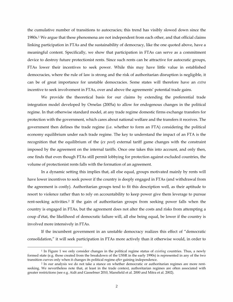
Figure 1: Number of Free Trade Agreements in force & cumulative number of new democracies and of new autocracies (1948-2007)

Notes: “New democracy” denotes a transition to democracy and “new autocracy” denotes a transition to autocracy. Both definitions are based on data from Cheibub et al. (2010). For the data sources on Free Trade Agreements, see notes in online Appendix 2 (http://personal.lse.ac.uk/ornelas/Liu&Ornelas_Appendices.pdf).

Consider Figure 1. The bars show the cumulative number of free trade agreements (FTAs) in

force, while the solid line shows the cumulative number of transitions to democracy throughout the

world since 1948. Both trends have accelerated since the early 1990s. The dotted line shows instead

2

the cumulative number of transitions to autocracies; this trend has visibly slowed down since the

1980s.1 We argue that these phenomena are not independent from each other, and that official claims

linking participation in FTAs and the sustainability of democracy, like the one quoted above, have a

meaningful content. Specifically, we show that participation in FTAs can serve as a commitment

device to destroy future protectionist rents. Since such rents can be attractive for autocratic groups,

FTAs lower their incentives to seek power. While this may have little value in established

democracies, where the rule of law is strong and the risk of authoritarian disruption is negligible, it

can be of great importance for unstable democracies. Some states will therefore have an extra

incentive to seek involvement in FTAs, over and above the agreements’ potential trade gains.

We provide the theoretical basis for our claims by extending the preferential trade

integration model developed by Ornelas (2005a) to allow for endogenous changes in the political

regime. In that otherwise standard model, at any trade regime domestic firms exchange transfers for

protection with the government, which cares about national welfare and the transfers it receives. The

government then defines the trade regime (i.e. whether to form an FTA) considering the political

economy equilibrium under each trade regime. The key to understand the impact of an FTA is the

recognition that the equilibrium of the (ex post) external tariff game changes with the constraint

imposed by the agreement on the internal tariffs. Once one takes this into account, and only then,

one finds that even though FTAs still permit lobbying for protection against excluded countries, the

volume of protectionist rents falls with the formation of an agreement.

In a dynamic setting this implies that, all else equal, groups motivated mainly by rents will

have lower incentives to seek power if the country is deeply engaged in FTAs (and withdrawal from

the agreement is costly). Authoritarian groups tend to fit this description well, as their aptitude to

resort to violence rather than to rely on accountability to keep power give them leverage to pursue

rent-seeking activities.2 If the gain of authoritarian groups from seeking power falls when the

country is engaged in FTAs, but the agreement does not alter the costs and risks from attempting a

coup d’état, the likelihood of democratic failure will, all else being equal, be lower if the country is

involved more intensively in FTAs.

If the incumbent government in an unstable democracy realizes this effect of “democratic

consolidation,” it will seek participation in FTAs more actively than it otherwise would, in order to

1 In Figure 1 we only consider changes in the political regime status of existing countries. Thus, a newly

formed state (e.g. those created from the breakdown of the USSR in the early 1990s) is represented in any of the two transition curves only when it changes its political regime after gaining independence.

2 In our analysis we do not take a stance on whether democratic or authoritarian regimes are more rent-seeking. We nevertheless note that, at least in the trade context, authoritarian regimes are often associated with greater restrictions (see e.g. Aidt and Gassebner 2010, Mansfield et al. 2000 and Mitra et al. 2002).

3

weaken the authoritarian threat. Yet even if the dictatorial group takes control despite the FTA, the

agreement will constrain its rent-extraction activities. For both of these reasons, unstable

democracies tend to enter in FTAs more frequently than other countries. In turn, participation in

FTAs increases the likelihood of democracy survival in those countries.

Analyzing the formation of FTAs and the strength of democracy in 126 countries over 1948-

2007, we obtain empirical support for both of our main theoretical results. Employing duration

analysis techniques, we find that greater participation in FTAs lowers the likelihood of democracy

failure in a country. Using the estimated hazard rates from the duration analysis, we find as well

that a higher risk of democratic breakdown induces countries to participate more actively in FTAs.

Our empirical results are robust to many different econometric specifications and alternative

measures of democratic transition.

One of our empirical challenges is to define how unstable a democracy is. We do so by

relying on the approach pursued by Persson and Tabellini (2009), who estimate the likelihood of

democratic breakdown employing the concept of “democratic capital.” The domestic component of

democratic capital takes into account the history of democracy in the country. The longer the

country has experienced democracy, and the more recent is its democratic experience, the greater

the country’s stock of domestic democratic capital. The foreign component of democratic capital

encompasses instead current levels of democracy abroad. The greater the number of democratic

countries, and the closer those democracies are to a country, the greater is that country’s stock of

democratic foreign capital. Along with other covariates, these two components of democratic capital

allow us to estimate the likelihood of democracy failure in a country. Our finding that greater

participation in FTAs significantly reduces this probability helps to explain why democratic

experiences have been particularly successful since the late 1980s.

Having estimated the likelihood of democracy failure, we use its fitted values to estimate

changes in FTA participation. In doing so, we consider only the portion of the likelihood that is not

predicted by FTA participation. Our finding that higher levels of regime uncertainty induce

democratic governments to participate more actively in FTAs helps to rationalize the outbreak of

regionalism since the early 1990s.

Interestingly, our predictions hold consistently only for full-fledged agreements, signed

under GATT’s Article XXIV. Article XXIV requires free trade agreements to cover most of the trade

among the members and that members liberalize fully vis-à-vis each other. By contrast, agreements

signed under the Enabling Clause of the GATT permit many exceptions and are often not fully

implemented. We do not find any significant association between those partial-scope preferential

4

trade agreements and democracy survival, or between political instability and formation of partial-

scope agreements. These stark differential results offer support for the rent-destructing mechanism

we put forward, as the partial-scope arrangements, unlike those signed under Article XXIV, impose

very few restrictions on the availability of rents from protection.

To our knowledge, we are the first to argue that engagement in FTAs helps democracies

endure because of its rent destruction effects. The essence of this idea is related to the commitment

rationale for trade agreements espoused by Maggi and Rodriguez-Clare (1998, 2007), although in

their analyses a government enters in a free trade agreement not to affect its successor’s policies, but

its own (otherwise time-inconsistent) future policies. And Pevehouse (2002) is the only other to

connect participation in trade agreements to the durability of democracy. He argues that joining

(although not the participation on its own) an international organization that has high “democratic

density” tends to increase the longevity of new democracies because of signaling effects. In line with

his contention, but differently from our analysis, Pevehouse includes in his empirical analysis not

only free trade agreements but also many international organizations that are unrelated to

international trade. Following Pevehouse, we also test whether FTAs help to sustain democracies

only because democratic countries demand democracy from their FTA partners. However, we find

that the role of an FTA in helping to sustain a country’s democracy is not greater when the

agreement is with more democratic partners. Thus, pressure from FTA partners is not what drives

our results.

Our second finding is also novel and refines some previous results. Mansfield, Milner and

Rosendorff (2002) find that pairs of democratic countries are more likely to share a trade agreement

than pairs in which at least one country has an authoritarian political regime.3 We take the Mansfield

et al.’s finding on board—we only consider democracies—but dig deeper to understand whether

democracies at different stages in their “consolidation” process have different incentives to engage

in FTAs. We find that they do: among democracies, those facing threats to their democratic regimes

are especially keen to form FTAs.

Mansfield and Pevehouse (2006), like us, distinguish between different types of democracies

and their willingness to join international organizations. Specifically, they find that countries that

have undergone a transition to democracy in the previous five years are more likely to join

international organizations, in particular those made up of more democratic states. Two central

differences between our analysis and Mansfield and Pevehouse’s are worth emphasizing. First, we

3 Mansfield, Milner and Pevehouse (2008) find that this holds for different types of trade agreements except

the “shallowest” ones, according to a five-tier classification.

5

estimate each country’s hazard out of democracy (rather than just distinguishing new democracies

from old democracies). Second, we do not pool all types of international organizations together. This

difference matters, as we find a strong effect of democratic instability on FTA participation but not

on participation in partial-scope trade agreements.

The idea that governments can manipulate state variables to constrain their successors’

choices was first advanced in the macroeconomics political economy literature.4 More recently,

Acemoglu and Robinson (2006) have developed a general framework to study circumstances when

an incumbent democratic government can design economic policies to irreversibly change the

expected net benefit of future coups.5 A related reasoning is employed here to show that a

democratic government, when faced with the prospect of political disruption, may want to limit the

ability of a potential authoritarian government to create rents through trade policies. We innovate in

this dimension by showing, theoretically and empirically, that an FTA can be an effective tool for that

purpose.6

There is also an important line of research that links democracy to trade liberalization and

openness.7 The forces typically emphasized in that literature are however quite different from the

mechanism we advance here. Moreover, and critically, in this paper we focus on the role of trade

agreements, where an external commitment makes the policy costly enough to reverse so that it can

credibly affect the action of future governments.8 A unilateral tariff reduction would clearly not

fulfill this requirement.

The paper proceeds as follows. Section 2 describes the model. Section 3 presents the analysis

of the incentives to form a free trade agreement. Section 4 discusses our empirical strategy. The data

is presented in Section 5. We show our empirical results in Section 6. We conclude in Section 7.

4 See e.g. the pioneering contributions by Alesina and Tabellini (1990) and Persson and Svensson (1989). 5 They demonstrate, for example, how trade and capital account liberalization reduce equilibrium taxation

under democracy while also rendering coups more costly through the impact of openness on factor prices. 6 This contrasts with an alternative (and rather ubiquitous) view in the trade literature that regards FTAs as

rent-creating devices (e.g. Grossman and Helpman 1995). See Freund and Ornelas (2010) for a discussion of that literature.

7 See for example Giavazzi and Tabellini (2005), O’Rourke and Taylor (2007), Lopez-Cordova and Meissner (2008), and Stroup and Zissimos (2011). There is, of course, also a vast literature on the determinants of democracy and of its durability. See Barro (1999) for a classic reference for the former and Przeworski et al. (1996) for the latter.

8 See Bagwell and Staiger (2010) for a discussion of this and other roles of trade agreements.

6

2. THE MODEL

2.A. The economic structure

We consider a 3-country, N-sector competitive economy where in each sector there is a “natural

importer” country that would import the good from the other two countries under free trade. Goods

are produced under constant returns to scale. One unit of the numeraire good 0 is produced with

one unit of labor. All other goods j = 1…N – 1 are produced with labor and a sector-specific factor.

Thus, whenever good 0 is produced in equilibrium, which we assume to be the case, the wage rate

equals unity and general equilibrium forces are absorbed by that sector.

The analysis is conducted from the perspective of a “Home” country. Home’s population

consists of a continuum of agents with measure one. Each agent is endowed with one unit of labor,

whereas specific factors are owned by a negligible fraction of the population. Consumers have

quasi-linear utility of the form [ ]∑ −

=−+=

1

12 2/)(N

jjj0 qAqqU , which generates demand Dj = A – p j

for good j.

Home is the natural importer of goods m = 1…M, country Y is the natural importer of a

subset E of different goods, and country Z is the natural importer of the remaining (N – M – E – 1)

non-numeraire products. Home’s owners of the specific factor used in sector j earn πj(pj), where pj

denotes the price of good j in Home’s market. In the non-numeraire sectors, the domestic supply of

each imported good m is Sm(pm) = dmpm and the supply of each exported good x is Sx(px) = dxpx,

where dx > dm > 0. An analogous specification applies for the supply and demand structures of

countries Y and Z. Home can use specific import tariffs in each import sector; other policy

instruments are assumed unavailable. We represent Home’s tariff on imports from country j by tj, j =

Y, Z. Because all import sectors are identical, we will write prices and tariffs without sector-

identifying superscripts.

Prices in the three countries are linked by arbitrage conditions. For a generic product

imported by Home, this condition is

(1) p = pY + tY = pZ + tZ,

provided that tariffs are not prohibitive. Using this arbitrage condition, market-clearing requires

(2) D(p) – Sm(p) = Sx(p – tY) – D(p – tY) + Sx(p – tZ) – D(p – tZ).

Using the expressions for demand and supplies defined above, condition (2) can be rewritten as

(3) ρ++γ= )(),(ˆ YZYZ ttttp ,

where γ ≡ 3A/(3+dm+2dx) and ρ ≡ (1+dx)/(3+dm+2dx).

7

When Home is not a member of a free trade agreement, it follows GATT’s requirement of

non-discrimination. When Home is in an FTA, imports from the FTA partner are duty free, but

imports from the excluded country remain taxed, although the country’s optimal external tariff will

in general change as a result of the FTA.

2.B. The political structure

We consider that any group represented in the government enjoys power because there are rents for

holding office. The sources of those rents are transfers/bribes, which the private sector offers to

government officials in exchange for more favorable policies. Thus, the rents are specific to

incumbency, as in models like Besley and Coate’s (2001).

Policymakers also care about national welfare. Numerous reasons can explain this concern.

For example, the policymaker could represent a large group in the society, which benefits from a

more prosperous economy. Or maybe policymakers that are good at promoting national welfare

obtain more public support, which may affect the duration of their office tenure. Since modeling the

precise way in which policymakers form their preferences is not essential for our analysis, we take

an agnostic view and simply assume that whoever is in power sets policy considering both its

welfare consequences and its capacity to attract transfers.

Let us define the measures of welfare. Welfare generated in a specific-factor import sector is

denoted by Wm(t), whereas Wx represents welfare from a specific-factor export sector. The former is

defined as the sum of consumers’ surplus, tariff revenue and producers’ surplus generated in that

sector; the latter is defined as the sum of consumers’ and producers’ surplus in the sector. Welfare

aggregated across all non-numeraire import and export sectors is then WM(t) ≡ MWm(t) and WX ≡ (N

- M - 1)Wx, respectively.9 National welfare, W(t), aggregates welfare across all sectors:

∑∑ −

+==++=++≡

1

11)(1)(1)( N

MxxM

mmXM WtWWtWtW .

The preference of the government is specified as

(4) ,),(),( 1

11 ∑∑ −

+==+≡

N

MxxmM

mm GTtGTtG

with Gx ≡ Wx and

(4’) ,)(),( mmmm bTtWTtG +≡

9 Note that we denote welfare in import-competing sectors as a function of the tariff, but not in export

sectors. In reality, W x also depends on tariffs, but on those imposed by foreign countries Y and Z. Since those tariffs are given from the perspective of the Home government under any trade regime, we employ this more concise representation for notational ease.

8

where Tm denotes the transfer from import-competing sector m to the government, ,1∑ =

≡M

mmTT and

b>0 reflects the “rent-seeking bias” of the government, or how susceptible to bribes/transfers its

policies are. Thus, if for example the government’s rent-seeking bias were very high, it would care

mainly about rents. Notice that the government sets policy according to (4) regardless of its nature,

democratic or not. We adopt this assumption not because we believe that both types of governments

implement identical policies. It is simply that our main results do not depend on this distinction, and

we have nothing to add to the (extensive) debate on whether democracies or autocracies are more

rent-seeking.10 What is essential here is only that the rents from holding office depend on the policies

implemented.

We assume that producers within each industry can overcome free-riding problems in their

lobbying activities. Because of the symmetry and independence across sectors, we focus on a single

import-competing sector. The net payoff of producers in such a sector corresponds to the industry’s

aggregate profits, πm(t), subtracted of the transfers it gives to the local government, Tm.

As in Maggi and Rodríguez-Clare (1998), we model the interaction between government and

each domestic industry as a Nash bargaining game, where each side obtains half of the total surplus

from the negotiation process.11 Under the Nash bargaining protocol, the outcome of the bargaining

process is jointly efficient. Thus, the “political tariff” resulting from this interaction satisfies

(5) )]()(max[arg tbtWt mmp π+= ,

where the term in brackets represents (up to a constant) the joint payoff of the government and the

industry in a representative import-competing sector. We concentrate on the case where the solution

to problem (5) is interior. This corresponds to assuming that b < bmax ≡ (1+dm)(dx–dm)/(1+dx)dm.

2.C. Equilibrium payoffs

If the private sector were able to capture the entire surplus from lobbying, it would only need to

compensate the government for the distortions that tp creates. In this case, the government would

obtain just its reservation payoff, which is equivalent to how much it could get in the absence of

10 Dixit (2010) provides a nuanced and insightful general discussion of rent-seeking behavior in democracies

and autocracies. Grossman and Helpman (1996) provide microfoundations for the weights in equation (4’), but in a model of electoral competition, whereas our context is one where a potential autocrat considers taking over the country, not through the ballot box but through force.

11 One may want to distinguish the bargaining power of the government relative to the domestic industry depending on whether it is democratic or autocratic. For example, one may argue that the forces limiting rent-seeking behavior are weaker in a dictatorship because autocracies are less accountable, implying a higher bargaining power for the government in autocracies. Since this has no bearing on our results, we take the simpler route of assuming that government and private sector always split the surplus from lobbying.

9

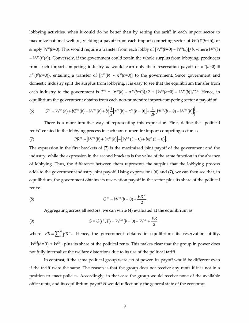
lobbying activities, when it could do no better than by setting the tariff in each import sector to

maximize national welfare, yielding a payoff from each import-competing sector of Wm(tp(b=0)), or

simply Wm(b=0). This would require a transfer from each lobby of [Wm(b=0) – Wm(b)]/b, where Wm(b)

≡ Wm(tp(b)). Conversely, if the government could retain the whole surplus from lobbying, producers

from each import-competing industry m would earn only their reservation payoff of πm(b=0) ≡

πm(tp(b=0)), entailing a transfer of [πm(b) – πm(b=0)] to the government. Since government and

domestic industry split the surplus from lobbying, it is easy to see that the equilibrium transfer from

each industry to the government is Tm = [πm(b) – πm(b=0)]/2 + [Wm(b=0) – Wm(b)]/2b. Hence, in

equilibrium the government obtains from each non-numeraire import-competing sector a payoff of

(6) [ ] [ ]⎭⎬⎫

⎩⎨⎧ −=+=π−π+=+= )()()()()()()( bWbW

bbbbbWbbTbWG mmmmmmmm 0

210

21 .

There is a more intuitive way of representing this expression. First, define the “political

rents” created in the lobbying process in each non-numeraire import-competing sector as

(7) [ ] [ ])()()()( 00 =π+=−π+≡ bbbWbbbWPR mmmmm .

The expression in the first brackets of (7) is the maximized joint payoff of the government and the

industry, while the expression in the second brackets is the value of the same function in the absence

of lobbying. Thus, the difference between them represents the surplus that the lobbying process

adds to the government-industry joint payoff. Using expressions (6) and (7), we can then see that, in

equilibrium, the government obtains its reservation payoff in the sector plus its share of the political

rents:

(8) 2

0m

mm PRbWG +== )( .

Aggregating across all sectors, we can write (4) evaluated at the equilibrium as

(9) 2

0 PRWbWTtGG XMp ++==≡ )(),( ,

where .1∑ =

≡M

mmPRPR Hence, the government obtains in equilibrium its reservation utility,

[WM(b=0) + WX], plus its share of the political rents. This makes clear that the group in power does

not fully internalize the welfare distortions due to its use of the political tariff.

In contrast, if the same political group were out of power, its payoff would be different even

if the tariff were the same. The reason is that the group does not receive any rents if it is not in a

position to enact policies. Accordingly, in that case the group would receive none of the available

office rents, and its equilibrium payoff H would reflect only the general state of the economy:

10

(10) XMp WbWtGH +=≡ )(),( 0 .

Since WM(b=0) ≥ WM(b) and PR ≥ 0, it follows directly from (9) and (10) that there are benefits from

holding office.

2.D. Coup threat

We consider a simple 2-period environment. In the first period there is a democratically elected

government in power. There is however a group of citizens representing a segment of the

population that is not in the government, which may attempt to take power through force. We are

agnostic about the identity of the citizens represented by this group; it could be the military as well

as part of the country’s capitalists or the upper class, for example. In any case, if a coup is attempted

and is successful, the authoritarian group takes power in the second period.

Naturally, numerous factors affect the probability of success of a coup, which we denote by

ρ. For example, success will be more likely the stronger the “support” of the pro-coup citizens and

the weaker the “resistance” from the segments of the population opposed to the coup. There is also

an important random (or at least ex ante unknown) element driving the success of any coup. We do

not model explicitly this probability, because quantifying those forces would be remarkably difficult.

We highlight, however, that the probability is likely to be strongly affected (negatively) by the

country’s stock of “democratic capital” (DC): ∂ρ(DC)/∂DC < 0. The notion of democratic capital,

introduced by Persson and Tabellini (2009), proxies the strength of the country’s democratic

institutions, and in this sense it provides a useful and concise way of capturing several forces

highlighted in the voluminous literature on the durability of democracies. Specifically, in the

definition of Persson and Tabellini (2009) the current stock of DC in a country is determined by both

the level of democracy in the country’s neighbors and by the country’s democratic history.

Accordingly, they reason that in nations with enduring democratic tradition, where the rule of law is

strong, democratic capital will be abundant and significantly limit the possibility of political

disruption. Conversely, in countries lacking solid institutions, where the rule of law is weak,

democratic capital will be scarce, thus opening a tangible opportunity for successful coups. Since the

level of democratic capital in a country can be considered exogenous (or at least pre-determined) to

the relevant political groups, we will rely on it in our empirical analysis.

Both the democratic government and the authoritarian group discount future payoffs

according to a common discount factor δ ∈ [0, 1]. To understand when the authoritarian group will

attempt to subvert the country’s democratic order, we model the group’s problem as simply as

possible. In particular, we assume that, if the takeover attempt is successful, the authoritarian group

11

imposes a dictatorship in the country and obtains its office payoff G in the second period. If the

takeover attempt is unsuccessful, the group bears a fixed cost K > 0.12

When a coup is attempted, the present value payoffs of the incumbent and of the

authoritarian group are represented, respectively, as

(12) ])[( HGGD ρ+ρ−δ+=Γ 1

and

(13) ]))([( GKHHA ρ+−ρ−δ+=Γ 1 .

If no coup were attempted, the incumbent government and the authoritarian group receive,

respectively, G and H in each period.

The (risk-neutral) authoritarian group attempts to take power if and only if the expected

utility from the endeavor is positive: ΓA > (1 + δ)H. Using (13), this condition is equivalent to

(14) KHG )()( ρ−>−ρ 1 .

That is, the authoritarian group will attempt to take power if its expected gain from seeking power is

large relative to the expected cost of a failed coup. To make explicit what is behind this decision, we

use expressions (9) and (10) to rewrite condition (14) as

(15) [ ] KDC

DCPRbWbW MM

)()(-)(-)(

ρρ

>+=1

20 .

In a consolidated democracy, where democratic capital is very high, an attempt against the county’s

democratic system is unlikely, unless the costs of failure are too low—which is rarely the case—or

the gains from holding power are very significant. Our central goal is to analyze how a free trade

agreement affects the latter, and through that channel the endurance of democracy in a country.

Naturally, an FTA can be used to affect future policies only if its reversal is costly enough to

inhibit future governments from reversing the arrangement. While here we simply assume that

FTAs are irreversible, it would be relatively straightforward to extend the current model so that

irreversibility becomes an equilibrium result, e.g. by relying on McLaren’s (2002) notion that

governments incur in “negotiating costs” when forming (or withdrawing from) FTAs. Ultimately,

FTAs matter for commitment as long as there is a non-trivial cost to reverse them.13

12 Parameter K provides a proxy for the many kinds of penalties that could apply in such a case—incarceration, extradition, death and the like.

13 Irreversibility is also coherent with history, as preferential trading arrangements de facto implemented are seldom turned down later on. Even in the rather rare circumstances when authoritarian regimes gained control of a country that participated in an effective trade agreement, the arrangement has usually been honored, as for example in Swaziland, a member of SACU. An exception to this rule—to our knowledge the only one—is the Andean Pact, from which President Hugo Chávez withdraw Venezuela in 2005. The other cases of implemented agreements being later disrupted are in Central America (CACM) and in the Caribbean (CARIFTA/CARICOM), but in both cases the

12

3. THE DECISION TO FORM A FREE TRADE AGREEMENT

A free trade agreement between two countries is represented by the elimination of tariffs on

each other’s imports in all sectors included in the agreement. Thus, the equilibrium under an FTA is

analogous to the one described in Section 2, the only difference being the constraint imposed on

some (potentially all) of the partners’ reciprocal import tariffs. Without loss of generality, we let

Home’s potential FTA partner be country Y.

A certain FTA can be implemented by the incumbent government for reasons related or

unrelated to the authoritarian threat. There are four possibilities. First, the country may already be a

consolidated democracy, in the sense that condition (15) holds neither with nor without FTAs. This

is the standard case considered in the regionalism literature, and it is not our goal to analyze it

further here. Rather, we focus on situations where FTAs can be formed for “strategic” reasons.

Second, it is possible that the country’s democracy is so fragile that condition (15) is satisfied

whether or not there is an FTA in place. In that case, while an FTA cannot be used to prevent a coup,

the possibility of losing power can affect the incentives of the incumbent government with respect to

the formation of the agreement.

Finally, it is possible that an FTA affects the expected payoff of the authoritarian group and,

as a result, its incentives to attempt to take power. In general, an FTA could either increase or

decrease the incentives for a coup, making it worth seeking when it would not be without the

agreement, or making the coup not worth pursuing when it would be without the FTA.

Before starting our analysis, we need however to describe the effects of an FTA on the level

of available political rents and the role of parameter b in shaping its welfare effects. These results set

the basis for the analysis of the political viability of FTAs.

3.A. The rent destruction effect

Ornelas (2005a) shows that an FTA moderates the role of political economy forces in the

determination of tariffs, and that the mitigation of the politically driven distortions corresponds to a

source of welfare gain that is more relevant, the more far-reaching the government’s political

economy motivations. Furthermore, an FTA diminishes the rents created in the lobbying process.

Intuitively, because the arrangement provides free access to the partner’s exporters, the market share

of the domestic industry shrinks, at any given external tariff. As a result, the FTA makes any price

agreements were disrupted due to balance of payments constraints during the debt crisis of the 1980’s. Both were fully reactivated in the early 1990’s.

13

increase brought by a marginal increase in the external tariff less valuable for the import-competing

industries, lowering their incentives to lobby for higher external tariffs. In equilibrium, these lower

incentives result in a lower external tariff and in fewer rents for the government.14 The following

lemma summarizes these effects.15

Lemma 1. The rent destruction effect of FTAs (Ornelas 2005a)

Everything else constant, an FTA

(a) improves Home’s welfare by more (or reduces it by less), the higher the government’s

rent-seeking bias; and

(b) reduces the political rents generated in the political process.

Lemma 1 allows us to analyze the conditions under which the Home government would

choose to form an FTA.16 The decision regarding the formation of an FTA is based on the anticipated

impact of the agreement. The government implements the agreement if and only if it increases the

government’s present value payoff. Note that the effects described in Lemma 1 are larger, the

greater the number of specific-factor import-competing sectors included in the FTA.

Before proceeding to analyze how the possibility of political disruption affects the

willingness of the democratic government to form free trade agreements, let us define some useful

notation. We henceforth attach subscript “F” to all variables when they are evaluated under an FTA.

We adopt subscript “ΔF” to represent the equilibrium change in any variable due to the FTA. For

example, xFWΔ denotes the aggregate welfare change in a non-numeraire export sector due to the

agreement, whereas )(bW mFΔ and )( 0=Δ bW m

F denote, respectively, the actual aggregate welfare

impact of the FTA on a non-numeraire import sector and the equivalent effect under a hypothetical

administration whose only concern is national welfare (equivalent to a situation where lobbying is

effectively banned). Finally, let IM denote the number of specific-factor import-competing sectors

included in the FTA under analysis, with IM ≤ M. Aggregating the welfare impact of the agreement

14 There is robust empirical evidence that the formation of free trade areas in developing countries (largely

the focus of our analysis) leads to declining external tariffs (see Estevadeordal et al. 2008 for evidence on ten Latin America countries and Calvo-Pardo et al. 2011 for evidence on ten Southeast Asia countries), although not for developed countries (see Limao 2006). While measuring protectionist rents directly is very difficult, the level of tariffs provides a good proxy for them; see Freund and Ornelas (2010) for a general discussion.

15 These results do not hinge on the perfectly competitive structure adopted by Ornelas (2005a), which we follow here. Analogous results obtain also under oligopolistic competition (Ornelas 2005b).

16 Naturally, an FTA is formed only if all prospective members endorse it. We conduct the discussion from the perspective of the Home country, but an analogous analysis would apply for country Y.

14

on both types of sectors, we then define )()( bWIbW mF

MMF ΔΔ ≡ and .x

FXX

F WIW ΔΔ ≡ Analogously,

.mF

MF PRIPR ΔΔ ≡

3.B. FTAs that do not affect the probability of political disruption

We begin analyzing the case where there is a possibility of political disruption but this possibility is

unaffected by the existence of FTAs—that is, condition (15) holds regardless of FTAs.

In this case, the equilibrium payoff of the incumbent democratic government under the FTA

corresponds to

(16) ])-[( FFFDF HGG ρ+ρδ+=Γ 1 .

The condition under which the democratic government supports the FTA when the authoritarian

threat is inevitable is 0>ΓΓ≡ΓΔDD

FDF - . Using equations (12) and (16), D

FΔΓ can be rewritten as

])[( FFFDF HGG ΔΔΔΔ ρ+ρδ+=Γ -1 .

Using expressions (9) and (10) and manipulating, this expression becomes

(17) XF

MF

FMF

DF WbWPRbW ΔΔ

ΔΔΔ δ++δρ+⎥

⎦

⎤⎢⎣

⎡+=ρδ+=Γ )()()()]([ 1

20-11 .

Thus, the incumbent democratic government supports the FTA in this case if

(18) 01220211 >δ++δρ++=ρδ+ ΔΔΔΔXF

MFF

MF WbWPRbW )()(])()][-([ .

The interesting case is when the democratic government changes its stance toward an FTA

because of the authoritarian threat. An FTA is (ordinarily) politically feasible if

(19) 002 >++= ΔΔΔ FXF

MF PRWbW ])([ .

The next proposition shows that the authoritarian threat can make an otherwise politically infeasible

FTA (i.e., one for which condition (19) does not hold) into a politically feasible one.

Proposition 1. Even if the authoritarian threat cannot be affected, the mere possibility of political

disruption can turn an otherwise politically unfeasible FTA into a viable one. By contrast, the

possibility of disruption cannot render unfeasible an otherwise feasible FTA.

Proof: We need to show first that D

FΔΓ increases with ρ. Using (19), we have that

(20) ⎥⎦

⎤⎢⎣

⎡=δ=

ρΓ Δ

ΔΔΔ

2-0- FM

FMF

DF PRbWbW

dd )()( .

We know from Lemma 1 that 0<ΔFPR and that the welfare impact of an FTA is increasing in the

rent-seeking bias of the government, so that .)()( 00- >=ΔΔ bWbW MF

MF Accordingly, expression (20) is

15

unambiguously positive, so DFΔΓ increases as the probability of disruption rises. As a result, an FTA

that is politically unfeasible when there is no chance of political disruption can become viable if the

likelihood of political disruption is high enough. That is, an FTA that does not satisfy condition (19)

can satisfy criterion (18) for sufficiently high ρ. On the other hand, the reverse cannot happen: if an

FTA is politically viable when there is no chance of political disruption, it remains viable if a

possibility of change in power through force arises. That is, an FTA that satisfies condition (19) also

satisfies criterion (18) for any ρ > 0.

Proposition 1 shows that the possibility of political disruption can enhance the political

feasibility of FTAs by creating a “strategic” motivation for their adoption. Strategically supported

FTAs arise when, between conditions (18) and (19), only the former is satisfied, so that

(21) )()( 000 >ρΓ<≤=ρΓ ΔΔDF

DF .

An FTA can be implemented for strategic reasons because the democratic government, if out of

power, will not receive any of the lobbying-related rents. In that case, the government would benefit

from an FTA because the agreement constrains the welfare-distorting political activities of the

authoritarian group if it gets in power. Thus, a government that expects to lose power to a dictatorial

group might seek an FTA simply to constrain the policies of the incoming authoritarian group. Since

this strategic motivation is more relevant when disruption is more likely, it follows that “democratic

instability” incites the formation of free trade agreements. 17

The number of Home’s import-competing sectors susceptible to lobbying that are included

in the FTA, IM, also affects the possibility of strategically supported FTAs.

Proposition 2. The set of parameters under which the possibility of political disruption turns an FTA

politically viable increases with the number of Home’s specific-factor import-competing

sectors included in the agreement (IM).

Proof: To prove this result, it suffices to show that the probability of disruption, ρ, is a strategic

complement of IM in the function ,DFΔΓ which gives the criterion for the political viability of FTAs.

This function is represented in the left-hand side of (18). Based on the definition of welfare

aggregated across all non-numeraire import sectors included in the agreement, we have that

17 It is easy to see that this strategic motivation for signing FTAs is stronger, the greater the rent-seeking bias

of the autocrat. This follows because the forces underlined in Lemma 1 are stronger, the higher the rent-seeking bias of the group setting policies. This suggests that an authoritarian threat can make strategic FTAs particularly appealing, since despite some disagreement, the majority of views in the literature seem to agree that autocracies tend to pursue particularly distortionary policies (see Dixit 2010).

16

)].()([)()( 0-0- === ΔΔΔΔ bWbWIbWbW mF

mF

MMF

MF Accordingly, the FTA affects political rents only in the

included sectors: ( )mF

MF PRIPR ΔΔ = . Therefore, it follows that

02

-0-22

>⎥⎦

⎤⎢⎣

⎡=δ=

ρΓ Δ

ΔΔΔ

mFm

FmFM

DF PRbWbW

dIdd )()()( .

Hence, the set of parameters under which condition (21) is satisfied enlarges as IM increases.

Thus, the more comprehensive the FTA is, the greater the extra incentive of the democratic

government to form the agreement because of the authoritarian threat. The reason is that, if Home

imports more widely from its FTA partner in sectors where there is active lobbying, the agreement

becomes more rent-destructing. While this is helpful for the country as a whole, it is detrimental to

those in office who benefit from those rents. Under the threat of political disruption, however, the

government understands that the loss of rents will be borne instead by the authoritarian group, if it

is successful in gaining power. The destruction of rents is therefore less critical in the democratic

government’s evaluation of the agreement.

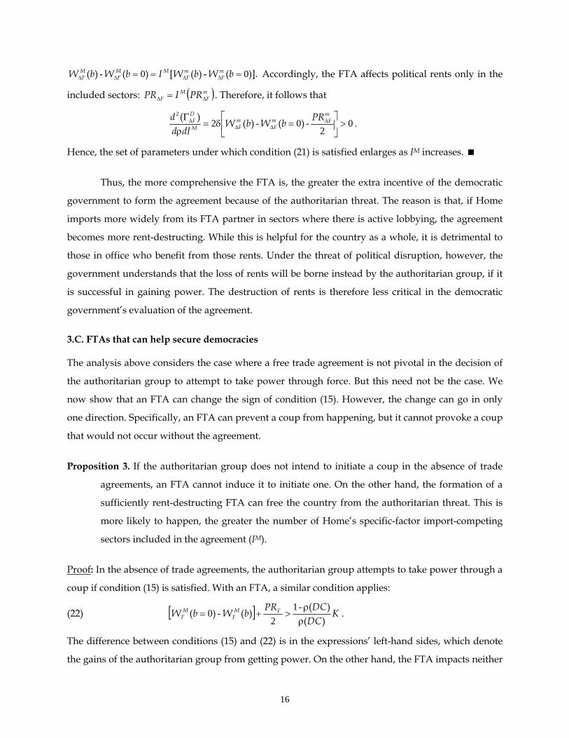
3.C. FTAs that can help secure democracies

The analysis above considers the case where a free trade agreement is not pivotal in the decision of

the authoritarian group to attempt to take power through force. But this need not be the case. We

now show that an FTA can change the sign of condition (15). However, the change can go in only

one direction. Specifically, an FTA can prevent a coup from happening, but it cannot provoke a coup

that would not occur without the agreement.

Proposition 3. If the authoritarian group does not intend to initiate a coup in the absence of trade

agreements, an FTA cannot induce it to initiate one. On the other hand, the formation of a

sufficiently rent-destructing FTA can free the country from the authoritarian threat. This is

more likely to happen, the greater the number of Home’s specific-factor import-competing

sectors included in the agreement (IM).

Proof: In the absence of trade agreements, the authoritarian group attempts to take power through a

coup if condition (15) is satisfied. With an FTA, a similar condition applies:

(22) [ ] KDC

DCPRbWbW FMF

MF )(

)(-)(-)(ρρ

>+=1

20 .

The difference between conditions (15) and (22) is in the expressions’ left-hand sides, which denote

the gains of the authoritarian group from getting power. On the other hand, the FTA impacts neither

17

the probability of success of a coup nor the costs of a failed coup attempt. Subtracting the left-hand

side of inequality (15) from the left-hand side of inequality (22), we obtain

(23) [ ] 02

0 <+= ΔΔΔ

FMF

MF

PRbWbW )(-)( ,

where the negative sign follows directly from Lemma 1. Thus, if condition (15) is not satisfied,

condition (21) will not be satisfied either, implying that an FTA cannot provoke a coup that

otherwise would not occur. Conversely, condition (15) can be satisfied while condition (21) is not,

implying that an FTA can be critical to prevent the authoritarian group from seeking power. Finally,

note that the left-hand side of (23) decreases with IM:

[ ] 02

025

<+== ΔΔΔ

mFm

FmFM

PRbWbWdI

lhsd )(-)()]([ .

Thus, the range of parameters under which an FTA is pivotal in preventing the authoritarian threat

is larger, the greater the number of non-numeraire import-competing sectors the FTA includes.

Proposition 3 shows that, because of the rent-destructing effects of FTAs, a free trade

agreement can critically reduce the incentives of the authoritarian group to attempt to subvert the

country’s democratic system. In this sense, an FTA can help to constrain the emergence of

authoritarian regimes, especially if the bloc is significantly rent-destructing, as in that case it will be

more effective in lowering the gains from power of the authoritarian group. Relying on the common

notion that the availability of rents can entice political turbulence—while the unavailability of rents

can prevent it—the proposition’s novelty stems from the recognition of free trade agreements as

instruments to restrain the gains from rent-seeking behavior.

We still need to ask, however, whether the incumbent democratic government would

actually want to implement the arrangement. The next proposition shows that the possibility of

using an FTA to block a coup necessarily raises the government’s incentives to sign an agreement.

Proposition 4. An FTA can become politically feasible by being pivotal to prevent a coup.

Proof: When an FTA cannot prevent the authoritarian group from seeking power through force, it is

politically viable if .])[( 0-1 >ρ+ρδ+=Γ ΔΔΔΔ FFFDF HGG When the agreement reverses the decision of

the authoritarian group, it is adopted by the democratic government if

])[( HGGGG FF ρ+ρδ+>δ+ -1 ,

18

where the left-hand side represents the present value of the government under the agreement (and

no authoritarian threat) and the right-hand side corresponds to its expected present value without

the FTA (and with the authoritarian threat). This condition can be rewritten as

(24) 0-1 >δρ+δ+ Δ )()( HGG F .

Now notice that the left-hand side of (24) is greater than DFΔΓ if ,FF HG > which is true from the

definitions of FG and FH , which are analogous to those in (9) and (10). Hence, even if DFΔΓ < 0,

condition (24) can be satisfied.

Proposition 1 asserts that the possibility of political disruption can render feasible an

otherwise unfeasible free trade agreement. Proposition 4 indicates that the political support for an

FTA is further enhanced if the agreement can also play a role in preventing disruption of the

political system. This is true even though here we abstract from any ideological motivation the

incumbent democratic government may have; if the government perceived a benefit per se from

maintaining democracy in the country, its incentive to form an FTA that can serve that purpose

would be further enhanced.

Our results thus suggest that free trade agreements—especially those that are particularly

effective in destroying rents—can be useful to prevent an authoritarian threat. This can be especially

important in fledgling democracies, given the instability that typically follows the end of dictatorial

regimes. In fact, the establishment of new democracies has often been followed by the formation of

preferential arrangements (or the accession to existing ones). This was the case, for example, of all

Mercosur members, of Greece, Portugal and Spain in their accession to the European Community,

and of the EU agreements with the countries of Central and Eastern Europe shortly after the fall of

the iron curtain. The European Community was itself established not long after the end of autocratic

regimes in some of its original members (Germany and Italy). It is therefore not surprising that the

consolidation of democratic regimes is often presented as one of the primary goals in the formation

of free trade agreements, as the World Trade Organization (2011) notes. Our analysis provides a

coherent explanation for this link between democratic consolidation and the establishment of free

trade agreements. We now turn to showing that these relationships are also empirically robust.

4. EMPIRICAL STRATEGY

The model has two main predictions about the relationship between FTAs and democracy,

which imply the following hypotheses:

19

H1. Participation in FTAs lowers the probability of democratic failure.

H2. Unstable democracies are more likely to form FTAs.

To test H1, our dependent variable is a dummy indicating whether democracy was

interrupted, or alternatively the length of democratic spells. This allows us to estimate the

probability that democracy will fail in the country, which we denote by Prob(enddemo). We define

democracy failure in different ways, based alternatively on Polity IV data and on a dichotomous

classification from Cheibub et al. (2010); we explain this in detail in Section 5. The key independent

variable is a measure of the intensity of the country’s participation in FTAs.

To test H2, our dependent variable is the change in a country’s FTA participation. The key

independent variable is a measure of democratic instability, reflecting the expectation that the

democratic regime may fail in the country.

As indicated in the Introduction, our problem is related to the one studied by Persson and

Tabellini (2009), who examine the determinants (in particular the effect of income) of the stability of

democracies and the impact of this perceived stability on income growth. Our empirical strategy

resembles their approach.

4.A. Testing H1: Participation in FTAs and democracy survival

We estimate the likelihood of democratic failure relying on the concepts of domestic democratic

capital (DOM) and foreign democratic capital (FOR) developed by Persson and Tabellini (2009),

while adding a variable that captures the intensity of a country’s participation in FTAs. DOM is a

measure of the democratic history of the country, whereas FOR measures current levels of

democracy in the world.18 Other explanatory variables include economic factors (e.g. GDP per

capita, denoted by vector X) and geographical and institutional factors (e.g. war indicators, continent

of location and legal origin, denoted by vector Z).

The dataset covers only countries’ democratic spells. We estimate a discrete time duration

analysis modeled as logit, which can be implemented as follows:

(25) log(P/(1-P)) = α0 + α1FTA-1 + α2DOM-1 + α3FOR-1 + α4X-1 + α5Z-1 + u,

where P denotes Prob(enddemo) and subscript -1 indicates that the variable is lagged one year.19

18 In the next section we provide a precise definition of both variables. 19 An alternative to this logit specification would be a complementary loglog (cloglog) regression, where we

treat the time interval as discrete or grouped by year. However, when the probability of positive outcomes is small as in our case, where democratic failures account for only 2.4% of the sample (see Table 1), a cloglog link function is similar to a logistic link function. Hence the coefficients obtained from a cloglog regression can be exponentiated and

20

The variable FTA in equation (25) represents the extent of rent destruction produced by the

country’s participation in FTAs in a given year—i.e. the country’s “FTA rent-destructing intensity.”

Measuring the FTA intensity of a country is far from trivial. Despite a prolific literature on the

consequences of preferential trade integration, that line of research offers no guidance on how to

measure this intensity. In fact, most empirical regionalism papers simply use dummies to represent

FTA participation. While this may be adequate for other purposes, such a measure is inappropriate

here for several reasons. First, unlike other studies where the unit of observation is a country dyad,

we need a measure of FTA participation at the country level, since we want to estimate the

endurance of democracy in individual countries. And while some countries participate in a single

(or no) FTA, others are members of multiple agreements. Second, there is wide heterogeneity among

FTAs. While some arrangements are fully implemented, others are not, implying that preferences

actually offered are few and small, and therefore entail little destruction of rents. Furthermore, while

some agreements are very large (e.g. the European Union), others are tiny, including some that are

numerous in terms of members (e.g. CARICOM). Third, even within a given FTA, the impact of the

bloc can be very different on each member. Consider NAFTA: while it has a very large impact on

Mexico, the smallest member, its impact is much less pronounced on the United States, the largest

member.

All of these matter for our analysis. According to Proposition 3, only sufficiently rent-

destructing FTAs have an effect on the sustainability of democracy. We clearly need, therefore, a

more precise measure of the intensity of a country’s participation in FTAs than what FTA dummies

can offer. In our model, where all sectors are symmetric, the extent of rent destruction within an FTA

is given by the number of import-competing sectors included in the agreement. More generally, it

depends also on how large the export sectors of the FTA members are relative to Home’s import-

competing sectors. To capture both, we use in our main regressions the share of imports from FTA

members. This variable is not perfect for our purposes, because it does not tell whether the imports

from the FTA partners are in sectors where lobbying takes place, which is where the rent destruction

effect of FTAs will be operative. Still, it varies monotonically with the degree of implementation of

the agreement and with the importance of the agreement for the country in question. Consequently,

it is very likely to be positively correlated also with the variable IM from our model, which

represents the extent to which import-competing sectors where lobbying happens are included in

the agreement. Hence, the import share from FTA members can provide a useful proxy for the

understood in terms of an odds ratio. Since logistic regressions are more conventional than cloglog ones, we focus on the former. Results from cloglog regressions are very similar.

21

country-level degree of rent destruction engendered by the FTAs a country belongs to, and is

probably much superior to alternative proxies available in the literature.

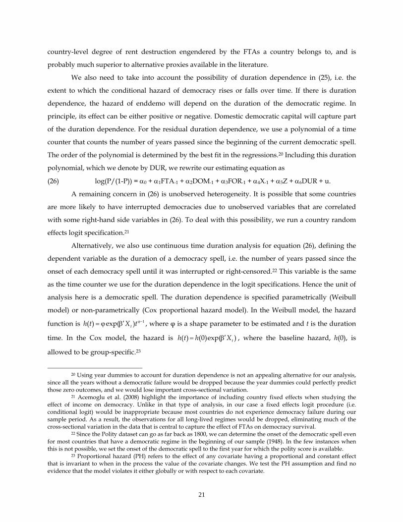
We also need to take into account the possibility of duration dependence in (25), i.e. the

extent to which the conditional hazard of democracy rises or falls over time. If there is duration

dependence, the hazard of enddemo will depend on the duration of the democratic regime. In

principle, its effect can be either positive or negative. Domestic democratic capital will capture part

of the duration dependence. For the residual duration dependence, we use a polynomial of a time

counter that counts the number of years passed since the beginning of the current democratic spell.

The order of the polynomial is determined by the best fit in the regressions.20 Including this duration

polynomial, which we denote by DUR, we rewrite our estimating equation as

(26) log(P/(1-P)) = α0 + α1FTA-1 + α2DOM-1 + α3FOR-1 + α4X-1 + α5Z + α6DUR + u.

A remaining concern in (26) is unobserved heterogeneity. It is possible that some countries

are more likely to have interrupted democracies due to unobserved variables that are correlated

with some right-hand side variables in (26). To deal with this possibility, we run a country random

effects logit specification.21

Alternatively, we also use continuous time duration analysis for equation (26), defining the

dependent variable as the duration of a democracy spell, i.e. the number of years passed since the

onset of each democracy spell until it was interrupted or right-censored.22 This variable is the same

as the time counter we use for the duration dependence in the logit specifications. Hence the unit of

analysis here is a democratic spell. The duration dependence is specified parametrically (Weibull

model) or non-parametrically (Cox proportional hazard model). In the Weibull model, the hazard

function is 1−ϕβ′ϕ= tXth t )exp()( , where φ is a shape parameter to be estimated and t is the duration

time. In the Cox model, the hazard is )exp()0()( tXhth β′= , where the baseline hazard, h(0), is

allowed to be group-specific.23

20 Using year dummies to account for duration dependence is not an appealing alternative for our analysis,

since all the years without a democratic failure would be dropped because the year dummies could perfectly predict those zero outcomes, and we would lose important cross-sectional variation.

21 Acemoglu et al. (2008) highlight the importance of including country fixed effects when studying the effect of income on democracy. Unlike in that type of analysis, in our case a fixed effects logit procedure (i.e. conditional logit) would be inappropriate because most countries do not experience democracy failure during our sample period. As a result, the observations for all long-lived regimes would be dropped, eliminating much of the cross-sectional variation in the data that is central to capture the effect of FTAs on democracy survival.

22 Since the Polity dataset can go as far back as 1800, we can determine the onset of the democratic spell even for most countries that have a democratic regime in the beginning of our sample (1948). In the few instances when this is not possible, we set the onset of the democratic spell to the first year for which the polity score is available.

23 Proportional hazard (PH) refers to the effect of any covariate having a proportional and constant effect that is invariant to when in the process the value of the covariate changes. We test the PH assumption and find no evidence that the model violates it either globally or with respect to each covariate.

22

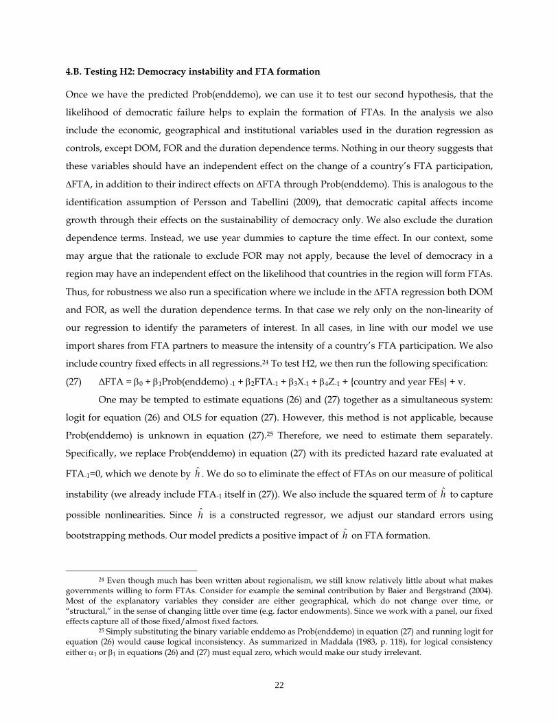
4.B. Testing H2: Democracy instability and FTA formation

Once we have the predicted Prob(enddemo), we can use it to test our second hypothesis, that the

likelihood of democratic failure helps to explain the formation of FTAs. In the analysis we also

include the economic, geographical and institutional variables used in the duration regression as

controls, except DOM, FOR and the duration dependence terms. Nothing in our theory suggests that

these variables should have an independent effect on the change of a country’s FTA participation,

ΔFTA, in addition to their indirect effects on ΔFTA through Prob(enddemo). This is analogous to the

identification assumption of Persson and Tabellini (2009), that democratic capital affects income

growth through their effects on the sustainability of democracy only. We also exclude the duration

dependence terms. Instead, we use year dummies to capture the time effect. In our context, some

may argue that the rationale to exclude FOR may not apply, because the level of democracy in a

region may have an independent effect on the likelihood that countries in the region will form FTAs.

Thus, for robustness we also run a specification where we include in the ΔFTA regression both DOM

and FOR, as well the duration dependence terms. In that case we rely only on the non-linearity of

our regression to identify the parameters of interest. In all cases, in line with our model we use

import shares from FTA partners to measure the intensity of a country’s FTA participation. We also

include country fixed effects in all regressions.24 To test H2, we then run the following specification:

(27) ΔFTA = β0 + β1Prob(enddemo) -1 + β2FTA-1 + β3X-1 + β4Z-1 + {country and year FEs} + v.

One may be tempted to estimate equations (26) and (27) together as a simultaneous system:

logit for equation (26) and OLS for equation (27). However, this method is not applicable, because

Prob(enddemo) is unknown in equation (27).25 Therefore, we need to estimate them separately.

Specifically, we replace Prob(enddemo) in equation (27) with its predicted hazard rate evaluated at

FTA-1=0, which we denote by h . We do so to eliminate the effect of FTAs on our measure of political

instability (we already include FTA-1 itself in (27)). We also include the squared term of h to capture

possible nonlinearities. Since h is a constructed regressor, we adjust our standard errors using

bootstrapping methods. Our model predicts a positive impact of h on FTA formation.

24 Even though much has been written about regionalism, we still know relatively little about what makes

governments willing to form FTAs. Consider for example the seminal contribution by Baier and Bergstrand (2004). Most of the explanatory variables they consider are either geographical, which do not change over time, or “structural,” in the sense of changing little over time (e.g. factor endowments). Since we work with a panel, our fixed effects capture all of those fixed/almost fixed factors.

25 Simply substituting the binary variable enddemo as Prob(enddemo) in equation (27) and running logit for equation (26) would cause logical inconsistency. As summarized in Maddala (1983, p. 118), for logical consistency either α1 or β1 in equations (26) and (27) must equal zero, which would make our study irrelevant.

23

Unlike in our study of H1, here the analysis is not necessarily at the country level.

Accordingly, we also employ a discrete-time duration analysis of a large bilateral panel dataset

covering years 1960-2007. Each observation in the bilateral data corresponds to two countries (i.e., a

dyad). The key independent variables are the estimated hazard rates of the countries in a dyad, as

predicted from equation (26). The dependent variable is a dummy indicating an FTA relationship

between two countries. Although this approach brings about all the problems related to the

heterogeneity of FTAs discussed above, it has the advantage of being very conventional in (and

therefore more comparable with) the empirical regionalism literature.

Notice that the discrete choice regressions often used for binary FTA cross-section data

analysis (e.g. Baier and Bergstrand 2004) would be inappropriate for panel data analysis like ours,

because it requires the dependent variable (an FTA dummy) to be conditionally independent over

time.26 This problem does not arise in our discrete time duration analysis. Following Liu (2008,

2010), we only need to drop all but the first positive outcome of the dependent variable for each

dyad over the sample period. Once the repeated “1”s are dropped, the problem of conditional

dependence disappears. Note that the “event failure” in this instance is two countries entering into a

trade agreement, and a spell is defined as the length of time until two countries form an agreement.

5. DATA

We have a panel with 126 countries that have experienced democracy at some point during

1948-2007. Not every country is included because our study is restricted to democracies. Online

Appendix 1 (http://personal.lse.ac.uk/ornelas/Liu&Ornelas_Appendices.pdf) lists the countries

covered in our enddemo duration analysis. More than 200 countries are covered in the construction

of our FTA measures, as explained below.

In our empirical analysis, free trade agreements cover both free trade areas and customs

unions, which we refer to as full-fledged free trade agreements (or simply FTAs, for brevity). We

also provide results for partial-scope preferential trade agreements (which we refer to as PTAs), as a

test to see whether the mechanism at work is indeed the destruction of rents, which should be

significantly less pronounced in PTAs than in FTAs. Data for the agreements come from the WTO

website and from information available elsewhere. Online Appendix 2 lists the agreements in our

dataset with their types (FTAs or PTAs) and other information about the data sources. We define

26 For example, Mexico signed NAFTA with the U.S. and Canada in 1994, and NAFTA remains in place for

all the following years, so the independence assumption is obviously violated.

24

agreement types based primarily on whether the agreement is signed according to GATT’s Article

XXIV (FTAs) or the Enabling Clause (PTAs).27 Although most agreements are in the FTA category,

the import shares of PTAs are nontrivial. As shown in Table 1, the average import share from PTAs

in our sample is 0.065, compared to 0.191 for FTAs.

As discussed in the previous section, our preferred measure of FTA participation is a

country’s imports from FTA partners as a share of its total imports in a given year. We use an

analogous definition for PTA participation:

FTA_impsh: a country’s imports from FTA partners as a share of its total imports;

PTA_impsh: a country’s imports from PTA partners as a share of its total imports.

We obtain the import data from the IMF Direction of Trade Statistics. To construct the shares, we

carefully consider the dates of the formation of new blocs, of the accession of new members, and of

the de-activation of existing blocs.

As we follow Persson and Tabellini’s (2009) general estimation strategy, our first definition

of democracy failure follows their definition, which relies on Polity IV data (available at

http://www.systemicpeace.org/polity/polity4.htm), we also adopt their definition of democracy

failure. This entails defining a regime as “democratic” if its polity2 score (which ranges from -10 to

10, with higher values representing more democratic regimes) is strictly positive.28 In a democratic

spell, enddemo is zero as long as democracy remains uninterrupted and becomes unity when it

ends. If a democracy does not end during our sample, enddemo is right-censored and only takes

zeros. There are 78 episodes of enddemo in our sample according to this definition; online Appendix

3A lists them. For those transitions, the median score before the change is 6, whereas the median

score after the change is -5.5; the median drop in the polity2 score is 9 points. A representative

example of the median case of democracy failure is Laos from 1959 to 1960, when its polity score fell

from 8 to -1.

We also use a different measure of democracy failure from a recent database defining

transition to autocracy (“tta”) developed by Cheibub et al. (2010, with data available at

https://netfiles.uiuc.edu/cheibub/www/DD_page.html).29 Their measure has the important

advantage of offering a binary classification of democracy/autocracy that yields a straightforward

definition of the transitions—unlike the Polity index, where transition needs to be defined according

27 There are exceptions. For example, MERCOSUR was signed under the Enabling Clause, but is classified as a free trade area (customs union after 1995).

28 Countries enter the sample as they become independent, but only if they have a strictly positive polity2 score, since our study is restricted to democracies.

29 Cheibub et al. (2010) extend the classification proposed initially by Alvarez et al. (1996).

25

to (necessarily) arbitrary thresholds.30 There are 62 cases of enddemo in our sample according to this

definition (see online Appendix 3B).

Following Persson and Tabellini (2009), the construction of DOM and FOR is based on

polity2 scores. DOM is defined as

∑−=τ

=τ

ττ− δδ−=

0

0

1tt

tiit dDOM ,)( ,

where δ is a discount factor and di,t-τ is a dummy for a strictly positive polity2 score. The first

positive dummy for each country is either the first year with a strictly positive polity2 score or the

first year the country appears in the Polity dataset, which for some countries goes back to 1800. As

Persson and Tabellini, we find that what really matters for democratic stability in DOM is current

DOM (i.e. the current democratic spell), whereas the portion of DOM due to previous democratic

spells is usually insignificant in the regressions. Accordingly, we use current DOM in all of our

regressions, so t0 corresponds to the first year in which dit = 1 in the current democratic spell. For the

discount factor, we adopt δ = .95; results change little for δ ∈ [.94, .99], the range considered by

Person and Tabellini. In turn, FOR is defined as

∑≠

⎟⎟⎠

⎞⎜⎜⎝

⎛−=

ijt

ijjtit N

DEqDist

PolityFOR /1 ,

where Polityjt is country j’s polity2 score at t (rescaled to the [0,1] interval), Distij is the distance

between the capitals of countries i and j, DEq is half the length of the equator, and Nt is the number

of independent countries in the world at t. Thus, the closer a country is to other democracies, the

greater its own stock of foreign capital.

GDP per capita data come from the World Development Indicators database. Data on wars

come from the Correlates of War dataset and includes all wars a country was involved in. Legal

origin data are drawn from La Porta et al. (1999). Colonial history variables come from the CIA’s

World Fact Book. WTO membership data come from the WTO website. Trade openness measures

are obtained from the Penn World Table 6.3. The data used to calculate the number of international

organizations (IO) come from the database for International Governmental Organizations (IGO,

v2.3).31 The data on formal military leader as chief executive are based on Gandhi and Przeworski

(2006).32 Table 1 lists the definitions of all the variables used in the main regressions and provides

30 Despite the arbitrariness, as we will see the choice of polity score threshold turns out to matter little for

our qualitative results. 31 Available at http://www.correlatesofwar.org/COW2%20Data/IGOs/IGOv2.3.htm 32 We thank James Raymond Vreeland for kindly sharing the data with us.

26

some descriptive statistics. The data used for the bilateral analysis are similar to the data used by Liu

(2010), extended to 2007.

6. EMPIRICAL RESULTS

6.A. Does participation in FTAs affect democracy survival?

We study first the impact of lagged FTA participation on the duration of democracy. We start by

plotting domestic democratic capital against FTA participation for all observations in our sample,

where we identify by a “1” the cases where democracy ends in a country, according to Cheibub et

al.’s data (2010). As Figure 2 shows, democracy is rarely reversed in countries deeply engaged in

FTAs.33 The large majority of cases in which democracy ends happens in countries whose FTA

shares are either nil or very close to nil. A high level of domestic democratic capital also appears to

protect democracy, although there are a non-trivial number of cases where democracy fails despite a

high level of democratic capital.

Figure 2: Cases of transitions to autocracy [“tta” from on Cheibub et al.’s (2010) data]

.....................................................................

.

.

.

.

..

.

.

.

.

..

..

..

.

.............. . . ..... .. . .... . . ... . .. .. . .. ...

..

......................... . . ......

.......1......1...1......

.

.

.1......

.

.

.

.

.

.

.

..

..

...

. .. ..

.. . ...

..

... .

..

..

..

..

..

......

.........

.............. ...... ....... . ............ . . . ..

.

.

.

.

.

.

.

.

.

.

.

. ... .

... ..

..

...........

.........

. . .. ... . ... . .....

... . . ... .. .... ............................ ...... .... ..

...................

.

.

.

.

.

.

.

.

.

.

.

.

.

..1

.

.

. ..... .. . .... .

.

.

..............................

...

..

..

.........

............................

.

...............................1.

.

.

.

.

.

.

.

.

.

.

..... ...

. .. ... ..

...

.

.

.

.

.

.

.

.

.

.

.

.

.

..

..

..

..

..

..

..

...

...

........

.

.

.

.

.

.

.

.

.

.

.

.

..

..1

.

.

..................

.

.

.

.

.

...

...

.

..

.......

..

...........................................

.

..

..

..

..

..

..

... .

.. .. ..... .... ............ ........ ..... . ..........

.

.

.

.

.

.

.

.

.1...1.................................. .. .... .. ................ ........ .. ..........1.. ....

....

.

..........................

..

..

...

...

...

..

..

......................... .............. . ........

......................................... ... . . .. .. ..........

......................... .. . . . ....

.

.

.

.

..

..

. 1. .. .

......................... ...... ........ .... . .. ..

.

..

..

..

..

..

..

..

...

...

...

.1...............

.

.

.

.

.

.

.

...

..

..

. . .. ..1.......

.

.

.

.

.

.

.

.

.

.

.

.

.

.

..

..

..

..

..

..

..

...

...

...

....

.....

.....

................

.

.

.

.1

.

.

....

.

.

.

.

.

.

....................................... . . .....

..

.

.

.1..................... ........

.

.

.

.1. .........

1............. .. . . . . ... .... . .. ................. . ... . .... ....

................................. ... ... . ... .. . . .

..... ...

..

..

.

..

....1...............................................................

.

.

.

.

.

.

.

.

.

.

.

.

.

.

..

..

..

..

..

..

..

...

...

.. . ...

..

..

...

..

..

..

.

.

...........................................

.

.

.......................

.

.

.

.

.

.

.

.

.................

.

.

.

.

.

.

.

.

.

.

.

.

.

..

..

..

..

........

.

.

.

.

.

.

.

.

.

.

.

.

...1....

.

..........

.

.

.

.

.

.

.

.

.

.

.

.

.

.. . .. .. .1

. . ....

.

.

..

.

.

.

.

......... . ... ............................. . . .. ... ....

.

.

.

.

.

.

.

.

.

.

...

.... . . .. .. . . .

................. .. . . .......... . .... . .. ................

.

..

..

..

..

..

..

.. .

.

.

.

.

.

.

.

.

.

.

.

.

.

.

..

.

.

.

.

.

.

.

.

.

.

.

.

.

.1.......

...

...

....

.....

......

.........

........ ......... ... . .........

.

.

.

.

.

.

.

.

.

..

. . . . . . . . . . .. .... . .. .... . .. . . ..... .. . ... . .. . . . ....

......................... . . ............ ..... .....

.

.

.

.

.

.

.

.

.

.

.

.

.

..

..

..

..

..

..

...

..

..

..

....

. ...

.

..

..

..

..

...

....

... ..........1........1........... ....

..

..

.

..

....

.

.

.

.

.

.

.

.

.

.

..

..

..

..

.1......

.

.

.

.

.

.

..

...

..

...

.. .. . .. . ..... . ... .

.

.

.

.

.

.1...... .. 1 ..

...

.

..

...... . ...1...

.

.

.

.

.

.

..

..

..... .. ...

. .

............... ...... ............. .. . .. .. ... . ....................... . ...

..

....1 .

..

.

.

...

..

..

..

.. .. . . ..........

.

.

..

..

..

..

..

..

. .

.....

.

.

... ....

..............

.. ...

.... ..

.. ..

..........................................

.

..

...

..

..

..

.. ...

.

.

.

.

.

.

.

.

.

.

.

.

.

.

.

..

..

..

..

..

..

..

...

...

...

....

.....

.......... ..

.

........................................... ... .. . . ..

...

..

..

..................................................

.

.

.

.

.

.....

................ .... ................ ... .... .. . . ...... .. .

..

...

...

...

....

.....

..... .. ... . ....... .... .. ..... . . .. . .. . . ..

.

.

.

.

.

.

.

.

.

.

.

.

.

.

..

..

..

..

..

..

..

...

...

...

. ... .. .. ... .. . . .... ....

.

.

.

.

.

.

.

.

.

..

. . . . ... . . . . . . . .. . .. ...

. . .. . . ... .... . ... . .. . ......

.

.

.

.

.

.

.

.

.....

.. . .

.... .....

..

...

...

.. ... . ..... . .. .

............. .. ... .... .......... .. . . .. ..... .. . .. . . . . .. . ..... . .... ... ... ...

.

......................................

.

.

.

.

.

......................................................................1..

.

.

.

.

.

.

.

................

.

.

.

.

.

.

.

.

.

.

.

.

.

.

..

. ....

.................................. ... ......... .. ..... . . .. ...

.

.

.

.

.1................................ . . . .. .. .... .. . ....

..

..

...

..

... ..

.

.

.

.

.

.

.

..

..

..

..

..

..

..

...

.1..............

.

........................

.

.

.

.

..

.

.

.

.

.....

................................. .........................

.......... .............................. .... . ..... . ...

.

..

..

...

..

..

.. . .

.

.

.

..

...

..

..

.. .

................................

.

.

.

.

.

.

.

.

.

.

.

.

.

..

.

...............................

.

.

.

.

.

..

..

..

..

.

.

.

.

.

.

.

.

.

.

.

.

.

.

..

..

..

..

..

..

..

...

...

. .... . . . . ... .. .. .

..................................

..

...

.........

....... ............ .......... . . .. .... .... ... .. ...

.

.

.

.

.

.

.

.

.

.

.

.

.

..

..

..

..

..

..

..

...

.. .......

.............................................. ..

....

..

..

..

..

.

.

..

..

..

..

..

.. ..

..................................

.

.

.

.

.

.

.

.

.

.

.

.

.

..

..

......................................... ... .. . ... ......................

.

.

.

.

.

..

..

..

..

.

.

.

.

.

.

.

.

.

.

.

.

.

.

..

..

............................

.

.

.

.

.

.

.

.

.

.

.1...

.

.

................................... . ... . ... ..... . .. .. .. .. . ..

.

.

..

....

..

..

..

... .

................................

...

.1..

...

..

....

.

.

.

.

.

.1............

.

.

.

.1......... . .....

..

...

.

...

......................................................1....

.

.

.

.

.

.

.

.

.

.

.

.1....................

.

.

.

.

.

.

.

.

.

.

.

.... ... .

.

..

..

..

..

..

...

. . .... . .. ... ... . ...

..........................................

..

..

..

..

..

..

.. ... .

1.......

.

.

.

.

.

.1

.

.

.

.

.1..........

.

.

.

.

.

.

.

.

.

.

.1..

.

.

.

..

....

..

...

.

.

.

.

.

.

..

..

..

...

... . ..

..

..........................................

.

..

...

..

..

...

.. ...

............ . ..... ... .......

...

..

.

..

..

..

.. . . ...

... . ...

......

.......................... .. ....................................................

.

..

..

..

..

...

....

.

.

..

..

..

..

...

..

. .

............ ....... .... ..... ...... .. ......................................................... .. .... ...................................... .... .. . ..

..

..

..

.

.

.

.

.

.1

.

.

....................... .... 1... .

..

...

.

.

.

.

.

...

..

..

..

..

..

..

.

..

..

...

..

..

...

.

.

.

.

.

.

.

.

.1......................................

....

.....

......

.........

.................

........... . . . .... .

............................

.

.

.

.

.

.

.

.

.

..

...

... .. ..

. . ... .

.....

.

.

.

.

.

.

.

.

.

.

.

.

.

.

..

..

..

..

..

..

..

.1.

...

...

....

.....

......

.. .. . .. .

.

.1......

.

.

.

.1................

.

.

.1....... .. . .... ....

................................ ... . . ..

....

.....

... . . . . .. . .. .. .......... . .... ....... .. ... ... .. .... ............. .. .. ... .. .... ..... .. ..... . ...... .. .... . .. . .. ... .

..

.....

.

.

.

.............

.

.

.

.

.

.

.

..

... .. .. . .. ..... ..............................................

..

......................

....

.

.1.

.

.

.

.

.

.

.

.

.

.

.

.

.1

..

....

......

..1.

................................. . .. . ....... .....

.

.

.

.

......

..

.... ....

..

..

..

..

...

. .... .....

....

...................................... . ..... .. . ..

.

.

.

.

.

.

.

.

.

.

.

.

..

..

..

..

..

.

.

.

.

.

.

.

.

.

.1..

.

.

.

.

.

.

.

.

...

..

.. . .

.. . .....

..... . .. .. .. .....

.

.

..............

.

.

.

.

.

.1.......................

.

...

..

..

..

..

...

.......................... .... .......

............ ............ . .. .. . . .. . . .. . . ... .... . ... . ... . . ............................................. ..... . . .. ..........

....

.

.

.

.

.

.

.

.

.

.

.

.

.

.

..

..

...1...........

.

.

.

.

.

..

...

....

. .... ... .

............................................... ..... .. .. .. ..1..........

.

.

.

.

.

.

.

.

.

.

.

.

.

..

..

..

..

..

..

..

...

...

..... ....

.....

..

........................................ ... ...... . . ............................................................. . ...... . . . . . .. . ....

.

.

........................

.

.

.

.

.

.

.

.

.

.

.

.

.

.

..

.

.

.

.

.

.

.

.

.

.

.

.

.

.

.

..

.

.

.

.

..................

0.2

.4.6

.81

DO

M

0 .2 .4 .6 .8 1FTA_impsh

Notes: The “1”s represent the transitions to autocracies (tta=1); the small dots represent all other cases.

33 In the online Appendix 4, we show a figure analogous to Figure 2 using the Polity data to define

democratic failure.

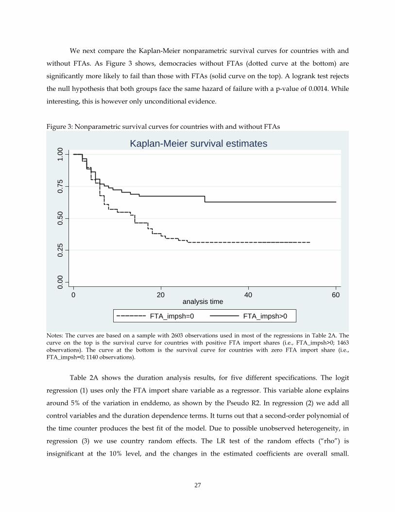
27

We next compare the Kaplan-Meier nonparametric survival curves for countries with and

without FTAs. As Figure 3 shows, democracies without FTAs (dotted curve at the bottom) are

significantly more likely to fail than those with FTAs (solid curve on the top). A logrank test rejects

the null hypothesis that both groups face the same hazard of failure with a p-value of 0.0014. While

interesting, this is however only unconditional evidence.

Figure 3: Nonparametric survival curves for countries with and without FTAs

0.00

0.25

0.50

0.75

1.00

0 20 40 60analysis time

FTA_impsh=0 FTA_impsh>0

Kaplan-Meier survival estimates

Notes: The curves are based on a sample with 2603 observations used in most of the regressions in Table 2A. The curve on the top is the survival curve for countries with positive FTA import shares (i.e., FTA_impsh>0; 1463 observations). The curve at the bottom is the survival curve for countries with zero FTA import share (i.e., FTA_impsh=0; 1140 observations).

Table 2A shows the duration analysis results, for five different specifications. The logit

regression (1) uses only the FTA import share variable as a regressor. This variable alone explains

around 5% of the variation in enddemo, as shown by the Pseudo R2. In regression (2) we add all

control variables and the duration dependence terms. It turns out that a second-order polynomial of

the time counter produces the best fit of the model. Due to possible unobserved heterogeneity, in

regression (3) we use country random effects. The LR test of the random effects (“rho”) is

insignificant at the 10% level, and the changes in the estimated coefficients are overall small.

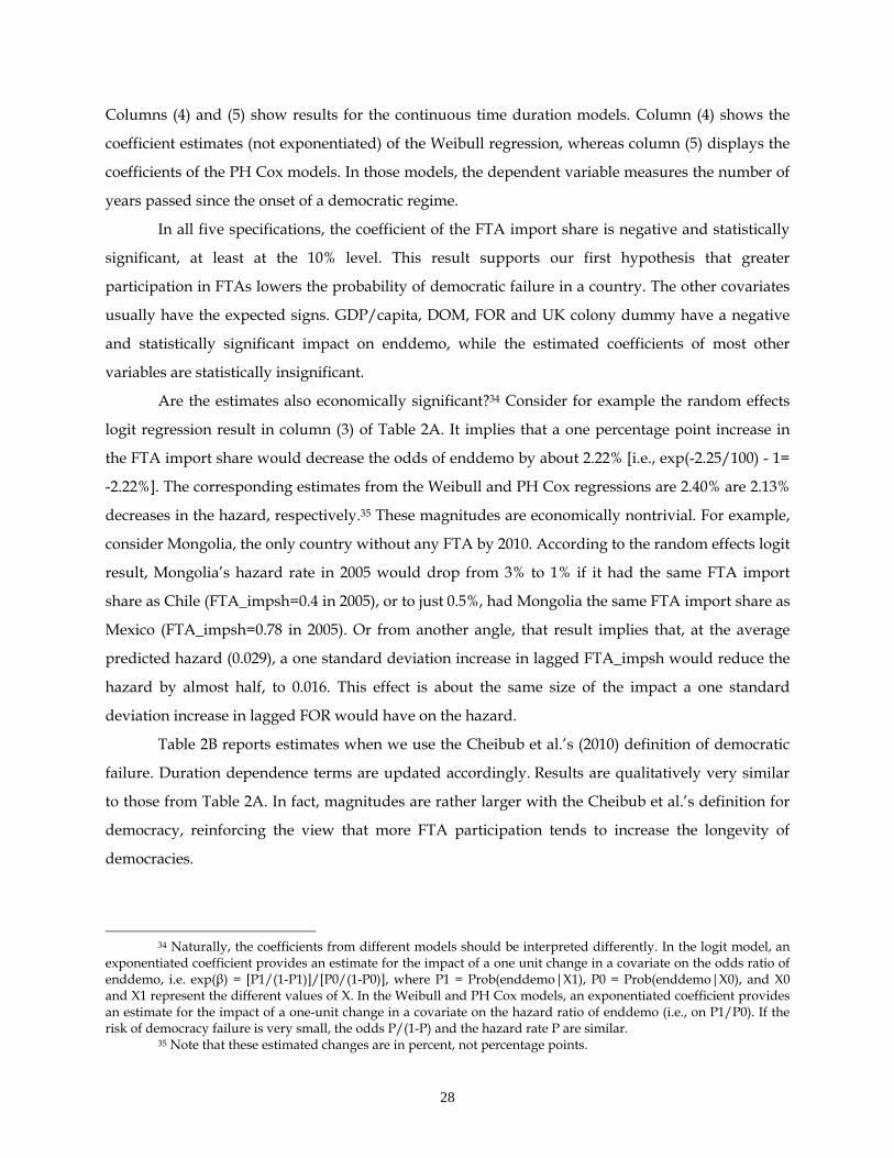
28

Columns (4) and (5) show results for the continuous time duration models. Column (4) shows the

coefficient estimates (not exponentiated) of the Weibull regression, whereas column (5) displays the

coefficients of the PH Cox models. In those models, the dependent variable measures the number of

years passed since the onset of a democratic regime.

In all five specifications, the coefficient of the FTA import share is negative and statistically

significant, at least at the 10% level. This result supports our first hypothesis that greater

participation in FTAs lowers the probability of democratic failure in a country. The other covariates

usually have the expected signs. GDP/capita, DOM, FOR and UK colony dummy have a negative

and statistically significant impact on enddemo, while the estimated coefficients of most other

variables are statistically insignificant.

Are the estimates also economically significant?34 Consider for example the random effects

logit regression result in column (3) of Table 2A. It implies that a one percentage point increase in

the FTA import share would decrease the odds of enddemo by about 2.22% [i.e., exp(-2.25/100) - 1=

-2.22%]. The corresponding estimates from the Weibull and PH Cox regressions are 2.40% are 2.13%

decreases in the hazard, respectively.35 These magnitudes are economically nontrivial. For example,

consider Mongolia, the only country without any FTA by 2010. According to the random effects logit

result, Mongolia’s hazard rate in 2005 would drop from 3% to 1% if it had the same FTA import

share as Chile (FTA_impsh=0.4 in 2005), or to just 0.5%, had Mongolia the same FTA import share as

Mexico (FTA_impsh=0.78 in 2005). Or from another angle, that result implies that, at the average

predicted hazard (0.029), a one standard deviation increase in lagged FTA_impsh would reduce the

hazard by almost half, to 0.016. This effect is about the same size of the impact a one standard

deviation increase in lagged FOR would have on the hazard.

Table 2B reports estimates when we use the Cheibub et al.’s (2010) definition of democratic

failure. Duration dependence terms are updated accordingly. Results are qualitatively very similar

to those from Table 2A. In fact, magnitudes are rather larger with the Cheibub et al.’s definition for

democracy, reinforcing the view that more FTA participation tends to increase the longevity of

democracies.

34 Naturally, the coefficients from different models should be interpreted differently. In the logit model, an

exponentiated coefficient provides an estimate for the impact of a one unit change in a covariate on the odds ratio of enddemo, i.e. exp(β) = [P1/(1-P1)]/[P0/(1-P0)], where P1 = Prob(enddemo|X1), P0 = Prob(enddemo|X0), and X0 and X1 represent the different values of X. In the Weibull and PH Cox models, an exponentiated coefficient provides an estimate for the impact of a one-unit change in a covariate on the hazard ratio of enddemo (i.e., on P1/P0). If the risk of democracy failure is very small, the odds P/(1-P) and the hazard rate P are similar.

35 Note that these estimated changes are in percent, not percentage points.

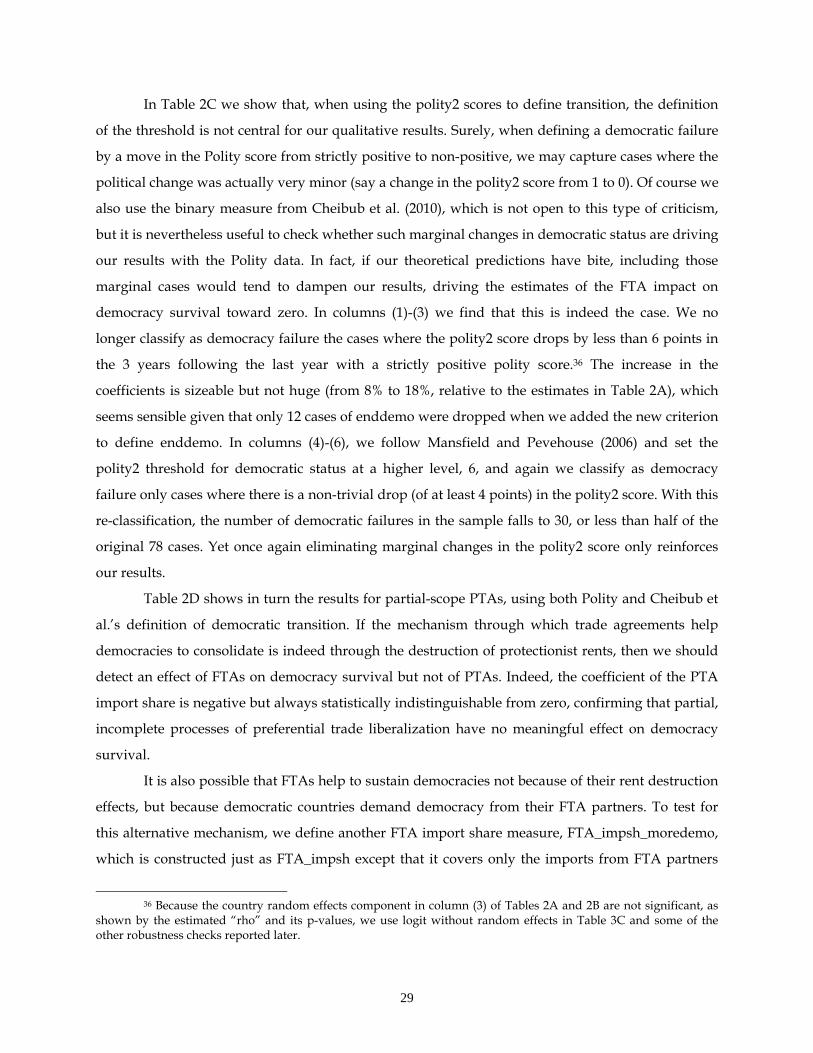
29

In Table 2C we show that, when using the polity2 scores to define transition, the definition

of the threshold is not central for our qualitative results. Surely, when defining a democratic failure

by a move in the Polity score from strictly positive to non-positive, we may capture cases where the

political change was actually very minor (say a change in the polity2 score from 1 to 0). Of course we

also use the binary measure from Cheibub et al. (2010), which is not open to this type of criticism,

but it is nevertheless useful to check whether such marginal changes in democratic status are driving

our results with the Polity data. In fact, if our theoretical predictions have bite, including those

marginal cases would tend to dampen our results, driving the estimates of the FTA impact on

democracy survival toward zero. In columns (1)-(3) we find that this is indeed the case. We no

longer classify as democracy failure the cases where the polity2 score drops by less than 6 points in

the 3 years following the last year with a strictly positive polity score.36 The increase in the

coefficients is sizeable but not huge (from 8% to 18%, relative to the estimates in Table 2A), which

seems sensible given that only 12 cases of enddemo were dropped when we added the new criterion

to define enddemo. In columns (4)-(6), we follow Mansfield and Pevehouse (2006) and set the

polity2 threshold for democratic status at a higher level, 6, and again we classify as democracy

failure only cases where there is a non-trivial drop (of at least 4 points) in the polity2 score. With this

re-classification, the number of democratic failures in the sample falls to 30, or less than half of the

original 78 cases. Yet once again eliminating marginal changes in the polity2 score only reinforces

our results.

Table 2D shows in turn the results for partial-scope PTAs, using both Polity and Cheibub et

al.’s definition of democratic transition. If the mechanism through which trade agreements help

democracies to consolidate is indeed through the destruction of protectionist rents, then we should

detect an effect of FTAs on democracy survival but not of PTAs. Indeed, the coefficient of the PTA

import share is negative but always statistically indistinguishable from zero, confirming that partial,

incomplete processes of preferential trade liberalization have no meaningful effect on democracy

survival.

It is also possible that FTAs help to sustain democracies not because of their rent destruction

effects, but because democratic countries demand democracy from their FTA partners. To test for

this alternative mechanism, we define another FTA import share measure, FTA_impsh_moredemo,

which is constructed just as FTA_impsh except that it covers only the imports from FTA partners

36 Because the country random effects component in column (3) of Tables 2A and 2B are not significant, as

shown by the estimated “rho” and its p-values, we use logit without random effects in Table 3C and some of the other robustness checks reported later.

30

with more democratic regimes, according to the polity2 scores. We add that variable to the

regression to capture the additional effect that FTAs with more democratic countries may have on the

political regime. If only the pressure from more democratic partners matters for the relationship, the

coefficient on FTA_impsh_moredemo would be significant but not the coefficient on FTA_impsh.

Table 2E shows the results. As expected, the statistical significance of the coefficients on the FTA

import share variables is relatively low due to the high correlation between them (0.51).

Nevertheless, the results still indicate a significant role of participation in FTAs on the sustainability

of democracy. On the other hand, there is no distinguishable additional effect of having the FTAs

with more democratic partners. Thus, pressure from more democratic FTA partners does not seem

to be the driver of our results.

6.B. Are unstable democracies more likely to seek participation in FTAs?

We now turn to our second hypothesis. We use the predicted hazard rate from the duration analysis

to estimate how democratic instability affects FTA formation. The results from our main

specification are reported in the first three columns of Table 3A. The first column shows the

enddemo logit regression with both FTA and PTA import shares.37 As discussed in Section 4, to

capture only the portion of the hazard unaffected by trade agreements, we predict the hazard after

setting FTA and PTA import shares to 0. Columns (2) and (3) display the regressions with the

predicted hazard, where the dependent variable is the change in the FTA import share from the

previous year (ΔFTA). We also include the square of the predicted hazard to allow for possible

nonlinear effects. Year dummies are included to capture global trends in the formation of trade

agreements. To control for unobserved heterogeneity across countries, country fixed effects are also

included in the regression. Because the hazard is predicted from the first stage with sampling errors,

we use bootstrapping (500 replications) to adjust the standard errors.

In column (2), the coefficient of the predicted hazard rate is significant at the 1% level. This

result supports our theoretical prediction that unstable democracies tend to form more FTAs than

stable democracies. We can also quantify the magnitude of the effect. At the mean value of the

hazard (0.029), a one standard deviation increase in the hazard (0.039) would lead to about one

percentage point increase in the FTA import share. Or consider for example the case of Guatemala

from 1966 to 1967, when its hazard shot up to 0.062 from 0.006. According to our estimates, this

37 We use logit without country random effects in the first stage because the random effects component is

always insignificant, as shown in Tables 2A and 2B. The second-stage ΔFTA regressions do not change in any qualitatively important way when we use the other specifications in Table 2A. The same is true if we use Cheibub et al.’s (2010) definition for transition to autocracy as the dependent variable in the first stage.

31

should lead to an increase of 1.94 percentage points in Guatemala’s FTA import share (the actual

increase was 2.65 percentage points).

In column (3), we repeat the analysis from column (2) but include DOM, FOR and duration

dependence terms in the second-stage regression. The purpose of doing this is to check if our results

are sensitive to these exclusion variables. The estimated coefficient of the hazard show little

sensitivity to those changes.38

The last two columns of Table 3A report the results from the analogous exercise for the

formation of partial-scope trade agreements, ΔPTAs. The hazard is now indistinguishable from zero

in statistical terms. Thus, political instability has no identifiable effect on the formation of partial-

scope trade agreements. This is consistent with the mechanism we develop, where unstable

democracies seek to diminish the rents available to those in power by increasing participation in

FTAs—but not in PTAs.

6.C. A bilateral analysis of democracy instability and FTA participation

We also run bilateral structural regressions. Each observation is associated with a country dyad. The

dependent variable is a dummy variable, equal to one if the two countries have a trade agreement in

that year. As discussed earlier, using dummy variables for FTAs makes it impossible to condition

the results on the importance of the agreement for the countries involved. On the other hand, this

approach has the advantage of paralleling more closely the existing regionalism literature, including

the previous analyses of democracy and FTA formation.

Our key explanatory variables are Hazard_i and Hazard_j, which are the predicted hazards

for countries i and j based on the enddemo logit regression in the first column of Table 3A. Other

covariates include variables usually controlled for in bilateral FTA analyses: the sum and the

absolute difference of the two countries’ GDP and GDP/capita in a dyad, the distance between

them, a border dummy, a common colony dummy, a military conflict dummy, a political alliance

dummy, and the product of the two countries’ remoteness, defined as the distance to the rest of the

world weighted by countries’ GDP.39 We include as well the polity2 score for each country in a

dyad, and some additional variables used by Mansfield, Milner and Rosendorff (2002) and

Mansfield, Milner and Pevehouse (2008), such as bilateral trade, WTO membership, and hegemony.

See the footnotes of Table 3B for more information on those variables.

38 We also tried both excluding DOM and the duration dependence terms while keeping FOR in the second

stage. The results remain virtually unchanged. 39 For more information on these variables and data sources, see Liu (2010).

32

The results from the bilateral analysis are reported in Table 3B.40 The first two columns are

for FTAs. Note that stronger democracies, as measured by higher polity2 scores, are more likely to

be involved in an FTA than weaker democracies, in line with previous findings in the literature (e.g.

Mansfield, Milner and Rosendorff 2002). Nevertheless, even controlling for the current strength of

democracy, the effect of the expectation of democratic failure on FTA participation, as measured by

the predicted hazard rates, remains positive and highly significant. Most of the other variables have

the expected signs as well.

The last two columns consider partial-scope PTAs. Analogously to Table 3A, the hazard

rates become statistically indistinguishable from zero in all the regressions, confirming that

democracy instability has no effect on the formation of partial-scope trade agreements.

6.D. Robustness

In this section we discuss the robustness of our results in several dimensions. First, does our FTA

import share variable capture mostly changes (deepening) of existing FTAs or the formation of new

FTAs? Although the interpretation of the results is similar in both cases, it is useful to disentangle

the two effects to check whether the formation of new FTAs matters on its own. To do so, in Table 4

we use, instead of the lagged shares of imports from FTA partners, the share of imports in 1960 of

the FTA partners in the previous year. This measure, therefore, excludes all variation in our main

independent variable except the variation that comes from the formation of new FTA links. As Table

4 shows, the magnitude of the FTA coefficients is qualitatively similar to (in fact, about 50% larger

than) those in Table 2A.

Second, as discussed in the Introduction, several studies relate openness to democracy. To

check whether our FTA measure captures more than general openness, we add an openness

variable, defined as (imports+exports)/GDP, and a WTO membership dummy as additional

regressors to our existing enddemo regressions. The logit, Weibull and PH Cox regression results,

reported in columns (1)-(3) of Table 5, are quite similar to those from Table 2A, and the two newly

added variables are highly insignificant.

Third, motivated by the findings of Pevehouse (2002), that participation in international

organizations, broadly defined and not limited to regional trade agreements, can help democracies

to endure, we also test whether the effects we find for FTAs are not capturing the effect of

engagement in international organizations (IOs) more generally. This would matter, as the reasoning

40 Those results are based on pooled data logit regressions with standard errors clustered by dyad.

Regressions with dyad random effects, available upon request, produce similar results.

33

for the latter relies on signaling effects, whereas our emphasis is on a commitment to destroy

protectionist rents. Fourth, Cheibub (2006) shows that having a former military leader as the chief

executive has a negative effect on democracy survival. This is confirmed by the extreme bound

analysis in Gassebner et al. (2009). In Table 5, columns (4)-(6), we include the lagged number of IOs a

country belongs to and a dummy variable indicating whether the executive leader is a former

military officer (we explain under the table how these variables are constructed). Results are

virtually unchanged, and the coefficients on the IO variable and formal military leader in the

country are statistically indistinguishable from zero, indicating that our findings are not picking up

these effects.

Fifth, it is possible that our results are driven by a small number of observations for which

alternative mechanisms may generate the same statistical association. For example, many previously

socialist countries both established democratic regimes and entered in FTAs during the 1990s, but

also went through many other economic and institutional changes. Are those countries alone

responsible for our statistically significant coefficients? We check that by dropping all previously

socialist states from our regressions. Table 6, columns (1)-(3), show the results for logit, Weibull and

PH Cox regressions. Results are very similar to those with the full sample. Interestingly, the

magnitude of the estimated coefficient on our FTA variable is actually somewhat higher in the

restricted sample. This probably reflects the fact that some socialist countries that became

democracies later reverted to autocracies, despite effective participation in FTAs (e.g. Azerbaijan).

A related concern is that some trade agreements contain rules specifying that members must

be democratic. This was a pre-condition for accession of the Central and Eastern European countries

to the European Union. Mercosur added a similar clause for all of its members in 1998. For those

countries, democracy and FTA participation must therefore be significantly linked and this may

have an important effect on our estimations. In columns (4)-(6) of Table 6 we drop the observations

for which such rules apply (i.e. all Mercosur members since 1998 and the Central and Eastern

European countries once they entered the European Union). Again, results are very similar to those

from Table 2A.

Our democracy consolidation result could arise simply because less rent-seeking

democracies may be more likely to sign FTAs and may also last longer, relative to more rent-seeking

democracies. This would imply that our results may be driven by omission of a measure on how

rent-seeking a country is. A measure for this variable is generally extremely hard to find, but

Gawande et al. (2009) provide estimates for that weight for 54 countries/regions. Although the

subset of countries is small relative to our sample, it provides a useful proxy. We include such a

34

measure (1/b) in our enddemo regressions. Table 7 shows the logit, Weibull and PH Cox regression

results, using both polity2 and Cheibub et al. (2010) measures. We find that this variable is always

highly insignificant, whereas the FTAimpsh variable remains significantly in all regressions even

though only up to 48 countries are covered in those regressions.

We also perform a number of robustness checks in our structural regressions. First, does the

hazard of democratic failure actually predict the formation of new FTAs, or just the deepening of

existing FTAs? To eliminate variation in the dependent variable that is unrelated to the formation of

new FTA/PTA links, in Table 8 we repeat the regressions in Table 3A using the measure of FTA and

PTA participation that considers 1960 import shares instead of lagged ones. Results from the two

tables are overall very similar, confirming that democratic instability indeed helps to predict the

formation of new FTAs (but not of new PTAs), as a more direct interpretation of our model suggests.

Second, is it really the expectation of regime change (proxied by the predicted hazard) that

induces more FTAs? One alternative is that a recent change in regime, from autocracy to democracy,

is what causes more FTAs. Another is that volatility in the degree of democracy has an effect on its

own. Our estimated hazard may be correlated with both recent changes in political regime and the

volatility of democracy. To test whether it is indeed the expectation of regime change that matters,

we include in the ΔFTA regression, in addition to the predicted hazard, one of the following

variables: (1) reg_change, a dummy indicating whether a country’s polity2 increased from a non-

positive to a strictly positive score, lagged by one year; and (2) var(Polity)_10yr, the variance of

polity2 scores during the last 10 years, which is used to capture recent regime instability. The results

are reported in columns (1)-(2) of Table 9. In both cases, the newly added variable is highly

insignificant, while the predicted hazard remains statistically significant. These results corroborate

the idea that what really matters for FTA formation is the expectation of a possible of democratic

disruption.

Third, it is conceivable that our empirical results may be identifying a more general

phenomenon than the model suggests. For example, governments may form more FTAs as a

consequence of general political competition within an electoral system, and not specifically because

of the threat from autocrats. If the risk of democratic collapse is positively associated with more

political competition within a democracy, our finding that the threat of the democratic system

induces FTA formation may be driven by regular political competition within a democracy. To test

for that, we include a measure of political competition in the ΔFTA regression. We use the variable

35

POLCOMP from Polity IV, which codes the degree of political competition in the country.41 The

results are reported in the last column of Table 9. Again, the newly added variable is statistically

insignificant, while the predicted hazard remains statistically significant and displays similar

magnitude. This suggests that regular political competition in a country is not an important driver of

FTA formation, unlike the expectation of democratic disruption.

Finally, negotiating an FTA is a process that can take several years. This suggests that the

relationship may be more precise if we use lags of the explanatory variables in our ΔFTA

regressions. In the online Appendix 5 we show several alternative ways of estimating the structural

ΔFTA_impsh regression. In one alternative, the dependent variable is the 5-year difference in

FTA_impsh and most of the explanatory variables (X) are lagged by 5-years. In another we use

similar definitions except that we calculate first the 5-year moving averages of most of the variables,

before taking their 5-year lags or 5-year difference. Please refer to the notes in the appendix for more

details. Overall, the estimated coefficients of the hazard and its squared term become significantly

larger, as expected.42

Put together, these robustness checks boost confidence that we are capturing our intended

mechanism, rather than the workings of some omitted variable that affects both FTA formation and

political regimes in general.

6.E. Endogeneity

A potential problem in our analysis is reverse causality between FTA and Prob(enddemo). Since we

do not estimate the two equations jointly, we have to address this issue in each equation.

In our structural estimation, the endogeneity of the hazard is unlikely to be a problem

because we use the predicted hazard as a function of exogenous variables only, after setting the FTA

and PTA variables to zero. In other words, the predicted hazard in the ΔFTA equation is the

exogenous component of Prob(enddemo). In the bilateral structural regressions, the potential

endogeneity problem is further reduced because we drop the repeated “1”s of the FTA dummy.

Keeping only the first positive outcome, we eliminate the possibility of feedbacks from FTAs to the

predicted hazard of democracy.

41 This variable measures both the regulation of participation and the competitiveness in the political

process. According to the Polity IV Dataset User’s Manual, POLCOMP reaches its maximum score when “relatively stable and enduring political groups regularly compete for political influence and positions with little use of coercion; ruling groups and coalitions regularly, voluntarily transfer central power to competing groups; and no significant groups, issues, or types of conventional political action are regularly excluded from the political process.”

42 For example, the results in the first specification imply that the 5-year effect of the hazard on FTA formation is around 5 times larger than the one indicated in Table 3A.

36

In the enddemo regressions, endogeneity of the FTA variable may not be a problem either. If

the risk of democratic failure induces greater FTA participation, as our structural regression

indicates, this reverse causation will likely lead to an over-estimation of the lagged FTA coefficient in

the enddemo regression. Without addressing this endogeneity issue, we find a negative effect of

FTAs on enddemo. Had we eliminated it, the estimate would tend to be even more negative. In

other words, the reverse causality problem biases against the hypothesis that FTAs reduce the risk of

democratic failure.

We have also addressed the endogeneity of FTA_impsh in the enddemo duration

regressions formally, with a two-stage least squares (2SLS) approach. Although our specifications

for the enddemo regression are all nonlinear, we now estimate it using a linear probability model

(LMP) so that we can apply 2SLS. Another benefit of LMP is that we can use country fixed effects in

the enddemo regression. To run 2SLS, we need instruments (IVs) for FTA_impsh. Valid IVs should

be correlated with FTA_impsh but not with enddemo. We construct our instrument based on the

contagion effects of FTA formation. Egger and Larch (2008) and Baldwin and Jaimovich (2010), using

spatial econometric methods in a bilateral data setting, find strong evidence for contagion effects in

FTA formation. We also use bilateral data to construct the instrument, but the final contagion

measure is at the country level, to fit into our country*year panel data analysis. We first calculate for

each year t the FTA_impshijt for all of the trading partners (j) of a country (i) after excluding country

i’s own FTA imports from j. Contagionit of country i in year t is calculated as the average FTA_impshijt

weighted by 1/log(distanceij), where distanceij is the great circle distance between i and j. We also use

log(GDPjt/distanceij) and (GDPjt/distanceij) as alternative weights in the definition of Contagion.

In Table 10, we use each of the Contagion measures as the instrument for FTA_impsh (all

lagged by one year). Both country fixed effects and year dummies are included in all the first and

second stage regressions. The first stage regression results show that Contagion is a very strong

instrument for FTA_impsh. In all of the second stage regressions, lagged FTA_impsh remains

significant at either the 1% or the 5% level.43 Due to the bias in LMP estimates, we do not take too

seriously the magnitudes of the estimated coefficients. The results in Table 10 can at least show that

our previous finding is robust to the consideration of the endogeneity of the FTA_impsh.

43 Notice that the coefficients in Table 10 are not directly comparable to those in Table 2A because we use

LMP instead of logit, Weibull or PH Cox to estimate the enddemo regression in Table 10.

37

7. CONCLUSION We study the relationship between a country’s participation in free trade agreements and the

sustainability of its democracy. We develop a model centered on the destruction of rents caused by

FTAs. The model delivers two main results. First, deeper engagement in FTAs increases the

longevity of democracies. Second, political instability promotes FTA participation.

Relying on the concept of democratic capital developed by Persson and Tabellini (2009) to

estimate countries’ hazards out of democracy, we test and confirm our two main predictions in a

sample of 126 countries over 60 years. Our results suggest that the rent destruction forces of FTAs

constitute an important channel through which our predictions manifest. Our measure of FTA

intensity is aimed at capturing those forces. Moreover, the predictions hold for “proper,” GATT

1947-compatible free trade areas and customs unions, but not for partial-scope agreements based on

GATT’s Enabling Clause. We also find that the impact of FTAs on democracy survival is not greater

when the partners are more democratic, so it is not simply a matter of democratic countries

demanding democracy from their FTA partners. It is not that general political competition induces

FTA formation either; only the uncertainty related to the possibility of major changes in the political

regime matters.

While all this is “good news” for democratic countries involved in FTAs, we must emphasize

that participation in FTAs is, unsurprisingly, no panacea: they can help to consolidate democracies,

but their reach is limited. Our estimates make this limit clear. The effect is nevertheless comparable

to the effect of other forces highlighted in the literature, such as the spread and strength of

democracies in neighboring countries. Similarly, although we have found that democratic instability

pushes governments to engage in FTAs, there are as well many reasons other than democratic

instability that also foster participation in FTAs.

Our study pushes forward a growing political science literature that seeks to uncover links

between democracy and FTA participation. We depart from it by focusing on a specific

mechanism—the destruction of rents in FTAs—that allows us to be more specific about the

relationship. The paper also provides a clear departure from the perspective often taken by

economists, who tend to focus exclusively on the strictly economic aspects of the causes and

consequences of FTAs.44 Purely economic motives certainly help, but cannot fully explain the

44 A notable exception is the recent study by Martin, Mayer and Thoenig (2010), who use the frequency of

wars between two countries in the distant past to test whether FTAs lower the probability of war between them. They find that they do, especially when the trade gains associated with the FTA are high, indicating an interesting complementarity effect between trade and security gains from FTAs.

38

intensity of the ongoing outbreak of regionalism. We show that the instability of democracies is

another important contributing factor to this trend. Yet much remains to be known about the

interplay between trade agreements and democracy. We look forward to future research to further

illuminate this relationship.

REFERENCES

Acemoglu, Daron, and James A. Robinson (2006). Economic Origins of Dictatorship and Democracy. New York: Cambridge University Press. Acemoglu, Daron, Simon Johnson, James A. Robinson, and Pierre Yared (2008). “Income and Democracy.“ American Economic Review 98(3), 808-42. Aidt, Toke, and Martin Gassebner (2010). “Do Autocratic States Trade Less?” World Bank Economic Review 24(1), 38-76. Alesina, Alberto, and Guido Tabellini (1990). “A Positive Theory of Fiscal Deficits and Government Debt.” Review of Economic Studies 57, 403-414. Alvarez, Michael, Jose A. Cheibub, Fernando Limongi and Adam Przeworski, A. (1996). “Classifying political regimes.” Studies in Comparative International Development, 31(2), 3–36. Bagwell, Kyle, and Robert W. Staiger (2010). “The WTO: Theory and Practice.” Annual Review of Economics 2, 257-282. Baier, Scott L., and Jeffrey H. Bergstrand (2004). “Economic Determinants of Free Trade Agreements.” Journal of International Economics 64(1), 29-63. Baldwin, Richard, and Dany Jaimovich (2010). “Are Free Trade Agreements Contagious?” NBER Working Paper No. 16084. Barro, Robert (1999). “Determinants of Democracy.” Journal of Political Economy 107(6), S158-S183. Besley, Timothy, and Stephen Coate (2001). “Lobbying and Welfare in a Representative Democracy.” Review of Economic Studies 68(1), 67-82. Calvo-Pardo, Hector, Caroline Freund, and Emanuel Ornelas (2011). “The ASEAN Free Trade Agreement: Impact on Trade Flows and External Trade Barriers.” In Robert J. Barro & Jong-Wha Lee (eds.), Costs and Benefits of Economic Integration in Asia, Oxford: Oxford University Press. Cheibub, José Antonio (2006). Presidentialism, Parliamentarism, and Democracy. Cambridge University Press, New York. �

Cheibub, José Antonio, Jennifer Gandhi, and James Raymond Vreeland (2010). “Democracy and dictatorship revisited.” Public Choice 143(1-2), 67-101.

39

Dixit, Avinash (2010). “Democracy, Autocracy, and Bureaucracy.” Journal of Globalization and Development 1(1), Article 1. Egger, Peter, and Mario Larch (2008).“Interdependent Preferential Trade Agreement Memberships: An Empirical Analysis.” Journal of International Economics 76(2): 384-99.

Estevadeordal, Antoni, Caroline Freund, and Emanuel Ornelas (2008). “Does Regionalism Affect Trade Liberalization towards Non-Members?” Quarterly Journal of Economics 123(4), 1531-1575. Frankel, Jeffery A., Ernesto Stein, and Shang-Jin Wei (1997). Regional Trading Blocs. Washington, DC: Institute for International Economics. Freund, Caroline, and Emanuel Ornelas (2010). “Regional Trade Agreements.” Annual Review of Economics 2, 139-166. Gandhi, Jennifer, and Adam Przeworski (2006). “Cooperation, Cooptation, and Rebellion under Dictatorship.” Economics & Politics 18, 1-26. Gassebner, Martin, Michael J. Lamla, and James Raymond Vreeland (2009). “Extreme Bounds of Democracy.” KOF Working Paper No. 224. Gawande, Kishore, Pravin Krishna, and Marcelo Olarreaga (2009). “What Governments Maximize and Why: The View from Trade.” International Organization 63, 491–532. Giavazzi, Francesco, and Guido Tabellini (2005). “Economic and Political Liberalizations.” Journal of Monetary Economics 52, 1297-1330. Grossman, Gene, and Elhanan Helpman (1995). “The Politics of Free-trade Agreements.” American Economic Review 85, 667–90. Grossman, Gene, and Elhanan Helpman (1996). “Electoral Competition and Special Interest Politics.” Review of Economic Studies 63(2), 265-86. La Porta, Raphael, Florencio Lopez-De-Silanes, Andrei Shleifer, and Robert W. Vishny (1999). “The Quality of Government.” Journal of Law, Economics and Organization 15, 222-79. Limao, Nuno (2006). “Preferential Trade Agreements as Stumbling Blocks for Multilateral Trade Liberalization: Evidence for the U.S.” American Economic Review 96, 896-914. Liu, Xuepeng (2008). “The Political Economy of Free Trade Agreements: An Empirical Investigation.” Journal of Economic Integration 23(2), 237-271. Liu, Xuepeng (2010). “Testing Conflicting Political Economy Theories: Full-fledged vs. Partial-scope Regional.” Southern Economic Journal 77(1), 78-103. Lopez-Cordova, Ernesto, and Christopher M. Meissner (2008). “The Impact of International Trade on Democracy: A Long-Run Perspective.” World Politics 60(4), 539-575. Maddala, Gangadharrao Soundalyarao (1983). Limited-Dependent and Qualitative Variables in Econometrics. Cambridge, MA: Cambridge University Press.

40

Maggi, Giovanni, and Andrés Rodríguez-Clare (1998). “The Value of Trade Agreements in the Presence of Political Pressures.” Journal of Political Economy 106(3), 574-601. Maggi, Giovanni, and Andrés Rodríguez-Clare (2007). “A Political-Economy Theory of Trade Agreements.” American Economic Review 97(4), 1374-1406. Mansfield, Edward D., Helen V. Milner, and Jon C. Pevehouse (2008). “Democracy, Veto Players, and the Depth of Regional Integration.” World Economy 31(1), 67-96. Mansfield, Edward D., Helen V. Milner, and Peter B. Rosendorff (2000). “Free to Trade: Democracies, Autocracies, and International Trade.” American Political Science Review 94(2), 305-321. Mansfield, Edward D., Helen V. Milner, and Peter B. Rosendorff (2002). “Why Democracies Cooperate More: Electoral Control and International Trade Agreements.” International Organization 56(3), 477–513. Mansfield, Edward D., and Jon C. Pevehouse (2006). “Democratization and International Organizations.” International Organization 60(1), 137-167. Martin Philippe, Thierry Mayer, and Mathias Thoenig (2010). “The Geography of Conflicts and Free Trade Agreements.” Mimeo. McLaren, John (2002). “A Theory of Insidious Regionalism.” Quarterly Journal of Economics 117(2), 571-608. Mitra, Devashish, Dimitrios Thomakos, and Mehmet Ulubasogly (2002). “‘Protection for Sale’ in A Developing Country: Democracy vs. Dictatorship.” Review of Economics and Statistics 84(3), 497-508. Ornelas, Emanuel (2005a). “Rent Destruction and the Political Viability of Free Trade Agreements.” Quarterly Journal of Economics 120(4), 1475-1506. Ornelas, Emanuel (2005b). “Endogenous Free Trade Agreements and the Multilateral Trading System.” Journal of International Economics 67(2), 471-497. O’Rourke, Kevin H., and Alan M. Taylor (2007). “Democracy and Protectionism.” In Timothy J. Hatton, Kevin H. O’Rourke, and Alan M. Taylor (eds.), The New Comparative Economic History: Essays in Honor of Jeffrey G. Williamson. Cambridge, Mass.: MIT Press. Persson, Torsten, and Lars Svensson (1989). “Why a Stubborn Conservative Would Run a Deficit: Policy with Time-Inconsistent Preferences.” Quarterly Journal of Economics 104, 325-345. Persson, Torsten, and Guido Tabellini (2009). “Democratic Capital: The Nexus of Political and Economic Change.” American Economic Journal: Macroeconomics 1(2), 88-126. Pevehouse, Jon C. (2002). “With A Little Help from My Friends? Regional Organizations and the Consolidation of Democracy.” American Journal of Political Science 46(3), 611-626. Przeworski , Adam, Michael Alvarez, Jose A. Cheibub and Fernando Limongi (1996). “What Makes Democracies Endure?” Journal of Democracy 7, 39-55.

41

Schiff, Maurice, and Alan L. Winters (2003). Regional Integration and Development. Washington, DC: Oxford University Press. Stroup, Caleb, and Benjamin Zissimos (2011). “Pampered Bureaucracy and Trade Integration.” Mimeo. World Trade Organization (2011). “Preferential Trade Agreements and the WTO: from Co-existence to Coherence.” The World Trade Report 2011.

Table 1: Descriptive statistics of variables Variable Description Mean S.D. Min Max enddemo Dummy indicating the end of a democracy 0.024 0.153 0 1 lFTA_impsh Lagged import share from FTA partners 0.191 0.268 0 0.925 lPTA_impsh Lagged import share from PTA partners 0.065 0.128 0 0.646 ΔFTA_impsh Change in FTA_impsh from previous year 0.011 0.073 -0.451 0.772 ΔPTA_impsh Change in PTA_impsh from previous year 0.002 0.032 -0.442 0.502 llgdppc Lagged log(GDP/capita) 7.830 1.471 4.400 10.540 lDOM Lagged current domestic democratic capital 0.535 0.338 0 0.99997 lFOR Lagged foreign democratic capital 0.045 0.138 -0.217 0.261 war Current war indicator 0.066 0.248 0 1 lwar Lagged war indicator 0.070 0.254 0 1 legor3 leg_origin=Socialism 0.120 0.325 0 1 africa Africa dummy 0.189 0.391 0 1 middleeast Middle East region dummy 0.033 0.180 0 1 Spain_colony UK colony dummy 0.184 0.388 0 1 UK_colony Spain colony dummy 0.344 0.475 0 1 duration Duration of a democracy (# of years passed) 35.086 43.842 1 208 Hazard Predicted hazard used in structural regressions 0.029 0.039 0 0.378 Note: This table is based on a sample with 2603 observations used in most of the regressions in Table 2A, except for Hazard, which is based on the first regression in Table 3A (number of observation = 2625).

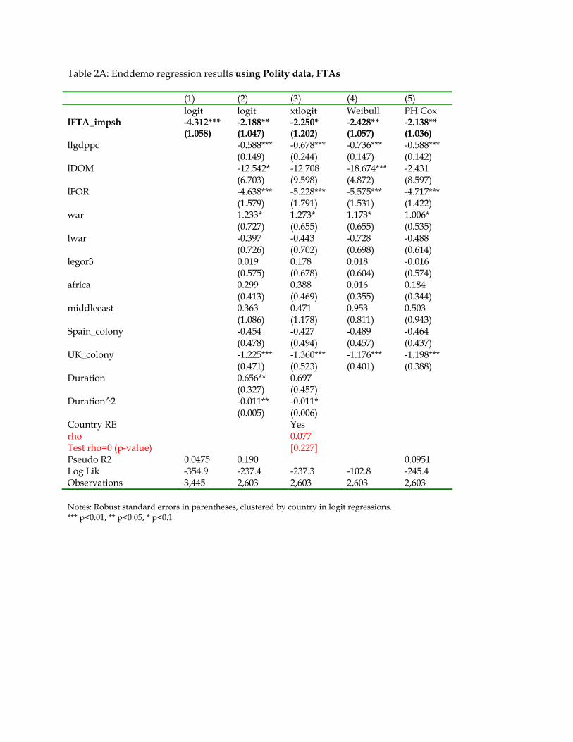
Table 2A: Enddemo regression results using Polity data, FTAs (1) (2) (3) (4) (5) logit logit xtlogit Weibull PH Cox lFTA_impsh -4.312*** -2.188** -2.250* -2.428** -2.138** (1.058) (1.047) (1.202) (1.057) (1.036) llgdppc -0.588*** -0.678*** -0.736*** -0.588*** (0.149) (0.244) (0.147) (0.142) lDOM -12.542* -12.708 -18.674*** -2.431 (6.703) (9.598) (4.872) (8.597) lFOR -4.638*** -5.228*** -5.575*** -4.717*** (1.579) (1.791) (1.531) (1.422) war 1.233* 1.273* 1.173* 1.006* (0.727) (0.655) (0.655) (0.535) lwar -0.397 -0.443 -0.728 -0.488 (0.726) (0.702) (0.698) (0.614) legor3 0.019 0.178 0.018 -0.016 (0.575) (0.678) (0.604) (0.574) africa 0.299 0.388 0.016 0.184 (0.413) (0.469) (0.355) (0.344) middleeast 0.363 0.471 0.953 0.503 (1.086) (1.178) (0.811) (0.943) Spain_colony -0.454 -0.427 -0.489 -0.464 (0.478) (0.494) (0.457) (0.437) UK_colony -1.225*** -1.360*** -1.176*** -1.198*** (0.471) (0.523) (0.401) (0.388) Duration 0.656** 0.697 (0.327) (0.457) Duration^2 -0.011** -0.011* (0.005) (0.006) Country RE Yes rho 0.077 Test rho=0 (p-value) [0.227] Pseudo R2 0.0475 0.190 0.0951 Log Lik -354.9 -237.4 -237.3 -102.8 -245.4 Observations 3,445 2,603 2,603 2,603 2,603 Notes: Robust standard errors in parentheses, clustered by country in logit regressions. *** p<0.01, ** p<0.05, * p<0.1

Table 2B: Enddemo regression results using Cheibub et al.’s (2010) democracy data, FTAs (1) (2) (3) (4) (5) logit logit xtlogit Weibull PH Cox lFTA_impsh -5.869*** -3.535** -3.668* -3.390* -2.761* (1.266) (1.617) (2.210) (1.737) (1.625) llgdppc -0.341 -0.367* -0.578** -0.443** (0.210) (0.220) (0.230) (0.201) lDOM -2.324 -2.447 -3.625*** -1.943 (1.420) (1.578) (1.198) (1.515) lFOR -5.184*** -5.336*** -5.987*** -5.226** (1.781) (1.816) (2.197) (2.056) war 0.918 0.895 1.212* 1.578*** (1.007) (0.804) (0.656) (0.552) lwar -0.429 -0.406 -0.875 -1.201** (0.985) (0.860) (0.606) (0.575) legor3 -18.549 -15.305*** -44.212 (8,353) (0.797) (0.000) africa 1.418** 1.475** 1.714** 1.167** (0.612) (0.614) (0.696) (0.562) middleeast -18.656 -13.503*** -43.585 (16,628) (1.226) (0.000) Spain_colony 0.525 0.526 0.534 -0.046 (0.551) (0.495) (0.616) (0.574) UK_colony -0.883* -0.958* -1.138** -0.968* (0.511) (0.573) (0.565) (0.549) Duration 0.144** 0.162* (0.062) (0.090) Duration^2 -0.003** -0.003* (0.001) (0.002) Country RE Yes rho 0.038 Test rho=0 (p-value) [0.359] Pseudo R2 0.0626 0.185 0.196 Log Lik -295.7 -164.1 -164.0 -59.70 -105.4 Observations 3,727 1,886 2,252 2,151 2,151 Notes: Robust standard errors in parentheses, clustered by country in logit regressions. *** p<0.01, ** p<0.05, * p<0.1

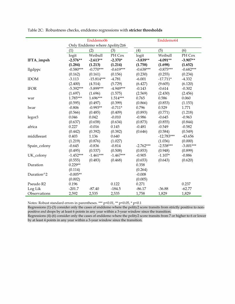
Table 2C: Robustness checks, enddemo regressions with stricter thresholds Enddemo06

Only Enddemo where Δpolity2≥6 Enddemo64

(1) (2) (3) (4) (5) (6) logit Weibull PH Cox logit Weibull PH Cox lFTA_impsh -2.576** -2.613** -2.370* -3.839** -4.091** -3.907** (1.284) (1.213) (1.214) (1.758) (1.698) (1.652) llgdppc -0.580*** -0.770*** -0.619*** -0.638*** -0.875*** -0.682*** (0.162) (0.161) (0.156) (0.230) (0.255) (0.234) lDOM -3.113 -15.814*** -4.781 -6.001 -17.711* -4.332 (2.400) (4.514) (5.729) (6.427) (9.605) (6.120) lFOR -5.392*** -5.899*** -4.949*** -0.143 -0.614 -0.302 (1.697) (1.696) (1.575) (2.569) (2.430) (2.456) war 1.785*** 1.696*** 1.514*** 0.765 0.586 0.060 (0.595) (0.497) (0.399) (0.866) (0.853) (1.153) lwar -0.806 -0.993** -0.711* 0.796 0.529 1.771 (0.566) (0.485) (0.409) (0.893) (0.771) (1.218) legor3 0.046 0.042 -0.010 -0.986 -0.645 -0.963 (0.637) (0.658) (0.634) (0.873) (0.855) (0.844) africa 0.227 -0.016 0.145 -0.481 -0.549 -0.582 (0.442) (0.392) (0.382) (0.646) (0.584) (0.549) middleeast 0.403 1.136 0.640 -12.783*** -43.656 (1.219) (0.876) (1.027) (1.036) (0.000) Spain_colony -0.645 -0.836 -0.814 -2.762*** -2.538*** -3.001*** (0.495) (0.537) (0.508) (0.853) (0.948) (0.899) UK_colony -1.452*** -1.461*** -1.467*** -0.905 -1.107* -0.886 (0.555) (0.483) (0.468) (0.653) (0.643) (0.620) Duration 0.229** 0.358 (0.114) (0.264) Duration^2 -0.005** -0.008 (0.002) (0.005) Pseudo R2 0.196 0.122 0.271 0.237 Log Lik -201.7 -87.40 -184.5 -86.17 -36.88 -62.77 Observations 2,592 2,535 2,535 1,758 1,829 1,829 Notes: Robust standard errors in parentheses. *** p<0.01, ** p<0.05, * p<0.1 Regressions (1)-(3) consider only the cases of enddemo where the polity2 score transits from strictly positive to non-positive and drops by at least 6 points in any year within a 3-year window since the transition. Regressions (4)-(6) consider only the cases of enddemo where the polity2 score transits from 7 or higher to 6 or lower by at least 4 points in any year within a 3-year window since the transition.

Table 2D: Enddemo regression results, partial-scope PTAs Enddemo based on Polity “tta” based on Cheibub et al. (1) (2) (3) (4) (5) (6) logit Weibull PH Cox logit Weibull PH Cox lPTA_impsh -0.274 -0.738 -0.418 -0.293 2.155 2.172 (1.759) (1.584) (1.495) (1.727) (1.758) (1.487) llgdppc -0.622*** -0.752*** -0.617*** -0.392* -0.654*** -0.474** (0.146) (0.143) (0.137) (0.210) (0.241) (0.207) lDOM -13.191* -18.669*** -3.232 -2.705* -3.729*** -2.285 (6.878) (4.922) (8.135) (1.461) (1.182) (1.527) lFOR -5.071*** -5.617*** -4.992*** -5.996*** -7.912*** -7.207*** (1.463) (1.480) (1.388) (1.493) (2.212) (2.012) war 1.246* 1.175* 1.004* 0.877 1.245* 1.616** (0.740) (0.658) (0.542) (1.038) (0.702) (0.645) lwar -0.455 -0.777 -0.538 -0.512 -1.065* -1.341** (0.747) (0.712) (0.629) (1.008) (0.639) (0.627) legor3 -0.324 -0.524 -0.416 -15.408*** -44.209 (0.568) (0.580) (0.570) (0.838) (0.000) africa 0.302 -0.021 0.172 1.496** 1.901*** 1.490** (0.424) (0.374) (0.364) (0.622) (0.720) (0.620) middleeast 0.595 1.253 0.745 -13.366*** -43.602 (1.211) (0.894) (1.013) (1.239) (0.000) Spain_colony -0.317 -0.349 -0.336 0.688 0.735 0.111 (0.516) (0.464) (0.449) (0.572) (0.609) (0.573) UK_colony -1.132** -1.039*** -1.092*** -0.848* -1.154** -1.075** (0.457) (0.374) (0.379) (0.502) (0.574) (0.537) Duration 0.670** 0.147** (0.336) (0.062) Duration^2 -0.011** -0.003** (0.005) (0.001) Pseudo R2 0.182 0.087 0.175 0.193 Log Lik -239.6 -105.4 -247.6 -166.0 -60.80 -105.7 Observations 2,603 2,603 2,603 1,886 2,151 2,151 Notes: The dependent variable in regressions (1)-(3) is the enddemo measure based on the Polity Scores. The dependent variable in regressions (4)-(6) is the transition to autocracy “tta” measure from Cheibub et al. (2010). Robust standard errors in parentheses, clustered by country in logit regressions. *** p<0.01, ** p<0.05, * p<0.1

Table 2E: Enddemo regression results, more democratic FTAs vs. less democratic FTAs

(1) (2) (3) (4) (5) logit logit xtlogit Weibull PH Cox lFTA_impsh -4.694*** -2.186* -2.223 -2.716** -2.206* (1.188) (1.294) (1.523) (1.342) (1.258) lFTA_impsh_moredemo 1.252 -0.006 -0.073 0.855 0.196 (1.619) (1.855) (2.535) (1.970) (1.837) llgdppc -0.588*** -0.678*** -0.739*** -0.589*** (0.150) (0.244) (0.149) (0.144) lDOM -12.541* -12.699 -18.694*** -2.442 (6.675) (9.602) (4.878) (8.601) lFOR -4.638*** -5.228*** -5.611*** -4.722*** (1.587) (1.792) (1.559) (1.433) lwar 1.233* 1.273* 1.175* 1.006* (0.726) (0.655) (0.658) (0.534) legor3 -0.397 -0.443 -0.727 -0.487 (0.725) (0.702) (0.699) (0.613) africa 0.019 0.180 -0.004 -0.022 (0.570) (0.681) (0.598) (0.568) middleeast 0.299 0.388 0.018 0.183 (0.414) (0.469) (0.355) (0.345) socialist_trans 0.363 0.471 0.958 0.505 (1.086) (1.178) (0.811) (0.943) Spain_colony -0.454 -0.426 -0.496 -0.465 (0.477) (0.494) (0.457) (0.437) UK_colony -1.225*** -1.359*** -1.195*** -1.201*** (0.474) (0.524) (0.410) (0.390) Duration 0.656** 0.697 (0.326) (0.457) Duration^2 -0.011** -0.011* (0.005) (0.006) Country RE Yes rho 0.078 Test rho=0 (p-value) [0.276] Pseudo R2 0.048 0.190 0.095 Log Lik -354.7 -237.4 -237.3 -102.7 -245.4 Observations 3,445 2,603 2,603 2,603 2,603 Notes: lFTA_impsh_moredemo covers only the FTA partners with more democratic regimes based on Polity scores. Robust standard errors in parentheses, clustered by country in logit regressions. *** p<0.01, ** p<0.05, * p<0.1.

Table 3A: Structural ΔFTA and ΔPTA regression results enddemo ΔFTA_impsh ΔPTA_impsh (1) (2) (3) (4) (5) Hazard 0.405*** 0.370*** -0.049 0.002 (0.154) (0.157) (0.068) (0.087) Hazard^2 -0.855 -0.802* -0.188 -0.334 (0.527) (0.482) (0.214) (0.267) lFTA_impsh -2.249** -0.143*** -0.153*** (1.054) (0.019) (0.019) lPTA_impsh -0.626 -0.092*** -0.102*** (1.683) (0.016) (0.018) llgdppc -0.591*** 0.009 0.005 -0.003 -0.002 (0.155) (0.009) (0.010) (0.004) (0.005) lDOM -12.239* -0.023 -0.011 (6.746) (0.027) (0.011) lFOR -4.391*** 0.228*** -0.054* (1.504) (0.087) (0.037) war 1.221* -0.007 -0.006 0.010*** 0.009*** (0.722) (0.009) (0.008) (0.004) (0.004) lwar -0.391 0.001 -0.000 -0.003 -0.002 (0.719) (0.006) (0.007) (0.004) (0.004) legor3 -0.047 (0.587) africa 0.259 (0.412) middleeast 0.461 (1.183) UK_colony -1.210*** (0.463) Spain_colony -0.436 (0.498) Duration 0.644* 0.001 0.000 (0.329) (0.001) (0.000) Duration^2 -0.010** -0.000 -0.000** (0.005) (0.000) (0.000) remoteness -0.676 -1.063* -0.123 -0.021 (0.636) (0.596) (0.263) (0.293) Year Dummies Yes Yes Yes Yes Country FE Yes Yes Yes Yes Within R-squared 0.122 0.129 0.103 0.107 Observations 2,625 2,603 2,603 2,603 2,603 Notes: Hazard is the predicted hazard based on the enddemo logit regression in the first column after lFTA_impsh and lPTA_impsh are set to zero. Standard errors, in parentheses, are clustered by country in the logit regression in column (1). Standard errors in the second stage (columns (2)-(5)) are corrected by bootstrapping (500 replications). *** p<0.01, ** p<0.05, * p<0.1

Table 3B: Bilateral structural FTA and PTA duration regression results (1960-2007)

FTAs PTAs (1) (2) (3) (4) Hazard_i 5.746** 6.162** -0.361 -1.161 (2.484) (2.659) (1.477) (1.635) Hazard_j 5.692** 6.243** -0.234 -1.074 (2.481) (2.654) (1.496) (1.663) Polity_i 0.062** -0.041 (0.025) (0.027) Polity_j 0.065*** -0.042 (0.025) (0.027) ldist -1.425*** -1.427*** -0.441*** -0.442*** (0.074) (0.074) (0.120) (0.121) ltrade 0.017 0.013 0.060*** 0.059*** (0.013) (0.013) (0.016) (0.016) gdpsum 0.082*** 0.100*** 0.214*** 0.212*** (0.025) (0.026) (0.035) (0.035) dgdp -0.163*** -0.165*** -0.328*** -0.322*** (0.025) (0.025) (0.041) (0.042) gdppcsum 0.324*** 0.259*** -0.595*** -0.572*** (0.041) (0.043) (0.047) (0.048) dgdppc -0.301*** -0.301*** -0.251*** -0.235*** (0.037) (0.037) (0.065) (0.067) border -0.577*** -0.588*** 0.503* 0.429 (0.187) (0.190) (0.295) (0.306) bothin 0.526** 0.424* 0.381 0.419 (0.230) (0.223) (0.433) (0.432) onein -0.258 -0.303 0.763* 0.772* (0.228) (0.222) (0.429) (0.431) remote -9.166*** -8.851*** 19.959*** 19.663*** (1.634) (1.627) (1.692) (1.747) hegemony -36.732*** -36.537*** 27.710*** 26.074*** (5.910) (5.914) (5.338) (5.330) Observations 145,414 145,414 142,932 142,932 Pseudo R2 0.286 0.288 0.257 0.259 Log Lik -4072 -4064 -1495 -1491 Notes: Hazard_i and Hazard_j are the predicted hazards of countries i & j in a dyad based on the enddemo logit regression in the first column of Table 3A. polity_i and polity_j are the Polity scores of i & j in dyad. ldist is the logarithm of the great circle distance. ltrade is the logarithm of the total trade between i & j in a given year. gdpsum & dgdp are the sum and the absolute difference of the GDPs of the two countries in a dyad. gdppcsum & dgdppc are the sum and the absolute difference of the GDP/capita of the two countries in a dyad. border is a land contingency dummy. bothWTO and oneWTO measure how many countries in a dyad are GATT/WTO members. remoteness is the product of the two countries’ remoteness as defined in the text. hegemony is the percentage of global trade accounted for by the country that conducts the greatest amount of commerce in a given year. The following covariates are also included in the regressions but not listed to save space. evercol equals one if the two countries in a dyad have ever had colonial relationship. comcol equals one if the two countries in a dyad have ever shared the same colonizer. hostility is the average hostility level during our sample period. alliance is a political alliance dummy. Duration dependence is captured by a polynomial of the duration of a democracy up to fourth order. For more detailed information on variable definitions and data sources, please refer to Liu (2010). Robust standard errors in parentheses, clustered by country dyad. *** p<0.01, ** p<0.05, * p<0.1.

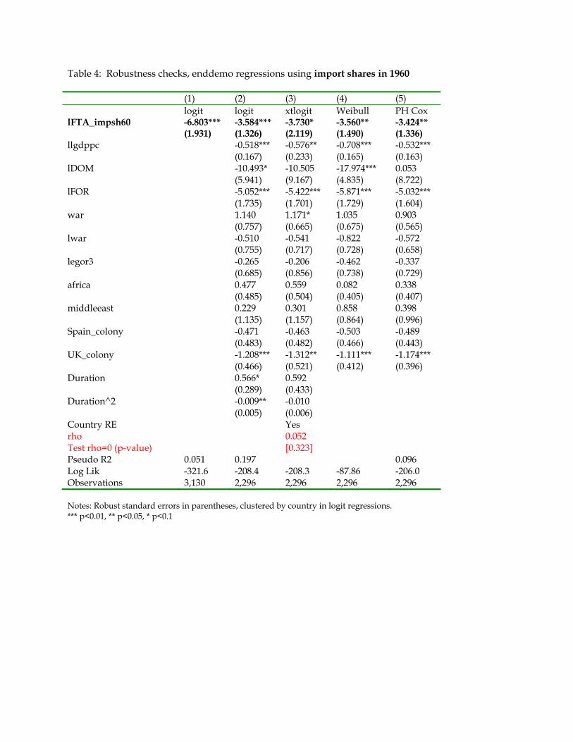
Table 4: Robustness checks, enddemo regressions using import shares in 1960 (1) (2) (3) (4) (5) logit logit xtlogit Weibull PH Cox lFTA_impsh60 -6.803*** -3.584*** -3.730* -3.560** -3.424** (1.931) (1.326) (2.119) (1.490) (1.336) llgdppc -0.518*** -0.576** -0.708*** -0.532*** (0.167) (0.233) (0.165) (0.163) lDOM -10.493* -10.505 -17.974*** 0.053 (5.941) (9.167) (4.835) (8.722) lFOR -5.052*** -5.422*** -5.871*** -5.032*** (1.735) (1.701) (1.729) (1.604) war 1.140 1.171* 1.035 0.903 (0.757) (0.665) (0.675) (0.565) lwar -0.510 -0.541 -0.822 -0.572 (0.755) (0.717) (0.728) (0.658) legor3 -0.265 -0.206 -0.462 -0.337 (0.685) (0.856) (0.738) (0.729) africa 0.477 0.559 0.082 0.338 (0.485) (0.504) (0.405) (0.407) middleeast 0.229 0.301 0.858 0.398 (1.135) (1.157) (0.864) (0.996) Spain_colony -0.471 -0.463 -0.503 -0.489 (0.483) (0.482) (0.466) (0.443) UK_colony -1.208*** -1.312** -1.111*** -1.174*** (0.466) (0.521) (0.412) (0.396) Duration 0.566* 0.592 (0.289) (0.433) Duration^2 -0.009** -0.010 (0.005) (0.006) Country RE Yes rho 0.052 Test rho=0 (p-value) [0.323] Pseudo R2 0.051 0.197 0.096 Log Lik -321.6 -208.4 -208.3 -87.86 -206.0 Observations 3,130 2,296 2,296 2,296 2,296 Notes: Robust standard errors in parentheses, clustered by country in logit regressions. *** p<0.01, ** p<0.05, * p<0.1

Table 5: Robustness checks, enddemo (polity) regressions with additional control variables (4) (5) (6) (1) (2) (3) logit Weibull PH Cox logit Weibull PH Cox lFTA_impsh -3.432*** -3.430** -3.322*** -3.467*** -3.510** -3.331** (1.294) (1.480) (1.280) (1.301) (1.449) (1.330) llgdppc -0.458*** -0.690*** -0.474*** -0.496*** -0.690*** -0.498*** (0.176) (0.171) (0.174) (0.174) (0.172) (0.168) lDOM -10.689* -18.009*** -1.795 -10.267 -17.864*** 5.216 (5.979) (4.794) (11.085) (6.289) (4.881) (9.899) lFOR -4.436** -5.606*** -4.467** -4.702*** -5.652*** -4.496*** (1.897) (1.778) (1.775) (1.720) (1.780) (1.588) war 1.169 0.993 0.966 1.148 1.056 0.869 (0.748) (0.696) (0.587) (0.791) (0.753) (0.603) lwar -0.409 -0.731 -0.516 -0.547 -0.861 -0.611 (0.744) (0.714) (0.663) (0.780) (0.787) (0.671) legor3 -0.222 -0.384 -0.328 -0.353 -0.514 -0.418 (0.696) (0.757) (0.729) (0.705) (0.747) (0.750) africa 0.540 0.106 0.392 0.478 0.092 0.353 (0.495) (0.413) (0.415) (0.477) (0.401) (0.403) middleeast 0.066 0.849 0.196 0.204 0.843 0.371 (1.116) (0.848) (0.963) (1.140) (0.859) (0.997) Spain_colony -0.563 -0.507 -0.607 -0.455 -0.502 -0.456 (0.546) (0.517) (0.483) (0.488) (0.471) (0.447) UK_colony -1.049** -1.016** -1.061** -1.238** -1.137** -1.180*** (0.528) (0.445) (0.441) (0.519) (0.482) (0.432) Duration 0.574** 0.555* (0.289) (0.307) Duration^2 -0.009** -0.009* (0.005) (0.005) WTO_formal -0.214 -0.042 -0.241 (0.348) (0.312) (0.321) Openness -0.003 -0.003 -0.003 (0.007) (0.006) (0.006) Lagged IOnum -0.006 -0.003 -0.007 (0.008) (0.008) (0.007) Formal military leader 0.085 0.037 0.221 (0.450) (0.428) (0.395) Pseudo R2 0.202 0.099 0.198 0.098 Log Lik -207.1 -86.98 -205.0 -208.1 -87.78 -205.5 Observations 2,291 2,291 2,291 2,290 2,290 2,290 Notes: Robust standard errors in parentheses, clustered by country. *** p<0.01, ** p<0.05, * p<0.1. WTO_formal is unity if a country is a formal GATT/WTO member in a given year and zero otherwise. Openness is defined as (export + import) / GDP. IO_num measures the number of international organizations a country belongs to in a given year during 1948-2005 based on IGO database v2.3 (only full membership is considered). For years before 1965, data are available only at 5-year intervals. We assume that IOnum within two years before or after 1950 is the same as the IOnum in 1950. The same rule applied to years around 1955, 1960 and before 1965. To avoid losing many observations, we assign zeros to countries with missing IOnum data. Former military leader is unity if a country’s chief executive is a former military leader and zero otherwise, based on the data from Gandhi and Przeworski (2006).

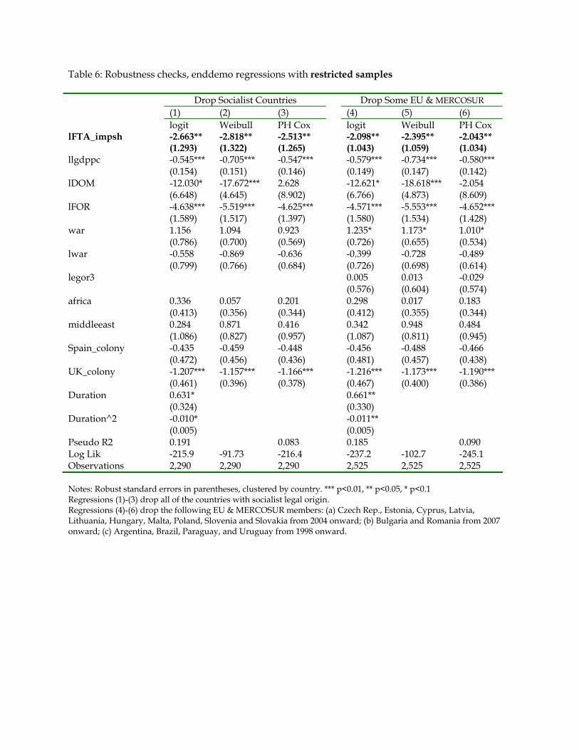
Table 6: Robustness checks, enddemo regressions with restricted samples Drop Socialist Countries Drop Some EU & MERCOSUR (1) (2) (3) (4) (5) (6) logit Weibull PH Cox logit Weibull PH Cox lFTA_impsh -2.663** -2.818** -2.513** -2.098** -2.395** -2.043** (1.293) (1.322) (1.265) (1.043) (1.059) (1.034) llgdppc -0.545*** -0.705*** -0.547*** -0.579*** -0.734*** -0.580*** (0.154) (0.151) (0.146) (0.149) (0.147) (0.142) lDOM -12.030* -17.672*** 2.628 -12.621* -18.618*** -2.054 (6.648) (4.645) (8.902) (6.766) (4.873) (8.609) lFOR -4.638*** -5.519*** -4.625*** -4.571*** -5.553*** -4.652*** (1.589) (1.517) (1.397) (1.580) (1.534) (1.428) war 1.156 1.094 0.923 1.235* 1.173* 1.010* (0.786) (0.700) (0.569) (0.726) (0.655) (0.534) lwar -0.558 -0.869 -0.636 -0.399 -0.728 -0.489 (0.799) (0.766) (0.684) (0.726) (0.698) (0.614) legor3 0.005 0.013 -0.029 (0.576) (0.604) (0.574) africa 0.336 0.057 0.201 0.298 0.017 0.183 (0.413) (0.356) (0.344) (0.412) (0.355) (0.344) middleeast 0.284 0.871 0.416 0.342 0.948 0.484 (1.086) (0.827) (0.957) (1.087) (0.811) (0.945) Spain_colony -0.435 -0.459 -0.448 -0.456 -0.488 -0.466 (0.472) (0.456) (0.436) (0.481) (0.457) (0.438) UK_colony -1.207*** -1.157*** -1.166*** -1.216*** -1.173*** -1.190*** (0.461) (0.396) (0.378) (0.467) (0.400) (0.386) Duration 0.631* 0.661** (0.324) (0.330) Duration^2 -0.010* -0.011** (0.005) (0.005) Pseudo R2 0.191 0.083 0.185 0.090 Log Lik -215.9 -91.73 -216.4 -237.2 -102.7 -245.1 Observations 2,290 2,290 2,290 2,525 2,525 2,525 Notes: Robust standard errors in parentheses, clustered by country. *** p<0.01, ** p<0.05, * p<0.1 Regressions (1)-(3) drop all of the countries with socialist legal origin. Regressions (4)-(6) drop the following EU & MERCOSUR members: (a) Czech Rep., Estonia, Cyprus, Latvia, Lithuania, Hungary, Malta, Poland, Slovenia and Slovakia from 2004 onward; (b) Bulgaria and Romania from 2007 onward; (c) Argentina, Brazil, Paraguay, and Uruguay from 1998 onward.

Table 7: Robustness check, enddemo regressions with estimated weight on social welfare (1/b) Enddemo based on Polity “tta” based on Cheibub et al. (1) (2) (3) (4) (5) (6) logit Weibull PH Cox logit Weibull PH Cox lFTA_impsh -4.800** -4.944* -4.396** -5.947** -6.076** -4.805** (2.148) (2.953) (2.083) (2.481) (2.429) (2.285) llgdppc -0.748** -0.882*** -0.688*** -0.214 -0.301 -0.304 (0.323) (0.318) (0.253) (0.338) (0.307) (0.286) lDOM -7.316 -8.910** 15.807 -3.614** -2.580 -2.165 (8.436) (4.058) (0.000) (1.811) (1.589) (1.490) lFOR -8.076*** -7.514*** -7.510*** -2.473 -3.485 -2.177 (2.854) (2.462) (2.042) (1.510) (2.620) (2.345) war 2.266* 1.654 0.724 1.169 1.471 1.444 (1.360) (1.020) (0.485) (1.139) (1.077) (0.993) lwar -1.458 -1.481 -0.115 -0.817 -0.531 -0.361 (1.157) (0.976) (0.567) (1.006) (0.918) (0.899) legor3 -17.045*** -43.033 -13.393*** -38.979*** (0.908) (0.000) (1.199) (1.048) africa 18.797*** 18.706*** 24.462 -13.858*** -39.183*** (2.082) (6.094) (0.000) (1.453) (1.403) Spain_colony -0.776 -0.409 -0.625 0.098 -0.454 -0.562 (0.707) (0.612) (0.585) (0.608) (0.599) (0.666) UK_colony -19.221*** -20.126*** -25.016*** -2.144* -2.977*** -2.419** (1.829) (5.900) (0.585) (1.205) (1.130) (1.032) Duration 0.545 0.203*** (0.379) (0.059) Duration^2 -0.009* -0.003** (0.005) (0.001) 1/b -0.026 0.013 -0.009 -0.036 -0.124 -0.061 (0.037) (0.052) (0.042) (0.062) (0.114) (0.094) Country RE Yes Yes Pseudo R2 0.301 0.274 0.190 0.235 Log Lik -80.58 -33.49 -55.67 -91.61 -26.83 -40.10 Observations 1,279 1,348 1,348 1,165 1,192 1,192 Notes: Robust standard errors in parentheses, clustered by country. *** p<0.01, ** p<0.05, * p<0.1. 1/b is the weight on social welfare relative to special interests estimated by Gawande et al. (2010).

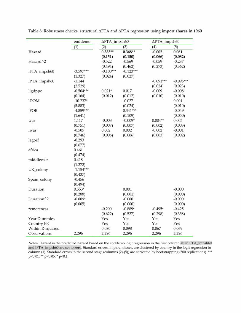
Table 8: Robustness checks, structural ΔFTA and ΔPTA regression using import shares in 1960 enddemo ΔFTA_impsh60 ΔPTA_impsh60 (1) (2) (3) (4) (5) Hazard 0.333** 0.368** -0.002 0.061 (0.151) (0.150) (0.066) (0.082) Hazard^2 -0.522 -0.569 -0.059 -0.237 (0.494) (0.462) (0.273) (0.362) lFTA_impsh60 -3.597*** -0.100*** -0.123*** (1.327) (0.024) (0.027) lPTA_impsh60 -1.144 -0.091*** -0.095*** (2.529) (0.024) (0.023) llgdppc -0.504*** 0.021* 0.017 -0.009 -0.008 (0.164) (0.012) (0.012) (0.010) (0.010) lDOM -10.237* -0.027 0.004 (5.883) (0.024) (0.010) lFOR -4.859*** 0.341*** -0.049 (1.641) (0.109) (0.050) war 1.117 -0.008 -0.009* 0.004** 0.003 (0.751) (0.007) (0.007) (0.002) (0.003) lwar -0.505 0.002 0.002 -0.002 -0.001 (0.746) (0.006) (0.006) (0.003) (0.002) legor3 -0.293 (0.677) africa 0.461 (0.474) middleeast 0.418 (1.272) UK_colony -1.154*** (0.437) Spain_colony -0.456 (0.494) Duration 0.553* 0.001 -0.000 (0.288) (0.001) (0.000) Duration^2 -0.009* -0.000 -0.000 (0.005) (0.000) (0.000) remoteness -0.200 -0.889* -0.495* -0.425 (0.622) (0.527) (0.298) (0.358) Year Dummies Yes Yes Yes Yes Country FE Yes Yes Yes Yes Within R-squared 0.080 0.098 0.067 0.069 Observations 2,296 2,296 2,296 2,296 2,296 Notes: Hazard is the predicted hazard based on the enddemo logit regression in the first column after lFTA_impsh60 and lPTA_impsh60 are set to zero. Standard errors, in parentheses, are clustered by country in the logit regression in column (1). Standard errors in the second stage (columns (2)-(5)) are corrected by bootstrapping (500 replications). *** p<0.01, ** p<0.05, * p<0.1

Table 9: Robustness checks, structural ΔFTA regression with additional controls (1) (2) (3) ΔFTA_impsh ΔFTA_impsh ΔFTA_impsh Hazard 0.422*** 0.424** 0.442** (0.157) (0.165) (0.177) Hazard^2 -0.806 -0.912 -0.887 (0.538) (0.591) (0.586) lFTA_impsh -0.143*** -0.144*** -0.149*** (0.017) (0.018) (0.018) llgdppc 0.009 0.009 0.010 (0.010) (0.010) (0.010) war -0.009 -0.007 -0.008 (0.009) (0.009) (0.010) lwar 0.002 0.001 0.003 (0.007) (0.007) (0.007) remoteness -0.698 -0.696 -0.833 (0.637) (0.588) (0.601) lreg_change -0.014** (0.007) var(Polity)_10yr -0.000 (0.000) lpolcomp 0.002 (0.001) Year dummies Yes Yes Yes Country FE Yes Yes Yes Within R-squared 0.124 0.123 0.129 Observations 2,603 2,603 2,541 Notes: Hazard is the predicted hazard based on the enddemo logit regression in the first column in Table 3A. Standard errors are corrected by bootstrapping (500 replications). *** p<0.01, ** p<0.05, * p<0.1. lreg_change is a dummy indicating if a country’s polity score changes sign from non-positive to strictly positive in our sample used for the enddemo logit regression in the first column in Table 3A, lagged by one year. var(Polity)_10yr is the variance of polity scores during the last 10 years. lpolcomp measures the degree of general political competition in a country, as defined in Polity IV, lagged by one year.

Table 10: endogeneity of FTAimpsh in enddemo regressions, 2SLS IV = Contagion

weighted by log(dist) IV = Contagion

weighted by log(GDP)/log(dist)

IV = Contagion weighted by GDP/dist

(1) (2) (3) (4) (5) (6) 1st stage

lFTA_impsh 2nd stage enddemo

1st stage lFTA_impsh

2nd stage enddemo

1st stage lFTA_impsh

2nd stage enddemo

lFTA_impsh -0.280** -0.531** -1.095*** (0.115) (0.234) (0.339) llgdppc 0.010 -0.058*** 0.025 -0.046** 0.027 -0.021 (0.041) (0.015) (0.044) (0.019) (0.042) (0.025) lDOM 0.031 0.084** 0.053 0.111** 0.100 0.174** (0.131) (0.042) (0.134) (0.051) (0.124) (0.068) lFOR 0.092 -0.158** 0.280* -0.039 0.295 0.228 (0.159) (0.068) (0.154) (0.119) (0.187) (0.170) war 0.035* 0.038* 0.035* 0.047** 0.033 0.065** (0.021) (0.020) (0.020) (0.023) (0.021) (0.030) lwar 0.000 -0.023 -0.002 -0.025 -0.006 -0.029 (0.014) (0.019) (0.015) (0.021) (0.015) (0.027) Duration 0.001 0.004*** 0.001 0.005*** 0.000 0.005*** (0.004) (0.001) (0.004) (0.001) (0.003) (0.002) Duration^2 0.000 0.000 0.000 0.000 0.000 0.000** (0.000) (0.000) (0.000) (0.000) (0.000) (0.000) lcontagion_ldist 74.764*** (19.755) lcontagion_lgdpldist 0.458** (0.186) lcontagion_gdpdist 0.371* (0.208) Country FE Yes Yes Yes Yes Yes Yes Partial R2 0.034 0.010 0.008 F Statistics for IV 88.60 24.85 19.97 R-squared 0.374 -0.035 0.357 -0.228 0.357 -1.079 Observations 2,603 2,601 2,603 2,601 2,603 2,601 Notes: Standard errors are in parentheses. *** p<0.01, ** p<0.05, * p<0.1. In regressions (1)-(2), the instrument (IV) used for FTA_impsh of a country is the average FTAimpsh of all other countries (ROW) weighted by log(distance), after excluding this country’s own FTA imports from FTAimpsh. In regressions (3)-(4), the instrument (IV) used for FTA_impsh of a country is the average FTAimpsh of all other countries (ROW) weighted by log(GDP)/log(distance), after excluding this country’s own FTA imports from FTAimpsh. In regressions (5)-(6), the instrument (IV) used for FTA_impsh of a country is the average FTAimpsh of all other countries (ROW) weighted by GDP/distance, after excluding this country’s own FTA imports from FTAimpsh. All of these IVs are lagged by one year.