FOG Freiberg Online Geology FOG is an electronic journal registered under ISSN 1434-7512

2008, VOL 19

Seasonal changes in the arsenic distribution of newly drilled wells tapping different aquifers in the Bangladesh delta

Joerg Steinborn

List of contents

LIST OF FIGURES IV

LIST OF TABLES VI

LIST OF APPENDICES VI

LIST OF ABBREVIATIONS VII

ABSTRACT 1

1. OBJECTIVES AND DELIVERABLES 2

1.1. OBJECTIVES 2 1.2. DELIVERABLES 3

2. BANGLADESH – A GENERAL INTRODUCTION TO THE GEOGENIC ARSENIC CONTAMINATION 4

3. DESCRIPTION OF THE INVESTIGATION AREA 13

3.1. STUDY AREA - SELECTION CRITERIA AND SPECIFICS 13 3.2. VEGETATION AND LAND USE 14 3.3. CLIMATE 15 3.4. GEOLOGY 16 3.4.1. GEOLOGY AND GEOMORPHOLOGY 16 3.4.2. GEOLOGICAL EVOLUTION OF THE BENGAL BASIN 18 3.4.3. LITHOLOGICAL UNITS – STRATIGRAPHY 20 3.4.4. HYDROGEOLOGY 22 3.5. HYDROGEOCHEMISTRY 24

4. METHODOLOGY 26

4.1. FIELD ACTIVITIES 26 4.1.1. CORE DRILLING AND TEST FIELD SETUP 26 4.1.2. MONITORING 29 4.1.2.1. Electrochemical parameters 30 4.1.2.2. Photometry 32 4.1.2.3. Sample preservation 34 4.1.2.4. Mapping 35 4.2. LABORATORY 36 4.2.1. DOC/ TIC 36 4.2.2. IC – CATIONS 37 4.2.3. IC – ANIONS 37 4.2.4. IC – ICP – MS 38 4.3. REMOTE SENSING 39 4.3.1. TNTATLAS – IMPORTANT TOOLS 41

List of contents

5. RESULTS AND DISCUSSION 42

5.1. DIGITAL ATLAS 42 5.1.1. GROUPS AND LAYERS 42 5.1.2. LEGENDS OF THE LAYERS 44 5.2. HYDROGEOCHEMISTRY 47 5.2.1. DATA EVALUATION 47 5.2.1.1. Charge imbalance by PhreeqC 47 5.2.1.2. Measured vs. Calculated Specific Conductance after ROSSUM (1975) 49 5.2.1.3. As/P totals vs. sum of As/P species 51 5.2.2. SPATIAL DISTRIBUTION 53 5.2.3 DEPTH DEPENDENT HYDROCHEMICAL CHANGES 63 5.2.4 SEASONAL HYDROCHEMICAL CHANGES 74

6. RECOMMENDATIONS 82

7. ACKNOWLEDGEMENTS 84

8. REFERENCES 85

9. APPENDIX 89

List of figures

- IV -

List of figures

Fig.2.1. Distribution of As in groundwater from shallow tube wells in Bangladesh 5

Fig.2.2. (a) Arsenite and (b) arsenate speciation as a function of pH 7

Fig.2.3. Eh-pH diagram for aqueous As species in the system As-O2-H2O at 25°C 8

Fig.2.4. Eh/pe-pH diagram for aqueous P species 10

Fig.3.1.1. BGS“special study areas”(left); Satellite Image from study area (right) 13

Fig.3.3.1. Climate chart for Comilla district, Bangladesh 15

Fig.3.4.1.1. Main geomorphologic units of Bangladesh 17

Fig.3.4.2.1. Surrounding regions of the Bengal Basin 18

Fig.3.4.2.2. Tectonic elements of the GBM delta system 19

Fig.3.4.3.1. Drilling profile 21

Fig.3.4.4.1. Hydrogeological cross section from Bangladesh’s North to South 23

Fig.4.1.1.1. Overview of well configuration at the test field 27

Fig.4.1.1.2. Well construction by the local „hand flapping“ method 28

Fig.4.1.2.1. Sampling procedure for village wells 29

Fig.5.2.1.1.1. Calculated charge imbalances for (a) mapped wells and (b)

monitoring wells 48

Fig.5.2.1.2.1. Comparison of measured conductivity with calculated conductivity 50

Fig.5.2.1.3.1. Phosphorus (a) and arsenic (b) in comparison to sum of species 52

Fig.5.2.2.1. Distribution of (a) total arsenic and (b) total phosphorus vs. depth 54

Fig.5.2.2.2a. Contour line plots for As(tot), P(tot), As(III), As(V) 55

Fig.5.2.2.2b. Contour line plots for Eh, Fe(tot), Mn(tot), Phosphate 56

Fig.5.2.2.3. Piper diagram for groundwater characterisation 57

Fig.5.2.2.4. Ammonia vs. As(tot) as well as As(III) 58

Fig.5.2.2.5. As(tot) vs. P(tot), Fe(tot), Mn(tot), Eh, HCO3- and SO4 59

Fig.5.2.2.6. Comparison As(tot) for the (a) test field and (b) mapping against depth 61

Fig.5.2.2.7. Total arsenic (a) and total phosphorus (b) vs. well-age 62

Fig.5.2.3.1. Depth profile of the core drilling and the test field 64

Fig.5.2.3.2. Reduced grey sand vs. oxidised, brown sand 65

Fig.5.2.3.3. Vertical profile of hydrochemical mean characteristics at the test field 67

Fig.5.2.3.4. Total As vs. total phosphorus 68

Fig.5.2.3.5. Total phosphorus vs. NH4 69

List of figures

- V -

Fig.5.2.3.6. Total arsenic vs. SO4 70

Fig.5.2.3.7. Model of how arsenic pollution occurs in shallow wells 71

Fig.5.2.4.1. Mean monthly P and T over the last 10 years (1997 – 2006) in comparison

to the mean monthly precipitation and temperature during the period of investigation 74

Fig.5.2.4.2. Mean groundwater table in comparison to the daily rainfall 76

Fig.5.2.4.3. Seasonal changes of As(tot) in different depths of the test field 78

Fig.5.2.4.4. Seasonal changes of arsenite in different depths of the test field 80

List of tables – list of appendices

- VI -

List of tables

Table 4.1.2.4. Mapped household wells 35

Table 4.2.1.1. Device-specific attributes for TIC/DOC speciation 36

Table 4.2.2.1. Detection limits for cation analysis 37

Table 4.2.3.1. Detection limits for anion analysis 37

Table 5.2.1.2.1. Wells with charge imbalances > + 10 % 51

Table 5.2.4.1. Infiltration time of deposition according to HAZEN; 77

Table 5.2.4.2. Well by well correlation between total arsenic and total phosphorus 81

List of appendices

Appendix 1a: Comparison of measured conductivity and calculated conductivity 90

Appendix 1b: Mean percent error between measured and calculated conductance 92

Appendix 2a: Comparison of total arsenic with sum of arsenic species 92

Appendix 2b: Comparison of total phosphorus with sum of phosphorus species 93

Appendix 3: Dendrogram of the hierarchical cluster analysis – MAP 93

Appendix 4: Distribution of total phosphorus and P-species at mapping wells 94

Appendix 5: Dendrogram of the hierarchical cluster analysis – TF 95

Appendix 6: Piper diagram – major cations and anions at the monitoring wells 95

Appendix 7: Total arsenic vs. (a) total iron 96

Appendix 8: Averaged kf for the upper aquifer at the core drilling at hospital ground 96

Appendix 9: Seasonal changes of total phosphorus concentrations 97

Appendix 10a: Seasonal changes of EC in different depths (9 – 27 m) of the test field 97

Appendix 10b: Seasonal changes of EC in different depths (115 – 280 m) 98

List of abbreviations

- VII -

List of abbreviations

As Arsenic

As(III) Inorganic trivalent arsenic

As(V) Inorganic pentavalent arsenic

As(tot) Total arsenic

BGL Bangladesh

BGS British Geological Survey

DIC Dissolved inorganic carbon

DOC Dissolved organic carbon

DOM Dissolved organic matter

EC Conductance

Eh Redox potential

ETP Potential evaporation

ETR Evaporation

ETRTURC Evaporation adapted from TURC

BGM Ganges – Brahmaputra – Meghna

GIS Geographical information system

GPS Global Positioning System

IC-ICP-MS Ion chromatography-inductively coupled plasma mass spectrometry

ICP-MS Inductively coupled plasma mass spectrometry

MAP Mapping wells

OM Organic matter

PE Polyethylene

pH pH-value

R² R-square, coefficient of determination

SI Saturation Index

TC Total carbon

TF Test field

TIC Total inorganic carbon

TOC Total organic carbon

UTM Universe Transverse Mercator

WGS84 World Geodetic System 1984

List of abbreviations

- VIII -

WHO World Health Organisation

Wt% Weight in percent

XRD X-Ray diffraction

Abstract

- 1 -

Abstract

The study site is located at Comilla in the southeast of Bangladesh, where 60 % of the wells

exceed the World Health Organisation (WHO) guideline value for drinking water of 10 µg/L

of arsenic, and was chosen based on available nation-wide As surveys to span the entire

spectrum of As concentrations in Bangladesh’s groundwater. From February to July 2007, a

detailed hydrochemical monitoring was performed on 7 newly drilled monitoring wells

tapping the upper Holocene aquifer and the deeper Late-Pleistocene aquifer. The deliverables

from hydrochemistry were associated to sedimentological characteristics of the depth profile,

investigated within another master thesis. Additionally, depth and spatial dependent changes

in chemistry at 48 house and irrigation wells were determined once in the dry season and once

in the rainy season.

From the recent findings it can be concluded that highest arsenic concentrations in the

groundwater are associated with the grey reduced sediments from the upper aquifer (<300

µg/L), where reducing conditions forced the reduction and dissolution of FeOOH and thus the

subsequent release of sorbed arsenic into the groundwater. Maximum arsenic levels were

observed in depths between 12 and 36 m and increased with the onset of the monsoonal

rainfalls due to seasonal occurring stronger reducing conditions. Species analyses revealed

that arsenite was the dominant As-species (67 – 99 %) at almost all the wells, while arsenate

was detected in minor quantities. Remarkably high ammonium (up to 200 mg/L) and

phosphorus (up to 6 mg/L) concentrations in 36 m depth result from the degradation of peat

fragments observed within the depth profile. Further phosphorus is also released when

FeOOH is reductively dissolved. Sediments from the shallow aquifer were brown in colour

and indicate more likely oxidized conditions. In these sediments reduction is incomplete and

the resorption of As to residual FeOOH keeps the arsenic concentrations in the groundwater

below 70 µg/L. Dissolved Fe(II) is high at these layers (< 150 mg/).

Objectives and deliverables

- 2 -

1. Objectives and deliverables

Arsenic contaminates groundwater across southern, central and eastern Bangladesh as well as

the Indian region West Bengal. Groundwater from the Holocene alluvium of the Ganges,

Brahmaputra and Meghna Rivers (GBM) locally exceeds 200 times the World Health

Organisation (WHO) guideline value for drinking water of 10 µg/L of arsenic. Thus millions

of people in both Bangladesh and West Bengal are exposed to contaminated drinking water

supply, an enormous health risk. Symptoms like skin diseases, losses on blood vessels (Black

Foot Disease), skin pigmentation changes and cancer types of skin, lung, liver, and bladder

are typical evidences for arsenical poisoning. The aim of this study was to link the arsenic

distribution at the study site in Comilla District, Bangladesh, with the arsenic problem in

whole Bangladesh. Therefore the study was focused on spatial, seasonal, and depth dependent

hydrochemical changes within the studied area.

1.1. Objectives

The objects of the study were to:

• Collect information from previous projects, analysing and partly reinterpreting them

• Map all irrigation and house wells in the study area with well depth, water table,

year of installation as well as infrastructure (roads, bridges, schools, hospital, market

place, etc.) & land use

• Determine the depth and seasonal dependent changes in chemistry, especially for

redox-sensitive elements (Fe[II], total iron, NH4+, NO2

-, NO3-, total Mn, Mn[II], and

S2-) at the newly drilled test field considering the different lithologs from the test

field, the core drilling, and old drillings

• Determine the depth and spatial dependent changes in chemistry at 56 house and

irrigation wells in the dry season and at selected wells in the rainy season

• Determine correlations between arsenic and other trace elements

• Measure groundwater tables and interpret seasonal variations in correlation with rain

events considering rainfall data

Objectives and deliverables

- 3 -

• Determine associations between sediment properties (e.g., mineralogy, content of

organic matter, iron, manganese, and phosphorus) and arsenic concentrations in

groundwater.

1.2. Deliverables

Considering the main objectives given above, the major deliverables of this master thesis

were aimed to be:

• Presenting a single-layer digital atlas, based on a Quickbird satellite image,

combining the digitized features (e.g. house wells, irrigation wells), thematic layers

(e.g. roads, boundaries, rivers, infrastructure), a base map and hydrochemical data.

Different databases (e.g. locations and characteristics of the analyzed sites, on-site

and laboratory data on hydrochemistry, arsenic speciation) are attached to the digital

atlas.

• Comparing the recent hydrochemical findings with results from previous projects to

confirm the representativeness of the study site with regard to whole Bangladesh.

• Linking the arsenic concentrations in the groundwater with the associated

sedimentological characteristics of the depth profile.

• Contrasting changes in the arsenic distribution at different aquifers with seasonal

characteristics, such as irrigation in dry season, monsoon rains, etc.

Introduction

- 4 -

2. Bangladesh – a general introduction to the

geogenic arsenic contamination

Bangladesh and the Indian region West Bengal are located within the world’s largest delta,

formed by the Ganges-Brahmaputra-Meghna River System and are influenced by monsoonal

climate. Until the early 1970s the river water was widely used as drinking water.

Thenceforward drinking water supply was changed from pathogenic contaminated surface

water, which resulted in waterborne diseases such as cholera and dysentery that caused

millions of deaths, to groundwater from wells (RAVENSCROFT et al. 2004). From the early

seventies till nowadays more than six million hand pump tube wells, typically drilled to

between 20 and 70 m, were installed with the help of international organisations, such as the

UN (KINNIBURGH et al. 2003) and to provide clean water to the population without

thorough investigation of the quality of the groundwater.. Nowadays, over 90 % of drinking

and irrigation water is delivered from shallow wells.

One to two decades after changing to groundwater based drinking water supply, disease

patterns like skin diseases, losses on blood vessels (Black Foot Disease), skin pigmentation

changes and cancer types of skin, lung, liver, and bladder were detected, attendant symptoms

for arsenic poisoning. The delivered water from tube wells is seen as the reason for that.

Symptoms may take five to fifteen years or longer to develop (RAVENSCROFT et al. 2004).

Arsenic was first identified in the groundwater of West Bengal in 1983 (RAVENSCROFT et

al. 2004). This information was unknown in Bangladesh until the early 1990s

(RAVENSCROFT et al. 2004). The number of patients with typical symptoms for arsenic

poisoning has been estimated by a range between 5,000 and 200,000 in the West Bengal

region up to the year 2000 (SMITH et al., 2000). The number in Bangladesh is unknown but

must be multiple higher.

Nowadays it is assumed that more than 30 % of all wells exceed the Bangladesh drinking

water standard of 50 μg/L; 5 – 10 % of the wells exceed that limit by more than six times. So,

50 of the 64 districts of Bangladesh and 9 out of the total 18 districts in West Bengal have

drinking water wells above the local level. At least 30 – 35 million people in Bangladesh and

6 million people in West Bengal are assumed to be exposed to arsenic contaminated drinking

water at concentrations above 50 µg/L (SMEDLEY and KINNIBURGH, 2001).

Introduction

- 5 -

The World Health Organisation (WHO) recommended a guideline of 10 µg/L in 1993.

According to the WHO standards, more than 50 million people in Bangladesh are exposed to

contaminated water (Sharma et al. 2006). The worst affected area is in the southeast of

Bangladesh, where in some districts more than 90 % of the wells are affected (SMEDLEY

and KINNIBURGH, 2001) (see figure 2.1). Areas with arsenic concentrations exceeding

300 µg/L can be found in the lower catchment areas of the Ganges-Brahmaputra-Meghna

(GBM) system.

Fig. 2.1. Distribution of As in groundwater from shallow (<150 m) tubewells in Bangladesh (SMEDLEY and KINNIBURGH, 2001)

It has been shown, that especially Holocene alluvial aquifers of the Ganges-Brahmaputra-

Meghna River System are highly affected. Due to sea-level rise (from 18 Ka to 7 Ka BP) and

higher temperatures, the Holocene sediments are dark-grey, highly micaceous, unweathered

and organic matter is present at up to 6 % by weight (see 3.4.4). The affected aquifers are

generally shallow (less than 100 – 150 m deep) and in most affected areas, the aquifer

sediments are capped by a layer of clay or silt, which restricts exchange with the atmosphere,

and thus oxygen supply to the aquifers. In conjunction with organic matter, deposited with the

sediments, this phenomenon leads to reducing conditions and favours the mobilisation of As.

Introduction

- 6 -

Redox changes due to rapid burial of the alluvial and deltaic sediments included the reduction

of arsenic to As(III), desorption of As(V) from Fe oxides and reductive dissolution of the

oxides themselves. According to SMEDLEY and KINNBURGH (2001), high arsenic

concentrations in Bengal aquifers may be associated with:

• areas with relatively low rainfall and high evaporation or runoff, resulting in low

recharge;

• very low groundwater flow rates as a result of silts and fine sands within alluvial

floodplains and delta areas and an extremely small hydraulic gradient;

• low gradient-areas with flushing times over 200 ka per pore volume;

• areas of low flow like inside river meanders and in closed basins

Low arsenic concentrations are associated with:

• coarse sands in fluvial areas at the base of incised channels;

• medium porosity and high hydraulic conductivities;

• relatively rapid flushing of 2-10 ka per pore volume;

• high groundwater gradients;

Pleistocene aquifers, older alluvial sediments and deeper aquifers (> 150 m) can be seen to be

free of arsenic that is why they are preferred for irrigation and drinking water since a couple

of years. But there is the risk to suck arsenic contaminated groundwater into the deeper

aquifers as a result of excessive exploitation of deeper aquifers.

The transported and deposited sediments derived from the upland Himalayan catchments and

from basement complexes of the northern and western parts of West Bengal. Major

arseniciferous minerals are ore minerals and their alteration products which are relative rare in

natural environments. They are found in close relation with the transition minerals as well as

Cd, Pb, Ag, Au, Sb, P, W, and Mo.

Arsenic can occur in the environment in several oxidation states (-3, 0, +3 and +5)

(RAVENSCROFT et al., 2001). Organic arsenic is produced by biological activities but can

be neglected for groundwaters in the Bengal Basin because it is generally linked to industrial

pollution or partially reducing conditions in organic carbon rich zones (SEMDLEY and

KINNIBURGH, 2001). GAULT et al. (2004) found no evidence of significant concentrations

of thioarsenate species which can be an important form of dissolved arsenic in groundwaters

that contain moderate sulphide concentrations.

Introduction

- 7 -

In natural waters with pH typically between 6.5 and 8.5, arsenic appears usually in the

inorganic form as oxyanions of zero-charged trivalent arsenite (H3AsIIIO30) at reducing

conditions or negatively charged pentavalent arsenate (H2AsVO4- or HAsO4

2-) under oxidising

conditions (fig. 2.3). However, groundwaters with high concentrations of arsenic are

dominated by arsenite, ranging between 70 and 100 % (ZHENG et al., 2004), as it is regarded

as the most mobile form of arsenic.

The redox potential is a dominant factor for controlling the arsenic speciation and the arsenic

mobilisation into groundwater over a wide range of redox conditions. High arsenic

concentrations are always associated with reducing conditions. The mobility, toxicity and bio

availability is strongly regulated by the oxidation state of the arsenic complex. Arsenite seems

to be much more mobile and toxic than arsenate.

Following speciations are controlled as a ratio of pH and redox potential (fig. 2.2. and 2.3.):

• H2AsO4- is dominant at low pH (<6.9) and under oxidising conditions;

• HAsO42- becomes dominant under oxidising conditions but increasing pH;

• uncharged H3AsO40 at extremely acidic (pH<2.0) and AsO4

3- at extremely alkaline

conditions (pH >12) under oxidising conditions;

• uncharged H3AsO30 under reducing conditions at pH less than 9.2;

• H2AsO3- at pH > 9.2 and HAsO3

2- at about pH > 12;

Fig.2.2. Arsenite (a) and arsenate (b) speciation as a function of pH with an ionic strength of 0.01 M (SMEDLEY and KINNIBURGH, 2001)

Introduction

- 8 -

Fig. 2.3. Eh-pH diagram for aqueous As species in the system As-O2-H2O at 25°C and 1 bar total pressure; pH-values, typically for natural water are grey-shaded (SMEDLEY and KINNIBURGH, 2001)

Three main theories of arsenic mobilisation might explain the pollution of groundwater in the

Bengal Basin and have been confirmed in several studies (RAVENSCROFT et al., 2001;

RAVENSCROFT et al., 2004; SMEDLEY and KINNIBURGH, 2002):

I. Pyrite oxidation and irrigation drawdown

Oxidation of arsenic containing pyrite as a reason for arsenic contamination in Bangladesh

was rejected by several authors.

Arsenic has a high affinity to sulphide minerals, where Sulphur can be substituted in the

crystal structure. Arsenian Pyrite (Fe(S, As)2), Arsenopyrite (FeAsS), Realgar (AsS) and

Orpiment (As2S3) are important minerals resulting from such a substitution. Besides being

an important component of ore bodies, pyrite can be also formed in low temperature

sedimentary environments under reducing conditions and plays an important role in recent

geochemical cycles (SMEDLEY and KINNIBURGH, 2001). It can be found especially in

river sediments, lake and marine sediments. Pyrite is being primarily formed under

reducing conditions in conjunction with organic deposits. Soluble arsenic can be

incorporated in the crystal structure during the formation.

Introduction

- 9 -

The oxidation of pyrite is seen in relation with the drawdown of the water table as a result

of intensive irrigation. Oxygen can find its way into previously anoxic aquifer sediments.

Within aerobic systems, pyrite isn’t stable and oxidises to Fe oxides under formation of

Sulphate (SO4), acidity and trace constituents like arsenic. That is the cause for arsenic

problems and acidification of mine drainages around sulphide rich coal mines.

RAVENSCROFT et al. (2001) attempted to relate the distribution of arsenic

contamination to that of irrigation but they have not shown any relation to each other.

Another reasons for rejecting pyrite oxidation as a mechanism is based on the fact, that the

concentrations of arseniciferous pyrite at the sediments are too little to be important. Both

pyritic and organic sulphur has been detected in several studies (NICKSON et al., 2000;

AAN, 1999; J.M. MCARTHUR, unpublished; DPHE, 1999) with maximum contents less

than 0.3 %. Furthermore, the release of sulphate during the oxidation of pyrite should

correlate with the dissolved As. In reality, iron and sulphate are mutually exclusive in

solution (Ravenscroft et al. 2001; Kinniburgh and Smedley 2001). But the sulphate

concentration does not match with that of arsenic because arsenic concentration > 50 µg/L

occur only where sulphate concentrations are less than 30 mg/L. Lastly, shallow tube

wells (< 10 m) are most exposed to atmospheric oxygen and would be affected highest, if

arsenic would be originated from pyrite. But normally, the shallow wells are affected less.

In conclusion, pyrite is a sink, but not a source of arsenic (RAVENSCROFT et al., 2001).

II. Competitive exchange of phosphate from fertilizer

Phosphorus commonly occurs almost exclusively in the environment as fully oxidised

phosphate (primarily H2PO4− and HPO4

2−, where the oxidation state of phosphorus is +5)

[HANRAHAN et al., 2004]. Inorganic P can occur in the environment in five different

oxidation states (-3, 0, +1, +3 and +5), similar to arsenic. In the main, geogenic sources of

phosphorus are the minerals Apatite (magmatic), Phosphorite (sedimentary), and seaspray.

Additionally, the use of phosphate fertilizers in Bangladesh has been increased immensely

within the last 15 years because cropping was switched from one crop to three crops per

year. This lead to the assumption, that the arsenic contamination could be a result of

increased phosphate input at least in part.

The fertilizer phosphate displaces arsenic from FeOOH as a result of competitive anion

exchange (ACHARYYA et al., 2000), owed to the fact that both, arsenic and phosphorus,

form similar anionic complexes. For illustration see fig. 2.2. in comparison with fig. 2.4.:

Introduction

- 10 -

Fig. 2.4. Eh/pe-pH diagram for aqueous P species. For calculations involving equilibrium between reduced P species and phosphine (i.e., dashed lines including PH3), an equilibrium concentration of 10−6 M for the reduced P compound was assumed. (HANRAHAN et al., 2004)

Nevertheless, phosphorus as a displacement for Arsenic was rejected by several authors

(RAVENSCROFT et al., 2001; HANRAHAN et al., 2004; Acharyya et al., 2000). On the

one hand the use of phosphorus is ubiquitous but on the over hand amounts used are not

high in a worldwide comparison. According to RAVENSCROFT et al. (2001), there are

largely areas of Bangladesh, where groundwater is free of both arsenic and phosphorus.

But especially at these regions irrigation is most intense and also use of fertilizer is

highest. Based on this fact, any link between arsenic and fertilizer seems incoherent.

A study of MANNING and GOLDBERG (1996) has shown that phosphorus in a

concentration of 5 mg/L would desorb at most 2 µg/L of arsenic to mineral surfaces.

Another argument seems the content of uranium at phosphate fertilizers, used as a tracer

for fertilizer phosphate (RAVENSCROFT et al., 2001). But in Bangladesh concentrations

of uranium are high where concentrations of phosphorus are low to zero. Furthermore,

concentrations of uranium decrease in greater depth (no uranium was found in

depths > 41 m) whilst concentrations of phosphorus increase with depth.

Introduction

- 11 -

III. Reduction of arsenicrich hydrous iron oxides (FeOOH)

The third theory, known as the reduction of arsenicrich hydrous iron oxides hypothesis, is

now accepted as the principal mechanism of arsenic mobilization in the anoxic surface-

and groundwater of the alluvial aquifers in the Bengal Basin (e.g. AHMED et al., 2004;

RAVEBSCROFT et al., 2001; MCARTHUR et al., 2001, KINNIBURGH and

SMEDLEY, 2001). Microbial oxidation of organic carbon (concentrations may reach up

to 6 % in aquifer sediment) forms the basis of FeOOH reduction:

8FeOOH + CH3COOH + 14H2CO3 8Fe2+ + 16HCO3-+ 12 H2O

This process is accompanied by microbial reduction of arsenate [As(V)], which is strongly

sorbed onto iron hydroxides, to arsenite [As(III)], when anoxic conditions (Eh < 200 mV)

develop during sediment burial (NICKSON et al., 1998; NICKSON et al., 2000). This is

shown in the fact, that arsenic is present basically as arsenite (RAVENSCROFT et al.,

2001). The reduction of iron hydroxides is widespread and strong in organic rich and fine-

grained deltaic sediments, shown by high concentrations of dissolved iron up to 80 mg/L,

primarily present as Fe2+ (NICKSON et al., 2000). Due to the reduction process, arsenic-

rich hydrous iron oxides are dissolved and release both Fe2+ and the sorbed load of the

hydrous iron oxides, which includes arsenic. Arsenic accumulates as a result of an

extremely low regional hydraulic gradient that caused low flushing rates (KINNIBURGH

et al. 2003). High arsenic concentrations might be associated with high iron

concentrations. In addition, HCO3- ions are generated which explains the relationship

between arsenic and HCO3-. NICKSON et al. (2000) and various authors

(RAVENSCROFT et al., 2001; NICKSON et al., 1998; APPELO et al., 2002;

SAFFIULLAH, 1998) mentioned that in most cases poor correlations existing between

Fe2+ and As. Presumably, poor correlations could arise from re-precipitation of iron, re-

adsorption of arsenic onto fresh hydrous iron oxides (FeOOH) or precipitation of Fe2+ as

siderite FeCO3 (WELCH and LICO, 1998). Wells with high amounts of HCO3- and Fe2+

are oversaturated with siderite and slightly with calcite and dolomite.

The spatial distribution of phosphorus in tube wells corresponds to that of arsenic;

however the well by well correlation of arsenic and phosphorus is insignificant. This can

be explained by a shared diagenetic origin for both arsenic and phosphorus

(RAVENSCROFT et al., 2001). Moreover, both arsenic and phosphorus form anions that

sorbs strongly to hydrous iron oxides, even though phosphorus was rejected as a

Introduction

- 12 -

displacement for Arsenic by several authors (RAVENSCROFT et al., 2001;

HANRAHAN et al., 2004; ACHARYYA et al., 2000).

It seems to be obvious that high concentrations of arsenic occur in groundwater where

microbial reduction of FeOOH has released and reduced sorbed arsenic. Organic matter is

required as trigger, the so called redox driver (MCARTHUR et al., 2000). Therefore, the

distribution of organic matter (OM) in the aquifer sediments is the main control on the

distribution of arsenic contamination and may be present in several forms (RAVENSCROFT

et al., 2001):

• Concentrations of less than 0.5 % TOC (total organic carbon) are typical for

disseminated organic matter of the fluvial sands in the Bengal Basin (NICKSON et

al., 1998). During transport at receiving streams, organic matter is being reduced

before it gets incorporated into the sediment. After dissemination through the sands,

organic matter will be left cellulose rich and unfavourable for bacterial metabolism.

Disseminated organic matter at fluvial sands seems to be irrelevant in contribution to

FeOOH reduction. Higher concentrations of arsenic may occur where pyrite has

formed and scavenged arsenic from solution. But this theory can be mostly rejected

for Bangladesh, as aforementioned.

• Peat beds are common beneath the Old Meghna Estuarine Floodplain in Greater

Commilla, Sylhet, Gopalganj-Khulna Peat Basin, and the shallow aquifer system in

Lakshmipur (MCARTHUR et al., 2001). Peat has been found in Holocene sediments

and occurs extensively beneath arsenic contaminated areas (RAVENSCROFT et al.,

2001). Indicators for peaty sediments are increased concentrations for TOC (up to

8 %), biogenic methane and the presence of ammonium in wells in concentrations up

to 24 mg/L (DPHE, 2000; HOQUE, 1998). In addition, there is a strong correlation

between ammonium and phosphorus (MCARTHUR et al., 2001). According to

RAVENSCROFT et al., (2001) the spatial distribution of peat corresponds with that of

arsenic.

Investigation area

- 13 -

3. Description of the investigation area 3.1. Study area - selection criteria and specifics

The study area with an extent of approximately 10 sq km is located 50 km south-east of the

capital Dhaka at Titas, Daudkandi Upzilla, Comilla District (UTM WGS84, Zone 46N:

274000E 2613000N – 276000E 2609000N, Atlas Bangladesh 2007). The site at Titas,

Comilla was shortlisted along with the British Geological Survey “special study areas” named

Chapai Nawabganj (25 % of the wells > 50 μg/L As), Faridpur (41 % of the wells > 50 μg/L

As) and Lakshmipur (55 % of the wells >50 μg/L).

Figure 3.1.1. British Geological Survey “special study areas” (left); Satellite Image from the investigation area (right); modified according to KINNIBURGH and SMEDLEY (2001)

Finally, the site at Comilla has been chosen, because according to the “national guideline for

drinking water”, 65 % of all shallow wells at this area exceed the local drinking water

standard of 50 µg/L for arsenic. Field tests confirmed this; totals up to 420 µg/L were

detected. The area was selected, because of the high arsenic level, closeness to the Meghna

River and optimal logistic location due to its closeness to the capital.

First samplings of the shallow tube well at the health complex in November 2006 showed that

the groundwater chemistry at the test field has a low mineralization compared to the general

groundwater composition. The approximately 12 m deep well is labelled with sample code

Investigation area

- 14 -

BGL MAP 02 01. The water is almost pH-neutral (7.13), partially reductive (Eh: 84.3 mV),

has low dissolved oxygen (0.25 mV) and the conductivity was 255 µS/cm. Major cations are

Na+ (9.7 mg/L), K+ (2.2 mg/L), Ca2+ (27.9 mg/L), Mg2+ (8.2 mg/L) and NH4+ (0.4 mg/L). The

major anions are F- (0.2 mg/L), Cl- (11.7 mg/L) and PO43- (0.8 mg/L). TIC was measured with

26.58 mg/L and DOC with 0.69 mg/L.

The water can be defined as a Ca-HCO3 type because of the predominance of calcium and

TIC. Total arsenic is 76 µg/L and total phosphorus 817 µg/L.

3.2. Vegetation and land use

Bangladesh, with the world’s largest delta of the Ganges-Brahmaputra-Meghna River System

is influenced by monsoonal climate, which is favourable for agriculture. The proportion of

agricultural land use of total land area (147,570 sq) is highest in Bangladesh (around 70 %),

compared to South Asia in general (ALAUDDIN and QUIGGIN, 2007). Since 1950, the ratio

of agricultural land to total land was increasing and declined in the 1990’s, because the

extensive margin of cultivation may have been exhausted (ALAUDDIN and QUIGGIN,

2007). At present, agricultural areas have a size of 103,299 ha of which 88.9 % is arable crop.

The rising population (150 million), with an annual growth of 1.7 %, leads to the

intensification of farming by modifying farming techniques in order to increase food

production. The land person ratio is estimated at 0.12 ha per person. From between the early

1960’s irrigation has increased from rare usage to up to presently 56 % of total arable crop.

As a consequence of intensive dry season irrigation, a high degree of intensification of

agriculture has developed in Bangladesh, which allowed multiple cropping. Supplementary

use of chemical fertilizers increased with 84.7 kg of nutrients per ha of arable crop.

High yielding varieties of rice and wheat were introduced in the course of development.

Cultivation of arable crop is subdivided mainly in rice fields (approximately 67 %) and

secondarily wheat and field fruits e.g. corn, chilli, potatoes, etc.

Rivers are distributed with a surface ratio of approximately 6,400 sq km, stagnant waters

cover 4,245 sq km. Forests have an estimated surface of 19,610 sq km which is about 13.3

percent of the total land area of the country. Rural built-up areas, urban areas and

infrastructure extend over an area of approximately 16,100 sq km. Comilla is typical for

Bangladesh, approximately 64 % of the land is used for farming, 18 % for settling, and 18 %

are divided in rivers, stagnant waters and fallow.

Investigation area

- 15 -

3.3. Climate

Bangladesh has a tropical monsoon climate characterized by two main seasons, a dry season

from October to April and a rainy season from June to October (REIMANN, 1993). The

mean monthly minimum temperatures in January vary from 10 to 12 °C, from June to August

between 20 and 25°. The mean monthly maximum temperatures vary from 25 to 28 °C in

January to between 32 and 35 °C in June to August. Temperature and humidity increase

during March to May. The period between June to October is characterized by a hot and very

wet climate. Potential evapotranspiration rises from 70 to 90 mm in wintertime to about 180

mm from March to May. In monsoon time, evapotranspiration stabilises at between 115 and

145 mm and falling, with the end of the rainy season in November. Up to 85 % of the annual

rainfall occurs during the May to September monsoon. Approximately 10 % of the

precipitation occurs during the so called “Nor’Westers”, heavy rainfalls originated from the

Mediterranean and only 5 % of rainfall occurs during the five month dry season between

November and March. During this period, agriculture is not possible without irrigation. The

mean annual rainfall ranges between 1,250 mm in the western central region and 5,000 mm in

the north-east.

Jan Feb Mar Apr May Jun Jul Aug Sep Oct Nov Dec

mm

0

100

200

300

400

500

600°C

10

15

20

25

30

35

40Average rainfall in mm Average Temperature in °C (min)Average Temperature in °C (max)

Fig. 3.3.1. Climate chart for Comilla district, Bangladesh. Period of data collection ranges from 01/1994 to 12/ 2004, daily measured values. Station No.: CL356 (Longitude: 91.175; Latitude: 23.462) (Bangladesh Water Development Board (BWDB))

The annual temperature – precipitation distribution for the investigation area is presented in

figure 3.3.1.; the mean annual rainfall is of 1838 mm with a maximum of 480 mm in

June/July and a minimum in May.

Investigation area

- 16 -

3.4. Geology 3.4.1. Geology and geomorphology

Bangladesh, with a size of 147,570 sq km, is situated in the north-eastern corner of the Indian

subcontinent at the head of the Bay of Bengal. The Bengal Basin, which constitutes the major

part of Bangladesh and the adjoining part of West Bengal, is bordered by the Himalaya and an

uplifted block of Precambrian Shield (Shillong Plateau) to the north (AHMED et al., 2004), a

Precambrian basement complex (Indian Platform) to the west, and the Indo-Burman ranges to

the east (Morgan and McIntire 1959). More than 16 km thick synorogenic Cenozoic

sediments are deposited in the basin derived from the Himalayan and Indo-Burman ranges

(Uddin and Lundberg, 1998). According to AHMED et al. (2004), tertiary sediments in

Bangladesh mainly comprise sandstone and shale sequences, while Pleistocene sediments are

mostly represented by clay, overlain by Holocene alluvium.

The combined deltas of the Ganges, Brahmaputra and Meghna (GBM) river systems lie

within Bangladesh (SMEDLEY and KINNIBURGH, 2001). This complex river system can

be seen as the driving force for sediment transport and deposition. The source of the sediment

loads is glacial and periglacial weathered rock from the Himalaya. The sediment load includes

eroded ultramafic rocks from northern parts of the high Himalayas and granitic and high

grade metamorphic rock from central and southern parts, with quartz, biotite and feldspar as

characteristic minerals.

Sediments from lower altitudes derive from the Damodar and Dareeling coalfields (coals and

shales containing high amounts of pyrite), the Rajmahal Traps (basalts with pyrite) and the

Gangetic Plains (lateric materials). These sediments are eroded and transported by the GBM

system, crossing these areas.

According to SMELDLEY and KINNIBURGH (2001) a characteristic geomorphology has

developed as a consequence of a series of glacio-eustatic sea level cycles and long-term

tectonic activity. Bangladesh can be divided into two environments of sediment deposition:

the continental fluvial environment north of Ganges and lower Meghna and the southern

estuarine delta environment (fig. 3.4.1.1).

Investigation area

- 17 -

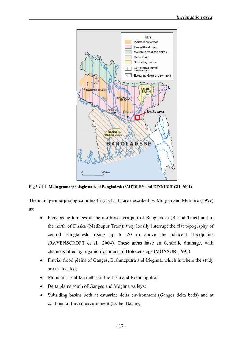
Fig 3.4.1.1. Main geomorphologic units of Bangladesh (SMEDLEY and KINNIBURGH, 2001)

The main geomorphological units (fig. 3.4.1.1) are described by Morgan and McIntire (1959)

as:

• Pleistocene terraces in the north-western part of Bangladesh (Barind Tract) and in

the north of Dhaka (Madhupur Tract); they locally interrupt the flat topography of

central Bangladesh, rising up to 20 m above the adjacent floodplains

(RAVENSCROFT et al., 2004). These areas have an dendritic drainage, with

channels filled by organic-rich muds of Holocene age (MONSUR, 1995)

• Fluvial flood plains of Ganges, Brahmaputra and Meghna, which is where the study

area is located;

• Mountain front fan deltas of the Tista and Brahmaputra;

• Delta plains south of Ganges and Meghna valleys;

• Subsiding basins both at estuarine delta environment (Ganges delta beds) and at

continental fluvial environment (Sylhet Basin);

Investigation area

- 18 -

3.4.2. Geological evolution of the Bengal Basin

The pre-Quaternary development of the Bengal Basin started in the Permo-Carboniferous,

but the significant processes are closely linked to tectonic activities in the Tertiary. Marine

sediments were filling the initially passive Bengal Basin during Cretaceous times

(SMELDLEY and KINNIBURGH, 2001). In Eocene times, the Indian plate collided with the

Burmese Plate, which resulted in the uplift of the Burmese Hills. Eroded sediments from the

Burmese hills were deposited in the Bengal Basin. After ALAM et al. (2002), the Bengal

Basin evolved from a passive continental margin in the pre-Oligocene to a separated ocean

basin at the beginning of the Miocene. The collision of the Indian Plate with the Burma and

Tibetan (Eurasian) Plates after the separation of the Indian Plate from the southern continent

of Gondwana resulted in a large settling rate into the Bengal Basin, south of the Himalayas

and west of the Burmese Hills. The erosional discharge of the Orogen yielded the

accumulation of 1–15 km thick clastic sediments in the Bengal foredeep.

Three geo-tectonic provinces developed (fig. 3.4.2.1): the Stable Shelf, a passive to

extensional cratonic margin in the west, the Central Deep Basin, a remnant ocean basin and

the Chittagong – Tripura Fold Belt.

Fig. 3.4.2.1. The Bengal Basin and surrounding regions in the Early Miocene. (1) The Stable Shelf; (2) The Central Deep Basin; (3) The Chittagong – Tripura Fold Belt (ALAM et al., 2002)

Investigation area

- 19 -

Tectonic activities along the Dauki Fault (fig. 3.4.2.1) during the Pliocene resulted in the

uplift of the Shillong Plateau and the subsidence of the Garo Rajmahal Gap. The formation of

the north-south trending Tripura Chittagong fold belt can be seen in connection with this

event. The Brahmaputra entered into the Bengal Basin diverted from the Shillong Hills in the

west to the eastern area of Sylhet (fig. 3.4.1.1). The current course of the Brahmaputra, a

north-south trending faulted trench, separates Barind and the Madhupur Tracts, two uplifted

and tilted blocks (fig 3.4.2.2).

Fig 3.4.2.2. Tectonic elements of the Ganges – Brahmaputra – Meghna delta system (SMEDLEY and KINNIBURGH, 2001)

The south-west to north-east striking Calcutta-Mymensingh Hinge Zone divides the Bengal

Basin in two crustal domains (SMEDLEY and KINNIBURGH, 2001). In the north of

Bangladesh the basement is formed by the Rangpur Platform and the Bogra Shelf beneath a

thin cover of Cretaceous to recent sediments (fig. 3.4.2.2).The areas south of the Hinge Zone

(Faridpur, Hatiya and Sylhet Troughs) are underlain by oceanic crust.

The Quaternary period is affected by approximately 120 ka of glacio-eustatic cycles

(SMEDLEY and KINNIBURGH, 2001), global climatic changes, the uplift of the Himalayas

and subsidence in the Bengal basin as a result of huge alluvial sedimentations

(RAVENSCROFT et al., 2003). Monsoonal circulations and thereby caused high rainfalls and

Investigation area

- 20 -

river flows were eliminated by Himalayan glaciations. The global sea level was at about 50 m

below its present level with a minimum peak of 130 m at 18 ka BP during the Pleistocene

(RAVENSCROFT et al., 2004). Consequently, the Ganges, Brahmaputra and Meghna carved

deeply into the sediment and left incised channels within a series of terraces. The recent

configuration of the Ganges Delta has mainly developed from a Holocene sea-level rise which

promoted a landward migration of the system (ALAM, 2003). The sedimentation rate was

high and subsidence rates of 1 to 4 mm per year with the maximum in the Sylhet Basin were

characteristic for Holocene times. The Pleistocene terraces are now largely buried by

Holocene floodplains. Maximum sedimentations on the submarine fan appeared during the

postglacial transgression between 12.8 and 9.7 ka BP.

3.4.3. Lithological units – Stratigraphy

The Quaternary in the Bengal Basin is subdivided into the following stratigraphical units,

described according to ALAM et al. (1990):

• The Late Pleistocene to Holocene forms major aquifers beneath recent floodplains

and is represented by the Chandina Formation as well as the Dhamrai Formation.

Maximum thickness is less than 150 m. Upward fining, grey micaceous, medium

and coarse sands to silt with organic mud and peat are characteristic;

• The Lower Pleistocene is represented by the Madhupur Clay and the Barind Clay

Formations, with a thickness of between 6 and 60 m. Red-brown to grey and silty

clay, residual deposits, kaolinite and iron oxides are characteristic. Frequently, the

Lower Pleistocene is absent beneath Holocene floodplains.

• The Plio-Pleistocene is represented by the Dihing Formation as well as the Dupi-

Tila Formation. Characteristically are unconsolidated yellowish-brown to light grey,

medium and coarse sands to clays, depleted in mica and organic matter. The Plio-

Pleistocene forms major aquifers beneath Holocene terraces and hills and deeper

aquifers beneath the Holocene floodplains. The maximum thickness may reach

values up to 6500 m.

Investigation area

- 21 -

Fig. 3.4.3.1. Drilling profile from a 259.0 m drilling at the Upazilla Health Complex Titas, Comilla

Investigation area

- 22 -

3.4.4. Hydrogeology

In the following, a generic summary of the hydrogeological situation in Bangladesh is

presented (taken from SMEDLEY and KINNIBURGH 2001).

Most data of Quaternary alluvial aquifers were raised during the 1980’s by internationally

funded irrigation projects.

Bangladesh’s topography, geology and hydrology are influenced by the three rivers Ganges,

Brahmaputra and Meghna (GBM) and the associated affluents, river branches and connecting

channels (REIMANN, 1993). Their deposits of unconsolidated Pleistocene and Holocene

alluvial sediments form one of the most productive aquifer systems in the world (SMEDLEY

and KINNIBURGH, 2001). Altogether, they have an estimated length of 24,000 km

(RASHID 1977). Floods, as a combination of annual monsoon rains, melt water from the

Himalayas and tidal-level increase in the Bay of Bengal fully recharge the aquifer system

each year. Supplementary to the summer monsoons, heavy rainfalls originated from the

Mediterranean (so called “Nor’Westers”) can appear in April and May (REIMANN, 1993).

Deeper aquifers are exploited within the coastal regions below shallow zones of saline water

intrusions. Freshwater may be also available from older, Tertiary strata in depths of 1,800 m

(JONES, 1985). According to UNICEF, large quantities of groundwater exist at shallow

depths. Nowadays, more than 95 % of drinking water supply in Bangladesh is abstracted from

shallow tube wells.

SMEDLEY and KINNIBURGH (2001) classified the main aquifers of Bangladesh as follows:

• Late Pleistocene to Holocene coarse sands, gravels and cobbles of the Tista and

Brahmaputra mega-fans and basal fan delta gravels along the incised Brahmaputra

channel. Due to sea-level rise (from 18 Ka to 7 Ka BP) and higher temperatures the

Holocene sediments are dark-grey, highly micaceous, unweathered and organic

matter is present at up to 6 % by weight (fig 3.4.4.1);

• braided-river coarse sands and gravels deposited along the incised palaeo-Ganges,

lower Brahmaputra and Meghna main channels from Late Pleistocene to Holocene

(fig 3.4.4.1);

Investigation area

- 23 -

• At depths > 150 m: stacked fluvial main channel medium to coarse sands from

Early to Middle Pleistocene, deposited in the Khulna, Noakhali, Jessore / Kushtia

and western moribund Ganges delta areas in the subsiding delta basin. Younger

Late Pleistocene to Holocene sand contains saline groundwater in coastal areas (fig

3.4.4.1);

• Red-brown medium to fine sands from Early to Middle Pleistocene underlie grey

Holocene medium to fine sands in the Old Brahmaputra and Chandina areas.

• Early to Middle Pleistocene coarse to fine fluvial sands of the Dupi Tila Formation

(tens to more than a hundred metres thick) underlie the Madhupur and Barind

Tracts, an important confined aquifer with low vertical and horizontal permeability

in north-west and north-central Bangladesh, capped by deposits of Madhupur Clay

Residuum. The Madhupur sediments, deposited during several pre-200 ka BP

glacio-eustatic cycles in former channels of Brahmaputra, have undergone several

periods of flushing and weathering resulting in the formation of red iron-oxide

cements and inter-bedded grey sticky clays. (fig 3.4.4.1)

Fig. 3.4.4.1. Hydrogeological cross section from Bangladesh’s North to South. Geological structures and groundwater flow patterns are shown. (SMEDLEY and KINNIBURGH 2001)

Investigation area

- 24 -

The headwaters of the Ganges, Brahmaputra and Meghna river system mainly drain parts of

the Himalayas and plains of India, Nepal and Tibet. Only 7.5 percent of the total catchment

area (1.5 million sq km) lies in Bangladesh. The average annual rainfall ranges between

300 mm in Nepal to 11,615 mm at Cherrapunji on the Meghalaya Plateau, India. The mean

annual rainfall in Bangladesh ranges between 1,250 mm in the western central region and

5,000 mm in the north-east.

Floods occur frequently during the period of monsoonal rainfalls, but the degree of flooding is

very variable. The expanse of total flooded land area in Bangladesh ranges between 2.1

percent (3149 sq km) in 1982 and 56.9 percent (82,000 sq km) in 1988.

3.5. Hydrogeochemistry

The chemistry of Bangladesh’s aquifers has been studied extensively during the last three

decades, after the dimension of the arsenic poisoning came to light (e.g. NICKSON et al.,

1998; NICKSON et al., 2000; MANNING and GOLDBERG, 1996; SMEDLEY and

KINNBURGH, 2001; SMEDLEY and KINNBURGH, 2002, AHMED et al., 2004). AHMED

et al. (2004) characterises Bangladesh’s groundwater chemistry and geochemical

characteristics of the aquifer sediments as follows:

The groundwater pH is generally near neutral to slightly alkaline (6.2 – 7.6). Dissolved

oxygen is less than 1 mg/L and Eh values range between 500 and – 400 mV, mildly oxidising

to strongly reducing conditions. Bangladesh’s groundwater’s are mostly from HCO3 and

Ca – Mg – HCO3 type, in exceptional cases from Ca – Na – HCO3 or Na – Cl type. The major

ion composition seems to be controlled by depth and lithology and is dominated by HCO3-

(ranging between 320 and 600 mg/L). Lower concentrations of SO42- (<3 mg/L) and NO3

-

(< 0.22 mg/L) are characteristic with a few exceptions. On the other hand, phosphate

concentrations are high with values of up to 8.75 mg/L. Major cations are distributed as

follows and show variations with depth: Ca (21 – 122 mg/L), Mg (14 – 41 mg/L), Na

(7 – 150 mg/L) and K (1.5 – 13.5 mg/L). Variabilities as a function of depth are reflected also

in concentrations of total As (2.5 – 846 µg/L), total iron (0.4 – 15.7 mg/L) and Mn (0.02 –

1.86 mg/L). The dominant arsenic species are represented by As(III) with a share between

67 and 99 % and, in some wells, As(V). Highest concentrations are usually in alluvial aquifers

of less than 150 m depth and levels of contamination reaches its maximum at depths between

10 and 50 m (HASAN et al., 2008).

Investigation area

- 25 -

Iron shows high correlations with HCO3- and PO4

3- but low with total arsenic, even though

this might have been expected. Ferrous iron precipitates as siderite (FeCO3), which shows a

positive SI of between 0.42 and 0.75. The SI values for calcite and dolomite are close to

equilibrium, which show that Bangladesh’s aquifers are not controlled by the dissolution of

the carbonates. Furthermore, high levels of HCO3- appear to correlate with the concentrations

of dissolved organic carbon (DOC = 1.15 – 14.2 mg/L) in groundwater. DOC concentrations

indicate trends of variation with both As(III) and total iron. Sources for high concentrations

might be organic matter in Holocene aquifers (see chapter 2).

Sulphate and Nitrate concentrations are near detection limit and there is no significant

correlation with arsenic. Microbial activities could turn into an increase of sulphide

(< 2 mg/L) and ammonia (< 13.2 mg/L). At elevated ammonia concentrations, high

concentrations of As(III) were also detected.

The following hydrogeochemical investigations have been conducted in the Comilla district

before:

• HASAN et al. (2008) investigated shallow alluvial aquifers in Daudkandi Upzilla up

to a depth of 25 m. Water samples were taken for later hydrochemical

determinations at laboratory. Sediment-samples were taken for later geochemical

and mineralogical investigations. The results show, that the upper part of the aquifer

(< 6.5 m depth) is distinguished by low dissolved concentrations of As, Fe and

HCO3- but relatively high Mn, SO4

2- and NO3- concentrations. The lower part of the

aquifer is high in As (>10 µg/L) coupled with high Fe and HCO3-. Manganese is low

as well as SO42- and NO3

-.

• ZAHID et al., (2007) did investigations at shallow (25-33 m) and deep (191-318 m)

tube-wells at the south-east of Bangladesh (Kachua Upazilla), near the investigation

area. The groundwater was divided in two groundwater-types: the Na–Cl type and

the Na–Ca–Mg–HCO3 type. The major ion trends are Na+ > Ca2+ > Mg2+ > K+ and

Cl– > HCO3– > SO4

2–. The As concentration was detected as 140–585 µg/l down to

33 m depth of upper aquifer in Kachua area, whereas moderate values were detected

at the 2nd and 3rd aquifer(< 1– 44 µg/l) .

Methodology

- 26 -

4. Methodology 4.1. Field activities

The study area is located in Titas, Daudkandi Upzilla, Comilla District and was selected on

the basis of an initial screening undertaken in November 2006 (see 3.1). Field activities

undertaken as part of this study comprise an intrusive investigation and subsequent

monitoring along with a survey on household and irrigation wells in the study area.

Field activities were undertaken between February, 9th and July, 31st 2007. Cores were used

to acquire stratigraphical information and to retrieve undisturbed samples for further detailed

classification and sorption tests in laboratory setups (LISSNER, 2008). Stratigraphical

information acquired from the cores was used to decide on specific installation designs of the

monitoring wells. Following the installation of the monitoring wells, water level and

hydrochemical monitoring was undertaken to observe seasonal changes, as explained in

section 4.1.2.

Parallel to the monitoring programme, the information was gathered for household and

irrigation wells in the area in order to determine the spatial distribution of hydrogeochemical

parameters to be presented in a digital atlas. A description of mapping programme is

presented in the section 4.1.2.4. Lab analysis conducted in Germany and Canada on the

collected samples is described in chapter 4.2.

4.1.1. Core drilling and test field setup

Core drilling was performed by rotary drilling and cable percussion to a final depth of 84 m.

Drilling fluid was a bentonite-water mixture. Drilling equipment and handling was arranged

by a local company. The drilling was stratigraphically logged and core samples were taken in

2” and 4” PVC liners. Altogether, 37 samples were taken and sealed immediately after

extraction with paraffin wax. Samples of broken liners or unconsolidated material that was

not retained in the liner were refilled in bags. In an on site glove bag the samples were divided

in subsamples and packed in nitrogen filled polyethylene bags to avoid contact with the

atmosphere. Sediment classification and laboratory sorption tests with the collected material

were performed within another master thesis (LISSNER, 2008). The core drilling was used

Methodology

- 27 -

for sampling and stratigraphically logging only. After achieving the final depth, the borehole

was sealed and abandoned.

On the basis of the stratigraphic information obtained the layout of the future test field was

developed. The approximately 20 m long and 5 m wide test field was set up in approximately

55 m distance to the core drilling, where seven individual sampling wells were installed at a

depth of 9 m (30 ft), 15 m (50 ft), 21 m (70 ft), 26 m (85 ft), 27 m (90 ft), 35 m (115 ft), and

85 m (280 ft) (fig. 4.1.1.1.). Test well BGL TF 90 was drilled to a depth of approx. 40 m in

the hope to catch a supposed sand-layer. However, that was not the case, so the bore hole was

screened in a depth of 27 m and the lower part was sealed by a solid pipe. The boreholes were

not cored, but the sediment slurry was sampled continuously to observe changes in

stratigraphy.

An individual sampling code was given to each monitoring well in order to differentiate the

single wells and measuring days. The following format was adapted: BGL- (stands for

Bangladesh), TF- (stands for test field) and a number reflecting the depth in feet. The single

measuring days are characterised by a consecutive number. For example the first monitoring

at the 30 ft well is identified by the sample code BGL TF 30 01. In the following the

monitoring wells will be labelled by these sample code.

Fig. 4.1.1.1. The monitoring wells TF 30, TF 50, TF 70, TF 85 and TF 90 tapping the upper aquifer. TF 115 is sunken in a sand layer lens immediately below the major upper aquifer and TF 280 is sunken in the lower aquifer. Scale independent diagram

Methodology

- 28 -

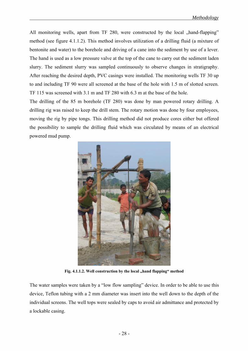
All monitoring wells, apart from TF 280, were constructed by the local „hand-flapping”

method (see figure 4.1.1.2). This method involves utilization of a drilling fluid (a mixture of

bentonite and water) to the borehole and driving of a cane into the sediment by use of a lever.

The hand is used as a low pressure valve at the top of the cane to carry out the sediment laden

slurry. The sediment slurry was sampled continuously to observe changes in stratigraphy.

After reaching the desired depth, PVC casings were installed. The monitoring wells TF 30 up

to and including TF 90 were all screened at the base of the hole with 1.5 m of slotted screen.

TF 115 was screened with 3.1 m and TF 280 with 6.3 m at the base of the hole.

The drilling of the 85 m borehole (TF 280) was done by man powered rotary drilling. A

drilling rig was raised to keep the drill stem. The rotary motion was done by four employees,

moving the rig by pipe tongs. This drilling method did not produce cores either but offered

the possibility to sample the drilling fluid which was circulated by means of an electrical

powered mud pump.

Fig. 4.1.1.2. Well construction by the local „hand flapping“ method

The water samples were taken by a “low flow sampling” device. In order to be able to use this

device, Teflon tubing with a 2 mm diameter was insert into the well down to the depth of the

individual screens. The well tops were sealed by caps to avoid air admittance and protected by

a lockable casing.

Methodology

- 29 -

4.1.2. Monitoring

Altogether, 196 groundwater samples were taken: 140 (7 wells x 20 campaigns plus several

replicates of the same sample for quality control) samples at the test field and 56 of both

village and irrigation wells. Where possible, water table was measured using a light indicator.

Samples were taken by low flow pumping, using a portable, battery-powered aspirated

Ismatec pump (fig. 4.1.2.1). Irrigation wells were sampled by the farmer’s mobile diesel

powered irrigation pumps. Village wells were sampled without any exception by the so-called

Hand-pump No.5. Since the commonly installed “hand pump No. 5” is a piston pump and

thus a sealed system, it was not possible to lower a Teflon tube into the well without

removing the entire hand pump. Therefore, a bucket was used as connector (fig. 4.1.2.1).

Before sampling, the well was pumped for at least 15 minutes, giving flow rates of 1000 to

3000 ml/min to that amount to the purging of approximately three to five volumes of the well.

However, due to the construction of a piston rod hand-pump a complete exclusion of water-air

contact is not given.

Fig. 4.1.2.1. Sampling procedure for village wells by connection of a bucket (to avoid oxygen contamination and to connect the Hand-pump NO.5 with the transportable pump)

For sampling, water was continuously delivered to the bucket by hand pumping. Continuous

overflow guaranteed exclusion of atmospheric oxygen to a certain extend. The sample was

sucked by the peristaltic pump from the bottom of the bucket.

Methodology

- 30 -

Redox-sensitive parameters and chemical species were measured at the sampling site.

Temperature, pH, Eh, conductivity and dissolved O2 generally were determined in a flow-

through cell. Between the flow-through cell and the battery-powered pump, an interconnected

T-distribution piece allowed taking water samples at the same time. Water samples were

taken for onsite photometry and laboratory analyses. Alkalinity and acidity were determined

by titration with NaOH and HCl in the field.

4.1.2.1. Electrochemical parameters

The onsite parameters such as pH, dissolved oxygen, conductivity, redox potential and

temperature were measured by electrodes in a flow through cell. The flow through-cell and

the electrodes were rinsed by the first litre of sample water over a period of about 10 minutes.

Thereafter, the flow-through cell was refilled under continuous circulation of sample water

and values were taken in time steps of 5, 10, 20, 30, 40 and 50 min.

The pH was measured with a combination SenTix 97/T pH electrode with integrated

temperature probe. The displaying measurement instrument was a Hach HQ40d Multi Meter,

which was used simultaneously for oxygen. For pH measurement a two point calibration with

pH 4 and pH 7 buffer solutions was performed at least once a day. The pH values of the study

area were close to neutral, ranging between 6.20 and 7.50. Upon completion of

measurements, the probe was secured in a KCl filled protecting cap.

Dissolved oxygen was determined with a HACH HQ40d Multi Meter (luminescent based

oxygen sensor with an integrated temperature probe). The displaying measurement instrument

was, as aforementioned a Hach HQ40d Multi Meter, which was used simultaneously for the

pH measurement. The sensor came pre-calibrated from HACH. There was no option for user-

defined calibration. Concentrations for oxygen were indicated in percent as well as mg/L.

The redox potential (Eh) was determined as EMF (in mV) with an Ag/AgCl Pt 4805/S7

probe on the WTW MultiLine P4. Values for EMF ranged approximately between -150 and

200 mV. The EMF values were drifting strongly at the beginning of the measurement; if there

was a slight difference between the 40 minutes and 50 minutes values in mV, equilibrium was

accepted. Upon completion of measurement, the probe was regenerated and protected by a

Methodology

- 31 -

KCl filled protecting cap. The following calculation was used to convert the EMF value to the

Eh value:

[ ] )98.2247443.0()( +°•−+= CetemperaturmeasuredEMFEh (eq.1)

The conductivity was determined with a TetraCon 325 conductivity cell with integrated

temperature probe on the WTW MultiLine P4. The equilibration was reached after about

10 minutes. The values at the different wells ranged between 100 and 3200 µS/cm. A direct

calibration of the conductivity-probe wasn’t possible, but the accuracy was checked by testing

a normalised 0.01 mol/L KCl standard solution (0.01 mol/L =1413 µS/cm). If there was a

significant deviation, the possibility was given to adapt the cell constant (c) at the WTW

MultiLine P4.

As aforementioned, water temperature was determined with three probes: the SenTix 97/T

pH electrode, the HACH HQ20 luminescent dissolved oxygen sensor, and the TetraCon 325

conductivity cell. The three measurement instruments showed similar values with deviations

less than 0.1 °C. Thus, a mean temperature was calculated from the three determinations.

The titration of inorganic carbon species (CO2, HCO3-) was done directly at the field site.

Alkalinity (KS 4.3) was determined with 0.1 N HCl and acidity (KB 8,2) with 0.1 N NaOH

using a digital titrator HACH Acidity Test Kit, Model AC-DT. The pH was monitored with

the afore mentioned SenTix 97/T pH electrode with integrated temperature probe. From the

consumption of acid or base, alkalinity and acidity can be calculated by the following

formula:

SS

VcVK •

= (eq.2)

SB

VcVK •

= (eq. 3)

V = volume of added HCl or NaOH in mL c = concentration of HCl or NaOH in mol/L VS = sample volume

Methodology

- 32 -

The volume of consumed acid or base was displayed in rotation units and can be converted by

the following formula in millilitre:

1000800••=

SVN

rotations

V (eq. 4)

N = normality of acid or base

4.1.2.2. Photometry

The redoxsensitive elements Fe2+, Mn2+, NO3-, NO2

-, NH3-, and S2- were analyzed in the field

by photometry to avoid both chemical and microbial oxidation during storage. Total iron and

manganese were also determined on-site. The photometer used in the field was a HACH

DR/890 Colorimeter. Before measuring, the photometry vials were first rinsed with distilled

water and afterwards rinsed two times with filtered sample water. All samples were filtered by

hand, using the Membrex 25 CA filter stacked on top of a PE-syringe (25 ml and 100 ml).

Cellulose Acetate filters with a pore size of 0.2 µm were used and replaced for each sample.

Total iron was determined with method 8008 with a detection range of between 0.03 and

3.00 mg/L. The standard deviation for this method is + 0.017 mg/L. The FerroVer reagent

reacts with all dissolved iron species in the sample to form soluble Fe(II). The Fe(II) reacts

with the 1,10-Phenantrolin-Indicator in the reagent to an orange-coloured complex. Sample

water was used as blank value; the required sample quantity was 10 ml. Concentrations in the

study area ranged between lower than detection limit and 150 mg/l, so that dilution was

necessary. Interferences may appear at high levels of Cl- (> 185,000 mg/L), Mg (> 100,000

mg/L) and S2-.

Method 8146 was used for determining Fe(II) with a detection range of between 0.03 and

3.00 mg/L. The standard deviation for this method is + 0.017 mg/L. The 1,10 Phenanthroline-

indicator interacts with the Fe(II) in the sample and forming an orange coloured complex.

Sample water was used as blank value; the required sample quantity was 25 ml.

Concentrations in the study area ranged between the lower than detection limit and 150 mg/L.

Dilution was necessary.

Methodology

- 33 -

Fe(III) was determined by subtracting Fe(II) from Total Iron.

Total manganese was determined by method 8149 with a detection range of 0.020 and

0.700 mg/L. The standard deviation for this method is + 0.013 using a standard solution with

0.5 mg/L total manganese. An ascorbic acid reagent is used initially to reduce all oxidised

forms of manganese to Mn2+. An alkaline-cyanide reagent is added to mask any potential

interference. PAN-indicator is then added to combine with the Mn2+ to form an orange-colour

complex. Distilled water was used as blank; the required sample quantity was 25 ml.

Concentrations in the study area ranged between the lower detection limit and less than 1

mg/L. Interferences can appear at high levels of aluminium (> 20.0 mg/L), copper

(> 50 mg/L) and iron (> 5 mg/L).

Mn (II) was determined by a self-modified method 8149 with assuming the same detection

limit of between 0.020 and 0.700 mg/L and standard deviation of + 0.013. The fundamental

idea is to skip the ascorbic acid reagent, which reduces all oxidised forms of manganese to

Mn2+ and determining originally present Mn2+ directly by adding the alkaline-cyanide reagent

and the PAN Indicator. As a matter of fact, values with this method were less than values for

total manganese. However, the method was not tested with standardized Mn2+-solutions, yet.

Medium concentrations of Nitrate were determined by method 8171with a detection limit of

0.2 and 5.0 mg/L. The standard deviation for this method is + 0.1 mg/L using a standard

solution of 3.0 mg/L NO3--N. Cadmium metal (NitraVer 5) reduces nitrate present in the

sample to nitrite. The nitrite ion reacts in an acidic medium with sulfanilic acid to form an

intermediate diazonium salt, which couples to gentisic acid to form an amber-coloured

product. Sample water was used as blank; the required sample quantity was 10 ml. Interfering

substances can be ferric ions, chloride, and nitrite. Concentrations in the study area ranged

between lower than detection limit and less than 2 mg/L.

Low concentrations of Nitrite were determined by method 8507 with a detection limit of

between 0.005 and 0.350 mg/L. The standard deviation for this method is + 0.001 mg/L using

a standard solution of 0.250 mg/L nitrite nitrogen. Nitrite in the sample reacts with sulfanilic

acid (NitriVer3 Nitrite Reagent Powder Pillows) to form an intermediate diazonium salt. This

couples with chromotropic acid to produce a pink coloured complex directly proportional to

the amount of nitrite present. Sample water was used as blank; the required sample quantity

Methodology

- 34 -

was 10 ml. Interfering substances can be ferric ions, ferrous ions and nitrate. Concentrations

in the study area ranged between lower than detection limit and less than 0.200 mg/L.

Ammonia (as NH4+-N) was determined by method 8155 with a detection limit of between

0.02 and 0.5 mg/L. The standard deviation for this method is + 0.02 mg/L using a standard

solution of 0.40 mg/L ammonia nitrogen. Ammonia compounds combine with chlorine to

form monochloramine. Monochloramine reacts with salicylate to form 5-aminosalicylate. The

5-aminosalicylate is oxidised in the presence of a sodium nitroprusside catalyst to form a

blue-coloured compound. The blue colour is masked by the yellow colour from the excess

reagent present to give a final green-coloured solution. Distilled water was used as blank; the

required sample quantity was 10 ml. Interfering substances can be iron (all levels), nitrate

(> 100 mg/L), calcium (>1000 mg/L as CaCO3) and nitrite (> 12 mg/L). Concentrations in the

study area ranged between the lower detection limit and above 150 mg/L. Dilution was

necessary.

Method 8131 was used for determining Sulphide (S2-) with a detection limit between

0.01 and 0.70 mg/L. The standard deviation for this method is + 0.02 mg/L using a standard

solution of 0.73 mg/L sulphide. Hydrogen sulphide and acid-soluble metal sulphides react

(sulphide reagent 1) with N, N-dimethyl-p-phenylenediamine oxalate (sulphide reagent 2) to

form methylene blue. The intensity of the blue colour is proportional to the sulphide

concentration. Distilled water was used as blank; the required sample quantity was 25 ml.

Concentrations in the study area ranged between the lower detection limit and less than

0.10 mg/L.

4.1.2.3. Sample preservation

For later analyses at the laboratory, water samples were taken for speciation, totals, major

cations and anions. All samples were filtered manually using the Membrex 25 CA filter

Holder stacked on top of a syringe (25 ml and 100 ml). Cellulose Acetate filter with a pore

size of 0.2 µm were used and replaced for each sample. Before collecting the water samples,

the new bottles were rinsed with filtered sample water twice, to avoid contaminations. For

quality check, triplicates were taken at different wells at intervals of 3 weeks.

Below, all used bottle types are listed, stating bottle size, material, preservation, intended use

and the analyzing laboratory:

Methodology

- 35 -

• 50 ml PE bottle, no preservation IC (cations, anions; Freiberg)

• 100 ml glass bottle, no preservation TIC / DOC (Freiberg)

• 50 ml PE bottle, 500 µL 1:1 HNO3 ICP-MS (totals; Trent)

• 60 ml HDPE bottle, 500 µL 1:1 HCl IC-ICP-MS (As+P-species; Trent)

4.1.2.4. Mapping

Mapping as a basis for the digital atlas was done beside the periodical monitoring work at the

test field. In an initial inspection, the size of the mapping area was set to approximately

10 km². For orientation, distinctive waypoints such as market-places, bridges, main buildings,

transmitters and factory-buildings were located by GPS (Garmin eTrex). Land use and

infrastructure were mapped by walking along roads, side roads, footpaths and rivers, using the

tracking function of GARMIN handhold GPS.

The next step was to map all irrigation and domestic wells with information such as position,

well depth, water-table, year of installation, owner, pipe casing, and use. Hydrochemical

information such as arsenic or iron concentration were registered when known by the owner.

It was not possible to read depth to groundwater at domestic wells, because the pumps are a

closed system. The same problem occurred with irrigation wells when pumping. Sulphide

concentrations were measured with on-site photometry when the well water had a rotten egg

smell, which is an indication of elevated concentrations. Altogether, 202 domestic and 161

irrigation wells have been mapped within investigation area.

Table 4.1.2.4. Mapped household wells were selected for sampling. Selection criterion was, to sample wells of different depths and ages. The table shows the selection of sampled well

< 30 ft 30 - 50 ft 50 - 60 ft 60 - 70 ft 70 - 80 ft 80 - 100 ft 100 - 120 ft > 120 ft < 1 a - MAP43 - - MAP06 MAP05 MAP42 -

1 - 5 a - MAP30 MAP27 - MAP41/14 MAP01 - MAP03 5 - 10 a MAP26 MAP31/12 - MAP04/07 MAP29 - - -

10 - 15 a MAP13 MAP44 MAP15 MAP47 MAP46 - - - 15 - 20 a - - - MAP45 - - - -

> 20 a - - MAP28 MAP25 - - - -

Based on the information, 26 domestic wells from different depths and ages were sampled in

the dry season and analysed for the complete chemistry program (Table 4.1.2.4.1). Wells with

increased arsenic concentrations were re-sampled during the rainy season. Irrigation wells

Methodology

- 36 -

were sampled, where pumps were in operation. Altogether, 22 irrigation wells were sampled

during the dry season; fields were flooded during the rainy season so that resampling was

impossible.

The chemistry program was the same as described in former chapters (see chapters 4.1.2.1;

4.1.2.2; 4.1.2.3). Redox-sensitive parameters and chemical species were measured at the

sampling site. Temperature, pH, Eh, conductivity, and dissolved O2 generally were

determined in a flow-through cell. Water samples were taken for on-site photometry and

laboratory analyses. Alkalinity and acidity were determined by titration.

To distinguish between samples from monitoring and mapping, an individual sampling code

was given to each well from the mapping campaign in order to differentiate the single wells.

The following format was adapted: BGL- (stands for Bangladesh), MAP- (stands for

mapping) and a consecutive number, starting with 01. Repetitive measurements are

characterised by the second number, with a maximum of 02. For example sampling at the first

well investigated during the mapping campaign is identified by the sample code BGL MAP

01 01.

4.2. Laboratory 4.2.1. DOC/ TIC

For the determination of total inorganic carbon (TIC) and dissolved organic carbon (DOC),

filtered samples were sent in 100 ml glass bottles to Freiberg University, Germany without

preservation. Speciation was done by the liquiTOC (elementar Analysensysteme GmbH) with

a detection limit of between 0.1 and 5000 mgCorg/L and a standard deviation of + 0.05

mgCorg/L. Device-specific attributes are described in the following table:

Table 4.2.1.1. Device-specific attributes for TIC/DOC speciation

Device: "liquiTOC" (Elementar Analysensysteme GmbH) IR - channels: IR 1: 2.4 ml sample; detection limit: 0 - 49 mg Corg/L IR 2: 5.0 ml sample; detection limit: 50 - 300 mg Corg/L IR 3: 10.0 ml sample; detection limit: > 300 mg Corg/L calibration: TIC: sodium carbonate DOC: potassium hydrogen phalate detector: UV detector carrier gas: oxygen with 3 bar

Methodology

- 37 -

4.2.2. IC – cations

The concentrations of the major cations Lithium, Potassium, Sodium, Ammonia, Calcium,

and Magnesium were determined by ion chromatography (IC). Therefore, filtered samples

were sent in 50 ml PE bottles to Freiberg University, Germany without preservation. The ion

chromatograph in use was a Merck HITACHI system model 6000A L5025, equipped with a

RT 125-4.6-column. The detector was a Merck HITACHI L3720 Conductivity detector. No

suppressor column was in use. The eluent was 2 mM HNO3 + 0.9 mM Dipicolinacid + 0.75

mM Crown Ether with a flow rate of 1.0 ml/min. In case of high cation concentrations,

samples were analyzed at different dilutions. The detection limits for the cations are shown at

table 4.2.2.1:

Table 4.2.2.1. Detection limits for cation analysis

Lithium Potassium Sodium Ammonia Calcium Magnesium

detection limit: 0.05 mg/L 0.4 mg/L 0.1 mg/L 0.2 mg/L 0.3 mg/L 0.3 mg/L

4.2.3. IC – anions

The concentrations of the major anions Chloride, Bromide, Nitrate, Fluoride, Phosphate and

Sulphate were determined by ion chromatography (IC). Therefore, filtered samples were sent

in 50 ml PE bottles to Freiberg University, Germany without preservation. The ion

chromatograph in use was an Eppendorf Biotronic IC 2001, equipped with a FGC II AN-P

separation column and pre-column. The suppressor column was an Eppendorf Biotronic FGC

1 AG P. Detector was a conductivity detector with a range of 100 µS/cm. The eluent was

1.8 mmol/L Na2CO3 + 0.6 mmol/L NaHCO3 with a flow rate of 1.5 ml/min. In case of high

anion concentrations, samples were analyzed at different dilutions. The detection limits for

the anions are shown at table 4.2.3.1:

Table 4.2.3.1. Detection limits for anion analysis

Chloride Bromide Nitrate Fluoride Phosphate Sulfate

detection limit: 0.1 mg/L 0.2 mg/L 0.3 mg/L 0.05 mg/L 1.0 mg/L 0.3 mg/L

Methodology

- 38 -

4.2.4. IC – ICP – MS

For arsenic and phosphorous speciation, acidified samples were sent off to Trent University,

Peterborough, Canada. Speciation was done by anion-exchange chromatography (Dionex,

Sunnyvale, CA, column: IonPac AS-16) coupled to inductively coupled plasma mass-

spectrometry (Elan®DRC® II, PerkinElmer, Shelton, CT) using a strongly alkaline eluent

(0.1 M NaOH) to preserve potentially occurring thioarsenate species. Simultaneous ICP-MS

on-line detection of arsenic (as AsO+, m/z = 91), phosphorous (as PO+, m/z = 47), and sulphur

(as SO+, m/z = 48) in eluting compounds was accomplished using the dynamic reaction cell

(DRC®) technology with O2 as reaction gas as described previously (Planer-Friedrich et al.

2007). Species identification was achieved by retention time match with commercial

standards. Arsenite, arsenate, and phosphate were quantified using standard solutions made

from solids (NaAsO2, J.T.Baker, Phillipsburg, NJ; Na2HAsO4, Sigma-Aldrich, Oakville, ON;

NH4H2PO4, SCP Science, Bale d´Urfé, QC). Due to the lack of a commercial standard,

monothioarsenate was identified via retention time match with a synthesized

monothioarsenate standard (Wallschläger and Stadey 2007) and routinely quantified using the

arsenate calibration curve. A new phosphorous species was detected with a retention time of

approximately 185 s that neither matched the retention times of a phosphite standard

(Na2(PHO3) ⋅5H2O, Riedel-de-Haen. Seelze, Germany; retention time 260 s) nor exactly that

of a hypophosphite standard (H2NaO2P⋅H2O, Sigma-Aldrich, Oakville, ON; retention time

175-180 s), even though it was close to the latter. Until further identification it is referred to as

“unknown P-species” in the following. Its quantification is based on the hypophosphite

calibration curve.

Arsenic and phosphorous total concentrations were determined independently from the sum of

species by ICP-MS. Correction via an internal rhodium standard (RhCl3⋅H2O, SCP Science,

Bale d´Urfé, QC) was applied in case of longer analytical runs to compensate for instrument

sensitivity drift. An analytical reference material (TM-DWS, Environment Canada, National

Water Research Institute) was included in each run as standard check.

Methodology

- 39 -

4.3. Remote sensing

The Digital Atlas „Atlas Bangladesh 2007“ is based on the results of hydrogeological and

hydrogeochemical field works at Titas, Daudkandi Upzilla, Comilla District, Chittagong

Division, Bangladesh. The period of data acquisition was between February 2007 and July

2007 (see chapter 4.1.2.4).

Presentation of the spatial data was done with the GIS software TNTmips, version 2005:71

(MicroImages Inc.). This program includes TNTaltlas, free viewing software, which allows

the visualization of the digital atlas.

To generate the digital atlas, it was first necessary to import the Satellite Image (QuickBird,

ID 1010010005888203, Acquisition Date 20070320, 60 cm 4-band PSM RGBI). The image

comprises an area of 5000 * 5000 m and has a ground resolution of 60cm. The image was

already georeferenced, so no further refurbishment was necessary. The four channels were

combined for true colour displaying. Based on the satellite image, the percentage of land use

was determined by a supervised, semiautomatic classification in off-shade mode. The land use

areas were summarised in fallow, houses-congested areas, sand- and water surfaces, and

farmland. Based on a field survey, land use areas were identified and marked by taking GPS

coordinates (located by GPS [Garmin eTrex]). These coordinates were read out with Garmin

Map Source software, version 6.13.4, and were imported as reference points into TNTmips.

The next step was to import further coordinates into TNTmips, divided in:

• House wells – labelled as HW in field site and marked as red dots in the atlas;

• Irrigation wells – labelled as IRR in field site and marked as blue squares in the atlas;

• Monitoring wells – labelled as TF in field site and marked as green dots in the atlas;

• Infrastructure – marked by individual symbols;

• Roads, Hydrogeology – taken by GPS in tracking mode with a dot spacing of 25 m

These coordinates were imported as vector objects, standardised to the Universal Transverse

Mercator System (UTM) Zone 46 North CM93E. Assigned to these vector points, additional

tables with information such as well-age, owner, use, features, hydrochemistry, etc. were

imported as databases. From these tables, three groups for hydrochemistry were created:

Chemistry HW, Chemistry IRR and Chemistry TF. Within these three groups, different

notations were chosen to illustrate hydrochemical features, based on the internal feature

Methodology

- 40 -

tables. TIC/DOC, major anions, major cations, total arsenic/phosphorus, and their species

were displayed as pie charts and bar charts, respectively. Therefore, a SML-script was written,

defining size, shape, colours and graphic rendition for all charts. Additionally, the

concentrations are printed next to the charts, also based on a SML-script. Conductivity, redox-

potential, and dissolved oxygen are displayed as bubbles, size and colour depending on the

represented concentration: small size with blue colour for low concentrations, medium size

with green colour for moderate concentrations, and big size with red colour for high

concentrations.

The spatial distribution for each TIC/DOC, total As/P, arsenate, arsenite, phosphate, iron,

manganese, and ammonia is shown by contour lines, plotted with Golden Software Surfer 8.

Therefore, the coordinates as well as the associated hydrochemical values were imported to

the internal excel-table in Surfer. Only wells from depths ranging between 12 m and 25 m,

assumed to show the highest effects, were considered. The next step was to create the grid

with a lattice spacing of 5 mm per cell with Kriging as gridding method. The grids were

exported as grd-files; contour lines were exported as mif-files. Colouring was made in

TNTmips, choosing red colour for high values and blue for low values. These raw data were

imported separately to TNTmips and regrouped for each element. Those wells, characterising

the grid, are shown as a vector layer, divided in house wells (HW), irrigation wells (IRR) with

known depths, and irrigations wells (IRR) with unknown depths. Supplementary, those wells

with depths lower than 25 m and less than 12 m are presented by size depending pie charts for

corresponding elements, based on a SML-script.

Methodology

- 41 -

4.3.1. TNTatlas – important tools

Viewing tools

Different viewing tools are available within TNTatlas. TNTatlas is a free software product

from MicroImages for viewing hierarchical atlases prepared in TNTmips with HyperIndex

Linker, or for single-layout atlases. The available atlas is a single-layout.

Redraw: use after selecting a new layer to refresh the view

Full Zoom: to revert from detailed view to general view

Previous View: restore previous view and zoom

Zoom In: enlarge view

Zoom Out: reduce view

Zoom Box: default viewing setting; by holding the left mouse button, a rectangle can be

drawn in the region of interest; right mouse button confirms selection

Working tools

Geo Toolbox: opens an additional window including working tools for measuring

lengths, areas or to get point information. Therefore, different geometric types like arcs,

polygons etc. are available. Sketches can be drawn.

Select: single vector objects can be chosen by this tool. Click the vector of interest by the

left mouse button, go to the associated group and layer and select a feature table. A red dot

will mark the selected point information.

Clicking on groups or layers by right mouse button provides several functions

Results and discussion

- 42 -

5. Results and discussion 5.1. Digital Atlas

The “Digital Maps” layout contains a 5km x 5km Quickbird RGBI Satellite Photo and a

georeferenced base map to give an overview about the location. Moreover, detailed

information including land use, infrastructure and water supply by irrigation and village wells

are given in further layers. Different chart types and contour line-plots present the

hydrogeochemical situation at the investigation area and give a spatial and depth dependent

summary for groundwater components like anions, cations, redox sensitive elements and field

parameters as well as arsenic and phosphorus. These features and additional data are included

in tables belonging to the vector objects.

In addition to the data acquisition as the general basis of the digital atlas, a weekly monitoring

was done on seven wells within the established test field. A major purpose of the digital atlas

was thus to provide background information to relate observations from the test field to a

larger context and interpret them considering the overall spatial distribution of

hydrogeochemical parameters. The digital atlas should be considered as a snapshot of the

whole arsenic problem at one of the most highly affected regions in Bangladesh. TNTmips

version 2005:71 provides the basis for the digital atlas.

5.1.1. Groups and layers

The digital atlas is subdivided in several thematic groups that are further separated in different

layers. Altogether these twenty groups can be abstracted into three thematic categories: the

hydrogeochemistry of sampling points for mapping, the spatial distribution of selected

chemical elements, and some basis cartographic information comprising of topography, land

use and infrastructure. All layers were georeferenced by the Universal Transverse Mercator

(UTM) Zone 46 North CM93E. Below the groups are described in the order of the digital

atlas from top to bottom. Navigation is described in chapters 4.3.1 and 4.3.2.

Groups and layers are divided in:

Results and discussion

- 43 -

Chemistry HW: contains eleven vector layers with hydrogeochemical features for the

mapped house wells (HW) which were sampled between February and April. The layers

represent from top down total arsenic, total phosphorus, arsenic species, phosphorus species,

total inorganic carbon (TIC) and dissolved organic carbon (DOC), Eh, oxygen, conductivity,

pH, and temperature, cations (Li+, Na+, NH4+, K+, Mn+, Ca2+, Mg2+) and anions (F-, Cl-, NO2

-,

NO3-, PO4

3-, SO42-). The totals are presented in bar charts. Species, carbon, cations, and

anions are displayed in pie charts and the on site parameters represented as different coloured

and sized pins (see 5.1.4).

Chemistry IRR: contains eleven vector layers (see chemistry HW) for the mapped irrigation

wells, which were sampled between February and April.

Chemistry TF: contains eleven vector layers (see chemistry HW) for the monitoring wells at

the test field. Wells in test field were sampled in regular intervals of about one week over a

period of six month. The Chemistry TF group displays chemical data from middle of March,

to get contemporary and comparable data to the house wells (HW) and irrigation wells (IRR).

WHO/EPA: The three layers show drinking water standards for arsenic, manganese and iron

by different coloured and sized pins. As the layer name implies, the standards are derived

from the World Health Organisation (WHO) for arsenic (10 µg/L) and manganese (0.4 mg/L)

and the Environmental Protection Agency (EPA) for iron. The second value represents the

local limit for arsenic in Bangladesh.

As(tot) vs. P(tot): In these two layers, pie charts reflect relative concentrations for arsenic

and phosphorus by bubble size.

ISO: The ISO groups display the spatial distribution of selected hydrogeochemical

compounds in the investigation area. Each group is composed of four layers. Wells with

depths between 12 m and 25 m are shown as a black/with contour line map and coloured

contour line plots that can be activated independently. Shallow (<12 m) or deep (>25 m) wells

are highlighted by pie charts, bubble size reflects relative concentrations for each element.

The digital atlas contains eleven ISO groups for total arsenic, arsenate, arsenite, total

phosphorus, unidentified phosphorus, phosphate, total iron, divalent iron, trivalent iron, total

manganese, TIC, DOC, and ammonia.

Results and discussion

- 44 -

Sampling points for mapping: contains three vector layers with all wells mapped in the

investigation area. HW displays all house wells, IRR all irrigation wells and TF refers to the

newly tapped monitoring wells at the test field. The coordinates were determined by GPS. In

addition, feature tables give information about age, depth, finishing, use, and owner, if the

information was available. Wells, which were analysed for their complete chemistry (see the

chemistry groups) are labelled by the sample code MAP.

Topography, land use and, infrastructure: The raster layer “Satellite Image” (QuickBird,

ID 1010010005888203, Acquisition Date 20070320, 60 cm 4-band PSM RGBI) with a

ground resolution of 60cm serves as the general basis of the digital atlas. The raster layer

“Land use” is based on the satellite image and was edited by a supervised, semiautomatic

classification. The vector layer infrastructure is based on field measurements. Roads and

hydrogeology were georeferenced in TNTmips.

5.1.2. Legends of the Layers

For the most part, the layers of the atlas Bangladesh 2007 are self-explanatory by legends and

symbols. In some layers, a legend was not possible due to limited functions of TNTmips. In

the following, these layers will be explained, starting from the top to bottom.

• Each individual ISO group comprises the same kind of layers, exemplified by the

group ISO As(tot), containing ISO wells, an contour line plot and a black/white

contour layer. These layers are self-explanatory by legends. The layer

Arsenic(total) in shallow (<12 m) and or deep (>25 m) wells comprises pie charts

for arsenic in shallow or deep wells. The higher the arsenic concentration, the bigger

the pie charts. Additionally, the single pie-charts are labelled with the associated

well depth.

Results and discussion

- 45 -

• The layer As(tot) vs. P(tot) compares total

arsenic concentrations in µg/L to total

phosphorus in µg/L. For both arsenic and

phosphorus, amount dependent pie charts were

chosen, based on a SML-script. The pie-chart for

arsenic is yellow-coloured, that for phosphorus

again is pink coloured.

• The TNT atlas contains three chemistry groups: Chemistry HW, Chemistry IRR and

Chemistry TF. Each chemistry group comprises the same kind of layers,

exemplified by the group Chemistry IRR, containing layers for total arsenic, total

phosphorus, arsenic species, phosphorus species, TIC/DOC, Eh, dissolved oxygen,

conductivity, pH, and temperature, major cations and major anions. Apart from the

layers for Eh in mV, Oxygen in mV and Conductance in µS/cm, each layer is based

on a SML-script, which excludes an internal legend. In the following, these layers

will be explained, starting from the top to bottom:

o The layer Anions contains pie-

charts for all major anions.

Colouring for each element was

chosen as follows: (sulphate),

(chloride), (phosphate),

(nitrate), (bromide) and

(fluoride). Concentrations are

listed at the right site;

o The layer Cations contains pie-

charts for major cations. Colouring

for each element was chosen as

follows: (calcium), (sodium),

(magnesium), (potassium),

(Fe[III]), (manganese),

(ammonia), (Fe[II]), and

(lithium). Concentrations are listed at the right site;

Results and discussion

- 46 -

o The layer TIC/DOC contains pie-

charts for main total inorganic carbon

and dissolved organic carbon.

Colouring was chosen as follows:

(TIC) and (DOC). Values are

given at the right site;

o The layer Phosphorus species

contains pie-charts, divided in

phosphate and unidentified

phosphorus species. Colouring

was chosen as follows:

(phosphate) and

(unidentified P). Concentrations are plotted at the right site in µg/L.

o The layer Arsenic species

contains pie-charts. Colouring

was chosen as follows:

(arsenite), (arsenite)

and (Monothioarsenate).

Concentrations are given at the

right site in µg/L.

o Within the layers P(tot) and As(tot),

concentrations for total phosphorus

and total arsenic are shown as bar-

graphs. The bar-graph for phosphorus

is coloured red, that for arsenic is light

green. Additionally, concentrations are

plotted at the right site of each chart. If

both layers are activated, As and P can

be compared with each other.

Results and discussion

- 47 -

5.2. Hydrogeochemistry 5.2.1. Data evaluation

During the field activities, 7 sampling sites were investigated at the test field, another 48 in

the surrounding area. Altogether, 196 water samples were taken; 140 at the test field and 56 at

the mapped sites. Redox sensitive parameters (pH, dissolved oxygen, conductivity, redox

potential, temperature), and redox sensitive constituents (Fe2+, Mn2+, NO3-, NO2

-, NH3-, S-

plus total Fe and Mn) were measured at the sampling sites (see chapters 4.1.2.1., 4.1.2.2.).

Major anions and cations, total inorganic carbon (TIC) and species for arsenic and phosphorus

were analysed in different laboratories (see chapter 4.2.). Values below detection limit were

replaced by 0.3 * detection limit; missing values were labelled by the general code -999.

5.2.1.1. Charge imbalance by PhreeqC

The accuracy check of the water analyses from field site and laboratory was done by

calculating the charge imbalance with the hydrogeochemical modelling program PhreeqC

version 2.15 using the WATEQ4F-database. The program PhreeqC uses the following

equation for calculating the charge imbalance:

[ ] [ ]( )[ ] [ ]( )∑∑

∑∑+

−∗=

LmeqanionsLmeqcationsLmeqanionsLmeqcations

orPercentErr//

//100 (eq. 5)

For field measurements with a wide range of error sources, values < + 10 % are considered as

tolerable and values < + 5 % can be seen as accurate. Potential errors such as inaccurate

dilution in the field and laboratory, errors in sample acidification and preservation, etc. might

sum up and contribute to the observed charge imbalance besides analytical problems.

Beside the major cations and anions, on-site parameters such as pH, dissolved oxygen, redox

potential and temperature were included for error calculation with PhreeqC. The results of the

accuracy check are represented in figure 5.2.1.1.1 for (a) mapped wells and (b) monitoring

wells at the test field.

Results and discussion

- 48 -

Fig. 5.2.1.1.1. Calculated charge imbalances for (a) mapped wells and (b) monitoring wells at test field.

Modelling was done with PhreeqC, version 2.15

Due to a partial instrument failure (HACH HQ40d Multi Meter), values for oxygen and pH

were not measured at the monitoring well BGL TF 30 18 on the 08.07.2007. Electrochemical

parameters were not taken and photometry was not conduced at the monitoring wells BGL TF

Results and discussion

- 49 -

85 19, 90 19 and 280 19 due to heavy monsoonal rains. These parameters were interpolated

for the accuracy check by linear regression based on the remaining data from the same well at

different sampling times. The interpolated values will not find attention for further

evaluations.

The accuracy check with PhreeqC (PARKHURST, 1995) resulted for the most part in errors

< + 5 %. But especially at the BGL TF 280 series, a deficit of cations with charge imbalances

less than -5 % was recognized in most cases. This could be due to high dilution ratios (up to

1:500) for ammonia (>100 mg/L) and Fe[II] (> 100 mg/L) in the field with correspondingly

high potential for inaccuracies. Dilutions in the laboratory with ratios of up to 1:15 were

necessary for carbon (> 120 mg/L), chloride (> 500 mg/L) and sodium (>200 mg/L), a further

source of error.

5.2.1.2. Measured vs. Calculated Specific Conductance after ROSSUM (1975)

As the charge balance as described before only gives the information on either deficit of

cations or excess of anions, an additional parameter is needed to determine the source of error.

Thus, conductivity was calculated based on the sum of specific conductances for individual

species as calculated by PhreeqC and compared with the measured conductivity. The

calculation was done in an Excel-file considering specific conductances for CO32-, HCO3

-,

SO42-, Cl-, NO3

-, F-, Br-, HSO4-, Ca 2+, Mg2+, Na+, K+, Li+, Fe2+, Al3+, Ba2+, Fe3+ and Sr2+,

taken from ROSSUM (1975). In cases where the calculated conductance exceeds the

measured conductance, negative charge balance indicates an excess of anions, whereas

positive charge balance indicates an excess of cations. If the measured conductance is greater

than the calculated conductance, negative charge balance indicates a deficit of cations,

whereas a positive charge balance indicates a deficit of anions.

Figure 5.2.1.2.1 shows that the measured conductivity exceeds the calculated conductivity at

almost all monitoring wells from test the field with exception of well BGL TF 115 at the

measurement-series 01 (23.02.2007), 16 (25.06.2006) and 17 (03.07.2007). Also at the

mapped wells, the measured conductance exceeds the calculated conductance without

exception. Therefore, a deficit of cations and anions is present at almost all wells. The mean

deviations range 18.1 % at well BGL TF 115 and 33.4 % at well BGL TF 85 (see appendix

1b). The calculated specific conductance after ROSSUM is designed for EC-values less than

1000 µS/cm. At values > 1000 µS/cm, inaccuracies may appear. However, also values within

Results and discussion

- 50 -

the range of calculation were less than the measured values from field site. Problems with the

EC electrode were already encountered in the field and thought to have been solved by re-

adjustment of the cell constant. Apparently this was not the case and the unacceptable high

discrepancies between calculated and measured conductivities are most likely due to wrong

values for the latter. Therefore, the calculated conductivity will be used in the following,

under the assumption that these values are more exact.

Fig. 5.2.1.2.1. Comparison of measured conductivity with calculated conductivity for each monitoring well at the test field, linear plotting

In spite of re-measurements for cations, anions and TIC/DOC, the limit of tolerance (< +

10 %) was exceeded in the following wells, shown at table 5.2.1.2.1. As shown in table

5.2.1.2.1, the measured conductance exceeds the calculated conductance in all cases, which is

why a negative percent error indicates a deficit of cations and a positive percent error

indicates a deficit of anions. As aforementioned at chapter 5.2.1.1, possible sources of error

could be high dilution ratios (up to 1:500) for ammonia (>100 mg/L) and Fe[II] (> 100 mg/L)

in the field with correspondingly high potential for inaccuracies. Dilutions in the laboratory

with ratios of up to 1:15 were necessary for carbon (> 120 mg/L), chloride (> 500 mg/L) and

sodium (>200 mg/L). But this is not a reason for high charge imbalances at the wells BGL TF

Results and discussion

- 51 -

30 and 70, because dilutions were unnecessary. Presumably, these imbalances might be based

on errors in measurement at the field and laboratory respectively.

Table 5.2.1.2.1. Wells with charge imbalances > + 10 %. The percent error was determined with PhreeqC;

the deficit of ions was determined due to a comparison between the measured conductance and the

calculated conductance

Sample-code % error Measured EC Calculated EC Comment BGLTF 30 03 -11.3 286.2 194.0 deficit of cations BGLTF 30 07 -10.6 384.0 210.0 deficit of cations BGLTF 30 19 11.0 236.0 158.0 deficit of anions BGLTF 70 06 -12.0 315.6 253.0 deficit of cations BGLTF 280 05 -10.3 2605.0 1833.0 deficit of cations BGLTF 280 08 -10.8 3150.0 1863.0 deficit of cations BGLMAP 37 01 11.2 388.0 241.0 deficit of anions BGLMAP 43 02 10.3 231.5 166.0 deficit of anions

5.2.1.3. As/P totals vs. sum of As/P species

Arsenic and phosphorus species were determined by IC-ICP-MS, totals were determined

independently by ICP-MS. On the assumption that all species for phosphorus and arsenic

were detected and correctly quantified, the sum of it should give the same values as the

independently measured concentrations for arsenic and phosphorus totals. For this purpose,

the sum of species was compared with totals by using linear regression (fig. 5.2.1.3.1) and

individually for each monitoring well (see appendix 2a and 2b). In comparison to arsenic and

phosphorus totals, excess values for the sum of species could reveal errors in measurements

either during speciation or determination of totals. If values for the sum of species are less

than total As/P, this could also be an indication for an undetected arsenic and/or phosphorus

species. Values for the measurement-series 16 (25.06.2006) were not taken into account,

because these samples were not acidified in the field and show thus expectedly lower total

concentrations due to precipitation.

According to figure 5.2.1.3.1b, the values for total arsenic and sum of arsenic species show a

significant correlation (P < 0.05) and match well at concentrations less than approximately

150 µg/L. Between 150 µg/L and 250 µg/L, total As exceeds the sum of As-species in the

majority of cases, observable at the wells BGL TF 70 and 90 (see appendix 2a). At values >

250 µg/L, the sum of As-species exceeds total arsenic in all cases, observable at the wells

BGL TF 85 and BGL TF 115 (see appendix 2a). The distribution of total phosphorus vs. sum

Results and discussion

- 52 -

of phosphorus species also show a significant correlation (P < 0.05). The totals-species ratio

for phosphorus is balanced at values less than approximately 4000 µg/L, as shown in figure

5.2.1.3.1a. At values greater than 4000 µg/L, perceptible deviations occur in favour of totals

as well as species and can be assigned to BGL TF 115, the only well at such high

concentrations (see appendix 2b).

Fig. 5.2.1.3.1. Phosphorus (a) and arsenic (b) in comparison to sum of species

Results and discussion

- 53 -

5.2.2. Spatial distribution

As described in chapter 4.1.2.4, mapping was done to put the results from hydrochemical

weekly monitoring at the test field site (see chapter 4.1.2) into a bigger context in relation to

the spatial distribution of groundwater components like anions, cations, redox-sensitive

elements, and field parameters as well as arsenic and phosphorus in the surrounding area.

Altogether, 363 wells were registered, 201 house wells (HW) and 162 irrigation wells (IRR).

Of these, 26 house wells and 22 irrigation wells were selected for analyses of the complete

hydrochemical program. The irrigation wells were chosen randomised by considering

working pumps and regular distances to the test field site. Furthermore, house wells were

selected to cover a wide range of different ages and depths (see figure 4.1.2.4). Most of the

wells are constructed in depths ranging from 12 m to 25 m, apart from two deeper wells

(BGL MAP42 = 35 m and BGL MAP 03 = 275 m) and four shallow wells in depths less than

12 m (BGL MAP 13, 26, 30, and 31). Altogether, 9 irrigation wells are unknown in depth

because the water table was not measurable with the pumps installed. A later determination

was not possible, because re-localization of the well was impossible due to device-specific

deviations of GPS and closeness to other irrigation wells. These wells were adopted with

depths of between 18.0 m and 21.0 m, usual for irrigation wells. In the following, these wells

will be treated equally to wells with known depths.

The hydrogeochemistry of both Bangladesh and West Bengal (India) is summarized in

chapter 3.5. In the study area at Titas, Daudkandi Upzilla, Comilla District (see figure 3.1.1),

situated in the south-east of Bangladesh, almost all wells are increased in total arsenic and

exceed the local drinking water standard of 50 µg/L, some more than fourfold. Only three

wells (BGL MAP 22, 32 and 44) are below the local drinking water standard, but exceed the

international guideline for arsenic (10 µg/L). From all sampled wells, 57 % exceed 100 µg/L

and 6 % exceed 200 µg/L. The dominant arsenic species at nearly all wells is arsenite (the

As(III)/As(tot) ratio is between 60 to 92 %) and, at well BGL MAP 18 arsenate at a rate of

68.4 %. The predominance of arsenite was also reported by several authors (SMEDLEY and

KINNIBURGH, 2001; BGS; AHMED et al., 2004). An As distribution-map for the study area

was prepared with the results of mapping, suggesting that arsenic is increased at most of the

shallow wells (see figure 5.2.2.2). AHMED et al. (2004) describes that maximum of arsenic

concentrations occur at depths between 20 and 50 m, whereas samples shallower than 10 m

and deeper than 150 m are basically As free. This was confirmed by several authors

Results and discussion

- 54 -

(SMEDLEY and KINNIBURGH, 2001; HASAN et al., 2008; ZAHID et al., 2007; ZHENG et

al., 2004; RAVENSCROFT et al., 2001; RAVENSCROFT et al., 2005). In the study area,

arsenic is increased at depths between 12 and 35 m, whereas shallow wells (< 10 m) can be

seen as less affected or arsenic-free respectively (see figure 5.2.2.1). Apart from BGL MAP

03 (275 m), depths less than 35 m were not sampled during the mapping campaign, so that a

general statement in consideration of water quality can't be made (see figure 5.2.2.1). As

figure 5.2.2.2 suggests, high concentrations of arsenic are equally distributed through-out the

study area as well as phosphorus.

Phosphorus commonly occurs in study area and at the test field as fully oxidised phosphate

with rates between 76 and 99.8 %; remaining rates belong to unidentified phosphorus species,

which is dominant at BGL MAP 03, 20, 26, 30 and 31 (see appendix 4). Total phosphorus

ranges from approximately <100 to 1400 µg/L (see figure 5.2.2.1). Phosphate as dominant

species was also reported in several publications (BHATTACHARYA et al., 2002; AHMED

et al., 2004; HANRAHAN et al., 2004)

Fig. 5.2.2.1. Distribution of (a) total arsenic and (b) total phosphorus vs. depth

Eh values were determined to be in the range of mildly oxidising conditions (100 – 350 mV),

typically for arseniciferous groundwaters (ZHENG at al. 2004; BHATTACHARYA et al.,

2002; AHMED et al., 2004). Several authors reported redox potentials typically less than

100 mV (SMEDLEY and KINNIBURGH, 2002; BGS and DPHE, 2001). The groundwater

pH at all wells is in the near-neutral range (6.5 – 7.3). For the most part, iron occurs as

reduced Fe(II) with values of between 0.2 and 14.1 mg/L so that concentrations of total iron

are almost similar distributed (0.8 – 20 mg/L). Fe(III) is less than 1 mg/L. High

concentrations were determined for manganese (0.28 – 1.34 mg/L), HCO3- (<500 mg/L),

SO42- (< 30 mg/L). Chloride (< 30 mg/L), Ammonia (<1 mg/L), Nitrate (< 0.8 mg/L), Nitrite

Results and discussion

- 55 -

(< 0.03 mg/L), Bromide (< 0.01 mg/L) and Sulphide (< 0.04 mg/L) are generally low. With

respect to whole Bangladesh, this was also reported by several authors (SMEDLEY and

KINNIBURGH, 2002; MC ARTHUR et al.,2000; RAVENSCROFT et al., 2003; NATH et

al., 2007; ZAHID et al., 2007; HASAN et al., 2008). Total inorganic carbon (TIC)

concentrations mainly ranging between 26.0 and 56.0 mg C/L, dissolved organic carbon

(DOC) is generally low (< 3.7 mg/L). The spatial distribution of As(tot), arsenite, arsenate,

Fe(II), Mn and Eh in the study area is represented at figure 5.2.2.2.

Fig. 5.2.2.2a Contour line plots showing the spatial distribution of (I) total arsenic, (II) total phosphorus,

(III) arsenate and (IV) arsenite; (continued at Fig. 5.2.2.2b)

Results and discussion

- 56 -

Fig. 5.2.2.2b Contour line plot showing the spatial distribution of (V) redox potential, (VI) total iron, (VII)

total manganese and (VIII) phosphate; screenshot from Atlas Bangladesh 2007; mapping wells are

displayed as white dots, the sample code is shortened; main streets are displayed grey, rivers blue

As aforementioned, the hydrochemistry shows a relative homogeneous composition at the

study area and the groundwater can be defined as a Ca – HCO3 type, because of the

predominance of calcium and HCO3- at almost all wells, shown at figure 5.2.2.3. This water

type was reported also in other studies (AHMED et al., 2003; ZHENG et al., 2004;

RAVENSCROFT et al., 2004; MCARTHUR et al., 2000). An exception is shown at the six

Results and discussion

- 57 -

high mineralized house wells (BGL MAP 04, 26, 30, 40, 31, 44). Dominant ions are

represented by HCO3-, sodium + potassium and calcium; chloride is increased. Therefore, the

groundwater from these wells can be distinguished as Ca – Na – HCO3- type (AHMED et al.,

2003; RAVENSCROFT et al., 2004). A reason could be that these high ionised waters are

influenced by a source of Na+ and Cl-. According to ZHENG et al.(2004), the source of

elevated Na+ and Cl- at relatively shallow depths (14 and 34 m) might come from seawater

intrusion, sea salt aerosol deposition or remnant seawater. Seawater intrusions seem to be

implausible, due to the fact that the coastline is far (approx. 100 km) from study area.

Increased Na+ and Cl- concentrations might be explained by the fact that the study area is

situated at the fringe of the estuarine delta environment, southern of Ganges and lower

Meghna (fig. 3.4.1.1). Thrusts of saltwater at exceptionally flooding events could be a

potential explanation. Traces of bromide (0.1 – 0.4 mg/L) supporting this assumption.

Fig. 5.2.2.3. Piper diagram, showing the determination of major cations and anions at the study area,

divided in 3 groups: Group I (green): HCO3- is dominant, chloride is increased; the Na+K ratio to Ca is

about 1:1; Group II (black): dominant in Ca and HCO3- as well as group III, but sulphate is slightly

elevated

For statistical evaluation of the major cations and anions, a hierarchical cluster analysis was

performed with the statistical software Systat, version 12. The analysis, done with the Ward

method, divided the 48 wells into three major groups (see appendix 3, figure 5.2.2.3). To test

the dissolved elements for significance a Spearman Rank Order correlation was done with the

Results and discussion

- 58 -

statistical software SigmaStat (version 3.5). The statistical significance was defined at the 5 %

level. In the Bengal Basin, several authors found correlations between dissolved elements and

arsenic. The influence of DOC indicates trends of variation with both As(III) and Fe(tot), as

described by AHMED et al. (2004), was not found. There is no significant relationship

between DOC and arsenite (P = 0.21) as well as total iron (P = 0.223). A significant

relationship between phosphorus and arsenic, as reported by MCARTHUR et al. (2000), may

be evidenced (P < 0.05, n = 56; see figure 5.2.2.5). This can be explained by a shared

diagenetic origin for both arsenic and phosphorus (RAVENSCROFT et al., 2001). Moreover,

both arsenic and phosphorus form anions that sorb strongly to hydrous iron oxides, even

though phosphorus was rejected as a displacement for arsenic by several authors

(RAVENSCROFT et al., 2001; HANRAHAN et al., 2004; ACHARYYA et al., 2000).

According to MCARTHUR et al. (2000), phosphorus enrichment parallels the distribution of

arsenic enrichment and is concentrated mostly in northeast and southeast Bangladesh,

presentable at the study area (see figure 5.2.2.2a).

As figure 5.2.2.4 suggests, a significant dependency between ammonia and As(tot) (P < 0.05,

n = 56) as well as arsenite (P < 0.05, n = 56) has been proven for the investigation area

(AHMED et al. 2004). However, an inverse relationship, as suggested by RAVENSCROFT et

al. (2005) was not detectable (see figure 5.2.2.4). If ammonia is increased, this may be an

indication for decomposition of high amounts of organic matter. High amounts of organic

residuals from nearby peat cause much FeOOH reduction, the release of large amounts of

arsenic and so high arsenic concentrations (RAVENSCROFT et al., 2001). This could explain

the correlation between arsenic and ammonia.

Fig. 5.2.2.4. Ammonia vs. As(tot) as well as As(III)

Results and discussion

- 59 -

Fig 5.2.2.5. As(tot) vs. P(tot), Fe(tot), Mn(tot), Eh, HCO3

- and SO4

HASAN et al. (2008) reported correlations between arsenic and total iron, RAVENSCROFT

et al. (2005) mentioned an inverse relationship. This can be rejected for the study area

(P = 0.061, n = 56), as described in previous publications (AHMED et al., 2004;

Results and discussion

- 60 -

MCARTHUR et al., 2000; NICKSON et al., 2000; SMEDLEY and KINNIBURGH, 2002;

VAN GEEN et al., 2004; see figure 5.2.2.5). An inverse relationship between Eh and arsenic

(P = 0.104, n = 56) as well as iron (GAULT et al., 2005) was not detectable. Correlations

between arsenic and manganese (HASAN et al., 2008) were not found (P = 0.342, n = 56).

A negative correlation between arsenic and sulphate (AHMED et al., 2004; RAVENSCROFT

et al., 2001; SMEDLEY and KINNIBURGH, 2002, HARVEY et al., 2006) can be excluded

for the study area (see figure 5.2.2.5; P = 0.08, n = 56). A relation between HCO3- and arsenic

(NICKSON et al., 2000; HARVEY et al., 2006) was not found.

However, where good correlations with As are found at the Bengal Basin, these are only

applicable locally and are of limited value for quantitative prediction of arsenic concentrations

(SMEDLEY and KINNIBURGH, 2002). For example the positive correlation between As

and Fe, as described by AHMED et al. (2004), is not true for Bangladesh as a whole, as

suggested by SMEDLEY and KINNIBURGH (2002). This is also the case at the study area.

As aforementioned at chapter 2, non correlated data could arise from re-precipitation of iron,

re-adsorption of arsenic onto fresh hydrous iron oxides (FeOOH) or precipitation of Fe2+ as

siderite FeCO3 (WELCH and LICO, 1998).

At the newly drilled test field, situated in the centre of the study area (see figure 5.2.2.2),

monitoring wells were installed at depths of 9 m (30 ft), 15 m (50 ft), 21 m (70 ft), 26 m

(85 ft), 27 m (90 ft), 35 m (115 ft), and 85 m (280 ft) (see figure 4.1.1.1). Also there, a

correlation between arsenic and phosphorus was found (P < 0.05, n = 140). A connection

between dissolved iron and arsenic can be negated for the whole depth profile, but is true for

individual sections, as explained in chapter 5.2.3. However, section I and II on their own

show a significant dependency between arsenic and iron (P < 0.05, n = 100). Furthermore, an

inverse relation of dissolved sulphate with arsenic was detected at the test field, but was not

found in the surrounding area. In the main, the test field can be seen as representative for

Comilla due to the fact that the hydrochemical features are similar at both the test field and

the mapping site.

As aforementioned, the maximum arsenic concentrations occur at depths between 20 and

50 m, whereas samples shallower than 10 m and deeper than 150 m are basically As free. This

is in accordance with findings of previous investigations (RAVENSCROFT et al., 2001;

SMEDLEY and KINNIBURGH, 2001; HASAN et al., 2008; ZAHID et al., 2007; ZHENG et

al., 2004; RAVENSCROFT et al., 2001; RAVENSCROFT et al., 2005). At depths less than

10 m, both mapping wells and monitoring wells are below the local drinking water standard

of 50 μg/L (see figure 5.2.2.6). At depths between 12 and 35 m, the mean concentrations of

Results and discussion

- 61 -

arsenic are increased with a maximum peak at 35 m in the test field and 21 m in the

surrounding area (see figure 5.2.2.6).

At a depth of 85 m (BGL TF 280), mean concentrations for arsenic were measured at a level

just above the local drinking water standard (see figure 5.2.2.6). At the deepest well (275 m)

in the study area, BGL MAP 03, arsenic was not detected, or was rather below the detection

limit of 0.2 µg/L.

Fig. 5.2.2.6. Comparison of mean As(tot) + standard deviation for the (a) test field and (b) mapping wells

against the depth; the red line describes the local drinking water standard (50 µg/L)

Summarizing the above, the newly drilled test field can be seen as representative for the

arsenic problem in Bangladesh. Almost 94 % of all measured wells are above the local

drinking water standard of 50 μg/L, which was reported as typically for shallow wells at the

south-east of Bangladesh (SMEDLEY and KINNBURGH, 2001). However, in comparison to

the highest affected regions in Bangladesh (e.g. Chandpur) with arsenic-levels above

300 µg/L (SMEDLEY and KINNBURGH, 2001), the study area at Titas, Daudkandi Upzilla,

Comilla District can be seen as moderate affected. Nearly all wells are dominated by

inorganic, trivalent arsenite (H3AsIIIO30) due to mildly oxidising conditions (100 – 350 mV)

confirming previous studies in the vicinity (ZHENG at al. 2004; BHATTACHARYA et al.,

2002; AHMED et al., 2004). The groundwater type and composition at the study area can be

seen as typical for Bangladesh as mentioned in several studies (e.g. SMEDLEY and

KINNIBURGH, 2002; MC ARTHUR et al.,2000; RAVENSCROFT et al., 2003; NATH et

al., 2007; ZAHID et al., 2007; HASAN et al., 2008). As reported for the Bengal Basin, the

Results and discussion

- 62 -

arsenic distribution against the depth is representative at the test field as well as the

surrounding area. Relations were found between arsenic and phosphorus as well as ammonia.

Several authors (e.g. KINNIBURGH et al., 2003; MCARTHUR et al., 2004) reported

correlations between the well age and arsenic content, based on the assumption that arsenic

concentrations may rise after a well is installed. The main idea is that irrigation wells, which

have much greater effects on the local groundwater system, are installed in the region at the

same time as the house wells where arsenic is measured. Arsenic concentrations may rise after

pumping commences.

Fig. 5.2.2.7. Total arsenic (a) and total phosphorus (b) vs. well-age

As figure 5.2.2.7 suggests, increasing arsenic-concentrations at shallow tube wells are not

relatable to the well-age at the study are (P = 0.728, n = 48). This statement is based on the

deliverables from mapping, but with the addition, that the comparison between arsenic and

well-age was combined from different wells, sampled only one-time, in some cases twice.

This leads into a limitation of its significance. However, it would be more meaningful to do a

continuous monitoring (>5a) at selected wells, but this was not possible within these project.

Results and discussion

- 63 -

5.2.3 Depth dependent hydrochemical changes

The study-site is located in the south-east of the capital Dhaka at Titas, Daudkandi Upzilla,

Comilla District, close to the main river channel of the Meghna River. As described in chapter

4.1, a core drilling was constructed to retrieve undisturbed samples at intervals of 3 m for

further detailed classification and sorption tests in laboratory setups and to acquire

stratigraphical information (see figure 4.1.1.1). On the basis of the litholog, five main

stratigraphical units are to distinguish (LISSNER, 2008):

0. 0 – 3 m: filling material;

I. 3 – 6 m: sandy silt and grey to brown fine sand;

II. 6 – 27 m reduced grey fine sand and silt, in 26 m peat fragments (Holocene aquifer);

III. 27 – 79 m silty clay to clay, in 61 to 73 m peat fragments, lens of coarser sediment

(fine sand) in 34 m;

IV. 79 – 83 m channel of oxidised brown fine in the upper part to medium sand in the

lower part of aquifer (deeper Pleistocene aquifer);

V. > 83 m clay to heavy clay; According to HARVEY et al. (2002), this quaternary sequence is typical for southern and

south-eastern Bangladesh. The study site is thus representative for the area. The upper 3 m

sediment is landfill material and thus not significant for further interpretations. Based on the

litholog, 6 test-wells were constructed into the upper Holocene aquifer with depths of 9 m

(30 ft), 15 m (50 ft), 21 m (70 ft), 26 m (85 ft), 27 m (90 ft), and 35 m (115 ft), and one

monitoring well was constructed into the deeper, Late-Pleistocene aquifer at a depth of 85 m

(280 ft) (fig. 4.1.1.1.). Despite the closeness to the core drilling (approx. 55 m), the thickness

of the individual layers in the test field diverged from that of the core drilling (figure 5.2.3.1).

According to LISSNER (2008), the soil type of the first layer (I) is mainly silt (89 % silt with

11 % clay, no sand). It can be assumed, that the brownish sand between the silt layer and the

top of the shallow aquifer is oxic, so the groundwater is (mean Eh 230 mV). The upper

aquifer (layer II) is dominated by sand, silt (15 – 48 %) and clay (1 – 3 %) occurred in minor

fractions. At a depth of approx. 30 m, a lens of silty clay was located, containing peat

fragments. At the bottom of the Holocene aquifer (layer II) the percentage of sand within

grain size distribution is increased. Texture is loose and single grained. The ensuing aquitard

is mainly composed of silt (46 – 91 %) and clay (4 – 44 %). Peat beds were found in the core

Results and discussion

- 64 -

drilling between a depth of 60 and 70 m and are also supposed to be at the test field. This is

confirmed up to a depth of 40 m, due to the findings from the wells, constructed by the local

„hand-flapping” method (see chapter 4.1.1). The deeper aquifer consists of particularly loose

and single-grained material with brown sand as the main soil fraction. The deepest aquitard

(layer V) was not reached at the test field.

Fig. 5.2.3.1. Depth profile of the core drilling and the test field (in approx. 55 m distance) with main sediment layers at the right; solid As, Fe and OM vs. depth at the left

The brown colour of the sediment at the upper aquifer as well as the deeper aquifer derives

from iron hydroxides (VAN GEEN et al., 2004; see figure 5.2.3.2). Reduction of FeOOH has

occurred but it has not been completed, as the brown colour of sediment suggests

(MCATHUR et al, 2004).

Results and discussion

- 65 -

The role played by FeOOH within the contaminated grey sediments (figure 5.2.3.2) of the

Holocene aquifer is much more complex. According to the theory, that arsenic is released

from FeOOH by organic carbon, iron(oxy)hydroxides must exist in the Holocene aquifers or

have existed recently (HARVEY et al., 2006). It is believed that as the brown colour derives

from the presence of FeOOH, the grey colour of the subjacent Holocene aquifer-sand occurs

when these oxides have been more or less completely destroyed (VAN GEEN et al., 2003).

However, FeOOH has not been definitely documented in the grey sediment (HARVEY et al.,

2002). So, the aquifer sediments must be poised in a geochemical state where the inventory of

FeOOH is nearly (or recently) exhausted, yet arsenic has not been flushed away by flowing

groundwater (HARVEY et al., 2006).

Fig. 5.2.3.2. Reduced sediment from the upper aquifer on the right (I) and oxidised, brown sand (II) from the deeper aquifer on the left

High arsenic concentrations were found in the clay layers at the study area, which mainly

consist of smectite, kaolinite, chlorite, and mica as determined by XRD. These clay-minerals

can act as active sorption sites for arsenic.

Arsenic concentrations associated with quartz and feldspar, from which the sandy aquifer is

mainly composed, are generally relatively low (SMEDLEY and KINNIBURGH, 2002). In the

sediments from the core drilling, LISSNER (2008) found As-concentrations with a maximum

of 0.9 µg/g in sandy sediment and 3.8 µg/g in clays and peats.

Results and discussion

- 66 -

Hydrochemical features (see chapter 4.1.2) were monitored from February to July, altogether

20 campaigns. Due to the findings, the depth profile can be divided in four sections:

• Section I (<10 m; upper aquifer): groundwater wit low concentrations of As (22

µg/L), low to medium iron, ammonia and organic carbon (figure 5.2.3.3); from Ca -

HCO3-type (see appendix 6);

• Section II (< 26 m, upper aquifer): groundwater with high concentrations of As >

100 µg/L, low to medium iron, ammonia and organic carbon (figure 5.2.3.3); from

Ca - HCO3-type (see appendix 6); HCO3- ranges between 170 and 290 mg/L

increasing with depth;

• Section III (> 26 m, upper aquifer): high As, P, NH4, and DOC concentrations

(figure 5.2.3.3); high mineralized groundwater from Na (350 mg/L) – HCO3(710

mg/L)-type (see appendix 6); Chloride is high (335 mg/L), Bromide was detected

(2.1 mg/L);

• Section IV (85 m, lower aquifer): moderate As, high NH4, Fe(tot) and DOC

concentrations (figure 5.2.3.3); high mineralized groundwater from Na (270 mg/L) –

HCO3 (370 mg/L)-type (see appendix 6), which is typical for brown and oxidised

sediments (RAVENSCROFT et al., 2001); Chloride is high (528 mg/L) as well as

Bromide (3.6 mg/L);

The pH in the upper aquifers is near neutral while the pH in the lower aquifer is slightly lower

with 6.3. The higher pH may be due to the higher exchange capacity of the fine-grained

clayey sediments, which are enriched in clay, chlorite, mica and OM (LISSNER 2008).

Except for section I (230 mV), Eh was measured with values between 170 and 200 mV,

indicating partially reducing conditions. Sulphide was generally low (< 0.1 mg/L), a reason to

exclude pyrite degradation as main mechanism for arsenic accumulation at our study site

comparable to what has been described for Bangladesh’s aquifers previously (e.g. SMEDLEY

and KINNIBURGH, 2001; MCARTHUR et al., 2001; RAVENSCROFT et al., 2001). SO4

was measured at each well, ranging between 5.1 mg/L at the shallowest well and less than

1 mg/L at the deeper piezometers (see figure 5.2.3.3).

Results and discussion

- 67 -

Nitrate (< 0.6 mg/L) and Nitrite (< 0.01 mg/L) are generally low. Furthermore, Manganese

was measured at each depth showing concentrations between 0.3 mg/L and 0.7 mg/L. This

might be an indication for presence and reduction of MnO2 (MCARTHUR et al., 2004).

Fig. 5.2.3.3. Vertical profile of hydrochemical mean characteristics at the test field. (a) dissolved total As

and As-species; (b) dissolved total P and phosphorus; (c) Fe(II) and NH4+; (d) DOC and total manganese

Apart from depths less than 10 m (section I), all wells exceed the local drinking water

standard for arsenic of 50 µg/L with a maximum peak at a depth of 36 m (section III). The

dominant species is arsenite. This was also found in several previous studies (ZHENG at al.

2004; BHATTACHARYA et al., 2002; AHMED et al., 2004, MCARTHUR et al., 2004). At a

depth of 10 m (section I), arsenic was found in lower concentrations (Ø = 22 µg/L; see figure

5.2.3.3), which was reported as typical for Bangladesh by several authors (SMEDLEY and

KINNIBURGH, 2001; HASAN et al., 2008; ZAHID et al., 2007; ZHENG et al., 2004;

RAVENSCROFT et al., 2001; RAVENSCROFT et al., 2005); the arsenate/arsenite ratio is

nearly 1:1. This corresponds to the deliverables from mapping, as described in chapter 5.2.2.

Groundwaters in the upper aquifers contained dissolved Fe in slight concentrations

(> 1 mg/L) at depths < 21 m to medium concentrations in depths between 21 and 36 m

(2 – 3 mg/L). In the lower aquifer, dissolved iron was extremely elevated (> 100 mg/L), so the

groundwaters are anoxic because they contain dissolved Fe (MCARHTUR et al., 2004). As

described in chapter 4.1.2.2, total iron as well as Fe(II) was determined by photometry with a

detection range between 0.03 and 3.00 mg/L. Due to this, high dilutions at field site with a

Results and discussion

- 68 -

ratio of 1:50 were necessary, which had adverse effects to the accuracy of measurement.

However, dissolved iron, mainly available as Fe(II), is high at the Late-Pleistocene aquifer

(see figure 5.2.3.3).

Dissolved organic carbon is low (< 1 mg/L) at section I and the upper part of section II. At the

lower part of section II (< 26 m), medium concentrations of dissolved organic carbon (DOC)

were determined with between 2 and 3 mg C/L. At section III, directly beneath the lens of

silty clay, mean DOC-concentrations of 17 mg C/L were determined. Ammonia is elevated at

section III (33 mg/L) as well as phosphorus (5400 µg/L). According to RAVENSCROFT et

al. (2001), an indicator of the degradation of much organic matter is the presence of high

ammonia and phosphorus in the mg/L range, but this will be discussed later at this section.

However, the high values for ammonia at section III as well as section IV have to be handled

with care, based on the fact that interferences with other dissolved elements might appear,

especially iron at all levels (see chapter 4.1.2.2). Due to the upper detection limit of 0.5 mg/L

for ammonia, determined by photometry, high dilutions at field site with a ratio of 1:400 were

necessary which had adverse effects to the accuracy of measurement.

Section I and section II on their own show a significant correlation between arsenite and

phosphorus (P < 0.05, n = 100; see figure 5.2.3.4) as well as section-III and section-IV

(P < 0.05; n = 40, not plotted). This is also valid for the whole sequence as shown in figure

5.2.3.4b (P < 0.05, n = 140), even if the dependency is not linear.

Fig. 5.2.3.4. Total As vs. total phosphorus at (a) depths less than 26 m (sections I, II) and (b) for the whole

depth-profile (section III [black circle], S-IV [red circle]). Data-points derive from the monitoring between

February and July

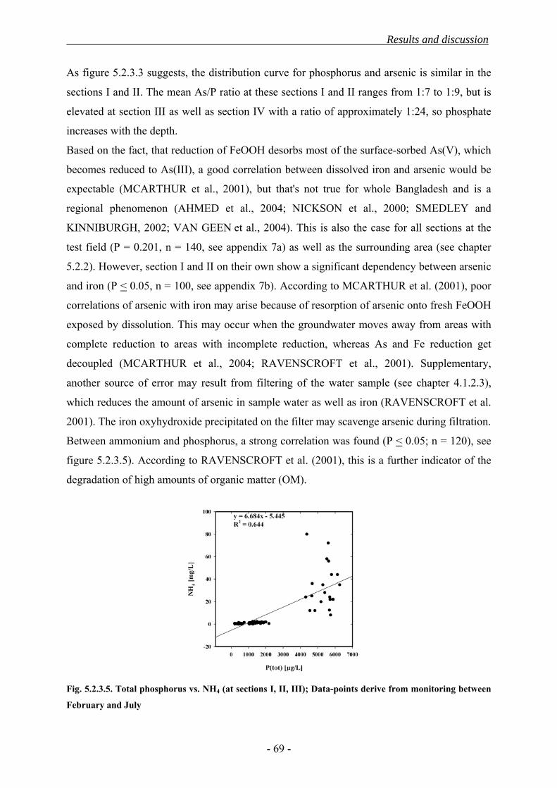
Results and discussion

- 69 -

As figure 5.2.3.3 suggests, the distribution curve for phosphorus and arsenic is similar in the

sections I and II. The mean As/P ratio at these sections I and II ranges from 1:7 to 1:9, but is

elevated at section III as well as section IV with a ratio of approximately 1:24, so phosphate

increases with the depth.

Based on the fact, that reduction of FeOOH desorbs most of the surface-sorbed As(V), which

becomes reduced to As(III), a good correlation between dissolved iron and arsenic would be

expectable (MCARTHUR et al., 2001), but that's not true for whole Bangladesh and is a

regional phenomenon (AHMED et al., 2004; NICKSON et al., 2000; SMEDLEY and

KINNIBURGH, 2002; VAN GEEN et al., 2004). This is also the case for all sections at the

test field (P = 0.201, n = 140, see appendix 7a) as well as the surrounding area (see chapter

5.2.2). However, section I and II on their own show a significant dependency between arsenic

and iron (P < 0.05, n = 100, see appendix 7b). According to MCARTHUR et al. (2001), poor

correlations of arsenic with iron may arise because of resorption of arsenic onto fresh FeOOH

exposed by dissolution. This may occur when the groundwater moves away from areas with

complete reduction to areas with incomplete reduction, whereas As and Fe reduction get

decoupled (MCARTHUR et al., 2004; RAVENSCROFT et al., 2001). Supplementary,

another source of error may result from filtering of the water sample (see chapter 4.1.2.3),

which reduces the amount of arsenic in sample water as well as iron (RAVENSCROFT et al.

2001). The iron oxyhydroxide precipitated on the filter may scavenge arsenic during filtration.

Between ammonium and phosphorus, a strong correlation was found (P < 0.05; n = 120), see

figure 5.2.3.5). According to RAVENSCROFT et al. (2001), this is a further indicator of the

degradation of high amounts of organic matter (OM).

Fig. 5.2.3.5. Total phosphorus vs. NH4 (at sections I, II, III); Data-points derive from monitoring between

February and July

Results and discussion

- 70 -

Furthermore, the obviously inverse relation of dissolved sulphate (see figure 5.2.3.6) with

arsenic in the groundwater suggest that oxidative dissolution of pyrite has not liberated

arsenic.

Fig. 5.2.3.6. Total arsenic vs. SO4 (at all sections); Data-points derive from monitoring between February

and July

As explained in chapter 2, reduction of ironhydroxide (FeOOH) and release of its sorbed

arsenic load to solution is seen as the main mechanism by which groundwater in the Bengal

Basin becomes polluted with arsenic (e.g. MCATHUR et al., 2000; RAVENSCROFT et. al,

2001; SMEDLEY and KINNIBURGH, 2002). Based on this theory arsenic accumulation at

the test field will be explained in the following.

According to MCATHUR et al. (2001), peat is the main redox driver and its biodegradation

drives extreme degrees of FeOOH reduction and supplies high concentrations of arsenic to the

groundwater. The distribution of peat and arsenic can be related to Late Pleistocene and

Holocene aquifers, just as the upper and lower aquifer at the test field area. RAVENSCROFT

et al. (2001) reported that reduction of FeOOH is accompanied by reduction of arsenate to

arsenite. As aforementioned, this fact is observable at the test field in each depth (except <

section I) and is an indication for reduction of FeOOH, as shown in figure 5.2.3.3.

Biodegradation of peat releases short-chain carboxylic acids and methylated amines that will

drive FeOOH reduction and ammonium production (RAVENSCORFT et al., 2001). Due to

the fact that these molecules do not migrate far from their peat source, this might be an

explanation that arsenic concentrations are so strongly dependent on depth. In the following, a

schematic of the process of how arsenic pollution affects individual wells will be related to

the monitoring wells from the test field, as shown in figure 5.2.3.7.

Results and discussion

- 71 -

Fig. 5.2.3.7. Model of how arsenic pollution occurs in shallow wells in the Bengal Basin. Hydraulic

gradients cause downward movement of water during the wet season. (RAVENSCROFT et al., 2001)

Adopting the model of RAVENSCROFT et al. (2001), the case D can be related to the well

BGL MAP 30 (section I), which is only slightly contaminated with arsenic, as it was expected

due to several reports (SMEDLEY and KINNIBURGH, 2001; HASAN et al., 2008; ZAHID

et al., 2007; ZHENG et al., 2004; RAVENSCROFT et al., 2001; RAVENSCROFT et al.,

2005). The recharging groundwaters are oxic, which will prevent redox processes except oxic

degradation. A layer of brown, oxidised sand was found in the top of the aquifer.

Even if the As concentration is low in the upper part of the Holocene aquifer, the slight As-

content derives from a slight degree of reduction of FeOOH. This may due to organic matter

migration downwards, which is the driving force of reduction of FeOOH (e.g. MCATHUR et

al., 2001; MCATHUR et al., 2004; RAVENSCROFT et. al, 2001; SMEDLEY and

KINNIBURGH, 2002). The content of organic matter (OM) in solid phase was measured with

approx. 0.3 wt% (LISSNER 2008). Dissolved organic carbon (DOC), an indication for

microbial processes, is around 0.7 mg C/L. A further explanation for the absence of high As

concentrations is that sorbed As was flushed from the sediment, due to the fact that

groundwater circulation is highest at these part of aquifer.

The case C might be the reason for the moderate to high dissolved arsenic contents above the

peat layer at depths between >10 and 27 m (see figure 5.2.3.7). As mentioned before, high

concentrations of As prevailed over the whole thickness (>10 m – 36 m, sections I - III) of the

grey Holocene aquifer with a maximum at 36 m (see figure 5.2.3.3). The concentrations of As

Results and discussion

- 72 -

in the lower part (> 26 m) of the aquifer are higher (> 200 µg/L) than they are in the upper

part (around 100 µg/L).

The arsenic pollution above a peat layer caused due to migration of arsenic in response to

strong pumping. However, due to the fact that the water samples were taken by low-flow

sampling, an explanation might be the intense irrigation at the surrounding agricultural crops.

Furthermore, migration of organic residuals upwards cause local FeOOH reduction and

additional arsenic release. According to LISSNER (2008), the content of organic matter (OM)

ranged between 0.5 wt% and 2 wt%, increasing with closeness to the silty and peaty lens of

clay (see figure 5.2.3.1), as well as dissolved organic carbon (DOC), ranging between 1 and

2.7 mg C/L (see figure 5.2.3.3). Supplementary, the presence of SO4 is localised where

organic matter is present (MCARTHUR et al., 2004; see figure 5.2.3.3).

The case B gives an explanation for the high arsenic concentrations at section III, screened

directly beneath the lens of organic rich clay. High amounts of organic residuals from nearby

peat cause an intense FeOOH reduction, the release of large amounts of arsenic and so high

arsenic concentrations (RAVENSCROFT et al., 2001). As mentioned before, dissolved

organic carbon and also ammonia is increased, an indication for decomposition of high

amounts of organic matter. Elevated concentrations of phosphorus in the mg/L range are

released to groundwater from the fermentation of buried peat deposits, as confirmed by

several authors (MCARTHUR et al., 2000; RAVENSCROFT et al., 2001). This is also the

case at section III, overlain by a peaty and silty lens of clay (see figure 5.2.3.3). According to

MCARTHUR et al. (2000), phosphorus enrichment parallels the distribution of arsenic

enrichment and is concentrated mostly in northeast and southeast Bangladesh, presentable at

the study area (see figure 5.2.2.2a).

The same case might be responsible for high amounts of ammonia as well as iron at section

IV, even if arsenic is moderate and oxic circumstances are dominant. However, high

dissolved Fe concentrations in the deeper aquifer are associated with the brown coloured sand

from the top of the aquifer (LISSNER 2008), which implicate the incomplete dissolution of

iron(hydr)oxides and the release of Fe and As in the groundwater (MCARTHUR et al., 2004)

(see figure 5.2.3.3). Additionally, LISSNER (2008) extracted high amounts of Fe (24 µg/g)

from the sediment which suggests the occurrence of iron(hydr)oxides in the deeper aquifer

(see figure 4.2.3.1).

The incomplete dissolution of FeOOH and the brown colour results from a long termed period

of oxidative weathering during the lowering of sea-level that occurred between 125 and 18 ka

(MCARTHUR et al., 2004). This weathering must have generated FeOOH by oxidation of

Results and discussion

- 73 -

biotite and other Fe-bearing minerals in the sediment. So, the main difference between the

Holocene (sections I - III) and the Late-Pleistocene aquifer (section IV) is the higher content

of FeOOH in the deeper aquifer. An explanation for the absence of high As concentrations is

that sorbed As was flushed from the deep aquifer during the lowering of the sea-level, as

mentioned before (MCARTHUR et al., 2001; MCARTHUR et al., 2004; RAVENSCROFT et

al., 2001; SMEDLEY and KINNIBURGH, 2002). Supplementary, dissolved arsenic is

presumably low in these sediments because of the capacity of iron(oxy)hydroxides to adsorb

arsenic (HARVEY et al., 2006).

Certainly, the schematic at figure 5.2.3.7 is simplified. Migration processes in Bangladesh’s

aquifers are influenced by numerous factors such as low regional hydraulic gradients, micro-

topographic effects, surface water bodies, deep rooted vegetation, seasonal flooding and water

logging (RAVENSCROFT et al., 2001). The behaviour of groundwater flow and migration

processes were not the subject of this project but will be presented elsewhere (HÄRTIG

2008). It has long been known that the formation of soluble arsenic sulphur complexes plays an

important role in aquatic reducing environments. Worldwide investigations at reducing

environments have been proven that arsenic has a high affinity to sulphur compounds. The

geochemical interaction between arsenic and reduced sulphur species may play an important

role for the mobility and toxicity of arsenic in sulphate reducing environments. This fact was

not proven for groundwater in Bangladesh yet (GAULT et al., 2005).

Beside the already mentioned arsenic species arsenate and arsenite, a third species was

detected at the test field at BGL TF 90: Monothioarsenate (H3AsSO3) was measured with a

maximum level of 32µg/L in the dry season (February). Monothioarsenate was generally

highest at BGL TF 90 whereas Monothioarsenate was not detected at BGL TF 30 as well as

280. A seasonal trend was not detectable, but it seems that the concentrations decrease during

the monitoring.

The formation of H3AsSO3 is strongly dependent on pH and dissolved oxygen. The

occurrence of thioarsenic species is limited to a pH ranging from near neutral to alkaline

Additionally, their formation depends on the arsenic:sulphur ratio in the solution. Either they

can be formed by reaction of arsenite with elemental sulphur under alkaline conditions or by

alkaline dissolution of As bearing sulphide minerals, e.g. Orpiment and Realgar.

Results and discussion

- 74 -

5.2.4 Seasonal hydrochemical changes

As described in chapter 4.1.2, hydrochemical mapping was done at the study area at Titas,

Daudkandi Upzilla, Comilla District to put the region into context of the whole arsenic

problem in Bangladesh. Additionally, a weekly monitoring (see chapter 4.2.1) was done to

collect data over a period of one year to find out seasonal changes in the arsenic distribution at

the newly drilled test field tapping different aquifers. Altogether, 20 campaigns were arranged

at an interval of approximately one week to capture hydrochemical changes resulting from the

annual heavy rainfall in the end of April, the onset of the rainy season due to monsoonal

precipitation as well as the influence of intensive irrigation in the surrounding area. During

the 20 campaigns, 140 water samples and several additional replicates of the same sample for

quality control were taken. The water table was measured at the piezometers using a light

indicator. Data acquisition was carried out over a period from February to end of July. No

water tables were measured at the second, sixth and fourteenth campaign. The water table

between the 10th and 11th as well as the 13th and 14th campaign was measured within a two-

week time period, other than the common period of one week. For this reason, potential

temporary groundwater table variations were not recorded.

Fig. 5.2.4.1. Mean monthly precipitation and temperature over the last 10 years (1997 – 2006) in

comparison to the mean monthly precipitation and temperature during the period of investigation (2007)

Results and discussion

- 75 -

Meteorological data over a period of 10 years, consisting of daily rainfall, temperature, and

evaporation derived from the Bangladesh Meteorological Department. In figure 5.2.4.1, the

year 2007 is compared to the deposition and temperature from the last 10 years (1997 – 2006).

Therefore, deposition in the year 2007 can be characterized as above averaged in comparison

to the last decade. The annual rainfall in 2007 was 2497mm whereas the average of the last

decade was 2197mm. Especially the monsoonal rains in the main rainy season in June

(approx. 550 mm/month) and July (approx. 650mm/month) were notably heavier than the

years before (see figure 5.2.4.1), whereas the May can be characterised as exceptionally hot

and dry. Generally, the initiation of the monsoonal rains in 2007 was later than the average

from the previous decade. The period between January and March was inconspicuous, instead

of subtly lower temperatures and lower rainfall in March (see figure 5.2.4.1).

According to the Bangladesh Meteorological Department, the annual potential evaporation

was measured with 13404 mm/a. To get an estimation of the amount of infiltration and run off

from annual deposition, the real evaporation (ETR) was calculated by a simplified equation

adapted from TURC. The choice of this equation is owed to the fact, that it is generally

applicable worldwide and limited to the annual sum of deposition and average annual

temperature as constituents.

[ ] 5.02)/(9.0 T

TURCIP

PETR+

= (eq.6)

305.025300 TTIT •+•+= (eq.7)

ETRTURC = annual value of real evaporation after TURC [mm/a]

P = annual sum of uncorrected deposition [mm/a]

T = average annual temperature [°C]

The sum of annual deposition at 2007 is 2497mm; the average annual temperature in 2007 is

25.1°C. Therefore, the real evaporation was estimated with 1439 mm/a. Consequently,

1058mm became infiltrated or ran off respectively. But as mentioned before, the calculation

adapted from TURC is an imprecise method and is used merely for estimation of annual total

amounts of evaporation. It does not account location, natural cover, soil composition, etc.

were unaccounted for calculation and are undocumented within the study.

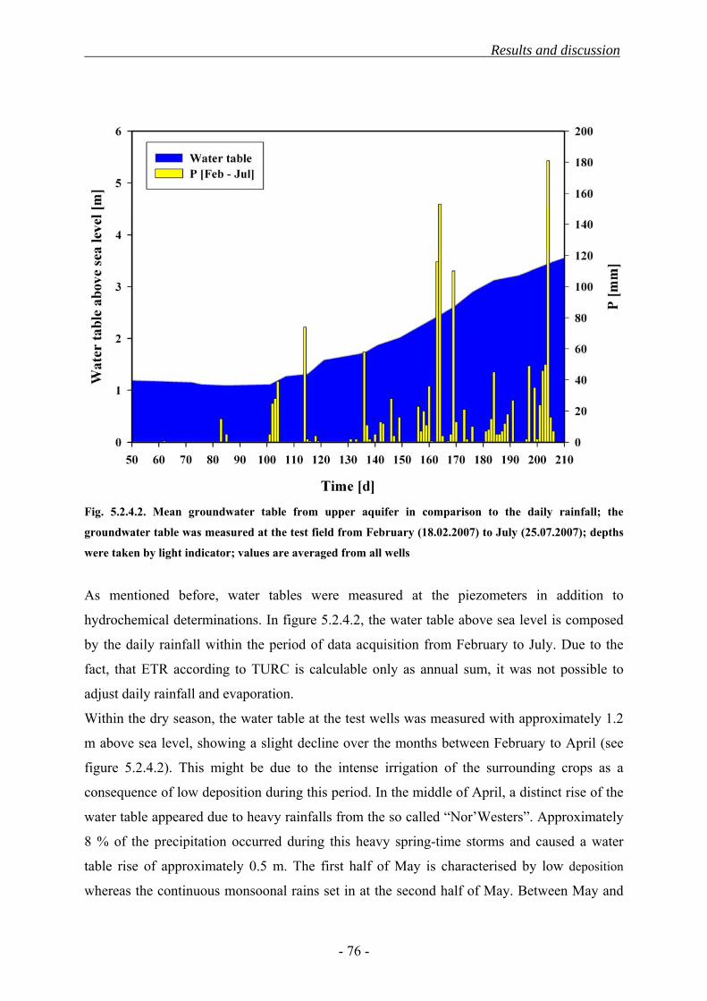
Results and discussion

- 76 -

Fig. 5.2.4.2. Mean groundwater table from upper aquifer in comparison to the daily rainfall; the

groundwater table was measured at the test field from February (18.02.2007) to July (25.07.2007); depths

were taken by light indicator; values are averaged from all wells

As mentioned before, water tables were measured at the piezometers in addition to

hydrochemical determinations. In figure 5.2.4.2, the water table above sea level is composed

by the daily rainfall within the period of data acquisition from February to July. Due to the

fact, that ETR according to TURC is calculable only as annual sum, it was not possible to

adjust daily rainfall and evaporation.

Within the dry season, the water table at the test wells was measured with approximately 1.2

m above sea level, showing a slight decline over the months between February to April (see

figure 5.2.4.2). This might be due to the intense irrigation of the surrounding crops as a

consequence of low deposition during this period. In the middle of April, a distinct rise of the

water table appeared due to heavy rainfalls from the so called “Nor’Westers”. Approximately

8 % of the precipitation occurred during this heavy spring-time storms and caused a water

table rise of approximately 0.5 m. The first half of May is characterised by low deposition

whereas the continuous monsoonal rains set in at the second half of May. Between May and

Results and discussion

- 77 -

July alone, 55 % (1355 mm) of the annual deposition were released during this period and led

to a rise of the water table of almost 2.1 m up to the end of the data acquisition (see figure

5.2.4.2).

To estimate the infiltration time of deposition into the upper aquifer, the kf-value was

calculated based on the grain size distribution taken from sieve analysis. For this purpose, the

infiltration behaviour was assumed to be vertical and the aquifer is simplified as saturated

zone over the whole thickness. To estimate the kf-value from grain size distribution, the

method according to HAZEN seems to be most suitable (eq.8).

2

10 )(0116.0 dkf HAZEN •= (eq.8)

Table 5.2.4.1. Infiltration time of deposition into the upper aquifer, estimated according to HAZEN

m/sec m/min m/h m/d m/week 1.98E-06 1.19E-04 7.12E-03 0.17 1.20

Kf-values were calculated for several zones of the aquifer, averaged and summed up to a total

value (see appendix 8). Regarding the deliverables from table 5.2.4.1, infiltration water from

the surface should require approximately 8 to 10 weeks before arriving a depth of 10 m.

Furthermore, it should take more than half a year to influence BGL TF 115 at a depth of 36 m.

But as aforementioned, the method according to HAZEN is extremely simplified with no

consideration to flow conditions, distinction of saturated and unsaturated zones, rooting, etc.

Results and discussion

- 78 -

As described in chapter 5.2.3, arsenic concentrations are strongly dependent on depth. But due

to the fact, that Bangladesh’s groundwaters are influenced by such extreme changes (as

described before in this chapter) between dryness in connection with excessive irrigation and

heavy monsoonal rainfalls with extensive flooding, changes in the hydrochemistry might be

expectable. Figure 5.2.4.3 represents the depth and seasonal dependent distribution of total

arsenic in the monitoring wells.

Fig. 5.2.4.3. Seasonal changes of total arsenic concentrations in different depths of the test field

It is obvious, that changing weather conditions have strong effects on arsenic concentrations.

As mentioned before, heavy rainfalls appeared in the second half of April (see figure 5.2.4.2).

In conjunction with this short timed storm event, a considerable degradation of the arsenic

concentrations can be observed at depths between 15 and 25 m. The same downward

movement is observable for phosphorus (see appendix 9). Errors in the detection of total

arsenic can be excluded due to the fact that the sums of the arsenic species (measured

independently from the totals) show the same decline (see appendix 2a). This gives the

suggestion that dissolved arsenic has been temporary flushed away due to the infiltration of

Results and discussion

- 79 -

deposition water. Noticeable changes in the mineralisation have not been detected (see

appendix 10), so dilution effects can be excluded.

The intensity of degradation of the arsenic concentrations is decreasing with depth. In a depth

of 15m, the arsenic concentration decreases temporary to a level of 20 µg/L, a deficit of

approximately 130 µg/L. At BGL TF 70 (21 m), arsenic decreases with a delay of one

monitoring campaign to a level of 20 µg/L, a deficit of 80 µg/L. Supplementary, BGL TF 85

(25 m) shows a deficit of still 50 µg/L, but increases shortly after to its maximum of 250 µg/L

(see figure 5.2.4.3). Also BGL TF 50 and 70 drop back rapidly to their previous levels. At the

same time, arsenic increases at BGL TF 90 from a value of 150 µg/L to 230 µg/L. It seems to

be obvious that arsenic is getting vertically flushed from shallower into deeper regions of the

aquifer. In comparison to the estimated infiltration time from kf, the effective infiltration time

seems to be much higher.

Within the period between May (the onset of the monsoonal rains) and the end of data

acquisition in July, a continuous increase in the arsenic concentrations was detected at the

depths with the highest concentrations (25 – 36 m). A considerable degradation of the arsenic

concentrations can be observed at BGL TF 90 between the second half of June and the second

half of July. This phenomenon cannot be noticed at the other depths and the investigation of

causes would be too speculative. But it seems that arsenic is getting locally flushed by

horizontal groundwater flows, especially enforced in the rainy season. Therefore, it would be

essential to understand the annual cycle of groundwater flow, controlled by irrigation and the

groundwater recharge by rainfall.

The monitoring wells in shallower depths (21 m) have more balanced arsenic concentrations,

even if the values at the rainy season are slightly increased in comparison to the dry season

(see figure 5.2.4.3). BGL TF 30 is characterised by continuous low arsenic concentrations.

Also BGL TF 280 shows only slight changes in arsenic concentrations over the whole

monitoring campaign. This can be explained by the fact, that the recharging groundwaters are

oxic, which will prevent redox processes except oxic degradation. Nevertheless, this is not

true for the groundwaters from the grey Holocene fine sand. The deeper the well the higher is

the arsenic concentration as well as the seasonal fluctuations.

However, these changes in the arsenic concentrations become even more apparent by

consideration of arsenite. As figure 5.2.4.4 suggests, especially the deeper wells between 25

and 36 m show an obvious increase in arsenite with the beginning of the rainy season. As

described in chapter 5.2.3, these depths are strongly influenced by organic matter due to a lens

of silty and peaty clay. The increase in dissolved arsenite is an evidence for seasonally

Results and discussion

- 80 -

occcuring stronger reducing conditions, due to the massive rise of the water table.

Additionally, it seems that sedimentary bounded arsenic is getting mobilised which explains

the increase in total arsenic in the groundwater. As a reminder: according to the theory of

reduction of arsenic-rich hydrous iron oxides (FeOOH), peat is the main redox driver and its

biodegradation drives extreme degrees of FeOOH reduction and supplies high concentrations

of arsenic to the groundwater. The reduction of FeOOH is accompanied by reduction of

arsenate to arsenite, which explains the rise of arsenite and therefore total arsenic.

Fig. 5.2.4.4. Seasonal changes of total arsenite concentrations in different depths of the test field

In connection with an increased biodegradation of peat as the main redox driver, several

authors (MCARTHUR et al., 2000; RAVENSCROFT et al., 2001) reported increased

concentrations of ammonia as well as dissolved organic carbon. Additionally, increased

concentrations of phosphorus in the mg/L range are released to the groundwater from the

fermentation of buried peat deposits. It is not possible to give a general statement about the

seasonal behaviour of dissolved phosphorus in relation to arsenic. At the shallowest well

between 9 and 21 m, a significant positive correlation between arsenic and phosphorus was

determined (see table 5.2.4.1). But this is not true for each depth, as table 5.2.4.1 clarifies.

Results and discussion

- 81 -

Therefore, no relation between both arsenic and phosphorus was measurable at BGL TF 85,

90 and 280. BGL TF 115 (which is highest affected by arsenic), shows an inverse relation

between both arsenic and phosphorus. The process behind is not yet understood clear

(RAVENSCROFT et al., 2001). But is seems that the reduction of FeOOH is accompanied by

a supply of high concentrations of arsenic and a displacement of phosphorus respectively.

This phenomenon is not occurring in wells with low rates of biodegradation of organic matter.

Table 5.2.4.1. Well by well correlation between total arsenic and total phosphorus (P = value for statistical

significance, r = correlation coefficient, n = number of samples) TF30 TF50 TF70 TF85 TF90 TF115 TF280

P 0.000 0.000 0.000 0.538 0.056 0.0285 0.0584 r 0.747 0.742 0.844 -0.144 0.433 -0.689 0.428 n 20 20 20 20 20 20 20

An inverse correlation was also detected between arsenic and dissolved organic carbon at

BGL TF 115 (P < 0.05, n = 20; not plotted). According to RAVENSCROFT et al. (2001),

dissolved organic is being degraded by driving redox processes. Due to the seasonal affective

stronger reducing conditions and consequently the enlarged biodegradation of organic matter

(OM), this can be an explanation for the inverse correlation.

As described in previous chapters, the concentrations for ammonia at BGL TF 115 and 280

are not representative for statements about seasonal changes. Interferences with other

dissolved elements might appear, especially iron at all levels (see chapter 4.1.2.2). Since there

is an detection limit of 0.5 mg/L for ammonia, determined by photometry, high dilutions at

field site with a ratio of 1:400 were necessary which had adverse effects to the accuracy of

measurement. However, ammonia is extremely high at BGL 115 and 280, an obvious

indicator for an increased biodegradation of peat.

Recommendations

- 82 -

6. Recommendations

The present report is based on field works in Bangladesh from February to July 2007. The

field work was divided mainly in two sections: a weekly monitoring at the newly drilled test

wells and mapping works at the surrounding area. During the long termed data acquisition of

six month, various problems and errors occurred and new ideas evolved for following studies.

Therefore, some recommendations will be given in the following.

• Within a multiplicity of previous studies, shallow tube wells were tested for arsenic

in Bangladesh, just as performed in this study. A fractional amount of these wells is

lithological logged. It can be assumed that arsenic contaminations in the

groundwater are in close connection with the sedimentary composition of the

underground. Therefore, geophysical methods provide an opportunity to detect peat

and clay lenses and to determine the thickness of aquifers as well as aquicludes.

Both geoelectric and seismic are suitable methods for subsurface survey. Therefore,

geoelectric is particularly suitable to locate clay as well as peat lenses whereas

seismic is probably better suited for determining continuous layers.

• In chapter 5.2.4, the kf-value was calculated from the grain size distribution of the

samples in order to estimate the infiltration time of rain water into the upper aquifer.

Therefore, the infiltration behaviour was simplified as vertical. To specify the model

of groundwater circulation, it is unavoidable to perform more specific aquifer tests.

Suitable methods are pumping and tracer tests in conjunction with the deliverables

from sediment analysis.

• During the monsoonal rainfalls large parts of Bangladesh are flooded. However, the

degree of flooding is intensified by the Ganges-Brahmaputra-Meghna river system

bringing large amounts of water from India and the Himalayas and therefore large

amounts of sedimentary load. Due to this fact, it could be revealing to determine the

floodwater as well as its deposits for arsenic loads.

Recommendations

- 83 -

• Several authors reported good correlations between arsenic concentrations in

shallow tube wells and the age of the wells. This cannot be confirmed within the

recent study but it would be more meaningful to do a continuous monitoring (>5a)

at selected wells.

• For hydrochemistry, redoxsensitive elements (Fe2+, Mn2+, NO3-, NO2

-, NH3-, and

S2-) were measured by photometry at the field site. As described in previous

chapters, some wells had high concentrations of dissolved iron as well as ammonia,

especially BGL TF 115 and BGL TF 280. First of all, high dilutions were necessary

(ammonia approx. 1:400; iron approx. 1:50), which leads to inaccuracies, due to the

fact that the field equipment is exposed to a multitude of strains. This can be seen in

the inhomogeneity of the values for iron and ammonia. To decrease the dilution

factor (and thus inaccuracies), it is possible to use photometry programs with higher

ranges (e.g. HACH method 10023 for ammonia). As described in chapter 4.1.2.2,

ammonia detection can be disturbed by iron at all levels. Laboratory investigations

at laboratory are necessary to determine the influence of iron on ammonia.

• The detection of fluoride and nitrite by ion chromatography can be disturbed by

chloride due to similar retention times of the three anions. A shift of the retention

times could therefore help to avoid these interferences and can be achieved by an

eluent adjustment.

Acknowledgments

- 84 -

7. Acknowledgements

I like to thank the following people:

• My first supervisor Prof. Dr. Broder J. Merkel who supported this work by

professional suggestions (especially at statistical problems), during the whole

editing time. I also like to thank him for proofreading

• Special thanks go to Dr. Britta Planer-Friedrich for involving me in her DFG-project

and for the opportunity to work abroad and to complete my study with such an

impression. Her engagement, experience in the field and laboratory, availability for

my asking as well as proofreading was essential for finishing my thesis

• Prof. Dr. Qumrul Hassan, Dr. Anwar Zahid and Masud Khan for my stay in

Bangladesh and on-site support at Dhaka University

• Special thanks go to Rashed and Tanvir who welcomed me with amity and made my

residence in Bangladesh to a unique experience. I would also like to thank their

families for their kindness and hospitableness

• I like to thank my parents, who gave me the mental and financial support

• H.J. Peter and Sascha Kummer for their support at the laboratory in Freiberg

(Germany)

• My friends for their support

• My fellow students for helpful suggestions

References

- 85 -

8. References

Acharyya S. K., Lahiri S., Raymahashay B. C., and Bhowmik A. (1999) Arsenic toxicity of

groundwater in parts of the Bengal basin in India and Bangladesh: the role of Quaternary stratigraphy

and Holocene sea-level fluctuation. Environmental Geology 39(10), 1127-1137.

Ahmed K. M., Bhattacharya P., Hasan M. A., Akhter S. H., Alam S. M. M., Bhuyian M. A. H.,

Imam M. B., Khan A. A., and Sracek O. (2004) Arsenic enrichment in groundwater of the alluvial

aquifers in Bangladesh: an overview. Applied Geochemistry 19(2), 181-200.

Alam M., Alam M. M., Curray J. R., Chowdhury A. L. R., and Gani M. R. (2003) An overview of

the sedimentary geology of the Bengal Basin in relation to the regional tectonic framework and basin-

fill history. Sedimentary Geology 155(3-4), 179-208.

Alauddin M. and Quiggin J. (2008) Agricultural intensification, irrigation and the environment in

South Asia: Issues and policy options. Ecological Economics 65(1), pp. 111-124

Bhattacharya P., Jacks G., Ahmed K. M., Routh J., Khan A. A. (2002) Arsenic in Groundwater of

the Bengal Delta Plain Aquifers in Bangladesh. Bull. Environ. Contam. Toxicol. 69, 538–545

Breit G. N., Whitney J., Foster A., Welch A. H., Yount J., Sanzolone R., Islam M. K., Islam M.

S., Islam M. M., Sutton S., and Newville M. (2001) Preliminary Evaluation of Arsenic Cycling in

the Sediments of Bangladesh. USGS Report, 4.

DPHE (1999) Groundwater studies for arsenic contamination in Bangladesh. Final Report. Rapid

Investigation Phase. Department of Puplic Health Engineering, Government of Bangladesh. Mott

MacDonald.

Gault A.G., Jana J., Chakraborty S., Mukherjee P., Sarkar M., Nath B., Polya D.A., Chatterjee

D. (2004) Preservation strategies for inorganic arsenic species in high iron, low-Eh groundwater from

West Bengal, India. Anal Bioanal Chem 381, 347–353

Hanrahan G., Salmassi T. M., Khachikian C. S., Foster K. L. (2005) Reduced inorganic

phosphorus in the natural environment: significance, speciation and determination. Talanta 66, 435–

444

References

- 86 -

Harvey C. F., Ashfaque K. N., Yu W., Badruzzaman A. B. M., Ali M. A., Oates P. M., Michael

H. A., Neumann R. B., Beckie R., Islam S., Ahmed M. F. (2006) Groundwater Dynamics and

Arsenic Contamination in Bangladesh. Chemical Geology 228 (1-3 SPEC. ISS.), pp. 112-136

Hasan M. A., v. Brömsen M., Bhattacharya P., Ahmed K. M., Sikder A. M., Jacks G., Sracek O.

(2008) Geochemistry and mineralogy of shallow alluvial aquifers in Daudkandi upazila in the Meghna

flood plain, Bangladesh. Environ Geol

Kinniburgh D. G. and Smedley P. L. (2001) Arsenic contamination of groundwater in Bangladesh.

British Geological Survey & Department of Public Health Engineering.

Kinniburgh D. G. and Smedley P. L. (2002) A review of the source, behaviour and distribution of

arsenic in natural waters. Applied Geochemistry 17, 517-568.

Kinniburgh D. G. and Smedley P. L., Davies J., Milne C.J., Gaus I., Trafford J.M., Burden S.,

Huq S.M.I., Ahmed N., Ahmed M.K. (2003) The scale and causes of the groundwater arsenic

problem in Bangladesh. Arsenic in groundwater: geochemistry and occurrence. Kluwer Academic

Publishers, 211-257.

Lißner H. (2008) Column experiments simulating various scenarios for arsenic

mobilization in Bangladesh.- Freiberg Online Geoscience FOG Vol. 18, ISSN

1434-7512 (http://www.geo.tu-freiberg.de/fog/issues.html)

Manning B. A. and Goldberg S. (1996) Modeling competitive adsorption of arsenate with phosphate

and molybdate on oxide minerals. Soil Science Society of America Journal 60(1), 121-131.

McArthur J. M., Ravenscroft P., Safiullah S., Thirlwall M. F. (2000) Arsenic in groundwater:

testing mechanisms for sedimentary aquifers in Bangladesh. Water Resources Research 37(1), 109-

117

McArthur J. M., Banerjee D. M., Hudson-Edwards K. A., Mishra R., Purohit R., Ravenscroft

P., Cronin A., Howarth R. J., Chatterjee A., Talukder T., Lowry D., Houghton S., and Chadha

D. K. (2004) Natural organic matter in sedimentary basins and its relation to arsenic in anoxic ground

water: the example of West Bengal and its worldwide implications. Applied Geochemistry 19(8),

1255-1293.

References

- 87 -

Nath B., Sahu S.J., Jana J., Mukherjee-Goswami A., Roy S., Sarkar M.J., Chatterjee S. (2007)

Hydrochemistry of arsenic-enriched aquifer from rural West Bengal, India: A study of the arsenic

exposure and mitigation option. Water Air Soil Pollut 190, 95–113

Nickson R., McArthur J., Burgess W., Ahmed K. M., Ravenscroft P., and Rahman M. (1998)

Arsenic poisoning of Bangladesh groundwater. Nature 395(6700), 338-338.

Nickson R. T., McArthur J. M., Ravenscroft P., Burgess W. G., and Ahmed K. M. (2000)

Mechanism of arsenic release to groundwater, Bangladesh and West Bengal. Applied Geochemistry

15(4), 403-413.

Parkhurst, D.L. (1995): Public health and regulatory aspects of inorganic nitrogen compounds in

drinking water –International workshop, Inorganic Nitrogen Compounds and Water Supply, Hamburg

Planer-Friedrich B., London J., Mccleskey R. B., Nordstrom D. K., and Wallschlaeger D. (2007)

Thioarsenates in geothermal waters – determination, preservation, and geochemical role.

Environmental Science and Technology 41(15), 5245-5251.

Ravenscroft P., Burgess W. G., Ahmed K. M., Burren M., and Perrin J. (2005) Arsenic in

groundwater of the Bengal Basin, Bangladesh: Distribution, field relations, and hydrogeological

setting. Hydrogeology Journal 13(5-6), 727-751.

Ravenscroft P., McArthur J., and Hoque B. (2001) Geochemical and Palaeohydrological Controls

on Pollution of Groundwater by Arsenic. Arsenic exposure and health effects (ed. W. R. Chappell, C.

O. Abernathy, and R. L. Calderon), pp. 53-78. Elsevier Science Ltd.

Rahman MM, Chowdhury UK, Mukherjee SC, Mondal BK, Paul K, Lodh D, Biswas BK,

Chanda CR, Basu GK, Saha KC, Roy S, Das R, Palit SK, Quamruzzaman Q, Chakraborti D

(2001) Chronic Arsenic Toxicity in Bangladesh and West Bengal, India – A Review and Commentary.

Clinical Toxicology 39(7), 683-700

Reimann K. U., (1993): Geology of Bangladesh – Beiträge zur regionalen Geologie der Erde.

Gebrüder Bornträger, Berlin – Stuttgart

Rossum J.R. (1975) Checking the accuracy of water analysis through the use of conductivity.-J.

American Water Works Association 67(4), 204-205

References

- 88 -

van Geen A., Rose J., Thoral S., Garnier J., Zheng Y., and Bottero J. (2004) Decoupling of As

and Fe release to Bangladesh groundwater under reducing conditions. Part II: Evidence from sediment

incubations. Geochimica et Cosmochimica Acta 68(17), 3475-3486.

Wallschläger D. and Stadey C. J. (2007) Determination of (Oxy)thioarsenates in Sulfidic Waters.

Analytical Chemistry 79, 3873-3880.

Welch A.H., Lico M.S. (1998) Factors controlling As and U in shallow ground water, southern

Carson Desert, Nevada. Applied Geochemistry 13,(4), 521-539

Zahid A., Hassan M.Q., Balke K.D., Flegr M., Clark D.W. (2007) Groundwater chemistry and

occurrence of arsenic in the Meghna floodplain aquifer, southeastern Bangladesh. Environ Geol 54,

1247–1260

Zheng Y., Stute M., van Geen A., Gavrieli I., Dhar R., Simpson H. J., Schlosser P., and Ahmed

K. M. (2004) Redox control of arsenic mobilization in Bangladesh groundwater. Applied

Geochemistry 19(2), 201-214.

- 89 -

9. Appendix

Appendix

- 90 -

Appendix 1a: Comparison of both measured conductivity and calculated conductivity for mapped wells

(MAP) and monitoring wells from test field (TF). The percent error derive from difference between EC

measured and EC calculated

Soln Sample code

EC measured

EC calculated

deviation [EC rec - Eccalc]

Percent error Soln Sample

code EC

measured EC

calculated deviation [EC rec - Eccalc]

Percent error

1 TF3001 252.0 185.0 67.0 26.6 99 TF9019 460.6 309.0 151.6 32.92 TF3002 259.5 186.0 73.5 28.3 100 TF9020 480.0 296.0 184.0 38.33 TF3003 286.2 194.0 92.2 32.2 101 TF11501 2558.0 2681.0 -123.0 -4.84 TF3004 279.6 207.0 72.6 26.0 102 TF11502 3201.0 2620.0 581.0 18.25 TF3005 255.5 180.0 75.5 29.5 103 TF11503 2056.0 1803.0 253.0 12.36 TF3006 309.6 211.0 98.6 31.8 104 TF11504 2430.0 1844.0 586.0 24.17 TF3007 384.0 210.0 174.0 45.3 105 TF11505 3381.0 2564.0 817.0 24.28 TF3008 372.8 224.0 148.8 39.9 106 TF11506 2540.0 1856.0 684.0 26.99 TF3009 333.2 206.0 127.2 38.2 107 TF11507 3006.0 1919.0 1087.0 36.210 TF3010 243.3 175.0 68.3 28.1 108 TF11508 3840.0 2611.0 1229.0 32.011 TF3011 328.3 233.0 95.3 29.0 109 TF11509 1896.0 1429.0 467.0 24.612 TF3012 315.6 198.0 117.6 37.3 110 TF11510 2964.0 2105.0 859.0 29.013 TF3013 269.8 181.0 88.8 32.9 111 TF11511 3283.0 2501.0 782.0 23.814 TF3014 200.8 142.0 58.8 29.3 112 TF11512 3168.0 1830.0 1338.0 42.215 TF3015 209.8 152.0 57.8 27.6 113 TF11513 2705.0 1730.0 975.0 36.016 TF3016 237.5 171.0 66.5 28.0 114 TF11514 1956.0 1678.0 278.0 14.217 TF3017 244.5 189.0 55.5 22.7 115 TF11515 1434.0 1399.0 35.0 2.418 TF3018 269.5 188.0 81.5 30.2 116 TF11516 1001.0 1045.0 -44.0 -4.419 TF3019 236.0 158.0 78.0 33.1 117 TF11517 1130.0 1158.0 -28.0 -2.520 TF3020 215.2 164.0 51.2 23.8 118 TF11518 1419.0 1335.0 84.0 5.921 TF5001 300.6 239.0 61.6 20.5 119 TF11519 1192.0 1063.0 129.0 10.822 TF5002 308.4 246.0 62.4 20.2 120 TF11520 1082.0 963.0 119.0 11.023 TF5003 317.4 234.0 83.4 26.3 121 TF28001 2390.0 1825.0 565.0 23.624 TF5004 326.2 238.0 88.2 27.0 122 TF28002 2635.0 1848.0 787.0 29.925 TF5005 318.0 221.0 97.0 30.5 123 TF28003 2733.0 1840.0 893.0 32.726 TF5006 325.5 241.0 84.5 26.0 124 TF28004 2766.0 1780.0 986.0 35.627 TF5007 357.0 231.0 126.0 35.3 125 TF28005 2605.0 1833.0 772.0 29.628 TF5008 354.9 227.0 127.9 36.0 126 TF28006 2814.0 1821.0 993.0 35.329 TF5009 348.6 235.0 113.6 32.6 127 TF28007 2805.0 1844.0 961.0 34.330 TF5010 333.9 231.0 102.9 30.8 128 TF28008 3150.0 1863.0 1287.0 40.931 TF5011 312.0 232.0 80.0 25.6 129 TF28009 2802.0 1862.0 940.0 33.532 TF5012 331.1 239.0 92.1 27.8 130 TF28010 2850.0 1851.0 999.0 35.133 TF5013 335.4 235.0 100.4 29.9 131 TF28011 2820.0 1811.0 1009.0 35.834 TF5014 311.7 228.0 83.7 26.9 132 TF28012 2710.0 1834.0 876.0 32.335 TF5015 319.8 227.0 92.8 29.0 133 TF28013 2937.0 1845.0 1092.0 37.236 TF5016 292.5 218.0 74.5 25.5 134 TF28014 2892.0 1865.0 1027.0 35.537 TF5017 298.2 225.0 73.2 24.5 135 TF28015 2620.0 1343.0 1277.0 48.738 TF5018 309.0 219.0 90.0 29.1 136 TF28016 2540.0 1852.0 688.0 27.139 TF5019 327.3 225.0 102.3 31.3 137 TF28017 2558.0 1888.0 670.0 26.240 TF5020 313.5 217.0 96.5 30.8 138 TF28018 2700.0 1902.0 798.0 29.641 TF7001 292.2 228.0 64.2 22.0 139 TF28019 2713.8 1872.0 841.8 31.042 TF7002 301.0 236.0 65.0 21.6 140 TF28020 2787.0 1842.0 945.0 33.943 TF7003 309.6 236.0 73.6 23.8 141 MAP0101 367.5 267.0 100.5 27.344 TF7004 315.3 233.0 82.3 26.1 142 MAP0201 255.0 190.0 65.0 25.545 TF7005 315.0 228.0 87.0 27.6 143 MAP0301 298.8 235.0 63.8 21.446 TF7006 315.6 253.0 62.6 19.8 144 MAP0401 1084.0 890.0 194.0 17.947 TF7007 337.4 240.0 97.4 28.9 145 MAP0501 470.0 340.0 130.0 27.7

Appendix

- 91 -

Appendix 1a (continued)

Soln Sample code

EC measured

EC calculated

deviation [EC rec - Eccalc]

Percent error Soln Sample

code EC

measured EC

calculated deviation [EC rec - Eccalc]

Percent error

48 TF7008 330.4 246.0 84.4 25.5 146 MAP0601 343.0 243.0 100.0 29.249 TF7009 342.3 239.0 103.3 30.2 147 MAP0701 470.0 341.0 129.0 27.450 TF7010 320.4 227.0 93.4 29.2 148 MAP0801 380.8 292.0 88.8 23.351 TF7011 307.5 227.0 80.5 26.2 149 MAP0901 498.0 394.0 104.0 20.952 TF7012 324.6 225.0 99.6 30.7 150 MAP1001 367.5 267.0 100.5 27.353 TF7013 340.9 230.0 110.9 32.5 151 MAP1101 376.0 290.0 86.0 22.954 TF7014 316.8 212.0 104.8 33.1 152 MAP1201 934.0 753.0 181.0 19.455 TF7015 326.9 231.0 95.9 29.3 153 MAP1301 481.0 386.0 95.0 19.856 TF7016 307.8 232.0 75.8 24.6 154 MAP1401 305.1 225.0 80.1 26.357 TF7017 301.8 224.0 77.8 25.8 155 MAP1501 260.5 199.0 61.5 23.658 TF7018 305.4 217.0 88.4 28.9 156 MAP1601 308.0 244.0 64.0 20.859 TF7019 309.0 213.0 96.0 31.1 157 MAP1701 413.0 307.0 106.0 25.760 TF7020 316.2 217.0 99.2 31.4 158 MAP1801 456.0 342.0 114.0 25.061 TF8501 419.0 300.0 119.0 28.4 159 MAP1901 300.3 235.0 65.3 21.762 TF8502 436.0 312.0 124.0 28.4 160 MAP2001 270.0 203.0 67.0 24.863 TF8503 465.0 323.0 142.0 30.5 161 MAP2101 395.2 282.0 113.2 28.664 TF8504 437.0 313.0 124.0 28.4 162 MAP2201 284.4 225.0 59.4 20.965 TF8505 481.0 321.0 160.0 33.3 163 MAP2301 345.1 272.0 73.1 21.266 TF8506 471.0 329.0 142.0 30.1 164 MAP2401 309.0 240.0 69.0 22.367 TF8507 543.0 315.0 228.0 42.0 165 MAP2501 460.0 350.0 110.0 23.968 TF8508 528.0 316.0 212.0 40.2 166 MAP2601 755.0 612.0 143.0 18.969 TF8509 474.0 333.0 141.0 29.7 167 MAP2701 364.7 243.0 121.7 33.470 TF8510 501.0 326.0 175.0 34.9 168 MAP2801 353.9 233.0 120.9 34.271 TF8511 487.0 317.0 170.0 34.9 169 MAP2901 437.0 305.0 132.0 30.272 TF8512 481.0 319.0 162.0 33.7 170 MAP3001 508.0 376.0 132.0 26.073 TF8513 508.0 323.0 185.0 36.4 171 MAP3101 1158.0 950.0 208.0 18.074 TF8514 490.0 307.0 183.0 37.3 172 MAP3201 398.4 283.0 115.4 29.075 TF8515 478.0 309.0 169.0 35.4 173 MAP3301 331.8 244.0 87.8 26.576 TF8516 425.0 291.0 134.0 31.5 174 MAP3401 616.0 395.0 221.0 35.977 TF8517 439.0 311.0 128.0 29.2 175 MAP3501 584.0 409.0 175.0 30.078 TF8518 469.0 308.0 161.0 34.3 176 MAP3601 486.0 342.0 144.0 29.679 TF8519 435.9 301.0 134.9 30.9 177 MAP3701 388.0 241.0 147.0 37.980 TF8520 478.0 308.0 170.0 35.6 178 MAP3801 567.0 406.0 161.0 28.481 TF9001 396.8 310.0 86.8 21.9 179 MAP3901 350.0 233.0 117.0 33.482 TF9002 439.0 314.0 125.0 28.5 180 MAP4001 531.0 376.0 155.0 29.283 TF9003 419.0 308.0 111.0 26.5 181 MAP4101 389.6 275.0 114.6 29.484 TF9004 443.0 308.0 135.0 30.5 182 MAP4201 808.0 523.0 285.0 35.385 TF9005 461.0 313.0 148.0 32.1 183 MAP4301 237.0 175.0 62.0 26.286 TF9006 455.0 305.0 150.0 33.0 184 MAP4401 958.0 701.0 257.0 26.887 TF9007 482.0 310.0 172.0 35.7 185 MAP4501 581.0 404.0 177.0 30.588 TF9008 485.0 308.0 177.0 36.5 186 MAP4601 356.3 237.0 119.3 33.589 TF9009 495.0 309.0 186.0 37.6 187 MAP4701 385.6 261.0 124.6 32.390 TF9010 459.0 302.0 157.0 34.2 188 MAP4801 380.0 262.0 118.0 31.191 TF9011 491.0 333.0 158.0 32.2 189 MAP0102 383.6 278.0 105.6 27.592 TF9012 492.0 314.0 178.0 36.2 190 MAP0402 798.0 627.0 171.0 21.493 TF9013 502.0 311.0 191.0 38.0 191 MAP2502 506.0 356.0 150.0 29.694 TF9014 484.0 304.0 180.0 37.2 192 MAP2702 380.0 254.0 126.0 33.295 TF9015 475.0 298.0 177.0 37.3 193 MAP2902 499.0 350.0 149.0 29.996 TF9016 378.4 276.0 102.4 27.1 194 MAP4102 373.1 273.0 100.1 26.897 TF9017 414.0 299.0 115.0 27.8 195 MAP4202 768.0 539.0 229.0 29.898 TF9018 472.0 304.0 168.0 35.6 196 MAP4302 231.5 166.0 65.5 28.3

Appendix

- 92 -

Appendix 1b: Mean percent error and mean deviation between measured and calculated conductance

Sample code

Mean percent error

Mean deviation [µS/cm]

Mean conductivity [µS/cm]

TF30 31.0 87.4 275.1 TF50 28.3 91.7 322.1 TF70 27.4 87.1 316.8 TF85 33.3 158.2 472.3 TF90 32.9 152.6 459.2 TF115 18.1 505.4 2312.1 TF280 33.4 920.3 2741.4 MAP 26.9 124.2 469.6

Appendix 2a: Comparison of total arsenic with sum of arsenic species for each monitoring well at test field

Appendix

- 93 -

Appendix 2b: Comparison of total phosphorus with sum of phosphorus species for each monitoring well at test field

Appendix 3: Dendrogram of the hierarchical cluster analysis using the ward method showing three major

groups for surrounding wells

Appendix

- 94 -

Appendix 4: Distribution of total phosphorus and P-species at mapping wells; Rate phosphate of total

phosphorus

Sample code

Unidentified P-species

[µg/L]

PO43-

[µg/L] Total P [µg/L]

% rate PO43-

of P(tot) Sample code Unidentified

P-species [µg/L]

PO43-

[µg/L] Total P [µg/L]

% rate PO43-

of P(tot)

MAP0101 228.5 0.0 489.1 0.0 MAP2901 220.0 320.0 383.1 83.5MAP0201 164.9 630.0 817.1 77.1 MAP3001 185.0 51.0 94.0 54.2MAP0301 348.3 69.5 189.3 36.7 MAP3101 190.9 50.8 0.0 24.9MAP0401 122.5 866.8 1090.7 79.5 MAP3201 13.1 231.5 260.1 -4.4MAP0501 128.6 1815.0 1910.0 95.0 MAP3301 22.7 67.2 528.0 12.7MAP0601 181.3 1082.5 1223.2 88.5 MAP3401 72.3 276.0 362.6 76.1MAP0701 194.0 1111.0 1215.3 91.4 MAP3501 193.2 861.9 1133.8 76.0MAP0801 194.2 875.0 935.7 93.5 MAP3601 205.9 185.2 353.4 52.4MAP0901 146.8 919.7 1226.5 75.0 MAP3701 253.1 395.4 591.4 66.9MAP1001 182.0 1317.5 1313.3 100.3 MAP3801 27.5 166.9 871.6 19.1MAP1101 179.3 750.7 925.5 81.1 MAP3901 281.9 632.0 809.2 78.1MAP1201 220.2 411.0 536.9 76.6 MAP4001 207.8 706.6 908.7 77.8MAP1301 141.7 114.2 169.6 67.3 MAP4101 248.1 421.9 560.4 75.3MAP1401 211.0 756.9 921.0 82.2 MAP4201 199.9 551.3 778.3 70.8MAP1501 195.2 591.5 714.0 82.8 MAP4301 355.2 770.8 819.7 94.0MAP1601 159.8 601.5 763.1 78.8 MAP4401 263.9 136.0 104.8 129.9MAP1701 242.6 743.5 915.7 81.2 MAP4501 389.4 479.4 534.3 89.7MAP1801 215.5 602.4 801.0 75.2 MAP4601 320.1 529.2 564.7 93.7MAP1901 166.3 310.5 418.6 74.2 MAP4701 423.7 913.6 1023.6 89.3MAP2001 225.0 177.0 295.2 60.0 MAP4801 336.0 394.5 405.2 97.4MAP2101 215.0 583.8 772.9 75.5 MAP0102 379.4 373.2 456.1 81.8MAP2201 131.1 290.8 454.0 64.1 MAP0402 208.4 780.8 873.5 89.4MAP2301 183.3 413.5 506.8 81.6 MAP2502 284.3 291.4 296.2 98.4MAP2401 246.1 1151.5 1204.8 95.6 MAP2702 407.5 740.5 827.3 89.5MAP2501 177.1 216.6 382.3 56.7 MAP2902 323.4 326.1 354.2 92.1MAP2601 173.8 73.1 40.2 181.6 MAP4102 325.9 552.1 629.3 87.7MAP2701 264.2 579.6 798.2 72.6 MAP4202 254.5 602.3 801.5 75.1MAP2801 44.0 359.2 391.5 91.7 MAP4302 397.8 696.8 807.2 86.3

Appendix

- 95 -

Appendix 5: Dendrogram of the hierarchical cluster analysis using the ward method showing two major

groups for the major ions from monitoring wells

Appendix 6: Piper diagram, showing the determination of major cations and anions at the monitoring

wells in different depths, divided in 2 major groups: Group I (TF30, TF50, TF70, TF85, TF90): Ca and

HCO3- dominated; Group II (TF115, TF280): Na and HCO3

- dominated

Appendix

- 96 -

Appendix 7: Total arsenic vs. (a) total iron (at the sections I – IV; n = 140), (b) total iron (at section I and

II; n = 100) Data-points derive from monitoring between February and July

Appendix 8: Averaged kf for the upper aquifer at the core drilling at hospital ground, depending on the

method after HAZEN. Grain size distribution was done by sieve analysis

Sample- code d10 [mm] d60 [mm] HAZEN kf =

0.0116*(d10)² from [m] to [m]

BAN-3 0.010 0.10 1.16E-06 0.0 6.7 BAN-4 0.015 0.12 2.61E-06 7.6 8.2 BAN-5 0.010 0.13 1.16E-06 9.1 9.8 BAN-6 0.008 0.08 7.42E-07 10.7 11.3 BAN-7 0.010 0.16 1.16E-06 12.2 12.8 BAN-8 0.012 0.15 1.67E-06 13.7 14.3 BAN-9 0.010 0.15 1.16E-06 15.2 15.8 BAN-10 0.012 0.15 1.67E-06 16.8 17.4 BAN-11 0.009 0.15 9.40E-07 17.4 18.9 BAN-12 0.015 0.12 2.61E-06 18.9 19.5 BAN-13 0.015 0.12 2.61E-06 19.5 20.1 BAN-14 0.013 0.13 1.96E-06 20.1 20.7 BAN-15 0.013 0.13 1.96E-06 20.7 21.3 BAN-16 0.011 0.12 1.40E-06 21.3 21.9 BAN-17 0.012 0.10 1.67E-06 21.9 22.6 BAN-18 0.012 0.10 1.67E-06 22.6 23.2 BAN-19 0.010 0.09 1.16E-06 23.2 23.8 BAN-20 0.010 0.09 1.16E-06 23.8 24.4 BAN-22 0.018 0.19 3.76E-06 24.4 25.0 BAN-23 0.020 0.30 4.64E-06 25.0 25.6 BAN-24 0.020 0.30 4.64E-06 25.6 26.2 Mean: 0.013 0.14 1.977E-06

Appendix

- 97 -

Appendix 9: Seasonal changes of total phosphorus concentrations in different depths of the test field

Appendix 10a: Seasonal changes of EC in different depths (9 – 27 m) of the test field

Appendix

- 98 -

Appendix 10b: Seasonal changes of EC in different depths (115 – 280 m) of the test field