frequency distribution cross-tabulation 12 data... · 0dunhw 5hvhdufk /&( frequency...

��

��

��

Frequency DistributionCross-Tabulation

��

1) Overview

2) Frequency Distribution

3) Statistics Associated with Frequency Distribution

i. Measures of Location

ii. Measures of Variability

iii. Measures of Shape

4) Introduction to Hypothesis Testing

5) A General Procedure for Hypothesis Testing

6) Cross-Tabulations

7) Statistics Associated with Cross-Tabulation

��

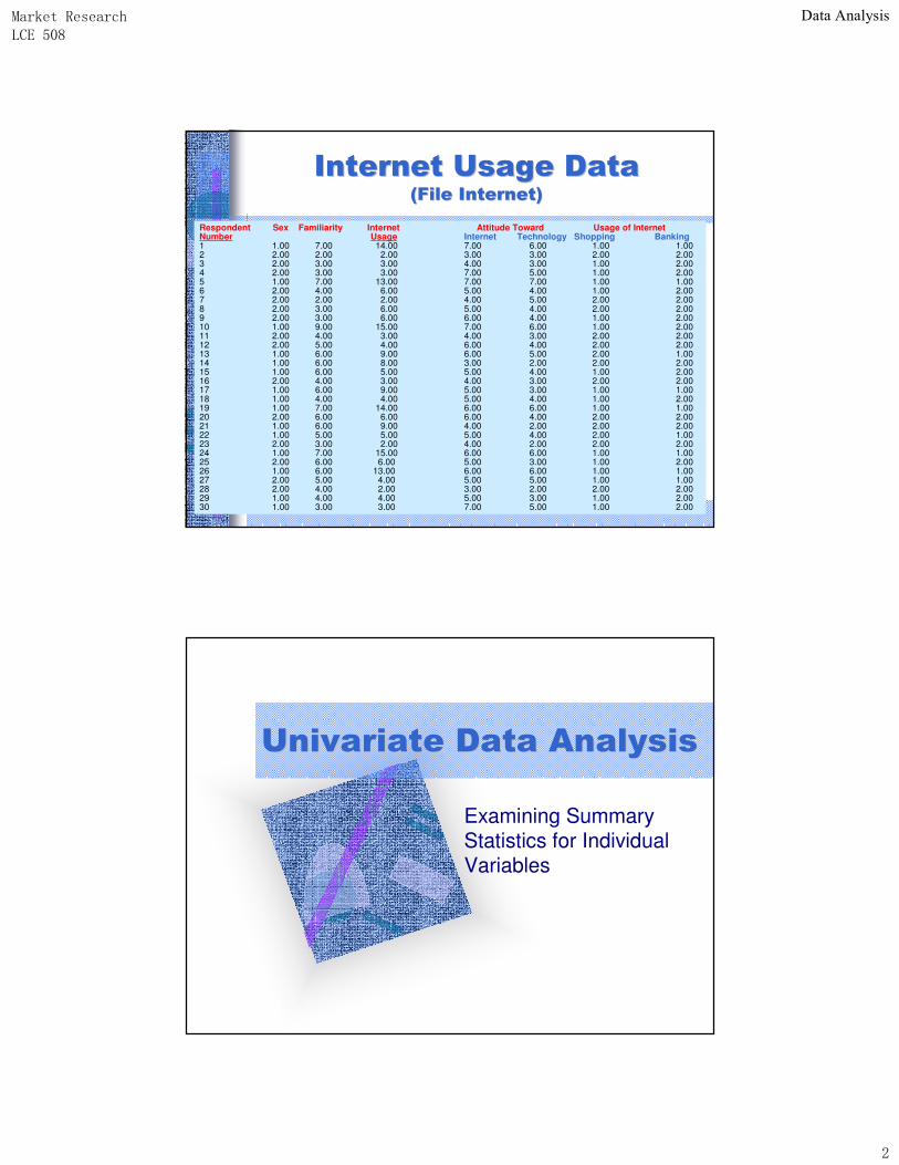
Respondent Sex Familiarity Internet Attitude Toward Usage of InternetNumber Usage Internet Technology Shopping Banking1 1.00 7.00 14.00 7.00 6.00 1.00 1.002 2.00 2.00 2.00 3.00 3.00 2.00 2.003 2.00 3.00 3.00 4.00 3.00 1.00 2.004 2.00 3.00 3.00 7.00 5.00 1.00 2.00 5 1.00 7.00 13.00 7.00 7.00 1.00 1.006 2.00 4.00 6.00 5.00 4.00 1.00 2.007 2.00 2.00 2.00 4.00 5.00 2.00 2.008 2.00 3.00 6.00 5.00 4.00 2.00 2.009 2.00 3.00 6.00 6.00 4.00 1.00 2.0010 1.00 9.00 15.00 7.00 6.00 1.00 2.0011 2.00 4.00 3.00 4.00 3.00 2.00 2.0012 2.00 5.00 4.00 6.00 4.00 2.00 2.0013 1.00 6.00 9.00 6.00 5.00 2.00 1.0014 1.00 6.00 8.00 3.00 2.00 2.00 2.0015 1.00 6.00 5.00 5.00 4.00 1.00 2.0016 2.00 4.00 3.00 4.00 3.00 2.00 2.0017 1.00 6.00 9.00 5.00 3.00 1.00 1.0018 1.00 4.00 4.00 5.00 4.00 1.00 2.0019 1.00 7.00 14.00 6.00 6.00 1.00 1.0020 2.00 6.00 6.00 6.00 4.00 2.00 2.0021 1.00 6.00 9.00 4.00 2.00 2.00 2.0022 1.00 5.00 5.00 5.00 4.00 2.00 1.0023 2.00 3.00 2.00 4.00 2.00 2.00 2.0024 1.00 7.00 15.00 6.00 6.00 1.00 1.0025 2.00 6.00 6.00 5.00 3.00 1.00 2.0026 1.00 6.00 13.00 6.00 6.00 1.00 1.0027 2.00 5.00 4.00 5.00 5.00 1.00 1.0028 2.00 4.00 2.00 3.00 2.00 2.00 2.00 29 1.00 4.00 4.00 5.00 3.00 1.00 2.0030 1.00 3.00 3.00 7.00 5.00 1.00 2.00

��

��

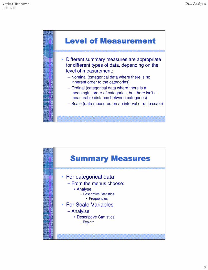
Examining Summary Statistics for Individual Variables

��

��

• Different summary measures are appropriate for different types of data, depending on the level of measurement:– Nominal (categorical data where there is no

inherent order to the categories) – Ordinal (categorical data where there is a

meaningful order of categories, but there isn't a measurable distance between categories)

– Scale (data measured on an interval or ratio scale)

��

• For categorical data– From the menus choose:

• Analyse– Descriptive Statistics

• Frequencies

• For Scale Variables– Analyise

• Descriptive Statistics– Explore

��

��

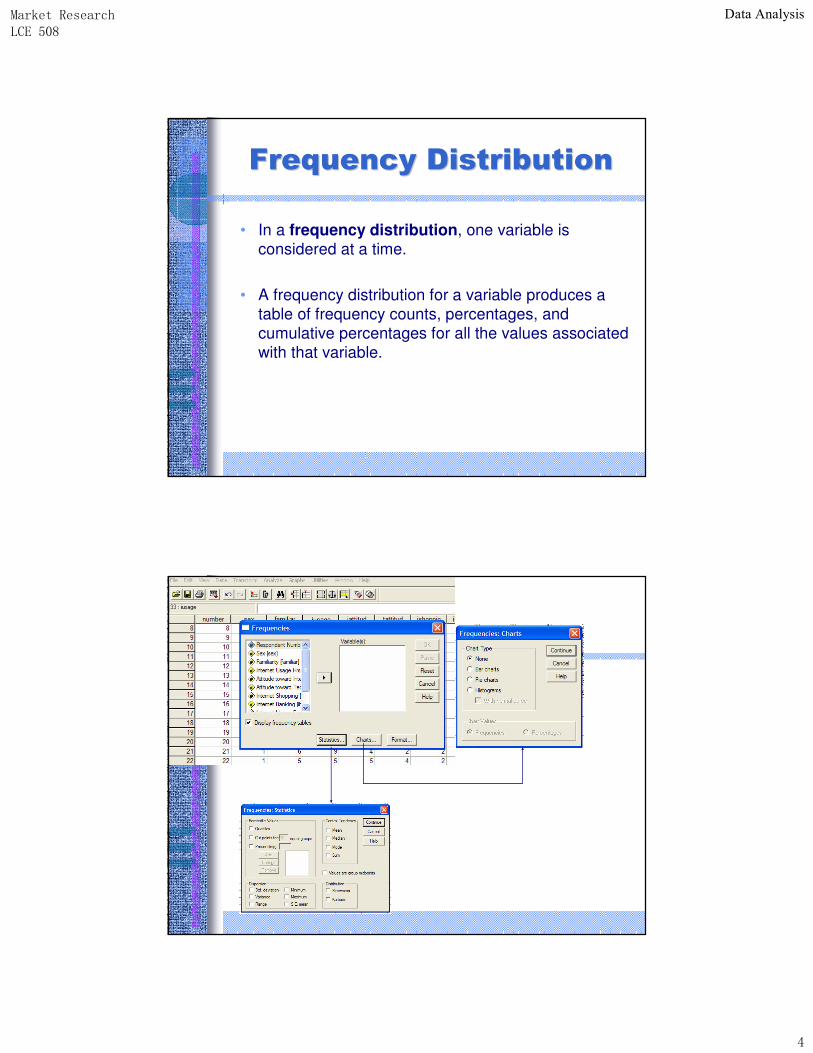
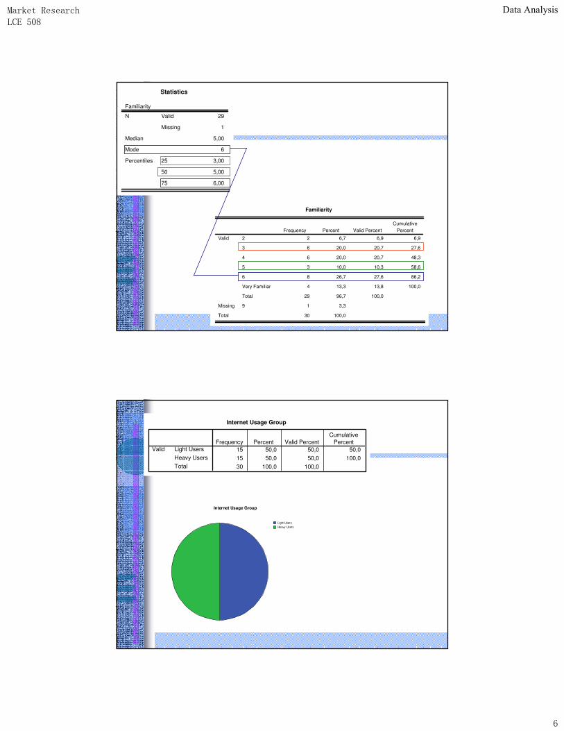
• In a frequency distribution, one variable is considered at a time.

• A frequency distribution for a variable produces a table of frequency counts, percentages, and cumulative percentages for all the values associated with that variable.

��

��

� ��

�

�

� � � � � � � � ��

��

�

��

� � ��

� � ��

� � ��

� � ��

� � ��

��

��

�

� ��

�

�

�� !�� !��

� � � � � ��

�

�

�

�

�

�

�

��

��

�

��

Statistics

Familiarity

29

1

5,00

6

3,00

5,00

6,00

Valid

Missing

N

Median

Mode

25

50

75

Percentiles

Familiarity

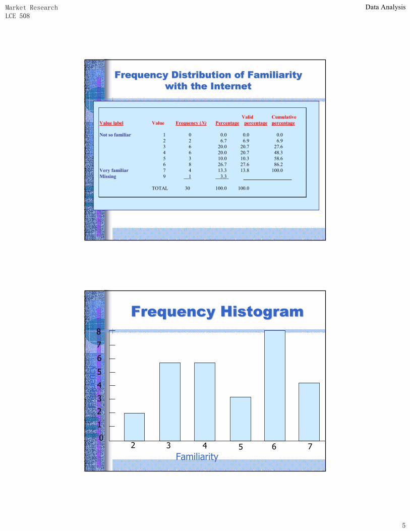
2 6,7 6,9 6,9

6 20,0 20,7 27,6

6 20,0 20,7 48,3

3 10,0 10,3 58,6

8 26,7 27,6 86,2

4 13,3 13,8 100,0

29 96,7 100,0

1 3,3

30 100,0

2

3

4

5

6

Very Familiar

Total

Valid

9Missing

Total

Frequency Percent Valid PercentCumulative

Percent

Internet Usage Group

15 50,0 50,0 50,015 50,0 50,0 100,030 100,0 100,0

Light UsersHeavy UsersTotal

ValidFrequency Percent Valid Percent

CumulativePercent

Light UsersHeavy Users

Internet Usage Group

��

• The mean, or average value, is the most commonly used measure of central tendency.

• The mode is the value that occurs most frequently. It represents the highest peak of the distribution. The mode is a good measure of location when the variable is inherently categorical or has otherwise been grouped into categories.

��

��

��

• The median of a sample is the middle value when the data are arranged in ascending or descending order.

• If the number of data points is even, the median is usually estimated as the midpoint between the two middle values – by adding the two middle values and dividing their sum by 2.

• The median is the 50th percentile.

��

��

��

��

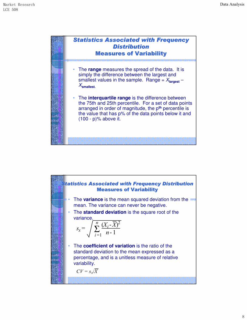
• The range measures the spread of the data. It is simply the difference between the largest and smallest values in the sample. Range = Xlargest –Xsmallest.

• The interquartile range is the difference between the 75th and 25th percentile. For a set of data points arranged in order of magnitude, the pth percentile is the value that has p% of the data points below it and (100 - p)% above it.

��

��

��"�� "��

• The variance is the mean squared deviation from the mean. The variance can never be negative.

• The standard deviation is the square root of the variance.

• The coefficient of variation is the ratio of the standard deviation to the mean expressed as a percentage, and is a unitless measure of relative variability.

��

�

� � �Σ� ��

�

��

��

��"�� "��

��

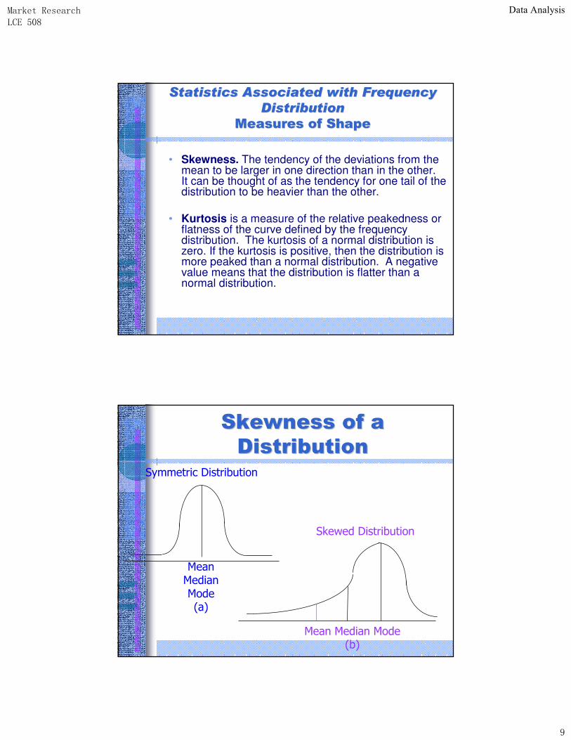
• Skewness. The tendency of the deviations from the mean to be larger in one direction than in the other. It can be thought of as the tendency for one tail of the distribution to be heavier than the other.

• Kurtosis is a measure of the relative peakedness or flatness of the curve defined by the frequency distribution. The kurtosis of a normal distribution is zero. If the kurtosis is positive, then the distribution is more peaked than a normal distribution. A negative value means that the distribution is flatter than a normal distribution.

��

��

�� #�� #�

�$��$��

��

��

��

�� !�"

�� !�"

��

%��%��

�� !��"�� #

��

&��&��''(��(��

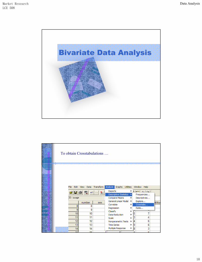
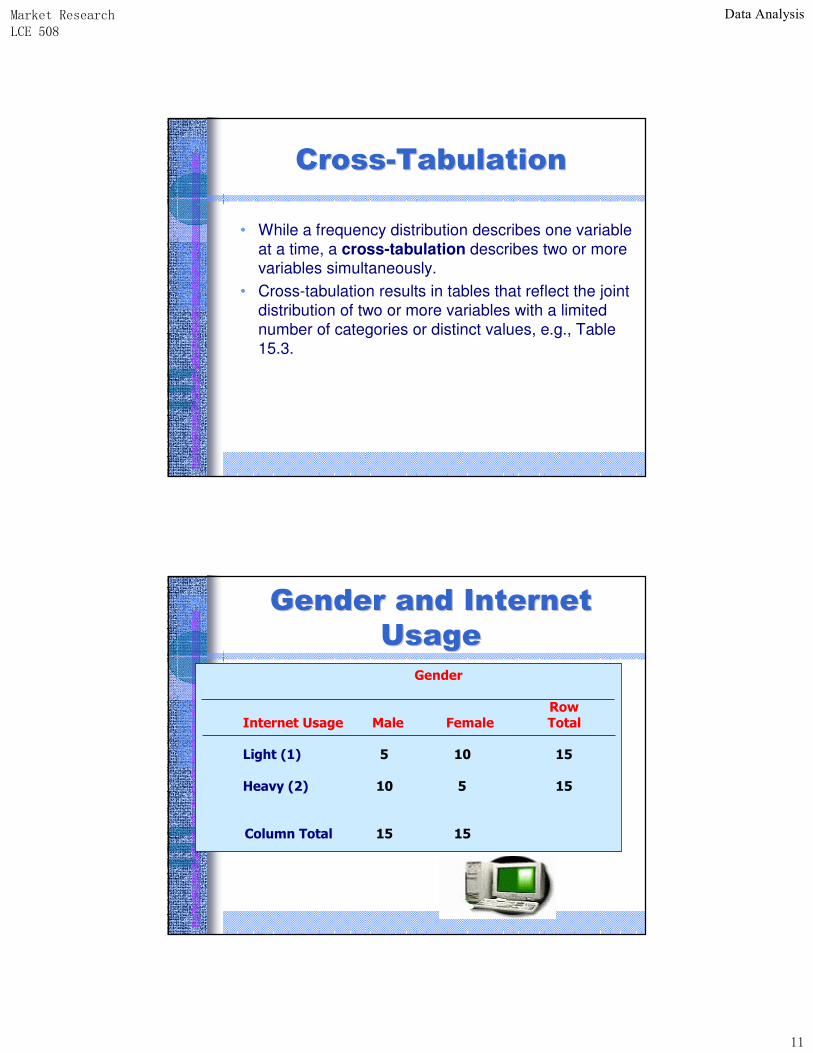
• While a frequency distribution describes one variable at a time, a cross-tabulation describes two or more variables simultaneously.

• Cross-tabulation results in tables that reflect the joint distribution of two or more variables with a limited number of categories or distinct values, e.g., Table 15.3.

)��)��

��

��

� � � � � � � � � ��

��

��!��"��

��

(��"��&��(��"��&��''

(��(��

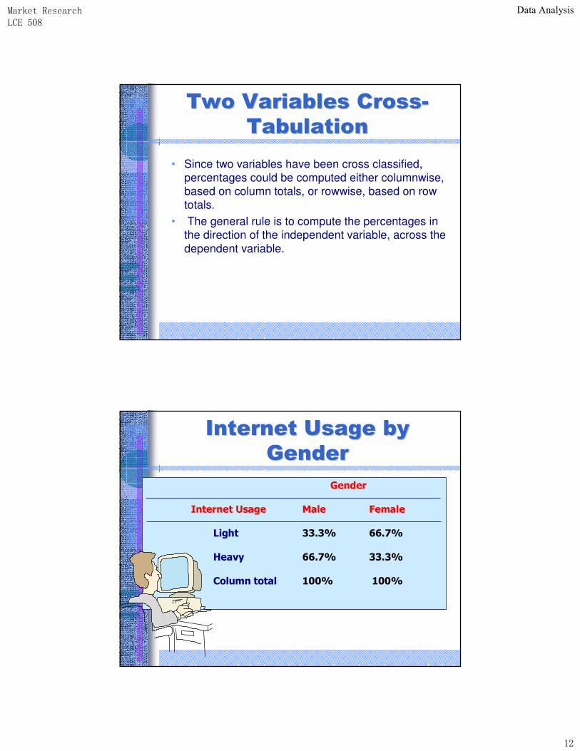
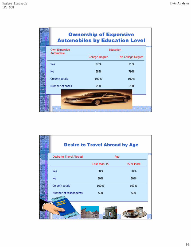
• Since two variables have been cross classified, percentages could be computed either columnwise, based on column totals, or rowwise, based on row totals.

• The general rule is to compute the percentages in the direction of the independent variable, across the dependent variable.

��

)��)��

� ��

�

� ��

�

� � �� ##$#% � � &&$'% �

�

� � �� &&$'% � � ##$#% �

�

� � !��"�� % � � ��% �

��

)�� )��

��

��#��$��%��&�� '�%(�� )��*�� +�� ,�-� � ��,�-� � � ��,�-�

�� ,�-� � ��,�-� � � ��,�-�

*�� &�� *�� &��

� ��

. �(��/��(��

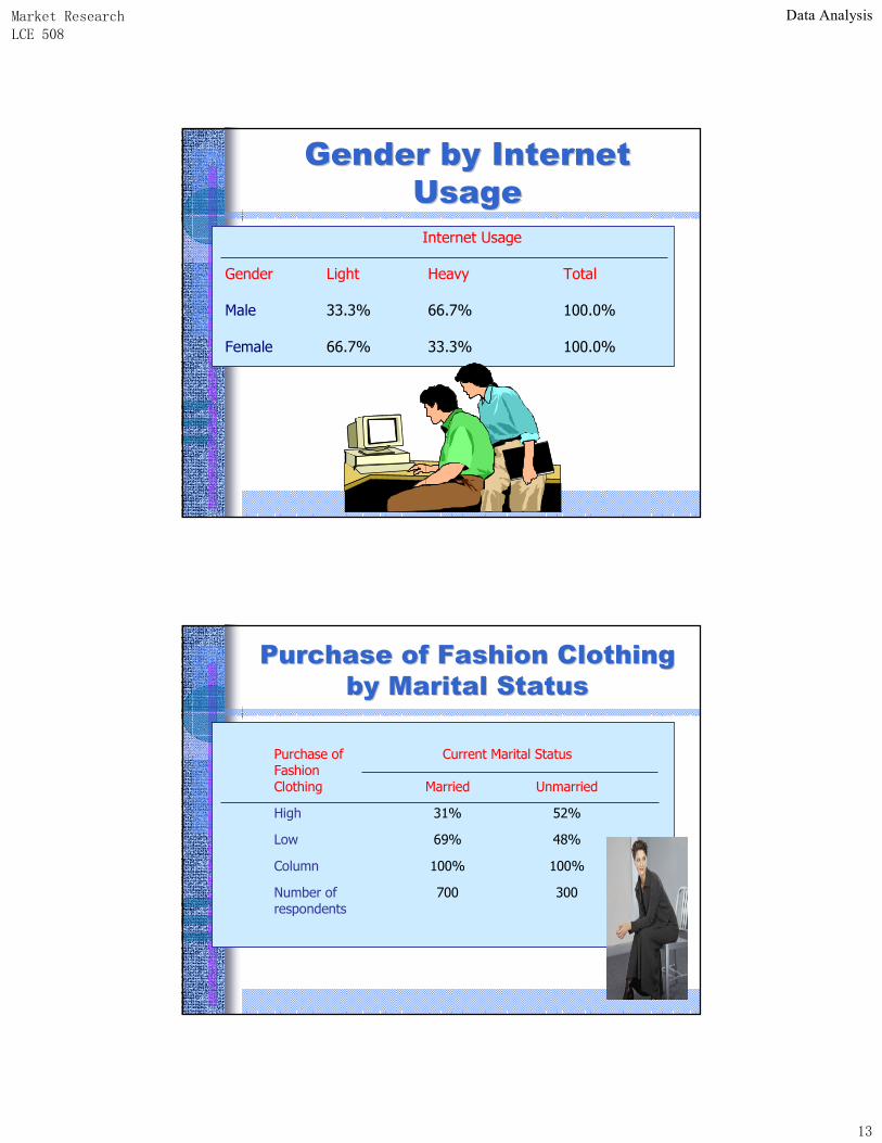
0 ��

0��(��%� �� $��

)�%(� ��-� ��-�

'�� 1-� ��-�

0�� -� ��-�

2 ��/��3��

��

��

��

+�� #��,-#��+�� #��,-#��

�� ,�� ,��

4��563��*��7 ��

5� ��

� 0��%��%�� 2��0��%��%��

8�� -� ��-�

2�� -� �1-�

0�� -� ��-�

2 ��/��

�

�

��(�� (��

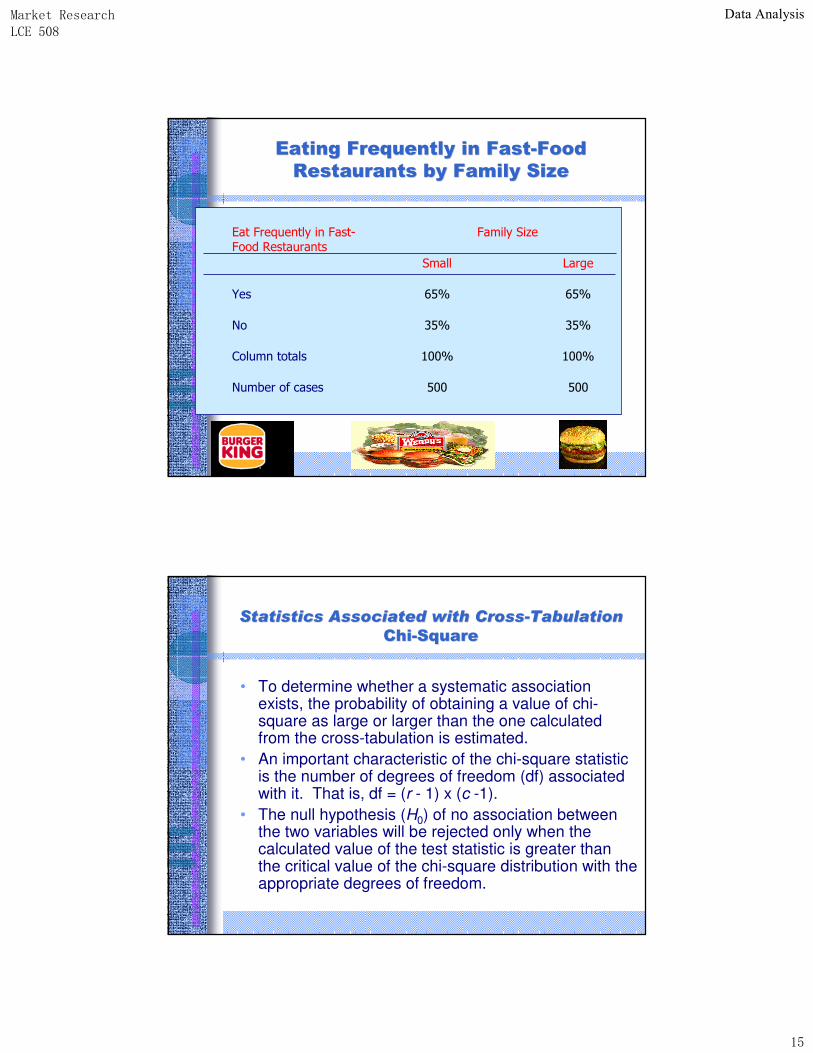
��+�*��7�� 7%��

� '��(��

8�� -� ��-�

2�� -� ��-�

0�� -� ��-�

2 ��/��3��

�

�

��

,�� ,�� ''��

.�� /�.�� /�

5�� 9��:��

��;��

� �� '�%��

8�� -� ��-�

2�� -� ��-�

0�� -� ��-�

2 ��/��

�

�

• To determine whether a systematic association exists, the probability of obtaining a value of chi-square as large or larger than the one calculated from the cross-tabulation is estimated.

• An important characteristic of the chi-square statistic is the number of degrees of freedom (df) associated with it. That is, df = (r - 1) x (c -1).

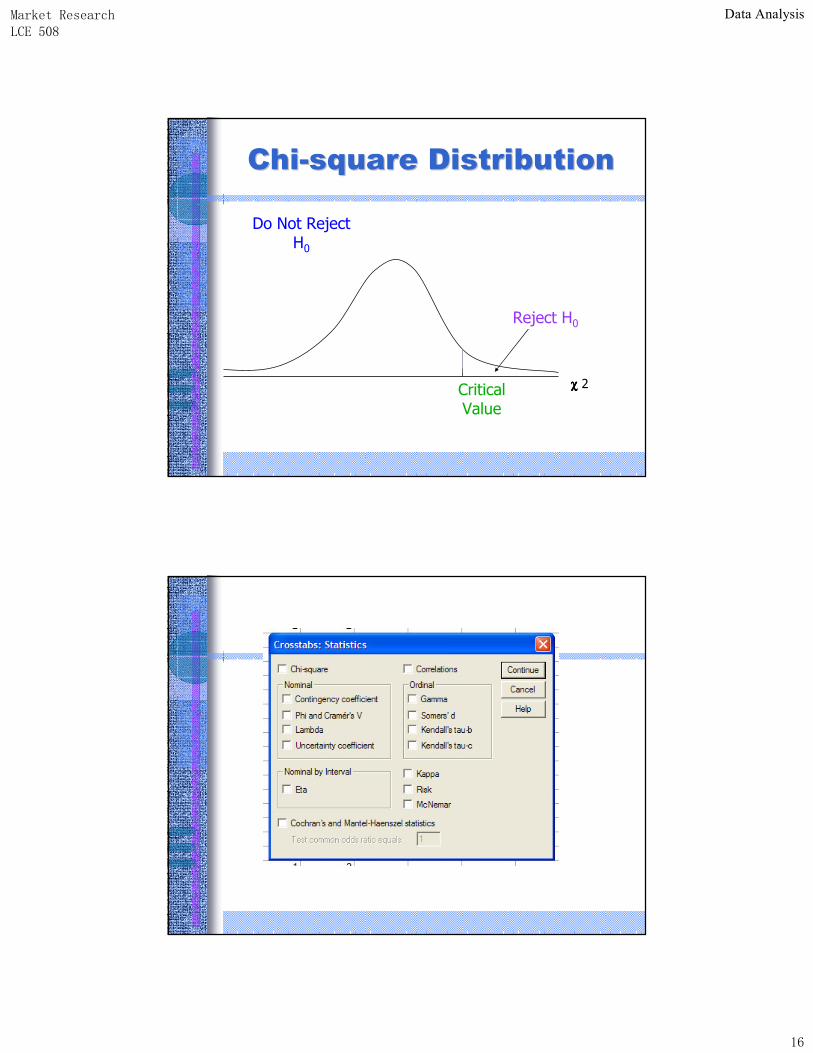
• The null hypothesis (H0) of no association between the two variables will be rejected only when the calculated value of the test statistic is greater than the critical value of the chi-square distribution with the appropriate degrees of freedom.

��

& �& �''��

��

& �& �''��

:�<��)�

��2��:�<��)�

0��=��

χχχχ �

��

��

Nominal Data

• The phi coefficient ( ) is used as a measure of the strength of association in the special case of a table with two rows and two columns (a 2 x 2 table).

• The phi coefficient is proportional to the square root of the chi-square statistic

• The value ranges between:– 0 (indicating no association between the row and column

variables and values)– And 1 (indicating a high degree of association between the

variables)• The maximum value possible depends on the number

of rows and columns in a table

φ

φ��χ��

��

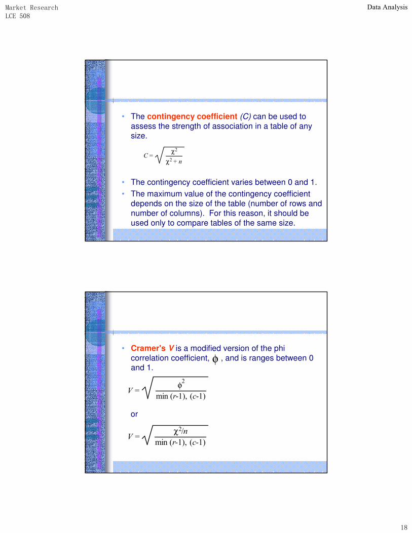
• The contingency coefficient (C) can be used to assess the strength of association in a table of any size.

• The contingency coefficient varies between 0 and 1. • The maximum value of the contingency coefficient

depends on the size of the table (number of rows and number of columns). For this reason, it should be used only to compare tables of the same size.

��χ�

χ��$��

• Cramer's V is a modified version of the phi correlation coefficient, , and is ranges between 0 and 1.

or

φ

��φ�

%��& ��

��χ��

%��& ��

��

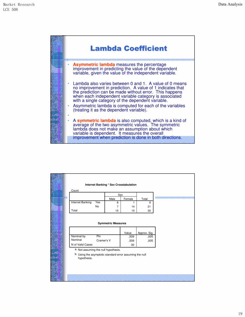
• Asymmetric lambda measures the percentage improvement in predicting the value of the dependent variable, given the value of the independent variable.

• Lambda also varies between 0 and 1. A value of 0 means no improvement in prediction. A value of 1 indicates that the prediction can be made without error. This happens when each independent variable category is associated with a single category of the dependent variable.

• Asymmetric lambda is computed for each of the variables (treating it as the dependent variable).

•• A symmetric lambda is also computed, which is a kind of

average of the two asymmetric values. The symmetric lambda does not make an assumption about which variable is dependent. It measures the overall improvement when prediction is done in both directions.

�� &�� &��

Internet Banking * Sex Crosstabulation

Count

8 1 97 14 21

15 15 30

YesNo

Internet Banking

Total

Male FemaleSex

Total

Symmetric Measures

,509 ,005,509 ,005

30

PhiCramer's V

Nominal byNominal

N of Valid Cases

Value Approx. Sig.

Not assuming the null hypothesis.a.

Using the asymptotic standard error assuming the nullhypothesis.

b.

��

��

Ordinal Data

• Kendall´s Tau b– is the most appropriate with square tables in which the

number of rows and the number of columns are equal– Its value varies between +1 and -1– The sign of the coefficient indicates the direction of the

relationship– and its absolute value indicates the strength, with larger

absolute values indicating stronger relashionships

• For a rectangular table in which the number of rows is different than the number of columns, Kendall´stau c should be used

��

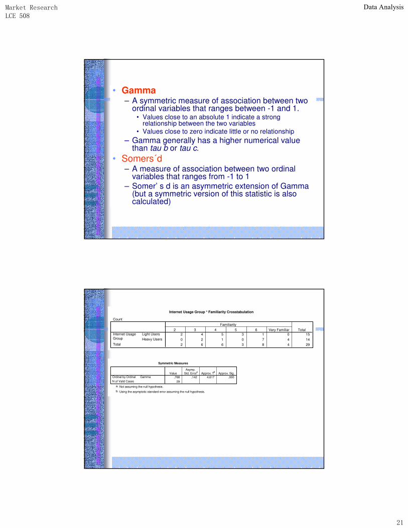
• Gamma– A symmetric measure of association between two

ordinal variables that ranges between -1 and 1.• Values close to an absolute 1 indicate a strong

relationship between the two variables• Values close to zero indicate little or no relationship

– Gamma generally has a higher numerical value than tau b or tau c.

• Somers´d– A measure of association between two ordinal

variables that ranges from -1 to 1– Somer’ s d is an asymmetric extension of Gamma

(but a symmetric version of this statistic is also calculated)

Internet Usage Group * Familiarity Crosstabulation

Count

2 4 5 3 1 0 150 2 1 0 7 4 142 6 6 3 8 4 29

Light UsersHeavy Users

Internet UsageGroup

Total

2 3 4 5 6 Very FamiliarFamiliarity

Total

Symmetric Measures

,768 ,142 4,617 ,00029

GammaOrdinal by OrdinalN of Valid Cases

ValueAsymp.

Std. Errora Approx. Tb Approx. Sig.

Not assuming the null hypothesis.a.

Using the asymptotic standard error assuming the null hypothesis.b.

��

&��&��''(��(��

*��*��

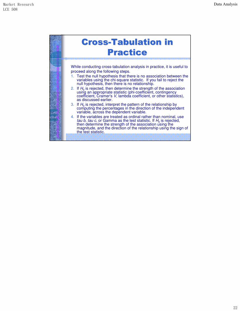
While conducting cross-tabulation analysis in practice, it is useful toproceed along the following steps.1. Test the null hypothesis that there is no association between the

variables using the chi-square statistic. If you fail to reject the null hypothesis, then there is no relationship.

2. If H0 is rejected, then determine the strength of the association using an appropriate statistic (phi-coefficient, contingency coefficient, Cramer's V, lambda coefficient, or other statistics), as discussed earlier.

3. If H0 is rejected, interpret the pattern of the relationship by computing the percentages in the direction of the independent variable, across the dependent variable.

4. If the variables are treated as ordinal rather than nominal, usetau b, tau c, or Gamma as the test statistic. If H0 is rejected, then determine the strength of the association using the magnitude, and the direction of the relationship using the sign of the test statistic.

frequency distribution cross-tabulation 12 data... · 0dunhw 5hvhdufk /&( frequency...

Documents