freshwater algae: identification and use as … ota/xyz p2: abc c03 jwbk440/bellinger march 15, 2010...
TRANSCRIPT
P1: OTA/XYZ P2: ABCc03 JWBK440/Bellinger March 15, 2010 15:33 Printer Name: Yet to Come
3Algae as Bioindicators
Biological indicators (bioindicators) may be definedas particular species or communities, which, by theirpresence, provide information on the surroundingphysical and/or chemical environment at a particu-lar site. In this book, freshwater algae are consid-ered as bioindicators in relation to water chemistry –otherwise referred to as ‘water quality’.
The basis of individual species as bioindicatorslies in their preference for (or tolerance of) particularhabitats, plus their ability to grow and out-competeother algae under particular conditions of water qual-ity. Ecological preferences and bioindicator potentialof particular algal phyla are discussed in Chapter 1.This chapter considers water quality monitoring andalgal bioindicators from an environmental perspec-tive, dealing initially with general aspects of algaeas bioindicators and then specifically with algae inthe four main freshwater systems – lakes, wetlands,rivers and estuaries.
3.1 Bioindicators and water quality
Freshwater algae provide two main types of informa-tion about water quality.
� Long-term information, the status quo. In the caseof a temperate lake, for example, routine annualdetection of an intense summer bloom of the colo-nial blue-green alga Microcystis is indicative ofpre-existing high nutrient (eutrophic) status.
� Short-term information, environmental change. Ina separate lake situation, detection of a change insubsequent years from low to high blue-green dom-inance (with increased algal biomass) may indicatea change to eutrophic status. This may be an ad-verse transition (possibly caused by human activ-ity) that requires changes in management practiceand lake restoration.
In the context of change, bioindicators can thusserve as early-warning signals that reflect the ‘health’status of an aquatic system.
3.1.1 Biomarkers and bioindicators
In the above example, environmental change (to aeutrophic state) is caused by an environmental stressfactor – in this case the influx of inorganic nu-trients into a previously low-nutrient system. Theresulting loss or dominance of particular bioindica-tor species is preceded by biochemical and phys-iological changes in the algal community referredto as ‘biomarkers.’ These may be defined (Adams,2005) as short-term indicators of exposure to envi-ronmental stress, usually expressed at suborganismallevels – including biomolecular, biochemical andphysiological responses. Examples of algal biomark-ers include DNA damage (caused by high UV irra-diation, exposure to heavy metals), osmotic shock(increased salinity), stimulation of nitrate and nitritereductase (increased aquatic nitrate concentration)
Freshwater Algae: Identification and Use as Bioindicators Edward G. Bellinger and David C. SigeeC© 2010 John Wiley & Sons, Ltd
P1: OTA/XYZ P2: ABCc03 JWBK440/Bellinger March 15, 2010 15:33 Printer Name: Yet to Come
100 3 ALGAE AS BIOINDICATORS
Physiological
Biochemical
Biomolecular
Reproduction
Bioenergetics
Growth
Competition success
seconds-days
days-weeks
weeks-years
ENVIRONMENTALCHANGE
ENVIRONMENTAL MONITORING
BIOMARKERS BIOINDICATOR
SPECIES
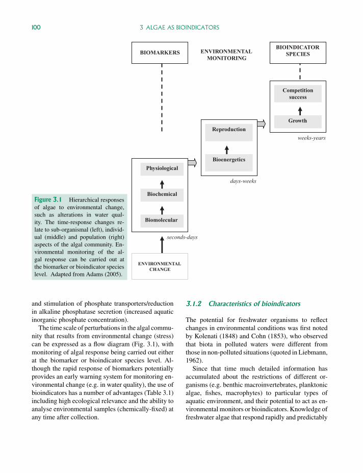
Figure 3.1 Hierarchical responsesof algae to environmental change,such as alterations in water qual-ity. The time-response changes re-late to sub-organismal (left), individ-ual (middle) and population (right)aspects of the algal community. En-vironmental monitoring of the al-gal response can be carried out atthe biomarker or bioindicator specieslevel. Adapted from Adams (2005).
and stimulation of phosphate transporters/reductionin alkaline phosphatase secretion (increased aquaticinorganic phosphate concentration).
The time scale of perturbations in the algal commu-nity that results from environmental change (stress)can be expressed as a flow diagram (Fig. 3.1), withmonitoring of algal response being carried out eitherat the biomarker or bioindicator species level. Al-though the rapid response of biomarkers potentiallyprovides an early warning system for monitoring en-vironmental change (e.g. in water quality), the use ofbioindicators has a number of advantages (Table 3.1)including high ecological relevance and the ability toanalyse environmental samples (chemically-fixed) atany time after collection.
3.1.2 Characteristics of bioindicators
The potential for freshwater organisms to reflectchanges in environmental conditions was first notedby Kolenati (1848) and Cohn (1853), who observedthat biota in polluted waters were different fromthose in non-polluted situations (quoted in Liebmann,1962).
Since that time much detailed information hasaccumulated about the restrictions of different or-ganisms (e.g. benthic macroinvertebrates, planktonicalgae, fishes, macrophytes) to particular types ofaquatic environment, and their potential to act as en-vironmental monitors or bioindicators. Knowledge offreshwater algae that respond rapidly and predictably
P1: OTA/XYZ P2: ABCc03 JWBK440/Bellinger March 15, 2010 15:33 Printer Name: Yet to Come
3.1 BIOINDICATORS AND WATER QUALITY 101
Table 3.1 Main Features of Biomarkers and Bioindicators in the Assessment of EnvironmentalChange
Major Features Biomarkers Bioindicators
Types of response Subcellular, cellular Individual-communityPrimary indicator of Exposure EffectsSensitivity to stressors High LowRelationship to cause High LowResponse variability High LowSpecificity to stressors Moderate-high Low-moderateTimescale of response Short LongEcological relevance Low HighAnalysis requirement Immediate, on site Any time after collection (fixed sample)
Adapted from Adams, 2005.
to environmental change has been particularly useful,with the identification of particular indicator speciesor combinations of species being widely used in as-sessing water quality.
Single species
In general, a good indicator species should have thefollowing characteristics:
� a narrow ecological range
� rapid response to environmental change
� well defined taxonomy
� reliable identification, using routine laboratoryequipment
� wide geographic distribution.
Combinations of species
In almost all ecological situations it is the combina-tion of different indicator species or groups that isused to characterize water quality. Analysis of all orpart of the algal community is the basis for multivari-ate analysis (Section 3.4.3), application of bioindices(Sections 3.2.2 and 3.4.4) and use of phytopigmentsas diagnostic markers (Section 3.5.2)
3.1.3 Biological monitoring versus chemicalmeasurements
In terms of chemistry, water quality includes inor-ganic nutrients (particularly phosphates and nitrates),organic pollutants (e.g. pesticides), inorganic pollu-tants (e.g. heavy metals), acidity and salinity. In anideal world, these would be measured routinely in allwater bodies being monitored, but constraints of costand time have led to the widespread application ofbiological monitoring.
The advantages of biological monitoring over sep-arate physicochemical measurements to assess waterquality are that it:
� reflects overall water quality, integrating the effectsof different stress factors over time; physicochemi-cal measurements provide information on one pointin time.
� gives a direct measure of the ecological im-pact of environmental parameters on the aquaticorganisms.
� provides a rapid, reliable and relatively inexpensiveway to record environmental conditions across anumber of sites.
Biological monitoring has been particularly use-ful, for example, in implementing the European
P1: OTA/XYZ P2: ABCc03 JWBK440/Bellinger March 15, 2010 15:33 Printer Name: Yet to Come
102 3 ALGAE AS BIOINDICATORS
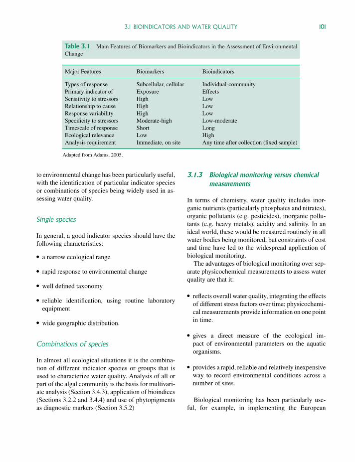
Table 3.2 Trophic Classification of Temperate Freshwater Lakes, Based on a Fixed Boundary System
Trophic Category
Ultraoligotrophic Oligotrophic Mesotrophic Eutrophic Hypertrophic
Nutrient concentration (µg l−1)Total phosphorus (mean annual value) <4 4–10 10–35 35–100 >100Orthophosphatea <2 2–5 5–100 >100DINa <10 10–30 30–100 >100Chlorophyll a concentration (µg l−1)Mean concentration in surface waters <1 1–2.5 2.5–8 8–25 >25Maximum concentration in surface waters <2.5 2.5–8 8–25 25–75 >75Total volume of planktonic algaeb 0.12 0.4 0.6–1.5 2.5–5 >5Secchi depth (m)Mean annual value >12 12–6 6–3 3–1.5 <1.5Minimum annual value >6 >3.0 3–1.5 1.5–0.7 <0.7
Table adapted from Sigee (2004). Lakes are classified according to mean nutrient concentrations and phytoplankton productivity (shadedarea). Boundary values are mainly from the OECD classification system (OECD, 1982), with the exception of orthophosphate anddissolved inorganic nitrogen (DIN), which are from Technical Standard Publication (1982).aOrthophosphate and DIN are measured as the mean surface water concentrations during the summer stagnation period.bTotal volumes (% water) of planktonic algae are for Norwegian lakes, growth season mean values (Brettum, 1989).
Union Directive relating to surface water quality (94C222/06, 10 August 1994), where Member States wereobliged to establish freshwater monitoring networksby the end of 1998.
3.1.4 Monitoring water quality: objectives
Environmental monitoring of aquatic systems, par-ticularly in relation to water quality, provides infor-mation on:
� Seasonal dynamics. In temperate lakes these in-clude hydrological measurements (water flows, res-idence time), thermal and chemical stratificationand changes in nutrient availability at the lakesurface. Epilimnion concentrations of nitrates andphosphates can fall to very low levels towards theend of stratification (late summer), and the lakecould then be dominated by algae such as dinoflag-ellates (e.g. Ceratium) and colonial blue-greens(e.g. Microcystis) which are able to carry out diur-nal migrations into the nutrient-rich hypolimnion.
� Classification of ecosystems in relation to waterquality, productivity and constituent organisms.
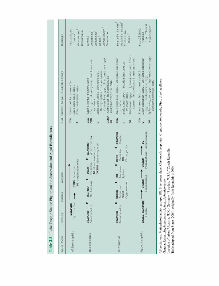
The most widely used classification (for both loticand lentic systems) is based on inorganic nutri-ent concentrations, with division into oligotrophic,mesotrophic and eutrophic systems (Table 3.2). De-tection and analysis of indicator algae (Table 3.3)provides a quick assessment of trophic statusand possible human contamination of freshwaterbodies.
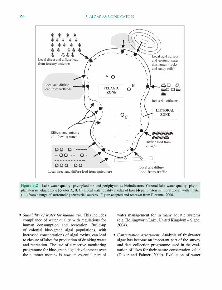
� Dynamics of nutrient and pollutant entry into theaquatic system via point or diffuse loading. Local-ized or diffuse entry of contaminants can be studiedby analysis of benthic algal communities. The po-tential use of these littoral algae in lakes, wherewater quality at the lake edge directly relates todifferent types of inflow from the catchment area,is shown in Fig. 3.2.
� Human impacts. Long-term monitoring of anthro-pogenic effects within the ecosystem – includingchanges (Section 3.2.3) such as eutrophication, in-crease in organic pollutants, acidification and heavymetal contamination. Analysis of indicator diatomswithin sediment cores has been particularly usefulin monitoring long-term changes in water qualityand general ecology (Section 3.2.2).
P1: OTA/XYZ P2: ABCc03 JWBK440/Bellinger March 15, 2010 15:33 Printer Name: Yet to Come
Tabl
e3
.3L
ake
Tro
phic
Stat
us:P
hyto
plan
kton
Succ
essi
onan
dA
lgal
Bio
indi
cato
rs
Lake Type
Spring Summer Autumn
Mid-Summer Algal Bioindicators
Example
Oligotrophic
DIATOMS
Cyclotella
DINO
Ceratium
BG
Gomphosphaeria
DIA Cyclotella comensis
Rhizosolenia spp.
G Staurodesmus spp.
Carinthian
Lakes1
Wastwater2
Ennerdale
Mesotrophic
DIATOMS
CHRYSO
DINO
DIATOMS
Asterionella Mallomonas Ceratium Asterionella
BG
Gomphosphaeria
GREEN Sphaerocystis
DIA Tabellaria flocculosa
CHR Dinobryon divergens, Mallomonas
caudata
G Sphaerocystis schroeteri,
Dictyosphaerium elegans,
Cosmarium spp, Staurastrum spp
DINO Ceratium hirundinella
BG Gomphosphaeria spp.
Lunzer
Untersee1
Bodensee3
Erken4
Windermere2
Grasmere
Eutrophic
DIATOMS
GREEN
BG
DINO
DIATOMS
Asterionella Eudorina Anabaena Ceratium Steph.
CRYPT Aphan. BG
Cryptomonas
Microcystis
DIA Aulacoseira spp., Stephanodiscus
rotula
G Eudorina spp., Pandorina morum,
Volvox spp.
BG Anabaena spp., Aphanizomenon flos-
aquae, Microcystis aeruginosa
Prairie Lakes5
Norfolk Broad2
Rostherne
Mere2
Hypertrophic
SMALL DIATOMS GREEN GREEN BG
Steph. Scenedesmus Pediaastrum Aphanocapsa
DIA Stephanodiscus hantzschii
G Scenedesmus spp., Ankistrodesmus
spp., Pediastrum spp.
BG Aphanocapsa spp., Aphanothece spp,
Synechococcus spp.
Fertilised
waters
e.g. Třeboň
fishponds6
Abb
revi
atio
ns:M
ain
phyt
opla
nkto
ngr
oups
:BG
,blu
e-gr
een
alga
e;C
hrys
o,ch
ryso
phyt
es;C
rypt
,cry
ptom
onad
s;D
ino,
dino
flage
llate
s.G
ener
a:St
eph.
,Ste
phan
odis
cus;
Aph
an.,
Aph
aniz
omen
on.
Loc
atio
nof
lake
s:1A
ustr
ia,2
UK
,3G
erm
any,
4Sw
eden
,5U
SA,6
Cze
chR
epub
lic.
Tabl
ead
apte
dfr
omSi
gee
(200
4),o
rigi
nally
from
Rey
nold
s(1
990)
.
103
P1: OTA/XYZ P2: ABCc03 JWBK440/Bellinger March 15, 2010 15:33 Printer Name: Yet to Come
104 3 ALGAE AS BIOINDICATORS
Effects and mixing of inflowing waters
Local and diffuse load from wetlands
Local direct and diffuse load from forestry activities
Diffuse load from villages
Local direct and diffuse load from agriculture
Local acid surface and groiund water discharges (rocky and sandy soils)
Industrial effluents
Local and diffuseload from traffic
A
B
C
LITTORALZONE
PELAGICZONE
Figure 3.2 Lake water quality: phytoplankton and periphyton as bioindicators. General lake water quality: phyto-plankton in pelagic zone (° sites A, B, C). Local water quality at edge of lake (• periphyton in littoral zone), with inputs(→) from a range of surrounding terrestrial sources. Figure adapted and redrawn from Eloranta, 2000.
� Suitability of water for human use. This includescompliance of water quality with regulations forhuman consumption and recreation. Build-upof colonial blue-green algal populations, withincreased concentrations of algal toxins, can leadto closure of lakes for production of drinking waterand recreation. The use of a reactive monitoringprogramme for blue-green algal development overthe summer months is now an essential part of
water management for in many aquatic systems(e.g. Hollingworth Lake, United Kingdom – Sigee,2004).
� Conservation assessment. Analysis of freshwateralgae has become an important part of the surveyand data collection programme used in the eval-uation of lakes for their nature conservation value(Duker and Palmer, 2009). Evaluation of water
P1: OTA/XYZ P2: ABCc03 JWBK440/Bellinger March 15, 2010 15:33 Printer Name: Yet to Come
3.2 LAKES 105
quality is also important for existing conservationsites. In the United Kingdom, a large number offreshwater Sites of Special Scientific Interest (SS-SIs) are believed to be affected by eutrophication(Nature Conservancy Council, 1991; Carvalho andMoss, 1995). In the case of lakes, the role of algalbioindicators in this assessment is based both oncontemporary organisms (Section 3.2.1) and fossildiatoms within sediments (Section 3.2.2).
3.2 Lakes
The use of algae as bioindicators of water qualityis influenced by the long-term retention of water inlake systems and also by the age of the lake. Reten-tion of water can be quantified as ‘water retentiontime’ (WRT), which is the average time that wouldbe taken to refill a lake basin with water if it wereemptied. WRT for most lakes and reservoirs is about1 to 10 years, but some of the world’s largest lakeshave values far in excess of this – including extremevalues of 6000 and 1225 years respectively for LakesTanganyika (Africa) and Malawi (Africa).
Characteristics of lake hydrology and age result in:
� Phytoplankton dominance. In moderate to high nu-trient deep lakes, phytoplankton populations areable to grow and are retained by the system (notflushed out). Their dominance over non-planktonicalgae and macrophytes means they are routinelyused as bioindicators.
� Long-term exposure. In many lakes, planktonic andbenthic algae have relatively long-term exposure toparticular conditions of water quality and relate tospecific chemical and physical characteristics overextended periods of time (weeks to years).
� Endemic species. Some of the world’s largest lakeshave existed over a long period of time – includingLakes Tanganyika (Africa: 2–3 million years[My]), Malawi (Africa: 4–9 My) and Baikal(Russia: 25–30 My). Long-term evolution withinthese independent and enclosed aquatic systemshas led to the generation of high proportions ofunique species (endemism), with over 50% en-
demic fauna and flora in Lakes Tanganyika andBaikal (Martens, 1997). The presence of substan-tial levels of endemism in these large water bod-ies, together with the fact that even non-endemicspecies may have unique adaptations, means thatconventional bioindices will need to be adjusted tosuit particular situations.
3.2.1 Contemporary planktonic and attachedalgae as bioindicators
Both planktonic algae (present in the main water bodyof the lake – pelagic zone), and attached algae (oc-curring around the edge of the lake – littoral zone)have been used to monitor water quality (Fig. 3.2).
Phytoplankton: general water quality
Most studies on lakes (see Section 3.2.3) have usedthe phytoplankton (rather than benthic) communityfor contemporary environmental assessment, since itis the main algal biomass, is readily sampled at sitesacross the lake and many planktonic species havedefined ecological preferences. Analysis of the phy-toplankton community from a number of sites acrossthe lake also provides information about aquatic con-ditions in general, and is the basis of broad categoriza-tion of lakes in relation to water quality, particularlytrophic state – see later.
Attached algae: ecological status and localizedwater quality
Although there have been relatively few studies us-ing attached (benthic and epiphytic) algae to assesswater quality, analysis of non-planktonic (mainly lit-toral) algae can provide useful information on generalecology and local water quality.
General ecological status As well planktonicalgae, attached algae are also important in provid-ing a measure of the general ecology of the lake.This is recognized in the European Union Framework
P1: OTA/XYZ P2: ABCc03 JWBK440/Bellinger March 15, 2010 15:33 Printer Name: Yet to Come
106 3 ALGAE AS BIOINDICATORS
Directive (WFD: European Union, 2000), which re-quires Member States to monitor the ecology of waterbodies to achieve ‘good ecological status’. Macro-phytes and attached algae together form one ‘bi-ological element’ that needs to be assessed underthis environmental programme (see also ‘multiproxyapproach’ – Section 3.2.2).
Local water quality Various authors have anal-ysed benthic or epiphytic algal populations in relationto water quality, including the extensive periphytongrowths that occur in the littoral region of many lakes.These algae are particularly useful in relation to lo-cal water conditions (e.g. localized accumulations ofmetal toxins, point source and diffuse loading at theedge of the lake), since their permanent location atparticular sites gives a high degree of spatial resolu-tion within the water body.
Localized metal accumulations Cattaneo et al.(1995) studied periphyton growing epiphytically inmacrophyte beds of a fluvial lake in the St LawrenceRiver (Canada), to see if they could resolve periphy-ton communities in relation to water quality (toxicand non-toxic levels of mercury) under differing eco-logical conditions (e.g. fine versus coarse sediment).The periphyton, composed of green algae (40%),blue-greens (25%) diatoms (25%) and other phyla,was collected from various sites and analysed in termsof taxonomic composition and size profile. Multi-variate (cluster and biotic index) analysis of peri-phyton communities gave greatest separation in re-lation to physical ecological (particularly substrate)conditions rather than water quality. The authors rec-ommended that the use of benthic algae as aquaticbioindicators should involve sampling from similarsubstrate sites to eliminate ecological variation otherthan water quality.
Point source and diffuse loading at the edge ofthe lake Water quality in the littoral zone may differconsiderably from that in the main part of the lake.This is partly due to the proximity of the terrestrialecosystem (with inflow from the surrounding catch-ment area) and partly due to the distinctive zone oflittoral macrophyte vegetation, making an importantbuffer zone between the shore and open water (Elo-ranta, 2000). Analysis of littoral algae, either by mul-tivariate analysis or determination of bioindices, hasthe potential to provide information on water quality
at particular sites along the edge of the lake in re-lation to point discharges (stream inflows, industrialand sewage discharges) and diffuse loadings. The lat-ter include input from surrounding agricultural land,discharges from domestic areas, traffic pollutants andloading from local ecosystems such as forests andpeat bogs (Eloranta, 2000) – Fig. 3.2.
Sampling and analysis of littoral algae Al-though attached algal communities (as with phyto-plankton) can theoretically be related to water qualityin terms of total biomass, this does not correlate wellwith nutrient loading (King et al., 2006) – chieflydue to grazing and (in eutrophic waters) competitionwith phytoplankton. Also, nutrients in the water canbe supplemented by nutrients arising from the sub-stratum.
Species counts, on the other hand, can provide auseful measure of water quality. Recent recommenda-tions for littoral sampling (King et al., 2006: see alsoSection 2.10) concentrate particularly on diatoms –collecting specimens from stones and macrophytes(Fig. 2.29), since these substrata are particularly com-mon at the edge of lakes. Epipelic diatoms (present onmud and silt) are probably less useful as bioindicatorssince they are particularly liable to respond to sub-strate ‘pore-water’ chemistry rather than general wa-ter quality. The epipelic diatom community of manylowland lakes also tends to be dominated by Frag-ilaria species, which take advantage of favourablelight conditions in the shallow waters, but are poorindicators of water quality – having wide tolerance tonutrient concentrations. Having obtained samples andcarried out species counts of diatoms from habitatswithin the defined littoral sampling area, weighted-average indices can be calculated as with river di-atoms (Section 3.4.5/6) and related to water quality.
3.2.2 Fossil algae as bioindicators: lakesediment analysis
Recent water legislation, including the US CleanWater Act (Barbour et al., 2000) and the EuropeanCouncil Water Framework Directive (WFD: Euro-pean Union, 2000) have required the need to assesscurrent water status in relation to some baselinestate in the past. This baseline state (referred to as
P1: OTA/XYZ P2: ABCc03 JWBK440/Bellinger March 15, 2010 15:33 Printer Name: Yet to Come
3.2 LAKES 107
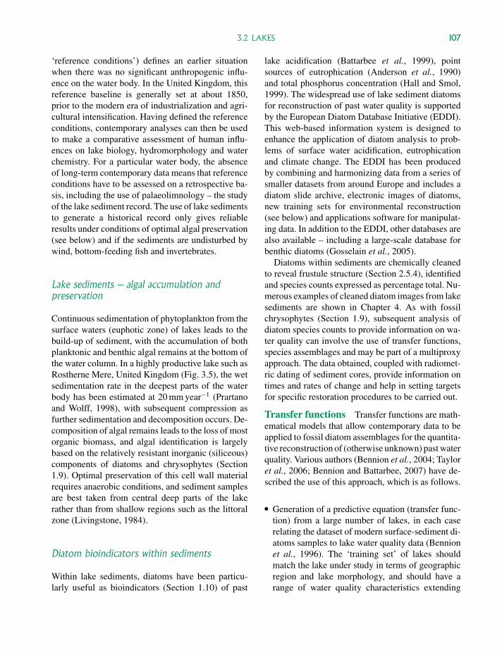
‘reference conditions’) defines an earlier situationwhen there was no significant anthropogenic influ-ence on the water body. In the United Kingdom, thisreference baseline is generally set at about 1850,prior to the modern era of industrialization and agri-cultural intensification. Having defined the referenceconditions, contemporary analyses can then be usedto make a comparative assessment of human influ-ences on lake biology, hydromorphology and waterchemistry. For a particular water body, the absenceof long-term contemporary data means that referenceconditions have to be assessed on a retrospective ba-sis, including the use of palaeolimnology – the studyof the lake sediment record. The use of lake sedimentsto generate a historical record only gives reliableresults under conditions of optimal algal preservation(see below) and if the sediments are undisturbed bywind, bottom-feeding fish and invertebrates.
Lake sediments – algal accumulation andpreservation
Continuous sedimentation of phytoplankton from thesurface waters (euphotic zone) of lakes leads to thebuild-up of sediment, with the accumulation of bothplanktonic and benthic algal remains at the bottom ofthe water column. In a highly productive lake such asRostherne Mere, United Kingdom (Fig. 3.5), the wetsedimentation rate in the deepest parts of the waterbody has been estimated at 20 mm year−1 (Prartanoand Wolff, 1998), with subsequent compression asfurther sedimentation and decomposition occurs. De-composition of algal remains leads to the loss of mostorganic biomass, and algal identification is largelybased on the relatively resistant inorganic (siliceous)components of diatoms and chrysophytes (Section1.9). Optimal preservation of this cell wall materialrequires anaerobic conditions, and sediment samplesare best taken from central deep parts of the lakerather than from shallow regions such as the littoralzone (Livingstone, 1984).
Diatom bioindicators within sediments
Within lake sediments, diatoms have been particu-larly useful as bioindicators (Section 1.10) of past
lake acidification (Battarbee et al., 1999), pointsources of eutrophication (Anderson et al., 1990)and total phosphorus concentration (Hall and Smol,1999). The widespread use of lake sediment diatomsfor reconstruction of past water quality is supportedby the European Diatom Database Initiative (EDDI).This web-based information system is designed toenhance the application of diatom analysis to prob-lems of surface water acidification, eutrophicationand climate change. The EDDI has been producedby combining and harmonizing data from a series ofsmaller datasets from around Europe and includes adiatom slide archive, electronic images of diatoms,new training sets for environmental reconstruction(see below) and applications software for manipulat-ing data. In addition to the EDDI, other databases arealso available – including a large-scale database forbenthic diatoms (Gosselain et al., 2005).
Diatoms within sediments are chemically cleanedto reveal frustule structure (Section 2.5.4), identifiedand species counts expressed as percentage total. Nu-merous examples of cleaned diatom images from lakesediments are shown in Chapter 4. As with fossilchrysophytes (Section 1.9), subsequent analysis ofdiatom species counts to provide information on wa-ter quality can involve the use of transfer functions,species assemblages and may be part of a multiproxyapproach. The data obtained, coupled with radiomet-ric dating of sediment cores, provide information ontimes and rates of change and help in setting targetsfor specific restoration procedures to be carried out.
Transfer functions Transfer functions are math-ematical models that allow contemporary data to beapplied to fossil diatom assemblages for the quantita-tive reconstruction of (otherwise unknown) past waterquality. Various authors (Bennion et al., 2004; Tayloret al., 2006; Bennion and Battarbee, 2007) have de-scribed the use of this approach, which is as follows.
� Generation of a predictive equation (transfer func-tion) from a large number of lakes, in each caserelating the dataset of modern surface-sediment di-atoms samples to lake water quality data (Bennionet al., 1996). The ‘training set’ of lakes shouldmatch the lake under study in terms of geographicregion and lake morphology, and should have arange of water quality characteristics extending
P1: OTA/XYZ P2: ABCc03 JWBK440/Bellinger March 15, 2010 15:33 Printer Name: Yet to Come
108 3 ALGAE AS BIOINDICATORS
beyond the investigation site. In the study by Ben-nion et al. (2004), for example, a north-west Eu-ropean training set of 152 relatively small shallowlakes was used for the smaller productive Scottishlochs, and a training set of 56 relatively large, deeplakes was used for the larger, deeper, less produc-tive test sites.
� Application of the training set transfer functionsto fossil diatom assemblages in sediment cores toderive past water chemistry. Reconstruction of pastenvironmental conditions involves weighted aver-aging (WA) regression and calibration, with WApartial least squares (WA-PLS) analysis (Bennionet al., 2004).
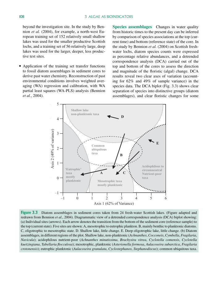
Species assemblages Changes in water qualityfrom historic times to the present day can be inferredby comparison of species associations at the top (cur-rent time) and bottom (reference state) of the core. Inthe study by Bennion et al. (2004) on Scottish fresh-water lochs, diatom species counts were expressedas percentage relative abundances, and a detrendedcorrespondence analysis (DCA) carried out of thetop and bottom of the cores to assess the directionand magnitude of the floristic (algal) change. DCAresults reveal two clear axes of variation (account-ing for 62% and 49% of sample variance) in thespecies data. The DCA biplot (Fig. 3.3) shows clearseparation of species into distinctive groups (diatomassemblages), and clear floristic changes for some
0 1 2 3 4 5 6 –1 Axis 1 (62% of Variance)
Axi
s 2
(49%
of
vari
ance
)
A
B
C
D
E
Shallow lake non-planktonic taxa
‘Eutrophic’ taxa mostly planktonic
Acidophilous to circumneutral Nutrient-poor taxa
Mesotrophic taxa mostly planktonic
Common ubiquitous taxa
0
1
2
3
4
5
–1
Figure 3.3 Diatom assemblages in sediment cores taken from 24 fresh-water Scottish lakes. (Figure adapted andredrawn from Bennion et al., 2004). Diagrammatic view of a detrended correspondence analysis (DCA) biplot showing:(a) Individual sites (arrows). Each arrow denotes the transition from the bottom of the sediment core (reference sample) tothe top (current state). Five sites are shown: A, mesotrophic to eutrophic plankton. B, mainly benthic to planktonic diatoms.C, oligotrophic to mesotrophic state. D. Shallow lake, little change. E. Deep oligotrophic lake, little change. (b) Diatomassemblages, in different regions of the plot. Shallow lake, non-planktonic (Achnanthes, Cocconeis, Cymbella, Fragilaria,Navicula); acidophilous nutrient-poor (Achnanthes minutissima, Brachysira vitrea, Cyclotella comensis, Cyclotellakuetzingiana, Tabellaria flocculosa); mesotrophic, planktonic (Asterionella formosa, Aulacoseira subarctica, Fragilariacrotonensis); eutrophic planktonic (Aulacoseira granulata, Cyclostephanos, Stephanodiscus); common ubiquitous taxa.
P1: OTA/XYZ P2: ABCc03 JWBK440/Bellinger March 15, 2010 15:33 Printer Name: Yet to Come
3.2 LAKES 109
sites (Fig. 3.3 A, B, C), which indicated clear alter-ations in water quality. In a number of deep lochs(C), limited eutrophication has occurred, with tran-sition from a Cyclotella/Achnanthes assemblage to aspecies combination (Asterionella/Aulacoseira) typ-ical of mesotrophic waters. Some shallow lochs (B)also showed nutrient increase, indicated by transitionfrom a non-planktonic (largely benthic) to a plankton-dominated diatom population. In other cases, deepoligotrophic (E) and shallow (D) lochs showed lit-tle change in diatom assemblage, indicating minimalalteration in water quality.
Multiproxy approach In a multiproxy ap-proach, diatoms are just one of a number of groupsof organisms that are counted and analysed withinthe lake sediments (Bennion and Battarbee, 2007).For European limnologists, the stimulus for a multi-proxy approach has come with the most recent Wa-ter Framework Directive (WFD; European Union,2000). This focuses on ecological integrity rather thansimply chemical water quality, for which the use ofhydro-chemical transfer functions and diatom speciesassemblage analysis are not sufficient.
Multiproxy analysis uses as broad a range of or-ganisms within the food web (e.g. pelagic food web)as possible, commensurate with those biota with re-mains that persist in the sediment in an identifiableform. In addition to micro-algae (diatoms, chrys-ophytes), fossil indicators also include macroalgae(Charophyta), protozoa (thecamoebae), higher plants(pollen and macro-remains), invertebrates (chirono-mids, ostracods, cladocerans) and vertebrates (fishscales).
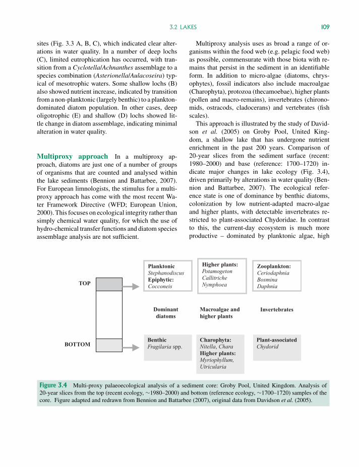
This approach is illustrated by the study of David-son et al. (2005) on Groby Pool, United King-dom, a shallow lake that has undergone nutrientenrichment in the past 200 years. Comparison of20-year slices from the sediment surface (recent:1980–2000) and base (reference: 1700–1720) in-dicate major changes in lake ecology (Fig. 3.4),driven primarily by alterations in water quality (Ben-nion and Battarbee, 2007). The ecological refer-ence state is one of dominance by benthic diatoms,colonization by low nutrient-adapted macro-algaeand higher plants, with detectable invertebrates re-stricted to plant-associated Chydoridae. In contrastto this, the current-day ecosystem is much moreproductive – dominated by planktonic algae, high
BenthicFragilaria spp.
Charophyta:Nitella, CharaHigher plants: Myriophyllum,Utricularia
Plant-associatedChydorid
PlanktonicStephanodiscusEpiphytic:Cocconeis
Higher plants: PotamogetonCallitriche Nymphoea
Zooplankton: CeriodaphniaBosminaDaphnia
Dominantdiatoms
Macroalgae and higher plants
Invertebrates
TOP
BOTTOM
Figure 3.4 Multi-proxy palaeoecological analysis of a sediment core: Groby Pool, United Kingdom. Analysis of20-year slices from the top (recent ecology, ∼1980–2000) and bottom (reference ecology, ∼1700–1720) samples of thecore. Figure adapted and redrawn from Bennion and Battarbee (2007), original data from Davidson et al. (2005).
P1: OTA/XYZ P2: ABCc03 JWBK440/Bellinger March 15, 2010 15:33 Printer Name: Yet to Come
110 3 ALGAE AS BIOINDICATORS
nutrient-adapted macrophytes and abundant zoo-plankton populations.
Other examples of a multiproxy approach to lakesediment analysis include the studies of Cattaneoet al. (1998) on heavy metal pollution in Italian Laked’Orta (Section 3.2.2) and studies on eutrophicationin six Irish lakes (Taylor et al., 2006). The latter studyinvolved sediment analysis of cladocerans, diatomsand pollen from mesotrophic-hypertrophic lakes, toreconstruct past variations in water quality and catch-ment conditions over the past 200 years. The resultsshowed that five of the lakes were in a far more pro-ductive state compared to the beginning of the sedi-ment record, with accelerated enrichment since 1980.
3.2.3 Water quality parameters: inorganic andorganic nutrients, acidity and heavymetals
A wide range of chemical parameters can beconsidered in relation to general lake water quality– including total salt content (conductivity), inor-ganic nutrients (nitrogen and phosphorus), solubleorganic nutrients, acidity, heavy metal contami-nation and presence of coloured matter (causedparticularly by humic materials). The diversity andinter-relationships of different lakes in relation tothese characteristics was emphasized by the studyof Rosen (1981), evaluating lake types and relatedplanktonic algae from August sampling of 1250Swedish standing waters. A summary from this studyof algae characteristic of Swedish acidified lakes,oligotrophic forest lakes (varying in phosphoruscontent and conductivity), humic lakes, mesotrophicand eutrophic lakes is given by Willen (2000).
In this section, the role of algae as bioindica-tors is considered in reference to four main as-pects of lake water quality – inorganic nutrients,soluble organic nutrients, acidity and heavy metalcontamination.
Inorganic nutrient status: oligotrophic toeutrophic lakes
The trophic classification of lakes, based primarilyon inorganic nutrient status, has become the major
descriptor of different lake types. Its importance re-flects:
� the key role that nutrients have on the productiv-ity, diversity and identity of algae and other lakeorganisms
� a major distinction between deep mountain lakes(typically oligotrophic) and shallow lowland lakes(typically eutrophic)
� the major impact that humans have on changingthe ecology of lakes, typically from oligotrophic toeutrophic
� ecological problems that may arise as lakes changefrom eutrophic to hypertrophic, leading to degen-erative changes that can only be reversed by humanintervention.
The diverse ecological effects that increasing nu-trient concentrations have on lake ecology have beenwidely reported (e.g. Kalff, 2002; Sigee, 2004), in-cluding the ecological destabilization that occurs atvery high nutrient concentrations.
Definition of terms Lake classification, fromoligotrophic (low nutrient) to mesotrophic and eu-trophic (high nutrient), is based on the twin crite-ria of productivity and inorganic nutrient concentra-tion – particularly nitrates and phosphates. Variousschemes have been proposed to define these terms,including one developed by the Organization forEconomic Cooperation and Development (OECD,1982). This scheme (Table 3.2) uses fixed bound-ary values for nutrient concentration (mean annualconcentration of total phosphorus), and productivity(chlorophyll-a concentration, Secchi depth). In thisscheme, for example, the mean annual concentra-tion of total phosphorus ranges from 4–10 µg l−1 foroligotrophic lakes, and 35–100 µg l−1 for eutrophicwaters. In addition to total phosphorus, boundariesfor the main soluble inorganic nutrients – orthophos-phate and dissolved inorganic nitrogen (nitrate, ni-trite, ammonia) have also been designated (TechnicalStandard Publication, 1982).
P1: OTA/XYZ P2: ABCc03 JWBK440/Bellinger March 15, 2010 15:33 Printer Name: Yet to Come
3.2 LAKES 111
Phytoplankton net production (biomass) is de-termined either as chlorophyll-a concentration(mean/maximum annual concentration in surface wa-ters) or as Secchi depth (mean/maximum annualvalue). Examples of total volumes of planktonic al-gae at different trophic levels (Norwegian lakes) arealso given in Table 3.2, together with characteristicbioindicator algae.
Algae as bioindicators of inorganic trophicstatus
Planktonic algae within lake surface (epilimnion)samples can be used to define lake trophic status interms of their overall productivity (Table 3.2) andspecies composition (Table 3.3). Species composi-tion can be related to trophic status in four mainways – seasonal succession, biodiversity, bioindica-tor species and determination of bioindices.
1. Seasonal succession. In temperate lakes, thedevelopment of algal biomass and the sequence ofphytoplankton populations (seasonal succession) di-rectly relate to nutrient availability. In all cases theseason commences with a diatom bloom, but subse-quent progression (Reynolds, 1990) can be separatedinto four main categories (Table 3.3).
� Oligotrophic lakes. In low nutrient lakes the springdiatom bloom is prolonged, and diatoms may dom-inate for the whole growth period. Chrysophytes(Uroglena) and desmids (Staurastrum) may alsobe present, and in some lakes Ceratium and Gom-phosphaeria may be able to grow in the nutrient-depleted waters by migrating down the water col-umn to higher nutrient conditions.
� Mesotrophic lakes. These have a shorter diatombloom (dominated by Asterionella), often followedby a chrysophyte phase then mid-summer dinoflag-ellate, blue-green and green algal blooms.
� Eutrophic lakes. In high nutrient lakes, the springdiatom bloom is further limited, leading to a clear-water phase (dominated by unicellular algae), fol-lowed by a mid-summer bloom in which large
unicellular (Ceratium), colonial filamentous (An-abaena) and globular (Microcystis) blue-greenspredominate.
� Hypertrophic lakes. These include artificially fertil-ized fish ponds (Pechar et al., 2002) and lakes withsewage discharges, and are dominated through-out the season by small unicellular algae withshort life cycles. The algae form a successionof dense populations, out-competing larger colo-nial organisms which are unable to establishthemselves.
2. Species diversity. Bioindices of species diver-sity can be derived from species counts and fall intothree main categories (Sigee, 2004) – species rich-ness (Margalef index), species evenness/dominance(Pielou index, Simpson index) and a combination ofrichness and dominance (Shannon–Wiener index).
One of the most commonly-used indices (d), devel-oped by Margalef (1958), combines data on the totalnumber of species identified (S) and total number ofindividuals (N), where:
d = (S − 1)/ loge N (3.1)
During the summer growth phase, species diversityis typically low in oligotrophic lakes, rising progres-sively in mesotrophic and eutrophic lakes, but fallingagain in some eutrophic/hypertrophic lakes wheresmall numbers of species may out-compete other al-gae. The effects of increasing nutrient levels on al-gal diversity (d) are illustrated by Reynolds (1990),with summer-growth values of 3–6 for the nutrient-deficient North Basin of Lake Windermere (UnitedKingdom) – falling to levels of 2–4 in a nutrient-rich lake (Crose Mere, United Kingdom) and 0.2–2for a hypertrophic water body (fertilized enclosure,Blelham Tarn, United Kingdom).
3. Bioindicator species. Some algal species andtaxonomic groups show clear preferences for par-ticular lake conditions, and can this act as potentialbioindicators. In a broad comparison of oligotrophicversus eutrophic waters, desmids (green algae) tendto occur mainly in low nutrient waters while colonial
P1: OTA/XYZ P2: ABCc03 JWBK440/Bellinger March 15, 2010 15:33 Printer Name: Yet to Come
112 3 ALGAE AS BIOINDICATORS
blue-green algae are more typical of eutrophic waters.Such generalizations are not absolute, however, sincesome desmids (e.g. Cosmarium meneghinii, Stauras-trum spp.) are typical of meso- and eutrophic lakes,while colonial blue-green algae such as Gomphos-phaeria are also found in oligotrophic waters.
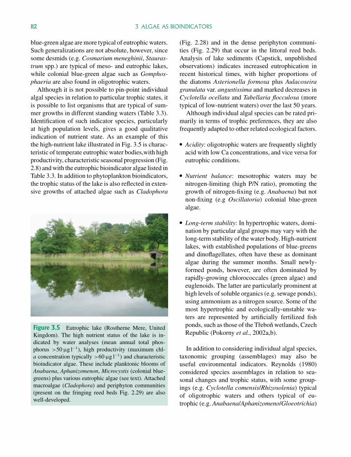
Although it is not possible to pin-point individualalgal species in relation to particular trophic states, itis possible to list organisms that are typical of sum-mer growths in different standing waters (Table 3.3).Identification of such indicator species, particularlyat high population levels, gives a good qualitativeindication of nutrient state. As an example of thisthe high-nutrient lake illustrated in Fig. 3.5 is charac-teristic of temperate eutrophic water bodies,with highproductivity, characteristic seasonal progression (Fig.2.8) and with the eutrophic bioindicator algae listed inTable 3.3. In addition to phytoplankton bioindicators,the trophic status of the lake is also reflected in exten-sive growths of attached algae such as Cladophora
Figure 3.5 Eutrophic lake (Rostherne Mere, UnitedKingdom). The high nutrient status of the lake is in-dicated by water analyses (mean annual total phos-phorus >50 µg l−1), high productivity (maximum chl-a concentration typically >60 µg l−1) and characteristicbioindicator algae. These include planktonic blooms ofAnabaena, Aphanizomenon, Microcystis (colonial blue-greens) plus various eutrophic algae (see text). Attachedmacroalgae (Cladophora) and periphyton communities(present on the fringing reed beds Fig. 2.29) are alsowell-developed.
(Fig. 2.28) and in the dense periphyton communi-ties (Fig. 2.29) that occur in the littoral reed beds.Analysis of lake sediments (Capstick, unpublishedobservations) indicates increased eutrophication inrecent historical times, with higher proportions ofthe diatoms Asterionella formosa plus Aulacoseiragranulata var. angustissima and marked decreases inCyclotella ocellata and Tabellaria flocculosa (moretypical of low-nutrient waters) over the last 50 years.
Although individual algal species can be rated pri-marily in terms of trophic preferences, they are alsofrequently adapted to other related ecological factors.
� Acidity: oligotrophic waters are frequently slightlyacid with low Ca concentrations, and vice versa foreutrophic conditions.
� Nutrient balance: mesotrophic waters may benitrogen-limiting (high P/N ratio), promoting thegrowth of nitrogen-fixing (e.g. Anabaena) but notnon-fixing (e.g Oscillatoria) colonial blue-greenalgae.
� Long-term stability: In hypertrophic waters, domi-nation by particular algal groups may vary with thelong-term stability of the water body. High-nutrientlakes, with established populations of blue-greensand dinoflagellates, often have these as dominantalgae during the summer months. Small newly-formed ponds, however, are often dominated byrapidly-growing chlorococcales (green algae) andeuglenoids. The latter are particularly prominent athigh levels of soluble organics (e.g. sewage ponds),using ammonium as a nitrogen source. Some of themost hypertrophic and ecologically-unstable wa-ters are represented by artificially fertilized fishponds, such as those of the Trebon wetlands, CzechRepublic (Pokorny et al., 2002a,b).
In addition to considering individual algal species,taxonomic grouping (assemblages) may also beuseful environmental indicators. Reynolds (1980)considered species assemblages in relation to sea-sonal changes and trophic status, with some group-ings (e.g. Cyclotella comensis/Rhizosolenia) typicalof oligotrophic waters and others typical of eu-trophic (e.g. Anabaena/Aphanizomeno/Gloeotrichia)
P1: OTA/XYZ P2: ABCc03 JWBK440/Bellinger March 15, 2010 15:33 Printer Name: Yet to Come
3.2 LAKES 113
and hypertrophic (Pediastrum/Coelastrum/Oocystis)states. Consideration of algae as groups rather thanindividual species leads on to quantitative analysisand determination of trophic indices.
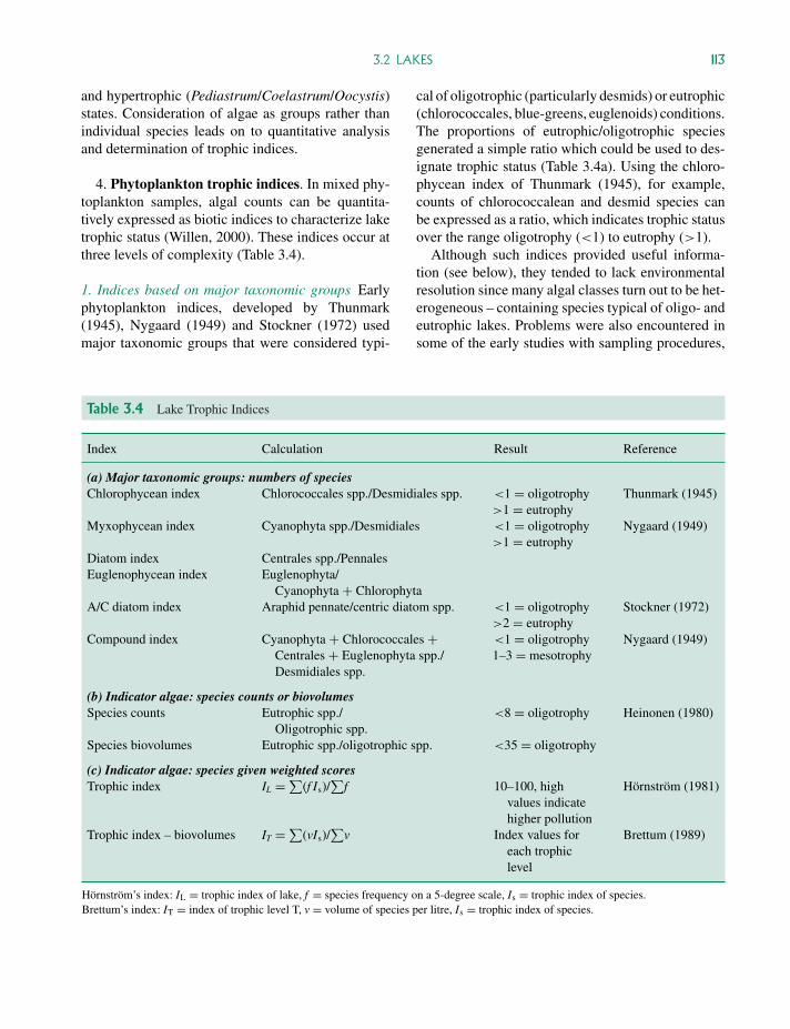
4. Phytoplankton trophic indices. In mixed phy-toplankton samples, algal counts can be quantita-tively expressed as biotic indices to characterize laketrophic status (Willen, 2000). These indices occur atthree levels of complexity (Table 3.4).
1. Indices based on major taxonomic groups Earlyphytoplankton indices, developed by Thunmark(1945), Nygaard (1949) and Stockner (1972) usedmajor taxonomic groups that were considered typi-
cal of oligotrophic (particularly desmids) or eutrophic(chlorococcales, blue-greens, euglenoids) conditions.The proportions of eutrophic/oligotrophic speciesgenerated a simple ratio which could be used to des-ignate trophic status (Table 3.4a). Using the chloro-phycean index of Thunmark (1945), for example,counts of chlorococcalean and desmid species canbe expressed as a ratio, which indicates trophic statusover the range oligotrophy (<1) to eutrophy (>1).
Although such indices provided useful informa-tion (see below), they tended to lack environmentalresolution since many algal classes turn out to be het-erogeneous – containing species typical of oligo- andeutrophic lakes. Problems were also encountered insome of the early studies with sampling procedures,
Table 3.4 Lake Trophic Indices
Index Calculation Result Reference
(a) Major taxonomic groups: numbers of speciesChlorophycean index Chlorococcales spp./Desmidiales spp. <1 = oligotrophy
>1 = eutrophyThunmark (1945)
Myxophycean index Cyanophyta spp./Desmidiales <1 = oligotrophy>1 = eutrophy
Nygaard (1949)
Diatom index Centrales spp./PennalesEuglenophycean index Euglenophyta/
Cyanophyta + ChlorophytaA/C diatom index Araphid pennate/centric diatom spp. <1 = oligotrophy
>2 = eutrophyStockner (1972)
Compound index Cyanophyta + Chlorococcales +Centrales + Euglenophyta spp./Desmidiales spp.
<1 = oligotrophy1–3 = mesotrophy
Nygaard (1949)
(b) Indicator algae: species counts or biovolumesSpecies counts Eutrophic spp./
Oligotrophic spp.<8 = oligotrophy Heinonen (1980)
Species biovolumes Eutrophic spp./oligotrophic spp. <35 = oligotrophy
(c) Indicator algae: species given weighted scoresTrophic index IL = ∑
(f Is)/∑
f 10–100, highvalues indicatehigher pollution
Hornstrom (1981)
Trophic index – biovolumes IT = ∑(vIs)/
∑v Index values for
each trophiclevel
Brettum (1989)
Hornstrom’s index: IL = trophic index of lake, f = species frequency on a 5-degree scale, Is = trophic index of species.Brettum’s index: IT = index of trophic level T, v = volume of species per litre, Is = trophic index of species.
P1: OTA/XYZ P2: ABCc03 JWBK440/Bellinger March 15, 2010 15:33 Printer Name: Yet to Come
114 3 ALGAE AS BIOINDICATORS
0.1 0.2 0.3 0.4 0.5 0.6 0.1
0
5
10
15
20
25
1980
1845
1960
1700
1500
A/C Ratio
Yea
r (A
.D.)
Dep
th in
Cor
e (c
m)
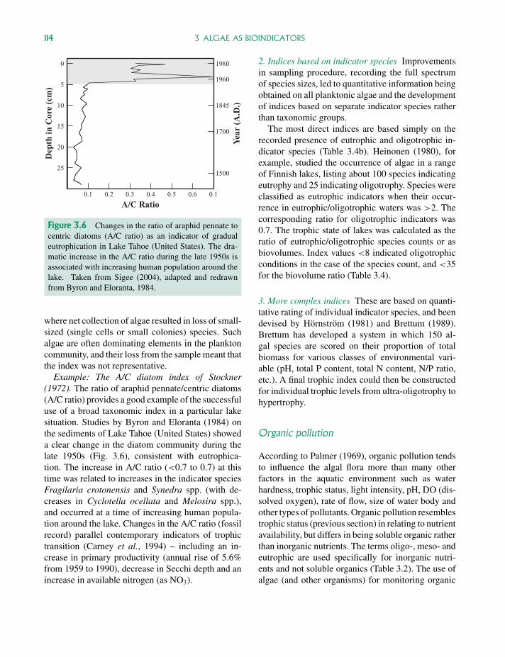
Figure 3.6 Changes in the ratio of araphid pennate tocentric diatoms (A/C ratio) as an indicator of gradualeutrophication in Lake Tahoe (United States). The dra-matic increase in the A/C ratio during the late 1950s isassociated with increasing human population around thelake. Taken from Sigee (2004), adapted and redrawnfrom Byron and Eloranta, 1984.
where net collection of algae resulted in loss of small-sized (single cells or small colonies) species. Suchalgae are often dominating elements in the planktoncommunity, and their loss from the sample meant thatthe index was not representative.
Example: The A/C diatom index of Stockner(1972). The ratio of araphid pennate/centric diatoms(A/C ratio) provides a good example of the successfuluse of a broad taxonomic index in a particular lakesituation. Studies by Byron and Eloranta (1984) onthe sediments of Lake Tahoe (United States) showeda clear change in the diatom community during thelate 1950s (Fig. 3.6), consistent with eutrophica-tion. The increase in A/C ratio (<0.7 to 0.7) at thistime was related to increases in the indicator speciesFragilaria crotonensis and Synedra spp. (with de-creases in Cyclotella ocellata and Melosira spp.),and occurred at a time of increasing human popula-tion around the lake. Changes in the A/C ratio (fossilrecord) parallel contemporary indicators of trophictransition (Carney et al., 1994) – including an in-crease in primary productivity (annual rise of 5.6%from 1959 to 1990), decrease in Secchi depth and anincrease in available nitrogen (as NO3).
2. Indices based on indicator species Improvementsin sampling procedure, recording the full spectrumof species sizes, led to quantitative information beingobtained on all planktonic algae and the developmentof indices based on separate indicator species ratherthan taxonomic groups.
The most direct indices are based simply on therecorded presence of eutrophic and oligotrophic in-dicator species (Table 3.4b). Heinonen (1980), forexample, studied the occurrence of algae in a rangeof Finnish lakes, listing about 100 species indicatingeutrophy and 25 indicating oligotrophy. Species wereclassified as eutrophic indicators when their occur-rence in eutrophic/oligotrophic waters was >2. Thecorresponding ratio for oligotrophic indicators was0.7. The trophic state of lakes was calculated as theratio of eutrophic/oligotrophic species counts or asbiovolumes. Index values <8 indicated oligotrophicconditions in the case of the species count, and <35for the biovolume ratio (Table 3.4).
3. More complex indices These are based on quanti-tative rating of individual indicator species, and beendevised by Hornstrom (1981) and Brettum (1989).Brettum has developed a system in which 150 al-gal species are scored on their proportion of totalbiomass for various classes of environmental vari-able (pH, total P content, total N content, N/P ratio,etc.). A final trophic index could then be constructedfor individual trophic levels from ultra-oligotrophy tohypertrophy.
Organic pollution
According to Palmer (1969), organic pollution tendsto influence the algal flora more than many otherfactors in the aquatic environment such as waterhardness, trophic status, light intensity, pH, DO (dis-solved oxygen), rate of flow, size of water body andother types of pollutants. Organic pollution resemblestrophic status (previous section) in relating to nutrientavailability, but differs in being soluble organic ratherthan inorganic nutrients. The terms oligo-, meso- andeutrophic are used specifically for inorganic nutri-ents and not soluble organics (Table 3.2). The use ofalgae (and other organisms) for monitoring organic
P1: OTA/XYZ P2: ABCc03 JWBK440/Bellinger March 15, 2010 15:33 Printer Name: Yet to Come
3.2 LAKES 115
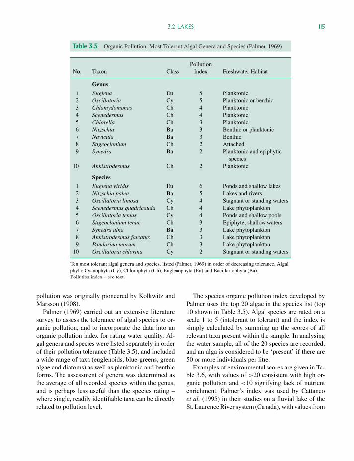
Table 3.5 Organic Pollution: Most Tolerant Algal Genera and Species (Palmer, 1969)
No. Taxon ClassPollution
Index Freshwater Habitat
Genus
1 Euglena Eu 5 Planktonic2 Oscillatoria Cy 5 Planktonic or benthic3 Chlamydomonas Ch 4 Planktonic4 Scenedesmus Ch 4 Planktonic5 Chlorella Ch 3 Planktonic6 Nitzschia Ba 3 Benthic or planktonic7 Navicula Ba 3 Benthic8 Stigeoclonium Ch 2 Attached9 Synedra Ba 2 Planktonic and epiphytic
species10 Ankistrodesmus Ch 2 Planktonic
Species
1 Euglena viridis Eu 6 Ponds and shallow lakes2 Nitzschia palea Ba 5 Lakes and rivers3 Oscillatoria limosa Cy 4 Stagnant or standing waters4 Scenedesmus quadricauda Ch 4 Lake phytoplankton5 Oscillatoria tenuis Cy 4 Ponds and shallow pools6 Stigeoclonium tenue Ch 3 Epiphyte, shallow waters7 Synedra ulna Ba 3 Lake phytoplankton8 Ankistrodesmus falcatus Ch 3 Lake phytoplankton9 Pandorina morum Ch 3 Lake phytoplankton
10 Oscillatoria chlorina Cy 2 Stagnant or standing waters
Ten most tolerant algal genera and species. listed (Palmer, 1969) in order of decreasing tolerance. Algalphyla: Cyanophyta (Cy), Chlorophyta (Ch), Euglenophyta (Eu) and Bacillariophyta (Ba).Pollution index – see text.
pollution was originally pioneered by Kolkwitz andMarsson (1908).
Palmer (1969) carried out an extensive literaturesurvey to assess the tolerance of algal species to or-ganic pollution, and to incorporate the data into anorganic pollution index for rating water quality. Al-gal genera and species were listed separately in orderof their pollution tolerance (Table 3.5), and includeda wide range of taxa (euglenoids, blue-greens, greenalgae and diatoms) as well as planktonic and benthicforms. The assessment of genera was determined asthe average of all recorded species within the genus,and is perhaps less useful than the species rating –where single, readily identifiable taxa can be directlyrelated to pollution level.
The species organic pollution index developed byPalmer uses the top 20 algae in the species list (top10 shown in Table 3.5). Algal species are rated on ascale 1 to 5 (intolerant to tolerant) and the index issimply calculated by summing up the scores of allrelevant taxa present within the sample. In analysingthe water sample, all of the 20 species are recorded,and an alga is considered to be ‘present’ if there are50 or more individuals per litre.
Examples of environmental scores are given in Ta-ble 3.6, with values of >20 consistent with high or-ganic pollution and <10 signifying lack of nutrientenrichment. Palmer’s index was used by Cattaneoet al. (1995) in their studies on a fluvial lake of theSt. Laurence River system (Canada), with values from
P1: OTA/XYZ P2: ABCc03 JWBK440/Bellinger March 15, 2010 15:33 Printer Name: Yet to Come
116 3 ALGAE AS BIOINDICATORS
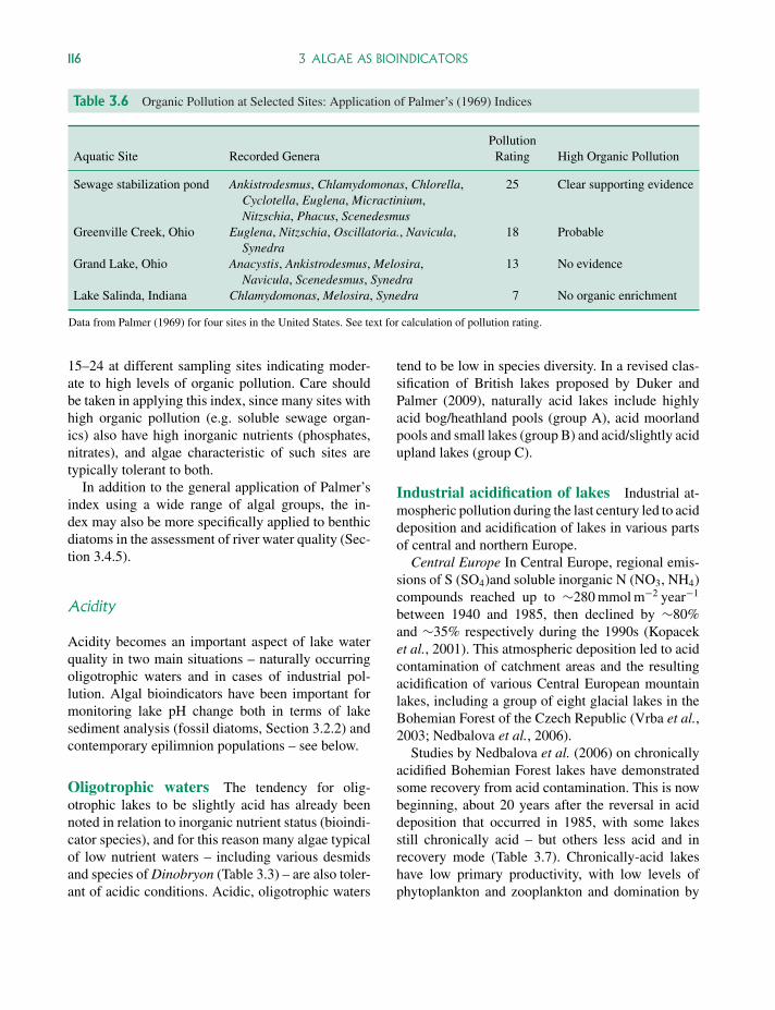
Table 3.6 Organic Pollution at Selected Sites: Application of Palmer’s (1969) Indices
Aquatic Site Recorded GeneraPollution
Rating High Organic Pollution
Sewage stabilization pond Ankistrodesmus, Chlamydomonas, Chlorella,Cyclotella, Euglena, Micractinium,Nitzschia, Phacus, Scenedesmus
25 Clear supporting evidence
Greenville Creek, Ohio Euglena, Nitzschia, Oscillatoria., Navicula,Synedra
18 Probable
Grand Lake, Ohio Anacystis, Ankistrodesmus, Melosira,Navicula, Scenedesmus, Synedra
13 No evidence
Lake Salinda, Indiana Chlamydomonas, Melosira, Synedra 7 No organic enrichment
Data from Palmer (1969) for four sites in the United States. See text for calculation of pollution rating.
15–24 at different sampling sites indicating moder-ate to high levels of organic pollution. Care shouldbe taken in applying this index, since many sites withhigh organic pollution (e.g. soluble sewage organ-ics) also have high inorganic nutrients (phosphates,nitrates), and algae characteristic of such sites aretypically tolerant to both.
In addition to the general application of Palmer’sindex using a wide range of algal groups, the in-dex may also be more specifically applied to benthicdiatoms in the assessment of river water quality (Sec-tion 3.4.5).
Acidity
Acidity becomes an important aspect of lake waterquality in two main situations – naturally occurringoligotrophic waters and in cases of industrial pol-lution. Algal bioindicators have been important formonitoring lake pH change both in terms of lakesediment analysis (fossil diatoms, Section 3.2.2) andcontemporary epilimnion populations – see below.
Oligotrophic waters The tendency for olig-otrophic lakes to be slightly acid has already beennoted in relation to inorganic nutrient status (bioindi-cator species), and for this reason many algae typicalof low nutrient waters – including various desmidsand species of Dinobryon (Table 3.3) – are also toler-ant of acidic conditions. Acidic, oligotrophic waters
tend to be low in species diversity. In a revised clas-sification of British lakes proposed by Duker andPalmer (2009), naturally acid lakes include highlyacid bog/heathland pools (group A), acid moorlandpools and small lakes (group B) and acid/slightly acidupland lakes (group C).
Industrial acidification of lakes Industrial at-mospheric pollution during the last century led to aciddeposition and acidification of lakes in various partsof central and northern Europe.
Central Europe In Central Europe, regional emis-sions of S (SO4)and soluble inorganic N (NO3, NH4)compounds reached up to ∼280 mmol m−2 year−1
between 1940 and 1985, then declined by ∼80%and ∼35% respectively during the 1990s (Kopaceket al., 2001). This atmospheric deposition led to acidcontamination of catchment areas and the resultingacidification of various Central European mountainlakes, including a group of eight glacial lakes in theBohemian Forest of the Czech Republic (Vrba et al.,2003; Nedbalova et al., 2006).
Studies by Nedbalova et al. (2006) on chronicallyacidified Bohemian Forest lakes have demonstratedsome recovery from acid contamination. This is nowbeginning, about 20 years after the reversal in aciddeposition that occurred in 1985, with some lakesstill chronically acid – but others less acid and inrecovery mode (Table 3.7). Chronically-acid lakeshave low primary productivity, with low levels ofphytoplankton and zooplankton and domination by
P1: OTA/XYZ P2: ABCc03 JWBK440/Bellinger March 15, 2010 15:33 Printer Name: Yet to Come
3.2 LAKES 117
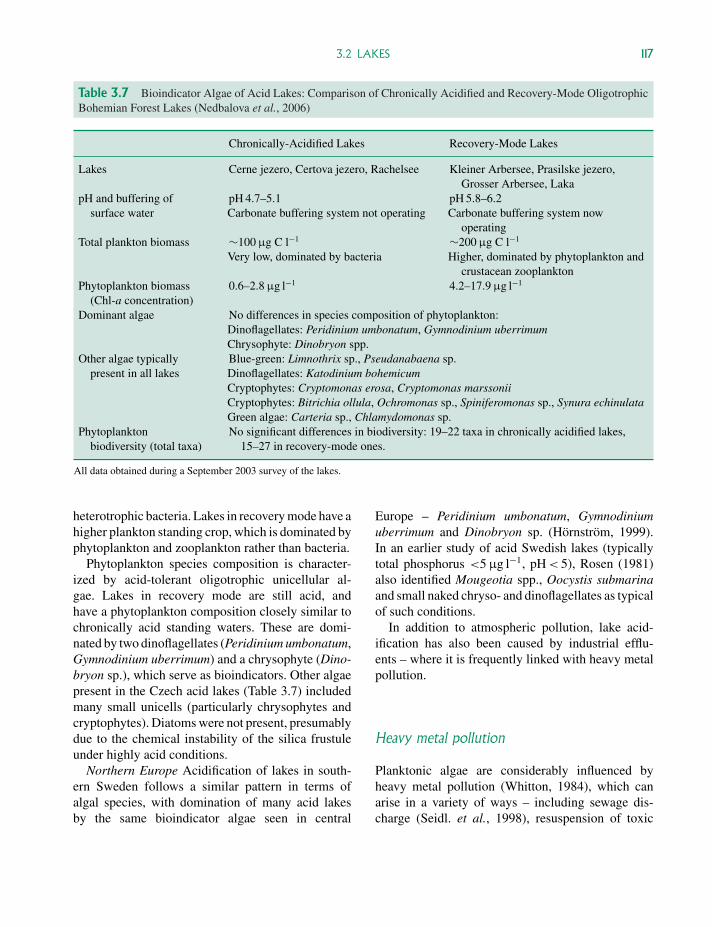
Table 3.7 Bioindicator Algae of Acid Lakes: Comparison of Chronically Acidified and Recovery-Mode OligotrophicBohemian Forest Lakes (Nedbalova et al., 2006)
Chronically-Acidified Lakes Recovery-Mode Lakes
Lakes Cerne jezero, Certova jezero, Rachelsee Kleiner Arbersee, Prasilske jezero,Grosser Arbersee, Laka
pH and buffering ofsurface water
pH 4.7–5.1Carbonate buffering system not operating
pH 5.8–6.2Carbonate buffering system now
operatingTotal plankton biomass ∼100 µg C l−1
Very low, dominated by bacteria∼200 µg C l−1
Higher, dominated by phytoplankton andcrustacean zooplankton
Phytoplankton biomass(Chl-a concentration)
0.6–2.8 µg l−1 4.2–17.9 µg l−1
Dominant algae No differences in species composition of phytoplankton:Dinoflagellates: Peridinium umbonatum, Gymnodinium uberrimumChrysophyte: Dinobryon spp.
Other algae typicallypresent in all lakes
Blue-green: Limnothrix sp., Pseudanabaena sp.Dinoflagellates: Katodinium bohemicumCryptophytes: Cryptomonas erosa, Cryptomonas marssoniiCryptophytes: Bitrichia ollula, Ochromonas sp., Spiniferomonas sp., Synura echinulataGreen algae: Carteria sp., Chlamydomonas sp.
Phytoplanktonbiodiversity (total taxa)
No significant differences in biodiversity: 19–22 taxa in chronically acidified lakes,15–27 in recovery-mode ones.
All data obtained during a September 2003 survey of the lakes.
heterotrophic bacteria. Lakes in recovery mode have ahigher plankton standing crop, which is dominated byphytoplankton and zooplankton rather than bacteria.
Phytoplankton species composition is character-ized by acid-tolerant oligotrophic unicellular al-gae. Lakes in recovery mode are still acid, andhave a phytoplankton composition closely similar tochronically acid standing waters. These are domi-nated by two dinoflagellates (Peridinium umbonatum,Gymnodinium uberrimum) and a chrysophyte (Dino-bryon sp.), which serve as bioindicators. Other algaepresent in the Czech acid lakes (Table 3.7) includedmany small unicells (particularly chrysophytes andcryptophytes). Diatoms were not present, presumablydue to the chemical instability of the silica frustuleunder highly acid conditions.
Northern Europe Acidification of lakes in south-ern Sweden follows a similar pattern in terms ofalgal species, with domination of many acid lakesby the same bioindicator algae seen in central
Europe – Peridinium umbonatum, Gymnodiniumuberrimum and Dinobryon sp. (Hornstrom, 1999).In an earlier study of acid Swedish lakes (typicallytotal phosphorus <5 µg l−1, pH < 5), Rosen (1981)also identified Mougeotia spp., Oocystis submarinaand small naked chryso- and dinoflagellates as typicalof such conditions.
In addition to atmospheric pollution, lake acid-ification has also been caused by industrial efflu-ents – where it is frequently linked with heavy metalpollution.
Heavy metal pollution
Planktonic algae are considerably influenced byheavy metal pollution (Whitton, 1984), which canarise in a variety of ways – including sewage dis-charge (Seidl. et al., 1998), resuspension of toxic
P1: OTA/XYZ P2: ABCc03 JWBK440/Bellinger March 15, 2010 15:33 Printer Name: Yet to Come
118 3 ALGAE AS BIOINDICATORS
sediments (Nayar et al., 2004) and industrial effluentdischarge.
Cattaneo et al. (1998) studied the response of lakediatoms to heavy metal contamination, analysing sed-iment cores in a northern Italian lake (Lake d’Orta)subject to industrial pollution.
Environmental changes Lake d’Orta had beenpolluted with copper, other metals (Zn, Ni, Cr) andacid (down to pH 4) for a period of over 50 years –commencing in 1926 and reaching maximum pol-lutant levels (30–100 µg Cu l−1) between 1950 and1970. Lake sediment cores collected after 1990 wereanalysed for fossil remains of diatoms, thecamoe-bians (protozoa) and cladocerans (zooplankton), allof which showed a marked reduction in mean sizeduring the period of industrial pollution.
Diatom response to pollution The initial im-pact of pollution, recorded by contemporary analy-ses, was to dramatically reduce populations of phyto-plankton, zooplankton, fish and bacteria. Subsequentsediment core analyses of diatoms showed that heavymetal pollution:
� Caused a marked decrease in the mean size of indi-viduals. The proportion of cells with a biovolumeof <102 µm3 increased from under 10% of the totalpopulation in 1920 to over 60% in 1950.
� The decrease in mean diatom size was causedprimarily by a change in taxonomic compositionfrom assemblages dominated by Cyclotella comen-sis (102–103 µm3) and C. bodanica (103–104 µm3)to populations dominated by Achnanthes minutis-sima (<102 µm3).
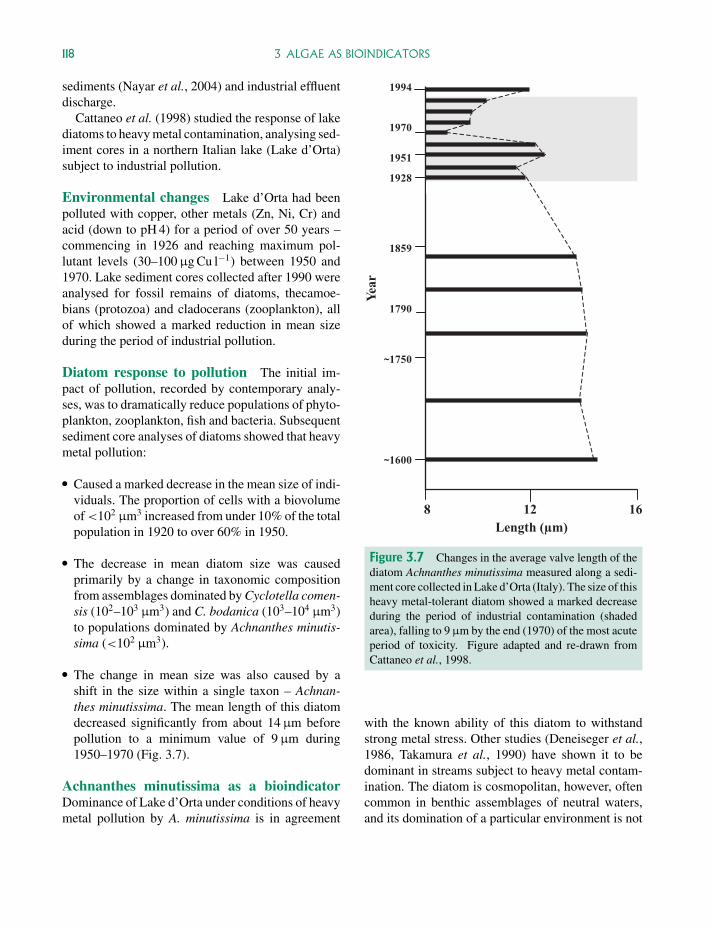
� The change in mean size was also caused by ashift in the size within a single taxon – Achnan-thes minutissima. The mean length of this diatomdecreased significantly from about 14 µm beforepollution to a minimum value of 9 µm during1950–1970 (Fig. 3.7).
Achnanthes minutissima as a bioindicatorDominance of Lake d’Orta under conditions of heavymetal pollution by A. minutissima is in agreement
1994
1970
1951
1928
1859
1790
~1750
~1600
8 12 16Length ( m)
Yea
r
Figure 3.7 Changes in the average valve length of thediatom Achnanthes minutissima measured along a sedi-ment core collected in Lake d’Orta (Italy). The size of thisheavy metal-tolerant diatom showed a marked decreaseduring the period of industrial contamination (shadedarea), falling to 9 µm by the end (1970) of the most acuteperiod of toxicity. Figure adapted and re-drawn fromCattaneo et al., 1998.
with the known ability of this diatom to withstandstrong metal stress. Other studies (Deneiseger et al.,1986, Takamura et al., 1990) have shown it to bedominant in streams subject to heavy metal contam-ination. The diatom is cosmopolitan, however, oftencommon in benthic assemblages of neutral waters,and its domination of a particular environment is not
P1: OTA/XYZ P2: ABCc03 JWBK440/Bellinger March 15, 2010 15:33 Printer Name: Yet to Come
3.3 WETLANDS 119
therefore directly indicative of heavy metal pollu-tion. In spite of this, the presence of dominant pop-ulations (coupled with a decrease in mean cell size)is consistent with severe environmental stress – andwould corroborate other environmental data indicat-ing heavy metal or acid contamination.
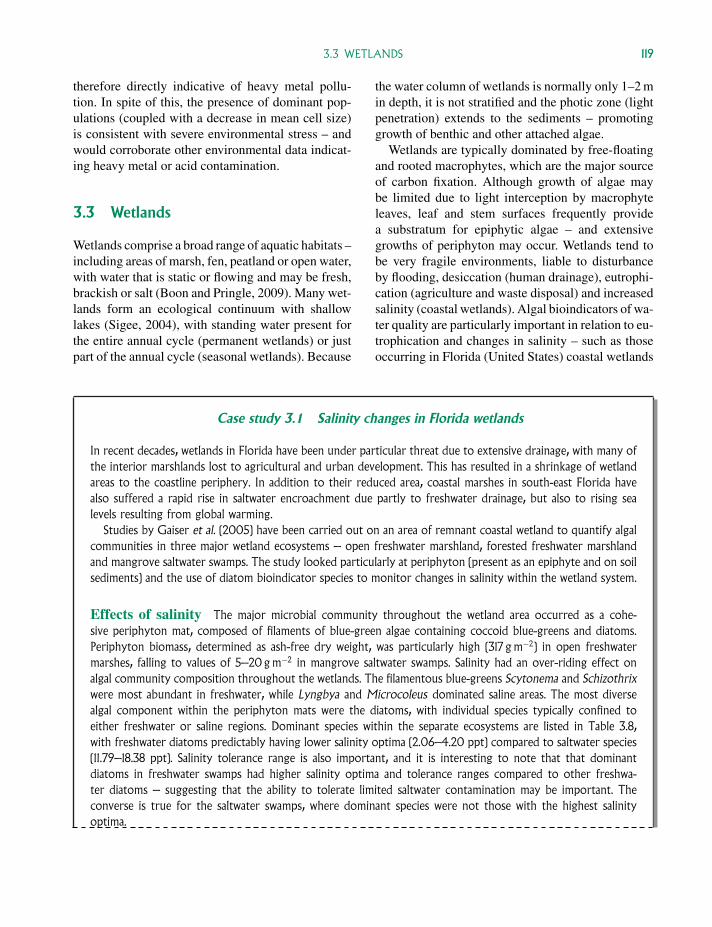
3.3 Wetlands
Wetlands comprise a broad range of aquatic habitats –including areas of marsh, fen, peatland or open water,with water that is static or flowing and may be fresh,brackish or salt (Boon and Pringle, 2009). Many wet-lands form an ecological continuum with shallowlakes (Sigee, 2004), with standing water present forthe entire annual cycle (permanent wetlands) or justpart of the annual cycle (seasonal wetlands). Because
the water column of wetlands is normally only 1–2 min depth, it is not stratified and the photic zone (lightpenetration) extends to the sediments – promotinggrowth of benthic and other attached algae.
Wetlands are typically dominated by free-floatingand rooted macrophytes, which are the major sourceof carbon fixation. Although growth of algae maybe limited due to light interception by macrophyteleaves, leaf and stem surfaces frequently providea substratum for epiphytic algae – and extensivegrowths of periphyton may occur. Wetlands tend tobe very fragile environments, liable to disturbanceby flooding, desiccation (human drainage), eutrophi-cation (agriculture and waste disposal) and increasedsalinity (coastal wetlands). Algal bioindicators of wa-ter quality are particularly important in relation to eu-trophication and changes in salinity – such as thoseoccurring in Florida (United States) coastal wetlands
Case study 3.1 Salinity changes in Florida wetlands
In recent decades, wetlands in Florida have been under particular threat due to extensive drainage, with many ofthe interior marshlands lost to agricultural and urban development. This has resulted in a shrinkage of wetlandareas to the coastline periphery. In addition to their reduced area, coastal marshes in south-east Florida havealso suffered a rapid rise in saltwater encroachment due partly to freshwater drainage, but also to rising sealevels resulting from global warming.
Studies by Gaiser et al. (2005) have been carried out on an area of remnant coastal wetland to quantify algalcommunities in three major wetland ecosystems – open freshwater marshland, forested freshwater marshlandand mangrove saltwater swamps. The study looked particularly at periphyton (present as an epiphyte and on soilsediments) and the use of diatom bioindicator species to monitor changes in salinity within the wetland system.
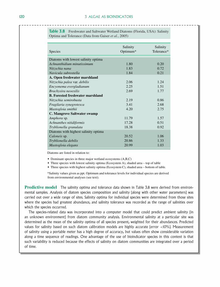
Effects of salinity The major microbial community throughout the wetland area occurred as a cohe-sive periphyton mat, composed of filaments of blue-green algae containing coccoid blue-greens and diatoms.Periphyton biomass, determined as ash-free dry weight, was particularly high (317 gm−2) in open freshwatermarshes, falling to values of 5–20 gm−2 in mangrove saltwater swamps. Salinity had an over-riding effect onalgal community composition throughout the wetlands. The filamentous blue-greens Scytonema and Schizothrixwere most abundant in freshwater, while Lyngbya and Microcoleus dominated saline areas. The most diversealgal component within the periphyton mats were the diatoms, with individual species typically confined toeither freshwater or saline regions. Dominant species within the separate ecosystems are listed in Table 3.8,with freshwater diatoms predictably having lower salinity optima (2.06–4.20 ppt) compared to saltwater species(11.79–18.38 ppt). Salinity tolerance range is also important, and it is interesting to note that that dominantdiatoms in freshwater swamps had higher salinity optima and tolerance ranges compared to other freshwa-ter diatoms – suggesting that the ability to tolerate limited saltwater contamination may be important. Theconverse is true for the saltwater swamps, where dominant species were not those with the highest salinityoptima.
P1: OTA/XYZ P2: ABCc03 JWBK440/Bellinger March 15, 2010 15:33 Printer Name: Yet to Come
120 3 ALGAE AS BIOINDICATORS
Table 3.8 Freshwater and Saltwater Wetland Diatoms (Florida, USA): SalinityOptima and Tolerance (Data from Gaiser et al., 2005)
SpeciesSalinity
Optimum*Salinity
Tolerance*
Diatoms with lowest salinity optimaAchnanthidium minutissimum 1.80 0.20Nitzschia nana 1.83 0.72Navicula subrostella 1.84 0.21A. Open freshwater marshlandNitzschia palea var. debilis 2.06 1.24Encyonema evergladianum 2.25 1.51Brachysira neoexilis 2.69 1.77B. Forested freshwater marshlandNitzschia semirobusta 2.19 0.86Fragilaria synegrotesca 3.41 2.68Mastogloia smithii 4.20 2.75C. Mangrove Saltwater swampAmphora sp. 11.79 1.57Achnanthes nitidiformis 17.28 0.51Tryblionella granulata 18.38 0.92Diatoms with highest salinity optimaCaloneis sp. 20.52 1.06Tryblionella debilis 20.86 1.33Mastogloia elegans 20.99 1.03
Diatoms are listed in relation to:
� Dominant species in three major wetland ecosystems (A,B,C)� Three species with lowest salinity optima (Ecosystem A), shaded area – top of table� Three species with highest salinity optima (Ecosystem C), shaded area – bottom of table.
*Salinity values given as ppt. Optimum and tolerance levels for individual species are derivedfrom environmental analyses (see text).
Predictive model The salinity optima and tolerance data shown in Table 3.8 were derived from environ-mental samples. Analysis of diatom species composition and salinity (along with other water parameters) wascarried out over a wide range of sites. Salinity optima for individual species were determined from those siteswhere the species had greatest abundance, and salinity tolerance was recorded as the range of salinities overwhich the species occurred.
The species-related data was incorporated into a computer model that could predict ambient salinity (inan unknown environment) from diatom community analysis. Environmental salinity at a particular site wasdetermined as the mean of the salinity optima of all species present, weighted for their abundances. Predictedvalues for salinity based on such diatom calibration models are highly accurate (error <10%). Measurementof salinity using a portable meter has a high degree of accuracy, but values often show considerable variationalong a time sequence of readings. One advantage of the use of bioindicator species in this context is thatsuch variability is reduced because the effects of salinity on diatom communities are integrated over a periodof time.
P1: OTA/XYZ P2: ABCc03 JWBK440/Bellinger March 15, 2010 15:33 Printer Name: Yet to Come
3.4 RIVERS 121
3.4 Rivers
Until recently, monitoring of river water qualityin many countries (Kwandrans et al., 1998) wasbased mainly on Escherichia coli titre (sewage con-tamination) and chlorophyll-a concentration (trophicstatus). Chlorophyll-a classification of the FrenchNational Basin Network (RNB), for example, dis-tinguished five water quality levels (Prygiel andCoste, 1996): normal (chlorophyll-a concentration≤10 µg ml−1), moderate pollution (10–≤60), distinctpollution (60–≤120), severe pollution (120–≤300)and catastrophic pollution (>300).
The use of microalgae as bioindicators was pio-neered by Patrick (Patrick et al., 1954) and has con-centrated particularly on benthic organisms, since therapid transit of phytoplankton with water flow meansthat these algae have little time to adapt to envi-ronmental changes at any point in the river system.In contrast, benthic algae (periphyton and biofilms)are permanently located at particular sites, integrat-ing physical and chemical characteristics over time,and are ideal for monitoring environmental qual-ity. Examples of benthic algae present on rocks andstones within a fast-flowing stream are shown inFig. 2.23. The use of the periphyton communityfor biomonitoring normally involves either the entirecommunity, or one particular taxonomic group – thediatoms.
3.4.1 The periphyton community
Analysis of the entire periphyton community clearlygives a broader taxonomic assessment of the ben-thic algal population compared to diatoms only,but the predominance of filamentous algae makesquantitative analysis difficult. Various authors haveused periphyton analysis to characterize water qual-ity, including a study of fluvial lakes by Catta-neo et al. (1995 – Section 3.2.1). This showedthat epiphytic communities could be monitored bothin terms of size structure and taxonomic compo-sition, leading to statistical resolution of physi-cal (substrate) and water quality (mercury toxicity)parameters.
3.4.2 River diatoms
Contemporary biomonitoring of river water qualityhas tended to concentrate on just one periphyton con-stituent – the diatoms. These have various advantagesas bioindicators – including predictable tolerancesto environmental variables, widespread occurrencewithin lotic systems, ease of counting and a speciesdiversity that permits a detailed evaluation of envi-ronmental parameters. The major drawbacks to di-atoms in this respect is the requirement for complexspecimen preparation and the need for expert identi-fication.
Attached diatoms can be found on a variety of sub-strates including sand, gravel, stones, rock, wood andaquatic macrophytes (Table 2.6). The composition ofthe communities that develop is in response to waterflow, natural water chemistry, eutrophication, toxicpollution and grazing.
Various authors have proposed precise protocolsfor the collection, specimen preparation and numeri-cal analysis of benthic diatoms to ensure uniformityof water quality assessment (see below). More gen-eral aspects of periphyton sampling are discussed inSection 2.10.
Sample collection
The sampling procedure proposed by Round (1993)involves collection of diatom samples from a reachof a river where there is a continuous flow of wa-ter over stones. About five small stones (up to 10 cmin diameter) are taken from the river bed, avoidingthose covered with green algal or moss growths. Thediatom flora can be removed from the stones either inthe field or back in the laboratory. As an alternativeto natural communities, artificial substrates can beused to collect diatoms at selected sample sites. Theseovercome the heterogeneity of natural substrata andconsequently standardize comparisons between col-lection sites, but presuppose that the full spectrum ofalgal species will grow on artificial media. Dela-Cruzet al. (2006) used this approach to sample diatomsin south-eastern Australian rivers, suspending glassslides in a sampling frame 0.5 m below the water sur-face. Slides were exposed over a 4-week period to
P1: OTA/XYZ P2: ABCc03 JWBK440/Bellinger March 15, 2010 15:33 Printer Name: Yet to Come
122 3 ALGAE AS BIOINDICATORS
allow adequate recruitment and colonization of pe-riphytic diatoms before identifying and enumeratingthe assemblages.
Specimen preparation
The diatoms are then cleaned by acid digestion, andan aliquot of cleaned sample is then mounted on amicroscope slide in a suitable high refractive indexmounting medium such as Naphrax. Canada balsamshould not be used as it does not have a high enoughrefractive index to allow resolution of the markingson the diatom frustule.
Cleaning diatoms and mounting them in Naphraxmeans that identification and counts are made frompermanent prepared slides, rather than from volumeor sedimentation chambers (Section 2.5.2). It is nor-mal to use a ×10 eyepiece and a ×100 oil immersionobjective lens on the microscope for this purpose. Be-fore counting it is always desirable to scan the slideat a ×200 or ×400 magnification to determine whichare the dominant species.
Numerical analysis
Diatoms on the slide are identified to either genusor species level and a total of 100–500+ counted,depending on the requirements of the analysis beingused. Once the counting has been completed and theresults recorded in a standardized format, the datamay be processed.
In recent times there has developed a dual approachto analysis of periphytic diatoms in relation to waterquality:
� evaluation of the entire diatom community (Section3.4.3), often involving multivariate analysis
� determination of numerical indices based on keybioindicator species (Section 3.4.4).
Individual studies have either used these ap-proaches in combination (e.g. Dela-Cruz et al., 2006)or separately.
3.4.3 Evaluation of the diatom community
The term ‘diatom community’ refers to all the di-atom species present within an environmental sam-ple. Species counts can either be expressed directly(number of organisms per unit area of substratum) oras a proportion of the total count. Evaluation of thediatom community in relation to water quality mayeither involve analysis based on main species, or amore complex statistical approach using multivariatetechniques.
Main species
Various authors have considered different levels ofwater quality in terms of distinctive diatom assem-blages. Round (1993) proposed the following classifi-cation, based on results from a range of British rivers.In this assessment five major zones (categories) ofincreasing pollution (inorganic and organic solublenutrients) were described:
Zone 1: Clean water in the uppermost reachesof a river (low pH) Here the dominant specieswere the small Eunotia exigua and Achnanthes mi-crocephala, both of which attached strongly to stonesurfaces.
Zone 2: Richer in nutrients and a little higherpH (around 5.6–7.1) This zone was dominatedby Hannaea arcus, Fragilaria capucina var lanceo-lata and Achnanthes minutissima. Tabellaria floccu-losa and Peronia fibula were also common in someinstances.
Zone 3: Nutrient rich with a higher pH(6.5–7.3) Dominant diatoms included Achnanthesminutissima with Cymbella minuta in the middlereaches and Cocconeis placetula, Reimeria sinuateand Amphora pediculus in the lower reaches.
Zone 4: Eutrophic but flora restricted throughother inputs Fewer sites in this category werefound and more work was considered necessary toprecisely typify its flora. However the major di-atom associated with the decline in water quality was
P1: OTA/XYZ P2: ABCc03 JWBK440/Bellinger March 15, 2010 15:33 Printer Name: Yet to Come
3.4 RIVERS 123
Gomphonema parvulum together with the absence ofspecies in the Amphora, Cocconeis, Reimeria group.
Zone 5: Severely polluted sites, where the di-atom flora is very restricted As with Zone 4 notmany sites in this category have been investigated andmore work is needed. The flora was frequently dom-inated by small species of Navicula (e.g. N. atomusand N. pelliculosa). Detailed identification of thesesmall species can be difficult, especially if only a lightmicroscope is available. Round (1993) concluded thatidentification to species level for these was unnec-essary and merely to record their presence in largenumbers is enough. If the pollution is not extremethere may be associated species present such as Gom-phonema parvulum, Amphora veneta and Naviculaaccomoda. Other pollution-tolerant species includeNavicula goeppertiana and Gomphonema augur.
Round’s diatom assessment for British rivers iscompared with those of other analysts in Table 3.9 forcategories of moderate and severe nutrient pollution.Although there is substantial similarity in terms ofspecies composition, differences do occur – to someextent reflecting differences in river sizes and ge-ographical location. These differences highlight theproblems involved in attempting to establish standardspecies listings for water quality evaluation.
Multivariate analysis
Multivariate analysis can be used to compare diatomassemblages and to make an objective assessment ofspecies groupings in relation to environmental param-eters. Soininen et al. (2004) analysed benthic diatomcommunities in approximately 200 Finnish streamsites to determine the major environmental correlatesin boreal running waters. Multivariate statistical anal-ysis was used to define:
� diatom assemblage types
� key indicator species that differentiated betweenthe various assemblage groups
� relative contribution of local environmental factorsand broader geographical parameters in determin-ing diatom community structure.
The results showed that the ∼200 sites sampledcould be resolved into major groupings which corre-sponded to distinctive ecoregions (Table 3.10). En-vironmental parameters characterizing these groupsrelated to water quality (conductivity, total P concen-tration, water humic content), local hydrology andregional factors. The impact of local hydrology isshown by the presence of planktonic diatoms in ben-thic samples where rivers are connecting lakes (GroupD) or have numerous ponds and lakes within the wa-tercourses (Group J). Group H had a very distinctdiatom flora characteristic of this extreme subarcticregion.
These authors concluded that although analysisof diatom communities provides a useful indica-tion of water quality, hydrology and regional factorsmust also be taken into account. The different di-atom communities identified in this study comparedwell with those documented for stream macroin-vertabrates, suggesting that bioassessment of borealwaters in Finland would benefit from integrated mon-itoring of these two taxonomic groups.
3.4.4 Human impacts and diatom indices
Diatom indices have been widely used in assessingwater quality and in monitoring human impacts onfreshwater systems. The latter can be considered ei-ther in terms of change from an original state, or inrelation to specific human effects.
Change from a ‘natural’ community
The use of benthic diatom populations to assessanthropogenic impacts on water quality impliescomparison of current conditions to a natural originalcommunity, with deviation from this due to humanactivities such as eutrophication, toxic pollutionand changes in hydrology. This concept is implicitin some major research programmes, such as theEuropean Council Water Framework Directive(WFD: European Union, 2000) where the baselineis referred to as ‘reference conditions.’ In the caseof lakes (Section 3.2.2), reference conditions canbe determined by on-site extrapolation into the past
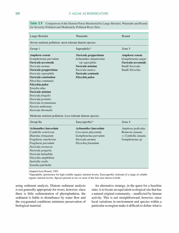
P1: OTA/XYZ P2: ABCc03 JWBK440/Bellinger March 15, 2010 15:33 Printer Name: Yet to Come
124 3 ALGAE AS BIOINDICATORS
Table 3.9 Comparison of the Diatom Floras Monitored by Lange-Bertalot, Watanabe and Roundfor Severely-Polluted and Moderately-Polluted River Sites
Lange-Bertalot Watanabe Round
Severe nutrient pollution: most tolerant diatom species.
Group 1 Saprophilic* Zone 5
Amphora venetaGomphonema parvulumNavicula accomodaNavicula atomusNavicula goeppertianaNavicula saprophilaNavicula seminulumNitzschia communisNitzschia paleaSynedra ulnaNavicula minimaNavicula frugalisNavicula permitisNavicula twymanianaNavicla umbonataNavicula thermalis
Navicula goeppertianaAchnanthes minutissima
var saprophilaNavicula minimaNavicula muticaNavicula seminulaNitzschia palea
Amphora venetaGomphonema augurNavicula accomodaSmall NaviculaSmall Nitzschia
Moderate nutrient pollution: Less-tolerant diatom species.
Group IIa Eurysaprobic* Zone 4
Achnanthes lanceolataCymbella ventricosaDiatoma elongatumFragilaria vaucheriaeFragilaria parvulumNavicula avenaceaNavicula gregariaNavicula halophilaNitzschia amphibianSurirella ovalisSynedra pulchella
Achnanthes lanceolataCocconeis placentulaGomphonema parvulumNavicula atomusNitzschia frustulum
Amphora pediculusReimeria sinuata= Cymbella sinuataGomphonema sp.
Adapted from Round, 1993.*Saprophilic (preference for high soluble organic nutrient levels), Eurysaprobic (tolerant of a range of solubleorganic nutrient levels). Species present in two or more of the lists area shown in bold.
using sediment analysis. Diatom sediment analysisis not generally appropriate for rivers, however, sincethere is little sedimentation of phytoplankton, thesediment is liable to disturbance by water flow andthe oxygenated conditions minimize preservation ofbiological material.
An alternative strategy, in the quest for a baselinestate, is to locate an equivalent ecological site that hasa natural original community – unaffected by humanactivity. This is not straightforward, however, sincelocal variations in environment and species within aparticular ecoregion make it difficult to define what is
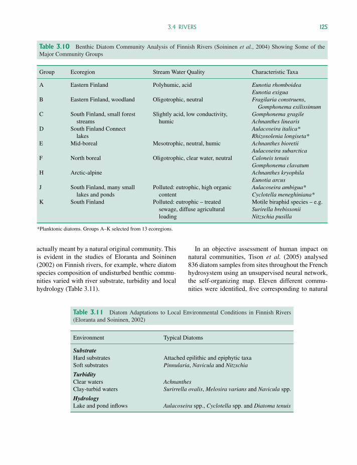
P1: OTA/XYZ P2: ABCc03 JWBK440/Bellinger March 15, 2010 15:33 Printer Name: Yet to Come
3.4 RIVERS 125
Table 3.10 Benthic Diatom Community Analysis of Finnish Rivers (Soininen et al., 2004) Showing Some of theMajor Community Groups
Group Ecoregion Stream Water Quality Characteristic Taxa
A Eastern Finland Polyhumic, acid Eunotia rhomboideaEunotia exigua
B Eastern Finland, woodland Oligotrophic, neutral Fragilaria construens,Gomphonema exilissimum
C South Finland, small foreststreams
Slightly acid, low conductivity,humic
Gomphonema gragileAchnanthes linearis
D South Finland Connectlakes
Aulacoseira italica*Rhizosolenia longiseta*
E Mid-boreal Mesotrophic, neutral, humic Achnanthes bioretiiAulacoseira subarctica
F North boreal Oligotrophic, clear water, neutral Caloneis tenuisGomphonema clavatum
H Arctic-alpine Achnanthes kryophilaEunotia arcus
J South Finland, many smalllakes and ponds
Polluted: eutrophic, high organiccontent
Aulacoseira ambigua*Cyclotella meneghiniana*
K South Finland Polluted: eutrophic – treatedsewage, diffuse agriculturalloading
Motile biraphid species – e.g.Surirella brebissoniiNitzschia pusilla
*Planktonic diatoms. Groups A–K selected from 13 ecoregions.
actually meant by a natural original community. Thisis evident in the studies of Eloranta and Soininen(2002) on Finnish rivers, for example, where diatomspecies composition of undisturbed benthic commu-nities varied with river substrate, turbidity and localhydrology (Table 3.11).
In an objective assessment of human impact onnatural communities, Tison et al. (2005) analysed836 diatom samples from sites throughout the Frenchhydrosystem using an unsupervised neural network,the self-organizing map. Eleven different commu-nities were identified, five corresponding to natural
Table 3.11 Diatom Adaptations to Local Environmental Conditions in Finnish Rivers(Eloranta and Soininen, 2002)
Environment Typical Diatoms
SubstrateHard substrates Attached epilithic and epiphytic taxaSoft substrates Pinnularia, Navicula and Nitzschia
TurbidityClear waters AchnanthesClay-turbid waters Surirrella ovalis, Melosira varians and Navicula spp.
HydrologyLake and pond inflows Aulacoseira spp., Cyclotella spp. and Diatoma tenuis
P1: OTA/XYZ P2: ABCc03 JWBK440/Bellinger March 15, 2010 15:33 Printer Name: Yet to Come
126 3 ALGAE AS BIOINDICATORS
(undisturbed) conditions and relating to five differentecoregions (i.e. river types with similar altitude rangeand geological characteristics). The six other commu-nities were typical of rivers that had been disturbedby human activity. Although natural variability oc-curred within individual ecoregions (similar to thatnoted in Finnish rivers, see above), this was greatlyexceeded by the effects of pollution at the differentsampling sites. The study aimed to identify diatomindicators for different types of anthropogenic distur-bance by comparing benthic diatom communities innatural and disturbed sites.
Use of bioindicators
An alternative approach to analysing human impact interms of general disturbance is to use diatom indiceswith indicator species that directly reflect particularenvironmental changes resulting from human activi-ties. Individual species can be numerically weightedto reflect their degree of environmental specificity.Bioindicators may relate to single parameters suchas total-P (trophic diatom index – TDI; e.g. Hofman,1996) or reflect more general aspects of water qual-ity, combining organic loading and inorganic nutri-ent concentration (IPS: index of pollution sensitivity,GDI: generic diatom index). Diatom indicator listsfor other variables such as salinity, trophy, nitrogenmetabolism types, pH and Oxygen requirements havealso been published (van Dam et al., 1994).
3.4.5 Calculation of diatom indices
As with lake phytoplankton indices (Section 3.2.3)the benefit of river diatom indices is that they reducecomplex biological communities (involving a rangeof species) to a single numerical value. This providesa very simple quantitative evaluation which can be ap-preciated and used by biologists and non-biologistsalike. The disadvantage of an index is that poten-tially useful information may be lost as counts of in-dividual species are brought together and combinedinto a general evaluation. Diatom indices, based onbioindicator algae, are either single or multiple taxonassessments.
Single taxon assessment
Indices based on a single species represent a verysimple environmental approach.
� Kothe’s Index. This is referred to as the ‘speciesdeficiency index’ (F) and relates the number ofcells (N1) of a particular key species at site 1 to thenumber (Nx) at site x, where:
F = N1 − Nx
N1× 100 (3.2)
This very simple index is assessing environmental im-pact on a single species. It assumes that site 1 is thetypical one for that river and that changes in the num-bers of the selected species will occur at other sites(for example a decline with downstream pollution).
Multiple taxon indices
Most diatom indices are based on multiple taxa (gen-era or species). They are determined either in termsof the presence/absence of key indicator species (e.g.Palmer’s index) or are based on the weighted averageequation of Zelinka and Marvan (1961):
Index =
n∑j=1
a j s jv j
n∑j=1
a jv j
(3.3)
Where:aj = is the relative abundance (proportion) of
species j in the samplesj = the pollution sensitivity of species jvj = the indicator value of species jn = is the number of species counted in the sam-
ple.
Different indices adapt this equation in differentways, and the performance of a particular index de-pends on which taxa are used, the number of taxa andthe values given for the constants s and v for eachtaxon. The values of individual indices based on thisequation vary from 1 to a maximum value equal to thehighest value of s. Commonly used indices includethe following.
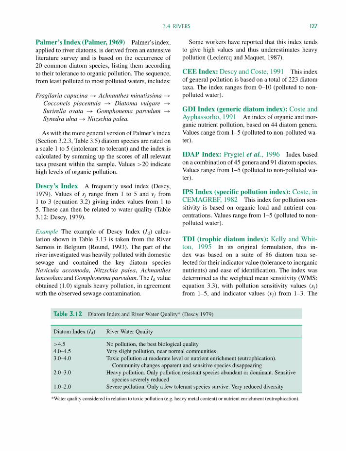
P1: OTA/XYZ P2: ABCc03 JWBK440/Bellinger March 15, 2010 15:33 Printer Name: Yet to Come
3.4 RIVERS 127
Palmer’s Index (Palmer, 1969) Palmer’s index,applied to river diatoms, is derived from an extensiveliterature survey and is based on the occurrence of20 common diatom species, listing them accordingto their tolerance to organic pollution. The sequence,from least polluted to most polluted waters, includes:
Fragilaria capucina → Achnanthes minutissima →Cocconeis placentula → Diatoma vulgare →Surirella ovata → Gomphonema parvulum →Synedra ulna → Nitzschia palea.
As with the more general version of Palmer’s index(Section 3.2.3, Table 3.5) diatom species are rated ona scale 1 to 5 (intolerant to tolerant) and the index iscalculated by summing up the scores of all relevanttaxa present within the sample. Values >20 indicatehigh levels of organic pollution.
Descy’s Index A frequently used index (Descy,1979). Values of sj range from 1 to 5 and vj from1 to 3 (equation 3.2) giving index values from 1 to5. These can then be related to water quality (Table3.12: Descy, 1979).
Example The example of Descy Index (Id) calcu-lation shown in Table 3.13 is taken from the RiverSemois in Belgium (Round, 1993). The part of theriver investigated was heavily polluted with domesticsewage and contained the key diatom speciesNavicula accomoda, Nitzschia palea, Achnantheslanceolata and Gomphonema parvulum. The Id valueobtained (1.0) signals heavy pollution, in agreementwith the observed sewage contamination.
Some workers have reported that this index tendsto give high values and thus underestimates heavypollution (Leclercq and Maquet, 1987).
CEE Index: Descy and Coste, 1991 This indexof general pollution is based on a total of 223 diatomtaxa. The index ranges from 0–10 (polluted to non-polluted water).
GDI Index (generic diatom index): Coste andAyphassorho, 1991 An index of organic and inor-ganic nutrient pollution, based on 44 diatom genera.Values range from 1–5 (polluted to non-polluted wa-ter).
IDAP Index: Prygiel et al., 1996 Index basedon a combination of 45 genera and 91 diatom species.Values range from 1–5 (polluted to non-polluted wa-ter).
IPS Index (specific pollution index): Coste, inCEMAGREF, 1982 This index for pollution sen-sitivity is based on organic load and nutrient con-centrations. Values range from 1–5 (polluted to non-polluted water).
TDI (trophic diatom index): Kelly and Whit-ton, 1995 In its original formulation, this in-dex was based on a suite of 86 diatom taxa se-lected for their indicator value (tolerance to inorganicnutrients) and ease of identification. The index wasdetermined as the weighted mean sensitivity (WMS:equation 3.3), with pollution sensitivity values (sj)from 1–5, and indicator values (vj) from 1–3. The
Table 3.12 Diatom Index and River Water Quality* (Descy 1979)
Diatom Index (Id) River Water Quality
>4.5 No pollution, the best biological quality4.0–4.5 Very slight pollution, near normal communities3.0–4.0 Toxic pollution at moderate level or nutrient enrichment (eutrophication).
Community changes apparent and sensitive species disappearing2.0–3.0 Heavy pollution. Only pollution resistant species abundant or dominant. Sensitive
species severely reduced1.0–2.0 Severe pollution. Only a few tolerant species survive. Very reduced diversity
*Water quality considered in relation to toxic pollution (e.g. heavy metal content) or nutrient enrichment (eutrophication).
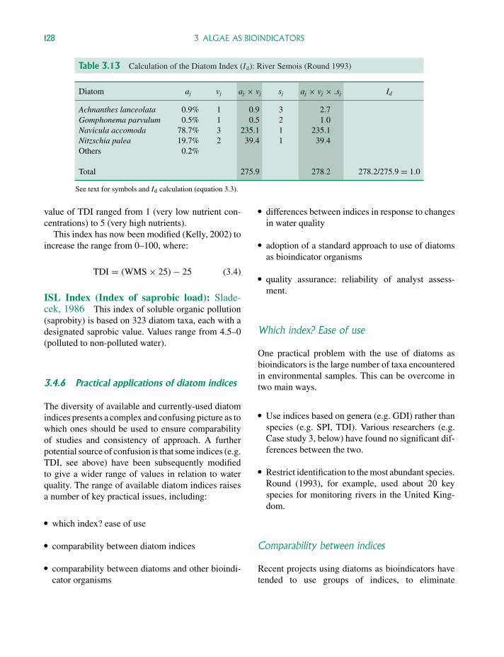
P1: OTA/XYZ P2: ABCc03 JWBK440/Bellinger March 15, 2010 15:33 Printer Name: Yet to Come
128 3 ALGAE AS BIOINDICATORS
Table 3.13 Calculation of the Diatom Index (Id): River Semois (Round 1993)
Diatom aj vj aj × vj sj aj × vj × .sj Id
Achnanthes lanceolata 0.9% 1 0.9 3 2.7Gomphonema parvulum 0.5% 1 0.5 2 1.0Navicula accomoda 78.7% 3 235.1 1 235.1Nitzschia palea 19.7% 2 39.4 1 39.4Others 0.2%
Total 275.9 278.2 278.2/275.9 = 1.0
See text for symbols and Id calculation (equation 3.3).
value of TDI ranged from 1 (very low nutrient con-centrations) to 5 (very high nutrients).
This index has now been modified (Kelly, 2002) toincrease the range from 0–100, where:
TDI = (WMS × 25) − 25 (3.4)
ISL Index (Index of saprobic load): Slade-cek, 1986 This index of soluble organic pollution(saprobity) is based on 323 diatom taxa, each with adesignated saprobic value. Values range from 4.5–0(polluted to non-polluted water).
3.4.6 Practical applications of diatom indices
The diversity of available and currently-used diatomindices presents a complex and confusing picture as towhich ones should be used to ensure comparabilityof studies and consistency of approach. A furtherpotential source of confusion is that some indices (e.g.TDI, see above) have been subsequently modifiedto give a wider range of values in relation to waterquality. The range of available diatom indices raisesa number of key practical issues, including:
� which index? ease of use
� comparability between diatom indices
� comparability between diatoms and other bioindi-cator organisms
� differences between indices in response to changesin water quality
� adoption of a standard approach to use of diatomsas bioindicator organisms
� quality assurance: reliability of analyst assess-ment.
Which index? Ease of use
One practical problem with the use of diatoms asbioindicators is the large number of taxa encounteredin environmental samples. This can be overcome intwo main ways.
� Use indices based on genera (e.g. GDI) rather thanspecies (e.g. SPI, TDI). Various researchers (e.g.Case study 3, below) have found no significant dif-ferences between the two.
� Restrict identification to the most abundant species.Round (1993), for example, used about 20 keyspecies for monitoring rivers in the United King-dom.
Comparability between indices
Recent projects using diatoms as bioindicators havetended to use groups of indices, to eliminate
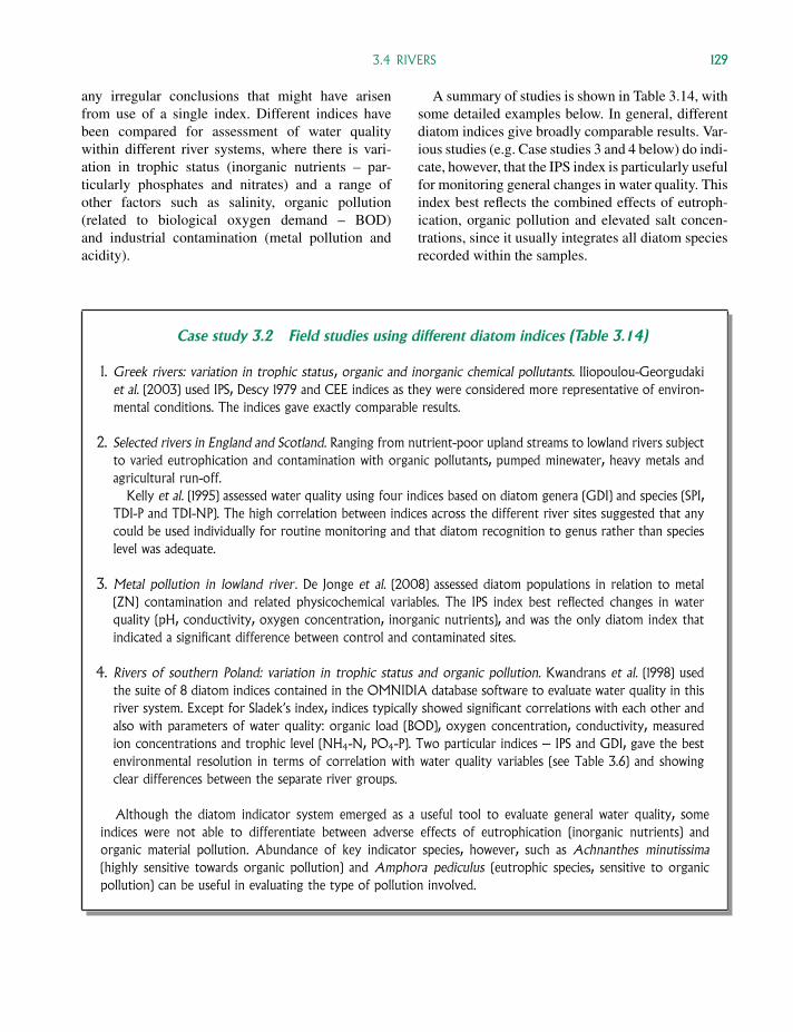
P1: OTA/XYZ P2: ABCc03 JWBK440/Bellinger March 15, 2010 15:33 Printer Name: Yet to Come
3.4 RIVERS 129
any irregular conclusions that might have arisenfrom use of a single index. Different indices havebeen compared for assessment of water qualitywithin different river systems, where there is vari-ation in trophic status (inorganic nutrients – par-ticularly phosphates and nitrates) and a range ofother factors such as salinity, organic pollution(related to biological oxygen demand – BOD)and industrial contamination (metal pollution andacidity).
A summary of studies is shown in Table 3.14, withsome detailed examples below. In general, differentdiatom indices give broadly comparable results. Var-ious studies (e.g. Case studies 3 and 4 below) do indi-cate, however, that the IPS index is particularly usefulfor monitoring general changes in water quality. Thisindex best reflects the combined effects of eutroph-ication, organic pollution and elevated salt concen-trations, since it usually integrates all diatom speciesrecorded within the samples.
Case study 3.2 Field studies using different diatom indices (Table 3.14)
1. Greek rivers: variation in trophic status, organic and inorganic chemical pollutants. Iliopoulou-Georgudakiet al. (2003) used IPS, Descy 1979 and CEE indices as they were considered more representative of environ-mental conditions. The indices gave exactly comparable results.
2. Selected rivers in England and Scotland. Ranging from nutrient-poor upland streams to lowland rivers subjectto varied eutrophication and contamination with organic pollutants, pumped minewater, heavy metals andagricultural run-off.
Kelly et al. (1995) assessed water quality using four indices based on diatom genera (GDI) and species (SPI,TDI-P and TDI-NP). The high correlation between indices across the different river sites suggested that anycould be used individually for routine monitoring and that diatom recognition to genus rather than specieslevel was adequate.
3. Metal pollution in lowland river. De Jonge et al. (2008) assessed diatom populations in relation to metal(ZN) contamination and related physicochemical variables. The IPS index best reflected changes in waterquality (pH, conductivity, oxygen concentration, inorganic nutrients), and was the only diatom index thatindicated a significant difference between control and contaminated sites.
4. Rivers of southern Poland: variation in trophic status and organic pollution. Kwandrans et al. (1998) usedthe suite of 8 diatom indices contained in the OMNIDIA database software to evaluate water quality in thisriver system. Except for Sladek’s index, indices typically showed significant correlations with each other andalso with parameters of water quality: organic load (BOD), oxygen concentration, conductivity, measuredion concentrations and trophic level (NH4-N, PO4-P). Two particular indices – IPS and GDI, gave the bestenvironmental resolution in terms of correlation with water quality variables (see Table 3.6) and showingclear differences between the separate river groups.
Although the diatom indicator system emerged as a useful tool to evaluate general water quality, someindices were not able to differentiate between adverse effects of eutrophication (inorganic nutrients) andorganic material pollution. Abundance of key indicator species, however, such as Achnanthes minutissima(highly sensitive towards organic pollution) and Amphora pediculus (eutrophic species, sensitive to organicpollution) can be useful in evaluating the type of pollution involved.
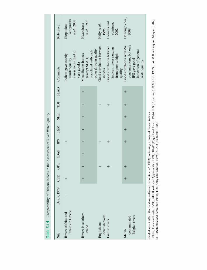
P1: OTA/XYZ P2: ABCc03 JWBK440/Bellinger March 15, 2010 15:33 Printer Name: Yet to Come
Tabl
e3
.14
Com
para
bilit
yof
Dia
tom
Indi
ces
inth
eA
sses
smen
tof
Riv
erW
ater
Qua
lity
Site
Des
cy,1
979
CE
EG
DI
IDA
PIP
SL
&M
SHE
TD
ISL
AD
Com
men
tsR
efer
ence
Riv
ers
Alf
eios
and
Pine
ios
inG
reec
e+
++
Indi
ces
gave
exac
tlysi
mila
rqu
ality
asse
ssm
ents
(bad
tove
rygo
od.)
Ilio
poul
ou-
Geo
rgud
aki
etal
.,20
03
Riv
ers
inso
uthe
rnPo
land
++
++
++
++
Mos
tdia
tom
indi
ces
(exc
eptS
LA
D)
corr
elat
edw
ithea
chot
her
&w
ater
qual
ity
Kw
andr
ans
etal
.,19
98
Eng
lish
and
Scot
tish
rive
rs+
++
Goo
dco
rrel
atio
nbe
twee
nin
dice
sK
elly
etal
.,19
95Fi
nnis
hri
vers
++
+G
ood
corr
elat
ion
betw
een
indi
ces:
rive
rsra
ngin
gfr
ompo
orto
high
qual
ity
Elo
rant
aan
dSo
inin
en,
2002
Met
al-
cont
amin
ated
Bel
gian
rive
rs
++
++
++
+G
ood
corr
elat
ion
with
Zn
conc
entr
atio
ns,b
uton
lyIP
Sga
vego
odin
dica
tion
ofge
nera
lw
ater
qual
ity
De
Jong
eet
al.,
2008
Shad
edar
ea:O
MN
IDIA
data
base
soft
war
e(L
ecoi
nte
etal
.,19
93)
cont
aini
nga
rang
eof
diat
omin
dice
s.1C
EE
(Des
cyan
dC
oste
,199
1),G
DI
(Cos
tean
dA
ypha
ssor
ho,1
991)
,ID
AP
(Pry
giel
and
Cos
te,1
996)
,IPS
(Cos
te,i
nC
EM
AG
RE
F,19
82),
L&
M(L
ecle
rcq
and
Maq
uet,
1987
),SH
E(S
chie
fele
and
Schr
eine
r,19
91),
TD
I(K
elly
and
Whi
tton,
1995
),SL
AD
(Sla
dace
k,19
86).
130
P1: OTA/XYZ P2: ABCc03 JWBK440/Bellinger March 15, 2010 15:33 Printer Name: Yet to Come
3.4 RIVERS 131
Case study 3.3 Comparisons of diatom indices with other bioindices
1. Use of different bioindicators for assessing water quality in Greek Rivers. Iliopoulou-Georgudaki et al.(2003). This study was carried out on river sites with water quality ranging from very poor to very goodand used bioindices based on diatoms (see previously) plus four other groups of organisms. Sampling offish and macrophyte vegetation gave only limited environmental assessment, with macrophytes in particularbeing incapable of a graded response to varying degrees and kinds of stress. Macroinvertebrates and diatomsrecorded the full range of pollution conditions, but indices based on macroinvertebrates were consideredto be the most sensitive – responding more readily than diatoms to transient changes to environmentalstate.
2. Selected rivers in England and Scotland. Kelly et al. (1995) found that their diatom indices were significantlycorrelated with two benthic macroinvertebrate indices – BMWP (Biological Monitoring Working Partyscores) and ASPT (Average Score Per Taxon), both used routinely for water quality monitoring in theUnited Kingdom.
3. Metal pollution in lowland river. Comparison of macroinvertebrates and diatoms as bioindicators by DeJonge et al. (2008) showed that diatom communities most closely reflected changes in metal concentration,with distinct taxa being associated with low (e.g. Tabellaria flocculosa) moderate (Nitzschia palea) andhigh (Eolimna minima) zinc levels. In contrast to diatoms, macroinvertebrate communities most closelyfollowed physical-chemical variables and the effects of metal pollution. The combined use of both groupsfor biomonitoring was considered to be more appropriate than separate use of either.
Comparison to other bioindicator organisms
Although routine monitoring of all but the deepestrivers has been based for many years on macroinver-tebrates (e.g. De Pauw and Hawkes, 1993), a rangeof other bioindicator organisms is available. Theseinclude diatoms, other algae, fish, aquatic and ri-parian macrophytes. Various authors have made si-multaneous comparisons of some or all of these toassess the relative usefulness of particular groupsof organisms – with particular emphasis on diatomsand macroinvertebrates. In the examples below (con-tinued from the previous section), diatom commu-nities showed comparable changes to macroinver-tebrates in relation to water quality, but (with theexception of the IPS index) were generally lesssensitive.
Response to changes in water quality
One important aspect of algal bioindicators is thatthey are able to detect a rapid change in water qual-ity. Because of their shorter generation time, diatomcommunities are potentially able to respond morerapidly than other bioindicator groups (e.g. macroin-vertebrates, fish), which integrate water quality overlonger time frames.
The time sequence of diatom change can be inves-tigated by transferring diatom biofilms from pollutedto non-polluted waters, and record:
� how different diatom indices compare over fixedtime periods
� the time needed for different indices to indicate asignificant change in water quality.
P1: OTA/XYZ P2: ABCc03 JWBK440/Bellinger March 15, 2010 15:33 Printer Name: Yet to Come
132 3 ALGAE AS BIOINDICATORS
Biofilm studies by Rimet et al. (2005), showed thatsome indices (e.g. CEE, TDI – high sensitivity) re-sponded more rapidly than others (GDI, ILM, SLA –intermediate sensitivity) to environmental change.All indices showed significant change (integrationinterval) within 40–60 days of biofilm transfer.
Standardization of approach
The above studies indicate that benthic diatoms pro-vide the basis for a standard approach to river moni-toring, able to be used as an alternative (or addition) tomacroinvertebrate sampling. Individual commonly-used diatom indices appear to correlate significantlywith macroinvertebrate data, and also with each other(see above). Studies by Kelly et al.(1995) have alsoshown that benthic diatom indices do not changesignificantly either with season or with major flowevents (both of which can influence invertebrate pop-ulations) – suggesting that diatom indices are robustand that consistent results can be obtained throughoutthe year.
Standard procedures are important in ensuringcomparability of results. These include standardiza-tion of sampling procedures (Kelly et al., 1998),adoption of analyst quality controls (see below), ac-cess to common data bases and use of comparablediatom indices.
Access to common databases Access to web-based data sites such as the European DiatomDatabase Initiative (EDDI) promotes a standard ap-proach to identification, data acquisition and manipu-lation. Although this site has particularly applicationfor palaeolimnology (Section 3.2.2), other databasesspecifically on benthic diatoms (Gosselain et al.,2005) may be more applicable to river studies.
Comparable diatom indices Although a singlediatom index (coupled with the identification of keydiatom indicator taxa) would be adequate for envi-ronmental monitoring, the trend is for diatom countsto be fed into a database for determination of multi-ple indices. The general availability of the OMNIDIAdatabase software (Lecointe et al., 1993), incorporat-ing indices summarized in Table 3.14, is particularlyuseful in this respect.
The indices contained in the OMNIDIA softwareare based on European diatom communities andclearly apply most directly to European rivers. Appli-cation of this software in other parts of the world re-quires the incorporation of local (endemic) species, asemphasized by Taylor et al. (2007) in their studies onSouth African rivers. It is also important to check thatcosmopolitan species have similar ecological prefer-ences in different parts of the world. Dela-Cruz et al.(2006), for example, assessed the suitability of ‘north-ern hemisphere’ ecological tolerance/preference datafor periphytic diatoms in south-eastern Australianrivers before using bioindicator indices.
Quality assurance
Although techniques for standardized sampling of di-atoms (Section 2.10.1), and different types of indices(Section 3.4.5) are well defined, the final environ-mental assessment ultimately depends on the ana-lyst’s ability to accurately record species compositionfrom the environmental samples. Quality assessmentof analyst performance is important, since regulatoryagencies must be confident that data produced by theirstaff are relevant and accurate. In Europe, for exam-ple, the requirement of water companies to install nu-trient removal facilities in certain large sewage treat-ment works (Urban Wastewater Treatment Directive– European Community, 1991) is determined by as-sessment of water quality and is highly expensive.The use of benthic diatoms in the implementation ofthis directive (Kelly, 2002) must be reliable.
In the case of chemical analyses of water qual-ity (including soluble nitrates and phosphates) thesituation is relatively simple, since chemical param-eters are relatively few, with comparisons that areunivariate and amenable to conventional parametricstatistics. In contrast to this, biological monitoring ismore complex – based on field samples containingmany species, all of which may contribute to the as-sessment. These species counts may be assessed aspresence/absence or in terms of relative abundance.
� Presence/absence. Invertebrate analyses in theUnited Kingdom are carried out on this basis,with water quality being determined in relation tothe presence/absence of key benthic invertebratedata (Mason, 1996). Reliability of assessment by
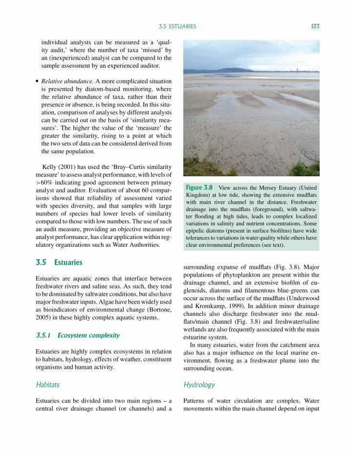
P1: OTA/XYZ P2: ABCc03 JWBK440/Bellinger March 15, 2010 15:33 Printer Name: Yet to Come
3.5 ESTUARIES 133
individual analysts can be measured as a ‘qual-ity audit,’ where the number of taxa ‘missed’ byan (inexperienced) analyst can be compared to thesample assessment by an experienced auditor.
� Relative abundance. A more complicated situationis presented by diatom-based monitoring, wherethe relative abundance of taxa, rather than theirpresence or absence, is being recorded. In this situ-ation, comparison of analyses by different analystscan be carried out on the basis of ‘similarity mea-sures’. The higher the value of the ‘measure’ thegreater the similarity, rising to a point at whichthe two sets of data can be considered derived fromthe same population.
Kelly (2001) has used the ‘Bray–Curtis similaritymeasure’ to assess analyst performance, with levels of>60% indicating good agreement between primaryanalyst and auditor. Evaluation of about 60 compar-isons showed that reliability of assessment variedwith species diversity, and that samples with largenumbers of species had lower levels of similaritycompared to those with low numbers. The use of suchan audit measure, providing an objective measure ofanalyst performance, has clear application within reg-ulatory organizations such as Water Authorities.
3.5 Estuaries
Estuaries are aquatic zones that interface betweenfreshwater rivers and saline seas. As such, they tendto be dominated by saltwater conditions, but also havemajor freshwater inputs. Algae have been widely usedas bioindicators of environmental change (Bortone,2005) in these highly complex aquatic systems.
3.5.1 Ecosystem complexity
Estuaries are highly complex ecosystems in relationto habitats, hydrology, effects of weather, constituentorganisms and human activity.
Habitats
Estuaries can be divided into two main regions – acentral river drainage channel (or channels) and a
Figure 3.8 View across the Mersey Estuary (UnitedKingdom) at low tide, showing the extensive mudflatswith main river channel in the distance. Freshwaterdrainage into the mudflats (foreground), with saltwa-ter flooding at high tides, leads to complex localizedvariations in salinity and nutrient concentrations. Someepipelic diatoms (present in surface biofilms) have widetolerances to variations in water quality while others haveclear environmental preferences (see text).
surrounding expanse of mudflats (Fig. 3.8). Majorpopulations of phytoplankton are present within thedrainage channel, and an extensive biofilm of eu-glenoids, diatoms and filamentous blue-greens canoccur across the surface of the mudflats (Underwoodand Kromkamp, 1999). In addition minor drainagechannels also discharge freshwater into the mud-flats/main channel (Fig. 3.8) and freshwater/salinewetlands are also frequently associated with the mainestuarine system.
In many estuaries, water from the catchment areaalso has a major influence on the local marine en-vironment, flowing as a freshwater plume into thesurrounding ocean.
Hydrology
Patterns of water circulation are complex. Watermovements within the main channel depend on input
P1: OTA/XYZ P2: ABCc03 JWBK440/Bellinger March 15, 2010 15:33 Printer Name: Yet to Come
134 3 ALGAE AS BIOINDICATORS
from the sea (tidal currents), river (freshwater dis-charge), surface drainage and ground sources (fresh-water discharge). Mixing of freshwater and saltwaterwithin the main channel results in an intermediatezone of brackish water – the ‘salt wedge,’ wheredense sea water underlies an upper freshwater layer.The salt wedge is a permanent feature that movesup and down the main channel with advancing andreceding tide. Periodic movement water out of theestuary into the surrounding ocean leads to a plumeof fresh or brackish water in the bay area.
Weather
Estuaries are markedly affected by local weatherevents such as droughts, high rainfall (flooding) andwinds. During the autumn of 1999, for example,hurricanes inundated North Carolina (United States)with as much as 1 m of rainfall, causing a major floodin the watershed of Pimlico Sound (Paerl et al., 2005).Sediment and nutrient-laden water displaced morethan 80% of the Sound’s volume, depressed salinityby >70% and accounted for half the annual load ofnitrogen in this nitrogen-sensitive region.
Estuarine organisms
Many algae living in or around estuaries are typicallyadapted to either freshwater or saline conditions, andhave restricted habitats (e.g. Section 3.3 – diatomsin coastal wetlands). Other estuarine organisms havebecome tolerant of a range of conditions. Diurnal andseasonal changes in tidal flow mean that planktonicorganisms in the main water channel are subjectedto wide periodic fluctuations in salinity, and biotaoccurring on the surface of mudflats are exposed toextremes of salinity change, desiccation and irradia-tion. The typically high nutrient level of river inflowalso signals a further difference between freshwaterand saline organisms in terms of productivity, with amarked increase in carbon fixation from freshwateralgae when saline water is displaced (Section 3.5.2).
Algal diversity: the mudflat biofilm Organismdiversity within the complex estuarine environmentis illustrated by the area of mudflats, where local-
ized drainage and inflow (Fig. 3.8) lead to numeroussmall-scale salinity and nutrient gradients (Under-wood et al., 1998). Epipelic diatoms are the maingroup of algae inhabiting these intertidal sediments,forming surface biofilms that have high levels of pro-ductivity. Algae associated with estuarine sedimentsare also important in substrate stabilization (Section2.7.2) and are in dynamic interchange with planktonicpopulations (Section 1.1.4).
Although many epipelic diatoms are cosmopoli-tan in their distribution, indicating broad toleranceof environmental variations, others are more spe-cific. Analysis of diatom distribution within localsalinity gradients led Underwood et al. (1998) toclassify some diatoms as oligohaline (0.5–4% offull salinity: Navicula gregaria), mesohaline (5–18%:Navicula phyllepta) and polyhaline (18–30%: Pleu-rosigma angulatum, Plagiotropis vitrea). Variationsalong a nutrient gradient indicated some species(Nitzschia sigma) typical of high nutrient conditions,while others (Navicula phyllepta, Pleurosigma an-gulatum) were more common at low nutrient levels.Similar studies by Agatz et al. (1999) on tidal flatepipelic diatoms also demonstrated nutrient-tolerant(Nitzschia sigma) and nutrient-intolerant (Achnan-thes, Amphora) taxa. The above algae serve asbioindicators for microenvironmental (local) condi-tions of pore water quality.
Human activity
Human activity has a major and varied effect on estu-aries, and is a dominant source of stress and change.At least half the world’s population resides in estuar-ine watersheds (Paerl et al., 2005), greatly increasingsediment and nutrient loads to downstream estuarineand coastal systems. This results in deterioration ofwater quality and an overall decline in the ecologicaland economic condition of the coastal zone, includingloss of fisheries habitat and resources.
3.5.2 Algae as estuarine bioindicators
Algae have been used to monitor changes in waterquality of estuaries and coastal systems in relation totwo main aspects: changes in salinity and increasesin inorganic nutrient levels (eutrophication). The
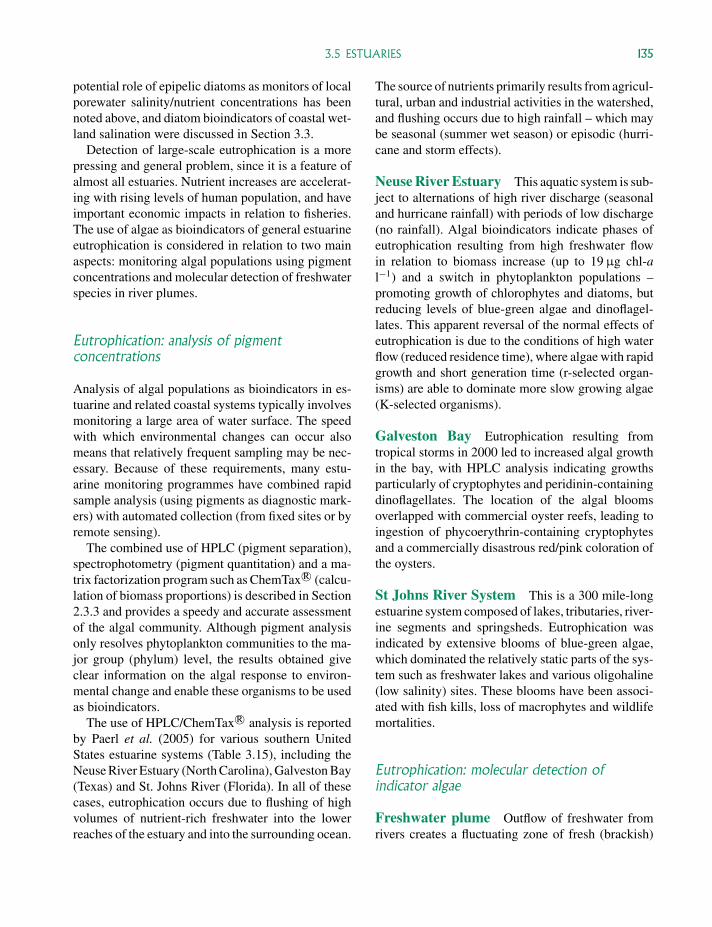
P1: OTA/XYZ P2: ABCc03 JWBK440/Bellinger March 15, 2010 15:33 Printer Name: Yet to Come
3.5 ESTUARIES 135
potential role of epipelic diatoms as monitors of localporewater salinity/nutrient concentrations has beennoted above, and diatom bioindicators of coastal wet-land salination were discussed in Section 3.3.
Detection of large-scale eutrophication is a morepressing and general problem, since it is a feature ofalmost all estuaries. Nutrient increases are accelerat-ing with rising levels of human population, and haveimportant economic impacts in relation to fisheries.The use of algae as bioindicators of general estuarineeutrophication is considered in relation to two mainaspects: monitoring algal populations using pigmentconcentrations and molecular detection of freshwaterspecies in river plumes.
Eutrophication: analysis of pigmentconcentrations
Analysis of algal populations as bioindicators in es-tuarine and related coastal systems typically involvesmonitoring a large area of water surface. The speedwith which environmental changes can occur alsomeans that relatively frequent sampling may be nec-essary. Because of these requirements, many estu-arine monitoring programmes have combined rapidsample analysis (using pigments as diagnostic mark-ers) with automated collection (from fixed sites or byremote sensing).
The combined use of HPLC (pigment separation),spectrophotometry (pigment quantitation) and a ma-trix factorization program such as ChemTax R© (calcu-lation of biomass proportions) is described in Section2.3.3 and provides a speedy and accurate assessmentof the algal community. Although pigment analysisonly resolves phytoplankton communities to the ma-jor group (phylum) level, the results obtained giveclear information on the algal response to environ-mental change and enable these organisms to be usedas bioindicators.
The use of HPLC/ChemTax R© analysis is reportedby Paerl et al. (2005) for various southern UnitedStates estuarine systems (Table 3.15), including theNeuse River Estuary (North Carolina), Galveston Bay(Texas) and St. Johns River (Florida). In all of thesecases, eutrophication occurs due to flushing of highvolumes of nutrient-rich freshwater into the lowerreaches of the estuary and into the surrounding ocean.
The source of nutrients primarily results from agricul-tural, urban and industrial activities in the watershed,and flushing occurs due to high rainfall – which maybe seasonal (summer wet season) or episodic (hurri-cane and storm effects).
Neuse River Estuary This aquatic system is sub-ject to alternations of high river discharge (seasonaland hurricane rainfall) with periods of low discharge(no rainfall). Algal bioindicators indicate phases ofeutrophication resulting from high freshwater flowin relation to biomass increase (up to 19 µg chl-al−1) and a switch in phytoplankton populations –promoting growth of chlorophytes and diatoms, butreducing levels of blue-green algae and dinoflagel-lates. This apparent reversal of the normal effects ofeutrophication is due to the conditions of high waterflow (reduced residence time), where algae with rapidgrowth and short generation time (r-selected organ-isms) are able to dominate more slow growing algae(K-selected organisms).
Galveston Bay Eutrophication resulting fromtropical storms in 2000 led to increased algal growthin the bay, with HPLC analysis indicating growthsparticularly of cryptophytes and peridinin-containingdinoflagellates. The location of the algal bloomsoverlapped with commercial oyster reefs, leading toingestion of phycoerythrin-containing cryptophytesand a commercially disastrous red/pink coloration ofthe oysters.
St Johns River System This is a 300 mile-longestuarine system composed of lakes, tributaries, river-ine segments and springsheds. Eutrophication wasindicated by extensive blooms of blue-green algae,which dominated the relatively static parts of the sys-tem such as freshwater lakes and various oligohaline(low salinity) sites. These blooms have been associ-ated with fish kills, loss of macrophytes and wildlifemortalities.
Eutrophication: molecular detection ofindicator algae
Freshwater plume Outflow of freshwater fromrivers creates a fluctuating zone of fresh (brackish)
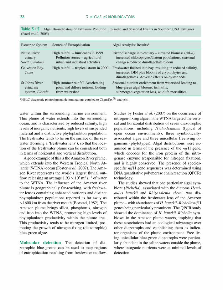
P1: OTA/XYZ P2: ABCc03 JWBK440/Bellinger March 15, 2010 15:33 Printer Name: Yet to Come
136 3 ALGAE AS BIOINDICATORS
Table 3.15 Algal Bioindicators of Estuarine Pollution: Episodic and Seasonal Events in Southern USA Estuaries(Paerl et al., 2005)
Estuarine System Source of Eutrophication Algal Analysis: Results*
Neuse Riverestuary
North Carolina
High rainfall – hurricanes in 1999Pollution source – agriculturalurban and industrial activities
River discharge into estuary – elevated biomass (chl-a),increased chlorophytes/diatom populations, seasonalchanges-reduced dinoflagellate bloom
Galveston Bay.Texas
High rainfall – tropical storm in 2000 Freshwater flushed into bay, resulting in reduced salinity,increased DIN plus blooms of cryptophytes anddinoflagellates. Adverse effects on oyster beds
St Johns Riverestuarinesystem, Florida
High summer rainfall Acceleratingpoint and diffuse nutrient loadingfrom watershed
Seasonal nutrient enrichment from watershed leading toblue-green algal blooms, fish kills,submerged-vegetation loss, wildlife mortalities
*HPLC diagnostic photopigment determinations coupled to ChemTax R© analysis.
water within the surrounding marine environment.This plume of water extends into the surroundingocean, and is characterized by reduced salinity, highlevels of inorganic nutrients, high levels of suspendedmaterial and a distinctive phytoplankton population.The freshwater tends to lie on the surface of the sea-water (forming a ‘freshwater lens’), so that the loca-tion of the freshwater plume can be considered bothin terms of horizontal and vertical distribution.
A good example of this is the Amazon River plume,which extends into the Western Tropical North At-lantic (WTNA) ocean (Foster et al., 2007). The Ama-zon River represents the world’s largest fluvial out-flow, releasing an average 1.93 × 10⁵ m3 s−1 of waterto the WTNA. The influence of the Amazon riverplume is geographically far-reaching, with freshwa-ter lenses containing enhanced nutrients and distinctphytoplankton populations reported as far away as>1600 km from the river mouth (Borstad, 1982). TheAmazon plume brings silica, phosphorus, nitrogenand iron into the WTNA, promoting high levels ofphytoplankton productivity within the plume area.This productivity tends to be nitrogen limited, pro-moting the growth of nitrogen-fixing (diazotrophic)blue-green algae.
Molecular detection The detection of dia-zotrophic blue-greens can be used to map regionsof eutrophication resulting from freshwater outflow.
Studies by Foster et al. (2007) on the occurrence ofnitrogen-fixing algae in the WTNA targeted the verti-cal and horizontal distribution of seven diazotrophicpopulations, including Trichodesmium (typical ofopen ocean environments), three symbiotically-associated algae and three unicellular freeliving or-ganisms (phylotypes). Algal distributions were ex-amined in terms of the presence of the nif H gene,which encodes for the iron protein of the nitro-genase enzyme (responsible for nitrogen fixation),and is highly conserved. The presence of species-specific nif H gene sequences was determined usingDNA quantitative polymerase chain reaction (QPCR)technology.
The studies showed that one particular algal sym-biont (Richelia), associated with the diatoms Hemi-aulus hauckii and Rhizosolenia clevei, was dis-tributed within the freshwater lens of the Amazonplume – with abundances of H. hauckii–Richelia nif Hgenes being particularly prominent. The QPCR studyshowed the dominance of H. hauckii–Richelia sym-bioses in the Amazon plume waters, implying thatthese associations had an ecological advantage overother diazotrophs and establishing them as indica-tor organisms of the plume environment. Free liv-ing unicellular blue-green diazotrophs were particu-larly abundant in the saline waters outside the plume,where inorganic nutrients were at minimal levels ofdetection.