Friction and compliance identification in a vehicle's

steering system

B.A.M van Daal (s020479)

DCT 2007.095 Extern traineeship report Coach(es) Ir. P.v.d.Linden (LMS) Ir. T. Geluk (LMS) Prof. Dr. H.Nijmeijer Supervisor: Prof. Dr. H.Nijmeijer Eindhoven University of Technology Department Mechanical Engineering Dynamics and Control Group Eindhoven, July, 2007

i

Abstract Modern vehicles have a very good road - steering wheel feedback, resulting in a good steering feel. Most of the time the vehicle is driven in a straight line or a small maneuver is made. This is called on-center driving. The steering feel during on-center driving is mainly determined by the frictions and compliances in the different parts and connections of the steering system. In this research we study if it is possible to identify the frictions and compliances in the steering system in order to characterize the steering feel. It is investigated which on-center parameters can characterize the steering feel. Test descriptions to obtain proper measurement data are made and on-center tests have been performed. From the measurement data the on-center parameters can be determined. Besides this a full vehicle motion model is built in order to simulate the on-center tests. A procedure to obtain information about the frictions and compliances in the steering system has been defined. From the measurement data, obtained from the performed tests, the on-center parameters are determined. The parameters are compared with the on-center parameters obtained from simulation data and it is concluded that the model gives proper results. On the basis of the measurement data it is proven that a friction and compliance identification will be feasible.

ii

Samenvatting Moderne voertuigen hebben een zeer goede wegdek – stuur feedback, hetgeen resulteert in een goed stuurgevoel. Het grootste gedeelte van de tijd wordt met een voertuig in rechte lijn gereden, of een kleine manoeuvre wordt gemaakt. Dit wordt on-center rijden genoemd. Het stuurgevoel tijdens on-center rijden wordt voornamelijk bepaald door de wrijvingen en rekken in de verschillende onderdelen en verbindingen van het stuursysteem. In dit onderzoek wordt bekeken of de wrijvingen en rekken in het stuursysteem geïdentificeerd kunnen worden, zodat het stuurgevoel gekarakteriseerd kan worden. Onderzocht wordt welke on-center parameters het stuurgevoel kunnen karakteriseren. Testbeschrijvingen om goede meetdata te verkrijgen zijn gemaakt en on-center testen zijn uitgevoerd. Daarnaast is er een volledig voertuig model gemaakt om de on-center testen te simuleren. Een procedure om informatie te verkrijgen over de wrijvingen en rekken in een stuursysteem is gedefinieerd. Uit de meetdata, verkregen uit uitgevoerde testen, zijn de on-center parameters bepaald. De parameters zijn vergeleken met de on-center parameters welke uit de simulatie data zijn verkregen. Hieruit kan geconcludeerd worden dat het model goede resultaten geeft. Aan de hand van de meetdata is aangetoond dat wrijving en rek identificatie haalbaar is.

iii

Acknowledgements I would like to thank my supervisor and coaches Henk Nijmeijer, Peter van der Linden and Theo Geluk for their guidance throughout my research. Their support with advice and comments during this research was very valuable. I enjoyed the weekly meetings very much and I once again found out that meetings can still be full of laughter without getting inefficient. I would also like to thank the Romanian trainees Luchu, Julian, Mirchea, Hunor and Mihai with who I had some serious discussions during coffee breaks, discussions which were continued at nights on my "kot" in the Bierbeekstraat. A special word of thanks goes to my parents who made it possible for me to study at the Technical University of Eindhoven and who helped me to move my stuff from the room in Eindhoven to my room in Leuven. Last but not least I like to thank the coffee machine at LMS, the Simpsons at VT4 and my motorbike. The coffee machine proved to be my best friend during the afternoons and helped me to keep my attention to the work. Every night from 19:00 till 20:00, VT4 broadcasted the Simpsons and delivered my daily dose of humor. My old motorbike, a Yamaha XT550 from 1981, bought for 250 euros, carried me every weekend from Leuven to my parents place and back, a total of 16 weeks times 170 km = 2720 km. The XT has proven to be a reliable partner.

0

Contents Abstract i Samenvatting ii Acknowledgements iii 1. Introduction........................................................................................................................2

1.1 Report outline .........................................................................................................3 2. On-center parameters..........................................................................................................4

2.1 On-center weave test.....................................................................................................4 2.1.1 Test description......................................................................................................4 2.1.2 Parameters .............................................................................................................4

2.2 Step steer test................................................................................................................6 2.3 Test conditions..............................................................................................................7

3. Chrysler Neon model..........................................................................................................8 4. Instrumentation and measurements .....................................................................................9

4.1 Steering wheel angle .....................................................................................................9 4.2 Steering wheel torque .................................................................................................10 4.3 Lateral and vertical acceleration..................................................................................11 4.4 Yaw rate .....................................................................................................................12 4.5 Measurements and data acquisition .............................................................................13

5. Data interpretation ............................................................................................................15 5.1 Processing of V.LM model data..................................................................................15

5.1.1 Time trajectories ..................................................................................................15 5.1.2 Steering wheel torque versus steering wheel angle ...............................................16 5.1.3 Yaw rate versus steering wheel angle ...................................................................18 5.1.4 Lateral acceleration versus steering wheel angle...................................................19

5.2 Processing of the measurement data............................................................................20 5.2.1 Data interpretation and filtering............................................................................20 5.2.2 Lateral acceleration versus steering wheel angle...................................................23 5.2.3 Yaw rate ..............................................................................................................23 5.2.4 Comparison accelerations steering gear housing...................................................27

6. Comparison measurements and simulation .......................................................................30 6.1 Creating input for V.LM .............................................................................................30 6.2 Yaw rate .....................................................................................................................30 6.3 Lateral acceleration versus steering wheel angle .........................................................32

7. Friction and compliance identification ..............................................................................34 8. Conclusions and recommendations ...................................................................................37

8.1 Conclusions ................................................................................................................37 8.2 Recommendations.......................................................................................................38

Bibliography.........................................................................................................................39 Appendix A, Testing ............................................................................................................40

Weave test ........................................................................................................................40 Step steer test....................................................................................................................40 Test conditions .................................................................................................................40

Appendix B, Neon Suspension .............................................................................................42 Appendix C, Bushings..........................................................................................................44

1

Appendix D, Butterworth filters ...........................................................................................45 Overview..........................................................................................................................45 Transfer function ..............................................................................................................46

Appendix E, Instrumentation ................................................................................................47 Lateral acceleration...........................................................................................................47 Yaw rate ...........................................................................................................................47 Data acquisition................................................................................................................47

Appendix F, Matlab..............................................................................................................49 Generating steering wheel input........................................................................................49

Perfect sine ...................................................................................................................49 Sine with noise .............................................................................................................49

Generating road profile.....................................................................................................49 Processing the simulation data ..........................................................................................50 Processing the measurement data......................................................................................51

Filter the signals ...........................................................................................................51 Plot the data..................................................................................................................51 Calculate the lateral displacement of the steering gear housing .....................................52 Compare measurement data with simulated data ...........................................................52

Appendix G, V.LM ..............................................................................................................53 G.1 Suspension and steering system of the Chrysler Neon ................................................53

G.1.1 Front suspension .................................................................................................53 G.1.2 Steering system ...................................................................................................54 G.1.3 Rear suspension...................................................................................................55

G.2 Implementation in Virtual.Lab Motion.......................................................................56 G.2.1 Front suspension .................................................................................................56 G.2.2 Steering system ...................................................................................................56 G.2.3 Rear suspension...................................................................................................56 G.2.4 Future improvements...........................................................................................57

G.3 Defining maneuvers using Matlab and Cada-X ..........................................................57 G.3.1 Steer input...........................................................................................................57 G.3.2 Road profile ........................................................................................................58

2

1. Introduction Modern vehicles have a very good road to steering wheel feedback, resulting in a good steering feel. Most of the time the vehicle is driven in a straight line or a small maneuver is made. This type of driving is defined as on-center driving. The steering feel during on-center driving is mainly determined by the friction and compliance in the different parts and connections of the steering system. Standard tests in order to identify the total friction and compliance in the steering system already exist [1]. In order to understand more about the steering feel during on-center driving, it is desired to know the friction and compliance which are present in the different connections of the steering system. In this research it will be investigated if a complete friction and compliance identification will be feasible. The research consists of three parts. Firstly it has to be investigated which on-center tests have to be done in order to obtain proper measurement data. From this measurement data the important parameters for on-center driving have to be calculated. Secondly it has to be investigated how the frictions and compliances in the different parts of the steering system can be identified. Thirdly a full vehicle motion model has to be built in order to be able to predict the behavior of the vehicle and the occurring friction forces and compliances in the steering system during on-center simulations. In [1], [2], [3] and [4] descriptions are given for on-center tests. Also definitions for the parameters for on-center driving are given. These papers give a description for both subjective and objective tests. In this research we are only interested in objective tests. On the basis of these papers some tests have been performed and the data has been processed. In [5] and [6] descriptions are given for the front- and rear suspension and the steering system. This literature has been used to build a full vehicle motion model. Measurement data and simulation data are compared and give satisfactory results. After this the full vehicle model will be validated. This will partly be done by comparing the on-center parameters obtained from the simulation results with on-center parameters found in literature and found by measurements. For the measurements a vehicle will be fitted with a simple instrumentation and some on-center tests will be performed. It will be investigated how the desired data can be obtained by an as simple as possible instrumentation. A method to obtain the desired information from both the measurement and the simulation data will be determined. An interpretation of the results will be given and conclusions regarding both the results and the measurements will be drawn. It will be investigated how the full vehicle model has to be updated. Also recommendations will be given for the instrumentation during future measurements and how the measurements have to be performed. Finally a method to identify the friction and compliance in the steering system will be defined. It will be investigated what type of instrumentation will be needed and at which locations the vehicle has to be instrumented in order to identify the different frictions and compliances.

3

This research has been performed in association with LMS International, a company that has a lot of experience in the field of vehicle dynamic testing. From the results obtained it has become clear that an investigation to identify the frictions and compliances in a steering system will be feasible.

1.1 Report outline In chapter 2 a detailed description is given for the different on-center tests and the testing conditions. Also a method is given to obtain the desired on-center parameters and an interpretation of these parameters is given. Typical values for the on-center parameters which are found in literature will be compared by the values found from the simulations and the measurements. This will be discussed in chapter 5. In chapter 3 everything about the full vehicle motion model can be found and it will be discussed how the model has been built. In this chapter it can also be found what still needs to be updated in order to get a representative model. Finally in chapter 3 a description is given on how a desired steering wheel and road profile can be generated in order to be able to simulate every possible maneuver. In chapter 5 it is discussed how the data, generated during the simulation, is processed and which results and conclusions can be withdrawn from this data. In chapter 5 it also discussed how the data, obtained from measurements, is processed. The tests and the instrumentation are discussed in chapter 4. In this chapter also a brief description is given for the data acquisition system. In chapter 6 it is discussed how the data obtained from measurements and simulation correlate to each other. Also some recommendations are given for future measurements. In chapter 7 it is described how the frictions and compliances in the steering system can be identified. For both the instrumentation and the locations of the instrumentation recommendations are given. Finally all the conclusions and recommendations for future work are described in chapter 8.

4

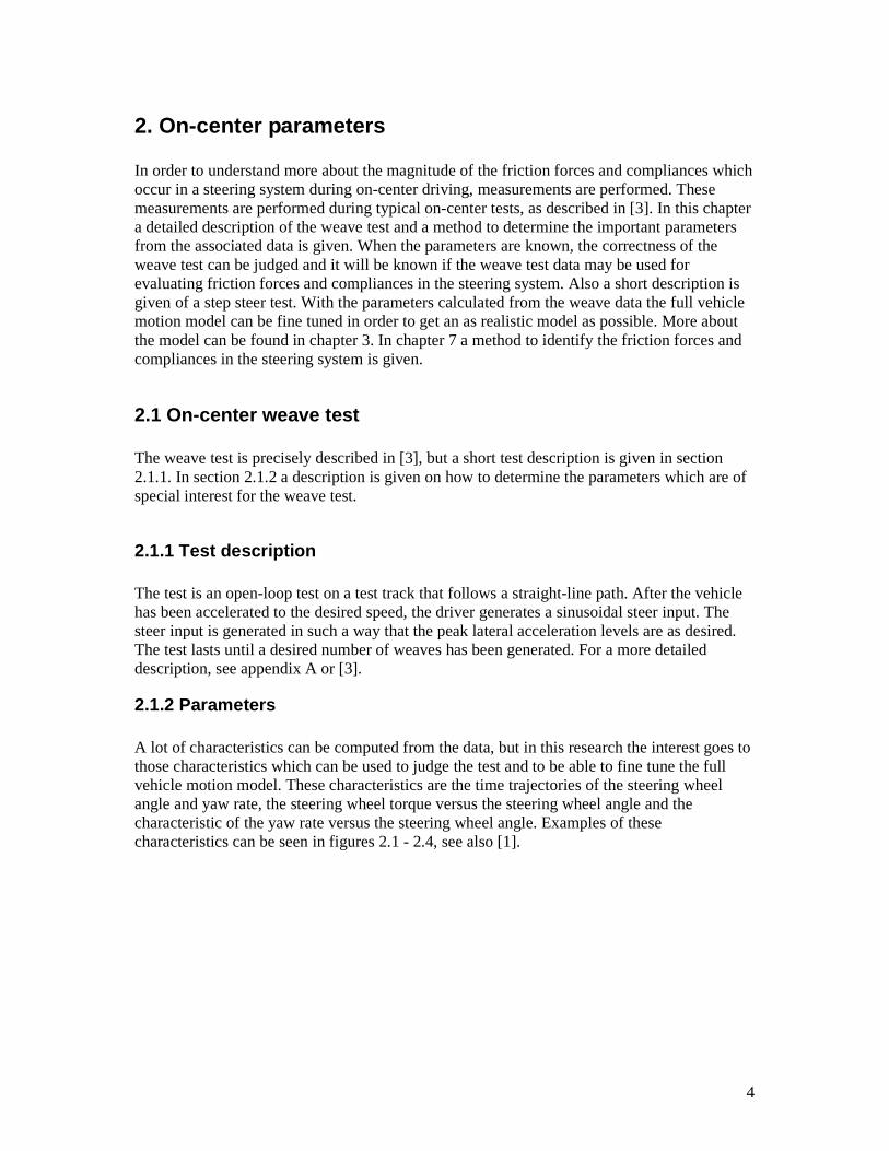
2. On-center parameters In order to understand more about the magnitude of the friction forces and compliances which occur in a steering system during on-center driving, measurements are performed. These measurements are performed during typical on-center tests, as described in [3]. In this chapter a detailed description of the weave test and a method to determine the important parameters from the associated data is given. When the parameters are known, the correctness of the weave test can be judged and it will be known if the weave test data may be used for evaluating friction forces and compliances in the steering system. Also a short description is given of a step steer test. With the parameters calculated from the weave data the full vehicle motion model can be fine tuned in order to get an as realistic model as possible. More about the model can be found in chapter 3. In chapter 7 a method to identify the friction forces and compliances in the steering system is given.

2.1 On-center weave test The weave test is precisely described in [3], but a short test description is given in section 2.1.1. In section 2.1.2 a description is given on how to determine the parameters which are of special interest for the weave test.

2.1.1 Test description The test is an open-loop test on a test track that follows a straight-line path. After the vehicle has been accelerated to the desired speed, the driver generates a sinusoidal steer input. The steer input is generated in such a way that the peak lateral acceleration levels are as desired. The test lasts until a desired number of weaves has been generated. For a more detailed description, see appendix A or [3].

2.1.2 Parameters A lot of characteristics can be computed from the data, but in this research the interest goes to those characteristics which can be used to judge the test and to be able to fine tune the full vehicle motion model. These characteristics are the time trajectories of the steering wheel angle and yaw rate, the steering wheel torque versus the steering wheel angle and the characteristic of the yaw rate versus the steering wheel angle. Examples of these characteristics can be seen in figures 2.1 - 2.4, see also [1].

5

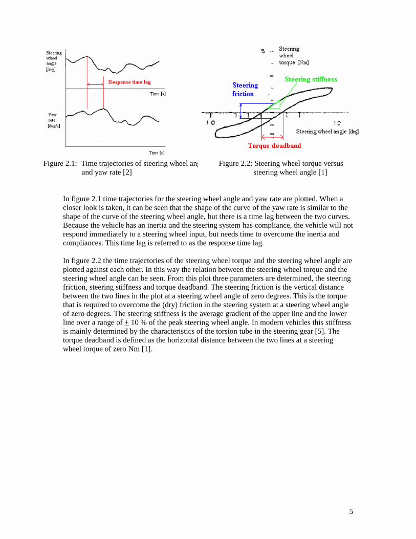
Figure 2.1: Time trajectories of steering wheel angle and yaw rate [2]

Figure 2.2: Steering wheel torque versus steering wheel angle [1]

In figure 2.1 time trajectories for the steering wheel angle and yaw rate are plotted. When a closer look is taken, it can be seen that the shape of the curve of the yaw rate is similar to the shape of the curve of the steering wheel angle, but there is a time lag between the two curves. Because the vehicle has an inertia and the steering system has compliance, the vehicle will not respond immediately to a steering wheel input, but needs time to overcome the inertia and compliances. This time lag is referred to as the response time lag. In figure 2.2 the time trajectories of the steering wheel torque and the steering wheel angle are plotted against each other. In this way the relation between the steering wheel torque and the steering wheel angle can be seen. From this plot three parameters are determined, the steering friction, steering stiffness and torque deadband. The steering friction is the vertical distance between the two lines in the plot at a steering wheel angle of zero degrees. This is the torque that is required to overcome the (dry) friction in the steering system at a steering wheel angle of zero degrees. The steering stiffness is the average gradient of the upper line and the lower line over a range of + 10 % of the peak steering wheel angle. In modern vehicles this stiffness is mainly determined by the characteristics of the torsion tube in the steering gear [5]. The torque deadband is defined as the horizontal distance between the two lines at a steering wheel torque of zero Nm [1].

6

Figure 2.3: Yaw rate versus steering wheel angle [1]

Figure 2.4: Lateral acceleration versus steering wheel angle [1]

From figure 2.3 the values for the yaw rate response gain and the response deadband are determined. The yaw rate response gain is the average gradient of the upper line and the lower line over a range of + 20 % of the steering wheel angle. The yaw rate response gain again is determined by the inertias of the vehicle and the compliances of the steering system. The response deadband is defined as the horizontal distance between the two lines at a steering wheel angle of zero degrees. When the steering wheel is turned, the vehicle does not respond immediately; the steering wheel can be turned a few degrees before the vehicle starts to respond. This effect can be seen in the figure as the response deadband. Figure 2.4 shows the plot of the lateral acceleration versus the steering wheel angle. From this plot the values for the lateral acceleration deadband, the angle deadband and the steering sensitivity are determined. The lateral acceleration deadband is the vertical distance between the two lines. The angle deadband is the horizontal distance between the two lines. As described above, the vehicle does not respond immediately to a change in steering wheel angle. The angle deadband can be felt as the change in steering wheel angle before the vehicle responds. The steering sensitivity is defined as the average gradient over a range of + 20 % of the peak steering angle. The steering sensitivity can be felt as how fast the vehicle responds to a change in steering wheel angle. A vehicle with a high steering sensitivity is very sensitive for changes in steering wheel angle; a small change in steering wheel angle would cause the vehicle to have a relative high lateral acceleration. With a high steering sensitivity the vehicle will be “nervous”. From this description it is concluded that at least the signals for the steering wheel angle, steering wheel torque, lateral acceleration and the yaw rate have to be measured during the tests in order to judge the correctness of the tests. For determination of the friction forces and the compliances in the steering system a larger instrumentation is needed, see also chapter 7.

2.2 Step steer test The step steer test is a simple test which gives more insight in the behavior of the friction forces and the strains in the steering system during a large radius curvature, or during a passing maneuver. Because the interest still lies in quantifying the on-center behavior the step

7

steer test will be more gently performed than a regular step steer test which is done in Vehicle Dynamics testing, see also [4]. The test starts when the vehicle is accelerated to desired speed. Then the driver generates a desired steering wheel angle as fast as possible. This can be done for multiple steering wheel angles. A detailed description can be found in appendix A or [4]. From this data the time trajectories of the compliances in the steering system can be obtained and the friction forces and energy dissipation in the different connections can be determined. Also the V.LM model can be optimized using this information.

2.3 Test conditions To be sure to gain correct data which is not corrupted by the conditions of the road, vehicle or nature, the test conditions are extremely important. A detailed description can be found in [3], [7] and appendix A.

8

3. Chrysler Neon model In this chapter the full vehicle model of the Chrysler Neon will be discussed. LMS has developed its own software for amongst other things full vehicle motion simulations. The software used for these motion simulations is called LMS Virtual.Lab Motion (V.LM). First it is explained what kind of suspension and steering system the Neon is equipped with and how they are implemented in V.LM. After this some Matlab routines used to generate a steer input and a road profile for simulation of on-center tests will be introduced. For this research the Chrysler Neon model built in V.LM is of the old type Chrysler Neon (1995 up to 1998). This type of Neon is equipped with an independent front and rear suspension. The front suspension is of the McPherson type, and is equipped with a stabilizer bar. The rear suspension is an independent 3-Link suspension, without a stabilizer bar. The steering system is a power steered rack and pinion type. More information can be found in appendix G. Using [6] a full vehicle model of the Chrysler Neon is built in V.LM. The coordinates of the real geometry of a Chrysler Neon was unknown, for this reason the V.LM model is built with use of existing V.LM models and FE models. An important component of the full vehicle model is the tire model. For all maneuvers the tire will generate forces and moments which will result in forces in the steering system and suspensions. Because the steering wheel torque is one of the parameters we are specifically interested in, it is important that the simulated forces of the tire are similar to forces generated in a real maneuver with a real tire. For this reason the tire model used in the V.LM model should be the same as the tire used for the maneuvers. This is not the case yet; now a simple tire is modeled. A future improvement is that the model will be equipped with a more realistic tire model like a TNO tire model. For more information about tire models, see [12]. V.LM gives the user the opportunity to define time trajectories for the steering wheel input and the road profile. Fully automatic scripts are designed in Matlab. One script to construct a steering wheel input, where the user can choose between a perfect sine, or a sine with noise added. For the road profile a different script is constructed. The user can choose between all kinds of road roughness. With these scripts a simulation can be as close to reality as possible, see appendix G for more information. From this all it can be concluded that we have a model which is capable of simulating a maneuver as described in [3] and [1]. In chapter 5 and 6 the results of the data from the simulations and measurements is discussed and the model proves to give proper data. In order to make the model more realistic some things have to be changed. From the front suspension and the steering system some slight changes in the geometry have to be made, which can be done very easily. For both the front- and the rear suspension the characteristics for the springs and dampers have to be changed to real characteristics, this can also be done very easily. For the front- and rear suspension the parameters for the bushings have to be changed into the real parameters. For the front suspension, steering system and some parts of the rear suspension the values for the masses and inertias have to be changed. Also friction, compliance and power steering have to be implemented in the model. For this thorough knowledge of the V.LM software is required.

9

4. Instrumentation and measurements In chapter 3 the V.LM model is discussed. With the model all tests as described in chapter 2 are simulated. In order to be able to validate the model some measurements from the weave tests as described in chapter 2 are performed. For the measurements an instrumentation for measuring the steering wheel angle, steering wheel torque, lateral acceleration and yaw rate is necessary. Because not all instrumentation is available and renting of instrumentation is very expensive, also a way for a simple instrumentation is found. In this chapter both a description for very accurate and a very simple instrumentation is given.

4.1 Steering wheel angle A very precise measurement device for measuring the steering wheel angle, steering wheel speed and the steering wheel torque is the MSW Measurement Steering Wheel for non-contact measurement of steering speed and angle. The MSW is delivered by Corrsys Datron and is deliverable in two types, a 50 Nm version for automobiles and a 250 Nm version for light trucks. More information about these instruments can be found in [14]. For the measurements a draw wire sensor, the WDS-750-P60-SR-U, is used. The draw wire housing is attached with X60 adhesive to aluminum tape, stuck at the gear shifter housing, the draw wire is attached to the steering wheel.

Figure 4.1: Steering wheel angle instrumentation

In figure 4.1 the set-up of the draw wire sensor can be seen. The draw wire is attached tangential to the steering wheel. Turning the steering wheel anti clockwise results in pulling the draw wire out of the draw wire sensor housing, turning the steering wheel clockwise results in the draw wire being pulled into the sensor housing. The draw wire is pulled

10

automatically into the sensor housing by a relative strong rotational spring. This method for measuring the steering wheel angle proves to be a precise method, see also chapter 5.

4.2 Steering wheel torque For measuring the steering wheel torque the MSW Measurement Steering Wheel can be used, but a less expensive instrumentation is to use strain gages. With strain gages the torsion of the steering axis (see figure 3.2) can be measured. The torsion can be correlated to the steering wheel torque. Torsional strain is measured as in figure 4.2 with a total of four strain gages. In order to measure torsional strain the four strain gages have to be positioned as in figure 4.2.

Figure 4.2: Position strain gages

The strain gages used at LMS can measure in a range of [2-1500] microstrain (µε). Typical steering wheel torques during on-center weave maneuvers are torques up to 2 Nm. In order to have a good resolution, the minimum strain at a steering wheel torque of 2 Nm should be 20 µε. For safety reasons the steering axis is constructed to have a much lower strain at a steering wheel torque of 2 Nm. For this reason the diameter of the steering axis has to be reduced in order have a higher torsional strain at steering wheel torques of 2 Nm. Attention should be paid to a safe construction, a safety has to be built in, in order to be able to do a drastic steering maneuver at all times when there is a hazard. The steering axis exists of two parts. In figure 4.3 these parts are represented.

Figure 4.3: Steering axis Part 1 and part 2 are each connected on one side via a cardan joint to the steering gear housing and the steering wheel respectively. Part 1 is connected with part 2 via a spline connection,

11

this makes it possible for part 1 to translate freely in part 2, but they are fixed in rotational direction. The strain gages can be positioned on either part 1 or part 2. Part 1 usually is a solid shaft with a smallest diameter of approximately 18 mm. Part 2 is a tube with a diameter of approximately 25 mm. and a wall thickness of 3 mm. Values for the diameter of wall thickness are calculated in order to have a strain of 20 µε at a steering wheel torque of 2 Nm. For part 1 the diameter has to be reduced to 10.84 mm or for part 2 the wall thickness has to be reduced to 0.26 mm. Because at the inner side of part 2 is a spline connection, this will not be possible. For this reason the steering wheel torque can only be measured by reducing the diameter of part 1 and placing the strain gages on this part. Because only a loan car was available, this instrumentation has not been done and the steering wheel torque has not been measured during the tests.

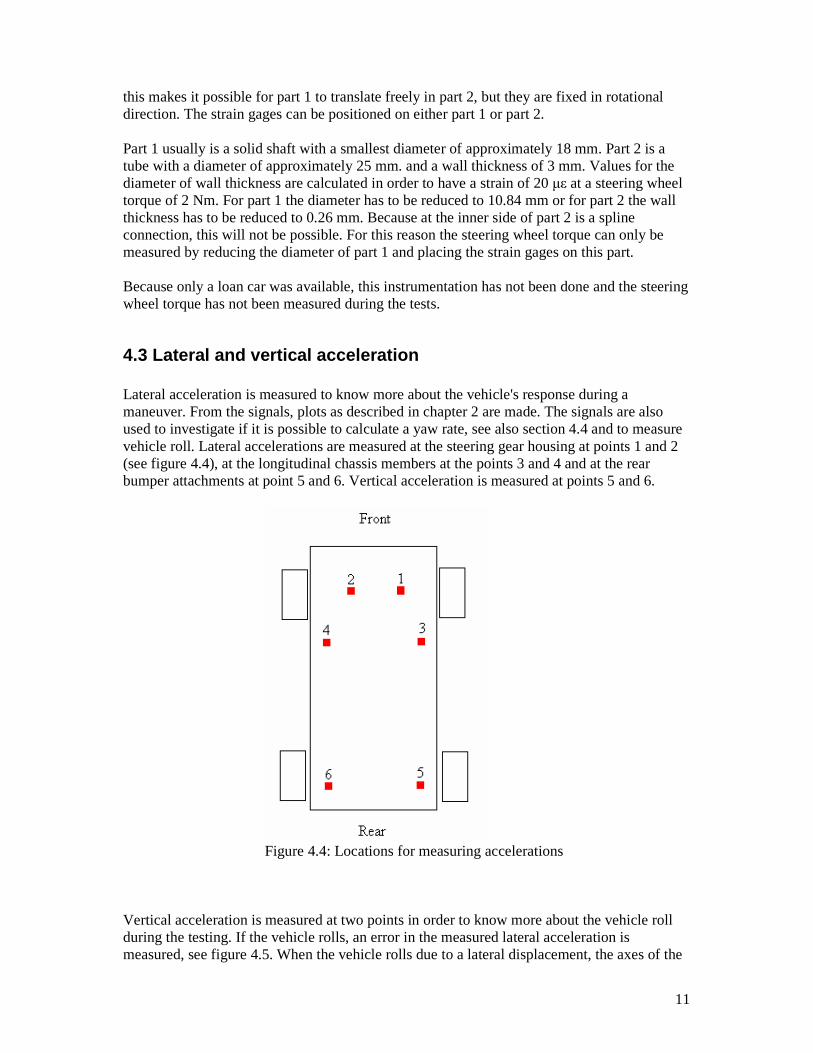
4.3 Lateral and vertical acceleration Lateral acceleration is measured to know more about the vehicle's response during a maneuver. From the signals, plots as described in chapter 2 are made. The signals are also used to investigate if it is possible to calculate a yaw rate, see also section 4.4 and to measure vehicle roll. Lateral accelerations are measured at the steering gear housing at points 1 and 2 (see figure 4.4), at the longitudinal chassis members at the points 3 and 4 and at the rear bumper attachments at point 5 and 6. Vertical acceleration is measured at points 5 and 6.

Figure 4.4: Locations for measuring accelerations

Vertical acceleration is measured at two points in order to know more about the vehicle roll during the testing. If the vehicle rolls, an error in the measured lateral acceleration is measured, see figure 4.5. When the vehicle rolls due to a lateral displacement, the axes of the

12

accelerometer also rolls and the accelerometer will measure aym. The real lateral acceleration of the vehicle is ayr and will have a higher magnitude than the measured value aym. Because the on-center weave test is not an extreme test it is expected that vehicle roll is negligible and aym will be very close to ayr. In chapter 5 the signals for the lateral and vertical accelerations are evaluated.

Figure 4.5: Error in measured lateral acceleration

For measuring the lateral or vertical acceleration, accelerometers have to be used which are able to measure low frequency accelerations. As described in chapter 2 the weave test consists of a steering wheel input of 0.2 Hz. Only DC (Direct Current) accelerometers are able to measure this low frequency level acceleration. The MWS 5401 and Kyowa AS-10B sensors are used for measuring the accelerations. More information about these sensors can be found in appendix E.

4.4 Yaw rate The yaw rate is measured to be able to characterize the effectiveness of the SWA, see also chapter 2. Usually yaw rate is measured with a gyro module. At LMS no gyro modules are available. For this reason it is investigated if it is possible to calculate the yaw rate from the lateral accelerations at points 4 and 6 or points 3 and 5 on a similar way as described in [15]. Calculating yaw rate this way is also reducing costs. When a maneuver is made, the speeds V4y and V6y will differ (see figure 4.6), resulting in a yaw rateψ& .

13

Figure 4.6: Speeds during maneuver

The yaw rate can be calculated by:

( ) [ ]sL

VV yy 064 3602

⋅−

=π

ψ& , (4.1)

where V4y is the lateral speed at point 4, V6y the lateral speed at point 6 and L the distance between point 4 and 6. Because no information is known about the lateral speeds at the points 4 and 6, the measured lateral acceleration signals have to be integrated with respect to time. This procedure to process the data and the results are described in chapter 5.

4.5 Measurements and data acquisition All measurements are performed with a Renault Laguna, see figure 4.7. All measurements are performed with the same test driver for reproducible results. Measurements are done on public road. During measurements the frequency of the steer input is triggered with a stopwatch. After each measurement (four in total) the data is evaluated to check if the peak lateral acceleration levels were approximately + 1-2 m/s2 during the measurements. Measurements are made during dry weather and low wind velocity. On the passenger seat the data-acquisition system is positioned. On the back seat the operator of the laptop is seated in the middle of the car. All measurement devices are connected to a data acquisition system developed by LMS, the Scadas. For the measurements the Scadas3 is used. The Scadas3 is connected to a laptop via a SCSI card. On the laptop the in home developed LMS software Test.Lab 7A is installed. All data during measurements is recorded with Test.Lab at a sample frequency of 512 Hz and after the measurements exported to ASCI files for processing in Matlab, see also chapter 5. During measurements the Scadas3 is connected to the car its battery for the power supply.

14

The draw wire sensor is connected to a PQFA module in the Scadas3, see [16]. The output signal from the draw wire sensor is a voltage and can be connected directly to the Scadas3. The draw wire sensor needs a power supply and is connected to the car its battery. All signals from the accelerometers are based on strain gage technology. The module in the Scadas3 for connecting strain gage measurement devices to is the PQBA module. Because the MWS 5401 3D accelerometer generates an output voltage which is too high for the PQBA module, an extra resistance wire is needed to connect in between the accelerometer and the PQBA module. The output voltage of the Kyowa AS-10B is correct and these accelerometers are connected directly to the PQBA modules.

15

5. Data interpretation From both the V.LM model and the measurements a lot of data is obtained. In chapter 2 it is described what parameters can be determined from this data in order to characterize the correctness of the maneuvers and to have more information about the vehicle its response. All processing is done with use of Matlab. In this chapter briefly the processing of the data is described and the results are presented. First the processing of the data from the V.LM model is described, after this the processing of the data from the measurements is described and finally the results are compared in order to validate the V.LM model.

5.1 Processing of V.LM model data V.LM calculates a great lot of data during a simulation. For every part (chassis, knuckles, steering rods and so on) time trajectories for the forces, torques, speeds, accelerations and so on are calculated. All on-center parameters except response time lag (torque deadband, steering friction, steering stiffness, response deadband and yaw rate response gain), are determined from the curves of steering wheel torque versus steering wheel angle and from yaw rate versus steering wheel angle. Response time lag is calculated from the time trajectories of the steering wheel angle and yaw rate.

5.1.1 Time trajectories The processing starts with reducing the data. As known, the V.LM model needs time to stabilize during the beginning of the simulation and the data from both the first and the last weave contain errors due to starting and ending effects. Also the interest only goes out to the data contained from the weaves. The data reduction algorithm reduces the data in such a way that only information of the second weave up till the second last weave will be kept for calculation of all on-center parameters. After the data reduction the algorithm calculates all on-center parameters as described in [3]. The plot of the time trajectories, zoomed for half a period, can be seen in figure 5.1. From these trajectories the response time lag is obtained. As can be seen in the figure, there is a phase lag between the steering wheel angle and the yaw rate. The line for the yaw rate passes trough zero at a later moment than the line for the steering wheel angle. The reason for this lies amongst others in the reason that due to inertias the vehicle needs time to response to a steering wheel input. The distance between these lines is computed and from this plot the response time lag is found to be 0.06 seconds. From literature [1], [2] it is known that a response time lag of 0.14 seconds is a realistic value. The vehicle which is used for testing in this paper (Jaguar XJ40) is like a Chrysler Neon a luxury car, but the Jaguar is a heavier type, so values for the on-center parameters may vary a bit. A possible reason for the difference between the value calculated from the V.LM data and found in literature is that the V.LM model lacks some very important information about a good tire model and frictions and compliances of the steering system. The tire model used in the V.LM model is a complex tire model, which contains only information about the lateral stiffness, cornering stiffness, lateral damping and friction coefficient. All these parameters are described as linear parameters. The parts in the V.LM model are modeled as rigid bodies, so no compliances are taken into

16

account. The inertias used in the model are estimated and are not exact values corresponding to the inertias of the real Chrysler Neon vehicle. Probably the inertias are estimated too low, which will result in a faster vehicle response and thus a lower response time lag.

11.5 12 12.5 13 13.5 14 14.5 15 15.5

-8

-6

-4

-2

0

2

4

6

8

SWA / SWT / ay / Yaw rate - Time, REDUCED DATA

Time [s] →

SWA [deg]

SWT [Nm]

ay [ms-2]

Yaw rate [o/s]

Figure 5.1: Time trajectories

5.1.2 Steering wheel torque versus steering wheel angle The plot for the steering wheel torque versus the steering wheel angle obtained from the simulation results can be seen in figure 5.2. A typical plot from the steering wheel torque versus the steering wheel angle, obtained from measurements, can be seen in figure 5.3. From figure 5.2 the parameters for the steering friction, steering stiffness and torque deadband are calculated. From literature [1], [2] it is known that typical values for the steering friction, steering stiffness and torque deadband are 1.14 Nm, 0.230 Nm/deg and 5.3 deg respectively. Values calculated from the simulation data for steering friction, steering stiffness and torque deadband are 0.031 Nm, 0.079 Nm/deg and 0.385 deg respectively. The difference between these values of the steering friction (vertical distance between the two lines in figure 5.2 at a steering wheel angle of 0 deg) can be attributed to the lack of steering friction modeled in the V.LM model. In the V.LM model no friction is modeled in the steering system, where in a normal passenger car in the steering system consists friction in every connection, see also section 3.1.2. This can also be seen in figure 5.1 where no shift in the steering wheel torque occurs when the derivative of the steering wheel angle changes from sign (this happens at maximum and minimum values of the steering wheel angle). When (static) friction would be modeled in the V.LM model, the steering wheel torque at maximum

17

and minimum steering wheel angle would be expected to have a step in magnitude in order to overcome the friction forces in the steering system.

-10 -8 -6 -4 -2 0 2 4 6 8 10-1

-0.8

-0.6

-0.4

-0.2

0

0.2

0.4

0.6

0.8

1SWT - SWA

SWA [deg]

SW

T [

Nm

]

Figure 5.2: Steering wheel torque – steering wheel angle, simulation results

Figure 5.3: Steering wheel torque – steering wheel angle, literature [1]

The difference in the torque deadband (horizontal distance between the two lines in figure 5.2 at a steering wheel torque of 0 Nm) can be explained by the following. Due to the lack of friction, the two lines in figure 5.2 are vertically located too close to each other. For this reason the horizontal distance between the lines will also be to close and the torque deadband will be very small. In the V.LM model no hydraulic power steering is modeled (see also section 3.1.2). A hydraulic power steering makes use of a torsion bar. The amount of torsion is the measure for the steering wheel torque and will result in a change of boost pressure for the steering gear [8]. In the V.LM model no torsion bar is modeled. Because of this the steering stiffness computed from the simulation data could be lower than the steering stiffness of a real vehicle would be. Combined with an inaccurate tire model it will be clear that the magnitude of the steering stiffness will differ from the steering stiffness found in literature. When a closer look is taken to the shape of the plots in figures 5.2 and 5.3 some conclusions can be made. It can be seen that the plot in figure 5.3 “flattens out” at higher steering wheel angles, where the plot in figure 5.2 is almost linear. This effect can be attributed to the tire model and the lack of hydraulic power steering or a wrong steering gear mesh. As stated above, all parameters of the tire model are linear parameters. From [12] it is known that the tire does not behave linear at all. Because of the non-linear behavior of the tire, the self aligning moments calculated during simulation can be wrong. The self aligning moment will generate the lateral forces in the steering rods and the needed steering wheel torque will change. The lack of hydraulic steering system in the V.LM model can also be a reason why the plot in figure 5.2 does not flatten out. The hydraulic steering system behaves very non-linear [9]. A typical characteristic of the steering wheel torque versus the rack force (lateral forces on steering gear generated by the steering rods) can be seen in figure 5.4.

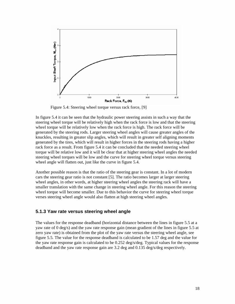
18

Figure 5.4: Steering wheel torque versus rack force, [9]

In figure 5.4 it can be seen that the hydraulic power steering assists in such a way that the steering wheel torque will be relatively high when the rack force is low and that the steering wheel torque will be relatively low when the rack force is high. The rack force will be generated by the steering rods. Larger steering wheel angles will cause greater angles of the knuckles, resulting in greater slip angles, which will result in greater self aligning moments generated by the tires, which will result in higher forces in the steering rods having a higher rack force as a result. From figure 5.4 it can be concluded that the needed steering wheel torque will be relative low and it will be clear that at higher steering wheel angles the needed steering wheel torques will be low and the curve for steering wheel torque versus steering wheel angle will flatten out, just like the curve in figure 5.4. Another possible reason is that the ratio of the steering gear is constant. In a lot of modern cars the steering gear ratio is not constant [5]. The ratio becomes larger at larger steering wheel angles, in other words, at higher steering wheel angles the steering rack will have a smaller translation with the same change in steering wheel angle. For this reason the steering wheel torque will become smaller. Due to this behavior the curve for steering wheel torque verses steering wheel angle would also flatten at high steering wheel angles.

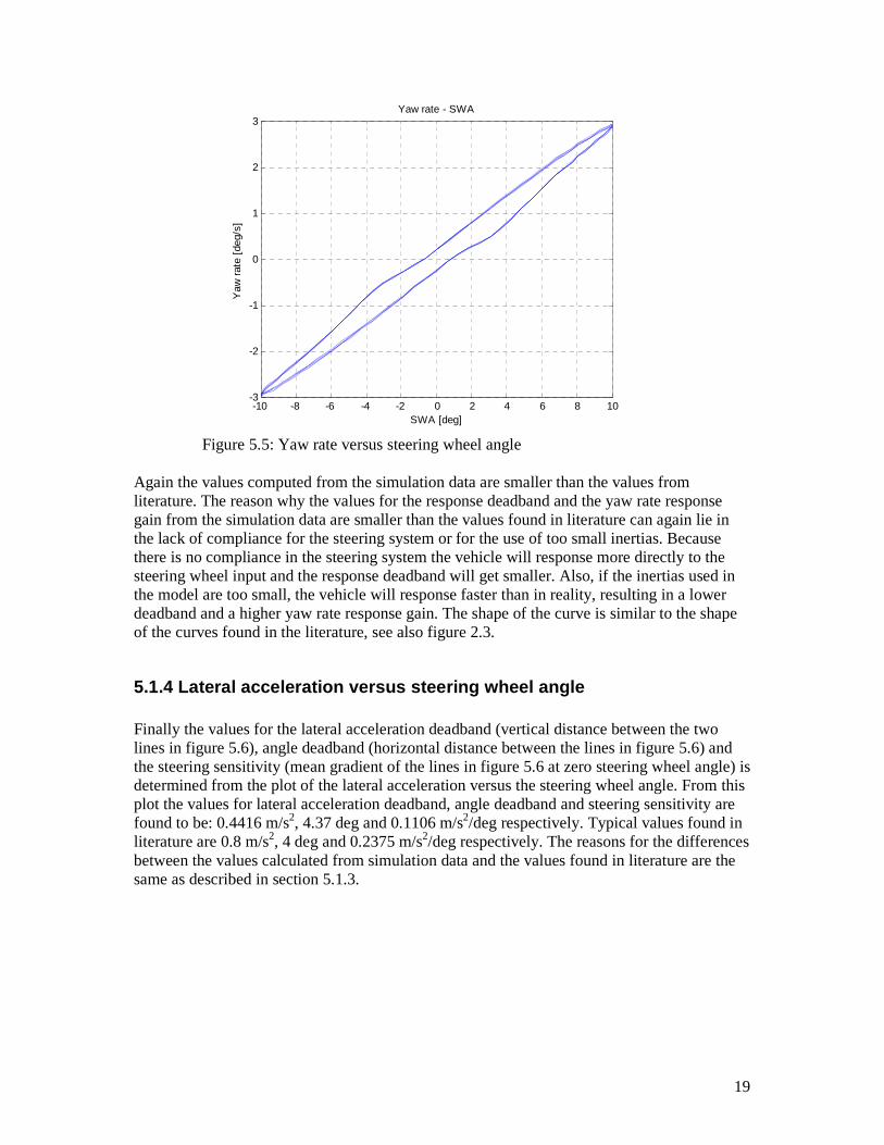
5.1.3 Yaw rate versus steering wheel angle The values for the response deadband (horizontal distance between the lines in figure 5.5 at a yaw rate of 0 deg/s) and the yaw rate response gain (mean gradient of the lines in figure 5.5 at zero yaw rate) is obtained from the plot of the yaw rate versus the steering wheel angle, see figure 5.5. The value for the response deadband is calculated to be 1.57 deg and the value for the yaw rate response gain is calculated to be 0.252 deg/s/deg. Typical values for the response deadband and the yaw rate response gain are 3.2 deg and 0.135 deg/s/deg respectively.

19

-10 -8 -6 -4 -2 0 2 4 6 8 10-3

-2

-1

0

1

2

3Yaw rate - SWA

SWA [deg]

Yaw

rat

e [d

eg/s

]

Figure 5.5: Yaw rate versus steering wheel angle

Again the values computed from the simulation data are smaller than the values from literature. The reason why the values for the response deadband and the yaw rate response gain from the simulation data are smaller than the values found in literature can again lie in the lack of compliance for the steering system or for the use of too small inertias. Because there is no compliance in the steering system the vehicle will response more directly to the steering wheel input and the response deadband will get smaller. Also, if the inertias used in the model are too small, the vehicle will response faster than in reality, resulting in a lower deadband and a higher yaw rate response gain. The shape of the curve is similar to the shape of the curves found in the literature, see also figure 2.3.

5.1.4 Lateral acceleration versus steering wheel angle Finally the values for the lateral acceleration deadband (vertical distance between the two lines in figure 5.6), angle deadband (horizontal distance between the lines in figure 5.6) and the steering sensitivity (mean gradient of the lines in figure 5.6 at zero steering wheel angle) is determined from the plot of the lateral acceleration versus the steering wheel angle. From this plot the values for lateral acceleration deadband, angle deadband and steering sensitivity are found to be: 0.4416 m/s2, 4.37 deg and 0.1106 m/s2/deg respectively. Typical values found in literature are 0.8 m/s2, 4 deg and 0.2375 m/s2/deg respectively. The reasons for the differences between the values calculated from simulation data and the values found in literature are the same as described in section 5.1.3.

20

-10 -8 -6 -4 -2 0 2 4 6 8 10-1.5

-1

-0.5

0

0.5

1

1.5

ay - SWA

Steering wheel angle [deg]

Late

ral a

ccel

erat

ion

[m/s

2 ]

Figure 5.6: Lateral acceleration versus steering wheel angle

5.2 Processing of the measurement data In chapter 2 the reason for the need of a simple instrumentation is given. With an instrumented vehicle weave tests are done. Results are discussed in this section.

5.2.1 Data interpretation and filtering In figure 5.7a the time trajectory for the steering wheel angle can be seen, in figure 5.7b a time trajectory for the lateral acceleration on the chassis can be seen (from sensor 4, see also chapter 4). The other time trajectories can be found on the CD.

0 10 20 30 40 50 60 70 80 90 100-200

-150

-100

-50

0

50Steering wheel angle, time trace

Ste

erin

g w

heel

ang

le [

deg]

Time [s] 0 10 20 30 40 50 60 70 80 90 100

-5

-4

-3

-2

-1

0

1

2

3Lateral acceleration, sensor 4, time trace

Time [s]

Late

ral a

ccel

erat

ion

[m/s

2 ]

Figure 5.7a: Draw wire sensor, time trajectory Figure 5.7b: Lateral acceleration, sensor 4, time

trajectory

21

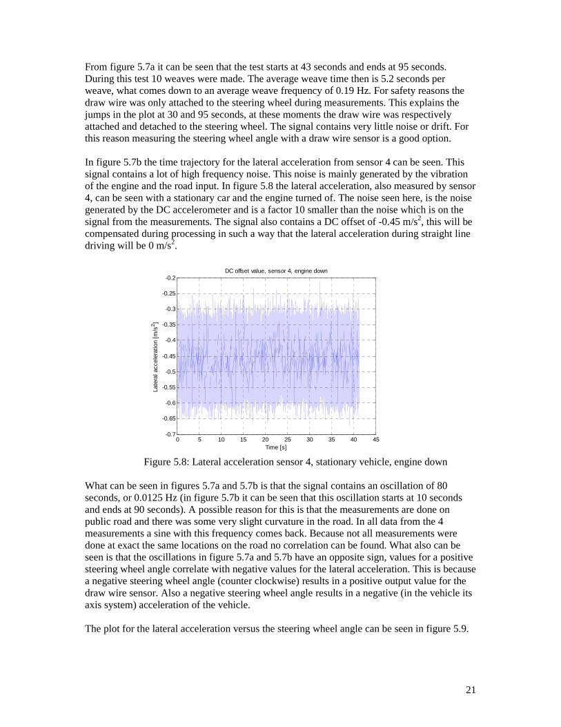
From figure 5.7a it can be seen that the test starts at 43 seconds and ends at 95 seconds. During this test 10 weaves were made. The average weave time then is 5.2 seconds per weave, what comes down to an average weave frequency of 0.19 Hz. For safety reasons the draw wire was only attached to the steering wheel during measurements. This explains the jumps in the plot at 30 and 95 seconds, at these moments the draw wire was respectively attached and detached to the steering wheel. The signal contains very little noise or drift. For this reason measuring the steering wheel angle with a draw wire sensor is a good option. In figure 5.7b the time trajectory for the lateral acceleration from sensor 4 can be seen. This signal contains a lot of high frequency noise. This noise is mainly generated by the vibration of the engine and the road input. In figure 5.8 the lateral acceleration, also measured by sensor 4, can be seen with a stationary car and the engine turned of. The noise seen here, is the noise generated by the DC accelerometer and is a factor 10 smaller than the noise which is on the signal from the measurements. The signal also contains a DC offset of -0.45 m/s2, this will be compensated during processing in such a way that the lateral acceleration during straight line driving will be 0 m/s2.

0 5 10 15 20 25 30 35 40 45-0.7

-0.65

-0.6

-0.55

-0.5

-0.45

-0.4

-0.35

-0.3

-0.25

-0.2DC offset value, sensor 4, engine down

Time [s]

Late

ral a

ccel

erat

ion

[m/s

2 ]

Figure 5.8: Lateral acceleration sensor 4, stationary vehicle, engine down

What can be seen in figures 5.7a and 5.7b is that the signal contains an oscillation of 80 seconds, or 0.0125 Hz (in figure 5.7b it can be seen that this oscillation starts at 10 seconds and ends at 90 seconds). A possible reason for this is that the measurements are done on public road and there was some very slight curvature in the road. In all data from the 4 measurements a sine with this frequency comes back. Because not all measurements were done at exact the same locations on the road no correlation can be found. What also can be seen is that the oscillations in figure 5.7a and 5.7b have an opposite sign, values for a positive steering wheel angle correlate with negative values for the lateral acceleration. This is because a negative steering wheel angle (counter clockwise) results in a positive output value for the draw wire sensor. Also a negative steering wheel angle results in a negative (in the vehicle its axis system) acceleration of the vehicle. The plot for the lateral acceleration versus the steering wheel angle can be seen in figure 5.9.

22

-200 -150 -100 -50 0 50-4

-3

-2

-1

0

1

2

3

4Lateral acceleration versus steering wheel angle

Steering wheel angle [deg]

Late

ral a

ccel

erat

ion

[m/s

2 ]

Figure 5.9: Lateral acceleration versus steering wheel angle

It will be clear that from this plot no parameters (lateral acceleration deadband, angle deadband and steering sensitivity) can be determined, because no proper hysteresis loop is obtained (see also figure 2.4 and figure 5.6). It also becomes clear that the dataset from which the plots are made has to be reduced; we are only interested in the data during the weaves and data recorded before and after the weaves is deleted. Due to the high frequency noise no proper hysteresis loop can be observed in figure 5.9, for this reason the signal has to be filtered with a lowpass filter. For filtering and data reduction a Matlab Simulink model is built. For filtering a fifth order Butterworth filter with lowpass frequency of 2 Hz. was used (for more information about Butterworth filters, see appendix D). The reduced, filtered data can be seen in figure 5.10.

0 5 10 15 20 25 30 35 40 45 50

-3

-2

-1

0

1

2

3

Reduced time data, sensor 4

Time [s]

Late

ral a

ccel

erat

ion

[m/s

2 ]

Original data

Filtered data

Figure 5.10: Reduced, filtered time data, sensor 4.

23

Due to the use of the Butterworth filter, the filtered data has a phase lag, which also can be seen in figure 5.10. The signal for the steering wheel angle needs no filtering, because the signal contains no noise. Still the steering wheel angle data is filtered in order to be sure that all data has the same phase lag. If the filtered data from the lateral accelerations is compared with the unfiltered data from the steering wheel angle, wrong conclusions are drawn.

5.2.2 Lateral acceleration versus steering wheel angle With the filtered data again the plot is made for the lateral acceleration versus the steering wheel angle, see figure 5.11.

-15 -10 -5 0 5 10 15-2.5

-2

-1.5

-1

-0.5

0

0.5

1

1.5

2Lateral acceleration versus steering wheel angle

Late

ral a

ccel

erat

ion

[m/s

2 ]

Steering wheel angle [deg]

Figure 5.11: Lateral acceleration versus steering wheel angle, filtered signal In this plot the hysteresis loop can be seen. Also the effect of noise on the steering wheel input becomes clear. If the steering wheel input would have been a perfect sine with no noise included and a frequency of 0.2 Hz for all weaves, the curves in the plot would have overlapped each other, see also figure 5.6. It will be clear that a lot of attention needs to be paid to a proper steering wheel input during testing and a steer robot may be preferred. The parameters for the lateral acceleration deadband, the angle deadband and the steering sensitivity determined from this plot are 0.3218 m/s2, 2.359 deg and 0.1153 m/s2/deg respectively. These values are compared to the values from the simulation data in chapter 6.

5.2.3 Yaw rate With the filtered data the yaw rate is computed as described in chapter 4. In order to compute the lateral speed from the signals of the lateral acceleration, the low frequency oscillation (see figures 5.7a and 5.7b) is filtered out of the signal with a second order highpass Butterworth filter, with cut-off frequency of 0.08 Hz . If the data does not pass a highpass filter, the integrated signal will rapidly increase to very high values. In figure 5.12a this effect can be seen. In figure 5.12b the calculated lateral speed after filtering from sensor 4 is shown.

24

0 10 20 30 40 50 600

5

10

15

20

25

30

35Calculated lateral speed, without filtering

Time [s]

Late

ral s

peed

[m

/s]

0 10 20 30 40 50 60-2

-1.5

-1

-0.5

0

0.5

1

1.5

2Calculated lateral speed after filtering

Time [s]

Late

ral s

peed

[m

/s]

Figure 5.12a: Calculated lateral speed without filtering

Figure 5.12b: Calculated lateral speed with filtering

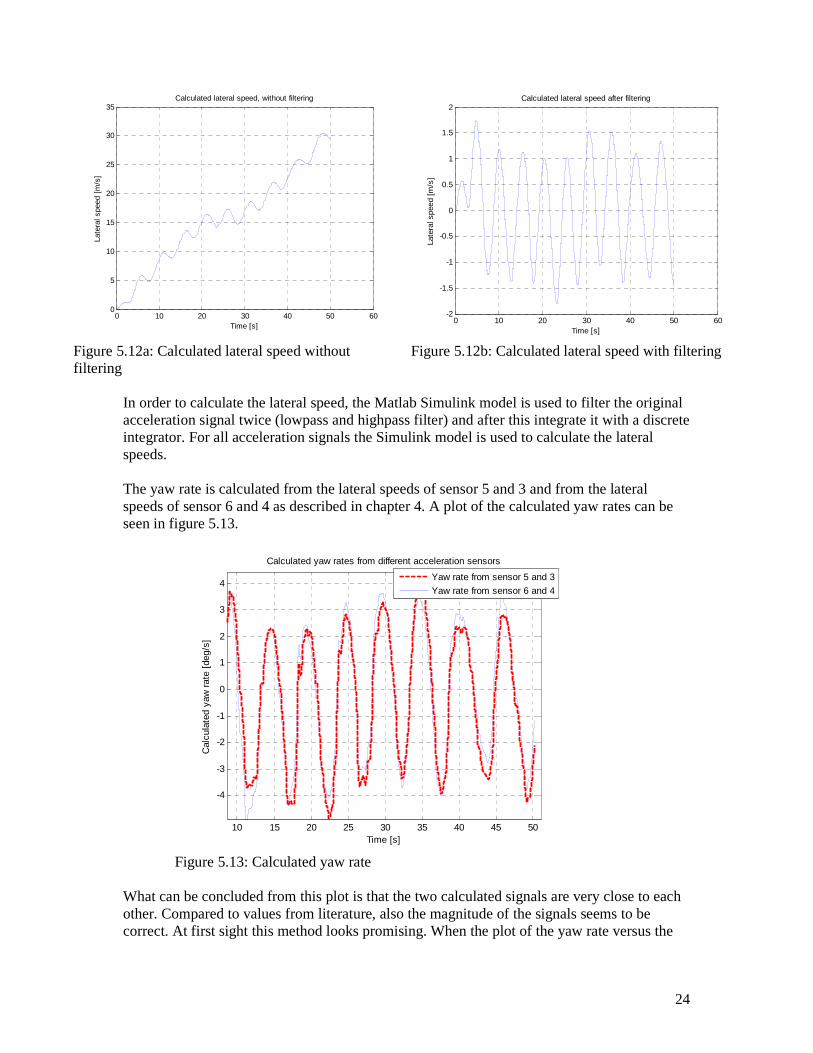
In order to calculate the lateral speed, the Matlab Simulink model is used to filter the original acceleration signal twice (lowpass and highpass filter) and after this integrate it with a discrete integrator. For all acceleration signals the Simulink model is used to calculate the lateral speeds. The yaw rate is calculated from the lateral speeds of sensor 5 and 3 and from the lateral speeds of sensor 6 and 4 as described in chapter 4. A plot of the calculated yaw rates can be seen in figure 5.13.

10 15 20 25 30 35 40 45 50

-4

-3

-2

-1

0

1

2

3

4

Time [s]

Cal

cula

ted

yaw

rat

e [d

eg/s

]

Calculated yaw rates from different acceleration sensors

Yaw rate from sensor 5 and 3

Yaw rate from sensor 6 and 4

Figure 5.13: Calculated yaw rate

What can be concluded from this plot is that the two calculated signals are very close to each other. Compared to values from literature, also the magnitude of the signals seems to be correct. At first sight this method looks promising. When the plot of the yaw rate versus the

25

steering wheel angle is made (see figure 5.14) and compared with plots found in literature (figure 2.3), it becomes clear that this hysteresis loop can not be used.

-15 -10 -5 0 5 10 15-6

-4

-2

0

2

4

6Yaw rate - SWA

Steering wheel angle [deg]

Yaw

rat

e [d

eg/s

]

Figure 5.14: Yaw rate versus steering wheel angle, sensor 5 and 3

It can be concluded that no reliable hysteresis plot is obtained with the calculated yaw rate and the filtered steering wheel angle; both the lateral acceleration deadband (3 m/s2) and the angle deadband (12 deg) are too large. The problem most probably comes with the filtering. For calculating the yaw rate, the data needs to be filtered twice. After every filter operation the data obtains a phase lag, and the shape of the curve changes, see figure 5.15.

2 4 6 8 10 12 14 16 18 20 22-15

-10

-5

0

5

10

15

20

Time [s]

Ste

erin

g w

heel

ang

le [

deg]

SWA

Original SWA

SWA after lowpass

SWA after low- and highpass

Figure 5.15: Steering wheel angle, effect of filtering

26

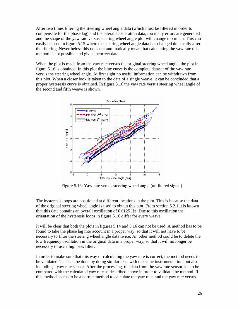
After two times filtering the steering wheel angle data (which must be filtered in order to compensate for the phase lag) and the lateral acceleration data, too many errors are generated and the shape of the yaw rate versus steering wheel angle plot will change too much. This can easily be seen in figure 5.15 where the steering wheel angle data has changed drastically after the filtering. Nevertheless this does not automatically mean that calculating the yaw rate this method is not possible and gives incorrect data. When the plot is made from the yaw rate versus the original steering wheel angle, the plot in figure 5.16 is obtained. In this plot the blue curve is the complete dataset of the yaw rate versus the steering wheel angle. At first sight no useful information can be withdrawn from this plot. When a closer look is taken to the data of a single weave, it can be concluded that a proper hysteresis curve is obtained. In figure 5.16 the yaw rate versus steering wheel angle of the second and fifth weave is shown.

Figure 5.16: Yaw rate versus steering wheel angle (unfiltered signal)

The hysteresis loops are positioned at different locations in the plot. This is because the data of the original steering wheel angle is used to obtain this plot. From section 5.2.1 it is known that this data contains an overall oscillation of 0.0125 Hz. Due to this oscillation the orientation of the hysteresis loops in figure 5.16 differ for every weave. It will be clear that both the plots in figures 5.14 and 5.16 can not be used. A method has to be found to take the phase lag into account in a proper way, so that it will not have to be necessary to filter the steering wheel angle data twice. An other method could be to delete the low frequency oscillation in the original data in a proper way, so that it will no longer be necessary to use a highpass filter. In order to make sure that this way of calculating the yaw rate is correct, the method needs to be validated. This can be done by doing similar tests with the same instrumentation, but also including a yaw rate sensor. After the processing, the data from the yaw rate sensor has to be compared with the calculated yaw rate as described above in order to validate the method. If this method seems to be a correct method to calculate the yaw rate, and the yaw rate versus

27

steering wheel angle plot will become representative, no yaw rate sensor will be required any more.

5.2.4 Comparison accelerations steering gear housing During the weave tests the steering wheel angle changes constantly. Every moment different forces and torques are generated which are transmitted from the tires via the knuckles and the steering rods through the steering gear housing to the chassis. The steering gear housing is mounted with bushings to the chassis. The bushings have a finite stiffness and during a maneuver the steering gear housing will have some small displacements with respect to the chassis. In order to try to learn more about the displacement of the steering gear housing during a maneuver, the lateral accelerations are compared. First the lateral acceleration from the chassis is calculated at the point where the lateral acceleration of the steering gear housing is measured.

Figure 5.17: Schematic overview of sensors

This means, from the lateral accelerations of sensors 5 and 3, the lateral acceleration of the chassis at point 1 can be calculated (see figure 5.17). The sensors at point 5 and point 3 are fixed to the chassis, where the sensor at point 1 is fixed to the steering gear housing. The lateral acceleration of the chassis at point 1 can be calculated as:

( ) ( ) 5211

531 aLL

L

aaa ++

−= (5.1)

where a3, a5, L1 and L2 are as specified in figure 5.17. Because the lateral distance between point 1 and point 3 (and also between point 1 and point 5) is much smaller than L1 + L2, errors in calculated lateral acceleration due to a different lateral distance of the points will be negligible. Calculation of the lateral acceleration of the chassis at point 2 is done in a similar way, by comparing the lateral accelerations of point 4 and point 6 with each other.

28

Figure 5.18 shows the calculated lateral acceleration of the chassis at point 1 and the measured lateral acceleration of the steering gear housing at point 1. The figure for point 2 looks similar. For calculation the filtered signals are used.

0 2 4 6 8 10 12 14 16 18 20

-1.5

-1

-0.5

0

0.5

1

1.5

2

Time [s]

Late

ral a

ccel

erat

ion

[m/s

2 ]

Comparison lateral acceleration steering gear, point 1

Filtered data

Computed data

Figure 5.18: Comparison between calculated and measured lateral acceleration, point 1

From this plot it can be concluded that at point 1 the computed peak accelerations of the chassis are slightly higher than the measured peak accelerations of the steering gear housing. Further it can be concluded that the two curves are almost identical for lateral acceleration levels of + 80 % of the peak acceleration values. The shapes of the curves only differ at the peak regions of the lateral acceleration. This can be explained by the fact that the steering gear housing is mounted via non-infinite stiff bushings to the chassis. When the steering wheel velocity changes from sign, which happens at the peak values of lateral acceleration, the force in the bushings will change direction. This will also result in a change of the deformation of the bushings. The difference in magnitude between the two curves can be explained by the fact that there could have been a drift on the sensitivity of the accelerometers during the measurements. When this occurs, the accelerometers will measure a slightly different acceleration. In order to know if the computed accelerations at point 1 (or point 2) are representative acceleration, these accelerations are be further compared with the measured accelerations. When the accelerations are integrated twice, it will be possible to look what the displacement from the steering gear housing with respect to the chassis is. For integration again a Matlab Simulink model is used. The measured acceleration is subtracted from the calculated acceleration. From this the difference in acceleration is returned. When this signal is

29

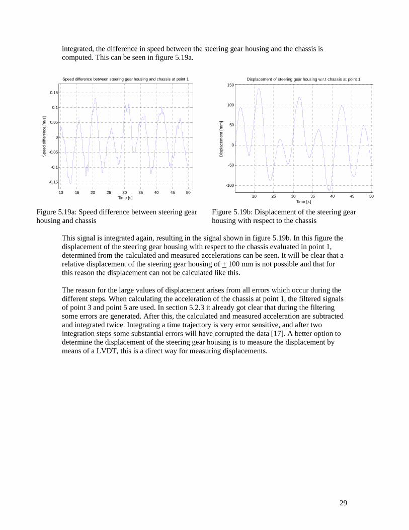
integrated, the difference in speed between the steering gear housing and the chassis is computed. This can be seen in figure 5.19a.

This signal is integrated again, resulting in the signal shown in figure 5.19b. In this figure the displacement of the steering gear housing with respect to the chassis evaluated in point 1, determined from the calculated and measured accelerations can be seen. It will be clear that a relative displacement of the steering gear housing of + 100 mm is not possible and that for this reason the displacement can not be calculated like this. The reason for the large values of displacement arises from all errors which occur during the different steps. When calculating the acceleration of the chassis at point 1, the filtered signals of point 3 and point 5 are used. In section 5.2.3 it already got clear that during the filtering some errors are generated. After this, the calculated and measured acceleration are subtracted and integrated twice. Integrating a time trajectory is very error sensitive, and after two integration steps some substantial errors will have corrupted the data [17]. A better option to determine the displacement of the steering gear housing is to measure the displacement by means of a LVDT, this is a direct way for measuring displacements.

10 15 20 25 30 35 40 45 50

-0.15

-0.1

-0.05

0

0.05

0.1

0.15

Speed difference between steering gear housing and chassis at point 1

Time [s]

Spe

ed d

iffer

ence

[m

/s]

20 25 30 35 40 45 50

-100

-50

0

50

100

150Displacement of steering gear housing w.r.t chassis at point 1

Time [s]

Dis

plac

emen

t [m

m]

Figure 5.19a: Speed difference between steering gear housing and chassis

Figure 5.19b: Displacement of the steering gear housing with respect to the chassis

30

6. Comparison measurements and simulation From the time trajectories obtained from both the measurements and the simulations a lot of information is acquired, see also chapter 5. In order to validate the V.LM model and to compare measured and simulated data, the measured steering wheel angle is used in a simulation with V.LM. In this chapter the results obtained from the measured data and the simulated data are compared.

6.1 Creating input for V.LM As described in chapter 3, the user can define a spline curve for the steering wheel input and the road profile. In order to simulate a maneuver which is as close to measurements as possible, these spline curves are generated from the data obtained from measurements. The data from the measured steering wheel angle is written to an excel file. Because no data for the road profile is available, a smooth road, similar to the test track, is generated and used for simulation (see chapter 3). After the simulation the measured steering wheel angle and the generated steering wheel angle during simulation are plotted in one figure to make sure that the steering input is correctly applied. From the plot it can be concluded that the data from the measured and the simulated steering wheel angles overlap. This proves that the simulated maneuver is equal to the maneuver during measurements and the data from both simulation and measurements can be compared. Still the V.LM model can not be validated with the measurement data, because the measurements are performed with a Renault Laguna, where a Chrysler Neon is modeled. The results can only be compared to check if the order of magnitude is correct. In order to validate the V.LM model, new measurements have to be performed with a Chrysler Neon.

6.2 Yaw rate In section 5.2.3 plots for the calculated yaw rate and yaw rate versus steering wheel angle obtained from the measurement data are shown. From the simulation data for the yaw rate is available. In figure 6.1 the time trajectories for the simulated yaw rate and the calculated yaw rate from measurement data can be seen.

31

12 14 16 18 20 22 24 26 28 30-5

-4

-3

-2

-1

0

1

2

3

4

5

Time [s]

Cal

cula

ted

yaw

rat

e [d

eg/s

]

Yaw rates

Yaw rate from sensor 5 and 3

Yaw rate from sensor 6 and 4

Yaw rate from simulation

Figure 6.1: Time trajectories yaw rate

What can be seen directly is that the shape from the curves of the simulated and calculated yaw rates is similar. There is no phase lag between the curves. The magnitude from the simulated yaw rate and the calculated yaw rate differs slightly. The reason for this is the same as described in section 5.2.4, during measurements a drift on the sensitivity of the accelerometers occurred. From the simulation data the plot for the yaw rate versus the steering wheel angle is obtained. This plot, together with the plot of the calculated yaw rate versus the unfiltered steering wheel angle is shown in figure 6.2.

Figure 6.2: Yaw rate versus steering wheel angle

32

It can be seen that the loop from the simulated yaw rate versus the steering wheel angle (simulation data) contains only a very little hysteresis part. In section 5.1.3 it is already discussed that the lack of a hysteresis part comes from wrong values for the vehicle its inertias and the lack of compliance of the steering system. The yaw rate response gain (mean gradient at zero yaw rate) though is approximately equal for both the calculated data and the simulated data. In order to validate the simulated data, the yaw rate has to be tracked during measurements and should be compared with the simulated data. What is concluded is that the order of magnitude is correct. Because it is not known if the calculated yaw rates are representative, no validation of the V.LM model can be done with the calculated yaw rates.

6.3 Lateral acceleration versus steering wheel angle In section 5.2.2 the plot for the lateral acceleration versus the steering wheel angle, obtained from the measurement data, is presented. In figure 6.3 the plot for the lateral acceleration versus the steering wheel angle, obtained from the simulation data, can be seen.

-15 -10 -5 0 5 10 15-2

-1.5

-1

-0.5

0

0.5

1

1.5

2

Steering wheel angle [deg]

Late

ral a

ccel

erat

ion

[m/s

2 ]

Lateral acceleration versus steering wheel angle

measured data

simulated data

Figure 6.3: Lateral acceleration versus steering wheel angle, measurements and simulation

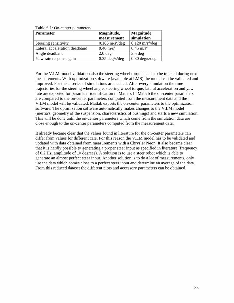
It can be concluded that both plots describe a proper hysteresis loop and the loops almost overlap each other. The on-center parameters (steering sensitivity, lateral acceleration deadband and angle deadband) which are obtained from both plots are close to each other and have the same order of magnitude, see table 6.1.

33

Table 6.1: On-center parameters Parameter Magnitude,

measurement Magnitude, simulation

Steering sensitivity 0.185 m/s2/deg 0.120 m/s2/deg Lateral acceleration deadband 0.40 m/s2 0.45 m/s2 Angle deadband 2.0 deg 3.5 deg Yaw rate response gain 0.35 deg/s/deg 0.30 deg/s/deg For the V.LM model validation also the steering wheel torque needs to be tracked during next measurements. With optimization software (available at LMS) the model can be validated and improved. For this a series of simulations are needed. After every simulation the time trajectories for the steering wheel angle, steering wheel torque, lateral acceleration and yaw rate are exported for parameter identification in Matlab. In Matlab the on-center parameters are compared to the on-center parameters computed from the measurement data and the V.LM model will be validated. Matlab exports the on-center parameters to the optimization software. The optimization software automatically makes changes to the V.LM model (inertia's, geometry of the suspension, characteristics of bushings) and starts a new simulation. This will be done until the on-center parameters which come from the simulation data are close enough to the on-center parameters computed from the measurement data. It already became clear that the values found in literature for the on-center parameters can differ from values for different cars. For this reason the V.LM model has to be validated and updated with data obtained from measurements with a Chrysler Neon. It also became clear that it is hardly possible to generating a proper steer input as specified in literature (frequency of 0.2 Hz, amplitude of 10 degrees). A solution is to use a steer robot which is able to generate an almost perfect steer input. Another solution is to do a lot of measurements, only use the data which comes close to a perfect steer input and determine an average of the data. From this reduced dataset the different plots and accessory parameters can be obtained.

34

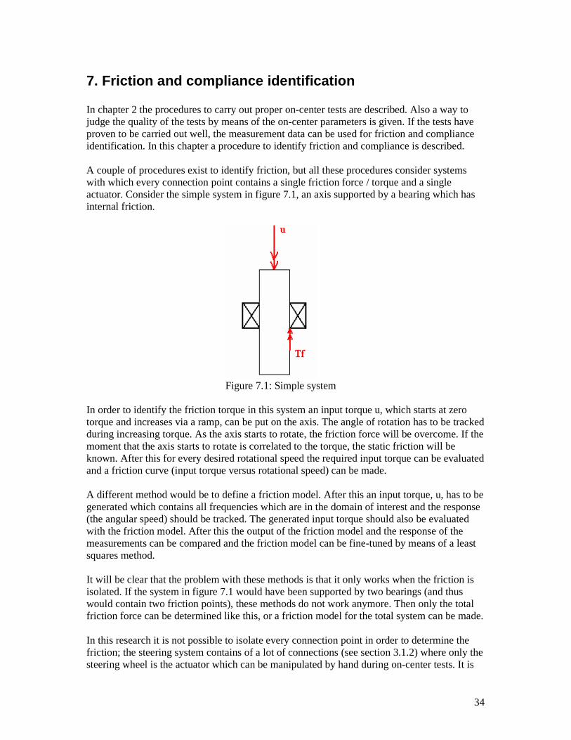
7. Friction and compliance identification In chapter 2 the procedures to carry out proper on-center tests are described. Also a way to judge the quality of the tests by means of the on-center parameters is given. If the tests have proven to be carried out well, the measurement data can be used for friction and compliance identification. In this chapter a procedure to identify friction and compliance is described. A couple of procedures exist to identify friction, but all these procedures consider systems with which every connection point contains a single friction force / torque and a single actuator. Consider the simple system in figure 7.1, an axis supported by a bearing which has internal friction.

Figure 7.1: Simple system

In order to identify the friction torque in this system an input torque u, which starts at zero torque and increases via a ramp, can be put on the axis. The angle of rotation has to be tracked during increasing torque. As the axis starts to rotate, the friction force will be overcome. If the moment that the axis starts to rotate is correlated to the torque, the static friction will be known. After this for every desired rotational speed the required input torque can be evaluated and a friction curve (input torque versus rotational speed) can be made. A different method would be to define a friction model. After this an input torque, u, has to be generated which contains all frequencies which are in the domain of interest and the response (the angular speed) should be tracked. The generated input torque should also be evaluated with the friction model. After this the output of the friction model and the response of the measurements can be compared and the friction model can be fine-tuned by means of a least squares method. It will be clear that the problem with these methods is that it only works when the friction is isolated. If the system in figure 7.1 would have been supported by two bearings (and thus would contain two friction points), these methods do not work anymore. Then only the total friction force can be determined like this, or a friction model for the total system can be made. In this research it is not possible to isolate every connection point in order to determine the friction; the steering system contains of a lot of connections (see section 3.1.2) where only the steering wheel is the actuator which can be manipulated by hand during on-center tests. It is

35

also not possible to determine a single friction model which is valid for all maneuvers. Every steering wheel angle will generate a different wheel angle, resulting in different self aligning moments of the tires and different forces in the total steering system. With changing forces in the steering system also the (static) friction forces change. Also a friction model describes the friction force for a wide range of speeds, where the speed of the parts in the steering system with respect to the chassis is very low. In this research it is of special interest to understand at which location in the steering system energy is absorbed and thus the friction forces have to be determined in every connection point. A valid method to identify friction in the steering system is to measure the forces or torques in all parts of the steering system before and after the point where friction is located. In this way the friction can be calculated as the difference between the measured forces (or torques) before and after the point where the friction is located. This is explained by means of figure 7.2.

Figure 7.2: System with multiple friction points

For the system in figure 7.2 the next relations can be formulated:

2222

12111

fs

fss

TTJ

TTTJ

−=

−−=

θ

θ&&

&&

(7.1)

where J1 is the inertia between sensor 1 and 2 (marked area), J2 the inertia of the rest of the axis, 1θ&& the rotational acceleration of the axis between sensor 1 and 2, 2θ&& the rotational acceleration of the rest of the axis, Ts1 the measured torque by sensor 1, Ts2 the measured torque by sensor 2, Tf1 the friction torque generated by bearing 1 and Tf2 the friction torque generated by bearing 2.

36

If it is assumed that the axis is infinite stiff and 1θ&& will be equal to 2θ&& and no dynamics will occur than the left part of relation (7.1) will become zero and (7.1) can be written as:

22222

2111211

0

0

sffs

ssffss

TTTTJ

TTTTTTJ

=⇒=−=

−=⇒=−−=

θ

θ&&

&&

(7.2)

Because Ts2 is known, Tf2 is known (lower relation). Ts1 is also known and thus will Tf1 be known (upper relation). The forces and torques can be measured either with strain gages, see [18], or with force cells. A force cell can be placed directly in between two axes (cut one axis in half and place the force cell between the two ends) and has a high accuracy. Because it is also of interest what the magnitude of compliance of the steering system is, it is preferred to use strain gages. In this way both the compliance of the different parts and the friction in every connection can be measured. A problem with the strain gages will be that parts as the steering axis, of steering rods have to be reduced in diameter in order to be able to measure enough strain (see also chapter 4). The assumption made to define relation (7.2), that all parts have an infinite stiffness and that 1θ&&

and 2θ&& are equal than no longer holds. As long as both 1θ&& and 2θ&& are equal to zero, the relation

is still true, but during driving tests 1θ&& and 2θ&& will probably not be equal to zero. This problem can be solved by placing a sensor extra. When sensor 1 and sensor 2 are very close to the friction point, the bearing in this case, J1 will reduce to almost zero. Near to bearing 2 the other sensor can be placed in order to reduce J2 to almost zero. The product of

11θ&&J and 22θ&&J will become negligible and relation (7.2) can be used again. It will be clear that a very complicated instrumentation will be needed. Also serious attention should be paid to safety. If some parts of the steering system have been reduced in diameter, the steering system will become weaker. At all adapted parts a safety restriction should be built.

37

8. Conclusions and recommendations The research consists of three goals. First it is investigated which on-center tests have to be done in order to obtain proper measurement data. After this it is investigated how the frictions and compliances in the different parts of the steering system can be identified. Finally a full vehicle motion model is built.

8.1 Conclusions From the data which is obtained during measurements or simulations, the on-center parameters are determined. With the on-center parameters the data from the measurements and simulations are compared and the V.LM model is partly validated and updated. Also the correctness of the data obtained from the test can be judged with use of the on-center parameters. The algorithms to process the data obtained from both the measurements and the simulations are fast and correct algorithms. Research shows that with a very simple instrumentation it is possible to measure the steering wheel angle and lateral acceleration in a sufficient accurate way. The signals measured by the DC accelerometers contain a lot of noise, but after filtering a good signal remains. Lateral accelerations can be measured down to 0.01 Hz. A V.LM model is built in order to simulate maneuvers. With the use of the algorithms every possible maneuver can be defined and simulated with the V.LM model. The V.LM model is not yet complete. The geometry of both the front and the rear suspension comes close to the real geometry of a Chrysler Neon, but the steering system lacks some important factors. No steering friction or compliance and hydraulic assisted power steering is implemented, parameters for the bushings and inertias are incorrect (but close to real values) and the characteristics for the spring stiffness and damping are still unknown. Despite the lack of these important factors, the results obtained from measurement and simulation data are still close to each other. Also the on-center parameters which are determined from both the data obtained from measurements and simulations are close to each other. A method to calculate the yaw rate from two lateral acceleration signals is described. The yaw rate calculated from two lateral acceleration signals has the same magnitude as the yaw rate determined from the data obtained from simulations under the same circumstances as the measurements. The method looks promising but needs to be validated. It is investigated if the displacement of the steering gear housing with respect to the chassis can be determined by means of comparing acceleration signals. This method can not be applied due to too many errors in the method of calculation. Displacements can better be measured with a LVDT displacement device. During measurements it is very difficult / hardly possible to generate a steering wheel input which comes close to a perfect sine with a frequency of 0.2 Hz and a constant amplitude ( + 15 degrees with the vehicle used for testing during this research). This can also be seen in the plots obtained from the measurement data. For this reason it will be hard to generate a correct steering wheel input in such a way that the measurement can be judged as a correct measurement.

38

A method to identify the occurring frictions and compliances in the steering system during maneuvers is defined. A description is given which instrumentation has to be used and where the instrumentation has to be located. A very complicated instrumentation has to be used and several parts of the steering system have to be reduced in diameter in order to be able to measure a proper amount of strain.

8.2 Recommendations The V.LM model lacks some important factors as steering friction or compliance, hydraulic assisted power steering, parameters for the bushings and inertias (still close to real values) and the characteristics for the spring stiffness and damping. Due to this, no proper value for the steering wheel torque is calculated during simulation. The lack of compliance, incorrect values for the inertias and a fault tire model results in an incorrect vehicle response. The V.LM model for this reason needs to be updated. The method to calculate the yaw rate from two lateral acceleration signals looks promising. When the calculated yaw rate and the yaw rate from the simulation data are compared, it can be observed that they are very close. Still this does not mean that the calculated yaw rate is correct. In order to validate this method, similar on-center tests have to be performed where also the yaw rate needs to be measured with a gyro. After the measurements the signal from the gyro and the calculated yaw rate have to be compared. Generating a correct steering wheel input during measurement is hardly possible. For this reason not all data can be used. This problem is solved by using a steering robot. A different method is to only use the fragments of the measurement data where the steering wheel input is correct. From the fragments a new dataset can be generated. In order to use the signals for the lateral acceleration to calculate the yaw rate, the signals need to be filtered twice, once by a lowpass and once by a highpass filter. After every filter a phase lag is added to the signal. When the plot is made from the steering wheel angle versus the yaw rate, no proper hysteresis plot is obtained. It is shown that this comes from the highpass filter which drastically changes the data for the steering wheel angle. A proper plot is obtained if the data for the yaw rate is plotted against the original data for the steering wheel angle where the phase lag has been taken into account for. The DC acceleration sensors needs to be connected to the PQBA modules of the Scadas3 by resistance wires. This method brings a lot of trouble. A better option is to use the PQBA2 modules, where the DC acceleration sensors can be connected directly to.

39

Bibliography [1] D.G. Farrer, "An Objective Measurement Technique for the Quantification of On- Centre Handling Quality", SAE-paper 930827, 1993. [2] K.D. Norman, "Objective Evaluation of On-Center Handling Performance", SAE-paper 840069, 1984. [3] ISO 13674-1, "Road vehicles - Test method for the quantification of on-centre handling - Part 1: Weave Test", ISO 13674-1:2003, International Organization for Standardization, 2003. [4] J.P. Chrstos, P.A. Grygier, "Experimental Testing of a 1994 Ford Taurus for NADSdyna Validation", SAE-paper 970563, 1997. [5] J.D Halderman, "Automotive chassis systems: brakes, steering, suspension, and alignment", Englewood Cliffs, Prentice Hall, 1996. [6] Chrysler Corporation, "1998 Neon (RHD & LHD) Interactive Electronic Service Manual". [7] SAE-J266, "Steady-State directional control test procedures for passenger cars and light trucks",SAE J266v001, SAE International, 01-1996. [8] P.E. Pfeffer, M. Harrer, D.N. Johnston, R.P. Shinde, "Modelling of a hydraulic steering system", F2006V164, 2006. [9] W.K. Adams, R.W. Topping, "The Steering Characterizing Functions (SCFs) and Their Use in Steering System Specification, Simulation, and Synthesis", SAE-paper 2001-01-1353, 2001. [10] J.W. Post, E.H. Law, "Modeling, Characterization and Simulation of Automobile Power Steering Systems for the Prediction of On-Center Handling", SAE-paper 960178, 1996. [11] J.W. Post, E.H. Law, "Procedure for the Characterization of Friction in Automobile Power Steering Systems", SAE-paper 960933, 1996. [12] H.B. Pacejka, "Tyre and vehicle dynamics", Butterworth-Heinemann, Amsterdam, 2006. [13] A.G. Goktan, A. Yetkin, "Road Load Data Estimation on Multiaxial Test Rigs for Exhaust System Vibrations", SAE-paper 2002-01-0805, 2002. [14] Corrsys-Datron Sensorsysteme GmbH, "Measurement Steering Wheel for non-contact measurement of steering speed and angle, USER MANUAL", D041-50-01-01E. [15] C.R. Carlson, "Yaw Rate Estimation from Differential Wheel Speeds", Stanford University, 2002. [16] LMS Instruments, "LMS SCADAS III User Manual", 2004. [17] M.T. Heath, "Scientific computing, An Introductory Survey", 2nd edition, ISBN 0-07- 112229-X [18] Omega Engineering, Inc, "Positioning strain gages to monitor bending, axial, shear, and torsional loads", 1999.

40

Appendix A, Testing

Weave test The test is an open-loop test on a test track that follows a straight-line path. The driver should accelerate the vehicle in a straight line to a speed of 100 km/h. When the speed is reached the driver starts a steer input with a frequency of 0.2 Hz + 10%, or a steer robot can be used. A stopwatch can be used for the timing. The maximum steering wheel angle should big enough to reach a lateral acceleration with a peak value of 2 m/s2, but not bigger than 4 m/s2. The tolerance on the lateral acceleration is + 10%. The output of the lateral acceleration has to be monitored in real time in order to enable the driver to establish the steering wheel amplitude necessary to generate the desired lateral acceleration. During testing the speed should not vary more from the nominal value than + 3%, for this reason cruise control is desired. When the driver, instead of a steer robot, generates the steer input the test should have a duration of at least 40 s, sufficient to capture at least 8 weaves.

Step steer test The step steer test starts when the vehicle is accelerated to 100 km/h. The tolerance on the speed is + 3 %. The driver then as soon as possible turns the steering wheel to an angle of 5 degrees + 10 %. Steering stops can be used to be able to have a correct input of the steering wheel. The steering wheel will be kept at this angle for 5 seconds in order to allow the vehicle to reach steady-state. After this the steering wheel is released and the test continues until the vehicle has reached steady-state again. This test has to be done for steering wheel angles of -5, +5, -10, +10, -20 and +20 degrees of steering wheel input. Data has to be recorded 3 seconds before the test starts until 5 seconds after the vehicle has reached steady-state after releasing the steering wheel.

Test conditions The test track should have a uniform hard surface which is free op contaminants and which has a gradient, in any direction, of not more than 1 %. A high-friction test surface is recommended. For the weave test the test track shall follow a straight-line path. The ambient wind speed should not exceed 5 m/s at a height above the ground of not less than 1 m. Tires with known characteristics should be used wherever possible. When the history of the tire is not known, new tires should be used, because it is known that the tire characteristics change throughout the life of the tire and affect the on-center handling significant. All wheel/tire assemblies should be balanced before use. Tires shall be inflated to have the cold pressure specified by the vehicle manufacturer. The tolerance for setting the cold pressure is + 5 kPa for pressures up to 250 kPa, and + 2 % for pressures above 250 kPa. All operating components and adjustments likely to influence test results (wheel rims, springs, suspension parts, wheel alignment) shall be inspected to ensure that they meet the manufacturer’s specifications. All instrumentation and ballast must be secured to prevent shift in vehicle center of gravity.

41

The total vehicle mass for the minimum loading condition shall consist of the complete vehicle curb mass plus the masses of the driver and instrumentation. Instrumentation shall be located to produce a loading distribution of approximately equivalent to 2 passengers in the front seats. The maximum loading condition is the complete curb mass plus 68 kg for each seat in the passenger compartment and the maximum luggage mass specified by the manufacturer, equally distributed over the luggage compartment.

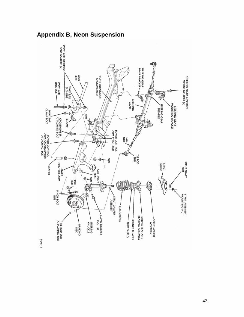
42

Appendix B, Neon Suspension

43

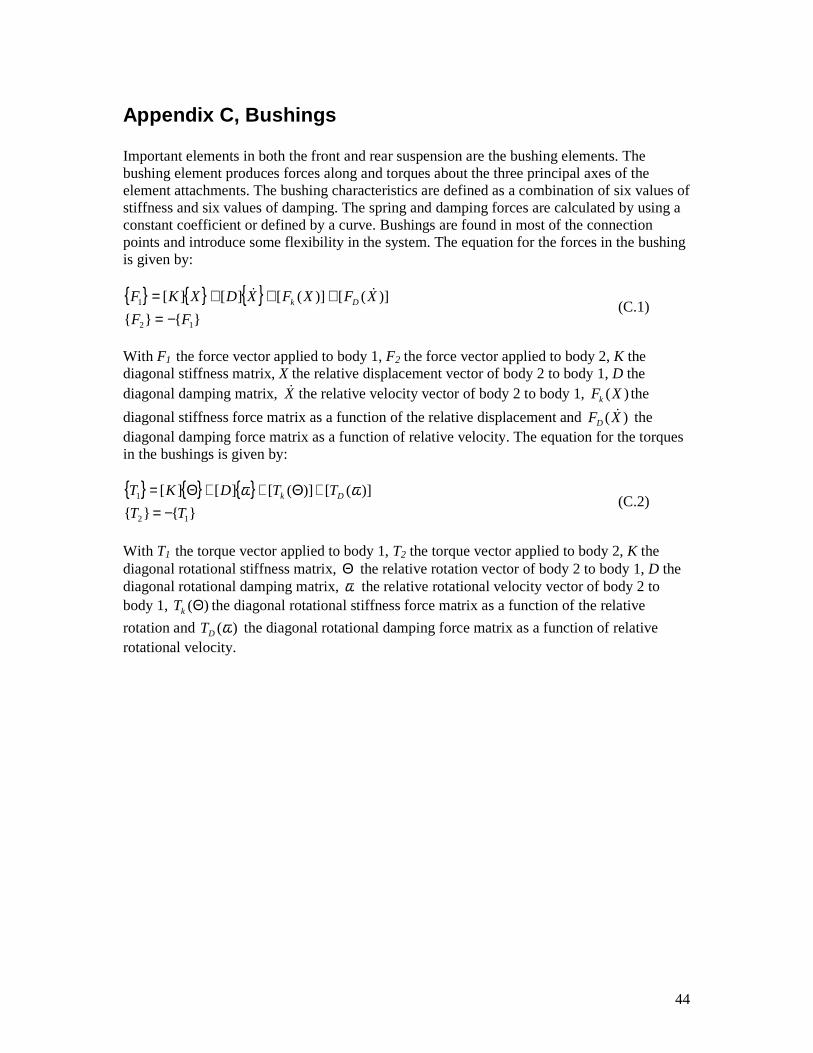
44

Appendix C, Bushings Important elements in both the front and rear suspension are the bushing elements. The bushing element produces forces along and torques about the three principal axes of the element attachments. The bushing characteristics are defined as a combination of six values of stiffness and six values of damping. The spring and damping forces are calculated by using a constant coefficient or defined by a curve. Bushings are found in most of the connection points and introduce some flexibility in the system. The equation for the forces in the bushing is given by: { } { } { }

}{}{

)]([)]([][][

12

1

FF

XFXFXDXKF Dk

−=+++= &&

(C.1)

With F1 the force vector applied to body 1, F2 the force vector applied to body 2, K the diagonal stiffness matrix, X the relative displacement vector of body 2 to body 1, D the diagonal damping matrix, X& the relative velocity vector of body 2 to body 1, )(XFk the

diagonal stiffness force matrix as a function of the relative displacement and )(XFD& the

diagonal damping force matrix as a function of relative velocity. The equation for the torques in the bushings is given by: { } { } { }

}{}{

)]([)]([][][

12

1

TT

TTDKT Dk

−=+Θ++Θ= ωω

(C.2)

With T1 the torque vector applied to body 1, T2 the torque vector applied to body 2, K the diagonal rotational stiffness matrix, Θ the relative rotation vector of body 2 to body 1, D the diagonal rotational damping matrix, ω the relative rotational velocity vector of body 2 to body 1, )(ΘkT the diagonal rotational stiffness force matrix as a function of the relative

rotation and )(ωDT the diagonal rotational damping force matrix as a function of relative rotational velocity.

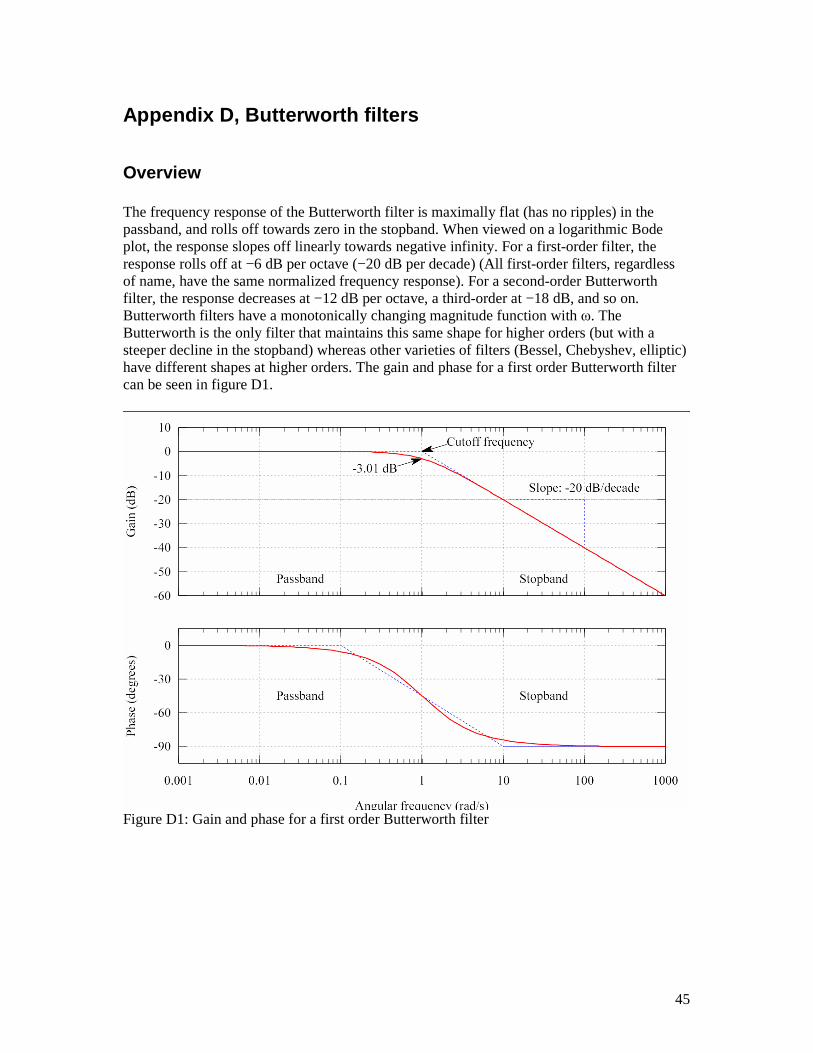
45

Appendix D, Butterworth filters

Overview The frequency response of the Butterworth filter is maximally flat (has no ripples) in the passband, and rolls off towards zero in the stopband. When viewed on a logarithmic Bode plot, the response slopes off linearly towards negative infinity. For a first-order filter, the response rolls off at −6 dB per octave (−20 dB per decade) (All first-order filters, regardless of name, have the same normalized frequency response). For a second-order Butterworth filter, the response decreases at −12 dB per octave, a third-order at −18 dB, and so on. Butterworth filters have a monotonically changing magnitude function with ω. The Butterworth is the only filter that maintains this same shape for higher orders (but with a steeper decline in the stopband) whereas other varieties of filters (Bessel, Chebyshev, elliptic) have different shapes at higher orders. The gain and phase for a first order Butterworth filter can be seen in figure D1.

Figure D1: Gain and phase for a first order Butterworth filter

46

Transfer function

Like all filters, the typical prototype is the low-pass filter, which can be modified into a high-pass filter, or placed in series with others to form band-pass and band-stop filters, and higher order versions of these.

The gain G(ω) of an n-order Butterworth low pass filter is given in terms of the transfer function H(s) as:

where

• n = order of filter

• ωc = cutoff frequency (approximately the -3dB frequency)

• G0 is the DC gain (gain at zero frequency)

It can be seen that as n approaches infinity, the gain becomes a rectangle function and frequencies below ωc will be passed with gain G0, while frequencies above ωc will be suppressed. For smaller values of n, the cutoff will be less sharp.

We wish to determine the transfer function H(s) where s = σ + jω. Since H(s)H(-s) evaluated at s = jω is simply equal to |H(ω)|2, it follows that:

The poles of this expression lie on a circle of radius ωc at equally spaced points. The transfer function itself will be specified by just the poles in the negative real half-plane of s. The k-th pole is specified by:

and hence,

The transfer function may be written in terms of these poles as:

The denominator is a Butterworth polynomial in s.

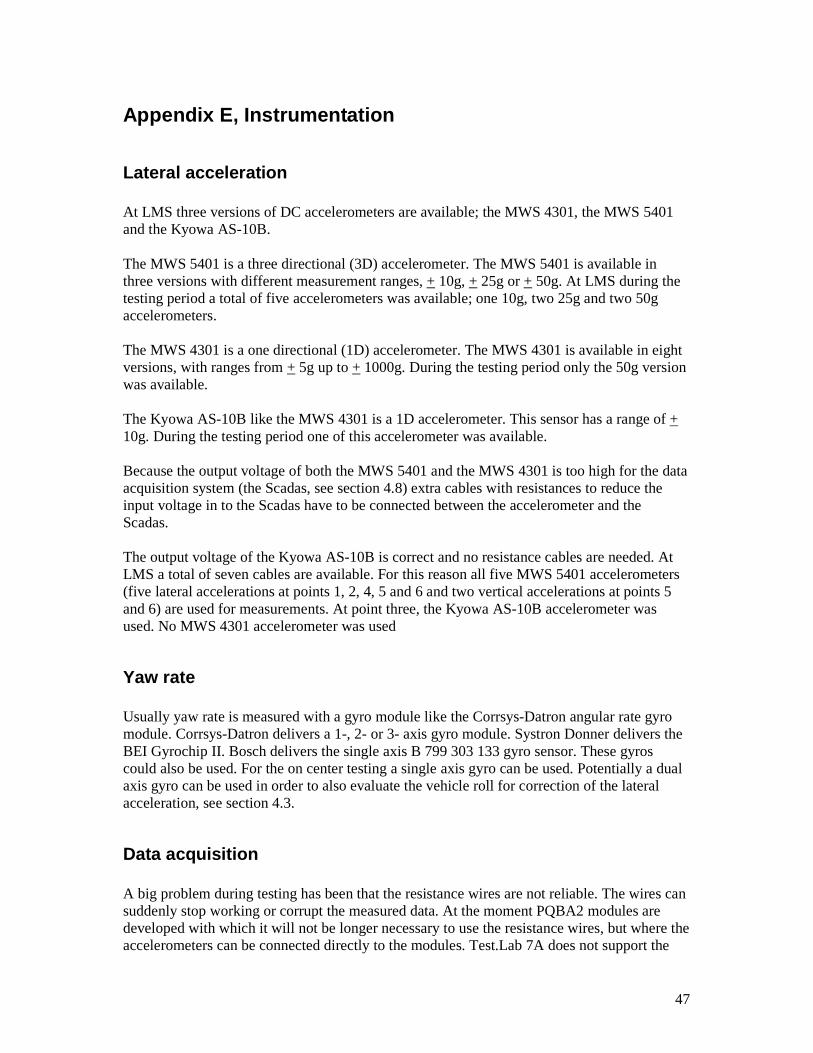
47

Appendix E, Instrumentation

Lateral acceleration At LMS three versions of DC accelerometers are available; the MWS 4301, the MWS 5401 and the Kyowa AS-10B. The MWS 5401 is a three directional (3D) accelerometer. The MWS 5401 is available in three versions with different measurement ranges, + 10g, + 25g or + 50g. At LMS during the testing period a total of five accelerometers was available; one 10g, two 25g and two 50g accelerometers. The MWS 4301 is a one directional (1D) accelerometer. The MWS 4301 is available in eight versions, with ranges from + 5g up to + 1000g. During the testing period only the 50g version was available. The Kyowa AS-10B like the MWS 4301 is a 1D accelerometer. This sensor has a range of + 10g. During the testing period one of this accelerometer was available. Because the output voltage of both the MWS 5401 and the MWS 4301 is too high for the data acquisition system (the Scadas, see section 4.8) extra cables with resistances to reduce the input voltage in to the Scadas have to be connected between the accelerometer and the Scadas. The output voltage of the Kyowa AS-10B is correct and no resistance cables are needed. At LMS a total of seven cables are available. For this reason all five MWS 5401 accelerometers (five lateral accelerations at points 1, 2, 4, 5 and 6 and two vertical accelerations at points 5 and 6) are used for measurements. At point three, the Kyowa AS-10B accelerometer was used. No MWS 4301 accelerometer was used

Yaw rate Usually yaw rate is measured with a gyro module like the Corrsys-Datron angular rate gyro module. Corrsys-Datron delivers a 1-, 2- or 3- axis gyro module. Systron Donner delivers the BEI Gyrochip II. Bosch delivers the single axis B 799 303 133 gyro sensor. These gyros could also be used. For the on center testing a single axis gyro can be used. Potentially a dual axis gyro can be used in order to also evaluate the vehicle roll for correction of the lateral acceleration, see section 4.3.

Data acquisition A big problem during testing has been that the resistance wires are not reliable. The wires can suddenly stop working or corrupt the measured data. At the moment PQBA2 modules are developed with which it will not be longer necessary to use the resistance wires, but where the accelerometers can be connected directly to the modules. Test.Lab 7A does not support the

48

PQBA2 modules, but Test.Lab 7B does. In future measurements it will certainly we worth to install Test.Lab 7B and use the PQBA2 modules when the MWS 5401 or MWS 4301 accelerometers are used.

49

Appendix F, Matlab First of all make sure Matlab R14 or higher is installed, with Simulink. For generating a steering wheel input and a road profile the matlab scripts steerinput.m and roadprofile.m can be used.

Generating steering wheel input The user has two options; generate a perfect sine steer input or generate a steer input with noise.

Perfect sine The script steerinput.m can be used to generate a steerinput for a weave test. In order to generate a sinusoidal steer input, just type >>steerinput in the command screen. The script is fully automated. Parameters for maximum steering wheel angle, steering frequency, number of sweeps, stabilizing time at start of simulation and end of simulation, time step. The generated data will be exported to an excel file (steerinput.xls) in the current directory. Make sure that the steer input in V.LM is linked to the correct excel file! When the matlab script has been run a message for time-table synchronization should appear in V.LM.

Sine with noise The script steerinput_cadax.m can be used to generate a sinusoidal steerinput which contains noise. The script reads the data which is generated with CadaX and exports it to an excel file. The steerinput_cadax script is not fully automated and will only run from the editor screen. The noise generated in CadaX is a sine signal, added with a noise signal, filtered by a butterworth filter with a cut-off frequency of 5 Hz, to generate a sine with noise up to 5 Hz. This signal has to be exported to a text file. Make sure that the timestep (1/sample frequency) at line 20 of the steerinput_cadax script is the same as the timestep which is chosen in CadaX. At line 28 the text file which is generated in CadaX is imported in matlab. Make sure that the correct text file is imported. Make sure that in line 30 the correct data matrix is used. Similar to the steerinput script, an excel file will be generated in the current directory. Again make sure that in V.LM the steerinput is linked to the right excel file.

Generating road profile The roadprofile.m script can be used for this. This is a fully automated script. In the command screen just type >>roadinput. The script then asks what type of road has to be generated, the speed of the vehicle during simulation, simulation time, and a data reduction factor (the higher the DRF, the faster the simulation will be, but the less accurate the generated profile will be). From this a road profile will be generated. Make sure that the file roadprofile.mat is placed in the current directory. This file contains the data for the road

50

profile and the script will not run without this file (see line 53 of the script). For more information, type >> help roadprofile.

Processing the simulation data All simulation data is processed with the main.m script. This script determines values for the response time lag, torque deadband, steering friction, steering stiffness, response deadband and the yaw rate response gain. For every parameter a different script is made and will be called in main.m. The script is not automated and has to be filled in by hand. The basic structure used by me is that 3 directories are made: a current directory, a directory with the simulation data and a directory where the calculated parameters can be saved to. In the current directory the files: main.m, DR.m, LS.m, FREQ.m, RTL.m, TD.m, SF.m, StSt.m, RD.m and YRRG.m have to be placed. Make sure that line 46 (main.m) contains the current directory. The simulation data has to be exported in V.LM to a text file. The text file should contain a column for time, steering wheel angle, steering wheel torque, lateral acceleration, yaw rate, speed and wheel angle. V.LM automatically uses the first column for the time information. Make sure that in V.LM the data for exporting will be selected in the right sequence. So first click on SWA, than on steering wheel torque, then lateral acceleration, after this yaw rate, speed and finally wheel angle. If this is not done, V.LM will write fault data in the different columns and the main.m script will not run! When exporting, make sure that write combined will be selected. The text file which contains the simulation data has to be placed in the computed_data directory, make sure line 50 contains the right directory. The last step of the processing is that the computed data is exported to a .mat file with the same name as the text file. This .mat file will be generated in the motion_output directory, make sore that line 48 contains this directory. At line 40 and 44 values for the domain of which the steering sensitivity and the yaw rate response gain can be defined. A value of 1 will mean that the values for steering sensitivity of yaw rate are calculated over a domain of -1 to +1 degrees (or deg/s). For more information about this, see the report. At line 52 the size of the matrix with reduced data can be given. During the data reduction, a new matrix is generated with information in which we are interested in. With the value at line 52 is will be determined which information has to be used in the reduced matrix. A value of 2 means that only the first two columns of the original file will be used (so the reduced matrix only contains information about the time and the steering wheel angle). A value of 6 means that all columns will be used. The main script shows the results at the command screen and plots one figure which contains the reduced time trajectories and one figure (subplot) which contains the plots of steering wheel angle versus steering wheel torque, steering wheel angle versus lateral acceleration, lateral acceleration versus steering wheel torque and steering wheel angle versus yaw rate. Fore more information type >>help main in the command screen. For more information about the different scripts used for processing, type >> help DR, LS, FREQ, RTL, TD, SF, StSt, RD or YRRG.

51

Processing the measurement data The measurement data will be processed with use of Matlab Simulink. For the exact sequence, see the report.

Filter the signals After the signals have gotten the DC offset and they are trimmed (if necessary), the signals will be filtered. For this the filt_sig.m script can be used. This script imports the data which is exported with TestLab and processes it. Again different directories are used; one for the mfiles, one directory with the simulink files and one directory which contains the time trajectories generated by TestLab. Make sure that line 7 contains the right directory where the time trajectories (text files) are placed. When multiple tests have been performed, and the data of every test is stored in a different directory, line 5 can be used. This line contains the name of the directory where the measurement data is stored in which you are interested. Line 11 contains the name of the text file which belongs to a sensor. This text file contains the time trajectory. Make sure that line 48 contains the directory where the filtered.mdl simulink model is located. This simulink model filteres the signal (see line 51). The filt_sig script returns two figures, one with the original signal and the filtered signal and one figure with the integral of the filtered signal. For more information about the filtering, open the filtered.mdl file. In order to process all the signals, run the filt_all_signals.m script. This script operates similar to the filt_sig.m file, but also exports the computed data to a .mat file with the same name as the text file which contains the original time trajectory. At line 7 the name of the different directories with the text files belonging to the different tests can be specified. I did 4 tests, so I had 4 directories with text files. At line 8 the name of the different text files can be specified. I had 10 signals during my measurements, so here 10 text names are specified. The directory names specified at line 7 are used at line 13, the text names specified at line 8 are used at line 17. Again a simulink model is used. Make sure that the link to the simulink model at lines 42 and 45 are correct. The filt_all_signals.m script saves all computed data to a .mat file with the same name as the original text file to the same directory where the original text files are located.

Plot the data The plotdata.m script plots all the data computed with the filt_all_signals.m script. At line 6 the name of the directory where the data (.mat files!) is located has to be specified. It is only possible to plot the data from just one test at a time. At line 10 the names of the .mat files can be specified. I had 10 sensors, so here 10 names are filled in. Make sure that at line 13 the name of the .mat file which will be imported is correct. The script returns a number of figures which is 2x the number of time trajectories. In figure 1 the original time trajectory and the filtered signal is plotted. In figure 11 the integrated signal (integrated from the filtered signal) is plotted. This is the same for pictures 2 and 12, 3 and 13, 4 and 14 and so on.

52

Calculate the lateral displacement of the steering gear housing The lateral displacement of the steering gear housing w.r.t. the chassis can be computed with the steeringgearacc.m file. With my signals this script did not return proper results, but this is due to corrupted signals, the script works fine! At line 8 the directory where the data from the sensors are placed can be specified. At lines 10 - 22 the used data is imported. For more information about the procedure on how to calculate the displacements of the steering gear housing, see the report. At lines 24 and 25, columns 55 and 62 the longitudinal distance between the different sensors have to be specified. At line 43 it has to be specified from which signal the displacement of the steering gear housing will be calculated. At line 50 the steeringgear.mdl simulink model is called. Make sure that this model is located in the directory specified at line 48. The steeringgearacc.m script returns four figures; one figure with the measured acceleration and the calculated acceleration from sensor 1, a similar figure from sensor 2, one figure which contains the difference in speed between the steering gear housing and the chassis and one figure which contains the displacement of the steering gear housing with respect to the chassis.

Compare measurement data with simulated data The data from the measurements and the simulation can be compared to each other with the compare_measurements_simulations.m file. Make sure to set the currect directory where the simulation data is placed at line 8. The right filename has to be specified at line 10. Make sure that the directory at line 12 is the one where the measurement data is place. From lines 14 - 23 the data is imported in which we are interested, namely the steering wheel angle (21_offset), lateral acceleration at the front of the vehicle (13_offset and 8_offset) and lateral acceleration at the back of the vehicle (9_offset and 11_offset). At lines 39 and 41 the yaw rate is calculated. Make sure that the longitudinal distance between the sensors is specified at lines 39 and 41, at column 29. The script returns 9 figures. In figure 1 the measured steering wheel angle (from measurements) and the simulated steering wheel angle can be seen. From this picture one can see if the simulation has been a good simulation. In figure 2 the measured and simulated lateral acceleration can be seen. In figure 3 the calculated yaw rates (from measurement data, see report) and the simulated yaw rate can be seen. In figure 4 again the measured and simulated lateral acceleration can be seen, but now in a subplot. In figure 5 the steering wheel angle versus yaw rate (from measurement data) can be seen. Because it is not a clear picture, two curves belonging to different weaves are plotted in different colors. In figure 6 the signals for the measured and simulated steering wheel angle and the yaw rates from measurement data and simulation data can be seen. In figure 7 a plot can be seen from the steering wheel angle versus the yaw rate from simulation data. In figure 8 only the yaw rates can be seen. In figure 9 the steering wheel angle versus the yaw rate is plotted for the measurement data and the simulation data.

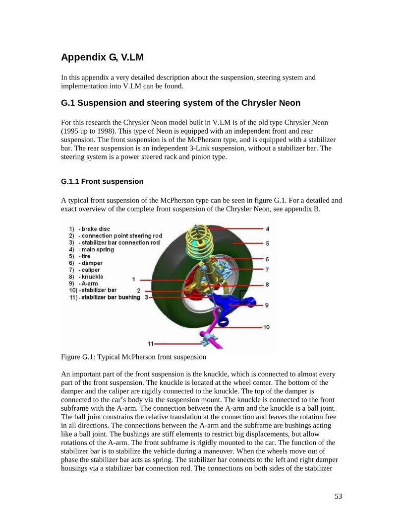
53

Appendix G, V.LM In this appendix a very detailed description about the suspension, steering system and implementation into V.LM can be found.

G.1 Suspension and steering system of the Chrysler Neon For this research the Chrysler Neon model built in V.LM is of the old type Chrysler Neon (1995 up to 1998). This type of Neon is equipped with an independent front and rear suspension. The front suspension is of the McPherson type, and is equipped with a stabilizer bar. The rear suspension is an independent 3-Link suspension, without a stabilizer bar. The steering system is a power steered rack and pinion type.

G.1.1 Front suspension A typical front suspension of the McPherson type can be seen in figure G.1. For a detailed and exact overview of the complete front suspension of the Chrysler Neon, see appendix B.

Figure G.1: Typical McPherson front suspension An important part of the front suspension is the knuckle, which is connected to almost every part of the front suspension. The knuckle is located at the wheel center. The bottom of the damper and the caliper are rigidly connected to the knuckle. The top of the damper is connected to the car’s body via the suspension mount. The knuckle is connected to the front subframe with the A-arm. The connection between the A-arm and the knuckle is a ball joint. The ball joint constrains the relative translation at the connection and leaves the rotation free in all directions. The connections between the A-arm and the subframe are bushings acting like a ball joint. The bushings are stiff elements to restrict big displacements, but allow rotations of the A-arm. The front subframe is rigidly mounted to the car. The function of the stabilizer bar is to stabilize the vehicle during a maneuver. When the wheels move out of phase the stabilizer bar acts as spring. The stabilizer bar connects to the left and right damper housings via a stabilizer bar connection rod. The connections on both sides of the stabilizer

54

bar are ball joints. The stabilizer bar is connected to the body with the stabilizer bar bushings. These bushings allow free rotation of the stabilizer bar, but restrict displacements. The wheels are mounted to a spindle (see also figure G.3), which is connected to the knuckle with a revolute joint. In this way the spindle can turn in the knuckle round the wheels rolling axis. The steering rod, which is not shown in the figure but can be seen in figure 3.2, is connected to the knuckle via a ball joint. Since the bushings of the A-arm allow rotations and the connections of the steering rod and the stabilizer bar are ball joints it is clear that the vertical motion of the suspension mass is mainly determined by the stiffness of the tire, the stiffness of the main spring, the damping characteristics of the damper and the stiffness of the suspension mount [5],[6].

G.1.2 Steering system The steering system modeled in V.LM is based on the steering system in figure G.2.

Figure G.2: Steering system The steering system used in the Chrysler Neon is of the rack and pinion type. The steering gear converts rotation of the pinion gear into translation of the rack and thus translation of the steering rods, causing steering of the wheels and turning of the vehicle. The steering wheel is connected to the pinion gear via the steering axis and two cardan joints. In this way it is possible to position the steering gear housing and steering wheel where desired. The steering wheel is rigidly connected to the steering axis. The steering axis is supported with a cylindrical joint in the steering column. The cylindrical joint allows no translations and only one rotation, namely rotation around the steering axis. The steering rods are connected to the end of the rack with a ball joint. The rack has one degree of freedom and is allowed to translate only in lateral direction, causing inward and outward moving of the steering rods. The steering gear housing is connected rigidly to the front subframe [5], [6].

55

In the V.LM model all parts are modeled as rigid parts. When a passenger car is equipped with a hydraulic power steering, a torsion tube will be located in the steering gear. The torsion of the torsion tube is a measure for the steering wheel torque. This torsion tube mainly determines the stiffness of the steering system [8], [9]. In the V.LM model no hydraulic power steering is modeled and thus a part of flexibility will not be present in the model. Also in a normal passenger car a chain of friction is present in the steering system [10], [11]. The steering axis is usually supported by two bearings which inhabit friction and in the steering gear also friction is present. For modeling both the friction and the hydraulic power steering thorough knowledge of the V.LM software is needed. For this reason the V.LM model is not equipped with friction in the steering system, front- and rear suspension and no hydraulic power steering is modeled.

G.1.3 Rear suspension A typical 3 Link rear suspension is shown in figure G.3. For a detailed and exact overview of the complete rear suspension of the Chrysler Neon, see appendix B.

Figure G.3: 3-Link rear suspension The rear suspension looks similar to the front suspension, but the connection from the knuckle to the subframe is different. The knuckle is connected with two lateral arms to the rear subframe. The lateral arms are on one end connected with bushings to the knuckle and on the other end with bushings to the rear subframe. The tension strut is connected on one end with a bushing to the chassis and on the other end with a bushing to the knuckle. The suspension strut for the 3-Link rear suspension is mounted similar as with the front suspension, at the bottom rigidly to the knuckle, at the top to the chassis via the suspension mount. The rear suspension of the old type Chrysler Neon is not equipped with a stabilizer bar and for this reason a stabilizer bar is not modeled in V.LM. Again, since the bushings of the two lateral arms and tension strut allow rotation of these elements, it is clear that the vertical motion of

56

the suspension mass is mainly determined by the stiffness of the tire, the stiffness of the main spring, the damping curve of the damper and the stiffness of the suspension mount [5], [6].

G.2 Implementation in Virtual.Lab Motion Using [6] a full vehicle model of the Chrysler Neon is built in V.LM. The coordinates of the real geometry of a Chrysler Neon was unknown, for this reason the V.LM model is built with use of existing V.LM models and FE models.

G.2.1 Front suspension The geometry of the front suspension is based on an existing V.LM model which was suited with a McPherson front suspension, the McPherson model. The car from the McPherson model is a similar sized car to the Chrysler Neon. The coordinates of the geometry are recalculated in such a way that the Chrysler Neon model has the correct track width. Due to the lack of information about the real Chrysler Neon spring- and damping characteristics of the suspension struts, spring- and damping characteristics for the front suspension are based on the McPherson. All bodies; chassis, subframe, knuckle, A-arms, steering rods and spindles are modeled as rigid bodies. Masses and inertias of the different bodies are based on the values of the McPherson model and should be adjusted to values belonging to a Chrysler Neon. Characteristics for the bushings (more information about bushings can be found in appendix C) are not known, for this reason the characteristics are the same as in the McPherson model. The connections between the different bodies are as described in section G.1.1.

G.2.2 Steering system The steering system in the V.LM model is modeled similar as in the McPherson model. The coordinates of the geometry are recalculated in such a way that the steering gear housing and steering wheel are located as in the Chrysler Neon. All bodies; steering rods, steering axis and rack and pinion are modeled as rigid bodies. Masses and inertias are based on the McPherson model and should be adjusted to values belonging to a Chrysler Neon. The connections between the different bodies are as described in section G.1.2.

G.2.3 Rear suspension The geometry of the rear suspension is based on a FE model. The FE model only contained information about the geometry and mass and inertia properties. The characteristics of the springs and dampers are based on an existing V.LM model which was suited with a 5-Link rear suspension, the 5-Link model. Again all bodies; subframe, knuckles, lateral arms, tension struts and spindles are modeled as rigid bodies. Characteristics for the bushings are not known and no FE- or V.LM model existed with characteristics for bushings in the rear suspension. For this reason a 3D stiffness of 2e6 N/m is used. This value is not representative for the real bushing parameters, but will have the correct order of magnitude, and the simulation results will not be corrupted due to completely wrong bushing parameters. The alignment of the bushings for both the front suspension and rear suspension are based on [6] and are correct.

57

G.2.4 Future improvements An important component of the full vehicle model is the tire model. For all maneuvers the tire will generate forces and moments which will result in forces in the steering system and suspensions. Because the steering wheel torque is one of the parameters we are specifically interested in, it is important that the simulated forces of the tire are similar to forces generated in a real maneuver with a real tire. For this reason the tire model used in the V.LM model should be the same as the tire used for the maneuvers. This is not the case yet; now a simple tire is modeled. A future improvement is that the model will be equipped with a more realistic tire model like a TNO tire model. For more information about tire models, see [12]. The body and rims of an old type Chrysler Neon have already been modeled and implemented in the model. From this all it can be concluded that we have a model which is capable of simulation a maneuver as described in [3] and [1]. In chapter 5 and 6 the results of the data from the simulations and measurements is discussed and the model proves to give proper data. In order to make the model more realistic some things have to be changed. From the front suspension and the steering system some slight changes in the geometry have to be made, which can be done very easily. For both the front- and the rear suspension the characteristics for the springs and dampers have to be changed to real characteristics, this can also be done very easily. For the front- and rear suspension the parameters for the bushings have to be changed into the real parameters. For the front suspension, steering system and some parts of the rear suspension the values for the masses and inertias have to be changed. Also friction, compliance and power steering have to be implemented in the model. For this thorough knowledge of the V.LM software is required.

G.3 Defining maneuvers using Matlab and Cada-X In V.LM the user has the option to define a maneuver by using text of excel files. For generating a steer input a time dependent trajectory will be generated and exported to an excel file. A height – distance dependant road profile will be generated and will also be exported to an excel file. It will be clear that the maneuver will be an open-loop maneuver; no controller is implemented for the simulation. From [7] and [1] we know that the maneuver has to be open-loop. The signal for the steer input will be generated by Cada-X and will be exported to an excel file by Matlab. The road profile will be generated and exported by Matlab. It will be clear that every possible maneuver can be generated.

G.3.1 Steer input During the simulation the vehicle responses generated by steering wheel input will be calculated. From [1] and [3] we know that the on-center parameters can only be calculated from data which comes from a simulation of a weave with a steer input of 0.2 Hz and a maximum lateral acceleration of 1 ms-2. The steer input will be created with a Matlab script, steerinput.m.

58

In the steerinput script the user is given the possibility to change the maximum steering wheel angle at maximum lateral acceleration of 1 ms-2, the frequency of the input and the timestep. Because the model needs some stabilizing time at the beginning of the simulation, the user is given the option to define when the weaves will begin. This is typically 5 seconds after the simulation has started. From these parameters a perfect sine is generated and exported to an excel file. Every time the steerinput script has generated a new excel file, the file will be automatically reloaded in V.LM and a conformation appears in V.LM. During early road tests, to look if the defined maneuvers would be possible, we found that it is nearly impossible to generate a perfect sine for the steer input by hand. The results of the on-center tests are very sensitive for variations in frequency and amplitude of the steer input [1]. Because of this a maneuver will be simulated with a steer input which contains band related noise. Using Cada-X a sine with added noise is generated. A steer input generated by hand typically contains noise up to 5 Hz. For this reason the generated signal is filtered with a Butterworth filter with a cut-off frequency of 5 Hz and an order of 2 (-12 dB per octave), for more information about Butterworth filters see appendix D. The filtered signal is exported to a text file. In Matlab the steerinput script again generates a signal for the steer input and exports the data to the excel file. In figure G.4 several steer inputs generated by Matlab and Cada-X can be seen.

5 6 7 8 9 10 11 12 13 14

-10

-8

-6

-4

-2

0

2

4

6

8

10

Steer input, ZOOMED

time [s]

Ste

erin

g w

heel

ang

le [

deg]

Perfect sine

Noise 3 Hz

Noise 5 Hz

Figure G.4: Steer input

G.3.2 Road profile One of the requirements of the test track is that the track is flat with as minimal road noise as possible. Results of a test will be influenced when the track does not fulfill the requirements [3]. In order take some road roughness into account during simulation a matlab script has

59

been designed to generate a road profile, the roadprofile script. In V.LM the road which is used for simulation can, similar as with the steer input, be defined using a time table or loaded from an excel file. The roadprofile script exports the profile to an excel file. To generate a proper road profile one must look at the power spectral density of the profile. A proper road profile has a slope of -2 dB per decade in the power spectral density plot [13]. From the PSD plot (power spectral density plot) also the road roughness can be obtained. The height of the line in the PSD plot is a measure for the road roughness. In figure G.5 the calculated road profile with its PSD can be seen.

10-1

100

101

102

10-10

10-8

10-6

10-4

10-2

100

PSD Road profile

Frequency [Hz]

PS

D [

(m2 )/

Hz]

Road profilefit

ISOG

ISOE

ISOC

ISOA

0 200 400 600 800 1000 1200 1400-258

-256

-254

-252

-250

-248

-246

-244

-242

-240Computed road profile

X [m]

Z [

mm

]

Figure G.5: Calculated road profile and its PSD

The user can specify the speed, the simulation time and a scale factor in order to get the desired road profile. The computed road profile is the lowest plot in figure G.5. The length of the road profile (horizontal axis in the lower plot) will be computed from the speed and the simulation time. The height of the road profile (vertical axis in the lower plot) will be the measured road profile multiplied by a scale factor.

60

The scale factors are based on the ISO classes for road profiles. The PSD's belonging to the scale factors can be seen in the upper plot. A very good road is classed as ISO A (the pink line in the PSD plot), a medium road is classed as ISO C (green line), a very bad road is classed as ISO E (cyan line) and an off-road profile is classes as ISO G (black line), see also [13]. The PSD belonging to the computed road profile is the blue curve. Trough the blue curve a line is fitted in order to determine which ISO class the calculated road profile belongs to. With a combination of both the steerinput and roadprofile scripts a simulation for every maneuver on every kind of road will be possible.