friendship-based routing protocol for delay tolerant networks · desenvolver um protocolo de...
TRANSCRIPT

Friendship-based Routing Protocol for Delay Tolerant
Networks
Francisco Xavier Amélio Fernandes
Thesis to obtain the Master of Science Degree in
Electrical and Computer Engineering
Supervisor: Prof. Paulo Rogério Barreiros D’Almeida Pereira
Examination Committee
Chairperson: Prof. António Manuel Raminhos Cordeiro Grilo
Supervisor: Prof. Paulo Rogério Barreiros D’Almeida Pereira
Member of the Committee: Prof. Miguel Nuno Dias Alves Pupo Correia
November 2017

ii

iii
To my girlfriend, parents and sister, for all the strength and support.

iv

v
Abstract
Delay Tolerant Networks are characterized by not having permanent end-to-end connections, often
leading to intermittent connectivity, long and variable delays and high error rates. Sending a message
between two points may take hours, weeks or even months. Mobile Social Networks are particular
scenarios on which nodes are seen as individuals, with inherent social habits, carrying hand-held
devices which communicate with each other within a certain wireless range. The scope of this Master’s
thesis was to develop a routing protocol based on the social property of Friendship to use on such
networks, designated as Friendship Protocol. The protocol allows nodes to consider other nodes to be
friends if they maintain contact frequently, regularly and in long-lasting sessions. The forwarding scheme
consists in only delivering the message to nodes which are friends of the destination. To evaluate the
performance of this protocol, the ONE Simulator was used. The Friendship Protocol performance was
analysed and compared to other three routing protocols while varying the network load. In the end, the
Friendship Protocol showed that it could reach a high delivery rate and a very low overhead. For every
network load tested, the results for the delivery rate were never lower than the other routing protocols
and the overhead ratio was several times lower. It was also proposed a dynamic threshold version, on
which the friendship threshold changes over time as it corresponds to a portion of the best friend weight.
The results of this dynamic version were similar of the first version’s, only this time with roughly half of
the overhead.
Keywords
Delay Tolerant Networks, Mobile Social Networks, Routing Protocol, Friendship, The ONE Simulator.

vi
Resumo
As Redes Tolerantes a Atrasos são caracterizadas por não possuírem ligações ponto-a-ponto
permanentes, levando a que as conexões sejam geralmente intermitentes e sujeitas a longos e
variáveis atrasos, assim como a uma taxa elevada de erros. Nestas redes, enviar uma mensagem pode
demorar horas, semanas ou até meses. As Redes Móveis Sociais envolvem cenários particulares de
Redes Tolerantes a Atrasos em que os nós são pessoas, naturalmente com comportamentos sociais,
que carregam consigo dispositivos portáteis que comunicam sem-fios com outros dispositivos desde
que estejam dentro de um determinado alcance. O objectivo desta dissertação de mestrado foi
desenvolver um protocolo de encaminhamento ajustado a esse cenário que explora o conceito de
Amizade como propriedade social. Ao protocolo desenvolvido atribuiu-se o nome de Friendship. O
protocolo permite que os nós considerem outros como amigos caso detectem que os seus contactos
são frequentes, regulares e de longa duração. As mensagens, por sua vez, só são enviadas para
amigos do nó destinatário da mensagem. Para avaliar o desempenho do protocolo, usou-se o simulador
the ONE. O desempenho do Friendship foi analisado e equiparado a outros três protocolos existentes
na literatura para diferentes cargas de rede. O Friendship não foi ultrapassado por nenhum outro
protocolo em termos de taxa de entrega de mensagens, ao passo que em termos de número de réplicas
difundidas na rede superou inequivocamente a concorrência para todas as cargas. Foi também
proposta uma versão alternativa do Friendship em que o limiar de amizade deixa de ser um valor fixo
e passa a ser uma porção do peso do melhor amigo, atribuindo desta forma um certo dinamismo a este
parâmetro, dado que o peso de cada amizade varia com o tempo. Esta versão alternativa obteve
resultados semelhantes à primeira, com excepção do número de réplicas difundidas que diminuiu para
cerca de metade em relação à primeira versão.
Palavras-Chave
Redes Tolerantes a Atrasos, Redes Sociais Móveis, Protocolo de encaminhamento, Amizade,
Friendship, Simulador The ONE.

vii
Table of Contents
Abstract .................................................................................................................................................. v
Resumo.................................................................................................................................................. vi
Table of Contents ................................................................................................................................ vii
List of Figures ....................................................................................................................................... ix
List of Tables .......................................................................................................................................... x
List of Acronyms .................................................................................................................................. xi
List of Software ................................................................................................................................... xiii
Chapter 1: Introduction ......................................................................................................................... 1
1.1. Context ...................................................................................................................................... 2
1.2. Document structure .................................................................................................................. 4
Chapter 2: Delay Tolerant Networks .................................................................................................... 5
2.1. Introduction ............................................................................................................................... 6
2.2. DTN Architecture Overview ...................................................................................................... 6
2.3. Routing Protocols ..................................................................................................................... 7
2.3.1. Social-oblivious Protocols .............................................................................................. 9
2.3.2. Social-aware Protocols ................................................................................................ 10
2.3.2.1. The BubbleRap Protocol ................................................................................... 12
2.3.2.2. The Friendship Based Routing Protocol ........................................................... 14
2.4. Applications ............................................................................................................................. 17
2.5. The ONE Simulator ................................................................................................................. 20
Chapter 3: Friendship Protocol .......................................................................................................... 25
3.1. Concept................................................................................................................................... 26
3.2. The Protocol ............................................................................................................................ 26
3.3. A dynamic threshold version ................................................................................................... 34
Chapter 4: Simulation Results ........................................................................................................... 36
4.1. Performance evaluation .......................................................................................................... 37
4.2. Phase I: Tuning ....................................................................................................................... 37
4.2.1. Settings ........................................................................................................................ 38
4.2.2. Epidemic Protocol ........................................................................................................ 40
4.2.3. Prophet Protocol .......................................................................................................... 40

viii
4.2.4. BubbleRap Protocol ..................................................................................................... 41
4.2.4.1 Influence of the familiar threshold parameter ..................................................... 41
4.2.4.2 Influence of the k parameter............................................................................... 42
4.2.5. Friendship Protocol ...................................................................................................... 43
4.2.5.1. Classic Friendship: Influence of the fixed threshold .......................................... 44
4.2.5.2. Dynamic Friendship: Influence of the dynamic threshold ................................. 45
4.3. Phase II: Traffic load variation ................................................................................................ 46
4.3.1 Delivery Rate ................................................................................................................. 47
4.3.2 Overhead ratio .............................................................................................................. 48
4.3.3 Average Delay ............................................................................................................... 50
Chapter 5: Conclusions ...................................................................................................................... 52
References ........................................................................................................................................... 55

ix
List of Figures
Figure 1 – Internet World penetration rates by geographic regions (data from June 30, 2017) ............. 3
Figure 2 – Differences between a DTN and TCP/IP network stack (extracted from [4]). ........................ 7
Figure 3 – Example of a graph scheme .................................................................................................. 8
Figure 4 - Example of a SG ..................................................................................................................... 9
Figure 5 – Example of a Binary Spray-and-Wait (extracted from [2]). .................................................. 10
Figure 6 – Community structures in a social graph, each represented with a different colour (extracted
from [11]). ................................................................................................................................................ 11
Figure 7 – BUBBLE algorithm (extracted from [19]). ............................................................................. 13
Figure 8 – Example of a k-clique community with k=4 (extracted from [25]). ....................................... 14
Figure 9 – Different encounter histories between nodes i and j in the time interval [0, T] (adapted from
[15]). ....................................................................................................................................................... 15
Figure 10 – Encounter history between nodes i and j in the upper graph and between j and k in the lower
graph (extracted from [15]). ................................................................................................................... 16
Figure 11 – Example of an IPN.............................................................................................................. 18
Figure 12 – Practical example of a military application (adapted from [33]). ........................................ 19
Figure 13 – Overview of The ONE Simulator (extracted from [37]). ..................................................... 21
Figure 14 - GUI of The ONE Simulator. ................................................................................................. 23
Figure 15 – Batch mode of The ONE Simulator in Eclipse IDE ............................................................ 24
Figure 16 – Flowchart of the Friendship Protocol.................................................................................. 34
Figure 17 – Metropolitan area of Helsinki, Finland, presented on the GUI mode of The ONE simulator.
............................................................................................................................................................... 38
Figure 18 – Delivery rate vs. message generation rate ........................................................................ 48
Figure 19 – Overhead ratio vs. message generation rate ..................................................................... 49
Figure 20 – Average Delay vs. message generation rate ..................................................................... 51

x
List of Tables
Table 1 – List of some social-aware routing protocols and their properties .......................................... 12
Table 2 - Nodes' settings ....................................................................................................................... 39
Table 3 – Epidemic Protocol results ...................................................................................................... 40
Table 4 – Prophet Protocol results ........................................................................................................ 41
Table 5 – Influence of the familiar threshold parameter in the Bubble Rap Protocol results ................ 42
Table 6 – Influence of the k parameter in the Bubble Rap Protocol results .......................................... 43
Table 7 – Influence of the fixed threshold in the classic Friendship Protocol results ............................ 45
Table 8 – Influence of the dynamic threshold in the Dynamic Friendship Protocol results ................... 46

xi
List of Acronyms
AN Airborne Network
BP Bundle Protocol
CG Contact Graph
CPU Central Processing Unit
DINET Deep Impact Network
DTN Delay-tolerant Networks
ESA European Space Agency
FN Friend Network
GPS Global Positioning System
GUI Graphical User Interface
ICMN Intermittently Connected Mobile Networks
IDE Integrated Development Environment
IPN Interplanetary Internet
ISS International Space Station
MBM Map-Based Movement
METERON Multi-Purpose-End-To-End Robotic Operation Network
MSN Mobile Social Network
NASA National Aeronautics and Space Administration
ONE Opportunistic Networking Environment
POI Points of Interest
RAM Random Access Memory
RMBM Routed Map-Based Movement
RSPM Relative Social Pressure Metric
RW Random Walk
RWP Random Waypoint

xii
SG Social Graph
SP Social Pressure
SPM Social Pressure Metric
SPMBM Shortest Path Map-Based Movement
SWIM Shared Wireless Infostation Model
TE Time Epoch
TTL Time-to-live
USA United States of America
WDM Working Day Movement
WG Wireless Graph

xiii
List of Software
Eclipse Java EE IDE Integrated development environment tool to write code in Java
Draw.io 7.5.4 Flowcharts application
MS Excel 2016 Spreadsheet application
MS Word 2016 Word processor
The ONE Simulator A simulator for Delay Tolerant Networks

1
Chapter 1: Introduction
This introductory chapter presents a brief overview of DTN’s evolution, the motivation to the topic, the
scope of this Master’s thesis and the structure of the document.

2
1.1. Context
The motivation for research in Delay-tolerant Networks (DTNs) appeared in the middle of the twentieth
century when the Soviet Union started to invest in space exploration with a plan for launching the first
artificial satellite to space. On October 1957, they were successful on launching a satellite to space, the
Sputnik 1. After that, the United States of America (USA) decided that they should compete with the
Soviet Union and also start space exploration projects in order to achieve technological dominance as
a superpower. The result was the creation of the Advanced Research Projects Agency (ARPA), which
is known today as Defense Advanced Research Projects Agency (DARPA). After some time, this
governmental agency started to fund multiple companies, like the National Aeronautics and Space
Administration (NASA), in order to develop an Interplanetary Internet (IPN). As the architecture for an
IPN started to be developed, it was detected early on that the existing technology needed to be adapted
in order to support the obstacles of space, namely the high propagation delays, frequent disconnections
and packet corruptions. Researchers rapidly understood that the protocols and algorithms used for
terrestrial communications could not be the same ones used for space communications. In the beginning
of the 21th century, some of the ideas of IPN started to be applied to terrestrial communications and the
term DTN started to be used. As the problem was challenging, the DTN research area started to attract
a lot of researchers. Technologically speaking, almost everything needed to be rethought to support the
obstacles of a DTN and also to support the heterogeneity of resources, from powerful computers to
minuscule sensors.
After multiple research articles and conferences, there are nowadays several organizations focused in
developing the DTN research area. Some of them are still focused on space communications but others
already started working with other scenarios where the communications infrastructures are limited or
inexistent and end-to-end connectivity may not always be available, which is the case of some
developing countries. Figure 1 is a graph extracted from internetworldstats.com which shows the
Internet penetration rate per region of the globe in 2017. The current disparities of Internet access
around the world are portrayed as the graph shows that while the penetration rates are above 80% in
developed regions like North America and Europe, the world’s average is nearly 50%, meaning that half
of the population is currently not using the Internet. Africa and Asia, the two most populated continents
and also the ones with the most least developed countries, both have the lowest penetration rates,
reaching as low as 31.2% in Africa. A DTN deployment could bring significant advantages for people
which have no access to communications either because there are no infrastructures or cannot afford
the ones that exist. As a solution to this matter, and since hand-held communication devices like
cellphones are getting cheaper these days, researchers started to focus on networks on which nodes
are individuals carrying portable devices with connection wireless capabilities. As multiple links appear
and disappear as these individuals move, the idea is to provide every person in the world the opportunity
of accessing global information by using their movements as leverage.

3
Figure 1 – Internet World penetration rates by geographic regions (data from June 30, 2017)
A natural catastrophe is another type of a situation on which a DTN solution can be useful to help
recovering the communications. The Loon Project [1] is an example of a successful application on such
unfortunate scenarios on which balloons were used to provide internet access via 4G to people during
the 2017’s extreme rains and floods in Peru. Over the course of three months, users caught in the middle
of the catastrophe were able to send and receive this way 160 GB-worth of data, the equivalent of
around thirty million instant messages.
To sum up, DTNs can be used in multiple scenarios with a relatively fast and cheap deployment when
compared to more complex communications infrastructure-based solutions. The current Master’s thesis
is motivated by this vision of how determinant can DTNs be in real scenarios of the present day world,
where new networking possibilities were introduced by the extensive deployment of wireless devices.
The scope of this thesis is to implement and assess the performance of a DTN routing protocol that
takes into consideration the social relationship between nodes in the forwarding decision. The routing
protocol is called Friendship Protocol, as it favors forwarding messages to nodes which contact
frequently, regularly, and in long-lasting sessions the message recipient, and thus are seen as being
friends of the destination. This thesis aims to take conclusions whether or not the Friendship protocol is
suitable for a real case scenario on which the nodes are people and try to communicate wirelessly
without an existing infrastructure, as several tests were conducted throughout a simulator in order to
assess the performance according to my implementation.

4
1.2. Document structure
This thesis document is composed by the following six chapters:
Chapter 1 – Introduction;
Chapter 2 – Delay Tolerant Networks;
Chapter 3 – Friendship Protocol;
Chapter 4 – Simulation Results;
Chapter 5 – Conclusions.
The first chapter provides a brief overview of the DTNs’ evolution and also what makes DTNs a relevant
topic nowadays. A description of this Master’s thesis scope and the structure of the document are also
presented.
Chapter 2 contains a theoretical overview of DTNs, a list of social-oblivious and social-aware routing
protocols and where such protocols can be used and a specification of real applications. The final section
concludes the chapter by explaining the functioning of the simulator that was chosen to obtain results.
Chapter 3 details the implementation of the Friendship protocol with an emphasis on the major
algorithms used. This chapter is meant to describe the main idea behind the protocol and give a general
idea about how information is treated along the work flow.
Chapter 4 presents the simulation results that were generated by comparing the Friendship protocol
with others while varying the network load.
Lastly, Chapter 5 presents the conclusion of this work and some considerations for future work that
would complement this thesis.
5
Chapter 2: Delay Tolerant Networks
This chapter provides an overview of DTNs’ fundamentals and its state of art.

6
2.1. Introduction
The characteristics of the environment can affect significantly the performance of a telecommunications
network. Traditional end-to-end based routing algorithms are highly efficient when there is a well
determined complete path from a source to a destination (e.g. the Internet). However, when the paths
are unstable and suffer from constant disruption, these solutions work poorly and compromise end-to-
end communications. In order to address the routing problem that arises from such challenged
environments, a different kind of networks with alternative routing algorithms was designed. These are
called Delay Tolerant Networks (DTNs).
DTNs can be seen as a set of disconnected time-varying clusters of nodes, where delays can be very
large and unpredictable. There are many real scenarios which fall into this paradigm. Examples include
sub-aquatic exploration, inter-planetary communication, rural areas, military battlefields, wildlife tracking
and habitat monitoring, etc. Intermittently connected mobile networks (ICMNs) are mobile wireless
networks and belong to the general category of DTNs. Node mobility is exploited to overcome the lack
of end-to-end connectivity and deliver messages to its destinations.
Routing schemes are usually evaluated by some common metrics. In a general way, three basic metrics
could be defined [2]:
a. Delivery Ratio: The ratio between the number of delivered messages over the number of
generated messages;
b. Overhead Ratio: The ratio between the number of total transmissions minus the number of
messages delivered over the number of messages delivered;
c. Delivery Delay: Time duration between the messages generation and delivery.
The routing objective provides a tradeoff between minimizing the overhead ratio and maximizing the
delivery ratio. Although DTNs’ applications are inherently tolerant to long delivery delays, lowering this
parameter should also be a target.
2.2. DTN Architecture Overview
To overcome the challenge of having no end-to-end path between source and destination during a
communication session, the DTN architecture was specified in RFC4838 [3]. The architecture is based
on particular design principles such as the use of variable-length messages (not limited-sized packets)
to improve the scheduling and path selection decisions and the use of storage within the network to
support store-carry-and-forward operations over long timescales and multiple paths.
DTN services are provided by the Bundle Protocol (BP). The architecture works as a store-carry-and-
forward overlay network. As depicted in Figure 2, the BP introduces a new layer on the TCP/IP Stack
Model called the “bundle layer”, between transport and application layers. The BP interfaces with
different transport protocols through a “convergence layer” adapter. The convergence layer manages

7
the protocol-specific details of interfacing with the underlying protocols and presents a consistent
interface to the bundle layer.
Figure 2 – Differences between a DTN and TCP/IP network stack (extracted from [4]).
The protocol data units are called “Bundles” and comprise all application layer data required for an
interaction between end systems. These bundles are passed between entities that participate on BP
communications, referred to as “bundle nodes”. A Bundle payload is the application data which is the
purpose for the transmission (the actual message). It is possible that several instances of the same
bundle may co-exist in the network, stored in the memory of multiple nodes.
2.3. Routing Protocols
The ability to route data from a source to a destination is a fundamental ability that all communication
networks must include. DTN routing presents the challenge of finding the most adequate node to forward
messages to in the scenario that end-to-end paths might not exist at all time. For this reason, DTN
routing protocols employ a store-carry-and-forward approach, i.e. nodes hold messages until a suitable
node to forward them is found.
The routing process can be unicast, multicast or anycast. Unicast routing relies on the principle that the
destination is unique, while multicast routing implies that the destination is a group of nodes. Anycast
routing, in turn, is a method on which the destination is any node in a group of potential receivers.
Multicast and anycast routing fall outside the scope of this work.
Based on [5], routing protocols can be summarized into two major categories, social-oblivious and
social-aware (also known as traditional and social-based) based on the information that nodes take in
account for taking forwarding decisions. In social-oblivious protocols, a certain number of message
replicas are diffused through the network in hope that one will eventually reach the destination. On the
other hand, social-aware protocols significantly rely on the nodes’ social relations to route messages to
the most promising next hop in terms of probability of success of the delivery. Social patterns are

8
normally less volatile than mobility and social metrics are seen as intrinsic proprieties that can enhance
routing efficiency.
DTNs are often represented through an undirected graph (G), on which the set of vertices (V) represent
the nodes and the set of edges (E) represent the connections between them. An edge between two
nodes u and v can be addressed as {u,v}, denoting u as the tail node and v as the head node. In brief,
a graph is represented as G = (V,E). A clique, in an undirected graph G is a subset of the vertices, C ⊆ V,
such that every two distinct vertices are adjacent. Visually, nodes are represented by circles and
connections by lines. An example of a graph scheme is depicted in Figure 3.
Figure 3 – Example of a graph scheme
In Computer Science, a square matrix called adjacency matrix is typically used to represent a finite
graph. The elements of the matrix indicate whether pairs of vertices are adjacent or not in the graph as
the columns and lines represent each node. The binary value of 1 indicates the presence of a link
between the respective column node and the line node, and a 0 means the opposite. The diagonal
elements of the matrix are all zero, since edges from a vertex to itself are not allowed in this kind of
graphs. Undirected graphs have the particularity of being symmetric.
Routing solutions rely on the existence of wireless links if node mobility is taken in account. Typically,
these links are not persistent in time and the topology of the network changes frequently. A dynamic
DTN is only representable by a three-dimensional graph, designated as wireless graph (WG). A WG
captures the network topology every time that the topology changes, possibly resulting on several
graphs over time. Those instants are called time epochs (TEs). Associated with a graph, a particular
adjacency matrix designated as connectivity matrix G(TE) indicates which nodes are within transmission
range with others in a certain TE.
Physical connections are very useful information for any routing solution. As the amount of knowledge
available to the protocol increases, average delay and delivery ratio improves. However, the complete
knowledge of the WG is not realistic because nodes have limited storage and processing capacity. It is
not possible in most of real scenario situations to obtain deterministic information about future
encounters. The solution from researchers was to introduce the contact graph (CG). The CG aims for
the prediction of future encounters from statistics of the WG by assuming that the process of mobility is

9
ergodic and stationary. Entries in the connectivity matrix G(contact) are no longer binary, but a value
between 0 and 1. The weight of the links is calculated by the aggregation of multiple WGs during different
TEs. For example, in a situation on which 5 TEs have passed, the expression for calculating the contact
matrix would be
𝐺(𝑐𝑜𝑛𝑡𝑎𝑐𝑡) =1
5∑ 𝐺(𝑇𝐸)
5
𝑇𝐸=1
.
There is also a third type of graph, the social graph (SG), which infers social information that cannot be
obtained by a CG. A SG indicates connections only to nodes belonging to the same community. For
example, regarding the SG depicted in Figure 4, it is possible to say that A, B and C belong to the same
community as well that D and E belong to a different one. There is a higher probability of node D to meet
node E, yet it does not mean that D will never meet node A.
Figure 4 - Example of a SG
2.3.1. Social-oblivious Protocols
Within DTN routing protocols, the social-oblivious family relies on the replication approach to achieve a
sufficient delivery without considering the candidate node selection. These are generally simple to
implement as it does not require each node to have knowledge about the network.
Direct Delivery [6] is a very simple protocol in which the source node constantly keeps the message until
the destination is in proximity, not considering relay nodes. The number of hops required for delivery is
only one, rather than multiple times using intermediate node forwarding, which may work when the
message Time-to-live1 (TTL) is long enough. However, it should be noted that a short TTL scenario may
impose that messages never reach their destination due to long message delay.
Epidemic [7] spreads the message through all nodes encountered and primes for maximum delivery
ratio when usage of resources (e.g. buffer space and bandwidth) are not taken in account. The protocol
is based on the process of diffusion: each node that carries a message will replicate it to every neighbor
available in its range if they do not have a replica. Research shows that delivery success ratio is high
but at the cost of a high buffer space used by each node and a high transmission overhead.
1 Time-to-live is a time value in a message that tells a DTN node whether or not the message is still useful in the network. The message should be discarded when the TTL reaches zero.

10
The Spray-and-Wait [8] protocol combines the diffusion speed of Epidemic and the simplicity of Direct
Delivery. There are two versions, the source spray and the binary spray. In the first version, the source
node starts by replicating (“spraying”) a predefined number of T message copies, one at each encounter.
The relay nodes follow a Direct Delivery behavior, as well as the source node when all its T replicas are
transmitted. The second version is an optimal approach to promote fast diffusion by adopting a more
distributed spraying. The source keeps T/2 replicas and distributes the other half to the first node
encountered. Subsequently, the node that received the T/2 replicas follow the same behavior and sends
T/4 replicas to the first encountered. This process goes on until each node has only one copy of the
message. After that, every node keeps the message until it finds the destination. Figure 5 shows an
example of binary Spray-and-Wait, where the source node starts with T=4 messages to diffuse. Source
node A encounters B which does not have the message M, so T=(4/2) copies of M are sent to B and the
remaining 2 copies stay with A. The process continues until every node has one message only.
Figure 5 – Example of a Binary Spray-and-Wait (extracted from [2]).
[8] shows that the Spray-and-wait outperforms Epidemic in terms of overhead and delivery delays, being
very scalable as the size of the network or connectivity level increase.
The PRoPHET protocol [9] is a slightly more sophisticated protocol that calculates delivery probabilities
of nodes based on their WGs. The estimated delivery probability increases whenever there is a direct
contact with a node or with a node that has a high probability of meeting the target node, and decreases
with time if there are no encounters. If an encountered node has a higher delivery probability than the
node that carries the message, a replica of that message will be sent to the encountered node.
2.3.2. Social-aware Protocols
As the name suggests, social-aware protocols explore the social behavior of the nodes that compose a
DTN. This kind of protocols not only deal with dynamic network information (e.g. instantaneous location
and encounters) but also aim to explore social relations among nodes. This information tends to be more
stable over time and thus can provide reliable mechanisms for selecting the best forwarding node.
Social structures can be inferred from the social nature of human mobility. Social-aware routing protocols
exploit several social proprieties, also called social metrics, which derive from Sociology. Several
surveys such as [2], [10] and [11] suggest that there are five main social proprieties explored by the

11
majority of the proposed DTN social protocols: Community, Friendship, Centrality, Similarity and
Selfishness.
Community is a prominent concept in both sociology and ecology. The word “community” as first defined
by the Oxford English Dictionary [12] refers to groups of people living in the same place or having a
particular characteristic in common, or as a “body of people” with common interests. Additionally, a
second definition refers to “a feeling of fellowship with others, as a result of sharing common attitudes,
interests and goals”. [13] demonstrates that it is more likely that a member of a given community will
interact with a member of the same community rather than with a randomly chosen member of the entire
population. It is presumed that, by analogy, devices within the same community have higher chances of
meeting each other. On the DTN routing context, communities are calculated or estimated from a social
graph derived from the past encounters of the nodes. Figure 6 represents a situation on which we have
three community structures in a contact graph. It can be seen that there are more ways to route
messages within the structures as there are more alternative paths due to the existence of several
edges, in comparison to communications between nodes from different communities.
Figure 6 – Community structures in a social graph, each represented with a different colour (extracted from [11]).
Friendship is another concept in sociology that describes close personal relationships. It has been
observed in sociology [11] that individuals generally establish friendships with others that share the same
interests, perform similar actions and frequently meet (the homophily phenomenon). In DTNs, friendship
can accordingly be determined if two nodes maintain long-duration regular contacts. It is assumed that
friend nodes, as in real world, share more common interests than with the rest.
The Centrality of a node describes the social importance of its represented person in a social network.
It is widely used in graph theory and network analysis and is a quantitative indicator of the structural
importance of a vertex in relation to others within a graph. Typically, a node is considered central if it
plays an important role in the connectivity of the graph, i.e. if the node is able to connect easily to others.
Thus, in DTNs, a central node is considered to be a good candidate to be a relay node. The three most
common centrality metrics [15] are degree centrality, closeness centrality and betweenness centrality.
Degree centrality, the most basic one, is defined as the number of direct neighbors of a given node.
Closeness centrality is the sum of the shortest path distances between the node and every other within

12
the graph. Betweenness centrality, on the other hand, takes into account the global structure of the
network and can be defined as the number of shortest paths passing through a given node.
Similarity measures the degree of separation between individuals in social networks. This concept
assumes that there is a higher probability of two people connecting if they have connections in common.
Thus, in DTNs, this property allows estimating the probability of a node to encounter another one based
on the number of common neighbors between them. There are other ways to define similarity though,
such as similarity based on the number of shared interests or the number of shared locations.
The last property presented is Selfishness, a well-studied concept in sociology and economics.
Analogous to human behavior, nodes can behave selfishly in DTNs and focus only on maximizing their
own utilities, without contributing with other nodes. A node may find individually useless to forward
messages if, for instance, it consumes too much resources from him or the source node is a stranger. A
selfish DTN node may drop others’ messages and replicate their own messages in excess, significantly
degrading other nodes’ performance. Protocols basically control this selfish behavior and thus enhance
routing efficiency.
Table 1 is based on [11] and [18] and shows a number of social-aware protocols that make use of these
properties to improve their routing decisions. In the following sub-sections, two of these protocols are
explained in further detail.
Table 1 – List of some social-aware routing protocols and their properties
Social Properties
Routing Protocol Community Centrality Similarity Friendship Selfishness
BubbleRap [19] Yes Yes
Friendship Based Routing [15] Yes Yes
SSAR [20] Yes
SimBet [21] Yes Yes
SMART [22] Yes
Label [23] Yes
Rank [24] Yes
2.3.2.1. The BubbleRap Protocol
As seen in Table 1, the BubbleRap protocol [19] is based on two social proprieties, community and
centrality. BubbleRap is based on the Label [23] and Rank [24] algorithms. The former uses explicit
labels in nodes to identify the communities which they belong, while the latter relays messages to nodes
with higher centrality than the current node. According to [19], both Label and Rank algorithms have
some drawbacks. The Label algorithm is not capable of forwarding messages away from the source
when the destination is socially far, while the Rank algorithm is not viable for wide scenarios as small
communities are hard to reach and each node does not have a view of a global ranking. In order to
overcome these limitations, the authors of BubbleRap proposed a new algorithm, named BUBBLE [19].

13
The forwarding mechanism in BubbleRap works in a way that if a node wants to send a message to a
certain destination, in the first place it should “bubble” this message to a node which has higher global
rank until the message reaches a node which has the same label of the destination’s node community.
After that, global ranking is ignored and instead messages are forwarded based on local ranks. In this
way, messages will either successfully reach destinations or eventually expire. Contrary to what
happened in the Rank algorithm, in BubbleRap nodes are able to consider global rankings even though
they do not know the entire ranking table. This process can easily be transposed to a real-life scenario.
Imagine that a person that belongs to a certain village wants to send a message to another one that
lives on a remote destination and only knows its name. The first approach would be to deliver the
message to a person around that is more popular. That person would do the same until the message
reaches someone that travels a lot between the current village and the village of the person which is the
recipient. That person would deliver the message to the destination community and look for the most
popular people within it. This mechanism can be seen in Figure 7, in which the first arrow on the left
represents the global ranking.
Figure 7 – BUBBLE algorithm (extracted from [19]).
The authors also proposed an alternative version of BUBBLE, on which the sender is able to delete the
message from its buffer after it reaches the destination’s community. To differentiate each from another,
this altered version was named BUBBLE-B algorithm while the version without this feature is known as
BUBBLE-A algorithm. According to [19], both algorithms reach identical delivery ratios but BUBBLE-B
is capable of reducing the number of messages on the network.
Technically, each node has the capability to detect the communities it belongs to and calculate its
centrality values. Communities are detected by one of two possible ways, which are using labels or
using a distributed mechanism. According to [19], the k-clique is a viable option to use as a distributed

14
mechanism. A k-clique community is defined as a union of all complete sub-graphs of size k (k-cliques)
that can be reached from each other through a series of adjacent k-cliques, being two k-cliques adjacent
if they share k-1 nodes. As k is increased, the k-clique communities shrink, but on the other hand become
more cohesive since their member nodes have to be part of at least one k-clique. An example of
communities created by this mechanism is presented in Figure 8, in which red nodes belong to different
k-clique communities.
Figure 8 – Example of k-clique communities with k=4 (extracted from [25]).
In terms of centrality, betweeness centrality is locally estimated by considering degree centrality due to
the experimental correlation observed [19]. According to BubbleRap’s authors, there are two ways to
determine it, through a single window (S-Window) approach or through a cumulative window (C-
Window) approach. S-Window considers that at a given time, nodes, in order to forward messages, will
check how many other nodes they have met in the previous unit-time slot, while in C-Window, nodes
will calculate an average value for all the previous unit-time slots.
As stated in [19], the core of the BubbleRap protocol is an algorithm called DiBuBB, which is a modified
version of BUBBLE on which the algorithm is implemented in a distributed way, the mechanism used for
detecting communities is k-clique and it uses a C-Window approach to find centrality values. To calculate
global and local ranks with the C-Window approach, it uses a unit-time slot of 6 hours, which means that
during one period of 6 hours, nodes will be using values gathered from the previous 6 hour period.
2.3.2.2. The Friendship Based Routing Protocol
Friendship Based Routing [15] is a single-copy protocol which, as its name suggests, adopts Friendship
as its key factor. The community concept is also explored as each node has its own group of friends,
which are regarded as close relationships on which forward opportunities are frequent. Communities
are based on each node’s point of view and utilize time dependent interactions with others, and would
be the primary criteria for forwarding messages. The community is a set of nodes that are direct or
indirect friends, and thus they are designated as Friend Networks (FN). Messages should be sent to a

15
contact only if the destination is among their friends. These concepts will be further explained in the next
paragraphs.
Metrics that take in account a single behavioral feature of a node’s encounter history have deficiencies.
Regarding Figure 9 as an example, consider the four different encounter histories between node i and
j. Cases (a) and (b) have the same frequency but contact durations are longer on the latter, thus (b)
offers better contact opportunities than (b). A metric exclusively based on frequency would fail in this
situation. On the other hand, a metric solely based on total contact duration could lead to wrong
decisions in some situations. (b) and (d) both have the same total contact durations, but since frequent
encounters enable nodes to exchange messages more often, case (d) is preferable to case (b) for
opportunistic routing. The average separation period can also be an inadequate characteristic to
explore. Case (c) and (d), for instance, have both the same total contact duration and average
separation period. However, case (d) is preferred to (c) due to the even distribution of contacts.
Figure 9 – Different encounter histories between nodes i and j in the time interval [0, T] (adapted from [15]).
The previous existing metrics take into account some of these features but not all at the same time.
Researchers on [15] found a link metric, designated as the Social Pressure Metric (SPM), that reflects
the node’s relations in a more accurate way than the previous existing metrics. It is considered that for
two nodes to be friends, they need to contact frequently, regularly, and in long-lasting sessions. Two
nodes may meet infrequently, but regularly, and still be considered friends. Naturally, such friendship is
still weaker than a one with frequent and regular contacts.
SPM may be interpreted as a measure of the social pressure that leads friends to meet and share
experiences. Formally,
𝑆𝑃𝑀𝑖,𝑗 =∫ 𝑓(𝑡)𝑑𝑡
𝑇
𝑡=0
𝑇,
where 𝑓(𝑡) represents the time remaining to the next encounter of the two nodes at time t. If at a time 𝑡
the nodes are in contact, then 𝑓(𝑡) = 0. 𝑓(𝑡) could thus be defined as
𝑓(𝑡) = {𝑡𝑛𝑒𝑥𝑡 − 𝑡, 𝑡 < 𝑡𝑛𝑒𝑥𝑡
0, 𝑜𝑡ℎ𝑒𝑟𝑤𝑖𝑠𝑒,
whereas 𝑡𝑛𝑒𝑥𝑡 represents the instant of the next encounter. The higher the SPM value between two
nodes, the longer a node has to wait, on average, to contact the other. Intuitively, the link weight
(describing the friendship) is inversely proportional to the SPM, and is defined as

16
𝜔𝑖,𝑗 =1
𝑆𝑃𝑀𝑖,𝑗
.
The direct friends of a node i would be every node j which makes 𝑆𝑃𝑀𝑖,𝑗 go over a certain threshold
level 𝜏.
Indirect friends are also included on the FN. This happens when nodes have a very close friend in
common so that they can contact frequently through this common friend. In order to identify those
indirect friendships, the relative SPM metric (RSPM) is proposed. The 𝑅𝑆𝑃𝑀𝑖,𝑘|𝑗 is a quantity that
represents the average delivery delay of a message that followed the path <i,j,k> if messages are
generated at every time instant.
Indirect friendship message forwarding presupposes that the process involves two distinct stages.
Consider the indirect friendship that assumes the path <i,j,k>. The first stage starts at the last encounter
of node i and j and ends when node i and j finish their next encounter. Yet, if there are other encounters
between them before any meeting between j and k, then the last one is considered. The duration of this
stage is denoted by 𝒕𝒂,𝒙, where 𝒙 is the number of the information passing segment. This is the time
where node i transmits messages to node j. The second stage, in turn, starts when the first one finishes
and ceases when node j meets k. This is the time when messages having k as destination are stored at
j and simply wait for the final encounter. An example is given in Figure 10, in which there are three
information passing sessions among nodes i and k via j, during a total time period T.
Figure 10 – Encounter history between nodes i and j in the upper graph and between j and k in the lower
graph (extracted from [15]).
Denoting the total number of sessions as n, the 𝑅𝑆𝑃𝑀𝑖,𝑘|𝑗 metric is defined as
𝑅𝑆𝑃𝑀𝑖,𝑘|𝑗 =1
𝑇× ∑ ∫ (𝑡𝑎,𝑥 + 𝑡𝑏,𝑥 − 𝑡)𝑑𝑡
𝑡𝑎,𝑥
𝑡=0
𝑛
𝑥=1
.
Since the intermediate node j records all of its encounter history with i and k, this node will be responsible
for the computation of the RSPMs and informing nodes of their indirect friendships. The link weight is
defined as the inverse of this quantity,
𝜔𝑖,𝑗,𝑘 =1
𝑅𝑆𝑃𝑀𝑖,𝑘|𝑗
.

17
The indirect friends of a node i would then be every node k which makes 𝑅𝑆𝑃𝑀𝑖,𝑘|𝑗 go over a certain
threshold level 𝜏.
Friendship communities should address the periodic variations of relationships. This concept leads to
the determination of different communities for each time interval of the day, in order to depict nodes’
routines to make better routing decisions. Thus, taking in mind that both direct and indirect friends belong
to the nodes’ FN, the friendship community relative to a time interval is formally defined as
𝐹𝑁𝑖 = {𝑗|𝜔𝑖,𝑗 > 𝜏 ∧ 𝑖 ≠ 𝑗} ∪ {𝑘|𝜔𝑖,𝑗,𝑘 > 𝜏 ∧ 𝜔𝑖,𝑗 > 𝜏 ∧ 𝑖 ≠ 𝑗 ≠ 𝑘}.
It is thought that this approach offers a more precise indirect friendship detections in comparison to the
ones based only in transitivity, which basically consider the links between nodes individually and assume
a virtual link between i and k if 𝜔𝑖,𝑗𝜔𝑗,𝑘 > 𝜏. If a node j has a weak direct link with k, 𝜔𝑖,𝑗𝜔𝑗,𝑘 could be
lower than 𝜏. However, if node j usually meets node k in a short period after the encounter with i, k could
still be considered an indirect friend of i under the proposed approach. For example, imagine the
situation where a friend of a prisoner pays him regular and long visits. After every visit, the person has
to check out of the prison facility and contacts the doorman very briefly. Under the transitivity approach,
the visitor would probably not be considered as a good relay for messages from the prisoner to the
doorman due to the brief and sporadic nature of their contacts. Although, since the contacts always
happen after the visitor encounters the prisoner, the proposed approach correctly considers the visitor
as a good relay node for messages to the doorman.
However, the protocol working in this way would fail to capture the impact of temporal changes of node
relations. Considering the fact that the main activities of people are periodic, it is reasonable to expect
similar behaviors in other social DTNs. For instance, a node can be a friend from work, school, or home
of another node and their encounter times would differ accordingly. To reflect the periodic variation of
the strength of friendship, the authors of [15] propose that friendship communities should be periodic
and relative to a certain time interval of the day, meaning that each nodes’ community should be different
at each timeslot.
In conclusion, the forwarding strategy in this protocol comes down to relaying a message only if the
destination is among the encountered node’s friend network at the current timeslot and its friendship
weight is superior. The primary purpose is to reduce overhead and make an efficient use of the networks’
resources.
2.4. Applications
The popularity of DTNs is increasing as different practical usages are appearing on very different fields.
There are several examples of challenging scenarios on which research on this field can directly be
applied. In this section, some of them are explained in further detail. The following paragraphs are based
on [26], [27] and [28].
One application of DTNs is deep space communications. The main purpose is to have inter-planetary
communications over large distances and connect dispersed networks in space. An example of an IPN

18
can be seen in Figure 11. In this figure, geostationary satellites are represented by green circles, yellow
triangles represent fixed stations, grey rectangles are explorers, dotted lines represent discontinuous
connections and full edges continuous connectivity. As a matter of fact, this very model has been tested
by NASA through an experiment called Deep Impact Network (DINET) [29]. The Multi-Purpose-End-To-
End Robotic Operation Network (METERON) [30] is an application of DTNs for space communication
on which rovers, a type of cars used for planetary explorations, can be controlled by astronauts from
distance. In conjunction with the European Space Agency (ESA), NASA has been able to control a small
robot vehicle located in Earth from the International Space Station (ISS).
Figure 11 – Example of an IPN
Another application of DTNs is wildlife tracking. A well-known project within the DTN research is the
ZebraNet [31], which started in 2004. The purpose of this project is to permit biologists to obtain
information about the mobility patterns of zebras from Kenya through a system composed by tracking
collars and base stations. Each zebra specimen carries a collar equipped with a Global Positioning
System (GPS), a radio transceiver, a memory unit and a Central Processing Unit (CPU). Collars make
use of the GPS to periodically store information about the animal geo-location. Base-stations, in turn,
are deployed in cars and used by researchers to gather data from zebras on the field from time to time.
Chances are that only a few zebras pass within the range of the base stations so the store-carry-and-
forward approach is used to reach the objective of tracking information of the majority of the animals.
An identical project is the Shared Wireless Infostation Model (SWIM) [32], this one intended to be used

19
on whales. Instead of collars and mobile stations on cars, radio tags and mobile stations floating in water
are used. In both projects, collars and radio tags represent what is described as nodes along this thesis.
DTNs can also be used for military purposes, like in Airborne Networks (ANs). Such networks aim to
connect the three major domains of warfare: Air, Space and Terrestrial. The AN is engineered to utilize
all airborne assets to connect with space and surface networks building a communications platform
across all domains, being the main objective to relay tactical information in a war zone. Infrastructure
will forward messages between each other if they are within a certain range. This concept can be applied
to a scenario where multiple terrestrial units are deployed apart from each other and traditional
communication systems fail. Under these conditions, DTNs can represent an important role as
communications could still be possible. If an airplane passes first near the first brigade and after some
time near the second, that aerial infrastructure can represent an intermediate node, and messages will
reach the destination within some delay. This example can be seen in Figure 12, on which message
transmissions are represented by arrows.
Figure 12 – Practical example of a military application (adapted from [33]).
The final application presented in this section are the so-called Mobile Social Networks (MSNs), an
increasingly popular type of DTNs. MSNs are of growing significance as a result of the explosive
deployment of mobile personal wireless devices among people, such as smartphones and GPS devices.
Such devices can generally transfer data in two ways [43] – by transmitting it over a wireless network
interface or by being carried by its user from location to location. The established connections are
therefore seen as “opportunities” that arise whenever mobile devices come into wireless range due to
the mobility of their users. This kind of scenario is common in several regions of the world where
broadband access infrastructure is limited to a number of locations (e.g. home or work) but users happen
to cross other users while in between such locations. MSNs could also be utilized in the case of

20
exceptional circumstances such as natural disasters or terrorist attacks that affect telecommunication
infrastructures, where opportunistic networking may be the only feasible way to forward relevant
messages between people. The ultimate goal of MSNs is to provide a networking functionality alongside
access networks, where user’s applications make use of both types of bandwidth in a transparent way.
One of the experiments on such networks was the Intel iMote [43], which consisted on distributing small
platforms comprising a processor, Bluetooth radio and a flash Random Access Memory (RAM), to
attendees at a conference in Miami to use them in their pockets as much of their day as possible. The
devices would collect data about their movement patterns and the results stored in the flash RAM. This
experiment revealed that nodes (people, in essence) behave differently as some individuals are more
active and popular than others. This led to the notion that identifying shared communities could help
significantly when forwarding data between two nodes. Moreover, it was observed that forwarding
algorithms capture different contact patterns between nodes at different times of the day. The
conclusions of this work would induce researchers to explore human-like social characteristics to
enhance the performance of routing protocols in MSNs.
2.5. The ONE Simulator
Currently, there is not a universal routing solution as all protocols proposed so far are greatly dependent
of the scenario itself. Simulations play an important role in analyzing the behavior of DTN routing
protocols as it is only by experiment that each protocol’s performance can be assessed. Ideally, the best
approach would be to deploy the routing protocol in a real scenario and let it run for months or even
years. Even though some tests were run this way, this is clearly not a viable way to gather results as the
timescale is generally too wide and modifications are commonly introduced in each protocol creation
process. A valuable alternative is to create a virtual scenario ran by a simulator program on which the
configuration parameters are adjustable. The advantages are not only linked with obtaining faster results
due to the computation power of computers, but also having the possibility of easily controlling the
resources and changing the environment at the user desire. Naturally, most of the researchers in the
field of the DTNs tend to test protocols this way.
It is possible to find in literature several simulators for routing protocols, such as the OMNeT++ [34], the
ns Simulator, both versions ns-2 [35] and ns-3 [36], and The Opportunistic Networking Environment
(ONE) Simulator [37]. These are all discrete event open-source simulators, which is ideal for research.
Due to the support available in the form of official websites and an extensive community of experienced
bloggers, those are also the most popular ones. The ONE Simulator was chosen to be used in this
Master thesis due to the fact that it the only one originally designed just for the purpose of DTNs.
Although the other listed simulators also allow DTN testing, the number of default DTN modules and
user contributions in The One is far superior compared to others.
In this section a brief description of The ONE Simulator is presented as all information comes from [37],
which is an article that describes its functionalities as designed and implemented by the original author
Ari Keranen.

21
The ONE simulator is a Java agent-based discrete event simulator. The agents are called nodes,
following the same nomenclature of the previous sections, and they are capable of simulating the store-
carry-and-forward behavior. Each node possesses a set of capabilities as a radio interface, memory
storage, movement and a certain energy consumption, which can be configurable. The simulator comes
with a pre-defined number of modules, which are completely modifiable. The simulator is written in the
Java programming language, a popular high-level language. Although the original version of The ONE
Simulator already provided great research tools at the time, the idea was that the functionalities would
improve over time as user contributions would appear, as in fact did. Therefore, the simulator is not yet
finished and neither will be. The creator started by doing the core and some functionalities, and user
contributions eventually appeared with time making it a community open project. Besides, it is also
possible to add new modules, but an integration phase will also be needed. This simulator could have
some limitations, but what was already done has made important results viable in this research area.
The most relevant features of this simulator are the modeling of node movement, inter-node contacts,
routing and message handling. Although some minor modifications could be done in all four categories,
the majority of work of this thesis will be focused in the routing feature. Lower layers of communication
are modeled in a basic way and wireless link characteristics are simpler. The way it works is such that
two nodes can communicate if they are within a certain radio range and that communication will follow
a pre-defined constant data rate. The simulator generates automatic report files after each simulation to
be further analyzed in order to produce graphics. Figure 13 shows a schematic of The ONE Simulator
architecture.
Figure 13 – Overview of The ONE Simulator (extracted from [37]).
Movement models consist in a set of algorithms and rules that are used to define the mobility pattern of
nodes. The simulator allows the user to create its own new model, load external models or use default
models. Tools like BonnMotion [38] or TRANSIMS [39] can be used to generate new models. External

22
GPS traces, in turn, are available at CRAWDAD [40]. The simulator itself comes with a variety of
movement models by default which seems enough for the purpose of protocol testing. To start, there
are two implementations of random models, Random Walk (RW) and Random Waypoint (RWP).
Movement in RW is random in a way that for each node, a destination is assigned, only for it to choose
its own direction and speed from a predefined range. When the node reaches its destination, a new
destination is assigned and so on. Each node acts independently and the direction and speed are
independent from past assigned values. This model, however, does not contemplate movement pauses
and thus is considered unrealistic. RWP, in turn, assigns a random pause time on top of RW and
direction, speed and pause assignment follow a uniform distribution. Analogously to what happened in
the RW model, in the RWP, destinations are randomly assigned during the simulation and nodes move
towards them at a constant speed. When reached, they stay at the destination for a few moments until
a new destination is assigned. However, these two movement models are considered to be unrealistic
if we are thinking of humans. Map-based models consist in restricting nodes’ movement to a pre-defined
set of paths on a map, which typically represent streets and roads. In this simulator, there are three
default models of this type, Map-Based Movement (MBM), Routed Map-Based Movement (RMBM) and
Shortest Path Map-Based Movement (SPMBM). The MBM model is based on the RW as nodes move
in a random way on pre-defined paths on the map. When a path is selected, they follow it only to turn
back when the end is reached or turn when an intersection of paths is found. In this movement pattern,
it is also possible to restrict zones of the map to a group of nodes, which corresponds to a more realistic
approach. Pedestrians and vehicles can be distinguished in this way. The RMBM model is based on the
MBM and introduces pre-defined routes which nodes may follow. Those routes are composed by a
number of map points on which nodes will stop for a certain time. The shortest path will always be
chosen between points by using the Dijkstra algorithm. The SPMBM model, in turn, is another enhanced
version of the MBM on which Points of Interest (POIs) are introduced. The POIs are points in the map
which represent common places in a city, like shopping centers, schools or cinemas and so on. Each
POI has a probability to be chosen different from other destinations that are not considered as a POI. A
drawback of map-based models is that they do not create realistic inter-contact time and contact time
distributions. Finally, in terms of Human-based models, there is one already implemented on The ONE,
the Working Day Movement Model (WDM). As the name suggests, this model aims to replicate a typical
day in the human society. To do that, this model considers three phases during a working day, which are
sleeping, working and hanging out with after work, each of these with a different model. It also introduces
the possibility of a node to travel alone or in groups and can have into account communities and social
ties. The WDM is the most realistic model between the ones stated, as it simulates a typical MSN
scenario.
Event Generators indicate how messages are generated in the simulator. In The ONE, there are two
possibilities, the first being the simulator itself to generate messages and the second is to load an
external event file. When the simulator generates messages, it is possible to choose source, destination,
size of messages and also the interval between messages. Regarding the messaging flow, they can go
in just one direction or nodes are able to send reply messages in some cases.

23
Routing is the way messages are forwarded until they reach the destination. By default, the simulator
comes with a number of social-oblivious protocols already implemented, which are Epidemic, Spray and
Wait, PRoPHET, Direct Delivery, First Contact and MaxProp, some of these already described in section
2.3.1. In terms of social-based protocols there is no protocol already implemented by default. However,
there are some user’s contributions which can be found in the official website (e.g. dLife [16]) or through
a web search engine (e.g. BubbleRap).
Lastly listed is the Visualization and Results, consisting in the possibility to obtain the results data
through reports that are generated using the report module. There are several types of reports that come
by default, but it is possible to create personalized ones with the information that the user requires.
Those reports can then be visualized through separate text files.
In terms of simulation, the user has two options, to make use of the Graphical User Interface (GUI) or
the batch mode, which can be both be ran from a shell or from an integrated development
environment(IDE) as Eclipse [42]. An example of a GUI output is shown in Figure 14.
Figure 14 – GUI of The ONE Simulator.
The GUI allow users to visualize and control useful information which include, among other features,
single node and message tracking, pausing the simulation and applying filters to select the events to be
seen on the event log panel. The GUI is very useful at a debugging phase as it can offer a specific view

24
of what is happening with nodes and messages. The disadvantage of using the GUI is the time spent in
simulations. Because there is a graphical interface, the time consumed in a simulation is greater when
compared to the batch mode. Therefore, experienced users often prefer to use the batch mode to run
simulations. Figure 15 shows the batch mode integrated in the IDE Eclipse. Here, users do not have the
same special features of the GUI mode.
Figure 15 – Batch mode of The ONE Simulator in Eclipse IDE
However, it is possible in the Batch mode to run several simulations in sequence without user
intervention, which is a very practical feature. Since obtaining results typically requires some time, batch
mode is useful because it can helps reducing it.
In conclusion, The ONE Simulator is a powerful framework which brings the possibility to add new
functionalities to meet the user requirements, making it very adequate to use for the purpose of this
work.
25
Chapter 3: Friendship Protocol
This chapter describes the key topics behind the implementation of the Friendship Protocol, a
friendship-based routing protocol designed for MSNs.

26
3.1. Concept
The Friendship protocol is a social-based routing protocol for DTNs which utilizes the ideas proposed in
[15]. It is a protocol meant to be used in a MSN scenario on which the nodes are human people. Since
the source code adopted by the original authors was unavailable, the interpretation and implementation
of this protocol is personal and adjusted to take advantage of The ONE Simulator functionalities.
In sum, a metric is proposed to detect the quality of friendships between individuals accurately. Utilizing
this metric, the community of each node is defined as the set of nodes having close friendship relations
with this node either directly or indirectly. The decision of a friendship being close or not will come down
to the node analyzing if friendship metric is above or not a certain threshold.
This protocol takes into account that node relations often change with time periodically and addresses
the fact that people’s main activities often occur with regularity, so the friendship communities are
periodic and take respect to a certain period, or timeslot, of the day.
3.2. The Protocol
This section is about the implementation of the Friendship protocol and the main ideas behind it. The
pseudo-code of the most relevant algorithms used in the Friendship Protocol is presented in the
following order:
getTimeSlotInformation
timeCorrect
neighborDetected
neighborLeft
shouldSendMessageToHost
requestRSPM
Time has a great importance for the Friendship protocol. As previously stated, nodes analyze encounter
information independently at each timeslot. It was fixed that the duration of each timeslot would be 3
hours, being a 24 hour day a set of 8 timeslots. The reason behind the selection of the 3 hour period
comes from [15], where the authors concluded empirically that it led to the best results considering the
possible change of people’s behavior in their daily lives and regularity of behaviors. Each node has
access to the global time (in seconds) of the simulator, as if each one had a chronometer that started
counting on the exact time the simulation started. This global time counting is crucial to measure time
events. However, time must be manipulated properly to allow nodes to situate themselves in terms of
timeslots. Nodes must be aware of which timeslot they are in order to assign friendship communities to
the respective timeslot.
Algorithm 1 is an algorithm which takes as an input a global time t in seconds and uses it to obtain some
useful information about the current timeslot, namely the current timeslot index, the start and end instant
of the timeslot in matter and on which day of simulation corresponds the global time. The timeslot
indexes go from 1 to 8, as there are 8 different timeslots at each day. Both the start and end instant of

27
the timeslot are retrieved in terms of global time. The simulation day is obtained by using the ceiling
function, which maps the input to the least integer that is greater than or equal to the input, on the ratio
of the global time over 86400 seconds (24 hours).
Algorithm 1 - getTimeslotInformation
Input: Time t;
Output: Timeslot timeslot_index; Time start_of_timeslot; time end_of_timeslot; day sim_day;
1: sim_day = ⌈ t / 86400 ⌉
2: if t is a multiple of 86400 then
3: sim_day++
4:end if
5: start_of_timeslot = (sim_day-1)*86400
6: end_of_timeslot = start_of_timeslot + 3 hours
7: for timeslot_index from 1 to 8
8: if time t is between the start and end of the timeslot then
9: return timeslot_index, start_of_timeslot, end_of_timeslot and sim_day
10: else
11: start_of_timeslot += 3 hours
12: end_of_timeslot += 3 hours
13: end if
14: end for
Algorithm 2 has a key role in this protocol as it converts global time to local time, regarding the timeslot.
In essence, this algorithm “corrects” the global time values by defining a new origin of the time axis that
corresponds to the beginning of the timeslot in matter. For instance, a global time value of 6 hours would
be converted to 0 hours because that time instant coincides with the beginning of the third timeslot of
the day. However, one should mind that the origin of each local time axis always take respect to the
beginning of the first day timeslot, meaning that, for example, a 24.5 hour global time would be converted
to 3.5 hours in local time, as it refers as it refers to the time experienced in the period of the first timeslot
(00h00 – 03h00) of the first day plus 0.5 hours on the corresponding timeslot of the second day.

28
Algorithm 2 - timeCorrect
Input: Time t;
Output: Time t_corrected
1: start_of_timeslot, sim_day = getTimeSlotInformation(t);
2: t_corrected=(sim_day-1)* 3 hours + (t - start_of_timeslot)
3: return t_corrected
The next two algorithms, Algorithm 3 and 4, are part of the routines which are called whenever a
connection is established or lost, respectively. The main purpose of these algorithms is to update the
SPM and RSPM metrics.
The SPM update process will be explained firstly. Recalling the SPM definition from a node i to j as
presented in section 2.3.2.2. The Friendship Based Routing Protocol
𝑆𝑃𝑀𝑖,𝑗 =∫ 𝑓(𝑡)𝑑𝑡
𝑇
𝑡=0
𝑇,
where 𝑓(𝑡) represents the time remaining to the next encounter of the two nodes at time t, it is possible
to simplify the expression to facilitate its computation by each node. If there are n intermeeting times in
the time period T, then the SPM from a node i to j is
𝑆𝑃𝑀𝑖,𝑗 =∑ 𝑡𝑖𝑛𝑡𝑒𝑟,𝑥
2𝑛
𝑥=1
2𝑇 ,
being 𝑡𝑖𝑛𝑡𝑒𝑟,𝑥 the 𝑥th intermeeting time value registered. In this way, nodes do not have to keep a record
of the entire encounter history with each node, which would be expensive in terms of memory and CPU,
only needing to keep summing to the numerator squares of the intermeeting times and dividing it by the
double of the current time. Therefore, it makes sense that the two situations on which it is possible to
update SPM towards a certain node is when a connection with it is established or lost. In Algorithm 3
and 4, the variable totalS represents the current numerator of the simplified SPM expression, naturally
concerning a certain timeslot and encountered node. In Algorithm 3, which is run whenever there is a
new contact, the first task is to record the time instant in which the encounter started (line 3). Then, if
this was a node never found before in the current timeslot, the node initializes the time instant of the last
encountered to the value of 0 seconds, as well as totalS with a null value, implicating that the SPM value
is also 0 seconds (lines 4 and 5). The fact that the initialization occurs only upon an encounter allows
saving some resources as nodes do not do it for nodes they never meet. Lines 7 to 10 reveal the
computation process culminating in the update of the SPM in line 10. The SPM update process also
extends to Algorithm 4, which is called whenever a connection is lost. This algorithm utilizes information
collected in Algorithm 3 and generally only records the time instant in which the encounter ended (line
8) and updates SPM by dividing totalS by the double of the current time (line 9). However, a timeslot

29
overlap may have occurred, meaning that the two nodes started a connection in a different timeslot than
the one in which they have terminated it. In this case, part of the session is registered as belonging to
the previous timeslot and the remaining to the current timeslot, by recursively calling neighborDetected
and neighborLeft (lines 4 and 5) before updating SPM. neighborLeft is called for the end of the previous
timeslot and neighborDetected for the beginning of the current timeslot. The fact that neighborLeft is
called for the instant start_of_timeslot subtracted by 0.1 seconds is because the simulation step of The
ONE simulator is exactly 0.1 seconds, which means that it is the last time instant of the previous timeslot.
The process of updating RSPM also extends to both Algorithms 3 and 4. The notation used in the next
paragraph will be the used in Figure 10 and this figure should be taken in account when interpreting this
metric. The RSPM represents the average delivery delay towards a certain node if they followed the
two-hop path <i,j,k>. Two stages are considered. The first one, stage a, starts at the last meeting of node
i with node j and ends at the time node i's next contact with j ends, assuming that at any message
generated at node i can be transferred to node j when they are in contact. However, if there are any
subsequent meetings with j before any meeting of j with k, then the last one is considered. During this
stage, node i transfers messages to node j. The second stage, stage b, starts when the first one ends
and finishes when node j meets k. Denoting the total number of sessions as n, the definition of RSPM
from a node i to k crossing j as presented in section 2.3.2.2
𝑅𝑆𝑃𝑀𝑖,𝑘|𝑗 =1
𝑇× ∑ ∫ (𝑡𝑎,𝑥 + 𝑡𝑏,𝑥 − 𝑡)𝑑𝑡
𝑡𝑎,𝑥
𝑡=0
𝑛
𝑥=1
,
In order to ease the computation process at each node, this expression can be simplified to
𝑅𝑆𝑃𝑀𝑖,𝑘|𝑗 =∑ 2𝑡𝑏,𝑥𝑡𝑎,𝑥 + 𝑡𝑎,𝑥
2𝑛
𝑥=1
2𝑇 .
The first thing that comes to sight is that both encounter histories of i meeting j and j meeting k need to
be taken into account for the computation of the RSPM. Naturally, the node responsible for the
computation of the RSPMs is the intermediate node j, which has direct access to both records, so every
node should maintain updated the RSPM values on which it is the intermediate node. This node is
afterwards responsible of informing other nodes about their RSPM values on which the intermediate
node is itself. In Algorithm 3, the variable totalR represents the current numerator of the simplified RSPM
expression. Note that the RSPM only is updated in the case that a meeting (b session) with the
destination node k occurred after a first encounter with the sender node i (a session), a condition denoted
in line 13 of Algorithm 3. The variables startA, endA, startB and endB, as its names suggest, take
respect to the start time instants of an a session and b session, respectively, as defined in Figure 10.
However, one shall note that the order of the arguments of such variables as an RSPM calculation is
entirely different if considering the path <k,j,i> instead of <i,j,k>. In this way, the condition of line 13 of
Algorithm 3 is only true if and only if endA(timeslot_index, k, otherHost) is altered on a run of Algorithm
4 (line 10).

30
Algorithm 3 - neighborDetected
Input: Time t; Node otherHost;
Output: (none);
1: timeslot_index, start_of_timeslot, end_of_timeslot, sim_day = getTimeSlotInformation(t)
2: time_corrected=timeCorrect(t)
3: start_of_encounter(timeslot_index,otherHost)=time_corrected
4: if there are no records of encountering otherHost in timeslot timeslot_index then
5: initialize end_of_encounter(timeslot_index,otherHost) = 0 seconds and
totalS(timeslot_index,otherHost) = 0 seconds2
6: end if
7: intermeeting_time= start_of_encounter(timeslot_index,otherHost) -
end_of_encounter(timeslot_index,otherHost)
8: previous_totalS = totalS(timeslot_index,otherHost)
9: totalS(timeslot_index,otherHost) = previous_totalS + (intermeeting_time)2
10: SPM(timeslot_index,otherHost)= totalS(timeslot_index,otherHost) / (2*time_corrected)
11: for every other host k in the network besides the encountered node
12: endB(timeslot_index,otherHost,k)=time_corrected
13: if there are no records of encountering otherHost in timeslot timeslot_index then
14: initialize startA(timeslot_index,otherHost,k)= 0 seconds and
endA(timeslot_index,otherHost,k)= 0 seconds and
totalR(timeslot_index,otherHost,k)=0 seconds2
16: end if
17: if endA(timeslot_index, k, otherHost) is superior than startA(timeslot_index, k, otherHost)
then
18: tb = endB(timeslot_index, k, otherHost)- startB(timeslot_index, k, otherHost)
19: ta = endA(timeslot_index, k, otherHost)- startA(timeslot_index, k, otherHost)
20: previous_totalR = totalR(timeslot_index, k, otherHost)
21: totalR(timeslot_index, k, otherHost)= previous_totalR * 2* ta * tb + ta2
31
22: RSPM(timeslot_index, k, otherHost)= totalR(timeslot_index, k, otherHost) /
(2*time_corrected)
23: startA(timeslot_index, k, otherHost) = endA(timeslot_index, k, otherHost)
24: end if
25: end for
26: return
Algorithm 4 - neighborLeft
Input: Time t; Node otherHost;
Output: (none);
1: timeslot_index, start_of_timeslot, end_of_timeslot, sim_day = getTimeSlotInformation(t)
2: time_corrected=timeCorrect(t)
3: if a timeslot overlap occurred then
4: neighborLeft(otherHost, start_of_timeslot-0.1)
5: neighborDetected(otherHost, start_of_timeslot)
6: else
7: end_of_encounter(timeslot_index,otherHost) = time_corrected
8: SPM(timeslot_index,otherHost)= totalS(timeslot_index,otherHost) / (2*time_corrected)
9: for every other host k in the network besides the node that has just left
10: endA(timeslot_index,otherHost,k)= time_corrected
11: startB(timeslot_index,otherHost,k)= time_corrected
12: end for
13: return
The next two algorithms, Algorithm 5 and 6, represents the two situations where decisions are made
based on friendship weights. Recalling what was presented in section 2.3.2.2. The Friendship Based
Routing Protocol, a link weight ω, hereby designated as friendship weight since it describes in essence
how strong a friendship is, is defined as the inverse quantity of SPM or RSPM, whichever the lowest. In

32
this way, the lower the SPM / RSPM quantity, the higher is the friendship weight. Formally, the FN is
defined as
𝐹𝑁 = {𝑗|𝜔𝑖,𝑗 > 𝜏 ∧ 𝑖 ≠ 𝑗} ∪ {𝑘|𝜔𝑖,𝑗,𝑘 > 𝜏 ∧ 𝜔𝑖,𝑗 > 𝜏 ∧ 𝑖 ≠ 𝑗 ≠ 𝑘},
being 𝜏 the minimum friendship weight for a node be considered as a friend and thus part of the FN.
FNs always concern a certain timeslot, resulting in nodes having 8 different FNs corresponding to the 8
timeslots of the day. One shall note that, for indirect friends, it is required that the intermediate node is
a friend itself in order to add them to the FN. Having this fact in mind, it would only make sense to ask
RSPM information from an encountered node if that node itself is part of our FN. Algorithm 5 shows the
procedure for requesting RSPM values upon an encounter.
Algorithm 5 - requestRSPM
Input: Time t; Node otherHost
Output: Boolean
1: timeslot_index = getTimeSlotInformation(t);
2: if the friendship weight ω towards otherHost is above the threshold τ on the current timeslot then
3: request RSPM values regarding itself towards every other node on which otherHost is the
intermediate node
4: return true
5: else
6: return false
Algorithm 6 is the last algorithm to be executed upon a new connection is established and it is when the
node actually decides if it is going to forward or not the messages stored in its buffer. At this point,
Algorithm 3 and 5 have been run, so the node has its FN updated in the current timeslot. Algorithm 6
will be called for each message stored in buffer. In the case that the encountered node is the final
destination of the message (line 2), the message is forwarded and deleted from the buffer. If the
destination of the message is part of the FN of the encountered node (line 7), then the message is sent
and deleted from the buffer only if their friendship is stronger (line 8). In every other case, the message
remains with the host and is not sent. In this way, messages are only relayed to nodes which are friends
of the destination and their friendship is stronger than ours towards the final recipient.

33
Algorithm 6 - shouldSendMessageToHost
Input: Time t; Message m; Node otherHost;
Output: Boolean “answer”;
1: timeslot_index = getTimeSlotInformation(t);
2: if the otherHost is the destination of the message m then
4: send message m to otherHost and delete m from buffer
5: return true
6: end if
7: if the destination of the message is on otherHost friendship community then
8: if otherHost’s friendship weight ω towards destination is superior to ours
9: send message m to otherHost and delete m from buffer
10: return true
11: end if
12: return false
13: end if
14: return false
Figure 16 summarizes the information presented in this section in the form of a flowchart.
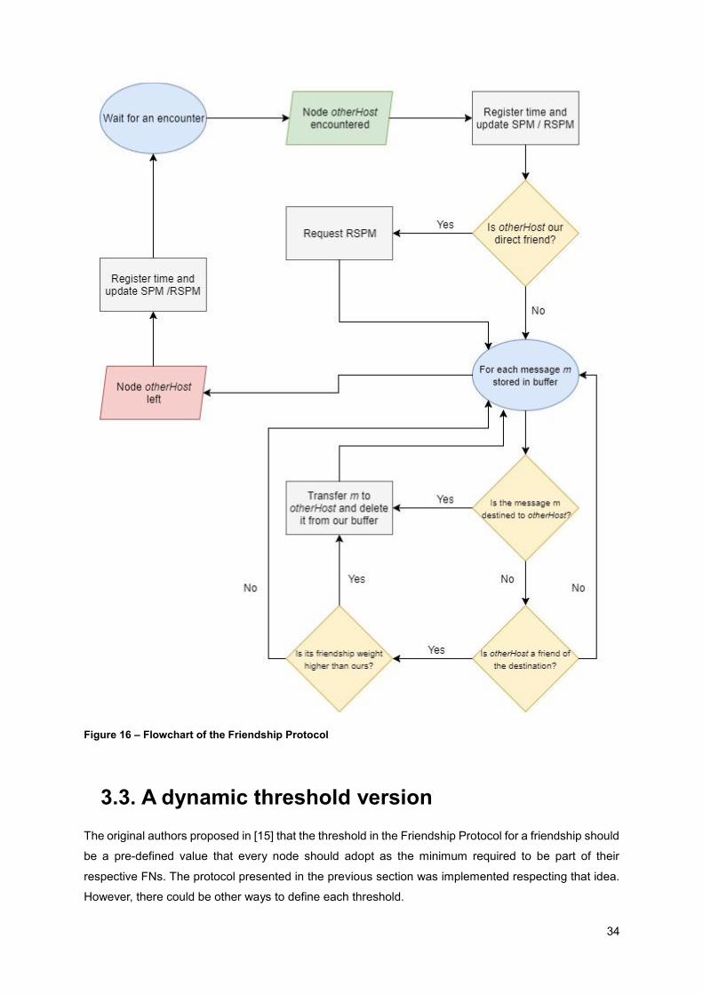
34
Figure 16 – Flowchart of the Friendship Protocol
3.3. A dynamic threshold version
The original authors proposed in [15] that the threshold in the Friendship Protocol for a friendship should
be a pre-defined value that every node should adopt as the minimum required to be part of their
respective FNs. The protocol presented in the previous section was implemented respecting that idea.
However, there could be other ways to define each threshold.

35
An altered version of Friendship is also proposed in this thesis on which is thought that the threshold
should be different for each node. It may be beneficial to assume that since nodes have different routines
and encounter frequencies, they should also have different friendship perceptions. The idea is that the
friendship threshold should instead be a portion of its best friend weight and not a fixed value that each
node should adopt. Formally,
𝜏 = ∆% × 𝑚𝑎𝑥({𝜔𝑖,𝑗 ∧ 𝑖 ≠ 𝑗} ∪ {𝜔𝑖,𝑗,𝑘, 𝑖 ≠ 𝑗 ≠ 𝑘}),
being ∆% an arbitrary portion in the form of percentage. By comparing every friendship with its best
friendship, nodes could adjust the number of nodes in their FNs based in the amount of activity (in other
words, “nodes encountered”) that each one has. Because the friendship weights of the nodes’ friends
change over time, the threshold would vary along, resulting in a dynamism that would follow each node’s
vision in terms of friends. It is not certain, however, which portion leads to the best performance results
as only by experiment can that be assessed.
To differentiate each version of the Friendship Protocol, the one proposed in this section is hereby
designated as Dynamic Friendship as the other stays as the Classic Friendship version. To sum up, the
only difference between these two versions is that, in Dynamic Friendship, the threshold is defined as a
fraction of its best friend weight which has consequently to be updated on a regular basis. More
concretely, the threshold update in Dynamic Friendship occurs whenever there is a change of a
connection state.

36
Chapter 4: Simulation Results
This chapter describes the scenario tested and the results that were obtained through simulation. There
is a subsection which describes the performance evaluation, a subsection that reveals the results which
allowed the optimization of the protocols and finally a subsection in which all protocols are compared
under different network load conditions.

37
4.1. Performance evaluation
The ONE simulator was used to assess and evaluate the Friendship protocol under a particular scenario.
As known, the simulator can depict several results of different metrics by generating reports for further
analysis. In this Master thesis, the parameters that are going to be evaluated are the delivery rate, the
average delay of each delivered message and the produced overhead. Even though achieving a decent
delivery rate is the ultimate goal for any protocol of this kind, it is still of interest to consider the message
delivery delay to find out how much time it takes for a message to be delivered. The overhead ratio, in
turn, is an indicator of how the system resource utilization is affected which could be crucial as valuable
resources such as bandwidth and buffer space are not wasted.
Naturally, the performance of a protocol could only be considered positive or negative when compared
to other protocols under the same circumstances. The protocols chosen to be tested along with
Friendship are the Epidemic, Prophet and BubbleRap protocols, which all have particular characteristics
that might be drawbacks when compared with Friendship. The Epidemic protocol was chosen due to its
ability to maximize the delivery rate at the expense of a high overhead. Prophet adds some intelligence
to Epidemic by calculating a delivery predictability, but relies on an aging process and on the transitivity
property. BubbleRap is a popular social protocol that combines centrality and community, yet depicts
those metrics on a global manner and does not take in account nodes routines as nodes’ behaviors may
change at different periods of the day. The author of the source code used for the implementation of the
BubbleRap protocol is PJ Dillon [44] from the University of Pittsburgh, whereas for Epidemic and Prophet
the source code was available by default in the ONE simulator.
In the initial phase, the primary objective is to tune BubbleRap’s parameters k and Familiar Threshold
and Friendship’s Friendship Threshold in order to optimize their performance under the given scenario
conditions. The Familiar Threshold corresponds in BubbleRap to the minimum time which a node must,
in aggregate, remain in contact with other in order to be considered part of its community, while the
Friendship Threshold in the Friendship Protocol is the minimum friendship weight a node must achieve
to be considered a friend. A dynamic parameter tuning approach has also been tested on Friendship to
understand if nodes benefit from having individual thresholds, and, if so, which portion of their maximum
friendship weight serves them best. The second phase of the simulations has the purpose of assessing
the effect of traffic load in the network by varying the number of created messages per time unit, now
that we have the protocols optimized. It should be interesting to see how the protocols’ performance
depends on the network load as it should give us a wider picture of their behavior. Furthermore, it should
help us clarify the consequences of having a dynamic tuning mechanism in detriment of a fixed
threshold.
4.2. Phase I: Tuning
The scenario selected is the metropolitan area of the city of Helsinki, Finland, as shown in Figure 17.
This is the default map of The ONE simulator and it serves the purpose of this work well, as it offers

38
multiple paths for nodes to move around. Even though it could not be visually noted in Figure 17, the
map contains roads used by vehicles and pedestrians and sidewalks that are restricted to pedestrians.
Figure 17 – Metropolitan area of Helsinki, Finland, presented on the GUI mode of The ONE simulator.
4.2.1. Settings
The settings of the simulation represent the core of the scenario. The following parameters were chosen
with the intention of having a realistic scenario and remained unchanged on every protocol test.
There are three types of nodes circulating on top of the map, on a total of 114 nodes: pedestrians (90),
trams (12) and buses (12). The main idea is that both pedestrians and vehicles possess an equipment
like a smartphone with an integrated network interface that they use to exchange messages with others.
All nodes belong to a certain group on which they are assigned the same characteristics, as described
on Table 2.
Trams and buses have the movement pattern RMBM, which means that both groups follow a regular
pattern between two location points over time, with brief stops on the way. The main difference between
these vehicles is that pedestrians are only allowed to ride buses, as if they had only a bus pass and not
a tram pass. Buses and trams that are within the same group follow the same movement pattern.

39
Pedestrians, in turn, follow the much more complex movement pattern WDM. These nodes are
programmed to have a daily routine resembling a working individual which has a home, a job office and
favorite socializing spots. Whereas the home and job office of each pedestrian is randomly located at
any point of the map, pedestrians of the same group are limited to a certain zone of the city to socialize,
as if they preferred those meeting spots. Also, pedestrians within the same group can only ride the buses
that are located near their favorite meeting spots and no other vehicles. All pedestrians spend 8 hours
at work and after that they have a 75% probability to go socialize for 1 to 2 hours with 2 to 8 other people.
They always return home until the next morning, and then repeat their routine.
The buffer size represents the space available at a node to store messages. The size chosen for each
node’s buffer is 1 GB, which is a plausible value taking in account that a typical smartphone nowadays
easily has around 8 GB of internal storage. It is important to refer also that every time a message arrives
at a node and there is no buffer space available, a default drop policy is triggered where the node will
search for the oldest messages in the buffer and remove them until there is enough space for the
incoming one.
In terms of network interfaces, all groups of nodes use a single Wi-Fi interface with a constant throughput
of 10 Mbps and limited to a communication range of 10 meters. The throughput is set to 10 Mbps as an
average data rate which is constant for every position within the radio range2. In turn, the 10 meters
range limitation may also seem inappropriate as there are currently access points that can reach up to
100 meters outdoors (e.g. a traditional 2.4 GHz access point), but, since the simulator does not take in
account attenuations from obstacles like buildings, using a short fixed range results is a good
approximation of reality.
Table 2 - Nodes' settings
Group #Nodes Speed [m/s] Buffer Size [MB] Movement Model
1: Pedestrians (PedA) 30 0.8 to 1.4
1000
WDM
2: Buses (ABus) 4 7.0 to 10.0 RMBM
3: Pedestrians (PedB) 30 0.8 to 1.4 WDM
4: Buses (BBus) 4 7.0 to 10.0 RMBM
5: Pedestrians (PedC) 30 0.8 to 1.4 WDM
6: Buses (CBus) 4 7.0 to 10.0 RMBM
7: Trams (ATram) 4 7.0 to 10.0 RMBM
8: Trams (BTram) 4 7.0 to 10.0 RMBM
9: Trams (CTram) 4 7.0 to 10.0 RMBM
In this scenario, message creation parameters are also very relevant. In order to create a more realistic
scenario, both source and destination addresses were limited only to 13 nodes, meaning that only these
2 The ONE simulator handles radio transmissions by setting that the throughput is constant within the radio range and null for
higher distances. This is actually a limitation of the simulator as in a real scenario there are generally significant attenuations along the signal path which reduces the throughput along the way.

40
few nodes produce new messages and the rest only serve as relay nodes. In this way, the traffic pattern
is asymmetric and thus not uniformly distributed, which is closer to what occurs in reality. Message sizes
vary randomly from 3 MB to 15 MB and are created at a rate of 3 messages per minute. It was also
established that each message would have a maximum of 1.5 days to live.
In order to gather more consistent results, four simulations with different seeds were run in every test.
Therefore, each value presented is an average of the results for these four simulations with a confidence
interval associated. In all cases, a 95% confidence interval is considered. The simulation time is 8 days
on all cases.
4.2.2. Epidemic Protocol
Theoretically, the Epidemic Protocol would achieve the maximum possible delivery rate if there were no
constraints in terms of buffer size and bandwidth on a network, which makes it a good protocol to be
compared with others. However, since we are simulating a realistic scenario with limited resources and
the overhead is generally high with Epidemic, it was expected that it would underperform as it in fact
did. After testing the Epidemic Protocol under this scenario conditions, the protocol was able to deliver
9860 out of the 34560 messages created, which corresponds to a delivery rate of 28.53 %. To achieve
this result, the protocol created an overhead of 1012.70, meaning that it needed approximately 1013
times more transmissions than the ideal protocol which requires only one transmission per delivered
message. In turn, the average latency for this protocol was 19837.28 seconds which means that
messages took an average of 5.51 hours to reach the destination. These results confirm the initial
prediction and are shown in Table 3.
Table 3 – Epidemic Protocol results
Delivery Rate [%] Overhead Average Latency [s]
28.53 ± 1.58 1012.70 ± 105.61 19837.28 ± 1334.65
4.2.3. Prophet Protocol
Prophet Protocol’s controlled flooding mechanism provides some efficiency in comparison with the
Epidemic, so it was expected that the overhead would decrease substantially at the very least. The
results were interesting as the delivery rate was virtually the same as Epidemic’s, with a value of 28.26%.
As expected, the overhead decreased 31% relatively to Epidemic to the value of 698.26. The average
delay also decreased to 15548.63 seconds, which is equivalent to 4.32 hours, approximately. Even
though Prophet’s overall performance was superior to Epidemic’s, it may be that Prophet misuses
networks’ static information in this scenario due to its inherent aging feature. The aging mechanism
seems to be problematic as a result of nodes regularly spending long periods away from others (e.g.
some pedestrians live alone and daily spend 8+ hours at home) as delivery probabilities dramatically
decrease over these periods, resulting on a performance similar to Epidemic in terms of delivery rate.
These results were gathered in Table 4.

41
Table 4 – Prophet Protocol results
Delivery Rate [%] Overhead Average Latency [s]
28.26 ± 1.78 698.26 ± 106.67 15548.63 ± 1016.90
4.2.4. BubbleRap Protocol
Since it was known that Bubble Rap’s performance was directly influenced by the pre-determined
number of k-cliques (k) and the cumulative time threshold used to decide if a node can be part of other
nodes’ community (familiar threshold), the purpose of the initial tests was to determine which values for
these parameters leads to the optimal performance of the protocol.
4.2.4.1 Influence of the familiar threshold parameter
In order to assess the influence of the familiar threshold parameter, k was fixed at 4 and the familiar
threshold was varied from 100 to 10000 seconds. The simulation results are presented in Table 5. For
small values of the familiar threshold, only the value of 100 was tested since values too low mean that
nodes, after meeting one time, would belong to the same community and that would lead to lower results
in terms of delivery rate, allowing fortuitous contacts to be added to a host’s community. It was observed
that, regarding the delivery rate, the best results occurred for higher values of the familiar threshold.
Generally speaking, the results above the familiar threshold of 2000 seconds were so similar that they
were considered to be statistically equal according to the confidence interval. For this reason, some
results above 3000 were omitted since they led to very similar results. It could also be observed that for
the BubbleRap protocol the overhead ratio was around 52, much lower than Epidemic’s or Prophet’s,
which is logical since message relaying is much more selective in this protocol. The average delay of
the delivered messages also improved significantly, roughly to values between 12000 and 13000
seconds. This fact also makes sense in the way that the paths used by BubbleRap typically are much
more efficient than the previously tested protocols.
Since delivery rates tend to stabilize for familiar thresholds above 2200 seconds, it is thought that these
thresholds are enough in order to avoid adding fortuitous contacts to become part of each other’s
community in this scenario. Therefore, regarding the values tested, any familiar threshold above 2200
would serve the purpose of this task as all lead to an optimal result. Thus, and although another
threshold in this range could have been selected, the chosen familiar threshold was 2500 seconds with
a delivery rate of 26.21%, an overhead ratio of 50.97 and an average latency of 12741.93 seconds,
which corresponds to roughly 3.5 hours.
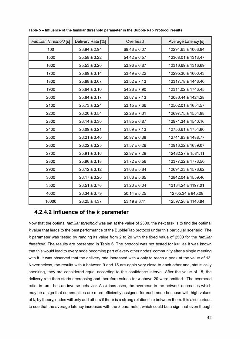
42
Table 5 – Influence of the familiar threshold parameter in the Bubble Rap Protocol results
Familiar Threshold [s] Delivery Rate [%] Overhead Average Latency [s]
100 23.94 ± 2.94 69.48 ± 6.07 12294.63 ± 1068.94
1500 25.58 ± 3.22 54.42 ± 6.57 12368.01 ± 1313.47
1600 25.53 ± 3.20 53.96 ± 6.87 12316.69 ± 1316.69
1700 25.69 ± 3.14 53.49 ± 6.22 12295.30 ± 1600.43
1800 25.68 ± 3.07 53.52 ± 7.13 12317.78 ± 1446.40
1900 25.64 ± 3.10 54.28 ± 7.90 12314.02 ± 1746.45
2000 25.64 ± 3.17 53.67 ± 7.13 12086.44 ± 1424.28
2100 25.73 ± 3.24 53.15 ± 7.66 12502.01 ± 1654.57
2200 26.20 ± 3.54 52.28 ± 7.31 12697.75 ± 1554.98
2300 26.14 ± 3.30 51.85 ± 6.87 12971.34 ± 1540.16
2400 26.09 ± 3.21 51.89 ± 7.13 12753.61 ± 1754.80
2500 26.21 ± 3.40 50.97 ± 6.38 12741.93 ± 1488.77
2600 26.22 ± 3.25 51.57 ± 6.29 12913.22 ± 1639.07
2700 25.91 ± 3.16 52.97 ± 7.29 12482.27 ± 1581.11
2800 25.96 ± 3.18 51.72 ± 6.56 12377.22 ± 1773.50
2900 26.12 ± 3.12 51.08 ± 5.84 12694.23 ± 1578.62
3000 26.17 ± 3.20 51.66 ± 5.65 12842.04 ± 1559.46
3500 26.51 ± 3.76 51.20 ± 6.04 13134.24 ± 1197.01
4000 26.34 ± 3.79 50.14 ± 5.25 12705.34 ± 845.08
10000 26.25 ± 4.37 53.19 ± 6.11 12597.26 ± 1140.84
4.2.4.2 Influence of the k parameter
Now that the optimal familiar threshold was set at the value of 2500, the next task is to find the optimal
k value that leads to the best performance of the BubbleRap protocol under this particular scenario. The
k parameter was tested by ranging its value from 2 to 20 with the fixed value of 2500 for the familiar
threshold. The results are presented in Table 6. The protocol was not tested for k=1 as it was known
that this would lead to every node becoming part of every other nodes’ community after a single meeting
with it. It was observed that the delivery rate increased with k only to reach a peak at the value of 13.
Nevertheless, the results with k between 9 and 15 are again very close to each other and, statistically
speaking, they are considered equal according to the confidence interval. After the value of 15, the
delivery rate then starts decreasing and therefore values for k above 20 were omitted. The overhead
ratio, in turn, has an inverse behavior. As k increases, the overhead in the network decreases which
may be a sign that communities are more efficiently assigned for each node because with high values
of k, by theory, nodes will only add others if there is a strong relationship between them. It is also curious
to see that the average latency increases with the k parameter, which could be a sign that even though

43
communities have stronger relationship within themselves, nodes tend to follow less efficient paths as
they may have issues on finding the proper bridges for the destination community. The best
performances were for values of k between 10 and 15, which seems adequate since the total nodes in
the network is 114. In sum, the performance chosen as the best for the BubbleRap protocol occurred
for a familiar threshold of 2500 and a k of 13, resulting on a delivery rate of 30.59%, an overhead ratio
of 41.76 and an average delay of 14258.18 seconds, which approximately corresponds to 4 hours.
Table 6 – Influence of the k parameter in the Bubble Rap Protocol results
k Delivery Rate [%] Overhead Average Latency [s]
2 24.78 ± 2.90 57.62 ± 5.18 12528.16 ± 1494.74
3 25.87 ± 2.92 52.86 ± 7.34 12428.23 ± 1337.26
4 26.21 ± 3.40 50.97 ± 6.38 12741.93 ± 1488.77
5 26.64 ± 3.53 49.67 ± 4.81 12834.01 ± 1648.25
6 27.73 ± 3.25 47.62 ± 2.48 13182.28 ± 1717.78
7 28.36 ± 3.95 46.12 ± 1.90 13154.04 ± 1482.99
8 29.21 ± 4.29 45.21 ± 2.71 13273.55 ± 1544.88
9 29.91 ± 3.68 43.67 ± 3.23 13810.40 ± 2072.70
10 30.25 ± 3.50 42.70 ± 3.76 14249.07 ± 1748.46
11 30.40 ± 3.32 42.32 ± 3.74 14249.73 ± 1909.67
12 29.59 ± 4.79 41.96 ± 4.08 14184.13 ± 1776.30
13 30.59 ± 3.24 41.76 ± 4.03 14258.18 ± 1871.40
14 30.56 ± 3.23 41.75 ± 4.05 14295.16 ± 1942.78
15 30.54 ± 3.28 41.82 ± 3.93 14236.10 ± 1903.31
20 27.33 ± 4.42 41.76 ± 3.91 14259.25 ± 1897.49
4.2.5. Friendship Protocol
Lastly, the Friendship Protocol was tested in order to assess its performance under the chosen scenario.
Similarly to BubbleRap, the Friendship Protocol also has a tunable feature called the friendship threshold
that has to be adapted to each scenario as it influences directly its performance under a particular
scenario. As explained in Chapter 3, the friendship threshold (τ) is the minimum friendship weight that
two nodes must have to be considered friends and is measured in inverse time units. The larger the
value of the threshold τ, the closer are friendships and thus higher are the forwarding opportunities
among friends. On the other hand, by having a large threshold, the communities of friends could be so
selective that messages do not flow properly on the network. The classic version of this protocol
presupposes that a fixed friendship threshold exists for every node as friendship is seen as an absolute
social property. The dynamic version of the protocol proposed in this thesis assumes the idea that
friendship should be relative and friendship thresholds should be individually chosen by each node as a
portion of their maximum friendship weights, i.e., their best friendships. The main purpose of these initial

44
tests is for the classic Friendship Protocol to assess which fixed threshold leads to the optimal
performance and for the dynamic Friendship to discover which portion of the maximum friendship leads
to the best results under this scenario.
4.2.5.1. Classic Friendship: Influence of the fixed threshold
In order to find which friendship threshold τ leads to the optimal performance under the circumstances
of this scenario, several simulations have been run while varying this parameter and the results were
compared. In order to simplify the interpretation of the threshold values, the values presented are the
inverse of the respective threshold (1 / τ) which represents the Social Pressure (SP) metric and allow
us to have the perception of the average forward delay to one node if another had a new message to
deliver at each time unit.
The SP threshold values tested ranged from 15 minutes to 3 hours, on 15 minute intervals, so a total of
12 threshold values were tested. A 0 minutes SP threshold value was not considered as that would lead
to an infinite friendship threshold level, which means that friendship communities would not even be
formed. Since the Friendship Protocol uses 3 hour timeslots to analyze nodes behavior and friendships
are depicted based on the current timeslot, it also did not make much sense to consider SP threshold
values above 3 hours because that would mean that, among friends, the minimum time to encounter
another would exceed the current timeslot and thus friendship communities would not be properly
captured. The lower the minimum average forward delay required, the more selective friendship
communities tend to be, as only average delays below this value are selected as friends.
The results for the classic version of the Friendship Protocol are presented in Table 7. In terms of delivery
rate, the minimum scores were for the lowest values of the SP threshold which may be an indicator that
communities with those friendship thresholds are too restrictive. The delivery rates start increasing with
the SP threshold only to stabilize around the value of 2 hours. The highest average delivery rate was
found at a SP threshold of 2 hours and 15 minutes, which requires friend nodes to meet each other on
average every 2 hours and 15 minutes, at least. In terms of the overhead ratio, this protocol had an
incredible performance of having less than 3 copies per new message on the network for each threshold
tested. It was noted that the overhead increases with the SP which makes sense since there are more
message relaying when communities are less restrictive. The average latency, in turn, is also affected
by the decrease of friendship community restrictions and increases quite significantly with the SP
threshold. As messages are only relayed if the destination node is in the encountered node’s community,
it is comprehensible that since communities contain weaker friendships, the average delay of the
delivered messages increases.
Although that it was hard to find a conclusion on which value led to the optimal overall performance
since the results did not differ much in terms of delivery rate according to the confidence interval, the
performance chosen as optimal was for the SP threshold of 2 hours and 15 minutes, corresponding to
the maximum delivery rate of 36.53%, an overhead ratio of 2.4 and an average delay of 18858.08
seconds (5.24 hours).

45
Table 7 – Influence of the fixed threshold in the classic Friendship Protocol results
SP Threshold Delivery Rate [%] Overhead Average Latency [s]
0 h 15 min 34.05 ± 2.26 0.53 ± 0.03 14062.39 ± 573.27
0 h 30 min 34.75 ± 0.79 0.69 ± 0.07 14575.13 ± 1294.62
0 h 45 min 34.37 ± 2.69 0.83 ± 0.07 14643.43 ± 990.31
1 h 00 min 34.51 ± 0.84 1.13 ± 0.19 15053.48 ± 1610.62
1 h 15 min 35.52 ± 2.53 1.26 ± 0.14 16732.08 ± 794.69
1 h 30 min 35.33 ± 0.96 1.76 ± 0.27 16890.59 ± 1512.26
1 h 45 min 36.26 ± 1.22 1.91 ± 0.22 18882.00 ± 2120.26
2 h 00 min 35.70 ± 0.86 2.25 ± 0.28 18273.39 ± 2033.33
2 h 15 min 36.53 ± 1.38 2.40 ± 0.28 18858.08 ± 1931.46
2 h 30 min 35.58 ± 0.93 2.68 ± 0.45 18029.01 ± 1963.77
2 h 45 min 36.14 ± 1.79 2.72 ± 0.27 18247.13 ± 1915.42
3 h 00 min 35.46 ± 0.76 2.94 ± 0.42 17792.57 ± 1336.92
4.2.5.2. Dynamic Friendship: Influence of the dynamic threshold
The dynamic version of the Friendship Protocol assumes the idea that each node should have its own
friendship threshold level as a portion of its best friendship. As explained in Chapter 3, every time there
is a new connection, the node evaluates which of its friend is the best, i.e. which one of the nodes
belonging to its friendship community has the higher weight, and updates its friendship threshold level
to a portion of that weight offering dynamism for the friendship community formation. However, it was
unknown which threshold the node should adopt as it certainly would affect Friendship’s performance.
In order to assess which fraction should be adopted according to the chosen scenario, the dynamic
friendship threshold was varied from 10% to 90 % of the best friend’s threshold, on intervals of 10%. By
increasing this fraction, one should expect that friendship communities are more open and thus more
nodes are seen as friends, since the threshold value is lower as well. By decreasing the fraction, in turn,
communities are more restricted as the threshold gets closer to the weight of the best friendship.
Naturally, neither the 0% nor 100% fraction values were tested, as that would mean that every node
encountered would be considered a friend or only the nodes’ best friend is considered to be a friend,
respectively, which would go against the Friendship Protocol’s concept.
The results are shown Table 8. In terms of the delivery rate, it is interesting to see that the most restrictive
friendship communities corresponded to the lower performances, around 33%. In fact, increasing the
portion for the dynamic threshold actually increased the delivery rate in a general way. The maximum
delivery rate was registered for a dynamic threshold of 80% of the best friendship weight, with a value
of 35.23%. In terms of the overhead ratio, this version of the Friendship Protocol followed the pattern
observed in the classic version on which the overhead decreased whenever communities were more
selective, i.e. the friendship thresholds were higher. Nevertheless, similarly to what happened with the

46
classic version, the overhead was undoubtedly lower when compared to other protocols, as for each
threshold tested the overhead ratio was less than 3. Analogously to the classic version, the average
latency is also generally lower for low levels of dynamic thresholds, for the same reasons stated before.
The dynamic threshold chosen as optimal was 80%, which corresponded to a delivery rate of 35.23%,
an overhead ratio of 1.13 and an average latency of 18377.66 seconds, which corresponds to
approximately 5.1 hours. The second best value was for the 60% threshold with a smaller confidence
interval. However, it was decided that the best overall performance was for the 80% threshold, since the
overhead ratio was lower.
Table 8 – Influence of the dynamic threshold in the Dynamic Friendship Protocol results
Dynamic Threshold [%] Delivery Rate [%] Overhead Average Latency [s]
10 33.17 ± 1.76 2.99 ± 0.23 16687.03 ± 2027.94
20 33.15 ± 1.26 2.73 ± 0.19 17280.51 ± 1508.55
30 33.36 ± 0.57 2.32 ± 0.15 17241.77 ± 1620.80
40 34.64 ± 1.40 2.01 ± 0.29 18255.85 ± 1195.68
50 34.24 ± 0.98 1.74 ± 0.15 18213.84 ± 1624.55
60 34.97 ± 0.80 1.53 ± 0.24 18032.09 ± 1716.23
70 34.22 ± 1.86 1.26 ± 0.13 18085.39 ± 1608.38
80 35.23 ± 1.57 1.13 ± 0.20 18377.66 ± 2124.14
90 33.54 ± 2.06 0.88 ± 0.11 17032.57 ± 1796.13
4.3. Phase II: Traffic load variation
The next task was to vary the network load and assess each protocol’s behavior under different
congestion conditions. The scenario used was exactly the same as the previous, except for the message
generation intervals parameter. As the purpose of this phase is to determine how the protocols’
performance depends on the network load, the simulations were now run for ten different message
generation intervals: 6, 7, 8, 10, 12, 15, 20, 30, 60 and 120 seconds. It was known that Epidemic excels
in terms of delivery rate whenever the buffer size and bandwidth are not constraining, so the reference
used to choose the least message generation rate tested (0.5 messages / minute) was the one on which
the Epidemic Protocol matched other protocols’ performance in terms of delivery rate. In turn, no more
tests were run for rates above 10 messages / minute as at that point all protocols’ performances
converged in terms in the delivery rate and average latency metrics, which is an indicator that the
network is so congested that messages are discarded in their majority simply because there is no
available space on the nodes’ buffer.
In the next three sub-sections, the protocol’s performances are analyzed under these conditions in terms
of delivery rate, average latency and overhead, respectively. Each metric analysis is illustrated with a
chart figure to help clarify their dependencies on the network load. The 95% confidence intervals are
represented on each point of the chart.

47
4.3.1 Delivery Rate
The results of the evolution of the delivery rate metric with the message generation rate in the network
are depicted in Figure 18. As expected, the delivery rate lowered for all protocols when the message
generation rate increased, as a higher number of new messages in the network is likely to lead to a
higher degree of congestion in the network. The maximum value registered for the delivery rate was
55.90%, corresponding to the Dynamic Friendship Protocol with a rate of 0.5 messages / minute. In turn,
the minimum registered was 16.03 % for the Prophet Protocol at the rate of 10 messages / minute.
Similarly to what happened in the Tuning Phase, Epidemic and Prophet Protocols revealed statistically
equal performances according to the confidence interval, which confirms that Prophet converges into
the Epidemic Protocol as its controlled flooding mechanisms fail in this scenario. In terms of delivery
rate, there is no clear benefit on using Prophet in detriment of Epidemic. However, for the lower message
creation rates, both protocols’ delivery rate improves significantly as the congestion in the network is
reduced, statistically matching every other protocol at the rate of 0.5 new messages / minute.
Although BubbleRap’s delivery rates were generally better than the previous protocols stated, they were
not superior to both versions of the Friendship Protocol delivery rates. In fact, it is clear that the
Friendship Protocol had the best results from 1 to 4 messages / minute, while on the other ranges their
delivery rates are considered statistically equal to BubbleRap’s due to the confidence interval.
In terms of delivery rate, results show that there is no clear benefit of using the dynamic version of the
Friendship Protocol instead of the classic version. On average terms, the classic version marginally
beats the dynamic version for message creation rates above 2 messages / minute, while the dynamic
version takes advantage for lower message generation rates.
In conclusion, both versions of the Friendship Protocol had positive performances in terms of the delivery
rate metric, as no other protocol tested showed better results according to the confidence interval.
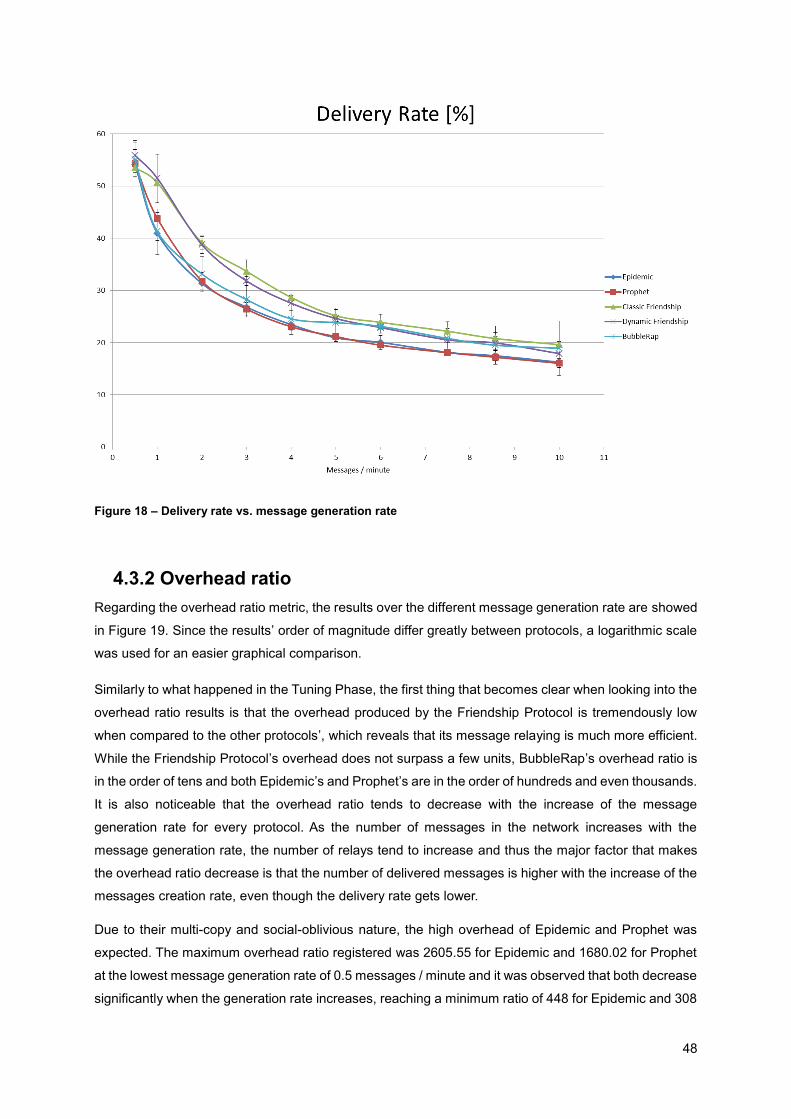
48
Figure 18 – Delivery rate vs. message generation rate
4.3.2 Overhead ratio
Regarding the overhead ratio metric, the results over the different message generation rate are showed
in Figure 19. Since the results’ order of magnitude differ greatly between protocols, a logarithmic scale
was used for an easier graphical comparison.
Similarly to what happened in the Tuning Phase, the first thing that becomes clear when looking into the
overhead ratio results is that the overhead produced by the Friendship Protocol is tremendously low
when compared to the other protocols’, which reveals that its message relaying is much more efficient.
While the Friendship Protocol’s overhead does not surpass a few units, BubbleRap’s overhead ratio is
in the order of tens and both Epidemic’s and Prophet’s are in the order of hundreds and even thousands.
It is also noticeable that the overhead ratio tends to decrease with the increase of the message
generation rate for every protocol. As the number of messages in the network increases with the
message generation rate, the number of relays tend to increase and thus the major factor that makes
the overhead ratio decrease is that the number of delivered messages is higher with the increase of the
messages creation rate, even though the delivery rate gets lower.
Due to their multi-copy and social-oblivious nature, the high overhead of Epidemic and Prophet was
expected. The maximum overhead ratio registered was 2605.55 for Epidemic and 1680.02 for Prophet
at the lowest message generation rate of 0.5 messages / minute and it was observed that both decrease
significantly when the generation rate increases, reaching a minimum ratio of 448 for Epidemic and 308

49
for Prophet. In terms of the overhead ratio metric, the benefits of using Prophet in detriment of Epidemic
are clearly observed as the overhead is substantially lower for Prophet at all times.
BubbleRap, in turn, is a social-aware protocol, so it was expected that message relaying would be much
more efficient as it takes advantage of social information of the network. That was actually demonstrated
by the overhead ratio results that shows significantly lower values than Epidemic’s and Prophet’s,
reaching a maximum of 64.58 at the message generation rate of 0.5 messages / minute and a minimum
of 21.28 at the rate of 8.57 messages /minute.
Friendship is a social propriety which describes close personal relationships, so it was expected
beforehand that message relaying would be much more selective as messages only get forwarded to
friends of the destination to avoid unnecessary transmissions. This revealed to be true as the overhead
ratio was substantially lower for Friendship than for all other protocols tested. The maximum overhead
ratio was 2.72 for the classic version and 1.24 for the dynamic version at the lowest message generation
rate of 0.5 messages / minute, whilst the minimum registered was 1.91 and 0.88 respectively, at the
highest generation rate of 10 messages / minute. These results reveal the major benefit of using the
dynamic version of Friendship in detriment of the classic version, as the overhead ratio of the dynamic
version is roughly half of the classic’s for all rates and thus reveals to be more efficient.
Figure 19 – Overhead ratio vs. message generation rate

50
4.3.3 Average Delay
The results regarding the average delay metric are presented in Figure 20. The first general impression
when analyzing the data was that the average message latency decreases for every protocol tested
when the message generation rate increases, which is concordant with the idea that a significant part
of the messages is discarded due to network congestion as several nodes have fully occupied buffers
and have to discard messages in order to receive new ones.
From the generation rate of 0.5 to 2 messages / minute, which corresponds to the lowest network load
tested, the dynamic version of the Friendship Protocol stands out as it presented the highest average
delay, reaching a maximum of 35635.04 seconds for the rate of 0.5 messages / minute. The classic
version of Friendship presents the second highest latency on this range, which reveals that paths chosen
by the Friendship Protocol within low congestion are not the ones which lead to the quickest message
deliveries, which is a drawback when comparing to the other protocols tested.
Above the rate of 2 messages / minute, only Epidemic clearly stands out presenting the highest delays,
as other protocols converge in terms of average latency. As stated before, at this point the network load
is high enough to induce message dropping due to lack of buffer space. However, Epidemic seems to
avoid part of this issue as every path possible is attempted due to its naïve replication nature.
In conclusion, these results expose the implications of using Friendship as the primary social property
to relay messages, as it may take more time to find a friend of a destination and thus the average latency
is increased, which is more evident in the case on which friendship is considered to be dynamic and
relative to each node.

51
Figure 20 – Average Delay vs. message generation rate

52
Chapter 5: Conclusions
This chapter reviews the work done in this Master thesis, outlines the main conclusions and points out
aspects to be developed in future work.

53
The main objective of this thesis was to assess and compare the performance of the Friendship Protocol,
a social-aware DTN routing protocol mainly based in the social concept of Friendship. In order to do it,
several chapters were written. Those will be briefly summarized.
Chapter 1 presented a brief overview of the DTN scientific field evolution, the motivation to the topic of
this Master’s thesis and the scope of this work. This was the starting point to all of the research and
development done.
In Chapter 2, the fundamentals of DTNs are presented. This chapter starts with a brief description of
DTNs and how routing schemes are evaluated, followed by a section solely dedicated to the typical
network architecture of a DTN and after that, an analysis on the state of the art routing protocols is
presented. In the end of this chapter, the existing simulators to test protocols for DTNs are referred and
the one used in this document is analyzed in further detail.
In Chapter 3, the developed Friendship protocol is presented. In this chapter, it is possible to understand
what is the main idea behind this protocol and how it was implemented, illustrated with the pseudo-
codes of the most important algorithms and a flowchart. The Friendship protocol is based in two
important concepts for social-aware routing protocols in DTNs: Friendship and Community. Node
relations are always analysed for a certain period of the day and are depicted through a friendship
weight, which is the inverse of one of two metrics, which are SPM and RSPM. SPM indicates the average
delay for meeting a certain node and RSPM the average delay that messages would suffer if they had
to cross a certain intermediate node to reach a second. Nodes are considered to be friends if their
friendship weight is superior to a certain threshold. Only nodes that are friends belong to their
communities, and messages are only relayed if the destination is friend of the encountered node. As an
alternative of a fixed threshold approach, a second version of this protocol on which the threshold is a
portion of the current best friendship is proposed, meaning that friendship standards change from node
to node.
In Chapter 4, the conditions on which the Friendship protocol was tested and evaluated are explained
in detail. The protocol performance was compared to Epidemic’s, Prophet’s and BubbleRap’s. The first
phase of simulations was merely to adjust the configurable parameters of BubbleRap and Friendship.
After the optimal parameters were found, the second phase was an assessment of how the protocols’
performance changed with the number of messages in the network. Several conclusions were stated
on this chapter.
In terms of delivery rate, both versions of the Friendship Protocol had a positive performance as no
other protocol tested showed better results according to the confidence interval, for every network load
value tested. The overhead ratio, in turn, was substantially lower for the two Friendship versions than
for all other protocols tested. The results also revealed that the overhead ratio of the dynamic version is
roughly half of the classic’s. In terms of average delay, however, the two versions of Friendship led to
worst values, as they generally took longer to get messages delivered when compared to other
protocols.

54
The single advantage observed when using the dynamic version of Friendship in detriment of the classic
version was that as the overhead ratio of the dynamic version is roughly half of the classic’s for all load
values and thus reveals to be more efficient.
It is important to take into account that, despite the effort to recreate real scenarios in the simulator, the
real world is far too complex and many simplifications had to be introduced. Regardless of these
simplifications, the obtained results provided some insights on how protocols really work under a MSN
scenario.
As suggestions for future work for the topic, it would be interesting to collect some social data regarding
BubbleRap’s and Friendship’s performance in the simulations, such as the number of communities
formed or average number of nodes per community for the BubbleRap or the average number of friends
per node for Friendship, as that would definitely allow a more precise tuning. Additionally, it would also
be relevant to test the protocols in different scenarios to check how Friendship behaves under conditions
different than of a MSN, the type of network which clearly it was designed for. Lastly, it could also be
worthwhile to create a multiple-copy version of the Friendship Protocol, as that may result in significant
performance gains.

55
References
[1] Project Loon, 2017. [Online]. Available: https://x.company/loon/ [Accessed: 11-Oct-2017].
[2] Cao and Sun, Routing in Delay/Disruption Tolerant Networks: A Taxonomy, Survey and Challenges,
IEEE Communications Surveys & Tutorials, vol. 15, no. 2, pp. 654-677, 2013.
[3] V. Cerf, et al., Delay-Tolerant Networking Architecture, IETF RFC 4838, April 2007.
[4] Paul Muri et al., User Datagram and Bundle Protocol for Distributed Small Satellite Topologies,
Journal of Wireless Networking and Communications, vol. 3, no. 3, p. 19-28, 2013.
[5] C. Boldrini, K. Lee, M. Önen, J. Ott, E. Pagani, Opportunistic networks, Computer Communications
48, pp.1-4, 2014.
[6] M. Grossglauser and D. Tse, Mobility increases the capacity of ad hoc wireless networks, IEEE/ACM
Transactions on Networking, vol. 10, no. 4, pp. 477-486, 2002.
[7] A. Vahdat and D. Becker, Epidemic routing for partially-connected ad hoc wireless networks, Duke
University Technical Report Cs-2000-06, Tech. Rep., 2000.
[8] Spyropoulos, Thrasyvoulos, Konstantinos Psounis and Cauligi S. Raghavendra, Spray and wait: an
efficient routing scheme for intermittently connected mobile networks, Proceedings of the 2005 ACM
SIGCOMM Workshop on Delay-tolerant networking, pp. 252-259, ACM, 2005.
[9] A. Lindgren, A. Doria, E. Davies, and S. Grasic, Probabilistic Routing Protocol for Intermittently
Connected Networks, IETF RFC 6693, 2012.
[10] F. Xia, L. Liu, J. Li, J. Ma, and A. V Vasilakos, Socially-Aware Networking: A Survey IEEE Syst. J.,
vol. 9, no. 3, pp. 1–18, 2015.
[11] Y. Zhu, B. Xu, X. Shi, and Y. Wang, A survey of social-based routing in delay tolerant networks:
Positive and negative social effects, IEEE Communication Surveys & Tutorials, vol. 15, no. 1, pp. 387–
401, 2013.
[12] Community. (1989). Oxford English Dictionary.
[13] S. Okasha, Altruism, group selection and correlated interaction, British Journal for the Philosophy
of Science, vol. 56, no.4, pp. 730–725, 2005
[14] N. Magaia, A. Francisco, P. Pereira, M. Correia, Betweenness Centrality in Delay Tolerant Networks:
A Survey, Ad Hoc Networks 2015;33:284–305, 2015.

56
[15] E. Bulut, B. K. Szymanski, Exploiting friendship relations for efficient routing in mobile social
networks, IEEE Transactions Parallel Distributed Systems, vol. 23, no. 12, pp. 2254-2265, Dec. 2012.
[16] W. Moreira, P. Mendes, S. Sargento, Opportunistic routing based on daily routines, Proc.
WoWMoM, 2012
[17] B. Guidi et al., Distributed protocols for Ego Betweenness Centrality computation in
DOSNs, Pervasive Computing and Communications Workshops, 2014 IEEE International Conference,
2014.
[18] H. A. Nguyen and S. Giordano, Routing in Opportunistic Networks, 1st ed. Springer-Verlag New
York, 2011.
[19] P. Hui, J. Crowcroft, and E. Yoneki, BUBBLE Rap: Social-based forwarding in delay-tolerant
networks, IEEE Transactions on Mobile Computing, vol. 10, no. 11, pp. 1576–1589, 2011.
[20] Q. Li, S. Zhu, and G. Cao, Routing in Socially Selfish Delay Tolerant Networks, INFOCOM’10,
2010, pp. 857–865.
[21] E. Daly and M. Haahr, Social Network Analysis for Routing in Disconnected Delay-Tolerant
MANETs, MobiHoc’07, 2007, pp. 32–40.
[22] K. Chen and H. Shen, SMART: Lightweight distributed Social Map based Routing in Delay Tolerant
Networks, 20th IEEE International Conference on Network Protocols (ICNP), 2012.
[23] P. Hui and J. Crowcroft, How Small Labels create Big Improvements, Workshops’07, 2007, no. April,
pp. 65–70.
[24] L. A. Adamic, R. M. Lukose, A. R. Puniyani, and B. A. Huberman, Search in power-law networks,
Physics Review E, vol. 64, 2001.
[25] G. Palla, I. Farkas, I. Derényi, and T. Vicsek, Uncovering the overlapping community structure of
complex networks in nature and society, Nature, vol. 435, pp. 814–818, 2005.
[26] K. Wei, X. Liang, and K. Xu, A Survey of Social-Aware Routing Protocols in Delay Tolerant Networks:
Applications, Taxonomy and Design-Related Issues, Communication Surveys & Tutorials, IEEE, vol. 16,
no. 1, pp. 556–578, 2014.
[27] L. Gao, S. Yu, T. H. Luan, and W. Zhou, Delay Tolerant Networks, 1st ed. Springer International
Publishing, 2015.
[28] W. Sun, C. Liu, and D. Wang, Delay-Tolerant Networking and Its Application, vol. 51, no. Iccsit 2011,
pp. 238–244, 2012.
[29] J. Wyatt, S. Burleigh, R. Jones, L. Torgerson, S. Wissler, E. J. Wyatt, S. C. Burleigh, R. M. Jones,
J. L. Torgerson, and S. S. Wissler, Disruption Tolerant Networking Flight Validation Experiment on
NASA’s EPOXI Mission, 2009 First International Conference on Advances in Satellite and Space
Communications, 2009, pp. 187–196.

57
[30] V. S. Raj and R. M. Chezian, DELAY – Disruption Tolerant Network (DTN), its Network
Characteristics and Core Applications, International Journal Computer Science & Mobile Computing,
vol. 2, no. 9, pp. 256–262, 2013.
[31] P. Juang, H. Oki, Y. Wang, M. Martonosi, P. Peh Li-Shiuan, and D. Rubenstein, Energy-Efficient
Computing for Wildlife Tracking: Design Tradeoffs and Early Experiences with ZebraNet, Proceedings
of the 10th International Conference on Architectural Support for Programming 75 Languages and
Operating Systems (ASPLOS 2002), 2002.
[32] T. Small and Z. J. Haas, The Shared Wireless Infostation Model - A New Ad Hoc Networking
Paradigm (or Where there is a Whale, there is a Way), MobiHoc ’03, 2003, pp. 233–244.
[33] T. Jonson, J. Pezeshki, V. Chao, K. Smith, and J. Fazio, Application of delay tolerant networking
(DTN) in airborne networks, Proceedings - IEEE Military Communications Conference MILCOM, 2008.
[34] Ó. R. Helgason and K. V. Jónsson, Opportunistic networking in OMNeT++, Proceedings of the 1st
international conference on Simulation tools and techniques for communications, networks and systems
& workshops (SIMUTOOLS’08), 2008, pp. 1–8.
[35] ns-2, 1996. [Online]. Available: https://www.isi.edu/nsnam/ns/. [Accessed: 26-Set-2017].
[36] ns-3, 2008. [Online]. Available: https://www.nsnam.org/. [Accessed: 26-Set-2017].
[37] A. Keränen, J. Ott, and T. Kärkkäinen, The ONE Simulator for DTN Protocol Evaluation,
Proceedings of the Second International ICST Conference on Simulation Tools and Techniques, 2009
[38] BonnMotion - A mobility scenario generation and analysis tool [Online]. Available:
https://sys.cs.uos.de/bonnmotion/index.shtml. [Accessed: 28-Sep-2017].
[39] TRANSIMS [Online]. Available: http://ndssl.vbi.vt.edu/apps/transims/. [Accessed: 28-Jul-2017].
[40] CRAWDAD [Online]. Available: http://www.crawdad.org/. [Accessed: 20-Aug-2017].
[41] W. Moreira, P. Mendes, and S. Sargento, Social-aware Opportunistic Routing Protocol Based on
User’s Interactions and Interests, in Proc. of AdhocNets, 2013.
[42] Eclipse [Online]. Available: https://www.eclipse.org/. [Accessed: 11-Sep-2017].
[43] Hui P., Chaintreau A., Scott J., Gass R., Crowcroft J., Diot C., Pocket switched networks and human
mobility in conference environments, Proceedings of ACM SIGCOMM workshop on DTN (WDTN), 2005
[44] P. Dillon, Additions and Modifications to The ONE (Opportunistic Network Emulator) [Online].
Available: https://www.github.com/knightcode/the-one-pitt. [Accessed: 04-Dec-2017].