from external to internal rebalancing · vii contributors ashvin ahuja is a senior economist in the...
TRANSCRIPT


I N T E R N A T I O N A L M O N E T A R Y F U N D
EDITORS
Anoop Singh, Malhar Nabar, and Papa N’Diaye
China’s Economy in Transition
From External to Internal Rebalancing
©International Monetary Fund. Not for Redistribution
© 2013 International Monetary Fund
Cover design: IMF Multimedia Services Division
Cataloging-in-Publication DataJoint Bank-Fund Library
China’s economy in transition : from external to internal rebalancing / editors, Anoop Singh, Malhar Nabar, and Papa N’Diaye. – Washington, D.C. : International Monetary Fund, 2013. p. ; cm.
Includes bibliographical references. ISBN: 978-1-48430-393-1 (paper)
1. China—Economic conditions. 2. Exports—China. I. Singh, Anoop. II. Nabar, Malhar. III. N’Diaye, Papa M’B. P. (Papa M’Bagnick Paté). IV. International Monetary Fund.
HC427.95.C45 2013
Disclaimer: The views expressed in this book are those of the authors and should not be reported as or attributed to the International Monetary Fund, its Executive Board, or the governments of any of its members.
Please send orders to:International Monetary Fund, Publication ServicesP.O. Box 92780, Washington, DC 20090, U.S.A.
Tel.: (202) 623-7430 Fax: (202) 623-7201E-mail: [email protected]
Internet: www.imfbookstore.org
©International Monetary Fund. Not for Redistribution

iii
Contents
Acknowledgments v
Contributors vii
Abbreviations xi
Introduction and Overview 1
PART I A SHIFT IN FOCUS: FROM EXTERNAL TO INTERNAL IMBALANCES
1 An End to China’s Imbalances? ..................................................................................9Ashvin Ahuja, Nigel Chalk, Malhar Nabar, Papa N’Diaye, and Nathan Porter
2 Investment in China: Too Much of a Good Thing? .......................................... 31Il Houng Lee, Murtaza Syed, and Liu Xueyan
3 China’s Rapid Investment, Potential Output, and Output Gap .................. 47Papa N’Diaye and Steven Barnett
4 Determinants of Corporate Investment in China: Evidence from Cross-Country Firm-Level Data .................................................................... 57Nan Geng and Papa N’Diaye
5 Interest Rates, Targets, and Household Saving in Urban China ................. 81Malhar Nabar
PART II IMPLICATIONS FOR CHINA’S TRADING PARTNERS
6 Implications for Asia from Rebalancing in China ..........................................107Olaf Unteroberdoerster
7 Investment-Led Growth in China: Global Spillovers .....................................115Ashvin Ahuja and Malhar Nabar
8 The Spillover Effects of a Downturn in China’s Real Estate Investment ......................................................................................................137Ashvin Ahuja and Alla Myrvoda
©International Monetary Fund. Not for Redistribution

iv Contents
PART III POLICY IMPLICATIONS
9 Chronicle of a Decline Foretold: Has China Reached the Lewis Turning Point? ................................................................................................157Mitali Das and Papa N’Diaye
10 How Pro-Poor and Inclusive Is China’s Growth? A Cross-Country Perspective ...................................................................................................................181Ravi Balakrishnan, Chad Steinberg, and Murtaza Syed
11 De-Monopolization toward Long-Term Prosperity in China .....................201Ashvin Ahuja
12 Transforming China: Insights from the Japanese Experience of the 1980s .................................................................................................................217Papa N’Diaye
13 The Next Big Bang: A Road Map for Financial Reform in China ...............243Nigel Chalk and Murtaza Syed
14 Summation ..................................................................................................................267Markus Rodlauer
Index ...........................................................................................................................................271
©International Monetary Fund. Not for Redistribution

v
Acknowledgments
The authors would like to express their gratitude to IMF colleagues whose work on China and Asia has been instrumental in shaping the chapters that appear in this volume, particularly Steve Barnett, Nigel Chalk, and Markus Rodlauer. The analysis presented here has also benefited from discussions with officials and ana-lysts in China, elsewhere in Asia, and in Washington, D.C.
We are grateful to Imel Yu and Alla Myrvoda for assistance with putting the volume together, and to Joe Procopio for editing the volume and coordinating its production.
The opinions expressed in this book, as well as any errors, are the sole respon-sibility of the authors and do not necessarily reflect the views of other members of the IMF staff, Asian authorities, or the Executive Directors and Management of the IMF.
©International Monetary Fund. Not for Redistribution

This page intentionally left blank
©International Monetary Fund. Not for Redistribution
vii
Contributors
Ashvin Ahuja is a Senior Economist in the IMF’s Asia and Pacific Department and leads the missions to the Lao People’s Democratic Republic. He covered China and Hong Kong SAR from 2010 to 2012. Before joining the IMF in 2010, Mr. Ahuja worked at the Bank of Thailand. He holds a PhD in econom-ics from the University of Minnesota.
Ravi Balakrishnan completed his PhD in economics at the London School of Economics. Since joining the IMF, he has worked on various countries, includ-ing the United States, as well as on the World Economic Outlook, before taking up his current position as the IMF’s Resident Representative based in Singapore. His policy and research interests cover labor and job dynamics, inflation dynamics, exchange rate dynamics and capital flows, and capital mar-kets and financial systems. His research has been published in the European Economic Review, the Journal of International Money and Finance, and IMF Staff Papers.
Steve Barnett is a Division Chief in the Asia and Pacific Department of the IMF. He has spent the better part of the past 10 years covering Asia, including serv-ing as Assistant Director at the IMF Office for Asia and the Pacific in Tokyo, Resident Representative in China, and Resident Representative in Thailand. Before joining the IMF in 1997, he earned his PhD in economics from the University of Maryland. He has a bachelor’s degree in economics from Stanford University, as well as a master’s degree in Russian and East European Studies, also from Stanford.
Nigel Chalk is Deputy Director in the Asia and Pacific Department and headed the IMF’s missions to China and Hong Kong SAR from 2008 to 2011. Before that, he worked on a range of emerging market countries, including Russia, the Republic of Korea, Brazil, and Argentina. He holds a master’s degree in eco-nomics from the London School of Economics and a PhD from the University of California, Los Angeles.
Mitali Das is a Senior Economist in the IMF’s Research Department. Before joining the Fund in 2009, Ms. Das taught at Columbia University from 1998 to 2006 and the University of California, Davis, between 2006 and 2009. At the IMF, she has worked in the Open-Economy Macroeconomics and Multilateral Surveillance divisions of the Research Department. She received a PhD in economics from the Massachusetts Institute of Technology in 1998.
Nan Geng is an Economist in the IMF’s European Department. Since joining the IMF, she has worked on a range of Asian and European economies, including China, and produced publications on inflation and monetary policy, exchange rate unification, deleveraging and credit growth, spillover, and fiscal adjustment
©International Monetary Fund. Not for Redistribution

viii Contributors
and debt sustainability. Ms. Geng, a Chinese national, holds a PhD in econom-ics from the University of California, Santa Cruz.
Il Houng Lee was the IMF’s Chief Resident Representative in Beijing, China, from 2010 to 2013. Mr. Lee joined the IMF through the Economist Program in 1989. Since then, he has worked in various departments, and his country assignments in Asia have included a wide range of economies including Japan, Thailand, Malaysia, the Philippines, and Vietnam. Before coming to China, he was an Advisor in the Asia and Pacific Department working as the mission chief on the Philippines. Mr. Lee has a BSc in economics from the London School of Economics, and a PhD in economics from Warwick University. He taught economics at Warwick University and at the National Economics University in Hanoi.
Liu Xueyan is a Senior Fellow in the Academy of Macroeconomic Research at the National Development and Reform Commission (NDRC) of China. Ms. Xueyan has a PhD in economics from Nankai University. Her contribution to this volume was co-authored with Il Houng Lee and Murtaza Syed, Resident Representatives in China, while she was a visiting scholar at the IMF office in Beijing.
Alla Myrvoda is a Research Analyst in the IMF’s Asia and Pacific Department, covering China, Hong Kong SAR, and Taiwan Province of China. Before join-ing the Fund in 2011, Ms. Myrvoda worked at the Urban Institute. She holds a master’s degree in economics from Johns Hopkins University.
Malhar Nabar is a Senior Economist in the IMF’s Asia and Pacific Department, covering China and Hong Kong SAR. He previously worked in the Regional Studies Division of the Asia and Pacific Region. His research interests are in financial development, investment, and productivity growth. Before joining the IMF in 2009, Mr. Nabar was on the economics faculty at Wellesley College. He holds a PhD in economics from Brown University.
Papa N’Diaye is Deputy Division Chief in the IMF Strategy, Policy, and Review Department. Before this, Mr. N’Diaye worked on the China, Japan, and Malaysia desks at the IMF. He studied at Sorbonne University, special-izing in macroeconomics and econometrics, and taught macroeconomics to undergraduate students at Dauphine University. Mr. N’Diaye has numerous publications on various topics, including monetary policy, asset prices, mac-roprudential policies, fiscal policy, and rebalancing growth in China.
Nathan Porter is Deputy Division Chief in the IMF’s Strategy, Policy, and Review Department. Previously he worked in the Asia and Pacific Department, covering China and Hong Kong SAR. Mr. Porter holds a PhD in economics from the University of Pennsylvania.
Markus Rodlauer is Deputy Director of the IMF’s Asia and Pacific Department. He was head of the team that prepared the 2012 and 2013 Article IV Consultations for the People’s Republic of China. His previous operational
©International Monetary Fund. Not for Redistribution

Contributors ix
responsibilities include being Deputy Director in the Western Hemisphere Department, Assistant Director in the Asian Department, and IMF Representative to Poland and the Philippines. Mr. Rodlauer worked with the Ministry of Foreign Affairs of Austria before joining the IMF. His academic training includes degrees in law, economics, and international relations.
Anoop Singh has been Director of the Asia and Pacific Department of the IMF since November 2008. Before this, Mr. Singh was Director of the Western Hemisphere Department. Mr. Singh, an Indian national, holds graduate and postgraduate degrees from the universities of Bombay and Cambridge and the London School of Economics. His other appointments at the IMF have included Director, Special Operations, in the Office of the Managing Director; Senior Advisor, Policy Development and Review Department; Assistant Director, European Department; and IMF Resident Representative in Sri Lanka. His additional work experience includes Special Advisor to the Governor of the Reserve Bank of India (I.G. Patel and Manmohan Singh); Senior Economic Advisor to the Vice President, Asia Region, the World Bank; adjunct professor at Georgetown University; and sometime lecturer at Bombay University. Mr. Singh has worked and written on macroeconomics, surveil-lance, and crisis management issues, helping design IMF-supported programs in emerging market, transition, and developing countries in South and Southeast Asia, Eastern Europe, and Latin America. He led missions to Thailand, Indonesia, and Malaysia during the Asian crisis; to Vietnam, Bulgaria, and Albania during their early transition experiences; and to a num-ber of other countries in Asia and in the Americas, including Argentina, Australia, China, India, Japan, and the Philippines.
Chad Steinberg is a Senior Economist in the IMF’s Strategy, Policy, and Review Department. He joined the IMF in 2002 and was most recently assigned to the IMF’s Regional Office for Asia and the Pacific in Tokyo between 2008 and 2012. His research interests include international trade, economic develop-ment, and labor markets. He holds a PhD from Harvard University.
Murtaza Syed is the IMF’s Deputy Resident Representative in China. He has previously covered a broad range of Asian economies, including Japan, the Republic of Korea, Hong Kong SAR, and Lao PDR. He has also been involved in the IMF’s regional surveillance in Asia and its programs with Dominica and Myanmar. His research interests include trade, investment, inequality, fiscal sustainability, and financial spillovers. Mr. Syed has a PhD in economics from Oxford University (Nuffield College). Before joining the IMF, he worked at the Institute for Fiscal Studies in London and the United Nations Development Programme–sponsored Human Development Center in Islamabad.
Olaf Unteroberdoerster is Deputy Chief of the IMF’s Regional Studies Division for the Asia and Pacific Region. His research interests include international trade, financial integration and liberalization, and economic rebalancing. He is currently also IMF Mission Chief for Cambodia, and between 2007 and 2009
©International Monetary Fund. Not for Redistribution

x Contributors
was the IMF’s Resident Representative in Hong Kong SAR. Before joining the IMF in 1998, Mr. Unteroberdoerster was a visiting researcher at Hitotsubashi University and the United Nations University, both in Tokyo. He studied eco-nomics and business administration in Germany, France, and the United States and holds a PhD in international economics and finance from Brandeis University.
©International Monetary Fund. Not for Redistribution

xi
BVAR Bayesian vector autoregressionCD certificate of depositDOTS Direction of Trade StatisticsFAI fixed asset investmentFAVAR factor-augmented vector autoregressionFDI foreign direct investmentG7 Group of SevenG20 Group of 20GIMF Global Integrated Monetary and Fiscal ModelLTP Lewis Turning PointNAIRU nonaccelerating inflation rate of unemploymentNIE newly industrialized economyOLS ordinary least squaresPBC People’s Bank of ChinaPPP purchasing power parityREER real effective exchange rateSAR Special Administrative RegionTFP total factor productivityUN United NationsWEO World Economic OutlookWTO World Trade Organization
Abbreviations
©International Monetary Fund. Not for Redistribution

This page intentionally left blank
©International Monetary Fund. Not for Redistribution

1
INTRODUCTION AND OVERVIEW
ANOOP SINGH, MALHAR NABAR, AND PAPA N’DIAYE
By the time China joined the World Trade Organization (WTO) in 2001, its economy had already experienced slightly more than two decades of “reform and opening-up.” The shift from a domestically oriented, planned economy to an outward-looking, more market-driven one had, on the eve of WTO accession, placed China in the bracket of the world’s 10 largest exporters. What happened next, with its WTO membership, was almost inevitable, but the speed at which China shot to the top was astounding. To put this rise in perspective, in 2001, China’s exports were roughly three-quarters of Japan’s, just under half of Germany’s, and about a third of U.S. exports. By 2003, China had overtaken Japan to become the world’s third-largest exporter; in 2006, it moved into the second spot ahead of the United States; and by 2008, its exports had surpassed those of Germany, the leading exporter at the time.
EXTERNAL IMBALANCES IN THE AFTERMATH OF WTO ACCESSION
Reflecting the proliferation of Chinese exports in global markets, the statistics told a story of an economy becoming ever more reliant on external demand. Exports as a share of the national economy grew from 20 percent in 2001 to 35 percent in 2007; the net contribution of external demand to China’s growth doubled compared with the 1990s; and the external imbalance captured by China’s current account surplus grew from 1¼ percent of GDP in 2001 to more than 10 percent of GDP in 2007.
Within a few years of this rapid acceleration in the outward orientation of China’s economy, analysts began to worry about China’s widening current account in the context of growing global imbalances—mainly the financing of U.S. external deficits by a combination of East Asian, German, and oil-producer surpluses.1 The concern was that the large imbalances were unsustainable and would unwind chaotically once investors became wary of financing the U.S. external deficit. Higher borrowing costs would then push the U.S. economy into recession. Emerging markets that had come to rely on U.S. demand for their exports would suffer growth collapses and rising unemployment rates.2 Even the
1 See, for example, Obstfeld and Rogoff , 2005; Roubini and Setser, 2005.2 Th is is the downside scenario envisaged in the IMF’s 2006 Multilateral Consultation initiative, which led to commitments by the large current account surplus and defi cit countries (China, the euro area, Japan, Saudi Arabia, and the United States) to reduce global imbalances through a shared strategy that included structural reforms, fi scal consolidation, and greater exchange rate fl exibility.
©International Monetary Fund. Not for Redistribution

2 Introduction and Overview
seemingly unstoppable Chinese economy would not emerge unscathed. Against this backdrop, the leadership in China publicly acknowledged concerns with its pattern of economic growth.3
And then just as suddenly as China’s external surplus had emerged, it began to shrink. From a peak of more than 10 percent of GDP in 2007, the current account surplus declined to less than 2 percent of GDP by 2011. The trigger for the correction was different from what experts had predicted in that it was the collapse of U.S. housing, not a broad flight from dollar-denominated securities, that led to the worst contraction in global economic activity since the Great Depression. China’s exports as a share of GDP fell to 26 percent in 2011. And net external demand subtracted from growth in China for two out of the four years following the onset of the global financial crisis. Remarkably, the economy continued expanding at more than 9 percent each year during 2008–11, in part because of a forceful policy response from the Chinese authorities.
China’s declining external imbalance raises the prospect of a new phase for the economy in which domestic engines of growth play a more important role. In the first instance, this would be in the best interests of China’s economy, allowing its vast manufacturing capacity to be deployed domestically, reducing its dependence on uncertain external demand, and ensuring more sustainable growth. At the same time, the shift would also place the world economy on a more solid footing, with China providing a steadily expanding market for exports from elsewhere, helping to compensate somewhat for the weak demand in advanced economies. Considering its importance for contributing to stable and sustainable global growth, a central question is to what extent this transition is already under way in China. More specifically, is the compression in China’s current account a sign of a durable shift in the drivers of its growth away from exports and investment toward consumption?
DOMESTIC IMBALANCES ADVANCE AS EXTERNAL ONES RETREAT
This book brings together recent research by IMF staff on questions concerning the rebalancing under way in China. The decline in the current account surplus to nearly a fifth of its precrisis peak is no doubt a major reduction in China’s
3 See Premier Wen Jiabao’s press conference at the National People’s Congress in March 2007, http://www.china.org.cn/200714/2007-03/16/content_1203204.htm. Premier Wen acknowledged “Th ere are structural problems in China’s economy which cause unsteady, unbalanced, uncoordinated, and unsustainable development. Unsteady development means overheated investment as well as excessive credit supply and liquidity and surplus in foreign trade and international payments. Unbalanced devel-opment means uneven development between urban and rural areas, between diff erent regions and between economic and social development. Uncoordinated development means that there is lack of proper balance between the primary, secondary, and tertiary sectors and between investment and con-sumption. Economic growth is mainly driven by investment and export. Unsustainable development means that we have not done well in saving energy and resources and protecting the environment. All these are pressing problems facing us, which require long-term eff orts to resolve.”
©International Monetary Fund. Not for Redistribution

Singh, Nabar, and N’Diaye 3
external imbalance, and policy efforts have contributed much in reorienting the economy toward domestic demand. So far, however, the decline in the external surplus has not been accompanied by a decisive shift toward consumption-based growth. Instead, the compression in the external surplus has been accomplished through fixed investment rising higher as a share of the national economy. The continued reliance on investment raises questions about how durable the com-pression in the external surplus will be and whether the current growth model, which has had unprecedented success in lifting about 500 million people out of poverty during the last three decades, is sustainable. In a nutshell, even as exter-nal imbalances appear to be receding, domestic imbalances seem to be on the rise. This turn of events creates risks of persistent overcapacity, deflationary pres-sures, and large financial losses. Alternatively, if final domestic demand is not forthcoming, Chinese firms may look outward and push the excess capacity onto world markets at the risk of depressing prices and triggering retaliatory trade action.
The analysis in this volume covers three main themes—the reasons for the decline in China’s current account and signs of growing domestic imbalances; the implications for China’s trading partners; and policy lessons for seeing the process through to achieve a stable, sustainable, and more inclusive transformation of China’s growth model. The first section begins with an overview of China’s cur-rent account surplus in the context of global imbalances and the factors that account for its sharp decline since 2007. Undoubtedly, the shrinking external imbalance has been directly influenced by the collapse in external demand when the global financial crisis broke and the subsequent weak recovery. But other fac-tors also appear to be at work, including changes in the terms of trade, a gradual appreciation of the renminbi, and a step increase in investment as China builds infrastructure and capacity in new areas of manufacturing.
The remainder of Part I examines various dimensions of rising domestic imbalances. Chapters 2 through 4 focus on investment. An important distinction in this discussion is between the stock of capital and the flow of investment: the chapters find that although China’s capital-to-output ratio is within the range of that of other emerging markets, its investment ratio appears too high according to multiple metrics. Sectoral analysis indicates that manufacturing, real estate, and infrastructure have been the main drivers of investment in recent years. The heavy dependence on investment and capital accumulation has meant that capac-ity has run ahead of final demand, and China has operated with excess capacity for most of the 2000s.
Chapter 5 looks at household saving and consumption in more detail. In urban China, households living in an environment defined by rapid change, reforms to the social safety net, and growing aspirations regarding house pur-chases have self-insured to provide a buffer against fluctuations in income and health. Declines in the rate of return on those savings have induced them to save more out of disposable income to meet their saving targets. The key implication is that an increase in the real return on saving would enable households to achieve their saving goals more easily and could curb the high propensity to save.
©International Monetary Fund. Not for Redistribution

4 Introduction and Overview
THE IMPACT ON TRADING PARTNERS
Part II of the book explores the potential consequences for other economies of China’s growing domestic imbalances. Chapters 6 and 7 analyze the impact on trading partners of China’s external rebalancing and the tilt toward investment. Economies that have benefited from China’s rapid investment may see their exports suffer if domestic imbalances were to disrupt growth in China. Specifically, regional supply chain economies and commodity exporters with rela-tively less-diversified economies would be most vulnerable to an investment slowdown in China. The spillover effects from investment in China would also register strongly across a range of macroeconomic, trade, and financial variables among G20 trading partners, particularly Germany and Japan.
A related question, examined in Chapter 8, is the more specific impact of real estate investment activity on trading partners and the potential fallout from a disorderly correction in the real estate sector. Real estate investment is about a quarter of total fixed asset investment in China. A sudden decline in real estate investment in China would have an appreciable impact on overall activity in China and large spillover effects on commodity prices and economic growth in a number of China’s G20 trading partners. Machinery and commodity exporters among the G20 would suffer the largest impact from a correction in real estate activity in China.
POLICY IMPLICATIONS
The final part of the book explores what remains to be done to secure the trans-formation to a consumption-based and more inclusive growth model in China. Chapter 9 provides the motivation for reform through the lens of demographics. China’s growth miracle has thus far relied heavily on absorbing excess labor from the countryside into factories in export-oriented manufacturing. Although China still has a pool of surplus labor and is not expected to reach the Lewis Turning Point (at which this excess supply will be exhausted) until about 2020, time is running out on when the existing framework can be modified with relatively low adjustment costs.
A critical part of this adjustment will involve making growth even more inclu-sive. China’s urban-rural income gap has widened since 2000, and wage dispari-ties across provinces appear to have risen as well. Chapter 10 examines the policies that could make growth more inclusive in China. The main point is that there is room to expand spending on health and education, and to broaden the benefits of growth by improving the functioning of the labor markets. More broadly, enhancing the inclusiveness of growth and widening labor market opportunities will entail dismantling barriers to entry across various sectors. As Chapter 11 documents, removing these barriers is especially relevant in services and domesti-cally oriented industries. Encouraging the entry of new firms and improving contestability would substantially raise China’s income per capita, mainly through gains in total factor productivity.
©International Monetary Fund. Not for Redistribution

Singh, Nabar, and N’Diaye 5
Some of the challenges China faces in making these adjustments are similar to the ones encountered in preceding decades by other economies in the region. Chapter 12 looks at the insights from Japan’s experience with the transition to a services-based economy in the 1980s and potential hurdles China may face as it embarks on a similar transformation. Japan provides lessons on the limits to an export-oriented growth strategy; the mix of macroeconomic, structural, and exchange rate policies for rebalancing the economy toward the nontradables sec-tor; and the role of financial sector reform in structural change.
The insights related to financial liberalization are especially relevant for the current phase of China’s development. Financial sector reform, particularly inter-est rate deregulation and continued real effective exchange rate appreciation, would lower investment and help rebalance growth toward private consumption. As Chapter 13 highlights, delays in financial liberalization, or pursuing reform simultaneously on multiple fronts, could pose risks for China. Instead, proceed-ing according to a clearly defined sequence during the next half-decade would help expand employment opportunities across the economy, contribute to improvements in living standards, and allow the economy to rebalance toward private consumption while maintaining stable and strong growth.
The stakes associated with seeing the process of domestic rebalancing through are high for China and for the world economy. In 2011, China offered a glimpse of its potential to act as an engine of final demand when it became the single largest contributor to global consumption growth (Barnett, Myrvoda, and Nabar, 2012). But this large increment to global consumption was the result of its over-all economy growing much faster than that of other economies, not from an appreciable increase in China’s household consumption as a share of the national economy. As the chapters in this book indicate, there are multiple aspects to rebalancing China’s growth model away from exports and investment toward private consumption. Addressing these various dimensions will make China’s growth model more stable, sustainable, and even more inclusive. Such an out-come for the world’s second-largest economy will, in turn, contribute substan-tially to improving medium-term global economic prospects.
REFERENCES
Barnett, S., A. Myrvoda, and M. Nabar, 2012, “Sino-Spending,” Finance and Development, Vol. 9, No. 3 (September).
Obstfeld, M., and K. Rogoff, 2005, “Global Current Account Imbalances and Exchange Rate Adjustments,” Brookings Papers on Economic Activity, Vol. 1, pp. 67–123.
Roubini, N., and B. Setser, 2005, “Will the Bretton Woods 2 Regime Unravel Soon? The Risk of a Hard Landing in 2005–2006,” Paper presented at the Symposium on the “Revived Bretton Woods System: A New Paradigm for Asian Development?” organized by the Federal Reserve Bank of San Francisco and the University of California Berkeley, San Francisco, February 4.
©International Monetary Fund. Not for Redistribution

This page intentionally left blank
©International Monetary Fund. Not for Redistribution

PART I
A Shift in Focus: From External to Internal Imbalances
©International Monetary Fund. Not for Redistribution

This page intentionally left blank
©International Monetary Fund. Not for Redistribution

9
CHAPTER 1
An End to China’s Imbalances?
ASHVIN AHUJA, NIGEL CHALK, MALHAR NABAR, PAPA N’DIAYE, AND NATHAN PORTER
Global imbalances have been a central theme of the international economic policy debate for much of the last decade, prompted by large and sustained current account deficits in the United States and counterpart surpluses in China, Germany, and many of the oil-producing economies. This chapter focuses on the external imbalance in China, examining the factors underlying the post-2008 drop in China’s current account surplus and analyzing the prospects for the external surplus going forward. It finds that China’s current account surplus should remain modest in the coming years. However, despite the likelihood that China’s medium-term current account will stay below its precrisis range, it is too early to conclude that “rebalancing” has truly been achieved in China. Although imbalances do not currently seem to be manifesting themselves as a feature of China’s external accounts, the evidence points to a domestic imbalance because the economy continues to rely on high levels of investment.
INTRODUCTION
As early as 2005, analysts and academics became concerned about the prospects for, and sustainability of, growing current account imbalances in the world’s larg-est economies (see, for example, Obstfeld and Rogoff, 2005). In the United States, low saving rates and growing household consumption—fueled in part by what later turned out to be a bubble in the property market—sucked in imports from abroad, causing the trade and current account deficits to balloon. Of course, this deficit had a counterpart in the United States’ principal trading partners. Among the oil producers, strong demand and rising prices resulted in growing trade sur-pluses and rising net foreign asset positions. In Germany and Japan, external surpluses rose steadily throughout the early part of the 2000s, mainly on account of rising trade surpluses but also, in Japan’s case, because of rapidly growing income flows accruing on Japan’s significant stock of foreign assets. Finally, begin-ning in 2004, the trade surplus in China took an unprecedented turn upward, which, in turn, created significant pressure for the renminbi to strengthen.1
1 An alternative view was that global imbalances had emerged as a by-product of underdeveloped financial markets in emerging economies (for example, Cooper 2007; and Caballero, Farhi, and Gourinchas, 2008). In this interpretation, savings from emerging economies were channeled uphill to advanced economies, particularly the United States, in search of safe and liquid assets (as the result of
©International Monetary Fund. Not for Redistribution

10 An End to China’s Imbalances?
Researchers viewed this system of growing global surpluses and deficits as a renewed “Bretton Woods II” system (Dooley, Folkerts-Landau, and Garber, 2003, 2004; Roubini and Setser, 2005). The principal concern among commentators was that, at some point, the global system would be unwilling to continue to finance the growing imbalances in the United States (particularly in financing the U.S. fiscal position), which would lead to a sudden stop in capital flows to the United States, a spike in U.S. treasury yields, a weaker U.S. dollar, and a collapse in both external deficits and surpluses. This disorderly unwinding was predicted to be painful, creat-ing macroeconomic and financial instability and a collapse of global growth.
The global economy did fall into a crisis—the worst tailspin since the Great Depression—but in a manner that was far from what was predicted by Bretton Woods II proponents (see Delong, 2008; and Dooley, Folkerts-Landau, and Garber, 2009). Catastrophic failures of risk management and financial regulation were exposed—spilling out from the U.S. real estate market—culminating in the startling failure of Lehman Brothers, the near-collapse of the international finan-cial system, and a sharp global recession. All of this occurred with relatively mod-est movements in the real exchange rates of both the deficit and the surplus economies (Figure 1.1).
As a by-product of the Great Recession, current account surpluses and deficits across the globe contracted. The U.S. saving rate moved sharply upward, and external demand collapsed. Japan’s current account surplus fell from 4.8 percent
a lack of such assets in these countries’ domestic economies). But as Obstfeld and Rogoff (2010) argue, based on the findings of Gruber and Kamin (2008) and Acharya and Schnabl (2010), little evidence suggests that capital flows from emerging to advanced economies were systematically related to the state of financial development, or that it was principally emerging economies’ demand for risk-free assets that was financing the U.S. current account deficit.
60
80
100
120
140
2000 2001 2002 2003 2004 2005 2006 2007 2008 2009 2010 2011 2012
ChinaIn
dex,
200
0 =
100
Euro area Japan United States
Figure 1.1 Real Effective Exchange Rate (Index, 2000 = 100)Source: IMF INS database and staff calculations.
©International Monetary Fund. Not for Redistribution
Ahuja, Chalk, Nabar, N’Diaye, and Porter 11
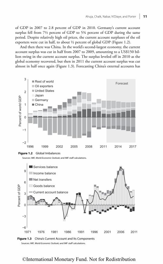
of GDP in 2007 to 2.8 percent of GDP in 2010. Germany’s current account surplus fell from 7½ percent of GDP to 5¾ percent of GDP during the same period. Despite relatively high oil prices, the current account surpluses of the oil exporters were cut in half, to about ½ percent of global GDP (Figure 1.2).
And then there was China. In the world’s second-largest economy, the current account surplus was cut in half from 2007 to 2009, amounting to a US$150 bil-lion swing in the current account surplus. The surplus leveled off in 2010 as the global economy recovered, but then in 2011 the current account surplus was cut almost in half once again (Figure 1.3). Forecasting China’s external accounts has
−6
−3
0
3
6
9
1971 1976 1981 1986 1991 1996 2001 2006 2011
Services balance
Income balance
Net transfers
Goods balance
Per
cent
of G
DP
Current account balance
Figure 1.3 China’s Current Account and Its ComponentsSources: IMF, World Economic Outlook; and IMF staff calculations.
−2
−1
0
1
2
3
1996 1999 2002 2005 2008 2011 2014 2017
Rest of world ForecastOil exportersUnited StatesJapanGermany
Per
cent
of w
orld
GD
P
China
Forecast
Figure 1.2 Global ImbalancesSources: IMF, World Economic Outlook; and IMF staff calculations.
©International Monetary Fund. Not for Redistribution

12 An End to China’s Imbalances?
always been challenging, in part reflecting rapid structural change, uncertainties surrounding China’s terms of trade, and difficulty predicting the path of the global recovery—but the scale of this current account reversal has been far sharper and more durable than expected.
This chapter focuses on describing the dynamics behind the fall in China’s external surplus since 2007. It aims to assess what has driven the external imbal-ance to shrink and provides a revised outlook for the current account in the medium term.
THE RECENT PATH OF CHINA’S EXTERNAL IMBALANCE
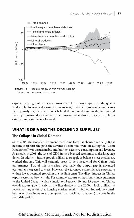
Until 2004, China’s external imbalances were relatively small with the trade sur-plus averaging only 3 percent of GDP during the period 1994−2003 (Figure 1.4). At a more disaggregated level, the trade surplus or deficit for various product components was also very small, although the trade surplus for textiles grew steadily during the period. Starting in 2004, the size of China’s imbalance acceler-ated, most notably as the result of an upswing in net exports of machinery and mechanical devices. This upswing was offset, in part, by a significant expansion of China’s trade deficit in minerals (largely metals and energy products). Despite these equalizing factors, as a share of GDP, China’s current account was able to rise to double digits by the eve of the global financial crisis, and at the time, few signs indicated that the pace of growth of the imbalance was set to slow down anytime soon.
However, what happened next was an extraordinary set of global circum-stances that combined to set off the worst global financial crisis in the post–World War II period. Against this external backdrop, China’s current account surplus was cut in half between 2007 and 2009 and, by 2011, had fallen to 1.9 percent of GDP. This compression in the external surplus was largely a result of a falling trade balance (which went from 9 percent of GDP in 2007 to 3.3 percent of GDP in 2011).
Certainly the drop in the trade balance has a cyclical component. After all, growth and demand in the global economy were damaged by the global financial crisis, and balance sheet repair and ongoing deleveraging were expected to weigh on growth well into the medium term. At the same time, the significantly higher demand for imported minerals (Figure 1.4) and energy was a side effect of China’s policy response to the global financial crisis—to put in place a significant infra-structure-driven stimulus funded by high credit growth.
Nevertheless, more lasting forces have also been at work, affecting the trade surplus in both directions. Domestic costs are rising, the costs of imported inputs (particularly commodities) have risen, and the stimulative effects on trade that were created by China’s accession to the World Trade Organization (WTO) may be waning. However, the relocation of global manufacturing capacity to China (financed by significant foreign direct investment [FDI] inflows) continues and
©International Monetary Fund. Not for Redistribution
Ahuja, Chalk, Nabar, N’Diaye, and Porter 13
capacity is being built in new industries as China moves rapidly up the quality ladder. The following discussion aims to weigh these various competing factors first by analyzing the main forces behind the recent decline in the surplus and then by drawing ideas together to summarize what this all means for China’s external imbalance going forward.
WHAT IS DRIVING THE DECLINING SURPLUS?
The Collapse in Global Demand
Since 2008, the global environment that China faces has changed radically. It has become clear that the path the advanced economies were on during the “Great Moderation” was unsustainable and built on excessive consumption and leverage. As a result, in 2008, the level of GDP in the advanced economies took a large step down. In addition, future growth is likely to struggle as balance sheet excesses are worked through. This will certainly prove to be a headwind for China’s trade performance. Part of this is cyclical; eventually the output gap in advanced economies is expected to close. However, the advanced economies are expected to endure lower potential growth in the medium term. The direct impact on China’s export sector has been visible. For example, exports of machinery and equipment to the United States—which contributed between 10 and 15 percent of China’s overall export growth early in the first decade of the 2000s—look unlikely to recover as long as the U.S. housing market remains subdued. Indeed, the contri-bution of these items to export growth has declined to about 5 percent in the postcrisis period.
−40
−20
0
20
1993 1995 1997 1999 2001 2003 2005 2007 2009 2011
Trade balance
Machinery and mechanical devices
Textile and textile articles
Miscellaneous manufactured articles
Mineral productsOther items
U.S
. dol
lars
(bill
ion)
Figure 1.4 Trade Balance (12-month moving average)Sources: CEIC Data; and IMF staff calculations.
©International Monetary Fund. Not for Redistribution

14 An End to China’s Imbalances?
One additional aspect of China’s export performance worth highlighting is that, although overall external demand has suffered as a result of the global finan-cial crisis, China’s ability to gain a larger share of those external markets appears to have been relatively unaffected. Even in 2008, when global trade collapsed, China was still able to gain market share, and since then, the pace of China’s market share gains has broadly returned to the level prevailing before the global crisis. At an aggregate level, China has, since 2003, managed to increase its share of world exports by an average of about ¾ percentage point per year.
While maintaining its foothold in traditional areas, China has also started to make a concerted push into industries typically dominated by more advanced economies. Prominent examples of these new growth areas include wind turbines, solar panels, automobiles, and semiconductor devices. In the wind energy indus-try, for example, China increased its share of global capacity from 16½ percent in 2009 to 22¾ percent in 2010, overtaking the United States as a world leader in wind energy capacity. Thus, China has increased its global market share in exports of wind energy equipment to about 6 percent (as of September 2011) from almost zero five years earlier. Similarly, China has moved rapidly to build production facilities in solar panels, and the upswing in China’s global export share in this industry has come at the expense of Japan and Germany (in part, as multinationals from those countries move their production facilities into China).
A Step Increase in Investment
In 2008, as the global financial system melted down, China responded early and resolutely with a large stimulus package that was designed to prop up domestic demand and offset the large shock emanating from the coming collapse in exter-nal demand. This stimulus created the conditions for a dramatic step-up in investment, to 47 percent of GDP from 42 percent (Figure 1.5). Much of that
20
40
60
Consumption
Per
cent
of G
DP
Household consumptionInvestment
1992 1996 2000 2004 2008 2011
Figure 1.5 Domestic DemandSources: CEIC Data; and IMF staff calculations.
©International Monetary Fund. Not for Redistribution

Ahuja, Chalk, Nabar, N’Diaye, and Porter 15
investment was concentrated in transportation, utilities, and housing construc-tion. A direct consequence of this investment has been to remove many of the infrastructure bottlenecks that existed and to increase the connectivity between provinces. Ultimately, these advances will serve to improve the competitiveness of China’s industry, in part as it facilitates industrial relocation to lower-cost areas within China (particularly the central and western provinces).
As the global economy started to recover, China’s spending on infrastructure began to wane, which created a hole in aggregate demand that was quickly filled by an upswing in private sector manufacturing investment. It appears this manu-facturing capacity is being built predominantly in a range of relatively higher-end manufacturing industries. In the coming years, this growth in manufacturing capacity could potentially lead to future increases in exports (as China sells these goods onto global markets). Alternatively, this capacity could be deployed domes-tically through sales to Chinese industries and households. Finally, there is a chance that it could remain underutilized (which would open up the question of how and whether the financing for these investments will be serviced). At this point, the purpose for which this new capacity will be used remains an important question but very difficult to predict.
The Role of Commodities and Capital Goods
As discussed, one of the by-products of the step increase in fixed investment has been a significant increase in China’s demand for commodities. This growth in demand took off first in metals followed by strong import growth in machinery and energy products. Both private and public investment projects have proved to be very import intensive. Some opportunistic cyclical stockpiling of commodities has occurred, and inventory data show stockbuilding in upstream industries such as ferrous metal mining (about 15 percent year-over-year growth in 2011) and nonferrous metal mining (about 25 percent year over year). Overall, however, little evidence points to a secular rise in inventories, which would suggest that this import demand is largely being used as an input to domestic production (see Ahuja and others, 2012, for more details).
The Terms of Trade
The sustained strength in imports of commodities and minerals has reinforced a dynamic that has been at work for several years now, going back to well before the global financial crisis. During the past several years, imports have become more linked to commodities and minerals, for which supply is relatively inelastic and global prices have been rising. At the same time, exports have become increas-ingly tilted toward machinery and equipment, for which supply is relatively elastic, competition is significant, and relative prices have been falling.
As a result, aside from 2009 and 2012, China’s terms of trade have been steadily worsening. This result may not be surprising from a historical standpoint. Several other economies that have witnessed export-oriented growth (notably Japan and the newly industrialized economies) were affected by similar terms of
©International Monetary Fund. Not for Redistribution

16 An End to China’s Imbalances?
trade declines along their development paths (Figure 1.6). In China’s case, this dynamic is further fueled by the fact that, in both export and import markets, the country has become so large as to no longer be a price taker. As a result, to some modest degree, China may well be generating a decline in its own terms of trade, creating a self-equilibrating mechanism that drives China’s terms of trade and creates countervailing downward pressures on China’s external surplus, through global prices.2
Exchange Rate Appreciation
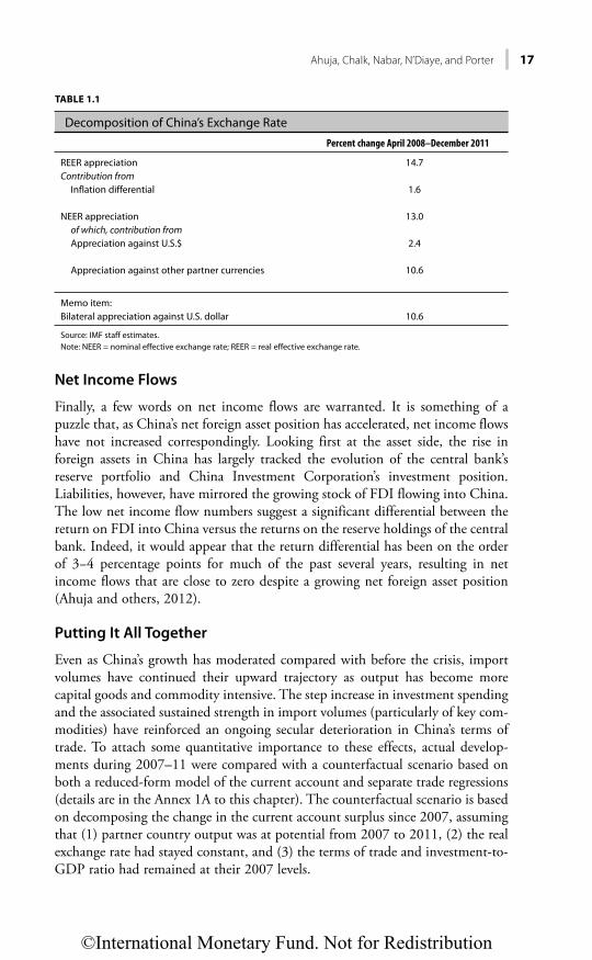
The exchange rate appreciated 14¾ percent in real terms during April 2008–December 2011, but as mentioned above, this change masks considerable varia-tion within the interval. A significant portion of this appreciation took place in 2008, after which the pace slowed markedly through the crisis and recovery (and has included intervals of real depreciation). Most of the real appreciation was due to movements in nominal exchange rates relative to major trading partner currencies, whereas the portion of the real appreciation accounted for by inflation differentials relative to trading partners has been relatively minor (Table 1.1).
2 The deteriorating terms of trade could also generate negative income effects as prices of imported goods rise, which would lower domestic demand and partly offset the narrowing of the external sur-plus. But this offset so far appears to be relatively muted in China’s case, with domestic spending (particularly investment) continuing to rise rapidly even as import prices have risen.
50
100
150
Inde
x
200
1 6 11 16 21 26 31 36 41 46 51 56 61
China (1979–2011) Japan (1955–2010)
Rep. of Korea (1965–2010) NIEs (1967–2010)
Germany (1952–2010) China forecast (2012–16)
Years since growth take-off
Figure 1.6 Terms of Trade of Selected Economies since Growth Take-OffSources: IMF, World Economic Outlook; and IMF staff calculations.Note: NIE = Newly Industrialized Asian Economies.
©International Monetary Fund. Not for Redistribution
Ahuja, Chalk, Nabar, N’Diaye, and Porter 17
Net Income Flows
Finally, a few words on net income flows are warranted. It is something of a puzzle that, as China’s net foreign asset position has accelerated, net income flows have not increased correspondingly. Looking first at the asset side, the rise in foreign assets in China has largely tracked the evolution of the central bank’s reserve portfolio and China Investment Corporation’s investment position. Liabilities, however, have mirrored the growing stock of FDI flowing into China. The low net income flow numbers suggest a significant differential between the return on FDI into China versus the returns on the reserve holdings of the central bank. Indeed, it would appear that the return differential has been on the order of 3−4 percentage points for much of the past several years, resulting in net income flows that are close to zero despite a growing net foreign asset position (Ahuja and others, 2012).
Putting It All Together
Even as China’s growth has moderated compared with before the crisis, import volumes have continued their upward trajectory as output has become more capital goods and commodity intensive. The step increase in investment spending and the associated sustained strength in import volumes (particularly of key com-modities) have reinforced an ongoing secular deterioration in China’s terms of trade. To attach some quantitative importance to these effects, actual develop-ments during 2007–11 were compared with a counterfactual scenario based on both a reduced-form model of the current account and separate trade regressions (details are in the Annex 1A to this chapter). The counterfactual scenario is based on decomposing the change in the current account surplus since 2007, assuming that (1) partner country output was at potential from 2007 to 2011, (2) the real exchange rate had stayed constant, and (3) the terms of trade and investment-to-GDP ratio had remained at their 2007 levels.
TABLE 1.1
Decomposition of China’s Exchange Rate
Percent change April 2008–December 2011
REER appreciation 14.7Contribution from Inflation differential 1.6
NEER appreciation 13.0 of which, contribution from Appreciation against U.S.$ 2.4
Appreciation against other partner currencies 10.6
Memo item:Bilateral appreciation against U.S. dollar 10.6
Source: IMF staff estimates.Note: NEER = nominal effective exchange rate; REER = real effective exchange rate.
©International Monetary Fund. Not for Redistribution

18 An End to China’s Imbalances?
The calculations suggest that the terms of trade decline contributed between one-fifth and two-fifths of the decline in the current account surplus during 2007–11 (Table 1.2). The acceleration in investment accounted for one-quarter to one-third of the decline, whereas the appreciation of the currency contributed between one-fifth and one-third. Below-potential growth in partner countries had a slightly smaller effect. Overall, the conclusion is that growing domestic investment, worsening terms of trade, weakening external demand, and apprecia-tion of the REER explain a large share of the postcrisis decline in the current account surplus. That said, it should be noted that these calculations are based on a partial equilibrium approach and have to be interpreted with some caution. For example, they do not account for feedback effects between these various factors (such as the linkages between high investment in China and rising global com-modity prices).
POLICY REFORM, DEMOGRAPHICS, AND COST PRESSURES
Policy Reforms
The Chinese government has rightly focused its policy efforts since the global financial crisis on a range of areas designed to accelerate the transformation of the Chinese economic model, improve livelihoods, and raise domestic consumption. Access to primary health care has been improved through the construction of new health care facilities, particularly in previously underserved rural communities. A new government health insurance program has been launched nationwide, and subsidies for a core set of prescription drugs have been introduced. In addition, the existing government pension scheme is being expanded to cover urban
TABLE 1.2
Estimated Contributions to the Decline in China's Current Account Surplus, 2007–11 (percent of GDP)
Estimated Trade Elasticities1 Reduced-Form Current Account Equation
Actual 2007 10.1 10.1Actual 20112 2.8 2.8Decline −7.3 −7.3
Contributing factors:Terms of trade −1.6 −3.6Foreign demand −1.1 −1.4Investment −1.8 −2.6REER −2.1 −1.3Others −0.8 1.5
Source: IMF staff calculations.Note: REER = real effective exchange rate.1Elasticities based on estimated calculations for exports and imports of goods and services. 2Preliminary actual.
©International Monetary Fund. Not for Redistribution

Ahuja, Chalk, Nabar, N’Diaye, and Porter 19
unemployed workers across the country and to make those pensions more por-table within China. Also, the absolute level of pensions has been increased, par-ticularly for the elderly poor.
In addition to health care and pensions, improving access to affordable hous-ing has been an important policy objective. The 12th Five-Year Plan, launched in 2011, aims to construct 36 million low-income housing units by 2016. The wider availability of low-cost housing has the potential to ease the budget con-straints of low-income groups and release savings currently locked up in financing home purchases.
So far, however, it is still too early to conclude that the initiatives to build out the social safety net and increase the provision of social housing have led precau-tionary saving to decline or have created sufficient momentum for household consumption to durably reverse the secular decline as a share of GDP that has been seen since 2000.
At the same time that these housing and social reforms have been undertaken, greater policy emphasis has been placed on market-based pricing of factor inputs and the scaling back of subsidies. Nevertheless, the low cost of many of China’s factor inputs—including land, water, energy, labor, and capital—still creates incentives for an overly capital-intensive means of production. Factor inputs are priced below prices that would be expected to equilibrate supply and demand and are also low relative to international comparators. For instance, in many cases, industrial land is provided for free to enterprises to attract investment, and the price of water in China is about one-third of that of international comparators. Cross-country data on the cost of energy show that the prices of gasoline and electricity in China are low relative to much of the rest of the world. Studies estimate that the total value of China’s factor market distortions could be almost 10 percent of GDP.3 However, China is making progress in bringing some energy costs in line with international levels: oil product prices have been indexed to a weighted basket of international crude prices. natural gas prices have been steadi-ly increased, and preferential power tariffs for energy-intensive industries have been removed.
Again, so far these rising costs, along with higher wages and the more appreci-ated currency, appear to have had little effect on corporate saving. Geographical relocation, strong productivity, and modest increases in export prices are helping to defray cost pressures that firms may be facing.
Overall, although the policy reforms that have been undertaken are valuable and necessary, and structural forces are at work that should help redistribute resources and shift behaviors, little evidence indicates that these efforts have cre-ated a decisive turnaround in national saving behavior, either at the corporate or the household level. However, many of these policies are likely to have long lags before their impact on saving behavior is clearly seen. It may well be that an effect
3 See Huang and Tao (2010) or Huang (2010). Also see IMF (2011) for more discussion on relative factor costs comparing China with other economies.
©International Monetary Fund. Not for Redistribution

20 An End to China’s Imbalances?
on household income and consumption will become steadily more discernible in the coming years.
Urbanization
In addition to the policy efforts taken by the government to lessen its external imbalances, raise household income, expand the services sector, and boost con-sumption, some important underlying structural changes are also under way. Over the decades, urbanization has proceeded steadily and is now at the point that half of the Chinese population is living in urban areas. This process has tended to be commodity intensive; new housing and infrastructure built to accommodate this growing urban citizenry has put downward pressure on the trade surplus. At the same time, this shift has raised the standard of living for many Chinese, lifting millions out of poverty and creating a vibrant urban middle class. This process undoubtedly has been associated with growing consumption of tradable goods, some imported from abroad but the majority produced within China. Thus, while manufacturing capacity has been expanding at a breathtaking pace, a large share of this capacity has been deployed to provide goods to the domestic market. That fact is becoming increasingly evident as the domestic economy—particularly the interior of the country—develops and companies relocate production facilities out of the coastal areas and closer to these fast-growing local markets.4
Demographic Change
A second important structural factor has been China’s unique demographics. China is fast approaching the point at which its labor force will start to shrink; already, the size of the cohorts that are younger than 24 years old has begun to decline. This change is naturally going to tighten labor markets and put upward pressure on wages as the labor-supply curve moves from perfectly elastic to mod-erately upward sloping, as is now happening. Although China is not yet at the so-called Lewis Turning Point, it has entered a period in which real wages are going to continue to rise and increasingly at a rate that is faster than productivi-ty.5 These ongoing shifts in factor markets—both labor and other inputs—are clearly important and, over time, should lead to rising cost pressures. This will also have implications for the external imbalance. Nonetheless, it is still too early to conclude that rising cost pressures have been responsible, in a meaningful way, for China’s shrinking external surplus. As seen in the decomposition of the REER appreciation in Table 1.1, the contribution of the inflation differential (which reflects, in part, the influence of factor cost differences) has been rela-tively minor.
4 The process has been facilitated by the loosening of restrictions on household registration require-ments in certain interior urban areas such as Chongqing. For more details, see The Economist (2012). 5 See Chapter 9 for a detailed analysis of this issue.
©International Monetary Fund. Not for Redistribution

Ahuja, Chalk, Nabar, N’Diaye, and Porter 21
THE OUTLOOK FOR CHINA’S EXTERNAL SURPLUS
As discussed above, prospects for China’s external surplus are closely linked to the outlook for the principal drivers of the recent decline—external demand, the level of investment, and the future trends for China’s terms of trade and domestic costs. The outlook draws on the conclusions of the various modeling approaches described in Annex 1A but also imposes some degree of judgment given the uncer-tainties. Therefore, these projections are predicated on the assumption that many of the recent shifts underpinning the surplus reversal will be persistent, in particular,
• China continues to gain global market share at the average pace seen during the past decade, but in an environment of generally weak growth in China’s main trading partners (as described in the April 2012 World Economic Outlook).
• The elevated level of investment spending continues, keeping the investment-to-GDP ratio close to current levels and well above the precrisis average.
• China’s terms of trade continue to steadily deteriorate (by ½ percent per year).
• The usual World Economic Outlook assumption that China’s REER remains constant continues to be true.
• As the global recovery gathers momentum in the medium term, the rates of return on China’s reserve portfolio increase, leading to a growing surplus on the income account.
• Under these conditions, net exports will likely improve in real terms as global demand slowly recovers, but the current account surplus will not rise to anywhere near the levels seen before the global financial crisis. Instead, the current account surplus is expected to stay close to current levels in the near term and rise in the medium term but only to about 4 to 4½ percent of GDP by 2017 (Figure 1.7).
The downside risks to the outlook for the current account are considerable. They are partly tied to the global outlook, but the pace of continued structural change in China’s economy is also subject to uncertainty. For example, various factors—including the beneficial impact of WTO accession in 2001, strong growth in manufacturing productivity, a relocation of global production facilities to China, and low-cost factors of production—created the conditions for the country’s export market share to rise rapidly since the early 2000s. China is expected to continue building its export market share and to rotate its product mix toward higher-end manufacturing. This process may, however, face head-winds from the slow recovery in global demand. It is also possible that market share gains will moderate relative to the rate experienced since early in the 2000s as China’s export mix gets closer to the technology frontier and opportunities for technology transfer and the relocation of overseas production facilities diminish. Finally, if past experience can be extrapolated, China’s real exchange rate may continue to appreciate, which, again, will diminish the size of the external surplus.
©International Monetary Fund. Not for Redistribution

22 An End to China’s Imbalances?
WHAT DOES THIS REVISED OUTLOOK FOR CHINA’S CURRENT ACCOUNT IMPLY FOR THE PATH OF GLOBAL IMBALANCES?
The implications of changes in China’s current account for global imbalances is a big question that does not lend itself to a neatly wrapped answer. The issue also goes well beyond China and requires that the imbalances in many other large economies be examined. However, there are three major points:
• First, the Chinese economy is growing rapidly, so even though the increase in the size of the imbalance in the medium term is relatively modest, it would still translate into a growing share of the aggregate external balance of surplus economies in the future. Furthermore, relative to the size of the world economy, the rapid growth in the Chinese economy would indicate an increase in the current account to 0.6 percent of global GDP in the medium term from 0.2 percent in 2012 (high growth ensures that China’s economy becomes a larger and larger share of global output through time). By this metric, the current account surplus is far from negligible, albeit well below the share of global GDP that China’s current account surplus reached in 2007–08.
• Second, the fading of China’s external surplus does not mean global imbal-ances are solved. Rather, these global imbalances may be rearranging them-selves into a different geographical constellation. China’s external surplus may well have migrated elsewhere, aided, in part, by the impact China is having on global prices and its own terms of trade.
−6
−3
0
3
6
9
1971 1986 2001 2016
Services balance
Income balance
Net transfers
Goods balance
Per
cent
of G
DP
Current account balance
Figure 1.7 Projection to 2016 of China’s Current Account and Its ComponentsSource: IMF, World Economic Outlook.
©International Monetary Fund. Not for Redistribution

Ahuja, Chalk, Nabar, N’Diaye, and Porter 23
• Third, unless consumption can soon be catalyzed, the decline in the external surplus will have come at the expense of a widening imbalance in China’s domestic economy. However, such an imbalance is not merely a domestic issue. If left unresolved, it has the potential to generate macroeconomic and financial instability in China’s economy, which, because of China’s size and systemic importance, will undoubtedly have consequences for global mac-roeconomic and financial stability.
CONCLUSION
The decline in China’s external surplus has been impressive and should be wel-comed. However, this adjustment has largely been the result of very high levels of investment, a weak global environment, and an increased pace of commodity prices that outstrips the rising price of Chinese manufactured goods. Although all three of these factors are likely to continue to put downward pressure on the external imbalance, the “rebalancing” in China advocated by the IMF over the past several years is not occurring.6 Certainly, the policy thrust of the 12th Five-Year Plan is very much focused on raising household income, boosting consump-tion, and facilitating expansion of the service sector. In the coming years, if these ongoing structural reforms continue to be implemented, China does have the potential to evolve from a largely investment-based to a more consumption-based decline in its external imbalance. If successful, this would ultimately prove to be a more lasting shift that would increase the welfare of the Chinese people and contribute significantly to strong, sustained, and balanced global growth.
6 See, for example, IMF (2010, 2011).
©International Monetary Fund. Not for Redistribution

24 An End to China’s Imbalances?
ANNEX 1A. EMPIRICAL ANALYSIS
A number of different models have been estimated to explain the external sur-plus—see, for example, Aziz and Li (2007), Cheung, Chinn, and Qian (2012), or Mann and Pluck (2007). The analysis in this annex looks at four different approaches—a structural dynamic stochastic general equilibrium model, a multi-variate Bayesian vector autoregression (BVAR) model, a reduced-form time series model of the current account, and an approach using simpler trade equations—and examines their predictions for the future path of China’s current account surplus.
In most cases, these forecasts assume a constant real effective exchange rate (REER); the World Economic Outlook (WEO) projections for global demand; and a path of steady, medium-term fiscal consolidation in China. If the exchange rate appreciates in real terms (because of either faster nominal appreciation or a sus-tained increase in domestic cost pressures that translates into larger inflation dif-ferentials relative to trading partners) or external demand is weaker, the current account will undoubtedly be below these projected ranges.
• Global Integrated Monetary and Fiscal Model (GIMF). The first approach uses the IMF’s multicountry dynamic general equilibrium model.7 The model captures the vertical trade structure and other key features of trade between China, advanced economies, emerging economies, and the rest of the world. Simulations using the GIMF show that a combination of stronger global demand and a lower fiscal deficit creates the conditions for a rise in exports and a decline in commodity imports. As a result, the current account surplus would be predicted to increase to about 4 percent in the medium term.
• Bayesian VAR (BVAR). The second method uses higher-frequency, quar-terly data based on the BVAR methodology (Österholm and Zettelmeyer, 2007). The model includes trading partners’ demand, domes-tic demand, property prices, consumer price index inflation, commodity price changes, interest rates, the fiscal balance (as a percentage of GDP), the current account balance (as a percentage of GDP), the money supply, and the REER. Similarly to the GIMF approach, the out-of-sample forecasts assume a steady path of fiscal consolidation and a global recovery as pro-jected by the WEO. Simulations using the BVAR model show a much stronger and earlier rise in the trade surplus. The model forecasts that the current account surplus would rise to about 5 percent of GDP by 2014 (Figure 1A.1).
• Reduced-form current account model. A third approach uses a set of vari-ables similar to those in the BVAR. Specifically, the reduced-form model relates China’s current account share of GDP to real GDP growth, China’s
7 See Kumhof and others (2010) for a description of the model.
©International Monetary Fund. Not for Redistribution

Ahuja, Chalk, Nabar, N’Diaye, and Porter 25
trading partners’ real GDP growth, the REER, the terms of trade, and ratio of the lagged current account to GDP. • The model was estimated for 1986−2011 using the generalized method
of moments approach. All parameters are significant and with signs con-sistent with economic theory (Table 1A.1).
• In the short term, a 1 percentage point increase in China’s real GDP growth reduces the current account surplus by 1/3 percent of GDP; a 1 percentage point increase in trading partners’ growth increases China’s current account surplus by about ½ percent of GDP; a 10 percent real effective exchange rate appreciation would lower the surplus by 1 percent of GDP; an improvement in the terms of trade up to a threshold would improve China’s current account surplus. Above that threshold, the income effect from the improvement in the terms of trade would start to dominate, leading to a reduction in the current account surplus as the terms of trade improve. In the longer term, the effects of these variables are about 2¾ times larger.
• The model predicts that a gradual strengthening of demand for China’s exports, steady annual GDP growth in China, a slight deterioration in the terms of trade, and a constant REER would leave China’s current account surplus at less than 4 percent of GDP by 2017 (Figure 1A.2). This predic-tion is despite an in-sample overestimation of the 2011 current account surplus by 2¼ percent of GDP (i.e., in 2011 the model predicts a current account surplus of 4¼ percent of GDP versus the 1.9 percent of GDP outturn).
0
2
4
6
8
2010 2012 2014 2016
WEO
Bayesian VAR
GIMF
Per
cent
of G
DP
Figure 1A.1 Current Account Balance Projections Using Different ModelsSource: IMF staff calculations.Note: GIMF = Global Integrated Monetary and Fixed Model; VAR = vector autoregression; WEO = IMF World Economic Outlook.
©International Monetary Fund. Not for Redistribution

26 An End to China’s Imbalances?
• Trade equations. One recurrent theme in estimating trade equations for China is that the estimated elasticity of exports to external demand is very large.8 At the same time, on the import side, an important driver of imports has been the level of exports (about ½ of imports in some way or another are destined as inputs for goods that are processed and then eventually exported to third countries). To take into account these two features of
8 For example, in Aziz and Li (2007), a 1 percent increase in external demand is associated with a 5 or 6 percent increase in China’s exports. This far outstrips the typical elasticity in other countries and is the counterpart of China’s rapid growth in global export market share. Such a large export response is clearly unsustainable and should eventually decline, although the timing of that decline is highly uncertain (Guo and N’Diaye, 2009).
−4
0
4
Per
cent
of G
DP
8
12
1986 1991 1996 2001 2006 2011 2016
Reduced-form modelforecast
WEO
Figure 1A.2 Current Account Forecast Based on Time Series ModelSources: IMF, World Economic Outlook; and IMF staff calculations.Note: WEO = World Economic Outlook.
TABLE 1A.1
Generalized Method of Moments Estimate of Current Account Balance(Percent of GDP)
Parameter Estimates
Real GDP growth −0.30 [.001]Trading partners, real GDP growth 0.43 [.000]REER −0.09 [.006]Terms of trade (lagged 1 year) 0.42 [.000]Terms of trade squared (lagged 1 year) −2.8E-03 [.000]Current account balance (lagged 1 year) 0.64 [.000]Dummy 2009–11 −2.99 [.000]J-stat 3.01
Source: IMF staff calculations.Note: Generalized method of moments estimates over the sample 1986–2011. Figures in brackets are p-values. REER = real effective exchange rate.
©International Monetary Fund. Not for Redistribution

Ahuja, Chalk, Nabar, N’Diaye, and Porter 27
China’s trade, a simple modified trade model is used.9 In particular, FDI is included in the export equation as a proxy for the expansion of China’s tradables production and increased involvement in cross-border production sharing. On the import side, the effect of processing trade is captured by including exports in the import equation. With FDI in the export regres-sion, the elasticity of exports to foreign demand falls from 5 to 2, whereas including exports in the import equation reduces the elasticity of imports to domestic demand from 1.4 to 0.6 (Table 1A.2). Using these models to forecast, and assuming a modest decline in inward FDI as a share of GDP, the trade surplus falls to about 3 percent of GDP in the medium term. However, the forecast is subject to significant uncertainty and is highly sensitive to the path of future FDI inflows; if FDI stays about the same share of GDP as in 2011, the model would forecast the trade surplus to be some 6 percentage points of GDP higher in the medium term.
9 See Bems and others (forthcoming) for details.
TABLE 1A.2
Trade Elasticities
Export Elasticities Import Elasticities
with respect to: Standard Model Augmented Model Standard Model Augmented Model
Foreign demand 5.46*** 2.28**FDI/GDP 2.15***
Domestic demand 1.39*** 0.62*Exports 0.49**
REER −0.32 −0.30** 0.52** 0.42*
Source: IMF staff calculations.Note: *significant at 10%; **significant at 5%; ***significant at 1%.FDI/GDP = Foreign direct investment divided by GDP; REER = Real effective exchange rate.
©International Monetary Fund. Not for Redistribution

28 An End to China’s Imbalances?
REFERENCES
Acharya, Viral V., and Philipp Schnabl, 2010, “Do Global Banks Spread Global Imbalances? The Case of Asset-Backed Commercial Paper during the Financial Crisis of 2007−09,” IMF Economic Review, Vol. 58, No. 1, pp. 37–73.
Ahuja, Ashvin, Nigel Chalk, Malhar Nabar, Papa N’Diaye, and Nathan Porter, 2012, “An End to China’s Imbalances,” IMF Working Paper 12/100 (Washington: International Monetary Fund).
Aziz, Jahangir, and Xiangming Li, 2007, “China’s Changing Trade Elasticities,” IMF Working Paper 07/266 (Washington: International Monetary Fund).
Bems, Rudolfs, Joshua Felman, David Reichsfeld, and Shaun Roache, forthcoming, “Why Has China’s Current Account Surplus Declined?” IMF Working Paper (Washington: International Monetary Fund).
Caballero, Ricardo, Emmanuel Farhi, and Pierre-Olivier Gourinchas, 2008, “An Equilibrium Model of ‘Global Imbalances’ and Low Interest Rates,” American Economic Review, Vol. 98, No. 1, pp. 358–93.
Cheung, Yin-Wong, Menzie Chinn, and XingWang Qian, 2012, “Are Chinese Trade Flows Different?” Journal of International Money and Finance, Vol. 31, No. 8, pp. 2127–46.
Cooper, Richard N., 2007, “Living with Global Imbalances,” Brookings Papers on Economic Activity, Vol. 2, pp. 91–110.
De Long, J. Bradford, 2008, “The Wrong Financial Crisis,” VOX. http://www.voxeu.org/index.php?q=node/2383.
Dooley, Michael P., David Folkerts-Landau, and Peter Garber, 2003, “An Essay on the Revived Bretton Woods System,” NBER Working Paper No. 9971 (Cambridge, Massachusetts: National Bureau of Economic Research).
———, 2004, “The Revived Bretton Woods System: The Effects of Periphery Intervention and Reserve Management on Interest Rates and Exchange Rates in Center Countries,” NBER Working Paper No. 10332 (Cambridge, Massachusetts: National Bureau of Economic Research).
———, 2009, “Bretton Woods II Still Defines the International Monetary System,” Pacific Economic Review, Vol. 14, No. 3, pp. 297–311.
The Economist, 2012, “Changing Migration Patterns: Welcome Home,” February 25.Gruber, Joseph W., and Steven B. Kamin, 2008, “Do Differences in Financial Development
Explain the Global Pattern of Current Account Imbalances?” International Finance Discussion Paper No. 923 (Washington: Board of Governors of the Federal Reserve System).
Guo, Kai, and Papa N’Diaye, 2009, “Is China’s Export-Oriented Growth Sustainable?” IMF Working Paper 09/172 (Washington: International Monetary Fund).
Huang, Yiping, 2010, “Krugman’s Chinese Renminbi Fallacy,” VoxEU.org, March 26.———, and Kunyu Tao, 2010, “Causes and Remedies of China’s External Imbalances,” China
Center for Economic Research Working Paper No. E2010002 (Beijing: Peking University).International Monetary Fund (IMF), 2010, “People’s Republic of China Article IV
Consultation—Staff Report; Staff Statement; Public Information Notice on the Executive Board Discussion,” IMF Country Report 10/238 (Washington).
———, 2011, “People’s Republic of China Article IV Consultation—Staff Report; Staff Statement; Public Information Notice on the Executive Board Discussion,” IMF Country Report 11/192 (Washington).
Kumhof, Michael, Douglas Laxton, Dirk Muir, and Susanna Mursula, 2010, “The Global Integrated Monetary and Fiscal Model—Theoretical Structure,” IMF Working Paper 10/34 (Washington: International Monetary Fund).
Mann, Catherine L., and Katharina Plück, 2007, “Understanding the U.S. Trade Deficit: A Disaggregated Perspective,” in G-7 Current Account Imbalances: Sustainability and Adjustment, ed. by Richard Clarida (Chicago: University of Chicago Press) pp. 247–82.
©International Monetary Fund. Not for Redistribution

Ahuja, Chalk, Nabar, N’Diaye, and Porter 29
Obstfeld, M., and K. Rogoff, 2005, “Global Current Account Imbalances and Exchange Rate Adjustments,” Brookings Papers on Economic Activity, 2005, Vol. 1, pp. 67–123.
———, 2010, “Global Imbalances and the Financial Crisis: Products of Common Causes,” in Asia and the Global Financial Crisis, ed. by Reuven Glick and Mark M. Spiegel (San Francisco: Federal Reserve Bank of San Francisco).
Österholm, P., and J. Zettelmeyer, 2007, “The Effect of External Conditions on Growth in Latin America,” IMF Working Paper 07/176 (Washington: International Monetary Fund).
Roubini, Nouriel, and Brad Setser, 2005, “Will the Bretton Woods 2 Regime Unravel Soon? The Risk of a Hard Landing in 2005−2006,” Paper presented at the Symposium on the “Revived Bretton Woods System: A New Paradigm for Asian Development?” organized by the Federal Reserve Bank of San Francisco and the University of California Berkeley, San Francisco, February 4.
©International Monetary Fund. Not for Redistribution

This page intentionally left blank
©International Monetary Fund. Not for Redistribution

31
CHAPTER 2
Investment in China: Too Much of a Good Thing?
IL HOUNG LEE, MURTAZA SYED, AND LIU XUEYAN
As documented in Chapter 1, much of the decline in China’s current account surplus has been accomplished by boosting investment as a share of the national economy. This chapter assesses the appropriateness of China’s current investment levels. It finds that although China’s capital-to-output ratio is within the range of other emerging markets, its economic growth rate stands out, partly as the result of a surge in investment since 2000. Moreover, its investment is significantly higher than suggested by a cross-country panel estimation. This deviation has been accumulating since 2000, and at nearly 10 percent of GDP is now larger and more persistent than experienced by other Asian economies leading up to the Asian crisis of the late 1990s. However, because China’s investment is predominantly financed by domestic savings, a crisis appears unlikely when assessed against dependency on external funding. But this does not mean that the cost is nil. Rather, it is distributed to other sectors of the economy through a hidden transfer of resources, estimated to average 4 percent of GDP per year.
INTRODUCTION
In non–resource rich countries, most economic takeoffs are strongly associated with high levels of investment. Asia, in particular, is a typical example of how high investment has facilitated rapid economic growth.1 Investment alone, of course, does not explain the growth story. Total factor productivity (TFP), labor supply, and savings in the neoclassical sense, and market access and efficient financial intermediation from the macro aspect, all play important roles. Moreover, in Asia’s case, economies have also benefited from exports. Even during periods when investment has been below its long-term trend, Asian economies have enjoyed rapid growth through access to expanding global markets, notably during most of the 1970s when the newly industrialized economies were taking off.
However, high investment has also proven to be costly. Although Asian countries usually have a high saving rate, several countries resorted to foreign financing to maintain even-higher investment ratios. Although this strategy enabled them to achieve a faster growth path for some time, typically it eventually led to a banking
1 During 1970–2010, the correlation between a five-year moving average investment-to-GDP ratio and economic growth was about 0.83 in developing Asia. The correlation is somewhat weaker at 0.74 for advanced economies, the G7, for example.
©International Monetary Fund. Not for Redistribution

32 Investment in China: Too Much of a Good Thing?
or foreign exchange crisis, from which it took several years to recover (Figure 2.1). These crises occurred because the cost of financing such high rates of investment was often mispriced, only to be corrected abruptly. In emerging economies, mispricing often involved currency and maturity mismatches, the risk of which was obscured by implicit guarantees or lack of information. In other words, an artifically low cost of financing supported excessive investment, including in property and manufactur-ing sectors, which eventually resulted in a crisis. This pattern was also observed in other emerging markets outside Asia, such as in Latin America during the 1980s.
This chapter compares China’s current investment level with those of compara-tor economies.2 It finds that China’s capital-to-output ratio is within the range of other emerging markets, but its pace of growth stands out from the rest, partly as the result of a surge in investment since 2000. Moreover, when measured against a norm estimated from a cross-country panel, its investment is too high. Although a crisis appears unlikely when assessed against dependency on external funding, concerns arise about the underlying domestic strain associated with financing such a high level of investment, which appears to be implicitly borne by households. This
2 Results of recent studies at the macro level on the question of whether China overinvests have been largely inconclusive, with Bai, Hsieh, and Qian (2006) and Lu and others (2008) suggesting not, while Rawski (2002); Dong, Zhang, and Shek (2006); Barnett and Brooks (2006); and Qin and Song (2009) argue otherwise. Microeconomic studies have tended to find greater support for misallocation of investment, including Liu and Siu (2009); Dollar and Wei (2007); Hsieh and Klenow (2009); Ding, Guariglia, and Knight (2010); and Geng and N’Diaye (2012). However, much of the literature imposes a number of strong assumptions, and few papers compare China’s investment with that in the rest of the world.
10
20
30
40
50
1 4 7 10 13 16 19 22 25 28 31 34 37 40 43 46
Indonesia (1970) China (1978)Thailand (1965) Rep. of Korea (1963)
Onset of crisisMalaysia (1974)
Years after take-off
Per
cent
of G
DP
Figure 2.1 Gross Capital FormationSource: IMF staff estimates.Note: Year of take-off for each economy given in parentheses.
©International Monetary Fund. Not for Redistribution

Lee, Syed, and Xueyan 33
chapter also contributes to the literature by harnessing the insights, sparse assump-tions, and increased degrees of freedom that come from using an up-to-date panel of comparator economies, with both the countries and the time coverage carefully selected to match China’s economic features and phase of development.
The rest of the chapter is structured as follows: The next section motivates the analysis by comparing China’s investment with a group of other emerging market economies. A simple welfare maximization model is then introduced to illustrate that assessing the appropriateness of the level of investment requires a more com-prehensive approach than the neoclassical indicators. The subsequent section uses a panel estimation to derive an investment “norm” based on fundamentals across countries and the implict cost of supporting China’s high investment level is estimated. The last section concludes.
CHINA’S INVESTMENT FROM A COMPARATIVE PERSPECTIVE
As a first proxy of whether a country’s investment is too high or low, it is instruc-tive to compare the investment- and capital-to-output ratios of that economy with estimates of their long-term equilibrium (steady-state) levels.3 On this basis, China was underinvesting in the 1970s and to a lesser extent in the 1980s (Figure 2.2). China’s investment has since picked up, especially after 2000. By 2005, China’s capital-to-output ratio was close to its long-term level, so its investment-to-GDP ratio should theoretically have tended to fall back toward its steady-state value.
3 According to the neoclassical model’s golden rule, such a level of investment is defined as i* = k*(g +d)/(1 + g), where (i*) is the steady-state level of investment based on estimates of a steady-state capital-to-output ratio (k*), the depreciation rate (d), and the rate of potential output growth (g). Relative to the golden rule equilibrium, China is currently overinvesting. See Annex 2A to this chapter for details.
0.85
0.90
0.95
1.00
1.05
1.10
1.15
1.20
0.0 0.2 0.4 0.6 0.8 1.0 1.2 1.4 1.6 1.8
Other economiesChina (2007–2011)China (2000–05)
China (1990–95)China (1980–85)China (1970–75)
Investment-to-output ratio
Cap
ital-t
o-ou
tput
ratio
Overinvestment
Underinvestment
Figure 2.2 Capital- and Investment-to-Output Ratios (emerging market economies, relative to steady-state level in 2007–11)
Sources: Penn World Tables; IMF, World Economic Outlook database; and IMF staff calculations.
©International Monetary Fund. Not for Redistribution

34 Investment in China: Too Much of a Good Thing?
However, during 2007–11, to counter the adverse effect of the global economic and financial crisis, China raised its investment further. Depending on the assumptions, China may have been overinvesting by between 12 and 20 percent of GDP relative to its steady-state desirable value during this period.
Of course, a number of limitations arise with this approach to assessing the appropriateness of the level of investment. In particular, the estimates do not capture structural changes such as a shift away from capital-intensive growth or in the efficiency of investment over time. Indeed, there is no a priori reason to pre-sume that an economy growing faster so as to catch up with advanced economies should have a lower capital-to-output ratio, that is, below its long-term level, or that its investment rate should be above its long-term level. This will depend on several other factors, notably TFP.
On some simple metrics, China’s investment efficiency is still broadly in line with that of other emerging economies. As shown in Figure 2.3, China’s capital-to-output ratio has increased relative to those of other emerging markets since about 1990. However, it is still broadly within the average cross-country range. What stands out is China’s growth, showing that its achievement during this period has been unique.
However, China’s strong performance comes at a price. In the 1990s, China was within the bounds experienced by emerging markets worldwide for the rela-tionship between investment rates and capital-to-output ratios (Figure 2.4), but it has since gravitated to an extreme outlier position that is suggestive of potential overinvestment. China now requires ever higher investment to generate the same amount of growth. Unless TFP surges, with export performance expected to remain subdued in the medium term (given both sluggish demand overseas and diminishing opportunities for dramatic gains in China’s market share), the con-tribution of investment to growth will need to reach 60–70 percent to support the same amount of growth (Figures 2.5). Under such a strategy, vulnerabilities will likely grow in the form of hidden deadweight that will have to be paid for in the future in one form or another.
Moreover, consumption has declined to about 40 percent of GDP, partly as the result of falling household income as a share of GDP. In fact, household income has risen very rapidly except relative to overall GDP growth. The latter, as discussed above, was pulled up by an increasing contribution from investment. To the extent that growth is to improve the quality of living standards by provid-ing more value added to households, a falling consumption share raises questions about the very purpose of the current investment-based growth model.
WHAT CAN AGGREGATE CROSS-COUNTRY DATA REVEAL?
Under a welfare-maximizing state, intertemporal consumption preferences will determine the level of consumption. However, the relative time preference for consumption is not directly observable. An indirect way of measuring
©International Monetary Fund. Not for Redistribution

Lee, Syed, and Xueyan 35
Figure 2.3 Growth and Capital-to-Output Ratios for Emerging Market Economies, 1990–95 and 2007–11
Sources: Penn World Tables; IMF, World Economic Outlook database; and IMF staff calculations.Note: Small squares represent other emerging market economies.
1.0
1.5
2.0
2.5
3.0
3.5
0 2 4 6 8 10 12Real GDP growth
Cap
ital-t
o-ou
tput
ratio
China
a. 1990–95
1.0
1.5
2.0
2.5
3.0
3.5
420 6 8 10 12Real GDP growth
Cap
ital-t
o-ou
tput
ratio
China
b. 2007–11
intertemporal preference would be to assume that the average level of consump-tion, or investment, of a relatively large sample of countries approximates such a preference. Then, an optimal investment level, or a “norm,” could be defined as the level that would maximize social or household welfare. This level of invest-ment will be determined by economic fundamentals, including the real interest rate and the depreciation rate (see Lee, Syed, and Xueyan, 2012, for details) and can be estimated from regressions linking cross-country investment rates over time to a set of fundamentals.
Dynamic panel data models were run for 36 economies for the period 1955–2009. The panel was unbalanced, with one innovation being that the starting
©International Monetary Fund. Not for Redistribution

36 Investment in China: Too Much of a Good Thing?
period for each economy was calibrated to capture its economic takeoff (and associated elevated levels of investment). This county-specific starting period ensures that the investment norm is not biased downward and in fact represents a higher bar than usual for detecting any potential overinvestment. The sample consists of emerging market economies, as well as Japan and Taiwan Province of China. About one-third of the sample is made up of Asian economies. The empirical strategy allows for changes in preferences over time, but imposes a “normal” preference for intertemporal consumption across emerging markets relative to fundamentals. By carefully calibrating this around takeoff periods, and by including China’s Asian peers that have also tended to rely heavily on invest-ment, this average is likely to be adequately representative.
Figure 2.4 Capital- and Investment-to-Output Ratios for Emerging Market Economies, 1990–95 and 2007–11
Sources: Penn World Tables; IMF, World Economic Outlook database; and IMF staff calculations.Note: Small squares represent other emerging market economies.
1.0
1.5
2.0
2.5
3.0
3.5
10 15 20 25 30 35 40 45Investment-to-output ratio
Cap
ital-t
o-ou
tput
ratio
China
a. 1990–95
1.0
1.5
2.0
2.5
3.0
3.5
10 15 20 25 30 35 40 45 50Investment-to-output ratio
Cap
ital-t
o-ou
tput
ratio
China
b. 2007–11
©International Monetary Fund. Not for Redistribution

Lee, Syed, and Xueyan 37
The models relate the investment-to-GDP ratio in country x at time t to a host of explanatory variables motivated by theory (Lee, Syed, and Xueyan, 2012). These variables include the lagged dependent variable; savings-to-GDP and credit-to-GDP measures to capture the availability of financing; real lending rates
Figure 2.5 Contributions to GDP GrowthSource: IMF staff estimates.Note: ICOR—Incremental capital-to-output ratio.
0.0
0.5
1.0
1.5
2.0
2.5
3.0
3.5
4.0
4.5
5.0
1.5
2.0
2.5
3.0
3.5
4.0
4.5
5.0
5.5
6.0
1979
1980
1981
1982
1983
1984
1985
1986
1987
1988
1989
1990
1991
1992
1993
1994
1995
1996
1997
1998
1999
2000
2001
2002
2003
2004
2005
2006
2007
2008
2009
2010
2011
2012
2013
2014
2015
2016
ICOR (left scale)
Per
cent
of t
otal
Capital formation contribution to growth (right scale)
a. Contribution of investment to GDP growth
−20
−10
0
10
20
30
40
50
60
Per
cent
of t
otal
70
80
90
100
1978 1980 1982 1984 1986 1988 1990 1992 1994 1996 1998 2000 2002 2004 2006 2008 2010 2012 2014 2016
Final consumption expenditure Gross capital formation Net exports
b. Other contributions to GDP growth
©International Monetary Fund. Not for Redistribution

38 Investment in China: Too Much of a Good Thing?
to capture the cost of capital; the exports-to-GDP ratio to capture the potential external contributions to investment; real growth rates as a proxy for the return to capital; the level of real GDP to capture the level of economic development; age-dependency ratios to capture the potential impact of demographics; and macroeconomic uncertainty captured by the standard deviation of three-year rolling windows of real GDP growth and the reserves-to-GDP ratio to measure the need for countries to save to counter volatile capital flows. These variables are grounded in the underlying model outlined in Lee, Syed, and Xueyan (2012) as well as others developed in the literature, such that the estimation is better thought of as being structural in nature, and not reduced form.
The models are estimated in first differences (to control for fixed effects) using generalized method of moments to account for the presence of the lagged dependent variable (which renders an ordinary least squares fixed-effects model inconsistent), measurement error, and potential endogeneity of the regressors (by using their lagged values as instruments).4 The estimation also includes time dummies, covering both the Asian crisis of the late 1990s and the 2008–09 global financial crisis. Provided no higher-order serial correlation is present in the residuals and the instruments are valid, this approach should yield unbi-ased and consistent parameter estimates. Both of these conditions are tested using standard tests.
The estimated investment equations fit the actual data well for most econo-mies and suggest the following (with column 5 of Table 2.1 being the preferred specification):
• Investment tends to be persistent. The lagged dependent variable is large and significant, indicating inertia in aggregate levels of investment.
• Stronger output growth leads to higher investment. Including exports in this speci-fication does not lead to a significant coefficient (column 6), suggesting that the primary route through which globalization affects investment is by leading to stronger overall economic growth and hence raising the returns to capital.
• An increase in the cost of capital lowers investment. Higher real interest rates reduce investment, as expected.
• Increased availability of credit is associated with higher investment. The analy-sis used both change in credit and the saving-to-GDP ratio as the relevant measure, and found the former to render the latter insignificant.
• As economies develop, they typically need higher investment. To capture poten-tial nonlinearities and thresholds beyond which this positive relationship no longer holds, the analysis also included a squared per capita GDP term. However, this term was not significant, suggesting that the economies in the sample are on average still “taking-off.” This is not surprising given that the majority remain in the middle-income category.
4 See Annex 2A to this chapter for details.
©International Monetary Fund. Not for Redistribution

Lee, Syed, and Xueyan 39
• Macroeconomic uncertainty leads to lower investment. Conditioning for the standard deviation of three-year rolling windows of GDP growth, the alter-native proxy variable of changes in reserves was not significant. This out-come suggests that higher uncertainty does lead to lower investment but that this effect is better captured by the volatility of growth rather than the accumulation of reserves (which, after all, may be driven by considerations other than precautionary motives).
• Aging of the population reduces investment, possibly because it leads to slower growth and thus reduces the returns to investment. Investment will consequently fall in the absence of technological progress and other struc-tural changes that raise labor productivity. The results suggest that this effect
TABLE 2.1
Results of Investment Regressions
(1) (2) (3) (4) (5) (6)
Lagged dependent variable
0.652**(0.07)
0.628**(0.06)
0.630**(0.07)
0.615**(0.06)
0.652**(0.08)
0.664**(0.07)
Real per capita GDP growth
0.372**(0.05)
0.339**(0.04)
0.350**(0.04)
0.329**(0.05)
0.364**(0.05)
0.390**(0.53)
Growth in credit (annual percent of GDP)
0.033**(0.01)
0.030**(0.01)
0.023*(0.01)
0.032*(0.02)
0.031*(0.02)
Real per capita GDP (U.S. dollars)
0.0002*(0.00)
0.0003*(0.00)
0.0002*(0.00)
0.0002*(0.00)
Age-dependency ratio1
−0.560*(0.35)
−0.696*(0.39)
−0.612*(0.36)
−0.622**(0.36)
Uncertainty2 −0.271** −0.200** −0.203**(0.09) (0.07) (0.06)
Real interest rate −0.043** −0.041**(0.02) (0.02)
Exports-to-GDP −0.036(0.04)
p-value of specification tests
m2 test (no second-order serial correlation in residuals)
0.201 0.241 0.239 0.266 0.25 0.23
Hansen test (instru-ment validity)
1.000 1.000 1.000 1.000 1.000 1.000
Number of economies
36 36 36 36 36 36
Number of observations
892 892 892 892 718 718
Time period 1955−2009 1955–2009 1955–2009 1955–2009 1955–2009 1955–2009
Sources: World Bank, World Development Indicators; IMF, World Economic Outlook; and IMF staff calculations.Note: Dependent variable is investment-to-GDP ratio. First-differenced general method of moments specifications, with
year dummies. Instruments are lagged values of regressors. Robust t-statistics in parentheses. * and ** indicate significance at the 10 percent and 5 percent levels, respectively.
1 Ratio of population over age 65 to population ages 15–64.2 Standard deviation of three-year rolling window of real GDP growth.
©International Monetary Fund. Not for Redistribution

40 Investment in China: Too Much of a Good Thing?
dominates any short-term increase in investment as firms invest more to substitute capital for labor as a means of coping with a growing shortage of workers.5
Using these parameter estimates, investment in China may currently be about 10 percent of GDP higher than suggested by fundamentals (Figure 2.6). Even allowing for elevated investment levels associated with most economic takeoffs, the econometric evidence suggests that China is overinvesting. China’s predicted investment norm since 1985 has ranged between 33 and 43 percent of GDP. In reality, it has fluctuated in a much broader band of 35–49 percent of GDP. The model consistently predicts a lower norm for China, but until 2000, the devia-tions were usually not that significant and typically closed over a five-year time horizon.
A probit model suggests that the error term is positively associated with the probability of a crisis (Table 2.2). The analysis uses the error terms of the above regression, as well as a number of other variables previously considered to have explanatory power for predicting economic crises, as a measure of overinvestment.
5 The relative magnitude of the impact is, of course, smaller than the size of the estimated coefficients because of the different scales of the explanatory variables. With estimation in first differences, the annual change in the demographic variable is very small. As a result, the actual impact of the other variables on investment is significantly larger. For example, excluding the demographic variable from the specification increases the predicted level of investment in China by only 1 percent of GDP in 2009.
30
35
40
45
50
1985 1987 1989 1991 1993 1995 1997 1999 2001 2003 2005 2007 2009
ActualIn
vesm
ent-t
o-G
DP
ratio
Predicted norm
Figure 2.6 Actual and Predicted Investment-to-GDP Ratio, ChinaSource: IMF staff calculations.
©International Monetary Fund. Not for Redistribution
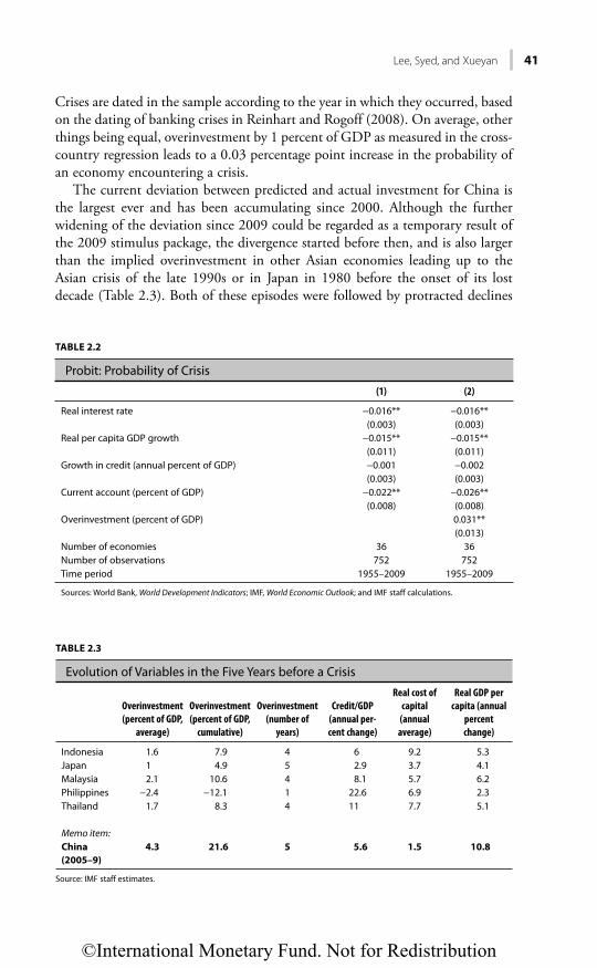
Lee, Syed, and Xueyan 41
Crises are dated in the sample according to the year in which they occurred, based on the dating of banking crises in Reinhart and Rogoff (2008). On average, other things being equal, overinvestment by 1 percent of GDP as measured in the cross-country regression leads to a 0.03 percentage point increase in the probability of an economy encountering a crisis.
The current deviation between predicted and actual investment for China is the largest ever and has been accumulating since 2000. Although the further widening of the deviation since 2009 could be regarded as a temporary result of the 2009 stimulus package, the divergence started before then, and is also larger than the implied overinvestment in other Asian economies leading up to the Asian crisis of the late 1990s or in Japan in 1980 before the onset of its lost decade (Table 2.3). Both of these episodes were followed by protracted declines
TABLE 2.2
Probit: Probability of Crisis
(1) (2)
Real interest rate −0.016** −0.016**(0.003) (0.003)
Real per capita GDP growth −0.015** −0.015**(0.011) (0.011)
Growth in credit (annual percent of GDP) −0.001 −0.002(0.003) (0.003)
Current account (percent of GDP) −0.022** −0.026**(0.008) (0.008)
Overinvestment (percent of GDP) 0.031**(0.013)
Number of economies 36 36Number of observations 752 752Time period 1955–2009 1955–2009
Sources: World Bank, World Development Indicators; IMF, World Economic Outlook; and IMF staff calculations.
TABLE 2.3
Evolution of Variables in the Five Years before a Crisis
Overinvestment
(percent of GDP,
average)
Overinvestment
(percent of GDP,
cumulative)
Overinvestment
(number of
years)
Credit/GDP
(annual per-
cent change)
Real cost of
capital
(annual
average)
Real GDP per
capita (annual
percent
change)
Indonesia 1.6 7.9 4 6 9.2 5.3Japan 1 4.9 5 2.9 3.7 4.1Malaysia 2.1 10.6 4 8.1 5.7 6.2Philippines −2.4 −12.1 1 22.6 6.9 2.3Thailand 1.7 8.3 4 11 7.7 5.1
Memo item:China
(2005–9)
4.3 21.6 5 5.6 1.5 10.8
Source: IMF staff estimates.
©International Monetary Fund. Not for Redistribution

42 Investment in China: Too Much of a Good Thing?
in growth and investment. Credit growth (particularly postcrisis) and the cost of capital in China in recent years also appear to be in dangerous territory compared with experiences in other countries. Mechanically applying the coefficient esti-mates from the probit model to China’s estimated overinvestment shows that the probability of a crisis would rise from 8 percent in 2005 to about 20 percent in 2013. These numbers are only indicative, however. Not only does the usual uncertainty surround these parameter estimates, but as discussed below, the nature of China’s investment model is very different from that of other emerging markets and tends to reduce the probability of a crisis relative to the average country in the sample.
However, the trigger of a crisis, if ever, in China will likely be different from the triggers in other countries. What distinguishes China from the rest is its rela-tive lack of reliance on external funding for domestic investment. In large part, this is due to its high saving rate. However, various studies indicate that saving is arbi-trarily high because of controls in the financial sector that de facto result in a subsidy transfer from households and small and medium enterprises to large cor-porations, estimated to be close to 4 percent of GDP per year.6 Whereas in other countries the high cost of excess investment has been exposed in the form of bank stress or a foreign exchange market crisis, in China, it will likely be captured in, or triggered by, any one of the weak links in this implicit subsidy system.
CONCLUSION
China’s extraordinary economic performance since 1980 undoubtedly is in large part attributable to investment. Despite the prolonged period of heavy invest-ment, China’s capital-to-output ratio is still in the range of those of other emerg-ing market economies while its growth rate has far outpaced others since 1990. Nevertheless, the marginal contribution of an extra unit of investment to growth has been declining, requiring ever larger increases in investment to generate an equal amount of growth. Now, with the ratio of investment to GDP already close to 50 percent, the current growth model may have run its course.
Measured against a norm estimated from panel data for a large number of countries, China is overinvesting. Moreover, the deviation that has been accumu-lating since 2000 is larger and more persistent than the estimated overinvestment in other Asian economies leading up to the Asian crisis of the late 1990s. The latest divergence was understandably the result of the 2009 measures used to contain the spillover from the global financial crisis. The government is well aware of the challenge posed by excessive reliance on investment and is thus accel-erating its effort to reorient the economy, by moderating investment growth while promoting consumption.
6 See Lee, Syed, and Xueyan (2012) for details on this estimate. A large portion of the burden of financing overinvestment is borne by households, while small and medium enterprises are paying a higher price for capital because of the funding priority given to larger corporations.
©International Monetary Fund. Not for Redistribution

Lee, Syed, and Xueyan 43
Although a crisis appears unlikely when assessed against dependency on exter-nal funding, potential strains from financing overinvestment still exist and could be quite large. Assuming the conditions that prevailed in other emerging market economies during their pre- and postcrisis periods also apply to China, the prob-ability of a crisis in China would mechanically be about one in five. However, because of the differences in the modality of financing investment, an external crisis of the kind experienced by many other emerging market economies appears very unlikely to occur in China. However, this does not mean that there is no cost. Rather, the cost is distributed to other sectors of the economy in the form of a hidden, implicit transfer of resources, estimated to average 4 percent of GDP every year.
The challenge will be to engineer a gradual reduction in investment to a path that would maximize social welfare. Because that path is not identifiable, the norm estimated using a large sample of emerging market economies could provide some guidance. Based on cross-country regressions, lowering China’s investment by 10 percentage points of GDP over time would bring it to levels consistent with fundamentals. Otherwise, vulnerabilities will continue to build. To the extent that elevated levels of investment during the postcrisis period in China were somehow abnormal and necessitated by the sharp external slowdown, the challenge now is how to return to a more “normal” level of investment without compromising growth and macroeconomic stability. Obviously, reaching the level itself should not be the only goal, but should be accompanied by reforms that would raise productivity and efficiency while ensuring that the fruits of China’s remarkable growth are shared more equitably across different economic agents, in particular, ordinary Chinese households. International experience shows that these are pre-requisites for sustainable growth in any country.
©International Monetary Fund. Not for Redistribution

44 Investment in China: Too Much of a Good Thing?
ANNEX 2A. IMPLEMENTING THE NEOCLASSICAL APPROACH
• Neoclassical model: Steady-state level of investment (i*) is given by i* = k*(g +d)/(1 + g), based on estimates of a steady-state capital-to-output ratio (k*), the depreciation rate (d),and the rate of potential output growth (g).
• Capital stock: Derived from the standard perpetual inventory method. Data on gross fixed real investment during 1950‒80 are obtained from Penn World Tables, and from 1980 onward from the IMF World Economic Outlook (WEO) database. The initial estimate of capital stock is obtained assuming that the country is at a steady-state capital-to-output ratio in 1950. To obtain this ratio, the averages of k, g, and d for 1950–60 are used (Easterly and Levine, 2001, adopt a similar methodology). Alternative assumptions are used (e.g., setting it equal to 10 times the initial level of investment), and the results show that the guess at the initial capital stock becomes relatively unimportant decades later.
• k*: For a given depreciation rate, k* is found to be the maximum value of the capital-to-output ratio on average over long periods (15 and 20 years) between 1950 and 2011. This helps ensure robustness, particularly vis-à-vis boom and bust periods. The average capital-to-output ratio for the countries in the sample is about 2½ during 1950–2011 and for industrial countries it was similar during 1970–2011.
• d: A number of depreciation rates were used—5, 7, and 10 percent. Results shown in the text are for a 7 percent depreciation rate, but results are robust to alternatives.
• g: Two sets of assumptions are used for potential growth—the maximum growth rate (capped at five) over long periods between 1950 and 2011 for each country, and medium-term projections for growth from the latest WEO database (which, at about 8 percent, are higher for China). Results shown in the text are based on the latter, but are generally robust. Because these growth rates are higher for China, they present a stricter test of over-investment because i* is larger.
Cross-country investment regressionsAggregate-level panel data are used to estimate the following investment model:
ε⎛ ⎞Δ = + Δ + Δ⎜ ⎟⎝ ⎠ , ,t i t itit
Ic b Z
GDP (2A.1)
in which I/GDP is the investment-to-GDP ratio (from the WEO database) and Z is a vector of additional variables, including the lagged dependent variable, real per capita GDP growth, uncertainty (measured as the standard deviation of three-year rolling windows of real GDP) (all from the WEO); growth in credit as
©International Monetary Fund. Not for Redistribution

Lee, Syed, and Xueyan 45
a percentage of GDP, real GDP per capita in U.S. dollar terms, the age-depen-dency ratio (defined as the ratio of the population over age 65 to the working-age population), and the real interest rate (all from the World Bank World Development Indicators database).
The sample was unbalanced, covering the period 1955–2009, and included the following emerging market economies (starting year in parentheses): Albania (1993); Algeria (1994); Argentina (1970); Armenia (1995); Belarus (1995); Bolivia (1979); Brazil (1970); Bulgaria (1991); Chile (1970); China (1982); Colombia (1970); Croatia (1994); Czech Republic (1997); Egypt (1970); Hungary (1989); India (1970); Indonesia (1971); Iran (2004); Israel (1980); Japan (1955); the Republic of Korea (1963); Malaysia (1970); Mexico (1971); Morocco (1978); Pakistan (2004); Peru (1986); Philippines (1970); Poland (1991); Romania (1994); South Africa (1964); Sri Lanka (1978); Taiwan Province of China (1965); Thailand (1970); Turkey (1973); Venezuela (1984); and Vietnam (1993).
©International Monetary Fund. Not for Redistribution

46 Investment in China: Too Much of a Good Thing?
REFERENCES
Bai, Chong-en, Chang-Tai Hsieh, and Yingyi Qian, 2006, “The Return to Capital in China,” Brookings Papers on Economic Activity, No. 2, pp. 61–88.
Barnett, S., and R. Brooks, 2006, “What’s Driving Investment in China?” IMF Working Paper 06/265 (Washington: International Monetary Fund).
Ding, S., A. Guariglia, and J. Knight, 2010, “Does China Overinvest? Evidence from a Panel of Chinese Firms,” Economics Series Working Paper No. 520 (Oxford: University of Oxford).
Dollar, D., and S.J. Wei, 2007, “Das (Wasted) Capital: Firm Ownership and Investment Efficiency in China,” IMF Working Paper 07/9 (Washington: International Monetary Fund).
Dong, H., W. Zhang, and J. Shek, 2006, “How Efficient Has Been China’s Investment? Empirical Evidence from National and Provincial Data,” HKMA Working Paper No. 0619 (Hong Kong SAR: Hong Kong Monetary Authority).
Easterly, W., and R. Levine, 2001, “It’s Not Factor Accumulation: Stylized Facts and Growth Models,” World Bank Economic Review, Vol. 15, No. 2, pp. 177–219.
Geng, N., and P. N’Diaye, 2012, “Determinants of Corporate Investment in China: Evidence from Cross-Country Firm Level Data,” IMF Working Paper 12/80 (Washington: International Monetary Fund).
Hsieh, C.T., and P.J. Klenow, 2009, “Misallocation and Manufacturing TFP in China and India,” Quarterly Journal of Economics, Vol. 124, No. 4, pp. 1403–48.
Lee, I., M. Syed, and L. Xueyan, 2012, “Is China Over-investing and Does it Matter?” IMF Working Paper 12/277 (Washington: International Monetary Fund).
Liu, Q., and A. Siu, 2009, “Institutions and Corporate Investment: Evidence from Investment-Implied Return on Capital in China,” Journal of Financial and Quantitative Analysis, Vol. 46, No. 6, pp. 1831–63.
Lu, F., G. Song, J. Tang, H. Zhao, and L. Liu, 2008, “Profitability of China’s Industrial Firms (1978–2006),” China Economic Journal, Vol. 1, No. 1, pp. 1–31.
Qin, Duo, and H. Song, 2009, “Sources of Investment Inefficiency: The Case of Fixed-Asset Investment in China,” Journal of Development Economics, Vol. 90, No. 1, pp. 94–105.
Rawski, T., 2002, “Will Investment Behavior Constrain China’s Growth?” China Economic Review, Vol. 13, No. 4, pp. 361–72.
Reinhart, C.M., and K.S. Rogoff, 2008, “Banking Crises: An Equal Opportunity Menace,” NBER Working Paper No. 14587 (Cambridge, Massachusetts: National Bureau of Economic Research).
©International Monetary Fund. Not for Redistribution

47
CHAPTER 3
China’s Rapid Investment, Potential Output, and Output Gap
PAPA N’DIAYE AND STEVEN BARNETT
The rapid increase in China’s investment ratio since 2000 has important implications for the potential output of the economy and the output gap. This chapter estimates China’s potential output and provides estimates of the output gap. The results indicate that China has a large output gap that could take some time to close and would require structural reforms beyond standard demand-management tools.
INTRODUCTION
China’s rapid investment since 2000 has contributed to a substantial buildup of capacity. Measures of China’s capital stock using the perpetual inventory method show that China’s capital-to-output ratio stood between 2¼ and 2½ times higher than other countries at a similar stage of development (Figure 3.1). Nevertheless, it has been argued that China’s low stock of capital per capita, particularly as com-pared with advanced economies, means that the country has room to invest further.
100
150
200
250
300
0 10 20 30 40 50 60 70
Rea
l cap
ital-s
tock
-to-G
DP
ratio
(per
cent
)
GDP per capita (US$ thousand)
China
Figure 3.1 Capital-Stock-to-GDP Ratio and GDP per Capita (select industrial and emerging market economies, 2006–12 average)
Sources: IMF, World Economic Outlook; and IMF staff estimates.
©International Monetary Fund. Not for Redistribution

48 China’s Rapid Investment, Potential Output, and Output Gap
This argument does not hold for several reasons. First, it is not clear why China’s low per capita capital stock relative to advanced economies would be a justifica-tion for it to invest at such a rapid pace. Second, there is no doubt that China has investment needs, particularly in infrastructure. For example, the OECD reports that, notwithstanding having a comparable land area and four times the popula-tion of the United States, China’s total length of paved roads is about half that in the United States. Similarly, the total length of the railway network in China is about one-third of that in the United States. However, as shown in Chapter 2, China is investing much more than what fundamentals would suggest and more than what other countries with similar growth strategies were investing during their boom periods (Figure 3.2). It is also not clear whether this investment is being efficiently allocated. Specifically, the increase in investment since 2008 has created problems of underutilized capacity in several key sectors of the economy (Figure 3.3). Average capacity utilization in key industries, such as steel, cement, and automobiles, has declined from just under 80 percent before the crisis to about 60 percent in 2013. The underutilization of capacity partly reflects lower demand from China’s trading partners since the global financial crisis, and partly reflects China’s decision to build capital stock ahead of future domestic demand. With prospects for demand from China’s trading partners weaker than before the crisis, it is important for China to successfully rebalance its economy toward private consumption. This rebalancing will ensure that today’s idle capital stock will be utilized later, making the underlying investment productive.
Figure 3.2 Share of Investment in GDP*Sources: IMF, World Economic Outlook; and IMF staff estimates.* Gross fixed capital formation.
0
10
20
30
40
Per
cent
, ind
ex b
egin
ning
in p
erio
d =
1
50
1 4 7 10 13 16 19 22 25 28 31 34 37 40
Germany (1955–94)
Period (years)
Japan (1955–82)Rep. of Korea (1963–2002) China (1979–2012)
©International Monetary Fund. Not for Redistribution

N’Diaye and Barnett 49
ESTIMATING CHINA’S POTENTIAL OUTPUT
China’s rapid growth and the ongoing changes in its economic structure make esti-mating potential output particularly challenging. Over the years, many methods have been proposed for measuring potential output. One idea that always lies close to the surface is that there is some production function that links output to available inputs of labor, capital, and raw materials, given the current technology, and that one can think of the current level of potential output as what would emerge from this produc-tion function, given the current levels of fixed inputs and sustainable levels of variable inputs. Although this idea is useful in a general sense, and indeed motivates the idea that there is some link between conditions in labor markets and conditions in prod-uct markets, it has been found that, in practice, not much is added to the precision of measures of excess demand by the structure of the production function. The uncertainty in pinning down potential output is simply transferred into uncertainty about total factor productivity.1 Moreover, for an economy experiencing major struc-tural change, a production function approach may not be reliable because it may not fully account for an increase in the share of capital stock that has become obsolete.
The modern standard methodology for measuring potential output is to use some variant of filtering. Thus, time-series techniques are used to fit trend lines through the data, and these trends provide the measures of the underlying “equi-librium” values.2 It is important to stress that in referring to these values as
1 This does not mean that production functions are not useful in other ways. In more complex models with stocks, it is essential to have an explicit link between investment spending and the creation of productive capacity.2 The phrase “trend lines” is used to describe the series identified as potential output, the non-accelerating inflation rate of unemployment, and so on. They are not necessarily straight lines.
50
60
70
80
90
Per
cent
100
1990 1993 1996 1999 2002 2005 2008 2011
Figure 3.3 China: Average Capacity Utilization RateSource: IMF staff calculations.
©International Monetary Fund. Not for Redistribution
50 China’s Rapid Investment, Potential Output, and Output Gap
equilibrium values, the perspective is that of the effect on inflation. The trend lines are used to define gaps—deviations of actual observed values from these trends—that are, in turn, used to describe the dynamics of inflation and the policy control process. These measures are determined, at least in part, by their ability to represent these processes. It is not the case, for example, that the filter-based measure of “potential” output means that this is the best that could be done with the best possible use of all resources without constraints. For example, capi-tal put in place under different conditions may not be malleable or useful at all in new industries. Labor may need new skills or to be relocated to achieve the longer-term production function possibilities frontier. What is measured using this filtering technique represents what can be produced today, given all the con-straints, without generating inflationary pressures.
The methodology used to estimate China’s potential output combines the two approaches described above, the production function and a filtering technique, following IMF (2006). It uses information from both the supply side and the demand side to condition the estimates of potential output. The essential idea behind this approach is that one can profit from considering more than just the data on output. In particular, since we know that there is a link between labor input and output, it may be useful to exploit information about the degree of excess demand in the labor market. Similarly, the behavior of inflation informs us about the likely existence of excess demand/supply in the product market.
The methodology treats the filtering problem as a small system, in which the estimates of potential output, trend labor participation, hours worked, capacity utili-zation, the non-accelerating inflation rate of unemployment (NAIRU), and some of the parameters of the dynamic model are determined simultaneously, allowing the analysis to account for interactions among unemployment, output, variable inputs, and inflation. The resulting trend estimates of output, variable inputs, and the unem-ployment rate should be seen as the levels that can be used without causing inflation to rise or fall; in other words, potential is defined as how much the economy could produce without generating inflation while fully utilizing available capacity and labor.
The system consists of five structural equations (see Annex 3A)—a production function, a Phillips curve, a NAIRU, an Okun’s law, and a resource utilization relationship—and several identities.
• The production function, equation (3A.4) in the annex, links output to hours worked, capital, and total factor productivity, with the share of hours worked and capital fixed at their averages of about 0.5 and 0.5, respectively. At potential, hours worked is the product of working-age population, trend participation rate, trend average hours worked, and 1 minus the NAIRU. The trend participation rate and average hours worked as well as the NAIRU are determined simultaneously, consistent with stable inflation. At the same time, the potential capital stock series is the product of the capital stock and the trend capacity utilization rate. Total factor productivity depends on past realizations of total factor productivity.
• The Phillips curve, equation (3A.2) in the annex, relates inflation to expected inflation, terms of trade shocks (changes in import prices and oil prices), and
©International Monetary Fund. Not for Redistribution

N’Diaye and Barnett 51
past values of the output gap. The influence of excess demand is captured through the output gap. This model is a backward-looking autoregressive model that has been employed extensively to estimate the parameters of reduced-form expectations-augmented Phillips curves. Inflation expectations are modeled as a pure distributed lag of past inflation, with a restriction that the coefficients sum to 1. The influence of import price and oil price pass-throughs are also added to the inflation process. It is important to stress that, because it is the inflation expectations series that matters in the Phillips curve, an alternative specification for the inflation expectations process would alter the gap estimates.
• The NAIRU equation, equation (3A.7) in the annex, relates the unemploy-ment rate to the past unemployment rate, capturing some persistence in the dynamics of unemployment.
• The Okun’s law equation, equation (3A.8) in the annex, links the move-ments in unemployment to those in the output gap. Some degree of persis-tence in the dynamics of the unemployment gap is captured by the presence of the lagged values of the unemployment gap. By the same token, the resource utilization equation (equation (3A.11) in the annex) links the capacity utilization rate to the output gap, with excess demand translating into tight capacity.
Implications for Potential Output Growth and the Output Gap
Estimates of China’s potential growth rate suggest an annual rate of about 10 percent on average for the past decade (Figure 3.4). Potential output has contin-ued to grow at about 10 percent even as actual GDP growth fell to 9.3 percent at
0
2
4
6
8
10
12
1994 1996 1998 2000 2002 2004 2006 2008 2010
TFP
Per
cent
Labor Capital
Figure 3.4 China: Potential Output GrowthSource: IMF staff estimates.Note: TFP = total factor productivity.
©International Monetary Fund. Not for Redistribution

52 China’s Rapid Investment, Potential Output, and Output Gap
the onset of the global financial crisis because the government put in place a mas-sive stimulus package that further boosted investment. The estimates also suggest that capital accumulation accounted for more than 57 percent of potential output growth, total factor productivity growth accounted for about 38 percent, and labor inputs accounted for about 5 percent.
The consequence of such high potential growth in the face of slowing activity is large slack in the economy. Unlike output gap estimates based on standard fil-tering techniques such as the Hodrick-Prescott filter, IMF staff estimates of the output gap suggest the Chinese economy was 5 percent below potential at end-2011 (Figure 3.5). Although this is certainly a jarring number, what needs to be remembered is that China has had a structural output gap for the best part of a decade. The gap was closing in the run-up to the financial crisis, but doing so based upon an unsustainable level of external demand. Even in 2007, when growth exceeded 14 percent, nonfood inflation was very low and stable, suggest-ing the economy was still operating below capacity. Then, in 2008, the govern-ment put in place an enormous investment stimulus that propped up growth but built out capacity in a range of areas.
Looking ahead, it is clear that closing China’s large output gap could take some time and would certainly require more than standard demand-management tools. Indeed, this excess capacity is the reflection of the economy’s heavy reliance on investment—the sustainability of which can be questioned—encouraged by vari-ous cost advantages, including low costs of capital, labor, utilities, pollution, energy, land, and tax incentives, as discussed in Chapter 4. Therefore, closing this output gap will require accelerating structural reforms to promote the rebalancing of the economy away from investment and toward consumption, which could mean lower potential output growth.
−8
−6
−4
−2
0
2
4
1993 1995
Per
cent
of p
oten
tial o
utpu
t
1997 1999 2001 2003 2005 2007 2009 2011
Model
Hodrick-Prescottfilter
Figure 3.5 Estimates of China’s Output GapSource: IMF staff estimates.
©International Monetary Fund. Not for Redistribution

N’Diaye and Barnett 53
ANNEX 3A. EQUATIONS IN THE MODEL
(3A.1) Output decomposition
100t
t t
ygapy y= +
(3A.2) Phillips curve
( )1 1 2 2 3 3 1 2 3 4
ð5 6
ð ð ð ð 1 ð
ð ð
t t t t t
imp oilt t t t tygap ygap
ψ ψ ψ ψ ψ ψ
ψ ψ β ε
− − − −= + + + − − −
+ + + +ΩΔ +
(3A.3) Unemployment rate
t t tunr u ugap= −
(3A.4) Stochastic process for potential output
( ) ( )1 1 1 11 1 yt t t t t t ty k nh y k nhλ λ ρ λ λ ε− − −⎡ ⎤− − − = − − − +⎣ ⎦
(3A.5) Potential capital stock
t t tk k cu= +
(3A.6) Stochastic process for the output gap
1 1ygap
t t tygap ygapδ ε−= +
(3A.7) Stochastic process for the NAIRU
1u
t t tu u ε−= +
(3A.8) Stochastic process for the unemployment gap
1 1ugap
t t t tugap ugap ygapϕ μ ε−= + +
(3A.9) Capacity utilization
t t tcu c u cugap= +
(3A.10) Stochastic process for trend capacity utilization
1cu
t t tcu cu ε−= +
©International Monetary Fund. Not for Redistribution

54 China’s Rapid Investment, Potential Output, and Output Gap
(3A.11) Stochastic process for the capacity utilization gap
0 1 1cugap
t t t tcugap cugap ygapθ θ ε−= + +
(3A.12) Potential labor input
= + + + − ≈ + + −ln(1 )t t t t t t t t tnh pop h part u pop h part u
(3A.13) Hours worked
t t th h hgap= +
(3A.14) Stochastic process for trend hours worked
1h
t t th h ε−Δ = Δ +
(3A.15) Stochastic process for the hours worked gaphgap
t thgap ε=
(3A.16) Participation rate
= +t t tpart part partgap
(3A.17) Stochastic process for trend participation rate
ε−Δ = Δ +1tpart
t ttpart part
(3A.18) Stochastic process for the participation rate gap
ε= partgapt tpartgap
©International Monetary Fund. Not for Redistribution
N’Diaye and Barnett 55
DEFINITION OF VARIABLES
y is 100 times the logarithm of real GDP
y is 100 times the logarithm of potential output growth
ygap is the output gap
π is 400 times the quarterly percent change in the consumer price index (using the difference in logarithms as an approximation)
πimp is 400 times the quarterly percent change in the implicit import deflator (using the difference in logarithms as an approximation)
πoil is 400 times the quarterly percent change in the World Economic Outlook crude oil price index defined as a simple average of three spot prices: Dated Brent, West Texas Intermediate, and the Dubai Fateh (in the United States) (using the difference in logarithms as an approximation)
k is the capital stock
k is potential capital stock
h is the average weekly hours worked
h is potential hours worked
part is the participation rate
p a r t is the trend participation rate
u is the unemployment rate
u is the NAIRU
pop is the working-age population
cu is the capacity utilization rate
cugap is the capacity utilization gap
REFERENCES
International Monetary Fund (IMF), 2006, “Japan: Selected Issues,” IMF Country Report 06/276 (Washington).
©International Monetary Fund. Not for Redistribution

This page intentionally left blank
©International Monetary Fund. Not for Redistribution
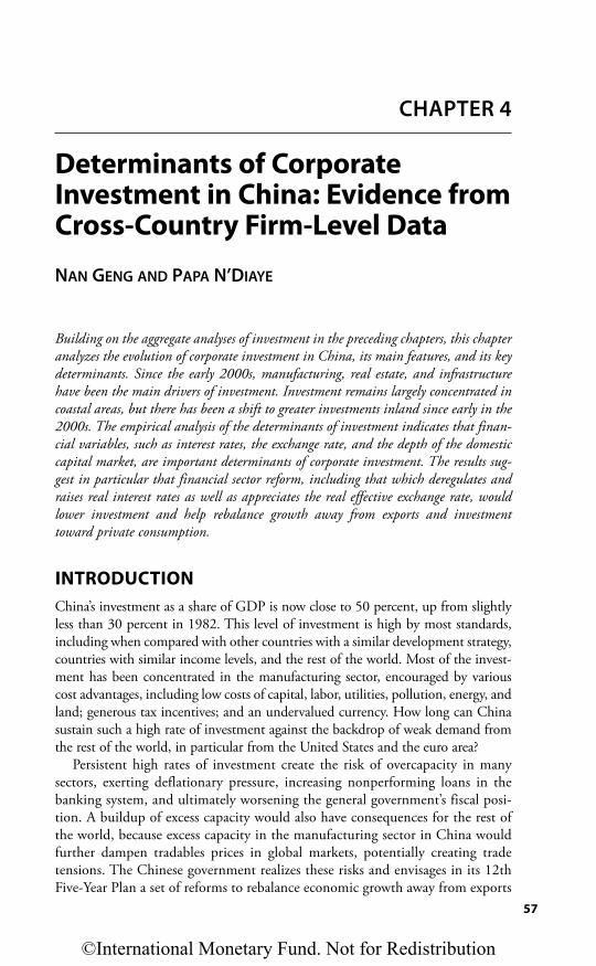
57
CHAPTER 4
Determinants of Corporate Investment in China: Evidence from Cross-Country Firm-Level Data
NAN GENG AND PAPA N’DIAYE
Building on the aggregate analyses of investment in the preceding chapters, this chapter analyzes the evolution of corporate investment in China, its main features, and its key determinants. Since the early 2000s, manufacturing, real estate, and infrastructure have been the main drivers of investment. Investment remains largely concentrated in coastal areas, but there has been a shift to greater investments inland since early in the 2000s. The empirical analysis of the determinants of investment indicates that finan-cial variables, such as interest rates, the exchange rate, and the depth of the domestic capital market, are important determinants of corporate investment. The results sug-gest in particular that financial sector reform, including that which deregulates and raises real interest rates as well as appreciates the real effective exchange rate, would lower investment and help rebalance growth away from exports and investment toward private consumption.
INTRODUCTION
China’s investment as a share of GDP is now close to 50 percent, up from slightly less than 30 percent in 1982. This level of investment is high by most standards, including when compared with other countries with a similar development strategy, countries with similar income levels, and the rest of the world. Most of the invest-ment has been concentrated in the manufacturing sector, encouraged by various cost advantages, including low costs of capital, labor, utilities, pollution, energy, and land; generous tax incentives; and an undervalued currency. How long can China sustain such a high rate of investment against the backdrop of weak demand from the rest of the world, in particular from the United States and the euro area?
Persistent high rates of investment create the risk of overcapacity in many sectors, exerting deflationary pressure, increasing nonperforming loans in the banking system, and ultimately worsening the general government’s fiscal posi-tion. A buildup of excess capacity would also have consequences for the rest of the world, because excess capacity in the manufacturing sector in China would further dampen tradables prices in global markets, potentially creating trade tensions. The Chinese government realizes these risks and envisages in its 12th Five-Year Plan a set of reforms to rebalance economic growth away from exports
©International Monetary Fund. Not for Redistribution

58 Determinants of Corporate Investment in China: Evidence from Cross-Country Firm-Level Data
and investment toward private consumption. Key to such a structural change is the plan to reform the financial system, which includes liberalizing interest rates, developing capital markets, reforming the exchange rate system, and raising the costs of various inputs to production—capital, labor, energy, land, water—and reducing the high level of corporate saving and investment.
This chapter provides an overview of corporate investment in China and its key determinants using both macro- and firm-level data for China and evidence from other economies’ experience. The empirical frameworks relate investment as a share of output to standard determinants of investment (including growth, real interest rates, and measures of uncertainty) as well as to indicators of financial sector development. The main highlights are as follows:
• Investment remains driven mainly by manufacturing, real estate, and more recently infrastructure. It is largely concentrated in coastal areas despite a recent move inland, reflecting the government’s urbanization efforts, focus on rural development, and construction of large interprovincial transporta-tion networks (especially railways and roads).
• China’s effective cost of capital is low, especially when compared with the high level of return investment can generate, creating strong incentives for firms to overinvest.
• The empirical analysis of the determinants of investment indicates that finan-cial variables such as interest rates, the exchange rate, and the depth of the domestic capital market are important determinants of corporate investment.
• The results suggest that financial sector reform, including that which raises interest rates, appreciates the real effective exchange rate, and develops the domestic capital market, would lower corporate investment and help rebal-ance the Chinese economy. All else equal, developing the domestic capital market alone would increase investment.
The remainder of the chapter is organized as follows: The next section pro-vides an overview of the evolution of investment in China and the factors that have influenced it. It is followed by a section that discusses the role of the cost of capital, and a section that presents the empirical frameworks.
EVOLUTION OF INVESTMENT
At close to 50 percent of GDP, China’s investment is high by most standards. First, China’s level of investment stands out when compared with economies that have had a similar development strategy of relying heavily on exports. This has not always been the case; in the early years of China’s development, both the level and evolution of investment appeared similar to that of other export-oriented economies such as Germany, Japan, and the Republic of Korea (Figure 4.1). Second, China’s investment stands out when compared with economies with similar income levels, notwithstanding the large variation in the level of investment by these economies (Figure 4.2). Finally, China’s investment is high when compared with the rest of the world (Figure 4.3).
©International Monetary Fund. Not for Redistribution

Geng and N’Diaye 59
From the national accounts, investment in China has contributed more than half of GDP growth on average since early 2000 (5¼ percentage points out of average growth of 10 percent). Little is known about the effectiveness of invest-ment, but existing research suggests a high depreciation rate of capital, in the range of 10–15 percent, and a declining incremental capital-to-output ratio (Figure 4.4). Estimates of China’s capital stock using perpetual inventory methods
0
10
20
30
40
50
1 5 9 13 17 21 25Period (years)
29 33 37 41 45
Japan (1955–82)
Per
cent
, ind
ex b
egin
ning
in p
erio
d 1
China (1979–2010)
Rep.of Korea (1963–2002) Germany (1955–94)
Figure 4.1 Share of Investment in GDPSources: CEIC Data; and IMF staff calculations.
0
10
20
30
40
50
0 10,000 20,000 30,000 40,000 50,000 60,000 70,000
China
Per capita GDP (average 2004–10 US$)
Fixe
d in
vest
men
t-to-
GD
P ra
tio(a
vera
ge 2
004–
10)
Figure 4.2 Investment-to-GDP Ratio and per Capita GDPSources: CEIC Data; and IMF, World Economic Outlook.
©International Monetary Fund. Not for Redistribution

60
De
term
ina
nts o
f Co
rpo
rate
Inve
stme
nt in
Ch
ina
: Ev
ide
nce
from
Cro
ss-Co
un
try Firm-Le
vel D
ata
0
10
20
Per
cent
30
40
50
Sol
omon
Isla
nds
Phi
lippi
nes
Uni
ted
Kin
gdom
Bra
zil
Isra
elC
ambo
dia
Ger
man
yU
rugu
ayU
nite
d S
tate
sS
wed
enE
gypt
Gre
ece
Net
herla
nds
Den
mar
kS
outh
Afri
caFi
nlan
dP
olan
dTu
rkey
Rus
sia
Italy
Mal
aysi
aFr
ance
Cos
ta R
ica
Hon
g K
ong
SA
RC
hile
Mex
ico
Sw
itzer
land
Bel
gium
Col
ombi
aA
ustri
aS
erbi
aH
unga
ryP
ortu
gal
Taiw
an P
rovi
nce
of C
hina
Can
ada
Irela
ndA
rgen
tina
New
Zea
land
Japa
nLi
thua
nia
Ukr
aine
Ecu
ador
Icel
and
Sri
Lank
aC
zech
Rep
ublic
Slo
vak
Rep
ublic
Sin
gapo
reC
roat
iaS
love
nia
Rom
ania
Thai
land
Indo
nesi
aB
ulga
riaLa
tvia
Spa
inA
ustra
liaE
ston
iaR
epub
lic o
f Kor
eaIn
dia
Mon
golia
Viet
nam
Chi
na
Figure 4.3 Investment-to-GDP RatioSources: CEIC Data; and IMF World Economic Outlook.©International Monetary Fund. Not for Redistribution
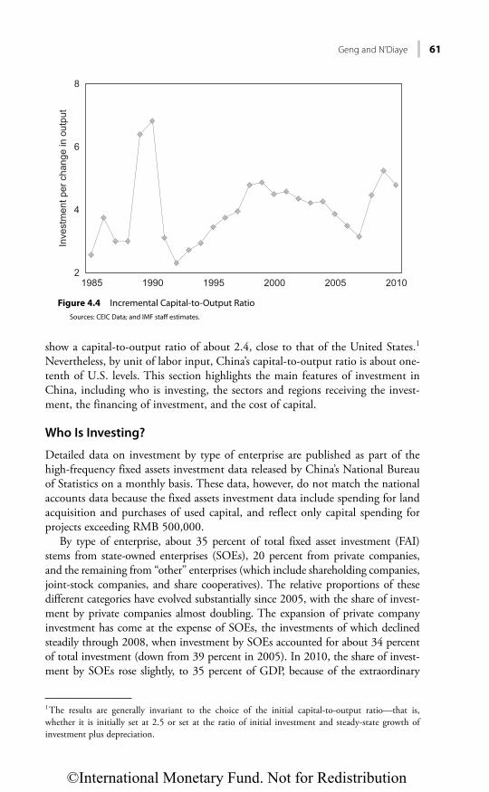
Geng and N’Diaye 61
show a capital-to-output ratio of about 2.4, close to that of the United States.1 Nevertheless, by unit of labor input, China’s capital-to-output ratio is about one-tenth of U.S. levels. This section highlights the main features of investment in China, including who is investing, the sectors and regions receiving the invest-ment, the financing of investment, and the cost of capital.
Who Is Investing?
Detailed data on investment by type of enterprise are published as part of the high-frequency fixed assets investment data released by China’s National Bureau of Statistics on a monthly basis. These data, however, do not match the national accounts data because the fixed assets investment data include spending for land acquisition and purchases of used capital, and reflect only capital spending for projects exceeding RMB 500,000.
By type of enterprise, about 35 percent of total fixed asset investment (FAI) stems from state-owned enterprises (SOEs), 20 percent from private companies, and the remaining from “other” enterprises (which include shareholding companies, joint-stock companies, and share cooperatives). The relative proportions of these different categories have evolved substantially since 2005, with the share of invest-ment by private companies almost doubling. The expansion of private company investment has come at the expense of SOEs, the investments of which declined steadily through 2008, when investment by SOEs accounted for about 34 percent of total investment (down from 39 percent in 2005). In 2010, the share of invest-ment by SOEs rose slightly, to 35 percent of GDP, because of the extraordinary
1 The results are generally invariant to the choice of the initial capital-to-output ratio—that is, whether it is initially set at 2.5 or set at the ratio of initial investment and steady-state growth of investment plus depreciation.
2
4
6
8
1985 1990
Inve
stm
ent p
er c
hang
e in
out
put
1995 2000 2005 2010
Figure 4.4 Incremental Capital-to-Output RatioSources: CEIC Data; and IMF staff estimates.
©International Monetary Fund. Not for Redistribution

62 Determinants of Corporate Investment in China: Evidence from Cross-Country Firm-Level Data
stimulus package put in place by the government in response to the global financial crisis. A downward trend can also be observed in the share of foreign-funded firms, with their investment declining from about 11 percent in 2005 to about 6½ percent in 2010. These foreign-funded firms include firms from Hong Kong SAR, Macao SAR, Taiwan Province of China, and other economies (Figure 4.5).
Although listed firms’ data show trends similar to those of SOEs and private compa-nies, the level is very different from that observed in FAI data (Figure 4.6). One main
0
20
40
60
80
0
50
100
2005 2006 2007 2008 2009 2010
OtherForeignState-owned enterprise
Per
cent
of G
DP
Per
cent
of i
nves
tmen
t
PrivateCollectiveTotal (% of GDP, right scale)
Figure 4.5 China: Fixed Asset Investment by Enterprise TypeSources: CEIC Data; and IMF staff calculations.
3
4
5
0
50
100
2005 2006 2007 2008 2009 2005 2006 2007 2008 2009
Other PrivateForeign CollectiveState-owned enterprise Total investment (% of GDP, right scale)
Distribution of investment Distribution of companies
Per
cent
of G
DP
Per
cent
Figure 4.6 Ownership Structure and Investment by Type of Ownership of Listed Firms in ChinaSources: World Scope and WIND databases; and IMF staff calculations.
©International Monetary Fund. Not for Redistribution
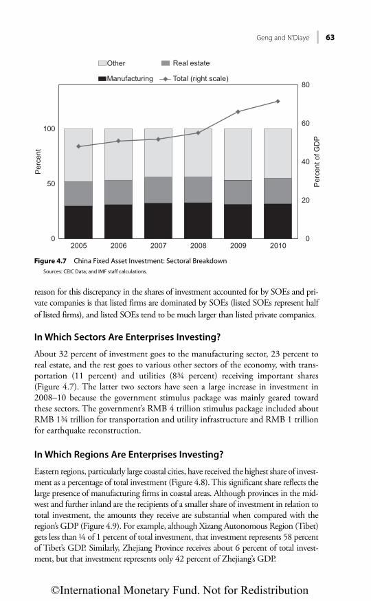
Geng and N’Diaye 63
reason for this discrepancy in the shares of investment accounted for by SOEs and pri-vate companies is that listed firms are dominated by SOEs (listed SOEs represent half of listed firms), and listed SOEs tend to be much larger than listed private companies.
In Which Sectors Are Enterprises Investing?
About 32 percent of investment goes to the manufacturing sector, 23 percent to real estate, and the rest goes to various other sectors of the economy, with trans-portation (11 percent) and utilities (8¾ percent) receiving important shares (Figure 4.7). The latter two sectors have seen a large increase in investment in 2008–10 because the government stimulus package was mainly geared toward these sectors. The government’s RMB 4 trillion stimulus package included about RMB 1¾ trillion for transportation and utility infrastructure and RMB 1 trillion for earthquake reconstruction.
In Which Regions Are Enterprises Investing?
Eastern regions, particularly large coastal cities, have received the highest share of invest-ment as a percentage of total investment (Figure 4.8). This significant share reflects the large presence of manufacturing firms in coastal areas. Although provinces in the mid-west and further inland are the recipients of a smaller share of investment in relation to total investment, the amounts they receive are substantial when compared with the region’s GDP (Figure 4.9). For example, although Xizang Autonomous Region (Tibet) gets less than ¼ of 1 percent of total investment, that investment represents 58 percent of Tibet’s GDP. Similarly, Zhejiang Province receives about 6 percent of total invest-ment, but that investment represents only 42 percent of Zhejiang’s GDP.
0
20
40
60
80
0
50
100
2005 2006 2007 2008 2009 2010
Other
Manufacturing
Real estate
Per
cent
of G
DP
Per
cent
Total (right scale)
Figure 4.7 China Fixed Asset Investment: Sectoral BreakdownSources: CEIC Data; and IMF staff calculations.
©International Monetary Fund. Not for Redistribution

64 Determinants of Corporate Investment in China: Evidence from Cross-Country Firm-Level Data
XizangZhejiangProvince
Black: >5.0 PercentGray: 2.5−5.0 PercentLight gray: 1.0−2.5 PercentWhite: <1.0 Percent
Figure 4.8 China: Investment by Region as Share of Total, Average 2005–10 (Percent of total)
XizangZhejiangProvince
Black: 60−80 PercentGray: 50−80 PercentLight gray: 40−50 PercentWhite: 0−40 Percent
Figure 4.9 China: Investment by Region as Share of GDP, Average 2005–10 (Percent of GDP)
This reflects in many ways the significant role of SOEs in less-developed regions and the fact that SOEs tend to invest more than other enterprises (Barnett and Brooks, 2006).
How Is Investment Financed?
Investment is financed primarily through retained earnings and bank loans. Financing through self-raised funds now accounts for slightly less than 60 percent of total financing according to FAI data, up from about 54 percent in 2005 (Figure 4.10). This large and increasing share of financing through self-raised funds reflects the healthy profits of Chinese corporations and the fact that until recently many firms paid small, if any, dividends (compared with companies in other economies). Before 2007, SOEs were not required to pay dividends to the state. Since the 2007 State Capital Management Budget reform, SOEs are often required to pay annual dividends of at least 5–10 percent of profits, depending on the industry. Enterprises in industries with low competition are required to pay 10 percent.2 Dividends are
2 Military SOEs and some particular types of SOEs (under the umbrella of specific public institutions) were initially exempt from this requirement. In 2011, the dividends payment requirements were raised to 10–15 percent, but military SOEs and SOEs under the umbrella of specific public institutions were required to pay 5 percent of their profits to the state.
©International Monetary Fund. Not for Redistribution
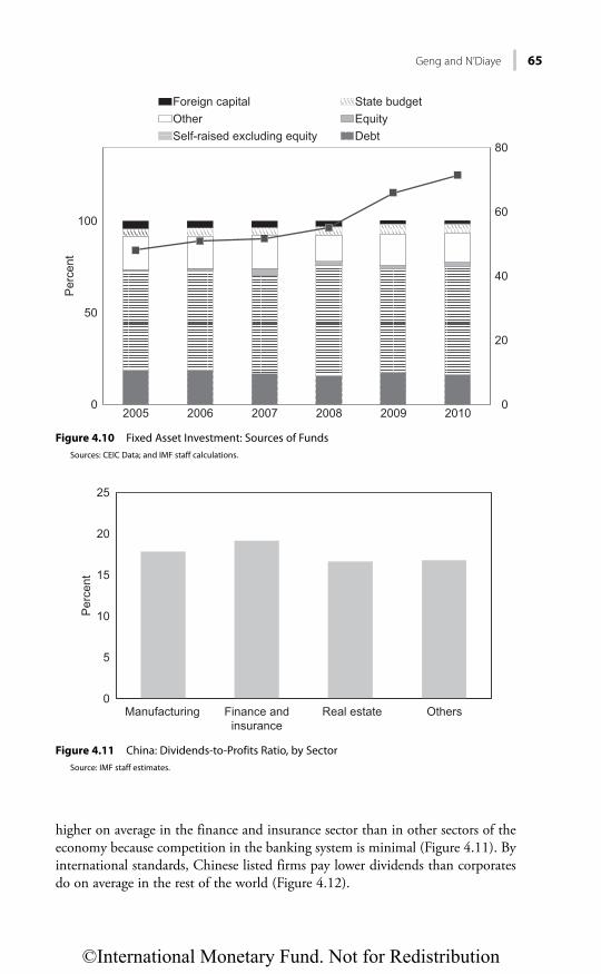
Geng and N’Diaye 65
higher on average in the finance and insurance sector than in other sectors of the economy because competition in the banking system is minimal (Figure 4.11). By international standards, Chinese listed firms pay lower dividends than corporates do on average in the rest of the world (Figure 4.12).
0
5
10
15
20
25
Manufacturing
Per
cent
Finance andinsurance
Real estate Others
Figure 4.11 China: Dividends-to-Profits Ratio, by SectorSource: IMF staff estimates.
0
20
40
60
80
0
50
100
2005 2006 2007 2008 2009 2010
Foreign capital State budgetOther
Per
cent
EquitySelf-raised excluding equity Debt
Figure 4.10 Fixed Asset Investment: Sources of FundsSources: CEIC Data; and IMF staff calculations.
©International Monetary Fund. Not for Redistribution

66 Determinants of Corporate Investment in China: Evidence from Cross-Country Firm-Level Data
Implications for Corporate Saving
The requirement for SOEs to pay to the state at least 5–10 percent dividends did little to reduce corporate saving or the self-financing of investment because dividends paid by SOEs are paid into a special capital budget that is used to finance state enter-prise investment (IMF, 2009). This dividend policy, the lack of contestability in many markets, and cheap capital all contribute to relatively large (gross) savings for Chinese listed and nonlisted corporations by international standards (Figures 4.13 and 4.14).
0 10 20Percent
30 40
China
Emerging Europe
Developed Americas
Emerging Asia
Developed Asia
Middle East
Developed Europe
Emerging Americas
Global mean
Figure 4.12 Dividends-to-Profits Ratio by Development RegionSource: IMF staff estimates.
0
10
20
30
Por
tuga
lTh
aila
ndTa
iwan
Pro
vinc
e of
Chi
na
Per
cent
of G
DP
Indi
aC
hile
Italy
Fran
ceS
pain
Sou
th A
frica
Irela
ndU
nite
d S
tate
sP
olan
dE
gypt
Ger
man
yM
exic
oC
olom
bia
Hun
gary
Sw
eden
Gre
ece
Aus
tralia
Slo
veni
aU
nite
d K
ingd
omN
ew Z
eala
ndA
ustri
aB
elgi
umB
razi
lM
oroc
coD
enm
ark
Nor
way
Rep
ublic
of K
orea
Phi
lippi
nes
Cze
ch R
epub
licFi
nlan
dS
lova
k R
epub
licC
anad
aN
ethe
rland
sS
witz
erla
ndJa
pan
Chi
naVe
nezu
ela
Figure 4.13 Corporate Saving, by CountrySources: United Nations database; and IMF staff estimates.
©International Monetary Fund. Not for Redistribution
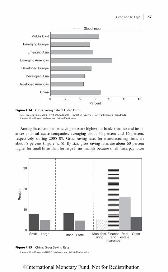
Geng and N’Diaye 67
Among listed companies, saving rates are highest for banks (finance and insur-ance) and real estate companies, averaging about 30 percent and 16 percent, respectively, during 2005–09. Gross saving rates for manufacturing firms are about 5 percent (Figure 4.15). By size, gross saving rates are about 60 percent higher for small firms than for large firms, mainly because small firms pay lower
0 3 5 8 10 13 15
China
Developed Americas
Developed Asia
Developed Europe
Emerging Americas
Emerging Asia
Emerging Europe
Middle East
Global mean
Percent
Figure 4.14 Gross Saving Rate of Listed FirmsNote: Gross Saving = Sales − Cost of Goods Sold − Operating Expenses – Interest Expenses − DividendsSources: WorldScope database; and IMF staff estimates.
0
10
20
30
Small Large Manufact-uring
Financeand
insurance
Realestate
OtherState
Per
cent
Other
Figure 4.15 China: Gross Saving RateSources: WorldScope and WIND databases; and IMF staff calculations.
©International Monetary Fund. Not for Redistribution

68 Determinants of Corporate Investment in China: Evidence from Cross-Country Firm-Level Data
dividends than large firms and have less access to credit, which forces them to rely more on retained earnings for financing investment. This latter reason also explains why non–state owned firms save more than state-owned firms.
The second largest source of financing of corporate investment is debt, includ-ing bank loans and corporate bonds. Borrowing represents about 17 percent of total investment financing by listed firms. Bank financing is the prime source of debt financing: China’s large saving rates for both the private sector (especially households—household savings now represent about 23½ percent of GDP and are primarily in the banking system, earning on average negative real interest rates since 2003) and the public sector provide ample and cheap funds. At the macro-economic level, bank loans accounted for about 63 percent of total social financ-ing (a broad measure of credit) as of end-2011, while corporate bonds accounted for 11 percent of total social financing (Figure 4.16).
COST OF CAPITAL
China’s capital-intensive growth relies on various low-cost factor inputs, including land, water, energy, labor, and capital. These relatively cheap inputs offer Chinese firms a competitive edge and create incentives for capital-intensive means of produc-tion. Studies estimate that the total value of China’s factor market distortions could be almost 10 percent of GDP (Huang and Tao, 2010). Factor inputs are priced below market for many industries and are low compared with those in other economies.
Land and water. In China, all land belongs to the state, and local governments have the discretion to sell industrial land-use rights to companies for up to 50 years. In many cases, industrial land is provided for free to enterprises to attract investment (Huang, 2010). The price for water in China is about one-third of the average of a sample of international comparators (Figure 4.17).
Energy. Cross-country data on the cost of energy show that the price of gasoline in China is relatively low, although similar to that in the United States (Figure 4.18).
0
4
8
12
16
0
4
8
12
16
2006 2007 2008 2009 2010 2011 2011:Q1 Q2 Q3 Q4 2012:Q1 Q2 Q3
Entrusted loansCumulative Flows
RM
B (t
rillio
n)
RM
B (t
rillio
n)
OtherEquityCorporate bondsBank acceptanceTrust loansBank loans
Figure 4.16 Social FinancingSources: CEIC Data Company Ltd.; and IMF staff estimates.
©International Monetary Fund. Not for Redistribution

G
en
g a
nd
N’D
iaye
69
0
2
4
US
$ pe
r cub
ic m
eter
6
8
Cub
aU
zbek
ista
nS
ri La
nka
Pak
ista
nS
audi
Ara
bia
Syr
iaB
ahra
inM
adag
asca
rE
gypt
Hon
dura
sIn
dia
Alg
eria
Viet
nam
Arg
entin
aVe
nezu
ela
Geo
rgia
Mal
aysi
aA
zerb
aijia
nM
ongo
liaE
thio
pia
Kaz
akhs
tan
Taiw
an P
rovi
nce
of C
hina
Ken
yaB
elar
usM
oroc
coP
hilip
pine
sP
eru
Chi
naM
oldo
vaN
iger
iaM
ali
Mex
ico
Jord
anR
ussi
aB
otsw
ana
Pan
ama
Hon
g K
ong
SA
RN
epal
Arm
enia
Rw
anda
Ser
bia
Ukr
aine
Indo
nesi
aS
outh
Afri
caR
ep. o
f Kor
eaB
ulga
riaC
hile
Italy
Rom
ania
Qat
arP
ales
tine
Bra
zil
Icel
and
Om
anLa
tvia
Gre
ece
Isra
elTu
rkey
Lith
uani
aTh
e B
aham
asS
pain
Japa
nP
ortu
gal
Net
herla
nds
Uni
ted
Ara
b E
mira
tes
Uni
ted
Sta
tes
Cro
atia
Can
ada
Sw
eden
Est
onia
Pol
and
Slo
vak
Rep
ublic
Hun
gary
Cze
ch R
epub
licS
inga
pore
Aus
tralia
Nor
way
Aus
tria
New
Zea
land
Finl
and
Uni
ted
Kin
gdom
Fran
ceB
elgi
umG
erm
any
Sw
itzer
land
Luxe
mbo
urg
Den
mar
k
China
Average
Figure 4.17 Water Prices, by CountrySources: Global Water Intelligence; and IMF staff estimates.
©International Monetary Fund. Not for Redistribution
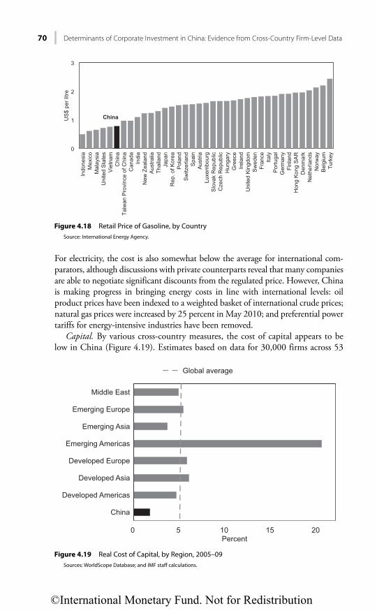
70 Determinants of Corporate Investment in China: Evidence from Cross-Country Firm-Level Data
For electricity, the cost is also somewhat below the average for international com-parators, although discussions with private counterparts reveal that many companies are able to negotiate significant discounts from the regulated price. However, China is making progress in bringing energy costs in line with international levels: oil product prices have been indexed to a weighted basket of international crude prices; natural gas prices were increased by 25 percent in May 2010; and preferential power tariffs for energy-intensive industries have been removed.
Capital. By various cross-country measures, the cost of capital appears to be low in China (Figure 4.19). Estimates based on data for 30,000 firms across 53
0 5 10 15 20
China
Developed Americas
Developed Asia
Developed Europe
Emerging Americas
Emerging Asia
Emerging Europe
Middle East
Global average
Percent
Figure 4.19 Real Cost of Capital, by Region, 2005–09Sources: WorldScope Database; and IMF staff calculations.
0
1
2
3
Indo
nesi
a
US
$ pe
r litr
e
Mex
ico
Mal
aysi
aU
nite
d S
tate
sV
ietn
amC
hina
Taiw
an P
rovi
nce
of C
hina
Can
ada
Indi
aN
ew Z
eala
ndA
ustra
liaTh
aila
ndJa
pan
Rep
. of K
orea
Pol
and
Sw
itzer
land
Spa
inA
ustri
aLu
xem
bour
gS
lova
k R
epub
licC
zech
Rep
ublic
Hun
gary
Gre
ece
Irela
ndU
nite
d K
ingd
omS
wed
enFr
ance
Italy
Por
tuga
lG
erm
any
Finl
and
Hon
g K
ong
SA
RD
enm
ark
Net
herla
nds
Nor
way
Bel
gium
Turk
ey
China
Figure 4.18 Retail Price of Gasoline, by CountrySource: International Energy Agency.
©International Monetary Fund. Not for Redistribution

Geng and N’Diaye 71
economies show that the real cost of capital—defined as a weighted average of the real costs of bank loans, bonds, and equity—faced by Chinese listed firms is below the global average.3 The low cost of capital reflects the lower cost of equity for Chinese firms relative to the rest of world. Chinese firms, mainly SOEs, pay little if any dividends, compared with the global average (dividend payments aver-aged 33 percent of profits during 2000–08 according to World Bank [2009]). On average, equity costs are about 5 percent in China as compared with 12 percent for the rest of the world (Figure 4.20). With regard to the cost of debt, Chinese listed firms are not out of line with companies in the rest of the world. Real effec-tive interest rates paid by Chinese listed firms average about 2½ percent com-pared with a world average of 2¾ percent during 2005–09 (Figure 4.21).
Capital appears to be especially cheap when assessed relative to its high pro-ductivity in China. In particular, an estimate of the marginal product of repro-ducible capital (i.e., capital adjusted for land) shows that China’s return to capital is well above the average real loan rate of many advanced and emerging market economies (Figure 4.22).4
This gap between real lending rates and the marginal product of capital is a rent that is shared between financial and nonfinancial corporations. Assuming the
3 Weights are assumed to be the relative shares of equity and debt in corporate liabilities. Here the cost of equity is measured following the methodology in ECB (2004).4 The marginal product of reproducible capital in China is estimated following Caselli and Freyer (2005) and is the ratio of the income share of capital excluding land and other nonreproducible items to the capital-to-output ratio. The capital stock is derived from the perpetual inventory method. Alternative estimates of the return to capital in China by Bai, Hsieh, and Qian (2006) show a return to capital of about 20 percent in 2005, down from 25 percent during 1973–93.
0 10 20 30 40 50 60
China
Developed Americas
Developed Asia
Developed Europe
Emerging Americas
Emerging Asia
Emerging Europe
Middle East
Global average
Percent
Figure 4.20 Real Cost of Equity, by RegionSources: WorldScope database; and IMF staff calculations.
©International Monetary Fund. Not for Redistribution

72 Determinants of Corporate Investment in China: Evidence from Cross-Country Firm-Level Data
marginal product of capital (net of depreciation) is equal to the return on capital, this return can be distributed to banks, households, and nonfinancial corpora-tions, with banks being remunerated at the spread between average deposit and lending rates, households being paid real deposit rates, and nonfinancial corpora-tions getting the remainder of the marginal product of capital. This simple exercise shows that, in China, the returns to capital are largely shared between financial and nonfinancial corporations (Figure 4.23). Households have subsidized these
−2
0
2
4
6
8
10
0 5 10 15 20Marginal product of capital adjusted for land (percent)
China
Aver
age
real
inte
rest
rate
(per
cent
)
Figure 4.22 Marginal Product of Capital (Adjusted for Land) versus Average Real Interest Rate, 2004–10
Source: IMF staff estimates.
0 1 2 3 4 5
China
Developed Americas
Developed Asia
Developed Europe
Emerging Americas
Emerging Asia
Emerging Europe
Middle East
Global average
Percent
Figure 4.21 Real Effective Interest Rate on Debt, by RegionSources: WorldScope database; and IMF staff calculations.
©International Monetary Fund. Not for Redistribution

Geng and N’Diaye 73
corporations, on average, since 2003, given that China’s real deposit rates were negative during that period. Raising the cost of capital in China will therefore allow households to keep some of the returns to their capital, and help support consumption.5 Nonfinancial corporations get a slightly bigger share of the return to capital than do financial corporations. This distribution of the return to capital among the various players in China’s economy is in stark contrast with what is observed in countries like India, the Republic of Korea, Japan, the United States, and the United Kingdom. Unlike in China, households in these countries get at least some share of the returns to capital and the corporate sector ends up appro-priating relatively little of the returns to capital.6
EMPIRICAL DETERMINANTS OF INVESTMENT
Both firm-level and cross-country data are used to explain the dynamics of invest-ment in China. For the analysis based on firm-level data, corporate capital expen-diture (in relation to sales) is regressed on past capital expenditure, the capital-to-output ratio squared, stock market capitalization relative to GDP, real interest rates, the change in the real effective exchange rate, real GDP growth, the current account balance relative to GDP, the foreign-debt-to-GDP ratio, the relative price of capital to output, and the volatility of output. These variables capture the
5 See Guo and N’Diaye (2010) on the role of property income in private consumption in China. 6 This representation might not accurately depict the situation in the United States because corpora-tions rely less on bank financing than elsewhere. U.S. flow of funds data suggest that as of end-Sep-tember 2011, bank loans accounted for about 3½ percent of total nonfinancial corporates’ liabilities, while corporate bonds accounted for about 40 percent of total liabilities.
−2
0
2
4
6
8
China
Per
cent
India Japan Rep. ofKorea
UnitedKingdom
UnitedStates
Corporate sectorBanksDepositorsTotal return to capital
Figure 4.23 Distribution of Real Returns to Bank-Intermediated CapitalSource: IMF staff estimates.
©International Monetary Fund. Not for Redistribution

74 Determinants of Corporate Investment in China: Evidence from Cross-Country Firm-Level Data
effects of various factors, including stickiness in investment, adjustment costs (captured by the capital-to-output ratio squared), capital market development, the cost of capital, exchange rates, country risk, countries’ levels of development, profit opportunities, uncertainty, and the availability of external financing.
The model is estimated using the dynamic panel data estimator developed by Arellano and Bond (1991) with both an unbalanced panel of 27,997 firms across 53 economies and an unbalanced panel of 1,908 firms in China during 1990–2009.7 To handle simultaneity, lagged values of the contemporaneous regressors were used as instruments, and a special correction for correlation was applied. All variables that enter with a lag on the right-hand side of the equation are consid-ered exogenous. The set of instruments also includes country dummies, but no country dummies are included in the regression itself.
Table 4.1 shows the results of the firm-level data regressions. The “Cross Country” column shows the results based on cross-country data and the “China” column shows the results for China only.8 The results based on cross-country
7 See Annex 4A to this chapter for a description of the data.8 Both results pass the autocorrelation test at order 1 and 2 (AR(1) and AR(2)) and the overidentifica-tion test (Hansen’s J-statistic).
TABLE 4.1
Determinants of Corporate Investment, from Firm-Level Data
Explanatory Variables Cross Country China
Capital expenditure ratio (lagged 1 year) 0.307** −0.031**(0.000) (0.002)
Investment adjustment cost ((K/Y)^2 (lagged 1 year)) −0.004** −0.030**(0.000) (0.000)
Stock market capitalization/GDP 1.043** 0.080**(0.011) (0.003)
Real interest rate (lagged 1 year) −2.420** −0.253**(0.199) (0.008)
Appreciation of REER −0.411** −0.417**(0.076) (0.009)
Real GDP growth 1.620** …(0.245) …
Current account balance/GDP (lagged 1 year) 2.700** −2.230**(0.387) (0.062)
Foreign debt risk −1.342** −4.104**(0.089) (0.062)
Relative price of capital to GDP 5.081** 1.467**(0.206) (0.044)
Volatility of GDP growth (lagged 1 year) −3.260** −4.210**(0.489) (0.124)
Observations 185,217 7,532Number of firms 27,997 1,908Ar(1) 0.019 0.008Ar(2) 0.117 0.267Hansen J Test (prob>c2) 0.72 0.45
Source: IMF staff estimates.Note: Generalized method of moments estimates using an unbalanced panel of firms over the period 1990–2009. Robust
standard errors in parentheses, with ** indicating significance at 5 percent level. REER = real effective exchange rate.
©International Monetary Fund. Not for Redistribution

Geng and N’Diaye 75
data indicate that investment is positively related to capital market development, output growth, and the relative price of capital, and negatively related to adjust-ment costs, real interest rates, changes in the real effective exchange rate, country risk, and uncertainty. Although most of these results are consistent with the pri-ors—for example, capital market development increases financing opportunities and instruments (Beck and Levine, 2001; Leahy and others, 2001)—the sign of the relative price of capital is less obvious. Indeed, as shown in Caselli and Freyer (2005), the price of capital relative to that of output is higher the less advanced the economy. With investment rates being in general higher in less-developed economies, the result in Table 4.1 could simply be capturing the positive relation-ship that exists between the level of development and the level of investment.
Table 4.2 shows the results of the estimation of a similar investment equation using aggregate national accounts data. The model relates total investment to real interest rates (lagged), real GDP growth, volatility of growth, indicators of
TABLE 4.2
Determinant of Investment, from Aggregate Data
Explanatory Variables Coefficients
Number of listed companies per 10,000 people 3.900**(0.507)
Real interest rate (lagged 1 year) −0.054**(0.019)
Appreciation of REER 0.121(0.044)
Real GDP growth 0.215**(0.053)
Current account balance/GDP (lagged 1 year) −0.073**(0.023)
Foreign debt risk −0.013**(0.003)
Relative price of capital to GDP 0.198**(0.090)
Volatility of GDP growth (lagged 1 year) −0.118 (0.079)
Relative per capita GDP −2.114**(0.772)
Constant 22.228**(0.531)
Number of listed companies per 10,000 people (China specific) 1151.2**(80.637)
China-specific real interest rate (lagged 1 year) −0.351**(0.092)
China-specific appreciation of REER −0.254**(0.070)
China-specific constant 5.110**(0.721)
Observations 840Number of economies 52Durbin-Watson Test (p-value) 0.33
Source: IMF staff estimates. Note: Generalized method of moments estimates using an unbalanced panel of firms over the
period 1990–2009. Robust standard errors in parentheses, with ** indicating significance at the 5 percent level. REER = real effective exchange rate.
©International Monetary Fund. Not for Redistribution

76 Determinants of Corporate Investment in China: Evidence from Cross-Country Firm-Level Data
financial development (the number of listed firms per 10,000 people), indicators of economic development, the debt-to-GDP ratio, and the change in the exchange rate. Dummy variables specific to China were introduced to see wheth-er China stands out. The model was estimated using the generalized method of moments estimator using an unbalanced panel of 52 economies.
Overall, the results are consistent with the priors. Investment falls with real interest rates, uncertainty, countries’ levels of development, and increases in coun-tries’ external financial risk. Investment rises with growth opportunities, financial development, and an appreciating currency except for China, which may reflect the importance of manufacturing firms. In more detail, the following results in Tables 4.1 and 4.2 are noteworthy:
• Real interest rates have a negative impact on investment. At the aggregate level, an increase of 100 basis points in real interest rates reduces corporate investment in China by about ½ percent of GDP. Based on these estimates, raising real interest rates to the level of the marginal product of capital net of depreciation would probably lower investment by about 3 percent of GDP. The estimated effect for China of real interest rates on investment is much larger than the average of the other 52 economies in the panel. The impact of interest rate changes on corporate investment is about half as large when estimated based on firm-level data. This outcome could possibly reflect the smaller reliance of this sample (which consists of large, listed enterprises) on bank-intermediated financing.
• Exchange rate appreciation also lowers investment. A 10 percent apprecia-tion would reduce total investment by about 1 percent of GDP. The large concentration of manufacturing companies in the firm-level sample means that the estimated impact of exchange rate appreciation from the firm-level data is much larger.
• Indicators of capital market development suggest more-developed financial systems tend to promote higher investment, largely by easing the financing constraints faced by firms.
CONCLUSION
This chapter analyzes the evolution of investment in China, its main features, and its key determinants. In recent years, the manufacturing, real estate, and infra-structure sectors have been the main drivers of investment. Investment remains largely concentrated in coastal areas, although a slow move inland in recent years has been detected. The empirical analysis of the determinants of investment indi-cates that financial variables, such as interest rates, the exchange rate, and the depth of the domestic capital market, are important determinants of corporate investment. The results suggest, in particular, that financial sector reform, includ-ing that which raises real interest rates and appreciates the real effective exchange rate, would lower investment and help rebalance growth away from exports and investment toward private consumption.
©International Monetary Fund. Not for Redistribution

Geng and N’Diaye 77
ANNEX 4A. DATA DEFINITION
The firm-level data used in this chapter are from the Worldscope database and WIND database, which report data on listed financial and nonfinancial corpora-tions’ annual financial statements during the period 1990–2009 for more than 50 economies worldwide. Tables 4A.1, 4A.2, and 4A.3 present an overview of these economies and the distribution of companies in the sample.
Tables 4A.2 and 4A.3 provide information on the ownership and industry distribution of the China-specific listed firms. The tables show that the sample is dominated by manufacturing firms, mainly state owned (including companies belonging to government agencies, the State-Owned Assets Supervision and Administration Commission, and other SOEs).
TABLE 4A.1
Distribution of Firms
Economy Number of Firms Share of Sample (percent)
Argentina 65 0.23 Australia 1,614 5.76 Austria 82 0.29 Belgium 112 0.40 Brazil 169 0.60 Canada 1,139 4.07 Chile 166 0.59 China 1,908 6.82
Colombia 26 0.09 Czech Republic 11 0.04 Denmark 168 0.60 Egypt 68 0.24 Finland 119 0.43 France 554 1.98 Germany 614 2.19 Greece 165 0.59 Hong Kong SAR 919 3.28 Hungary 34 0.12 India 1,944 6.94 Indonesia 334 1.19 Ireland 45 0.16 Israel 154 0.55 Italy 265 0.95 Japan 3,790 13.54 Korea, Rep. of 880 3.14 Luxembourg 26 0.09 Malaysia 938 3.35 Mexico 108 0.39 Morocco 20 0.07 Netherlands 131 0.47 New Zealand 130 0.46 Norway 178 0.64 Pakistan 140 0.50 Peru 65 0.23 Philippines 187 0.67 Poland 332 1.19
(Continued )
©International Monetary Fund. Not for Redistribution
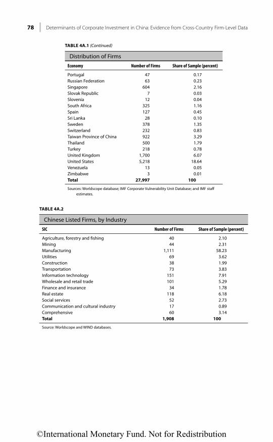
78 Determinants of Corporate Investment in China: Evidence from Cross-Country Firm-Level Data
TABLE 4A.1 (Continued)
Distribution of Firms
Economy Number of Firms Share of Sample (percent)
Portugal 47 0.17 Russian Federation 63 0.23 Singapore 604 2.16 Slovak Republic 7 0.03 Slovenia 12 0.04 South Africa 325 1.16 Spain 127 0.45 Sri Lanka 28 0.10 Sweden 378 1.35 Switzerland 232 0.83 Taiwan Province of China 922 3.29 Thailand 500 1.79 Turkey 218 0.78 United Kingdom 1,700 6.07 United States 5,218 18.64 Venezuela 13 0.05 Zimbabwe 3 0.01 Total 27,997 100
Sources: Worldscope database; IMF Corporate Vulnerability Unit Database; and IMF staff estimates.
TABLE 4A.2
Chinese Listed Firms, by Industry
SIC Number of Firms Share of Sample (percent)
Agriculture, forestry and fishing 40 2.10 Mining 44 2.31 Manufacturing 1,111 58.23 Utilities 69 3.62 Construction 38 1.99 Transportation 73 3.83 Information technology 151 7.91 Wholesale and retail trade 101 5.29 Finance and insurance 34 1.78 Real estate 118 6.18 Social services 52 2.73 Communication and cultural industry 17 0.89 Comprehensive 60 3.14 Total 1,908 100
Source: Worldscope and WIND databases.
©International Monetary Fund. Not for Redistribution

Geng and N’Diaye 79
TABLE 4A.3
Chinese Listed Firms, by Actual Ownership
Ownership Type Number of Firms Share of Sample (percent)
Government agency 137 7.18SASAC 762 39.94SOE 81 4.25Private 826 43.29Collective 19 1.00Foreign 58 3.04University 9 0.47Other 16 0.84Total 1,908 100
Sources: Worldscope and WIND databases; and IMF staff estimates.Note: SASAC = State-Owned Assets Supervision and Administration Commission; SOE = State-owned enterprise.
©International Monetary Fund. Not for Redistribution

80 Determinants of Corporate Investment in China: Evidence from Cross-Country Firm-Level Data
REFERENCES
Arellano, M., and S. Bond, 1991, “Some Tests of Specification for Panel Data: Monte Carlo Evidence and Applications to Employment Equations,” Review of Economic Studies, Vol. 58, pp. 277–97.
Bai, C., C. Hsieh, and Y. Qian, 2006, “The Return to Capital in China,” NBER Working Paper No. 12755 (Cambridge, Massachusetts: National Bureau of Economic Research).
Barnett, S., and R. Brooks, 2006, “What’s Driving Investment in China?” IMF Working Paper 06/265 (Washington: International Monetary Fund).
Beck, T., and R. Levine, 2001, “Stock Markets, Banks, and Growth: Correlation or Causality,” Policy Research Working Paper No. 2670 (Washington: World Bank).
Caselli, F., and J. Freyer, 2005, “The Marginal Product of Capital,” NBER Working Paper No. 11551 (Cambridge, Massachusetts: National Bureau of Economic Research).
European Central Bank (ECB), 2004, “The Results of the October 2004 Bank Lending Survey for the Euro Area,” Box 2 in Monthly Bulletin November 2004 (Frankfurt: European Central Bank).
Guo, K., and P. N’Diaye, 2010, “Determinants of China’s Private Consumption: An International Perspective,” IMF Working Paper 10/93 (Washington: International Monetary Fund).
Huang, Y., 2010, “China’s Great Ascendancy and Structural Risks: Consequences of Asymmetric Market Liberalization,” Asian-Pacific Economic Literature, Vol. 24, No. 1, pp. 65–85.
———, and K.Y. Tao, 2010, “Causes and Remedies of China’s External Imbalances,” Paper prepared for the conference “Trans-Pacific Rebalancing,” jointly organized by the Asian Development Bank Institute and the Brookings Institution, Tokyo, March 3–4.
International Monetary Fund (IMF), 2009, “Building a Sustained Recovery,” in Asia and Pacific Regional Economic Outlook, October (Washington).
Leahy, M., S. Schich, G. Wehinger, F. Pelgrin, and T. Thorgeirsson, 2001, “Contributions of Financial Systems to Growth in OECD Countries,” OECD Economics Department Working Paper No. 280 (Paris: Organization for Economic Cooperation and Development).
World Bank, 2009, “Effective Discipline with Adequate Autonomy: The Direction for Further Reform of China’s SOE Dividend Policy,” Report No. 53254 (Washington).
©International Monetary Fund. Not for Redistribution

81
CHAPTER 5
Interest Rates, Targets, and Household Saving in Urban China
MALHAR NABAR
An important aspect of domestic imbalances in China is the relatively low share of household consumption in the national economy (down to about 36 percent of GDP in 2011 from 46 percent early in the first decade of the 2000s). The flip side is the rising household saving rate. This chapter studies urban household saving rates across China’s provinces for the period 1996–2009, during which the urban household saving rate at the national level increased from 19 percent of disposable income to 30 percent. It finds that urban saving rates rose with the decline in real interest rates for this period. This association suggests that Chinese households save with a target level of saving in mind. A main policy implication is that an increase in real deposit interest rates may help lower household saving and boost domestic consumption.
INTRODUCTION
In the mid-1990s, China’s urban household saving rate stood at 19 percent of disposable income. A decade and a half later, the saving rate touched 30 percent. This increase occurred during a period in which the economy grew rapidly and expectations of improved livelihoods, higher earnings, and greater prosperity took root. Such influences might have been expected to dampen rather than trigger savings impulses.
At the same time that household saving rates rose, China’s growth model became more reliant on exports and investment. Rebalancing China’s economy back toward consumption will require, among other policies, measures that induce households to save less and spend more. This chapter examines what role financial reform, in particular, interest rate liberalization and an increase in real deposit interest rates, can play in influencing household saving rates in China.
Although a large body of research has examined the determinants of house-hold saving in China, little attention has been directed to interest rates and their impact on saving decisions. Bank deposits are currently the primary saving vehi-cle available to Chinese households. Therefore, the return households earn on these bank deposits could potentially influence household saving behavior in a tangible way. This research assesses how interest rates affect household saving
©International Monetary Fund. Not for Redistribution

82 Interest Rates, Targets, and Household Saving in Urban China
decisions using a panel data set that covers China’s 31 provincial-level administra-tive units for the period 1996–2009.
The main findings are as follows:• Panel estimates suggest that household saving responds strongly to a change
in the real interest rate. A 1 percentage point increase in the real rate of return on bank deposits lowers the urban household saving rate by 0.6 per-centage point.
• A comparison of the relationship across subperiods shows that the associa-tion is stronger in the later period, 2003–09, relative to the earlier period, 1996–2002. The relationship is robust to the inclusion of variables that proxy for other influences on saving such as life-cycle considerations and self-insurance against income volatility.
• The evidence also indicates that when the return on alternative investments is high (for example, when real property price growth is relatively strong), a decline in the real return on bank deposits does not have as negative an impact on household portfolios.
• The results suggest that China’s households save to meet a multiplicity of needs—retirement consumption, purchase of durables, self-insurance against income volatility, and health shocks—and act as though they have a target level of saving in mind. An increase in financial rates of return, which would raise the return on saving, makes it easier for them to meet their sav-ing targets. Financial reform that boosts interest rates could therefore have a strong effect on current tendencies to save. As financial development pro-ceeds and alternative investment opportunities become more readily avail-able, portfolio diversification may further enable households to meet their saving targets more easily, potentially contributing to lower rates of saving out of current disposable income.
The chapter is organized as follows: The next section summarizes recent trends in household saving rates in China and provides a brief overview of previous research in this area. Subsequent sections outline the target saving hypothesis, present the empirical analysis, and discuss policy implications and the importance of liberalizing interest rates within the context of an appropriately sequenced set of financial reforms.
HOUSEHOLD SAVING IN CHINA
Context
China’s economic performance has understandably attracted attention from poli-cymakers and academic researchers attempting to explain its various dimensions. The transformation of the economy has taken place at an unprecedented pace. By successfully maintaining close to double-digit rates of GDP growth for nearly two decades, China has lifted millions out of poverty and the prospects of a middle-class lifestyle are increasingly within the reach of an ever-wider cross section of
©International Monetary Fund. Not for Redistribution

Nabar 83
society. These accomplishments have been made without any major disruptions to growth.
In an economy that has experienced such rapid expansion and the accompany-ing structural transformation in modes of production and distribution, one aspect that has stood out is the decline in the household consumption share of GDP and the associated increase in saving rates. Figure 5.1 (from expenditure-based nation-al accounts data and the flow of funds) shows the relative decline in consumption as a share of GDP over time. China’s consumption share of GDP is now well below the levels seen in countries with similar levels of per capita income (IMF, 2009).
Aziz and Cui (2006) argue that a significant portion of the decline in China’s consumption share of GDP can be accounted for by the decline in the share of GDP of household disposable income. Furthermore, household interest income as a share of GDP has also fallen. Lardy (2008) estimates that in the first quarter of 2008, household interest income as a share of GDP was about 4 percentage points lower than would have been the case had households received the same real rates of return on bank deposits as in 2002 (i.e., had nominal deposit rates been adjusted to keep pace with inflation since 2002).
Although shifts in factor income shares might explain some portion of the decline in the consumption share of GDP, as Figure 5.1 shows, consumption has also been falling as a fraction of disposable income. Guo and N’Diaye (2010) argue that China’s relatively low private consumption can be accounted for by conditioning factors such as the low levels of services sector development and financial development and low real interest rates. They also point out that
Figure 5.1 Relative Decline in ConsumptionSources: CEIC Data Company Ltd.; and IMF staff estimates.
30
50
70
90
1996 1999 2002 2005 2008
Per
cent As a share of disposable income
As a share of GDP
©International Monetary Fund. Not for Redistribution

84 Interest Rates, Targets, and Household Saving in Urban China
consumption can be linked to these fundamentals without invoking China-specific cultural attributes as explanatory variables.
The complement of a declining consumption share is an increase in the house-hold saving rate. Figure 5.2 shows the national average urban and rural saving rates computed from household survey data compiled annually by China’s National Bureau of Statistics. The saving rates are calculated using per capita income and consumption. For the urban series, the measure of income used is disposable income per capita; for the rural series the measure used is net income per capita. As seen in Figure 5.2, survey data indicate that urban saving rates have increased since the mid-1990s, with an acceleration in 2003–09. Rural saving rates have not shown as consistent a pattern: they rose in the late 1990s, before reaching a plateau and then declining slightly. Since 2006, they appear to be on the rise again. This chapter focuses on the urban saving rate, leaving the rural saving rate for future analysis.
Previous Explanations
Household saving behavior in China has been the focus of considerable empirical research in recent years. Previous work in this area has mainly analyzed survey data drawn from a sample of Chinese cities or specific rural areas (for example, Banerjee, Meng, and Qian, 2010; Chamon and Prasad, 2010; Giles and Yoo, 2007). A smaller set of literature has looked at developments at the national level (Modigliani and Cao, 2004; Kuijs, 2006) or across provinces (Kraay, 2000;
Figure 5.2 Household Saving RatesSources: CEIC Data Company Ltd.; and IMF staff estimates.
10
15
20
25
Per
cent
of d
ispo
sabl
e in
com
e
30
1996 1998 2000 2002 2004 2006 2008
Urban Rural
©International Monetary Fund. Not for Redistribution

Nabar 85
Horioka and Wan, 2007; Wei and Zhang, 2011). The rise in saving rates has been variously attributed to demographic changes and life-cycle considerations, pre-cautionary saving for self-insurance purposes, household formation, and spread-ing home ownership.
Demographic changes and life-cycle considerations have been linked to the increase in household saving rates in both macro-level analyses (Modigliani and Cao, 2004) and micro-level research (Banerjee, Meng, and Qian, 2010). Modigliani and Cao (2004) argue that the rise in the saving rate is in line with the predictions of a standard life-cycle model in which savings follow a hump-shaped profile (negative saving in early years of life gives way to positive saving and wealth accumulation in the working years, followed by dissaving during retirement). They point out that China’s high growth in recent decades has meant that the saving of the young has more than offset the dissaving of the elderly, leading to a net increase in the saving rate. Banerjee, Meng, and Qian (2010) use a sample of urban households covering 19 cities across nine provinces and find further evidence in favor of the life-cycle model. In the absence of pension sys-tems and developed financial markets, children are viewed as a substitute means of old age support. Using the variation in family size induced by the One Child Policy in the 1970s, Banerjee, Meng, and Qian (2010) find that family planning policies have contributed to an increase in household saving and wealth accumu-lation for retirement, with a large portion of the increase coming from households that have a daughter.
A second category of explanation ties the increase in household saving to a higher private burden of health and education expenditures since the 1990s. This explanation has been advanced for urban households (Chamon and Prasad, 2010) as well as more broadly for the country as a whole (Blanchard and Giavazzi, 2006). Chamon and Prasad (2010) study a sample of urban households drawn from 10 provinces for 1992–2005, a period in which the iron rice bowl welfare system was dismantled.1 They conclude that the decline in provision of these important ser-vices by state-owned enterprises (SOEs) contributed to an increase in saving across the age distribution of the population. Young households increased their saving to finance education expenditures for their children, while older households saved more to provide a buffer against uncertain health expenditures. Blanchard and Giavazzi (2006) document the rising share of out-of-pocket expenses in total health spending for the 1990s and the particularly heavy load borne by rural households in this regard. They argue that the self-insurance motive is a key factor behind the rising saving rate during this period.2
1 See Naughton (2007), Chapters 8 and 13, for an overview of this reform including the restructuring of SOEs. Starting in 1993, more than 30 million SOE workers (about 40 percent of the SOE work-force) were laid off (p. 301). The total number of industrial SOEs declined from 120,000 in the mid-1990s to 31,750 in 2004 (Naughton, 2007, p. 313). 2 Self-insurance and intrafamily in-kind transfers have also had a bearing on other outcomes, such as participation in the migrant labor market (Giles and Mu, 2007). In turn, micro-level evidence from rural surveys indicates the role of migrant labor networks in determining the strength of the precau-tionary saving motive: as the size of the migrant labor network expands, both poor and non-poor rural
©International Monetary Fund. Not for Redistribution

86 Interest Rates, Targets, and Household Saving in Urban China
A related hypothesis that connects SOE reform, self-insurance, and the rising saving rate is put forward by Chamon, Liu, and Prasad (2010). The authors use a sample of urban households from nine provinces for the period 1989–2006 to show that higher income uncertainty in the aftermath of SOE reform and restruc-turing has induced young households to save more over time, while pension reforms and lower retirement benefits have led older households to increase their saving as well. These two developments at opposite ends of the age distribution have contributed to a more pronounced U-shape in the cross-sectional age-saving profile in recent years relative to the 1990s.
Another important development in the 1990s was the privatization of the urban housing stock. Chamon and Prasad (2010) find evidence that the increase in saving rates, particularly among young households, is caused in part by home-ownership objectives. Home ownership in urban areas has grown rapidly since the initial transfer of the housing stock from SOEs to urban residents, often at below-market prices (Naughton, 2007, p. 123). However, the spread of mortgage finance has not kept pace, and home purchases to a large extent are still almost entirely financed out of savings.
The home-ownership and household-formation motives also play a central role in the hypothesis advanced by Wei and Zhang (2011). Their study looks at a province-level panel covering the period 1978–2006 and a sample drawn from the 2002 Chinese Household Income Project. Wei and Zhang’s hypothesis is that home ownership is an effective way of signaling wealth and prosperity in the mar-riage market, thereby raising the probability of securing a good partner in the competitive matching process. The desire to acquire a home as a signaling device induces higher saving before the purchase of the home. Wei and Zhang find that households with a son tend to save relatively more in provinces with more skewed sex ratios.
The diverse conclusions from the several studies undertaken pose a challenge for distilling the policy implications of measures that might help curb savings and lift household consumption. Across these studies, the samples differ (urban versus rural, the particular subset of cities studied, and the periods covered), making it difficult to compare results effectively and draw conclusions on macro develop-ments or policy measures that can be implemented at a national level. Conclusions themselves vary, sometimes in diametrically opposite ways: Banerjee, Meng, and Qian (2010) find that households with a daughter increase their saving relatively more and interpret this as a sign that children are substitutes for retirement saving; Wei and Zhang (2011) point out that households with sons have seen a relatively larger increase in saving and use this to support their argument on home owner-ship acting as a signal in the competitive marriage market. A further challenge for drawing clear policy messages arises when increasing household saving is reviewed within the environment of the growing external imbalance since 2003.
households reduce their precautionary saving when a wider pooling of risks becomes possible (Giles and Yoo, 2007). The importance of intrafamily transfers in compensating for the shortfalls of the social safety net has been documented by Cai, Giles, and Meng (2006).
©International Monetary Fund. Not for Redistribution
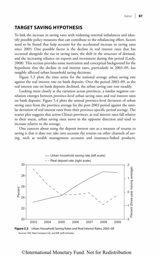
Nabar 87
TARGET SAVING HYPOTHESIS
To link the increase in saving rates with widening external imbalances and iden-tify possible policy measures that can contribute to the rebalancing effort, factors need to be found that help account for the accelerated increase in saving rates since 2003. One possible factor is the decline in real interest rates that has occurred alongside the rise in saving rates, the shift in the structure of demand, and the increasing reliance on exports and investment during this period (Lardy, 2008). This section provides some motivation and conceptual background for the hypothesis that the decline in real interest rates, particularly in 2003–09, has tangibly affected urban household saving decisions.
Figure 5.3 plots the time series for the national average urban saving rate against the real interest rate on bank deposits. Over the period 2003–09, as the real interest rate on bank deposits declined, the urban saving rate rose steadily.
Looking more closely at the variation across provinces, a similar negative cor-relation emerges between province-level urban saving rates and real interest rates on bank deposits. Figure 5.4 plots the annual province-level deviation of urban saving rates from the province average for the post-2003 period against the simi-lar deviation of real interest rates from their province-specific period average. The scatter plot suggests that across China’s provinces, as real interest rates fall relative to their mean, urban saving rates move in the opposite direction and tend to increase relative to the average.
One concern about using the deposit interest rate as a measure of returns to saving is that it does not take into account the returns on other channels of sav-ing, such as wealth management accounts and insurance-linked products.
Figure 5.3 Urban Household Saving Rates and Real Interest Rates, 2003–09Sources: CEIC Data Company Ltd.; and IMF staff estimates.
−2
−1
0
1
2
20
22
24
26
Per
cent
Per
cent
(thr
ee-y
ear m
ovin
g av
erag
e)
28
30
2003 2004 2005 2006 2007 2008 2009
Urban household saving rate (left scale)Real deposit rate (right scale)
©International Monetary Fund. Not for Redistribution
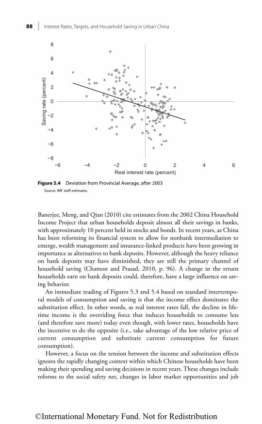
88 Interest Rates, Targets, and Household Saving in Urban China
Banerjee, Meng, and Qian (2010) cite estimates from the 2002 China Household Income Project that urban households deposit almost all their savings in banks, with approximately 10 percent held in stocks and bonds. In recent years, as China has been reforming its financial system to allow for nonbank intermediation to emerge, wealth management and insurance-linked products have been growing in importance as alternatives to bank deposits. However, although the heavy reliance on bank deposits may have diminished, they are still the primary channel of household saving (Chamon and Prasad, 2010, p. 96). A change in the return households earn on bank deposits could, therefore, have a large influence on sav-ing behavior.
An immediate reading of Figures 5.3 and 5.4 based on standard intertempo-ral models of consumption and saving is that the income effect dominates the substitution effect. In other words, as real interest rates fall, the decline in life-time income is the overriding force that induces households to consume less (and therefore save more) today even though, with lower rates, households have the incentive to do the opposite (i.e., take advantage of the low relative price of current consumption and substitute current consumption for future consumption).
However, a focus on the tension between the income and substitution effects ignores the rapidly changing context within which Chinese households have been making their spending and saving decisions in recent years. These changes include reforms to the social safety net, changes in labor market opportunities and job
Figure 5.4 Deviation from Provincial Average, after 2003Source: IMF staff estimates.
−8
−6
−4
−2
0
2
4
6
8
−6 −4 −2 0 2 4 6
Sav
ing
rate
(per
cent
)
Real interest rate (percent)
©International Monetary Fund. Not for Redistribution
Nabar 89
security, shifting aspirations with regard to the purchase of consumer durables and housing, demographic changes associated with an aging population and skewed gender ratios, and significant changes in investment returns on household saving portfolios.
In such a rapidly changing environment, with limited use of financial services such as consumer loans, insurance, and annuities, households may instead aim to self-insure and build a buffer against income and health shocks, or target a level of wealth accumulation (relative to income) to purchase indivisible consumer durables.3 In this case, the low returns on saving may cause the actual level of wealth to fall below the targeted level of wealth and induce households to save more to make up the shortfall.4
The notion that households behave as though they have some target in mind and base their decisions on wanting to achieve their target has been explored in various contexts. In the macroeconomics literature, Carroll (1997, 2001) devel-ops buffer-stock models of saving in which households choose consumption levels in each period with the intention of meeting a target wealth-to-income ratio that determines how much of their future consumption will rely on returns from capital relative to labor income. Households adjust their current consumption (and hence their saving) depending on where the actual wealth-to-income ratio is relative to its target level. Batini, N’Diaye, and Rebucci (2005); Laxton, N’Diaye, and Pesenti (2006); and Pesenti (2008) develop open economy dynamic stochastic general equilibrium models in which interna-tional portfolio diversification is based on a target net foreign asset position, derived from financial intermediaries’ assessment of the optimal exposure to the global economy.
Targets have also been studied in the micro literature. Camerer and others (1997) study the labor supply decisions of New York City cab drivers. Their research concludes that the cab drivers allocate their labor supply with a target income for the day in mind. When the drivers reach their target, the probabil-ity of quitting for the day rises sharply. On days when fares are easy to come by, the drivers reach their target relatively quickly and then substitute leisure for labor.
The empirical literature on household saving in China has already pointed to indirect evidence in support of the target saving hypothesis (Chamon and Prasad, 2010). When real interest rates decline, as they have in recent years, wealth is eroded, leading households to save more to replenish depleted wealth in much the same way as, on slow fare days, New York City cab drivers have to ply more routes for longer hours to meet their income targets.
3 This is not to suggest that households target a particular fixed level of wealth or saving. As the scale of the economy grows and income rises, the actual targeted wealth or saving will also evolve in line with other indicators. 4 The intuition is seen easily in a simple two-period model as outlined in Nabar (2011).
©International Monetary Fund. Not for Redistribution

90 Interest Rates, Targets, and Household Saving in Urban China
The empirical analysis in the next section studies this hypothesis at length by looking at developments since 1996 and then by splitting the sample into two subperiods, 1996–2002 and 2003–09.
EMPIRICS
Data and Descriptive Statistics
The data for this study are drawn from annual editions of the China Statistical Yearbook and Urban Household Income and Expenditure Surveys (both issued by the National Bureau of Statistics). The variables included in the analysis proxy for the main saving motives studied in previous research (summarized above). The sample covers all 31 provinces, federal municipalities, and autonomous regions for the period 1996–2009.
Table 5.1 reports descriptive statistics for the main variables of interest. The household saving rate is calculated using annual per capita provincial data on urban disposable income and urban consumption expenditure. The real interest rate is calculated using the one-year nominal interest rate on bank deposits deflated by province-level annual inflation. As seen from the table, the averages for the two series move in opposite directions across the two subintervals.
At the same time, several notable changes have occurred during this period that are likely to have had some bearing on saving decisions. Income volatility has increased, leaving workers exposed to more variable earnings. The age distribu-tion of the population has shifted to the right, with a slight increase in the elderly dependency ratio and an appreciable decline in the child dependency ratio—both demographic shifts suggest that life-cycle saving influences could also have had an impact on household saving rates during this time. Signs of SOE reform and restructuring are evident in the sharp decline in the fraction of work-ers employed by SOEs, a change that has left workers with a less comprehensive safety net than they had been accustomed to. Finally, real property price growth accelerated during the second half of the sample, and average household size declined. Both developments point to rising demand for residential property and increases in home ownership, changes that could have accelerated the increase in saving rates to finance purchases of housing and other durable assets. As discussed in more detail below, these changes could have also simultaneously affected the real interest rate even as they had an impact on saving decisions, which would be an argument for their inclusion in the empirical analysis to avoid problems of omitted variable bias.
The remainder of this section provides estimates of the influence of these various determinants and assesses what impact the decline in real interest rates has had on urban household saving rates. Baseline estimates from three different specifications are presented first, before robustness tests are conducted using the variables listed in Table 5.1.
©International Monetary Fund. Not for Redistribution

Nabar 91
Baseline Estimates
The main specification is
, 1 , 2 , ,j t j j t j t j ts X rμ β β ε= + + + , (5.1)
in which the saving rate is regressed on a vector of covariates X and the real inter-est rate. In the baseline version, the covariates include the growth rate of income and volatility. Additional controls are introduced in the robustness tests.
The main coefficient of interest is b2. A statistically significant finding of b2 < 0 would indicate that the decline in real interest rates since the 1990s could have potentially contributed to the increase in the saving rate.
TABLE 5.1
Descriptive Statistics for Household Saving Analysis
Variable Description
Full Sample
(1996–2009)
Subsample
(1996–2002)
Subsample
(2003–09)
Urban household saving rate
Percent of disposable income 22.8 20.0 25.5(5.2) (3.9) (5.0)
Real interest rate Percent, per year 1.4 2.9 -0.1(2.5) (2.1) (1.8)
Growth rate of dis-posable income
Percent 10.6 10.6 10.6(4.0) (5.2) (2.1)
Income volatility Percent (coefficient of variation, disposable income growth)
13.4 12.7 14.1(5.0) (6.4) (2.9)
Elderly dependency ratio
Population 65+/working-age population, percent
11.2 10.3 12.2(2.5) (2.3) (2.4)
Child dependency ratio
Population below 15/working-age population, percent
30.9 34.8 26.5(9.0) (8.3) (7.6)
SOE share Fraction of workers employed by SOEs
68.2 73.4 62.2(13.5) (10.2) (14.4)
Urban property income
Property income share of total disposable income
1.8 1.9 1.7(1.2) (1.3) (1.0)
Residential property prices
RMB/square meter 2,407.0 1,666.4 2,860.9(1,706.0) (892.6) (1,916.0)
Real property price growth (residential)
Year-over-year percent change 7.9 4.8 9.4(10.9) (9.7) (11.2)
Sex ratio Number of males per 100 females
103.8 104.7 103.1(3.5) (3.3) (3.39)
Household size Average number of residents in a household
3.5 3.7 3.3(0.5) (0.5) (0.43)
Administrative units Provinces, federal municipali-ties, autonomous regions
31 31 31
Observations Province-year units 429 212 217
Sources: China Statistical Yearbook, Urban Household Income and Expenditure Survey (National Bureau of Statistics).Note: Number of observations reported in each sample is for urban household saving rates; number of observations for
other variables vary depending on data availability. Standard deviation in parentheses. SOE = State-owned enter-prise.
©International Monetary Fund. Not for Redistribution

92 Interest Rates, Targets, and Household Saving in Urban China
Ordinary Least Squares (OLS) and Fixed Effects Table 5.2 reports results from the OLS and fixed effects regressions. The first column confirms a statistically significant negative correlation between real inter-est rates and urban saving rates across the sample. The magnitude is economi-cally significant as well. A decline in real interest rates from the average for the first half of the sample (2.9 percent) to the average for the second half of the sample (−0.1 percent) is associated with an increase in the saving rate of approxi-mately 1½ percentage points.
The two other covariates included in the regression are standard proxies for life-cycle saving influences and precautionary saving motives (Kraay, 2000; Horioka and Wan, 2007).5 If the realized growth rate of income is regarded as a predictor of future income growth, an increase in the growth rate of income should be associated with a decrease in current saving rates because households will defer retirement saving to a future stage in the life cycle (Chamon, Liu, and Prasad, 2010). This prediction is borne out by the negative coefficient on the growth rate of mean disposable income in the first column. The OLS regression also indicates that higher income volatility is associated with an increase in the
5 The growth rate of mean disposable income is calculated as the annual percent change of four-year moving averages and the volatility of disposable income is calculated as the coefficient of variation over four-year windows.
TABLE 5.2
Baseline Regression Estimates
OLS Fixed Effects
(1) (2) (3) (4)
Real interest rate −0.483*** −0.550***(0.104) (0.0826)
Nominal interest rate −1.775***(0.235)
CPI inflation 0.0388(0.0701)
Growth rate of income −0.597** −0.779*** 0.327 −1.250***(0.244) (0.196) (0.236) (0.180)
Volatility of income 0.547*** 0.583*** 0.382** 1.011***(0.184) (0.160) (0.141) (0.145)
SAMPLE YEARS 1996–2009 1996–2009 1996–2009 1996–2009
Number of provinces, regions, municipalities
31 31 31 31
Observations 428 428 428 428R-squared 0.14 0.24 0.37 0.17
Source: IMF staff estimation.Note: Dependent variable: Urban saving rate. Robust standard error in parentheses. CPI = consumer price index;
OLS = ordinary least squares.*** Significant at the 1 percent level.** Significant at the 5 percent level.* Significant at the 10 percent level.
©International Monetary Fund. Not for Redistribution
Nabar 93
saving rate, suggesting that households hold back on consumption and prefer to build up their buffers against future shocks when income uncertainty increases.
The regression in the second column controls for time-invariant, province-level fixed effects. The fixed effects primarily capture locational differences (coastal versus interior provinces) that affect the economic environment in which the saving decisions are made and real interest rates are determined. The statistical significance and signs of all three coefficients are robust to this change in specifi-cation. In particular, the real interest rate continues to be negatively associated with the urban saving rate, suggesting that a decline in the rate of return on household saving leads to a compensating increase in the saving rate.
An immediate concern is that the real interest rate is simply reflecting varia-tions in the inflation rate rather than the financial (nominal) rate of return on bank deposits. The third and fourth columns report results from fixed effects regressions that separately introduce the nominal rate of return and the inflation rate. Although the nominal interest rate is administered centrally and is identical across provinces, its level varies over time. The effects can be distinguished from general year effects because there are multiple instances of the nominal interest rate remaining unchanged across years. In other words, the number of distinct observations for the nominal interest rate is fewer than the number of years in the sample. Of course, if an omitted variable changes at exactly the same time as the nominal interest rate, inference on the effects of the nominal interest rate will be prevented, but this seems unlikely. The results in the third and fourth columns indicate that the coefficient on the nominal interest rate is negative and signifi-cant, but that a statistically significant relationship between inflation and the saving rate is absent. This suggests that it is indeed the financial rate of return that seems to matter for the effect of the real interest rate reported in the first and second columns.
Panel Generalized Method of Moments (GMM) EstimationTo allow for the possibility that saving behavior is persistent, the regressions in Table 5.3 introduce lagged saving rates to the set of regressors. Because the intro-duction of the lagged dependent variable biases fixed effects estimates, the speci-fication used is Arellano-Bond panel GMM estimation, which allows for the inclusion of the lagged saving rate along with other explanatory variables.
The first column shows that the relationship is robust to this change in speci-fication. However, when the sample period is split into the two subintervals (1996–2002 and 2003–09), as seen from Columns 2 and 3, the effect is signifi-cant only in the second subperiod. This suggests that the association has emerged in recent years, as the decline in real interest rates has become more entrenched.
Columns 4–6 repeat the specifications but for a smaller sample that excludes the five autonomous regions (Guangxi, Inner Mongolia, Ningxia, Xinjiang, Xizang/Tibet).6 The pattern is robust to focusing only on the smaller subset of
6 Variations in population policy, which affect the ethnic populations in the autonomous regions dif-ferently from the rest of the country, may introduce differences in saving behavior between the
©International Monetary Fund. Not for Redistribution

94 Interest Rates, Targets, and Household Saving in Urban China
provinces: Even after the autonomous regions are excluded, the association between real interest rates and urban saving rates is negative and significant in the second half of the sample period. The absolute value of the coefficient on the real interest rate in Column 6 is slightly smaller than the corresponding coefficient in Column 3, suggesting that saving rates are slightly less responsive to changes in the interest rate in the group of 26 provinces and federal municipalities than they are for the larger sample covering all 31 province-level administrative units.
Robustness: Additional Controls
Although the panel GMM estimation controls for the two main variables used in province-level macro analyses of the determinants of saving rates in China (growth rate of disposable income and volatility), concerns remain that the coef-ficient on the real interest rate may be soaking up the influence of other omitted variables that affect the saving rate. This subsection considers the main hypothesis
autonomous regions as a group and the rest of the country. See Gu and others (2007) on the exemp-tions to the One Child Policy and details of variations in implementation across the provinces.
TABLE 5.3
Baseline Estimates, Split Samples
(1) (2) (3) (4) (5) (6)
Lagged saving rate 0.736*** 0.192 0.720*** 0.638*** 0.161 0.593***(0.0740) (0.128) (0.108) (0.0364) (0.115) (0.0778)
Real interest rate −0.167* 0.148 −0.177*** −0.110 0.114 −0.155**(0.0860) (0.144) (0.0680) (0.0747) (0.137) (0.0702)
Growth rate of income
−0.0549 −0.487** 0.303 −0.120 −0.536*** 0.0227(0.110) (0.201) (0.191) (0.124) (0.205) (0.271)
Volatility of income 0.0340 0.317** −0.00429 0.0864 0.337** 0.172(0.0945) (0.160) (0.128) (0.104) (0.162) (0.156)
SAMPLE YEARS 1996–2009 1996–2002 2003–09 1996–2009 1996−2002 2003−09
Autonomous regions included
YES YES YES NO NO NO
Number of provinces, regions, municipalities
31 31 31 26 26 26
Observations 394 177 217 335 153 182Arellano-Bond test of
no second-order autocorrelation in first-differenced errors (p-value)
0.57 0.88 0.51 0.51 0.70 0.80
Source: IMF staff estimations.Note: Dependent variable: Urban saving rate. Panel generalized method of moments estimation. Robust standard errors
in parentheses. *** Significant at the 1 percent level.** Significant at the 5 percent level.* Significant at the 10 percent level.
©International Monetary Fund. Not for Redistribution

Nabar 95
put forward from the survey-based micro literature. All regressions are estimated for the period 2003–09, during which the negative association between real inter-est rates and urban saving rates appears to have emerged.
Age DistributionAs noted above, the age structure of the population has been changing rapidly in China, in part as a result of the One Child Policy instituted in the 1970s, in part due to improvements in health care, and also because of changes in desired fertil-ity. Changes in the age structure could potentially trigger changes in spending patterns that influence consumer prices and thus the real interest rate, even as they directly influence the saving rate. This would point to potential omitted variables bias in the baseline regressions reported in Tables 5.2 and 5.3.
Table 5.4 reports results from regressions that include the elderly dependency ratio and the child dependency ratio measured by province. Columns 1 and 2 report the effects of the elderly dependency ratio for the full set of provinces and for the subset excluding the autonomous regions, respectively. The relationship between the real interest rate and the saving rate is robust to the inclusion of the elderly dependency ratio, and the magnitude itself is larger than in the baseline (Table 5.3, Columns 3 and 6). The coefficient on the elderly dependency ratio itself is robust and suggests that as the population ages, saving rates increase, pos-sibly to finance larger health expenditures.
TABLE 5.4
Analysis of Saving Rate, Controlling for Age Structure
(1) (2) (3) (4)
Lagged saving rate 0.653*** 0.446*** 0.485*** 0.326***(0.123) (0.101) (0.0732) (0.110)
Real interest rate −0.315** −0.204*** 0.00871 −0.0459(0.153) (0.0733) (0.115) (0.104)
Growth rate of income 0.199 0.0782 0.129 0.169(0.255) (0.299) (0.239) (0.255)
Volatility of income 0.0257 0.178 −0.0196 0.112(0.138) (0.149) (0.131) (0.147)
Elderly dependency ratio 0.351* 0.190(0.182) (0.181)
Child dependency ratio −0.597** −0.306**(0.262) (0.148)
SAMPLE YEARS 2003–09 2003–09 2003–09 2003–09
Autonomous regions included YES NO YES NONumber of provinces, regions, municipalities 31 26 31 26Observations 186 156 186 156Arellano-Bond test of no second-order autocorrela-
tion in first-differenced errors (p-value)0.49 0.99 0.58 0.96
Source: IMF staff estimations.Note: Dependent variable: Urban saving rate. Panel generalized method of moments estimation. Robust standard errors
in parentheses.*** Significant at the 1 percent level.** Significant at the 5 percent level.* Significant at the 10 percent level.
©International Monetary Fund. Not for Redistribution
96 Interest Rates, Targets, and Household Saving in Urban China
The final two columns report estimates from regressions that include the child dependency ratio. The coefficient on the real interest rate is no longer statistically significant. Although the coefficient is not statistically significant, the negative relationship between the real interest rate and the urban saving rate emerges in the sample that excludes autonomous regions. The child dependency ratio itself is associated negatively with the saving rate, suggesting that children and financial saving are possible substitutes in the sense that as the number of children declines, the potential for intergenerational transfers later in life dimin-ishes, leading parents to save more today. As Columns 3 and 4 demonstrate, the effect is present regardless of whether the entire set of provinces is included or only the subset excluding the autonomous regions is examined. Thus, variations in the implementation of the One Child Policy across the autonomous regions compared with the remaining provinces do not seem to affect the relationship between the child dependency ratio and the urban saving rate. It is therefore difficult to establish whether changes in desired fertility or the effects of the policy lie behind the negative relationship between the child dependency ratio and the urban saving rate.
Employment Structure and Sources of Household Income The SOE reform and restructuring of the 1990s, involving mass layoffs and downsizing,7 introduced significant and far-reaching changes in labor market prospects, retirement income security, health insurance, and ownership of the urban housing stock. Such a shift in the implicit social safety net would be expected to trigger large changes in household spending and saving decisions. Comparing across provinces and over time, as SOE influence declines (captured by SOE share of employees), a rise in saving rates should appear to protect against the higher uncertainty to which the workers formerly employed by SOEs are now exposed.
If SOE reform and restructuring also affected production and distribution networks and introduced significant province-level variation in pricing of con-sumer products, the reforms would have been associated with fluctuations in the underlying structural inflation rate across provinces, and thus the real interest rate. Columns 1 and 2 of Table 5.5 include the SOE share of employment as an additional robustness check. The relationship between the real interest rate and the household saving rate is robust to including this proxy for the erosion of the implicit social safety net previously provided by SOEs. Furthermore, the coeffi-cient on the SOE share goes in the direction predicted by theory. As the SOE share declines, household saving rates rise to strengthen household defenses against higher income volatility and a less comprehensive social insurance mechanism.
Along with SOE reform, in the 1990s households also received a large transfer from the state in the form of residential property stock and the potential for
7 The number of SOEs went from 120,000 in the mid-1990s to 31,750 in 2004 and nearly 40 percent of the SOE workforce was laid off during this time; see Naughton (2007) for details.
©International Monetary Fund. Not for Redistribution

Nabar 97
another form of income through rents. To the extent that provinces where house-holds have come to rely on property income as a more important source of dis-posable income also experienced more rapid increases in inflation (which trig-gered larger declines in the real interest rate), a regression that fails to include property income share as an additional control will be subject to omitted variable bias. To address this concern, Columns 3 and 4 report results from regressions in which the property income share of household disposable income is included as an additional control. The relationship between the real interest rate and the urban household saving rate is robust to including this additional control. The sign on the coefficient itself suggests that in provinces where households depend more on property income, households tend to have higher saving rates out of disposable income, possibly because more productive saving opportunities are available (such as through the purchase of residential property that can then be rented out).
Saving to Buy Property The privatization of the urban housing stock that started in the late 1990s intro-duced a noticeable change in household tenure choices with an increasing frac-tion of urban households choosing to buy homes (by 2005, the proportion of owner-occupied urban housing units had exceeded 80 percent, up from
TABLE 5.5
Analysis of Saving Rate, Controlling for SOE Share of Employment, Property Income Share
(1) (2) (3) (4)
Lagged saving rate 0.630*** 0.307*** 0.579*** 0.432***(0.143) (0.113) (0.0751) (0.0982)
Real interest rate −0.259** −0.177** −0.286** −0.192***(0.128) (0.0722) (0.127) (0.0731)
Growth rate of income −0.0758 0.0321 −0.0168 0.0549(0.264) (0.250) (0.294) (0.271)
Volatility of income 0.0699 0.0966 0.0402 0.160(0.113) (0.130) (0.137) (0.147)
SOE share of employment −0.231*** −0.208***(0.0668) (0.0589)
Property income share 1.939* 0.669**(1.054) (0.314)
SAMPLE YEARS 2003–09 2003–09 2003–09 2003–09
Autonomous regions included YES NO YES NONumber of provinces, regions, municipalities 31 26 31 26Observations 186 156 186 156Arellano-Bond test of no second-order autocorre-
lation in first-differenced errors (p-value)0.45 0.94 0.48 0.90
Source: IMF staff estimations.Note: Dependent variable: Urban saving rate. Panel generalized method of moments estimation. Robust standard errors
in parentheses. SOE = State-owned enterprise.*** Significant at the 1 percent level.** Significant at the 5 percent level.* Significant at the 10 percent level.
©International Monetary Fund. Not for Redistribution

98 Interest Rates, Targets, and Household Saving in Urban China
48 percent in 1999; Naughton, 2007, p. 123). Housing finance options have remained limited, however, because bank lending continues to be primarily focused on enterprises (only 13 percent of the outstanding loan portfolio as of end-2010 was allocated to residential mortgages). As a result, one possible expla-nation for the rapid increase in household saving is that it is intended for housing purchase. In an environment in which home ownership is increasingly wide-spread, saving decisions would be expected to conform over time as households plan for an eventual home purchase.
To the extent that rapid house price increases are associated with other rela-tively more rapid general consumer price growth, residential property prices could have a negative association with real interest rates even as they are positively associated with the urban saving rate. This raises yet another concern of omitted variable bias in the regressions reported in Table 5.3.
The regressions reported in Table 5.6 use two proxies to control for the influ-ence of the property motive: the level of the residential property price and the growth rate of real property prices. Columns 1 and 2 indicate that the association between the real interest rate and urban saving rates is robust to including the level of the residential property price. The pattern is repeated in Columns 3 and 4, in which the growth rate of real property prices is introduced. The property motive itself is significant in the first two columns, indicating that urban saving rates tend to be higher in provinces with high levels of property prices.
TABLE 5.6
Analysis of Saving Rate, Controlling for Property Prices
(1) (2) (3) (4)
Lagged saving rate 0.617*** 0.385*** 0.712*** 0.733***(0.0598) (0.0789) (0.0400) (0.0789)
Real interest rate −0.254*** −0.191*** −0.177** −0.144*(0.0788) (0.0628) (0.0799) (0.0733)
Growth rate of income −0.233 −0.135 0.294 0.154(0.301) (0.252) (0.201) (0.278)
Volatility of income 0.0952 0.111 0.000660 0.147(0.125) (0.136) (0.129) (0.168)
Property price level 3.283*** 3.335***(0.807) (0.669)
Real property price growth 0.000693 −0.00841(0.0113) (0.0127)
SAMPLE YEARS 2003–09 2003–09 2003–09 2003–09
Autonomous regions included YES NO YES NONumber of provinces, regions, municipalities 31 26 31 26Observations 217 182 217 182Arellano-Bond test of no second-order autocor-
relation in first-differenced errors (p-value)0.50 0.89 0.14 0.11
Source: IMF staff estimation.Note: Dependent variable: Urban saving rate. Panel generalized method of moment estimation. Robust standard error in
parentheses. *** Significant at the 1 percent level.** Significant at the 5 percent level.* Significant at the 10 percent level.
©International Monetary Fund. Not for Redistribution

Nabar 99
Additional Household Attributes A final set of robustness checks introduces the gender ratio and average household size as additional controls. The gender composition of the population may influ-ence marriage prospects, household formation, and the impulse to save to purchase a home (Wei and Zhang, 2011). To the extent that marriages are largely formed within the province (i.e., few matches take place across provinces), provincial variation in the gender composition (number of males per 100 females) can be used as a proxy for the household-formation motive for saving.
Average household size reflects the influence that the number of coresidents may have on the saving rate of the average household. As household size increas-es, at least two possible effects on saving emerge. First, a larger household could imply more coresident adults (elderly, for example) and so greater possibilities to tap into resources accumulated through their past saving.
Second, variation in household size could also arise because of children in the home. Those households with a child may be relatively less concerned about sav-ing for retirement purposes than those households without a child because the possibilities for intergenerational transfers are greater in the first set.
As the first two columns in Table 5.7 indicate, introducing the variation of gender composition as an additional control does not affect the significance or the sign of the coefficient on the real interest rate. Gender composition itself
TABLE 5.7
Analysis of Saving Rate, Including Gender Ratios and Household Size
(1) (2) (3) (4)
Lagged saving rate 0.718*** 0.593*** 0.752*** 0.743***(0.0445) (0.0774) (0.0453) (0.0651)
Real interest rate −0.191** −0.159** −0.178** −0.193***(0.0836) (0.0704) (0.0870) (0.0733)
Growth rate of income 0.352** 0.0316 0.122 0.399(0.175) (0.269) (0.244) (0.272)
Volatility of income −0.0366 0.166 −0.115 −0.111(0.128) (0.152) (0.160) (0.182)
Sex ratio (number of males per 100 females) 0.104 0.0225(0.133) (0.0721)
Household size −4.594** −3.635***(2.060) (1.401)
SAMPLE YEARS 2003–09 2003–09 2003–09 2003–09
Autonomous regions included YES NO YES NONumber of provinces, regions, municipalities 31 26 31 26Observations 217 182 155 130Arellano-Bond test of no second-order autocor-
relation in first-differenced errors (p-value)0.14 0.80 0.78 0.39
Source: IMF staff estimation.Note: Dependent variable: Urban saving rate. Panel generalized method of moment estimation. Robust standard error in
parentheses. *** Significant at the 1 percent level.** Significant at the 5 percent level.* Significant at the 10 percent level.
©International Monetary Fund. Not for Redistribution

100 Interest Rates, Targets, and Household Saving in Urban China
does not have a significant effect on the urban saving rate. This may reflect, in part, two competing effects that cancel each other. A larger number of males relative to females may lead to lower saving for retirement because there may be an expectation of a greater degree of intergenerational transfer from the male child to the elderly parents relative to the transfers that potentially take place from a female child. But an increase in the sex ratio may increase the competi-tion for marriage matches and therefore strengthen motives to save to purchase a home.
Columns 3 and 4 introduce average household size as an additional control. The main coefficient of interest on the real interest variable continues to be negative and significant with the introduction of this new control. Average house-hold size itself is negatively associated with the urban saving rate: As household size declines across provinces and over time, the urban saving rate rises. The negative coefficient is consistent with the two possible explanations outlined above.8
As this section has demonstrated, the baseline estimates are robust to the inclu-sion of several additional controls, each of which could affect household saving and the real interest rate, as argued above. Nevertheless, these results should be interpreted with some caveats. First, other factors could also influence the prov-ince-level saving rate, such as changes in the household income and wealth distri-bution during the 1990s and 2000s. A more disaggregated, household-level data analysis would be required to capture the variation in saving rates induced by shifts in the income and wealth distribution. Second, differences in local govern-ment spending on social insurance versus physical infrastructure might introduce variations in provincial social safety nets. Since the global financial crisis, for example, numerous measures have been taken to enhance social safety nets. Access to primary health care has been improved through the construction of new health facilities. A new government health insurance program has been launched. The existing government pension scheme is being expanded to cover urban unemployed workers across the country, and the newly introduced rural pension scheme now covers 60 percent of all counties (see IMF, 2011, for more details). The SOE share variable used in the analysis here might not be adequately captur-ing these differences across provinces that could influence saving behavior. A more detailed breakdown of government expenditures would need to be included in the analysis to reflect the influence of social safety nets on household saving behavior.
The next section discusses possible policy options for increasing the return on saving within the broader agenda of financial reform in China.
8 See Nabar (2011) for additional tests that suggest if financial reform creates a greater menu of higher-paying saving options for households, households could substitute and switch their portfolios toward higher-return assets. In turn, households would find it easier to meet their target accumula-tion, meaning they could save less and consume more out of disposable income.
©International Monetary Fund. Not for Redistribution
Nabar 101
INTEREST RATE LIBERALIZATION AND FINANCIAL REFORM
China has made significant progress toward strengthening its financial system. Bank balance sheets have been made more robust by shifting nonperforming loans to asset management companies, and banks have subsequently been recapi-talized. The major banks have been listed on international stock exchanges, and the system has become more commercially oriented. Risk management standards have been enhanced and supervisory and regulatory capacity has been signifi-cantly widened to cover banking, insurance, and capital markets. Financial mar-ket development has proceeded at a steady pace on multiple fronts with the establishment of exchange-traded and interbank bond markets (IMF, 2011).
Nevertheless, as Table 5.1 and Figure 5.3 indicate, real interest rates have declined steadily since 2003. Banks have so far not had to compete aggressively for household deposits because the ceiling on deposit rates limits how far they can go to lure depositors away from competitors; furthermore, the combination of limited alternative saving options through nonbank channels and capital controls reduces contestability from outside the banking system. But, as attested to by the growing popularity of wealth management products, households would move deposits out of the banks to earn higher returns if given more choice regarding saving options. Greater flexibility and choice for household portfolio allocation would exert more competitive pressure on banks, raising interest rates and the return on household saving in the process.9
As outlined in previous IMF work in this area, interest rate liberalization would need to take place within the context of a financial reform agenda that is appropriately sequenced while also maintaining sufficient flexibility to adapt to evolving circumstances (IMF, 2011, and Chapter 13 of this volume). Before inter-est rates can be deregulated to enable them to guide the allocation of saving and credit in the system, the significant existing liquidity overhang in the financial system would need to be drained. Greater exchange rate flexibility, which would minimize the injection of liquidity via the balance of payments, and more use of central bank open market operations to influence interbank rates are essential prerequisites.
To minimize the risks of a disorderly liberalization, loosening of lending stan-dards, and a surge in credit, regulatory and supervisory capacity would need to be strengthened to close gaps in coverage. With surplus liquidity drained from the system and an enhanced regulatory framework in place, the authorities could begin liberalizing interest rates by lifting the deposit rate ceiling.
As interest rate liberalization proceeds and a strong regulatory framework is developed, a wider range of saving options could be made more easily accessible to households by encouraging greater participation of mutual funds, money mar-ket funds, and insurance-linked investment products in the capital market. This
9 Feyzioğlu, Porter, and Takáts (2009) use model-based simulations to show that interest rate liberal-ization in China would lift interest rates and the return on saving.
©International Monetary Fund. Not for Redistribution

102 Interest Rates, Targets, and Household Saving in Urban China
broader financial market development will, in time, cover a range of securities from equity to corporate fixed-income instruments to government bonds across the maturity spectrum.
Finally, the range of instruments and investment options can be expanded to include cross-border claims by removing capital controls and allowing for unre-stricted two-way flows of capital.10
Eventually, with this greater flexibility and choice in saving vehicles, house-holds will be able to achieve more efficient allocations of saving and extract higher returns from their portfolios. As demonstrated in the regression analysis, an increase in financial rates of return could potentially contribute to a decline in the share of household disposable income that is saved. Combined with the impact of higher interest rates on corporate saving and investment behavior (see Chapter 4 of this volume), the cumulative effect of financial reform on the sav-ing-investment imbalance would be large. An appropriately sequenced set of financial reforms, therefore, could have a substantial impact on rebalancing China’s economy.
CONCLUSION
This chapter argues that the increase in urban saving rates in China is linked, in part, to the decline in real interest rates, particularly after 2003. Although the result can be interpreted as a case of the income effect outweighing the substitu-tion effect, this would be a narrow reading of the context in which Chinese households have been making their saving decisions in recent years. In an envi-ronment in which the underlying fundamentals are changing as rapidly as has been the case in China since the late 1990s, a more relevant framework for analyz-ing saving responses is a target saving model. Chinese households appear to save to meet multiple needs, including self-insurance, retirement consumption, and purchase of durable assets, and act as though they have a saving target in mind. Changes in real interest rates affect the rate of return on household saving and the degree of difficulty in meeting that saving target. Since 2003, the decline in real interest rates seems to have lowered actual saving accumulation below the target. Households appear to have responded by boosting their rates of saving out of current disposable income to raise actual financial wealth closer to the target.
The relationship between real interest rates and the urban saving rate was found to be robust to the inclusion of other variables that proxy for commonly invoked savings impulses such as life-cycle considerations or the precautionary motive. The association was also found to be robust to changes in the sample of provinces, moving from the full set of China’s 31 provincial-level administrative units to a smaller subset that excludes the five autonomous regions.
10 Lardy and Douglass (2011) argue that interest rate liberalization must precede capital account lib-eralization to lower the risk of households transferring their deposits out of the banks and thereby undermining the stability of the domestic banking system.
©International Monetary Fund. Not for Redistribution

Nabar 103
The results of this study suggest that financial reform, a sustained increase in interest rates on bank deposits, and wider access to alternative investment oppor-tunities would make it easier for households to meet their target saving accumula-tion. To the extent this lowers saving out of current disposable income and increases private consumption, financial reform could potentially contribute sig-nificantly toward rebalancing China’s economy.
REFERENCES
Aziz, J., and L. Cui, 2007, “Explaining China’s Low Consumption: The Neglected Role of Household Income,” IMF Working Paper 07/181 (Washington: International Monetary Fund).
Banerjee, A., Xin Meng, and N. Qian, 2010, “The Life Cycle Model and Household Savings: Micro Evidence from Urban China” (unpublished; New Haven, Connecticut: Yale University).
Batini, N., P. N’Diaye, and A. Rebucci, 2005, “The Domestic and Global Impact of Japan’s Policies for Growth,” IMF Working Paper 05/209 (Washington: International Monetary Fund).
Blanchard, O., and F. Giavazzi, 2006, “Rebalancing Growth in China: A Three-Handed Approach,” CEPR Discussion Paper No. 5403 (London: Center for Economic Policy Research).
Cai, Fang, J. Giles, and Xin Meng, 2006, “How Well Do Children Insure Parents against Low Retirement Income? An Analysis Using Survey Data from Urban China,” Journal of Public Economics, Vol. 90, No. 12, pp. 2229–55.
Camerer, C., L. Babcock, G. Loewenstein, and R. Thaler, 1997, “Labor Supply of New York City Cabdrivers: One Day at a Time,” Quarterly Journal of Economics, Vol. 112, No. 2, pp. 407–41.
Carroll, C., 1997, “Buffer-Stock Saving and the Life Cycle/Permanent Income Hypothesis,” Quarterly Journal of Economics, Vol. 112, No. 1, pp. 1–55.
———, 2001, “A Theory of the Consumption Function, With and Without Liquidity Constraints,” Journal of Economic Perspectives, Vol. 15, No. 3, pp. 23–45.
Chamon, M., Kai Liu, and E. Prasad, 2010, “Income Uncertainty and Household Savings in China,” IMF Working Paper 10/289 (Washington: International Monetary Fund).
Chamon, M., and E. Prasad, 2010, “Why Are Saving Rates of Urban Households in China Rising?” American Economic Journal: Macroeconomics, Vol. 2, No. 1, pp. 93–130.
Feyzioğlu, T., N. Porter, and E. Takáts, 2009, “Interest Rate Liberalization in China,” IMF Working Paper 09/171 (Washington: International Monetary Fund).
Giles, J., and Ren Mu, 2007, “Elderly Parent Health and the Migration Decision of Adult Children: Evidence from Rural China,” Demography, Vol. 44, No. 2, pp. 265–88.
Giles, J., and K. Yoo, 2007, “Precautionary Behavior, Migrant Networks, and Household Consumption Decisions: An Empirical Analysis Using Household Panel Data from Rural China,” Review of Economics and Statistics, Vol. 89, No. 3, pp. 534–51.
Gu Baochang, Wang Feng, Guo Zhigang, and Zhang Erli, 2007, “China’s Local and National Fertility Policies at the End of the Twentieth Century,” Population and Development Review, Vol. 33, No. 1, pp. 129–47.
Guo, K., and P. N’Diaye, 2010, “Determinants of China’s Private Consumption: An International Perspective,” IMF Working Paper 10/93 (Washington: International Monetary Fund).
Horioka, C., and Junmin Wan, 2007, “The Determinants of Household Saving in China: A Dynamic Panel Analysis of Provincial Data,” Journal of Money, Credit, and Banking, Vol. 39, No. 8, pp. 2077–96.
©International Monetary Fund. Not for Redistribution

104 Interest Rates, Targets, and Household Saving in Urban China
International Monetary Fund (IMF), 2009, Regional Economic Outlook—Global Crisis: The Asian Context (Washington). http://www.imf.org/external/pubs/ft/reo/2009/APD/eng/areo0509.pdf.
———, 2011, “People’s Republic of China: Staff Report for the 2011 Article IV Consultation” (Washington). www.imf.org/external/pubs/ft/scr/2011/cr11192.pdf.
Kraay, A., 2000, “Household Saving in China,” World Bank Economic Review, Vol. 14, No. 3, pp. 545–70.
Kuijs, L., 2006, “How Will China’s Saving-Investment Balance Evolve?” World Bank Policy Research Working Paper No. 3958 (Washington: World Bank).
Lardy, N., 2008, “Financial Repression in China,” Policy Brief 08-8 (Washington: Peterson Institute for International Economics).
———, and P. Douglass, 2011, “Capital Account Liberalization and the Role of the Renminbi,” PIIE Working Paper 11-6 (Washington: Peterson Institute for International Economics).
Laxton, D., P. N’Diaye, and P. Pesenti, 2006, “Deflationary Shocks and Monetary Rules: An Open-Economy Scenario Analysis,” NBER Working Paper No. 12703 (Cambridge, Massachusetts: National Bureau of Economic Research).
Modigliani, F., and Shi Larry Cao, 2004, “The Chinese Saving Puzzle and the Life-Cycle Hypothesis,” Journal of Economic Literature, Vol. 42, No. 1, pp. 145–70.
Nabar, M., 2011, “Targets, Interest Rates and Household Saving in Urban China,” IMF Working Paper 11/223 (Washington: International Monetary Fund).
Naughton, B., 2007, The Chinese Economy: Transitions and Growth (Cambridge, Massachusetts: MIT Press).
Pesenti, P., 2008, “The Global Economy Model (GEM): Theoretical Framework,” IMF Staff Papers, Vol. 55, No. 2, pp. 243–84.
Wei, Shang-Jin, and Xiabo Zhang, 2011, “The Competitive Saving Motive: Evidence from Rising Sex Ratios and Savings Rates in China,” Journal of Political Economy, Vol. 119, No. 3, pp. 511–64.
©International Monetary Fund. Not for Redistribution
Implications for China’s Trading Partners
PART II
©International Monetary Fund. Not for Redistribution

This page intentionally left blank
©International Monetary Fund. Not for Redistribution

107
CHAPTER 6
Implications for Asia from Rebalancing in China
OLAF UNTEROBERDOERSTER
The second section of the book, beginning with this chapter, examines how China’s main trading partners have been affected by the developments analyzed in the first part. This chapter studies the implications for Asian economies of China’s declining external surplus. The rest of Asia has benefited from China’s strong domestic demand, in particular for commodities and capital goods, since the worldwide recession touched off by the 2008–09 global financial crisis. But even as China’s external surplus has declined, concern has arisen that new domestic imbalances may be emerging. As a result, Asian trading partners may face growing headwinds to their exports should China’s domestic imbalances eventually disrupt its high growth. The importance of vertical supply-chain linkages also suggests that trading partners’ exports to China would also be hurt if China’s exports were to slow.
INTRODUCTION
How China rebalances can have profound implications for Asian trading part-ners. For example, Asian capital goods and commodities exporters may benefit from continued strong Chinese investment demand, but could be in for a hard landing if Chinese investment is the source of growing domestic imbalances, as discussed in the preceding part of this book. However, consumption-based rebal-ancing in China would benefit those Asian trading partners with a relatively large share of consumer goods in their exports. To the extent that China’s exports may slow permanently relative to rapid growth during the first decade of the 2000s, exports of those Asian economies that are highly integrated in Chinese supply-chain networks may also slow. Therefore, to analyze the implications of China’s rebalancing, this chapter looks at the relative importance for different economies in the Asia region of China as a market for final goods, a supply-chain hub, and a potential competitor.
This chapter draws heavily on analysis of Asian supply-chain networks in Mohommad, Unteroberdoerster, and Vichyanond (2012), and analysis presented in IMF (2012).
©International Monetary Fund. Not for Redistribution

108 Implications for Asia from Rebalancing in China
CHINA AS A SOURCE OF REGIONAL FINAL DEMAND
Which economies in Asia will benefit from more domestic-demand-led growth in China? As highlighted in Chapter 1, it is important to distinguish between invest-ment- and consumption-based growth. Although China has become a growing source of demand for other economies in Asia, its demand for investment goods has risen more sharply than its demand for consumer goods, generally by a ratio of 2:1 (Figure 6.1).1 The traditional capital goods exporters in Asia—Japan and the Republic of Korea—have been particularly exposed to China’s investment demand.
High investment ratios in China may not be sustainable from a domestic perspective, but they may also fall if China’s export growth were to slow perma-nently. There is a close relationship between China’s investment and its exports. First, both exports and manufacturing fixed asset investment have been shifting from low- to high-tech products. Second, China’s major sources of foreign direct investment are aligned with its major import sources in the manufacturing pro-cess (Figure 6.2), which is a result of the growing vertical trade integration that has fueled China’s rise as a leading exporter (see discussion below).
Were China to rebalance through consumption-based growth, Association of Southeast Asian Nations (ASEAN) economies appear well positioned to benefit, given their relative strength in consumer goods exports. However, the benefits for regional trading partners may be small. First, despite rapid growth, China’s role
1 This estimate is based on value added–based trade flows that net out intermediate goods exports destined for third markets other than China.
Figure 6.1 Value Added Linked to China’s Final Demand: Selected Asian Economies (investment demand relative to consumption demand)
Sources: United Nations, Comtrade database; and IMF staff calculations.Note: ASEAN = Association of Southeast Asian Nations. * ASEAN includes Indonesia, Malaysia, the Philippines, Singapore, and Thailand.
0.0
0.2
0.4
0.6
0.8
1.0
Inve
stm
ent d
eman
d re
lativ
eto
con
sum
ptio
n de
man
d 1.2
1.4
1.6
ASEAN* Rep. of Korea Japan
2000 2010
TaiwanProvinceof China
©International Monetary Fund. Not for Redistribution
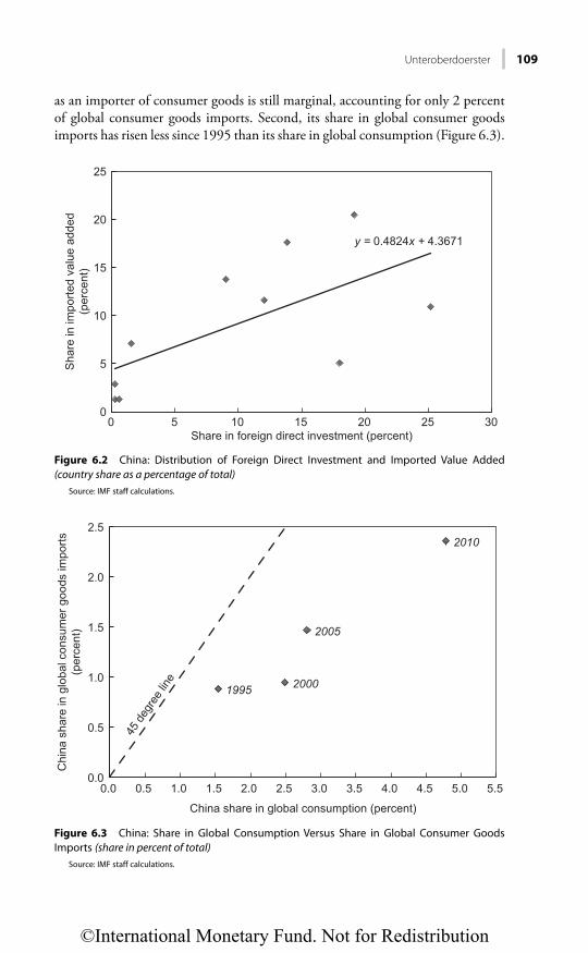
Unteroberdoerster 109
as an importer of consumer goods is still marginal, accounting for only 2 percent of global consumer goods imports. Second, its share in global consumer goods imports has risen less since 1995 than its share in global consumption (Figure 6.3).
Figure 6.2 China: Distribution of Foreign Direct Investment and Imported Value Added (country share as a percentage of total)
Source: IMF staff calculations.
y = 0.4824x + 4.3671
0
5
10
15
20
25
0 5 10 15 20 25 30
Sha
re in
impo
rted
valu
e ad
ded
(per
cent
)
Share in foreign direct investment (percent)
Figure 6.3 China: Share in Global Consumption Versus Share in Global Consumer Goods Imports (share in percent of total)
Source: IMF staff calculations.
1995 2000
2005
2010
0.0
0.5
1.0
1.5
2.0
2.5
0.0 0.5
45 d
egre
e lin
e
1.0 1.5 2.0 2.5 3.0 3.5 4.0 4.5 5.0 5.5
China share in global consumption (percent)
Chi
na s
hare
in g
loba
l con
sum
er g
oods
impo
rts(p
erce
nt)
©International Monetary Fund. Not for Redistribution
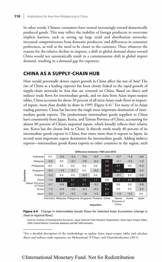
110 Implications for Asia from Rebalancing in China
In other words, Chinese consumers have turned increasingly toward domestically produced goods. This may reflect the inability of foreign producers to overcome implicit barriers, such as setting up large retail and distribution networks, increased competitiveness from domestic producers, and differences in consumer preferences, as well as the need to be closer to the customer. Thus, whatever the reasons for the relative decline in imports, a shift in global demand shares toward China would not automatically result in a commensurate shift in global import demand, resulting in a demand gap for exporters.
CHINA AS A SUPPLY-CHAIN HUB
How would potentially slower export growth in China affect the rest of Asia? The rise of China as a leading exporter has been closely linked to the rapid growth of supply-chain networks in Asia that are centered on China. Based on direct and indirect trade flows for intermediate goods, and on data from Asian input-output tables, China accounts for about 50 percent of all intra-Asian trade flows in import-ed inputs, more than double its share in 1995 (Figure 6.4).2 For many of its Asian trading partners, China has become the single most important destination of inter-mediate goods exports. The predominant intermediate goods suppliers to China have consistently been Japan, Korea, and Taiwan Province of China, accounting for almost 80 percent of China’s imported inputs, which broadly reflects their relative size. Korea has the closest link to China. It directly sends nearly 40 percent of its intermediate goods exports to China, four times more than it exports to Japan, its second most important export destination for intermediate goods. Adding indirect exports—intermediate goods Korea exports to other countries in the region, such
2 For a detailed description of the methodology to update Asian input-output tables and calculate direct and indirect trade exposures, see Mohommad, N’Diaye, and Unteroberdoerster (2011).
Figure 6.4 Change in Intermediate Goods Flows for Selected Asian Economies (change in share in regional flows)
Sources: Institute of Development Economics, Japan External Trade Research Organization, Asian Input Output Tables, 2000; United Nations, Comtrade database; and IMF staff estimates.
Japan
Korea
Taiwan Provinceof China
China
Thailand
0.0
Singapore
Philippines
Malaysia
Indonesia
Indonesia Malaysia Philippines Singapore Thailand China TaiwanProvince of
China
Korea Japan
Difference between 1995 and 2010
Expo
rter
s
Importers
0.0
−0.5
0.1
0.1
0.2 0.3
1.2
0.0 0.0
0.0
0.0
0.0
0.0
0.0
0.0
0.0
0.0
0.0 0.0
0.0
0.8
2.9
2.9
1.7
1.7
0.0
4.7
8.4
6.7
0.0
0.0
1.1 1.1
−0.5
−0.2
−0.2
−0.2
−0.2
−0.2
−2.2
−0.5
−0.8
−2.0
−1.4
−1.4
−0.7
−1.3
−3.3 −2.7
−0.2
−0.7 −1.8
−1.8 −6.6
−1.0
−0.7
−0.4
−0.4 −0.4
−0.4
−0.5
−0.6
0.0
−1.0
1.6
0.1
0.1
−0.1
−0.1
−1.6 −1.6
−0.1
−0.1
−0.1
4.2
−0.3
−0.3
−0.3
−0.3
−0.3
©International Monetary Fund. Not for Redistribution

Unteroberdoerster 111
as the ASEAN economies, that eventually find their way into Chinese produc-tion—Korea exports about 60 percent of its intermediate goods to China.
The effect of vertical trade integration appears to dominate export-demand relationships between China and its Asian trading partners. Overall, intermediate goods exports have accounted for about 70 percent of the annual export growth in Asia over the first decade of this century, more than double the contribution of final (consumer and capital) goods. Outsourcing to China is likely signifi-cantly stronger if capital goods exports as inputs are also considered (Figure 6.5). As noted in Chapter 1, China’s ascent as a leading exporter has been accompanied by the highest investment rates of any emerging market economy in recent decades. Capital goods exports to China now account for 20 to 25 percent of Japan’s and Korea’s total capital goods exports, making China by far their single most important capital goods export destination in Asia, and comparable to the United States or the European Union as export markets.
As a result of greater vertical integration, the correlation of Asian economies’ exports to China with Chinese exports has increased for most economies since 2000 (Figure 6.6).
Regression estimates suggest that a 1 percentage point drop in Chinese export growth would lower the growth of exports of other Asian economies to China by about ⅔ of 1 percentage point.3
At the same time, for most Asian countries for which exports are primarily in manufactured goods as opposed to commodities, exports to China are mainly a
3 Based on a country fixed-effects panel regression (1995–2010) of countries’ exports to China on the real bilateral exchange rate, Chinese real domestic demand, and Chinese real exports.
Figure 6.5 Japan and the Republic of Korea: Capital Goods Exports (by destination)Source: United Nations, Comtrade database; and IMF staff estimates.
0
5
10
15
20
25
30
35
40
1998–2000 2007–09 1998–2000 2007–09
China
Per
cent
of t
otal
exp
orts
United States Euro area
Japan Rep. of Korea
©International Monetary Fund. Not for Redistribution

112 Implications for Asia from Rebalancing in China
function of Chinese exports, rather than Chinese domestic demand, which would be suggested by standard trade models. By contrast, for those few economies in the region that export predominantly commodities, exports to China are deter-mined by Chinese domestic demand (Table 6.1).4
CHINA AS A COMPETITOR
Because of vertical trade integration, shifts in export (and import) market shares do not fully capture China’s changing role as a competitor to other Asian econo-mies. In fact, the increase of China’s share in leading markets, using gross exports based on direction of trade statistics, overstates its share on a value added basis netting out direct and indirect inputs from other Asian economies. In the United States, for example, China’s direct share of gross imports of final goods from Asia has increased to 62 percent in 2010, whereas, on a value added basis, China’s share is less than 50 percent (Figure 6.7). In other words, greater vertical special-ization has so far mitigated the impact of horizontal competition.
4 Consistent with the role of capital goods as imported inputs, Eichengreen, Rhee, and Tong (2007) find that Asian exports to China are positively affected by the growth of Chinese exports and “that this effect is mainly felt in markets for capital goods (p. 201).” Similarly, Johansson (2006) finds that inward foreign direct investment positively affects Chinese electronics exports, providing further evi-dence of outsourcing through investment.
Figure 6.6 Correlation of Exports to China with Exports from China for Selected Asian Economies (1 quarter lag)
Source: IMF staff calculations.
−0.1
0.0
0.1
0.2
0.3
0.4
0.5
New
Zea
land
Hon
g K
ong
SA
R
Phi
lippi
nes
Aus
tralia
Thai
land
Japa
n
Mal
aysi
a
Indo
nesi
a
Sin
gapo
re
Rep
. of K
orea
2000–05 2006–11
Taiw
anP
rovi
nce
of C
hina
©International Monetary Fund. Not for Redistribution

Unteroberdoerster 113
TABLE 6.1
Determinants of Asian Exports to China1
Chinese Domestic Demand Chinese Exports
Commodity exportersAustralia (1.79)Indonesia (0.68)New Zealand (1.66)
Manufacturing exporters
India (1.03) Hong Kong SAR (0.81)Japan (1.28)Korea (1.18)Malaysia (0.90)Philippines (2.95)Singapore (1.78)Thailand (1.37)
Source: IMF staff estimates.1Numbers in parentheses denote elasticity of exports to China at 5 percent level of significance. Shaded areas
indicate no significance at 5 percent level.
For more advanced economies in Asia, therefore, the increase in competition as China’s exports shift increasingly toward high-tech goods will also depend on China’s ability to capture a larger share of the value chain. Whereas the imported content in Chinese exports gradually increased through the mid-2000s, it started falling afterward.5 Going forward, these trends could be reinforced in the future by China’s rapid buildup in physical and human capital, allowing it to capture
5 IMF staff estimates based on Asian input-output tables suggest that the domestic value added in Chinese manufactured goods fell from about 90 percent in 1995 to 75 percent in 2005, but has increased since then to about 80–85 percent in 2010.
Figure 6.7 U.S. Imports from Asia for Final Demand, 2010 (market share by source)Source: IMF staff calculations.
0
10
20
30
40
50
60
70
80
90
100
Value added
Per
cent
Direction of trade
Other Asia Japan and Rep. of Korea China
©International Monetary Fund. Not for Redistribution

114 Implications for Asia from Rebalancing in China
large parts of the technology-intensive value chain. In addition, rising fuel and transportation costs could also lead to a partial reversal of vertical trade integra-tion by reducing the number of locations in a production chain.
CONCLUSION
China’s external trade surplus has fallen substantially. As discussed in Chapter 1, this decline mainly reflects a secular worsening of China’s terms of trade and robust import growth fueled by investment demand. Moreover, prospects for China to sustain the high export growth since 2003 remain uncertain. Taken together, while China’s external imbalances retreat, new domestic imbalances may be emerging. As a result, Asian trading partners that have benefited from invest-ment-led growth in China may face growing headwinds to their exports. Given the importance of vertical supply-chain links with China, they would also be hurt if China’s exports were to slow. By contrast, increasing direct and indirect access to the Chinese consumer goods markets could offer lasting benefits for Asian trading partners.
REFERENCES
Eichengreen, B., Y. Rhee, and H. Tong, 2007, “China and the Exports of Other Asian Countries,” Review of World Economics, Vol. 143, No. 2, pp. 201–26.
International Monetary Fund, 2012, Regional Economic Outlook: Asia and Pacific, April (Washington).
Johansson, F., 2006, “Chinese Export of Electrical Machinery Equipments: An Estimated Demand Function” (Jongkoping, Sweden: Internationella Handelshogskolan).
Mohommad, A., P. N’Diaye, and O. Unteroberdoerster, 2011, “Rebalancing Growth in Asia,” in Rebalancing Growth in Asia: Economic Dimensions for China, ed. by V. Arora and R. Cardarelli (Washington: International Monetary Fund).
Mohommad, A., O. Unteroberdoerster, and J. Vichyanond, 2012, “Implications of Asia’s Regional Supply Chain for Rebalancing Growth,” Journal of Asian Business, Vol. 25, No. 1, pp. 5–27.
©International Monetary Fund. Not for Redistribution

115
CHAPTER 7
Investment-Led Growth in China: Global Spillovers
ASHVIN AHUJA AND MALHAR NABAR
China’s growth model became increasingly dependent on investment during the first decade of the 2000s, and its footprint in global imports widened substantially. Several economies in China’s supply chain are increasingly exposed to the country’s investment-based growth and face growing risks from a deceleration in investment in China. This chapter quantifies potential global spillovers from an investment slowdown in China, finding that a 1 percentage point slowdown in investment in China is associated with a reduction of global growth of slightly less than one-tenth of a percentage point. The impact is about five times larger than in 2002. Regional supply chain economies and commodity exporters with relatively less diversified economies are most vulnerable to an investment slowdown in China. The spillover effects also register strongly across a range of macroeconomic, trade, and financial variables among G20 trading partners.
INTRODUCTION
China’s growth model became increasingly dependent on investment during the first decade of the 2000s. Investment contributed about ½ of China’s GDP growth during this time, with particularly large contributions toward the end of the decade. In part, this investment growth reflects the step increase in infrastruc-ture investment during the 2008–10 stimulus response to the global financial crisis. Investment as a share of GDP increased by close to 6 percentage points during this period (relative to precrisis), reaching 48 percent of GDP in 2010. However, it increasingly appears that other forces, including the ongoing urban-ization process, the more recent emphasis on social housing construction, and capacity building in high-end manufacturing and services, are also contributing to investment growth.
Associated with these changes in the profile of investment are important shifts in China’s import basket. As more of its manufacturing gets onshored, the share of machinery imports has been gradually declining (Figure 7.1). At the same time, with China increasingly drawing in larger volumes of minerals and metals, their share of total imports has grown steadily (Figure 7.2).
These developments have had a noticeable impact on global trade flows. Major exporters of commodities, capital goods, parts, and components have been sending
©International Monetary Fund. Not for Redistribution

116 Investment-Led Growth in China: Global Spillovers
an increasing fraction of their exports to China during the course of the decade (Figure 7.3). This change in trade flows reflects, to some extent, the fact that sup-ply chains have been increasingly routed through China as the final stage of assem-bly (see IMF, 2012, for more details).
The importance of exports to China, when assessed relative to trading part-ner GDP, shows even sharper increases for several economies. This ratio has, on
0
15
30
45
Mac
hine
ry
Per
cent
of t
otal
Min
eral
pro
duct
s
Met
als
Che
mic
al p
rodu
cts
Mac
hine
ry
Min
eral
pro
duct
s
Met
als
Che
mic
al p
rodu
cts
Mac
hine
ry
Min
eral
pro
duct
s
Met
als
Che
mic
al p
rodu
cts
Mac
hine
ry
Min
eral
pro
duct
s
Met
als
Che
mic
al p
rodu
cts
2002–04 2005–07 2008–09 2010–11
Figure 7.1 China: Composition of ImportsSources: CEIC Data; and IMF staff estimates.
0
50
100
150
200
250
300
350
Jan-05 Jul-06 Jan-08 Jul-09 Jan-11
Copper ore
Inde
x (2
005:
Q1
= 10
0)
Iron ore
Figure 7.2 Mineral Import Volumes (three-month moving average)Sources: CEIC Data; and IMF staff estimates.
©International Monetary Fund. Not for Redistribution

Ahuja and Nabar 117
average, quadrupled during the decade (Figure 7.4). Particularly exposed are Asian regional economies such as Taiwan Province of China, Malaysia, and the Republic of Korea—all of which are important exporters of capital goods, parts, and components for final assembly in China.
United StatesGermany
Japan
Australia
South AfricaBrazil
Chile
Percentage of exports destined for China, 2001
Per
cent
age
of e
xpor
ts d
estin
ed fo
r Chi
na, 2
011
PeruIran
Saudi Arabia
Taiwan Province of China Korea, Rep. of
MalaysiaPhilippines
Thailand
Zambia
Kazakhstan
0
5
10
15
20
25
30
35
40
0 5 10 15
2011
2001
Greater share of exportsgoing to China in 2011than in 2001
Figure 7.3 Exports to China as a Share of Total Exports, 2001 and 2011Source: IMF staff estimates.
GermanyJapan
AustraliaSouth AfricaBrazil
Chile
PeruIran
Saudi Arabia
Taiwan Province of China
Korea, Rep. of
Malaysia
Philippines
Thailand
Zambia
Kazakhstan
0
5
10
15
20
0 1 2 3 4 5
2001
2011
Exposure greaterin 2011 than in 2001
United States
Percentage of national GDP, 2001
Per
cent
age
of n
atio
nal G
DP,
201
1
Figure 7.4 Exports to China as a Share of National GDP, 2001 and 2011Source: IMF staff estimates.
©International Monetary Fund. Not for Redistribution

118 Investment-Led Growth in China: Global Spillovers
ASSESSING EXPOSURES TO INVESTMENT-LED GROWTH IN CHINA
China’s reliance on investment-based growth raises questions about how the new capacity will be used. Capacity that finds its way onto world markets by way of new exports and that is perceived to be putting downward pressure on global prices would create the potential for retaliatory trade actions that eventually come back to hurt the Chinese economy and slow investment (see Guo, 2011, for more details). Another possibility is that the new capacity remains underutilized, with adverse effects on bank balance sheets and credit conditions (which would make the financing of subsequent investment difficult). A rapid investment slowdown in China under either of these two outcomes will undoubtedly have a global impact, given China’s size and systemic importance.
To get a sense of the potential magnitudes, the spillover from China on trading partner j is measured as,
= ×, , j t j t tChina spillover exCHN China Fixed Investment growth , (7.1)
in which
⎛ ⎞= ⎜ ⎟⎝ ⎠
jj
toExportsexCHN
GDPchina . (7.2)
China Fixed Investment growtht is measured as the annual percentage change of real gross fixed capital formation from the national accounts. This spillover mea-sure varies across countries in a given year based on their export exposure to China and also varies over time based on fluctuations in China’s fixed investment growth. By construction, it only measures the influence of Chinese activity on other economies through the direct trade channel. Indirect trade exposures through vertically integrated intermediate economies are not captured. Another concern with this measure is that it does not reflect financial exposures, which would also have a bearing on growth in trading partners. However, with the comprehensive system of capital controls in place and the dominance of domestic sources of financing, the financial spillover channel is likely to be limited.
The effect of the spillover from China on trading partner growth is estimated using a broad sample of 64 economies exposed to China through the export chan-nel described above. The sample covers 2002–11 (starting with China’s entry into the World Trade Organization) and includes the full set of Organization for Economic Cooperation and Development economies, emerging markets classified under the MSCI index, and key commodity producers. The main specification is
α β β β
β
−= + + +
+ +
, 1 , 1 2 , 3 ,
4 , ,
.
j t j j t j t j t
j t j t
GDP growth GDP growth China spillover ToT
Volatility e (7.3)
©International Monetary Fund. Not for Redistribution

Ahuja and Nabar 119
The main coefficient of interest in this regression is b2, which captures the effect of spillovers from China’s investment activity on growth in trading partner j. Additional controls include partner country lagged growth, the annual percentage change in terms of trade (ToTj,t), and macroeconomic volatility (Volatilityj,t measured as the standard deviation of GDP growth calculated over moving five-year windows).
The regression is also estimated using different measures of fixed investment growth in China: overall, manufacturing, and nontradables.1 Manufacturing and nontradables fixed investment are calculated by applying shares from fixed asset investment data (available only from 2003 onward) to the national accounts series on real gross fixed capital formation. This breakdown allows for a comparison of likely effects from a slowdown in investment concentrated in manufacturing versus a deceleration concentrated in nontradables.
EFFECTS OF AN INVESTMENT SLOWDOWN IN CHINA
The impact of China’s investment-led growth on trading partners has strength-ened as China’s growth model tilts more toward investment and its global foot-print on imports widens (Annex 7A, Tables 7A.2–7A.5). Aggregating across all 64 economies (weighted by their purchasing power parity [PPP] shares), the impact on global growth of a 1 percentage point slowdown in investment in China is just under one-tenth of a percentage point. The impact is about five times larger than in 2002 (estimated to be 0.02 percentage point). The most heavily exposed economies are those within the Asian regional supply chain, such as Taiwan Province of China, Korea, and Malaysia (Figure 7.5). The results from Annex 7A, Table 7A.5 (estimated based on the sample years covering the global financial crisis and the stimulus response in China) suggest that if investment growth declines by 1 percentage point in China, GDP growth in Taiwan Province of China, for example, falls by slightly more than nine-tenths of a percentage point. Among the advanced economy exporters of capital goods, Japan suffers a decline of just over one-tenth of a percentage point in response, while growth in Germany declines by a slightly smaller amount.
Among commodity exporters, the impact of a slowdown in investment growth in China is likely to be largest on mineral ore exporters with relatively less diversi-fied economies and a higher concentration of exports to China. In response to a 1 percentage point slowdown in investment growth in China, the estimated effect on Chile’s growth is a reduction of close to two-fifths of a percentage point (Figure 7.6). By contrast, the larger commodity exporters with more diversified econo-mies, such as Australia and Brazil, suffer relatively smaller declines in growth.
A sectoral decomposition of China’s overall fixed investment in manufactur-ing and nontradables shows that the magnitude of spillovers from a slowdown in manufacturing nontradables fixed investment (NFI) are broadly similar to the
1 The nontradables sector is defined to include utilities, construction, transport and storage, informa-tion technology, wholesale and retail trade, catering, banking and insurance, real estate, leasing and commercial services, education, health care, sport and entertainment, and public administration.
©International Monetary Fund. Not for Redistribution
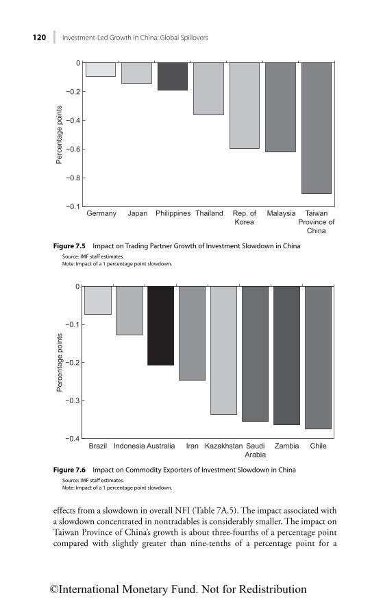
120 Investment-Led Growth in China: Global Spillovers
effects from a slowdown in overall NFI (Table 7A.5). The impact associated with a slowdown concentrated in nontradables is considerably smaller. The impact on Taiwan Province of China’s growth is about three-fourths of a percentage point compared with slightly greater than nine-tenths of a percentage point for a
−0.1
−0.8
−0.6
−0.4
−0.2
0
Germany
Per
cent
age
poin
ts
Japan Philippines Thailand Rep. ofKorea
Malaysia TaiwanProvince of
China
Figure 7.5 Impact on Trading Partner Growth of Investment Slowdown in ChinaSource: IMF staff estimates.Note: Impact of a 1 percentage point slowdown.
−0.4
−0.3
−0.2
−0.1
0
Brazil Indonesia
Per
cent
age
poin
ts
Australia Iran Kazakhstan SaudiArabia
Zambia Chile
Figure 7.6 Impact on Commodity Exporters of Investment Slowdown in ChinaSource: IMF staff estimates.Note: Impact of a 1 percentage point slowdown.
©International Monetary Fund. Not for Redistribution
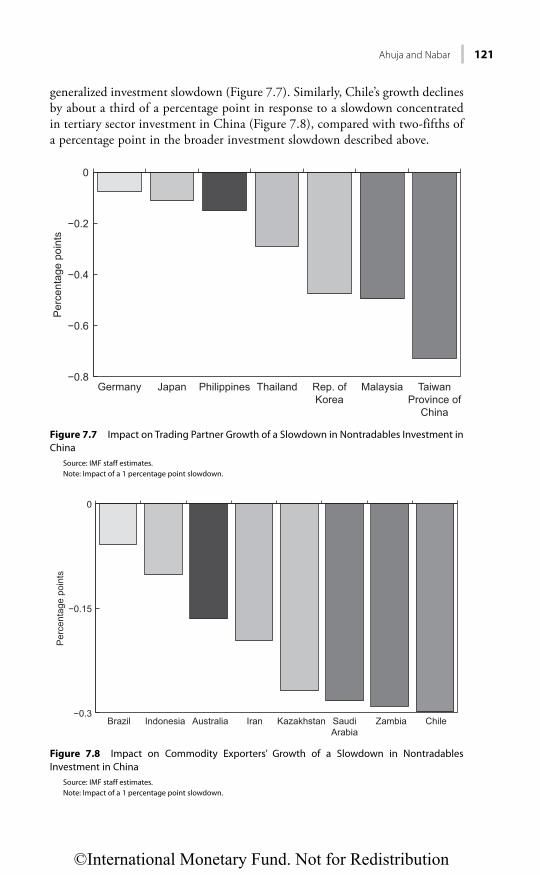
Ahuja and Nabar 121
generalized investment slowdown (Figure 7.7). Similarly, Chile’s growth declines by about a third of a percentage point in response to a slowdown concentrated in tertiary sector investment in China (Figure 7.8), compared with two-fifths of a percentage point in the broader investment slowdown described above.
−0.8
−0.6
−0.4
−0.2
0
Germany
Per
cent
age
poin
ts
Japan Philippines Thailand Rep. ofKorea
Malaysia TaiwanProvince of
China
Figure 7.7 Impact on Trading Partner Growth of a Slowdown in Nontradables Investment in China
Source: IMF staff estimates.Note: Impact of a 1 percentage point slowdown.
−0.3
−0.15
0
Brazil Indonesia
Per
cent
age
poin
ts
Australia Iran Kazakhstan SaudiArabia
Zambia Chile
Figure 7.8 Impact on Commodity Exporters’ Growth of a Slowdown in Nontradables Investment in China
Source: IMF staff estimates.Note: Impact of a 1 percentage point slowdown.
©International Monetary Fund. Not for Redistribution
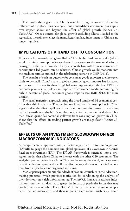
122 Investment-Led Growth in China: Global Spillovers
The results also suggest that China’s manufacturing investment reflects the influence of the global business cycle, but nontradables investment has a spill-over impact above and beyond the effect of global growth (Annex 7A, Table A7.6). Once a control for global growth excluding China is added to the regression, the spillover effect via manufacturing fixed investment in China is no longer significant.
IMPLICATIONS OF A HAND-OFF TO CONSUMPTION
If the capacity currently being installed in China is absorbed domestically (which would require consumption to accelerate in response to the structural reforms envisaged in the 12th Five-Year Plan), a smooth hand-off from investment- to consumption-led growth can be achieved. China’s growth would moderate into the medium term as outlined in the rebalancing scenario in IMF (2011).
The benefits of such an outcome for consumer goods exporters are, however, likely to be small. China’s share in global consumer goods imports has increased at a slower pace than its share in global consumption since the late 1990s. It currently plays a small role as an importer of consumer goods, accounting for only 2 percent of global consumer goods imports (see IMF, 2012, for more details).
The panel regression approach using the broad sample of 64 economies con-firms that this is the case. The low import intensity of consumption in China suggests that the direct spillover effect from consumption growth on trading partner growth is negligible. A similar exercise to the one outlined above, but that instead quantifies potential spillovers from consumption growth in China, shows that the effects on trading partner growth are insignificant (Annex 7A, Table 7A.7).
EFFECTS OF AN INVESTMENT SLOWDOWN ON G20 MACROECONOMIC INDICATORS
A complementary approach uses a factor-augmented vector autoregression (FAVAR) to gauge the domestic and global spillovers of a slowdown in China’s fixed asset investment (FAI). The FAVAR framework is extended into a two-region model that allows China to interact with the other G20 economies. The analysis captures the feedback from China to the rest of the world, and vice versa, over time. It also captures the spillover effect among the rest of the G20 econo-mies from a specific event originated in China.
Market participants monitor hundreds of economic variables in their decision-making processes, which provides motivation for conditioning the analysis of their decisions on a rich information set. The FAVAR framework extracts infor-mation from the rich data set to gauge the impact of particular forces that may not be directly observable. These “forces” are treated as latent common compo-nents that are interrelated, and their impacts on economic variables are traced
©International Monetary Fund. Not for Redistribution

Ahuja and Nabar 123
through impulse response functions. Accounting for unobserved variables pro-vides a better chance of avoiding findings based on spurious association.
Briefly, the model is a stable FAVAR in growth (except for balances and inter-est rates) with five common factors for each region (China and the rest of the G20 economies) and China’s FAI.2 The model uses one lag. The Cholesky factor from the residual covariance matrix is used to orthogonalize the impulses, thereby imposing an ordering of the variables in the VAR and treating investment as exogenous in the period of shock. The results are robust to reordering within fac-tor groups.
The data set is a balanced panel of 390 monthly time series from the G20 stretching from January 2000 to September 2011, with 68 China-specific vari-ables and 322 from the rest of the G20. The sample contains at least one full cycle of investment in China. It starts right before China’s entry into the WTO and spans the time when the country became increasingly integrated with the world economy.
Because the model is in growth, the experiment assumes an exogenous, tem-porary, one standard deviation growth shock to China’s FAI. The shock dampens within three quarters and dissipates fully after about 40 months. Specifically, this is a one-time 15 percentage point (seasonally adjusted, annualized) drop in FAI growth that largely reverts to trend growth within seven to eight months.3 Whereas this is a temporary, negative growth shock, the decline in FAI level is permanent. The shock is approximately equivalent to a 2½ percent drop from the real FAI baseline level in 12 months. The analysis does not assume any policy response beyond that already in the sample. Peak impacts in each 24-month period are reported with standard error bands in Figures 7.9–7.13. Impacts on levels 12 months after the shock, in percentage below baseline, are also derived and reported for comparison in Annex 7B, Tables 7B.1 and 7B.2.
A temporary shock to China’s FAI growth would reverberate around the world, with the spillover impacts on G20 economies dissipating after about five to eight quarters (Figures 7.9 and 7.10). In this exercise, the approximate impact on GDP growth would vary with the size of the industrial-production-to-GDP ratio in each economy.4 The implied peak impact on PPP-weighted G20 GDP growth is −0.2 percentage point, which translates to about 0.1 percent below baseline at 12 months after the shock originated in China (see Annex 7B, Table 7B.1). Overall, capital goods manufacturers that have sizable direct expo-sure to China (through exports to China as a percentage of own GDP) and are highly integrated with the rest of the G20 (therefore sharing adverse feedback
2 More detailed descriptions of the model and estimation strategy can be found in Ahuja and Myrvoda (2012). 3 A one standard deviation shock is equivalent to 1.2 percentage points in month-over-month, season-ally adjusted, growth rates.4 Industrial production is defined differently from country to country. The Organization for Economic Cooperation and Development definition includes production in mining, manufacturing, and public utilities (electricity, gas, and water), but excludes construction.
©International Monetary Fund. Not for Redistribution
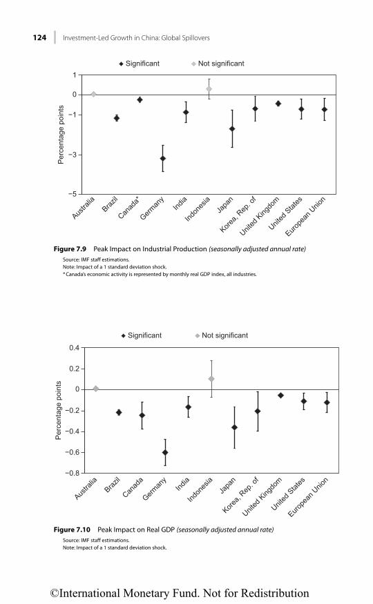
124 Investment-Led Growth in China: Global Spillovers
−5
−3
−1
1
0
Austra
liaBraz
il
Canad
a*
German
yInd
ia
Indon
esia
Japa
n
Korea,
Rep. o
f
United
King
dom
United
Stat
es
Europe
an U
nion
SignificantP
erce
ntag
e po
ints
Not significant
Figure 7.9 Peak Impact on Industrial Production (seasonally adjusted annual rate)Source: IMF staff estimations.Note: Impact of a 1 standard deviation shock.* Canada’s economic activity is represented by monthly real GDP index, all industries.
−0.8
−0.6
−0.4
−0.2
0
0.2
0.4
Austra
liaBraz
il
Canad
a
German
yInd
ia
Indon
esia
Japa
n
Significant Not significant
Korea,
Rep. o
f
United
King
dom
United
Stat
es
Europe
an U
nion
Per
cent
age
poin
ts
Figure 7.10 Peak Impact on Real GDP (seasonally adjusted annual rate)Source: IMF staff estimations.Note: Impact of a 1 standard deviation shock.
©International Monetary Fund. Not for Redistribution
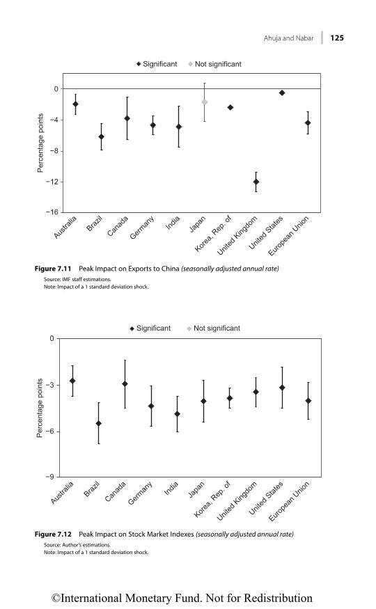
Ahuja and Nabar 125
−16
−12
−8
−4
0
Austra
liaBraz
il
Canad
a
German
yInd
iaJa
pan
Korea,
Rep. o
f
United
King
dom
United
Stat
es
Europe
an U
nion
Significant Not significant
Per
cent
age
poin
ts
Figure 7.11 Peak Impact on Exports to China (seasonally adjusted annual rate)Source: IMF staff estimations.Note: Impact of a 1 standard deviation shock.
−9
−6
−3
0
Austra
lia
Per
cent
age
poin
ts
Brazil
Canad
a
German
yInd
iaJa
pan
Korea,
Rep. o
f
United
King
dom
United
Stat
es
Europe
an U
nion
Significant Not significant
Figure 7.12 Peak Impact on Stock Market Indexes (seasonally adjusted annual rate)Source: Author’s estimations.Note: Impact of a 1 standard deviation shock.
©International Monetary Fund. Not for Redistribution

126 Investment-Led Growth in China: Global Spillovers
from a negative shock in China with other trading partners such as Germany and Japan) would see more of the impact on economic activity. One year out, the impact is also sizable for Canada. The impact on Indonesia’s output is not statis-tically significant over the entire period, likely because coal exports to China became important only toward the end of the first decade of the 2000s.
The results also show that global trade activity would decline (total exports and total imports for every G20 economy would weaken), which suggests that economies that derive significant benefit from global trade expansion and have deeper links via supply chain countries over the past decade, such as Germany and Japan, should be more hard hit in the second round (see also Chapter 8). The impact on Korea’s GDP peaks within the first two quarters and fades away more quickly, consistent with Korea’s large direct exposure to China, but second-round effects through supply chain countries are smaller than for Japan and Germany.
The slowdown in growth of exports to China for Brazil, India, and Korea mir-rors the impacts on their industrial production growth (Figure 7.11). For the United Kingdom, however, from which exports to China slow the most, the exports to China are not an important component of final demand, and the impact on economic activity looks to be moderate.5 Brazil, whose exports to China are agricultural and heavy in mineral commodities, would also experience nonnegligible spillover effects on export growth. Australia’s relatively large direct
5 Exports to China are mostly in machinery, equipment, and industrial supplies for the United Kingdom and mineral commodities and primary metal products for India. Canada’s exports to China are more diversified in minerals and manufactured commodities.
−10
−8
−6
−4
−2
0
2
Zinc Nickel
Per
cent
age
poin
ts
Lead Copper Aluminum Iron ore Silver Rubber Gold
Significant Not significant
Figure 7.13 Peak Impact on World Metal and Rubber Prices (seasonally adjusted annual rate)Source: Author’s estimations.Note: Impact of a 1 standard deviation shock.
©International Monetary Fund. Not for Redistribution

Ahuja and Nabar 127
exposure to China suggests a substantial direct impact, but other forces (e.g., the Australian dollar exchange rate behaves as a shock absorber) seem to blunt the effect on Australia’s industrial production, which accounts for about 20 percent of GDP. Nevertheless, other indicators, such as employment growth and total import growth (not shown here), point to a slowdown in Australia’s economic activity. Overall trade expansion with China would also slow as global and China demand growth weaken.
The spillover effects are also captured in asset prices (Figure 7.12). Specifically, the impact on the stock market indexes in G20 economies would be as large as 5–5½ percentage points in India and Brazil and between 4 and 4½ percentage points in the euro area, Germany, and Japan—and would last for as long as four to five quarters.
Even as nonfuel primary commodity price inflation—especially metal price inflation—retreats, the impact on global inflation appears to be almost negligible. A global growth slowdown, initiated by a temporary investment growth slow-down in China, would lead to a drop in iron ore, aluminum, copper, lead, nickel, and zinc price growth of as much as 3–9 percentage points (Figure 7.13). This is equivalent to a decline in price levels of about 2–5½ percent below baseline levels, one year out (see Annex 7B, Table 7B.2). How crude oil prices would be affected in this exercise is unclear (the impulse responses show a drop in crude price growth, with peak at about three quarters after impact, but the responses are not statistically significant).
The model suggests that the role of China’s investment drive in boosting construction-related metal prices between 2008 and 2011 has been significant. Annex 7B, Table 7B.4 reports the extent of China’s contribution to metal price growth during 2008–11, with the counterfactual (no investment drive) scenario assuming China’s real gross fixed capital formation had grown at the same pace as real GDP, so that the investment-to-GDP ratio was maintained at its end-2007 level.
CONCLUSION
A rapid investment slowdown in China is likely to have large spillover effects on a number of China’s trading partners. At the macro level, each 1 percentage point deceleration in China’s investment growth is estimated to subtract between one-half and nine-tenths of a percentage point from GDP growth in regional supply chain economies such as Taiwan Province of China, Korea, and Malaysia. Major commodity producers with relatively large exposures to China, such as Chile and Saudi Arabia, are also likely to suffer substantial growth declines in response to an investment deceleration in China.
The spillover effects from an investment slowdown in China also register strongly across a range of macroeconomic, trade, and financial variables among G20 trading partners as well as world commodity prices. Within this group, a decline in China FAI would have a substantial impact on capital goods manufac-turing economies with relatively sizable exports to China (as a percentage of own
©International Monetary Fund. Not for Redistribution

128 Investment-Led Growth in China: Global Spillovers
GDP) and that are highly integrated with the rest of the G20, such as Germany and Japan. For economies that rely less on China’s demand, such as the United Kingdom and India, the spillover effects on industrial production and aggregate output are moderate. Important commodities exporters, such as Canada and Brazil, would experience nonnegligible spillover effects on export growth, which would translate into somewhat significant output losses and slowdowns in overall economic activity. Worsened global growth prospects would also be reflected in commodity prices. One year after the shock, commodity prices, especially metal prices, could fall by as much as 0.8–2.2 percent from baseline levels for every 1 percent drop in China’s FAI.
©International Monetary Fund. Not for Redistribution

Ahuja and Nabar 129
ANNEX 7A. REGRESSION RESULTS AND CONTRIBUTIONS TO GROWTH FROM EXPORTS TO CHINA, SELECT ECONOMIES
Regression Results
TABLE 7A.1
Summary Statistics for Analysis of Investment Spillovers, 2002–11
Mean
Standard
Deviation Minimum Maximum
Year-over-year percent changeChina fixed investment 13.5 3.7 9.7 23.5China manufacturing fixed investment 16.6 2.9 11.0 20.6China nontradables fixed investment 11.4 6.2 5.6 26.8
Exports to China/GDP, percentAustralia 2.4 1.4 1.1 5.0Brazil 1.0 0.4 0.5 1.8Chile 4.7 2.2 1.8 8.0Germany 1.3 0.4 0.7 2.0Japan 2.1 0.6 1.0 2.8Korea 8.3 2.6 4.1 12.0Malaysia 8.6 3.2 5.2 16.6Taiwan Province of China 12.9 4.9 3.3 18.0United States 0.4 0.2 0.2 0.7
Sources: IMF, Direction of Trade Statistics and World Economic Outlook.
TABLE 7A.2
Fixed Effects Regression for WTO Period, 2002–11
Total Investment Manufacturing Nontradables
(1) (2) (3)
China spillover effect 0.0128*** 0.0381*** 0.0255***(0.00418) (0.0106) (0.00561)
Terms of trade 9.69e-06*** 0.000589 0.000260(1.85e-06) (0.00303) (0.00306)
Volatility of growth −0.424 −0.771*** −0.854***(0.271) (0.231) (0.247)
SAMPLE YEARS 2002–11 2002–11 2002–11
Number of countries 64 64 64Observations 640 448 448R-squared 0.03 0.13 0.14
Source: IMF staff estimations.Note: Dependent variable: Real GDP Growth, year-over-year percent change. Fixed effects estimation. Robust standard
errors in parentheses. *** Significant at 1 percent level.** Significant at 5 percent level.* Significant at 10 percent level.
©International Monetary Fund. Not for Redistribution

130 Investment-Led Growth in China: Global Spillovers
TABLE 7A.3
Fixed Effects Regression for Global Crisis and Stimulus Period, 2008–11
Total Investment Manufacturing Nontradables
(1) (2) (3)
China spillover effect 0.0741*** 0.0901*** 0.0561***(0.0105) (0.0201) (0.00747)
Terms of trade −0.00414 −0.00159 −0.00393(0.00433) (0.00428) (0.00433)
Volatility of growth −0.828*** −0.566*** −0.897***(0.146) (0.184) (0.141)
SAMPLE YEARS 2008–11 2008–11 2008–11
Number of countries 64 64 64Observations 256 256 256R-squared 0.2 0.14 0.21
Source: IMF staff estimations.Note: Dependent variable: Real GDP Growth, year-over-year percent change. Fixed effects estimation. Robust standard
errors in parentheses. *** Significant at 1 percent level.** Significant at 5 percent level.* Significant at 10 percent level.
TABLE 7A.4
Generalized Method of Moments Regression for WTO period, 2002–11
Total Investment Manufacturing Nontradables
(1) (2) (3)
Lagged GDP growth 0.230*** −0.127 −0.0751(0.0527) (0.0886) (0.0950)
China spillover effect 0.0332*** 0.0457*** 0.0367***(0.00840) (0.0132) (0.00718)
Terms of trade −2.50e-06 −1.91e-06 −0.000655(1.27e-05) (0.00321) (0.00332)
Volatility of growth −0.299 −1.312*** −1.407***(0.278) (0.289) (0.263)
SAMPLE YEARS 2002–11 2002–11 2002–11
Number of countries 64 64 64Observations 640 384 384Arellano-Bond test of no second-order auto-
correlation in first-differenced errors (p-value)0.22 0.08 0.15
Source: IMF staff estimations.Note: Dependent variable: Real GDP Growth, year-over-year percent change. Panel generalized method of moments esti-
mation. Robust standard error in parentheses. *** Significant at 1 percent level.** Significant at 5 percent level.* Significant at 10 percent level.
©International Monetary Fund. Not for Redistribution

Ahuja and Nabar 131
TABLE 7A.5
Generalized Method of Moments Regression for Global Crisis and Stimulus Period, 2008–11
Total Investment Manufacturing Nontradables
(1) (2) (3)
Lagged GDP growth −0.130 −0.241** −0.122(0.139) (0.113) (0.139)
China spillover effect 0.0543*** 0.0511*** 0.0434***(0.0103) (0.0116) (0.00797)
Terms of trade −0.00685 −0.00632 −0.00684(0.00430) (0.00394) (0.00424)
Volatility of growth −1.973*** −2.006*** −2.001***(0.423) (0.378) (0.416)
SAMPLE YEARS 2008–11 2008–11 2008–11
Number of countries 64 64 64Observations 256 256 256Arellano-Bond test of no second-order autocor-
relation in first-differenced errors (p-value)0.11 0.28 0.12
Source: IMF staff estimations.Note: Dependent variable: Real GDP Growth, year-over-year percent change. Panel generalized method of moments esti-
mation. Robust standard error in parentheses. *** Significant at 1 percent level.** Significant at 5 percent level.* Significant at 10 percent level.
TABLE 7A.6
Generalized Method of Moments Robustness Check for Global Crisis and Stimulus Period, 2008–11
Total Investment Manufacturing Nontradables
(1) (2) (3)
Lagged GDP growth −0.0805 −0.0412 −0.0772(0.0803) (0.0949) (0.0809)
China spillover effect 0.0250*** 0.00889 0.0211***(0.00815) (0.00973) (0.00608)
Terms of trade −0.000646 −0.00199 −0.000725(0.00297) (0.00280) (0.00297)
Volatility of growth −1.363*** −1.119*** −1.388***(0.276) (0.332) (0.274)
World growth ex China 0.696*** 0.875*** 0.684***(0.0920) (0.109) (0.0916)
SAMPLE YEARS 2008–11 2008–11 2008–11
Number of countries 64 64 64Observations 256 256 256Arellano-Bond test of no second-order autocor-
relation in first-differenced errors (p-value)0.43 0.05 0.49
Source: IMF staff estimations.Note: Dependent variable: Real GDP Growth, year-over-year percent change. Panel generalized method of moments esti-
mation. Robust standard error in parentheses. *** Significant at 1 percent level.** Significant at 5 percent level.* Significant at 10 percent level.
©International Monetary Fund. Not for Redistribution

132 Investment-Led Growth in China: Global Spillovers
TABLE 7A.7
Spillover Effects of Consumption Growth in China
(1) (2)
Lagged GDP growth 0.198*** −0.240*(0.0541) (0.131)
China spillover effect (consumption) −0.0110 −0.0319(0.0145) (0.0362)
Terms of trade 5.13e-06 −0.00472(1.49e-05) (0.00427)
Volatility of growth −0.345 −2.059***(0.285) (0.430)
SAMPLE YEARS 2002–11 2008–11
Number of countries 64 64Observations 640 256Arellano-Bond test of no second-order autocorrelation in first-
differenced errors (p-value)0.77 0.45
Source: IMF staff estimations.Note: Dependent variable: Real GDP Growth, year-over-year percent change. Panel generalized method of moments esti-
mation. Robust standard error in parentheses. *** Significant at 1 percent level.** Significant at 5 percent level.* Significant at 10 percent level.
A decomposition of exports by product type for large capital goods exporters and commodity producers shows that the contribution to growth generated by exports to China has increased sharply during the period of the financial crisis and the stimulus response in China (Figure 7A.1).
In contrast to the cross-country regression in the main text, this calculation is a straight bilateral accounting exercise and does not provide a causal effect of
Figure 7A.1 Contribution to Growth of Exports to China, Period AverageSources: IMF, Direction of Trade Statistics; and IMF staff estimates.
−1
1
0
3
5
Japan
Per
cent
age
poin
ts
Germany Japan Rep. ofKorea
Rep. ofKorea
Germany
Capital goods Transport equipment excluding passenger cars
Passenger cars Real GDP growth (percent)
2001–07 2008–11
©International Monetary Fund. Not for Redistribution

Ahuja and Nabar 133
specific spillovers from China’s investment activity. It does, however, confirm the result from the cross-country exercise of the growing influence of China on trad-ing partner growth. The calculation also shows that despite accounts of the rise of luxury goods exports (such as high-end passenger cars) to China from Japan and Germany, the fraction of growth they account for in these source economies is still relatively small. Finally, with regard to large commodity exporters, the con-tribution to growth from mineral exports to China has more than doubled during 2008–11 compared with 2001–07. For Australia, they accounted for slightly less than one-half of growth in the later interval. For Brazil, the accounting exercise confirms that the economy appears to be well diversified and exports to China account for a relatively small fraction of overall growth even during the period of infrastructure expansion in China (Figure 7A.2).
Figure 7A.2 Contribution to Growth of Mineral Exports to China, Period AverageSources: IMF, Direction of Trade Statistics; and IMF staff estimates.
−1
1
0
3
5
Australia
Per
cent
age
poin
ts
Brazil Australia Brazil
Real GDP growth (percent)
2001–07 2008–11
©International Monetary Fund. Not for Redistribution

134 Investment-Led Growth in China: Global Spillovers
ANNEX 7BTABLE 7B.1
Impacts on Economic Activity Indicators One Year After a 1-Percent Exogenous Decline in China's Real Total Fixed Asset Investments (percent below baseline level)
World Indicators Industrial Production Real GDP
Argentina 0.54 0.11Australia* 0.02 0.00Brazil 0.25 0.05Canada** n.a. 0.06China 0.12 0.10France 0.17 0.02Germany 0.61 0.11India 0.28 0.05Indonesia* 0.15 0.05Italy 0.46 0.08Japan 0.55 0.12Mexico 0.34 0.09Russian Federation 0.25 0.05Saudi Arabia 0.09 0.02South Africa 0.30 0.05Korea, Rep. of 0.14 0.04Turkey 0.45 0.09United Kingdom 0.13 0.02United States 0.21 0.03European Union 0.19 0.03
PPP-weighted average 0.06
Source: IMF staff estimations.Note: A one standard deviation decline in growth is equivalent to a 2.5 percent decline in total
fixed asset investment levels from baseline. n.a = Not available; PPP = purchasing-power parity.
* Estimates for Australia and Indonesia are not statistically significant.** Canada’s economic activity is represented by monthly real GDP index, all industries.
TABLE 7B.2
Impacts on Selected Commodity Prices One Year After a 1 Percent Exogenous Decline in China's Real Total Fixed Asset Investment (percent below baseline level, year-over-year)
World Prices:
Metals 1.3Nonfuel primary commodities 0.7Zinc 2.2Nickel 1.8Lead 1.8Copper 1.6Iron ore 0.8Aluminum 1.0Rubber 0.6Silver 0.6Gold 0.2
Source: IMF staff estimations.Note: A one standard deviation decline in growth is equivalent to a 2.5 percent decline in total
fixed asset investment levels from baseline.
©International Monetary Fund. Not for Redistribution
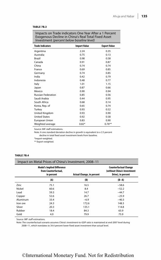
Ahuja and Nabar 135
TABLE 7B.3
Impacts on Trade indicators One Year After a 1 Percent Exogenous Decline in China's Real Total Fixed Asset Investment (percent below baseline level)
Trade Indicators Import Value Export Value
Argentina 2.24 0.35Australia 0.75 0.13Brazil 0.98 0.58Canada 0.91 0.87China 0.74 0.74France 0.69 0.85Germany 0.74 0.85India 0.42 0.79Indonesia 0.48 0.77Italy 1.01 1.15Japan 0.87 0.66Mexico 0.90 0.94Russian Federation 0.85 0.56Saudi Arabia 0.44 0.95South Africa 0.68 0.14Korea, Rep. of 0.65 0.74Turkey 0.93 0.52United Kingdom 0.93 0.90United States 0.92 0.58European Union 0.83 0.90Weighted average 0.82* 0.76**
Source: IMF staff estimations.Note: A one standard deviation decline in growth is equivalent to a 2.5 percent
decline in total fixed asset investment levels from baseline.*Import-weighted. ** Export-weighted.
TABLE 7B.4
Impact on Metal Prices of China's Investment, 2008–11
Model's Implied Difference
from Counterfactual,
in percent Actual Change, in percent
Counterfactual Change
(without China's Investment
Drive), in percent
(A) (B) (B−A)
Zinc 75.1 16.5 −58.6Nickel 60.6 8.4 −52.2Lead 59.3 14.7 −44.7Copper 52.6 26.7 −25.9Aluminum 33.4 −6.9 −40.3Iron ore 24.3 172.6 148.3Silver 20.3 135.1 114.8Rubber 18.4 84.3 65.9Gold 4.0 79.9 75.9
Source: IMF staff estimations.Note: The counterfactual scenario assumes China's investment-to-GDP ratio is maintained at end-2007 level during
2008–11, which translates to 34.4 percent lower fixed asset investment than actual level.
©International Monetary Fund. Not for Redistribution
136 Investment-Led Growth in China: Global Spillovers
REFERENCES
Ahuja, A., and A. Myrvoda, 2012, “The Spillover Effects of a Downturn in China’s Real Estate Investment,” Working Paper 12/266, (Washington: International Monetary Fund).
Guo, Kai, 2011, “Factor Pricing, Overcapacity, and Sustainability Risks,” People’s Republic of China Spillover Report—Selected Issues (unpublished; Washington: International Monetary Fund).
International Monetary Fund, 2011, “People’s Republic of China: 2011 Article IV Consultation,” Country Report 11/192 (Washington).
International Monetary Fund, 2012, “Is China Rebalancing? Implications for Asia,” in Asia and Pacific Regional Economic Outlook, April (Washington).
©International Monetary Fund. Not for Redistribution

137
CHAPTER 8
The Spillover Effects of a Downturn in China’s Real Estate Investment
ASHVIN AHUJA AND ALLA MYRVODA
This chapter assesses the impact of a downturn in China’s real estate investment on economic activity in China and among its trading partners. The analysis finds that a 1 percent decline in China’s real estate investment would shave about 0.1 percent off China’s real GDP within the first year, with negative spillovers to China’s G20 trading partners that would cause global output to decline by roughly 0.05 percent from base-line. Japan, the Republic of Korea, and Germany would be among the hardest hit. In that event, commodity prices, especially metal prices, could fall by as much as 0.8–2.2 percent below baseline one year after the shock.
INTRODUCTION
Real estate investment accounts for a quarter of total fixed asset investment (FAI) in China (Figure 8.1). It has been growing at about 30 percent per year during 2010–11 (Figure 8.2). The relatively new private property market in China has always been susceptible to excessive price growth, requiring intervention by the authorities over the years. The underlying structural features of the economy, namely low real interest rates in a high-growth environment, the underdeveloped financial system (offering few alternative assets), and a closed capital account, foster overinvestment in real estate and create an inherent tendency toward bub-bles in the property market, posing risks to market sustainability and financial stability.
To contain real estate bubbles, the authorities rely largely on quantity-based tools, the effectiveness of which tends to erode as more transactions are intermedi-ated outside the banking system, requiring more potent policy responses. In the most recent property boom episode, which started about mid-2009, the authori-ties escalated their response with restrictions on second and third home pur-chases in larger cities and credit limits on property developers. Thus far, the authorities appear to have succeeded in curbing market exuberance while main-taining robust investment growth, chiefly through an expansion of social housing programs and a selective easing of financial conditions for first-time home buyers (Figure 8.3). Nevertheless, developers’ financial conditions are deteriorating, and
©International Monetary Fund. Not for Redistribution

138 The Spillover Eff ects of a Downturn in China’s Real Estate Investment
Primaryindustry (2%) Mining (4%)
Manufacturing (34%)
Utilities (5%)
Real estate (25%)
Other (30%)
Figure 8.1 Fixed Asset Investment by Industry, 2011 (percent of total)Source: CEIC Data.
−50
−25
0
25
50
75
100
2000 2001 2002 2003 2004 2005 2006 2007 2008 2009 2010 2011 2012
Real estate investment
Per
cent
Residential property price
Figure 8.2 Property Price and Real Estate Investment (year-over-year growth)Sources: CEIC Data Company Ltd.; and IMF staff estimates.
©International Monetary Fund. Not for Redistribution

Ahuja and Myrvoda 139
there is a tail risk that policy overtightening could turn near-term price expecta-tion decidedly negative as high inventory-to-sales ratios compress developers’ profitability further, leading to a collapse in real estate investment.
The risk to growth and financial stability of a collapse in real estate investment in China is high, based on the expected economic repercussion should that event come to pass. The analysis based on China’s input-output data shows that the real-estate-dependent construction industry, which accounts for 7 percent of GDP, creates significant final demand in other domestic sectors; that is, it has among the highest degrees of backward linkage, particularly to mining, manufac-turing of construction material, metal and mineral products, machinery and equipment, consumer goods, as well as real estate services (Figure 8.4). Moreover, real estate is the principal source of collateral for external financing of private and state-owned enterprises as well as of local government investment projects, and other economic activities. As a result, a decline in real estate investment has the potential to disrupt the production chain throughout China’s economy and gen-erate spillovers to G20 trading partners.
The real estate sector’s extensive industrial and financial linkages make it a special type of economic activity, especially in economies in which the credit creation process relies primarily on collateral, like in China. As a result, the impact on economic activity of a collapse in real estate investment in China—though a low-probability event—would be sizable, with large spillovers to a number of China’s trading partners. Using a two-region factor-augmented vector autoregression (VAR) model that allows for interaction between China and the rest of the G20 economies, the analysis in this chapter finds that a 1 percent decline in China’s real estate investment would result in a decline of about 0.1 percent of China’s real GDP within the first year, with negative impacts on
−40
0
40
80
Per
cent
120
2008 2009 2010 2011 2012
National Chengdu Shenzhen Shanghai Beijing
Figure 8.3 Property Prices (year-over-year growth)Source: CEIC Data; Soufun; and IMF staff calculations.
©International Monetary Fund. Not for Redistribution

140 The Spillover Eff ects of a Downturn in China’s Real Estate Investment
China’s G20 trading partners that would cause global output to decline by roughly 0.05 percent from baseline. Japan, Korea, and Germany would be among the hardest hit. In that event, commodity prices, especially metal prices, could fall by as much as 0.8–2.2 percent below baseline one year after the shock.
MEASURING THE SPILLOVER EFFECTS
This chapter uses a factor-augmented VAR (FAVAR) approach pioneered by Bernanke, Boivin, and Eliasz (2005) to gauge the domestic and global spillovers of a slowdown in China’s real estate investment in the event of a sharp property market correction. Following Boivin and Giannoni (2008), the FAVAR frame-work is extended into a two-region model that allows China to interact with the rest of the world (represented in this experiment by the other G20 economies). The analysis captures the feedback from China to the rest of the world, and vice versa, over time. It also captures the spillover effects between the rest of the G20 economies from a specific event originated in China.
The fact that market participants monitor hundreds of economic variables in their decision-making process provides motivation for conditioning the analysis of their decisions on a rich information set. The FAVAR framework extracts information from the rich data set to gauge the impact of particular forces that may not be directly observable. These “forces” are treated as latent common com-ponents, which are interrelated, and their impacts on economic variables are
0.0 0.5 1.0 1.5 2.0 2.5 3.0Agriculture (AG)
Mining (MN)
Food Manufacturing (FD)
Textile, Garment, and Leather Manufacturing (TM)
Other Manufacturing (OM)
Utility (UT)
Coking, Coal Gas, and Petroleum Processing (PT)
Chemical Industry (CH)
Construction Material and Non Metallic MineralProduct Manufacturing (CM)
Metal Product Manufacturing (MP)
Machinery Equipment Manufacturing (ME)
Construction Industry (CI)
Transport, Post, and Telecom (TR)
Wholesale, Retail, Accommodation, and Catering (WR)
Real Estate, Leasing, and Commercial Service (RE)
Banking and Insurance (BI)
Other Service (OS) ItselfMNCMMPMEOthers
Figure 8.4 The Construction Industry’s Backward Linkages to Selected ContributorsSources: CEIC Data Company Ltd.; OECD; and IMF staff estimates. Note: Bars for each industry correspond to data for (starting with lowest) 1995, 2000, 2005, and 2007.
©International Monetary Fund. Not for Redistribution

Ahuja and Myrvoda 141
traced through impulse response functions. Accounting for unobserved variables provides a better chance that findings based on spurious association can be avoid-ed.1 The data set is a balanced panel of 390 monthly time series from the G20 stretching from January, 2000, to September, 2011, with 68 China variables and 322 from the rest of the world (Table 8.1). The sample contains at least one full cycle of real estate investment in China. It covers the period since China entered the World Trade Organization and became increasingly integrated with the world economy.
The experiment assumes an exogenous, temporary, one standard deviation growth shock to China’s real estate investment. The shock dampens within a few months and dissipates fully after about 36 months. Specifically, this is a one-time, 49 percentage point (seasonally adjusted, annualized) drop in real estate invest-ment growth that largely reverts to trend growth within four to five months.2 Although this is a temporary, negative growth shock, the decline in real estate investment level is permanent. The shock is approximately equivalent to a 2 per-cent drop from baseline in the real estate investment level after 12 months. The analysis does not assume any policy response beyond that which was already in the sample.
Figures 8.5–8.15 report 24-month peak impacts (with error bands) following a one standard deviation shock to real estate investment. Impacts on levels 12 months after the shock, in percent below baseline, are also derived and report-ed for comparison in Tables 8.2–8.5.
1 A more detailed description of the model and estimation strategy can be found in Ahuja and Myrvoda (2012).2 A one standard deviation shock is equivalent to 3 percentage points in month-over-month, season-ally adjusted, growth rates.
TABLE 8.1
Data Set Description
Data China (68 variables) G20 Excluding China (322 variables)
Real Economy Industrial production, Gross value added, Investment, Consumption, Floor space, Land area purchased/developed
Industrial production
Labor Urban employment Employment (total/nonfarm) Financial M2, Credit, Short-term interest rates,
Shanghai Composite, US$/RMBM2, Credit, Short-term interest rates, Treasury bond spreads, Stock market indices, US$/National currency
Trade Exports (components), Imports (compo-nents), Trade balance
Exports, Exports to China, Imports, Imports from China, Trade balance
Prices Consumer price index, Producer price index, House price, Commodity prices (local)
Consumer price index, Producer price index, Terms of trade, Commodity prices
Source: IMF staff.Note: M2 = broad money.
©International Monetary Fund. Not for Redistribution

142 The Spillover Eff ects of a Downturn in China’s Real Estate Investment
TABLE 8.2
Impacts on Selected China Indicators of a Decline in China's Real Estate Investment
China Indicators
Impact
(percent, year-over-year)
Gross value added, real 0.1GDP, real 0.1Retail sales, real 0.1Exports 0.7Imports 0.8Total FAI 0.4Residential property Price 0.7 Floor space sold 1.5
Source: IMF staff estimations.Note: Impacts one year after a 1 percent exogenous decline in China’s real
estate investment. A one standard deviation decline in growth is equivalent to a 2 percent decline in real estate investment levels from baseline. FAI - Fixed asset investment.
TABLE 8.3
Impacts on Selected Economic Activity Indicators of a Decline in China's Real Estate Investment (percent, year-over-year)
World Indicator Industrial Production Real GDP
Argentina 0.52 0.10Australia1 0.01 0.00Brazil 0.28 0.05Canada2 0.06 0.06China3 0.12 0.10France 0.15 0.02Germany 0.64 0.12India 0.27 0.05Indonesia 0.02 0.01Italy 0.47 0.08Japan 0.50 0.11Mexico 0.32 0.08Russian Federation 0.23 0.05Saudi Arabia 0.08 0.02South Africa 0.29 0.04Korea, Rep. of 0.19 0.06Turkey 0.46 0.10United Kingdom 0.08 0.01United States 0.20 0.03European Union 0.17 0.03
PPP-weighted average 0.06
Source: IMF staff estimations.Note: Impacts one year after a 1 percent exogenous decline in China’s real estate investment on selected economic activity
indicators. A one standard deviation decline in growth is equivalent to a 2 percent decline in real estate investment levels from baseline. PPP = purchasing-power parity.
1 Estimate for Australia is not statistically significant.2 Canada's economic activity is represented by monthly real GDP Index, all industries.3 China's industrial sector activity is represented by gross industrial value added.
©International Monetary Fund. Not for Redistribution

Ahuja and Myrvoda 143
TABLE 8.4
Impacts on Trade Indicators of a Decline in China's Real Estate Investment (percent, year-on-year)
Trade Indicator Total Imports Total Exports
Argentina 2.23 0.38Australia 0.73 0.21Brazil 0.97 0.69Canada 0.90 0.85China 0.78 0.68France 0.75 0.88Germany 0.74 0.81India 0.51 0.95Indonesia 0.00 0.82Italy 0.98 1.02Japan 0.83 0.64Mexico 0.91 0.93Russian Federation 0.81 0.73Saudi Arabia 0.45 1.00South Africa 0.84 0.20Korea, Rep. of 0.65 0.78Turkey 0.94 0.47United Kingdom 0.92 0.94United States 0.90 0.61European Union 0.83 0.86
Weighted average 0.821 0.762
Source: IMF staff estimations.Note: Impacts one year after a 1 percent exogenous decline in China’s real estate investment on selected trade indicators.
A one standard deviation decline in growth is equivalent to a 2 percent decline in real estate investment levels from baseline.
1Import-weighted.2Export-weighted.
TABLE 8.5
Impacts on Selected Commodity Prices of a Decline in China’s Real Estate Investment
World Prices Impact (percent)
Metals 2.7Nonfuel primary commodities 1.3Zinc 4.3Nickel 3.7Lead 3.2Copper 3.1Iron ore 1.6Aluminum 2.1Rubber 1.6Silver 1.5Gold 0.4
Source: IMF staff estimations.Note: Impacts one year after a one standard deviation exogenous decline in China’s real estate investment on selected commodity prices. A one standard deviation decline in growth is equivalent to a 2 percent decline in real estate investment levels form baseline.
©International Monetary Fund. Not for Redistribution

144 The Spillover Eff ects of a Downturn in China’s Real Estate Investment
DOMESTIC FEEDBACK
A rapid slowdown in growth in real estate investment would reverberate across the economy, lowering investment in a broad range of sectors. Given the strong back-ward linkages to other industries, especially manufacturing of construction mate-rial, metal and mineral products, and machinery and equipment, a temporary, one standard deviation decline in real estate investment growth would cause investment in the manufacturing and heavy secondary industries to drop by as much as 1½ percentage points within the first year. (Whether a slowdown would occur in investment growth in primary industry, which contains mining, is unclear [Figure 8.5].) This result translates into a total FAI decline of approxi-mately 0.8 percent from the baseline level 12 months after the shock (see Table 8.2).
Other components of demand respond in a consistent fashion. Export growth, particularly of manufacturing exports, would fall by about 2¼ percentage points mainly from diminishing trading partners’ demand (Figure 8.6). The deteriora-tion in domestic demand and weaker export growth would bring import growth down by roughly 5¾ percentage points at peak impact. Equivalently, exports and imports would fall by about 1.4 and 1.6 percent, respectively, below baseline levels 12 months after the shock (see Table 8.2). A large fall in imports also results from a significant share of processing trade in total trade. More important, the strong import responses reflect robust linkages of real estate activity to domestic industries that require inputs from abroad, namely manufacturing of construction
−3
−2
−1
0
1
2
FAI: Primary industry
Per
cent
age
poin
ts
FAI: Secondary industry FAI: Tertiary industry
Significant Not significant
Figure 8.5 China: Peak Impact on Investment in Industry (seasonally adjusted annual rate)Source: IMF staff estimations.Note: Impact of a one standard deviation shock to China real estate investment. FAI = Fixed asset investment.
©International Monetary Fund. Not for Redistribution

Ahuja and Myrvoda 145
−8
−6
−4
−2
0Significant Not significant
Primaryproducts
Mineralfuel,
lubricants
Manufacturing Chemicalproducts
Manufac-tured
goods
Machineryand
transport
Manufacturingexports
Exports Imports
Per
cent
age
poin
ts
Figure 8.6 China: Peak Impact on Exports and Imports (seasonally adjusted annual rate)Source: IMF staff estimations.Note: Impact of a one standard deviation shock to China real estate investment.
material, mineral and metal products, as well as machinery and equipment.3 China’s real effective exchange rate (REER) and the bilateral RMB/US$ exchange rate do not seem to help cushion exports in a meaningful way even though the rate of appreciation (depreciation) appears to slow down (accelerate) slightly and lasts about two or three quarters.
Consumption would be dampened as income and wealth expansion (includ-ing house price appreciation and stock market valuation) slow down. Real retail sales would dip by 0.5 percent at peak impact (Figure 8.7). The end result would be a drop in total industrial value added and output. All in all, industrial gross value added growth would fall by about 0.4 percentage point at peak, which is consistent with a 0.3 percentage point decline in real GDP on an annualized basis.4 The impact would be felt almost immediately and would start to dissipate after four quarters. These events would translate into a decline of about 0.3 and 0.2 percent below baseline levels for gross value added and GDP, respectively, one year out (Table 8.2).
3 The results are consistent with the input-output analysis, not shown in this chapter, that shows that machinery and equipment manufacturing as well as mining have the highest import coefficients, fol-lowed by chemical industry. 4 A 1 percentage point decline in real industrial value added growth is consistent with a decline in real GDP growth for China of about 0.8 percentage point.
©International Monetary Fund. Not for Redistribution
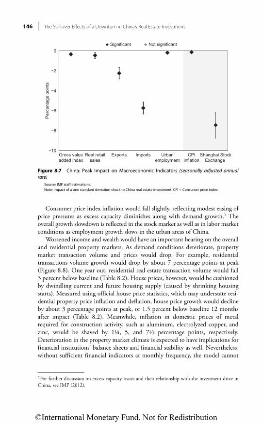
146 The Spillover Eff ects of a Downturn in China’s Real Estate Investment
Consumer price index inflation would fall slightly, reflecting modest easing of price pressures as excess capacity diminishes along with demand growth.5 The overall growth slowdown is reflected in the stock market as well as in labor market conditions as employment growth slows in the urban areas of China.
Worsened income and wealth would have an important bearing on the overall and residential property markets. As demand conditions deteriorate, property market transaction volume and prices would drop. For example, residential transactions volume growth would drop by about 7 percentage points at peak (Figure 8.8). One year out, residential real estate transaction volume would fall 3 percent below baseline (Table 8.2). House prices, however, would be cushioned by dwindling current and future housing supply (caused by shrinking housing starts). Measured using official house price statistics, which may understate resi-dential property price inflation and deflation, house price growth would decline by about 3 percentage points at peak, or 1.5 percent below baseline 12 months after impact (Table 8.2). Meanwhile, inflation in domestic prices of metal required for construction activity, such as aluminum, electrolyzed copper, and zinc, would be shaved by 1¼, 5, and 7⅓ percentage points, respectively. Deterioration in the property market climate is expected to have implications for financial institutions’ balance sheets and financial stability as well. Nevertheless, without sufficient financial indicators at monthly frequency, the model cannot
5 For further discussion on excess capacity issues and their relationship with the investment drive in China, see IMF (2012).
−10
−8
−6
−4
−2
0Significant Not significant
Gross valueadded index
Real retailsales
Exports
Per
cent
age
poin
ts
Imports Urbanemployment
CPIinflation
Shanghai StockExchange
Figure 8.7 China: Peak Impact on Macroeconomic Indicators (seasonally adjusted annual rate)
Source: IMF staff estimations.Note: Impact of a one standard deviation shock to China real estate investment. CPI = Consumer price index.
©International Monetary Fund. Not for Redistribution

Ahuja and Myrvoda 147
−12
−10
−8
−6
−4
−2
0
Residentialproperty price
Commoditybuilding: Floorspace started
Commoditybuilding: Floor
spacecompleted
Residentialcommodity
building: Floorspace
completed
Floor spacesold
Floor spacesold:
Residential
Significant Not significant
Per
cent
age
poin
ts
Figure 8.8 China: Impact on Property Market (seasonally adjusted annual rate)Source: IMF staff estimations.Note: Impact of a one standard deviation shock to China real estate investment.
uncover the relationships between a property market slowdown and financial stability indicators.6
GLOBAL SPILLOVER
A temporary shock to China’s real estate investment growth would have spillover implications around the world, with the impacts on G20 economies lasting approximately four to five quarters. In this exercise, the approximate impact on GDP growth would vary with the size of the industrial-production-to-GDP ratio in each economy (Figures 8.9 and 8.10).7 The implied peak impact on purchas-ing-power-parity-weighted G20 GDP growth is −0.2 percentage point, which translates to about 0.1 percent below baseline 12 months after the shock origi-nated in China (Table 8.3). Overall, capital goods manufacturers that have sizable direct exposures to China through exports to China as a percentage of own GDP and that are highly integrated with the rest of the G20—therefore sharing adverse feedback from a negative shock in China with other trading partners, such as
6 Data availability aside, financial exposures to the property sector are likely to be larger than official data suggest, considering the increasing prominence of off-balance-sheet activities at banks, trust company lending, the shadow banking system, and unobserved intercompany lending, which could be property related.7 Industrial production is defined differently from country to country. The Organization for Economic Cooperation and Development definition includes production in mining, manufacturing, and public utilities (electricity, gas, and water), but excludes construction.
©International Monetary Fund. Not for Redistribution
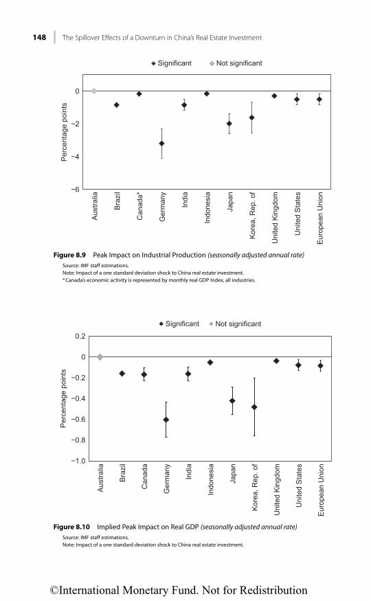
148 The Spillover Eff ects of a Downturn in China’s Real Estate Investment
−6
−4
−2
0A
ustra
lia
Bra
zil
Can
ada*
Ger
man
y
Indi
a
Indo
nesi
a
Japa
n
Kor
ea, R
ep. o
f
Uni
ted
Kin
gdom
Uni
ted
Sta
tes
Eur
opea
n U
nion
Significant Not significantP
erce
ntag
e po
ints
Figure 8.9 Peak Impact on Industrial Production (seasonally adjusted annual rate)Source: IMF staff estimations.Note: Impact of a one standard deviation shock to China real estate investment.* Canada’s economic activity is represented by monthly real GDP Index, all industries.
−1.0
−0.8
−0.6
−0.4
−0.2
0
0.2
Aus
tralia
Per
cent
age
poin
ts
Bra
zil
Can
ada
Ger
man
y
Indi
a
Indo
nesi
a
Japa
n
Kor
ea, R
ep. o
f
Uni
ted
Kin
gdom
Uni
ted
Sta
tes
Eur
opea
n U
nion
Significant Not significant
Figure 8.10 Implied Peak Impact on Real GDP (seasonally adjusted annual rate)Source: IMF staff estimations.Note: Impact of a one standard deviation shock to China real estate investment.
©International Monetary Fund. Not for Redistribution

Ahuja and Myrvoda 149
Germany, Japan, and Korea—would see more of the impact to industrial produc-tion and GDP. The results also show that global trade activity would decline (total exports and total imports for every G20 economy would weaken), which suggests that economies, such as Germany and Japan, that derive significant benefit from global trade expansion and have deepened links via supply chain countries during the past decade, should be more hard hit in the second round (Table 8.4). The impact on Korea’s GDP peaks within the first two quarters and fades away more quickly, which is consistent with Korea’s large direct exposure to China, but sec-ond-round effects through supply chain countries are smaller than in Japan and Germany (also see Riad, Asmundson, and Saito, 2012).
Trade expansion with China and overall global trade would also slow as global and China demand growth weakens (Table 8.4). For the United Kingdom and India, exports to China would bear the brunt of the impact, but because they are not important components of final demand in these economies, the impact on economic activity would be relatively moderate.8 Commodities exporters to China, such as Australia, Brazil, and Canada, would also experience nonnegligible spillover effects on export growth (Figure 8.11).9 Australia’s relatively large direct exposure to China would suggest a larger direct impact, but other forces seem to
8 Exports to China are mostly in machinery, equipment, and industrial supplies for the United Kingdom and mineral commodities and primary metal products for India. 9 Canada’s exports to China are more diversified in mineral and manufactured commodities.
−10
−6
−2
2
0
Austra
lia
Per
cent
age
poin
ts
Brazil
Canad
a
German
yInd
iaJa
pan
Significant Not significant
Korea,
Rep. o
f
United
King
dom
United
Stat
es
Europe
an U
nion
Figure 8.11 Peak Impact on Exports to China (seasonally adjusted annual rate)Source: IMF staff estimations.Note: Impact of a one standard deviation shock to China real estate investment.
©International Monetary Fund. Not for Redistribution

150 The Spillover Eff ects of a Downturn in China’s Real Estate Investment
blunt the effect on Australia’s industrial production, for example, the Australian dollar exchange rate works as a shock absorber. Nevertheless, other indicators, such as employment growth and total import growth (not shown here), point to a slowdown in Australia’s economic activity. The impact on Indonesia’s exports would likely come through China’s coal demand. Because coal exports to China have risen sharply since late in the first decade of the 2000s, the impact on Indonesia’s real GDP could be larger today than shown in Table 8.3.
The growth spillover effects are also reflected in asset prices and valuation. Specifically, the impact on financial wealth generation, as represented by the expansion of stock market indexes in the G20 economies, would be tangible and would remain for as long as four to five quarters (Figure 8.12). Related to this, a general decline in sovereign bond spreads (cumulative over the first 12 months after impact; Figure 8.13) seems to signal concerns about future global growth, in accord with the immediate impacts on industrial production shown earlier. In the United States’ case, the initial flattening of the yield curve is reversed about two quarters after the shock, which suggests that U.S. recovery prospects could be faster than those of other G20 economies. The result for Australia is consistent with the estimated impact on that country’s industrial production.
A global growth slowdown and a drop in China’s demand for base metal imports, initiated by a China real estate investment decline, could lead to a drop in iron ore, aluminum, copper, lead, nickel, and zinc price growth of between 2¾ and 8 percentage points (Figures 8.14 and 8.15). The impact on overall metal
−6
−4
−2
0
Austra
lia
Per
cent
age
poin
ts
Brazil
Canad
a
German
yInd
iaJa
pan
Significant Not significant
Korea,
Rep. o
f
United
King
dom
United
Stat
es
Europe
an U
nion
Figure 8.12 Peak Impact on Stock Market Index (seasonally adjusted annual rate)Source: IMF staff estimations.Note: Impact of a one standard deviation shock to China real estate investment.
©International Monetary Fund. Not for Redistribution

Ahuja and Myrvoda 151
−0.7
−0.5
−0.3
−0.1
0.10
0.3
Austra
lia
Per
cent
age
poin
ts
Canad
a
Gernam
yInd
iaIta
lyJa
pan
Significant Not significant
Korea,
Rep. o
f
United
King
dom
United
Stat
es
Europe
an U
nion
Figure 8.13 Peak Impact on Sovereign Bond Spreads (12-month cumulative)Source: IMF staff estimations.Note: Impact of a one standard deviation shock to China real estate investment.
−6
−4
−2
0
CPI Sugar
Per
cent
age
poin
ts
Agricultural rawmaterials
Metals Nonfuelprimary
commodities
Significant Not significant
Figure 8.14 Peak Impact on World Prices (seasonally adjusted annual rate)Source: IMF staff estimations.Note: Impact of a one standard deviation shock to China real estate investment. CPI = Consumer price index.
©International Monetary Fund. Not for Redistribution

152 The Spillover Eff ects of a Downturn in China’s Real Estate Investment
−10
−6
−2
0
Zinc Nickel
Per
cent
age
poin
ts
Lead Copper Iron ore Aluminum Rubber Silver Gold
Significant Not significant
Figure 8.15 Peak Impact on World Metal and Rubber Prices (seasonally adjusted annual rate)Source: IMF staff estimations.Note: Impact of a one standard deviation shock to China real estate investment.
prices could last four quarters—up to five or six quarters for lead and zinc, possibly as the result of a weaker supply response. This result is equivalent to a decline in price levels of about ½–4½ percent below baseline levels, one year out (Table 8.5). How crude oil prices would be affected is unclear in this exercise—the impulse responses show a drop in crude price growth, with a peak about three quarters after impact, but they are not statistically significant. Even as nonfuel primary com-modity price inflation retreats, the impact on global inflation appears modest.
CONCLUSION
Real estate investment accounts for a quarter of total FAI in China. The impact on economic activity of a hypothetical collapse in real estate investment in China is sizable, with large spillovers to a number of China’s trading partners. A 1 per-cent decline in China’s real estate investment would shave about 0.1 percent off China’s real GDP within the first year, with negative spillovers on China’s G20 trading partners that would cause global output to decline by roughly 0.06 per-cent from baseline. Japan, Korea, and Germany would be among the hardest hit. In that event, commodity prices, especially metal prices, could fall by as much as 0.8–2.2 percent below baseline one year after the shock.
Overall, capital goods manufacturers that have sizable direct exposures to China (especially Japan and Korea) and are highly integrated with the rest of the G20, therefore sharing the adverse feedback from a negative shock in China with other trading partners, would experience larger declines in industrial production and GDP. Worsened global growth prospects would be reflected in asset prices
©International Monetary Fund. Not for Redistribution

Ahuja and Myrvoda 153
and sovereign bond spreads. In that event, commodity prices, especially construc-tion-related metal prices, would also fall.
The sample contains at least one full cycle of real estate investment and prop-erty market data in China, and covers the period of China’s increasing integration with the world economy. Strictly from a statistical point of view, this relatively short sample is expected to make statistical relationships harder to detect and will be an important constraint on the richness of the model. Nevertheless, as the results suggest, there is still sufficient statistical information in the sample to deliver useful insights about China’s interaction with the world in the recent past. It must be stressed, however, that China is more important to the global econo-my today than the sample would suggest, and a real estate investment bust in China is not likely to be a linear event as measured by the model. The impact on G20 trading partners, and therefore global growth today, could be larger than reported here.
REFERENCES
Ahuja, A., and A. Myrvoda, 2012, “The Spillover Effects of a Downturn in China’s Real Estate Investment,” IMF Working Paper No. 12/266 (Washington: International Monetary Fund).
Bernanke, B., J. Boivin, and P. Eliasz, 2005, “Measuring the Effects of Monetary Policy: A Factor-Augmented Vector Autoregressive (FAVAR) Approach,” Quarterly Journal of Economics, Vol. 120, No.1, pp. 387–422.
Boivin, J., and M. Giannoni, 2008, “Global Forces and Monetary Policy Effectiveness,” NBER Working Paper No. 13736 (Cambridge, Massachusetts: National Bureau of Economic Research).
International Monetary Fund, 2012, “People’s Republic of China: Staff Report for the 2012 Article IV Consultation,” IMF Country Report No. 12/195 (Washington).
Riad, N., I. Asmundson, and M. Saito, 2012, “China’s Trade Balance Adjustment: Spillover Effects,” 2012 Spillover Report–Background Paper (Washington: International Monetary Fund).
©International Monetary Fund. Not for Redistribution

This page intentionally left blank
©International Monetary Fund. Not for Redistribution

PART III
Policy Implications
©International Monetary Fund. Not for Redistribution

This page intentionally left blank
©International Monetary Fund. Not for Redistribution
157
CHAPTER 9
Chronicle of a Decline Foretold: Has China Reached the Lewis Turning Point?
MITALI DAS AND PAPA N’DIAYE
The final section of the book examines what needs to be done to complete the process of domestic rebalancing. Impending demographic changes make reform ever more urgent. China is on the eve of a demographic shift that will have profound conse-quences on its economic and social landscape. Within a few years the working-age population will reach a historical peak, and then begin a precipitous decline. This fact, along with anecdotes of rapidly rising migrant wages and episodic labor shortages, has raised questions about whether China is poised to cross the Lewis Turning Point, a juncture at which it would move from a vast supply of low-cost workers to a labor shortage economy. Crossing this threshold will have far-reaching implications for both China and the rest of the world. This chapter empirically assesses when the transition to a labor shortage economy is likely to occur. The central result is that on current trends, the Lewis Turning Point will emerge between 2020 and 2025. Alternative scenarios—with higher fertility, greater labor force participation rates, financial reform, or higher productivity—may peripherally delay or accelerate the onset of the turning point, but demographics will be the dominant force driving the depletion of surplus labor.
INTRODUCTION
China’s large pool of surplus rural labor has played a key role in maintaining low inflation and supporting China’s extensive growth model. In many ways, China’s economic development echoes Sir Arthur Lewis’s model, which argues that in an economy with excess labor in a low-productivity sector (agriculture in China’s case), wage increases in the industrial sector are limited by wages in agriculture, as labor moves from the farms to industry (Lewis, 1954). Productivity gains in the industrial sector, achieved through more investment, raise employment in the industrial sector and the overall economy. Productivity running ahead of wages in the industrial sector makes the industrial sector more profitable than if the economy were at full employment, and promotes higher investment. As surplus labor in agriculture is exhausted, industrial wages rise faster, industrial profits are squeezed, and investment falls. At that point, the economy is said to have crossed the Lewis Turning Point (LTP) (Figure 9.1).
©International Monetary Fund. Not for Redistribution
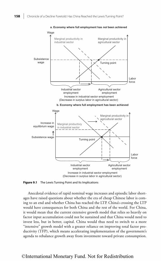
158 Chronicle of a Decline Foretold: Has China Reached the Lewis Turning Point?
Anecdotal evidence of rapid nominal wage increases and episodic labor short-ages have raised questions about whether the era of cheap Chinese labor is com-ing to an end and whether China has reached the LTP. China’s crossing the LTP would have consequences for both China and the rest of the world. For China, it would mean that the current extensive growth model that relies so heavily on factor input accumulation could not be sustained and that China would need to invest less, but in better, capital. China would thus need to switch to a more “intensive” growth model with a greater reliance on improving total factor pro-ductivity (TFP), which means accelerating implementation of the government’s agenda to rebalance growth away from investment toward private consumption.
Wage
Turning pointSubsistence
wage
Marginal productivity inindustrial sector
Increase in industrial sector employment(Decrease in surplus labor in agricultural sector)
Marginal productivity inagricultural sector
a. Economy where full employment has not been achieved
Laborforce
Industrial sectoremployment
Agricultural sectoremployment
Wage
Turning pointSubsistence wage
Marginal productiviyin industrial sector
Increase in industrial sector employment(Decrease in surplus labor in agricultural sector)
Marginal productivity inagricultural sector
b. Economy where full employment has been achieved
Laborforce
Increase inequilibrium wage
Industrial sectoremployment
Agricultural sectoremployment
Figure 9.1 The Lewis Turning Point and Its Implications
©International Monetary Fund. Not for Redistribution

Das and N’Diaye 159
Successfully rebalancing China’s growth pattern would yield significant positive external spillovers to the rest of the world, potentially raising output, particularly in those economies within the supply chain (mainly emerging Asia) and commod-ity exporters, and somewhat more limited spillovers to advanced economies (IMF, 2011). Moreover, rising labor costs—the impact of which will be felt in prices and corporate profit margins in China—will have implications for trade, employment, and price developments in key trading partners.
Against this backdrop, this chapter presents estimates of China’s excess labor supply using a general procedure developed in Rosen and Quandt (1978), Quandt and Rosen (1986), and Rudebusch (1986). The empirical model attributes an explicit role to population composition, labor force participation, and productiv-ity—characteristics of the Chinese labor market most likely to be relevant in an analysis of excess supply. The remainder of the chapter is organized as follows: The next section provides a brief overview of recent trends in China’s labor market. The subsequent section presents the empirical framework and is followed by a section that presents baseline results. A scenario analysis around a central baseline forecast of future trends in the labor market is presented in the penultimate section, and the last section concludes.
RECENT DEVELOPMENTS
China’s labor markets first came into focus in 2004, when reports of migrant labor shortages in the export-oriented coastal regions began to emerge. Anecdotal evidence of large increases in migrant wages in this period was viewed by some as an indication that China had depleted a previously vast supply of surplus labor, and the transition to a mature economy had begun (Garnaut, 2006; Cai and Wang, 2008). This view was bolstered by the demographic transition, in particu-lar, a slowdown in the growth of the working-age population and a rising propor-tion of elderly to young Chinese workers. An alternative perspective, however, viewed rising migrant wages as a consequence of labor market segmentation (the result, for instance, of the household registration system, limited portability of benefits, and rising rural reservation wages), thus consistent with the coexistence of shortages on the coast and surplus labor inland (Chan, 2010; Zhang, Yang, and Wang, 2010; Knight, Deng, and Li, 2011).
Developments in the Chinese labor market since 2009 are reminiscent of the episode in the middle of the first decade of the 2000s—after a lull, wage increas-es have again been rapid, especially in inland provinces as companies relocate from the coast. However, the authors’ reading of recent developments in Chinese labor markets suggests no conclusion about whether surplus Chinese labor has been exhausted. Despite localized signs of labor market pressures, aggregate nominal wage growth has ranged between 12 and 15 percent annually since 2000. Corporate profits have remained high, and even rose during 2009–11, as wage growth has trailed productivity gains. These developments appear inconsistent with the basic premise of the LTP depicted in Figure 9.2 (panel a). Anecdotally,
©International Monetary Fund. Not for Redistribution
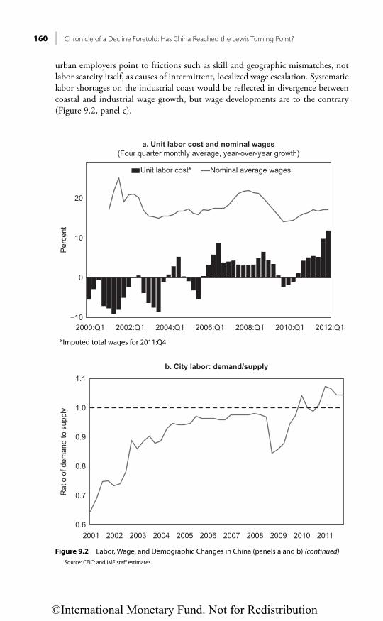
160 Chronicle of a Decline Foretold: Has China Reached the Lewis Turning Point?
urban employers point to frictions such as skill and geographic mismatches, not labor scarcity itself, as causes of intermittent, localized wage escalation. Systematic labor shortages on the industrial coast would be reflected in divergence between coastal and industrial wage growth, but wage developments are to the contrary (Figure 9.2, panel c).
0.6
0.7
0.8
0.9
1.0
1.1
2001
Rat
io o
f dem
and
to s
uppl
y
2002 2003 2004 2005 2006 2007 2008 2009 2010 2011
b. City labor: demand/supply
Figure 9.2 Labor, Wage, and Demographic Changes in China (panels a and b) (continued)Source: CEIC; and IMF staff estimates.
−10
0
10
Per
cent
20
2000:Q1 2002:Q1 2004:Q1 2006:Q1 2008:Q1 2010:Q1 2012:Q1
Unit labor cost* Nominal average wages
a. Unit labor cost and nominal wages(Four quarter monthly average, year-over-year growth)
*Imputed total wages for 2011:Q4.
©International Monetary Fund. Not for Redistribution

Das and N’Diaye 161
Other evidence, however, suggests tightening labor market conditions. Urban registration records indicate that the margin between city demand and supply of labor has progressively narrowed and is now effectively closed (Figure 9.2, panel b).1 The pace of industry relocation to the interior provinces—where wages
1 This measure comes from the National Bureau of Statistics of China. However, it is unclear whether all firms are required to record demand and whether both informal and formal workers are recorded in the measure of labor supply.
5
10
15
20
25
2008:Q1 2008:Q3 2009:Q1 2009:Q3 2010:Q1 2010:Q3 2011:Q1 2011:Q3
Coastal
c. Wage growth: Coastal vs. interior
Per
cent
Interior
−10
−5
0
5
10
15
20
1950
Per
cent
1960 1970 1980 1990 2000 2010 2020 2030 2040 2050
d. Growth of working-age population
Figure 9.2 Labor, Wage, and Demographic Changes in China (panels c and d) (continued)Source: IMF staff estimates.
©International Monetary Fund. Not for Redistribution
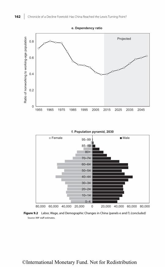
162 Chronicle of a Decline Foretold: Has China Reached the Lewis Turning Point?
0
0.2
0.4
0.6
0.8
1955 1965
Rat
io o
f non
wor
king
to w
orki
ng-a
ge p
opul
atio
n
1975 1985 1995 2005 2015 2025 2035 2045
e. Dependency ratio
Projected
80,000 60,000 40,000 20,000 0 20,000 40,000 60,000 80,0000–4
10–14
20–24
30–34
40–44
50–54
60–64
70–74
80+
85–89
95–99Female Male
f. Population pyramid, 2030
Figure 9.2 Labor, Wage, and Demographic Changes in China (panels e and f ) (concluded)Source: IMF staff estimates.
©International Monetary Fund. Not for Redistribution

Das and N’Diaye 163
are lower and the large reserve of rural labor resides—has picked up since the 2008–09 global financial crisis.2 Parallel developments, such as an uptick in labor activism since the financial crisis, are also consistent with the strengthened bar-gaining power that accompanies a shrinking pool of labor. The rise in wages also reflects the government’s decision to increase minimum wages as a means to sup-port household income and promote consumption.
Thus, overall, labor market developments paint a mixed picture of excess labor: Wage developments do not suggest exhaustion of surplus labor, whereas employ-ment, industrial relocation, and some policies signal tightening conditions.
However, demographics more forcefully suggest an imminent transition to a labor shortage economy. China is poised to undergo a profound demographic shift within the next decade, driven by the mutually reinforcing phenomena of declining fertility and aging. The UN projects that growth of the working-age (ages 15–64) population will turn negative about 2020 (Figure 9.2, panel d). This forecast potentially understates prospects for a labor shortage because industry employees are predominantly young (Garnaut, 2006); the growth rate of the core 20–39-year-old subpopulation, for example, shrank to zero in 2010 (Figure 9.3), and is projected to decline faster than the overall working-age population through 2035. Population data also show that after a protracted period of “demographic dividend,” the share of dependents—those ages younger than 15 and older than 64 in China’s population—bottomed out in 2010, and will rise to nearly 50 per-cent by 2035 (Figure 9.2, panel e).
Because the looming demographic changes are large, irreversible, and inevita-ble in the medium term, they will be key to the evolution of excess labor in China. Other factors could, however, be pivotal in accelerating or slowing this process. More progress in hukou reform (easing the ability of workers in prov-inces to move to cities) could spur rural labor to move to the city. Training rural workers to meet the skill requirements of industrial jobs could decongest urban labor bottlenecks. Although the Chinese primary sector employs nearly half of the labor force, agricultural value added was only about one-fifth of 2011 GDP. Raising agricultural productivity—by raising mechanization to comparators’ lev-els, for instance—could result in a sizable release of rural workers that could partially offset shortfalls in urban labor demand.
In summary, the combined implications of demographics, labor develop-ments, and policies suggest that China likely is on the eve of the LTP, but give little indication about when the transition will occur. Against this background, the next section attempts to gauge China’s excess labor supply and project its likely evolution.
2 Industrial relocation to the inland may not necessarily be a reflection of coastal cost pressures and instead reflect, for instance, expansion into the vast consumer base in inland provinces. In this sce-nario, labor bottlenecks in coastal areas may simply be a result of migrants’ rising reservation wages for coastal employment, given greater opportunities inland.
©International Monetary Fund. Not for Redistribution

164 Chronicle of a Decline Foretold: Has China Reached the Lewis Turning Point?
EMPIRICAL FRAMEWORK
To quantify excess labor supply in China, a first step is to identify the appropriate analytical framework. One approach (e.g., Lucas and Rapping, 1969; Barro and Grossman, 1971) is the conventional simultaneous equation model. This approach assumes the labor market is in equilibrium, that is, that real wages clear the labor market and unemployment results from labor market frictions, such as mismatch, preferences (i.e., intertemporal substitution) and government policies. An alternative framework is the disequilibrium approach, which assumes that the observed real wage does not clear the labor market (Rosen and Quandt, 1978). Instead, in this approach the observed quantity of employment is the minimum of the notional supply of and demand for labor, and unemployment results from excess labor supply, that is, the supply of labor exceeds demand at the observed real wage (see, e.g., Quandt and Rosen, 1986; Hajivassiliou, 1993). In practice, this means that the excess supply of labor includes both the actual unemployed and underemployed, which would encompass part of China’s large pool of migrant workers. Survey data from the National Bureau of Statistics show that about 169 million migrant workers were seeking jobs outside their home provinces as of end-September 2012. The number of unemployed people stood at 21.5 mil-lion as of end-2011, amounting to about 3 percent of the total labor force (the unemployment rate in urban areas is 4.1 percent).
Stylized facts of the Chinese labor market described above, in particular, wage growth that has trailed productivity growth for more than a decade, in addition to a rural share of the labor force near 50 percent and a labor share of income that is both low and has declined some 20 percentage points since 1980 (Aziz and Cui, 2007), suggest that the disequilibrium framework is well suited for analyzing the
150
250
350
450
550
Mill
ions
of p
eopl
e650
1950
1960
1970
1980
1990
2000
2010
2020
2030
2040
2050
25–39 years of age
Less than 15 and greater than 64 years of age
Figure 9.3 Demographic PressuresSources: UN Population Database; and IMF staff estimates.
©International Monetary Fund. Not for Redistribution

Das and N’Diaye 165
Chinese labor market. Moreover, this framework is sufficiently general to nest the equilibrium approach as a limiting case. The main equations used in the analysis are described in Annex 9A; details of the approach are in Rosen and Quandt (1978), Quandt and Rosen (1986), and Rudebusch (1986).
RESULTS
The model is estimated using annual observations from 1992 through 2010. The dependent variable, L, is the natural logarithm of the total number of employees in urban and rural areas, including those in the government sector, state-owned enterprises, and the private sector. The wage variable, W, is nominal aggregate wages in billion renminbi deflated by the consumer price index (CPI). Wealth is measured as households’ nominal net financial assets, while TFP is residually calculated from a standard growth accounting model with fixed labor and capital shares. Population, labor force, and working-age data are from the United Nations population database. A full list of the sources and definitions of the vari-ables is given in Table 9.1.
Results are reported in Table 9.2 with estimated standard errors in parenthe-ses.3 Overall, the results are of the expected signs and of plausible magnitudes. The wage elasticity of labor demand is negative. Furthermore, the absolute value of the elasticity of labor demand with respect to real wages is less than 1, consis-tent with the stylized fact that labor costs in China represent a low fraction of total firm costs. The effect of TFP, which is assumed to raise labor demand by
3 Note, because the model is derived by assuming that ≥ 0, critical test values for the estimated are obtained from one-sided t-tables. This restriction is not imposed in estimation. Nonnegativity of is a testable assumption, and statistically significant nonnegativity of is a rejection of equilibrium in the labor market.
TABLE 9.1
Variable Definitions and Sources
Variable Description Sources
L Ln of total employment; millions CEIC DataW Ln of aggregate annual nominal wages deflated by CPI;
billion renminbiCEIC Data
GDPp Ln of weighted average of real GDP growth in Chinese trade partners; percent
WEO, DOTS, IMF staff calculations
TFP Total factor productivity, residually calculated from growth accounting
CEIC Data, WEO, IMF staff calculations
H Participation rate times population; millions UN, WDIWealth Net household financial wealth; 100 million renminbi Haver Analytics U Unemployment rate; percent CEIC Data
Note: CPI = consumer price index; DOTS = Direction of Trade Statistics; Ln = natural log; WDI = World Development Indicators; WEO = World Economic Outlook.
©International Monetary Fund. Not for Redistribution

166 Chronicle of a Decline Foretold: Has China Reached the Lewis Turning Point?
increasing profitability, is positive, as expected, while trading partner GDP also has the expected positive sign but is statistically insignificant.4
Estimated supply-side coefficients are also consistent with theory. The wage elasticity of labor supply is positive and smaller in absolute size than the wage elasticity of labor demand, conforming to the stylized fact of a large pool of sur-plus labor in China. The wealth variable is negative, suggesting that an increase in households’ net worth induces an increase in their consumption of leisure and a decline in hours supplied; conversely, the unemployment rate has the expected positive association with the supply of labor, supporting the presence of the “added-worker” effects. Finally, the elasticity of labor supply with respect to the
4 Because the parameter appears in both the supply and demand equations, estimation is done by three-stage least squares of (9A.6). This approach yields the added benefit of doubling the observations available for estimation. In estimating the model, it is assumed that the errors 1 and 2 are each seri-ally uncorrelated and (ei1, ei2) ~ N(0, ) where is possibly nondiagonal, that is, the errors may be contemporaneously correlated. Furthermore, it is assumed that only the wage variable is endogenous.
TABLE 9.2
Estimated Regression Coefficients for Excess Labor
Variable Coefficient
Labor demand Wages −.063**
(.013) GDPp .001
(.01) TFP .353**
(.036) Constant 7.3*
(.137)Labor supply Wages .050**
(.007) Wealth −.018**
(.0002) Unemployment .0968**
(.033) Participation Rate × population .0005**
(.0001) Constant 5.6**
(.101)Excess supply indicator .018**
(.0009)Number of observations 36Pseudo R-squared .82
Note: Dependent variable: Employment (second stage). Standard errors in paren-theses. See footnotes 3 and 4 in the text for additional details about the estimator.
* denotes statistical significance at the 10 percent error level; ** significance at the 5 percent error level.
©International Monetary Fund. Not for Redistribution

Das and N’Diaye 167
scale variable, H, is positive, consistent with the idea that an increase in the size of the potential labor force is associated with an increase in aggregate labor supply.
The estimated coefficient on the excess supply indicator variable, , is positive and statistically significant at the 10 percent error level, suggesting that labor market tightness, measured as the deviation of the unemployment rate from its nonaccelerating inflation level, is statistically informative about the presence of excess labor. Furthermore, significance of is rejection of the null hypothesis in an equilibrium model (see Annex 9A).
The excess labor supply implied by these results is presented in Figure 9.4. There are several features to note: (1) China has had an excess supply of labor continuously since at least 1991; (2) the estimated surge in excess supply around 2000–04 coincides with the end of the reforms of state-owned enterprises, which resulted in job-shedding, underemployment, and unemployment; (3) after falling continuously between 2004 and 2008, surplus labor rises abruptly in 2009–10, reflecting the impact the global financial crisis has had on labor demand; and (4) the model generates an excess supply estimate of about 160 million in 2007, which encompasses the frequently cited 150–200 million estimate of the National Population Development Strategy Research Report (2007).
SCENARIO ANALYSIS
The empirical estimates presented above point to a long period of excess labor supply, notwithstanding significant job creation since about 1980 (which amounted to about 350 million jobs). Because the key question in this chapter is about the onset of the LTP, this section considers several scenarios to forecast the evolution of excess labor supply.
0
50
100
Mill
ions
of w
orke
rs
150
1992 1994 1996 1998 2000 2002 2004 2006 2008
Figure 9.4 Estimated Excess Supply LevelsSource: IMF staff estimates.
©International Monetary Fund. Not for Redistribution

168 Chronicle of a Decline Foretold: Has China Reached the Lewis Turning Point?
Baseline Scenario
The central forecast of the path of excess labor is the baseline scenario. Forecasts under the baseline are derived by making the following assumptions about the paths of variables that have been identified as key determinants of the notional supply of and demand for labor.
Real wage adjustment. Real wages at time t depend on real wages in the past two periods, on contemporaneous inflation, inflation in the past period, and the nonaccelerating inflation rate of unemployment (NAIRU) in the current period:
*1 1 2 2 3 4 1 5t t t t t tW W W Uγ γ γ γ γ− − −= + + π + π + + . (9.1)
The presence of lagged real wages captures potential sluggishness in real wage adjustments. Inflation, p, is included to reflect that workers’ (nominal) wage demands rise with inflation. Finally, U *, the NAIRU, is expected to affect wages because of the assumption that tighter labor market conditions (i.e., lower NAIRU) are likely to increase workers’ bargaining power and result in higher wages. Inflation and NAIRU forecasts through 2017 are drawn from the IMF World Economic Outlook (WEO), and both variables are assumed to grow at the 2017 rate thereafter.
Household net wealth. The evolution of net financial wealth (NFW) is derived from a standard wealth accumulation equation in which net wealth increases each period as the result of interest payments on the stock, and the new flow from household saving:
( )1 1 t t tNFW NFW i Household Savingα−= × + + × , (9.2)
in which i is the nominal deposit rate and is a constant fraction of household saving that is assumed to flow into household wealth every period. The parameter
is estimated from a time series regression of NFW on household saving. The forecast of household saving is, in turn, derived by assuming that the household-saving-to-GDP ratio follows WEO projections of China’s private-saving-to-GDP ratio.
Demographics. Population and working-age population (15–64 years) are obtained from the “constant fertility” variant of the UN population database. The constant fertility projections assume that the fertility rate through 2050 remains at the average rate of 2005–10. Forecasts of the labor force are derived from a nonlinear regression of the time series of labor force on a constant, the stock of working-age population, and its square (Figure 9.5).5
TFP. The TFP level is assumed to increase annually at the average of its 2005–10 growth rate (3.9 percent) until 2017, and remain at its 2017 level there-after.
5 Although the labor force could potentially include those outside the working-age population, this regression has high predictive power (adjusted R 2 = .998).
©International Monetary Fund. Not for Redistribution

Das and N’Diaye 169
Unemployment rate. Forecasts are from the WEO through 2017. From 2017 onward, the unemployment rate is assumed to stay fixed at the 2017 rate (4 percent).
Partner GDP growth. Real GDP projections of China’s eight largest trading partners, weighted by export shares, are obtained from the WEO and Direction of Trade Statistics (DOTS).6 Real growth rates after 2017 are assumed to stay at the 2017 level; export shares are fixed at their 2011 level.
Under these assumptions, the projected path of excess supply in the baseline scenario indicates that China’s excess supply of labor peaked in 2010 and is on the verge of a sharp decline: from 151 million in 2010, to 57 million in 2015, and 33 million in 2020 (Figure 9.6). The LTP is projected to emerge between 2020 and 2025, when excess supply turns negative (i.e., the labor market moves into excess demand). The rapid rate of decline in excess supply closely follows the projected path of the dependency ratio, which bottomed out in 2010 and is pro-jected to rise rapidly. 7 The projected path of excess labor supply also reflects the expected evolution of wealth, which reduces labor supply, and TFP, which raises labor demand, in the baseline.
Baseline results are derived under the assumption that market conditions and economic policies remain unchanged. However, the significant demographic transition, the changing external environment, and rising social needs may well spur an endogenous policy response that could alter the structure of the economy, and an endogenous market response (e.g., higher wages, greater bargaining power) is also likely to emerge. In addition, the government’s plans to change the
6 These are the euro area, Hong Kong SAR, Japan, Korea, Singapore, the United Kingdom, the United States, and emerging and developing economies. This group received more than 92 percent of all Chinese exports in each year of the sample.7 The dependency ratio (less than 15 plus greater than 64 years of age, in fraction of the population) is not in the model; however, the working-age ratio is captured in the scale variable given that the participation rate is measured as working-age population normalized by the size of the labor force.
600620640660680700720740760780800820
1992
1993
1994
1995
1996
1997
1998
1999
2000
2001
2002
2003
2004
2005
2006
2007
2008
2009
2010
Actual
Mill
ions
of w
orke
rs
Regression estimates
Figure 9.5 Labor Force, Actual and Regression EstimatesSources: IMF staff estimates.
©International Monetary Fund. Not for Redistribution

170 Chronicle of a Decline Foretold: Has China Reached the Lewis Turning Point?
technological mix of industry, urbanization, and income distribution outlined in the 12th Five-Year Plan will likely impact the LTP by shifting the supply of or the demand for labor (or both). Therefore, the following section considers the conse-quences of assuming a higher fertility rate, a higher labor force participation rate, financial sector reform, and product market reform. The results of these scenarios are given in Table 9.3 and Figure 9.7.
Increase in the Fertility Rate
The first scenario considers the effects of a one-time permanent increase in the fertility rate, for example, by selective relaxation of the One Child Policy. This scenario is simulated using the UN’s “high-fertility” variant to forecast working-age population,8 and using these new variables to forecast the labor force. All other variables are left as in the baseline scenario.9
8 The UN’s high-fertility variant assumes 0.5 children more than the constant-fertility variant.9 In each subsequent scenario, with the exception of the variable whose impact on the LTP is exam-ined, all other forecasts are left as in the baseline.
−300
−200
−100
0
Mill
ions
of w
orke
rs
100
200
1992 2002 2012 2022
Actual Baseline projection
2030
Figure 9.6 Baseline Scenario: Surplus LaborSource: IMF staff estimates.
TABLE 9.3
Excess Labor Supply Scenarios (millions)
Scenario 2015 2020 2025 2030
Baseline 57.1 33.2 −27.8 −137.5Higher fertility 51.9 36.0 −16.8 −126.3Higher labor force participation 92.3 68.1 5.31 −114.1Financial sector reform 57.0 10.5 −70.4 −220.5Product market reform 54.9 11.6 −44.0 −153.7
©International Monetary Fund. Not for Redistribution

Das and N’Diaye 171
Results are given in Figure 9.8. The estimates indicate that in a higher-fertility scenario, the LTP is delayed relative to the baseline. This result is consistent with the priors because higher fertility will result in a larger working-age population and larger potential labor force. However, the increase in excess supply relative to the baseline is small, rising from 33 million to 36 million in 2020 and from −27.8 million to −16.8 million in 2025. There are two possible explanations. First, higher fertility increases the potential labor force with a delay because it takes time for new larger cohorts to join the workforce. Second, the UN high-fertility variant is a modest increase in fertility that lifts China’s fertility rate of about 1.6 to just around the replacement-level fertility rate of 2.1, with a correspondingly small induced increase in the working-age population relative to the baseline.10
Higher Labor Force Participation Rates
This scenario analyzes the impact of greater labor force participation on the LTP. Participation rates in China are high relative to comparators, but have fallen since the mid-1990s, from 0.87 in 1995 to 0.82 in 2010 (Figure 9.9). Given the dis-position toward hiring younger workers and a relatively low retirement age, this decline reflects the growing share of older workers in the labor force. The stability
10 Fertility rates are from Golley and Tyers (2006), replacement rate estimates from Zhang and Zhao (2006). The working-age population in the high-fertility variant is larger than the baseline working-age population by 0 percent, 1.4 percent, and 4 percent in 2025, 2030, and 2035, respectively.
−300
−200
−100
0
Mill
ions
of w
orke
rs
100
200
1992 2002 2012 2022
Actual High fertility scenario Higher participation rate
Financial reform Product market reform Baseline
2030
Figure 9.7 Alternative Scenarios: Surplus LaborSource: IMF staff estimates.
©International Monetary Fund. Not for Redistribution
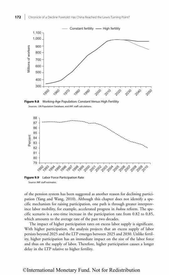
172 Chronicle of a Decline Foretold: Has China Reached the Lewis Turning Point?
of the pension system has been suggested as another reason for declining partici-pation (Yang and Wang, 2010). Although this chapter does not identify a spe-cific mechanism for raising participation, one path is through greater interprov-ince labor mobility, for example, accelerated progress in hukou reform. The spe-cific scenario is a one-time increase in the participation rate from 0.82 to 0.85, which amounts to the average rate of the past two decades.
The impact of higher participation rates on excess labor supply is significant. With higher participation, the analysis projects that an excess supply of labor persists beyond 2025 and the LTP emerges between 2025 and 2030. Unlike fertil-ity, higher participation has an immediate impact on the size of the labor force and thus on the supply of labor. Therefore, higher participation causes a longer delay in the LTP relative to higher fertility.
1,100Constant fertility
Mill
ions
of w
orke
rsHigh fertility
1,000
900
800
700
600
500
400
300
1950
1960
1970
1980
1990
2000
2010
2020
2030
2040
2050
Figure 9.8 Working-Age Population: Constant Versus High FertilitySources: UN Population Database; and IMF staff calculations.
79
2010
2009
2008
2007
2006
2005
2004
2003
2002
2001
2000
1999
1998
1997
1996
1995
1994
1993
1992
8081828384
Per
cent
85868788
Figure 9.9 Labor Force Participation RateSource: IMF staff estimates.
©International Monetary Fund. Not for Redistribution

Das and N’Diaye 173
Financial Sector Reform
The financial reform scenario considered here is a very specific one: interest rate deregulation that lifts deposit rates. The channel by which interest rates is assumed to affect excess supply is the wealth effect: Higher deposit rates raise the return on the stock of wealth, but decrease the flow into wealth as households meet saving targets more easily, which, in turn, reduces the supply of labor. The scenario is simulated for a 5 percentage point increase in nominal deposit rates, using estimates of the saving response to interest rates in Nabar, 2011 (also see Chapter 5 in this volume).
The results indicate that financial reform accelerates the crossing of the LTP. Whereas in the baseline the excess supply of labor in 2020 was in the range of 30 million, interest rate liberalization would reduce this excess to about 10 million, and the LTP would occur shortly after 2020. Because the depletion of excess labor is likely to be associated with higher wages, potentially raising labor’s share of income, financial reform along the lines of this scenario is broadly consistent with Chinese authorities’ objectives of raising household income in the medium term.
Product Market Reform
The final scenario considers product market reform that lifts TFP. Although TFP contribution to output growth in China has been positive since 1990, its growth has slowed in recent years. Raising TFP is consistent with a wide variety of poli-cies announced in the 12th Five-Year Plan, such as greater competition in the services sector and investment in higher value added activities. Unlike in the other scenarios, higher TFP works through the labor demand side in this framework, raising firm profitability and thus the demand for labor (Freeman, 1980). This scenario is simulated through a one-time permanent increase in the growth rate of TFP to 4.5 percent, the average TFP growth since 1990.
The impact on the LTP from higher TFP is qualitatively similar to financial reform: a faster decline of excess labor supply, and a faster emergence of the LTP, relative to the baseline. However, this result is, in part, a consequence of the model specification in which TFP does not directly affect the supply of labor. In an alternative setup (e.g., Pissarides and Valenti, 2007) in which gains in produc-tivity translate into lower unemployment—and thus a lower notional supply of labor—a smaller decrease in excess labor supply could result.
CONCLUSION
China is on the cusp of a demographic shift that will have profound consequenc-es on its economic and social landscape. Within a few years the working-age population will reach a historical peak, and will then begin a precipitous decline. The core of the working-age population, those ages 20–39 years, has already begun to shrink. With this, the vast supply of low-cost workers—a core engine of China’s growth model—will dissipate, with potentially far-reaching domestic and external implications.
©International Monetary Fund. Not for Redistribution

174 Chronicle of a Decline Foretold: Has China Reached the Lewis Turning Point?
This chapter empirically assesses when labor shortages might emerge. The central result is that, barring an endogenous market or policy response, the excess supply of labor—the reserve of unemployed and underemployed workers (cur-rently in the range of 150 million)—will fall to about 30 million by 2020 and the LTP will be crossed between 2020 and 2025.
An endogenous policy response to potential labor shortages is, however, likely as the government tries to slow the transition to the LTP. Market mechanisms that result in higher wages as labor markets tighten, or induce a transition to more capital-intensive production, may also offset the shrinking labor pool. Scenario analysis reveals that higher fertility through relaxation of the one-child policy and greater labor force participation through hukou reform will delay depletion of excess labor. Financial reform and higher TFP, conversely, accelerate the transition to a labor shortage economy, through wealth effects and greater profitability of firms, respectively.
Quantitative estimates of the excess supply of labor and the timing of the LTP presented in this chapter are inherently uncertain. In addition, alternative sce-nario exercises are analyzed for specific reforms of particular magnitudes and do not take into account potential inter-scenario effects (e.g., the offsetting impacts of higher fertility and financial sector reform). That said, the main point of the analysis is that market and policy responses to the declining labor surplus will be largely peripheral; demographic forces play a dominant role in the imminent transition to a labor shortage economy.
©International Monetary Fund. Not for Redistribution

Das and N’Diaye 175
ANNEX 9A. THE DISEQUILIBRIUM MODEL OF THE LABOR MARKET
Labor Demand. Aggregate demand for labor is specified as a function of the endogenous real wage, TFP—reflecting the standard Cobb-Douglas production function in which profit-maximizing firms demand more labor with technologi-cal progress—and partner GDP growth, a proxy for demand conditions given China’s high dependence on exports. The model is log-linear with an additive stochastic error:
1 1 2 3 1 ,DL W GDPp TFP= α +β +β +β + ε (9A.1)
in which LD denotes the natural logarithm of the notional aggregate demand for labor; W is the natural log of gross real wages (gross nominal wages deflated by the consumer price index); GDPp is the natural log of the real GDP-weighted growth rate of trading partners; and TFP is total factor productivity, calculated as the residual of a growth accounting framework with capital and labor shares assumed in the literature.11
Labor Supply. Aggregate labor supply depends on real wages, net household wealth, the scale of the potential labor force (approximated by the participation rate interacted with population), and the unemployment rate. The unemploy-ment rate is included to capture “added-worker effects,” that is, the notion that under weak labor demand conditions, households may send additional individu-als to look for work, resulting in a positive observed association between the sup-ply of labor and the unemployment rate (Basu, Genicot, and Stiglitz, 2000):
2 4 5 6 7 2ln ,SL W H Wealth U= α +β +β +β +β + ε (9A.2)
in which LS is notional aggregate supply of labor, H denotes the natural log of the scale variable, and U is the unemployment rate.
In the equilibrium model, the observed quantity of labor equates the notional supply of labor, LS, with the notional demand for labor, LD. In the disequilibrium model, however, it is assumed that the observed quantity, L, is the minimum of the notional labor supplied and demanded:
( )= min ,S DL L L . (9A.3)
This assumption implies that if LS > LD, then L = LD and the observed quan-tity lies only on the demand curve, whereas LS < LD indicates L = LS and the observed quantity lies only on the supply curve. This is the key contrast with the equilibrium model (L = LS = LD), because in the disequilibrium case, the demand for and supply of labor are unobservable unless they are the minimum in equation (9A.3). The deterministic function is defined as
*( )S DL L I I− = δ − , (9A.4)
11 TFP is in level terms.
©International Monetary Fund. Not for Redistribution
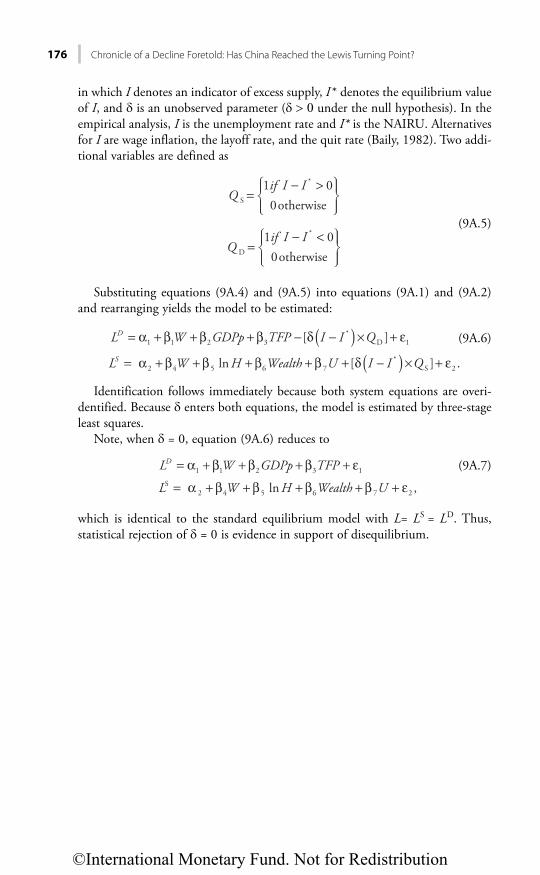
176 Chronicle of a Decline Foretold: Has China Reached the Lewis Turning Point?
in which I denotes an indicator of excess supply, I * denotes the equilibrium value of I, and is an unobserved parameter ( under the null hypothesis). In the empirical analysis, I is the unemployment rate and I* is the NAIRU. Alternatives for I are wage inflation, the layoff rate, and the quit rate (Baily, 1982). Two addi-tional variables are defined as
*
S
1 00 otherwiseif I I
Q⎧ ⎫− >⎪ ⎪= ⎨ ⎬⎪ ⎪⎩ ⎭
(9A.5)
*
D
1 00 otherwiseif I I
Q⎧ ⎫− <⎪ ⎪= ⎨ ⎬⎪ ⎪⎩ ⎭
Substituting equations (9A.4) and (9A.5) into equations (9A.1) and (9A.2) and rearranging yields the model to be estimated:
( )*1 1 2 3 D 1[ ]DL W GDPp TFP I I Q= α +β +β +β − δ − × + ε (9A.6)
( )*2 4 5 6 7 S 2 ln [ ] .SL W H Wealth U I I Q= α +β +β +β +β + δ − × + ε
Identification follows immediately because both system equations are overi-dentified. Because enters both equations, the model is estimated by three-stage least squares.
Note, when = 0, equation (9A.6) reduces to
1 1 2 3 1 DL W GDPp TFPα +β +β +β + ε= (9A.7)
S
2 4 5 6 7 2 l ,nL W H Wealth U= α +β +β +β +β + ε
which is identical to the standard equilibrium model with L= LS = LD. Thus, statistical rejection of = 0 is evidence in support of disequilibrium.
©International Monetary Fund. Not for Redistribution
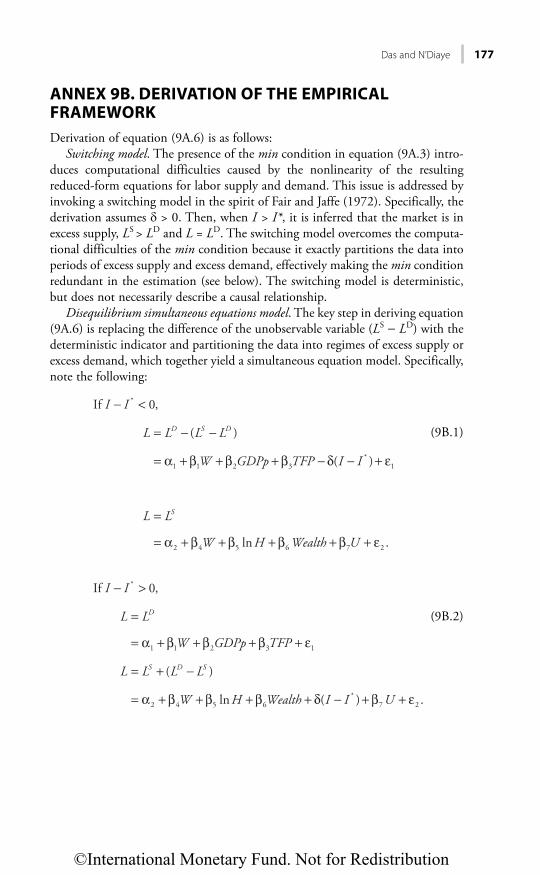
Das and N’Diaye 177
ANNEX 9B. DERIVATION OF THE EMPIRICAL FRAMEWORK
Derivation of equation (9A.6) is as follows:Switching model. The presence of the min condition in equation (9A.3) intro-
duces computational difficulties caused by the nonlinearity of the resulting reduced-form equations for labor supply and demand. This issue is addressed by invoking a switching model in the spirit of Fair and Jaffe (1972). Specifically, the derivation assumes > 0. Then, when I > I*, it is inferred that the market is in excess supply, LS > LD and L = LD. The switching model overcomes the computa-tional difficulties of the min condition because it exactly partitions the data into periods of excess supply and excess demand, effectively making the min condition redundant in the estimation (see below). The switching model is deterministic, but does not necessarily describe a causal relationship.
Disequilibrium simultaneous equations model. The key step in deriving equation (9A.6) is replacing the difference of the unobservable variable (LS − LD) with the deterministic indicator and partitioning the data into regimes of excess supply or excess demand, which together yield a simultaneous equation model. Specifically, note the following:
*
*1 1 2 3 1
2 4 5 6 7 2
If 0,
( )
( )
ln
.
D S D
S
I I
L L L L
W GDPp TFP I I
L L
W H Wealth U
− <
= − −
= α +β +β +β − δ − + ε
=
= α +β +β +β +β + ε
(9B.1)
*
1 1 2 3 1
*2 4 5 6 7 2
If 0,
( )
ln ( )
.
D
S D S
I I
L L
W GDPp TFP
L L L L
W H Wealth I I U
− >
=
= α +β +β +β + ε
= + −
= α +β +β +β + δ − +β + ε
(9B.2)
©International Monetary Fund. Not for Redistribution

178 Chronicle of a Decline Foretold: Has China Reached the Lewis Turning Point?
REFERENCES
Aziz, J., and L. Cui, 2007, “Explaining China’s Low Consumption: The Neglected Role of Household Income,” IMF Working Paper 7/181 (Washington: International Monetary Fund).
Baily, M., 1982, Workers, Jobs and Inflation (Washington: The Brookings Institution).Barro, R.J., and H.I. Grossman, 1971, “A General Disequilibrium Model of Income and
Employment,” American Economic Review, Vol. 61, No. 1, pp. 82–93. Basu, K., G. Genicot, and J.E. Stiglitz, 2000, “Unemployment and Wage Rigidity When Labor
Supply Is a Household Decision,” Working Paper 00-10 (New York: Cornell University, Center for Analytic Economics).
Cai, F., and M. Wang, 2008, “A Counterfactual Analysis on Unlimited Surplus Labor in Rural China,” China and the World Economy, Vol. 16, No. 1, pp. 51–65.
Chan, K.W., 2010, “A China Paradox: Migrant Labor Shortage amidst Rural Labor Supply Abundance,” Eurasian Geography and Economics, Vol. 51, No. 4, pp. 513–30.
Fair, R., and A. Jaffe, 1972, “Methods of Estimation for Markets in Disequilibrium,” Econometrica, Vol. 40, pp. 497–514.
Freeman, R., 1980, “The Evolution of the American Labor Market, 1948–80,” in The American Economy in Transition, ed. by M. Feldstein (Chicago: University of Chicago Press).
Garnaut, R., 2006, “The Turning Point in China’s Economic Development,” in The Turning Point in China’s Economic Development, ed. by Ross Garnaut and Ligang Song (Canberra: Asia Pacific Press).
Golley, J., and R. Tyers, 2006, “China’s Growth to 2030: Demographic Change and the Labour Supply Constraint,” Australian National University Working Paper (Canberra).
Hajivassiliou, V., 1993, “Macroeconomic Shocks in an Aggregative Disequilibrium Model,” Cowles Foundation Discussion Paper No. 2063 (New Haven, Connecticut: Cowles Foundation, Yale University).
International Monetary Fund (IMF), 2011, People’s Republic of China: Spillover Report for the 2011 Article IV Consultation and Selected Issues (Washington). www.imf.org/external/pubs/ft/scr/2011/cr11193.pdf.
Knight, J., Q. Deng, and S. Li, 2011, “The Puzzle of Migrant Labour Shortage and Rural Labour Surplus in China,” China Economic Review, Vol. 22, No. 4, pp. 585–600.
Kwan, C.H., 2007, “China Shifts from Labor Surplus to Labor Shortage: Challenges and Opportunities in a New Stage of Development” (Tokyo: Research Institute of Economy Trade and Industry).
Lewis, W.A., 1954, “Economic Development with Unlimited Supplies of Labour,” Manchester School, Vol. 22, No. 2, pp. 139–92.
Lucas, R.E., and L. Rapping, 1969, “Real Wages, Employment, and Inflation,” Journal of Political Economy, Vol. 77, pp. 721–54.
Nabar, M., 2011, “Targets, Interest Rates and Household Saving in Urban China,” IMF Working Paper 11/223 (Washington: International Monetary Fund).
National Population Development Strategy Research Report, 2007. Pissarides, M., and G. Valenti, 2007, “The Impact of TFP Growth on Steady-State
Unemployment,” International Economic Review, Vol. 48, pp. 607–40.Quandt, R.E., and H. Rosen, 1986, “Unemployment, Disequilibrium and the Short Run
Phillips Curve: An Econometric Approach,” Journal of Applied Econometrics, Vol. 1, No. 3, pp. 235–53.
Rosen, H., and R.E. Quandt, 1978, “Estimation of a Disequilibrium Aggregate Labor Market,” Review of Economics and Statistics, Vol. 60, No. 3, pp. 371–79.
Rudebusch, G.D., 1986, “Testing for Labor Market Equilibrium with an Exact Excess Demand Disequilibrium Model,” Review of Economics and Statistics, Vol. 68, No. 3, pp. 468–76.
©International Monetary Fund. Not for Redistribution
Das and N’Diaye 179
Yang, D.U., and M. Wang, 2010, “Demographic Aging and Employment in China,” Institute of Population and Labour Economics, Chinese Academy of Social Sciences.
Zhang, G., and Z. Zhao, 2006, “Reexamining China’s Fertility Puzzle: Data Collection and Quality over the Last Two Decades,” Population and Development Review, Vol. 32, pp. 293–321.
Zhang, X, J. Yang, and S. Wang, 2010, “China Has Reached the Lewis Turning Point,” IFPRI Discussion Paper No. 977 (Washington: International Food Policy Research Network).
©International Monetary Fund. Not for Redistribution

This page intentionally left blank
©International Monetary Fund. Not for Redistribution

181
CHAPTER 10
How Pro-Poor and Inclusive Is China’s Growth? A Cross-Country Perspective
RAVI BALAKRISHNAN, CHAD STEINBERG, AND MURTAZA SYED
Poverty in China has fallen dramatically over the last 35 years of reform and opening up. However, inequality has increased since the early 1990s, dampening the impact of China’s growth on poverty reduction and making it among the most unequal large economies in the world. This chapter finds that although China’s recent period of growth has remained strongly pro-poor, it has been less inclusive compared with other regions. Based on cross-country experiences, policies that could broaden the benefits of growth in China include a fairer fiscal tax and expenditure system, higher public spending on health and education, enhanced social safety nets including conditional cash transfers, greater assistance for vulnerable workers, reforms to increase labor income, and improvements to financial access. As a beneficial by-product, many of these policies would also facilitate the rebalancing of China’s growth model by ratio-nalizing saving, boosting household incomes, and unleashing consumption.
INTRODUCTION
Income inequality has risen across much of the world since 1990. The academic literature attributes this rise to three main factors: globalization, skill-biased tech-nological change, and the decreasing bargaining power of workers. In addition, country-specific features may also be at play, including diminished social spend-ing, barriers to labor mobility, and geographic disparities. The 2008–09 global financial crisis and recent social turmoil in different parts of the world have heightened awareness of the potential impact of rising inequality on economic and social stability and the sustainability of growth. Such concerns have not bypassed China, where policymakers are placing high priority on finding ways to arrest rising inequality and share the fruits of growth more equitably.
This chapter quantifies the degree to which China’s recent growth has been pro-poor and inclusive, and discusses what factors drive these outcomes and which policies could be considered to help make growth more broad-based and equita-ble. The main findings are that China’s impressive growth has translated into a dramatic reduction in poverty. However, inequality has increased sharply since 1990, dampening the impact of growth on poverty reduction. As a result, relative
©International Monetary Fund. Not for Redistribution

182 How Pro-Poor and Inclusive Is China’s Growth? A Cross-Country Perspective
to other regions and in contrast to its own experience of equitable growth in the 1980s, China’s recent period of growth has been less inclusive. To rein in this trend, opportunities are available for policy measures to broaden the benefits of growth, notably enhanced spending on health and education, stronger social safety nets, labor market interventions, and financial inclusion. Many of these policies would also help rebalance the Chinese economy toward household and private consumption.
This chapter is organized as follows: The next section motivates the research by comparing recent trends in poverty and inequality in China with those in other regions of the world. The two subsequent sections propose ways to quan-tify how pro-poor and inclusive growth is in any economy and use a regression approach to assess China’s performance on these metrics relative to its peers. The final section draws lessons from international experiences in poverty-reduction initiatives and proposes potential policy interventions for broadening the benefits of growth in China.
POVERTY, INEQUALITY, AND GROWTH: CHINA IN AN INTERNATIONAL CONTEXT
Since 1990, growth in China and most Asian economies has been robust and higher on average than in other emerging regions. In turn, this growth has trans-lated into significant reductions in poverty (Table 10.1).
When China’s reforms began, it was one of the poorest countries in the world. In 1981, 84 percent of its population lived on less than $1.25 a day, the fifth-largest poverty incidence in the world. By 2008, this proportion had fallen to 13 percent, well below the developing-country average (Figure 10.1). Nevertheless, China’s large population means that it still remains home to almost 175 million people who live in extreme poverty.
TABLE 10.1
People Living on Less Than $1.25 Per Day
Percent of Population
Number
(millions)
Percent
of World
Total
Number
(millions)
Percent
of World
Total
1990 2008 1990 2008
Europe and Central Asia 2 <1 9 <1 2 0Latin America and The Caribbean 12 6 53 3 37 3Middle East and North Africa 6 3 13 1 9 1Sub-Saharan Africa 57 48 290 15 386 30Asia 55 25 1,544 81 855 66 China 60 13 683 36 173 13 India 47 33 433 23 395 31 Rest of Asia 58 31 427 22 287 22Total 43 22 1,909 1,290
Source: World Bank, PovcalNet database.Note: At 2005 purchasing-power-parity prices.
©International Monetary Fund. Not for Redistribution
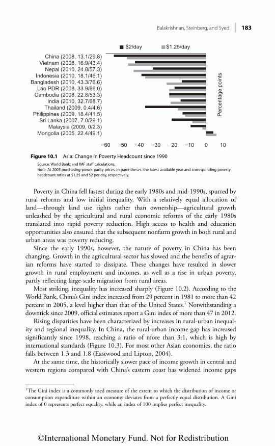
Balakrishnan, Steinberg, and Syed 183
Poverty in China fell fastest during the early 1980s and mid-1990s, spurred by rural reforms and low initial inequality. With a relatively equal allocation of land—through land use rights rather than ownership—agricultural growth unleashed by the agricultural and rural economic reforms of the early 1980s translated into rapid poverty reduction. High access to health and education opportunities also ensured that the subsequent nonfarm growth in both rural and urban areas was poverty reducing.
Since the early 1990s, however, the nature of poverty in China has been changing. Growth in the agricultural sector has slowed and the benefits of agrar-ian reforms have started to dissipate. These changes have resulted in slower growth in rural employment and incomes, as well as a rise in urban poverty, partly reflecting large-scale migration from rural areas.
Most striking, inequality has increased sharply (Figure 10.2). According to the World Bank, China’s Gini index increased from 29 percent in 1981 to more than 42 percent in 2005, a level higher than that of the United States.1 Notwithstanding a downtick since 2009, official estimates report a Gini index of more than 47 in 2012.
Rising disparities have been characterized by increases in rural-urban inequal-ity and regional inequality. In China, the rural-urban income gap has increased significantly since 1998, reaching a ratio of more than 3:1, which is high by international standards (Figure 10.3). For most other Asian economies, the ratio falls between 1.3 and 1.8 (Eastwood and Lipton, 2004).
At the same time, the historically slower pace of income growth in central and western regions compared with China’s eastern coast has widened income gaps
1 The Gini index is a commonly used measure of the extent to which the distribution of income or consumption expenditure within an economy deviates from a perfectly equal distribution. A Gini index of 0 represents perfect equality, while an index of 100 implies perfect inequality.
China (2008, 13.1/29.8)Vietnam (2008, 16.9/43.4)
Nepal (2010, 24.8/57.3)Indonesia (2010, 18.1/46.1)
Bangladesh (2010, 43.3/76.6)Lao PDR (2008, 33.9/66.0)
Cambodia (2008, 22.8/53.3)India (2010, 32.7/68.7)
Thailand (2009, 0.4/4.6)Philippines (2009, 18.4/41.5)
Sri Lanka (2007, 7.0/29.1)Malaysia (2009, 0/2.3)
$2/day $1.25/day
−60 −50 −40 −30 −10 0 10
Per
cent
age
poin
ts
−20
Mongolia (2005, 22.4/49.1)
Figure 10.1 Asia: Change in Poverty Headcount since 1990Source: World Bank; and IMF staff calculations.Note: At 2005 purchasing-power-parity prices. In parentheses, the latest available year and corresponding poverty headcount ratios at $1.25 and $2 per day, respectively.
©International Monetary Fund. Not for Redistribution
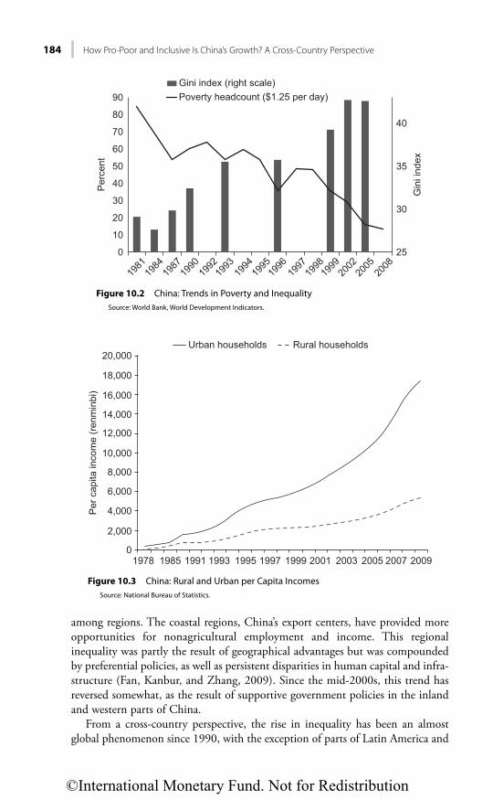
184 How Pro-Poor and Inclusive Is China’s Growth? A Cross-Country Perspective
among regions. The coastal regions, China’s export centers, have provided more opportunities for nonagricultural employment and income. This regional inequality was partly the result of geographical advantages but was compounded by preferential policies, as well as persistent disparities in human capital and infra-structure (Fan, Kanbur, and Zhang, 2009). Since the mid-2000s, this trend has reversed somewhat, as the result of supportive government policies in the inland and western parts of China.
From a cross-country perspective, the rise in inequality has been an almost global phenomenon since 1990, with the exception of parts of Latin America and
90
80
70
60
50
40
40
Gini index (right scale)Poverty headcount ($1.25 per day)
35
30
25
30
20
10
0
1981
1984
1987
1993
1994
1995
2002
2008
Gin
i ind
ex
Per
cent
2005
1999
1998
1997
1996
1992
1990
Figure 10.2 China: Trends in Poverty and InequalitySource: World Bank, World Development Indicators.
1978
20,000
18,000
16,000
14,000
12,000
10,000
8,000
6,000
4,000
2,000
01985 1991 1993
Urban households
Per
cap
ita in
com
e (r
enm
inbi
)
Rural households
1995 1997 1999 2001 2003 2005 2007 2009
Figure 10.3 China: Rural and Urban per Capita IncomesSource: National Bureau of Statistics.
©International Monetary Fund. Not for Redistribution
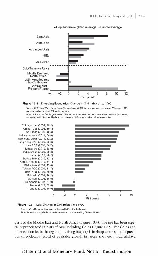
Balakrishnan, Steinberg, and Syed 185
parts of the Middle East and North Africa (Figure 10.4). The rise has been espe-cially pronounced in parts of Asia, including China (Figure 10.5). For China and other economies in the region, this rising inequity is in sharp contrast to the previ-ous three-decade record of equitable growth in Japan, the newly industrialized
East Asia
South Asia
Advanced Asia
NIEs
ASEAN-5
Sub-Saharan AfricaMiddle East and
North AfricaLatin America and
the CaribbeanCentral and
Eastern Europe−4 −2 0 2 4 6
Gini points8 10 12
Population-weighted average Simple average
Figure 10.4 Emerging Economies: Change in Gini Index since 1990Source: CEIC Data; World Bank, PovcalNet database; WIDER income inequality database; Milanovic, 2010; national authorities; and IMF staff calculations.Note: ASEAN-5 = five largest economies in the Association of Southeast Asian Nations (Indonesia, Malaysia, the Philippines, Thailand, and Vietnam); NIE = newly industrialized economies.
China, urban (2008, 35.2)China, rural (2008, 39.4)
Sri Lanka (2006, 40.3)Indonesia, rural (2011, 34.0)
Indonesia, urban (2011, 42.2)Hong Kong SAR (2006, 53.3)
Lao PDR (2008, 36.7)Singapore (2010, 48.0)
India, urban (2009, 39.3)Japan (2010, 28.7)
Bangladesh (2010, 32.1)Korea, Rep. of (2010, 34.1)
Philippines (2009, 43.0)Taiwan POC (2009, 31.7)
India, rural (2009, 30.0)Malaysia (2009, 46.2)Vietnam (2008, 35.6)
Cambodia (2008, 37.9)Nepal (2010, 32.8)
Thailand (2009, 40.0)
−4 −2 0 2 4Gini points
6 8 10
Figure 10.5 Asia: Change in Gini Index since 1990Source: World Bank; national authorities; and IMF staff calculations.Note: In parentheses, the latest available year and corresponding Gini coefficients.
©International Monetary Fund. Not for Redistribution

186 How Pro-Poor and Inclusive Is China’s Growth? A Cross-Country Perspective
economies (NIEs), the members of the Association of Southeast Asian Nations, and China itself (Figure 10.6). At the same time, even as the size and purchasing power of China’s middle class has grown, its share of overall income has fallen while that of the richest quintile has increased. By contrast, in Latin America and in the Middle East and North Africa, the share of the richest quintile has fallen. Earlier work (IMF, 2006) attributes the rise in inequality around the world to skill-biased technological change and the transition from agriculture to industry for lower-income Asian economies (consistent with the Kuznets hypothesis).2
HOW PRO-POOR IS CHINA’S GROWTH?
Going beyond these stylized facts, regression analysis can be used to quantify how pro-poor and inclusive China’s growth is relative to other emerging regions.3 There are various ways to interpret what it means for growth to be inclusive and pro-poor. This chapter follows the Ravallion and Chen (2003) approach and defines growth as pro-poor simply if it reduces poverty. Inclusive growth, in con-trast, is defined as growth that is not associated with an increase in inequality, following Rauniyar and Kanbur (2010). More specifically, this chapter defines growth as inclusive when it is not associated with a reduction in the share of the bottom quintile of the income distribution.
2 Jaumotte, Lall, and Papageorgiou (2008) also argue that skill-biased technological progress is a key driver of rising inequality.3 For the econometric analysis, the main sources of data are the latest versions of the PovcalNet data-base (updated in July 2012) and the Penn World Tables. PovcalNet was chosen because major efforts have been made to make its inequality and poverty data comparable across surveys and countries: It draws on 700 household surveys and 120 countries (econ.worldbank.org/povcalnet). Household survey data for the NIEs are added to this, resulting in an unbalanced panel between 1971 and 2010, with the sample skewed toward the latter part of the period.
−10 −8
Hong Kong SAR (1971–86, 42.0)Korea, Rep. of (1965–88, 33.6)
Indonesia (1964–87, 32.0)Malaysia (1970–89, 48.4)
Singapore (1973–89, 39.0)Japan (1962–90, 35.0)
India (1960–90, 29.7)Taiwan Province of China (1964–85, 29.0)
Philippines (1971–88, 44.5)Thailand (1971–89, 43.8)
Sri Lanka (1963–90, 30.1)Bangladesh (1973–92, 28.3)
Nepal (1976–84, 30.06)China (1953–85, 31.4)
Gini points−6 −4 −2
−20.2
0 2
−24.4
Figure 10.6 Asia: Change in Gini Index before 1990Source: Milanovic, 2010; and IMF staff calculations.Note: In parentheses, the time period and end-value for the Gini coefficients.
©International Monetary Fund. Not for Redistribution

Balakrishnan, Steinberg, and Syed 187
To examine the relationship between poverty reduction and growth, the fol-lowing regression is estimated:
ln Pi,t = gi + bi,d lnyi,t + di,t ln GINIi,t + rd + ei,t, (10.1)
in which Pi,t is the poverty headcount below the $2 per day line in country i at time t, Yi is a country dummy, yi,t is per capita income in country i at time t’, GINIi,t is the Gini coefficient in country i at time t, and d is a set of decade dum-mies. Because the equation is in logs, b gives the impact of income growth on poverty reduction, and d gives the impact of a change in the Gini coefficient. Both b and d are allowed to vary across countries and decades.
To estimate the fixed effects, a set of benchmark countries is needed. Because the main interest of this analysis is to compare China with the rest of Asia and Latin America, all countries falling in other emerging and developing regions—notably, Europe and Central Asia, the Middle East and North Africa, and sub-Saharan Africa—are included in the benchmark category. An instrumental variables approach is used to take account of endogeneity bias and potential measurement error in the income variable. In particular, lags of real per capita income as mea-sured in the Penn World Tables are used to instrument the household-survey-based average income variable.
The regression analysis presented in Table 10.2 suggests that for all countries in the sample, growth is in general pro-poor, with growth leading to significant declines in poverty across all economies and time periods. Specifically, a 1 percent increase in real per capita income leads to about a 2 percent decline in the pov-erty headcount (column 1). However, a 1 percent increase in the Gini coefficient almost directly offsets the beneficial impact on poverty reduction of the same increase in income. This finding is consistent with other work that suggests that the incidence of extreme poverty in China would have fallen to less than 5 percent had inequality not increased after 1990 (ADB, 2012).
Moreover, inequality interacts with income, meaning that a higher level of inequality tends to reduce the impact of income growth on poverty reduction (column 2). As an illustration, an increase in the Gini coefficient of about 25 percent (as in urban China from 1995 to 2005) reduces the impact of a 1 per-cent increase in income to about a 1½ percent decline in the poverty head-count from 2 percent in the base case. The implication of this result is that past rises in inequality are likely to reduce the future impact of income growth on poverty, even if the level of inequality remains constant. In addition, the impact of growth on poverty reduction is found to be somewhat lower during the 1990s, possibly as a result of a change in the nature of growth (column 3).
The relationship, however, varies across regions and economies (columns 4 and 5 and Figure 10.7). In particular, in East Asia and Latin America, income growth has a significantly lower impact on poverty than it does in the Middle East and North Africa, Eastern Europe and Central Asia, and sub-Saharan Africa, the baseline economies. The impact is particularly weak in India and Indonesia,
©International Monetary Fund. Not for Redistribution
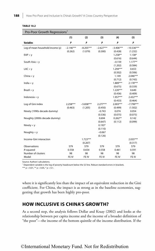
188 How Pro-Poor and Inclusive Is China’s Growth? A Cross-Country Perspective
TABLE 10.2
Pro-Poor Growth Regressions1
Variables
(1)
P
(2)
P
(3)
P
(4)
P
(5)
P
Log of mean household income (y) –2.146*** –8.205*** –2.627*** –3.406*** –10.536***(0.262) (1.079) (0.300) (0.428) (1.232)
EAP y 1.258** 1.138*(0.616) (0.644)
South Asia y –0.159 1.177**(1.202) (0.584)
LAC y 1.294*** 0.653(0.502) (0.506)
China y 1.149 2.046***(0.712) (0.743)
India y 1.889*** 2.178***(0.675) (0.559)
Brazil y 1.220*** 0.640(0.436) (0.409)
Indonesia y 1.957*** 2.432***(0.433) (0.464)
Log of Gini index 2.258*** –5.838*** 2.277*** 2.003*** –7.799***(0.463) (1.205) (0.450) (0.499) (1.502)
Ninety (1990s decade dummy) –0.743 0.074 0.054(0.536) (0.075) (0.075)
Noughty (2000s decade dummy) 0.694 0.262** 0.142(0.647) (0.112) (0.099)
Ninety y 0.193*(0.110)
Noughty y –0.067(0.126)
Income-Gini interaction 1.723*** 2.035***(0.267) (0.317)
Observations 579 579 579 579 579R-squared 0.558 0.654 0.558 0.461 0.591Number of clusters 98 98 98 98 98Model FE IV FE IV FE IV FE IV FE IV
Source: Authors’ calculations.1 Dependent variable is the log of poverty headcount below the $2 line. Robust standard errors in brackets.*** p < 0.01, ** p < 0.05, * p < 0.1.
where it is significantly less than the impact of an equivalent reduction in the Gini coefficient. For China, the impact is as strong as in the baseline economies, sug-gesting that growth has been highly pro-poor.
HOW INCLUSIVE IS CHINA’S GROWTH?
As a second step, the analysis follows Dollar and Kraay (2002) and looks at the relationship between per capita income and the income of a broader definition of “the poor”—the income of the bottom quintile of the income distribution. If the
©International Monetary Fund. Not for Redistribution
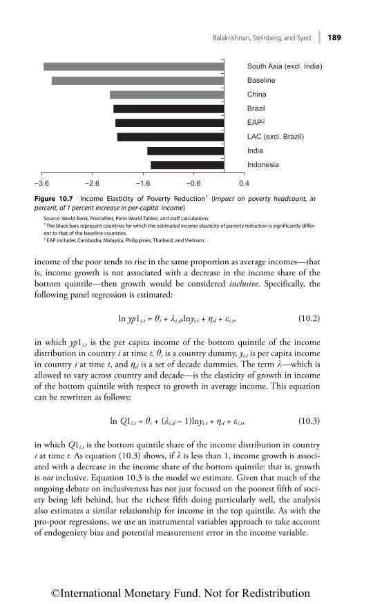
Balakrishnan, Steinberg, and Syed 189
income of the poor tends to rise in the same proportion as average incomes—that is, income growth is not associated with a decrease in the income share of the bottom quintile—then growth would be considered inclusive. Specifically, the following panel regression is estimated:
ln yp1i,t = qi + li,d,lnyi,t + hd + ei,t, (10.2)
in which yp1i,t is the per capita income of the bottom quintile of the income distribution in country i at time t, qi is a country dummy, yi,t is per capita income in country i at time t, and hd is a set of decade dummies. The term l—which is allowed to vary across country and decade—is the elasticity of growth in income of the bottom quintile with respect to growth in average income. This equation can be rewritten as follows:
ln Q1i,t = qi + (li,d – 1)lnyi,t + hd + ei,t, (10.3)
in which Q1i,t is the bottom quintile share of the income distribution in country i at time t. As equation (10.3) shows, if l is less than 1, income growth is associ-ated with a decrease in the income share of the bottom quintile: that is, growth is not inclusive. Equation 10.3 is the model we estimate. Given that much of the ongoing debate on inclusiveness has not just focused on the poorest fifth of soci-ety being left behind, but the richest fifth doing particularly well, the analysis also estimates a similar relationship for income in the top quintile. As with the pro-poor regressions, we use an instrumental variables approach to take account of endogeniety bias and potential measurement error in the income variable.
Figure 10.7 Income Elasticity of Poverty Reduction1 (impact on poverty headcount, in percent, of 1 percent increase in per-capita income)
Source: World Bank, PovcalNet, Penn World Tables; and staff calculations.1 The black bars represent countries for which the estimated income elasticity of poverty reduction is significantly differ-ent to that of the baseline countries. 2 EAP includes Cambodia, Malaysia, Philippines, Thailand, and Vietnam.
−3.6 −2.6 −1.6 −0.6 0.4
Indonesia
India
LAC (excl. Brazil)
EAP2
Brazil
China
Baseline
South Asia (excl. India)
©International Monetary Fund. Not for Redistribution

190 How Pro-Poor and Inclusive Is China’s Growth? A Cross-Country Perspective
The results are shown in Table 10.3. If all observations are simply pooled, the familiar Dollar-Kraay result is obtained—that average incomes of the poorest fifth of society rise proportionately with per capita income (column 1), something which also holds for the richest fifth (column 4). However, once the analysis instruments for the income variable (columns 2 and 5), then the income of the bottom quintile rises significantly less than proportionately with average income, and the income of the top quintile rises significantly more than proportionately with average income.
Moreover, these elasticities vary significantly across regions and countries (col-umns 3 and 6). For the bottom quintile, the elasticity is significantly less than 1 for China, as well as for the NIEs and South Asia (excluding India), whereas for Brazil, it is significantly greater than 1 (Figure 10.8).4 Turning to the top quintile, the results are the mirror image of those for the bottom quintile, except for the NIEs (Figure 10.9). The elasticity is significantly greater than 1 for China, the
4 Although the elasticity for China is not significantly different from that of the baseline at the 10 percent level (column 3 of Table 10.3), further c2 tests show that it is significantly different from 1 at the 1 percent level.
TABLE 10.3
Inclusive Growth Regressions1
Variables
(1)
InQ1
(2)
InQ1
(3)
InQ1
(4)
InQ5
(5)
InQ5
(6)
InQ5
Log of mean household income (y)
–0.025 –0.142** –0.097 0.040* 0.119*** 0.060
(0.043) (0.061) (0.126) (0.023) (0.034) (0.061)EAP y 0.126 –0.142
(0.180) (0.101)NIEs y –0.430*** 0.098
(0.126) (0.062)LAC y 0.133 –0.068
(0.186) (0.080)South Asia y –0.480*** 0.390**
(0.178) (0.185)China y –0.204 0.138**
(0.128) (0.062)Brazil y 0.469*** –0.260***
(0.126) (0.063)India y 0.320 –0.224
(0.305) (0.146)Indonesia y 0.049 –0.030
(0.133) (0.069)Observations 661 633 633 661 633 633R- squared 0.001 –0.027 0.017 0.021 –0.019 0.064Model FE FE IV FE IV FE FE IV FE IVNumber of clusters 107 105 105 107 105 105
Source: Authors’ calculations.1 Dependent variable is the log share of the income distribution of the bottom/top quintile. Robust standard errors in brackets.*** p < 0.01, ** p < 0.05, * p < 0.1.
©International Monetary Fund. Not for Redistribution

Balakrishnan, Steinberg, and Syed 191
0 0.2 0.4 0.6 0.8 1 1.2 1.4
South Asia (excl. India)NIEs
ChinaBaseline
IndonesiaEAP2
LAC (excl. Brazil)India
Brazil
Figure 10.8 Degree of Inclusiveness of Growth1 (impact on income of the bottom quintile, in percent, of a 1 percent increase in per-capita income)
Source: World Bank Development Indicators; and IMF staff estimates.1 The black bars represent countries for which the estimated degree of inclusiveness is significantly different from one. 2 EAP includes Cambodia, Malaysia, Philippines, Thailand, and Vietnam.
NIEs, and South Asia (excluding India), and significantly less than 1 for Brazil (column 6). In sum, the results suggest that growth has generally not been inclu-sive in China, nor in the NIEs and South Asia (excluding India), whereas it has been inclusive in Brazil.5
Finally, using the regression estimates, Table 10.4 investigates the impor-tance of growth to the welfare of the poor. It constructs measures of pro-poor and inclusive growth for Brazil, China, India, Indonesia, Mexico, and the Russian Federation for recent decades. The table shows that although the income elasticities of poverty and income of the bottom quintile vary signifi-cantly across economies, per capita income growth remains a key driver of
5 One important caveat is that Brazil entered the 1990s with a relatively higher level of inequality.
Figure 10.9 Degree of Inclusiveness of Growth1 (impact on income of the top quintile, in per-cent, of a 1 percent increase in per-capita income)
Source: World Bank Development Indicators; and IMF staff estimates.1 The black bars represent countries for which the estimated degree of inclusiveness is significantly differentfrom one. 2 EAP includes Cambodia, Malaysia, Philippines, Thailand, and Vietnam.
0 0.2 0.4 0.6 0.8 1 1.2 1.4
South Asia (excl. India)ChinaNIEs
BaselineIndonesia
LAC (excl. Brazil)EAP2India
Brazil
©International Monetary Fund. Not for Redistribution

192 How Pro-Poor and Inclusive Is China’s Growth? A Cross-Country Perspective
TABLE 10.4
Pro-Poor and Inclusive Growth Measures
[1]
Elasticity of
Poverty w.r.t.
Income
Growth1
[2]
Degree of
Inclusiveness1
[3]
Income
Growth2
[4]
Change
in Gini
[5]=[1] × [3]
+ 2 × [4]
Predicted
Change in
Poverty (%)
[6] = [2] × [3]
Predicted
Change in
Bottom Fifth
Income (%)
China 1980s −3.4 0.7 84 54 −177 59China 1990s −3.4 0.7 88 36 −227 61China 2000s −3.4 0.7 123 22 −377 86Brazil 1980s −2.2 1.4 24 5 −43 33Brazil 1990s −2.2 1.4 5 −3 −18 7Brazil 2000s −2.2 1.4 34 −9 −92 47India 1990s −1.5 1.0 10 −1 −17 10India 2000s −1.5 1.0 26 9 −21 26Indonesia 1990s −1.4 1.0 15 −5 −31 15Indonesia 2000s −14 1.0 90 23 −84 90Mexico 1990s −2.1 1.0 −17 −3 31 −17Mexico 2000s −2.1 1.0 41 −4 −94 41Russia 1990s −3.4 1.0 −47 −26 110 −47Russia 2000s −3.4 1.0 92 12 −289 92
Source: World Bank, PovcalNet; Penn World Tables; and IMF staff calculations.1 Set equal to the value for the baseline countries when the null of a significant difference cannot be rejected.2 As proxied by 100 times the change in the log over the corresponding period.
income of the poorest fifth of society. Some of the more specific results include the following:
• Inequality has widened in China, in contrast with Brazil and Mexico. Still, China has experienced greater poverty reduction because of its larger growth in average income.
• The importance of average income growth is reinforced when looking at trends in Indonesia and Russia. For both economies in the first decade of the 2000s relative to the 1990s, poverty reduction was much greater despite worsening inequality, because growth was much higher.
• A similar story emerges when looking at measures of inclusive growth. For example, although growth has been only half as inclusive in China as compared with Brazil, the income of the poorest fifth of society has increased by rela-tively more in China because average income growth has been much stronger.
TOWARD MORE INCLUSIVE GROWTH IN CHINA: SOME LESSONS FROM INTERNATIONAL EXPERIENCE
This section discusses policies that could reduce inequality and increase inclusive-ness, based on the regression results and international experience.6 It is by no means exhaustive and the multiple factors behind rising inequality suggest that a
6 In the Asian context, evidence indicates that the labor share of income, public education spending, years of schooling, industry employment, and financial reform significantly increase the degree of inclusiveness (Balakrishnan, Steinberg, and Syed, 2013).
©International Monetary Fund. Not for Redistribution

Balakrishnan, Steinberg, and Syed 193
set of mutually reinforcing policies will likely be needed, and that the necessary mix will vary from country to country.
In China, boosting household incomes would appear to be a key priority for addressing inequality. Higher incomes could be achieved, for instance, by decreas-ing existing subsidies to capital in the form of artificially low input costs, promot-ing services and agriculture that tend to be more labor intensive, continuing to raise minimum wages, and raising the returns to household savings through interest rate reform and financial development.
Fiscal Policy
Increasing government spending on education and health. The relatively low amount of public spending on education and health as a share of GDP in China points to an important potential role for fiscal policy in strengthening inclusiveness (Figure 10.10). Increased spending is particularly important in the face of rising skill premiums and increasing returns to human capital. Between 1988 and 2003, wage returns to one additional year of schooling increased in China to 11 percent from 4 percent (Zhang and others, 2005) and disparities in educational attain-ment beyond primary school have also emerged.
Tax and spending effort. In addition, adjusting the level and structure of taxes and spending may have a part to play. In Organization for Economic Cooperation and Development (OECD) countries, taxes and transfer policies have also been estimated to reduce inequality by about a quarter (OECD, 2012). In sharp con-trast, the redistributive impact of fiscal policy in developing economies is severely restricted by lower overall levels of both taxes and transfers—whereas average tax ratios for advanced economies exceed 30 percent of GDP, ratios in Asia and the Pacific are only about half that level and among the lowest in developing regions (Bastagli, Coady, and Gupta, 2012). At about 20 percent of GDP, China’s tax ratio is on the low side. Partly as a result, social spending is also substantially lower in developing economies, at about 8 percent of GDP compared with 15 percent of GDP in advanced economies, with lower transfers and health spending explaining most of the difference. Again, China is an even greater outlier on the low side. Public expenditures on health, pensions, and other forms of social pro-tection only amount to 5.7 percent of GDP in China. On average, economies at similar levels of development spend more than twice as much.
Tax and spending structure. Greater reliance on less progressive tax and spend-ing instruments adds to the problem. In Asia and the Pacific, indirect taxes account for half of tax revenue, compared with less than one-third in advanced economies. In China, the situation is even more extreme, with taxes on incomes and profits making up only about one-quarter of total tax revenue. Broadening the tax base and improving the progressivity of some taxes could also be consid-ered in China.7 Meanwhile, participation in social insurance schemes remains
7 The Asian Development Bank notes that only 11 types of personal income are subject to taxation. Moreover, while some of these are taxed at progressive rates (wages and salaries), others are taxed at a flat rate (such as income from personal services, royalties, and rental and lease income).
©International Monetary Fund. Not for Redistribution

194 How Pro-Poor and Inclusive Is China’s Growth? A Cross-Country Perspective
a. Employment laws and inclusiveness
Indonesia
Brazil
IndiaLAC
EAP
China
NIEs
SA
0.7
0.6
0.5
Em
ploy
men
t law
s in
dex1
0.4
0.3
0.20.3 0.5 0.7 0.9
Degree of inclusiveness1.1 1.3
Others
b. Minimum wage and inclusiveness
Indonesia
Brazil
India
LAC
EAP
China
NIEsSA
0.4
0.35
0.25
0.3
Min
imum
wag
e/ a
vera
ge v
alue
add
ed
0.2
0.15
0.10.3 0.5 0.7 0.9
Degree of inclusiveness1.1 1.3
Others
Figure 10.10 Labor Market Institutions and InclusivenessSource: Botero and others, 2004; World Bank, Doing Business; and IMF staff estimates.Note: EAP = East Asia and Pacific; LAC = Latin America and the Caribbean; NIEs = newly industrialized economies; SA = South Asia. The light gray diamonds represent countries for which the estimated degree of inclusiveness is significantly different from one. 1Measures the protection of labor and employment laws as the average of alternative employment contracts, the cost of increasing hours worked, the cost of firing workers, and dismissal procedures.
©International Monetary Fund. Not for Redistribution

Balakrishnan, Steinberg, and Syed 195
limited in many developing countries like China (particularly in rural areas), and expenditure on social assistance programs is often low and poorly targeted. According to the Asian Development Bank (ADB), about one-third of the poor population in China do not have access to any social programs. Thus, reliance on targeted social expenditures aimed at vulnerable households, including for health and education, could be increased. Conditional cash transfer programs are being increasingly used in low-income emerging economies. Brazil and Mexico have two of the largest schemes (in the former, Bolsa Familia covers about 25 percent of the population) with transfers contingent on requirements such as children’s school attendance or vaccination records. Both are considered to have been successful, with the Mexican program being associated with a 10 percent reduction in poverty within two years of its introduction. In Asia, the Philippines introduced a conditional cash transfer program in 2008 (the 4Ps) to help redirect resources toward socially desirable programs in a well-targeted way. By 2012, it was budgeted to reach 60 percent of the poor. In India, the recently launched unique identity scheme holds significant promise in ensuring better targeting of social schemes and allowing the vulnerable to access the welfare system.
Intergovernmental fiscal arrangements. In China, the existing system of inter-governmental fiscal relations may be compounding the problem. Fiscal decentral-ization is much higher in China than in OECD and middle-income countries, particularly on the spending side. More than half of all expenditure, including social spending, takes place at the subprovincial level. The result has been that poor villages cannot afford to provide good services, and poor households cannot afford the high private costs of basic public services. With regard to public spend-ing on education, large differences in per capita allocations are found across provinces. Overall public spending per capita in the richest province is almost 50 times that in the poorest (ADB, 2012), although the go-west policy in place since 2000 has helped to narrow some of these gaps.
Other social safety nets. In China, the World Bank estimates that only about 30 percent of the labor force contributed to a pension scheme in 2008, with participation especially limited among migrants. This proportion compares to an average coverage rate of 60 percent in OECD countries (OECD, 2009). As well as increasing inclusiveness, enhancing such safety nets would also reduce precau-tionary motives to save, thereby increasing consumption and facilitating the needed rebalancing of China’s economy. Ensuring the sustainability of these welfare programs will be important, however, given China’s aging population. A key question about such policies is their fiscal cost. The Bolsa Familia program in Brazil only costs 0.4 percent of GDP, and recent IMF work on China (Barnett and Brooks, 2010) argues that a minimum social safety net can be provided at low cost, with more comprehensive nets funded by broadening the tax base and increasing some taxes, along with reallocating existing spending. In addition, some policies may have no fiscal cost, such as unemployment insurance schemes in which employees and employers contribute to individual accounts. Regarding education, in many cases the challenge is to improve quality. Expanding pension
©International Monetary Fund. Not for Redistribution

196 How Pro-Poor and Inclusive Is China’s Growth? A Cross-Country Perspective
provision could entail costs, but not necessarily if benefits are provided on a defined contribution basis and contribution rates are increased.
Labor Market Policies
Labor share of income. Across most of the OECD as well as Asia, the past two decades have seen a decline in the income share of labor and a rise in that of capital—in China, the labor share fell from an estimated 50 percent during the early 1990s to about 40 percent by the middle of the first decade of the 2000s. This disproportion contributes to inequality, because capital income tends to be less evenly distributed than income from basic wage labor. It is partly the result of technological change that the return to capital has risen and the employment elasticity of growth has declined; according to the ADB, between 1991 and 2011, the employment elasticity of growth fell from 0.44 to 0.28 in China. In the case of China, this has been exacerbated by an artificially low cost of capital. The historically large pool of surplus labor in rural areas has also reduced the bargaining power of workers, contributing to holding wages low relative to productivity.
Bargaining power of workers. Academic work also links rising inequality to the weaker bargaining power of workers (Levy and Temin, 2007). Indeed, addressing labor market duality and the use of minimum wages are being increasingly advo-cated across the world to support the income of low-earning workers. In this vein, China’s February 2013 announcement of a 35-point plan to tackle income inequality includes a provision to raise minimum wages to at least 40 percent of average salaries by 2015 across most regions. These effects seem to matter empir-ically. Inclusive growth is positively associated with the degree of employment protection and minimum wage levels (Figure 10.10). Although recent increases have made minimum wage rates in China relatively favorable compared with other emerging regions, employment protection appears weak, possibly reflecting the predicament of migrant workers.
Labor market impediments. In China, additional labor market interventions could be considered. In particular, restrictions on rural-urban migration under the hukou system—whereby workers without urban registrations have difficulty accessing housing, social services, and social security—have limited opportunities for the relatively poor rural population. Anecdotal evidence suggests that practical difficulties continue to complicate selling or mortgaging rural land, compounding the problem. In addition, worker training and skills upgrading would help make growth more employment friendly.
Financial Access
A burgeoning literature demonstrates that financial development not only pro-motes economic growth but also helps apportion it more evenly. According to some estimates, for the lowest quintile, the benefits of financial development are split roughly equally between those associated with faster growth and those from
©International Monetary Fund. Not for Redistribution

Balakrishnan, Steinberg, and Syed 197
greater income equality (Beck, Demirgüç-Kunt, and Levine, 2007). Financial market imperfections—such as asymmetric information and costs associated with transactions and contract enforcement—hit poor and small-scale entrepreneurs hardest because they typically lack collateral, credit histories, and connections. These deficiencies prevent capital from flowing to poor individuals, even if they have projects with high prospective returns, thereby reducing the efficiency of capital allocation and aggravating inequality. By addressing these imperfections and creating enabling conditions for financial markets and instruments to devel-op—such as insurance products that facilitate adjustment to shocks—govern-ments can not only spur growth but also help ensure that it is distributed more evenly.
How does China currently fare on financial development compared with its peers? There is appreciable disparity across Asia (Figure 10.11). Financial deepen-ing—a measure of the level of financial services, typically proxied by broad-money-to-GDP—is positively associated with per capita income, and is elevated in China, reflecting high domestic saving and strong external inflows.
However, deepening by itself may not translate into financial services being broadly available across firms and households, making “access to finance” equally important as financial deepening. Across the globe, high-income countries tend, on average, to have almost 12 times more bank branches and 30 times more automated teller machines for every 100,000 adults than do low-income
Figure 10.11 Financial Deepening, Latest Year AvailableSource: World Bank Development Indicators; and IMF staff estimates.
3501214
1086420
−2−4−6
Hon
g K
ong
SA
RJa
pan
Chi
na
Mal
aysi
aS
inga
pore
Thai
land
Wor
ldVi
etna
mA
ustra
liaN
ew Z
eala
ndM
iddl
e in
com
eN
epal
Indi
aK
orea
, Rep
. of
Sou
th A
sia
Phi
lippi
nes
Ban
glad
esh
Sub
-Sah
aran
Afri
caE
urop
e an
d C
entra
l Asi
aLo
w in
com
eIn
done
sia
Sri
Lank
aC
ambo
dia
Lao
PD
R
Latin
Am
eric
a an
d C
arib
bean
Mid
dle
Eas
t and
Nor
th A
frica
Hig
h in
com
e
Eas
t Asi
a an
d P
acifi
c
300
250
200
150
Per
cent
of G
DP
Per
cent
100
50
0
Broad money in percent of GDP (left scale)Annual average growth, in percent(2000–09; right scale)
©International Monetary Fund. Not for Redistribution

198 How Pro-Poor and Inclusive Is China’s Growth? A Cross-Country Perspective
countries. Indeed, lack of access to finance is a major impediment in many parts of Asia, including in China, where more than half the population and a signifi-cant proportion of small and medium enterprises lack access to the formal finan-cial system (IFC, 2010).
Moreover, there is evidence that access to finance is positively correlated with relative success in reducing poverty incidence and ensuring equity across Asian economies (Beck, Demirgüç-Kunt, and Levine, 2007). For China, several empirical studies suggest that uneven access to financial services has contributed to inequality. Zhang and others (2003) find that after controlling for other fac-tors—such as provincial infrastructure, institutional transition in rural areas, and degree of international integration—differential financial development and urban biases in lending have contributed significantly to the rise in China’s urban-rural income disparity since the late 1980s. Financial development—mea-sured as total rural loans to rural GDP—has been found to contribute signifi-cantly to reducing rural inequality in China (Liang, 2008). Tellingly, three of the poorest provinces in China—Tibet, Yunnan, and Sichuan—have more than 50 unbanked counties.
How might the Chinese government address the twin goals of supporting growth and reducing inequality? International experience provides some direc-tion. First is ensuring macroeconomic stability as financial systems are liberalized, and particularly as they are opened up to the rest of the world, because financial shocks typically hit the poor hardest (see Chapter 13 for a discussion of a road map designed for China). Second is identifying and removing impediments to financial access without directing particular outcomes. Expanding credit avail-ability by promoting rural finance, extending micro-credit, promoting credit information sharing, and developing venture capital markets should significantly expand credit availability (Beck and Demirgüç-Kunt, 2006). Third, because pov-erty is often relatively higher in rural areas, is ensuring that regulations—such as loan classification criteria and capital requirements—do not discriminate against the provision of finance to the rural poor, including the agricultural sector. Fourth is bolstering the legal environment and financial market infrastructure, including property rights and contract enforceability. For instance, well-defined processes for securing collateral in the event of default can encourage banks to lend more to small and medium enterprises, and developing capital markets can help broaden the channels for financial access. Fifth is promoting regulatory policies that foster transparency and competition among financial institutions (Levine, 2011), rather than those that channel credit to politically favored ends (see, e.g., Barth and others, 2009).
In addition to arresting the rising tide of inequality in China, many of the policies discussed in this chapter have the potential to rationalize savings and boost household incomes, reducing the bias toward capital and large corporates, and unleashing consumption. In this way, these measures would have the positive side effect of facilitating the needed rebalancing of China’s growth model toward households, workers, and consumption.
©International Monetary Fund. Not for Redistribution

Balakrishnan, Steinberg, and Syed 199
REFERENCES
Asian Development Bank (ADB), 2012, “Confronting Rising Inequality in China,” in Asian Development Outlook 2012 (Manila).
Balakrishnan, R., C. Steinber g, and M. Syed, 2013, “The Elusive Quest for Inclusive Growth: Growth, Poverty and Inequality in Asia,” IMF Working Paper 13/152 (Washington: International Monetary Fund).
Barnett, S,. and S. Brooks, 2010, “China: Does Government Health and Education Spending Boost Consumption?” IMF Working Paper 10/16 (Washington: International Monetary Fund).
Barth, J.R., C. Lin, P. Lin, and F.M. Song, 2009, “Corruption in Bank Lending to Firms: Cross-Country Evidence on the Beneficial Role of Competition and Information Sharing,” Journal of Financial Economics, Vol. 91, pp. 361–88.
Bastagli, F., D. Coady and S. Gupta, 2012, “Income Inequality and Fiscal Policy,” IMF Staff Discussion Note 12/8R (Washington: International Monetary Fund).
Beck, T.H.L., and A. Demirgüç-Kunt, 2006, “Small and Medium-Size Enterprises: Access to Finance as a Growth Constraint,” Journal of Banking and Finance, Vol. 30, No. 11, pp. 2931–43.
———, and M. Martinez Peria, 2008, “Banking Services for Everyone? Barriers to Bank Access and Use around the World,” World Bank Economic Review, Vol. 22, No. 3, pp. 397–430.
———, and R. Levine, 2007, “Finance, Inequality and the Poor,” Journal of Economic Growth, Vol. 12, No. 1, pp. 27–49.
Berg, A., and Ostry, J., 2011, “Inequality and Unsustainable Growth: Two Sides of the Same Coin?” IMF Staff Discussion Note 11/08 (Washington: International Monetary Fund).
Botero, Juan C., Simeon Djankov, Rafael La Porta, Florencio Lopez-de-Silanes, and Andrei Shleifer, 2004, “The Regulation of Labor,” Quarterly Journal of Economics, Vol. 119, No. 4, pp. 1339–82.
Dollar, D., and A. Kraay, 2002, “Growth is Good for the Poor,” Journal of Economic Growth, Vol. 7, No. 3, pp. 195–225.
Duflo, Esther, 2011, “Balancing Growth with Equity: The View from Development,” paper prepared for the Federal Reserve Bank of Kansas City’s Economic Policy Symposium, Jackson Hole, Wyoming, August 25–27.
Eastwood, R., and M. Lipton, 2004, “Rural and Urban Income Inequality and Poverty: Does Convergence between Sectors Offset Divergence within Them?” in Inequality, Growth, and Poverty in an Era of Liberalization and Globalization, ed. by G.A. Cornia (Oxford, United Kingdom: Oxford University Press).
Fan, S., R. Kanbur, and X. Zhang, 2009, “Regional Inequality in China: An Overview,” in Regional Inequality in China: Trends, Explanations and Policy Responses, ed. by S. Fan, R. Kanbur, and X. Zhang (New York, New York: Routledge).
International Finance Corporation, 2010, “Access to Finance: Annual Review Report” (Washington: World Bank).
International Monetary Fund (IMF), 2006, “Rising Inequality and Polarization in Asia,” in Asia Pacific Regional Economic Outlook, October (Washington).
Jaumotte, F., S. Lall, and C. Papageorgiou, 2008, “Rising Income Inequality: Technology, or Trade and Financial Globalization?” IMF Working Paper 08/185 (Washington: International Monetary Fund).
Levine, R., 2011, “Finance, Regulation and Inclusive Growth,” paper presented at OECD and World Bank Conference on “Challenges and Policies for Inclusive Growth,” Paris, March 24–25.
Liang, Z., 2008, “Financial Development and Income Inequality in Rural China: 1991–2000,” in Understanding Inequality and Poverty in China: Methods and Applications, ed. by Guanghua Wan (New York, New York: Palgrave Macmillan) pp. 72–88.
©International Monetary Fund. Not for Redistribution

200 How Pro-Poor and Inclusive Is China’s Growth? A Cross-Country Perspective
Levy, F.S., and P. Temin, 2007, “Inequality and Institutions in 20th Century America,” Working Paper No. 07-17 (Cambridge, Massachusetts: MIT Department of Economics).
Organization for Economic Cooperation and Development (OECD), 2009, “Pensions at a Glance: Asia/Pacific,” 2009 ed. (Paris).
———, 2012, “Income Inequality and Growth: The Role of Taxes and Transfers,” OECD Economics Department Policy Note No. 9 (Paris).
Rauniyar, G. and R. Kanbur, 2010, “Inclusive Development: Two Papers on Conceptualization, Application, and the ADB Perspective, “ (Manila: Asian Development Bank).
Ravallion, M., and S. Chen, 2003, “Measuring Pro-Poor Growth,” World Bank Policy Research Working Paper No. 2666 (Washington: World Bank).
Zhang, J., Y. Zhao, A. Park, and X. Song, 2005, “Economic Returns to Schooling in Urban China,” Journal of Comparative Economics, Vol. 33, pp. 730–53.
Zhang, Q., M. Liu, R. Tao, and V. Chen, 2003, “Development of Financial Intermediaries and Urban-Rural Income Inequality in China” (in Chinese), Working paper, Peking University.
©International Monetary Fund. Not for Redistribution

201
CHAPTER 11
De-Monopolization toward Long-Term Prosperity in China
ASHVIN AHUJA
During the past decade, the average Chinese worker earned roughly nine times less and was 10 times less productive than the average American at purchasing power par-ity. Current consensus attributes large differences in output per worker to differences in total factor productivity (TFP). Evidence suggests that most of the United States–China TFP differences lie in the inefficiency of China’s domestic-oriented service and agricultural sectors. This chapter focuses on (1) the evidence of monopoly rights and their influence on work practices improvement at China’s firms and plants and (2) the evidence that policy arrangements have encouraged more competition in merchandise manufacturing and heavy industries while barriers to market access remain high against new firms in the domestic market (especially in services). The empirical analysis suggests that China can enhance long-term income per capita by a factor of 10, largely through TFP gains, by implementing reforms to weaken protection of monopolies and encourage entry in all industries.
INTRODUCTION
Between 2000 and 2009, the average Chinese worker earned approximately nine times less than the average American, and the typical Chinese worker was less productive than his or her American counterpart by a factor of roughly 10 when measured at purchasing power parity (PPP).1
What accounts for such large differences in income per capita between China and the United States? Current consensus in growth and development accounting mainly attributes large differences in output per worker between rich and poor countries to differences in TFP while assigning a significantly lesser role to gaps in physical and human capital stocks.2 Conclusions based on cross-country micro-data approaches to productivity measurement and comparison also con-firm these results (see Baily and Solow, 2001). With regard to the difference between China and the United States, Hall and Jones (1999) estimate that
1 Based on 2000–09 real GDP per capita at purchasing power parity (PPP), chain method, and real GDP per worker at PPP from the Penn World Table version 7.0.2 See, for example, Klenow and Rodriguez-Clare (1997); Hall and Jones (1999); Jasso, Rosenzweig, and Smith (2000); Easterly and Levine (2001); Hendricks (2002); Caselli (2005); and Hsieh and Klenow (2010).
©International Monetary Fund. Not for Redistribution

202 De-Monopolization toward Long-Term Prosperity in China
Chinese output per worker would be about half that of U.S. output per worker without the large difference in TFP alone.3
A stream of research papers has focused on what accounts for such large TFP differences across countries. Systematic resource misallocation is a key theme. Restuccia and Rogerson (2008) and Hsieh and Klenow (2009), for example, find that misallocation of resources across firms can have important effects on aggre-gate TFP. Focusing on China, India, and the United States, Hsieh and Klenow (2009) quantify large manufacturing TFP losses from resource misallocation in the periods before China joined the World Trade Organization (WTO). Viewed from a static, standard monopolistic competition model, they show that moving to “U.S. efficiency” would increase China’s manufacturing TFP by about 30–50 percent based on 1997–98 data. The literature offers other specific mech-anisms by which resource misallocation could lower aggregate TFP, such as labor market regulations (e.g., Hopenhayn and Rogerson, 1994; and Lagos, 2006), deficiency in capital allocation vis-à-vis managerial talent (e.g., Caselli and Gennaioli, 2003; and Buera and Shin, 2013), and vested interests’ ability to block firms from introducing better work practices (Parente and Prescott, 1997, 1999).
Lewis (2004a, 2004b) offers evidence from 13 emerging and advanced econo-mies linking institutions and policy arrangements to subpar performance of industry- and economy-wide TFP. The overarching lesson from these studies is that the time path of aggregate productivity levels is highly correlated with the economic policy arrangements countries choose (specifically regarding the ability and incentives of organized forces in each society to resist the adoption of supe-rior technology and persist in inefficient usage of currently operating ones). The main obstacles to productivity growth and economic progress in poor countries are the many policies that limit market competition.
In the case of the United States and China, the aggregate TFP gap is approxi-mately 13 times in favor of the United States (Figure 11.1).4 Differences between the United States’ and China’s manufacturing TFP levels appear much smaller at about 1.3–1.5 times (Hsieh and Klenow, 2009). Thus, even accounting for mea-surement errors, most of the differences in aggregate productivity, and therefore living standards, between China and the United States have to be rooted in the inefficiency in the nonmanufacturing sectors—mostly domestic-oriented services and agriculture. In line with this observation, He and others (2012) report that China’s nontradable TFP growth has been about 2.2–2.5 percent per year lower than manufacturing-heavy tradable TFP growth during 2001–10.
This chapter documents the links between TFP outcomes and “monopoly rights” in the domestic market (especially in services) and subpar work practice in China, as well as the links between TFP and policy reform to encourage more
3 Measured with labor quality–adjusted TFP gap and assuming fixed aggregate capital and human capital stock.4 The TFP gap size is based on 2005–07 data, after adjusting capital stock to PPP, but not adjusted for labor quality. Measured productivity levels for China could be distorted by various subsidized factor prices (capital, land, and energy, as well as intellectual property).
©International Monetary Fund. Not for Redistribution

Ahuja 203
competition via external trade in merchandise manufacturing and heavy indus-tries. It finds that resistance to better work practices, which surfaces to access large opportunities for rent seeking and is more prevalent in some domestic-oriented (nontradable) industries, is likely to be a significant impediment to China’s long-term economic prospects.
The chapter also explores the extent to which reforming the monopoly-rights policy arrangement that China currently employs can enhance long-term income per capita, using a general equilibrium model with a strategic game developed by Parente and Prescott (1999). The defining feature of the model is the existence of state protection of vested interest groups and industry insiders that can undertake strategic actions against “high-technology” firms attempting to enter.
The model, once calibrated to China and U.S. growth facts, can capture dis-crepancies in PPP-adjusted GDP per capita between the two economies reason-ably well. The discrepancy in GDP per capita is mainly accounted for by differ-ences in TFP, consistent with cross-country work in growth and development accounting. Specifically, the model predicts that China’s long-term GDP per capita could be higher by as much as a factor of 10 under the “free enterprise” arrangement than under the protected monopoly-rights arrangement that well approximates the economy today. The increase in per capita income is driven by the 3.5-fold increase in China’s TFP (with reproducible capital share remaining at about 0.45). Over time, physical capital accumulation, as well as education and skill acquisition, will follow as their rates of return rise with higher TFP.
The model also predicts that the unit price of the goods and services produced in the sectors with barriers to entry relative to that of goods and services produced in the competitive sector is about 3¼ times higher in China under monopoly rights than in the United States with free enterprise. This is roughly the ratio of
8.510.0
13.0
10.0
1.3
0
5
10
Tim
es15
Real GDP percapita, PPP(2000–09)
Output perworker, PPP(2000–09)
TFP, rawlabor
(2005–07)
TFP, laborquality
adjusted (1988)
ManufacturingTFP (1998)
FIgure 11.1 U.S. Income and Productivity Relative to ChinaSources: Hall and Jones, 1999; Hsieh and Klenow, 2009; Penn World table 7.0; and author’s calculations.Note: PPP = Purchasing-power parity; TFP = total factor productivity.
©International Monetary Fund. Not for Redistribution

204 De-Monopolization toward Long-Term Prosperity in China
the price of investment goods to the price of consumption goods across rich and poor countries in the Aten, Summers, and Heston data (three to four times).
The principal insight from the stylized model is that these long-term gains are made through improvements in TFP rather than factor accumulation (e.g., through high fixed asset investment growth); and the gains are made by shifting away from monopoly rights to the free enterprise policy arrangement. The result should facilitate a policy discussion about the direction of ongoing corporate and financial reforms in China. Specifically, ongoing reform efforts should target productivity improvement rather than factor accumulation. Drawing lessons from the extraordinary success in Chinese manufacturing exports, China should persist with reform to weaken protection and encourage entry in all industries. Competitive pressure from multinationals and new domestic firms will help transform work practices across Chinese firms.5 More products and services will be produced at more affordable prices. Wages will rise and converge across sectors. More firms operating in China will innovate and export best practices to the world. Chinese workers and households will be made better off as rent-seeking activities fade away. As a result, the large income gap between China and leading industrial countries will eventually be eliminated.
The rest of the chapter proceeds as follows: The next section presents salient evidence of protected monopoly rights and discusses work practices at Chinese firms. It is followed by sections that give the intuition behind the model and that outline the model’s calibration and report findings.
EVIDENCE OF MONOPOLY RIGHTS AND WORK PRACTICES AT CHINESE PLANTS
Published empirical findings on industry- and firm-level productivity in China are rare and centered on the manufacturing sector. Existing industry-level accounts of productivity in China’s nonmanufacturing sectors are largely based on case studies done by the McKinsey Global Institute (MGI). China’s manufactur-ing sector enjoyed exceptionally fast productivity growth in the decades before and after China’s entry into the WTO.6 This manufacturing productivity boom follows the gradual application of zhengqi fenkai policy, which formally separates government functions from business operations. The government first applied the policy to the consumer goods industry and then to high technology and heavy manufacturing in preparation for global competition (Woetzel, 2008). After entry into the WTO, favoritism reserved for large state-owned firms began fading, and private domestic firms moved to the forefront of the rapidly changing business
5 The reform efforts may need to be properly sequenced to manage resistance from vested interest groups, but sequencing is beyond the scope of this chapter.6 He and others (2012) estimate annual tradable (mostly manufacturing) TFP growth at between 4.6 and 5.4 percent between 2002 and 2007. Guo and N’Diaye (2009) estimate manufacturing TFP growth at 6½ percent per year on average between 2002 and 2007. Bosworth and Collins’ (2007) industry TFP growth during 1993–2004 averages 6.2 percent per year.
©International Monetary Fund. Not for Redistribution
Ahuja 205
landscape. State-owned manufacturing plants, which used to run at 40 percent less TFP than private domestic plants, started to exit, their numbers falling from 29 percent of total firms in 1998 to only 8 percent in 2005 (Hsieh and Klenow, 2009). Regardless of ownership type, exit means survivors now run plants at a much higher average TFP. Furthermore, the rise in market competition is largely reflected in the exits of SOEs, mostly small and medium-sized, and the rapid growth of private firms (Conway and others, 2010). With improved SOE gover-nance, SOEs are becoming more efficient and behaving more like private firms.
Successful industries have benefited from government policies, notably access to factors of production at subsidized prices, market access barriers, and policies that encourage domestic purchasing of goods and services (to guarantee revenue pools). Nevertheless, it would be a mistake to attribute the strides made in manu-facturing productivity simply to government support. Not only have many gov-ernment-backed projects not been successful, but there are many examples of successful firms that face competitive pressure from the global market. To cite a few, the Chinese communications equipment industry has improved its quality and gained market acceptance in advanced economies. China’s solar and wind power industries are using new manufacturing techniques to create more efficient solar panels and are already supplying sophisticated, vital components for the industry worldwide (Orr and Roth, 2012).
Indeed, the success stories in Chinese manufacturing productivity growth performance seem to fit well with other cross-country case studies. Evidence from case studies from 13 emerging and advanced economies reveals that policy arrangements that limit competition can potentially result in subpar performance of industry- and economy-wide aggregate TFP7 (Lewis, 2004a, 2004b). The suc-cess of China’s manufacturing sector confirms a clear link between pressure from global competition and powerful incentives and the ability to adopt better tech-nology and improve work practices.
Despite this progress, influential partners, protection from competition, and extensive pricing power continue to characterize China’s business sector (World Bank, 2011; Conway and others, 2010).8 China’s services (nontradables) sectors clearly lack pressure from competition. He and others (2012) offer insights into the large discrepancy between tradables (dominated by manufacturing) and non-tradables TFP growth in China since 2000.
Overall, China’s economy is still dominated by state and state-partner monop-olies, which are shielded from meaningful competition in the domestic market by
7 The countries covered are Australia, Brazil, France, Germany, India, Japan, the Netherlands, Poland, the Russian Federation, the Republic of Korea, Sweden, the United Kingdom, and the United States. Each study analyzes 6 to 13 industries and compares their performance with that of the same indus-tries in a subset of other countries. These are detailed studies of individual businesses spanning “state-of-the-art auto plants to black-market street vendors.”8 Conway and others (2010) attribute this fast-paced improvement to reforms in the new company law and the new bankruptcy law, which help reduce the time needed to register or close a business, increase the recovery rate from bankruptcy, and reduce the minimum amount of capital needed to start a firm.
©International Monetary Fund. Not for Redistribution

206 De-Monopolization toward Long-Term Prosperity in China
state support, regulations,9 licensing, and technology-sharing rules (Figure 11.2). These firms tend to be large, capital-intensive, and well-connected; concentrated in “strategic” and “pillar” sectors; and benefit from subsidies as well as preferential access to finance, land, and other resources. They are not confined to electricity generation and distribution, natural gas, and water, but are also outside of the industrial sector, such as banking, telecommunications, and the media.10 Subsidies to these firms can work effectively to promote employment growth, deter entry, and discourage more productive work practices. Finally, murky own-ership rights and unsystematically kept titles, financial records, collateral, and pledges increase due diligence costs and work as barriers against potential entrants, especially those that are smaller or not homegrown (Figures 11.3).11
Even in the externally competitive manufacturing sector, evidence indicates that policy arrangements could obstruct improvements in work practices and productivity. Significant waste occurs even at high-productivity plants run by multinational industry leaders, which reduces profits by 20–40 percent at some plants (Aminpour and Woetzel, 2006). The inefficiency arises not from a weak profit motive on the part of the plant managers, but can be partly attributed to the way foreign firms tend to gain market access, that is, via partnership with large SOEs or through business acquisitions. Although this process secured “the right locations, the right government relationships, the right joint ventures, [which] shut out other [players] from this market” for years if not a decade, multination-als have inherited “hard to change legacy work processes, employee mind-sets [as well as] manufacturing approaches” (Hexter and Woetzel, 2007, pp. 1, 2). In some cases, introducing a procurement process practiced in these multinationals’ estab-lished home markets—an “innovation” in China—could generate substantial savings for their operations in China. Nevertheless, many multinationals have been able to run plants less efficiently than in Europe and the United States and still “come out way ahead” with the advantage of relatively low costs of labor and intermediate inputs sourced locally. In this way, high profit margins and business growth can undercut the incentive to change work practices and improve opera-tional efficiency.
To adapt best practices to local market conditions and execute superlative operating performance, a business would require reliable markets and customer data, quality suppliers, and efficient distribution networks, which are not readily
9 For instance, services, such as legal and accounting, maritime and air transport, and the postal sector could benefit from foreign providers through higher foreign direct investment (FDI) if restrictions on form of ownership, maximum equity stake, and geographic scope, and line of business restrictions as well as minimum capital requirement (not equally imposed on domestic competitors) were to be removed (OECD, 2009). Currently, much of the services sector FDI goes into real estate and banking, which is gradually opening up.10 Despite the stated intention to open up these sectors to private investment, they are still dominated by public enterprises.11 World Bank (2011) ranks China 79th out of 183 economies for overall “ease of doing business,” and rates China unfavorably on obstacles to “starting a business” (rank 151th out of 183 economies), “dealing with construction permits” (rank 181st) and “investor protection” (rank 93rd).
©International Monetary Fund. Not for Redistribution

Ahuja 207
0
1
2
Sca
leS
cale
3
4
5
6U
S
OE
CD
OE
CD
EM
s
Chi
na
US
OE
CD
OE
CD
EM
sC
hina US
OE
CD
OE
CD
EM
sC
hina US
OE
CD
OE
CD
EM
sC
hina US
OE
CD
OE
CD
EM
sC
hina US
OE
CD
OE
CD
EM
sC
hina
US
OE
CD
OE
CD
EM
s
Chi
na US
OE
CD
OE
CD
EM
s
Chi
na
Involvement inbusiness operation
State control Public ownership
0
2
4
6
Scope ofpublicenterprisesector
Governmentinvolvement ininfrastructuresector
Directcontrol overbusinessenterprise
Pricecontrols
Use ofcommandand controlregulation
Figure 11.2 State Control Indicators, 2008 (minimum to maximum on a scale of 1 to 6)Source: OECD, 2011.Note: EM = Emerging market; OECD = Organization for Economic Cooperation and Development; US = United States.
available in China. These impediments clearly indicate relatively poor service sec-tor productivity, including financial services (MGI, 2006). Manufacturing pro-ductivity, already high and close to the U.S. level, is likely to improve further, provided quality and cost of service inputs improve.
©International Monetary Fund. Not for Redistribution

208 De-Monopolization toward Long-Term Prosperity in China
These studies help shed light on the underlying cause for TFP differences across countries. They are consistent with the idea that incentives and the ability of existing firms to dictate industry work practices can be an important mecha-nism by which resources are misallocated. State protection makes cost of entry by other foreign and domestic firms prohibitive, in turn generating immense value to these monopoly rights. Their lessons seem to be consistent with the theory proposed by Parente and Prescott (1999), which holds that state actions to
Figure 11.3 Barriers to Entrepreneurship Indicators 2008 (minimum to maximum on a scale of 1 to 6)
Source: OECD, 2011.Note: EM = Emerging market; OECD = Organization for Economic Cooperation and Development; US = United States.1 Network sectors include, among others, electricity generation and distribution, natural gas, water, telecommunications, banking, and the media.
0
2
Sca
leS
cale
4
6
Licenseand permits
system
Communication andsimplification of rules
and procedures
Barrier to entry innetwork sectors1
Barrier to entry inother services
OECD
a. Barriers to entry
b. Administrative burdens
OECD EMs US China
0
2
4
6
Administrative burdensfor corporations
Administrative burdensfor sole proprietor firms
Sector-specificadministrative burdens
US OECD OECD EMs China
©International Monetary Fund. Not for Redistribution

Ahuja 209
prohibit or distort firms’ incentives to change work practices tend to be irrelevant unless the state also protects the industry from outside competition.
THE MODEL’S ENVIRONMENT AND EQUILIBRIA: SOME INTUITION12
To measure potential gains from de-monopolization, this chapter relies on the framework and model of Parente and Prescott (1999). This relatively simple, closed-economy model has a strategic mechanism that allows vested interests to impede economic progress. The vested interest groups have valuable monopoly rights that are tied to existing production technology. In every period, no take-up of better technology or work practices as well as inefficient use of existing ones is a possible outcome of a strategic game between two players: the protected coalition of factor suppliers and a potential entrant who has to pay to overcome entry resistance.
The model has two production sectors using constant-returns-to-scale tech-nologies with no fixed costs. Industries are competitive, though they need not be private. There are economic rents in the model.
Under the monopoly-rights arrangement, coalition members can set up firms with protected rights to operate existing technology. Because of these rights, every firm in the industry employing that technology must hire coalition members. The coalition’s objective is to maximize per member income by setting membership size, compensation, and work practices levels (or productivity). In the model, coalition size acts as a deterrent to entry.
Because these protected rights have value, potential entrants must pay to over-come the coalition’s resistance to their market entry. If entry occurs, then the entrant uses a superior technology. In the game, the return to entry depends on the strength of state protection as well as coalition size. When protection is weak, entry occurs because the minimum coalition size necessary to deter entry is too large to provide adequate compensation to recruit and retain members. As a result, firms in every industry always end up adopting better work practices. At the other end of the spectrum, when protection is strong, entry cannot occur at all and every firm operates the current, inferior technology. Interestingly, when state protection is not too strong, the minimum-deterrent-coalition size is larger than the number of members required to produce competitive equilibrium out-put. In this case, firms not only fail to adopt better work practices, they also operate the existing inferior technology inefficiently. This is the relevant case for this analysis of China.
Under the free enterprise policy arrangement—or equivalently, a de-monopo-lized arrangement—there is no coalition to deter entry and all agents act in a perfectly competitive way.
The model economy consists of three sectors: household, agriculture, and indus-try. In any given period, a household can be one of these three: an agricultural
12 The model is developed in detail in Ahuja (2012).
©International Monetary Fund. Not for Redistribution

210 De-Monopolization toward Long-Term Prosperity in China
worker, an industrial worker, or an industrial entrepreneur who adopts a technol-ogy to produce goods and services.
A household is endowed with one unit each of labor and land services. Each household values only agricultural goods and differentiated (industrial) goods. Households do not value leisure. They want to smooth consumption over time and derive enjoyment from variety.
There are three constant-returns-to-scale production technologies in the industrial sector—low, medium, and high efficiency levels, ranked according to the required amount of labor input per unit of output. An entrepreneurial house-hold forming an industrial firm can adopt any technology without incurring any firm-specific investment.
In the agricultural sector, there is a constant-returns-to-scale, nested, constant-elasticity-of-substitution production function in which the mix of intermediate industrial goods is treated as a substitute for the composite labor-land input.13
Monopoly-Rights Arrangement: The Equilibrium and Some Intuition
In the model, monopoly rights are only relevant to the industrial sector. The agricultural sector (which may also be thought to include some services) is per-fectly competitive.14 In each industry, any individual can use the low technology, and entry and exit are free for those operating with the medium technology. Entry obstruction applies only to the high-technology firms.
Workers and entrepreneurs in the industrial sector can form coalitions. Protected monopoly rights are extended only to existing firms employing the medium technology. These rights are protected throughout the life of the coali-tion, the length of which depends on the ability to provide surplus rents to its members.
The coalition in any industry that uses the medium technology has the right to limit its membership size, set the compensation (or wage) rate, and dictate work practices. The coalition dictates work practices by determining the pro-ductivity level, that is, up to the medium technology level, but which could be inefficiently used. A potential entrant employing the high technology has to pay an entry cost to overcome the resistance associated with the protection of the valuable monopoly rights. The entry cost, measured in units of labor ser-vices, depends on the strength of state protection and the coalition size (which, in this case, varies with its production capacity).15 The larger the residual mar-ket left over from the monopolists, the more a new firm should be willing to pay to enter.
13 See Ahuja (2012) for details.14 Examples of these included services are home or market production of goods and services such as bicycle repair shops, hair salons, restaurants, and the like in developing countries.15 The assumption that entry costs increase in proportion to population size (which is also the size of the coalition) also ensures that all results are population-size invariant.
©International Monetary Fund. Not for Redistribution
Ahuja 211
The Monopoly-Rights Equilibrium
Next, the entry game for an industry, defined as the symmetric no-entry steady-state equilibrium, is described. There is an equilibrium for this strategic game. An equilibrium can be either that of “no-entry” or with entry in every industry in steady state. An equilibrium is characterized by utility maximization in the house-hold sector, profit maximization in the agricultural sector, market clearing, and a subgame perfect equilibrium to the game in each industry. In this game, the two players take as given the demand for industry output and the wage in the com-petitive agricultural sector. These givens ensure that the equilibrium solution obtained through agents’ utility and firms’ profit maximization is consistent with players’ strategic behavior and that noncredible (e.g., entry) threats are not exer-cised in equilibrium.
In this game, conditional on entry, Bertrand price competition is in effect, which means that the entrant has a marginal cost that is tied to the agricultural wage and can produce any quantity demanded by consumers. The coalition has zero marginal cost up to the capacity constraint because its members are commit-ted to working in that industry for the period.
In equilibrium, (real) factor input prices are equal to their respective marginal products; the ratio of differentiated goods prices to agricultural goods prices is equal to the ratio of the respective marginal utilities of their consumption; house-holds exhaust their budgets; and quantity supplied must equal quantity demand-ed in every market. Moreover, the entrant will pick an output price such that the investment it has to make to overcome resistance and enter the market will be exactly the maximum profit generated from residual demand; hence, the mini-mal-deterrent entry condition. Confronted by an entering firm with better tech-nology, the coalition maximizes per member income by choosing supply output as efficiently as it can to minimize the entrant’s profit, given the entry price set by the entrant. The coalition members would set work practices at the maximum level whenever entry threat prospects are credible.16 Finally, equilibrium profit is zero at every medium-technology firm because total revenue equals total cost, which is to say that wages paid to coalition members equal their marginal revenue product.
The Competitive Equilibrium
In this particular economy, a unique competitive equilibrium exists, characterized as follows: The price of industry output equals the marginal cost tied to high technology, because this is what a competitive firm uses. In addition, wages are equalized across sectors.
16 The coalition will also set work practices and the wage rate so that equilibrium price equals mar-ginal cost at every competing low-technology firm. The combined choice of work practices and wage rate set by the coalition must be consistent with an equilibrium condition that the nominal wage paid to a worker at a low-technology firm has to equal that worker’s marginal revenue product.
©International Monetary Fund. Not for Redistribution
212 De-Monopolization toward Long-Term Prosperity in China
Calibration and Findings
Once the empirical counterparts of each sector are specified, preference, indus-trial sector technology, and farm sector parameters can be calibrated to replicate the key “stylized” relationships among model aggregates. The calibrated model can then measure the potential gains from eliminating monopoly rights in China.
The numerical results from the calibrated model are as follows: Under free enterprise, agricultural and small services firms use much fewer labor inputs, but much more differentiated intermediate goods relative to total output. Under monopoly rights, agricultural households (or equivalently, the no-barrier-to-entry and labor-intensive sector) are poorer than industrial households and consume less on a per capita basis.
Wages tend to equalize across sectors under free enterprise because there are no economic rents to be derived and protected. Prices are different across arrange-ments (monopoly rights vs. free enterprise). “Industrial” goods that are produced by protected firms are more expensive under monopoly rights than they would be under free enterprise. As a result, firms use less of the intermediate goods and services in the monopoly-rights economy.
In a free-enterprise economy, “agricultural” households face budget constraints similar to those faced by “industrial” households. They consume a roughly equal amount. In addition, the “agricultural” households will get to consume relatively more of the “industrial” goods and services in the free-enterprise economy (because the relative price of “industrial” goods is now much lower).
The long-term results also appear to be quantitatively sensible.17 The “indus-trial” sector generates the lion’s share of the total value added and wage income under free enterprise; however, “agriculture’s” shares of the total value added and wage income shrink by as much as four times. Furthermore, the unit price of “industrial” goods relative to “agricultural” goods is about 3¼ times higher in the poor country with monopoly rights than in the rich country with free enterprise. This is roughly the ratio of the prices of investment goods to consumption goods across rich and poor countries in international data.
In the long term, the effect on output from eliminating monopoly rights is substantial. GDP in PPP terms in the model increases by as much as 3½ times in steady state. Because there is no capital in the model, and labor and land services are assumed to be similar across arrangements, this number is equivalent to the difference in TFP between the two arrangements. Without a TFP difference of this magnitude (and assuming fixed aggregate capital and human capital stock for the sake of comparison), Chinese output per worker under monopoly rights would be about 45 percent of its output per worker under free enterprise, which is close to the number (50 percent of U.S. output per worker) calculated by Hall
17 To allow for direct comparison across economies, a common set of “international prices” is calcu-lated and used to compute real GDP at PPP and their values are compared, based on the Geary-Khamis method (Kravis, Heston, and Summers, 1982).
©International Monetary Fund. Not for Redistribution

Ahuja 213
and Jones (1999).18 Inefficient operation of inferior technology in a large swath of industry and services accounts for lower aggregate TFP in China vis-à-vis the United States (which, in the model, stands for China under “free enterprise”) in the long term. In this calibration, the “industrial” sector achieves only about half of its potential productivity.
In a richer model with capital accumulation, the effect on output from increases in TFP would be amplified because capital would accumulate endoge-nously in response to increasing TFP to keep the long-term rate of return con-stant. The difference in GDP per capita (at PPP) between the two arrangements would then be equal to the factor difference in TFP (here, 3½) raised to the power of 1/(1 minus reproducible capital share). Given China’s reproducible capital share of approximately 0.45, the adjusted difference in GDP per capita at PPP would be about 10 times, roughly similar to the measured difference between U.S. and China output per capita and output per worker at PPP between 2000 and 2009 (8.5 and 10 times, respectively).
CONCLUSION
A large number of research papers have stressed that misallocation of resources across firms can adversely affect aggregate TFP in an economy. This chapter uses an abstract model that incorporates the strategic behavior of vested interest groups to block adoption of better work practices to measure potential gains from eliminating protected monopoly rights in China. Confronted with entering firms—domestic or foreign—armed with better technology, rational vested inter-est groups that are not protected will have no choice but to set their own work practices at the best standard available to compete. The same outcome would materialize whenever entry threat prospects are credible.
The numerical results in this chapter require a few caveats. The simple abstract model used could be an inaccurate approximation of China and the United States. There could well be large measurement error in the data, as well as lack of data, both of which lead to inaccuracies in the calibration exercise. Therefore, this calculation is very much a first pass. Nevertheless, the results underscore the stra-tegic importance of competition in improving total factor productivity.
The long-term results reported here appear to be quantitatively sensible based on a comparison with long-term experience in the United States. The large gaps in TFP and GDP per capita between China and the United States today could be narrowed significantly if China transforms its inefficient monopoly-rights arrangement in the domestic market (especially in the services sector) into one that minimizes vested interest groups’ ability and incentives to discourage better technology and work practices. Should China de-monopolize its domestic mar-ket, Chinese GDP per capita could be 10 times higher than otherwise in the long
18 This calculation uses capital shares of 0.5 and 0.36 for China and the United States, respectively.
©International Monetary Fund. Not for Redistribution

214 De-Monopolization toward Long-Term Prosperity in China
term. More important, most of that increase will have originated from TFP gains. And the room for reallocation gains should come mainly from the services sector.
As China continues with reform, it can apply the same fundamental insights that have made manufacturing exports a phenomenal success to achieve world-class services and agricultural sector TFP. The reform efforts should therefore focus on productivity improvement in financial services, construction (which is by far the most labor intensive), transportation, education, health, telecommu-nications, and utilities. By persisting with reform to weaken protection and encourage entry, competitive pressure will help transform work practices across Chinese firms.
With these reform efforts, business strategies based on creating and sustaining privileged access will be increasingly outdated. More services will be produced at more affordable prices. Wages will rise and converge across sectors. Over time, physical capital accumulation, as well as education and skill acquisition, will nec-essarily follow to normalize the rates of return, which will have risen from higher TFP. More Chinese firms will innovate and export best practices to the world. Chinese workers and households will be made considerably better off than other-wise as the dead weight is removed. And the large income gap between China and today’s leading industrial countries will be eliminated.
REFERENCES
Ahuja, A., 2012, “De-monopolization Toward Long-Term Prosperity in China,” Working Paper 12/75 (Washington: International Monetary Fund).
Aminpour, S.. and J.R. Woetzel, 2006, “Applying Lean Manufacturing in China,” The McKinsey Quarterly, 2006 special edition: Serving the New Chinese Consumer, pp. 106–15.
Baily, M.N., and R.M. Solow, 2001, “International Productivity Comparisons Built from the Firm Level,” Journal of Economic Perspectives, Vol. 15, No. 3, pp. 151–72.
Bosworth, B., and S.M. Collins, 2007, “Accounting for Growth: Comparing China and India,” NBER Working Paper No. 12943 (Cambridge, Massachusetts: National Bureau of Economic Research).
Buera, F., and Y. Shin, 2013, “Financial Frictions and the Persistence of History: A Quantitative Exploration,” Journal of Political Economy, Vol. 121, No. 2, pp. 221–72.
Caselli, F., 2005, “Accounting for Income Differences across Countries,” in Handbook of Economic Growth, Vol. 1A., ed. by P. Aghion and S. Durlauf (Amsterdam: Elsevier).
———, and N. Gennaioli, 2003, “Dynastic Management,” NBER Working Paper No. 9442 (Cambridge, Massachusetts: National Bureau of Economic Research).
Conway, P., R. Herd, T. Chalaux, P. He, and J. Yu, 2010, “Product Market Regulation and Competition in China,” OECD Economics Department Working Paper No. 823 (Paris: OECD Publishing).
Easterly, W., and R. Levine, 2001, “It’s Not Factor Accumulation: Stylized Facts and Growth Models,” World Bank Economic Review, Vol. 15, No. 2, pp. 177–219.
Guo, K., and P. N’Diaye, 2009, “Is China’s Export-Oriented Growth Sustainable?” IMF Working Paper 09/172 (Washington: International Monetary Fund).
Hall, R.E., and C.I. Jones, 1999, “Why Do Some Countries Produce So Much More Output per Worker than Others?” Quarterly Journal of Economics, Vol. 114, No. 1, pp. 83–116.
He, D., W. Zhang, G. Han, and T. Wu, 2012, “Productivity Growth of the Non-tradable Sectors in China,” Working Paper No. 082012 (Hong Kong SAR: Hong Kong Monetary Authority).
©International Monetary Fund. Not for Redistribution

Ahuja 215
Hendricks, Lutz, 2002, “How Important is Human Capital for Development? Evidence from Immigrant Earnings,” American Economic Review, Vol. 92, No. 1, pp. 198–219.
Heston, A., R. Summers, and B. Aten, 2011, Penn World Table Version 7.0 (Philadelphia, Pennsylvania: Center for International Comparisons of Production, Income and Prices at the University of Pennsylvania).
Hexter, J., and J.R. Woetzel, 2007, “Bringing Best Practice to China,” The McKinsey Quarterly, McKinsey Global Institute.
Hopenhayn, H., and R. Rogerson, 1994, “Job Turnover and Policy Evaluation: A General Equilibrium Analysis,” Journal of Political Economy, Vol. 101, pp. 915–38.
Hsieh, C.T., and P.J. Klenow, 2009, “Misallocation and Manufacturing TFP in China and India,” Quarterly Journal of Economics, Vol. 124, No. 4, pp. 1403–48.
———, 2010, “Development Accounting,” American Economic Journal: Macroeconomics, Vol. 2, No. 1, pp. 207–23.
Jasso, G., M.R. Rosenzweig, and J.P. Smith, 2000, “The Earnings of US Immigrants: Skill Transferability and Selectivity” (New York, New York: Department of Economics, New York University).
Klenow, Peter J., and Andres Rodriguez-Clare, 1997, “The Neoclassical Revival in Growth Economics: Has It Gone Too Far?” NBER Macroeconomics Annual 1 (Cambridge, Massachusetts: National Bureau of Economic Research).
Kravis, I.B., A. Heston, and R. Summers, 1982, World Product and Income: International Comparison of Real Gross Product (Baltimore, Maryland: Johns Hopkins University Press).
Lagos, R., 2006, “A Model of TFP,” Review of Economic Studies, Vol. 73, pp. 983–1007.Lewis, W.W., 2004a, “The Power of Productivity: Poor Countries Should Put Their Consumers
First,” The McKinsey Quarterly, No. 2.———, 2004b, The Power of Productivity: Wealth, Poverty and the Threat to Global Stability,
(Chicago, Illinois: University of Chicago Press).McKinsey Global Institute (MGI), 2006, “Putting China’s Capital to Work: The Value of
Financial System Reform,” McKinsey and Company.Organization for Economic Cooperation and Development (OECD), 2009, “OECD Review
of Regulatory Reform—China: Defining the Boundary between the Market and the State” (Paris: OECD Publishing).
———, 2011, Product Market Regulation Database (Paris).Orr, G., and E. Roth, 2012, “A CEO’s Guide to Innovation in China,” The McKinsey Quarterly,
February.Parente, S.L., and E.C. Prescott, 1997, “Monopoly Rights: A Barrier to Riches,” Research
Department Staff Report No. 236/JV (Minneapolis, Minnesota: Federal Reserve Bank of Minneapolis).
———, 1999, “Barriers to Riches,” Third Walras-Pareto Lecture, University of Lausanne, October.
Restuccia, D., and R. Rogerson, 2008, “Policy Distortions and Aggregate Productivity with Heterogeneous Plants,” Review of Economic Dynamics, Vol. 11, pp. 707–20.
Woetzel, J.R., 2008, “Reassessing China’s State-Owned Enterprises,” The McKinsey Quarterly, McKinsey Global Institute, July.
World Bank, 2011, “China – Doing Business 2011: Making a Difference for Entrepreneurs,” (Washington).
©International Monetary Fund. Not for Redistribution

This page intentionally left blank
©International Monetary Fund. Not for Redistribution
217
CHAPTER 12
Transforming China: Insights from the Japanese Experience of the 1980s
PAPA N’DIAYE
China is poised on the brink of a transition to a services-based economy. The Japanese experience of the 1980s, examined in this chapter, provides several insights about the way to manage such a transition and the downsides to avoid. In particular, Japan offers useful insights on the limits to an export-oriented growth strategy; the role of exchange rates, macroeconomic policies, and structural reforms in rebalancing the economy toward the nontradables sector; and the risks associated with financial liber-alization. The similarities between the Chinese economy today and the Japanese economy of the 1980s make these insights relevant for China. With the benefit of analyzing the Japanese experience, but acknowledging the important differences between the two economies, China should be able to successfully rebalance its growth pattern while avoiding the downsides encountered by Japan.
INTRODUCTION
This chapter looks at the Japanese experience during the 1980s and asks the following question: What policies are needed for China to transition to a high-productivity, services-based economy while avoiding years of stagnation and deflation?
The Chinese economy today shares many similarities with the Japanese economy of the 1980s. Like Japan at that time, China’s growth strategy is export oriented and capital intensive; the tradables sector plays a dominant role; saving rates are high; and the current account surplus is large. Like Japan in the 1980s, the Chinese economy has achieved a remarkable transformation over the span of three decades to become the world’s second largest economy. This achievement reflects years of reform efforts to open up the Chinese economy and make it more market oriented.1 However, this policy of export-led growth is becoming harder to sustain, given the economy’s size and large presence in world markets (Guo and N’Diaye, 2009). Like Japan in the 1980s, China faces considerable domestic and international pressure to rebalance its export-oriented economy
1 For a comprehensive review of China’s reforms, see Chow (2002).
©International Monetary Fund. Not for Redistribution

218 Transforming China: Insights from the Japanese Experience of the 1980s
toward a more consumption-based one, with a greater share of growth coming from the nontradables sector. The prospects for China to continue export-dependent growth have become even dimmer recently because the global finan-cial crisis has taken its toll on growth in advanced economies, particularly the United States and the euro area—China’s major export markets—prompting analysts to revise downward the medium-term prospects for demand from these economies. In the face of a weaker outlook for the demand for exports, the Chinese government has put in place a range of structural measures aimed at shifting the pattern of growth away from exports and investment toward private consumption. These measures have been accompanied by supportive macroeco-nomic policies, which, as in Japan in the 1980s, have fueled rapid increases in asset prices (Ahuja and others, 2010).
The lessons from the Japanese experience of the 1980s that China can take to heart are the following:
• There are limits to an export-led growth strategy.• Shifting toward greater reliance on the services sector requires a combina-
tion of real effective exchange rate appreciation, macroeconomic policies to support demand, and structural reforms to develop the nontradables sector.
• Supportive macroeconomic policies can alleviate the short-term adverse impact of exchange rate appreciation on activity and employment in the tradables sector.
• However, if maintained for too long, these same supportive macroeco-nomic policies can sow the seeds of future volatility, inflating bubbles in asset markets.
• Such risks are compounded if this transition is being managed at the same time that the financial system is being liberalized. Careful management of financial liberalization is warranted.
However, the comparison with Japan can take us only so far. The Chinese economy today differs in many ways from the Japanese economy of the 1980s, including in its stage of economic, demographic, and financial development, as well as in the structure of the economy, the political regime that governs it, and the global environment. Many of these differences could actually serve to help China avoid the economic stagnation Japan experienced and enable the economy to successfully rebalance its growth. However, achieving this rebalancing will require China to undertake a range of reforms and skillfully implement macro-economic policies. The need to move ahead with reforms has become more press-ing because of the demographic pressures the country will likely face in the medium term. Policies will have to balance the need to support domestic demand against the risks of fueling imbalances in asset markets. At the same time, the government will need to ensure that the financial system is well regulated and supervised to prevent risks from emerging on the balance sheets of banks, house-holds, and corporates. Reforms will need to include leveling the playing field between the tradables and the nontradables sectors, further opening up the
©International Monetary Fund. Not for Redistribution

N’Diaye 219
economy to foreign competition, developing financial markets, and increasing government spending on health and education (Blanchard and Giavazzi, 2005; Barnett and Brooks, 2010; N’Diaye, Zhang, and Zhang, 2009).
The remainder of the chapter is organized as follows: The next two sections discuss Japan’s macroeconomic policy stance and currency reform, respectively, during the 1980s. The subsequent section focuses on the financial liberalization measures Japan introduced in the run-up to the asset price bubble, and is fol-lowed by a section that presents an overview of the structural changes Japan has undergone during its development process. The final section draws key insights for China from the Japanese experience.
THE MACROECONOMIC POLICY STANCE
Japan entered the 1980s with large fiscal deficits—a result of the government’s attempts to regain the growth momentum stalled by the oil shocks of the 1970s (Figure 12.1). Output growth had slowed from about 8 percent on average during the first half of the 1970s to 4 percent during the second half. Growth remained about that level in the first half of the 1980s, on the back of strong net external demand. Strong external demand helped offset weaknesses in domestic demand as fiscal consolidation proceeded apace with higher social security payments and expenditure control. Monetary policy was torn between the need to support demand and concerns that low interest rates could further weaken the yen relative to the dollar given large interest rate differentials with the United States. Although
–6
–5
–4
–3
–2
–1
0
1
1979 1980 1981 1982 1983 1984 1985 1986 1987 1988
Per
cent
of G
DP
Figure 12.1 Japan: General Government Balance, 1979–88Source: IMF staff estimates.
©International Monetary Fund. Not for Redistribution

220 Transforming China: Insights from the Japanese Experience of the 1980s
monetary conditions were not wholly supportive, the monetary policy stance shifted from a tight stance—needed to fight the inflationary consequences of the oil shocks—to a looser stance aimed at supporting activity (Figure 12.2).
CURRENCY REALIGNMENT AND ITS AFTERMATH
Slower growth momentum abroad and persistent twin deficits in the United States in the mid-1980s heightened pressures in Japan for protectionist measures.2 Against the backdrop of increased trade tensions, G5 member countries (France, Germany, Japan, the United Kingdom, and the United States) adopted the Plaza Accord on September 22, 1985.
The Plaza meeting was prompted by a desire to achieve greater convergence in policies and performance among the G5 countries and to develop a more appro-priate pattern of exchange rates, given that external imbalances among major industrial countries were expected to remain large—with a persistent current account deficit in the United States and matching external surpluses in Japan and, to a lesser extent, in Germany. The United States committed to reducing its bud-get deficit; Japan committed to continuing fiscal consolidation while allowing
2 In January 1985, following talks between President Reagan and Prime Minister Nakasone, consulta-tion committees comprising high-level officials from Japan and the United States were set up, and market-oriented, sector-specific consultations began in four sectors: telecommunications, forest prod-ucts, pharmaceuticals and medical equipment, and electronics. Market-opening measures were then introduced in April.
–2
0
2
4
6
8
10
12
1979 1981 1983 1985 1987 1989
Japan: Real GDP GrowthJapan: Real Money Growth (M2+CD)
Per
cent
Figure 12.2 Japan: GDP and Real Money Growth, 1979–90Source: IMF staff estimates. Note: M2 = Broad money; CD = Certificates of deposits.
©International Monetary Fund. Not for Redistribution

N’Diaye 221
local governments to invest more, providing an environment conducive to private sector development, and pursuing monetary policy in a flexible manner with due attention paid to the exchange rate. Measures to promote private sector develop-ment in Japan included privatizing public enterprises, further liberalizing finan-cial markets, enlarging the consumer and mortgage credit markets, and providing better access to domestic markets.
Following the Plaza meeting and heavy, coordinated intervention in foreign exchange markets, the yen appreciated sharply against the U.S. dollar, by 20 per-cent between end-1984 and end-1985, and by about 10 percent in the week following the Plaza Accord (Figure 12.3). However, for these foreign exchange trends to continue, it was necessary to move ahead with other policy commit-ments. In subsequent weeks, Japanese interest rates rose sharply after a prolonged period of stability. This rise was prompted by indications from the Bank of Japan that it would not offset the appreciation of the exchange rate with a loosening of domestic monetary conditions, but would instead be encouraging interest rates to rise further. As a result, short-term interest rates jumped by some 1½ percentage points, and long-term interest rates rose by about 1 percentage point. By the third week of November 1985, short-term rates had risen by a further 25 basis points. However, subsequent weaknesses in domestic demand prompted a loosening of the monetary stance thereafter.
On the fiscal side, a stimulus package was announced on October 15, 1985 (to be implemented at the level of local governments and public enterprises, whose operations were financed by the Fiscal Investment Loan Program), and included liberalization of the conditions attached to loans provided by the
100
150
200
250
300
1/2/19
85
3/2/19
85
5/2/19
85
7/2/19
85
9/2/19
85
11/2/
1985
1/2/19
86
3/2/19
86
5/2/19
86
7/2/19
86
9/2/19
86
11/2/
1986
Yen/
U.S
.$ e
xcha
nge
rate
Figure 12.3 Yen to U.S. Dollar Movements around the Plaza AccordSource: IMF staff estimates.
©International Monetary Fund. Not for Redistribution
222 Transforming China: Insights from the Japanese Experience of the 1980s
Housing Loan Corporation. The measure was expected to generate additional loans of about 3 percent of private residential investment. The 1986/87 budget provided new three-year tax credits for interest on housing loans of up to 1 per-cent for private loans. These measures helped boost private consumption and residential investment, but were insufficient to offset the declining contribution to growth from net exports and the falling off of business investment in manu-facturing. As a result, growth slowed substantially, falling from 6¼ percent in 1985 to 2¾ percent in 1986. Employment in manufacturing declined moder-ately, and disguised unemployment rose. Manufacturing profits fell by as much as 32 percent in the first half of 1986,3 with sharp declines in most industries, especially in steel, shipbuilding, electronics, and automobiles. Other sectors fared better, however, with a boom in construction and strong growth in services, including wholesale and retail trade. On the external front, notwithstanding a turnaround in trade volumes in the direction of external adjustment, the external current account surplus continued to widen, owing mainly to a decline in oil prices. Many analysts considered the continued widening of the current account as transitory, perhaps reflecting the “J-curve” effects of exchange rate changes (Krugman, 1991).
In the face of continued external imbalances and protectionist measures, the G6 countries (G5 plus Canada) concluded the Louvre Accord on February 22, 1987. According to the terms of this agreement, Japan committed to implement-ing an extensive package of economic measures geared toward supporting domes-tic demand and facilitating the flow of resources to developing countries.
FINANCIAL LIBERALIZATION
Before the Plaza Accord, Japan’s financial system was highly regulated, and there were several barriers to foreign entry (Guttman, 1987). Interest rates were regu-lated using segmented markets and were shielded from external influence through capital controls. Both domestic and external factors played a part in the liberaliza-tion of Japan’s financial system. Domestic factors included pressure from deposi-tors who wanted higher returns on their savings; the increased share of self-financed investment by cash-rich corporations, which lowered the demand for bank credit; and the deteriorating fiscal position. External pressures also came from the United States, where a wave of deregulation had allowed Japanese inves-tors to acquire significant holdings in U.S. assets, which, together with the weak yen, prompted calls for Japan to open up its financial markets and make yen-denominated assets more attractive.
The deregulation of Japan’s financial system between 1980 and 1986 focused on expanding market access, liberalizing deposit interest rates, increasing the availability of financial instruments, and removing barriers between the opera-
3 The government provided support to hard-hit small and medium enterprises through subsidized loans under the condition that those enterprises restructure to serve the domestic market.
©International Monetary Fund. Not for Redistribution

N’Diaye 223
tions of banking institutions and securities dealers. Major changes included (1) easing of the restrictions governing a variety of offshore yen transactions—includ-ing the issuance of euro-yen bonds, euro-yen lending to Japanese residents, and the issuance of euro-yen certificates of deposit (CDs); (2) easing of the restrictions on domestic banks’ issuance of CDs; and (3) loosening of restrictions on some types of capital outflows (Annex 12A). Other changes included the removal of restrictions on forward foreign exchange transactions, on banks’ spot conversion of foreign currencies into yen, and on the sale of foreign CDs and commercial paper in Japan. There were also various initiatives to increase the participation of foreign financial institutions in Japan’s capital markets. The liberalization of capital inflows and outflows (which had started in the 1970s) and the growing internationalization of the yen resulted in substantial flows of foreign capital into Japan in the 1980s. The main channels for these inflows were the foreign acquisi-tion of yen-denominated securities in the Japanese market and, to a lesser extent, the issuance of external bonds by Japanese firms.
Liberalization of financial markets and interest rates led the Bank of Japan to rely more heavily on indirect instruments for monetary policy rather than on direct controls on money growth.4 Liberalization also resulted in a significant decline in deposit rates, an increase in credit (for use both in Japan and abroad), and a rapid rise in the demand for money market certificates (Figure 12.4). These
4 Monetary policy’s focus on money growth had followed the first oil shock and the Bank of Japan’s increased emphasis on controlling inflation.
0
0.5
1.0
1.5
2.0
2.5
3.0
3.5
1980 1981 1982 1983 1984 1985 1986 1987 1988 1989
Deposit rate (ordinary)Share of certificates of deposit in money stock
Per
cent
Figure 12.4 Japan: Deposit Rates and Certificates of Deposit before and after Liberalization of the Financial System
Source: IMF staff estimates.
©International Monetary Fund. Not for Redistribution

224 Transforming China: Insights from the Japanese Experience of the 1980s
outcomes were at odds with the Japanese authorities’ concerns that were expressed before the liberalization of interest rates that deposit rates would increase, lending rates would be stagnant, and bank profits would be squeezed.5 Liberalization also heavily influenced the portfolio choices of nonfinancial corporations by provid-ing them with a much wider range of liquid instruments that were remunerated at market rates. Financial reform and liberalization led to a large buildup of liquid assets by corporations, which, in turn, fueled broad money growth in 1985–86, mainly noticeable with the introduction of money market certificates and an increase in the availability of CDs. However, following the liberalization of inter-est rates on large time deposits, the growth of CDs slowed relative to that of large time deposits.
ECONOMIC OUTCOMES
GDP Convergence
The liberalization of Japan’s financial system marked the culmination of years of reform and the end of the longest expansion period in Japan’s history (1955–82), during which per capita income caught up with that of the United States and Europe. Japan’s per capita GDP increased 17-fold between 1955 and 1982, from 25 percent of U.S. per capita GDP to more than 75 percent (Figure 12.5).
Japan’s rapid catch-up was achieved through an effective use of abundant and cheap labor in the early stages of the country’s development, as well as intensive use of capital and strong productivity gains. Domestic investment accounted for more than 30 percent of GDP throughout that rapid growth period, supported by capital costs that were kept low through financial sector regulations (Figure 12.6).6 In addition, the government’s industrial policies in the early stages of development spurred investment in key manufacturing sec-tors, such as steel, shipbuilding, and chemicals, and targeted industries bene-fited from subsidized loans, subsidies to exports, import restrictions, and generous allocations of foreign reserves (which, given the existing capital con-trols, were critical for firms carrying out their expansion plans). Japanese cor-porations invested about 2 percent of GDP in research and development, similar to U.S. and German firms, and acquired new technologies through joint ventures and special agreements. The sectoral composition of investment shifted over time, with changes in the structure of industry away from raw
5 See IMF staff report for the 1984 Article IV consultation with Japan. Following liberalization, the authorities stressed the importance of improvements in the supervision of financial institutions and other aspects of the regulatory framework to ensure stability of the system in a liberalized environ-ment. They undertook a review of capital-asset and liquidity ratios and other prudential parameters and prepared legislation to strengthen and broaden the deposit insurance system.6 See Ando and Auerbach (1988a, 1988b) for a comparison of the cost of capital in the United States and Japan.
©International Monetary Fund. Not for Redistribution

N’Diaye 225
materials processing toward high-technology fields. This structural shift was largely the result of efforts initiated following the oil price shock in the mid-1970s and was sustained by rapid technological advances toward industrial restructuring.
0
10
20
30
40
50
60
70
80
90
1 4 7 10 13 16 19 22 25 28 31 34 37
Japan (1955–82)China (1979–2009)
Number of years of expansion
GD
P p
er c
apita
rela
tive
to th
e U
nite
d S
tate
s
Figure 12.5 Japan and China: Convergence of per Capita GDP Relative to the United States during Expansion
Source: IMF staff estimates. Note: In purchasing-power parity.
0
10
20
30
40
50
60
1 3 5 7 9 11 13 15 17 19 21 23 25 27 29 31 33 35 37 39
Japan (1955–82)China (1979–2008)
Per
cent
(ind
ex b
egin
ning
per
iod
1)
Number of years of expansion
Figure 12.6 Japan and China: Share of Investment in GDP during ExpansionSource: IMF staff estimates.
©International Monetary Fund. Not for Redistribution

226 Transforming China: Insights from the Japanese Experience of the 1980s
High Saving Rates
Japan’s rapid capital accumulation was financed by high domestic saving, reflecting primarily private saving, particularly household saving rates. Gross national saving rose from a little less than 22 percent of GDP in 1950 to a peak of about 40 percent in the early 1970s, before falling to about 32 percent in 1982 (Figure 12.7). Most saving was from the private sector, with household saving accounting for slightly less than half. Several explanations for Japan’s high saving rates during those years have been proposed, including cultural factors (Confucianism), an underdeveloped social security system, a generous bonus system for workers, various tax incentives, substantial down payments associated with high housing and land prices, life-cycle, and bequest motives (Horioka, 1988; Ito, 1992). However empirical studies have shown that these factors alone cannot account for the high saving rate (Hayashi, 1986).
External Surplus
Japan’s large savings were not exported to the rest of the world until about the early 1980s, when Japan’s current account soared, reaching about 4 percent of GDP in 1986 (Figure 12.8). The rise in the current account was caused in part by the strength of the U.S. dollar against major currencies, particularly the yen. Between 1978 and 1984, the yen depreciated against the U.S. dollar by about 20 percent (from 195 ¥/$ at end-1978 to about 251 ¥/$ at end-1984). This depreciation reflected better growth prospects abroad, which encouraged Japanese
20
25
30
35
40
45
50
1 4 7 10 13 16 19 22 25 28 31
Japan (1955–87)China (1980–2009)
Per
cent
of G
DP
Number of years of expansion
Figure 12.7 Japan and China: Gross National Saving during ExpansionSource: IMF, World Economic Outlook database.
©International Monetary Fund. Not for Redistribution

N’Diaye 227
corporations to adopt a relatively more outward-looking investment strategy; the desire to increase on-site production to avoid trade frictions and protectionist actions against Japanese-manufactured exports in other industrial countries; increases in loans by Japanese parent companies to their foreign subsidiaries because of relatively higher interest rates prevailing in overseas markets; growing demand by various nations for Japan’s industrial cooperation; and incentives offered by the governments of host countries, which increased the profitability of Japanese investment in production facilities abroad.
The Shift toward Services
The years of rapid growth and development in Japan were accompanied by shifts in the dominant sector of the economy, moving from agriculture to manufactur-ing and then from manufacturing to services. From 1955 to the early 1980s, the share of employment in agriculture fell from just less than 40 percent to less than 10 percent (Figure 12.9). Manufacturing employment peaked at slightly more than 35 percent in the mid-1970s, while employment in the services sector rose steadily, reaching slightly less than 60 percent in the 1980s. The shift toward services was accompanied by an appreciation of the yen in real effective terms (Figure 12.10). However, structural reforms were needed to support and maintain this shift toward the services sector and consolidate its gains. Accordingly, in May 1986, the government proposed measures (the Maekawa report) to promote a
–6
–4
–2
0
2
4
6
8
10
12
–300
–200
–100
0
100
200
300
400
500
600
1 4 7 10 13 16 19 22 25 28 31
Japan (1955–87, left scale)China (1980–2009, left scale)Japan (1955–87, right scale)China (1980–2009, right scale)
Per
cent
of G
DP
US
$ bi
llion
Number of years of expansion
Figure 12.8 Japan and China: Current Account Balance during ExpansionSource: IMF staff estimates.
©International Monetary Fund. Not for Redistribution

228 Transforming China: Insights from the Japanese Experience of the 1980s
domestic demand-led growth strategy. Key measures included trade and financial liberalization, deregulation and administrative reform, reduced restrictions on land use, increased consumer spending supported by cuts in the income tax, and early implementation of a five-day work week. However, implementation of
0
10
20
30
40
50
60
70
80
1 3 5 7 9 11 13 15 17 19 21 23 25 27 29 31 33
Japan (1955–87)China (1979–2007)
Per
cent
(ind
ex b
egin
ning
per
iod
1)
Number of years of expansion
Figure 12.9 Japan and China: Share of Employment in Primary Industry during ExpansionSource: IMF staff estimates.
0
30
60
90
120
150
180
210
240
0
10
20
30
40
50
60
70
1 3 5 7 9 11 13 15 17 19 21 23 25 27 29 31 33
Japan (1955–87, left scale)China (1979–2007, left scale)Japan REER (right scale)China REER (right scale)
Per
cent
(ind
ex b
egin
ning
per
iod
1)
Rea
l effe
ctiv
e ex
chan
ge ra
te
Number of years of expansion
Figure 12.10 Japan and China: Share of Employment in Tertiary Industry during ExpansionSource: IMF staff estimates.
©International Monetary Fund. Not for Redistribution

N’Diaye 229
many of the recommendations from the Maekawa report was delayed, in part owing to stiff opposition from Japan’s corporate sector.
Changes in the Industrial Cost Structure
As the Japanese economy transitioned toward a services-based economy, income rose, and by the early 1980s, Japan was no longer a cheap labor economy (Figure 12.11). Rising labor costs across all sectors, together with an appreciating yen, prompted less-competitive manufacturing firms to relocate abroad. The yen appre-ciated in real effective terms by about 140 percent from the first quarter of 1964 to the fourth quarter of 1987 (about 3¾ percent a year), of which 40 percentage points occurred during 1985–87, when the Plaza and Louvre Accords were signed. Inflation differentials played an important role in the real effective appreciation of the yen during Japan’s years of structural change, particularly the inflation that followed the two oil shocks of the 1970s. Inflation rose to about 25 percent in 1974, remaining relatively high during the second half of the 1970s, and spiked again in 1980 from the effects of the second oil shock (Figure 12.12). Subsequently, the Bank of Japan’s tight policy stance and improved productivity in the manufac-turing sector helped keep inflation under control.
Urbanization and Demographics
Changes to Japan’s occupational and industrial structures were reflected in the urbanization of the Japanese economy (Figure 12.13). Demographic changes may also have driven the urbanization process because the demand for services
0
20
40
60
80
100
120
140
160
180
1 2 3 4 5 6 7 8 9 10 11 12 13 14 15 16 17 18 19 20 21 22 23 24 25 26 27 28 29 30 31 32 33 34
Japan: Total economy (1955–87)
Japan: Manufacturing (1955–87)
China: Manufacturing (1980–2009)
Inde
x (2
000
= 10
0)
Number of years of expansion
Figure 12.11 Japan and China: Unit Labor Cost during ExpansionSource: IMF staff estimates.
©International Monetary Fund. Not for Redistribution

230 Transforming China: Insights from the Japanese Experience of the 1980s
–5
0
5
10
15
20
25
30
1 4 7 10 13 16 19 22 25 28
Japan CPI inflation (1955–87)China CPI inflation (1980–2009)
Per
cent
Number of years of expansion
Figure 12.12 Japan and China: Consumer Price Index Inflation during ExpansionSource: IMF staff estimates. Note: CPI = cunsumer price index
0
10
20
30
40
50
60
70
1 3 5 7 9 11 13 15 17 19 21 23 25 27 29 31 33
Japan (1955–87)China (1980–2008)
Per
cent
of p
opul
atio
n in
urb
an a
reas
Number of years of expansion
Figure 12.13 Japan and China: Urbanization Rate during ExpansionSource: United Nations, World Urbanization Prospects database.
©International Monetary Fund. Not for Redistribution

N’Diaye 231
typically increases with an aging population. These demographic pressures are less acute in China today, but they are on the horizon (Figure 12.14). United Nations population projections show a doubling of China’s elderly dependency rate by 2025 (Figure 12.15). This trend will likely have a negative effect on growth and could complicate the reallocation of labor from the tradables to the nontradables sector (see Chapter 9).
The differences between the occupational structure of the Japanese economy in the 1980s and the Chinese economy today reflect the stage of urbanization of the two economies. In the early 1980s, Japan’s urbanization was at a far more advanced stage than that of China today. In fact, urbanization in China today is at Japan’s level in 1955, the onset of its longest expansion period. Disparities between rural and urban areas are more pronounced in China than they were in Japan in the 1980s. For China, the Gini coefficient expanded from 30 percent in 1980 to close to 50 percent in 2008 and has since declined slightly (but remains above 47 percent); in Japan, however, it stayed within the range of 35 to 40 per-cent from 1960 to the mid-1980s.
INSIGHTS FROM THE JAPANESE EXPERIENCE
The development processes of Japan and of China show many similarities, particularly in saving and investment patterns. During the first 20 years of the convergence process, the level of China’s investment, most of which is
0
2
4
6
8
10
12
14
16
18
1 4 7 10 13 16 19 22 25 28 31
Japan (1955–87)China (1980–2008)R
atio
of t
hose
ove
r age
64
to th
ose
ages
15–
64(p
erce
nt)
Number of years of expansion
Figure 12.14 Japan and China: Old-Age Dependency RatioSource: World Bank, World Development Indicators database.
©International Monetary Fund. Not for Redistribution

232 Transforming China: Insights from the Japanese Experience of the 1980s
concentrated in the manufacturing sector, has been comparable to that of Japan in the 1970s. However, China’s investment has surpassed that of Japan since about 2008, supported by various cost advantages, including a low cost of capital and of utilities, pollution, energy, and land, as well as tax incentives, an undervalued currency, and a large pool of savings.7 China today has an even higher national saving rate than Japan did in the 1980s, with most sav-ings stemming from the private sector. The reasons for this high saving rate are believed to be similar to the ones mentioned above for Japan, especially those relating to lack of social safety nets and low levels of public spending on education (Barnett and Brooks, 2010). China’s saving exceeded investment earlier in its development process than did Japan’s saving, occurring in an external environment marked by a great appetite for foreign financing, with the United States running unprecedentedly high and persistent deficits, and by an undervalued renminbi.
The industrial transformations of the two economies are also similar. China’s transfer of labor to the services sector is akin to the trend that occurred in Japan, but with far more challenging initial conditions. From 1979 to 2007, the share of employment in the primary sector fell from 70 percent to 40 per-cent, while that of the services sector rose from 10 percent to about 30 percent. Unlike in Japan, however, the shift of labor to the services sector was accompa-nied by a real effective depreciation of the renminbi and declining unit labor
7 Studies estimate the total value of China’s factor market distortions could be almost 10 percent of GDP (Huang and Tao, 2010).
0
10
20
30
40
50
60
70
1950
1955
1960
1965
1970
1975
1980
1985
1990
1995
2000
2005
2010
2015
2020
2025
2030
2035
2040
2045
2050
Rat
io o
f tho
se o
ver a
ge 6
4 to
thos
e ag
es 1
5–64
(per
cent
)
Figure 12.15 China: Past and Projected Old-Age Dependency RatioSource: IMF staff estimates.
©International Monetary Fund. Not for Redistribution

N’Diaye 233
costs until the mid-2000s—a trend that has been reversed since then. The fall in unit labor costs before the mid-2000s may have been related to the reform of state-owned enterprises in the late 1990s, which led to layoffs for more than 40 million workers.
Like Japan, China’s development outcomes have been remarkable. China’s economy grew at an average of 10 percent annually, with per capita GDP more than 26 times higher in 2009 than it was in 1980, about the time that China began its reforms. So far, 500 million people have been lifted out of poverty, and an estimated 380 million jobs have been created since 1978. However, although China has now become the second largest economy in the world behind the United States, it is still a developing economy with per capita GDP less than one-tenth that of the United States’ and much smaller than that of Japan in the 1980s. Thus, China has considerable room to grow, provided that the right policies are put in place to enable a timely and orderly transition to a domestic-demand-led economy. However, China’s presence in global markets today is now equivalent to what Japan’s was at its peak (Figure 12.16), which is fueling protectionist pressure from several trading partners.
The pressure on China to appreciate the renminbi and rebalance its economy away from exports and investment toward private consumption resembles Japan’s situation in the mid-1980s, although external imbalances are much larger and more persistent than they were then. Since 2006, multilateral and bilateral discus-sions between large current account surplus and deficit countries (China, Japan, the United States, the euro area, and Saudi Arabia) have led to commitments to reduce global imbalances through a shared strategy that includes structural
0
2
4
6
8
10
12
14
1 4 7 10 13 16 19 22 25 28 31 34 37 40 43 46 49 52 55
Japan (1955–2008)China (1979–2008)
Mar
ket s
hare
(per
cent
)
Number of years of expansion
Figure 12.16 Japan and China: Market Share during ExpansionSource: IMF staff estimates.
©International Monetary Fund. Not for Redistribution

234 Transforming China: Insights from the Japanese Experience of the 1980s
reforms to increase domestic demand, exchange rate flexibility, and fiscal con-solidation depending on countries’ external positions.8 Notwithstanding these commitments, little progress was made until the global financial crisis highlighted the urgency of resolving global imbalances. China, for its part, has introduced a set of measures since 2006 to reform its pension and health care system that go some way toward reducing households’ precautionary savings and boosting demand, although not to the extent required to bring private consumption to a position consistent with that of other countries at a comparable level of develop-ment. The government has committed to pursuing its efforts to rebalance the economy, but the undervalued renminbi continues to generate headwinds against such efforts.
Japan’s experience of the 1980s provides useful insights about the limits to export-oriented growth and the importance of a timely transition to domestic-demand-led growth, including the package of reforms to the exchange rate, financial liberalization, and structural reforms needed to get there. Japan’s case also highlights the dangers of asset price inflation and the potential headwinds that could arise from changing demographics in China.
Role of the Exchange Rate in the Shift toward Services
Japan’s experience shows that shifting toward greater reliance on the services sec-tor requires a combination of real appreciation of the exchange rate, supportive macroeconomic policies, and structural reforms to develop the nontradables sec-tor.9 Although some analysts have attributed Japan’s economic stagnation of the 1990s to the yen appreciation following the Plaza meeting, there is no evidence to that effect. In fact, analysis of the aftermath of the Plaza meeting shows that the growth and employment impact of exchange rate appreciation can be allevi-ated with supportive macroeconomic policies. By 1988, even as the current account had declined to about 2½ percent of GDP, real GDP growth had rebounded to more than 7 percent and the unemployment rate had already started to fall (Figures 12.17 and 12.18).
The Chinese government recognizes the role the exchange rate plays in rebal-ancing growth toward private consumption and increasing the importance of services and has vowed to reform its exchange rate system in a gradual manner. From 2005 to mid-2008, the renminbi was allowed to appreciate against the U.S. dollar and in effective terms. The outbreak of the global financial crisis, however, put this policy on hold until mid-2010, but it has since resumed. A gradual appre-ciation of the renminbi could facilitate the rebalancing of China’s economy.10 Some have argued, however, that an appreciation of its exchange rate would open up the risk of the economy’s falling into deflation and a liquidity trap (McKinnon,
8 See, for example, the summary on multilateral consultation discussion in IMF (2007). 9 For a broad perspective on lessons from episodes of current account reversals, see IMF (2010).10 The issue of the required pace of appreciation of the renminbi to support rebalancing is beyond the scope of this chapter.
©International Monetary Fund. Not for Redistribution

N’Diaye 235
2006). The uncertainty about future renminbi appreciation, according to this argument, would create a negative risk premium that would drive Chinese interest rates below world interest rates, bringing them closer to zero and leaving China unable to respond to the deflationary pressure. This argument rests on a theoreti-
0.0
0.5
1.0
1.5
2.0
2.5
3.0
3.5
4.0
4.5 100
90
70
80
60
50
40
30
20
10
01981 1982 1983 1984 1985 1986 1987 1988 1989 1990
Current account balance(left scale)
Real effectiveexchange rate
(right scale)
Per
cent
of G
DP
Inde
x (2
000=
100)
Figure 12.17 Japan: Current Account Balance and Real Effective Exchange Rate, 1981–90Source: IMF staff estimates.
0
1
2
3
4
5
6
7
8
1
1.5
2
2.5
3
3.5
4
1980 1981 1982 1983 1984 1985 1986 1987 1988 1989 1990
Plaza Accord (1985)
Louvre Accord(1987)
Real GDP growth(left scale)
Unemployment rate(right scale)
Per
cent
Per
cent
Figure 12.18 Japan: Real GDP Growth and Unemployment RateSource: IMF staff estimates.
©International Monetary Fund. Not for Redistribution

236 Transforming China: Insights from the Japanese Experience of the 1980s
cal world with perfect capital mobility and perfect substitutability of assets, while assuming significant uncertainty would surround a future appreciation. However, judging from the gradual and predictable appreciation path of 2005–08, such negative risk premiums from uncertainty around appreciation would likely be negligible. Moreover, the idea that China could experience deflation as a result of appreciation assumes the renminbi would appreciate above its equilibrium value and ignores potential inflationary pressures that could stem from stronger domes-tic demand as rebalancing is supported by structural reforms that increase house-holds’ real income. In Japan’s case, several sources of deflation were in play at the time the currency was appreciating, including weak demand that followed the bursting of the asset bubble, the broken monetary transmission mechanism, and ineffective monetary policy. These factors are not at work in China now.
Financial Liberalization
Japan’s experience with interest rate liberalization suggests that liberalizing inter-est rates in the context of a banking system with excess liquidity, if not properly managed with appropriate monetary policy, could cause deposit rates to fall and lead to an unintended injection of significant monetary stimulus to the economy (Figure 12.19). In contrast to Japan in the 1980s, China’s financial system remains highly regulated, notwithstanding some progress on liberalizing interest rates. Interest rate liberalization began in the mid-1990s and included the
0
2
4
6
8
10
12
14
1980
:Q1
1981
:Q1
1982
:Q1
1983
:Q1
1984
:Q1
1985
:Q1
1986
:Q1
1987
:Q1
1988
:Q1
1989
:Q1
1990
:Q1
1991
:Q1
Actual short-term rate
Neutral short-term rate
Per
cent
Figure 12.19 China: Short-Term Interest Rates, 1980–91Source: Unsal, 2010.
©International Monetary Fund. Not for Redistribution
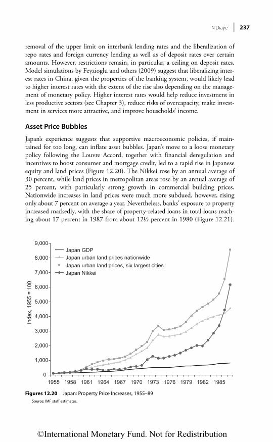
N’Diaye 237
removal of the upper limit on interbank lending rates and the liberalization of repo rates and foreign currency lending as well as of deposit rates over certain amounts. However, restrictions remain, in particular, a ceiling on deposit rates. Model simulations by Feyzioglu and others (2009) suggest that liberalizing inter-est rates in China, given the properties of the banking system, would likely lead to higher interest rates with the extent of the rise also depending on the manage-ment of monetary policy. Higher interest rates would help reduce investment in less productive sectors (see Chapter 3), reduce risks of overcapacity, make invest-ment in services more attractive, and improve households’ income.
Asset Price Bubbles
Japan’s experience suggests that supportive macroeconomic policies, if main-tained for too long, can inflate asset bubbles. Japan’s move to a loose monetary policy following the Louvre Accord, together with financial deregulation and incentives to boost consumer and mortgage credit, led to a rapid rise in Japanese equity and land prices (Figure 12.20). The Nikkei rose by an annual average of 30 percent, while land prices in metropolitan areas rose by an annual average of 25 percent, with particularly strong growth in commercial building prices. Nationwide increases in land prices were much more subdued, however, rising only about 7 percent on average a year. Nevertheless, banks’ exposure to property increased markedly, with the share of property-related loans in total loans reach-ing about 17 percent in 1987 from about 12½ percent in 1980 (Figure 12.21).
0
1,000
2,000
3,000
4,000
5,000
6,000
7,000
8,000
9,000
1955 1958 1961 1964 1967 1970 1973 1976 1979 1982 1985
Japan GDPJapan urban land prices nationwideJapan urban land prices, six largest citiesJapan Nikkei
Inde
x, 1
955
= 10
0
Figures 12.20 Japan: Property Price Increases, 1955–89Source: IMF staff estimates.
©International Monetary Fund. Not for Redistribution

238 Transforming China: Insights from the Japanese Experience of the 1980s
The subsequent protracted adjustment in goods and asset markets and the needed deleveraging in household, bank, and nonfinancial corporate balance sheets contributed to Japan’s “lost decade” of deflation, public debt accumulation, and stagnation.
In China, the government’s countercyclical response to the global financial crisis, which included several measures to increase infrastructure spending and household consumption and rapid credit growth, has fueled strong increases in asset prices. On the face of it, the situation in China is similar to that in Japan in the 1980s, with rapid credit growth, investment, and increases in asset prices (Figure 12.22). However, there are fundamental differences between the two economies in the strength of the balance sheets of households, corporations, and the government; the fundamentals that drive asset prices; and in the policy response to asset price developments.
• Leverage. Chinese households’ debt is one-fifth that of Japanese households in the 1980s; Chinese corporate debt is about half the size of Japanese corpo-rate debt; and government debt stands at about 20 percent of GDP in China, compared with about 67 percent in Japan at the peak of the property bubble.
• Fundamentals. Differences in fundamentals include the stage of urbaniza-tion, the structure of the population, and the stage of development with potential output growth in China of about 8–10 percent, compared with 4 percent in Japan in the 1980s. These data for China would imply rapid increases in asset prices, although not as strong as were observed in 2009–10.
• Policies. In Japan, monetary conditions were kept too loose for too long, and leverage was allowed to build up. In China, the authorities have already
4
6
8
10
12
14
16
18
1970 1972 1974 1976 1978 1980 1982 1984 1986
Sha
re o
f con
stru
ctio
n an
d re
al e
stat
e lo
ans
in to
tal l
oans
(per
cent
)
Figure 12.21 Japan: Construction and Real Estate Loans in Total LoansSource: IMF staff estimates.
©International Monetary Fund. Not for Redistribution

N’Diaye 239
taken measures to stem the run-up in property prices, such as increases in reserve requirements, tighter underwriting and prudential standards, and slower credit growth.
Another key fundamental difference is in the stage of development of the countries’ respective financial sectors: Japan’s was largely liberalized, whereas China’s financial sector remains heavily controlled. Although the propensity nonetheless exists for a run-up in asset prices, policies can play a role. The right calibration of policies—including prudent monetary policy and an increase in
0
20
40
60
Inde
xIn
dex
Per
cent
Per
cent
Inde
xIn
dex
80
100
120
–9 –8 –7 –6 –5 –4 –3 –2 –1 0 1 2 3 4 5 6 7
Nikkei (1989=100)Shanghai compositeIndex (2007=100)
0
2
4
6
8
10
12
14
–11–10 –9 –8 –7 –6 –5 –4 –3 –2 –1 0 1 2 3 4 5
–11–10 –9 –8 –7 –6 –5 –4 –3 –2 –1 0 1 2 3 4 5
–11–10 –9 –8 –7 –6 –5 –4 –3 –2 –1 0 1 2 3 4 5–11–10 –9 –8 –7 –6 –5 –4 –3 –2 –1 0 1 2 3 4 5
–11–10 –9 –8 –7 –6 –5 –4 –3 –2 –1 0 1 2 3 4 5
Japan real estateinvestmentChina real estateinvestment
b. Real estate investment a. Stock exchange indexes
0
20
40
60
80
100
120
Japan urban land pricesnationwide (1991=100)
China property prices(2009=100)
c. Property prices nationwide
Years from peak (peak = 0) Years from peak (peak = 0)
Years from peak (peak = 0)
Years from peak (peak = 0) Years from peak (peak = 0)
Years from peak (peak = 0)
0
20
40
60
80
100
120
Japan: Urban land prices, sixlargest cities (1991=1000)China: Property prices (average,six cities 2009=100)
d. Property prices in major cities
0
10
20
30
40
50
60
70
80
90
Japan households debt to GDP
China households debt to GDP
e. Households debt-to-GDP around peak property prices
0
20
40
60
80
100
120
140
160
180
200
Japan corporate debt to GDPChina corporate debt to GDP
f. Corporate debt-to-GDP aroundpeak property prices
Figure 12.22 Japan and China: Asset Prices and Balance Sheets around Peaks.Source: CEIC database.
©International Monetary Fund. Not for Redistribution

240 Transforming China: Insights from the Japanese Experience of the 1980s
real interest rates—should allow China to avoid the boom-bust asset cycle that Japan experienced.
Overall, the Japanese experience of the 1980s provides useful insights about the way China could manage a successful rebalancing to a domestic-demand-led economy and the downsides to avoid. In particular, Japan offers useful insights on (1) the limits to an export-oriented growth strategy; (2) the role of exchange rates, macroeconomic policies, and structural reforms in rebalancing the economy toward the nontradables sector; and (3) the risks associated with financial liberal-ization. These insights provide optimism that the ongoing rebalancing process in the Chinese economy can be managed.
©International Monetary Fund. Not for Redistribution

N’Diaye 241
ANNEX 12A. FINANCIAL LIBERALIZATION MEASURES IN JAPAN AND CHINA
Japan
1980 Introduction of national bond fund with minimum holding period of six months1981 Minimum holding period 1982 Liberalized rules on issuance of yen-denominated securities by nonresidents1983 Removal of some restrictions on zero-coupon bonds1984 Minimum size of certificates of deposit reduced from ¥500 million to ¥300 million1984 Ceiling on foreign-government-guaranteed bonds increased by 50 percent1984 Credit rating required for yen borrowing lowered to AA, down from AAA1984 Easing restrictions on issuance of euro-yen bonds1984 Removal of restrictions on foreign lending1984 Removal of exchange swaps controls1984 Nonresidents exempted from withholding tax on foreign currency government bonds 1984 Liberalization of short-term euro-yen loans to residents and issuance of euro-yen
certificates1984 Easing of restrictions on secondary market activities for banks1985 Collateralized loans for securities houses and brokerage licenses for bond future trading
allowed1985 Minimum size of certifcates of deposit reduced to ¥100 million and maturity to one
month1985 Removal of withholding tax on euro-yen bonds for Japanese residents1985 Pension funds and trust banking management by foreign banks allowed1985 Foreign firms trading on Tokyo Stock Exchange1985 Liberalization of interest rates on time deposits of more than ¥1 billion1986 Credit rating required for yen borrowing lowered to A, down from AA1986 Liberalization of interest rates on time deposits of more than ¥300 million1987 Liberalization of interest rates on time deposits of more than ¥100 million
China: Liberalization of Interest Rates
1996 Abolished the upper limit on interbank lending rates1997 Liberalized repo rates1998–2004 Gradually increased the upper limit on lending rates1999 Began to gradually allow different institutions to negotiate rates on
deposits of more than Y30 million with greater than five-year maturity2000 Liberalized foreign currency lending rates2000 Liberalized foreign currency deposit rates for deposits over $3 million2003 Removed floor on foreign currency deposit rates2003 Liberalized deposit rates on pounds, francs, Swiss francs, and Canadian dollars2004 Liberalized all foreign currency deposit rates with maturity greater than one year2004 Removed ceiling on all lending rates (except for urban and rural credit
cooperatives, which have a cap of 130 percent over reference rates)2004 Removed floor on all deposit rates2013 Removed floor on lending rates
Sources: Guttman, 1987; and Feyzioglu, Porter, and Takats, 2009.
©International Monetary Fund. Not for Redistribution
242 Transforming China: Insights from the Japanese Experience of the 1980s
REFERENCES
Ahuja A., L. Cheung, H. Gaofeng, N. Porter, and W. Zhang, 2010, “Are House Prices Rising Too Fast in China?” IMF Working Paper 10/274 (Washington: International Monetary Fund).
Ando, A., and A. Auerbach, 1988a, “The Corporate Cost of Capital in Japan and the United States: A Comparison,” in Government Policy towards Industry in the United States and Japan, ed. by J.B. Shoven (New York: Cambridge University Press).
———, 1988b, “The Cost of Capital in the United States and Japan: A Comparison,” Journal of the Japanese and International Economies, Vol. 2, pp. 134–58.
Barnett, S., and R. Brooks, 2010, “China: Does Government Health and Education Spending Boost Consumption?” IMF Working Paper 10/16 (Washington: International Monetary Fund).
Blanchard, O., and F. Giavazzi, 2005, “Rebalancing Growth in China: A Three-Handed Approach,” MIT Working Paper 05-32 (Cambridge, Massachusetts: MIT Department of Economics).
Chow, Gregory, 2002, “China’s Economic Transformation” (New York: Blackwell Publishing).Feyzioglu, T., N. Porter, and E. Takáts, 2009, “Interest Rate Liberalization in China,” IMF
Working Paper 09/171 (Washington: International Monetary Fund).Guo, K., and P. N’Diaye, 2009, “Is China’s Export-Oriented Growth Strategy Sustainable?”
IMF Working Paper 09/172 (Washington: International Monetary Fund).Guttman, W., 1987, “Japanese Capital Markets and Financial Liberalization,” Asian Survey, Vol.
27, No. 12, pp. 1256–67.Hayashi, F., 1986, “Why Is Japan’s Saving Rate so Apparently High?” NBER Macroeconomics
Annual 1986 (Cambridge, Massachusetts: MIT Press) pp. 147–210.Horioka, C.Y., 1988, “Saving for Housing Purchase in Japan,” Journal of the Japanese and
International Economies, Vol. 2, No. 3 (September), pp. 351–84.Huang, Y., and K.Y. Tao, 2010, “Causes and Remedies of China’s External Imbalances,” Paper
prepared for the conference on “Trans-Pacific Rebalancing,” jointly organized by the Asian Development Bank Institute and the Brookings Institution, Tokyo, March 3–4.
International Monetary Fund (IMF), 2007, “Staff Report on the Multilateral Consultation on Global Imbalances with China, the Euro Area, Japan, Saudi Arabia, and the United States” (Washington). http://www.imf.org/external/np/pp/2007/eng/062907.pdf.
———, 2010, World Economic Outlook: Getting the Balance Right: Transitioning out of Sustained Current Account Surpluses (Washington).
Ito, T., 1992, The Japanese Economy (Cambridge, Massachusetts: MIT Press).Krugman, P., 1991,“Has the Adjustment Process Worked?” (Washington: Institute for
International Economics).McKinnon, R., 2006, “China’s Exchange Rate Trap: Japan Redux?” American Economic Review,
Vol. 96, No. 2, pp. 427–31.N’Diaye, P., P. Zhang, and W. Zhang, 2009, “Structural Reform, Intra-Regional Trade, and
Medium-Term Growth Prospects of East Asia and the Pacific—Perspectives from a New Multi-Region Model,” Journal of Asian Economics, Vol. 21, No. 1, pp. 20–36.
Unsal, D. Filiz, 2010, “Box 2.1. Assessing Monetary Policy Stances in Asia,” in Regional Economic Outlook Asia and Pacific: Leading the Global Recovery, Rebalancing for the Medium Term (Washington: International Monetary Fund).
©International Monetary Fund. Not for Redistribution

243
CHAPTER 13
The Next Big Bang: A Road Map for Financial Reform in China
NIGEL CHALK AND MURTAZA SYED
Managed well, financial reform will generate significant benefits—in growth, employment, and standards of living—that will help sustain China’s spectacular development and accelerate the rebalancing of its growth model. Done right, it could be as significant as the state-owned enterprise reform of the 1990s. Conversely, a pro-longed delay in financial liberalization or implementing it in a poorly sequenced or badly executed manner would pose substantial risks for China and spill over onto an already fragile global economy. This chapter presents the rationale for financial reform in China and outlines a road map that could be implemented over the next three to five years.
INTRODUCTION
Liquidity control has traditionally been a hallmark of prudent macroeconomic management in China, contributing significantly to the country’s sustained and stable economic development. Since the mid-1990s, the authorities have relied on a wide-ranging system of controls to lock up the large amounts of structural liquidity generated by China’s economic model. The financial system is flush with liquidity, both because of a high stock of savings (Figure 13.1) held domestically by China’s closed capital account, and because of large external inflows associated with the country’s balance of payments surpluses, as well as the corresponding foreign currency intervention historically necessary to resist appreciation of the exchange rate (Figure 13.2).
To prevent this liquidity from fueling dangerous lending booms and asset bubbles, the People’s Bank of China (PBC) has historically relied on control—predominantly direct tools like quantitative limits on bank credit, regulation of deposit and loan rates, and relatively high reserve requirements.
These tools have proven effective for conducting macroeconomic management during most of China’s past, given the historically bank-based nature of China’s financial system. Nevertheless, a by-product of these policies has been artificially low loan and deposit rates, which have created incentives for banks to allocate much of their lending to very large, capital-intensive enterprises, and has lowered the costs of sterilizing China’s foreign currency intervention.
©International Monetary Fund. Not for Redistribution

244 The Next Big Bang: A Road Map for Financial Reform in China
However, China’s financial landscape has changed dramatically in the wake of the massive credit stimulus that was used to counter the effects of the 2008–09 global financial crisis. Credit was first unleashed through banks, placing pressure on their balance sheets and contributing to a rapid run-up in property prices. Since the crisis, more and more credit has been intermediated outside the banking
Figure 13.1 Decomposition of Saving, 1994–2010Sources: CEIC Data Company Ltd.; and IMF staff estimates.
0
20
40
60
1994 1997 2000 2003 2006 2009
Corporate Household Public Total
2011
Per
cent
of G
DP
–140
–90
–40
10
60
110
160
210
Dec. 2006 Apr. 2008
Cha
nge
in p
erce
nt o
f net
fore
ign
asse
ts o
ver 1
2 m
onth
s
Aug. 2009 Dec. 2010 Apr. 2012
Reserve requirements, change over 12 monthsOpen market operations, 12-month rolling totalTotal
Withdraw
Inject
Figure 13.2 People’s Bank of China’s Sterilization of Foreign ExchangeSources: CEIC Data Company Ltd.; and IMF staff estimates.
©International Monetary Fund. Not for Redistribution

Chalk and Syed 245
system, through channels that are harder to control and regulate under existing frameworks. In the absence of reforms, the attendant risks for macroeconomic and financial stability will continue to grow.
So what does this all mean? Because it is the world’s second largest economy, a safe, stable, well-regulated, and efficient system of financial intermediation in China is in everyone’s best interests. Since the onset of the global crisis, we have learned all too well of the enormous global social costs that financial instability in systemic economies can create.
Moreover, sustaining China’s spectacular growth record will be impossible without a modern financial system that efficiently intermediates savings and allo-cates capital. Financial reform will be necessary to achieve many of the key themes identified in the 12th Five-Year Plan, including (1) boosting household income, by increasing the returns to savings; (2) increasing consumption, through prudently managed household credit as well as instruments that smooth consumption and hedge risk; (3) reducing income disparities, through better access to financial ser-vices, including in rural areas; (4) increasing employment, through a more appro-priate pricing of capital and a move toward a more labor-intensive means of production (Figure 13.3); and (5) supporting the development of new industries, by reallocating resources on market terms and making more financing available to small and medium enterprises and start-ups, including in the services sector.
It is also worth bearing in mind that China is, in any case, outgrowing its cur-rent system of direct government influence over the allocation and pricing of credit. Certainly, this managed approach allowed for strong growth following the start of China’s reform efforts, in part because sectors with high growth potential were easier to identify. However, the system was not perfect, and generated
0
1
2
3
4
5
0 2 4 6 8 10
China
GDP growth (percent)
Em
ploy
men
t gro
wth
(per
cent
)
Figure 13.3 Average Employment Growth, 2004–10, Industrial Countries and Emerging Markets
Sources: IMF (2011).
©International Monetary Fund. Not for Redistribution

246 The Next Big Bang: A Road Map for Financial Reform in China
significant downsides in the form of overcapacity, a capital-intensive means of production (Figure 13.4), a tendency for asset bubbles (Figure 13.5), and a peri-odic need for public-funded bank recapitalizations. With the Chinese economy growing in size and complexity, the ability to productively steer credit directly is diminishing and the costs of misallocating resources are growing.
The rest of this chapter is organized as follows: The next two sections lay out the case for financial reform in China by highlighting the potential benefits of action and the growing risks from inaction, respectively. The subsequent section analyzes the experience of a number of China’s G20 peers, with a focus on inden-tifying lessons for the composition and sequencing of reforms that would help ensure that the full benefits of financial liberalization are realized and costs mini-mized. Applying these lessons to China’s specific context, the penultimate section develops a broad road map for financial reform in China that could be imple-mented in the medium term.
THE BENEFITS OF REFORM
What could China gain from financial reform? First, a well-executed financial reform program will allow the Chinese economy to adapt steadily to the ongoing, worldwide evolution in financial intermediation and to maximize the benefits from an increasingly diverse set of financial markets and instruments. Developing credible competition for the banks—in the form of corporate bond markets, deeper and more liquid equity markets, mutual funds, exchange-traded funds, derivatives, and other financial products—will create incentives for the whole
–100
–50
0
50
100
2000 2002 2004 2006 2008 2010
Other S5 countries range
Non-China Asia range China
Per
cent
of t
he m
argi
nal p
rodu
ct o
f cap
ital
Figure 13.4 Imputed Subsidy to CapitalSource: IMF (2011).Note: Non-China Asia = Indonesia, the Republic of Korea, Singapore, and Taiwan Province of China. Other S5 = Euro area, Japan, UK, U.S.
©International Monetary Fund. Not for Redistribution

Chalk and Syed 247
financial system to operate in a more effective and productive manner. Capital will be allocated more efficiently, and companies—particularly smaller enter-prises—that are currently denied access to bank loans will have new options for financing their operations.1
Second, well-designed reform, accompanied by a robust regulatory infrastruc-ture that spans all forms of financial intermediation and guarantees seamless coordination across regulators, will help ensure that the financial system contin-ues to develop in a robust way without excessive risk taking, lowering the possibil-ity of future financial volatility and disruption.
Third, making a broader range of alternative investment instruments available to households will increase the return on their savings,2 allow households and corporate savers to hold more diversified portfolios of assets, and reduce the ten-sions that are currently evident from having housing viewed as a preferred store of value (Figure 13.6).
And finally, financial reform will facilitate China’s move toward a more mod-ern means of macroeconomic control, one that deploys market-clearing prices to determine the availability and cost of credit rather than having both the price and quantity of loans regulated by the government. This move will strengthen the monetary transmission mechanism and give the central bank greater ability to fine-tune policy in response to changing economic conditions (Feyzioglu, Porter, and Takats, 2009).
These benefits are well known to China’s policymakers and were highlighted in the 12th Five-Year Plan, which included a clear commitment to moving ahead
1 See Chapter 3 in this volume and Feyzioglu (2009).2 See Chapter 5.
2
3
4
5
Dec-02 Nov-03 Oct-04 Sep-05 Aug-06 Jul-07 Jun-08 May-09 Apr-10
Market priceEstimated benchmark price
Thou
sand
renm
inbi
per
met
ers
squa
red
Figure 13.5 China: Residential Housing Prices, 2002–09Sources: IMF (2010).
©International Monetary Fund. Not for Redistribution

248 The Next Big Bang: A Road Map for Financial Reform in China
with the reform of China’s financial system, as well as recent policy intentions announced by the incoming leadership.
THE RISKS OF INACTION
If China does not implement reforms, what could go wrong? China has long been characterized by a very deep financial system but one that has relied pre-dominantly on banks to intermediate enormous levels of household and corpo-rate savings. However, this bank-dominated structure is now changing. Since the global financial crisis, China has experienced an acceleration in the pace of financial innovation; an expansion of new ways to intermediate savings; and a migration of resources out of the banks and into other forms of financial inter-mediation, such as trusts, wealth management products, and corporate bonds (Figure 13.7).
The diversification and development of financial markets and instruments is generally good (Figure 13.8), facilitating a more efficient means of allocating China’s capital, opening up financing opportunities for companies that previ-ously were unable to get bank loans, and increasing the level of remuneration that households receive on their savings.
However, these changes also pose risks to financial and macroeconomic stabil-ity. Regulation of the nonbank system of intermediation is weaker and less well developed than that for banks. Care is also needed to ensure that banks are healthy enough to withstand a steady loss of resources implied by a growing non-bank system. Evidence is already appearing of growing liquidity pressures on
–2
0
2
4
6
8
China India Japan Korea,Rep. of
UnitedKingdom
UnitedStates
Corporate sector
Banks
Depositors
Total return to capital
Rea
l ret
urn
(per
cent
)
Figure 13.6 Distribution of Returns to Bank-Intermediated CapitalSource: Chapter 3 of this volume.
©International Monetary Fund. Not for Redistribution
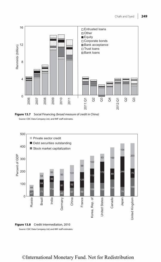
Chalk and Syed 249
0
4
8
12
16 Entrusted loansOtherEquityCorporate bondsBank acceptanceTrust loansBank loans
Ren
min
bi (t
rillio
n)
2006
2007
2008
2009
2010
2011
2011
:Q1
2012
:Q1
Q2
Q2
Q3
Q3
Q4
Figure 13.7 Social Financing (broad measure of credit in China)Source: CEIC Data Company Ltd.; and IMF staff estimates.
4771
114
45 67 69109 106
13474
14864
49
81 52
125
113172
89246 75
44
5455
93 131
99103
63 169
104
203
0
100
200
300
400
500
Rus
sia
Bra
zil
Indi
a
Ger
man
y
Chi
na
Fran
ce
Kore
a, R
ep. o
f
Uni
ted
Sta
tes
Can
ada
Japa
n
Uni
ted
Kin
gdom
Private sector creditDebt securities outstanding
Stock market capitalization
Per
cent
of G
DP
Figure 13.8 Credit Intermediation, 2010Source: CEIC Data Company Ltd; and IMF staff estimates.
©International Monetary Fund. Not for Redistribution

250 The Next Big Bang: A Road Map for Financial Reform in China
smaller banks in China. In addition, the underlying system of macroeconomic control needs to evolve with the times. In particular, the current regulation of interest rates distorts the pricing of deposits and creates huge incentives for resources to migrate out of the banks to institutions that are not subject to such controls on the rates of return they offer. Why put your money in a bank depos-it that earns less than inflation when you can choose from a convenient array of more lucrative wealth management products instead? Furthermore, international experience demonstrates that the use of administrative limits on the quantity of bank lending as a means to exercise macroeconomic control is likely to become less and less effective as financial innovation takes hold and more and more inter-mediation takes place outside of the banks.
Therefore, financial reform is essential to sustaining the ability of China’s policymakers to effectively guide the macroeconomy, ensure that the expansion of nonbank channels proceeds safely and soundly, and prevent the banking system from being undermined by a loss of deposits and funding.
REAPING THE BENEFITS AND AVOIDING THE PITFALLS: LESSONS FROM INTERNATIONAL EXPERIENCE
A number of China’s G20 peers have reformed their financial sectors, and their experiences provide important lessons. As in China, their pre-reform financial sector landscapes were often characterized by a heavy bias toward bank interme-diation, rigid segmentation across financial institutions by function, low levels of competition, regulated interest rates, a large public sector role (including directed lending and state guarantees of financial institutions), the conduct of monetary policy mainly through direct instruments, and capital controls. In addition, coun-tries embarking on financial liberalization have encountered several challenges, and their reform efforts have often led to periods of financial volatility and crisis (see Annex 13A for a summary of the major steps and mistakes made by other G20 economies as they moved toward a more modern and market-based financial system). From international experience, a few broad lessons stand out:
1. Financial sector weaknesses should be sought out and addressed before liberal-ization begins, including ensuring institutions have the ability to adequate-ly price and manage risks; recapitalizing or restructuring systemically important institutions; and enhancing corporate governance. Unaddressed weaknesses create the potential for financial institutions to take greater risks to boost returns and cover up their underlying vulnerabilities. These vulnerabilities will then grow as financial reform proceeds, potentially cul-minating in weaknesses in systemically important institutions.
2. The macroeconomic policy framework should move toward market-based mon-etary policy at an early stage, and should be based on indirect instruments and include increased exchange rate flexibility. Before financial reform proceeds, the monetary authority needs to have at its disposal sufficient macroeco-
©International Monetary Fund. Not for Redistribution

Chalk and Syed 251
nomic control tools to prevent an unintended surge in lending or creation of the conditions for large capital inflows.
3. Implicit public guarantees of financial institutions should be explicitly with-drawn during the early stages of liberalization. Blanket backing should be replaced with an explicit scheme for deposit insurance. Ensuring that banks face hard budget constraints would be an important prerequisite for a more commercially oriented banking system that adequately prices risk and effi-ciently allocates credit. Hard constraints also help mitigate moral hazard risks and prevent banks from taking undue risks as restrictions on bank activities are eased and new markets are opened.
4. The financial, legal, and accounting framework should be revised before embarking on major reforms, in particular with regard to regulatory and super-visory frameworks. The major prerequisites include (1) clear objectives and mandates for the responsible agencies; (2) regulatory independence, with appropriate accountability; (3) adequate resources (staff and funding); and (4) effective enforcement and resolution powers.
5. The regulatory and supervisory perimeter needs to be sufficiently wide and well coordinated to prevent regulatory arbitrage and identify emerging vulnerabilities. Virtually all postliberalization crises can be traced to inadequate supervision or to regulations not keeping up with changing financial landscapes. All potentially systemically important financial institutions, including nonbank financial institutions, need to be within the perimeter before restrictions on financial activities are sig-nificantly relaxed and new markets developed. The regulatory and supervisory framework should be empowered to limit concentration in bank ownership and require clear identification of beneficial owners (to mitigate the risks of connected lending). Activities in nonbank financial institutions in particular should be monitored closely; these institutions should be prohibited from taking deposits.
6. Measures to deepen financial and capital markets should move in parallel with reform of the banking system. Financial market development is important to improving the allocation of capital and to creating competition. However, lopsided sequencing can have significant effects on bank balance sheets by undermining banks’ deposit base or by eroding their pool of corporate clients. Loss of deposits and clients, in turn, can lead banks to increase risk exposures.
7. Many of the important objectives of financial sector reform—including greater competition and efficiency, and enhanced risk management—depend on hav-ing market-determined deposit and loan rates. Interest rate liberalization facilitates the development of a market-based monetary policy framework that is based on indirect instruments and has an effective transmission mechanism. Interest rate liberalization provides increased scope for macro-economic control to mitigate the risks of instability as reforms proceed. Other goals, such as enhanced competition, allocative efficiency, and
©International Monetary Fund. Not for Redistribution

252 The Next Big Bang: A Road Map for Financial Reform in China
stronger risk management, all rely on allowing prices (interest rates) to provide the right market-based signals.
8. But successful liberalization of interest rates has several preconditions. These preconditions include a stable macroeconomic environment, an absorption of excess liquidity, an interest rate structure that is not in serious disequi-librium before liberalization, an active and well-functioning money mar-ket, and a sound payments system. Strong supervision policies and instru-ments and a flexible and effective monetary policy framework are also required. In particular, monetary policy needs to guard against the develop-ment of an excess supply of credit as interest rate constraints are removed. In successful cases of liberalization (such as Australia, Belgium, and Canada), credit expansion was reined in by a deliberate containment of liquidity and increases in real interest rates (Figures 13.9 and 13.10). Conversely, other countries—such as Argentina, Chile, and Mexico—lost control of monetary aggregates as they liberalized, injecting enormous amounts of credit and monetary stimulus into their economies that culmi-nated in asset bubbles and banking crises.
9. Opening to international portfolio flows should occur only after the bulk of financial sector reform has been achieved. The current scale of global capital flows and the increasing sophistication and interconnectedness of the world’s financial markets create large risks for those economies that open themselves up to international capital flows before the distortions
–15
–10
–5
0
5
10
Argentina(1977)
Australia(1981)
Mexico(1994)
Chile(1974)
Canada(1980)
Belgium(1986)
Per
cent
Figure 13.9 Real Interest Rates Following Interest Rate Liberalization (three-year average)Source: CEIC Data Company Ltd.; and IMF staff estimates.
©International Monetary Fund. Not for Redistribution

Chalk and Syed 253
and misalignments in their domestic financial systems are resolved. The early stages of capital account liberalization can open up to stable long-term sources of financing, such as direct investment inflows. However, full liberalization—including for short-term portfolio flows—should be put in place only after the bulk of financial sector reform has taken hold.
DESIGNING A ROAD MAP FOR CHINA
There is certainly no “one size fits all” approach to sequencing financial sector liberalization, especially in an economy as sophisticated and complex as China’s. In many cases, the appropriate pace and sequencing of reforms will involve mul-tiple trade-offs, and judgment must be exercised in a dynamic manner as the financial system evolves in potentially unpredictable ways when reforms are implemented. As the situation for many comparator countries demonstrates, the agenda for financial reform is a complex, multiyear undertaking. However, start-ing now will ensure that this process can be largely completed within a three-to-five-year horizon. A broad road map for reform should include adopting a new monetary policy framework; raising real interest rates; strengthening and expand-ing regulatory coverage of the financial system, including putting in place a broad set of tools for crisis management; developing financial markets and alternative means of intermediation; deregulating interest rates; and, eventually, opening up the capital account (Table 13.1).
75
115
155
195
235
T T+1 T+2 T+3 T+4 T+5 T+6 T+7
Argentina (1977)
Sweden (1983)
Norway (1985)
Thailand (1990)
Finland (1986)
Date of banking crisis
Inde
x, 1
00 =
T, t
ime
of li
bera
lizat
ion
Years following liberalization
Figure 13.10 Private Credit Growth Following Interest Rate LiberalizationSource: CEIC Data Company Ltd.; and IMF staff estimates.
©International Monetary Fund. Not for Redistribution

254 The Next Big Bang: A Road Map for Financial Reform in China
TABLE 13.1
China: A Roadmap for Financial Reforms
RECOMMENDATION IMPLEMENTATION CONSIDERATIONS
SEQUENCE
STAGE I STAGE II STAGE III
Deepening commercialization and market orientation of financial system
Absorb liquidity To move to a "true" market clearing for capital and prevent excess liquidity from leading to rapid credit growth during reform process.
Conduct open market operations, placing PBC bills at market-determined prices.Steadily increase entire structure of deposit and loan rates.
Reform monetary control instruments To increase scope for macroeconomic control to mitigate risks of instability during reform process and pave way for greater role for markets in setting interest rates and determining pace of credit growth.
Greater exchange rate flexibility.Greater reliance on indirect instru-ments, focused on market rate, while narrowing corridor on inter-bank rates.Introduce reserve averaging to decrease interest rate volatility.Remunerate reserves at market-determined rate.Ensure open market operations are conducted in market-based way, with quantities determined by market-clearing equilibrium associated with given target for interest rates.Phase out direct government influ-ence on pace of growth, allocation, and pricing of credit.Move monetary framework away from targets for monetary aggre-gate growth and toward well-specified policy objective (e.g., inflation and activity).
Need to build technical capacity for design and implementation of frame-work.
Liberalize interest rates (for parallel construction with other recommendations)
To increase efficiency of credit alloca-tion, while paving the way for improved competition and risk man-agement in the banking sector and providing a benchmark for pricing other financial products and services.
Raise (and eventually eliminate) ceiling on deposit rates.
Could commence with deposit rate deregulation to minimize risk of excessive competition for market share and damaging undercutting of interest margins. Begin with longer-term deposits and then expand to demand deposits.
(Continued)
©International Monetary Fund. Not for Redistribution
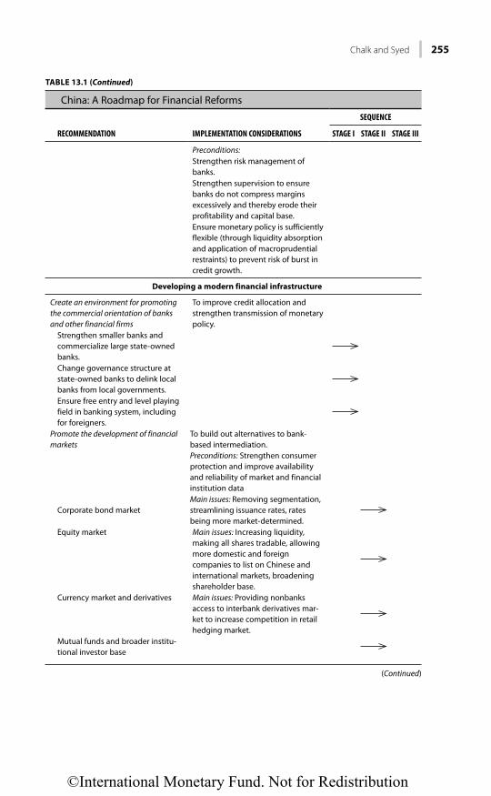
Chalk and Syed 255
China: A Roadmap for Financial Reforms
RECOMMENDATION IMPLEMENTATION CONSIDERATIONS
SEQUENCE
STAGE I STAGE II STAGE III
Preconditions:Strengthen risk management of banks.Strengthen supervision to ensure banks do not compress margins excessively and thereby erode their profitability and capital base.Ensure monetary policy is sufficiently flexible (through liquidity absorption and application of macroprudential restraints) to prevent risk of burst in credit growth.
Developing a modern financial infrastructure
Create an environment for promoting the commercial orientation of banks and other financial firms
To improve credit allocation and strengthen transmission of monetary policy.
Strengthen smaller banks and commercialize large state-owned banks.Change governance structure at state-owned banks to delink local banks from local governments.Ensure free entry and level playing field in banking system, including for foreigners.
Promote the development of financial markets
To build out alternatives to bank-based intermediation. Preconditions: Strengthen consumer protection and improve availability and reliability of market and financial institution data
Corporate bond marketMain issues: Removing segmentation, streamlining issuance rates, rates being more market-determined.
Equity market Main issues: Increasing liquidity, making all shares tradable, allowing more domestic and foreign companies to list on Chinese and international markets, broadening shareholder base.
Currency market and derivatives Main issues: Providing nonbanks access to interbank derivatives mar-ket to increase competition in retail hedging market.
Mutual funds and broader institu-tional investor base
TABLE 13.1 (Continued)
(Continued)
©International Monetary Fund. Not for Redistribution

256 The Next Big Bang: A Road Map for Financial Reform in China
China: A Roadmap for Financial Reforms
RECOMMENDATION IMPLEMENTATION CONSIDERATIONS
SEQUENCE
STAGE I STAGE II STAGE III
Expand range of commercially available insurance products, including life, health, and annuities and private pension plans.Expand use and availability of financial products, including lend-ing and deposit products.
Precondition: Priced off benchmark RMB yield curve set by market.
Consider securitization and other "trust" products.
Precondition: Subject to strict regula-tion and transparency.
Strengthen supervisory, regulatory, and crisis management frameworks
To ensure risks are contained as reforms advance.
Integrating with the global financial system.
Liberalize external account
Ease restrictions on capital outflows.To provide broader range of interna-tional assets to Chinese investors.
Move existing controls from quan-tity- to price-based regulations.Expand Qualified Domestic Institutional Investor program, fol-lowed by more broad-based removal of restrictions.Take further steps to international-ize RMB.
Respond to market demands.
Liberalize inflows.Gradual expansion of Qualified Foreign Institutional Investor program until quotas no longer binding.
Open first to foreign direct invest-ment, then longer-term fixed income products.Open up to inflows into most-liquid primary markets before secondary markets.Allow inflows of RMB before foreign exchange inflows.At final stage, expand to secondary mar-kets for equities and short-term debt.
Promote foreign and cross-border competition
Remove tax and regulatory barriers for foreign financial institutions to participate in domestic markets, and for domestic institutions to go out.
Precondition: Subject to appropriate supervision and risk management.
Source: IMF staff estimates.
TABLE 13.1 (Continued)
A New Framework for Monetary Policy
Financial reform should involve a reinvention of the current framework to move away from the current system’s reliance on controls on deposit rates, the exchange rate, and the quantity of credit to one in which the central bank has
©International Monetary Fund. Not for Redistribution

Chalk and Syed 257
clear objectives for growth, inflation, and financial stability. In addition, the PBC should be given flexibility and control over the macroprudential and mon-etary tools that will be needed to achieve these goals.
As a first step, the high levels of liquidity currently residing in the financial system would need to be absorbed. Judging the extent of this liquidity absorption, however, will be complicated by the lack of reliable price signals and the fact that the “true” level of liquidity in the system is masked by the lack of fully market-determined interest rates, the presence of direct controls on credit, and adminis-trative determination of both the price and quantity of central bank paper issued. Nevertheless, as a first step, open market operations should be deployed to absorb the liquidity overhang by placing central bank paper at market-determined rates and moving the structure of deposit and loan rates closer to the neutral real inter-est rate.
At the same time, the ongoing liquidity injection that is created by large-scale foreign currency intervention will need to be decreased by appreciating the exchange rate to the point at which the currency market is more balanced and there are genuine two-way flows in the balance of payments and two-way move-ments in the exchange rate (Figure 13.11). This would lessen the need for mon-etary tools—including reserve requirements and open market operations—to be so geared toward sterilizing foreign currency inflows and managing the currency. Instead, policies could be reoriented toward a more market-based and countercy-clical approach focused on the domestic economy.
With liquidity absorbed and interest rates clearing the capital market, the central bank can then shift toward the use of more indirect monetary instruments to exercise macroeconomic control. The central bank can begin using short-term
5.0
5.5
6.0
6.5
7.0
7.5
8.0
8.50.0
0.5
1.0
1.5
2.0
2.5
3.0
3.5
2000 2001 2002 2003 2004 2005 2006 2007 2008 2009 2010 2011 2012
Foreign reserves (left scale)Exchange rate (right scale)
U.S
.$ (t
rillio
n)
Ren
min
bi p
er U
.S. d
olla
r
Figure 13.11 China: Exchange Rate and Foreign ReservesSource: CEIC Data Company Ltd.; and IMF staff estimates.
©International Monetary Fund. Not for Redistribution

258 The Next Big Bang: A Road Map for Financial Reform in China
rates—perhaps the seven-day repo rate—as its effective operational target for monetary policy and phase out direct influence on the growth, allocation, and pricing of credit. The PBC would be able to effectively influence short-term rates through open market operations and could conduct daily open market operations using quantities determined by achieving market-clearing at a given target level for the policy interest rate. Reserve averaging could be introduced to decrease interest rate volatility, and reserve requirements could be remunerated at a mar-ket-determined rate.
Because financial innovation and development makes money demand unsta-ble, targeting M2 would no longer be a feasible proposition and a new framework for the conduct of monetary policy would be needed. In particular, the PBC could move toward a monetary policy regime that has objectives for growth, infla-tion, and financial stability that are achieved through a combination of interest rates and macroprudential tools.
Improving Regulation and Supervision
As the system evolves, the government will need to be nimble in adapting to the changing environment by increasing the commercial orientation of the banking system, bolstering its crisis management capabilities, and strengthening supervi-sory efforts to identify and manage macrofinancial vulnerabilities.
Further advances in the regulatory and supervisory regime will be needed to ensure it is sufficiently adaptable and dynamic to react in a new environment of tighter liquidity, indirect monetary control, and, eventually, liberalized interest rates. In a more liberalized environment, strict supervision will be needed to pre-vent banks or nonbank institutions from engaging in unsafe practices to boost profitability or gain market share. Particular attention will be needed to address the supervisory and regulatory gaps that will inevitably emerge in a more dynam-ic and liberalized setting. To this end, investments should be made to improve stress-testing capabilities; increase oversight for the largest financial institutions; overhaul the crisis management and resolution framework; build a process for the orderly exit of weak or failing financial institutions; develop clear rules on central bank emergency liquidity support; put in place a formal deposit insurance scheme; and pursue better data quality and collection. Interagency regulatory and supervisory coordination will also need to become more ongoing and systematic, identifying and resolving regulatory gaps. A key step will be to establish a perma-nent, high-level, interagency financial stability committee that would monitor and identify macrofinancial vulnerabilities and implement a macroprudential framework geared toward preventing the buildup of systemic risks.
Developing Broader Channels for Intermediation
Strengthening nonbank financial intermediation will be an important objective of financial reform. Nonbank institutions will compete with the banking system, offer companies alternate avenues for project financing, and provide households
©International Monetary Fund. Not for Redistribution

Chalk and Syed 259
with a broader range of financing and investment possibilities. Expansion of nonbank areas of intermediation will, however, need to move largely in tandem with reform of bank-based intermediation. Failure of these developments to occur on parallel tracks could create incentives for a faster migration of resources out of the banks (into bonds, equities, trusts, leasing, and wealth management prod-ucts), creating accompanying supervisory and regulatory challenges and the potential for destabilizing the banking system.
The focus should be on dismantling impediments to the development of alter-nate markets and instruments but with corresponding clarity about the regula-tions and responsibilities of those new institutions. Priorities include reducing segmentation, increasing liquidity, and simplifying regulatory requirements in equity and bond markets. In addition, efforts should be made to encourage a broad institutional investor base—including pension, insurance, and mutual fund companies.
In conjunction with developing a wider range of investment products, enhanced regulation and supervision will help ensure that risks to financial stabil-ity are well managed. In addition, a comprehensive framework for disclosure and consumer protection will be needed to ensure investors are fully aware of the risks they undertake when diversifying their assets away from bank deposits. For pru-dential reasons, precedence should be given to gaining experience with straight-forward instruments before allowing more sophisticated ones, such as securitized and trust products.
Liberalizing Loan and Deposit Rates
With a robust monetary framework in place, and with interest rates rising to clear the capital market, the next step will be for the central bank to move away from the regulation of loan and deposit rates (Figure 13.12). The preferred strategy would be to gradually lift the ceiling on deposit rates, allowing them to be deter-mined by banks on a competitive basis. Competitive determination would facili-tate an increase in the cost of funding and a move toward a corresponding increase in loan rates. The ceiling could be lifted in stages based on the term of the deposits, to allow banks time to adjust.
With interest rates liberalized, financial institutions should be held account-able for managing their risks. In particular, regulated firms that are deemed by their supervisor to be well capitalized and well managed could be granted more discretion and held accountable for conducting their operations prudently and in compliance with the regulatory framework. Similarly, customers of financial products could assume greater responsibility for their own financial decisions, complemented by adequate consumer protection, disclosure, and improved financial literacy.
It will be essential to ensure, as this transition proceeds, that it does not trans-late into an unintended loosening of monetary and credit conditions. Knowing when to rein in monetary and credit conditions will be complicated by the
©International Monetary Fund. Not for Redistribution

260 The Next Big Bang: A Road Map for Financial Reform in China
increased difficulty, resulting from the ongoing financial reform and liberaliza-tion, of predicting the appropriate pace of monetary growth. Nevertheless, mon-etary policy would need to be attentive and used actively to counter the poten-tially unpredictable impact of interest rate liberalization on liquidity, credit growth, and monetary conditions.
The process will need to be carefully managed—through both the use of mon-etary policy tools to adapt liquidity conditions and the application of macropru-dential restraints—to counter any surge in credit growth as interest rates become more market determined. Particular attention will need to be paid to ensuring credit does not expand at a precipitous rate either in the aggregate or to particular sectors (for example, to real estate or consumer credit). As interest rates are deregulated, regulatory and supervisory tools must be used to their fullest to ensure that the banks do not engage in overly aggressive competition or unsafe practices to attract deposits, expand lending, or compress margins to gain market share.
Greater freedom to set loan and deposit rates will create incentives for the banks to manage and price risk better and will make money market interest rates more representative of true financial conditions. At the same time, a more mar-ket-determined system of interest rates will provide valuable price signals for macroeconomic policymaking and will strengthen the transmission mechanism for monetary policy.
Opening Up the Capital Account
As the domestic financial system becomes more market based with fewer distor-tions in the determination of market-clearing levels of credit and interest rates,
0
5
10
15
20
25
0
2
4
6
8
10
2007 2008 2009 2010 2011 2012
Required reserve ratio (right scale)1-year nominal lending rate (left scale)1-year PBC bill rate (left scale)1-year deposit rate (left scale)
Per
cent
Per
cent
Figure 13.12 China: Short-Term Interest Rates, 2007–12Source: IMF staff estimates.Note: PBC = People’s Bank of China.
©International Monetary Fund. Not for Redistribution

Chalk and Syed 261
China can then proceed to dismantle its extensive system of controls on capital flows.
The early stages of capital account liberalization should focus on removing restrictions on more stable, long-term sources of financing such as direct invest-ment flows (as is already being done). As the reform process advances—with market-determined interest rates, a robust monetary policy and regulatory frame-work in place, a flexible currency, banks operating prudently, and the domestic financial system liberalized—the stage would be set to ease restrictions on short-term inflows. As restrictions are eased, the current qualified foreign institutional investor and qualified domestic institutional investor system could be effectively used to open up the account in stages and at a different pace for different forms of investments.
CONCLUSION
The motivation for financial reform in China is clear. Before the global crisis, China was on a firm trajectory toward a more modern financial system capable of addressing the challenges of a more mature and complex economy. However, when financial systems across the globe suffered severe setbacks, Chinese policy-makers naturally paused. But in the medium term, China needs to regain and maintain the pace of change.
Thus, it is encouraging to note the prominent role assigned to financial reforms in the 12th Five-Year Plan and by the new Chinese leadership. Indeed, the road map laid out above can be completed over a three-to-five-year horizon. Well-executed financial liberalization is the next big wave of reform that China needs. It could be as significant as the state-owned enterprise reform of the 1990s, laying the foundations for continued strong growth in China in the coming decades.
This chapter outlines a broad road map that encompasses both the key ele-ments and the sequencing of the required financial reform effort. Continuing to defer progress in this area heightens the risk that the financial system will evolve in an uncoordinated and disorderly fashion, outpacing supervisory capabilities and revealing regulatory gaps.
The likelihood is high that developments may already be proceeding on a timetable that is being driven not by careful, preemptive, and concerted policy planning but rather in an ad hoc way, propelled by the accelerating pace of market disintermediation and innovation. Such a trajectory is in the interests of neither China nor the rest of the world.
©International Monetary Fund. Not for Redistribution

26
2 T
he
Ne
xt Big
Ba
ng
: A R
oa
d M
ap
for Fin
an
cial R
efo
rm in
Ch
ina
ANNEX 13A. FINANCIAL REFORMS: LESSONS FROM COUNTRY EXPERIENCES
Initial Conditions Sequencing Outcomes Path to Crisis
INDONESIA (1982–96)
Financial sector reforms were part of a broad effort to diversify the economy and expand the role of the private sector.
Phase I (1982–86): Indirect monetary poli-cy instruments were introduced, interest rates were liberalized, and credit ceilings were phased out.
During the early stages of reform, real interest rates moved higher to market-clearing levels, and the more efficient private banks began to build market share.
As the capital account became more open, domestic imbalances in the financial sys-tem combined with a tightly managed exchange rate gave rise to a surge in spec-ulative capital inflows. Domestic banks borrowed heavily offshore in foreign cur-rency to fund rapid growth in local curren-cy loans. Regulatory efforts to dissuade such carry trades were largely too little and too late.
Financial sector was dominated by five large state-owned banks, gov-ernment-directed lending was prevalent, interest rates were reg-ulated (and typically negative in real terms), and the growth in bank credit was subject to admin-istrative ceilings.
Phase II (1987–92): Restrictions on the activities of banks were loosened, directed lending was reduced, and there was great-er latitude in the operations of foreign banks. Reserve requirements were equal-ized across the banking industry, removing a source of preferential treatment for the state banks. Prudential regulation and supervision were enhanced. Capital account liberalization began in 1989, with controls on portfolio and bank capital inflows steadily eased.
Macroeconomic policies were kept restrictive, par-ticularly with fiscal policy steadily tightening. However, vulnerabilities began to build up in the second phase of reforms during 1987–92, but these risks were left largely undiagnosed. In large part these were due to weak corporate gover-nance, inadequate regulation and supervision, and a macroeconomic policy mix that encouraged large speculative capital inflows.
As the Asian financial crisis unfolded in 1997, the weaknesses in the Indonesian financial sector—including currency and maturity mismatches—were exposed, put-ting strains on corporate and bank balance sheets and, eventually, ending in a full-blown systemic banking crisis.
On the capital account, outflows had been mostly liberalized, but inflows were subject to strict controls.
Despite increasing competition, bank ownership remained highly concentrated and large private banks, which were subsidiaries of politically pow-erful business conglomerates, were able to use their influence to circumvent regulatory limits
©International Monetary Fund. Not for Redistribution

C
ha
lk an
d S
yed
2
63
related to connected lending. Large parts of the financial sector (and their largest corporate bor-rowers) were perceived to be covered by implicit public guarantees, a perception that had been strengthened by a succession of opaque bailouts. There was an absence of a clear framework to resolve failing institutions and banks had few incentives to manage downside risks. Overcapacity in the financial sector grew over a number of years, spurring excessive lending to relatively unproduc-tive sectors, including real estate.
JAPAN (1975–90)
Pre-reform financial sector land-scape was dominated by banks with limited options for savers, low regulated interest rates, and strict limits on bond issuance. The financial sector was also charac-terized by rigid segmentation of financial institutions by function.
The capital account was liberalized early
in the process. In the 1980 Foreign Exchange Control Act, corporate borrowers were given greatly expanded opportuni-ties to raise funds overseas.
The lopsided pace of liberalization caused the banks to quickly lose many of their best borrowers, while savers had few choices but to remain in bank deposits. As a result, many large and medium enterprises reduced their dependence on bank financing and increased their funding from bond and equity markets, where nonbank financial insti-tutions were large investors.
In the early 1990s, Japan’s real estate bub-ble burst, and the resulting decline in property prices, equity prices, and eco-nomic growth exposed the underlying vul-nerabilities on bank balance sheets.
Discretionary administrative guid-ance was the principal method of financial regulation, with “convoy regulation” aimed at ensuring financial institutions evolved at the same pace, implicitly inhibit-ing competition. As financial liber-alization began, Japan did, how-ever, have a largely open capital account.
Liberalization was asymmetric. Corporate borrowers were provided access to a broader range of funding alternatives before savers were given choices in invest-ment instruments. A number of new mar-kets grew, including a commercial paper and corporate bond market, but retail investors were given only limited access.
During1980–90, the ratio of bank debt to total assets for large, publicly listed manufacturing firms dropped by almost 20 percentage points (to less than 15 percent). However, household deposits continued to rise because barriers to entry into the investment trust business remained high and banks were not permitted to market investment management services. The loss of corporate clients and banks’ efforts to continue to build market share led them to expand their exposure to the property market and to smaller firms.
The deceleration of economic growth impaired the capacity of small businesses to repay, nonperforming real estate loans skyrocketed as collateral values plummet-ed, and the fall in equity prices shrank bank capital. The banking system became mired in a collapse from which it has yet to fully recover.
(Continued )
©International Monetary Fund. Not for Redistribution

26
4 T
he
Ne
xt Big
Ba
ng
: A R
oa
d M
ap
for Fin
an
cial R
efo
rm in
Ch
ina
Deposit rate liberalization proceeded
slowly and at a slower pace than lending rates. Indeed, it took until 1994 for deposit rates to be fully market determined.
Lending decisions became heavily influenced by collateral values (rather than a notion of capacity to repay), credit standards weakened, and between 1980 and 1990, loans to the real estate industry doubled. Much of the remainder of the banks’ loan book was devoted to small firms, with correspond-ingly higher credit risks.
KOREA (1980–96)
Financial sector was largely state owned, highly regulated, and used as an allocation tool by the gov-ernment to advance its economic development agenda. Monetary policy was conducted using inter-est rate and credit ceilings as well as reserve requirements.
Early reforms included bank privatiza-
tion and measures to increase financial
competition, although the banking sector emerged from the privatization process with ownership concentrated among large industrial conglomerates. Nonbank institu-tions developed, albeit increasingly owned and controlled by these industry groups.
In 1994, the ceiling on foreign currency lending by domestic banks was eliminated but limits on banks’ medium- and long-term borrowing from international markets were retained.
Between 1994 and 1997, banks rapidly built up huge maturity mismatches on their balance sheets, and the financial sec-tor became exposed to economically unvi-able projects through a complex network of cross-holdings within industrial groups and connected lending.
The government guided resources to its preferred sectors by a com-bination of directed credit and preferential lending rates. The capital account was largely closed.
Progress was also made in developing
money and interbank markets, an important precursor for a move to a more indirect monetary policy, and the govern-ment somewhat scaled back its efforts to direct credit.
As a result, Korean banks began to finance their domestic long-term foreign currency lending with short-term foreign currency loans.
By 1997, banks and nonbank institutions found it increasingly difficult to roll over their external short-term funding, leading to an exhaustion of official reserves and an all-out balance of payments crisis.
Regulatory standards for loan classifica-
tion, provisioning, accounting, and
large exposures saw little improvement, while supervision remained fragmented.
At the same time, there were large gaps in the pru-dential regulations relating to foreign exchange exposures in overseas branches and offshore funds, which accounted for a significant buildup in short-term external liabilities.
Restrictions on capital inflows began to
be weakened in 1989, largely by allowing financial institutions to borrow offshore.
Initial Conditions Sequencing Outcomes Path to Crisis
JAPAN (1975–90)
ANNEX 13A. (Continued)
©International Monetary Fund. Not for Redistribution

C
ha
lk an
d S
yed
2
65
MEXICO (1988–93)
In the late 1980s, to combat high inflation and low growth, Mexico undertook a broad set of reforms to increase the role of markets in various aspects of the economy.
Mexico pursued a rapid pace of financial reform that was contemporaneous with a broad effort at macroeconomic stabiliza-tion and capital account liberalization.
Bank balance sheets grew rapidly both before and after privatization, as banks tried to capture market share in a newly liberalized market. In response, the authorities began to tighten prudential regula-tions between 1991 and 1993 by increasing mini-mum capital adequacy ratios to 8 percent from 6 percent; strengthening loan classification and pro-visioning rules; and imposing stricter limits on for-eign exchange positions.
In the wake of liberalization, the newly privatized Mexican financial institutions began to increasingly fund their opera-tions through over-the-counter structured notes that were linked to exchange rate developments.
The banking system was largely publicly held and segmented across sectors, interest rates were regulated, and supervision was generally weak.
1989–90: A big-bang program of sweep-ing reforms was introduced, including eliminating interest rate controls; replacing very high reserve requirements with liquidity ratios; removing restrictions on private sector lending; ending mandatory lending to the public sector; and removing sector segmentation (which allowed for the emergence of universal banks).
However, the new regulatory and supervisory framework was seriously deficient and concealed a range of increasing vulnerabilities, not least weak-nesses in the Mexican accounting system. Banks were required to classify as nonperforming only that portion of the loan (or the interest payment) that was due but had not yet been repaid. Banks were also permitted to exercise significant discre-tion in the risk classification of their loans, which allowed them to inflate capital ratios.
Accounting rules allowed the banks to book these positions as claims that were not counted toward their net open foreign exchange position. The increasing bank exposures triggered a balance of payments and financial crisis in 1994, which was amplified by the balance sheet weaknesses that were hidden within the system.
1991–92: Eighteen domestic banks were privatized. Before the banks were sold, the government provided unlimited state-backed deposit insurance.
In addition, there was no consolidated accounting for universal banks, making it hard to judge risks at a group level. Domestic banks were able to circum-vent prudential regulations designed to prevent currency mismatches while large interest rate dif-ferentials and the exchange rate peg provided strong incentives for carry trades.
Source: IMF (1999); and IMF staff research.
©International Monetary Fund. Not for Redistribution
266 The Next Big Bang: A Road Map for Financial Reform in China
REFERENCES
Feyzioglu, T., 2009,“Does Good Financial Performance Mean Good Financial Intermediation in China?” IMF Working Paper 09/170 (Washington: International Monetary Fund).
———, Nathan Porter, and Elod Takats, 2009, “Interest Rate Liberalization in China,” IMF Working Paper 09/171 (Washington: International Monetary Fund).
International Monetary Fund, 1999, Sequencing Financial Sector Reforms: Country Experiences and Issues” ed. by B. Johnston and V. Sundararajan (Washington: International Monetary Fund ) .
———, 2010, “People’s Republic of China: 2010 Article IV Consultation—Staff Report” IMF Country Report 10/238 (Washington).
———, 2011, “People’s Republic of China: 2011 Article IV Consultation—Staff Report” IMF Country Report 11/192 (Washington).
©International Monetary Fund. Not for Redistribution

267
CHAPTER 14
Summation
MARKUS RODLAUER
The previous chapters of this book make the case for a new and decisive round of reforms in China to shift the economy toward more inclusive, services-oriented, consumer-based growth. They also lay out the key economic reforms that will secure this transition, based on new analysis in many areas as well as insights from the experiences of other economies in the region. As is evident from this analysis, there are multiple dimensions to rebalancing China’s economy away from exports and state-led investment toward private consumption. To be sure, this transfor-mation is already under way in many areas. For example, in recent years the ter-tiary share of employment has risen, and household consumption as a share of GDP has picked up slightly since 2010. Nonetheless, seeing this process through successfully is a challenge that has become more urgent and has rightly drawn the focused attention of the country’s policymakers. To summarize, what are the key reforms to be accomplished in the years ahead?
FINANCIAL SECTOR REFORMS
The broad objective is to foster robust and inclusive economic growth, facilitate internal rebalancing, and safeguard financial stability by continuing the move to a more commercially oriented financial system and a market-based monetary policy framework. Because this transformation takes time along with some learning-by-doing, a renewed focus on early progress is critical to ensure that reform keeps pace with the rapidly evolving financial environment.
China already has a head start compared with other high-growth economies with regard to financial deepening. Bank deposits and credit as shares of GDP are higher in China than in many other economies, but financial intermediation needs to be shifted from the larger state-owned enterprises (SOEs) toward the services sector and dynamic, smaller enterprises. Put differently, the efficiency of credit allocation should be improved by curbing the incentives to advance credit to large corporations perceived to operate with a sovereign guarantee on their liabilities. The priorities are the following:
• Interest rate liberalization. Notable progress has already been made with interest rate liberalization, including the greater flexibility introduced in mid-2012 and the removal of the lending rate floor in mid-2013. As the next step, the upward margin on deposit rates could be raised further, which will reduce regulatory arbitrage that currently favors wealth management
©International Monetary Fund. Not for Redistribution

268 Summation
products over bank deposits. Liberalization of deposit could be completed in the coming years by further widening the margin of upward flexibility.
• Supervision and regulation. The priority is to further strengthen regulation and supervision of nonbank and off-balance-sheet intermediation to ensure that risks are properly disclosed and accounted for, institutions hold ade-quate buffers against potential losses, markets operate transparently, and the pace of growth does not result in systemic risks. As financial reform pro-gresses and interest rates are liberalized, close monitoring and effective supervision of banks, particularly smaller banks, are critical to guard against the risk of destabilizing competition.
• Institutional setting. Introducing deposit insurance and improving the reso-lution framework are key to dealing with weak or failing financial institu-tions in a manner that is predictable and orderly and that sets the right incentives for savers, borrowers, and intermediaries. Losses on assets backing nondeposit instruments should be borne by investors, which is a critical step to promoting risk-awareness and preventing the perception that investments are implicitly guaranteed.
• Monetary framework. As interest rates continue to be liberalized and quanti-tative limits or guidance on credit are relied upon less and less, the central bank will need to use interest rates as the primary instrument of monetary policy. This shift will require improvements in liquidity management, including moving to reserve averaging as soon as possible and making it easier to use the central bank’s standing facilities, which should create a cor-ridor for the targeted interest rate.
• Continued strengthening and commercialization of banks. Major progress has been made on this front since 1990, including the listing of large state banks, recapitalization, and commercial reforms of key institutions. Continuing along this path will be critical to ensuring that reformed banks will be able to compete and intermediate effectively and safely in the new, increasingly market-oriented environment.
These reforms will yield significant economic benefits by improving the allocation of financing, especially to the more dynamic private sector; supporting domestic rebalancing by boosting household capital income while discouraging investment in low-yielding projects; and facilitating progress in other areas such as capital account liberalization and reforms to the SOE sector. In the rapidly changing financial environment, SOE reform has become increasingly urgent to contain financial sector risks and, thereby, help safeguard macroeconomic stability.
Reforms in Other Areas
To achieve the overarching goals of rebalancing—boosting household consump-tion while reining in excessive investment and raising productivity across sec-tors—the incentive structure that guides household and corporate decisions will need to be reshaped with additional reforms to the services sector, social
©International Monetary Fund. Not for Redistribution
Rodlauer 269
insurance, the fiscal framework, and factor pricing. Besides financial sector reforms, the priorities are the following:
• Services sector deregulation. The widening of labor market opportunities and the raising of household disposable income will entail dismantling barriers to entry across various sectors, especially in services such as telecommunica-tions, banking, and utilities. Encouraging the entry of new firms and improving contestability would substantially raise per capita income. In this context, reform of the household registration system will enable workers to relocate more easily, facilitate a more efficient matching of workers with vacancies, and provide more flexibility to generate clusters of high-skilled workers and high-value-added jobs—all of which are essential if China is to continue climbing up the value chain.
• Social insurance. Getting households to lower their precautionary saving will require further action on multiple fronts. The multiple national, pro-vincial, private, and public pension programs should be simplified and made portable, with a view to ensuring greater participation in pension schemes covering all categories of workers—urban, rural, and migrant. Continued progress in broadening health care coverage and reducing out-of-pocket expenses will also help to reduce precautionary savings, espe-cially with more comprehensive insurance coverage for catastrophic and chronic conditions.
• Fiscal framework. Strengthening and reordering local government finances will reduce local government reliance on land sales for revenue and curb the tendency toward excessive investment. Improving revenue sources and achieving a better assignment of revenue and expenditure responsibilities at lower levels of government are key priorities. A broad-based property tax and new revenue-sharing arrangements between the central and lower levels of government, for example, could improve local finances. Very high social contribution rates act as a significant drag on household disposable income, and lowering them would lift the share of remuneration captured by house-holds and induce them to consume more. Such reductions could be achieved in a revenue-neutral way by offsetting them by, for example, higher energy taxes, dividend payouts from SOEs, or other revenue mea-sures that support the desired redirection of resources from investment and large SOEs toward smaller, domestically oriented firms.
• Factor price reform. The relatively low cost of factor inputs has tilted the economy toward capital-intensive production. Allowing input costs to rise closer to levels in comparator economies and better aligning the cost of capital with its return would reduce the excess rents earned by firms, limit investment, and move it toward domestically oriented sectors.
• Exchange rate policy. The pace of international reserves accumulation moder-ated significantly in 2012. Going forward, the market should be allowed to play an increasingly strong role in determining the exchange rate, including by continuing to reduce intervention in the medium term. Lessening
©International Monetary Fund. Not for Redistribution

270 Summation
intervention should allow the real effective exchange rate to continue appre-ciating in the medium term and facilitate resource reallocation toward domestically oriented sectors.
Together with the financial reforms outlined above, reforms in these areas will help accelerate the transition to more inclusive, services-oriented, consumer-based growth in China. In turn, more balanced, high-quality growth in China will contribute significantly to sustained global growth.
©International Monetary Fund. Not for Redistribution

271
AAgricultural sector, 157, 183
total factor productivity, 202Asian economies
China as competitor in, 112–14China as source of fi nal demand for,
108–10, 108f, 109fChina as supply-chain hub for, 110–12implications of China’s imbalances for,
107–14implications of investment patterns in
China for, 119importance of exports to China from,
116–17, 117fincome inequality in, 183, 185–86,
185f, 187–88investment patterns and trends in,
31–36, 32f, 33f, 35f, 36f, 41–42, 41t, 48, 48f
poverty rate in, 182, 182t, 183fpublic spending patterns in, 193–94rural-urban income gap in, 183
Asset prices, 237–40Association of Southeast Asian Nations,
186Australia, 126–27, 133, 149–50
BBond markets, global spillover eff ects of
real estate investment in China, 150, 150f , 151f
Brazil, 126, 127, 128, 133, 149, 190, 191–92, 195
Bretton Woods II, 10
CCanada, 128, 149Capacity utilization rate, 48, 49f, 51,
53–54, 57–58, 118Capital fl ows
fi nancial reform implementation, 252–53, 257, 260–61
Japan’s fi nancial liberalization in 1980s, 223–24
recent patterns, 17Capital reserves, 17Capital-to-output ratio, 31, 32, 33–34,
33f, 35f, 36f, 42, 47–48, 47f, 51–52, 59–61, 59f, 61f
Chile, 119, 127China Investment Corporation, 17Communications equipment industry, 205Competition
barriers to entry, 206, 208fbenefi ts of fi nancial reform, 246–47current conditions, 205–6lack of, in services sector, 205lessons from reform of manufacturing
sector, 204–5Consumption patterns and trends
China’s global share, 109–10, 109fChina’s investment policy and, 34determinants of, 83–84domestic imbalances and, 81future challenges for China, 158global spillover eff ects of changes in
China’s, 122, 131–32tgoals of fi nancial reform, 245household, 83income and, 83, 83fmodeling methodologies, 34–36policies to infl uence, 81policy reform goals, 57–58real estate investment eff ects, 145recent developments in, 2–3regional implications of China’s, 107as share of GDP, 83, 83f
Corporate savingbenefi ts of fi nancial reform, 247dividend payments and, 66, 67–68intermediation, 248, 249finternational comparison, 66fpatterns and trends, 19, 244f
Index
[Page numbers followed by b, f, n, or t refer to boxed text, fi gures, notes, or tables, respectively.]
©International Monetary Fund. Not for Redistribution

272 Index
sectoral diff erences, 67size of fi rm and, 67–68
Credit marketsChina’s policy response to Great
Recession, 12cost of capital, 70–73, 196determinants of investment, 38in fi nancial reform roadmap, 259–60,
268goals of fi nancial reform, 245growth after interest rate liberalization,
253fhousehold debt, 238nonbank system, 244–45, 248–50outcomes of stimulus spending, 244–45sources of private investment fi nancing,
68See also Interest rates
Current account, Japan’s, 226–27, 227f, 235f
lessons from transition to service economy, 217, 218, 231–40
Current account imbalances, China’salternative modeling scenarios, 17,
24–27, 25fcomponents of, 11f, 18tcontributing factors, 9, 18, 18teff ect of reforms to address income
inequality, 181, 182future prospects for, 2, 9, 11–12, 21,
22f, 23, 217–18global imbalances and, 22–23implications for Asian economies, 3–5,
107, 114policy reforms to correct, 268–70pressure for rebalancing of, 233–34recent developments in, 2–3recent path of, 11, 12–13, 227fsalient issues in analysis of, 3–5spillover eff ects of rebalancing, 159World Trade Organization accession
and, 1–2See also Trade, China’s
DDemographic patterns and trends
age distribution, 163, 164f, 231ffuture challenges for China in, 20, 157,
163, 173
household saving and, 85, 90, 95–96, 95t
investment and, 39–40in Japan, 229–31, 231flabor market and, 20, 161f, 162f, 163,
173Deposit insurance, 268Dividend payments, 64–65, 65f, 66f,
67–68, 71Domestic demand, China’s
implications for Asian economies of, 107, 108–10
industrial inventories and, 15policy reform eff ects, 20recent patterns in, 15
EEducation
household saving and, 85public spending on, 193wage returns to, 193
Energycosts, 19, 68–70, 70fglobal spillover eff ects of real estate
investment in China, 152Equity costs, 71, 71fExchange rates
contribution to current account imbalances, 18
current account modeling methodologies, 24–25
decomposition of, 16, 17tfuture prospects for China, 234–36Great Recession and, 10, 10finvestment behavior and, 58, 76projections, 21recent patterns in, 16, 257frecommendations for reform, 269–70in transition to services economy, 218,
220–22, 234–36External imbalances, generally
causes of, 9–10nglobal concerns about, 9, 10, 22–23global implications of investment
patterns in China, 118–22global trends, 11fGreat Recession and, 10–11See also Current account imbalances,
China’s
©International Monetary Fund. Not for Redistribution

Index 273
FFactor inputs
cost, 19, 68, 269economic growth and, 68market distortions, 19, 269
Family size and structure, 85, 86, 90, 95–96, 99–100, 99t
Fertility rate, 170–71Financial reform
capital account liberalization, 260–61deregulation outcomes in labor market,
173developing broader intermediation in,
258–59eff ects of inaction in, 248–50goals, 58, 245, 267identifying system weaknesses for, 250to infl uence savings and consumption,
101–2, 103interest rate liberalization, 101–2,
222–24, 241t, 251–52, 252f, 253f, 267–68
Japan’s, of 1980s, 222–24, 223flessons from international experience,
250–53, 262–65tloan and deposit deregulation, 259–60,
268monetary policy, 256–58rationale, 244–48, 268to rebalance growth, 76recent, 101risks and opportunities in, 5, 243, 261,
267roadmap for, 253, 254–56t, 261supervision and regulation in, 258, 268
Financial sectoraccess to, distribution of wealth and,
196–99challenges for China in transition to
service economy, 218–19competition in, 101institutional risk analysis in, 259intermediation, 244–45, 248, 249fliquidity control policies and outcomes,
243, 257nonbank system, 244–45, 248–50,
258–59policy reform eff ects on investment in,
57, 58
prospects for, in absence of reform, 248–50
surplus liquidity in, 101systemic risk analysis in, 258See also Financial reform; Interest rates
Five Year Plan, 12th, 19, 23, 57–58, 173, 247–48, 261. See also Policy reforms
Foreign direct investmentrecent patterns in, 12–13, 17trade patterns and, 108, 109f
GG20 economies
eff ects of investment slowdown in China on, 122–28, 124f, 125f, 137, 139–40, 147–50, 148–51f
lessons from fi nancial reform experiences, 250–53
General equilibrium modeling, 24Generalized method of moments
estimations, 26t, 38, 93–94Germany, 1, 9, 14, 58, 133, 220
Great Recession in, 11spillover eff ects from China, 119, 126,
127–28, 137, 149, 152Gini index, 183, 184f, 185f, 187Global Integrated Monetary and Fiscal
Model, 24Great Recession
China’s policy response to, 12, 14–15, 18–19, 51–52, 61–62, 218, 238, 261
eff ects of investment and consumption in China on global trade after, 129–32t
future challenges for recovery from, 13global outcomes of, 10–11investment patterns in China after, 115labor market outcomes, 167outcomes in China, 2, 11–12
Growth, China’sbenefi ts of fi nancial reform, 246–48consumer price index during, 230fcontributions to, 37f, 115, 157current account balance during, 227festimates of potential output, 49–52future challenges and opportunities, 233global implications of, 22gross national savings during, 226fas inclusive, 186, 188–92
©International Monetary Fund. Not for Redistribution
274 Index
international comparison of, 31investment and, 31, 37–42, 37f, 42, 59,
76, 115Japan’s growth and, 225f, 226f, 227f,
228f, 229f, 230f, 231–32labor costs during, 229fas pro-poor, 186–88, 188trecent patterns, 51–52, 82–83, 182share of investment in GDP during, 225fsignifi cance of real estate investment in,
137, 139, 152standard of living and, 34trade sector, 1–2unequal distribution in, 181urbanization rate during, 230f
HHealth care
household saving and, 85policy reforms after Great Recession,
18, 100public spending on, 193
Hodrick-Prescott fi lter, 52, 52fHong Kong, 62Household saving
benefi ts of fi nancial reform in, 247deposit options for, 101–2determinants of, 81, 85–86, 90, 91t,
95–100domestic imbalances and, 81interest rates and, 81–82, 87–88, 87f,
88f, 90–94, 98, 101, 102, 103intermediation, 248, 249fmotivation and goals for, 82, 89, 102patterns and trends, 68, 81, 84, 84f,
232, 244fas percent of disposable income, 81as percent of GDP, 68social safety net and, 19
Housing markethousehold saving behavior and, 86, 90,
97–98, 98tinvestment growth in, 115policy objectives, 19price trends, 247freal estate investment spillover eff ects
on, 146urbanization trends, 20See also Real estate investment
IIncome, household
distribution of return to capital, 73goals of fi nancial reform, 245household consumption and, 83, 83fhousehold saving and, 81inclusive aspects of China’s growth,
188–92from interest, 83intrafamily transfers, 85–86npatterns and trends, 34policy reform eff ects, 20real estate investment spillover eff ects
on, 146rural-urban gap in, 183services sector deregulation to raise, 269See also Inequality in China; Wages
Income, per capitamonopoly rights policy and, 203,
213–14prospects for improving, 201
India, 73, 126, 127, 128, 149, 195income inequality in, 187–88, 191–92
Indonesia, 126, 150income inequality in, 187–88, 191–92
Inequality in Chinafi nancial access and, 196–99, 197f, 198fgeographic patterns, 183–84, 195global trends and, 181, 182–86goals of fi nancial reform, 245labor market and, 196patterns and trends, 181–82, 183, 184f,
186–92policies to address, 4, 181, 182,
192–99rural-urban income gap, 183, 198sources of, 181, 186
Infl ation, 20estimates of China’s potential output
and, 50, 51interest rates and, 93
Infrastructure spendingafter fi nancial crisis, 14–15in China’s investment-led growth, 115current levels, 48private sector investment, 57, 58
Interest ratescost of capital, 71current regulation, 250
©International Monetary Fund. Not for Redistribution

Index 275
deregulation outcomes in labor market, 173
fi nancial reform strategies, 101–2, 241t, 251–52, 267–68
future prospects for China, 236–37household saving and, 81–82, 87–88,
87f, 88f, 90–94, 98, 101, 102, 103infl ation and, 93international comparison of, 71, 72finvestment behavior and, 38, 57, 58,
75, 76Japan’s currency realignment and, 221Japan’s fi nancial liberalization in 1980s,
222–24, 241tliberalization outcomes, 252f, 253fpolicy reform goals, 58preconditions for liberalization, 252short-term patterns, 236f, 260f
Investment patterns and trendsin China, 33–34, 40f, 47–48, 57, 58, 232concerns about, 32–33, 34, 40–43, 57–58consumption patterns and, 34contribution to current account
imbalances, 18cost of capital and, 38, 58crisis risk and, 40–41, 41t, 43demographic trends and, 39–40development status and, 38, 76distribution by fi rm ownership type,
61–63, 62fdistribution of fi xed asset investment by
industry, 138feconomic growth and, 31, 42, 59, 115fi nancing of, 31–32, 42future challenges, 43, 48, 57GDP ratio, 21, 33–34, 37–42, 37f, 47f,
57, 60fglobalization eff ects, 38global spillover eff ects from, 115, 118–
27, 120f, 121f, 129–31t, 132–33, 134–35t
government debt, 238inertia in, 38intergovernmental arrangements in
China, 195international comparisons of, 31–36,
32f, 33f, 35f, 36f, 41–42, 41t, 48, 48f, 58, 59f
macroeconomic uncertainty and, 39
mispricing errors in fi nancing of, 31–32neoclassical modeling of, 44–45sectoral distribution of, 14–15, 48, 57–58social protection spending, 193–94,
195–96spillover eff ects of real estate investment
in, 144strategies for assessing appropriateness
of, 34strategies for reducing wealth inequality,
193–95trade patterns and, 17, 108See also Private investment; Stimulus
spending in China
JJapan, 1, 9, 14, 41, 58, 73, 119, 126, 127,
128, 133, 149, 152China’s development course similar to,
217–18current account balance, 226–27, 235fdemographic trends, 229–31, 231feconomic performance in expansion
period, 224–31exchange rate policy in 1980s, 220–22,
235ffi nancial sector liberalization in 1980s,
222–24, 223fGreat Recession in, 10–11growth, 219, 219f, 220f, 224–25, 225fincome inequality in, 185–86lessons from transition to service
economy, 5, 217, 218, 231–40macroeconomic policy in 1980s, 219–20real estate market, 221–22, 237–38,
237f, 238fregional trade, 110, 111spillover eff ects of real estate investment
in China, 137transition to service economy, 227–29unemployment rate in 1980s, 235furbanization, 230f, 231
KKorea, Republic of, 58, 73, 117, 119, 126,
149, 152regional trade, 110, 111spillover eff ects of real estate investment
in China, 137
©International Monetary Fund. Not for Redistribution

276 Index
LLabor market
bargaining power of workers, 196demographic patterns and trends, 20,
157, 161f, 162f, 163, 173distribution of wealth and, 196during economic growth in China and
Japan, 228f, 229festimates of China’s potential output
and, 50, 51evolution of excess supply in, 165–73,
167f, 169f, 170f, 170t, 171fgoals of fi nancial reform, 245international comparison of
employment growth, 245finvestment trends and, 39–40migration restrictions and, 196modeling methodology, 164–65,
175–77participation rates, 171–72policies to infl uence supply in, 173,
174recent developments in, 159–63, 160f,
161fservices sector deregulation and, 269shift to services sector, 232–33unemployment rate in 1980s Japan,
235fSee also Lewis Turning Point; Total
factor productivity; WagesLand use rights, 183Lehman Brothers, 10Lewis Turning Point, 4, 20
defi nition, 157demographic trends and, 157, 163evidence for, 158global implications, 159implications for growth in China,
158–59projected onset of, 157, 169, 170–74,
174recent movement toward, 159–63
Louvre Accord, 222, 237
MMacao, 62Macroeconomic policies
goals of fi nancial reform, 247liquidity control, 243
in preparation for fi nancial reform, 250–51
to support transition to service economy, 218, 219–20, 237–40
Malaysia, 117, 119, 127Manufacturing sector, China’s
capacity utilization, 48, 57corporate saving rate, 67current sources of ineffi ciency in,
206domestic demand, 15future prospects for, 12–13, 13,
14, 15implications of real estate investment
decline for, 144–45input costs, 19inventories, 15investment growth in, 115lessons from reform of, 204–5multinational corporations in, 206private sector investment in, 15, 57, 58,
63, 63fspillover eff ects of investment slowdown
in, 119–22total factor productivity in, 202trade patterns, 12, 15
Manufacturing sector, Japan’s, 222Metals and minerals markets, 126f, 127,
133, 133f, 134t, 135t, 137, 143t, 146, 150–52, 152f
Mexico, 191–92, 195Middle class, 20, 186Migrant labor, 85–86n, 159, 196Mining, 12, 15. See also Metals and
minerals marketsMonetary policy reform, 256–58, 268Monopoly rights policy
benefi ts of de-monopolization, 204, 212–14
current coverage, 205–6, 207fgrowth of manufacturing industry after
reform of, 204–5modeling methodology, 209–11per capita income and, 203price eff ects of, 203–4total factor productivity and, 202–3,
213–14Multinational corporations in China’s
manufacturing sector, 206
©International Monetary Fund. Not for Redistribution

Index 277
NNewly industrialized economies
distribution of wealth in, 185–86, 190–91
Non-accelerating infl ation rate of unemployment, 50, 51, 53, 168
OOkun’s law, 51One Child Policy, 85, 95, 96, 170–71
PPension system, 18–19, 195, 269Phillips curve, 50–51, 53Plaza Accord, 220–21, 234Policy reforms
to address wealth inequality, 4, 181, 182, 184, 192–99
benefi ts of de-monopolization, 204to close output gap, 52eff ects on total factor productivity,
202–3to encourage competition, 202–3future prospects, 19–20, 267goals of, 18, 23, 57–58implications for Lewis Turning Point,
158–59to infl uence household saving and
consumption, 81, 86, 88–89, 101–2, 103, 234
to infl uence labor supply, 173, 174poverty reduction and, 183private sector investment and, 57for rebalancing, 268–70response to Great Recession, 12, 14–15,
18–19, 51–52, 261for transition to service economy, 218–
19, 227–29See also Financial reform
Povertyaccess to fi nance and, 198China’s growth as pro-poor, 186–88patterns and trends, 181, 182–83, 182t,
183f, 191–92Private investment
corporate saving and, 65, 65f, 66–68, 66f
cost of capital and, 68, 70–73determinants of, 57, 58, 73–76, 74t, 75t
dividend payments and, 64–65, 65f, 66f
fi nancing of, 64–65, 65fby foreign-funded fi rms, 62geographical distribution of, 57, 58,
63–64, 76patterns and trends in, 15, 61policy reform goals for, 57–58returns to capital, 71–73, 72fsectoral distribution of, 57, 58, 63, 63f,
76state-owned enterprise investment and,
61–63, 62fSee also Investment patterns and trends
Private sectorcurrent government involvement in,
205–6, 207fdistribution by fi rm ownership type,
62f, 79tfi rm distribution by industry in, 78tinternational comparison of structure
of, 77–78tSee also Monopoly rights policy; Private
investmentPrivatization of housing stock, 86
RReal estate investment, 4
backward linkages from, 139, 140fcommodity price outcomes of, 143tcost of industrial land, 68crisis risk from, 139domestic spillover eff ects, 137, 139,
142t, 144–47, 146f, 152eff ects on global trade, 143t, 144, 145ffuture prospects, 137–39global spillover eff ects of, 137, 139–40,
142t, 147–53in Japan, 221–22, 237–38, 237f,
238fmarket characteristics, 137modeling spillover eff ects of, 139,
140–41, 153patterns and trends, 137, 138f, 139fprivate sector, 57, 58, 63, 63fregulation and oversight, 137–39share of fi xed asset investment, 137,
138fSee also Housing market
©International Monetary Fund. Not for Redistribution

278 Index
Regulationimplementation of fi nancial reforms,
258, 268nonbank fi nancial system, 244–45,
248–50, 268preparation for fi nancial reform, 251
Returns to capital, 71–73, 72fRural areas, 183, 198, 199Russian Federation, 191–92
SSaudi Arabia, 127Saving. See Corporate saving; Household
savingServices economy, transition to
challenges for China in, 218–19currency realignment to support,
220–22exchange rate policy in, 234–36fi nancial liberalization in, 222–24,
236Japan’s policies in, 227–29lessons from Japan’s experience in, 5,
217, 218, 231–40macroeconomic reforms to support,
219–20, 237–40Services sector, China’s
deregulation of, for rebalancing, 269lack of competition in, 205total factor productivity, 202See also Services economy, transition to
Social welfare programs, 19, 100cash transfers, 195public spending, 193–94, 195–96
Solar energy, 14, 205State-owned enterprises, 64, 66, 71, 85n
benefi ts of manufacturing sector reform, 204–5
investment share of, 61–62reform eff ects on household saving, 86,
90, 96–97, 97treform eff ects on labor supply, 167
Stimulus spending in Chinaeff ectiveness of, 15infrastructure spending, 14–15, 115outcomes in credit market, 244–45response to Great Recession, 12, 14,
51–52sectoral distribution, 63
state-owned enterprise investments and, 61–62
Stock markets, global spillover eff ects from China, 127, 146, 150, 150f
Subsidies, 10Supply chain networks, 107
eff ect of investment slowdown in China, 115, 149
implications of China’s status in, for regional economies, 110–12, 110f
vulnerability to investment slowdown in China in, 119
TTaiwan Province of China, 62, 110, 111,
117, 119, 127Tax policy and collection
China’s current, 193recommendations for local government
reforms, 269strategies to reduce inequality, 193–95
Textiles trade, 12Tibet, 63Time-series modeling of current account,
24–25, 26tTotal factor productivity
benefi ts from gains in, 203–4capital-to-output ratios and, 31, 34determinants of China’s performance,
202–3, 208–9estimates of China’s potential output, 49–52future challenges for China, 158growth of manufacturing sector after
reforms, 204–5ineffi ciencies in current manufacturing
sector, 206–7in labor market modeling, 165–66, 168monopoly rights and, 202–3, 208–9,
213–14prospects for improving, 201recent patterns and trends, 173, 201–2,
203freform outcomes in labor supply, 173sectoral distribution, 202
Tradecapacity utilization and, 57–58causes of export market growth, 21, 110China as source of regional fi nal
demand, 108–10, 108f, 109f
©International Monetary Fund. Not for Redistribution

Index 279
China as supply-chain hub for regional economies, 110–12, 116
China’s import demand, 108–9, 111–12, 112f, 113t, 115, 116f
contribution to current account imbalances, 18
current account modeling methodologies, 26–27, 27f
in estimates of China’s potential output, 50–51
future prospects for, 13, 15, 21, 113–14, 218
Great Recession and, 2, 13–14implications of domestic imbalances
for, 107implications of real estate investment
decline, 143t, 144, 145finvestment and, 17market share patterns, 14, 21patterns and trends, 1–2, 12, 13f, 15–
16, 17, 21, 112f, 114, 115–16, 116fregional comparison, 16f, 112fregional signifi cance, 116–17, 117fspillover eff ects of consumption patterns
in China, 122, 131–32t, 135tspillover eff ects of investment patterns
in China, 118–22, 120f, 121f, 127–28, 129–31t, 132–33, 149–50, 149f
World Trade Organization accession and growth in, 1
Transportation infrastructure, 48, 58, 63
UUncertainty, 39, 75, 76United Kingdom, 73, 128, 149United States, 1, 48, 73, 73n, 183
capital-to-output ratio, 61China’s exports to, 13, 112current account defi cits in, 9, 10
Great Recession in, 10imports from Asia, 113fPlaza Accord, 220–21wind energy industry of, 14worker wages and productivity in,
201–2, 203fUrbanization, 20, 58, 115, 163, 183, 196,
230f, 231Utilities, 63
VVector autoregression modeling, 24, 122,
139, 140–41
WWages
elasticity of labor demand, 165elasticity of labor supply, 166Japan’s transition to service economy
and, 229labor market modeling techniques,
164–65, 168in Lewis Turning Point model, 157minimum, 196recent developments, 159–60, 160f,
161freturns to education, 193trends in, 20, 196, 201–2, 203f
Water, 19, 68, 69fWind energy industry, 14, 205World Economic Outlook, 21, 24World Trade Organization, 1–2, 12, 129t,
202
XXizang Autonomous Region, 63
ZZhejiang Province, 63, 64f
©International Monetary Fund. Not for Redistribution
