From farm to retail: costs and margins of selected

food industries in South Africa

by

Thomas Bernhard Funke

Submitted in partial fulfilment of the requirements for the degree

Magister Commercii (Agricultural Economics)

in the

Faculty of Economic and Management Sciences

University of Pretoria

November 2006

ii

Acknowledgments

I would like to express my sincere gratitude to my supervisor and co-

supervisor, Professor Johann Kirsten and Dr. Ferdinand Meyer, for their

continued support, guidance and for giving me the opportunity to further

develop my skills at the Bureau for Food and Agricultural Policy. I would also

like to thank all the members at the Bureau for Food and Agricultural Policy,

especially Ghian du Toit, Michela Cutts and PG Strauss, for encouraging and

guiding me in my research activities.

To Peter, my brother, Nikki, my sister, and Sigrid, my mother, thank you for all

your support and for helping me develop the skills which are needed to

succeed at everything one does. To my late grandfather, Wolfgang Funke and

my grandmother, Hannelore Funke, thank you for showing me what it is like to

lead a successful life and how one should apply the skills which God has

given us. Finally, to God, the Almighty, thank you for giving us the tools to be

creative and the everlasting strength to carry on!

Thomas Funke

Pretoria

November 2006

iii

Declaration

I declare that

“From farm to retail: costs and margins of selected food industries

in South Africa”

is my own work, that all the sources used or quoted have been indicated and

acknowledged by means of a complete reference, and that this thesis was not

previously submitted by me for a degree at another university.

T. B. Funke Date

iv

Abstract

From farm to retail: costs and margins of selected food industries in South Africa

Degree: MCom: Agricultural Economics

Department: Agricultural Economics, Extension and Rural Development

Study leader: Prof. Johann Kirsten

Co-study leader: Dr. Ferdinand Meyer

This dissertation highlights the need for a formal methodology to be developed in

order to unpack complicated supply chains and to publish information that explains

how the farm value or farm to retail price spread of certain products can be

calculated and how these results are to be analysed.

It is for this reason that the study reviews and applies the methodology used for the

calculation of price spreads and farm values. It applies the methodology to five food

supply chains of maize, fresh milk, beef, poultry and sugar. The analysis of farm

values and spread has already been developed in an international context but it has

not of yet been applied in the South African context. It is therefore the aim of this

dissertation to illustrate how this methodology can be applied here and how this can

be done on a continuous basis.

The main objectives of the study are:

• To review and apply the methodology used for the calculation of price

spreads and farm value, as well as to analyse trends of five agricultural

commodities in the food sector.

• To understand not so much on what is behind the previous rise in food

prices, but rather on why; when the farm or producer prices fall, do retail

v

prices on certain goods not fall by the same margin? The question that

needs to be asked is who or what is responsible for this? A detailed analysis

of the supply chain of various products could prove invaluable in the process

of understanding price movements.

• To investigate the degree of transparency of information in the South African

food sector is investigated by looking at the market share that the various

supermarket chains hold. Since competition and concentration of role

players within this sector of the economy plays such a vital role in the

determination of the market’s fairness, it is important that the size and the

percentage of market share that the retailers hold in the market is

researched and understood. A special section focuses on the market share

that some retailers hold as a percentage share of the entire supermarket

retail sector.

• To discuss the estimation of the specific cost incurred, at various levels,

within the maize-to-maize meal and beef-to-beef products supply chains, in

detail. This involves designing a framework for the continuous analysis of

food prices and costs contained within these two supply chains and

understanding the costs incurred by the different role players.

In applying the methodology to estimate farm value and farm to retail price spread it

is determined some of the commodities such as beef, milk and sugar experienced a

slight widening of the farm to retail price spread, while the opposite occurred with the

price spread of maize meal and broiler meat. A widening farm to retail price spread

shows that farmers’ share in terms of the retail price is declining and as a result their

share of the final product has become less. Farmers in the beef, milk and sugar

sectors experienced this while maize and chicken farmers experienced the opposite,

in other words a narrowing spread and as a result they are earning more of the final

product.

vi

In applying the various econometric tests in order to test for asymmetric price

behaviour in the various supply chains it was found that in four of the five supply

chains the transmission of increases in producer prices where not smoothly and

timely transmitted to the retail price. The models that fared worst in the analyses

were those of the sugar, beef, fresh milk and a part of the maize supply chain. The

inabilities of the models to show any form of significance, even when tested

economic theory is applied indicate that something is amiss within the supply chains.

Asymmetric price transmissions, a lack of accurate data or unjust market behaviour

by role players within the supply are some of the factors that could be responsible for

this. The analysis in chapter 5 is based on these findings. A proposed framework for

an in depth analysis of such a supply chain is documented there.

The detailed analysis of costs and margins in the maize to maize meal and beef

supply chains, have shown that there are many stages along the supply chain, where

various costs and profits can have severe influences. In chapter 5 a detailed analysis

has been done on this with the objective of developing a framework that can be

applied to an industry. This chapter lends specific detail as to where the influences of

such costs can be the greatest.

The results point out that, of the five supply chains, only two of them, namely chicken

and maize (from farm gate to miller), adhered to some form of economic theory,

whereas the other three either suffered from insignificant/unrepresentative data or

actual price transmission asymmetry. On the basis of this, the supply chains of both

super maize meal and the five selected beef cuts were unpacked with the profit

margin and the role player’s cost of formation at the different levels within the value

chains. A conclusion can be made that parts of the maize supply chain (milldoor to

retailer), the beef supply chain, the sugar supply chain and the dairy supply chain all

vii

suffer from asymmetric price transmissions or alternatively, a data discrepancy. This

conclusion is drawn from the fact that the Error Correction Models ECMs for these

specific industries failed most of the diagnostic tests and contained some insignificant

variables. The diagnostic tests did not only test for misspecification but included a

standard procedure, using the Jarque Bera test for normality, the ARCH LM test for

heteroscedasticity, the White test for heteroscedasticity as well as the Breusch

Godfrey test for serial correlation. The fact that the ECMs of these supply chains had

these problems does give rise to a concern as to the transmission of prices within

some of the supply chains within the South African food industry.

The applied methodology used in unpacking of the supply chains, was applied with

the aim of developing a framework that can be adapted and used for similar analyses

in future. The aim of this methodology was solely on developing and applying a

methodology to two of the five supply chains, partly based on the results in chapter 4

but also on the importance of the commodities in the South African food industry, and

to illustrate, by using real data, how this framework can benefit future research.

viii

Table of contents

Acknowledgments................................................................................................... ii

Declaration.............................................................................................................. iii

Abstract................................................................................................................... iv

Table of contents...................................................................................................viii

List of tables ........................................................................................................... xi

List of figures......................................................................................................... xii

Chapter 1: Introduction ...........................................................................................1

1.1 Background ........................................................................................................1

1.2 Problem statement .............................................................................................2

1.3 Objectives of the study .......................................................................................5

1.4 Justification.........................................................................................................7

1.5 Methodology and data ........................................................................................8

1.6 Outline of the study.............................................................................................9

Chapter 2: An overview of the South African food industry...............................10

2.1 Introduction.......................................................................................................10

2.2 The current structure of the South African agricultural sector............................11

2.3 The structure of the South African food manufacturing sector...........................14

2.4 The structure and the concentration of the South African food retail sector ......15

2.4.1 Retail pricing strategies...............................................................................18

2.5 Factors in the food supply chain resulting in possible inefficiencies and

eventually higher retail prices ..................................................................................19

2.5.1 Confidential rebates....................................................................................20

2.5.2 Returns and losses .....................................................................................20

2.5.3 Management of the cold chain....................................................................21

2.5.4 Relationships ..............................................................................................22

2.6 Summary..........................................................................................................22

Chapter 3: A methodological note on estimating the farm value, the retail value

and the farm-to-retail price spread of food products..........................................24

3.1 Introduction.......................................................................................................24

3.2 Methodology for estimating the values and price spreads within a food supply

chain .......................................................................................................................25

3.2.1 The farm value...........................................................................................26

3.2.2 The farm-to-retail price spread...................................................................28

3.3 Estimating the farm values and farm-to-retail price spreads for selected food

products in South Africa ..........................................................................................29

ix

3.3.1 Maize.........................................................................................................30

3.3.1.1 Farm value of maize .........................................................................30

3.3.1.2 Farm-to-retail price spread of maize..................................................32

3.3.2 Beef ...........................................................................................................36

3.3.2.1 Farm value of beef ............................................................................36

3.3.2.2 Farm-to-retail price spread of beef ....................................................38

3.3.3 Milk ............................................................................................................40

3.3.3.1 Farm value of milk.............................................................................40

3.3.3.2 Farm-to-retail price spread of milk.....................................................41

3.3.4 Sugar..........................................................................................................43

3.3.4.1 Farm value of sugar ..........................................................................43

3.3.4.2 Farm-to-retail price spread of sugar ..................................................44

3.3.5 Broiler meat ...............................................................................................46

3.3.5.1 The farm value of broiler meat ..........................................................46

3.3.5.2 The farm-to-retail price spread of broiler meat ..................................47

3.4 Summary..........................................................................................................48

Chapter 4: Testing for asymmetric price transmission in agricultural supply

chains.....................................................................................................................49

4.1 Introduction.......................................................................................................49

4.2 Causes of asymmetric price transmissions .......................................................51

4.3 A price transmission estimation method ............................................................53

4.3.1 Stationarity, unit roots and random walk ......................................................53

4.3.1.1 The Dickey-Fuller unit root test (DF), the Augmented Dickey-Fuller test

(ADF) and the Phillips-Perron (PP) unit root test .....................................................54

4.3.2 Co-integration and the Engle and Granger test for co-integration ................55

4.3.3 The Error Correction Model .........................................................................57

4.3.4 The Engle-Granger two step procedure and the Engle-Yoo third step

procedure ................................................................................................................58

4.3.5 The data set to be used ..............................................................................60

4.4 The estimation procedure ..................................................................................61

4.4.1 Unit root test summary................................................................................61

4.4.2 Co-integration relationships, the ADF test for co-integration and the error

correction model......................................................................................................62

4.4.2.1 Maize .................................................................................................63

4.4.2.2 Beef ....................................................................................................66

4.4.2.3 Sugar..................................................................................................68

4.4.2.4 Fresh milk ..........................................................................................69

x

4.4.2.5 Broilers ..............................................................................................70

4.5 Summary...........................................................................................................71

Chapter 5: Analysing two supply chains with observed asymmetric price

transmission ..........................................................................................................74

5.1 Introduction.......................................................................................................74

5.2 Cost factors influencing the profitability of supply chains ..................................75

5.2.1 Packaging materials ...................................................................................75

5.2.2 Payment terms ............................................................................................75

5.2.3 Transport costs............................................................................................76

5.2.4 Storage costs..............................................................................................76

5.2.5 Manufacturer / Supplier – Retailer relationships..........................................76

5.3 The maize supply chain .....................................................................................77

5.3.1 Introduction..................................................................................................77

5.3.2 The maize to maize meal supply chain ........................................................79

5.3.3 From the farm gate to the mill door ..............................................................80

5.3.4 From the mill door to the retailer ..................................................................82

5.3.5 Unpacking of the entire super maize meal supply chain ..............................84

5.3.6 Trends in margins and spreads....................................................................87

5.4 The beef supply chain........................................................................................92

5.4.1 Introduction.................................................................................................92

5.4.2 Farm-to-retail store .....................................................................................93

5.4.3 Trends in the farm value, retail value, price spreads and prices of inputs ..97

5.4.3.1 The farm value and retail value of beef ..............................................98

5.4.3.2 The farm-to-retail price spread and farm value share of beef ..............99

5.4.3.3 The costing and pricing by feedlots, abattoirs and retailers ..............101

5.4.3.3.1 Pricing, profits and costs at feedlots .....................................101

5.4.3.3.2 Pricing, profits and costs at abattoir level .............................104

5.4.3.3.3 Pricing and profits at wholesale and retail level ....................106

5.5 Conclusion.......................................................................................................107

Chapter 6: Summary and conclusions...............................................................109

References............................................................................................................114

Annex A: Results and empirical application ...........................................................119

Annex B: Proposed co-integration relationships of the variables............................123

Annex C: The Engle – Granger test for co-integration ...........................................124

Annex D: Diagnostic tests performed on the various ECMs...................................125

Annex E: The Engle Yoo third step procedure.......................................................127

xi

Annex F: Rewriting the equation back to its levels and simulating the model

dynamically ...........................................................................................................129

List of tables

Table 2.1: Number of farming units and gross farming income per province, 2002..12

Table 2.2: Different forms of commercial farming enterprises in South Africa ..........13

Table 2.3: Market share and turnover of various South African supermarkets. ........16

Table 4.1: Summary of the unit root tests performed on the various prices..............61

Table 4.2: Proposed error correction model for maize (farm gate to milldoor)..........65

Table 4.3: Proposed error correction model for maize (milldoor to retailer)..............65

Table 4.4: Proposed error correction model for beef................................................67

Table 4.5: Proposed error correction model for sugar..............................................69

Table 4.6: Proposed error correction model for fresh milk........................................70

Table 4.7: Proposed error correction model for broilers ...........................................71

Table 5.1: Assumptions regarding the maize supply chain. .....................................84

Table 5.2: The maize-to-super maize meal supply chain for August 2006. ..............85

Table 5.3: Summary of values from the maize to super maize meal value chain .....86

Table 5.4: The nine biggest feedlots in South Africa and the average number of

animals standing at the feedlot at any specific point in time.....................................95

Table 5.5: An overview of the South African abattoir industry. .................................96

Table 5.6: Vertical integration up to abattoir level by selected feedlots. ...................97

Table 5.7: Calculation of the buying margin for December 2005............................103

Table 5.8: Calculations of the feeding margin using December 2005 costs ...........103

Table 5.9: Costs and profits within the abattoir cost structure ................................105

Table 5.10: Percentage changes in the retail prices of selected beef cuts from

January 2002 - January 2003 ................................................................................106

xii

List of figures

Figure 3.1: Calculating the farm value of maize .......................................................31

Figure 3.2: The difference between the retail value and farm value of super maize

meal, 2002 – 2005...................................................................................................35

Figure 3.3: The difference between the adjusted farm value, the farm-to-retail price

spread and the retail value of the selected beef cuts, 2002 – 2005..........................39

Figure 3.4: The difference between the farm value, the farm-to-retail price spread and

the retail price of full cream milk, 2002 – 2005.........................................................42

Figure 3.5: The farm to retail price spread of white sugar, 2002 – 2005...................45

Figure 3.6: The difference between the producer price, farm-to-retail price spread

and the retail price of fresh broiler meat, 2002 – 2005. ............................................47

Figure 5.1: Farm-to-retail price spread and farm value share of super maize meal..78

Figure 5.2: An example of the grain supply chain. ...................................................79

Figure 5.3: Prices and cost of the farm gate to mill door leg of the maize to maize

meal supply chain....................................................................................................81

Figure 5.4: The mill door to retail leg of the maize to maize meal supply chain........83

Figure 5.5: Conversion costs and raw material price (maize at mill door) as a

percentage of the retail price. ..................................................................................87

Figure 5.6: Relation between the miller to retail margin, the SAFEX nearby contract

price and the average monthly retail price, Jan 2004 – Dec 2005............................88

Figure 5.7: The real wholesale to retail margin, Feb 2000 – Dec 2005. ...................89

Figure 5.8: Comparison of the real wholesale-to-retail margin and the wholesale

margin as a percentage of the retail price................................................................90

Figure 5.9: The super maize meal retail price and the conversion costs as a

percentage of the retail price. ..................................................................................91

Figure 5.10: The supply chain of the South African red meat industry .....................94

Figure 5.11: The adjusted farm value and retail value spreads for the selected beef

cuts, 2002 – 2005....................................................................................................98

Figure 5.12: Farm value share and farm-to-retail price spread of the selected beef

products, 2002 – 2005...........................................................................................100

Figure 5.13: Retail prices of the selected cuts from January 2002 – December 2005

..............................................................................................................................106

xiii

Abbreviations

ADF Augmented Dickey Fuller test

BTT Board of Tariffs and Trade

CC Competition Commission

DLN_A2BEEF Differenced national weighted average A2

quality beef price

DLN_A2BEEFLAG Differenced and 1 month lagged national

weighted average A2 quality beef price

DLN_CHKPP Differenced chicken producer price

DLN_FGPRWM Differenced farm gate producer price of white

maize

DLN_FMPP Differenced fresh milk producer price

DLN_MDPWM Differenced milldoor price of white maize

DLN_SGCPRSALAG Differenced and lagged sugar cane price for

South Africa

ECM Error Correction Model

ERS Economic Research Service, at the United

States Department of Agriculture

FPMC Food Price Monitoring Committee

LN_AMDPSG Log of the average milldoor price of sugar

LN_A2BEEF Log of the national weighted average slaughter

price of A2 quality beef

LN_CHKPP Log of the chicken producer price

LN_FGPRWM Log of the farm gate price of white maize

LN_FMPP Log of the fresh milk producer price

LN_WDPWM Log of the milldoor price of white maize

xiv

LN_SGCPRSA Log of the sugar cane price of South Africa

MPOSA Milk Producers Organisation of South Africa

NDA National Department of Agriculture

PP Phillips Perron test

RESID_BEEFLAG Lagged residual generated from the beef co-

integration equation

RESID_CHKLAG Lagged residual generated from the chicken co-

integration equation

RESID_MDFGCOINTL Lagged residual generated from the farm gate

to milldoor co-integration equation

RESID_NEWMILKLAG Lagged residual generated from the fresh milk

co-integration equation

RESID_RETMDPLAG Lagged residual generated from the milldoor to

retail co-integration relationship

RESID_SUGARLAG Lagged residual generated from the sugar co-

integration relationship

RMAA Red Meat Abattoir Association

RV Recoverable Value

SADC Southern African Development Community

SAFEX South African Futures Exchange

SAMIC South African Meat Industry Company

USDA United States Department of Agriculture

SHIFT 04 Shift introduced in 2004 as the source of the

retail prices changed

1

Chapter 1

Introduction

1.1 Background

The study follows a report released by the Food Price Monitoring Committee and

their investigation into the sudden rise in food prices as a result of the strong

depreciation of the Rand against all major currencies during the end of 2001. The

literature review will specifically focus on research that has been conducted on price

transmission, as well as on the unpacking of supply chains in the South African food

sector. The main analyses in this regard have been done as a result of investigations

into unjustified food price increases. None of the research activities undertaken by

the Food Price Monitoring Committee have attempted to establish a framework for

the South African context which can be used on a continuous basis.

Previous investigations that were undertaken in order to understand the reasons for

food price hikes in South Africa include the Board on Tariffs and Trade (1992), An

investigation into the Price Mechanisms in the Food Chain, Report No.3273. The

BTT was given the task of investigating the price mechanisms of the food chain and

to make recommendations with specific reference to the price gap between producer

and consumer prices; in other words, price spread, the nature of the trend in this gap

and the reasons therefore. The other points under review include the nature and

influence of structures in the production, processing, distribution and marketing of

food products and the possible influence of vertical integration in the production,

processing, distribution and marketing of food products.

Another report that focuses on the 2002 price hikes in South Africa is a report written

by the Competition Commission of South Africa (2002). The commission was called

2

upon by Minister Erwin to investigate the upsurge of food price within the South

African economy. The report, with the title Inquiry into Food Price Rises, found that

six of the seventeen chosen products experienced price hikes due to reasons

unrelated to production price increases.

The investigation into the food price rises, by the Competition Commission in 2002,

led to the formation of a Food Price Monitoring Committee (FPMC). The committee

was established in terms of Section 7 of the Marketing of Agricultural Products Act,

No 47 of 1996 and it decided to monitor the prices of a basket of 26 basic food items

in order to investigate any sharp or unjust price increases, to further investigate price

formation mechanisms in selected supply chains, to review the effectiveness of

government monitoring and information dissemination on food prices, to establish

and maintain a national food pricing monitoring database, to monitor the Southern

African Development Community (SADC) food situation and finally, to investigate

incidents of predatory and monopolistic tendencies in collaboration with the

Competition Commission (CC).

One of the committee’s recommendations was that a report containing information on

retail prices and the cost of food processing should be released at least every six

months to act as an ‘early warning system’. The topic of this dissertation was formed

as a result of this recommendation.

1.2 Problem statement

Towards the end of 2001 and the beginning of 2002, the South African Rand

experienced a sharp depreciation against all major currencies in the world. The weak

currency, together with rising commodity and food prices, triggered processes which

3

sent inflation spiralling out of the target range of 6%, which had been set by the

country’s monetary and fiscal authorities (FPMC, 2003).

The profitability of farmers within the South African agricultural sector is largely

influenced by the producer price of their commodities. In the case of maize, the

producer price influences the price of maize meal, animal feed and, as a

consequence, the price of milk and other dairy products, poultry, mutton, lamb and

beef. Due to this interconnectedness in the supply chain and the amount of inputs

that are sourced from elsewhere, it is rather obvious why the value of the local

exchange rate, as it directly influences the producer prices, is of such a major

concern to the various role players within the economy. The depreciation of the

Rand, therefore, made a sudden rise in food prices inevitable. The concern, however,

lies therein that after the Rand’s appreciation against the US Dollar, food prices

showed no signs of returning to their previous levels. One of the findings which the

FPMC made was that, ‘while it is true that these prices came down from their peaks

in 2002 and early 2003, the decline was in all cases not as large as the initial

increases during 2001/2002’ (FPMC, 2003).

When food prices rise and only level off thereafter, but do not decline in the same

proportion as producer prices, even though all factors indicate that this should have

been the case, consumers will and should complain. Consumers will blame the

retailers and manufacturers for not bringing down their prices and, therefore, for

making larger than necessary profits. In so doing, public pressure will mount and the

government will be forced to take some form of action. Retailers and manufacturers

(or processors), on the other hand, can use each other as scapegoats in order to

cover up their previous actions. If the retailer is blamed, he could shift the blame to

the manufacturer and stand by his story that he is maintaining a constant mark-up on

all of his products. The manufacturer, on the other hand, can argue that he is

4

producing at his lowest possible cost and, therefore, cannot bring his prices down

any further. The manufacturer could then shift the blame to the retailer again and say

that the retailer is practicing unethical behaviour by charging such high prices.

Most products are ordered in advance, for example, a miller will hedge himself and,

thereby, reduce the risk he is running in the case of a price increase or decrease. If

there is a sudden change in price it will then take a while before the effect of the

change filters through the supply chain and reaches the final consumer. This

delayed change might cause the consumer to believe that unjust market practices

are taking place, while in fact the price change is only taking some time to filter

through the entire system.

Diamant (October 2003), Managing Director of Diamant’s Quality Products, makes a

good point in his article by saying that,

“We have no consumer watchdog to champion our cause as consumers. The media is very limited, as it has to protect advertising revenue. Nor is the government doing much. No wonder that the food prices are out of control. And we don’t complain, we don’t write letters nor do we boycott those offending products and stores. By keeping quiet we consent to unreasonably high prices and unfair practices.”

Furthermore, he states that the consumers innocently assume that the retail price in

the supermarket is the cost price plus a ‘reasonable mark-up’ for the manufacturer,

distributor and retailer. Diamant summarises the result of a complicated supply chain,

a complicated supply chain being a supply chain with intricate relationships and

functions at various levels, by arguing that, ‘it is more complicated than what meets

the eye and, therefore, it is a lot easier to get away with unethical strategies.’

A problem that exists within the supply chains is that the prices of most commodities

are only published on producer and retail level. These prices are also referred to as

observable data. What is needed to make supply chains more transparent are price

5

publications at both the retail and processor level, as well as the format of a cost

structure that gives various interested parties in the industry an idea of what costs

and prices within the supply chain are made up of and to what extent they contribute

to the retail price of the commodity. Without transparency of costs and prices

contained within a supply chain, it cannot be unpacked and analysed.

This dissertation highlights the need for a formal methodology to be developed in

order to unpack complicated supply chains and to publish information that explains

how the farm value or farm-to-retail price spread of certain products can be

calculated, as well as how these results are to be analysed.

1.3 Objectives of the study

The objectives of this dissertation are to review and apply the methodology used for

the calculation of price spreads and farm value, as well as to analyse trends of five

agricultural commodities in the food sector. This dissertation will also give examples

illustrating how this methodology can be applied and how it can help to analyse

abnormal movements in the price spreads of food products, as well as define at

which levels these costs actually play a significant role. The analysis of farm values

and price spread has already been developed in an international context, but it has

not of yet been applied in the South African context. It is, therefore, the aim of this

dissertation to illustrate how this methodology can be applied and how this can be

done on a continuous basis.

The focus of this dissertation will not be so much on the reasons for the previous rise

in food prices, but rather on why food prices rose; in other words, when the farm or

producer prices fall, do retail prices on certain goods not fall by the same margin?

The question that needs to be asked is, ‘Who or what is responsible for this?’ A

6

detailed analysis of the supply chain of various products could prove invaluable in the

process of understanding price movements.

Furthermore, the methodology used in the various calculations concerning the

dissecting of the different food supply chains of maize, fresh milk, beef, poultry and

sugar, is focused on specifically. These calculations include the estimation of the

farm value, the farm-to-retail price spread and the retail value. This dissertation also

entails a detailed description of what the marketing margins of these food items

represent.

The degree of transparency of information in the South African food sector is

investigated by looking at the market share that the various supermarket chains hold.

Since competition and concentration of role players within this sector of the economy

plays such a vital role in the determination of the market’s fairness, it is important that

the size and the percentage of market share that the retailers hold in the market is

researched and understood. A section of this dissertation especially focuses on the

market share that some retailers hold as a percentage share of the entire

supermarket retail sector.

The final objective of this dissertation is to discuss the estimation of the specific cost

incurred, at various levels, within the maize-to-maize meal and beef-to-beef products

supply chains, in detail. There are a few other reasons for this decision. Firstly, maize

meal is the staple food of South Africa and, therefore, the occurrences that take

place within the chain play an important role in issues such as food security. The

reason why beef was chosen as the second supply chain to be analysed is that it is

one of the most important protein sources in the South African food industry and, as

a result, also plays an important role in the nutrition of the nation. The objective

involves designing a framework for the continuous analysis of food prices and costs

7

contained within these two supply chains, as well as understanding the costs

incurred by the different role players. The various costs and price structures of the

maize-to-maize meal and beef-to-fresh beef products supply chains are identified.

These costs and prices at various levels of the supply chain and their possible

composition are also discussed in detail.

In short, this dissertation aims to clearly represent information needed to understand

a shift in food prices and the resultant effects on the rest of the economy.

Furthermore, it aims at developing a sound methodology to calculate and define the

farm values, farm-to-retail price spreads and retail values of a specific group of

commodities. The final aim is to ensure a greater understanding by the consumers of

the dynamics of food prices within the maize-to-maize meal and beef-to-beef

products supply chain.

1.4 Justification

Up to this point in time there has been a lack of information with respect to the

analysis of farm values and price spreads of agricultural commodities in South Africa.

More specifically, there have not been any formal reports analysing and applying the

type of methodology utilised in this dissertation to the South African food industry on

a continuous basis. The information contained in this dissertation aims to

complement the South African Food Cost Review which has recently been released

by the National Department of Agriculture and the National Agricultural Marketing

Council. This dissertation aims to refine and formally document the methodology

used in this report and secondly, to define methods and means which could, in

future, give the writers of the report some additional tools to work with.

8

1.5 Methodology and data

The methodology applied in this dissertation is to a large extent based on work done

by the United States Department of Agriculture (USDA) and its employees. Hahn

(2004), an economist within the Market and Trade division of the Economic Research

Service (ERS) at the USDA, developed the methodology for these calculations which

forms the basis of the context of this thesis.

The methodology used for testing the five food value chains for any variations in the

expected price transmissions is based on the work done by David A. Dickey and

Wayne A. Fuller (1979), as well as Robert F. Engle and Clive W.J. Granger (2003),

on the characteristics of time series analyses and various econometric procedures.

The data used in this study is secondary in nature and consists mainly of retail,

producer and wholesale prices. The data sources vary amongst the products,

ranging from the data firm ACNielsen to the National Department of Agriculture and

the central statistical service, Statistics South Africa, as well as various producer

organisations. The producer prices have, to the largest extent, been collected from

the respective producer organisations and represent the product’s monthly national

average price. The retail prices have been collected from the data firm ACNielsen,

the National Department of Agriculture and Statistics South Africa. These retail prices

represent the monthly national weighted average price for every product. The final

retail price is made up of weighted average retail prices from 1500 supermarkets

nationwide. The prices are weighted according to the quantity of certain branded

products sold. If more products of a certain brand are sold, then that retail will

receive a greater weight of the final price than a brand which sells less products.

9

1.6 Outline of the study

This dissertation is organised into six chapters. Chapter 2 gives a general overview

of the current agricultural and food market structure and trends in food prices. The

third chapter discusses the methodology regarding the calculations of the different

measures (the farm value, the farm-to-retail price spread and the retail value) which

express the costs involved in the production of the various food items (maize, fresh

milk, beef, poultry and sugar) and their values at different levels of their individual

food supply chains. The fourth chapter contains a detailed description of five

dissected food supply chains, with specific focus on the different role players within

every sector. In Chapter 5, two of the five supply chains are unpacked and analysed.

The sixth and final chapter focuses on future recommendations to the various role

players in the economy, as well as some final remarks on the study and a conclusion.

10

Chapter 2

An overview of the South African food industry

2.1 Introduction

A sound understanding of how the political, economic and climatological

environments influence the price formation of various food items along the different

supply chains is of the utmost importance. Without such an understanding, the

different role players within this sector of the economy are bound to have difficulties

in judging whether the prices are at acceptable levels or whether they have been

artificially manipulated. Before an analysis of prices can be conducted, however, it is

necessary to determine the structure and composition of the food industry in South

Africa.

Sections of the South African food sector will now be discussed. The primary

producers of raw materials for the food sector are the farmers. These products are

required for the processing of food items into products that are eventually found on

the shelves of the supermarket and grocery stores. The food manufacturers and food

processors undertake the processing of these raw materials into food items. In most

instances, the processors sell their products to the retailers, who in turn supply the

market. The retailer distributes, markets and sells the final product to the consumer.

Retailers mostly sell branded products, which they receive from the food

manufacturers, but in some instances, also sell products of their own brand to

consumers.

The objective of this chapter is to present a general overview of the South African

food sector with a fair amount of detail regarding the different price determinants

11

within this sector. By so doing, the different roles of players in the supply chain are

observed and analysed.

This chapter is organised into two main sections. It begins with a general overview of

the South African agricultural sector, with specific focus on the history of and the

concentration within this sector. The second section of this chapter specifically

focuses on the market structure of the South African food sector. This section draws

attention to the food manufacturing and food wholesale sectors, as well as the retail

food sector in South Africa.

2.2 The current structure of the South African agricultural sector

Apart from wheat and rice, the South African agricultural sector is self-sufficient in

virtually all major agricultural products. The agricultural sector also plays an important

role in the South African economy in that it provides one million jobs and at primary

level contributes approximately 2.4% to the Gross Domestic Product (AFRINEM,

2005).

The structure, in terms of the market, has expanded to such an extent that the sector

now boasts with around 1000 primary agricultural cooperatives and agribusinesses

and 15 central cooperatives (SAOnline, 2004). The deregulation process during the

1990s has seen the primary structure of the South African agricultural sector change.

Many cooperatives have changed to a private company structure and, as a result, the

focus of these companies has shifted to become more profit orientated.

The number of farms in the commercial agricultural sector had the following influx

pattern. During 1952 the commercial farming sector accounted for approximately

12

119 556 and then declined to reach 59 960 by 1983 (World Bank, 1994). In 1996

there were around 60 938 commercial farming units, but according to the 2002

census, the number of agricultural farming units are estimated at 45 818 (Statistics

South Africa, 2005).

The number of farming units and their respective gross farming income per province

is represented in the table below. The table clearly indicates that the highest

concentration of commercial farming units is located in the Free State, followed by

the Western Cape and the North West Province. Interestingly enough, the farming

units in the Western Cape account for the highest percentage of gross farm income,

followed by the Free State and Kwazulu-Natal. The smallest number of commercial

farming units is located in Gauteng and the farming units with the lowest gross

farming income are those in the Eastern Cape.

Table 2.1: Farming units and gross farming income per province, 2002

Source: Statistics South Africa, Agricultural Census, 2002.

Table 2.2 represents the different types of ownership found in commercial farming

enterprises and the percentage of the total gross farming income for which each of

these types of farming enterprises account. The enterprises range from sole

Commercial farming units Gross farming income Province

Number R ‘000

Free State 8531 8 797 838

Western Cape 7185 11 637 553

North West 6114 3 671 553

Northern Cape 5349 4 883 597

Mpumalanga 5104 5 765 736

Eastern Cape 4376 4 097 970

Kwazulu - Natal 4038 6 473 296

Limpopo 2915 4 247 864

Gauteng 2206 3 753 332

South Africa 45818 53 329 068

13

proprietorships to public companies and government enterprises. The table clearly

presents how the various types of farming enterprises are distributed in terms of

number and how the gross farming income of these commercial farming units is

distributed throughout the sector.

The sole proprietorships account for the largest percentage share of the gross

farming income, followed by the private companies and close corporations. Individual

or sole-proprietorships form the largest proportion of the commercial farming sector,

followed by private companies, close corporations, partnerships and family

businesses. Types of enterprises that are not very common in the agricultural sector

are government enterprises, public companies, public corporations and co-operative

societies. The reasons for this are that these types of companies are better suited in

structure to be located at different levels of the supply chain.

Table 2.2: Different forms of commercial farming enterprises in South Africa

Source: Statistics South Africa, Agricultural Census, 2002.

Production animals and animal products have always accounted for the largest share

of total agricultural production. The gross value of this product category has

Commercial farming units Gross farming income Type of ownership

Number % of Total

Individual (sole proprietorship) 34848 50.67

Private 3347 31.32

Close Corporation 3095 7.48

Partnership 2461 6.95

Family 2044 3.04

Government Enterprise 10 0.01

Public Company 5 0.47

Public Corporation 5 0.06

Co-operative society 5 0.01

Total 45818 100

14

constantly increased from 1990/1991 up until 2002/2003. Field crops have also

increased in gross value, except for 2003/2004 when the gross value had declined

slightly from that of the year 2002/2003. Horticultural products have also followed a

similar trend, increasing constantly and then levelling off towards 2002/2003.

0

5000

10000

15000

20000

25000

30000

35000

1990/91 1995/96 2000/2001 2002/2003 2003/2004

Field crops Horticulture Animal products

R m

illio

n

Figure 2.1: The gross value of production per main branch, 1990 - 2004.

Source: Statistics South Africa, Abstracts of Agricultural Statistics (2005) and Agricultural Census, (2002).

2.3 The structure of the South African food manufacturing sector

The food manufacturing sector consists of 11 downstream sub-sectors. These sub-

sectors include meat processing, dairy products, preservation of food and

vegetables, grain mill products, sugar mills and refineries, cocoa, chocolate and

sugar confectionery, prepared animal feeds, bakery products and other food

products. The industry produces high-quality commodities and is a strong and

competitive sector at both the local and international levels. In general, the food

processing industry is largely self-sufficient and closely linked to the agricultural

15

sector, benefiting from being a major producer of numerous agricultural commodities

(Louw, Kirsten & Madevu, 2004).

There are more than 1800 food production companies in South Africa alone

(Economic Intelligence Unit, 2004). The ten largest companies in the food industry

together produce approximately 68% of the total industry’s output. Some of these

companies include Tiger Brands (SA), Unilever (UK/Netherlands), Nestlé

(Switzerland) and Danone (France) (Louw et al, 2004). The food manufacturing

sector has a high concentration of large firms. The four largest firms control about

one – third of the market which, in any market’s terms, is a high share. A definite

trend is that international firms are entering the South African market and are,

therefore, forcing South African firms to become more productive and efficient

(Esterhuizen, 2006).

2.4 The structure and the concentration of the South African food retail sector

The South African food retail sector is oligopolistic in nature, meaning that a few

large companies dominate the market. In South Africa it is commonplace for retailers,

even though they trade under a variety of names, to be owned by the same parent

company. Shoprite, for example, owns stores such as OK grocer, Checkers, Sentra,

Megasave and Value (Planet Retail, 2006). This might obscure the degree of

concentration within the retail sector.

The South African retail sector consists of four main supermarket groups and the

different market shares have been calculated according to total sales at retail level. In

1999, the Shoprite group was the dominant supermarket group with a 31% market

share of all retail sales. This changed and in 2004 the market shares of the Shoprite

16

group declined to approximately 26.3% of all retail sales. In 2005, Shoprite’s market

share declined further to 26.2%. The Pick ‘n Pay supermarket group boasted a

market share of 21.9% during 1999 and, like some of the other chains, managed to

increase their market share to 24.7% in 2004. This improved even further to 25.3% in

2005. The Spar group, which incorporates Kwik Spar, Spar and Super Spar stores,

had a 15% share of the market during 1999. This also increased slightly in 2004. It

reached 15.2% in 2004 and 15.3% 2005. The niche market sector is being served by

the high quality and high price store, Woolworths, which had a market share of

10.4% during 1999. As consumer trends and preferences changed, so did the market

share of Woolworths. During 2004 and 2005 the group claimed 10.4% and 10.1% of

the market, respectively. The rest of the market share belongs to the Metcash,

Massmart and Forecourt groups and their combined market share is represented in

the last row of table 2.3 (Planet Retail, 2006).

Table 2.3: Market share and turnover of various South African supermarkets.

Source: Planet Retail, 2006.

1999 2004 2005

Supermarket

chain Owned

by

Market

share

(%)

Retail

banner

sales

(USD /

million)

Market

share

(%)

Retail

banner

sales

(USD /

million)

Market

share

(%)

Retail

banner

sales

(USD /

million)

Spar Tiger 15 $ 1 600 15.2 $ 2 576 15.3 $ 2 809

Pick ‘n Pay Pick ‘n Pay 21.9 $ 2 345 24.7 $ 4 175 25.3 $ 4 638

Shoprite / Checkers Shoprite 31.0 $ 3 312 26.3 $ 4 452 26.2 $ 4 796

Woolworths Wooltru 10.4 $ 1 115 10.4 $ 1 759 10.1 $ 1 857

Others - 21.7 $ 2 316 23.4 $ 3 970 23.1 $ 4 208

Total 100 $ 10 688 100 $ 16 932 100 $ 18 308

17

Based on the market share information above, even though it differs to some degree,

it can be assumed that a few large players dominate in the retailing industry. In

general, the biggest retailer seems to be Pick ‘n Pay, followed by Shoprite and the

Spar group.

Even though a number of different sub-stores belong to the main supermarket groups

and even though these can be acquired by means of signing a franchise agreement,

it is possible that these stores can compete directly with one another for the same

customers even though they carry similar names. Each store will, therefore, practice

its own pricing strategies in order to gain a bit more of the market. This relates

directly to the standard geographic market definition.

The Competition Commission (2002) found evidence that smaller grocery stores,

speciality shops and alternative format stores are affecting the way in which

supermarkets position themselves strategically and how they price their products.

Therefore, perhaps Binkley and Connor were correct in their 1985 article, An

alternative view of pricing in retail food markets, when they came to the conclusion

that the degree of supermarket rivalry is no longer the only competitive force in the

food retail sector, but that the competition from new store formats, which include fast

food outlets and small niche sellers such as Woolworths Food stores, is a part of the

new factors affecting grocery prices.

It can be concluded that the retail food sector is concentrated and, therefore, high

barriers exist within the market at entrance points. Even though this is the case, a

dual situation between concentration and competition still exists.

18

2.4.1 Retail pricing strategies

The retail food chain industry in South Africa generally uses more than one retail

pricing strategy. This is mainly due to the competitive prices among retail food chains

and the fact that pricing is one of the central aspects in the sector (Competition

Commission, 2002). The pricing strategies that are generally found within the sector

include third degree price discrimination. This strategy entails charging different

prices to different consumers for the same goods or service and, furthermore,

indicates that differentiation is not severe. Commodity bundling is another strategy.

This strategy entails the bundling together of several different products and then

selling them at a single ‘bundle price’. Block pricing is a strategy in which identical

products are packed together, which forces the customer to make an ‘all or nothing’

purchasing decision.

The final two strategies that will be looked at in this section are price matching and

national price setting. The idea behind the ‘price matching’ strategy is that the retailer

challenges the public to bring them a quote of a lower price on the same product or

service and they promise that they will match, or even beat it, by offering a lower

price. Some retail chains prefer the strategy of national price setting because it

creates a very uniform and, therefore, simpler system (Competition Commission,

2002). By so doing, the retail chain can advertise nationally and can, therefore, use a

single advertisement for all the stores under the same name.

An example will be the difference in pricing strategies between a ‘Kwik Spar’ and a

‘Super Spar’. The Kwik Spar, as it operates longer hours and, therefore, offers more

convenience to various consumers, is able to charge a higher price for its products

as the consumers are willing to pay for the convenience that the store offers. The

Super Spar on the other hand, is bigger in size and, therefore, offers a greater variety

19

in products. As the inventory turnover ratio usually increases with the size of the

store, the Super Spar is able to sell its products at a lower mark-up and, therefore, it

is able to compete with the main super stores such as Pick ‘n Pay and Checkers. The

difference is that the operating hours of the Super Spar are a lot less than those of

the Kwik Spar and is, therefore, viewed as less convenient to the consumers.

2.5 Factors in the food supply chain resulting in possible inefficiencies and eventually higher retail prices

This section of the chapter discusses a set of factors that could make food supply

chains inefficient and, therefore, result in higher costs and higher prices. This section

in this chapter is relevant because it deals with these situations and strategies that

role players, in various supply chains, use and deal with on a daily basis. This section

gives some insight and some background as to what might be behind a widening

farm-to-retail price spread that is further discussed in Chapter 3.

There are a few main factors and practices within the supplier-retailer relationship

that can cause conflict and friction within the supply chain. The result of such

conflicts may eventually be extra out of bounds costs and inefficiencies, which will

ultimately result in a price increase that the consumer has to bear.

Factors of influence include confidential rebates, returns on no-sales and in-store

breakages and losses, poor management of the cold chain for perishables, poor care

and management of supplier packaging materials and losses, as well as long periods

before payment and price are the only issues in the relationship (FPMC, 2003).

20

2.5.1 Confidential rebates

A confidential rebate is a discount negotiated between the supplier and the retailer

and is usually based on the volume of goods traded between them. The confidential

rebate is meant to cover the support that retailers offer in terms of advertising, shelf

space and listings, for example. Most retailers believe that the current practice of

confidential rebates is both a sound and ethical practice and should not be tampered

with. They also believe that a reduction in the confidential rebate will not save any

money as it is already so integrated within the value chain (FPMC, 2003).

The argument, that surrounds the use of these confidential rebates, focuses on the

smaller supplier’s situation. An example would be a situation in which a small

supplier delivers to a large retail store. The large retailer will demand a rebate and,

since the supplier has little negotiating power, the supplier could be forced to give up

whatever profit he could have made and, as a result, may find it difficult to stay in

business. Confidential rebates can, at maximum levels, sometimes be as high as

12% – 15% (FPMC, 2003).

2.5.2 Returns and losses

Another point of concern is the policy of retailers regarding returns and losses.

Generally there are a number of main forms of ‘return policies’ These are the ‘sell-or-

return’ policy, the ‘no-return’ policy and the ‘return on no-sales’ policy. The ‘sell or

return’ policy requires the supplier to carry all of the costs of the damaged or expired

product. According to the Food Price Monitoring Committee’s final report (2003),

manufacturers and suppliers are of the opinion that a ‘sell or return’ policy is the

better option, as it allows retailers to cut their additional mark-ups on all items since

they do not need to cover the additional costs resulting from damaged or expired

goods. Suppliers are then in a position to recover a portion of the lost revenue by

repacking and reselling the goods to the lower income market segments. A ‘no-

21

return’ policy is completely different, as it forces the retailer to carry the entire cost of

the damaged and/or expired goods. This means that the retailer adjusts his price

accordingly and, therefore, charges a higher retail price. The ‘return on no-sales’

policy is distinguished from the other policies, as items that are not sold can be

returned to the manufacturer. This can result in abuse of the retailers as they may be

inclined to over order and then return the balance as ‘no-sales’ (FPMC, 2003).

2.5.3 Management of the cold chain

The management of the cold chain is another factor that may influence the retail

price of certain commodities. The cold chain refers to the supply chain of a product

that needs to be kept below a certain temperature from the point when it is harvested

until the point when it reaches the shelf in the supermarket. A study conducted by

Diamant (2003) reveals that temperatures in fridges were consistently 9oC when they

have to be below 3oC. A similar situation is revealed in the frozen foods section.

Temperatures are found to be varying between +3oC and – 15oC, generally too warm

to keep food frozen.

Higher temperatures in the cold chains can lead to increased spoilage and, as a

result, increased returns, as well as customer dissatisfaction. Some suppliers have

pointed out that poor receiving areas, as well as congestions occurring in these

areas, are to blame for these problems. One possibility of improvement could include

delivering during the night, which will result in fewer delays and, as a result, a

cheaper and more efficient delivery service, ensuring better quality products on the

shelves and fewer out-of-stock situations (FPMC, 2003).

22

2.5.4 Relationships

In the past, relationships between retailers and manufacturers would have been

described as a cut-throat business. Both retailers and manufacturers were trying to

benefit as much as possible from the situation and, in the process, neither really

cared what happened to the other party. Today, the relationships are described as

being different. Suppliers constantly point out that the relationships between

manufacturers and their market retailers and wholesalers have matured into practical

relationships governed by a more open and constructive atmosphere, dealing with

many more issues than just the price and credit terms. Suddenly retailers and

wholesalers are recognising that a sound relationship with their supplier is in their

best interest (FPMC, 2003).

A general problem, however, is that the suppliers are still at the mercy of the retailers

regarding the delivery of goods. If a supplier does not fulfil the needs of the retailer,

then he runs the risk of being de-listed. Such behaviour is not beneficial to either one

of the parties and results in conflicts and disagreements. The eventual outcome is a

higher price and an ever-increasing trend in which retailers attempt to secure the

supply chain and, in so doing, gain full control over it. By so doing, they can monitor

the costs involved in the production process of a commodity more easily and,

therefore, regulate the price of the commodity more easily. This can eventually lead

to higher profits for the retailer. The retail price of the commodity will not necessarily

be higher though.

2.6 Summary

The South African agricultural sector has experienced some difficulties over the past

few years and is still experiencing some of these difficulties. The sector moved away

from a high level of protection to a relatively free market in which the market forces

23

play an enormous role and sometimes cause havoc. The problem then arises if the

market reacts unexpectedly and the prices fluctuate, causing a severe shift in profits.

The role players, in this particular sector, need to be very competitive in order to

absorb such price fluctuation and remain profitable thereafter.

The food retail and manufacturing sectors, on the other hand, are somewhat

different. It does not necessarily matter to the sectors whether prices on either end

of the supply chain fluctuate widely or not. These sectors possess the ability to ‘pass

the buck’ onto the consumer. If there is a substantial fluctuation in the prices of farm

products, they simply adjust their prices at the retail level to cancel out this change.

The importance of building a sound relationship within the supply chain has definitely

gained in weight. This is important, as a constant supply of goods is a necessity in an

industry that needs to keep consumers satisfied. What needs to be understood is

that even though both sectors have different roles to fulfil in the industry, both have

one thing in common: they need consumer satisfaction to survive. Prices that are too

high and unsatisfied consumers affect both sectors equally.

24

Chapter 3

A methodological note on estimating the farm value, the retail value and the farm-to-retail price spread of

food products

3.1 Introduction

Consumers seldom purchase food or food products directly from farmers. Every

product that is sold in a retail store undergoes transformation as it moves up the

supply chain. The price the consumer pays for food is almost invariably higher than

payment received by the farmers. This is because the product has to move along a

so-called value chain. The supply chain is the process during which the product loses

mostly physical mass, but always gains in value as it is processed and extra costs,

such as packaging and distribution, are incurred. In brief, the farm value represents

the value of the farm products equivalent to foods purchased by or for the consumer

at the point of sale.

The farm-to-retail price spread, on the other hand, represents the difference between

what the consumer pays and what the farmer receives. Price spreads do, however,

not always behave as they should and often fluctuate greatly from one month to the

next. Short term fluctuations are termed ‘dynamic price adjustments’. This means

that it takes some time before the price adjusts to the economic conditions. Dynamic

price adjustments tend to temporarily move price spreads higher or lower than what

they ought to be (Hahn, 2004).

To calculate the price spread of a product, the farm value needs to be subtracted

from the retail value. The farm value can be seen as a measure of the return, or

payment, farmers received for the farm product equivalent of retail food sold to the

25

consumer, while the retail value is the average cost per kilogram of rebuilding the

commodity with products contained within the retail store.

This chapter focuses on identifying and reviewing the methods needed for estimating

all these values. The first section of this chapter focuses on the definitions of the

values and spreads, as well as the idea behind defining them. Furthermore, attention

is given to the theory behind these methods of calculation, as well as the flaws which

are experienced with respect to the documentation and calculation of these values

within the South African food sector.

3.2 Methodology for estimating the values and price spreads within a food supply chain

The adjustment to price shocks along the supply chain from producer to wholesale

and on to retail levels, and vice versa, is an important characteristic of the functioning

of markets. As such, the process of price transmission through the supply chain has

long attracted the attention of agricultural economists and policy makers (Vavra,

2005). From 2002, the subject of price transmissions in the supply chain, within the

South African food sector, has been increasingly linked to the discussion on higher

retail food prices and the widening of marketing margins. The ongoing argument is

that a reduction in the farm price of a certain commodity may not be immediately or

fully transmitted to the final consumer. Role players need to ask themselves why this

is the case. A delay or non-transmission of a change in the farm price leads to a

widening of the spread. Certain measures have been developed to measure the

widening of spreads and, in particular, the change in earnings which the farmer

receives. These measures are referred to as the farm value and the farm-to-retail

price spread.

26

3.2.1 The farm value

In theory, the farm value can be seen as a measure of the return, or payment,

farmers receive for the farm product equivalent of retail food sold to the consumer.

The farm value is calculated by multiplying the farm price by the quantity of farm

product equivalent of food sold at retail level. The farm value usually represents a

larger quantity than the retail unit because the food stuffs that farmers produce lose

weight through storage, processing and distribution (Elitzak, 1997).

The Economic Research Service (ERS) of the United States Department of

Agriculture (2002) defines the farm value share as K, which is equal to ( )rf PP /θ ,

and the farm-to-retail price spread as S, the spread being equal to Pr - �Pf. In both

equations, Pf is the market’s average farm price and Pr is the market’s average retail

price, while θ denotes a fixed farm-input-food-output coefficient. The fixed farm-

input-food-output coefficient is an estimate of the production ratio on the farm. This

estimate is frequently revised by the ERS when publications are updated. The ERS

found that this estimate of the farm share does not reflect the changes in consumer

demand for marketing services for the products that they purchase. They then

decided that a new set of estimates should be established which, unlike the previous

set, relaxes the assumption of a fixed input-output coefficient. This new formula of

the farm value has its roots in the following equation:

fr PQFPM )/(−=

M denotes the new farm-to-retail price spread, Q denotes the composite consumer

demand (for a particular industry’s output) and F denotes the industry’s demand for

farm inputs. What this new equation implies is that ]1[/ KPM r −= where the farm

share K is defined naturally as (Pf Ff / Pr Q).

Jayne and Traub (2004) use a slightly different approach in their article, as they

27

specifically focus on the estimation of the marketing margin. Their article defines an

equation which can be used to calculate the monthly maize marketing margin. The

equation which is used in the article is as follows:

titt UXMM += **β

MMt is the difference between the retail price of maize meal and the millers’ purchase

price of maize grain in month t, modified by the grain-to-meal extraction rates. This

margin is referred to as the ‘wholesale-to-retail’ margin. *tX includes all the

exogenous variables affecting this marketing margin and Ut is an identical and

independently distributed error term (Jayne & Traub, 2004). The article illustrates

some adjustment to the formula so that it compensates for the lack in observable

data. The term **itX β is rewritten as ititit HXX αββ +=** , where Xt contains the

observable data and Ht the unobservable data. In other words, the data generating

process can be defined as:

titt

titt

UHV

where

VXMM

+=

+=

α

β

Vt is a world representation of the stochastic component of itH α and Ut (Jayne &

Traub, 2004).

Jayne and Traub (2004) define an equation with which they can calculate the

marketing margin of maize in South Africa. It is difficult to compare this approach to

the equation used by the ERS, as they are both used to measure different things.

Nonetheless, both may come in handy when a supply chain needs to be unpacked.

In the following chapters, a similar approach is followed in order to calculate and

analyse the values and spreads in the South African context.

28

3.2.2 The farm-to-retail price spread

The farm to retail price spread is the difference between the farm value and the retail

price. It represents the payments for all the assembling, processing, transporting and

retailing charges added to the value of the products after they leave the farm gate.

Price spreads are sometimes confused with marketing margins. Marketing margins

represent the difference between the sales of a given firm and the cost of goods sold.

There is often a time lag between the receipts and the final sale of commodities

involved in the calculation of this figure. Spreads, on the other hand, represent the

difference between the retail and farm prices of a specific product at a given point in

time (Elitzak, 1997).

Price spreads are often divided into three different stages. Data firms and

government departments often collect prices at three different stages along the

supply chain. The points of collection are very often at farm level (the farm gate

price), at wholesale level (the packing plant) and at retail level (the grocery store).

These different prices are then used to calculate the different price spreads for

different products. These price spreads include the farm-to-wholesale, the wholesale-

to-retail and the farm-to-retail price spread. This section focuses only on the farm-to-

retail price spreads. The reason for this is that data on prices at the wholesale level

are not readily available.

The farm-to-retail price spread has the function of helping producers measure the

efficiency and equity of the food marketing system and, as a result, improve their

knowledge of what consumers want from their producers, for example, meat. The

main concern that the producers have is to get their fair share. When looking at the

true definition of the price spread, it can be seen as similar to the costs and profits of

29

the marketing system that moves the farm product from the farm to the consumer

and processes it along the way to its final form (Hahn, 2004).

It is rather common that high or increasing price spreads, as was the case during late

2002, often lead to controversy. Farmers and producers often blame low farm gate

prices on high price spreads. At the other end of the scale, consumers blame high

retail prices on high price spreads. It is a fact that increasing price spreads can both

inflate retail prices and deflate farm prices (Hahn, 2004).

It is important to understand why this is the case. Adding value to products will result

in a lower percentage of the consumer food Rand being passed on to farmers.

Therefore, a higher demand for value added products and a lower farm share of the

consumer food Rand will not generally lead to decreases in farm prices (Hahn,

2004). In general, it is said that food price spreads fluctuate greatly from month to

month. This repetitive fluctuation is termed a dynamic price adjustment. This means

that price spreads can be temporarily higher or lower than what they should be. The

price adjustment dynamics will then tend to adjust prices so that price spreads move

towards the levels where they ought to be (Hahn, 2004).

3.3 Estimating the farm values and farm-to-retail price spreads for selected food products in South Africa

This section attempts to apply the theory discussed above to five food items in South

Africa. The food items that were chosen vary in nature, but their industries are related

in some aspects. The food items include: super maize meal, five beef cuts, fresh full

cream milk, white sugar and fresh whole chicken.

30

3.3.1 Maize

3.3.1.1 Farm value of maize

The farm gate price of maize is equal to the spot price that is traded on the South

African Futures Exchange, less the transport differential and storage costs. The

reason for having a transport differential is that grain is produced in many locations

throughout South Africa, but is traded and priced in Randfontein. The transport

differential is, therefore, subtracted from the producer price to give a purchaser an

idea of what it would cost him to transport the maize, which he purchased from

anywhere in the country, to Randfontein. The storage costs are subtracted as, in the

most likely event, the farmer will not have the capacity to store his produce on his

farm and, as a result, will have to make use of the cooperatives storage facilities.

Factors such as the demand for maize, the supply thereof (in the current season and

the carry-over stock) as well as the number of contracts traded, the world market

condition and the exchange rate, together determine what the eventual spot price will

be. The spot price is quoted at Randfontein, close to Johannesburg. The Food Price

Monitoring Committee found that a four month lag exists between the average

SAFEX spot price, the price that is used in this analysis, and the average monthly

retail price of maize meal. The Committee proved that SAFEX white maize price

increases will cause the consumer maize meal price to increase between three and

four months later, due to the correlation being highest in these months (FPMC,

2003).

This section only focuses on two of the four variations of maize meal which are

consumed by South Africans, namely super and special maize meal, as these are the

most popular products. The other variations, which include sifted and un-sifted maize

meal, are not discussed in this dissertation. The basic difference between the two

types of meal is the rate of extraction. Super maize meal is more refined and,

31

therefore, has a lower extraction rate of around 63%, whereas the extraction rate of

special maize meal is closer to 79% (National Chamber of Milling, 2006). What this

means is that super maize meal is finer than special maize meal and, therefore,

takes more maize grain to produce the same quantity than is the case with special

maize meal. As a result of this, the farm values of the two products will differ

significantly. The figure below sketches the farm value calculation graphically.

Figure 3.1: Calculating the farm value of maize

Average farm gate price

(Farmer)

Average maize producer price, nearby

contract (SAFEX)

(+)Transport - , handling - and storage

costs

Extraction rate (62.5% for super

maize meal)

Extraction rate (78.8% for special

maize meal)

Farm value of super maize meal

(R/t)

Farm value of special maize meal

(R/t)

(x)

(+)

(=)

(=)

32

Figure 3.1 represents the core fundamental analysis behind the estimation of the

farm value of maize meal. The farm value is the measure of return, or payment,

farmers receive for their product equivalent of retail food to the consumer (Elitzak,

1999). The magnitude of the farm value differs among the different maize meal types.

This is mostly due to the extraction rate. As can be seen in Figure 3.1, super maize

meal has a lower extraction rate than special maize meal, meaning that more maize

grain is required to produce one ton of super maize meal compared to that required

to produce special maize meal. The farm value of super maize meal is, therefore,

expected to be higher than the farm value of special maize meal.

3.3.1.2 Farm-to-retail price spread of maize

Even though South Africa is a reliable surplus producer of maize, its downstream

marketing system has managed to keep prices of maize meal above levels obtained

in other countries despite the fact that mean wholesale grain prices in South Africa

are relatively low compared to its regional neighbours (Jayne & Traub, 2004).

Findings from Jayne’s study further indicate that the maize sub-sector’s

milling/retailing margins rose from 20% to 40% in the first four to five years after

deregulation and that there appears to be a rising trend in the size of the margin over

time (Jayne & Traub, 2004).

The milling/retailing margin, referred to in the above paragraph, is the difference

between the retail price of maize meal and the price at which millers purchase maize

after accounting for the extraction rates and the value of by-products produced in the

milling process (Jayne & Traub, 2004). The retail/milling margin differs from the farm-

to-retail price spread in that the farm-to-retail price spread of maize involves a

complete analysis of the farm-to-retail supply chain. This involves an analysis of the

prices paid and costs incurred at all the different stages of the supply chain. The

33

farm-to-retail price spread of maize describes the entire value adding process that

maize undergoes before it ends up on the shelves of the retail store.

Once the maize is harvested on the farm, it needs to be transported to and stored on

the premises of the storage facility or silo. When the farmer delivers his/her maize for

storage in the silo, it is unknown whether this maize has been sold or not as the sale

of grain takes place by means of a ‘silo certificate’. After the delivery of the maize to

the silo, the farmer is issued a silo certificate and it is up to him/her whether or not

he/she is going to sell the certificate. As maize prices fluctuate widely, the farmer is

exposed to a price risk. This risk can be minimised by means of a hedge. It is

important to understand that the silo owner does not take possession of the maize,

but merely provides a service and then charges the farmer for it by means of a

storage and handling fee at a specific cost per month (FPMC, 2003). The actual farm

gate price that the farmer then receives is the price for which he sells the silo

certificate less the transport, which he had to cover, and the storage and handling

costs, which he had to pay to the silo owner. The resultant price is known as the farm

gate price.

Once the maize is at the silo, the miller comes into the picture. The assumption is

made that the miller purchases the maize from the producer and not the silo owner.

The silo owner merely acts as the agent of the buyer of maize, who in this case is the

miller or processor. The buyer determines the price, the quality of the grain and

where and when the stock will be utilised. Thereafter, the silo owner only acts as the

supplier of storage and handling facilities (FPMC, 2003). Once the maize has been

purchased and the buyer has decided how it needs to be utilised, the maize is

transported to the mill and these costs, as well as the storage costs at the mill, need

to be accounted for by the miller. One of the by-products of the milling process is

hominy chop. The miller sells the by-product and receives additional revenue.

34

The retail price represents the weighted average price at which maize meal sells in

retail stores. In the supply chain, the retail price is represented as a nationwide

average price for which one ton of maize meal retails. The farm-to-retail price spread

then constitutes the difference between the farm gate price, the price at which the

farmer sells his maize after his transport and storage costs have been subtracted and

the weighted annual average retail price.

The retail prices are collected by the data firm ACNielsen from over 1500 retail stores

across the country. The data is collected by every retail store by means of a scanner

system. Every item that is sold is deducted from the retail store’s inventory system

and this, together with the price at which the product was sold, is then registered on

the stores computer system. The information is then gathered by the data company

and a national average price for a certain product is then calculated by taking the

amounts and the different prices at which the product was sold at different locations

into account.

The observable price data, in other words the producer and retail price data, was

obtained from the Food Cost Review program at the University of Pretoria for use in

this dissertation. The transport and storage costs have been obtained from the South

African Futures Exchange and the National Chamber of Milling, respectively. Both

costs serve as an estimate of the national average. The transport cost from the farm

gate to the silo was calculated as the SAFEX transport differential to all major maize

silos. The storage cost per ton also differs from silo to silo, but again experts were

consulted to give a rough estimate of their average handling and storage day tariffs

per ton.

35

0.00

500.00

1000.00

1500.00

2000.00

2500.00

3000.00

3500.00

4000.00

4500.00

Jan-

02

Mar

-02

May

-02

Jul-0

2

Sep

-02

Nov

-02

Jan-

03

Mar

-03

May

-03

Jul-0

3

Sep

-03

Nov

-03

Jan-

04

Mar

-04

May

-04

Jul-0

4

Sep

-04

Nov

-04

Jan-

05

Mar

-05

May

-05

Jul-0

5

Sep

-05

Nov

-05

Retail value Farm value 4 month lag FTRPS super maize meal

R/to

n

Figure 3.2: The difference between the retail value and farm value of super

maize meal, 2002 – 2005.

The figure above represents an example of what the price spread of maize meal

looked like during the past four years.

This figure indicates the increases in the price spreads during September 2003,

which, in turn, was the result of food price investigations being launched. The retail

value, represented by the top line, increased and reached its peak during January

2003. The farm value, represented by the solid line, followed a similar trend at first,

but levelled off towards the end of 2002 and then declined sharply thereafter. The

figure depicts the exact argument raised in Chapter 1, namely that farm prices

levelled off and even declined, but retail prices did not. Jayne and Traub (2004)

found that margins accruing to millers and retailers had risen from 29% to 42%

between 1997 and 2003. Furthermore, they found that there is a rising trend in the

margin size over time. From these findings, one can conclude that some degree of

asymmetric price transmission does exist within the maize-to-maize meal supply

chain and that further investigations are needed to explain this.

36

3.3.2 Beef

3.3.2.1 Farm value of beef

A beef carcass is basically made up of five ‘quarters’. Two front quarters, two

hindquarters and the ‘fifth quarter’ that is comprised of the skin, hide, off cuts, fat,

hooves and some bones. What makes the calculation of beef’s farm value so

complicated is the fact that every different cut of the beef carcass sells at a different

price in the retail store. In order to simplify this problem, it is necessary to devise a

method by which such terminologies are simplified and standardised. The aim of

having a farm value and a farm-to-retail price spread is to be able to compare price

spreads which are consistent for a standard animal over time and not price spreads

for each individual period’s most representative animal (Elitzak, 1997).

An explanation for the current methodology, which has been designed and applied by

Hahn (2004), for the calculation of the various values of beef, follows. As previously

mentioned, the entire carcass is divided up into five ‘quarters’. The front two quarters

of the standard carcass are made up of the hump, neck, shin, bolo, chuck, flat rib,

brisket, prime rib, thin flank and wing rib. The two rear quarters of the carcass are

made up of the loin, rump, fillet, topside, silverside, aitchbone and thick flank. The

fifth quarter represents the trimmings, fats, kidneys and bones. Now that the cuts are

known, each one is allocated a certain percentage, representative of their weight in

the entire carcass (SAMIC, 2005). The percentage that is allotted to the various cuts

is known as the percentage mass. In order to calculate the farm value, an average

representative retail price needs to be allotted to each one of the cuts. This retail

price is then multiplied by the percentage mass of every cut and the result of this is

the farm value for the specific cut. Current retail pricing methods, which are used by

the meat industry role players, define the percentage cut factor, which is calculated

by dividing the retail price with the total value of the carcass (SAMIC, 2005).

37

The calculation of the farm value, based on a number of assumptions, includes that a

standard carcass is cut up in a standard way and sold, in a standard form, in the

retail store. The important assumption is that a carcass in South Africa should have a

standard weight assigned to it. This weight will obviously vary from species to

species, but it is important that some consensus is reached. The Red Meat Abattoir

Association has set the standard average weight of a carcass at 220 kg. The 220 kg

carcass is made up of the cuts discussed previously, with the exception of the fifth

quarter. The cuts that are analysed in this dissertation are part of the country’s most

important beef products, as monitored by Statistics South Africa. The cuts in the food

basket include rump steak, which makes up about 16.72 kg of the total weight, sirloin

steaks, which make up 11.22 kg, topside beef at 16.94 kg, chuck at 23.09 kg and

brisket at 17.6 kg (RMAA, 2004).

As mentioned before, the standard definition of the farm value is the measure of the

return, or payment, which the farmers receive for the farm product equivalent of the

retail food sold to the consumer (Hahn, 2004). When calculating the farm value of the

beef products contained in the food basket, one needs to take the average weight of

all of these products into account. This weight is then representative of the ‘extraction

rate’ which is multiplied by the average auction price. The formula below represents

how this methodology can be applied in the case of rump steak:

)(/92.235)(/11.14)(72.16~ FVkgRASPkgRAWkgRumpFV =×=

AW is the abbreviation for the average weight of the cut, which is then multiplied by

the average slaughter price, denoted by ASP. The result of this calculation then

represents the actual farm value, FV, for that selected cut. The same methodology

applies to the other selected cuts which are mentioned above. It is important to note

that each cut makes up its own unique percentage of the entire carcass.

38

3.3.2.2 Farm-to-retail price spread of beef

The farm-to-retail price spread constitutes the difference between the farm value,

which is calculated with the help of the given formulas in section 3.3.2.1, and the

retail price of the selected cuts at a number of retail stores throughout the country. It

should be noted that there is a clear distinction between the farm-to-retail price

spread of beef and the gross margin of beef. It is true that the gross margin and the

farm-to retail-price spread are related and that increases in the gross margins are

likely to cause increases in the price spreads. The simplest definition of the farm-to-

retail price spread is that the price spread is the difference between the value of an

animal at the farm and its value at the grocery store (Hahn, 2004). The formula for

calculating the farm to retail price spread can be denoted by the following:

FVRVFTRPS −=

where FTRPS represents the farm-to-retail price spread, RV, the retail value and FV,

the farm value. In order to calculate the spread one needs to know exactly what is

meant by the value at the grocery store or the retail value. Hahn (2004) defines the

retail value as average price per pound of all the cuts an animal produces. In other

words, the retail value is the average cost per kilogram, rebuilding the animal with

meat parts only from the grocery store. This rebuilding process would include the

assumptions with respect to the average weight of a carcass and the average weight

of the respective cuts.

The farm-to-retail price spread in the beef sector, as is the case in many other

industries, is mainly influenced by three factors. These factors, as stated by

Gardener (2003), are the shifts in retail demand, the shifts in farm commodity supply

and the changes in the marketing input supply. In a South African context, this will

definitely be the case. A change in the farm commodity supply will cause a shortage

of supply in the market. The result of this is a higher price and, consequently, a

39

narrowing of the farm-to-retail price spread. A shift in the retail demand will have a

similar effect. If the demand for the commodity increases, the prices at retail level will

also rise and, with that, a widening of the farm-to-retail price spread takes place. The

variable factor, which is of concern to this dissertation, is to what extent the farm-to-

retail price spread widens or narrows and, more specifically, why this occurs.

R 0.00

R 500.00

R 1,000.00

R 1,500.00

R 2,000.00

R 2,500.00

R 3,000.00

R 3,500.00

Jan-

02

Apr

-02

Jul-0

2

Oct

-02

Jan-

03

Apr

-03

Jul-0

3

Oct

-03

Jan-

04

Apr

-04

Jul-0

4

Oct

-04

Jan-

05

Apr

-05

Jul-0

5

Oct

-05

Ran

ds

R 0.00

R 500.00

R 1,000.00

R 1,500.00

R 2,000.00

R 2,500.00

Adjusted Farm value for selected cuts Retail value of selected cuts Spread

Rand value of the FV

and FTR

PS

Figure 3.3: The difference between the adjusted farm value, the farm-to-retail

price spread and the retail value of the selected beef cuts, 2002 – 2005.

The figure above represents the price spread for the selected cuts contained within

the food basket. The farm and retail values have been calculated according to

methodology previously discussed.

The retail value of the selected cuts rose steeply towards the end of 2002, but then

levelled off thereafter. The farm value followed a similar trend, which is related to the

retail value. The spikes in the farm value during 2002 were not as severe as in the

case of the retail value, but they did occur shortly after each other, signalling a

degree of price transmission. The farm-to-retail price spread also spiked during this

40

period, but then declined at a steady pace during 2004 and levelled off between

R2000 and R2500 per selected carcass cuts.

3.3.3 Milk

3.3.3.1 Farm value of milk

The farm value of milk, as is the case with beef, is rather complicated to calculate.

The reason for this is that fresh milk is used in numerous production processes of

other commodities such as cheese, butter, yoghurt, cream, ice-cream and many

more. The farm value of milk will differ for each one of these products depending on

the so-called extraction rate or original percentage that remained in the product after

processing.

The methodology used for calculating the farm value of milk is based on information

gathered directly from the United States Department of Agriculture (USDA) and the

Milk Producers’ Organisation of South Africa (MPOSA). Milk, at retail level, is by law

required to contain a certain percentage of milk fat and skim solids. Milk fat content at

retail level is, therefore, regulated at around 3.3%, while skim solids average around

9%. Unprocessed or raw milk usually contains around 3.67% milk fat and

approximately 9% skim solids (MPO, 2006; USDA, 2006).

In order to obtain the conversion factor or extraction rate, the full cream milk fat

percentage is divided by the milk fat percentage of raw milk. The result or conversion

factor on a milk fat basis will thus have a factor of around 0.9, given the calculation of

3.3/3.67 (USDA, 2006). The same principle applies to low fat milk, which, in South

Africa, has a milk fat basis of 2% and will thus have a factor of 2/3.67 or 0.545.

41

%%

RMFMF

CF =

In the formula, the conversion factor is calculated by dividing the milk fat percentage,

denoted by MF%, and by the raw milk fat percentage, denoted by RMF%.

Interestingly enough, it is not the pasteurisation process or other heat treatments that

lead to this result, but rather what percentage of skim milk and fat solids the

processors decide should be in the final products. The fat that may be taken out

during the processing of fluids is then added to other products, where the producer

receives some value for it. This indicates that the farm value will differ noticeably

between the different dairy products.

3.3.3.2 Farm-to-retail price spread of milk

The farm-to-retail price spread of dairy products differs from product to product. As

discussed in the farm value section of this chapter, the extraction factor differs

among the different types of dairy products, such as full cream and low fat milk,

depending on the degree of processing through which the product goes before it

reaches its final, desired form. As a result, the farm value differs from product to

product. This section only focuses on the farm-to-retail price spread of both fresh full

cream and low fat milk.

The retail prices that are used in this dissertation were collected by the data firm

ACNielsen from a total of 1500 stores nationwide. The retail products that are

included in the database are the standard one litre full cream and low fat fresh milk

sachets.

42

The farm-to-retail price spread can then be calculated by subtracting the farm

equivalent value of milk from the retail price. In other words, the farm-to-retail price

spread of milk is calculated by subtracting the farm value from the retail value

FVRVFTRPS −=

As in the previous section, the farm-to-retail price spread is represented by FTRPS,

the retail value by RV and the farm value by FV. The figure below represents the

difference between the farm value and retail price of full cream milk. It is important to

note that a different set of retail prices has been used from 2004 onwards. The

reason for this is that the retail prices from the data company ACNielsen have been

collected from a greater number of stores and, therefore, give a more representative

picture. Unfortunately, this data only ranges from 2004 onwards and, therefore, the

STATSSA data series had to be used before then. The econometric analysis in

Chapter 4 takes this structural break into account by imposing a shift variable.

0.00

0.50

1.00

1.50

2.00

2.50

3.00

3.50

4.00

4.50

5.00

5.50

May

-02

Jul-0

2

Sep

-02

Nov

-02

Jan-

03

Mar

-03

May

-03

Jul-0

3

Sep

-03

Nov

-03

Jan-

04

Mar

-04

May

-04

Jul-0

4

Sep

-04

Nov

-04

Jan-

05

Mar

-05

May

-05

Jul-0

5

Sep

-05

Nov

-05

Farm value of full cream milk Retail price full cream milk FTRPS full cream milk

R/li

tre

change in the source of the retail price

Figure 3.4: The difference between the farm value, the farm-to-retail price

spread and the retail price of full cream milk, 2002 – 2005.

43

The graph displays a relatively constant farm value over time, compared to a

constantly increasing retail price and a resultant increase in the farm-to-retail price

spread.

3.3.4 Sugar

3.3.4.1 Farm value of sugar

The farm value of sugar is calculated by multiplying the price that the farmer receives

by the extraction rate of sugar. The price that the farmer receives is referred to as the

RV or the recoverable value. The South African Sugar Association accounts for the

total sales of sugar and molasses in both the local and international markets. After all

the industrial charges have been deducted, the net divisible proceeds are shared

between the grower, millers and refiners in terms of a fixed division of proceeds

provided for in Clause 166 of the Sugar Industry Agreement. A provisional

recoverable value price is then declared on a monthly basis and this recoverable

value is applied to all of the cane that is delivered during that specific season. A final

RV price is declared during March of every season (SA Canegrowers, 2005).

RV is to the advantage of processors because it recognises the effect of sucrose

percentage cane, non-sucrose percentage cane and fibre percentage cane on sugar

production. The RV percentage that determines the RV price is calculated using the

following formula:

cFdNSRV −−=%

S is the sucrose percentage cane delivered, N is representative of the non-sucrose

percentage cane delivered and F is the fibre percentage of cane delivered. The

coefficients ‘d’ and ‘c’ stand for the relative value of sucrose lost from sugar

production per unit of non-sucrose, taking into account the value of molasses

44

recovered per unit of non-sucrose and the loss of sucrose from sugar production per

unit of fibre, respectively. In South Africa, the ‘c’ value is calculated based on a three

season moving average, while the ‘d’ factor is calculated monthly and is based on a

three season rolling average and current sugar and molasses price estimates (SA

Canegrowers, 2005). The individual sugar cane farmer, therefore, cannot influence

the RV price directly, but can improve his income by making sure that the cane which

he delivers is of a high RV percentage or quality. The RV price is quoted per ton of

recoverable value or RV. The price may pose a problem in Chapter 4 as it only exists

in an annual time series. The RV value is plotted in Figure 3.5 below.

Research has indicated that the conversion rate or the extraction rate, in other words

the amounts of sugar cane required to produce one ton of sugar, is between 8.78

and 8.33. It is recommended that an average of 8.5 is used in the calculations (Moor,

2005). This means that on average, every ton of sugar cane delivered to a sugar mill

produces approximately 117.6 kg of sugar. The farm value of sugar can thus be

calculated by applying the following formula:

ETRRVFV ×=

FV represents the farm value of sugar, RV the recoverable value and ETR the

extraction rate.

3.3.4.2 Farm-to-retail price spread of sugar

The farm-to-retail price spread of sugar is the difference between what consumers

pay for sugar at retail level and what the farmer receives for an equivalent amount of

sugar cane at farm level, namely the RV price times the extraction rate. As pointed

out in section 3.2.1.4, the farm value of sugar is directly influenced by the RV price

that the cane-growers receive. The farm value is, therefore, calculated by multiplying

this RV price with the extraction rate.

45

The farm-to-retail price spread shows the price of all utility-adding activities and

functions performed by middlemen such as the sugar millers, the transporters, the

wholesalers and the retailers. The farm-to-retail price spread also includes the profits

that have been earned by these middlemen (Kohls & Uhl, 1998). The formula below

depicts how the farm-to-retail price spread is calculated:

FVRVFTRPS −=

FTRPS represents the farm-to-retail price spread, RV represents the retail value and

FV is representative of the farm value. Figure 3.5 indicates the trend of the farm-to-

retail price spread of sugar from 2002 up until the end of 2005. As the figure

indicates, it followed a slightly increasing trend from 2002 up until 2003. The trend,

however, seemed to level off from April 2003 onwards.

0

1000

2000

3000

4000

5000

6000

Jan-

02

Apr

-02

Jul-0

2

Oct

-02

Jan-

03

Apr

-03

Jul-0

3

Oct

-03

Jan-

04

Apr

-04

Jul-0

4

Oct

-04

Jan-

05

Apr

-05

Jul-0

5

Oct

-05

146

148

150

152

154

156

158

160

162

164

166

White sugar retail value Farm to retail price spread Farm value

R/ton

R/ton

Figure 3.5: The farm to retail price spread of white sugar, 2002 – 2005.

The farm value has a peculiar pattern. The reason for this pattern is that the farm

value is partly made up of the RV price and, due to the annual estimation of the RV

price, it will remain constant for one year at a time. In the following year, the RV price

46

is estimated and adjusted as the season closes. Once the final ton of sugar cane is

harvested and tested for it sucrose and fibre content, the RV price is finalised.

3.3.5 Broiler meat

3.3.5.1 The farm value of broiler meat

A number of assumptions regarding the standard broiler carcass need to be made.

Firstly, the standard weight of a broiler carcass has to be defined. After consultation

with both the USDA and South African industry experts, it seems that a

representative weight of a standard carcass size of a slaughtered chicken can be set

at approximately 2.5 kg. The second assumption that needs to be made, so that a

farm value can be calculated, is how much of the carcass weight is contained in the

food basket. In the case of broiler meat, this is quite simple to answer, since whole

fresh and whole frozen birds are included in the food basket. The procedure of

calculating the farm value is, therefore, a lot simpler than in the case of beef, as a

chicken, in this instance, is not divided into five ‘quarters,’ but is instead sold as a

fresh whole bird, as well as a frozen whole bird. Various chicken pieces, such as

drumsticks, fillets and wings, are also retailed, but these are not analysed in this

dissertation.

The farm value of a chicken carcass is then calculated by multiplying the slaughter

price of a standard frozen and fresh whole broiler with the average standard weight.

The result will be the so called farm value, which, in turn, represents what the farmer

earns, or what the measure of his return is, given the farm product equivalent of retail

food sold to the consumer. The farm value calculation is represented by the following

formula:

CWSPFV ×=

47

FV represents the farm value, SP the slaughter price per carcass and CW the weight

of a standard carcass.

3.3.5.2 The farm-to-retail price spread of broiler meat

The farm-to-retail price spread of broiler meat represents the spread between the

retail value and the farm value of broiler meat, of which the calculation is explained in

section 3.3.5.1. It is rather obvious that the farm-to-retail price spread differs from

the other products that are analysed. In this case, one hopes to see that the farm-to-

retail price spread of a frozen broiler is somewhat lower than the farm-to-retail price

spread of a fresh broiler. The reason for this is that the retail price of a frozen broiler,

which is sold as a lower quality and, therefore, cheaper product, should be less than

the retail price of a fresh whole bird.

Of all the commodities, the trend in producer and retail prices of broiler meat seemed

most similar. This is graphically displayed in the figure below. A detailed analysis of

this follows in Chapter 4.

0

2

4

6

8

10

12

14

16

18

20

Jan-

02

Mar

-02

May

-02

Jul-0

2

Sep

-02

Nov

-02

Jan-

03

Mar

-03

May

-03

Jul-0

3

Sep

-03

Nov

-03

Jan-

04

Mar

-04

May

-04

Jul-0

4

Sep

-04

Nov

-04

Jan-

05

Mar

-05

May

-05

Jul-0

5

Sep

-05

Nov

-05

Broiler producer price Broiler meat retail prices Farm to retail price spread

R /k

g

Figure 3.6: The difference between the producer price, farm-to-retail price

spread and the retail price of fresh broiler meat, 2002 – 2005.

48

3.4 Summary

A methodology defining values and price spreads along the supply chain is important

in order to define and quantify the different role players within the chain. Without such

a methodology it would be difficult to, for example, substantiate claims, as well as to

know how farmers are performing and whether their share of the food basket has

declined. This chapter, in light of the above, attempted to define the different farm

values and farm-to-retail price spreads of five products, as well as to discuss

methods and formulas which can be used to calculate these values and spreads.

49

Chapter 4

Testing for asymmetric vertical price transmission in agricultural supply chains

4.1 Introduction

After discussing a set of procedures in Chapter 3 which could aid individuals

interested in calculating the values and price spreads in the supply chain, more

advanced empirical techniques can now be applied to conduct an in-depth analysis

of price movement on different levels in the chain. The figures in Chapter 3 indicate

that in most cases it is expected that the retail prices can, to some degree, be

explained by the producer prices. In other words, a change in the producer price

should to some degree be transmitted to the retail price and this price should adjust

accordingly. However, in some cases, it appeared as if some abnormal behaviour

occurred in this regard and that asymmetric price transmission could be more

common that what it is generally believed to be.

All over the world economists have long been concerned with the transmission of

market shocks through the various stages of agricultural supply chains. Vertical price

relationships are typically characterised by their magnitude, speed and nature of

adjustments through the supply chain after market shocks that are generated at

different levels of the marketing process (Vavra & Goodwin, 2005).

In the context of this definition, the underlying links across agents at different levels

of activity, from production to consumption and vice versa, may be summarised in a

single set of measures that define the speed and size of the impacts of a shock in

prices at one level on the prices up- or downstream. An example of this would be if a

positive shock in the raw commodity market at the farm level induces an upwards

50

shock to the farm price. What then are the size and the timing of any impacts on the

wholesale and retail prices? The size of effects that are transmitted across levels is

typically of central concern, although the speed of adjustment is equally important.

The speed at which markets adjust to shocks is determined by the actions of market

agents who are involved in the transactions that link market levels, including, for

example, wholesalers, distributors, processors, retailing firms and the like (Vavra &

Goodwin, 2005). The issue of asymmetric price transmission is taking on renewed

prominence due to its potentially important welfare and policy implications. Meyer

and von Cramon-Taubadel (2004) observe that a possible implication of asymmetric

price transmission is that consumers are not benefiting from a price reduction at the

producer’s level, or producers may not be benefiting from a price increase at the

retail level.

Thus, under asymmetric price transmission, the distribution of welfare effects across

levels and among agents, following shocks to a market, will be altered relative to the

case of symmetric price transmission. These aspects, as identified by Vavra and

Goodwin (2005), can be restated as four fundamental questions:

• How great is the response at each level due to a shock of a given size at

another level? (magnitude)

• Are there significant lags in adjustment? (speed)

• Do adjustments, following positive and negative shocks at a certain marketing

level, exhibit asymmetry? (nature)

• Do adjustments differ depending on whether a shock is transmitted up or

down the supply chain? (directions)

It should be noted that asymmetries can occur within any aspect of the adjustment

process. Price transmission may be asymmetric in its speed and magnitude and

could differ depending on whether the price shock is positive or negative and whether

it is being transmitted up or down the chain (Vavra & Goodwin, 2005).

51

This chapter uses a methodology developed by Dickey and Fuller (1979), which was

later refined by a number of other authors, among which are Vavra and Goodwin

(2005). The main objective of this chapter is to compare and test the prices of the

various commodity supply chains for price transmission characteristics on different

levels of the chain and to identify if these are contrary to general economic principals.

The results of these tests are then used to draw conclusions and shed some light on

the findings of Chapter 3.

4.2 Causes of asymmetric price transmissions

Ball and Mankiw (1994) noted that in the presence of inflation and nominal input price

shocks, the use of menu costs by agents may lead to more resistance to lower prices

than to increase them. Bailey and Brorsen (1989) also pointed out that asymmetries

in price adjustments may be caused by asymmetries in the underlying cost

adjustments. Alternatively, retailers selling perishable goods may be reluctant to

raise prices in line with an increase in farm level prices, given the risk that they will be

left with the unsold, unspoiled product (Ward, 1982). This would, in turn, cause

asymmetries in price changes that are beneficial for suppliers and consumers, but

detrimental for retailers. Blinder (1994) and Blinder, Canetti, Lebow and Rudd (1998)

found that merchants often believed themselves to be disciplined by the fear of being

‘out of line’ with their market competitors when costs rose, implying asymmetric

responses to cost increases and decreases. Other authors, argue that asymmetric

price transmission, the phenomenon where prices at the one end of the supply chain

do not change at the same pace as prices at the other end of the supply chain, is the

rule rather than the exception (Peltzmann, 2000).

Response may also be asymmetric due to inventory management strategies.

Retailers may reduce their prices more slowly compared to the pace of reduction in

52

farm-level prices, so as to avoid running out of stock (Reagan & Weitzman, 1982).

Balke, Brown and Yücel (1998) showed that accounting methods, such as FIFO (first

in first out), could cause asymmetric adjustments to price shocks. Wohlgenant (1985)

also demonstrated that lags between the retail and the wholesale food prices can be

explained by the inventory behaviour of retailers. The argument that stock building

and the non-negative constraint on inventory could lead to asymmetric price

responses, was also put forward by Blinder (1982).

Gardener (1975) pointed out that, in addition to other causes, farm-to-retail price

asymmetries may be the result of government intervention to support producer

prices. Although these and other explanations have been discussed and even

demonstrated theoretically or empirically, it is the presence of non-competitive

behaviour in the market place that is often identified as, or claimed to be, the culprit

for asymmetric price transmission. However, the discussion of asymmetric price

adjustments has taken place in the shadow of widespread suspicions that agents in

concentrated industries are pricing in a manner to capture profits for themselves

rather than behave in a competitive manner and allow price signals to pass up and

down the chain unmolested. Likewise, when observers consider interaction between

highly concentrated processors and ‘stereotyped’ small farmers, the common belief is

that processors may be more likely to pass down-stream price decreases than

down–stream price increases to these farmers. In both cases, asymmetric price

transmission results from the concentrated agents’ exploitation of their perceived

market power. Zachariasse and Bunte (2003) note that market power may explain

why prices are not fully transmitted, while oligopolistic and oligopsonistic

interdependence may give rise to lags in price adjustment. They argue that the risk of

invoking a price war may make firms reluctant to lower prices, leading to an

asymmetry in the price reaction of positive versus negative price shocks.

53

4.3 A price transmission estimation method

Von Cramon-Taubadel and Fahlbusch (1994) were among the first to incorporate the

concept of co-integration into models of asymmetric price transmission. Varva and

Goodwin (2005) suggest that in the case of co-integration between non-stationary

time series, an error correction model (ECM), extended by the incorporation of

asymmetric adjustment terms, provides a more appropriate specification for testing

asymmetric price transmission. This method allows for asymmetric adjustments by

distinguishing between positive and negative shocks in error correction terms. Meyer

and von Cramon-Taubadel (2004) do, however, argue that as the co-integration and

the ECMs are based on the idea of a long-run disequilibrium, which disallows

individual prices to drift apart in the long-term disequilibrium, it is only possible to

consider asymmetry with respect to the speed of the price transmission and not the

magnitude. In addition, the presence of asymmetries may invalidate the standard

tests, such as the Dickey and Fuller tests for stationarity or the Johansen test for co-

integration. Finally, their methods are based on linear error correction, whereby a

constant proportion of any deviation from the long-run equilibrium is corrected

regardless of the size of this deviation. That means that this model requires

functional relationships underlying the price transmission process in order to be

fundamentally linear.

4.3.1 Stationarity, unit roots and random walk

Stationarity is defined as a quality of a process in which the statistical parameters of

the process do not change with time. It follows that a non-stationary time series or

stochastic process evolves over time. It may, however, have trends in its mean or

variance. A variable that contains unit roots is said to be non-stationary, thus the

terms non-stationarity, random walk and unit root can be treated as synonymous

(Gujarati, 2003). Many economic time series are non-stationary and some

54

transformation, such as differencing or detrending, is needed to transform them into

stationary time series (Vavra & Goodwin, 2005). As Granger and Newbold (1974)

found, a problem of non-stationarity may be spurious regression. This phenomenon

appears to have a significant relationship among variables, but the results are in fact

without economic meaning. If a time series is differenced once and the differenced

series is stationary, the series is then integrated of order 1 or denoted by I(1). It is,

therefore, imperative that every time series, which is to be used in the following price

transmission analyses, is tested for the presence of unit roots by means of the

Augmented Dickey-Fuller tests (ADF) and the Phillips-Perron test (PP):

ttt yY εβ += −1

If � equals 1, the model is said to be characterised by a unit root problem and that it

is a series containing non-stationary characteristics. In order for the series to be

stationary, � must be less than unity in absolute value. Hence, stationarity of a

variable requires that -1 < � < 1.

4.3.1.1 The Dickey-Fuller unit root test (DF), the Augmented Dickey-Fuller test (ADF) and the Phillips-Perron (PP) unit root test

One needs to start with an explanation of the function when explaining the Dickey-

Fuller unit root test: ttt uYY += −1β , where -1 � β � 1 and where ut is a white noise

error term. The general idea behind the unit root test is to regress the term Yt on its

lagged value Yt-1 and then to find out if the estimated term β is statistically equal to

1. When this is the case, then the term Yt is non-stationary (Gujarati, 2003). The

calculation of this process is as follows:

ttt

tttt

ttttt

uYY

uYYY

uYYYY

+=∆∴+−=−+−=−

−

−−

−−−

1

11

111

)1(

δβ

β

55

δ = ( β -1) and ∆ are the first difference operators. The test works in such a way that

the ttt uYY +=∆ −1δ is estimated and the null hypothesis is tested for δ = 0. If this is

the case, then β =1, which again means that we have a unit root and, as a result, the

time series under consideration is termed to be non-stationary (Gujarati, 2003).

There is, however, one shortcoming of the DF test - that the error term ut is assumed

to be uncorrelated. This chapter will make use of the more improved version of the

Dickey Fuller test, namely the Augmented Dickey Fuller or ADF test. This test is

conducted by ‘augmenting’; by adding lagged values of the dependent variable tY∆

to the equation:

�=

−− +∆+++=∆m

itititt YYtY

1121 εαδββ

In this equation, �t is a pure white noise term and �Y t-1 = (Yt-1 – Yt-2), �Yt-2 = (Yt-2 –

Yt-3). The number of lagged indifference terms to include is determined empirically.

The idea is to include enough terms so that the error term is serially uncorrelated. In

short, the ADF test also tests whether the null hypothesis of δ = 0 holds. The ADF

test also follows the same asymptotic distribution as the DF statistic and, as a result,

the same critical value can be used (Gujarati, 2003).

The Phillips-Perron (PP) test uses non-parametric statistical methods to take care of

the serial correlation in the error terms, without adding lagged difference terms. The

distribution of the PP test is the same as the distribution of the ADF test statistic

(Gujarati, 2003).

4.3.2 Co-integration and the Engle and Granger test for co-integration

Chapter 3 focuses on the relationship between the farm and the retail price. Co-

integration is the process where two variables have a long-term relationship between

56

them. This process can, therefore, help in understanding the relationship between

the farm and the retail price. If there are combinations of integrated variables that are

stationary, then such variables are said to be co-integrated. This means that they

share a common unit root and that the sequence of stochastic shocks is common to

both. If two non-stationary series are co-integrated, then, by definition, the extent by

which they diverge from each other will have stationary characteristics and will reflect

only the disequilibrium. Therefore, co-integration captures the equilibrium

relationship, even between non-stationary series, within a stationary model. Co-

integration, therefore, implies that prices move closely together in the long-run,

although in the short-run, they drift apart. In short, it can be stated that co-integration

analysis is concerned with estimating the long-run relationship among non-stationary,

integrated variables (Vavra & Goodwin, 2005).

Engle and Granger (1987) developed a rather simple procedure to test for co-

integration, which comprises of estimating the static co-integrating regression and

applying unit root tests, such as the ADF and PP, to estimate the residuals in order to

test the null hypothesis of non co-integration Yt= � + �xt + vt. If y and x are I(1), then

the residual t from the regression of those series would also be I(1), unless they are

co-integrated. The null hypothesis of non co-integration is accepted if the residuals

are distributed I(1), but if the residuals are distributed I(0), then the null hypothesis is

rejected and, therefore, it can be concluded that the variables y and x are co-

integrated. The requirement for the test is that co-integration needs to exist among

the variables at a 5% level of significance for it to be statistically significant.

To explain the test for co-integration, the following example will be considered. Let us

consider the estimation ttt xY εβ += −1 . The model then tests for co-integration is

given by:

57

�−

=−− +∆+=∆

1

1

*1

*ρ

ερερεi

tititt w

While wt is the white noise term, ρ * = ( ρ 1+ ρ 2+ ρ 3+ ρ ρ ) -1 (Harris, 1995). From

this, the null hypothesis is then written as follows:

0:

0:*

1

*0

<

=

ρρ

H

H

The H0 represents non co-integration and, therefore, non-stationary residuals, while

the H1 represents co-integration and, as a result, stationary residuals.

The standard ADF test specifically states that the distribution of the t statistic is non-

standard, neither conforming to the t distribution, nor to the Dickey-Fuller distribution.

The distribution of the t statistic is then tested by comparing the t stats with those

calculated by Mackinnon (1991). Mackinnon uses the following formula:

22

11)( −−

∞ ++= TTpC φφφ

While C(p) is the p percentage critical value, T is the sample size. The φ ’s are

obtained from the Mackinnon’s tables, taking into account the deterministic structure

and desired levels of significance. It should be remembered that one of the critical

requirements for the test to work is that the variables employed in the equation are all

I(1), which is the case in this exercise.

4.3.3 The Error Correction Model

The procedure followed to incorporate the concept of co-integration into models of

asymmetric price transmission, was first tested by von Cramon-Taubadel and

Fahlbusch (1994). In short, their approach involves a standard error correction

model, which is extended by the incorporation of asymmetric adjustment terms. The

procedure that is followed involves estimating the relationship between prices, in this

58

case farm, retail and, in some instances, wholesale prices, by ordinary least squares

and then performing tests of spurious regression. If the prices can be referred to as

being co-integrated, the estimated coefficient of the OLS is an estimate of the long-

term equilibrium relationship between them. During the second step, an ECM is

estimated. The model includes the so-called error correction term which measures

deviations from the long-run equilibrium between the two prices. The inclusion of this

term allows the estimated price to respond to the changes in the explanatory price,

but also corrects any deviations from the long-run equilibrium that may be left over

from previous periods. Splitting the error correction term into positive and negative

components makes it possible to test for asymmetric price transmission (Vavra &

Goodwin, 2005). The ECM could possibly look like this:

�=

−−

−+−

++− +++∆+=∆

k

jtttjtjt evvPP

111

21

1 γγβα

P1 and P2 are two vertically related prices, � is the difference indicator, �j and γ are

the estimated coefficients and v+ and v- are the positive and negative deviations from

the long-run equilibrium (Vavra & Goodwin, 2005).

The ECM is then evaluated by a set of diagnostic tests and these are run in order to

determine that the model fulfils its statistical requirements. The tests include the

Jarque Bera test of normality, the Arch LM test of heteroscedasticity, the White test

for heteroscedasticity, the Breusch Godfrey and Ljung-Box tests for serial correlation,

as well as the Ramsey Reset test of misspecification.

4.3.4 The Engle-Granger two step procedure and the Engle-Yoo third step procedure

A relatively simple two step procedure was proposed by Engle and Granger (1987) in

order to estimate an error correction model. The first step requires the static co-

integration regression to be estimated by means of ordinary least squares. If this

59

regression tests positive for the presence of co-integration, the function is then said

to describe the long-run relationship between y and x and the parameter vector,

which is also referred to as the co-integrating vector. During the second step,

residuals are saved from the OLS first step estimation of the long-run equilibrium and

are used in the error correction model. The only drawback is that when residuals are

used, the results may be sensitive to the normalisation rule. This means that the

results could indicate that the variables are co-integrated. This is so when one

variable is used for the normalisation, but is not so when another variable is used for

the normalisation. In this case, it is possible that only sub-sets of variables are co-

integrated.

The Engle-Yoo third step procedure requires the making of a new residual series,

originating from the ECM. This is then regressed by multiplying the variables that

were used in the proposed co-integration procedure with the coefficient of the lagged

residual series, as generated in the ECM. The results of this regression are then

used to calculate the value of the new coefficient of the lagged residual value, as well

as the value of the new t stat. The Engle-Yoo third step procedure is performed in

order to adjust the long-run coefficients and associated t–statistics for initial bias.

This procedure then allows for accurate statements regarding the magnitudes and

the statistical evaluation of the long-run coefficients. As mentioned previously, the

step is performed by regressing the independent variables from the co-integrating

relationship, and then multiplying them by the error correction parameter on the

residuals of the error correction model. In short, the coefficients from this regression

are the corrections to the original long-run parameter estimates, and their standard

errors are the standard errors associated with the corrected parameter estimates.

• Step 1 in the procedure is known as the co-integration relationship:

60

ttt XY ∈+= β

• Step two represents the ECM:

tttttt vZLXLYLY +∆+∆+∆+∈=∆ −− )()()( 2111 θθφδ

This equation includes the lagged residual represented by �t-1.

• Step three represents the Engle-Yoo third step:

ttt wXv +−= )*( δα

In the Engle-Yoo third step, the negative lagged residual’s coefficient is multiplied by

the independent variable of the co-integration equation to give the value of the error

term.

4.3.5 The data set to be used

The phenomenon of symmetric price transmission can be described as the process

in which the transmission of prices within a value chain occurs at a similar rate. In

other words, an upward or downward rate of change in the prices at producer level

will, to a large extent, be reflected as similar in magnitude, speed and direction of

price at the retail level. The error correction model methodology, as described

previously, is employed in the following section in order to test the five different

commodity supply chains for symmetric price transmissions between farm and retail

prices.

The data set that is analysed in the following section is also used in Chapter 3. It

comprises of a complete set of national average monthly prices collected at both the

retail and the farm level. The retail prices used were, on the most part, collected by

the data firm ACNielsen. The producer prices were, on the most part, collected by

61

producer organisations. The exception is the farm gate price of maize, which is

calculated by subtracting the transport differential and the handling and storage fees

from the four month lagged SAFEX price. The frequency of the data set for all of the

reviewed products was monthly and it ranged from January 2002 up to December

2005, making up a total of 48 observations. The data sets for sugar and maize

included the mill door prices, which is the price at which the commodity is sold once it

leaves the mill. These prices represented a few problems, as they were mostly

estimated as a proxy and, as was the case with sugar, proved statistically

insignificant. As a result, the series was discarded.

4.4 The estimation procedure

4.4.1 Unit root test summary

The test for unit roots and stationarity is the first and foremost test that has to be

conducted in any ECM estimation procedure. Any series that is to be used in any

regression estimation needs to be stationary so that it will make significant sense. A

series is said to be integrated in order d, written I(d), if after it is differenced d times it

becomes stationary. This means that a variable which is stationary and, therefore,

does not need to be differenced, can be denoted by I(0). The table below reveals that

all of the variables need to be differenced once in order to become stationary.

Table 4.1: Summary of the unit root tests performed on the various prices

Variable Status Conclusion

Beef Ln Retail I (0) Non-Stationary ∆ ∆ ∆ ∆ Retail I(1) Stationary Ln Farm I(0) Non-Stationary ∆ ∆ ∆ ∆ Farm I(1) Stationary

62

Sugar Ln Retail I(0) Non-Stationary ∆ ∆ ∆ ∆ Retail I(1) Stationary Ln Wholesale I(0) Non-Stationary ∆ ∆ ∆ ∆ Wholesale I(1) Stationary Ln Farm I(0) Non-Stationary ∆ ∆ ∆ ∆ Farm I(1) Stationary

Maize Status Conclusion Ln Retail I(0) Non-Stationary ∆ ∆ ∆ ∆ Retail I(1) Stationary Ln Wholesale I(0) Non-Stationary ∆ ∆ ∆ ∆ Wholesale I(1) Stationary Ln Farm I(0) Non-Stationary ∆ ∆ ∆ ∆ Farm I(1) Stationary Chicken Ln Retail I(0) Non-Stationary ∆ ∆ ∆ ∆ Retail I(1) Stationary Ln Farm I(0) Non-Stationary ∆ ∆ ∆ ∆ Farm I(1) Stationary Dairy Ln Retail I(0) Non-Stationary ∆ ∆ ∆ ∆ Retail I(1) Stationary Ln Farm I(0) Non-Stationary ∆ ∆ ∆ ∆ Farm I(1) Stationary

As table 4.1 indicates, all of the variables used in the simulation process had to be

differenced of order one in order to become stationary. The test results can be found

in Annex A of this dissertation.

4.4.2 Co-integration relationships, the ADF test for co-integration and the error correction model

The rational behind co-integration is that if a combination of non-stationary variables

is stationary, then the use of an ordinary least squares estimation is again justified.

When this is the case, it can then be stated that co-integrating coefficients can be

63

identified with parameters in the long-run relationship between the variables. It is

important to remember with regard to co-integration relationships that the signs and

magnitudes of the variables can be economically and statistically evaluated and that

these have to make sense for the equation to be acceptable (Enders, 2004). The

procedure, as explained before, will be applied to the five products under review. The

sections below describe this process for each of the commodities and the

consequent results.

4.4.2.1 Maize

The supply chain of super maize meal is split into two separate parts, the first being

from the farm gate to the mill door and the second part being from the mill door to the

retail store. The reason for this is that if asymmetry should be identified and should

exist somewhere within the chain, it would be easier to identify exactly where in the

chain this could be. Another reason for using this approach is that, in this instance,

data is available, where this is not the case for any of the other supply chains that are

being analysed.

The farm gate price is the price which the farmer receives for his maize once he has

delivered it to the silo. The mill door price, on the other hand, is the price for which

maize meal sells once the grain has been processed by the millers. It, in other words,

is the price for which retailers purchase maize meal from the millers. The farm gate

price is calculated by subtracting the transport differential, as well as storage and

handling fees from the four month lagged SAFEX price, while the mill door price

incorporates all the expenses which the miller has to deal with in order to produce his

maize meal. The mill door price is a calculated price which is checked by industry

role players in order to make sure that it is within range.

64

The farm gate to mill door section of the supply chain indicates that a great deal of

co-integration among the farm gate and the mill door prices existed. The economic

interpretation of the farm gate price is as follows. If the farm gate price of maize, of

which the calculation is explained in Figure 3.1 in Chapter 3, increases by 1%, then

the mill door price of maize will, according to the proposed co-integration relationship,

increase with 0.92%. Statistically, the p value of the variable is also significant, below

a 1% level of significance.

The mill door-to-retail price side of the supply chain, on the other hand, seemed to be

less sensitive to their respective price changes and the resultant transmission

thereof. Economically, the coefficients of this proposed co-integration relationship

also made perfect sense. According to the co-integration relationship, a 1% increase

in the mill door price of maize would result in a 0.29% increase in the retail price of

super maize meal. Statistically, the p value was also significant below a 1% level of

significance.

The results from the Engle-Granger test for co-integration indicate which part of the

supply chain is possibly experiencing a higher degree of asymmetric price

transmission. The farm gate-to-mill door supply chain passed the test for co-

integration at a 1% level of significance, meaning that a co-integration among the

variables definitely exists. The mill door-to-retail supply chain, on the other hand,

failed the tests for co-integration at every level of significance, meaning that the

chance of any form of co-integration existing among the variables contained in the

model was rather limited.

The error correction model for the farm gate-to-mill door part of the supply chain gave

the impression that the mill door price could be explained almost perfectly by the

farm gate price and the lagged residual, which is created by the proposed co-

65

integration relationship. With an adjusted R square of 91.8% and a number of

significant variables, it seemed as if this part of the supply chain would exhibit the

least problems.

The diagnostic tests conducted on the error correction model did, however, reveal

another scenario. The farm gate-to-mill door model failed all tests except White’s test

for heteroscedasticity, meaning that there is a huge problem with the way in which

relationships among the variables were portrayed and that a perfect example of the

spurious regression phenomenon may have existed. To conclude, it is fair to state

that the mill door price, given the availability and quality of the data used, cannot be

explained by the movements in the farm gate price and, therefore, a possible case of

asymmetric price transmission may exist here.

Table 4.2: Proposed error correction model for maize (farm gate to milldoor)

Dependent variable: DLN_MDPWM

Variable Coefficient Std Error t - statistic Prob.

DLN_FGPRWM 1.080309 0.057213 18.88223 0.0000

RESID_MDFGCOIONTL -0.146714 0.059474 -2.466848 0.0175

Adjusted R square 0.918

Table 4.3: Proposed error correction model for maize (milldoor to retailer)

Dependent Variable: DLN_RETSUPMM

Variable Coefficient Std. Error t-statistic Prob.

DLN_MDPWM 0.083481 0.045628 1.829583 0.0739

RESID_RETMDPLAG -0.168261 0.066885 -2.515663 0.0155

Adjusted R square 0.158

66

Even though the mill door-to-retail co-integration relationship failed the Engle-

Granger co-integration test, meaning that the variables are co-integrated at a level of

more than 10%, the error correction model for this leg of the supply chain was

constructed and interestingly enough, the variable used to explain the retail price of

super maize meal was significant, even though the adjusted R square value was

rather low. When the proposed series of diagnostic tests were conducted on the error

correction model, it passed every single test at a reasonable level of significance. It

can, therefore, be concluded that even though the variables are co-integrated at a

certain level above 10% and, in variable terms, this is not great, at least some of the

variation at retail level can be explained by the variation in the mill door price.

4.4.2.2 Beef

In the case of beef, the coefficient of the slaughter price of A2 quality beef, in the

proposed co-integration relationship, is 0.2943. Economically, this means that a 1%

increase in the farm gate price or, in this instance, the slaughter price of beef, will

have a 0.29% increasing impact on the retail value of the five selected cuts of beef.

The shift variable was introduced so as to compensate for the change in the retail

price, which took place due to a lack of the same consistent time series. The values

of the R square, F statistic and the t statistic are invalid and, as a result, they are not

reported or interpreted in this section.

The co-integration relationship then needs to be tested for co-integration by using the

Engle-Granger test. As explained in section 4.3.2, three different critical values need

to be calculated in order to determine if co-integration exists at different levels of

significance. For simplicity’s sake, co-integration will be tested at a 1%, 5% and 10%

level of significance. The beef model shows a form of co-integration at a 10% level

67

of significance, meaning that the variables used in the model show very little signs of

integration at 1% and 5%.

The results of the error correction model of beef indicate that the different given

variables that were used in order to explain the retail value of the selected cuts (the

dependent variables), which included the differenced weighted average slaughter

price for A2 quality beef and the differenced weighted average lagged slaughter price

for A2 quality beef, explain only to a minimal extent the trend of the retail value of the

selected beef cuts. The error correction model shows few signs of significance

among the variables and also boasts a relatively low R squared value of 26.8%.

Interestingly enough, the model passes all of the diagnostic tests which are

conducted in order to see whether some form of a problem exists, be it

misspecification, heteroscedasticity or serial correlation but to name a few, with the

data contained in the model.

Table 4.4: Proposed error correction model for beef

Dependent variable: DLN_RBEEF

Variable Coefficient Std. Error t-statistic Prob.

DLN_A2BEEFLAG -0.067274 0.054379 -1.237125 0.2253

DLN_A2BEEF 0.014570 0.066387 0.219476 0.8277

RESID_BEEFLAG -0.306875 0.080250 -3.823982 0.0006

C -0.001671 0.003644 -0.458622 0.6497

Adjusted R square 0.208

It can, therefore, be concluded that, given the available data and the proposed co-

integration relationships, price asymmetry within the specific supply chain does exist.

68

4.4.2.3 Sugar

The proposed co-integration relationship of sugar has significant coefficients, which,

as is required by the co-integration procedure, make sense both economically and

statistically. Due to the regulated nature of the South African sugar sector, it was

decided that both the sugar cane producer price, as well as the mill door price,

should be used as variables to explain the nature of the retail price of sugar. A 1%

increase in the sugar cane price will have a possible increasing effect of 2.9% on the

retail price of sugar. A similar scenario counts for a 1% increase in the mill door price

of sugar. As this price increases with 1%, the retail price may see an increase of

approximately 1.85%.

From a statistical point of view, the proposed co-integration relationships pass the co-

integration test at a 1% level of significance, meaning that co-integration among the

variables at this level of significance exists. The Engle-Granger test for co-

integration came up with a test variable of -3.83, which, given the calculation of the

Engle-Granger critical value, cannot be rejected even at a 1% level of significance.

The error correction model for sugar again indicates a similar problem, as in the case

of beef. The variables, namely the differenced mill door and sugar cane prices,

contained in the model are insignificant, which, together with a low adjusted R

square, means that the retail price of sugar is not explained by the mill door price, the

sugar cane price nor by a combination of the two. The figure in Chapter 3 which

represents the farm value, the retail value and the farm-to-retail price spread,

indicates that, while the farm value remained relatively constant on a year to year

basis, the retail value did not. The retail value increased continuously from 2002

onwards, consequently widening the farm-to-retail price spread.

69

Table 4.5: Proposed error correction model for sugar

Dependent variable: DLN_RETWSG

Variable Coefficient Std. Error t-statistic Prob.

DLN_SGCPRSALAG 0.298780 0.515547 0.579538 0.5663

RESID_SUGARLAG -0.479985 0.151527 -3.167653 0.0034

C 0.001758 0.002534 0.693961 0.4927

Adjusted R square 0.208

It can, therefore, be concluded that the existence of asymmetric price transmission

within the South African sugar supply chain is rather high.

4.4.2.4 Fresh milk

The proposed co-integration relationship of fresh milk estimates that a 1% increase in

the fresh milk producer price could result in a 0.62% increase in the retail price of

fresh full cream milk. The relationship also passed the Engle-Granger test of co-

integration at a 5% level of significance, meaning that the variables are indeed co-

integrated at this level.

The resultant error correction model, as is the case with some other supply chains,

displayed signs of statistical insignificance, as the p values of some of the variables

are not significant. The adjusted R square is also not very high, at 22.45%. This, as

in some of the other cases, again leads to the conclusion that there may be some

form of abnormality within the supply chain of this specific product, be it in the form of

asymmetric price transmission or unfair market practices.

70

Table 4.6: Proposed error correction model for fresh milk

Dependent variable: DLN_RETFFCM

Variable Coefficient Std. Error t-statistic Prob.

DLN_FMPP -0.133185 0.235949 -0.564466 0.575

RESID_NEWMILKLAG -0.269429 0.068833 -3.914222 0.0003

C 0.003264 0.003381 0.965315 0.3397

Adjusted R square 0.224

4.4.2.5 Broilers

The proposed co-integration relationship for broilers indicates that the broiler

producer price is indeed a function of the whole fresh chicken retail price. The

producer price time series was supplied by industry role players. It represents the

price which the producer receives once he delivers his stock to the chicken

processor. The retail price of chicken has been sourced from ACNielsen and

represents the weighted average retail price for fresh chickens on a per kilogram

basis. The retail price was collected from 1500 stores nationwide and was weighted

according to quantities sold by different stores.

The producer price is significant and has a coefficient of 0.76, meaning that a 1%

increase in the producer price of broilers will have a 0.76% increasing effect on the

retail price of fresh whole chicken. The relationship also passed the Engle-Granger

test for co-integration at a 1% level of significance, revealing that the variables were

indeed co-integrated.

The error correction model possibly suited the broiler relationship the best of all the

models mentioned up until now. The broiler producer price variable was significant

and, with an adjusted R square value of 43%, it can be stated that a change in the

producer price of broilers has an impact on the retail price of chicken.

71

Table 4.7: Proposed error correction model for broilers

Dependent variable : DLN_RETCHK

Variable Coefficient Std. error t-statistic Prob.

DLN_CHKPP 0.537407 0.136676 3.931973 0.0003

RESID_CHKLAG -0.0615570 0.132581 -4.642971 0.0000

Adjusted R square 0.432

Even though there may still be a form of asymmetric price transmission within the

supply chain, meaning that the change in the farm gate price is not symmetrically

transmitted to the retail price, the change in producer price is significantly transmitted

to a certain level. As the retail price is, to a large extent, explained by the producer

price, it is rather safe to assume that this should also be so in future and if, for some

reason, this should change, then one can assume an abnormality in the supply chain.

This specific ECM also passed all of the proposed diagnostic tests, documented in

Annex E of this dissertation. Again, it is safe to assume that there is only a minimal

structural problem with the data.

4.5 Summary

Asymmetries can occur within any aspect of the price adjustment process. Price

transmission may be asymmetric in its speed and magnitude or could differ,

depending on whether the price shock is positive or negative and whether it is being

transmitted up or down in the supply chain (Vavra & Goodwin, 2005). This chapter

focused mainly on the magnitude of a positive and upward price transmission in the

supply chain. With the help of the error correction mechanism, the supply chains with

the highest degree of price asymmetry and/or abnormality have been identified.

72

The results indicate that the greatest level of asymmetric price transmission and

unexplained retail prices exist within the maize, beef, sugar and dairy supply chains.

In the case of maize, the mill door price is explained well enough by the farm gate

price, but the explanation of the retail price in light of the mill door price, does not

conform to economic theory. The ECM for beef indicates that few signs of

significance between the farm gate price and the retail price exist. In other words, the

model shows that the retail price cannot be explained well by the farm gate price. A

similar problem exists in the case of sugar. The retail price of sugar is not explained

by the mill door price of sugar, nor is it explained by the sugar cane price. The ECM

that was developed to test the significance of the retail price of fresh milk and its

responsiveness to the farm gate price indicated that the variables that have been

used in the model have no significance and, as a result, asymmetric price

transmission exists in the supply chain. The ECM developed for the broiler supply

chain is the only model that conforms the most to the expected economic theory and

it indicates that, within this supply chain, the producer price could best explain the

retail prices.

Every one of the other four supply chains would qualify for a closer inspection, but it

was decided that the maize-to-maize meal and the beef supply chains are the chains

which are to be unpacked and analysed in this dissertation. The reason why these

two supply chains were chosen is simple. Firstly, the empirical analysis done on the

maize supply chain suggests that price asymmetry is present in a section of the

supply chain. Secondly, maize is South Africa’s main staple food and the activities

that take place within the supply chain are of the utmost importance. As in the case

of maize, the empirical evidence from the beef ECM suggests that price asymmetry

takes place in the supply chain. It is also one of the most important protein sources in

South Africa.

73

If the retail price could not be sufficiently explained by the farm gate and/or mill door

price, then surely the economics within the chain are not what they should be. The

aim of this chapter was to present an empirical analysis on observable price data of

five different supply chains and to test whether these supply chains conform to

economic theory. Chapter 5 will present two examples of how the unpacking of such

supply chains can be done in order to point out at which level factors influencing the

smoothness of price transmission has occurred. Chapter 5 only proposes a

framework that can accomplish such an analysis. It does not constitute an actual

analysis of the supply chains, as this would constitute an extensive research analysis

on its own.

74

Chapter 5

Analysing two supply chains with observed asymmetric price transmission

5.1 Introduction

Chapter 4 discussed the use of econometric modelling techniques to identify possible

asymmetric price transmission within a number of supply chains. Some of the results

from Chapter 4 indicate that some form of data discrepancy or, alternatively, some

form of price asymmetry within these product supply chains does indeed exist.

Econometric analysis has its limits, as it only tracks the price variations at the various

ends of the supply chain and not the possible price abnormalities within every actual

leg of the chain itself. For this reason, one needs to look at the supply chains in

closer detail and analyse those production processes which could have contributed

to the abnormal behaviour within the chain.

In Chapter 4, there were some supply chains in which the empirical results indicated

that price transmission does not take place. As a result of this finding, two supply

chains were chosen to be analysed in Chapter 5. These are the maize-to-maize meal

and the beef supply chains. There are a few other reasons for this decision. Firstly,

maize meal is the staple food of South Africa and, therefore, the occurrences that

take place within the chain play an important role in issues such as food security. The

reason why beef was chosen as the second supply chain to be analysed is that it is

one of the most important protein sources in the South African food industry and, as

a result, also plays an important role in the nutrition of the nation.

In this chapter, available knowledge and information on the costs and structures

within the chains is used in order to define and quantify the different profit margins

within the separate levels of the supply chain. Supply chains which have been

75

unpacked in other studies all found to have a few critical factors influencing their role

player’s profitability. These critical factors include retail pricing, confidential rebates,

returns and losses, the management of the cold chain, packaging materials, payment

terms and manufacturer/supplier–retailer relationships. A discussion of these so-

called cost factors follows.

5.2 Cost factors influencing the profitability of supply chains

5.2.1 Packaging materials

Primary producers believe that consumer prices could be lower if retailers took

greater care of the supplier packaging material and be held responsible for the

mishandling of products in their stores. The general feeling of suppliers is that

retailers seldom take good care of the supplier packaging materials. In an industry

where packaging materials make up a large component of the overall cost of the

product, this may be considered as inappropriate behaviour.

5.2.2 Payment terms

Payment terms, in general, vary from retailer to retailer, but they mostly vary between

7 and 90 days (FPMC, 2003). The Food Price Monitoring Committee’s final report

found that the general view of manufacturers is that they seldom experience

problems with credit payment terms, but that it is preferred if the payment is made

within a short time frame rather than within a long time frame. Most manufacturers

agreed that they did, in some instances, experience problems with retailers, if the

credit repayment terms were within the region of 60 days.

76

5.2.3 Transport costs

An investigation by the Food Price Monitoring Committee (2003) has found that retail

and transport margins have a huge impact on food prices. There is also a concern

that the South African Transport Policy, as currently implemented, is eroding

competitiveness of South African goods, particularly because of inefficiencies in the

rail transport system. The ERS confirmed this in their most recent CPI forecasts, in

which they blamed the 1% increase in the consumer price index on ‘…retailers

passing on higher energy and transportation costs to consumers in the form of

slightly higher retail prices.’

5.2.4 Storage costs

The cost of storage plays an important role in the food industry, as food is of such a

nature, namely perishable and bulky, that it makes it difficult to store. At some stage

in the supply chain the food items need to be stored, be it in cold storage or a dry

storage depot. The storage costs of maize, in most instances, are charged to and

must be settled by the farmer for the time that he makes use of the storage facility.

Once the maize is sold to a processor, but is still kept at the premises, the processor

is then liable and needs to compensate the silo owner for his service. This cost is

reflected in the retail price. Wohlgenant (1985) finds that if firms buy more raw

material in a season and increase their holding stock, a downward pressure will be

exerted on to the retail price and, as a result, the retail price will not rise by as much

as it would in the absence of inventories.

5.2.5 Manufacturer / Supplier – Retailer relationships

In the past, relationships among the various role players in any supply chain has

been characterised by hard negotiations with each of the parties at the negotiating

77

table, pursuing their own private interests. This activity in the supply chain has,

however, changed recently at an extremely fast pace and the competitive consumer

goods market has caused retailers and manufacturers alike to recognise the value in

developing and maintaining a sound relationship with their suppliers. In some

consumer goods industries, the suppliers still feel that they are being mistreated by

the big retailers and that the only choice they have is to accept the terms stipulated to

them or otherwise face delisting (FPMC, 2003).

Now that the factors that have the most influence on the various prices within the

supply chain have been identified and discussed, the unpacking of the chain can be

addressed. Since it has been established that retail prices, confidential rebates,

returns and losses, the cold chain, packaging materials, payment terms and

relationships all influence the prices and potential profits within a supply chain, a

detailed analysis needs to be conducted in order to determine at which points within

the chain these factors will play a role. A methodology for performing exactly such an

analysis is, therefore, defined. Section 5.2 and 5.3 include a detailed discussion of

both the maize and beef supply chains, describing exactly how and at which level

these profits and costs are calculated within the two chains.

5.3 The maize supply chain

5.3.1 Introduction

Maize is the single most important grain crop in South Africa, both in the animal feed

and human staple food consumption sectors. During 2003/2004, for example, maize

made the largest contribution of the field crops to the total gross value of agricultural

production, with a value of R8.32 billion. Slaughtered chicken made the biggest

contribution to the livestock sector, with R10.29 billion (NDA, 2005). As many

industries are dependent on a healthy maize industry for their survival, the

78

importance of tracking the movements in the farm-to-retail price spread, as well as in

the farm value share of this commodity, becomes even more obvious. The farm-to-

retail price spread, as mentioned in Chapter 3, represents the spread between the

actual farm value of the commodity and the representative retail value of the product

during the same month. The farm value share is, however, a concept which has not

yet been discussed in previous chapters of this dissertation. The farm value share is

calculated by dividing the farm value by consumer expenditures and it is, thereafter,

reported as a percentage. Over time, the share reflects relative changes in

expenditures for farm products, food marketing services and retail food products.

During 2005, the farm value share of super maize meal reached a maximum level of

54.44% in March. The farm value share, however, averaged 36.92% for the entire

year and this was mostly due to a very low farm gate price towards the middle of

2005. The figure below represents the trends in the farm-to-retail price spread and

farm value share of super maize meal from January 2002 up until December 2005.

0%

20%

40%

60%

80%

100%

120%

140%

160%

180%

Jan-

02

Apr

-02

Jul-0

2

Oct

-02

Jan-

03

Apr

-03

Jul-0

3

Oct

-03

Jan-

04

Apr

-04

Jul-0

4

Oct

-04

Jan-

05

Apr

-05

Jul-0

5

Oct

-05

0

500

1000

1500

2000

2500

Farm value share of super maize meal FTRPS super maize meal

FV s

hare

%

FTRPS

R

/ton

Figure 5.1: Farm-to-retail price spread and farm value share of super maize

meal.

79

5.3.2 The maize to maize meal supply chain

The grain supply chain in South Africa consists of a number of different legs, as

grains can be either exported or sold on the local market via retail stores or some

sort of wholesale outlet. Figure 5.2 clearly shows what a typical grain supply chain

may look like:

Figure 5.2: An example of the grain supply chain.

Source: Spencer, 2004.

Point 1 represents the farm gate price, which is the price the farmer earns after he

has deducted his harvesting costs, his cost of transporting the grain to the silo and

the cost of storing the maize at the silo from the market price, given the existing

market conditions.

Point 2 represents the average market price, or the price for which white maize

trades on SAFEX. In this example, the SAFEX price is trading at a four month lag as

it, on average, takes millers four months to process the grain into the final product.

Farm production

Logistics Milling Retail

marketing

Grain exports

Distribution Food service

1

2 3

4 5

6

80

The Grain Silo Industry (2002) state that the entire country’s storing capacity is

estimated at around 17.5 million tons, of which 85% is owned by 22 silo owners. In

terms of market share, there are three co-operative/companies that own 70.3% of all

the domestic grain storage facilities. These co-operatives/companies are Senwes

with 31.2%, Afgri with 21% and Noordwes with 18.1%.

Point 3 on the chart represents the mill door price. The mill door price is the price the

miller pays for purchasing grain from the silo/farmer at the lagged market price. The

miller adds the cost of transporting the maize from the silo to the mill and the cost of

storing the maize at the mill, to the market price. The income which the miller makes

from selling the by-product of the milling process, called ‘chop’ and mostly consisting

of fibre and the outer shells of the grain, to the feed industry is then deducted from

the overall cost and the result is the mill door price.

Point 4 in the supply chain is the wholesale price. This is the price which the miller

earns after he sells the maize meal, mostly in large quantities, to the retailer. Point 5

is the retail price at which the everyday consumer purchases maize meal in the

supermarket or grocery store. Point 6 represents the exporter realisation prices.

5.3.3 From the farm gate to the mill door

This first leg of the maize supply chain describes the process of value adding from

the point where the grain is harvested and then transported from the field to the silo

where it is eventually stored. By subtracting the costs of transport and storage from

the overall SAFEX price, which is lagged by four months, one can estimate the

eventual farm gate price, represented in Figure 5.3 by point 2. This is the price the

farmer receives after taking all of his expenses into account. White maize then needs

to be transported to the nearest mill if the mill is not within the region of the silo.

81

Another cost that needs to be added is the storage costs of grain at the mill. The

miller earns some extra income from the chop he sells to the feed industry. After

these additional storage costs have been added and the income from chop is

subtracted, the result gives us an estimate of the mill door price. The mill door price

is the price the miller then pays for the maize to be delivered to, and stored at the mill

so that he can start processing it. The formula for this is as follows:

( ) chopstoragetransportlagsafexmd YCCPP −++= 4

Pmd, the mill door price, is represented by point 3, while Psafex4lag , the SAFEX price

with a four month lag, is represented by point 1 in Figure 5.3. Ctransport, the cost of

transporting the maize from the silo to the mill once the miller has purchased it, and

Cstorage, the cost that the miller incurs when he needs to handle and store the grain at

the mill, are both represented by point 4. Ychop, the income that the miller receives

from selling the remaining chop off to the feed industry, is represented by point 5.

Cultivation Primary processing

Figure 5.3: Prices and cost of the farm gate to mill door leg of the maize to maize meal supply chain.

Source: Spencer, 2004.

Harvest, transport, storage costs

1

2 3

4

5

Farmer Miller

82

5.3.4 From the mill door to the retailer

Once the miller has purchased his grain, the processing will take place. The maize

grain is crushed and milled to form a powdery substance, maize meal. This process

varies depending on which product the miller wants to produce. As mentioned in

Chapter 3, every one of the products discussed has a different extraction rate. In the

case of super maize meal, the extraction rate averages around 62.5%, meaning that

it takes approximately 1.6 tons of white maize grain to produce one ton of super

maize meal. Apart from dealing with the extraction rate for his maize meal, the miller

also needs to consider the costs that are involved when processing maize. The miller

incurs costs from storing, handling and transporting maize from the silo to the mill.

The miller also needs to be aware of his other processing costs, such as basic

production or milling costs, his packaging, distribution, administration and other

capital costs, all of which need to be met before he can carry on with his everyday

operations. The total mill site costs are made up of the following:

millsiteMill

ondistributimillsitemillsite

sellingwharehouseadtsmatpackpackagingproductionmillsite

TCFLCFCTC

CCTC

CCCCC

++=+=

+++= ,min,cos..

The total cost which the mill incurs is represented by Cmillsite. This is made up of

Cproduction, direct production costs; the actual milling cost per ton; Cpackaging, the labour

cost required for packaging; Cpack.mat,costs, the costs of packaging material and

resultant losses and Cadmin,wharehouse,selling, which are all the other costs involved with

running the mill efficiently. The TCmillsite cost is then the sum of the above mentioned

costs plus the actual cost of distributing the maize meal to the different retailers,

denoted by Cdistribution. The total mill site cost of production, represented by TCMill, is a

sum of all the mill site costs, such as TCmillsite and the fixed FC, as well as floating

capital costs (FLC) associated with the production of maize meal.

83

The second leg of the supply chain is represented by Figure 5.4 below. The miller

has an option as to how he wants to distribute his product. Individual supply chains

differ from miller to miller depending on the size of the mill and the mill’s respective

market share compared to the national market. Figure 5.4 represents, graphically,

what the miller-to-consumer leg of the supply chain could look like.

Figure 5.4: The mill door to retail leg of the maize to maize meal supply chain.

Source: Spencer, 2004.

The miller has a number of distribution channels open to him once he has milled the

grain into meal. At retail level there are chain retailers, for example, the major

supermarket groups, as well as some food service agencies and the individual small

scale, mostly rural, retailers or spaza shops. Most of the major millers in South Africa

pack their own product at the mill and then sell it off to the retailer under their own

brand. This means that, in some cases, the miller controls most of the primary

processing leg of the maize supply chain, as the packers and food marketers, in

Miller

Packer

Food

marketer

Wholesaler

Export Markets (Bulk)

Chain Retailers

Food service

Other Retailers

Primary processing Market logistics Retail

84

some instances, belong to the miller’s company. Between the primary processing

level and the retail level lie the wholesalers. In South Africa, the wholesalers are

playing a less and less important role, as most of the major supermarket stores are

sourcing their products directly from the miller. Retailers then service the consumer

directly, either in bulk or in smaller quantities.

The discussion to follow focuses on the links between the miller and the chain

retailer, as most maize meal is sold via this marketing channel in South Africa. As a

result of this, there is one assumption that needs to be made, namely how much

profit the retailer is making given an average retail price per ton.

5.3.5 Unpacking of the entire super maize meal supply chain

A number of assumptions need to be repeated in order for this section to make

sense. The table below presents these assumptions:

Table 5.1: Assumptions regarding the maize supply chain.

Source: FPMC, 2003.

Description / Assumption Calculation

1. Producer / Farm gate price SAFEX price – transport and handling costs

2. Transport costs Avg SAFEX transport differential

3. Handling costs Est avg handling costs and storage day tariffs

4. Millers Located closer to silo than to the farmers

5. Income from sales chop [0.99ton-(extraction rate*0.99ton)+(screenings of

0.1ton)]*[0.7*yellow maize price]

[Amount of chop per ton]*[price of chop]

6. Lag 4 month lag between the average monthly SAFEX

spot price and the average monthly retail price

7. Mill site costs Annually available

85

Table 5.2: The maize-to-super maize meal supply chain for August 2006.

Description Unit August 04 August 05 1. The farm gate price (4 month lag)

R/ton grain 1010.61 431.95

Transport cost: Farm to silo R/ton grain 76.00 89.00 Handling and storage costs: Costs to farmer R/ton grain 25.00 25.00 SAFEX White maize average nearby contract price (4 month lag)

R/ton grain

1111.61 545.95

Transport cost: Silo to Mill door R/ton grain 56.00 69.00 Handling and storage cost: Costs to miller R/ton grain 25.00 31.00 Income from sales chop R/ton chop 318.12 206.10 2. Mill door price

R/ton grain 874.49 439.85

Manufacturing cost Production cost (milling cost) R/ton grain 84.34 86.17 Packing cost R/ton grain 19.85 20.28 Packing material costs and losses R/ton grain 104.74 107.05 Administration, Warehouse and selling R/ton grain 187.61 191.74 Mill site costs

R/ton grain 396.54 405.24

Distribution costs R/ton grain 164.29 167.83 Total mill site costs

R/ton grain 560.83 573.07

Fixed capital costs R/ton grain 180.00 183.97 Floating capital costs R/ton grain 45.74 46.75 Total costs R/ton grain 786.57 803.79 Cost of production of super maize meal Conversion costs R/ton grain 786.57 803.79 Average cost of maize (mill door price) R/ton grain 874.49 439.85 Total super maize meal cost

R/ton grain 1661.06 1243.64

Dividend by average extraction for super maize meal 0.625 0.625 Average cost of super maize meal

R/ton meal 2657.69 1989.83

Miller to retail margin

R/ton meal 130.31

269.78

3. Monthly average retail price

R/ton meal 2788.00

2259.61

Source: Structure from the National Chamber of Milling, 2003 but own data and estimations made.

As discussed before, the farm value is a measure of the return farmers receive for

the farm product equivalent of food sold to consumers. The farm value, as given in

Table 5.3 below, is calculated by dividing the farm gate price by the average

extraction rate, which is assumed to be 62.5%. The August 2005 farm value for super

86

maize meal was R691.12 per ton. This low farm value was mainly due to the low

producer prices that were experienced during that period.

The farm-to-retail price spread, as discussed in more detail in Chapter 3, is the

difference between the farm value and the retail price. Table 5.3 indicates a large

farm-to-retail price spread. This is mainly due to the low producer prices and

resultant low farm value, as well as the relatively high retail prices. The farm-to-retail

price spread in August 2004 was R1171.02 per ton, compared to R1568.49 per ton in

August 2005.

Table 5.3: Summary of values from the maize to super maize meal value chain Description Units August 04 August 05 Farm value of super maize meal R/ton grain 1616.98 691.12 Farm-to-retail price spread R/ton meal 1171.02 1568.49 Farm value share of retail maize meal % 58.00% 30.59% Miller-to-retail margin R/ton meal 130.31 269.78 Conversion costs as % of Retail price % 45.14% 56.92% Mill door price of grain as % of Retail price % 50.19% 31.15%

The farm value share is the proportion farmers receive from the amount consumers

spend on the market basket of food purchased in retail grocery stores. When

calculating the farm value share, the farm value of maize is divided by the retail price

of maize. For August 2005 the farm value share was 30.59%. This was again due to

the low farm value and relatively high retail prices.

Figure 5.5 below presents the conversion costs and raw material costs as a

percentage of the retail price. The graph reveals is that since 2004, the conversion

costs in the maize meal chain have again become a greater part of the total retail

price. With the producer price surges in 2002, the raw material costs made up a

larger percentage of the retail price, but as the entire system ‘cooled down’, the

87

pattern reversed itself again and in 2005, the conversion costs made up a larger part

of the retail price than the raw material price.

0.00%

10.00%

20.00%

30.00%

40.00%

50.00%

60.00%

70.00%

2001 2002 2003 2004 2005

Coversion costs as percentage of Retail price Maize price (milldoor) as percentage of Retail price

%

Figure 5.5: Conversion costs and raw material price (maize at mill door) as a

percentage of the retail price.

5.3.6 Trends in margins and spreads

One should be careful not to confuse margins and spreads in any way. A spread is

the difference between the retail price and the farm value of a product. It represents

the payments for all of the value adding costs after the products have left the farm

gate. Marketing margins, on the other hand, represent the difference between the

sales of a given company and the cost of goods sold. In other words, the margin is

representative of the profits which the industry makes given the specific market

conditions.

The miller-to-retail margin represents all of the profits, costs and other expenses

which occur from the time the miller purchases the maize at the silo, to the

calculation of the mill door price, up to where the retailer sells the maize to the

everyday consumer. This, in other words, is then representative of the entire profits

which are made within the secondary industry. Figure 5.6 depicts how closely related

88

the miller-to-retail margin is to the spot price of white maize and the average monthly

retail price of super maize meal.

(500.00)

-

500.00

1,000.00

1,500.00

2,000.00

2,500.00

3,000.00

3,500.00

4,000.00Ja

n-04

Feb

-04

Mar

-04

Apr

-04

May

-04

Jun-

04

Jul-0

4

Aug

-04

Sep

-04

Oct

-04

Nov

-04

Dec

-04

Jan-

05

Feb

-05

Mar

-05

Apr

-05

May

-05

Jun-

05

Jul-0

5

Aug

-05

Sep

-05

Oct

-05

Nov

-05

Dec

-05

White maize nearby contract 4 month lag Average monthly retail price Miller to retail margin

R/to

n

Figure 5.6: Relation between the miller to retail margin of super maize meal the

SAFEX nearby contract price of white maize and the average monthly retail price of super maize meal, Jan 2004 – Dec 2005.

As Figure 5.6 points out, the margin became negative when the retail and the SAFEX

white maize nearby contract prices showed peaks. This means that some of the

millers actually made a loss during some months, especially when prices at both

ends of the supply chain were unfavourable. As the retail price and the SAFEX price

declined, the margin actually increased into positive territory.

The wholesale-to-retail margin is another important margin worth considering. The

miller-to-retail margin differs from the wholesale-to-retail margin in that it takes the

difference between the retail price and the price at which the millers purchase maize,

after taking the extraction rates and the values of the by-products into account. The

wholesale-to-retail margin does not take any processing costs, which the milling

industry supplies, into account and only focuses on the inflationary increases or

decreases, which are experienced with respect to the productive costs and profits.

89

Due to the fact that the margin is calculated in real terms, and that inflationary

impacts are excluded from the margin, it can, therefore, be interpreted and explained

using different reasons.

Real Wholesale -to-Retail Margin

0

500

1000

1500

2000

2500

3000

Feb-

00

Apr

-00

Jun-

00

Aug

-00

Oct

-00

Dec

-00

Feb-

01

Apr

-01

Jun-

01

Aug

-01

Oct

-01

Dec

-01

Feb-

02

Apr

-02

Jun-

02

Aug

-02

Oct

-02

Dec

-02

Feb-

03

Apr

-03

Jun-

03

Aug

-03

Oct

-03

Dec

-03

Feb-

04

Apr

-04

Jun-

04

Aug

-04

Oct

-04

Dec

-04

Feb-

05

Apr

-05

Jun-

05

Aug

-05

Oct

-05

Dec

-05

R/to

n

Real Milldoor Price Real Super Maize meal retail price

1 2

Figure 5.7: The real wholesale to retail margin of super maize meal, Feb 2000 –

Dec 2005.

Figure 5.7 depicts the real wholesale-to-retail margin of super maize meal, in other

words, the difference between the real mill door price of grain and the real retail price

of super maize meal. As can be seen, in the past there were a few points in time

where the margin between the two prices actually moved apart. Point 1 shows clearly

that the two prices moved a bit closer together, while point 2 clearly indicates that the

two price series are moving apart. As inflation does not play a role in this, the

question needs to be asked, ‘Why this is occurring?’ Figure 5.7 may solve this

problem as it depicts firstly, how the wholesale-to-retail margin has moved on its own

and secondly, how much, in percentage terms, the wholesale margin comprises of

the retail price. Figure 5.8 then looks at the increases in conversion costs, followed

by an analysis of whether the increases in conversion costs have caused an increase

in the margin.

90

0

200

400

600

800

1000

1200

1400

1600

1800

2000

Feb-

00

May

-00

Aug

-00

Nov

-00

Feb-

01

May

-01

Aug

-01

Nov

-01

Feb-

02

May

-02

Aug

-02

Nov

-02

Feb-

03

May

-03

Aug

-03

Nov

-03

Feb-

04

May

-04

Aug

-04

Nov

-04

Feb-

05

May

-05

Aug

-05

Nov

-05

0%

10%

20%

30%

40%

50%

60%

70%

80%

90%

Real Wholesale -to- Retail Margin Wholesale Margin as % of Retail price -Real

RW

TRM

R

/ton

WM

RP

%

Figure 5.8: Comparison of the real wholesale-to-retail margin of super maize

meal and the wholesale margin as a percentage of the retail price

The real margins where calculated by discounting the nominal terms with the inflation

rate. The real margin gives a representation of the trend that the margin follows once

the inflation rate is taken out of the equation. The wholesale-to-retail margin has, on

average, continued to increase since 2000, ending in 2005 on R1607.89 per ton. This

is the margin’s highest value since March 2004, where it peaked at R1743.02 per

ton. The wholesale margin, as a percentage of the retail price, declined over the five

year period relative to the retail price, meaning that other factors made up a larger

and larger part of the retail price over time.

It must be asked which factors could have an increasing effect on the wholesale-to-

retail margin. The product incurs a number of costs along the wholesale-to-retail leg

of the supply chain. These costs include storage, distribution, marketing and

handling. Profits also account for some part of this margin. If the trend in the costs

can be accounted for by representing it as a percentage of the final retail price, then

91

it will be interesting to see how the remaining part of the retail price, in other words,

the percentage that is not accounted for by the costs, behaves in this period. A

decrease in the costs as a percentage of the retail price and an increase in the retail

price, signals an increase in margins and profits.

Costs always play an important role in the retail price of a product. An increase in the

milling, processing, administration and/or distribution costs will always influence the

profit margin, but it must be asked whether they justify an abnormally high increase in

the retail price or not.

0

500

1000

1500

2000

2500

3000

3500

4000

2000/01 2001/02 2002/03 2003-2004 2004-20050%

5%

10%

15%

20%

25%

30%

35%

Retail price Conversion costs as a percentage of the retail price

Ret

ail p

rice

R/to

n

CC

RP

%

Figure 5.9: The super maize meal retail price and the conversion costs as a

percentage of the retail price.

If all of the previous assumptions are indeed correct, then Figure 5.9 provides some

answers to the questions that have been previously asked. The line, which is

parabolically shaped, explains the increase in the wholesale-to-retail margin. The

costs of producing maize meal were transferred directly to the consumer, as shown

in Figure 5.8. The wholesale-to-retail margin increased and the wholesale margin, as

92

a percentage of the retail price, increased, but at a decreasing rate. This is further

supported by Figure 5.9, which indicates that during the last months of 2005, the

period in which the increases in the margin where discovered, the conversion costs

made up an increasingly larger amount of the retail price than that of one or two

years ago, for example. The percentage increased from 19.38% in 2002/03 to

22.09% in 2003/04 and, finally, to 29.21% in 2004/05.

The procedure discussed in this section represents a framework that can be followed

and adapted to analyse the margins, costs and prices incurred within supply chains.

The procedure is simple and yet it pinpoints to sections in supply chains that could

experience unjustified price increases.

5.4 The beef supply chain

5.4.1 Introduction

In South Africa, stock farming is the only viable agricultural activity in a large part of

the country. Of the 122.3 million hectares of land surface of South Africa, 68.61% is

suitable for raising livestock, in particular cattle, sheep and goats (FPMC, 2003).

The red meat industry evolved from a highly regulated environment to one that is

totally deregulated today and since 1997, the year of deregulation, all prices in the

industry are determined by the market forces of demand and supply (FPMC, 2003). It

is estimated that there are approximately 20 000 to 25 000 commercial farmers

currently farming with livestock. The country’s herds, according to the National

Department of Agriculture, consist of 2.39% bulls, 63.71% cows of the age two and

older, 17.07% heifers aged one to two years, 18.20% calves, 6.71% young oxen and

2.5% oxen (NDA, 2003).

93

The following section analyses the entire supply chain and discusses the various role

players within the chain, as well as the levels of the supply chain at which changes in

retail prices can be verified.

5.4.2 Farm-to-retail store

In their investigation, the Food Price Monitoring Committee found that the entire beef

supply chain has become increasingly vertically integrated. The committee further

established that this integration is mainly fuelled by the feedlot industry, where most

of the large feedlot owners also own their own abattoirs, or at least have some

business interest in certain abattoirs. Furthermore, some feedlots have integrated

themselves further down the chain and sell directly to consumers through their own

retail outlets, while others have integrated vertically towards the wholesale level

(FPMC, 2003).

Figure 5.10 represents the red meat industry structure. The arrows in the diagram

indicate the direction of the flow of products.

94

Figure 5.10: The supply chain of the South African red meat industry Source: Food Price Monitoring Committee, 2003.

Figure 5.10 indicates how prices could flow from the producer right through to the

consumer. Producers who have engaged in economies of scale can manage to

bypass feedlots and, in so doing, deliver their livestock directly to the abattoir. In

South Africa, the feedlot industry produces around 70% to 80% of all the beef in the

formal sector. It is estimated that, at any point in time, the feedlot industry has the

capacity of 420 000 heads of cattle (FPMC, 2003). On average, animals enter the

feedlot system when they have a live body mass of between 200 and 220 kg. The

Primary producer

Feedlot

Abattoir

Wholesaler

Retailer

Processor

Hides and skins

Importers / Exporters

Consumers

95

animals then remain in the feedlot for 100 days, after which they should realise a

carcass weight of approximately 220 kg to 225 kg (FPMC, 2003). Table 5.4 gives an

indication of the capacity of the largest nine feedlots in South Africa and where they

are located.

Table 5.4: The nine biggest feedlots in South Africa and the average number of animals standing at the feedlot at any specific point in time

Name Location Nr of animals at any

specific time

Karan beef

Heidelberg

70 000

Kolosus / Vleissentraal Pochefstroom

Magaliesburg 40 000

EAC Group

Sasolburg

Harrismith

Bethlehem

35 000

Beefcor Bronkhorstspruit 25 000

Chalmar beef Bapsfontein 15 000

Sparta beef Marquard 40 000

Beefmaster Christiana 20 000

Crafcor Cato ridge 30 000

SIS Bethal 22 000

Total

297 000

Source: Food Price Monitoring Committee, 2003.

The abattoir within the supply chain seems to be one of the most important links, as

all of the products have to flow through them in order to reach their final destination.

All the different meat quality grades, including the fifth quarter, are mostly distributed

via the abattoir. The abattoir also supplies the wholesalers, exporters and processors

directly with carcasses.

96

Abattoirs in South Africa are categorised according to classes. For example, only

40% of all slaughterings are performed by abattoirs that may slaughter an unlimited

number of animals. These abattoirs would fall under the Class A category. Class B

abattoirs are defined as abattoirs where 50 to 100 units are slaughtered. When one

adds the Class B category abattoirs to the grand total, then it can be concluded that

60% of all slaughterings in South Africa take place in a highly regulated environment.

Table 5.5 gives an overview of how these abattoirs function and what categorises

them.

Table 5.5: An overview of the South African abattoir industry.

Class Slaughter unit* Nr of abattoirs Estimated slaughtering per Class (%)

A 100+ 33 40

B 50-100 38 20

C 15-50 38 15

D 8-15 70 15

E <8 162 10

* 1 cattle = 1 horse = 3 weaners = 5 pigs = 15 sheep ** It should also be noted that there could be at least 80 Class E abattoirs more than official statistics suggest Source: RMAA, 2002

The Food Price Monitoring Committee found that most of the Class A and B abattoirs

have some links to the feedlots. In general, it is estimated that at least 60% of the

80% of animals that go through the feedlots are slaughtered by vertically integrated

abattoirs. Table 5.6 represents the vertical integration up to abattoir level by selected

feedlots.

97

Table 5.6: Vertical integration up to abattoir level by selected feedlots.

Source: Food Price Monitoring Committee, 2003.

Wholesalers, processors, retailers and exporters then purchase the whole carcasses

directly from the abattoirs and, in most cases, add value to them by dissecting them

into the different cuts. This chapter only discusses the selected cuts as they appear

in the South African food basket. These cuts, as discussed in Chapter 3, comprise of

rump steak, sirloin steak, topside, chuck and brisket.

5.4.3 Trends in the farm value, retail value, price spreads and prices of inputs

When one adapts the methodology, which is explained in Chapter 3, an adjusted

farm value is generated and this then represents the value of the farm product’s

equivalent as it is purchased by the consumer. The retail value takes the weight of

the selected food basket cuts into account and multiplies this weight with each of the

selected product’s retail prices. The final retail value for all of the selected cuts is a

sum of the individual values. The farm-to-retail price spread is calculated by

subtracting the farm value from the retail value.

Feedlot Abattoir Karan Beef Balfour Crafcor Cato Ridge SIS Witbank EAC Vereeniging, Wolwehoek, Harrismith Beefmaster Kimberley Sparta Beef Welkom Beefcor Krugersdorp Chalmar Beef Bapsfontein Kolosus Bullbrand

98

5.4.3.1 The farm value and retail value of beef

R 0.00

R 500.00

R 1,000.00

R 1,500.00

R 2,000.00

R 2,500.00

R 3,000.00

R 3,500.00

Jan-

02

Mar

-02

May

-02

Jul-0

2

Sep

-02

Nov

-02

Jan-

03

Mar

-03

May

-03

Jul-0

3

Sep

-03

Nov

-03

Jan-

04

Mar

-04

May

-04

Jul-0

4

Sep

-04

Nov

-04

Jan-

05

Mar

-05

May

-05

Jul-0

5

Sep

-05

Nov

-05

Ran

d

Adjusted Farm value for selected cuts Retail value Figure 5.11: The adjusted farm value and retail value spreads for the selected

beef cuts, 2002 – 2005.

As indicated by Figure 5.11 above, the adjusted farm value for the selected cuts

slowly increased over time, from a value of R1000 per selected cuts per carcass in

January 2002 to around R1364 in December 2005. The adjusted farm value for the

selected cuts of beef per carcass showed some spikes during the latter half of 2002

and again during the first semester of 2004. As indicated by Figure 5.11, these

spikes seemed to occur approximately four months before the equivalent spike in the

retail price took place. In other words, the effect of the price increase in the producer

price/farm value takes four months to filter through to the retail price.

The retail value for the selected beef products also increased slightly from 2002 up

until 2005. In January 2002, the retail value was R2605 for the selected cuts per

carcass. The retail value then reached a peak in January 2003 once the spike in the

farm value finally filtered through. Unlike in the case of the farm value, this peak in

the retail value even exceeded the retail value in December 2005, which stood at

R3031. Graphs can sometimes be deceiving, therefore, we need to calculate these

99

increases in percentage terms in order to see by what percentage the values

increased.

The farm value increased by 26.60% from January 2002 up until October 2002,

whereas the retail value for the selected cuts of beef only increased by 23.08% from

January 2002 up until January 2003. As previously mentioned, January 2003 was

chosen as the retail value spiked the most during that month. Therefore, even though

the retail value increased by a far larger margin between January 2002 and January

2003, when it reached its peak, in percentage terms it still increased by 3.52% less

than the farm value when taking the same peak in values into account.

When one looks at the entire period, the farm value of the selected beef cuts

increased by 43.09%, while the retail value for the same products only increased by

16.37%. This then indicates that the farm value increased by a far greater amount, in

percentage terms, than the retail value over the same period. This basically means

that the farmers were better off in 2005 than what they were in 2002.

5.4.3.2 The farm-to-retail price spread and farm value share of beef

Figure 5.12 represents the movement of the farm value share of selected beef

products as well as the farm-to-retail price spread of those same products. The farm

value share is represented by the bars while the farm-to-retail price spread is

depicted by the solid line.

100

0.00%

10.00%

20.00%

30.00%

40.00%

50.00%

60.00%

70.00%

80.00%

90.00%

100.00%

Jan-

02Fe

b-02

Mar

-02

Apr

-02

May

-02

Jun-

02Ju

l-02

Aug

-02

Sep

-02

Oct

-02

Nov

-02

Dec

-02

Jan-

03Fe

b-03

Mar

-03

Apr

-03

May

-03

Jun-

03Ju

l-03

Aug

-03

Sep

-03

Oct

-03

Nov

-03

Dec

-03

Jan-

04Fe

b-04

Mar

-04

Apr

-04

May

-04

Jun-

04Ju

l-04

Aug

-04

Sep

-04

Oct

-04

Nov

-04

Dec

-04

Jan-

05Fe

b-05

Mar

-05

Apr

-05

May

-05

Jun-

05Ju

l-05

Aug

-05

Sep

-05

Oct

-05

Nov

-05

Dec

-05

0

500

1000

1500

2000

2500

Farm value share of the selected beef cuts Farm to retail price spread of the selected beef cuts

%

R / kg

s of selected cuts

Figure 5.12: Farm value share and farm-to-retail price spread of the selected

beef products, 2002 – 2005

It is interesting to see how the farm-to-retail price spread peaked together with the

retail value. The farm value share, being an indication of what percentage the farm

value makes up of the retail value, followed a very similar pattern to the farm value,

decreasing to its lowest point in the two year period of 30.73% in March 2003. The

farm value share then increased and since 2004, generally averages above 40%.

The farm-to-retail price spread, on average, decreased from its highest peak during

January 2003 and levelled off, never dipping below a value of R1300.

There are a few points that can be highlighted when analysing the relationship

between the beef producer prices or, in this case, the beef farm value and the retail

value of the same products:

• It seems that the producer prices and retail prices move in tandem

• The farm value share of beef products varies between 31% and 47% and,

during the period under review, averaged around 41%.

101

• There seems to be some lag effect between the producer price/farm value

and the retail value of these selected beef products.

• The farm value share and the farm-to-retail price spread seem to move in

opposite directions. This is to be expected, as the farm value share

expresses, in percentage terms, how much the farm value makes up of the

retail value. Therefore, if the retail price increases, but the farm value does

not, then the share will decline, but the spread will increase.

5.4.3.3 The costing and pricing by feedlots, abattoirs and retailers

5.4.3.3.1 Pricing, profits and costs at feedlots

The South African feedlot industry is characterised by the fact that supply and

demand forces generally determine the purchase prices at which weaners are

bought. In general, producers will shop around in order to receive the best price,

while feedlots will sometimes approach farmers or farmers will offer their animals to

particular feedlots with certain prices in mind. It is also well known that feedlots will

pay for quality. If farmers, therefore, produce the right type of animals, they will

receive a premium from the feedlot. Feedlots are also keen to purchase animals from

producers, even if the producers lived further away, but were to produce meat at a

higher quality (FPMC, 2003). Feedlots, therefore, seem to be focused on purchasing

the right quality animals, even if it means purchasing them at a premium.

Feedlots, who are positioned further along the supply chain, sell the carcasses and

the fifth quarter to wholesalers and retailers and again the prices are determined by

demand and supply conditions. Wholesalers and retailers will buy where the price is

right and the associated quality is best (FPMC, 2003).

102

The Food Price Monitoring Committee found that a general characteristic or problem,

which the feedlot industry was experiencing, was that of negative buying margins and

positive feeding margins. An example would be a feedlot which purchases a weaner

of 200 kg at R9 per kg. At a dressing percentage, this refers to the weight of the

carcass after the animal has been slaughtered of 48% of its weight. It would mean

that the feedlot is actually paying R18.75 per kg, while the market price per kg is

averaging R14.11 per kg. This would then have been the negative buying margin.

The positive feeding margin is a scenario in which the value per kg carcass weight

gained is higher than the cost of feeding the animal to gain a kg of carcass weight.

For example, if we assume that an average daily feed ration costs R1.27 per kg and

an animal eats 9 kg to gain 1.5 kg in live weight per day, then the feed costs amount

to R11.43 per day. In any industry there are overhead costs to take into account. If

we assume that these costs are R1.50 per day, this then brings the total daily feeding

cost to R12.93. The total daily feeding cost is then divided by the kilograms in live

weight gained per day. Therefore, 12.93 is divided by 1.5 and the result is 8.62,

which is the feed cost required for the animal to gain 1 kg of live weight. The

calculation is then taken further in order to find the feeding cost per day per kilogram

of carcass weight gained. The R8.62 is, therefore, divided by 0.65. The result is

then a value of R13.26, which, in other words, means that the feed to produce 1 kg of

carcass weight costs R13.26 at a market price of R14.11 per kilogram.

Below follows a discussion which uses the methodology discussed above. This

methodology was also used by the Food Price Monitoring Committee in 2003.

103

Table 5.7: Calculation of the buying margin for December 2005

Source: Formulas from Food Price Monitoring Committee, 2003 values from the industry.

Table 5.7 represents the calculations necessary to calculate the buying margins. This

is a decision the feedlot is faced with when purchasing weaners. The smaller the

margin is for them the better the final weighed up result will be.

Table 5.8: Calculations of the feeding margin using December 2005 costs

Description Feedstock cost

per kg December ‘05

Overhead costs per day December ‘05

Calculation Result

Feeding cost

per day per kg of live weight

gained per day

R1.27 x 9kg = R 11.43 / kg R 1.50 per day 12.93 / 1.5

=8.62

Feeding cost is R 8.62 per kg of

live weight gained per day

Feeding cost

per day per kg carcass weight

gained

- - R 8.62 / 0.65 = 13.26

The feed cost to produce 1 kg of carcass weight

is R 13.26

The feeding

margin

- - R 13.26 – 8.62 =4.64

The positive feed margin is R

4.64 per kg

Source: Formulas from Food Price Monitoring Committee, 2003 values from the industry.

The feeding margin ultimately determines whether the feedlot will lose a lot of money

or whether they will make some money on their livestock. In this case, we have a

negative buying margin of R3.84 per kg and a positive feeding margin of R4.64 per

kg. The result is a net profit of R0.80 per kg. This then translates into a profit of R176

per 220 kg carcass. In 2002, however, the feedlots made losses of between R200

and R600 per carcass. The argument was that if they could regulate the industry,

they would definitely not suffer such huge losses. The Food Price Monitoring

Description Market price December ‘05

Feedlot price December ‘05 Calculation Result

Buying margin R 15.95 / kg R 9.50 / kg

15.95 - (9.50/48%) = -3.84

R -3.84

104

Committee concluded that although this industry is characterised by a large degree

of concentration, it is still unable to affect the market significantly in any way and

market forces still have the greatest influence.

5.4.3.3.2 Pricing, profits and costs at abattoir level

There are a number of definitions at abattoir level which need to be considered and

understood. The first definition refers to the abattoir sales price. The abattoir sales

price is the average price per carcass as stipulated to the trade directly after

slaughter. The slaughter price excludes costs such as VAT, the slaughtering fee,

transportation costs and the fifth quarter. The second definition refers to the abattoir’s

purchase price. This price is the cold carcass weight and the additional value of the

fifth quarter, namely the total price as paid to the feedlot or producer, excluding VAT

(Olivier, 2004).

There are three different types of payments which producers, feedlots and

wholesalers make use of when they trade with an abattoir. In the first case, the

abattoir retains the offal and the hide. In the second case, the abattoir only retains

the offal and in the third case, the abattoir retains nothing and only a slaughtering fee

is negotiated. Interestingly enough, the offal enters the informal market and sells at

its peak in the winter months, not in summer, as the buyers normally have limited

cold storage facilities.

In the case where the abattoir purchases the animal, slaughters it and finally sells it

off, the abattoir cost structure looks something like this:

105

Table 5.9: Costs and profits within the abattoir cost structure

Description Cost units Calculation of costs Example of costs

Abattoir purchase price

R/kg Average monthly price

R14.70

Carcass mass initial kg/head

Kg Weight per carcass 207.20

Abattoir monthly slaughter capacity

Units Units 240

Abattoir slaughter days per month Units Units 21

Total expenditure on carcasses R/carcass

Average monthly price x carcass weight

R3045.84

Fifth quarter income R/carcass

Average income per fifth quarter x LSU

R367.34

Total abattoir purchasing expense less fifth quarter income

R/carcass Total expenditure on carcass – fifth quarter income

R2678.50

Total purchasing expense

R/carcass Same as above

R2678.50

Operating expenses

R/carcass Total operating overhead

R213. 37

Fixed capital costs

R/carcass Financing costs etc.

R1058.33

Total cost to abattoir per carcass R/carcass

Sum of total purchasing cost, total operating expenses and total fixed capital costs

R3950.20

Abattoir selling price

R/kg Average monthly price

R14.90

Carcass mass cold kg / head

Kg Weight per carcass

205.13

Total income from sales R Abattoir selling price x

carcasses sold

R3056.44

Abattoir profit from sales per carcass

R/carcass Total income from sales / number of units sold – total cost per animal

- R893. 77

Slaughter fee R/head Total fixed cost x 20% + operating cost 424.67

Source: Olivier, 2004.

106

5.4.3.3.3 Pricing and profits at wholesale and retail level

0

10

20

30

40

50

60

Jan-

02

Mar

-02

May

-02

Jul-0

2

Sep

-02

Nov

-02

Jan-

03

Mar

-03

May

-03

Jul-0

3

Sep

-03

Nov

-03

Jan-

04

Mar

-04

May

-04

Jul-0

4

Sep

-04

Nov

-04

Jan-

05

Mar

-05

May

-05

Jul-0

5

Sep

-05

Nov

-05

Retail price rump Retail price brisket Retail price for topside

Retail price chuck Retail price for sirloin

R/k

g

Figure 5.13: Retail prices of the selected cuts from January 2002 – December

2005 Source: Calculated from Statistics South Africa data, 2005.

The retail prices followed a relatively constant trend except for the spike towards the

end of 2002. The figure above indicates that the increase in the retail prices was

greater among the higher value beef cuts than among the lower value beef cuts,

such as brisket and chuck. Table 5.10 below represents the percentage changes in

the different retail products from January 2002 up until January 2003.

Table 5.10: Percentage changes in the retail prices of selected beef cuts from January 2002 - January 2003

Product Units January 2002 January 2003 % change

Rump R/kg 41.37 51.26

24%

Sirloin R/kg 39.75 52.85

33%

Topside R/kg 30.71 35.87

17%

Brisket R/kg 23.27 27.55

18%

Chuck R/kg 23.3 28.77

23%

Source: Calculated from Statistics South Africa data, 2005.

107

In terms of percentage changes, the higher value products, such as rump and sirloin,

experienced price increases of 24% and 33% respectively, while the lower value

products, such as topside, brisket and chuck, only saw price increases of 17%, 18%

and 23% respectively.

These alternative increases in retail prices over a year period could mean that

retailers work towards making better profits from higher value added products, such

as rump steak and sirloin, and fewer profits from cuts such as chuck and brisket. The

Food Price Monitoring Committee made similar findings in their 2002 report. They

found that, ‘the profit margins on beef products in the South African retail sector are

very thin and that, to a large extent, retailers make an outright loss on a product like

stewing beef’ (FPMC, 2003).

The model developed in Chapter 4 shows that by using the available data, retail

prices of the identified cuts cannot be explained as a function of the beef producer

price and, therefore, some form of unjustified price situation may exist along the

supply chain. The unpacking of the beef supply chain has certainly identified costs at

certain levels of the chain where it would be possible for role players to either

manipulate prices or charge abnormally high rates in order to make substantially

larger and unfair monetary gains. One needs to ask whether a substantially larger

increase in one or two of the higher value beef products is justified when other

calculations, for the same period of time, show that lower value products increased,

sometimes by only half of that margin.

5.5 Conclusion

The widening of farm-to-retail price spreads and error correction models that indicate

that the retail prices are not, as expected, explained by the farm gate prices, have

108

resulted in a need for a more detailed discussion of supply chains and the different

cost structures at different levels within the chain.

The methodology used to unpack the above mentioned supply chains gives

researchers the necessary framework to detect abnormalities and even pin point

where such abnormalities occurred if unexplained price spread discrepancies are

identified. The framework is designed to represent a relatively standard form of a

chain and should more detail be needed, it can be added without any huge

complications.

The findings in Chapter 4 have certainly been reinforced and by applying this

methodology to a supply chain, it has become clear that there are many areas where

discrepancies can exist. The only question that remains is to what degree are

discrepancies unfair and at what level in the chain do they need to occur in order to

be justified

109

Chapter 6

Summary and conclusions

Peltzmann (2000) argues that asymmetric price transmission in agricultural supply

chains is the rule rather than the exception and concludes that, since asymmetric

price transmission is prevalent in the majority of producer and consumer markets,

standard economic theory that does not account for this situation must be incorrect.

Meyer and von Cramon-Taubadel (2004) also found that a possible implication of

asymmetric price transmission is that consumers are not benefiting from a price

reduction at the producers’ level or, on the other hand, producers may not benefit

from a price increase at the retail level. The general opinion of the two authors was

thus, that under asymmetric price transmission, the distribution of welfare effects

across levels and among role players will not be the same, as is in the case of

symmetric price transmission.

What has been described in the paragraph above does not only occur in the

developed world, but reflects what occurred during 2002 when the South African food

industry experienced similar phenomena. The problem of the possible effects on the

South African food industry, together with the phenomenon of price transmission, be

it symmetric or asymmetric in nature, led to the formulation of a statement and a set

of objectives which this dissertation aimed to address within its context.

The objectives of this dissertation were to review and analyse producer and retail

price trends of five specific products in the food sector, as well as to apply a

methodology that provides the food sector with a framework for the continued

analysis of food prices, with the aim of contributing to the understanding of the costs

involved in transforming and relocating the different food products from the farm all

110

the way to the shelf of a retail store. The dissertation further aimed to test five

different food supply chains for asymmetric price transmission and, if this was to be

the case, to identify two chains which would then be unpacked in greater detail with

the aim of identifying potential problem areas within those chains. The critical costs in

these supply chains would then be identified and an idea would be given as to at

what level of the supply chain these costs play important roles.

At first, an overview of the South African food and agricultural sector was studied in

order to establish which factors led to the creation of a market structure as it stands

in South Africa today. Since Peltzman (2000) argues that asymmetric price

transmission may be a characteristic of competitive, as well as oligopolistic market

structures, it was thought that it is wise to understand the South African market

structure, but not to blame possible asymmetries on that alone. It is better rather to

investigate possible problem areas among the various role players within each one of

the five selected supply chains. These potential problem areas could possibly include

the granting of confidential rebates, company policies on returns and losses, the

management of the cold chain and soundness of the relationship between the

manufacturer and the retailer.

After addressing the problem statement, five product supply chains, which are

interesting in nature and each have different industries, were identified. The products

were not chosen on the market structure alone, but because it was understood that

some form of problem with data transparency could exist. The five product supply

chains that were identified are those of five different beef cuts, super maize meal,

fresh full cream milk, fresh whole chicken and sugar. Previously developed and

documented methodology on quantifying the price spreads and farm values was then

used and applied to these food value chains in order to make them more transparent.

111

An econometric modelling technique, in the form of an error correction model

approach, was employed to test the five different supply chains for possible

asymmetric price transmission and their adherence to economic theory. The error

correction model approach helps the researcher with concrete and supportive

evidence as to what has possibly been identified as a concern when the farm value

and the farm-to-retail price spread have been calculated. The ECM methodology can

be used in great detail to test the relationship between the different prices in each

supply chain.

Although the methodology that has been developed addresses critical questions

asked about supply chains and applies potential ways of solving them, it still requires

the researcher to have a concrete understanding of how and why certain costs and

profit margins exist along certain levels of the chain and why they are necessary for

the continued production of the specific product. The applied methodology also

requires the researcher to fully understand the market structures which govern the

markets to which this methodology has to be applied, as well as how the resultant

price formation at different levels of the supply chain will affect other role players.

From experience, it is sometimes dangerous to point fingers at various role players

within the market and to accuse them of abnormal behaviour based solely on

calculations of the farm-to-retail price spread and marketing margins. The

methodology does, however, provide a basis of knowing that something abnormal is

occurring within the supply chain and that it needs to be investigated further.

The results from Chapter 4 point out that, of the five supply chains, only two of them,

namely chicken and maize (from farm gate to miller), adhered to some form of

economic theory, whereas the other three either suffered from

insignificant/unrepresentative data or actual price transmission asymmetry. The

results of this exercise indicated that, of the five supply chains, at least three of them

112

showed some signs of either asymmetry within the value chain or other possible data

discrepancies. On the basis of this, the supply chains of both super maize meal and

the five selected beef cuts were unpacked with regards to the profit margin and the

role player’s cost formation at the different levels within the value chains. It may be

concluded that part of the maize supply chain (mill door to retailer), the beef supply

chain, the sugar supply chain and the dairy supply chain all suffer from asymmetric

price transmissions or, alternatively, a data discrepancy. This conclusion is drawn

from the fact that the ECMs for these specific industries failed most of the diagnostic

tests and contained some insignificant variables. The diagnostic tests did not only

test for misspecification, but included a standard procedure, using the Jarque Bera

test for normality, the ARCH LM test for heteroscedasticity, the White test for

heteroscedasticity, as well as the Breusch Godfrey test for serial correlation. The fact

that the ECMs of these supply chains had these problems gives rise to a concern as

to the transmission of prices within some of the supply chains within the South

African food industry. Policy makers should be well aware of the fact that, in times of

high food price inflation, role players within these supply chains could benefit to a

greater extent than what is fair.

Chapter 5 discusses the maize-to-maize meal and beef supply chains in detail. The

chapter applies a methodology to unpack the chains, with the aim of developing a

framework that can be adapted and used for similar analyses in the future. The aim

of the chapter was solely to develop and apply a methodology to two completely

different supply chains and to illustrate, by the use of real data, how this framework

can benefit future research.

Future studies could make use of the proposed methodology to unpack supply

chains in every detail and at relevant costs and prices, should evidence exist that

abnormalities, be they in the form of price asymmetry or other data related issues,

113

have occurred within a given product’s supply chain or better still, at a certain level of

that supply chain. An opportunity exists for future studies to focus on the dynamic

interaction between the various role players in the value chain, instead of focussing

on advance modelling techniques, as presented within this context. Elements such

as confidential rebates and the policy on returns and losses are key drivers that

determine the level of price transmission through various levels of the chain and

these could definitely add value if they were researched further. There are many

other food items of which their supply chains need to be researched, unpacked and

for which some form of continuous analysis framework needs to be established. The

dynamics within supply chains change on a continuous basis and, therefore, the

proposed analyses should not be conducted once off, but rather on a regular basis.

Based on the results of such a proposed study, conclusions can be drawn and the

necessary steps taken to ensure that the representative producer’s organisation is

notified and that measures are taken to rectify this situation.

114

References

ACNielsen, 2005. Retail prices of selected commodities.

Afrinem, 2005. Annual report 2005. African institute for economic modelling,

University of Pretoria, Pretoria, South Africa.

Bailey, D.V. and B.W. Brorsen (1989). “Price Asymmetry in Spatial Fed Cattle

Markets”, Western Journal of Agricultural Economics. Vol 14: 246 – 252.

Balke, N.S., Brown S.P.A. and M.K. Yücel (1998). “Crude oil and Gasoline prices:

An asymmetric Relationship?”, Federal Reserve Bank of Dallas, Economic

Review, 2-11.

Ball, L. and N.G. Mankiw (1994). “Asymmetric Price Adjustment and Economic

Fluctuations”, Economic Journal, Vol. 104: 247 – 261.

Blinder, A.S. (1982). “Inventories and Sticky Prices: More on the Microfoundation

of Macroeconomics”, American Economic Review, Vol. 72 (3): 334 – 348.

Blinder, A.S. (1994). “On Sticky Prices: Academic Theories Meet the Real World.”

In Monetary Policy, ed. N.G. Mankiw, Chicago: University of Chicago Press.

Blinder, A.S., Canetti, E.R., Lebow, D.E. and J.B. Rudd (1998). Asking About

Prices: A New Approach to Understanding Price Stickiness. New York: Sage

Foundation.

Board on Tariffs and Trade (1992), An investigation into the Price Mechanisms in

the Food Chain, Report No.3273, BTT, Pretoria.

Competition Commission of South Africa (2002), Inquiry into Food Price Rises,

Pretoria, South Africa.

Diamant N. (2003). South African Food Review, October 2003.

Dickey, D. and W.A. Fuller (1979). “Distribution of the Estimate for

Autoregressive Time Series with a Unit Root”, Journal of the American

Statistical Association, Vol. 74: 427 – 431.

115

Elitzak, H. (1997). “Food Cost Review 1950 – 97”, Economic Research Service,

United States Department of Agriculture, Report number 780.

Ender, W. (2004). Applied Econometric time series. Second Edition. Wiley and

Sons, 2004.

Engle, R.F. and C.W.J. Granger (1987). “Co-integration and Error Correction:

Representation, Estimation, and Testing”, Econometrica. Vol. 55: 251 - 276.

Esterhuizen, D., J. van Rooyen and L. D’Haese (2006). “Analysing the

competitiveness of the South African Agribusiness Sector in a Dynamic

World”. Unpublished PhD Thesis, Department of Agricultural Economics,

Extension and Rural Development, University of Pretoria.

Food Price Monitoring Committee, 2003. Final report of the Food Price

Monitoring Committee. Pretoria, South Africa.

Gardener, B. (1975). “The Farm-to-Retail price spread in a Competitive Food

Industry”, American Journal of Agricultural Economics, Vol 57 (3) : 399 – 410,

August 1975.

Garderner, B. (2003). “ US food quality standards: Fix for market failure or costly

anachrosim?”, American Journal of Agricultural Economics, Vol 85 (3): 725 –

730, August 2003.

Grain Silo Industry (2002). www.sansor.org/members/g/grainsilo

Granger, C.W.J. and P. Newbold (1974). “Spurious Regression in Econometrics”,

Journal of Econometrics, Vol (2): 111 – 120.

Gujarati, D.N. (2003). Basic Econometrics. 4th edition. Mcgraw Hill, 2003. Chapter

21 and 22.

Hahn, W. (2004). “Beef and Pork values and price spreads explained”, LDP-M-

118-01, Economic Research Service, USDA, 2004.

Jayne T.S. and L. Ndibongo Traub (2004). “The Effects of Market Reform on

Maize Marketing Margins in South Africa”, MSU International Development

116

Working Paper, Number 82. Department of Agricultural Economics, Michigan

State University.

Kohls, R.L. and J.N. Uhl (1998). Marketing of agricultural products. 8th edition.

Prentice hall. Upper Saddle River. USA

Louw A, Kirsten J F and H Madevu (2004). “Securing Small Producer

Participation in Restructured Agri-food Systems in South Africa”. ABSA Chair

in Agribusiness, University of Pretoria, Pretoria, South Africa.

Mackinnon (1991). Values and formulas from the Mackinnon’s tables in Gujarati,

D.N. (2003). Basic Econometrics. 4th Edition. Mcgraw Hill, 2003.

Meyer J. and S. von Cramon-Taubadel (2004). “Asymmetric Price Transmission:

A Survey”, Journal of Agricultural Economics. Vol. 55: 581 – 611.

Milk Producers Organisation (2006) www.mpo.co.za and personal

communication

Moor, G. (2005). Personal communication

National Chamber of Milling, (2003). Personal communication.

National Chamber of Milling, (2006). www.grainmilling.org.za

NDA (2003). “Economic review of South African Agriculture 2002/2003.”

Directorate Agricultural Statistics. ISBN 1-86871-147-1.

NDA (2005). “Abstracts of Agricultural Statistics 2005”. Directorate of Agricultural

Statistics.

Olivier, G.O. (2004). “An analysis of the South African beef supply chain: From

farm to fork ”, published Masters Thesis, Rand Afrikaans University.

Peltzman S. (2000). “Price rise faster than they fall “, Journal of Political

Economy, Vol 108 (3): 477 – 502, 2000.

Planet Retail (2006). www.planetretail.net

Reagan, P. and M. Weitzman (1982). “Asymmetries in price and quantity

adjustment by the competitive firm”, Journal of Economic Theory, Vol. 27, 410

– 420.

117

Red Meat Abattoir Association (2002). Red Meat Abattoir Association Annual

Report 2002.

South African Meat Industry (2005). www.samic.co.za

South Africa Online (2004). http://www.saonline.co.za

South African Canegrowers (2005). http://www.sacanegrowers.co.za

Spencer, S. (2004). “Price determination in the Australian Food Industry, A

Report”, Australian Government, Department of Agriculture, Fisheries and

Forestry, Canberra.

Statistics South Africa (2005). Agricultural Census 2002. http://www.statsa.gov.za

United States Department of Agriculture, (2006). Personal communication.

Von Cramon-Taubadel, S. and S. Fahlbusch (1994). “Identifying asymmetric

price transmission with Error Correction Models”, Poster Session EAAE

European Seminar in Reading.

Vavra, P and B. Goodwin (2005). “Analysis of price transmissions along the food

chain.”, OECD Food, Agriculture and Fisheries Working Papers, No. 3, OECD

Publishing.

Ward, R.W. (1982). “Asymmetry in Retail, Wholesale, and Shipping Point Prices

for Fresh Fruits and Vegetables”, American Journal of Agricultural

Economics. Vol. 62: 205 – 212.

Wohlgenant, M.K. (1985). “Competitive Storage, Rational Expectations, and

Short Run Food Price Determines”, American Journal of Agricultural

Economics. Vol. 67, No.4, pp. 739 – 748.

Wohlgenant, M.K. (2001). “Marketing Margins: Empirical Analysis”, in Bruce

Gardener and Gordon Rausser, ed., Handbook of Agricultural Economics,

Volume 1, Amsterdam: Elsevier Science B.V., Chapter 16, pp.934 – 970.

World Bank, Southern Africa Department (1994). “South African Agriculture:

Structure, performance and options for the future”, Discussion paper 6.

Washington D.C., USA.

118

Zachariasse, V. and F. Bunte (2003). How are farmers faring in the changing

balance of power along the food supply chain?, OECD Conference: Changing

Dimensions of the Food Economy: Exploring the Policy Issues, The Hague, 6-

7 February 2003.

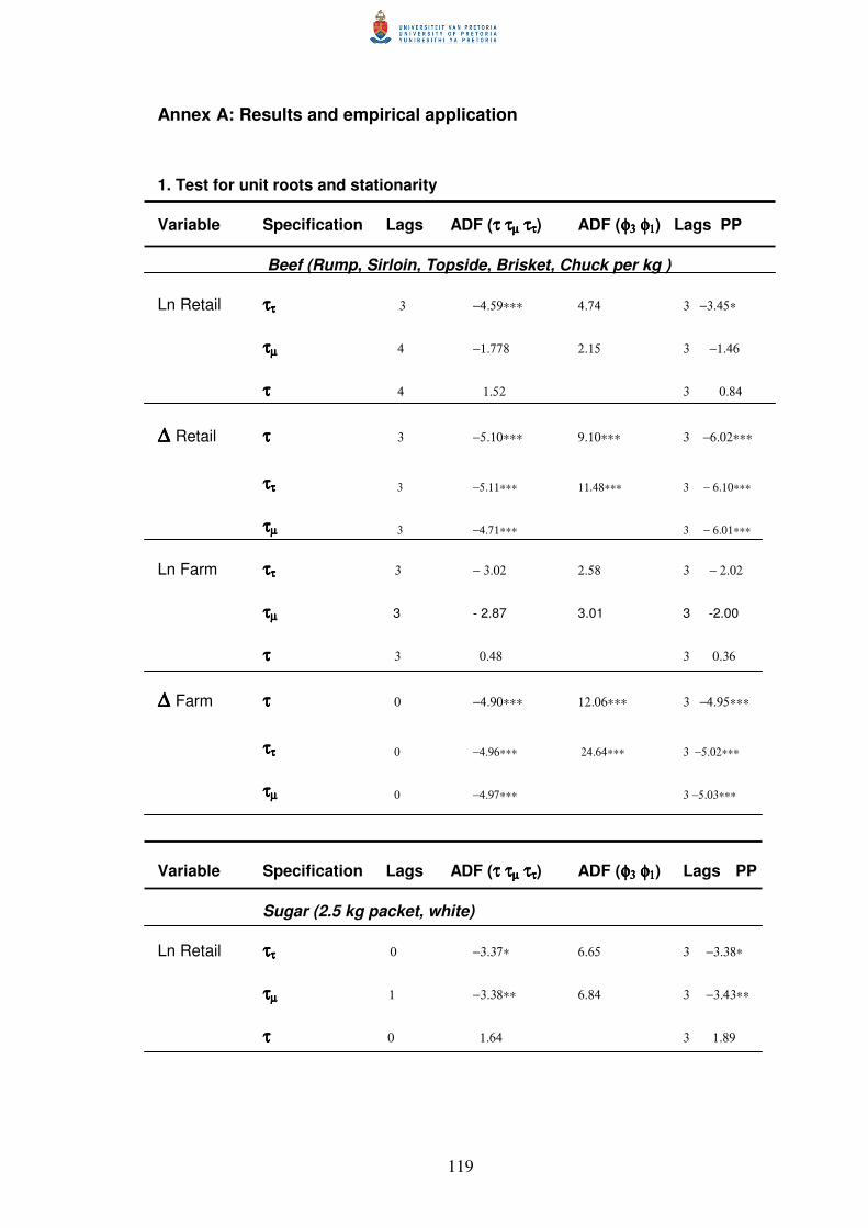
119

Annex A: Results and empirical application

1. Test for unit roots and stationarity

Variable Specification Lags ADF (τ ττ ττ ττ τµµµµ τ τ τ τττττ) ADF (φφφφ3333 φ φ φ φ1111) Lags PP

Beef (Rump, Sirloin, Topside, Brisket, Chuck per kg )

Ln Retail ττττττττ 3 −4.59∗∗∗ 4.74 3 −3.45∗

ττττµµµµ 4 −1.778 2.15 3 −1.46

ττττ 4 1.52 3 0.84

∆ ∆ ∆ ∆ Retail ττττ 3 −5.10∗∗∗ 9.10∗∗∗ 3 −6.02∗∗∗

ττττττττ 3 −5.11∗∗∗ 11.48∗∗∗ 3 − 6.10∗∗∗

ττττµµµµ 3 −4.71∗∗∗ 3 − 6.01∗∗∗

Ln Farm ττττττττ 3 − 3.02 2.58 3 − 2.02

ττττµµµµ 3 - 2.87 3.01 3 -2.00

ττττ 3 0.48 3 0.36

∆ ∆ ∆ ∆ Farm ττττ 0 −4.90∗∗∗ 12.06∗∗∗ 3 −4.95∗∗∗

ττττττττ 0 −4.96∗∗∗ 24.64∗∗∗ 3 −5.02∗∗∗

ττττµµµµ 0 −4.97∗∗∗ 3 −5.03∗∗∗

Variable Specification Lags ADF (τ ττ ττ ττ τµµµµ τ τ τ τττττ) ADF (φφφφ3333 φ φ φ φ1111) Lags PP

Sugar (2.5 kg packet, white)

Ln Retail ττττττττ 0 −3.37∗ 6.65 3 −3.38∗

ττττµµµµ 1 −3.38∗∗ 6.84 3 −3.43∗∗

ττττ 0 1.64 3 1.89

120

∆ ∆ ∆ ∆ Retail ττττ 0 −8.33∗∗∗ 34.82∗∗∗ 3 −8.43∗∗∗

ττττττττ 0 −8.12∗∗∗ 65.97∗∗∗ 3 −8.13∗∗∗

ττττµµµµ 0 − 7.68∗∗∗ 3 −7.66∗∗∗

Ln Wholesale ττττττττ 0 − 1.48 1.63 3 −1.49

ττττµµµµ 0 − 1.81 3.25 3 −1.80

ττττ 0 0.83 3 0.8

∆ ∆ ∆ ∆ Wholesale ττττ 0 − 6.84∗∗∗ 23.39∗∗∗ 3 −6.84∗∗∗

ττττττττ 0 − 6.73∗∗∗ 45.41∗∗∗ 3 −6.74∗∗∗

ττττµµµµ 0 − 6.71∗∗∗ 3 −6.71∗∗∗

Ln Farm ττττττττ 0 − 1.37 1.67 3 −1.36

ττττµµµµ 0 −1.71 2.93 3 −1.75

ττττ 0 −0.39 3 − 0.35

∆ ∆ ∆ ∆ Farm ττττ 0 −6.81∗∗∗ 23.20∗∗∗ 3 −6.83∗∗∗

ττττττττ 0 −6.65∗∗∗ 44.24∗∗∗ 3 −6..65∗∗∗

ττττµµµµ 0 −6.67∗∗∗ 3 −7.63∗∗∗

Variable Specification Lags ADF (τ ττ ττ ττ τµµµµ τ τ τ τττττ) ADF (φφφφ3333 φ φ φ φ1111) Lags PP

Maize (Super and Special, 5kg packets)

Ln Retail ττττττττ 0 -3.22* 7.11*** 3 -3.25*

ττττµµµµ 0 −0.96 0.93 3 −1.18

ττττ 0 −0.10 3 −0.1

∆ ∆ ∆ ∆ Retail ττττ 0 −5.66∗∗∗ 16.08∗∗∗ 3 −5.66∗∗∗

ττττττττ 0 −5.44∗∗∗ 29.57∗∗∗ 3 −5.45∗∗∗

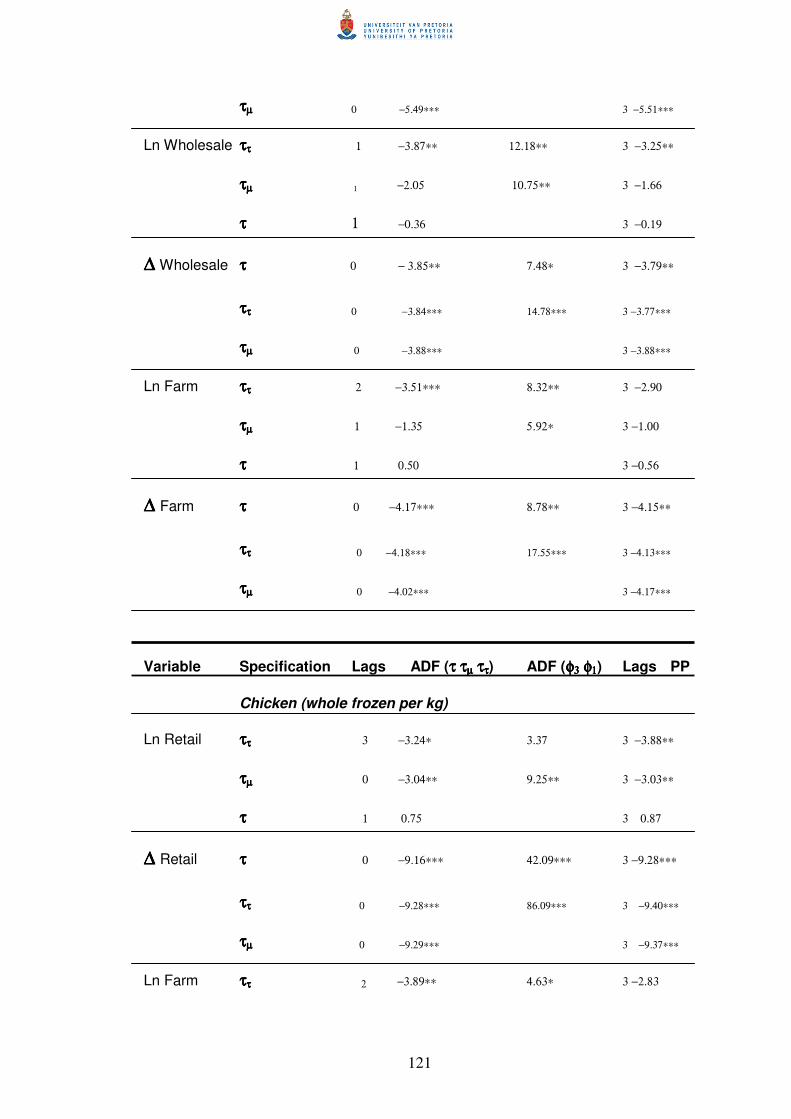
121

ττττµµµµ 0 −5.49∗∗∗ 3 −5.51∗∗∗

Ln Wholesale ττττττττ 1 −3.87∗∗ 12.18∗∗ 3 −3.25∗∗

ττττµµµµ 1 −2.05 10.75∗∗ 3 −1.66

ττττ 1 −0.36 3 −0.19

∆ ∆ ∆ ∆ Wholesale ττττ 0 − 3.85∗∗ 7.48∗ 3 −3.79∗∗

ττττττττ 0 −3.84∗∗∗ 14.78∗∗∗ 3 −3.77∗∗∗

ττττµµµµ 0 −3.88∗∗∗ 3 −3.88∗∗∗

Ln Farm ττττττττ 2 −3.51∗∗∗ 8.32∗∗ 3 −2.90

ττττµµµµ 1 −1.35 5.92∗ 3 −1.00

ττττ 1 0.50 3 −0.56

∆ ∆ ∆ ∆ Farm ττττ 0 −4.17∗∗∗ 8.78∗∗ 3 −4.15∗∗

ττττττττ 0 −4.18∗∗∗ 17.55∗∗∗ 3 −4.13∗∗∗

ττττµµµµ 0 −4.02∗∗∗ 3 −4.17∗∗∗

Variable Specification Lags ADF (τ ττ ττ ττ τµµµµ τ τ τ τττττ) ADF (φφφφ3333 φ φ φ φ1111) Lags PP

Chicken (whole frozen per kg)

Ln Retail ττττττττ 3 −3.24∗ 3.37 3 −3.88∗∗

ττττµµµµ 0 −3.04∗∗ 9.25∗∗ 3 −3.03∗∗

ττττ 1 0.75 3 0.87

∆ ∆ ∆ ∆ Retail ττττ 0 −9.16∗∗∗ 42.09∗∗∗ 3 −9.28∗∗∗

ττττττττ 0 −9.28∗∗∗ 86.09∗∗∗ 3 −9.40∗∗∗

ττττµµµµ 0 −9.29∗∗∗ 3 −9.37∗∗∗

Ln Farm ττττττττ 2 −3.89∗∗ 4.63∗ 3 −2.83

122

ττττµµµµ 1 −2.50 4.38∗ 3 −2.42

ττττ 4 1.06 3 −0.67

∆ ∆ ∆ ∆ Farm ττττ 3 −4.57∗∗∗ 6.66∗∗ 3 −5.33∗∗∗

ττττττττ 3 −4.62∗∗∗ 8.53∗∗∗ 3 −5.37∗∗∗

ττττµµµµ 3 −4.50∗∗∗ 3 −5.39∗∗∗

Variable Specification Lags ADF (τ ττ ττ ττ τµµµµ τ τ τ τττττ) ADF (φφφφ3333 φ φ φ φ1111) Lags PP

Dairy (1 lt fresh milk sachets full)

Ln Retail ττττττττ 0 −2.64 4.88∗ 3 −2.63

ττττµµµµ 0 −3.00∗∗ 9.04∗∗ 3 −3.00

ττττ 0 0.78 3 0.76

∆ ∆ ∆ ∆ Retail ττττ 0 −6.41∗∗∗ 19.31∗∗∗ 3 −6.19∗∗∗

ττττττττ 0 −5.98∗∗∗ 35.76∗∗∗ 3 −5.95∗∗∗

ττττµµµµ 0 −5.96∗∗∗ 3 −5.93∗∗∗

Ln Farm ττττττττ 0 −2.37 4.05∗ 3 −2.37

ττττµµµµ 0 −1.14 1.30 3 −1.27

ττττ 0 −0.13 3 −0.133

∆ ∆ ∆ ∆ Farm ττττ 0 −6.67∗∗∗ 22.27∗∗∗ 3 −6.67∗∗∗

ττττττττ 0 −6.49∗∗∗ 42.16∗∗∗ 3 −6.51∗∗∗

ττττµµµµ 0 −6.56∗∗∗ 3 −6.57∗∗∗

* statistically significant at 10% level

** statistically significant at a 5% level

*** statistically significant at a 1% level

123

Annex B: Proposed co-integration relationships of the variables

Proposed co-integration relationship for beef products (Dependent Variable:LN_RBEEF)

Proposed co-integration relationship for sugar (Dependent Variable: LN_RETWSG)

Variable Coefficient Std. Error t-Statistic

LN_SGCPRSA 2.916576 0.671457 4.343651 LN_AMDPSG 1.850634 0.247800 7.468270

C -27.35697 5.308662 -5.153271

Proposed co-integration relationship for maize (Dependent Variable: LN_RETSUPMM)

Variable

Coefficient

Std. Error

t-Statistic

LN_MDPWM 0.294659 0.042644 6.909785 C 0.768083 0.286053 2.685105

Proposed co-integration relationship for maize (Dependent Variable: LN_MDPWM)

Variable

Coefficient

Std. Error

t-Statistic

LN_FGPRWM 0.975827 0.002572 379.4597

Proposed co-integration relationship for chicken (Dependent Variable: LN_RETPCHK)

Variable

Coefficient

Std. Error

t-Statistic

LN_CHKPP 0.719042 0.091751 7.836846 C 1.055892 0.223501 4.724329

Proposed co-integration relationship for dairy: (DependentVariable:LN_RETFFCM) Variable Coefficient Std. Error t-Statistic

LN_FMPP 0.617356 0.182742 3.378295 C 1.136346 0.113784 9.986836

Variable

Coefficient

Std. Error

t-Statistic

SHIFT04 LN_A2BEEF

C

-0.081441 0.294327 7.203037

0.020300 0.081861 0.204376

-4.011863 3.595461 35.24406

124

Annex C: The Engle – Granger test for co-integration

1. Beef

N Model % significance

Lags ADF: C(p) Conclusion

1 3 -2.69 < -3.571 No cointegration

5 3 -2.69 < -2.923 No cointegration 1 Constant, no trend

10 3 -2.69 > -2.599 Cointegration 2. Sugar n Model % significance Lags ADF: C(p) Conclusion

1 0 -3.83 > -3.571 Cointegration 5 0 -3.83 > -2.923 Cointegration

1 Constant, no trend

10 0 -3.83 > -2.599 Cointegration 3. Maize – Retail price and Milldoor price n Model % significance Lags ADF: C(p) Conclusion

1 0 -1.69 < -3.571 No cointegration 5 0 -1.69 < -2.923 No cointegration

1 Constant, no trend

10 0 -1.69 < -2.599 No cointegration 4. Maize Milldoor price and farm gate price n Model % significance Lags ADF: C(p) Conclusion

1 1 -3.77 > -3.571 Cointegration 5 1 -3.77 > -2.923 Cointegration

1 Constant, no trend

10 1 -3.77 > -2.599 Cointegration 5. Chicken n Model % significance Lags ADF: C(p) Conclusion

1 0 -4.56 > -3.571 Cointegration 5 0 -4.56 > -2.923 Cointegration

1 Constant, no trend

10 0 -4.56 > -2.599 Cointegration 6. Dairy n Model % significance Lags ADF: C(p) Conclusion

1 0 -2.93 < -3.571 No cointegration 5 0 -2.93 > -2.923 Cointegration

1 Constant, no trend

10 0 -2.93 < -2.599 Cointegration

125

Annex D: Diagnostic tests performed on the various ECMs

1. Beef Test H0 Test statistic p-value Conclusion

Jarque - Bera Not normally distributed 0.058463 0.971192 Normally

distributed

ARCH LM No heteroscedasticity 0.039505 0.842452 Homoscedastic

White No heteroscedasticity 7.529704 0.274621 Homoscedastic

Breusch – Godfrey

No serial correlation 1.050199 0.591497 No

autocorrelation Ramsey Reset

No misspecification 3.087191 0.378376 No

misspecification 2. Sugar Test H0 Test statistic p-value Conclusion Jarque - Bera

Not normally distributed

0.283053 0.868032 Normally distributed

ARCH LM No heteroscedasticity

0.618014

0.431786

Homoscedastic

White No heteroscedasticity

1.476320

0.687746

Homoscedastic

Breusch – Godfrey

No serial correlation

1.912416

0.384348

No serial correlation

Ramsey Reset

No misspecification 0.384348

0.254536

No misspecification

3. Maize (Farmgate to Milldoor) Test H0 Test statistic p-value Conclusion Jarque - Bera

Not normally distributed

4.725606 0.094156 Not normally distributed

ARCH LM No heteroscedasticity

16.56965

0.000047

Heteroscedastic

White No heteroscedasticity

6.174065

0.186521

Homoscedastic

Breusch - Godfrey

No serial correlation

20.71469

0.000032

Serial correlation

Ramsey Reset

No misspecification 9.178181

0.027013

Misspecification

4. Maize (Milldoor to Retail) Test H0 Test statistic p-value Conclusion Jarque - Bera

Not normally distributed

0.805142 0.668599 Normally distributed

ARCH LM No heteroscedasticity

1.356658

0.244118

Homoscedastic

White No heteroscedasticity

0.356747

0.985862

Homoscedastic

Breusch - Godfrey

No serial correlation

1.143573

0.564516

No serial correlation

Ramsey Reset

No misspecification 4.022398

0.259056

No misspecification

126

5. Chicken Test H0 Test statistic p-value Conclusion Jarque – Bera

Not normally distributed

0.187720 0.910410 Normally distributed

ARCH LM No heteroscedasticity

0.989731

0.319808

Homoscedastic

White No heteroscedasticity

2.402124

0.662244

Homoscedastic

Breusch – Godfrey

No serial correlation

1.816412

0.403247

No serial correlation

Ramsey Reset

No misspecification

2.728172

0.435461

No misspecification

6. Fresh full cream milk Test H0 Test statistic p-value Conclusion Jarque – Bera

Not normally distributed

185.3311 0.000000 Not normally distributed

ARCH LM No heteroscedasticity

0.185485

0.666701

Homoscedastic

White No heteroscedasticity

24.73876

0.000057

Heteroscedastic

Breusch - Godfrey

No serial correlation

1.402804

0.495889

No serial correlation

Ramsey Reset

No misspecification

23.24922

0.000036

Misspecification

127

Annex E: The Engle Yoo third step procedure

The Engle Yoo third step regression requires that coefficient of the lagged residual in

the ECM is multiplied by the by every explanatory variable in the co-integration

relationship except for any dummy, shift or constant variables. The Engle Yoo third

step regression will however only be performed with residual values from the ECMs

that passed all of the diagnostic tests in the previous section.

1. Beef

Results from the Engle Yoo third step regression Variable Coefficients Standard error

0.306875*LN_A2BEEF -0.001023 0.008633

Variables Original coefficients

3rd step coefficients

New coefficients (elasticity)

3rd step standard error

New t stat

LN_A2BEEF 0.294327 -0.001023 0.293304 0.008633 33.97475

2. Sugar

Results from the Engle Yoo third step regression Variables Coefficients Standard error

0.479985*LN_SGCPRSA -0.124555 0.236575

0.479985*LN_AMDPSG 0.079053 0.150329

Variables Original coefficients

3rd step coefficients

New coefficients (elasticity)

3rd step standard error

New t stat

LN_SGCPRSA 2.916576 -0.124555 2.792021 0.236575 11.801843

LN_AMDPSA 1.850634 0.079053 1.929687 0.150329 12.836425

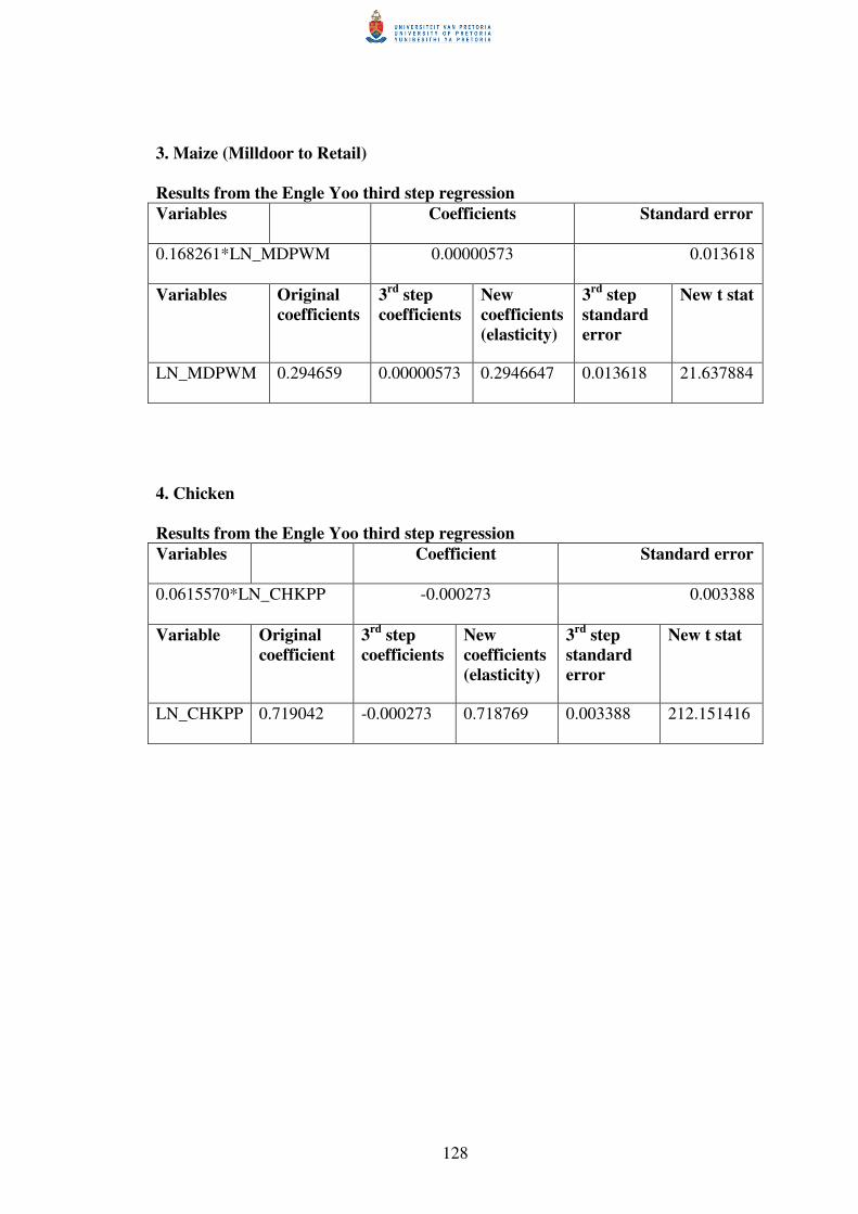
128

3. Maize (Milldoor to Retail)

Results from the Engle Yoo third step regression Variables Coefficients Standard error

0.168261*LN_MDPWM 0.00000573 0.013618

Variables Original coefficients

3rd step coefficients

New coefficients (elasticity)

3rd step standard error

New t stat

LN_MDPWM 0.294659 0.00000573 0.2946647 0.013618 21.637884

4. Chicken

Results from the Engle Yoo third step regression Variables Coefficient Standard error

0.0615570*LN_CHKPP -0.000273 0.003388

Variable Original coefficient

3rd step coefficients

New coefficients (elasticity)

3rd step standard error

New t stat

LN_CHKPP 0.719042 -0.000273 0.718769 0.003388 212.151416

129

Annex F: Rewriting the equation back to its levels and simulating the

model dynamically

The ECMs are then simulated in order to see how close the model represents the actual data.

Below are some of the ECMs and their output with respect to the other variables. The solid

line is always the model’s output whilst the dotted line is the original retail price.

1. Sugar

10.5

11.0

11.5

12.0

12.5

13.0

13.5

02:01 02:07 03:01 03:07 04:01 04:07 05:01 05:07

RETWSG RETWSGORG

2. Maize

10

12

14

16

18

20

02:01 02:07 03:01 03:07 04:01 04:07 05:01 05:07

LN_RETSUPMM_M RETSUPMM

130

3. Chicken

14

15

16

17

18

19

02:01 02:07 03:01 03:07 04:01 04:07 05:01 05:07

RETPCHK RETAIL

4. Dairy

3.8

4.0

4.2

4.4

4.6

4.8

5.0

5.2

02:01 02:07 03:01 03:07 04:01 04:07 05:01 05:07

LN_RETFFCM_M RETFFCM