CEP Discussion Paper No 650

September 2004

Is There a Market for Work Group Servers?

Evaluating Market Level Demand Elasticities

Using Micro and Macro Models

John Van Reenen

Abstract This paper contains an empirical analysis demand for “work-group” (or low-end) servers. Servers are at the centre of many US and EU anti-trust debates, including the Hewlett-Packard/Compaq merger and investigations into the activities of Microsoft. One question in these policy decisions is whether a high share of work servers indicates anything about shortrun market power. To investigate price elasticities we use model-level panel data on transaction prices, sales and characteristics of practically every server in the world. We contrast estimates from the traditional “macro” approaches that aggregate across brands and modern “micro” approaches that use brand-level information (including both “distance metric” and logit based approaches). We find that the macro approaches lead to overestimates of consumer price sensitivity. Our preferred micro-based estimates of the market level elasticity of demand for work group servers are around 0.3 to 0.6 (compared to 1 to 1.3 in the macro estimates). Even at the higher range of the estimates, however, we find that demand elasticities are sufficiently low to imply a distinct “anti-trust” market for work group servers and their operating systems. It is unsurprising that firms with large shares of work group servers have come under some antitrust scrutiny. Keywords: demand elasticities, network servers, computers, anti-trust JEL classification: O3, L1, L4 This paper was produced as part of the Centre’s Productivity and Innovation Programme. The Centre for Economic Performance is financed by the Economic and Social Research Council. Acknowledgements Ernst Berndt, Tim Besley, Thomas Buettner, Cristina Caffarra, Chris Cavanagh, Peter Davis, Ulrich Kaiser, Franz Palm, Steve Pischke, Bob Stillman and seminar participants at Leuven, LSE, Mannheim and Maastricht have all given useful comments on earlier versions of the paper. I would like to thank Hristina Dantcheva, Jose Garcia Martin and Rameet Singha for help in preparing the data. Particular thanks are due to Mark Terranova for much help with the technological details of networks. The author has been a consultant for Sun Microsystems in the past, but the opinions expressed here are entirely in a personal capacity and responsibility for all errors remains his own. John Van Reenen is Director of the Centre for Economic Performance and Professor of Economics, London School of Economics. Address for correspondence: Centre for Economic Performance, London School of Economics, Houghton Street, London, WC2A 2AE; e-mail: j.vanreenen@lse.ac.uk Published by Centre for Economic Performance London School of Economics and Political Science Houghton Street London WC2A 2AE All rights reserved. No part of this publication may be reproduced, stored in a retrieval system or transmitted in any form or by any means without the prior permission in writing of the publisher nor be issued to the public or circulated in any form other than that in which it is published. Requests for permission to reproduce any article or part of the Working Paper should be sent to the editor at the above address. © John Van Reenen, submitted 2004 ISBN 0 7530 1780 6

1. Introduction

The motivation of this paper is both practical and methodological. The practical aspect is to provide, for the first time, estimates of demand elasticities for network servers. Servers are a vital but rarely studied element of the digital economy that have moved to centre stage in recent anti-trust debates in the US and Europe. The methodological aspect of the paper is to provide systematic comparisons of estimates of demand systems based on the “micro” brand-level approaches common in applied industrial organization to the more aggregate estimates familiar in the macro-literature. We show that there are large aggregation biases of the macro approach compared to our preferred micro approaches. In the late 1980s computing architecture went through a paradigm shift. The mainframe-orientated system evolved swiftly towards the "PC client/server" computer architecture that is familiar today2. Instead of computer intelligence being centralised and users interacting via “dumb” terminals, processing power was more decentralised, distributed between PCs with their own operating systems and increasingly powerful servers linking these PCs together in networks. The economics literature on ICT (information and communication technologies) is large, but has generally ignored severs3. This is a surprising omission given that total expenditure on servers was about $56bn in 20004, and server expenditure has been growing at a faster rate than corporate spending on PCs. Furthermore, the market for work group servers (the “low end” side of the market) has become a major area of anti-trust debate. First, the merger between Hewlett-Packard and Compaq is one of a large number of consolidations of hardware vendors. Second, the European Commission has recently concluded that Microsoft used its monopoly in PC operating systems to dominate the work group server space through limiting “interoperability” between Windows and rival operating systems5. The remedy in the US Microsoft case also focuses on server operating systems as “middleware” which poses a potential platform threat to Microsoft’s PC monopoly6. Figure 1 shows that in the first quarter of 2001 58% of low end servers ran a version of the Windows operating system compared to only 21% at the start of 1996. Large shares of sales of work group servers would not be a concern if there was easy substitutability for other forms of ICT – i.e. if work group servers were not a “relevant market” in anti-trust jargon. A practical objective of this paper is, therefore, to estimate the magnitude of the market level elasticity of demand to investigate whether there is “a market for work group servers”7.

2 See Bresnahan and Greenstein (1996) for an economic analysis of this transition. 3 The literature has mainly focused on the impact of ICT on productivity, hedonic prices and welfare (e.g. Bresnahan (1989), Brynjolfsson (1996, 1997), Greenstein (1997)). When ICT is disaggregated at all it tends to be PCs or mainframes that are the focus. 4 International Data Corporation (2000b) 5 http://europa.eu.int/rapid/pressReleasesAction.do?reference=IP/04/382&format=HTML&aged=0&language=EN&guiLanguage=en

6 See Carlton and Waldman (2002) for an analysis of why a monopolist may leverage into a complementary market in order to stifle future competition in his primary market. 7 Showing that there is a relevant market is not sufficient to demonstrate anti-competitive effects, of course. Even if a firm does gain a large share it may do so by competitive means.

2

In pursuing this question we estimate at a macro level and a micro (brand/model) level. Although applied I.O. has focused on increasingly sophisticated brand level demand estimation for differentiated products8, many authors have kept to the traditional macro-approach of using time series data estimated across all brands in a region9. The macro approach has a major advantage in requiring significantly less data and computational complexity than the micro approach. Even those who argue for micro approaches sometimes claim that it is better to use macro data if the question is focused on the market level elasticity of demand10. The macro approach has serious downsides, however. Not only is it inefficient as the cross sectional information on brand prices and quantities is ignored, but it is likely to lead to inconsistent estimates of demand elasticities due to aggregation biases. The basic macro approach (and its attendant problems) can be illustrated in Figure 211 which plots quality adjusted prices against quality adjusted quantities. It is tempting to interpret the slope of the line as an estimate of the demand elasticity: exogenous technical change shifts an upward sloping supply curve to the right, tracing out the stable demand curve. Apart from the issue of demand shocks (which also affect the micro estimates) there is a problem that the quality adjusted price deflator will appear on the right hand side of the demand equation and in the denominator of quality adjusted quantity on the left hand side of the equation. This will lead to a negative bias – i.e. if the true demand elasticity is inelastic there will be a bias towards finding that customers are more price sensitive than they actually are. This may be one reason why many of the existing “macro” estimates are close to negative unity12 (we also find estimates of around unity in the macro-approach). To investigate these issues we estimate demand systems for servers using a model-level quarterly panel that contains information on (essentially) all servers between 1996 and 2001. We focus on the US where our data is richest, but also present results for Western Europe and Japan. Our main empirical finding is that the estimated demand elasticities for work group server systems (i.e. the hardware/software bundle) are sufficiently inelastic to suggest a separate product market. Methodologically, we also find significant upwards bias from the macro estimates (suggesting absolute values of demand elasticities of the work group server market of around 1 to 1.3) compared to micro-estimates (suggesting elasticities of around 0.25 to 0.55). The situation on the software side is more complex since the demand for operating systems is a derived demand. Since the operating system is only a minor fraction of the total price, 8 See inter alia Berry et al (1995), Nevo (200), Pinske et al (2002). Unfortunately our “micro” approach does not have consumer level data like Petrin (2002) or Berry et al (2004). 9 For example, Chow (1967), Brynjolfsson (1996, 1997), Gordon (2002), Reddy et al (2001). Schmalensee (2000) and others have relied on these estimates. 10 For example, Werden and Froeb (1994, p.4) 11 This figure uses estimates from our implementation of the macro approach described in sub-section 3.1 below. 12 Chow (1967) uses US data between 1955 and 1965 and regresses the log of the quality adjusted quantity of computers against the log hedonic price, log GDP and a constant. He finds an elasticity of 1.04 (1.44 when dropping GDP). Brynjolfsson (1996) presents a series of estimates for "office, computing and accounting machinery" (OCAM) for more recent US data between 1970 and 1989. His central estimates are also around unity (for the whole economy) but range between 0.6 and 1.4. Gordon (2002) finds that the elasticity has fallen in absolute value from 1.96 in 1972-87, to 1.19 in 1987-1995 to 1.15 between 1995 and 1999 (these do not condition on GDP, though). Brynjolfsson (1997) analyses aggregate mainframe sales between 1968 and 1981 and finds an elasticity of demand of 1.05.

3

however, we argue that the derived demand elasticity for the operating system will tend to be even more inelastic than the demand elasticity for the hardware/software bundle. This implies, subject to many caveats, that the operating systems for work group servers are also an anti-trust market. The paper is organised as follows. Section 2 gives a basic introduction to the role of servers in modern computing and discusses the substitution possibilities between low-end and high-end servers. Section 3 describes the theoretical framework we use and section 4 discusses econometric issues. Section 5 details the data and section 6 contains the results. We draw out the implications of the results for the elasticity of demand for work group servers and their operating systems (OS) in section 7 and offer some concluding comments in section 8. 2. Network servers in modern computing

2.1 Client-server networks

Computing can be performed locally on stand-alone appliances such as using a laptop computer away from the office. Most computing, however, is performed on multi-user networks in which users communicate through ‘clients’ and in which much of the computing activity takes place behind the scenes on ‘servers’13. The clients in a client-server network take many forms. Some are ‘intelligent,’ such as a desktop computer; others are ‘non-intelligent,’ such as a dumb terminal (e.g. an ATM machine). Servers vary in size and in the nature of the tasks they are asked to perform. The mixture of servers in a client-server network depends on the kinds of computing that the network is designed to support. The server requirements of a small office, for example, are considerably different than the server requirements of a large international bank. Like all computers, servers consist of both hardware (e.g. the processors and storage facilities/memory) and software (e.g. the operating system). Server hardware is manufactured using various types of processors. Intel processors are used in many servers, and Microsoft’s Windows operating system is compatible only with hardware that uses Intel processors. Novell’s NetWare and SCO’s UNIX variants are also designed to run on Intel processors. The leading hardware manufacturers for Intel-based servers include Compaq/HP, Dell, and IBM. Server vendors typically sell Intel-based systems on a non-integrated basis. An organisation usually buys server hardware from one vendor with the server operating system installed from another vendor (or, the organization will install the server operating system itself). Server systems are also sold on an integrated basis in which the vendor supplies both the server hardware and a proprietary operating system that has been specially designed for the vendor’s hardware. Sun, HP and IBM are the leading suppliers of these integrated server systems.14 Each of these firms uses its own flavour of UNIX as the operating system for its server system.

13 For a basic discussion of servers see, for example, Sybex (2001) 14 Sun combines its Solaris operating system with its SPARC processors, HP combines its HP-UX operating system with its PA-RISC processors (although these are to be shifted to IA-64), IBM combines its AIX operating system with its Power and Power PC processors, SGI offers the IRIX operating system combined with its MIPS chips. COMPAQ has Tru4UNIX and Digital UNIX combined with its Alpha chips. IBM and COMPAQ also offer non-UNIX operating systems for servers. For IBM the operating systems are OS390 (originally for mini-computers) and OS400 (originally for main frames) that run on the S390 and AS400 chips respectively. COMPAQ has OpenVMS.

4

Linux is another alternative as a server operating system. Linux is open source software that was developed by volunteers interacting largely over the Internet. It is “shareware” and is available for free. Linux can run on all types of hardware and remains available on the Internet for no charge.

2.2 Work group servers versus enterprise servers

One of the principal benefits of a computer network is that it allows an organisation to share computer resources among multiple users. Clients connected to a network can share printers and files. Application programmes can be maintained on central servers and then ‘served’ to clients on an as-needed basis. Work group servers are used to perform a number of the basic “infrastructure” services needed for the computers in a network to share resources. Work group servers most commonly handle security (authorisation and authentication of users when they connect their clients to the network), file services (accessing or managing files or disk storage space), print services, directory services (keeping track of the location and use of network resources), messaging and e-mail, and key administrative functions in the management of the work group network. In addition to these infrastructure services, work group servers also execute certain kinds of server-side applications. The application programmes that run on work group servers tend to be standardised applications that are used uniformly across business environments.15 Work group servers are also used to execute portions of distributed applications.16 The ability to share resources such as printers, files and application programmes is one benefit of a computer network. In many organisations, there is a pressing need to manage enormous amounts of data - inventory control, airline reservations and banking transactions are just a few examples. The ‘mission-critical’ data used for these purposes need to be stored, updated, quality controlled, and protected. They also need to be readily available to authorised users. The servers that perform these mission-critical data functions are frequently referred to as enterprise servers. Enterprise servers tend to be larger and significantly more expensive than work group servers. In our sample period a work group server usually has one (or sometimes two) microprocessors and modest memory (around four gigabytes). A work group server can provide services for up to about 100 clients, although 25-35 clients would be more common. Enterprise servers, in contrast, tend to have at least eight processors, usually cost more than $100,000 and in some circumstances can cost more than $1 million. The uses to which mission-critical data are put, and the methods by which they are stored, accessed and used, vary widely across organisations. Thus, in contrast to the standardised applications that run on work group servers, application programmes for enterprise servers tend to be custom written and specific to a particular organisation. Reliability and security are especially important for these servers. Large costs are incurred if vital data are corrupted or 15 Exchange and SQL Server are examples of standardised applications that run on work group servers. Exchange is a server application programme that works with Outlook on the client side to provide communication services such as group e-mail, scheduling and address books. SQL Server is a server application that allows users to interrogate and work with databases stored on servers. For more information on these Microsoft server applications, see http://www.microsoft.com/servers. 16 A distributed application is one that relies on objects stored across a number of computers - both clients and servers. Work group servers are also used for local administration; remote access services (accessing the server from a remote location through a communications link); terminal services (enabling client devices to use applications or data residing on the server); and, in some cases, for hosting web sites.

5

‘go down’ for even a short period. The consequences may be even worse if unauthorised users are able to access an organisation’s confidential data. This need for reliability and security means that enterprise servers require robust operating systems that are not susceptible to crashes and that have highly developed security features.

2.3 N-tier architectures

Because there are fundamental differences between the functions performed by work group servers and enterprise servers, modern computer networks typically have multiple tiers, in which each tier performs a distinct set of functions. The number of tiers in a computer network can vary, depending on the size and complexity of the organisation. For this reason, multiple tier architectures are frequently described as N-tier structures. Generally, however, N-tier network architectures have at least three distinct layers: 1. First tier – the presentation tier. This is the user environment with the associated menu,

display, screen, dialogue boxes, etc. The presentation tier will typically sit upon a desktop or other form of client computer;

2. Second (or ‘middle’) tier – the business logic tier. This tier has the resources needed to operate basic business processes.

3. Third tier – the data tier. This is where all the data are physically stored and managed. This tier may itself be divided into a number of sub-tiers. The systems and software that comprise this tier have to ensure predictable, reliable and secure access to data inquiries. These will sit on larger enterprise-level servers.

Even though this description may suggest that substitution possibilities between work group and enterprise servers are limited, a network architect has to make decisions at the margin regarding whether to allocate certain network functions to a work group server or to an enterprise server. If this is a large enough margin for discretion then there may be substantial substitution possibilities.

The limits on the ability of a network architect to add functions typically performed by a work group server to an enterprise server relate to cost efficiency, isolation and flexibility. First, it is more cost efficient to locate many functions on work group servers because these functions do not require so much computing power and one can make do with cheaper hardware and operating systems. Training costs are also particularly important17. Second, isolating the data layer protects the data stored in the enterprise level from crashes that could be caused by access from more mundane tasks. Where there is a need for high reliability and security, it is undesirable to mix data management at the enterprise function level with the more trivial tasks of writing letters or opening a web page. Third, to perform all server functions on one layer reduces organizational flexibility. Work group servers can be adapted to the needs of particular sub-groups in the organisation, enabling greater decentralisation18. Work group servers allow

17 The specialised skills and training needed to manage the data layer machines are not needed to manage work group machines. It costs much less for an engineer to fix a bug in a work group server than in an enterprise server. 18 For the importance of organisational decentralisation and the efficient exploitation of ICT see Bresnahan, Brynjolfsson and Hitt (2002).

6

local administrators to make changes within local business units that are not necessary or desirable across the entire business19.

Against these considerations is the fact that customers can cluster20 work group servers together into server “farms” that can mimic some of the functionalities of enterprise servers. Although some industry observers regard clustering as less secure and reliable than a single enterprise server, the ability to cluster opens up more substitution possibilities. Ultimately, the sensitivity of customer demand to changes in price must be an empirical issue. We now turn to ways in which this can be econometrically modelled. 3. Modelling Framework

We follow the standard approach of considering the demand for operating systems as a derived demand21. This overwhelming majority of sales of server operating systems take place when the hardware for the server is sold. Since every server requires an operating system (OS) to use applications and provide infrastructure services, it seems natural to first consider the demand for the server system (i.e. the hardware/software bundle). There are several possible methods of modelling the demand side of the server market. We contrast two basic approaches: a “macro” strategy and a “micro” strategy. This is somewhat of a misnomer as the macro approach will also use micro data (to construct the hedonic price index), but the distinction is that the crucial econometric estimates of demand in the macro approach will be on the data aggregated across all brands. Within the macro approach we distinguish between logit based models and the distance metric approach. The approaches are not nested within each other as they rely on different assumptions. Still, we believe a comparison between the methods is instructive as typically authors plumb for one approach or another and argue for superiority on a prior or practical grounds rather than considering a variety of methods.

3.1 Macro Approach: Multi-level modelling

In the first approach to examining the demand for computers we follow the common method of estimating a multi-level demand system based on two-stage budgeting approach (see Gorman, 1971). Versions of this approach have been the most common way to estimate at aggregate demand elasticities for computers22. The customer is assumed to follow the decision process sketched in Figure 3. The “top” level decision is how much expenditure to allocate on servers rather than other items (such as other ICT expenditures). The “middle” level decision is how much of the server expenditure to allocate to work group servers rather than enterprise servers. The “bottom” level is what brands of servers to buy, conditional on a budget for a particular

19 For example, work group servers allow a network administrator to tailor report or letter templates to the particular needs of different departments to reflect different addresses, customers and conditions of business. 20 This is also known as “horizontal scaling” by software engineers. 21 For example, Schmalensee (2000) or Foncel and Ivaldi (2001). 22 For example, Chow, 1967, Brynjolfsson, 1996, 1997, Gordon, 2002.

7

group of servers. This seems a natural ordering to use to test the null hypothesis that work group servers and enterprise servers are close substitutes23.

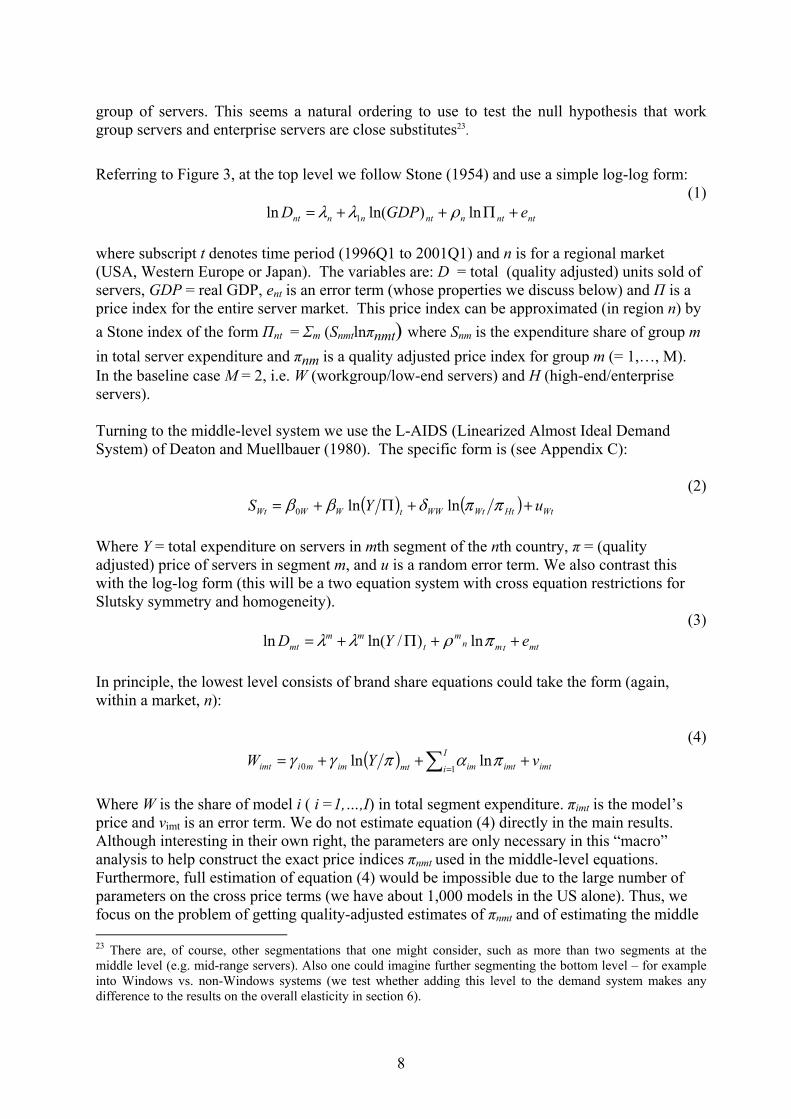
Referring to Figure 3, at the top level we follow Stone (1954) and use a simple log-log form:

(1) ntntnntnnnt eGDPD +Π++= ln)ln(ln 1 ρλλ

where subscript t denotes time period (1996Q1 to 2001Q1) and n is for a regional market (USA, Western Europe or Japan). The variables are: D = total (quality adjusted) units sold of servers, GDP = real GDP, ent is an error term (whose properties we discuss below) and Π is a price index for the entire server market. This price index can be approximated (in region n) by a Stone index of the form Πnt = Σm (Snmtlnπnmt) where Snm is the expenditure share of group m in total server expenditure and πnm is a quality adjusted price index for group m (= 1,…, M). In the baseline case M = 2, i.e. W (workgroup/low-end servers) and H (high-end/enterprise servers). Turning to the middle-level system we use the L-AIDS (Linearized Almost Ideal Demand System) of Deaton and Muellbauer (1980). The specific form is (see Appendix C):

(2) ( ) ( ) WtHtWtWWtWWWt uYS ++Π+= ππδββ lnln0

Where Y = total expenditure on servers in mth segment of the nth country, π = (quality adjusted) price of servers in segment m, and u is a random error term. We also contrast this with the log-log form (this will be a two equation system with cross equation restrictions for Slutsky symmetry and homogeneity).

(3) mttmn

mt

mmmt eYD ++Π+= πρλλ ln)/ln(ln

In principle, the lowest level consists of brand share equations could take the form (again, within a market, n):

(4) ( ) ∑ =

+++= I

i imtimtimmtimmiimt vYW10 lnln παπγγ

Where W is the share of model i ( i =1,…,I) in total segment expenditure. πimt is the model’s price and vimt is an error term. We do not estimate equation (4) directly in the main results. Although interesting in their own right, the parameters are only necessary in this “macro” analysis to help construct the exact price indices πnmt used in the middle-level equations. Furthermore, full estimation of equation (4) would be impossible due to the large number of parameters on the cross price terms (we have about 1,000 models in the US alone). Thus, we focus on the problem of getting quality-adjusted estimates of πnmt and of estimating the middle 23 There are, of course, other segmentations that one might consider, such as more than two segments at the middle level (e.g. mid-range servers). Also one could imagine further segmenting the bottom level – for example into Windows vs. non-Windows systems (we test whether adding this level to the demand system makes any difference to the results on the overall elasticity in section 6).

8

and top equations. In the next sub-section we investigate a version of equation (4) where we place greater structure on our assumptions over consumer utility.

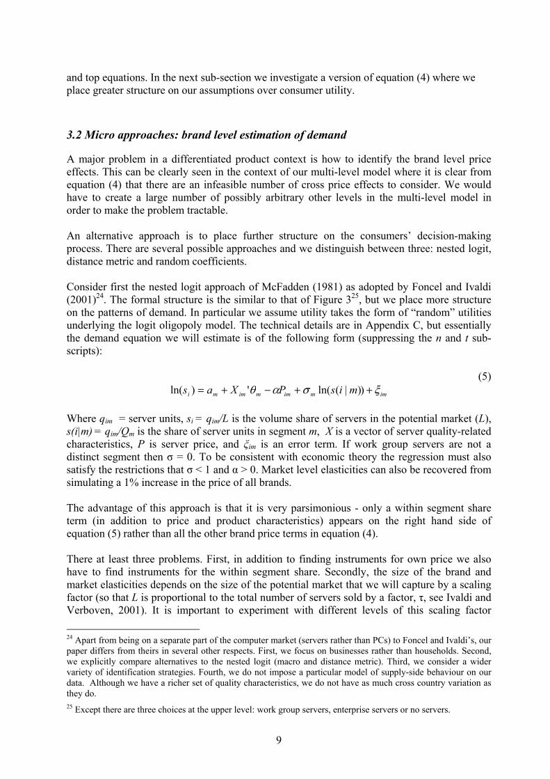
3.2 Micro approaches: brand level estimation of demand

A major problem in a differentiated product context is how to identify the brand level price effects. This can be clearly seen in the context of our multi-level model where it is clear from equation (4) that there are an infeasible number of cross price effects to consider. We would have to create a large number of possibly arbitrary other levels in the multi-level model in order to make the problem tractable. An alternative approach is to place further structure on the consumers’ decision-making process. There are several possible approaches and we distinguish between three: nested logit, distance metric and random coefficients. Consider first the nested logit approach of McFadden (1981) as adopted by Foncel and Ivaldi (2001)24. The formal structure is the similar to that of Figure 325, but we place more structure on the patterns of demand. In particular we assume utility takes the form of “random” utilities underlying the logit oligopoly model. The technical details are in Appendix C, but essentially the demand equation we will estimate is of the following form (suppressing the n and t sub-scripts):

(5) immimmimmi misPXas ξσαθ ++−+= ))|(ln(')ln(

Where qim = server units, si = qim/L is the volume share of servers in the potential market (L), s(i|m) = qim/Qm is the share of server units in segment m, X is a vector of server quality-related characteristics, P is server price, and ξim is an error term. If work group servers are not a distinct segment then σ = 0. To be consistent with economic theory the regression must also satisfy the restrictions that σ < 1 and α > 0. Market level elasticities can also be recovered from simulating a 1% increase in the price of all brands. The advantage of this approach is that it is very parsimonious - only a within segment share term (in addition to price and product characteristics) appears on the right hand side of equation (5) rather than all the other brand price terms in equation (4). There at least three problems. First, in addition to finding instruments for own price we also have to find instruments for the within segment share. Secondly, the size of the brand and market elasticities depends on the size of the potential market that we will capture by a scaling factor (so that L is proportional to the total number of servers sold by a factor, τ, see Ivaldi and Verboven, 2001). It is important to experiment with different levels of this scaling factor

24 Apart from being on a separate part of the computer market (servers rather than PCs) to Foncel and Ivaldi’s, our paper differs from theirs in several other respects. First, we focus on businesses rather than households. Second, we explicitly compare alternatives to the nested logit (macro and distance metric). Third, we consider a wider variety of identification strategies. Fourth, we do not impose a particular model of supply-side behaviour on our data. Although we have a richer set of quality characteristics, we do not have as much cross country variation as they do. 25 Except there are three choices at the upper level: work group servers, enterprise servers or no servers.

9

relating the actual to potential market, in order to check the robustness of the results. Finally, as is well known the tight structure can often lead to implausible elasticities, especially on the cross price terms. Pinkse et al (2002) suggests an alternative “distance metric” approach where all other prices enter the brand equations (as with the multi-level model) but these are weighted by a distance function that depends inter alia on the product characteristics26. In particular, demand for server qi in segment m can be written

(7) immi

jjijiim uQPbaq +++= ∑ ς

where B = [bij] is a I x I symmetric, negative semi-definite matrix. Model prices (p) are normalised on the outside good. Following Slade (2004) and Pinske et al (2002) we parameterise ai and bii as functions of the brand characteristics, i.e. ai = a(Xi) and bii = b(Xim). The off-diagonal elements of B are assumed to be functions of vectors of measures of distance between brands in some set of metrics bij = g(dij) where dij is the “distance” between brands i and j (e.g. in memory). We experimented with many different X’s and functional forms of the distance metric in the application using an adjusted R2 criterion27. A third micro approach is to allow the coefficients on price and other characteristics to be random (Berry et al, 1995). This allows a much more plausible range of cross price elasticities than the nested logit at the price of significantly higher levels of computational complexity. We are pursuing this approach in current research (Davis et al, in process).

3.3 Hedonic regressions

To calculate quality-adjusted prices for the macro approach, we first estimate hedonic price equations using every model in every quarter in every region. We then calculate a hedonic price index for work group and enterprise level servers used in the middle level demand equation for each region. We also use the weighted average enterprise and work group server hedonic price indices to calculate a price index for the overall server market to use in the top level equation. The basic form of the hedonic regression for server systems that we use is28:

(8) inmttnmtnmtinmtinmt vdaXP ++′= γln

26 This form of this model can be rationalised by assuming customers have normalised quadratic utility functions (flexible in price). With our assumptions over the functional form of the distance metric this generates equation (7). 27 Empirically we found (like Slade, 2004) that a simple inverse function of absolute distance worked well. In

other words rival prices are weighted by DMPij = ∑ ≠

−+ijjji XX, ||1

1. But we also show robustness to

including other forms of rival price (such as average work group server price and enterprise server price). 28 We considered and tested many other functional forms, including higher order polynomials in the characteristics.

10

An observation i is vendor, family, model and operating system specific in quarter t. So in equation (7) Pinmt = the price of model i of server type m in region n at time t. d= a set of time dummies, X = a vector of characteristics (such as the model’s main memory and clock speed). We estimate equation (7) separately for each market segment (i.e. workgroup servers and enterprise servers) in each region. We restrict the coefficients to be the same between any two adjacent quarters, but allow them to be different for any quarters more than two quarters apart. In other words we estimate a regression for 1996Q1-Q2 pooled, for 1996Q2 –Q3 pooled, etc. This specification is statistically preferred to imposing common slopes on the characteristic vector over all time periods. The theoretical basis of equation (7) is controversial and should only be seen as a rough first order approximation to the “correct” price index29. The discussion in sub-section 3.2 sketched a more structural approach to the price equation based on an explicit utility foundation that illustrates some of the problems with interpreting equation (7), such as the problem of identifying changes in characteristics from changes in the mark-up. Nevertheless, following the standard method for constructing such an index seems like a good starting point to examine the evolution of prices in this market. 3.4 Derived Demand for Work Group server operating systems

The bulk of this paper will be concerned with estimating a plausible range of values for the unconditional elasticity of demand for work group servers systems (i.e. the hardware/OS bundle). Call this elasticity E’WW. This denotes the proportionate impact on quantity of work group servers sold from a proportionate increase in the price of work group servers. But we are also interested in the elasticity of demand for the operating systems on work group servers, EOS. Under certain assumptions one can define and decompose the elasticity of demand for work group server operating systems, EOS , in the following way:

(8)

W

OSWW

OS

OSOS P

PE

PQ

E *'lnln

=

∂∂

=

where QOS is the quantity sold of operating systems for work group servers, POS is the price of operating systems for work group servers, PW is the price of the server hardware/software bundle. There are two key assumptions underlying the derived demand formula. First, we are assuming fixed coefficients - which every server has to have a single operating system - so a unit increase the demand for servers will lead to a unit increase the demand for server operating systems. This is uncontroversial. Second, we are assuming that the substitution between the work group server OS and other inputs is zero. If there were other substitute inputs then an additional term would have to be added to equation (8) to reflect the elasticity of substitution between the work group OS and this other input. One possible substitute input would be the operating systems of enterprise level servers. There are good reasons for believing that these alternative OSes are very poor substitutes. This is because the enterprise-level OS do not have to inter-operate closely with PC OS - they mainly interact with other servers (see the discussion of N-tiering above). The pre-dominantly UNIX based operating systems at the enterprise level

29 See Ekeland, Heckman and Neisham (2004) or Pakes (2003). Van Reenen (2004) compares many different methods of calculating hedonic price indices. These can be different for the absolute degree of price falls, but make less of a difference for the relative change in prices between work group and enterprise servers.

11

are would find it very difficult to be substitutable for the predominantly Windows-based operating systems at the work group level. We discuss these issues in more detail in section 7.

Direct estimation of the elasticities between operating systems is practically impossible because of the difficulties in obtaining exact information on the "price" of operating systems30. Nevertheless it is possible to get some idea of the average cost of the operating system in total work group server cost (POS/PW). International Data Corporation (IDC) estimate that in aggregate operating systems constitute about 10 to 15% of the overall price of a server. Thus the relevant elasticity for the market we are considering is 10-15% of the estimated server elasticity (see section 7 below). This is an example of the “importance of being unimportant” (Henderson, 1922, p.25) – the derived demand elasticity is much lower than the overall elasticity because the price of the server system bundle does not change very much when the OS cost rises31. 4. Econometric Issues Consider the estimation of a stochastic form of equation (5).

(9) itiimitit XPay υηθα +++−= '0

Assuming that the X variables are exogenous the critical question is how to obtain consistent estimates of α32. OLS will generally be biased for a number of reasons. Demand shocks will tend to raise price and quantity simultaneously leading to an underestimate of the absolute magnitude of the demand elasticity. The demand shocks could be due to permanent omitted product characteristics (ηi) or transitory shocks to economic expectations (the part of the υit that is correlated with Pit). 4.1 Unobserved Heterogeneity and brand specific effects

If the bias is solely due to omitted characteristics then this could be dealt with by transforming the data to remove the brand specific effects. The results section will consider fixed effect approaches, but note that they have well known disadvantages. First, it will be hard to identify the impact of model characteristics as these vary little over time: they are highly persistent regressors. Secondly, the inclusion of fixed effects will tend to accentuate attenuation bias associated with classical measurement error. Thirdly, including a full set of dummy variables (i.e. performing “within groups”) will still result in inconsistent estimates in finite samples unless the regressors are strictly exogenous (which price is not). Consequently we will also consider GMM estimators based around differencing the data that can deal with weakly exogenous and endogenous regressors. 30 This is because (a) the OS is bundled with the hardware, (b) the pricing of licenses is highly complex and unavailable from IDC on a model by model average. 31 There are at least two other factors that could affect the derived demand formula that we have not modelled. First, we have ignored the impact of the purchase of an OS on the demand for future upgrades. But upgrades only accounted for 7% of all server OS shipped in 1999 (IDC, 2000a), so they are not likely to be very important. Similarly we have not included any effect of a price rise of a server OS in reducing the demand for complementary applications software (there is no data on these). 32 In the nested logit we also have the issue of the segment variable that is a function of quantity. In the macro equation we have the problem that the dependent variable is a generated regressor.

12

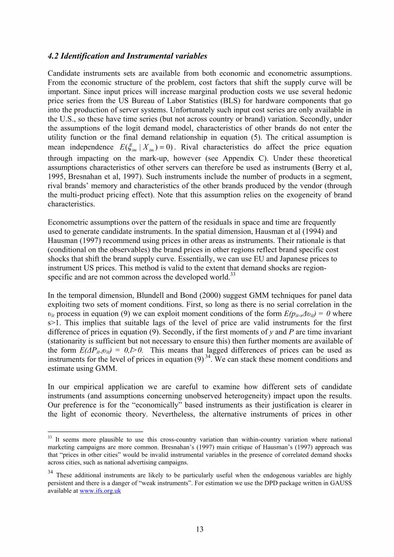
4.2 Identification and Instrumental variables

Candidate instruments sets are available from both economic and econometric assumptions. From the economic structure of the problem, cost factors that shift the supply curve will be important. Since input prices will increase marginal production costs we use several hedonic price series from the US Bureau of Labor Statistics (BLS) for hardware components that go into the production of server systems. Unfortunately such input cost series are only available in the U.S., so these have time series (but not across country or brand) variation. Secondly, under the assumptions of the logit demand model, characteristics of other brands do not enter the utility function or the final demand relationship in equation (5). The critical assumption is mean independence )0)|( =imim XE ξ . Rival characteristics do affect the price equation through impacting on the mark-up, however (see Appendix C). Under these theoretical assumptions characteristics of other servers can therefore be used as instruments (Berry et al, 1995, Bresnahan et al, 1997). Such instruments include the number of products in a segment, rival brands’ memory and characteristics of the other brands produced by the vendor (through the multi-product pricing effect). Note that this assumption relies on the exogeneity of brand characteristics. Econometric assumptions over the pattern of the residuals in space and time are frequently used to generate candidate instruments. In the spatial dimension, Hausman et al (1994) and Hausman (1997) recommend using prices in other areas as instruments. Their rationale is that (conditional on the observables) the brand prices in other regions reflect brand specific cost shocks that shift the brand supply curve. Essentially, we can use EU and Japanese prices to instrument US prices. This method is valid to the extent that demand shocks are region-specific and are not common across the developed world.33 In the temporal dimension, Blundell and Bond (2000) suggest GMM techniques for panel data exploiting two sets of moment conditions. First, so long as there is no serial correlation in the υit process in equation (9) we can exploit moment conditions of the form E(pit-s∆υit) = 0 where s>1. This implies that suitable lags of the level of price are valid instruments for the first difference of prices in equation (9). Secondly, if the first moments of y and P are time invariant (stationarity is sufficient but not necessary to ensure this) then further moments are available of the form E(∆Pit-lυit) = 0,l>0. This means that lagged differences of prices can be used as instruments for the level of prices in equation (9) 34. We can stack these moment conditions and estimate using GMM. In our empirical application we are careful to examine how different sets of candidate instruments (and assumptions concerning unobserved heterogeneity) impact upon the results. Our preference is for the “economically” based instruments as their justification is clearer in the light of economic theory. Nevertheless, the alternative instruments of prices in other

33 It seems more plausible to use this cross-country variation than within-country variation where national marketing campaigns are more common. Bresnahan’s (1997) main critique of Hausman’s (1997) approach was that “prices in other cities” would be invalid instrumental variables in the presence of correlated demand shocks across cities, such as national advertising campaigns. 34 These additional instruments are likely to be particularly useful when the endogenous variables are highly persistent and there is a danger of “weak instruments”. For estimation we use the DPD package written in GAUSS available at www.ifs.org.uk

13

regions and lagged prices could in principle improve efficiency substantially, even if the theory is correctly specified. Formally, we test the validity of the different instrumental variables by considering the Sargan-Hansen test of the over-identification restrictions. Empirically, we find evidence of problems with using “other country” prices as instruments in the micro equations. We also consider the reduced forms, in particular the explanatory power of the excluded instruments in the second stage in the reduced forms. This is particularly important in the light of the finite sample biases that are possible when the instruments are weakly correlated with the endogenous variables (e.g. Staiger and Stock, 1997).

4.3 Endogenous Stratification

As a practical issue we follow industry observers (and the European Commission) in defining the work group server segment in relation to price. IDC defined work group servers as those priced below $100,000. Price serves as a proxy for the type of work group functions that servers perform, as such precise information is generally not available for the models sold. This raises the issue of endogenous sample stratification (e.g. Hausman and Wise, 1984) and the attendant biases with truncating a sample based on an endogenous variable. To mitigate these issues we select the samples based on an initial condition: whether the server cost more of less than $100,000 when it first entered the market35. Even selecting on initial conditions can cause bias if there is correlation between the current shock and the initial condition. We check our main estimating strategy by using truncated regression and selection correction techniques to investigate whether this makes any difference to the results.

4.4 Investment Issues and dynamics

The approach we have followed is familiar in the consumer demand literature, but it is firms, not individuals who purchase servers. Would it not be more appropriate to model server investment explicitly as an investment decision? The answer to this is, “yes, in principle”. The investment literature is currently in some disarray now because the foundations for the standard quadratic adjustment cost model have been called into serious question36. Although there is little consensus over the appropriate form of the investment equation, costs of adjustment will certainly imply some longer dynamics in our model. Therefore, we test for the sensitivity of our finding to alternative dynamic forms by including lags of the endogenous and exogenous variables.

4.5 Market Power and the “cellophane fallacy”

We need to be concerned about the so-called “cellophane” fallacy (named after a US antitrust case involving DuPont). In general, the higher the estimated elasticity, the less inclined we are to treat the product in question as a relevant market. High elasticities, in general, suggest the availability of good substitutes. But, high elasticities can also be the result of an exercise of market power. In general, a monopolist will not operate in the inelastic portion of the demand 35 We also experimented with other ways of defining the market (such as using the number of processors) and alternative price thresholds (such as $25,000 or $50,000). Our results are robust to these alternatives. 36 See Bond and Van Reenen (2003) for a survey

14

curve so a high elasticity at the current price is not necessarily evidence of a broader market. Prices and market level elasticities may be high precisely because some firm has succeeded in monopolising a relevant market. It is important to remember that this will bias our estimates towards finding elasticities that are too large and make it harder for us to find evidence that work group servers constitute a relevant market.

5. Data

A full set of descriptive statistics can be found in Appendix B. We have used data from the International Data Corporation's (IDC) Quarterly tracker database37. This enables us to analyse the evolution of price, revenue and unit sold of every server since the first quarter of 1996 through the first quarter of 2001 in three major regions (USA, Western Europe, Japan) 38. In principle IDC covers the population of models. It gathers revenue and characteristics data from vendors in all the main regions and then cross checks the company totals with global HQs and its own customer surveys. Transaction prices (called “street prices” by IDC) are also estimated on a region-specific, quarterly, model-by-model basis based on discussions with industry participants. These prices take into account the various discounts offered off the list price as well as trade-ins. Looking in a cross section we define an observation in a region as a vendor-family-model-operating system. A model (we use model and brand interchangeably) is distinguished within a family (with some grouping). So a typical example would be Sun Microsystem’s (vendor) Ultra-Enterprise (family) 1000HE series (model) running UNIX (OS). A full set of descriptive statistics is available in Appendix B. At its most disaggregate we have 14,359 observations in the USA with between 500 and 750 models per quarter. There are 33 separately identified vendors most of whom will have only two or three families (IBM has the most models and seventeen individual “families”). One obvious concern is that the IDC data only has basic model characteristics. To address this we invested substantial time in collecting extra data on server characteristics ourselves and matched them into the IDC data (see Appendix B). We used the IDC Quarterly Tracker as our “population” and matched in new server characteristics by name and by time period. We used a wide variety of sources to obtain these data including the trade publication Datasources, company web pages, back issues of computer magazines and their web pages and major resellers. We collected a wide variety of characteristics, the most informative of which were memory, internal storage and clock/processor speed39. The final dataset covered 60% of the IDC models and over 80% of the revenues of all servers40. For the micro demand estimations

37 7th June 2001 version. For a full description of this database and the recent evolution of the market see IDC (1998,2000b) 38 We have done some analysis on the world market as a whole. The other regional data in IDC (“Rest of Asia” and “Rest of World”) appeared less reliable due to smaller sample size. 39 Other characteristics included cache size on chip, cache size on board, list price, disk capacity in cabinet, maximum external storage, maximum I/O channels per processor, maximum I/O bandwidth. These had less explanatory power in the hedonic regressions than the three variables we focused on. 40 Because of this partial coverage we also test the robustness of the results using only the IDC characteristics.

15

we focused on the US market were we have most observations in order to avoid pooling across countries. These characteristics we have include memory (RAM), total clock speed (i.e. MHZ per processor multiplied by the number of Central Processing Units), whether the system is rack-optimised41, the number of rack slots, the chip architecture (RISC, CISC or IA32), motherboard type (e.g. Symmetric Parallel Processing - SMP, Massively Parallel Processing - MPP), the types of operating system used (Windows, UNIX, Netware, OS390/OS400, VMS6 and others – including Linux), and vendor dummies. For calculating server hedonic prices we use adjacent quarter regressions we then construct a price index by linking the quality-adjusted prices in the current quarter to the quality-adjusted prices in the previous quarters. This is done for each pair of quarters for each server type (work group/enterprise) and for each region. The quality-adjusted price index is calculated from the

coefficients on the time dummies, i.e. in the standard way)exp(^

nmta 42. Except for the first and last years we took a three-quarter moving average of the index to smooth out any large quarter-to-quarter fluctuations43. We also experimented with many different forms of indices44 such as Laspeyres, Paasche and Fisher Ideal index. We found that the standard method of simply using the exponent of un-weighted regression coefficients on the time dummy was reasonably similar to these more sophisticated methods (as have others – e.g. Hausman et al, 1994). Some experiments with these alternatives are presented in the robustness tests45. We collected GDP, exchange rate, consumer price and PPP information from the OECD. Input cost indices were collected from various sources. Input prices for servers include the FRB’s (Federal Reserve Board) quality adjusted price index for semi-conductor chips (Aizorbe, 2000), BLS (Bureau of Labor Statistics) quality adjusted price indices for hard disk drives and other secondary electronic input products. Raw prices have fallen rapidly among servers (at about 15% per annum) and quality has improved dramatically (recall figure 2). Appendix B also gives some descriptive statistics. IBM, Compaq, HP, and Sun Microsystems have been the leading work group server hardware vendors throughout our sample period. Dell Computers entered in late 1995 and has grown dramatically to also be a major player by the end of the period (see Figure B1). Demand for work group servers has been growing throughout this time period and the share of work group servers in total expenditure has risen in all three regions. In the first quarter of 1996 53.9% of total server expenditure in Europe was on work group systems. By 2001Q1 this

41 Rack mounted servers are designed to fit into nineteen inch racks. They are growing in importance and allow multiple machines to be clustered or managed in a single location. 42 It is well known that the OLS estimate of anmt is not an unbiased estimate of the antilog of the coefficient. Consequently when estimating the level of price from the hedonic function in log-log form we add the standard correction of adding 0.5*exp(υ) to the predicted price, see Goldberger (1968). 43 The smoothing reduces transitory measurement error which will generally cause attenuation bias leading to estimates of the demand elasticity biased towards zero in absolute value. 44 See inter alia Berndt and Rappaport (2001) and Berndt et al (1995). 45 We also experimented with other variables (such as a model age variable) and functional forms (such as multiple interactions). The quality-adjusted prices that resulted from using these more complicated alternatives were similar to the results from the simpler regressions described above.

16

had risen to 58.1%. The rise in the US was from 51.6% to 57.1% and in Japan the increase was even more dramatic, from 35.4% to 55.7%. 6. Results

6.1 “Macro” level Demand Analysis

We first compute hedonic prices for the various markets using standard methods. Log(prices) are regressed on server characteristics and time dummies, allowing the effects of quality on price to change over time. There are 120 separate regressions (20 periods x 3 regions x 2 server types) estimated to construct the basic hedonic price indices. Space constraints mean that we cannot give all the results of all 120 regressions so Table 1 gives an illustrative example of a hedonic regression for US work group servers in the first two quarters of 200046. The time dummy coefficient indicates that quality adjusted prices for work group servers fell by about 7% between the first and second quarter of 2000. Increasing main memory by 10% is associated with an increase of price of about 3.6%, whereas increasing clock speed by 10% is associated with a 1.6% increase in price. Scalability is also highly important increasing the number of racks by 10% is associated with price increases of about 12%47. We use the estimates from the time dummies in these regressions to construct price indices for the macro regressions. The coefficients on the quality variables are allowed to change over time using the “adjacent quarter” approach described above. Figure 2 contains our estimate of hedonic prices for all servers in the US48. It is clear that there have been substantial falls in quality adjusted prices over time. Table 2 reports the demand estimates pooled across regions with diagnostics in a separate table below (Table 2A). In Table 2 the “top level” estimates are in panel A and the (critical) middle level estimates are in panel B. Panel C at the foot of the table reports the conditional and unconditional elasticity of demand for work group servers. Looking at the top level equation for total server demand (panel A) the price coefficient is much larger in magnitude for the IV estimate (0.75) than for the OLS estimate (0.47). Since unobserved demand shocks (such as omitted quality) would cause a spurious positive correlation between prices and quantities, this bias is what we would expect. By contrast, there does not appear to be much bias associated

46 A detailed comparison of different estimates of server price indices is in Van Reenen (2004). The price regressions are potentially subject to truncation bias as the dependent variable is cut at $100,000 on its initial value. To check for the importance of truncation bias we first re-estimated the hedonic regressions using truncated regression methods of Hausman and Wise (1984). The marginal effects from the truncated regressions were almost identical to the marginal effects from the OLS models for both server types in all regions in all time periods. Since the truncation is not on the current value, but on the initial value we also experimented with a Heckman (1979) selectivity model. The selection equation is for the initial price (below/above $100,000) and then the inverse Mills ratio is included in the price regression. Again, the implied marginal effects were practically identical. 47 The coefficients on the quality characteristics are significantly different for work group level servers compared to enterprise level servers at the 5% level. This is suggestive, although not conclusive, evidence that we are dealing with different markets. 48 Quality-adjusted prices have fallen much faster than raw prices, for both enterprise and work group servers. This and this fall is particularly disguised by solely looking at the raw prices of enterprise servers.

17

with the middle level relative price coefficient49. Column (3) uses only input costs in the IV set and drops the prices in other countries as instruments. Column (4) does the opposite experiment and drops input costs using only other prices. The coefficients do not significantly change with these alternative specifications and the implied unconditional elasticities lie in a range of 1.11 to 1.36 Table 2A presents some diagnostics showing that we cannot formally reject the Hausman test that OLS and IV results are the same. This raises the concern that the instruments may have little power50, so the other rows report the joint significance of the excluded instruments in the reduced form. As can be seen the excluded instruments are highly significant in both the top level and the middle level. Table 3 disaggregates the results by each of the three regions. Column (1) replicates the results from the pooled regression for comparison and the next columns report results for the USA, Japan and the EU respectively. Looking at panel B, the middle level results, show that the relative price terms are correctly signed and significant across all regions, being largest in the EU and smallest in Japan. The top-level equations are poorly estimated, however, being insignificant in all three regions. This is due to the collinearity between GDP and the hedonic price trend, a common problem in the literature (see Chow, 1967). The pooled results achieve identification from the differential region specific trends in prices. The middle level results (which are most important for the elasticity calculations) achieve identification through variation in relative work group vs. enterprise prices. The relative price term has much more within country variation than the overall price trends. Putting the estimates together shows a variation in unconditional elasticities between 1 and 1.3 (panel C). In terms of diagnostics, the serial correlation tests in Western Europe and the USA can detect no signs of autocorrelation. In Japan, on the other hand, there is a rejection of the LM test. This appears to be related to problems of dynamic mis-specification as the LM test fails to reject in Japan when we include a lagged dependent variable51. We have subjected these macro results to a number of robustness tests that are summarized in Appendix A (see Table A1). We examine the impact on the elasticities of including time trends, experimenting with different functional forms, using alternative ways of constructing the quality adjusted prices, including longer dynamics and re-estimating on a larger sample with fewer characteristics. Although there is some variation in the precise bounds of the elasticity, a central estimate of 1 to 1.3 still emerges.

49 Possibly because we are using relative prices, so some of the OLS biases probably cancel out. 50 The problem of “weak instruments” has been the subject of much attention in the econometric literature in recent years (see, for example, Staiger and Stock, 1997). A test of the joint significance of the excluded instruments in the reduced form equations is regarded as a good diagnostic tool in this regard. 51 In the dynamic model the LM test gives a χ2 (1) of 0.559(p-value =0.454). Note that the long-run marginal effect of relative prices in the dynamic model for Japan is -0.172 compared to -0.204 in the static model. The unconditional elasticity of demand (see Table A1 in Appendix A) is also similar (1.08 instead of 1.05).

18

6.2 “Micro” level demand analysis

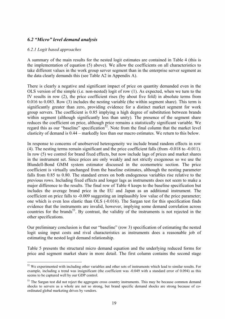
6.2.1 Logit based approaches A summary of the main results for the nested logit estimates are contained in Table 4 (this is the implementation of equation (5) above). We allow the coefficients on all characteristics to take different values in the work group server segment than in the enterprise server segment as the data clearly demands this (see Table A2 in Appendix A). There is clearly a negative and significant impact of price on quantity demanded even in the OLS version of the simple (i.e. non-nested) logit of row (1). As expected, when we turn to the IV results in row (2), the price coefficient rises (by about five fold) in absolute terms from 0.016 to 0.083. Row (3) includes the nesting variable (the within segment share). This term is significantly greater than zero, providing evidence for a distinct market segment for work group servers. The coefficient is 0.85 implying a high degree of substitution between brands within segment (although significantly less than unity). The presence of the segment share reduces the coefficient on price, although price remains a statistically significant variable. We regard this as our “baseline” specification52. Note from the final column that the market level elasticity of demand is 0.44 – markedly less than our macro estimates. We return to this below. In response to concerns of unobserved heterogeneity we include brand random effects in row (4). The nesting terms remain significant and the price coefficient falls (from -0.018 to -0.011). In row (5) we control for brand fixed effects, but now include lags of prices and market shares in the instrument set. Since prices are only weakly and not strictly exogenous so we use the Blundell-Bond GMM system estimator discussed in the econometric section. The price coefficient is virtually unchanged from the baseline estimates, although the nesting parameter falls from 0.85 to 0.80. The standard errors on both endogenous variables rise relative to the previous rows. Including fixed effects and longer lags as instruments does not seem to make a major difference to the results. The final row of Table 4 keeps to the baseline specification but includes the average brand price in the EU and Japan as an additional instrument. The coefficient on price falls to -0.009 suggesting an implausibly low value of the price parameter; one which is even less elastic than OLS (-0.016). The Sargan test for this specification finds evidence that the instruments are invalid, however, implying some demand correlation across countries for the brands53. By contrast, the validity of the instruments is not rejected in the other specifications. Our preliminary conclusion is that our “baseline” (row 3) specification of estimating the nested logit using input costs and rival characteristics as instruments does a reasonable job of estimating the nested logit demand relationship. Table 5 presents the structural micro demand equation and the underlying reduced forms for price and segment market share in more detail. The first column contains the second stage

52 We experimented with including other variables and other sets of instruments which lead to similar results. For example, including a trend was insignificant (the coefficient was -0.049 with a standard error of 0.094) as this seems to be captured well by our GDP control. 53 The Sargan test did not reject the aggregate cross country instruments. This may be because common demand shocks to servers as a whole are not so strong, but brand specific demand shocks are strong because of co-ordinated global marketing drives by vendors.

19

demand equation and the other columns present the first-stage reduced forms. The specification is the same as row 3 in table 4. Notice that across all three equations own memory and own clock speed is statistically significant and important control variables (they are associated with higher model price and market share, other things equal). The reduced forms show that rival memory reduces own prices and own market share as we would expect. The number of products in the segment is associated with lower share and lower prices. By contrast a larger number of a vendors’ own products in the work group segment increases price (presumably through a multi-product pricing effect) but lowers own share (possibly through a cannibalisation effect). Higher input costs also have a significantly positive impact on own prices54. So, overall our instruments are not only valid, but have power in the reduced forms The model level elasticities have an unweighted mean of 5.9 (see Table A3 for their distribution across vendors). But the market level elasticities are of most interest and these are given in the final column of Table 4. The estimates on our preferred nested logit IV results range between 0.25 and 0.4455. These are lower than the “macro” elasticities and suggest substantial upwards bias from estimates that rely on aggregated data. Using OLS (row 1) or the invalid “other country” instruments of row 6 leads to even lower estimated elasticities (the highest elasticity in the table is the simple IV logit: 0.72). We conducted many other experiments to see if the econometric method was underestimating the elasticity: none of these changed the qualitative results56. 6.2.2 Distance Metric Approach As an alternative micro based model we experimented with the “distance metric” approach described in sub-section 3.2. These are reported in Table 6. Column (1) includes the standard variables and own brand price (which is negative and significant). Column (2) includes the prices of other brands weighted by the “distance metric” using memory as the key variable (the further away is the other brand in “memory space”, the lower is the weight given to the price of the rival brand). This is positive and significant, as expected, implying important substitution effects among brands of work group servers. The instruments are significant in the reduced forms for own price and distance weighted rival price at the 1% level57. The third column includes the simple average price in the segment, which is also positive but individually insignificant (the two rival price variables being jointly significant at the 5% level). Finally column (4) includes the price in the enterprise server segment. This is entirely insignificant, indicating the low substitutability between the two types of server and supporting the evidence of a separate market between work group and enterprise servers. 54 The enterprise server equation was not so well behaved (see Table A2). There is a significant impact of price in the OLS but this becomes insignificant when instrumented in row 2 (although still larger in magnitude and correctly signed). When the nesting term is included is the third and fourth rows it is significant and very similar in magnitude to that of the work group server equation. The price term remains insignificant, however. The poorer performance of the enterprise equations seems due to the greater difficulty of finding adequate brand level instruments. 55 Note that using a lower potential market factor of τ = 2 leads to even lower estimates of the elasticity of demand (e.g. 0.412 in row 3, 0.232 in row 4 and 0.336 in row 5). 56 For example: (1) choosing alternative instrument sets based on other characteristics, (2) including an extra nest based on the operating system type, (3) allowing coefficients to vary over time. 57 In the reduced form for price the F(7,2407)=8.16 and in the reduced form for (distance weighted) rival price the F(7,2407) = 15.72.

20

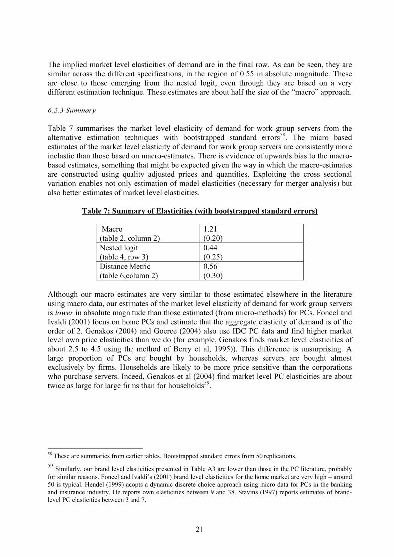
The implied market level elasticities of demand are in the final row. As can be seen, they are similar across the different specifications, in the region of 0.55 in absolute magnitude. These are close to those emerging from the nested logit, even through they are based on a very different estimation technique. These estimates are about half the size of the “macro” approach. 6.2.3 Summary Table 7 summarises the market level elasticity of demand for work group servers from the alternative estimation techniques with bootstrapped standard errors58. The micro based estimates of the market level elasticity of demand for work group servers are consistently more inelastic than those based on macro-estimates. There is evidence of upwards bias to the macro-based estimates, something that might be expected given the way in which the macro-estimates are constructed using quality adjusted prices and quantities. Exploiting the cross sectional variation enables not only estimation of model elasticities (necessary for merger analysis) but also better estimates of market level elasticities.

Table 7: Summary of Elasticities (with bootstrapped standard errors)

Macro (table 2, column 2)

1.21 (0.20)

Nested logit (table 4, row 3)

0.44 (0.25)

Distance Metric (table 6,column 2)

0.56 (0.30)

Although our macro estimates are very similar to those estimated elsewhere in the literature using macro data, our estimates of the market level elasticity of demand for work group servers is lower in absolute magnitude than those estimated (from micro-methods) for PCs. Foncel and Ivaldi (2001) focus on home PCs and estimate that the aggregate elasticity of demand is of the order of 2. Genakos (2004) and Goeree (2004) also use IDC PC data and find higher market level own price elasticities than we do (for example, Genakos finds market level elasticities of about 2.5 to 4.5 using the method of Berry et al, 1995)). This difference is unsurprising. A large proportion of PCs are bought by households, whereas servers are bought almost exclusively by firms. Households are likely to be more price sensitive than the corporations who purchase servers. Indeed, Genakos et al (2004) find market level PC elasticities are about twice as large for large firms than for households59.

58 These are summaries from earlier tables. Bootstrapped standard errors from 50 replications. 59 Similarly, our brand level elasticities presented in Table A3 are lower than those in the PC literature, probably for similar reasons. Foncel and Ivaldi’s (2001) brand level elasticities for the home market are very high – around 50 is typical. Hendel (1999) adopts a dynamic discrete choice approach using micro data for PCs in the banking and insurance industry. He reports own elasticities between 9 and 38. Stavins (1997) reports estimates of brand-level PC elasticities between 3 and 7.

21

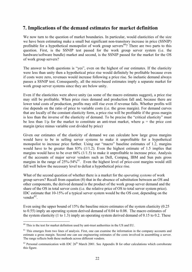
7. Implications of the demand estimates for market definition

We now turn to the question of market boundaries. In particular, would elasticities of the size we have been estimating make a small but significant non-transitory increase in price (SSNIP) profitable for a hypothetical monopolist of work group servers60? There are two parts to this question. First, is the SSNIP test passed for the work group server system (i.e. the hardware/software bundle) market and second, is the SSNIP passed for the market for the OS of work group servers? The answer to both questions is “yes”, even on the highest of our estimates. If the elasticity were less than unity then a hypothetical price rise would definitely be profitable because even if costs were zero, revenues would increase following a price rise. So inelastic demand always passes a SSNIP test. Consequently, all the micro-based estimates imply a separate market for work group server systems since they are below unity. Even if the elasticities were above unity (as some of the macro estimates suggest), a price rise may still be profitable. When price rises demand and production fall and, because there are lower total costs of production, profits may still rise even if revenue falls. Whether profits will rise depends on the ratio of price to variable costs (i.e. the gross margin). For demand curves that are locally of the constant elasticity form, a price rise will be profitable if the gross margin is less than the inverse of the elasticity of demand. To be precise the “critical elasticity” must be less than 1/µ for the market to constitute an anti-trust market, where µ = the price cost margin (price minus variable cost divided by price). Given our estimates of the elasticity of demand we can calculate how large gross margins would have to be in selling server systems to make it unprofitable for a hypothetical monopolist to increase price further. Using our “macro” baseline estimates of 1.2, margins would have to be greater than 83% (1/1.2). Even the highest estimate of 1.5 implies that margins would have to be over 66% (1/1.5) to make it unprofitable to increase price. Analysis of the accounts of major server vendors such as Dell, Compaq, IBM and Sun puts gross margins in the range of 25%-54%61. Even the highest level of price-cost margins would still fall well below the necessary level to defeat a hypothetical price rise. What of the second question of whether there is a market for the operating systems of work group servers? Recall from equation (8) that in the absence of substitution between an OS and other components, the derived demand is the product of the work group server demand and the share of the OS in total server costs (i.e. the relative price of OS to total server system price). IDC estimate that 10-15% of a typical server system would be the OS cost, depending on the vendor62. Even using the upper bound of 15% the baseline micro estimates of the system elasticity (0.25 to 0.55) imply an operating system derived demand of 0.04 to 0.08. The macro estimates of the system elasticity (1 to 1.3) imply an operating system derived demand of 0.15 to 0.2. These 60 This is the test for market definition used by anti-trust authorities in the US and EU. 61 This emerges from two lines of analysis. First, one can examine the information in the company accounts and estimate a gross margin. Second one can use engineering estimates of the costs involved in assembling a server. The range reflects both these methods across different vendors. 62 Personal communication with IDC 26th March 2001. See Appendix B for other calculations which corroborate this figure.

22

are very inelastic demand elasticities that clearly imply a distinct market for the operating systems of work group servers. The main caveat to this conclusion would be if it were easy for firms to substitute enterprise level OS in work group level OS. There are likely to be barriers to doing this, at least between Microsoft's Windows OS (which are pre-dominant in the work group level – see Figure 1) and enterprise level OS that are predominantly UNIX-based. This is because of the interoperability limitations between the two types of software that appear to have become progressively worse over time, particularly with Windows 2000. The European Commission (2004), for example, has argued that Microsoft does not disclose critical extensions to its interfaces and protocols in its file systems (CIFs), its security system (Kerberos), and its directory service (Active Directory). These are detailed in European Commission (2004)63. To fully empirically investigate the interoperability issue is outside the scope of the current paper, but it is an important topic for future work (Genakos et al, 2004). In summary, we believe that the evidence points towards a distinct anti-trust market for both work group server systems and the operating systems of work group servers. 8. Conclusions This paper has examined the market for work group servers. Servers are a large and growing part of the knowledge economy, yet have received little attention from empirical economists despite their importance for contemporary anti-trust policies, the US “productivity miracle” and the welfare effects of information technology. Our main findings are easily summarised. First, we have quantified the fall in the quality- adjusted prices of servers over the 1996-2001 period: these have been dramatic. Second, we have generated estimates of the demand elasticities of work group servers finding much larger magnitudes from an approach based on macro data (1.1 to 1.3) compared approaches based on the “micro” data (0.25 to 0.55). This is important, as many of the existing conclusions on welfare and anti-trust have relied on estimates based on the macro-data. Nevertheless, even if we use the higher macro-based estimates, there appears to be a distinct anti-trust market for work group servers and their operating systems. This does not, of course, mean that firms with high shares of these markets are necessarily harming consumer welfare. But is does mean that the actions of such firms will come under greater anti-trust scrutiny than it would if work group servers were part of a wider market for all servers or for all forms of computing. There are many directions in which this research needs to be extended. The next logical step would be to focus in more detail in retrieving model-level elasticities by more sophisticated logit-based methods than the nested logit that have been the focus of the current work. A second extension would be to investigate in more detail the welfare implications of the price reductions and new good introduction in the server market. Third, empirical tests of innovation and the economic incentives to degrade interoperability need to be developed. Genakos et al (2004) have developed theoretical models that are being combined with the data from the server and PC market. Finally, we need to consider more carefully the investment side of the dynamic issues in greater detail (e.g. Ito, 1997) especially the role of entry and exit. All these areas are being pursued. 63 There are many good sources in the trade press. For example: “Microsoft Keberos Shuck and Jive” by Dominic Hill in The Industry Standard (May 11, 2000) or Charles Babcock “Keberos Made to Heel to Windows 2000” in Inter@active Week (Feb 28, 2000).

23

Table 1: Example of Hedonic Regression Work Group servers, USA, 2000Q1-Q2

Dependent variable: log(quarterly model price)

Variable Coefficient Standard error 2000Q2 dummy -0.069 0.036 Log(Main memory in MB) 0.359 0.024 Log(Clock speed in MHZ) 0.159 0.028 Log(internal storage in GB) 0.072 0.021 Server is rack-optimised 0.972 0.065 Log(Number of racks) 1.183 0.066 RISC Chip 1.101 0.103 Symmetric multiprocessing 0.470 0.074 Operating systems Windows .158 0.057 Netware -0.001 0.053 UNIX 0.177 0.058 Linux -0.162 0.055 OS390/OS400 -0.180 0.148 VMS 0.554 0.196 Selected Vendors Compaq 0.277 0.089 Dell 0.179 0.083 Fujitsu/Siemens 0.398 0.133 IBM 0.206 0.086 HP 0.366 0.075 Sun -0.352 0.178 No. observations 1067 Adjusted R-squared .58

NOTES: This is an example of one of the 120 quarterly hedonic price regressions. The base for Operating Systems and vendors is “other”

24

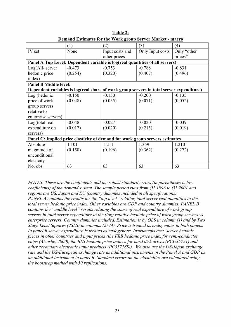
Table 2: Demand Estimates for the Work group Server Market - macro

(1) (2) (3) (4) IV set None Input costs and

other prices Only Input costs Only “other

prices” Panel A Top Level: Dependent variable is log(real quantities of all servers) Log(All- server hedonic price index)

-0.473 (0.254)

-0.753 (0.320)

-0.788 (0.407)

-0.831 (0.496)

Panel B Middle level: Dependent variables is log(real share of work group servers in total server expenditure) Log (hedonic price of work group servers relative to enterprise servers)

-0.150 (0.048)

-0.150 (0.055)

-0.200 (0.071)

-0.135 (0.052)

Log(total real expenditure on servers)

-0.048 (0.017)

-0.027 (0.020)

-0.020 (0.215)

-0.039 (0.019)

Panel C: Implied price elasticity of demand for work group servers estimates Absolute magnitude of unconditional elasticity

1.101 (0.150)

1.211 (0.196)

1.359 (0.362)

1.210 (0.272)

No. obs 63 63 63 63 NOTES: These are the coefficients and the robust standard errors (in parentheses below coefficients) of the demand system. The sample period runs from Q1 1996 to Q1 2001 and regions are US, Japan and EU (country dummies included in all specifications) PANEL A contains the results for the “top level” relating total server real quantities to the total server hedonic price index. Other variables are GDP and country dummies. PANEL B contains the “middle level” results relating the share of real expenditure of work group servers in total server expenditure to the (log) relative hedonic price of work group servers vs. enterprise servers. Country dummies included. Estimation is by OLS in column (1) and by Two Stage Least Squares (2SLS) in columns (2)-(4). Price is treated as endogenous in both panels. In panel B server expenditure is treated as endogenous. Instruments are: server hedonic prices in other countries and input prices (the FRB hedonic price index for semi-conductor chips (Aizorbe, 2000), the BLS hedonic price indices for hard disk drives (PCU35721) and other secondary electronic input products (PC3571SS)). We also use the US-Japan exchange rate and the US-European exchange rate as additional instruments in the Panel A and GDP as an additional instrument in panel B. Standard errors on the elasticities are calculated using the bootstrap method with 50 replications.

25

Table 2A: Diagnostics for Table 2 top level middle level 1 Hausman test; Chi-

Squared(df), p-value 1.58(5) 0.90

3.0(4) 0.56

2 Joint test of all IVs excluded from second stage; F-test (df), p-value

9.97(7,51) 0.001<

36.41(7,51) 0.001<

3 Joint test of selected IVs excluded from second stage; F-test (df), p-value: Input costs only

14.37(3,51) 0.001<

5.61(3,51) 0.002

4 Joint test of selected IVs excluded from second stage; F-test (df), p-value: prices in other regions only

6.21(2,51) .004

12.23(4,51) 0.001

5 Other variables in reduced form

GDP, country dummies

GDP

6 Autocorrelation 0.154 0.314 7 Sargan 0.120 0.350

NOTES: These tests are on the model pooled across countries from Table 2 column (2).

26

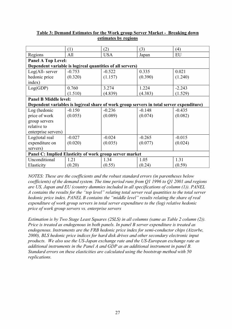
Table 3: Demand Estimates for the Work group Server Market - Breaking down estimates by regions

(1) (2) (3) (4) Regions All USA Japan EU Panel A Top Level: Dependent variable is log(real quantities of all servers) Log(All- server hedonic price index)

-0.753 (0.320)

-0.522 (1.157)

0.335 (0.390)

0.021 (1.240)

Log(GDP) 0.760 (1.510)

3.274 (4.839)

1.224 (4.383)

-2.243 (1.529)

Panel B Middle level: Dependent variables is log(real share of work group servers in total server expenditure) Log (hedonic price of work group servers relative to enterprise servers)

-0.150 (0.055)

-0.236 (0.089)

-0.148 (0.074)

-0.435 (0.082)

Log(total real expenditure on servers)

-0.027 (0.020)

-0.024 (0.035)

-0.265 (0.077)

-0.015 (0.024)

Panel C: Implied Elasticity of work group server market Unconditional Elasticity

1.21 (0.20)

1.34 (0.55)

1.05 (0.24)

1.31 (0.59)

NOTES: These are the coefficients and the robust standard errors (in parentheses below coefficients) of the demand system. The time period runs from Q1 1996 to Q1 2001 and regions are US, Japan and EU (country dummies included in all specifications of column (1)). PANEL A contains the results for the “top level” relating total server real quantities to the total server hedonic price index. PANEL B contains the “middle level” results relating the share of real expenditure of work group servers in total server expenditure to the (log) relative hedonic price of work group servers vs. enterprise servers Estimation is by Two Stage Least Squares (2SLS) in all columns (same as Table 2 column (2)). Price is treated as endogenous in both panels. In panel B server expenditure is treated as endogenous. Instruments are the FRB hedonic price index for semi-conductor chips (Aizorbe, 2000), BLS hedonic price indices for hard disk drives and other secondary electronic input products. We also use the US-Japan exchange rate and the US-European exchange rate as additional instruments in the Panel A and GDP as an additional instrument in panel B. Standard errors on these elasticities are calculated using the bootstrap method with 50 replications.

27

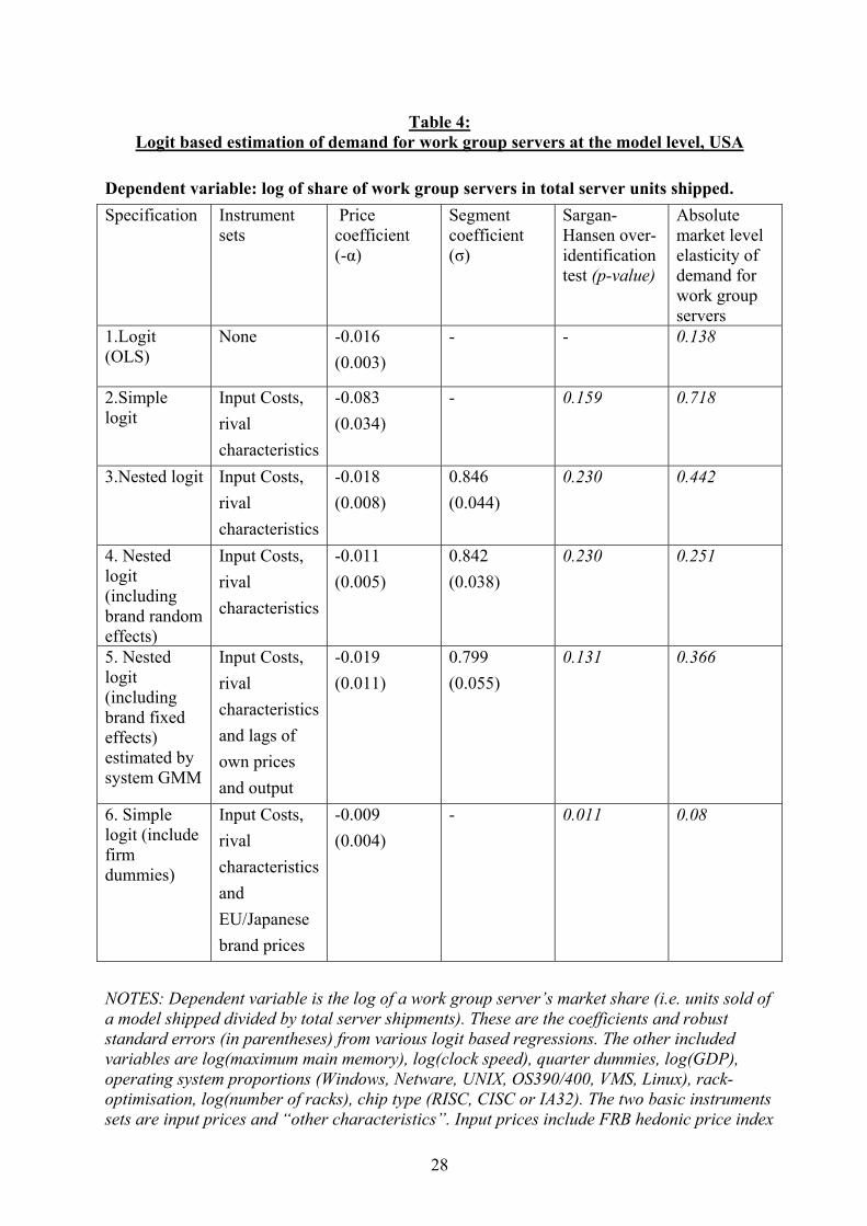
Table 4: Logit based estimation of demand for work group servers at the model level, USA

Dependent variable: log of share of work group servers in total server units shipped. Specification Instrument

sets Price coefficient (-α)

Segment coefficient (σ)

Sargan-Hansen over-identification test (p-value)

Absolute market level elasticity of demand for work group servers

1.Logit (OLS)

None -0.016 (0.003)

- - 0.138

2.Simple logit

Input Costs, rival characteristics

-0.083 (0.034)

- 0.159 0.718

3.Nested logit Input Costs, rival characteristics

-0.018 (0.008)

0.846 (0.044)

0.230 0.442

4. Nested logit (including brand random effects)

Input Costs, rival characteristics

-0.011 (0.005)

0.842 (0.038)

0.230 0.251

5. Nested logit (including brand fixed effects) estimated by system GMM

Input Costs, rival characteristics and lags of own prices and output

-0.019 (0.011)

0.799 (0.055)

0.131 0.366

6. Simple logit (include firm dummies)

Input Costs, rival characteristics and EU/Japanese brand prices

-0.009 (0.004)

- 0.011 0.08

NOTES: Dependent variable is the log of a work group server’s market share (i.e. units sold of a model shipped divided by total server shipments). These are the coefficients and robust standard errors (in parentheses) from various logit based regressions. The other included variables are log(maximum main memory), log(clock speed), quarter dummies, log(GDP), operating system proportions (Windows, Netware, UNIX, OS390/400, VMS, Linux), rack-optimisation, log(number of racks), chip type (RISC, CISC or IA32). The two basic instruments sets are input prices and “other characteristics”. Input prices include FRB hedonic price index

28

for semi-conductor chips (Aizorbe, 2000), BLS hedonic price indices for hard disk drives and other secondary electronic input products. “Other characteristics” include: total number of products, number of vendors’ own products in the work group segment, count of rival memory. Sample is the “Big Six” vendors (Compaq, Dell, HP, IBM, NEC and Sun). There are 1593 observations (we aggregate over operating systems). Row (5) is estimated using the Blundell and Bond (2000) GMM-SYS estimator in DPD. Instruments include lags of market shares and prices. These are lagged levels dated t-2 to t-4 in the first difference equations and the first difference at t-1 in the levels equations. Row (6) includes “other countries’ prices” – the average of the model’s price in Japan and Europe. The final column gives the absolute magnitude of the market level unconditional elasticity of demand for work group servers using a potential market factor of τ = 10.

29

Table 5: Work group Market Share Equation and reduced forms

Structural

demand equation

Reduced Forms

Dependent variable

(1) Share of model in total servers

(2) Share of model in work group segment

(3) Model Price

Model price -0.018 (0.008)

Model’s share in work group segment

0.846 (0.044)

Number of Vendor’s own products in segment

-0.042 (0.012)

0.206 (0.080)

Total number of products

-0.014 (0.009)

-0.019 (0.064)

Rival main memory

0.818a (0.623)

-0.805b (0.431)

Input price 0.149 (0.627)

9.529 (4.319)

Own log(memory)

0.125 (0.063)

0.089 (0.051)

7.795 (0.349)

Own log(speed) 0.078 (0.023)

0.225 (0.090)

0.458 (0.622)

OS dummies(6) Yes Yes Yes Quarter dummies (3)

Yes Yes Yes

Firm dummies (6)

Yes Yes Yes

NOTES: These are the coefficients and robust standard errors (in parentheses) from IV regressions (in column (1) from Table 4 row 3) and OLS in columns (2) and (3). The other included variables are operating system proportions (Windows, Netware, UNIX, OS390/400, VMS, Linux), chip types (RISC, CISC or IA32), whether the server is rack optimised, the number of racks, three input cost variables ( FRB hedonic price index for semi-conductor chips, BLS hedonic price indices for hard disk drives and BLS hedonic price index for other secondary electronic input products), a full set of firm dummies (Compaq/Digital/ Tandem), Dell, HP, IBM (Sequent), NEC, Sun Microsystems), ln(GDP) and quarter dummies. acoefficient multiplied by 1010 bcoefficient multiplied by 108

30

Table 6: Distance Metric Specification of demand for work group servers (1) (2) (3) (4) Own Price -0.127

(0.028) -0.110 (0.030)

-0.137 (0.037)

-0.138 (0.039)

DMP, Distance weighted rival prices (in segment)

1.069a (0.429)

0.839a (0.470)

0.826a (0.049)

Average price in work group server segment

0.099 (0.065)

0.106 (0.113)

Average price in enterprise server segment

0.803 (1.047)

Absolute market level elasticity of demand for work group servers (τ = 10)

0.565

0.562 0.553

a Coefficient and standard error divided by 100 NOTES: Dependent variable is the level of a work group server’s quantity shipped. These are the coefficients and robust standard errors (in parentheses) from various regressions. Distance metric uses the difference in the absolute value of the model’s memory from other brands in the

segment; i.e. DMPi=∑ ≠

−+ijjji

j

MEMMEMp

, ||1. All variables are normalized by their own

mean value. Own price and rival prices always treated as endogenous. The other included variables are log(memory), log(clock speed), quarter dummies, log(GDP), operating system proportions (Windows, Netware, UNIX, OS390/400, VMS, Linux), rack-optimization, log(number of racks), chip type (RISC, CISC or IA32). The instruments sets are input prices “other characteristics” and the distance metric itself (results are robust to exclusion of distance metric from IV set). Input prices include FRB hedonic price index for semi-conductor chips (Aizorbe, 2000), BLS hedonic price indices for hard disk drives and other secondary electronic input products. “Other characteristics” include: total number of products, number of vendors’ own products in the work group segment, count of rival memory. Sample is the “Big Six” vendors (Compaq, Dell, HP, IBM, NEC and Sun).

31

References

Aizorbe, A. (2000) “The FRB Price Index for Semi-computers, 1993-1999” Board of Governors for the Federal Reserve System, December. Berndt, Ernst and Rappaport, Neal (2001) “Price and Quality of Desktop and mobile personal computers: A quarter century historical overview”, American Economic Review, 268-271 Berndt, E., Griliches, Zvi and Rappaport, Neal (1995) “Econometric Estimates of Prices Indexes of Personal computers in the 1990s” Journal of Econometrics, 68:1, 243-268 Berry, Stephen (1994) “Estimating discrete choice models of product differentiation” RAND Journal of Economics, 25, 2, 242-262 Berry, Stephen, Levinsohn, Jim and Pakes, Ariel (1995) “Automobile prices in Market Equilibrium” Econometrica 63, 841-890 Berry, Stephen, Levinsohn, Jim and Pakes, Ariel (2004) “Differentiated Product demand systems from a combination of micro and macro data: The new car market”, Journal of Political Economy, 1, 1,112, 68-105 Blundell, R. and Bond, S. (2000) “Initial Conditions and moment restrictions in dynamic panel data models” Journal of Econometrics, 68, 29-52 Bond, Stephen and Van Reenen, John (2003) "Micro-econometric models of investment and employment" LSE mimeo www.ifs.org/innovation/bondvanr.pdf Bresnahan, Timothy (1986) “Measuring the spillovers from technical advance: Mainframe computers in financial services” American Economic Review, 76, 4, 742-755 Bresnahan, Timothy (1996) Comment on Jerry Hausman (1997) “Valuation of New Goods under perfect and imperfect competition” Chapter 5 in Timothy Bresnahan and Robert Gordon (eds) The Economics of New Goods, Chicago: University of Chicago Press Bresnahan, Timothy and Greenstein, Shane (1996) “Technical Progress and Co-invention in computing and in the uses of computers” Brooking Papers on Economic Activity: Microeconomics, 1-78 Bresnahan, Timothy, Stern, Scott and Trajtenberg, Manuel (1997) “Market segmentation and the sources of rents from innovation: personal computers in the late 1980s” RAND Journal of Economics 28, 0, S17-S44 Bresnahan, Timothy, Brynjolfson, Erik and Lauren Hitt (2002) "Information Technology, Workplace Organization and the Demand for Skilled Labor: Firm Level Evidence", NBER Working Paper N° 7136, Quarterly Journal of Economics Brynjolfson, Erik (1996) ”The contribution of information technology to consumer welfare” Informations Systems Research, 7, 3, 281-300.

32

Brynjolfson, Erik (1997) Comment on Greenstein, Shane “From Superminis to Supercomputers: Estimating Surplus in the Computing market” Chapter 8 in Timothy Bresnahan and Robert Gordon (eds) The Economics of New Goods, Chicago: University of Chicago Press Carlton, D. and Waldman (2002) “The strategic choice of tying to preserve and create market power” RAND Journal of Economics, 33, 2, 194-220 Chow, Gregory (1967) “Technological Change and the Demand for Computers” American Economic Review, 57, 1117-1130 Davis, Peter, Huse, Christian and Van Reenen, John (In process) “Random coefficient demand estimation for servers”, LSE mimeo Deaton, Angus and Muellbauer, John (1980) “An Almost Ideal Demand System” American Economic Review, 70, 312-326 Ekeland, I., Heckman, J. and Nesheim, L. (2004) “Identification and estimation of hedonic models” Journal of Political Economy, 1, 2, 112, S360-S109 European Commission (2004) Judgment on European Commission vs. Microsoft, Brussels, 24th March 2004. Foncel, J. and Ivaldi, M. (2001) “Operating System Prices in the Home PC market” mimeo Institut D’Economie Industrielle, May. Genakos, C., Kuhn, K. and Van Reenen, J. (2004) “The incentive to degrade interoperability: Theory and Evidence” LSE mimeo Genakos, C. (2004) “Differential Merger Effects: The case of Personal Computers”, mimeo London Business School Goeree, M. (2004) “Advertising in the US PC Industry”, mimeo University of Amsterdam Goldberger, A. (1968) “The interpretation and estimation of Cobb Douglas Production Fucntions” Econometrica, 35, 464-472 Gordon, Robert (2001) “Does the New Economy measure up to the great inventions of the past?” Journal of Economic Perspectives, 14, 4, 48-74 Gordon, Robert (2002) “Technology and Economic Performance in the American Economy” in Richard Nelson, Benn Steil, and David Victor (eds) Innovation and Economic Performance Gorman, Terrance (1970) “Two Stage Budgeting”, mimeo University of North Carolina reprinted in C. Blackorby and A. F. Shorrocks (eds) Separability and Aggregation Volume I: The Collected Works of Terrance Gorman, Oxford: Oxford University Press Greenstein, Shane (1997) “From Superminis to Supercomputers: Estimating Surplus in the Computing market” Chapter 8 in Timothy Bresnahan and Robert Gordon (eds) The Economics of New Goods, Chicago: University of Chicago Press

33

Hausman, Jerry and Wise, David (1984) “Social Experimentation, truncated distributions and efficient estimation” Econometrica, 45, 919-938 Hausman, Jerry, Leonard, Gregory and Zona, Douglas (1994) “competitive analysis with Differentiated Products” Annales d’Economie et de Statistique, 34, 159-180 Hausman, Jerry (1997) “Valuation of New Goods under perfect and imperfect competition” Chapter 5 in Timothy Bresnahan and Robert Gordon (eds) The Economics of New Goods, Chicago: University of Chicago Press Heckman, James (1979) “Sample selection bias as a specification error” Econometrica, 47, 153-161 Hendel, Igal (1999) “Estimating Multiple discrete choice models: an application to computerization returns” Review of Economic Studies, 66(2), 227, 423-446 Henderson, D.H. (1922) Supply and Demand. London: Nisbet Holdway, Michael (2000) “Quality adjusted computer prices in a producer price: an overview” www.stats.bls.gov/ppicomqa.htm International Data Corporation (1998) "IDC's Server Market Methodology, Database Structure, and Definitions", IDC report #15909R, April 1998 International Data Corporation (2000a) "Server Operating Environments Market Forecast and Analysis, 2000-2004", IDC report #22347, June 2000 International Data Corporation (2000b) "Server Market Forecast and Analysis, 1996-2004", IDC report #22538, July 2000, pp.11-14 Ito, Harumi (1997) “The Structure of Adjustment costs in mainframe computing investment”, mimeo, Brown University. Ivaldi, M. and Verboven, F. (2001) “Quantifying the effects of horizontal mergers in European Competition Policy” Centre for Economic Policy Research Discussion Paper No. 2697 McFadden, Daniel (1981) “Econometric Models of Probabilistic Choice” in Charles Manski and Dan McFadden (eds) Structural Analysis of Discrete Data with Econometric Applications, Cambridge Mass: MIT Press Nevo, Aviv (2002) “Measuring Market Power in the Ready to Eat Cereal Industry” Econometrica, 69, 307-342 Pakes, A. (2003) “A Reconsideration of hedonic price indices with an application to PCs” American Economic Review, 93, 5, 1578-1596 Pesaran, M. H. and Smith, R. (1994) “A Generalised R2 criterion for Regression Models estimated by the instrumental variable method” Econometrica, 62, 705-710

34

Petrin, A (2002) “Quantifying the benefits of new products: The case of the Minivan”, Journal of Political Economy, 11, 705-729 Pinkse, J., Slade, M. and Brett, C. (2002) “Spatial Price Competition: A Semi-parametric approach” Econometrica, 70: 1111-1155 Reddy, Bernard, Evans, David, and Nichols, Albert (1999) “Why does Microsoft Charge so little for Windows?” NERA January 7th Reddy, Bernard, Evans, David, Nichols, Albert and Schmalensee, Richard (2001) “A Monopolist would still charge more for Windows: A Comment on Werden” Review of Industrial Organization, 18, 263-268 Rosen, S. (1974) “Hedonic Prices and Implicit Markets: Product Differentiation in Pure Competition” Journal of Political Economy, 82, 34-55 Schmalensee, Richard (2000) “Anti-trust issues in Schumpeterian Industries” American Economic Review, 90, 192-196 Slade, M. (2004) “Market Power and Joint Dominance in UK Brewing” Journal of Industrial Economics, LII, 1, 133-164 Staiger, D. and Stock, J.H. (1997) “Instrumental Variable estimation with weak instruments” Econometrica, 65, 557-586 Sybex (2001) Networking Complete, San Francisco: Sybex Stavins, J. (1997) “Estimating Demand elasticities in a differentiated product industry: The Personal Computer market” Journal of Economics and Business, 49, 347-367 Stone, Richard (1954) “Linear expenditure Systems and demand analysis: an application to the pattern of British Demand” Economic Journal, 64, 511-27 Triplett, Jack (1989) “Price and technological change in a capital good: A survey of research in computers” Chapter 4 in Dale Jorgenson and Ralph Landau Technology and Capital Formation Cambridge MA: MIT Press, 127-213 United States Courts of Appeal (2001) United States vs. Microsoft Corporation, No. 00-4212 Van Reenen, John (2004) “Hedonic Prices for Network Servers”, mimeo, London School of Economics Verboven, Frank (1996) “International Price Discrimination in the European Car market” Rand Journal of Economics, 27, 240-268 Werden, Gregory (2001) “Microsoft’s pricing of Windows and the economics of derived demand monopoly” Review of Industrial Organization, 18, 257-262 Werden, Gregory and Froeb, L. (1994) “The Effects of Mergers in Differentiated Products Industries: Logit demand and merger policy” Journal of Law and Economics, 10

35

White (1980) “A heteroskedastic-consistent covariance matrix estimator and a direct test for heteroskedacity” Econometrica, 48, 817-838

36

Figure 1: Shares of the work group server operating systems, Q1 1996 – Q4 2001

0%

10%

20%

30%

40%

50%

60%

70%

1996

Q1

1996

Q3

1997

Q1

1997

Q3

1998

Q1

1998

Q3

1999

Q1

1999

Q3

2000

Q1

2000

Q3

2001

Q1

2001

Q3

Win/NT

Unix

Netw are

Linux

Other

NOTES: Worldwide unit market shares. Work group servers defined as systems that entered at a price point of under $100,000

SOURCE: IDC Quarterly Server Tracker

37

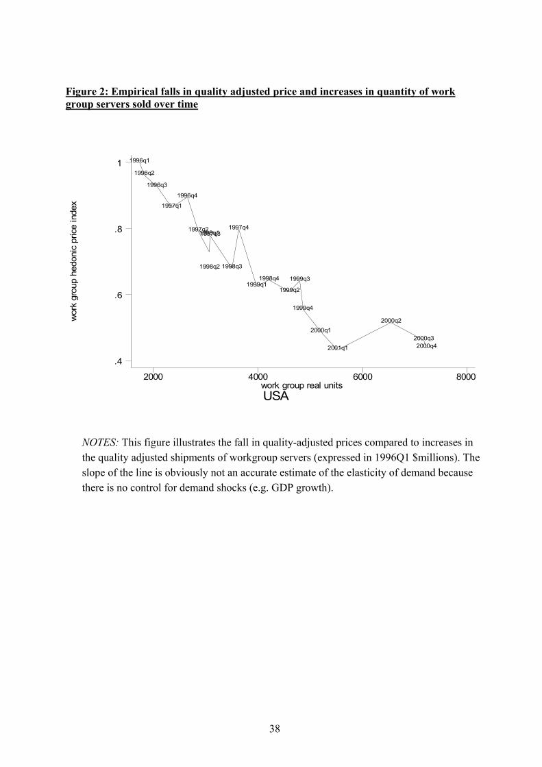
Figure 2: Empirical falls in quality adjusted price and increases in quantity of work group servers sold over time

wor

k gr

oup

hedo

nic

pric

e in

dex

USAwork group real units

2000 4000 6000 8000

.4

.6

.8

1 1996q1

1996q2

1996q3

1997q1

1996q4

1997q21998q1

1998q2

1997q3

1998q3

1997q4

1999q11998q4

1999q2

1999q3

1999q4

2000q1

2001q1

2000q2

2000q32000q4

NOTES: This figure illustrates the fall in quality-adjusted prices compared to increases in the quality adjusted shipments of workgroup servers (expressed in 1996Q1 $millions). The slope of the line is obviously not an accurate estimate of the elasticity of demand because there is no control for demand shocks (e.g. GDP growth).

38

39

Figure 3: Multi-level Model

Total expenditure on ICT equipment Total server expenditure other expenditure TOP LEVEL Work group server Enterprise servers MIDDLE LEVEL Brands/models SUN IBM HP COMPAQ … SUN IBM HP… BOTTOM LEVEL

Appendices to “Is there a market for work group servers”

by John Van Reenen

Appendix A: Some Additional Robustness Tests

We report here some additional findings and robustness tests. We subjected the “macro” estimates in Tables 2 and 3 to a large number of additional tests. Since the main issue of interest is the size of the demand elasticity we detail how the size of this elasticity changes in different experiments. In Table A1, row (1) simply reproduces the unconditional elasticity of demand from the main results to compare with the experiments. Some of the identification for our results arises from the secular downward trend in the hedonic price of servers so row (2) simply adds a trend variable to the regressions “switching off” this useful source of variation. There is a fall in the size of the elasticity in the US and pooled results but overall the elasticities are similar to the baseline in row (1). Row (3) uses the log-log formulation in the middle level instead of the Linearized AIDS functional form (equation (3) in sub-section 3.1). Some researchers prefer this functional form (e.g. Hausman et al, 1994). Row (4) uses an alternative approach to quality-adjust prices. We follow the so-called “matched model” approach that involves examining the evolution of prices for identical models over time (see Triplett, 1989). Since model characteristics do not change much over time this should control for quality more rigorously than the hedonic regression method. Hedonic regressions have the problem that we may not have fully controlled for all the relevant quality characteristics. One problem with the matched model method is that it ignores the first year in which a model was born (there is no pre-entry data to match with a new model) and so will suffer from a “new goods” bias1. It also suffers from a bias because the models who exit would have had the largest falls in prices as they were made obsolete2. We can see in row (4) that this alternative price index leads to lower elasticity in Japan but quite similar results elsewhere. In order to preserve degrees of freedom our basic model is static. In row (5) we allow a more general dynamic form of the model by including lags of all the variables on the right hand side of the regressions and including a lagged dependent variable3. We then use the coefficients to calculate the long-run effects. This leads to the lowest estimated elasticities in the table (0.6 in the USA and EU). Finally we re-analysed the data using a restricted set of server characteristics that enables us estimate the hedonic price regressions on the full IDC sample

1 This is why in the US the BLS and other statistical agencies that historically have used matched model approaches are switching to use more hedonic-based approaches. We partially deal with the new goods problem by following Triplett (1989) and using a so-called “composite” index. This uses hedonic prices in the first quarter a model appears and then uses the matched model approach for the rest of the model’s life. We use a chain-weighted Laspeyres form of the price index, weighting by revenue shares in the previous period, but updating the shares in every period. 2 This is emphasised by Pakes (2003) and found empirically in the server market by Van Reenen (2004). 3 So in the middle level regressions the additional right hand side variables are: lagged work group shares, lagged relative prices and lagged real total server expenditure. In the top level regressions the additional variables on the right hand side are: lagged total server price index, lagged GDP, lagged GDP deflator and lagged total server quantity sold. The long run effects are the sum of the coefficients on the current and first lag of the price terms divided by unity minus the coefficient on the lagged dependent variable.

1

(recall that 20% of sales could not be matched to memory and speed information). Again, this makes little difference to the results. Looking over the large number of experiments in Table A1 as a whole, the estimates of the unconditional demand elasticity varies between 0.6 and 1.5. Our baseline estimate of an elasticity of 1.2 is in the middle of this range. Table A2 presents nested logit results for enterprise servers. There is a significant impact of price in the OLS but this becomes insignificant when instrumented in row 2 (although still larger in magnitude and correctly signed). When the nesting term is included is the third row it is significant and slightly larger in magnitude than that of the work group server equation. The price term remains insignificant, however. The poorer performance of the enterprise equations seems due to the greater difficulty of finding adequate brand level instruments4. It may also reflect some further quality characteristics at the high end of the server market that that we have not adequately controlled for. Table A3 also reports some distributions of model level own price elasticities from the nested logit results of Table 4. The weighted mean is 3 and the unweighted mean is 5.9 (this is because the more numerous lower priced servers have lower elasticities – see equation (A18) in Appendix C). Looking across the different vendors, models sold by NEC seem to have the lowest elasticities and models sold by IBM the highest.

4 “Other characteristics” are jointly significant in the reduced form for the nesting share (p-value of 0.028) but insignificant in the reduced form for price (p-value 0.347).

2

Table A1: Robustness of the results to alternative ways of estimating the unconditional elasticity of demand for work group servers

Experiment All USA Japan Europe 1 Basic Results (from

Table 3 panel C) 1.21 (0.20)

1.34 (0.55)

1.05 (0.24)

1.31 (0.59)

2 Adding a time trend to the middle and top equations

1.0 0.98 1.1 1.38

3 Log-log in middle level instead of L-AIDS (3SLS with Slutsky Symmetry imposed but not homogeneity)

1.32 1.05 1.14 1.36

4 Using a “matched model” price index instead of a hedonic price index

1.1 1.5 0.8 1.1

5 Allowing a more general dynamic form in middle and top level (i.e. include the first lag of all variables, including the lagged dependent variable, on the right hand side of the equation). Long-run elasticities reported

1.1 0.6 1.08 0.6

6 restricted server characteristics on larger sample

1.2 1.3 0.98 0.94

NOTES: These are the unconditional price elasticity of demands for work group servers. They are derived from estimation of the system of equations is precisely the same way as reported in the main results in Tables 2 and 3.

3

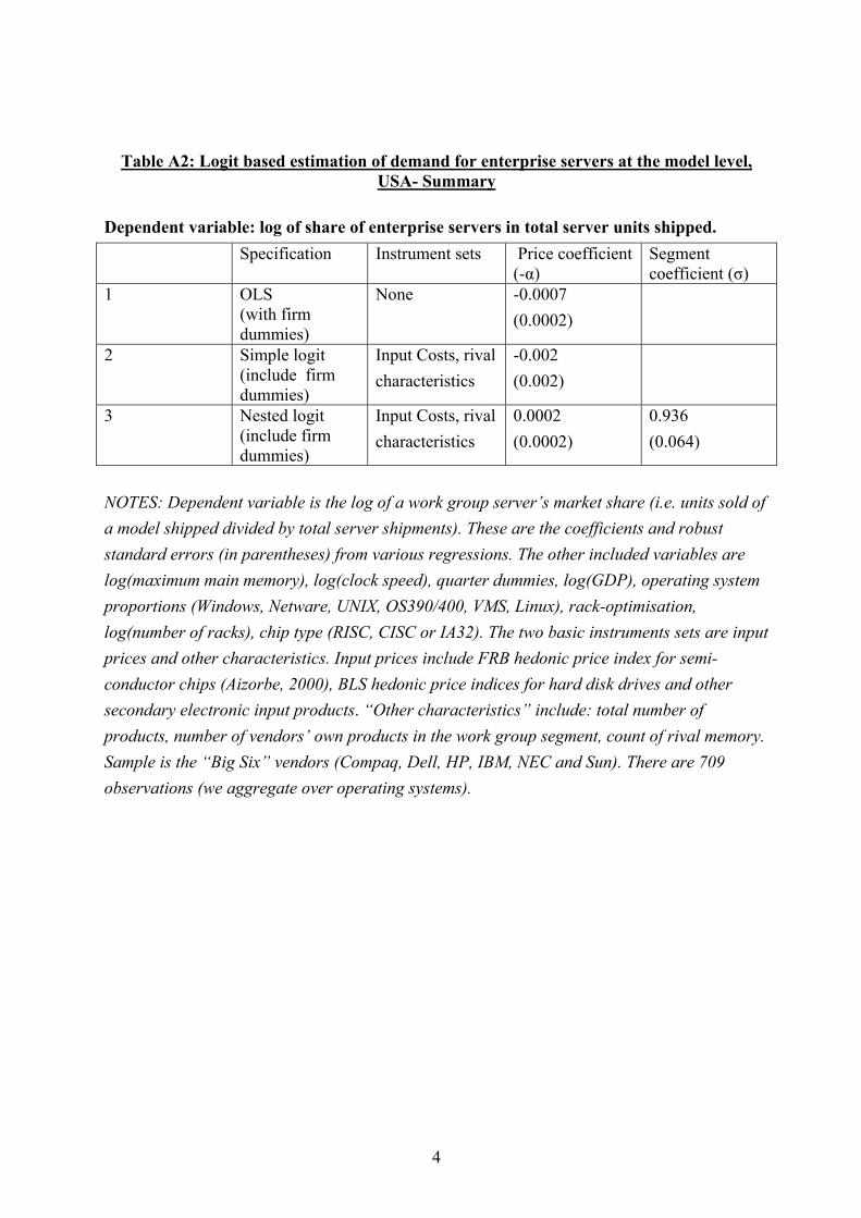
Table A2: Logit based estimation of demand for enterprise servers at the model level, USA- Summary

Dependent variable: log of share of enterprise servers in total server units shipped. Specification Instrument sets Price coefficient

(-α) Segment coefficient (σ)

1 OLS (with firm dummies)

None -0.0007 (0.0002)

2 Simple logit (include firm dummies)

Input Costs, rival characteristics

-0.002 (0.002)

3 Nested logit (include firm dummies)

Input Costs, rival characteristics

0.0002 (0.0002)

0.936 (0.064)

NOTES: Dependent variable is the log of a work group server’s market share (i.e. units sold of a model shipped divided by total server shipments). These are the coefficients and robust standard errors (in parentheses) from various regressions. The other included variables are log(maximum main memory), log(clock speed), quarter dummies, log(GDP), operating system proportions (Windows, Netware, UNIX, OS390/400, VMS, Linux), rack-optimisation, log(number of racks), chip type (RISC, CISC or IA32). The two basic instruments sets are input prices and other characteristics. Input prices include FRB hedonic price index for semi-conductor chips (Aizorbe, 2000), BLS hedonic price indices for hard disk drives and other secondary electronic input products. “Other characteristics” include: total number of products, number of vendors’ own products in the work group segment, count of rival memory. Sample is the “Big Six” vendors (Compaq, Dell, HP, IBM, NEC and Sun). There are 709 observations (we aggregate over operating systems).

4

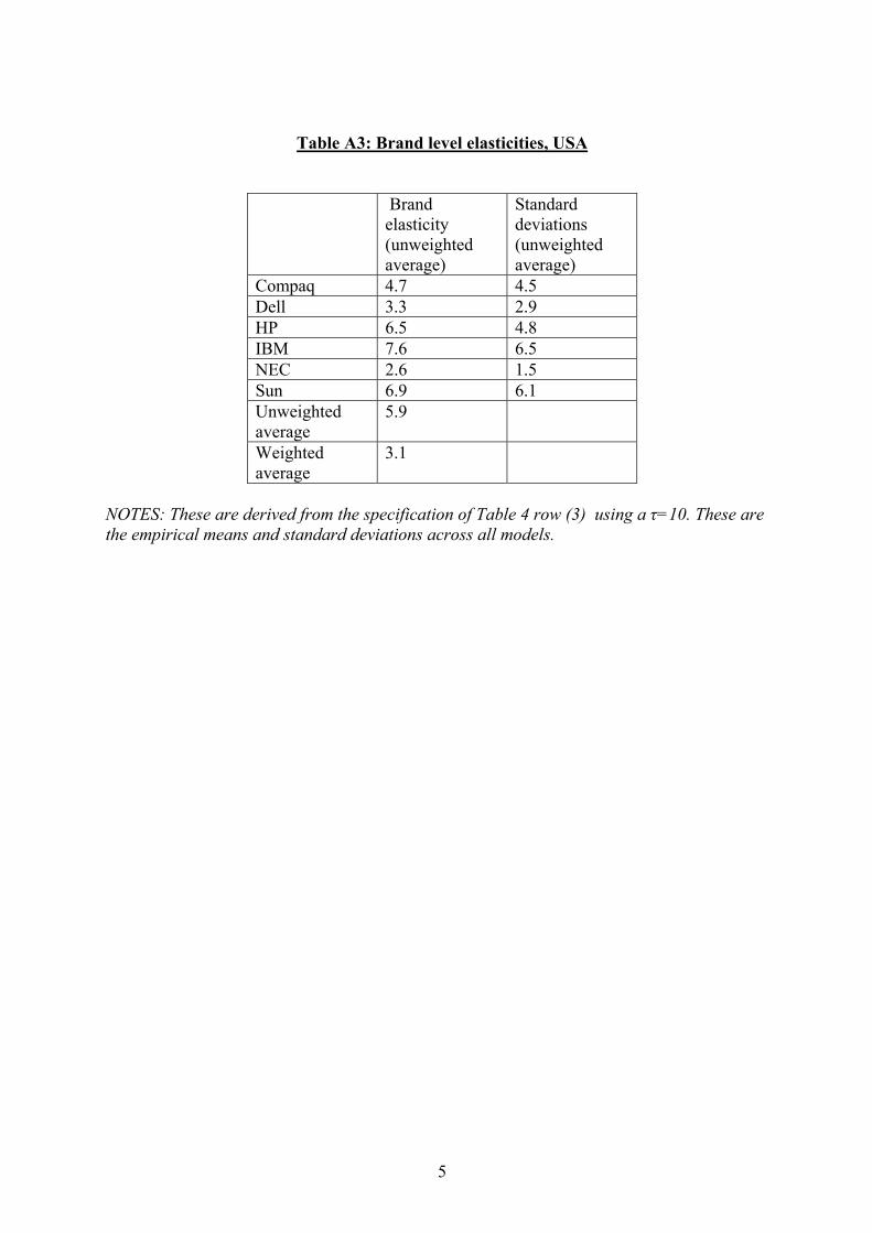
Table A3: Brand level elasticities, USA

Brand elasticity (unweighted average)

Standard deviations (unweighted average)

Compaq 4.7 4.5 Dell 3.3 2.9 HP 6.5 4.8 IBM 7.6 6.5 NEC 2.6 1.5 Sun 6.9 6.1 Unweighted average

5.9

Weighted average

3.1

NOTES: These are derived from the specification of Table 4 row (3) using a τ=10. These are the empirical means and standard deviations across all models.

5

Appendix B: Data

Data Construction International Data Corporation (IDC) produces a “Quarterly Tracker” Database that is derived from directly questioning vendors on their pricing and total revenues of models in all the main regions. Units sold are estimated from the transaction price and revenue data by model. These are then used to calculate global totals and these are cross-checked with head offices for inconsistencies. There are also some customer surveys that are used as a further reality check on prices (see IDC, 1998, for more information on methodology). IDC gives figures for both sales of new model ("initial server shipments", ISS) and major upgrades. An upgrade occurs when the old server is extensively reconfigured (e.g. new processors added) and the name/number of the model is therefore changed by the vendor. 95% of all units in the IDC data are ISS rather than upgrades. Dropping the upgrades and re-estimating solely on ISS data gives similar results to those reported here. Models that were priced above $5m were dropped from the analysis as we considered these 31 machines to be more like mainframes than servers (0.7% of the sample). The IDC data come in current dollars. We first convert all IDC prices into nominal currencies using average OECD exchange rates prevailing over the relevant quarter. Nominal currencies are appropriate for the demand system. Nominal GDP and the GDP deflators were taken from the OECD. As discussed in the text we matched in additional server characteristics from major server vendors: Compaq/Digital/Tandem, Dell, Fujitsu, Hewlett-Packard, IBM, ICL, Siemens and Sun. We used a wide variety of sources to obtain these data including company web-pages (e.g. http://www.compaq.com/products/quickspecs/QuickSpecs_Archives/QuickSpecs_Archives.HTML), back issues of computer magazines and their web pages (e.g. www.pcworld.com) and major resellers (e.g. www.digitalbasics.com). These sources specify the technical characteristics of the different models. We also received help by contacting some of these organisations directly. We collected a wide variety of characteristics, the most informative of which were memory, internal storage and clock/processor speed5. The final dataset covered over 80% of the revenues of all servers. Our primary method of matching was through the model name, but we could also use characteristics common to IDC and the model specification to check the accuracy of the match (e.g. maximum number of processors). Models are sometimes aggregated by IDC across several versions. IDC weights the final characteristics according to importance (i.e. by revenue). Since we did not have revenues by version we considered the minimum version, the median version and the maximum version. The results are given for the characteristics of the median version, but using the minimum or maximum made little difference to the results6. To

5 Other characteristics included cache size on chip, cache size on board, list price, disk capacity in cabinet, maximum external storage, maximum I/O channels per processor, maximum I/O bandwidth. These had less explanatory power in the hedonic regressions than the three variables we focused on. 6 We did our best to identify changes in the server characteristics over time. For example, we used press articles to identify launch dates of new versions (i.e. updates in processor speed and memory) or product withdrawal

6

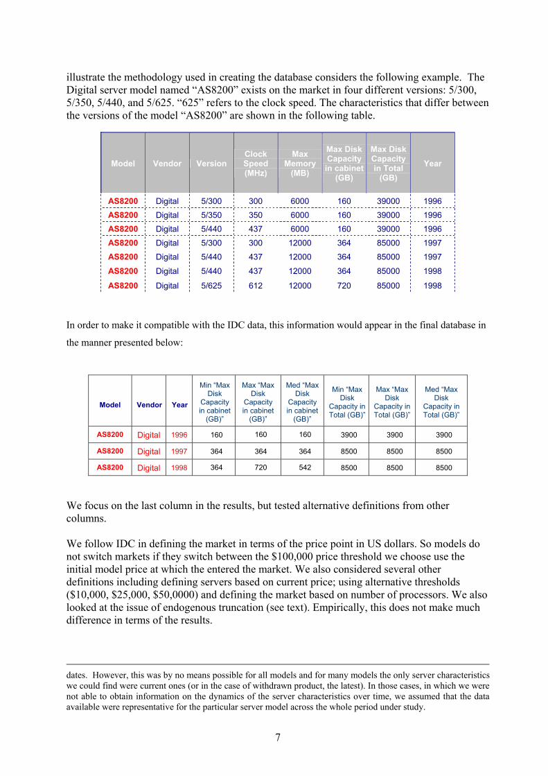
illustrate the methodology used in creating the database considers the following example. The Digital server model named “AS8200” exists on the market in four different versions: 5/300, 5/350, 5/440, and 5/625. “625” refers to the clock speed. The characteristics that differ between the versions of the model “AS8200” are shown in the following table.

Model Vendor Version Clock Speed (MHz)

Max Memory

(MB)

Max Disk Capacity in cabinet

(GB)

Max Disk Capacity in Total

(GB) Year

AS8200 Digital 5/300 300 6000 160 39000 1996

AS8200 Digital 5/350 350 6000 160 39000 1996

AS8200 Digital 5/440 437 6000 160 39000 1996

AS8200 Digital 5/300 300 12000 364 85000 1997

AS8200 Digital 5/440 437 12000 364 85000 1997

AS8200 Digital 5/440 437 12000 364 85000 1998

AS8200 Digital 5/625 612 12000 720 85000 1998

In order to make it compatible with the IDC data, this information would appear in the final database in

the manner presented below:

Model Vendor Year

Min “Max Disk

Capacity in cabinet

(GB)”

Max “Max Disk

Capacity in cabinet

(GB)”

Med “Max Disk

Capacity in cabinet

(GB)”

Min “Max Disk

Capacity in Total (GB)”

Max “Max Disk

Capacity in Total (GB)”

Med “Max Disk

Capacity in Total (GB)”

AS8200 Digital 1996 160 160 160 3900 3900 3900

AS8200 Digital 1997 364 364 364 8500 8500 8500

AS8200 Digital 1998 364 720 542 8500 8500 8500

We focus on the last column in the results, but tested alternative definitions from other columns. We follow IDC in defining the market in terms of the price point in US dollars. So models do not switch markets if they switch between the $100,000 price threshold we choose use the initial model price at which the entered the market. We also considered several other definitions including defining servers based on current price; using alternative thresholds ($10,000, $25,000, $50,0000) and defining the market based on number of processors. We also looked at the issue of endogenous truncation (see text). Empirically, this does not make much difference in terms of the results.

dates. However, this was by no means possible for all models and for many models the only server characteristics we could find were current ones (or in the case of withdrawn product, the latest). In those cases, in which we were not able to obtain information on the dynamics of the server characteristics over time, we assumed that the data available were representative for the particular server model across the whole period under study.

7

Descriptive Statistics A large number of descriptive statistics are given below. Table B1 shows the number of models by quarter used in the hedonic regressions. As noted in the main text there are a similar number of models on sale in the US and the Europe (about 700 by the end of the period) but a smaller number on sale in Japan (about 450). This is a combination of the fact that Japan in a smaller market and, as it well known, import penetration is often more difficult in the Japanese market than in Europe or North America7. Figure B1 shows the evolution of market share of the five largest work group server vendors. Compaq overtook IBM as market leader in the middle of our sample period. HP and Sun are also major players throughout the period. The most dramatic change is the rapid rise of Dell who entered near the start of our sample period and have grown rapidly to be major contenders in the industry (note that Dell have not made much inroad into the enterprise server end of the market). Means of all variables across all quarters are in Table B2 (these are weighted by total units sold in each region). Microsoft is dominant among server OS vendors, particularly in Japan. The US tends to have tends to have higher quality servers, on average, as measured by characteristics (memory, storage, number of CPUs). Work group servers have a lower total share of expenditure in Japan than in the US and Europe. The average price of a server is lowest in the US ($16,000), a bit higher in the EU ($17,000) and significantly higher in Japan ($28,000). Table B3 reports changes over time in the key variables across regions. There have been spectacular gains in the performance and quality of servers over this time period. Maximum memory has increased by a factor of 7.5 in Europe the period 1996-2000, for example. Table B4 displays some hedonic price correlation matrices. These show that both the level of server prices is highly correlated across countries. Operating System cost as a proportion of total server cost

An important piece of information is that the OS is about 10-15% of the cost of the hardware-software system on average. IDC communicated this, but we checked this number in several ways.

In the Quarterly Tracker data the cost of the OS and Client Access Licenses (CALs) are included in the overall system price. For non-integrated vendors such as Microsoft, it is possible to get a separate estimate of the cost of the OS from the bundled system. IDC estimate that the “street price” for Windows OS including five basic CALS is about $700 per Microsoft server in the Quarterly Tracker. An average system would have more clients hooked up. IDC estimate that for such an average system this would cost about $750 per Microsoft server (Personal communication from IDC, 30th July 2001). One can also estimate a figure from the "Server Operating Environments (SOE) and Software Platforms" report (August 1999). In Table 1 Server operating environment revenues for Windows NT Platform (in 1998) were $1,390 million. On Table 4 total software license shipments for Windows NT were 1,814 million. Dividing revenue by units gives an average "street price" for a Windows OS (including

7 See “The Land that time forgot” The Economist 30 June 2001, p.76

8

CALS) of about $766. The difference between the two figures is trivial. These are, of course, below the full list price of Microsoft Windows because of the various discounts offered. The average price of an under $100,000 system sold in the US in 2000 was $8350. This implies that the proportionate cost of the operating system (including CALs) was 9%(=$750/$8350).

9

Table B1:

Number of Observations by Time Period and Region

Time USA JAPAN Western Europe

1996q1 602 299 529 1996q2 582 306 508 1996q3 597 350 530 1996q4 623 363 616 1997q1 596 390 629 1997q2 619 423 654 1997q3 644 413 666 1997q4 699 418 700 1998q1 745 388 655 1998q2 724 384 700 1998q3 692 329 754 1998q4 708 321 741 1999q1 736 362 739 1999q2 696 432 749 1999q3 664 363 668 1999q4 706 390 669 2000q1 755 389 637 2000q2 821 393 702 2000q3 771 410 648 2000q4 726 450 704 2001q1 653 447 703 Total 14359 8020 13901

NOTE: An observation corresponds to a model in a particular quarter in a particular country. A model is defined as specific to a hardware-OS combination as defined by IDC.

10

Table B2 Means of Variables by region (weighted by volume sold)

USA JAPAN Western Europe

Operating System Windows 0.41 0.65 0.42Netware 0.26 0.06 0.25UNIX 0.20 0.14 0.21Linux 0.06 0.03 0.05OS/390 and OS/400 0.02 0.01 0.03Vms 0.01 0.001 0.01Other OS 0.05 0.11 0.04Characteristics Base memory (MB) 248 214 202Maximum memory (MB) 5476 4663 4221Clock speed (MhZ) 370 411 372Internal storage (GB) 243 145 222Xrack, Rack-optimised 0.16 0.07 0.12IA32 ,chip, Intel 32 bit 0.82 0.76 0.83RISC, Reduced Instruction Set Chip 0.17 0.15 0.17CISC, Complex Instruction Set Chip 0.01 0.09 0.01Up, Uni-Parallel Processor 0.27 0.40 0.34Smp, Symetrically Parallel 0.73 0.60 0.66Number of racks 2.30 1.08 2.27CPU capacity 2.64 2.48 2.34number of CPUs 1.66 1.49 1.36Share of expenditure on workgroup servers under the threshold of: <$25,000 0.344 0.261 0.357<$50,000 0.455 0.348 0.464<$100,000 0.527 0.441 0.544price of server in $1000s 15.72 27.71 16.66 Number of observations 14359 8020 13901

NOTES: These are weighted means (weight is number of units sold in a region). All models of servers used across all time periods.

11

Table B3: Changes in key variables over time and across regions US JAPAN EU Price ($1000s) 1996 26.8 42.1 21.3 1997 21.7 39.1 19.3 1998 16.0 33.0 17.6 1999 13.4 20.5 13.8 2000 12.1 17.9 15.6 2001Q1 11.2 14.7 14.13 Maximum memory (MB)

US JAPAN EU

1996 1401 1089 953 1997 2312 1974 1652 1998 3660 3878 2857 1999 5244 3150 4056 2000 8760 7905 7158 Base memory (MB)

US JAPAN EU

1996 100 89 81 1997 124 110 99 1998 180 153 146 1999 233 183 170 2000 378 297 320 Overall Clock Speed (MhZ)

US JAPAN EU

1996 196 211 170 1997 331 343 309 1998 448 433 372 1999 633 517 493 2000 971 820 702 Internal Storage (GB)

US JAPAN EU

1996 63 28 36

12

1997 173 91 135 1998 292 155 212 1999 306 152 235 2000 332 174 280 NOTES: All models weighted by volume of shipments. Prices are in nominal $1000s. In the base quarter (1996Q1) exchange rate differences are normalized to unity. After this period, changes in prices reflect changes in exchange rates, server mix and prices. The weakness of the Euro vs. the dollar is the reason for the rise in nominal server prices in the EU in 2000

13

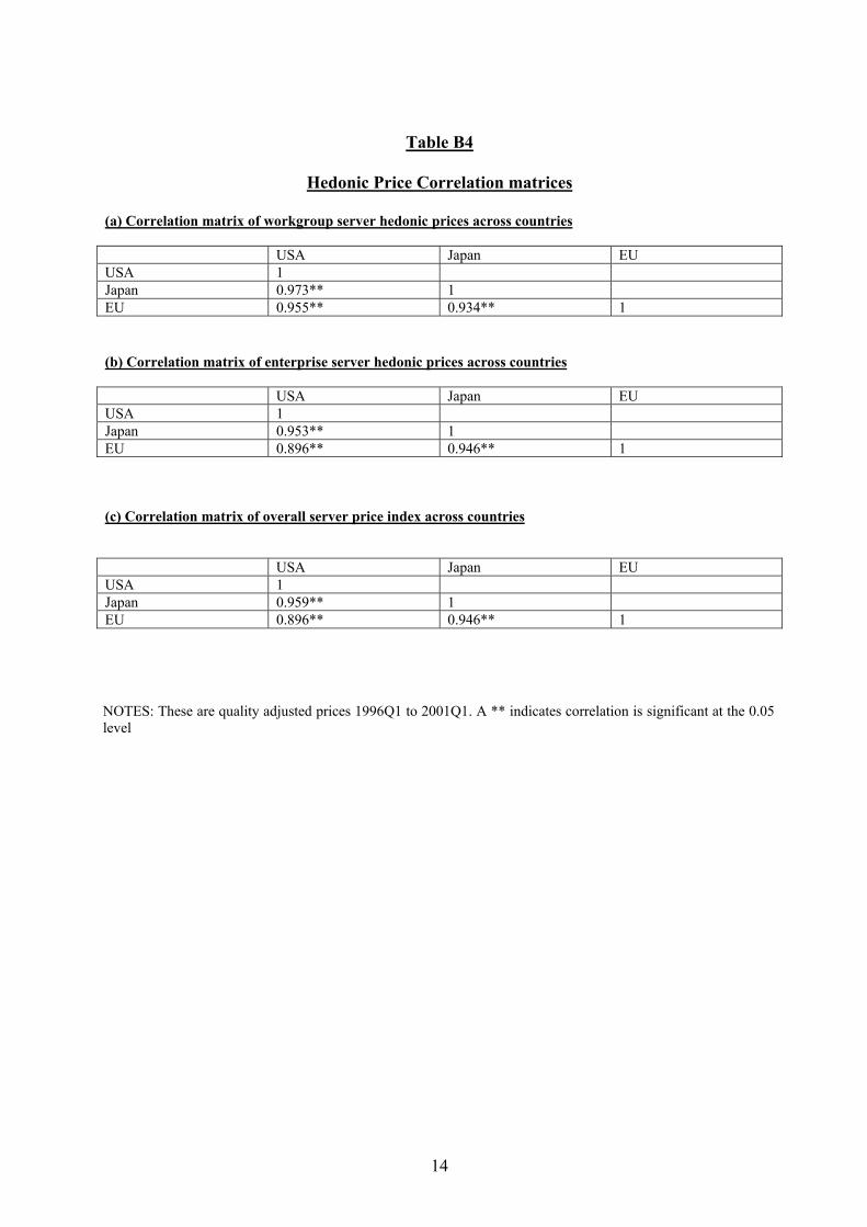
Table B4

Hedonic Price Correlation matrices

(a) Correlation matrix of workgroup server hedonic prices across countries USA Japan EU USA 1 Japan 0.973** 1 EU 0.955** 0.934** 1 (b) Correlation matrix of enterprise server hedonic prices across countries USA Japan EU USA 1 Japan 0.953** 1 EU 0.896** 0.946** 1 (c) Correlation matrix of overall server price index across countries USA Japan EU USA 1 Japan 0.959** 1 EU 0.896** 0.946** 1 NOTES: These are quality adjusted prices 1996Q1 to 2001Q1. A ** indicates correlation is significant at the 0.05 level

14

Figure B1: Shares of main hardware vendors in the work group server market

time

IBM Compaq Dell HP

1996q2 1997q3 1998q4 2000q1 2001q2

0

10

20

30

HP

COMPAQ

DELL SUN

IBM

NOTES: These are the market shares (in worldwide revenues) of the main 5 hardware vendors in the work group server market (under $100,000).

15

Appendix C: Details of Economic Models

C.A. Nested Logit Model

Demand Consider there are N separate markets where n = 1,…,N is one region (i.e. US, Japan or EU) in one time period. Market size is Ln. We will drop the n-index for simplicity in what follows. Each customer, f = 1,…., F can buy up to one good in each market8 or select the outside good. This means a customer chooses one of the set M = {W, H, 0} where W indicates a work group server, H a higher level/enterprise server and 0 the outside good. Once this group is chosen the customer then chooses a model. Indirect utility for customer f purchasing model i is given by:

(A1) f

imimimf VU ε+=

Vim is the mean utility of all customers buying i, and is the unobserved variables that explain customer f’s departure from the common utility level. The mean utility level can be further decomposed as:

fimε

(A2)

imimimim pVV ξξα ++−= where imV is the deterministic part that depends on the specific model-type of server, ξ is a market specific component and imξ is a random term reflecting the effect of unobserved characteristics of models on the mean utility. pim is the price of the selected product and α is a parameter of interest to be estimated. The random part is specified as a weighted sum of unobserved variables as follows f

imε(A3)

Fffim

fm

fim ,....1,)1( =∀−+= νσνε

where σ is a parameter to be estimated and indicates how closely correlated are consumers’ preferences within a server segment. The random components at each stage of the decision tree are endowed with the required distributions so that , , and satisfy the extreme value distribution. These assumptions give rise to the nested logit model.

fmν

fimνσ )1( − f

imε

The model allows us to decompose si, the unconditional probability of selecting a server i as the product of two probabilities:

• s(i|m), the probability of choosing server i conditional on choosing a server of type m and

• s(m) the probability of choosing a server of type m. To see this note that the probability of choosing model i conditional on choice of server type {W,H,0} for the logit model is:

(A4) 8 See Hendel (1999) or Smith (2002) for an extension to the case of multi-good purchases.

16

∑ ∈

=mIi im

im

VV

mis'

)exp()exp(

)|(µ

µ

where µ = 1/(1- σ) The probability of a server type m is

(A5)

∑=

m m

m

VV

ms)exp(

)exp()(

Vm is an inclusive value defined as

(A6)

mIi imm DVVm

ln)exp(ln 11 −∈

− == ∑ µµµ

Utility associated with the outside good is normalised so that V0 = 0 and

(A7)

s(0) = s0 = [Σmexp(Vm)]-1 = D0-1

The unconditional probability of selecting model i is

(A8) si = s(i|m)s(m)

or

ln si = lns(i|m) + lns(m) From (A4) and (A6)

(A9)

m

im

DV

mis)exp(

)|(µ

=

From (A5) and (A6) (A10)

0

/1

)(D

Dms m

µ

=

Combining (A4) with (A9) and (A10) gives

(A11)

0

/1)exp(m)s(m)|s(i

DD

DV

s m

m

imi

µµ==

17

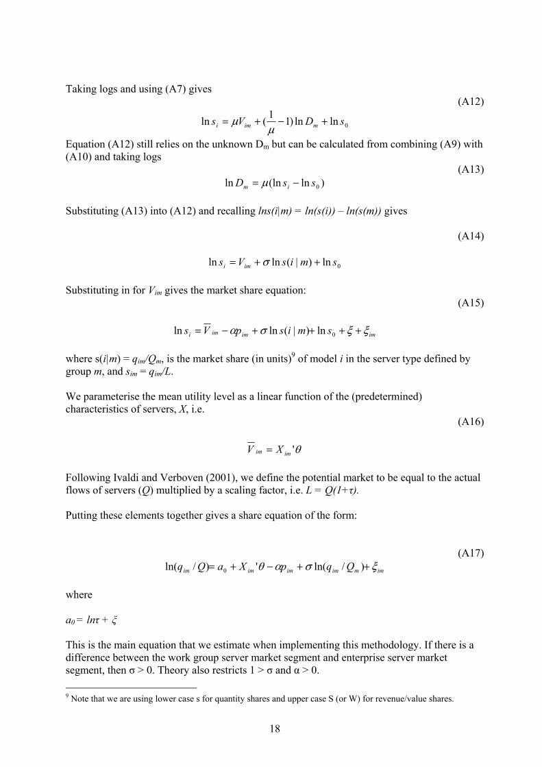
Taking logs and using (A7) gives

(A12)

0lnln)11(ln sDVs mimi +−+=µ

µ

Equation (A12) still relies on the unknown Dm but can be calculated from combining (A9) with (A10) and taking logs

(A13) )ln(lnln 0ssD im −= µ

Substituting (A13) into (A12) and recalling lns(i|m) = ln(s(i)) – ln(s(m)) gives

(A14)

0ln)|(lnln smisVs imi ++= σ Substituting in for Vim gives the market share equation:

(A15)

imimimi smispVs ξξσα ++++−= 0ln)|(lnln where s(i|m) = qim/Qm, is the market share (in units)9 of model i in the server type defined by group m, and sim = qim/L. We parameterise the mean utility level as a linear function of the (predetermined) characteristics of servers, X, i.e.

(A16)

θ'imim XV = Following Ivaldi and Verboven (2001), we define the potential market to be equal to the actual flows of servers (Q) multiplied by a scaling factor, i.e. L = Q(1+τ). Putting these elements together gives a share equation of the form:

(A17) immimimimim QqpXaQq ξσαθ ++−+= )/ln(')/ln( 0

where a0 = lnτ + ξ This is the main equation that we estimate when implementing this methodology. If there is a difference between the work group server market segment and enterprise server market segment, then σ > 0. Theory also restricts 1 > σ and α > 0. 9 Note that we are using lower case s for quantity shares and upper case S (or W) for revenue/value shares.

18

The own elasticity of demand for a particular model is therefore

(A18)

)1

1(σ

αη−

−= miiii rqp

where

LQr

mm

11)1

( +−

=σ

σ

The cross price elasticity of demand for model i with respect to model j (in the same server segment) is

(A19)

mjjijm rqpαη = The cross price elasticity of demand for model i with respect to model j (in another server segment) is

Lqp jj

ijm

αη ='

More aggregate elasticities can be estimated by simulating a 1% increase in all server prices and using (A18) and (A19). This is what we do to calculate the aggregate elasticities reported. Supply Consider the generic program for a multi-product firm, h, with models i in the set Zh. We assume that in each market the firm plays Nash in prices (for differentiated products). For a particular brand the first order condition is:

∑≠∈

=−∂∂

+−∂∂

+ijZj

jji

jii

i

ii

h

cppq

cppq

q 0)()(

where ci is marginal cost of brand i. In elasticity form this FOC can be re-written

∑≠∈

−−

+−

=−ijZj

jjiii

jij

ii

iii

h

cpq

qpcp )(

ηη

η

The first term on the right hand side is the usual own price elasticity effect whereas the second term reflects the incentives of the multi-product firm. The closer are two substitute models owned by the same firm, the higher will be their joint price, other things equal. Inspection of

19

this equation immediately suggests the different possible instruments for price in the demand equation

• Cost shifters which exogenously move ci. These will include the quality-adjusted price of inputs (such as semi-conductor chips). Prices of brands in other countries are also meant to proxy for model-specific costs shifts.

• Secondly, factors that exogenously shift the own brand elasticity of demand are candidate instruments. Under the assumption that brand numbers and characteristics are (econometrically) exogenous we can use (i) the number of other products in the market segment and (ii) the characteristics of other brands. A larger number of products will increase the own brand elasticity (in absolute value).

• Thirdly, the number and characteristics of the other products produced by firm h will also impact on pricing through the second term.

Given explicit functional forms we can solve the FOC analytically. In fact the nested logit has a closed form solution. If there are I models there are I equations that enable a solution for each brand’s mark-up (π). The formula is complex (see Foncel and Ivaldi, 2001) but can be expressed as (for firm h)

),,,;,,( LQQZfcp mhiii σθαπ =−= Given estimates of the parameters, the margins or marginal costs can be checked against any actual data to check the plausibility of the estimates. Alternatively, a comparison with actual margins can be used to test the assumption of Nash pricing versus co-ordinated pricing (see Nevo, 2001; Slade, 2004). Another strategy is to assume a parametric relationship between marginal costs and brand characteristics (cf. Bresnahan, 1987, Greenstein, 1997). For example

iii Xc ωκ += ' and form the supply side pricing equation

iimhi XLQQZfp ωκσθα ++= '),,,;,,( Given the assumed functional forms this can be written (e.g. Berry, 1994)

[ ] iimiii QqQqXp ωσσασκ +−−−

−+= −1)/ln()1()/ln(1(1' (A20)

This equation illustrates the problem with the standard hedonic pricing equation that only has the first term on the right hand side. We also need a correction for the variation in the mark-up that is the second (endogenous) term. The supply equation can be stacked with the demand side in a two-equation system. This can be estimated by FIML or non-linear three stage least squares with the structural cross equation restrictions imposed. In principle this should improve efficiency of the estimate parameters. It does impose more structure on the precise way in which firms are interacting in the product market, however, and if the Nash assumption is incorrect the estimates of the demand

20

parameters will be biased. Consequently we focus only on the demand side of the estimation without imposing any constraints from the supply side equations. C.B. Multi-level model

In the middle-level system we use the L-AIDS (Linearized Almost Ideal Demand System) of Deaton and Muellbauer (1980a, 1980b).

( ) ∑ =++Π+= M

m nmtnmtnkntnmnmnmt uYS10 loglog πδββ (B1)

where Y = total expenditure on servers in mth segment of the nth country, π = (quality adjusted) price of servers in segment m, and u is a random error term. So, for workgroup servers (suppressing the region n sub-scripts) we have:

( ) WtHtWHWtWWtWWWt uYS +++Π+= πδπδββ logloglog0 (B2) Since we are in the two-good case, homogeneity plus Slutsky symmetry imply δWW = -δWH. Imposing these restrictions means that we can simplify equation (B2) to:

( ) ( ) WtHtWtWWtWWWt uYS ++Π+= ππδββ loglog0 (B3)

The enterprise-level server equation analogous to equation (B3) also replaces the left-hand-side variable by the expenditure share of enterprise-level servers sold, and the right-hand-side variables remain the same. But there is no additional information in this equation and all its parameters can be recovered from equation (B3). Consider the elasticities of interest. By definition, SW = PWQW/Y where QW is the quantity of workgroup servers. Taking logarithms of both sides and differentiating with respect to the log of the price of workgroup servers implies that we can write the elasticity of demand for workgroup servers with respect to their price as:

(B4)

WW

W

WW

W

PYS

SPQ

loglog

log11

loglog

∂∂+

∂∂

+−=∂∂

π

Since

1loglog

=∂∂

W

W

Pπ

Define the conditional elasticity of demand (i.e. holding nominal server expenditure, Y, fixed) as EWW. Using equations (B2) this is

(B5)

21

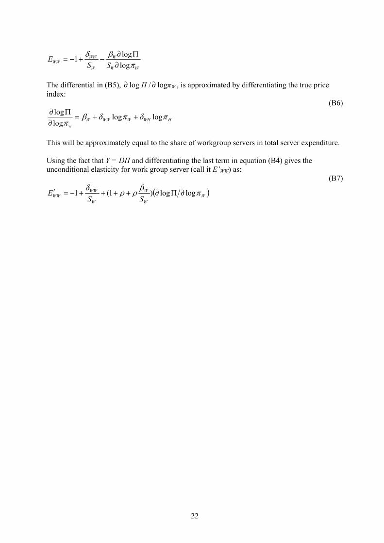
22

WW

W

W

WWWW SS

Eπ

βδloglog1

∂Π∂−+−=

The differential in (B5), ∂ log Π / logπ∂ W , is approximated by differentiating the true price index:

(B6)

HWHWWWWw

πδπδβπ

loglogloglog ++=

∂Π∂

This will be approximately equal to the share of workgroup servers in total server expenditure. Using the fact that Y = DΠ and differentiating the last term in equation (B4) gives the unconditional elasticity for work group server (call it E’WW) as:

(B7)

( WW

W

W

WWWW SS

E π )βρρδloglog)1(1 ∂Π∂++++−=′

CENTRE FOR ECONOMIC PERFORMANCE Recent Discussion Papers

649 Rachel Griffith

Stephen Redding Helen Simpson

Foreign Ownership and Productivity: New Evidence from the Service Sector and the R&D Lab

648 Fredrik Andersson Simon Burgess Julia I. Lane

Cities, Matching and the Productivity Gains of Agglomeration

647 Richard B. Freeman Douglas Kruse Joseph Blasi

Monitoring Colleagues at Work: Profit-Sharing, Employee Ownership, Broad-Based Stock Options and Workplace Performance in the United States

646 Alberto Bayo-Moriones Jose E. Galdon-Sanchez Maia Güell

Is Seniority-Based Pay Used as a Motivation Device? Evidence from Plant Level Data

645 Stephen Machin Olivier Marie

Crime and Benefit Sanctions

644 Richard B. Freeman Are European Labor Markets As Awful As All That?

643 Andrew B. Bernard Stephen Redding Peter K. Schott

Comparative Advantage and Heterogeneous Firms

642 Patricia Rice Anthony J. Venables

Spatial Determinants of Productivity: Analysis for the Regions of Great Britain

641 Kwok Tong Soo Zipf’s Law for Cities: A Cross Country Investigation

640 Alan Manning We Can Work it Out: the Impact of Technological Change on the Demand for Low Skill Workers

639 Bianca De Paoli Monetary Policy and Welfare in a Small Open Economy

638 Kimberly Ann Elliott Richard B. Freeman

White Hats or Don Quixotes? Human Rights Vigilantes in the Global Economy

637 Barbara Petrongolo Gender Segregation in Employment Contracts

636 Ann Bartel Richard B. Freeman Casey Ichniowski Morris Kleiner

Can a Work Organization Have an Attitude Problem? The Impact of Workplaces on Employee Attitudes and Economic Outcomes

635 Paul Gregg Rosanna Scutella Jonathan Wadsworth

Reconciling Workless Measures at the Individual and Household Level: Theory and Evidence from the United States, Britain, Germany, Spain and Australia

634 Stephen Nickell Employment and Taxes

633 Fabiano Schivardi Roberto Torrini

Threshold Effects and Firm Size: the Case of Firing Costs

632 Paul Gregg Jonathan Wadsworth

Two Sides to Every Story: Measuring the Polarisation of Work

631 Jeremy Grant Thomas Kirchmaier

Corporate Ownership Structure and Performance in Europe

630 Neal Knight-Turvey Andrew Neal Michael A. West Jeremy Dawson

The Impact of an Innovative Human Resource Function on Firm Performance: the Moderating Role of Financing Strategy

629 Nicholas Oulton A Statistical Framework for the Analysis of Productivity and Sustainable Development

628 Vasileios Gkionakis Short Job Tenures and Firing Taxes in the Search Theory of Unemployment

627 L. Rachel Ngai Christopher A. Pissarides

Balanced Growth With Structural Change

626 Malcolm Patterson Peter Warr Michael West

Organizational Climate and Company Productivity: the Role of Employee Affect and Employee Level

The Centre for Economic Performance Publications Unit Tel 020 7955 7673 Fax 020 7955 7595 Email info@cep.lse.ac.uk

Web site http://cep.lse.ac.uk