Policy Research Working Paper 7071

From Tapering to Tightening

The Impact of the Fed’s Exit on India

Kaushik BasuBarry Eichengreen

Poonam Gupta

Development Economics Vice PresidencyOffice of the Chief EconomistOctober 2014

WPS7071P

ublic

Dis

clos

ure

Aut

horiz

edP

ublic

Dis

clos

ure

Aut

horiz

edP

ublic

Dis

clos

ure

Aut

horiz

edP

ublic

Dis

clos

ure

Aut

horiz

ed

Produced by the Research Support Team

Abstract

The Policy Research Working Paper Series disseminates the findings of work in progress to encourage the exchange of ideas about development issues. An objective of the series is to get the findings out quickly, even if the presentations are less than fully polished. The papers carry the names of the authors and should be cited accordingly. The findings, interpretations, and conclusions expressed in this paper are entirely those of the authors. They do not necessarily represent the views of the International Bank for Reconstruction and Development/World Bank and its affiliated organizations, or those of the Executive Directors of the World Bank or the governments they represent.

Policy Research Working Paper 7071

This paper is a product of the Office of the Chief Economist, Development Economics Vice Presidency. It is part of a larger effort by the World Bank to provide open access to its research and make a contribution to development policy discussions around the world. Policy Research Working Papers are also posted on the Web at http://econ.worldbank.org. The authors may be contacted at pgupta5@worldbank.org.

The “tapering talk” starting on May 22, 2013, when Federal Reserve Chairman Ben Bernanke first spoke of the possibil-ity of the U.S. central bank reducing its security purchases, had a sharp negative impact on emerging markets. India was among those hardest hit. The rupee depreciated by 18 percent at one point, causing concerns that the country was heading toward a financial crisis. This paper contends that India was adversely impacted because it had received large capital flows in prior years and had large and liquid financial markets that were a convenient target for investors seek-ing to rebalance away from emerging markets. In addition, India’s macroeconomic conditions had weakened in prior years, which rendered the economy vulnerable to capital outflows and limited the policy room for maneuver. The paper finds that the measures adopted to handle the impact

of the tapering talk were not effective in stabilizing the financial markets and restoring confidence, implying that there may not be any easy choices when a country is caught in the midst of rebalancing of global portfolios. The authors suggest putting in place a medium-term policy framework that limits vulnerabilities in advance, while maximizing the policy space for responding to shocks. Elements of such a framework include a sound fiscal balance, sustainable current account deficit, and environment conducive to investment. In addition, India should continue to encourage relatively stable longer-term flows and discourage volatile short-term flows, hold a larger stock of reserves, avoid excessive appre-ciation of the exchange rate through interventions with the use of reserves and macroprudential policy, and prepare the banks and firms to handle greater exchange rate volatility.

From Tapering to Tightening: The Impact of the Fed’s Exit on India

Kaushik Basu, Barry Eichengreen and Poonam Gupta1

Keywords: Balance of Payments, Economic Management, Macroeconomic Policy, Macroeconomic Vulnerability, Monetary Policy

1 We thank Shankar Acharya, Rahul Anand, Paul Cashin, Tito Cordella, Manoj Govil, Muneesh Kapur, Ken Kletzer, Rakesh Mohan, Zia Qureshi, Y.V. Reddy, David Rosenblatt, Aristomene Varoudakis, and participants of the India Policy Forum, 2014, for very useful discussions and comments, and Serhat Solmaz for excellent research assistance.

I. Introduction

On May 22, 2013, Federal Reserve Chairman Ben Bernanke first spoke of the possibility of the Fed tapering its security purchases. His “tapering talk” had a sharp negative impact on financial conditions in emerging markets.2 India was among those hardest hit. Between May 22, 2013, and the end of August 2013, its exchange rate depreciated by 18 percent, bond spreads increased, and equity prices fell. The reaction was sufficiently pronounced for the press to warn that India might be heading toward a full-blown financial crisis, the kind that requires a country to seek IMF assistance.3

In this paper we ask three questions about this episode. Why was the impact of the Fed’s announcement on India’s financial markets so severe? How effective were the policy measures undertaken in response? How can India prepare itself for the normalization of monetary policy in advanced economies and more broadly to react to global liquidity cycles?

Eichengreen and Gupta (2014) analyzed the impact of the Fed’s tapering talk on exchange rates, foreign reserves and equity prices in emerging markets between April and August 2013.4 They established that an important determinant of the impact was the volume of capital flows that countries received in prior years and the size of their local financial markets. Those which received larger inflows of capital and had larger and liquid financial markets experienced more pressure on their exchange rates, reserves, and equity prices once the “tapering talk” began. This may be interpreted as showing that investors are better able to rebalance their portfolios away from an emerging economy when the country in question has a relatively large and liquid financial market.

This paper elaborates the Indian case. India ranks high in terms of the size and liquidity of its financial markets and the extent of capital flows it received in prior years and became an easy target for investors seeking to rebalance away from emerging markets.

In addition, Eichengreen and Gupta show that the emerging markets that had allowed their real exchange rate to appreciate and the current account deficit to widen during the period of quantitative easing felt a larger impact. Similar vulnerabilities had built in India too in prior years. Its current account deficit had increased and real exchange rate had appreciated markedly. In addition, its fiscal deficit had increased, and inflation at about 10 percent was proving to be stubbornly high. These macroeconomic weaknesses had surfaced in the midst of a sharp growth slowdown. Although the level of foreign reserves was considered comfortable by some metrics, the effective coverage they provided had declined unmistakably since 2008.

2 The period of the tapering talk is generally referred to that between May 22, 2013 and September 18, 2013. 3 See e.g. “India in crisis mode as rupee hits another record low”, http://money.cnn.com/2013/08/28/investing/india-rupee/; “India’s Financial Crisis, Through the Keyhole”, http://www.economist.com/blogs/banyan/2013/08/india-s-financial-crisis.

4 Subsequently the Federal Reserve started tapering its purchases of securities in December 2013, reducing it by $10 bn each month. It has since then tapered six more times, each time by $10 bn and is expected to end the program in October, 2014, with a last reduction of $15 bn in the purchase of securities.

2

The specific factors contributing to the high fiscal or current account deficit in India also indicated increased economic and financial vulnerabilities. The increase in fiscal deficit was due to an increase in current expenditure (in response to the global financial crisis of 2008, the headwinds of which were palpable in India by early 2009), rather than to a pick-up in public investment. The increase in current account deficit, largely a mirror effect of the increased current expenditure, was characterized by some deflection of private savings into the import of gold. It reflected a dearth of attractive domestic outlets for personal savings in a high inflation environment, where real returns on many domestic financial investments had turned negative. Loose monetary policy in advanced countries meanwhile made those deficits easy to finance, further relieving the pressure to compress them. Rebalancing by global investors when the Fed broached the subject of tapering highlighted these vulnerabilities.

The authorities adopted a range of measures in response. They intervened in the foreign

exchange market, hiked interest rates, raised the import duty on gold, encouraged capital inflows from nonresident Indians, eased demand pressure in the foreign exchange market by opening a separate swap window for oil importing companies, opened a swap line with the Bank of Japan, and restricted capital outflows from residents and Indian companies. We empirically estimate the impact of these measures on the exchange rate and financial markets. Our results show that some of these measures, including the separate swap window for oil importing companies, were of limited help in stabilizing the financial markets. Others, like initiatives restricting capital outflows, actually undermined confidence and proved counterproductive.

The results imply that there may not be any easy choices when a country is in the midst of rebalancing of global portfolios. We suggest putting in place a medium-term policy framework that limits vulnerabilities in advance, while maximizing the policy space for responding to shocks. Elements of such a framework include holding a larger stock of reserves; avoiding excessive appreciation of the exchange rate through interventions using reserves and macroprudential policy; signing swap lines with other central banks where feasible; preparing the banks and the corporates to handle greater exchange rate volatility; adopting a clear communication strategy; avoiding measures that could damage confidence, such as restricting outflows; and managing capital inflows to encourage relatively stable longer-term flows while discouraging short-term flows.5 A sound fiscal balance, sustainable current account deficit, and environment conducive for investment are other more obvious elements of this policy framework.

5 See Zhang and Zoli (2014) and the literature cited therein for the recent contributions on the use of macro prudential policies, in particular loan to value ratio, debt to income ratio, required reserves ratio, countercyclical provisioning and countercyclical capital requirements in Asian economies. See Cordella, Vegh and Vuletin (2014) on the use of reserve requirements as a countercyclical macroprudential tool in developing countries.

3

II. The Effects of the Tapering Talk on India

As documented in Eichengreen and Gupta (2013), the tapering talk affected a large number of emerging markets. Using the data for 53 emerging markets (which have their own currency and exchange rate), they calculated cumulative changes in their exchange rates, stock prices, bond spreads and reserves between April 2013 and, alternatively, end of June, end of July and end of August 2013. The resulting distribution of exchange rate changes over the months through August is portrayed in Panel A of Figure 1. The data show that the exchange rate depreciated in 36 of the 53 countries between April and June.6 Despite some subsequent recovery, by August exchange rates for 30 of the 53 countries remained below their levels seen in April. The average rate of depreciation in these 30 countries was over 6 percent, and exchange rates for about half the countries depreciated by more than 5½ percent.

Panel B provides further details on the distribution of exchange rate changes between April and August. The largest depreciation was experienced by Brazil, India, South Africa, Turkey and Uruguay, where the exchange rate depreciated by at least 9 percent, and Brazil experienced the largest depreciation of 17 percent. Data for stock markets are available for fewer countries; 25 of the 38 countries for which we have the data experienced some decline in their stock markets. The average decline in these 25 countries was 6.9 percent (Panel C, Figure 1). For six emerging markets (Chile, Indonesia, Kazakhstan, Peru, Serbia, and Turkey), the decline was more than 10 percent. In comparison, India had a relatively modest decline in its stock market (at month-end values). Reserves declined for 29 of 51 countries between April and August, with the largest declines seen in the Dominican Republic, Hungary, Indonesia, Sri Lanka, and Ukraine.7

6 We extracted the data on exchange rate, reserves and stock markets from the Global Economic Monitoring database of the World Bank, on October 29, 2013. 7 We dropped countries where events other than the tapering talk clearly dominated the impact on financial markets. For example Pakistan where there was a large increase in stock prices due to developments unrelated to tapering—it had agreed to a $5.3 billion loan from the IMF on July 5, boosting reserves and leading to rallies in stocks, bonds and the rupee (Bloomberg, July 5, 2013). We also dropped Egypt where foreign reserves rose by 33 percent between April and July, 2013 due to aid from other countries.

4

Figure 1: Exchange Rate, Stock Market and Reserves in Emerging Markets during the Tapering Talk

A: Distribution of % change in exchange rate over time shows that the effect spread and increased

through August

B: Cumulative effect on exchange rate (% change) during April-Aug, 2013, India is among

the countries with the largest depreciation

C: Cumulative effect on stock market index (%

change) between April-Aug, 2013 is rather modest for India

D: Cumulative effect on external reserves (% change) during April-Aug, 2013, reserves

declined by nearly 6 percent in India

Source: Data on exchange rates, reserves and stock markets are from the Global Economic Monitoring database of the World Bank. Calculations are based on end of month values. See Eichengreen and Gupta (2014) for details.

Even though the tapering talk affected a large number of emerging markets, much of the market commentary focused on five countries, Brazil, Indonesia, India, Turkey and South Africa, christened as “Fragile Five”. Table 1 summarizes the effect on these five countries. As is evident from the table, the exchange rates depreciated and reserves declined in all five countries, while equity

0.0

5.1

.15

.2

-4 0 4 8 12 16 20Exchange Rate Depreciation

Apr-Aug 2013 Apr-July 2013Apr-June 2013

05

1015

Num

ber

of C

ount

ries

-4 0 4 8 12 16 20Exchange Rate Depreciation April-Aug 2013

India

02

46

810

Num

ber o

f Cou

ntrie

s

-30 -25 -20 -15 -10 -5 0 5 10 15 20 25 30Percent Change in Stock Market August-April, 2013

India

05

1015

Num

ber

of C

ount

ries

-25 -20 -15 -10 -5 0 5 10 15 20Percent Change in Reserves April-August,2013

India

5

prices declined in all but South Africa. The largest exchange rate depreciation occurred in Brazil, the largest decline in stock prices was in Turkey, and the largest reserve loss was observed in Indonesia. Within this group India had the second largest exchange rate depreciation and the second largest decline in reserves.

Table 1: Effect of Tapering Talk on “Fragile Five” Countries (April-August, 2013)

Exchange Rate Depreciation

% change in Stock Prices

% Change in Reserves

Brazil 17.01 -5.28 -3.07

Indonesia 8.33 -14.21 -13.30

India 15.70 -3.32* -5.89

Turkey 9.21 -15.38 -4.56

South Africa 10.60 6.81 -5.05 Note: Calculated using data from the Global Economic Monitor database of the World Bank. * Decline in stock prices in India was about 10 percent if calculated using daily data between May 22 and August 31, 2013.

This period was also marked by significant volatility in financial markets in the affected countries. Highlighting the Indian case in Table 2, we show that the short-term volatility, measured by the standard deviation of percentage change in exchange rates, stock market prices and reserves (using daily data for exchange rate and equity prices and weekly data for reserves) was quite large in summer 2013, compared to the previous months.

Table 2: Volatility in India during the Tapering Talk (Standard deviation of percent changes using daily or weekly data)

s.d. of % change in

daily exchange rate

s.d. of % change in daily stock prices

s.d. of % change in weekly stock of foreign reserves

Tapering Talk: May 23, 2013-August 31, 2013

4.95 3.62 1.82

Previous three Months (Feb 21, 2013-May 22, 2013)

0.9 2.81 0.73

Previous one year (May 21, 2012-May 22, 2013)

1.71 6.92 1.05

Note: Standard deviation calculated using daily data on nominal exchange rate and stock market index from Bloomberg; and weekly data on foreign reserves from the RBI.

6

III. Why Was India Affected So Severely?

We contend that the impact was large on India for two reasons. First, India’s large and liquid financial markets had received significant volumes of capital flows in prior years, making it a convenient target for investors seeking to rebalance away from emerging markets; and second, its macroeconomic vulnerabilities had increased in the years prior to the tapering talk, making it vulnerable to capital outflows and limiting the policy room to address the shock that the tapering talk initiated.

In their analysis of the impact of the Fed’s tapering talk on the exchange rates, foreign

reserves and equity prices of emerging markets between May 2013 and August 2013, Eichengreen and Gupta (2014) found that the countries with larger financial markets and larger capital inflows in the prior years experienced more exchange rate depreciation and larger reserve losses during the tapering talk. Evidently, investors are more easily able to rebalance their portfolios away from an economy when the country in question has a relatively large and liquid financial market (possibly they incur a smaller loss of value and need to withdraw only from a few large markets than sell their assets in many small markets). India ranks high in terms of the size and liquidity of its financial markets and the extent of capital flows it received in prior years (see Figure 2 and Table 3). Whether measured in absolute terms or as percent of GDP, India is among the top quartile of countries, or for some indicators among the top few emerging economies, for various measures of the size and liquidity of financial markets.

7

Figure 2: Size and Liquidity of Financial Markets and the Effect on Exchange Rate during the Tapering Talk

A: Larger private external financing in 2010-2012 implied larger exchange rate depreciation during the

tapering talk

B: Larger financial markets proxied by the stock of portfolio liabilities in 2012 implied larger exchange

rate depreciation during the tapering talk

C: Larger financial markets proxied by stock market capitalization/GDP in 2012 implied larger exchange

rate depreciation during the tapering talk

D: More liquid domestic markets, measured by turnover ratio in stock market implied larger

exchange rate depreciation during the tapering talk

Source: Eichengreen and Gupta (2014)

ALBARM

AZE

BGRBIH

BLR

BRA

CHL

CHN

COL

CRI

DOM

GHA

GTM

HRVHUN

IDN

IND

JAM

JOR

KAZ

KEN

LBN

LKA

LTULVA MAR

MEX

MKD

MYS

PAK

PERPHL

POLROM

RUS

SRB

THA

TUN

TUR

UKR VENVNM

ZAF

-50

510

15E

xcha

nge

Rat

e D

epre

ciat

ion

4 6 8 10 12Cumulative Capital Flows 2010-2012

BGR

BLR

BRA

CHL

CHN

COL

GTM

HRVHUN

IDN

IND

ISR

JAM

JOR

KAZ

LTULVAMAR

MEX

MUS

MYS

PAK

PERPHL

POLROM

SGP

SRB

THATUR

UKR

URY

ZAF

-50

510

15E

xcha

nge

Rat

e D

epre

ciat

ion

8 10 12 14Log Portfolio Investment 2012

ARM BGR

BRA

CHL

CHN

COL

CRI

CZE

GHA

HKG

HRVHUN

IDN

IND

ISR

JAM

JOR

KAZ

KEN

KORLBN

LKA

LTULVA MAR

MEX

MKD

MUS

MYS

PAK

PERPHL

POLROM

RUS

SGP

SRB

THA

TUN

TUR

UKRVENVNM

ZAF

-50

510

15E

xcha

nge

Rat

e D

epre

ciat

ion

20 25 30Stock Market Capitalization 2012

ARG

ARMBGR

BRA

CHL

COL

CRI

GHA

HRVHUN

IDN

IND

JAM

JOR

KAZ

KEN

LBN

LKA

LTULVAMAR

MEX

MYS

PAK

PERPHL

POLROU

RUS

SRB

THA

TUN

TUR

UKRVENVNM

ZAF

-50

510

15

0 50 100 150Turnover_Ratio_Stock_WDI_2012

8

Table 3: Size of the Financial Market and Cumulative Capital Inflows were Large in India prior to the Tapering Talk compared to other Emerging Markets ($ billion or % of GDP)

Number of Countries

Mean Median Top Quartile India

Capital Inflows in 2010-2012, GFSR, bn $*

43 65.6 21 57 218

Stock Market Capitalization in 2012, bn $, WDI

47 302 32.9 383 1260

Stock of Portfolio Liabilities, 2012, IFS, bn $

36 92 30.4 151 186

Stock Market Capitalization, % of GDP in 2012, WDI

47 52 36.3 61.8 68.6

Stock of Portfolio Liabilities % of GDP, 2012, IFS

29 22.4 21.7 33.2 10

Note: Data on capital inflows, consisting of private inflows of bonds, equity, and loans is from the IMF’s Global Financial Stability Report. Data on stock market capitalization is from the World Development Indicators; and the data on portfolio liability is from the International Financial Statistics.

A second reason for the impact of the Fed’s tapering talk on India was the macroeconomic imbalances that were apparent at its outset. Eichengreen and Gupta show that the emerging markets that had allowed their real exchange rate to appreciate and the current account deficit to widen during the period of quantitative easing saw a larger impact. Similar vulnerabilities had built in India too in prior years. Its current account deficit had increased from about 1 percent of GDP in 2006 to nearly 5 percent in 2013; and its real exchange rate had appreciated markedly. In addition, the fiscal deficit had increased, and inflation at about 10 percent was proving to be stubbornly high (Figure 3). These macroeconomic weaknesses had surfaced in the midst of a sharp growth slowdown. Although the level of foreign reserves was considered comfortable by some metrics, the effective coverage they provided had declined unmistakably since 2008. The policy interest rate was high, having been increased by the Reserve Bank of India (RBI) from 3.25 percent in December 2009 to 8.50 percent in December 2012. The large fiscal deficit and high policy rate implied little room for maneuver in fiscal and monetary policy.8

Specific factors contributing to the high fiscal or current account deficit also indicated increased economic and financial vulnerabilities. The increase in fiscal deficit was due to an increase in current expenditure, in response to the global financial crisis of 2008, the headwinds of which were palpable in India by early 2009, rather than to a pick-up in public investment. The increase in current account deficit, largely a mirror effect of the increased current expenditure, was characterized by some deflection of private savings into the import of gold, reflecting a dearth of attractive domestic outlets for personal savings in a high inflation environment, where real returns on many domestic financial investments had turned negative (see Figure 4). Loose monetary policy in advanced countries meanwhile made those deficits easy to finance, further relieving the pressure to compress them.

8 In a paper presented at India Policy Forum, 2013, Kapur and Mohan had cautioned that such macroeconomic imbalances indicated heightened vulnerabilities to a financial crisis.

9

Figure 3: Macroeconomic Imbalances were apparent in India at the outset of the Tapering Talk

Growth Rate was declining… Inflation was Persistently High….

Fiscal deficit was High… Current Account Deficit was Increasing…

Reserve Coverage had Declined Real Exchange Rate had Appreciated

Sources: GDP, CSO; CPI Inflation, Citi Research; Gross Fiscal Deficit, Current Account Deficit, Reserve Bank of India; Reserves to M2 Ratio, IFS; Real Effective Exchange Rate (CPI based, six currency), RBI; Bilateral RER calculated using data from IFS. Years refer to fiscal years.

3

4

5

6

7

8

9

10

2006

2007

2008

2009

2010

2011

2012

2013

GDP Growth

3

5

7

9

11

13

2006

2007

2008

2009

2010

2011

2012

2013

CPI Inflation

3456789

10

2006

2007

2008

2009

2010

2011

2012

2013

Combined Fiscal Deficit, % of GDP

0

1

2

3

4

5

2006

2007

2008

2009

2010

2011

2012

2013

Current Account Deficit, % of GDP

20

25

30

35

2006

2007

2008

2009

2010

2011

2012

2013

India Reserves to M2 Ratio

95

105

115

125

135

2006

2007

2008

2009

2010

2011

2012

2013

Real Exchange Rate (2006=100)

Real Effective ExchangeBilateral RER with USD

10

Figure 4: The Level and Quality of Fiscal Deficit and Current Account Deficit indicated Vulnerabilities at the outset of the Tapering Talk

Sources: Gross Fiscal Deficit, FDI, Gold Import, Current Account Deficit, Reserve Bank of India; Subsidies, Ministry of Petroleum and Natural Gas, Govt. of India; Investment, CSO; Portfolio Flows, Bloomberg.

0.0

0.4

0.8

1.2

1.6

0

2

4

6

8

10

2006

2007

2008

2009

2010

2011

2012

increase in fiscal deficit was partly due to subsidies (% GDP)

Combined Government Fiscal Deficit (LHS)Food Subsidies (RHS)Fertiliser Subsidies(RHS)Petroleum Subsidies (RHS)

0.0

0.5

1.0

1.5

2.0

2.5

3.0

3.5

0

1

2

3

4

5

2006

2007

2008

2009

2010

2011

2012

2013

increase in current account deficit was partly due to an gold imports (% of

GDP)

Current Account Deficit (LHS)

Gold Import (RHS)

0

4

8

12

16

20

2006

2007

2008

2009

2010

2011

2012

2013

business enviornment was not conducive for investment (% change

in investment)

-20

-10

0

10

20

30

40

50

0

10

20

30

40

50

2006

2007

2008

2009

2010

2011

2012

2013

deficits were financed by volatile portfolio capital inflows

FDI (LHS)

Portfolio Flows(RHS)

11

India fared worse than the median emerging market for most of the indicators of the macroeconomic vulnerabilities, or worse than the three-fourths of them for some of the indicators, including the level of debt, fiscal deficit, inflation and reserves (Table 4).

Table 4: Comparison of Macroeconomic Variables for India with other Emerging Markets in 2012

Variable Number of Countries

Mean Median Bottom Quartile*

India

Economic growth, 2012 53 3.01 3.27 1.41 4.7

Public debt % of GDP, 2012 52 47.68 44.10 59.60 66.70

Fiscal deficit % of GDP, 2012 53 3.14 3.30 4.80 7.97

Current Account Deficit % of GDP, 2012 53 2.89 3.10 7.47 4.79

Inflation, CPI, 2012 52 4.96 3.80 6.13 10.44

Reserves to M2 ratio, 2012 52 0.38 0.32 0.24 0.21

RER appreciation, % (during 2010-2012) 50 3.00 2.50 4.29 3.54 Note: *values refer to the country at the bottom 25 percentile for economic growth and reserves and the country at the top 25 percentile for all other variables. Sources as in Eichengreen and Gupta (2014).

Drawing on Eichengreen and Gupta (2014), we consider the factors that were associated with the impact of the tapering talk on exchange rate as well as on stock prices and reserves. We calculate weighted average of changes in exchange rates, foreign reserves and stock prices in two separate indices. We calculate the first index, which we call the Capital Market Pressure Index I, as a weighted average of percent depreciation of exchange rate and reserves losses between April 2013 and August 2013, where the weights are the inverse of the standard deviations of monthly data from January 2000 to August 2013.

Capital Market Pressure Index I =% 𝐸𝑥𝑐ℎ𝑎𝑛𝑔𝑒 𝑅𝑎𝑡𝑒 𝐷𝑒𝑝𝑟𝑒𝑐𝑖𝑎𝑡𝑖𝑜𝑛

𝜎𝑒𝑥𝑐ℎ𝑎𝑛𝑔𝑒 𝑟𝑎𝑡𝑒+

% 𝐷𝑒𝑐𝑙𝑖𝑛𝑒 𝑖𝑛 𝑅𝑒𝑠𝑒𝑟𝑣𝑒𝑠𝜎𝑟𝑒𝑠𝑒𝑟𝑣𝑒𝑠

A second index, Capital Market Pressure Index II, is similarly constructed as a weighted average of the percent depreciation of exchange rate, reserve loss and decline in stock prices between April 2013 and August 2013.9

9We construct these indices in a manner analogous to the exchange market pressure index in Eichengreen, Rose and Wyplosz (1995), which they constructed as a weighted average of changes in exchange rates, reserves, and policy interest rates, where the weights are the inverse of the standard deviation of each series. The number of countries for which we can construct the index declines from 51 for the first index to 37 for the second index. If we also include increase in bond yields in the index, the number of countries for which we would be able to construct it declines to 25.

12

Capital Market Pressure Index II

= % 𝐸𝑥𝑐ℎ𝑎𝑛𝑔𝑒 𝑅𝑎𝑡𝑒 𝐷𝑒𝑝𝑟𝑒𝑐𝑖𝑎𝑡𝑖𝑜𝑛

𝜎𝑒𝑥𝑐ℎ𝑎𝑛𝑔𝑒 𝑟𝑎𝑡𝑒+

% 𝐷𝑒𝑐𝑙𝑖𝑛𝑒 𝑖𝑛 𝑅𝑒𝑠𝑒𝑟𝑣𝑒𝑠𝜎𝑟𝑒𝑠𝑒𝑟𝑣𝑒𝑠

+% 𝐷𝑒𝑐𝑙𝑖𝑛𝑒 𝑖𝑛 𝑆𝑡𝑜𝑐𝑘 𝑀𝑎𝑟𝑘𝑒𝑡

𝜎𝑠𝑡𝑜𝑐𝑘

We regress exchange rate depreciation, Index I and Index II on macroeconomic conditions, financial market structure and institutional variables, estimating linear equations of the form:

Yi = αk Xk,i +εi (1)

where Yi is exchange rate depreciation, Index I or Index II for country i between April-August 2013. The explanatory variables, Xk, include cumulative private capital inflows during 2010-2012, stock of portfolio liabilities or stock market capitalization in 2012 as alternate measures of the size of financial markets; several alternate measures of macroeconomic conditions such as the increase in current account deficit, real exchange rate appreciation, foreign reserves, GDP growth, fiscal deficit, inflation or public debt; and institutional variables such as the exchange rate regime, capital account openness, or the quality of the business environment.

Since these variables are correlated, we include only one of them at a time from each category (size of financial markets, macroeconomic variables, and institutional variables). Results are similar using different proxies, reassuringly, so we report only a representative subset here. We take the values of the regressors in 2012 or their averages over the period 2010–2012 (either way, prior to the tapering talk).10

Results show that the countries with larger financial markets experienced larger exchange rate depreciation and reserve losses. Also evidently, deterioration in current account, extent of real exchange rate appreciation, and inflation (results are not reported here for specifications in which we include inflation, but are available on request) during the years of abundant global liquidity were associated with more exchange rate depreciation and larger increases in the composite indices in the summer of 2013 (Table 5).

This helps us understand why the same countries that complained about the impact of quantitative easing on their exchange rates in the earlier years also complained about the impact of the tapering talk in the summer of 2013. The countries most affected by or least able to limit the earlier impact on their real exchange rates were the same ones to subsequently experience large and uncomfortable real exchange rate reversals, in other words. Standardized coefficients, to compare

10 We also consider some other available measures of the size and liquidity of the financial markets. The alternate measures are strongly correlated with each other and give similar results. Results hold if we calculate the dependent variables for April-July, 2013. Since most of these variables are persistent and correlated across years, it turns out to be inconsequential whether we use the data for just one year or period averages. More detailed results are available in Eichengreen and Gupta (2014).

13

quantitatively the coefficients of various regressors, show that the coefficient of the size of financial markets is the largest followed by the coefficients of real exchange rate and current account deficit. We do not find any other macroeconomic or institutional variables to be associated significantly with the impact of the tapering talk on the exchange rate or other variables.

Table 5: Regression Results for Factors Associated with Exchange Rate Depreciation and Capital Market Pressure Indices during April-August 2013

Dependent Variable % change in

nominal exchange

rate

Index I: (exchange rate, reserve)

Index II: (exchange

rate, reserve, stock prices)

% change in

nominal exchange

rate

Index I: (exchange

rate, reserve)

Index II: (exchange

rate, reserve, stock prices)

(1) (2) (3) (4) (5) (6) Increase in Current Account Deficit in 2010–12, over 2007–09

0.25** 0.17* 0.33*** 0.21** 0.07 0.23**

[2.58] [1.77] [3.27] [2.18] [0.74] [2.45] Avg. Annual % Change in RER, 2010–2012

-0.37*** -0.35*** -0.54***

[2.82] [3.21] [3.66] Size of Financial Markets (Private External Financing, 2010–12, Log)

1.42*** 0.71** 0.58 1.20*** 0.55** 0.23

[3.85] [2.65] [1.19] [3.16] [2.15] [0.41] Reserves/M2 Ratio, 2012 -2.53 1.52 4.32 -1.15 1.45 4.88 [0.73] [0.46] [1.03] [0.40] [0.51] [1.43] Observations 45 43 32 43 41 30 R-squared 0.43 0.24 0.29 0.49 0.36 0.43 Adj. R-squared 0.39 0.19 0.21 0.44 0.29 0.34

Note: We calculate average annual percent change in real exchange rate (RER) during 2010-2012, an increase in RER is depreciation;. Current account deficit is calculated as percent of GDP, we take average annual increase in current account deficit during 2010–12 over 2007–09. Index I is constructed as a weighted average of exchange rate depreciation and reserve loss, and Index II as the weighted average of exchange rate depreciation, reserve loss and decline in the index for stock prices; weights are the inverses of the standard deviations of respective series calculated using monthly data from January 2000 to August 2013. Robust t statistics are in parentheses. *** indicates the coefficients are significant at 1 percent level, ** indicates significance at 5 percent, and * significance at 10 percent level.

IV. Policy Response

India announced a range of policies to contain the impact of the global rebalancing on its exchange rate and financial markets. Most emerging markets increased their policy interest rates and intervened in the foreign exchange market to limit the volatility of the exchange rate and prevent exchange rate overshooting. The RBI similarly intervened in the foreign exchange market to limit the volatility and depreciation of the rupee, spending some $13 billion of reserves between end-May and end-September. Intervention was especially concentrated between June 17 and July 7, when weekly

14

declines in reserves were of the order of $3 billion. The RBI increased its overnight lending rate (the marginal standing facility rate) by 200 basis points to 10.25 percent on July 15th and tightened liquidity through open market operations and by requiring the banks to adhere to reserve requirements more strictly.

Gold imports being partly responsible for a large current account deficit, the government raised the import duty on gold on June 5th, August 13th, and September 18th, increasing it from 6 percent to 15 percent cumulatively. The RBI also imposed controversial new measures on August 14th to restrict capital outflows. These included reducing the limit on the amounts residents could invest abroad or repatriate for various reasons, including for purchasing property abroad.

India being an oil importing country, demand for foreign exchange from companies that import oil can add a significant amount to the overall demand for foreign exchange and thus affect the level and volatility of the exchange rate. The RBI opened a separate swap window for three public sector oil marketing companies on August 28, 2013, to exclude their demand from the foreign exchange market and reduce its volatility.11

There were then few additional policy actions in the second half of August, when the exchange rate depreciated most rapidly. This was a period of transition at the RBI, during which governor Dr. Subbarao was to retire on September 4, 2013, and a new governor had to be inducted. On August 6, 2013, the government announced that on September 4 Raghuram Rajan would take charge as the new governor of the RBI, and in the interim he would join the RBI as an Officer on Special Duty. Little policy communication or guidance was provided by the RBI during this interregnum, over which the exchange rate depreciated by nearly 10 percent.

On September 4, 2013, after formally joining the RBI as the governor, Rajan issued a

statement and held a press conference expressing confidence in the economy and highlighting its comfortable reserve position. He announced new measures to attract capital through deposits targeted at nonresident Indians and partially relaxed the restrictions on outward investment introduced previously. Another measure that possibly helped boost the availability of foreign exchange and calm the financial markets around this time was the extension of an existing swap line with Japan, which was increased from $15 billion to $50 billion. The extension of the swap line was negotiated between the Government of India and the Government of Japan and signed by their respective central banks.

We analyze the impact of these policy announcements on financial markets using “event-study” regressions. We compare the values of the exchange rate and financial market variables in a

11 None of these policy measures were novel in the Indian context, having been implemented at different instances in the past, e.g. the import duties on gold were prevalent until the early 1990s; deposits from the Indian diaspora were attracted in a similar fashion twice in the past, in 1998 and in 2000; a separate swap window was made available to the oil importing companies in 2008 to reduce the volatility in the foreign exchange market after the collapse of the Lehman brothers.

15

short window after the policy announcement (we report results for a 5 day post announcement window, but also considered shorter windows of 2 or 3 days which yielded similar results) with those prior to the announcement. For the control period, we consider two options, first, the entire tapering period from May 22 until the day of the policy announcement, and second, a shorter control period of 1 week prior to the announcement. Below we report results from the specifications in which we use this shorter control period of a week.

The regression specification is given in Equation 2, in which Y is either log exchange rate, log stock market index, portfolio debt flows, or portfolio equity flows (portfolio flows are in millions of US$). For some policy announcements, we also look at the impact on the turnover in the foreign exchange market.

Yt = constant + µ Bond Yield in the USt + α Tapering Talk Dummyt + β Dummy for a week prior to Policy Announcementt

+ γ Dummy for Policy Announcementt + εt (2) The regressors include US bond yields to account for global liquidity conditions and three

separate dummies, one each for the tapering period (from May 23, 2013-until a week before the policy announcement was made), for the week prior to the policy announcement, and for the week since the policy announcement. We estimate these regressions using data from January 1, 2013, up to the date the policy dummy takes a value of 1, dropping subsequent observations.12

(i) Increase in the Interest Rate (July 15)

To assess the impact of increase in interest rates on July 15, we construct the tapering

dummy to take a value of 1 from May 23 to July 7, the dummy for the week prior to the announcement takes a value of 1 from July 8 to July 14, and the dummy for increase in the interest rate takes a value 1 for five consecutive days from July 15 on which the financial markets were open.

The results in Table 6 show that the rate of currency depreciation, equity prices and debt

flows did not change significantly following the increase in interest rates. It would appear, then, that this initial policy response was ineffectual.

12 We acknowledge the limitations in being able to establish causality using these regressions, due to the difficulty in establishing the counterfactual and in controlling for all the relevant factors that may affect the financial markets.

16

Table 6: Effect of the Increase in the Marginal Standing Facility Rate

Note: Data used in the regressions runs from January 1, 2013-July 22, 2013. *, **, *** indicates that the coefficient is significantly different from zero at 10, 5 and 1 percent level of significance, t statistics are in parentheses. # the null hypothesis in each regression is that the policy announcement did not stabilize the market, and the alternative hypothesis is that it stabilized it; 1 percent level of significance is used to test the hypotheses, unless otherwise indicated.

The question is why. Comparing the increase in interest rates in the other Fragile Five countries (Figure 5), we can see that, except for South Africa, the other countries increased interest rates as well. Brazil started raising rates in May and continued doing so through the end of the year; the increase between May and September totaled 150 basis points. Indonesia first raised rates in July but continued raising them through September; the increase during May-September summed up to 100 basis points. India was different from the other countries in that it raised the interest rate by a larger amount all in one go.13 Decisiveness might be thought to signal commitment (this, presumably, is what the Indian authorities had in mind). Alternatively, a large increase in rates all at once may be perceived as a sign of panic, especially if taken against the backdrop of weak

13 One question of interest is whether a large one time increase is more effective, perhaps for signaling reasons, than several small increases spaced out over months.

(1) (2) (4) (5)

Log Exchange Rate

Log Stock Market Index

Portfolio Debt, $mn

Portfolio Equity, $mn

US Bond Yield 0.06*** -0.00 -183.96* 9.27

[7.55] [0.25] [1.74] [0.08]

Dummy for tapering May 22-July 7 (α) 0.04*** -0.01 -233.09*** -189.89***

[9.46] [0.56] [4.32] [3.20]

Dummy for a week prior to July 15, i.e. from July 8-July 14 (β) 0.05*** 0.00 -4.91 -376.24***

[5.99] [0.15] [0.05] [3.19]

Dummy for a week from July 15 (dummy=1 for 5 working days from July 15) (γ) 0.05*** 0.02 -21.38 -167.71

[6.28] [1.34] [0.21] [1.52]

Results for hypothesis comparing γ and β#

accept Ho: γ ≥ β, reject Ha: γ < β

accept Ho: γ ≤ β, reject Ha: γ > β

accept Ho: γ ≤ β, reject Ha: γ > β

accept Ho: γ ≤ β, reject Ha: γ > β

Constant 3.87*** 8.69*** 399.78** 137.50

[240.80] [264.27] [2.00] [0.63]

Observations 135 138 133 133 R-squared 0.89 0.03 0.40 0.25 Adj. R-squared 0.88 0.004 0.39 0.23

17

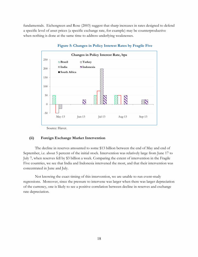
fundamentals. Eichengreen and Rose (2003) suggest that sharp increases in rates designed to defend a specific level of asset prices (a specific exchange rate, for example) may be counterproductive when nothing is done at the same time to address underlying weaknesses.

Figure 5: Changes in Policy Interest Rates by Fragile Five

Source: Haver.

(ii) Foreign Exchange Market Intervention

The decline in reserves amounted to some $13 billion between the end of May and end of

September, i.e. about 5 percent of the initial stock. Intervention was relatively large from June 17 to July 7, when reserves fell by $3 billion a week. Comparing the extent of intervention in the Fragile Five countries, we see that India and Indonesia intervened the most, and that their intervention was concentrated in June and July.

Not knowing the exact timing of this intervention, we are unable to run event-study regressions. Moreover, since the pressure to intervene was larger when there was larger depreciation of the currency, one is likely to see a positive correlation between decline in reserves and exchange rate depreciation.

-50

0

50

100

150

200

250

May-13 Jun-13 Jul-13 Aug-13 Sep-13

Changes in Policy Interest Rate, bps

Brazil Turkey

India Indonesia

South Africa

18

Figure 6: Weekly decline in Reserves (billion $) and percent change in Nominal Exchange Rate in India during May 23-End September, 2013

A: Contemporaneous Correlation

B: Reserve Declines lagged by a Week

May-23 May 31

June 7 June 14

June 21

June 28

July 5

July 12

July 19July 26

Aug 2

Aug 8

Aug 16

Aug 23

Aug 30

Sep 6

Sep 13

Sep 20

Sep 27

-4-2

02

4

-2 -1 0 1 2 3Decline in Reserves, $ bn

% Depreciation in Nominal Exchange Rate Fitted values

May 31

June 7June 14

June 21

June 28

July 5

July 12

July 19 July 26

Aug 2

Aug 8

Aug 16

Aug 23

Aug 30

Sep 6

Sep 13

Sep 20

Sep 27

-4-2

02

4

-2 -1 0 1 2 3Decline in Reserves lagged, $ bn

% Depreciation in Nominal Exchange Rate Fitted values

Exchange Dep=0.28+0.59***Reserve Decline (3.05)

Exchange Dep=0.83-0.26 Reserve Decline, lag (1.06)

19

Figure 6, where we plot the weekly change in reserves and the percentage change in the nominal exchange rate, confirms this. As predicted, we observe a positive correlation in Panel A (significant at the 1 percent level), i.e. a large decline in reserves was associated with greater exchange rate depreciation. In Panel B, we correlate percentage changes in the exchange rate and reserves, where the latter is lagged by a week. Here the correlation between the lagged values of decline in reserves and exchange rate depreciation is indistinguishable from zero.14

For one specific intervention announcement, however, we can do better. This is the foreign exchange swap window provided for oil importers. Oil adds up to $10 billion a month to India’s import bill. The demand for foreign exchange thus affects the level and volatility of the exchange rate (as per some estimates, the demand for foreign exchange from these companies is about $400 million a day). With this in mind, the RBI opened a separate swap window for three public sector oil companies on August 28, 2013, so as to remove their demand from the foreign exchange market. The measure can be thought of as analogous to foreign exchange market intervention, where rather than intervening when the demand for foreign exchange in general increases, the RBI automatically intervenes to meet the demand from the oil companies.

But why this particular form of foreign exchange market intervention should be preferable is not entirely clear. Moreover, it is not obvious either, whether with a daily turnover of about $50 billion in the onshore foreign exchange market, and presumably an equally large offshore market, the amount made available through the special swap window translated into a significant reduction in the demand for foreign exchange.

While some commentators reacted positively to this announcement, we find little evidence of a favorable impact on turnover in the onshore foreign exchange market, the exchange rate or equity markets in the week following. If anything, exchange rate depreciation accelerated in the week after this policy was announced (Table 7).

14 Similar charts for Turkey and Brazil, two other countries for which we have the weekly data on reserves, showed a similar relationship between the decline in reserves and exchange rate depreciation.

20

Table 7: Effect of the Separate Swap Window for Oil Importing Companies on Financial Markets

Note: Data used in the regressions runs from January 1, 2013-July 22, 2013. *, **, *** indicates that the coefficient is significantly different from zero at 10, 5 and 1 percent level of significance, t statistics are in parentheses. # the null hypothesis in each regression is that the policy announcement did not succeed in stabilizing the market, and the alternative hypothesis is that it succeeded; 1 percent level of significance is used to test the hypotheses, unless otherwise indicated.

(iii) Restrictions on Capital Outflows

On August 14, 2013, the RBI announced restrictions on capital outflows from Indian corporates and individuals. It lowered the limit on Overseas Direct Investment under the automatic route (i.e. the outflows which do not require prior approval of the RBI) from 400 percent to 100 percent of the net worth of the Indian firms, reduced the limit on remittances by resident individuals (which were permitted under the so-called Liberalized Remittances Scheme) from $200,000 to $75,000, and discontinued remittances for acquisition of immovable property outside India. Table 8 looks at outward remittances by residents subject to these restrictions. The amounts remitted were small, of the order of $100 million a month. There was no surge in remittances during the period of the tapering talk. Outflows were just $92 million in June and $110 million in July 2013, hence there does not seem to be an apparent justification for this restriction.

(1) (2) (3) (4) (5)

Log Exchange Rate

Log Stock Market Index

Log Forex Market Turnover

Portfolio Debt, $mn

Portfolio Equity, $mn

US Bond Yield 0.09*** -0.03** -0.22*** 113.02 -23.32

[13.15] [2.35] [2.87] [1.38] [0.29]

Dummy for tapering May 22-August 20 (α) 0.04*** 0.01 0.02 -281.76*** -179.39***

[8.00] [0.69] [0.36] [5.20] [3.40]

Dummy for a week prior to August 28, i.e. from August 21-August 27 (β) 0.09*** -0.06*** 0.13 -177.07 -288.62**

[9.70] [3.25] [1.20] [1.53] [2.56]

Dummy for a week from August 28 (dummy=1 for 5 working days from August 28) (γ) 0.13*** -0.06*** 0.15 -228.67** -171.92

[14.27] [3.11] [1.47] [2.11] [1.62]

Results for hypothesis comparing γ and β#

accept Ho: γ ≥ β, reject Ha: γ < β

accept Ho: γ ≤ β, reject Ha: γ > β

accept Ho: γ ≥ β, reject Ha: γ < β

accept Ho: γ ≤ β, reject Ha: γ > β

accept Ho: γ ≤ β, reject Ha: γ > β

Constant 3.83*** 8.74*** 11.33*** -158.07 198.73

[298.29] [342.55] [76.54] [1.02] [1.32]

Observations 165 168 164 162 162 R-squared 0.944 0.357 0.135 0.281 0.271 Adj. R-squared 0.943 0.341 0.113 0.263 0.252

21

Table 8: Amount of Outward Remittances under the Liberalized Remittances Scheme for

Resident Individuals (in million $) was rather modest

Avg. of 2012

Avg Jan-April 2013

May 2013

June 2013

July 2013

Aug 2013

Sep 2013

Oct 2013

Nov 2013

Dec 2013

Total 95.2 129.3 115.3 92.1 109.9 75.8 72.2 67.6 59.4 75.2

Deposits abroad 1.9 3.6 2.2 1.3 2.9 3.2 1.3 1.3 1.2 1.9

Purchase of Property 5 10.3 7.2 8.6 20.6 3 3.8 1.3 0.3 0.5

Investment in equity/debt 19.5 29.4 13.3 12.5 16.2 14.9 9.8 10.2 2.9 11.2

Gift 20.2 30.3 28.8 22.5 24.8 17.3 15.9 17.8 9.8 19.7

Donations 0.4 0.2 0.2 0.1 0.3 0.2 0.1 0.3 – 0.2

Travel 3.7 3.8 4.3 1.1 1 0.7 1 1 0.2 0.8 Maintenance of relatives 17.6 23.8 23.3 9.3 13.8 8.8 9.4 9.5 34.5 9.4

Medical Treatment 0.4 0.4 0.6 0.2 0.4 0.1 0.4 0.2 0.2 0.3

Studies Abroad 10.1 11.4 16.9 7.1 15.5 16.5 14.5 11.9 5.1 18.1

Others 16.5 16.5 18.5 29.4 14.5 11.1 16.2 13.9 5.2 13

Source: Reserve Bank of India.

Outflows once underway can be difficult to stem with these kinds of statutory restrictions, since incentives for evasion are strong. Table 9 confirms this. Here the dummy for the tapering period prior to the restrictions on outflows takes a value of 1 from May 22 to August 6, the dummy for the week prior to policy takes a value of 1 from August 7 to August 13, while the dummy for the policy announcements takes a value of 1 for five consecutive days from August 14. The results indicate that in the five days from the time when this announcement was made, the exchange rate depreciation and decline in stock market index were accentuated, while equity flows declined.

Commentary in the international financial press reflected the fears that these controls evoked (Economist, August 16, 2013, “…. India’s authorities have planted a seed of doubt: might India ‘do a Malaysia’ if things get a lot worse? Malaysia famously stopped foreign investors from taking their money out of the country during a crisis in 1998…”; and Financial Times, August 15, 2013, “… the measure smacks more of desperation than of sound policy”). It is perhaps revealing that none of the other members of the Fragile Five responded to the tapering talk by restricting outflows. India’s experience suggests that they were wise.

22

Table 9: Restrictions on Overseas Direct Investment (1) (2) (3) (4) (5)

Log Exchange Rate

Log Stock Market Index

Log Forex Market Turnover

Portfolio Debt, $mn

Portfolio Equity, $mn

US Bond Yield 0.08*** -0.00 -0.21** 84.99 -22.13

[11.10] [0.14] [2.40] [0.95] [0.24]

Dummy for tapering May 22-August 6 (α) 0.04*** -0.00 0.01 -269.33*** -181.64***

[9.26] [0.33] [0.26] [4.89] [3.28]

Dummy for a week prior to August 14, i.e. from August 7-August 13 (β) 0.06*** -0.05*** -0.06 -331.38*** -129.77

[7.51] [3.13] [0.57] [3.21] [1.25]

Dummy for a week from August 14 (dummy=1 for 5 working days from August 14) (γ) 0.07*** -0.07*** 0.03 -86.70 -228.04*

[7.98] [3.93] [0.31] [0.75] [1.97]

Results for hypothesis comparing γ and β#

Accept Ho: γ ≥ β, reject Ha: γ < β

Accept Ho: γ ≤ β, reject Ha: γ >

β

Accept Ho: γ ≥ β, reject Ha: γ < β

reject Ho: γ ≤ β, accept Ha: γ > β, at 5 %

Accept Ho: γ ≤ β, reject Ha: γ > β

Constant 3.85*** 8.68*** 11.29*** -105.41 196.49

[293.81] [323.85] [69.52] [0.62] [1.15]

Observations 156 159 155 154 154 R-squared 0.93 0.25 0.15 0.31 0.25 Adj. R-squared 0.93 0.23 0.12 0.29 0.23

Note: Data used in the regressions runs from January 1, 2013-August 21, 2013. *, **, *** indicates that the coefficient is significantly different from zero at 10, 5 and 1 percent level of significance, t statistics are in parentheses. # the null hypothesis in each regression is that the policy announcement did not succeed in stabilizing the market, and the alternative hypothesis is that it succeeded; 1 percent level of significance is used to test the hypotheses, unless otherwise indicated.

(iv) Import Duty on Gold (June 5, August 13, and September 18)

Rising gold imports being partly responsible for the deteriorating current account balance, import duties on gold were raised from the existing 6 percent to 8 percent on June 5 and further to 10 percent on August 13. On September 18, the duty on the imports of gold jewelry was then raised to 15 percent. Some other quantitative restrictions, such as prohibiting the import of gold coins, and a 20/80 rule requiring that 20 percent of the gold imports be made available to exporters while 80 percent could be used domestically, were introduced as well.

The results in Table 10 for the first duty increase on June 5 show that these duties had little

positive effect. The rate of exchange rate depreciation increased in the five day window following

23

the imposition of the duty, compared to the week before or the tapering period prior to that. The stock market declined, and portfolio inflows were smaller as well. These increases in import duties were ineffective because, rather than dealing with the causes of financial weaknesses, they only addressed the symptoms. Insofar as higher duties on gold imports were equivalent to tighter restraints on capital outflows, they appeared to have an analogous (unfavorable) impact on financial markets.

The increase in the duty on gold imports had some other unintended effects as well. Even

as they curtailed the import of gold (Figure 7), higher gold prices also dented exports of gold jewelry. The press reported frequent complaints from exporters about the increase in the price of gold bullion following the increase in duty. Moreover, a large difference between the domestic and international price of gold could generate incentives for smuggling of gold. The latter apparently did happen. The World Gold Council estimated that nearly 200 tons of gold was smuggled into India following the increase in duty (see Reuters, July 10, 2014). This is a reminder of the situation in India until the early 1990s, when due to high import duties on gold, as well as an artificially appreciated exchange rate, smuggling of gold was rampant and also contributed to a thriving parallel market for foreign exchange to convert proceeds from smuggled gold into rupees at a premium. As a part of the reforms of the early 1990s, import duties on gold were abolished and the exchange rate was devalued and eventually floated, bringing an end to smuggling as well as the parallel market for the exchange rate. All these are reasons not to rely too heavily on measures such as import duties and certainly not for too long.

24

Table 10: Increase in the Import Duty on Gold (on June 5) and the Effects on Exchange Rate and Financial Markets

(1) (2) (3) (4)

Log Exchange Rate

Log Stock Market Index

Portfolio Debt, $mn

Portfolio Equity, $mn

US Bond Yield -0.01 0.08*** -265.42* 337.23**

[0.70] [3.40] [1.72] [2.11]

Dummy for tapering May 22-May 28(α) 0.03*** 0.01 -154.11* -145.16

[5.41] [0.76] [1.77] [1.60]

Dummy for a week prior to June 5, i.e. from May 29-June 4 (β) 0.04*** 0.00 -231.18*** -143.40

[8.58] [0.06] [2.76] [1.65]

Dummy for a week from June 5 (dummy=1 for 5 working days from June 5) (γ) 0.06*** -0.02* -335.04*** -245.87***

[11.99] [1.76] [3.93] [2.77]

Results for hypothesis comparing γ and β#

Accept Ho: γ ≥ β, reject Ha: γ < β

Accept Ho: γ ≤ β, reject Ha: γ > β

Accept Ho: γ ≤ β, reject Ha: γ > β

Accept Ho: γ ≤ β, reject Ha: γ > β

Constant 4.01*** 8.53*** 552.79* -478.55 [243.27] [186.14] [1.91] [1.59] Observations 107 110 106 106 R-squared 0.727 0.146 0.332 0.088 Adj. R-squared 0.717 0.113 0.305 0.0516

Note: Data used in the regressions runs from January 1, 2013-June 10, 2013. *, **, *** indicates that the coefficient is significantly different from zero at 10, 5 and 1 percent level of significance, t statistics are in parentheses. # the null hypothesis in each regression is that the policy announcement did not succeed in stabilizing the market, and the alternative hypothesis is that it succeeded; 1 percent level of significance is used to test the hypotheses, unless otherwise indicated.

Figure 7: Duties on Gold Imports helped restrain the (reported) import of Gold

Source: Reserve Bank of India

0

1000

2000

3000

4000

5000

6000

7000

8000

9000

Dec-

11

Jan-

12

Feb-

12

Mar

-12

Apr-

12

May

-12

Jun-

12

Jul-1

2

Aug-

12

Sep-

12

Oct

-12

Nov

-12

Dec-

12

Jan-

13

Feb-

13

Mar

-13

Apr-

13

May

-13

Jun-

13

Jul-1

3

Aug-

13

Sep-

13

Oct

-13

Nov

-13

Dec-

13Gold Import (US$ Mn)

Jun.5,2013 Import duty on

gold raised to 8% from 6%

Aug.13,2013 Import duty on gold

raised to 10% from 8%

Sep.18,2013 Import duty on gold

raised to 15% from 10%

25

(v) Communication and Guidance

As noted earlier, there was little additional guidance from the government or the central bank in August, even as the exchange rate appeared to go into freefall (the exchange rate depreciated by nearly 10 percent from August 15 to September 4). On September 4, the new RBI governor issued a statement expressing confidence in the economy and highlighting its comfortable reserve position. He announced new measures to attract capital through deposits targeted at the Indian diaspora, and relaxed some of the restrictions on outward investment which had been tightened earlier. While we cannot separate out the effect on the markets of each of these different announcements, we can assess their combined effect. Table 11 shows that the exchange rate and stock market improved markedly within five days of the announcements on September 4.

Table 11: Policy Announcements, Statement and Press Conference on September 4, 2013

(1) (2) (3) (4) Log Exchange Rate Log Stock Market

Index Portfolio Debt, $ mn

Portfolio Equity, $ mn

US Bond Yield 0.11*** -0.05*** 144.73* -50.25 [14.42] [4.00] [1.86] [0.66] Dummy for tapering May 22-August 27 (α)

0.03*** 0.01 -293.92*** -170.32***

[5.67] [1.53] [5.50] [3.27] Dummy for a week prior to Sep 4, i.e. from Aug 28-Sep 3 (β)

0.11*** -0.04* -257.59** -147.36

[10.97] [1.94] [2.43] [1.43] Dummy for a week from Sep 4 0.07*** 0.02 -193.87* 75.12 (dummy=1 for 5 working days from Sep 4) (γ)

[6.20] [1.25] [1.70] [0.68]

p value for hypothesis γ= β, against the alternative hypothesis

Reject Ho: γ= β Accept Ha: γ< β

Reject Ho: γ= β Accept Ha: γ> β

reject Ho: γ= β

accept Ha: γ> β

reject Ho: γ= β accept Ha: γ> β

Constant 3.79*** 8.78*** -217.64 249.32* [269.90] [345.87] [1.48] [1.74] Number of observations 170 173 167 167 R-squared Adjusted R-squared 0.93 0.26 0.253 0.248 Note: Data used in the regressions runs from January 1, 2013-Sep 11, 2013. *, **, *** indicates that the coefficient is significantly different from zero at 10, 5 and 1 percent level of significance, t statistics are in parentheses. # the null hypothesis in each regression is that the policy announcement did not succeed in stabilizing the market, and the alternative hypothesis is that it succeeded; 1 percent level of significance is used to test the hypotheses, unless otherwise notes.

26

(vi) Summary In sum, many elements of the policy response to the tapering talk proved to be ineffective or counterproductive. The very sharp increase in policy interest rates, taken without adequate explanation and not accompanied by steps to address the underlying weaknesses of the economy, did not reassure the markets. Efforts to restrict capital outflows and discourage gold imports undermined confidence and encouraged evasion. The much-talked-about foreign exchange window for state-owned oil importers does not appear to have been effective according to our estimates. Better, in our view, would have been measured increases in interest rates and measured intervention in the foreign exchange market, supplemented by a clear communication strategy describing what other steps were being taken to address the underlying economic and financial weaknesses that had rendered the Indian economy vulnerable.

V. The Medium-Term Policy Framework

Once a country is in the midst of experiencing the impact of global rebalancing, there may not be any easy choices. It is better in our view to put in place a medium-term policy framework that limits vulnerabilities, avoiding that crisis in the first place while maximizing the policy space to respond to shocks. While maintaining a sound fiscal balance, sustainable current account deficit, and environment conducive to investment is, for obvious reasons, integral to such a framework, there are in addition some other less obvious elements. These include managing capital flows so as to encourage relatively stable longer-term flows while discouraging volatile short-term flows, avoiding excessive appreciation of the exchange rate through interventions using reserves and macroprudential policy, holding a larger stock of reserves, where feasible signing swap lines with other central banks, and preparing the banks and corporates to handle greater exchange rate volatility. We discuss some of these in greater detail below.

(i) Level of Reserves

Average reserve holding in emerging markets has increased sharply in the last four decades, from about 5 percent of GDP in the 1980s to 25 percent in 2010s (see Ghosh, Ostry and Tsangarides, 2012). Emerging markets hold reserves for a variety of reasons: mercantilist, as insurance against shocks to their current and capital accounts, as an indicator of external solvency, and as ammunition with which to stabilize the exchange rate. While in the 1980s and 1990s countries held reserves mainly to defend the level of their exchange rate and to insure against shocks to the current account, insuring against shocks to the capital account has become a more important motivation in the last two decades (Ghosh et al 2012).

There are several popular metrics available for the appropriate level of reserves. There is the

well-known Greenspan-Guidotti rule that an emerging market should hold reserves equivalent to a year of short-term liabilities. Rules based on import requirements consider reserves equivalent to about 3-6 months of imports to be adequate. Yet another metric defines the adequate level of

27

reserves with respect to the supply of broad money and considers reserves equivalent to 20 percent of M2 to be sufficient to guard against shocks to the capital account. The IMF considers any single metric to be inadequate and instead combines the aforementioned in a risk weighted composite index to assess the reserve adequacy of its member countries.

Even as India’s reserves appear adequate on most of these metrics, examining the level of

reserves more closely, one can observe two distinct eras since 2000 (Figure 8).15 The first lasted from 2000 to 2008, when reserves increased from $40 billion to $305 billion. Reserves then declined to $245 billion by end 2008, due to the withdrawals of capital after the collapse of Lehman Brothers. In the second era reserves were rebuilt to some $300 billion during 2009-2011, but only to the level last seen before the collapse of the Lehman Brothers, at which level they then remained broadly stable. There were no attempts to increase the reserves coverage further during this period. As a result, with the growth of the economy and external liabilities, the effective reserve coverage in India declined from 2008 (Figure 9), implying heightened vulnerability to current account or capital account shocks and a narrower room to intervene in the foreign exchange market.

Figure 8: The Stock of External Reserves in India has remained Stable since 2009 ($

billion)

Note: Total reserves include net foreign assets, SDR, and gold. Source: Reserve Bank of India.

15 India’s reserve level has been considered adequate in the IMF’s assessment of the Indian economy. The IMF is however currently revising its reserves metrics and is likely to revise upwards the desirable level of reserves for oil importing countries such as India, who need to hold a larger reserve buffer to meet the cost of importing oil, the demand for which is inelastic and the import bill often volatile due to the volatility of oil prices.

0

50

100

150

200

250

300

350

0

50

100

150

200

250

300

350

2000

01

2000

09

2001

05

2002

01

2002

09

2003

05

2004

01

2004

09

2005

05

2006

01

2006

09

2007

05

2008

01

2008

09

2009

05

2010

01

2010

09

2011

05

2012

01

2012

09

2013

05

2014

01

Total Reserves

Total Reserves Net of ForwardPositionNet Foreign Assets

28

Figure 9: Effective Coverage provided by Foreign Reserves has declined

In terms of External Debt Short Term Debt

GDP and in the Months of Imports

Source: Citi Bank Research. Total External Debt includes: long-term debt (multilateral, bilateral, IMF, trade credit, ECB, NRI&FC above 1 year maturity and Rupee debt) and short-term debt (NRI&FC deposits up to 1year maturity, bills and other instruments and other trade related debts).

The use of reserves to curb exchange rate volatility also differs across these two periods. There seems to have been a reluctance to use reserves since 2008 to modulate exchange rate volatility, reflected in smaller monthly percentage changes in reserves but increased volatility of the exchange rate between 2009 and 2012 (Figure 10). This increase in volatility is not confined just to the period immediately after the collapse of Lehman or that during the tapering talk, but extends

40

60

80

100

120

140

160

180

2003

2004

2005

2006

2007

2008

2009

2010

2011

2012

2013

2014

Reserves, % of External Debt

0

500

1000

1500

2000

2500

3000

2003

2004

2005

2006

2007

2008

2009

2010

2011

2012

2013

2014

Reserves, % of Short Term Debt

10

15

20

25

30

2003

2004

2005

2006

2007

2008

2009

2010

2011

2012

2013

2014

Reserves, % of GDP

4

8

12

16

2020

03

2004

2005

2006

2007

2008

2009

2010

2011

2012

2013

2014

Reserves in Months of Imports

29

through the entire period since 2009.16 This hints at more passive reserve management as a factor in increased volatility of the exchange rate.

Figure 10: Changes in Reserves and Volatility in Exchange Rate Since 2000

A: Percent Changes in Reserves (monthly) have become smaller since 2009…

Note: Averages are calculated for January 2000-September 2008 and April 2009-Decemebr 2013. These averages are significantly different from each other at 1 percent level of significance.

16 One might argue that the increased volatility of exchange rate is a global phenomenon, and afflicted all emerging markets post 2008. We calculated similar measures of volatility for all Fragile Five countries, but observed that besides India no other country experienced a similar increase in volatility. There is empirical evidence to support the idea that high levels of exchange rate volatility can distort investment decisions and affect long-term growth, especially in countries with low levels of financial development (see Serven 2003 and Aghion et al. 2009).

-.1-.0

50

.05

.1

2000m1 2002m1 2004m1 2006m1 2008m1 2010m1 2012m1 2014m1obs

% Change in Reserves Average 2000-2008Average 2008-2013

30

B: …..While the Volatility in Exchange Rates (monthly standard deviation) has Increased since 2009

Note: Averages are calculated for January 2000-September 2008 and April 2009-Decemebr 2013. These averages are significantly different from each other at 1 percent level of significance.

C: ….Increased volatility of Nominal Exchange Rate since 2009 is also evident in

daily data (larger spread is seen in % change in daily exchange rate)

Note: calculated using data from Bloomberg.

-4

-3

-2

-1

0

1

2

3

4

5

01/0

4/00

08/0

4/00

03/0

4/01

10/0

4/01

05/0

4/02

12/0

4/02

07/0

4/03

02/0

4/04

09/0

4/04

04/0

4/05

11/0

4/05

06/0

4/06

01/0

4/07

08/0

4/07

03/0

4/08

10/0

4/08

05/0

4/09

12/0

4/09

07/0

4/10

02/0

4/11

09/0

4/11

04/0

4/12

11/0

4/12

06/0

4/13

01/0

4/14

Collapse of Lehman Tapering Talk

0.5

11.

52

2000m1 2002m1 2004m1 2006m1 2008m1 2010m1 2012m1 2014m1obs

Std Dev of % Change in Exchange Rate Average 2000-2008Average 2008-2013

31

What about the cost of holding reserves? Reserves are typically invested in liquid treasury bills of the countries which issue hard currencies and generate returns lower than the domestic assets. Available estimates suggest that these costs are smaller than sometimes believed. Some researchers argue that the estimates of the cost of holding reserves should take in to account not just the interest rate differential, but also the valuation gains that accrue on reserves. Friedman (1953) suggested that if the central banks purchase dollars when the exchange rate is overvalued and sell them when it is undervalued, valuation changes may offset and even outweigh the interest rate differential. Similarly, Flood et al. (2002) suggested that once the capital gains arising from exchange rate changes are taken into account, the opportunity cost of holding reserves is likely to be small.

A recent regional report of the World Bank (see World Bank 2013) estimates the cost of

central bank intervention in the foreign exchange market for several emerging countries. These estimates suggest that the cost of intervention is small across countries and indeed negative for some of the countries. The report estimates a net gain to India from intervention in its foreign exchange market between 2005 and 2012 to be about 1 percent of its 2012 GDP.

The actual cost of intervention is likely to be yet smaller than the one which accounts for the

interest rate differential and the valuation effects (see Levy Yeyati, 2008), because larger reserve holdings may lower the cost of issuing sovereign or even private debt. The World Bank report suggests that if the central banks still deem the cost of holding reserves to be high, they may want to consider holding a proportion of their reserves in higher yield assets, than the lower yield treasury bills, as some central banks have indeed started doing. The report reminds that, since the central banks hold reserves for a variety of reasons, the entire cost cannot be attributed to any one objective, such as to smooth exchange rate movements.

(ii) Swap Lines as a Substitute for Reserves? But Swap Line with Whom?

Since there are costs as well as benefits to holding reserves and there is no consensus on

what constitutes an optimal level, a recent discussion that has gained some currency (as it were) is whether bilateral swap lines with other central banks, regional swap lines such as under the Chiang Mai initiative or BRICS Contingent Reserve Arrangement, or multilateral lines such as the liquidity arrangements with the IMF present attractive alternatives.

Eichengreen (2014) argues that, given the reluctance of the US Congress to authorize increased funding for the IMF, the Fed should contemplate extending swap lines to a larger number of emerging economies. Mohan and Kapur (2014) suggest that since monetary policies of the advanced economies have important spillovers for emerging markets, the latter ought to be offered swap facilities to limit this impact. Sheng (2014) too emphasizes the need for the emerging markets to rely on swap lines, but he points out that the swap lines with the US Fed are available only selectively, and the emerging markets in general do not figure in these. Hence he suggests that the emerging markets should consider a diverse set of arrangements, including signing swap

32

arrangements with China, which has emerged as a large regional as well as global player in offering these swap lines, and pursuing regional arrangements such as the Chiang Mai Initiative (CMI) or the Contingent Reserve Arrangement (CRA) being planned by the BRICS.

The most recent initiative along these lines is the BRICS’s CRA, negotiated in summer 2014,

under which the member countries committed $100 billion of reserves to the arrangement. India’s share is $18 billion, and it can withdraw twice as much from the arrangement. Just to put the size of this withdrawal facility in perspective for India, note that the net amount (above its own commitment to the pool) it can withdraw is less than half the size of its current swap line with Japan and barely 5 percent of its reserves. Revealingly, negotiation of an IMF program is a precondition for drawing funds from the BRICS’s CRA above the first 30 percent, just as in the CMI. The unencumbered 30 percent appears to be a rather modest amount.

The question about this arrangement is whether it will actually operate or would meet the

same fate as the CMI. Participants of the CMI have been reluctant to put actual cash on the barrelhead, since they are reluctant to impose policy conditions of the sort that will maximize the likelihood of them being paid back (conditionality among neighbors being politically delicate).17 There may similarly be a reluctance to provide net resources under the CRA. While any member country can request access to the swap line up to its limit, but that request must be acceded to by the providing parties. And whether they will accede is yet to be seen.

Rajan (2014) suggests that since the IMF possesses the expertise to operate such lines, is free

of political obligations to explain to the domestic stakeholders if a credit risk emerges in these arrangements, and has the capacity to bear such risks if they arise, swap arrangements should be channeled through it. Rajan also suggests that the IMF could act as a facilitator, helping countries identify the counterparts who would be amenable to signing the bilateral or regional swap arrangements, and if needed, mediating negotiation of these swap lines. He also proposes modifications to the IMF’s existing liquidity line so as to reduce the stigma of accessing the facility and ensure its wider use by the member countries.

The countries with which India might be able to sign bilateral swap lines would perhaps be

its large trading partners or the countries where foreign investment to India originates, in other words the countries which have a stake in the stability of its currency and economy. Such swap lines would be considered credible if signed with countries that are not considered to be in the same asset class as India by global investors, and thus are not likely to be affected in a similar manner by a rebalancing of global portfolios or global financial conditions. Based on these considerations, some

17 The $100 billion of reserves are not going into a common pool. Rather, each country will continue to hold its own reserves; the commitment to provide dollars against local currency is only on paper.

33

countries that India could explore bilateral swap lines with include the US, UK, Japan, the Republic of Korea, and the countries from which India imports its oil.18

Is a swap line with the US a viable option for India? Apparently the US is very selective in

offering these lines. In October 2008, the Federal Reserve Board agreed to offer liquidity swap lines to four large emerging markets, Mexico, Brazil, Singapore and Korea. These were for $30 billion each (similar in amount to the lines offered to Canada, Sweden, and Australia). The transcripts of Federal Open Market Committee (FOMC) meetings on October 23-24, 2008, suggest that these lines were offered not just because the countries in question faced liquidity risk, but also because they were considered of systemic importance to the United State, given their financial linkages with the US economy.19 Fed officials worried that if these countries faced liquidity problems, these could spill over to the US financial institutions, given the large presence of the US financial institutions in these countries. The FOMC was also emphatic that since all of these countries held substantial reserves, a large part in US treasury bonds, swap arrangements with them carried little credit risk.

Even then in essence the swap arrangements offered to the emerging markets were less

generous than the ones offered to the developed countries, and entailed additional safeguards. Emerging markets could draw only with the prior authorization of the Fed, with individual drawings each time limited to $5 billion; central banks were required to publicly announce when they drew on their lines and to provide details of the allocation of dollar liquidity they thus obtained. And though the Fed converted the dollar swap lines put in place during the global financial crisis with the Bank of Canada, Bank of England, European Central Bank, Bank of Japan, and Swiss National Bank into longer arrangements in October 2013, the swaps with emerging markets were allowed to expire after six months.20

There was extensive discussion in the committee on whether any other emerging markets

would be considered for swap arrangements if they approached the Fed. It acknowledged and discussed whether by selecting a small group of countries for the swap arrangements the Fed was exposing the rest of the countries, which were not offered similar arrangements, to negative market reactions. The committee decided that the swap lines would not be extended to any other emerging

18 While it is difficult to anticipate what amount of additional swap lines would provide the required buffer to India in addition to its existing $300 plus billion of reserves, but perhaps something of the order of $100 billion of unconditional line would be adequate. 19 Some of these contentions are confirmed by Aizenman et al (2010) in their empirical work conducted before these minutes were published. They established that the swap lines were offered selectively by the Fed to the countries with which the US had substantial trade and financial linkages. The few emerging markets it offered the lines to were the ones in which the US banks had exposure; hence the US inherently had a stake in their financial stability. Apparently India does not enjoy this advantage with the US. 20 The amounts of swap lines with developed economies were larger, adding upto $333 billion, compared to $120 billion offered to the emerging markets. Sheng compares the arrangements signed between the Fed and these emerging markets with the swap offers that the PBOC signed with about a score of developing countries most of which export commodities to China. The latter added up to over US$426 billion, implying that the China offered a more viable alternative to developing countries than the Fed.

34

country, which would instead be directed to utilize a new IMF facility, which was to be announced in conjunction with the Fed’s swap line the following day. Prasad (2014) and Steil (2014) note that in 2008 the Fed rebuffed requests for swaps from Chile, the Dominican Republic, Indonesia and Peru, and in 2012 it spurned a request from India. The swap arrangements that most emerging markets could access were with larger, more developed Asian economies such as China, Japan and Korea, rather than with the United States, European Union or other advanced economies (Figure 11).21

This leads us to conclude that India should not expect to rely on arrangements with the

United States, alone or even in part, in the event of future difficulties and should seek other alternatives.

India’s only existing swap line, other than the CRA, is with Japan, as noted above. This was

originally signed in 2008 for $3 billion, but was raised to $15 billion in December 2011, and again to $50 billion on September 6, 2013.22 Around the time when Japan extended its swap line with India, it also signed swap lines with Indonesia and the Philippines, and in addition was committed to swap lines to other countries in ASEAN as a part of the Chiang Mai Initiative. Given the extent of Japan’s existing commitments, there may be limits to how much further the existing India-Japan swap line can be expanded.

One multilateral option that India can consider is a precautionary facility with the IMF. As is well known, these precautionary lines of credit have been used very sparingly by the IMF members (only Mexico, Poland and Colombia have applied). Apparently, approaching the IMF for a precautionary line of credit conveys an adverse signal to market participants.23 Indian policy makers appear to be strongly convinced by this argument. It would be worth the investment to understand how countries like Mexico have managed to apply without suffering such stigma effects.

21 We have presented a selective list of swap lines that the Bank of China signed with other countries. 22 Our understanding is that under this agreement after the first $15bn, India can draw the rest $35 bn only after it has negotiated an IMF program. 23 A similar sentiment was recorded in the minutes of the Fed’s meetings held on October 28-29, 2008, where it was noted (by Nathan Sheets), that “…..these top-tier EMEs that we are recommending for swap lines are very reluctant to return to the IMF. Given the strength of their policies, they no longer view themselves as clients..”; and subsequently (Eric Rosengren) “….. going to the IMF will attach a fair amount of stigma [to the country]. … the spillover benefits to other countries will be negative, not positive, because of that stigma.”

35

Figure 11: Selective Recent Currency Swap Lines Offered by the Larger Asian Economies

Note: Sep.6, 2013: India and Japan signed $50bn currency swap agreement. Source: RBI. Oct.7, 2013: Indonesia and China signed $16bn currency swap agreement. Source: Bloomberg. Oct.12, 2013: Indonesia and Korea signed $10bn currency swap agreement. Source: WSJ. Dec.14, 2013: Indonesia and Japan signed $22.7bn currency swap agreement. Source: Bank of Indonesia Mar.26, 2013: Brazil and China signed $30bn currency swap agreement. Source: BBC Dec.16, 2013: Philippines and Japan signed $12bn currency swap agreement. Source: WSJ. Oct.13, 2013: UAE and Korea signed $5.4bn currency swap agreement. Source:globaltimes.com Oct.20, 2013: Malaysia and Korea signed $4.7 currency swap agreement. Source:Koreaherald.com Sep.9, 2013: Hungary and China sign $1.62bn currency swap line. Source:centralbanking.com Sep.13, 2013: Albania and China sign $0.33bn currency swap line. Source: Reuters Apr.2, 2014: Albania and China sign $0.34bn currency swap line. Source: Reuters Some bilateral currency swap lines are excluded from figures such as China-UK ($32.6bn), China-ECB ($57.2bn), and Korea-Australia ($7.4bn).

We conclude that there do not seem to be many leads for India to extend the swap lines for larger amounts or to sign new lines with advanced economies. While India could continue exploring these further with advanced economies as well as with oil exporting countries, it seems, just like the rest of the emerging world, it would continue to be on its own in handling the spillovers of monetary policy in advanced economies. A similar view has been aired by the IMF (2013), whereby, “Reserves remain a critical liquidity buffer for most countries. They are generally associated with lower crisis risk (crisis prevention) as well as space for authorities to respond to shocks (crisis mitigation).

0

10

20

30

40

50

60

India Indonesia Brazil Philippines UAE Malaysia Hungary Albania

Billion $

Currency Swap Lines

Bank of Japan

Bank of Korea

People's Bank of China

36

While other instruments, such as official credit lines and bilateral swap lines, are also external buffers, for most countries they principally act as a complement to their official reserves.”24

(iii) Managing Capital Flows

Capital flows that emerging markets receive are generally considered to be more volatile than the ones other countries receive. However recently Bluedorn et al. (2013) noted that private capital flows are typically volatile for all countries, across all points in time, and for all types of capital flows (bank flows, portfolio debt and equity flows, etc.). They recommended using macroeconomic and macroprudential measures to buttress economic and financial resilience to such volatility.

In a similarly dire view in its Global Financial Stability Report, published in April 2014, the IMF acknowledged that “the reduction in US monetary accommodation could have important spillovers for advanced and emerging market economies alike as portfolios adjust and risks are repriced.” It noted that the increased participation of foreign investors in domestic bond markets has increased the volatility of capital flows to emerging markets. Even as the financial markets have deepened and become more globalized, new asset classes have developed, and the role of bond funds—especially local currency bond funds, open-ended funds with easy redemption options, and funds investing only opportunistically in emerging markets—has increased. These global portfolio investors and bond flows are sensitive to global financial conditions. The Fund’s recommendation, of particular relevance to India, is to monitor and limit the size of foreign investors in local bond markets, even as the attempts are needed to increase the participation of local investors in the bond markets.

India actively monitors and manages its capital flows. It has retained quantitative restrictions

on several categories of capital inflows including on portfolio equity and debt flows. Total outstanding investment by foreign investors in government and corporate bonds are subject to different ceilings, while portfolio equity flows are subject to limits on such investment in each firm and in different sectors. India has also retained certain restrictions on capital outflows, but these apply mostly to residents. These restrictions limit the amounts that individuals can withdraw from the country each year, e.g., firms may invest abroad only up to a certain multiple of their net worth. The amounts that Indian firms can borrow abroad are also monitored and, in some instances, are subject to RBI approval; and there are limits on the interest rates at which the firms can borrow abroad.

Capital flows to India consist of FDI flows, portfolio debt and equity flows, borrowing abroad by Indian firms (called external commercial borrowings) and bank deposits by the Indian diaspora (often known as non-resident Indian deposits or NRI deposits). While FDI inflows and external commercial borrowings to India have been relatively stable, as has been the experience of other emerging markets, portfolio flows, and especially debt flows, into India have been more

24 The IMF however cautions, rightly so, that the reserves cannot substitute for sound fundamentals and a good policy framework.

37

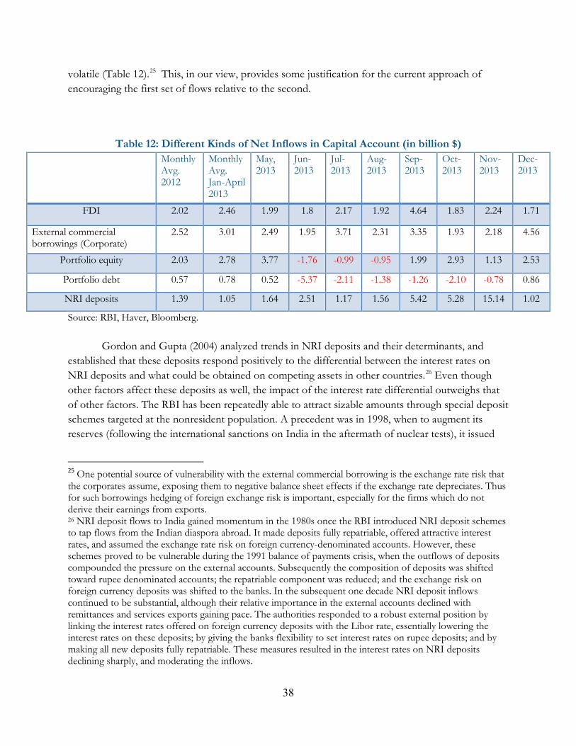
volatile (Table 12).25 This, in our view, provides some justification for the current approach of encouraging the first set of flows relative to the second.

Table 12: Different Kinds of Net Inflows in Capital Account (in billion $) Monthly

Avg. 2012

Monthly Avg. Jan-April 2013

May, 2013

Jun-2013

Jul-2013

Aug-2013

Sep-2013

Oct-2013

Nov-2013

Dec-2013

FDI 2.02 2.46 1.99 1.8 2.17 1.92 4.64 1.83 2.24 1.71

External commercial borrowings (Corporate)

2.52 3.01 2.49 1.95 3.71 2.31 3.35 1.93 2.18 4.56

Portfolio equity 2.03 2.78 3.77 -1.76 -0.99 -0.95 1.99 2.93 1.13 2.53

Portfolio debt 0.57 0.78 0.52 -5.37 -2.11 -1.38 -1.26 -2.10 -0.78 0.86

NRI deposits 1.39 1.05 1.64 2.51 1.17 1.56 5.42 5.28 15.14 1.02

Source: RBI, Haver, Bloomberg.

Gordon and Gupta (2004) analyzed trends in NRI deposits and their determinants, and established that these deposits respond positively to the differential between the interest rates on NRI deposits and what could be obtained on competing assets in other countries.26 Even though other factors affect these deposits as well, the impact of the interest rate differential outweighs that of other factors. The RBI has been repeatedly able to attract sizable amounts through special deposit schemes targeted at the nonresident population. A precedent was in 1998, when to augment its reserves (following the international sanctions on India in the aftermath of nuclear tests), it issued

25 One potential source of vulnerability with the external commercial borrowing is the exchange rate risk that the corporates assume, exposing them to negative balance sheet effects if the exchange rate depreciates. Thus for such borrowings hedging of foreign exchange risk is important, especially for the firms which do not derive their earnings from exports. 26 NRI deposit flows to India gained momentum in the 1980s once the RBI introduced NRI deposit schemes to tap flows from the Indian diaspora abroad. It made deposits fully repatriable, offered attractive interest rates, and assumed the exchange rate risk on foreign currency-denominated accounts. However, these schemes proved to be vulnerable during the 1991 balance of payments crisis, when the outflows of deposits compounded the pressure on the external accounts. Subsequently the composition of deposits was shifted toward rupee denominated accounts; the repatriable component was reduced; and the exchange risk on foreign currency deposits was shifted to the banks. In the subsequent one decade NRI deposit inflows continued to be substantial, although their relative importance in the external accounts declined with remittances and services exports gaining pace. The authorities responded to a robust external position by linking the interest rates offered on foreign currency deposits with the Libor rate, essentially lowering the interest rates on these deposits; by giving the banks flexibility to set interest rates on rupee deposits; and by making all new deposits fully repatriable. These measures resulted in the interest rates on NRI deposits declining sharply, and moderating the inflows.

38

the Resurgent India Bond--targeted at the NRI community, at an interest rate of 7¾ percent on US dollar deposits and raised $4.2 billion within days. It offered a second scheme in 2000, the Indian Millennium Deposit, and was able to raise $5.5 billion at an interest rate of 8½ percent. A similar phenomenon was observed during the tapering talk episode. By providing certain incentives to the banks, the RBI managed to attract a large amount of NRI deposits through banks—net deposit mobilization was of the order of $30 billion between September and December 2013. The success implies that marketing bonds or deposits to the Indian diaspora as a crisis mitigation strategy could be deployed in the future as well.

VI. Conclusion

Starting in May 2013, expectations that the Federal Reserve would begin reducing the pace of its securities purchases had a large adverse impact on emerging markets. India was among those hit hardest. Between May 22, 2013, and the end of August 2013, the rupee depreciated by 18 percent, and stock prices, foreign reserves and portfolio flows all declined. The reaction was sufficiently pronounced for the press to warn that India might be heading toward a financial crisis, the kind that requires an emerging market to resort to the IMF.

Why India? Because it had received large capital flows in prior years and had large and liquid financial markets that were a convenient target for investors seeking to rebalance away from emerging markets. An additional factor was that the macroeconomic conditions had weakened noticeably in prior years, which rendered the economy vulnerable to capital outflows and exchange rate depreciation and narrowed the policy space. The deterioration in fundamentals was intertwined with the sizable amounts of capital that India imported during the period of zero interest rates and quantitative easing in the United States and other advanced economies. Rebalancing by global investors when the Fed began to talk of tapering highlighted these vulnerabilities.

The authorities adopted several measures in response, intervening in the foreign exchange market, hiking interest rates, raising the import duty on gold, introducing measures to encourage capital flows from the Indian diaspora, easing demand pressure in foreign exchange markets by opening a separate swap window for oil importing companies, and extending a swap line with the Bank of Japan. The Reserve Bank also sought to restrict capital outflows from Indian residents and companies.

Many elements of the policy response to the tapering talk proved to be ineffective or counterproductive. The very sharp increase in policy interest rates, taken without adequate explanation and not accompanied by steps to address the underlying weaknesses of the economy, did not reassure the markets. Efforts to restrict capital outflows and discourage gold imports undermined confidence and encouraged evasion. The foreign exchange window for state-owned oil importers does not appear to have had much effect. Better, in our view, would have been measured increases in interest rates and measured intervention in the foreign exchange market, supplemented

39

by a clear communication strategy describing what other steps were being taken to address the underlying economic and financial weaknesses that had rendered the Indian economy vulnerable.

These results emphasize that once a country is affected by the global rebalancing of portfolios, there are no easy choices. Better is to put in place a medium-term policy framework that limits vulnerabilities, avoiding that crisis in the first place while maximizing policy space for responding to such shocks. Maintaining a sound fiscal balance, sustainable current account deficit, and environment conducive to investment are, for obvious reasons, integral to such a framework. In addition there are some less obvious elements. These include managing capital flows so as to encourage relatively stable longer-term flows while discouraging volatile short-term flows, avoiding excessive appreciation of the exchange rate through interventions using reserves and macroprudential policy, holding a larger stock of reserves, and preparing the banks and the corporates to handle greater exchange rate volatility. India’s experience also suggests abstaining from introducing new constraints on capital outflows in the midst of a crisis, since these can aggravate the loss of confidence. Finally, those who implement a medium-term framework and adopt emergency crisis-management measures, alike, need to adopt a clear communication strategy so as to interact smoothly and transparently with market participants.

40

References

Aghion, Philippe, Philippe Bacchetta, Romain Ranciere, and Kenneth Rogoff. 2009. “Exchange Rate Volatility and Productivity Growth: The Role of Financial Development,” Journal of Monetary Economics, Vol. 56, pp. 494-513.

Aizenman, Joshua and Gurnain Kaur Pasricha. 2010. “Selective Swap Arrangements and the Global Financial Crisis: Analysis and Interpretation,” International Review of Economics and Finance, Vol. 19, pp. 353 Bluedorn, John, Rupa Duttagupta, Jaime Guajardo, and Petia Topalova. 2013. “Capital Flows are Fickle: Anytime, Anywhere,” IMF Working Paper WP/13/183 , Washington DC. Cordella, Tito, Pablo Mariano Federico, Carlos A. Vegh, and Guillermo Vuletin. 2014. “ Reserve Requirements in the Brave New Macroprudential World, Brookings Institution,” World Bank Policy Research Working Paper No. 6793, Washington DC. Economist. 2013. “Capital controls in India, Fight the flight,” Aug 16th 2013, http://www.economist.com/blogs/freeexchange/2013/08/capital-controls-india

Eichengreen, Barry. 2014. “The Dollar and the Damage Done,” February 13, www.project-syndicate.org/columnist/barry-eichengreen

Eichengreen, Barry and Poonam Gupta. 2014. “Tapering Talk: The Impact of Expectations of Reduced Federal Reserve Security Purchases on Emerging Markets,” The World Bank Policy Research Working Paper Series 6754, Washington DC.

Eichengreen, Barry and Andrew Rose. 2003. “Does It Pay to Defend Against a Speculative Attack?” In Michael Dooley and Jeffrey Frankel eds., Managing Currency Crises in Emerging Markets, pp.61-82, Chicago: University of Chicago Press.

Eichengreen, Barry, Andrew Rose, Charles Wyplosz, Bernard Dumas and Axel Weber. 1995. “Exchange Market Mayhem: The Antecedents and Aftermath of Speculative Attacks,” Economic Policy, Vol.10(21), pp:249–312.

Flood, Robert, and Nancy Marion. 2002. “Holding International Reserves in an Era of High Capital Mobility”, IMF Working Paper, WP/02/62.

Financial Times. 2013. “India’s Capital Crisis: Reform, not Controls, is the Only Way to Revitalize the Economy,” August 15, http://www.ft.com/intl/cms/s/0/d469362e-05af-11e3-8ed5-00144feab7de.html#axzz3AsTAQP9w

Friedman, Milton. 1953. “The Case for Flexible Exchange Rates,” In Essays in Positive Economics, edited by Milton Friedman, pp.157-203, Chicago: University of Chicago Press.

41

Ghosh, Atish, Jonathan Ostry, Charalambos G. Tsangarides. 2012. “Shifting Motives: Explaining the Buildup in Official Reserves in Emerging Markets since the 1980s,” IMF working paper WP/12/34, Washington DC. Gordon, James and Poonam Gupta. 2004. “Nonresident Deposits in India: In Search of Return?,” Economic and Political Weekly, Vol. 39, pp. 4165-4174. International Monetary Fund. 2014. “Moving from Liquidity- to Growth-Driven Markets”, Global Financial Stability Report. International Monetary Fund. 2013. “Assessing Reserve Adequacy - Further Considerations,” IMF Policy Paper.

International Monetary Fund. Nov. 2013. “Assessing Reserve Adequacy - Further Considerations, Supplementary Information,” IMF Policy Paper.

International Monetary Fund.Feb. 2014. “Article IV Consultation report on India,” IMF Country Report No. 14/57.

International Monetary Fund. 2013-2014. “Article IV Consultation report on various Countries,” IMF Country Report No. 14/57.

Kaminsky, Graciela L., Carmen M. Reinhart, and Carlos A. Végh. 2005. “When It Rains, It Pours: Procyclical Capital Flows and Macroeconomic Policies,” NBER Macroeconomics Annual 2004, Vol.19, pp. 11-82, Massachusetts: National Bureau of Economic Research, Inc.

Kapur, Muneesh and Rakesh Mohan. 2014. “India’s Recent Macroeconomic Performance: An Assessment and Way Forward,” IMF Working Paper, WP/14/68, Washington DC. Levy Yeyati, Eduardo. 2008. “The Cost of Reserves,” Economics Letters, Vol. 100(1), pp. 39-42.

Michael, J. Fleming and Nicholas J. Klagge. 2010. “The Federal Reserve’s Foreign Exchange Swap Lines,” Current Issues in Economic and Finance, Vol. 16, No. 4, pp. 1-7, New York: Federal Reserve Bank of New York. Mohan, Rakesh and Muneesh Kapur. 2014. “Monetary Policy Coordination and the Role of central Banks,” IMF Working Paper, WP/14/70, Washington DC.

Prasad, Eswar. 2013. “The Dollar Trap: How the US Dollar Tightened its Grip on Global Finance,” New Jersey: Princeton University Press. Rajan, Raghuram. 2014. “Competitive Monetary Easing: Is It Yesterday Once More?,” Remarks at the Brookings Institution, Washington DC, http://rbi.org.in/scripts/BS_SpeechesView.aspx?Id=886

42

Reserve Bank of India. 2013-14. “Macroeconomic and Monetary Developments, First Quarter Review”.

Reserve Bank of India. 2013-14. “Macroeconomic and Monetary Developments, Second Quarter Review”.

Reserve Bank of India. 2013-14. “Macroeconomic and Monetary Developments, Third Quarter Review”.

Serven, Luis.2002. “Real Exchange Rate Uncertainty and Private Investment in LDCs,” The review of Economics and Statistics, Vol. 85 (1), pp. 212-218.

Sheng, Andrew. 2014. “Central Bank Currency Swaps Key to International Monetary System, East Asia Forum”.

Steil, Benn. 2014. “Taper Trouble, The International Consequences of Fed Policy,” Foreign affairs.

43

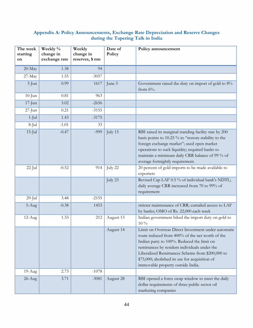
Appendix A: Policy Announcements, Exchange Rate Depreciation and Reserve Changes during the Tapering Talk in India

The week starting on

Weekly % change in exchange rate

Weekly change in reserves, $ mn

Date of Policy

Policy announcement

20-May 1.38 94

27-May 1.55 -3057

3-Jun 0.99 1617 June 5 Government raised the duty on import of gold to 8% from 6%.

10-Jun 0.81 963

17-Jun 3.02 -2656

27-Jun 0.21 -3155

1-Jul 1.43 -3175

8-Jul -1.01 33

15-Jul -0.47 -999 July 15 RBI raised its marginal standing facility rate by 200 basis points to 10.25 % to “restore stability to the foreign exchange market”; used open market operations to suck liquidity; required banks to maintain a minimum daily CRR balance of 99 % of average fortnightly requirement.

22-Jul -0.52 914 July 22 20 percent of gold imports to be made available to exporters

July 23 Revised Cap LAF 0.5 % of individual bank's NDTL; daily average CRR increased from 70 to 99% of requirement

29-Jul 3.48 -2155

5-Aug -0.38 1453 stricter maintenance of CRR; curtailed access to LAF by banks; OMO of Rs. 22,000 each week

12-Aug 1.33 212 August 13 Indian government hiked the import duty on gold to 10 %

August 14 Limit on Overseas Direct Investment under automatic route reduced from 400% of the net worth of the Indian party to 100%. Reduced the limit on remittances by resident individuals under the Liberalized Remittances Scheme from $200,000 to $75,000; abolished its use for acquisition of immovable property outside India.

19-Aug 2.73 -1078

26-Aug 3.71 -3081 August 28 RBI opened a forex swap window to meet the daily dollar requirements of three public sector oil marketing companies

44

4-Sep -0.7 -656 September 4 Limit on overseas direct investments, through External Commercial Borrowings, reinstated to 400% of net worth.

Offered a swap window to the banks to swap the fresh FCNR (B) dollar funds, mobilized for a minimum tenor of three years; at a fixed rate of 3.5% per annum. The overseas borrowing limit of 50% of the unimpaired Tier I capital raised to 100%; the borrowings mobilized under this provision could be swapped with the RBI at the option of the bank at a concessional rate of 100 basis points below the ongoing swap rate prevailing in the market; the schemes to remain open till Nov. 30, 2013.

New governor Rajan issued a statement outlining priorities and reiterating trust in the health of the economy; laid out the blueprint of further financial sector reforms.

9-Sep -2.68 500

16-Sep -1.92 1975 September 18 Government increased the import duty on gold jewelry to 15%

23-Sep 0.35 -1296 September 20 RBI increased the policy rate by 25 bps to 7.5%

October 7 RBI lowered the MSF rate by 50 bps to 9.0 percent and announced additional liquidity measures in the form of term repos of 7-day and 14-day tenor for the amount equivalent to 0.25 percent of banking system NDTL through variable rate auctions every Friday beginning October 11, 2013.

October 29 RBI lifted its policy repo rate by 25 bps to 7.75%

November 11 RBI receives US$ 17.5 billion under Forex Swap Window

November 20 RBI receives US$ 22.7 billion under Forex Swap Window

45