frontiers of geophysical simulation c -based flux …€¦ · xplicit e ulerian f inite-v olume Ö...
TRANSCRIPT

CHARACTERISTICS-BASED FLUX-FORM
SEMI-LAGRANGIAN METHODS FOR
ATMOSPHERIC SIMULATION
Matthew R. NormanRam Nair (NCAR)Hong Luo (NCSU)
Fredrick Semazzi (NCSU)
Department of Marine, Earth, & Atmospheric SciencesNorth Carolina State University
FRONTIERS OF GEOPHYSICAL SIMULATION
COURTESY MATTHEW
NORMAN

OUTLINE
• Introduction
• Methods & Model– Characteristics-Based Flux-Form Semi-Lagrangian
– Split-Explicit Time Stepping
• Future Work– Multi-Moment CB-FFSL
– Genuinely Multi-Dimensional CB-FFSL
COURTESY MATTHEW
NORMAN

SCALING, EFFICIENCY, & EFFECTIVENESS
• Modern architectures: 100,000+ processing cores– Models must scale massively parallel machines
– Pass as few messages as possible
• Scaling + … = Efficiency– Time step
– Single-node efficiency
• Efficiency + … = An Effective Model– Conservation
– Oscillations & Positivity
– Damping & Effective resolution
– Isotropy & Grid imprinting
– Properly balancing source terms and fluxes• Geostrophic, Hydrostatic, Thermal wind
COURTESY MATTHEW
NORMAN

THE EXTREMES OF EFFICIENCY
• Semi-implicit semi-Lagrangian
– Large time step
– High single-node efficiency
– Poor Scaling to 100,000+ processors
• Explicit Eulerian Galerkin Method
– Small time step
– Low single-node efficiency
– Good scaling to 100,000+ processors
• Explicit CB-FFSL Finite-Volume Method
– In between time step
– In between single-node efficiency
– Good scaling to 100,000+ processorsCOURTESY MATTHEW
NORMAN
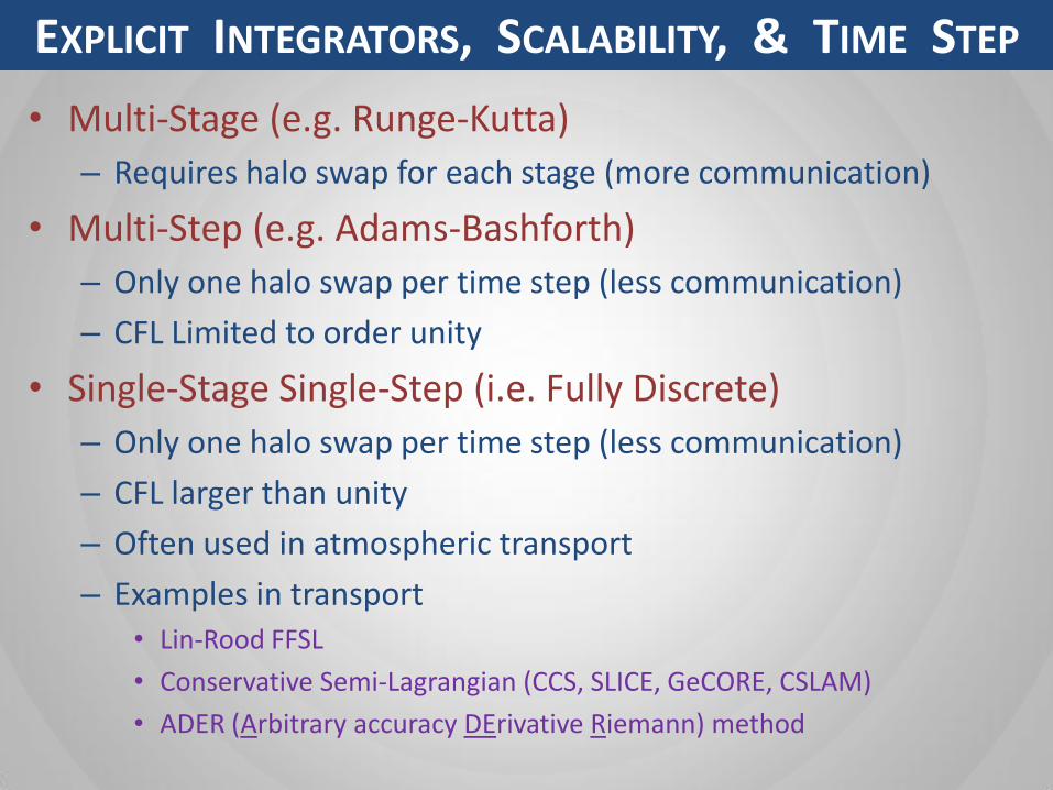
EXPLICIT INTEGRATORS, SCALABILITY, & TIME STEP
• Multi-Stage (e.g. Runge-Kutta)
– Requires halo swap for each stage (more communication)
• Multi-Step (e.g. Adams-Bashforth)
– Only one halo swap per time step (less communication)
– CFL Limited to order unity
• Single-Stage Single-Step (i.e. Fully Discrete)
– Only one halo swap per time step (less communication)
– CFL larger than unity
– Often used in atmospheric transport
– Examples in transport• Lin-Rood FFSL
• Conservative Semi-Lagrangian (CCS, SLICE, GeCORE, CSLAM)
• ADER (Arbitrary accuracy DErivative Riemann) methodCOURTESY M
ATTHEW N
ORMAN

EXPLICIT SEMI-LAGRANGIAN:FROM TRANSPORT TO NON-LINEAR EQUATIONS
• Method of Characteristics
– Transforms non-linear equation set into transport equations
– Characteristic variables materially conserved along characteristic trajectories
– Equation set must be hyperbolic
• Semi-Lagrangian Transport of Characteristics
– FFSL method guarantees conservation & allows flexibility
COURTESY MATTHEW
NORMAN

• Dry, compressible, inviscid, & non-hydrostatic equations
• Conserves:
– Mass
– Momentum
– Potential Temperature (& therefore entropy)
• Gravity source term
• Equation set is hyperbolic; thus allows characteristics
DRY ATMOSPHERIC EULER EQUATIONS
0
0
0
2
2
g
w
pw
wu
w
z
u
uw
pu
u
xw
u
t
constcs p log
L. A. Bauer, 1908, Phys. Rev.
COURTESY MATTHEW
NORMAN

EXPLICIT EULERIAN FINITE-VOLUME
0ˆ1
dnQF
Vt
Q
ΔQ
• Change in mean Q depends on flux through boundaries
• Fully Discrete: Time discretized by a direct integral
• We want to know the time-averaged flux through each cell boundary
_
i
iavgi
nn FV
tQQ ,
1
0
z
QH
x
QF
t
Q
COURTESY MATTHEW
NORMAN

CHARACTERISTICS-BASED FFSL METHOD
What is the flux at the cell boundary?
F(Qi-2) F(Qi-1) F(Qi) F(Qi+1) F(Qi+2)
Wave Speed
Upwind Cell
Decompose into characteristics
COURTESY MATTHEW
NORMAN

CHARACTERISTICS-BASED FFSL METHOD
5-cell stencil
wi(x)
Reconstruct Characteristic Var. for Upwind Cell
wi-2 wi-1 wi wi+1 wi+2
COURTESY MATTHEW
NORMAN

CHARACTERISTICS-BASED FFSL METHOD
Integrate w(x) over Domain of Dependence
wi
xi-1/2-λΔt
__
Time integral cast into upstream spatial integral over domain of dependence
COURTESY MATTHEW
NORMAN

• Adaptive use of stencils
– Create interpolants over multiple stencils
– Compute the oscillations of each interpolant
– Weight the most oscillatory interpolant the lowest
– Use the weighted sum of the interpolants
– Accuracy between 3rd and 5th order in the case below
WEIGHTED ESSENTIALLY NON-OSCILLATORY (WENO) RECONSTRUCTION (SHU 1999)
Wi-1Wi-2 Wi Wi+1 Wi+2
P5
P3,Left
P3,Center
P3,RightCOURTESY MATTHEW
NORMAN

• Initial Conditions
– Constant potential temperature
– Hydrostatic balance
– No wind
– 2 °K potential temperature perturbation
• Simulated for 1,000 s
• Δx = Δz = 150 m
• CFL=0.9 (Δt ≈ 0.38 s)
CONVECTIVE BUBBLE TEST CASE
Wicker & Skamarock (1998, MWR)
COURTESY MATTHEW
NORMAN
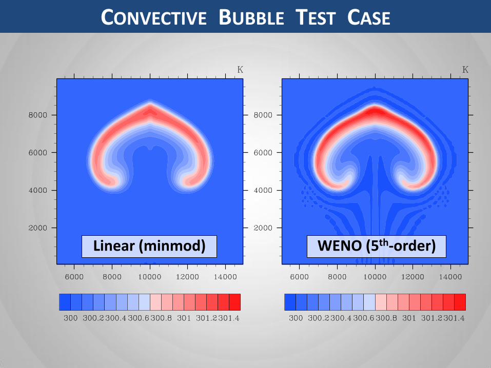
CONVECTIVE BUBBLE TEST CASE
Linear (minmod) WENO (5th-order)
COURTESY MATTHEW
NORMAN

STRAKA DENSITY CURRENT TEST CASE
• Initial Conditions (Straka et al, IJNMF, 1993)– Constant potential temperature– hydrostatic balance– no wind– -15 °K potential temperature perturbation
• Simulated for 900 s• Δx = Δz = 50 m• CFL=0.9 (Δt ≈ 0.13 s)
COURTESY MATTHEW
NORMAN

STRAKA DENSITY CURRENT TEST CASE: RESULTS
Linear (minmod)COURTESY MATTHEW
NORMAN
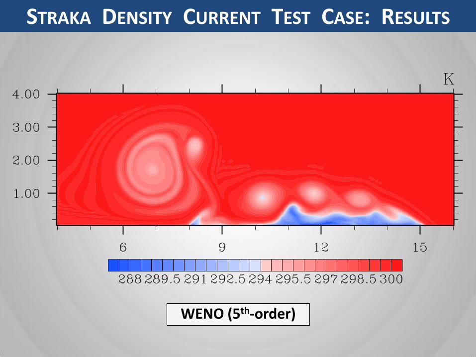
STRAKA DENSITY CURRENT TEST CASE: RESULTS
WENO (5th-order)COURTESY MATTHEW
NORMAN

• (CFL ≤ 1) + (5th-order) = 3 halo transfers
• (CFL ≤ 2) + (5th-order) = 4 halo transfers
CFL > 1: AN EXAMPLE
COURTESY MATTHEW
NORMAN

• Subcycle fast (acoustic) waves on a smaller time step
• Simulate slow (advection) waves on a larger time step
• 1st-order splitting error in equations
• Very easy to implement with characteristics
– u, u, u+cs, u-cs
• Implemented for rising thermal test case
– 3 fast time steps per slow time step
– WENO5 for slow waves & WENO5 for fast waves: 38% less CPU
– WENO5 for slow waves & WENO3 for fast waves: 59% less CPU
SPLIT-EXPLICIT TIME STEPPING
Slow Fast
COURTESY MATTHEW
NORMAN

SPLIT-EXPLICIT TIME STEPPING
WENO5 for slow, WENO5 for fast WENO5 for slow, WENO3 for fast
Is it worth it to use a cheaper method for fast waves?COURTESY M
ATTHEW N
ORMAN

SPLIT-EXPLICIT TIME STEPPING
10 fast time steps per slow time step: CFL=9.9
COURTESY MATTHEW
NORMAN
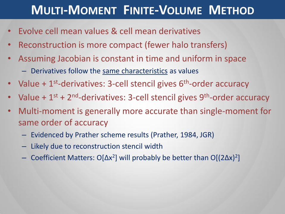
• Evolve cell mean values & cell mean derivatives
• Reconstruction is more compact (fewer halo transfers)
• Assuming Jacobian is constant in time and uniform in space– Derivatives follow the same characteristics as values
• Value + 1st-derivatives: 3-cell stencil gives 6th-order accuracy
• Value + 1st + 2nd-derivatives: 3-cell stencil gives 9th-order accuracy
• Multi-moment is generally more accurate than single-moment for same order of accuracy– Evidenced by Prather scheme results (Prather, 1984, JGR)
– Likely due to reconstruction stencil width
– Coefficient Matters: O*∆x2] will probably be better than O*(2∆x)2]
MULTI-MOMENT FINITE-VOLUME METHOD
COURTESY MATTHEW
NORMAN

• However, not certain how to couple with physics & boundaries– Physics alters cell means but not cell derivatives
– Other coupled models (sea ice, land, ocean, etc.) may not alter derivatives
– Derivatives then decouple from cell means and are no longer valid
– To use invalid derivatives would act against the physics alterations
– Probably leading to odd and unpredictable behavior!
Seemingly only two options
1. Reconstruct derivatives from altered cell means– Actually, this is less scalable than traditional FV
– Likely forfeits the accuracy gain of going multi-moment as well
2. Derive physics parameterizations that evolve derivatives– Not an easy task, but possible
– Requires coupled models to do the same
MULTI-MOMENT FINITE-VOLUME METHOD
COURTESY MATTHEW
NORMAN

• Accounts for multi-dimensional nature of characteristics
– Relaxes dependence on a rectangular mesh
– Great isotropy on any mesh
– Better tracer consistency with multi-dimensional transport
– Greatly reduces error at cubed-sphere panel edges and corners
• Implementation is the key
– Acoustic waves propagate along Mach cones
– Various levels of approximation possible
– Experimentation required to test approximations
• Possible application to characteristics-based DG methods
GENUINELY MULTI-DIMENSIONAL: BICHARACTERISTICS
COURTESY MATTHEW
NORMAN

LINEARIZED ACOUSTIC WAVE: MACH CONE
Trace acoustic wave back in time from point P
Renders a slanted cone
Radius: cs(tn+1-t)
Center: (x-Vx(tn+1-t) , y-Vy(tn+1-t))
Computing state variables at a point in time and space from upstream values requires integration in time!
Advection waves are integrated as zero-radius Mach cones (solution is decoupled from θ)
COURTESY MATTHEW
NORMAN

• Is it really worth it?
• Perhaps Not
– Acoustic waves are not the dominant dynamical influence
– It’s not cheap
• Perhaps So
– Splitting error is particularly large on the cubed-sphere
– Maybe the best way to achieve multi-dimensional consistency with tracers
– We could increase the sophistication of the advection wave integration
– Only way to have no splitting & large CFL in an explicit method
• Only experimentation will decide
– Likely depends on the CFL used
BICHARACTERISTICS: PRACTICAL ISSUES
COURTESY MATTHEW
NORMAN

Thanks for Your Attention
Questions and Comments
COURTESY MATTHEW
NORMAN

• Many ways to reconstruct (e.g. 4th-order)
– Use 4 4th-order accurate 0th-order derivatives (Trad. FV)
– Use 2 3rd-order accurate 1st-order derivatives& 2 4th-order accurate 0th-order derivatives (Mult. Mom. FV)
• Evolve multiple derivs. & use for compact reconstruction
• Most obvious in DG with Taylor basis
• Also done in nodal methods
HIGH-ORDER & HERMITE RECONSTRUCTION
COURTESY MATTHEW
NORMAN

• Why cubed-sphere?– Logically rectangular: Easy to reconstruct to arbitrary orders
– Equiangular Gnomonic: computational grid of uniform squares
– Near uniform cell area globally
– Dimensional splitting trivial
• Difficulties when a stencil is required (e.g. FV, DG + HWENO)– Panel edges & corners: coord. system changes, cell geometry changes
– High-order requires remapping onto extended local panel grid
– Requires a halo exchange
– Changing Jacobian reduces accuracy of reconstructions
CUBED-SPHERE GEOMETRY
COURTESY MATTHEW
NORMAN
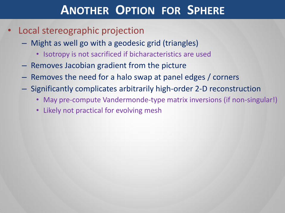
• Local stereographic projection– Might as well go with a geodesic grid (triangles)
• Isotropy is not sacrificed if bicharacteristics are used
– Removes Jacobian gradient from the picture
– Removes the need for a halo swap at panel edges / corners
– Significantly complicates arbitrarily high-order 2-D reconstruction
• May pre-compute Vandermonde-type matrix inversions (if non-singular!)
• Likely not practical for evolving mesh
ANOTHER OPTION FOR SPHERE
COURTESY MATTHEW
NORMAN

• Homogeneous Fluid Equations
• Apply chain rule to flux
• Diagonalize flux Jacobian into Eigenvectors and Eigenvalues
• Multiply equation by R-1
• Assume R-1 is constant & uniform
CHARACTERISTICS
0
x
QF
t
Q
0x
Q
Q
F
t
Q
Flux Jacobian
1 RRQ
F
01
x
QRR
t
Q
011
x
QR
t
QR
0
11
x
QR
t
QR
COURTESY MATTHEW
NORMAN

• Decoupled set of simple transport equations
• After transporting, retrieve state variables from:
CHARACTERISTICS
0
0
0
33
3
22
2
11
1
x
w
t
w
x
w
t
w
x
w
t
w
3
2
1
1
w
w
w
QRW
3
2
1
00
00
00
3
2
1
1
w
w
w
QRW
COURTESY MATTHEW
NORMAN

• Homogeneous Conservation Equations
• Spatially Differentiate the Conservation Equations
• Apply Chain Rule to Fluxes (Characteristic Form)
• “Freeze” the Jacobian (Constant in time, Uniform in space)
MULTI-MOMENT FINITE-VOLUME METHOD
0
x
QF
t
Q
0
x
QF
xx
Q
t
0
x
Q
Q
F
xx
Q
t
0
x
Q
xQ
F
x
Q
t
COURTESY MATTHEW
NORMAN

• 2-D Characteristic Form
• Diagonalize both Jacobians
• Create a directional Jacobian
• Diagonalize the directional Jacobian
• Left-Multiply by R-1(θ)
• Insert R(θ) R-1(θ)
GENUINELY MULTI-DIMENSIONAL: BICHARACTERISTICS
0z
Q
Q
H
x
Q
Q
F
t
Q
11 zzzzxxxx RRAQ
HRRA
Q
F
sincos
Q
H
Q
FA
1 RRA
0111
z
QAR
x
QAR
t
QR zx
011111
z
QRRAR
x
QRRAR
t
QR zx
COURTESY M
ATTHEW N
ORMAN

• “Freeze” the Jacobian & Pull R-1(θ) inside the derivatives
• Split Bx and Bz into a diagonal matrix and the remaining entries
GENUINELY MULTI-DIMENSIONAL: BICHARACTERISTICS
0
z
WB
x
WB
t
Wzx
QRWRARBRARB zzxx 111
011111
z
QRRAR
x
QRRAR
t
QR zx
'
,
'
, zDzzxDxx BBBBBB
S
z
WB
x
WB
t
WDzDx ,,
z
WB
x
WBS zx
''
COURTESY MATTHEW
NORMAN

• Integrate in time
• Left-Multiply by R(θ)
• Integrate in θ
• Predicts state variables at a point in space and time– Takes into account full multidimensional nature of the characteristics
– Contains a messy “source term” which must be integrated in time
– Line integrals in θ easily handled with quadrature
GENUINELY MULTI-DIMENSIONAL: BICHARACTERISTICS
S
z
WB
x
WB
t
WDzDx ,,
dtSWWn
n
t
tnnP
1
*,1,
dtSRWRQn
n
t
tnnP
1
*,1,
ddtSRdWRQn
n
t
tnnP
2
0
2
0*,1,
1
2
1
2
1
COURTESY MATTHEW
NORMAN

NH-SCALE GRAVITY WAVES TEST CASE
• Initial Conditions (Skamarock & Klemp, 1994, MWR)– Constant Brunt Vaisala frequency (10-2 s-1)
– hydrostatic balance
– 20 m/s horizontal wind
– 10-2 °K potential temperature perturbation
• Simulated for 3,000 s
• Δx = 1,000 m , Δz = 100 m
• CFL=0.9 (Δt ≈ 0.25 s)
COURTESY MATTHEW
NORMAN

NH-SCALE GRAVITY WAVES TEST CASE
Linear (minmod)COURTESY MATTHEW
NORMAN

NH-SCALE GRAVITY WAVES TEST CASE
WENO (5th-order)COURTESY MATTHEW
NORMAN
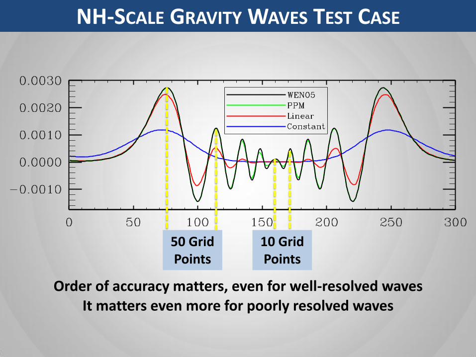
NH-SCALE GRAVITY WAVES TEST CASE
50 Grid Points
Order of accuracy matters, even for well-resolved wavesIt matters even more for poorly resolved waves
10 Grid Points
COURTESY MATTHEW
NORMAN