FRWuniverse in the laboratory

Neven Bilic1,2,* and Dijana Tolic1,†

1Rudjer Boskovic Institute, P.O. Box 180, HR-10002 Zagreb, Croatia2Departamento de Fısica, Universidade Federal de Juiz de Fora, 36036-330 Juiz de Fora, Minas Gerais, Brazil

(Received 29 September 2013; published 5 November 2013)

We consider an expanding relativistic fluid with spherical symmetry as a model for an analog

Friedmann-Robertson-Walker (FRW) spacetime. In the framework of relativistic acoustic geometry we

demonstrate how to mimic an arbitrary FRW spacetime with positive, zero, or negative spatial curvature.

In the Lagrangian description we show that a particular FRW spacetime is obtained by choosing the

appropriate potential. We discuss several examples and in particular the analog de Sitter spacetime in the

coordinate representation with positive and negative spatial curvature.

DOI: 10.1103/PhysRevD.88.105002 PACS numbers: 03.75.Kk, 04.40.Nr, 47.10.�g, 98.80.Jk

I. INTRODUCTION

The possibility that a curved (pseudo-Riemannian) ge-ometry of spacetime can be mimicked by fluid dynamics inMinkowski spacetime has been recently exploited in vari-ous contexts, including emergent gravity [1], the scalartheory of gravity [2], and acoustic geometry [3–5], toname but a few.

The basic idea is the emergence of an effective metric ofthe form

G�� ¼ ag�� þ bu�u�; (1)

which describes the effective geometry for acoustic per-turbations propagating in a perfect fluid potential flowwith u� / @��. The background spacetime metric g�� is

usually assumed flat and the coefficients a and b are relatedto the equation of state of the fluid and the adiabatic speedof sound. Equivalently, in a field-theoretical picture the

fluid velocity u� is derived from the scalar field as u� ¼@��=

ffiffiffiffiX

pand a and b are expressed in terms of the

Lagrangian and its first and second derivatives with respectto the kinetic energy term X ¼ g���;��;�.

In a slightly different context, the metric of the form (1)has been used to show that a pseudo-Riemann spacetimewith Lorentz signature may be derived from a Riemannmetric with Euclidean signature [6–8]. In that case, thevector u� represents the normalized gradient of a hypo-

thetical scalar field which governs the dynamics and thesignature of the effective spacetime.

The effective geometry of an expanding fluid seems apromising route to model an expanding spacetime, e.g., ofFriedmann-Robertson-Walker (FRW) type. However, anexpanding fluid alone is not a sufficiently powerful toolfor modeling an expanding spacetime of general relativity.At best, the fluid flow can be manipulated to provide acoordinate transformation to an arbitrary curved coordinate

frame, with the spacetime remaining flat. For example, aboost-invariant Bjorken-type spherical expansion providesa map of the Minkowski to the Milne spacetime—a homo-geneous, isotropic, expanding universe with the cosmologi-cal scale proportional to t and negative spatial curvature [9].In this paper we propose a mechanism in which the

metric (1) provides a laboratory model for an analogFRW spacetime with arbitrary spatial curvature. To modelan arbitrary FRW spacetime we make use of the effectiveacoustic geometry in which small perturbations propagateadiabatically. We show quite generally that in addition toan appropriately designed fluid expansion it is necessary tomanipulate the fluid equation of state to obtain the desiredgeometry. By making use of a specific type of fluid expan-sion in Minkowski spacetime it is possible quite generallyto map the Minkowski metric into spatially closed (k ¼ 1),open hyperbolic (k ¼ �1), or open flat (k ¼ 0) FRWacoustic metrics. The mappings to spatially flat and hyper-bolic universes have been already studied in a few specificapplications, such as spatially flat analog cosmology in anonrelativistic Bose-Einstein (BE) condensate [10], and anopen FRW metric in a Bjorken-like spherical expansionof a relativistic BE system [11] and of a hadronic fluid[12,13]. We extend these ideas to a more general case thatincludes all three types of FRW spatial geometries. It turnsout that an open FRW spacetime with zero or negativespatial curvature can be modeled in a rather straightfor-ward way using isentropic perfect fluids such as a Bose-Einstein condensate in the Thomas-Fermi limit. Themodeling of a closed FRW spacetime with positive spatialcurvature requires additional assumptions.We divide the remainder of the paper into five sections

and an appendix, starting with Sec. II, in which we give afield-theoretical description of our model. In the followingsection, Sec. III, we study the relativistic BE condensate inthe context of analog cosmology. Section IV reproducesthe results of Sec. II in terms of the conventional relativistichydrodynamics. In Sec. V we study the analog cosmologi-cal horizons and we present the spacetime diagrams for theanalog de Sitter universe. We summarize our results and

*bilic@irb.hr†dijana.tolic@irb.hr

PHYSICAL REVIEW D 88, 105002 (2013)

1550-7998=2013=88(10)=105002(11) 105002-1 � 2013 American Physical Society

give a brief outlook in Sec. VI. Finally, in Appendix Awe describe a general transformation from Minkowski tospatially curved conformal coordinates.

II. ANALOG SPACETIMES

We start with an expanding perfect fluid in Minkowskispacetime in spherical coordinates ðT; R; #; ’Þ,

ds2 ¼ dT2 � dR2 � R2d�2; (2)

and we demand that the effective acoustic metric in co-moving coordinates ðt; r; #; ’Þ takes the conformal FRWform with line element

ds2 ¼ �ðtÞ2�c2sdt

2 � dr2 � sin 2ð ffiffiffik

prÞ

kd�2

�: (3)

Here cs is the (generally time-dependent) speed of soundand the curvature k is positive, zero, or negative for aspacetime with spherical, flat, and hyperbolic spatial ge-ometry, respectively. To achieve this we first design thefluid flow so that it models a transformation fromMinkowski to conformal coordinates ðt; r; #; ’Þ using theprescription of Ibison [14], which we review inAppendix A. In the next section we describe the kinematicsof the fluid flow suitable for modeling an FRW spacetime.

A. Kinematics of the flow

Applying the transformation (A2) and (A3), we arrive atthe line element

ds2 ¼ a2ðt; rÞ�dt2 � dr2 � sin 2ð ffiffiffi

kp

rÞk

d�2

�; (4)

where a2ðt; rÞ is given by Eq. (A6). The particular choice� ¼ � ¼ 1 in Eq. (A6) gives

a2ðt; rÞ ¼ ðcos ð ffiffiffik

prÞ þ cos ð ffiffiffi

kp

tÞÞ�2: (5)

The new temporal and radial coordinates t and r and the

spatial curvature radius jkj�1=2 are measured in units ofm�1, where m is a yet unspecified mass scale. Hence, inunits of m2 the curvature equals k ¼ 1, 0, or �1.

Since the conformal factor a2 is a function of both t andr, the line element (4) is generally not FRW. However, fork ¼ �1, the expression for a may be simplified by takingthe limit � ! 0 in Eq. (A6), in which case we obtain a as afunction of t only,

aðtÞ ¼ e�t; (6)

where �may take the valueþ1 or�1, corresponding to anexpanding or collapsing universe, respectively.

The fluid which provides the desired map (A2) and (A3)from ðT; RÞ to ðt; rÞ coordinates is required to be at rest inðt; rÞ coordinates. In other words the expansion of the fluidis such that the new coordinate frame ðt; rÞ is comoving,i.e., the four-velocity of the flow in the new coordinateframe is

u� ¼ ða; 0; 0; 0Þ; u� ¼ ð1=a; 0; 0; 0Þ: (7)

Hence, the inverse transformation of (A2) and (A3) appliedto Eq. (7) yields the velocity components uT and uR in theoriginal Minkowski frame. Expressed in terms of t and rthese components are given by Eqs. (A16) and (A17).Specifically, for � ¼ 1 we have

uT ¼ 1þ cos ð ffiffiffik

prÞ cos ð ffiffiffi

kp

tÞcos ð ffiffiffi

kp

rÞ þ cos ð ffiffiffik

ptÞ ; (8)

uR ¼ sin ð ffiffiffik

prÞ sin ð ffiffiffi

kp

tÞcos ð ffiffiffi

kp

rÞ þ cos ð ffiffiffik

ptÞ : (9)

Again, for k ¼ �1 we may take the limit � ! 0 and theexpressions (A16) and (A17) reduce to

uT ¼ cosh ð�rÞ; (10)

uR ¼ sinh ð�rÞ; (11)

where � equals þ1 or �1, corresponding to an expandingor collapsing fluid, respectively. These velocities describe aspherically symmetric Bjorken-type expansion. This typeof expansion has been recently applied to mimic an openFRW metric in a relativistic BE system [11] and in ahadronic fluid [12,13].The above discussed limit � ! 0 that removes the r

dependence of the scale factor in Eq. (4) does not workfor k ¼ þ1 or 0. However, as we will shortly demonstrate,with the appropriate choice of the fluid Lagrangian we caneliminate r dependence even for a more general expansionof the form (8) and (9) applicable to any k ¼ 1, 0, or �1.Next, we derive a Lagrangian that describes a fluid

capable of modeling an FRW spacetime in terms of therelativistic acoustic geometry.

B. Mapping to an analogue FRW spacetime

For our purpose it proves advantageous to use the field-theoretical description of fluid dynamics [15]. Consider aLagrangianLðX; �Þ that depends on a dimensionless scalarfield � and on the kinetic energy term

X ¼ g���;��;�: (12)

For X > 0, the energy-momentum tensor

T�� ¼ 2LX�;��;� �Lg�� (13)

takes the perfect fluid form

T�� ¼ ðpþ Þu�u� � pg��; (14)

in which

u� ¼ @��ffiffiffiffiX

p : (15)

NEVEN BILIC AND DIJANA TOLIC PHYSICAL REVIEW D 88, 105002 (2013)

105002-2

Hence, the field � serves as the velocity potential. Thequantities

p ¼ L (16)

and

¼ 2XLX �L (17)

are identified as the pressure and energy density of thefluid, respectively, and the field equation

ð2LXg���;�Þ;� � @L=@� ¼ 0 (18)

is equivalent to the continuity equation. The subscript X inEq. (13)–(18) denotes a partial derivative with respect to X.

Small perturbations in the fluid propagate in an effectivecurved geometry with metricG�� which may be derived as

follows [1,16]. Consider a small perturbation around theclassical solution to the field equation (18). Replacing

�ðxÞ ! �ðxÞ þ ðxÞ (19)

and keeping only the terms quadratic in the derivatives of in the Taylor expansion of the Lagrangian, we obtain theeffective action

�S ¼ 1

2

Zd4x

ffiffiffiffiffiffiffiffi�Gp

m2G��@�@�; (20)

where

G�� ¼ m2cs2LX

�g�� �

�1� 1

c2s

�u�u�

�; (21)

with u� ¼ g��u� and u� as defined in Eq. (15). The matrixG�� is the inverse of the effective metric tensor,

G�� ¼ 2LX

m2cs½g�� � ð1� c2sÞu�u��; (22)

with determinant G � detG��. The mass parameter m in

Eqs. (20)–(22) is introduced to make G�� dimensionless

and the quantity cs is the so-called ‘‘effective’’ speed ofsound, defined as

c2s ¼ LX

LX þ 2XLXX

: (23)

Hence, the linear perturbations propagate in the effectivemetric (22) and the propagation is governed by the equa-tion of motion

1ffiffiffiffiffiffiffiffi�Gp @�ð

ffiffiffiffiffiffiffiffi�Gp

G��@�Þ þ � � � ¼ 0: (24)

The basic mechanism that leads to the the effective actionof the form (20) with Eq. (21) was first noticed by Unruh[17], who was also the first to point out that a supersonicflow may cause analog Hawking radiation.

Due to Eqs. (7) and (15), the field � in comovingcoordinates ðt; r; #;�Þ is a function of t only and thekinetic variable X is a function of both t and r,

X ¼ g00 _�2 ¼_�2

a2; (25)

where the overdot denotes a derivative with respect to t.The effective metric (22) in comoving coordinates takesthe form

G��¼2LXa2

m2cs

�

c2s

�1

�sin2ð ffiffiffik

prÞ=k

�sin2#sin2ð ffiffiffik

prÞ=k

0BBBBB@

1CCCCCA:

(26)

A comoving observer receives information transmitted byacoustic perturbations propagating in the analog spacetimewith the above effective acoustic metric.To construct an FRW metric we must get rid of the r

dependence of the conformal factor, i.e., we must choose aLagrangian with a functional dependence on X such thatthe factor a2 in Eq. (26) is canceled. Owing to Eq. (25) weimmediately conclude that LX must linearly depend on Xand hence our Lagrangian must be quadratic in X, i.e., wemay choose

L ¼ Vð�ÞX2; (27)

where V is an arbitrary function of �. This Lagrangian1

belongs to a wider class of the form L ¼ Lð ~XÞ, where~X ¼ fð�ÞX and fð�Þ is an arbitrary positive function of �.

By the field transformation ~�;� ¼ f1=2�;� the variable ~X

becomes the kinetic term of the field ~� and Lð ~XÞ takes theform of a purely kinetic k-essence which describes anisentropic fluid [18].From Eq. (27) and using Eq. (23), we find

c2s ¼ 1

3: (28)

A further restriction on the fluid functions p and isimposed by the field equation (18). Applying Eq. (18) toEq. (27) with � ¼ �ðtÞ, we obtain

_�3ð4V €�þ _V _�Þ ¼ 0: (29)

By inspection it may be verified that this equation, besidesthe trivial solution � ¼ const, has a solution that satisfies

1Note that the Lagrangian (27) is invariant under the confor-mal transformation of the metric and hence it describes aconformal fluid, which may also be seen by verifying that thecorresponding energy-momentum tensor is traceless.

FRW UNIVERSE IN THE LABORATORY PHYSICAL REVIEW D 88, 105002 (2013)

105002-3

Vð�Þ _�4 ¼ �m4; (30)

where � is an arbitrary dimensionless constant. EliminatingV from Eq. (27) by Eq. (30) and using Eqs. (16), (17), and(25), we find

p ¼ �m4

a4; ¼ 3�m4

a4: (31)

Then, the acoustic line element corresponding to themetric (26) takes the desired form

ds2 ¼ �ð�Þ2�d�2 � dr2 � sin 2ð ffiffiffi

kp

rÞk

d�2

�; (32)

where a transition to the conformal time is made bythe replacement � ¼ cst. With a convenient choice� ¼ ðcs=4Þ2 the cosmological scale factor reads

�ð�Þ ¼ Vð�ð�=csÞÞ1=4: (33)

In this way, we have shown that the acoustic analogmetric takes the conformal form of a general FRW space-time with positive, negative, or zero spatial curvaturedepending on the choice of k in the flow velocity (8) and(9). The evolution of the cosmological scale is determinedby the shape of the potential V in the Lagrangian (27).

It is instructive to study a few simple examples.

1. Static universe

The simplest possible case is the analog static spacetimewith potential V ¼ 1, i.e., with the Lagrangian

L ¼ X2: (34)

It is worth noting that an effective Lagrangian of this formhas been recently studied in the context of relativistic

superfluidity [19]. From Eq. (30) it follows that � ¼�1=4mt. Hence, if the fluid described by the Lagrangian(34) expands according to Eqs. (8) and (9) [or Eqs. (10) and(11) in the k ¼ �1 case], a comoving observer perceives astatic open (k ¼ �1) or closed (k ¼ 1) analog universe.

2. Analog de Sitter spacetime

We next consider the de Sitter (dS) geometry whichadmits all three representations with the correspondingline elements [14],

ds2 ¼

8>>><>>>:��2ðd�2 � dr2 � r2d�2Þ; k ¼ 0;

cos�2�ðd�2 � dr2 � sin 2rd�2Þ; k ¼ 1;

sinh�2�ðd�2 � dr2 � sinh 2rd�2Þ; k ¼ �1:

(35)

Comparing these with Eq. (32), together with Eqs. (30) and(33), we obtain V and _� as functions of � for each k.Replacing � ¼ cst and integrating _� over t, we obtain

4ffiffiffiffiffics

p�ðtÞ ¼

8><>:c2s t

2; k ¼ 0;

2 sin cst; k ¼ 1;

2 cosh cst; k ¼ �1:

(36)

Plugging these functions back into VðtÞ, we find

VdSð�Þ ¼ffiffiffi3

p16�2

(37)

for k ¼ 0 and

VdSð�Þ ¼ 3

ð ffiffiffi3

p � 4�2Þ2 (38)

for both k ¼ 1 and k ¼ �1 with the conditions �2 <ffiffiffi3

p=4

for k ¼ 1 and �2 >ffiffiffi3

p=4 for k ¼ �1.

As demonstrated by Ibison [14], the transformation (A2)and (A3) with � ¼ 1, � ¼ 2, and k ¼ �1 takes the dS lineelement in the k ¼ 0 representation

ds2 ¼ 1

T2ðdT2 � dR2 � R2d�2Þ (39)

to that in the k ¼ �1 representations of the type (32) with

�2 ¼ k

sin 2ð ffiffiffik

p�Þ : (40)

Hence, the inverse coordinate transformation back to theoriginal Minkowski coordinates takes our acoustic lineelement (32) with Eq. (40) to the conformal spatially flatdS line element (39), as it should because, by our construc-tion, the acoustic metric of the fluid at rest (i.e., with k ¼ 0velocity field) described by the potential (37) is k ¼ 0 deSitter in the conformal form.

3. Analog anti–de Sitter spacetime

Anti–de Sitter (AdS) spacetime is expressible only in thek ¼ �1 representation with line element [14]

ds2 ¼ 1

cosh 2�

�d�2 � dr2 � sinh 2r

kd�2

�: (41)

Repeating the above procedure, we find

VAdSð�Þ ¼ 3

ð ffiffiffi3

p þ 4�2Þ2 : (42)

III. BOSE-EINSTEIN CONDENSATE

In the context of relativistic acoustic geometry, an inter-esting example of a relativistic fluid is the BE condensate,which has been suggested in a recent paper [11] as a modelfor an analogue FRW universe.We first show that, under certain assumptions, self-

interacting complex scalar field theories are equivalent topurely kinetic k-essence models (for details see Ref. [20]).We will then analyze the acoustic metric and demonstratethat an appropriately chosen k-essence Lagrangian can

NEVEN BILIC AND DIJANA TOLIC PHYSICAL REVIEW D 88, 105002 (2013)

105002-4

simulate arbitrary k ¼ 0 and k ¼ �1 FRW model. As fork ¼ 1, purely kinetic k-essence Lagrangians are not suit-able for the simulation of k ¼ �1 FRW models except fora closed static universe, as in the first example of Sec. II B.

Consider the Lagrangian

L ¼ g����;��;� �Uðj�j2=m2Þ (43)

for a complex scalar field, where the potential U is anarbitrary function of j�j2=m2. The field � satisfies theKlein-Gordon (KG) equation

ðg���;�Þ;� þ dU

dj�j2 � ¼ 0: (44)

Using the representation

� ¼ �ffiffiffi2

p exp ð�i�Þ; (45)

the Lagrangian (43) may be recast into the form

L ¼ 1

2�2g���;��;� þ 1

2g���;��;� �U

��2

2m2

�: (46)

The KG equation (44) splits into two equations for the realscalar fields � and �,

ðYg���;�Þ;� ¼ 0; (47)

ðg���;�Þ;� þ�ðUY=m2 � XÞ ¼ 0; (48)

where we have introduced the abbreviations

X ¼ g���;��;�; Y ¼ �2

2m2; (49)

andUY denotes the derivativedU=dY. A nontrivial classicalsolution to either Eq. (44) or Eqs. (47) and (48) is called therelativistic Bose-Einstein condensate. The field configura-tion thus obtained corresponds to a two-component relativ-istic fluid.

The formalism of acoustic geometry is derived assuminga perfect irrotational fluid. Here, the energy-momentumtensor corresponding to the Lagrangian (43) represents acombination of two perfect fluids and generally cannot beput in the form of a single perfect fluid. However, if thespacetime variations of j�j are small on the scale smallerthan m�1, i.e., assuming �;� � m� , then the Thomas-

Fermi (TF) approximation [21,22] (or the eikonal approxi-mation [11]) applies. In this case, if dU=dj�j2 > 0 thefluid becomes perfect and the corresponding Lagrangian isequivalent to a Lagrangian that depends only on the kineticterm X [20]. This may be seen as follows.

The TF approximation amounts to neglecting the kineticterm g���;��;� in Eq. (46), in which case the Lagrangian

becomes

LTF ¼ m2XY �UðYÞ: (50)

The field equation (47) remains the same, whereas Eq. (48)reduces to

m2X �UY ¼ 0: (51)

Now, the energy-momentum tensor corresponding to theLagrangian (50) takes the perfect fluid form (14) withEq. (15) and

¼ YUY þU; p ¼ YUY �U: (52)

Obviously, the perfect-fluid description applies only ifUY > 0 which, generally, need not be true for the entirerange 0 Y 1. Hence, the BE fluid in the TF approxi-mation is perfect for those Y for which dU=dj�j2 > 0.Owing to Eq. (51) and the obvious relation

LX ¼ m2Y; (53)

Eq. (50) together with Eqs. (51) and (53) may be inter-preted as a Legendre transformation,

LðXÞ ¼ m2XY �UðYÞ: (54)

For a given U the Lagrangian LðXÞ can be found bysolving Eq. (51) for Y and plugging the solution intoEq. (54). Similarly, if LðXÞ is known, the potential Umay be derived by solving Eq. (53) for X and pluggingthe solution into Eq. (54).From the Lagrangian LðXÞ which now depends only on

the kinetic term X we find the equation of motion for thefield �,

ðLXg���;�Þ;� ¼ 0; (55)

which is equivalent to Eq. (47). However, one should barein mind that the field theories described by the Lagrangians(50) and (54), respectively, are equivalent only at theclassical level. The energy-momentum tensor constructedfrom Eq. (54) is of the form (14), with the parametricequation of state

¼ 2XLX �L; p ¼ L: (56)

This equation is just a different parametrization of theequation of state (52) which may be easily verified byusing Eq. (51) to substitute UY for X in Eq. (56).In the following we study an expanding fluid in terms of

the Lagrangian LðXÞ as a framework for an analog modelof an FRW universe. As before, the effective geometry incomoving coordinates is defined by the acoustic metric(26). However, the previous procedure of eliminating a2

in the conformal factor cannot be applied here,2 sinceLðXÞis now a general function of X. Nevertheless, in the case ofhyperbolic spatial geometry (k ¼ �1) the general coordi-nate transformation (A2) and (A3) to comoving coordi-nates may be simplified by taking the limit � ! 0. In this

2The only exception is LðXÞ ¼ X2, which describes a staticanalog universe, as in the first example of Sec. II B.

FRW UNIVERSE IN THE LABORATORY PHYSICAL REVIEW D 88, 105002 (2013)

105002-5

case the transformation (A10) and (A11) takes theMinkowski spacetime to the Milne spacetime, with theconformal factor a ¼ e�t being a function of t only. Thiscoordinate transformation corresponds to the Bjorken-typespherical expansion discussed already in a similar context[11–13]. In this case, X is a function of t only, and likewiseLX and cs. The effective acoustic line element in comov-ing coordinates,

ds2 ¼ 2LX

m2cse2�tðc2sdt2 � dr2 � sinh 2rd�2Þ; (57)

can be immediately cast into the conformal FRW form forany L ¼ LðXÞ by the transformation to the conformaltime,

� ¼Z

dtcs; (58)

where cs is defined in Eq. (23). Therefore, by choosingan appropriate interaction potential U [or equivalently, ak-essence Lagrangian LðXÞ] one can, in principle, mimicthe open hyperbolic FRW universe of arbitrary kind. Thisprocedure, albeit straightforward, is slightly more involvedthan the one explained in Sec. II because the speed ofsound is generally not constant.

Given a k-essence Lagrangian LðXÞ it is relatively easyto find the corresponding analog FRW spacetime. First,from the field equation (55) we find the relation

LX ¼ m3e�3�tX�1=2; (59)

from which we can express X, LðXÞ, and cs in terms of t.These in turn yield a functional dependence on t of theconformal factor

�2 � 2LX

m2cse2�t (60)

in the line element (57). Then, using Eqs. (23) and (58), wefind t as a function of the conformal time �, which in turnyields � ¼ �ð�Þ.

The reverse procedure is slightly more involved.Suppose we want to model a particular hyperbolic FRWspacetime of the form

ds2 ¼ �ð�Þ2ðd�2 � dr2 � sinh 2rd�2Þ: (61)

We need to find the Lagrangian L such that the conformalfactor of the corresponding acoustic line element (57) isequal to �ð�Þ, i.e., we require Eq. (60). First, from Eq. (59)and using Eq. (23), we find

c2s ¼ � �

6X

dX

dt: (62)

From this, with Eq. (60) and d� ¼ csdt, we obtain twocoupled differential equations,

dt

d�¼

�X

m

�1=2

e�t�ð�Þ2; (63)

1

X

dX

d�¼ �6�

�dt

d�

��1; (64)

the solution to which yields t as a function of X in aparametric form. This function can, in principle, be madeexplicit by eliminating the parameter �. Plugging tðXÞ intoEq. (59), we obtain LX as a function of X from which wefind LðXÞ ¼ R

dXLXðXÞ.We consider two examples, one for each procedure

discussed above.

A. Scalar Born-Infeld theory

As an easily tractable example, consider the BE inter-action potential

U ¼ m4ðY2 þ Y�2Þ; (65)

which, in the Thomas-Fermi limit, is equivalent to thescalar Born-Infeld theory with the k-essence-typeLagrangian [20,23]

L ¼ �m4ffiffiffiffiffiffiffiffiffiffiffiffiffiffiffiffiffiffiffiffiffi1� X=m2

q: (66)

This theory is based on the dynamics of a d-brane in thedþ 1-dimensional bulk [24,25] and is of particular interestin cosmology because of its potential for unifying darkenergy and dark matter in a single entity called theChaplygin gas [23,26–28]. Using the relation (59), thespeed of sound can be expressed as

cs ¼ ð1� X=m2Þ1=2 ¼ ð1þ e�6�tÞ�1=2: (67)

From this we find the relation between t and the conformaltime �,

e3�t ¼ sinh 3��; (68)

which may be used to express X, LðXÞ, and cs in termsof �. Then, using Eq. (60), one finds

�ð�Þ ¼ ðsinh 3��Þ�2=3 cosh 3��: (69)

B. Exponential expansion

As an example of the inverse problem that can be solvedanalytically, consider the scale factor in the form of anexponential function,

�ð�Þ ¼ e �: (70)

Equations (63) and (64) can be solved by the ansatz�X

m

�1=2

e�t�ð�Þ2 ¼ const � 1=cs: (71)

One easily finds that the Lagrangian is of the form

L ¼ m4�2�X�; (72)

where the power � satisfies

NEVEN BILIC AND DIJANA TOLIC PHYSICAL REVIEW D 88, 105002 (2013)

105002-6

ð�� 2Þ2 � 2ð2�� 1Þ ¼ 0; (73)

and the speed of sound is given by

c2 ¼ ð2�� 1Þ�1: (74)

Obviously, physical solutions must satisfy � 1. TheMilne universe ( ¼ �1) is obtained with � ¼ 1 and� ¼ 5 and the static hyperbolic universe ( ¼ 0) with� ¼ 2. The Lagrangian (72) with � ¼ 2 belongs to theclass discussed in Sec. II and may also be used to mimic astatic closed universe (k ¼ 1) with the help of the expan-sion (8) and (9).

IV. HYDRODYNAMIC PICTURE

Now we move from the field-theoretical description offluid dynamics to the standard relativistic hydrodynamicformalism to demonstrate less formally and perhaps moreconvincingly that an expanding fluid in Minkowski space-time can be mapped into an analog FRW spacetime of anyspatial curvature.

First we note that if we identify the particle numberdensity as

n ¼ 2ffiffiffiffiX

pLX (75)

and the specific enthalpy as

w ¼ pþ

n¼ ffiffiffiffi

Xp

; (76)

the effective metric (26) takes the form

G�� ¼ n

m2wcs½g�� � ð1� c2sÞu�u�� (77)

which, up to the normalization factor 1=m2, equals theacoustic metric derived in Ref. [4] for a perfect fluidpotential flow with velocity given by

wu� ¼ @�� (78)

and the adiabatic speed of sound cs defined as

c2s ¼ dp

d

��������s=n: (79)

It may be shown [29] that this definition of the speed ofsound coincides with the definition (23) of the effectivespeed of sound.

As before, the velocity potential � in comoving coordi-nates ðt; rÞ is a function of t only and hence

wu0 ¼ wa ¼ _�: (80)

Thus, the acoustic line element in comoving coordinatesreads

ds2 ¼ na3

m2cs _�

�c2sdt

2 � dr2 � sin 2ð ffiffiffik

prÞ

kd�2

�: (81)

Our aim is to make the above line element FRW, i.e., todesign a fluid for which the conformal factor and the speedof sound are functions of t only. For this purpose, we provethat the speed of sound cs and the conformal factor inEq. (81) will not depend on r if and only if the particlenumber density is a function of t and r of the form

n ¼ m3

a3fðtÞ; (82)

where fðtÞ is an arbitrary dimensionless function of t.First, suppose cs and the conformal factor are functions

of t only. Then, it follows immediately that n is of theform (82) with f ¼ cs _�=m. To prove the reverse, supposeEq. (82) holds. Then, clearly, the conformal factor will notdepend on r if cs does not depend on r. Hence, it issufficient to show that cs is independent of r. First wenote that

pþ ¼ wn ¼ m3

a4fðtÞ _�; (83)

as a consequence of Eqs. (80) and (82). This in turn impliesthat the pressure and density are generally of the form

p ¼ fpðtÞa4

þ ðt; aÞ; ¼ fðtÞa4

� ðt; aÞ; (84)

where is a yet unknown function of t and a, and fp and

f are functions of t such that

fp þ f ¼ m3fðtÞ _�: (85)

The function is not arbitrary since p and must satisfythe continuity equation

u�;� þ ðpþ Þu�;� ¼ 0; (86)

which follows from the energy-momentum conservation.We now demonstrate that is of the form ¼ gðtÞ=a4,where gðtÞ is a function that does not depend on r. UsingEqs. (7) and (84), the continuity equation (86) may bewritten as

_ ¼_f

a4þ ð3fp � fÞ _a

a5: (87)

Comparing this with the general expression for the timederivative of ,

_ ¼ @

@tþ @

@a_a; (88)

we have

@

@t¼

_f

a4;

@

@a¼ 3fp � f

a5: (89)

These two equations have a unique solution,

¼ � 3fp � f

4a4; (90)

FRW UNIVERSE IN THE LABORATORY PHYSICAL REVIEW D 88, 105002 (2013)

105002-7

and hence is indeed of the form gðtÞ=a4. Furthermore,from Eqs. (84) and (90) it follows that c2s ¼ p= ¼ 1=3,and hence cs is independent of r, which was to be shown.

Without loss of generality, we may set � 0 in Eq. (84),in which case Eq. (89) implies

3fp � f ¼ 0; _f ¼ 0; (91)

yielding the previously obtained expressions for the pres-sure and density (31), where � is an arbitrary positivedimensionless constant. Equations (31) provide a relationbetween the functions fðtÞ and _�. From Eqs. (31) and (83)we find _� ¼ 4�m=fðtÞ. Our fluid is then specified by

Eqs. (82) and (31). Furthermore, if we identify fðtÞ ¼4�3=4V1=4 and choose � ¼ ðcs=4Þ2 as before, the acousticline element (81) takes precisely the same conformal FRWform (32) with Eq. (33). The evolution of the cosmologicalscale is determined by the function fðtÞ that appears in theexpression (82) for the particle number density.

V. ANALOG HORIZONS

In this section we derive the expressions for the Hubbleand the apparent horizons for a general analog FRW space-time such as that in Secs. II and IV. The FRW line elementconsidered here is assumed to be in the conformal form(32), with the acoustic conformal time � ¼ cst. The properdistance dp and the comoving spatial distance r are related

by dp ¼ �r as usual, whereas the analog Hubble expansion

rate in conformal coordinates is given by

H ¼ _�

�2; (92)

where the overdot denotes a partial derivative with respectto �. We define the analog Hubble horizon as a two-dimensional spherical surface at which the magnitude ofthe analog recession velocity

vrec � Hdp ¼ r_�

�(93)

equals the maximally allowed velocity of sound, cs ¼ 1.Hence, the condition

r ¼ �

j _�j (94)

defines the location of the analog Hubble horizon.Next, we define the analog apparent horizon as a bound-

ary of the analog trapped region [13]. More precisely, theapparent horizon is defined as a two-dimensional surfaceon which one of the null expansions vanishes [30]. In thecase of spherical symmetry one can use a more practicaldefinition: the apparent horizon is a two-dimensional sur-face H such that the vector n�, normal to the surface of

spherical symmetry, is null on H. In our case it meansthat n� is null with respect to the acoustic metric. More

explicitly, the acoustic metric magnitude of the vector

n� ¼ @��� sin ð ffiffiffi

kp

rÞ= ffiffiffik

p �(95)

should be zero on H, i.e.,

G��n�n�jH ¼ 0: (96)

From this one finds the condition for the apparent horizon,

_�

�� ffiffiffi

kp

cot� ffiffiffi

kp

r�¼ 0; (97)

where k ¼ 1, �1. Any solution to Eq. (97) gives thelocation of the analog apparent horizon rH.Finally, we define the naive horizon as a two-

dimensional surface on which the radial velocity v �uR=uT equals the velocity of sound cs. In the case of astationary spherically symmetric flow, the apparent andnaive horizons coincide with the analog event horizon [3].As a simple example, we consider the analog de Sitter

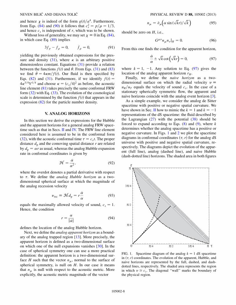
spacetime with positive or negative spatial curvature. Wehave shown in Sec. II how to mimic the k ¼ 1 and k ¼ �1representations of the dS spacetime: the fluid described bythe Lagrangian (27) with the potential (38) should beforced to expand according to Eqs. (8) and (9), where kdetermines whether the analog spacetime has a positive ornegative curvature. In Figs. 1 and 2 we plot the spacetimediagrams in conformal coordinates ð�; rÞ for the analog dSuniverse with positive and negative spatial curvature, re-spectively. The diagrams depict the evolution of the appar-ent (full line), analog (dashed line), and naive Hubble(dash-dotted line) horizons. The shaded area in both figures

r

FIG. 1. Spacetime diagram of the analog k ¼ 1 dS spacetimein ð�; rÞ coordinates. The evolution of the apparent, Hubble, andnaive horizons are represented by the full, dashed, and dash-dotted lines, respectively. The shaded area represents the regionin which v cs. The diagonal ‘‘wall’’ marks the boundary ofthe physical region.

NEVEN BILIC AND DIJANA TOLIC PHYSICAL REVIEW D 88, 105002 (2013)

105002-8

represents the region of supersonic flow, i.e., the region inwhich the fluid three-velocity v exceeds the speed of soundcs. The diagonal line tþ r ¼ � in Fig. 1 corresponds to thefuture infinity, i.e., the point R ¼ T ¼ 1 in Minkowskicoordinates.

VI. DISCUSSION AND CONCLUSIONS

We have demonstrated that it is possible, at least inprinciple, to model an FRW spacetime with arbitrary spa-tial curvature using a relativistic fluid and the associatedeffective acoustic geometry. To obtain the desired geome-try one needs to manipulate the fluid equation of state inaddition to an appropriately designed fluid expansion. Wehave shown in Sec. III that an open FRW spacetime withzero or negative spatial curvature can be modeled usingisentropic perfect fluids such as a Bose-Einstein conden-sate in the Thomas-Fermi limit. The modeling of a closedFRW spacetime with positive spatial curvature is possibleif the condition of isentropy is relaxed. This is achieved bya Lagrangian with a quadratic kinetic energy term multi-plied by a potential V, the choice of which determines theevolution of the analog cosmological scale. The acousticanalog metric takes the conformal form of a general FRWspacetime with positive, negative, or zero spatial curvaturedepending on the choice of the sign parameter k in theexpression (8) and (9) for the flow velocity.

It is conceivable that the analysis presented here is ofconsiderable theoretical interest for emergent gravitymodels, in particular for those in which the emergentgravity is based on fluid flow (for a comprehensive reviewand extensive list of references, see Ref. [31]). It is worthmentioning a few examples in which there is an obvious

connection to our analysis. The first one concerns thealready mentioned emergence of scalar gravity. As wasshown in Ref. [32], in the framework of the fluid-fieldcorrespondence one can go beyond analog gravity by in-troducing a scalar field Lagrangian that describes the dy-namics of a scalar field as an interaction of the field and itsassociated effective metric given by Eq. (22). This inter-action may be interpreted as a gravitational influence onthe field by its own effective metric [2,32]. Another ex-ample is the model of Janik and Peschanski [33] in whichperfect fluid hydrodynamics emerges as a consequenceof the AdS/CFT correspondence. In their approach theAdS/CFT correspondence relates a perfect conformal fluidon the boundary to an asymptotically AdS5 bulk. The linkto our study is twofold: first, the fluid described by theLagrangian (27) is conformal, and second, the longitudinalBjorken expansion of Ref. [33] is of the same form as ourspherical expansion (10) and (11) obtained from the moregeneral expression in the limit when the parameter �approaches zero. Assuming a true AdS/CFT duality, theboundary conformal fluid in the model of Ref. [33] mayalso be regarded as primary and the bulk as emergent [34].In our study so far we have discussed simple toy

models with no realistic fluid in mind. To the best ofour knowledge, the only realistic experimental set up for arelativistic-fluid laboratory is provided by high-energycolliders. In our previous papers [12,13] we suggested arelativistic collision model based on a spherical Bjorken-type expansion tomimic an open FRWuniverse. Tomodel aclosed universe, a different type of expansion is neededwiththe k ¼ 1velocity field (8) and (9). Presentlywe do not havea concrete proposal for how to do this in high-energycollisions. Maybe, with the advance of accelerator technol-ogy, one day it will be possible, e.g., by choosing appro-priate heavy ions and specially designed beam geometry toobtain the desired equation of state and expansion flow ofthe fluid. To confront themodelwith experiment and test theproperties of the analog spacetime it would be of interest toinvestigate the effects of cosmological particle productionin our relativistic model in the same way as it was done inthe nonrelativistic analog models of expanding universes[35,36]. Besides, the presence of a trapped region and theapparent horizon can, in principle, be detected by lookingfor a signal of the analog Hawking radiation in the particledistribution spectra.

ACKNOWLEDGMENTS

This work was supported by the Ministry of Science,Education and Sport of the Republic of Croatia underContract No. 098-0982930-2864 and partially supportedby the ICTP-SEENET-MTP Grant No. PRJ-09 ‘‘Stringsand Cosmology’’ in the frame of the SEENET-MTPNetwork. N. B. thanks CNPq, Brazil, for partial supportand the University of Juiz de Fora where a part of this workhas been completed.

r

FIG. 2. Spacetime diagram of the k ¼ �1 analog dS space-time. The evolution of the apparent, Hubble, and naive horizonsare represented by the full, dashed, and dash-dotted lines,respectively.

FRW UNIVERSE IN THE LABORATORY PHYSICAL REVIEW D 88, 105002 (2013)

105002-9

APPENDIX: TRANSFORMATIONS TOCONFORMAL COORDINATES

Here we describe the procedure [14] for a transformationfrom Minkowski spherical coordinates to conformal spa-tially closed or hyperbolic coordinates. We start from thebackground spacetime of the form

ds2 ¼ dT2 � dR2 � R2d�2; (A1)

and apply the following transformation:

Tðt; rÞ ¼ T0 þ �

2�2ffiffiffiffiffiffiffi�k

p ½fðtþ rÞ þ fðt� rÞ�; (A2)

Rðt; rÞ ¼ R0 þ �

2�2ffiffiffiffiffiffiffi�k

p ½fðtþ rÞ � fðt� rÞ�; (A3)

where

fðxÞ ¼ tanh

0@

ffiffiffiffiffiffiffi�kp2

xþ log�

1A; (A4)

T0, R0, �, and � are constants, and k ¼ 1, 0, �1 for thespherical, flat, or hyperbolic spatial geometry, respectively.Without loss of generality the offsets T0, R0, to the originsof T and R may be set to zero with the implicit assumptionthat in any result the coordinates T and R can be linearlyrescaled. This transformation takes the line element (A1) tothe conformal form

ds2 ¼ a2ðt; rÞ0@dt2 � dr2 � sin 2ð ffiffiffi

kp

rÞk

d�2

1A; (A5)

where

a2ðt; rÞ ¼ �2

�4½cosh ð ffiffiffiffiffiffiffi�kp

rÞ þ cosh ð ffiffiffiffiffiffiffi�kp

tþ 2 log�Þ�2 ;

(A6)

or equivalently, in terms of T and R,

a2ðT; RÞ ¼��

2�2� �2

2�kðT2 � R2Þ

�2 þ kT2: (A7)

These expressions can be simplified by a convenient choiceof the constants � and �. Specifically, for � ¼ 2 and � ¼ 1we obtain

a2ðt; rÞ ¼8><>:1; k ¼ 0;

4=ðcos rþ cos tÞ2; k ¼ þ1;

4=ðcosh rþ cosh tÞ2; k ¼ �1;

(A8)

a2ðT; RÞ ¼8><>:1; k ¼ 0;

½1� ðT2 � R2Þ=4�2 þ T2; k ¼ þ1;

½1þ ðT2 � R2Þ=4�2 � T2; k ¼ �1:

(A9)

A particularly simple transformation is obtained in thelimit � ! 0, in which case one must choose a nonzerooffset T0 in Eq. (A2) to obtain a finite result. In this limit

the transformation (A2)–(A4) with T0 ¼ �=ð�2ffiffiffiffiffiffiffi�k

p Þ takesthe form

T ¼ 2�effiffiffiffiffi�k

ptffiffiffiffiffiffiffi�k

p cosh� ffiffiffiffiffiffiffi�kp

r�; (A10)

R ¼ 2�effiffiffiffiffi�k

ptffiffiffiffiffiffiffi�k

p sinh� ffiffiffiffiffiffiffi�kp

r�; (A11)

which, obviously, makes sense only for k ¼ �1. Then weobtain the conformal representation of the Milne universe,

ds2 ¼ e2�tðdt2 � dr2 � sinh 2rd�2Þ; (A12)

where � may take the value þ1 or �1, corresponding toan expanding or collapsing universe, respectively. This isthe only possible nontrivial map from the Minkowskispacetime to an FRW spacetime with negative spatialcurvature. A direct map to an FRW space with positivespatial curvature is not possible with the coordinate trans-formation (A2).Consider next a spherically expanding (or contracting)

fluid such that the ðt; rÞ coordinate frame is comoving, i.e.,such that the flow velocity of the expanding fluid in thatframe is

u� ¼ ða; 0; 0; 0Þ: (A13)

Then, the components of the velocity in the ðT; RÞ coor-dinate frame are

uT ¼ g�1=200 T;t; (A14)

uR ¼ g�1=200 R;t: (A15)

Using this and Eqs. (A2)–(A4), we find the velocity com-ponents expressed in terms of t and r,

uT ¼2�2 þ cosh

� ffiffiffiffiffiffiffi�kp

r��e�

ffiffiffiffiffi�kp

t þ effiffiffiffiffi�k

pt�4

�2�2 cosh

�� ffiffiffi

kp

r�þ e�

ffiffiffiffiffi�kp

t þ effiffiffiffiffi�k

pt�4

; (A16)

uR ¼sinh

� ffiffiffiffiffiffiffi�kp

r��e�

ffiffiffiffiffi�kp

t � effiffiffiffiffi�k

pt�4

�2�2 cosh

�� ffiffiffi

kp

r�þ e�

ffiffiffiffiffi�kp

t þ effiffiffiffiffi�k

pt�4

; (A17)

and in terms of T and R,

uT ¼ 1

aðT; RÞ��

2�2þ �2

2�kðT2 þ R2Þ

�; (A18)

uR ¼ 1

aðT; RÞ�2

�kTR; (A19)

where aðT; RÞ is given by Eq. (A7).

NEVEN BILIC AND DIJANA TOLIC PHYSICAL REVIEW D 88, 105002 (2013)

105002-10

[1] E. Babichev, V. Mukhanov, and A. Vikman, J. HighEnergy Phys. 02 (2008) 101.

[2] M. Novello, E. Bittencourt, U. Moschella, E. Goulart,J.M. Salim, and J. D. Toniato, J. Cosmol. Astropart.Phys. 06 (2013) 014.

[3] M. Visser, Classical Quantum Gravity 15, 1767 (1998)[4] N. Bilic, Classical Quantum Gravity 16, 3953 (1999).[5] S. Kinoshita, Y. Sendouda, and K. Takahashi, Phys. Rev. D

70, 123006 (2004).[6] J. F. Barbero G., Phys. Rev. D 54, 1492 (1996).[7] J. F. Barbero G. and E. J. S. Villasenor, Phys. Rev. D 68,

087501 (2003).[8] S. Mukohyama and J.-P. Uzan, Phys. Rev. D 87, 065020

(2013).[9] M.A. Lampert, J. F. Dawson, and F. Cooper, Phys. Rev. D

54, 2213 (1996); G. Amelino-Camelia, J. D. Bjorken, andS. E. Larsson, Phys. Rev. D 56, 6942 (1997); M.A.Lampert and C. Molina-Paris, Phys. Rev. D 57, 83 (1998).

[10] C. Barcelo, S. Liberati, and M. Visser, Classical QuantumGravity 18, 1137 (2001).

[11] S. Fagnocchi, S. Finazzi, S. Liberati, M. Kormos, and A.Trombettoni, New J. Phys. 12, 095012 (2010).

[12] N. Bilic and D. Tolic, Phys. Lett. B 718, 223 (2012).[13] N. Bilic and D. Tolic, Phys. Rev. D 87, 044033 (2013).[14] M. Ibison, J. Math. Phys. (N.Y.) 48, 122501 (2007).[15] J. Garriga and V. F. Mukhanov, Phys. Lett. B 458, 219

(1999).[16] J. U. Kang, V. Vanchurin, and S. Winitzki, Phys. Rev. D

76, 083511 (2007).[17] W. Unruh, Phys. Rev. Lett. 46, 1351 (1981).[18] O. F. Piattella, J. C. Fabris, and N. Bilic, arXiv:1309.4282.[19] M. Mannarelli and C. Manuel, Phys. Rev. D 77, 103014

(2008).

[20] N. Bilic, Fortschr. Phys. 56, 363 (2008); Phys. Rev. D 78,105012 (2008).

[21] D. Jaksch, C.W. Gardiner, K.M. Gheri, and P. Zoller,Phys. Rev. A 58, 1450 (1998).

[22] A. S. Parkins and D. F. Walls, Phys. Rep. 303, 1 (1998).[23] N. Bilic, G. B. Tupper, and R.D. Viollier, Phys. Lett. B

535, 17 (2002).[24] R. Jackiw, Lectures on Fluid Dynamics. A Particle

Theorist’s View of Supersymmetric, Non-Abelian,Noncommutative Fluid Mechanics and d-branes(Springer-Verlag, New York, 2002).

[25] N. Bilic, G. B. Tupper, and R.D. Viollier, J. Phys. A 40,6877 (2007).

[26] A. Kamenshchik, U. Moschella, and V. Pasquier, Phys.Lett. B 511, 265 (2001).

[27] J. C. Fabris, S. V. B. Goncalves, and P. E. de Souza, Gen.Relativ. Gravit. 34, 53 (2002); 34, 2111 (2002).

[28] M. C. Bento, O. Bertolami, and A.A. Sen, Phys. Rev. D66, 043507 (2002).

[29] N. Bilic, G. B. Tupper, and R.D. Viollier, Phys. Rev. D 80,023515 (2009).

[30] S. A. Hayward, Phys. Rev. D 49, 6467 (1994).[31] C. Barcelo, S. Liberati, and M. Visser, Living Rev.

Relativity 8, 12 (2005); 14, 3 (2011).[32] M. Novello and E. Goulart, Classical Quantum Gravity 28,

145022 (2011).[33] R. A. Janik and R. B. Peschanski, Phys. Rev. D 73, 045013

(2006).[34] S. Carlip, arXiv:1207.2504.[35] C. Barcelo, S. Liberati, and M. Visser, Phys. Rev. A 68,

053613 (2003).[36] S. Weinfurtner, P. Jain, M. Visser, and C.W. Gardiner,

Classical Quantum Gravity 26, 065012 (2009).

FRW UNIVERSE IN THE LABORATORY PHYSICAL REVIEW D 88, 105002 (2013)

105002-11