Fuad Aleskerov, Vsevolod Petrushchenko

DEA BY SEQUENTIAL EXCLUSION OF ALTERNATIVES

Working Paper WP7/2013/02Series WP7

Mathematical methods for decision making in economics,

business and politics

Моscow 2013

A33

УДК 378:303.7ББК 74.58в7

А33

Editors of the Series WP7:Aleskerov Fuad, Mirkin Boris, Podinovskiy Vladislav

Aleskerov, F., Petrushchenko, V. DEA by sequential exclusion of alternatives : Working paper WP7/2013/02 [Тext] / F. Aleskerov, V. Petrushchenko ; National Research University “Higher School of Economics”. – Moscow : Publishing House of the Higher School of Economics, 2013. – 28 p.

Data Envelopment Analysis is a well-known non-parametric technique of efficiency evaluation which is actively used in many economic applications. However, DEA is not very well applicable when a sample consists of firms operating under drastically different conditions. Generally, it is difficult to define to what extent the analyzed sample is heterogeneous. We offer a new method of efficiency estimation based on a sequential exclusion of alternatives and standard DEA approach. This allows to assess efficiency in the case of heterogeneous set of firms. We obtain a connection between efficiency scores obtained via standard DEA model and the ones obtained via our algorithm. We also evaluate 29 Russian universities and compare results obtained by two techniques.

Key words: efficiency, Data Envelopment Analysis, sequential exclusion of alternatives, uni-versities’ efficiency.

УДК 378:303.7ББК 74.58в7

Fuad Aleskerov – Higher School of Economics, Moscow, Russia; Trapeznikov Institute of Control Sciences RAS, Moscow, Russia.

Vsevolod Petrushchenko – Higher School of Economics, Moscow, Russia.

© Aleskerov F., 2013© Petrushchenko V., 2013© Оформление. Издательский домВысшей школы экономики», 2013

Препринты Национального исследовательского университета «Высшая школа экономики» размещаются по адресу: http://www.hse.ru/org/hse/wp

1. Introduction

First, we briefly discuss Data Envelopment Analysis, which is one

of the most widespread and commonly used techniques of efficiency

evaluation. Cooper et al (1978) extended and generalized offered by

Farrell (1957) method. They showed that the problem of efficiency

evaluation can be formulated in terms of mathematical program as

maxu,v

(

θi =u1q1i + . . . + uNqNi

v1x1i + . . .+ vMxMi

)

subject to

u1q1i+...+uNqNi

v1x1i+...+vMxMi≤ 1,∀ i = 1, . . . , L;

uj ≥ 0,∀ j ∈ 1, . . . , N ;

vk ≥ 0,∀ k ∈ 1, . . . ,M,

where L is the number of firms in the sample, qji — j-th output

parameter (j ∈ 1, . . . , N) of i-th firm, xki — k-th input parameter

(k ∈ 1, . . . ,M) of i-th firm, u and v are weight vectors of appropriate

lengths. Finally, θi represents efficiency measure of i-th firm.

Cooper et al (1978) also showed that presented above model

can be simplified and rewritten in the form of linear program as

minλ,θi

θi (1)

subject to

−qi +Qλ ≥ 0;

θixi −Xλ ≥ 0;

λ ≥ 0,

(2)

3

where qi is N ×1 vector of output parameters of i-th firm, xi is M×1

vector of input parameters of i-th firm, Q is M ×L matrix of output

parameters of all firms, X is N ×L matrix of input parameters of all

firms, λ is L× 1 weight vector, one may interpret it as shadow prices,

(Coelli, (2005)). As in the previous case θi is the efficiency measure

of i-th firm.

The formulation (1)–(2) is fundamental and called CCR model

(after the names of its authors). Note that CCR allows to assess

efficiency only when constant return to scale takes place. Thereby

the program (1)–(2) is also called CRS DEA model. However, it is

easy to adjust the method to the situation with variable return to

scale, we only need to impose one additional constraint

1T · λ = 1, (3)

where 1T is a unit vector of the size 1× L.

The programm (1)–(2) with the restriction (3) is called VRS DEA

model. This modification was introduced in Charnes and Cooper

(1984). Note that VRS model is applicable if analyzed firms operate

at the non-optimal scale.

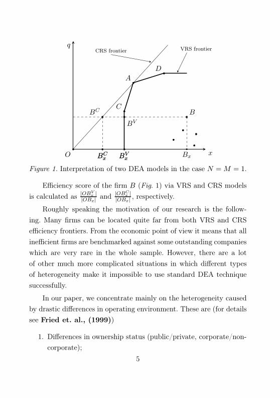
One can write dual to (1), (2), (3) linear programm and discover

a geometrical interpretation of the two discussed models in the case

of single input and output production (Fig. 1).

4

O x

qCRS frontier VRS frontier

B

A

C

D

Bx

BV

BC

BVxBC

x BVxBC

x

Figure 1. Interpretation of two DEA models in the case N = M = 1.

Efficiency score of the firm B (Fig. 1) via VRS and CRS models

is calculated as |OBVx |

|OBx|and |OBC

x ||OBx|

, respectively.

Roughly speaking the motivation of our research is the follow-

ing. Many firms can be located quite far from both VRS and CRS

efficiency frontiers. From the economic point of view it means that all

inefficient firms are benchmarked against some outstanding companies

which are very rare in the whole sample. However, there are a lot

of other much more complicated situations in which different types

of heterogeneity make it impossible to use standard DEA technique

successfully.

In our paper, we concentrate mainly on the heterogeneity caused

by drastic differences in operating environment. These are (for details

see Fried et. al., (1999))

1. Differences in ownership status (public/private, corporate/non-

corporate);

5

2. Location peculiarities (for universities — city/country, for elect-

rical companies — the density of population in the operating

area);

3. Differences in legislation.

There are a lot of papers dealing with the problem of the influence

of environmental parameters on efficiency scores, see Banker and

Morey (1986a, 1986b), Charnes, Cooper and Rhodes (1981),

Bessent and Bessent (1980), Ferrier and Lovell (1990). The

following solutions are commonly used

1. Partitioning of an original sample to the smaller groups by some

environmental factor (for instance, location in city – first group,

suburbs – second group, etc). Comparison is performed only

between subsamples;

2. Separate application of DEA to each cluster, then construction

of each firm’s projection onto its respective efficiency fronti-

er and launching one common DEA LP among the obtained

projections;

3. Imposition of additional restrictions to the DEA;

4. Composition of regression analysis with the approach 3.

One can find the detailed description of all methods, their strengths

and shortages in Coelli et al (2005). However, there are two common

disadvantages of the four offered techniques. First, they all are based

on the strict definition of environmental parameters. One has to expli-

citly conjecture that some factors have influence on the efficiency

values. This implies that some factors may be underestimated or,

6

conversely, overestimated. Second, in some situations it could be very

difficult to define and measure environmental variables, specially, if

we would like to take into account the influence of social, political,

legal or cultural impact.

Yet, there is another widespread technique of taking into account

heterogeneity of the sample. The idea is to combine the power of

clustering models with DEA. There are a number of authors applying

this methodology, see, e.g., Samoilenko, K.M.Osei-Bryson (2010);

Shin and Sohn, (2004); Hirschberg and Lye, (2001); Lemos et

al., (2005); Meimand et al., (2002); Sharma and Yu, (2009);

Marroquin et al., (2008); Schreyogg and von Reitzenstein,

(2008). Generally, clustering methods can be united with DEA via

two different ways. The first one is to apply clustering to the obtained

efficiency scores, then form appropriate reference subsets of firms and

apply DEA again. The second one is on the contrary based on the

application of clustering to initial set of firms and then comparison of

each firm within its reference set.

The structure of our algorithm differs from the standard approach-

es. We suggest to move the efficiency frontier to such an extent as to

make the evaluation reasonable.

The next chapter presents the method in the simplest possible

case with economy consisting of single input and output. Then we

introduce one of the possible ways to extend our model to the evalua-

tion of samples with arbitrary number of inputs and outputs. In the

last section we calculate efficiency scores of 29 Russian universities

using standard DEA and the new algorithm.

7

2. The model

In this section and throughout the rest of the text we use the

definition of efficient firms according to CRS model. We also restrict

our consideration to the situation with single input and output. Note

that in this case there may be several efficient firms if and only if all

of them are lying on the same ray which i) begins in the origin and

ii) has the highest slope amongst all analogous rays which connect

other firms with origin. Algebraically it means that several efficient

firms must have exactly the same minimal among others ratio of input

to output. Therefore without loss of generality we consider the case

when there is only one 100% efficient company in the sample.

Our purpose is to construct a new efficiency frontier which takes

into account heterogeneity of the evaluated sample. Recall that the

i-th firm in the sample is represented via two coordinates (xi, qi) in

the space of input-output parameters.

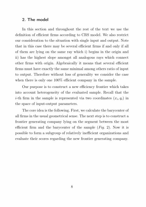
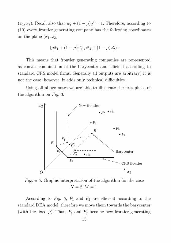
The core idea is the following. First, we calculate the barycenter of

all firms in the usual geometrical sense. The next step is to construct a

frontier generating company lying on the segment between the most

efficient firm and the barycenter of the sample (Fig. 2). Now it is

possible to form a subgroup of relatively inefficient organizations and

evaluate their scores regarding the new frontier generating company.

8

O x

qF1

F3

F4

F5

B

F6

F2

G

CRS frontier

New frontier

Barycenter

Figure 2. Graphic interpretation of the algorithm in the case

N = M = 1.

On the figure above initial sample consists of the firms F1, . . . ,

F6 and according to standard CRS model F1 is the efficient firm.

According to the introduced algorithm we calculate the barycenter

(point B) and construct the new frontier via generating phantom

firm G, lying on the segment BF1. Clearly, F3, . . . , F6 should be

benchmarked against the firm G. Still, F1 and F2 remain unevaluated,

to compute their efficiency scores we should repeat the same algorithm

excluding the firms F3, . . . , F6 from consideration.

It is of separate interest to define exact position of the frontier

generating company. It is clear that this location should be coherent

with some extent to heterogeneity. Roughly speaking, it means that

the higher heterogeneity within the sample the nearer generator to

the barycenter. Here we offer a straightforward method for calculation

of the heterogeneity degree of the sample. Consider the vector ~d of

Euclidian distances from the barycenter to all firms. Let heterogeneity

9

index µ be the ratio of the mean value of ~d to the maximum element

in ~d. Then the position of generating company is defined as

G = µB + (1 − µ)F1, (4)

where B is the barycenter of the sample and F1 is a 100% efficient

firm according to the standard DEA CRS model.

Note several important properties of the procedure. First, the

algorithm obviously converges for any sample. Second, the only firm

that remains efficient is the one which is efficient according to standard

CRS model. Besides there is a simple connection between DEA efficien-

cy scores and the ones obtained via the sequential process. Suppose

that current subgroup of firms is evaluated via frontier generating

firm G. Let F be in this subgroup, then

ECRS

F= ECRS

G· ENew

F, (5)

where the lower index stands for firms and the upper one does for

efficiency evaluation method. Note that the formula (5) follows immedi-

ately from the interpretation of CRS efficiency scores given in Fig. 1.

According to (5) our algorithm evaluates inefficient firms less

strictly than the standard CRS model. Again, the reason for such

alleviation is that the sample is heterogeneous and all firms cannot

be benchmarked against the firm which showed exceptional efficiency.

Such situations happen in practice very often and may occur, for

instance, because of the presence of some crucial environmental factors.

3. Extensions to general case

Consider now the case of a sample characterized by several input

and output variables. It is impossible to apply the considerations

10

above directly. Thus we construct a sequence of linear programs which

allow us to carry out the same algorithm in general case. Besides, we

want to preserve the following properties

i) Convergence of the procedure for any sample;

ii) The only firms that remain efficient are those which were efficient

according to standard CRS model;

iii) Some counterpart of the equality (5) should be obtained.

Recall that i-th firm is represented by the vector xi = (x1i, . . . , xNi)

of inputs and qi = (q1i, . . . , qMi) of outputs. Similarly to the previous

section we define the input and output parts of the barycenter as

bx = (x1, . . . , xN ),

and

bq = (q1, . . . , qM ),

where, as usual, the bar means the average value of a particular

parameter.

We will also need the heterogeneity index µ, defined as before as

the ratio of mean distance from barycenter to the maximal one1.

Let the whole sample be defined by the set of indices I = {1, . . . , L}.

Recall that there are N input and M output variables. We denote the

group of 100% efficient companies as a subset Ie = {i1, . . . , iS} ⊂ I.

Now, let Xe be the N × S matrix of input parameters of all efficient

1Note that this value can also be computed in a different way, for instance, via

expert evaluations.

11

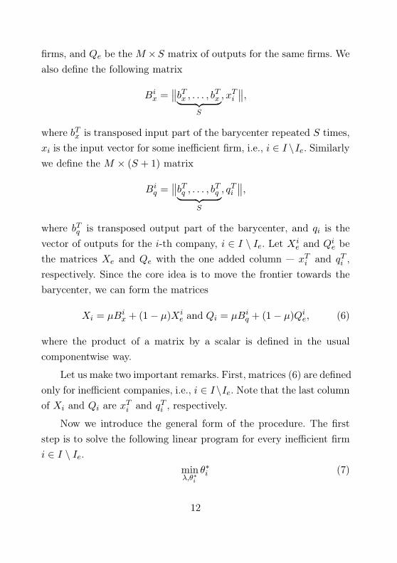
firms, and Qe be the M ×S matrix of outputs for the same firms. We

also define the following matrix

Bix =

∥∥bTx , . . . , b

Tx

︸ ︷︷ ︸

S

, xTi∥∥,

where bTx is transposed input part of the barycenter repeated S times,

xi is the input vector for some inefficient firm, i.e., i ∈ I \Ie. Similarly

we define the M × (S + 1) matrix

Biq =

∥∥bTq , . . . , b

Tq

︸ ︷︷ ︸

S

, qTi∥∥,

where bTq is transposed output part of the barycenter, and qi is the

vector of outputs for the i-th company, i ∈ I \ Ie. Let Xie and Qi

e be

the matrices Xe and Qe with the one added column — xTi and qTi ,

respectively. Since the core idea is to move the frontier towards the

barycenter, we can form the matrices

Xi = µBix + (1− µ)Xi

e and Qi = µBiq + (1− µ)Qi

e, (6)

where the product of a matrix by a scalar is defined in the usual

componentwise way.

Let us make two important remarks. First, matrices (6) are defined

only for inefficient companies, i.e., i ∈ I\Ie. Note that the last column

of Xi and Qi are xTi and qTi , respectively.

Now we introduce the general form of the procedure. The first

step is to solve the following linear program for every inefficient firm

i ∈ I \ Ie.

minλ,θ∗

i

θ∗i (7)

12

subject to

−qi +Qiλ ≥ 0;

θ∗i xi −Xiλ ≥ 0;

λ ≥ 0,

(8)

where Xi and Qi are defined in (6), λ is (S+1)×1 vector of constants,

xi and qi are input and output vectors for the i-th inefficient firm.

Finally, θ∗i is the corrected efficiency score of the i-th inefficient compa-

ny, however, there are two possible situations regarding this value.

Namely, we exclude all inefficient companies which get θ∗ < 1 from the

consideration and evaluate all others at the next step of the algorithm.

The procedure is repeated with the refreshed sample in the following

order

1. Calculation of the new barycenter;

2. Calculation of new Xi and Qi matrices for all inefficient companies;

3. For all inefficient companies left we calculate new efficiency

scores with respect to (7)-(8). All those which get θ∗ < 1 are

excluded;

4. Again, if some inefficient companies get θ∗ = 1, then we repeat

procedure from the step 1.

We did not take into account only one case, when matrices (6) are

organized in such a way that for all inefficient companies according

to (7)-(8) θ∗ = 1 holds. It means that the original frontier is moved

too much. Therefore we have to decrease the value of µ and begin

the procedure from the beginning. For instance, we can take the new

value of the heterogeneity index as µ2.

13

To conclude we make two remarks regarding the algorithm. The

convergence is guaranteed by construction. The set of efficient firms

is preserved as well. Although we cannot save the property (5), the

straightforward analog is the following. Since we use standard DEA

CRS model, we can calculate a projection of every inefficient firm

on the temporary frontier defined by (7)-(8) programm, see (Coelli,

2005) for details. Then it holds that

ECRS

F= ECRS

P· ENew

F, (9)

where ECRS

Fis the standard efficiency score of the firm F , ECRS

Pis

the efficiency of the projection P of the firm F on the new frontier

defined by (7)-(8). Finally, ENew

Fis the efficiency score of the firm F

according to our procedure.

Thus, we gave a theoretical description of the sequential DEA

process and showed the simplest properties of the procedure. Note

also, that our model with µ = 0 corresponds to the usual DEA CRS

model.

Now, let us give an example how the algorithm works for the case

of two inputs and single output parameter.

As always, we denote first input, second input, single output and

heterogeneity index defined in (4) as x1, x2, q and µ, respectively.

Apparently all efficient firms with coordinates (xe1, xe2, q

e) are moved

towards the barycenter via the following transformation

(xe1, xe2, q

e) 7−→ µ(x1, x2, q) + (1− µ)(xe1, xe2, q

e). (10)

It is known that in this case standard CRS model can be easily

visualized on the plane (x1

q, x2

q). Without loss of generality, suppose

all outputs are equal to 1, it allows to simplify the plane to the form

14

(x1, x2). Recall also that µq + (1− µ)qe = 1. Therefore, according to

(10) every frontier generating company has the following coordinates

on the plane (x1, x2)

(µx1 + (1− µ)xe1, µx2 + (1− µ)xe2) .

This means that frontier generating companies are represented

as convex combination of the barycenter and efficient according to

standard CRS model firms. Generally (if outputs are arbitrary) it is

not the case, however, it adds only technical difficulties.

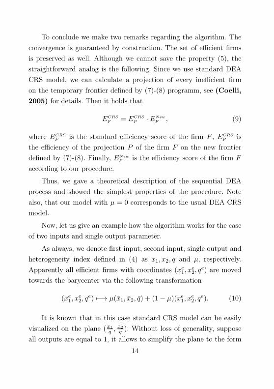
Using all above notes we are able to illustrate the first phase of

the algorithm on Fig. 3.

O x1

x2

F1

F2

F4

F3

F5

F6B

F8

F7

BarycenterF ′

2

F ′

1

New frontier

CRS frontier

P3

P ′

3

Figure 3. Graphic interpretation of the algorithm for the case

N = 2,M = 1.

According to Fig. 3, F1 and F2 are efficient according to the

standard DEA model, therefore we move them towards the barycenter

(with the fixed µ). Thus, F ′1 and F ′

2 become new frontier generating

15

firms. It is clear that on the first stage of the procedure we evaluate

only F3, . . . , F7 because F8 gets θ∗8 = 1. For instance, the efficiency

score of F3 can be determined as a ratio |OP ′3| to |OF3|, where P ′

3 is

the projection of F3 on the new frontier. Note that standard efficiency

of this firm is defined by |OP3||OF3|

, where P3 is a similar projection of F3

onto standard CRS frontier.

Finally, let us illustrate what the identity (9) means

ECRS

P′

3

· ENew

F3=

|OP3|

|OP ′3|·|OP ′

3|

|OF3|=

|OP3|

|OF3|= ECRS

F3,

where all notation is taken from Fig. 3.

To conclude this section, let us note also that the procedure

cannot be simplified and performed via some single-step modifica-

tion of the standard DEA model.

4. Empirical application

We apply now our model to evaluation of efficiency scores for

29 Russian universities and compare the results with the standard

DEA outcome. The detailed description of this research is presented

in Abankina et. al., (2012). To apply DEA we choose three input

parameters, which reflect main universities’ resources – the quality of

state financing, quality of professorial and teaching staff and quality

of entrants.

1. The ratio of budget funds to the number of students who get

tuition waiver (denoted as I1);

2. The percentage of employees who have a degree of Doctor of

Science (denoted as I2);

16

3. The quality of university entrants, to estimate this parameter

we use a mean value of Universal State Exam (USE), which is

mandatory for admission (denoted as I3).

and two output parameters

1. The ratio of non-budget income to the number of students paid

for higher education (denoted as Q1);

2. The score of scientific and publishing activity presented at:

http://www.hse.ru/org/hse/sc/interg (and denoted as Q2).

The first output indicates the attractiveness of a university for

the applicants and the second one is a proxy for success of scientific

and research work within a university. The descriptive statistics for

all parameters is presented below (29 observations for 2008).

Table 1. Descriptive statistics of input and output parameters

I1 I2 I3 Q1 Q2

Mean value 94.92 63.43 61.47 90.84 4.90

Variance 1038.10 36.18 25.85 931.04 14.78

Standard Deviation 32.21 6.01 5.08 30.51 3.84

Median 84.84 62.94 61.1 83.54 3.46

Minimum 53.71 55.76 54.2 43.19 1.47

Maximum 175.65 75.92 76.7 170.07 18.25

Sum 2752.80 1839.48 1782.8 2634.59 142.18

First, we calculate efficiency scores according to standard DEA

model. After that we apply our technique taking three distinct values

of heterogeneity index µ, namely, 0.2, 0.5 and 0.8. Appendix 1 contains

the detailed list of efficiency scores for all four cases.

We compare the results obtained via different models in two

ways. First, we rank all universities according to their efficiency scores

in each of four cases and compare different orderings via Kendall’s

17

distance, see Kendall (1938), i.e. we count all discordant pairs in

the two ranks and then normalize this value by dividing by the total

number of pairs in a list consisting of N objects. The discordant pair

(i, j) is the one for which i is better than j in the first rank and

j is better than i in the second one or vice versa. Consequently a

concordant pair is the one which is ranked in the same order in both

orderings.

Further, let us denote the number of discordant pairs as N− and

the number of concordant pairs as N+. Note that

N+ +N− = C2N =

N(N − 1)

2,

where C2N is a binomial coefficient.

According to this notation the Kendall’s distance may be calculated

as

K(r1, r2) =N−

N+ +N−=

2N−

N(N − 1), (11)

where r1 and r2 are different ranks consisting of N objects. Note that

the value of Kendall’s distance lie between 0 and 1, where 0 means

that two orderings are the same and 1 means that the two rankings

are inverse.

Table 2 shows the Kendall’s distance between all four types of

efficiency evaluation models.

Table 2. Kendall’s distances

DEA µ = 0.2 µ = 0.5 µ = 0.8

DEA 1.0000 - - -

µ = 0.2 0.0197 1.0000 - -

µ = 0.5 0.0493 0.0394 1.0000 -

µ = 0.8 0.1158 0.1108 0.0911 1.0000

18

Note that the distance between ranks obtained via the technique

is small. Moreover the nearer the value of µ to 1 the higher the bias

of new efficiency scores from the ones obtained via standard DEA.

As another measure of a difference between two rankings we

compute median, mean and minimal values of efficiency scores for

all four versions of our evaluations (recall that standard DEA can be

obtained from our model taking the value of µ = 0). The information

is given below.

Table 3. Median and mean values of efficiency scores for different

models (in percents)

DEA µ = 0.2 µ = 0.5 µ = 0.8

Median 70.50 76.94 88.12 95.84

Mean 71.33 75.55 82.17 90.05

Minimal 34.03 36.15 43.88 57.90

Again, Table 3 confirms that the obtained results are quite consis-

tent. With the increasing of heterogeneity index µ our model evaluate

all firms more and more mildly. All characteristics are increasing with

the growth of µ.

5. Conclusions

We have introduced a new algorithm of efficiency evaluation in

case when the sample is heterogeneous and the standard DEA model

does not work very well. One of the fundamental principles used is

that the geometric barycenter of a sample represents the average

situation of the evaluated sector of economy. Taking it into account,

the core idea of our technique is to move the efficiency frontier towards

the barycenter. It allows to evaluate all inefficient firms more mildly.

All these theoretical considerations are preformed via the sequential

19

solving of the number of linear programs.

Our algorithm has three important properties. First, the conver-

gence for any sample is guaranteed. Second, the set of firms that are

efficient according to the standard DEA model is preserved. Finally,

there is the simple connection between efficiency scores obtained via

DEA and our algorithm.

We tested our model on the real data set, containing information

on five parameters, concerning 29 Russian universities in 2008. The

developed technique shows consistent results, i.e., our model does not

crucially change the structure of a ranking by efficiency, however,

the efficiency scores grow when the heterogeneity of the sample is

increasing.

6. Acknowledgement

We thank Decision Choice and Analysis Laboratory and Scientific

Fund of HSE for partial financial support.

20

Appendix 1

Efficiency scores (in percents) for different models

№ DEA (µ = 0) µ = 0.2 µ = 0.5 µ = 0.8

1 70.50 76.94 89.39 87.71

2 64.68 68.96 79.54 95.26

3 52.44 55.40 60.76 71.95

4 48.30 51.39 57.11 68.11

5 65.67 73.80 88.12 98.26

6 34.03 36.15 43.88 70.73

7 86.63 92.42 93.96 99.07

8 57.41 64.41 76.66 91.67

9 74.94 79.27 87.12 90.52

10 70.68 78.55 93.74 99.19

11 100 100 100 100

12 94.79 96.09 96.44 99.38

13 92.26 97.20 97.70 95.84

14 83.60 88.49 97.36 99.85

15 79.79 89.52 94.50 99.49

16 77.51 87.16 92.32 99.57

17 96.60 97.92 98.26 99.45

18 57.69 60.94 66.82 79.31

19 57.90 61.42 67.89 76.38

20 100 100 100 100

21 63.27 67.29 75.81 98.19

22 60.50 64.16 70.85 79.56

23 44.10 46.74 51.57 57.90

24 60.09 64.07 74.98 89.64

25 44.17 49.55 58.97 70.52

26 58.65 64.15 77.75 95.46

27 72.43 78.83 91.35 98.60

28 100 100 100 100

29 100 100 100 100

Mean 71.33 75.55 82.17 90.05

21

References

1. Abankina, I.V., Aleskerov, F.T., Belousova, V.Y., Bonch-Osmo-

lovskaya, A.A., Petrushchenko, V.V., Ogorodniychuk, D.L., Yaku-

ba, V.I., Zin’kovsky K.V., (2012), “University Efficiency Evalua-

tion with Using its Reputational Component”, Lecture Notes in

Management Science, Tadbir Operational Research Group, Ltd,

4, 244-253.

2. Banker, R.D., A. Charnes and W.W. Cooper (1984), “Some

Models for Estimating Technical and Scale Inefficiencies in Data

Envelopment Analysis”, Management Science, 30, 1078-1092.

3. Banker, R.D., and R.C. Morey (1986a), “Efficiency Analysis for

Exogenously Fixed Inputs and Outputs”, Operations Research,

34, 513-521.

4. Banker, R.D., and R.C. Morey (1986b), “The Use of Categorical

Variables in Data Envelopment Analysis”, Management Science,

32, 1613-1627.

5. Bessent, A.M., and E.W. Bessent (1980), “Comparing the Compa-

rative Efficiency of Schools through Data Envelopment Analysis”,

Educational Administration Quarterly, 16, 57-75.

6. Charnes, A., W.W. Cooper and E. Rhodes (1978), “Measuring

the Efficiency of Decision Making Units”, European Journal of

Operational Research, 2, 429-444.

7. Charnes, A., W.W. Cooper and E. Rhodes (1981), “Evaluating

Program and Managerial Efficiency: An Application of Data

Envelopment Analysis to Program Follow Through”, Manage-

ment Science, 27, 668-697.

22

8. Coelli, T.J., D.P. Rao, C.J. O’Donnell, G.E. Battese (2005),

“An Introduction to Efficiency and Productivity Analysis”, 2nd

edition, Springer, N.Y..

9. Farrell, M.J. (1957), “The Measurement of Productive Efficiency”,

Journal of the Royal Statistical Society, Series A, CXX, Part 3,

253-290.

10. Ferrier, G.D., and C.A.K. Lovell (1990), “Measuring Cost Efficien-

cy in Banking: Econometric and Linear Programming Evidence”,

Journal of Econometrics, 46, 229-245.

11. Fried, H.O., S.S. Schmidt and S. Yaisawamg (1999), “Incor-

porating the Operating Environment into a Nonparametric Mea-

sure of Technical Efficiency”, Journal of Productivity Analysis,

12, 249-267.

12. Hirschberg, J.G., J.N. Lye, (2001), “Clustering in a Data Envelop-

ment Analysis Using Bootstrapped Efficiency Scores”, Department

of Economics – Working Papers Series 800, The University of

Melbourne.

13. Kendall, M.A., (1938) “New Measure of Rank Correlation”, Bio-

metrika, 30, 81–89.

14. Lemos, C.A.A., M.P. Lima, N.F.F. Ebecken, (2005), “DEA Imple-

mentation and Clustering Analysis using the K-means algorithm”,

Data Mining VI – Data Mining, Text Mining and Their Business

Applications, vol. 1, 2005, Skiathos, pp. 321–329.

15. Marroquin, M., M. Pena, C. Castro, J. Castro, M. Cabrera-

Rios, (2008), “Use of data envelopment analysis and clustering

23

in multiple criteria optimization”, Intelligent Data Analysis 12,

89–101.

16. Meimand, M., R.Y. Cavana, R. Laking, (2002), “Using DEA and

survival analysis for measuring performance of branches in New

Zealand’s Accident Compensation Corporation”, Journal of the

Operational Research Society, 53 (3), 303–313.

17. Samoilenko, S., K.M. Osei-Bryson, (2010), “Determining sources

of relative inefficiency in heterogeneous samples: Methodology

using Cluster Analysis, DEA and Neural Networks”, European

Journal of Operational Research, 206, 479-487.

18. Schreyogg, J., C. von Reitzenstein, (2008), “Strategic groups

and performance differences among academic medical centers”,

Health Care Management Review, 33 (3), 225–233.

19. Sharma, M.J., S.J. Yu, (2009), “Performance based stratification

and clustering for benchmarking of container terminals”, Expert

Systems with Applications, 36 (3), 5016–5022.

20. Shin, H.W., S.Y. Sohn, (2004), “Multi-attribute scoring method

for mobile telecommunication subscribers”, Expert Systems with

Applications, 26 (3), 363–368.

24

3

Алескеров, Ф. Т., Петрущенко, В. В. Оболочечный анализ данных с использованием последовательного исключения альтернатив : препринт WP7/2013/02 [Текст] / Ф. Т. Алескеров, В. В. Петрущенко ; Нац. исслед. ун-т «Высшая школа экономики». – М. : Изд. дом Высшей школы экономики, 2013. – 28 c. (in English).

Оболочечный анализ данных (ОАД) является хорошо известной непараметрической процедурой оценки эффективности, которая активно используется во многих экономических приложениях. Однако ОАД работает не самым лучшим образом, если выборка состоит из объектов, функционирующих в кардинально различных условиях. Вообще говоря, определение степени неоднородности выборки – чрезвычайно трудная задача. Мы предлагаем новый метод оценки эффективности, основанный на последовательном исключении альтернатив и стандартном ОАД. Это позволяет оценить эффективность в случае неоднородной выборки объектов. Мы устанавливаем связь между оценками эффективности, полученными стандартными ОАД и с помощью нового алгоритма. Мы также оцениваем 29 российских университетов и сравниваем результаты, полученные двумя методами.

Ключевые слова: эффективность, оболочечный анализ данных, последовательное исключение альтернатив, эффективность университетов.

Алескеров Ф.Т. – Национальный исследовательский университет «Высшая школа экономики», Москва; Институт проблем управления им. В.А. Трапезникова, Москва.

Петрущенко В.В. – Национальный исследовательский университет «Высшая школа экономики», Москва.

4

Препринт WP7/2013/02Серия WP7

Математические методы анализа решений в экономике, бизнесе и политике

5

Алескеров Фуад Тагиевич, Петрущенко Всеволод Владимирович

Оболочечный анализ данных с использованием последовательного исключения альтернатив

(на английском языке)

6

Отпечатано в типографии Национального исследовательского университета

«Высшая школа экономики» с представленного оригинал-макетаФормат 60×84 1/16. Тираж 15 экз. Уч.-изд. л. 1,2

Усл. печ. л. 1,6. Заказ № . Изд. № 1541Национальный исследовательский университет

«Высшая школа экономики» 125319, Москва, Кочновский проезд, 3

Типография Национального исследовательского университета «Высшая школа экономики»