Full NameFull Name

Phone #Phone # BirthdayBirthday

Parents’ NamesParents’ Names

Mom Cell/Work #Mom Cell/Work # Dad Cell/Work #Dad Cell/Work #

Parent email:Parent email:

Extracurricular Activities:Extracurricular Activities:

List the Math Courses you have List the Math Courses you have taken and the grade you receivedtaken and the grade you received

11stst

22ndnd

33rdrd

4th4th

Turn your card overTurn your card over

Write something interesting about Write something interesting about yourself on the back… something yourself on the back… something you want us to know….you want us to know….

AP Statistics Section 1.1

Displaying Distributions with Graphs

Distributions A distribution can be a table or a

graph. It tells us all the values a variable can take, and how often it takes those values.

Think about how data is “distributed”.

Examples of Distributions

Race Proportion

White 62.8%

African American

28.4%

Asian 5.6%

Hispanic 3.2%

White

AfricanAmerican

Asian

Hispanic

Let’s start with a little vocab!

Individuals: People, animals, or things for which you are collecting data.

Variables: The values of data you are collecting (ex. How many miles a person travels in a week). Always be specific.

Categorical vs. Quantitative Variables

Categorical variable – records in which category or group an individual belongs Examples: marital status, sex, birth

month, Likert scale Quantitative variable – takes

numerical values for which arithmetic operations make sense Examples: height, IQ, # of siblings

Categorical or Quantitative?

Race Proportion

White 62.8%

African American

28.4%

Asian 5.6%

Hispanic 3.2%

White

AfricanAmerican

Asian

Hispanic

Why it’s important to know the difference between categorical and quantitative variables

You will receive NO credit (really!) on the AP exam if you construct a graph that isn’t appropriate for that type of data

Type of Variable Appropriate Graph

Categorical Pie Chart, Bar Graph

Quantitative Dotplot, Stemplot, Histogram

Types of Graphs for Categorical Variables

Pie Chart Bar Graph

Note: The bars should not “touch” each other. Bars are labeled with the category name.

Pie Chart (Categorical) Categories must make up a whole. Percents must add up to 100%.

Music preferences in young adults 14 to 19.

Bar Graph (Categorical) Represent a count OR percent. These do not have to be part of a whole or add up

to 100%.

Percentage of Drivers Wearing Seat Belts by Region

0.00%

10.00%

20.00%

30.00%

40.00%

50.00%

60.00%

70.00%

80.00%

90.00%

Northeast Midwest South West

Region

Perc

en

t

Types of Graphs for Quantitative Variables

Dotplots—place a dot above each value of the variable for every time it occurs in the data set

Types of Graphs for Quantitative Variables

Stemplots – divide the data into “stems” and “leaves.”

Leaves include the last digit (you can round if necessary)

It is imperative you have a key.

How to interpret graphs Remember SOCS: Spread, outliers, center,

shape Spread—stating the smallest and largest

values (note: different from the range where you actually subtract the values). We will talk about other measures of spread later.

Outliers—values that differ from the overall pattern.

Center—the value that separates the observations so that about half take larger values and about half take smaller values (in the past, you may have heard this called median).

Shape—symmetric, skewed left, skewed right. We’ll learn more about shape later.

Activity

QUIETLY take your pulse for 60 seconds. Write it down on an index card. Do not put your name on the index card. Bring your index card to me.

Finish up the activity

Is this data quantitative or categorical?

How could we represent this data? Construct an appropriate graph with

your group members.

One-Variable Quantitative Data

The most common graph is a histogram.

It is useful for large data sets. NOTE—histograms are appropriate

graphs for one-variable quantitative data!!!

Note that the axes are

labeled!

The bars have equal width!!!

The height of each bar tells how many students fall into that class.

Bars include the starting value but not the ending value.

Reading a Histogram

There are 3 trees with heights between 60 and 64. How many trees have heights between 70 and 79?

From 70 to 80? Each value on the scale of the histogram is the START

of the next bar.

Another Example

Refer to p. 20 for an example of a histogram that has a “break” in the scale on one of the axes.

Using the TI Calculator to Construct Histograms

Follow the instructions on p. 21 to construct a histogram. Enter the data from Example 1.6 on p. 19.

Note: Clear Y= screen before beginning.

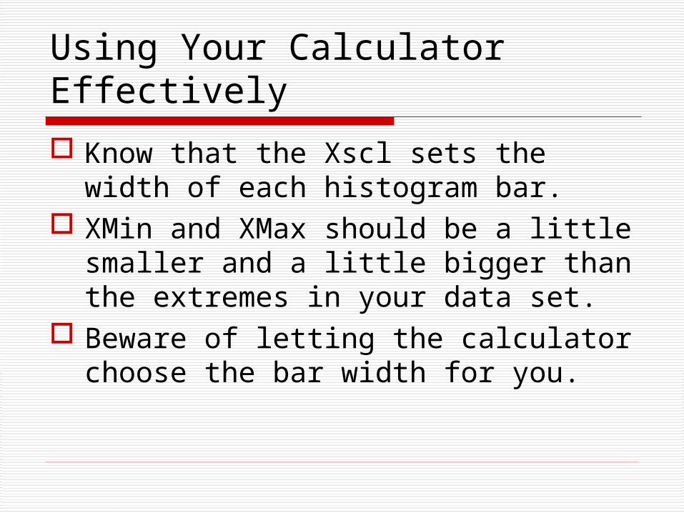
Using Your Calculator Effectively

Know that the Xscl sets the width of each histogram bar.

XMin and XMax should be a little smaller and a little bigger than the extremes in your data set.

Beware of letting the calculator choose the bar width for you.

Shape

Symmetric – the right and left sides of the histogram are approximately approximately mirror images of each other

Skewed Left – there is a long tail to the left

Skewed Right – there is a long tail to the right

Examples of Shape

Skewed left!

Skewed right!

Now what?

Constructing the graph is a “minor” step. The most important skill is being able to interpret the histogram.

Remember SOCS? Spread Outliers Center Shape

SOCS

Spread: from 7 to 22

Outliers: there do not appear to be any outliers.

Center: around 15 or 16

Shape: skewed left

Homework

Chapter 1 #9, 16, 18, 27, 38