full technical report: snow effects on water...

Full Technical Report: Snow effects on water availability

Copernicus Climate Change Service

Full Technical Report:

Snow effects on water availability

Author name: María José Pérez-‐Palazón, Jose Ignacio Migallón and María José Polo (coordinator)

Author organization: University of Córdoba (Spain)



Summary

The Guadalfeo River Basin (GRB) is a mountainous coastal watershed in southern Spain, highly influenced by the snow regime, and vulnerable to future climate variability. The GRB hydrology shifts from a snow-‐dominated regime in the North to a warm coastal regime in the South, in a 40-‐km distance. The climate variability adds complexity to this heterogeneous area. The uncertainty of snow occurrence and persistence for the next decades poses a challenge for the current and future water resource uses in the area. Adaptation plans will benefit from the predictability of water resource availability and regime. The development of easy-‐to-‐use climate indicators and derived decision-‐making variables is key to assess and face the economic impact of the potential changes.

The results assess the prevision of water allocation success on an annual and decadal basis in the new planning hydrological cycle, and they have provided a deeper insight on the seasonal future potential regime. Moreover, they are a basis to test the operational rules of the reservoir and the priority of use criteria. Regarding the hydropower generation, besides the evaluation of the potential future efficiency and provisions under the expected shift of the snow regime, further assessment on the minimum environmental flows and their impact on the activity is being done. Additional concern about the need of an adequate inflow measurement has been achieved and some actions to improve the gauging system are under work at present.

The C3S SIS for Water indicators provide an open framework to obtain assessment of the seasonality expected shifts in the river flow regime, and in the long term. Using these indicators has made it possible to quantify in a complex region the extent to which the likely impacts of climate on snow will affect the current water allocation scenario, and to identify the most vulnerable water uses in the area. This helps to foresee and anticipate close in time conflicts of water users, and it will be key in the adaptation assessment under course at the moment.



Contents Introduction ............................................................................................................................................ 1

Step 1: Extracting Climate Change Impact Indicators ......................................................................... 2

Description: ......................................................................................................................................... 2

Results: ............................................................................................................................................ 2

Step 2: Snow evolution and river flow simulations ............................................................................. 5

Description: ..................................................................................................................................... 5

Results: ............................................................................................................................................ 5

Step 3: Downscaling to a high spatial resolution ................................................................................ 8

Description: ..................................................................................................................................... 8

Results: ............................................................................................................................................ 8

Step 4: Assessment of changes. ........................................................................................................ 15

Description: ................................................................................................................................... 15

Results: .......................................................................................................................................... 16

Step 5 Integrated river basin management ....................................................................................... 19

Description: ................................................................................................................................... 19

Results: .......................................................................................................................................... 19

Step 6: Climate change adaptation strategies. .................................................................................. 22

Description: ................................................................................................................................... 22

Results: .......................................................................................................................................... 22

Conclusion of Full Technical Report ...................................................................................................... 25

References ............................................................................................................................................. 27


Full Technical Report: Snow effects on water availability 1

Introduction

The Guadalfeo River Basin (Figure 1) is a 1345 km2 Mediterranean mountainous coastal watershed in the Sierra Nevada National Park; the highly variable precipitation and snow regime in Sierra Nevada determines water availability at the seasonal and annual scales, and two connected reservoirs control both floods and water scarcity in the area. Tourism and high valued tropical crops in the coast

(Tropical Coast) compete for water during the warm season. At the same time, rural tourism and marginal agriculture are the economic basis in the northern mountain area (Alpujarras), where cultural and historical irrigation survives thanks to snowmelt flows. Hydropower generation system at the heads also depends on snowmelt during the cold/spring seasons, but environmental flows must be observed.

As public water manager, client 1 needs precise information on short/long term water availability for reservoir operation and hydrological planning. This includes restrictions to water allocation for client 2 (both urban and crop uses) and limitations to hydropower for client 3, who also benefits from sound forecasting of snowmelt. The future climatic context poses a risk for the current supply system and water resource availability on a long term basis; the need for operating/decision making tools was identified during the current hydrological plans development and all the participation meetings and conclusions. The Figure 2 shows the workflow followed in this report and its description.

Figure 2.Workflow description

ExtracNng Climate Change

Impact Indicators

Downscaling to a high spaNial resoluNon Snow evoluNon

and river flow simultaNons

Assessment of changes in

water resource availability

Integrated river basin

management

Climate change adaptaNon strategies

Figure 1. Digital Elevation Model of Guadalfeo river basin inthe context of the Mediterranean coast in South Spain.



Step 1: Extracting Climate Change Impact Indicators

Description: The CIIs listed in the table 1 were extracted and evaluated for both the reference and the 2000p2015 period; their monthly and annual regimes and trends were compared to the available local data at the study area. At a first attempt, ECVs of precipitation and temperature from the C3S SIS for Water Demonstrator were downscaled and compiled as inputs to the hydrological model WiMMed (GDFH, 2011)1, operational at the study site, to obtain river flow and evapotranspiration at selected control points. However, the results obtained from this, together with the later inclusion in C3S SIS for Water of river flow and ETp related indicators, led to a change of approach. River flow was targeted as the main CII in this study case, and local time series of river flow were used to perform the following downscaling step. The catchments and the associated CIIs used are:

• Granadino, subid 9752756 (coordenates 36.96,-‐3.27): River flow, Snow water equivalent• Órgiva, subid 9752600 (coordinates 36.92,-‐3.42): Snow water equivalent• Ízbor, subid 9752792 (coordinates 36.96,-‐3.58): Snow water equivalent• Motril-‐Salobrena, subid 9752880 (coordinates 36.81,-‐3.55): Wetness 1 and 2

Table 1. CIIs evaluated in this case study.

Climate Impact Indicators CIIs Indicator Spatial Resolution Temporary Resolution Precipitation Precipitation 0.5 degree grid

Catchment Daily

Temperature Temperature 0.5 degree grid Catchment

Daily

Water Quantity River flow 0.5 degree grid 5Km grid Catchment

Daily

Snow water equivalent 0.5 degree grid Catchment

Seasonality

Wetness 1 5Km grid Catchment

10 days Seasonality

Wetness 2 5Km grid Catchment

10 days Seasonality

1 All the publications supporting the specific modules and algorithms in WiMMed can be found in this webpage reference; some selected works have been also included in the final reference list (see page 24).

Results: After evaluating the indicators shown in Table 1, it was concluded that the catchment scale was the best to reproduce the local data. On the one hand, the 0.5 degree grid scale reflected greater dispersion of the data. The data on the 5-‐Km grid scale did not offer significant improvements with respect to catchment scale, and involved a higher computational cost in terms of simulations. The daily scale was chosen when this was available, for comparison with local data. In this way, they can be added to the time scale that best suits the needs of the clients. In the case of wetness and aridity, the use of 10-‐day scale was chosen. In the case of SWE, seasonality scale was used.



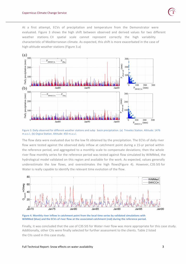
At a first attempt, ECVs of precipitation and temperature from the Demonstrator were evaluated. Figure 3 shows the high shift between observed and derived values for two different weather stations. CII spatial scale cannot represent correctly the high variability characteristic of Mediterranean climate. As expected, this shift is more exacerbated in the case of high-‐altitude weather stations (Figure 3.a)

Figure 3. Daily observed for different weather stations and subp basin precipitation. (a) Trevelez Station. Altitude: 1476 m.a.s.l.; (b) Orgiva Station. Altitude: 450 m.a.s.l.

The flow data were evaluated due to the low fit obtained by the precipitation. The ECVs of daily river flow were tested against the observed daily inflow at catchment point during a 15-‐yr period within the reference period, and aggregated to a monthly scale to compensate deviations; then the whole river flow monthly series for the reference period was tested against flow simulated by WiMMed, the hydrological model validated on this region and available for the work. As expected, values generally underestimate the low flows, and overestimates the high flows(Figure 4). However, C3S SIS for Water is really capable to identify the relevant time evolution of the flow.

Figure 4. Monthly river inflow in catchment point from the local time series by validated simulations with WiMMed (blue) and the ECVs of river flow at the associated catchment (red) during the reference period.

Finally, it was concluded that the use of C3S SIS for Water river flow was more appropriate for this case study. Additionally, other CIIs were finally selected for further assessment to the clients. Table 2 listed the CIIs used in this case study.



Table 2. CIIs used in this case study.

Climate Impact Indicators CIIs Indicator Spatial Resolution Temporary Resolution Precipitation Precipitation Catchment Daily Temperature Temperature Catchment Daily Water Quantity River flow Catchment Daily

Snow water equivalent Catchment Seasonality Wetness 1 Catchment 10 days Wetness 2 Catchment 10 days



Step 2: Snow evolution and river flow simulations

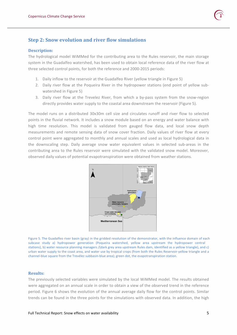
Description: The hydrological model WiMMed for the contributing area to the Rules reservoir, the main storage system in the Guadalfeo watershed, has been used to obtain local reference data of the river flow at three selected control points, for both the reference and 2000-‐2015 periods:

1. Daily inflow to the reservoir at the Guadalfeo River (yellow triangle in Figure 5)2. Daily river flow at the Poqueira River in the hydropower stations (end point of yellow sub-‐

watershed in Figure 5)3. Daily river flow at the Trevelez River, from which a by-‐pass system from the snow-‐region

directly provides water supply to the coastal area downstream the reservoir (Figure 5).

The model runs on a distributed 30x30m cell size and circulates runoff and river flow to selected points in the fluvial network. It includes a snow module based on an energy and water balance with high time resolution. This model is validated from gauged flow data, and local snow depth measurements and remote sensing data of snow cover fraction. Daily values of river flow at every control point were aggregated to monthly and annual scales and used as local hydrological data in the downscaling step. Daily average snow water equivalent values in selected sub-‐areas in the contributing area to the Rules reservoir were simulated with the validated snow model. Moreover, observed daily values of potential evapotranspiration were obtained from weather stations.

Figure 5. The Guadalfeo river basin (gray) in the gridded resolution of the demonstrator, with the influence domain of each subcase study a) hydropower generation (Poqueira watershed, yellow area upstream the hydropower central stations), b) water resource planning managers /(dark grey area upstream Rules dam, identified as a yellow triangle), and c) urban water supply to the coast area, and water use by tropical crops (from both the Rules Reservoir-‐yellow triangle and a channel-‐blue square from the Trevélez subbasin-‐blue area); green dot, the evapotranspiration station.

Results: The previously selected variables were simulated by the local WiMMed model. The results obtained were aggregated on an annual scale in order to obtain a view of the observed trend in the reference period. Figure 6 shows the evolution of the annual average daily flow for the control points. Similar trends can be found in the three points for the simulations with observed data. In addition, the high



variability of the different processes involved in the hydrological response in this area can be observed.

Figure 6. Annual mean daily flow evolution in the selected points of Guadalfeo area (1961-‐2000: (a) Rules dam (yellow triangle in Figure 5); (b) Poqueira River in the hydropower stations (end point of yellow sub-‐watershed in Figure 5); (c) Trevelez River (end point of blue sub-‐watershed in Figure 5).

Figure 7 shows the evolution of the annual mean daily value of the snow water equivalent averaged over the study area for the reference period, whose mean value is 38.7mm. Moreover, the decreasing trend obtained and the great variability throughout the period analyzed is shown.



Figure 7. Evolution of annual average daily water equivalent during the reference period in the study area.

The feasibility of producing transfer functions that relate the CIIs and the local data was assessed at this point. Figure 8 shows the comparison between the flow data obtained by the hydrological local model and those downloaded from the C3S SIS for Water (example of SMHI_RCA4_ECp EARTH model) platform at different time scales. As expected, the adjustment is better on a larger scale analyzed. Series do not represent correctly extreme occurrence values, as expected from the scale conflicts, and are not able to capture the variability of hydrological processes in the area. However, C3S SIS for Water data are really capable to identify the relevant time evolution of the flow and this was considered the best indicator for producing transfer functions.

Figure 8. Comparison of (a) daily, (b) monthly, (c) annual inflow to the Rules reservoir during the reference period (1970l 2000) from river flow (catchment) facilitated in Demonstrator (SMHI_RCA4_ECl EARTH) and river flow locally obtained from observations and hydrological modeling.



Step 3: Downscaling to a high spatial resolution

Description: 3.1. CII River flow

The ECVs of daily river flow were tested against the observed daily inflow at the Rules reservoir control point during the reference period, and aggregated to a monthly scale to perform the downscaling.

At the control point in the Poqueira River, the testing of daily river flow resulted in the selection of the same model for the analysis. In this case, the daily scale was conserved to meet the client’s needs. Finally, the same model was used to obtain daily river flow values at the Trevelez River control point (from which water is transferred to the southern area of the Guadalfeo River Basin). In both cases, values are higher since they are obtained for a larger contributing area; however, a relatively good agreement could be observed from the data despite the scale issue.

Following this, a bias correction and downscaling process was performed by means of specific transfer functions from the evaluation of values against the available local data at the time scales previously selected. These transfer functions were used to downscale both values during the reference period and projections.

3.2. CII Snow water equivalent and CII Wetness

Additional analysis was performed on CII Snow water equivalent values (mean monthly values for the reference period). SWE has been bias corrected and downscaled in the region with snow influence in the watershed from the monthly mean SWE daily values simulated with WiMMed and validated against local observations. Additionally, CII wetness1 and wetness 2 have been now analyzed for the Tropical Coast Area (data from catchmentp subid 9752544). Since they are defined as precipitation minus evapotranspiration, the values of mean monthly potential ET and real ET were estimated from them, respectively, bias corrected and tested against the available local observations (see weather station in Figure 5) during the 2004p 2010 periods.

Results:

3.1. CII River flow

The most suitable estimation from the Demonstrator was performed by the SMHI_RCAH_ECp EARTH model (Figure 9), which was selected for this study site. As expected, values generally underestimate the low flow values, and overestimate the high flow regime; this may be mostly due to the combined scale effects associated to grid size in the hydrological modelling and specifically to the snow simulation. The snow water equivalent is significantly underestimated in CIIs, which results in recession periods shorter than the observed ones, and peak flow values higher than the snowpinfluenced local values. However, C3S SIS for Water is really capable to identify the relevant time evolution of the monthly flow.



Figure 9. Comparison of mean monthly river flow values for each month of the year during the reference period (1970p 2000) upstream Rules dam, facilitate in C3S SIS for Water for available models (a. CSC REMO2009 MPIp ESMp LR; b. IPSLp IPSL.CM5Ap MR; c. KNMI RACMO22E ECp EARTH; d. SMHI RCA4 ECp EARTH; e. SMHI RCA4 HandGEM2p ES; f. Ensemble) and simulated with WiMMed.

a) Water resource planning for the Béznar-‐Rules system

After testing of different approaches, a transfer function was obtained for the monthly inflow for each month of the year during the reference period. Figure 10 shows these functions derived from monthly and local values.

Figure 10. Monthly transfer functions between monthly inflow to the Rules reservoir during the reference period (1970p2000) from river flow (catchment) facilitated in Demonstrator (SMHI_RCA4_ECp EARTH) and river flow locally obtained from observations and hydrological modelling. Each graph corresponds to a month of the year.



From each monthly transfer functions, the corresponding monthly river flow values for each future scenario have been obtained as a basis for the extraction of user-‐specific CIIs. Figure 11 shows these results for the whole 1970-‐2100 period aggregated on an annual basis.

Figure 11. Annual inflow to the Rules reservoir from observed values (1970p 2015) and aggregated values from the downscaled monthly values from river flow (catchment) facilitated in Demonstrator (SMHI_RCA4_ECp EARTH) corresponding to the future projections during the period 2000-‐2100 for the three future scenarios included in the Demonstrator and the future projections from de local hydrological model obtained by anomalies factors.

b) Water resource planning for hydropower generation

In this case, the daily values were downscaled after testing different methods, and the best approach was to obtain transfer functions portioning the variable domain. Transfer functions were obtained for three intervals in the whole domain of the daily values (separated by the 25 and 75 percentiles of the distribution), as Figure 12 shows (right). Despite a single transfer function could have been obtained the adopted division allowed a better performance of the procedure. Figure 12 (left) shows the finally resulting transfer function from the union of the three domain intervals.

Figure 12. Right: Transfer functions between daily inflow to the hydropower stations during the reference period (1970p 2000) from the downscaled values from the river flow (catchment) daily series facilitated by the Demonstrator (SMHI_RCA4_ECp EARTH,) and the daily river flow locally obtained from observations and hydrological modelling. Each graph corresponds to the intervals 0p 25, 25p 75, and higher than 75 percentiles of the downscaled variable distribution. Left: Transfer function representation for the whole domain distribution.



From these results, the corresponding daily river flow values for each future scenario have been obtained as a basis for the extraction of user-‐specific CIIs. Figure 13 shows these results for the whole 1970-‐2100 periods aggregated on an annual basis.

Figure 13. Annual mean river inflow to the hydropower station from local hydrological values (1970p 2015) and aggregated values from the downscaled daily values from river flow (catchment) facilitated in Demonstrator (SMHI_RCA4_ECp EARTH) corresponding to the future projections during the period 2000p 2100 for the three future scenarios included in the Demonstrator and the future projections from de local hydrological model obtained by anomalies factors.

c) Water supply for the coastal area

Again, the same time scale as in hydropower’s case is used to obtained transfer functions. These functions were obtained for three different intervals in the whole domain of the daily values. Figure 14 shows the finally resulting transfer function from the union of three domain intervals.

Figure 14. Right: Transfer functions between daily inflow to the Trevelez's basin during the reference period (1970p 2000) from the downscaled values from the river flow (catchment) daily series facilitated by the Demonstrator (SMHI_RCA4_ECpEARTH,) and the daily river flow locally obtained from observations and hydrological modelling. Each graph corresponds to the intervals 0p 25, 25p 75, and higher than 75 percentiles of the downscaled variable distribution. Left: Transfer function representation for the whole domain distribution

Figure 15 shows the aggregate annual flow obtained through the function and calculated for all available scenarios.



Figure 15. Annual mean river inflow to the Trevelez catchment from local hydrological values (1970p 2015) and aggregated values from the downscaled daily values from river flow (catchment) facilitated in Demonstrator (SMHI_RCA4_ECp EARTH) corresponding to the future projections during the period 2000p 2100 for the three future scenarios included in the Demonstrator and the future projections from de local hydrological model obtained by anomalies factors.

3.2 CII Snow water equivalent and CII Wetness

Figure 16 shows the performance of the different models included in C3S SIS for Water for the corrected CII values, and the transfer functions obtained for the three cases that include the whole set of future scenarios.

Figure 16. Comparison of mean monthly Snow Water Equivalent (SWE) values for each month of the year during the reference period (1970p 2000) from the corrected SWE values from the SWE (catchment) CII facilitated in the Demonstrator for different models, and from the validated simulations by the WiMMed model averaged over the contributing area upstream. Transfer functions are included for every model providing the three future scenarios included in the Demonstrator.

Figure 17 shows the performance of each model for ET estimation. As can be seen, a very good agreement is found between C3S SIS for Water and observed values for every model. Again, the "CSCp



REMO2009-‐MPI-‐ESM-‐LR" model shows the best performance, as for the SWE analysis (Figure 16). Finally, Figure 18 shows the transfer functions applied for the mean monthly values, for wet and dry season months separately, for both CIIs analyzed.

Figure 17. Comparison of the mean monthly Evapotranspiration (Potential: blue; Real: green) values (mm) for each month of the year during the available local observation period (2004p 2010) from wetness 1 and wetness 2 (catchment) CIIs facilitated in the Demonstrator for different models, and the monthly potential evapotranspiration from weather station data (mm).

Figure 18. Transfer functions between: (right) mean monthly Snow Water Equivalent (SWE) values for each month of the year during the reference period (1970p 2000) from the downscaled SWE values from the SWE (catchment) CII facilitated in the Demonstrator for the selected model, and from the validated simulations by the WiMMed model averaged over the contributing area upstream; (left) mean monthly Potential Evapotranspiration values for each month of the year during the period available of meteorological observed data (2004p 2010) from wetness 1 (catchment) CII facilitated in the Demonstrator for the selected model, and from the meteorological observed data.



Step 4: Assessment of changes.

Description: The estimation of these change rates by means of the comparison of the reference period and its posterior extension to the future scenarios is key to assess the further adaptation strategies. After a first analysis of the projections from 2000 to 2015, an additional correction was performed by means of the anomalies obtained from CIIs for the future projections and reference period, and the local values obtained for the reference period by both WiMMed simulation and observations.

This final correction based on anomalies was performed on the downscaled data sets to derive the final projections used in this case study, under the hypothesis that the relative change obtained from the anomalies (i.e. the difference between future and reference value, divided into the reference value) is applicable to the observed local data. The anomalies between downscaled projections and downscaled values for the reference period were obtained to define a factor of change for each variable under use and their associated time scales. These factors of change were applied then to the local data during the reference period to obtain the final data sets of future projections in the case study.

In this way, the flows simulated by the local model using the reference period are projected into the future. The projections were obtained by this 2p step process from first, the model (through transfer functions) and second, the local model (through factor of change). These flow projections were the basis to derive the local indicators that should assess the clients’ decisionp making process.

From the interaction with the clients during the case study, specific local indicators have been derived from successive checking and feedback, and their projections obtained for the corrected projections for the three future climate scenarios in this study


Water planning decision-‐makers selected the monthly scale for their interests, since water resource are pre-‐allocated on this basis following the approved water rights to each user. From their experience, their average monthly water supply from the Rules reservoir for the combination of both irrigation and urban supply varies between 8.5 and 12.0 hm3 during the last ten years. Following this, for each future decade, the downscaled and corrected monthly values were presented for each scenario and three local indicators were chosen (WiMMed projections in Fig. 19): 1) Number of months per year with monthly inflow to the Rules reservoir non-‐exceeding 8.5 hm3, and 2) those exceeding 12 hm3; 3) annual inflow to the Rules reservoir


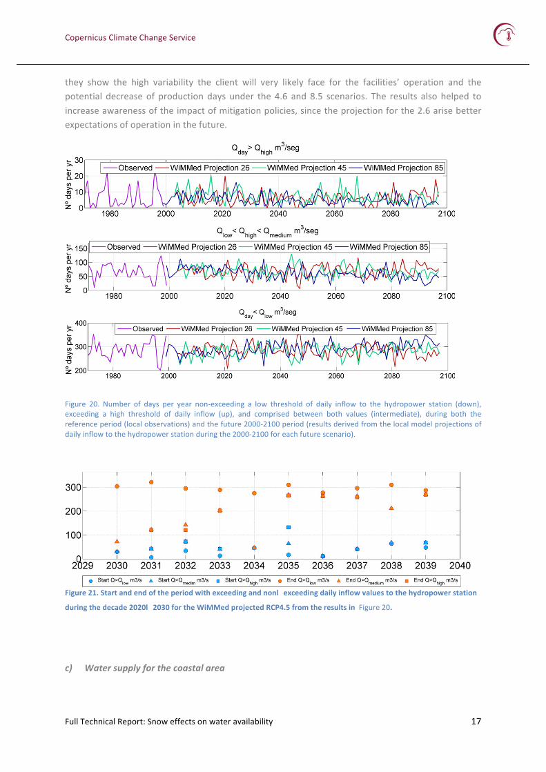
Similarly, for hydropower generation, a daily scale was selected by the client. Three reference values of inflow to the station were provided and five local indicators have been proposed from the corrected downscaled values (WiMMed projections in the graphs in Fig. 20p 21): 1) Number of days per year nonp exceeding a low threshold of daily inflow to the hydropower station, 2) those exceeding a high threshold and 3) those with intermediate daily inflow to the hydropower station; 4)



start (day of the year) and 5) end (day of the year) of the period with exceeding and non-‐exceeding values of daily inflow to the hydropower station


Again, a daily scale was selected by the client. The low threshold provided by the client for the by-‐pass water supply that they receive was used to obtain: 1) Number of days per year with daily by-‐pass flow non-‐exceeding 27 L/s.

Results:


Figure 19 shows both local indicators for the reference period (observations) and future scenarios (projections). As expected, projections are more restrictive than the reference period. For both periods, a negative trend can be observed in the case of number of months per year with monthly inflow exceeding 12 hm3. However, the trend is more monotonous for the other indicator analyzed.

Figure 19. Number of months per year non-‐exceeding 8.5 hm3 of monthly inflow to the Rules reservoir (up) and exceeding 12 hm3 of monthly inflow to the Rules reservoir (down) during both the reference period (local observations) and the future 2000-‐2100 period (results derived from the local model projections of monthly inflow to the Rules reservoir during the 2000-‐2100 for each future scenario).


Figure 20 and Figure 21 show both local indicators for the reference period (observations) and future scenarios (projections). The associated trends are not significant on a 10% of confidence level, but



they show the high variability the client will very likely face for the facilities’ operation and the potential decrease of production days under the 4.6 and 8.5 scenarios. The results also helped to increase awareness of the impact of mitigation policies, since the projection for the 2.6 arise better expectations of operation in the future.

Figure 20. Number of days per year non-‐exceeding a low threshold of daily inflow to the hydropower station (down), exceeding a high threshold of daily inflow (up), and comprised between both values (intermediate), during both the reference period (local observations) and the future 2000-‐2100 period (results derived from the local model projections of daily inflow to the hydropower station during the 2000-‐2100 for each future scenario).

Figure 21. Start and end of the period with exceeding and nonl exceeding daily inflow values to the hydropower station

during the decade 2020l 2030 for the WiMMed projected RCP4.5 from the results in Figure 20.




Figure 22 shows both local indicators for the reference period (observations) and future scenarios (projections). This indicator has been obtained from the excess flow taking into account the mandatory ecological flow in the area.

Figure 22. Number of days per year non-‐exceeding a low threshold of daily inflow to the water supply for the coastal area, during both the reference period (local observations) and the future 2000-‐2100 period (results derived from the downscaled projections of daily inflow to the hydropower station during the 2000-‐2100 for each future scenario).



Step 5 Integrated river basin management

Description: Once the projected flows for the different control points had been obtained, the objective of this step was to analyze the impacts on the projected changes on the current water demands in the case study area. For this, based on the current River Basin Management Plan, the different supply thresholds have been established at the control point of the Rules dam (Table 3), which is the water storage and supply system in this basin. From these values, the projected values of inflow to the reservoir for the different scenarios analyzed were tested against the annual current demands.

Table 3. Description of the water needs (data from the current River Basin Management Plan)

Water needs Quantity Environmental flow 30% annual flow Urban supply 12.82 hm3/year Irrigation 167.8 hm3/year Other uses 1.5 hm3/year

Results: The results show a clear decrease in the presence of snow for all scenarios and sub-‐periods in the future projected period, when compared to the average values during the reference period. However, the decrease in the available surface water is not that clear (Fig. 5). This points out to a major impact on snow occurrence and persistence, which affects the seasonal regime of the river inflow to the reservoir and thus the operational rules and storage capabilities during the wet season.

Figure 23 shows the water allocation results for the three scenarios analyzed, which have been derived from the results of this case study and the current water demands included in the Hydrological Plan of the area. The results show how both environmental flows and urban supply are not compromised by the impacts on river flow; however, irrigation water would not be guaranteed during different years, whose occurrence and persistence depends on the analysed scenario, and this demand is the most likely affected in the future scenarios. However, an analysis by decades (

Figure 25) shows for most of the cases how the number of years with deficit is coincident among scenarios.

The individual analysis of scenarios shows the influence of the snow regime on the time evolution and comparison among them. During the first decades, the warming impacts on snow provide the basin with increased river flows and, thus, the hardest scenario is not associated to higher deficits in water volumes in this early period. However, during the last decades this first impact on snow seems to be less significant and the scenarios tend to be hierarchized by the severity of the warming scenario.

The most unfavorable case appears for scenario RCP.2.6 with an annual deficit of 135.40 hm3. However, this scenario is not the one that presents the greatest number of years with a deficit, but it is the RCP.8.5 scenario that shows a more severe character (Figure 24) .The results highlight the need for adaptation plans to cope with the expected conflicts between irrigation users and environmental flow needs.



Figure 23. Evolution of the annual inflow to the Rules reservoir for a selected future climate scenario (RCP4.5) during the 2000p 2100 period, from the corrected downscaled river inflow from the river flow CII in the Demonstrator, together with the current water allocation in the basin (data from the current River Basin Management Plan).

Figure 24. Water deficit at the end of each decade during the 2000-‐2100 period to the Béznar-‐Rules system, calculating the decade final balance as the sum of annual deficits (Total demand -‐ Annual flow).



Figure 25. Number of years with water deficit (a) and maximum number of consecutive years with water deficit (b) during the 2000-‐2100 period to the Béznar-‐Rules system.



Step 6: Climate change adaptation strategies.

Description: The Andalusian Mediterranean Water District is the responsible water authority in the study area. From the River Basin Management Plan, the information shows that more than a 90% of the water resources come from surface waters, with a seasonal regime highly influenced by the snow dynamics, and a high impact of the snow changes in the expected changes in the river flow regime and water resource availability. To assess further the impact of the seasonal evolution of the snow, different study periods have been analyzed for the three future scenarios. In addition, a series of meetings have been held with the clients, to discuss the results obtained in this case study and with the aim of identifying the key issues to assess new adaptation strategies.

Results: Figure 26 shows the projected scenarios of the change of the mean monthly value of snow water equivalent in the contributing area upstream the Rules reservoir, the main system in the basin, averaged over three different intervals in the future. It can be observed that there is little change during the dry months of the year, since Sierra Nevada is currently a seasonal snow system with no perennial snowpacks. During the rest of the year, all scenarios project decreasing trends in the snow water equivalent, being the months of January to April the most affected by change. On the other hand, the RCP 8.5 scenario is the one that presents a more significant change with respect to the reference period. The spring months (April and May) also experiment a decrease in snow water equivalent. In the Mediterranean areas, where the summers are very hot and long, the melting of snow is very important in these spring months.

Figure 26. Evolution of mean monthly Snow Water Equivalent (SWE) values for each month of the year during the reference period (1970p 2000) and different periods (2020,2050,2080) from the corrected SWE (catchment) CII facilitated in the Demonstrator for the selected model.

From the previous results and following the successive meetings with the different clients, some conclusions were reached regarding adaptation strategies in this area. As a general conclusion, the assessment of the projected indicators tailored from each client’s needs in this case study points out to the deficit of water in the basin both on an annual and decadal scales, which highlights the need for a) the reservoir system, and b) the optimization of the operational rules in the reservoirs to minimize the risks associated to current demands not being met in the future. The analysis stresses the likely conflicts between irrigation water and the current requirements for environmental flows in



the future decades; the goals of environmental flows are under discussion in a changing framework, and the finally targeted objectives must be revisited under the light of a highly variable river flow regime. New water demands for irrigation must be analysed with caution by the Water Authority since an increase in the irrigated are in the basin will very likely lead to demands not being satisfied in many years, with the associated economic loss. On the other hand, urban consumption is not likely to be affected provided that this use is kept as first priority.

In this context, the results have enhanced the awareness of potential impacts and needs for adaptation action, as described in the previous paragrahs. However, some actions have been undertaken in the short term. The Water Authority is interested on a analysis of their operational rules in the Rules-‐Béznar reservoir system to minimize the risk of deficit situations on an annual and pluriannual basis, and initial collaboration has started on this issue. The hydropower company has decided to promote a monitoring system for low flows that, on one hand, let them control and certify their accomplishment of the environmental flow criteria and, on the other, help to a better assessment of the low flow regime in the snow-‐dominated rivers in the basin that contributes to meet the environmental requirements; this action is currently under development.



Conclusion of Full Technical Report

The goal of this case study was to obtain local climate impact indicators to assess water resource availability in this snow-‐influenced Mediterranean basin under different future climate scenarios, and test their suitability to identify adaptation strategies for previously identified users that represent the major water-‐related issues in this area. The workflow development during the project let us check out on each step the major strengths and weaknesses of the partial results and include corrections, when needed, and fully achieve the objectives. The project has provided insight on three major issues: i) the capability of data (and their scales) from global models to address adaptation issues in mountainous Mediterranean basins; ii) the capability of the interaction client-‐provider to enhance the quality of the climate indicators; iii) the key issues to be faced by the current water users in a context of global warming. The main outcomes associated to these major issues can be summarized as: i) Despite the scale issues posed by the local topography, river flow (daily data over

catchment) succeeded in providing an adequate representation of the hydrological response of this basin. Downscaling through local transfer function (from local data) plus an anomaly (futurel reference period) correction was necessary, and the availability of a hydrological model locally validated was key in this process.

ii) The interaction with the clients identified the significant time scales and type ofinformation critical in their operational protocols, but also helped providers to betterunderstand their restrictions and motivations, in order to define useful indicators. Thereliability of the information was the most helpful element to attain confidence on themethods.

iii) The assessment of projected indicators stresses the likely conflicts between irrigationwater and the requirements for environmental flows in the future decades. On-‐goingactions focus on the improvement of the monitoring network oriented to low flows,and the analysis of the environmental flow characterization for a betterrepresentation of processes. Future actions are proposed in terms of optimizing theoperational rules of the reservoir system in the area, and developing an operationalsystem for the start and closure of the generation season in the hydropower facilities.



References

GDFH (Research Group on Fluvial Dynamics and Hydrology). WiMMed model software, scientific fundamentals and users’ guide. 2011. Available at http://www.uco.es/dfh/index.php?option=com_content&view=article&id=52%3Ased-‐tempor-‐egestas&catid=36%3Adestacados&Itemid=64&lang=en , last accessed on October 31, 2017.

Plan Hidrológico de las Cuencas Mediterráneas 2015-‐2020. Consejería de Medio Ambiente y Ordenación del Territorio. Junta de Andalucía. 2015. Available at http://www.juntadeandalucia.es/medioambiente/site/portalweb/ , last accessed on October 31, 2017.

Additional information on WiMMed model (see Note 1 in page 2) can be found in the following publications:

J. Herrero, M.J. Polo, A. Moñino, M.A. Losada. 2009. An energy balance snowmelt model in a Mediterranean site. J. Hydrol., 371:98-‐107.

A. Millares, M.J. Polo, M.A. Losada. 2009. The hydrological response of baseflow in fractured mountain areas. Hydrol. Earth Sys. Sci., 13(7): 1261-‐1271.

C. Aguilar, J. Herrero, M.J. Polo. 2010. Topographic effects on solar radiation distribution in mountainous watershed and their influence on reference evapotranspiration estimates at watershed scale. Hydrol. Earth System Sci., 14: 2479-‐2494.

J. Herrero, M.J. Polo, M.A. Losada. 2011. Snow evolution in Sierra Nevada (Spain) from an energy balance model validated with Landsat TM data. Remote Sensing for Agriculture, Ecosystems, and Hydrology. Vol 8174. DOI: 10.117/12.898270

M.J. Polo, A. Díaz, M.P. González-‐Dugo. 2011. Interception modeling with vegetation time series derived from Landsat TM data. Remote Sensing for Agriculture, Ecosystems, and Hydrology. Vol 8174. DOI: 10.117/12.898144

C. Aguilar, M.J. Polo. 2011. Generating reference evapotranspiration surfaces from the Hargreaves equation at watershed scale. Hydrol. Earth System Sci., 15: 2495-‐2508.

M. Egüen, C. Aguilar, J. Herrero, A. Millares, M.J. Polo. 2012. On the influence of cell size in physically-‐based distributed hydrological modelling to assess extreme values in water resource planning. Nat. Hazard Earth Syst. Sci., 12: 1573-‐1582

J. Herrero, M.J. Polo. 2012. Parameterization of atmospheric longwave emissivity in a mountainous site for all sky conditions. Hydrol. Earth Syst. Sci., 16: 3139-‐3147.

A. Millares, Z. Gulliver, M.J. Polo. 2012. Scale effects on the estimation of erosion thresholds through a distributed and physically-‐based hydrological model. Geomorphology, 153-‐154: 115-‐126.

R. Pimentel, J. Herrero, Y. Zeng, Z. Su, M.J. Polo. 2015. Study of snow dynamics at subgrid scale in semiarid environments combining terrestrial photography and data assimilation techniques. Journal of Hydrometeorology, 16 (2): 563-‐578.

J. Herrero, M.J. Polo. 2016. Evaposublimation from the snow in the Mediterranean mountains of Sierra Nevada (Spain). The Cryosphere, 10(6): 2981-‐2998.

R. Pimentel, J. Herrero, M.J. Polo. 2017. Subgrid parameterization of snow distribution at a Mediterranean site using terrestrial photography. Hydrol. Earth System Sci., 21:805-‐820.



This work was developed under the contract C3S_411_Lot1_SMHI

Contractor: The Swedish Meteorological and Hydrological Institute (SMHI), Sweden

Sub-‐contractor: University of Córdoba (UCO), Spain

full technical report: snow effects on water...

Documents