fun3d analyses in support of the second aeroelastic ... analyses in support of the second...

FUN3D Analyses in Support of the Second AeroelasticPrediction Workshop

Pawel Chwalowski,∗ Jennifer Heeg†

NASA Langley Research Center, Hampton, VA 23681-2199

This paper presents the computational aeroelastic results generated in support of the second AeroelasticPrediction Workshop for the Benchmark Supercritical Wing (BSCW) configurations and compares them tothe experimental data. The computational results are obtained using FUN3D, an unstructured grid Reynolds-Averaged Navier-Stokes solver developed at NASA Langley Research Center. The analysis results includeaerodynamic coefficients and surface pressures obtained for steady-state, static aeroelastic equilibrium, andunsteady flow due to a pitching wing or flutter prediction. Frequency response functions of the pressure coeffi-cients with respect to the angular displacement are computed and compared with the experimental data. Theeffects of spatial and temporal convergence on the computational results are examined.

Nomenclature

Roman Symbols

Cp Coefficient of pressure

M, Mach Mach number

q Dynamic pressure

Greek Symbols

α , θ Angle of attack, angular displacement

f , f ∗ frequency, system’s primary frequency - Hz

Acronyms

AePW Aeroelastic Prediction Workshop

BSCW Benchmark Supercritical Wing

CAE Computational Aeroelasticity

CFD Computational Fluid Dynamics

CSD Cross Spectral Density

DDES Delayed Detached Eddy Simulation

DFT Discrete Fourier Transform

DPW Drag Prediction Workshop

FRF Frequency Response Function

HiLiftPW High Lift Prediction Workshop

OTT Oscillating Turntable

PAPA Pitch And Plunge Apparatus

PSD Power Spectral Density

∗Senior Aerospace Engineer, Aeroelasticity Branch, MS 340, Senior Member AIAA.†Senior Research Engineer, Aeroelasticity Branch, MS 340, Senior Member AIAA.

1 of 19

American Institute of Aeronautics and Astronautics

https://ntrs.nasa.gov/search.jsp?R=20160010115 2018-05-19T14:07:59+00:00Z

I. Introduction

T he first Aeroelastic Prediction Workshop (AePW-1) was held in April 20121–3 and served as a first step in assess-ing the state-of-the-art of computational methods for predicting unsteady flow fields and aeroelastic response. The

second Aeroelastic Prediction Workshop (AePW-2), held in January 2016, built on the experiences of the first work-shop by extending the benchmarking effort to aeroelastic flutter solutions. The configuration chosen for the AePW-2was the Benchmark Supercritical Wing (BSCW).4

The accuracy of computational methods has improved in recent years due to individual validation efforts likethose with the AGARD 445.6 wing,5 but multi-analyst code-to-code comparisons that can be used to assess the over-all current state-of-the-art in computational aeroelasticity (CAE) are limited. The idea for an Aeroelastic PredictionWorkshop (AePW) series was conceived at NASA in 2009, based on the success of two other workshop series thathave been conducted over the past decade: the Drag Prediction Workshop (DPW)6 series and the High Lift PredictionWorkshop (HiLiftPW)7 series. The intent for the AePW was to provide a forum for code-to-code comparisons involv-ing predictions of nonlinear aeroelastic phenomena and to stimulate upgrades for existing codes and the developmentof new codes.

For code validations in general, the type of aerodynamic and/or aeroelastic phenomena to be analyzed is importantsince a validation process typically progresses from simpler to more challenging cases. For the AePW series, the ap-proach being taken is to utilize existing experimental data sets in a building-block approach to incrementally validatetargeted aspects of CAE tools. Each block will represent a component of a more complex nonlinear unsteady aeroelas-tic problem, isolating it such that the contributing physics can be thoroughly investigated. The challenge selected forthe first AePW was the accurate prediction of unsteady aerodynamic phenomena on essentially rigid, geometricallysimple models, with an additional foray into systems with weak coupling between the fluid and the structure. Resultsfrom this first workshop helped guide the direction of the second workshop, with analyses extending to include flutterprediction and therefore, increasingly complicated flow fields.

This paper presents the computational aeroelastic results generated for the BSCW configuration using the NASALangley-developed computational fluid dynamics (CFD) software FUN3D8 and comparing those results to the exper-imental data. Information relevant to the numerical method employed will be presented first, including the grids used,the rigid steady-flow analysis, the dynamic analysis, and the post processing. Details associated with the BSCW testcases and their associated analyses using FUN3D will then be presented. Due to the large number of computationalanalyses and data generated, this paper presents only a subset of the results obtained for each test case.

II. Numerical Method

A. Grids

Unstructured grids consisting primarily of tetrahedra and prisms were used in this study. They were generated usingVGRID9 with input prepared using GridTool.10 The tetrahedral elements within the boundary layer were convertedinto prism elements using preprocessing options within the FUN3D software. Based on the AePW gridding guide-lines,11 three grids belonging to the same family were constructed. These grids and the corresponding FUN3D solu-tions are referred to as ‘coarse’, ‘medium’ and ‘fine’ in this paper. In addition, a separate and preliminary grid wasconstructed for use with the Delayed Detached Eddy Simulation (DDES) method. The resulting grid distributions forthe surface and plane of symmetry are presented in Figure 1.

B. Rigid Steady-Flow Analysis - FUN3D

Solutions to the Reynolds-Averaged Navier-Stokes (RANS) equations were computed using the FUN3D flow solverwith turbulence closure obtained using the “standard” Spalart-Allmaras one-equation model.12, 13 For the test casesat the low transonic Mach numbers selected for the BSCW, oscillations in pressure fore and aft of the shock arerelatively minor, so that the use of a flux limiter, with the accompanying adverse effects on solver convergence is notessential; however, selected analyses were completed with and without a flux limiter. Here, the flux limitation wasaccomplished with the Venkatakrishnan14 limiter, and inviscid fluxes were computed using the Roe scheme.15 For theasymptotically-steady cases, time integration was accomplished by an Euler implicit backwards difference scheme,with local time stepping to accelerate convergence. Most of the cases in this study were run for about 5000 iterationsto achieve convergence of forces and moments to within ±0.5% of the running average of the last 1,000 iterations.

2 of 19


(a) Coarse Grid, Grid A, 3 Million Nodes. (b) Medium Grid, Grid B, 9 Million Nodes.

(c) Fine Grid, Grid C, 27 Million Nodes. (d) Towards DDES, Grid D, 35 Million Nodes.

Figure 1. Coarse, Medium, Fine, and “Towards DDES” Grids.

C. Dynamic Analysis - FUN3D

Dynamic analyses of the BSCW configuration required moving body, and therefore, grid motion capability. The griddeformation in FUN3D is treated as a linear elasticity problem. In this approach, the grid points near the body canmove significantly, while the points farther away may not move at all. In addition to the moving body capability,the analysis of the BSCW configuration required dynamic aeroelastic capability, which is available in the FUN3Dsolver.16 For a dynamics aeroelastic analysis, FUN3D is capable of being loosely coupled with an external finiteelement solver,17 or in the case of the linear structural dynamics used in this study, an internal modal structural solvercan be utilized. This modal solver is formulated and implemented in FUN3D in a manner similar to other Langleyaeroelastic codes (CAP-TSD18 and CFL3D19). For the BSCW computation presented here, the structural modes wereobtained via a normal modes analysis (solution 103) with the Finite Element Model (FEM) solver MSC NastranT M .20

The modes were then interpolated to the surface mesh using the method developed by Samareh.21 The BSCW FEMwas built and described by Heeg.4

The BSCW dynamic analysis was performed in a multi-step process. First, the steady CFD solution was obtainedon the rigid body. For the forced-oscillation cases, the BSCW wing was then moved sinusoidally about the pitchaxis specified in the experiment. In the case of a dynamic aeroelastic flutter solution, a static aeroelastic solutionwas obtained first by restarting the CFD analysis from the rigid-steady solution in a time-accurate mode22 with astructural modal solver, allowing the structure to deform. A high value of structural damping (0.99) was used so thestructure could find its equilibrium position with respect to the mean flow before the dynamic response was started.Finally, the flutter solution was restarted from the static aeroelastic solution by setting the structural damping valueto zero and reducing the time step to approximately 500 or 5000 time steps per cycle which corresponds to 0.0002 or0.00002 seconds, respectively. A detailed temporal resolution study was also conducted and will be documented infuture publications; however, some aspects of the temporal resolution issues that were identified during this study aredescribed later in this paper.

3 of 19


D. Post Processing

The dynamic comparison data selected for AePW-2 consisted of the magnitudes and phases of frequency responsefunctions (FRFs). The FRFs of principal interest were the pressure coefficients (Cp) due to angular displacement.The FRF for each pressure coefficient was calculated at the principal frequency of the reference quantity (angulardisplacement).

Fourier analysis was performed on each dynamically-excited data set to produce FRFs for each pressure relativeto the displacement of the system. The FRFs were formed from power spectral and cross spectral densities (PSDsand CSDs), which were computed using Welch’s periodogram method. The Fourier coefficients used in computingthe PSDs and CSDs were generated using discrete Fourier transform (DFT) analysis of the time histories, employingoverlap-averaged ensembles of the data sets. The length of the ensembles and the frequency at which the data wasextracted were chosen based on statistical analysis of the results of varying the ensemble lengths. The objective invarying the block size was to exactly match the system’s primary frequency with a Fourier analysis frequency and thenmaximize the number of data blocks to reduce the processing-based uncertainty. A rectangular windowing was used;the windows were overlapped by 90% of the block size.

For BSCW, the magnitude of the frequency response function of Cp due to θ at the frequency f (i) as a function ofchord location is presented in this paper as: ∣∣∣∣Cp

θ( f ∗)

∣∣∣∣vs.xc

(1)

where f ∗ represents the system’s primary frequency.

III. AePW-2 Test Cases

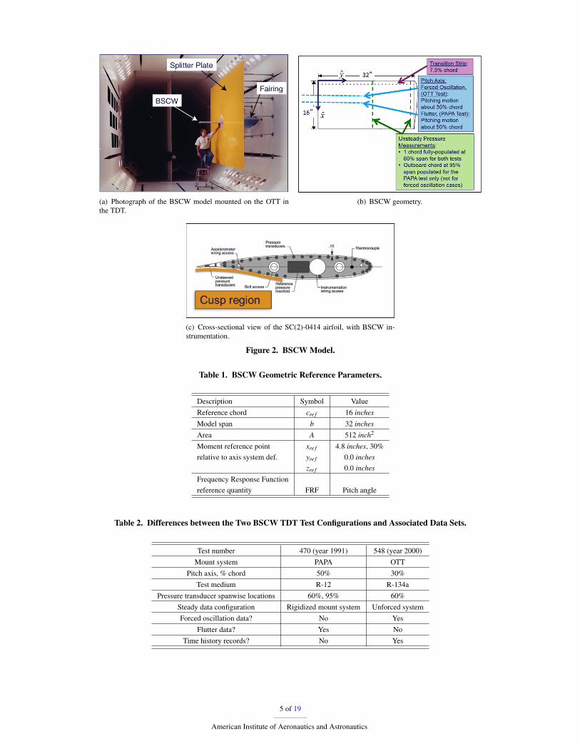
The BSCW model, shown in Figure 2, has a simple, rectangular, 16- x 32-inch wing planform, with a NASASC(2)-0414 airfoil. The BSCW geometric reference parameters are shown in Table 1. The model was mounted to alarge splitter plate, sufficiently offset from the wind-tunnel wall (40 inches) to (1) place the wing closer to the tunnelcenterline and (2) be outside the tunnel wall boundary layer.23 The wing was designed to be rigid, with the followingstructural frequencies for the combined installed wing and OTT mounting system: 24.1 Hz (spanwise first bendingmode), 27.0 Hz (in-plane first bending mode), and 79.9 Hz (first torsion mode). For instrumentation, the model haspressure ports at two chord-wise rows at the 60% and 95% span locations, with 22 ports on the upper surface, 17ports on the lower surface, and 1 port at the leading edge for each row. The BSCW model was tested in the NASATransonic Dynamics Tunnel (TDT) in two test entries. Differences between the two tests and their associated data setsare provided in Table 2. The first BSCW test in the early 1990’s, was performed on a flexible mount system, called thepitch and plunge apparatus (PAPA), which provides two-degree-of-freedom low-frequency flexible modes that emulatea plunge mode and a pitch mode. The BSCW/PAPA data consists of unsteady data at flutter points and averaged dataon a rigidified apparatus at the flutter conditions. For this PAPA test, both the inboard row at the 60% span station andthe outboard row at the 95% span station were populated with unsteady in-situ pressure transducers. The more recenttest in 2000, which served as the basis for one of the AePW-1 test cases, was performed on the oscillating turntable(OTT), which provided forced pitch oscillation data. For this OTT test, however, only the inboard row at the 60% spanstation was populated with unsteady in-situ pressure transducers.

Both of the TDT tests were conducted with the sidewall slots open. The BSCW/PAPA test was conducted withseveral flow transition strip configurations, but only data using size #35 grit was used for the workshop comparisons.For the BSCW/OTT test, the boundary-layer transition was also fixed at 7.5% chord using size #30 grit.

The BSCW flow conditions used in AePW-1 were challenging. Shock-induced separated flow dominated the uppersurface and the aft portion of the lower surface at the Mach 0.85 and 5◦ angle-of-attack case. Using this informationas a guide, two test cases just outside of the separated flow regime were emphasized for AePW-2 and are listed inTable 3. Steady and forced oscillation analyses were conducted at Mach 0.7, 3◦ angle of attack, and flutter analyseswere conducted at Mach 0.74, 0◦ angle of attack. An optional Case #3 at Mach 0.85, 5◦ angle of attack, which wasthe re-analysis of the AePW-1 case, was encouraged to apply the higher fidelity tools. This optional case was dividedinto three separate sub-cases based on the type of dynamic data acquired.

FUN3D analyses were conducted for all AePW-2 cases listed in Table 3. In the following sections of this paper,some of the FUN3D computational results obtained for the AePW-2 BSCW test cases will be presented with thecorresponding experimental data.

4 of 19


(a) Photograph of the BSCW model mounted on the OTT inthe TDT.

(b) BSCW geometry.

(c) Cross-sectional view of the SC(2)-0414 airfoil, with BSCW in-strumentation.

Figure 2. BSCW Model.

Table 1. BSCW Geometric Reference Parameters.

Description Symbol ValueReference chord cre f 16 inchesModel span b 32 inchesArea A 512 inch2

Moment reference point xre f 4.8 inches, 30%relative to axis system def. yre f 0.0 inches

zre f 0.0 inchesFrequency Response Functionreference quantity FRF Pitch angle

Table 2. Differences between the Two BSCW TDT Test Configurations and Associated Data Sets.

Test number 470 (year 1991) 548 (year 2000)Mount system PAPA OTT

Pitch axis, % chord 50% 30%Test medium R-12 R-134a

Pressure transducer spanwise locations 60%, 95% 60%Steady data configuration Rigidized mount system Unforced systemForced oscillation data? No Yes

Flutter data? Yes NoTime history records? No Yes

5 of 19


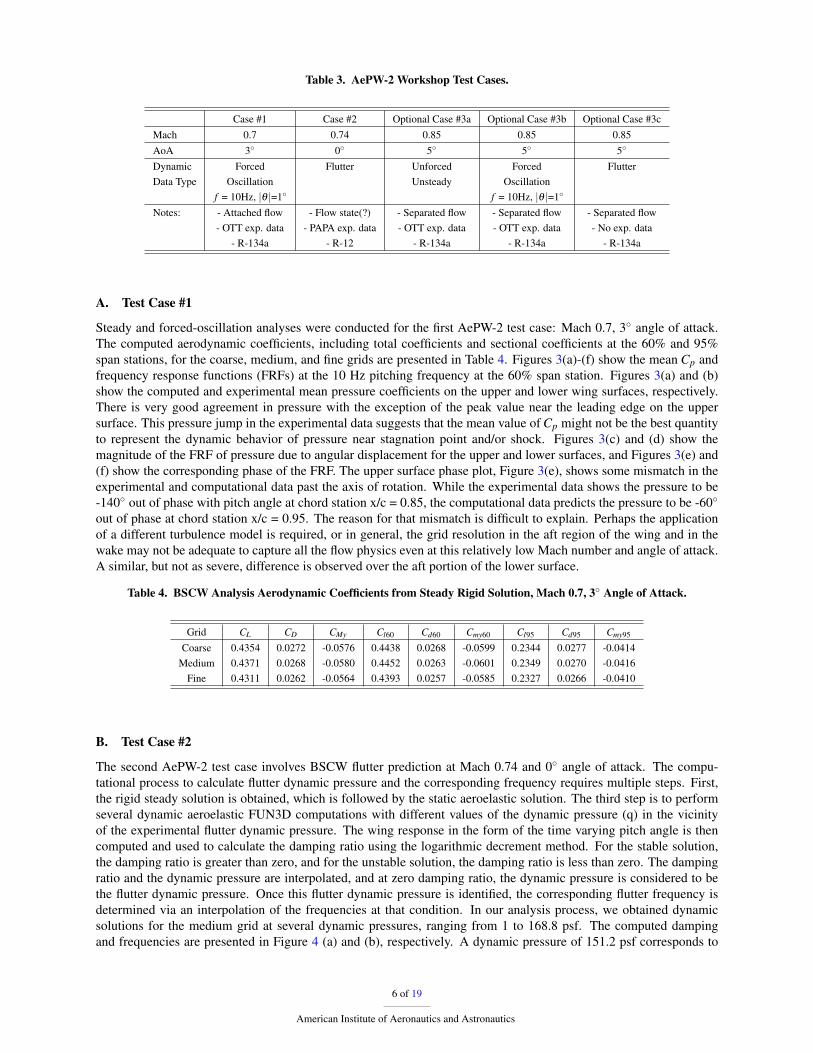
Table 3. AePW-2 Workshop Test Cases.

Case #1 Case #2 Optional Case #3a Optional Case #3b Optional Case #3cMach 0.7 0.74 0.85 0.85 0.85AoA 3◦ 0◦ 5◦ 5◦ 5◦

Dynamic Forced Flutter Unforced Forced FlutterData Type Oscillation Unsteady Oscillation

f = 10Hz, |θ |=1◦ f = 10Hz, |θ |=1◦

Notes: - Attached flow - Flow state(?) - Separated flow - Separated flow - Separated flow- OTT exp. data - PAPA exp. data - OTT exp. data - OTT exp. data - No exp. data

- R-134a - R-12 - R-134a - R-134a - R-134a

A. Test Case #1

Steady and forced-oscillation analyses were conducted for the first AePW-2 test case: Mach 0.7, 3◦ angle of attack.The computed aerodynamic coefficients, including total coefficients and sectional coefficients at the 60% and 95%span stations, for the coarse, medium, and fine grids are presented in Table 4. Figures 3(a)-(f) show the mean Cp andfrequency response functions (FRFs) at the 10 Hz pitching frequency at the 60% span station. Figures 3(a) and (b)show the computed and experimental mean pressure coefficients on the upper and lower wing surfaces, respectively.There is very good agreement in pressure with the exception of the peak value near the leading edge on the uppersurface. This pressure jump in the experimental data suggests that the mean value of Cp might not be the best quantityto represent the dynamic behavior of pressure near stagnation point and/or shock. Figures 3(c) and (d) show themagnitude of the FRF of pressure due to angular displacement for the upper and lower surfaces, and Figures 3(e) and(f) show the corresponding phase of the FRF. The upper surface phase plot, Figure 3(e), shows some mismatch in theexperimental and computational data past the axis of rotation. While the experimental data shows the pressure to be-140◦ out of phase with pitch angle at chord station x/c = 0.85, the computational data predicts the pressure to be -60◦

out of phase at chord station x/c = 0.95. The reason for that mismatch is difficult to explain. Perhaps the applicationof a different turbulence model is required, or in general, the grid resolution in the aft region of the wing and in thewake may not be adequate to capture all the flow physics even at this relatively low Mach number and angle of attack.A similar, but not as severe, difference is observed over the aft portion of the lower surface.

Table 4. BSCW Analysis Aerodynamic Coefficients from Steady Rigid Solution, Mach 0.7, 3◦ Angle of Attack.

Grid CL CD CMy Cl60 Cd60 Cmy60 Cl95 Cd95 Cmy95

Coarse 0.4354 0.0272 -0.0576 0.4438 0.0268 -0.0599 0.2344 0.0277 -0.0414Medium 0.4371 0.0268 -0.0580 0.4452 0.0263 -0.0601 0.2349 0.0270 -0.0416

Fine 0.4311 0.0262 -0.0564 0.4393 0.0257 -0.0585 0.2327 0.0266 -0.0410

B. Test Case #2

The second AePW-2 test case involves BSCW flutter prediction at Mach 0.74 and 0◦ angle of attack. The compu-tational process to calculate flutter dynamic pressure and the corresponding frequency requires multiple steps. First,the rigid steady solution is obtained, which is followed by the static aeroelastic solution. The third step is to performseveral dynamic aeroelastic FUN3D computations with different values of the dynamic pressure (q) in the vicinityof the experimental flutter dynamic pressure. The wing response in the form of the time varying pitch angle is thencomputed and used to calculate the damping ratio using the logarithmic decrement method. For the stable solution,the damping ratio is greater than zero, and for the unstable solution, the damping ratio is less than zero. The dampingratio and the dynamic pressure are interpolated, and at zero damping ratio, the dynamic pressure is considered to bethe flutter dynamic pressure. Once this flutter dynamic pressure is identified, the corresponding flutter frequency isdetermined via an interpolation of the frequencies at that condition. In our analysis process, we obtained dynamicsolutions for the medium grid at several dynamic pressures, ranging from 1 to 168.8 psf. The computed dampingand frequencies are presented in Figure 4 (a) and (b), respectively. A dynamic pressure of 151.2 psf corresponds to

6 of 19


(a) Mean Cp, Upper Surface. (b) Mean Cp, Lower Surface.

(c) |Cp/theta |, Upper Surface. (d) |Cp/theta |, Lower Surface.

(e) Phase Cp/theta, Upper Surface. (f) Phase Cp/theta, Lower Surface.

Figure 3. Mean Cp and Frequency Response Function: Magnitude and Phase of Pressure Due to Pitch Angle, Mach 0.7,Pitching Frequency f = 10 Hz case, Rec = 4.56 * 106, α = 3◦.

7 of 19


zero damping for the medium grid solution. Based on this medium grid solution, coarse and fine grid solutions wereobtained at dynamic pressures of both 152.0 psf and 168.8 psf. The resulting coarse and fine grid results predictedthe zero damping value to occur at dynamic pressures of 152.5 psf and 151.5 psf, respectively. The correspondingflutter frequency for all three grids was then determined to be approximately 4.2 Hz. An averaged dynamic pressure of151.7 was declared to be the computationally-obtained flutter dynamic pressure while the dynamic pressure of 168.8psi is an experimentally-measured flutter dynamic pressure. This also means that the computationally-obtained flutterdynamic pressure is approximately 10% below the experimental flutter dynamic pressure.

Tables 5 and 6 show aerodynamic coefficients obtained from the rigid steady and static aeroelastic solutions,respectively, at the experimental flutter dynamic pressure of 168.8 psf. There is a significant lift coefficient reductionbetween the two solutions. This reduction indicates that the wing pitches down due to the static aeroelastic effects.The predicted pitch-down angle values are -1.2◦, -1.3◦, and -1.0◦ for the coarse, medium, and fine grids, respectively.

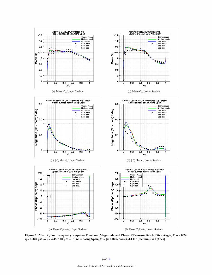
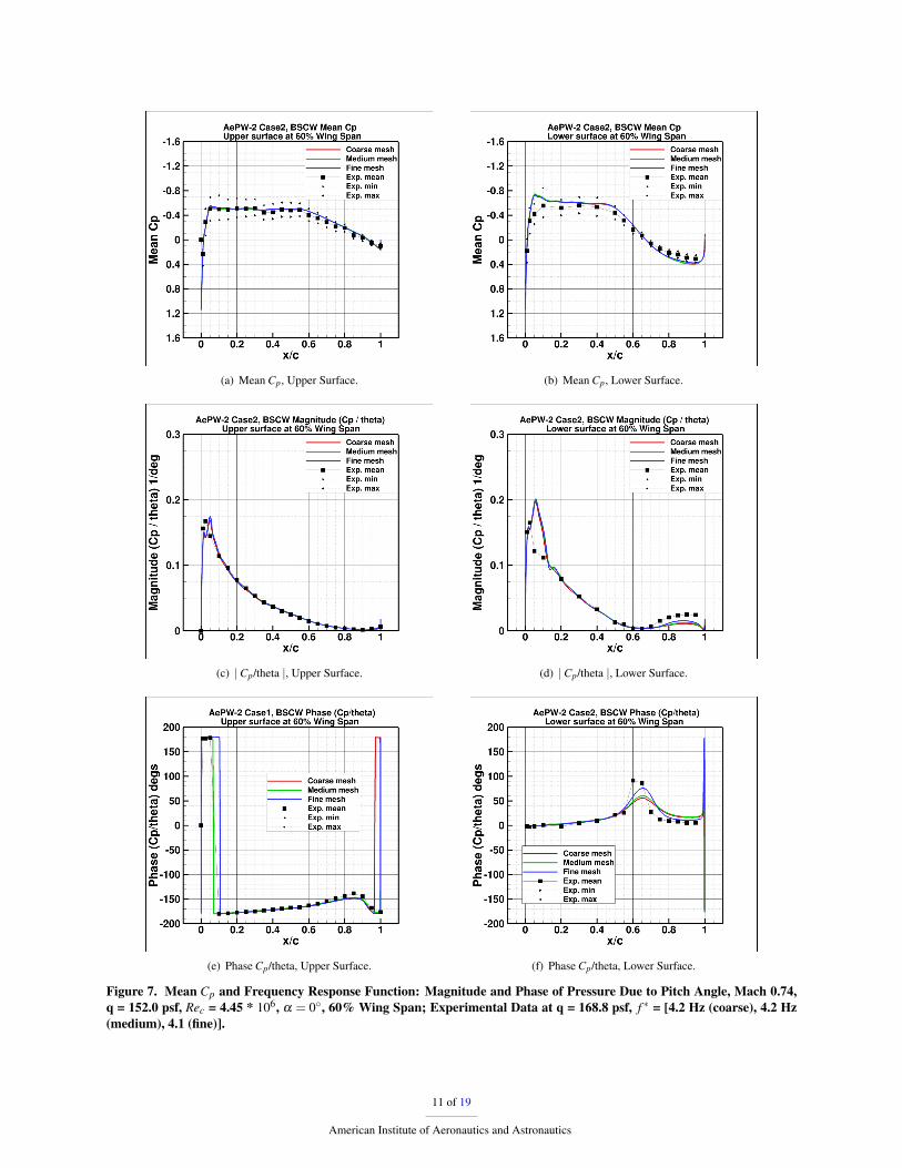
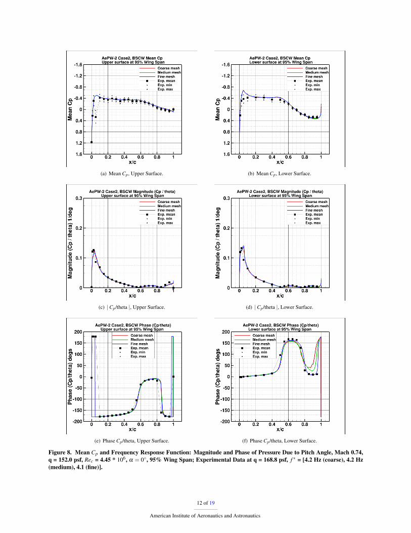
Figures 5(a)-(f) and Figures 6(a)-(f) show the mean Cp and frequency response functions computed from theFUN3D solution at the experimental flutter dynamic pressure of 168.8 psf at the 60% and 95% wing span stations,respectively. Figures 7(a)-(f) and Figures 8(a)-(f) shows the mean Cp and frequency response functions computed fromthe FUN3D solution at the dynamic pressure of 152.0 psf at 60% and 95% wing span stations, respectively. Thereis a very good agreement between the experimental and computational data at both the 152.0 and 168.8 psf dynamicpressures. The largest differences are noted near the leading edge of the wing on the lower surface for both span sta-tions. The other region of noticeable disagreement is in the lower surface cusp region, where the computations predictapproximately half the magnitude of response relative to the experiment. At the cusp leading edge, the computationalresults track the phase change observed in the experiment. Note, that the experimental flutter dynamic pressure is at q= 168.8 psf, but for comparison purposes, it is also plotted together with the computational data at q = 152 psf.

Table 5. BSCW Analysis Aerodynamic Coefficients from Steady Rigid Solution, Mach 0.74, q = 168.8 psf, AoA = 0◦.


Coarse 0.1840 0.0143 -0.0783 0.1905 0.0145 -0.0821 0.1030 0.0155 -0.0536Medium 0.1843 0.0138 -0.0783 0.1906 0.0140 -0.0821 0.1018 0.0150 -0.0529

Fine 0.1762 0.0133 -0.0755 0.1825 0.0135 -0.0792 0.0982 0.0146 -0.0515

Table 6. BSCW Analysis Aerodynamic Coefficients from Static Aeroelastic Solution, q = 168.8 psf, Mach 0.74, AoA = 0◦.


Coarse 0.0935 0.0123 -0.0856 0.0992 0.0124 -0.0898 0.0601 0.0135 -0.0600Medium 0.0937 0.0117 -0.0855 0.0992 0.0119 -0.0897 0.0583 0.0129 -0.0590

Fine 0.0890 0.0113 -0.0822 0.0946 0.0114 -0.0863 0.0556 0.0126 -0.0568

(a) Damping Value as a Function of Dynamic Pressure. (b) Frequency as a Funtion of Dynamic Pressure.

Figure 4. Case #2: Search for Flutter Dynamic Pressure and Flutter Frequency, Mach 0.74, Rec = 4.45 * 106, α = 0◦.

8 of 19





Figure 5. Mean Cp and Frequency Response Function: Magnitude and Phase of Pressure Due to Pitch Angle, Mach 0.74,q = 168.8 psf, Rec = 4.45 * 106, α = 0◦, 60% Wing Span, f ∗ = [4.1 Hz (coarse), 4.1 Hz (medium), 4.1 (fine)].

9 of 19





Figure 6. Mean Cp and Frequency Response Function: Magnitude and Phase of Pressure Due to Pitch Angle, Mach 0.74,q = 168.8 psf, Rec = 4.45 * 106, α = 0◦, 95% Wing Span, f ∗ = [4.1 Hz (coarse), 4.1 Hz (medium), 4.1 (fine)].

10 of 19





Figure 7. Mean Cp and Frequency Response Function: Magnitude and Phase of Pressure Due to Pitch Angle, Mach 0.74,q = 152.0 psf, Rec = 4.45 * 106, α = 0◦, 60% Wing Span; Experimental Data at q = 168.8 psf, f ∗ = [4.2 Hz (coarse), 4.2 Hz(medium), 4.1 (fine)].

11 of 19





Figure 8. Mean Cp and Frequency Response Function: Magnitude and Phase of Pressure Due to Pitch Angle, Mach 0.74,q = 152.0 psf, Rec = 4.45 * 106, α = 0◦, 95% Wing Span; Experimental Data at q = 168.8 psf, f ∗ = [4.2 Hz (coarse), 4.2 Hz(medium), 4.1 (fine)].

12 of 19


One of the most important lessons learned from analysis of the BSCW test case for AePW-1 was that more infor-mation on temporal convergence of both the unforced and the forced oscillation solutions was needed in order to assessthe quality of “goodness” of the results. Subsequent analyses have shown great sensitivity to temporal convergence,including changing the system from stable (flutter-free) to unstable (flutter). Understanding temporal convergencecriteria was therefore a high priority for AePW-2. The paragraph below briefly describes issues associated with theselection of the global time step size, the specification of the number of subiterations, and the convergence criteria atthe subiteration level in FUN3D for Case #2 of AePW-2.

Figure 9a shows the generalized displacements for Modes 1 and 2 when FUN3D was executed with three levelsof non-dimensional time-step sizes (DT) corresponding to dimensional time-step sizes of 0.0002, 0.002, and 0.004seconds. At these time steps, the solution behavior changes from stable (dt = 0.004 seconds - green curve), to slightlyunstable (dt = 0.002 seconds - black curve), to unstable (dt = 0.0002 seconds - red curve). All the solutions wereobtained by running FUN3D on a coarse grid with 15 subiterations at each global time step. Figure 9b shows thecontinuation of the temporal convergence study, where in addition to the solution with the time step of 0.0002 seconds(red curve; which is not visible because it is very close to the blue curve), two additional solutions were added. Onewas obtained with the same dt = 0.0002 seconds but with 1000 subiterations (blue curve). The second solution wasobtained by reducing the time-step size to 0.00002 seconds but the number of subiterations was kept at 15 (orangecurve). These three solutions produced nearly identical results. Therefore, it is concluded that the FUN3D solution ona coarse grid obtained with a time-step size of 0.0002 seconds and 15 subiterations (or more) is sufficient for Case #2flutter prediction. Similar analyses were performed running FUN3D on medium and fine grids. Those results showedthat a minimum of 25 subiterations with the time step of 0.0002 seconds are needed for Case #2 flutter prediction.Further investigation of these solutions showed that different convergence levels at the subiteration level were obtainedduring wing-motion cycle. Typically, when the actual angle of attack was at the highest value during the cycle, moresubiterations were needed to drop the residuals to the satisfactory level than when the angle of attack was small. Thisobservation led to additional analysis described below.

The FUN3D solver optionally employs a temporal error control parameter to provide a residual-cutoff region forthe solution to stop at the subiteration level and to proceed to the next global time step. This cutoff occurs when theresiduals drop below the product of that parameter and an estimate of the temporal error. In a typical BSCW FUN3Dcomputation, we specify 1000 subiterations and a temporal error control parameter of 0.1. This in turn resulted inabout 50 to 150 subiterations cutoff at each global time step. Further studies will evaluate the effect of the magnitudeof the temporal error control parameter on the flutter prediction.

(a) Computed Generalized Displacements at Three Time-Step Levels(DT = 1.2, 12, 24) and 15 subiterations.

(b) Computed Generalized Displacements at Two Time-Step Levels(DT = 1.2, 0.12) and 15 and 1000 subiterations.

Figure 9. Time History of the Generalized Displacements at Various Time-Step Sizes, BSCW, Mach 0.74, q = 168.8 psf, Rec= 4.45 * 106, α = 0◦.

13 of 19


C. Test Case #3

Test Case #3 is an optional workshop case that is a carry over from AePW-1. This case focused on the BSCW modelat Mach 0.85, 5◦ angle of attack. The AePW-1 results showed significant scatter in the data reported by the differentanalysis teams. Based on the AePW-1 results and recommendations from the community, this case was split into threeparts. The first sub-case, designated Case #3a here, assessed the rigid-steady versus rigid-unsteady flow calculationsin the presence of the shock-induced separated flow, which dominates the upper surface and the aft portion of thelower surface. The second sub-case, designated Case #3b, computed the flow around the wing undergoing forcedoscillation at 10 Hz. For both Cases, #3a and #3b, some experimental data is available. The most challenging anddifficult sub-case, designated Case #3c, was the flutter onset prediction at this condition. Unfortunately, experimentaldata does not exist for this case; so, it is considered to be a ‘blind’ test case.

1. Test Case #3a

This case assessed the unforced (or rigid) steady-state solutions and the unforced time-accurate solutions. The resultsdiscussed and presented here are for the medium-grid resolution. Tables 7, 8, and 9 list the computed mean aerody-namic coefficients with relevant statistical information. The statistical information was computed from the solution byexcluding the initial solution transient. For the data shown in Tables 7 and 9, FUN3D was run without a limiter, whileone was used for computing the data in Table 8. The difference in mean aerodynamic coefficients values between thesolutions is significant. Figure 10a shows the lift and pitching moment coefficients obtained during solution devel-opment. For the unforced steady-state solutions, the true steady state is never reached. This is because of the shockmovement and its interaction with the separated flow behind the shock. The unforced time-accurate solution followsthe unforced steady solution.

The mean shock location on the upper surface at 60% wing span is computed at different locations for solutionswith and without a limiter as presented in Figure 10b. It will be shown in the Case #3c analysis section of this paperthat the shock location has a significant influence on the flutter prediction. Figure10b also shows small differences inCp values on the upper and lower surfaces aft of the shock at 60% and 95% span stations for solutions with and withouta limiter. In general, the limiter adds additional numerical damping to stabilize the solution near strong gradients likeshocks. We believe that it is appropriate not to introduce this additional damping; nevertheless, we are showing bothsolutions.

Table 7. Test Case #3a: BSCW Analysis Aerodynamic Coefficients at Mach 0.85, α = 5◦, Medium Grid, FUN3D UnforcedSteady-State Solution without Limiter.

CL CD CMy Cl60 Cd60 Cmy60 Cl95 Cd95 Cmy95

Mean 0.3946 0.0755 -0.0276 0.4408 0.0783 -0.0326 0.2991 0.0541 -0.0331Mode 0.3858 0.0749 -0.0293 0.4036 0.0752 -0.0406 0.2906 0.0532 -0.0343

Median 0.3945 0.0755 -0.0278 0.4495 0.0785 -0.0341 0.300 0.0543 -0.0335Min 0.3858 0.0749 -0.0293 0.4036 0.0752 -0.0406 0.2906 0.0532 -0.0343Max 0.4016 0.0760 -0.0261 0.4659 0.0808 -0.0229 0.3034 0.0546 -0.0311Std 0.0042 0.0002 0.0009 0.0209 0.0015 0.0053 0.0040 0.0004 0.0009

Table 8. Test Case #3a: BSCW Analysis Aerodynamic Coefficients at Mach 0.85, α = 5◦, Medium Grid, FUN3D UnforcedSteady-State Solution with Limiter.


Mean 0.4245 0.0776 -0.0367 0.4775 0.0800 -0.0421 0.3128 0.0568 -0.0378Mode 0.4320 0.0778 -0.0388 0.4955 0.0792 -0.0411 0.3182 0.0576 -0.0396


14 of 19


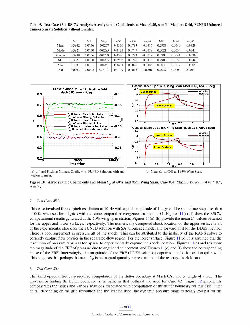
Table 9. Test Case #3a: BSCW Analysis Aerodynamic Coefficients at Mach 0.85, α = 5◦, Medium Grid, FUN3D UnforcedTime-Accurate Solution without Limiter.


Mean 0.3942 0.0756 -0.0277 0.4376 0.0783 -0.0315 0.2983 0.0540 -0.0329Mode 0.3821 0.0750 -0.0295 0.4123 0.0747 -0.0378 0.3021 0.0534 -0.0341


(a) Lift and Pitching Moment Coefficients, FUN3D Solutions with andwithout Limiter.

(b) Mean Cp, at 60% and 95% Wing Span.

Figure 10. Aerodynamic Coefficients and Mean Cp at 60% and 95% Wing Span, Case #3a, Mach 0.85, Rec = 4.49 * 106,α = 0◦.

2. Test Case #3b

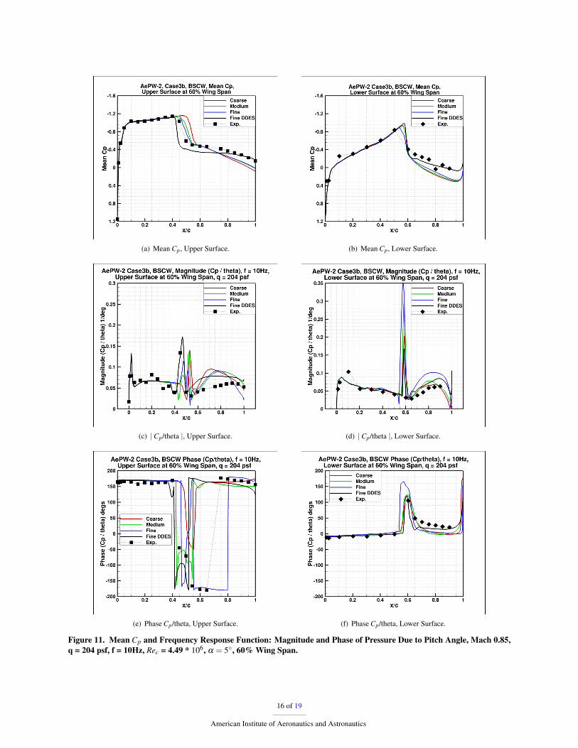
This case involved forced-pitch oscillation at 10 Hz with a pitch amplitude of 1 degree. The same time-step size, dt =0.0002, was used for all grids with the same temporal convergence error set to 0.1. Figures 11(a)-(f) show the BSCWcomputational results generated at the 60% wing-span station. Figures 11(a)-(b) provide the mean Cp values obtainedfor the upper and lower surfaces, respectively. The numerically-computed shock location on the upper surface is aftof the experimental shock for the FUN3D solution with SA turbulence model and forward of it for the DDES method.There is poor agreement in pressure aft of the shock. This can be attributed to the inability of the RANS solver tocorrectly capture flow physics in the separated-flow region. For the lower surface, Figure 11(b), it is assumed that theresolution of pressure taps was too sparse to experimentally capture the shock location. Figures 11(c) and (d) showthe magnitude of the FRF of pressure due to angular displacement, and Figures 11(e) and (f) show the correspondingphase of the FRF. Interestingly, the magnitude of the FRF (DDES solution) captures the shock location quite well.This suggests that perhaps the mean Cp is not a good quantity representation of the average shock location.

3. Test Case #3c

This third optional test case required computation of the flutter boundary at Mach 0.85 and 5◦ angle of attack. Theprocess for finding the flutter boundary is the same as that outlined and used for Case #2. Figure 12 graphicallydemonstrates the issues and various solutions associated with computation of the flutter boundary for this case. Firstof all, depending on the grid resolution and the scheme used, the dynamic pressure range is nearly 280 psf for the

15 of 19





Figure 11. Mean Cp and Frequency Response Function: Magnitude and Phase of Pressure Due to Pitch Angle, Mach 0.85,q = 204 psf, f = 10Hz, Rec = 4.49 * 106, α = 5◦, 60% Wing Span.

16 of 19


flutter boundary prediction at Mach 0.85. This is a very wide range and clearly requires further examination.As mentioned previously in the discussion of Case #3a, the application of a limiter in the solution process shifts

the predicted shock location aft on the upper surface of the wing, affecting the size of the separated region behindthe shock. The grid resolution affects shock strength and spatial distribution. As shown in Figure 12, the range ofthe dynamic pressure between the coarse and fine grid solutions with a limiter is nearly 200 psf. On the other hand,the corresponding range for the solutions without the limiter is only about 100 psf. In addition, a DDES solution ona fine grid produced a flutter boundary point in between the coarse- and fine-grid solutions. This very wide range ofpredictions prompted an attempt to calculate the flutter boundary over a wide range of Mach numbers from 0.6 to 0.85at 5◦ angle of attack.

The calculation at Mach 0.82 on a coarse grid produced a flutter boundary point at 200 psf. This calculation will beverified on a fine grid. The coarse grid calculations at Mach number of 0.8 and 0.74 did not establish flutter boundarypredictions at all. All solutions were always unstable, even with the dynamic pressure of 25 psf. On the other hand, thecalculations at Mach number of 0.6 and 0.7 predicted nearly identical flutter boundary dynamic pressure of about 100psf. The calculations at Mach 0.74 and Mach 0.8 were repeated using Grid D with the DDES turned on and off. Notethat the Grid D was constructed to better resolve the wake region and to make the grid more isotropic in the separatedflow region. One more grid refinement step is planned for future analysis. The calculation with the DDES turned onand off produced the same flutter boundary prediction. The solutions were stable at a dynamic pressure of 50 psf andunstable at 100 psf, with the flutter dynamic pressures at Mach 0.8 and Mach 0.74 computed to be 55 psf and 68 psf,respectively.

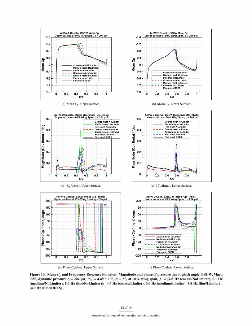
Figures 13(a)-(f) show the computational results generated at the 60% wing span station. Figures 13(a) and (b)show the mean pressures, Figures 13(c) and (d) show the magnitude of the FRF of pressure due to angular displace-ment, and Figures 13(e) and (f) show the corresponding phase of FRF. As discussed previously, the numerically-computed shock locations on the upper surface for the solutions with and without a limiter are different. The solutionswith the limiter for all three grid resolutions compute shock further aft on the upper surface than the solutions withoutthe limiter. The DDES solution and the fine grid solution without the limiter predicted the shock locations closest tothe leading edge.

Figure 12. Flutter Boundary Assessment, BSCW Case #3c, Mach 0.6 - 0.85, α = 5◦.

17 of 19





Figure 13. Mean Cp and Frequency Response Function: Magnitude and phase of pressure due to pitch angle, BSCW, Mach0.85, dynamic pressure q = 204 psf, Rec = 4.49 * 106, α = 5◦, at 60% wing span, f ∗ = [4.8 Hz (coarse/NoLimiter), 5.1 Hz(medium/NoLimiter), 5.0 Hz (fine/NoLimiter)]; [4.6 Hz (coarse/Limiter), 6.0 Hz (medium/Limiter), 4.8 Hz (fine/Limiter)];[4.9 Hz (Fine/DDES)].

18 of 19


IV. Concluding Remarks

Reynolds-Averaged Navier-Stokes analyses, including steady-state, static aeroelastic, forced excitation, and flutterwere performed as part of AePW-2 using the NASA Langley FUN3D software. The analyses were performed on allconfigurations and cases considered for the workshop involving the BSCW configuration. Aerodynamic coefficientsfrom the steady-state and time-accurate analyses were reported. When applicable, aerodynamic coefficients fromthe static-aeroelastic analyses were provided as well. The frequency response function of pressure due to angulardisplacement was calculated for the forced pitching and flutter cases and compared with the experimental data whenavailable.

The computationally obtained flutter dynamic pressure was 10% below the experimental flutter point for Case #2.The wide range of flutter-point prediction is reported for Case #3c. The wide predicted range is because it is verydifficult to computationally predict shock-induced separated flow for supercritical airfoils. In general, for the BSCWconfiguration, the computed shock location was located aft of the experimentally-measured shock location with theexception of the DDES solution. This was indicated by both the mean pressure distributions and the frequency responsefunctions.

Acknowledgments

The authors would like to acknowledge Dr. Robert Biedron of NASA Langley for his help in setting up FUN3Dpost processing routines and for valuable discussions and help in understanding of application of limiters and DDESin FUN3D .

References1Schuster, D. M., Chwalowski, P., Heeg, J., and Wieseman, C., “Summary of Data and Findings from the First Aeroelastic Prediction

Workshop,” International Conference on Computational Fluid Dynamics, ICCFD7 paper 3101, July 2012.2Heeg, J., Chwalowski, P., Schuster, D. M., Dalenbring, M., Jirasek, A., Taylor, P., Mavriplis, D. J., Boucke, A., Ballmann, J., and Smith, M.,

“Overview and Lessons Learned from the Aeroelastic Prediction Workshop,” IFASD Paper 2013-1A, June 2009.3Heeg, J., Chwalowski, P., Schuster, D. M., and Dalenbring, M., “Overview and lessons learned from the Aeroelastic Prediction Workshop,”

AIAA Paper 2013-1798, April 2013.4Heeg, J., Chwalowski, P., Schuster, D. M., Raveh, D., Jirasek, A., and Dalenbring, M., “Plans and Example Results for the 2nd AIAA

Aeroelastic Prediction Workshop,” AIAA Paper 2015-0437, Jan. 2015.5Silva, W., Chwalowski, P., and Perry, B., “Evaluation of linear, inviscid, viscous, and reduced-order modelling aeroelastic solutions of the

AGARD 445.6 wing using root locus analysis,” International Journal of Computational Fluid Dynamics, Vol. 28, Issue 3-4, 2014, pages 122-139.6”http://aiaa-dpw.larc.nasa.gov/”.7”http://hiliftpw.larc.nasa.gov/”.8”http://fun3d.larc.nasa.gov/papers/FUN3D_Manual-12.7.pdf”, NASA/TM-2015-218761.9Pirzadeh, S. Z., “Advanced Unstructured Grid Generation for Complex Aerodynamic Applications,” AIAA Paper 2008–7178, Aug. 2008.

10Samareh, J. A., “Unstructured Grids on NURBS Surfaces,” AIAA Paper 1993–3454.11”http://nescacademy.nasa.gov/workshops/AePW2/public/”.12”http://turbmodels.larc.nasa.gov/spalart.html”.13Spalart, P. R. and Allmaras, S. R., “A One-Equation Turbulence Model for Aerodynamic Flows,” La Recherche Aerospatiale, No. 1, 1994,

pp 5–21.14Venkatakrishnan, V., “Convergence to Steady State Solutions of the Euler Equations on Unstructured Grids with Limiter,” Journal of Com-

putational Physics, Vol. 118, No. 1, April 1995, pages 120-130.15Roe, P. L., “Approximate Riemann Solvers, Parameter Vectors, and Difference Schemes,” Journal of Computational Physics, Vol. 43, No.

2, October 1981, pages 357-372.16Biedron, R. T. and Thomas, J. L., “Recent Enhancements to the FUN3D Flow Solver for Moving-Mesh Applications,” AIAA Paper 2009-

1360, Jan. 2009.17Biedron, R. T. and Lee-Rausch, E. M., “Rotor Airloads Prediction Using Unstructured Meshes and Loose CFD/CSD Coupling,” AIAA Paper

2008-7341, 2008.18Batina, J. T., Seidel, D. A., Bland, S. R., and Bennet, R. M., “Unsteady Transonic Flow Calculations for Realistic Aircraft Configurations,”

AIAA Paper 1987-0850, 1987.19Bartels, R. E., Rumsey, C. L., and Biedron, R. T., “CFL3D Version 6.4 - General Usage and Aeroelastic Analysis,” NASA TM 2006-214301,

March 2006.20MSC Software, Santa Ana, CA, MSC Nastran, 2008, http://www.mscsoftware.com/products/msc_nastran.cfm.21Samareh, J. A., “Discrete Data Transfer Technique for Fluid-Structure Interaction,” AIAA Paper 2007–4309, June 2007.22Vatsa, V. N., Carpenter, M. H., and Lockard, D. P., “Re-evaluation of an Optimized Second Order Backward Difference (BDF2OPT) Scheme

for Unsteady Flow Applications,” AIAA Paper 2010-0122, Jan. 2010.23Schuster, D. M., “Aerodynamic Measurements on a Large Splitter Plate for the NASA Langley Transonic Dynamics Tunnel,” NASA TM

2001-210828, March 2001.

19 of 19


http://aiaa-dpw.larc.nasa.gov/

http://hiliftpw.larc.nasa.gov/

http://fun3d.larc.nasa.gov/papers/FUN3D_Manual-12.7.pdf

http://nescacademy.nasa.gov/workshops/AePW2/public/

http://turbmodels.larc.nasa.gov/spalart.html

http://www.mscsoftware.com/products/msc_nastran.cfm

fun3d analyses in support of the second aeroelastic ... analyses in support of the second...

Documents