funcionamiento del algoritmo del pcr: … · for one hour in a single bidding zone where all lines...

FUNCIONAMIENTO DEL ALGORITMO DEL PCR:

EUPHEMIA 09-04-2013

INTRODUCTION

For Power Exchanges: Most competitive price will arise & Overall welfare increases

For TSOs: Efficient capacity allocation

Market A Market B

P (€/MWh) P (€/MWh)

Q (MWh) Q (MWh) QB QA QB’ QA’

PA

PB PA’

Export Import

Isolated Markets Price

Differences

Coupled Markets Price convergence

PB’

PCR can have two functions:

Rotating Coordinator Role

PCR Algorithm & Matcher

How does PCR work?…

ALGORITHM EUPHEMIA

• EUPHEMIA is an algorithm that solves optimally the market coupling problem. – EUPHEMIA means: Pan-European Hybrid Electricity

Market Integration Algorithm. – Hybrid: It is hybrid because it supports both ATC-

based and flow-based network models, both standalone and in combination.

• It maximizes the welfare of the solution

For one hour in a single Bidding Zone where all lines are uncongested: • The intersection is the point where, for the same volume, the marginal price

the buyers are ready to pay is equal to the marginal price the producers are asking

• But it is also the point where the shaded area (=welfare) is maximal.

CLEARING PRICES

Demand

Supply

Producer surplus

Consumer surplus

Clearing price

€

MW Clearing volume

• LP example: One single market, no blocks. – Parameters

• Qo,h: volume corresponding to order o in period h; • Po,h: price corresponding to order o in period h;

– Variables • xo,h: acceptance fraction of order o in period h;

EUPHEMIA MODELISATION

8

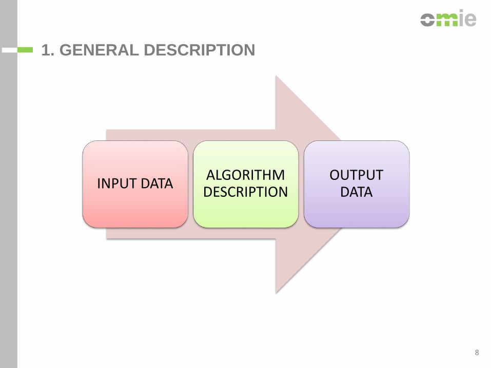
INPUT DATA ALGORITHM DESCRIPTION

OUTPUT DATA

1. GENERAL DESCRIPTION

8

9

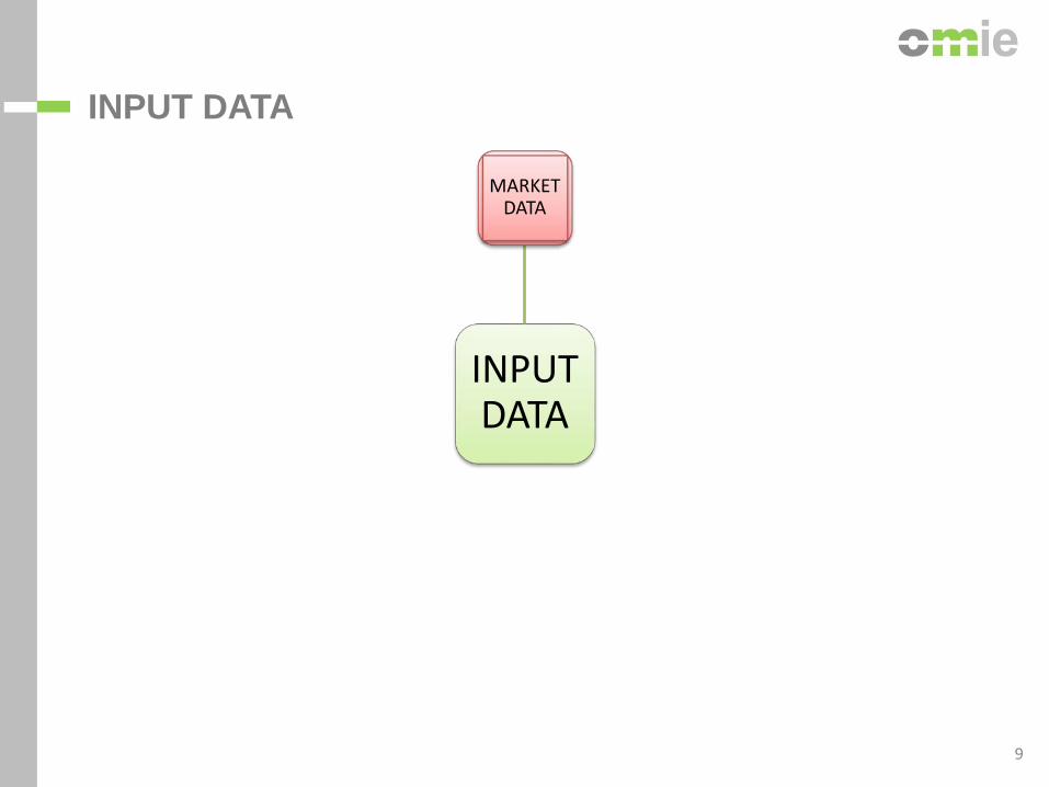
INPUT DATA

MARKET DATA

INPUT DATA

9

10

MARKET DATA

MARKET DATA

MARKETS

BIDDING Zone

e.g.:OMIE • SPAIN • PORTUGAL • MOROCCO

MARKET BOUNDARIES

PRICE BOUNDARIES

10

11

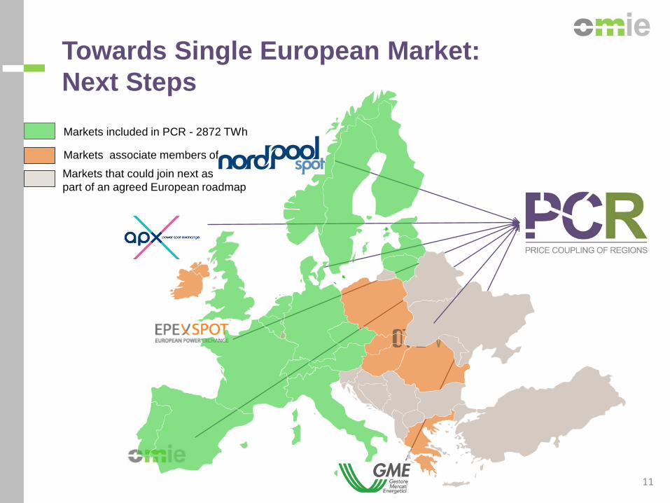
Markets associate members of PCR

Markets included in PCR - 2872 TWh

Markets that could join next as part of an agreed European roadmap

Towards Single European Market: Next Steps

11

12

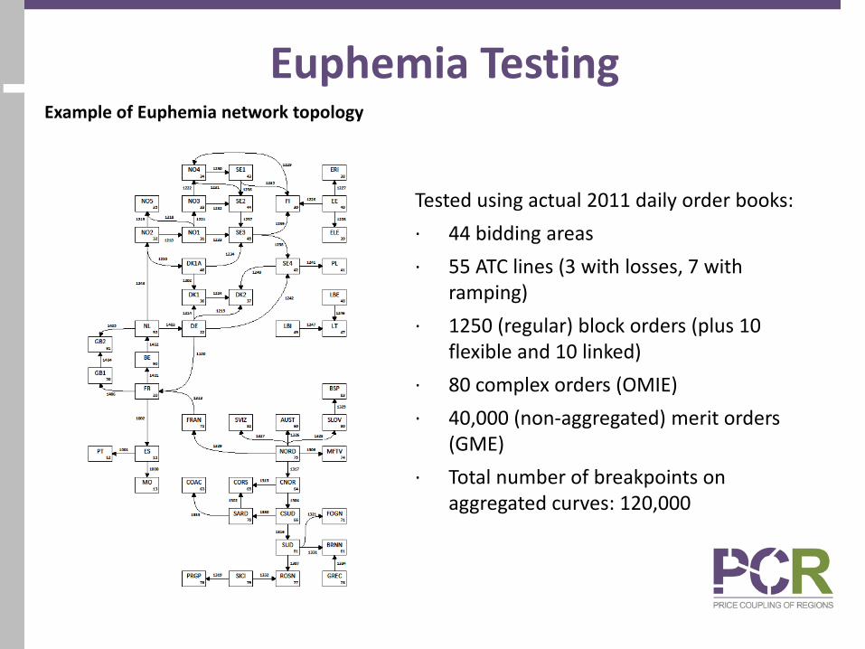
Euphemia Testing

Tested using actual 2011 daily order books: · 44 bidding areas · 55 ATC lines (3 with losses, 7 with

ramping) · 1250 (regular) block orders (plus 10

flexible and 10 linked) · 80 complex orders (OMIE) · 40,000 (non-aggregated) merit orders

(GME) · Total number of breakpoints on

aggregated curves: 120,000

Example of Euphemia network topology

13

INPUT DATA

MARKET DATA

ORDERS

INPUT DATA

13

14

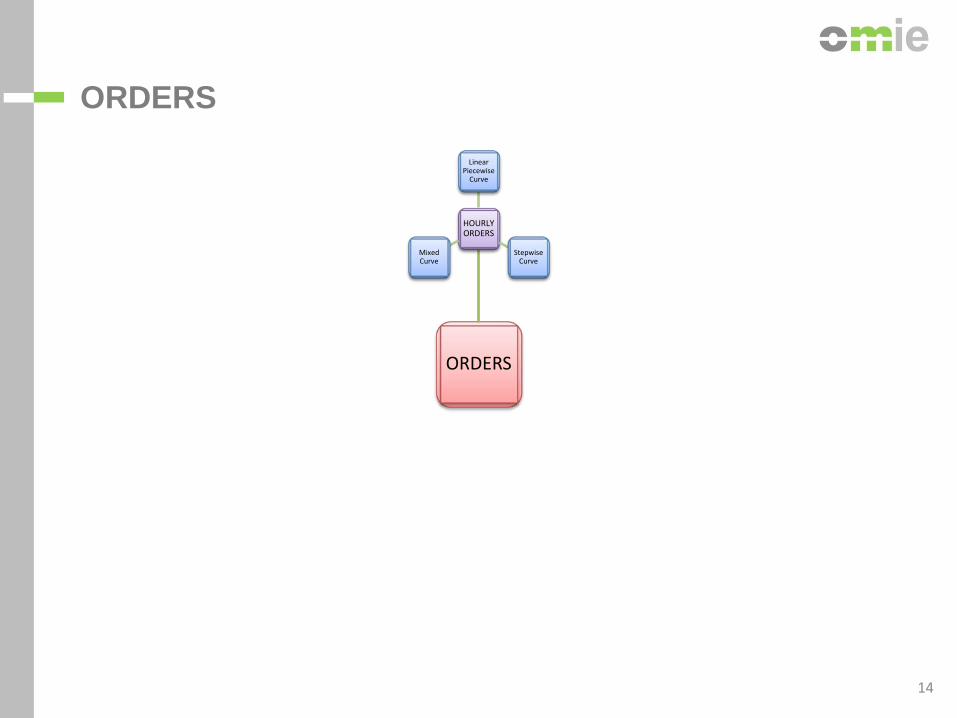
ORDERS

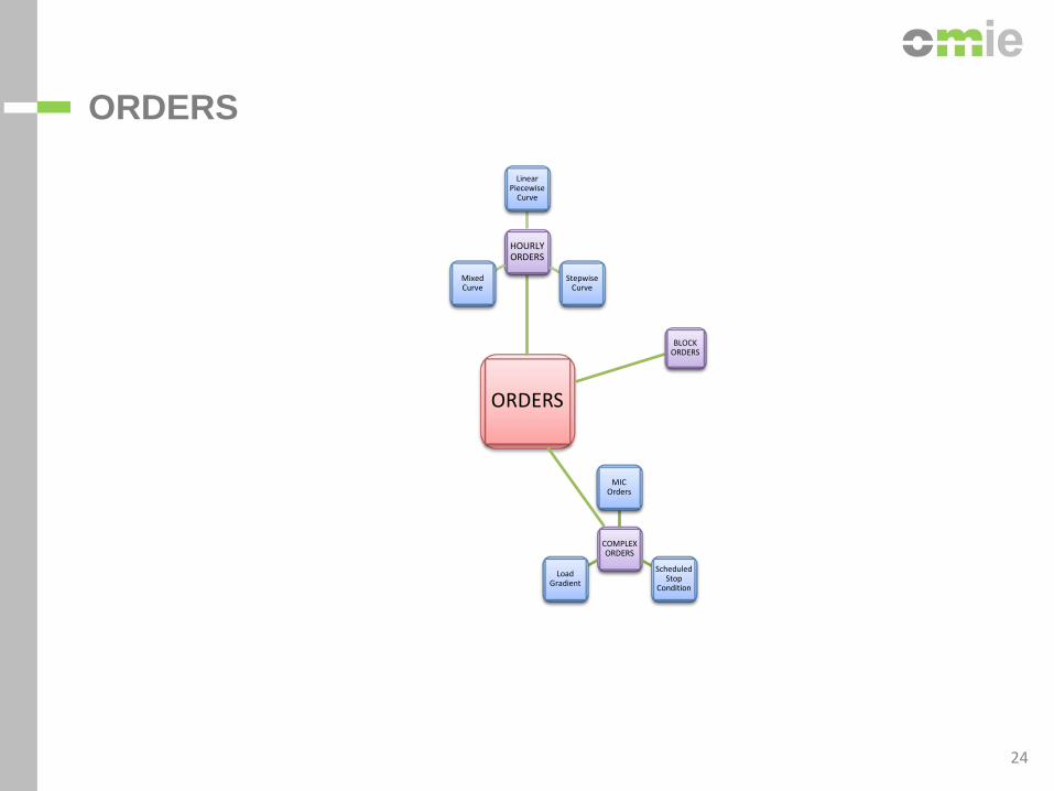
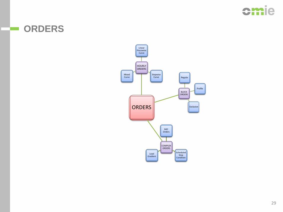
ORDERS

HOURLY ORDERS

Linear Piecewise

Curve

Stepwise Curve

Mixed Curve

14

15

LINEAR PIECEWISE HOURLY ORDERS

The volume term is delimited by an initial price at which the hourly order starts to be accepted and a final price at which the order is completely accepted. NORDPOOL and EPEX manages these kind of orders.

price0

price1

Q 15

16

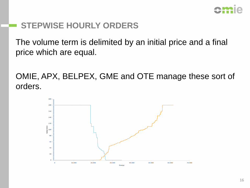
STEPWISE HOURLY ORDERS

The volume term is delimited by an initial price and a final price which are equal. OMIE, APX, BELPEX, GME and OTE manage these sort of orders.

16

17

ORDERS

ORDERS

HOURLY ORDERS

Linear Piecewise

Curve

Stepwise Curve

Mixed Curve

COMPLEX ORDERS

MIC Orders

17

18

MIC Orders are Stepwise Hourly Orders under an economical condition defined by two terms: • Tf: Fixed Term in Euros which shows the fixed costs of the whole amount of

energy traded in the order. • Tv: Variable Term in Euros per accepted MWh which shows the variable

costs of the whole amount of energy traded in the order. The same acceptance rules for Stepwise Hourly Orders are applied to MIC Orders plus the acceptance of the economic condition which is defined mathematically as:

Tf + Tv · (ΣhΣo∈h [qo · xo]) ≤Σh (MCPh· (Σo∈h [qo · xo]))

COMPLEX ORDERS. MIC ORDERS

18

19

ORDERS

ORDERS

HOURLY ORDERS

Linear Piecewise

Curve

Stepwise Curve

Mixed Curve

COMPLEX ORDERS

MIC Orders

Scheduled Stop

Condition

19

20

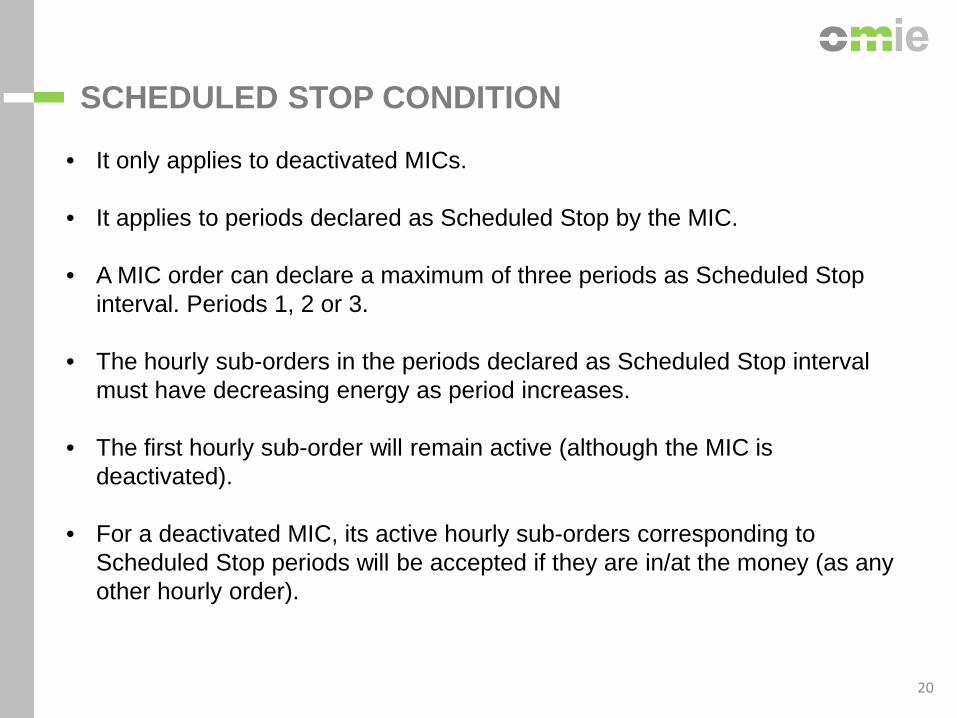
• It only applies to deactivated MICs. • It applies to periods declared as Scheduled Stop by the MIC.

• A MIC order can declare a maximum of three periods as Scheduled Stop

interval. Periods 1, 2 or 3.

• The hourly sub-orders in the periods declared as Scheduled Stop interval must have decreasing energy as period increases.

• The first hourly sub-order will remain active (although the MIC is

deactivated).

• For a deactivated MIC, its active hourly sub-orders corresponding to Scheduled Stop periods will be accepted if they are in/at the money (as any other hourly order).

SCHEDULED STOP CONDITION

20

21

ORDERS

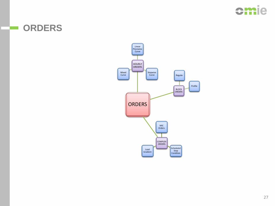
ORDERS

HOURLY ORDERS

Linear Piecewise

Curve

Stepwise Curve

Mixed Curve

BLOCK ORDERS

Regular

Profile

Exclusive Linked

Flexible “Hourly”

COMPLEX ORDERS

MIC Orders

Scheduled Stop

Condition

Load Gradient

21

22

The load gradient condition limits the variation between the accepted volume of an order in a period and the accepted volume of the same order in the adjacent periods. A Load Gradient Order (LG) is defined by the next terms: • Increase Gradient: Maximum increase gradient in MWh. • Decrease Gradient: Maximum decrease gradient in MWh. LG Orders must fulfill the following gradient condition:

(Σo∈h+1 [qo · xo]) ≤ (Σo∈h [qo · xo]) + Increase Gradient

(Σo∈h+1 [qo · xo]) ≥ (Σo∈h [qo · xo]) - Decrease Gradient

LOAD GRADIENT ORDER

NEW CONDITION!!

22

23

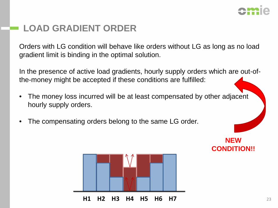
Orders with LG condition will behave like orders without LG as long as no load gradient limit is binding in the optimal solution. In the presence of active load gradients, hourly supply orders which are out-of-the-money might be accepted if these conditions are fulfilled: • The money loss incurred will be at least compensated by other adjacent

hourly supply orders. • The compensating orders belong to the same LG order.

LOAD GRADIENT ORDER

NEW CONDITION!!

H1 H2 H3 H4 H5 H6 H7 23

24

ORDERS

ORDERS

HOURLY ORDERS

Linear Piecewise

Curve

Stepwise Curve

Mixed Curve

BLOCK ORDERS

COMPLEX ORDERS

MIC Orders

Scheduled Stop

Condition

Load Gradient

24

25

ORDERS

ORDERS

HOURLY ORDERS

Linear Piecewise

Curve

Stepwise Curve

Mixed Curve

BLOCK ORDERS

Regular

COMPLEX ORDERS

MIC Orders

Scheduled Stop

Condition

Load Gradient

25

26

A participant can submit a Block order made up of: • Block type (buy or sell). • Block Price: Fixed price limit. • Block Volume: Volume of the block. • Block Period: Consecutive hours over which the block spans. A Block order cannot be accepted partially. Actually, it is either totally rejected or accepted when several blocks have the same characteristics.

REGULAR BLOCK ORDERS

BLOCK DESCRIPTION

BLOCK PERIOD BLOCK PRICE BLOCK

VOLUME

BLOCK B Hours 1-24 40 Euros -200 MWh

BLOCK S Hours 8-12 40 Euros 50 MWh

26

27

ORDERS

ORDERS

HOURLY ORDERS

Linear Piecewise

Curve

Stepwise Curve

Mixed Curve

BLOCK ORDERS

Regular

Profile

COMPLEX ORDERS

MIC Orders

Scheduled Stop

Condition

Load Gradient

27

28

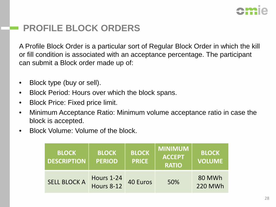
A Profile Block Order is a particular sort of Regular Block Order in which the kill or fill condition is associated with an acceptance percentage. The participant can submit a Block order made up of: • Block type (buy or sell). • Block Period: Hours over which the block spans. • Block Price: Fixed price limit. • Minimum Acceptance Ratio: Minimum volume acceptance ratio in case the

block is accepted. • Block Volume: Volume of the block.

PROFILE BLOCK ORDERS

BLOCK DESCRIPTION

BLOCK PERIOD

BLOCK PRICE

MINIMUM ACCEPT RATIO

BLOCK VOLUME

SELL BLOCK A Hours 1-24 Hours 8-12 40 Euros 50% 80 MWh

220 MWh

28

29

ORDERS

ORDERS

HOURLY ORDERS

Linear Piecewise

Curve

Stepwise Curve

Mixed Curve

BLOCK ORDERS

Regular

Profile

Exclusive

COMPLEX ORDERS

MIC Orders

Scheduled Stop

Condition

Load Gradient

29

30

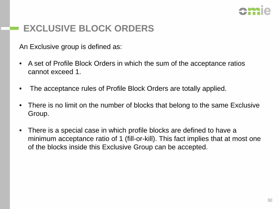
An Exclusive group is defined as: • A set of Profile Block Orders in which the sum of the acceptance ratios

cannot exceed 1.

• The acceptance rules of Profile Block Orders are totally applied.

• There is no limit on the number of blocks that belong to the same Exclusive Group.

• There is a special case in which profile blocks are defined to have a minimum acceptance ratio of 1 (fill-or-kill). This fact implies that at most one of the blocks inside this Exclusive Group can be accepted.

EXCLUSIVE BLOCK ORDERS

30

31

ORDERS

ORDERS

HOURLY ORDERS

Linear Piecewise

Curve

Stepwise Curve

Mixed Curve

BLOCK ORDERS

Regular

Profile

Exclusive Linked

COMPLEX ORDERS

MIC Orders

Scheduled Stop

Condition

Load Gradient

31

32

Regular and Profile Block orders may be linked together: • The acceptance of individual Block Orders depends on

the acceptance of other Block Orders. Two kinds of Linked Regular Blocks: Parent Block

Child Block

LINKED BLOCK ORDERS

32

33

ORDERS

ORDERS

HOURLY ORDERS

Linear Piecewise

Curve

Stepwise Curve

Mixed Curve

BLOCK ORDERS

Regular

Profile

Exclusive Linked


COMPLEX ORDERS

MIC Orders

Scheduled Stop

Condition

Load Gradient

33

34

• A Flexible Hourly Order is a Regular Block Order which lasts only one period. The period is said to be flexible and will be determined by the algorithm.

• In case of acceptance, it will only occur in one hour, but

the hour is flexible and that means it is not defined by the participant.

• The acceptance rules of regular Block Orders are totally applied.

FLEXIBLE HOURLY BLOCK ORDERS

34

35

ORDERS

ORDERS

HOURLY ORDERS

Linear Piecewise

Curve

Stepwise Curve

Mixed Curve

BLOCK ORDERS

Regular

Profile

Exclusive Linked


COMPLEX ORDERS

MIC Orders

Scheduled Stop

Condition

Load Gradient

PUN Orders

ITALIAN ORDERS

35

36

• Prezzo Unico Nazionale ▫ Most of the demand of Italy is submitted to a single

purchase price, regardless of its location ▫ This price must ensure that the revenues coming from

the consumers suffices to cover the payments to the producers (which occur at zonal prices)

PUN REQUIREMENT

36

37

ORDERS

ORDERS

HOURLY ORDERS

Linear Piecewise

Curve

Stepwise Curve

Mixed Curve

BLOCK ORDERS

Regular

Profile

Exclusive Linked


COMPLEX ORDERS

MIC Orders

Scheduled Stop

Condition

Load Gradient

PUN Orders

Merit Order

ITALIAN ORDERS

PTO Price Taking

37

38

In GME: • Selling offers receive their Bidding Zone marginal price. • Some of the buying bids pay their Bidding Zone price. These are called no-

PUN bids, related to pump plants. • The rest of the selling bids pay the common national PUN price which is

different from their Bidding Zone price PUN ORDERS This PUN price is defined as the average price of GME zonal marginal market prices, weighted by the purchase quantity assigned to PUN Orders in each Bidding Zone. That is:

PPUN * Σz Qz = Σz Pz * Qz

PUN ORDERS

38

39

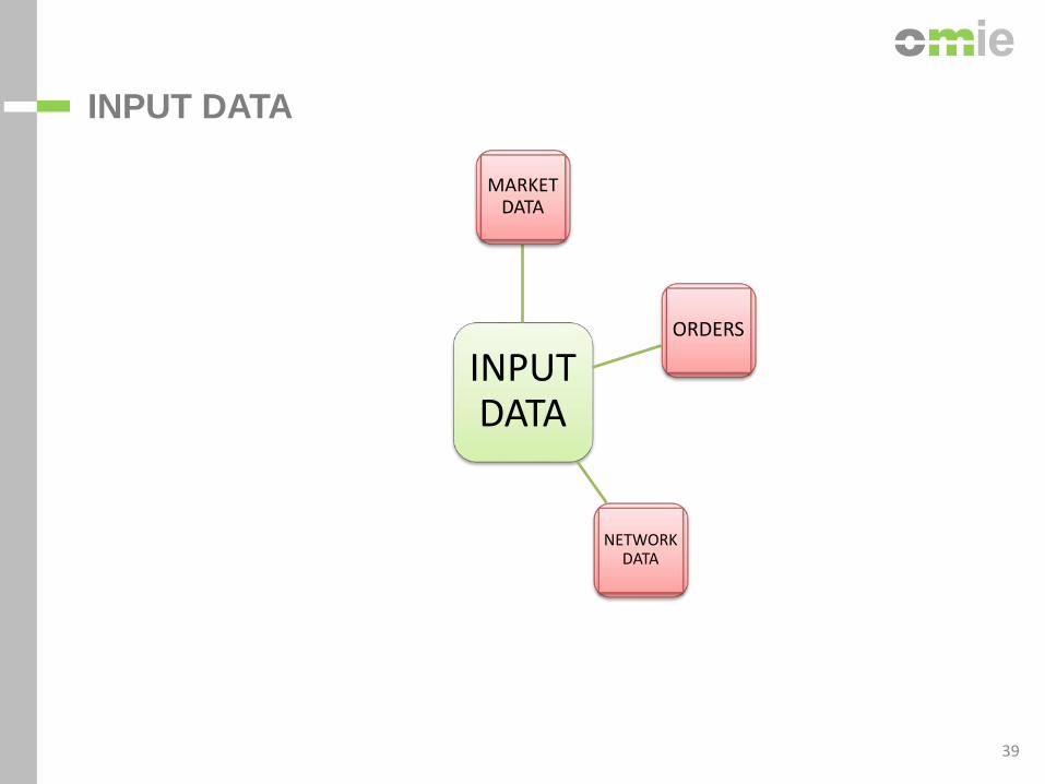
INPUT DATA

MARKET DATA

ORDERS

NETWORK DATA

INPUT DATA

39

40

NETWORK DATA

NETWORK DATA

BALANCE CONSTRAINTS

ATC MODEL • AREA BALANCE

FLOW BASED MODEL • GLOBAL

BALANCE

HYBRID MODEL • AREA BALANCE • GLOBAL

BALANCE

40

41

The energy balance concept is defined as the global supply must be equal to the global demand of all markets involved. Depending on the manner the interconnections are modeled, there are the following: • ATC network model: Where the interconnection between bidding zones is modeled

as if they were connected via a DC cable. The network is described as a set of lines between bidding zones with Available Transfer Capacity (ATC). Each line can support up to its ATC.

• Flow-based network model: Also known as PTDF model, with the bidding zones

connected in a meshed network with AC cables. It expresses the constraints arising from Kirchhoff’s laws and physical elements of the network in the different contingency scenarios considered by the TSOs. It translates those into linear constraints on the net positions of the different Bidding Zone in the same Balancing Area.

• Hybrid model: A mixture between these two.

BALANCE CONSTRAINTS

41

42

NETWORK DATA

NETWORK DATA

BALANCE CONSTRAINTS

ATC MODEL • AREA BALANCE

FLOW BASED MODEL • GLOBAL

BALANCE

HYBRID MODEL • AREA BALANCE • GLOBAL

BALANCE

INTERCON CONSTRAINTS

AVAILABLE TRANSFER

CAPACITY ATC

PTDF CONSTRAINTS

LINE RAMPING

RAMPING ON A LINE

RAMPING ON A SET OF

LINES

NET POSITION RAMPING

DAILY TOTAL VARIATION

HOURLY VARIATION

42

43

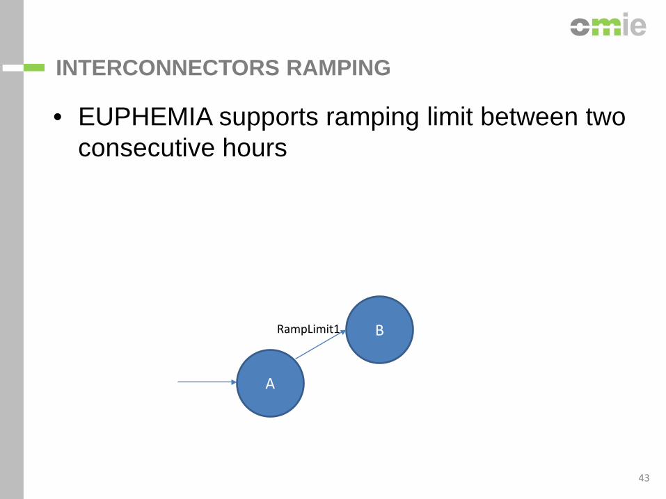
• EUPHEMIA supports ramping limit between two consecutive hours

A

B RampLimit1

INTERCONNECTORS RAMPING

43

44

• EUPHEMIA supports ramping limit between two consecutive hours in a list of links

A

C

B RampLimit1

RampLimit2


44

45

• EUPHEMIA supports defining ramping limits on interconnectors

• To handle ramping on different interconnectors, one could add a « dummy zone »

A

C

B

A’

RampLimit1

RampLimit2


45

46

• EUPHEMIA supports cumulative ramping limit between two consecutive hours in a list of links


46

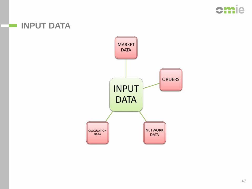
47

INPUT DATA

MARKET DATA

ORDERS

NETWORK DATA

CALCULATION DATA

INPUT DATA

47

48

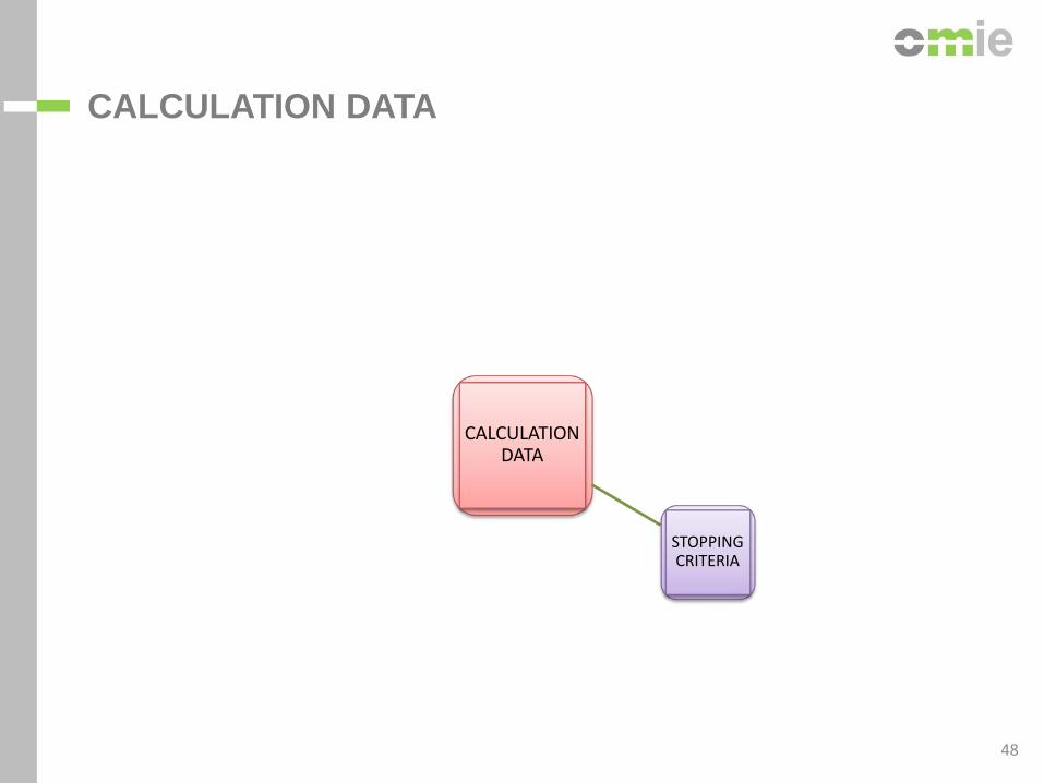
CALCULATION DATA

CALCULATION DATA

STOPPING CRITERIA

48

49

The algorithm will stop calculating whenever one of the following situations is reached: • The algorithm has explored all branches.

• The time limit has been overtaken. • The limit number of iterations has been overtaken.

STOPPING CRITERIA

49

50

CALCULATION DATA

CALCULATION DATA

STOPPING CRITERIA

ALLOWED TOLERANCES

50

51

INPUT DATA

MARKET DATA

ORDERS

NETWORK DATA

CALCULATION DATA

OTHER TSOs DATA

INPUT DATA

51

52

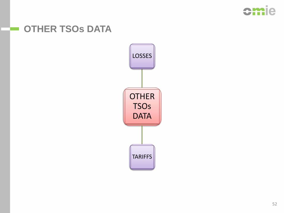
OTHER TSOs DATA

OTHER TSOs DATA

LOSSES

TARIFFS

52

53

In an ATC or hybrid network model, the DC cables might be operated by merchant companies which differ from TSOs. These companies levy the cost they incur for each passing MW to the cable. • When the line is congested:

(1-lossu,l,h) * MCPto – MCPfrom ≥ tariffu,l,h

(1-lossd,l,h) * MCPfrom – MCPto ≥ tariffd,l,h • When the line is uncongested:

(1-lossu,l,h) * MCPto – MCPfrom = tariffu,l,h

(1-lossd,l,h) * MCPfrom – MCPto = tariffd,l,h

TARIFFS

53

54

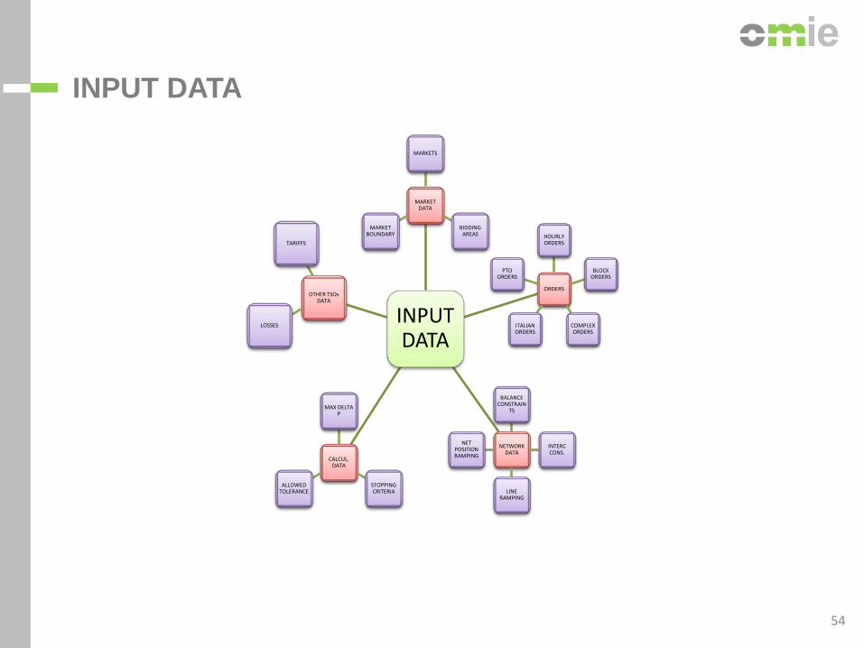
INPUT DATA

INPUT DATA

MARKET DATA

MARKETS

BIDDING AREAS

MARKET BOUNDARY

ORDERS

HOURLY ORDERS

BLOCK ORDERS

COMPLEX ORDERS

ITALIAN ORDERS

PTO ORDERS

NETWORK DATA

BALANCE CONSTRAIN

TS

INTERC CONS.

LINE RAMPING

NET POSITION RAMPING CALCUL.

DATA

MAX DELTA P

STOPPING CRITERIA

ALLOWED TOLERANCE

OTHER TSOs DATA

LOSSES

TARIFFS

54

55

ALGORITHM Introduction

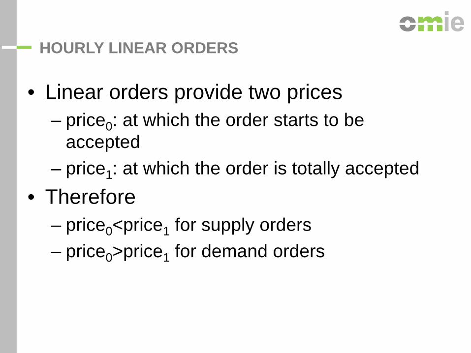
• Linear orders provide two prices – price0: at which the order starts to be

accepted – price1: at which the order is totally accepted

• Therefore – price0<price1 for supply orders – price0>price1 for demand orders

HOURLY LINEAR ORDERS

HOURLY LINEAR ORDERS

price0

price1

Q

MCP

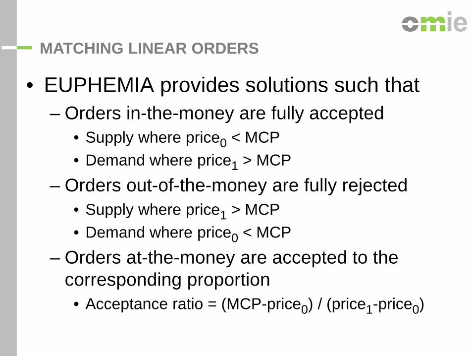
• EUPHEMIA provides solutions such that – Orders in-the-money are fully accepted

• Supply where price0 < MCP • Demand where price1 > MCP

– Orders out-of-the-money are fully rejected • Supply where price1 > MCP • Demand where price0 < MCP

– Orders at-the-money are accepted to the corresponding proportion

• Acceptance ratio = (MCP-price0) / (price1-price0)

MATCHING LINEAR ORDERS

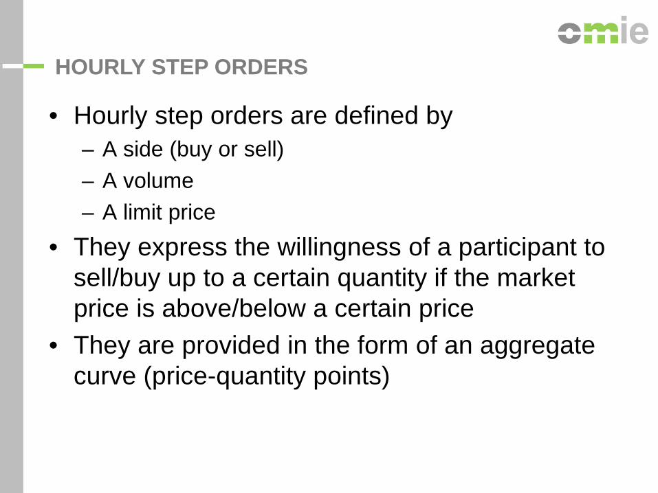
• Hourly step orders are defined by – A side (buy or sell) – A volume – A limit price

• They express the willingness of a participant to sell/buy up to a certain quantity if the market price is above/below a certain price

• They are provided in the form of an aggregate curve (price-quantity points)

HOURLY STEP ORDERS

HOURLY STEP ORDERS

MCP Q

• EUPHEMIA provides solutions such that – Orders in-the-money are fully accepted

• Supply at price < MCP • Demand at price > MCP

– Orders out-of-the-money are fully rejected • Supply at price > Market Clearing Price (MCP) • Demand at price < Market Clearing Price (MCP)

– Orders at-the-money can be curtailed

MATCHING STEP ORDERS

• Whenever a price interval is admissible • EUPHEMIA minimizes the distance to the middle

of the price interval

PRICE INDETERMINACY RULE

MCP Price interval Mid point

• Maximize traded volume

VOLUME INDETERMINACY RULE

MCP

Maximum volume

• Block orders are defined by – A side (buy or sell) – A volume on each period – A limit price

• They express the willingness of the participant to get either accepted in full on several periods or be totally rejected

BLOCK ORDERS

• EUPHEMIA provides solutions where – Block orders that are accepted are in-the-money, i.e.

there are no paradoxically accepted blocks (PAB) • Weighted average of the published MCPs is above limit price

for a supply block • Weighted average of the published MCPs is below limit price

for a demand block

– Block orders that are rejected might sometimes happen to be in-the-money

• Those are called paradoxically rejected (PRB)

MATCHING BLOCK ORDERS

• For a fixed selection of blocks, the PCR Market Coupling Problem can be written as a LP (or QP if linear orders)

– Solving this problem yields volumes and prices satisfying the Market Rules

– If there is no Paradoxically Accepted Block with respect to those prices, the block selection and the prices form a feasible solution to the MCP

• The optimal solution between those is the one with the highest welfare

EUPHEMIA MAIN IDEA

ALGORITHM Description

Block 1 Block 2 Block 3 In = 1 / Out =0

1 1 0 1 0 1 0 1 1 1 0 0 0 1 0 0 0 1 0 0 0 1 1 1

Welfare 75000 74000 76500 66700 65000 67050 56000 75900

A case with 3 blocks orders (1)

Welfare 75000 74000 76500 66700 65000 67050 56000 75900

• For each block selection – Check whether it creates

Paradoxically Accepted Blocks


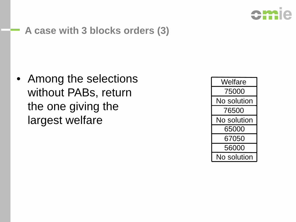
Welfare 75000

No solution 76500

No solution 65000 67050 56000

No solution

• Among the selections without PABs, return the one giving the largest welfare


Block 1 Block 2 Block 3 In = 1 / Out =0

1 1 0 1 0 1 0 1 1 1 0 0 0 1 0 0 0 1 0 0 0 1 1 1

Welfare 75000

No solution 76500

No solution 65000 67050 56000

No solution


• For each block selection – Check whether it creates Paradoxically

Accepted Blocks – Among the selections without PABs,

return the one giving the largest welfare • But this is not efficient

– If there are 100 blocks, there are 2100≈1030 possibilities…

Algorithm

• Branch-and-Bound method is a way to – Search among all these block selections in a structured

way – Find feasible solutions quickly – Prove early that large groups of these selections cannot

hold good solutions • The idea is as follows

– Try first without the kill-or-fill requirement – If the solution happens to have no fractional block, OK – If it has, then

• Select one block which is fractional • Create two subproblems (called branches)

– One where the block is killed – One where the block is filled

– Continue to explore until there is no unexplored branch

BRANCH AND BOUND (1)

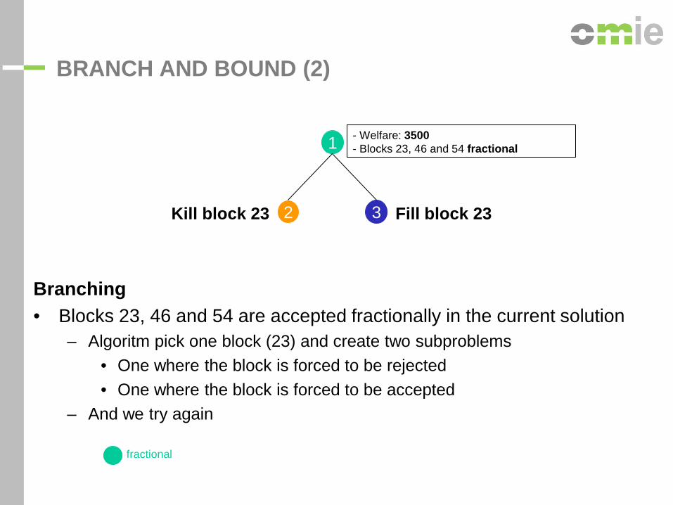
1 - Welfare: 3500 - Blocks 23, 46 and 54 fractional

fractional

Branching • Blocks 23, 46 and 54 are accepted fractionally in the current solution

– Algoritm pick one block (23) and create two subproblems • One where the block is forced to be rejected • One where the block is forced to be accepted

– And we try again

2 Kill block 23

3 Fill block 23


1

2 3

- Solution objective 1000 - Blocks 23 and 54 fractional

Kill block 23 - Welfare: 3050 - all blocks integral

fractional

1

2 3

- Welfare: 3500 - Blocks 23, 46 and 54 fractional

Price Problem • Once a candidate solution has

been found, we check whether there exists prices compatible with

– Block selection (i.e. no PAB)

• If such prices exist, we have a solution

Has solution!

New solution found


1

2 3

- Solution objective 1000 - Blocks 23 and 54 fractional

Kill block 23 - Welfare: 3050 - all blocks integral, there exist prices feasible solution found

fractional New solution found Integral, no prices

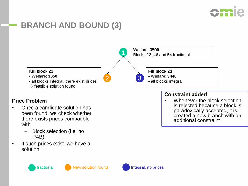
1

2 3


Fill block 23 - Welfare: 3440 - all blocks integral, no prices

Constraint added • Whenever the block selection

is rejected because a block is paradoxically accepted, it is created a new branch with an additional constraint


Price Problem • Once a candidate solution has

been found, we check whether there exists prices compatible with

– Block selection (i.e. no PAB)

• If such prices exist, we have a solution

1

2 3

4




Fill block 23 - Welfare: 3440 - all blocks integral, no prices Constraint added Fill block 23 + constraints - Welfare: 3300 - block 30 fractional

5 Fill block 23, Kill block 30 + constraints - Welfare: 3100 - all blocks integral, there exist prices better solution found!


1

2 3

4






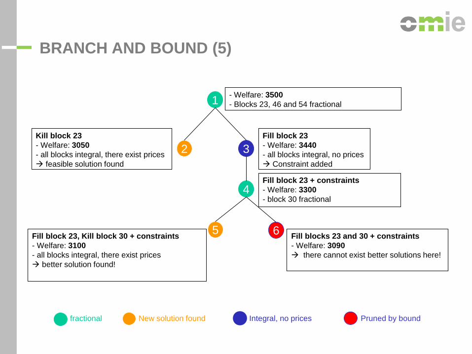
6 Fill blocks 23 and 30 + constraint - Welfare: 3090


• Suppose we already have a good valid solution (e.g. node )

• When exploring one branch (e.g. node ), we might see that even if we have not yet reached an integer solution, the current solution is not better than the best one we already have.

• Then we can decide to stop exploring this branch, since it will never lead to a better welfare than the current best solution

5

BOUNDING

6

1

2 3

4


fractional New solution found Integral, no prices Pruned by bound




6 Fill blocks 23 and 30 + constraints - Welfare: 3090 there cannot exist better solutions here!


OUTPUT DATA

Euphemia results • Price per bidding zone • Net position per bidding zone • Flows per interconnection • Matched energy per block, MIC and PUN orders

Iberian Market Results • Matched energy per Bid Unit

OUTPUT DATA

GRACIAS POR SU ATENCIÓN

funcionamiento del algoritmo del pcr: … · for one hour in a single bidding zone where all lines...

Documents