Santiago Escobar (Ed.)

Functional and (Constraint) LogicProgramming

18th International Workshop, WFLP’09

part of the Federated Conference on Rewriting, Deduction, andProgramming (RDP’09)

Brasılia, Brazil, June 28, 2009.

Informal Proceedings

Preface

This report contains the informal workshop proceedings of the 18th International Workshop onFunctional and (Constraint) Logic Programming (WFLP’09), held at Brasılia, Brazil, during June28, 2009. WFLP’09 is part of the Federated Conference on Rewriting, Deduction, and Programming(RDP’09). Previous meetings are: WFLP 2008 (Siena, Italy), WFLP 2007 (Paris, France), WFLP2006 (Madrid, Spain), WCFLP 2005 (Tallinn, Estonia), WFLP 2004 (Aachen, Germany), WFLP2003 (Valencia, Spain), WFLP 2002 (Grado, Italy), WFLP 2001 (Kiel, Germany), WFLP 2000(Benicassim, Spain), WFLP’99 (Grenoble, France), WFLP’98 (Bad Honnef, Germany), WFLP’97(Schwarzenberg, Germany), WFLP’96 (Marburg, Germany), WFLP’95 (Schwarzenberg, Germany),WFLP’94 (Schwarzenberg, Germany), WFLP’93 (Rattenberg, Germany), and WFLP’92 (Karl-sruhe, Germany).

The aim of the WFLP workshop is to bring together researchers interested in functional pro-gramming, (constraint) logic programming, as well as the integration of the two paradigms. Itpromotes the cross-fertilizing exchange of ideas and experiences among researchers and studentsfrom the different communities interested in the foundations, applications and combinations ofhigh-level, declarative programming languages and related areas.

The Program Committee of WFLP’09 collected three reviews for each paper and held anelectronic discussion during May 2009. The Program Committee selected 12 regular papers forpresentation at the workshop. In addition to the selected papers, the scientific program includestwo invited lectures by Claude Kirchner from the Centre de Recherche INRIA Bordeaux - Sud-Ouest, France and Roberto Ierusalimschy from the Departamento de Informatica, PUC-Rio, Brazil.I would like to thank them for having accepted our invitation.

I would also like to thank all the members of the Program Committee and all the referees fortheir careful work in the review and selection process. Many thanks to all authors who submittedpapers and to all conference participants. We gratefully acknowledge the Departamento de SistemasInformaticos y Computacion of the Universidad Politecnica de Valencia, who has supported thisevent. Finally, we express our gratitude to all members of the local organization of the FederatedConference on Rewriting, Deduction, and Programming (RDP’09), whose work has made theworkshop possible.

Brasılia, Brazil, Santiago EscobarJune 2009 WFLP’09 Chair

Organization

WFLP’09 is part of the Federated Conference on Rewriting, Deduction, and Programming (RDP’09).

Program Committee

Marıa Alpuente Universidad Politecnica de Valencia, SpainSergio Antoy Portland State University, USAChristiano Braga Universidade Federal Fluminense, BrazilRafael Caballero Universidad Complutense de Madrid, SpainDavid Deharbe Universidade Federal do Rio Grande do Norte, BrazilRachid Echahed CNRS, Laboratoire LIG, FranceMoreno Falaschi Universita di Siena, ItalyMichael Hanus Christian-Albrechts-Universitat zu Kiel, GermanyFrank Huch Christian-Albrechts-Universitat zu Kiel, GermanyTetsuo Ida University of Tsukuba, JapanWolfgang Lux Westfalische Wilhelms-Universitat Munster, GermanyMircea Marin University of Tsukuba, JapanCamilo Rueda Universidad Javeriana-Cali, ColombiaJaime Sanchez-Hernandez Universidad Complutense de Madrid, SpainAnderson Santana de Oliveira Universidade Federal do Rio Grande do Norte, Brazil

Additional Referees

Gloria AlvarezDemis BallisBernd BraßelLinda Brodo

Iliano CervesatoYukiyoshi KameyamaTemur KutsiaMiguel Palomino

Albert RubioClara SeguraPeter SestoftThierry Boy de la Tour

Rafael del Vado VırsedaToshiyuki YamadaHans Zantema

Sponsoring Institution

Departamento de Sistemas Informaticos y Computacion (DSIC)Universidad Politecnica de Valencia (UPV)

Table of Contents

Strategic Deduction . . . . . . . . . . . . . . . . . . . . . . . . . . . . . . . . . . . . . . . . . . . . . . . . . . . . . . . . . . . . . . . 1Claude Kirchner, Florent Kirchner, and Helene Kirchner

Programming with Multiple Paradigms in Lua . . . . . . . . . . . . . . . . . . . . . . . . . . . . . . . . . . . . . . . . 5Roberto Ierusalimschy

A Theoretical Framework for the Declarative Debugging of Functional Logic Programswith Lambda Abstractions . . . . . . . . . . . . . . . . . . . . . . . . . . . . . . . . . . . . . . . . . . . . . . . . . . . . . . . . . 15

Ignacio Castineiras Perez and Rafael del Vado Vırseda

Type Checking and Inference Are Equivalent in Lambda Calculi with Existential Types . . . . 31Yuki Kato and Ko ji Nakazawa

A Taxonomy of Some Right-to-Left String-Matching Algorithms . . . . . . . . . . . . . . . . . . . . . . . . 45Manuel Hernandez

A Simple Region Inference Algorithm for a First-Order Functional Language . . . . . . . . . . . . . 63Manuel Montenegro, Ricardo Pena, and Clara Segura

pFun: A Semi-explicit Parallel Purely Functional Language . . . . . . . . . . . . . . . . . . . . . . . . . . . . . 79Andre R. Du Bois, Gerson Cavalheiro, and Juliana Vizzotto

Realizing Multiparadigm Programming based on Hierarchical Graph Rewriting . . . . . . . . . . . 95Petra Hofstedt and Kazunori Ueda

Termination of Context-Sensitive Rewriting with Built-In Numbers and Collection DataStructures . . . . . . . . . . . . . . . . . . . . . . . . . . . . . . . . . . . . . . . . . . . . . . . . . . . . . . . . . . . . . . . . . . . . . . . 111

Stephan Falke and Deepak Kapur

Semantic Labelling for Proving Termination of Combinatory Reduction Systems . . . . . . . . . . 127Makoto Hamana

Fast and Accurate Strong Termination Analysis with an Application to Partial Evaluation . 141Michael Leuschel, Salvador Tamarit, and German Vidal

Advances in Type Systems for Functional Logic Programming . . . . . . . . . . . . . . . . . . . . . . . . . . 157Francisco J. Lopez-Fraguas, Enrique Martın-Martın, and Juan Rodrguez-Hortala

A Complete Axiomatization of Strict Equality over Infinite Trees . . . . . . . . . . . . . . . . . . . . . . . 173Javier Alvez and Francisco J. Lopez-Fraguas

Integrating ILOG CP technology into T OY . . . . . . . . . . . . . . . . . . . . . . . . . . . . . . . . . . . . . . . . . . 189Ignacio Castineiras and Fernando Saaenz-Perez

Strategic Deduction

Claude Kirchner, Florent Kirchner, and Hélène Kirchner

INRIAFrance

Abstract. In previous works, we have introduced the notion of abstractstrategies for abstract reduction systems and de�ned adequate propertiesof termination, con�uence and normalization under strategies. Thanks tothis abstract strategy concept, we draw a parallel between strategies forcomputation and strategies for deduction. Then, deduction rules can beviewed as rewrite rules, a deduction step as a rewriting step and a proofconstruction step as a narrowing step for an adequate abstract reductionsystem, possibly in constraint handling settings.

The fundamental complementarity between deduction and computation, asemphasized in particular in deduction modulo [9], gives now rise to a completelynew generation of proof assistants where customized deductions are performedmodulo appropriate and user de�nable computations [5,6]. This has in partic-ular the advantage to allow for a uniform implementation of higher-order and�rst-order logics [8,7] making possible the safe use of existing dedicated proofenvironments [16,10,4]. This generalizes classical approaches used in �rst-ordertheorem proving [17], as well as higher-order ones like PVS [18], TPS [1,2],Omega [3,19], Coq [11] or Mizar [20], to mention just a few.

Proof search in these environments goes back to the late sixties and thenthrought the design of ML as the metalanguage of LCF. It requires to guideproof discovery using so called strategies, tactics, tacticals or proof plans, termswidely used in arti�cial intelligence, in automated or interactive reasoning, insemantics of programming languages�as well as in every day life.

The collusion of deduction and computation in next-generation proof assis-tants has inspired our recent attempt at providing an uniform (domain-agnostic,if you will) de�nition for strategies, starting from a rule-based view point [13].

For term rewriting, reduction strategies study which expressions should beselected for evaluation and which rules should be applied. These choices are usu-aly made to increase the e�ciency of evaluation but may a�ect fundamentalproperties of computations such as con�uence or (non-)termination. Program-ming languages like TOM1, ELAN, Maude and Stratego allow for the explicitde�nition of the evaluation strategy, whereas languages like Clean, Curry, andHaskell allow for its modi�cation.

In theorem proving environments, including automated theorem provers,proof checkers, and logical frameworks, strategies (also called tacticals in some

1 http://tom.loria.fr

1

contexts) are used for proof search and proof planning, restriction of searchspaces, speci�cation of control components, combination of di�erent proof tech-niques and computation paradigms, or meta-level programming in reasoningsystems.

In this talk, we will recall the theoretical foundations of strategies and theconvergence of two points of view, namely rewriting-based computations on onehand, rule-based deduction and proof-search on the other hand.

While strategies for computation [12] essentially rely on the largely exploredand well-known domain of term reduction by rewriting or narrowing, strategiesfor deduction require to introduce an original point of view: we de�ne deductionrules as rewrite rules, a deduction step as a rewriting step, a deduction systemas an abstract reduction system. Proof construction in this context becomes nar-rowing derivation. Computation, deduction and proof search are then capturedby the foundational concept of abstract strategy.

Time permitting, we will show how deduction and proof search under con-straints could be investigated this way, especially using antipatterns [15,14].

References

1. Peter B. Andrews, Matthew Bishop, Sunil Issar, Dan Nesmith, Frank Pfenning,and Hongwei Xi. TPS: A Theorem Proving System for Classical Type Theory.Journal of Automated Reasoning, 16(3):321�353, June 1996.

2. Peter B. Andrews and Chad E. Brown. TPS: A hybrid automatic-interactivesystem for developing proofs. J. Applied Logic, 4(4):367�395, 2006.

3. Christoph Benzmüller, Matthew Bishop, and Volker Sorge. Integrating TPS andOmega. J. UCS, 5(3):188�207, 1999.

4. Frédéric Blanqui, Jean-Pierre Jouannaud, and Pierre-Yves Strub. Building Deci-sion Procedures in the Calculus of Inductive Constructions. In Jacques Duparcand Thomas Henziger, editors, 16th Annual Conference on Computer Science andLogic - CSL 2007, volume 4646 of Lecture Notes in Computer Science, Lausanne,Suisse, 2007. Springer Verlag.

5. Paul Brauner, Clément Houtmann, and Claude Kirchner. Principle of superdeduc-tion. In Luke Ong, editor, Proceedings of LICS, pages 41�50, jul 2007.

6. Paul Brauner, Clément Houtmann, and Claude Kirchner. Superdeduction at work.In Hubert Comon, Claude Kirchner, and Hélène Kirchner, editors, Rewriting, Com-putation and Proof. Essays Dedicated to Jean-Pierre Jouannaud on the Occasionof His 60th Birthday, volume 4600. Springer, jun 2007.

7. Guillaume Burel. Superdeduction as a Logical Framework. submitted, jan 2008.

8. Denis Cousineau and Gilles Dowek. Embedding Pure Type Systems in the lambda-Pi-calculus modulo. In Simona Ronchi Della Rocca, editor, TLCA, volume 4583of Lecture Notes in Computer Science, pages 102�117. Springer-Verlag, 2007.

9. Gilles Dowek, Thérèse Hardin, and Claude Kirchner. Theorem Proving Modulo.Journal of Automated Reasoning, 31(1):33�72, Nov 2003.

10. Gilles Dowek and Benjamin Werner. Arithmetic as a Theory Modulo. In JürgenGiesl, editor, RTA, volume 3467 of Lecture Notes in Computer Science, pages 423�437. Springer-Verlag, 2005.

11. Bruno Barras et al. The Coq Proof Assistant Reference Manual, 2006.

2

12. Claude Kirchner. Strategic Rewriting. Electr. Notes Theor. Comput. Sci. Proceed-ings of the 4th International Workshop on Reduction Strategies in Rewriting andProgramming - WRS'2004, Aachen, Germany, 124(2):3�9, 2005.

13. Claude Kirchner, Florent Kirchner, and Hélène Kirchner. Strategic Computationsand Deductions. In Reasoning in Simple Type Theory, volume 17 of MathematicalLogic and Foundations. College Publications, 2008.

14. Claude Kirchner, Radu Kopetz, and Pierre-Etienne Moreau. Anti-Pattern Match-ing. In 16th European Symposium on Programming (ESOP'07), Braga, Portugal,2007.

15. Claude Kirchner, Radu Kopetz, and Pierre-Etienne Moreau. Anti-Pattern Match-ing Modulo. In Carlos Martín-Vide, Friedrich Otto, and Henning Fernau, editors,Language and Automata Theory and Applications, Second International Confer-ence, LATA 2008, Tarragona, Spain, March 13-19, 2008. Revised Papers, volume5196 of Lecture Notes in Computer Science, pages 275�286, Tarragona, Spain, 2008.Springer.

16. Florent Kirchner and Claudio Sacerdoti Coen. The Fellowship proof manager.www.lix.polytechnique.fr/Labo/Florent.Kirchner/fellowship/, 2007.

17. William McCune. Semantic Guidance for Saturation Provers. Arti�cial Intelligenceand Symbolic Computation, pages 18�24, 2006.

18. Sam Owre, John Rushby, and Natarajan Shankar. PVS: A Prototype Veri�cationSystem. In Deepak Kapur, editor, Proc. 11th Int. Conf. on Automated Deduction,volume 607 of Lecture Notes in Arti�cial Intelligence, pages 748�752. Springer-Verlag, June 1992.

19. Jörg H. Siekmann, Christoph Benzmüller, and Serge Autexier. Computer sup-ported mathematics with Omega. J. Applied Logic, 4(4):533�559, 2006.

20. A. Trybulec and H. Blair. Computer Aided Reasoning with Mizar. In R. Parikh,editor, Logic of Programs. Springer Verlag, New York, 1985.

3

Programming with Multiple Paradigms in Lua

Roberto Ierusalimschy

PUC-Rio

1 Introduction

Lua is an embeddable scripting language used in many industrial applications(e.g., Adobe’s Photoshop Lightroom), with an emphasis on embedded systemsand games. It is embedded in devices ranging from cameras (Canon) to keyboards(Logitech G15) to network security appliances (Cisco ASA). In 2003 it was votedthe most popular language for scripting games by a poll by the site Gamedev1.In 2006 it was called a “de facto standard for game scripting” [1]. Lua is alsopart of the Brazilian standard middleware for digital TV [2].

Two key points in the design of the language that led to those uses areflexibility and small size. To achieve these two conflicting goals, the design em-phasizes the use of few but powerful mechanisms, such as first-class functions,associative arrays, and reflexive capabilities [3, 4]. So, although Lua is primar-ily a procedural language, it can be, and frequently is, used in several differentprogramming paradigms, such as functional, object-oriented, goal-oriented, andconcurrent programming, and also for data description.

In this presentation we will discuss what mechanisms Lua features to achieveits flexibility and how programmers use them for different paradigms.

2 Functional Programming

Lua offers first-class functions with lexical scoping. For instance, the followingcode is valid Lua code:

(function (a,b) print(a+b) end)(10, 20)

It creates an anonymous function that prints the sum of its two parameters andapplies that function to arguments 10 and 20.

All functions in Lua are anonymous dynamic values, created at run time.Lua offers a quite conventional syntax for creating functions, like this:

function fact (n)if n <= 1 then return 1else return n * fact(n - 1)end

end

1 http://www.gamedev.net/gdpolls/viewpoll.asp?ID=163

5

However, this syntax is simply sugar for an assignment:

fact = function (n)...

end

(This is quite similar to a define in Scheme [5].)Lua does not offer a letrec primitive. Instead, it relies on assignment to close

a recursive reference. For instance, a (strict) recursive fixed-point operator canbe defined like this:

local YY = function (f)

return function (x)return f(Y(f))(x)

endend

Or, using some sugar, like this:

local function Y (f)return function (x)

return f(Y(f))(x)end

end

This second fragment expands to the first one. In both cases, the Y in the functionbody is bounded to the previously declared local variable.

Of course, we can also define a strict non-recursive fixed-point combinator inLua:

Y = function (le)local a = function (f)return le(function (x) return f(f)(x) end)

endreturn a(a)

end

Despite being a procedural language, Lua frequently uses function values;several functions in the standard Lua library are higher-order. For instance,the sort function accepts a comparison function as argument. In its pattern-matching functions, text substitution accepts a replacement function that re-ceives the original text matching the pattern and returns its replacement. Thestandard library also offers some traversal functions, which receive a function tobe applied to every element of a collection.

Most programming techniques for (strict) functional programming also workwithout modifications in Lua. As an example, LuaSocket, the standard library fornetwork connection in Lua, uses functions to allow easy composition of differentfunctionalities when reading from and writing to sockets [6].

6

Most implementations of first-class functions with lexical scoping neglectassignment. Pure functional languages do not have assignment. In ML assignablecells have no names, so the problem does not arise. Some Scheme compilers(e.g., Orbit [7]) actually implement assignable variables as ML cells (assignmentconversions), on the correct ground that they are not used often.

None of those implementations fit Lua, a procedural language where assign-ment is the norm. Lua has added requirements that its compiler must be fast,to handle huge data-description “programs”, and small. So, Lua uses a simple,one-pass compiler with no intermediate representations which cannot performeven escape analysis.

Due to these technical restrictions, previous versions of Lua offered a re-stricted form of lexical scoping where a nested function could access the value ofan outer variable, but could not assign to such variable. Lua version 5, releasedin 2003, came with a novel technique for implementing closures that satisfies thefollowing requirements [8]:

– It does not impact the performance of code that does not use non-localvariables.

– It has an acceptable performance for imperative programs, where side effects(assignment) are the norm.

– It correctly handles sharing, where more than one closure modifies a non-local variable.

– It is compatible with the standard execution model for procedural languages,where variables live in activation records allocated in an array-based stack.

– It is amenable to a one-pass compiler that generates code on the fly, withoutintermediate representations.

3 Object-Oriented Programming

Lua has only one data-structure mechanism, the table. Tables are first-class,dynamically created associative arrays.

Tables plus first-class functions already give Lua partial support for objects.An object may be represented by a table: instance variables are regular tablefields and methods are table fields containing functions.

One missing ingredient is how to connect method calls with their respectiveobjects. If obj is a table with a method foo and we call obj.foo(), foo willhave no reference to obj. We could solve this problem by making foo a closurewith an internal reference to obj, but that is expensive, as each object wouldneed its own closure for each of its methods.

A better mechanism would be to pass the receiver as a hidden argument tothe method, as most object-oriented languages do. Lua supports this mechanismwith a new syntactic sugar, the colon operator : the syntax orb:foo() is sugarfor orb.foo(orb), so that the receiver is passed as an extra argument to the

7

method. There is a similar sugar for method definitions. The syntax

function obj:foo (...) ... end

is sugar for

obj.foo = function (self, ...) ... end

That is, the colon adds an extra parameter to the function, with the fixed nameself. The function body then may access instance variables as regular fields oftable self.

To implement classes and inheritance, Lua uses delegation [9, 10]. Delega-tion in Lua is very simple and is not directly connected with object-orientedprogramming; it is a concept that applies to any table. Any table may have adesignated “parent” table. Whenever Lua fails to find a field in a table, it triesto find that field in the parent table. In other words, Lua delegates field accessesinstead of method calls.

Let us see how this works. Let us assume an object obj and a call obj:foo().This call actually means obj.foo(obj), so Lua first looks for the key foo in tableobj. If obj has such field, the call proceeds as before. Otherwise, Lua looks forthat key in the parent of obj. (If the parent object has a parent, this query maytrigger another query in the parent’s parent and so on.) Once it found a valuefor that key, Lua calls it with the original object obj as the first argument, sothat obj becomes the value of the parameter self inside the method’s body.

For more advanced uses, a program may set a function as the “parent” ofa table. In that case, whenever Lua cannot find a key in the table it calls theparent function to do the query. This mechanism allows several useful patterns,such as multiple inheritance and inter-language inheritance (where a Lua objectmay delegate to a C object, for instance).

4 Goal-Oriented Programming

Goal-oriented programming involves solving a goal that is either a primitivegoal or a disjunction of alternative goals. These alternative goals may be, inturn, conjunctions of subgoals that must be satisfied in succession, each of themgiving a partial outcome to the final result. Two typical examples of goal-orientedprogramming are pattern matching [11] and Prolog-like queries [12].

In pattern-matching problems, the primitive goal is the matching of stringliterals, disjunctions are alternative patterns, and conjunctions represent se-quences. In Prolog, the unification process is an example of a primitive goal,a relation constitutes a disjunction, and rules are conjunctions. In those con-texts, we may implement a problem solver using a backtracking mechanism thatsuccessively tries each alternative until it finds an adequate result.

Although Lua does not offer any specific mechanism for this kind of prob-lem solving, we can use Lua coroutines [13] for the task. A well-known modelfor Prolog-style backtracking is the two-continuation model [14, 15], which needs

8

-- matching any character (primitive goal)

function any (S, pos)

if pos < string.len(S) then coroutine.yield(pos + 1) end

end

-- matching a string literal (primitive goal)

function lit (str)

local len = string.len(str)

return function (S, pos)

if string.sub(S, pos, pos+len-1) == str then

coroutine.yield(pos+len)

end

end

end

-- alternative patterns (disjunction)

function alt (patt1, patt2)

return function (S, pos)

patt1(S, pos); patt2(S, pos)

end

end

-- sequence of sub-patterns (conjunction)

function seq (patt1, patt2)

return function (S, pos)

local btpoint = coroutine.wrap(function() patt1(S, pos) end)

for npos in btpoint do patt2(S, npos) end

end

end

Fig. 1. A simple pattern-matching library.

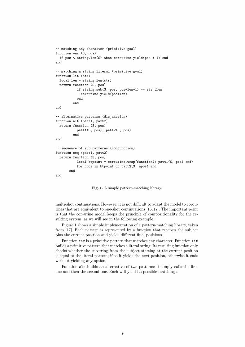
multi-shot continuations. However, it is not difficult to adapt the model to corou-tines that are equivalent to one-shot continuations [16, 17]. The important pointis that the coroutine model keeps the principle of compositionality for the re-sulting system, as we will see in the following example.

Figure 1 shows a simple implementation of a pattern-matching library, takenfrom [17]. Each pattern is represented by a function that receives the subjectplus the current position and yields different final positions.

Function any is a primitive pattern that matches any character. Function litbuilds a primitive pattern that matches a literal string. Its resulting function onlychecks whether the substring from the subject starting at the current positionis equal to the literal pattern; if so it yields the next position, otherwise it endswithout yielding any option.

Function alt builds an alternative of two patterns: it simply calls the firstone and then the second one. Each will yield its possible matchings.

9

Finally, function seq builds a sequence of two patterns. It runs the first oneinside a new coroutine to collect its possible results and runs the second patternfor each of these results.

The next fragment shows a simple use:

-- subjects = "abaabcda"-- pattern: (.|ab)..p = seq(alt(any, lit("ab")), seq(any, any))seq(p, print)(s, 1)-- results--> abaabcda 4--> abaabcda 5

It “sequences” the pattern with the print function, which prints its arguments(the subject plus the current position after matching p), and then calls theresulting pattern with the subject and the initial position (1).

5 Concurrent Programming

Lua avoids the problems of imperative programming with multithreading bycutting either preemption or shared memory.

Lua uses coroutines to achieve multithreading without preemption. A stackfulcoroutine [17] is essentially a thread; it is easy to write a simple scheduler with afew lines of code to complete the system [3]. This combination of coroutines witha scheduler results in collaborative multithreading, where each thread shouldexplicitly yield periodically. This kind of concurrency seems particularly apt forsimulation systems and games.2

Coroutines offer a very light form of concurrency. In a regular PC, a programmay create tens of thousands of coroutines without difficulties. Resuming oryielding a coroutine is slightly more expensive than a function call. Games, forinstance, may easily dedicate a coroutine for each relevant object in the game.

Lua may also achieve multithreading by cutting shared memory. In this case,a program creates several independent Lua states that behave like Unix pro-cesses. Each state has its own logical memory space with independent garbagecollection. All communication is done through message passing. Messages maycontain only primitive values, such as numbers or strings, because references (ad-dresses) have no meaning across different states. A main advantage of multiplestates is the ability to benefit from multi-core machines and true concurrency.Processes do not interfere with each other unless they explicitly request commu-nication.

Lua already offers multiple states: Lua is an embedded language, designed tobe used inside other applications. Therefore, it keeps all its state in dynamically-allocated structures, so that it does not interfere with other data from the ap-plication. However, the creation of new states can be done only in C and the2 Simula offered coroutines for this reason [18].

10

dan = name{first = "Daniel", last = "Friedman"}

mitch = name{last = "Wand",

first = "Mitchell",

middle = "P."}

chris = name{first = "Christopher", last = "Haynes"}

book{

author = {dan, mitch, chris},

title = "Essentials of Programming Languages",

edition = 2,

year = 2001,

publisher = "The MIT Press"

}

Fig. 2. Data description with SOL/Lua.

communication between states also needs some C code. So, multi-state con-currency cannot be implemented in pure Lua; it needs some external supportwritten in C. Currently there are at least two libraries with such support: Lu-aLanes [19], which uses tuple spaces for communication, and Luaproc [20], whichuses mailboxes.

6 Data Description

Lua was born from a data-description language, called SOL [21], a languagesomewhat similar to XML in intent. Lua inherited from SOL the support fordata description, but integrated that support into its procedural semantics.

SOL was somewhat inspired in BibTeX, a tool for creating and formatinglists of bibliographic references. A main difference between SOL and BibTeXwas that SOL had the ability to declare and nest declarations. Figure 2 shows atypical fragment, slightly adapted to meet the current syntax of Lua. SOL actedlike an XML DOM reader, reading the data file and building an internal treerepresenting that data; an application then could use an API to traverse thattree.

Lua mostly kept the original SOL syntax, with small changes. The semantics,however, was very different. In Lua, the code in Figure 2 is an imperative pro-gram. The syntax {first = "Daniel", ...} is a constructor : it builds a table,or associative array, with the given keys and values. The syntax name{...} issugar for name({...}), that is, it builds a table and calls function name withthat table as the sole argument. The syntax {dan,mitch,chris} again builds atable, but this time with implicit integer keys 1, 2, and 3, therefore representinga list. A program loading such a file should previously define functions name andbook with appropriate behavior. For instance, function book could add the tableto some internal list for later treatment.

Several applications use Lua for data description. Games frequently use Luato describe characters and scenes. HiQLab, a tool for simulating high frequency

11

resonators, uses Lua to describe finite-element meshes [22]. GUPPY uses Lua todescribe sequence annotation data from genome databases [23]. Some descrip-tions comprise thousands of elements running for a few million lines of code.These huge “programs” pose a heavy load on the Lua precompiler. To handlesuch files efficiently, and also for simplicity, Lua uses a one-pass compiler withno intermediate representations.

7 Final Remarks

Lua is a small and simple language, but is also quite flexible. In particular, wehave seen how it supports different paradigms, such as functional programming,object-oriented programming, goal-oriented programming, and data description.

Lua supports those paradigms not with many specific mechanisms for eachparadigm, but with few general mechanisms, such as tables (associative arrays),first-class functions, delegation, and coroutines. Because the mechanisms are notspecific to special paradigms, other paradigms are possible too. For instance,AspectLua [24] uses Lua for aspect-oriented programming.

All Lua mechanisms work on top of a standard procedural semantics. Thisprocedural basis ensures an easy integration among those mechanisms and be-tween them and the external world; it also makes Lua a somewhat conven-tional language. Accordingly, most Lua programs are essentially procedural, butmany incorporate useful techniques from different paradigms. In the end, eachparadigm adds important items into a programmer toolbox.

References

1. Millington, I.: Artificial Intelligence for Games. Morgan Kaufmann (2006)2. Associacao Brasileira de Normas Tecnicas: Televisao digital terrestre – Codificacao

de dados e especificacoes de transmissao para radiodifusao digital. (2007) ABNTNBR 15606-2.

3. Ierusalimschy, R.: Programming in Lua. second edn. Lua.org, Rio de Janeiro,Brazil (2006)

4. Ierusalimschy, R., de Figueiredo, L.H., Celes, W.: Lua 5.1 Reference Manual.Lua.org, Rio de Janeiro, Brazil (2006)

5. Kelsey, R., Clinger, W., Rees, J.: Revised5 report on the algorithmic languageScheme. Higher-Order and Symbolic Computation 11(1) (August 1998) 7–105

6. Nehab, D.: Filters, sources, sinks and pumps, or functional programming for therest of us. In de Figueiredo, L.H., Celes, W., Ierusalimschy, R., eds.: Lua Program-ming Gems. Lua.org (2008) 97–107

7. Adams, N., Kranz, D., Kelsey, R., Rees, J., Hudak, P., Philbin, J.: ORBIT: an opti-mizing compiler for Scheme. SIGPLAN Notices 21(7) (July 1986) (SIGPLAN’86).

8. Ierusalimschy, R., de Figueiredo, L.H., Celes, W.: The implementation of Lua 5.0.In: IX Brazilian Symposium on Programming Languages, Recife, PE (May 2005)63–75

9. Ungar, D., Smith, R.B.: Self: The power of simplicity. SIGPLAN Notices 22(12)(December 1987) 227–242 (OOPLSA’87).

12

10. Lieberman, H.: Using prototypical objects to implement shared behavior inobject-oriented systems. SIGPLAN Notices 21(11) (November 1986) 214–223(OOPLSA’86).

11. Griswold, R., Griswold, M.: The Icon Programming Language. Prentice-Hall, NewJersey, NJ (1983)

12. Clocksin, W., Mellish, C.: Programming in Prolog. Springer-Verlag (1981)13. de Moura, A.L., Rodriguez, N., Ierusalimschy, R.: Coroutines in Lua. Journal of

Universal Computer Science 10(7) (July 2004) 910–925 (SBLP 2004).14. Haynes, C.T.: Logic continuations. J. Logic Programming 4 (1987) 157–17615. Wand, M., Vaillancourt, D.: Relating models of backtracking. In: Proceedings of

the Ninth ACM SIGPLAN International Conference on Functional Programming,Snowbird, UT, ACM (September 2004) 54–65

16. Ierusalimschy, R., de Moura, A.L.: Some proofs about coroutines. Monografias emCiencia da Computacao 04/08, PUC-Rio, Rio de Janeiro, Brazil (2008)

17. de Moura, A.L., Ierusalimschy, R.: Revisiting coroutines. ACM Transactions onProgramming Languages and Systems 31(2) (2009) 6.1–6.31

18. Birtwistle, G., Dahl, O., Myhrhaug, B., Nygaard, K.: Simula Begin. PetrocelliCharter (1975)

19. Kauppi, A.: Lua Lanes — multithreading in Lua. (2009) http://kotisivu.

dnainternet.net/askok/bin/lanes/.20. Skyrme, A., Rodriguez, N., Ierusalimschy, R.: Exploring Lua for concurrent pro-

gramming. In: XII Brazilian Symposium on Programming Languages, Fortaleza,CE (August 2008) 117–128

21. Ierusalimschy, R., de Figueiredo, L.H., Celes, W.: The evolution of Lua. In: ThirdACM SIGPLAN Conference on History of Programming Languages, San Diego,CA (June 2007) 2.1–2.26

22. Koyama, T., et al.: Simulation tools for damping in high frequency resonators. In:4th IEEE Conference on Sensors, IEEE (October 2005) 349–352

23. Ueno, Y., Arita, M., Kumagai, T., Asai, K.: Processing sequence annotation datausing the Lua programming language. Genome Informatics 14 (2003) 154–163

24. Fernandes, F., Batista, T.: Dynamic aspect-oriented programming: An interpretedapproach. In: Proceedings of the 2004 Dynamic Aspects Workshop (DAW04).(March 2004) 44–50

13

A Theoretical Framework for the DeclarativeDebugging of Functional Logic Programs with

Lambda Abstractions ?

Ignacio Castineiras Perez and Rafael del Vado Vırseda

Dpto. de Sistemas Informaticos y ComputacionUniversidad Complutense de Madrid{ncasti,rdelvado}@sip.ucm.es

Abstract. In this paper, we extend the declarative method for diag-nosing wrong computed answers in first-order lazy functional logic pro-grams to the higher-order setting of the simply typed λ-calculus, whereprograms are presented by conditional pattern rewrite systems. Our ap-proach generalizes and combines declarative debugging techniques previ-ously developed for less expressive declarative programming paradigmsinvolving applicative rewrite rules instead of λ-abstractions and higher-order unification. Debugging starts with the observation of a wrong com-puted answer which the user regards as incorrect w.r.t. an intended modelthat provides a declarative description of the program’s semantics. De-bugging proceeds by exploring an abridged proof tree built on a higher-order rewriting logic with λ-abstractions that provides a purely declara-tive view of the computation. Finally, debugging ends with the detectionof a defined function rule in the program that is incorrect w.r.t. the in-tended model. We prove the logical correctness of the debugging methodfor any sound goal solving system whose computed answers are logicalconsequences of the program.

1 Introduction and Motivation

According to a well-known conception, programs in a declarative programminglanguage can be viewed as theories in some suitable logic, while computationscan be viewed as deductions. The Constructor-based ReWriting Logic CRWL [3, 4]provides a suitable framework for rule-based declarative (functional and logic)programming with non-deterministic and lazy functions with call-time choicesemantics, where programs are constructor-based Conditional Term Rewrite Sys-

tems (CTRS for short). As a concrete example, the following “Prolog-like” CTRS

fragment defines a possibly non-deterministic function loves, given by first-orderconditional rewrite rules (→) where the conditional part (formed only by equa-tions ==) is delimited by the “⇐” symbol:

? This work has been partially supported by the Spanish National ProjectsTIN2008-06622-C03-01, TIN2005-09027-C03-03, S-0505/TIC/0407, and UCM-BSCH-GR58/08-910502.

loves (john, mary) → trueloves (mary, Y ) → true ⇐ likes (Y, wine) == falseloves (X, mary) → true ⇐ loves (mary,X) == true

Since the classical notion of rewriting is not suitable in this setting, a new no-tion of rewriting is adopted as the basis of proof calculi for joinability (==)and reduction (→) statements. The most important result is the existence ofsound and complete lazy narrowing calculi [3, 4, 11] for solving goals in first-order CRWL-theories presented by CTRS-programs. Moreover, a higher-orderextension of CRWL is presented in [2] but using only applicative rewrite rulesinstead of λ-abstractions and higher-order unification.

In this paper, we use a higher-order rewriting logic (called GHRC) for declara-tive programming with higher-order functions and λ-terms as data structures toobtain more of the expressivity of higher-order functional programming. Moreprecisely, we adopt the framework of the simply typed λ-calculus in which termsare in βη-normal form and theories are presented by Conditional Pattern Rewrite

Systems (CPRS for short). As a simple example of such higher-order programs,we consider the following conditional pattern rewrite system (adapted from [5])defining a higher-order function diff , where diff (f, x) computes the differentialof a function f at some point x:

diff (λy. y, x) → 1diff (λy. sin(f(y)), x) → cos(f(x)) ∗ diff (λy. f(y), x) ⇐ −π/2 ≤ f(x) ≤ π/2diff (λy. ln(f(y)), x) → diff (λy. f(y), x)/f(x) ⇐ f(x) 6= 0

We are interested in the logical characterization and the practical applica-tion to debugging of the semantics of programs formalized by constructor-basedCPRSs, where the notion of lazy and possibly non-deterministic higher-orderfunctions and conditional equations involving λ-abstractions plays a central role.In contrast to more traditional frameworks such as equational logic and alterna-tive approaches such as needed rewriting [5] the higher-order rewriting logic onlambda abstractions GHRC has the ability to characterize the intended computa-tional behavior based on conditional higher-order narrowing for non-determinismin a correct and efficient way [3, 4, 11, 13].

A frequent claim about declarative programming languages is that the task ofreasoning about programs (as e.g., CTRSs or CPRSs) is easier than in other pro-gramming paradigms because of the existence of an underlying logic providingmore or less natural logical methods for that purpose. In the case of higher-orderfunctional logic programming, the proof calculus offered by our GHRC approachgives an attractive and mathematically well-founded basis for reasoning on thesemantics of programs. In particular, GHRC provides firm theoretical founda-tions for the declarative debugging of functional logic programs with lambdaabstractions, following the classical declarative debugging approach proposed in[10]. In order to illustrate the main features of this diagnosis technique and tomotivate the approach presented in this work we consider a simple debugging

16

Fig. 1. Computation tree for declarative debugging involving lambda abstractions

example. The following higher-order functional logic program involving lambdaabstractions is an erroneous fragment of the previous conditional pattern rewritesystem to compute the differential of a function:

diff (λy. y, x) → xdiff (λy. sin(f(y)), x) → sin(f(x)) ∗ diff (λy. f(y), x) ⇐ −π/2 ≤ f(x) ≤ π/2

The debugging technique starts with the observation of a solution computedfrom a goal and a CPRS by means of a suitable goal solving system (see,e.g., [5, 13]). For instance, we consider a goal to compute appropriate functionsλx, y. F (x, y) and λx.D(x) for which the differential of λy. sin (F (x, y)) at somepoint x ∈ [−π/2, π/2] satisfies λx. diff (λy. sin (F (x, y)), x) == λx.D(x). We ob-tain a substitution to represent the solution {F 7→ λx, y. y, D 7→ λx. sin (x) ∗ x}under the constraint −π/2 ≤ x ≤ π/2. The user regards this solution as incor-rect (because the user really expects as solution {F 7→ λx, y. y, D 7→ λx. cos (x)})according to their own intended model of the declarative description of the pro-gram’s semantics.

Then, debugging proceeds by exploring a suitable computation tree, obtainedas a proof tree in the logical calculus offered by the higher-order rewriting logicGHRC for the witness that the obtained computed answer is a solution of the ini-tial goal. This proof tree provides a purely declarative view of the computation,so that the user does not need to understand the complex underlying opera-tional mechanism based on conditional higher-order narrowing described in [5,13]. The computation tree for our current example is graphically represented inFig. 1 (more on its structure and construction will be explained in Section 5).Each node of this tree represents the computation of some observable result, de-pending on the results of its children nodes. Declarative diagnosis explores thisproof tree looking for a so-called buggy node which computes an incorrect resultfrom children whose results are correct; such a node must point to an incorrect

17

program fragment. The search for a buggy node can be implemented with thehelp of an external oracle (usually the user with some semi-automatic support)who has a reliable declarative knowledge of the expected program semantics.Finally, debugging ends with the detection of a function rule in the CPRS Rthat is incorrect w.r.t. the intended model I.

For instance, the computation tree depicted in Fig. 1 has a buggy nodein node B because λx. x is not the differential of the function λx. diff (λy. y, x).Therefore, the first pattern rewrite rule diff (λy. y, x) → x is incorrect w.r.t. theuser’s intended program semantics; as we have shown previously, the first ruleshould be diff (λy. y, x) → 1. After this correction, there is another buggy nodein node A because the differential of λy. sin (y) at point x is cos (x) instead ofsin (x). Indeed, the second conditional pattern rewrite rule is also incorrect w.r.t.the user’s intended model of the program as we have previously seen. After thisnew correction, no more wrong computed answers will be observed for the goaldiscussed above, and the right solution {F 7→ λx, y. y, D 7→ λx. cos (x)} is thenobtained.

The paper is structured as follows. In Section 2 we introduce the basic no-tions and notations from the λ-calculus and higher-order term rewriting whichare needed to understand the theoretical framework. In Section 3 we introducea higher-order conditional rewriting logic characterized by the proof systemGHRC, as a generalization of the proof system which underlies the first-orderrewriting logic CRWL. Section 4 is concerned with the model-theoretic semanticsfor GHRC-programs. In Section 5 we discuss the application of GHRC to thedevelopment of a declarative debugging technique of wrong computed answersfor functional logic programming with lambda abstractions. Finally, Section 6summarizes some conclusions and presents a brief outline of planned future work.

2 Preliminary Notions

We assume the reader is familiar with the notions and notations pertaining toλ-calculus and higher-order term rewriting (see, e.g., [5]). The set of types forsimply typed λ-terms is generated by a set B of base types (e.g., nat, bool) andthe function type constructor “→”. Simply typed λ-terms are generated in theusual way from a signature F of function symbols and a countably infinite setV of variables by successive operations of abstraction and application. We alsoconsider the enhanced signature F⊥ = F ∪ Bot, where Bot = {⊥b | b ∈ B}is a set of distinguished B-typed constants. The constant ⊥b is intended todenote an undefined value of type b. We employ ⊥ as a generic notation fora constant from Bot. In this paper, we assume the following conventions ofnotation: X, Y, Z,R, H, possibly primed or with subscripts, denote free variables;f, f ′ denote function symbols, and a a (free or bound) variable or a constant fromF ; l, r, s, t, u, possibly primed or with subscript, denote terms; π, π′, π1, π2, . . .denote terms of base type. We also define the arity of f ∈ F as ar(f) = n ≥ 0.A sequence of syntactic objects o1, . . . , on, where n ≥ 0, is abbreviated by on. Forinstance, the simply typed λ-term λx1. . . . λxk.(· · · (a t1) · · · tn) is abbreviated

18

by λxk.a(tn). Substitutions γ ∈ Subst(F⊥,V) are finite type-preserving mappingsfrom variables to terms, denoted by {Xn 7→ tn}, and extend homomorphicallyfrom terms to terms. By convention, we write ε for the identity substitution, tγinstead of γ(t), and γγ′ for the function composition γ′ ◦ γ.

The long βη-normal form of a term, denoted by tlηβ , is the η-expanded form

of the β-normal form of t. It is well-known that s =αβη t if slηβ =α tlη

β [6].Since βη-normal forms are always defined, we will in general assume that termsare in long βη-normal form and are identified modulo α-conversion. For brevity,we may write variables and constants from F in η-normal form, e.g., X insteadof λxk.X(xk). We assume that the transformation into long βη-normal form isan implicit operation, e.g., when applying a substitution to a term. With theseconventions, every term t has a unique long βη-normal form λxk.a(tn), wherea ∈ F⊥ ∪ V and a() coincides with a. The symbol a is called the root of t andis denoted by hd(t). We distinguish between the set T (F⊥,V) of partial terms(terms for short) and the set T (F ,V) of total terms. T (F⊥,V) is a poset withrespect to the approximation ordering v, defined as the least partial orderingsuch that:

λxk.⊥ v λxk.t t v ts1 v t1 · · · sn v tn

λxk.a(sn) v λxk.a(tn)

We adopt the convention that the free and bound variables inside a termare kept disjoint, and assume that bound variables with different binders havedifferent names. The set of free variables of a term t is denoted by FV(t). Tomanipulate terms, we define:

– The set of positions in t: Pos(λxk.a(tn)) = {1i | 0 ≤ i ≤ k} ∪ {1k.j.q | 1 ≤j ≤ n, q ∈ Pos(tj)}, where “.” denotes sequence concatenation and 1k is thesequence of 1 repeated k times. The empty sequence is denoted by ε. Notethat, with this convention, we have 10 = ε.

– The subterm t|p of t at some position p ∈ Pos(t):

(λxk.a(tn))|p ={

λxi+1 . . . xk.a(tn) if p = 1i with 0 ≤ i ≤ k,ti|q if p = 1k.i.q and 1 ≤ i ≤ n.

A position p is maximal in t if t|p is of base type. The set of maximal positionsin a term t is denoted by MPos(t).

– The sequence of variables abstracted on the path to position p ∈ Pos(t):

seqbv(t, p) =

ε if p = ε,x.seqbv(s, q) if t = λx.s and p = 1.q,seqbv(ti, q) if t = a(tn), 0 < i ≤ n, and p = i.q.

The set of variables abstracted on the path to position p ∈ Pos(t) is BV(t, p)= {seqbv(t, p)}, and the set of variables with bound occurrences in t is BV(t)=

⋃p∈Pos(t) BV(t, p). Moreover, we also define t�p = λxk.(t|p), where xk =

seqbv(t, p).

19

A pattern [9] is a term t for which all subterms t|p = X(tn), with X ∈ FV(t) andp ∈ MPos(t), satisfy the condition that t1↓η, . . . , tn↓η is a sequence of distinctelements of BV(t, p). Moreover, if all such subterms of t satisfy the additionalcondition BV(t, p) \ {t1↓η, . . . , tn↓η} = ∅, then the pattern t is fully extended. Itis well known that unification of patterns is decidable and unitary [9]. Therefore,for every t ∈ T (F⊥,V) and pattern π, there exists at most one matcher betweent and π, which we denote by matcher(t, π). An equation is a multiset {{s, t}},written s== t, where s, t ∈ T (F⊥,V) are terms of the same type.

In our theoretical framework, programs are considered as a special kind ofconditional rewrite systems over fully extended linear patterns, with conditionalequations between total terms.

Definition 1 (Programs). A Conditional Pattern Rewrite System (CPRS forshort) is a finite set of conditional rewrite rules of the form f(ln) → r ⇐ C,where

• f(ln) and r are total terms of the same base type,

• f(ln) is a fully extended linear pattern, and

• C is a (possibly empty) finite sequence of equations between total terms. Insymbols, C ≡ sm == tm, with si, ti ∈ T (F ,V) for i = 1, . . . ,m.

The term f(ln) is called the left hand side (lhs), r is the right hand side (rhs),and C is the conditional part of the pattern rewrite rule.

Each CPRS R induces a partition of F into Fd (defined function symbols)and Fc (data constructors):

Fd = {f ∈ F | ∃(f(ln) → r ⇐ C) ∈ R}, Fc = F \ Fd.

R is a constructor-based CPRS if each conditional pattern rewrite rule f(ln) →r ⇐ C satisfies the additional condition that l1, . . . , ln ∈ T (Fc,V).

Finally, we also find it convenient to define the xk-lifter of a term t:

Definition 2 (Lifter). Given a term t, a subset V of FV(t), and a sequencexk of distinct variables with no occurrences in t, the xk-lifter of t with respectto V is the term t↑xk�V, defined recursively as follows:

t↑xk�V =

λyl.(π↑(yl,xk)�V ) if t ≡ λyl.π,

a(t↑xk�Vn

)if t ≡ a(tn) with a 6∈ V,

X(xk, t↑xk�V

n

)if t ≡ X(tn) with X ∈ V.

The xk-lifter of a term t is the term t↑xk = t↑xk�FV(t) . We also define tlxk =λxk.(t↑xk). If C ≡ sm == tm is a sequence of equations then we write Clxk for

the sequence slxkm == t

lxkm .

20

3 The Higher-Order Rewriting Logic GHRC

In this section we extend the constructor-based Conditional ReWriting LogicCRWL from [3, 4], in order to deal with conditional pattern rewrite rules. Incontrast to Meseguer’s rewriting logic [8], which aims at modelling change causedby concurrent actions at a very high abstraction level, our rewriting logic intendsto model the evaluation of λ-terms in a constructor-based language involving lazyfunctions. As in [3, 4], we do not impose non-ambiguity conditions. This meansthat non-deterministic functions are allowed.

For all these reasons, we want to consider a (conditional) higher-order rewri-ting logic for declarative programming with non-strict and non-deterministicfunctions with call-time choice semantics, as an extension of the first-orderrewriting logic CRWL. In order to obtain this aim, we propose this logic as thebasis of a proof calculus, called GHRC, for reduction and joinability statementsto a common value, designed as a generalization of the first-order proof systemGORC which underlies the CRWL logic. First, we need to define the suitablenotion of value that is used in our setting with λ-abstractions and higher-orderunification.

Definition 3 (Values). A value is a partial term t which has the followingproperty:

∀ p ∈ MPos(t), ∀ (π → r ⇐ C) ∈ R : @ matcher(t�p, πlseqbv(t,p))

In this definition, we implicitly assume that FV(t)∩FV(π) = ∅. A total value isa value which is a total term. A value substitution is a substitution which bindsvariables to values. We write Val(F⊥,V) (resp., Val(F ,V)) for the set of values(resp., total values), and VSubst(F⊥,V) for the set of substitutions which bindvariables to values.

For a given CPRS R we want to derive statements of the following kind:

• reduction statements: s � t, where s, t ∈ T (F⊥,V) are of the same type,whose intended meaning is that the term s can be reduced to t, so that thepossibly partial term t approximates the denotation of s, as we will argue inSection 4.

• equality statements: s== t, which holds iff reduction statements s � u andt � u can be derived for some total value u ∈ Val(F ,V).

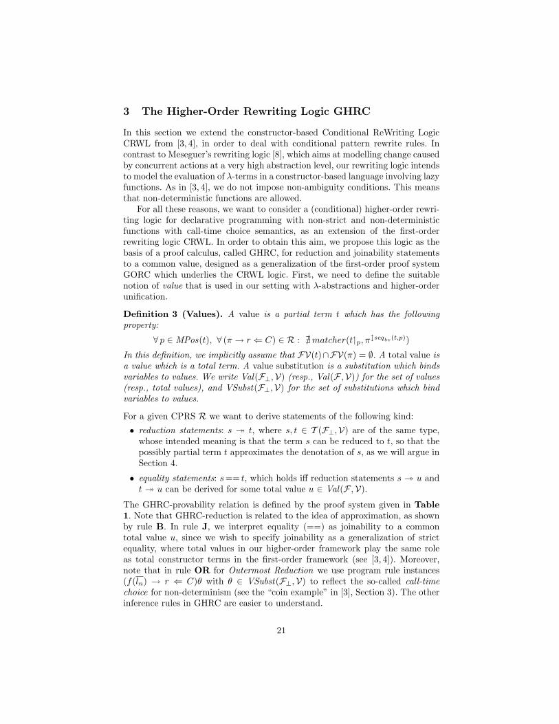
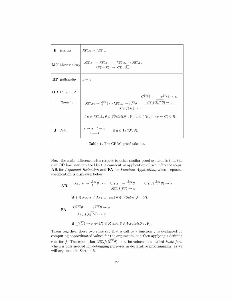
The GHRC-provability relation is defined by the proof system given in Table1. Note that GHRC-reduction is related to the idea of approximation, as shownby rule B. In rule J, we interpret equality (==) as joinability to a commontotal value u, since we wish to specify joinability as a generalization of strictequality, where total values in our higher-order framework play the same roleas total constructor terms in the first-order framework (see [3, 4]). Moreover,note that in rule OR for Outermost Reduction we use program rule instances(f(ln) → r ⇐ C)θ with θ ∈ VSubst(F⊥,V) to reflect the so-called call-timechoice for non-determinism (see the “coin example” in [3], Section 3). The otherinference rules in GHRC are easier to understand.

21

B Bottom λxk.π � λxk.⊥

MN Monotonicityλxk.s1 � λxk.t1 · · · λxk.sn � λxk.tn

λxk.a(sn) � λxk.a(tn)

RF Reflexivity s � s

OR Outermost

Reduction

Clxkθ rlxkθ � u

λxk.s1 � llxk1 θ · · ·λxk.sn � l

lxkn θ λxk.f(l

lxkn θ) � u

λxk.f(sn) � u

if u 6= λxk.⊥, θ ∈ VSubst(F⊥,V), and (f(ln) → r ⇐ C) ∈ R.

J Joins � u t � u

s == tif u ∈ Val(F ,V).

Table 1. The GHRC proof calculus.

Now, the main difference with respect to other similar proof systems is that therule OR has been replaced by the consecutive application of two inference steps,AR for Argument Reduction and FA for Function Application, whose separatespecification is displayed below:

ARλxk.s1 � l

lxk

1 θ · · · λxk.sn � llxkn θ λxk.f(llxk

n θ) � u

λxk.f(sn) � u

if f ∈ Fd, u 6= λxk.⊥, and θ ∈ VSubst(F⊥,V).

FAClxkθ rlxkθ � u

λxk.f(llxkn θ) � u

if (f(ln) → r ⇐ C) ∈ R and θ ∈ VSubst(F⊥,V).

Taken together, these two rules say that a call to a function f is evaluated bycomputing approximated values for the arguments, and then applying a defining

rule for f . The conclusion λxk.f(llxkn θ) � u introduces a so-called basic fact,

which is only needed for debugging purposes in declarative programming, as wewill argument in Section 5.

22

Detailed examples of GHRC-derivations in the form of proof trees in this kind ofrewriting logics can be found in [3, 4, 11] and Example 1 below. We write R `ϕif ϕ is a provable statement from a CPRS R, PT (ϕ) for the set of proof treesfor ϕ and PT L(ϕ) for the proof trees of PT (ϕ) which end with the applicationof an inference rule L ∈ {B,MN,RF,OR,J}. We also write R `L ϕ if thereexists a proof of R ` ϕ which ends with the application of rule L, and R 0L ϕif there is no such a proof.

Finally, to complete the presentation of the higher-order rewriting logic GHRCin a declarative programming setting, we give a definition for the class of goals(from a given CPRS R) and the set of solutions of a goal with which we aregoing to work.

Definition 4 (Goals and Solutions).

• A goal G for a given CPRS R is a multiset {{sn == tn}} of equations betweentotal terms of the same type. Equations are symmetric: s== t ≡ t == s.

• γ ∈ Subst(F⊥,V) is a solution of a goal G ≡ {{sn == tn}} if γ�FV(G) ∈VSubst(F⊥,V), and for each equation si == ti in G there exists a proof treePi ∈ PT (siγ == tiγ). The proof tree Pi is called a witness that γ is a solutionof si == ti.

We write Soln(G) for the set of solutions of a goal G.

Example 1. For the particular function f → λxs. pair(sum(xs), length(xs)),where pair is a data constructor, and

sum ([ ]) → 0 length ([ ]) → 0 fst (pair (x, y)) → xsum ([x|xs]) → x+sum(xs) length ([x|xs]) → 1+length(xs) snd (pair(x, y)) → y

we can check that γ = {E 7→ pair(0, 0), G 7→ λu, z.pair(u + fst(z), 1 + snd(z))}is a solution of the goal {{f([ ]) == E, λx, xs. f([x|xs]) == λx, xs.G(x, f(xs))}}.For example, we have the following logical proof in the GHRC-calculus for R `λx, xs. f([x|xs]) == λx, xs. pair(x + fst(f(xs)), 1 + snd(f(xs))), where R is aCPRS containing all the pattern rewrite rules mentioned in this example.

J λx, xs. f([x|xs]) == λx, xs. pair(x + fst(f(xs)), 1 + snd(f(xs)))OR λx, xs. f([x|xs]) � λx, xs. pair(x + sum(xs), 1 + length(xs))

RF λx, xs. [x|xs] � λx, xs. [x|xs]MN λx, xs. pair(sum([x|xs]), length([x|xs])) �

λx, xs. pair(x + sum(xs), 1 + length(xs))OR λx, xs. sum([x|xs]) � λx, xs. (x + sum(xs))

RF λx, xs. [x|xs] � λx, xs. [x|xs]RF λx, xs. (x + sum(xs)) � λx, xs. (x + sum(xs))

OR λx, xs. length([x|xs]) � λxs. (1 + length(xs))RF λx, xs. [x|xs] � λx, xs. [x|xs]RF λxs. (1 + length(xs)) � λxs. (1 + length(xs))

23

MN λs, xs. pair(x + fst(f(xs)), 1 + snd(f(xs))) �λx, xs. pair(x+sum(xs), 1+length(xs))

MN λxs. (x + fst(f(xs))) � λx, xs. (x + sum(xs))

RF λx. x � λx. x

OR λxs. fst(f(xs)) � λxs. sum(xs)

OR λxs. f(xs) � λxs. pair(sum(xs), length(xs))

RF λxs. xs � λxs. xs

RF λxs. pair(sum(xs), length(xs)) �λxs. pair(sum(xs), length(xs))

RF λxs. sum(xs) � λxs. sum(xs)

MN λxs. (1 + snd(f(xs))) � λxs. (1 + length(xs))

RF 1 � 1

OR λxs. snd(f(xs)) � λxs. length(xs)

OR λxs. f(xs) � λxs. pair(sum(xs), length(xs))

RF λxs. xs � λxs. xs

RF λxs. pair(sum(xs), length(xs)) �λxs. pair(sum(xs), length(xs))

RF λxs. length(xs) � λxs. length(xs)

ut

Finally, we give a result which characterizes the semantics proofs built withGHRC and generalizes useful known properties of CRWL-deductions for thefirst-order case (see [3, 4, 11] for more details). The proof is given in [14].

Lemma 1 (Basic Semantic Property of GHRC-deductions). Let s ∈Val(F⊥,V). If R ` s � t then t ∈ Val(F⊥,V), s w t, and R 0OR s � t.Moreover, if t ∈ Val(F ,V) then s ≡ t.

4 Intended Models of CPRS-Programs

In this section, we briefly introduce some notions and results on the declarativesemantics of CPRS-programs which are needed for the rest of the paper. Thesemantic definition of interpretation is simpler than the one in the first-order set-ting [3, 4, 14], where a more general notion of interpretation (under the name ofAlgebra) is presented. In our debugging scheme we will assume that the intendedmodel of a CPRS is an interpretation.

Definition 5 (Interpretations and Models).

(1) A basic fact λxk. f(tlxkn ) � u asserts that the (possibly non-linear) partial

term u ∈ Val (F⊥,V) approximates the result of f(tn), a fully extended linearpattern with the exact number of arguments expected by f ’s arity, and witharguments ti ∈ Val (F⊥,V), which represent the partial approximations off ’s actual parameters needed to compute u as result. Moreover, f(tn) and uare partial terms of the same base type.

24

(2) An interpretation I is a set of basic facts fulfilling the following require-ments for all f ∈ Fd with ar(f) = n, and f(tn), f(sn) fully extended linearpatterns with tn, sn ∈ Val (F⊥,V) arbitrary partial terms of the same basetype that t, s ∈ Val (F⊥,V):

• (λxk. f(tlxkn ) � λxk.⊥) ∈ I.

• If (λxk. f(tlxkn ) � λxk. t) ∈ I, λxk. t

lxk

i v λxk. slxk

i , λxk. t w λxk. s,

then also (λxk. f(slxkn ) � λxk. s) ∈ I.

• If (λxk. f(tlxkn ) � λxk. t) ∈ I and θ ∈ VSubst(F⊥,V), then (λxk.

f(tlxkn θ) � λxk. tθ) ∈ I.

(3) A given reduction or equality statement ϕ is valid in the interpretation I iffϕ is a provable statement from I in the semantic calculus GHRCI , consistingof the GHRC rules B, MN, RF and J together with the inference rule ORI :

ORIλxk. s1 � t

lxk

1 · · · λxk. sn � tlxkn u � s

λxk. f(sn) � s

if u 6= λxk.⊥ and (λxk. f(tlxkn ) � u) ∈ I.

In general, for every basic fact λxk. f(tlxkn ) � u, it can be proved that it is

valid in I iff (λxk. f(tlxkn ) � u) ∈ I.

(4) The denotation of a term t ∈ T (F⊥,V) is the set:

[[ t ]]I = { s ∈ Val (F⊥,V) | t � s is valid in I }

(5) I is a model of a given CPRS R (i.e., I |= R) iff every conditional patternrewrite rule (f(ln) → r ⇐ C) ∈ R is valid in I (i.e., I |= f(ln) → r ⇐ C):For any substitution θ ∈ VSubst (F⊥,V) and C ≡ sm == tm, either• [[ siθ ]]I ∩ [[ tiθ ]]I ∩ Val (F ,V) 6= ∅ (i.e., I satisfies Cθ) and [[ f(lnθ) ]]I

⊇ [[ rθ ]]I , or else• I does not satisfy Cθ.

Finally, from Definition 5 we can prove that the GHRC proof calculus is seman-tically sound.

Theorem 1 (Semantic Correctness of GHRC). If G ≡ {{sn == tn}} is agoal for a CPRS R and γ ∈ Soln (G) then γ ∈ Soln I (G) for all model I of R(i.e., every siγ == tiγ is valid in I).

Proof. The proof is quite standard and details can be found in [14]: It is sufficientto assume an arbitrarily given model I |= R and to prove that any GHRCinference rule whose premises are valid in I has a conclusion that is also validin I. ut

25

5 Declarative Debugging of Wrong Answers in GHRC

In this section, we extend the declarative method for diagnosing wrong computedanswers in first-order lazy functional logic programs [1] to the higher-order set-ting of functional logic programs with lambda abstractions.

Definition 6 (Symptoms and Errors). Assume that I is the intended modelfor a given CPRS R, and consider a substitution γ ∈ VSubst (F ,V) produced asa computed answer for the goal G ≡ {{sn == tn}} by a goal solving system.

(1) γ is a wrong answer w.r.t. I (serving as a symptom) iff γ /∈ Soln I(G)(i.e., there exists si == ti in G such that siγ == tiγ is not valid in I).

(2) R is incorrect w.r.t. I iff there exists some conditional pattern rewrite rule(f(ln) → r ⇐ C) ∈ R (manifesting an error) that is not valid in I (i.e.,I 6|= f(ln) → r ⇐ C).

We say that a goal solving system is called GHRC-sound iff for any computedanswer γ obtained for a goal G using a CPRS R we have that γ ∈ Soln (G). Thegoal solving calculus HOLNDT given in [13] is GHRC-sound. This claim can beproved by a straightforward adaptation of the soundness theorem for HOLNDT.Now we prove that the observation of an error symptom by any GHRC-soundgoal solving system implies the existence of some error in the CPRS-program.

Theorem 2. Assume that a GHRC-sound goal solving system computes γ ∈Subst (F ,V) as an answer for the goal G using a given CPRS R. If γ is a wronganswer w.r.t. the user’s intended model I then some conditional pattern rewriterule belonging to R is not valid in I.

Proof. Because of the GHRC-soundness of the goal solving system, we knowthat γ ∈ Soln (G). Then, from Theorem 1 we obtain γ ∈ SolnJ (G) for all modelJ of R. Since γ is a wrong answer w.r.t. the user’s intended model I, it must bethe case that γ /∈ Soln I(G) because of Definition 6. Therefore, we can concludethat the user’s intended model I is not a model of R. Then, by Definition 5,some conditional pattern rewrite rule belonging to R is not valid in I. ut

The debugging scheme proposed in [10] assumes that any terminated com-putation can be represented as a finite tree, called computation tree. The rootof this tree corresponds to the result of the main computation, and each nodecorresponds to the result of some intermediate subcomputation. According toprevious approaches in declarative debugging [1], our aim is to use proof treesin the GHRC proof calculus as computation trees. To this purpose, the onlyrelevant nodes are those which correspond to the conclusion of FA steps. Thisis because all the other inference rules in GHRC, being program independent,cannot give rise to incorrect steps. The debugger works by navigating the com-putation tree, looking for erroneous nodes. Following the terminology of [10], anerroneous node with no erroneous children in called a buggy node.

The next theorem guarantees the logical correctness of declarative debuggingwith GHRC-proof trees for functional logic programs with lambda abstractions:

26

Fig. 2. Computation tree in GHRC for declarative debugging

Theorem 3 (Declarative Diagnosis of Wrong Answers). Assume a wronganswer γ ∈ Subst (F ,V), computed for the goal G using a given CPRS R, suchthat γ /∈ Soln I(G), and I is the user’s intended model of R. Consider anyGHRC-proof tree witnessing γ ∈ Soln (G) as a computation tree, which mustexist due to the existence of GHRC-sound goal solving systems. Then, declarativedebugging has the following two properties:

(a) Completeness: navigating the computation tree will find a buggy node.(b) Soundness: every buggy node in the computation tree points to a conditional

pattern rewrite rule belonging to R which is not valid in I.

Proof. Item (a) follows immediately from the Weak Completeness of DeclarativeDebugging proved in [10], provided that the search strategy used to navigatethe tree does not miss existing buggy nodes. To prove item (b), assume thatthe intended model is I, and consider any given buggy node. This node must

contain a basic fact λxk. f(llxkn θ) � u which is not valid in I and has been

inferred as the conclusion of a FA inference step using some conditional patternrewrite rule belonging to R, say (f(ln) → r ⇐ C) ∈ R and θ ∈ VSubst (F⊥,V).

Therefore, the children of λxk. f(llxkn θ) � u in the GHRC-proof tree, Clxkθ

and rlxkθ � u are valid in I, because they are the children of a buggy node.With this we can conclude that Clxkθ and rlxkθ � u are valid in I (i.e., Isatisfies Clxkθ and u ∈ [[ rlxkθ ]]I), while λxk. f(llxk

n θ) � u is not valid in I(i.e., u /∈ [[ λxk. f(llxk

n θ) ]]I). Then [[ rlxkθ ]]I * [[ λxk. f(llxkn θ) ]]I , which means

(see Definition 5) that the conditional pattern rewrite rule (f(ln) → r ⇐ C) ∈ Ris not valid in I. ut

27

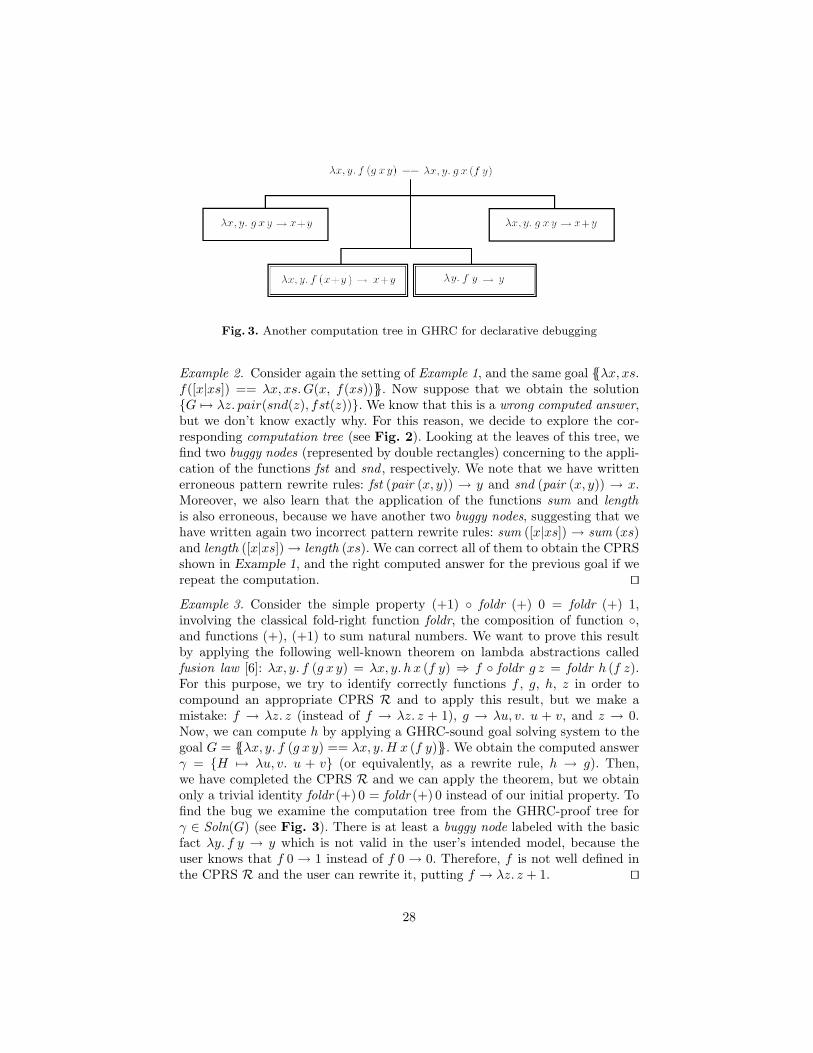
Fig. 3. Another computation tree in GHRC for declarative debugging

Example 2. Consider again the setting of Example 1, and the same goal {{λx, xs.f([x|xs]) == λx, xs.G(x, f(xs))}}. Now suppose that we obtain the solution{G 7→ λz. pair(snd(z), fst(z))}. We know that this is a wrong computed answer,but we don’t know exactly why. For this reason, we decide to explore the cor-responding computation tree (see Fig. 2). Looking at the leaves of this tree, wefind two buggy nodes (represented by double rectangles) concerning to the appli-cation of the functions fst and snd , respectively. We note that we have writtenerroneous pattern rewrite rules: fst (pair (x, y)) → y and snd (pair (x, y)) → x.Moreover, we also learn that the application of the functions sum and lengthis also erroneous, because we have another two buggy nodes, suggesting that wehave written again two incorrect pattern rewrite rules: sum ([x|xs]) → sum (xs)and length ([x|xs]) → length (xs). We can correct all of them to obtain the CPRSshown in Example 1, and the right computed answer for the previous goal if werepeat the computation. ut

Example 3. Consider the simple property (+1) ◦ foldr (+) 0 = foldr (+) 1,involving the classical fold-right function foldr, the composition of function ◦,and functions (+), (+1) to sum natural numbers. We want to prove this resultby applying the following well-known theorem on lambda abstractions calledfusion law [6]: λx, y. f (g x y) = λx, y. h x (f y) ⇒ f ◦ foldr g z = foldr h (f z).For this purpose, we try to identify correctly functions f , g, h, z in order tocompound an appropriate CPRS R and to apply this result, but we make amistake: f → λz. z (instead of f → λz. z + 1), g → λu, v. u + v, and z → 0.Now, we can compute h by applying a GHRC-sound goal solving system to thegoal G = {{λx, y. f (g x y) == λx, y. H x (f y)}}. We obtain the computed answerγ = {H 7→ λu, v. u + v} (or equivalently, as a rewrite rule, h → g). Then,we have completed the CPRS R and we can apply the theorem, but we obtainonly a trivial identity foldr (+) 0 = foldr (+) 0 instead of our initial property. Tofind the bug we examine the computation tree from the GHRC-proof tree forγ ∈ Soln(G) (see Fig. 3). There is at least a buggy node labeled with the basicfact λy. f y → y which is not valid in the user’s intended model, because theuser knows that f 0 → 1 instead of f 0 → 0. Therefore, f is not well defined inthe CPRS R and the user can rewrite it, putting f → λz. z + 1. ut

28

6 Conclusions and Future Work

We have presented a generalization of the declarative method for diagnosingwrong computed answers in first-order lazy functional logic programs to themore expressive setting of the simply typed λ-calculus, where the notion of lazyand possibly non-deterministic higher-order function plays a central role.

Planned future work will include further theoretical investigation to integratenon-equality constraints (e.g., see −π/2 ≤ f(x) ≤ π/2 and f(x) 6= 0 in Section1) in the conditional part of pattern rewrite rules, following the line of recentresearches on constraint rewriting logics for declarative programming [12].

References

1. R. Caballero, F.J. Lopez-Fraguas, and M. Rodrıguez-Artalejo. Theoretical Foun-dations for the Declarative Debugging of Lazy Functional Logic Programs. InProc. FLOPS’01, LNCS vol. 2024, pp. 170–184, 2001.

2. J.C. Gonzalez-Moreno, M.T. Hortala-Gonzalez, and M. Rodrıguez-Artalejo. Ahigher-order rewriting logic for functional logic programming. In Proc. ICLP’97,pp. 153–167, 1997.

3. J.C. Gonzalez-Moreno, M.T. Hortala-Gonzalez, F.J. Lopez-Fraguas, andM. Rodrıguez-Artalejo. A Rewriting Logic for Declarative Programming. In Proc.ESOP’96, LNCS vol. 1058, pp. 156–172, 1996.

4. J.C. Gonzalez-Moreno, M.T. Hortala-Gonzalez, F.J. Lopez-Fraguas, andM. Rodrıguez-Artalejo. An approach to declarative programming based on arewriting logic. Journal of Logic Programming, 40:47–87, 1999.

5. M. Hanus and C. Prehofer. Higher-order narrowing with definitional trees. Journalof Functional Programming, 9(1): 33–75, 1999.

6. J.R. Hindley and J.P. Seldin. Introduction to Combinatorics and λ-Calculus.Cambridge University Press, 1986.

7. F.J. Lopez-Fraguas and J. Sanchez-Hernandez. T OY: A Multiparadigm Declara-tive System. In Proc. RTA’99, Springer LNCS 1631, pp 244–247, 1999. System anddocumentation available at http://toy.sourceforge.net.

8. J. Meseguer. Conditional rewriting logic as a unified model of concurrency. TCS96, pp. 73–155, 1992.

9. D. Miller. A logic programming language with λ-abstraction, function variables,and simple unification. Journal of Logic and Computation, 1(4):497–536, 1991.

10. L. Naish. A Declarative Debugging Scheme. Journal of Functional and LogicProgramming, 1997-3.

11. R. del Vado-Vırseda. A Demand-driven Narrowing Calculus with OverlappingDefinitional Trees. In Proc. PPDP’03, ACM pp. 253–263, 2003.

12. R. del Vado-Vırseda. Declarative Constraint Programming with DefinitionalTrees. In Proc. FroCoS’05, LNAI vol. 3717, pp. 184–199, 2005.

13. R. del Vado-Vırseda. A Higher-Order Demand-Driven Narrowing Calculus withDefinitional Trees. In Proc. ICTAC’07, LNCS vol. 4711, pp. 169–184, 2007.

14. R. del Vado-Vırseda. A Higher-Order Rewriting Logic on Lambda Abstractionsfor Declarative Programming. Technical Report, Dpto. Sistemas Informaticosy Computacion, Universidad Complutense de Madrid, April 2009. available athttp://www.fdi.ucm.es/profesor/rdelvado/TR09.pdf.

29

Type Checking and Inference Are Equivalent inLambda Calculi with Existential Types

Yuki Kato? and Koji Nakazawa??

Graduate School of Informatics, Kyoto University, Kyoto 606-8501, Japan

Abstract. This paper shows that type-checking and type-inferenceproblems are equivalent in domain-free lambda calculi with existen-tial types, that is, type-checking problem is Turing reducible to type-inference problem and vice versa. In this paper, the equivalence is provedfor two variants of domain-free lambda calculi with existential types: oneis an implication and existence fragment, and the other is a negation,conjunction and existence fragment. This result gives another proof ofundecidability of type inference in the domain-free calculi with existence.Keywords. undecidability, existential type, type checking, type infer-ence, domain-free type system.

1 Introduction

Existential types correspond to second-order existence in logic by the Curry-Howard isomorphism, and so they are a natural notion from the point of viewof logic. They have been also studied actively from the point of view of com-puter science since Mitchell and Plotkin [10] showed that abstract data typesare existential types. Furthermore, calculi with existential types work as suit-able target calculi of continuation-passing-style (CPS) translations. Some studieson CPS translations for polymorphic calculi have shown that the negation (¬,which corresponds to continuation types), conjunction (∧, which corresponds toproduct types), and existence (∃) fragment of lambda calculus is an essence of atarget calculus of CPS translations for various systems, such as the polymorphiclambda calculus [5], the lambda-mu calculus [3, 7], and delimited continuations.Hasegawa [8] showed that a ¬∧∃-fragment is even more suitable as a target cal-culus of a CPS translation for delimited continuations such as shift and reset[2]. These can be seen as an extension of the study of Thielecke [17], in which heshowed that the negation and conjunction fragment of a lambda calculus sufficesfor a CPS calculus as the target of various first-order calculi.

Domain-free type systems [1], which are in an intermediate style betweenChurch and Curry style, are useful for studying some extensions of polymorphictyped calculi and for theoretical studies on CPS translations. In domain-free stylelambda calculi, types of parameters of functions are not explicitly annotated inlambda abstraction terms λx.M as in the Curry style, while as in the Church? yuki@kuis.kyoto-u.ac.jp

?? knak@kuis.kyoto-u.ac.jp

style, terms contain type information for second-order quantifiers, such as a typeabstraction λX.M for ∀-introduction rule, and a term 〈A,M〉 with a witnessA for ∃-introduction rule. In [6], it is shown that an extension of the Damas-Milner polymorphic type assignment system, which can be seen as a Curry-style formulation, with a control operator destroys the type soundness. Similarly,Fujita [3] showed that the Curry-style lambda-mu calculus, which is an extensionof the polymorphic lambda calculus and introduced by Parigot [13], does notenjoy the subject reduction property. Fujita introduced a domain-free lambda-mu calculus to have the subject reduction. In addition, the ¬ ∧ ∃-fragment ofthe domain-free typed lambda calculus works as a target calculus of a CPStranslation for the domain-free lambda-mu calculus.

Some decision problems on typability of terms in typed calculi have beenwidely studied. One is type-checking problem (TC), which is a problem thatasks whether Γ ` M : A is derivable for given Γ , M , and A. Type-inferenceproblem (TI) is another problem that asks whether there exist Γ and A such thatΓ ` M : A is derivable for given M . In the usual notation, TC asks Γ ` M : A?for given Γ , M , and A, and TI asks ? ` M :? for given M . In this paper, TC0

and TI0 denote type checking and inference for closed terms, respectively. Thesequestions are fundamentally important in typed lambda calculi.

For polymorphic types, we have already had some results on these problems.Wells [18] showed that TC and TI in the Curry-style polymorphic lambda cal-culus are equivalent and these problems are undecidable. Two problems are saidto be equivalent if one is Turing reducible to the other and vice versa, where adecision problem P is said to be Turing reducible to another problem Q whenthere exists computable function F such that for each instance p of P , F (p)is an instance of Q which holds if and only if p holds. Nakazawa and Tatsuta[12] showed that TC and TI in the domain-free polymorphic lambda calculusare equivalent, and these are undecidable. On the other hand, despite of theircomputational importance, properties of existential types have not been studiedenough yet. It is only recent that inhabitation problem, which corresponds toprovability of formulas, in the ¬∧∃-fragment was proved to be decidable in [16].TC and TI in domain-free lambda calculi with existential types were proved tobe undecidable in [11, 12]. However any direct relation between TC and TI forexistential types has not been known yet.

This paper proves that TC and TI are equivalent in two variants of domain-free lambda calculi with existential types: implication and existence fragmentDF-λ→∃, and negation, conjunction, and existence fragment DF-λ¬∧∃. Moreover,this result gives another proof of undecidability of TI in DF-λ→∃ and DF-λ¬∧∃.

First, we prove that TC and TI are equivalent in DF-λ→∃. In DF-λ→∃, it iseasy to prove that TI is Turing reducible to TC. The reduction from TC to TIis proved by adapting the idea of [12]. The key of the proof is the fact that, forgiven a closed term M and a type A, we can construct another closed term JM,A

which is typable if and only if ` M : A holds.Secondly, we prove that TC and TI are equivalent in DF-λ¬∧∃. Similarly to

DF-λ→∃, the proof of the reduction from TC to TI consists of two parts: the

32

reduction from TC to TC0 and that from TC0 to TI. However, we need a non-trivial idea to prove the reduction from TC to TC0 since DF-λ¬∧∃ does not haveimplication. In this paper, using the well-known fact that the implication A → Bis (classically) equivalent to ¬(A∧¬B), we show that TC can be reduced to TC0

in DF-λ¬∧∃. The proof of the other direction from TI to TC also consists of twoparts: TI can be reduced to TI0 , and TI0 can be reduced to TC. In order toprove the former part, the above idea can be used.

Figure 1 summarizes the related results including ours. In the diagram, P ≤Q means that the problem P is Turing reducible to Q, and P ' Q means thatP and Q are equivalent, that is, both P ≤ Q and Q ≤ P hold. F denotes thepolymorphic lambda calculus. SUP means the semi-unification problem and 2UPmeans the second-order-unification problem. Since undecidability of SUP and2UP has been already proved by Kfoury et al. [9] and Schubert [14], respectively,all of the problems in the diagram are undecidable. '∗ is the main result of thispaper, and it gives a new proof of undecidability of TI in DF-λ→∃ and DF-λ¬∧∃.

Curry style: SUP[18]≤ TC in F

[18]' TI in F

domain-free style: 2UP[4]≤ TC in DF-F

[12]' TI in DF-F

≤

[11]

≤

[11]

domain-free style: TC in DF-λ→∃/λ¬∧∃ '∗ TI in DF-λ→∃/λ¬∧∃

Fig. 1. TC and TI for polymorphic and existential types

The section 2 introduces the domain-free lambda calculi with existence:DF-λ→∃ and DF-λ¬∧∃. We state our main theorems in the section 3, and weprove them in the sections 4 and 5.

2 Domain-Free Lambda Calculi with Existence

In this section, we define the domain-free lambda calculi with Existential types:DF-λ→∃ and DF-λ¬∧∃.

As pointed out in [10], the existential types can be seen as the abstract datatypes in the following sense. If a term M has a type B[X := A], we can hidethe information of the type A by constructing the term 〈A,M〉, which has theexistential type ∃X.B. A term N of the existential type ∃X.B can be used with

33

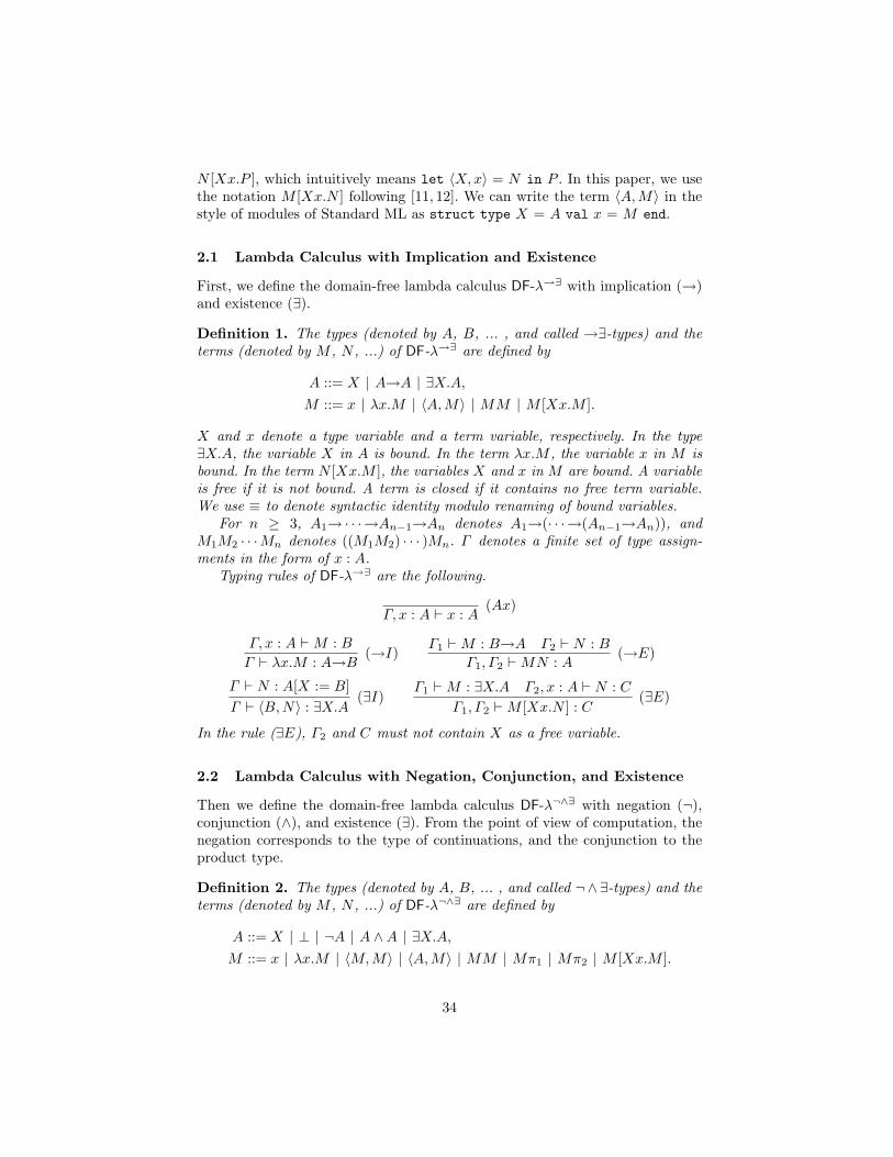
N [Xx.P ], which intuitively means let 〈X, x〉 = N in P . In this paper, we usethe notation M [Xx.N ] following [11, 12]. We can write the term 〈A,M〉 in thestyle of modules of Standard ML as struct type X = A val x = M end.

2.1 Lambda Calculus with Implication and Existence

First, we define the domain-free lambda calculus DF-λ→∃ with implication (→)and existence (∃).

Definition 1. The types (denoted by A, B, ... , and called →∃-types) and theterms (denoted by M , N , ...) of DF-λ→∃ are defined by

A ::= X | A→A | ∃X.A,

M ::= x | λx.M | 〈A,M〉 | MM | M [Xx.M ].

X and x denote a type variable and a term variable, respectively. In the type∃X.A, the variable X in A is bound. In the term λx.M , the variable x in M isbound. In the term N [Xx.M ], the variables X and x in M are bound. A variableis free if it is not bound. A term is closed if it contains no free term variable.We use ≡ to denote syntactic identity modulo renaming of bound variables.

For n ≥ 3, A1→· · ·→An−1→An denotes A1→(· · ·→(An−1→An)), andM1M2 · · ·Mn denotes ((M1M2) · · · )Mn. Γ denotes a finite set of type assign-ments in the form of x : A.

Typing rules of DF-λ→∃ are the following.

Γ, x : A ` x : A(Ax)

Γ, x : A ` M : B

Γ ` λx.M : A→B(→I)

Γ1 ` M : B→A Γ2 ` N : B

Γ1, Γ2 ` MN : A(→E)

Γ ` N : A[X := B]Γ ` 〈B,N〉 : ∃X.A

(∃I)Γ1 ` M : ∃X.A Γ2, x : A ` N : C

Γ1, Γ2 ` M [Xx.N ] : C(∃E)

In the rule (∃E), Γ2 and C must not contain X as a free variable.

2.2 Lambda Calculus with Negation, Conjunction, and Existence

Then we define the domain-free lambda calculus DF-λ¬∧∃ with negation (¬),conjunction (∧), and existence (∃). From the point of view of computation, thenegation corresponds to the type of continuations, and the conjunction to theproduct type.

Definition 2. The types (denoted by A, B, ... , and called ¬∧∃-types) and theterms (denoted by M , N , ...) of DF-λ¬∧∃ are defined by

A ::= X | ⊥ | ¬A | A ∧A | ∃X.A,

M ::= x | λx.M | 〈M,M〉 | 〈A,M〉 | MM | Mπ1 | Mπ2 | M [Xx.M ].

34

Bound and free variables, and closed terms are defined similarly to DF-λ→∃. Forn ≥ 3, A1 ∧ · · · ∧An−1 ∧An denotes A1 ∧ (· · · ∧ (An−1 ∧An)).

Typing rules of DF-λ¬∧∃ are the following.

Γ, x : A ` x : A(Ax)

Γ, x : A ` M : ⊥Γ ` λx.M : ¬A

(¬I)Γ1 ` M : ¬A Γ2 ` N : A

Γ1, Γ2 ` MN : ⊥ (¬E)

Γ1 ` M : A Γ2 ` N : B

Γ1, Γ2 ` 〈M,N〉 : A ∧B(∧I)

Γ ` M : A1 ∧A2

Γ ` Mπ1 : A1(∧E1)

Γ ` M : A1 ∧A2

Γ ` Mπ2 : A2(∧E2)

Γ ` N : A[X := B]Γ ` 〈B,N〉 : ∃X.A

(∃I)Γ1 ` M : ∃X.A Γ2, x : A ` N : C

Γ1, Γ2 ` M [Xx.N ] : C(∃E)

In the rule (∃E), Γ2 and C must not contain X as a free variable. Note thatthe typing rules of DF-λ¬∧∃ for the terms λx.M and MN differ from those ofDF-λ→∃.

3 Type Checking and Type Inference

In this section, we introduce two decision problems on typability of terms, andstate our main theorem.

Type checking (TC) is a problem that asks whether Γ ` M : A is derivablefor given Γ , M , and A. Type inference (TI) is a problem that asks whether thereexist Γ and A such that Γ ` M : A is derivable for given M . In the usualnotation, TC asks Γ ` M : A? for given Γ , M , and A, and TI asks ? ` M :? forgiven M .

These two problems are equivalent in the Curry-style polymorphic lambdacalculus [18], and in the domain-free polymorphic lambda calculus [12]. Twoproblems are said to be equivalent if one is Turing reducible to the other andvice versa. Hence the equivalence of TC and TI means that (i) for any instanceΓ ` M : A? of TC, we can effectively construct a term N such that the answerof the given instance of TC is the same as that of the instance ? ` N :? of TI,and (ii) for any instance ? ` M :? of TI, we can effectively construct an instanceΓ ` N : A? of TC whose answer is the same as the given instance of TI. TC0

and TI0 denote type checking and type inference for closed terms, respectively.In general, if a decision problem P1 is Turing reducible to another decision

problem P2, then decidability of P2 implies decidability of P1, and equivalentlyundecidability of P1 implies undecidability of P2. In [18, 12], they showed un-decidability of TI in the polymorphic lambda calculi by the Turing reducibilityof TC to TI. On the other hand, undecidability of TC and TI in the domain-free lambda calculi with existential types has been proved in [11, 12] by the re-ducibility of each problems for polymorphic types to those for existential types.

35

However, direct relationship between TC and TI for existential types has notbeen known yet. In this paper, we will prove that TC and TI are equivalent inDF-λ→∃ and DF-λ¬∧∃.

Theorem 1. 1. Type checking and type inference are equivalent in DF-λ→∃, thatis, type checking in DF-λ→∃ is Turing reducible to type inference in DF-λ→∃ andvice versa.

2. Type checking and type inference are equivalent in DF-λ¬∧∃.

This result gives another proof of undecidability of TI in these calculi since TCis undecidable in them.

For each system, the proof of the reduction from TC to TI consists of twoparts. First, we show that TC can be reduced to TC0. Secondly, we show thatTC0 can be reduced to TI.

The key of the proof of the reduction from TC0 to TI is the fact that wecan effectively construct a term JM,A from a given pair of a closed term M anda type A such that the instance ` M : A of TC0 is equivalent to the instance` JM,A :? of TI. By this fact, we can conclude that TC0 can be reduced to TI.In order to show that, we borrow the idea of [12] for polymorphic types.

In DF-λ→∃, the reduction from TC to TC0 is easy, whereas the reduction isnot easy to prove for DF-λ¬∧∃ due to absence of implication. In our proof, weshow that we can construct a DF-λ¬∧∃-term λx.M for a DF-λ¬∧∃-term M and avariable x such that Γ, x : A ` M : B holds if and only if Γ ` λx.M : ¬(A∧¬B)holds. By this construction, we can prove that TC can be reduced to TC0 inDF-λ¬∧∃.

Similarly, the proof of the reduction from TI to TC consists of two parts: thereduction from TI to TI0, and the reduction from TI0 to TC. For DF-λ¬∧∃, theproof of the reduction from TI to TI0 has the similar difficulties to the case ofthe reduction from TC to TC0. We can also use the same technique by λx.M toprove it.

We prove the equivalence in DF-λ→∃ in the section 4, where we show howto construct JM,A from M and A. In the section 5, we show the reduction fromproblems for open terms to those for closed terms, and prove the equivalence inDF-λ¬∧∃.

4 TC and TI are Equivalent in DF-λ→∃

In this section, we prove that TC and TI are equivalent in DF-λ→∃.At first, we show that TI is Turing reducible to TC (that is denoted by TI

≤ TC).

Proposition 1. TI in DF-λ→∃ is Turing reducible to TC in DF-λ→∃.

Proof. For a given instance ? ` M :? of TI in DF-λ→∃, we can effectively con-struct the list (x1, · · · , xn) of all of the free variables in M . Then the TI problem? ` M :? is equivalent to a TC problem ` λy.(λx.y)(λx1. · · ·λxn.M) : X→X?,where x and y are fresh variables. In fact, if the term λy.(λx.y)(λx1. · · ·λxn.M)

36

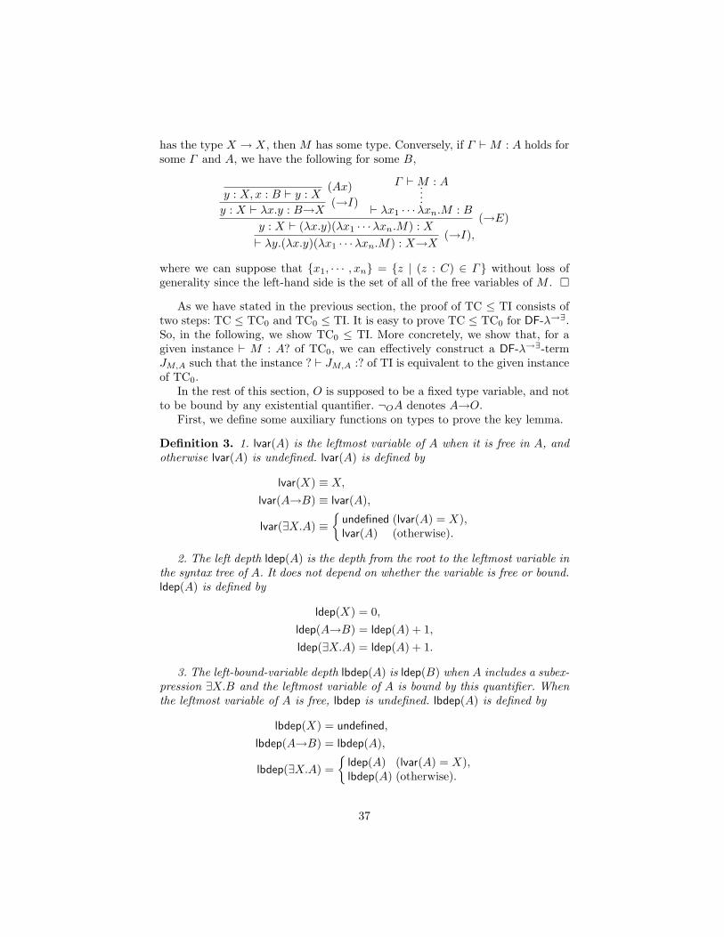
has the type X → X, then M has some type. Conversely, if Γ ` M : A holds forsome Γ and A, we have the following for some B,

y : X, x : B ` y : X(Ax)

y : X ` λx.y : B→X(→I)

Γ ` M : A....` λx1 · · ·λxn.M : B

y : X ` (λx.y)(λx1 · · ·λxn.M) : X(→E)

` λy.(λx.y)(λx1 · · ·λxn.M) : X→X(→I),

where we can suppose that {x1, · · · , xn} = {z | (z : C) ∈ Γ} without loss ofgenerality since the left-hand side is the set of all of the free variables of M . �

As we have stated in the previous section, the proof of TC ≤ TI consists oftwo steps: TC ≤ TC0 and TC0 ≤ TI. It is easy to prove TC ≤ TC0 for DF-λ→∃.So, in the following, we show TC0 ≤ TI. More concretely, we show that, for agiven instance ` M : A? of TC0, we can effectively construct a DF-λ→∃-termJM,A such that the instance ? ` JM,A :? of TI is equivalent to the given instanceof TC0.

In the rest of this section, O is supposed to be a fixed type variable, and notto be bound by any existential quantifier. ¬OA denotes A→O.

First, we define some auxiliary functions on types to prove the key lemma.

Definition 3. 1. lvar(A) is the leftmost variable of A when it is free in A, andotherwise lvar(A) is undefined. lvar(A) is defined by

lvar(X) ≡ X,

lvar(A→B) ≡ lvar(A),

lvar(∃X.A) ≡{

undefined (lvar(A) = X),lvar(A) (otherwise).

2. The left depth ldep(A) is the depth from the root to the leftmost variable inthe syntax tree of A. It does not depend on whether the variable is free or bound.ldep(A) is defined by

ldep(X) = 0,

ldep(A→B) = ldep(A) + 1,

ldep(∃X.A) = ldep(A) + 1.

3. The left-bound-variable depth lbdep(A) is ldep(B) when A includes a subex-pression ∃X.B and the leftmost variable of A is bound by this quantifier. Whenthe leftmost variable of A is free, lbdep is undefined. lbdep(A) is defined by

lbdep(X) = undefined,

lbdep(A→B) = lbdep(A),

lbdep(∃X.A) ={

ldep(A) (lvar(A) = X),lbdep(A) (otherwise).

37

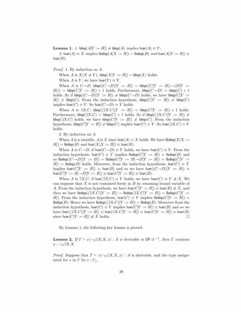
Lemma 1. 1. ldep(A[Y := B]) 6= ldep(A) implies lvar(A) ≡ Y ,2. lvar(A) ≡ X implies lbdep(A[X := B]) = lbdep(B) and lvar(A[X := B]) ≡

lvar(B).

Proof. 1. By induction on A.When A is X(X 6≡ Y ), ldep(X[Y := B]) = ldep(X) holds.When A is Y , we have lvar(Y ) ≡ Y .When A is C→D, ldep((C→D)[Y := B]) = ldep((C[Y := B])→(D[Y :=

B])) = ldep(C[Y := B]) + 1 holds. Furthermore, ldep(C→D) = ldep(C) + 1holds. So if ldep((C→D)[Y := B]) 6= ldep(C→D) holds, we have ldep(C[Y :=B]) 6= ldep(C). From the induction hypothesis, ldep(C[Y := B]) 6= ldep(C)implies lvar(C) ≡ Y . So lvar(C→D) ≡ Y holds.

When A is ∃X.C, ldep((∃X.C)[Y := B]) = ldep(C[Y := B]) + 1 holds.Furthermore, ldep(∃X.C) = ldep(C) + 1 holds. So if ldep((∃X.C)[Y := B]) 6=ldep(∃X.C) holds, we have ldep(C[Y := B]) 6= ldep(C). From the inductionhypothesis, ldep(C[Y := B]) 6= ldep(C) implies lvar(C) ≡ Y . So lvar(∃X.C) ≡ Yholds.

2. By induction on A.When A is a variable, A is X since lvar(A) ≡ X holds. We have lbdep(X[X :=

B]) = lbdep(B) and lvar(X[X := B]) ≡ lvar(B).When A is C→D, if lvar(C→D) ≡ Y holds, we have lvar(C) ≡ Y . From the

induction hypothesis, lvar(C) ≡ Y implies lbdep(C[Y := B]) = lbdep(B) andso lbdep((C→D)[Y := B]) = lbdep(C[Y := B]→D[Y := B]) = lbdep(C[Y :=B]) = lbdep(B) holds. Moreover, from the induction hypothesis, lvar(C) ≡ Yimplies lvar(C[Y := B]) ≡ lvar(B) and so we have lvar((C→D)[Y := B]) ≡lvar(C[Y := B]→D[Y := B]) ≡ lvar(C[Y := B]) ≡ lvar(B).

When A is ∃X.C, if lvar(∃X.C) ≡ Y holds, we have lvar(C) ≡ Y 6≡ X. Wecan suppose that X is not contained freely in B by renaming bound variable ofA. From the induction hypothesis, we have lvar(C[Y := B]) ≡ lvar(B) 6≡ X, andthen we have lbdep((∃X.C)[Y := B]) = lbdep(∃X.C[Y := B]) = lbdep(C[Y :=B]). From the induction hypothesis, lvar(C) ≡ Y implies lbdep(C[Y := B]) =lbdep(B). Hence we have lbdep((∃X.C)[Y := B]) = lbdep(B). Moreover from theinduction hypothesis, lvar(C) ≡ Y implies lvar(C[Y := B]) ≡ lvar(B) and so wehave lvar((∃X.C)[Y := B]) ≡ lvar(∃X.C[Y := B]) ≡ lvar(C[Y := B]) ≡ lvar(B)since lvar(C[Y := B]) 6≡ X holds. �

By Lemma 1, the following key lemma is proved.

Lemma 2. If Γ ` x〈¬O∃X.X, x〉 : A is derivable in DF-λ→∃, then Γ containsx : ¬O∃X.X.

Proof. Suppose that Γ ` x〈¬O∃X.X, x〉 : A is derivable, and the type assign-ment for x in Γ be x : Cx.

38

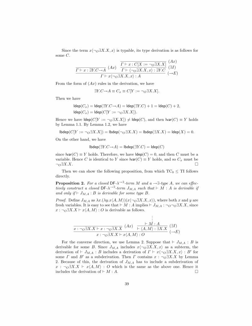
Since the term x〈¬O∃X.X, x〉 is typable, its type derivation is as follows forsome C.

Γ ` x : ∃Y.C→A(Ax)

Γ ` x : C[X := ¬O∃X.X](Ax)

Γ ` 〈¬O∃X.X, x〉 : ∃Y.C(∃I)

Γ ` x〈¬O∃X.X, x〉 : A(→E)

From the form of (Ax) rules in the derivation, we have

∃Y.C→A ≡ Cx ≡ C[Y := ¬O∃X.X].

Then we have

ldep(Cx) = ldep(∃Y.C→A) = ldep(∃Y.C) + 1 = ldep(C) + 2,

ldep(Cx) = ldep(C[Y := ¬O∃X.X]).

Hence we have ldep(C[Y := ¬O∃X.X]) 6= ldep(C), and then lvar(C) ≡ Y holdsby Lemma 1.1. By Lemma 1.2, we have

lbdep(C[Y := ¬O∃X.X]) = lbdep(¬O∃X.X) = lbdep(∃X.X) = ldep(X) = 0.

On the other hand, we have

lbdep(∃Y.C→A) = lbdep(∃Y.C) = ldep(C)

since lvar(C) ≡ Y holds. Therefore, we have ldep(C) = 0, and then C must be avariable. Hence C is identical to Y since lvar(C) ≡ Y holds, and so Cx must be¬O∃X.X. �

Then we can show the following proposition, from which TC0 ≤ TI followsdirectly.

Proposition 2. For a closed DF-λ→∃-term M and a →∃-type A, we can effec-tively construct a closed DF-λ→∃-term JM,A such that ` M : A is derivable ifand only if ` JM,A : B is derivable for some type B.

Proof. Define JM,A as λx.(λy.x〈A,M〉)(x〈¬O∃X.X, x〉), where both x and y arefresh variables. It is easy to see that ` M : A implies ` JM,A : ¬O¬O∃X.X, sincex : ¬O∃X.X ` x〈A,M〉 : O is derivable as follows.

x : ¬O∃X.X ` x : ¬O∃X.X(Ax)

....` M : A

` 〈A,M〉 : ∃X.X(∃I)

x : ¬O∃X.X ` x〈A,M〉 : O(→E)

For the converse direction, we use Lemma 2. Suppose that ` JM,A : B isderivable for some B. Since JM,A includes x〈¬O∃X.X, x〉 as a subterm, thederivation of ` JM,A : B includes a derivation of Γ ` x〈¬O∃X.X, x〉 : B′ forsome Γ and B′ as a subderivation. Then Γ contains x : ¬O∃X.X by Lemma2. Because of this, the derivation of JM,A has to include a subderivation ofx : ¬O∃X.X ` x〈A,M〉 : O which is the same as the above one. Hence itincludes the derivation of ` M : A. �

39

Proof (of Theorem 1.1). TI ≤ TC is proved in Proposition 1. TC ≤ TC0 is easilyproved in a similar way to Proposition 1. TC0 ≤ TI immediately follows fromProposition 2. �

5 TC and TI are Equivalent in DF-λ¬∧∃

In this section, we prove that TC and TI are equivalent in DF-λ¬∧∃.The proof is similar to DF-λ→∃, and consists of the following four parts: (i)

TC ≤ TC0, (ii) TC0 ≤ TI, (iii) TI ≤ TI0, and (iv) TI0 ≤ TC. In contrast toDF-λ→∃, neither (i) nor (iii) is easy to prove for DF-λ¬∧∃ due to absence ofimplication.

5.1 Translation to Closed Terms

First, we show TC≤TC0 and TI≤TI0. In DF-λ¬∧∃, we cannot type the termλx1. · · ·λxn.M , since N has to be typed with ⊥ in order to type the lambdaabstraction λx.N . So we define a construction λx.M , which can be consideredas an interpretation of the implication introduction in DF-λ¬∧∃. It should benoted that the construction can be defined as long as we have negation andconjunction, and so existence is not essential for the discussion in this subsection.

Definition 4. For any ¬ ∧ ∃-types A and B, A⇒B denotes the type ¬(A ∧¬B). Similarly to the ordinary implication →, A1⇒· · ·⇒An⇒B denotesA1⇒(· · ·⇒(An⇒B)). For a DF-λ¬∧∃-term M and a variable x, we define λx.Mas λc.(λx.(cπ2)M)(cπ1), where c is a fresh term variable.

It is easy to see that the set of free variables of λx.M is the set obtained byremoving x from the set of free variables of M .

Lemma 3. Γ, x : A ` M : B holds if and only if Γ ` λx.M : A⇒B.

Proof. Suppose that Γ, x : A ` M : B holds, and then we have the followingtype derivation for Γ ` λx.M : ¬(A ∧ ¬B).

c : A ∧ ¬B ` c : A ∧ ¬Bc : A ∧ ¬B ` cπ2 : ¬B

....Γ, x : A ` M : B

Γ, c : A ∧ ¬B, x : A ` (cπ2)M : ⊥Γ, c : A ∧ ¬B ` λx.(cπ2)M : ¬A

c : A ∧ ¬B ` c : A ∧ ¬Bc : A ∧ ¬B ` cπ1 : A

Γ, c : A ∧ ¬B ` (λx.(cπ2)M)(cπ1) : ⊥Γ ` λx.M : ¬(A ∧ ¬B)

Conversely, if we have Γ ` λx.M : ¬(A∧¬B), then its derivation must be inthe above form. �

Proposition 3. 1. TC in DF-λ¬∧∃ is Turing reducible to TC0 in DF-λ¬∧∃.2. TI in DF-λ¬∧∃ is Turing reducible to TI0 in DF-λ¬∧∃.

40

Proof. 1. For a given instance x1 : A1, · · · , xn : An ` M : B of TC, we caneffectively construct an instance ` λx1. · · ·λxn.M : A1⇒· · ·⇒An⇒B of TC0,which is equivalent to the given instance by Lemma 3.

2. For a given DF-λ¬∧∃-term M , let the list of free variables of M bex1, · · · , xn. It should be noted that we can effectively construct the list. Weshow that the instance ` λx1. · · ·λxn.M :? of TI0 is equivalent to the giveninstance ? ` M :? of TI.

If Γ ` M : B is derivable for some Γ and B, then Γ ′ ` M : B is derivable,where Γ ′ is {x1 : A1, · · · , xn : An} and each xi : Ai is contained in Γ . Then wehave ` λx1. · · ·λxn.M : A1⇒· · ·⇒An⇒B by Lemma 3, hence λx1. · · ·λxn.Mhas a type.

Conversely, if λx1. · · ·λxn.M has a type, then M has some type since it is asubterm of λx1. · · ·λxn.M . �

From the point of view of logic, the translation λx.M becomes clearer. Thejudgment x : A ` M : B implicitly means the implication A→B. Since DF-λ¬∧∃

has no implication, we have to interpret the implication by means of negationand conjunction. In order to do that, we use the well-known fact that A→B is(classically) equivalent to ¬(A ∧ ¬B), which is denoted by A⇒B in this paper.A⇒B is not an intuitionistic implication, since we cannot conclude B from A⇒Band A in the intuitionistic logic. We can consider an elimination rule for ⇒ suchas

Γ1 ` M : A⇒B Γ2 ` N : A

Γ1, Γ2 ` M@N : ¬¬B ,

where M@N is defined as λk.M〈N, k〉. We can consider that the constructionsλx.M and M@N realize the interpretation of the variant of implication, whichis implicitly implemented by “`”, in DF-λ¬∧∃.

The translation which maps λx.M to λx.M and MN to M@N is also im-portant from the point of view of computer science, since it can be consideredas a variant of continuation-passing-style translations into the lambda calculuswith continuation types and product types. Such translations have been studiedin [17, 5, 7].

In addition, note that we can construct a simpler closed term N and a typeC from a given instance x1 : A1, · · · , xn : An ` M : B of TC. N and C can bedefined as follows:

N ≡ λc.(λx1. · · · (λxn−1.(λxn.(cπn+1n+1)M)(cπn+1

n ))(cπn+1n−1) · · · )(cπ

n+11 ) : ⊥,

C ≡ ¬(A1 ∧ · · · ∧An ∧ ¬B),

where πnm is the m-th projection for n-tuples, which can be constructed by π1

and π2. Then we can show that x1 : A1, · · · , xn : An ` M : B holds if and onlyif ` N : C holds. This construction can be used to prove TI ≤ TI0 as well.

5.2 Proof of Equivalence

We complete the proof of equivalence in DF-λ¬∧∃. TC0 ≤ TI can be provedsimilarly to DF-λ→∃ by replacing ¬O by ¬.

41

Lemma 4. If Γ ` x〈¬∃X.X, x〉 : A is derivable in DF-λ¬∧∃, then Γ containsx : ¬∃X.X.

Proof. The definitions of auxiliary functions for negation and conjunction are

lvar(¬A) ≡ lvar(A),lvar(A ∧B) ≡ lvar(A),

ldep(¬A) = ldep(A) + 1,

ldep(A ∧B) = ldep(A) + 1,

lbdep(¬A) = lbdep(A),lbdep(A ∧B) = lbdep(A),

and the same statement as Lemma 1 holds for DF-λ¬∧∃. Hence the claim isproved similarly to Lemma 2. �

The following proposition is also proved similarly to DF-λ→∃.

Proposition 4. For a closed DF-λ¬∧∃-term M and a ¬ ∧ ∃-type A, we caneffectively construct a closed DF-λ¬∧∃-term J ′M,A such that ` M : A is derivableif and only if ` J ′M,A : B is derivable for some type B.

Proof. Define J ′M,A as λx.(λy.x〈A,M〉)(x〈¬∃X.X, x〉), where both x and y arefresh variables. The proof is similar to Proposition 2, using Lemma 4. Note thatthe lambda abstractions and function applications in J ′M,A correspond to theintroduction and elimination rules of negation. �

The theorem for DF-λ¬∧∃ is proved as follows.

Proof (of Theorem 1.2). TC ≤ TC0 and TI ≤ TI0 are proved by Proposition 3.TC0 ≤ TI immediately follows from Proposition 4. TI0 ≤ TC is easily provedsimilarly to DF-λ→∃, that is, each instance ` M :? of TI0 can be translated toan equivalent instance ` λy.(λx.y)M : ¬⊥ of TC. �

6 Concluding Remarks

In this paper, we show equivalence between type checking and type inference inthe domain-free lambda calculi with existential types: DF-λ→∃ and DF-λ¬∧∃.

We can consider other styles for existential types. For example, more implicittype assignment system for existential types was introduced in [15], whose typingrules for existential types are

Γ ` N : A[X := B]Γ ` 〈∃, N〉 : ∃X.A

(∃I),

Γ1 ` M : ∃X.A Γ2, x : A ` N : C

Γ1, Γ2 ` M [x.N ] : C(∃E)

.

42

Our proof of the reduction from TC to TI cannot be adapted to this variant,because the term JM,A explicitly contains the information of type A, whereasterms in the variant contain no explicit type information. Moreover, undecid-ability of TC and TI in the variant has not been known yet. So it would befuture work to study the relationship between TC and TI in the variant, anddecidability of them.

References

1. G. Barthe and M.H. Sørensen, Domain-free pure type systems. Journal of Func-tional Programming 10:412–452, 2000.

2. O. Danvy and A. Fillinski, Representing Control: a Study of the CPS Translation.Mathematical Structures in Computer Science 2(4):361–391, 1992.

3. K. Fujita, Explicitly typed λµ-calculus for polymorphism and call-by-value. In Pro-ceedings of 4th International Conference on Typed Lambda Calculi and Applications(TLCA 1999), LNCS 1581, pp. 162–177, 1999.

4. K. Fujita and A. Schubert, Partially Typed Terms between Church-Style and Curry-Style. In International Conference IFIP TCS 2000, LNCS 1872, pp. 505–520, 2000.

5. K. Fujita, Galois embedding from polymorphic types in to existential types. In Pro-ceedings of 7th International Conference on Typed Lambda Calculi and Applications(TLCA 2005), LNCS 3461, pp. 194–208, 2005.

6. R. Harper and M. Lillibridge, Polymorphic Type Assignment and CPS Conversion.Lisp and Symbolic Computation, 6:361–380, 1993.

7. M. Hasegawa, Relational parametricity and control. Logical Methods in ComputerScience, 2(3:3):1–22, 2006.

8. M. Hasegawa, Unpublished manuscript, 2007.9. A.J. Kfoury, J. Tiuryn and P. Urzyczyn, The Undecidability of the Semi-unification

Problem. Information and Computation 102:83–101, 1993.10. J.C. Mitchell and G.D. Plotkin, Abstract types have existential type. ACM Trans-

actions on Programming Languages and Systems 10(3):470–502, 1988.11. K. Nakazawa, M. Tatsuta, Y. Kameyama, and H. Nakano, Undecidability of Type-

Checking in Domain-Free Typed Lambda-Calculi with Existence. In the 17th EACSLAnnual Conference on Computer Science Logic (CSL 2008), LNCS 5213, pp. 477–491,2008.

12. K. Nakazawa and M. Tatsuta, Type Checking and Inference for Polymorphicand Existential Types. In the 15th Computing: the Australasian Theory Sympo-sium (CATS 2009), Conferences in Research and Practice in Information Technology(CRPIT), Vol. 94, 2009.

13. M. Parigot, λµ-calculus: an algorithmic interpretation of classical natural deduc-tion. In Proceedings of the International Conference on Logic Programming andAutomated Reasoning, LNCS 624, pp.190–201, 1992.

14. A. Schubert, Second-order unification and type inference for Church-style polymor-phism. In the 25th Annual ACM Symposium on Principles of Programming Languages(POPL ’98), pp.279–288, 1998.

15. M. Tatsuta, Simple saturated sets for disjunction and second-order existentialquantification. In Proceedings of 8th International Conference on Typed LambdaCalculi and Applications (TLCA 2007), LNCS 4583, pp. 366–380, 2007.

16. M. Tatsuta, K. Fujita, R. Hasegawa, and H. Nakano, Inhabitance of ExistentialTypes is Decidable in Negation-Product Fragment. In Proceedings of 2nd Interna-tional Workshop on Classical Logic and Computation (CLC2008), 2008.

43

17. H. Thielecke, Categorical Structure of Continuation Passing Style. Ph.D. Thesis,University of Edinburgh, 1997.

18. J.B. Wells, Typability and type checking in the second-order λ-calculus are equiva-lent and undecidable. In Proceedings of 9th Symposium on Logic in Computer Science(LICS ’94), pp. 176–185, 1994.

44

A Taxonomy of Some Right-to-LeftString-Matching Algorithms

Manuel Hernandez

Universidad Tecnologica de la Mixteca, Huajuapan de Lon, Oaxaca, Mexicomanuelhg@mixteco.utm.mx

Abstract. This paper presents a taxonomy of some exact, right-to-left,string-matching algorithms. The taxonomy is based on results obtainedby using logic program transformation over a naive and nondeterministicspecification. A derivation of the search part and some notes about thepreprocessing part of each algorithm is presented. The derivations showseveral design decisions behind each algorithm, and allow us to organizethe algorithms within a taxonomic tree, giving us a better understandingof these algorithms and possible mechanical procedures to derive them.

1 Introduction

Taxonomies of algorithms play an important role in structuring knowledge forcomputer programming [Par76,Dar78,Lau89,WZ96]. Some advantages of tax-onomies of algorithms are: a) We place each algorithm in parent-child relation-ships; b) we uncover the rationale behind the design of each algorithm; and, c)we can know better how an algorithm works, increasing our comprehension ofhow an algorithm can efficiently be implemented or automatically derived. Ataxonomy can also reveal certain faults in the design of an algorithm. We caneven discover minor variants as by-products of our main developments. We willshow program transformation is not only a tool to improve programs, but it alsocan be a useful tool for a better understanding of existing algorithms. This paperpresents a taxonomy, based on logic program transformation and decreasing ofnondeterminism, of some exact and right-to-left string-matching algorithms.

There are two main groups of string-matching algorithms classified accord-ing to a pair of schedules of character comparisons: either from left to right orfrom right to left. The Knuth–Morris–Pratt algorithm [KMP77] belongs to thefirst group. The search part of the Knuth–Morris–Pratt algorithm has been thesubject of intensive study in program derivation [CD89,Smi91,SGJ96]. However,the Knuth–Morris–Pratt algorithm is hardly used in practice. Instead, stringsearching is often implemented following the Boyer–Moore algorithm [Ste94] orsome variant; these algorithms belong to the second group. In this work we de-rive the complete version of the search part of the Boyer–Moore algorithm andsome of its variants using logic program transformation. By using the power-set construction, deterministic unfolding, constraint introduction via the clausesplitting rule, and extended folding, we show how to obtain Boyer–Moore-likeprograms from naive and nondeterministic logic programs.

Our main interest is centered on the search part of each algorithm, so that wewant to maximize the shift values and to minimize the number of comparisonsgiven a mismatch between the pattern and a portion of the text. The algorithmsto discuss are: The Boyer–Moore algorithm itself (BM algorithm, for short); theHorspool variant (BMH algorithm); the Partsch–Stomp variant (BMPS algo-rithm); and, the Apostolico–Giancarlo variant (BMAG algorithm). Some minorvariants will be byproducts of our main developments.

These algorithms are derived for the following reasons. The BM algorithm isone of the most valuable algorithms for string-matching in practice. The BMHvariant is highly practical for ordinary alphabets, such as the English alphabet.Its cost of preprocessing is low, and it is a simplification of the BM algorithm.The BMPS algorithm surpasses the BM algorithm in the search stage (the shiftsgiven by the BM are minor than those of the BMPS variant), although the costof preprocessing is high. Finally, the BMH and the BMPS variants, and the BMitself, have the deficiency of comparing again some characters already previouslytreated, but in the BMAG variant these re-comparisons are avoided because thisvariant incorporates in its design a memory. The method to place an algorithm inthe taxonomic tree is: A naive logic program solving the string-matching problemis presented, a derivation is carried out, and then the derivation is associatedwith a path, from the root to the leaf, of the taxonomic tree given in Fig. 1 (whereby pre-algorithms we mean some intermediate programs within the derivation).Leaves indicate a complete and terminal development of a derivation.

Right-to-leftnaive algorithm

Pre-algorithmsRRRR

Rllll

lWithoutmemory

SSSSSuu

Withmemory

BM BMPS BMH BMAG

Fig. 1: A taxonomic tree of some right-to-left string-matching algorithms.

1.1 Overview

We assume from our readers some basic familiarity with logic programming[Llo87] and logic program transformation [PP98]. An overview of this paper isas follows. Section 2 introduces the string-matching problem and describes theBoyer–Moore algorithm. Section 3 gives some basic logic program transformationtechniques and the main points of our derivations. Section 4 is devoted to derivethe BM algorithm and some of its variants. Section 5 presents some relatedwork and in Section 6 are given some conclusions.

46

2 The Boyer–Moore algorithm

The exact string-matching problem. The exact string-matching problem consistsin finding the occurrences (if any) of a string called the pattern within anotherstring called the text. Formally, let A be a non-empty and finite set called thealphabet. The elements of A are called characters. The set A∗ consists of finitesequences of characters of A and these sequences are called strings. We denoteby Set(S) the set of elements ocurring in the string S, and by #(S) its length.

Let S1 and S2 be two strings in A∗. The string S1 is a substring of S2 if S1 isa subsequence of S2. We define a partial order relation in A as follows: S1 � S2

if S1 is a substring of S2. If S1 � S2 we say that S1 occurs in S2. Let S, T bestrings. We define the concatenation of S and T , S ++T , as the new string ST .The set A∗ endowed with the operation ++ is a non-commutative monoid with aunit element called the empty word, ε. Given the strings S1 and S2, in the exactstring-matching problem we want to know whether S1 � S2. This is equivalentto know if there are two strings U and V such that S2 = U ++S1 ++V .

Let P and T be strings. A configuration between P and T is a static view ofP and T placed together to make comparisons between characters. The portionof the text of size #(P ) where P is placed is called a window of T . A transitionis a pair of configurations. The purpose of configurations is to explain how a newconfiguration is reached from a previous one, given a rule to do this transition.A matching schedule is an order (or permutation) to make comparisons betweencharacters of P and those in a window of T when trying to find P in T .

Naive string-matching algorithms. A first straightforward algorithm for solv-ing the exact string-matching problem is to begin with a configuration wherethe pattern is placed leftmost in the text with a left-to-right matching schedulewithin the window. If a mismatch occurs, we displace the window one characterto the right of the text and start the matching schedule again. If all charactersof the pattern and those correspondent within the window of the text match,an occurrence has been found. This process is repeated until we do not haveany new windows to explore. This is sometimes called the naive left-to-rightstring-matching algorithm. A second straightforward algorithm solving the ex-act string-matching problem originates the naive right-to-left string-matchingalgorithm: this time we align the pattern and the text again from the leftmostpart of the text, but we apply a right-to-left matching schedule in the currentwindow. In both algorithms, if mismatches happen every time we almost fin-ish comparing all characters of the pattern with those of the text, we obtain aworst-case performance, which is quadratic [CR94]. This situation, however, isunlikely to occur in practice, and the expected performance of this algorithm islinear. We will focus our attention on right-to-left string-matching algorithms.The representative algorithm of this kind is named the Boyer–Moore algorithm,which has a sublinear efficiency and is described in the next.

The Boyer–Moore algorithm. Boyer and Moore [BM77] improved the averagecase of the naive right-to-left string matching algorithm in a sublinear algorithm.

47

By inspecting the text character aligned with the rightmost pattern character,we have two cases: In case such a text character does not occur in the pattern, wecan slide the pattern its whole length, to surpass the bad character of the text; asa second case, if the text character is also in the pattern we can shift the patterna number of characters determined by the preprocessing phase, trying to alignthese good characters. If a partial match is discovered, in the next configurationthose rightmost parts that match would be aligned again, so that transitions areruled by the longest partial matches.

In case of a mismatch this algorithm uses two precomputed functions to shiftthe pattern to the right with respect to the text. These two shift functions arecalled the good suffix rule or δ2 function and the bad character rule or δ1 function.Both functions interact each other through the max function. There are severalvariants of the Boyer–Moore algorithm, depending on whether we use the δ1

or the δ2 function, or both. For example, we can use only the δ2 function. Byusing enhanced versions of partial deduction, this variant was derived in [HR03];in functional programming this variant was also derived in [Bir05]. Similarly,the variant that only uses δ1 was derived in [MACD01] and [HR01]. However,in several variants no memory is kept of partial matchings obtained from theprevious steps, as it was noticed in [AG86] and where is devised a variant ofthe Boyer–Moore algorithm that incorporates a memory, so avoiding redundantcomparisons. In every variant, the search is fast on average, because in manycases the number of characters shifted is close to the length of the pattern.

We now give a description of the BM algorithm [BM77,Ste94]. We denoteby Rk the kth character of a string R, trying to keep k in an appropriate range(otherwise, Rk is undefined). In addition, T denotes a text of length n and Pdenotes the pattern of length m. We try to apply the index i to the text Tand the index j to the pattern P . Consider first a mismatch between Pm andTi. If Ti does not occur in P at all, then the pattern is shifted m characters tothe right. The next comparison is then between Pm and Ti+m. If, on the otherhand, Ti does occur in P , with rightmost occurrence in Pk, then Ti and Pk arelined up (i.e. the pattern is shifted m− k characters) and the test is resumed bycomparing Pm with Ti+m−k.

To align a particular character of the pattern with that of the text, we usethe following δ1 function:

δ1(x)={

m if x 6∈ Set(P ) ,

m− k k = max{j ∈ N | Pj = x}If such a character exists in the text but does not exist in the pattern, we shiftthe pattern over the text the total length of the pattern, m.

Consider a match between Pm and Ti. Comparisons of pattern and textcharacters continue from right to left until a complete match is obtained or amismatch at Pj and Ti′ , say, occurs. In this case, the suffix of the pattern givenby Pj+1, . . . , Pm is equal to the text substring Ti′+1, . . . , Ti′+m−j , and Pj 6= Ti′ .

If Ti′ does not occur in p at all, we can then shift the pattern m− j positionsto the right (just past Ti′), and the next comparison will be between Pm andTi′+m. The text index will then be incremented by m positions.

48

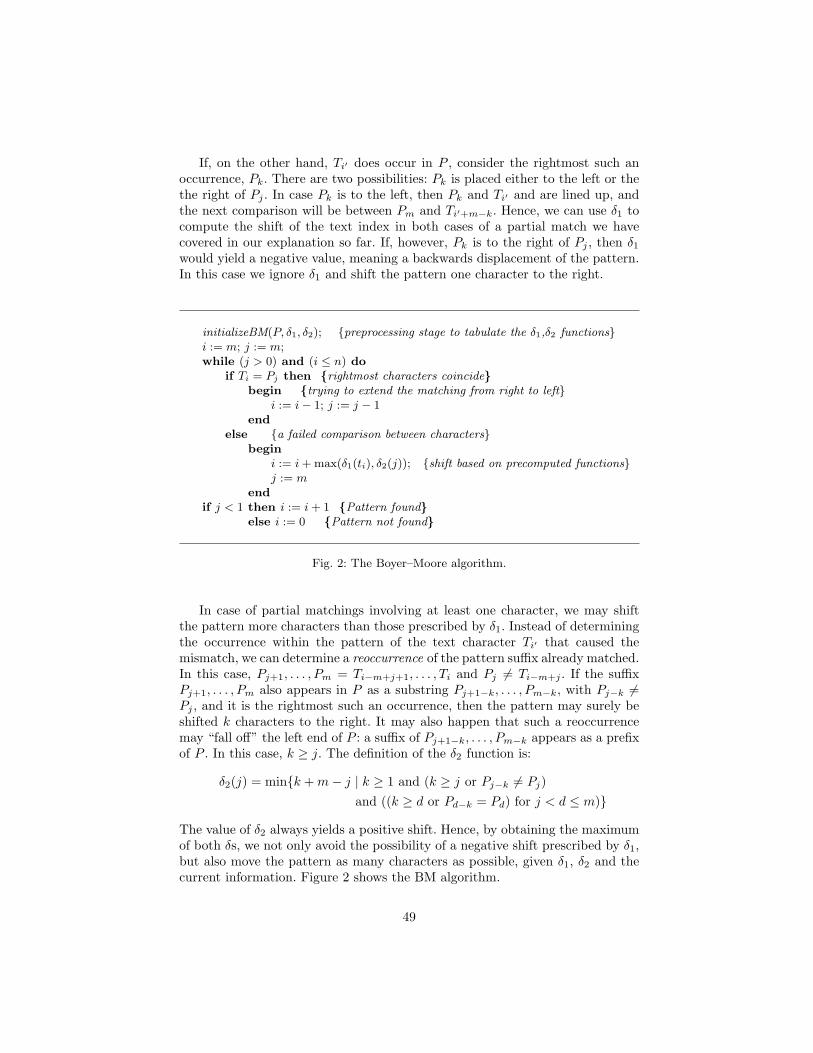
If, on the other hand, Ti′ does occur in P , consider the rightmost such anoccurrence, Pk. There are two possibilities: Pk is placed either to the left or thethe right of Pj . In case Pk is to the left, then Pk and Ti′ and are lined up, andthe next comparison will be between Pm and Ti′+m−k. Hence, we can use δ1 tocompute the shift of the text index in both cases of a partial match we havecovered in our explanation so far. If, however, Pk is to the right of Pj , then δ1

would yield a negative value, meaning a backwards displacement of the pattern.In this case we ignore δ1 and shift the pattern one character to the right.

initializeBM(P, δ1, δ2); {preprocessing stage to tabulate the δ1,δ2 functions}i := m; j := m;while (j > 0) and (i ≤ n) do

if Ti = Pj then {rightmost characters coincide}begin {trying to extend the matching from right to left}

i := i− 1; j := j − 1end

else {a failed comparison between characters}begin

i := i + max(δ1(ti), δ2(j)); {shift based on precomputed functions}j := m

endif j < 1 then i := i + 1 {Pattern found}

else i := 0 {Pattern not found}

Fig. 2: The Boyer–Moore algorithm.

In case of partial matchings involving at least one character, we may shiftthe pattern more characters than those prescribed by δ1. Instead of determiningthe occurrence within the pattern of the text character Ti′ that caused themismatch, we can determine a reoccurrence of the pattern suffix already matched.In this case, Pj+1, . . . , Pm = Ti−m+j+1, . . . , Ti and Pj 6= Ti−m+j . If the suffixPj+1, . . . , Pm also appears in P as a substring Pj+1−k, . . . , Pm−k, with Pj−k 6=Pj , and it is the rightmost such an occurrence, then the pattern may surely beshifted k characters to the right. It may also happen that such a reoccurrencemay “fall off” the left end of P : a suffix of Pj+1−k, . . . , Pm−k appears as a prefixof P . In this case, k ≥ j. The definition of the δ2 function is:

δ2(j) = min{k + m− j | k ≥ 1 and (k ≥ j or Pj−k 6= Pj)and ((k ≥ d or Pd−k = Pd) for j < d ≤ m)}

The value of δ2 always yields a positive shift. Hence, by obtaining the maximumof both δs, we not only avoid the possibility of a negative shift prescribed by δ1,but also move the pattern as many characters as possible, given δ1, δ2 and thecurrent information. Figure 2 shows the BM algorithm.

49

3 Logic programming and exact string matching

Having described our main algorithm to deal with, in this section we describesome logic program transformation tools to be used in our derivations as well asthe main guidelines of these derivations.

3.1 Logic program transformation tools

Equality theory. To use logic programming, we suppose the SLDNF-resolutionrule, and the conventional unification algorithm. Because the unification algo-rithm of logic programming is greedy and hides some, perhaps useful, infor-mation, we try to replace it by some explicit equation introduction, which isbasically an introduction of constraints. This equation introduction is logicallyjustified by using the standard equality theory of first-order logic; to deal withinequations we suppose Clark’s equality theory [Cla78]. Both of these tools areapplied over Herbrand universes. We will use some restricted forms of equations:An equation X = Y has normal form if X is a variable and Y is a term with-out any occurrence of X in Y (occur-check rule). An inequation is the negationof a normalized equation. Because equation introduction helps us to deal withseveral instances of variables, this tool is strongly related to the technique of par-tial evaluation named bounded static variation (also colloquially know as “TheTrick”), a binding-time source-program transformation [DRK06].

Deterministic unfolding. In the unfold/fold method [PP98], when we unfold aclause C with respect to an atom q and q is defined by several clauses, weobtain several clauses again. If we simplify these resultant clauses and get onlyone clause, we say that the unfolding is deterministic. If the surviving clause isunfolded again with respect the same atom A, and we get only one clause again,and so on, we have a succession of deterministic unfolding steps. If after n+1 ofthese unfolding steps we obtain two or more clauses, without any possibility ofeliminating some of them, we stop unfolding at step n, and we have a successionof deterministic unfolding steps of size n; this succession is a valuable tool forassuring termination when we apply the unfolding rule; moreover, this successionalso avoids dealing with an over-specialized program. The unfolding rule and the“extended” folding rule (where several clauses are used for folding) are the basiccomponents of the disjunctive partial deduction [PPR97]. An opportunity ofsimplifying clauses after unfolding is when we have in the body of the resultantsclauses an unsatisfiable set of atoms. For example, if we have:

p(X)←X = b ∧ q(X) (1)q(X)←X = a (2)q(X)←X = b (3)

by unfolding q(X) in (1) (underlined subgoal) we have the two clauses: p(X)←X = b∧X = a and p(X)←X = b∧X = b. The body of the first clause has theset of equations: {X = b, X = a}, which originates the following false fact: b = a

50

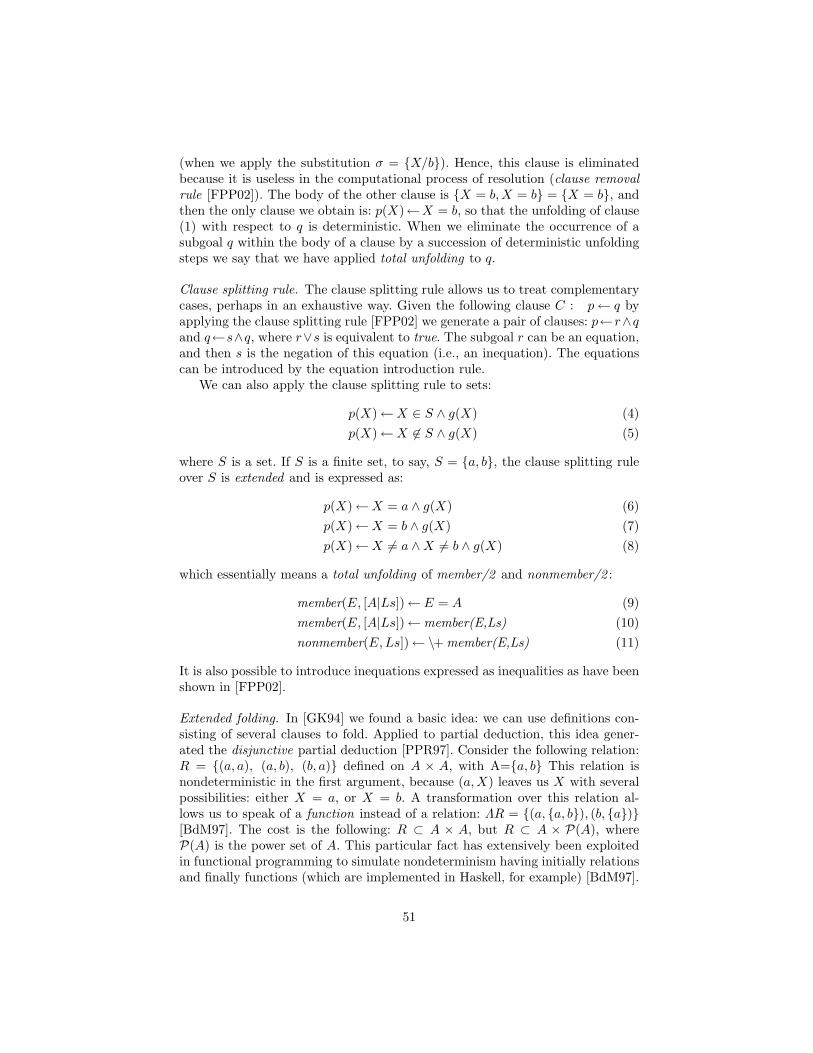
(when we apply the substitution σ = {X/b}). Hence, this clause is eliminatedbecause it is useless in the computational process of resolution (clause removalrule [FPP02]). The body of the other clause is {X = b, X = b} = {X = b}, andthen the only clause we obtain is: p(X)←X = b, so that the unfolding of clause(1) with respect to q is deterministic. When we eliminate the occurrence of asubgoal q within the body of a clause by a succession of deterministic unfoldingsteps we say that we have applied total unfolding to q.

Clause splitting rule. The clause splitting rule allows us to treat complementarycases, perhaps in an exhaustive way. Given the following clause C : p← q byapplying the clause splitting rule [FPP02] we generate a pair of clauses: p←r∧qand q←s∧q, where r∨s is equivalent to true. The subgoal r can be an equation,and then s is the negation of this equation (i.e., an inequation). The equationscan be introduced by the equation introduction rule.

We can also apply the clause splitting rule to sets:

p(X)←X ∈ S ∧ g(X) (4)p(X)←X 6∈ S ∧ g(X) (5)

where S is a set. If S is a finite set, to say, S = {a, b}, the clause splitting ruleover S is extended and is expressed as:

p(X)←X = a ∧ g(X) (6)p(X)←X = b ∧ g(X) (7)p(X)←X 6= a ∧X 6= b ∧ g(X) (8)

which essentially means a total unfolding of member/2 and nonmember/2 :

member(E, [A|Ls])← E = A (9)member(E, [A|Ls])←member(E,Ls) (10)nonmember(E,Ls])←\+ member(E,Ls) (11)

It is also possible to introduce inequations expressed as inequalities as have beenshown in [FPP02].

Extended folding. In [GK94] we found a basic idea: we can use definitions con-sisting of several clauses to fold. Applied to partial deduction, this idea gener-ated the disjunctive partial deduction [PPR97]. Consider the following relation:R = {(a, a), (a, b), (b, a)} defined on A × A, with A={a, b} This relation isnondeterministic in the first argument, because (a,X) leaves us X with severalpossibilities: either X = a, or X = b. A transformation over this relation al-lows us to speak of a function instead of a relation: ΛR = {(a, {a, b}), (b, {a})}[BdM97]. The cost is the following: R ⊂ A × A, but R ⊂ A × P(A), whereP(A) is the power set of A. This particular fact has extensively been exploitedin functional programming to simulate nondeterminism having initially relationsand finally functions (which are implemented in Haskell, for example) [BdM97].

51

In logic programming an application of the same technique results more nat-ural because we can model relations as predicates, and we would have a logicprogram as the following: {r(a, a)←, r(a, b)←, r(b, a)←}. By introducing equa-tions we have:

r(X, Y )←X = a ∧ Y = a (12)r(X, Y )←X = a ∧ Y = b (13)r(X, Y )←X = b ∧ Y = a (14)

We note that in the following set of clauses each clause shares with otherthe subgoal X = a. We name this common subgoal a pivot. The pivot in thefollowing set of clauses is boxed-in:

r(X, Y )← X = a ∧ Y = a (15)

r(X, Y )← X = a ∧ Y = b (16)

For folding, we create a new definition: g(Y ) ← Y = a and g(Y ) ← Y = b.Folding with respect to the pivot X = a and the new definition, we have the fol-lowing program, consisting of clauses r(a, Y )← g(Y ) and r(b, Y )← h(Y ), whereh(Y )← Y = a (by unfolding g/1 and h/1 in the body of these clauses we wouldobtain the original definition of r/2, which is described as in-situ folding.) Thisnew definition of r/2 is deterministic with respect to its first argument. So thatby using extended folding we decrease or eliminate nondeterminism to obtaindeterministic implementations. This method is rooted in the powerset construc-tion (named in [BdM97] as Eilenberg–Wright Lemma (p. 122)) to transformnondeterministic automata into deterministic ones.

3.2 Guidelines of our derivations

As we have seen, the pattern P occurs in a string T if there exist strings X1 andX2 such that T = (X1 ++ P ) ++ X2. We use this specification as a guide in thefollowing naive logic program that solves the string-matching problem:

substring(P, T )← append(X1, P, X2) ∧ append(X2, X3, T ) (17)

where append has the usual definition. We should notice the existential variablesX1 and X2, and that we associate append/3 to the left. Adapting our notationto logic programming, now we consider a particular pattern P = p1 . . . pn; thispattern is represented by the list [p1, . . . , pn], or as [p1 : pn], where with thenotation Oi : Oj we abbreviate the sequence of objects Oi, Oi+1, . . . , Oj if i < j,or the sequence Oi, Oi−1, . . . , Oj if j < i. If i = j, Oi : Oj = Oi. Moreover,we use Ai : Aj = Bi : Bj as an abbreviation of a conjunction of equations:Ai = Bi ∧ Ai+1 = Bi+1 ∧ . . . ∧ Aj = Bj . Indexes i and j follow the previousconvention if i < j or j > i. Again, if i = j, Ai : Aj = Bi : Bj is reduced toAi = Bi.

From the clause (17), and by using some standard techniques of logic programtransformation and partial deduction, we obtain the following clauses:

52

Program 1

ssP ([p1 : pm |L ])← (18a)ssP ([A |L ])← ssP (L) (18b)

This nondeterministic program can be read as a direct implementation of theleft-to-right string-matching algorithm, following the traditional unification al-gorithm over terms. However, to explicitly control the order of matching via anequational theory, we introduce equations in the body of clause (18a), to get:

Program 2

ssP ([A1 : Am |L ])←A1 : Am = p1 : pm (19a)ssP ([A |L ])← ssP (L) (19b)

To deal with a matching schedule from right to left, we invert the order of theequations of the clause (19a), and because we use a set of variables A1, . . . , Am

to access elements of the pattern, we apply a substitution to clause (19b):

Program 3

ssP ([A1 : Am |L ])←Am : A1 = pm : p1 (20a)ssP ([A1 : Am |L ])← ssP ([A2 : Am |L ]) (20b)

This program disallows to use texts of length lesser than m. Because this match-ing schedule, each particular mismatched character involves a suffix of the pat-tern (included the ε string). Thus, we have that either Am = pm or Am 6= pm;and, if Am = pm then either Am−1 = pm−1 or Am−1 6= pm−1, and so on. Finally,if Am : A2 = pm : p2 then either A1 = p1 or A1 6= p1. We call the program incor-porating in the body of its clauses these equations and inequations a program intriangular form.

Program 4

ssP ([A1 : Am |L ])←Am : A1 = pm : p1 (21a)ssP ([A1 : Am |L ])←Am 6= pm ∧ ssP ([A2 : Am |L ]) (21b)ssP ([A1 : Am |L ])←Am = pm ∧Am−1 6= pm−1 ∧ ssP ([A2 : Am |L ]) (21c)

...ssP ([A1 : Am |L ])←Am : A2 = pm : p2 ∧A1 6= p1 ∧ ssP ([A2 : Am |L ])(21d)ssP ([A1 : Am |L ])←Am : A1 = pm : p1 ∧ ssP ([A2 : Am |L ]) (21e)

We note that each clause in Prog. 4 corresponds with one of the following cases:Clauses (21a) and (21e) deal with a total match and possible reoccurrences ofthe pattern, respectively. Clause (21b) treats an initial mismatching. The otherclauses find partial matchings:

ssP ([A1 : Am |L ])←Am : Ak+1 = pm : pk+1∧Ak 6= pk∧ssP ([A2 : Am |L ]) (22)

53

where k is such that 1 ≤ k ≤ m−1. Each clause is unfolded enough with respectto ssP /1 through a succession of deterministic unfolding steps.

In Prog. 4 the nondeterminism has been increased, but we can do the follow-ing process to decrease it. We select Am = pm as pivot, because this subgoal iscommon to the body of several clauses, and define a new predicate to fold someclauses. Similarly, we select Am−1 = pm−1 as the next pivot. This process givesus every pivot, consecutively. Without any application of some other rule, apartfrom the folding rule, we would get the following cascade-like program:

Program 5

ssP ([A1 : Am |L ])←Am = pm ∧ new1([A1 : Am |L ]) (23)ssP ([A1 : Am |L ])←Am 6= pm ∧ ssP ([A2 : Am |L ]) (24)

new1([A1 : Am |L ])←Am−1 = pm−1 ∧ new2([A1 : Am |L ]) (25)new1([A1 : Am |L ])←Am−1 6= pm−1 ∧ ssP ([A2 : Am |L ]) (26)

. . .

newm−1([A1 : Am |L ])←A1 = p1 ∧ newm([A1 : Am |L ]) (27)newm−1([A1 : Am |L ])←A1 6= p1 ∧ ssP ([A2 : Am |L ]) (28)

newm([A1 : Am |L ])← (29)newm([A1 : Am |L ])← ssP ([A2 : Am |L ]) (30)

Further constraints will affect the number of new predicates, but the (definition-folding) process will be the same for each variant. The main idea is to decrease thelength of the size of the list [A2 : Am |L ] at each recursive call of ssP /1, becausewhen we decrease this size we increase the shift and, therefore, we decrease thenumber of comparisons. We will apply deterministic unfolding to carry out thisobjective, as we will see in the next section.

4 Deriving the search part of some variants of theBoyer–Moore algorithm

Now we derive the BM algorithm and some of its variants. First, we derivevariants restricted to use either the δ1 or the δ2 function. Next, we derive thesearch phase of the BM algorithm by using the maximum of both functions. Wecontinue with the derivation of the BMH and the BMPS algorithms. Finally,we derive the BMAG algorithm. This algorithm differs from the previous onesbecause it incorporates a memory, so avoiding at all to access twice or moretimes a character text.

We define an auxiliary predicate:

shift(1, [A |L1 ], L1)← (31a)shift(N, [A |L1 ], L2)←N1 is N − 1 ∧ shift(N1, L1, L2) (31b)

where shift(N,L1, L2) holds when L1 is L2 without its first N elements. Thispredicate will be useful in the following.

54

A variant involving δ1. We begin by applying the clause splitting rule to Clause(20b):

Program 6

ssP ([A1 : Am |L ])←Am : A1 = pm : p1 (32a)ssP ([A1 : Am |L ])←Am = pm ∧ ssP ([A2 : Am |L ]) (32b)ssP ([A1 : Am |L ])←Am 6= pm ∧ ssP ([A2 : Am |L ]) (32c)

We notice that the negative information of Ak 6= pk in Clause (32c) can bereinforced with the introduction of the constraints over sets given by ∈ and 6∈.Let Set(P ) be the set of characters of the pattern P = p1 : pm, and ρ be itscardinality (ρ ≤ m, where m is the length of the pattern). We apply the clausesplitting rule to (32c), using Am ∈ Sp ∨ Am 6∈ Set(P ), to obtain the followingother two clauses:

ssP ([A1 : Am |L ])←Am 6= pm ∧Am ∈ Set(P ) ∧ ssP ([A2 : Am |L ]) (33a)ssP ([A1 : Am |L ])←Am 6= pm ∧Am 6∈ Set(P ) ∧ ssP ([A2 : Am |L ]) (33b)

When we eliminate the subgoal (Am ∈ Set(P )) by unfolding, we get ρ newclauses; a clause, in particular, contains the following equation and inequation:Am 6= pm, Am = pm in its body, and this clause is eliminated. (Note thatunfolding Am 6∈ Set(P ) means to introduce ρ inequations.) In detail, we havethat from the clause (33a) we get the following new clauses:

ssP ([A1 : Am |L ])←Am 6= pm ∧Am = p1 ∧ ssP ([A2 : Am |L ]) (34)...

ssP ([A1 : Am |L ])←Am 6= pm ∧Am−1 = pm−1 ∧ ssP ([A2 : Am |L ]) (35)

whereas from the clause (33b) we get the clause:

ssP ([A1 : Am |L ])←Am 6= pm ∧Am 6= p1 ∧. . . ∧Am 6= pm ∧ ssP ([A2 : Am |L ]) (36)

where we can apply subgoal simplification (Am 6= pm, Am = pk, pk 6= pm impliesAm = pk).

After deterministic unfolding, for each value pi (except for pm, in Clause(32b)), we have a correspondent shift value. These values are asserted as facts,and these facts tabulate the δ1 function:

d1(p1, V1)← . . . d1(pm−1, Vm−1)← d1(pm, 1)← d1(x,m)←

where x is a meta-character indicating that x 6∈ Set(P ). Thus, we have thefollowing program:

Program 7

ssP ([A1 : Am |L ])←Am : A1 = pm : p1 (37a)ssP ([A1 : Am |L ])← d1(Am, V al) ∧

shift(V al, [A2 : Am |L ], L1) ∧ ssP (L1) (37b)

55

Because δ1(pm) = 0 we have to deal with this case in a special form (to force ashift different from zero, Boyer and Moore put δ1(pm) = 1). A conservative shiftof one character is enough for this case: we refrain from unfolding Clause (32b),according to Boyer and Moore, but deterministic unfolding could be appliedwithout any problem to (32b).

A variant involving only δ2. From the program in triangular form we can obtaina variant related to the δ2 function. To decrease the length of [A2 : An |L ] in therecursive call of ssP /1, we use deterministic unfolding. Depending on whetherpm : pk = pm+1 : pk+1 and pk−1 6= pk hold either we do not unfold or begin tounfold with respect to the definition of ssP /1 in Prog. 3.

We can get from the BM algorithm and its δ2 function an analogous of thenext table of the KMP algorithm. Let us consider the following clause:

ssP ([A1 : Am |L ])←Am : Ak+1 = pm : pk+1∧Ak 6= pk∧ssP ([A2 : Am |L ]) (38)

Name Am : Ak+1 = pm : pk+1 ∧ Ak 6= pk a semi-suffix of size k, denoted byssuf(k). For each ssuf(k) we obtain a value V sk:

d2(ssuf(1), V s1)← . . . d2(ssuf(m− 1), V sm−1)← d2(ssuf(m), V sm)←

Unfolding each clause of Prog. 4 we would get the δ2 function [HR01]. By usingthe shift/3 function:

ssP ([A1 : Am |L ])← d2(ssuf(k), V sk) ∧shift(V sk, [A2 : Am |L ], L1)) ∧ ssP (L1) (39)

When we execute Prog. 5, this program would incorporate in its search phasethe δ2 function. Nondeterminism, however, has been increased. The technique toderive a deterministic program is given by the cascade-like program of Subsec-tion 3.2, where nondeterminism is reduced, except for Clause (21e), which findsreoccurrences when a pattern overlaps with itself.

The max(δ1, δ2) function and the Boyer–Moore algorithm. Now we analyze theBM algorithm itself. In the search phase, the BM algorithm uses max(δ1, δ2).Consider the following subgoal: Am : Ak+1 = pm : pk+1 ∧Ak 6= pk. This subgoalincorporates information about a semi-suffix of size k, and information aboutAk 6= pk. With respect to the semi-suffix of size k we have found a value associ-ated with ssuf(k), trough the table d2. With respect to the inequation Ak 6= pk

we also have some information, stored in table d1. Each shift is correct, but ourobjective is to have the major shift possible to get the following clause:

ssP ([A1 : Am |L ])← d1(c, V al1) ∧ d2(ssuf(k), V al2) ∧max(V al1 − (m− k), V al2, V al) ∧shift(V al, [A1 : Am |L ], L1) ∧ ssP (L1) (40)

(V al1 − (m− k) could be negative or zero, but when taking the maximum, the0 value is discarded, because V2 is always positive.)

56

The justification is as follows. From: {p← r1, p← r2, r1←, r2←} we canderive a new program, {p←or(r1, r2), or(r1, r2)←r1, or(r1, r2)←r2, r1←, r2←}where or(r1, r2) is a subgoal having the possibility of producing answers.

The Horspool variant. In [Hor80] it was noticed the only purpose of δ2 is tooptimize the handling of repetitive patterns and avoid the worst case. In [Hor80]a simplified and practical variang of the BM algorithm was also presented. Thisvariant deals only with the δ1 function, and a particular value of the δ2 function:δ2(x)|x=m, where δ2(x)|x=m means to find the rightmost occurrence of pm. Thetext character that aligns with pm is always chosen (regardless of the positionwhere the mismatch occurred). From the clause

ssP ([A1 : An |L ])←Am = pm ∧ ssP ([A2 : An |L ]) (41)

by deterministic unfolding we get δ2(m). If we have δ12(pm) = δ2(m) andδ12(pk) = δ1(pk), for pk 6= pm, we obtain the Horspool variant. If we do notunfold clauses related to the other arguments in the δ2 function (BMH algo-rithm saves preprocessing in this part) we get the BMH algorithm.

The PS variant. After unfolding clause (33a), we get some clauses of the form:

ssP ([A1 : Am |L ])←Am 6= pm ∧Am = pk ∧ ssP ([A2 : Am |L ])

where Am is the rightmost character within the pattern. But the clause splittingrule can be applied to other rules having an inequation:

ssP ([A1 : Am |L ])←Am : Ak+1 = pm : pk+1 ∧Ak 6= pk ∧ ssP ([A2 : Am |L ])

and then we have a clause of the following form:

ssP ([A1 : Am |L ])←Am : Ak+1 = pm : pk+1 ∧Ak 6= pk

∧Ak = ps ∧ ssP ([A2 : Am |L ])

where ps ∈ Set(P ). If we align with respect to ps we have either some or none de-terministic unfolding steps. In every case, we have to shift at least one character.On the other hand, if we do some deterministic unfolding steps in ssP /1 and tryto satisfy the conjunction of equations Am : Ak+1 = pm : pk+1 ∧Ak 6= pk we getan advance related with δ2. In fact in xpk+1 : pm, according to Boyer and Moore,we move the pattern over the text a shift given by δ2 or by the value associatedwith x (x is a meta-symbol, representing a variable). And, due to pspk+1 : pm

implies xpk+1 : pm, shifts based on pspk+1 : pm are larger than those based onthe max of δ1 and δ2. In a certain way, this variant is most natural than theBM algorithm because we want exact reoccurrences of substrings. However, thepreprocessing of this variant is very high (we need to consider at least ρ ∗ mdistinct clauses). This variant was given in [PS90]. In the next paragraph wewill see an algorithm endowed with a memory, the BMAG algorithm.

57

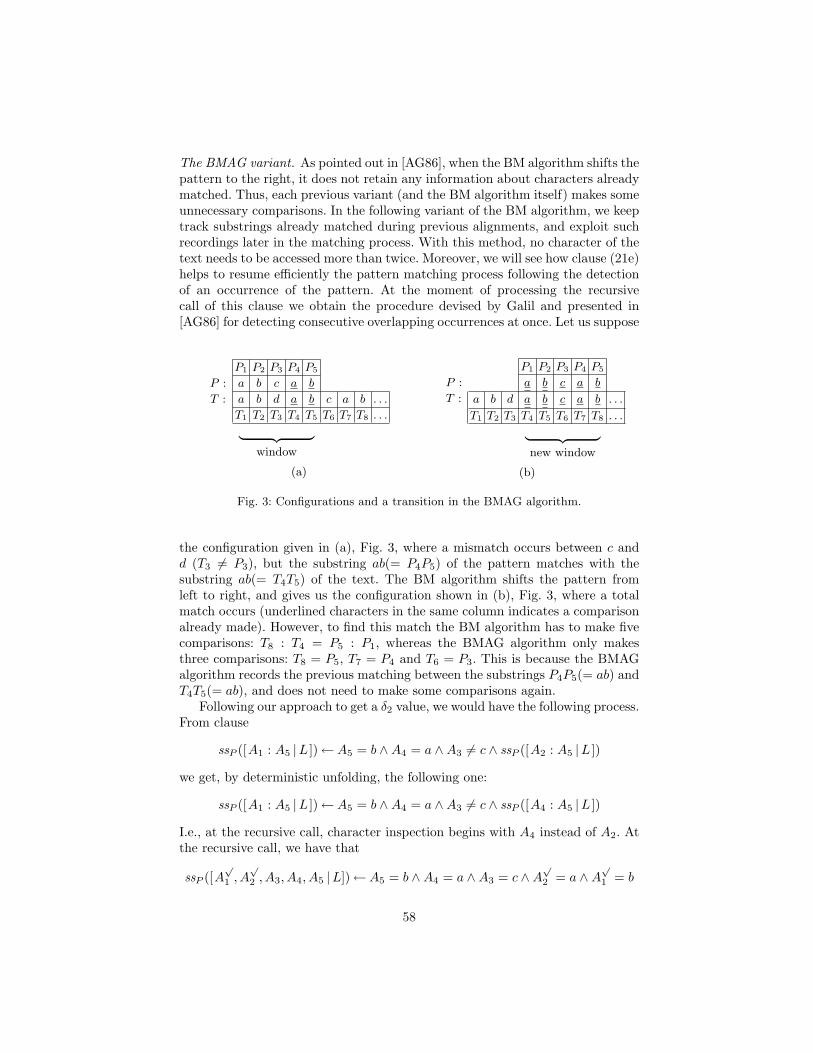
The BMAG variant. As pointed out in [AG86], when the BM algorithm shifts thepattern to the right, it does not retain any information about characters alreadymatched. Thus, each previous variant (and the BM algorithm itself) makes someunnecessary comparisons. In the following variant of the BM algorithm, we keeptrack substrings already matched during previous alignments, and exploit suchrecordings later in the matching process. With this method, no character of thetext needs to be accessed more than twice. Moreover, we will see how clause (21e)helps to resume efficiently the pattern matching process following the detectionof an occurrence of the pattern. At the moment of processing the recursivecall of this clause we obtain the procedure devised by Galil and presented in[AG86] for detecting consecutive overlapping occurrences at once. Let us suppose

P1 P2 P3 P4 P5

P : a b c a b

T : a b d a b c a b . . .

T1 T2 T3 T4 T5 T6 T7 T8 . . .| {z }window

(a)

P1 P2 P3 P4 P5

P : a b c a b

T : a b d a b c a b . . .

T1 T2 T3 T4 T5 T6 T7 T8 . . .| {z }new window

(b)

Fig. 3: Configurations and a transition in the BMAG algorithm.

the configuration given in (a), Fig. 3, where a mismatch occurs between c andd (T3 6= P3), but the substring ab(= P4P5) of the pattern matches with thesubstring ab(= T4T5) of the text. The BM algorithm shifts the pattern fromleft to right, and gives us the configuration shown in (b), Fig. 3, where a totalmatch occurs (underlined characters in the same column indicates a comparisonalready made). However, to find this match the BM algorithm has to make fivecomparisons: T8 : T4 = P5 : P1, whereas the BMAG algorithm only makesthree comparisons: T8 = P5, T7 = P4 and T6 = P3. This is because the BMAGalgorithm records the previous matching between the substrings P4P5(= ab) andT4T5(= ab), and does not need to make some comparisons again.

Following our approach to get a δ2 value, we would have the following process.From clause

ssP ([A1 : A5 |L ])←A5 = b ∧A4 = a ∧A3 6= c ∧ ssP ([A2 : A5 |L ])

we get, by deterministic unfolding, the following one:

ssP ([A1 : A5 |L ])←A5 = b ∧A4 = a ∧A3 6= c ∧ ssP ([A4 : A5 |L ])

I.e., at the recursive call, character inspection begins with A4 instead of A2. Atthe recursive call, we have that

ssP ([A√

1 , A√

2 , A3, A4, A5 |L])←A5 = b ∧A4 = a ∧A3 = c ∧A√

2 = a ∧A√

1 = b

58

where the√

in A√

1 , and A√

2 indicates that A1 and A2 are already known.To avoid unnecessary comparisons, we treat separately each case of overlap-

ping. In our example we continue as follows. We define a predicate ssbacP :

ssbacP ([A1, A2, A3, A4, A5 ])←A5 = b ∧A4 = a ∧A3 = c

for avoiding to compare again the substring ab:

ssP ([A1 : A5 |L ])←A5 = b ∧A4 = a ∧A3 6= c ∧ ssbacP ([A4 : A5 |L ])

Variables A1 and A2 are only used as places to be omitted in a re-scanning.Further optimizations can be achieved by applying our previous technology tossbac

P (clause splitting, deterministic unfolding, and folding, but now only toA5 = b ∧A4 = a ∧A3 = c).

Because there exist at most m suffixes of a pattern of length m, we deal withat most m special cases. Even more, some suffixes (implicit in the recursive call)of the same length can be analyzed as a particular case.

Formally, to derive the BMAG algorithm, we need some means to keep trackof which segments of the text matched some suffix of the pattern. In our deriva-tion, we detect such suffixes in the recursive call of each clause after applyingdeterministic unfolding to such a clause:

ssP ([A1 : Am|L ])←Am : Ak+1 = pm : pk+1 ∧Ak 6= pk ∧ (42)shift(d(k), [A2 : Am|L ], L1) ∧ ssP (L1) (43)

where d(k) is a displacement value (d(k) is always at least 1). With a displace-ment of d(k) we detect d(k)− 1 coinciding characters. The complementary partin the pattern has m− d(k) characters.

sspm:pm−d(k)

P p([A1 : Am|L ])←Am : Am−d(k) = pm : pm−d(k) (44)

Hence, d(k) characters are not more revisited. The new formulation of (43) is:

ssP ([A1 : Am|L ])←Am : Ak+1 = pm : pk+1 ∧Ak 6= pk ∧ (45)shift(d(k), [A2 : Am|L ], L1) ∧ sspm:pm−d(k)

P (L1) (46)

This is called prefix memorization in [CR02, p.30]. Applying the clause split-ting rule to the new defined predicates, we create new (sub)-triangular forms,to deal with every case of mismatching. If there exists a mismatching we callto ssP /1 (upper level) to deal with a possible total occurrence of the pattern.Furthermore, it is possible to do some extra deterministic unfolding steps and,finally, we can apply a systematic folding to the sub-triangular form to reducenondeterminism.

Let us detail the procedure. First, we create new definitions:

new([B1 : Bm |L ])←Bm : Bm−k = pm : pm−k (47)new([B1 : Bm |L ])← ssP ([B1 : Bm|L ]) (48)

We only need to analyze cases from Bm−k to Bm at the next call of ssP /1.The next task is to define new predicates to separately treat each clause. Nowwe apply the clause splitting rule, but only to Bm−k : Bm; next, we applydeterministic unfolding; finally, we fold for eliminating nondeterminism.

59

5 Related work

In [CD78,Dar78,RS83] the authors obtain families of several kind of algorithmsby using formal languages, but the mechanization of their derivations is left asan open problem. In our case, when dealing with string-matching algorithms,some parts of our derivations are mechanizable (mainly those parts supportedby partial deduction), but to obtain specific algorithms some human assistanceis necessary. In [PS90] and [Pep91] there are derivations of the search part ofthe BMPS variant. In [MACD01] there is a derivation of a simplified version(which includes the shifts given by the δ1 function) of the search part of theBoyer–Moore algorithm using a naive specification equipped with a database torecord comparisons. The complete search phase of the Boyer–Moore algorithmwas derived in [DRK06]. In [Bir05] there is a derivation of another variant ofthe Boyer–Moore algorithm, relying on the definition of δ2. In contrast to theseworks, we have begun with nondeterministic programs, and instead of explicitbacktracking, we have taken benefit from nondeterminism of logic programming.

6 Conclusions

This paper has shown several relationships among variants of an algorithm vialogic program transformation. The selection of design decisions has been guidedby known algorithms. The final programs have some inefficiency related with theaccess in linear time of lists. However, it can be asserted that all our machineryperforms well over specifications based on indexing; this has been showed at leastfor the BM variant restricted to use only the δ2 function in [HR03].

As future work, a proposal is to add some other string-matching algorithmsto the taxonomy presented here. In fact, at least two left-to-right algorithmscan also be obtained from our techniques by altering the matching schedule:the Morris–Pratt and the Knuth–Morris–Pratt algorithms. In a similar vein, theSimon algorithm, as described in [CR94], is another candidate to be derived andadded to the taxonomy. Depending on some more liberal matching schedules,some other algorithms could be included, for example, those described in [Sun90],and that hybrid algorithm described in [CP91], based on a complex preprocessingby factoring of the pattern.

Other possible taxonomies related to text processing would be based on tak-ing the text as static, instead of the pattern. McCreight and Ukkonen algorithmswould be good candidates to be derived. Approximate string-matching is alsoanother area to be explored.

Acknowledgments

Support for this work came from Consejo Nacional de Tecnologıa (CONACYT)and Universidad Tecnologica de la Mixteca (UTM). I would like to thank DavidRosenblueth by sharing with me some of his views on program transformation.I also grateful the reviewers of WFLP’09 for their valuable comments.

60

References

[AG86] Alberto Apostolico and Rafaelle Giancarlo. The Boyer–Moore–Galil stringsearching strategies revisited. SIAM J. Comput., 15(1):98–105, February1986.

[BdM97] Richard Bird and Oege de Moor. Algebra of Programming. Prentice Hall,1997.

[Bir05] Richard Bird. Polymorphic string matching. In Haskell’05, Tallin,Estonia,September 2005. ACM.

[BM77] Robert S. Boyer and J. Strother Moore. A Fast String Searching Algorithm.Communications of the Association for Computing Machinery, 20(10), Oc-tober 1977.

[CD78] Keith L. Clark and John Darlington. Algorithm classification through syn-thesis. The computer journal, 23(1):61–65, 1978.

[CD89] Charles Consel and Olivier Danvy. Partial Evaluation of Pattern Matchingin Strings. Information Processing Letters, 30(2):79–86, 1989.

[Cla78] Keith L. Clark. Negation as Failure. In H. Gallaire and J. Minker, editors,Logic and Databases, pages 293–322. Plenum Press, New York, 1978.

[CP91] Maxime Crochemore and Dominique Perrin. Two-way string-matching.Journal of the ACM, 38(3), July 1991.

[CR94] Maxime Crochemore and Wojciech Rytter. Text Algorithms. Oxford Uni-versity Press, 1994.

[CR02] Maxime Crochemore and Wojciech Rytter. Jewels of Stringology. WorldScientific Publishing, 2002.

[Dar78] John Darlington. A synthesis of several sorting algorithms. Acta Informat-ica, 11:1–30, 1978.

[DRK06] Olivier Danvy and Henning Rohde Korsholm. On obtaining the boyer–moore string-matching algorithm by partial evaluation. Information Pro-cessing Letters, 99(4), August 2006.

[FPP02] Fabio Fioravanti, Alberto Pettorossi, and Maurizio Proietti. Specializationwith clause splitting for deriving deterministic constraint logic programs.In Proceedings of the IEEE International Conference on Systems, Man, andCybernetics (SMC’02), Hammamet,Tunisia, October 2002. IEEE ComputerSociety Press.

[GK94] Manolis Gergatsoulis and Maria Katzouraki. Unfold/fold Transformationsfor Definite Clause Programs. In Manuel Hermenegildo and Jaan Penjam,editors, Programming Language Implementation and Logic Programming,volume 844 of Lecture Notes in Computer Science. 6th International Sym-posium, PLILP’94, Springer-Verlag, September 1994.

[Hor80] R. Nigel Horspool. Practical Fast Searching in Strings. Software—Practiceand experience, 10(6):501–506, 1980.

[HR01] Manuel Hernandez and David Rosenblueth. Development Reuse and theLogic Program Derivation of Two String-Matching Algorithms. In Proceed-ings of the 3rd International ACM SIGPLAN Conference on Principles andPractice of Declarative Programming (PPDP’01), pages 38–48, Florence,Italy, September 2001.

[HR03] Manuel Hernandez and David Rosenblueth. A Disjunctive Partial Deduc-tion of a Right-to-Left String-Matching Algorithm. Information ProceesingLetters, 87(5):235–241, September 2003.

61

[KMP77] Donald E. Knuth, James H. Morris, and Vaughan R. Pratt. Fast PatternMatching in Strings. SIAM Journal of Computation, 6(2):323–350, June1977.

[Lau89] Kung-Kiu Lau. A Note on Synthesis and Classification of Sorting Algo-rithms. Acta Informatica, 27:73–80, 1989.

[Llo87] John W. Lloyd. Foundations of Logic Programming. Springer-Verlag, se-cond edition, 1987.

[MACD01] Karoline Malmkjr, Torben Amtoft, Charles Consel, and Olivier Danvy. Theabstraction and instantiation of string-matching programs. In The Essenceof Computation: Complexity, Analysis, Transformation. Essays Dedicatedto Neil D. Jones, number 2566 in Lecture Notes in Computer Science, pages332–357. Springer-Verlag, 2001.

[Par76] David L. Parnas. On the design and development of program families. IEEETransactions of Software Engineering, SE-2(1):1–9, March 1976.

[Pep91] Peter Pepper. Literate Program Derivation: A Case Study. In M. Broy andM. Wirsing, editors, Methods of Programming, volume 544 of Lecture Noteson Computer Science, pages 101–124. Springer-Verlag, 1991.

[PP98] Alberto Pettorossi and Maurizio Proietti. Transformation of logic programs.In D.M. Gabbay, C.J. Hogger, and J.A. Robinson, editors, Handbook ofLogic in Artificial Intelligence and Logic Programming, volume 5, pages697–787. Oxford University Press, 1998.

[PPR97] Alberto Pettorossi, Maurizio Proietti, and Sophie Renault. Enhancing Par-tial Deduction via Unfold/Fold Rules. In Logic Program Synthesis andTransformation, volume 1207 of Lecture Notes in Computer Science. LOP-STR’96, Springer-Verlag, August 1997.

[PS90] Helmut A. Partsch and Frank A. Stomp. A fast pattern matching algorithmderived by transformational and assertional reasoning. Formal Aspects ofComputing, 2:109–122, 1990.

[RS83] John H. Reif and William L. Scherlis. Deriving efficient graphs algorithms.In Springer-Verlag, editor, Logic of programs (Proceedings 1983), volume164, pages 421–441. LNCS, 1983.

[SGJ96] Morten H. Sørensen, Robert Gluck, and Neil D. Jones. A positive super-compiler. Journal of functional programming, 6(6):811–838, 1996.

[Smi91] Donald A. Smith. Partial Evaluation of Pattern Matching in ConstraintLogic Programming Language. In Proceedings of the Symposium on PartialEvaluation and Semantics-Based Program Manipulation,PEPM’91, pages62–71, Connecticut, USA, June 1991. ACM Press.

[Ste94] Graham A. Stephen. String Searching Algorithms, volume 3 of LectureNotes Series on Computing. World Scientific Publishing, 1994.

[Sun90] Daniel M. Sunday. A very fast substring search algorithm. Communicationsof the ACM, 33(8), August 1990.

[WZ96] Bruce W. Watson and Gerard Zwaan. A taxonomy of sublinear multiplekeyword pattern matching algorithms. Science of Computer Programming,27(2):85–118, September 1996.

62

A Simple Region Inference Algorithm for aFirst-Order Functional Language ?

Manuel Montenegro, Ricardo Pena, Clara Segura

Departamento de Sistemas Informaticos y ComputacionUniversidad Complutense de Madrid, Spain

montenegro@fdi.ucm.es, {ricardo,csegura}@sip.ucm.es.

Abstract. Safe is a first-order eager language with facilities for pro-grammer controlled destruction and copying of data structures. It pro-vides also regions, i.e. disjoint parts of the heap, where the program allo-cates data structures. The runtime system does not need a garbage collec-tor and all allocation/deallocation actions are done in constant time. Thelanguage is aimed at inferring and certifying upper bounds for memoryconsumption in a Proof Carrying Code environment. Some of its analyseshave been presented elsewhere [8, 7]. In this paper we present an inferencealgorithm for annotating programs with regions which is both simpler tounderstand and more efficient than other related algorithms. Program-mers are assumed to write programs and to declare datatypes withoutany reference to regions. The algorithm decides the regions needed byevery function. It also allows polymorphic recursion with respect to re-gions. We show convincing examples of programs before and after regionannotation, prove the correctness and optimality of the algorithm, andgive its asymptotic cost.

1 Introduction

Safe1 [7] was introduced as a research platform for investigating the suitability offunctional languages for programming small devices and embedded systems withstrict memory requirements. The final aim is to be able to infer —at compiletime— safe upper bounds on memory consumption for most Safe programs. Thecompiler produces Java bytecode as a target language, so that Safe programscan be executed in most mobile devices and web navigators.

In most functional languages memory management is delegated to the run-time system. Fresh heap memory is allocated during program evaluation as longas there is enough free memory available. Garbage collection interrupts programexecution in order to copy or mark the live part of the heap so that the rest isconsidered as free. This does not avoid memory exhaustion if not enough freememory is recovered to continue execution. In that case the program simply? Work supported by the Ministry of Science grants AP2006-02154, TIN2008-

06622-C03-01/TIN (STAMP), and the Madrid Government grant S-0505/TIC/0407(PROMESAS).

1 http://dalila.sip.ucm.es/safe

aborts. The main advantage of this approach is that programmers do not haveto bother about low level details concerning memory management. Its maindisadvantages are:

1. The time delay introduced by garbage collection may prevent the programfrom providing an answer in a required reaction time.

2. Memory exhaustion may provoke unacceptable personal or economic damageto program users.

3. The programmer cannot easily reason about memory consumption.

These reasons make garbage collectors not very convenient for programmingsmall devices. A possibility is to use heap regions, which are disjoint parts of theheap that are dynamically allocated and deallocated. Much work has been donein order to incorporate regions in functional languages. They were introducedby Tofte and Talpin [13, 14] in MLKit by means of a nested letregion constructinferred by the compiler. The drawbacks of nested regions are well-known andthey have been discussed in many papers (see e.g. [4]). The main problem is thatin practice data structures do not always have the nested lifetimes required bythe stack-based region discipline.

In order to overcome this limitation several mechanisms have been proposed.An extension of Tofte and Talpin’s work [2, 11] allows to reset all the data struc-tures in a region, without deallocating the whole region. The AFL system [1]inserts (as a result of an analysis) allocation and deallocation commands sep-arated from the letregion construct, which now only brings new regions intoscope. In both cases, a deep knowledge about the hidden mechanism is neededin order to optimize the memory usage. In particular, it is required to writecopy functions in the program which are difficult to justify without knowing theannotations inferred later by the compiler.

Another more explicit approach is to introduce a language construct to freeheap memory. Hofmann and Jost [5] introduce a pattern matching constructwhich destroys individual constructor cells than can be reused by the memorymanagement system. This allows the programmer to control the memory con-sumed by the program and to reason about it. However, this approach givesthe programmer the whole responsibility for reusing memory, unless garbagecollection is used.

In order to overcome the problems related to nested regions, our functionallanguage Safe has a semi-explicit approach to memory control: it combines im-plicit regions with explicit destructive pattern matching, which deallocates in-dividual cells of a data structure. In Safe, regions are allocated/deallocated byfollowing a stack discipline associated to function calls and returns. Each func-tion call allocates a local working region, which is deallocated when the functionreturns. Region management does not add a significant runtime overhead be-cause all its related operations run in constant time [9]. Notice that regions andexplicit destruction are orthogonal mechanisms: we could have destruction with-out regions and the other way around. This combination of explicit destructionand implicit regions is novel in the functional programming field.

64

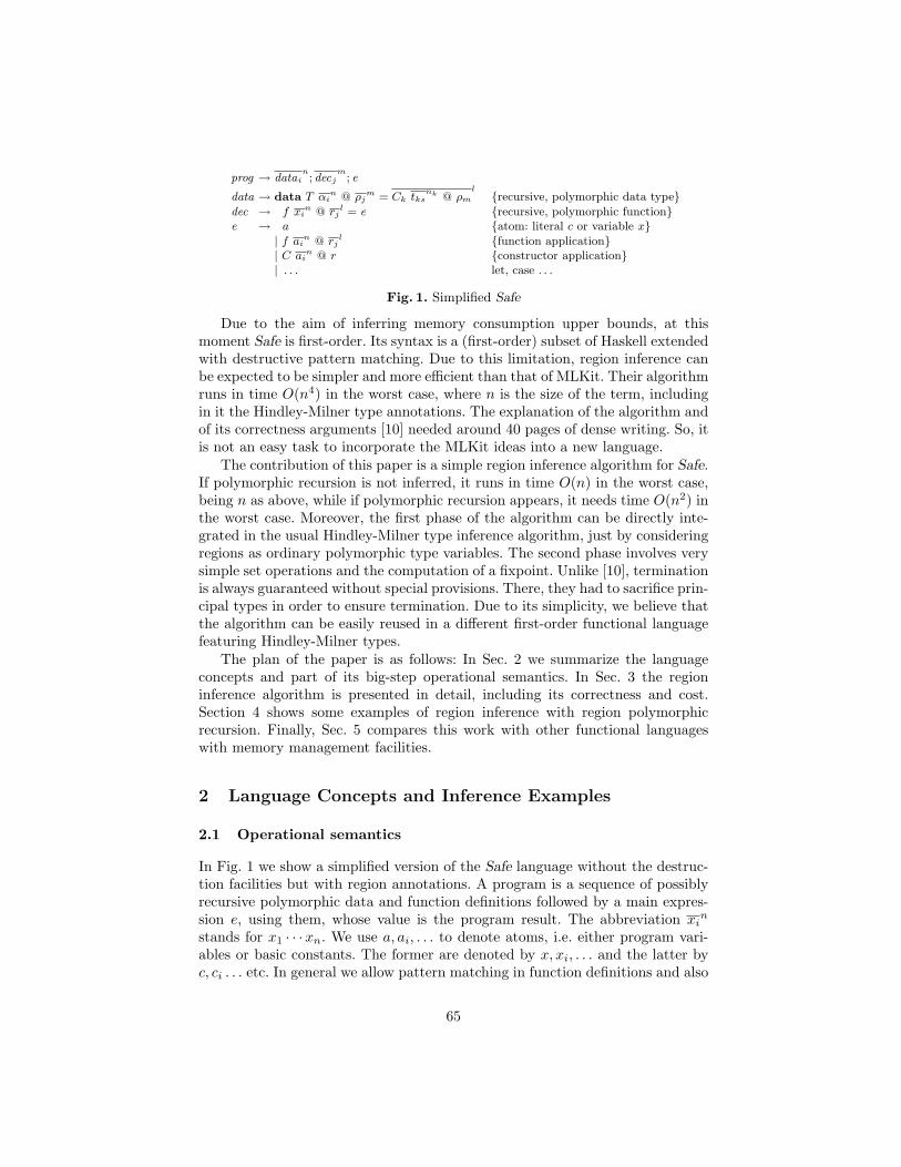
prog → datain; decj

m; e

data → data T αin @ ρj

m = Ck tksnk @ ρm

l{recursive, polymorphic data type}

dec → f xin @ rj

l = e {recursive, polymorphic function}e → a {atom: literal c or variable x}

| f ain @ rj

l {function application}| C ai

n @ r {constructor application}| . . . let, case . . .

Fig. 1. Simplified Safe

Due to the aim of inferring memory consumption upper bounds, at thismoment Safe is first-order. Its syntax is a (first-order) subset of Haskell extendedwith destructive pattern matching. Due to this limitation, region inference canbe expected to be simpler and more efficient than that of MLKit. Their algorithmruns in time O(n4) in the worst case, where n is the size of the term, includingin it the Hindley-Milner type annotations. The explanation of the algorithm andof its correctness arguments [10] needed around 40 pages of dense writing. So, itis not an easy task to incorporate the MLKit ideas into a new language.

The contribution of this paper is a simple region inference algorithm for Safe.If polymorphic recursion is not inferred, it runs in time O(n) in the worst case,being n as above, while if polymorphic recursion appears, it needs time O(n2) inthe worst case. Moreover, the first phase of the algorithm can be directly inte-grated in the usual Hindley-Milner type inference algorithm, just by consideringregions as ordinary polymorphic type variables. The second phase involves verysimple set operations and the computation of a fixpoint. Unlike [10], terminationis always guaranteed without special provisions. There, they had to sacrifice prin-cipal types in order to ensure termination. Due to its simplicity, we believe thatthe algorithm can be easily reused in a different first-order functional languagefeaturing Hindley-Milner types.

The plan of the paper is as follows: In Sec. 2 we summarize the languageconcepts and part of its big-step operational semantics. In Sec. 3 the regioninference algorithm is presented in detail, including its correctness and cost.Section 4 shows some examples of region inference with region polymorphicrecursion. Finally, Sec. 5 compares this work with other functional languageswith memory management facilities.

2 Language Concepts and Inference Examples

2.1 Operational semantics

In Fig. 1 we show a simplified version of the Safe language without the destruc-tion facilities but with region annotations. A program is a sequence of possiblyrecursive polymorphic data and function definitions followed by a main expres-sion e, using them, whose value is the program result. The abbreviation xi

n

stands for x1 · · ·xn. We use a, ai, . . . to denote atoms, i.e. either program vari-ables or basic constants. The former are denoted by x, xi, . . . and the latter byc, ci . . . etc. In general we allow pattern matching in function definitions and also

65

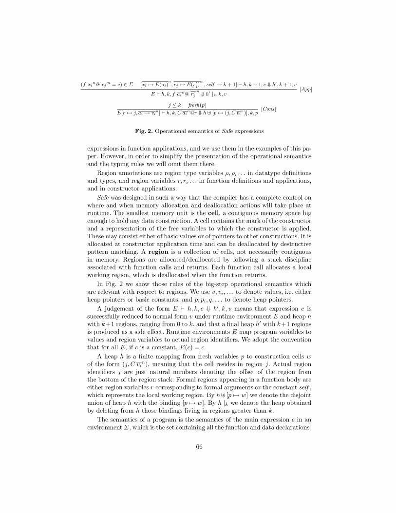
(f xin@ rj

m = e) ∈ Σ [xi 7→ E(ai)n, rj 7→ E(r′

j)m

, self 7→ k + 1] ` h, k + 1, e ⇓ h′, k + 1, v

E ` h, k, f ain@ r′

j

m ⇓ h′ |k, k, v[App]

j ≤ k fresh(p)

E[r 7→ j, ai 7→ vin] ` h, k, C ai

n@r ⇓ h ] [p 7→ (j, C vin)], k, p

[Cons]

Fig. 2. Operational semantics of Safe expressions

expressions in function applications, and we use them in the examples of this pa-per. However, in order to simplify the presentation of the operational semanticsand the typing rules we will omit them there.

Region annotations are region type variables ρ, ρi . . . in datatype definitionsand types, and region variables r, ri . . . in function definitions and applications,and in constructor applications.

Safe was designed in such a way that the compiler has a complete control onwhere and when memory allocation and deallocation actions will take place atruntime. The smallest memory unit is the cell, a contiguous memory space bigenough to hold any data construction. A cell contains the mark of the constructorand a representation of the free variables to which the constructor is applied.These may consist either of basic values or of pointers to other constructions. It isallocated at constructor application time and can be deallocated by destructivepattern matching. A region is a collection of cells, not necessarily contiguousin memory. Regions are allocated/deallocated by following a stack disciplineassociated with function calls and returns. Each function call allocates a localworking region, which is deallocated when the function returns.

In Fig. 2 we show those rules of the big-step operational semantics whichare relevant with respect to regions. We use v, vi, . . . to denote values, i.e. eitherheap pointers or basic constants, and p, pi, q, . . . to denote heap pointers.

A judgement of the form E ` h, k, e ⇓ h′, k, v means that expression e issuccessfully reduced to normal form v under runtime environment E and heap hwith k+1 regions, ranging from 0 to k, and that a final heap h′ with k+1 regionsis produced as a side effect. Runtime environments E map program variables tovalues and region variables to actual region identifiers. We adopt the conventionthat for all E, if c is a constant, E(c) = c.

A heap h is a finite mapping from fresh variables p to construction cells wof the form (j, C vi

n), meaning that the cell resides in region j. Actual regionidentifiers j are just natural numbers denoting the offset of the region fromthe bottom of the region stack. Formal regions appearing in a function body areeither region variables r corresponding to formal arguments or the constant self ,which represents the local working region. By h] [p 7→ w] we denote the disjointunion of heap h with the binding [p 7→ w]. By h |k we denote the heap obtainedby deleting from h those bindings living in regions greater than k.

The semantics of a program is the semantics of the main expression e in anenvironment Σ, which is the set containing all the function and data declarations.

66

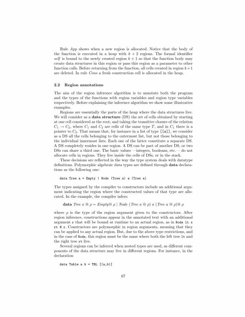
Rule App shows when a new region is allocated. Notice that the body ofthe function is executed in a heap with k + 2 regions. The formal identifierself is bound to the newly created region k + 1 so that the function body maycreate data structures in this region or pass this region as a parameter to otherfunction calls. Before returning from the function, all cells created in region k+1are deleted. In rule Cons a fresh construction cell is allocated in the heap.

2.2 Region annotations

The aim of the region inference algorithm is to annotate both the programand the types of the functions with region variables and region type variablesrespectively. Before explaining the inference algorithm we show some illustrativeexamples.

Regions are essentially the parts of the heap where the data structures live.We will consider as a data structure (DS) the set of cells obtained by startingat one cell considered as the root, and taking the transitive closure of the relationC1 → C2, where C1 and C2 are cells of the same type T , and in C1 there is apointer to C2. That means that, for instance in a list of type [[a]], we consideras a DS all the cells belonging to the outermost list, but not those belonging tothe individual innermost lists. Each one of the latter constitute a separate DS.A DS completely resides in one region. A DS can be part of another DS, or twoDSs can share a third one. The basic values —integers, booleans, etc.— do notallocate cells in regions. They live inside the cells of DSs, or in the stack.

These decisions are reflected in the way the type system deals with datatypedefinitions. Polymorphic algebraic data types are defined through data declara-tions as the following one:

data Tree a = Empty | Node (Tree a) a (Tree a)

The types assigned by the compiler to constructors include an additional argu-ment indicating the region where the constructed values of that type are allo-cated. In the example, the compiler infers:

data Tree a @ ρ = Empty@ ρ | Node (Tree a @ ρ) a (Tree a @ ρ)@ ρ

where ρ is the type of the region argument given to the constructors. Afterregion inference, constructions appear in the annotated text with an additionalargument r that will be bound at runtime to an actual region, as in Node lt x

rt @ r. Constructors are polymorphic in region arguments, meaning that theycan be applied to any actual region. But, due to the above type restrictions, andin the case of Node, this region must be the same where both the left tree lt andthe right tree rt live.

Several regions can be inferred when nested types are used, as different com-ponents of the data structure may live in different regions. For instance, in thedeclaration

data Table a b = TBL [(a,b)]

67

the following three region types will be inferred for the Table datatype:

data Table a b @ ρ1 ρ2 ρ3 = TBL ([(a, b)@ ρ1]@ ρ2)@ ρ3

In that case we adopt the convention that the last region type in the list is theoutermost one where the constructed values of the datatype are to be allocated.

After region inference, function applications are annotated with the addi-tional region arguments which the function uses to construct DSs. For instance,in the definition

concat [] ys = ys

concat (x:xs) ys = x : concat xs ys

the compiler infers the type concat :: ∀aρ1ρ2.[a]@ρ1 → [a]@ρ2 → ρ2 → [a]@ρ2

and annotates the text as follows:

concat [] ys @ r = ys

concat (x:xs) ys @ r = (x : concat xs ys @ r) @ r

The region of the output list and that of the second input list must be the samedue to the sharing between both lists introduced by the first equation. Functionsare also polymorphic in region types, i.e. they can accept as arguments any actualregions provided that they satisfy the type restrictions (for instance, in the caseof concat, that the second and the output lists must live in the same region).Sometimes, several region arguments are needed as in:

partition y [] = ([],[])

partition y (x:xs) | x <= y = (x:ls,gs)

| x > y = (ls ,x:gs)

where (ls,gs) = partition y xs

The inferred type is partition :: ∀ρ1ρ2ρ3ρ4.Int → [Int ]@ρ1 → ρ2 → ρ3 → ρ4 →([Int ]@ρ2, [Int ]@ρ3)@ρ4. The algorithm splits the output in as many regions aspossible. This gives more general types and allows the garbage to be deallocatedsooner.

When a function body is executing, the live regions are the working regions ofall the active function calls leading to this one. The live regions in scope are thosewhere the argument DSs live (for reading), those received as additional argu-ments (for reading and writing) and the own self region. The following examplebuilds an intermediate tree not needed in the output:

treesort xs = inorder (makeTree xs)

where the inferred types are as follows:

makeTree :: ∀aρ1ρ2.[a]@ρ1 → ρ2 → Tree a@ρ2

inorder :: ∀aρ1ρ2.Tree a@ρ1 → ρ2 → [a]@ρ2

treesort :: ∀aρ1ρ2.[a]@ρ1 → ρ2 → [a]@ρ2

After region inference, the definition is annotated as follows:

68

fresh(ρself ), ρself 6∈ regions(s) R = regions(tin) ∪ {ρj

l} ∪ regions(s)

Γ + [xi : ti]n

+ [rj : ρj ]l+ [self : ρself ] + [f : ∀ρ ∈ R . ti

n → ρjl → s] ` e : s

{Γ} f xin @ rj

l = e {Γ + [f : gen(∀ρ ∈ R . tin → ρj

l → s, Γ )]}[FUNB]

Σ(C) = σ sin → ρ → T @ρm � σ Γ = ([ai : si]

n

i=1) + [r : ρ]

Γ ` C ain@r : T @ρm [CONS]

Fig. 3. Rule for function definitions

treesort xs @ r = inorder (makeTree xs @ self) @ r

i.e. the intermediate tree is created in the self region and it is deallocated upontermination of treesort.

The region inference mechanism will not lead to rejecting programs. It alwayssucceeds although, of course, it will not be able to detect all garbage. Section 3explains how the algorithm works and shows that it is optimal in the sense thatit assigns as many DS as possible to the self region of the function at hand.

3 The Region Inference Algorithm

The main correctness requirement to the region inference algorithm is that theannotated type of each function can be assigned to the corresponding annotatedfunction in the type system defined in [7]. The main constraints posed by thatsystem with respect to regions are reflected in the function and constructortyping rules, shown in Fig. 3.

In rule [FUNB] the fresh (local) program region variable self is assigneda fresh type variable ρself that cannot appear in the function result type. Thisprevents dangling pointers arising by region deallocation at the end of a functioncall. The only regions in scope for writing are self and the argument regions.

Notice that region polymorphic recursion is allowed: inside the body e, dif-ferent applications of f may use different regions. We use gen(σ′, Γ ) and tf � σto respectively denote (standard) generalization of a type with respect to typevariables excluding region types, and instantiation of a polymorphic type.

The types of the constructors are given in an initial environment Σ builtfrom the datatype declarations. These types reflect the fact that the recursivesubstructures live in the same region. For example, in the case of lists and trees:

[ ] : ∀a, ρ.ρ → [a]@ρ(:) : ∀a, ρ.a → [a]@ρ → ρ → [a]@ρEmpty : ∀a, ρ.ρ → Tree a@ρNode : ∀a, ρ.Tree a@ρ → a → Tree a@ρ → ρ → Tree a@ρ

As a consequence, rule [CONS] may force some of the actual arguments to livein the same regions.

69

decorProg :: Assumps -> Prog a -> (Assumps, Prog ExpTipo)decorProg asInit (datas, defs, exp) = (as’,(datas’, concat defs’, exp’))

where (as,datas’) = decorDecsData asInit datasgroups = groupBy sameName defs(as’, defs’) = mapAccumL decorAndGenOuterDefs as groupsexp’ = decorAndGenMainExp as’ exp

Fig. 4. A high-level view of the Hindley-Milner inference algorithm

3.1 A high-level view of the algorithm

Figure 4 shows a high-level view of the Hindley-Milner (abbreviated HM in thefollowing) type inference algorithm of the Safe compiler, written in Haskell, inwhich some parts have to do with region inference.

The first phase, decorDecsData, annotates the data declarations with regionvariables and infers the types of the data constructors. These are saved in theassumption environment as. A fresh region variable is generated for each non-recursive nested data type and one more for the type being defined, which isplaced as an additional argument of each constructor. Only the recursive occur-rences are forced to have the same region arguments. All the region variables arereflected in the type so that all the regions in which the structure has a portionare known. In Sec. 2.2 we have shown some examples of the result produced bythis phase.

After this, the equations defs defining functions are grouped by functionname, traversed, and their HM-types and regions inferred for each function (al-gorithm decorAndGenOuterDefs, see below), accumulating the inferred type inthe assumption environment as in order to infer subsequent function definitions.Finally, the main expression exp of the program is inferred, and decorated bydecorAndGenMainExp (not shown).

3.2 Region inference of function definitions

Figure 5 shows in Haskell-like pseudocode the HM-inference process for a singlefunction consisting of a list Defs of equations. Let us call such function f .

We have a decoration phase decorAndGenEqs which generates fresh typeand region type variables, and equations relating types that have to be unified,but delays all the unifications to a subsequent phase. Some of these equationscorrespond to the usual HM type inference, e.g. a = [b] → b, but some otherunify region type variables, e.g. ρ1 = ρ2. The decoration phase generates aset Freshexpl of fresh region type variables assigned to the region arguments ofconstructor applications and (already inferred) function applications. This setwill be needed in the second phase of region inference.

Unification equations are solved by solveEqs and handleRecCalls. The formersolves all the equations in the usual HM style except those related to the recursiveapplications of f , which are solved in a special way by the latter. This is due tothe fact that the type trecj of every application of f should be a fresh instanceof the HM type t of the function with respect to the region types. Each region

70

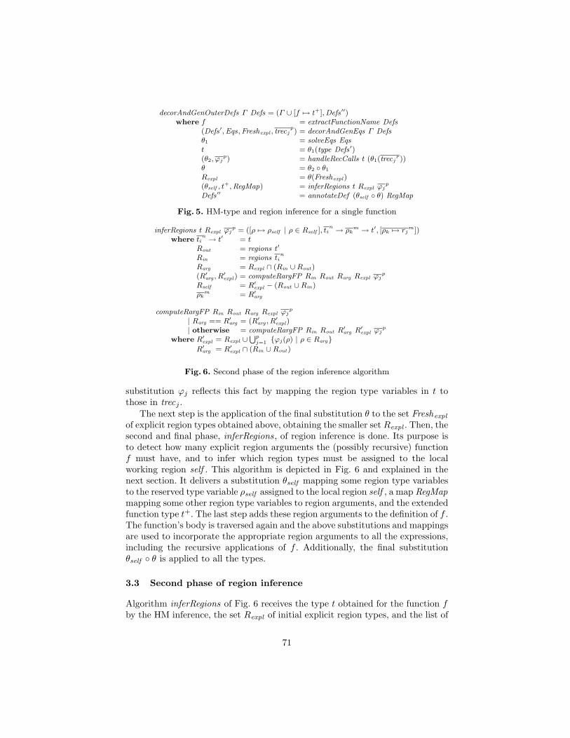
decorAndGenOuterDefs Γ Defs = (Γ ∪ [f 7→ t+],Defs ′′)where f = extractFunctionName Defs

(Defs ′,Eqs,Freshexpl , trecjp) = decorAndGenEqs Γ Defs

θ1 = solveEqs Eqst = θ1(type Defs ′)(θ2, ϕj

p) = handleRecCalls t (θ1(trecjp))

θ = θ2 ◦ θ1

Rexpl = θ(Freshexpl)(θself , t

+,RegMap) = inferRegions t Rexpl ϕjp

Defs ′′ = annotateDef (θself ◦ θ) RegMap

Fig. 5. HM-type and region inference for a single function

inferRegions t Rexpl ϕjp = ([ρ 7→ ρself | ρ ∈ Rself ], ti

n → ρkm → t′, [ρk 7→ rj

m])where ti

n → t′ = tRout = regions t′

Rin = regions tin

Rarg = Rexpl ∩ (Rin ∪Rout)(R′

arg , R′expl) = computeRargFP Rin Rout Rarg Rexpl ϕj

p

Rself = R′expl − (Rout ∪Rin)

ρkm = R′

arg

computeRargFP Rin Rout Rarg Rexpl ϕjp

| Rarg == R′arg = (R′

arg , R′expl)

| otherwise = computeRargFP Rin Rout R′arg R′

expl ϕjp

where R′expl = Rexpl ∪

Spj=1 {ϕj(ρ) | ρ ∈ Rarg}

R′arg = R′

expl ∩ (Rin ∪Rout)

Fig. 6. Second phase of the region inference algorithm

substitution ϕj reflects this fact by mapping the region type variables in t tothose in trecj .

The next step is the application of the final substitution θ to the set Freshexpl

of explicit region types obtained above, obtaining the smaller set Rexpl . Then, thesecond and final phase, inferRegions, of region inference is done. Its purpose isto detect how many explicit region arguments the (possibly recursive) functionf must have, and to infer which region types must be assigned to the localworking region self . This algorithm is depicted in Fig. 6 and explained in thenext section. It delivers a substitution θself mapping some region type variablesto the reserved type variable ρself assigned to the local region self , a map RegMapmapping some other region type variables to region arguments, and the extendedfunction type t+. The last step adds these region arguments to the definition of f .The function’s body is traversed again and the above substitutions and mappingsare used to incorporate the appropriate region arguments to all the expressions,including the recursive applications of f . Additionally, the final substitutionθself ◦ θ is applied to all the types.

3.3 Second phase of region inference

Algorithm inferRegions of Fig. 6 receives the type t obtained for the function fby the HM inference, the set Rexpl of initial explicit region types, and the list of

71

substitutions ϕjp associated to the recursive applications of f . First, it computes

the sets Rin and Rout of region type variables of respectively the argument andthe result parts of t. Let ρself be an additional fresh type variable for self .

Given these three sets, the region inference problem can be specified as findingthree sets R′

expl , R′arg and Rself , respectively standing for the sets of final explicit

region types, of region types needed as additional arguments of f , and of regiontypes that must be unified with ρself , subject to the following restrictions:

1. R′expl ⊆ Rself ∪R′

arg 3. Rself ∩ (Rin ∪Rout) = ∅2. Rself ∩R′

arg = ∅ 4. Every recursive application of f is typeable

The first one expresses that everything built by f ’s body must be in regions inscope. The second and third ones state that region self is fresh and hence differ-ent from any other region received as an argument or where an input argumentlives. These restrictions and the extension of (3) to Rout are enforced by thetyping rule [FUNB]. The last one can be further formalised by requiring that f ’stype, extended with the region arguments in R′

arg , can produce type instancesfor typing all the recursive applications of f , each one extended with as manyregion arguments as the cardinal of R′

arg . So, in order to satisfy restriction (4)one must provide a decoration of each recursive application of f with appropri-ate region arguments, of region types belonging either to Rself or to R′

arg , asrestriction (1) requires.

In Appendix ?? we show that any sets R′expl , R′

arg and Rself satisfying theserestrictions produce a version of f which admits a type in the type system. Thecorrectness of the type system with respect to the semantics was established in[7]. There, we proved that dangling pointers arising from region deallocation ordestructive pattern matching are never accessed by a well-typed program.

Notice that an algorithm choosing any R′arg ⊇ R′

expl and Rself = ∅ would becorrect according to this specification. But this solution would be very poor as,on the one hand no construction would ever be done in the self region and, onthe other, there might be region arguments never used. We look for an optimalsolution in two senses. On the one hand, we want R′

arg to be as small as possible,so that only those regions where data are built are given as arguments. On theother hand, we want Rself to be as big as possible, so that the maximum amountof memory is deallocated at function termination.

3.4 The kernel of the algorithm

Our algorithm initially computes Rarg = Rexpl ∩ (Rin ∪ Rout), by using theset Rexpl of initial explicit region types. Then, it starts a fixpoint algorithmcomputeRargFP (see Fig. 6) trying to get the type of f ’s recursive applicationsas instances of the type of f extended with the current set Rarg of arguments.It may happen that the set of explicit regions R′

expl may grow while consideringdifferent applications (see the examples in Sec. 4). Adding more explicit variablesto one application will influence the type of the applications already inferred.As R′

arg depends on R′expl , it may also grow. So, a fixpoint is used in order

to obtain the final R′arg and R′

expl from the initial ones. Due to our solution

72

above, R′arg cannot grow greater than Rin ∪Rout , so termination of the fixpoint

is guaranteed. Once obtained the final R′arg and R′

expl , the set Rself is computedas Rself = R′

expl − (Rin ∪ Rout). Notice that R′arg = R′

expl ∩ (Rin ∪ Rout) is aninvariant of the algorithm.

We show below that these choices maximise the data allocated to the selfregion, i.e. maximises garbage destruction.

3.5 Correctness, optimality and efficiency

First we prove that the proposed solution satisfies the above specification:

1. R′expl ⊆ (R′

expl − (Rin ∪Rout)) ∪ (R′expl ∩ (Rin ∪Rout))

2. (R′expl − (Rin ∪Rout)) ∩ (R′

expl ∩ (Rin ∪Rout)) = ∅3. (R′

expl − (Rin ∪Rout)) ∩ (Rin ∪Rout) = ∅

The three immediately follow by set algebra. We will show now that it is optimal:let us assume a different solution Rself , Rexpl , Rarg satisfying the above restric-tions. Notice that Rexpl ⊆ R′

expl by construction. Without loss of generality wecan rename those variables in Rexpl which decorate copy expressions, constructorapplications and function calls differerent from f , so that such decorations coin-cide with those in R′

expl . After such renaming Rexpl ⊆ Rexpl . We can also renamethe argument regions in recursive calls to f that also appear in R′

expl . For exam-ple, assume there is a recursive call decorated by R′

expl as f :: tin → ρ′1 → ρ′2 → t.

If that recursive call was decorated by Rexpl as f :: t′in→ ρ1 → ρ2 → ρ3 → t′,

then ρ1 would be renamed as ρ′1 and ρ2 as ρ′2.We must show that Rself ⊆ Rself and R′

arg ⊆ Rarg . Let us assume ρ ∈ R′arg .

By definition of R′arg , ρ ∈ R′

expl and ρ ∈ Rin ∪ Rout . By (3), ρ ∈ Rin ∪ Rout

implies that ρ /∈ Rself . Now we distinguish two cases:

ρ ∈ Rexpl As Rexpl ⊆ Rexpl , then ρ ∈ Rexpl . By (1) ρ ∈ Rarg .ρ ∈ R′

expl −Rexpl If ρ ∈ Rexpl , then by ρ ∈ Rarg . Otherwise, R′expl contains more

explicit variables which are also arguments of f than Rexpl . This case is notpossible because R′

expl is the least fixpoint of function computeRargFP byconstruction. By (4), Rexpl is also a fixpoint of computeRargFP ; otherwise,the recursive calls would not be typeable.

Consequently, ρ ∈ R′arg . So, Rarg is as small as possible. By constraints (2)

and (1), then Rself is as big as possible.Our sets are implemented as balanced trees, and operations such as ∪, ∩,

and ‘−’ are done in a time in Θ(n + m), being n and m the cardinalities ofthe respective sets, so each iteration of the fixpoint algorithm is linear with thenumber of region type variables occurring in a function body. As it is done in[10], considering as the term size n the sum of the sizes of the abstract syntaxtree and of the HM type annotations, each iteration needs time linear with thissize. If several iterations are needed, these cannot be more than the number ofregion type variables in Rin ∪Rout . This gives us O(n2) cost in the worst case.

73

4 Examples

As a first example, consider the previously defined function partition. A regionvariable ρ1 is created for the input list, so that it has type [Int ]@ρ1. In addi-tion seven fresh type region variables are generated, one for each constructorapplication, let say ρ2 to ρ8, and so Freshexpl = {ρ2, . . . , ρ8}. We show them asannotations in the program just in order to better explain the example:

partition y [ ] = ([ ] :: ρ2, [ ] :: ρ3) :: ρ4

partition y (x : xs) | x ≤ y = (x : ls :: ρ5, gs) :: ρ6

| x > y = (ls, x : gs :: ρ7) :: ρ8

where(ls, gs) = partition y xs

The type inference rules generate the following equations relative to these typeregion variables: ρ2 = ρ5, ρ3 = ρ7, and ρ4 = ρ6 = ρ8, so the initial Rexpl in thiscase is {ρ2, ρ3, ρ4}. After unification, the type of partition is Int → [Int ]@ρ1 →([Int ]@ρ2, [Int ]@ρ3)@ρ4, so Rin = {ρ1} and Rout = {ρ2, ρ3, ρ4}. Then, Rarg ={ρ2, ρ3, ρ4}. Now we shall compare the type of the definition (augmented withthe variables of Rarg) and the type used in the recursive call, where the tuple(ls, gs) is assumed to live in the region ρ9.

Definition: Int → [Int ]@ρ1 → ρ2 → ρ3 → ρ4 → ([Int ]@ρ2, [Int ]@ρ3)@ρ4

Rec. call: Int → [Int ]@ρ1 → ρ2 → ρ3 → ρ9 → ([Int ]@ρ2, [Int ]@ρ3)@ρ9

We obtain the region substitution ϕ = [ρ1 7→ ρ1, ρ2 7→ ρ2, ρ3 7→ ρ3, ρ4 7→ ρ9].As a consequence, the variable ρ9 is made explicit, so Rexpl = {ρ2, ρ3, ρ4, ρ9}.The set Rarg does not change and hence the fixpoint has been computed. Weget Rself = {ρ9} and the program is annotated as follows:

partition :: Int → [Int ]@ρ1 → ρ2 → ρ3 → ρ4 → ([Int ]@ρ2, [Int ]@ρ3)@ρ4

partition y [ ] @ r2 r3 r4 = ([ ]@r2, [ ]@r3)@r4

partition y (x : xs) @ r2 r3 r4 | x ≤ y = ((x : ls)@r2, gs)@r4

| x > y = (ls, (x : gs)@r3)@r4

where (ls, gs) = partition y xs @ r2 r3 self

Notice that the tuple resulting from the recursive call to partition is located inthe working region. Without polymorphic recursion this tuple would have to bestored in the output region r4, requiring O(n) space in a caller region.

Another example is the dynamic programming approach to computing bi-nomial coefficients by using the Pascal’s triangle. We start from the unit list[1], which corresponds to the 0-th row of the triangle. If [x0, x1, . . . , xi−1, xi] arethe elements located on the i-th row, then the elements of the i + 1-th row aregiven by the list [x0 +x1, x1 +x2, . . . , xi−1 +xi, xi]. The binomial coefficient

(nm

)can be obtained from the m-th element in the n-th row of the Pascal’s triangle.Function sumList , computes the i + 1-th row of the triangle from its i-th row:

sumList (x : [ ]) = (x : [ ] :: ρ2) :: ρ3

sumList (x : xs) = (x + y : sumList xs) :: ρ4 where (y : ) = xs

74

In the definition above we just show those region variables belonging toFreshexpl . Let us assume that after unification the input list has type [Int ]@ρ1. Inaddition, the variables ρ2, ρ3 and ρ4 are unified, so Rexpl = {ρ2} and the inferredtype (without region parameters) for sumList is [Int ]@ρ1 → [Int ]@ρ2. Hence weget Rin = {ρ1}, Rout = {ρ2} and Rarg = {ρ2}. We extend the signature ofsumList to [Int ]@ρ1 → ρ2 → [Int ]@ρ2.

Next we analyse the recursive call. Since the inferred type for xs is [Int ]@ρ1

and the type of the recursive call’s result is [Int ]@ρ2, the type for sumList inthis call is [Int ]@ρ1 → [Int ]@ρ2. By pairing with the type of sumList in thedefinition, we get that the additional argument needed in the recursive call alsohas type ρ2. Therefore, ρ2 is added to the set of explicit variables Rexpl . Sinceit was already in this set, Rexpl stays the same as the one calculated previouslyand hence Rarg also does, so the fixpoint has been reached. Finally we obtainRself = ∅ and the function is annotated as follows:

sumList :: [Int ]@ρ1 → ρ2 → [Int ]@ρ2

sumList (x : [ ]) @ r = (x : ([ ] @ r))@ rsumList (x : xs) @ r = (x + y : sumList xs @ r) @ r where (y : ) = xs

Function pascal iterates over the initial list in order to get the desired row.Below we show the region variables generated in constructor applications and innon-recursive function applications, just after type unification:

pascal 0 = (1 : [ ] :: ρ1) :: ρ1

pascal n = (1 : sumList (pascal (n− 1))) :: ρ1

The type inferred for pascal is Int → [Int ]@ρ1. Hence Rin = ∅, Rout = {ρ1}and Rexpl = {ρ1}, which gives us an initial Rarg = {ρ1}. The type signaturefor pascal changes accordingly to Int → ρ1 → [Int ]@ρ1. Let us assume that theresult of the recursive call to pascal has type [Int ]@ρ2. Therefore, the type ofthis function in the recursive call is Int → ρ2 → [Int ]@ρ2. Since ρ2 is now madeexplicit, it is added to Rexpl , which now contains the region variables {ρ1, ρ2}.However, Rarg stays the same and hence the fixpoint has been reached. Finally,we get Rself = {ρ2} and the program is annotated as follows:

pascal :: Int → ρ1 → [Int ]@ρ1

pascal 0 @ r = (1 : [ ] @ r)@ rpascal n @ r = (1 : sumList (pascal (n− 1) @ self ) @ r) @ r

The resulting list from the recursive call to pascal will be destroyed once thecalling function finishes. Hence a function call pascal n has a cost of O(n) inspace. Without polymorphic recursion the result of every recursive call would bebuilt in the output region r, which would imply a cost of O(n2) in space.

5 Related Work and Conclusions

The pioneer work on region inference is that of M. Tofte, J.-P. Talpin and theircolleagues on the MLKit compiler [14, 10] (in what follows, TT). Their languageis higher-order and they also support polymorphic recursion in region arguments.

75

The TT algorithm has two phases, respectively called S and R. The S-algorithmjust generates fresh region variables for values and introduces the lexical scope ofthe regions by using a letregion construct. The R-algorithm is responsible forassigning types to recursive functions. It deals with polymorphic recursion andalso computes a fixpoint. The total cost is in O(n4). The meaning of a typedexpression letregion ρ in e : µ is that region ρ does not occur free in typeµ, so it can be deallocated upon the evaluation of e. Our algorithm has someresemblances with this part of the inference, in the sense that we decide to unifywith ρself all the region variables not occurring in the result type of a function.They do not claim their algorithm to be optimal but in fact they create as manyregions as possible, trying to make local all the regions not needed in the finalvalue. One problem reported in [12] is that most of the regions inferred in the firstversions of the algorithm contained a single value so that region managementproduced a big overhead at runtime. Later, they added a new analysis to collapseall these regions into a single one local to the invocation (allocated in the stack).So, having a single local region self per function invocation does not seem tous to be a big drawback if function bodies are small enough. We believe thatpolymorphic recursion has a much bigger impact in avoiding memory leaks thanmultiplicity of local regions. So, we claim that the results of our algorithm arecomparable to those of TT for first-order programs.

A radical deviation from these approaches is [4] which introduces a type sys-tem in which region life-times are not necessarily nested. The compiler annotatesthe program with region variables and supports operations for allocation, releas-ing, aliasing and renaming. A reference-counting analysis is used in order todecide when a released region should be deallocated. The language is first-order.The inference algorithm [6] can be defined as a global abstract interpretationof the program by following the control flow of the functions in a backwardsdirection. Although the authors do not give either asymptotic costs or actualbenchmarks, it can be deduced that this cost could grow more than quadrati-cally with the program text size in the worst case, as a global fixpoint must becomputed and a region variable may disappear at each iteration. This lack ofmodularity could make the approach unpractical for large programs.

Another approach is [3] in which type-safe primitives are defined for creat-ing, accessing and destroying regions. These are not restricted to have nestedlifetimes. Programs are written and manually typed in a C-like language calledCyclone, then translated to a variant of λ-calculus, and then type-checked. So,the price of this flexibility is having explicit region control in the language.

The main virtue of our design is its simplicity. The previous works have norestrictions on the placement of cells belonging to the same data structure. Also,in the case of TT and its derivatives, they support higher-order functions. As aconsequence, the inference algorithms are more complex and costly. In our lan-guage, regions also suffer from the nested lifetimes constraint, since both regionallocation and deallocation are bound to function calls. However, the destructivepattern matching facility compensates for this, since it is possible to dispose ofa data structure without deallocating the whole region where it lives. Alloca-

76

tion and destruction are not necessarily nested, and our type system protectsthe programmer against misuses of this feature. Since allocation is implicit, theprice of this flexibility is the explicit deallocation of cells.

References

1. A. Aiken, M. Fahndrich, and R. Levien. Better static memory management: im-proving region-based analysis of higher-order languages. In ACM SIGPLAN Con-ference on Programming Languages Design and Implementation, PLDI’95, pages174–185. ACM Press, 1995.

2. L. Birkedal, M. Tofte, and M. Vejlstrup. From region inference to von Neumannmachines via region representation inference. In 23rd ACM Symposium on Prin-ciples of Programming Languages, POPL’96, pages 171–183. ACM Press, 1996.

3. D. Grossman, G. Morrisett, T. Jim, M. Hicks, Y. Wang, and J. Cheney. Region-based memory management in Cyclone. In ACM SIGPLAN Conference on Pro-gramming Languages Design and Implementation, PLDI’02, pages 282–293, 2002.

4. F. Henglein, H. Makholm, and H. Niss. A direct approach to control-flow sensitiveregion-based memory management. In 3rd ACM SIGPLAN International Con-ference on Principles and Practice of Declarative Programming, PPDP’01, pages175–186. ACM Press, 2001.

5. M. Hofmann and S. Jost. Static prediction of heap space usage for first-orderfunctional programs. In 30th ACM Symposium on Principles of ProgrammingLanguages, POPL’03, pages 185–197. ACM Press, 2003.

6. H. Makholm. A language-independent framework for region inference. Ph.D thesis,Univ. of Copenhagen, Dep. of Computer Science, Denmark, 2003.

7. M. Montenegro, R. Pena, and C. Segura. A type system for safe memory man-agement and its proof of correctness. In 10th International ACM SIGPLAN Sym-posium on Principles and Practice of Declarative Programming, PPDP’08, pages152–162, 2008.

8. M. Montenegro, R. Pena, and C. Segura. An inference algorithm for guarantee-ing safe destruction. In 18th International Symposium on Logic-Based ProgramSynthesis and Transformation, LOPSTR’08, Lecture Notes in Computer Science5438, pages 135–151, 2009.

9. R. Pena and C. Segura. Formally deriving a compiler for SAFE. In Draft Pro-ceedings of the 18th International Symposium on Implementation and Applicationof Functional Languages, IFL’06, Technical Report, 2006-S01. Eotvos Lorand Uni-versity, pages 429–446, 2006.

10. M. Tofte and L. Birkedal. A region inference algorithm. ACM Transactions onProgramming Languages and Systems, 20(4):724–767, 1998.

11. M. Tofte, L. Birkedal, M. Elsman, N. Hallenberg, T. H. Olesen, and P. Sestoft.Programming with regions in the MLKit (revised for version 4.3.0). Technicalreport, IT University of Copenhagen, Denmark, 2006.

12. M. Tofte and N. Hallenberg. Region-Based Memory Management in Perspective.In Invited talk Space 2001 Work., London, pages 1–8. Imperial College, Jan. 2001.

13. M. Tofte and J.-P. Talpin. Implementing the call-by-value lambda-calculus us-ing a stack of regions. In 21st ACM Symposium on Principles of ProgrammingLanguages, POPL’94, pages 188–201, Jan. 1994.

14. M. Tofte and J.-P. Talpin. Region-based memory management. Information andComputation, 132(2):109–176, 1997.

77

pFun: A semi-explicit parallel purely functional

language

Andre R. Du Bois1, Gerson Cavalheiro2, Juliana Vizzotto3

1 PPGInf - UCPel dubois@ucpel.tche.br2 UFPel

gerson.cavalheiro@ufpel.edu.br

UNIFRA juvizzotto@gmail.com

Abstract. In this paper we present the design and implementation ofpFun, a semi-explicit parallel purely functional language. Parallelism isintroduced in pFun through annotations. These annotations indicate ex-pressions that can be evaluated in parallel with the rest of the pro-gram. Task creation, synchronization and scheduling of computationson processors are managed automatically by pFun’s runtime system.pFun’s programming model and runtime system are described, and pre-liminary measurements of the current prototype implementation on anSMP-machine, a Beowulf Cluster and an small heterogeneous GRID arepresented.

1 Introduction

With the arrival of multi-core chips for domestic computers, parallel program-ming is becoming a mandatory feature in programming languages. Furthermore,networks are increasingly pervasive, and big companies are using clusters or gridsto solve large-scale computation problems. Parallel programming is hard, andit is difficult to find programmers that fully understand concurrency [23], evenmore considering the diversity of parallel architectures.

To address these challenges, we advocate the need of a programming platformthat hides most aspects of the architecture being used and limits the program-mer’s task to annotate expressions in the program that may be evaluated inparallel. Such a programming platform must be supported by an advanced run-time system that provides automatic creation, synchronization and schedulingof computations on processors.

Purely functional languages have an interesting property, called referential

transparency, that allows subexpressions of a purely functional program to beevaluated in parallel in any order, always delivering the same final result. Subex-pressions of a program will never have implicit control dependencies betweenthem, as the ones introduced by assignment [11]. Although referential trans-parency allows the evaluation of any sub-expression of a program in parallel, inpractice that would generate tasks that are too small in comparison with theoverhead of creating concurrent tasks to evaluate them [13]. Semi-explicit paral-lel functional languages [11] are languages that provide a mechanism to annotate

potentially parallel tasks and to control the granularity of these tasks but hidefrom the programmer aspects as task creation, synchronization and scheduling.

In this paper, we present pFun, a strict, strongly typed, semi-explicit parallelfunctional language. Parallelism is introduced in pFun through two constructs:par and sync, that provide an abstraction similar to Multilisp’s futures [20](Section 2.1). Creation, distribution and synchronization of tasks are left to theimplementation of the language, i.e., its runtime system. The par and sync

primitives are low level constructs to express parallelism and they can be usedto implement higher-level coordination primitives, such as algorithmic skeletons,i.e., higher-order functions that encapsulate common patterns of parallel com-puting [6].

The execution of programs on heterogeneous environments is provided bycompiling programs into architecture-independent byte-code, and pFun’s run-time system provides ways for serializing and communicating computations be-tween different processes or hosts. pFun’s runtime system is implemented usingstandard C and TCP/IP sockets for communication, maintaining a high degreeof portability. Distribution and scheduling of tasks is provided automatically bythe runtime system that is based on the GUM [25] virtual machine (Section 3.1).

This paper describes the design and implementation of pFun. The paper isorganized as follows: In the next section, we explain the pFun language andits primitives for parallel programming through examples. In section 3, pFun’sruntime system is described. Section 4 gives preliminary performance measure-ments of six different parallel programs. Finally, conclusions and future work arediscussed in Section 6.

2 The pFun Language

pFun is a strict parallel purely functional language with a syntax similar to theHaskell language [17]. The reader should be aware that pFun is not Haskell. Itssyntax is similar to Haskell only for convenience.

pFun’s syntax, semantics and parallel primitives will be presented throughexamples in the following Sections.

2.1 The pFun primitives for expressing parallelism

The pFun language provides two basic primitives for expressing parallelism: parand sync. The par primitive is used to express potential parallelism. It takesas an argument a pFun expression of any type and returns a reference to a Parvalue that represents an expression that could be evaluated in parallel:

par :: a -> Par a

The par primitive only indicates potential parallelism in the program and itdoes not guarantee that the expression will be evaluated in parallel with the restof the program. Task creation, scheduling, distribution and synchronization areleft to the implementation of the language described in Section 3.

80

The sync primitive receives as an argument a Par value and returns theresult of the evaluation of that expression:

sync :: Par a -> a

The operational behavior of the sync primitive is to block in its argumentif it is being evaluated (by a different processor or remote location) or to createa local thread to evaluate it. The sync primitive will only proceed once itsargument is evaluated to normal form.

The par and sync primitives provide the same abstraction as futures inMultilisp. The support for futures in Multilisp is given by two primitives, thatwould have the following types in Haskell:

future :: a -> a

touch :: a -> a

The future primitive creates a task to evaluate its argument and returns aplaceholder for the value that will be computed by the task. When an expressionneeds the value of a future, it can touch the future. If the future is unresolved,touch will block until the future is completely evaluated. In Multilisp, a futurecan also be implicitly touched by strict operations, i.e., if a strict operation needsthe value of a future, it will block until the result is computed. The future andtouch functions have similar expressiveness to par and sync. In pFun, the onlyway to get the result of a task is by using sync. This resembles the way thefuture abstraction is provided in modern object oriented languages like Java [9]and PLinQ [7]. Implicit touching of futures in Multilisp adds a high overheadin the implementation as every strict function must check if its argument is avalue or a future [20, 21]. As pFun is a strongly typed language checking tagsat runtime is not necessary for all operations. The only operation that needs tocheck tags is sync, as described in section 3.4. By wrapping a task in an ADT,pFun’s static type system can guarantee that sync will always be applied to Par

objects before they are used.We plan in the future to investigate how to, based on type information,

provide implicit touching of tasks by automatically inserting the sync operationin expressions.

2.2 Properties of par and sync

Semi-explicit parallel functional languages like Multilisp, GpH [24] and pFunbreak the abstraction offered by functional languages as programmers now haveto express fork/join parallelism in the code. Although primitives to expressfork/join parallelism were introduced, pFun is still a purely functional language.The primitives are well integrated in the language in the sense that the pro-grammer can reason about programs as if they were sequential. For any purelyfunctional expression exp written in pFun, the following expression will alwaysevaluate to true:

sync (par exp) == exp

81

It does not matter if a Par value is evaluated locally or on a remote processor,it will always return the same result. Hence, the following function

idps :: a -> a

idps x = sync (par x)

is equal to the identity function (id):

id x == idps x

for any expression x written in pFun.If someone wants to reason about par and sync, the Par data type should

be seen as an ADT:

data Par a = Par a

par :: a -> Par a

par x = Par x

sync :: Par a -> a

sync (Par x) = x

We are currently developing an operational semantics of pFun so that we canreason not only about the parallel algorithms but also about coordination, i.e.,how tasks are created, synchronized and distributed. The semantics of pFun iswork in progress and a draft version is available [19].

2.3 Example 1: Parallel Fibonacci

In this section we present a naive implementation of a parallel fibonacci function,just to demonstrate the use of the par and sync. A first parallel version of thefibonacci function can be implemented as:

parFib n = if (n<=1) then 1

else let

fib2 = par (parFib (n-2));

fib1 = par (parFib (n-1))

in (sync fib2) + (sync fib1);

In the definition of parFib, the two recursive calls are marked with the par

primitive to be computed in parallel. It can be very inefficient to create paralleltasks to evaluate every recursive call to parFib, since calculating fibonacci ofsmall numbers is a fine grained task. To solve this problem, we can write a moreefficient version of parFib that only creates parallel tasks when the argumentsupplied to parFib is larger than a threshold:

parFib n t = if (n<=t) then (seqFib n)

else let

fib2 = par (parFib (n-2) t);

fib1 = par (parFib (n-1) t)

in (sync fib2) + (sync fib1);

82

This new version of parFib takes an extra argument that controls the amountof parallel tasks created: if the argument supplied to parFib is smaller than thethreshold t, then seqFib is used instead of parFib.

2.4 Example 2: The parMap Skeleton

The par and sync primitives can be seen as low level constructs for parallelprogramming. Using these primitives it is possible to write more powerful ab-stractions for the pFun language, such as Algorithmic Skeletons [6]. Algorithmicskeletons are higher-order functions that encapsulate common patterns of par-allel computation.

For example, the function map, common in widely-used functional languages,is a higher-order function that takes two arguments, a function and a list, andapplies the function to every element of the list generating a new list. A parallelmap is a function that has the same type as the sequential map but applies thefunction argument to every element of the list in parallel.

To implement a parallel map in pFun, we first need a function to create paralleltasks:

parList:: (a->b) -> [a] -> [Par b]

parList f l = case l of

[] -> [];

(x:xs) -> (par (f x)) : (parList f xs);

The function parList creates a list of possible parallel tasks, and we need away of accessing the values computed by these tasks:

syncList :: [Par a] -> [a]

syncList list = map sync list;

Finally, the parMap skeleton is implemented using the functions parList andsyncList:

parMap :: (a->b) -> [a] -> [b]

parMap f l = syncList (parList f l);

Parallelism arises because parMap first uses parList to create the Par ob-jects, before syncList is used. If there are processors available they will startexecuting these Pars. Once all Pars are created, syncList is used to collect theresults. When syncList tries to consume the list produced by parList, it willeither block waiting for the result of a Par that is already being computed (inthat case the processor executing syncList will get another task to execute), orwill start executing one of the Par objects in the list.

3 The pFun Compiler and Runtime System

3.1 Distributed Scheduling

The pFun runtime runs a dynamic scheduler implementing a work stealing strat-egy. This scheduling is particularly interesting to exploit the inherent nestedfork-join program structure obtained by the par/sync parallel constructors.

83

Work stealing is a general denomination of a receiver-initiated class of dis-tributed load balancing schedulers. The basic algorithm assumes that the re-sponsibility for managing and executing the set of tasks generated by a runningapplication is shared among processors of a parallel machine. The number oftasks executing simultaneously on each processor is limited in order to alloweach processor to maintain a reserve of work represented by a ready tasks queue.The scheduler uses the length of ready queues as the load information. Also dis-tributed among the processors is the control for scheduling decisions. Dependingon the size of such queues a processor can start a scheduling operation. A proces-sor sends a request for new ready tasks (a work steal) to another randomly chosenprocessor when its local ready queue reaches a value below of a certain limit.When a processor receives a steal message it will answer with a task taken fromits local queue if the amount of work in reserve is above a certain limit; otherwisethe message is forwarded to another randomly chosen processor. pFun’s runtimesystem was mainly inspired by GUM (Graph reduction for a Unified Machinemodel) [25], a distributed virtual machine that implements GpH [24], a Haskellextension for parallel programming. Local thread scheduling and synchroniza-tion are implemented in a similar way to GUM. The main differences are onthe way work is distributed between nodes and on the portability of the system.The pFun runtime system was designed to be more adaptable to heterogeneousenvironments. Programs are compiled into byte-code, and the runtime system isimplemented using standard C and TCP/IP sockets for communication, main-taining a high degree of portability. The current prototype implementation ofpFun uses a simpler distributed model than GUM, based on work servers andslaves. The slave nodes are dedicated to execute tasks while work servers canalso answer steal requests. The par primitive adds a task to the ready queue ofa work server. Slaves are hosts that connect to a work server asking for compu-tations to execute. A slave receives work, executes it, and sends the result backto its server. Slaves keep no state: a message containing work carries all the codeand data needed to execute it. That is interesting for large scale networks sincethe code for the application does not need to be pre-loaded on all hosts. Havingthe pFun system installed on all locations, we can start a pFun program on onehost and it will spread to all locations. GUM is implemented on top of PVMand is designed to run on Beowulf clusters, hence all PEs (Processing Elements)know each other and they all function as work servers. GUM is also a closedsystem: all PEs must have the machine code for the application and once thesystem is running, no other PE can join the computation, while in pFun’s model,slaves and work-servers can join the computation at anytime. These differencesalso allow a higher degree of fault-tolerance in pFun: In GUM, if one of the PEsdies the whole computation has to stop as the state of the computation is sharedby all PEs. If a work server detects that a slave died it could send the task thatwas being evaluated by the dead slave to another one (although in the currentsystem, if a work server dies, it can not be recovered). The fact messages con-tain the code and data needed to execute tasks allows slaves to be executed in

84

Bag-Of-Tasks GRID middlewares like OurGrid [5], something that we want toexplore in the future.

pFun’s simpler distributed model and the compilation into byte-codes allowthe system to be used on heterogeneous environments with the cost of a poor per-formance on divide-conquerer parallel applications (as can be seen in Section 4).As future work, we plan to modify the current prototype to better exploit thecharacteristics of different parallel architectures (Section 6).

3.2 The compiler

The current prototype implementation of pFun supports a subset of Haskell’ssyntax with lets, algebraic data types and pattern matching (as in the exam-ples given in section 2). Programs are compiled into a set of supercombinators(functions with no free variables) in the way described in [18]. These supercom-binators are compiled into architecture independent byte-code (each supercom-binator generates a byte-code file). Having no free variables makes it easier toimplement the serialization algorithms as there are no environments to be com-municated. As the subset of Haskell implemented is accepted by any Haskellcompiler, type checking of parallel programs is done using GHCi [10] using thesequential definitions of par and sync given in section 2. We plan in the futureto have our own implementation of type checking, specially to investigate theautomatically insertion of the sync primitive described in section 2.

3.3 The Byte-Code Interpreter

The byte-code interpreter is an implementation of the SECD machine [15] usingonly one stack, and stack frames to separate nested function calls. The inter-preter, at run time, allocates its internal structures in a garbage collected heap(section 3.6).

3.4 Distributed Execution

Even though pFun is a strict functional language, in which the arguments offunctions are evaluated before function application, the par primitive has a dif-ferent semantics. The par primitive creates a suspension of its argument in theheap. A suspension represents an unevaluated expression. Suspensions are alsoused to implement partial applications of curried functions. For example, thefollowing expression:

par (f arg1 arg2 ... argn)

will create in the heap the suspension in Figure 1. It contains a header thatdescribes its type and layout, i.e., how many pointers to other heap objects it has.A suspension always contains a pointer to a function and an array of pointers tothe arguments to be consumed by the function when the computation is started.Once created, the suspension is attached to a Par object and added to a readyqueue. The Par object (Figure 2) is the value returned from a call to par.

A Par object can be in three states:

85

.

.

.

f

arg1

arg n

.

.

.

arg2

SuspensionHeader

Fig. 1. A suspension in the Heap

Header

state

Suspension

Blocked Threads

Par

Fig. 2. A Par Object

– Not Evaluated: In this case it can be sent to a slave to be evaluated remotelyor it can be evaluated locally when the scheduler of the byte-code interpreterruns out of runnable threads

– Being Evaluated: It is being evaluated either locally or by a remote pro-cessor

– Evaluated: It does not point to a suspension anymore, but to the result ofthe evaluation of a suspension

A call to sync always receives a Par object as its argument and it takes anaction based on the state of Par. If the Par object is in the Not Evaluated state,sync will create a local thread to evaluate the Suspension pointed by the Par.The current thread will be blocked and added to a list of blocked threads on thatPar object. Once the evaluation of the suspension is finished, the Par object isupdated to point to the result of the computation, and all threads blocked onit will be added to the pool of runnable threads. When sync finds a Par that isBeing Evaluated, it blocks the current thread and adds it to the list of blockedthreads on that object. If sync finds a Par that is Evaluated, it simply returnsthe result of the computation pointed by it.

The Scheduler of the byte-code interpreter executes the following loop:

1. If there are runnable threads, execute one of them2. If there are no runnable threads, create a new thread to evaluate a Par object

from the ready queue3. If the ready queue is empty, look for work on a work server

As in GUM, threads are never preempted and are executed until they com-plete or until they block waiting for a value being computed by another thread.This has the advantage of tending to decrease space usage and overall run-time [25].

When looking for work, the scheduler uses a simple protocol with the follow-ing messages:

– NeedWork: Message sent to a work server asking for work– Work: This message contains a serialized task to be executed by a slave or

work server. This message is sent by a work server to a slave or another workserver as an answer to a NeedWork message. A Work message contains all thecode and data needed to execute the task on a remote host

86

– NoWork: This message is the answer to a NeedWork message when the workserver has no work to give. In that case, the Scheduler will wait for sometime and reissue another NeedWork message later or send it to another workserver

– Result: A result message contains the result of the evaluation of a task. Itis the answer to a Work message. When a Result message is received, theoriginal Par object must be updated with the result of the evaluation andall threads blocked on that Par are added to the runnable pool.

When a work server receives a NeedWork message, it checks if there are avail-able tasks in its ready queue. If so, it sends the task (a suspension) back to theslave, using a Work message, where it will be evaluated.

To evaluate a suspension, a new thread is created: A thread object is allocatedin the heap, and the arguments of the expression are pushed onto the thread’sstack. The byte-code evaluator then jumps into the code for the function. Oncethe thread finishes evaluation, the result of the evaluation will be on top of thestack.

3.5 Serializing expressions

The graph representing the computation being communicated is packed at thesource and unpacked at the destination. Packing, or serializing, arbitrary graphstructures is not a trivial task and care must be taken to preserve sharing andcycles. Packing in pFun is done exactly in the same way as in GUM [25].

3.6 Garbage Collection

The current prototype implementation of the pFun runtime system has a gener-

ational garbage collector [12] for local GC. Garbage collection occurs locally ateach site and the roots for garbage collection are the stacks for all threads andthe ready queues. pFun’s garbage collector is parallel in the sense that garbagecollection occurs locally and independently at each site.

The main difference between a traditional garbage collector and the one usedin pFun is in the way it deals with Par objects: if during the evaluation of a taskby a slave GC occurs in the work server, when the result is back, the heapaddress of the original task is not valid anymore. Therefore, the Par object tobe updated with the result of the computation can not be found.

To solve this problem, when a Par object is created in the heap, it is givena stable address and we keep a table that maps stable addresses to actual heapaddresses. When garbage collection occurs, this table must be updated so thatstable addresses always point to the new heap addresses of Pars.

When a thread is sent to be evaluated on a remote location, its stable addressis sent together with it. When a client sends a Result message back to the serverit also contains the stable address of the original Par. The work server then findsthe original Par through the table of stable addresses, and updates it with theresult of the remote evaluation.

87

4 Preliminary results

The first set of experiments in this section were performed on 8 computers, eachwith an AMD Athlon(tm) XP 2400+ processor and 192MB of RAM, using oneas a work server and the other 7 as slaves. Table 1 shows the run times for 5different programs. The speedups reported here and throughout this section arerelative, i.e., improvement over the single-processor parallel execution. parFib isthe program given in section 2.3. pTak [14] is a parallel version of the Takeuchifunction. It is similar to parFib: parallelism is introduced at each recursive calland we use a threshold to control the amount of parallelism. The third programis parMapFib35 calculates 8 times the seqFib of 35. As parMap is used, thisprogram generates 8 threads that can be evaluated in parallel, one for eachelement of the list. The pMaze program searches for an exit in a maze. The mazeis represented as a tree and we use depth first search to find the exit. Parallelismis introduced with parMap. pCoins is a more realistic program: given a collectionof coins and an amount to be paid, it computes the number of possible ways topay it. It uses a divide-and-conquer algorithm and parallelism is again introducedwith the parMap skeleton.

Table 1. pFun on 8 nodes (1 work server and 7 slaves)

1 Proc 2 Proc 4 Proc 6 Proc 8 Proc(sec) (sec) (sec) (sec) (sec)

parFib 58.7 27.7 31.8 15.9 21.0pTak 44.2 25.6 26.2 28.5 31.5parMapFib35 103.1 51.3 31.2 26.8 15.6pMaze 46.7 23.2 13.9 9.3 9.3pCoins 48.5 35.9 36.1 36.2 37.5

Table 1 shows that, for the set-up used in the experiments, the distributedscheduling performed by pFun’s runtime system works better for data paral-lel programs (parMapFib35 and pMaze) than for divide-and-conquer programs(parFib, pTak and pCoins). parMapFib35 creates only 8 tasks, one for each com-puter, hence it improves run time for all number of processors measured. Thesame happens with pMaze that creates 10 threads of equal size, one to evaluateeach branch of the tree. In parFib there is an improvement of performance upto 6 processors, after that there is an increase of communication in the systemaffecting performance: there are many idle slaves sending messages asking forwork, and the work server’s ready queue is empty. pTak generates lots of threadsbut most of the threads are created not in the work server but in the slaves,hence most of the time there are some heavy-loaded slaves while other slaves areidle and the work server’s ready queue is empty. The performance of a divideand conquer algorithm could be improved if some of the slaves were substituted

88

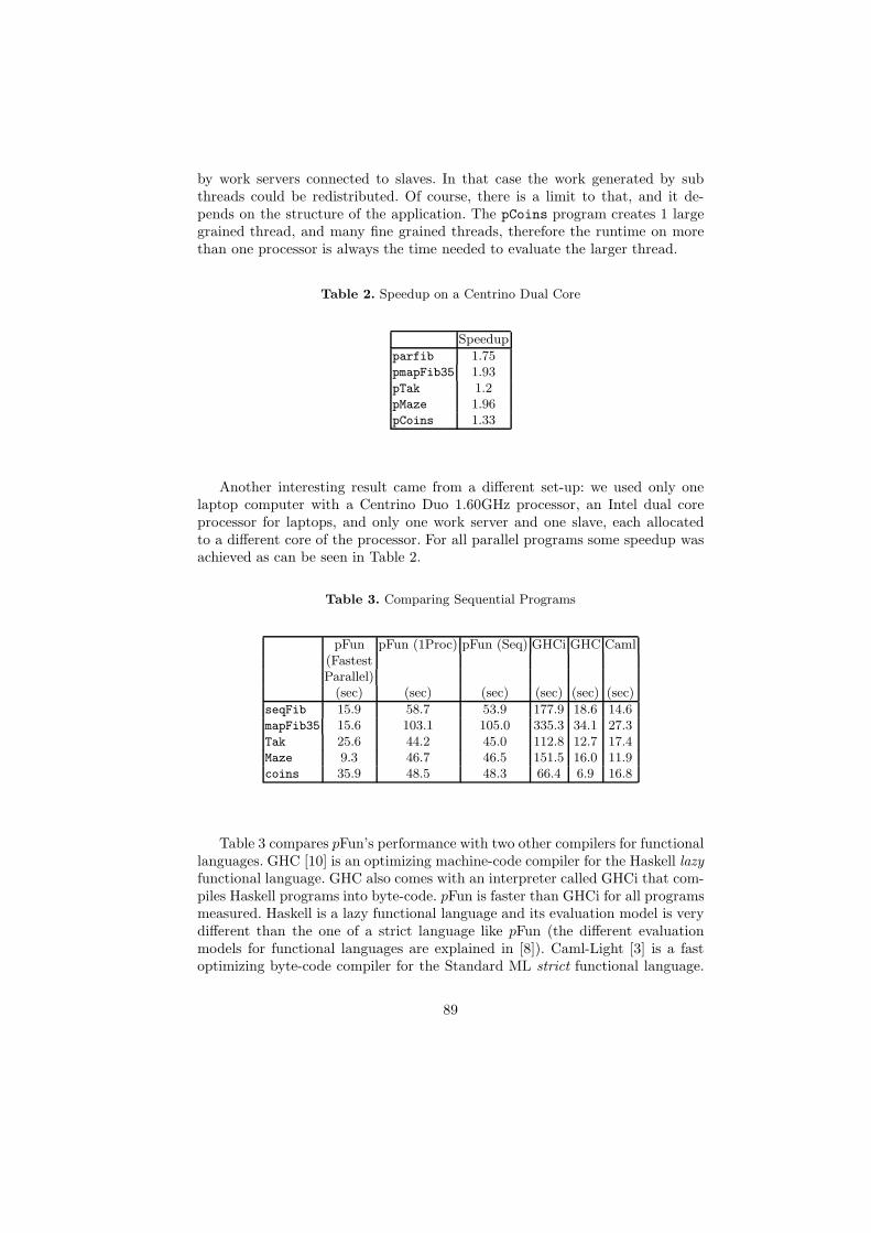
by work servers connected to slaves. In that case the work generated by subthreads could be redistributed. Of course, there is a limit to that, and it de-pends on the structure of the application. The pCoins program creates 1 largegrained thread, and many fine grained threads, therefore the runtime on morethan one processor is always the time needed to evaluate the larger thread.

Table 2. Speedup on a Centrino Dual Core

Speedup

parfib 1.75pmapFib35 1.93pTak 1.2pMaze 1.96pCoins 1.33

Another interesting result came from a different set-up: we used only onelaptop computer with a Centrino Duo 1.60GHz processor, an Intel dual coreprocessor for laptops, and only one work server and one slave, each allocatedto a different core of the processor. For all parallel programs some speedup wasachieved as can be seen in Table 2.

Table 3. Comparing Sequential Programs

pFun pFun (1Proc) pFun (Seq) GHCi GHC Caml(FastestParallel)

(sec) (sec) (sec) (sec) (sec) (sec)

seqFib 15.9 58.7 53.9 177.9 18.6 14.6mapFib35 15.6 103.1 105.0 335.3 34.1 27.3Tak 25.6 44.2 45.0 112.8 12.7 17.4Maze 9.3 46.7 46.5 151.5 16.0 11.9coins 35.9 48.5 48.3 66.4 6.9 16.8

Table 3 compares pFun’s performance with two other compilers for functionallanguages. GHC [10] is an optimizing machine-code compiler for the Haskell lazy

functional language. GHC also comes with an interpreter called GHCi that com-piles Haskell programs into byte-code. pFun is faster than GHCi for all programsmeasured. Haskell is a lazy functional language and its evaluation model is verydifferent than the one of a strict language like pFun (the different evaluationmodels for functional languages are explained in [8]). Caml-Light [3] is a fastoptimizing byte-code compiler for the Standard ML strict functional language.

89

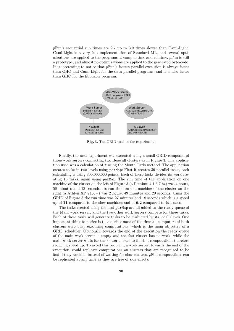
pFun’s sequential run times are 2.7 up to 3.9 times slower than Caml-Light.Caml-Light is a very fast implementation of Standard ML, and several opti-mizations are applied to the programs at compile time and runtime. pFun is stilla prototype, and almost no optimizations are applied to the generated byte-code.It is interesting to notice that pFun’s fastest parallel execution is always fasterthan GHC and Caml-Light for the data parallel programs, and it is also fasterthan GHC for the fibonacci program.

Fig. 3. The GRID used in the experiments

Finally, the next experiment was executed using a small GRID composed ofthree work servers connecting two Beowulf clusters as in Figure 3. The applica-tion used was a calculation of π using the Monte Carlo method. The applicationcreates tasks in two levels using parMap: First it creates 30 parallel tasks, eachcalculating π using 300,000,000 points. Each of these tasks divides its work cre-ating 15 tasks, again using parMap. The run time of the application on onemachine of the cluster on the left of Figure 3 (a Pentium 4 1.6 Ghz) was 4 hours,58 minutes and 13 seconds. Its run time on one machine of the cluster on theright (a Athlon XP 2400+) was 2 hours, 49 minutes and 20 seconds. Using theGRID of Figure 3 the run time was 27 minutes and 18 seconds which is a speedup of 11 compared to the slow machines and of 6.2 compared to fast ones.

The tasks created using the first parMap are all added to the ready queue ofthe Main work server, and the two other work servers compete for these tasks.Each of these tasks will generate tasks to be evaluated by its local slaves. Oneimportant thing to notice is that during most of the time all computers of bothclusters were busy executing computations, which is the main objective of aGRID scheduler. Obviously, towards the end of the execution the ready queueof the main work server is empty and the fast cluster has no work, while themain work server waits for the slower cluster to finish a computation, thereforereducing speed up. To avoid this problem, a work server, towards the end of theexecution, could replicate computations on clusters that are recognized to befast if they are idle, instead of waiting for slow clusters. pFun computations canbe replicated at any time as they are free of side effects.

90

5 Related Work

The potential of functional programming languages to support parallelism hasbeen recognized for a long time and several extensions for parallel programmingin functional languages have been implemented (for a survey on the field, thereader should refer to [11]). Here we discuss the ones that are more closely relatedto pFun.

The par and sync primitives provide the same abstraction as futures inMultilisp [20]. The idea of futures is old but it is nowadays being adopted in manymodern languages, e.g., [9, 22, 7]. pFun’s par only indicates potential parallelism.In Alice [22], when a future is created a new thread is started automatically toevaluate the computation. In Multilisp, after the call to future X, the new taskcreated to evaluate X is maintained active while the parent task is moved toa pending queue [20]. The creation of a future in Multilisp is a very expensiveoperation [20, 21], while par is only a mark saying that a expression could beevaluated in parallel with the current expression either locally or on a remotecomputer. In pFun the creation of a Par object is cheap: its like creating asuspension and adding a pointer to the ready queue. Creating a suspension is acheap operation: as can be seen in Figure 1 a suspension is just like a cons cell.

GPH [24] is a parallel extension of Haskell for parallel programming. Toexpress parallelism, the programmer uses a par combinator (similar to pFun’spar). Since Haskell is a lazy language, it is difficult to predict the order ofevaluation of expressions, thus the seq combinator must be used to controlsequencing. Furthermore, as Haskell is a lazy language, programmers have toforce the evaluation of expressions using evaluation strategies.

GRID/ML [1] is an extension of Standard ML for GRID programming. Itruns on top of the ConCert network [4], a peer-to-peer network of interconnectednodes, each running the same abstract machine. All nodes maintain a queue ofpending work, and they can steal work from other nodes. GRID/ML providesprimitives (similar to pFun’s primitives) to express parallelism and populate thenode’s queue of pending work. The GRID/ML system focuses mainly on fault-tolerant distributed programming: GRID applications are written as a series ofdeterministic functions that can be memorized by the network and restarted atany time. No measurements of their current implementation are given.

The work stealing scheduling strategy is widely used in practical applications,in particular we name the Cilk [2] programming environment. Cilk requires anextra effort by programmers: programs must be developed in a nested fork-joinstructure. Different from pFun, this programming effort is unnatural since Cilkextends an imperative programming language (C).

6 Conclusions and Future Work

We have presented the design and implementation of pFun, a strict parallel func-tional language. pFun provides a programming model based on annotations. Taskcreation, synchronization and load distribution are automatically managed by

91

its runtime system. Preliminary measurements for the prototype implementationshow that the work-stealing mechanism used for load balancing performs betterfor data parallel programs. As future work we want to adapt pFun’s runtimesystem to better exploit the characteristics of each parallel architecture. Workmessages contain code and data to be executed on slaves. That imposes a highoverhead when executing on multi-core machines as all code is already loadedin memory. For clusters, a work server could keep track of the code that wasalready sent to a slave. This would reduce significantly the size of messages inapplications that use parMap for example. Although not yet implemented, thecurrent implementation of the runtime system could provide a high degree offault tolerance. In the case of failure of one node, purely functional expressionscan be re-started at any time as they are free of side effects. Currently, all mes-sages contain the total heap size needed to unpack work. If a slave does nothave enough space it could reject the work message and ask for another one.Work servers could also ping slaves to see if they are still alive, and in the caseof failure, computations could be restarted on a different slave. At the languagelevel, we plan to investigate how pFun’s programming model could be extendedwith higher-level abstractions to express parallelism, e.g., using different paral-lel skeletons. The performance shown in Section 4 are promising since we haveobtained some speedup for different classes of architectures. As slaves do notdistribute work, the current load distribution mechanism performs poorly fordivide and conquer applications: towards the end of execution we have heavilyloaded slaves, while some slaves are idle and the ready queue of the work serveris empty. We plan to investigate the use of a distributed shared ready queue,where all locations can share work. This distributed queue could be implementedusing a distributed shared memory as in the MT System [16] or GUM [25].

Acknowledgements The authors would like to thank CNPq/Brazil for thefinancial support provided.

References

1. T. Murphy VII. ML Grid programming with Concert. In The 2006 ACM SIG-PLAN Workshop on ML (ML 2006). ACM press, 2006.

2. R. D. Blumofe, C. F. Joerg, B. C. Kuszmaul, C. E. Leiserson, K. H. Randall, andY. C. E. Zhou. Cilk: an efficient multithreaded runtime system. ACM SIGPLANNotices, 30(8):207–216, Aug. 1995.

3. The Caml-Light System. WWW page, http://caml.inria.fr/, 2005.4. B. Chang, K. Crary, M. Delap, R. Harper, J. Liszka, T. Murphy VII, and F. Pfen-

ning. Trustless GRID computing in ConCert . In Grid 2002. Springer-Verlag,2002.

5. W. Cirne, F. Brasileiro, N. Andrade, L. Costa, A. Andrade, R. Novaes, andM. Mowbray. Labs of the world, unite!!! Journal of Grid Computing, 4(3):225–246,2006.

6. M. Cole. Algorithmic Skeletons: Structured Management of Parallel Computation.Pitman, 1989.

92

7. J. Duffy and E. Essey. Running queries on multi-core processors. WWW page,MSD Magazine, http://msdn.microsoft.com/en-us/magazine/cc163329.aspx, 2008.

8. A. J. Field and P. G. Harrison. Functional Programming. Addison-Wesley, 1988.9. Futures. WWW page, http://java.sun.com/j2se/1.5.0/docs/api/java/util/concurrent/-

FutureTask.html, 2008.10. The Glasgow Haskell Compiler. WWW page, http://www.haskell.org/ghc, 2005.11. K. Hammond and G. Michaelson, editors. Research Directions in Parallel Func-

tional Programming. Springer-Verlag, UK, 1999.12. R. Jones and R. Lins. Garbage Collection: Algorithms for automatic dynamic

memory management. John Wiley and Sons, 1996.13. S. P. Jones and S. Singh. A tutorial on parallel and concurrent programming

in haskell. In Advanced Functional Programming Summer School, To appear inLNCS. Springer-Verlag, 2008.

14. S. B. Junaidu. A Parallel Functional Language Compiler for Message-PassingMulticomputers. PhD thesis, University of St Andrews, 2003.

15. P. Landin. The mechanical evaluation of expressions. The Computer Journal,6(4):308–320, 1964.

16. M. T. Morazan, D. R. Troeger, and M. Nash. Paging in a Distributed VirtualMemory, volume 3 of Trends in Functional Programming, pages 75–86. IntellectBooks, Bristol, UK, 2002.

17. S. Peyton Jones. Haskell 98 language and libraries: the revised report. Journal ofFunctional Programming, 1(13), 2003.

18. S. P. Peyton Jones and D. Lester. Implementation of Functional ProgrammingLanguages. Prentice Hall, 1987.

19. An Operational Semantics for pFun, a semi-explicit parallel functional language.WWW page, http://atlas.ucpel.tche.br/ dubois/pfunsem.pdf, 2008.

20. J. Robert H. Halstead. Multilisp: a language for concurrent symbolic computation.ACM Trans. Program. Lang. Syst., 7(4):501–538, 1985.

21. J. Robert H. Halstead. An assessment of Multilisp: lessons from experience. Int.J. Parallel Program., 15(6):459–501, 1986.

22. A. Rossberg, D. L. Botlan, G. Tack, T. Brunklaus, and G. Smolka. Alice Throughthe Looking Glass, volume 5 of Trends in Functional Programming, pages 79–96.Intellect Books, Bristol, UK, Feb. 2006.

23. H. Sutter. The free lunch is over: a fundamental turn toward concurrency insoftware. Dr. Dobb’s Journal, 30(3), March 2005.

24. P. W. Trinder, K. Hammond, H.-W. Loidl, and S. L. Peyton Jones. Algorithm+ Strategy = Parallelism. Journal of Functional Programming, 8(1):23–60, Jan.1998.

25. P. W. Trinder, K. Hammond, J. S. Mattson Jr., A. S. Partridge, and S. L. PeytonJones. GUM: a portable implementation of Haskell. In PLDI, Philadephia, May1996.

93

Realizing Multiparadigm Programming based onHierarchical Graph Rewriting

Petra Hofstedt1 and Kazunori Ueda2

1 Dept. of Electrical Engineering and Computer ScienceTechnical University of Berlin

ph@cs.tu-berlin.de2 Dept. of Computer Science, Waseda University

ueda@ueda.info.waseda.ac.jp

Abstract. The paper presents the new multiparadigm programminglanguage ccfl which allows the description of concurrent processes andof non-deterministic behavior and it discusses the compilation of ccflprograms into the hierarchical graph rewriting language lmntal.lmntal aims at the unification of paradigms of computation and supportsby its features and structure the transformation of ccfl programs suchthat we reached clear and simple compilation schemata.

1 Introduction

The concurrent, hierarchical graph rewriting language lmntal [16, 17] aims tounify various paradigms of computation resp. computational models. It has beenused for encoding various calculi [15, 14], e.g. the pure lambda calculus andthe ambient calculus. In this paper, we show the use of lmntal as base modeland target language for the compilation of programs of a new multiparadigmprogramming language ccfl.

The C oncurrent C onstraint-based Functional Language ccfl combines con-cepts from the functional and the constraint paradigms. ccfl allows besidesthe description of deterministic computations using a functional programmingstyle also the implementation of non-deterministic behavior based on constraints.Moreover, ccfl enables to describe systems of concurrent processes, whose com-munication and synchronization is based on the concurrent constraint program-ming (CCP) model [12].

The compilation of ccfl programs into lmntal rules is based on adaptionsof translation techniques for functional into logic languages. ccfl data elementsand variables are encoded by means of heap data structures handled duringrun-time in lmntal. The introduction of these data structures allows us to dealwith free variables and constraints in ccfl, to realize lazy evaluation, and iteven simplifies the lmntal rule-set generated from the compilation for handlinghigher-order functions and partial applications.

Encoding ccfl based on lmntal, we were able to underline three things:1) lmntal is well suited as base for the encoding of calculi and programming

languages, 2) it supports particularly the combination of concepts of differentparadigms and, thus, the realization of a multiparadigm language, and 3) thisis, accordingly, reachable by relatively simple compilation schemata.

Related Work lmntal has been used for the encoding of various calculi, as pre-sented by Ueda in [15, 14] e.g. for the pure lambda calculus and the ambientcalculus, resp. Like in the approach presented in this paper, the membrane con-struct of LMNtal plays an essential role for the clarity and simplicity of theencoding.

There are several functional languages allowing for concurrent computationof processes among them eden [8] and erlang [1], both using explicit notions forthe generation of processes and their communication and concurrent haskell[11] which supports threads via the IO monad.

The language goffin [2] combines haskell with a constraint-based coor-dination language to express parallelism and non-deterministic computation. Itprovides a similar structure like ccfl, while ccfl’s constraint abstractions aremore oriented to predicates than to functions and the ask-constraint’s function-ality is a bit more extended. Moreover, in [5] we discuss the extension of ccflconstraints to typical constraint systems.

curry [4] is a functional-logic language combining the functional and thelogic paradigms and builds on the evaluation principle narrowing in contrast toresiduation and non-deterministic choice in ccfl.

Beside the realization of ccfl based on hierarchical graph rewriting as dis-cussed in this paper, there exists a ccfl implementation for a parallel multicorearchitecture which supports the realization of data and task parallel skeletonsas presented in [6].

2 The Language CCFL

The multiparadigm programming language ccfl combines concepts and con-structs from the functional and the constraint-based paradigms. A ccfl pro-gram consists of data-type definitions, functions and user-defined constraints.Functions are used to express deterministic computations, while user-definedconstraints allow the description of cooperating processes and non-deterministicbehavior.

2.1 Functional Programming

ccfl’s functional sublanguage is a lazy language with polymorphic type system.A function consists of a type declaration and a definition allowing the typicalconstructs such as case-expressions, let-expressions, function application, andsome predefined infix operator applications, constants, variables, and construc-tor terms. A function call (without free variables) evokes a computation byreduction. Prog. 2.1 shows the definition of a polymorphic data-type List a anda function length computing the length of lists. In the following, we will use

96

Program 2.1 List length

data L i s t a = [ ] | a : ( L i s t a )

fun l e n g t h : : L i s t a −> Intdef l e n g t h l i s t = case l i s t of [ ] −> 0 ;

x : xs −> 1 + l e n g t h xs

the haskell-typical notions for lists, i.e. [] and e.g. [1,2,4] for an empty andnon-empty list, resp., and ”:” as the list constructor.

Free Variables Expressions in ccfl may contain free variables. Function ap-plications with free variables are evaluated using the residuation principle [13],that is, function calls are suspended until the variables are bound to expres-sions such that a deterministic reduction is possible. For example, a functioncall (4 + x) with free variable x will suspend. On the other hand, the applica-tion ( length [y ,1,x ]) successfully evaluates to 3 because the values of the freevariables y and x are not necessary to proceed with the computation.

2.2 Constraint-based Programming with CCFL

A user-defined constraint is given by its declaration and a constraint abstraction.A constraint abstraction consists of a head and a body which may contain thesame elements as a function definition. Additionally, the body can be definedby several alternatives the choice of which is decided by guards. A constraintabstraction is allowed to introduce free variables and each body alternative is aconjunction of constraint atoms. A constraint always has result type C.

ask- and tell-constraints Within a ccfl rule constraints may have two func-tionalities: tell -constraints generate concurrently working processes which maycreate knowledge in form of variable bindings (or constraints in general3). Theseprocesses may communicate over common variables. In contrast, ask -constraintsdo not generate knowledge but check for concrete variable bindings or con-straints. ask -constraints control the choice of (potentially competing) rules and,thus, allow to express the synchronization of concurrently working processes onthe one hand and non-deterministic computations on the other hand.

User-defined constraints mainly serve two purposes: expressing concurrentcomputations and dealing with non-determinism.

Concurrent Processes ccfl allows the description of systems of communi-cating and cooperating processes. Consider as an example Prog. 2.2 defining aproducer and a consumer communicating over a common buffer.3 In [5] we discuss the extension of ccfl by constraints of other domains, e.g. arith-

metic or finite-domain constraints.

97

Program 2.2 A producer-consumer setting

1 fun produce : : L i s t a −> C2 def produce bu f =3 with buf1 : : L i s t a , i tem : : a4 in . . . −− g e n e r a t e i t em h e r e t h e n

5 −− pu t i t i n t o t h e b u f f e r and c o n t i n u e

6 bu f =:= i tem : buf1 & produce buf178 fun consume : : L i s t a −> C9 def consume bu f =

10 bu f =:= f i r s t : buf1 −>11 . . . −− c on sume f i r s t h e r e

12 consume buf1 −− and c o n t i n u e

1314 fun main : : C15 def main = with bu f : : L i s t a16 in produce bu f & consume bu f

The main-function creates the buffer as a fresh variable buf using the with-construct and initiates the computation. The constraint applications produce bufand consume buf create concurrently working producer and consumer processes.The user-defined constraint produce (lines 1–6) describes the behavior of theproducer process. It generates buffer elements item, puts them into the bufferusing the equality constraint buf =:= item : buf1 and concurrently initiates thecomputation of the remaining buffer buf1 (lines 4–6). The consumer processmust wait until the buffer has been filled with at least one element first . This isensured by the match-constraint buf =:= first : buf1 (line 10) of the guard ofthe consume rule. Note that, in contrast, the producer process is not restrictedto synchronize with the consumer because the produce-rule is not guarded.

The constraints in the body of the rules are tell-constraints. They createprocesses which may compute bindings for the incorporated variables. Severaltell -constraints combined by the &-combinator (as in line 6) generate an accord-ing number of processes and they communicate over common variables. tell -constraints are either applications of user-defined or predefined constraints, e.g.produce buf1 in line 6, or they are equality constraints x =:= fexpr between avariable x and a functional expression fexpr (also see line 6). Equality constraintsare interpreted as strict. That is, the constraint t1 =:= t2 is satisfied, if both ex-pressions can be reduced to the same ground data term [4]. While a satisfiableequality constraint x =:= fexpr produces a binding of the variable x to the func-tional expression fexpr and terminates with result value Success, an unsatisfiableequality is reduced to the value Fail representing an unsuccessful computation.

The atoms of the guard of a user-defined constraint are ask-constraints. Ifa guard of a rule with matching left-hand side is entailed by the current accu-mulated bindings (and constraints in general), the concerning rule alternative

98

Program 2.3 A simple game of dice

1 fun game : : Int −> Int −> Int −> C2 def game x y n =3 case n of 0 −> x =:= 0 & y =:= 0 ;4 m −> with x1 , y1 , x1 , y2 : : Int5 in d i ce x1 & d i ce y1 &6 x =:= x1 + x2 & y =:= y1 + y2 &7 game x2 y2 (m−1)89 fun d i ce : : Int −> C

10 def d i ce x =11 member [ 1 , 2 , 3 , 4 , 5 , 6 ] x1213 fun member : : L i s t a −> a −> C14 def member l x =15 l =:= y : ys −> x =:= y |16 l =:= y : ys −> case ys of [ ] −> x =:= y ;17 z : z s −> member ys x

may be chosen for further derivation. In case that the guard fails or cannot bedecided (yet), this rule alternative is suspended. If all rule alternatives suspend,the computation waits (possibly infinitely) for a sufficient instantiation of theconcerning variables.

For ask -constraints, we distinguish between bound-constraints bound xchecking, whether a variable x is bound to a non-variable term, and match-constraints (e.g. line 10) x =:= c x1 . . . xn which test for a matching of the rootsymbol of a term bound to the variable x with a certain constructor c. Thevariables x1 . . . xn are fresh.

Non-deterministic Computations Ask -constraints support the program-ming of non-deterministic behavior. For an example consider Prog. 2.3. Theconstraint game x y n initiates a game between two players throwing the dice ntimes and reaching the overall values x and y, resp.

The tell -constraints dice x1 and dice y1 (line 5) non-deterministically pro-duce values which are consumed by the equality constraints x =:= x1 + x2 andy =:= y1 + y2, resp. Note that their computation is suspended until the argu-ments are (sufficiently) instantiated to apply the built-in function +.

The constraint abstraction member is the source of non-determinism in thisprogram. It chooses a value from a list. Since the match-constraints of the guardsof both alternatives are the same (lines 15 and 16), i.e. l =:= y : ys, the alter-natives are chosen non-deterministically which simulates the dice.

99

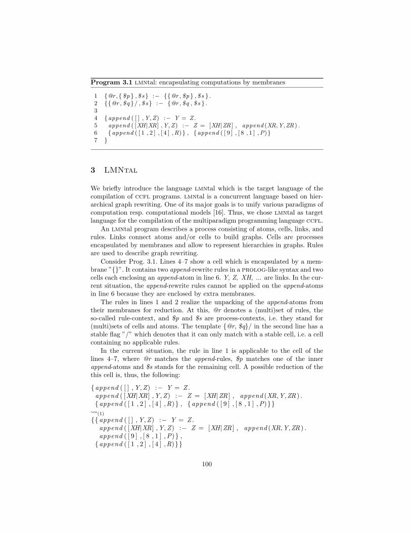
Program 3.1 lmntal: encapsulating computations by membranes

1 {@r ,{ $p } , $s} :− {{@r , $p } , $s } .2 {{@r , $q }/ , $s} :− {@r , $q , $s } .34 {append ( [ ] ,Y,Z) :− Y = Z .5 append ( [XH|XR] ,Y,Z) :− Z = [XH|ZR ] , append (XR,Y,ZR ) .6 {append ( [ 1 , 2 ] , [ 4 ] ,R)} , {append ( [ 9 ] , [ 8 , 1 ] ,P)}7 }

3 LMNtal

We briefly introduce the language lmntal which is the target language of thecompilation of ccfl programs. lmntal is a concurrent language based on hier-archical graph rewriting. One of its major goals is to unify various paradigms ofcomputation resp. computational models [16]. Thus, we chose lmntal as targetlanguage for the compilation of the multiparadigm programming language ccfl.

An lmntal program describes a process consisting of atoms, cells, links, andrules. Links connect atoms and/or cells to build graphs. Cells are processesencapsulated by membranes and allow to represent hierarchies in graphs. Rulesare used to describe graph rewriting.

Consider Prog. 3.1. Lines 4–7 show a cell which is encapsulated by a mem-brane ”{}”. It contains two append-rewrite rules in a prolog-like syntax and twocells each enclosing an append-atom in line 6. Y, Z, XH, ... are links. In the cur-rent situation, the append-rewrite rules cannot be applied on the append-atomsin line 6 because they are enclosed by extra membranes.

The rules in lines 1 and 2 realize the unpacking of the append-atoms fromtheir membranes for reduction. At this, @r denotes a (multi)set of rules, theso-called rule-context, and $p and $s are process-contexts, i.e. they stand for(multi)sets of cells and atoms. The template {@r, $q}/ in the second line has astable flag ”/” which denotes that it can only match with a stable cell, i.e. a cellcontaining no applicable rules.

In the current situation, the rule in line 1 is applicable to the cell of thelines 4–7, where @r matches the append-rules, $p matches one of the innerappend-atoms and $s stands for the remaining cell. A possible reduction of thethis cell is, thus, the following:

{append ( [ ] , Y, Z) :− Y = Z .append ( [XH|XR] ,Y, Z) :− Z = [XH|ZR ] , append (XR,Y,ZR ) .{append ( [ 1 , 2 ] , [ 4 ] ,R)} , {append ( [ 9 ] , [ 8 , 1 ] , P)}} (1)

{{append ( [ ] , Y, Z) :− Y = Z .append ( [XH|XR] ,Y, Z) :− Z = [XH|ZR ] , append (XR,Y,ZR ) .append ( [ 9 ] , [ 8 , 1 ] , P)} ,{append ( [ 1 , 2 ] , [ 4 ] ,R)}}

100

∗append

{{append ( [ ] , Y, Z) :− Y = Z .append ( [XH|XR] ,Y, Z) :− Z = [XH|ZR ] , append (XR,Y,ZR ) .P = [ 9 , 8 , 1 ] } ,{append ( [ 1 , 2 ] , [ 4 ] ,R)}}

The upper inner cell is now stable such that no rule is applicable inside. Thus,we can apply the second outer rule (line 2).

. . . (2)

{append ( [ ] , Y, Z) :− Y = Z .append ( [XH|XR] ,Y, Z) :− Z = [XH|ZR ] , append (XR,Y,ZR ) .P = [ 9 , 8 , 1 ] ,{append ( [ 1 , 2 ] , [ 4 ] ,R)}}

In this state, again the first outer rule (line 1) is applicable which yields aftera number of steps the following stable state:

{append ( [ ] , Y, Z) :− Y = Z .append ( [XH|XR] ,Y, Z) :− Z = [XH|ZR ] , append (XR,Y,ZR ) .P = [ 9 , 8 , 1 ] , R = [ 1 , 2 , 4 ] }

As one can see by the above example, lmntal supports a prolog-like syntax.However, there are fundamental differences.

The above example already demonstrated the use of process-contexts, rule-contexts, membrane enclosed cells, and the stable flag. Different from otherlanguages, the head of a rule may contain several atoms, even cells, rules,and contexts. A further important difference to other declarative languages arethe logical links of lmntal. What one may hold for variables in our program,e.g. Y, Z, XH, . . . are actually links. Their intended meaning strongly differsfrom that of variables. Declarative variables stand for particular expressions orvalues and, once bound, they stay bound throughout the computation and areindistinguishable from their value. Links in lmntal also connect to a structure orvalue. However, link connections may change. While this is similar to imperativevariables, links are used to interconnect exactly two atoms, two cells, or an atomand a cell to build graphs and they have, thus, (at most) two occurrences. Inrules, logical links must occur exactly twice.

Semantically, lmntal is a concurrent language realizing graph rewriting. Itinherits properties from concurrent logic languages. The rule choice is non-deterministic, but can be controlled by guards (not shown in the above example).As demonstrated above, the encapsulation of processes by membranes allows toexpress local computations and, it is possible to describe the migration of pro-cesses and rules between local computation spaces.

For a detailed description of lmntal we refer to [7, 16, 17]. In Sect. 4, wediscuss further examples of lmntal programs as results of the compilation processof ccfl programs.

101

4 Encoding CCFL into LMNtal

ccfl integrates functional and constraint programming. Since constraints canbe considered as particular functions, the code generation treats them uniformlysuch that we reach a proper unification of both paradigms. The transformationof ccfl functions and constraints is partially based on translation techniques [3,9, 10, 18] for functional into logic languages.

4.1 Functional Elements

Let us first consider the functional sublanguage of ccfl. A ccfl function defini-tion is translated into a set of lmntal rules. At this, there is one initial rule andpossibly a set of subordered rules realizing e.g. pattern matching as necessaryfor case-constructs.

ccfl data elements and variables are represented and processed by meansof heap data structures during run-time. However, to clarify the presentationin this section, we represent ccfl variables directly by lmntal links4 insteadand data structures by lmntal atoms. We concentrate on the heap structures inSect. 4.3 subsequently.

The right-hand side of a ccfl function definition is an expression composedby the typical constructs such as function applications, infix operator applica-tions, let- and case-constructs and variables, constants, and constructors. ccflinfix operations are mapped onto their lmntal counterparts. Function applica-tions are realized by an atom app (...) and an according app-rule which is alsoused for higher-order functions as discussed in Sect. 4.2. Case-expressions gener-ate extra lmntal rules for pattern matching, let-constructs are straightforwardrealized by equality constraints.

Example 1. Consider Prog. 4.1 as compilation result of the list length functionfrom Prog. 2.1.

The lmntal program illustrates the generation of different rule alternativesfrom the case-construct and the handling of function applications and predefinedinfix operations. Also note the additional link argument V0 of the length-rewriterule. This link is used to access the result of the rule application which is nec-essary because lmntal explicitly deals with graphs while a computation with afunctional language like ccfl yields an expression as result.

4.2 Higher-order Functions and Partial Application

We use a transformation scheme from [18] to allow higher-order func-tion application. For every ccfl function f x1 . . . xn = expr a rewrite ruleapp (f , x1, . . . , xn) :− f (x1, . . . , xn) is generated which in combination with

4 Moreover, we tolerate n-fold occurrences of links in rules, where n 6= 2. This is alsonot conform with lmntal, where links must occur exactly twice in a rule, but theproblem disappears with the introduction of heap data structures as well.

102

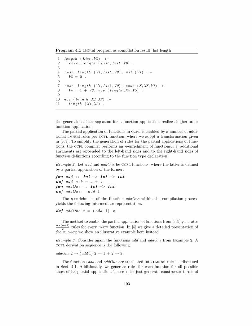
Program 4.1 lmntal program as compilation result: list length

1 l e n g t h ( Lis t ,V0) :−2 c a s e l e n g t h ( Lis t , Lis t ,V0) .34 c a s e l e n g t h (V1 , Lis t ,V0) , n i l (V1) :−5 V0 = 0 .67 c a s e l e n g t h (V1 , Lis t ,V0) , cons (X,XS ,V1) :−8 V0 = 1 + V3 , app ( l eng th ,XS ,V3) .9

10 app ( l eng th ,X1 ,X2) :−11 l e n g t h (X1 ,X2) .

the generation of an app-atom for a function application realizes higher-orderfunction application.

The partial application of functions in ccfl is enabled by a number of addi-tional lmntal rules per ccfl function, where we adopt a transformation givenin [3, 9]. To simplify the generation of rules for the partial applications of func-tions, the ccfl compiler performs an η-enrichment of functions, i.e. additionalarguments are appended to the left-hand sides and to the right-hand sides offunction definitions according to the function type declaration.

Example 2. Let add and addOne be ccfl functions, where the latter is definedby a partial application of the former.

fun add : : Int −> Int −> Intdef add a b = a + bfun addOne : : Int −> Intdef addOne = add 1

The η-enrichment of the function addOne within the compilation processyields the following intermediate representation.

def addOne x = ( add 1) x

The method to enable the partial application of functions from [3, 9] generatesn×(n+1)

2 rules for every n-ary function. In [5] we give a detailed presentation ofthe rule-set; we show an illustrative example here instead.

Example 3. Consider again the functions add and addOne from Example 2. Accfl derivation sequence is the following:

addOne 2 → (add 1) 2 → 1 + 2 → 3

The functions add and addOne are translated into lmntal rules as discussedin Sect. 4.1. Additionally, we generate rules for each function for all possiblecases of its partial application. These rules just generate constructor terms of

103

the function name and allow in this way to keep the data and to suspend thecomputation until the function can be fully applied.

add (A,B ,V0) :− V0 = A + B .addOne (V3 ,V4) :− app ( add , 1 ,X) , app (X,V3 ,V4) .

app ( add ,V0) :− add (V0 ) . // h a n d l i n g V0 = add ,

app ( add ,V0 ,V1) :− add (V0 ,V1 ) . // V1 = add V0 ,

app ( add (V0) ,V1 ,V2) :− add (V0 ,V1 ,V2 ) . // V2 = ( add V0 ) V1 ,

app ( add ,V0 ,V1 ,V2) :− add (V0 ,V1 ,V2 ) . // add a s HOF a r g . ,

app (addOne ,V0) :− addOne (V0 ) . // V0 = addOne ,

app (addOne ,V0 ,V1) :− addOne (V0 ,V1 ) . // addOne a s HOF a r g .

Using these lmntal rules we rewrite the atom addOne(2,R) which correspondsto the ccfl expression addOne 2:

addOne(2,R) app(add,1,X), app(X,2,R) add(1,X), app(X,2,R) ≡ app(add(1),2,R) add(1,2,R) R = 1+2 R = 3

The representation of data and variables by heap structures as run-timeenvironment as discussed in Sect. 4.3 allows to fuse the set of n×(n+1)

2 + 1 rulesfor handling partial applications and higher-order functions from the originalapproaches [3, 9, 18] into one unified rule.

4.3 Representing CCFL Expressions by Heap Structures

While links in lmntal look similar to variables, they have a different functionality(cf. Sect. 3). In [5] we elaborately discuss that a direct translation of ccfl vari-ables into lmntal links (and, thus, of ccfl data structures into lmntal atoms)would not be successful. Since links connect exactly two elements, i.e. cells oratoms, a representation of variables by links would disallow the representationof free variables and the sharing of data structures as needed for lazy evaluation.At least it can be shown [5] that a direct simulation is possible for a functionallanguage (without constraints) using a call-by-value evaluation strategy, wheremultiply used data structures are just completely copied. Copying of data struc-tures in lmntal is supported, even if not very efficiently treatable in general.

The introduction of a heap as run-time environment enables the representa-tion of free variables and the sharing of common data by different structures.This allows the compilation of user-defined constraints and rule guards and theimplementation of evaluation strategies using sharing of data structures.

The generation and transformation of heap structures is directly incorporatedinto the generated lmntal rules as result of the compilation process.

104

el (cons(double ),[ A],V0)

{$pA,+A}

el (...)

el (...)

{$p,on(V0)}

rewrites to

plus int (A1,A2,V0)

{$pA,+A1,+A2}

el (...)

el (...)

{$p,on(V0)}

Fig. 1. A graph rewriting rule double

Example 4. Consider the arithmetic function double.

fun doub le : : Int −> Intdef doub le a = a + a

The compilation according to the simplified schema from Sect. 4.1 yields thefollowing code.

doub le (A, V0) :− V0 = A + A .

Taking the handling of heap data structures into consideration we obtain thefollowing rule, where the atom plus int (A1,A2,V0) realizes a call to an appli-cation of the lmntal infix operator +.

e l ( cons ( doub le ) , [A ] , V0) , {$pA,+A} :−p l u s i n t (A1 , A2 , V0) , {$pA,+A1,+A2} .

Fig. 1 visualizes the generated lmntal rewrite rule. Non-variable ccfl-expressions5 are represented by atoms el (cons(F),OL,I), where the F is the func-tion or constructor name, OL is a list of (outgoing) links to cells connecting tothe structures of the arguments according to the original ccfl function, and Iis a (incoming) link from a cell which manages links onto the term. Accordingly,the ccfl term (double a) or double(A,V0) in the intermediate lmntal form,resp., yields the atom el (cons(double ),[ A],V0). Variables are handled similarly.Cells containing links, like {$p,on(V0)}, are used to connect between the atomsto build structures. In this way it is possible to realize sharing as illustrated bythe cell {$pA,+A1,+A2} which hold two incoming links +A1 and +A2 and oneoutgoing link onto the common shared structure (indicated by the gray outgoinglink onto the atom el (...) ).

5 This holds except for built-in functions, i.e. + is represented by a prelude ruleplus int .

105

el (cons(member),[L,X],V0)

{on(L0),$pL,+L}

el (cons(cons ),[Y,Ys],L0)

. . .

. . .

. . . . . .

Fig. 2. A heap structure representing the expression member (y : ys) x

4.4 Constraints and Rule Guards

User-defined constraints and functions are handled uniformly in the compilationprocess. Constraints in lmntal allow all the constructs as introduced for func-tions, but additionally free variables, a with-construct for the introduction of newvariables within a rule, ask -constraints in the rule guard and tell -constraints inits body.

Just like lmntal rules for ccfl functions, rules for user-defined constraintsmust hold an additional link in the rule head to connect to the computation resultbecause constraints must be accessible as elements e.g. for partial application.

Ask -constraints, i.e. bound- and match-constraints are realized by additionalatoms in the rule heads of the generated lmntal code matching for the accordingheap structures.

Example 5. The user-defined constraint member of Prog. 2.3 non-determini-stically chooses values from a given list. We either take the first element asresult value or initiate a further computation on the rest of the list.

The guards consist of identical match-constraints l =:= y : ys (lines 15 and16) to realize a non-deterministic choice. The compilation yields, thus, identicalrule heads matching the list structure (y : ys) or cons(Y,Ys), resp., as given be-low for both alternatives. The according heap structure is shown for illustrationin Fig. 2.

e l ( cons (member ) , [ L ,X ] , V0) ,e l ( cons ( cons ) , [Y, Ys ] , L0 ) ,{on (L0 ) , $pL ,+L} :−

. . .

For tell -constraints we distinguish between applications of user-defined con-straints which are just handled like function applications and equality constraintst1 =:= t2 (cf. Sect. 2.2). These latter base on a unification of the concerningsubexpressions t1 and t2 of the constraint. A unification mechanism for heapdata was implemented in lmntal: unify(L1,L2,R) unifies the heap structures

106

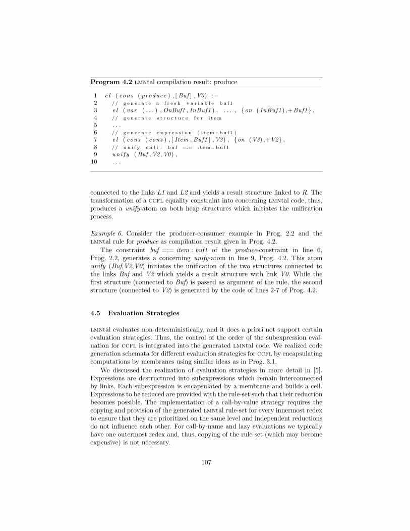
Program 4.2 lmntal compilation result: produce

1 e l ( cons ( produce ) , [ Buf ] ,V0) :−2 // g e n e r a t e a f r e s h v a r i a b l e b u f 1

3 e l ( var ( . . . ) , OnBuf1 , InBuf1 ) , . . . , {on ( InBuf1 ) ,+Buf1 } ,4 // g e n e r a t e s t r u c t u r e f o r i t em

5 . . .6 // g e n e r a t e e x p r e s s i o n ( i t em : b u f 1 )

7 e l ( cons ( cons ) , [ Item , Buf1 ] ,V3) , {on (V3) ,+V2} ,8 // u n i f y c a l l : b u f =:= i t em : b u f 1

9 un i f y (Buf ,V2 ,V0) ,10 . . .

connected to the links L1 and L2 and yields a result structure linked to R. Thetransformation of a ccfl equality constraint into concerning lmntal code, thus,produces a unify-atom on both heap structures which initiates the unificationprocess.

Example 6. Consider the producer-consumer example in Prog. 2.2 and thelmntal rule for produce as compilation result given in Prog. 4.2.

The constraint buf =:= item : buf1 of the produce-constraint in line 6,Prog. 2.2, generates a concerning unify-atom in line 9, Prog. 4.2. This atomunify (Buf,V2,V0) initiates the unification of the two structures connected tothe links Buf and V2 which yields a result structure with link V0. While thefirst structure (connected to Buf) is passed as argument of the rule, the secondstructure (connected to V2) is generated by the code of lines 2-7 of Prog. 4.2.

4.5 Evaluation Strategies

lmntal evaluates non-deterministically, and it does a priori not support certainevaluation strategies. Thus, the control of the order of the subexpression eval-uation for ccfl is integrated into the generated lmntal code. We realized codegeneration schemata for different evaluation strategies for ccfl by encapsulatingcomputations by membranes using similar ideas as in Prog. 3.1.

We discussed the realization of evaluation strategies in more detail in [5].Expressions are destructured into subexpressions which remain interconnectedby links. Each subexpression is encapsulated by a membrane and builds a cell.Expressions to be reduced are provided with the rule-set such that their reductionbecomes possible. The implementation of a call-by-value strategy requires thecopying and provision of the generated lmntal rule-set for every innermost redexto ensure that they are prioritized on the same level and independent reductionsdo not influence each other. For call-by-name and lazy evaluations we typicallyhave one outermost redex and, thus, copying of the rule-set (which may becomeexpensive) is not necessary.

107

5 Conclusion

We presented the multiparadigm programming language ccfl and its compila-tion into the hierarchical graph rewriting language lmntal. We think that ccflis a successful integration of the functional and constraint-based paradigms al-lowing a comfortable modeling of systems of concurrent processes and of deter-ministic and non-deterministic behavior.

The ability of the compilation target language lmntal to unify and to modelcomputation paradigms proved to be very useful for our compiler implementa-tion. It could be shown that modeling combined language paradigms in lmntalis possible in a convenient way and by means of clear transformations.

Acknowledgment The work of Petra Hofstedt has been supported by a post-doctoral fellowship No. PE 07542 from the Japan Society for the Promotion ofScience (JSPS).

References

1. Joe Armstrong, Robert Virding, Claes Wikstrom, and Mike Williams. ConcurrentProgramming in Erlang. Prentice Hall, 2nd edition, 2007.

2. Manuel M.T. Chakravarty, Yike Guo, Martin Kohler, and Hendrik C. R. Lock.Goffin: Higher-Order Functions Meet Concurrent Constraints. Science of Com-puter Programming, 30(1-2):157–199, 1998.

3. Mantis H. M. Cheng, Maarten H. van Emden, and B. E. Richards. On War-ren’s Method for Functional Programming in Logic. In Peter Szeredi David H.D. Warren, editor, Logic Programming, Proceedings of the Seventh InternationalConference, Jerusalem, Israel, ICLP 1990, pages 546–560. MIT Press, 1990.

4. Michael Hanus, Sergio Antoy, Bernd Braßel, Herbert Kuchen, Francisco J. Lopez-Fraguas, Wolfgang Lux, Juan Jose Moreno Navarro, and Frank Steiner. Curry: AnIntegrated Functional Logic Language. Technical report, 2006. Version 0.8.2 ofMarch 28, 2006.

5. Petra Hofstedt. CCFL – A Concurrent Constraint Functional Language. TechnicalReport 2008-08, Technische Universitat Berlin, 2008. http://iv.tu-berlin.de/

TechnBerichte/2008/2008-08.pdf, last visited 11 March 2009.6. Petra Hofstedt and Florian Lorenzen. Constraint Functional Multicore Program-

ming. In 4. Arbeitstagung Programmiersprachen – ATPS’09, Lecture Notes inInformatics (LNI), 2009. to appear.

7. LMNtal PukiWiki. http://www.ueda.info.waseda.ac.jp/lmntal/. last visited11 March 2009.

8. Rita Loogen, Yolanda Ortega-Mallen, and Ricardo Pena. Parallel Functional Pro-gramming in Eden. Journal of Functional Programming, 15(3):431–475, 2005.

9. Lee Naish. Adding equations to NU-Prolog. In Programming Language Implemen-tation and Logic Programming, 3rd International Symposium, PLILP’91, volume528 of Lecture Notes in Computer Science, pages 15–26. Springer, 1991.

10. Lee Naish. Higher-order logic programming in Prolog. Technical Report 96/2,Department of Computer Science, University of Melbourne, 1996.

11. Simon Peyton Jones, Andrew Gordon, and Sigbjorn Finne. Concurrent Haskell. In23rd ACM Symposium on Principles of Programming Languages – POPL, pages295–308, 1996.

108

12. Vijay A. Saraswat and Martin C. Rinard. Concurrent Constraint Programming.In 17th ACM Symposium on Principles of Programming Languages – POPL, pages232–245, 1990.

13. Gert Smolka. Residuation and Guarded Rules for Constraint Logic Programming.In Frederic Benhamou and Alain Colmerauer, editors, Constraint Logic Program-ming. Selected Research, pages 405–419. The MIT Press, 1993.

14. Kazunori Ueda. Encoding Distributed Process Calculi into LMNtal. ElectronicNotes in Theoretical Computer Science (ENTCS), 209:187–200, 2008.

15. Kazunori Ueda. Encoding the Pure Lambda Calculus into Hierarchical GraphRewriting. In Andrei Voronkov, editor, Rewriting Techniques and Applications –RTA, volume 5117 of Lecture Notes in Computer Science, pages 392–408. Springer,2008.

16. Kazunori Ueda and Norio Kato. LMNtal: a Language Model with Links andMembranes. In Proceedings of the Fifth International Workshop on MembraneComputing (WMC 2004), volume 3365 of LNCS, pages 110–125. Springer, 2005.

17. Kazunori Ueda, Norio Kato, Koji Hara, and Ken Mizuno. LMNtal as a UnifyingDeclarative Language. In Tom Schrijvers and Thom Fruhwirth, editors, Proceedingsof the Third Workshop on Constraint Handling Rules, Technical Report CW 452,pages 1–15. Katholieke Universiteit Leuven, 2006.

18. D.H.D. Warren. Higher-order extensions to PROLOG: Are they needed? MachineIntelligence, 10:441–454, 1982.

109

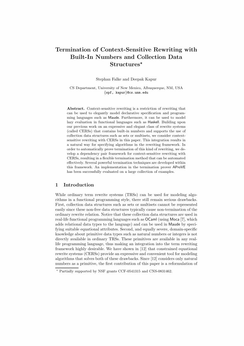
Termination of Context-Sensitive Rewriting with

Built-In Numbers and Collection Data

Structures⋆

Stephan Falke and Deepak Kapur

CS Department, University of New Mexico, Albuquerque, NM, USA{spf, kapur}@cs.unm.edu

Abstract. Context-sensitive rewriting is a restriction of rewriting thatcan be used to elegantly model declarative specification and program-ming languages such as Maude. Furthermore, it can be used to modellazy evaluation in functional languages such as Haskell. Building uponour previous work on an expressive and elegant class of rewrite systems(called CERSs) that contains built-in numbers and supports the use ofcollection data structures such as sets or multisets, we consider context-sensitive rewriting with CERSs in this paper. This integration results ina natural way for specifying algorithms in the rewriting framework. Inorder to automatically prove termination of this kind of rewriting, we de-velop a dependency pair framework for context-sensitive rewriting withCERSs, resulting in a flexible termination method that can be automatedeffectively. Several powerful termination techniques are developed withinthis framework. An implementation in the termination prover AProVE

has been successfully evaluated on a large collection of examples.

1 Introduction

While ordinary term rewrite systems (TRSs) can be used for modeling algo-rithms in a functional programming style, there still remain serious drawbacks.First, collection data structures such as sets or multisets cannot be representedeasily since these non-free data structures typically cause non-termination of theordinary rewrite relation. Notice that these collection data structures are used inreal-life functional programming languages such as OCaml (using Moca [7], whichadds relational data types to the language) and can be used in Maude by speci-fying suitable equational attributes. Second, and equally severe, domain-specificknowledge about primitive data types such as natural numbers or integers is notdirectly available in ordinary TRSs. These primitives are available in any real-life programming language, thus making an integration into the term rewritingframework highly desirable. We have shown in [12] that constrained equationalrewrite systems (CERSs) provide an expressive and convenient tool for modelingalgorithms that solves both of these drawbacks. Since [12] considers only naturalnumbers as a primitive, the first contribution of this paper is a reformulation of

⋆ Partially supported by NSF grants CCF-0541315 and CNS-0831462.

the ideas from [12] that allows for built-in integers.1 An integration of integersinto the term rewriting framework is important for automated termination prov-ing since most currently available termination techniques are based on syntacticconsiderations, whereas termination of algorithms operating on integers oftenrequires semantical reasoning.

Even though CERSs are an expressive and elegant tool for modeling algo-rithms, they do not incorporate reduction strategies that are commonly used indeclarative specification and programming languages such as Maude [9]. Context-sensitive rewriting [23, 25] has been introduced as an operational restriction ofterm rewriting that can be used to model such reduction strategies (the closerelationship between context-sensitive rewriting and Maude’s strat-annotationshas been investigated in [24]). Furthermore, context-sensitive rewriting allowsto model (certain aspects of) lazy evaluation as used in functional programminglanguages such as Haskell (for more on the relationship between lazy evalua-tion and context-sensitive rewriting, see [26]). In context-sensitive rewriting, thearguments where an evaluation may take place are specified for each functionsymbol and a reduction is only allowed at a position that is not forbidden by afunction symbol occurring somewhere above it. The second contribution of thispaper is to introduce context-sensitive rewriting for CERSs, thus combining theexpressiveness of CERSs with increased flexibility on the reduction strategy.

Example 1. Consider the following rewrite rules, where ins is used to add afurther element to a set:

from(x) → ins(x, from(x + 1))take(0, xs) → nil

take(x, ins(y, ys)) → cons(y, take(x − 1, ys))Jx > 0Kpick(ins(x, xs)) → x

drop(ins(x, xs)) → xs

Here, the function symbol from is used to generate the (infinite) subsets of in-tegers that are greater than or equal to the argument of from. The meaning of“Jx > 0K” in the second take-rule will be made precise in Sect. 2. Intuitively,it allows application of that rule only if the instantiation of the variable x is apositive number. The term take(2, from(0)) admits an infinite reduction in whichthe from-rule is applied again and again. However, there also is a finite reductionof that term which results in the normal form cons(0, cons(1, nil)). This reduc-tion can be enforced using context-sensitive rewriting if evaluation of the secondargument of ins is forbidden since the recursive call to from is then blocked. ♦

As for ordinary rewriting, termination is a fundamental property of context-sensitive rewriting. Since context-sensitive rewriting may result in a terminat-ing rewrite relation where regular rewriting is diverging, proving termination of

1 Another recent integration of integers into the term rewriting framework is presentedin [16]. The approach of [16] is incomparable to the approach of the present paper.On the one hand, [16] provides a more complete integration of integers since mul-tiplication and division are supported. On the other hand, [16] does not considercollection data structures or context-sensitive rewriting.

112

context-sensitive rewriting is quite challenging. For ordinary TRSs, a promisingapproach consists of the development of dedicated methods for proving termina-tion of context-sensitive rewriting. Examples for adaptations of classical methodsare context-sensitive recursive path orderings [8] and context-sensitive polyno-mial interpretations [27]. The main drawback of these adaptations is the limitedpower which is inherited from the classical methods. Adapting the more powerfuldependency pair method [4] to context-sensitive TRSs has been a challenge. Afirst adaptation of the dependency pair method to context-sensitive TRSs hasbeen presented in [2]. But this adaptation has severe disadvantages compared tothe ordinary dependency pair method since dependency pairs may be collapsing,which requires strong restrictions on how the method can be applied.

An alternative adaptation of the dependency pair method to context-sensitiveTRSs has recently been presented in [1]. This adaptation does not require collaps-ing dependency pairs and makes it much easier to adapt techniques developedwithin the ordinary dependency pair method to the context-sensitive case.

The third and main contribution of this paper is the development of a de-pendency pair method for context-sensitive rewriting with CERSs, taking [1] asa starting point. This adaptation is non-trivial since [1] is concerned with ordi-nary (syntactic) rewriting, whereas rewriting with CERSs is based on normal-ized equational rewriting that uses constructor equations and constructor rules.While the techniques presented in this paper are quite similar to the correspond-ing techniques in [1], their soundness proofs are more involved and cannot bepresented due to space constraints. They can be found in the full version [14],which furthermore contains additional techniques not presented in this paper.

After fixing terminology, Sect. 2 recalls and extends the CERSs introduced in[12]. In contrast to [12], it is now possible to consider built-in integers. Context-sensitive rewriting with CERSs is introduced in Sect. 3. The main technicalresult of this paper is presented in Sect. 4. By a non-trivial extension of [1],termination of context-sensitive rewriting with a CERS is reduced to showingabsence of infinite chains of dependency pairs. Sect. 5 introduces several power-ful termination techniques that can be applied in combination with dependencypairs. These techniques lift the most commonly used termination techniques in-troduced for CERSs in [12] to context-sensitive CERSs. An implementation ofthese techniques in the termination prover AProVE [17] is discussed and eval-uated in Sect. 6. This evaluation shows that our implementation succeeds inproving termination of a large class of context-sensitive CERSs.

2 Constrained Equational Rewrite Systems

Familiarity with the notation and terminology of term rewriting is assumed, see[5] for an in-depth treatment. This paper uses many-sorted term rewriting overa set S of sorts. It is assumed in the following that all terms, substitutions,replacements, etc. are sort-correct. For a signature F and a disjoint set V ofvariables, the set of all terms over F and V is denoted by T (F ,V). The set ofpositions of a term t is denoted by Pos(t), where Λ denotes the root position.

113

The set of variables occurring in a term t is denoted by V(t), and F(t) denotesthe set of function symbols occurring in t. This naturally extends to pairs ofterms, sets of terms, etc. The root symbol of a term t is denoted by root(t).

A context over F is a term C ∈ T (F ∪⋃

s∈S{�s},V). Here, �s : → s is afresh constant symbol of sort s, called hole. If the sort of a hole can be derivedor is not important, then � will be used to stand for any of the �s. If C isa context with n holes and t1, . . . , tn are terms of the appropriate sorts, thenC[t1, . . . , tn] is the result of replacing the occurrences of holes by t1, . . . , tn “fromleft to right”. A substitution is a mapping from variables to terms, where thedomain of the substitution may be infinite. The application of a substitution σ

to a term t is written as tσ, using postfix notation.

A finite set E = {u1 ≈ v1, . . . , un ≈ vn} of equations induces a rewriterelation →E by letting s →E t iff there exist a position p ∈ Pos(s) and asubstitution σ such that s|p = uiσ and t = s[viσ]p for some ui ≈ vi ∈ E . Thereflexive-transitive-symmetric closure of →E is denoted by ∼E . If equations areused in only one direction, they are called rules. A term rewrite system (TRS)

is a finite set R = {l1 → r1, . . . , lm → rm} of rules. Equational rewriting usesboth a set E of equations and a set R of rules. Intuitively, E is used to model“structural” properties, while R is used to model “simplifying” properties.

Definition 2 (E-Extended Rewriting). Let R be a TRS and let E be a set of

equations. Then s →E\R t if there exist a rule l → r ∈ R, a position p ∈ Pos(s),and a substitution σ such that (i) s|p ∼E lσ, and (ii) t = s[rσ]p.

Writing>Λ∼E and

>Λ−→E\R denotes that all steps are applied below the root,

and>Λ−→E\R−→! denotes normalization w.r.t.

>Λ−→E\R.

In order to allow for built-in numbers and collection data structures, [12] hasintroduced a new class of rewrite systems. Both built-in numbers and collectiondata structures are modeled using E-extended rewriting. In order to model theset of integers, recall that Z is an Abelian group with unit 0 that is generatedusing the element 1. Integers can thus be modeled using the function symbolsFZ = {0 : → int, 1 : → int, − : int → int, + : int×int → int}. Terms overFZ are written using a simplified notation, e.g., x−2 instead of x+((−1)+(−1)).

As is well-known, equational completion [21, 6] generates the following rulesSZ and equations EZ from the defining properties of Abelian groups:

x + 0 → x x + (−x) → 0

−− x → x (x + (−x)) + y → 0 + y

−0 → 0 x + y ≈ y + x

−(x + y) → (−x) + (−y) x + (y + z) ≈ (x + y) + z

Recall that equality w.r.t. the properties of Abelian groups is reduced to EZ-equivalence of →EZ\SZ

-normal forms. This idea can be used for natural numberswith FN = {0 : → nat, 1 : → nat, + : nat× nat → nat}, SN = {x + 0 → x},and EN = {x+ y ≈ y +x, x+(y + z) ≈ (x+ y)+ z} as well [12]. In the following,Th denotes one of Z or N, and base denotes the sort int or nat, respectively.

114

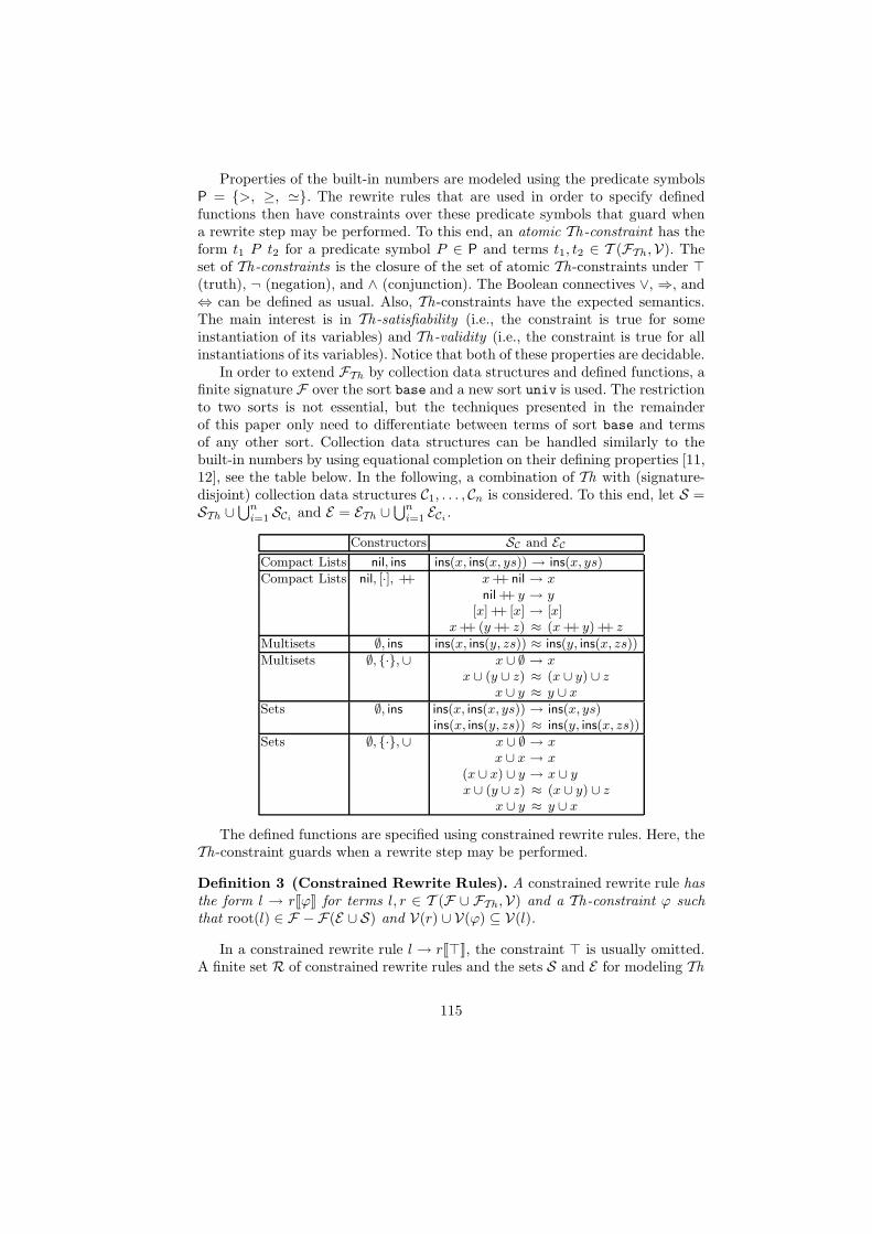
Properties of the built-in numbers are modeled using the predicate symbolsP = {>, ≥, ≃}. The rewrite rules that are used in order to specify definedfunctions then have constraints over these predicate symbols that guard whena rewrite step may be performed. To this end, an atomic Th-constraint has theform t1 P t2 for a predicate symbol P ∈ P and terms t1, t2 ∈ T (FTh ,V). Theset of Th-constraints is the closure of the set of atomic Th-constraints under ⊤(truth), ¬ (negation), and ∧ (conjunction). The Boolean connectives ∨, ⇒, and⇔ can be defined as usual. Also, Th-constraints have the expected semantics.The main interest is in Th-satisfiability (i.e., the constraint is true for someinstantiation of its variables) and Th-validity (i.e., the constraint is true for allinstantiations of its variables). Notice that both of these properties are decidable.

In order to extend FTh by collection data structures and defined functions, afinite signature F over the sort base and a new sort univ is used. The restrictionto two sorts is not essential, but the techniques presented in the remainderof this paper only need to differentiate between terms of sort base and termsof any other sort. Collection data structures can be handled similarly to thebuilt-in numbers by using equational completion on their defining properties [11,12], see the table below. In the following, a combination of Th with (signature-disjoint) collection data structures C1, . . . , Cn is considered. To this end, let S =STh ∪

⋃ni=1

SCiand E = ETh ∪

⋃ni=1

ECi.

Constructors SC and EC

Compact Lists nil, ins ins(x, ins(x, ys)) → ins(x, ys)

Compact Lists nil, [·], ++ x ++ nil → x

nil ++ y → y

[x] ++ [x] → [x]x ++ (y ++ z) ≈ (x ++ y) ++ z

Multisets ∅, ins ins(x, ins(y, zs)) ≈ ins(y, ins(x, zs))

Multisets ∅, {·},∪ x ∪ ∅ → x

x ∪ (y ∪ z) ≈ (x ∪ y) ∪ z

x ∪ y ≈ y ∪ x

Sets ∅, ins ins(x, ins(x, ys)) → ins(x, ys)ins(x, ins(y, zs)) ≈ ins(y, ins(x, zs))

Sets ∅, {·},∪ x ∪ ∅ → x

x ∪ x → x

(x ∪ x) ∪ y → x ∪ y

x ∪ (y ∪ z) ≈ (x ∪ y) ∪ z

x ∪ y ≈ y ∪ x

The defined functions are specified using constrained rewrite rules. Here, theTh-constraint guards when a rewrite step may be performed.

Definition 3 (Constrained Rewrite Rules). A constrained rewrite rule has

the form l → rJϕK for terms l, r ∈ T (F ∪ FTh ,V) and a Th-constraint ϕ such

that root(l) ∈ F − F(E ∪ S) and V(r) ∪ V(ϕ) ⊆ V(l).

In a constrained rewrite rule l → rJ⊤K, the constraint ⊤ is usually omitted.A finite set R of constrained rewrite rules and the sets S and E for modeling Th

115

and collection data structures as given above are combined into a constrained

equational rewrite system (CERS)2 (R,S, E). The rewrite relation of a CERSis defined as follows [12]. Notice that checking the instantiated constraint forvalidity requires the matching substitution to be Th-based, i.e., all variables ofsort base are mapped to terms from T (FTh ,V).

Definition 4 (Rewrite Relation of a CERS). For a CERS (R,S, E), let

sS→Th‖E\R t iff there exist l → rJϕK ∈ R, a position p ∈ Pos(s), and a Th-based

σ such that (i) s|p>Λ−→E\S−→! ◦

>Λ∼E lσ, (ii) ϕσ is Th-valid, and (iii) t = s[rσ]p.

It is shown in [14] thatS→Th‖E\R is decidable for the CERSs considered in

this paper. The function symbols occurring at the root position of left-hand sidesin R are of particular interest since they are the only function symbols that allowa reduction to take place. These are the defined symbols D(R).

3 Context-Sensitive Rewriting with CERSs

A context-sensitive rewriting strategy is given using a replacement map µ withµ(f) ⊆ {1, . . . , arity(f)} for every function symbol f ∈ F ∪ FTh . Replacementmaps specify the argument positions of function symbols where reductions areallowed. If the replacement map restricts reductions in a certain argument posi-tion, then the whole subterm below that argument position may not be reduced.Formally, µ is used to define the set Pos

µ(t) of active positions of a term t.Here, a position is active if it can be reached from the root of the term by onlydescending into argument positions that are not restricted by the replacementmap, i.e., Pos

µ(x) = {Λ} for x ∈ V and Posµ(f(t1, . . . , tn)) = {Λ} ∪ {i.p | i ∈

µ(f) and p ∈ Posµ(ti)}. Dually, the set of inactive positions of t is defined as

Pos6µ(t) = Pos(t)−Pos

µ(t). The concept of active positions can also be used todefine active (and inactive) subterms of a given term. tDµ s denotes that s is anactive subterm of t, i.e., t|p = s for an active position p ∈ Pos

µ(t). If p 6= Λ, thenthis is written t ⊲µ s. Analogously, t ⊲ 6µ s means that s is an inactive subterm

of t. The classification of active and inactive subterms can easily be extendedto other notions as well to obtain the sets Vµ(t) of variables occurring in activepositions in t, V 6µ(t) of variables occurring in inactive positions in t, etc.

Now a context-sensitive constrained equational rewrite system (CS-CERS)

(R,S, E , µ) combines a regular CERS with a replacement map. As already no-ticed in [15] for the AC -case, the permutative nature of the equations in Edisallows some choices of µ since inactive subterms may otherwise become ac-tive subterms (or vice versa) by applying equations from E . Therefore, µ needsto satisfy the following conditions:

µ(+) = {1, 2} µ(ins) = ∅ or µ(ins) = {1, 2}µ(−) = {1} µ( ++ ) = µ(∪) = {1, 2}

2 A more abstract definition of CERSs that allows for more general non-free datastructures is given in [14]. The main requirement for this is that →E\S is convergent.

116

The rewrite relation of a CS-CERS is obtained by a small modification ofDef. 4 such that the position where the reduction takes place has to be active.

Definition 5 (Rewriting with a CS-CERS). For a CS-CERS (R,S, E , µ),

let sS→Th‖E\R,µ t iff there exist l → rJϕK ∈ R, an active position p ∈ Pos

µ(s),

and a Th-based substitution σ such that (i) s|p>Λ−→E\S−→! ◦

>Λ∼E lσ, (ii) ϕσ is Th-

valid, and (iii) t = s[rσ]p.

Example 6. The CERS from Ex. 1 becomes a CS-CERS by considering the re-placement map µ with µ(ins) = ∅ and µ(f) = {1, . . . , arity(f)} for all f 6= ins.Then the reduction of the term take(2, from(0)) has the following form:

take(2, from(0))S→Th‖E\R,µ take(2, ins(0, from(1)))S→Th‖E\R,µ cons(0, take(2 − 1, from(1)))S→Th‖E\R,µ cons(0, cons(1, take(1 − 1, from(2))))S→Th‖E\R,µ cons(0, cons(1, nil))

Notice that an infinite reduction of this term is not possible since the recursivecall in the rule from(x) → ins(x, from(x + 1)) occurs in an inactive position. ♦

4 Dependency Pairs for Rewriting with CS-CERSs

Recall from [4] that dependency pairs are built from recursive calls to definedsymbols occurring in right-hand sides of R since only these recursive calls maycause non-termination. To this end, a signature F ♯ is introduced, containingthe function symbol f

♯ : s1 × . . . × sn → top for each function symbol f :s1× . . .×sn → s from F . Here, top is a fresh sort. For t = f(t1, . . . , tn), the termf

♯(t1, . . . , tn) is denoted by t♯. Then a dependency pair generated from a rule

l → rJϕK has the shape l♯ → t

♯JϕK, where t is a subterm of r with root(t) ∈ D(R).The main theorem for CERSs [12] states that a CERS is terminating if it is notpossible to construct infinite chains from the dependency pairs.

For context-sensitive rewriting, one might be tempted to restrict the gener-ation of dependency pairs to recursive calls occurring in active positions sincethese are the only places where reductions may occur. As shown in [2] for ordi-nary TRSs, this results in an unsound method if rules have migrating variables,i.e., variables x with r Dµ x but l 6⊲µ x for some rule l → r. The reason for thisis that recursive calls occuring in inactive positions might be promoted to ac-tive positions if they are matched to a migrating variable of another rule. Thus,[2] introduces collapsing dependency pairs for such migrating variables, but thiscauses severe disadvantages since it is hard to extend methods for proving ter-mination from ordinary rewriting to context-sensitive rewriting. While progresshas been made [2, 3, 19], the resulting methods are quite weak in practice.

An alternative to the collapsing dependency pairs needed in [2] has recentlybeen presented in [1]. The main observation of [1] is that only certain instantia-tions of the migrating variables need to be considered. A first, naive approach forthis would be to only consider instantiations by hidden terms, which are termswith a defined root symbol occurring inactively in right-hand sides of rules.

117

Definition 7 (Hidden Term). A term t is hidden for (R,S, E , µ) iff root(t) ∈D(R) and there exists a rule l → rJϕK ∈ R such that r ⊲ 6µ t.

In Ex. 6, the term from(x+1) is hidden since ins(x, from(x+1))⊲ 6µ from(x+1).As shown in [1] for ordinary TRSs, it does not suffice to only consider the hiddenterms. Instead, it becomes necessary to consider certain contexts that may bebuilt above a hidden term using the rewrite rules. Formally, this observation iscaptured using the notion of hiding contexts. The definition in this paper differsfrom the one given in [1] by also considering S and E .

Definition 8 (Hiding Contexts). Given a CS-CERS (R,S, E , µ), f ∈ F∪FTh

hides position i iff i ∈ µ(f) and either f ∈ F(E ∪ S) or there exist a rule

l → rJϕK ∈ R and a term s = f(s1, . . . , si, . . . , sn) with r ⊲ 6µ s and si Dµ x for

an x ∈ V or si Dµ g(. . .) with g ∈ D(R). A context C is hiding iff C = � or

C = f(t1, . . . , ti−1, C′, ti+1, . . . , tn) where f hides position i and C

′ is hiding.

In Ex. 6, + hides positions 1 and 2 and − and from hide position 1. Noticethat there are infinitely many hiding contexts, but that these hiding contexthave a regular shape. In order to represent all hiding contexts using only finitelymany dependency pairs, fresh function symbols Ubase and Uuniv and unhiding

dependency pairs are used.

Definition 9 (Context-Sensitive Dependency Pairs). Let (R,S, E , µ) be

a CS-CERS. The set of context-sensitive dependency pairs of R is defined as

DP(R, µ) = DPo(R, µ) ∪ DPu(R, µ) where

DPo(R, µ) = {l♯ → t♯JϕK | l → rJϕK ∈ R, r Dµ t, root(t) ∈ D(R)}

DPu(R, µ) = {l♯ → Us(x)JϕK | l → rJϕK ∈ R, r Dµ x, l 6⊲µ x}∪ {Us(g(x1, . . . , xi, . . . , xn)) → Us′(xi)J⊤K | g hides position i}∪ {Us(h) → h

♯J⊤K | h is a hidden term}

Here, Ubase : base → top and Uuniv : univ → top are fresh function symbols that

are added to F ♯ and s and s′ are the appropriate sorts. Furthermore, µ(Ubase) =

µ(Uuniv) = ∅ and µ(f ♯) = µ(f) for all f ∈ F .

Example 10. For Ex. 6, DP(R, µ) is as follows:

take♯(x, ins(y, ys)) → take♯(x − 1, ys) Jx > 0K (1)

take♯(x, ins(y, ys)) → Ubase(y) Jx > 0K (2)take♯(x, ins(y, ys)) → Uuniv(ys) Jx > 0K (3)

pick♯(ins(x, xs)) → Ubase(x) (4)

drop♯(ins(x, xs)) → Uuniv(ys) (5)

Uuniv(from(x + 1)) → from♯(x + 1) (6)Ubase(x + y) → Ubase(x) (7)Ubase(x + y) → Ubase(y) (8)

Ubase(−x) → Ubase(x) (9)Uuniv(from(x)) → Ubase(x) (10)

For this, recall the hidden terms and the hiding contexts from above. ♦

118

As usual in methods based on dependency pairs, context-sensitive depen-dency pairs can be used in order to build chains, and the goal is to show thatS→Th‖E\R,µ is terminating if there are no infinite minimal chains.

Definition 11 ((Minimal) (P ,R,S, E , µ)-Chains). Let (R,S, E , µ) be a CS-

CERS and let P be a set of dependency pairs. A (variable-renamed) sequence of

dependency pairs s1 → t1Jϕ1K, s2 → t2Jϕ2K, . . . from P is a (P ,R,S, E , µ)-chain

iff there exists a Th-based substitution σ such that tiσS→Th‖E\R,µ→∗ ◦

>Λ−→E\S−→! ◦

>Λ∼E

si+1σ and ϕiσ is Th-valid for all i ≥ 1. The above (P ,R,S, E , µ)-chain is min-

imal iff tiσ does not start an infiniteS→Th‖E\R,µ-reduction for all i ≥ 1.

Here,S→Th‖E\R,µ→∗ corresponds to reductions occurring strictly below the root

of tiσ and>Λ−→E\S−→! ◦

>Λ∼E corresponds to normalization and matching before ap-

plying si+1 → ti+1JϕiK at the root position. Notice that this definition of chainsis essentially identical to the non-context-sensitive case in [12]. Proving the mainresult for CS-CERSs constitutes the main technical contribution of this paper.The proof requires several technical lemmas and can be found in [14].

Theorem 12. Let (R,S, E , µ) be a CS-CERS. ThenS→Th‖E\R,µ is terminating

if there are no infinite minimal (DP(R, µ),R,S, E , µ)-chains.

In the next section, several techniques for showing absence of infinite chainsare presented. These techniques are given in the form of CS-DP processors thatoperate on CS-DP problems in the spirit of [18]. Here, a CS-DP problem has theform (P ,R,S, E , µ), where P is a finite set of dependency pairs and (R,S, E , µ)is a CS-CERS. A CS-DP processor is a function that takes a CS-DP problemas input and returns a finite set of CS-DP problems as output. A CS-DP pro-cessor Proc is sound iff for all CS-DP problems (P ,R,S, E , µ) with an infiniteminimal (P ,R,S, E , µ)-chain there exists a CS-DP problem (P ′

,R′,S′

, E ′, µ

′) ∈Proc(P ,R,S, E , µ) with an infinite minimal (P ′

,R′,S′

, E ′, µ

′)-chain. For a termi-nation proof of the CS-CERS (R,S, E , µ), sound CS-DP processors are appliedrecursively to the initial CS-DP problem (DP(R, µ),R,S, E , µ). If all resultingCS-DP problems have been transformed into ∅, then termination has been shown.

5 CS-DP Processors

This section introduces several sound CS-DP processors. Most of these processorsare similar to corresponding processors developed for the non-context-sensitivecase in [12]. The soundness proofs for the CS-DP processors are, however, moreinvolved than the corresponding soundness proofs in [12], see [14] for details.

5.1 Dependency Graphs

Like the corresponding DP processor from [12], the CS-DP processor introducedin this section decomposes a CS-DP problem into several independent CS-DP

119

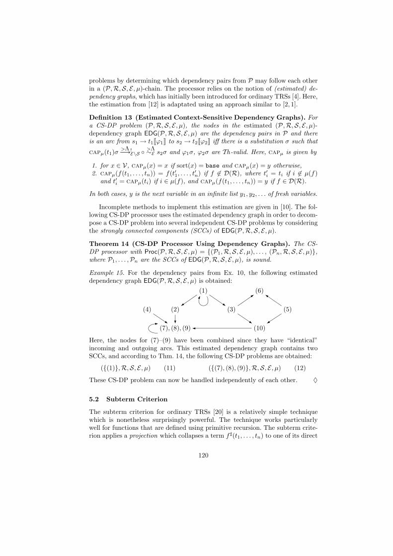
problems by determining which dependency pairs from P may follow each otherin a (P ,R,S, E , µ)-chain. The processor relies on the notion of (estimated) de-

pendency graphs, which has initially been introduced for ordinary TRSs [4]. Here,the estimation from [12] is adaptated using an approach similar to [2, 1].

Definition 13 (Estimated Context-Sensitive Dependency Graphs). For

a CS-DP problem (P ,R,S, E , µ), the nodes in the estimated (P ,R,S, E , µ)-dependency graph EDG(P ,R,S, E , µ) are the dependency pairs in P and there

is an arc from s1 → t1Jϕ1K to s2 → t2Jϕ2K iff there is a substitution σ such that

capµ(t1)σ>Λ−→E\S−→! ◦

>Λ∼E s2σ and ϕ1σ, ϕ2σ are Th-valid. Here, capµ is given by

1. for x ∈ V, capµ(x) = x if sort(x) = base and capµ(x) = y otherwise,

2. capµ(f(t1, . . . , tn)) = f(t′1, . . . , t

′n) if f 6∈ D(R), where t

′i = ti if i 6∈ µ(f)

and t′i = capµ(ti) if i ∈ µ(f), and capµ(f(t1, . . . , tn)) = y if f ∈ D(R).

In both cases, y is the next variable in an infinite list y1, y2, . . . of fresh variables.

Incomplete methods to implement this estimation are given in [10]. The fol-lowing CS-DP processor uses the estimated dependency graph in order to decom-pose a CS-DP problem into several independent CS-DP problems by consideringthe strongly connected components (SCCs) of EDG(P ,R,S, E , µ).

Theorem 14 (CS-DP Processor Using Dependency Graphs). The CS-

DP processor with Proc(P ,R,S, E , µ) = {(P1,R,S, E , µ), . . . , (Pn,R,S, E , µ)},where P1, . . . ,Pn are the SCCs of EDG(P ,R,S, E , µ), is sound.

Example 15. For the dependency pairs from Ex. 10, the following estimateddependency graph EDG(P ,R,S, E , µ) is obtained:

(1) (6)

(4) (2) (3) (5)

(7), (8), (9) (10)

Here, the nodes for (7)–(9) have been combined since they have “identical”incoming and outgoing arcs. This estimated dependency graph contains twoSCCs, and according to Thm. 14, the following CS-DP problems are obtained:

({(1)},R,S, E , µ) (11) ({(7), (8), (9)},R,S, E , µ) (12)

These CS-DP problem can now be handled independently of each other. ♦

5.2 Subterm Criterion

The subterm criterion for ordinary TRSs [20] is a relatively simple techniquewhich is nonetheless surprisingly powerful. The technique works particularlywell for functions that are defined using primitive recursion. The subterm crite-rion applies a projection which collapses a term f

♯(t1, . . . , tn) to one of its direct

120

subterms. Given a set P of dependency pairs and a subset P ′ ⊆ P , the methodconsists of finding a projection such that the collapsed right-hand side is a sub-term of the collapsed left-hand side for all dependency pairs in P , where thissubterm relation is furthermore strict for all dependency pairs from P ′. Thenthe dependency pairs in P ′ may be removed from the CS-DP problem.

Definition 16 (Projections). A projection is a mapping π that assigns to

every f♯ ∈ F ♯ with arity(f ♯) = n an i with 1 ≤ i ≤ n. The mapping that assigns

to every term f♯(t1, . . . , tn) the term tπ(f♯) is also denoted by π.

In the context of CERSs, the subterm relation modulo E can be used [12].For CS-CERSs, this relation needs to take the replacement map into account byonly considering subterms in active positions. This is similar to [2].

Definition 17 (E-µ-Subterms). Let (R,S, E , µ) be a CS-CERS and let s, t be

terms. Then t is a strict E-µ-subterm of s, written s⊲E,µ t, iff s ∼E ◦⊲µ ◦ ∼E t.

The term t is an E-µ-subterm of s, written s DE,µ t, iff s ⊲E,µ t or s ∼E t.

It is shown in [14] that ⊲E,µ and DE,µ are decidable for the sets E of equationsconsidered in this paper. Furthermore, the following properties can be shown.

Lemma 18. Let (R,S, E , µ) be a CS-CERS. Then ⊲E,µ is well-founded and

⊲E,µ and DE,µ are stable and compatible with ∼E .

Now the subterm criterion as outlined above can easily be implemented usinga CS-DP processor. Notice that the sets R and S do not need to be consideredwhen operating on the CS-DP problem (P ,R,S, E , µ).

Theorem 19 (CS-DP Processor Using the Subterm Criterion). For a

projection π, let Proc be a CS-DP processor with Proc(P ,R,S, E , µ) =

• {(P − P ′,R,S, E , µ)}, if P ′ ⊆ P such that

– π(s) ⊲E,µ π(t) for all s → tJϕK ∈ P ′, and– π(s) DE,µ π(t) for all s → tJϕK ∈ P − P ′.

• (P ,R,S, E , µ), otherwise.

Then Proc is sound.

Example 20. Recall the CS-DP problem (12) from Ex. 15, consisting of (7)–(9).Using π(Ubase) = 1, this CS-DP problem can easily be handled. ♦

5.3 Reduction Pairs

As usual in methods based on dependency pairs, well-founded relations on termsmay be used in order to remove dependency pairs from CS-DP problems. Theidea for this is simple: If all dependency pairs from a CS-DP problem are at leastweakly decreasing, then all dependency pairs that are strictly decreasing cannotoccur infinitely often in infinite chains and may thus be deleted.

Often, reduction pairs [22] are used for this purpose, and they can immedi-ately be applied for CS-CERSs as well. If the CS-CERS uses built-in naturalnumbers, then PA-reduction pairs [12] may be used. Here, it is shown that aspecial class of polynomial interpretations is applicable if integers are built-in.3

3 It is also possible to develop an abstract framework of Z-reduction pairs [10].

121

A Z-polynomial interpretation Pol fixes a constant cPol ∈ Z and maps• the symbols in FZ to polynomials over Z in the natural way, i.e., Pol(0) = 0,Pol(1) = 1, Pol(−) = −x1 and Pol(+) = x1 + x2,

• the symbols in F to polynomials over N such that Pol(f) ∈ N[x1, . . . , xn] ifarity(f) = n, and

• the symbols in F ♯ to polynomials over Z such that Pol(f ♯) ∈ Z[x1, . . . , xn] ifarity(f ♯) = n and Pol(f ♯) is weakly increasing in all xi where the i

th argumentof f

♯ has sort univ.Terms are mapped to polynomials by defining [x]Pol = x for variables x ∈ V and[f(t1, . . . , tn)]Pol = Pol(f)([t1]Pol , . . . , [tn]Pol).

Definition 21 (≻Pol , &Pol , and ∼Pol for Z-Polynomial Interpretations).

Let Pol be a Z-polynomial interpretation. Then s ≻Pol t iff [sσ]Pol ≥ cPol and

[sσ]Pol > [tσ]Pol for all ground substitutions σ : V(s) ∪ V(t) → T (F ∪ FZ).Analogously, s &Pol t iff [sσ]Pol ≥ [tσ]Pol for all ground substitutions σ : V(s) ∪V(t) → T (F ∪ FZ) and s ∼Pol t iff [sσ]Pol = [tσ]Pol for all ground substitutions

σ : V(s) ∪ V(t) → T (F ∪ FZ).

For constrained terms, it suffices to consider all substitutions σ that makethe constraint Z-valid. This is similar to the PA-reduction pairs of [12].

Definition 22 (≻Pol and &Pol on Constrained Terms). Let Pol be a Z-

polynomial interpretation, let s, t be terms and let ϕ be a Z-constraint. Then

sJϕK &Pol tJϕK iff sσ &Pol tσ for all Z-based substitutions σ such that ϕσ is

Z-valid. Similarly, sJϕK ≻Pol tJϕK iff sσ ≻Pol tσ for all Z-based substitutions σ

such that ϕσ is Z-valid.

Thus, sJϕK ≻Pol tJϕK if the following formulas are true in the integers:

∀x1, . . . , xn. ϕ ⇒ [s]Pol ≥ cPol

∀x1, . . . , xn. ϕ ⇒ [s]Pol > [t]Pol

Here, x1, . . . , xn are the variables occurring in [s]Pol or [t]Pol . This requirementmight be impossible to show if one of the xi has sort univ since then the possiblevalues it can take are not restricted by the Z-constraint ϕ. By restricting the Z-polynomial interpretation Pol such that for each f ∈ F with resulting sort univ,the polynomial Pol(f) may only depend on a variable xi if the i

th argument off has sort univ, an easier requirement is obtained since ground terms of sortuniv are then mapped to non-negative integers. Thus, it suffices to show that

∀x1, . . . , xk. ∀y1 ≥ 0, . . . , yl ≥ 0. ϕ ⇒ [s]Pol ≥ cPol

∀x1, . . . , xk. ∀y1 ≥ 0, . . . , yl ≥ 0. ϕ ⇒ [s]Pol > [t]Pol

are true in the integers, where x1, . . . , xk are the variables of sort base in [s]Pol

or [t]Pol and y1, . . . , yl are the variables of sort univ in [s]Pol or [t]Pol .Since Pol(−) is not monotonic in its argument, it becomes necessary to im-

pose restrictions on the CS-DP problem under which Z-polynomial interpreta-tions may be applied. More precisely, it has to be ensured that no reduction with

122

S→Th‖E\R,µ takes place below an occurrence of −. There are two possibilities:

1. All arguments of right-hand sides of P are terms from T (FZ,V). Then no

reductions w.r.t.S→Th‖E\R,µ can take place between instantiated dependency

pairs in a chain since chains are built using Z-based substitutions.2. F does not contain a function symbol with resulting sort base. Then, terms

with sort univ do not occur below occurrences of − and only terms with sort

univ are reducible byS→Th‖E\R,µ.

These possibilities give rise to two CS-DP processors. For the first possibility,notice that R, S, and E do not need to be considered.

Theorem 23 (CS-DP Processor Using Z-Polynomial Interpretations–

Version 1). Let Proc be a CS-DP processor with Proc(P ,R,S, E , µ) =

• {(P − P ′,R,S, E , µ)}, if all arguments of right-hand sides of P are terms

from T (FZ,V), Pol is a Z-polynomial interpretation, P ′ ⊆ P, and– sJϕK ≻Pol tJϕK for all s → tJϕK ∈ P ′

– sJϕK &Pol tJϕK for all s → tJϕK ∈ P − P ′

• {(P ,R,S, E , µ)}, otherwise.

Then Proc is sound.

If P contains right-hand sides with arguments that are not from T (FZ,V),then it might be possible to use a non-collapsing argument filter [22] for thefunction symbols f

♯ ∈ F ♯ that ensures that condition 1 is true afterwards.

Example 24. Recall the CS-DP problem (11) from Ex. 15, consisting of the de-pendency pair (1). Using a non-collapsing argument filtering that only retainsthe first argument of take♯, this dependency pair is transformed into

take♯(x) → take♯(x − 1) Jx > 0K

Now condition 1 from above is satisfied and Z-polynomial interpretations areapplicable. Indeed, using Pol(take♯) = x1 concludes the termination proof of therunning example. ♦

If condition 2 from above is satisfied, the following CS-DP processor canbe obtained. A refinement that only needs to consider syntactically determinedsubsets of R, S, and E is presented in [14].

Theorem 25 (CS-DP Processor Using Z-Polynomial Interpretations–

Version 2). Let Proc be a CS-DP processor with Proc(P ,R,S, E , µ) =

• {(P−P ′,R,S, E , µ)}, if F does not contain a function symbol with resulting

sort base, Pol is a Z-polynomial interpretation, P ′ ⊆ P, and– sJϕK ≻Pol tJϕK for all s → tJϕK ∈ P ′

– sJϕK &Pol tJϕK for all s → tJϕK ∈ (P − P ′) ∪R– l &Pol r for all l → r ∈ S– u ∼Pol v for all u ≈ v ∈ E

• {(P ,R,S, E , µ)}, otherwise.

Then Proc is sound.

123

6 Evaluation and Conclusions

This paper has presented a generalization of the constrained equational rewritesystems (CERSs) introduced in [12]. Then, context-sensitive rewriting strategiesfor these generalized CERSs have been investigated. The main interest has beenin the automated termination analysis for such context-sensitive CERSs. Forthis, a dependency pair framework for CS-CERSs has been developed, takingthe recent method of [1] for ordinary context-sensitive TRSs as a starting point.Then, many of the DP processors developed for non-context-sensitive rewritingin [12] have been adapted to the context-sensitive case.

The techniques presented in this paper have been fully implemented as partof the termination prover AProVE [17], resulting in AProVE-CERS. While mostof the implementation is relatively straightforward, the automatic generation ofsuitable Z-polynomial interpretations is non-trivial. Details on this can be foundin [13, 10]. In order to evaluate the effectiveness of the approach on “typical”algorithms, the implementation has been evaluated on a collection of 150 (bothcontext-sensitive and non-context-sensitive) examples. Most of these examplesstem from the Termination Problem Data Base, suitably adapted to make useof built-in integers and/or collection data structures. The majority of examplescorrespond to functional programs as written in, e.g., OCaml. Additionally, thecollection contains several examples corresponding to functional Maude modulestaken from [9] that operate on sets or multisets. The collection furthermore con-tains more than 40 examples that were obtained by encoding programs from theliterature on termination proving of imperative programs into CERSs. Withina time limit of 60 seconds for each example, AProVE-CERS succeeds in provingtermination of 140 (93.3%) of the examples, taking an average time of about 2seconds for one example. An empirical comparison with AProVE-Integer basedon the methods presented in [16] has been conducted on a subset of 80 exampleswhere the methods of [16] are applicable (i.e., examples that use neither context-sensitive strategies nor collection data structures). Out of these 80 examples,AProVE-CERS succeeds on 73, while AProVE-Integer succeeds on 72. There areexamples that can only be handled by AProVE-CERS but not by AProVE-Integer,and vice versa. On examples that can be handled by both AProVE-CERS andAProVE-Integer, the system AProVE-CERS that is based on the present paperis much faster than AProVE-Integer, usually by one or two orders of magnitude(in the most extreme case, AProVE-CERS succeeds in 0.1s while AProVE-Integer

needs 52.7s in order to prove termination). The detailed empirical evaluation isavailable at http://www.cs.unm.edu/∼spf/tdps/.

References

1. B. Alarcon, F. Emmes, C. Fuhs, J. Giesl, R. Gutierrez, S. Lucas, P. Schneider-Kamp, and R. Thiemann. Improving context-sensitive dependency pairs. InLPAR ’08, LNAI 5330, pages 636–651, 2008.

2. B. Alarcon, R. Gutierrez, and S. Lucas. Context-sensitive dependency pairs. InFSTTCS ’06, LNCS 4337, pages 297–308, 2006.

124

3. B. Alarcon, R. Gutierrez, and S. Lucas. Improving the context-sensitive depen-dency graph. ENTCS, 188:91–103, 2007.

4. T. Arts and J. Giesl. Termination of term rewriting using dependency pairs. TCS,236(1–2):133–178, 2000.

5. F. Baader and T. Nipkow. Term Rewriting and All That. Cambridge UniversityPress, 1998.

6. L. Bachmair and N. Dershowitz. Completion for rewriting modulo a congruence.TCS, 67(2–3):173–201, 1989.

7. F. Blanqui, T. Hardin, and P. Weis. On the implementation of construction func-tions for non-free concrete data types. In ESOP ’07, LNCS 4421, pages 95–109,2007.

8. C. Borralleras, S. Lucas, and A. Rubio. Recursive path orderings can be context-sensitive. In CADE ’02, LNAI 2392, pages 314–331, 2002.

9. M. Clavel, F. Duran, S. Eker, P. Lincoln, N. Martı-Oliet, J. Meseguer, and C. Tal-cott. All About Maude. LNCS 4350. Springer-Verlag, 2007.

10. S. Falke. Term Rewriting with Built-In Numbers and Collection Data Structures.PhD thesis, University of New Mexico, Albuquerque, NM, USA, 2009. To appear.

11. S. Falke and D. Kapur. Dependency pairs for rewriting with non-free constructors.In CADE ’07, LNAI 4603, pages 426–442, 2007.

12. S. Falke and D. Kapur. Dependency pairs for rewriting with built-in numbers andsemantic data structures. In RTA ’08, LNCS 5117, pages 94–109, 2008.

13. S. Falke and D. Kapur. A term rewriting approach to the automated terminationanalysis of imperative programs. In CADE ’09, LNAI 5663, pages 277–293, 2009.

14. S. Falke and D. Kapur. Termination of context-sensitive rewriting with built-innumbers and collection data structures. Technical Report TR-CS-2009-01, 2009.

15. M. C. F. Ferreira and A. L. Ribeiro. Context-sensitive AC-rewriting. In RTA ’99,LNCS 1631, pages 286–300, 1999.

16. C. Fuhs, J. Giesl, M. Plucker, P. Schneider-Kamp, and S. Falke. Proving termina-tion of integer term rewriting. In RTA ’09, LNCS 5595, pages 32–47, 2009.

17. J. Giesl, P. Schneider-Kamp, and R. Thiemann. AProVE 1.2. In IJCAR ’06, LNAI4130, pages 281–286, 2006.

18. J. Giesl, R. Thiemann, and P. Schneider-Kamp. The dependency pair framework.In LPAR ’04, LNAI 3452, pages 301–331, 2005.

19. R. Gutierrez, S. Lucas, and X. Urbain. Usable rules for context-sensitive rewritesystems. In RTA ’08, LNCS 5117, pages 126–141, 2008.

20. N. Hirokawa and A. Middeldorp. Tyrolean termination tool: Techniques and fea-tures. IC, 205(4):474–511, 2007.

21. J.-P. Jouannaud and H. Kirchner. Completion of a set of rules modulo a set ofequations. SIAM J. Comput., 15(4):1155–1194, 1986.

22. K. Kusakari, M. Nakamura, and Y. Toyama. Argument filtering transformation.In PPDP ’99, LNCS 1702, pages 47–61, 1999.

23. S. Lucas. Context-sensitive computations in functional and functional logic pro-grams. JFLP, 1998(1), 1998.

24. S. Lucas. Termination of rewriting with strategy annotations. In LPAR ’01, LNAI2250, pages 669–684, 2001.

25. S. Lucas. Context-sensitive rewriting strategies. IC, 178(1):294–343, 2002.26. S. Lucas. Lazy rewriting and context-sensitive rewriting. ENTCS, 64:234–254,

2002.27. S. Lucas. Polynomials for proving termination of context-sensitive rewriting. In

FOSSACS ’04, LNCS 2987, pages 318–332, 2004.

125

Semantic Labelling for ProvingTermination of Combinatory Reduction Systems

Makoto Hamana

Department of Computer Science, Gunma University, Japanhamana@cs.gunma-u.ac.jp

Abstract. We give a method of proving termination of higher-order rewrite rulesin Klop’s format called combinatory reduction system (CRS). The format CRSessentially covers the usual pure higher-order functional programs such as Haskell.Our method to prove termination, called higher-order semantic labelling, is anextension of a method known in the theory of term rewriting. This attaches se-mantics of the arguments to each function symbol. We systematically define thelabelling by using the complete algebraic semantics of CRS, Σ-monoids. We alsoexamine the power of higher-order semantic labelling by several examples. Thisincludes an interesting example from the viewpoint of functional programming.

1 Introduction

Rewrite rules appear everywhere in computer science. In programming language theory,we often use transformation of states, expressions, terms, or programs given by someform of rewrite rules. Functional programs such as Haskell can also be regarded asrewrite rules.

When reasoning with such rewrite rules, termination property is important, so weneed some way to ensure termination of rewrite rules. This topic has been extensivelyinvestigated in the field of term rewriting [BN98, Ter03]. In this paper, we deal withhigher-order rewrite rules in Klop’s format called combinatory reduction systems (CRSs)[Klo80]. The format CRS is known as the first detailed formulation of higher-orderrewriting system (i.e. rewriting system having the feature of variable binding and meta-level substitutions) in the theory of term rewriting. A CRS is essentially a set of rewriterules on second-order terms. In this paper, we give a method to prove termination(meaning strong normalisation) of a CRS, called higher-order semantic labelling. Thisis an extension of semantic labelling for first-order term rewriting systems (TRSs) givenby Zantema [Zan95]. Let us look at examples first.

Example 1 (CRS for the prefix sum of a list). Consider the following CRS P forcomputing the prefix sum of a list i.e. the list with the sum of all prefixes of a given listusing the higher-order function map (taken from [BR01]).

map(a.[a], nil)→ nil

map(a.[a], : )→ [] : map(a.[a], )ps(nil)→ nil

ps( : )→ : ps(map(a. + a, ))

We try to prove termination of the CRS P. A powerful decidable method to provetermination is known for CRSs, called General Schema [Bla00]. The idea of GeneralSchema is to control the arguments of the right-hand side recursive calls in a rewrite ruleby checking that they are smaller than the left-hand sides ones in the strict subterm order(as in the primitive recursion) extended in a multiset or lexicographic manner. However,General Schema cannot show termination of the CRS P because the argument of ps inthe right-hand side of the last rule is not a subterm of the argument of ps in the left-hand side. Intuitively, we know that the map function does not change the length ofthe argument of a list, thus we can see that a shorter list than x : xs is used in therecursive call of ps. To prove termination of ps, this “semantic” information (ratherthan syntactical structural decreasingness) must be taken into account.

Higher-order semantic labelling developed in this paper is a method to reflect suchinformation in rewrite rules. Here we use the “length” of a list for ps as the semantics.By using higher-order semantic labelling, we obtain the following labelled rules:

ps0(nil)→ nil

psi+1( : )→ : psi(map(a. + a, ))

for all i ∈ N (cf. Sec. 4.4). This i denotes the length of the argument of ps. Then, GeneralSchema succeeds in showing termination of the labelled rules with the precedence psi >ps j > map > : for i > j ∈ N because this time the subterm comparison is not needed byusing psi+1 > psi. The main theorem (Thm. 9) of higher-order semantic labelling weobtain is that if the labelled CRS is terminating, then the original CRS is terminating.Hence, we can conclude termination of P.

Contribution. The contribution of this paper is summarised as follows.

(i) Theoretical contribution.• We generalised semantics labelling for TRSs [Zan95] to higher-order semantic

labelling for CRSs in the framework of Σ-monoids. This also showed that Σ-monoids was certainly the right structure as the semantics of CRSs.• We showed that semantic labelled meta-terms form a Σ-monoid.• We identified the commutativity of the labelling operation with the substitu-

tions appearing in formulation of CRSs is an essential property to establishsemantic labelling.

(ii) Practical contribution. We showed usefulness of higher-order semantic labelling byseveral examples for which General Schema alone fails.

Background. Higher-order semantic labelling was firstly introduced for InductiveDatatype Systems [Ham07]. This paper simplifies the labelling method and appliesit to examples taken from functional programming. The semantics used in this paperis based on the algebraic semantics of CRS [Ham05], Σ-monoids. The notion of Σ-monoids was introduced by Fiore, Plotkin and Turi [FPT99], then a higher-order ab-stract syntax for free Σ-monoids was developed by the author [Ham04]. The algebraicsemantics for CRSs [Ham05] was a further application of this Σ-monoid structure. Theoutline of higher-order semantic labelling for CRSs (without proofs) has appeared in

128

13th International Conference on Logic for Programming Artificial Intelligence Rea-soning (LPAR’06) as a short paper.

Organisation. This paper is organised as follows. We first review the definition ofCRSs in Section 2 and the semantics of CRSs in Section 3. We give higher-order se-mantic labelling of CRSs in Section 4. In Section 5, we give the quasi-model version ofhigher-order semantic labelling and show several examples of termination proof usingour method. For lack of space, all omitted proofs are given in Appendix.

2 Combinatory Reduction Systems

CRS. We review the definition of CRSs. We use the definition of the standard reference[KOR93] of CRSs with a slight modification of syntax used in [DR98]: −.− and −[−]instead of ordinary ones [−]− and −(−) in [KOR93].

Assume a signature Σ of function symbols f l with arity, metavariables l with arity(in both cases the superscript l ∈ N is the arity).

(i) CRS terms have the form t ::= x | x.t | f l(t1, . . . , tl). These forms are respectivelycalled variables, abstractions, and function terms.

(ii) CRS meta-terms extend CRS terms to t ::= x | x.t | f l(t1, . . . , tl) | l [t1, . . . , tl].The last form is called a meta-application.

(iii) A valuation θ is a mapping that assigns to n-ary metavariable an n-ary substitute(a meta-level lambda notation, cf. [KOR93]) θ : - λ(x1, . . . , xn).t where t is aterm. Any valuation is extended to a function on meta-terms:

θ(x) = x θ( f (t1, . . . , tl)) = f (θ(t1), . . . , θ(tl))θ(x.t) = x.θ(t) θ([t1, . . . , tl]) = θ() (θ(t1), . . . , θ(tl)) (1)

Note that the right-hand side of the equation (1) uses an application at the meta-level to the substitute. The valuation is safe if there are no two substitutes θ() andθ(’) such that θ() contains a free variable x which appears also bound in θ(’).

(iv) CRS rules, written l → r, consist of two meta-terms l and r with the followingadditional restrictions:

(iv-a) l and r are closed (w.r.t. variables) meta-terms,(iv-b) l must be a “pattern”, i.e. a function term where all meta-applications have the

form [x1, . . . , xn] with distinct variables xi,(iv-c) r can only contain meta-applications with meta-variables occurring in the left-

hand side.The rewrite rule l → r is safe for θ, if for no in l and r, the substitute θ() hasa free variable x occurring in an abstraction x.− of l and r. A set of rewrite rulesunder the signature Σ is called a CRS and denoted by (Σ,R) or simply R.

(v) The CRS rewrite relation→R is generated by context and safe valuation closure ofa given CRS R:

l→ r ∈ Rθ(l)→R θ(r)

safe θs→R t

x.s→R x.ts→R t

f (. . . , s, . . .)→R f (. . . , t, . . .)

where l→ r must be safe for the safe valuation θ. The third rule means rewriting atthe i-th argument of f . We say that R is terminating if→R is well-founded.

129

Structural CRSs. In this paper, we treat only CRSs built from binding signatures (cf.Aczel’s contraction schemes [Acz78]), which we call structural CRSs. A (binding) sig-nature Σ is consisting of a set Σ of function symbols with an arity function a : Σ → N∗

(N∗ denotes the set of all finite sequences of natural numbers). A function symbol ofbinding arity 〈n1, . . . , nl〉, denoted by f : 〈n1, . . . , nl〉, has l arguments and binds ni

variables in the i-th argument (1 ≤ i ≤ l). For a formal treatment of named variablesmodulo α-equivalence in CRSs, we assume the method of de Bruijn levels [FPT99]for the naming convention of variables (N.B. not for metavariables) in CRSs. We alsouse the convention that n ∈ N denotes the set {1, . . . , n} (n is possibly 0). Under themethod of de Bruijn levels, this n means the set of variables from 1 to n. Structuralmeta-terms are of the form t ::= x | f (x1 · · · xi1.t1 , . . . , x1 · · · xil.tl) |

l [t1, . . . , tl] satis-fying the restriction generated by the inference system given blow. Fix an N-indexedset Z of metavariables defined by Z(l) , { | has arity l}. A meta-term t is structuralif n ` t is derived from the following rules for some n ∈ N.

x ∈ nn ` x

f : 〈i1, . . . , il〉 ∈ Σ n+i1 ` t1 · · · n+il ` tln ` f ( n+1 . . . n+i1.t1, . . . , n+1 . . . n+il.tl ) ∈ Z(l) n ` t1 · · · n ` tl

n ` [t1, . . . , tl]

By using these rules, we obtain meta-terms in the method of de Bruijn levels. A rewriterule 1. · · · n.l → 1. · · · n.r is called structural if l and r are structural, i.e. n ` l andn ` l. A CRS is structural if all rules are structural. A valuation θ is structural if forany mapping by θ : 7→ λ(x1, . . . , xn).t, t is a structural term and all variables in t areincluded in x1, . . . , xn. We may use the notation Z|n ` s → t for a rule or a rewrite stepif metavariables and variables in s and t are included in Z and n respectively. We mayalso simply write Z ` s→ t or n ` s→ t if another part is not important.

3 Semantics of CRSs

3.1 Binding Algebras

We review the notion of binding algebras [FPT99]. Let F be the category which hasfinite cardinals n = {1, . . . , n} (n is possibly 0) as objects, and all functions betweenthem as arrows. This is the category of object variables by the method of de Bruijnlevels (i.e. natural numbers) and their renamings. We use the functor category SetF. Anobject A of SetF is often called a presheaf . Subscripts may be used to denote parameters.The functor δ : SetF → SetF for “index extension” is defined by (δL)(n) = L(n + 1) forL ∈ SetF. To a binding signature Σ, we associate the signature functor Σ : SetF → SetFgiven by ΣA =

∐f :〈n1,...,nl〉∈Σ

∏1≤i≤l δ

ni A. A Σ-algebra is a pair (A, α) consisting of apresheaf A ∈ SetF called a carrier and a map ([ ] denotes a copair of coproducts)α = [ fA] f∈Σ : ΣA - A called a algebra structure, where fA is an operation fA :δn1 A × . . . × δnl A - A defined for each function symbol f : 〈n1, . . . , nl〉 ∈ Σ. The“presheaf of variables” V ∈ SetF is defined by V(n) = n, V(ρ) = ρ (ρ : m→ n in F). Forpresheaves A and B, (A • B)(n) , (

∐m∈N A(m) × B(n)m)/ ∼ where ∼ is the equivalence

relation generated by (t; uρ1, . . . , uρm) ∼ (A(ρ)(t); u1, . . . , ul) for ρ : m → l in F. Then,

130

(SetF, •,V) forms a monoidal category [Mac71], where the “substitution” monoidalproduct is defined as follows. An element of A(m) × B(n)m is denoted by (t; u1, . . . , um)where t ∈ A(m) and u1, . . . , um ∈ B(m). A representative of an equivalence class inA • B(n) is also denoted by this notation. Let Σ be a signature functor with strengthst defined by a binding signature. A Σ-monoid M = (M, α, η, µ) consists of a monoid(M, η : V→ M, µ : M •M → M) in the monoidal category (SetF, •,V) with a Σ algebrastructure α : ΣM → M satisfying µ ◦ (α • idM) = α ◦ Σµ ◦ st. A Σ-monoid morphismM - M′ is a morphism in SetF which is both Σ-algebra homomorphism and monoidmorphism.

An intuition of a Σ-monoid is an algebra with the operation of an interpretationof substitution on (semantics of) terms. This semantic substitution operation is calledmultiplication, typically denoted by β and µ in this paper. Why this is a multiplicationis that the substitution operation satisfies the monoid law in an abstract setting.

3.2 Algebra of Meta-terms

Let Z be an arbitrary N-indexed set of metavariables (cf. Sec. 2). The presheaf MΣZ ofmeta-terms is defined by MΣZ(n) = {t | n ` t}.We abbreviate n+1, . . . , n+k.t to n+~k.t. Forevery f : 〈i1, . . . , il〉 ∈ Σ, we define the map fT : δi1 MΣZ×· · ·×δil MΣZ - MΣZ in SetFby (t1, . . . , tl) - f (n+~i1.t1, . . . , n+~il.tl). The multiplication β : MΣZ•MΣZ - MΣZis a map in SetF that performs a substitution of variables defined inductively as follows.

β(n)(i; ~t) = ti β(n)([s1, . . . , sl]; ~t) = [β(n)(s1;~t), . . . , β(n)(sl;~t)]β(n)( f (m+~i1.s1, . . . ,m+~il.sl); ~t) = f (m+~i1. β(m+i1)(s1; upi1 (~t),m+1, . . . ,m+i1), . . .

m+~il. β(m+il)(sl; upil (~t),m+1, . . . ,m+il)

where f : 〈i1, . . . , il〉 ∈ Σ and ~t denotes t1, . . . , tm, and the weakening map from MΣZ(m)to MΣZ(m + i) is defined by upi , MΣZ(idm + wi) where wi : 0 → i. Then, the struc-tural meta-terms (MΣZ, [ fT ] f∈Σ, ν, β) is a free Σ-monoid over a presheaf Z, where ν :V - MΣZ in SetF is defined by x - x and Z(n) =

∐k∈N F(k, n) × Z(k) [Ham04].

Hereafter we abuse the notation to use Z to denote its presheaf version Z ∈ SetF in anassignment. We use the following “homomorphic extension” in this paper.

Definition 2. We call an assignment a morphism φ : Z - A of SetF whose targetA has a Σ-monoid structure (A, α, η, µ). By freeness, an assignment φ : Z - A isextended to the Σ-monoid morphism φ∗ : MΣZ - A defined by

φ∗n(x) = ηn(x) (x ∈ n)

φ∗n( f (n+~i1.t1, . . . , n+~il.tl)) = fA(φ∗n+i1 (t1), . . . , φ∗n+il (tl))

φ∗n([t1, . . . , tl]) = µn( φl(); φ∗n(t1), . . . φ∗n(tl) )

where f : 〈i1, . . . , il〉 ∈ Σ.

When the N-indexed set of metavariables Z = 0 (empty set), MΣ0 is the presheafof all structural terms (written as TΣV in [Ham05]). Moreover, MΣ0 forms the initial Σ-monoid [FPT99, Ham04]. An assignment θ : Z - MΣ0 gives a structural valuation,and θ∗ : MΣZ - MΣ0 gives its “homomorphic” extension on meta-terms. We alsocall a valuation an assignment θ : Z - MΣ0.

131

3.3 Algebraic Semantics of Rewriting

Henceforth, in this paper we consider structural CRSs only. So we just say “a CRS” fora structural CRS.

The notions of models and quasi-models for CRSs can be defined by immediatevariations of algebraic semantics in [Ham05]. For a presheaf A, we write ≥A for afamily of preorders {≥A(n)}n∈N, where ≥A(n) is a preorder on a set A(n) for each n ∈N. Let (A1,≥A1 ), . . . , (Al,≥Al ), (B,≥B) be presheaves equipped with preorders. A mapf : A1 × · · · × Al - B in SetF is weakly monotone if all n ∈ N, all a1, b1 ∈

A1(n), . . . , al, bl ∈ Al(n) with ak ≥A(n) bk for some k and a j = b j for all j , k, thenf (n)(a1, . . . , al) ≥B(n) f (n)(b1, . . . , bl). A weakly monotone V+Σ-algebra (A,≥A) is aV+Σ-algebra A = (A, [ν, [ fA] f∈Σ]), where ν : V - A, equipped with preorders{≥A(n)}n∈N, such that every operation fA is weakly monotone. Let A be a V + Σ-algebra.A term-generated assignment φ : Z - A is a morphism of SetF that is expressedas the composite Z

θ- MΣ0!A- A for some valuation θ, where !A is the unique

V + Σ-algebra homomorphism from the initial V + Σ-algebra MΣ0. A V+Σ-algebra Asatisfies a rewrite rule Z ` ~n.l → ~n.r if φ∗(n)(l) = φ∗(n)(r) for all term-generated as-signments φ : Z - A. A model A for a CRS (Σ,R) is a V+Σ-algebra A that satisfiesall rules in the weakening closure R◦ (cf. [Ham05]). A weakly monotone V+Σ-algebra(A,≥A) satisfies a rewrite rule Z ` ~n.l → ~n.r if φ∗(n)(l) ≥A(n) φ

∗(n)(r) for all term-generated assignments φ : Z - A. A quasi-model A for (Σ,R) is a weakly monotoneV+Σ-algebra A that satisfies all rules in the weakening closure R◦. An important factis that any Σ-monoid (M, α, ν, µ) gives a V+Σ-algebra (M, [ν, α]). Thus in this paper,we will basically work with Σ-monoids rather than V+Σ-algebras, which gives uniformsemantic treatment of algebras with substitutions.

4 Higher-Order Semantic Labelling

We are now ready to give our semantic labelling for CRSs. We extend semantic labellingfor TRSs by Zantema [Zan95] by a more abstract formulation along the idea of initialalgebra semantics in the framework of Σ-monoids.

4.1 Semantic Labelling for Meta-terms

Henceforth, we assume that Z is an N-indexed set of metavariables, Σ is a bindingsignature and M is a Σ-monoid. We introduce labelling of functions symbols: choosefor every f ∈ Σ a corresponding non-empty set S f of labels, called sort set. The bindingsignature Σ for labelled function symbols is defined by

Σ = { fp | f ∈ Σ, p ∈ S f }

where the binding arity of fp is defined to be the binding arity of f . A function symbolis labelled if S f contains more than one element. For unlabelled f , the set S f containingonly one element can be left implicit; in that case we will often write f instead of fp.

Choose for f : 〈i1, . . . , il〉 ∈ Σ, a sort map that is a morphism of SetF defined by

〈〈−〉〉 f : δi1 M × · · · × δil M - KS f .

132

where KS f ∈ SetF is the constant presheaf defined by KS f (n) = S f . If it is clear fromthe context, the superscript of 〈〈−〉〉 f will be omitted. The sort map was originally calleda projection, denoted by π f in [Zan95]. Then, as in the case of ordinary signature, wedefine MΣZ by the presheaf of all meta-terms generated by the labelled signature Σ.

Definition 3 (Labelling map). Let φ : Z - M be an assignment. The labelling mapφL : MΣZ - MΣZ is a morphism of SetF defined by

φLn : MΣZn

- MΣZn

φLn(x) = x φL

n([~t]) = [φLn~t]

φLn( f (n+~i1.t1, . . . , n+~il.tl)) = f〈〈φ∗n+i1 (t1),...,φ∗n+il (tl)〉〉

fn(n+~i1.φL

n+i1 t1, . . . , n+~il.φLn+il tl)

We state the following characterisation that clarifies what is the mathematical struc-ture of semantic labelled meta-terms. While it is mathematically natural, this algebraicviewpoint was not considered in the original proposal [Zan95].

Theorem 4. For each assignment φ : Z - M, (MΣZ, [ fφ] f∈Σ, νφ, βφ) is a Σ-monoid.

Corollary 5. For each assignment φ : Z → M, the labelling map φL : MΣZ → MΣZ isthe unique Σ-monoid morphism (MΣZ, [ fT ] f∈Σ, ν, β)→ (MΣZ, [ fφ] f∈Σ, νφ, βφ).

Below we describes the Σ-monoid structure. on MΣZ mentioned above for each assign-ment φ : Z - M. Let | − | be the function that erases all labels in a labeled meta-termfor the ordinary signature Σ.

Unit. νφ : V→ MΣZ is defined by x 7→ x.

Operations. For f : 〈i1, . . . , il〉 ∈ Σ, the corresponding operation fφ : δi1 MΣZ × · · · ×δil MΣZ - MΣZ is defined by

fφ(n)(s1, . . . , sl) = f〈〈φ∗n+i1(|s1 |),...,φ∗n+il

(|sl |)〉〉n(n + i1.s1, . . . , n + il.sl).

Multiplication. βφ : MΣZ • MΣZ - MΣZ is defined by

βφ(n)(x; ~t) = tx

βφ(n)([s1, . . . , sl]; ~t) = [βφ(n)(s1;~t), . . . , βφ(n)(sl;~t)]

βφ(n)( fq(m+~i1.s1, . . . ,m+~il.sl); ~t)

=

fp(m+~i1. βφ(m+i1)(s1; upm+i1 (~t),m+1, . . . ,m+i1), . . .) if m + 1 > nfp(n+~i1. βφ(n+i1)(s1; upn+i1 (~t), n+1, . . . , n+i1), . . .) if m + 1 ≤ n

where p = 〈〈φ∗(n)|βφ(n+i1)(s1; upi1 (~t), n+1, . . . , n+i1)|, . . . , φ∗(n)|βφ(n+il)(sl; upil (~t), n+1, . . . , n + il)|〉〉n. For the third clause, we assume that m is the length of ~t, and I is themaximum of i1, . . . , il, Note that the length of “upi1 (~t), n+1, . . . , n+i1” is m + i1, and itrenames m + k by n + k to make bound variables sense.

133

Laws. To check that MΣZ satisfies the monoid law is straightforward induction on meta-terms. To check the Σ-monoid law βφ ◦ ([ fφ] f∈Σ • id) = [ fφ] f∈Σ ◦ Σβφ ◦ st, we instantiatethis at n ∈ F and chase an element, this eventually becomes the equality

βφ(n)( fr(m+~i1.s1, . . . ,m+~il.sl); ~t) = fp(m+~i1. βφ(m+i1)(s1; upi1 (~t),m+1, . . . ,m+i1), . . .

m+~il. βφ(m+il)(sl; upil (~t),m+1, . . . ,m+il)

where r = 〈〈φ∗n+i1(|s1|), . . . , φ∗n+il

(|sl|)〉〉n and p is the one given above. This obviouslyholds by the definition of βφ.

4.2 Commutativity

In CRSs, there are two kinds of variables, i.e. “variables” and “metavariables”. Accord-ingly, there are two kinds of substitutions:

• substitution of variables (written as β in Lemma 6), to perform (essentially) theβ-reduction of an instantiated meta-application, such as an instance of []• substitution of metavariables (written as θ in Lemma 7), used to instantiate rewrite

rules, and formally called valuation (Def. 2).

The labelling map φL has to commute with these two substitutions. Why this is neededis that to establish higher-order semantic labelling, we translate a usual rewrite s →R tto the labelled rewrite φL

n s →RφL

nt (Prop. 8). This process requires to “push” substi-tutions outside of an application of the labelling map in a term in two levels (i.e. forvariables and for metavariables). This is nothing but commutativity of labelling withsubstitutions.

Lemma 6. Let φ : 0 - M be an assignment. Then, the following diagram com-mutes in SetF:

MΣ0 • MΣ0β - MΣ0

MΣ0 • MΣ0

φL • φL

?

βφ- MΣ0

φL

?

Proof. Since φL is a Σ-monoid morphism, the multiplication is preserved.

Lemma 7. Let φ : 0 - M and θ : Z - MΣ0 be assignments. Then, the followingdiagram commutes in SetF:

MΣZθ∗ - MΣ0

MΣZ

(φ∗θ)L

?

(φLθ)∗- MΣ0

φL

?

Here (−)∗ denotes the Σ-monoid morphism extension (−)∗ (cf. Def. 2) for the case ofthe labelled signature Σ.

134

4.3 Labelled System

For a given CRS (Σ,R) and Σ-monoid M, we define the labelled rules by

R = {Z ` ~n.φLnl→ ~n.φL

nr | Z ` ~n.l→ ~n.r ∈ R, assignment φ : Z - M}.

Thus R is a set of rewrite rules on labelled terms in MΣZ(0). So, (Σ,R) forms a CRSthat gives rewriting on Σ-terms. We have seen that the labelling map φL is a Σ-monoidmorphism, i.e. preserves Σ-meta-term structures. The following proposition states thatφL moreover preserves R-rewrite structures.

Proposition 8. Let M be a model of R. If we have CRS rewriting n ` s→R t on MΣ0n,then for the assignment φ : 0 - M, we have rewriting n ` φL

n s→RφL

nt on MΣ0n.

Theorem 9 (Higher-order semantic labelling). Let M be a model of R. A CRS R isterminating if and only if R is terminating.

Proof. For both directions, we prove contrapositions. [⇐]: By Prop. 8. [⇒]: By erasingall labels in rewrite steps. ut

4.4 Example

We illustrate how to apply the higher-order semantic labelling method. Higher-order se-mantic labelling itself merely transforms a CRS into a labelled one. We need separatelya way to prove termination of the labelled system. For this purpose, we use Blanqui’sversion of General Schema for CRSs [Bla00] to prove termination of labelled CRSsbecause in our experience, this is the most powerful decidablemethod to prove termina-tion of CRSs. General Schema uses a precedence which is a partial order on functionsymbols occurring in a CRS. Using a precedence, if General Schema satisfies all rewriterules of a given CRSs, we conclude termination of it [Bla00].

Example 10 (CRS for prefix sum). Consider the example of CRS P for computingprefix sum of lists given in Example 1. The CRS P is formulated under the bindingsignature Σ = {map : 〈1, 0〉,S, ps : 〈0〉, 0, nil : 〈〉,+, “ : ” : 〈0, 0〉}.

To use higher-order semantic labelling, we need a model of P. Here we take thepresheafMn , (Nn → N) of all functions on N. ThisM forms a monoid (cf. [FPT99]Sec. 2) in the monoidal category (SetF, •,V) by taking the multiplication β :M•M→M as the composition “◦”, and the unit ν : V → M as the projections of Cartesianproducts i 7→ πi. To construct a Σ-monoidM, we define a Σ-algebra structure onM.First, we define the operations at the stage 0 (here we call the component parameter ofa natural transformation stage):

mapM0( f , y) = y ps(x) = x :M0 (x, y) = y + 1 nilM0 = 0 x +M0 y = 0.

The idea of this model is to count the number of cons’s. The definition of :M0 reflectsthis idea and the definition of mapM0

comes from the observation that map does notchange the number of cons’s. For each f : 〈i1, . . . , il〉 ∈ Σ, the operation at stage n ≥ 1 isgiven by using pairing of functions fMn (a1, . . . , al) , fM0◦〈a1, . . . , al〉,more concretely,

135

fMn (a1, . . . , al)(Γ) = fM0 (a1(Γ), . . . , al(Γ)) for Γ ∈ Nn. This indeed gives a morphism ofSetF. We can straightforwardly check that this gives a model ofP. We label the functionsymbol ps and assume that other function symbols are unlabelled. We use the naturalnumbers N as the sort set S ps. The sort map is defined by 〈〈x〉〉ps

0 = x. Then, we have thefollowing labelled rules

ps0(nil)→ nil

psi+1( : )→ : psi(map(a. + a, ))

for all i ∈ N. General Schema succeeds in showing termination of this labelled CRSwith the precedence psi > ps j > map > nil, : for i > j ∈ N.

5 Labelling with Quasi-Models

Until now the model M was a presheaf and sort set S f was a set. Here we require themto be equipped with well-founded partial orders. The operations fM and sort map 〈〈−〉〉 fhave to be weakly monotone morphisms in SetF. Moreover, here M is only required tobe a quasi-model for a CRS, meaning that the interpretation of the left-hand side of arule is greater than or equal to (≥) the corresponding right-hand side.

We define this labelling with quasi-models formally. For f : 〈i1, . . . , il〉 ∈ Σ, we as-sociate a well-founded poset (S f ,≥S ) of sorts and a sort map that is a weakly monotonemorphism 〈〈−〉〉 f : δi1 M × · · · × δil M - KS f . The labelled signature Σ is defined byusing the sort set S f as in Sec. 4. Let (M,≥M) be a quasi-model for a CRS R. Using thesort map and the Σ-monoid M, the labelled CRS R is also defined by the same as in Sec.4.3. Moreover, we define the CRS Decr (called “decreasing rules”) over Σ to consist ofthe rules

fp(~i1.1[~i1], . . . , ~i1.l[~il]) → fq(~i1.1[~i1], . . . , ~i1.l[~il])

for all f : 〈i1, . . . , il〉 ∈ Σ and all p >S q ∈ S f . Here each metavariable k has arity ik(for 1 ≤ k ≤ l) and >S denotes the strict part of ≥S .

Proposition 11. Let (M,≥M) be a quasi-model for R. If we have rewriting n ` s →R ton MΣ0n, then for the assignment φ : 0 - M, n ` φL

n s →∗Decr;→R φLnt holds. Here

“;” denotes the sequential composition of relations.

Theorem 12. Let M be a quasi-model for a CRS R and R the labelled CRS with respectto M. Then R is terminating if and only if R ∪ Decr is terminating.

Example 13 (CRS for quick sort). We define the CRS R for quick sort by the follow-ing rules [BR01] with the rewrite rules of standard functions: if,++ , filter, “>”, “≤”.

0 > → false 0 ≤ → true > 0 → true s() ≤ 0 → falses() > s() → > s() ≤ s() → ≤ if(true, , ) → nil ++ →

if(false, , )→ ( : ) ++→ : ( ++)

136

filter(, nil)→ nil

filter(, : )→ if([], : filter(, ), filter(, ))qsort(nil)→ nil

qsort( : )→ qsort(filter(a. a ≤ , )) ++(( : nil) ++qsort(filter(a. a > , )))

To show termination of this CRS R by employing an RPO-like method is again dif-ficult because the argument of qsort in the right-hand side of the last rule (filter(· · · ))is structurally bigger than the argument of qsort in the left-hand side ( : ). Thus,General Schema fails to show termination. The higher-order RPO for the correspond-ing rewrite system written in the format called Inductive data type Systems [BJO02]also fails [BR01].

Here, we use higher-order semantic labelling with a quasi-model. We use the samecarrierMn , (Nn → N) as in Example 10, equipped with the usual order ≥ on N andits pointwise extension. We give a quasi-model that estimates the maximum bounds ofthe lengths of lists appearing in the arguments of functions in R. The operations nilM0

and :M0 are the same as in Example 10 and other operations are:

qsortM0(x) = x filterM0 (p, x) = x

++M0 (x, y) = max(x, y) :M0 (x, y) = y + 1 ifM0 (x, y, z) = max(y, z)

where max is the maximum function on N. This is indeed a quasi-model and cannot bea model because the interpretation of the rule for qsort (the last rule) is decreasing (≥).We label the function symbol qsort only. The sort map is the same as the case of ps:〈〈−〉〉qsort = 〈〈−〉〉ps, which is weakly monotone. Then, we have the labelled rules:

qsort0(nil)→ nilqsorti+1( : )→ qsorti(filter(a.a ≤ , )) ++(( : nil) ++

qsorti(filter(a.a > , ))) for all i ∈ Nqsorti()→ qsort j() for all i > j ∈ N

General Schema shows termination of the labelled CRS with the precedence qsorti >qsort j > filter > if,++, “>”, “≤” > nil, :, 0,S, true, false for i > j ∈ N.

6 Conclusion

We have given a method of proving termination of higher-order rewrite rules in Klop’sformat called combinatory reduction system (CRS). The method to prove termination,called higher-order semantic labelling, is an extension of a method known in the theoryof term rewriting. This attaches semantics of the arguments to each function symbol.We systematically define the labelling by using the complete algebraic semantics ofCRS, Σ-monoids. A key to establish the main theorem of semantic labelling was com-mutativity of labelling with two kinds of substitutions appearing in formulation of CRS.We have examined the power of higher-order semantic labelling by several examplestaken from functional programming. This shows usefulness of higher-order semanticlabelling in programming languages.

137

Acknowledgments. I am grateful to the anonymous referees for useful comments onimproving the presentation of the paper. This work is supported by the JSPS Grant-in-Aid for Scientific Research (19700006).

References[Acz78] P. Aczel. A general Church-Rosser theorem. Technical report, University of Manch-

ester, 1978.[BJO02] F. Blanqui, J.-P. Jouannaud, and M. Okada. Inductive data type systems. Theoretical

Computer Science, 272:41–68, 2002.[Bla00] Frederic Blanqui. Termination and confluence of higher-order rewrite systems.

In Rewriting Techniques and Application (RTA 2000), LNCS 1833, pages 47–61.Springer, 2000.

[BN98] F. Baader and T. Nipkow. Term Rewriting and All That. Cambridge University Press,1998.

[BR01] Cristina Borralleras and Albert Rubio. A monotonic higher-order semantic path or-dering. In Procs. 8th International Conference on Logic for Programming, ArtificialIntelligence and Reasoning (LPAR), LNCS 2250, pages 531–547, 2001.

[DR98] O. Danvy and K.H. Rose. Higher-order rewriting and partial evaluation. In RewritingTechniques and Applications, 9th International Conference, (RTA’98), LNCS 1379,1998.

[FPT99] M. Fiore, G. Plotkin, and D. Turi. Abstract syntax and variable binding. In Proc. 14thAnnual Symposium on Logic in Computer Science, pages 193–202, 1999.

[Ham04] M. Hamana. Free Σ-monoids: A higher-order syntax with metavariables. In AsianSymposium on Programming Languages and Systems (APLAS 2004), LNCS 3302,pages 348–363, 2004.

[Ham05] M. Hamana. Universal algebra for termination of higher-order rewriting,. In Pro-ceedings of 16th International Conference on Rewriting Techniques and Applications(RTA’05), LNCS 3467, pages 135–149. Springer, 2005.

[Ham07] Makoto Hamana. Higher-order semantic labelling for inductive datatype systems. InNinth ACM-SIGPLAN International Conference on Principles and Practice of Declar-ative Programming (PPDP’07), pages 97–108, 2007.

[Klo80] J.W. Klop. Combinatory Reduction Systems. PhD thesis, CWI, Amsterdam, 1980.volume 127 of Mathematical Centre Tracts.

[KOR93] J.W. Klop, V. van Oostrom, and F. van Raamsdonk. Combinatory reduction systems:Introduction and survey. Theor. Comput. Sci., 121(1&2):279–308, 1993.

[Mac71] S. Mac Lane. Categories for the Working Mathematician, volume 5 of Graduate Textsin Mathematics. Springer-Verlag, New York, 1971.

[Ter03] Terese. Term Rewriting Systems. Number 55 in Cambridge Tracts in TheoreticalComputer Science. Cambridge University Press, 2003.

[Zan95] H. Zantema. Termination of term rewriting by semantic labelling. Fundamenta Infor-maticae, 24(1/2):89–105, 1995.

A Appendix

A.1 Proof of Corollary 5

Let iφ : Z → MΣZ be the assignment into the Σ-monoid (MΣZ, [ fφ] f∈Σ, νφ, βφ) defined by 7→ . It is clear that i∗φ = φ

L by just comparing the definitions of φL and the Σ-monoidextension (−)∗. Hence φL gives a Σ-monoid morphism.

138

A.2 Proof of Lemma 7

By induction on meta-terms in MΣZ. The cases x and f (~s) ∈ MΣZn are straightforward.For the case [~t] ∈ MΣZn, we have the following.

lhs = φLθ∗([~t])

= φLβ(θ; θ∗~t) = βφ(φLθ; φLθ∗~t) (by Lemma 6)

rhs = (φLθ)∗(φ∗θ)L[~t]

= (φLθ)∗[(φ∗θ)L~t]

= βφ(φLθ; (φLθ)∗(φ∗θ)L~t)

= βφ(φLθ; φLθ∗~t) = lhs (by I.H.)

A.3 Proof of Proposition 8

By induction on proof trees of →R. Since R is structural, it suffices to consider thefollowing two cases [Ham05].

(i) Case n ` θ∗nl→R θ∗nr.This is derived from Z ` ~n.l → ~n.r ∈ R where θ : Z - MΣ0. Let φ : 0 - Mbe the assignment. Now we have a labeled rule

(φ∗θ)Lnl→ (φ∗θ)L

nr ∈ R.

By Lemma 7 and closedness of R-rewrite by the valuation φLθ : Z - MΣ0, wehave

φLn(θ∗nl) = (φLθ)

∗

n(φ∗θ)Lnl →

R(φLθ)

∗

n(φ∗θ)Lnr = φL

n(θ∗nr)

(ii) Case n ` f (. . . , n +~i.s, . . .)→R f (. . . , n +~i.t, . . .).This is derived from n + i ` s →R t. Since M is a model, notice φ∗n+is = φ

∗n+it. By

induction hypothesis, we have φLn+is→R φ

Ln+it. So,

φLn( f (. . . , n +~i.s, . . .))

= f〈〈...,φ∗n+i s,...〉〉n (. . . , n +~i.φLn+is, . . .)

= f〈〈...,φ∗n+it,...〉〉n (. . . , n +~i.φLn+is, . . .)

→R

f〈〈...,φ∗n+it,...〉〉n (. . . , n +~i.φLn+it, . . .)

= φLn( f (. . . , n +~i.t, . . .))

A.4 Proof of Proposition 11

By induction on proof trees of→R.

(i) Case n ` θ∗nl→R θ∗nr. This case is proved by the same as in the proof of Prop. 8.

139

(ii) Case n ` f (. . . , n + i.s, . . .)→R f (. . . , n + i.t, . . .)This is derived from n + i ` s →R t. Since (M,≥M) is a quasi-model, we haveφ∗n+is ≥M(n+i) φ

∗n+it. By induction hypothesis, we have φL

n+is →∗Decr;→R φ

Ln+it. No-

tice also that 〈〈−〉〉 is weakly monotone. So,

φLn( f (. . . , n + i.s, . . .)) = f〈〈...,φ∗

n+~is,...〉〉

n(. . . , n +~i.φL

n+is, . . .)

→∗Decr f〈〈...,φ∗n+it,...〉〉n (. . . , n +~i.φLn+is, . . .)

→∗Decr;→R f〈〈...,φ∗n+it,...〉〉n (. . . , n +~i.φLn+it, . . .)

= φLn( f (. . . , n +~i.t, . . .))

A.5 Proof of Theorem 12

For both directions, we prove contrapositions. [⇐]: By Prop. 11. [⇒]: By erasing alllabels in rewrite steps.

A.6 Structural CRSs as Typed CRSs

In [Bla00], Blanqui defined a version of higher-order rewriting format Inductive DataType Systems (IDTS), which he called “new definition of IDTS” ([Bla00] Def. 1). Wecall his “new definition of IDTS” typed CRS since as mentioned in his paper, it is asimply-typed version of CRS. Blow we show that our structural CRSs is a subclass ofBlanqui’s typed CRSs. Hence we can apply General Schema for typed CRSs given in[Bla00] to structural CRSs to show termination of structural CRSs.

To give a typed CRSs, the following alphabet A ([Bla00] Def. 1) is required. Intyped CRSs, types are simple types generated by the base types. (i) a set of base types,(ii) type-indexed collection of variables, (iii) type-indexed collection of function sym-bols, (iv) type-indexed collection of metavariables. Then the set of all meta-terms of atyped CRS is constructed fromA, and a typed CRS is a set of pairs of meta-terms.

Suppose that a structural CRS (Σ,R) using a N-indexed set Z of metavariables isgiven. We show that this gives rise to the following alphabet A and typed CRS. Weassume the only base type ι and all variables (now, natural numbers) have the base type.For each function symbol f : 〈i1, . . . , il〉 ∈ Σ, we assign to the type f : ιi1 , . . . , ιil → ιwhere ιi = (ι → · · · → ι) → ι (the part (ι → · · · → ι) denotes i-times ι). For eachmetavariable of arity n in Z, we associate a metavariable in A of the type ιn → ι.Then, the set of all structural meta-terms

⋃k∈N MΣZ(k) is equal to the set of all meta-

terms of typed CRS given in [Bla00] under this alphabetA. Thus, the structural CRS Ris a typed CRS. Valuations and generation of a rewrite relation for structural CRSs alsofit into those of typed CRS version.

140

Fast and Accurate Strong Termination Analysiswith an Application to Partial Evaluation?

Michael Leuschel1, Salvador Tamarit2, and German Vidal2

1 Institut fur Informatik, Universitat Dusseldorf, D-40225, Dusseldorf, Germanyleuschel@cs.uni-duesseldorf.de

2 DSIC, Technical University of Valencia, E-46022, Valencia, Spain{stamarit,gvidal}@dsic.upv.es

Abstract. A logic program strongly terminates if it terminates for anyselection rule. Clearly, considering a particular selection rule—like Pro-log’s leftmost selection rule—allows one to prove more goals terminating.In contrast, a strong termination analysis gives valuable information forthose applications in which the selection rule cannot be fixed in advance(e.g., partial evaluation, dynamic selection rules, parallel execution). Inthis paper, we introduce a fast and accurate size-change analysis that canbe used to infer conditions for both strong termination and strong quasi-termination of logic programs. We also provide several ways to increasethe accuracy of the analysis without sacrificing scalability. In the experi-mental evaluation, we show that the new algorithm is up to three ordersof magnitude faster than the previous implementation, meaning that wecan efficiently deal with programs exceeding 25,000 lines of Prolog.

1 Introduction

Analysing the termination of logic programs is a challenging problem that hasattracted a lot of interest (see, e.g., [5, 7, 23, 29] and references therein). However,strong termination analysis (i.e., termination for any selection rule) has receivedlittle attention, a notable exception being the work by Bezem [2], who introducedthe notion of strong termination by defining a sound and complete characterisa-tion (the so called recurrent programs). Also, we can find a well established lineof research on termination of logic programs with dynamic selection rules (e.g.,[25, 4, 24, 27, 26]). In these works, however, there are a number of assumptions,like the use of local selection rules (a slight extension of the left-to-right selectionrule), input-consuming derivations (i.e., derivations where input arguments arenot instantiated by SLD resolution steps [3]), etc., which are not useful in ourcontext.

In this work, we consider strong (quasi-)termination3 so that our results canbe applied to any application domain where the selection rule is not known in? This work has been partially supported by the Spanish Ministerio de Ciencia e In-

novacion under grant TIN2008-06622-C03-02, by the Generalitat Valenciana undergrant GVPRE/2008/001, and by the UPV (Programs PAID-05-08 and PAID-06-08).

3 A computation quasi-terminates if it reaches finitely many different states. This isan essential property in many contexts since it allows one to construct a finite rep-resentation of the search space, thus allowing for finite analysis and transformation.

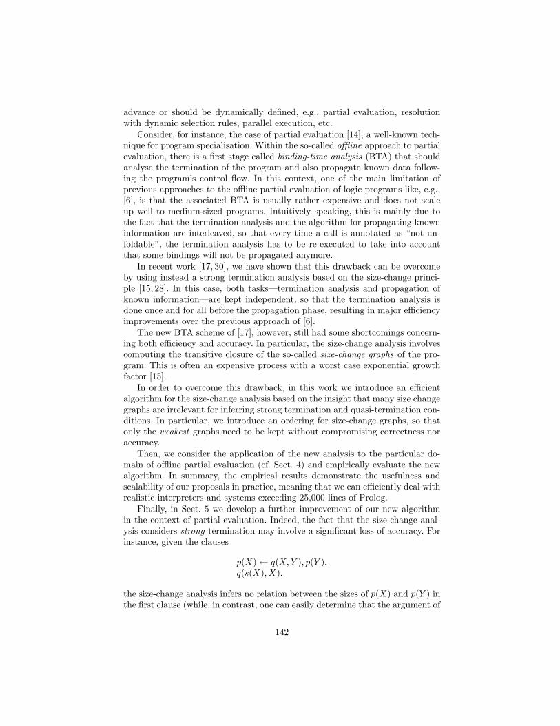
advance or should be dynamically defined, e.g., partial evaluation, resolutionwith dynamic selection rules, parallel execution, etc.

Consider, for instance, the case of partial evaluation [14], a well-known tech-nique for program specialisation. Within the so-called offline approach to partialevaluation, there is a first stage called binding-time analysis (BTA) that shouldanalyse the termination of the program and also propagate known data follow-ing the program’s control flow. In this context, one of the main limitation ofprevious approaches to the offline partial evaluation of logic programs like, e.g.,[6], is that the associated BTA is usually rather expensive and does not scaleup well to medium-sized programs. Intuitively speaking, this is mainly due tothe fact that the termination analysis and the algorithm for propagating knowninformation are interleaved, so that every time a call is annotated as “not un-foldable”, the termination analysis has to be re-executed to take into accountthat some bindings will not be propagated anymore.

In recent work [17, 30], we have shown that this drawback can be overcomeby using instead a strong termination analysis based on the size-change princi-ple [15, 28]. In this case, both tasks—termination analysis and propagation ofknown information—are kept independent, so that the termination analysis isdone once and for all before the propagation phase, resulting in major efficiencyimprovements over the previous approach of [6].

The new BTA scheme of [17], however, still had some shortcomings concern-ing both efficiency and accuracy. In particular, the size-change analysis involvescomputing the transitive closure of the so-called size-change graphs of the pro-gram. This is often an expensive process with a worst case exponential growthfactor [15].

In order to overcome this drawback, in this work we introduce an efficientalgorithm for the size-change analysis based on the insight that many size changegraphs are irrelevant for inferring strong termination and quasi-termination con-ditions. In particular, we introduce an ordering for size-change graphs, so thatonly the weakest graphs need to be kept without compromising correctness noraccuracy.

Then, we consider the application of the new analysis to the particular do-main of offline partial evaluation (cf. Sect. 4) and empirically evaluate the newalgorithm. In summary, the empirical results demonstrate the usefulness andscalability of our proposals in practice, meaning that we can efficiently deal withrealistic interpreters and systems exceeding 25,000 lines of Prolog.

Finally, in Sect. 5 we develop a further improvement of our new algorithmin the context of partial evaluation. Indeed, the fact that the size-change anal-ysis considers strong termination may involve a significant loss of accuracy. Forinstance, given the clauses

p(X)← q(X, Y ), p(Y ).q(s(X), X).

the size-change analysis infers no relation between the sizes of p(X) and p(Y ) inthe first clause (while, in contrast, one can easily determine that the argument of

142

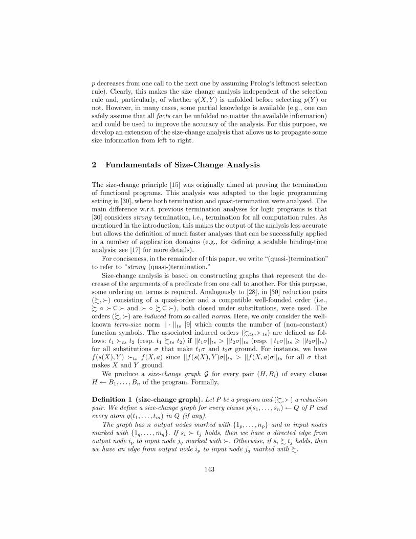
p decreases from one call to the next one by assuming Prolog’s leftmost selectionrule). Clearly, this makes the size change analysis independent of the selectionrule and, particularly, of whether q(X, Y ) is unfolded before selecting p(Y ) ornot. However, in many cases, some partial knowledge is available (e.g., one cansafely assume that all facts can be unfolded no matter the available information)and could be used to improve the accuracy of the analysis. For this purpose, wedevelop an extension of the size-change analysis that allows us to propagate somesize information from left to right.

2 Fundamentals of Size-Change Analysis

The size-change principle [15] was originally aimed at proving the terminationof functional programs. This analysis was adapted to the logic programmingsetting in [30], where both termination and quasi-termination were analysed. Themain difference w.r.t. previous termination analyses for logic programs is that[30] considers strong termination, i.e., termination for all computation rules. Asmentioned in the introduction, this makes the output of the analysis less accuratebut allows the definition of much faster analyses that can be successfully appliedin a number of application domains (e.g., for defining a scalable binding-timeanalysis; see [17] for more details).

For conciseness, in the remainder of this paper, we write “(quasi-)termination”to refer to “strong (quasi-)termination.”

Size-change analysis is based on constructing graphs that represent the de-crease of the arguments of a predicate from one call to another. For this purpose,some ordering on terms is required. Analogously to [28], in [30] reduction pairs(%,�) consisting of a quasi-order and a compatible well-founded order (i.e.,% ◦ �⊆� and � ◦ %⊆�), both closed under substitutions, were used. Theorders (%,�) are induced from so called norms. Here, we only consider the well-known term-size norm || · ||ts [9] which counts the number of (non-constant)function symbols. The associated induced orders (%ts,�ts) are defined as fol-lows: t1 �ts t2 (resp. t1 %ts t2) if ||t1σ||ts > ||t2σ||ts (resp. ||t1σ||ts > ||t2σ||ts)for all substitutions σ that make t1σ and t2σ ground. For instance, we havef(s(X), Y ) �ts f(X, a) since ||f(s(X), Y )σ||ts > ||f(X, a)σ||ts for all σ thatmakes X and Y ground.

We produce a size-change graph G for every pair (H,Bi) of every clauseH ← B1, . . . , Bn of the program. Formally,

Definition 1 (size-change graph). Let P be a program and (%,�) a reductionpair. We define a size-change graph for every clause p(s1, . . . , sn)← Q of P andevery atom q(t1, . . . , tm) in Q (if any).

The graph has n output nodes marked with {1p, . . . , np} and m input nodesmarked with {1q, . . . ,mq}. If si � tj holds, then we have a directed edge fromoutput node ip to input node jq marked with �. Otherwise, if si % tj holds, thenwe have an edge from output node ip to input node jq marked with %.

143

A size-change graph is thus a bipartite labelled graph G = (V,W,E) whereV = {1p, . . . , np} and W = {1q, . . . ,mq} are the labels of the output and inputnodes, respectively, and E ⊆ V ×W × {%,�} are the edges.

Example 1. Consider the following program MLIST :

(c1) mlist(L, I, [ ])← empty(L).(c2) mlist(L, I, LI)← nonempty(L), hd(L,X), tl(L,R),ml(X, R, I, LI).

(c3) ml(X, R, I, [XI|RI])← mult(X, I,XI), mlist(R, I,RI).

(c4) mult(0, Y, 0). (c5) mult(s(X), Y, Z)← mult(X, Y, Z1), add(Z1, Y, Z).(c6) add(X, 0, X). (c7) add(X, s(Y ), s(Z))← add(X, Y, Z).

(c8) hd([X | ],X ). (c9) empty([ ]).

(c10) tl([ |R],R). (c11) nonempty([ | ]).

which is used to multiply all the elements of a list by a given number. Theprogram is somewhat contrived in order to better illustrate our technique.

Here, the size-change graphs associated to, e.g., clause c3 are as follows:4

1ml

%ts // 1mult

2ml 2mult

3ml

%ts 44iiiiiii3mult

4ml

�ts 44iiiiiii

1ml 1mlist

2ml

%ts 44iiiiiii2mlist

3ml

%ts 44iiiiiii3mlist

4ml

�ts 44iiiiiii

using a reduction pair (%ts,�ts) induced from the term-size norm.

In order to identify the program loops, we should compute roughly a transitiveclosure of the size-change graphs by composing them in all possible ways.

Definition 2 (graph concatenation, idempotent multigraph). A multi-graph of P is inductively defined to be either a size-change graph of P or theconcatenation (see below) of two multigraphs of P . Given two multigraphs:

G = ({1p, . . . , np}, {1q, . . . ,mq}, E1) and H = ({1q, . . . ,mq}, {1r, . . . , lr}, E2)

w.r.t. the same reduction pair (%,�), then the concatenation

G • H = ({1p, . . . , np}, {1r, . . . , lr}, E)

is also a multigraph, where E contains an edge from ip to kr iff E1 contains anedge from ip to some jq and E2 contains an edge from jq to kr. If some of theedges are labelled with �, then so is the edge in E; otherwise, it is labelled with%.

We say that a multigraph G of P is idempotent when G = G • G. Intuitivelyspeaking, an idempotent multigraph represents a chain of multigraphs.4 In general, we denote with p/n a predicate symbol of arity n. However, in the ex-

amples, we simply write p for predicate p/n when no confusion can arise.

144

Example 2. For the program MLIST of Example 1, we have the following fouridempotent multigraphs:

1mlist 1mlist

2mlist

%ts // 2mlist

3mlist�ts // 3mlist

1ml 1ml

2ml 2ml

3ml

%ts // 3ml

4ml�ts // 4ml

1mult�ts // 1mult

2mult

%ts // 2mult

3mult 3mult

1add

%ts // 1add

2add�ts // 2add

3add�ts // 3add

that represent how the size of the arguments of the four potentially loopingpredicates changes from one call to another.

The main termination results from [17, 30] can be summarised as follows:

– A predicate p/n terminates if every idempotent multigraph for p/n containsat least one edge ip

�−→ ip, 1 ≤ i ≤ n, such that the i-th argument of everycall to this predicate is ground.5

– A predicate p/n quasi-terminates if every idempotent multigraph for p/n

contains edges j1p

R1−→ 1p, . . . , jnp

Rn−→ np, Ri ∈ {�,%}, and the argumentsj1, . . . , jn are ground in every call to p/n. Additionally, the considered quasi-order % should be well-founded and finitely partitioning [8, 29], i.e., thereshould not be infinitely many “equal” ground terms under %.

These conditions, though in principle undecidable, can be approximated in anumber of ways. For instance, in the context of partial evaluation, the computedbinding-times—static for definitely known arguments and dynamic for possiblyunknown arguments—can easily be used for this purpose (cf. Sect. 4.1).

3 A Procedure for Size-Change Analysis

In this section, we introduce a fast and accurate procedure for the size-changeanalysis of logic programs. In principle, a naive procedure for computing the setof idempotent multigraphs of a program may proceed as follows:

1. First, the size-change graphs of the program are built according to Def. 1.2. Then, after initialising a set M with the computed size-change graphs, one

proceeds iteratively as follows:(a) compute the concatenation of every pair of (not necessarily different)

multigraphs ofM;(b) update M with the new multigraphs.This process is repeated until no new multigraphs are added toM.

Unfortunately, such a naive algorithm is unacceptably expensive and does notscale up to even simple programs. Therefore, in the following, we introducea much more efficient procedure. Intuitively speaking, it improves the naiveprocedure by taking into account the following observations:5 A more relaxed condition based on the notion of instantiated enough w.r.t. a norm

[22] can be found in [17].

145

– Firstly, not all size-change graphs need to be constructed, but only those inthe path of a (potential) loop. For instance, in Example 1, the size-changegraph from mlist to empty cannot contribute to the construction of anyidempotent multigraph.

– Secondly, in many cases, computing the idempotent multigraphs for a singlepredicate for each loop suffices. For instance, in Example 2, the idempotentmultigraphs for both mlist and ml actually refer to the same loop. This issomehow redundant since either the two multigraphs will point out that bothpredicates terminate or that both of them may loop.

– Finally, when we have multigraphs G1 and G2 for a given predicate p/n suchthat termination of p/n using G1 always implies termination of p/n usingG2, then we can safely discard G2.

These observations allow us to design a faster procedure for size-change analysis.It proceeds in a stepwise manner as follows:

a) Identifying the program loops. In order to identify the (potential) pro-gram loops, we first construct the call graph of the program, i.e., a directed graphthat contains the predicate symbols as vertices and an edge from predicate p/nto predicate q/m for each clause of the form6 p(tn) ← B1, . . . , q(sm), . . . , Bk,k ≥ 1, in the program.

For instance, the call graph of program MLIST in Example 1 is as follows:

mlist**

rreeeeeeeeeeeeeeeeeeeuukkkkkk

�� ''OOOOOO mlll // multRR// addRR

empty nonempty hd tl

Then, we compute the strongly connected components (SCC) of the call graphand delete both trivial SCCs (i.e., SCCs with a single predicate symbol which isnot self-recursive) and edges between SCCs. We denote the resulting graph withscc(P ) for any program P . E.g., for program MLIST , scc(MLIST ) is as follows:

mlist**mlll multRR addRR

b) Determining the initial set of size-change graphs. We denote bysc graphs(P ) a subset of the size-change graphs of program P that fulfils thefollowing condition: there is a size-change graph from atom p(tn) to atom q(sm)in sc graphs(P ) iff there is an associated edge from p/n to q/m in scc(P ). E.g.,for program MLIST of Example 1, sc graphs(MLIST ) contains only four size-change graphs, while the naive approach would have constructed ten size-changegraphs.

In principle, only the size-change graphs in sc graphs(P ) need to be con-sidered in the size-change analysis. This refinement is correct since idempotent

6 We use tn to denote the sequence t1, . . . , tn.

146

multigraphs can only be built from the concatenation of a sequence of size-changegraphs that follows the path of a cycle in the call graph (i.e., a path of scc(P )).

Furthermore, not all concatenations between these size-change graphs are ac-tually required. As mentioned before, computing a single idempotent multigraphfor each (potential) program loop suffices. In the following, we say that S is acover set for scc(P ) if S contains at least one predicate symbol for each loop inscc(P ). We denote by CS(P ) the set of cover sets for scc(P ).

Definition 3 (initial size-change graphs). Let P be a program and S ∈CS(P ) be a cover set for scc(P ). We denote by i sc graphs(P, S) the size-changegraphs from sc graphs(P ) that start from a predicate of S.

Intuitively, the size-change graphs in i sc graphs(P, S) will act as the seeds ofour iterative process for computing idempotent multigraphs. As a consequence,only idempotent multigraphs for the predicates of S are produced. Therefore,the termination result of Sect. 2 should be rephrased as follows:

A predicate p/n terminates if there exists some (not necessarily different)predicate q/m in the same cycle of scc(P ) and every idempotent multigraphof q/m contains at least one edge iq

�−→ iq, 1 ≤ i ≤ m, such that the i-thargument of every call to this predicate q/m is ground.

(∗)

A similar condition could be given for quasi-termination. Proving the correctnessof this refinement is not difficult and relies on the fact that either all predicatesin a loop are terminating or none.

Example 3. Given the program MLIST of Ex. 1, both S1 = {mlist/3,mult/3, add/3}and S2 = {ml/4,mult/3, add/3} are cover sets for scc(MLIST ). For instance,the set i sc graphs(P, S1) contains only the three size-change graphs startingfrom mlist/3, mult/3 and add/3.

c) Computing the idempotent multigraphs. The core of our improvedprocedure for size-change analysis is shown in Fig. 1. The algorithm considersthe following ordering on multigraphs:

Definition 4 (weaker multigraph). Given two multigraphs G1 = 〈V1,W1, E1〉and G2 = 〈V2,W2, E2〉, we say that G1 is weaker than G2, in symbols G1 v G2,iff the following conditions hold:

– the output and input nodes coincide, i.e., V1 = V2 and W1 = W2, and– for every edge i

R1−→ j ∈ E1, R1 ∈ {�,%}, there exists an edge iR2−→ j ∈ E2,

R2 ∈ {�,%}, such that R1 v R2

where �v�, %v% and %v�, but � 6v%.

Basically, if a multigraph G is weaker than another multigraph H, then we havethat whenever termination can be proved with G only, it could also be provedwith both G and H. Indeed, if G v H and G′ v H′ then G •G′ v H•H′. Thus, byinduction, we can prove that for every size change graph derivable from H there

147

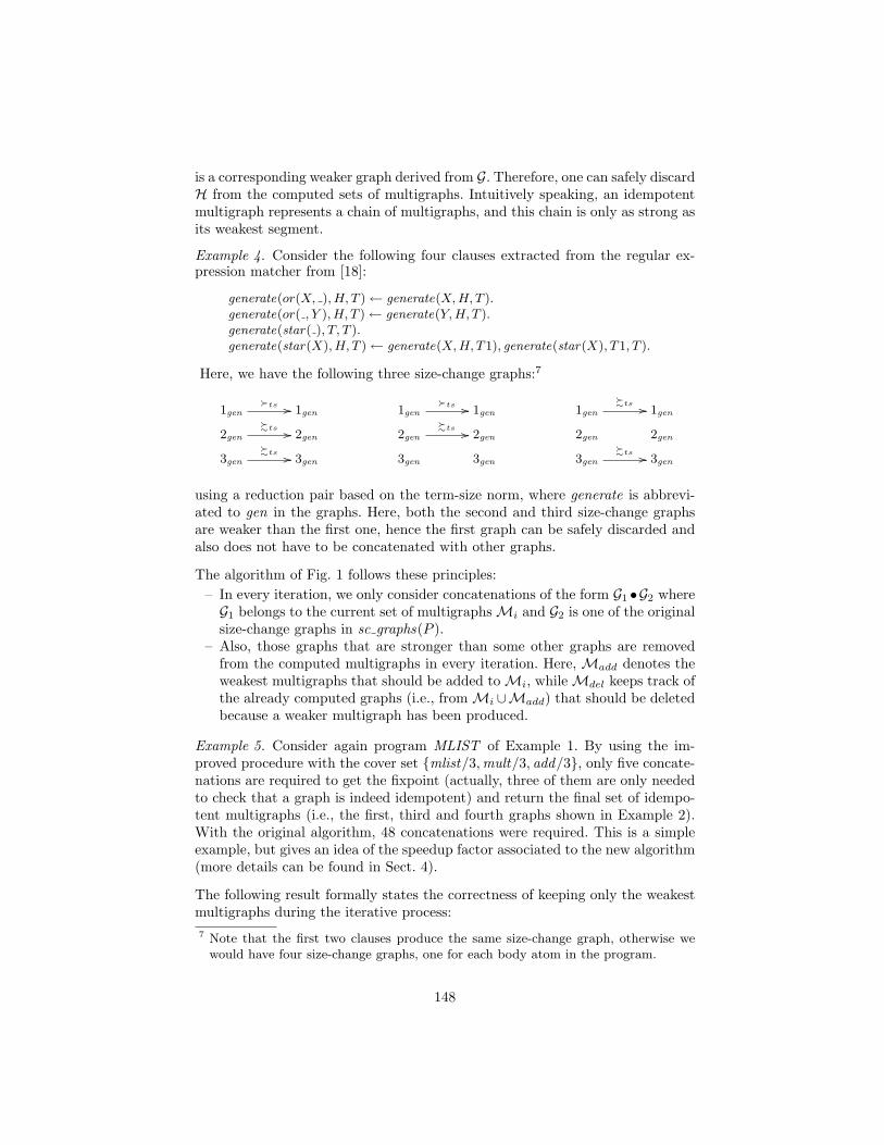
is a corresponding weaker graph derived from G. Therefore, one can safely discardH from the computed sets of multigraphs. Intuitively speaking, an idempotentmultigraph represents a chain of multigraphs, and this chain is only as strong asits weakest segment.

Example 4. Consider the following four clauses extracted from the regular ex-pression matcher from [18]:

generate(or(X, ), H, T )← generate(X, H, T ).generate(or( , Y ), H, T )← generate(Y, H, T ).generate(star( ), T, T ).generate(star(X), H, T )← generate(X, H, T1), generate(star(X), T1, T ).

Here, we have the following three size-change graphs:7

1gen�ts // 1gen

2gen

%ts // 2gen

3gen

%ts // 3gen

1gen�ts // 1gen

2gen

%ts // 2gen

3gen 3gen

1gen

%ts // 1gen

2gen 2gen

3gen

%ts // 3gen

using a reduction pair based on the term-size norm, where generate is abbrevi-ated to gen in the graphs. Here, both the second and third size-change graphsare weaker than the first one, hence the first graph can be safely discarded andalso does not have to be concatenated with other graphs.

The algorithm of Fig. 1 follows these principles:– In every iteration, we only consider concatenations of the form G1 •G2 whereG1 belongs to the current set of multigraphsMi and G2 is one of the originalsize-change graphs in sc graphs(P ).

– Also, those graphs that are stronger than some other graphs are removedfrom the computed multigraphs in every iteration. Here, Madd denotes theweakest multigraphs that should be added toMi, whileMdel keeps track ofthe already computed graphs (i.e., fromMi ∪Madd) that should be deletedbecause a weaker multigraph has been produced.

Example 5. Consider again program MLIST of Example 1. By using the im-proved procedure with the cover set {mlist/3,mult/3, add/3}, only five concate-nations are required to get the fixpoint (actually, three of them are only neededto check that a graph is indeed idempotent) and return the final set of idempo-tent multigraphs (i.e., the first, third and fourth graphs shown in Example 2).With the original algorithm, 48 concatenations were required. This is a simpleexample, but gives an idea of the speedup factor associated to the new algorithm(more details can be found in Sect. 4).

The following result formally states the correctness of keeping only the weakestmultigraphs during the iterative process:7 Note that the first two clauses produce the same size-change graph, otherwise we

would have four size-change graphs, one for each body atom in the program.

148

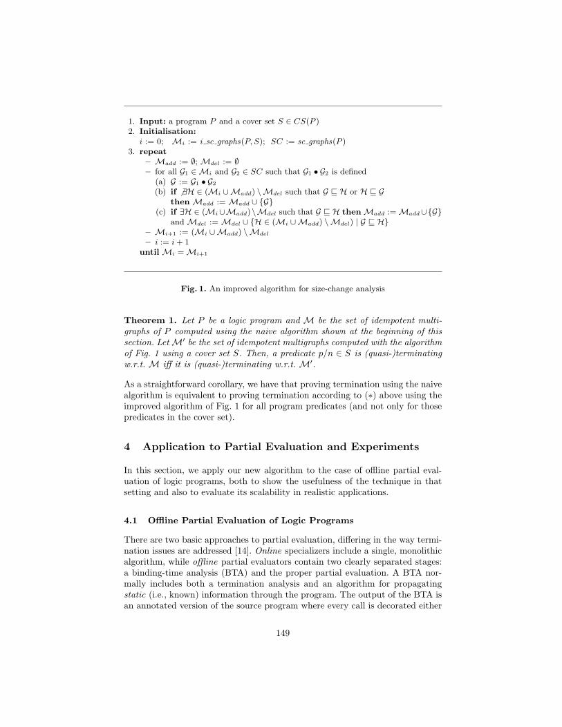
1. Input: a program P and a cover set S ∈ CS(P )2. Initialisation:

i := 0; Mi := i sc graphs(P, S); SC := sc graphs(P )3. repeat

– Madd := ∅; Mdel := ∅– for all G1 ∈Mi and G2 ∈ SC such that G1 • G2 is defined

(a) G := G1 • G2

(b) if 6 ∃H ∈ (Mi ∪Madd) \Mdel such that G v H or H v GthenMadd := Madd ∪ {G}

(c) if ∃H ∈ (Mi∪Madd)\Mdel such that G v H thenMadd :=Madd∪{G}andMdel := Mdel ∪ {H ∈ (Mi ∪Madd) \Mdel) | G v H}

– Mi+1 := (Mi ∪Madd) \Mdel

– i := i + 1untilMi =Mi+1

Fig. 1. An improved algorithm for size-change analysis

Theorem 1. Let P be a logic program and M be the set of idempotent multi-graphs of P computed using the naive algorithm shown at the beginning of thissection. LetM′ be the set of idempotent multigraphs computed with the algorithmof Fig. 1 using a cover set S. Then, a predicate p/n ∈ S is (quasi-)terminatingw.r.t. M iff it is (quasi-)terminating w.r.t. M′.

As a straightforward corollary, we have that proving termination using the naivealgorithm is equivalent to proving termination according to (∗) above using theimproved algorithm of Fig. 1 for all program predicates (and not only for thosepredicates in the cover set).

4 Application to Partial Evaluation and Experiments

In this section, we apply our new algorithm to the case of offline partial eval-uation of logic programs, both to show the usefulness of the technique in thatsetting and also to evaluate its scalability in realistic applications.

4.1 Offline Partial Evaluation of Logic Programs

There are two basic approaches to partial evaluation, differing in the way termi-nation issues are addressed [14]. Online specializers include a single, monolithicalgorithm, while offline partial evaluators contain two clearly separated stages:a binding-time analysis (BTA) and the proper partial evaluation. A BTA nor-mally includes both a termination analysis and an algorithm for propagatingstatic (i.e., known) information through the program. The output of the BTA isan annotated version of the source program where every call is decorated either

149

with unfold (to be evaluated) or memo (to be residualized, i.e., the call will be-come part of the residual program); also, every procedure argument is annotatedeither with static (definitely known at partial evaluation time) or dynamic (pos-sibly unknown at partial evaluation time). Typically, offline partial evaluatorsare faster but less precise than online partial evaluators.

In the following, patterns are expressions of the form p(b1, . . . , bn), with p/na predicate symbol of arity n and b1, . . . , bn binding-times. Here, we considera simple domain of binding-times with two elements: static and dynamic; morerefined domains can be found in, e.g., [6].

An offline partial evaluator takes an annotated program and an initial set ofatoms and proceeds iteratively as follows:

– First, the initial atoms are unfolded as much as possible according to theprogram annotations. This is called the local level of partial evaluation.

– Then, every atom in the leaves of the incomplete SLD trees produced in thelocal level are added—perhaps generalising some of their arguments—to theset of (to be) partially evaluated atoms. This is called the global level ofpartial evaluation.

Similarly, termination issues can be split into local and global termination, i.e.,termination of the local and global levels, respectively. Following the (quasi-)termination results sketched at the end of Sect. 2, source programs are anno-tated as follows:8

Local termination. If all idempotent multigraphs for a predicate p/n includean edge ip

�−→ ip and the i-th argument of p/n is static, then all calls to p/nare annotated with unfold; otherwise, they are annotated with memo.

Global termination. If all idempotent multigraphs for a predicate p/n includean edge jp

R−→ ip such that R ∈ {�,%} and its j-th argument is static,then the i-th argument of p/n can be kept as static; otherwise, it should beannotated as dynamic so that it will be generalised at the global level.

4.2 Prolog Implementation and Empirical Evaluation

We have implemented our new algorithm from Fig. 1 (cf. Sect. 3) for size-changeanalysis in SICStus Prolog. To be able to measure the effectiveness of the re-striction to SCCs (i.e., the restriction to sc graphs(P )) and the restriction toonly consider one predicate per loop (i.e., the restriction to i sc graphs(P, S) forsome cover set S), we have provided a way to turn these optimisations off. Wealso compare to the old implementation from [17], which includes none of thenew ideas presented in this paper.

An interesting implementation technique, which all three versions consider(not described in [17]), is the use of hashing9 to more quickly identify whichsize-change graphs already exist and which ones can be concatenated with each

8 The groundness of an argument is now replaced by the argument being static.9 We note that, in earlier versions of SICStus, term hash generates surprisingly many

collisions; a problem which we reported and which has been fixed in version 4.0.5.

150

other. All these three algorithms are integrated into the same BTA from [17],which provides a command-line interface. The BTA is by default polyvariant(but can be forced to be monovariant) and uses a domain with the followingvalues: static, list nv (for lists of non-variable terms), list, nv (for non-variableterms), and dynamic. The user can also provide hints to the BTA (see below).The implemented size-change analysis uses a reduction pair induced from theterm-size norm.

Evaluation of Efficiency. Figure 2 contains an overview of our empirical results,where all times are in seconds. A value of 0 means that the timing was below ourmeasuring threshold. The experiments were run on a MacBook Pro with a 2.33GHz Core2 Duo Processor and 3 GB of RAM. Our BTA was run using SICStusProlog 4.0.5. The first six benchmarks come from the DPPD [18] library, vanilla,ctl and lambdaint come from [16]. The picemul program is the PIC processoremulator from [11] with 137 clauses and 855 lines of code. javabc and javabc heapare Java Bytecode interpreters from [10] with roughly 100 clauses. peval are over2500 lines of Prolog from a partial evaluator for the ground representation from[20]. self app are the 1925 lines of our size-change analysis and BTA itself. dSLis an interpreter of 444 lines for the dSL specification language [31]. csp is thecore interpreter for full CSP-M from [21], consisting of 1771 lines of code. probis the core interpreter of ProB [19] for B machines, not containing the kernelpredicates or the model checker. It consists of 1910 lines of code and deals withB expressions, predicates and substitutions. promela is an interpreter for the fullPromela language (see, e.g., [13]), consisting of 1148 lines of code. Finally, goedelis the source code of the Godel system [12] consisting of 27354 lines of Prolog.10

The “noentry” annotation in Fig. 2 means that no entry point was provided,hence only the size-change analysis was performed (and no propagation of staticinformation).

The output of the new BTA (without SCC) and the old BTA from [17] areidentical as far as local and global annotations are concerned.

In summary, the new size change analysis is always faster and we see improve-ments of roughly three orders of magnitude on the most complicated examples(up to a factor of 3500 for prob (noentry)). We are able to deal with realisticinterpreters and systems exceeding 25K lines of code. For goedel, a small partof the inferred termination conditions are as follows:

is_not_terminating(parse_language1, 6, [d,_,_,_,_,_]).

global_binding_times(parse_language1, 6, [s,d,s,s,d,s]).

is_not_terminating(build_delay_condition, 4, [d,d,_,_]).

global_binding_times(build_delay_condition, 4, [s,s,d,d]).

In particular, this means that the analysis has inferred that the predicate parse language1

can be unfolded if the first argument is static, and that the first, third, fourthand last argument do not need to be generalised to ensure quasi-termination.10 Downloaded from http://www.cs.bris.ac.uk/Research/LanguagesArchitecture/goedel/

and put into a single file, removing module declarations and adapting some of thecode for SICStus 4.

151

Benchmark Old BTA New BTA New BTAfrom [17] (without SCC) (with SCC)

contains.kmp 0.01 0.00 0.00imperative-power 2.35 0.03 0.02liftsolve.app 0.02 0.01 0.01match-kmp 0.00 0.00 0.00regexp.r3 0.01 0.00 0.00ssuply 0.01 0.01 0.01

vanilla 0.01 0.00 0.00lambdaint 0.17 0.02 0.02picemul 0.31 0.15 0.15picemul (noentry) 0.18 0.01 0.01ctl 0.03 0.02 0.02javabc 0.03 0.03 0.03javabc heap 0.09 0.09 0.09peval 0.48 0.15 0.06self app (noentry) 0.34 0.20 0.05dSL 0.03 0.01 0.01csp (noentry) 5.16 0.21 0.09prob 387.12 1.41 0.61prob (noentry) 386.63 0.79 0.11promela (noentry) 330.05 0.35 0.34goedel (noentry) 1750.90 13.32 2.61

Fig. 2. Empirical results

Compared to the BTA from [6] using binary clauses rather than size-changeanalysis, the difference is even more striking. This BTA is in turn, e.g., 200 timesslower than the old BTA for the picemul example; see [17]. We have also triedthe latest version of Terminweb,11 based upon [5]. However, the online versionfailed to terminate successfully on, e.g., the picemul example (for which our size-change analysis takes 0.01 s). We have also tried TermiLog,12 but it timed outafter 4 minutes (the maximum time that can be set in the online version).

Evaluation of Precision. Without the use of the SCC optimisations in the al-gorithm of Fig. 1, the precision remains unchanged w.r.t. [17], and as such thesame specialisations can be achieved as described in [17] using hints: e.g., Jones-optimal specialisation for vanilla, reproducing the decompilation from Java byte-code to CLP from [10] or automatically generating the generated code from [11]for picemul.

With the SCC optimisations, we reduce the number of predicates that arememoised. This in turn also reduces the number of hints that a user has toprovide to obtain the desired specialisation.

For example, the vanilla example required two hints in [17] and now onlyone hint is required to obtain a good specialisation. For lambdaint 6 hints were11 http://www.cs.bgu.ac.il/∼mcodish/TerminWeb/12 http://www.cs.huji.ac.il/∼naomil/termilog.php

152

required in [17] to get good performance. Now only two hints are required,expressing the fact that the expression being evaluated and the list of boundvariable names are expected to be static and should not be generalised awayby the BTA.13 In the following section we show how the precision of the size-change analysis can be further improved in the setting of partial evaluation,further reducing the need for hints.

5 Propagating Partial Left-To-Right Information

In this section, we extend the size-change analysis in order to right-propagatesize information in some cases. Consider, e.g., clause (c2) in Example 1:

(c2) mlist(L, I, LI)← nonempty(L), hd(L,X), tl(L,R),ml(X, R, I, LI).

Since our size-change analysis considers strong termination, we compare the sizeof the head of the clause with the size of each atom in the body independently.Therefore, we get no relation between the sizes of list L in the head and its headX and tail R in the call to ml .

In some cases, however, one might assume some additional restrictions. Forinstance, in many partial evaluators a left-to-right selection rule is used withthe only exception that those calls which are annotated with memo are neverselected. Therefore, if we know that some calls can be fully unfolded withoutentering an infinite loop (the case, e.g., of non-recursive predicates), then one cansafely propagate the size relationships for the success patterns of these calls to thesubsequent atoms in the clause. In principle, these “fully unfoldable” calls canbe detected using a standard left-termination analysis (i.e., one that considers astandard left-to-right computation rule), e.g., [5], while size relations of successpatterns can be obtained from the computation of the convex hull of [1]. Here,though, we consider that this information is provided by the user by meansof hints of the form ’$FULLYUNFOLD’(p,n,size relations) where size_relations

are the interargument size relations for the success patterns of p/n. For instance,for the program MLIST of Ex. 1, we may have the following hints:

’$FULLYUNFOLD’(hd,2,[1>2]). ’$FULLYUNFOLD’(tl,2,[1>2]).

which should be read as “when the call to hd (resp. tl) succeeds, the size of itsfirst argument is strictly greater than the size of its second argument”. We notethat, in order to be safe, the interargument size relations should be based on thesame norm used induce the reduction pair considered in the size-change graphs.

Let us now describe how the size-change analysis can be improved by usingthis new kind of hints. Consider a clause of the form

P ← Q1, . . . , Qi−1, p(t1, . . . , tn), Qi+1, . . . , Qm.

13 This does not give exactly the same result; the solution with 6 hints memoises oneval if, which in this case leads to a more efficient version than memoising on eval.

153

together with the hint ’$FULLYUNFOLD’(p,n,I). Then, we first replace this clauseby the following ones:

P ← Q1, . . . , Qi−1, pentry(x1, . . . , xk, t1, . . . , tn).pentry(x1, . . . , xk, y1, . . . , yn)← p(y1, . . . , yn), pexit(x1, . . . , xk, y1, . . . , yn).pexit(x1, . . . , xk, y1, . . . , yn)← Qi+1, . . . , Qm.

where {x1, . . . , xk} = (Var(P,Q1, . . . , Qi−1)∩Var(Qi+1, . . . , Qm))\Var(p(t1, . . . , tn)).This transformation is clearly safe w.r.t. SLD resolution since the original clausecan be obtained by just unfolding both pentry and pexit.

Now, the size-change graphs of the first and third clauses are computed asusual. For the second clause, however, we assume that the atom p(y1, . . . , yn)could be fully unfolded producing the set of clauses

pentry(x1, . . . , xk, y1, . . . , yn)σ1 ← pexit(x1, . . . , xk, y1, . . . , yn)σ1.. . .pentry(x1, . . . , xk, y1, . . . , yn)σj ← pexit(x1, . . . , xk, y1, . . . , yn)σj .

where σ1, . . . , σj are the computed answers and the set of interargument sizerelations I safely approximates the size relations between the arguments of pentry

and pexit. Note that we do not need to fully unfold p/n to construct the size-change graphs (it is rather a device to show the correctness of our approach).Formally, for every relation i > j (resp. i > j) in the interargument size relations

for p/n, we should add an edge ipentry

�7−→ jpexit (resp. ipentry

%7−→ jpexit) to thesize-change graph from pentry to pexit. Moreover, we add an edge of the form

ipentry

%7−→ ipexit since both pentry and pexit are actually the same predicate.For instance, by considering the previous hints for program MLIST , the

clause (c2) is transformed into

(c21) mlist(L, I, LI)← nonempty(L), hdentry(L,X, I, LI).(c22) hdentry(L,X, I, LI)← hd(L,X), hdexit(L,X, I, LI).(c23) hdexit(L,X, I, LI)← tlentry(L,R,X, I, LI).(c24) tlentry(L,R,X, I, LI)← tl(L,R), tlexit(L,R,X, I, LI).(c25) tlexit(L,R,X, I, LI)← ml(X, R, I, LI).

Now, by using the interargument size relations for hd and tl , we construct thefollowing size-change graphs associated to clauses c22 and c24:

1hdentry �ts

**TTTTTTT%ts // 1hdexit

2hdentry

%ts // 2hdexit

3hdentry

%ts // 3hdexit

4hdentry

%ts // 4hdexit

1tlentry �ts

**UUUUUUU%ts // 1tlexit

2tlentry

%ts // 2tlexit

3tlentry

%ts // 3tlexit

4tlentry

%ts // 4tlexit

5tlentry

%ts // 5tlexit

Finally, by constructing the size-change graphs for clauses c21, c23 and c25 asusual, the size-change analysis can now infer the right relation between the sizesof list L in the atom mlist(L, I, LI) and the head X and tail R in the atomml(X, R, I, LI).

154

6 Discussion and Conclusion

In this paper, we have presented a new algorithm to perform strong termina-tion and quasi-termination inference using size-change analysis. The experimentshave shown that we can analyse the full 25K lines of source code of the Godelsystem in under three seconds. The main application of this algorithm is foroffline partial evaluation of large programs. In the experimental evaluation wehave shown that, with our new algorithm, we can now deal with realistic inter-preters, such as the interpreter for the full B specification language from [19].Together with the selective use of hints [17], we have obtained both a scalableand an effective partial evaluation procedure. The logical next step is to bringthis work to practical fruition, by, e.g., optimising the interpreter from [19] forparticular specifications, speeding up the animation and model checking process.This challenge has been on our research agenda for quite a while, and we nowbelieve that the goal can be achieved in the near future. One remaining technicalhurdle is the treatment of meta predicate annotations (the B interpreter usesmeta-predicates to implement delaying versions of negation and findall).

References

1. F. Benoy, A. King, and F. Mesnard. Computing convex hulls with a linear solver.TPLP, 5(1-2):259–271, 2005.

2. M. Bezem. Strong Termination of Logic Programs. Journal of Logic Programming,15(1&2):79–97, 1993.

3. Annalisa Bossi, Sandro Etalle, and Sabina Rossi. Properties of input-consumingderivations. TPLP, 2(2):125–154, 2002.

4. Annalisa Bossi, Sandro Etalle, Sabina Rossi, and Jan-Georg Smaus. Terminationof simply moded logic programs with dynamic scheduling. ACM Trans. Comput.Log., 5(3):470–507, 2004.

5. M. Codish and C. Taboch. A semantic basis for the termination analysis of logicprograms. Journal of Logic Programming, 41(1):103–123, 1999.

6. S.-J. Craig, J. Gallagher, M. Leuschel, and K.S. Henriksen. Fully Automatic Bind-ing Time Analysis for Prolog. In Proc. of LOPSTR’04, pages 53–68. SpringerLNCS 3573, 2005.

7. Danny De Schreye and Stefaan Decorte. Termination of logic programs: The neverending story. The Journal of Logic Programming, 19 & 20:199–260, May 1994.

8. S. Decorte, D. De Schreye, M. Leuschel, B. Martens, and K.F. Sagonas. Termi-nation Analysis for Tabled Logic Programming. In Proc. of LOPSTR’97, pages111–127. Springer LNCS 1463, 1998.

9. Allen Van Gelder. Deriving constraints among argument sizes in logic programs.Ann. Math. Artif. Intell., 3(2-4):361–392, 1991.

10. Miguel Gomez-Zamalloa, Elvira Albert, and German Puebla. Improving the de-compilation of Java bytecode to Prolog by partial evaluation. Electr. Notes Theor.Comput. Sci., 190(1):85–101, 2007.

11. K.S. Henriksen and J. Gallagher. Abstract interpretation of pic programs throughlogic programming. In SCAM, pp. 184–196. IEEE Computer Society, 2006.

12. Patricia Hill and John W. Lloyd. The Godel Programming Language. MIT Press,1994.

155

13. Gerard J. Holzmann. The model checker Spin. IEEE Trans. Software Eng.,23(5):279–295, 1997.

14. N.D. Jones, C.K. Gomard, and P. Sestoft. Partial Evaluation and Automatic Pro-gram Generation. Prentice-Hall, Englewood Cliffs, NJ, 1993.

15. C.S. Lee, N.D. Jones, and A.M. Ben-Amram. The Size-Change Principle for Pro-gram Termination. SIGPLAN Notices (Proc. of POPL’01), 28:81–92, 2001.

16. M. Leuschel, S.-J. Craig, M. Bruynooghe, and W. Vanhoof. Specialising Inter-preters Using Offline Partial Deduction. In Program Development in Computa-tional Logic, pages 340–375. Springer LNCS 3049, 2004.

17. M. Leuschel and G. Vidal. Fast Offline Partial Evaluation of Large Logic Programs.In Proc. of LOPSTR’08, pages 119–134. Springer LNCS 5438, 2009.

18. Michael Leuschel. The ecce partial deduction system and the dppd library ofbenchmarks. Obtainable via http://www.ecs.soton.ac.uk/~mal, 1996-2002.

19. Michael Leuschel and Michael Butler. ProB: A model checker for B. In KeijiroAraki, Stefania Gnesi, and Dino Mandrioli, editors, FME 2003: Formal Methods,LNCS 2805, pages 855–874. Springer-Verlag, 2003.

20. Michael Leuschel and Danny De Schreye. Creating specialised integrity checksthrough partial evaluation of meta-interpreters. The Journal of Logic Program-ming, 36(2):149–193, August 1998.

21. Michael Leuschel and Marc Fontaine. Probing the depths of CSP-M: A new FDR-compliant validation tool. In Proceedings ICFEM 2008, LNCS, pages 278–297.Springer-Verlag, 2008.

22. N. Lindenstrauss and Y. Sagiv. Automatic Termination Analysis of Logic Pro-grams. In Proc. of Int’l Conf. on Logic Programming (ICLP’97), pages 63–77. TheMIT Press, 1997.

23. Naomi Lindenstrauss, Yehoshua Sagiv, and Alexander Serebrenik. Proving Ter-mination for Logic Programs by the Query-Mapping Pairs Approach. In ProgramDevelopment in Computational Logic, pages 453–498, 2004.

24. Elena Marchiori and Frank Teusink. Termination of Logic Programs with DelayDeclarations. J. Log. Program., 39(1-3):95–124, 1999.

25. Lee Naish. Coroutining and the construction of terminating logic programs. Aus-tralian Computer Science Communications, 15(1):181–190, 1993.

26. Jan-Georg Smaus. Termination of Logic Programs Using Various Dynamic Selec-tion Rules. In Bart Demoen and Vladimir Lifschitz, editors, ICLP, volume 3132of Lecture Notes in Computer Science, pages 43–57. Springer, 2004.

27. J.-G. Smaus, P.M. Hill, and A. King. Verifying termination and error-freedom oflogic programs with block declarations. TPLP, 1(4):447–486, 2001.

28. R. Thiemann and J. Giesl. The Size-Change Principle and Dependency Pairs forTermination of Term Rewriting. Applicable Algebra in Engineering, Communica-tion and Computing, 16(4):229–270, 2005.

29. S. Verbaeten, K. Sagonas, and D. De Schreye. Termination Proofs for Logic Pro-grams with Tabling. ACM Transactions on Computational Logic, 2(1):57–92, 2001.

30. G. Vidal. Quasi-Terminating Logic Programs for Ensuring the Termination ofPartial Evaluation. In Proc. of PEPM’07, pages 51–60. ACM Press, 2007.

31. Bram De Wachter, Alexandre Genon, Thierry Massart, and Cedric Meuter. Theformal design of distributed controllers with dsl and Spin. Formal Asp. Comput.,17(2):177–200, 2005.

156

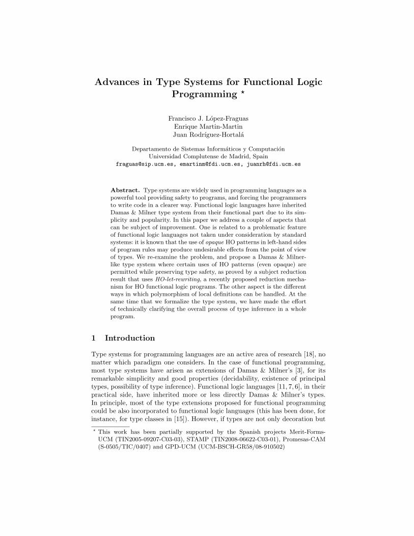
Advances in Type Systems for Functional LogicProgramming ?

Francisco J. Lopez-FraguasEnrique Martin-MartinJuan Rodrıguez-Hortala

Departamento de Sistemas Informaticos y ComputacionUniversidad Complutense de Madrid, Spain

fraguas@sip.ucm.es, emartinm@fdi.ucm.es, juanrh@fdi.ucm.es

Abstract. Type systems are widely used in programming languages as apowerful tool providing safety to programs, and forcing the programmersto write code in a clearer way. Functional logic languages have inheritedDamas & Milner type system from their functional part due to its sim-plicity and popularity. In this paper we address a couple of aspects thatcan be subject of improvement. One is related to a problematic featureof functional logic languages not taken under consideration by standardsystems: it is known that the use of opaque HO patterns in left-hand sidesof program rules may produce undesirable effects from the point of viewof types. We re-examine the problem, and propose a Damas & Milner-like type system where certain uses of HO patterns (even opaque) arepermitted while preserving type safety, as proved by a subject reductionresult that uses HO-let-rewriting, a recently proposed reduction mecha-nism for HO functional logic programs. The other aspect is the differentways in which polymorphism of local definitions can be handled. At thesame time that we formalize the type system, we have made the effortof technically clarifying the overall process of type inference in a wholeprogram.

1 Introduction

Type systems for programming languages are an active area of research [18], nomatter which paradigm one considers. In the case of functional programming,most type systems have arisen as extensions of Damas & Milner’s [3], for itsremarkable simplicity and good properties (decidability, existence of principaltypes, possibility of type inference). Functional logic languages [11, 7, 6], in theirpractical side, have inherited more or less directly Damas & Milner’s types.In principle, most of the type extensions proposed for functional programmingcould be also incorporated to functional logic languages (this has been done, forinstance, for type classes in [15]). However, if types are not only decoration but? This work has been partially supported by the Spanish projects Merit-Forms-

UCM (TIN2005-09207-C03-03), STAMP (TIN2008-06622-C03-01), Promesas-CAM(S-0505/TIC/0407) and GPD-UCM (UCM-BSCH-GR58/08-910502)

are to provide safety, one should be sure that the adopted system has indeed goodproperties. In this paper we tackle a couple of orthogonal aspects of existing FLPsystems that are problematic or not well covered by standard Damas & Milnersystems. One is the presence of so called HO patterns in programs, an expressivefeature allowed in some systems and for which a sensible semantics exists [4];however, it is known that unrestricted use of HO patterns leads to type unsafety,as recalled below. The second is the degree of polymorphism assumed for localpattern bindings, a matter with respect to which existing FP or FLP systemsvary greatly.

The rest of the paper is organized as follows. The next two subsections furtherdiscuss the two mentioned aspects. Sect. 2 contains some preliminaries about FLprograms and types. In Sect. 3 we expose the type system and prove its soundnesswrt. the let rewriting semantics of [10]. Sect. 4 contains a type inference relation,which let us find the most general type of expressions. Sect. 5 presents a methodto infer types for programs. Finally, Sect. 6 contains some conclusions and futurework. Omitted proofs can be found in [12].

1.1 Higher order patterns

In our formalism patterns appear in the left-hand side of rules and in lambdaor let expressions. Some of these patterns can be HO patterns, if they containpartial applications of function or constructor symbols. HO patterns can be asource of problems from the point of view of the types. In particular, it was shownin [5] that unrestricted use of HO patterns leads to loss of subject reduction, anessential property for a type system expressing that evaluation does not changetypes. The following is a crisp example of the problem.

Example 1 (Polymorphic Casting [2]). Consider the program consisting of therules snd X Y → Y , and true X → X, and false X → false, with the usualtypes inferred by a classical Damas & Milner algorithm. Then we can write thefunctions co (snd X) → X and cast X → co (snd X), whose inferred typeswill be ∀α.∀β.(α → α) → β and ∀α.∀β.α → β respectively. It is clear that theexpression and (cast 0) true is well-typed, because cast 0 has type bool (in factit has any type), but if we reduce that expression using the rule of cast theresulting expression and 0 true is ill-typed.

The problem arises when dealing with HO patterns, because unlike FO pat-terns, knowing the type of a HO pattern does not always permit us to know thetype of its subpatterns. In the previous example the cause is function co, becauseits pattern snd X is opaque and shadows the type of its subpattern X. Usualinference algorithms treat this opacity as polymorphism, and that is the reasonwhy it is inferred a completely polymorphic type for the result of the functionco.

In [5] the appearance of any opaque pattern in the left-hand side of the rulesis prohibited, but we will see that it is possible to be less restrictive. The key ismaking a distinction between transparent and opaque variables of a pattern:

158

a variable is transparent if its type is univocally fixed by the type of the pattern,and is opaque otherwise. We call a variable of a pattern critical if it is opaque inthe pattern and also appears elsewhere in the expression. The formal definitionof opaque and critical variables will be given in Sect. 3. With these notions wecan relax the situation in [5], prohibiting only those patterns having criticalvariables.

1.2 Local definitions

Functional and functional logic languages provide syntax to introduce local def-initions inside an expression. But in spite of the popularity of let-expressions,different implementations treat them differently because of the polymorphismthey give to bound variables. This difference can be observed in Ex. 2, being(e1, . . . , en) and [e1, . . . , en] the usual tuple and list notation respectively.

Example 2 (let expressions). Let e1 be let F = id in (F true, F 0), and e2 belet [F,G] = [id, id] in (F true, F 0, G 0, G false)

Intuitively, e1 gives a new name to the identity function and uses it twice witharguments of different types. Surprisingly, not all implementations consider thisexpression as well-typed, and the reason is that F is used with different typesin each appearance: bool → bool and int → int. Some implementations as Clean2.2, PAKCS 1.9.1 or KICS 0.81893 consider that a variable bound by a let-expression must be used with the same type in all the appearances in the bodyof the expression. In this situation we say that lets are completely monomorphic,and write letm for it.

On the other hand, we can consider that all the variables bound by thelet-expression may have different but coherent types, i.e., are treated polymor-phically. Then expressions like e1 or e2 would be well-typed. This is the decisionadopted by Hugs Sept. 2006, OCaml 3.10.2 or F# Sept. 2008. In this case, wewill say that lets are completely polymorphic, and write letp.

Finally, we can treat the bound variables monomorphically or polymorphi-cally depending on the form of the pattern. If the pattern is a variable, the lettreats it polymorphically, but if it is compound the let treats all the variablesmonomorphically. This is the case of GHC 6.8.2, SML of New Jersey v110.67or Curry Munster 0.9.11. In this implementations e1 is well-typed, while e2 not.We call this kind of let-expression letpm.

Fig. 1 summarizes the decisions of various implementations of functional andfunctional logic languages. The exact behavior wrt. types of local definitions isusually not well documented, not to say formalized, in those systems. One of ourcontributions is this paper is to technically clarify this question by adopting aneutral position, and formalizing the different possibilities for the polymorphismof local definitions.

159

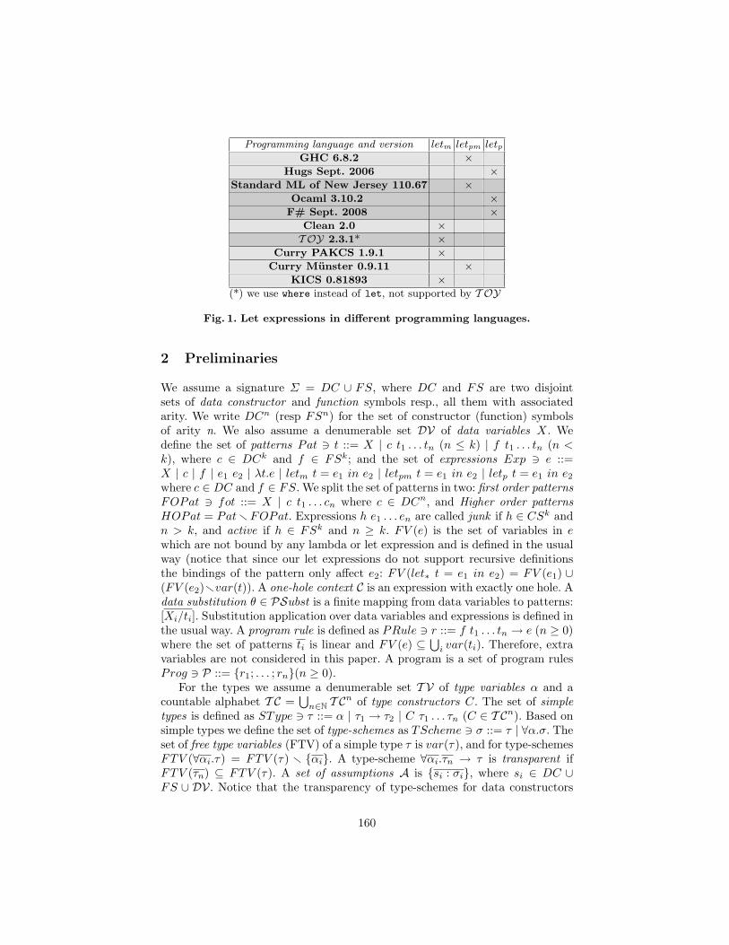
Programming language and version letm letpm letp

GHC 6.8.2 ×Hugs Sept. 2006 ×

Standard ML of New Jersey 110.67 ×Ocaml 3.10.2 ×

F# Sept. 2008 ×Clean 2.0 ×T OY 2.3.1* ×

Curry PAKCS 1.9.1 ×Curry Munster 0.9.11 ×

KICS 0.81893 ×(*) we use where instead of let, not supported by T OY

Fig. 1. Let expressions in different programming languages.

2 Preliminaries

We assume a signature Σ = DC ∪ FS, where DC and FS are two disjointsets of data constructor and function symbols resp., all them with associatedarity. We write DCn (resp FSn) for the set of constructor (function) symbolsof arity n. We also assume a denumerable set DV of data variables X. Wedefine the set of patterns Pat 3 t ::= X | c t1 . . . tn (n ≤ k) | f t1 . . . tn (n <k), where c ∈ DCk and f ∈ FSk; and the set of expressions Exp 3 e ::=X | c | f | e1 e2 | λt.e | letm t = e1 in e2 | letpm t = e1 in e2 | letp t = e1 in e2

where c ∈ DC and f ∈ FS. We split the set of patterns in two: first order patternsFOPat 3 fot ::= X | c t1 . . . cn where c ∈ DCn, and Higher order patternsHOPat = Pat r FOPat. Expressions h e1 . . . en are called junk if h ∈ CSk andn > k, and active if h ∈ FSk and n ≥ k. FV (e) is the set of variables in ewhich are not bound by any lambda or let expression and is defined in the usualway (notice that since our let expressions do not support recursive definitionsthe bindings of the pattern only affect e2: FV (let∗ t = e1 in e2) = FV (e1) ∪(FV (e2)rvar(t)). A one-hole context C is an expression with exactly one hole. Adata substitution θ ∈ PSubst is a finite mapping from data variables to patterns:[Xi/ti]. Substitution application over data variables and expressions is defined inthe usual way. A program rule is defined as PRule 3 r ::= f t1 . . . tn → e (n ≥ 0)where the set of patterns ti is linear and FV (e) ⊆

⋃i var(ti). Therefore, extra

variables are not considered in this paper. A program is a set of program rulesProg 3 P ::= {r1; . . . ; rn}(n ≥ 0).

For the types we assume a denumerable set T V of type variables α and acountable alphabet T C =

⋃n∈N T C

n of type constructors C. The set of simpletypes is defined as SType 3 τ ::= α | τ1 → τ2 | C τ1 . . . τn (C ∈ T Cn). Based onsimple types we define the set of type-schemes as TScheme 3 σ ::= τ | ∀α.σ. Theset of free type variables (FTV) of a simple type τ is var(τ), and for type-schemesFTV (∀αi.τ) = FTV (τ) r {αi}. A type-scheme ∀αi.τn → τ is transparent ifFTV (τn) ⊆ FTV (τ). A set of assumptions A is {si : σi}, where si ∈ DC ∪FS ∪ DV. Notice that the transparency of type-schemes for data constructors

160

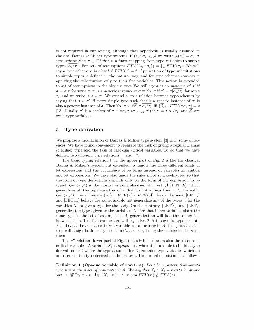
is not required in our setting, although that hypothesis is usually assumed inclassical Damas & Milner type systems. If (si : σi) ∈ A we write A(si) = σi. Atype substitution π ∈ T Subst is a finite mapping from type variables to simpletypes [αi/τi]. For sets of assumptions FTV ({si : σi}) =

⋃i FTV (σi). We will

say a type-scheme σ is closed if FTV (σ) = ∅. Application of type substitutionsto simple types is defined in the natural way, and for type-schemes consists inapplying the substitution only to their free variables. This notion is extendedto set of assumptions in the obvious way. We will say σ is an instance of σ′ ifσ = σ′π for some π. τ ′ is a generic instance of σ ≡ ∀αi.τ if τ ′ = τ [αi/τi] for someτi, and we write it σ � τ ′. We extend � to a relation between type-schemes bysaying that σ � σ′ iff every simple type such that is a generic instance of σ′ isalso a generic instance of σ. Then ∀αi.τ � ∀βi.τ [αi/τi] iff {βi}∩FTV (∀αi.τ) = ∅[13]. Finally, τ ′ is a variant of σ ≡ ∀αi.τ (σ �var τ ′) if τ ′ = τ [αi/βi] and βi arefresh type variables.

3 Type derivation

We propose a modification of Damas & Milner type system [3] with some differ-ences. We have found convenient to separate the task of giving a regular Damas& Milner type and the task of checking critical variables. To do that we havedefined two different type relations: ` and `•.

The basic typing relation ` in the upper part of Fig. 2 is like the classicalDamas & Milner’s system but extended to handle the three different kinds oflet expressions and the occurrence of patterns instead of variables in lambdaand let expressions. We have also made the rules more syntax-directed so thatthe form of type derivations depends only on the form of the expression to betyped. Gen(τ,A) is the closure or generalization of τ wrt. A [3, 13, 19], whichgeneralizes all the type variables of τ that do not appear free in A. Formally:Gen(τ,A) = ∀αi.τ where {αi} = FTV (τ) r FTV (A). As can be seen, [LETm]and [LETh

pm] behave the same, and do not generalize any of the types τi for thevariables Xi to give a type for the body. On the contrary, [LETX

pm] and [LETp]generalize the types given to the variables. Notice that if two variables share thesame type in the set of assumptions A, generalization will lose the connectionbetween them. This fact can be seen with e2 in Ex. 2. Although the type for bothF and G can be α → α (with α a variable not appearing in A) the generalizationstep will assign both the type-scheme ∀α.α → α, losing the connection betweenthem.

The `• relation (lower part of Fig. 2) uses ` but enforces also the absence ofcritical variables. A variable Xi is opaque in t when it is possible to build a typederivation for t where the type assumed for Xi contains type variables which donot occur in the type derived for the pattern. The formal definition is as follows.

Definition 1 (Opaque variable of t wrt. A). Let t be a pattern that admitstype wrt. a given set of assumptions A. We say that Xi ∈ Xi = var(t) is opaquewrt. A iff ∃τi, τ s.t. A⊕ {Xi : τi} ` t : τ and FTV (τi) * FTV (τ).

161

The previous definition is based on the existence of a certain type derivation,and therefore cannot be used as an effective check for the opacity of variables.Prop. 1 provides a more operational characterization of opacity that exploits theclose relationship between ` an type inference � presented in Sect. 4.

[ID]A ` s : τ

ifs ∈ DC ∪ FS ∪ DV∧ (s : σ) ∈ A ∧ σ � τ

[APP]

A ` e1 : τ1 → τA ` e2 : τ1

A ` e1e2 : τ

[Λ]

A⊕ {Xi : τi} ` t : τt

A⊕ {Xi : τi} ` e : τ

A ` λt.e : τt → τ

if {Xi} = var(t)

[LETm]

A⊕ {Xi : τi} ` t : τt

A ` e1 : τt

A⊕ {Xi : τi} ` e2 : τ2

A ` letm t = e1 in e2 : τ2

if {Xi} = var(t)

[LETXpm]

A ` e1 : τ1

A⊕ {X : Gen(τ1,A)} ` e2 : τ2

A ` letpm X = e1 in e2 : τ2

[LEThpm]

A⊕ {Xi : τi} ` h t1 . . . tn : τt

A ` e1 : τt

A⊕ {Xi : τi} ` e2 : τ2

A ` letpm h t1 . . . tn = e1 in e2 : τ2

if{Xi} = var(t1 . . . tn)∧ h ∈ DC ∪ FS

[LETp]

A⊕ {Xi : τi} ` t : τt

A ` e1 : τt

A⊕ {Xi : Gen(τi,A)} ` e2 : τ2

A ` letp t = e1 in e2 : τ2

if {Xi} = var(t)

[P]A ` e : τ

A `• e : τif critV arA(e) = ∅

Fig. 2. Rules of type system

Proposition 1. Xi ∈ Xi = var(t) is opaque wrt. A iff A⊕{Xi : αi} � t : τg|πg

and FTV (αiπg) * FTV (τg).

We write opaqueV arA(t) for set of opaque variables of t wrt. A. Now, we candefine the critical variables of an expression e wrt. A as those variables that,being opaque in a let or lambda pattern of e, are indeed used in e. Formally:

162

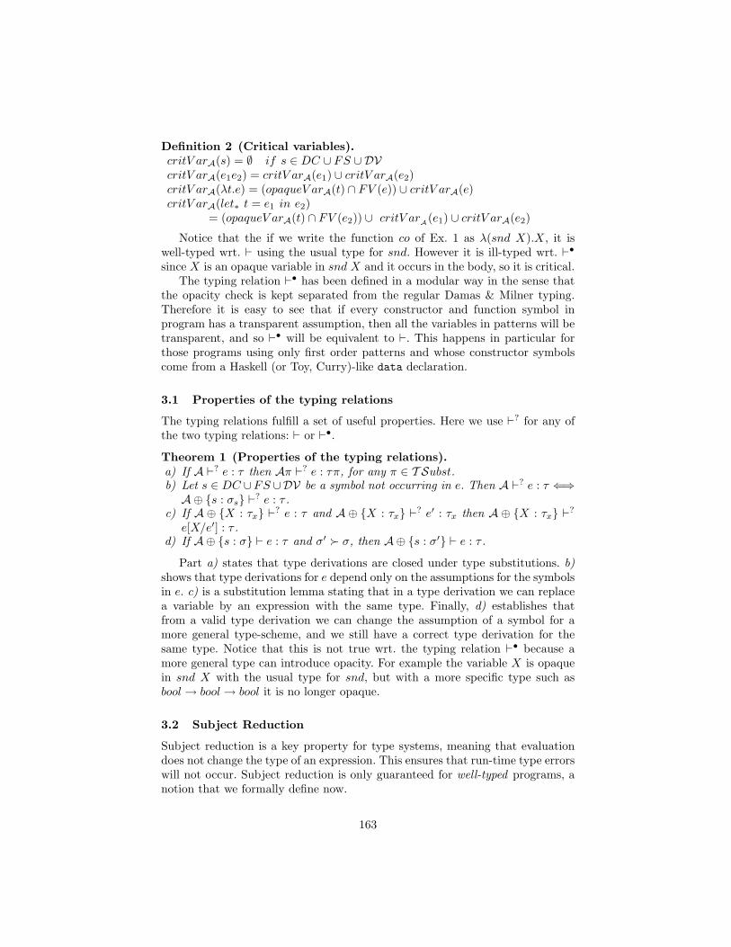
Definition 2 (Critical variables).critV arA(s) = ∅ if s ∈ DC ∪ FS ∪ DVcritV arA(e1e2) = critV arA(e1) ∪ critV arA(e2)critV arA(λt.e) = (opaqueV arA(t) ∩ FV (e)) ∪ critV arA(e)critV arA(let∗ t = e1 in e2)

= (opaqueV arA(t) ∩ FV (e2)) ∪ critV arA(e1) ∪ critV arA(e2)

Notice that the if we write the function co of Ex. 1 as λ(snd X).X, it iswell-typed wrt. ` using the usual type for snd. However it is ill-typed wrt. `•since X is an opaque variable in snd X and it occurs in the body, so it is critical.

The typing relation `• has been defined in a modular way in the sense thatthe opacity check is kept separated from the regular Damas & Milner typing.Therefore it is easy to see that if every constructor and function symbol inprogram has a transparent assumption, then all the variables in patterns will betransparent, and so `• will be equivalent to `. This happens in particular forthose programs using only first order patterns and whose constructor symbolscome from a Haskell (or Toy, Curry)-like data declaration.

3.1 Properties of the typing relations

The typing relations fulfill a set of useful properties. Here we use `? for any ofthe two typing relations: ` or `•.

Theorem 1 (Properties of the typing relations).a) If A `? e : τ then Aπ `? e : τπ, for any π ∈ T Subst.b) Let s ∈ DC ∪FS ∪DV be a symbol not occurring in e. Then A `? e : τ ⇐⇒A⊕ {s : σs} `? e : τ .

c) If A ⊕ {X : τx} `? e : τ and A ⊕ {X : τx} `? e′ : τx then A ⊕ {X : τx} `?

e[X/e′] : τ .d) If A⊕ {s : σ} ` e : τ and σ′ � σ, then A⊕ {s : σ′} ` e : τ .

Part a) states that type derivations are closed under type substitutions. b)shows that type derivations for e depend only on the assumptions for the symbolsin e. c) is a substitution lemma stating that in a type derivation we can replacea variable by an expression with the same type. Finally, d) establishes thatfrom a valid type derivation we can change the assumption of a symbol for amore general type-scheme, and we still have a correct type derivation for thesame type. Notice that this is not true wrt. the typing relation `• because amore general type can introduce opacity. For example the variable X is opaquein snd X with the usual type for snd, but with a more specific type such asbool → bool → bool it is no longer opaque.

3.2 Subject Reduction

Subject reduction is a key property for type systems, meaning that evaluationdoes not change the type of an expression. This ensures that run-time type errorswill not occur. Subject reduction is only guaranteed for well-typed programs, anotion that we formally define now.

163

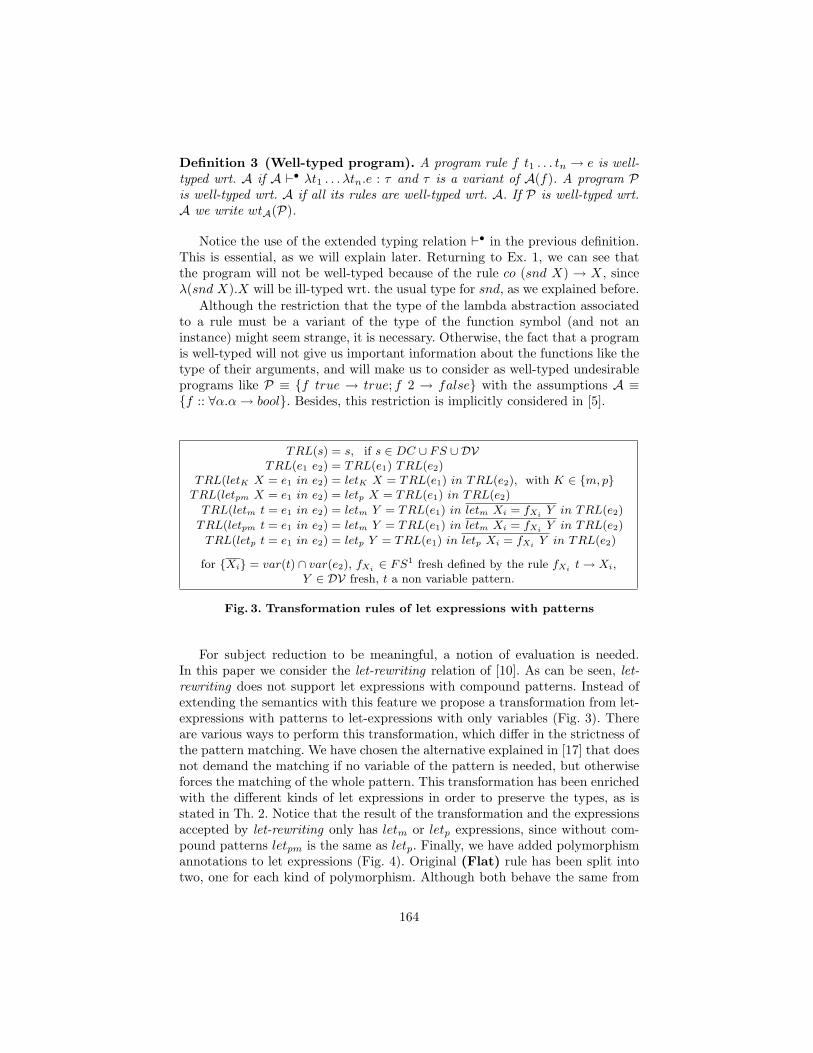
Definition 3 (Well-typed program). A program rule f t1 . . . tn → e is well-typed wrt. A if A `• λt1 . . . λtn.e : τ and τ is a variant of A(f). A program Pis well-typed wrt. A if all its rules are well-typed wrt. A. If P is well-typed wrt.A we write wtA(P).

Notice the use of the extended typing relation `• in the previous definition.This is essential, as we will explain later. Returning to Ex. 1, we can see thatthe program will not be well-typed because of the rule co (snd X) → X, sinceλ(snd X).X will be ill-typed wrt. the usual type for snd, as we explained before.

Although the restriction that the type of the lambda abstraction associatedto a rule must be a variant of the type of the function symbol (and not aninstance) might seem strange, it is necessary. Otherwise, the fact that a programis well-typed will not give us important information about the functions like thetype of their arguments, and will make us to consider as well-typed undesirableprograms like P ≡ {f true → true; f 2 → false} with the assumptions A ≡{f :: ∀α.α → bool}. Besides, this restriction is implicitly considered in [5].

TRL(s) = s, if s ∈ DC ∪ FS ∪ DVTRL(e1 e2) = TRL(e1) TRL(e2)

TRL(letK X = e1 in e2) = letK X = TRL(e1) in TRL(e2), with K ∈ {m, p}TRL(letpm X = e1 in e2) = letp X = TRL(e1) in TRL(e2)

TRL(letm t = e1 in e2) = letm Y = TRL(e1) in letm Xi = fXi Y in TRL(e2)

TRL(letpm t = e1 in e2) = letm Y = TRL(e1) in letm Xi = fXi Y in TRL(e2)

TRL(letp t = e1 in e2) = letp Y = TRL(e1) in letp Xi = fXi Y in TRL(e2)

for {Xi} = var(t) ∩ var(e2), fXi ∈ FS1 fresh defined by the rule fXi t → Xi,Y ∈ DV fresh, t a non variable pattern.

Fig. 3. Transformation rules of let expressions with patterns

For subject reduction to be meaningful, a notion of evaluation is needed.In this paper we consider the let-rewriting relation of [10]. As can be seen, let-rewriting does not support let expressions with compound patterns. Instead ofextending the semantics with this feature we propose a transformation from let-expressions with patterns to let-expressions with only variables (Fig. 3). Thereare various ways to perform this transformation, which differ in the strictness ofthe pattern matching. We have chosen the alternative explained in [17] that doesnot demand the matching if no variable of the pattern is needed, but otherwiseforces the matching of the whole pattern. This transformation has been enrichedwith the different kinds of let expressions in order to preserve the types, as isstated in Th. 2. Notice that the result of the transformation and the expressionsaccepted by let-rewriting only has letm or letp expressions, since without com-pound patterns letpm is the same as letp. Finally, we have added polymorphismannotations to let expressions (Fig. 4). Original (Flat) rule has been split intotwo, one for each kind of polymorphism. Although both behave the same from

164

the point of view of values, the splitting is needed to guarantee type preservation.λ-abstractions have been omitted, since they are not supported by let-rewriting.

(Fapp) f t1θ . . . tnθ →l rθ, if (f t1 . . . tn → r) ∈ P and θ ∈ PSubst

(LetIn) e1 e2 →l letm X = e2 in e1 X, if e2 is an active expression, variableapplication, junk or let rooted expression, for X fresh.

(Bind) letK X = t in e →l e[X/t], if t ∈ Pat

(Elim) letK X = e1 in e2 →l e2, if X 6∈ FV (e2)

(Flatm) letm X = (letK Y = e1 in e2) in e3 →l letK Y = e1 in (letm X =e2 in e3), if Y 6∈ FV (e3)

(Flatp) letp X = (letK Y = e1 in e2) in e3 →l letp Y = e1 in (letp X = e2 in e3)if Y 6∈ FV (e3)

(LetAp) (letK X = e1 in e2) e3 →l letK X = e1 in e2 e3, if X 6∈ FV (e3)

(Contx) C[e] →l C[e′], if C 6= [ ], e →l e′ using any of the previous rules

where K ∈ {m, p}

Fig. 4. Higher order let-rewriting relation →l

Theorem 2 (Type preservation of the let transformation). Assume A `•e : τ and let P ≡ {fXi ti → Xi} be the rules of the projection functions needed inthe transformation of e according to Fig. 3. Let also A′ be the set of assumptionsover that functions, defined as A′ ≡ {fXi : Gen(τXi ,A)}, where A �• λti.Xi :τXi |πXi . Then A⊕A′ `• TRL(e) : τ and wtA⊕A′(P).

Th. 2 also states that the projection functions are well-typed. Then if westart from a well-typed program P wrt. A and apply the transformation to allits rules, the program extended with the projections rules will be well-typedwrt. the extended assumptions: wtA⊕A′(P ] P ′). This result is straightforward,because A′ does not contain any assumption for the symbols in P, so wtA(P)implies wtA⊕A′(P).

Th. 3 states the subject reduction property for a let-rewriting step, but itsextension to any number of steps is trivial.

Theorem 3 (Subject Reduction). If A `• e : τ and wtA(P) and P ` e →l e′

then A `• e′ : τ .

For this result to hold it is essential that the definition of well-typed pro-gram relies on `•. A counterexample can be found in Ex. 1, where the pro-gram would be well-typed wrt. ` but the subject reduction property fails forand (cast 0) true.

The proof of the subject reduction property is based on the following lemma,an important auxiliary result about the instantiation of transparent variables.

165

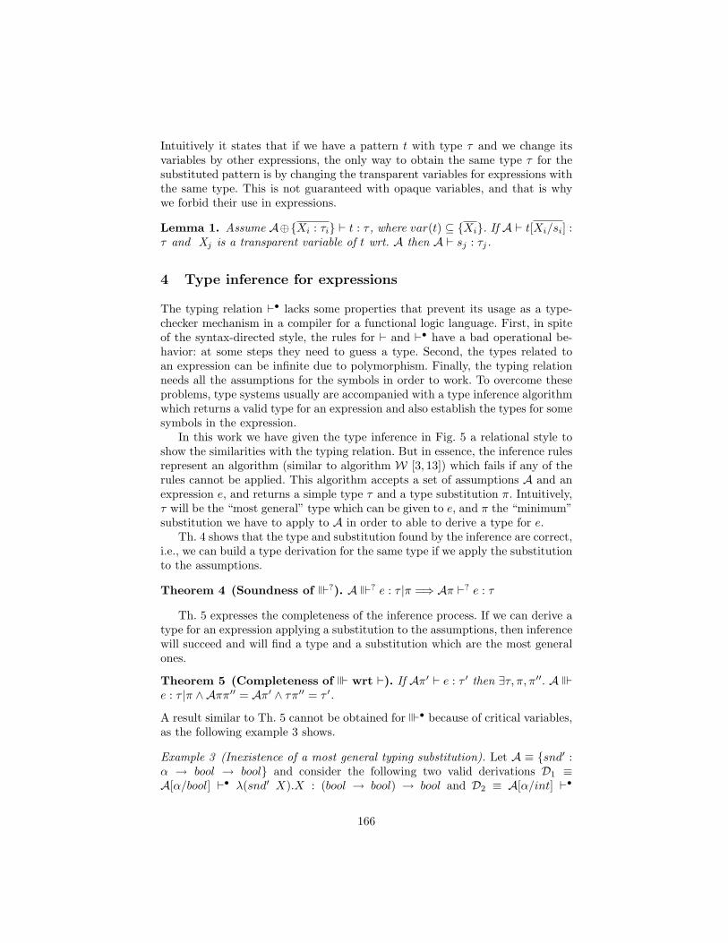
Intuitively it states that if we have a pattern t with type τ and we change itsvariables by other expressions, the only way to obtain the same type τ for thesubstituted pattern is by changing the transparent variables for expressions withthe same type. This is not guaranteed with opaque variables, and that is whywe forbid their use in expressions.

Lemma 1. Assume A⊕{Xi : τi} ` t : τ , where var(t) ⊆ {Xi}. If A ` t[Xi/si] :τ and Xj is a transparent variable of t wrt. A then A ` sj : τj.

4 Type inference for expressions

The typing relation `• lacks some properties that prevent its usage as a type-checker mechanism in a compiler for a functional logic language. First, in spiteof the syntax-directed style, the rules for ` and `• have a bad operational be-havior: at some steps they need to guess a type. Second, the types related toan expression can be infinite due to polymorphism. Finally, the typing relationneeds all the assumptions for the symbols in order to work. To overcome theseproblems, type systems usually are accompanied with a type inference algorithmwhich returns a valid type for an expression and also establish the types for somesymbols in the expression.

In this work we have given the type inference in Fig. 5 a relational style toshow the similarities with the typing relation. But in essence, the inference rulesrepresent an algorithm (similar to algorithm W [3, 13]) which fails if any of therules cannot be applied. This algorithm accepts a set of assumptions A and anexpression e, and returns a simple type τ and a type substitution π. Intuitively,τ will be the “most general” type which can be given to e, and π the “minimum”substitution we have to apply to A in order to able to derive a type for e.

Th. 4 shows that the type and substitution found by the inference are correct,i.e., we can build a type derivation for the same type if we apply the substitutionto the assumptions.

Theorem 4 (Soundness of �?). A �? e : τ |π =⇒ Aπ `? e : τ

Th. 5 expresses the completeness of the inference process. If we can derive atype for an expression applying a substitution to the assumptions, then inferencewill succeed and will find a type and a substitution which are the most generalones.

Theorem 5 (Completeness of � wrt `). If Aπ′ ` e : τ ′ then ∃τ, π, π′′. A �e : τ |π ∧ Aππ′′ = Aπ′ ∧ τπ′′ = τ ′.

A result similar to Th. 5 cannot be obtained for �• because of critical variables,as the following example 3 shows.

Example 3 (Inexistence of a most general typing substitution). Let A ≡ {snd′ :α → bool → bool} and consider the following two valid derivations D1 ≡A[α/bool] `• λ(snd′ X).X : (bool → bool) → bool and D2 ≡ A[α/int] `•

166

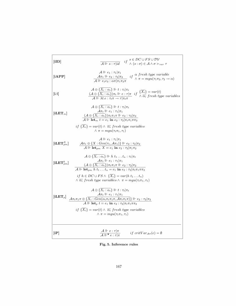
[iID] A � s : τ |id ifs ∈ DC ∪ FS ∪ DV∧ (s : σ) ∈ A ∧ σ �var τ

[iAPP]

A � e1 : τ1|π1

Aπ1 � e2 : τ2|π2

A � e1e2 : απ|π1π2πif

α fresh type variable∧ π = mgu(τ1π2, τ2 → α)

[iΛ]

A⊕ {Xi : αi} � t : τt|πt

(A⊕ {Xi : αi})πt � e : τ |πA � λt.e : τtπ → τ |πtπ

if{Xi} = var(t)∧ αi fresh type variables

[iLETm]

A⊕ {Xi : αi} � t : τt|πt

Aπt � e1 : τ1|π1

(A⊕ {Xi : αi})πtπ1π � e2 : τ2|π2

A � letm t = e1 in e2 : τ2|πtπ1ππ2

if {Xi} = var(t) ∧ αi fresh type variables∧ π = mgu(τtπ1, τ1)

[iLETXpm]

A � e1 : τ1|π1

Aπ1 ⊕ {X : Gen(τ1,Aπ1)} � e2 : τ2|π2

A � letpm X = e1 in e2 : τ2|π1π2

[iLEThpm]

A⊕ {Xi : αi} � h t1 . . . tn : τt|πt

Aπt � e1 : τ1|π1

(A⊕ {Xi : αi})πtπ1π � e2 : τ2|π2

A � letpm h t1 . . . tn = e1 in e2 : τ2|πtπ1ππ2

if h ∈ DC ∪ FS ∧ {Xi} = var(h t1 . . . tn)∧ αi fresh type variables ∧ π = mgu(τtπ1, τ1)

[iLETp]

A⊕ {Xi : αi} � t : τt|πt

Aπt � e1 : τ1|π1

Aπtπ1π ⊕ {Xi : Gen(αiπtπ1π,Aπtπ1π)} � e2 : τ2|π2

A � letp t = e1 in e2 : τ2|πtπ1ππ2

if {Xi} = var(t) ∧ αi fresh type variables∧ π = mgu(τtπ1, τ1)

[iP]A � e : τ |πA �• e : τ |π if critV arAπ(e) = ∅

Fig. 5. Inference rules

167

λ(snd′ X).X : (bool → bool) → int. It is clear that there is not a substitutionmore general than [α/bool] and [α/int] which makes possible a type derivationfor λ(snd′ X).X. The only substitution more general than these two will be[α/β] (for some β), converting X in a critical variable.

In spite of this, we will see that �• is still able to find the most generalsubstitution when it exists. To formalize that, we will use the notion of Π•

A,e,which denotes the set collecting all type substitution π such that Aπ gives sometype to e.

Definition 4 (Typing substitutions of e).Π•A,e = {π ∈ T Subst | ∃τ ∈ T ype. Aπ `• e : τ}

Now we are ready to formulate our result regarding the maximality of �•.

Theorem 6 (Maximality of �•).a) Π•

A,e has a maximum element ⇐⇒ ∃τg, πg ∈ T ype.A �• e : τg|πg.b) If Aπ′ `• e : τ ′ and A �• e : τ |π then exists a type substitution π′′ suchthat Aπ′ = Aππ′′ and τ ′ = τπ′′.

5 Type inference for programs

In the functional programming setting, type inference does not need to distin-guish between programs and expressions, because the program can be incor-porated in the expression by means of let expressions and λ-abstractions. Thisway, the results given for expressions are also valid for programs. But in ourframework it is different, because our semantics (let-rewriting) does not sup-port λ-abstractions and our let expressions do not define new functions but onlyperform pattern matching. Thereby in our case we need to provide an explicitmethod for inferring the types of a whole program. By doing so, we will alsoprovide a specification closer to implementation.

The type inference procedure for a program takes a set of assumptions Aand a program P and returns a type substitution π. The set A must containassumptions for all the symbols in the program, even for the functions defined inP. We want to reflect the fact that in practice some defined functions may comewith an explicit type declaration. Indeed this is a frequent way of documenting aprogram. Furthermore, type declarations are sometimes a real need, for instanceif we want the language to support polymorphic recursion [16, 9]. Therefore, forsome of the functions –those for which we want to infer types– the assumptionwill be simply a fresh type variable, to be instantiated by the inference process.For the rest, the assumption will be a closed type-scheme, to be checked by theprocedure.

Definition 5 (Type Inference of a Program). The procedure B for typeinference of a program {rule1, . . . , rulem} is defined as:

B(A, {rule1, . . . , rulem}) = π, if

168

1. A �• (ϕ(rule1), . . . , ϕ(rulem)) : (τ1, . . . , τm)|π.2. Let f1 . . . fk be the function symbols of the rules rulei in P such that A(f i)

is a closed type-scheme, and τ i the type obtained for rulei in step 1. Thenτ i must be a variant of A(f i).

ϕ is a transformation from rules to expressions defined as:

ϕ(f t1 . . . tn → e) = pair λt1. . . . λtn.e f

where () is the usual tuple constructor, with type () : ∀αi.α1 → . . . αm →(α1, . . . , αm); and pair is a special constructor of tuples of two elements of thesame type, with type pair : ∀α.α → α → α.

The procedure B has two important properties. It is sound: if the procedureB finds a substitution π then the program P is well-typed with respect to theassumptions Aπ (Th. 7). And second, if the procedure B succeeds it finds themost general typing substitution (Th. 8). It is not true in general that the ex-istence of a well-typing substitution π′ implies the existence of a most generalone. A counterexample of this fact is very similar to Ex. 3.

Theorem 7 (Soundness of B). If B(A,P) = π then wtAπ(P).

Theorem 8 (Maximality of B). If wtAπ′(P) and B(A,P) = π then ∃π′′ suchthat Aπ′ = Aππ′′.

Notice that types inferred for the functions are simple types. In order toobtain type-schemes we need and extra step of generalization, as discussed inthe next section.

5.1 Stratified Type Inference of a Program

It is known that splitting a program into blocks of mutually recursive functionsand inferring the types in order may reduce the need of providing explicit type-schemes. This situation is shown in the next example.

Example 4 (Program Inference vs Stratified Inference).A ≡ {true : bool, 0 : int, id : α, f : β, g : γ}P ≡ {id X → X; f → id true; g → id 0}P1 ≡ {id X → X}, P2 ≡ {f → id true}, P3 ≡ {g → id 0}

An attempt to apply the procedure B to infer types for the whole programfails because it is not possible for id to have types bool → bool and int → int atthe same time. We will need to provide explicitly the type-scheme for id : ∀α.α →α in order to the type inference to succeed, yielding types f : bool → bool andg : int → int. But this is not necessary if we first infer types for P1, obtainingδ → δ for id which will be generalized to ∀δ.δ → δ. With this assumption thetype inference for both programs P2 and P3 will succeed with the expected types.

A general stratified inference procedure can be defined in terms of the basicinference B. First, it calculates the graph of strongly connected components from

169

the dependency graph of the program, using e.g. Kosaraju or Tarjan’s algorithm[20]. Each strongly connected component will contain mutually dependent func-tions. Then it will infer types for every component (using B) in topological order,generalizing the obtained types before following with the next component.

Although stratified inference needs less explicit type-schemes, programs in-volving polymorphic recursion still require explicit type-schemes in order to infertheir types.

6 Conclusions and Future Work

In this paper we have proposed a type system for functional logic languages basedon Damas & Milner type system. As far as we know, prior to our work only [5]treats with technical detail a type system for functional logic programming. Ourpaper makes clear contributions when compared to [5]:

– By introducing the notion critical variables, we are more liberal in the treat-ment of opaque variables, but still preserving the essential property of subjectreduction; moreover, this liberality extends also to data constructors, drop-ping the traditional restriction of transparency required to them. This issomehow similar to what happens with existential types [14] or generalizedabstract datatypes [8], a connection that we plan to further investigate in thefuture.

– Our type system considers local pattern bindings and λ-abstractions (alsowith patterns), that were missing in [5]. In addition to that, we have madea rather exhaustive analysis and formalization of different possibilities forpolymorphism in local bindings.

– Subject reduction was proved in [5] wrt. a narrowing calculus. Here we do itwrt. an small-step operational semantics closer to real computations.

– In [5] programs came with explicit type declarations. Here we provide algo-rithms for inferring types for programs without such declarations that canbecame part of the type stage of a FL compiler.

We have in mind several lines for future work. As an immediate task weplan to implement and integrate the stratified type inference into the T OY[11] compiler. Apart from the relation to existential types mentioned above, weare interested in other known extensions of type system, like type classes orgeneric programming. We also want to generalize the subject reduction propertyto narrowing, using let narrowing reductions of [10], and taking into accountknown problems [5, 1] in the interaction of HO narrowing and types. Handlingextra variables (variables occurring only in right hand sides of rules) is anotherchallenge from the viewpoint of types.

References

1. S. Antoy and A. P. Tolmach. Typed higher-order narrowing without higher-orderstrategies. In Proc. International Symposium on Functional and Logic Program-ming (FLOPS 1999), pages 335–353, 1999.

170

2. B. Brassel. Post to the curry mailing list. http://www.informatik.uni-kiel.de/ curry/listarchive/0706.html, May 2008.

3. L. Damas and R. Milner. Principal type-schemes for functional programs. InProc. Symposium on Principles of Programming Languages (POPL 1982), pages207–212, 1982.

4. J. Gonzalez-Moreno, M. Hortala-Gonzalez, and M. Rodrıguez-Artalejo. A higherorder rewriting logic for functional logic programming. In Proc. InternationalConference on Logic Programming (ICLP 1997), pages 153–167. MIT Press, 1997.

5. J. Gonzalez-Moreno, T. Hortala-Gonzalez, and Rodrıguez-Artalejo, M. Polymor-phic types in functional logic programming. In Journal of Functional and LogicProgramming, volume 2001/S01, pages 1–71, 2001.

6. M. Hanus. Multi-paradigm declarative languages. In Proc. of the InternationalConference on Logic Programming (ICLP 2007), pages 45–75. Springer LNCS 4670,2007.

7. M. Hanus (ed.). Curry: An integrated functional logic language (version 0.8.2).Available at http://www.informatik.uni-kiel.de/~curry/report.html, March 2006.

8. S. L. P. Jones, D. Vytiniotis, S. Weirich, and G. Washburn. Simple unification-based type inference for gadts. In Proc. 11th ACM SIGPLAN International Con-ference on Functional Programming, ICFP 2006, pages 50–61. ACM, 2006.

9. A. J. Kfoury, J. Tiuryn, and P. Urzyczyn. Type reconstruction in the presence ofpolymorphic recursion. ACM Trans. Program. Lang. Syst., 15(2):290–311, 1993.

10. F. Lopez-Fraguas, J. Rodrıguez-Hortala, and J. Sanchez-Hernandez. Rewritingand call-time choice: the HO case. In Proc. 9th International Symposium on Func-tional and Logic Programming (FLOPS’08), volume 4989 of LNCS, pages 147–162.Springer, 2008.

11. F. Lopez-Fraguas and J. Sanchez-Hernandez. T OY: A multiparadigm declarativesystem. In Proc. Rewriting Techniques and Applications (RTA’99), pages 244–247.Springer LNCS 1631, 1999.

12. F. J. Lopez-Fraguas, E. Martin-Martin, and J. Rodrıguez-Hortala. Ad-vances in type systems for functional-logic programming (extended version).http://gpd.sip.ucm.es/enrique/papers/ATSFLPlong.pdf, 2009.

13. L. M. Martins Damas. Type Assignment in Programming Languages. PhD thesis,University of Edinburgh, April 1985. Also appeared as Technical report CST-33-85.

14. J. C. Mitchell and G. D. Plotkin. Abstract types have existential type. ACMTrans. Program. Lang. Syst., 10(3):470–502, 1988.

15. J. J. Moreno-Navarro, J. Marino, A. del Pozo-Pietro, A. Herranz-Nieva, andJ. Garcıa-Martın. Adding type classes to functional-logic languages. In 1996Joint Conf. on Declarative Programming, APPIA-GULP-PRODE’96, pages 427–438, 1996.

16. A. Mycroft. Polymorphic type schemes and recursive definitions. In Proc. 6thColloquium on International Symposium on Programming, pages 217–228, London,UK, 1984. Springer-Verlag.

17. S. Peyton Jones. The Implementation of Functional Programming Languages.Prentice Hall, 1987.

18. B. P. Pierce. Advanced topics in types and programming languages. MIT Press,Cambridge, MA, USA, 2005.

19. C. Reade. Elements of Functional Programming. Addison-Wesley, 1989.20. R. Sedgewick. Algorithms in C++, Part 5: Graph Algorithms, pages 205–216.

Addison-Wesley Professional, 2002.

171

A Complete Axiomatization of Strict Equalityover Infinite Trees?

Javier Alvez and Francisco J. Lopez-Fraguas

Universidad Complutense de Madridjavieralvez@fdi.ucm.es fraguas@sip.ucm.es

Abstract. Computing with data values that are some kind of trees —finite, infinite, rational— is at the core of declarative programming, eitherlogic, functional or functional-logic. Understanding the logic of trees istherefore a fundamental question with impact in different aspects, likelanguage design, including constraint systems or constructive negation,or obtaining methods for verifying and reasoning about programs. Thetheory of true equality over finite or infinite trees is quite well known. Inparticular, a seminal paper by Maher proved its decidability and gave acomplete axiomatization of the theory. However, the sensible notion ofequality for functional and functional-logic languages with a lazy evalua-tion regime is strict equality, a computable approximation to true equal-ity for possibly infinite and partial trees. In this paper, we investigatethe first-order theory of strict equality, arriving to remarkable and notobvious results: the theory is again decidable and admits a complete ax-iomatization, not requiring predicate symbols other than strict equalityitself. Besides, the results stem from an effective —taking into accountthe intrinsic complexity of the problem— decision procedure that can beseen as a constraint solver for general strict equality constraints.

1 Introduction

Computing with data values that are —or can be interpreted as— some kindof trees is at the core of declarative programming, either logic, functional orfunctional-logic programming. The family of trees may vary from finite trees, forthe case of standard logic programming, infinite rational trees, for the case ofProlog-II and variants, or infinite trees (that correspond to data values in con-structor data-types) for the case of functional or functional-logic programmingthat allow non-terminating programs by following a lazy evaluation regime.

Understanding trees, in particular the logical principles governing tree equal-ity, is a fundamental question with impact in different aspects of declarativeprogramming languages. For instance, adding constructive negation abilities toa logic language requires solving complex Herbrand constraints over finite trees.

? This work has been partially supported by the Spanish projectsTIN2005-09207-C03-03, TIN2008-06622-C03-01, S-0505/TIC/0407,UCM-BSCH-GR58/08-910502, TIN2007-66523 and GIU07/35.

The theory of true equality ≈1 over finite or infinite trees is quite well known.In a seminal paper [11], Maher proved its decidability and gave a completeaxiomatization for the cases of finite and infinite trees, and finite and infinitesignatures. In another influential paper [6], the authors provided more effectivedecision procedures, based on reduction to solved forms by quantifier elimination.

However, true equality is not the sensible notion to consider in lazy functionalor functional-logic languages like Haskell, Curry or Toy [12, 8, 4]. In those, thepossibility of non-terminating programs handled with lazy evaluation impliesthat denotations of expressions may be seen as infinite trees. Furthermore, treesmay be partial, in the sense that some of their components may be undefined.For instance, with the definitions loop = loop and l = [loop|l], l can be seen ascomputing the infinite partial list [⊥,⊥,⊥, . . .]. True equality over partial treesis not Scott continuous (hence not computable) and, therefore, must be replacedby a computable approximation, like strict equality ==, the restriction of ≈ tofinite and total trees. The theories of equality and of strict equality are far frombeing the same, starting by the fact that == is not even reflexive.

As far as we know, a comprehensive study of the full first-order theory ofstrict equality has not been done before. Certainly, strict equality is incorpo-rated as primitive in the aforementioned languages, and there are several worksincorporating various Herbrand constraint systems —and corresponding solvingprocedures— to functional logic languages [2, 9, 3]. But in all cases, the consid-ered class of formulae over == is only a subset of general first-order formulae.

The aim of this paper is precisely to investigate the full first-order theory ofstrict equality over the algebra IT of possibly infinite partial trees. Note thatdecidability and existence of complete axiomatization for ≈ says nothing aboutthe same problems for strict equality, even if == is a strict subset of ≈ (i.e.,∀x · y ( x == y → x ≈ y ) is valid in IT ). These are indeed the main questionstackled in this paper:− Does the theory of strict equality over IT admit a complete recursive axio-

matization?− In the affirmative case, is it possible that the axioms use only the symbol

==? We cannot discard a priori the possibility that the axiomatizationneeds an explicit connection of == to ≈, like the one stated above. If so, theresulting axiomatization would become more complicated due to the numberof required axioms and transformation rules.

− A complete recursive axiomatization of a theory implies its decidability (atleast a brute force decision procedure exists). Can we give a more practicaldecision procedure, in the style of [6]? As a matter of fact, such a procedure—if existing— will be itself a proof of completeness for the theory.

We obtain affirmative answers to these questions, both in the cases of infinite andfinite signatures. Our paper does not look for immediate applications, keepingin a theoretical realm and trying to achieve fundamental and not obvious resultsabout strict equality that could be a basis for potential applications: the design

1 By true equality we mean t1 ≈ t2 iff t1 and t2 are the same tree.

174

of constraint systems more expressive than existing ones or the development ofreasoning frameworks for functional-logic programs with built-in equality.

The organization of the paper is as follows: in the next section, we providepreliminary definitions and notation. In Section 3, we give an axiomatizationfor strict equality and introduce the transformation rules that will be used inthe decision methods of Section 4, distinguishing the cases of infinite and finitesignatures. Finally, in Section 5, we discuss complexity issues and future work.For the sake of space, proofs have been omitted, but the interested reader mayrefer to [1].

2 Preliminaries

Let V be a set of countable variables and Σ = PΣ ∪FΣ a signature of predicateand function symbols where each symbol s has an associated arity n, denoted bys/n, and PΣ exclusively consists of the symbol ==/2, known as strict equality.For technical convenience, we assume that FΣ contains at least a 0-ary functionsymbol (constant), an n-ary function symbol with n > 0 and a distinguished 0-ary function symbol ⊥ known as bottom. If Σ contains a finite number of functionsymbols, then Σ is said to be finite. Otherwise, Σ is infinite. By using the namefunction, we follow the tradition of first-order logic, but note that the notion offunction corresponds to the notion of free constructor in functional/functional-logic programming and not to defined function, which plays no role in this paper.

We consider the classical definitions of finite and infinite ground trees. Theinterested reader is referred to [5] for an exhaustive definition. A tree is said tobe partial if it contains ⊥ at some node. Otherwise, the tree is total. The algebraof finite and infinite trees are respectively denoted by FT and IT . Besides, wealso refer to [6] for the definitions that do not appear in this paper.

A term (or constructor term) is either a variable v ∈ V or an expression ofthe form f(t1, . . . , tn) where f/n ∈ FΣ and t1, . . . , tn are terms. For any termst and s, the expression t[s] denotes that s occurs in t (that is, s is a subterm oft). For any n > 0, a n-tuple of terms is denoted by 〈t1, . . . , tn〉 and abbreviatedby t. When convenient, we also treat t as the set of its components. As for thecase of trees, a term t is said to be partial if t = s[⊥], and t is total otherwise.We denote by Var(t) the set of variables occurring in t. Besides, a term is saidto be ground iff it is variable-free. The size of a term t is the number of functionsymbols occurring in t.

A sentence φ is an arbitrary first-order formula built with Σ. In our case,the only predicate symbol is ==. Thus atomic formulas are true, false, strictequations t1 == t2 or negated equations ¬t1 == t2. Being r = 〈r1, . . . , rn〉 ands = 〈s1, . . . , sn〉, the expression r == s abbreviates r1 == s1 ∧ . . . ∧ rn == sn

and ¬r == s abbreviates the disjunction of negated equations ¬r1 == s1 ∨. . . ∨ ¬rn == sn. Sentences may use propositional connectives (¬,∧,∨,→,↔)and quantifiers (∃,∀). The symbol Q stands for both kinds of quantifiers. Theset Free(φ) of free variables of φ is defined as usual. If Free(φ) = ∅, φ is closed.

175

φQ denotes the Q-closure of φ, and φQ\w denotes the sentence Qv φ, wherev = Free(φ) \ w.

Now we recall some semantics of first order logic. An interpretation A is acarrier set A together with interpretations for the symbols in Σ. Given A, anassignment σ maps variables to values in A. A models φ, written A |= φ, if φσis true (according to standard rules for truth-valuation) in A for any assignmentσ (σ is irrelevant if φ is closed).

A theory T is a set of closed sentences. A is a model of T , written A |= T ,if A |= φ for each φ ∈ T . A formula φ is a logical consequence of T , writtenT |= φ, if A |= φ whenever A |= T . This notation extends naturally to sets Φof formulas. A sentence φ is satisfiable (or solvable) in T , if T |= φ∃. A theoryT is complete iff for any closed sentence φ either T |= φ or T |= ¬φ holds. Thetheory TA of A is the set of all closed φ such that A |= φ. Note that TA is alwayscomplete. A complete axiomatization of A is a theory S ⊆ TA such that S |= TA(or, equivalently, S is a complete theory and A |= S). Usually one is interestedin recursive axiomatizations where the property ‘φ ∈ S’ is decidable.

Given two sentences φ1 and φ2, a transformation rule φ1 7→ φ2 replacesany occurrence of φ1 in a formula (module variable renaming) with φ2. Theapplication of a transformation rule R to φ1 yielding φ2 is denoted by φ1

R; φ2.

A transformation rule R is said to be correct in a theory T iff for any two formulasφ1 and φ2 such that φ1

R; φ2 we have that φ1 and φ2 are logically equivalent in

T , i.e., T |= φ1 ↔ φ2.

3 Strict Equality

Strict equality is a particular case of classical equality where, besides beingsyntactically equal, two terms have to be finite and total to be strictly equal.

Definition 1 (Strict equality). Two trees t1 and t2 are strictly equal, denotedby t1 == t2, iff t1 and t2 are the same finite and total tree. ut

Strict equality allows us to characterize the subset of IT consisting of finiteand total trees: x is a finite and total tree ⇐⇒ x == x.

In Figure 1, we propose an axiomatization of infinite trees with strict equal-ity, which is similar, but not equal, to the one of finite trees with equality given in[11]. The main difference comes from the fact that strict equality is not reflexive:non-finite/non-total trees are not strictly equal to themselves. Due to this prop-erty, ⊥ and the remaining function symbols in FΣ have a different treatment.The strict equality theory of infinite trees consisting of A1 −A6 is denoted byE . It is easy to see, by direct inspection, that IT |= E . However, whether ornot E is a complete theory (and, therefore, a complete axiomatization of == forIT ) is not a trivial question. It will be proved by means of a decision procedurebased on some equivalences under E used as transformation rules for quanti-fier elimination. The following property, which can be seen as a weak version ofreflexivity, is logical consequence of E .Proposition 1. E |= ∀x ( x == x ↔ ∃y x == y ) ut

176

(A1) For every f ∈ Σ such that f 6= ⊥

∀x ∀y ( f(x) == f(y) ↔ x == y )

(A2) For every f, g ∈ Σ such that f 6= g

∀x ∀y ¬f(x) == g(y)

(A3) For every term t[x] except x such that y = Var(t[x]) \ {x}

∀x ∀y ¬x == t[x]

(A4)∀x ¬x == ⊥

(A5) Symmetry∀x ∀y ( x == y → y == x )

(A6) Transitivity

∀x ∀y ∀z ( ¬x == y ∨ ¬y == z ∨ x == z )

Fig. 1. Axiomatization of Infinite Trees with Strict Equality

3.1 Transformation Rules

In Figure 2, we summarize the transformation rules that are used in Section 4 forproviding a decision method for E . Note that some conditions in the rules, likethe ones in rule R, are not necessary for correctness. Instead, those conditionsserve to discard the application of some rules when there exist more suitableones. Next, we prove that the transformation rules in Figure 2 are correct.

Theorem 1. The transformation rules in Figure 2 are correct in E. ut

4 A Decision Method for Strict Equality

In this section, we prove that the theory of strict equality is decidable by pro-viding an algorithm that transforms any initial constraint into an equivalentdisjunction of formulas in solved form. This algorithm is based on the well-known technique of quantifier elimination, as the algorithms proposed in [6, 11]for the equality theory. As in the above cited works, we distinguish two casesdepending on whether the signature is finite or infinite. In the case of infinitesignatures, E is already a decidable theory. However, for dealing with finite sig-natures, we have to adapt the Domain Closure Axiom (see [13]) to the case ofstrict equality in order to obtain a decidable theory. In the next subsections,we first provide a decision algorithm for the case of infinite signatures and thenadapt that algorithm for finite ones.

177

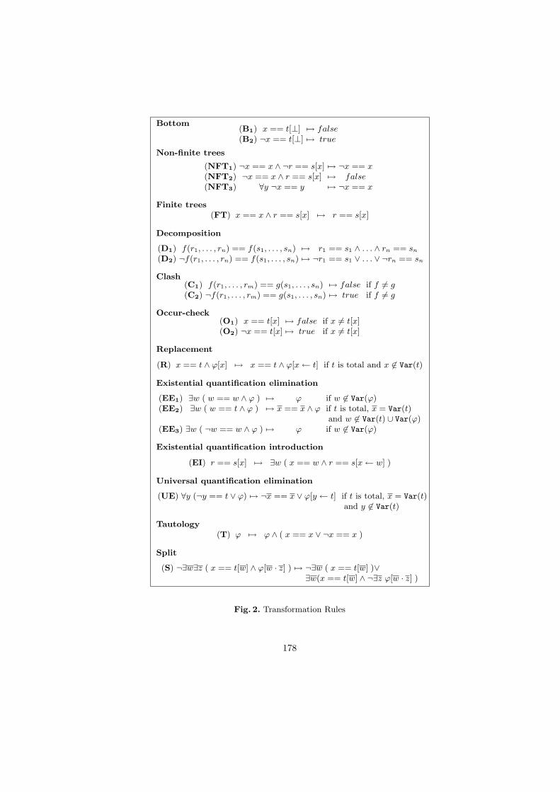
Bottom(B1) x == t[⊥] 7→ false(B2) ¬x == t[⊥] 7→ true

Non-finite trees

(NFT1) ¬x == x ∧ ¬r == s[x] 7→ ¬x == x(NFT2) ¬x == x ∧ r == s[x] 7→ false(NFT3) ∀y ¬x == y 7→ ¬x == x

Finite trees(FT) x == x ∧ r == s[x] 7→ r == s[x]

Decomposition

(D1) f(r1, . . . , rn) == f(s1, . . . , sn) 7→ r1 == s1 ∧ . . . ∧ rn == sn

(D2) ¬f(r1, . . . , rn) == f(s1, . . . , sn) 7→ ¬r1 == s1 ∨ . . . ∨ ¬rn == sn

Clash(C1) f(r1, . . . , rm) == g(s1, . . . , sn) 7→ false if f 6= g(C2) ¬f(r1, . . . , rm) == g(s1, . . . , sn) 7→ true if f 6= g

Occur-check(O1) x == t[x] 7→ false if x 6= t[x](O2) ¬x == t[x] 7→ true if x 6= t[x]

Replacement

(R) x == t ∧ ϕ[x] 7→ x == t ∧ ϕ[x← t] if t is total and x 6∈ Var(t)

Existential quantification elimination

(EE1) ∃w ( w == w ∧ ϕ ) 7→ ϕ if w 6∈ Var(ϕ)(EE2) ∃w ( w == t ∧ ϕ ) 7→ x == x ∧ ϕ if t is total, x = Var(t)

and w 6∈ Var(t) ∪ Var(ϕ)(EE3) ∃w ( ¬w == w ∧ ϕ ) 7→ ϕ if w 6∈ Var(ϕ)

Existential quantification introduction

(EI) r == s[x] 7→ ∃w ( x == w ∧ r == s[x← w] )

Universal quantification elimination

(UE) ∀y (¬y == t ∨ ϕ) 7→ ¬x == x ∨ ϕ[y ← t] if t is total, x = Var(t)and y 6∈ Var(t)

Tautology(T) ϕ 7→ ϕ ∧ ( x == x ∨ ¬x == x )

Split

(S) ¬∃w∃z ( x == t[w] ∧ ϕ[w · z] ) 7→ ¬∃w ( x == t[w] )∨∃w(x == t[w] ∧ ¬∃z ϕ[w · z] )

Fig. 2. Transformation Rules

178

4.1 Infinite Signatures

In order to provide a decision algorithm, we first define a solved form for infinitesignatures, called basic formula. Then, we show that two basic Boolean opera-tions —conjunction and negation— can be performed on basic formulas. And,finally, we describe the decision algorithm.

Definition 2. A basic formula for the variables x is either true, false or a con-straint ∃w c(x,w) such that

c(x,w) =∧

x1∈x1

¬x1 == x1 ∧ x2 == t ∧∧

wi∈w

ni∧j=1

(¬wi == sij)∀\w

where − x = x1 ∪ x2 and x1 ∩ x2 = ∅,− w = Var(t) and x ∩ w = ∅,− if sij is a variable, then sij ∈ w, otherwise sij is total, wi 6∈ Var(sij)

and Var(sij) ∩ x = ∅ for every wi ∈ w and 1 ≤ j ≤ ni.A formula is in basic normal form if it is of the form Qy ϕ[x · y] where ϕ is adisjunction of basic formulas for x · y. ut

Example 1. Let {a/0, g/1, f/2} ⊂ FΣ and x = {x1, x2, x3} ⊂ V. The sentences∃w ( ¬x1 == x1∧x2 = g(w1)∧x3 == g(w2)∧¬w1 == w2∧∀v ¬w2 == f(a, v) ),( ¬x1 == x1 ∧ ¬x2 == x2 ∧ ¬x3 == x3 ) and true are basic formulas for x. ut

First, we will show that the notion of basic formula is a solved form.

Theorem 2. Let Σ be an infinite signature. Any basic formula different fromfalse is satisfiable in E. ut

Then, we describe the transformation of any universally quantified disjunc-tion of negated equations into an equivalent disjunction of basic formulas.

Proposition 2. Any universally quantified disjunction of negated equations

∀v ( ¬w1 == t1 ∨ ¬w2 == t2 ∨ . . . ∨ ¬wn == tn )

where wi 6∈ v for each 1 ≤ i ≤ n can be transformed into an equivalent disjunctionof basic formulas for the variables x = Var(t1, . . . , tn) \ v. ut

Using the above transformation, we now describe the implementation of theBoolean operations conjunction and negation on basic formulas.

Proposition 3. A conjunction of disjunctions of basic formulas for x can betransformed into an equivalent disjunction of basic formulas for x. ut

In the next example, we show the transformation of a conjunction of two basicformulas into an equivalent disjunction of basic formulas for the same variables.

179

Example 2. Let {a/0, g/1, f/2} ⊂ FΣ and x = {x1, x2, x3} ⊂ V. The conjunctionof basic formulas for x ϕ1 = ∃w1 c1(x,w1) ∧ ∃w2 c2(x,w2) where

c1(x,w1) = ¬x1 == x1 ∧ x2 == w11 ∧ x3 == g(w1

2) ∧ ∀v ¬w11 == f(a, v)

c2(x,w2) = ¬x1 == x1 ∧ ¬x2 == x2 ∧ x3 == f(w21, w

22) ∧ ¬w2

1 == w22

is unsatisfiable since x2 == w11 ∧ ¬x2 == x2 is reduced to false by NFT2. On

the contrary, the conjunction ϕ2 = ∃w1 c1(x,w1) ∧ ∃w3 c3(x,w3) where

c3(x,w3) = ¬x1 == x1 ∧ x2 == f(w31, w

32) ∧ x3 == w3

1 ∧ ∀v ¬w32 == g(v)

is transformed in the following way. Since σ = mgu(w11 · g(w1

2), f(w31, w

32) ·w3

1) ={w1

1 ← f(g(w12), w

32), w

31 ← g(w1

2)}, ϕ2 is transformed into

∃w12 · w3

2 ( ¬x1 == x1 ∧ x2 == f(g(w12), w

32) ∧ x3 == g(w1

2) ∧∀v ¬f(g(w1

2), w32) == f(a, v) ∧ ∀v ¬w3

2 == g(v) ).

Then, the negated equation ∀v ¬f(g(w12), w

32) == f(a, v) is reduced to true

using rules D2 and C2. Thus, the resulting basic formula is

∃w12 ·w3

2 (¬x1 == x1∧x2 == f(g(w12), w

32)∧x3 == g(w1

2)∧∀v ¬w32 == g(v)). ut

Proposition 4. A negated disjunction of basic formulas for the variables x canbe transformed into an equivalent disjunction of basic formulas for x. ut

Example 3. Let {a/0, f/2} ⊂ FΣ and x = {x1, x2} ⊂ V. The negated basicformula for the variables x

ϕ = ¬∃w ( ¬x1 == x1 ∧ x2 == f(w, a) ∧ ∀v ¬w == f(a, v) )

is transformed as follows. First, ϕ is trivially equivalent to

( x1 == x1 ) ∨ ¬∃w ( x2 == f(w, a) ∧ ∀v ¬w == f(a, v) )

where ( x1 == x1 ) is transformed into the following basic formulas for x

∃w1 ( ¬x2 == x2 ∧ x1 == w1 ) ∨ ∃w2 · w3 ( x1 == w2 ∧ x2 == w3 )

using T, EI, R and FT. Besides, the remaining subformula is transformed into

¬∃w ( x2 == f(w, a) ) ∨ ∃w ( x2 == f(w, a) ∧ ¬∀v ¬w == f(a, v) )

using the rule S. The constraint ¬∃w ( x2 == f(w, a) ) is transformed into

( ¬x1 == x1 ∧ ¬x2 == x2 ) ∨∃w4 ( ¬x1 == x1 ∧ x2 == w4 ∧ ∀v ¬w4 == f(v, a) ) ∨∃w5 ( ¬x2 == x2 ∧ x1 == w5 ) ∨∃w6 · w7 ( x1 == w6 ∧ x2 == w7 ∧ ∀v ¬w7 == f(v, a) )

180

(EE4) ∃w ( v == v ∧n

i=1

(¬si == ti)∀\w ∧ ϕ ) 7→ ϕ

if w ∩ Var(ϕ) = ∅, v ⊆ w, si 6= ti, w ∩ Var(si, ti) 6= ∅ and eithersi (resp. ti) is not a variable or si ∈ w (resp. ti ∈ w) for each 1 ≤ i ≤ n

Fig. 3. Existential Quantification Elimination: Infinite Signatures

using T, EI, R and NFT1. Finally, ∃w ( x2 == f(w, a)∧¬∀v ¬w == f(a, v) ) ≡∃w ( x2 == f(w, a) ∧ ∃v w == f(a, v) ) is transformed into

∃w8 ( ¬x1 == x1 ∧ x2 == f(f(a,w8), a) ) ∨∃w9 · w10 ( x1 == w9 ∧ x2 == f(f(a,w10), a) )

using rules R, EE2 and FT on w, and T and EI on x1. ut

Next, we show that the elimination of the innermost block of quantifiers iscorrect in E when it is existential. For this purpose, we introduce the trans-formation rule in Figure 3, which allows to eliminate existential variables onlyoccurring in a conjunction of (universally quantified) negated equations. In thenext proposition, we prove the correctness of EE4.

Proposition 5. Let Σ be an infinite signature. The transformation rule EE4

is correct in E. ut

The elimination of the innermost block of existential quantifiers is used inthe decision algorithm given in Figure 4.

Theorem 3. Let Σ be an infinite signature, ∃w a(x · y, w · z) a basic formulafor the variables x · y of the form

∃w · z (∧

x1∈x1

¬x1 == x1 ∧∧

y1∈y1

¬y1 == y1 ∧ x2 == t ∧ y2 == r ∧ ϕ ∧ ψ )

where − w = Var(t) and z = Var(r) \ w,− ϕ is a finite conjunction of negated equations such that Free(ϕ) ⊆ w,− ψ =

∧ni=1(¬vi == si)∀\w·z and (vi ∪ Var(si)) ∩ z 6= ∅ for 1 ≤ i ≤ n.

The formulas ∃y [ ∃w a(x · y, w · z) ] and ∃w a′(x,w) where

a′(x,w) =∧

x1∈x1

¬x1 == x1 ∧ x2 == t ∧ ϕ

are equivalent in E. ut

Example 4. Let {a/0, g/1, f/2} ⊂ FΣ . The formulas

∃y [ ∃w1 · w2 ( x == g(w1) ∧ y == f(w2, a) ∧ ¬w1 == a ∧¬w1 == w2 ∧ ∀v ¬w2 == f(a, v) ) ]

and ∃w1 ( x == g(w1) ∧ ¬w1 == a ) are equivalent in E . ut

181

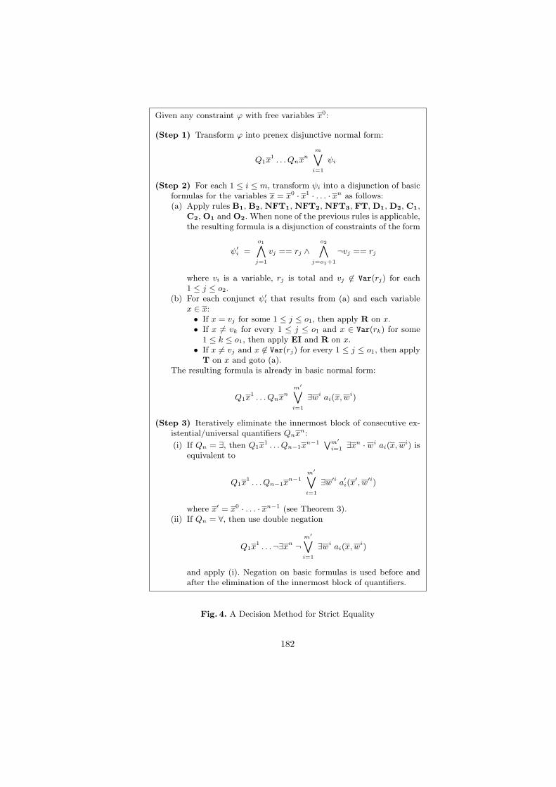
Given any constraint ϕ with free variables x0:

(Step 1) Transform ϕ into prenex disjunctive normal form:

Q1x1 . . . Qnx

nm_

i=1

ψi

(Step 2) For each 1 ≤ i ≤ m, transform ψi into a disjunction of basicformulas for the variables x = x0 · x1 · . . . · xn as follows:(a) Apply rules B1, B2, NFT1, NFT2, NFT3, FT, D1, D2, C1,

C2, O1 and O2. When none of the previous rules is applicable,the resulting formula is a disjunction of constraints of the form

ψ′i =

o1

j=1

vj == rj ∧o2

j=o1+1

¬vj == rj

where vi is a variable, rj is total and vj 6∈ Var(rj) for each1 ≤ j ≤ o2.

(b) For each conjunct ψ′i that results from (a) and each variablex ∈ x:• If x = vj for some 1 ≤ j ≤ o1, then apply R on x.• If x 6= vk for every 1 ≤ j ≤ o1 and x ∈ Var(rk) for some

1 ≤ k ≤ o1, then apply EI and R on x.• If x 6= vj and x 6∈ Var(rj) for every 1 ≤ j ≤ o1, then apply

T on x and goto (a).The resulting formula is already in basic normal form:

Q1x1 . . . Qnx

nm′_i=1

∃wi ai(x,wi)

(Step 3) Iteratively eliminate the innermost block of consecutive ex-istential/universal quantifiers Qnx

n:

(i) If Qn = ∃, then Q1x1 . . . Qn−1x

n−1 Wm′

i=1 ∃xn · wi ai(x,w

i) isequivalent to

Q1x1 . . . Qn−1x

n−1m′_i=1

∃w′i a′i(x′, w′i)

where x′ = x0 · . . . · xn−1 (see Theorem 3).(ii) If Qn = ∀, then use double negation

Q1x1 . . .¬∃xn ¬

m′_i=1

∃wi ai(x,wi)

and apply (i). Negation on basic formulas is used before andafter the elimination of the innermost block of quantifiers.

Fig. 4. A Decision Method for Strict Equality

182

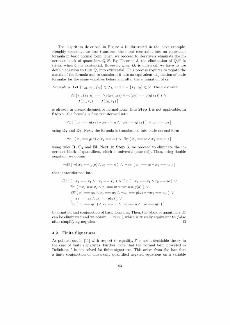
The algorithm described in Figure 4 is illustrated in the next example.Roughly speaking, we first transform the input constraint into an equivalentformula in basic normal form. Then, we proceed to iteratively eliminate the in-nermost block of quantifiers Qix

i. By Theorem 3, the elimination of Qixi is

trivial when Qi is existential. However, when Qi is universal, we have to usedouble negation to turn Qi into existential. This process requires to negate thematrix of the formula and to transform it into an equivalent disjunction of basicformulas for the same variables before and after the elimination of Qi.

Example 5. Let {a/0, g/1, f/2} ⊂ FΣ and x = {x1, x2} ⊂ V. The constraint

∀x [ ( f(x1, a) == f(g(x2), x2) ∧ ¬g(x2) == g(g(x1)) ) ∨f(x1, x2) == f(x2, x1) ]

is already in prenex disjunctive normal form, thus Step 1 is not applicable. InStep 2, the formula is first transformed into

∀x [ ( x1 == g(x2) ∧ x2 == a ∧ ¬x2 == g(x1) ) ∨ x1 == x2 ]

using D1 and D2. Next, the formula is transformed into basic normal form

∀x [ ( x1 == g(a) ∧ x2 == a ) ∨ ∃w ( x1 == w ∧ x2 == w ) ]

using rules R, C2 and EI. Next, in Step 3, we proceed to eliminate the in-nermost block of quantifiers, which is universal (case (ii)). Thus, using doublenegation, we obtain

¬∃x [ ¬( x1 == g(a) ∧ x2 == a ) ∧ ¬∃w ( x1 == w ∧ x2 == w ) ]

that is transformed into

¬∃x [ ( ¬x1 == x1 ∧ ¬x2 == x2 ) ∨ ∃w ( ¬x1 == x1 ∧ x2 == w ) ∨∃w ( ¬x2 == x2 ∧ x1 == w ∧ ¬w == g(a) ) ∨∃w ( x1 == w1 ∧ x2 == w2 ∧ ¬w1 == g(a) ∧ ¬w1 == w2 ) ∨( ¬x2 == x2 ∧ x1 == g(a) ) ∨∃w ( x1 == g(a) ∧ x2 == w ∧ ¬w == a ∧ ¬w == g(a) ) ]

by negation and conjunction of basic formulas. Then, the block of quantifiers ∃xcan be eliminated and we obtain ¬ [ true ], which is trivially equivalent to falseafter simplifying negation. ut

4.2 Finite Signatures

As pointed out in [11] with respect to equality, E is not a decidable theory inthe case of finite signatures. Further, note that the normal form provided inDefinition 2 is not solved for finite signatures. This arises from the fact thata finite conjunction of universally quantified negated equations on a variable

183

(A7) Domain Closure Axiom or DCA

∀x ( ¬x == x ∨_

f∈FΣ

∃w x == f(w) )

Fig. 5. Axiomatization of Infinite Trees with Strict Equality (contd.)

w may be unsatisfiable if only finite and total trees can be assigned to w. Forexample, being FΣ = {a/0, g/1}, we have that the constraint

∃w ( x == w ∧ ¬w == a ∧ ∀v ¬w == g(v) )

is unsatisfiable although ∃w ( ¬w == a ∧ ∀v ¬w == g(v) ) is satisfiable.Roughly speaking, the question is that all the function symbols of the signa-

ture can be used in a constraint. To solve this problem, we adapt the DomainClosure Axiom introduced in [13] to the case of strict equality (see Figure 5),which prevents the existence of isolated finite and total trees in the algebra. Notethat A7 does not provide any information about non-finite/non-total trees. Thetheory that results from the union of E and A7 is denoted by E?.

Existential Quantification Elimination

(EE5) ∃w ( v == v ∧n

i=1

¬si == ti ∧ ϕ ) 7→ ϕ

if w ∩ Var(ϕ) = ∅, v ⊆ w, si 6= ti and w ∩ Var(si, ti) = ∅ for 1 ≤ i ≤ n

Explosion

(E) ϕ[x] 7→ ϕ[x] ∧ [ ¬x == x ∨_

f∈FΣ

∃w x == f(w) ]

Fig. 6. Transformation Rules: Finite Signatures

Next, we show that E? is a decidable theory. For this purpose, we adapt all thedefinitions and results in Subsection 4.1 to the case of finite signatures. Besides,we add the new transformation rule E (see Figure 6) whose correctness directlyfollows from Axiom A7. This new rule allows for the elimination of universalquantification. Finally, regarding the elimination of existential quantifiers, wereplace the rule EE4, which is not correct in the case of finite signatures, withEE5 (see Figure 6). Next, we show that both rules are correct in E?.

Proposition 6. Let Σ be an finite signature. The transformation rule EE5 iscorrect in E?. ut

Proposition 7. The rule Explosion (E) is correct in E?. ut

184

The use of E for eliminating universal quantification is necessary because ournotion of solved form for finite signatures is free of universal variables.

Definition 3. A basic formula for the variables x is either true, false or a con-straint ∃w c(x,w) such that

c(x,w) =∧

x1∈x1

¬x1 == x1 ∧ x2 == t ∧∧

wi∈w

ni∧j=1

¬wi == sij

where − x = x1 ∪ x2 and x1 ∩ x2 = ∅,− w = Var(t) and x ∩ w = ∅,− if sij is a variable, then sij 6= wi, otherwise sij is total, Var(sij) ⊆ w− and wi 6∈ Var(sij) for every wi ∈ w and 1 ≤ j ≤ ni.

A formula is in basic normal form if it is of the form Qy ϕ[x · y] where ϕ is adisjunction of basic formulas for x · y. ut

As in the case of infinite signatures, the above notion of basic formula is asolved form.

Theorem 4. Let Σ be a finite signature. Any basic formula different from falseis satisfiable in E?. ut

Note that the syntactical form provided in Definition 3 is a particular caseof the one in Definition 2. The only difference is that universal quantification isnot allowed in the case of finite signatures. Further, there exists a very simpletransformation using E from formulas as defined in Definition 2 into formulasas defined above.

Proposition 8. Let Σ be a finite signature. Any constraint of the form

ϕ =∧

wi∈w

ni∧j=1

(¬wi == sij)∀\w

can be transformed into an equivalent disjunction of basic formulas for w. utBeing ∃w c(x,w) a formula as described in Definition 2, the conjunction of

negated equations in c(x,w) is transformed into a disjunction of basic formulasw as shown in Proposition 8. Then, the whole formula is transformed into anequivalent disjunction of basic formulas for x using R, EE2 and FT. This resultallows us to easily adapt Propositions 3 and 4 to the case of finite signatures.

Example 6. Let FΣ = {a/0, g/1, f/2} and x = {x1, x2} ⊂ V. The constraint

∃w ( ¬x1 == x1 ∧ x2 == f(w, a) ∧ ∀v ¬w == f(a, v) )

is transformed into a disjunction of basic formulas for x as follows. First, wetransform ∀v ¬w == f(a, v) into a disjunction of basic formulas for w using E:

∀v ¬w == f(a, v) ∧ [ ¬w == w ∨ w == a ∨ ∃z w == g(z) ∨∃z w == f(z1, z2) ]

≡ ¬w == w ∨ w == a ∨ ∃z w == g(z) ∨ (1)∃z ( w == f(z1, z2) ∧ ∀v ¬w == f(a, v) )

185

The first three subformulas are already basic formulas for w. Regarding the lastone, it is transformed using rules R and D2 as follows

∃z ( w == f(z1, z2) ∧ [ ¬z1 == a ∨ ∀v ¬z2 == v ] )≡ ∃z ( w == f(z1, z2) ∧ ¬z1 == a ) ∨ (2)∃z ( w == f(z1, z2) ∧ ∀v ¬z2 == v )

where the second subformula is equivalent to false by rules NFT3 and NFT2.Thus, ∀v ¬w == f(a, v) has been transformed into the disjunction of basicformulas for w in (1, 2). Finally, the conjunction of the above disjunction and¬x1 == x1 ∧ x2 == f(w, a) is transformed into

( ¬x1 == x1 ∧ x2 == f(a, a) ) ∨∃z ( ¬x1 == x1 ∧ x2 == f(g(z), a) ) ∨∃z ( ¬x1 == x1 ∧ x2 == f(f(z1, z2), a) ∧ ¬z1 == a )

using rules R, EE1 and NFT2. ut

Finally, in order to be able to apply the algorithm in Figure 4 to the case offinite signatures, we adapt the result in Theorem 3.

Theorem 5. Let Σ be a finite signature, ∃w a(x · y, w · z) a basic formula forthe variables x · y of the form

∃w · z (∧

x1∈x1

¬x1 == x1 ∧∧

y1∈y1

¬y1 == y1 ∧ x2 == t ∧ y2 == r ∧ ϕ ∧ ψ )

where − w = Var(t) and z = Var(r) \ w,− ϕ is a finite conjunction of negated equations such that Var(ϕ) ⊆ w,− ψ =

∧ni=1 ¬vi == si and (vi ∪ Var(si)) ∩ z 6= ∅ for each 1 ≤ i ≤ n.

The formulas ∃y [ ∃w a(x · y, w · z) ] and ∃w a′(x,w) where

a′(x,w) =∧

x1∈x1

¬x1 == x1 ∧ x2 == t ∧ ϕ

are equivalent in E?. ut

5 Conclusions and Future Work

We have axiomatized the theory of infinite trees with strict equality, denoted byeither E (infinite signatures) or E? (finite signatures). Besides, we have provideda decision algorithm, which proves that the theory is complete. Our algorithmfollows the proposal in [6] for the equality theory of finite trees. Further, it iseasy to see that the problem of deciding first-order equality constraints of finitetrees can be reduced to the decision problem of the theory of infinite trees withstrict equality: it suffices to restrict the value of every variable x in any formula

186

to be a finite and total tree by assertions of the form x == x. Thus, it followsfrom the results in [7, 14] that the decision problem of the theory of infinite treeswith strict equality is non-elementary (as lower bound).

Although direct applications of our results have been left out of the focus ofthe paper, we foresee some potential uses that will be subject of future work:Herbrand constraint solvers present in existing functional-logic languages, essen-tially corresponding to existential constraints, could be enhanced to deal withmore general formulas. Constructive failure [10, 9], the natural counterpart ofconstructive negation in the functional logic field, could also take profit of ourmethods, specially for the case of programs with extra variables, not consideredin the mentioned papers. For these envisaged continuations of our work it couldbe convenient to extend the theory and methods of this paper by adding twoadditional predicate symbols: strict disequality (a computable approximation ofnegation of strict equality) and true equality.

References

1. J. Alvez and F. J. Lopez-Fraguas. A complete axiomatization of strict equalityover infinite trees. Technical Report SIC-3-09, UCM, Madrid, 2009.

2. P. Arenas-Sanchez, A. Gil-Luezas, and F. J. Lopez-Fraguas. Combining lazy nar-rowing with disequality constraints. In M. V. Hermenegildo and J. Penjam, edi-tors, PLILP’94, volume 884 of Lecture Notes in Computer Science, pages 385–399.Springer-Verlag, 1994.

3. E. J. G. Arias, J. Marino-Carballo, and J. M. R. Poza. A proposal for disequalityconstraints in curry. Electr. Notes Theor. Comput. Sci., 177:269–285, 2007.

4. R. Caballero and J. Sanchez (eds.). TOY: A multiparadigm declarative language.Technical report, UCM, Madrid, July 2006.

5. A. Colmerauer. Equations and inequations on finite and infinite trees. In K. L.Clark and S. A. Tarnlund, editors, FGCS’84, pages 85–99, 1984.

6. H. Comon and P. Lescanne. Equational problems and disunification. Journal ofSymbolic Computation, 7(3/4):371–425, 1989.

7. K. J. Compton and C. W. Henson. A uniform method for proving lower boundson the computational complexity of logical theories. Annals of Pure and AppliedLogic, 48(1):1–79, 1990.

8. M. Hanus (ed.). Curry: An integrated functional logic language (version 0.8.2).Available at http://www.informatik.uni-kiel.de/~curry/report.html, March 2006.

9. F. J. Lopez-Fraguas and J. Sanchez-Hernandez. Failure and equality in functionallogic programming. Electr. Notes Theor. Comput. Sci., 86(3), 2003.

10. F. Lopez-Fraguas and J. Sanchez-Hernandez. A proof theoretic approach to fail-ure in functional logic programming. Theory and Practice of Logic Programming,4(1&2):41–74, 2004.

11. M. J. Maher. Complete axiomatizations of the algebras of finite, rational andinfinite trees. In LICS’1988, pages 348–357. IEEE Computer Society, 1988.

12. S. e. Peyton Jones. Haskell 98 Language and Libraries. The Revised Report. Cam-bridge Univ. Press, 2003.

13. R. Reiter. On closed world data bases. Logic and Data Bases, pages 55–76, 1978.14. S. G. Vorobyov. An improved lower bound for the elementary theories of trees.

In M. A. McRobbie and J. K. Slaney, editors, CADE-13, volume 1104 of LectureNotes in Computer Science, pages 275–287. Springer-Verlag, 1996.

187

Integrating ILOG CP technology into T OY?

Nacho Castineiras1 and Fernando Saenz-Perez2

1 Dept. Sistemas Informaticos y Computacion2 Dept. Ingenierıa del Software e Inteligencia Artificial

Universidad Complutense de Madridncasti@fdi.ucm.es, fernan@sip.ucm.es

Abstract. The constraint functional logic programming system T OYhas been using the SICStus Prolog finite domain (FD) constraint solver.In this work, we show how to integrate the ILOG CP FD constraint solv-ing technology into this system, with the aim of improving its applicationdomain and performance. We describe our implementation emphasizingthe synchronization between Herbrand computations in the T OY sideand FD constraint solving in the ILOG CP side. Finally, performanceresults are reported and discussed.

1 Introduction

T OY[1] is a system implemented in SICStus Prolog 3.12.8 [10]. Its operationalsemantics is based on a lazy narrowing calculus and includes several constraintdomains allowing its cooperation. This system allows Herbrand equality and dise-quality constraints (managed by the constraint domain H), linear and non-lineararithmetic constraints over reals (R), finite domain constraints over integers(FD), and a communication domain (M) which makes possible the cooperationamong H, R and FD. Whereas R as FD rely on the constraint solvers pro-vided by SICStus Prolog, solving in H and M needs an explicitly management[3]. T OY offers a wide range of finite domain constraints comparable to manyCLP(FD) systems, using a concrete constraint solving system as one of its com-ponents [5]. Here, we focus on this particular constraint domain for integratinga new constraint solving system based on ILOG CP technology.

The generic component architecture of the connection between T OY and itsexternal FD constraint system is shown to the left of Fig. 1. T OY identifies eachFD constraint during goal solving, and factorizes this (possibly) composed con-traint into primitive ones, adding new produced variables if necessary [3]. Then,it posts these primitive constraints to solveFD, which acts as an intermediarybetween T OY and the external FD system. solveFD sends the constraints tothis system and collects its computed answers.

? This work has been partially supported by the Spanish projects TIN2005-09207-C03-03, TIN2008-06622-C03-01, S-0505/TIC/0407 and UCM-BSCH-GR58/08-910502

1.1 T OY with SICStus Prolog: T OY(FDs)

T OY (referred to as T OY(FDs) from now on) has been using the FD con-straint system provided in the library clpfd of SICStus Prolog, which is ba-sically composed of a constraint store and solver. The component architectureof the connection between T OY and SICStus Prolog FD constraint system isshown in the middle of Fig. 1. Next, we show a basic example for illustratingthe use of the system T OY(FDs) with finite domains constraints.

Generic TOY(FDS) TOY(FDI)

TOY

Constraints

over integers

SICStus Prolog

Other

domains

Other

solvers FD external

system

solveFD SolveOther

TOY

Constraints

over integers

SICStus Prolog

Other

domains

Other

solvers clpfd

solveFD SolveOtrer

TOY

Constraints

over integers

Other

domains

SICStus

Prolog

Other

solvers ILOG CP

Application

SolveOther

Concert 2.6

Solver 6.6

solveFD

Fig. 1. Architectural Components

Example 1. Let’s consider that X is an integer between 5 and 12, Y is an integerbetween 2 and 17, X+Y=17 and X-Y=5. It is possible to solve this problem inT OY(FDs) as shown in the following interactive session:

TOY(FDs)> X #>= 5, X #<= 12, Y #>= 2, Y #<= 17,X #+ Y == 17, X #- Y == 5

yes{ 5 # + Y #= X,X # + Y #= 17,X in 10..12,Y in 5..7 }

Elapsed time: 0 ms.sol.1, more solutions (y/n/d/a) [y]?

noElapsed time: 0 ms.

However, the use of the SICStus Prolog FD system has some disadvantages:

– Recent works [2] have proved that its performance can be enhanced, neededwhen dealing with complex problems.

– The constraint solver works as a black-box for predefined search processing.This precludes user-defined interactions for pruning the search tree.

– There are no debugging capabilities allowing, for instance, to derive thesubset of infeasible constraints.

190

1.2 ILOG CP to improve T OYILOG CP 1.4 [6] is an industrial technology market leader. Its nature is declar-ative and provides a C++ API to access its libraries. Its constraint solver worksas a glass-box, allowing interactions during the solving process. It also includesdebugging techniques helping the user to discover the unfeasible subset of theconstraints set input. Its wide range of global constraints make possible to for-mulate different and complex properties. The use of different constraint solversfor a unique application domain is also allowed. Moreover, libraries for solvingspecific, efficient algorithms for complex scheduling problems are provided.

Any ILOG CP 1.4 application isolates objects responsible of modeling theuser problem from objects responsible of solving any concrete model. Followingthis idea, the problem is modeled in a generic language, easing the task of ex-pressing the constraints of the problem. Once the modeling phase is completed,the model can be solved by one or more different constraint solvers. The solverextracts all of the modeling objects contained into the model, creating a one-to-one object translation. This new objects belonging to the solver are semanticallyequivalent to the modeling objects, but their internal structure is targeted at thesolver. It is possible to access each object created by the solver through the asso-ciated object contained into the model. The most paradigmatic tool representingthis philosophy is ILOG OPL Studio [7]. ILOG CP 1.4 includes the library ILOGConcert 2.6 to provide the necessary interface for connecting models to solvers.Three libraries are provided for FD constraint solving:

– ILOG Solver 6.6, for generic FD problems solving.– ILOG Scheduler 6.6, with specific algorithms for solving scheduling problems.– ILOG Dispatcher 4.6, with specific algorithms for solving routing problems.

As a first approach, we will consider only ILOG Solver 6.6. For this case, anyILOG CP application needs the following set of ILOG Concert 2.6 and ILOGSolver 6.6 objects (see [6] for a detailed explanation):

– IloEnv env It manages the memory of any object of the application.– IloModel model(env) Is the main modeling object. Contains the set of

objects responsible of formulating the FD problem, which are:• IloIntVarArray vars(env) This vector is intended to make possible to

reference all of the decision variables of the model from a unique object.Each variable must be created previously byIloIntVar v(env, int lowerBound, int upperBound).

• IloConstraint c Each IloConstraint involves some IloIntVar ofvars. It can be added directly to the model, without being created pre-viously.

– IloSolver solver(env) It is the main solving object. It contains an ob-ject IloGoal goal which specifies the concrete search procedure to be used.solver main methods are:• solver.extract(model) Extracts the information contained into model.

For each IloIntVar and IloConstraint contained in model it createsan associated new IlcIntVar or IlcConstraint object.

• solver.solve(goal) Solves the extracted model.

191

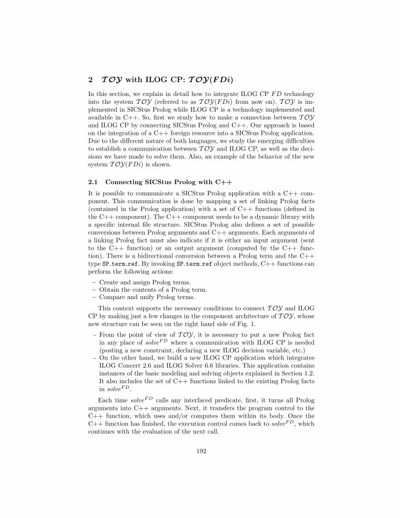
2 T OY with ILOG CP: T OY(FDi)

In this section, we explain in detail how to integrate ILOG CP FD technologyinto the system T OY (referred to as T OY(FDi) from now on). T OY is im-plemented in SICStus Prolog while ILOG CP is a technology implemented andavailable in C++. So, first we study how to make a connection between T OYand ILOG CP by connecting SICStus Prolog and C++. Our approach is basedon the integration of a C++ foreign resource into a SICStus Prolog application.Due to the different nature of both languages, we study the emerging difficultiesto establish a communication between T OY and ILOG CP, as well as the deci-sions we have made to solve them. Also, an example of the behavior of the newsystem T OY(FDi) is shown.

2.1 Connecting SICStus Prolog with C++

It is possible to communicate a SICStus Prolog application with a C++ com-ponent. This communication is done by mapping a set of linking Prolog facts(contained in the Prolog application) with a set of C++ functions (defined inthe C++ component). The C++ component needs to be a dynamic library witha specific internal file structure. SICStus Prolog also defines a set of possibleconversions between Prolog arguments and C++ arguments. Each arguments ofa linking Prolog fact must also indicate if it is either an input argument (sentto the C++ function) or an output argument (computed by the C++ func-tion). There is a bidirectional conversion between a Prolog term and the C++type SP term ref. By invoking SP term ref object methods, C++ functions canperform the following actions:

– Create and assign Prolog terms.– Obtain the contents of a Prolog term.– Compare and unify Prolog terms.

This context supports the necessary conditions to connect T OY and ILOGCP by making just a few changes in the component architecture of T OY, whosenew structure can be seen on the right hand side of Fig. 1.

- From the point of view of T OY, it is necessary to put a new Prolog factin any place of solveFD where a communication with ILOG CP is needed(posting a new constraint, declaring a new ILOG decision variable, etc.)

- On the other hand, we build a new ILOG CP application which integratesILOG Concert 2.6 and ILOG Solver 6.6 libraries. This application containsinstances of the basic modeling and solving objects explained in Section 1.2.It also includes the set of C++ functions linked to the existing Prolog factsin solveFD.

Each time solveFD calls any interfaced predicate, first, it turns all Prologarguments into C++ arguments. Next, it transfers the program control to theC++ function, which uses and/or computes them within its body. Once theC++ function has finished, the execution control comes back to solveFD, whichcontinues with the evaluation of the next call.

192

Creating a SICStus Prolog C++ Foreign ResourceSICStus Prolog needs two files for creating a dynamic library as, for instance

interface.dll, which could be used within a SICStus Prolog application:

– interface.pl Declares the mapping of each Prolog predicate to each C++function. It groups all of these functions in a unique resource. For example:foreign(f1,p1(+integer)).foreign(f2,p2(+term,-term)).foreign resource(interface,[f1,f2]).

– interface.cpp Includes the C++ functions mapped to Prolog facts. It addsas many auxiliary functions and libraries as needed. For example:void f1(long l){...}void f2(SP term ref t1, SP term ref t2){...}

SICStus Prolog supplies a tool, splfr [9], to create a dynamic library (sayinterface.dll), taking as input interface.pl and interface.cpp. The macrosplfr is used as a shortcut to the execution of some compiling and linking com-mands offered by Microsoft Visual C++ [8]. First of all, taking interface.plas input, it creates two new files, interface glue.c and interface glue.h,which provides the necessary glue code for the SICStus application.

2.2 Communication between T OY and ILOG CP

In this section we explain in detail how to implement T OY(FDi) in such a wayit accepts any T OY(FDs) input goal, including all FD constraints managedby the existing solveFD in T OY(FDs). Also, T OY(FDi) uses the same goalsolution structure as T OY(FDs) does. To achieve that behavior is necessary tosolve the following difficulties:

– As T OY is a system implemented in SICStus Prolog, in T OY(FDs) thecommunication between T OY and its FD technology is quite natural. How-ever, as ILOG CP is implemented in C++, some glue code is needed to fixthe impedance mismatch problem.

– ILOG CP and SICStus Prolog differ on their notion of solution of a FDproblem.

There have been four difficult tasks to achieve in the new system T OY(FDi).We explain each of them in the next subsections. When we make reference toany ILOG CP application object, we use the notation of Section 1.2. To thisend, we use model if we refer to the ILOG Concert 2.6 model object, we usesolver if we refer to the ILOG Solver 6.6 generic FD solver, and we use varsif we refer to the decision variables contained in model.

Managing Decision VariablesThe set of FD constraints of a T OY goal involves a set of logic variables

that we denote as ‘FD logic variables’. To model the FD constraint set withILOG CP, some points must be taken into account:

193

– We need to create as many IloIntVar decision variables as FD logic vari-ables take part into the FD constraint set. These variables must be addedto model and vars (the former to model the FD problem properly and thelatter to make possible to refer to each variable of the model from a uniqueobject).

– We must find a bijective relation that associates each FD logic variable ofthe T OY goal with each decision variable existing in the ILOG CP vectorvars.

– We model each FD constraint in ILOG CP over the set of decision variablesof the vector vars associated to the set of FD logic variables involved inthat FD constraint.

Whatever way of communication between T OY and ILOG CP, for each FDlogic variable we have three variables:

- The FD logic variable contained in T OY.- The decision variable modeled as an IloIntVar object in model.- The specific IlcIntVar object created by solver from its associatedIloIntVar object contained in model.

A first attempt for mapping a FD logic variable to a decision variable ofvars is tried. It intends to manage vars and a SP term ref vector, makingthem evolve simultaneously. The elements of the SP term ref vector are in factthe SP term ref conversion of the FD logic variables. Each time solveFD sendsa new FD constraint to ILOG CP, the associated C++ function will first look forits FD logic variables into the SP term ref vector. If it can not find any variable,we can assure that the C++ function is dealing with a new FD logic variablenot treated before. So, the C++ function adds this new FD logic variable tothe SP term ref vector last position, say i. Immediately, a new IloIntVar de-cision variable is created and added to model and vars[i]. When each FD logicvariable of the FD constraint sent by solveFD is contained at an index of theSP term ref vector, the FD constraint is modeled over the decision variables ofvars associated to these indexes.

However, this first attempt fails. This is due to the rules which govern thescope of a SP term ref. When a C++ function containing SP term refs (asarguments or dynamically created within it) finishes its execution, all theseSP term refs become invalid. Let’s see the next example, where an interfacebetween the Prolog predicates p1, p2 and p3 and the C++ functions f1, f2 andf3, resp, is defined. Functions f1 and f2 receive a Prolog term as an argument,while f3 receives two Prolog terms.

– Let’s call p3 with to occurrences of the logic variable X, as p3(X,X). If wemake SP compare(t1,t2) within f3(SP term ref t1, SP term ref t2)the result says that both SP term refs are in fact the same Prolog term.

– But, let’s do the call p1(X). We store t1 of f1(SP term ref t1) into aglobal vector <SP term ref>. When f1 finishes, the program control comesback to Prolog. Now, we call p2 with the logic variable X again, p2(X). If

194

we make SP compare(t1,t2) within f2(SP term ref t2) between t2 andthe SP term ref stored in the vector during f1, the result says that bothSP term refs are different. There is no doubt that both are in fact the sameProlog term. The problem is that, when f1 finish, the SP term ref storedin the vector becomes invalid.

The second and successful attempt relies on the management of the bijectiverelation, which is done into the Prolog application by the use of a list of FDlogic variables (referred to as L from now on). We want L to be used in eachsolveFD predicate. On one hand SICStus Prolog does not allow global variables.On the other hand, there is a logic variable Cin [4], which represents a mixedconstraints store and is common to each solveFD predicate. Our plan is to storeany data structure demanded by the communication between T OY and ILOGCP, specifically L, into Cin. Each time a solveFD predicate manages a new FDconstraint, we can check whether a FD logic variable belongs to L or not byaccessing to it within Cin. Any new FD logic variable is automatically added tothe end of L, say at position i. Here, a new call to the C++ function which createsa new IloIntVar is done. This function adds this decision variable to model andvars[i]. Once all FD logic variables of the FD constraint belongs to L, solveFD

determines their indexes, and put them as arguments to the C++ function, whichmodels the FD constraint by adding to model a new IloConstraint over theassociated positions of vars.

Synchronizing ILOG CP with T OYT OY can also bind its FD logic variables through an equality constraint in

the Herbrand solver. For example, in the goal TOY(FDi)> X #>= 0, X == 3 thevariable X is bound to the value 3. This is done by the Prolog terms unificationwhich results from the Herbrand equality constraint X == 3. This unificationis visible at any occurrence of that FD logic variable, particularly the one inL. This causes an inconsistency between the contents of L and vars. To repairthis lack of synchronization we must send an equality constraint to ILOG CP,making the mapped decision variable in vars equals to the bound value.

A first attempt tries to synchronize by an event-driven approach. To captureevents, SICStus Prolog provides the module of attributed variables. This mod-ule assigns attributes to a set of logic variables. Each time an attributed logicvariable is bound, the predicate verify attributes(+Var, +Value, +Goals)is triggered. We use the attribute fd for each FD logic variable. Thus, eachtime the Herbrand solver binds a FD logic variable, verify attributes(+Var,+Value, +Goals) will automatically call the C++ function which synchronizesthe associated decision variable of vars.

However, this first attempt fails. For this synchronization we need to knowwhich index does the associated decision variable have in vars. We can onlyget this index by looking for the FD logic variable in L. But, unfortunately, thearguments of verify attributes(+Var, +Value, +Goals) are fixed. SICStusProlog does not allow global variables, so there is no way to get access to L.

195

A second attempt consists of making the Herbrand solver responsible of call-ing the C++ synchronization function. But this idea must be rejected, becausethere is a basic principle of independency between the different solvers of thesystem T OY . Any solution to this problem must respect the idea of solving thesynchronization within solveFD.

The third (and successful) attempt modifies the internal structure of L. Nowit becomes a list of pairs. The first element of each pair contains the FD logicvariable, and the second one contains a flag which determines if the bound FDlogic variable has been synchronized with vars. Thus, while the FD logic variableis not bound, the value of the flag remains at 0. When the FD logic variablebecomes bound, the value of the flag indicates whether the variable of vars issynchronized or not.

Each time solveFD sends a new FD constraint to ILOG CP, it must previ-ously:

– Look for any pair in L (say at position i) whose pattern is [value,0]– Add to model the new IloConstraint vars[i]==value.– Change the pair at position i of L by [value,1]

Once there is no pairs with the pattern [value,0] in the list, solveFD isable to send the new FD constraint. If there are no more FD constraints, thepairs [value,0] will be synchronized at the end of the T OY goal. This synchro-nization attempt is clearly inefficient, making it a task to be improved in newreleases of T OY (FDi). Let’s see the next goal:

Toy(FDi)> X #>= 2, X == 1, X1 == 1, X2 == 1, ... , X1000 == 1

The first FD logic variable of the goal is X, which occurs at the first posi-tion of L and vars. The synchronization of X == 1 as vars[0] == 1 makes theFD problem infeasible. So, the T OY goal will fail after X == 1, and there is noneed of computing the rest of the goal expressions. However, the first equalityvars[0] == 1 is not computed until the next FD constraint is posted.As X == 1, X1 == 1, X2 == 1, ... , X1000 == 1 are computed byHerbrand solver there are no more FD constraints in the goal, so the synchro-nization will not occur until the end of the goal. The goal will useless computea thousand of successful expressions. After that, it synchronizes vars[0] == 1and fails.

Synchronizing T OY with ILOG CPILOG CP can bind variables in vars via the set of C++ functions concerning

the management of FD constraints. This produces a lack of synchronizationbetween the vector vars and L. To achieve the synchronization, whenever anyof this C++ functions binds to value vars[i], the pair contained at position iof L must be automatically unified with [value,1].

To this end, solveFD sends L to a C++ function as an input argument, andputs an output argument to obtain the new state of L computed within theC++ function. A new global variable of type vector<int,int> must be created

196

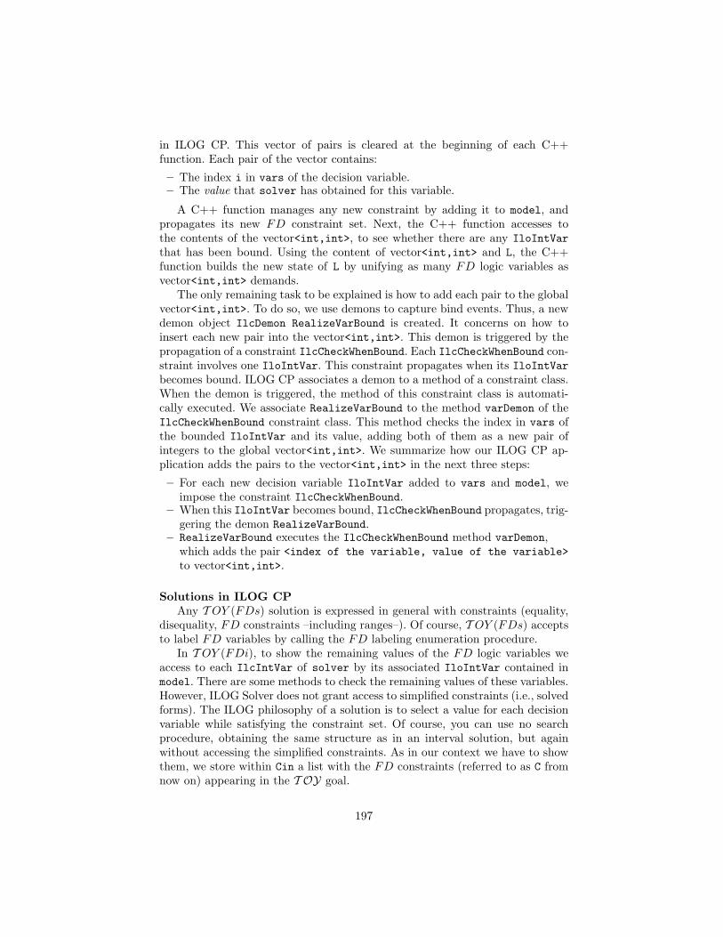
in ILOG CP. This vector of pairs is cleared at the beginning of each C++function. Each pair of the vector contains:

– The index i in vars of the decision variable.– The value that solver has obtained for this variable.

A C++ function manages any new constraint by adding it to model, andpropagates its new FD constraint set. Next, the C++ function accesses tothe contents of the vector<int,int>, to see whether there are any IloIntVarthat has been bound. Using the content of vector<int,int> and L, the C++function builds the new state of L by unifying as many FD logic variables asvector<int,int> demands.

The only remaining task to be explained is how to add each pair to the globalvector<int,int>. To do so, we use demons to capture bind events. Thus, a newdemon object IlcDemon RealizeVarBound is created. It concerns on how toinsert each new pair into the vector<int,int>. This demon is triggered by thepropagation of a constraint IlcCheckWhenBound. Each IlcCheckWhenBound con-straint involves one IloIntVar. This constraint propagates when its IloIntVarbecomes bound. ILOG CP associates a demon to a method of a constraint class.When the demon is triggered, the method of this constraint class is automati-cally executed. We associate RealizeVarBound to the method varDemon of theIlcCheckWhenBound constraint class. This method checks the index in vars ofthe bounded IloIntVar and its value, adding both of them as a new pair ofintegers to the global vector<int,int>. We summarize how our ILOG CP ap-plication adds the pairs to the vector<int,int> in the next three steps:

– For each new decision variable IloIntVar added to vars and model, weimpose the constraint IlcCheckWhenBound.

– When this IloIntVar becomes bound, IlcCheckWhenBound propagates, trig-gering the demon RealizeVarBound.

– RealizeVarBound executes the IlcCheckWhenBound method varDemon,which adds the pair <index of the variable, value of the variable>to vector<int,int>.

Solutions in ILOG CPAny T OY (FDs) solution is expressed in general with constraints (equality,

disequality, FD constraints –including ranges–). Of course, T OY (FDs) acceptsto label FD variables by calling the FD labeling enumeration procedure.

In T OY (FDi), to show the remaining values of the FD logic variables weaccess to each IlcIntVar of solver by its associated IloIntVar contained inmodel. There are some methods to check the remaining values of these variables.However, ILOG Solver does not grant access to simplified constraints (i.e., solvedforms). The ILOG philosophy of a solution is to select a value for each decisionvariable while satisfying the constraint set. Of course, you can use no searchprocedure, obtaining the same structure as in an interval solution, but againwithout accessing the simplified constraints. As in our context we have to showthem, we store within Cin a list with the FD constraints (referred to as C fromnow on) appearing in the T OY goal.

197

2.3 A T OY(FDi) Example

In this section we detail how goal solving works with the new system T OY(FDi)over the example 1:

Toy(FDi)> X #>= 5, X #<= 12, Y #>= 2, Y #<= 17,X #+ Y == 17, X #- Y == 5

We specify how the data structures of solveFD and ILOG CP evolve with eachexpression evaluation. On one hand we look at the state of L and C within Cin.On the other hand we look at the state of vars, model, solver by pointing outany IloIntVar, IloConstraint, IlcIntVar, IlcConstraint object accessedthrough them. For each goal expression any new element added to each datastructure is remarked in boldface. Figure 2 tries to make it clearer:

Fig. 2. TOY (FDi) data structures evolution over FD Constraint expression evaluation

– Figure 2a) represents the internal state of solveFD and ILOG CP data struc-tures at the end of Toy(FDi)> X #>= 5, X #<= 12 evaluation.

– Figure 2b1) and 2b2) describes which actions must be done for the correctmanagement of the new FD Constraint Y #>= 2.

198

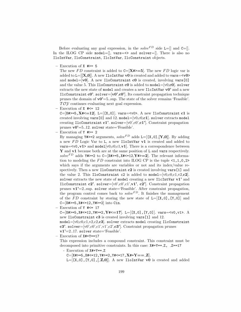
Before evaluating any goal expression, in the solveFD side L=[] and C=[].In the ILOG CP side model=[], vars=<> and solver=[]. There is also noIloIntVar, IloConstraint, IlcIntVar, IlcConstraint objects.

– Execution of X #>= 5The new FD constraint is added to C=[X#>=5]. The new FD logic var isadded to L=[[X,0]]. A new IloIntVar v0 is created and added to vars=<v0>and model=[v0]. A new IloConstraint c0 is created, involving vars[0]and the value 5. This IloConstraint c0 is added to model=[v0,c0]. solverextracts the new state of model and creates a new IlcIntVar v0’ and a newIlcConstraint c0’. solver=[v0’,c0’]. Its constraint propagation techniqueprunes the domain of v0’=5..sup. The state of the solver remains ‘Feasible’.T OY continues evaluating next goal expression.

– Execution of X #<= 12C=[X#>=5,X#<=12]. L=[[X,0]]. vars=<v0>. A new IloConstraint c1 iscreated involving vars[0] and 12. model=[v0,c0,c1]. solver extracts modelcreating IlcConstraint c1’. solver=[v0’,c0’,c1’]. Constraint propagationprunes v0’=5..12. solver state=‘Feasible’.

– Execution of Y #>= 2By managing Y#>=2 arguments, solveFD adds L=[[X,0],[Y,0]]. By addinga new FD Logic Var to L, a new IloIntVar v1 is created and added tovars=<v0,v1> and model[v0,c0,c1,v1]. There is a correspondence betweenY and v1 because both are at the same position of L and vars respectively.solveFD adds Y#>=2 to C=[X#>=5,X#<=12,Y#>=2]. The relevant informa-tion to modeling the FD constraint into ILOG CP is the tuple <1,1,0,2>which says if the arguments are variables or not and its index/value re-spectively. Then a new IloConstraint c2 is created involving vars[1] andthe value 2. This IloConstraint c2 is added to model=[v0,c0,c1,v2,c2].solver extracts the new state of model creating a new IlcIntVar v1’ andIlcConstraint c2’. solver=[v0’,c0’,c1’,v1’, c2’]. Constraint propagationprunes v1’=2..sup. solver state=‘Feasible’. After constraint propagation,the program control comes back to solveFD. It finishes the managementof the FD constraint by storing the new state of L=[[X,0],[Y,0]] andC=[X#>=5,X#<=12,Y#>=2] into Cin.

– Execution of Y #<= 17C=[X#>=5,X#<=12,Y#>=2,Y#<=17]. L=[[X,0],[Y,0]]. vars=<v0,v1>. Anew IloConstraint c3 is created involving vars[1] and 12.model=[v0,c0,c1,v2,c2,c3]. solver extracts model creating IlcConstraintc3’. solver=[v0’,c0’,c1’,v1’,c2’,c3’]. Constraint propagation prunesv1’=2..17. solver state=‘Feasible’.

– Execution of X#+Y==17This expression includes a compound constraint. This constraint must bedecomposed into primitive constraints. In this case: X#+Y== Z, Z==17

- Execution of X#+Y== ZC=[X#>=5,X#<=12,Y#>=2,Y#<=17,X#+Y== Z].L=[[X,0],[Y,0],[ Z,0]]. A new IloIntVar v0 is created and added

199

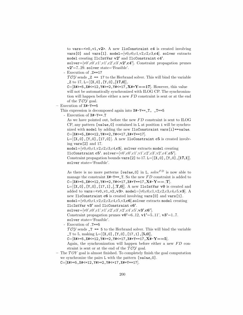
to vars=<v0,v1,v2>. A new IloConstraint c4 is created involvingvars[0] and vars[1]. model=[v0,c0,c1,v2,c2,c3,c4]. solver extractsmodel creating IlcIntVar v2’ and IlcConstraint c4’.solver=[v0’,c0’,c1’,v1’,c2’,c3’,v2’,c4’]. Constraint propagation prunesv2’=7..29. solver state=‘Feasible’.

- Execution of Z==17T OY sends _Z == 17 to the Herbrand solver. This will bind the variable_Z to 17, L=[[X,0],[Y,0],[17,0]],C=[X#>=5,X#<=12,Y#>=2,Y#<=17,X#+Y==17]. However, this valuewill not be automatically synchronized with ILOG CP. The synchroniza-tion will happen before either a new FD constraint is sent or at the endof the T OY goal.

– Execution of X#-Y==5This expression is decomposed again into X#-Y==_T, _T==5

- Execution of X#-Y== TAs we have pointed out, before the new FD constraint is sent to ILOGCP, any pattern [value,0] contained in L at position i will be synchro-nized with model by adding the new IloConstraint vars[i]==value.C=[X#>=5,X#<=12,Y#>=2,Y#<=17,X#+Y==17].L=[[X,0],[Y,0],[17,0]]. A new IloConstraint c5 is created involv-ing vars[2] and 17.model=[v0,c0,c1,v2,c2,c3,c4,c5]. solver extracts model creatingIlcConstraint c5’. solver=[v0’,c0’,c1’,v1’,c2’,c3’,v2’,c4’,c5’].Constraint propagation bounds vars[2] to 17. L=[[X,0],[Y,0],[17,1]].solver state=‘Feasible’.

As there is no more patterns [value,0] in L, solveFD is now able tomanage the constraint X#-Y==_T. So the new FD constraint is added toC=[X#>=5,X#<=12,Y#>=2,Y#<=17,X#+Y==17,X#-Y== T].L=[[X,0],[Y,0],[17,1],[ T,0]]. A new IloIntVar v0 is created andadded to vars=<v0,v1,v2,v3>. model=[v0,c0,c1,v2,c2,c3,c4,c5,v3]. Anew IloConstraint c6 is created involving vars[0] and vars[1].model=[v0,c0,c1,v2,c2,c3,c4,c5,v3,c6].solver extracts model creatingIlcIntVar v3’ and IlcConstraint c6’.solver=[v0’,c0’,c1’,v1’,c2’,c3’,v2’,c4’,c5’,v3’,c6’].Constraint propagation prunes v0’=6..12, v1’=5..11’, v3’=1..7.solver state=‘Feasible’.

- Execution of T==5T OY sends _T == 5 to the Herbrand solver. This will bind the variable_T to 5, making L=[[X,0],[Y,0],[17,1],[5,0]],C=[X#>=5,X#<=12,Y#>=2,Y#<=17,X#+Y==17,X#-Y==5].Again, the synchronization will happen before either a new FD con-straint is sent or at the end of the T OY goal.

– The T OY goal is almost finished. To completely finish the goal computationwe synchronize the pairs L with the pattern [value,0].C=[X#>=5,X#<=12,Y#>=2,Y#<=17,X#+Y==17].

200

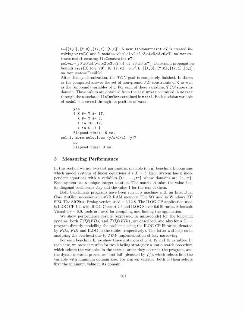
L=[[X,0],[Y,0],[17,1],[5,0]]. A new IloConstraint c7 is created in-volving vars[3] and 5. model=[v0,c0,c1,v2,c2,c3,c4,c5,v3,c6,c7]. solver ex-tracts model creating IlcConstraint c7’.solver=[v0’,c0’,c1’,v1’,c2’,c3’,v2’,c4’,c5’,v3’,c6’,c7’]. Constraint propagationbounds vars[3] to 5, v0’=10..12, v1’=5..7’. L=[[X,0],[Y,0],[17,1],[5,1]].solver state=‘Feasible’.After this synchronization, the T OY goal is completely finished. It showsas the computed answer the set of non-ground FD constraints of C as wellas the (unbound) variables of L. For each of these variables, T OY shows itsdomain. These values are obtained from the IlcIntVar contained in solverthrough the associated IloIntVar contained in model. Each decision variableof model is accessed through its position of vars.

yes{ X #+ Y #= 17,X #- Y #= 5,X in 10..12,Y in 5..7 }

Elapsed time: 16 ms.sol.1, more solutions (y/n/d/a) [y]?

noElapsed time: 0 ms.

3 Measuring Performance

In this section we use two test parametric, scalable (on n) benchmark programswhich model systems of linear equations A ∗ X = b. Each system has n inde-pendent equations with n variables [X1,...,Xn] whose domains are {1..n}.Each system has a unique integer solution. The matrix A takes the value i onits diagonal coefficients Ai,i and the value 1 for the rest of them.

Both benchmark programs have been run in a machine with an Intel DualCore 2.4Ghz processor and 4GB RAM memory. The SO used is Windows XPSP3. The SICStus Prolog version used is 3.12.8. The ILOG CP application usedis ILOG CP 1.4, with ILOG Concert 2.6 and ILOG Solver 6.6 libraries. MicrosoftVisual C++ 6.0. tools are used for compiling and linking the application.

We show performance results (expressed in miliseconds) for the followingsystems: both T OY(FDs) and T OY(FDi) just described, and also for a C++program directly modelling the problems using the ILOG CP libraries (denotedby FDs, FDi and ILOG in the tables, respectively). The latter will help us inanalysing the overhead due to T OY implementation of lazy narrowing.

For each benchmark, we show three instances of n: 4, 12 and 15 variables. Ineach case, we present results for two labeling strategies: a static search procedurewhich selects the variables in the textual order they occur in the program, andthe dynamic search procedure ‘first fail’ (denoted by ff), which selects first thevariable with minimum domain size. For a given variable, both of them selectsfirst the minimum value in its domain.

201

Also, we show the speedups of T OY(FDi) with respect to T OY(FDs) andILOG CP respectively. Specifically, we denote as:

– (a) to the speedup of T OY(FDi) with respect to T OY(FDs) using thestatic search procedure to solve the problem.

– (b) to the speedup of T OY(FDi) with respect to T OY(FDs) using the ‘firstfail’ search procedure.

– (c) to the speedup of T OY(FDi) with respect to ILOG CP C++ programusing the static search procedure.

– (d) to the speedup of T OY(FDi) with respect to ILOG CP C++ programusing the ‘first fail’ search procedure.

The benchmarks programs are:

– The solution [X1,...,Xn] holds: ∀i ∈ {1 . . . n} Xi = i. Performance mea-surement gives the following results:

n FDs FDsff FDi FDiff ILOG ILOGff (a) (b) (c) (d)4 0 15 0 0 15 15 1.0 - 0 012 31 1.750 156 516 15 281 5.0 0.29 10.4 1.8315 297 299,312 423 67,376 63 20,578 1.42 0.22 6.7 3.27

For this first benchmark, T OY(FDi) takes more time than T OY(FDs) forsolving with the static search procedure, but less time for the dynamic searchprocedure. The solving time difference between them grows as we increasethe number of variables for the benchmarks. Looking at how the domains ofthe variables evolve after the initial constraint propagation, we can concludethat the structure of the solution for this first benchmark fits quite well intothe static search procedure, while it is dramatically harmful to the dynamicsearch procedure. This help us to realize that, for problems where the neededexploration to obtain the solution is really small, then T OY(FDi) is slowerthan T OY(FDs). This is because of the time involved in the communicationbetween the Prolog implementation of T OY(FDi) and ILOG CP. However,as the nodes needed to be explored increase slightly, this waste of time isbalanced, making T OY(FDi) more efficient than T OY(FDs).

– The solution [X1, ,Xn] holds: ∀i ∈ {1..n} Xi = n − (i − 1). Performancemeasurement gives the following results:

n FDs FDsff FDi FDiff ILOG ILOGff (a) (b) (c) (d)4 16 16 16 31 31 15 1.0 1.93 0.51 2.0612 531 250 437 126 109 63 0.83 0.50 4 215 15,563 21,968 13,937 3,406 843 1,765 0.90 0.16 16.53 1.93

The above conclusions are clearly confirmed in this second benchmark, whereT OY(FDi) is faster than T OY(FDs) for both search procedures. In this case,the structure of the solution is dramatically harmful for the static strategy, whileit behaves better for the dynamic strategy. In the former, T OY(FDi) takes

202

slightly less solving time than T OY(FDs). In any case, these measurementspoint out that our first approach to integrate the ILOG CP technology intoT OY(FDi) is encouraging, but also that the management of the additionaldata structures used for the interface should be optimized.

4 Conclusions and Future Work

In this work, we have studied how to integrate the FD ILOG CP technologyinto the system T OY. We have shown that this technology offers some advan-tages over the existing system T OY based on the FD technology of SICStusProlog. We have described in detail our implementation, showing that the ap-plication architecture of T OY and ILOG CP are hard to integrate in terms ofa correct communication between them. We have shown by means of two scal-able benchmarks that the new system T OY(FDi) is faster than T OY(FDs)as the benchmark increases its size. However, we have concluded that there isa performance penalization due to the management of the data structures thatmake possible the connection of T OY with its new FD component. Therefore,optimizing this management will be the target of our immediate future work.In addition, backtracking management will be covered in a next work, togetherwith an extended set of benchmarks. Another subject of interest is to test otherconstraint libraries, as Gecode [11].

References

1. P. Arenas, S. Estevez, A. Fernandez, A. Gil, F. Lopez-Fraguas, M. Rodrıguez-Artalejo, and F. Saenz-Perez. T OY. a multiparadigm declarative language.version 2.3.1., 2007. R. Caballero and J. Sanchez (Eds.), Available athttp://toy.sourceforge.net.

2. R. G. del Campo and F. Saenz-Perez. Programmed Search in a Timetabling Prob-lem over Finite Domains. Electr. Notes Theor. Comput. Sci., 177:253–267, 2007.

3. S. Estevez-Martın, A. Fernandez, M. Hortala-Gonzalez, F. Saenz-Perez,M. Rodrıguez-Artalejo, and R. del Vado-Vırseda. On the Cooperation of the Con-straint Domains H, R and FD in CFLP . Theory and Practice of Logic Program-ming, 2009. Accepted for publication.

4. S. Estevez-Martın, A. J. Fernandez, and F. Saenz-Perez. About implementing aconstraint functional logic programming system with solver cooperation. In proc.of CICLOPS’07, pages 57–71, 2007.

5. A. J. Fernandez, T. Hortala-Gonzalez, F. Saenz-Perez, and R. del Vado-Vırseda.Constraint Functional Logic Programming over Finite Domains. Theory Pract.Log. Program., 7(5):537–582, 2007.

6. ILOG. ILOG Solver 6.6, Reference Manual, 2008.7. ILOG. ILOG OPL Studio 6.1, Reference Manual, 2009.8. Microsoft, 2005. http://msdn.microsoft.com/en-us/visualc/default.aspx.9. SICStus Prolog. Using SICStus Prolog with newer Microsoft C compilers.

10. SICStus Prolog, 2007. http://www.sics.se/isl/sicstus.11. The Gecode team. Generic constraint development environment. Available from

http://www.gecode.org, 2006.

203