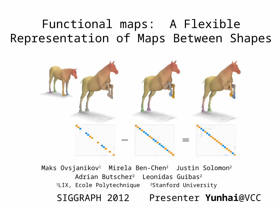
Functional maps: A Flexible Representation of Maps Between Shapes

SIGGRAPH 2012

Maks Ovsjanikov1 Mirela Ben-Chen2 Justin Solomon2

Adrian Butscher2 Leonidas Guibas2

1LIX, Ecole Polytechnique 2Stanford University

Presenter Yunhai@VCC

Introduction

• Shape matching• Rigid (rotation + translation)• Non-rigid (pairings of points or regions)

Correspondence

Correspondence

• The space of correspondences is exponential• Isometric matching: still a QAP (NP-hard)• No map continuity or global consistency

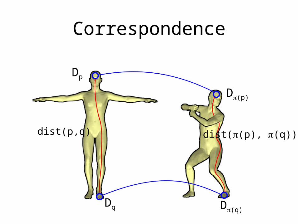
Correspondence

Dp

D(p)

Dq D(q)

dist(p,q) dist((p), (q))

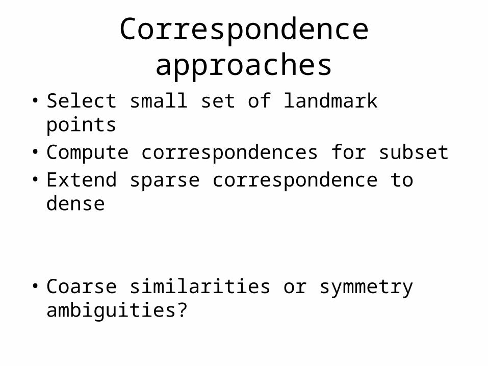
Correspondence approaches

• Select small set of landmark points• Compute correspondences for subset• Extend sparse correspondence to dense

• Coarse similarities or symmetry ambiguities?

Do we need Point-to-point correspondence?

• It is neither possible nor necessary , because– inherent shape ambiguities or – the user may only be interested in

approximate alignment

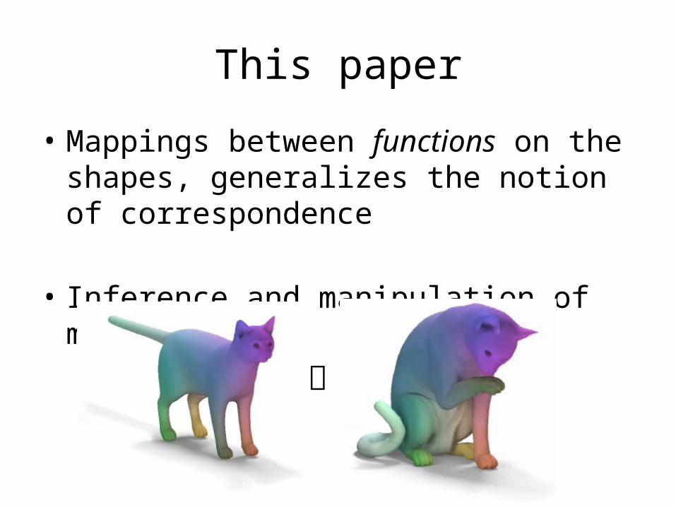
This paper

• Mappings between functions on the shapes, generalizes the notion of correspondence

• Inference and manipulation of maps

Overview

• Functional map representation• Properties (basis, continuity, linearity, …)• Inference (obtain a point-to-point map)• Applications– Shape matching– Map improvement– Shape collections– Segmentation transfer

• Bijective mapping• Manifolds M and N• T induces a transformation for functions

• Given scalar function We obtain with

Functional map representation

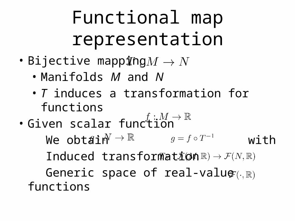
• Bijective mapping• Manifolds M and N• T induces a transformation for functions

• Given scalar function We obtain with Induced transformation Generic space of real-value functions

Functional map representation

Functional map representation

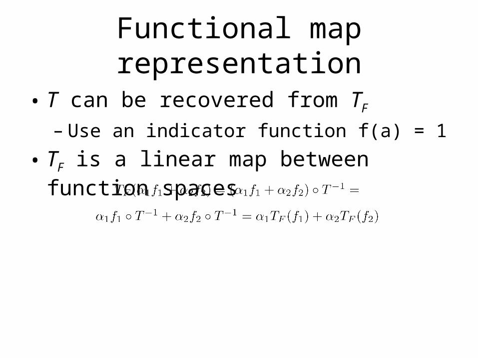
• T can be recovered from TF

– Use an indicator function f(a) = 1

• TF is a linear map between function spaces

Functional map representation

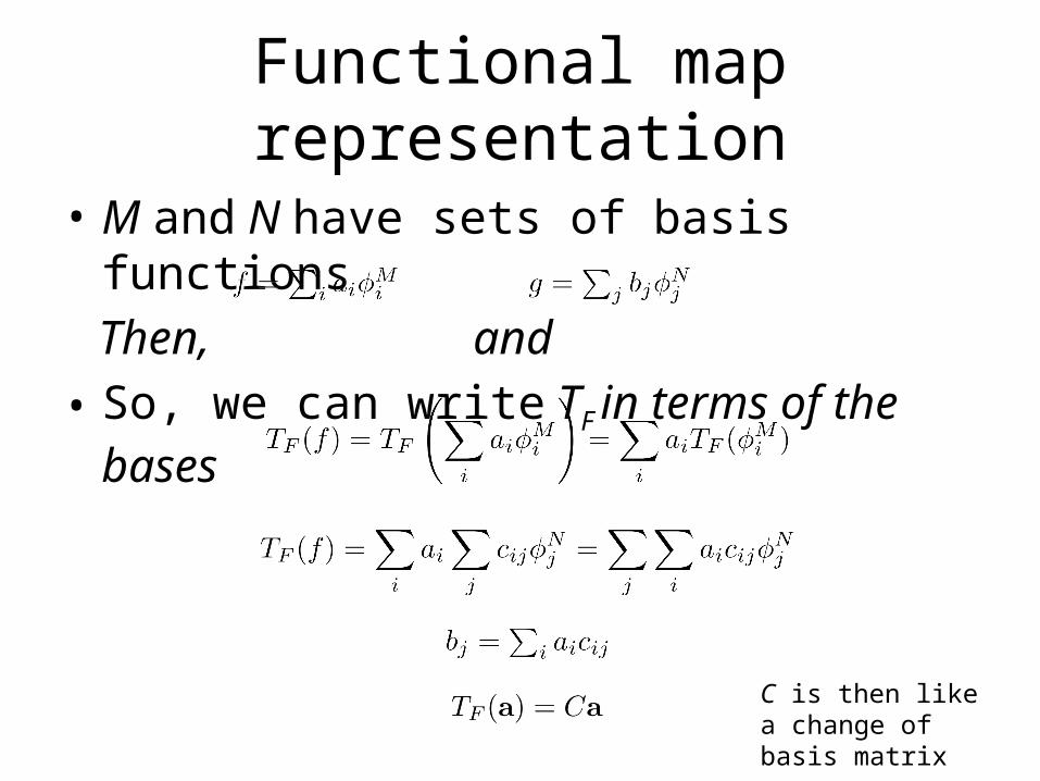
• M and N have sets of basis functions Then, and • So, we can write TF in terms of the bases

C is then like a change of basis matrix

Functional map representation

• Generalized linear functional mapping

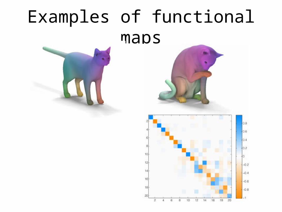
Examples of functional maps

Using Laplace-Beltrami eigenfunctionsLinear functional mapping is a 20x20 matrix

Examples of functional maps

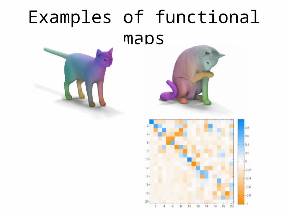
Examples of functional maps

Properties: choice of basis

• Example of basis– Indicator functions Permutation matrix

• Motivation– Reduce representation complexity – Better suited for continuous mappings

• Choose based on compactness and stability

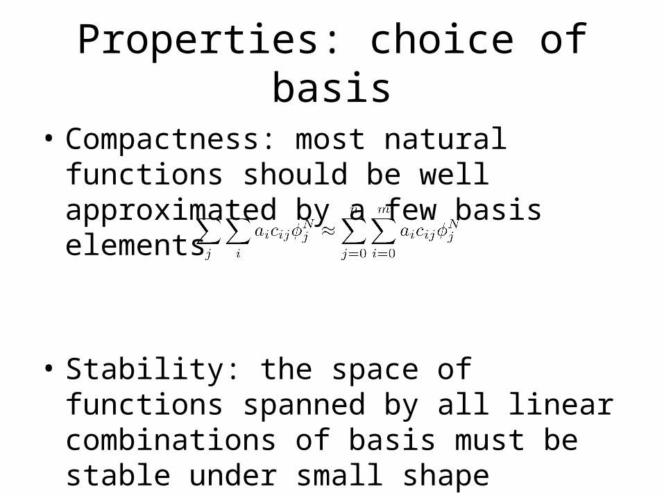
Properties: choice of basis

• Compactness: most natural functions should be well approximated by a few basis elements

• Stability: the space of functions spanned by all linear combinations of basis must be stable under small shape deformations

Properties: choice of basis

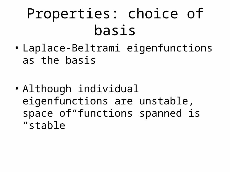
• Laplace-Beltrami eigenfunctions as the basis

• Although individual eigenfunctions are unstable, space of functions spanned is “stable”

Properties: choice of basis

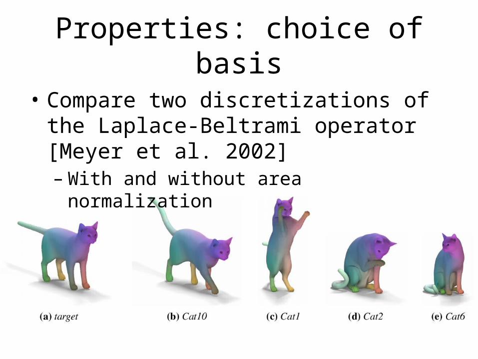
• Compare two discretizations of the Laplace-Beltrami operator [Meyer et al. 2002]– With and without area normalization

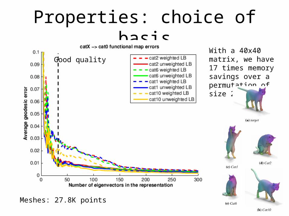
Properties: choice of basis

Meshes: 27.8K points

Good qualityWith a 40x40 matrix, we have 17 times memory savings over a permutation of size 27.8K

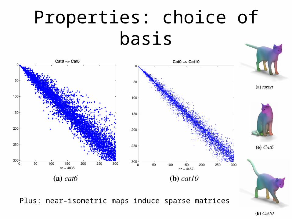
Properties: choice of basis

Plus: near-isometric maps induce sparse matrices

Properties: continuity

• Naturally handles map continuity• Three types of continuity:– Changes of the input functionImage varies continuously under changes of a– Image functionLaplace-Beltrami is well-suited for smooth functions is smooth– Representation• Any matrix C is a functional mapping

Properties: continuity

Mapping obtained using an interpolation between two maps: C = C1 + (1- )C2

Properties: linearity of constraints

• Descriptor preservation, e.g., f(x) = (x)– Function pres. implies approximate desc. pres.

• Landmark point correspondences– Use f(x) that is distance function to the landmark

• Segment correspondences– Also distance functions or indicator functions

Properties: operator commutativity

• W.r.t. linear operators on the shapes– E.g., symmetry

• An example– C is a map between a man and a woman– RF ,SF is the map the left hand to right hand on the

woman and man, respectively– Man ->Woman, Woman left->Woman right Man left -

> Woman right– Man left -> Man Right Man -> Woman Man Left ->

Woman Right

Properties: regularization constraints

• Not every matrix C is a point-to-point map• It is most meaningful to consider orthonormal

or nearly-orthonormal functional matrices

Map inversion and composition

• Finding an inverse of a map that is not a bijection can be challenging

• In the functional case, an inverse is given simply by the inverse of the matrix C

• A good approximation is the transpose of C

• Composition becomes matrix multiplication

Functional map inference

• Construct a large system of equations• Each equation is one constraint• Constraint for function preservation• Find the matrix C that satisfies the constraints• In fact, we will need many constraints to

obtain C in a least-squares sense• Thus, we need candidate point-to-point or

segment-to-segment correspondences

Map refinement and conversion

• Refine C and convert to a point-to-point map

• For each point x is the source embedding• Find closest point x’ in the target embedding• Find the optimal C by minimizing |Cx – x’|• Iterate this procedure

• Similar to spectral matching [Jain et al. 2007]• Differences

– Good initial estimate C– “Mixing” across eigenvectors

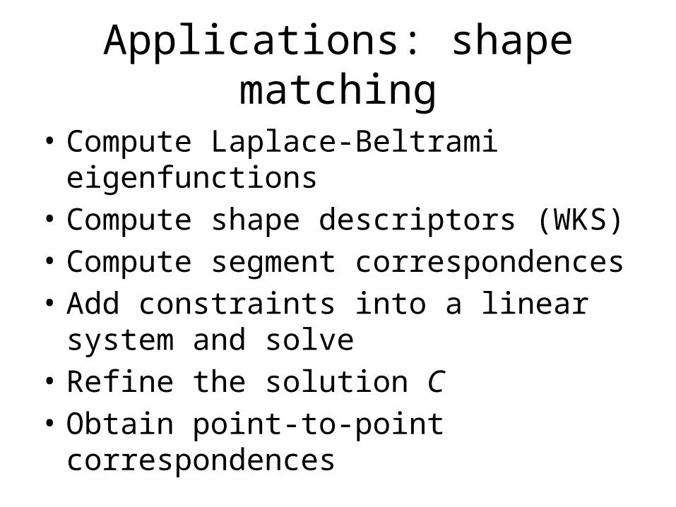
Applications: shape matching

• Compute Laplace-Beltrami eigenfunctions• Compute shape descriptors (WKS)• Compute segment correspondences• Add constraints into a linear system and solve• Refine the solution C• Obtain point-to-point correspondences

Applications: shape matching

• Applied on the benchmark of Kim et al. 2011

Examples of correspondences obtained

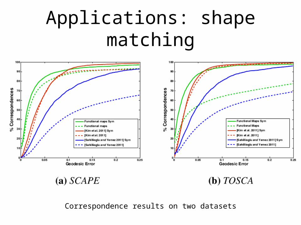
Applications: shape matching

Correspondence results on two datasets

Applications: map improvement

• The strength lies on the representation itself• Take point-to-point maps computed by the

other methods• Improve the maps with the functional maps• Adds regularization• Takes 15s for 50K point mesh in 3GHz CPU

Applications: map improvement

Color shows location of errors

Applications: map improvement

Color shows location of errors

Applications: map improvement

Evaluation on the benchmark

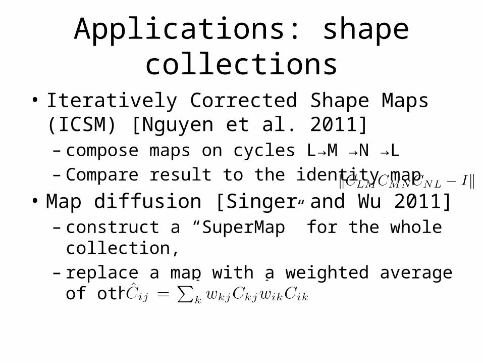
Applications: shape collections

• Iteratively Corrected Shape Maps (ICSM) [Nguyen et al. 2011] – compose maps on cycles L→M →N →L– Compare result to the identity map

• Map diffusion [Singer and Wu 2011]– construct a “SuperMap” for the whole collection,– replace a map with a weighted average of other

maps

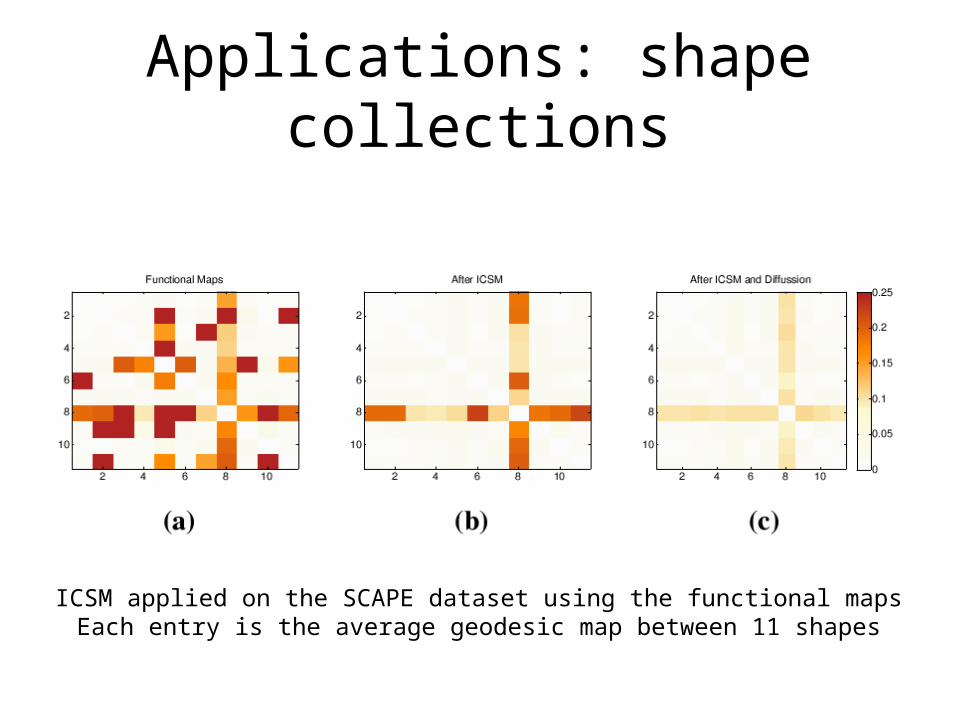
Applications: shape collections

ICSM applied on the SCAPE dataset using the functional mapsEach entry is the average geodesic map between 11 shapes

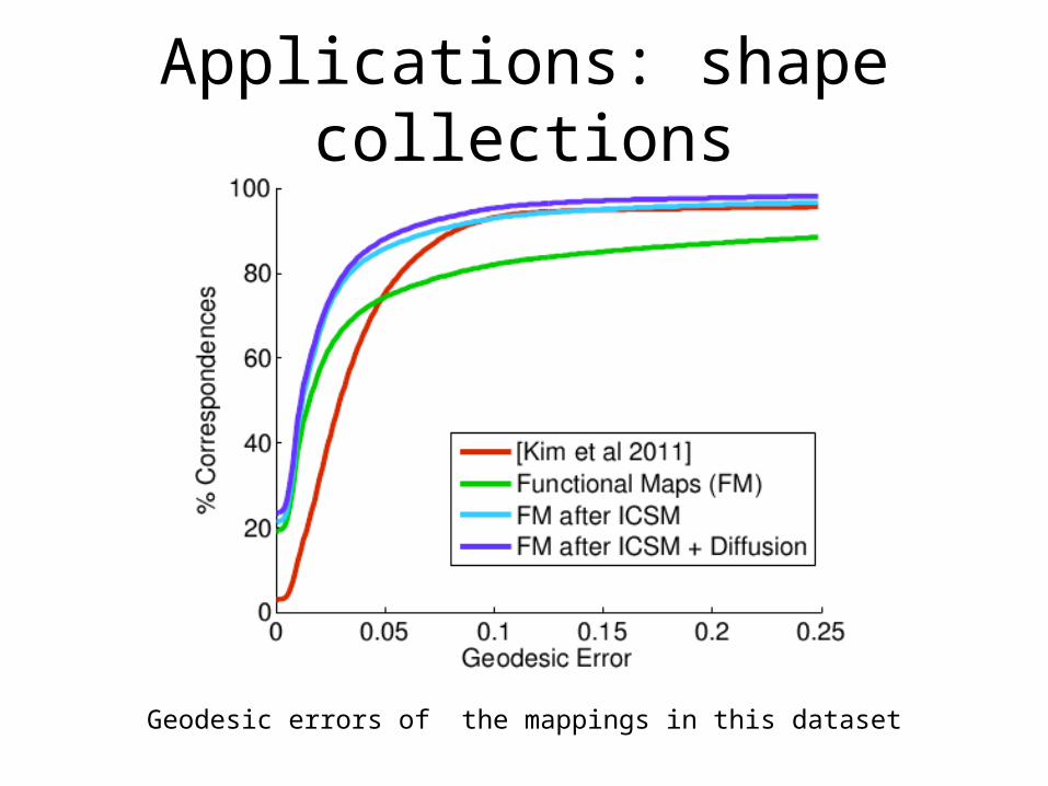
Applications: shape collections

Geodesic errors of the mappings in this dataset

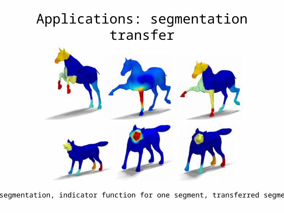
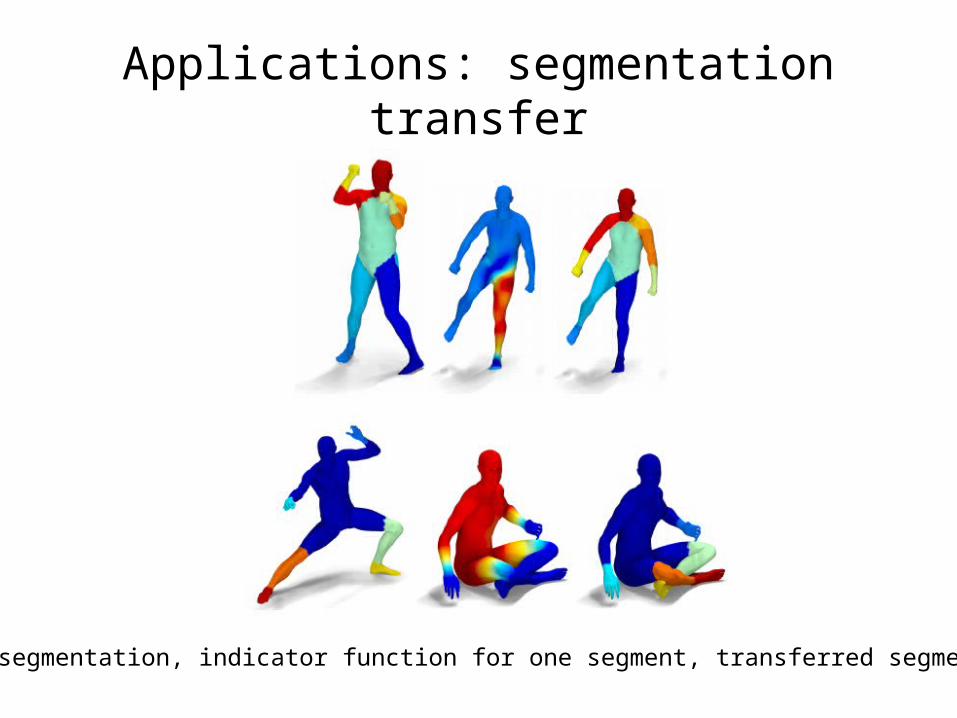
Applications: segmentation transfer

• Functional maps reduce the transfer of functions to matrix multiplication

• Without resorting to point-to-point maps

• Use indicator functions for segments• Perform matrix multiplication• Transform attributes into a “hard” clustering

Applications: segmentation transfer

Source segmentation, indicator function for one segment, transferred segmentation

Applications: segmentation transfer

Source segmentation, indicator function for one segment, transferred segmentation

Conclusion

• Novel representation of maps between shapes• Generalizes point-to-point maps• Constraints become linear

• More general classes of deformations?– Optimal choice of basis

Discussion

• In practice, could pose the method as: “find a correspondence between eigenfunctions”? Actually, People has used spectral basis to compute the shape map– JAIN, V., ZHANG, H., AND VAN KAICK, O. 2007. Non-rigid spectral

correspondence of triangle meshes. International Journal on Shape Modeling 13, 1, 101–124

– MATEUS, D., HORAUD, R. P., KNOSSOW, D., CUZZOLIN, F., AND BOYER, E. 2008. Articulated shape matching using Laplacian eigenfunctions and unsupervised point registration. In Proc. CVPR, 1–8.

• What does the representation really bring? a new concept functional map?