Functional summary statistics for the Johnson-Mehl model

February 22, 2013

Jesper Møller and Mohammad Ghorbani

Department of Mathematical Sciences, Aalborg University

Abstract

The Johnson-Mehl germination-growth model is a spatio-temporal point process model which amongother things have been used for the description of neurotransmitters datasets. However, for suchdatasets parametric Johnson-Mehl models fitted by maximum likelihood have yet not been evaluatedby means of functional summary statistics. This paper therefore invents four functional summarystatistics adapted to the Johnson-Mehl model, with two of them based on the second-order propertiesand the other two on the nuclei-boundary distances for the associated Johnson-Mehl tessellation.The functional summary statistics theoretical properties are investigated, non-parametric estimatorsare suggested, and their usefulness for model checking is examined in a simulation study. Thefunctional summary statistics are also used for checking fitted parametric Johnson-Mehl models fora neurotransmitters dataset.

Key words: germination-growth process, model checking, neurotransmitters, pair correlation function,spatio-temporal point process, tessellation, typical cell.

1 Introduction

This paper concerns statistical inference for the Johnson-Mehl germination-growth process in the d-

dimensional Euclidean space Rd, with a focus on model fitting and checking. The case d = 1 is of special

interest for modelling e.g. neurotransmitters datasets, but many of our results apply for d ≥ 1 as well.

Section 1.1 recalls the definition of the Johnson-Mehl model, Section 1.2 reviews the literature and the

applications of the model, and Section 1.3 states our main objectives and the outline of the paper.

1.1 The Johnson-Mehl model

The Johnson-Mehl germination-growth process results by a dependent thinning of a space-time Poisson

process as follows.

1

We start with a primary space-time Poisson process Φ ≡ (x1, t1), (x2, t2), . . . ⊂ Rd × [0,∞) with

intensity measure dxK(dt), where dx denotes Lebesgue measure on Rd and K is a non-zero locally finite

measure on [0,∞). For (xi, ti) ∈ Φ, we call (xi, ti) an event and think of xi as a nucleus (or germ) which

starts to grow at time ti with a constant speed v > 0 in all directions, unless xi has already been reached

by another nucleus xj which started to grow at a time tj < ti (with speed v in all directions); in the

latter case we say that (xi, ti) has been thinned. Let

Ti(y) ≡ T ((xi, ti), y) = ti + ‖xi − y‖/v

be the time that xi reaches a point y ∈ Rd. Then the unthinned events form a secondary space-time point

process, namely the Johnson-Mehl germination-growth process (or shortly Johnson-Mehl process) given

by

Ψ = (xi, ti) ∈ Φ : ti ≤ Tj(xi) for all (xj , tj) ∈ Φ with tj < ti.

Moreover, the growth along the ray of any growing nucleus stops when it reaches another growing

ray. Thereby a tessellation of Rd with cells

Ci = y ∈ Rd : Ti(y) ≤ Tj(y) for all j 6= iwith (xj , tj) ∈ Ψ, (xi, ti) ∈ Ψ, (1)

is created. This is called the Johnson-Mehl tessellation, see Johnson & Mehl (1939), Stoyan, Kendall

& Mecke (1995), Okabe, Boots, Sugihara & Chiu (2000), and the references therein. In the special

case where K is concentrated at time 0, the Johnson-Mehl tessellation is just a Voronoi tessellation

(Møller 1994; Okabe et al. 2000).

1.2 Applications and literature

Applications of the Johnson-Mehl model for d = 2 and d = 3 can be found in crystal growth (Kolmogorov

1937; Johnson & Mehl 1939), microstructural evolution in thin films (see Frost, Thompson & Walton

(1992) and the references therein), plant ecology (Kenkel 1990), and socio-economic cellular network

(Boots, Okabe & Thomas 2003). Biological applications of the model for d = 1 include DNA replication

(Vanderbei & Shepp 1988; Cowan, Chiu & Holst 1995), release of neurotransmitters at neuromuscular

synapses (Quine & Robinson 1990; Quine & Robinson 1992; Bennett & Robinson 1990; Chiu, Quine

& Stewart 2000; Molchanov & Chiu 2000; Chiu, Molchanov & Quine 2003), cell biology (Wolk 1975),

and lung carcinoma (Kayser & Stute 1989). The model has been well studied from a probabilistic point

of view, with the pioneering work by Kolmogorov (1937) and Johnson & Mehl (1939), and followed by

Meijering (1953), Gilbert (1962), Miles (1972), Horalek (1988, 1990) and Møller (1992, 1995). Statistical

2

analysis for the model has mainly been studied in the above-mentioned papers by Chiu and coworkers,

with most attention to the case d = 1 where maximum likelihood based inference is in fact feasible as

discussed in Section 2.4.

1.3 Aim and outline

To the best of our knowledge, though functional summary statistics play a fundamental role for analyzing

spatial and spatio-temporal point patterns (see e.g. Gabriel & Diggle (2009) and Møller & Ghorbani

(2012)), this is the first paper introducing functional summary statistics for the Johnson-Mehl model.

In the theory part (Sections 2-3), we consider the general case d ≥ 1, since applications occur for

d = 1, 2, 3 (cf. Section 1.2) and many ideas and results can easily be stated. In the application part

(Section 4 ), d = 1.

Section 2 provides the needed background material for this paper. Section 3 introduces our functional

summary statistics. First, two functional summary statistics based on the pair correlation function and

with some relation to the space-time inhomogeneous K-function (Gabriel & Diggle 2009) are invented.

Second, two functional summary statistics based on the nuclei-boundary distances for the Johnson-Mehl

tessellation are developed. The theoretical properties and non-parametric estimation of the functional

summary statistics are discussed. Section 4 presents the results of a simulation study when applying the

functional summary statistics for model checking in cases where a Johnson-Mehl model is correctly or

incorrectly specified. Moreover, for the same neurotransmitters dataset as analyzed in Chiu et al. (2003),

we check parametric Johnson-Mehl models estimated by maximum likelihood. Finally, technical details

are deferred to Appendixes A-D.

2 Preliminaries

This section introduces some notation, concepts, and parametric models used in the sequel.

2.1 Independence

Let Ω = Rd × [0,∞) be the space-time domain, and for A ⊆ Ω, let ΦA = Φ ∩ A and ΨA = Ψ ∩ A. For

(x, t) ∈ Ω, denote

C(x, t) = (y, u) ∈ Ω : T ((y, u), x) ≤ t

3

which is a cone consisting of those (y, u) ∈ Ω where y reaches x before or at time t when y starts to grow

at time u with speed v in all directions. Hence, with probability one,

Ψ = (x, t) ∈ Φ : ΦC(x,t) = (x, t). (2)

For A ⊆ Ω, define

A =⋃

(x,t)∈A

C(x, t) = (y, u) ∈ Ω : T ((y, u), x) < t for some (x, t) ∈ A.

By (2), ΨA depends on Φ only through ΦA. Therefore, for any Borel sets A,B ⊆ Ω,

ΨA and ΨB are independent if A ∩ B = ∅ (3)

since ΦA and ΦB are independent when A ∩ B = ∅. Consequently, we say that (xi, ti), (xj , tj) ∈ Ψ are

independent events if C(xi, ti) ∩ C(xj , tj) = ∅, that is, v(ti + tj) < ‖xi − xj‖.

2.2 Intensity

Henceforth we assume that K is absolutely continuous w.r.t. Lebsgue measure on [0,∞), with density κ.

It is also assumed that κ is chosen such that all integrals to follow exit. This will be the case if e.g. κ is

piecewise continuous.

Note that Ψ is stationary and isotropic in space, but inhomogeneous in time. Hence its intensity

function depends only on time and is given by

ρ(t) = P(ΦC(0,t) = ∅)κ(t) = exp

− ∫∫C(0,t)

κ(s) dxds

κ(t)

as obtained from (2) and the Slivnyak-Mecke theorem (Mecke 1967; Møller & Waagepetersen 2004). This

reduces to

ρ(t) = exp

(−∫ t

0

ωd[v(t− s)]dκ(s) ds

)κ(t) (4)

where ωd = πd/2/Γ(1 + d/2) is the volume of the unit ball in Rd. Indeed, ρ is non-constant no matter

the choice of κ.

4

2.3 Parametric models

We are particularly interested in the following parametric models.

M1: κ(t) = αtβ−1 where α > 0, β > 0. (5)

M2: κ(t) =αγβ

Γ(β)tβ−1 exp(−γt) where α > 0, β > 0, γ > 0. (6)

The models have been studied in Frost & Thompson (1987), Horalek (1988,1990), Møller (1992,1995),

Chiu (1995), and the papers discussed in Section 4.2.1.

For M1, combining (4) and (5), we obtain

ρ(t) = exp(−αωdvdtβ+dB(β, d+ 1)

)αtβ−1 (7)

which is an un-normalized generalized gamma density with shape parameter β and inverse scale parameter

α. For M2, κ is an un-normalized gamma density, and combining (4) and (6), we obtain

ρ(t) = exp

(−2αv

(tΓ(t;β, γ)− β

γΓ(t;β + 1, γ)

))αγβ

Γ(β)tβ−1 exp(−γt) if d = 1, (8)

ρ(t) = exp

(−παv2

(t2Γ(t;β, γ)− 2t

β

γΓ(t;β + 1, γ) +

(β + 1)β

γ2Γ(t;β + 2, γ)

))× αγβ

Γ(β)tβ−1 exp(−γt) if d = 2,

(9)

and similar but more and more complicated formulae can be derived for d ≥ 3. Here Γ(x;β, γ) denotes

the cumulative distribution functions of a Gamma distribution with shape parameter β and inverse scale

parameter γ. Plots of ρ under M1 and M2 are shown in Figure 1 where d = 1; similar plots are obtained

for d = 2.

2.4 Maximum likelihood

Assuming the nuclei are observed within a bounded region W ⊂ Rd, and ignoring edge effects due to

thinning caused by the unobserved events with nuclei outside W , the unthinned events with nuclei within

W are given by

ΨappW = (xi, ti) ∈ ΦW×[0,∞) : ti ≤ Tj(xi) for all (xj , tj) ∈ ΦW×[0,∞) with tj < ti. (10)

The space-time point process ΨappW has conditional intensity function

λ(x, t|Ht) = 1[t ≤ Ti(x) for all (xi, ti) ∈ ΨappW with ti < t]κ(t), (x, t) ∈W × [0,∞), (11)

5

0.0 0.5 1.0 1.5 2.0 2.5

0.0

0.5

1.0

1.5

2.0

2.5

0.0 0.5 1.0 1.5 2.0 2.50.

00.

51.

01.

52.

02.

5

Figure 1: The intensity function ρ(t) under M1 (left panel) and M2 (right panel) with d = 1, α = γ =v = 1, β = 0.5 (solid line), β = 1 (dashed line), β = 2 (dotted line), and β = 3 (dot-dashed line).

where 1[·] denotes the indicator function and Ht is the ‘history’ (i.e., the information about ΨappW up to

but not including time t), cf. Daley & Vere-Jones (2003).

Consider the problem of maximum likelihood estimation for (v, θ) when we have assumed a parametric

model κθ for the function κ, e.g. θ = (α, β) ∈ (0,∞)2 in case of M1 or θ = (α, β, γ) ∈ (0,∞)3 in

case of M2, and where v and θ are variation independent. Suppose we observe a realization ΨappW =

(x1, t1), . . . , (xn, tn) where n <∞ and ti 6= tj whenever i 6= j (this is almost surely the case). By (11)

and Section 7.2 in Daley & Vere-Jones (2003), the likelihood function is

L(θ, v) =1[ti + ‖xi − xj‖/v ≥ tj whenever ti < tj ]

[n∏i=1

κθ(ti)

]

× exp

− ∫∫W×[0,∞)

1[ti + ‖xi − x‖/v ≥ t whenever ti < t]κθ(t) dxdt

.

See also Chiu et al. (2003). If n ≥ 2, the maximum likelihood estimate (MLE) for v is seen to be smallest

pairwise relative distance

v = min1≤i<j≤n

‖xi − xj‖/|ti − tj |

since L(θ, v) is an increasing function of v ≤ v, and it is zero for v > v; if n ≤ 1, then the MLE does not

6

exist. Assuming n ≥ 2, the profile likelihood L(θ) = L(θ, v) is

L(θ) =

n∏i=1

κθ(ti) exp

−∫Ci

(∫ Ti(x)

0

κθ(t) dt

)dx

(12)

where Ti(x) = ti+ v‖x−xi‖ and Ci is the Johnson-Mehl cell as given by (1) when v is replaced by v, and

Ψ by (x1, t1), . . . , (xn, tn). When d = 1, the integral in (12) may easily be evaluated, while numeric

methods are needed for d ≥ 2.

The extension to the case with independent copies of ΨappW (as considered in Section 4) is straightfor-

ward. In particular, the MLE for v is simply the smallest pairwise relative distance obtained from the

realizations of these independent copies.

3 Functional summary statistics

3.1 Second-order analysis

The natural staring point when characterizing the second-order properties of Ψ is to consider the den-

sity of the second-order product for Ψ, denoted ρ(2)((x, s), (y, t)) for (x, s), (y, t) ∈ Ω, and called the

second-order product density for Ψ, see e.g. Møller & Ghorbani (2012) for a formal definition. Intu-

itively, ρ(2)((x, s), (y, t)) dxdsdy dt is the probability of observing one event of Ψ in an infinitesimally

small region of volume dxds around (x, s) and another event of Ψ in an infinitesimally small region of

volume dy dt around (y, t). Since Ψ is stationary and isotropic in space and ρ(2) is a symmetric function,

ρ(2)((x, s), (y, t)) depends only on x and y through r = ‖x− y‖, and it is symmetric w.r.t. s and t, so we

can write

ρ(2)((x, s), (y, t)) = ρ(2)0 (r, s, t) = ρ

(2)0 (r, t, s).

In Section 3.1.1, we determine ρ(2)0 and thereby the pair correlation function g defined by

g(r, t, s) =ρ

(2)0 (r, t, s)

ρ(s)ρ(t)if ρ(s)ρ(t) > 0, g(r, t, s) = 0 otherwise. (13)

This is used in Section 3.1.2 for constructing functional second-order summary statistics.

3.1.1 Pair correlation function

Using (2) and the Slivnyak-Mecke formula (Mecke 1967; Møller & Waagepetersen 2004) we see that

ρ(2)0 (r, s, t) = κ(s)κ(t)1[r > v|s− t|] exp

(−∫ ∫

κ(u)1[(z, u) ∈ C(x, s) ∪ C(y, t)] dz du

). (14)

7

Let b(x, r) denote the closed ball with center x and radius r > 0; set b(x, r) = ∅ if r ≤ 0. For u ≥ 0, let

V∩(r, s − u, t − u) denote the volume of the intersection b(x, v(s − u)) ∩ b(y, v(t − u)) corresponding to

the region in Ω of points z born at time u so that z reaches x before time s, and y before time t, when

growing with speed v in all directions. Combining (4) and (13)-(14) we obtain

g(r, s, t) = 1[v|s− t| < r < v(s+ t)] exp

(−∫ (s+t−r/v)/2

0

κ(u)V∩(r, s− u, t− u) du

)+ 1[r ≥ v(s+ t)] (15)

if κ(s) > 0 and κ(t) > 0, and g(r, t, s) = 0 otherwise. Thus g(r, s, t) ≤ 1, meaning that Ψ exhibits

regularity. For κ(s) > 0 and κ(t) > 0, g(r, s, t) as a function of r is zero if r ≤ v|s − t|; has a jump at

r = v|s− t| if and only if K([0, 2 mins, t]) > 0; is non-decreasing and continuous if r > v|s− t|; and is

one if r ≥ v(s+ t), which is in accordance with our concept of independent events, cf. (3).

In order to calculate V∩(. . .) in (15), note that for h ≥ 0 and l > 0,

Vd(l, h) =πd/2ld

2Γ(1 + d/2)I(2lh−h2)/l2((d+ 1)/2, 1/2) (16)

is the volume of a d-dimensional hyper-spherical cap of height h and radius l (Li 2011), where

Ic(a, b) =1

B(a, b)

∫ c

0

ua−1(1− u)b−1du with B(a, b) =Γ(a)Γ(b)

Γ(a+ b)(17)

is the regularized incomplete beta function. Thus, for r > v|s− t| and 0 ≤ u < (s+ t− r/v)/2,

V∩(r, s− u, t− u) = Vd

(v(s− u),

[v(t− u)]2 − (r − v(s− u))2

2r

)+ Vd

(v(t− u),

[v(s− u)]2 − (r − v(t− u))2

2r

). (18)

Particularly,

V∩(r, s− u, t− u) = v(s+ t− 2u)− r if d = 1

while more complicated expressions are available for d ≥ 2, see Appendix A.

Suppose that v|s− t| < r < v(s+ t), since this is the only case where it is not obvious what g is, cf.

(15). For simplicity, let d = 1. For model M1, combining (5), (15), and (18), we obtain

g(r, s, t) = exp

(− αv

β(β + 1)2β(s+ t− r/v)β+1

).

For model M2, combining (6), (15), and (18), we obtain

g(r, s, t) = exp

(−αv

(qΓ(q/2;β, γ)− 2β

γΓ(q/2;β + 1, γ)

)),

which is a strictly decreasing function of q, where q = s+ t− r/v.

8

3.1.2 Functional second-order summary statistics

Non-parametric estimates of the second-order properties of spatial and spatio-temporal point processes

play a fundamental role for exploratory and explanatory analysis of spatial and spatio-temporal point

patterns, see e.g. Gelfand, Diggle, Guttorp & Fuentes (2010). However, we will avoid non-parametric

estimation of the pair correlation function g, e.g. by extending the kernel estimators in Stoyan & Stoyan

(1996) from the spatial case to the space-time case, partly since these are much depending on the choice

of bandwidth and partly because g(r, s, t) is a three-dimensional function which is difficult to visualize.

In the spatial and space-time point process literature, second-order intensity-reweighted stationarity is

often assumed, which in the space-time case means that the pair correlation function is only a function of

r and t− s. This property is then exploited for constructing so-called (inhomogeneous) K-functions, ob-

tained by integrating the pair correlation function, and which are easy to estimate and use for exploratory

purpuses and for model checking of fitted models (Baddeley, Møller & Waagepetersen 2000; Gabriel &

Diggle 2009).

Since Ψ is not second-order intensity-reweighted stationary, cf. (15) and (18), we will instead propose

another way of constructing useful functional second-order summary statistics which have some relation

to the inhomogeneous space-time K-function and which are much related to our setting of the Johnson-

Mehl model. We let W ⊂ Rd denote a bounded observation window of Lebesgue measure |W | > 0,

and assume that a realization of ΨW×[0,∞) is observed. Moreover, we pretend that v, κ, and ρ are

known, though in practice, in all expressions to follow in this section, we may replace these parameters

by maximum likelihood estimates (Section 2.4).

Now, for R > 0, define

K1(R) = E∑i6=j

1 [xi ∈W, v(ti + tj) < ‖xi − xj‖ ≤ R]

|W |ρ(ti)ρ(tj)(19)

and

K2(R) = E∑i 6=j

1 [xi ∈W, ‖xi − xj‖ ≤ v(ti + tj), ‖xi − xj‖ ≤ R]

|W |ρ(ti)ρ(tj)(20)

where E · · · denotes expectation with respect to the Johnson-Mehl process. In (19), the condition v(ti +

tj) < ‖xi − xj‖ means that (xi, ti) and (xj , tj) are independent events, while in (20), the condition

‖xi − xj‖ ≤ v(ti + tj) means that (xi, ti) and (xj , tj) are dependent events, cf. (3).

The intuitive interpretation of K1 and K2 can be expressed in terms of the intensity re-weighted

measure Ψ1/ρ defined as the random diffuse measure with events given by the points in Ψ, where the

9

mass at (xi, ti) ∈ Ψ is 1/ρ(ti): if (x, s) is a ‘uniformly selected’ event of Ψ1/ρ, then K1(R) is the expected

number of independent events (y, t) of Ψ1/ρ with ‖x − y‖ ≤ R, and K2(R) is the expected number of

dependent events (y, t) of Ψ1/ρ with ‖x− y‖ ≤ R. Furthermore,

K1(R) +K2(R) = E∑i 6=j

1 [xi ∈W, ‖xi − xj‖ ≤ R]

|W |ρ(ti)ρ(tj)

is a limiting case of the space-time K-inhomogeneous function (Gabriel & Diggle 2009).

Let σd = 2πd/2/Γ(d/2) be the surface area of the unit ball in Rd. Using (15) and assuming that κ > 0,

we obtain

K1(R) =σd

2v2(d+ 2)Rd+2 (21)

while

K2(R) = σd

∫ ∞0

∫ ∞0

∫ ∞0

1 [v|s− t| < r ≤ v(s+ t), r ≤ R]

× exp

(−∫ (s+t−r/v)/2

0

κ(u)V∩(r, s− u, t− u) du

)dr dsdt

is more complicated to evaluate. Note that K1 does not depend on κ but only on the value of v, so in

this sense K1 is just a functional summary statistic for the (general) Johnson-Mehl model and how v has

been specified (or estimated). On the other hand, K2 depends on both κ and v.

Finally, for non-parametric estimation of K1 and K2, for x ∈W and r > 0, let w(x, r) denote Ripley’s

isotropic edge correction factor given by 1/σd times the surface area of W intersected by the boundary

of b(x, r) (Ripley 1976; Ripley 1977). Using (15), a straightforward calculation shows that

K1(R) =∑i 6=j

1 [xi ∈W, xj ∈W, v(ti + tj) < ‖xi − xj‖ ≤ R]

|W |ρ(ti)ρ(tj)w(xi, ‖xi − xj‖)(22)

is an unbiased estimator of K1(R), and

K2(R) =∑i 6=j

1 [xi ∈W, xj ∈W, ‖xi − xj‖ ≤ v(ti + tj), ‖xi − xj‖ ≤ R]

|W |ρ(ti)ρ(tj)w(xi, ‖xi − xj‖)(23)

is an unbiased estimator of K2(R). In (23) we have omitted in the indicator function the condition that

v|ti − tj | < ‖xi − xj‖, since this condition is satisfied almost surely. In practice we need to plug-in an

estimate of ρ in (22)-(23) as further discussed in Section 4.1. As illustrated in Section 4.1.2, since the

nuclei of dependent events are in sense closer than the nuclei of independent events, we should consider

results for K2(R) for smaller values of R, and results for K1(R) for not too small values of R.

10

3.2 Functional summary statistics based on nuclei-boundary distances of theJohnson-Mehl tessellation

In this section we define functional summary statistics based on the nuclei-boundary distances of the

Johnson-Mehl cells, and specified in terms of so-called typical Johnson-Mehl cell. As in Section 3.1.2,

we let W ⊂ Rd denote a bounded observation window of Lebesgue measure |W | > 0, and assume that a

realization of ΨW×[0,∞) is observed.

First, note that with probability one, each Johnson-Mehl cell Ci is compact and its nucleus xi is an

interior point of Ci (Møller 1992). Recall that Ci has its nucleus xi as a starting point for growth, cf.

(1). The spatial point process of nuclei is stationary and isotropic, with intensity

ζ =

∫ ∞0

ρ(t) dt =

∫ ∞0

exp

(−∫ t

0

ωd[v(t− s)]dκ(s) ds

)κ(t) dt. (24)

Henceforth we assume that 0 < ζ <∞. This is satisfied for models M1 and M2, where for model M1 we

obtain

ζ =

αβ+dΓ( β

β+d )

[αωdvdB(β, d+ 1)]β/(β+d)

by combining (7) and (24), while for model M2 we may calculate ζ by numerical methods using (8)-(9)

and (24).

Second, consider the typical Johnson-Mehl cell Co as defined in Appendix C. Intuitively, Co follows

the conditional distribution of a Johnson-Mehl cell given that its nucleus is located at an arbitrary fixed

point in Rd, which for specificity we let be the origin o, say. Let Ro denote the shortest distance from o

to the boundary of Co, and define So such that RoSo is the longest distance from o to the boundary of

Co. Note that So is a shape characteristic of Co, where 0 ≤ So ≤ 1 and large values of So corresponds

to a nearly spherical shape. Particularly, if d = 1, then either Co = [−Ro, RoSo] or Co = [−RoSo, Ro], so

except for a sign Co is determined by Ro and So. Similarly, for (xi, ti) ∈ Ψ, let Ri respective RiSi denote

the shortest respective longest distance from xi to the boundary of Ci. Then, as noticed in Appendix C,

the joint distribution of Ro and So is given as follows: for any Borel set F ⊆ [0,∞)× [0, 1],

ζ|W |P((Ro, So) ∈ F ) =

E∑

(xi,ti)∈ΨW×[0,∞)

1 [(Ri, Si) ∈ F and Tj(xi) > ti for all (xj , tj) ∈ Ψ \ (xi, ti)] . (25)

Third, denote D,E, F the distribution function of Ro, So, (Ro, So), respectively. Ignoring edge effects,

11

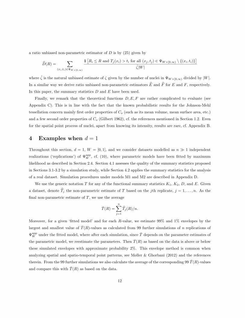
a ratio unbiased non-parametric estimator of D is by (25) given by

D(R) =∑

(xi,ti)∈ΨW×[0,∞)

1[Ri ≤ R and Tj(xi) > ti for all (xj , tj) ∈ ΨW×[0,∞) \ (xi, ti)

]ζ|W |

where ζ is the natural unbiased estimate of ζ given by the number of nuclei in ΨW×[0,∞) divided by |W |.In a similar way we derive ratio unbiased non-parametric estimators E and F for E and F , respectively.

In this paper, the summary statistics D and E have been used.

Finally, we remark that the theoretical functions D,E, F are rather complicated to evaluate (see

Appendix C). This is in line with the fact that the known probabilistic results for the Johnson-Mehl

tessellation concern mainly first order properties of Co (such as its mean volume, mean surface area, etc.)

and a few second order properties of Co (Gilbert 1962), cf. the references mentioned in Section 1.2. Even

for the spatial point process of nuclei, apart from knowing its intensity, results are rare, cf. Appendix B.

4 Examples when d = 1

Throughout this section, d = 1, W = [0, 1], and we consider datasets modelled as n 1 independent

realizations (‘replications’) of ΨappW , cf. (10), where parametric models have been fitted by maximum

likelihood as described in Section 2.4. Section 4.1 assesses the quality of the summary statistics proposed

in Sections 3.1-3.2 by a simulation study, while Section 4.2 applies the summary statistics for the analysis

of a real dataset. Simulation procedures under models M1 and M2 are described in Appendix D.

We use the generic notation T for any of the functional summary statistics K1, K2, D, and E. Given

a dataset, denote Tj the non-parametric estimate of T based on the jth replicate, j = 1, . . . , n. As the

final non-parametric estimate of T , we use the average

T (R) =

n∑j=1

Tj(R)/n.

Moreover, for a given ‘fitted model’ and for each R-value, we estimate 99% and 1% envelopes by the

largest and smallest value of T (R)-values as calculated from 99 further simulations of n replications of

ΨappW under the fitted model, where after each simulation, since T depends on the parameter estimates of

the parametric model, we reestimate the parameters. Then T (R) as based on the data is above or below

these simulated envelopes with approximate probability 2%. This envelope method is common when

analyzing spatial and spatio-temporal point patterns, see Møller & Ghorbani (2012) and the references

therein. From the 99 further simulations we also calculate the average of the corresponding 99 T (R)-values

and compare this with T (R) as based on the data.

12

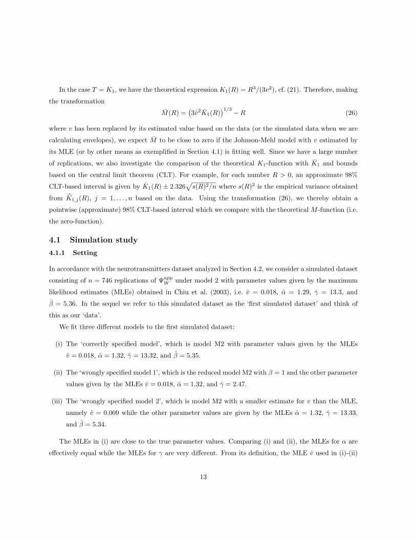
In the case T = K1, we have the theoretical expression K1(R) = R3/(3v2), cf. (21). Therefore, making

the transformation

M(R) =(3v2K1(R)

)1/3 −R (26)

where v has been replaced by its estimated value based on the data (or the simulated data when we are

calculating envelopes), we expect M to be close to zero if the Johnson-Mehl model with v estimated by

its MLE (or by other means as exemplified in Section 4.1) is fitting well. Since we have a large number

of replications, we also investigate the comparison of the theoretical K1-function with K1 and bounds

based on the central limit theorem (CLT). For example, for each number R > 0, an approximate 98%

CLT-based interval is given by K1(R)± 2.326√s(R)2/n where s(R)2 is the empirical variance obtained

from K1,j(R), j = 1, . . . , n based on the data. Using the transformation (26), we thereby obtain a

pointwise (approximate) 98% CLT-based interval which we compare with the theoretical M -function (i.e.

the zero-function).

4.1 Simulation study

4.1.1 Setting

In accordance with the neurotransmitters dataset analyzed in Section 4.2, we consider a simulated dataset

consisting of n = 746 replications of ΨappW under model 2 with parameter values given by the maximum

likelihood estimates (MLEs) obtained in Chiu et al. (2003), i.e. v = 0.018, α = 1.29, γ = 13.3, and

β = 5.36. In the sequel we refer to this simulated dataset as the ‘first simulated dataset’ and think of

this as our ‘data’.

We fit three different models to the first simulated dataset:

(i) The ‘correctly specified model’, which is model M2 with parameter values given by the MLEs

v = 0.018, α = 1.32, γ = 13.32, and β = 5.35.

(ii) The ‘wrongly specified model 1’, which is the reduced model M2 with β = 1 and the other parameter

values given by the MLEs v = 0.018, α = 1.32, and γ = 2.47.

(iii) The ‘wrongly specified model 2’, which is model M2 with a smaller estimate for v than the MLE,

namely v = 0.009 while the other parameter values are given by the MLEs α = 1.32, γ = 13.33,

and β = 5.34.

The MLEs in (i) are close to the true parameter values. Comparing (i) and (ii), the MLEs for α are

effectively equal while the MLEs for γ are very different. From its definition, the MLE v used in (i)-(ii)

13

is an overestimate. A simulation study in Chiu et al. (2000), but for another setting than ours, indicated

that the MLE v is not seriously biased. We therefore also consider the case (iii), where v = 0.009 is half

of the value of the MLE. Note that the MLEs for the other parameters are nearly the same in (i) and

(iii). For each of the three cases, we estimate the intensity function ρ by (8) with the parameter values

as specified in (i)-(iii), and this estimate of ρ is then used in (22)-(23) to obtain the estimates K1,j and

K2,j .

4.1.2 Results

The left panel of Figure 2 shows the theoretical M -function (the zero-line shown as a dot-dashed line)

together with the non-parametric estimate M and the pointwise 98% CLT-based confidence intervals

(dotted lines) for the M -function based on the first simulated dataset and v is estimated by the MLE (i.e.

as for the correctly specified model and for the incorrectly specified model 1). As expected, except for the

larger R-values, M(R) is approximately zero and the confidence intervals become wider as R increases.

As noticed at the end of Section 3.1.2, we should not consider results for K1(R) for too small values of

R. For R-values larger than about 0.05, the confidence intervals in Figure 2 contain zero as we might

expect, but for R < 0.05 we may question the value of the results. In particular, for smaller R-values

(R less than about 0.01), M(R) = R since there are no pairs of independent events at this scale; further

simulations confirmed that this happens frequently, cf. Figure 3 (to be discussed later). Furthermore,

in Figure 2, the mid panel is similar to the left panel but uses the estimate of v under the incorrectly

specified model 2. In this plot M and the pointwise 98% CLT-based confidence intervals are (mostly)

below zero. So the overall conclusion is that Figure 2 indicates no clear lack of fit for the Johnson-Mehl

model when estimating v by the MLE while there is a poor fit when estimating v by half of the MLE.

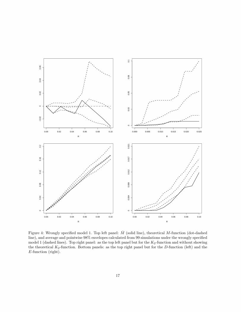
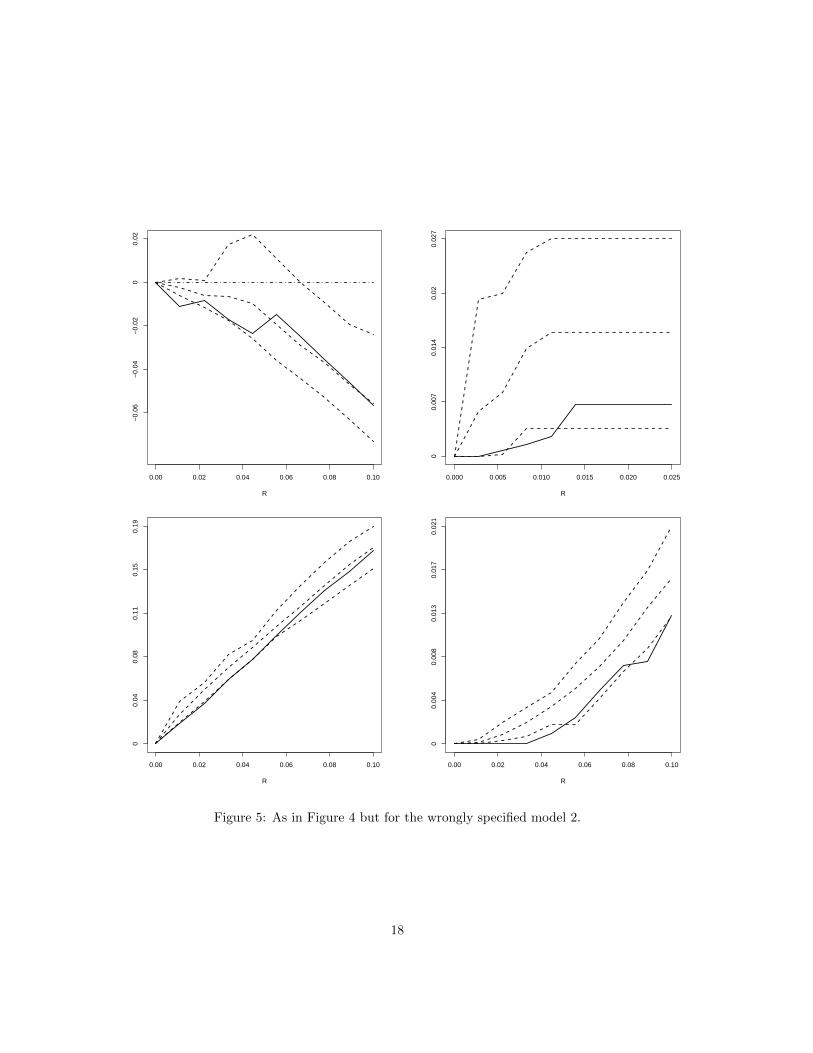
In Figures 3-5, the top left panels show the estimate M for the first simulated dataset (solid line),

the theoretical M -function (dot-dashed line), and the average and pointwise 98% envelopes (dashed

lines) obtained from M -functions calculated from 99 simulations under the correctly specified model

(Figure 3), the wrongly specified model 1 (Figure 4) and the wrongly specified model 2 (Figure 5),

respectively. Furthermore, the top right panels are as the top left panels but concern K2 and without

showing the theoretical K2-function. The bottom panels show D (left) and E (right) for the first simulated

dataset (solid lines) together with the average and pointwise 98% envelopes (dashed lines) obtained from

D-functions (left) and E-functions (right) calculated from 99 simulations under the correctly specified

model (Figure 3), the wrongly specified model 1 (Figure 4), and the wrongly specified model 2 (Figure 5),

respectively. The plots in Figures 3-5 taken together indicate a satisfactory fit for the correctly specified

14

0.00 0.02 0.04 0.06 0.08 0.10

R

−0.

15−

0.1

−0.

050

0.05

0.00 0.02 0.04 0.06 0.08 0.10

R−

0.15

−0.

1−

0.05

00.

05

0.00 0.02 0.04 0.06 0.08 0.10

R

−0.

4−

0.2

00.

20.

4

Figure 2: Left: theoretical M -function (dot-dashed line), M (solid line), and pointwise 98% CLT-basedconfidence intervals (dotted lines) for the M -function based on the first simulated dataset and when v isestimated by the MLE. Mid: as the left plot but when v is estimated by half of the MLE. Right: as theleft plot but for the neurotransmitters dataset fitted in Section 4.2.

model and an unsatisfactory fit for the wrongly specified models.

Similar results were obtained when repeating the simulations a number of times. So at least for cases

similar to the neurotransmitters dataset analyzed in the next section, our functional summary statistics

are useful tools for checking fitted parametric Johnson-Mehl models, including the fitted model in Chiu

et al. (2003).

4.2 Neurotransmitters dataset

This section applies our model checking procedures on the neurotransmitters dataset previously analyzed

in Chiu et al. (2003) and other papers discussed below.

4.2.1 Background

Bennett & Robinson (1990) suggested the following mechanism for neurotransmitters: The neuronal axon

terminal at the neuromuscular junction has branches that consist of strands containing many randomly

scattered sites. An action potential triggers the release of neurotransmitters to the synapse as the synaptic

vesicles diffuse into the cellular membrane. Each quantum released is assumed to cause the release of an

inhibitory substance which diffuses along the terminal at a constant rate preventing further releases in

the inhibited region. Thus, some potential releases have been prohibited (for more details, see Bennett

& Robinson (1990)).

Different neurotransmitters datasets (provided by Professor M. R. Bennett, Neurobiology Research

15

0.00 0.02 0.04 0.06 0.08 0.10

R

−0.

05−

0.02

00.

030.

05

0.000 0.005 0.010 0.015 0.020 0.025

R

00.

030.

050.

080.

1

0.00 0.02 0.04 0.06 0.08 0.10

R

00.

040.

080.

110.

150.

19

0.00 0.02 0.04 0.06 0.08 0.10

R

00.

005

0.01

0.01

50.

020.

026

Figure 3: Correctly specified model. Top left panel: M (solid line), theoretical M -function (dot-dashedline), and average and pointwise 98% envelopes calculated from 99 further simulations under the correctlyspecified model (dashed lines). Top right panel: as the top left panel but for the K2-function and withoutshowing the theoretical K2-function. Bottom panels: as the top right panel but for the D-function (left)and the E-function (right).

16

0.00 0.02 0.04 0.06 0.08 0.10

R

−0.

020

0.02

0.04

0.06

0.000 0.005 0.010 0.015 0.020 0.025

R

00.

030.

050.

080.

1

0.00 0.02 0.04 0.06 0.08 0.10

R

00.

040.

080.

120.

160.

2

0.00 0.02 0.04 0.06 0.08 0.10

R

00.

004

0.00

80.

012

0.01

70.

021

Figure 4: Wrongly specified model 1. Top left panel: M (solid line), theoretical M -function (dot-dashedline), and average and pointwise 98% envelopes calculated from 99 simulations under the wrongly specifiedmodel 1 (dashed lines). Top right panel: as the top left panel but for the K2-function and without showingthe theoretical K2-function. Bottom panels: as the top right panel but for the D-function (left) and theE-function (right).

17

0.00 0.02 0.04 0.06 0.08 0.10

R

−0.

06−

0.04

−0.

020

0.02

0.000 0.005 0.010 0.015 0.020 0.025

R

00.

007

0.01

40.

020.

027

0.00 0.02 0.04 0.06 0.08 0.10

R

00.

040.

080.

110.

150.

19

0.00 0.02 0.04 0.06 0.08 0.10

R

00.

004

0.00

80.

013

0.01

70.

021

Figure 5: As in Figure 4 but for the wrongly specified model 2.

18

Center, University of Sydney) have been analyzed in various ways, see Quine & Robinson (1992), Thom-

son, Lavidis, Robinson & Bennett (1995), Holst, Quine & Robinson (1996), Chiu et al. (2000), Molchanov

& Chiu (2000), and Chiu et al. (2003). We focus on the dataset analyzed in the latter three papers. It

consists of the times and the amplitudes of release of neurotransmitters in a series of 746 experiments

(after omitting some experiments due to multiple amplitudes or outliers). The range of the number of

releases is from 0 to 4, and the frequencies of experiments with 0, 1, 2, 3, and 4 releases are 101, 387,

210, 45, and 3, respectively. We follow the authors in using the transformations

nucleus = 5/√

amplitude, time = (released time− 500)/500. (27)

Chiu et al. (2003) fitted model M2 by maximum likelihood and obtained the MLEs v = 0.018, α = 1.29,

γ = 13.3, and β = 5.36.

4.2.2 Extension of model M1

Model M1 is inappropriate, since an empty realization of ΨappW is possible under M2 but not under M1,

and the neurotransmitters dataset includes in fact 101 empty realizations. We therefore extend M1 by

introducing a Bernoulli variable Z with parameter π ∈ (0, 1) such that P(Z = 0) = 1 − P(Z = 1) = π,

ΨappW = ∅ if Z = 0, and Ψapp

W follows M1 if Z = 1. Under this extension of M1, we have derived MLEs

v = 0.018, π = 0.135, α = 0.21, and β = 0.28. As the pair correlation function under the extended model

M1 is the same as under the original model M1, the functions K1 and K2 are unchanged under the two

models.

4.2.3 Results

The right panel of Figure 2 shows the theoretical M -function (dot-dashed line) together with the non-

parametric estimate M (solid line) and the pointwise 98% CLT-based confidence intervals (dotted lines)

for the M -function based on the neurotransmitters dataset and when v is estimated by the MLE. Ignoring

the results for the smaller R-values (where we have very few pairs of independent events), there is no

disagreement with the assumption of a Johnson-Mehl model with v estimated by the MLE.

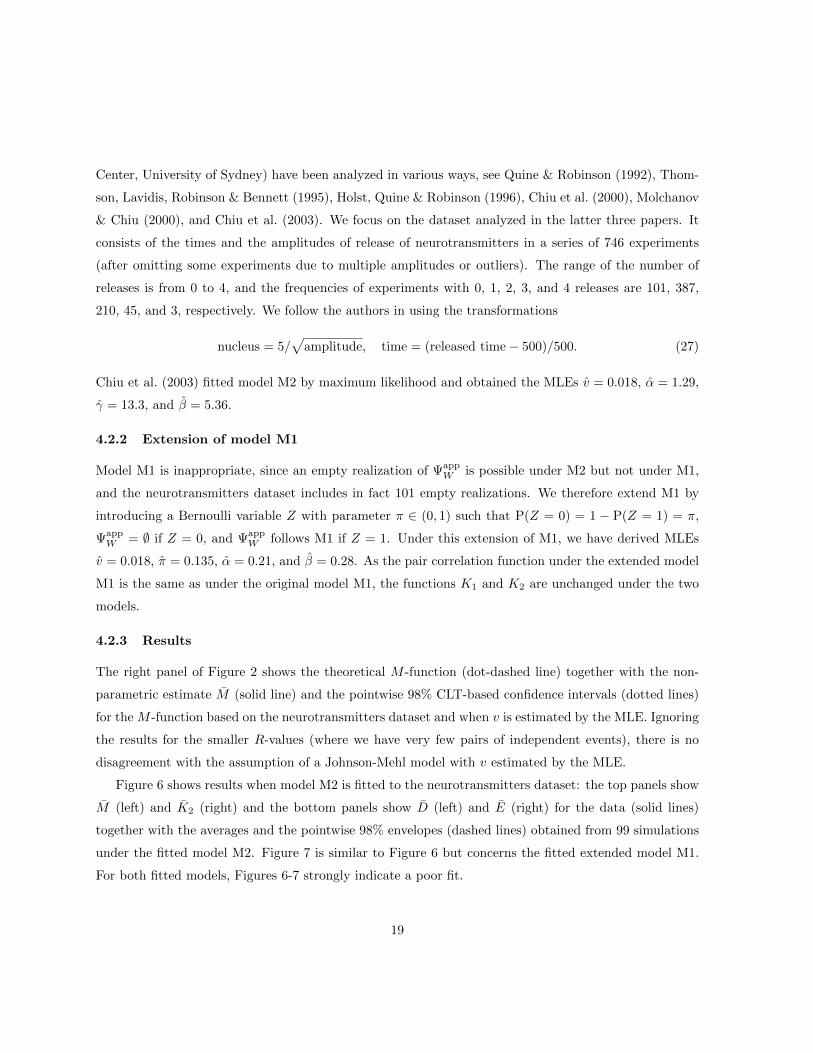
Figure 6 shows results when model M2 is fitted to the neurotransmitters dataset: the top panels show

M (left) and K2 (right) and the bottom panels show D (left) and E (right) for the data (solid lines)

together with the averages and the pointwise 98% envelopes (dashed lines) obtained from 99 simulations

under the fitted model M2. Figure 7 is similar to Figure 6 but concerns the fitted extended model M1.

For both fitted models, Figures 6-7 strongly indicate a poor fit.

19

0.00 0.02 0.04 0.06 0.08 0.10

R

−0.

10

0.1

0.2

0.3

0.000 0.005 0.010 0.015 0.020 0.025

R

00.

040.

070.

110.

14

0.00 0.02 0.04 0.06 0.08 0.10

R

00.

080.

150.

220.

3

0.00 0.02 0.04 0.06 0.08 0.10

R

00.

030.

060.

090.

12

Figure 6: Results for the fitted model M2. Top left panel: M for the data (solid line), the theoretical M -function (dot-dashed line), and the average and pointwise 98% envelopes calculated from 99 simulationsunder the fitted model M2 (dashed lines). Top right panel: as top left panel but for the K2-function andwithout showing the theoretical K2-function. Bottom panels: as top right panel but for D-function (left)and E-function (right).

20

0.00 0.02 0.04 0.06 0.08 0.10

R

−0.

020

0.02

0.04

0.06

0.000 0.005 0.010 0.015 0.020 0.025

R

012

.525

37.5

50

0.00 0.02 0.04 0.06 0.08 0.10

R

00.

150.

30.

450.

6

0.00 0.02 0.04 0.06 0.08 0.10

R

0.15

00.

040.

080.

110.

15

Figure 7: As Figure 6 but for the fitted extended model M1.

21

Chiu et al. (2000, 2003) claimed that the nuclei obtained by the transformation in (27) are ”roughly

uniform on [0,1]”, but the histogram in the top left panel of Figure 8 is clearly showing a non-uniform

distribution. The Q-Q plot in the lower left panel of Figure 8 is showing that the times obtained by the

transformation in (27) are not well described by the gamma distribution fitted by Chiu et al. (2003).

Instead of the transformations (27), using the transformations

nuclei = F ((log(amplitude)− 4.6)/0.4), time = (released time− 523)/500, (28)

and reestimating the parameters by maximum likelihood, we obtained a better agreement with a uniform

and a gamma distribution, cf. the right panels of Figure 8. Here F denotes the cumulative distribution

function for the standard normal distribution, and 4.6 respective 0.4 are the average respective the

standard deviation of the log-transformed amplitudes. However, plots of the functional summary statistics

for this case are very similar to those in Figures 6-7 (the plots are therefore omitted here). We are therefore

in doubt if the neurotransmitters dataset may be well described by a parametric Johnson-Mehl model.

Acknowledgment

Supported by the Danish Council for Independent Research—Natural Sciences, grant 12-124675, ”Math-

ematical and Statistical Analysis of Spatial Data”, and by the Centre for Stochastic Geometry and

Advanced Bioimaging, funded by a grant from the Villum Foundation. We thank Sung Nok Chiu for

providing the neurotransmitters dataset studied in Section 4.2.

Appendix A: the volume of the intersection of two balls

For r > v|s− t| and 0 ≤ u < (s+ t− r/v)/2, combining (16)-(18), we obtain

V∩(r, s− u, t− u) = [v(t− u)]2

cos−1

(r2 + [v(t− u)]2 − [v(s− u)]2

2rv(t− u)

)× [v(s− u)]

2cos−1

(r2 + [v(s− u)]2 − [v(t− u)]2

2rv(s− u)

)− 1

2

√(−r + v(s− u) + v(t− u))(r + v(s− u)− v(t− u))

×√

(r − v(s− u) + v(t− u))(r + v(s− u) + v(t− u)) if d = 2,

V∩(r, s− u, t− u) =π

12r(v(s+ t)− 2vu− r)2

(r2 − 3v2[(t− u)2 + (s− u)2]

+ 2r[v(s+ t)− 2uv] + 6[v2(t− u)(s− u)])

)if d = 3.

22

5 Amplitude

Fre

quen

cy

0.2 0.4 0.6 0.8 1.0 1.2

080

159

238

318

F((log(Amplitude) − 4.6) 0.4)

Fre

quen

cy

0.0 0.2 0.4 0.6 0.8 1.0

048

9714

619

4

* *****************************************

************************************************************************************************************************************************************

*************************************************************************************************************************************************************************************************************************************************************

******************************************************************************************************************************************************************************************************************

***************************************************************************************************************

**********************************************************************************

**********************************************

*******************************

**************

****

***

******

** *

*

*

*

0.0 0.2 0.4 0.6 0.8 1.0 1.2

Theoretical Quantiles

Sam

ple

Qua

ntile

s

00.

51.

11.

62.

1

* *****************

******************************************************************

**************************************************************************************************************

***************************************************************************************************************************************

***************************************************************************************************************

******************************************************************************************************************

************************************************************************************************

******************************************************************************

*********************************************

***************************************

*************************************

*****************************

*********************

**************

*******

**

*****

* *

* *

* *

Theoretical Quantiles

Sam

ple

Qua

ntile

s

00.

30.

60.

91.

2

0 0.3 0.5 0.8 1

Figure 8: Top panels: histogram for the nuclei obtained by the transformation in (27) (left) or (28)(right). Bottom panels: Q-Q plot for the times obtained by the transformation in (27) (left) or (28)(right).

23

Appendix B: the pair correlation function for the process of nuclei

The second-order product density for the process of nuclei is for any x, y ∈ Rd with r = ‖x−y‖ > 0 given

by ρ(2)(x, y) = ρ(2)0 (r), where

ρ(2)0 (r) =

∫ ∞0

∫ ∞0

ρ(2)0 (r, s, t) dsdt. (29)

It is easily seen that the corresponding pair correlation function

g(r) = ρ(2)0 (r)/ζ2

is less than one, which shows that the nuclei exhibit regularity. In principle g(r) could be calculated using

(29) and the results in Section 3.1.1, but in general we obtain some integral expressions which have to be

evaluated by numerical methods. For example, for d = 1, we obtain

g(r) =

∫ ∞0

∫ ∞0

[κ(s)κ(t)1[r > v|s− t|] exp

(−∫ maxs,t

0

κ(u)[v(s+ t− 2u) + r] du

)]dsdt/ζ2.

If κ is constant (model M1 with β = 1), a closed form expression of g in terms of the cumulative

distribution function of the standard normal distribution is available.

Appendix C: the typical Johnson-Mehl cell

The typical Johnson-Mehl cell Co, or more precisely its distribution, can be defined as follows (Møller

1992).

The nucleus of Co is given by an arbitrary fixed point o, let us say the origin of Rd. The time where

the nucleus o starts to grow is a random variable To which is independent of Φ and has density ρ/ζ. For

t > 0, let

C(o, t; Ψ) = y ∈ Rd : T ((o, t), y) ≤ Ti(o) for all (xi, ti) ∈ Ψ

denote the set of those points first reached by o when considering all the growing nuclei from the Johnson-

Mehl process Ψ. By definition, the conditional distribution of Co given To = t is the same as the

conditional distribution of C(o, t; Ψ) given that Ti(o) > t for all (xi, ti) ∈ Ψ, i.e. when o is not thinned

by Ψ. In other words, considering the Johnson-Mehl tessellation generated by both (o, To) and Φ, Co is

the cell with nucleus o and as a matter of fact, with probability one, Co is compact and o is an interior

point of Co.

24

Combining this definition with the Slivnyak-Mecke formula (Mecke 1967; Møller & Waagepetersen

2004), we obtain that (25) holds for any Borel set W . Furthermore,

D(r) = 1−∫∫

P (Φ ∩H(t, r) = ∅)κ(t) dxdt/ζ, r > 0,

where

H(t, r) = (y, u) ∈ Rd × [0, t] : ‖y‖ ≤ 2r + v(t− u)

∪ (y, u) ∈ Rd × (t, t+ r/v] : v(t− u) ≤ ‖y‖ ≤ 2r + v(t− u).

For instance, for model M1 and d = 1, we obtain

D(r) = 1−∫

exp

(−2α

β

(2r(t+ r/v)β +

v

β + 1tβ+1

))αtβ−1 dt/ζ.

This illustrates that D,E, F are given by integral expressions which may only be evaluated by numerical

methods.

Appendix D: simulation procedure

First, we consider simulation of ΨappW under the extension of M1 given in Section 4.2.1 when d = 1. This

boils down to how to simulate under the original model M1, where we use the following inversion method.

Suppose u1, u2, . . . are independent realizations of exponentially distributed random variables with

unit rate. Then u1, u1 + u2, . . . are forming a realization of a unit rate Poisson process on [0,∞). The

integrated intensity

Λ(t) ≡∫ t

0

αsβ−1 ds = αtβ/β, t ≥ 0,

has inverse Λ−1(u) = (βu/α)1/β , so t1 = Λ−1(u1), t2 = Λ−1(u1 + u2), . . . are forming a realization of a

Poisson process on [0,∞) with intensity function αtβ−1. To each ti, attach a point xi ∈W , where these

points are independent realizations of uniformly distributed random variables on W which in turn are

independent of the exponentially distributed random variables. Then (x1, t1), (x2, t2), . . . is a realization

of the Poisson process ΦW×[0,∞) under M1.

Now, as in Section 4, let W = [0, 1]. Then we simulate a realization of ΨappW under M1 as follows. We

start by generating (x1, t1) and t2 and by setting ΨappW = (x1, t1). We stop if t2 ≥ T , where T is the

time W is covered when x1 is growing spherically with speed v, i.e. T = maxT1(0), T2(1). If t2 < T ,

then we have to generate x2 and to check if (x2, t2) is thinned by (x1, t1). If it is not, i.e. if T1(x2) > t2,

then we include (x2, t2) in ΨappW and update T by the time at which W is covered when x1 and x2 are

25

growing spherically with speed v, i.e. T = maxT1(0), T2(1), T1,2, where T1,2 = (t1 + t2 + (x2− x1)/v)/2

is the time at which the rays growing from x1 and x2 are meeting. If t3 ≥ T then we stop, and else we

continue in the same way until we obtain the first time where ti ≥ T (with probability one, this happens

at some point).

Next, to simulate under model M2 within W = [0, 1], we first generate the primary space-time Poisson

process Φ restricted to [0, 1]×[0,∞): this is straightforward as the number of events is Poisson distributed

with mean α, the xi are uniformly distributed on W , the ti are gamma distributed with shape parameter

β and inverse scale parameter γ, and all the xi and all the ti are independent. Second, using the thinning

mechanism described in Section 1.1, we obtain the events of ΨappW .

References

Baddeley, A., Møller, J. & Waagepetersen, R. (2000). Non- and semi-parametric estimation of interaction

in inhomogeneous point patterns, Statistica Neerlandica 54: 329–350.

Bennett, M. R. & Robinson, J. (1990). Probabilistic secretion of quanta from nerve terminals at synaptic

sites on muscle cells: Non-uniformity, autoinhibition and the binomial hypothesis, Proceedings of the

Royal Society of London. Series B, Biological Sciences 239: 1049–1052.

Boots, B., Okabe, A. & Thomas, R. (eds) (2003). Modelling Geographical Systems: Statistical and

Computational Applications, Kluwer Academic Publishers, Dordrecht.

Chiu, S. N. (1995). Limit theorems for the time of completion of Johnson-Mehl tessellations, Advances

in Applied Probability 27: 889–910.

Chiu, S. N., Molchanov, I. S. & Quine, M. P. (2003). Maximum likelihood estimation for germination-

growth processes with application to neurotransmitters data, Journal of Statistical Computation and

Simulation 73: 725–732.

Chiu, S. N., Quine, M. P. & Stewart, M. (2000). Nonparametric and parametric estimation for a linear

germination-growth model, Biometrics 56: 755–760.

Cowan, R., Chiu, S. N. & Holst, L. (1995). A limit theorem for the replication time of a DNA molecule,

Journal of Applied Probability 32: 296–303.

Daley, D. J. & Vere-Jones, D. (2003). An Introduction to the Theory of Point Processes. Volume I:

Elementary Theory and Methods, second edn, Springer-Verlag, New York.

26

Frost, H. J. & Thompson, C. V. (1987). The effect of nucleation conditions on the topology and geometry

of two-dimensional grain structures, Acta Metallurgica et Materialia 35: 529–540.

Frost, H. J., Thompson, C. V. & Walton, D. T. (1992). Simulation of thin film grain structures–II.

Abnormal grain growth, Acta Metallurgica et Materialia 40: 779–793.

Gabriel, E. & Diggle, P. J. (2009). Second-order analysis of inhomogeneous spatio-temporal point process

data, Statistica Neerlandica 63: 43–51.

Gelfand, A. E., Diggle, P. J., Guttorp, P. & Fuentes, M. (2010). Handbook of Spatial Statistics, CRC

Press, Boca Raton.

Gilbert, E. N. (1962). Random subdivisions of space into crystals, Annals of Mathematical Statistics

33: 958–972.

Holst, L., Quine, M. P. & Robinson, J. (1996). A general stochastic model for nucleation and linear

growth, Annals of Applied Probability 6: 903–921.

Horalek, V. (1988). A note on the time-homogeneous Johnson-Mehl tessellation, Advances of Applied

Probability 20: 684–685.

Horalek, V. (1990). ASTM grain-size model and related random tessellation models, Materials Charac-

terization 25: 263–284.

Johnson, W. A. & Mehl, R. F. (1939). Reaction kinetics in processes of nucleation and growth, Transac-

tions of the American Institute of Mining and Metallurgical Engineers 135: 416–458.

Kayser, K. & Stute, H. (1989). Minimum spaning tree, Voronoi’s tessellation and Johnson-Mehl diagrams

in human lung carcinoma, Pathology, Research and Practice 185: 729–734.

Kenkel, N. C. (1990). Spatial competition models for plant populations, COENOSES 5: 149–158.

Kolmogorov, A. N. (1937). On the statistical theory of the crystallization of metals, Bulletin of the

Academy of Sciences of the USSR, Mathematical Series 1: 355–359.

Li, S. (2011). Concise formulas for the area and volume of a hyperspherical cap, Asian Journal of

Mathematics and Statistics 4: 66–70.

Mecke, J. (1967). Stationare zufallige Maße auf lokalkompakten Abelschen Gruppen, Zeitschrift fur

Wahrscheinlichkeitstheorie und verwandte Gebiete 9: 36–58.

27

Meijering, J. L. (1953). Interface area, edge length, and number of vertices in crystal aggregates with

random nucleation, Philips Research Reports 8: 270–290.

Miles, R. E. (1972). The random subdivision of space, Supplement to Advances of Applied Probability

4: 243–266.

Molchanov, I. S. & Chiu, S. N. (2000). Smoothing techniques and estimation methods for nonstationary

Boolean models with applications to coverage processes, Biometrika 87: 265–283.

Møller, J. (1992). Random Johnson-Mehl tessellations, Advances in Applied Probability 24: 814–844.

Møller, J. (1994). Lectures on Random Voronoi Tessellations, Lecture Notes in Statistics 87, Springer-

Verlag, New York.

Møller, J. (1995). Generation of Johnson-Mehl crystals and comparative analysis of models for random

nucleation, Advances in Applied Probability 27: 367–383.

Møller, J. & Ghorbani, M. (2012). Aspects of second-order analysis of structured inhomogeneous spatio-

temporal point processes, Statistica Neerlandica 66: 472–491.

Møller, J. & Waagepetersen, R. P. (2004). Statistical Inference and Simulation for Spatial Point Processes,

Chapman and Hall/CRC, Boca Raton.

Okabe, A., Boots, B., Sugihara, K. & Chiu, S. N. (2000). Spatial Tessellations. Concepts and Applications

of Voronoi Diagrams, second edn, Wiley, Chichester.

Quine, M. P. & Robinson, J. (1990). A linear random growth model, Journal of Applied Probability

27: 499–509.

Quine, M. P. & Robinson, J. (1992). Estimation for a linear growth model, Statistics and Probability

Letters 15: 293–297.

Ripley, B. D. (1976). The second-order analysis of stationary point processes, Journal of Applied Proba-

bility 13: 255–266.

Ripley, B. D. (1977). Modelling spatial patterns (with discussion), Journal of the Royal Statistical Society

Series B 39: 172–212.

Stoyan, D., Kendall, W. S. & Mecke, J. (1995). Stochastic Geometry and Its Applications, second edn,

Wiley, Chichester.

28

Stoyan, D. & Stoyan, H. (1996). Estimating pair correlation functions of planar cluster processes, Bio-

metrical Journal 38: 259–271.

Thomson, P. C., Lavidis, N. A., Robinson, J. & Bennett, M. R. (1995). Probabilistic secretion of quanta

at somatic motor-nerve terminals: The fusion-pore model, quantal detection and autoinhibition,

Philosophical Transactions: Biological Sciences 349: 197–214.

Vanderbei, R. & Shepp, L. (1988). A probabilistic model for the time to unravel a strand of DNA,

Stochastic Models 4: 299–314.

Wolk, C. P. (1975). Formation of one-dimensional patterns by stochastic processes and by filamentous

blue-green algae, Developmental Biology 46: 370–382.

29