fundamental mechanisms of the growth and …sbf1/papers/pna.pdfq. j. r. meteorol. soc.(2002),128,...

Q. J. R. Meteorol. Soc. (2002), 128, pp. 775–796

Fundamental mechanisms of the growth and decay of the PNAteleconnection pattern

By STEVEN B. FELDSTEIN¤

The Pennsylvania State University, USA

(Received 11 December 2000; revised 24 October 2001)

SUMMARY

This investigation performs diagnostic analyses on NCEP/NCAR re-analysis data, and also does forced,nonlinear, barotropic model calculations to examine the dynamical mechanisms associated with the growth anddecay of the Paci� c/North American teleconnection pattern (PNA). The diagnostic calculations include projectionand composite analyses of each term in the stream-function-tendency equation.

The results of the diagnostic analyses and model calculations reveal a PNA life cycle that is complete withinapproximately 2 weeks and is dominated by linear processes. The growth of the two upstream PNA anomalycentres is found to be by barotropic conversion from the zonally asymmetric climatological � ow, and the twodownstream PNA anomaly centres by linear dispersion. The PNA anomaly growth eventually ceases because ofchanges in the spatial structure of the anomaly. An analysis of the role of Ekman pumping is performed with avery simple model. The results, although qualitative, suggest that the decay of the PNA may be through Ekmanpumping. An examination of the role of transient eddy vorticity � uxes indicates that they play an important roleduring some stages of the PNA life cycle. Lastly, the model calculations also reveal a crucial role played by thedivergence term in maintaining the PNA anomaly in a quasi-� xed position.

KEYWORDS: Low-frequency variability Teleconnection patterns

1. INTRODUCTION

The results of two recent observational studies suggest that the Paci� c/North Amer-ican teleconnection pattern (hereafter PNA) undergoes a life cycle of growth and decaywithin a time span of about 2 weeks (Feldstein 2000; Cash and Lee 2001). Feldstein(2000) examined the power spectral properties of a number of different teleconnectionpatterns. For the PNA, it was found that the power spectrum of the daily un� lteredprincipal component (PC) time series closely matched that of a � rst-order Markov (rednoise) process with a decorrelation time-scale of 7.7 days. (The decorrelation time-scaleis de� ned to be the time it takes for the autocorrelation function of a � rst-order Markovprocess to decay by a factor of e.) Consistently, Cash and Lee (2001) showed with alinear multivariate stochastic model that the PNA is the most probable spatial pattern toevolve from the � rst optimal perturbation. In fact, they found this property to be veryrobust, as more than 70% of the observed PNA events were found to arise from thisprocess. In addition, Cash and Lee (2001), and also the idealized modelling study ofFranzke et al. (2001), showed that the PNA anomaly completes its life cycle of growthand decay within about 2 weeks.

A number of different theories have been proposed that may account for thegrowth and maintenance of low-frequency anomalies, such as the PNA. These include:(1) barotropic growth due to the zonal asymmetry of the climatological � ow (e.g. Fred-eriksen 1983; Simmons et al. 1983; Branstator 1990, 1992), (ii) growth due to lineardispersion from a source of topographic or diabatic heating (e.g. Hoskins and Karoly1981), (iii) a combined baroclinic/barotropic instability or initial-value development(e.g. Dole and Black 1990; Black and Dole 1993), (iv) changes in quasi-stationaryeddies due to zonal mean-� ow � uctuations (e.g. Branstator 1984; Nigam and Lindzen1989; Kang 1990), and (v) feedback by high-frequency transient eddy � uxes (e.g. Eggerand Schilling 1983; Lau 1988; Branstator 1992; Ting and Lau 1993).¤ Corresponding address: EMS Environment Institute, The Pennsylvania State University, University Park,PA 16802, USA. e-mail: [email protected]° Royal Meteorological Society, 2002.

775

776 S. B. FELDSTEIN

The present study examines the dynamical processes associated with the temporalevolution of the PNA. The approach adopted includes an examination of the compositetemporal evolution of each term in the stream-function-tendency equation (the inverseLaplacian of the vorticity equation) during the PNA life cycle. With this approach,whichwill be complemented by both linear and nonlinear barotropic model calculations, itwill be possible to isolate which dynamical process account for both the growth and thedecay of the PNA.

In section 2 the data and diagnostic techniques are described. This is followedin section 3 by an examination of the spatial structure of the PNA. The temporalevolution of the PNA is brie� y described in section 4, followed by a projection analysisin section 5. The results from the composite stream-function-tendency equation arepresented in section 6, followed by barotropic model calculations in section 7. Theconclusions are given in section 8.

2. DATA AND DIAGNOSTIC TECHNIQUES

The daily (00 UTC) 300 mb stream-function � eld is used. This quantity is obtainedby logarithmic interpolation from the daily (00 UTC) National Centers for Environmen-tal Prediction/National Center for Atmospheric Research (NCEP/NCAR) re-analysisvorticity � eld in sigma coordinates (where sigma equals pressure divided by surfacepressure). These data cover the years from 1979 to 1995 for the months of November toMarch. The seasonal cycle is removed at each grid point. The seasonal cycle is obtainedby taking the calendar mean for each day and applying a 20-day low-pass digital � lter.All data used in this study are at rhomboidal 30 resolution. The PNA is identi� ed byapplying a rotated principal component analysis (RPCA) with a varimax rotation to thedata. As the covariance matrix is used, the corresponding PC time series (in this study,the PC time series will also be referred to as the PNA index time series) is orthonormal.

A 31-point, 10-day, low-pass digital � lter is applied to the stream-function-tendencyequation. The effect of using this � lter is simply to smooth the temporal evolutionof each term in the stream-function-tendency equation, slightly, without altering theinterpretation. As shown by Feldstein (1998), the in� uence of this particular � lter isnegligible for anomalies which grow or decay within a time period as short as 5 days.Furthermore, the same 10-day cut-off is used to distinguish between low- and high-frequency transient eddies. Although to a large degree this cut-off frequency is arbitrary,it is selected because eddy � uxes on either side of this cut-off frequency tend to yielddifferent structural properties (Hoskins et al. 1983).

(a) De� nitionsPersistent episodes are de� ned using an objective method adopted from Horel

(1985) and Mo (1986) (see also Feldstein 1998). A pattern correlation r at day t andlag ¿ is de� ned as

r.t; ¿ / DhÃ 0.¸; µ; t/Ã 0.¸; µ; t C ¿ /i

¾ fÃ 0.¸; µ; t/g¾ fÃ 0.¸; µ; t C ¿ /g; (1)

where Ã.¸; µ; t/ is the anomalous (deviation from the seasonal cycle) stream functionat longitude ¸ and latitude µ , and Ã 0 D Ã.¸; µ; t/ ¡ hÃ.¸; µ; t/i; ¾ 2fÃ 0.¸; µ; t/g DhfÃ 0.¸; µ; t/g2i, where the angle brackets denote a horizontal average over the northernhemisphere. If both r.t; ¿ / and r.t C 1; ¿ / > rc, for ¿ D 1 to 5 days, a persistent episodeis de� ned to have taken place. For this study, a value of rc D 0:254 is used, which

GROWTH AND DECAY OF THE PNA TELECONNECTION PATTERN 777

corresponds to the 95% con� dence level. The number of degrees of freedom is obtainedfrom the Fisher Z-transformation (see Feldstein and Lee 1996). For each persistentepisode, an onset day is de� ned to correspond to the � rst day of the persistent episode.One additional requirement is imposed on the de� nition of a persistent episode. This isthat the magnitude of the PC for the PNA exceeds one standard deviation on the onsetday. Also, when the PC is positive (negative) during a persistent episode, that episodewill be referred to as corresponding to the positive (negative) phase. Furthermore, if theonset day of one persistent episode takes place within 15 days of the end of the previouspersistent episode, and if both episodes are of the same phase, then the latter persistentepisode is discarded. Using this de� nition, it is found that there are 26 (29) persistentepisodes for the positive (negative) phase.

(b) Stream-function-tendency equationThe primary technique used in this study is a composite analysis of each term in the

stream-function-tendency equation (Cai and van den Dool 1994; Feldstein 1998), whichcan be written as

@ÃL

@tD

8X

iD1

»i C R; (2)

where

»1 D r¡2³

¡.vLr C vL

d /1

a

df

dµ

´

»2 D r¡2.¡[vr] r³ L ¡ vLr r[³ ]/ C r¡2.¡[vd] r³ L ¡ vL

d r[³ ]/

»3 D r¡2.¡v¤r r³ L ¡ vL

r r³ ¤/ C r¡2.¡v¤d r³ L ¡ vL

d r³ ¤/

»4 D r¡2f¡.f C ³ /r vLd ¡ ³ Lr vdg

»5 D r¡2.¡vLr r³ L/L C r¡2f¡r .vL

d ³ L/gL

»6 D r¡2.¡vHr r³ H/L C r¡2f¡r .vH

d ³ H/gL

»7 D r¡2.¡vLr r³ H/L C r¡2f¡r .vL

d ³ H/gL C r¡2.¡vHr r³ L/L

C r¡2f¡r .vHd ³ L/gL

»8 D r¡2f¡k r £ .!L@v=@p/g C r¡2f¡k r £ .!@vL=@p/gC r¡2f¡k r £ .!0@v0=@p/gL;

and Ã is the stream function, ³ the relative vorticity, v the horizontal wind vector,v the meridional wind component, ! the vertical wind component, a the earth’s radius,p the pressure, k the unit vector in the vertical direction, and f the Coriolis parameter.The term R corresponds to a residual, and includes physical processes that have beenneglected such as frictional dissipation. The subscripts ‘r’ and ‘d’ represent the rotationaland divergent components of the horizontal wind, respectively, and the superscripts ‘L’and ‘H’ indicate the application of the 10-day low-pass and high-pass � lter, respectively.For the low-pass � lter, the 1979–1995 November to March time mean is also subtracted.An overbar denotes a time mean, a prime a deviation from the time mean, squarebrackets a zonal average, and an asterisk a deviation from the zonal average. Standardde� nitions are used for all remaining terms. The term @ÃL=@t is calculated using centredtime differences. One important property of (2) is that although this equation describes

778 S. B. FELDSTEIN

Figure 1. The (a) uni� ed daily, and (b) monthly averaged � rst rotated empirical orthogonal function, thatcorresponds to the Paci� c/North American teleconnection pattern. The fractional variance is shown in the upper

right corner of each frame. Dashed contours are negative, and the zero contour is omitted.

the low-frequency evolution of the stream-function anomaly, it indicates that part ofthe low-frequency stream function is driven by anomalous eddy � uxes associated withhigh-frequency transients.

As discussed by Feldstein (1998), »1 involves planetary vorticity advection bythe anomaly, »2 (»3) the interaction of the anomaly with the zonal mean (zonallyasymmetric) climatological � ow, and »4 the divergence term. The term »5 correspondsto the interaction amongst all low-frequency transient eddies, and »6 to the forcing byhigh-frequency transient eddies. Also, as shown by Feldstein (1998), the terms »7 and»8, which correspond to the anomalous cross-frequency vorticity � ux and tilting terms,make a negligible contribution to the stream-function tendency. Thus, these two termswill not be considered in the remainder of this study.

3. PNA SPATIAL STRUCTURE

The � rst rotated empirical orthogonal function (REOF1) from the daily, un� ltered300 mb stream-function � eld is shown in Fig. 1(a). The quadrapole pattern seen istypical for a PNA pattern, with centres over the subtropical Paci� c near Hawaii, southof the Aleutian Islands, north-western Canada, and the south-eastern United States(e.g. Wallace and Gutzler 1981). (It should be noted that there is no prominent patternthat is in quadrature with REOF1. This indicates that REOF1 corresponds to a stationary,not a propagating, pattern.) Most studies of the PNA use either monthly or seasonalaveraged data. Thus, with the same dataset, an RPCA is performed on the monthlyaveraged 300 mb stream-function � eld (Fig. 1(b)). As can be seen, the two patterns arevery similar, the most noticeable differences being the larger zonal scale and the tworelatively stronger downstream centres in the monthly-averaged data. For each of thesecalculations, 12 unrotated EOFs were retained. Both the illustrated spatial patterns, andthe corresponding PC time series, were found to be rather insensitive to the numberof retained unrotated EOFs, when tested over a range of between 10 and 20 unrotatedEOFs.

In order to test the similarity quantitatively between the two REOF1 patterns inFig. 1, the following procedure is adopted. First, the daily PC time series is taken and


a new time series is generated consisting of monthly averages. This time series is thencorrelated with the monthly PC time series. Such a calculation yields a linear correlationof 0.83. As a measure that the REOFs in Fig. 1 do indeed correspond to PNA patternsfound in other studies, the monthly PC time series for REOF1 was correlated with themonthly PNA index made available from the Climate Prediction Center, for the sameset of 85 winter months as in the present study. The linear correlation was found tobe 0.84. Given that the Climate Prediction Center follows a different methodology,e.g. applies the RPCA to a different pressure level, i.e. 700 mb, and uses a differentvariable, i.e. geopotential height, this large linear correlation does give one con� dencethat the two REOFs in Fig. 1 do indeed correspond to a PNA.

It is important to emphasize that the precise location or phase of each of the fouranomaly centres of the PNA is not very robust. For example, amongst the numerouspapers that have been published on the PNA, using different methodologies and datasets,a range of patterns have appeared that are collectively referred to as the PNA. Thecommon feature to most of these so-called PNA patterns is that there is a wave trainwith two anomaly centres over the North Paci� c and two over North America, as inFig. 1. However, the precise location of these individual anomaly centres varies fromone study to the next. Even within the same dataset, as shown in the rotated EOFanalysis of Kushnir and Wallace (1989), the exact location of the four PNA anomalycentres is sensitive to the type of rotation used. Thus, there is no single spatial patternthat can be referred to as the PNA, since the geographic location of all four anomalycentres is not unique. As a result, it seems best to refer to all those patterns with theabove characteristics as being PNA-like patterns. In the context of the present study,this implies that we are examining the properties of one particular PNA-like pattern,i.e. the pattern obtained through a varimax rotation, the most popular method of rotationused in studies of low-frequency variability. (In this study, when the term PNA is used,it is important to note that it is the patterns in Fig. 1 that are being referred to, and notto all PNA-like patterns). Nevertheless, given the similarity of all PNA patterns, it isanticipated that the results of this study would at least apply qualitatively to all PNA-like patterns. However, a sensitivity analysis for a range of PNA-like patterns is beyondthe scope of this study.

It is also important to state that since the winter season is de� ned to include � vedifferent months, this study is overlooking the property that teleconnection patterns suchas the PNA undergo some seasonal variation (Barnston and Livezey 1987). However,such a lengthy winter season was chosen so as to include all onset days within themonths of December to February, while allowing for an examination of lagged � eldsthat extend §20 days into November and March.

4. TEMPORAL EVOLUTION OF THE PNA

The temporal evolution of the PNA can be succinctly described by examiningcomposites of the PNA index (Fig. 2(a) for the positive phase and Fig. 3(a) for thenegative phase). As can be seen, for both phases, the PNA index grows and decaysrapidly, completing most of its life cycle within approximately 15 days. One noticeabledifference between the two phases, however, is that for the negative phase the PNA indexremains at about 30% of its peak value for about 10 days after undergoing substantialdecline. This point is discussed in more detail in section 6. The temporal evolutionof the anomalous composite 300 mb stream-function � eld for the positive phase (thenegative phase shows similar characteristics) is illustrated in Fig. 4. As a measure oflocal statistical signi� cance, the corresponding t-values that exceed the 95% con� dence

780 S. B. FELDSTEIN

Figure 2. (a) Composite time series of the Paci� c/North American teleconnection pattern index for the positivephase. Time-lagged projections of the following combinations of terms onto the daily un� ltered � rst rotatedempirical orthogonal function: (b)

P8iD1 »i (full line),

P4iD1 »i (dashed line); (c) »3 (full line), »4 (dashed line);

(d) »6 (full line), »5 (short-dashed line), incoherent eddy contribution to »5 (long-dashed line). The units for theordinate in each frame are arbitrary. See text for explanation of terms.

level for a two-sided t-test are shown with shading in Fig. 4. At 4 days before onset(Fig. 4(a)), the four centres associated with the PNA are already present. However, asthe two upstream centres are located about 30± east of the corresponding centres inREOF1 (see Fig. 1(a)), the composite PNA index remains small at this lag. By onset(Fig. 4(b)), the two upstream centres have moved westward toward the Asian jet andthe entire pattern has ampli� ed. The PNA spatial pattern is maintained through 4 daysafter onset (Fig. 4(c)) (the maximum-amplitude anomaly occurs at lag C2 days), afterwhich rapid decay takes place (Fig. 4(d)). Also, the signal of the Kushnir–Branstatormode (Branstator 1987; Kushnir 1987) seems to be present in Fig. 4. One of the featuresof the Kushnir–Branstator mode is westward anomaly propagation over North Americaand the North Paci� c. An examination of Figs. 5(c) and 5(d) of Branstator (1987) showswestward propagation of negative stream-function anomalies over North America andthe subtropical Paci� c and also westward propagation of a positive stream-functionanomaly off the west coast of North America. These same features are seen between


Figure 3. As for Fig. 2, except for the negative phase. In order to compare Figs. 2 and 3, the signs of each curvein Fig. 3 have been changed.

lag ¡4 days and onset in Fig. 4. This suggests that the initial development of the PNAmay be associated with the Kushnir–Branstator mode.

The global � eld signi� cance (Livezey and Chen 1983) of the patterns in Fig. 4 wasalso examined. A series of 1000 Monte Carlo composite patterns was � rst obtained inwhich the onset days were selected randomly. It was found that 5% of these patternshad more than 8.6% of their area exceed the 95% con� dence level for a 2-sided t-test.As all four frames in Fig. 4 were found to have greater than 8.6% of their area exceedthe above requirements for a t-test (for Figs. 4(a), 4(b), 4(c), and 4(d), 15.2%, 30.0%,22.5%, and 10.0%, respectively, of the area was found to exceed the 95% con� dencelevel for a 2-sided t-test), each of the spatial patterns in Fig. 4 does indeed pass the � eldsigni� cance test at the 95% con� dence level.

5. PROJECTIONS

In order to summarize the role of each term on the right-hand side (r.h.s.) of (2), weproject each of these terms onto the REOF1 spatial pattern. The projection, Pi , can be

782 S. B. FELDSTEIN

Figure 4. Composites of the anomalous 300 mb stream-function � eld at (a) lag ¡4 days, (b) lag 0 days, (c) lagC4 days, and (d) lag C8 days. Contour interval is 2 £ 106 m2s¡1. Dashed contours are negative, and the zerocontour is omitted. Dense (light) stippling indicates positive (negative) t-values that exceed the 95% con� dence

level.

written as

Pi DX

j

»ij .¸; µ/r1j .¸; µ/ cos1=2 µ; (3)

where »ij is the ith term on the r.h.s. of (2) and rij is the REOF1, both expressed atthe j th grid point. The summation in (3) extends over all grid points in the northernhemisphere.

In order to illustrate the meaning of this projection, we examine the equationobtained by projecting both sides of (2) onto REOF1. We began by noting that forsuf� ciently large N , the stream-function � eld can be written as

ÃL ’NX

nD1

an.t/rn.¸; µ/=cos1=2µ; (4)


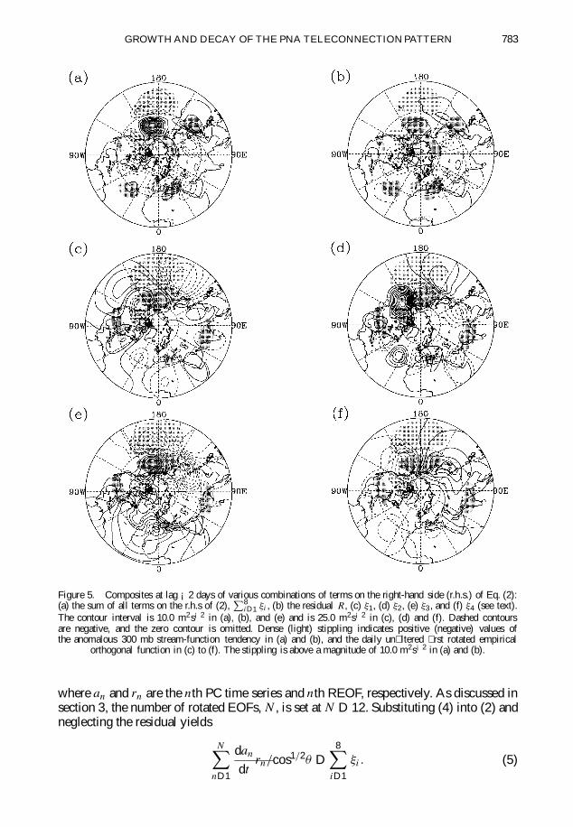
Figure 5. Composites at lag ¡2 days of various combinations of terms on the right-hand side (r.h.s.) of Eq. (2):(a) the sum of all terms on the r.h.s of (2),

P8iD1 »i , (b) the residual R, (c) »1, (d) »2, (e) »3 , and (f) »4 (see text).

The contour interval is 10.0 m2s¡2 in (a), (b), and (e) and is 25.0 m2s¡2 in (c), (d) and (f). Dashed contoursare negative, and the zero contour is omitted. Dense (light) stippling indicates positive (negative) values ofthe anomalous 300 mb stream-function tendency in (a) and (b), and the daily un� ltered � rst rotated empirical

orthogonal function in (c) to (f). The stippling is above a magnitude of 10.0 m2s¡2 in (a) and (b).

where an and rn are the nth PC time series and nth REOF, respectively. As discussed insection 3, the number of rotated EOFs, N , is set at N D 12. Substituting (4) into (2) andneglecting the residual yields

NX

nD1

dan

dtrn=cos1=2µ D

8X

iD1

»i : (5)

784 S. B. FELDSTEIN

Multiplying (5) by r1 cos1=2 µ and integrating over the domain results in

da1

dt

X

j

r21 C

da2

dt

X

j

r1r2 C ¢ ¢ ¢ Cda12

dt

X

j

r1r12 D8X

iD1

X

j

r1»i cos1=2 µ: (6)

All N D 12 terms on the left-hand side (l.h.s.) of (6) have nonzero values, which is amanifestation of the nonorthogonality of rotated EOFs. However, a calculation of eachterm on the l.h.s. of (6) reveals that the � rst term is more than 25 times larger than eachof the other terms at most lags during the persistent episode. In fact, neglecting all butthe � rst term on the l.h.s. of (6) is found to yield an error in the value of da1=dt which isof the order of 10%. Thus, to an excellent approximation, the projection in (3) representsthe in� uence of individual »i on the rate of change with time of the PNA index.

The various projections for the positive phase are examined in Fig. 2, and for thenegative phase in Fig. 3. A comparison between the projection of the sum of ‘linear’terms, i.e.

P4iD1 »i and that for all the terms

P8iD1 »i (Figs. 2(b) and 3(b)) indicates

that the linear terms play a crucial role during both the growth and the decay of thePNA anomaly. For example, during the positive phase (Fig. 2(b)), the linear termsaccount for essentially all of the anomaly growth and about one half of the anomalydecay. For the negative phase (Fig. 3(b)), on the other hand, the linear terms accountfor about two thirds of the anomaly growth, and most of the anomaly decay. A closeexamination of each of the � rst four »i terms shows for both phases that the PNA growthis dominated by »3 (Figs. 2(c) and 3(c)). This term, referred to as stationary advectionby Feldstein (1998), involves an energy transfer from the climatological stationaryeddies to the anomaly (e.g. Frederiksen 1983; Simmons et al. 1983; Branstator 1990,1992). Furthermore, for both phases, it is found that during the anomaly decay it is thedivergence term, »4, that dominates the � rst four »i terms (Figs. 2(c) and 3(c)). Also,the projections by the ‘nonlinear’ terms »5 and »6 (Figs. 2(d) and 3(d)), i.e. the low- andhigh-frequency transient eddy � uxes, reveal that »5 and »6 tend to oppose one anotherat most lags. This cancellation between the two bands of transient eddy � uxes lowersthe role played by transient eddy � uxes during the PNA life cycle. Therefore, becausethe projections during the growth (decay) stage are dominated by »3 (»4), the resultsof this projection analysis suggest that the composite PNA anomaly can be describedas undergoing a life cycle dominated by linear growth and linear decay. The growth isprimarily through stationary advection and the decay through divergence.

It is also important to discuss some of the potential drawbacks of the projectiontechnique. Firstly, the projection is onto a stationary anomaly pattern, i.e. REOF1.The advantage of this type of projection, as discussed earlier, is that it allows foran unambiguous estimate of the in� uence of the terms on the r.h.s. of (2) on thePC tendency. Furthermore, when the stream-function anomaly is quasi-stationary andresembles REOF1, such as between lags 0 and lag C8 days (see Figs. 4(b) to 4(d)) it isanticipated that the projections onto REOF1 also determine which terms on the r.h.s. of(2) affect the instantaneous stream-function anomaly. However, if the stream-functionanomaly undergoes substantial propagation, as is evident at negative lags in Fig. 4, theprojections onto REOF1 still describe the in� uence of the terms on the r.h.s. of (2) onthe PC tendency, but are no longer accurate at describing the in� uence of these terms onthe instantaneous stream-function anomaly.

In order to quantify the limitations of projecting onto REOF1, the projectionsonto REOF1 are compared with those onto the instantaneous stream-function-anomalypattern. The latter projection is a measure of the extent to which terms on the r.h.s.of (2) in� uence the temporal evolution of the instantaneous stream-function anomaly.


As expected, the two types of projections were found to be similar primarily duringthe persistent episode (for a de� nition of persistent episode, see subsection 2(a)), andalso for up to 2 days before the onset day (not shown). During this time period, thedifferences between the two types of projections were less than 30% at most lags.On the other hand, at earlier lags, when the stream-function-anomaly propagation ismost pronounced, larger differences between the two types of projections were found.Amongst the differences noted, it was found that the projection onto the instantaneousstream-function anomaly indicated an initiation of anomaly growth about 4 days earlierthan that shown in Figs. 2 and 3. Such a result is to be expected when the stream-function anomaly propagates. Also, between lag ¡10 and lag ¡5 days, it is found thatthe projection by the sum of the high- and low-frequency transient eddy � uxes is abouttwice that by the stationary advection term. This suggests that at the earliest stage ofthe anomaly evolution, the initial disturbance, which grows east of the PNA region,is excited by transient eddy � uxes. Such a result appears to be consistent with Doleand Black (1990) and Black and Dole (1993) who � nd that baroclinic processes areimportant during the growth of North Paci� c low-frequency anomalies.

Another potential limitation involves the property that the projection encompassesthe entire northern hemisphere. It is plausible that small local contributions to the pro-jections from locations where the anomaly is weak could make a signi� cant contributionto the hemispherically integrated projections illustrated in Figs. 2 and 3. To address thisquestion, projections corresponding to those shown in Figs. 2 and 3 were re-calculatedfor a domain con� ned between 150±E, 60±W, the equator, and the north pole. This do-main encompasses the four main centres of the PNA anomaly illustrated in Fig. 1. Theresults of this calculation revealed only small changes for the projections associatedwith stationary advection and the high- and low-frequency transient eddy � uxes, i.e. atmost lags the difference between the full projection and that con� ned to the PNA regionwas less than 15%. The changes for the divergence term were somewhat larger, but notlarge enough to alter the dynamical interpretation, as the difference between the twotypes of projections was less than 35% at most lags. These results verify that all of theprojections shown in Figs. 2 and 3 are dominated by the PNA anomaly.

6. STREAM-FUNCTION-TENDENCY EQUATION

The spatial structure of various terms on the r.h.s. of (2) is now illustrated. As thegeneral characteristics are similar for both phases, this is shown only for the positivephase. First, we evaluate to what extent the budget is balanced, as there are a numberof possible sources of error that are present. This includes errors from the � nite-differencing schemes, interpolation from sigma onto the 300 mb pressure surface, theexclusion of the cross-frequency vorticity � ux and tilting terms, and neglected physicalprocesses such as frictional dissipation. The extent to which the budget is balancedis � rst examined by overlaying contours of the sum of the terms on the r.h.s. of (2)(neglecting the residual) on shading of the stream-function tendency, i.e. the l.h.s. of (2)(see Fig. 5(a)). For this purpose, lag ¡2 days is selected, which is close to the time whenthe PNA index is increasing most rapidly. As can be seen, there is a very good matchbetween the two � elds at most locations, especially in the PNA region. In Fig. 5(b), thecontours of the residual term are shown, also overlaying shading of the stream-functiontendency. As can be seen, at most locations, and especially where the stream-functionanomaly has its largest amplitude, the residual term is much smaller than the stream-function tendency, indicating that the budget is reasonably well balanced. (A similardegree of balance is found for the negative phase.)

786 S. B. FELDSTEIN

Composites of the linear terms, i.e. »1, »2, »3, and »4, are shown in Figs. 5(c) to5(f). These � elds are illustrated with contours overlaying shading of the daily REOF1spatial pattern. Again lag ¡2 days is selected, in order to illustrate the characteristicsof these terms while the PNA anomaly is growing most rapidly. As is typical fora Rossby wave, the planetary (relative) vorticity advection, »1 (»2), acts to drive theanomalies westward (eastward). Consistent with the projection in Fig. 2(c), the spatialpattern for »3 accounts for strong ampli� cation of the stream-function anomaly. Lastly,the anomalous divergence, »4, drives the stream-function anomaly westward. Suchwestward propagation is consistent with the anomalous divergence corresponding tothe anomalous secondary circulation induced by anomalous vorticity advection (Holton1992). A similar relation between blocking anomalies and the divergence term wasfound by Cash and Lee (2000). Also, the composite of the sum of these four linearterms results in substantial cancellation (not shown). Very similar characteristics werefound for the low-frequency anomaly by Feldstein (1998).

Next some of the properties of the low-frequency interaction term, »5, are examined.It is � rst bene� cial to separate »5 into a contribution solely from the composite stream-function anomaly and a contribution which does not include the composite, referredto here as ‘incoherent eddies’. This separation can be accomplished by � rst writingthe wind and vorticity � elds as vL D vL

C C vLI and ³ D ³ L

C C ³ LI , respectively, where

the subscript ‘C’ denotes the composite stream-function anomaly, and the subscript ‘I’denotes the incoherent eddy contribution. Then, the � rst term in »5, which involvesrelative vorticity advection amongst the low-frequency transients, can be rewrittenwithout the r¡2 operator as

.¡vLr r³ L/L D .¡vL

rC r³ LC /L C .¡vL

rC r³ LI /L C .¡vL

rI r³ LC /L C .¡vL

rI r³ LI /L:

(7)

The � rst term on the r.h.s. of (7) is referred to as the ‘self interaction’ by the compositestream-function anomaly. The sum of the latter three terms on the r.h.s. of (7), referredto as the ‘incoherent low-frequency vorticity advection’, is dominated by .¡vL

rI r³ LI /L.

It should be noted that a similar separation could be applied to the second term in »5.However, as it is found that the contribution from the composite � eld is negligible forthat term, such a separation is not made.

Before examining the spatial structure of »5, let us look at the projection made by»5 with the self-interaction term being neglected (see Figs. 2(d) and 3(d)). As can beseen, this particular projection is very similar to that for »5. This implies that the self-interaction term plays a minor role and that the »5 in� uence on the amplitude of the PNAindex is primarily through the incoherent eddies.

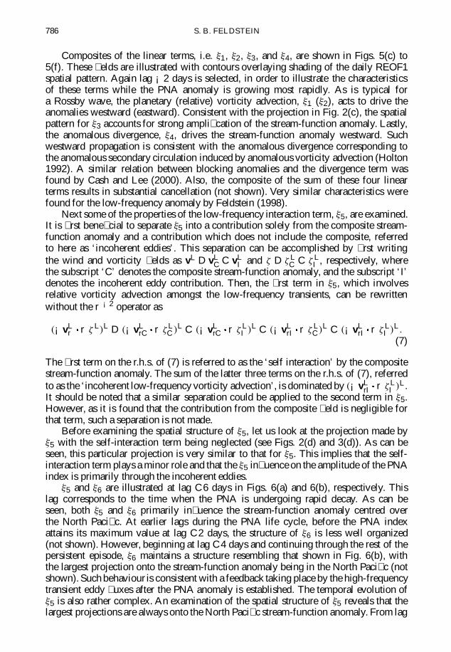
»5 and »6 are illustrated at lag C6 days in Figs. 6(a) and 6(b), respectively. Thislag corresponds to the time when the PNA is undergoing rapid decay. As can beseen, both »5 and »6 primarily in� uence the stream-function anomaly centred overthe North Paci� c. At earlier lags during the PNA life cycle, before the PNA indexattains its maximum value at lag C2 days, the structure of »6 is less well organized(not shown). However, beginning at lag C4 days and continuing through the rest of thepersistent episode, »6 maintains a structure resembling that shown in Fig. 6(b), withthe largest projection onto the stream-function anomaly being in the North Paci� c (notshown). Such behaviour is consistent with a feedback taking place by the high-frequencytransient eddy � uxes after the PNA anomaly is established. The temporal evolution of»5 is also rather complex. An examination of the spatial structure of »5 reveals that thelargest projections are always onto the North Paci� c stream-function anomaly. From lag


Figure 6. Composites at lag C6 days for various terms on the right-hand side of Eq. (2); (a) »5, (b) »6, and (c) »4(see text). The contour interval is 10.0 m2s¡2 in (a) and (b) and is 25.0 m2s¡2 in (c). Dashed contours are negative,and the zero contour is omitted. Dense (light) stippling indicates positive (negative) values of the daily un� ltered

� rst rotated empirical orthogonal function.

¡6 days to lag C2 days, this projection in the North Paci� c is positive, and from lag C2to lag C10 days this projection is negative, as illustrated in Fig. 6(a).

As discussed in section 3, for the negative phase, after completing much of its decay,the PNA index remains at about 30% of its peak value for about 10 days. Inspectionof the projections in Fig. 3 reveals that to a large extent this is attributable to »6, thedriving by the high-frequency transient eddies. Compared with the positive phase, anexamination of »6 for the negative phase (not shown) veri� es that it has a spatial patternvery much like that for the positive phase, but of opposite sign, and that this particularspatial pattern persists for a much longer period of time. However, no explanation forthis negative phase prolongation of »6 is offered.

Amongst the linear terms during the PNA decay, »1, »2, and »3, retain the samespatial structure as during the PNA growth. On the other hand, the divergence term,»4, exhibits more substantial changes between the growth and decay phases (compareFig. 5(f) with Fig. 6(c), which correspond to lag ¡2 and lag C6 days, respectively).

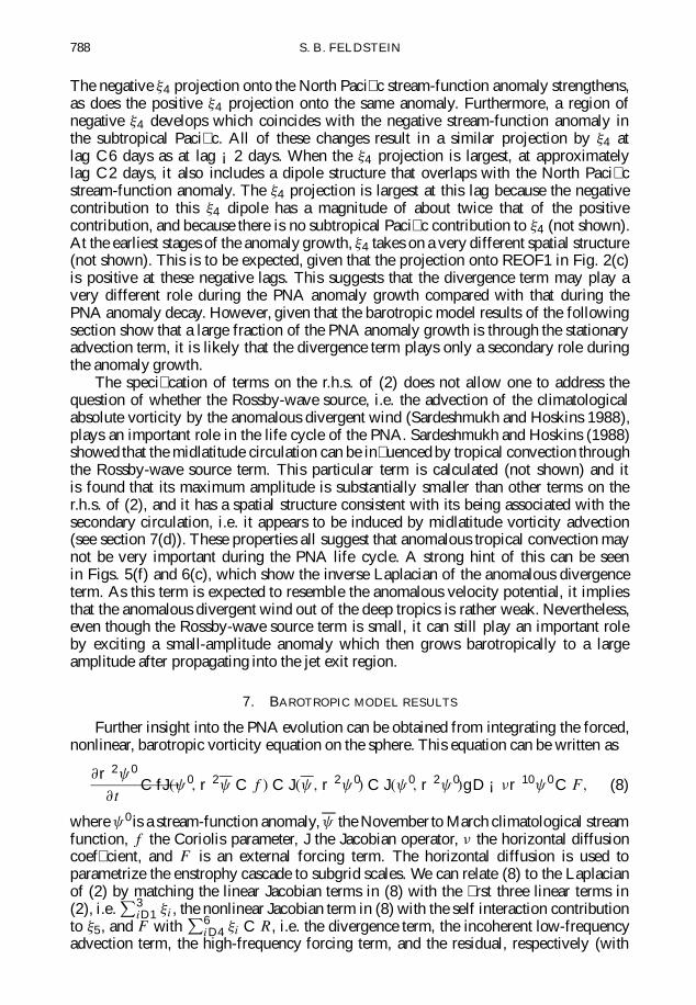
788 S. B. FELDSTEIN

The negative »4 projection onto the North Paci� c stream-function anomaly strengthens,as does the positive »4 projection onto the same anomaly. Furthermore, a region ofnegative »4 develops which coincides with the negative stream-function anomaly inthe subtropical Paci� c. All of these changes result in a similar projection by »4 atlag C6 days as at lag ¡2 days. When the »4 projection is largest, at approximatelylag C2 days, it also includes a dipole structure that overlaps with the North Paci� cstream-function anomaly. The »4 projection is largest at this lag because the negativecontribution to this »4 dipole has a magnitude of about twice that of the positivecontribution, and because there is no subtropical Paci� c contribution to »4 (not shown).At the earliest stages of the anomaly growth, »4 takes on a very different spatial structure(not shown). This is to be expected, given that the projection onto REOF1 in Fig. 2(c)is positive at these negative lags. This suggests that the divergence term may play avery different role during the PNA anomaly growth compared with that during thePNA anomaly decay. However, given that the barotropic model results of the followingsection show that a large fraction of the PNA anomaly growth is through the stationaryadvection term, it is likely that the divergence term plays only a secondary role duringthe anomaly growth.

The speci� cation of terms on the r.h.s. of (2) does not allow one to address thequestion of whether the Rossby-wave source, i.e. the advection of the climatologicalabsolute vorticity by the anomalous divergent wind (Sardeshmukh and Hoskins 1988),plays an important role in the life cycle of the PNA. Sardeshmukh and Hoskins (1988)showed that the midlatitude circulation can be in� uenced by tropical convection throughthe Rossby-wave source term. This particular term is calculated (not shown) and itis found that its maximum amplitude is substantially smaller than other terms on ther.h.s. of (2), and it has a spatial structure consistent with its being associated with thesecondary circulation, i.e. it appears to be induced by midlatitude vorticity advection(see section 7(d)). These properties all suggest that anomalous tropical convection maynot be very important during the PNA life cycle. A strong hint of this can be seenin Figs. 5(f) and 6(c), which show the inverse Laplacian of the anomalous divergenceterm. As this term is expected to resemble the anomalous velocity potential, it impliesthat the anomalous divergent wind out of the deep tropics is rather weak. Nevertheless,even though the Rossby-wave source term is small, it can still play an important roleby exciting a small-amplitude anomaly which then grows barotropically to a largeamplitude after propagating into the jet exit region.

7. BAROTROPIC MODEL RESULTS

Further insight into the PNA evolution can be obtained from integrating the forced,nonlinear, barotropic vorticity equation on the sphere. This equation can be written as

@r2Ã 0

@tC fJ.Ã 0; r2Ã C f / C J.Ã; r2Ã 0/ C J.Ã 0; r2Ã 0/g D ¡ºr10Ã 0 C F; (8)

where Ã 0 is a stream-function anomaly, Ã the November to March climatological streamfunction, f the Coriolis parameter, J the Jacobian operator, º the horizontal diffusioncoef� cient, and F is an external forcing term. The horizontal diffusion is used toparametrize the enstrophy cascade to subgrid scales. We can relate (8) to the Laplacianof (2) by matching the linear Jacobian terms in (8) with the � rst three linear terms in(2), i.e.

P3iD1 »i , the nonlinear Jacobian term in (8) with the self interaction contribution

to »5, and F withP6

iD4 »i C R, i.e. the divergence term, the incoherent low-frequencyadvection term, the high-frequency forcing term, and the residual, respectively (with


this de� nition of R, the cross-frequency vorticity � ux and tilting terms, i.e. »7 and »8,are included in the residual).

For this model calculation, rhomboidal 30 resolution is used, the same as that in thediagnostic calculations. Also, the value chosen for º is 8 £ 1037 m8s¡1. Furthermore,only the results for the positive phase are illustrated, as all of the essential features to bepresented are also found for the negative phase. For the initial stream-function � eld, thecomposite stream-function anomaly at a particular lag will be used. Composite valuesare also used for the forcing term F . Because the NCEP/NCAR re-analysis data are notavailable for every model time step (the barotropic model uses 48 time steps per day,and the known values of F are for the daily lags corresponding to 00 UTC), the valuesof F at each intermediate time step are approximated by using linear interpolation.

The unavoidable use of interpolation to determine F at each intermediate time stepresults in some error in the forcing terms. These errors in F must cause the model andobserved anomalies to diverge gradually over time. As we will see, it is found that themodel integrations are reasonably accurate when integrated over several days. However,for much longer model integrations, such as 10 days, noticeable differences between themodel and observed anomalies were found.

(a) Growth stageFirst the results of barotropic model integrations starting at lag ¡4 days are ex-

amined. The time period encompassing this model integration will be referred to asthe growth stage. The extent to which this model simulates the PNA growth can beseen by comparing Fig. 4(b), i.e. the lag 0 composite anomalous stream-function � eld,with Fig. 7(f), the model run with all three forcing terms and the residual present. Thiscomparison shows there is a large degree of similarity, especially in the region where thePNA has a large contribution. Figures 7(a) and 7(b) illustrate the results of the unforcedlinear and unforced nonlinear runs, respectively. In both of these runs, F D 0, and inthe linear run the nonlinear Jacobian in (8) is set to zero. As can be seen, except forthe slight westward displacement of the two Paci� c anomalies in Fig. 7(b) relative toFig. 7(a), these two runs yield extremely similar results, indicating that the nonlinearJacobian in (8), which represents the self interaction term in (7), plays a very minorrole. We can also see from Fig. 7(a) that substantial growth of the stream-function-anomaly pattern occurs in the linear unforced run (compare Fig. 7(a) with Fig. 4(a),which shows the initial � ow for this calculation). Although not shown, inspection ofthe stationary advection term for the linear, unforced model run reveals a spatial patternwith two dominant anomalies over the North Paci� c, as in Fig. 5(e). This suggests thatthe two upstream anomalies in the North Paci� c grow via the stationary advection term,and implies that the two downstream anomalies grow via linear dispersion.

If we compare the locations of the stream-function anomaly centres in Fig. 7(a) withthose of the corresponding observed composite stream-function anomaly in Fig. 4(b),we can see that the absence of the forcing terms in (8) leaves some noticeable errors inspatial structure. In particular, each of the model’s anomaly centres is located to the eastof the corresponding observed anomaly centre. Much of these differences are remediedby including the divergence term on the r.h.s. of (8) (Fig. 7(d)). In addition, for the twoanomalies over the Paci� c, the integration with the divergence term alone looks muchmore similar to that with all the forcing terms present (Fig. 7(f)) than those with just thehigh-frequency forcing (Fig. 7(c)) or the incoherent low-frequency advection forcingterm (Fig. 7(e)), indicating that the divergence term has the most in� uence of the threeforcing terms.

790 S. B. FELDSTEIN

Figure 7. Anomalous stream-function � eld for the 4-day barotropic model integration. Start date is lag ¡4 days.The results shown are for (a) the unforced linear model, J.Ã 0; r2Ã 0/ D 0 and F D 0, (b) the unforced nonlinearmodel, J.Ã 0; r2Ã 0/ 6D 0 and F D 0, (c) the forced nonlinear model only with »6 6D 0, (d) the forced nonlinearmodel only with »4 6D 0, (e) the forced nonlinear model only with the incoherent contribution to »5 6D 0, and(f) the forced nonlinear model with »4, »5 , and »6 all nonzero. The residual term, R, from Eq. (2), is also includedamongst the forcing terms in (f). The contour interval is 2 £ 106 m2s¡1 . Dashed contours are negative, and thezero contour is omitted. Dense (light) stippling denotes positive (negative) values with a magnitude in excess of

4 £ 106 m2s¡1 . See text for explanation of terms.


Figure 8. As Fig. 7, except with a start date of lag C4 days, and an integration time of 3 days.

(b) Persistence stageThe barotropic model results for an integration beginning on the onset day yield

many of the same characteristics as those for the growth stage (not shown). The timeperiod covered by this model integration is denoted as the persistence stage. As forthe growth stage, the unforced linear and nonlinear runs yield very similar results.For these integrations, it is found that the subtropical stream-function anomaly decaysvery slightly, the North Paci� c anomaly strengthens slightly, and the two downstreamanomalies further amplify. Also, it is found that the divergence term is the mostimportant of the three forcing terms. The divergence term again shifts the stream-function-anomaly centres upstream keeping them in a quasi-� xed position.

792 S. B. FELDSTEIN

(c) Decay stageNext the model integration beginning at lag C4 days is examined; the time period

of this calculation is referred to as the decay stage (Fig. 8). However, in contrastto the previous stages, this integration is performed for only 3 days, as the stream-function anomaly in the model integration is found to diverge from the observed stream-function anomaly more rapidly during the decay stage. The degree to which the modelintegration simulates the PNA can be found by comparing Fig. 8(f), the model solutionwith all three forcing terms present, with the anomalous composite stream-function� eld at lag C7 days which, although not shown, is very similar to the stream-function� eld in Fig. 4(d), except for a slightly larger amplitude. As can be seen, the modelintegration does capture all four PNA anomaly centres reasonably well. As for thetwo previous stages, the linear and nonlinear unforced runs give very similar results(Figs. 8(a) and 8(b)). The two upstream stream-function anomalies decay while thetwo downstream anomalies continue to grow (compare with the initial � ow shown inFig. 4(c)). In contrast to the integrations for the two previous stages, during the decaystage the forcing terms have a much greater in� uence and, as can be seen, cause thestream-function anomaly to undergo substantial decay (Fig. 8(f)). Thus, because thestream-function-anomaly centres are retained in the unforced model runs, and yet decayin the fully forced model run (Fig. 8(f)), this result suggests that the decay of the PNA isnot through linear dispersion. Also, as during the growth and persistence stages, thedivergence term is the most important of the forcing terms (see Figs. 8(c) to 8(f)),although the incoherent low-frequency advection term is also playing an important rolein the anomaly decay.

Although, as discussed in the above paragraph, linear dispersion does not seem toaccount for the overall decay of the PNA anomaly pattern, the unforced linear modelresults shown in Fig. 8(a) are consistent with linear dispersion weakening (strength-ening) the upstream (downstream) stream-function-anomaly centres. This contrasts theunforced linear model results for the growth and persistence stages, as described above,where upstream anomaly growth was obtained. Since the background � ow is identicalin each integration, these differences in the unforced linear integrations must be dueto changes in the spatial structure of the stream-function anomalies. (An examinationof why the anomalies do change their shape is beyond the scope of this study.) Thus,since the projections, composite plots, and model integrations all suggest that the PNAgrows via the energy gained through stationary advection, a linear process, it must bebecause of these changes in the spatial structure of the stream-function anomalies thatthe barotropic growth of the upstream anomaly centres eventually ceases.

(d ) Ekman pumpingThere are several plausible mechanisms that may account for the decay of the PNA.

A list of mechanisms would include decay through anomalous Ekman pumping, thermaladvection, and diabatic heating. Although the results to be presented below are notde� nitive, they do hint at an important role for Ekman pumping, as different variablesshow characteristics that are consistent with anomaly decay via Ekman pumping.

In order to estimate the in� uence of Ekman pumping, the divergence term, »4, isseparated into two parts, i.e.

»4 D ¡8X

iD1;i 6D4

®»i C »4ek: (9)


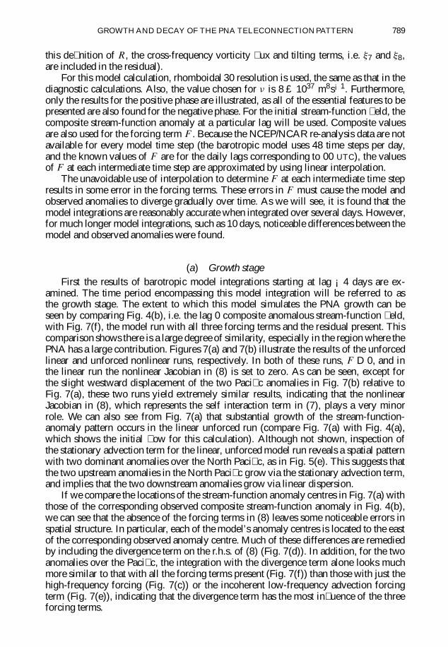
Figure 9. The lag C6 day (a) stream-function tendency due to the anomalous ‘Ekman’ divergence, »4ek , and(b) anomalous surface pressure. (c) The anomalous stream-function � eld from the barotropic model integrationfor the decay stage with the anomalous ‘Ekman’ divergence set to zero. The contour intervals are (a) 10.0 m2s¡2 ,(b) 150 N m¡2, and (c) 2 £ 106 m2s¡1 . Dashed contours are negative, and the zero contour is omitted. Dense

(light) stippling in (c) denotes positive (negative) values with a magnitude in excess of 4 £ 106 m2s¡1 .

The � rst term on the r.h.s. of (9) represents the divergence associated with the secondarycirculation due to upper-tropospheric vorticity advection. This term simply representsthe adjustment of the � ow toward thermal-wind balance due to the anomalous vorticityadvection. The parameter ®, which is a measure of the strength of the secondarycirculation, must have a magnitude less than unity, as the secondary circulation alwaysacts to weaken the in� uence of the processes that drives it. After specifying ®, the secondterm on the r.h.s. of (9) can be determined. Physically, »4ek can be induced by thermaladvection, diabatic heating, and friction (e.g. Ekman pumping), as mentioned above,and also by that part of vorticity advection not captured by the � rst term on the r.h.s.of (9). Also, although it is of course impossible to show with complete con� dence that»4ek does indeed correspond to the in� uence of Ekman pumping, by showing that thespatial structure of »4ek is consistent with that expected for Ekman pumping, one canargue qualitatively that PNA decay through Ekman pumping is indeed plausible.

794 S. B. FELDSTEIN

In order for surface friction to in� uence the 300 mb stream-function anomaly, theanomalous vertical circulation driven by Ekman pumping must be deep, i.e. extendthrough the depth of the troposphere. Furthermore, Ekman pumping requires that »4ektakes on speci� c characteristics. These include that »4ek should be similar in spatialstructure but opposite in sign to both (a) the 300 mb stream-function anomaly, and (b) thesurface pressure anomaly. The � rst requirement is necessary simply because »4ek mustbe damping the stream-function anomaly. The second point, which links the stream-function anomaly to the surface circulation where friction is generated, needs furtherdiscussion. Because the in� uence of surface friction requires a deep anomalous verticalcirculation, the sign of the divergence anomaly in the upper troposphere that results fromEkman pumping must be opposite to that for the divergence anomaly near the surface.Furthermore, at the surface, a positive (negative) pressure anomaly always coincideswith a positive (negative) divergence anomaly, via downgradient cross-isobaric � ow.Thus, combining these properties, upper-tropospheric convergence, i.e. a negative »4ek,must coincide with a positive surface pressure anomaly.

The approach adopted is to vary ® and examine if for a range of ® values whetherthe two requirements of the above paragraph are satis� ed. Figure 9(a), shows »4ekestimated from (9) using ® D 0:6. The anomalous surface pressure � eld is illustrated inFig. 9(b). Both of these � elds are illustrated at lag C6 days, a time when the stream-function anomaly is rapidly decaying. As can be seen, the two requirements of theabove paragraph are indeed satis� ed, since »4ek (Fig. 9(a)) and the anomalous surfacepressure � eld (Fig. 9(b)) both closely resemble the positive stream-function anomalyin the North Paci� c (Fig. 4(b) and 4(c)). Thus, keeping in mind the assumptions madeand the qualitative nature of these calculations, these � ndings are consistent with thehypothesis that the PNA is decaying through frictional processes via Ekman pumping.

Further support for the role of Ekman pumping in the decay of the PNA can beobtained by integrating the barotropic model with the ‘Ekman pumping contribution’ tothe divergence set equal to zero, and with the same initial � ow as that correspondingto Fig. 8. When this integration is performed (Fig. 9(c)), it can be seen that the stream-function anomalies decay only slightly, and that the PNA is mostly retained.

8. CONCLUSIONS

This study investigates some of the dynamical mechanisms associated with thegrowth and decay of the Paci� c/North American teleconnection pattern (PNA). Throughthe use of projections, composites of various terms in the stream-function-tendencyequation, a series of calculations with a forced, nonlinear, barotropic model, anda crude estimate of the role of Ekman pumping, a rather simple picture of PNAevolution is presented. The growth of the two upstream anomaly centres of the PNAis found to occur through barotropic energy conversion from the zonally asymmetricclimatological � ow. This is consistent with numerous other studies of low-frequencyvariability, e.g. Simmons et al. (1983). Dispersion then transfers energy to the twodownstream anomaly centres. Divergence is found to be important, as it causes upstreamanomaly propagation, which allows the two upstream anomaly centres to remain ina quasi-� xed position in the Asian jet exit region. However, as the PNA anomalyundergoes its life cycle, the horizontal shape of the two upstream anomalies graduallychanges. This results in a reduction of the barotropic growth followed by decay ofthe PNA through Ekman pumping. This entire cycle is complete within approximately2 weeks. It is important to emphasize that the above Ekman-pumping argument is only


qualitative, and does not rule out the possibility of baroclinic processes causing thedecay of the PNA.

The above � ndings suggest that the PNA evolution is dominated by linear processes,as found by Feldstein (1998) for another anomaly pattern in a general-circulation model.However, at various stages during the PNA life cycle it was found that the nonlineartransient eddy � uxes can play an important role. Nevertheless, the overall dominance ofthe linear terms suggests that to lowest order the PNA life cycle has the characteristicsof a linear initial-value problem.

Many studies of low-frequency variability have used barotropic models. However,by analysing the normal mode and optimal growth properties of the observed atmos-pheric � ow, and also with the aid of stochastic modelling, a number of papers (Borgesand Sardeshmukh 1995; Blade 1996; Sardeshmukh et al. 1997; Newman et al. 1997)have shown that barotropic processes alone cannot account for the temporal evolu-tion of low-frequency anomalies. Furthermore, as the authors of these studies discuss,additional processes, such as baroclinic effects, i.e. divergence, diabatic heating, etc.,and transient eddy forcing, must play a crucial role in the life cycle of low-frequencyanomalies. The results of the present study provide additional support for these ideas.

ACKNOWLEDGEMENTS

This research was supported by the National Science Foundation through GrantsATM-9712834 and ATM-0003039. I would like to thank Dr Sukyoung Lee for herbene� cial discussions, and also two anonymous reviewers. In addition, I would liketo thank the National Oceanic and Atmospheric Administration Climate DiagnosticsCenter for providing me with the NCEP/NCAR reanalysis dataset.

REFERENCES

Barnston, A. G. and Livezey, R. E. 1987 Classi� cation, seasonality, and persistence of low-frequencyatmospheric circulation patterns. Mon. Weather Rev., 115,1083–1126

Black, R. X. and Dole, R. M. 1993 The dynamics of large-scale cyclogenesis over the North Paci� cOcean. J. Atmos. Sci., 50, 421–442

Blade, I. 1996 On the relationship of barotropic singular modes to thelow-frequency variability of a general circulation model.J. Atmos. Sci., 53, 2393–2399

Borges, M. D. andSardeshmukh, P. D.

1995 Barotropic Rossby wave dynamics of zonally varying upper-level� ows during northern winter. J. Atmos. Sci., 52, 3779–3796

Branstator, G. 1984 The relationship between the zonal mean � ow and quasi-stationary waves in the midtroposphere. J. Atmos. Sci., 41,2163–2178

1987 A striking example of the atmosphere’s leading traveling pattern.J. Atmos. Sci., 44, 2310–2323

1990 Low-frequency patterns induced by stationary waves. J. Atmos.Sci., 47, 629–648

1992 The maintenance of low-frequency atmospheric anomalies.J. Atmos. Sci., 49, 1924–1945

Cai, M. and van den Dool, H. M. 1994 Dynamical decomposition of low-frequency tendencies. J. Atmos.Sci., 51, 2086–2100

Cash, B. A. and Lee, S. 2000 Dynamical process of block evolution. J. Atmos. Sci., 57, 3202–3218

2001 Observed nonmodal growth of the Paci� c–North American tele-connection pattern. J. Climate, 14, 1017–1028

Dole, R. M. and Black, R. X. 1990 Life cycles of persistent anomalies. Part II: The development ofpersistent negative height anomalies over the North Paci� cOcean. Mon. Weather Rev., 118, 824–846

Egger, J. and Schilling, H.-D. 1983 On the theory of the long-term variability of the atmosphere.J. Atmos. Sci., 40, 1073–1085

796 S. B. FELDSTEIN

Feldstein, S. B. 1998 The growth and decay of low-frequency anomalies in a GCM.J. Atmos. Sci., 55, 415–428

2000 The time-scale, power spectra, and climate noise properties ofteleconnection patterns. J. Climate, 13, 4430–4440

Feldstein, S. B. and Lee, S. 1996 Mechanisms of zonal index variability in an aquaplanet GCM.J. Atmos. Sci., 53, 3541–3555

Franzke, C., Fraedrich, K. andLunkeit, F.

2001 Teleconnections and low-frequency variability in idealized exper-iments with two storm tracks. Q. J. R. Meteorol. Soc., 127,1321–1339

Frederiksen, J. S. 1983 A uni� ed three-dimensional instability theory of the onsetof blocking and cyclogenesis. II: Teleconnection patterns.J. Atmos. Sci., 40, 2593–2609

Holton, J. R. 1992 An introduction to dynamic meteorology. Academic Press, SanDiego, USA

Horel, J. D. 1985 Persistence of the 500 mb height � eld during northern hemispherewinter. Mon. Weather Rev., 113, 2030–2042

Hoskins, B. J. and Karoly, D. 1981 The steady linear response of a spherical atmosphere to thermaland orographic forcing. J. Atmos. Sci., 38, 1179–1196

Hoskins, B. J., James, I. N. andWhite, G. H.

1983 The shape, propagation, and mean-� ow interaction of large-scaleweather systems. J. Atmos. Sci., 40, 1595–1612

Kang, I.-S. 1990 In� uence of zonal mean � ow change on stationary wave � uctua-tions. J. Atmos. Sci., 47, 141–147

Kushnir, Y. 1987 Retrograding wintertime low-frequency disturbances over theNorth Paci� c Ocean. J. Atmos. Sci., 44, 2727–2742

Kushnir, Y. and Wallace, J. M. 1989 Low-frequency variability in the northern hemisphere winter:Geographical distribution, structure and time-scale depen-dence. J. Atmos. Sci., 46, 3122–3142

Lau, N.-C. 1988 Variability of the observed midlatitude storm tracks in relation tolow-frequency changes in the circulation pattern. J. Atmos.Sci., 45, 2718–2743

Livezey, R. E. and Chen, W. Y. 1983 Statistical � eld signi� cance and its determination by Monte Carlotechniques. Mon. Weather Rev., 115, 46–59

Mo, K. C. 1986 Quasi-stationary states in the southern hemisphere. Mon. WeatherRev., 114, 806–823

Newman, M., Sardeshmukh, P. D.and Penland, C.

1997 Stochastic forcing of the wintertime extratropical � ow. J. Atmos.Sci., 54, 435–455

Nigam, S. and Lindzen, R. S. 1989 The sensitivity of stationary waves to variations in the basic statezonal � ow. J. Atmos. Sci., 46, 1746–1768

Sardeshmukh, P. D. andHoskins, B. J.

1988 The generation of global rotational � ow by steady idealized trop-ical divergence. J. Atmos. Sci., 45, 1228–1251

Sardeshmukh, P. D., Newman, M.and Borges, M. D.

1997 Free barotropic Rossby wave dynamics of the wintertime low-frequency � ow. J. Atmos. Sci., 54, 5–23

Simmons, A. J., Wallace, J. M. andBranstator, G.

1983 Barotropic wave propagation and instability and atmospheric tele-connection patterns. J. Atmos. Sci., 40, 1363–1392

Ting, M. and Lau, N.-C. 1993 A diagnostic and modeling study of the monthly mean winter-time anomalies appearing in an 100-year GCM experiment.J. Atmos. Sci., 50, 2845–2867

Wallace, J. M. and Gutzler, D. S. 1981 Teleconnections in the geopotential height � eld during the north-ern hemisphere winter. Mon. Weather Rev., 109, 784–812

fundamental mechanisms of the growth and …sbf1/papers/pna.pdfq. j. r. meteorol. soc.(2002),128,...

Documents