fundamentals for radio engineers

7/31/2019 Fundamentals for Radio Engineers

http://slidepdf.com/reader/full/fundamentals-for-radio-engineers 1/32

Basic Stuffs for Radio Communication Engineers

○ Functions (Plot following functions!)

1-dimensional functions

( ) 10 f x = , 2 2( ) , 3, 2 5 f x x x x= + + , ( ) 30cos(2 ) f t t π = ( ) 30cos(120 ) f t t π = ,

( ) 30cos(120 )3

f t t π

π = + , ( ) 30cos(120 ) f t t π π = + ,

( ) 10 j z

x E z eπ −= ,

( )2( ) 10

i z

x E z eπ

π − +

= , 2( ) 10 j z

x E z eπ −= 2( ) 10

j z

x E z eπ

−

=

2-dimensional functions

( , ) 5 f x y = , 2 2( , ) f x y x y= + , 2 2( , ) 5 f x y x y= + + , ( , ) 2 f x y x y= + ,

( , ) 5cos(10 )v z t t zπ π = −

3-dimesional functions

( , , ) 3 f x y z = , ( , , ) 3 f x y z x= , ( , , ) 3 f x y z y= , 2 2 2( , , ) f x y z x y z= + + ,2 2 2( , , ) 2 f x y z x y z= + + + , ( , , ) 2 cos f z ρ φ ρ φ =

○ Derivatives

-ordinary(상미분)

0

( ) ( ) ( ) ( ) ( )lim ( x

df x f x x f x f x x f x x

dx x xΔ →

+ Δ − + Δ −= ≈ Δ

Δ Δsmall)

-partial(편미분)

0

( , ) ( , ) ( , )

lim x

f x y f x x y f x y

x xΔ →

∂ + Δ −

=∂ Δ

0

( , ) ( , ) ( , )lim y

f x y f x y y f x y

y yΔ →

∂ + Δ −=

∂ Δ

Prob) Obtain the ordinary derivativesdf

dxof the following functions using the

definitions mentioned above. What is the meaning of them?



( ) 10 f x = , 2 2( ) , 3, 2 5 f x x x x= + + , 4 3 2( ) 5 3 2 2 5 f x x x x x= + − − + , ( ) 30cos(2 ) f t t π =

( ) 30cos(120 ) f t t π = , ( ) 30cos(120 )3

f t t π

π = + , ( ) 30cos(120 ) f t t π π = + ,

( ) 30sin(120 ) f t t π = , ( ) 30sin(120 )3

f t t π

π = + , ( ) 30sin(120 ) f t t π π = + ,

23 2 1( ) x x f x e− + +=

Prob) Obtain the partial derivatives of the functions2( )V x x= (V)

2 2( , )V x y x y= + (V)2 2 2( , , )V x y z x y z= + + (V)

2 2 2( , , ) 1 2 3 4 2 3 4 2 3 4 ( ) x y z x y z x y z xy yz zx V φ = + + + + + + + + +

with units. What is the meaning of them

x

φ ∂

∂,

y

φ ∂

∂,

z

φ ∂

∂,

2

2 x

φ ∂

∂,

2

2 y

φ ∂

∂,

2

2 z

φ ∂

∂,

2

x y

φ ∂

∂ ∂,

2

y z

φ ∂

∂ ∂,

2

z x

φ ∂

∂ ∂

○ Integration

( )b

a f x dx∫ (area), ( , )

b d

a c f x y dxdy∫ ∫ (volume)

Prob) Plot the integrand, obtain the values of the integrations, and express their

meanings.

4

0(2 3) x dx+∫ ,

42

0(4 ) x dx

−

∫ ,3

1( 1)( 3) x x dx− −∫ ,

010sin d

π

θ θ ∫ 2

010sin d

π

θ θ ∫ ,

22

0sin d

π

θ θ ∫ ,2

2

0

1sin

2d

π

θ θ π ∫

,2

2

0

1cos

2d

π

θ θ π ∫

,2 3

2 2

2 3( ) x y dxdy

− −+∫ ∫

○ Dot(내적) and cross product(외적) of vectors

• Dot product

cos( ) A B AB θ =i (scalar)



A

Bθ

θ cos A

θ cos B

( cos ) ( cos ) A B A B A Bθ θ = =i

When 0θ = ° , A B AB=i . When 90θ °= , 0 A B =i . When 180θ °= , A B AB= −i .

1 2 3 x y z A a a a a a a= + + ,1 2 3 x y z B b a b a b a= + +

Unit vector | |

A Aa A A= = , | |

B Bb B B= =

1 2 3 1 2 3 1 1 2 2 3 3cos( ) ( ) ( ) x y z x y A B AB a a a a a a b a b a b a b a b a bθ = = + + + + = + +i i (scalar)

2 2| || | cos(0) | | A A A A A A= = =i ,2 2( ) | || | cos(180 ) | | ( 1) A A A A A A− = ° = − = −i

1cos( ) cos( ) A b A Aθ θ = =i i (projection of A on B or projection of A on b )

θ

A

b

1 cos cos A b A Aθ θ = = ⋅ ⋅ =i

A bi

1cos( ) cos( ) B a B Bθ θ = =i i (projection of B on A or projection of A on b )



1 x A a a=i , 2 y A a a=i , 3 z A a a=i

Ex) 2 3 x y z A a a a= + − , x y B a a= + , ( ) / 2 x yb a a= +

projection of A on B =3 3 2

( 2 3 )22 2

x y

x y z

a a A b a a a

+= + − = =i i

projection of A on xa = 1 x A a =i

projection of A on ya = 2 y A a =i

projection of A on za = 3 z A a = −i

2

1 x x xa a a= =i , 1 y ya a =i , 1 z za a =i

0 x ya a =i , 0

y za a =i , 0 z xa a =i

• Cross Product

sin( )n A B a AB θ × = (

na is the unit vector following the right hand rule.)

A

B

θ

sinn

A B a AB θ × =

na

If 1 2 3 x y z A a a a a a a= + + and 1 2 3 x y z B b a b a b a= + + ,

A B×

1 2 3 1 2 3 2 3 3 2 3 1 1 3 1 2 2 1( ) ( ) ( ) ( ) ( )

x y z x y z x y za a a a a a b a b a b a a a b a b a a b a b a a b a b= + + × + + = − + − + −

1 2 3

1 2 3

x y za a a

a a a

b b b

⎡ ⎤⎢ ⎥

= ⎢ ⎥⎢ ⎥⎣ ⎦

| |n

A Ba

A B

×=

×

1 x ya a× = , 1 y za a× = , 1 z xa a× =

0 x xa a× = , 0 y ya a× = , 0 z za a× =



Prob) Given that 2 3 x y z A a a a= − + and

x y B a a= − − , obtain the followings and

discuss the meaning of them with a simple sketch..

a , a ai , b , b bi , A Bi , B Ai , A B× , B A× , A Ai , ( ) A A−i , A ai , A bi , B bi ( projection

of A on B ), B ai ( projection of B on A ), na , Angle between A and B

○ Field(장)

• Scalar field(스칼라장) : gives a number for each point in space

Prob) Draw the following scalar fields.

2 2( , )h x y x y= + , 2 2 2( , , )T x y z x y z= + + ,10

( , , )T z ρ φ ρ

= ,10

( )V r r

=

• Vector field(벡터장) : gives a vector for each point in space

( , , ) ( , , ) ( , , ) ( , , ) x x y y z z A x y z A x y z a A x y z a A x y z a= + +

Prob) Draw the following vector fields.

( , , ) 3 x A x y z a= , ( , , ) x A x y z xa= , ( , , ) 2 y A x y z xa= , ( , , ) 3 z A x y z xa= ,

( , ) x yF x y xa ya= + ,2 2

( , )x y ya xa

G x y x y

− +=

+, 2 2( , , ) 3 2 x y z A x y z xyza x ya z a= + − ,

10( , , ) H z aφ ρ φ

ρ = ,

10( , , ) r E r a

r θ φ = ,

10( , , ) E r a

r θ θ φ = ,

10( , , ) H r a

r φ θ φ =

• Vector calculus

미소 길이 벡터(differential displacement)

x y zdl dxa dya dza= + + , zdl d a d a dza ρ φ ρ ρ φ = + + ,

sinr dl dra rd a r d aθ φ θ θ φ = + + (m)

미소 면적 벡터(differential surface vector)

xds dydza= ,

ydzdxa , z

dxdya ,

( )ds d dza ρ ρ φ = , dzd aφ

ρ , ( ) z

d d a ρ φ ρ ,

( )( sin ) r ds rd r d aθ θ φ = , ( sin )( )r d dr a

θ θ φ , ( )dr rd aφ θ

미소 체적(differential volume)

dv dxdydz= , ( )d d dz ρ ρ φ ( d d dz ρ ρ φ = ), ( )( sin )dr rd r d θ θ φ ( 2 sinr drd d θ θ φ = )



Need to understandl A dl∫ i (circulation around l ),

S A ds∫ i (net outward flux of A from

a surface S), vV dv ρ ∫ (volume integral of the scalar field v ρ over the volume V)

Ex) A magnetic flux density is given by2 2 2( , , ) 2( ) 3( ) 3 ( / ) x y z B x y z x y a x y a xya Wb m= + + + + . Determine the total magnetic

x

y

z

2m

2m

flux ϕ flowing out of the rectangular surface.

Sol)2 2 2( , , 0) 2( ) 3( ) 3 ( / ) x y z B x y z x y a x y a xya Wb m= = + + + + ,

zds dxdya= ,

2 22 2

2 2

0 00 0

( , , 0) 3 3 12( )2 2S

x y B x y z ds xdx ydy Wbϕ

⎡ ⎤ ⎡ ⎤= = = = =⎢ ⎥ ⎢ ⎥

⎣ ⎦ ⎣ ⎦∫ ∫ ∫i

Prob) When the surface is given by y=0( 0 2 x≤ ≤ , 0 2 z≤ ≤ ), determine the total

magnetic flux(Wb) flowing out of the surface in –y direction.

• Gradient(경도)

: The gradient of a scalar field gives a vector field.

Gradient ( , , ) x y z

f f f f f x y z a a a

x y z

∂ ∂ ∂= ∇ = + +

∂ ∂ ∂(vector field)

- ( ) x

df f x a

dx∇ =

2( ) 2 x f x x f xa= ⇒ ∇ = (What does this mean?)

- ( , ) x y

f f f x y a a

x y

∂ ∂∇ = +

∂ ∂

2 2( , ) 2 2 x y f x y x y f xa ya= + ⇒ ∇ = + (What does this mean?)

- ( , , ) x y z

f f f f x y z a a a

x y z

∂ ∂ ∂∇ = + +

∂ ∂ ∂



2 2 2( , , ) ( ) ( , , ) 2 2 2 ( / ) x y zV x y z x y z Volts V x y z xa ya za V m= + + ⇒ ∇ = + +

(What does this mean?)

2

10 10( ) ( ) ( ) ( / )r V r V V r a V m

r r = ⇒ ∇ = − (What does this mean?)

• Divergence(발산)

Electric flux density(전속밀도) ( , , ) ( , , ) ( , , ) ( , , ) x x y y z z D x y z D x y z a D x y z a D x y z a= + +

( 2 / Coul m ) (Vector field)

Divergence30

( )lim

( )

yS x z

v

D ds Coul D D D D

v m x y zΔ →

∂∂ ∂= = + +Δ ∂ ∂ ∂

∫i

3( ) ( ) ( / ) x y z x x y y z za a a D a D a D a D Coul m

x y z

∂ ∂ ∂= + + + + = ∇

∂ ∂ ∂i i (Scalar

field)

• Curl(회전)

( , , ) ( , , ) ( , , ) ( , , ) x x y y z z H x y z H x y z a H x y z a H x y z a= + + (A/m)

Curl20

( )lim ( ) ( ) ( )

( )

y yS x x z zn x y z

s

H dl A H H H H H H H a a a a

s m y z z x x yΔ →

∂ ∂∂ ∂∂ ∂= = − + − + −

Δ ∂ ∂ ∂ ∂ ∂ ∂

∫ i

2( ) ( ) ( / ) x y z x x y y z za a a H a H a H a H A m

x y z

∂ ∂ ∂= + + × + + = ∇ ×

∂ ∂ ∂(Vector field)

Ex)

( , , ) 2 x y A x y z a a= +

30(/ ) A m⇒ ∇ =i

20(/ ) A m⇒ ∇× =

( , , ) 2 x A x y z xa=

32(/ ) A m⇒ ∇ =i 2

0(/ ) A m⇒ ∇× =



2( , , ) 10 x A x y z x a=

320 (/ ) A x m⇒ ∇ =i 2

0(/ ) A m⇒ ∇× =

( , , ) 3 y A x y z xa=

30(/ ) A m⇒ ∇ =i 23 (/ ) z A a m⇒ ∇× =

Ex) Given that 3 2( , , ) 2 ( ) 5V x y z xyz x y z= + + + + (V),

( , , ) 2 3( ) 4 x y z D x y z xyza x y a za= + + + (Coul/ 2

m ), and

( , , ) 3( ) 5 x y z H x y z xyza x y a a= + + + (A/m), obtain the followings and say what are their

meanings.

1, 0, 0| x y zV = = =∇ , 0, 1, 0| x y z D = = =∇i , 0, 0, 1| x y z H = = =∇ ×

Solution )2( , , ) (2 3 ) (2 2 ) (2 1) ( / ) x y zV x y z yz x a xz y a xy a V m∇ = + + + + +

1, 0, 0( , , ) | 3 x y z x zV x y z a a= = =⇒ ∇ = + (gives a voltage change of 10 V per unit length (m) in the

direction of 3 x za a+ )

3( , , ) 2 3 4( / ) D x y z yz Coul m∇ = + +i

3

0, 1, 0( , , ) | 7( / )

x y z D x y z Coul m= = =⇒ ∇ =i (gives a divergence of 7 Couls per unit volume (3

m ))

2( , , ) ( ) ( ) ( ) ( ) (3 )( / ) y y x x z z

x y z y z

H H H H H H H x y z a a a a xy a xz A m

y z z x x y

∂ ∂∂ ∂∂ ∂∇ × = − + − + − = + −

∂ ∂ ∂ ∂ ∂ ∂2

0, 0, 1( , , ) | 3 ( / ) x y z z

H x y z a A m= = =⇒ ∇ × = (gives a circulation of 3A per unit area (2

m ) with a

reference direction za )

Prob) Given that2

( , , )V x y z x y xyz= + (Volts) ,2( , , ) 2 3cos( ) 4 z

x y z D x y z xyza x y a e a−= + + + (Coul/ 2

m ) and

2( , , ) 2 3cos( ) 4 z

x y z H x y z xyza x y a e a−= + + + (A/m), obtain the followings and get the

meaning of them.

V ∇ , D∇i , H ∇ ×

Prob) Determine the divergence and curl of the following vector fields.



2( , , ) x z

P x y z x yza xza= +

2( , , ) sin cos zQ z a za z a ρ φ ρ φ ρ θ ρ φ = + +

○ Complex numbers(복소수)2 1 j = −

j z a jb re r

φ φ = + = = ∠

2 2| | ( ) z Magnitude z r a b= = = + , ( ) ( , )Phase z Angle a bφ = =

( cos ) ( sin ) (cos sin ) j z re r j r r j

φ φ φ φ φ = = + = +

*( ) j

z a jb re r φ φ −= − = = ∠ − ,

* *( ) z z=

*Re( ) Re( ) z z a= = , Im( ) z b= ,

*Im( ) z b= −

1 1 1 z a jb= + , 2 2 2 z a jb= + 1 2 1 2 1 2( ) ( ) z z a a j b b⇒ + = + + +

1 2 1 2 1 2( ) ( ) z z a a j b b⇒ − = − + −

1

1 1

j z r e

φ = , 2

2 2

j z r e

φ = 1 2 1 2( )

1 2 1 2 1 2

j j j z z r e r e r r e

φ φ φ φ +⇒ = =

1 1

1 1 1( ) j jnn n n z r e r eφ φ ⇒ = =

1

1 2

2

( )1 1 1

2 2 2

j j

j

z r e r e

z r e r

φ φ φ

φ

−⇒ = =



1 z

2 z

1r

2r

1φ 2

φ

21φ φ +

21r r

213 z z z =

3 1 2 z z z=

3

2

1

z z

z= 3

2

1

z z

z=

* 2 2 * 2| | | |

j j zz re re r z z

φ φ −= = = =

jba z +=

jba z −=*

φ

φ −

a z z 2* =+

b j z z 2* =−

22*|| r z zz ==

r

r

1 2 1 2( )*

1 2 1 2 1 2 1 2 1 2 1 2[cos( ) sin( )] j j j

z z r e r e r r e r r jφ φ φ φ φ φ φ φ − −= = = − + −

Ex) 31 5 5 3 10

j

z j eπ

= + = , 62 1 3 2

j

z j eπ

= + =



1| | 10 z = , 1( )3

Phase zπ

=

*31 5 5 3 10

j

z j e

π −

= − = ,*

62 1 3 2

j

z j e

π −

= − =

*

1 1Re( ) Re( ) 5 z z= = , 1Im( ) 5 3 z = , *

1Im( ) 5 3 z = −

3 6 21 2 10 2 20 20

j j j

z z e e e jπ π π

= = = , 2 2

2 2 2* | | 10 z z z= = 2

2 2 23 31 (10 ) 10

j j

z e eπ π

= = ,5

5 5 53 31 (10 ) 10

j j

z e eπ π

= = ,

* 3 6 61 2 10 2 20

j j j

z z e e eπ π π

−

= =

31 6

2 6

10 5 55 3

2 22

j j

j

z ee j

ze

π

π

π = = = +

1112

3 2 3 625 5 3 10 10 10 j j j

j e e eπ π π ⎛ ⎞

+ = = =⎜ ⎟⎝ ⎠

i

2 j

j eπ

= , 1 je

π ±− =3

2 2 j j

j e eπ π

−

− = =

Prob) Calculate the followings*

1 2(3 4)

( 1 6)(2 ) j j z

j j−=

− + +

2

1

4 8

j z

j

+=

−

2

3

3

1

2

j z j

j

⎡ ⎤+= ⎢ ⎥−⎣ ⎦

45

4 6 30 5 3 j z j e

°= ∠ ° + − +

Ans) 1 0.1644 9.46 z = ∠ − ° , 2 0.3976 54.2 z = ∠ °

3 0.24 0.32 z j= + , 4 2.903 8.707 z j= +

○ Instantaneous and phasor forms, power (Low-frequency circuit)

( ) cos( )m V v t V wt φ = + (instantaneous form) V j

mV V eφ ⇔ = (phasor form)



t ω

( ) cos( )m V

v t V t ω φ = +

Re

Im

⇒2

π π 3

2

π 2π

V j

mV V e

φ =

mV

V φ

V φ

t Re

Im

2

3

22

( ) cos( 0)mv t V t ω = +

0 j

mV V e=

t ω

( ) cos( )2

mv t V t π ω = +

mV

Re

Im

⇒2

π π 3

2

π 2π

2

π

2 j

mV V eπ

=



t ω

( ) cos( ) cos( )m m

v t V t V t ω π ω = + = −

Re

Im

⇒2

π π 3

2

π 2π j

m mV V e V

π = = −

π

)2cos()2

3

cos()(

π

ω

π

ω −=+= t V t V t v mm

22

3 π π j

m

j

m eV eV V −

==

How to recover the instantaneous form ( )v t from the phasor form V :

( ) Re( ) jwt v t Ve=

)0( =t Vet j ω ω

)2

(π

ω ω =t Vet j

)( π ω ω =t Ve t j

)2

3(

π ω

ω =t Vet j

)cos()Re()( V m

t j j

m t V Vet veV V V φ ω ω φ +==⇒=

Re

Im



( ) cos( ) I j

m I mi t I wt I I eφ φ = + ⇔ =

( ) Re( ) jwt i t Ie=

+

-

v(t) R,L,C

i(t)

Source generated instantaneous powerp(t)=v(t)i(t)(W)

Circuit size L<<

Instantaneous power ( ) ( ) ( ) cos( )cos( )( )m m V I p t v t i t V I wt wt W φ φ = = + + (function of

time)

Average power0 0

1 1( ) cos( )cos( )

T T

m m V I P p t dt V I wt wt dt T T

φ φ = = + +∫ ∫

[ ]*

0

1 1 1cos(2 ) cos( ) cos( ) Re( )2 2 2

T m m

V I V I m m V I

V I wt dt V I VI T φ φ φ φ φ φ = + + + − = − =∫

2( )T

w

π =

Complex power( )*1 1 1

2 2 2V V I I j j j

m m m mS VI V e I e V I eφ φ φ φ −−= = =

1 1cos( ) sin( )

2 2m m V I m m V I V I j V I P jQφ φ φ φ = − + − = +

[P: Real power(유효전력), Q: Reactive power(무효전력)]

1Re( ) cos( )

2m m V I P S V I φ φ = = − ,

1Im( ) sin( )

2m m V I Q S V I φ φ = = −

Impedance( )

V

V I

I

j jm m

j

m m

V e V V Z e R jX

I I e I

φ φ φ

φ

−= = = = +

(R: Resistance, X: Reactance)



Admittance 1Y G jB Z

= = + (G: conductance, B: susceptance)

* * 2 2 21 1 1 1 1| | ( ) | | | |

2 2 2 2 2S VI ZII I R jX I R j I X P jQ= = = + = + = +

* * 2 2 21 1 1 1 1( ) | | ( ) | | | |

2 2 2 2 2S VI V YV V G jB V G j V B P jQ= = = − = − = +

Prob) A voltage source ( ) 100cos(10 )( )2

v t t V π

= + is connected with a load and the

current flowing through the load is 1) ( ) 5 cos( )( )2i t wt A

π

= + , 2) ( ) 5cos( )( )i t wt A= ,

3) ( ) 5cos( )( )i t wt Aπ = + , 4) ( ) 5cos( )( )6

i t wt Aπ

= + , 5) ( ) 5cos( )( )2

i t wt Aπ

= − . For each

case, obtain the complex power S, average real power(평균유효전력) P, average

reactive power (평균유효전력) Q, and load impedance Z(Mark the impedance Z on the

complex plane and discuss whether it is passive or active(resonant, inductive,

capacitive).



Prob) Given that 100 100V j= + (V) and 20 2 I = (A), obtain ( )v t , ( )i t , ( ) p t , real

average power P from the definition0

1( )

T

P p t dt

T

= ∫ , complex power S, average real

power P from Re(S), reactive power Q from Im(S), and the impedance Z (Mark the

impedance Z on the complex plane and discuss whether it is passive or active(resonant,

inductive, capacitive).

Prob) Given that 100(1 )V j= − (V) and 20 2 I = (A), obtain ( )v t , ( )i t , ( ) p t , real


1( )

T

P p t dt T





Prob) Given that 100(1 )V j= − (V) and 20(1 ) I j= − (A), obtain ( )v t , ( )i t , ( ) p t , real


1( )

T

P p t dt T





○ Instantaneous and phasor forms, power (High-frequency or microwave circuit)

Consider the forward traveling voltage and current waves:

( )( , ) cos( ) ( ) V j z j z

m V mv z t V wt z V z V e V e β φ β β φ

− + + −= − + ⇔ = = ( )

( , ) cos( ) I j z j z

m I mi z t I wt z I I e I e β φ β β φ − + + −= − + ⇔ = =

Complex power( ) ( )( )*1 1 1

( ) ( )2 2 2

V V I I j z j j z

m m m m

S V z I z V e I e V I e β φ φ φ β φ − + −− += = =

1 1cos( ) sin( )

2 2m m V I m m V I V I j V I P jQφ φ φ φ = − + − = +

[P: Real power(유효전력), Q: Reactive power(무효전력)]

1Re( ) cos( )

2m m V I P S V I φ φ = = − ,

1Im( ) sin( )

2m m V I Q S V I φ φ = = −

○ Instantaneous and phasor forms, power (High-frequency or microwave fields)



The phasor ( ) ( ) ( ) ( ) x x y y z z E r E r a E r a E r a= + + is enough to specify the time-harmonic

fields.

( , ) Re[ ( ) ]

jwt

E r t E r e= Re ( ) Re ( ) Re ( ) j t j t j t

x x y y z za E r e a E r e a E r eω ω ω ⎡ ⎤ ⎡ ⎤ ⎡ ⎤= + +⎣ ⎦ ⎣ ⎦ ⎣ ⎦

( , ) E r t :Instantaneous form, ( ) E r : phasor form

Representation of vector fields in instantaneous forms (No j !!!)

( , ) ( , , , ) ( , , , ) ( , , , ) ( , , , ) x x y y z z E r t E x y z t E x y z t a E x y z t a E x y z t a= = + + : Rectangular

( , ) ( , , , ) ( , , , ) ( , , , ) ( , , , ) z z E r t E z t E z t a E z t a E z t a ρ ρ φ φ

ρ φ ρ φ ρ φ ρ φ = = + + : Cylindrical

( , ) ( , , , ) ( , , , ) ( , , , ) ( , , , )r r E r t E r t E r t a E r t a E r t aθ θ φ φ

θ φ θ φ θ φ θ φ = = + + : Spherical

( , , , ) x E x y z t , ( , , , ) y E x y z t , ( , , , ) z E x y z t , etc are all real scalar fields.

Representation of fields in phasor forms (No t !!!)

( ) ( , , ) ( , , ) ( , , ) ( , , ) x x y y z z E r E x y z E x y z a E x y z a E x y z a= = + + : Rectangular

( ) ( , , ) ( , , ) ( , , ) ( , , ) z z E r E z E z a E z a E z a ρ ρ φ φ

ρ φ ρ φ ρ φ ρ φ = = + + : Cylindrical

( ) ( , , ) ( , , ) ( , , ) ( , , )r r E r E r E r a E r a E r aθ θ φ φ

θ φ θ φ θ φ θ φ = = + + : Spherical

( , , ) x E x y z , ( , , )

y E x y z , ( , , ) z E x y z , etc are all complex scalar fields.

.

Ex) ( , , ) 10( 2 ) j z

x y E x y z a j a eβ −= +

( ) ( 2)( , , , ) Re(10 ) Re( 2 ) Re[10 ] Re[2 ] j z jwt j z jwt j wt z j wt z

x y x y E x y z t a e e a j e e a e a e β β β β π − − − − +⇒ = + = +

cos( ) cos( 2) x y

a wt z a wt z β β π = − + − +

( , , ) 10 ( , , , ) Re[ ( , , ) ] Re[ 10 ] j r j r

jwt jwt

r r r

e e E r j E r t E r e j e

r r

β β

θ φ θ φ θ φ − −

= − ⇒ = = −

210 10Re[ ] cos( 2) j j r jwt

e e e wt zr r

π β β π − −= = − −

( 3) ( 3)

( , , , ) 20cos( 3) ( , , ) 20 20

j z j z

H z t wt z a H z e a e a

β π β π

ρ ρ ρ ρ φ β π ρ φ

− + − −

= − + ⇒ = =

Prob) Instantaneous form → Phasor form8( , ) 10cos(10 10 60 ) A x t t x= − + °

( , ) 2sin(10 )4

yP x t t x aπ

= + −

( , ) 5sin( 2 ) x A z t wt z a= −

2( , ) 15 cos( ) y

z B y t e wt y a−= −

( , ) 5cos 8sin( ) y zC x t wta wt x a= − −



910( , , ) cos(10 3 ) D z t t z aφ ρ

ρ = −

Phasor form → Instantaneous form2

320

10 j x

x y B a e a

j

π

= +

( , ) ( )sin jx

x zQ x y e a a yπ = −

( ) 10 j zV z e

β −= 20( ) 5 (3 4) z y A x je a j xa

− °= − +

( 4)( ) 10 5kz j kz

z y B z e a j e aπ − += +

3 3 42( ) sin j x j x

C x e x e j

π − −= +

• Conversion of equations in instantaneous forms to phasor forms

)(t v

)(t i

)(t v R)(t v L )(t vC

- ( ) ( ) Rv t Ri t =

Re( ) Re( ) j t j t

RV e R Ieω ω ⇒ =

( )Re 0 j t

RV RI e

ω ⎡ ⎤⇒ − =⎣ ⎦ RV RI ⇒ =

-( ) ( )

( ) L

d t di t v t L

dt dt

λ = =

( )Re( )

Re( ) Re ( ) Re

j t

j t j t j t L

d Ie d V e L L Ie j LIe

dt dt

ω

ω ω ω ω

⎡ ⎤ ⎡ ⎤⎣ ⎦⇒ = = =⎢ ⎥⎣ ⎦

( )Re 0 j t

LV j LI eω ω ⎡ ⎤⇒ − =⎣ ⎦ LV j LI ω ⇒ =

-( )( )

( ) C dv t dq t i t C

dt dt = =

( )Re( )

Re( ) Re ( ) Re

j t

C j t j t j t

C C

d V e d Ie C C V e j CV e

dt dt

ω

ω ω ω ω ⎡ ⎤ ⎡ ⎤⎣ ⎦⇒ = = =⎢ ⎥⎣ ⎦

( )Re 0 j t

C I j CV eω ω ⎡ ⎤⇒ − =⎣ ⎦ C I j CV ω ⇒ =



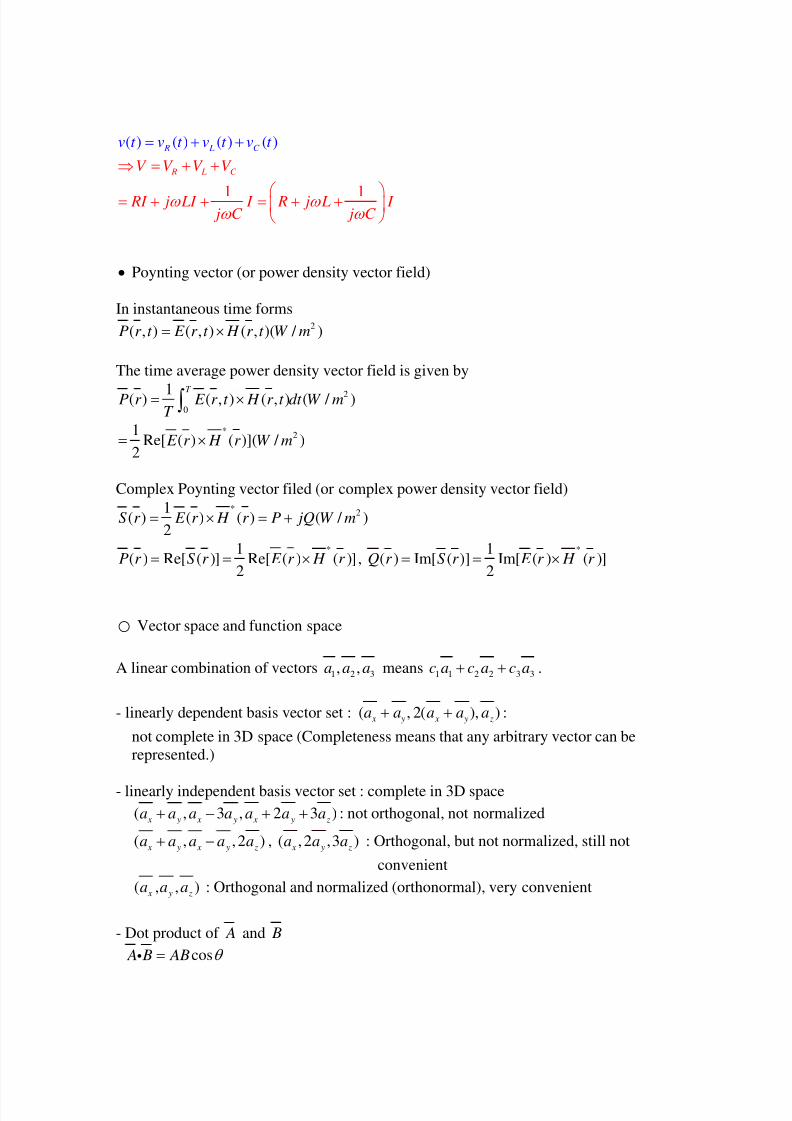
( ) ( ) ( ) ( ) R L C v t v t v t v t = + +

R L C V V V V ⇒ = + +

1 1 RI j LI I R j L I j C j C

ω ω ω ω

⎛ ⎞= + + = + +⎜ ⎟⎝ ⎠

• Poynting vector (or power density vector field)

In instantaneous time forms2

( , ) ( , ) ( , )( / )P r t E r t H r t W m= ×

The time average power density vector field is given by

2

01( ) ( , ) ( , ) ( / )T P r E r t H r t dt W mT

= ×∫

*21

Re[ ( ) ( )]( / )2

E r H r W m= ×

Complex Poynting vector filed (or complex power density vector field)*

21( ) ( ) ( ) ( / )

2S r E r H r P jQ W m= × = +

*1( ) Re[ ( )] Re[ ( ) ( )]

2P r S r E r H r = = × ,

*1( ) Im[ ( )] Im[ ( ) ( )]

2Q r S r E r H r = = ×

○ Vector space and function space

A linear combination of vectors 1 2 3, ,a a a means 1 1 2 2 3 3c a c a c a+ + .

- linearly dependent basis vector set : ( , 2( ), ) x y x y za a a a a+ + :

not complete in 3D space (Completeness means that any arbitrary vector can be

represented.)

- linearly independent basis vector set : complete in 3D space

( , 3 , 2 3 ) x y x y x y za a a a a a a+ − + + : not orthogonal, not normalized

( , , 2 ) x y x y za a a a a+ − , ( , 2 ,3 )

x y za a a : Orthogonal, but not normalized, still not

convenient

( , , ) x y za a a : Orthogonal and normalized (orthonormal), very convenient

- Dot product of A and B

cos A B AB θ =i



- Othogonality(직교성) means

0 x ya a =i

0 y za a =i

0 z xa a =i

- Normalization means

2

1 1 x x x xa a a a= = ⇒ =i

2

1 1 y y y ya a a a= = ⇒ =i

2

1 1 z z z za a a a= = ⇒ =i

A linear combination of linearly independent basis vectors can represent any vector in

space. If we use orthonormal basis vectors, it is also very convenient.

1 2 3 x y z A c a c a c a= + +

x

y

z

A

ya Ac ⋅=2

xa Ac ⋅=1

za Ac ⋅=

3

1 x A a c=i (projection of A on xa )

2 y A a c=i (projection of A on ya ),

3 z A a c=i (projection of A on za )

The function space is similar to the vector space.

The function ( ) f t can be represented by a linear combination of its basis functions.



1 1 2 2 3 3 4 4

1

... n n

n

f c c c c cφ φ φ φ φ ∞

=

= + + + + = ∑

Especially, the periodic function ( ) f t with a period T can be represented by a linear

combination of cos and sin harmonics.

- Orthogonal basis function set:

( )0 0 01,cos ,cos 2 ,cos3 ,....t t t ω ω ω : not complete, can only represent even functions

( )0 0 01,sin ,sin 2 ,sin 3 ,....t t t ω ω ω : not complete, can only represent odd function

( )0 0 0 0 0 01,cos ,cos 2 ,cos3 ,...,sin ,sin 2 ,sin 3 ,...t t t t t t ω ω ω ω ω ω : complete(can represent

any functions), but not

normalized

where the fundamental radian frequency is given by 0

2( / )rad s

T

π ω =

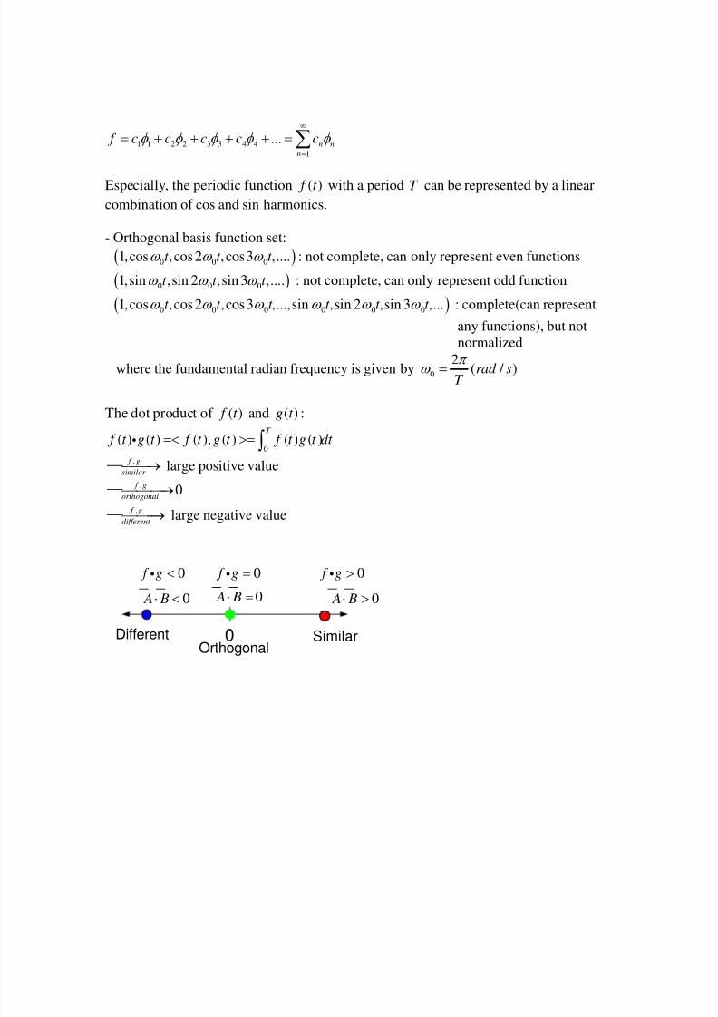
The dot product of ( ) f t and ( )g t :

0( ) ( ) ( ), ( ) ( ) ( )

T

f t g t f t g t f t g t dt =< >= ∫i

, f g

similar ⎯⎯→ large positive value

,0

f g

orthogonal ⎯⎯⎯→

, f g

different ⎯⎯⎯→ large negative value

0=⋅ B A

0Orthogonal

Different Similar

0>⋅ B A0<⋅ B A

0 f g <i 0 f g =i 0 f g >i



( ) f t

( )g t

t

t

t

( ) ( ) f t g t

0, ( ) ( ) 0

T

f g f g f t g t dt =< >= =∫i

T

T

T

A

B

Orthogonal vectors and functions

0 A B =i

+

- -+

( ) f t

( )g t

t

t

t

( ) ( ) f t g t

0, ( ) ( ) 0

T

f g f g f t g t dt =< >= >∫i

T

T

T

A

B

Similar vectors and similar functions

0 A B >i

+ + +

( ) f t

( )g t

( ) ( ) f t g t

0, ( ) ( ) 0

T

f g f g f t g t dt =< >= <∫i

A

B

0 A B <i



- Orthonormal basis function set:

0 0 0 0 0 0

1 2 2 2 2 2 2

, cos , cos 2 , cos3 ,..., sin , sin 2 , sin 3t t t t t t T T T T T T T ω ω ω ω ω ω

- Orthogonality means

0 0 00

1 2 1 2 2cos , cos cos 0

T

t t tdt T T T T T

ω ω ω = = =∫i

0 0 0 0 0 00

2 2 2 2 2cos cos 2 cos , cos 2 cos cos 2 0

T

t t t t t tdt T T T T T

ω ω ω ω ω ω = = =∫i

0 0 0 0 0 00

2 2 2 2 2cos sin cos , sin cos sin 0T t t t t t tdt T T T T T

ω ω ω ω ω ω = = =∫i

0 0 0 0 0 00

2 2 2 2 2sin sin 2 sin , sin 2 sin sin 2 0

T

t t t t t tdt T T T T T

ω ω ω ω ω ω = = =∫i

i

i

- Normalization means

2

01 1 1 1 1 1, 1T dt

T T T T T T = = = =∫i

2

0 0 0 0 0

2 2 2 2 2cos cos cos , cos cost t t t t

T T T T T ω ω ω ω ω = =i

2 00

0 0

1 cos 22 2cos 1

2

T T t tdt dt

T T

ω ω

+= = =∫ ∫

2

0 0 0 0 0

2 2 2 2 2

cos 2 cos 2 cos 2 , cos 2 cos 2t t t t t T T T T T ω ω ω ω ω = =i

2 00

0 0

1 cos 42 2cos 2 1

2

T T t tdt dt

T T

ω ω

+= = =∫ ∫

2

0 0 0 0 0

2 2 2 2 2sin sin sin , sin sint t t t t

T T T T T ω ω ω ω ω = =i

2 00

0 0

1 cos 22 2cos 1

2

T T t tdt dt

T T

ω ω

−= = =∫ ∫

.



⇒ 1

1T

= , 0

2cos 1n t

T ω = , 0

2sin 1n t

T ω =

In summary, the orthonormal basis functions have the property that

0( ) ( ) ( ), ( ) ( ) ( ) 0

T

i j i j i jt t t t t t dt φ φ φ φ φ φ =< >= =∫i for i j≠

= 1 for i j=

A linear combination of linearly independent basis functions can represent any periodic

functions. . If we use orthonormal basis functions, it is very convenient.

0 1 0 2 0 1 0 2 0

1 2 2 2 2( ) cos cos 2 ... sin sin 2 ... f t a a t a t b t b t

T T T T T ω ω ω ω = + + + + + +

T

1

t T

0cos2 ω

t

T 0sin

2ω

t T

02sin2

ω

0a

1a

1b

2b )(t f

0

1( ) f t a

T =i ( projection of ( ) f t on

1

T )

0 1

2( ) cos f t t a

T ω =i ( projection of ( ) f t on

0

2cos t

T ω )



0 2

2( ) cos 2 f t t a

T ω =i ( projection of ( ) f t on 0

2cos2 t

T ω )

i

i

0 1

2( ) sin f t t b

T ω =i ( projection of ( ) f t on

0

2sin t

T ω )

0 2

2( ) sin 2 f t t b

T ω =i ( projection of ( ) f t on 0

2sin 2 t

T ω )

i

i

In summary, 0 0 01 1

1 2 2

( ) cos sinn nn n f t a a n t b n t T T T ω ω

∞ ∞

= =

= + +

∑ ∑

(called as Fourier series)

where

0

1( )a f t

T = i ( projection of ( ) f t on

1

T )

0

2( ) cosn

a f t n t T

ω = i ( projection of ( ) f t on 0

2cos n t

T ω )

02( ) sin

nb f t n t

T ω = i ( projection of ( ) f t on 0

2 sin n t T

ω )

( na , nb : all real number)

Instead of sinusoidal basis functions which consist of cos and sin , we may use the

exponential orthonormal basis function set

0 0 0 02 201 1 1 1 1(..., , , , , ,...)

j t j t j t j t j t e e e e e

T T T T T

ω ω ω ω − − − .

The complex functions 1( )t φ and 2 ( )t φ are orthogonal if

*

1 20

( ) ( ) 0T

t t dt φ φ =∫ .

For example, 01 j t

eT

ω −and 0

1 j t e

T

ω are orthogonal since

0 0 0

*

2

0 00 0 0

1 1 1 1(cos 2 sin 2 ) 0

T T T j t j t j t

e e dt e dt t j t dt T T T T

ω ω ω ω ω − −⎛ ⎞

= = − =⎜ ⎟⎜ ⎟⎝ ⎠

∫ ∫ ∫

The exponential orthonormal basis function set given above is the normalized one since



0 0 0

2 *

0

1 1 1T jn t jn t jn t

e e e dt T T T

ω ω ω ⎛ ⎞

= ⎜ ⎟⎜ ⎟⎝ ⎠

∫

00

0

1 11 1

T jn t j t

e dt eT T

ω = = ⇒ =∫ .

Now, we can conveniently represent any periodic function with

0 0 0 02 20

2 1 0 1 2

1 1 1 1 1( ) ... ...

j t j t j t j t j t f t c e c e c e c e c eT T T T T

ω ω ω ω − − −− −= + + + + + +

The price we have to pay for using just one kind of basis functions is that the radian

frequencies must be extended to negative ones to form complex conjugate pairs for therepresentation of a real function ( ) f t .

Note that the pair, for example, 02

2

1 j t c e

T

ω −− and 02

2

1 j t c e

T

ω must be a complex

conjugate pair. *

2 2( )c c−⇒ = to represent a real function.

To determine 2c− , we do 021 j t e

T

ω i operations on both sides of the equation.

0 0 02 2 2

2 2

1 1 1( ) ...0 0...

j t j t j t f t e c e e c

T T T

ω ω ω −− −= + + =i i

0 0 0

0

1 1 1( ) ( ), ( )

T jn t jn t jn t

nc f t e f t e f t e dt

T T T

ω ω ω − − −⇒ = =< >= ∫i

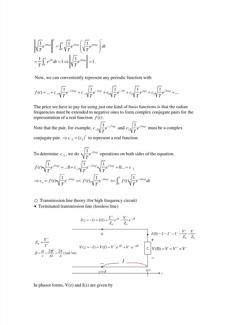
○ Transmission line theory (for high frequency circuit)

• Terminated transmission line (lossless line)

ZL

zZ=0

l jl je

Z

V e

Z

V l I l z I

β β −−+

−==−=00

)()(

l jl jeV eV lV l zV

β β −−+ +==−= )()(

l z −=

l

+

+

= I

V Z

0

) / (22

mrad f

f

v λ

π

λ

π ω β ===

−+ +== V V V V )0(

+

-

00

)0( Z

V

Z

V I I I I

−+−+ −=−==

In phasor forms, V(z) and I(z) are given by



( )j z j z

V z V e V e β β + − −= + , ( ) ( )

j l j lV z l V l V e V e

β β + − −= − = = +

+V

−V

1l 2l

2l jeV β −+

2l jeV

β −

1l jeV

β +

1l jeV

β −−

−+ += V V V 22 l jl jeV eV V

β β −−+ +=11 l jl jeV eV V

β β −−+ +=

0 0

( ) j z j zV V I z e e Z Z

β β

+ −

−= − ,0 0

( ) ( ) j l j lV V I z l I l e e Z Z

β β

+ −

−= − = = −

At 0 z = , ( 0) (1)V z V V V + −= = = + → ,

0 0

( 0) (2) L

V V V I z I I I

Z Z Z

+ −+ −= = = + = − = →

V + : known,

V − , V : unknown

Using equations (1) and (2), we obtain

0

0

L

L

Z Z V V

Z Z

− +−=

+,

0

2 L

L

Z V V

Z Z

+=+

Prob) When V + =10 and 0 50 Z = , obtain ( )V l and ( ) I l , and plot | ( ) |V l , [ ( )] phase V l ,

| ( ) | I l , [ ( )] phase I l as a function of l β in case of 50 L Z = ,

L Z = ∞ (open),

and 0 L Z = (short).

The reflection coefficient at the load(z=0)is defined as

0 ( ; )0

0

(0) 1 L L Z Z Z open L

L

Z Z V

V Z Z

−→∞

+

−Γ = = ⎯⎯⎯⎯⎯⎯⎯→

+

03 1

2 L Z Z = ⎯⎯⎯→

0 ( )0 L Z Z matched = ⎯⎯⎯⎯⎯→

0

1

31

2

L Z Z =

⎯⎯⎯→ −

0 ( 0)1 L L Z Z Z = → ⎯⎯⎯⎯⎯→ −

and transmission coefficient at the load(z=0) is defined as



0 ( ; )

0

2(0) 1 (0) 2 L L Z Z Z open L

L

Z V T

V Z Z

→∞

−= = = + Γ ⎯⎯⎯⎯⎯⎯⎯→

+

03 3

2 L

Z Z =

⎯⎯⎯→

0 ( )1 L Z Z matched = ⎯⎯⎯⎯⎯→

0

1

31

2

L Z Z =

⎯⎯⎯→

0 ( 0; )0 L L Z Z Z short = → ⎯⎯⎯⎯⎯⎯→

( ) ( ) j l j lV z l V l V e V e β β + − −= − = = +

2( ) ( ) (0) j l

j l

j l

V e z l l e

V e

β β

β

− −−

+Γ = − = Γ = = Γ

3, , ,...

2 2,2 ,3 ,...

(0)l

l

λ λ λ

β π π π

=

= ⎯⎯⎯⎯→Γ

1-1

j

-j

)0(Γl jel

β 2)0()(

−Γ=Γ

)(lΓ

)(lΓ− )4 / ( π β =Γ l

)2 / ( π β =Γ l

)4 / 3( π β =Γ l

)( π β =Γ l

( ) ( ) (0) j l j l j l j l

V z l V l V e V e V e V e β β β β + − − + + −

= − = = + = + Γ 2

[1 (0) ] [1 ( )] j l j l j lV e e V e l

β β β + − += + Γ = + Γ

0 0 0 0

(0)( ) ( ) j l j l j l j lV V V V

I z l I l e e e e Z Z Z Z

β β β β + − + +

− −Γ= − = = − = −

2

0 0

[1 (0) ] [1 ( )] j l j l j lV V e e e l

Z Z

β β β + +

−= − Γ = − Γ

Input power



2*

*

0 0

1 1Re ( ) Re ( )

2 2 2in

V V P V I V W

Z Z

+++ + +

⎡ ⎤⎛ ⎞⎡ ⎤ ⎢ ⎥= = =⎜ ⎟⎣ ⎦

⎢ ⎥⎝ ⎠⎣ ⎦

Reflected power2 2 2

0 0

( )2 2

ref

V V P W

Z Z

− + Γ= =

Power consumed in the load

( )*

*

0 0

1 1Re Re

2 2 L

V V P VI V V

Z Z

+ −+ −

⎡ ⎤⎛ ⎞⎡ ⎤ ⎢ ⎥= = + −⎜ ⎟⎣ ⎦

⎢ ⎥⎝ ⎠⎣ ⎦

2 2* *

0 0 0

1 ( ) ( )Re

2

V V V V V V

Z Z Z

+ − − + − +⎡ ⎤−⎢ ⎥= − +⎢ ⎥⎣ ⎦

(Note that* *

( ) ( )V V V V − + − +− is purely imaginary.)

2 2 2 2 2

0 0 0 02 2 2 2in ref

V V V V P P

Z Z Z Z

+ − + + Γ= − = − = −

Power conservation law:

in ref LP P P− = or in ref LP P P= +

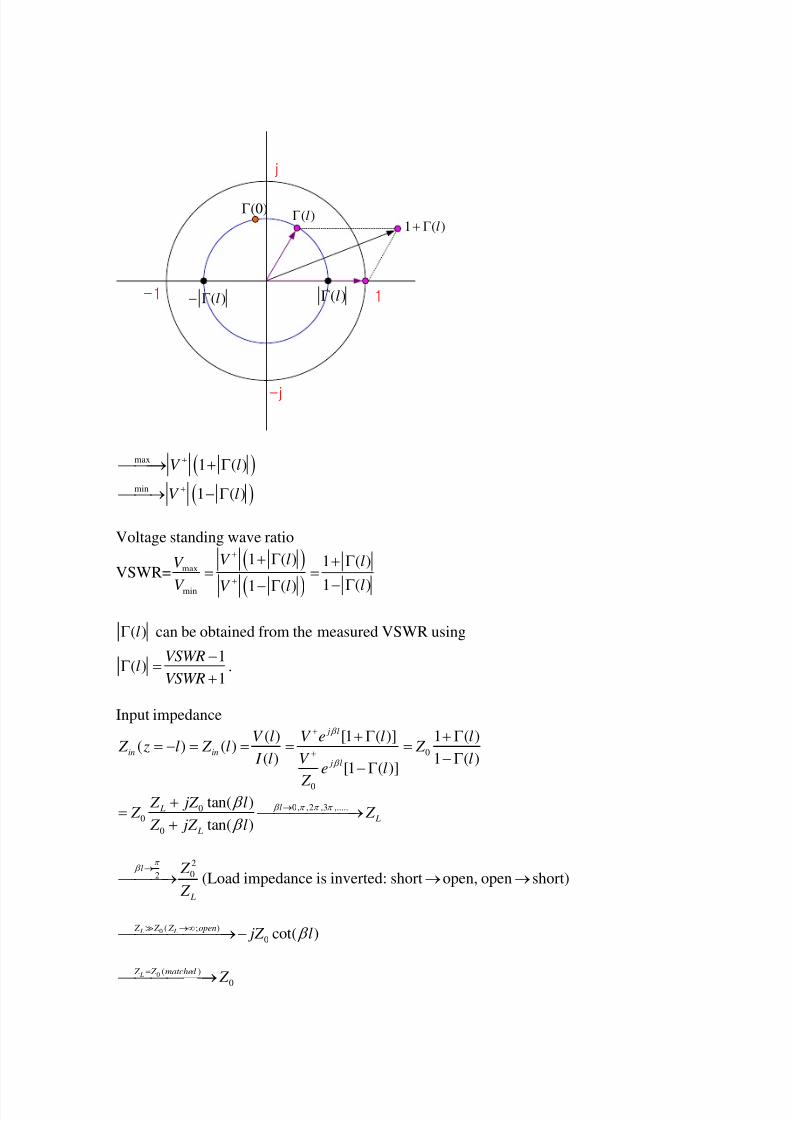
Absolute value of voltage along the line:2( ) 1 (0) 1 ( ) j l

V l V e V l β + − += + Γ = + Γ



1-1

j

-j

)0(Γ)(lΓ

)(1 lΓ+

)(lΓ)(lΓ−

( )max1 ( )V l

+ ⎯⎯⎯→ + Γ

( )min 1 ( )V l+ ⎯⎯→ − Γ

Voltage standing wave ratio

VSWR=( )

( )

max

min

1 ( ) 1 ( )

1 ( )1 ( )

V l lV

V lV l

+

+

+ Γ + Γ= =

− Γ− Γ

( )lΓ can be obtained from the measured VSWR using

1( )

1

VSWRl

VSWR

−Γ =

+.

Input impedance

0

0

( ) [1 ( )] 1 ( )( ) ( )

( ) 1 ( )[1 ( )]

j l

in in

j l

V l V e l l Z z l Z l Z

V I l le l

Z

β

β

+

+

+ Γ + Γ= − = = = =

− Γ− Γ

0, ,2 ,3 ,.....00

0

tan( )

tan( )

l L L

L

Z jZ l Z Z

Z jZ l

β π π π β

β

→+= ⎯⎯⎯⎯⎯⎯→

+

2

02l

L

Z

Z

π β →

⎯⎯⎯→ (Load impedance is inverted: short → open, open → short)

0 ( ; )

0 cot( ) L L Z Z Z open jZ l β

→∞ ⎯⎯⎯⎯⎯⎯⎯→ −

0 ( )

0

L Z Z matched

Z

=

⎯⎯⎯⎯⎯⎯→



0 ( 0; )

0 tan( ) L L Z Z Z short jZ l β

→ ⎯⎯⎯⎯⎯⎯⎯→

0

0

( ) [1 ( )] 1 ( )( ) ( )

( ) 1 ( )[1 ( )]

j l

in in

j l

V l V e l l Z z l Z l Z

V I l le l

Z

β

β

+

+

+ Γ + Γ= − = = = =

− Γ− Γ

Normalized input impedance

0

( ) 1 ( )( )

1 ( )

inin

Z l l z l

Z l

+ Γ= =

− Γ

0

( ) ( ) 1( )

( ) 1

in in

in

Z l z ll

Z z l

−Γ = =

+

Smith chart : ( )in z l r jx= + ( )

( )in

Want l

Want z l

−Γ

− ⎯⎯⎯→←⎯⎯⎯⎯ ( )lΓ

r=1r=0

x=0

x=1

x=-1

1)( =Γ↔∞= open zin1)(0 −=Γ↔= short zin)(

01

matching

zin =Γ↔=

°≈Γ↔+= 5.6345.01 j

in e j z

°−≈Γ↔−= 5.6345.01

j

ine j z

°=Γ↔= 90 j

in e j z

°−=Γ↔−= 90 j

ine j z

Smith chart (Complex Γ plane mapped to in z r jx= + )

Prob) When 0 50( ) Z = Ω , obtain (0)Γ , ( )8

lλ

Γ = , ( )4

lλ

Γ = , ( )2

lλ

Γ = , ( )l λ Γ = , (0)in z

( )8

in z lλ

= , ( )4

in z lλ

= , ( )2

in z lλ

= , and ( )in z l λ = in case of

L Z = ∞ (open), 150( ) L Z = Ω ,

50( ) L Z = Ω , 50 /3( ) L Z = Ω , and 0 L Z = (short) by calculation and using the Smith chart.

Prob) When 20( )V V + = and 0 50( ) Z = Ω , obtain (0)Γ , V

− , V V V + −= + , VSWR,

inP ,

ref P , and LP , in case of L Z = ∞ (open), 150( ) L Z = Ω , 50( ) L Z = Ω , 50 /3( ) L Z = Ω ,

and 0 L Z = (short).

fundamentals for radio engineers

Documents