fundamentals in nuclear physics
TRANSCRIPT

Fundamentals in Nuclear Physics

The Ecole Polytechnique, one of France’s top academic institutions, has a long-standing tradition of producing exceptional scientific textbooks for its students.The original lecture notes, the Cours de l’Ecole Polytechnique, which were writtenby Cauchy and Jordan in the nineteenth century, are considered to be landmarksin the development of mathematics.The present series of textbooks is remarkable in that the texts incorporate themost recent scientific advances in courses designed to provide undergraduatestudents with the foundations of a scientific discipline. An outstanding level ofquality is achieved in each of the seven scientific fields taught at the Ecole: pureand applied mathematics, mechanics, physics, chemistry, biology, and econom-ics. The uniform level of excellence is the result of the unique selection of aca-demic staff there which includes, in addition to the best researchers in its ownrenowned laboratories, a large number of world-famous scientists, appointed aspart-time professors or associate professors, who work in the most advancedresearch centers France has in each field.Another distinctive characteristics of these courses is their overall consistency;each course makes appropriate use of relevant concepts introduced in the othertextbooks. This is because each student at the Ecole Polytechnique has to acquirebasic knowledge in the seven scientific fields taught there, so a substantial linkbetween departments is necessary. The distribution of these courses used to berestricted to the 900 students at the Ecole. Some years ago we were very success-ful in making these courses available to a larger French-reading audience. Wenow build on this success by making these textbooks also available in English.

Jean-Louis BasdevantJames RichMichel Spiro
FundamentalsIn Nuclear PhysicsFrom Nuclear Structure to Cosmology
With 184 Figures

Prof. Jean-Louis BasdevantEcole PolytechniqueDepartement de PhysiqueLaboratoire Leprince-Ringuet91128 [email protected]
Dr. James RichDapnia-SPPCEA-Saclay91191 [email protected]
Dr. Michel SpiroIN2P3-CNRS3 Rue Michel-Ange75794 Paris cedex [email protected]
Cover illustration: Background image—Photograph of Supernova 1987A Rings. Photo credit Chris-topher Burrows (ESA/STScI) and NASA, Hubble Space Telescope, 1994. Smaller images, from topto bottom—Photograph of Supernova Blast. Photo credit Chun Shing Jason Pun (NASA/GSFC),Robert P. Kirshner (Harvard-Smithsonian Center for Astrophysics), and NASA, 1997. Interior ofthe JET torus. Copyright 1994 EFDA-JET. See figure 7.6 for further description. The combustionchamber at the Nova laser fusion facility (Lawrence Livermore National Laboratory, USA). Insidethe combustion chamber at the Nova laser fusion facility (Lawrence Livermore National Labora-tory, USA) The Euratom Joint Research Centres and Associated Centre.
Library of Congress Cataloging-in-Publication DataBasdevant, J.-L. (Jean-Louis)
Fundamentals in nuclear physics / J.-L. Basdevant, J. Rich, M. Spiro.p. cm.
Includes bibliographical references and index.ISBN 0-387-01672-4 (alk. paper)1. Nuclear physics. I. Rich, James, 1952– II. Spiro, M. (Michel) III. Title.
QC173.B277 2004539.7—dc22 2004056544
ISBN 0-387-01672-4 Printed on acid-free paper.
©2005 Springer Science+Business Media, Inc.All rights reserved. This work may not be translated or copied in whole or in part without thewritten permission of the publisher (Springer Science+Business Media, Inc., 233 Spring Street, NewYork, NY 10013, USA), except for brief excerpts in connection with reviews or scholarly analysis.Use in connection with any form of information storage and retrieval, electronic adaptation, com-puter software, or by similar or dissimilar methodology now known or hereafter developed is for-bidden.The use in this publication of trade names, trademarks, service marks and similar terms, even ifthey are not identified as such, is not to be taken as an expression of opinion as to whether or notthey are subject to proprietary rights.
Printed in the United States of America. (EB)
9 8 7 6 5 4 3 2 1 SPIN 10925645
springeronline.com

Preface
Nuclear physics began one century ago during the “miraculous decade” be-tween 1895 and 1905 when the foundations of practically all modern physicswere established. The period started with two unexpected spinoffs of theCrooke’s vacuum tube: Roentgen’s X-rays (1895) and Thomson’s electron(1897), the first elementary particle to be discovered. Lorentz and Zeemanndeveloped the the theory of the electron and the influence of magnetism onradiation. Quantum phenomenology began in December, 1900 with the ap-pearance of Planck’s constant followed by Einstein’s 1905 proposal of whatis now called the photon. In 1905, Einstein also published the theories ofrelativity and of Brownian motion, the ultimate triumph of Boltzman’s sta-tistical theory, a year before his tragic death. For nuclear physics, the criticaldiscovery was that of radioactivity by Becquerel in 1896.
By analyzing the history of science, one can be convinced that there issome rationale in the fact that all of these discoveries came nearly simul-taneously, after the scientifically triumphant 19th century. The exception isradioactivity, an unexpected baby whose discovery could have happened sev-eral decades earlier.
Talented scientists, the Curies, Rutherford, and many others, took the ob-servation of radioactivity and constructed the ideas that are the subject of thisbook. Of course, the discovery of radioactivity and nuclear physics is of muchbroader importance. It lead directly to quantum mechanics via Rutherford’splanetary atomic model and Bohr’s interpretation of the hydrogen spectrum.This in turn led to atomic physics, solid state physics, and material science.Nuclear physics had the important by-product of elementary particle physicsand the discovery of quarks, leptons, and their interactions. These two fieldsare actually impossible to dissociate, both in their conceptual and in theirexperimental aspects.
The same “magic decade” occurred in other sectors of human activity. Thesecond industrial revolution is one aspect, with the development of radio andtelecommunications. The automobile industry developed at the same period,with Daimler, Benz, Panhard and Peugeot. The Wright brothers achieved adream of mankind and opened the path of a revolution in transportation.Medicine and biology made incredible progress with Louis Pasteur and manyothers. In art, we mention the first demonstration of the “cinematographe”

VI Preface
by Auguste and Louis Lumiere on december 28 1895, at the Grand Cafe, onBoulevard des Capucines in Paris and the impressionnist exhibition in Parisin 1896.
Nowadays, is is unthinkable that a scientific curriculum bypass nuclearphysics. It remains an active field of fundamental research, as heavy ionaccelerators of Berkeley, Caen, Darmstadt and Dubna continue to producenew nuclei whose characteristics challenge models of nuclear structure. Ithas major technological applications, most notably in medicine and in en-ergy production where a knowledge of some nuclear physics is essential forparticipation in decisions that concern society’s future.
Nuclear physics has transformed astronomy from the study of planetarytrajectories into the astrophysical study of stellar interiors. No doubt the mostimportant result of nuclear physics has been an understanding how the ob-served mixture of elements, mostly hydrogen and helium in stars and carbonand oxygen in planets, was produced by nuclear reactions in the primordialuniverse and in stars.
This book emerged from a series of topical courses we delivered since thelate 1980’s in the Ecole Polytechnique. Among the subjects studied were thephysics of the Sun, which uses practically all fields of physics, cosmology forwhich the same comment applies, and the study of energy and the environ-ment. This latter subject was suggested to us by many of our students whofelt a need for deeper understanding, given the world in which they weregoing to live. In other words, the aim was to write down the fundamentalsof nuclear physics in order to explain a number of applications for which wefelt a great demand from our students.
Such topics do not require the knowledge of modern nuclear theory thatis beautifully described in many books, such as The Nuclear Many BodyProblem by P. Ring and P Schuck. Intentionally, we have not gone into suchdevelopments. In fact, even if nuclear physics had stopped, say, in 1950 or1960, practically all of its applications would exist nowadays. These appli-cations result from phenomena which were known at that time, and needonly qualitative explanations. Much nuclear phenomenology can be under-stood from simple arguments based on things like the Pauli principle and theCoulomb barrier. That is basically what we will be concerned with in thisbook. On the other hand, the enormous amount of experimental data noweasily accesible on the web has greatly facilitated the illustration of nuclearsystematics and we have made ample use of these resources.
This book is an introduction to a large variety of scientific and techno-logical fields. It is a first step to pursue further in the study of such or suchan aspect. We have taught it at the senior undergraduate level at the EcolePolytechnique. We believe that it may be useful for graduate students, ormore generally scientists, in a variety of fields.
In the first three chapters, we present the “scene” , i.e. we give the basicnotions which are necessary to develop the rest. Chapter 1 deals with the

Preface VII
basic concepts in nuclear physics. In chapter 2, we describe the simple nu-clear models, and discuss nuclear stability. Chapter 3 is devoted to nuclearreactions.
Chapter 4 goes a step further. It deals with nuclear decays and the fun-damental electro-weak interactions. We shall see that it is possible to give acomparatively simple, but sound, description of the major progress particlephysics and fundamental interactions made since the late 1960’s.
In chapter 5, we turn to the first important practical application, i.e.radioactivity. We shall see examples of how radioactivity is used be it inmedicine, in food industry or in art.
Chapters 6 and 7 concern nuclear energy. Chapter 6 deals with fission andthe present aspects of that source of energy production. Chapter 7 deals withfusion which has undergone quite remarkable progress, both technologicallyand politically in recent years with the international ITER project.
Fusion brings us naturally, in chapter 8 to the subject of nuclear as-trophysics and stellar structure and evolution. Finally, we present an intro-duction to present ideas about cosmology in chapter 9. A more advanceddescription can be found in Fundamentals of Cosmology, written by one ofus (J. R.).
We want to pay a tribute to the memory of Dominique Vautherin, whoconstantly provided us with ideas before his tragic death in December 2000.We are grateful to Martin Lemoine, Robert Mochkovitch, Hubert Flocard,Vincent Gillet, Jean Audouze and Alfred Vidal-Madjar for their invaluablehelp and advice throughout the years. We also thank Michel Casse, BertrandCordier, Michel Cribier, David Elbaz, Richard Hahn, Till Kirsten, SylvaineTurck-Chieze, and Daniel Vignaud for illuminating discussions on variousaspects of nuclear physics.
Palaiseau, France Jean-Louis Basdevant, James Rich, Michel SpiroApril, 2005

Contents
Introduction . . . . . . . . . . . . . . . . . . . . . . . . . . . . . . . . . . . . . . . . . . . . . . . . . . 1
1. Basic concepts in nuclear physics . . . . . . . . . . . . . . . . . . . . . . . . . 91.1 Nucleons and leptons . . . . . . . . . . . . . . . . . . . . . . . . . . . . . . . . . . . 91.2 General properties of nuclei . . . . . . . . . . . . . . . . . . . . . . . . . . . . . . 11
1.2.1 Nuclear radii . . . . . . . . . . . . . . . . . . . . . . . . . . . . . . . . . . . . 121.2.2 Binding energies . . . . . . . . . . . . . . . . . . . . . . . . . . . . . . . . . 141.2.3 Mass units and measurements . . . . . . . . . . . . . . . . . . . . . . 17
1.3 Quantum states of nuclei . . . . . . . . . . . . . . . . . . . . . . . . . . . . . . . 251.4 Nuclear forces and interactions . . . . . . . . . . . . . . . . . . . . . . . . . . . 29
1.4.1 The deuteron . . . . . . . . . . . . . . . . . . . . . . . . . . . . . . . . . . . . 311.4.2 The Yukawa potential and its generalizations . . . . . . . . 351.4.3 Origin of the Yukawa potential . . . . . . . . . . . . . . . . . . . . . 381.4.4 From forces to interactions . . . . . . . . . . . . . . . . . . . . . . . . 39
1.5 Nuclear reactions and decays . . . . . . . . . . . . . . . . . . . . . . . . . . . . . 411.6 Conservation laws . . . . . . . . . . . . . . . . . . . . . . . . . . . . . . . . . . . . . . 43
1.6.1 Energy-momentum conservation . . . . . . . . . . . . . . . . . . . . 441.6.2 Angular momentum and parity (non)conservation . . . . 461.6.3 Additive quantum numbers . . . . . . . . . . . . . . . . . . . . . . . . 461.6.4 Quantum theory of conservation laws . . . . . . . . . . . . . . . 48
1.7 Charge independence and isospin . . . . . . . . . . . . . . . . . . . . . . . . . 511.7.1 Isospin space . . . . . . . . . . . . . . . . . . . . . . . . . . . . . . . . . . . . 511.7.2 One-particle states . . . . . . . . . . . . . . . . . . . . . . . . . . . . . . . 521.7.3 The generalized Pauli principle . . . . . . . . . . . . . . . . . . . . . 551.7.4 Two-nucleon system . . . . . . . . . . . . . . . . . . . . . . . . . . . . . . 551.7.5 Origin of isospin symmetry; n-p mass difference . . . . . . 56
1.8 Deformed nuclei . . . . . . . . . . . . . . . . . . . . . . . . . . . . . . . . . . . . . . . . 581.9 Bibliography . . . . . . . . . . . . . . . . . . . . . . . . . . . . . . . . . . . . . . . . . . . 62Exercises . . . . . . . . . . . . . . . . . . . . . . . . . . . . . . . . . . . . . . . . . . . . . . . . . . 62
2. Nuclear models and stability . . . . . . . . . . . . . . . . . . . . . . . . . . . . . . 672.1 Mean potential model . . . . . . . . . . . . . . . . . . . . . . . . . . . . . . . . . . . 692.2 The Liquid-Drop Model . . . . . . . . . . . . . . . . . . . . . . . . . . . . . . . . . 74
2.2.1 The Bethe–Weizsacker mass formula . . . . . . . . . . . . . . . 74

X Contents
2.3 The Fermi gas model . . . . . . . . . . . . . . . . . . . . . . . . . . . . . . . . . . . 772.3.1 Volume and surface energies . . . . . . . . . . . . . . . . . . . . . . . 792.3.2 The asymmetry energy . . . . . . . . . . . . . . . . . . . . . . . . . . . . 81
2.4 The shell model and magic numbers . . . . . . . . . . . . . . . . . . . . . . 812.4.1 The shell model and the spin-orbit interaction . . . . . . . 852.4.2 Some consequences of nuclear shell structure . . . . . . . . . 88
2.5 β-instability . . . . . . . . . . . . . . . . . . . . . . . . . . . . . . . . . . . . . . . . . . . 902.6 α-instability . . . . . . . . . . . . . . . . . . . . . . . . . . . . . . . . . . . . . . . . . . . 942.7 Nucleon emission . . . . . . . . . . . . . . . . . . . . . . . . . . . . . . . . . . . . . . . 982.8 The production of super-heavy elements . . . . . . . . . . . . . . . . . . . 1002.9 Bibliography . . . . . . . . . . . . . . . . . . . . . . . . . . . . . . . . . . . . . . . . . . . 101Exercises . . . . . . . . . . . . . . . . . . . . . . . . . . . . . . . . . . . . . . . . . . . . . . . . . . 101
3. Nuclear reactions . . . . . . . . . . . . . . . . . . . . . . . . . . . . . . . . . . . . . . . . . 1073.1 Cross-sections . . . . . . . . . . . . . . . . . . . . . . . . . . . . . . . . . . . . . . . . . . 108
3.1.1 Generalities . . . . . . . . . . . . . . . . . . . . . . . . . . . . . . . . . . . . . . 1083.1.2 Differential cross-sections . . . . . . . . . . . . . . . . . . . . . . . . . . 1113.1.3 Inelastic and total cross-sections . . . . . . . . . . . . . . . . . . . . 1123.1.4 The uses of cross-sections . . . . . . . . . . . . . . . . . . . . . . . . . . 1133.1.5 General characteristics of cross-sections . . . . . . . . . . . . . 115
3.2 Classical scattering on a fixed potential . . . . . . . . . . . . . . . . . . . 1213.2.1 Classical cross-sections . . . . . . . . . . . . . . . . . . . . . . . . . . . . 1223.2.2 Examples . . . . . . . . . . . . . . . . . . . . . . . . . . . . . . . . . . . . . . . 123
3.3 Quantum mechanical scattering on a fixed potential . . . . . . . . 1263.3.1 Asymptotic states and their normalization . . . . . . . . . . . 1273.3.2 Cross-sections in quantum perturbation theory . . . . . . . 1293.3.3 Elastic scattering . . . . . . . . . . . . . . . . . . . . . . . . . . . . . . . . . 1323.3.4 Quasi-elastic scattering . . . . . . . . . . . . . . . . . . . . . . . . . . . . 1353.3.5 Scattering of quantum wave packets . . . . . . . . . . . . . . . . 136
3.4 Particle–particle scattering . . . . . . . . . . . . . . . . . . . . . . . . . . . . . . 1433.4.1 Scattering of two free particles . . . . . . . . . . . . . . . . . . . . . 1433.4.2 Scattering of a free particle on a bound particle . . . . . . 1463.4.3 Scattering on a charge distribution . . . . . . . . . . . . . . . . . 1493.4.4 Electron–nucleus scattering . . . . . . . . . . . . . . . . . . . . . . . . 1513.4.5 Electron–nucleon scattering . . . . . . . . . . . . . . . . . . . . . . . . 153
3.5 Resonances . . . . . . . . . . . . . . . . . . . . . . . . . . . . . . . . . . . . . . . . . . . . 1573.6 Nucleon–nucleus and nucleon–nucleon scattering . . . . . . . . . . . . 161
3.6.1 Elastic scattering . . . . . . . . . . . . . . . . . . . . . . . . . . . . . . . . . 1613.6.2 Absorption . . . . . . . . . . . . . . . . . . . . . . . . . . . . . . . . . . . . . . 167
3.7 Coherent scattering and the refractive index . . . . . . . . . . . . . . . 1693.8 Bibliography . . . . . . . . . . . . . . . . . . . . . . . . . . . . . . . . . . . . . . . . . . . 171Exercises . . . . . . . . . . . . . . . . . . . . . . . . . . . . . . . . . . . . . . . . . . . . . . . . . . 171

Contents XI
4. Nuclear decays and fundamental interactions . . . . . . . . . . . . . 1754.1 Decay rates, generalities . . . . . . . . . . . . . . . . . . . . . . . . . . . . . . . . . 175
4.1.1 Natural width, branching ratios . . . . . . . . . . . . . . . . . . . . 1754.1.2 Measurement of decay rates . . . . . . . . . . . . . . . . . . . . . . . 1764.1.3 Calculation of decay rates . . . . . . . . . . . . . . . . . . . . . . . . 1784.1.4 Phase space and two-body decays . . . . . . . . . . . . . . . . . . 1834.1.5 Detailed balance and thermal equilibrium . . . . . . . . . . . 184
4.2 Radiative decays . . . . . . . . . . . . . . . . . . . . . . . . . . . . . . . . . . . . . . . 1874.2.1 Electric-dipole transitions . . . . . . . . . . . . . . . . . . . . . . . . . 1884.2.2 Higher multi-pole transitions . . . . . . . . . . . . . . . . . . . . . . . 1904.2.3 Internal conversion . . . . . . . . . . . . . . . . . . . . . . . . . . . . . . . 193
4.3 Weak interactions . . . . . . . . . . . . . . . . . . . . . . . . . . . . . . . . . . . . . . 1954.3.1 Neutron decay . . . . . . . . . . . . . . . . . . . . . . . . . . . . . . . . . . . 1964.3.2 β-decay of nuclei . . . . . . . . . . . . . . . . . . . . . . . . . . . . . . . . . 2024.3.3 Electron-capture . . . . . . . . . . . . . . . . . . . . . . . . . . . . . . . . . 2074.3.4 Neutrino mass and helicity . . . . . . . . . . . . . . . . . . . . . . . . 2094.3.5 Neutrino detection. . . . . . . . . . . . . . . . . . . . . . . . . . . . . . . . 2144.3.6 Muon decay . . . . . . . . . . . . . . . . . . . . . . . . . . . . . . . . . . . . . 218
4.4 Families of quarks and leptons . . . . . . . . . . . . . . . . . . . . . . . . . . . 2214.4.1 Neutrino mixing and weak interactions . . . . . . . . . . . . . . 2214.4.2 Quarks . . . . . . . . . . . . . . . . . . . . . . . . . . . . . . . . . . . . . . . . . . 2284.4.3 Quark mixing and weak interactions . . . . . . . . . . . . . . . . 2324.4.4 Electro-weak unification . . . . . . . . . . . . . . . . . . . . . . . . . . . 235
4.5 Bibliography . . . . . . . . . . . . . . . . . . . . . . . . . . . . . . . . . . . . . . . . . . . 241Exercises . . . . . . . . . . . . . . . . . . . . . . . . . . . . . . . . . . . . . . . . . . . . . . . . . . 241
5. Radioactivity and all that . . . . . . . . . . . . . . . . . . . . . . . . . . . . . . . . 2455.1 Generalities . . . . . . . . . . . . . . . . . . . . . . . . . . . . . . . . . . . . . . . . . . . . 2455.2 Sources of radioactivity . . . . . . . . . . . . . . . . . . . . . . . . . . . . . . . . . 246
5.2.1 Fossil radioactivity . . . . . . . . . . . . . . . . . . . . . . . . . . . . . . . 2475.2.2 Cosmogenic radioactivity . . . . . . . . . . . . . . . . . . . . . . . . . . 2525.2.3 Artificial radioactivity . . . . . . . . . . . . . . . . . . . . . . . . . . . . 254
5.3 Passage of particles through matter . . . . . . . . . . . . . . . . . . . . . . . 2565.3.1 Heavy charged particles . . . . . . . . . . . . . . . . . . . . . . . . . . . 2575.3.2 Particle identification . . . . . . . . . . . . . . . . . . . . . . . . . . . . . 2635.3.3 Electrons and positrons . . . . . . . . . . . . . . . . . . . . . . . . . . . 2655.3.4 Photons . . . . . . . . . . . . . . . . . . . . . . . . . . . . . . . . . . . . . . . . . 2665.3.5 Neutrons . . . . . . . . . . . . . . . . . . . . . . . . . . . . . . . . . . . . . . . . 269
5.4 Radiation dosimetry . . . . . . . . . . . . . . . . . . . . . . . . . . . . . . . . . . . . 2705.5 Applications of radiation . . . . . . . . . . . . . . . . . . . . . . . . . . . . . . . . 273
5.5.1 Medical applications . . . . . . . . . . . . . . . . . . . . . . . . . . . . . . 2735.5.2 Nuclear dating . . . . . . . . . . . . . . . . . . . . . . . . . . . . . . . . . . . 2745.5.3 Other uses of radioactivity . . . . . . . . . . . . . . . . . . . . . . . . 280
5.6 Bibliography . . . . . . . . . . . . . . . . . . . . . . . . . . . . . . . . . . . . . . . . . . . 281Exercises . . . . . . . . . . . . . . . . . . . . . . . . . . . . . . . . . . . . . . . . . . . . . . . . . . 282
XII Contents
6. Fission . . . . . . . . . . . . . . . . . . . . . . . . . . . . . . . . . . . . . . . . . . . . . . . . . . . . 2856.1 Nuclear energy . . . . . . . . . . . . . . . . . . . . . . . . . . . . . . . . . . . . . . . . . 2856.2 Fission products . . . . . . . . . . . . . . . . . . . . . . . . . . . . . . . . . . . . . . . . 2876.3 Fission mechanism, fission barrier . . . . . . . . . . . . . . . . . . . . . . . . 2906.4 Fissile materials and fertile materials . . . . . . . . . . . . . . . . . . . . . . 2956.5 Chain reactions . . . . . . . . . . . . . . . . . . . . . . . . . . . . . . . . . . . . . . . . 2976.6 Moderators, neutron thermalization . . . . . . . . . . . . . . . . . . . . . . . 2996.7 Neutron transport in matter . . . . . . . . . . . . . . . . . . . . . . . . . . . . . 301
6.7.1 The transport equation in a simple uniform sphericallysymmetric medium . . . . . . . . . . . . . . . . . . . . . . . . . . . . . . . 302
6.7.2 The Lorentz equation . . . . . . . . . . . . . . . . . . . . . . . . . . . . . 3056.7.3 Divergence, critical mass . . . . . . . . . . . . . . . . . . . . . . . . . . 306
6.8 Nuclear reactors . . . . . . . . . . . . . . . . . . . . . . . . . . . . . . . . . . . . . . . 3086.8.1 Thermal reactors . . . . . . . . . . . . . . . . . . . . . . . . . . . . . . . . . 3096.8.2 Fast neutron reactors . . . . . . . . . . . . . . . . . . . . . . . . . . . . 3166.8.3 Accelerator-coupled sub-critical reactors . . . . . . . . . . . . . 3196.8.4 Treatment and re-treatment of nuclear fuel . . . . . . . . . . 322
6.9 The Oklo prehistoric nuclear reactor . . . . . . . . . . . . . . . . . . . . . . 3236.10 Bibliography . . . . . . . . . . . . . . . . . . . . . . . . . . . . . . . . . . . . . . . . . . . 326Exercises . . . . . . . . . . . . . . . . . . . . . . . . . . . . . . . . . . . . . . . . . . . . . . . . . . 327
7. Fusion . . . . . . . . . . . . . . . . . . . . . . . . . . . . . . . . . . . . . . . . . . . . . . . . . . . . 3297.1 Fusion reactions . . . . . . . . . . . . . . . . . . . . . . . . . . . . . . . . . . . . . . . . 330
7.1.1 The Coulomb barrier . . . . . . . . . . . . . . . . . . . . . . . . . . . . . 3317.1.2 Reaction rate in a medium . . . . . . . . . . . . . . . . . . . . . . . . 3357.1.3 Resonant reaction rates . . . . . . . . . . . . . . . . . . . . . . . . . . . 338
7.2 Reactor performance criteria . . . . . . . . . . . . . . . . . . . . . . . . . . . . . 3397.3 Magnetic confinement . . . . . . . . . . . . . . . . . . . . . . . . . . . . . . . . . . . 3427.4 Inertial confinement by lasers . . . . . . . . . . . . . . . . . . . . . . . . . . . . 3467.5 Bibliography . . . . . . . . . . . . . . . . . . . . . . . . . . . . . . . . . . . . . . . . . . . 349Exercises . . . . . . . . . . . . . . . . . . . . . . . . . . . . . . . . . . . . . . . . . . . . . . . . . . 349
8. Nuclear Astrophysics . . . . . . . . . . . . . . . . . . . . . . . . . . . . . . . . . . . . . 3518.1 Stellar Structure . . . . . . . . . . . . . . . . . . . . . . . . . . . . . . . . . . . . . . . 351
8.1.1 Classical stars . . . . . . . . . . . . . . . . . . . . . . . . . . . . . . . . . . . . 3528.1.2 Degenerate stars . . . . . . . . . . . . . . . . . . . . . . . . . . . . . . . . . 359
8.2 Nuclear burning stages in stars . . . . . . . . . . . . . . . . . . . . . . . . . . . 3638.2.1 Hydrogen burning . . . . . . . . . . . . . . . . . . . . . . . . . . . . . . . . 3638.2.2 Helium burning . . . . . . . . . . . . . . . . . . . . . . . . . . . . . . . . . . 3668.2.3 Advanced nuclear-burning stages . . . . . . . . . . . . . . . . . . . 3698.2.4 Core-collapse . . . . . . . . . . . . . . . . . . . . . . . . . . . . . . . . . . . . 370
8.3 Stellar nucleosynthesis . . . . . . . . . . . . . . . . . . . . . . . . . . . . . . . . . . 3738.3.1 Solar-system abundances . . . . . . . . . . . . . . . . . . . . . . . . . . 3738.3.2 Production of A < 60 nuclei . . . . . . . . . . . . . . . . . . . . . . . 3768.3.3 A > 60: the s-, r- and p-processes . . . . . . . . . . . . . . . . . . . 376

Contents XIII
8.4 Nuclear astronomy . . . . . . . . . . . . . . . . . . . . . . . . . . . . . . . . . . . . . 3818.4.1 Solar Neutrinos . . . . . . . . . . . . . . . . . . . . . . . . . . . . . . . . . . 3828.4.2 Supernova neutrinos . . . . . . . . . . . . . . . . . . . . . . . . . . . . . . 3908.4.3 γ-astronomy . . . . . . . . . . . . . . . . . . . . . . . . . . . . . . . . . . . . . 392
Exercises . . . . . . . . . . . . . . . . . . . . . . . . . . . . . . . . . . . . . . . . . . . . . . . . . . 394
9. Nuclear Cosmology . . . . . . . . . . . . . . . . . . . . . . . . . . . . . . . . . . . . . . . 3979.1 The Universe today . . . . . . . . . . . . . . . . . . . . . . . . . . . . . . . . . . . . . 399
9.1.1 The visible Universe . . . . . . . . . . . . . . . . . . . . . . . . . . . . . . 4009.1.2 Baryons . . . . . . . . . . . . . . . . . . . . . . . . . . . . . . . . . . . . . . . . . 4019.1.3 Cold dark matter . . . . . . . . . . . . . . . . . . . . . . . . . . . . . . . . . 4019.1.4 Photons . . . . . . . . . . . . . . . . . . . . . . . . . . . . . . . . . . . . . . . . . 4029.1.5 Neutrinos . . . . . . . . . . . . . . . . . . . . . . . . . . . . . . . . . . . . . . . 4039.1.6 The vacuum . . . . . . . . . . . . . . . . . . . . . . . . . . . . . . . . . . . . . 404
9.2 The expansion of the Universe . . . . . . . . . . . . . . . . . . . . . . . . . . . 4059.2.1 The scale factor a(t) . . . . . . . . . . . . . . . . . . . . . . . . . . . . . . 407
9.3 Gravitation and the Friedmann equation . . . . . . . . . . . . . . . . . . 4109.4 High-redshift supernovae and the vacuum energy . . . . . . . . . . . 4169.5 Reaction rates in the early Universe . . . . . . . . . . . . . . . . . . . . . . 4169.6 Electrons, positrons and neutrinos . . . . . . . . . . . . . . . . . . . . . . . . 4209.7 Cosmological nucleosynthesis . . . . . . . . . . . . . . . . . . . . . . . . . . . . . 4249.8 Wimps . . . . . . . . . . . . . . . . . . . . . . . . . . . . . . . . . . . . . . . . . . . . . . . . 434Exercises . . . . . . . . . . . . . . . . . . . . . . . . . . . . . . . . . . . . . . . . . . . . . . . . . . 436
A. Relativistic kinematics . . . . . . . . . . . . . . . . . . . . . . . . . . . . . . . . . . . . 441
B. Accelerators . . . . . . . . . . . . . . . . . . . . . . . . . . . . . . . . . . . . . . . . . . . . . . 445
C. Time-dependent perturbation theory . . . . . . . . . . . . . . . . . . . . . 451C.0.1 Transition rates between two states . . . . . . . . . . . . . . . . . 451C.0.2 Limiting forms of the delta function . . . . . . . . . . . . . . . . 453
D. Neutron transport . . . . . . . . . . . . . . . . . . . . . . . . . . . . . . . . . . . . . . . . 455D.0.3 The Boltzmann transport equation . . . . . . . . . . . . . . . . . 455D.0.4 The Lorentz equation . . . . . . . . . . . . . . . . . . . . . . . . . . . . . 456
E. Solutions and Hints for Selected Exercises . . . . . . . . . . . . . . . . 461
F. Tables of numerical values . . . . . . . . . . . . . . . . . . . . . . . . . . . . . . . . 469
G. Table of Nuclei . . . . . . . . . . . . . . . . . . . . . . . . . . . . . . . . . . . . . . . . . . . 471
References . . . . . . . . . . . . . . . . . . . . . . . . . . . . . . . . . . . . . . . . . . . . . . . . . . . . 507
Index . . . . . . . . . . . . . . . . . . . . . . . . . . . . . . . . . . . . . . . . . . . . . . . . . . . . . . . . . 511

Introduction
Nuclear physics started by accident in 1896 with the discovery of radioactiv-ity by Henri Becquerel who noticed that photographic plates were blackenedwhen placed next to uranium-sulfide crystals. He, like Poincare and manyothers, found the phenomenon of “Becquerel rays” fascinating, but he nev-ertheless lost interest in the subject within the following six months. We canforgive him for failing to anticipate the enormous amount of fundamental andapplied physics that would follow from his discovery.
In 1903, the third Nobel prize for Physics was awarded to Becquerel, andto Pierre and Marie Curie. While Becquerel discovered radioactivity, it wasthe Curies who elucidated many of its characteristics by chemically isolatingthe different radioactive elements produced in the decay of uranium. ErnestRutherford, became interested in 1899 and performed a series of brilliantexperiments leading up to his discovery in 1911 of the nucleus itself. Arguablythe founder of nuclear physics, he was, ironically, awarded the Nobel prize inChemistry in 1908.
It can be argued, however, that the first scientists to observe and studyradioactive phenomena were Tycho Brahe and his student Johannes Kepler.They had the luck in 1572 (Brahe) and in 1603 (Kepler) to observe brightstellae novae, i.e. new stars. Such supernovae are now believed to be ex-plosions of old stars at the end of their normal lives.1 The post-explosionenergy source of supernovae is the decay of radioactive nickel (56Ni, half-life6.077 days) and then cobalt (56Co, half-life 77.27 days). Brahe and Keplerobserved that the luminosity of their supernovae, shown in Fig. 0.1, decreasedwith time at a rate that we now know is determined by the nuclear lifetimes.
Like Becquerel, Brahe and Kepler did not realize the importance of whatthey had seen. In fact, the importance of supernovae dwarfs that of radioactiv-ity because they are the culminating events of the process of nucleosynthesis.This process starts in the cosmological “big bang” where protons and neu-tron present in the primordial soup condense to form hydrogen and helium.Later, when stars are formed the hydrogen and helium are processed through1 Such events are extremely rare. In the last millennium, only five of them have
been seen in our galaxy, the Milky Way. The last supernova visible to the nakedeye was seen on February 23, 1987, in the Milky Way’s neighbor, the LargeMagellanic Cloud. The neutrinos and γ-rays emitted by this supernova wereobserved on Earth, starting the subject of extra-solar nuclear astronomy.

2 Introduction
0 100 200 300 400
−4
−2
0
2
4
6
exp(−t / 111days)
log(
flux
)
t (days)Fig. 0.1. The luminosity of Kepler’s supernova as a function of time, as recon-structed in [4]. Open circles are European measurements and filled circles are Ko-rean measurements. Astronomers at the time measured the evolution of the lumi-nosity of the supernovae by comparing it to known stars and planets. It has beenpossible to determine the positions of planets at the time when they were observed,and, with the notebooks, to reconstruct the luminosity curves. The superimposedcurve shows the rate of 56Co decay using the laboratory-measured half life. Thevertical scale gives the visual magnitude V of the star, proportional to the loga-rithm of the photon flux. V = 0 corresponds to a bright star, while V = 5 is thedimmest star that can be observed with the naked eye.
nuclear reactions into heavier elements. These elements are ejected into theinterstellar medium by supernovae. Later, some of this matter condenses toform new stellar systems, now sometimes containing habitable planets madeof the products of stellar nucleosynthesis.
Nuclear physics has allowed us to understand in considerable quantitativedetail the process by which elements are formed and what determines theirrelative abundances. The distribution of nuclear abundances in the SolarSystem is shown in Fig. 8.9. Most ordinary matter2 is in the form of hydrogen(∼ 75% by mass) and helium (∼ 25%). About 2% of the solar system materialis in heavy elements, especially carbon, oxygen and iron. To the extent thatnuclear physics explains this distribution, it allows us to understand why we2 We leave the question of the nature of the unknown cosmological “dark matter”
for Chap. 9.

Introduction 3
live near a hydrogen burning star and are made primarily of elements likehydrogen, carbon and oxygen.
A particularly fascinating result of the theory of nucleosynthesis is thatthe observed mix of elements is due to a number of delicate inequalities ofnuclear and particle physics. Among these are
• The neutron is slightly heavier than the proton;• The neutron–proton system has only one bound state while the neutron–
neutron and proton–proton systems have none;• The 8Be nucleus is slightly heavier than two 4He nuclei and the second
excited state of 12C is slightly heavier than three 4He nuclei.
We will see in Chaps. 8 and 9 that modifying any of these conditions wouldresult in a radically different distribution of elements. For instance, makingthe proton heavier than the neutron would make ordinary hydrogen unstableand none would survive the primordial epoch of the Universe.
The extreme sensitivity of nucleosynthesis to nuclear masses has gener-ated a considerable amount of controversy about its interpretation. It hingesupon whether nuclear masses are fixed by the fundamental laws of physicsor are accidental, perhaps taking on different values in inaccessible regionsof the Universe. Nuclear masses depend on the strengths of the forces be-tween neutrons and protons, and we do not now know whether the strengthsare uniquely determined by fundamental physics. If they are not, we mustconsider the possibility that the masses in “our part of the Universe” are asobserved because other masses give mixes of elements that are less likely toprovide environments leading to intelligent observers. Whether or not such“weak-anthropic selection” had a role in determining the observed nuclearand particle physics is a question that is appealing to some, infuriating toothers. Resolving the question will require better understanding of the originof observed physical laws.
Some history
The history of nuclear physics can be divided into three periods. The first be-gins with the discovery radioactivity of the nucleus and ends in 1939 with thediscovery of fission. During this period, the basic components (protons andneutrons) of the nucleus were discovered as well as the quantum law governingtheir behavior. The second period from 1947 to 1969 saw the development ofnuclear spectroscopy and of nuclear models. Finally, the emergence of a mi-croscopic unifying theory starting in the 1960s allowed one to understand thestructure and behavior of protons and neutrons in terms of the fundamentalinteractions of their constituent particles, quarks and gluons. This period alsosaw the identification of subtle non-classical mechanisms in nuclear structure.
Since the 1940s, nuclear physics has seen important developments, butmost practical applications and their simple theoretical explanations were

4 Introduction
in place by the mid 1950s. This book is mostly concerned with the simplemodels from the early period of nuclear physics and to their application inenergy production, astrophysics and cosmology.
The main stages of this first period of nuclear physics are the following[5, 6].
• 1868 Mendeleev’s periodic classification of the elements.• 1895 Discovery of X-rays by Roentgen.• 1896 Discovery of radioactivity by Becquerel.• 1897 Identification of the electron by J.J. Thomson.• 1898 Separation of the elements polonium and radium by Pierre and Marie
Curie.• 1908 Measurement of the charge +2 of the α particle by Geiger and
Rutherford.• 1911 Discovery of the nucleus by Rutherford; “planetary” model of the
atom.• 1913 Theory of atomic spectra by Niels Bohr.• 1914 Measurement of the mass of the α particle by Robinson and Ruther-
ford.• 1924–1928 Quantum theory (de Broglie, Schrodinger, Heisenberg, Born,
Dirac).• 1928 Theory of barrier penetration by quantum tunneling, application to
α radioactivity, by Gamow, Gurney and Condon.• 1929–1932 First nuclear reactions with the electrostatic accelerator of
Cockcroft and Walton and the cyclotron of Lawrence.• 1930–1933 Neutrino proposed by Pauli and named by Fermi in his theory
of beta decay.• 1932 Identification of the neutron by Chadwick.• 1934 Discovery of artificial radioactivity by F. and I. Joliot-Curie.• 1934 Discovery of neutron capture by Fermi.• 1935 Liquid-drop model and compound-nucleus model of N. Bohr.• 1935 Semi-empirical mass formula of Bethe and Weizsacker.• 1938 Discovery of fission by Hahn and Strassman.• 1939 Theoretical interpretation of fission by Meitner, Bohr and Wheeler.
To these fundamental discoveries we should add the practical applicationsof nuclear physics. Apart from nuclear energy production beginning withFermi’s construction of the first fission reactor in 1942, the most importantare astrophysical and cosmological. Among them are
• 1938 Bethe and Weizsacker propose that stellar energy comes from ther-monuclear fusion reactions.
• 1946 Gamow develops the theory of cosmological nucleosynthesis.• 1953 Salpeter discovers the fundamental solar fusion reaction of two pro-
tons into deuteron.

Introduction 5
• 1957 Theory of stellar nucleosynthesis by Burbidge, Burbidge, Fowler andHoyle.
• 1960– Detection of solar neutrinos• 1987 Detection of neutrinos and γ-rays from the supernova SN1987a.
The scope of nuclear physics
In one century, nuclear physics has found an incredible number of applica-tions and connections with other fields. In the most narrow sense, it is onlyconcerned with bound systems of protons and neutrons. From the beginninghowever, progress in the study of such systems was possible only because ofprogress in the understanding of other particles: electrons, positrons, neutri-nos and, eventually quarks and gluons. In fact, we now have a more completetheory for the physics of these “elementary particles” than for nuclei as such.3
A nuclear species is characterized by its number of protons Z and numberof neutrons N . There are thousands of combinations of N and Z that leadto nuclei that are sufficiently long-lived to be studied in the laboratory. Theyare tabulated in Appendix G. The large number of possible combinations ofneutrons and protons is to be compared with the only 100 or so elementscharacterized simply by Z.4
A “map” of the world of nuclei is shown in Fig. 0.2. Most nuclei areunstable, i.e. radioactive. Generally, for each A = N + Z there is only one ortwo combinations of (N, Z) sufficiently long-lived to be naturally present onEarth in significant quantities. These nuclei are the black squares in Fig. 0.2and define the bottom of the valley of stability in the figure.
One important line of nuclear research is to create new nuclei, both highup on the sides of the valley and, especially, super-heavy nuclei beyond theheaviest now known with A = 292 and Z = 116. Phenomenological argumentssuggest that there exists an “island of stability” near Z = 114 and 126 withnuclei that may be sufficiently long-lived to have practical applications.
The physics of nuclei as such has been a very active domain of research inthe last twenty years owing to the construction of new machines, the heavy ionaccelerators of Berkeley, Caen (GANIL), Darmstadt and Dubna. The physicsof atomic nuclei is in itself a domain of fundamental research. It constitutesa true many-body problem, where the number of constituents is too largefor exact computer calculations, but too small for applying the methods ofstatistical physics. In heavy ion collisions, one discovers subtle effects such aslocal superfluidity in the head-on collision of two heavy ions.3 This is of course a false paradox; the structure of DNA derives, in principle, com-
pletely from the Schrodinger equation and Quantum Electrodynamics. Howeverit is not studied it that spirit.
4 Different isotopes of a same element have essentially the same chemical proper-ties.

6 Introduction
Z=
20
Z=
28Z
=28
Z=
50Z
=50
Z=
82Z
=82
N=20
N=28N=28
N=50N=50
N=82N=82
N=126N=126
Z=
20
N
Z
nucl
eon
emis
sion
spon
tane
ous
fiss
ion
β α
last
neu
tron
unb
ound
half
−lif
e> 1
0
prot
onun
boun
d
last
yr8
deca
yde
cay
A=100
A=200
Fig. 0.2. The nuclei. The black squares are long-lived nuclei present on Earth.Unbound combinations of (N, Z) lie outside the lines marked “last proton/neutronunbound.” Most other nuclei β-decay or α-decay to long-lived nuclei.

Introduction 7
Nuclear physics has had an important by-product in elementary particlephysics and the discovery of the elementary constituents of matter, quarksand leptons, and their interactions. Nuclear physics is essential to the under-standing of the structure and the origin of the world in which we live. Thebirth of nuclear astrophysics is a decisive step forward in astronomy and incosmology. In addition, nuclear technologies play an important role in mod-ern society. We will see several examples. This book is intended to be a firstintroduction to a large variety of scientific and technological fields. It can bea first step in the study of the vast field of nuclear physics.
Bibliography
On the history of nuclear and particle physics:
1. Abraham Pais Inward Bound, Oxford University Press, Oxford, 1986.2. Emilio Segre, From X rays to Quarks, Freeman, San Francisco, 1980.
Introductory textbooks on nuclear physics
1. B. Povh, K. Rith, C. Scholz and F. Zetsche, Particles and Nuclei, Spring-er, Berlin, 2000.
2. W.N. Cottingham and D.A.Greenwood, Nuclear Physics, Cambridge Uni-versity Press, Cambridge, 2002.
3. P.E. Hodgson, E. Gadioli and E. Gadioli Erba, Introductory NuclearPhysics, Clarendon Press, Oxford, 1997.
4. Harald Enge, Introduction to Nuclear Physics, Addison-Wesley, Read-ing, 1966.
5. J. S. Lilley, Nuclear Physics, Wiley, Chichester, 2001.
Advanced textbooks on nuclear physics
1. Nuclear Structure A. Bohr and B. Mottelson, Benjamin, New York, 1969.2. M.A. Preston and R.K. Bhaduri, Structure of the Nucleus, Addison-
Wesley, Reading, 1975.3. S.M. Wong, Nuclear Physics, John Wiley, New York, 1998.4. J.D. Walecka,Theoretical Nuclear and Subnuclear Physics, Oxford Uni-
versity Press, Oxford, 1995.5. A. de Shalit and H. Feshbach,Theoretical Nuclear Physics, Wiley, New
York, 1974.6. D.M. Brink, Nuclear Forces, Pergamon Press, Oxford, 1965.7. J.M. Blatt and V.F. Weisskopf, Theoretical Nuclear Physics, John Wiley
and Sons, New-York, 1963.

1. Basic concepts in nuclear physics
In this chapter, we will discuss the basic ingredients of nuclear physics. Section1.1 introduces the elementary particles that form nuclei and participate innuclear reactions. Sections 1.2 shows how two of these particles, protons andneutrons, combine to form nuclei. The essential results will be that nucleihave volumes roughly proportional to the number of nucleons, ∼ 7 fm3 pernucleon and that they have binding energies that are of order 8 MeV pernucleon. In Sect. 1.3 we show how nuclei are described as quantum states. Theforces responsible for binding nucleons are described in Sect. 1.4. Section 1.5discusses how nuclei can be transformed through nuclear reactions while Sect.1.6 discusses the important conservation laws that constrain these reactionsand how these laws arise in quantum mechanics. Section 1.7 describes theisospin symmetry of these forces. Finally, Sect. 1.8 discusses nuclear shapes.
1.1 Nucleons and leptons
Atomic nuclei are quantum bound states of particles called nucleons of whichthere are two types, the positively charged proton and the uncharged neutron.The two nucleons have similar masses:
mnc2 = 939.56 MeV mpc2 = 938.27 MeV , (1.1)
i.e. a mass difference of order one part per thousand
(mn − mp)c2 = 1.29 MeV . (1.2)
For nuclear physics, the mass difference is much more important than themasses themselves which in many applications are considered to be “infi-nite.” Also of great phenomenological importance is the fact that this massdifference is of the same order as the electron mass
mec2 = 0.511 MeV . (1.3)
Nucleons and electrons are spin 1/2 fermions meaning that their intrinsicangular momentum projected on an arbitrary direction can take on onlythe values of ±h/2. Having spin 1/2, they must satisfy the Pauli exclusionprinciple that prevents two identical particles (protons, neutrons or electrons)

10 1. Basic concepts in nuclear physics
from having the same spatial wavefunction unless their spins are oppositelyaligned.
Nucleons and electrons generate magnetic fields and interact with mag-netic fields with their magnetic moment. Like their spins, their magneticmoments projected in any direction can only take on the values ±µp or ±µn:
µp = 2.792 847 386 (63)µN µn = −1.913 042 75 (45)µN , (1.4)
where the nuclear magneton is
µN =eh
2mp= 3.152 451 66 (28) × 10−14MeV T−1 . (1.5)
For the electron, only the mass and the numerical factor changes
µe = 1.001 159 652 193 (40)µB , (1.6)
where the Bohr magneton is
µB =qh
2me= 5.788 382 63 (52) × 10−11MeV T−1 . (1.7)
Nucleons are bound in nuclei by nuclear forces, which are of short rangebut are sufficiently strong and attractive to overcome the long-range Coulombrepulsion between protons. Because of their strength compared to electromag-netic interactions, nuclear forces are said to be due to the strong interaction(also called the nuclear interaction).
While protons and neutrons have different charges and therefore differ-ent electromagnetic interactions, we will see that their strong interactionsare quite similar. This fact, together their nearly equal masses, justifies thecommon name of “nucleon” for these two particles.
Some spin 1/2 particles are not subject to the strong interaction andtherefore do not bind to form nuclei. Such particles are called leptons to dis-tinguish them from nucleons. Examples are the electron e− and its antipar-ticle, the positron e+. Another lepton that is important in nuclear physics isthe electron–neutrino νe and electron-antineutrino νe. This particle playsa fundamental role in nuclear weak interactions. These interactions, as theirname implies, are not strong enough to participate in the binding of nucleons.They are, however, responsible for the most common form of radioactivity,β-decay.
It is believed that the νe is, in fact, a quantum-mechanical mixture of threeneutrinos of differing mass. While this has some interesting consequences thatwe will discuss in Chap. 4, the masses are sufficiently small (mνc
2 < 3 eV)that for most practical purposes we can ignore the neutrino masses:
mνi ∼ 0 i = 1, 2, 3 . (1.8)
As far as we know, leptons are elementary particles that cannot be con-sidered as bound states of constituent particles. Nucleons, on the other hand,are believed to be bound states of three spin 1/2 fermions called quarks. Two

1.2 General properties of nuclei 11
species of quarks, the up-quark u (charge 2/3) and the down quark d (charge-1/3) are needed to construct the nucleons:
proton = uud , neutron = udd .
The constituent nature of the nucleons can, to a large extent, be ignored innuclear physics.
Besides protons and neutrons, there exist many other particles that arebound states of quarks and antiquarks. Such particles are called hadrons. Fornuclear physics, the most important are the three pions: (π+, π0, π+). Wewill see in Sect. 1.4 that strong interactions between nucleons result fromthe exchange of pions and other hadrons just as electromagnetic interactionsresult from the exchange of photons.
1.2 General properties of nuclei
Nuclei, the bound states of nucleons, can be contrasted with atoms, the boundstates of nuclei and electrons. The differences are seen in the units used byatomic and nuclear physicists:
length : 10−10m (atoms) → 10−15m = fm (nuclei)
energy : eV (atoms) → MeV (nuclei)
The typical nuclear sizes are 5 orders of magnitude smaller than atomic sizesand typical nuclear binding energies are 6 orders of magnitude greater thanatomic energies. We will see in this chapter that these differences are due tothe relative strengths and ranges of the forces that bind atoms and nuclei.
We note that nuclear binding energies are still “small” in the sense thatthey are only about 1% of the nucleon rest energies mc2 (1.1). Since nucleonbinding energies are of the order of their kinetic energies mv2/2, nucleonswithin the nucleus move at non-relativistic velocities v2/c2 ∼ 10−2.
A nuclear species, or nuclide, is defined by N , the number of neutrons,and by Z, the number of protons. The mass number A is the total numberof nucleons, i.e. A = N + Z. A nucleus can alternatively be denoted as
(A, Z) ↔ AX ↔ AZX ↔ A
ZXN ,
where X is the chemical symbol associated with Z (which is also the numberof electrons of the corresponding neutral atom). For instance, 4He is thehelium-4 nucleus, i.e. N = 2 and Z = 2. For historical reasons, 4He is alsocalled the α particle. The three nuclides with Z = 1 also have special names
1H = p = proton 2H = d = deuteron 3H = t = triton
While the numbers (A, Z) or (N, Z) define a nuclear species, they donot determine uniquely the nuclear quantum state. With few exceptions, anucleus (A, Z) possesses a rich spectrum of excited states which can decay

12 1. Basic concepts in nuclear physics
to the ground state of (A, Z) by emitting photons. The emitted photons areoften called γ-rays. The excitation energies are generally in the MeV rangeand their lifetimes are generally in the range of 10−9–10−15 s. Because of theirhigh energies and short lifetimes, the excited states are very rarely seen onEarth and, when there is no ambiguity, we denote by (A, Z) the ground stateof the corresponding nucleus.
Some particular sequences of nuclei have special names:
• Isotopes : have same charge Z, but different N , for instance 23892 U and 235
92 U.The corresponding atoms have practically identical chemical properties,since these arise from the Z electrons. Isotopes have very different nuclearproperties, as is well-known for 238U and 235U.
• Isobars : have the same mass number A, such as 3He and 3H. Because ofthe similarity of the nuclear interactions of protons and neutrons, differentisobars frequently have similar nuclear properties.
Less frequently used is the term isotone for nuclei of the same N , butdifferent Z’s, for instance 14C6 and 16O8.
Nuclei in a given quantum state are characterized, most importantly, bytheir size and binding energy. In the following two subsections, we will discussthese two quantities for nuclear ground states.
1.2.1 Nuclear radii
Quantum effects inside nuclei are fundamental. It is therefore surprising thatthe volume V of a nucleus is, to good approximation, proportional to thenumber of nucleons A with each nucleon occupying a volume of the order ofV0 = 7.2 fm3. In first approximation, stable nuclei are spherical, so a volumeV AV0 implies a radius
R = r0A1/3 with r0 = 1.2 fm . (1.9)
We shall see that r0 in (1.9) is the order of magnitude of the range of nuclearforces.
In Chap. 3 we will show how one can determine the spatial distributionof nucleons inside a nucleus by scattering electrons off the nucleus. Elec-trons can penetrate inside the nucleus so their trajectories are sensitive tothe charge distribution. This allows one to reconstruct the proton density,or equivalently the proton probability distribution ρp(r). Figure 1.1 showsthe charge densities inside various nuclei as functions of the distance to thenuclear center.
We see on this figure that for A > 40 the charge density, therefore theproton density, is roughly constant inside these nuclei. It is independent ofthe nucleus under consideration and it is roughly 0.075 protons per fm3.Assuming the neutron and proton densities are the same, we find a nucleondensity inside nuclei of

1.2 General properties of nuclei 13
H/10
He
Mg
V Sb BiSrC
2 4 6 8r (fm)
0.15
0.10
0.05
char
ge d
ensi
ty (
e f
m)
−3
Fig. 1.1. Experimental charge density (e fm−3) as a function of r(fm) as determinedin elastic electron–nucleus scattering [8]. Light nuclei have charge distributions thatare peaked at r = 0 while heavy nuclei have flat distributions that fall to zero overa distance of ∼ 2 fm.
Table 1.1. Radii of selected nuclei as determined by electron–nucleus scattering [8].The size of a nucleus is characterized by rrms (1.11) or by the radius R of theuniform sphere that would give the same rrms. For heavy nuclei, the latter is givenapproximately by (1.9) as indicated in the fourth column. Note the abnormallylarge radius of 2H.
nucleus rrms R R/A1/3 nucleus rrms R R/A1/3
(fm) (fm) (fm) (fm) (fm) (fm)
1H 0.77 1.0 1.0 16O 2.64 3.41 1.352H 2.11 2.73 2.16 24Mg 2.98 3.84 1.334He 1.61 2.08 1.31 40Ca 3.52 4.54 1.326Li 2.20 2.8 1.56 122Sb 4.63 5.97 1.207Li 2.20 2.8 1.49 181Ta 5.50 7.10 1.259Be 2.2 2.84 1.37 209Bi 5.52 7.13 1.2012C 2.37 3.04 1.33

14 1. Basic concepts in nuclear physics
ρ0 0.15 nucleons fm−3 . (1.10)
If the nucleon density were exactly constant up to a radius R and zero beyond,the radius R would be given by (1.9). Figure 1.1 indicates that the densitydrops from the above value to zero over a region of thickness ∼ 2 fm aboutthe nominal radius R.
In contrast to nuclei, the size of an atom does not increase with Z implyingthat the electron density does increase with Z. This is due to the long-rangeCoulomb attraction of the nucleus for the electrons. The fact that nucleardensities do not increase with increasing A implies that a nucleon does notinteract with all the others inside the nucleus, but only with its nearestneighbors. This phenomenon is the first aspect of a very important propertycalled the saturation of nuclear forces.
We see in Fig. 1.1 that nuclei with A < 20 have charge densities that arenot flat but rather peaked near the center. For such light nuclei, there is nowell-defined radius and (1.9) does not apply. It is better to characterize suchnuclei by their rms radius
(rrms)2 =∫
d3rr2ρ(r)∫d3rρ(r)
. (1.11)
Selected values of rrms as listed in Table 1.1.Certain nuclei have abnormally large radii, the most important being
the loosely bound deuteron, 2H. Other such nuclei consist of one or twoloosely bound nucleons orbiting a normal nucleus. Such nuclei are calledhalo nuclei [7]. An example is 11Be consisting of a single neutron around a10Be core. The extra neutron has wavefunction with a rms radius of ∼ 6 fmcompared to the core radius of ∼ 2.5 fm. Another example is 6He consisting oftwo neutrons outside a 4He core. This is an example of a Borromean nucleusconsisting of three objects that are bound, while the three possible pairs areunbound. In this case, 6He is bound while n-n and n-4He are unbound.
1.2.2 Binding energies
The saturation phenomenon observed in nuclear radii also appears in nuclearbinding energies. The binding energy B of a nucleus is defined as the negativeof the difference between the nuclear mass and the sum of the masses of theconstituents:
B(A, Z) = Nmnc2 + Zmpc2 − m(A, Z)c2 (1.12)
Note that B is defined as a positive number: B(A, Z) = −EB(A, Z) whereEB is the usual (negative) binding energy.
The binding energy per nucleon B/A as a function of A is shown in Fig.1.2. We observe that B/A increases with A in light nuclei, and reaches abroad maximum around A 55 − 60 in the iron-nickel region. Beyond, itdecreases slowly as a function of A. This immediately tells us that energy

1.2 General properties of nuclei 15
H2
He3
He4 Be8C12 O16 Ne20
U235
Pb208
Ba138
Fe56 62NiSr88
O16
He 4
Si28
H3
Si28Mg24
7.0
9.0
8.0
0 50 100 150 200 250
0
A
A28242084 1612
8
6
4
2
B/A
(M
eV)
B/A
(M
eV)
Fig. 1.2. Binding energy per nucleon, B(A, Z)/A, as a function of A. The upperpanel is a zoom of the low-A region. The filled circles correspond to nuclei that arenot β-radioactive (generally the lightest nuclei for a given A). The unfilled circlesare unstable (radioactive) nuclei that generally β-decay to the lightest nuclei for agiven A.

16 1. Basic concepts in nuclear physics
can be released by the “fusion” of light nuclei into heavier ones, or by the“fission” of heavy nuclei into lighter ones.
As for nuclear volumes, it is observed that for stable nuclei which are nottoo small, say for A > 12, the binding energy B is in first approximationadditive, i.e. proportional to the number of nucleons :
B(A, Z) A × 8 MeV ,
or more precisely
7.7 MeV < B(A, Z)/A < 8.8 MeV 12 < A < 225 .
The numerical value of ∼ 8 MeV per nucleon is worth remembering!The additivity of binding energies is quite different from what happens
in atomic physics where the binding energy of an atom with Z electrons in-creases as Z7/3, i.e. Z4/3 per electron. The nuclear additivity is again a man-ifestation of the saturation of nuclear forces mentioned above. It is surprisingfrom the quantum mechanical point of view. In fact, since the binding energyarises from the pairwise nucleon–nucleon interactions, one might expect thatB(A, Z)/A should increase with the number of nucleon pairs A(A − 1)/2.1
The additivity confirms that nucleons only interact strongly with their near-est neighbors.
The additivity of binding energies and of volumes are related via theuncertainty principle. If we place A nucleons in a sphere of radius R, we cansay that each nucleon occupies a volume 4πR3A/3, i.e. it is confined to alinear dimension of order ∆x ∼ A−1/3R. The uncertainty principle 2 thenimplies an uncertainty ∆pi ∼ hA1/3/R for each momentum component. Fora bound nucleon, the expectation value of pi must vanish, 〈pi〉 = 0, implyinga relation between the momentum squared and the momentum uncertainty
(∆pi)2 = 〈p2i 〉 − 〈pi〉2 = 〈p2
i 〉 . (1.13)
Apart from numerical factors, the uncertainty principle then relates the meannucleon kinetic energy with its position uncertainty⟨
p2
2m
⟩∼ h2
2m
A2/3
R2 . (1.14)
Since R r0A1/3 this implies that the average kinetic energy per nucleon
should be approximately the same for all nuclei. It is then not surprising thatthe same is true for the binding energy per nucleon.3 We will see in Chap. 2how this comes about.1 In the case of atoms with Z electrons, it increases as Z4/3. In the case of pairwise
harmonic interactions between A fermions, the energy per particle varies as A5/6.2 See for instance J.-L. Basdevant and J. Dalibard, Quantum mechanics , chapter
16, Springer-Verlag, 2002.3 The virial theorem only guarantees that for power-law potentials these two ener-
gies are of the same order. Since the nuclear potential is not a power law, excep-tions occur. For example, many nuclei decay by dissociation, e.g. 8Be → 4He 4He.Considered as a “bound” state of two 4He nuclei, the binding energy is, in fact,

1.2 General properties of nuclei 17
As we can see from Fig. 1.2, some nuclei are exceptionally strongly boundcompared to nuclei of similar A. This is the case for 4He, 12C, 16O. As weshall see, this comes from a filled shell phenomenon, similar to the case ofnoble gases in atomic physics.
1.2.3 Mass units and measurements
The binding energies of the previous section were defined (1.12) in terms ofnuclear and nucleon masses. Most masses are now measured with a precisionof ∼ 10−8 so binding energies can be determined with a precision of ∼ 10−6.This is sufficiently precise to test the most sophisticated nuclear models thatcan predict binding energies at the level of 10−4 at best.
Three units are commonly used to described nuclear masses: the atomicmass unit (u), the kilogram (kg), and the electron-volt (eV) for rest energies,mc2. In this book we generally use the energy unit eV since energy is amore general concept than mass and is hence more practical in calculationsinvolving nuclear reactions.
It is worth taking some time to explain clearly the differences betweenthe three systems. The atomic mass unit is a purely microscopic unit in thatthe mass of a 12C atom is defined to be 12 u:
m(12C atom) ≡ 12 u . (1.15)
The masses of other atoms, nuclei or particles are found by measuring ratiosof masses. On the other hand, the kilogram is a macroscopic unit, being de-fined as the mass of a certain platinum-iridium bar housed in Sevres, a suburbof Paris. Atomic masses on the kilogram scale can be found by assembling aknown (macroscopic) number of atoms and comparing the mass of the assem-bly with that of the bar. Finally, the eV is a hybrid microscopic-macroscopicunit, being defined as the kinetic energy of an electron after being acceleratedfrom rest through a potential difference of 1 V.
Some important and very accurately known masses are listed in Table1.2.
Mass spectrometers and ion traps. Because of its purely microscopiccharacter, it is not surprising that masses of atoms, nuclei and particles aremost accurately determined on the atomic mass scale. Traditionally, thishas been done with mass spectrometers where ions are accelerated by anelectrostatic potential difference and then deviated in a magnetic field. Asillustrated in Fig. 1.3, mass spectrometers also provide the data used todetermine the isotopic abundances that are discussed in Chap. 8.
The radius of curvature R of the trajectory of an ion in a magnetic fieldB after having being accelerated from rest through a potential difference Vis
negative and 8Be exists for a short time (∼ 10−16s) only because there is anenergy barrier through which the 4He must tunnel.

18 1. Basic concepts in nuclear physics
s3
ion source
electrostaticanalyzer
90 degrees2
s1
Vsource
+V
−V
current output
electronmultiplier
analyzer60 degree magetic
s4
sourceV Vsource
186
187
188 18
919
019
2 187
188
189
190
192
curr
ent o
utpu
t
curr
ent o
utpu
t
Fig. 1.3. A schematic of a “double-focusing” mass spectrometer [9]. Ions areaccelerated from the source at potential Vsource through the beam defining slit S2at ground potential. The ions are then electrostatically deviated through 90 degand then magnetically deviated through 60 deg before impinging on the detectorat slit S4. This combination of fields is “double focusing” in the sense that ions ofa given mass are focused at S4 independent of their energy and direction at theion source. Mass ratios of two ions are equal to the voltage ratios leading to thesame trajectories. The inset shows two mass spectra [10] obtained with sources ofOsO2 with the spectrometer adjusted to focus singly ionized molecules OsO+
2 . Thespectra show the output current as a function of accelerating potential and showpeaks corresponding to the masses of the long-lived osmium isotopes, 186Os−192Os.The spectrum on the left is for a sample of terrestrial osmium and the heights of thepeaks correspond to the natural abundances listed in Appendix G. The spectrumon the right is for a sample of osmium extracted from a mineral containing rheniumbut little natural osmium. In this case the spectrum is dominated by 187Os fromthe β-decay 187Re → 187Ose−νe with t1/2 = 4.15 × 10¹⁰yr (see Exercise 1.15).

1.2 General properties of nuclei 19w
eigh
ted
abun
danc
eBendingMagnet
Quadrupole
40 m
1
10
100
500 510 520 530 540 550 560
N=Z−3
N=Z−2N=Z+2
N=Z+3
N=Z−1 N=Z+1N=Z
1
100
10
535534533532531530529528527526
K
Cr
Sc TiCr Mn
Fe50 37
47
40 4246 48
V
Fe
Mn
revolution time (ns)
Ca39
Ti
Sc41
injection
Fig. 1.4. Measurement of nuclear masses with isochronous mass spectroscopy [11].Nuclei produced by fragmentation of 460 MeV/u 84Kr on a beryllium target at GSIlaboratory are momentum selected [12] and then injected into a storage ring [13].About 10 fully ionized ions are injected into the ring where they are stored forseveral hundred revolutions before they are ejected and a new group of ions injected.A thin carbon foil (17 µg cm−2) placed in the ring emits electrons each time it istraversed by an ion. The detection of these electrons measures the ion’s time ofpassage with a precision of ∼ 100 ps. The periodicity of the signals determinesthe revolution period for each ion. The figure shows the spectrum of periods formany injections. The storage ring is run in a mode such that the non-relativisticrelation for the period, T ∝ q/m is respected in spite of the fact that the ions arerelativistic. The positions of the peaks for different q/m determine nuclide masseswith a precision of ∼ 200 keV (Exercise 1.16).

20 1. Basic concepts in nuclear physics
Table 1.2. Masses and rest energies for some important particles and nuclei. Asexplained in the text, mass ratios of charged particles or ions are most accuratelydetermined by using mass spectrometers or Penning trap measurements of cyclotronfrequencies. Combinations of ratios of various ions allows one to find the ratio ofany mass to that of the 12C atom which is defined as 12 u. Masses can be convertedto rest energies accurately by using the theoretically calculable hydrogen atomicspectrum. The neutron mass is derived accurately from a determination of thedeuteron binding energy.
particle mass m mc2
(u) (MeV)
electron e 5.485 799 03 (13) × 10−4 0.510 998 902 (21)proton p 1.007 276 470 (12) 938.271 998 (38)neutron n 1.008 664 916 (82) 939.565 33 (4)deuteron d 2.013 553 210 (80) 1875.612 762 (75)12C atom 12 (exact) 12 × 931.494 013 (37)
R =√
2Em
qB=
√2V
B
√m
q, (1.16)
where E = qV is the ion’s kinetic energy and q and m are its charge andmass. To measure the mass ratio between two ions, one measures the potentialdifference needed for each ion that yields the same trajectory in the magneticfield, i.e. the same R. The ratio of the values of q/m of the two ions is theratio of the two potential differences. Knowledge of the charge state of eachion then yields the mass ratio.
Precisions of order 10−8 can be obtained with double-focusing mass spec-trometers if one takes pairs of ions with similar charge-to-mass ratios. In thiscase, the trajectories of the two ions are nearly the same in an electromag-netic field so there is only a small difference in the potentials yielding thesame trajectory. For example, we can express the ratio of the deuteron andproton masses as
md
mp= 2
md
2mp + me − me
= 2[
md
2mp + me
] [1 − me/mp
2(1 + me/mp)
]−1
. (1.17)
The first factor in brackets, md/(2mp +me), is the mass ratio between a deu-terium ion and singly ionized hydrogen molecule.4 The charge-to-mass ratioof these two objects is nearly the same and can therefore be very accuratelymeasured with a mass spectrometer. The second bracketed term contains a4 We ignore the small (∼ eV) electron binding energy.

1.2 General properties of nuclei 21
small correction depending on the ratio of the electron and proton masses.As explained below, this ratio can be accurately measured by comparingthe electron and proton cyclotron frequencies. Equation (1.17) then yieldsmd/mp.
Similarly, the ratio between md and the mass of the 12C atom (= 12 u) canbe accurately determined by comparing the mass of the doubly ionized carbonatom with that of the singly ionized 2H3 molecule (a molecule containing 3deuterons). These two objects have, again, similar values of q/m so theirmass ratio can be determined accurately with a mass spectrometer. Thedetails of this comparison are the subject of Exercise 1.7. The comparisongives the mass of the deuteron in atomic-mass units since, by definition, thisis the deuteron-12C atom ratio. Once md is known, mp is then determinedby (1.17).
Armed with me, mp, md and m(12C atom) ≡ 12 u it is simple to find themasses of other atoms and molecules by considering other pairs of ions andmeasuring their mass ratios in a mass spectrometer.
The traditional mass-spectrometer techniques for measuring mass ratiosare difficult to apply to very short-lived nuclides produced at accelerators.While the radius of curvature in a magnetic field of ions can be measured,the relation (1.16) cannot be applied unless the kinetic energy is known. Fornon-relativistic ions orbiting in a magnetic field, this problem can be avoidedby measuring the orbital period T = m/qB. Ratios of orbital periods fordifferent ions then yield ratios of charge-to-mass ratios. An example of thistechnique applied to short-lived nuclides is illustrated in Fig. 1.4.
The most precise mass measurements for both stable and unstable speciesare now made through the measurement of ionic cyclotron frequencies,
ωc =qB
m. (1.18)
For the proton, this turns out to be 9.578 × 10⁷rad s−1 T−1. It is possible tomeasure ωc of individual particles bound in a Penning trap. The basic config-uration of such a trap in shown in Fig. 1.5. The electrodes and the externalmagnetic field of a Penning trap are such that a charged particle oscillatesabout the trap center. The eigenfrequencies correspond to oscillations in thez direction, cyclotron-like motion in the plane perpendicular to the z direc-tion, and a slower radial oscillation. It turns out that the cyclotron frequencyis sum of the two latter frequencies.
The eigenfrequencies can be determined by driving the corresponding mo-tions with oscillating dipole fields and then detecting the change in motionalamplitudes with external pickup devices or by releasing the ions and measur-ing their velocities. The frequencies yielding the greatest energy absorptionsare the eigenfrequencies.
If two species of ions are placed in the trap, the system will exhibit theeigenfrequencies of the two ions and the two cyclotron frequencies determined.

22 1. Basic concepts in nuclear physics
VB
Penning trap 2 6 T
ion detector
RFQ Trap
60 keV DC
Isolde beam
4.7 T
cooling trap
ion bunches
2.5 keV
90 deg bender
0 2 4 6 8 10 12mea
n T
OF
(µ s
)
390360330300
270
1300610 (Hz)ν −
Fig. 1.5. The Isoltrap facility at CERN for the measurement of ion masses. Thebasic configuration of a Penning trap is shown in the upper left. It consists oftwo end-cap electrodes and one ring electrode at a potential difference. The wholetrap is immersed in an external magnetic field. A charged particle oscillates aboutabout the center of the trap. The cyclotron frequency, qB/m can be derived fromthe eigenfrequencies of this oscillation and knowledge of the magnetic field allowsone to derive the charge-to-mass ratio. In Isoltrap, the 60 keV beam of radioactiveions is decelerated to 3 keV and then cooled and isotope selected (e.g. by selectiveionization by laser spectroscopy) in a first trap. The selected ions are then releasedinto the second trap where they are subjected to an RF field. After a time oforder 1 s, the ions are released and detected. If the field is tuned to one of theeigenfrequencies, the ions gain energy in the trap and the flight time from trap todetector is reduced. The scan in frequency on the bottom panel, for singly-ionized70Cu, t1/2 = 95.5 s [15], demonstrates that frequency precisions of order 10−8 canbe obtained.

1.2 General properties of nuclei 23
The ratio of the frequencies gives the ratio of the masses. Precisions in massratios of 10−9 have been obtained [14].
The neutron mass. The one essential mass that cannot be determinedwith these techniques is that of the neutron. Its mass can be most simply de-rived from the proton and deuteron masses and the deuteron binding energy,B(2, 1)
md = mp + mn − B(2, 1)/c2 . (1.19)
The deuteron binding energy can be deduced from the energy of the photonemitted in the capture of neutrons by protons,
n p → 2H γ . (1.20)
For slow (thermal) neutrons captured by stationary protons, the initial kineticenergies are negligible (compared to the nucleon rest energies) so to very goodapproximation, the 2H binding energy is just the energy of the final statephoton (Exercise 1.8):
B(2, 1) = Eγ
(1 +
Eγ
2mdc2
). (1.21)
The correction in parenthesis comes from the fact that the 2H recoils fromthe photon and therefore carries some energy. Neglecting this correction, wehave
mn = md − mp + Eγ/c2 . (1.22)
Thus, to measure the neutron mass we need the energy of the photon emittedin neutron capture by protons.
The photon energy can be deduced from its wavelength
Eγ =2πhc
λγ, (1.23)
so we need an accurate value of hc. This can be found most simply by con-sidering photons from transitions of atomic hydrogen whose energies can becalculated theoretically. Neglecting calculable fine-structure corrections, theenergy of photons in a transition between states of principal quantum num-bers n and m is
Enm = (1/2)α2mec2 (n−2 − m−2) , (1.24)
corresponding to a wavelength
λnm =2πhc
(1/2)α2mec2 (n−2 − m−2)=
1R∞ (n−2 − m−2)
, (1.25)
where R∞ = α2mec2/4πhc is the Rydberg constant and α = e2/4πε0hc ∼
1/137 is the fine-structure constant. This gives
2πhc = λmn
(n−2 − m−2) (1/2)α2mec
2 = R−1∞ (1/2)α2mec
2 . (1.26)

24 1. Basic concepts in nuclear physics
The value of R∞ can be found from any of the hydrogen lines by using(1.25) [16]. The currently recommended value is [17]
R∞ = 10 973 731.568 549(83)m−1 . (1.27)
Substituting (1.26) into (1.23) we get a formula relating photon energiesand wavelengths
Eγ
mec2 =R−1
∞λγ
(1/2)α2 . (1.28)
The fine-structure constant can be determined by a variety of methods, for ex-ample by comparing the electron cyclotron frequency with its spin-precessionfrequency.
The wavelength of the photon emitted in (1.20) was determined [18] bymeasuring the photon’s diffraction angle (to a precision of 10−8 deg) on asilicon crystal whose interatomic spacing is known to a precision of 10−9
yielding
λγ = 5.576 712 99(99) × 10−13m . (1.29)
Substituting this into (1.28), using the value of me (Table 1.2) and then using(1.21) we get
B(2, 1)/c2 = 2.388 170 07(42) × 10−3 u . (1.30)
Substituting this into (1.19) and using the deuteron and proton masses givesthe neutron mass.The eV scale. To relate the atomic-mass-unit scale to the electron-voltenergy scale we can once again use the hydrogen spectrum
mec2 =
4πhcR∞α2 . (1.31)
The electron-volt is by definition the potential energy of a particle of chargee when placed a distance r = 1 m from a charge of q = 4πε0r, i.e.
1 eV =eq
4πε0rr = 1 m, q = 1.112 × 10⁻¹⁰ C . (1.32)
Dividing (1.31) by (1.32) we get
mec2
1 eV=
4π
α3
e
1.112 × 10⁻¹⁰CR∞
1 m−1 . (1.33)
We see that in order to give the electron rest-energy on the eV scale we needto measure the atomic hydrogen spectrum in meters, e in units of Coulombs,and the unit-independent value of the fine-structure constant. The currentlyaccepted value is given by (1.3). This allows us to relate the atomic-mass-unitscale to the electron-volt scale by simply calculating the rest energy of the12C atom:
mc2 (12C atom) = mec2 12 ume
= 12 × 931.494 013 (37) MeV , (1.34)
or equivalently 1 u = 931.494013 MeV/c2.

1.3 Quantum states of nuclei 25
The kg scale. Finally, we want to relate the kg scale to the atomic massscale. Conceptually, the simplest way is to compare the mass of a knownnumber of particles (of known mass on the atomic-mass scale) with the massof the platinum-iridium bar (or one of its copies). One method [19] uses acrystal of 28Si with the number of atoms in the crystal being determinedfrom the ratio of the linear dimension of the crystal and the interatomicspacing. The interatomic spacing can determined through laser interferom-etry. The method is currently limited to a precision of about 10−5 becauseof uncertainties in the isotopic purity of the 28Si crystal and in uncertaintiesassociated with crystal imperfections. It is anticipated that once these errorsare reduced, it will be possible to define the kilogram as the mass of a certainnumber of 28Si atoms. This would be equivalent to fixing the value of theAvogadro constant, NA, which is defined to be the number of atoms in 12 gof 12C.
1.3 Quantum states of nuclei
While (A, Z) is sufficient to denote a nuclear species, a given (A, Z) willgenerally have a large number of quantum states corresponding to differentwavefunctions of the constituent nucleons. This is, of course, entirely anal-ogous to the situation in atomic physics where an atom of atomic numberZ will have a lowest energy state (ground state) and a spectrum of excitedstates. Some typical nuclear spectra are shown in Fig. 1.6.
In both atomic and nuclear physics, transitions from the higher energystates to the ground state occurs rapidly. The details of this process will bediscussed in Sect. 4.2. For an isolated nucleus the transition occurs with theemission of photons to conserve energy. The photons emitted during the de-cay of excited nuclear states are called γ-rays. A excited nucleus surroundedby atomic electrons can also transfer its energy to an electron which is sub-sequently ejected. This process is called internal conversion and the ejectedelectrons are called conversion electrons. The energy spectrum of γ-rays andconversion electrons can be used to derive the spectrum of nuclear excitedstates.
Lifetimes of nuclear excited states are typically in the range 10−15 −14−10s. Because of the short lifetimes, with few exceptions only nuclei inthe ground state are present on Earth. The rare excited states with lifetimesgreater than, say, 1 s are called isomers. An extreme example is the firstexited state of 180Ta which has a lifetime of 1015 yr whereas the ground stateβ-decays with a lifetime of 8 hr. All 180Ta present on Earth is therefore in theexcited state.
Isomeric states are generally specified by placing a m after A, i.e.180mTa . (1.35)

26 1. Basic concepts in nuclear physics
h ω
h ω2
16 17 18O O O
106Pd
242Pu0
2.
1.4
8
0
E (
MeV
)
E (
MeV
)
0+
3−
2+1−
5/2+
1/2+
1/2−
5/2−
3/2−
0+
2+
0+2+
1−
0+
2+
0+
4+
0+2+
4+
6+
8+
10+
12+
14+
16+
0+
3/2+
2+
3+
4+
Fig. 1.6. Spectra of states of 16O, 17O 18O (scale on the left) and of 106Pd, and242Pu (scale on the right). The spin-parities of the lowest levels are indicated. 17Ohas the simplest spectrum with the lowest states corresponding to excitations a asingle neutron outside a stable 16O core. The spectrum of 106Pd exhibits collectivevibrational states of energy hω and 2hω. The spectrum of 242Pu has a series ofrotational states of JP = 0+, 2+.....16+ of energies given by (1.40).
While exited states are rarely found in nature, they can be produced incollisions with energetic particles produced at accelerators. An example is thespectrum of states of 64Ni shown in Fig. 1.7 and produced in collisions with11 MeV protons.
A quantum state of a nucleus is defined by its energy (or equivalently itsmass via E = mc2) and by its spin J and parity P , written conventionallyas
JP ≡ spinparity . (1.36)
The spin is the total angular momentum of the constituent nucleons (in-cluding their spins). The parity is the sign by which the total constituentwavefunction changes when the spatial coordinates of all nucleons changesign. For nuclei, with many nucleons, this sounds like a very complicatedsituation. Fortunately, identical nucleons tends to pair with another nucleonof the opposite angular momentum so that in the ground state, the quan-tum numbers are determined by unpaired protons or neutrons. For N -even,Z-even nuclei there are none implying

1.3 Quantum states of nuclei 27
0 0.0 photon energy (MeV)
ener
gy (
MeV
)
A 0+
C
A
BA
B (/20)
(/200)
D CFE 0+D 4+
CB DB EB FB
(/20)
FC
p 64Ni p’ 64 Ni*
(MeV)pE’
E p = 11 MeV
θ=60 deg
129
B 2+
4.0
1
2.07
2
1.35
2.28
2.61
2.972.87
Fig. 1.7. Spectra of states of 64Ni as shown in the left. The excited states can beproduced by bombarding 64Ni with protons since the target nucleus can be placed inan excited state if the proton transfers energy to it. The spectrum on the top right isa schematic of the energy spectrum of final-state protons (at fixed scattering angleof 60 deg) for an initial proton energy of 11 MeV (adapted from [20]). Each protonenergy corresponds to an excited state of 64Ni: E′
p ∼ 11 MeV − ∆E where ∆E isthe energy of the excited state relative to the ground state (Exercise 1.17). Onceproduced, the excited states decay by emission of photons or conversion electrons asindicated by the arrows on the left. The transitions that are favored are determinedby the spins and parities of each state. The photon spectrum for the decays of the6 lowest energy states is shown schematically on the lower right.
JP = 0+ even − even nuclei (ground state) . (1.37)
For even–odd nuclei the quantum numbers are determined by the unpairednucleon
J = l ± 1/2 P = −1l even − odd nuclei (ground state) , (1.38)
where l is the angular momentum quantum number of the unpaired nucleon.The ± is due to the fact that the unpaired spin can be either aligned oranti-aligned with the orbital angular momentum. We will go into more detailin Sect. 2.4 when we discuss the nuclear shell model.
Spins and parities have important phenomenological consequences. Theyare important in the determination the rates of β-decays (Sect. 4.3.2) andγ-decays (Sect. 4.2) because of selection rules that favor certain angular mo-mentum and parity changes. This is illustrated in Fig. 1.7 where one sees that

28 1. Basic concepts in nuclear physics
excited states do not usually decay directly to the ground state but ratherproceed through a cascade passing through intermediate excited states. Sincethe selection rules for γ-decays are known, the analysis of transition rates andthe angular distributions of photons emitted in transitions that are impor-tant in determining the spins and parities of states. Ground state nuclearspins are also manifest in the hyperfine splitting of atomic atomic spectra(Exercise 1.12) and nuclear magnetic resonance (Exercise 1.13).
In general, the spectra of nuclear excited states are much more compli-cated than atomic spectra. Atomic spectra are mostly due to the excitationsof one or two external electrons. In nuclear spectroscopy, one really faces thefact that the physics of a nucleus is a genuine many-body problem. One dis-covers a variety of subtle collective effects, together with individual one- ortwo-nucleon or one α-particle effects similar to atomic effects.
The spectra of five representative nuclei are shown in Fig. 1.6. The first,16O, is a very highly bound nucleus as manifested by the large gap betweenthe ground and first excited states. The first few excited states of 17O have arather simple one-particle excitation spectrum due to the unpaired neutronthat “orbits” a stable 16O core. Both the 16O and 18O spectra are morecomplicated than the one-particle spectrum of 17O.
For heavier nuclei, collective excitations involving many nucleons becomemore important. Examples are vibrational and rotational excitations. Anexample of a nucleus with vibrational levels is 106Pd in Fig. 1.6. For thisnucleus, their are groups of excited states with energies
En = hω(n + 3/2) n = 0, 1, 2..... . (1.39)
More striking are the rotational levels of 242Pu in the same figure. The classi-cal kinetic energy of a rigid rotor is L2/2I where L is the angular momentumand I is the moment of inertia about the rotation axis. For a quantum rotorlike the 242Pu nucleus, the quantization of angular momentum then impliesa spectrum of states of energy
EJ =L2
2I=
h2J(J + 1)2I
J = 0, 2, 4...... , (1.40)
where J is the angular momentum quantum number. For A-even-Z-evennuclei, only even values of J are allowed because of the symmetry of thenucleus. Many heavy nuclei have a series of excited states that follow thispattern. These states form a rotation band. If a nucleus is produced in a highJ in a band, it will generally cascade down the band emitting photons ofenergies
EJ − EJ−1 =h2J
I. (1.41)
The spectrum of photons of such a cascade thus consists of a series of equallyspaced energies. One such spectrum is illustrated in Fig. 1.9.
The energy spectrum allows one to deduce the nuclear moment of inertiathrough (1.41). The deduced values are shown in Fig. 1.8 for intermediate

1.4 Nuclear forces and interactions 29
0
1
120 16014080 100N
I / I
rigi
d
0
0.2
defo
rmat
ion
2 β
Fig. 1.8. The nuclear moments of inertia divided by the moment of a rigid sphere,(2/5)mR2 ∼ (2/5)Amp × (1.2 fmA1/3)2. The moments are deduced from the (1.40)and the energy of the first 2+ state. Nuclei far from the magic number N = 80 andN = 126 have large moments of inertial, implying the rotation is due to collectivemotion. The scale on the right shows the nuclear deformation (square of the relativedifference between major and minor axes) deduced from the lifetime of the 2+
state [24]. As discussed in Sect. 4.2, large deformations lead to rapid transitionsbetween rotation levels. We see that nuclei far from magic neutron numbers aredeformed by of order 20%.
mass nuclei. We see that for nuclei with N ∼ 100 and N ∼ 150, the momentof inertia is near that for a rigid body where all nucleons rotate collectively,I = (2/5)mR2. If the angular momentum where due to a single particlerevolving about a non-rotating core, the moment of inertia would be a factor∼ A smaller and the energy gap a factor ∼ A larger. We will see in Section1.8 that these nuclei are also non-spherical so that the rotational levels areanalogous to those of diatomic molecules.
Many nuclei also possess excited rotation bands due to a metastable de-formed configuration that has rotational levels. An example of such a spec-trum is shown in Fig. 1.9. This investigation of such bands is an importantarea of research in nuclear physics.
1.4 Nuclear forces and interactions
One of the aims of nuclear physics is to calculate the energies and quantumnumbers of nuclear bound states. In atomic physics, one can do this starting

30 1. Basic concepts in nuclear physics
0.6 0.8 1.0 1.2 1.4 1.6
200
400
600
0
coun
ts
30
25
20
15
10
5
0
E (
MeV
)
26
3436
3840
42 4446
48 5052
54 5658
60
γ (MeV)
22+
30+
40+
50+
60+
30+
40+
0+
10+
20+
prolate
oblate
prolate superdeformed
28 3032
E
Fig. 1.9. Excited states of 152Dy. The bottom panel [21] shows the spectrum ofstates, including (on the left) the ground state rotation band for a prolate nucleusand (on the right) a super-deformed band extending from JP ∼ 22+ to 60+. Nu-clei in states of a rotation band generally cascade rapidly down the band, givingcoincident photons that are evenly spaced in energy. The top panel [22] shows the“picket fence” spectrum of photons produced in a cascade of the super-deformedband.

1.4 Nuclear forces and interactions 31
from first principles. In fact Coulomb’s law (or more generally the equations ofelectromagnetism) determines the interactions between electrons and nuclei.Spin corrections and relativistic effects can be calculated perturbatively tovery good accuracy because of the smallness of the fine structure constantα = e2/4πε0hc ∼ 1/137. Together with the Pauli principle which leads to theshell structure of electron orbitals, these facts imply that one can calculatenumerically spectra of complex atoms despite the difficulties of the many-body problem.
Unfortunately, none of this holds in nuclear physics. Forces between nu-cleons are neither simple nor fully understood. One of the reasons for thisis that the interactions between nucleons are “residuals” of the fundamentalinteractions between quarks inside the nucleons. In that sense, nuclear in-teractions are similar to Van der Waals forces between atoms or molecules,which are also residual or “screened” Coulomb interactions. For these rea-sons, forces between nucleons are described by semi-phenomenological forms,e.g. (1.56), which are only partly deduced from fundamental principles.
Reversing the order of inference, physicists could have derived the formof Coulomb’s law from the spectrum of bound states of the hydrogen atom.This is not possible in nuclear physics because there is only one two-nucleonbound state, the deuteron. In the next subsection, we will find that there ismuch to be learned from this fact but it will not be sufficient to derive thenucleon–nucleon potential in all its detail. To do this, we will need to attackthe more difficult problem of nucleon–nucleon scattering. This will be donein Chap. 3. When we do this, we will be confronted with the other majordifficulty of nuclear forces: the coupling constants are large so perturbativetreatments do not apply as systematically as in atomic physics.
1.4.1 The deuteron
There is only one A = 2 nucleus, the deuteron, and it has no excited states.Its binding energy, quantum numbers, and magnetic moments are
B(2, 1) = 2.225 MeV JP = 1+ µd = 0.857µN . (1.42)
Note that B(2, 1) is quite small compared to typical nuclear binding energies,8 MeV per nucleon.
We also note that to good approximation µd = µp +µn. This suggests thethe magnetic moment comes only from the spins of the constituents, implyingthat the nucleons are in a state of vanishing orbital angular momentum,l = 0. In fact, this turns out only to be a good first approximation since thedeuteron is slightly deformed, possessing a small quadrupole moment. Thisrequires that the wavefunction have a small admixture of l = 2. Both l = 0and l = 2 are consistent with the parity of the deuteron since for two-nucleonstates, the parity is −1l.
Since the deuteron has spin-1 and is (mostly) in an l = 0 state, the spinsof the nucleons must be aligned, i.e. the total spin, stot = sn + sp, must

32 1. Basic concepts in nuclear physics
take on the quantum number s = 1. The other possibility is s = 0. Since thedeuteron is the only bound state, we conclude
n p (s = 1) bound n p (s = 0) unbound .
We conclude that the neutron–proton potential is spin-dependent.What about the neutron–neutron and proton–proton potentials and the
fact that there are no bound states for these two systems? If the strong inter-actions do not distinguish between neutrons and protons, the non-existenceof a s = 0 neutron–proton state is consistent with the non-existence of theanalogous pp and nn states:
n n (s = 0) unbound p p (s = 0) unbound ,
i.e. all nucleon–nucleon s = 0, l = 0 states are unbound. On the other hand,the non-existence of pp and nn s = 1, l = 0 states is explained by thePauli principle. This principle requires that the total wavefunction of pairsof identical fermions be antisymmetric. Loosely speaking, this is equivalentto saying that when two identical fermions are at the same place (l = 0),their spins must be anti-aligned. Thus, the l = 0, s = 1 proton–proton andneutron–neutron states are forbidden.
We make the important conclusion that the existence of a n p bound stateand the non-existence of n n and p p bound states is consistent with the strongforce not distinguishing between neutrons and protons but only if the forceis spin-dependent.
The existence of an s = 1 state and non-existence of s = 0 states wouldnaively suggest that the nucleon–nucleon force is attractive for s = 1 andrepulsive for s = 0. This is incorrect. In fact the nucleon–nucleon force isattractive in both cases. For s = 1 it is sufficiently attractive to produce abound state while for s = 0 it is not quite attractive enough.
We can understand how this comes about by considering the 3-dimensionalsquare well potential shown in Fig. 1.10:
V (r) = −V0 r < R V (r) = 0 r > R . (1.43)
While it is hardly a realistic representation of the nucleon–nucleon potential,its finite range, R, and its depth V0 can be chosen to correspond more or lessto the range and depth of the real potential. In fact, since for the momentwe only want to reproduce the deuteron binding energy and radius, we havejust enough parameters to do the job.
The bound states are found by solving the Schrodinger eigenvalue equa-tion (−h2
2m∇2 + V (r)
)ψ(r) = Eψ(r) , (1.44)
where m is the reduced mass m ∼ mp/2 ∼ mn/2. The l = 0 solutions dependonly on r, so we set ψ(r) = u(r)/r and find a simpler equation

1.4 Nuclear forces and interactions 33
V(r)=0
r=R
κ r)
V(r)=−V
r
|u| 2
V(r)0
u(r) = sin kr
u(r) = exp(−
Fig. 1.10. A square-well potential and the square of the wavefunction ψ(r) =u(r)/r. The depth and width of the well are chosen to reproduce the binding energyand radius of the deuteron. Note that the wavefunction extends far beyond theeffective range of the s = 1 nucleon–nucleon potential.
(−h2
2m
d2
dr2 + V (r))
u(r) = Eu(r) . (1.45)
The solutions for E < 0 oscillate for r < R
u(r < R) ∝ A sin kr + B cos(kr) k(E) =
√2m(V0 + E)
h, (1.46)
and are exponentials for r > R
u(r > R) ∝ C exp(−κr) + D exp(κr) κ(E) =√−2mE
h. (1.47)
We set B = 0 to prevent ψ from diverging at the origin and D = 0 to makethe wavefunction normalizable. Requiring continuity at r = R of u(r) andu′(r) we find the condition that determines the allowed values of E
k(E) cot k(E)R = −κ(E) . (1.48)
We note that for r → 0, the function on the left, k cot kr, is positive andremains so until kr = π/2. Since the quantity on the left is negative therequirement for at least one bound state is that there exist an energy E < 0such that
k(E)R > π/2 , (1.49)
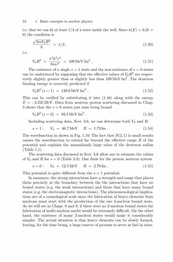
34 1. Basic concepts in nuclear physics
i.e. that we can fit at least 1/4 of a wave inside the well. Since k(E) < k(E =0) the condition is
√2mV0R2
h> π/2 , (1.50)
i.e.
V0R2 >
π2h2c2
8mc2 = 109 MeV fm2 . (1.51)
The existence of a single s = 1 state and the non-existence of s = 0 statescan be understood by supposing that the effective values of V0R
2 are respec-tively slightly greater than or slightly less than 109 MeV fm2. The deuteronbinding energy is correctly predicted if
V0R2 (s = 1) = 139.6 MeV fm2 . (1.52)
This can be verified by substituting it into (1.48) along with the energyE = −2.225 MeV. Data from neutron–proton scattering discussed in Chap.3 shows that the s = 0 states just miss being bound
V0R2 (s = 0) ∼ 93.5 MeV fm2 . (1.53)
Including scattering data, Sect. 3.6, we can determine both V0 and R:
s = 1 : V0 = 46.7 MeV R = 1.73 fm . (1.54)
The wavefunction in shown in Fig. 1.10. The fact that B(2, 1) is small resultscauses the wavefunction to extend far beyond the effective range R of thepotential and explains the anomalously large value of the deuteron radius(Table 1.1).
The scattering data discussed in Sect. 3.6 allow one to estimate the valuesof V0 and R for s = 0 (Table 3.3). One finds for the proton–neutron system
s = 0 : V0 = 12.5 MeV R = 2.79 fm . (1.55)
This potential is quite different from the s = 1 potential.In summary, the strong interactions have a strength and range that places
them precisely at the boundary between the the interactions that have nobound states (e.g. the weak interactions) and those that have many boundstates (e.g. the electromagnetic interactions). The phenomenological implica-tions are of a cosmological scale since the fabrication of heavy elements fromnucleons must start with the production of the one 2-nucleon bound state.As we will see in Chaps. 8 and 9, if there were no 2-nucleon bound states thefabrication of multi-nucleon nuclei would be extremely difficult. On the otherhand, the existence of many 2-nucleon states would make it considerablysimpler. The actual situation is that heavy elements can be slowly formed,leaving, for the time being, a large reserve of protons to serve as fuel in stars.

1.4 Nuclear forces and interactions 35
1.4.2 The Yukawa potential and its generalizations
We want to consider more realistic potentials than the simple potential (1.43).This is necessary to completely describe the results of nucleon–nucleon scat-tering (Chap. 3) and to understand the saturation phenomenon on nuclearbinding. The subject of nucleon–nucleon potentials is very complex and wewill give only a qualitative discussion. Our basic guidelines are as follow:
• Protons and neutrons are spin 1/2 fermions, and therefore obey the Pauliprinciple. We have already seen in the previous subsection how this restrictsthe number of 2-nucleon states.
• Nuclear forces are attractive and strong, since binding energies are roughlya 106 times the corresponding atomic energies. They are however shortrange forces : a few fm. The combination of strength and short range makes2-nucleon systems only marginally bound but creates a rich spectrum ofmany-nucleon states.
• They are “charge independent.” Nuclear forces are blind to the electriccharge of nucleons. If one were to “turn off” Coulomb interactions, thenuclear proton–proton potential would be the same as the neutron–neutronpotential. A simple example is given by the binding energies of isobars suchas tritium and helium 3 : B(3H) = 8.492 MeV > B( 3He) = 7.728 MeV. Ifthe difference ∆B = 0.764 MeV is attributed to the Coulomb interactionbetween the two protons in 3He, ∆B = e2 < 1/r12 > /4πε0, one obtainsa very reasonable value for the mean radius of the system : R ≈ 2 fm (thiscan be calculated or measured by other means). We shall come back to thisquestion in a more quantitative way when we discuss isospin.
• Nuclear forces saturate. As we have already mentioned, this results in thevolumes and binding energies of nuclei being additive and, in first approx-imation, proportional to the mass number A. This is a remarkable factsince it is reminiscent of a classical property and not normally present inquantum systems. It appears as if each nucleon interacts with a given fixednumber of neighbors, whatever the nucleus.
The theoretical explanation of the saturation of nuclear forces is subtle.The physical ingredients are the short range attractive potential (r ∼ 1 fm),a hard core repulsive force at smaller distances r < 0.5 fm, and the Pauliprinciple. Being the result of these three distinct features, there is no simpleexplanation for saturation. It is simple to verify that the Pauli principle alonecannot suffice, and that any power law force does not lead to saturation(Exercise 1.9).
Many properties of nuclear forces can, be explained quantitatively by thepotential proposed by Yukawa in 1939:
V (r) = ghc
rexp(−r/r0) . (1.56)
The factor hc is present so that the coupling constant g is dimensionless. Aswe will see in the next section, forces between particles are due, in quantum

36 1. Basic concepts in nuclear physics
field theory, to the quantum exchange of virtual particles. The range r0 of aforce is the Compton wavelength h/mc of the exchanged particle of mass m.Yukawa noticed that the range of nuclear forces r0 1.4 fm, corresponds tothe exchange of a particle of mass 140 MeV. This is how he predicted theexistence of the π meson. The discovery of that particle in cosmic rays was adecisive step forward in the understanding of nuclear forces.
When applied to a two-nucleon system, the potential (1.56) is reducedby a factor of (mπ/2mp)2 ∼ 10−2 because of spin-parity considerations. Adimensionless coupling constant of g 14.5 explains the contribution of theπ meson to the nucleon–nucleon force.
It is necessary to add other exchanged particles to generate a realisticpotential. In fact, the general form of nucleon–nucleon strong interactionscan be written as a linear superposition of Yukawa potentials :
V (r) =∑
i
gihc
rexp(−µir) (1.57)
where the sum is over a discrete or continuous set of exchanged particles withmasses given by µi = mic/h.
However, we need some more elements to explain saturation and preventa nuclear “pile-up” where all nucleons collapse to an object of the size of theorder of the range of the strong interactions.
First, one must add a strong repulsive shorter range potential, called a“hard core”interaction. This potential is of the form (1.56) with a negativecoupling constant g and a range r0 0.3 fm. The physical origin of therepulsive core is not entirely understood but it certainly includes the effect ofthe Pauli principle that discourages placing the constituent quarks of nucleonsnear each other.
Second, spin effects and relativistic effects must be taken into account.One writes the potential as the sum of central potentials with spin-dependentcoefficients:
V = VC(r) + ΩTVT(r) + ΩSOVSO(r) + ΩSO2VSO2(r) , (1.58)
where VC is a pure central potential and the other terms are spin dependent.The most important is the tensor potential VT with
ΩT = [3(σ1 · r/r) (σ2 · r/r) − σ1 · σ2] (1.59)
where σ1 and σ2 are the Pauli spin matrices for the two nucleon spins. Figure1.11 shows how this term has the important effect of inducing a correlationbetween the position and spin of the two nucleons. This results in a permanentquadrupole moment for the deuteron. It is also the dominant force in bindingthe deuteron. However, it averages to zero for multi-nucleon systems whereit plays a minor role.
The last two terms in (1.58) are spin-orbit interactions:
hΩSO = (σ1 + σ2) · L (1.60)

1.4 Nuclear forces and interactions 37
n
p n
p
n p
Fig. 1.11. The tensor potential for the s = 1 state (1.59) makes the configurationon the right (σ ·r = 0) have a different potential energy than the two configurationson the left (σ · r = 0). This results in the permanent quadrupole moment of thedeuteron.
S=0p−p n−n p−n p−n
V
50
−200
−150
−100
−50
0
100
150
V(r
) (
MeV
)
r (fm)121
r (fm)
S=1
VC VSO
VC
T
2
Fig. 1.12. The most important contributions to the nucleon–nucleon potentials inthe s = 0 state (left) and the s = 1 state (right) (the so-called Paris potential).The two central potentials VC depend only on the relative separations. The tensorpotential VT is of the form (1.59) is responsible for the deuteron binding and forits quadrupole moment. The spin-orbit potential is VSO.

38 1. Basic concepts in nuclear physics
h2ΩSO2 = (σ1 · L)(σ2 · L) + (σ2 · L)(σ1 · L) (1.61)
where L is the orbital angular momentum operator for the nucleon pair.Figure 1.12 shows the most important contributions to the nucleon–
nucleon potential [23]. For spin-anti-aligned nucleons (s = 0), only the centralpotential contributes.
Finally, we note that to correctly take into account the charge indepen-dence of nuclear forces the formalism of isospin (Sect. 1.7) must be used.
1.4.3 Origin of the Yukawa potential
The form (1.56), which is derived from quantum field theory, can be under-stood quite simply. Consider a de Broglie wave
ψ = exp(− i(Et − p.r)/h
). (1.62)
The Schrodinger equation in vacuum is obtained by using E = p2/2m andthen taking the Laplacian and the time derivative. Assume now that we usethe relativistic relation between energy and momentum :
E2 = p2c2 + m2c4
(this is how Louis de Broglie proceeded initially). By taking second-orderderivatives of (1.62) both in time and in space variables we obtain the Klein—Gordon equation :
1c2
∂2ψ
∂t2− ∇2ψ + µ2ψ = 0 (1.63)
where we have set µ = mc/h. Originally, this equation was found bySchrodinger. He abandoned it because it did not lead to the correct rela-tivistic corrections for the levels of the hydrogen atom.5 It was rediscoveredlater on by Klein and Gordon.
Forgetting about the exact meaning of ψ in this context, (1.63) is thepropagation equation for a relativistic free particle of mass m. In the casem = 0, i.e., the photon, we recover the propagation equation for the electro-magnetic potentials :
1c2
∂2ψ
∂t2− ∇2ψ = 0 . (1.64)
The classical electrostatic potential produced by a point charge is obtainedas a static, isotropic, time-independent solution to this equation with a sourceterm added to represent a point-like charge at the origin, i.e.,
∇2V (r) = − q
ε0δ(r) , (1.65)
5 Schrodinger did not have in mind spin and magnetic spin-orbit corrections. Theseeffects are accounted for by the Dirac equation, the relativistic wave equationfor a spin 1/2 particle

1.4 Nuclear forces and interactions 39
whose solution is
V (r) =q
4πε0 r. (1.66)
Similarly, by looking for static, isotropic solutions of the Klein–Gordonequation 1.63 with a point-like source at the origin :
∇2V (r) − µ2(r) = −g(hc)4π
δ(r) , (1.67)
one can readily check that the Yukawa potential (1.56)
V (r) = g(hc/r) exp(−µr) , (1.68)
satisfies this equation. The solution V (r) = g(hc/r) exp(+µr) is discardedsince it diverges at infinity.
1.4.4 From forces to interactions
We have emphasized that, in quantum field theory, forces between particlesare described by the exchange of virtual particles. The interactions can bedescribed by (Feynman) “diagrams” like those shown in Fig. 1.13. Each dia-gram corresponds to a scattering amplitude that can be calculated accordingto the rules of quantum field theory. As we will see in Chap. 3, the effectivepotential is Fourier transform of the amplitude.
In quantum electrodynamics, the exchange of massless photons leads tothe Coulomb potential. The exchange of massive particles leads to Yukawa-like potentials. One example is the exchange of pions as shown in the firsttwo diagrams in Fig. 1.13. These diagrams contribute to the nucleon–nucleonpotential of Fig. 1.12 and lead to the binding of nucleons and to nucleon–nucleon scattering.
π
N
N’ N’
N
π
n
p n
p
γ Z
N N N N
N’ N’ N’ N’
+−0
Fig. 1.13. Diagrams contributing to the nucleon–nucleon interaction due to theexchange of a pion, a photon and a Z0. In these diagrams N and N ′ represent eithera proton or a neutron. The two first diagrams with the exchange of a neutral orcharged pion generates the long-range part of the nucleon–nucleon potential. Thephoton exchange diagram generates the Coulomb interaction between protons andthe magnetic interaction between any nucleons. The diagram with Z exchange isnegligible for the nucleon–nucleon interactions but dominates for neutrino-neutronscattering since the neutrino has no strong interactions.

40 1. Basic concepts in nuclear physics
e_
n
WW W
p
ν
n n
ν
p p
ν e+
e_
__
Fig. 1.14. Some diagrams with the exchange of a W. The two diagrams on theleft contribute to inelastic neutrino scattering. The diagram on the right leads toneutron decay.
Other massive particles can be exchanged between particles, for examplethe Z0 boson
mZ c2 = 91.188 GeVhc
mZ c2 = 2.11 × 10⁻³ fm . (1.69)
This particle is the mediator of the neutral current sector of the weak in-teractions as illustrated in the fourth diagram of Fig. 1.13. It thus leads toa Yukawa-like potential between particles of the form (1.56). Compared topion exchange, the Yukawa potential has a range about 10−3 times smaller.The effective coupling is also much smaller being of order
gZ ∼ α . (1.70)
To compare with the strong interactions, we estimate an effective value ofV0R
2 by taking R ∼ 2 × 10⁻³fm and V0 ∼ αhc/R:
V0R2 ∼ 3 × 10⁻³ MeV fm2 , (1.71)
i.e. about 5 orders of magnitude smaller than that of the strong interactions(1.52) and (1.53). We conclude that Z0 can play no role in nucleon–nucleonbinding or scattering.
On the other hand, Z0 exchange plays the essential role in neutrino–nucleon elastic scattering. This is because the neutrino has only weak inter-actions.
The use of particle exchange to describe potentials obviously has directapplications in bound states and elastic scattering. If one includes the pos-sibility of the exchange of charged particles, we can also describe inelasticreactions, some of which are shown in Fig. 1.14. These diagrams show pro-cesses where the particle exchanged is the charged partner of the Z0 boson,the W±
mWc2 = 80.42 GeV . (1.72)
This particle mediates the so-called charged-current weak interactions. Theyplay the essential cosmological role of changing neutrons into protons and viceversa. They thus play an essential role in the cosmological and astrophysicalsynthesis of heavy elements. On Earth, they are mostly seen in neutrino

1.5 Nuclear reactions and decays 41
scattering and β-decay as illustrated in Fig. 1.14 and discussed further in thenext section.
Table 1.3 summarizes the interactions important in nuclear physics andtheir exchanged particles. The weak and electromagnetic interactions arefundamental interactions that will be discussed in more detail in Chap. 4.The ordinary strong interactions that lead to binding of nucleons in nu-clei are “effective” in the sense that, as previously emphasized, they are thescreened residuals due to the fundamental chromodynamic interactions be-tween quarks.
Table 1.3. The interactions involving elementary particles. The strong interac-tions are considered to be screened quantum chromodynamic interactions.
interaction examples of reactions exchanged particle
weak neutral current νn → νn Zweak charged current νn → e−p Welectromagnetic ep → ep γstrong np → np π and other hadronschromodynamic quark–quark scattering gluons
1.5 Nuclear reactions and decays
Nuclear species can be transformed in a multitude of nuclear reactions. Innuclear reactions involving only strong and electromagnetic interactions, thenumber of protons and the number of neutrons are conserved separately. Animportant example is neutron absorption followed by photon emission, theso-called “ (n, γ) ” reaction:
n(A, Z) → γ (A + 1, Z) i.e. (A, Z) (n, γ) (A + 1, Z) . (1.73)
The second form is a standard way of denoting the reaction. Other reactionsare “ (p, γ) ” reactions
p (A, Z) → γ (A + 1, Z + 1) i.e. (A, Z) (p, γ) (A + 1, Z + 1) , (1.74)
“(n, p)” reactions
n (A, Z) → p (A, Z − 1) i.e. (A, Z) (n, p) (A, Z − 1) , (1.75)
and “(p, n)” reactions
p (A, Z) → n (A, Z + 1) i.e. (A, Z) (p, n) (A, Z + 1) . (1.76)
In all these reactions, the final state nucleus may be produced in an excitedstate so additional photons are produced in de-excitation.

42 1. Basic concepts in nuclear physics
Many nuclei can decay to lighter nuclei by redistributing the nucleonsamong “daughter” nuclei. The most important are “α-decays” with the emis-sion of a 4He nucleus :
(A, Z) → (A − 4, Z − 2) 4He , (1.77)
for instance 238U → 234Th 4He. The condition for a nucleus to be stableagainst α-decay is
m(A, Z) < m(A − 2, Z − 2) + m(2, 2) . (1.78)
Alpha decay will be studied in more detail in Sect. 2.6.α-decay is a special case of spontaneous fission into two lighter nuclei
with, perhaps, the emission of k neutrons, such as:
(A, Z) → (A′, Z ′) (A′′, Z ′′) + k n , (1.79)
with A′ + A′′ + k = A and Z ′ + Z ′′ = Z. Such decays occur mostly for veryheavy nuclei. They will be studied in more detail in Chap. 6.
While the strong and electromagnetic interactions responsible for theabove reactions separately conserve the number of neutrons and the num-ber of protons, neutrons and protons can be transformed into each other bythe weak interactions mentioned in the previous section. These interactionsare weak in the sense that the rates of reactions they induce are in generalmuch slower than those due to the electromagnetic or strong interactions.Weak interactions will be studied in some detail in Chap. 4. Here, we notethat weak nuclear interactions are usually signaled by the participation of anelectron–neutrino, νe. Two examples are electron capture by a proton andneutrino capture by a neutron
e− p ↔ νe n . (1.80)
We see that when the proton is transformed to a neutron or vice-versa, anelectron or positron is created or absorbed to conserve charge. Since all par-ticles in these reactions have spin 1/2, the neutrino is necessary to conserveangular momentum. All other possible weak interactions can be found bymoving particles from left to right and changing them to their antiparticles,e.g.
νe p ↔ e+ n . (1.81)
Another possibility is spontaneous neutron decay
n → p e− νe . (1.82)
This decay is allowed by energy conservation, (mn − mp−me)c2 = 0.78 MeV,and the free neutron has a mean-lifetime of
τn = 886.7 ± 1.9 s . (1.83)
Of course, the fact that mp < mn + me means that the corresponding decayof free protons is forbidden

1.6 Conservation laws 43
p → n e+ νe energy not conserved. (1.84)
Since the weak interactions can turn protons into neutrons and vice versawhile conserving the total number of nucleons, their most important role isthe decay of radioactive isobars via so-called β-decays:
(A, Z) → (A, Z + 1) e−νe (A, Z) → (A, Z − 1) e+νe . (1.85)
These two reactions are the nuclear equivalents of the two fundamental decays(1.82) and (1.84). Another form of β-decay (or transmutation) is electroncapture
e− (A, Z) → (A, Z − 1) νe , (1.86)
i.e. the nuclear equivalent of (1.80) This latter reaction is possible if thenucleus is surrounded by atomic electrons but cannot happen in the case ofan isolated nucleus.
A nucleus is stable against the β-decays (1.85) if it is sufficiently lightcompared to its two neighboring isobars:
m(A, Z) < m(A, Z ± 1) + me , (1.87)
where m(A, Z) stands for the mass of the (A, Z) nucleus. The condition forit to be stable against both β-decay and electron capture is slightly different:the mass of the atom containing A − Z neutrons, Z protons and Z electronsmust be smaller than the masses of its two neighboring isobars :
m(A, Z) + Zme < m(A, Z ± 1) + (Z ± 1)me . (1.88)
(In the above formula, we neglect the electronic binding energies which arecomparatively much smaller.) In general, for each value of the mass number A,there exist only one or two stable isobars. The other nuclei are radioactive anddecay to the stable isobars by a series of β-decays and/or electron captures.
While the weak interactions do not conserve separately the number ofprotons and the number of neutrons, they do (as do the strong and electro-magnetic interactions) conserve electric charge and baryon number, i.e. thetotal number of nucleons. Baryon number is conserved in nuclear reactionsbut it is believed that very rare, as yet unobserved, reactions allow baryonnumber non-conservation. On the other hand, electric charge conservation isbelieved to be absolute.
1.6 Conservation laws
The investigation of the fundamental constituents of matter and their inter-actions comes from the experimental and theoretical analysis of reactions.These reactions can be scattering experiments with or without production ofparticles, and decays of the unstable particles produced in these reactions.

44 1. Basic concepts in nuclear physics
Various fundamental conservation laws govern nuclear reactions. The lawsallow the identification of particles, i.e. the determination of their masses,spins, energies, momenta etc.
The most important laws are energy-momentum conservation, angularmomentum conservation and electric charge conservation. In nuclear physics,other laws play an important role such as lepton number, baryon number andisospin conservation.
In this book, we shall mainly make use of simple “selection rules” impliedby these conservation laws. In this section, we will first discuss the experi-mental and phenomenological consequences of the most important laws. Wewill then show how the conservation laws are related to invariance proper-ties of transition operators between initial and final states, or, equivalently,invariance laws of Hamiltonians of the systems under consideration.
1.6.1 Energy-momentum conservation
By far the most important conservation law is that for Energy-momentum.For example, in nuclear β-decay
(A, Z) → (A, Z + 1) e− νe (1.89)
we require
EA,Z = EA,Z+1 + Ee + Eνe , (1.90)
and
pA,Z = pA,Z+1 + pe + pνe . (1.91)
These two laws are only constraints. As discussed in later chapters, the waythat momentum and energy are distributed between the decay products de-pends on the details of the interaction responsible for the reaction.
When one applies energy-momentum conservation, it is of course neces-sary to take into account the masses of initial and final particles by using therelativistic expression for the energy
E = (p2c2 + m2c4)1/2 (1.92)
for a free particle of mass m. The square root in this formula often makes cal-culations very difficult. However, in nuclear physics, nuclei and nucleons areusually non-relativistic, v = pc2/E c, and one can use the non-relativisticapproximation :
E =√
p2c2 + m2c4 mc2 + p2/2m , (1.93)
i.e. the energy is the sum of the rest energy mc2 and the non-relativistickinetic energy p2/2m. On the other hand, photons and neutrinos are rela-tivistic:
E =√
p2c2 + m2c4 pc + m2c4/2pc , (1.94)

1.6 Conservation laws 45
where the mass term m2c4/2pc can usually be neglected for neutrinos andalways for the massless photon E = pc.
The presence of non-relativistic and relativistic particles in a given re-action results in the very useful fact that, viewed in the center-of-mass, themomentum is shared democratically between all final state particles whereasthe kinetic energy is carried mostly by the relativistic particles. This is mosteasily seen in the decay of an excited nucleus:
(A, Z)∗ → (A, Z) γ . (1.95)
Energy conservation in the initial rest frame implies
m∗c2 = mc2 +p2
2m+ pc , (1.96)
where m∗ and m are the masses of the excited and unexcited nuclei andp is the common momentum of the final nucleus and photon. (Momentumconservation requires that these two momenta be equal.) It is clear that thephoton energy pc is much greater than the nuclear kinetic energy:
p2
2m= pv/2 pc for v c . (1.97)
Neglecting p2/2m in (1.96), we see that the photon energy is then to goodapproximation proportional to the mass difference
pc ∼ (m∗ − m)c2 . (1.98)
Using this value for the momentum, we find that the ratio between the nuclearkinetic energy and the photon energy is
p2/2m
pc= (1/2)
m∗ − m
m. (1.99)
This is at most of order 10−3 in transitions between nuclear states.In more complicated reactions like three-body decays, one generally finds
that the momentum is evenly distributed on average among the final-stateparticles. Once again, this implies that the kinetic energy is taken by thelightest particles.
In nuclear physics, one often mentions explicitly the energy balance inwriting reactions
A + B → a1 + a2 + an + Q (1.100)
where
Q = (Σmi − Σmf)c2 . (1.101)
If the reaction can take place when A and B are at rest, Q is the total kineticenergy of the particles in the final state. If Q is negative, the reaction isendothermic and it can only take place if the energy in the center-of-mass isabove the energy threshold.

46 1. Basic concepts in nuclear physics
An important example in producing heavy elements is neutron captureaccompanied by the production of k photons:
n + (A, Z) → (A + 1, Z) + kγ + Q (1.102)
The fact that binding energies per nucleon are ∼ 8 MeV means that Q ispositive and of order 8 MeV (near the bottom of the stability valley). Sincethe final state photons are the only relativistic particles, we can expect thatthey take all the energy,
∑Eγ ∼ Q. A detailed calculation of the constraints
of energy-momentum conservation confirms this (Exercise 1.10).Of course, some reactions involve no relativistic particles, for example
d t → n 4He + 17.58 MeV. (1.103)
We leave it to Exercise 1.11 to show that in the limit of low-center-of-massenergy, the final state neutron takes the majority of the 17.58 MeV.
1.6.2 Angular momentum and parity (non)conservation
Angular momentum conservations plays a different role than that of energy-momentum conservation. The latter can by verified to a useful precision inindividual events where the energies and momenta of final-state particles canbe compared with those of the initial-state particles. This is because there isa relatively well-defined correspondence between momentum wavefunctions(plane waves) and the classical tracks of particles that are actually observed,i.e. a plane wave of wave vector k and angular frequency ω generates a de-tector response that appears to be due to a classical particle of momentumhk and energy E = hω.
On the other hand, the wavefunctions corresponding to a definite angularmomentum, correspond to certain angular dependence of the function aboutthe origin. This information is lost when an individual track going in a par-ticular direction is measured. It can be recovered only by observing manyevents and reconstructing the angular distribution.
The same consideration applies to parity which gives the behavior of awavefunction under reversal of all coordinates. Its conservation can only beverified in the distribution of tracks. As it turns out, parity is not in factconserved in the weak interactions, as we will see in Chap. 4.
1.6.3 Additive quantum numbers
As we have already emphasized nuclear reactions may or may not respectcertain additive conservations laws. The most important is electric chargeconservation which is believed to be absolutely respected in all interactions.
The second most respectable conservation law is that of baryon number,i.e. the total number of nucleons (neutrons and protons), minus the totalnumber of anti-nucleons (antiprotons and antineutrons). For instance, the

1.6 Conservation laws 47
reaction p d → pp γ conserves electric charge but not baryon number and istherefore not observed. Conversely, the photo-disintegration of the deuteron,γ d → p n, is allowed and observed. The baryon number conservation forbidsthe decay of the proton, such as in the reaction p → e+γ. The present ex-perimental limit on the proton lifetime, τp > 1032 yr shows that the baryonnumber is conserved to very good accuracy.
Finally, we mention lepton number. The electron and the neutrinos arecalled leptons. The lepton number (more precisely the “electron lepton num-ber”) Le is defined as the difference between the total number of leptons(electrons and neutrinos) and the total number of anti-leptons (anti-electronsand antineutrinos)
Le ≡ N(e−) + N(νe) − N(e+) − N(νe) , (1.104)
where N(e−) is the number of electrons, N(νe) the number of neutrinos, etc.Le is conserved in nuclear reactions involving electrons and neutrinos. In neu-tron decay, for instance, n → p+e−+νe, an antineutrino is produced togetherwith the electron in order to conserve the lepton number. This antineutrinothen can interact and produce a positron but not an electron:
νe + p → e+ + n but not νe + n → e− + p . (1.105)
There exist two other types of charged leptons, the µ± (mµ = 105.66 MeV)and the τ± (mτ = 1777.03 MeV). Each of these leptons is associated with itsown neutrino νµ and ντ both of which have very small masses. The “muon”and “tauon” lepton numbers are defined in the same way as the electronlepton number:
Lµ ≡ N(µ−) + N(νµ) − N(µ+) − N(νµ) , (1.106)
Lτ ≡ N(τ−) + N(ντ) − N(τ+) − N(ντ) . (1.107)
They are both conserved separately. Since mµ and mτ are much larger thancharacteristic nuclear energy scales (∼ 1 MeV), the µ and τ leptons havefewer applications in nuclear physics than in particle physics.
In the same way as the strong nuclear interactions show that the neutronis a neutral partner of the proton, weak interactions show that the νe actsas a neutral partner of the electron (and similarly for the νµ and µ, andfor the ντ and τ). We have been careful to use the words “acts as” becauseit is now believed the separate conservation of electron, muon and tauonlepton numbers is only an effective conservation law. Recent experiments on“neutrino oscillations” that are discussed in Chap. 4 indicate that the onlytruly conserved number is the sum of the 3 lepton numbers:
L = Le + Lµ + Lτ . (1.108)

48 1. Basic concepts in nuclear physics
1.6.4 Quantum theory of conservation laws
A quantum system described by a state vector |ψ〉 evolves with time in a waygoverned by the Schrodinger equation and the system’s Hamiltonian operatorH:
d|ψ(t)〉dt
= H |ψ(t)〉 . (1.109)
It is interesting to see how the dynamics defined by (1.109) conspires toconserve a quantity associated with a time-independent operator A. Oneanswer is given by Ehrenfest’s theorem relating the time development of anoperator’s expectation value to the operator’s commutator with H:
ddt
〈ψ(t)|A|ψ(t)〉 =1ih
〈ψ(t)|[A, H]|ψ(t)〉 , (1.110)
which follows simply from (1.109) and its Hermitian conjugate. We see thatthe expectation value is time independent if the operator commutes with H.
In nuclear physics, we are generally interested in transitions betweenstates and we would like to see how selection rules that constrain the transi-tions are generated. Consider the transition amplitude of a system from aninitial state |i〉 to a final state |f〉, both eigenstates of a Hamiltonian H0,due to a transition Hamiltonian HT . The total Hamiltonian of the system isH = H0 +HT . In first-order perturbation theory, i.e. in Born approximation,for f = i, the amplitude γi→f is proportional to the matrix element of HT
between initial and final states
γi→f ∝ 〈f |HT |i〉 . (1.111)
If A commutes with H0 we can take the initial and final states to be alsoeigenstates of A with eigenvalues ai and af , respectively,
A|i〉 = ai|i〉 , A|f〉 = af |f〉 . (1.112)
Since we suppose that A commutes with HT , we obtain
〈f |[A, HT ]|i〉 = (af − ai)〈f |HT |i〉 ∝ (af − ai)γi→f = 0 . (1.113)
Therefore, either γi→f = 0, i.e. the transition is forbidden, or, if it is notforbidden, af = ai. The quantity A is conserved in any transition if A com-mutes with the transition Hamiltonian. While we have shown this only inBorn approximation, the property can be extended to all orders of perturba-tion theory.
The conservation of a quantity described by the operator A is equivalentto the invariance of the Hamiltonian with respect to unitary transformationsdefined by the operator
D(α) = exp(iαA) , (1.114)
where α is an arbitrary real number. The operator D is unitary, i.e. D+D = 1,because A is Hermitian. The unitary transformation of states |ψ〉 and ofoperator B, associated with D is

1.6 Conservation laws 49
|ψ′〉 = D|ψ〉 B′ = DBD+ . (1.115)
From the commutation relation [A, H] = 0, we deduce
[D, H] = 0 ⇒ H = DHD† . (1.116)
In other words, the Hamiltonian H is invariant under the unitary transfor-mation D associated with the operator A.
We see that the conservation of A in the transitions induced by H isa result of the invariance of H in the unitary transformation D. To thissymmetry property of the Hamiltonian there corresponds a conservation lawof the quantity A. The operator A is called the infinitesimal generator of thetransformation D.
We also notice that equation (1.114) defines a group of transformationsD(α)D(β) = D(α + β). In the case of (1.114), the group is Abelian, orcommutative.
It is interesting to associate the various conservation laws of the previoussubsections with invariances. The Schrodinger equation (1.109) follows from
|ψ(t)〉 = exp (iHt) |ψ(t = 0)〉 , (1.117)
if we assume that the Hamiltonian is time-independent. Equation (1.117) tellsus that the Hamiltonian is the generator of translations in time. Energy istrivially conserved because the Hamiltonian commutes with itself so we canconclude that energy conservation occurs for any time-invariant system. Inother words, it occurs in any isolated system.
Total momentum conservation comes from the invariance under transla-tions in space. The infinitesimal generator of the group of space translationsis the total momentum P . Let D(x0) be an element of this group
D(x0) = exp(ix0 · P /h) , (1.118)
the translation invariance of the Hamiltonian can be written equivalently as[H, D] = 0 ⇔ [H, P ] = 0. If H is translation invariant, in a process leadingfrom an initial state of total momentum P i to a final state of total momentumP f , one has
[H, D] = 0 ⇒ P i = P f . (1.119)
The conservation of the total angular momentum follows from the rotationinvariance of the transition Hamiltonian. Consider a rotation of an angle αaround an axis along the unit vector u and set α = αu. The correspondingunitary operator is
Dα = exp(iα · J/h) . (1.120)
Consider an initial state which is an eigenstate of J2 and Jz with eigenvaluesji, mi, the transition to a final state |f〉 can happen only if it is also aneigenstate of J2 and Jz with the same eigenvalues :
〈f, jf , mf |HT |i, ji, mi〉 = δjf jiδmf mi
〈h〉 (1.121)

50 1. Basic concepts in nuclear physics
Since in nuclear processes one measures momenta of particles, it is throughthe angular distributions of particles that one measures the conservation ofangular momentum.
We note that the infinitesimal generators Jx, Jy and Jz do not commute,i.e. the group of rotations is non-Abelian. A consequence of this is that theend result of two successive rotations (about different axes) depends on theorder that the two rotations are performed. This can be confirmed by rotatingmacroscopic objects.
The invariances associated with the additive quantum numbers can beunderstood by considering transformations generated by one component ofthe angular momentum which we take to be the z component:
D(ϕ) = exp(iϕJz/h) . (1.122)
These transformations form an Abelian group.The invariance of H under rotations around the z axis yields the conserva-
tion of the component Jz of the angular momentum along this axis. Considera set of n subsystems whose state vector is factorized :
|ψ〉 = |α1, m1〉 ⊗ |α2, m2〉 ⊗ . . . ⊗ |αn, mn〉 . (1.123)
The z component of the angular momentum is
M =∑
mi ⇒ Jz =∑
i
Jiz (1.124)
and the rotation operator around the z axis is
D(ϕ)|ψ〉 = eiMϕ|ψ〉 . (1.125)
Therefore, M appears as an additive quantum number. The conservation ofM =
∑mi can also be seen as the invariance of the matrix element 〈χ|HT |ψ〉
under the phase transformations :
|ψ〉 → eiMϕ|ψ〉, |χ〉 → eiM ′ϕ|χ〉 . (1.126)
The group of phase transformations defined in this way is called the unitarygroup U(1). It is the rotation group in the plane : x + iy → eiϕ(x + iy).
This is how one can represent the conservation of any additive quantumnumber. Consider for instance the electric charge Q and a union of subsystemsas in (1.123)
|ψ〉 = |α1, q1〉 ⊗ |α2, q2〉 ⊗ . . . ⊗ |anaq〉 (1.127)
whose total charge is Q =∑
qi. Under the phase transformation |ψ〉 →eiλQ|ψ〉, |χ〉 → eiλQ′ |χ〉 where λ is an arbitrary real number, the invarianceof 〈χ|H|ψ〉 → eiλ(Q−Q′)〈χ|H|ψ〉 implies the conservation of charge : Q = Q′.
This type of invariance is called gauge invariance of the first kind. In 1929,Hermann Weyl remarked that the choice λ = constant is non-natural fromthe point of view of relativity. In fact, space-like separated points are notrelated, therefore it doesn’t have much physical meaning to change the phase

1.7 Charge independence and isospin 51
of states in these points in the same way. If λ depends on the point underconsideration : λ(x, t), one deals with a gauge transformation of the secondkind. In this latter formulation, gauge invariance has dynamical consequenceswhich underly all present theories of fundamental interactions. At present,the conservation of electric charge appears to be an absolute conservationlaw. On the other hand, baryon number conservation is expected to be onlyapproximately conserved.
We end this discussion by noting that in a more formal approach to quan-tum mechanics, one can start with invariance principles, next define observ-ables by making use of the infinitesimal generators of various transforma-tions, and finally deduce the commutation relations of the observables fromthe structure of the invariance groups under consideration (Galileo group,Poincare group, etc.). The proof of the fundamental commutation relation[x, px] = ih starting form (1.118) is an example.
In many cases, the Hamiltonian is invariant under other transformationgroups than translations or rotations. In all cases, the same property willappear, i.e. a symmetry induces a conservation law. Such properties are veryimportant in the theories of fundamental interactions and, because of this,group theory plays a crucial role in elementary particle physics.
1.7 Charge independence and isospin
We argued in Sect. 1.4 that nuclear forces are rather insensitive to the electriccharge. For instance, we have compared the binding energies of 3H and 3He,whose difference can be understood as originating solely from the Coulombrepulsion of the protons. Figure 1.15 shows that this is a systematic effect formirror nuclei, i.e. pairs of nuclei for which N and Z are interchanged.
Many other observations confirm charge independence. Spectroscopy pro-vides many spectacular examples. For example, the spectra of the mirrornuclei for A = 11, 12 and 13, shown on Fig. 1.16, are remarkably similar.
1.7.1 Isospin space
Charge independence is more subtle than just saying that protons and neu-trons can be replaced by one another in nuclear forces. It is formalized byusing the concept of “isotopic spin” or, better, isospin T , that was introducedby Heisenberg in 1932.6
A spin 1/2 particle is a two-state system, since a measurement of theprojection of its spin along an axis can lead to one of the two results ±h/2.Similarly, the proton and the neutron can be considered as two different statesT3 = ±1/2 of a single physical object of isospin T = 1/2, the nucleon. We
6 The translation of Heisenberg’s original paper can be found in D.M. Brink, Nu-clear Forces.

52 1. Basic concepts in nuclear physicsB
/A (
MeV
)∆
0.00 80.00 0.00
0.50
AFig. 1.15. The difference in binding energy per nucleon, B/A, for pairs of “mirrornuclei”, i.e. pairs with Z and N interchanged. The lower points are pairs with|Z − N | = 1 and the upper points are pairs with |Z − N | = 2. The lines show theprediction of the semi-empirical mass formula (2.13) which supposes that neutronsand protons have identical strong interactions and that the difference in bindingenergy comes only from the Coulomb repulsion of the protons.
therefore introduce an abstract three-dimensional Euclidean-like space called“isospin space.” We will choose operators that allow us to perform rotationsin this space. The spin formalism in isospin space is the same as that fornormal spin in the Euclidean space.
Let T be the vector isospin operator, i.e. a set of three operatorsT1, T2, T3. These three operators have the commutation relations of a usualangular momentum, up to the h factor :
T ∧ T = iT . (1.128)
The eigenvalues T (T + 1) and T3 of the commuting observables T 2 and T3are the same as those of usual angular momentum (up to h factors).
Heisenberg’s idea is to assume that nuclear strong interactions are rotationinvariant in isospin space. The families of “hadrons”, i.e. particles whichhave strong nuclear interactions, can be classified in isospin multiplets ( T =0, 1/2, 1, 3/2 . . .). Different members of each multiplet can be distinguishedby their value of T3 which is linearly related to their charge.
1.7.2 One-particle states
The nucleon has isospin 1/2. In other words, each of the operators T1, T2and T3 which are associated with this particle have eigenvalues ±1/2. The

1.7 Charge independence and isospin 53
11Be
11B
11C
12 12 12N
13 13 13OB C C N
mirror mirror mirror
0
8 8
0
4 4
E (
MeV
)
1/2+1/2−
3/2−
1/2−
5/2−
3/2−
3/2+
3/2−
1/2−
5/2−
3/2−
3/2+
1+
2+
2−
1−0+
3−
2+
4−
1+
1−
1−
2−
0+
2+
0+
1+
2+2−
1−
0+
3−
1+
2−
3−
1−
1−
1/2−
1/2+
5/2+
5/2+
5/2−
1/2−
1/2+
5/2+
3/2+7/2+
5/2−
3/2+
3/2−
7/2−
1/2+
7/2−
3/2−3/2−
5/2+
1/2+
5/2+
5/2+1+
3+3−
7/2+
3/2+
1−2−
Fig. 1.16. Spectra of the low-lying levels for nuclei with A = 11, 12, and 13. Thepairs of nuclei with N and Z interchanged (mirror nuclei) have remarkably similarspectra
operator T 2 = T 21 + T 2
2 + T 23 is proportional to the identity with eigenvalue
3/4.The states |p〉 and |n〉, are, by definition, the eigenstates of the particular
operator T3
T3|p〉 = (1/2)|p〉 , T3|n〉 = (−1/2)|n〉 . (1.129)
In actual physics, the operator T3 plays a special role since electric chargeis related to T3 by
Q = T3 + 1/2 . (1.130)
The action of T1 and T2 on these states, with T± = T1±T2, can be writtenas
T+|p〉 = 0 T−|n〉 = 0 (1.131)T1|p〉 = (1/2)|n〉 T1|n〉 = (1/2)|p〉 (1.132)T2|p〉 = (i/2)|n〉 T2|n〉 = (−i/2)|p〉 . (1.133)
An arbitrary nucleon state |N〉 is written

54 1. Basic concepts in nuclear physics
|N〉 = α |p〉 + β |n〉 |α|2 + |β|2 = 1 . (1.134)
We remark that all of this is an abstraction applicable only to a worldwithout electromagnetism. A state such as
1√2
(|T3 = 1/2〉 + |T3 = −1/2〉) , (1.135)
which is oriented along the direction T2 cannot be observed physically. Sinceit is a superposition of a proton and a neutron, it is both of charge 0 and 1;at the same time it creates and doesn’t create an electrostatic field. As such,it is a superposition of two macroscopically different states, an example of a“Schrodinger cat.”
It is often convenient to use matrix representations for the states andoperators. For the single-nucleon space we have
|p〉 =(
10
), |n〉 =
(01
), |N〉 =
(αβ
)(1.136)
We use the Pauli matrices τ ≡ τ1, τ2, τ3,
τ1 =(
0 11 0
)τ2 =
(0 −ii 0
)τ3 =
(1 00 −1
)(1.137)
which satisfy the commutation relations
τ ∧ τ = 2i τ . (1.138)
The nucleon isospin operators are:
T = (1/2)τ . (1.139)
Rotation invariance in isospin space amounts to saying that the nucleon–nucleon interaction is invariant under the transformations
|p′〉 = e−iφ/2 cos(θ/2)|p〉 + eiφ/2 sin(θ/2)|n〉 ,|n′〉 = −e−iφ/2 sin(θ/2)|p〉 + eiφ/2 cos(θ/2)|n〉 .
(1.140)
Besides nucleons, there are hundreds of other strongly interacting parti-cles. These particles, most of which are highly unstable, are called hadrons.Hadrons are characterized by their isospin, their electric charge, and otheradditive more exotic quantum numbers such as “strangeness,” “charm,” etc,that we will study in Chap. 4. For instance, the π mesons, which mediate someof the nuclear strong forces, have zero baryon number and form a triplet ofcharge states (π+, π0, π−) whose masses are close. It is natural to considerthem as the three states of an isospin triplet, the π meson, of isospin T = 1.Following (1.129) we write
T3|π±〉 = ± |π±〉 , T3|π0〉 = 0 . (1.141)
The relation (1.130) between electric charge and T3 can be generalized to
Q = T3 + Y/2 , (1.142)
where this relation defines the “hypercharge” Y for a multiplet. Clearly wehave Y = 1 for nucleons and Y = 0 for π mesons.

1.7 Charge independence and isospin 55
1.7.3 The generalized Pauli principle
The Pauli principle states that two identical fermions must be in an antisym-metric state. If the proton and the neutron were truly identical particles upto the projection of their isospin along the axis T3, a state of several nucleonsshould be completely antisymmetric under the exchange of all variables, in-cluding isospin variables. If we forget about electromagnetic interactions, andassume exact invariance under rotations in isospin space, the Pauli principleis generalized by stating that an A-nucleon system is completely antisymmet-ric under the exchange of space, spin and isospin variables. This assumptiondoes not rest on as firm a foundation as the normal Pauli principle and is onlyan approximation. However, we can expect that it is a good approximation,up to electromagnetic effects.
The generalized Pauli principle restricts the number of allowed quantumstates for a system of nucleons. We shall see below how this determines theallowed states of the deuteron.
1.7.4 Two-nucleon system
The isospin states of a two-nucleon system are constructed in the same man-ner as the states of two spin 1/2 particles.
The total isospin T of the system corresponds to:
T = 1 or T = 0
and the four corresponding eigenstates are :
|T = 1, T3〉 :
⎧⎨⎩
|T = 1, T3 = 1〉 = |pp〉|T = 1, T3 = 0〉 = (|pn〉 + |np〉)/√
2|T = 1, T3 = −1〉 = |nn〉
(1.143)
|T = 0, T3 = 0〉 : |0, 0〉 = (|pn〉 − |np〉)/√
2 . (1.144)
We recall that, just as for spin, the three states |T = 1, M〉 are collectivelycalled the isospin triplet. They are symmetric under the exchange of thecomponents of the two particles along T3. The state |T = 0, 0〉 is called theisospin singlet state. It is antisymmetric in that exchange. The triplet statetransforms as a vector under rotations in isospin space. The singlet state isinvariant under those rotations.
A series of simple but important consequences follow from these consid-erations.
• The Hamiltonian of two (or more) nucleons is invariant under rotationsin isospin space so we can expect that the energies of all states in a givenmultiplet are equal (neglecting electromagnetic effects). In the two-nucleonsystem, rather than three independent Hamiltonians (i.e. one for p−p, onefor p − n and one for n − n), there are only two, one Hamiltonian for thethree T = 1 states and an independent Hamiltonian for the T = 0 state.

56 1. Basic concepts in nuclear physics
• The antisymmetric isospin T = 0 state is the state of the deuteron, theonly nucleon–nucleon bound state. The deuteron has a symmetric spatialwavefunction. It is mainly an s–wave.7 Owing to the generalized Pauliprinciple, it must have a symmetric spin state, i.e. S = 1, and a totalangular momentum J = 1.
• There are no bound symmetric isospin states (T = 1). The interaction isonly slightly weaker than in the T = 0 state, there exists what is calledtechnically a “virtual state,” nearly bound.
• We see with this example that charge independence is more subtle thana simple invariance with respect to interchange of neutrons and protons.Otherwise, we would be sure to observe a neutron–neutron bound state(possibly unstable under β decay) in addition to the deuteron.
Isospin states of a system of A nucleons are constructed in the same wayas total spin states of A spin-1/2 particles. If a nucleus has isospin T , weexpect to observe 2T +1 isobars which have similar physical properties. Thisis the case for the isobars 11B5 and 11C6 whose spectra are shown on Fig.1.16, and which form an isospin 1/2 doublet.
A nucleus (Z, N) has an isospin T at least equal to |N −Z|/2. We expectto observe at least 2T +1 = |N −Z|+1 isobars of different charges, but withsimilar nuclear properties.
The electric charge of a system of A nucleons, of total isospin T is, ac-cording to (1.130),
Q = T3 + A/2 .
A is (obviously) the baryon number of the system.
1.7.5 Origin of isospin symmetry; n-p mass difference
The near-equality of the proton and neutron masses is a necessary ingredientfor isospin symmetry to appear. This symmetry can be understood quitenaturally in the context of the quark model where nucleons are states ofthree quarks. The proton is a (uud) bound state of two u quarks of charge2/3 and one d quark of charge -1/3. The neutron is a (udd) bound state, withtwo d quarks and one u quark.
Quarks interact according to the laws of “quantum chromodynamics”or QCD. In this theory, forces are universal in the sense that they makestrictly no distinction between types, or flavors, of quarks involved. The onlydifference between the u and d quarks are their masses or charges and wecan expect that the proton and neutron masses differ because of the differingquark masses and/or from electromagnetic effects.
It is tempting to suppose that isospin is an exact symmetry of strongnuclear interactions and that electromagnetism is a calculable, and compar-atively small, correction. In that framework, it would be natural to assume7 A small d-wave component is necessary in order to explain that the deuteron is
not spherical, as mentioned previously.

1.7 Charge independence and isospin 57
that, in the absence of electromagnetic forces, the proton and neutron massesshould be equal and that their difference originates from calculable electro-magnetic effects.
We know experimentally that the proton and neutron are extended ob-jects; as we shall see in Chap. 3, the proton has a radius of the order r ∼ 1 fm.To first approximation, the neutron does not have an electrostatic energy. Theelectrostatic energy of the proton is of the order of
Ees q2e
4πε0 r 1.3 MeV , (1.145)
which is indeed very close to the observed value neutron–proton mass differ-ence, except for the wrong sign!
This argument shows that, unfortunately, within our assumptions, theproton should be heavier than the neutron. This is a very old problem, andnobody has ever been able to give an answer, except that there must be anadditional contribution which reverses the sign of this number.
The only way out, at present, is to shift the problem down to quarkmasses. Since the proton is a (uud) state and the neutron a (udd) state, wesimply assume that the d-quark mass is larger than the u-quark mass. This iscompletely arbitrary. The origin of mass, i.e. quark masses and more generallyall particle masses, is one of the great issues of contemporary physics.
Of course, this ad hoc explanation is not at all satisfactory. We needan explanation because the sign of the neutron–proton mass difference hastremendous consequences. If the proton were heavier than the neutron, itwould be unstable either by β-decay
p → n e+ ν , (1.146)
or by electron capture:
e− p → ν n . (1.147)
From the point of view of chemistry and biology, this could have seriousconsequences since all existing life relies on the existence of molecules thatcontain 1H which could not be stable if mp > mn.
The forms of life we know of would only exist if one could replace 1H bydeuterium 2H which is chemically quite similar. As we shall see in Chap. 9,most of the 1H and 2H in the Universe is a remnant of the nuclear reactionsthat occurred in the first three minutes of the Universe. Very little deuteriumwas produced (in the actual situation with mp < mn) and it is difficult tosee how much more would have been produced if the mass hierarchy werereversed. To summarize the argument, most of the nuclei produced were 1Hand 4He. Interchanging the proton and neutron masses would amount toreplacing the 1H − 4He mixture by a similar mixture of free stable neutronsand 4He. The 2H necessary for life would have to be produced later (forinstance during the formation of the solar system) via neutron fusion nn →

58 1. Basic concepts in nuclear physics
2H e−ν. Compared to the enormous supply of 1H kindly supplied by the bigbang in the case of mn > mp, this source of hydrogen seems problematic.
If sufficient hydrogen could not be produced, it is not clear whether an-other form of chemistry could exist and be rich enough to generate life. Atthe very least, it is probable that the absence of hydrogen would considerablyincrease the time scale necessary in order to build living systems.
1.8 Deformed nuclei
In our discussion of nuclear radii, we implicitly assumed that nuclei have aspherical shape. This is a good approximation for nuclei that have “magicnumbers” of neutrons or protons: 8, 20, 28, 50, 82, or 126. We will see in Sect.2.4, that these numbers come from the shell structure of the nucleus that isanalogous to the shell structure of atomic electrons. Nuclei with magic num-bers of neutrons or protons have a “closed shell” that encourages a sphericalshape.
prolate Q>0 oblate Q<0
Fig. 1.17. Two charge distributions, one with a positive quadrupole moment Q > 0(prolate) and one with a negative moment Q < 0 (oblate). The vertical lines shownthe axis of cylindrical symmetry. Nuclear states with angular momentum quantumnumbers (j, m) will have the symmetry axis oriented randomly according to theappropriate spherical harmonic, Ylm(θ, φ) with l = j. For example, a j = 0 deformednucleus has a randomly oriented symmetry axis.
Nuclei with Z or N far from a magic number are generally deformed. Thesimplest deformations are so-called quadrupole deformations where the nu-cleus can take either an prolate shape (rugby ball) or oblate shape (cushion),as illustrated in Fig. 1.17. A quadrupole deformation retains one symmetryaxis (z axis), and the electric quadrupole is defined by

1.8 Deformed nuclei 59
Q =1V
∫d3r(3z2 − r2)ρ(r) , (1.148)
where ρ(r) is the charge density and V is the volume of the nucleus. Spher-ically symmetric distribution have Q = 0 while rugby balls have Q > 0 andcushions have Q < 0. For an ellipsoid of uniform density, the relative differ-ence between the lengths of the major and minor axes, β, is simply relatedto the the quadrupole moment:
Q ∼ 6√5π
ZeR2 β β 1 . (1.149)
As shown in Fig. 1.8, deformations of order 10% are common in the groundstates of nuclei far from magic numbers. Excited “super-deformed bands”with higher deformations are also observed. They are currently an importanttopic of research.
It is important to distinguish between the intrinsic deformation of a clas-sical charge distribution from that of a nucleus in a state of definite angularmomentum quantum numbers, (j, m). In quantum mechanics, the symmetryaxis of a quadrupole cannot be taken to point in a fixed direction. Rather ithas an amplitude to point in any direction that is determined by the appro-priate spherical harmonic Ylm(θ, φ) with j = l. For example, an intrinsicallydeformed nucleus with j = 0 has its symmetry axis pointed in a random di-rection, since Y00 = 1/
√4π. Thus, this quantum state has a spherically sym-
metric charge distribution in spite of the fact that the nucleus is deformed.This is analogous to the case of the ground state atomic hydrogen where thevector pointing from the proton to the electron is randomly oriented.
Nuclear deformation has several physical manifestations that are mostlyrelated to the non-spherical distribution of electric charge.
• Rapid transitions between nuclear rotation levels of energy (1.40). As wewill discuss more thoroughly in Section 4.2, this can be understood clas-sically since a spinning spherically symmetric charge distribution does notcreate a classical radiation field whereas a spinning asymmetric distribu-tion does. Thus, bands of rotation states in deformed nuclei like 242Pu inFig. 1.6 exhibit rapid cascades where an excited state decays via a seriesof (J + 2) → J decays down to the ground (j = 0) state. This resultsin a “picket fence” spectrum of evenly spaced lines, as shown in Fig. 1.9for 152Dy. More complicated deformations, octopole, hexapole, and so on,result in more complicated spectra [25].
• The elimination of diffraction minima in electron–nucleus scattering, asdiscussed in Sect. 3.4.4. Diffraction minima that are pronounced in spher-ical nuclei are washed out for deformed nuclei because the orientation ofthe nucleus must be averaged over, leading to a “fuzzier” nucleus with nowell-defined surface.
• The hyperfine splitting of the energy levels of atoms and molecules (Ex-ercise 1.12). As illustrated in Fig. 1.17, this comes about if the nucleus

60 1. Basic concepts in nuclear physics
is surrounded by a non-spherically symmetric electron cloud. This effectadds to the normal hyperfine splitting due to the interaction of the nuclearmagnetic moment with the magnetic field created by atomic electrons. Itshould be noted that the quadrupole effect allows one to determine the signof the quadrupole moment. It turns out that the most deformed nuclei haveQ > 0 (prolate deformation).
θ z
x
y
electrondeformednucleus
cloud
Fig. 1.18. The energy of a non-spherical nucleus surrounded by a non-sphericaldistribution of electrons depends on the orientation of the nuclear symmetry axiswith respect to the electron cloud. The figure shows a prolate nucleus at the center ofa donut-shaped electron cloud in the xy-plane. The nuclear symmetry axis makes anangle θ with respect to the z axis. Orientations with θ ∼ 0 have a larger electrostaticenergy than those with θ ∼ π/2 since the mean nucleon-electron distance is greatestfor θ = 0. Quantum-mechanically, the symmetry axis cannot be taken to point ina fixed direction. For a rigid object of definite J2 and Jz, the amplitude for thesymmetry axis to make and angle θ with the z axis is given by the appropriatespherical harmonic, Ylm(θ, φ) where l = J and m = Jz. The spherical harmonicswith m = l are maximized at θ = π/2 while those with m = 0 are maximized atθ = 0. We can therefore expect that, in general, the electrostatic energy of a prolatenucleus is lowest for the largest |Jz| states. The magnitude of the effect is estimatedin Exercise 1.12. Note that there can be no quadrupole hyperfine splitting for nucleiwith J = 0 or J = 1/2 since in these two cases there is only one possible value of|Jz|.
Muonic atoms
The small hyperfine effects due to nuclear deformation become dominanteffects in muonic atoms. The muon µ, which was discovered in 1937 andwhose existence is still somewhat of a mystery, is basically a heavy electron.It is elementary, or point-like in the same way as the electron. It has the sameelectric charge and the same spin, but it is 200 times heavier, mµ = 206.8me.It is unstable, decaying into an electron and two neutrinos:

1.8 Deformed nuclei 61
µ− → e− νe νµ (1.150)
with a lifetime of τ = 2 × 10⁻⁶s. The muon-neutrino νµ is associated withthe muon in the same way that the electron neutrino νe is associated withthe electron.
4.4 4.5 4.6(MeV)E x−ray
200
200
400
600
coun
tsco
unts
400
0
Eu153
151Eu
2p1/2 1s1/2 1/21s3/22p
Fig. 1.19. Transition lines of the 2p1/2 and 2p3/2 states to the 2s1/2 state in muoniceuropium (Z = 63) [26]. As detailed in Exercise 1.14, the energy of all transitionphotons are near the expected value ∼ (3/8)(Zα)2mµc
2. In the 151Eu spectrum,one sees the expected fine-structure splitting between the 2p1/2 and 2p3/2 states of∼ (Zα)4mµc
2 and the hyperfine splitting of the 2p3/2 level due mostly to the slightdeformation of the 151Eu nucleus. On the other hand, the 153Eu nucleus is stronglydeformed, resulting in a very complicated spectrum. The complication is due to thefact that the eigenstates of the muonic atom are are mixtures of the ground stateof the 153Eu nucleus and its excited states.
In particle accelerators, one produces muons, one can slow then down inmatter and have them captured by atoms, inside which they form hydrogen-like atoms.

62 1. Basic concepts in nuclear physics
In a multi-electron atom, the muon is not constrained by the Pauli prin-ciple. The µ thus cascades down to the lowest energy orbitals where it is inthe direct vicinity of the nucleus at a distance aµ ∼ h2/Zmµe
2, 200 timessmaller than the corresponding Bohr radius of internal electrons. It thereforeforms a hydrogen-like atom of charge Z around the nucleus, oblivious to thepresence of the other electrons at larger distances from the nucleus.
The muon lifetime is considerably larger than the total time ≈ 10−14 secfor it to cascade to the inner orbitals and even larger compared to the atomictime scale h3/mµe
4 ≈ 10−19 s (the orbital period of the muon). The µ cantherefore be considered stable.
For heavy nuclei, the Bohr radius of a muonic atom is of the same orderas the nuclear radius. In lead, for instance, Z = 82, of radius R ≈ 8.5 fm, theBohr radius is aµ ≈ 3.1 fm. The µ therefore penetrates the nucleus, having a90 % probability to be inside the nucleus in the ground state. Because of this,the study of muonic atom spectra gives useful information on the structure ofnuclei, in particular on the charge (i.e. proton) distribution inside the nuclei.
In the case of a spherical nucleus, the potential is harmonic inside thenucleus (assuming a uniform charge density) and Coulomb-like outside. Thedeviation of the position of levels compared to the Coulomb case gives infor-mation about the radial charge distribution. If the nucleus is non-spherical,the states of the same l but different m are split.
A spectacular example is given by the two isotopes 151Eu and 153Eu ofeuropium Z = 63, whose spectra are given on Fig. 1.19. The lighter isotopeis relatively spherical. Conversely, the spectrum of 153Eu is much more com-plex. In other words, if 151Eu absorbs two neutrons (neutral particles anddo not affect directly the Coulomb forces) the proton distribution completelychanges. Needless to say that this provides very useful information on nuclearstructure.
1.9 Bibliography
1. The Nuclear Many-Body Problem, P. Ring and P. Schuck, Springer Verlag(1980).
2. Nuclear Forces D.M. Brink, Pergamon Press, Oxford (1965).
Exercises
1.1 Compare the mass of 1 mm3 of nuclear matter and the mass of the Earth(∼ 6 × 1024 kg).
1.2 A commonly used quantity is the mass excess defined as

Exercises for Chapter 1 63
∆ ≡ m(A, Z) − A × 1 u . (1.151)
Derive an expression for ∆ in terms of the nuclear binding energy B(A, Z).
1.3 Figure 1.2 shows that 3H has more tightly bound than 3He. Why is it,then, that 3H β-decays to 3He?
1.4 Calculate the recoil energy of 208Pb in the c.m. decay 212Po → 208Pb+α.(The masses of the nuclei can be calculated from the data in Appendix G.)
1.5 Consider the reaction γ +12 C → 3 4He. What is the threshold energy ofthe reaction? If two α-particles have the same momentum in the c.m. system,what fraction of the energy is carried by the third particle ?
1.6 The A = 40 isotopes of calcium (Z = 20), potassium (Z = 19) and argon(Z = 18) have respective binding energies −332.65 MeV, −332.11 MeV and−335.44 MeV. What β decays are allowed between these nuclei? Specify theavailable energy Q in the final state. What peculiarity appears?
1.7 In Sect. 1.2.3 we showed how the proton–deuteron mass ratio can bedetermined accurately from the ratio of the masses the ionized deuteriumatom and a singly ionized hydrogen molecule. To place these two nuclei onthe atomic-mass-unit scale, we need the mass ratio of the deuteron and thenon-ionized 12C atom (≡ 12 u). This ratio can be accurately determined fromthe ratio of the masses of the singly-ionized 2H3 molecule and the doubly-ionized 12C atom. To do this, show that
3md
12 u=[
3md + 2me
m(12, 6) + 4me
] [1 − me/6u
1 + 2me/(3md)
], (1.152)
where the first bracketed term on the right is the aforementioned ratio. Thesecond bracketed factor differs from unity only by small factors dependingon the ratio of electron and nuclear masses and are therefore second-ordercorrections that need not be known as accurately as the first term.
1.8 Verify (1.21).
1.9 Consider a quantum system of A pairwise interacting fermions with two-body attractive interactions of the form V (r) = −g2/r. Using the uncertaintyrelation 8 〈p2〉 ≥ A2/3h2〈1/r〉2 show that < E > /A −A4/3 ·g4 m/8h2, and8 See J.-L. Basdevant and J. Dalibard, Quantum mechanics, chapter 16, Springer-
Verlag, 2002.

64 1. Basic concepts in nuclear physics
r 2h2A−1/3/mg2. This is a usual cumulative effect for attractive forces:energies per particle increase and radii decrease as the number of particlesincreases. The powers 4/3 and −1/3 are specific to the Coulomb-type in-teractions but one can verify that, for a harmonic potential, one obtains|E/A| ∼ A5/6 and for a spherical well, |E/A| ∼ A2/3. This shows that thePauli principle alone cannot lead to saturation of nuclear forces.
1.10 Write the momentum- and energy-conservation equations for reaction(1.102). Show that if the initial neutron and nucleus are at rest, the final-statephotons takes nearly all the released energy, Q.
1.11 Write the momentum- and energy-conservation equations for reaction(1.103). Show that in the limit where the initial particles are at rest, theneutron takes most of the released energy, Q = 17.58 MeV.
1.12 The energies associated with the magnetic-dipole and electric-quadru-pole moments of nuclei contribute to the hyperfine structure of atoms andmolecules. The purpose of this exercise is to estimate the size of these energiescompared to atomic binding energies ∼ α2mec
2.Nuclei interact with a magnetic field via the Hamiltonian
H = −B · µ (1.153)
where µ is the nuclear magnetic moment
µ = gAZeJ
2mA, (1.154)
where J is the nuclear spin and and gA is of order unity. The energies of the(2j + 1) states are
Em =gA Ze|B|
2mAmh m = −j,−(j − 1).....(j − 1), j . (1.155)
Consider a nucleus surrounded by a non-spherically symmetric electroncloud as in Fig. 1.18. Atomic electrons move at velocities ∼ αc with respectto the nucleus. Argue that the magnetic field seen by the nucleus is of order
|B| ∼ µ0 αce
a20
∼ α2h
ea20
, (1.156)
where a0 = h/(αmec) is the Bohr radius giving the typical nuclear–electrondistances. Show that this leads to a splitting of nuclear levels of order
∆E ∼ gAα4 me
mpmec
2 . (1.157)
This splitting is a factor α2(me/mp) smaller than the binding energy and afactor me/mp smaller than the fine structure (spin orbit) splittings.

Exercises for Chapter 1 65
The energy associated with the nuclear electric-quadrupole moment canbe estimated by calculating the electrostatic energy of the configuration inFig. 1.18 as a function of the angle θ. (θ ∼ 0 corresponds to |Jz| ∼ 0 andθ ∼ π/2 corresponds to |Jz| ∼ J .) Argue that energy difference between θ = 0and θ = π/2 for a highly deformed nucleus is of order
∆E ∼ Z2α2mec2 R2
a20
(1.158)
where R is the length of the longest nuclear dimension. Compare ∆E withthat due the magnetic moment (1.157). What energy splitting would youexpect for a slightly deformed nucleus? How would the splitting be differentfor an oblate nucleus?
1.13 Consider a proton-rich material that is placed in a magnetic fieldof |B| = 1 T. What is the energy difference between a proton with its spinaligned with B and one with its spin anti-aligned? Supposing thermal equi-librium at kT = 300 K, what is the relative number of proton spins alignedand anti-aligned with the magnetic field. What frequency oscillating field caninduce transitions from the more populated state to the less populated one?
The absorption of energy by such a field tuned to the correct frequencyis called nuclear magnetic resonance (NMR). It is the basis of magnetic res-onance imaging (MRI) where the number of protons in a sample is deducedfrom the absorbed power. In medical applications, why is this techniquemostly useful for deducing the amount of hydrogen and not other elements?
Consider two protons in a molecule separated by 10−10m. Compare theexternal magnetic field of 1 T with the magnetic field seen by a proton due tothe spin of its neighbor. The extra magnetic field shifts the resonant frequencymaking it sensitive to the molecular structure of the sample.
1.14 Estimate the transition energies of the 151Eu atom shown in Fig. 1.19by supposing that the muon forms a hydrogen-like atom.
1.15 The osmium mass spectrum on the right of Fig. 1.3 is due to osmiumextracted from a mineral containing 0.32% rhenium and 0.00161% osmium[10]. Using the half-life and isotopic abundance of 187Re from Table 5.2 derivethe age of the mineral. Discuss what is meant by this “age”.
1.16 The data of Fig. 1.4 gave the first precise measurement of the atomicmass of 48Mn. Taking the binding energies of 46Cr and 50Fe as known (fromAppendix G), use the data to estimate the binding energy of 48Mn. Whatprecision can be obtained with this method?

66 1. Basic concepts in nuclear physics
1.17 The purpose of this exercise is to estimate the energy spectrum of theprotons recoiling from collisions with 64Ni nuclei (Fig. 1.7). Since the protonis much lighter than 64Ni, we can anticipate that most of the kinetic energywill be taken by the proton. Under this assumption, use energy conservationto show that the energy of the final state proton is E′
p = Ep −∆E where ∆Eis the energy of the produced excited state of 64Ni relative to the ground state.Use momentum conservation to estimate the momentum and kinetic energy ofthe recoiling 64Ni for protons recoiling at 60o from the beam direction. Finally,re-estimate the proton energy by imposing energy conservation taking intoaccount the recoil of the 64Ni.

2. Nuclear models and stability
The aim of this chapter is to understand how certain combinations of N neu-trons and Z protons form bound states and to understand the masses, spinsand parities of those states. The known (N, Z) combinations are shown in Fig.2.1. The great majority of nuclear species contain excess neutrons or protonsand are therefore β-unstable. Many heavy nuclei decay by α-particle emis-sion or by other forms of spontaneous fission into lighter elements. Anotheraim of this chapter is to understand why certain nuclei are stable againstthese decays and what determines the dominant decay modes of unstable nu-clei. Finally, forbidden combinations of (N, Z) are those outside the lines inFig. 2.1 marked “last proton/neutron unbound.” Such nuclei rapidly (within∼ 10−20s) shed neutrons or protons until they reach a bound configuration.
The problem of calculating the energies, spins and parities of nuclei is oneof the most difficult problems of theoretical physics. To the extent that nucleican be considered as bound states of nucleons (rather than of quarks and glu-ons), one can start with empirically established two-nucleon potentials (Fig.1.12) and then, in principle, calculate the eigenstates and energies of manynucleon systems. In practice, the problem is intractable because the numberof nucleons in a nucleus with A > 3 is much too large to perform a directcalculation but is too small to use the techniques of statistical mechanics. Wealso note that it is sometimes suggested that intrinsic three-body forces arenecessary to explain the details of nuclear binding.
However, if we put together all the empirical information we have learned,it is possible to construct efficient phenomenological models for nuclear struc-ture. This chapter provides an introduction to the characteristics and physicalcontent to the simplest models. This will lead us to a fairly good explanationof nuclear binding energies and to a general view of the stability of nuclearstructures.
Much can be understood about nuclei by supposing that, inside the nu-cleus, individual nucleons move in a potential well defined by the mean in-teraction with the other nucleons. We therefore start in Sect. 2.1 with a briefdiscussion of the mean potential model and derive some important conclusionsabout the relative binding energies of different isobars. To complement themean potential model, in Sect. 2.2 we will introduce the liquid-drop modelthat treats the nucleus as a semi-classical liquid object. When combined with

68 2. Nuclear models and stability
Z=
20
Z=
28Z
=28
Z=
50Z
=50
Z=
82Z
=82
N=20
N=28N=28
N=50N=50
N=82N=82
N=126N=126
Z=
20
N
Z
nucl
eon
emis
sion
spon
tane
ous
fiss
ion
β α
last
neu
tron
unb
ound
half
−lif
e> 1
0
prot
onun
boun
d
last
yr8
deca
yde
cay
A=100
A=200
Fig. 2.1. The nuclei. The black squares are long-lived nuclei present on Earth.Combinations of (N, Z) that lie outside the lines marked “last proton/neutronunbound” are predicted to be unbound by the semi-empirical mass formula (2.13).Most other nuclei β-decay or α-decay to long-lived nuclei.

2.1 Mean potential model 69
certain conclusions based on the mean potential model, this will allow us toderive Bethe and Weizsacker’s semi-empirical mass formula that gives thebinding energy as a function of the neutron number N and proton numberZ. In Sect. 2.3 we will come back to the mean potential model in the formof the Fermi-gas model. This model will allow us to calculate some of theparameters in the Bethe–Weizsacker formula.
In Sect. 2.4 we will further modify the mean-field theory so as to explainthe observed nuclear shell structure that lead to certain nuclei with “magicnumbers” of neutrons or protons to have especially large binding energies.
Armed with our understanding of nuclear binding, in Sections 2.5 and 2.6we will identify those nuclei that are observed to be radioactive either via β-decay or α-decay. Finally, in Sect. 2.8, we will discuss attempts to synthesizenew metastable nuclei.
2.1 Mean potential model
The mean potential model relies on the observation that, to good approxima-tion, individual nucleons behave inside the nucleus as independent particlesplaced in a mean potential (or mean field) due to the other nucleons.
In order to obtain a qualitative description of this mean potential V (r),we write it as the sum of potentials v(r − r′) between a nucleon at r and anucleon at r′:
V (r) =∫
v(r − r′)ρ(r′)dr′ . (2.1)
In this equation, the nuclear density ρ(r′), is proportional to the probabilityper unit volume to find a nucleus in the vicinity of r′. It is precisely thatfunction which we represented on Fig. 1.1 in the case of protons.
We now recall what we know about v and ρ. The strong nuclear interactionv(r − r′) is attractive and short range. It falls to zero rapidly at distanceslarger than ∼ 2 fm, while the typical diameter on a nucleus is “much” bigger,of the order of 6 fm for a light nucleus such as oxygen and of 14 fm for lead.In order to simplify the expression, let us approximate the potential v by adelta function (i.e. a point-like interaction)
v(r − r′) ∼ −v0δ(r − r′) . (2.2)
The constant v0 can be taken as a free parameter but we would expect thatthe integral of this potential be the same as that of the original two-nucleonpotential (Table 3.3):
v0 =∫
d3rv(r) ∼ 200 MeV fm3 , (2.3)
where we have used the values from Table 3.3. The mean potential is thensimply

70 2. Nuclear models and stability
V (r) = −v0ρ(r) . (2.4)
Using ρ ∼ 0.15 fm−3 we expect to find a potential depth of roughly
V (r < R) ∼ −30 MeV , (2.5)
where R is the radius of the nucleus.The shapes of charge densities in Fig. 1.1 suggest that in first approxi-
mation the mean potential has the shape shown in Fig. 2.2a. A much-usedanalytic expression is the Saxon–Woods potential
V (r) = − V0
1 + exp(r − R)/R(2.6)
where V0 is a potential depth of the order of 30 to 60 MeV and R is theradius of the nucleus R ∼ 1.2A1/3 fm. An even simpler potential which leadsto qualitatively similar results is the harmonic oscillator potential drawn onFig. 2.2b:
V (r) = −V0[1 −( r
R
)2] = −V0 +
12Mω2r2 r < R (2.7)
with V0 = 12Mω2R2, and V (r > R) = 0. Contrary to what one could believe
from Fig. 2.2, the low-lying wave functions of the two potential wells (a) and(b) are very similar. Quantitatively, their scalar products are of the order of0.9999 for the ground state and 0.9995 for the first few excited states for anappropriate choice of the parameter ω in b. The first few energy levels of thepotentials a and b hardly differ.
Fig. 2.2. The mean potential and its approximation by a harmonic potential.
In this model, where the nucleons can move independently from one an-other, and where the protons and the neutrons separately obey the Pauliprinciple, the energy levels and configurations are obtained in an analogousway to that for complex atoms in the Hartree approximation. As for the elec-trons in such atoms, the proton and neutron orbitals are independent fermionlevels.
It is instructive, for instance, to consider, within the mean potential no-tion, the stability of various A = 7 nuclei, schematically drawn on Fig. 2.3.The figure reminds us that, because of the Pauli principle, nuclei with a large

2.1 Mean potential model 71
νe
−_e νe
−_eνe
7n 7H 7He
7Li Be7 B7
e−_
−e _eν νe
e+νe
e+
Fig. 2.3. Occupation of the lowest lying levels in the mean potential for variousisobars A = 7. The level spacings are schematic and do not have realistic positions.The proton orbitals are shown at the same level as the neutron orbitals whereas inreality the electrostatic repulsion raises the protons with respect to the neutrons.The curved arrows show possible neutron–proton and proton–neutron transitions.If energetically possible, a neutron can transform to a proton by emitting a e−νepair. If energetically possible, a proton can transform to a neutron by emittinga e+νe pair or by absorbing an atomic e− and emitting a νe. As explained in thetext, which of these decays is actually energetically possible depends on the relativealignment of the neutron and proton orbitals.
excess of neutrons over protons or vice versa require placing the nucleons inhigh-energy levels. This suggests that the lowest energy configuration will bethe ones with nearly equal numbers of protons and neutrons, 7Li or 7Be. Weexpect that the other configurations can β-decay to one of these two nucleiby transforming neutrons to protons or vice versa. The observed masses ofthe A = 7 nuclei, shown in Fig. 2.4, confirm this basic picture:
• The nucleus 7Li is the most bound of all. It is stable, and more stronglybound than its mirror nucleus 7Be which suffers from the larger Coulombrepulsion between the 4 protons. In this nucleus, the actual energy levelsof the protons are increased by the Coulomb interaction. The physical

72 2. Nuclear models and stability
properties of these two nuclei which form an isospin doublet, are verysimilar.
• The mirror nuclei 7B and 7He can β-decay, respectively, to 7Be and 7Li. Infact, the excess protons or neutrons are placed in levels that are so highthat neutron emission is possible for 7He and 3-proton emission for 7B andthese are the dominant decay modes. When nucleon emission is possible,the lifetime is generally very short, τ ∼ 10−22s for 7B and ∼ 10−21s for7He.
• No bound states of 7n, 7H, 7C or 7N have been observed.
Li
B
He7
777
7
Be
He 3p
He n6
4ν ν
e+_
e_
e_
ν
mc2
(MeV
)
0.
12.
Fig. 2.4. Energies of the A = 7 isobars. Also shown are two unbound A = 7 states,6Hen and 4He 3p.
This picture of a nucleus formed with independent nuclei in a mean po-tential allows us to understand several aspects of nuclear phenomenology.
• For a given A, the minimum energy will be attained for optimum numbersof protons and neutrons. If protons were not charged, their levels wouldbe the same as those of neutrons and the optimum would correspond toN = Z (or Z ± 1 for odd A). This is the case for light nuclei, but as Aincreases, the proton levels are increased compared to the neutron levelsowing to Coulomb repulsion, and the optimum combination has N > Z.For mirror nuclei, those related by exchanging N and Z, the Coulombrepulsion makes the nucleus N > Z more strongly bound than the nucleusZ > N .
• The binding energies are stronger when nucleons can be grouped into pairsof neutrons and pairs of protons with opposite spin. Since the nucleon–nucleon force is attractive, the energy is lowered if nucleons are placednear each other but, according to the Pauli principle, this is possible onlyif they have opposite spins. There are several manifestations of this pairing

2.1 Mean potential model 73
effect. Among the 160 even-A, β-stable nuclei, only the four light nuclei,2H, 6Li, 10B, 14N, are “odd-odd”, the others being all “even-even.” 1
• The Pauli principle explains why neutrons can be stable in nuclei while freeneutrons are unstable. Possible β-decays of neutrons in 7n, 7H, 7He and 7Liare indicated by the arrows in Fig. 2.3. In order for a neutron to transforminto a proton by β-decay, the final proton must find an energy level suchthat the process n → pe−νe is energetically possible. If all lower levelsare occupied, that may be impossible. This is the case for 7Li becausethe Coulomb interaction raises the proton levels by slightly more than(mn − mp − me)c2 = 0.78 MeV. Neutrons can therefore be “stabilized ” bythe Pauli principle.
• Conversely, in a nucleus a proton can be “destabilized” if the reactionp → n+e+νe can occur. This is possible if the proton orbitals are raised, viathe Coulomb interaction, by more than (mn+me−mp)c2 = 1.80 MeV withrespect to the neutron orbitals. In the case of 7Li and 7Be shown in Fig.2.4, the proton levels are raised by an amount between (mn + me − mp)c2
and (mn −me −mp)c2 so that neither nucleus can β-decay. (The atom 7Beis unstable because of the electron-capture reaction of an internal electronof the atomic cloud 7Be e− →7 Li νe.)
We now come back to (2.7) to determine what value should be assignedto the parameter ω so as to reproduce the observed characteristics of nuclei.Equating the two forms in this equation we find
ω(A) =(
2V0
M
)1/2
R−1 . (2.8)
Equation (2.5) suggests that V0 is independent of A while empirically weknow that R is proportional to A1/3. Equation (2.8) then tells us that ω isproportional to A−1/3. To get the phenomenologically correct value, we takeV0 = 20 MeV and R = 1.12A1/3 which yields
hω =(
2V0
mpc2
)1/2hc
R∼ 35 MeV × A−1/3 . (2.9)
We can now calculate the binding energy B(A = 2N = 2Z) in this model.The levels of the three-dimensional harmonic oscillator are En = (n+3/2)hωwith a degeneracy gn = (n+1)(n+2)/2. The levels are filled up to n = nmaxsuch that
A = 4nmax∑n=0
gn ∼ 2n3max/3 (2.10)
i.e. nmax ∼ (3A/2)1/3. (This holds for A large; one can work out a simple butclumsy interpolating expression valid for all A’s.)
The corresponding energy is1 A fifth, 180mTa has a half-life of 1015yr and can be considered effectively stable.

74 2. Nuclear models and stability
E = −AV0 + 4nmax∑n=0
gn(n + 3/2)hω ∼ −AV0 +hωn4
max
2. (2.11)
Using the expressions for hω and nmax we find
∼ −8 MeV × A (2.12)
i.e. the canonical binding energy of 8 MeV per nucleon.
2.2 The Liquid-Drop Model
One of the first nuclear models, proposed in 1935 by Bohr, is based on theshort range of nuclear forces, together with the additivity of volumes and ofbinding energies. It is called the liquid-drop model.
Nucleons interact strongly with their nearest neighbors, just as moleculesdo in a drop of water. Therefore, one can attempt to describe their proper-ties by the corresponding quantities, i.e. the radius, the density, the surfacetension and the volume energy.
2.2.1 The Bethe–Weizsacker mass formula
An excellent parametrization of the binding energies of nuclei in their groundstate was proposed in 1935 by Bethe and Weizsacker. This formula relies onthe liquid-drop analogy but also incorporates two quantum ingredients wementioned in the previous section. One is an asymmetry energy which tendsto favor equal numbers of protons and neutrons. The other is a pairing energywhich favors configurations where two identical fermions are paired.
The mass formula of Bethe and Weizsacker is
B(A, Z) = avA − asA2/3 − ac
Z2
A1/3 − aa(N − Z)2
A+ δ(A) . (2.13)
The coefficients ai are chosen so as to give a good approximation to theobserved binding energies. A good combination is the following:
av = 15.753 MeV
as = 17.804 MeV
ac = 0.7103 MeV
aa = 23.69 MeV
and
δ(A) =
⎧⎨⎩
33.6A−3/4 if N and Z are even−33.6A−3/4 if Nand Z are odd0 si A = N + Z is odd .
The numerical values of the parameters must be determined empirically(other than ac), but the A and Z dependence of each term reflects simplephysical properties.

2.2 The Liquid-Drop Model 75
• The first term is a volume term which reflects the nearest-neighbor inter-actions, and which by itself would lead to a constant binding energy pernucleon B/A ∼ 16 MeV.
• The term as, which lowers the binding energy, is a surface term. Internalnucleons feel isotropic interactions whereas nucleons near the surface of thenucleus feel forces coming only from the inside. Therefore this is a surfacetension term, proportional to the area 4πR2 ∼ A2/3.
• The term ac is the Coulomb repulsion term of protons, proportional toQ2/R, i.e. ∼ Z2/A1/3. This term is calculable. It is smaller than the nuclearterms for small values of Z. It favors a neutron excess over protons.
• Conversely, the asymmetry term aa favors symmetry between protons andneutrons (isospin). In the absence of electric forces, Z = N is energeticallyfavorable.
• Finally, the term δ(A) is a quantum pairing term.
The existence of the Coulomb term and the asymmetry term means thatfor each A there is a nucleus of maximum binding energy found by setting∂B/∂Z = 0. As we will see below, the maximally bound nucleus has Z =N = A/2 for low A where the asymmetry term dominates but the Coulombterm favors N > Z for large A.
The predicted binding energy for the maximally bound nucleus is shownin Fig. 2.5 as a function of A along with the observed binding energies.The figure only shows even–odd nuclei where the pairing term vanishes. Thefigure also shows the contributions of various terms in the mass formula.We can see that, as A increases, the surface term loses its importance infavor of the Coulomb term. The binding energy has a broad maximum in theneighborhood of A ∼ 56 which corresponds to the even-Z isotopes of ironand nickel.
Light nuclei can undergo exothermic fusion reactions until they reachthe most strongly bound nuclei in the vicinity of A ∼ 56. These reactionscorrespond to the various stages of nuclear burning in stars. For large A’s, theincreasing comparative contribution of the Coulomb term lowers the bindingenergy. This explains why heavy nuclei can release energy in fission reactionsor in α-decay. In practice, this is observed mainly for very heavy nuclei A >212 because lifetimes are in general too large for smaller nuclei.
For the even–odd nuclei, the binding energy follows a parabola in Z for agiven A. An example of this is given on Fig. 2.6 for A = 111. The minimumof the parabola, i.e. the number of neutrons and protons which correspondsto the maximum binding energy of the nucleus gives the value Z(A) for themost bound isotope :
∂B
∂Z= 0 ⇒ Z(A) =
A
2 + acA2/3/2aa∼ A/2
1 + 0.0075 A2/3 . (2.14)
This value of Z is close to, but not necessarily equal to the value of Z thatgives the stable isobar for a given A. This is because one must also take

76 2. Nuclear models and stability
Asymmetry
Coulomb
Surface
10.
12.
14.
16.
8.
E (
MeV
)
100 200 A150500
Fig. 2.5. The observed binding energies as a function of A and the predictionsof the mass formula (2.13). For each value of A, the most bound value of Z isused corresponding to Z = A/2 for light nuclei but Z < A/2 for heavy nuclei.Only even–odd combinations of A and Z are considered where the pairing term ofthe mass formula vanishes. Contributions to the binding energy per nucleon of thevarious terms in the mass formula are shown.
into account the neutron–proton mass difference in order to make sure of thestability against β-decay. The only stable nuclei for odd A are obtained byminimizing the atomic mass m(A, Z)+Zme (we neglect the binding energiesof the atomic electrons). This leads to a slightly different value for the Z(A)of the stable atom:
Z(A) =(A/2)(1 + δnpe/4aa)
1 + acA2/3/4aa∼ 1.01
A/21 + 0.0075A2/3 (2.15)
where δnpe = mn−mp−me = 0.75 MeV. This formula shows that light nucleihave a slight preference for protons over neutrons because of their smaller

2.3 The Fermi gas model 77
mass while heavy nuclei have an excess of neutrons over protons because anextra amount of nuclear binding must compensate for the Coulomb repulsion.
For even A, the binding energies follow two parabolas, one for even–evennuclei, the other for odd–odd ones. An example is shown for A = 112 on Fig.2.6. In the case of even–even nuclei, it can happen that an unstable odd-oddnucleus lies between two β-stable even-even isotopes. The more massive of thetwo β-stable nuclei can decay via 2β-decay to the less massive. The lifetimefor this process is generally of order or greater than 1020 yr so for practicalpurposes there are often two stable isobars for even A.
The Bethe–Weizsacker formula predicts the maximum number of protonsfor a given N and the maximum number of neutrons for a given Z. The limitsare determined by requiring that the last added proton or last added neutronbe bound, i.e.
B(Z + 1, N) − B(Z, N) > 0 , B(Z, N + 1) − B(Z, N) > 0 , (2.16)
or equivalently
∂B(Z, N)∂Z
> 0 ,∂B(Z, N)
∂N> 0 . (2.17)
The locus of points (Z, N) where these inequalities become equalities estab-lishes determines the region where bound states exist. The limits predictedby the mass formula are shown in Fig. 2.1. These lines are called the protonand neutron drip-lines. As expected, some nuclei just outside the drip-linesare observed to decay rapidly by nucleon emission. Combinations of (Z, N)far outside the drip-lines are not observed. However, we will see in Sect. 2.7that nucleon emission is observed as a decay mode of many excited nuclearstates.
2.3 The Fermi gas model
The Fermi gas model is a quantitative quantum-mechanical application ofthe mean potential model discussed qualitatively in Sect. 2.1. It allows oneto account semi-quantitatively for various terms in the Bethe–Weizsackerformula. In this model, nuclei are considered to be composed of two fermiongases, a neutron gas and a proton gas. The particles do not interact, butthey are confined in a sphere which has the dimension of the nucleus. Theinteractions appear implicitly through the assumption that the nucleons areconfined in the sphere.
The liquid-drop model is based on the saturation of nuclear forces andone relates the energy of the system to its geometric properties. The Fermimodel is based on the quantum statistics effects on the energy of confinedfermions. The Fermi model provides a means to calculate the constants av,as and aa in the Bethe–Weizsacker formula, directly from the density ρ of thenuclear matter. Its semi-quantitative success further justifies for this formula.

78 2. Nuclear models and stability
Tc
Ru
Rh
Pd
Ag
Cd
In
Sn
Sb
Te
I
Xe
Ru
Rh
Pd
Ag
CdIn
Sn
Sb
TeRu
Rh
Pd Ag
Cd
InSn
Sb
Te
A=112A=111
N=55Z=43
0
4
8
2.12 s
11 s
23.4 m
7.45 d2.80 d
35.3 m
75 s
19.3 s
21.03 h
2.0 m
2.1 s
1.75 s
3.13 h
14.97 m
51.4 s
Z=54
N=72
(MeV
)
β+
β_
β_
β+
Z
2m
c∆
A=111
A=112
A=111
A=112
Fig. 2.6. The systematics of β-instability. The top panel shows a zoom of Fig. 2.1with the β-stable nuclei shown with the heavy outlines. Nuclei with an excess ofneutrons (below the β-stable nuclei) decay by β− emission. Nuclei with an excess ofprotons (above the β-stable nuclei) decay by β+ emission or electron capture. Thebottom panel shows the atomic masses as a function of Z for A = 111 and A = 112.The quantity plotted is the difference between m(Z) and the mass of the lightestisobar. The dashed lines show the predictions of the mass formula (2.13) after beingoffset so as to pass through the lowest mass isobars. Note that for even-A, therecan be two β-stable isobars, e.g. 112Sn and 112Cd. The former decays by 2β-decayto the latter. The intermediate nucleus 112In can decay to both.

2.3 The Fermi gas model 79
The Fermi model is based on the fact that a spin 1/2 particle confined toa volume V can only occupy a discrete number of states. In the momentuminterval d3p, the number of states is
dN = (2s + 1)V d3p
(2πh)3, (2.18)
with s = 1/2. This number will be derived below for a cubic container butit is, in fact, generally true. It corresponds to a density in phase space of 2states per 2πh3 of phase-space volume.
We now place N particles in the volume. In the ground state, the particlesfill up the lowest single-particle levels, i.e. those up to a maximum momentumcalled the Fermi momentum, pF, corresponding to a maximum energy εF =p2F/2m. The Fermi momentum is determined by
N =∑
p<pF
dN =V p3
F
3π2h3 . (2.19)
This determines the Fermi energy
εF =p2F
2m=
h2
2m(3π2n)
2/3(2.20)
where n is the number density n = N/V . The total (kinetic) energy E of thesystem is
E =∑
p<pF
p2
2m=
35N εF . (2.21)
In a system of A = Z +N nucleons, the densities of neutrons and protonsare respectively n0(N/A) and n0(Z/A) where n0 ∼ 0.15 fm−3 is the nucleondensity. The total kinetic energy is then
E = EZ + EN = 3/5
[Z
h2
2m(3π2 Zn0
A)2/3
+ Nh2
2m(3π2 Nn0
A)2/3]
. (2.22)
In the approximation Z ∼ N ∼ A/2, this value of the nuclear density corre-sponds to a Fermi energy for protons and neutrons of
εF = 35 MeV , (2.23)
which corresponds to a momentum and a wave number
pF = 265MeV/c , kF = pF/h = 1.33 fm−1 . (2.24)
2.3.1 Volume and surface energies
In fact, the number of states (2.18) is slightly overestimated since it corre-sponds to the continuous limit V → ∞ where the energy differences between

80 2. Nuclear models and stability
levels vanishes. To convince ourselves, we examine the estimation of the num-ber of levels in a cubic box of linear dimension a. The wavefunctions andenergy levels are
ψn1,n2,n3(x, y, z) =
√8a3 sin(
n1πx
a) sin(
n2πy
a) sin(
n3πz
a) (2.25)
E = En1,n2,n3 =h2π2
2ma2 (n21 + n2
2 + n23) , (2.26)
with ni > 0, and one counts the number of states such that E ≤ E0, E0fixed, which corresponds to the volume of one eighth of a sphere in the spacen1, n2, n3. In this counting, one should not take into account the threeplanes n1 = 0, n2 = 0 and n3 = 0 for which the wavefunction is identicallyzero, which does not correspond to a physical situation. When the number ofstates under consideration is very large, such as in statistical mechanics, thiscorrection is negligible. However, it is not negligible here. The correspondingexcess in (2.19) can be calculated in an analogous way to (2.18); one obtains
∆N =p2F S
8πh2 =m εF S
4πh2 (2.27)
where S is the external area of the volume V (S = 6 a2 for a cube, S = 4πr20
for a sphere).2
The expression (2.19), after correction for this effect, becomes
N =V p3
F
3π2h3 − S p2F
4 πh2 . (2.28)
The corresponding energy is
E =∫ pF
0
p2
2mdN (p) =
V εFp3F
5π2h2 − S εFp2F
8πh2 . (2.29)
The first term is a volume energy, the second term is a surface correction, ora surface-tension term.
To first order in S/V the kinetic energy per particle is therefore
EN =
35εF (1 +
π S h
8V pF+ . . .) . (2.30)
In the approximation Z ∼ N ∼ A/2, the kinetic energy is of the form :
Ec = a0A + asA2/3 (2.31)
with
a0 =35εF = 21 MeV , as =
35εF
3πh
8 r0 pF= 16.1 MeV . (2.32)
2 On can prove that these results, expressed in terms of V and S, are independentof the shape of the confining volume, see R. Balian and C. Bloch, Annals ofPhysics, 60, p.40 (1970) and 63, p.592 (1971).

2.4 The shell model and magic numbers 81
The second term is the surface coefficient of (2.13), in good agreement withthe experimental value. The mean energy per particle is the sum av = a0 −Uof a0 and of a potential energy U which can be determined experimentallyby neutron scattering on nuclei (this is analogous to the Ramsauer effect).Experiment gives U ∼ −40 MeV, i.e.
av ∼ 19 MeV , (2.33)
in reasonable agreement with the empirical value of (2.13).
2.3.2 The asymmetry energy
Consider now the system of the two Fermi gases, with N neutrons and Zprotons inside the same sphere of radius R. The total energy of the two gases(2.22) is
E =35εF
(N(
2N
A)2/3 + Z(
2Z
A)2/3)
, (2.34)
where we neglect the surface energy. Expanding this expression in the neutronexcess ∆ = N − Z, we obtain, to first order in ∆/A,
E =35εF +
εF
3(N − Z)2
A+ . . . . (2.35)
This is precisely the form of the asymmetry energy in the Bethe–Weizsackerformula. However, the numerical value of the coefficient aa ∼ 12 MeV ishalf of the empirical value. This defect comes from the fact that the Fermimodel is too simple and does not contain enough details about the nuclearinteraction.
2.4 The shell model and magic numbers
In atomic physics, the ionization energy EI , i.e. the energy needed to extractan electron from a neutral atom with Z electrons, displays discontinuitiesaround Z = 2, 10, 18, 36, 54 and 86, i.e. for noble gases. These discontinuitiesare associated with closed electron shells.
An analogous phenomenon occurs in nuclear physics. There exist manyexperimental indications showing that atomic nuclei possess a shell-structureand that they can be constructed, like atoms, by filling successive shells of aneffective potential well. For example, the nuclear analogs of atomic ionizationenergies are the “separation energies” Sn and Sp which are necessary in orderto extract a neutron or a proton from a nucleus
Sn = B(Z, N) − B(Z, N − 1) Sp = B(Z, N) − B(Z − 1, N) . (2.36)
These two quantities present discontinuities at special values of N or Z, whichare called magic numbers. The most commonly mentioned are:

82 2. Nuclear models and stability
2 8 20 28 50 82 126 . (2.37)
As an example, Fig. 2.7 gives the neutron separation energy of lead isotopes(Z = 82) as a function of N . The discontinuity at the magic number N = 126is clearly seen.
124116 120 128N
10
5
0
Sn
(MeV
) Pb 126208
Fig. 2.7. The neutron separation energy in lead isotopes as a function of N . Thefilled dots show the measured values and the open dots show the predictions of theBethe–Weizsacker formula.
The discontinuity in the separation energies is due to the excess bindingenergy for magic nuclei as compared to that predicted by the semi-empiricalBethe–Weizsacker mass formula. One can see this in Fig. 2.8 which plotsthe excess binding energy as a function of N and Z. Large positive valuesof B/A(experimental)-B/A(theory) are observed in the vicinity of the magicnumbers for neutrons N as well as for protons Z. Figure 2.9 shows the dif-ference as a function of N and Z in the vicinity of the magic numbers 28, 50,82 and 126.
Just as the energy necessary to liberate a neutron is especially large atmagic numbers, the difference in energy between the nuclear ground state andthe first excited state is especially large for these nuclei. Table 2.1 gives thisenergy as a function of N (even) for Hg (Z = 80), Pb (Z = 82) and Po (Z =84). Only even–even nuclei are considered since these all have similar nucleonstructures with the ground state having JP = 0+ and a first excited stategenerally having JP = 2+. The table shows a strong peak at the doubly magic208Pb. As discussed in Sect. 1.3, the large energy difference between rotation

2.4 The shell model and magic numbers 83
Sn50132
82
Pb82208
126
Ni7828 50
Ni7828 50
Sn50132
82
Pb82208
126
20
0.20
40 60 80Z
B/A
(M
eV)
∆
0.00
0.00
∆B
/A (
MeV
)0.20
100−0.05
−0.056020 100 140 N
Fig. 2.8. Difference in MeV between the measured value of B/A and the valuecalculated with the empirical mass formula as a function of the number of protonsZ (top) and of the number of neutrons N (bottom). The large dots are for β-stablenuclei. One can see maxima for the magic numbers Z, N = 20, 28, 50, 82, and 126.The largest excesses are for the doubly magic nuclides as indicated.

84 2. Nuclear models and stability
N=
126
Z=50
N=
28
Z=28
Z=28
N=
82
N=
50N
=50
∆ B/A = 0.12 MeV
= 0.06 MeV
< 0 MeV
B/A = 0.2 MeV
= 0.1 MeV
< 0 MeV
Z=82
Z=50
Fig. 2.9. Difference between the measured value of B/A and the value calculatedwith the mass formula as a function of N and Z. The size of the black dot increaseswith the difference. One can see the hills corresponding to the values of the magicnumbers 28,50,82 and 126. Crosses mark β-stable nuclei.

2.4 The shell model and magic numbers 85
states for 208Pb is due to its sphericity. Sphericity is a general characteristicof magic nuclides, as illustrated in Fig. 1.8.
Table 2.1. The energy difference (keV) between the ground state (0+) and thefirst excited state (2+) for even–even isotopes of mercury (Z = 80), lead (Z = 82)and polonium (Z = 84). The largest energy difference is for the the double-magic208Pb. As discussed in Sect. 1.3, this large difference between rotational states isdue to the sphericity of 208Pb.
N→ 112 114 116 118 120 122 124 126 128 130 132Hg 423 428 426 412 370 440 436 1068Pb 260 171 304 1027 960 900 803 2614 800 808 837Po 463 605 665 677 684 700 687 1181 727 610 540
2.4.1 The shell model and the spin-orbit interaction
It is possible to understand the nuclear shell structure within the frameworkof a modified mean field model. If we assume that the mean potential energyis harmonic, the energy levels are
En = (n + 3/2)hω n = nx + ny + nz = 0, 1, 2, 3 . . . , (2.38)
where nx,y,z are the quantum numbers for the three orthogonal directions andcan take on positive semi-definite integers. If we fill up a harmonic well withnucleons, 2 can be placed in the one n = 0 orbital, i.e. the (nx, ny, nz) =(0, 0, 0). We can place 6 in the n = 1 level because there are 3 orbitals,(1, 0, 0), (0, 1, 0) and (0, 0, 1). The number N(n) are listed in the third rowof Table 2.2.
We note that the harmonic potential, like the Coulomb potential, has thepeculiarity that the energies depend only on the principal quantum numbern and not on the angular momentum quantum number l. The angular mo-mentum states, |n, l, m〉 can be constructed by taking linear combinations ofthe |nx, ny, nz〉 states (Exercise 2.4). The allowed values of l for each n areshown in the second line of Table 2.2.
Table 2.2. The number N of nucleons per shell for a harmonic potential.
n 0 1 2 3 4 5 6
l 0 1 0,2 1,3 0,2,4 1,3,5 0,2,4,6
N(n) 2 6 12 20 30 42 56∑N 2 8 20 40 70 112 168

86 2. Nuclear models and stability
The magic numbers corresponding to all shells filled below the maximumn, as shown on the fourth line of Table 2.2, would then be 2, 8, 20, 40, 70,112 and 168 in disagreement with observation (2.37). It might be expectedthat one could find another simple potential that would give the correct num-bers. In general one would find that energies would depend on two quantumnumbers: the angular momentum quantum number l and a second giving thenumber of nodes of the radial wavefunction. An example of such a l-splittingis shown in Fig. 2.10. Unfortunately, it turns out that there is no simplepotential that gives the correct magic numbers.
The solution to this problem, found in 1949 by M. Goppert Mayer, andby D. Haxel J. Jensen and H. Suess, is to add a spin orbit interaction foreach nucleon:
H = Vs−o(r) · s/h2 . (2.39)
Without the spin-orbit term, the energy does not depend on whether thenucleon spin is aligned or anti-aligned with the orbital angular momentum.The spin orbit term breaks the degeneracy so that the energy now depends onthree quantum numbers, the principal number n, the orbital angular momen-tum quantum number l and the total angular momentum quantum numberj = l±1/2. We note that the expectation value of · s is (Exercise 2.5) givenby
· s
h2 =j(j + 1) − l(l + 1) − s(s + 1)
2s = 1/2 .
= l/2 for j = l + 1/2
= −(l + 1)/2 for j = l − 1/2 . (2.40)
For a given value of n, the energy levels are then changed by an amountproportional to this function of j and l. For Vs−o < 0 the states with the spinaligned with the orbital angular momentum (j = l + 1/2) have their energieslowered while the states with the spin anti-aligned (j = l − 1/2) have theirenergies raised.
The orbitals with this interaction included (with an appropriately chosenVs−o) are shown in Fig. 2.10. The predicted magic numbers correspond toorbitals with a large gap separating them from the next highest orbital. Forthe lowest levels, the spin-orbit splitting (2.40) is sufficiently small that theoriginal magic numbers, 2, 8, and 20, are retained. For the higher levels, thesplitting becomes important and the gaps now appear at the numbers 28, 50,82 and 126. This agrees with the observed quantum numbers (2.37). We notethat this model predicts that the number 184 should be magic.
Besides predicting the correct magic numbers, the shell model also cor-rectly predicts the spins and parities of many nuclear states. The groundstates of even–even nuclei are expected to be 0+ because all nucleons arepaired with a partner of opposite angular momentum. The ground states of

2.4 The shell model and magic numbers 87
1s
1p
1d2s
1f2p
1g
2d3s
1h
2f
3p
1i
2g3d4s
h
h
h
h
h
h
h
0 ω
1 ω
2 ω
3 ω
4 ω
5 ω
spin
−or
bit
split
ting
(2j+
1)
orbi
tal−
split
ting
ener
gyha
rmon
ic−
osci
l.
mag
ic n
umbe
r
mag
ic n
umbe
r
6hω
184
126
82
50
2820
8
22
8
20
70
168
40
112
16428
126
10
142468
10
122468
102648426
24
2
4s 1/23d 3/2
3d 5/22g9/2
2g 7/21 i 11/2
1i 13/23p 1/23p 3/2
2f 5/22f 7/2
1h 9/2
1h 11/2
1g 7/2
2d 1/22d 3/2
1s 1/2
1p 3/21p 1/2
1d 3/2
1d 1/22s 1/2
1f 7/2
1f 5/22p 3/22p 1/2
1g 9/2
3s 1/2
1j 15/2
Fig. 2.10. Nucleon orbitals in a model with a spin-orbit interaction. The two left-most columns show the magic numbers and energies for a pure harmonic potential.The splitting of different values of the orbital angular momentum l can be arrangedby modifying the central potential. Finally, the spin-orbit coupling splits the levelsso that they depend on the relative orientation of the spin and orbital angularmomentum. The number of nucleons per level (2j + 1) and the resulting magicnumbers are shown on the right.

88 2. Nuclear models and stability
odd–even nuclei should then take the quantum numbers of the one unpairednucleon. For example, 17
9 F8 and 178 O9 have one unpaired nucleon outside a
doubly magic 168 O8 core. Figure 2.10 tells us that the unpaired nucleon is in
a l = 2, j = 5/2. The spin parity of the nucleus is predicted to by 5/2+ sincethe parity of the orbital is −1l. This agrees with observation. The first excitedstates of 17
9 F8 and 178 O9, corresponding to raising the unpaired nucleon to the
next higher orbital, are predicted to be 1/2+, once again in agreement withobservation.
On the other hand, 158 N7 and 15
8 O7 have one “hole” in their 16O core.The ground state quantum numbers should then be the quantum numbers ofthe hole which are l = 1 and j = 1/2 according to Fig. 2.10. The quantumnumbers of the ground state are then predicted to be 1/2−, in agreementwith observation.
The shell model also makes predictions for nuclear magnetic moments .As for the total angular momentum, the magnetic moments results from acombination of the spin and orbital angular momentum. However, in thiscase, the weighting is different because the gyromagnetic ratio of the spindiffers from that of the orbital angular momentum. This problem is exploredin Exercise 2.7.
Shell model calculations are important in many other aspects of nuclearphysics, for example in the calculation of β-decay rates. The calculations arequite complicated and are beyond the scope of this book. Interested readersare referred to the advanced textbooks.
2.4.2 Some consequences of nuclear shell structure
Nuclear shell structure is reflected in many nuclear properties and in therelative natural abundances of nuclei. This is especially true for doubly magicnuclei like 4He2, 16O8 and 40Ca20 all of which have especially large bindingenergies. The natural abundances of 40Ca is 97% while that of 44Ca24 isonly 2% in spite of the fact that the semi-empirical mass formula predicts agreater binding energy for 44Ca. The doubly magic 100Sn50 is far from thestability line (100Ru56) but has an exceptionally long half-life of 0.94 s. Thesame can be said for , 48Ni20, the mirror of 48Ca28 which is also doubly magic.56Ni28 is the final nucleus produced in stars before decaying to 56Co and then56Fe (Chap. 8). Finally, 208
82 Pb126 is the only heavy double-magic. It, alongwith its neighbors 206Pb and 207Pb, are the final states of the three naturalradioactive chains shown in Fig. 5.2.
Nuclei with only one closed shell are called “semi-magic”:
• isotopes of nickel, Z = 28;• isotopes of tin, Z = 50;• isotopes of lead, Z = 82;• isotones N = 28 (50Ti, 51V, 52Cr,54Fe, etc.)• isotones N = 50 (86Kr, 87Rb, 88Sr, 89Y, 90Zr, etc.)

2.4 The shell model and magic numbers 89
• isotones N = 82 (136Xe, 138Ba, 139La, 140Ce, 141Pr, etc.)
These nuclei have
• a binding energy greater than that predicted by the semi-empirical massformula,
• a large number of stable isotopes or isotones,• a large natural abundances,• a large energy separation from the first excited state,• a small neutron capture cross-section (magic-N only).
The exceptionally large binding energy of doubly magic 4He makes αdecay the preferred mode of A non-conserving decays. Nuclei with 209 <A < 240 all cascade via a series of β and α decays to stable isotopes of leadand thallium. Even the light nuclei 5He, 5Li and 8Be decay by α emissionwith lifetimes of order 10−16 s.
While 5He rapidly α decays, 6He has a relatively long lifetime of 806ms. This nucleus can be considered to be a three-body state consisting of 2neutrons and an α particle. This system has the peculiarity that while beingstable, none of the two-body subsystems (n-n or n-α) are stable. Such systemsare called “Borromean” after three brothers from the Borromeo family ofMilan. The three brothers were very close and their coat-of-arms showed threerings configured so that breaking any one ring would separate the other two.
Shell structure is a necessary ingredient in the explanation of nucleardeformation. We note that the Bethe–Weizsacker mass formula predicts thatnuclei should be spherical, since any deformation at constant volume increasesthe surface term. This can be quantified by a “deformation potential energy”as illustrated in Fig. 2.11. In the liquid-drop model a local minimum is foundat vanishing deformation corresponding to spherical nuclei. If the nucleus isunstable to spontaneous fission, the absolute minimum is at large deformationcorresponding to two separated fission fragments (Chap. 6).
Since the liquid-drop model predicts spherical nuclei, observed deforma-tion must be due to nuclear shell structure. Deformations are then linkedto how nucleons fill available orbitals. For instance, even–even nuclei havepaired nucleons. As illustrated in Fig. 2.12, if the nucleons tend to popu-late the high-m orbitals of the outer shell of angular momentum l, then thenucleus will be oblate. If they tend to populate low-m orbitals, the nucleuswill be prolate. Which of these cases occurs depends on the details of thecomplicated nuclear Hamiltonian. The most deformed nuclei are prolate.
Because of these quantum effects, the deformation energy in Fig. 2.11 willhave a local minimum at non-vanishing deformation for non-magic nuclei. It isalso possible that a local minimum occurs for super-deformed configurations.These metastable configurations are seen in rotation band spectra, e.g. Fig.1.9.
We note that the shell model predicts and “island of stability” of super-heavy nuclei near the magic number (A, N, Z) = (298, 184, 114) and (310,

90 2. Nuclear models and stability
deformation
pote
ntia
l ene
rgy liquid drop
deformationsuper−
ground−state deformation
Fig. 2.11. Nuclear energies as a function of deformation. The liquid-drop modelpredicts that the energy has a local minimum for vanishing deformation because thisminimizes the surface energy term. (As discussed in Chap. 6, in high-Z nuclei theenergy eventually decreases for large deformations because of Coulomb repulsion,leading to spontaneous fission of the nucleus.) As explained in the text, the shellstructure leads to a deformation of the ground state for nuclei with unfilled shells.Super-deformed local minima may also exist.
184, 126). The lifetimes are estimated to be as high as 106 yr making themof more than purely scientific interest. As discussed in Sect. 2.8, attempts toapproach this island are actively pursued.
Finally, we mention that an active area or research concerns the study ofmagic numbers for neutron-rich nuclei far from the bottom of the stabilityvalley. It is suspected that for such nuclides the shell structure is modified.This effect is important for the calculation of nucleosynthesis in the r-process(Sect. 8.3).
2.5 β-instability
As already emphasized, nuclei with a non-optimal neutron-to-proton ratiocan decay in A-conserving β-decays. As illustrated in Fig. 2.6, nuclei with anexcess of neutrons will β− decay:
(A, Z) → (A, Z + 1) e− νe (2.41)
which is the nuclear equivalent of the more fundamental particle reaction
n → p + e− + νe . (2.42)

2.5 β-instability 91
m=0
m=1
m=l
core
z zm=l−1 θ
Fig. 2.12. The distribution of polar angle θ for high-l orbitals with respect to thesymmetry (z) axis. In 0+ nuclei, nucleons pair up in orbitals of opposite angularmomentum. In partially-filled shells, only some of the m orbitals will be filled. If thepairs populate preferentially low |m| orbitals, as on the left, the nucleus will take adeformed prolate shape. If the pairs populate preferentially high |m| orbitals, as onthe right, the nucleus will take an oblate shape. The spherical core of filled shellsis also shown.
Nuclei with an excess of protons will either β+ decay
(A, Z) → (A, Z − 1) e+ νe (2.43)
or, if surrounded by atomic electrons, decay by electron capture
e− (A, Z) → (A, Z − 1) νe . (2.44)
These two reactions are the nuclear equivalents of the particle reactions
e− p → n νe p → n e+ νe . (2.45)
In order to conserve energy-momentum, proton β+-decay is only possible innuclei.
The energy release in β−-decay is given by
Qβ− = m(A, Z) − m(A, Z + 1) − me
= (B(A, Z + 1) − B(A, Z)) + (mn − mp − me) (2.46)
while that in β+-decay is
Qβ+ = m(A, Z) − m(A, Z − 1) − me
= (B(A, Z − 1) − B(A, Z)) − (mn − mp − me) . (2.47)
The energy release in electron capture is larger than that in β+-decay

92 2. Nuclear models and stability
Qec = Qβ+ + 2me (2.48)
so electron capture is the only decay mode available for neighboring nucleiseparated by less than me in mass.
The energy released in β-decay can be estimated from the semi-empiricalmass formula. For moderately heavy nuclei we can ignore the Coulomb termand the estimate is
Qβ ∼ 8aa
A|Z − A/2| ∼ 100 MeV
A. (2.49)
As with all reactions in nuclear physics, the Q values are in the MeV range.β-decays and electron captures are governed by the weak interaction. The
fundamental physics involved will be discussed in more detail in Chap. 4.One of the results will be that for Qβ me, the decay rate is proportionalto the fifth power of Qβ
λβ ∝ G2F Q5
β ∼ 10−4s−1(
Qβ
1 MeV
)5
Qβ mec2 (2.50)
where the Fermi constant GF, given by GF/(hc)3 = 1.166 10−5 GeV−2, is theeffective coupling constant for low-energy weak interactions. The constantof proportionality depends in the details of the initial and final state nuclearwavefunctions. In the most favorable situations, the constant is of order unity.
Figure 2.13 shows the lifetimes of β emitters as a function of Qβ. The lineshows the maximum allowed rate, which, for Qβ mec
2, is ∼ (G2FQ5)−1. For
Qβ < 1 MeV, lifetimes of β+ emitters are shorter that those of β− emittersbecause of the contribution of electron capture.
Electron captures are also governed by the weak interactions and, as such,capture rates are proportional to G2
F. We will see in Chap. 4 that the decayrate is roughly
λec ∝ (αZmec2)3G2
F Q2ec , (2.51)
where α ∼ 1/137 is the fine structure constant. The strong Z dependencecomes from the fact that the decay rate is proportional to the probabilitythat an electron is near the nucleus, i.e. the square of the wavefunction atthe origin for the inner electrons. This probability is inversely proportional tothe third power of the effective Bohr radius of the inner shell atomic electrons.This gives the factor in parentheses in the decay rate.
For nuclei that can decay by both electron capture and β+-decay, theratio between the two rates is given by
λec
λβ+∼ (Zα)3
Q2ec(mec
2)3
(Qec − 2mec2)5Qec > 2mec
2 . (2.52)
We see that electron capture is favored for high Z and low Qec, while β+ isfavored for low Z and high Qec.

2.5 β-instability 93
15
−5
10
10
10
10
0.1 1.0 10.Q β (MeV)
β−
β+
neutron
t 1/2
(sec
)t 1
/2(s
ec)
510
1
10
−510
1
510
10
Fig. 2.13. The half-lives of β− (top) and β+ (bottom) emitters as a function of Qβ.The line corresponds to the maximum allowable β decay rate which, for Qβ mec
2
is given by t−11/2 ∼ G2
FQ2β . The complete Qβ dependence will be calculated in Chap.
4. For Qβ < 1MeV, the lifetimes of β+ emitters are shorter than those for β−
emitters because of the contribution of electron-capture.

94 2. Nuclear models and stability
As seen in Fig. 2.13, β-decay lifetimes range from seconds to years. Ex-amples are ∼ 10−5 s for 7He and ∼ 1024 s for 50V. The reasons for this largerange will be discussed in Chap. 4.
2.6 α-instability
Because nuclear binding energies are maximized for A ∼ 60, heavy nuclei thatare β-stable (or unstable) can generally split into more strongly bound lighternuclei. Such decays are called “spontaneous fission.” The most common formof fission is α-decay:
(A, Z) → (A − 4, Z − 2) + 4He , (2.53)
for example
• 232Th90 → 228Ra88 α + 4.08MeV ; t1/2 = 1.4 1010 yr• 224Th90 → 220Ra88 α + 7.31MeV ; t1/2 = 1.05 s• 142Ce58 → 138Ba56 α + 1.45MeV ; t1/2 ∼ 5.1015 yr• 212Po84 → 208Pb82 α + 8.95MeV ; t1/2 = 3.10−7s
Figure 2.14 shows the energy release, Qα in α-decay for β-stable nuclei.We see that most nuclei with A > 140 are potential α-emitters. However,naturally occurring nuclides with α-half-lives short enough to be observedhave either A > 208 or A ∼ 145 with 142Ce being lightest.
The most remarkable characteristic of α-decay is that the decay rate is anexponentially increasing function of Qα. This important fact is spectacularlydemonstrated by comparing the lifetimes of various uranium isotopes:
• 238U → 234Th α + 4.19 MeV ; t1/2 = 1.4 × 10¹⁷ s• 236U → 232Th α + 4.45 MeV ; t1/2 = 7.3 × 10¹⁴ s• 234U → 230Th α + 4.70 MeV ; t1/2 = 7.8 × 10¹² s• 232U → 228Th α + 5.21 MeV ; t1/2 = 2.3 × 10⁹ s• 230U → 226Th α + 5.60 MeV ; t1/2 = 1.8 × 10⁶ s• 228U → 224Th α + 6.59 MeV ; t1/2 = 5.6 × 10² s
The lifetimes of other α-emitters are shown in Fig. 2.61.This strong Qα dependence can be understood within the framework of a
model introduced by Gamow in 1928. In this model, a nucleus is consideredto contain α-particles bound in the nuclear potential. If the electrostaticinteraction between an α and the rest of the nucleus is “turned off,” the α’spotential is that of Fig. 2.16a. As usual, the potential has a range R and adepth V0. Its binding energy is called Eα. In this situation, the nucleus iscompletely stable against α-decay.
If we now “turn on” the electrostatic potential between the α and therest of the nucleus, Eα increases because of the repulsion. For highly chargedheavy nuclei, the increase in Eα can be sufficient to make Eα > 0, a situationshown in Fig. 2.16b. Such a nucleus, classically stable, can decay quantum

2.6 α-instability 95
3010
−6 238U
Bi209
212Po
Sm148
8Be 208Pb
0 50 100 150 250200
10
−10
0
A
Qα
(MeV
)
sec
yryr
secyr
1010
10
11
Fig. 2.14. Qα vs. A for β-stable nuclei. The solid line shows the prediction of thesemi-empirical mass formula. Because of the shell structure, nuclei just heavier thanthe doubly magic 208Pb have large values of Qα while nuclei just lighter have smallvalues of Qα. The dashed lines show half-lives calculated according to the Gamowformula (2.61). Most nuclei with A > 140 are potential α-emitters, though, becauseof the strong dependence of the lifetime on Qα, the only nuclei with lifetimes shortenough to be observed are those with A > 209 or A ∼ 148, as well as the lightnuclei 8Be, 5Li, and 5He.
mechanically by the tunnel effect. The tunneling probability could be triviallycalculated if the potential barrier where a constant energy V of width ∆:
P ∝ cte e−2K∆ , K =
√2m(V − Eα)
h2 . (2.54)
To calculate the tunneling probability for the potential of Fig. 2.16b, it is suf-ficient to replace the potential with a series of piece-wise constant potentialsbetween r = R and r = b and then to sum:
P ∝ e−2γ γ =∫ b
R
√2(V (r) − Eα)mc2
h2c2dr (2.55)
where V (r) is the potential in Fig. 2.16b. The rigorous justification of thisformula comes from the WKB approximation studied in Exercise 2.9.
The integral in (2.55) can be simplified by defining the dimensionlessvariable
u =E
V (r)= r
E
2(Z − 2)αhc. (2.56)

96 2. Nuclear models and stability
76
100
0 4 8 12Qα (MeV)
t 1/2
(sec
)
10
10Z=64 92
10
20
1
−1010
106
84
Fig. 2.15. The half-lives vs. Qα for selected nuclei. The half-lives vary by 23 ordersof magnitude while Qα varies by only a factor of two. The lines shown the predictionof the Gamow formula (2.61).
RR bα
E
r
E
r
V(r) = 4πε
E
α
r0
2
E
(b)(a)
2(Z−2)e
Fig. 2.16. Gamow’s model of α-decay in which the nucleus contains a α-particlemoving in a mean potential. If the electromagnetic interactions are “turned off”, theα-particle is in the state shown on the left. When the electromagnetic interactionis turned on, the energy of the α-particle is raised to a position where it can tunnelout of the nucleus.

2.6 α-instability 97
We then have
γ =2(Z − 2)e2
4πε0h
√2mα
E
∫ 1
umin
√u−1 − 1 du . (2.57)
For large Z, (2.56) suggests that it is a reasonably good approximation totake umin = 0 in which case the integral is π/2. This gives
γ = 2π(Z − 2)αc
v(2.58)
where v =√
2E/mα is the velocity of the α-particle after leaving the nucleus.For 238U we have 2γ ∼ 172 while for 228U we have 2γ ∼ 136. We see how thesmall difference in energy leads to about 16 orders of magnitude difference intunneling probability and, therefore, in lifetime.
To get a better estimate of the lifetime, we have to take into accountthe fact that umin > 0. This increases the tunneling probability since thebarrier width is decreased. It is simple to show (Exercise 2.8) that to goodapproximation
γ =2Z√
(Eα(MeV ))− 3
2
√ZR(fm) . (2.59)
The dependence of the lifetime of the nuclear radius provided one of the firstmethods to estimate nuclear radii.
The lifetime can be calculated by supposing that inside the nucleus theα bounces back and forth inside the potential. Each time it hits the bar-rier it has a probability P to penetrate. The mean lifetime is then justT/P where T ∼ R/v′ is the oscillation frequency for the α of velocityv′ =
√2mα(Eα + V0). This induces an additional Qα dependence of the life-
time which is very weak compared to the exponential dependence on Qα dueto the tunneling probability. If we take the logarithm of the lifetime, we cansafely ignore this dependence on Qα, so, to good approximation, we have
ln τ(Qα, Z, A) = 2γ + const , (2.60)
with γ given by (2.15). Numerically, one finds
log(t1/2/1 s) ∼ 2γ/ ln 10 + 25 , (2.61)
which is the formula used for the lifetime contours in Figs. 2.14 and 2.15.One consequence of the strong rate dependence on Qα is the fact that
α-decays are preferentially to the ground state of the daughter nucleus, sincedecays to excited states necessarily have smaller values of Qα. This is illus-trated in Fig. 2.17 in the case of the decay 228U → α 228Th. In β-decays, theQβ dependence is weaker and many β-decays lead to excited states.
We note that the tunneling theory can also be applied to spontaneousfission decays where the nucleus splits into two nuclei of comparable massand charge. In this case, the barrier is that of the deformation energy shownin Fig. 2.11. Note also that the decay

98 2. Nuclear models and stability
68%
Th
32%
228 U
69 y
0.5
1
0
E (
MeV
)
Q α=5.402 MeV228
5x10⁻⁵%5x10⁻⁵%
6x10⁻⁶%
2x10⁻⁵%
5x10⁻⁵%
0+2+
4+
1−
5−
8+7−
0+
0.0029%0.3%
0+
3−6+
2+10+
Fig. 2.17. The decay 228U → α 228Th showing the branching fractions to thevarious excited states of 228Th. Because of the strong rate dependence on Qα, theground state his highly favored. There is also a slight favoring of spin-parities thatare similar to that of the parent nucleus.
21286 Rn → 198
80 Hg 146 C (2.62)
has also been observed, providing an example intermediate between α decayand spontaneous fission.
2.7 Nucleon emission
An extreme example of nuclear fission is the emission of single nucleons. Thisis energetically possible if the condition (2.16) is met. This is the case for theground states of all nuclides outside the proton and neutron drip-lines shownin Fig. 2.1. Because there is no Coulomb barrier for neutron emission and amuch smaller barrier for proton emission than for α emission, nuclei that candecay by nucleon emission generally have lifetimes shorter than ∼ 10−20s.
While few nuclides have been observed whose ground states decay bynucleon emission, states that are sufficiently excited can decay in this way.This is especially true for nuclides just inside the drip-lines. An example is theproton rich nuclide 43V whose proton separation energy is only 0.194 MeV. Allexcited states above this energy decay by proton emission. The observation ofthese decay is illustrated in Fig. 2.18. Another example if that of the neutron-rich nuclide 87Br (Fig. 6.13). We will see that such nuclei have an importantrole in the operation of nuclear reactors.

2.7 Nucleon emission 99
2
4
56
10
8 97
31
80
60
40
20
0
beam
1 3 4 5 6proton energy (MeV)
coun
ts p
er 2
5 ke
V
radioactive
100
100
coun
ts p
er 2
ms
2
250200150decay time (ms)
10050
xyE
beam stop
E∆
43Cr
8.2 MeV
43V42Ti +p
Qec=15.9 MeV
t1/2 = 21.6 +−0.7 ms
Fig. 2.18. The decay of the proton rich nuclide 43Cr. Radioactive nuclei are pro-duced in the fragmentation of 74.5 MeV/nucleon 58Ni nuclei incident on a nickeltarget at GANIL [27]. After momentum selection, ions are implanted in a silicondiode (upper right). The (A, Z) of each implanted nucleus is determined from en-ergy loss and position measurements as in Fig. 5.10. The implanted 43Cr β-decayswith via the scheme shown in the upper right, essentially to the 8.2 MeV excitedstate of 43V. This state then decays by proton emission to 42Ti. The proton de-posits all its energy in the silicon diode containing the decaying 43Cr and the spec-trum of protons shows the position of excited states of 42Ti. The bottom panelgives the distribution of time between the ion implantation and decay, indicatingt1/2(43Cr) = 21.6 ± 0.7 ms.

100 2. Nuclear models and stability
Highly excited states that can emit neutrons appear is resonances in thecross-section of low-energy neutrons. Examples are shown in Fig. 3.26 forstates of 236U and 239U that decay by neutron emission to 235U and 238U.These states are also important in the operation of nuclear reactors.
2.8 The production of super-heavy elements
One of the most well-known results of research in nuclear physics has beenthe production of “trans-uranium” elements that were not previously presenton Earth. The first trans-uranium elements, neptunium and plutonium, wereproduced by neutron capture
n 238U → 239U γ , (2.63)
followed by the β-decays239U → 239Np e− νe t1/2 = 23.45 m (2.64)
239Np → 239Pu e− νe t1/2 = 2.3565 day . (2.65)
The half-life of 239Pu is sufficiently long, 2.4 × 10⁴ yr, that it can be studiedas a chemical element.
Further neutron captures on 239Pu produce heavier elements. This is thesource of trans-uranium radioactive wastes in nuclear reactors. As shown inFig. 6.12, this process cannot produce nuclei heavier than 258
100Fm which decayssufficiently rapidly (t1/2 = 0.3 ms) that it does not have time to absorb aneutron.
Elements with Z > 100 can only be produced in heavy-ion collisions. Mosthave been produced by bombardment of a heavy element with a medium-Anucleus. Figure 2.19 shows how 260Db (element 104) was positively identifiedvia the reaction
15N 249Cf → 260Db + 4n . (2.66)
Neutrons are generally present in the final state since the initially producedcompound nucleus, in this case 264Db, generally emits (evaporates) neutronsuntil reaching a bound nucleus. Such reactions are called fusion-evaporationreactions.
The heaviest element produced so far is the unnamed element 116, pro-duced as in Fig. 2.20 via the reaction [29]
4820Ca 248
96 Cm → 296116 . (2.67)
A beam of 48Ca is used because its large neutron excess facilitates the pro-duction of neutron-rich heavy nuclei.3 As shown in the figure, a beam of 48Ca3 Planned radioactive beams (Fig. 5.5) using neutron-rich fission products will
increase the number of possible reactions, though at lower beam intensity.

Exercises for Chapter 2 101
ions of kinetic energy 240 MeV impinges on a target of CmO2. At this energy,the 296116 is produced in a very excited state that decays in ∼ 10−21 s byneutron emission
296116 → 292116 4n . (2.68)
The target is sufficiently thin that the 292116 emerges from the target withmost of its energy.
Only about 1 in 1012 collisions result in the production of element 116,most inelastic collisions resulting in the fission of the target and beam nuclei.It is therefore necessary to place beyond the target a series of magnetic andelectrostatic filters so that only rare super-heavy elements reach a silicon-detector array downstream.
The 292116 ions then stop in the silicon-detector array where they even-tually decay. The three sequences of events shown in Fig. 2.20 have beenobserved. The three sequences are believed to be due to the same nuclidebecause of the equality, within experimental errors, of the Qα. The lifetimesfor each step are also of the same order-of magnitude so the half-lives canbe estimated. The use of (2.61) then allows one to deduce the (A, Z) of thenuclei, confirming the identity of element 116.
Efforts to produce of super-heavy elements are being vigorously pursued.They are in part inspired by the prediction of some shell models to have anisland of highly-bound nuclei around N ∼ 184, Z ∼ 120. There are spec-ulations that elements in this region may be sufficiently long-lived to havepractical applications.
2.9 Bibliography
1. Nuclear Structure A. Bohr and B. Mottelson, Benjamin, New York, 1969.2. Structure of the Nucleus M.A. Preston and R.K. Bhaduri, Addison-
Wesley, 1975.3. Nuclear Physics S.M. Wong, John Wiley, New York, 1998.4. Theoretical Nuclear Physics A. de Shalit and H. Feshbach, Wiley, New
York, 1974.5. Introduction to Nuclear Physics : Harald Enge, Addison-Wesley (1966).
Exercises
2.1 Use the semi-empirical mass formula to calculate the energy of α particlesemitted by 235U92. Compare this with the experimental value, 4.52 MeV. Notethat while an α-particles are unbound in 235U individual nucleons are bound.Calculate the energy required to remove a proton or a neutron from 235U.

102 2. Nuclear models and stability
α emitters
decay time
10 20 30 keV
8 8.2 8.4 8.6 MeV 10 20 30 40 s
8.58.0 9.0 MeV 1 2 3 s
beam
mylar tapenozzle
Ge diode (x−ray)
He jet
No256
258Lr
257Lr
260Db
=1.52 s1/2t3
10
210
10
50
100decay timedistribution
of 260Db
spectrum of
spectrum of
10 1
2
6
8
4
10
5
1
4
10
30Lr
256 258Lr t 1/2 =23.6 s
spectrum of
produced in 249Cf
15N
collisions
α emittersfollowing260
Db decay
distribution256of Lr
x−raysconincident
260 Dbwith
decay
Expected for256 Lr
(α)Si diode
Fig. 2.19. The production and identification of element 105 260Db via the reaction249Cf(15N, 4n)260Db [28]. As shown schematically on the bottom right, a beamof 85 MeV 15N nuclei (Oak Ridge Isochronous Cyclotron) is incident on a thin(635 µg cm−2) target of 249Cf (Cf2O3) deposited on a beryllium foil (2.35mg cm−2).Nuclei emerging from the target are swept by a helium jet through a nozzle wherethey are deposited on a mylar tape. After a deposition period of ∼ 1 s, the tapeis moved so that the deposited nuclei are placed between two counters, a silicondiode to count α-particles and a germanium diode to count x-rays. The α-spectrum(upper left) shows three previously well-studied nuclides as well has that of 260Dbat ∼ 9.1MeV. The top right panel shows the distribution of decay times indicatingt1/2 = 1.52±0.13s. Confirmation of the identity of 260Db comes from the α-spectrumfor decays following the the 9.1 MeV α-decays. The energy spectrum indicates thatthe following decay is that of the previously well-studied 256Lr. (The small amountof 258Lr is due to accidental coincidences. Finally, the chemical identity of the Lris confirmed by the spectrum of x-rays following the atomic de-excitation. (The Lris generally left in an excited state after the decay of 260Db.)

Exercises for Chapter 2 103
116292
116296
114288
112284
110280
4n
α
α
α
SF
10.56 MeV
9.09 MeV53.9 s
2.42 s9.81 MeV
46.9 ms
221 MeV14.3 s
116292
116296
114288
112284
110280
4n
α
α
α
SF
10.56 MeV
9.09 MeV53.9 s
2.42 s9.81 MeV
46.9 ms
221 MeV14.3 s
116292
116296
114288
112284
110280
4n
α
α
α
SF
10.56 MeV
9.09 MeV53.9 s
2.42 s9.81 MeV
46.9 ms
221 MeV14.3 s
116
July 19, 2000 May 2, 2001 May 8, 2001
detectortime−of−flight48Ca
beam
magneticquadrupole
248Cm
target
electrostaticdeflectors magnetic
quadrupole
magneticdeflectors
arraydetectorsilicon
24896Cm +
4820 Ca 296
Fig. 2.20. The production of element 116 in 48Ca-248Cm collisions. The top panelshows the apparatus used by [29]. Inelastic collisions generally produce light fissionnuclei. Super-heavy nuclei are separated from these light nuclei by a system of mag-netic and electrostatic deflectors and focusing elements. Nuclei that pass throughthis system stop in a silicon detector array (Chap. 5) that measures the time, posi-tion and deposited energy of the nucleus. Subsequent decays are then recorded andthe decay energies measured by the energy deposited in the silicon. The bottompanel shows 3 observed event sequences that were ascribed in [29] to production anddecay of 296116. The three sequences all have 3 α decays whose energies and decaytimes are consistent with the hypothesis that the three sequences are identical.

104 2. Nuclear models and stability
2.2 The radius of a nucleus is R r0A1/3 with r0 = 1.2 fm. Using Heisen-
berg’s relations, estimate the mean kinetic momentum and energy of a nu-cleon inside a nucleus.
2.3 Consider the nucleon-nucleon interaction, and take the model V (r) =(1/2)µω2r2 − V0 for the potential. Estimate the values of the parametersω and V0 that reproduce the size and binding energy of the deuteron. Werecall that the wave function of the ground state of the harmonic oscillator isψ(r, θ, φ) ∝ exp(−mωr2/2h). Is a = 1 state bound predicted by this model?
2.4 Consider a three-dimensional harmonic oscillator, V (r) = (1/2)mω2r2.the energy eigenvalues are
En = (n + 3/2)hω n = nx + ny + nz , (2.69)
where nx,y,z are the quantum numbers for the three orthogonal directionsand can take on positive semi-definite integers. We denote the correspondingeigenstates as |nx, ny, nz〉. They satisfy
x|nx, ny, nz〉 =√
nx − 1α
|nx − 1, ny, nz〉 +√
nx + 1α
|nx + 1, ny, nz〉 ,
and
ip|nx, ny, nz〉 =√
nx − 1α
|nx − 1, ny, nz〉 −√
nx + 1α
|nx + 1, ny, nz〉 ,
where α =√
2mω/h. Corresponding relations hold for y and z. These statesare not generally eigenstates of angular momentum but such states can beconstructed from the |nx, ny, nz〉. For example, verify explicitly that the E =(1/2)hω and E = (3/2)hω states can be combined to form l = 0 and l = 1states:
|E = (1/2)hω, l = 0, lz = 0〉 = |0, 0, 0〉 ,
|E = (3/2)hω, l = 1, lz = 0〉 = |1, 0, 0〉 ,
|E = (3/2)hω, l = 1, lz = ±1〉 = (1/√
2) (|0, 1, 0〉 ± i|0, 0, 1〉) .
2.5 Verify equations (2.40).
2.6 Use Fig. 2.10 to predict the spin and parity of 41Ca.
2.7 The nuclear shell model makes predictions for the magnetic moment ofa nucleus as a function of the orbital quantum numbers. Consider a nucleus

Exercises for Chapter 2 105
consisting of a single unpaired nucleon in addition to a certain number ofpaired nucleons. The nuclear angular momentum is the sum of the spin andorbital angular momentum of the unpaired nucleon:
J = S + L . (2.70)
The total angular momentum (the nuclear spin) is j = l±1/2 for the nucleonspin aligned or anti-aligned with the nucleon orbital angular momentum. Thetwo types of angular momentum do not contribute in the same way to themagnetic moment:
µ = gleL
2m+ gs
eS
2m(2.71)
where m ∼ mp ∼ mn is the nucleon mass, gl = 1 (gl = 0) for an unpairedproton (neutron) and gs = 2.792×2 (gs = −1.913×2) for a proton (neutron).The ratio between the magnetic moment and the spin of a nucleus is thegyromagnetic ratio, g. It can be defined as
g ≡ µ · J
J · J(2.72)
Use (2.40) to show that
g = (j − 1/2)gl + (1/2)gs for l = j − 1/2 (2.73)
g =j
j + 1[(j + 3/2)gl − (1/2)gs] for l = j + 1/2 . (2.74)
Plot these two values as a function of j for nuclei with one unpaired neutronand for nuclei with one unpaired proton. Nuclei with one unpaired nucleongenerally have magnetic moments that fall between these two values, knownas the Schmidt limits.
Consider the two (9/2)+ nuclides, 8336Kr and 93
41Nb. Which would you ex-pect to have the larger magnetic moment?
2.8 Verify (2.59) by using
limumin→0
∫ 1
umin
√u−1 − 1du ∼
∫ 1
0
√u−1 − 1du −
∫ umin
0
√u−1du .
2.9 To justify (2.55) write the wavefunction as
ψ(r) = C exp(−γ(r)) + D exp(+γ(r)) . (2.75)
In the WKB approximation, we suppose that ψ(r) varies sufficiently slowlythat we can neglect (d2/dr2)γ(r) ∼ 0 . In this approximation, show that
d2ψ
dr2 ∼ (dγ
dr)2
ψ (2.76)

106 2. Nuclear models and stability
and that the Schrodinger becomes
(dγ
dr)2
ψ +2M
h2 (E − 2Ze2
4πε0r)ψ = 0 , (2.77)
i.e.
(dγ
dr) =
√2M
h2 (E − 2Ze2
4πε0r) , (2.78)
which is the desired result.

3. Nuclear reactions
In the last chapter we studied how nucleons could combine with each other toform bound states. In this chapter we consider how free particles and nucleican interact with each other to scatter or initiate nuclear reactions. The con-cepts we will learn have great practical interest because they will allow us,in later chapters, to understand the generation of thermal energy in nuclearreactors and stars. However, in this chapter we will primarily be concernedwith learning how to obtain information about nuclear interactions and nu-clear structure from scattering experiments. In such experiments, a beam offree particles (electrons, nucleons, nuclei) traverses a target containing nuclei.A certain fraction of the beam particles will interact with the target nuclei,either scattering into a new direction or reacting in a way that particles arecreated or destroyed.
Classically, the character of a force field can be found by following thetrajectory of test particles. The oldest example is the use of planets andcomets to determine the gravitational field of the Sun. The nuclear force cannot be studied directly with this technique because its short range makes itimpossible to follow trajectories through the interesting region where, in anycase, quantum mechanics limits the usefulness of the concept of trajectory.It is generally only possible to measure the probability of a certain typeof reaction to occur. In such circumstances, it is natural to introduce thestatistical concept of “cross-section” for a given reaction.
Cross-sections will be discussed in general terms in the Sect. 3.1. Thesections that follow will present various ways of calculating cross-sectionsfrom knowledge of the interaction Hamiltonian.
Section 3.2 will tackle the simple problem of a particle moving into a fixedpotential well. The cross-section will be calculated first supposing that theparticle follows a classical trajectory and then by using quantum perturba-tion theory on plane waves. The use of perturbation theory will allow us totreat both elastic and simple “quasi-elastic” collisions due to electromagneticor weak interactions. The section will end with a discussion of elastic scat-tering of wave packets that will allow us to better understand the angulardistribution of scattered particles
The most important potential treated in Sect. 3.2 will be the Yukawapotential

108 3. Nuclear reactions
V (r) =ghc
rexp(−r/r0) . (3.1)
As mentioned in Sect. 1.4, this potential describes the long-range componentof the nucleon–nucleon potential. Unfortunately, the dimensionless couplingg is too large for the perturbative methods of Sect. 3.2 to be applicable. Theinterest of the Yukawa potential in this section will be rather the two limitsr0 → ∞ and r0 → 0. In the first limit the Yukawa potential becomes theCoulomb potential
V (r) =ghc
rg = Z1Z2α , (3.2)
where Z1 and Z2 are the charges of the interacting particles and α =e2/4πε0hc ∼ 1/137 is the fine structure constant. In the other limit r0 → 0,the potential is
V (r) = 4πGδ3(r) G = ghcr20 . (3.3)
This potential is useful in discussing weak-interaction processes where G is oforder the Fermi constant GF. The techniques of Sect. 3.2 will therefore allowus to treat scattering and reactions due to the weak and electromagneticinteractions.
Section 3.4 will show how to take into account the fact that the scatter-ing potential is not fixed, but due to a particle that will itself recoil fromthe collision. This will allow us to treat processes where the target is a com-plicated collection of particles that can be perturbed by the beam particle.With these techniques, we will learn how it is possible to determine the chargedistribution in nuclei.
Section 3.5 will show how short-lived “resonances” can be produced duringcollisions.
Section 3.6 will introduce the more difficult problem of nucleon–nucleonand nucleon–nucleus scattering where the interaction potential can no longerbe considered as weak. This problem will complete our treatment of thedeuteron in Sect. 1.4.
Finally, in Sect. 3.7 we will learn how coherent forward scattering in amedium leads to a neutron refractive index. An application of this subjectwill be the production of ultra low-energy neutron beams.
3.1 Cross-sections
3.1.1 Generalities
To introduce cross-sections, it is conceptually simplest to consider a thin sliceof matter of area L2 containing N spheres of radius R, as shown in Fig. 3.1.A point-like particle impinging upon the slice at a random position will have

3.1 Cross-sections 109
L
dz
.
Fig. 3.1. A small particle incident on a slice of matter containing N = 6 targetspheres of radius R. If the point of impact on the slice is random, the probabilitydP of it hitting a target particle is dP = NπR2/L2 = σndz where the numberdensity of scatterers is n = N/(L2dz) and the cross section per sphere is σ = πR2.
a probability dP of hitting one of the spheres that is equal to the fraction ofthe surface area covered by a sphere
dP =NπR2
L2 = σndz σ = πR2 . (3.4)
In the second form, we have multiplied and divided by the slice thickness dzand introduced the number density of spheres n = N/(L2dz). The “cross-section” for touching a sphere, σ = πR2, has dimensions of “area/sphere.”
While the cross-section was introduced here as a classical area, it can beused to define a probability dPr for any type of reaction, r, as long as theprobability is proportional to the number density of target particles and tothe target thickness:
dPr = σr n dz . (3.5)
The constant of proportionality σr clearly has the dimension of area/particleand is called the cross-section for the reaction r.
If the material contains different types of objects i of number density andcross-section ni and σi, then the probability to interact is just the sum of theprobabilities on each type:
dP =∑
i
niσi (3.6)

110 3. Nuclear reactions
Because nuclear radii are of order of a few femtometer we can anticipatethat the cross-sections for nuclear reactions involving the strong interactionswill often be of order 1 fm2. In fact, the units of cross-section most often usedis the “barn,”
1 b = 100 fm2 = 10−28 m2 . (3.7)
We will see in this chapter that nuclear weak interactions generally havecross-sections about 20 orders of magnitude smaller.
It should be emphasized that (3.5) supposes that the total probabilityfor a type of reaction is found by summing the probabilities for reactions oneach particle in the target. This assumption breaks down if interference isimportant, as in Bragg scattering on crystals or in elastic scattering at verysmall angles. In these cases, it is necessary to add amplitudes for scatter-ing on target particles rather than probabilities. We emphasize that, in fact,adding amplitudes always gives the correct probability but in most cases therandom phases for amplitudes from different target particles gives a dP thatis proportional to the number of scatters rather than to its square. Equation(3.5) is therefore applicable except in special circumstances.
While we have introduced the cross-section in the context of particlesincident upon a target, cross-sections are of more general applicability. Forexample, consider a pulse of classical electromagnetic radiation of a givenenergy density that impinges on a target. A cross-section can then be definedin terms of the fraction dF of energy flux that is scattered out of the originaldirection
dF = σndz . (3.8)
We can take n to be the number density of atoms, so σ has dimensions ofarea/atom. This definition of the cross-section makes no reference to incidentparticles but only to incident energy.
The Thomson scattering cross-section of photons on electrons was origi-nally derived in this manner by treating the interaction between a classicalelectromagnetic wave and free electrons. Consider a plane wave propagatingin the z direction with the electric field oriented along the x direction:
Ex = E cos(kz − ωt) . (3.9)
The (time averaged) electromagnetic energy energy flux (energy per unit areaper unit time) is proportional to the square of the electric field:
incident energy flux =ε0cE
2
2. (3.10)
Suppose there is a free electron placed at the origin. It will be accelerated bythe electric field and will oscillate in the direction of the electric field with itsacceleration given by
x(t) =eE
mecos(ωt) . (3.11)

3.1 Cross-sections 111
The accelerated charge then radiates electromagnetic energy with a powergiven by the Larmor formula:
radiated power =e2
6πε0c3 〈x2〉 = c4π
3ε0E
2(
e2
4πε0mec2
)2
, (3.12)
where 〈〉 means time-average. The total cross-section defined by (3.8) is
σ =power radiated
incident energy flux=
8π
3
(e2
4πε0mec2
)2
= 0.665 b . (3.13)
This is just the famous Thomson cross-section for the scattering of an elec-tromagnetic wave on a free electron. Quantum mechanically, this can beinterpreted as the scattering of photons on free electrons. Since the energyflux is proportional to the photon flux, the Thomson cross-section is thecross-section for the elastic scattering of photons on electrons. It turns outthat the quantum-mechanical calculation gives the same result in the limithω mec
2, i.e. that the photon energy be much less than the electron restenergy. The cross-section for higher energy photons and for photons scatter-ing on bound electrons requires a quantum-mechanical calculation.
3.1.2 Differential cross-sections
The probability for elastic scattering is determined by the elastic scatteringcross-section
dPel = σel n dz . (3.14)
Going beyond this simple probability, we can ask what is the probabilitythat the elastic scatter results in the particle passing through a detector ofarea dx2 at a distance r from the target and angle θ with respect to theinitial direction. The geometry in shown in Fig. 3.2 where the detector isoriented so that it is perpendicular to the vector between it and the target.The probability is proportional to the product of the probability of a scatterand the probability that the scattered particle goes through the detector. Ifthe scattering angle is completely random, the second is just the ratio of dx2
and the area of the sphere surrounding the target
dPel,θ = σel n dzdx2
4πr2 isotropic scattering . (3.15)
The solid angle covered by the detector is dΩ = dx2/r2 so
dPel,θ =dσ
dΩn dz dΩ , (3.16)
where the differential scattering cross section is dσ/dΩ = σel/4π for isotropicscattering. In general, the scattering is not isotropic so dσ/dΩ is a functionof θ. If the target or beam particles are polarized, it can be a function of theazimuthal angle φ.

112 3. Nuclear reactions
The total elastic cross-section determines the total probability for elasticscattering so
σel =∫
dΩdσ
dΩ=∫ 2π
0dφ
∫ π
0sin θdθ
dσ
dΩ(θ, φ) . (3.17)
r
θ
dxdetector
target
Fig. 3.2. A particle incident on a thin slice of matter containing n scatterers perunit volume of cross-section σ. A detector of area dx2 is placed a distance r fromthe target and oriented perpendicular to r. If an elastic scatter results in a randomscattering angle, the probability to detect the particle is dP = ndzσ(dx2/4πr2) =ndz(σ/4π)dΩ, where dΩ = x2/r2 is the solid angle covered by the detector.
3.1.3 Inelastic and total cross-sections
In general for a reaction creating N particles
a b → x1 x2 . . . xN (3.18)
the probability to create the particles xi in the momentum ranges d3pi cen-tered on the momenta pi is given by
dP =dσ
d3p1 . . .d3pNnb dz d3p1 . . .d3pN . (3.19)
The differential cross-section dσ/d3p1 . . .d3pN will be a singular functionbecause only energy–momentum conserving combinations have non-vanishingprobabilities.
The total probability for the reaction a b → x1 . . . xN is
dPab→x1...xN= σab→x1...xN
nbdz (3.20)

3.1 Cross-sections 113
where the reaction cross-section is
σab→x1...xN=∫
d3p1 . . .
∫d3pN
dσ
d3p1 . . .d3pNd3p1 . . .d3pN . (3.21)
The total probability that “anything” happens to the incident particle asit traverses the target of thickness dz is just the sum of the probabilities ofthe individual reactions
dP = σtotnbdz (3.22)
where the total cross-section is
σtot =∑
i
σi . (3.23)
3.1.4 The uses of cross-sections
Cross-sections enter into an enormous number of calculations in physics. Con-sider a thin target (Fig. 3.1 ) containing a density n of target particles thatis subjected to a flux of beam particles F (particles per unit area per unittime). If particles that interact in the target are considered to be removedfrom the beam (scattered out of the beam or changed into other types ofparticles), then the probability for interaction dP = σnbdz implies that theF is reduced by
dF = −Fσndz , (3.24)
equivalent to the differential equation
dF
dz= −F
l, (3.25)
where the “mean free path” l is
l =1
nσ. (3.26)
For a thick target, (3.25) implies that the flux declines exponentially
F (z) = F (0)e−z/l . (3.27)
If the material contains different types of objects i of number density andcross-section ni and σi, then (3.6) implies that the mean free path is givenby
l−1 =∑
i
niσi . (3.28)
The mean lifetime of a particle in the beam is the mean free path dividedby the beam velocity v
τ =l
v=
1nTσtotv
. (3.29)
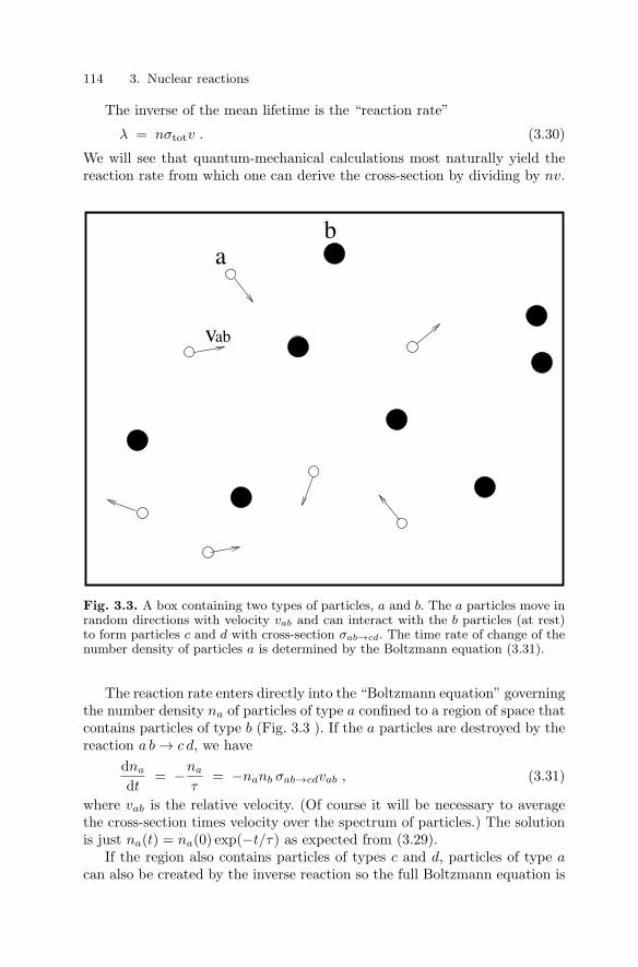
114 3. Nuclear reactions
The inverse of the mean lifetime is the “reaction rate”
λ = nσtotv . (3.30)
We will see that quantum-mechanical calculations most naturally yield thereaction rate from which one can derive the cross-section by dividing by nv.
v
ab
ab
Fig. 3.3. A box containing two types of particles, a and b. The a particles move inrandom directions with velocity vab and can interact with the b particles (at rest)to form particles c and d with cross-section σab→cd. The time rate of change of thenumber density of particles a is determined by the Boltzmann equation (3.31).
The reaction rate enters directly into the “Boltzmann equation” governingthe number density na of particles of type a confined to a region of space thatcontains particles of type b (Fig. 3.3 ). If the a particles are destroyed by thereaction a b → c d, we have
dna
dt= −na
τ= −nanb σab→cdvab , (3.31)
where vab is the relative velocity. (Of course it will be necessary to averagethe cross-section times velocity over the spectrum of particles.) The solutionis just na(t) = na(0) exp(−t/τ) as expected from (3.29).
If the region also contains particles of types c and d, particles of type acan also be created by the inverse reaction so the full Boltzmann equation is

3.1 Cross-sections 115
dna
dt= −nanbσab→cdvab + ncndσcd→abvcd . (3.32)
3.1.5 General characteristics of cross-sections
The magnitude of a reaction cross-section depends on the energetics of thereaction (elastic, inelastic–endothermic, inelastic–exothermic) and the inter-action responsible for the reaction (strong, electromagnetic, or weak). Addi-tionally, at low energy, inelastic reactions between positively charged ions arestrongly suppressed by the Coulomb barrier. In this section we review howthese effects are manifested in the energy (Fig. 3.4) and angular dependences(Fig. 3.6) of cross-sections.
Elastic scattering The elastic cross-section depends on whether or not thescattering is due to long-range Coulomb interactions or to short-range stronginteractions. As we will see in Sect. 3.2, the differential cross-section betweentwo isolated charged particles diverges at small angles like dσ/dΩ ∝ θ−4.The total elastic cross-section is therefore infinite. For practical purposes,this divergence is eliminated because the Coulomb potential is “screened” atlarge distances by oppositely charged particles in the target. Nevertheless, theconcept of total elastic cross-section for charged particles is not very useful.
Elastic neutron scattering is due to the short-range strong interaction sothe differential cross-section does not diverge at small angles and the totalelastic cross-section (calculated quantum mechanically) is finite. The elasticcross-sections are shown in Fig. 3.4 for neutron scattering on 1H, 2H and6Li. The 1H cross-section is flat at low energy before decreasing slowly forE > 1 MeV. The low energy value, σel ∼ 20 b, is surprisingly large comparedto that expected from the range of the strong interaction, π(2 fm)2 ∼ 0.1 b.We will see in Sect. 3.6 that this is due to the fact that the proton–neutronsystem is slightly unbound if the two spins are anti-aligned (and slightlybound if they are aligned). For neutron momenta greater than the inverserange r of the strong interactions, p > h/r [p2/2mn > h2/(r2mn) > 1 MeV],the cross-section drops down to a value more in line with the value expectedfrom the range of the strong interactions.
The elastic cross-section for 6Li shows a resonance at En ∼ 200 keV whichresults from the production of an excited state of 7Li that decays back ton 6Li. The level diagram of 7Li is shown in Fig. 3.5. For heavy nuclei, thereare many excited states leading to a very complicated energy dependenceof the cross-section, as illustrated for uranium in Fig. 3.26. The process ofresonant production will be discussed in Sect. 3.5.
The angular distribution for elastic neutron–nucleus scattering is isotropicas long as p < h/R (R=nuclear radius) as illustrated in Fig. 3.6 andexplained in Sect. 3.6. For p > h/R the angular distribution approaches thatexpected for diffraction from a semi-opaque object of radius R.

116 3. Nuclear reactions
H1
H2
Li6
(n,
(n,
(p,
γ)
γ)
γ)
(n,p)
(n,t)
(n,γ)
1
1
10 10 101 2 4 6
1
10
10
10
10
10
10
10
10
10−6
−4
−2
−4
−6
−2
−6
−4
−2
E(eV)
(bar
n)σ
(n,n)
(n,n)
(n,n)
Fig. 3.4. Examples of reaction cross-sections on 1H, 2H, and 6Li [30]. Neutron elas-tic scattering, (n,n), has a relatively gentle energy dependence while the exothermicreactions, (n, γ) and 6Li(n, t)4He (t=tritium=3H), have a 1/v dependence at lowenergy. The exothermic (p, γ) reaction is suppressed at low energy because of theCoulomb barrier. The reaction 6Li(n, p)6Be has an energy threshold. The fourthexcited state of 7Li (Fig. 3.5) appears as a prominent resonance in n6Li elasticscattering and in 6Li(n, t)4He.

3.1 Cross-sections 117
0
10E
(M
eV)
Li
Li
H
n
7
6
3 4He
6.6687.459
0.477
4.630
Fig. 3.5. The energy levels of 7Li and two dissociated states n−6 Li and 3H− 4He.The first excited state of 6Li decays to the ground state via photon emission whilethe higher excited states decay to 3H−4He. The fourth and higher excited states canalso decay to n−6 Li. The fourth excited state (7.459MeV) appears prominently asa resonance in n 6Li elastic scattering and in the exothermic (n,t) reaction n 6Li →3H4He. The resonance is seen at En ∼ 200 keV in Fig. 3.4.
Inelastic scattering Inelastic reactions with no Coulomb barrier havecross-section dependences at low energy that depend on whether the re-action is exothermic or endothermic. Exothermic reactions generally havecross-section proportional to the inverse of the relative velocity, σ ∝ 1/v.This leads to a velocity-independent reaction rate λ ∝ σv. Examples in thefigures are neutron radiative capture (n, γ) reactions. The nucleus 7Li alsohas an exothermic strong reaction n7Li → 3H 4He. The resonance observedin elastic scattering is also observed in the inelastic channel since the resonantstate (Fig. 3.5) can decay to 3H 4He.
Endothermic reactions have an energy threshold as illustrated in Fig. 3.4by the (n,p) reaction n6Li → p6Be.
Coulomb barriers The low-energy cross-section for inelastic reactions arestrongly affected by Coulomb barriers through which a particle must tunnelfor the reaction to take place. Cross-sections for two exothermic reactions on2H are shown in Fig. 3.4. The barrier-free (n, γ) reaction n 2H → γ 3H hasthe characteristic 1/v behavior at low energy. On the other hand, the (p, γ)reaction between charged particles p 2H → γ 3He is strongly suppressed at

118 3. Nuclear reactions
cosθ
dσ/d
cos
1
9
208
Be
H
Pb
1MeV
100MeV (x20)
0.1 MeV
1 MeV
10 MeV
0.1 MeV
1 MeV (x0.5)
10 MeV (x0.2)
800 MeV (x50)
θ(b
arn)
05
0
0
5
5
−1 1
Fig. 3.6. The differential cross-section, dσ/d cos θ = 2πdσ/dΩ, for elastic scatter-ing of neutrons on 1H, 9Be and 208Pb at incident neutron energies as indicated [30].At low incident momenta, p < h/Rnucleus, the scattering is isotropic whereas forhigh momenta, the angular distribution resembles that of diffraction from a disk ofradius R. Neutron scattering on 1H at high-energy also has a peak in the backwarddirections coming from the exchange of charged pions (Fig. 1.13).

3.1 Cross-sections 119
low energy. Its cross section becomes comparable to the (n, γ) reaction onlyfor proton energies greater than the potential energy at the surface of the 6Linucleus ∼ 3αhc/2.4 fm ∼ 1.8 MeV.High-energy inelastic collisions The Coulomb barrier becomes ineffectiveat sufficiently high energy, Ecm > Z1Z2αhc/R where R is the sum of the radiiof the nuclei of charges Z1 and Z2. In this case, the total inelastic cross-sectionbecomes of order of the geometrical cross-section πR2. At energies < 1 GeV,most inelastic collisions involve a simple break up of one or both of the nuclei,leading to the production of the unstable nuclei present in Fig. 0.2. Theseare called fragmentation reactions for medium-A nuclei while the breakup ofa heavy nucleus is called collision-induced fission. Fragmentation of a targetby protons or neutrons is called spallation.
110 115 120 125 130 135 150
−110
10
10
10
10
10
cros
s−se
ctio
n (b
)
fragment mass number A
Te isotopes
−5
−4
−2
−3
−6
Fig. 3.7. The production of tellurium isotopes in the fragmentation of 129Xe(790 MeV/nucleon) on a 27Al target (open circles) and the collision-induced fis-sion of 238U (750 MeV/nucleon) on a Pb target (filled circles) [31]. Fragmentationleads to proton-rich isotopes while fission leads to neutron-rich isotopes.
Figure 3.7 gives the distribution of tellurium isotopes produced in thefragmentation of 129Xe on a 27Al target and the collision-induced fission of238U on a Pb target (filled circles) [31]. Fragmentation of Xe leads to proton-rich isotopes since mostly neutrons are ejected during the collision. Fissionof uranium gives neutron-rich isotopes because of its large neutron-to-protonratio. Reactions like these are the primary source of radioactive nuclides nowused in the production of radioactive beams.
Occasionally, the target and projectile nuclei may fuse to form a muchheavier nucleus. The produced nucleus is generally sufficiently excited to emit

120 3. Nuclear reactions
neutrons until a bound nucleus is produced. Such reactions are called fusion–evaporation reactions. This is the mechanism used to produce trans-uraniumnuclei, as discussed in Sect. 2.8. The cross-section for the production of theheaviest elements is tiny, of order 10 pb for element 110.
For center-of-mass energies > 1 GeV/nucleon, inelastic nuclear collisionsgenerally result in the production of pions and other hadrons. Collisions ofcosmic-ray protons with nuclei in the upper atmosphere produce pions whosedecays give rise to the muons that are the primary component of cosmic raysat the Earth’s surface (Fig. 5.4).
Finally, we mention that for center-of-mass energies > 100 GeV/nucleon,certain collisions between heavy ions are believed to produce a state of mattercalled a quark–gluon plasma where the constituents of nucleons and hadronsare essentially free for a short time before recombining to form hadrons andnucleons. Such a state is also believed to exist in neutron stars (Sect. 8.1.2)and in the early Universe (Chap. 9).
Photons We have already calculated the cross-section (3.13) for elastic scat-tering of low-energy photons on free electrons. Since the cross-section is in-versely proportional to the square of the electron mass, we can anticipatethat the cross-section on free protons is 20002 times smaller and thereforenegligible. This is because photon scattering is analogous to classical radia-tion of an accelerated charge, and a heavy proton is less easily acceleratedthan an electron.
The most important contributions to the photon cross-section on matterhave nothing to do with nuclear physics. The important processes, shown inFig. 5.12, are Compton scattering on atomic electrons
γ atom → atom+ e− γ , (3.33)
photoelectric absorption
γ atom → atom+ e− , (3.34)
and pair production
γ (A, Z) → e+e− (A, Z) . (3.35)
Pair production dominates at energies above the threshold Eγ = 2mec2.
Just as photons can breakup atoms through photoelectric absorption,they can excite or break up nuclei through photo-nuclear absorption. Thecross-sections for this process on 2H and 208Pb are shown in Fig. 3.8. Thecross-section for dissociation of 2H exhibits a threshold at Eγ = 2.22 MeV,the binding energy of 2H. The cross-section for dissociation of 208Pb exhibitsa broad giant resonance structure typical of heavy nuclei. Such resonancescan be viewed semi-classically as the excitation of a collective oscillation ofthe proton in the nucleus with respect to the neutrons.

3.2 Classical scattering on a fixed potential 121
1
10
σ(b
arn)
0E(MeV)200
2H (x100)
Pb208
Fig. 3.8. The cross-sections for photo-dissociation of 2H and of 208Pb [30]. Thecross-section of Pb exhibits a giant resonance typical of heavy nuclei.
Neutrinos Methods for calculating neutrino cross-sections will be presentedin Sects. 3.2 and 3.4. Since neutrinos are subject to only weak interactions,their cross sections are considerably smaller than those of other particles.For neutrino energies much less than the masses of the intermediate vec-tor bosons, mWc2 = 80.4 GeV and mZc2 = 91.2 GeV the cross-sections areproportional to the square of the Fermi constant
G2F
(hc)4= 5.297 × 10−48 m2MeV−2 . (3.36)
By dimensional analysis, this quantity must be multiplied by the square ofan energy to make a cross-section. The cross-sections for several neutrinoinduced reactions are given in Table 3.1. For nuclear physics, neutrinos ofenergy Eν ∼ 1 MeV are typical so, multiplying (3.36) by 1 MeV2, gives cross-sections of order 10−48m2.
3.2 Classical scattering on a fixed potential
In this section, we consider the scattering of a particle in a fixed force fielddescribed by a potential V (r). This corresponds to situations where the factthat the target particle recoils has little effect on the movement of the beamparticle because the kinetic energy of the recoiling target particle can beneglected. For a beam particle of mass mb and momentum pb incident on a

122 3. Nuclear reactions
Table 3.1. The cross-sections for selected neutrino-induced reactions importantfor nuclear physics. The energy range where the formulas are valid are given. Apartfrom G2
F given by (3.36), the cross-sections depend on the “weak mixing angle”sin2 θw = .2312±0.0002, the “Cabibo angle” cos θc = 0.975±0.001, and the “axial-vector coupling” gA = 1.267 ± 0.003. The meaning of these quantities is discussedin Chap. 4.
reaction cross-section
νe e− → νe e− G2FE2
cm4π(hc)4
[(2 sin2 θw + 1)2 + 4
3 sin4 θw]
Ecm mec2
νe e− → νe e− G2FE2
cm4π(hc)4
[13 (2 sin2 θw + 1)2 + 4 sin4 θw
]Ecm mec
2
νµ e− → νµ e− G2FE2
cm4π(hc)4
[(2 sin2 θw − 1)2 + 4
3 sin4 θw]
Ecm mec2
νµ e− → νµ e− G2FE2
cm4π(hc)4
[13 (2 sin2 θw − 1)2 + 4 sin4 θw
]Ecm mec
2
νe n → e− p G2FE2
νπ(hc)4 cos2 θc
[1 + 3g2
A
]mec
2 Eν mpc2
νe p → e+ n G2FE2
νπ(hc)4 cos2 θc
[1 + 3g2
A
]mec
2 Eν mpc2
target of mass mt, it can be shown (Exercise 3.5) that the target recoil hasnegligible effect if the target rest-energy mtc
2 is much greater than the beamenergy
mtc2 Eb =
√m2
bc4 + p2bc2 . (3.37)
Since nucleons and nuclei are so much heavier than electrons and neutrinos,these conditions will be satisfied in physically interesting situations. Thisfact, plus the mathematical simplification coming from ignoring target recoil,justifies spending some time on potential scattering. We will therefore firsttreat the problem classically by following the trajectories of particles throughthe force field. This will be followed by two quantum-mechanical treatments,the first using perturbation theory and plane waves, and the second usingwave packets.
3.2.1 Classical cross-sections
Classically, cross-sections are calculated from the trajectories of particles inforce fields. Consider a particle in Fig. 3.9 that passes through a sphericallysymmetric force field centered on the origin. The particle’s original trajectoryis parametrized by the “impact parameter” b which would give the particle’sdistance of closest approach to the force center if there were no scattering.
The scattering angle θ(b) depends on the impact parameter, as in thefigure. The relation θ(b) or b(θ) can be calculated by integrating the equations

3.2 Classical scattering on a fixed potential 123
θ(b)θ (b+db)
b
db
2πbdb V>0
Fig. 3.9. The scattering of a particle of momentum p by a repulsive force. Thetrajectories for impact parameters b and b + db are shown. The probability that aparticle is scattered by an angle between θ(b) and θ(b + db) is proportional to thesurface area 2πbdb.
of motion with the initial conditions pz = p, px = py = 0. The probabilitythat a particle is scattered into an interval dθ about θ is proportional tothe area of the annular region between b(θ) and b(θ + dθ) = b + db, i.e.dσ = 2πbdb. The solid angle corresponding to dθ is dΩ = 2π sin θdθ. Thedifferential elastic scattering cross-section is therefore
dσ
dΩ(θ) =
2πbdb
2π sin θdθ=∣∣∣∣ b(θ)sin θ
· db
dθ
∣∣∣∣ . (3.38)
A measurement of dσ/dΩ determines the relation b(θ) which in turn givesinformation about the potential V .
3.2.2 Examples
We can apply (3.38) to several simple cases:
• Scattering of a point particle on a hard immovable sphere. The angle-impact parameter relation is
b = R cos θ/2 , (3.39)
where R is the radius of the sphere. The cross section is then
dσ
dΩ= R2/4 ⇒ σ = πR2 (3.40)
so the total cross-section is just the geometrical cross section of the sphere.In the case of scattering of two spheres of the same radius, the total scat-tering cross-section is σ = 4πR2.
• Scattering of a charged particle in a Coulomb potential
V (r) =Z1Z2e
2
4πε0r, (3.41)
where Z1 is the charge of the scattered particle, and Z2 is the charge ofthe immobile target particle. This historically important reaction is called

124 3. Nuclear reactions
“Rutherford scattering” after E. Rutherford who demonstrated the exis-tence of a compact nucleus by studying α-particle scattering on gold nuclei.The unbound orbits in the Coulomb potential are hyperbolas so the scat-tering angle is well-defined in spite of the infinite range of the force. For anincident kinetic energy Ek = mv2/2, the angle-impact parameter relationis
b =Z1Z2e
2
8πε0Ekcot(θ/2) . (3.42)
The cross-section is then
dσ
dΩ=(
Z1Z2e2
16πε0Ek
)2 1sin4 θ/2
. (3.43)
We note that the total cross-section σ =∫
(dσ/dΩ)dΩ diverges because ofthe large differential cross-section for small-angle scattering:
dσ
dΩ∼(
Z1Z2e2
4πε0Ek
)2 1θ4 (θ 1) . (3.44)
This divergence is due to the fact that incident particles of arbitrarilylarge impact parameters are deflected. The total elastic cross-section forscattering angles greater than θmin is (using dΩ ∼ 2πθdθ for θ 1)
σ(θ > θmin) ∼(
Z1Z2e2
4πε0Ek
)2π
θ2min
(θmin 1) . (3.45)
• Scattering of particles in a Yukawa potential
V (r) =ghc
re−r/r0 . (3.46)
This potential is identical to the Coulomb potential for r r0 but ap-proaches zero much faster for r > r0. Unlike the case of the Coulombpotential, there is no analytical solution for particle trajectories. It is nec-essary to integrate numerically the equations of motion to find θ(b) anddσ/dΩ. The result is shown in Fig. 3.10 for an incident particle of energyEk = 10ghc/r0. We see that for b < r0 (corresponding to θ > 0.1) thescattering angle approaches that for the Coulomb potential, as expectedsince the two potentials have the same form for r/r0 → 0. For b > r0, thescattering angle is smaller than the angle for Rutherford scattering sincethe Yukawa force falls rapidly for r r0. It follows that the differentialcross section for small angles is smaller than that for Rutherford scattering,diverging as θ−2 rather than as θ−4. The elastic cross section still divergesbut only logarithmically, σ(θmin) ∝ log(θmin). We see from the figure that
σ(θ > 0.01) = π[b(0.01)]2 ∼ 4πr20 . (3.47)
An angle of 0.01 is already quite small and to get a much higher cross-section one has to go to considerably smaller angles. For the Yukawa po-tential, πr2
0 therefore gives the order of magnitude of the cross-section

3.2 Classical scattering on a fixed potential 125
for scattering by measurably large angles. We shall see below that in thequantum-mechanical calculation, the cross-section is finite.
b/r 0 Ω
/dσ
log
d
10.10.01 0.01 0.1 1
1
2
θ θ(radians) (radians)
2
4
θ−4
−2
θ
θθ−1
θ =k
g hc/r0
E
Fig. 3.10. The scattering of a non-relativistic particle in a Yukawa potential V (r) =ghc e−r/r0/r. The initial kinetic energy of the particle is taken to be 10ghc/r0 sothat it can penetrate to about r = r0/10. The left solid curve shows the numericallycalculated impact parameter b(θ) in units of r0. The right solid curve shows thelogarithm of the differential scattering normalized to the backward scattering cross-section (θ = π). For comparison, the dashed lines show the same functions for theCoulomb potential V (r) = ghc/r. For θ > 0.1, we have b < r0 and the two potentialsgive nearly the same results. This is to be expected since the two potentials arenearly equal for r r0. For b r0, the Yukawa scattering angle is much less thanthe Coulomb scattering angle because the force drops of much faster with distance.As a consequence, the cross section is smaller.
Much of our knowledge of nuclear structure comes from the scatteringof charged particles (generally electrons) on nuclei. This is because high-energy charged particles penetrate inside the nucleus and their scattering-angle distribution therefore gives information on the distribution of charge inthe nucleus. We will see that the correct interpretation of these experimentsrequires quantum-mechanical calculation of the cross-sections. However, itturns out that the quantum-mechanical calculation of scattering in a 1/rpotential gives the same result as the classical Rutherford cross-section foundabove. This means that the Rutherford cross-section can be used to interpret

126 3. Nuclear reactions
experiments using positively charged particles whose energy is sufficiently lowthat they cannot penetrate inside the nucleus.
This is how, in 1908, Rutherford discovered that the positive charge insideatoms is contained in a small “nucleus.” Rutherford reached this conclusionafter hearing of the results of experiments by Geiger and Marsden study-ing the scattering of α-particles on gold foils. While most α’s scattered intothe forward direction, they occasionally scatter backward. This was impos-sible to explain with the then popular “plum pudding” model advocated byJ.J. Thomson where the atom consisted of electrons held within a positivelycharged uniform material. A heavy α-particle cannot be deflected through asignificant angle by the much lighter electron. On the other hand, scatter-ing at large angle would be possible in rare nearly head-on collisions with amassive, and therefore immobile, gold nucleus.
After this brilliant insight, Rutherford spent some time (2 weeks [5]) cal-culating the expected angular distribution which turned out to agree nicelywith the observed distribution. Rutherford’s model naturally placed the lightelectrons in orbits around the heavy nucleus.
Another 17 years were necessary to develop the quantum mechanics thatexplains atomic structure and dynamics.
We expect the Rutherford cross-section calculation to fail if the electroncan penetrate inside the nucleus. Classically, this will happen for head-oncollisions if the initial kinetic energy of the α particle is greater than theelectrostatic potential at the nuclear surface:
Ek =2Ze2
4πε0R=
2Zαhc
R∼ 1.2 A2/3 MeV , (3.48)
where 2Z is the product of the α-particle and nuclear charges, α is the finestructure constant, and we have used R ∼ 1.2A1/3 fm and Z ∼ A/2. Weexpect the backward scattering to be suppressed for energies greater than thisvalue. The naturally occurring α-particles used by Rutherford have energiesof order 6 MeV so the effect can only be seen for Z/A1/3 < 3 correspondingto A < 11. Rutherford and collaborators used this effect to perform the firstmeasurement of nuclear radii.
3.3 Quantum mechanical scattering on a fixed potential
Quantum mechanical collision theory is treated at length in many text-books. 1 In this section, we will present two simple approximate methodsapplicable to scattering due to weak and electromagnetic interactions. The1 See for instance M. L. Goldberger and K. M. Watson, Collision Theory, John
Wiley & Sons, 1964; K. Gottfried, Quantum Mechanics, W. A. Benjamin, 1966; J-L. Basdevant and J. Dalibard, Quantum Mechanics Chapter 18, Springer-Verlag,2002.

3.3 Quantum mechanical scattering on a fixed potential 127
first uses standard time-dependent perturbation theory applied to momen-tum eigenstates and the second uses wave packets. The first is an essentialpart of this chapter because it can be easily generalized to inelastic scatter-ing. The second is mostly a parenthetical section intended to improve ourunderstanding of the physics.
To prepare the ground for the perturbation calculation, we first brieflydiscuss the concept of asymptotic states and their normalization. Other tech-nical ingredients, the limiting forms of the Dirac δ function, and basics resultsof time-dependent perturbation theory in quantum mechanics are reviewedin Appendix C.
3.3.1 Asymptotic states and their normalization
In studying nuclear, or elementary interactions, we are most of the timenot interested in a space-time description of phenomena.2 Instead, we studyprocesses in which we prepare initial particles with definite momenta and faraway from one another so that they are out of reach of their interactions at aninitial time t0 in the “distant past” t0 ∼ −∞. We then study the nature andthe momentum distributions of final particles when these are also out of rangeof the interactions at some later time t in the “distant future” t → +∞. (Thesize of the interaction region is of the order of 1 fm, the measuring deviceshave sizes of the order of a few meters.)
Fig. 3.11. Asymptotic states in a collision
Under these assumptions, the initial and final states of the particles un-der consideration are free particle states. These states are called asymptoticstates. The decay of an unstable particle is a particular case. We measure theenergy and momenta of final particles in asymptotic states.2 One exception is the case of “neutrino oscillations” discussed in Sect. 4.4.

128 3. Nuclear reactions
By definition, the asymptotic states of particles have definite momenta.Therefore, strictly speaking, they are not physical states, and their wavefunctions eipx/h are not square integrable. Physically, this means that we areactually interested in wave packets who have a non vanishing but very smallextension ∆p in momentum, i.e. ∆p/|p| 1.
It is possible to work with plane waves, provided one introduces a propernormalization. A limiting procedure, after all calculations are done, allows toget rid of the intermediate regularizing parameters. This is particularly simplein first order Born approximation, which we will present first. The completemanipulation of wave packets is possible but somewhat complicated. How-ever, it gives interesting physical explanations for various specific problems,and we shall discuss it in Sect. 3.3.5.
We will consider that the particles are confined in a (very large but finite)box of volume L3. We will let L tend to infinity at the end of the calcula-tion. Besides its simplicity, this procedure allows to incorporate relativistickinematics of ingoing and outgoing particles in a simple manner.
In such a box of size L, the normalized momentum eigenstates are
|p〉 → ψp(r) = L−3/2eip·r/h inside the box , (3.49)
ψp(r) = 0 outside the box .
These wave functions are normalized in the sense that∫|ψp(r)|2 d3r = 1 . (3.50)
For convenience, we will define here the Hilbert space with periodicboundary conditions : in one dimension ψ(L/2) = ψ(−L/2) and ψ′(L/2) =ψ′(−L/2) (this amounts to quantizing the motion of particles on a large circleof radius R = L/2π). In such conditions, the operators p = (h/i)∂/∂x and p2
have a discrete spectrum pn = 2πnh/L. In three dimensions the quantizationof momentum is p = (2πh/L)(n1, n2, n3), where the ni are arbitrary integers.
The advantage of using periodic boundary conditions is that the states(3.49) are normalized eigenstates of both the energy and the momentum, aswe wish. This is not the case in the usual treatment of a “particle in a box”where one requires that the wave function vanish at the edge of the box. Theenergy eigenfunctions in this case are
ψE(r) = L−3/2 sin nxπx/L sin nyπy/L sin nzπz/L (3.51)
where nx, ny, nz are positive integers and E = π2h2(n2x + n2
y + n2z)/2mL2. In
this case the energy eigenfunctions are not eigenstates of momentum. How-ever, both boundary conditions give the same density of states so we neednot worry about which regularization procedure is used.
The orthogonality relation between momentum eigenstates
〈p|p′〉 = δn1n′1δn2n′
2δn3n′
3

3.3 Quantum mechanical scattering on a fixed potential 129
can also be written in the following manner, useful to take limits,
〈p|p′〉 = (2πh/L)3∆3L(p − p′) , (3.52)
where ∆3L(p − p′) is a limiting form of the delta function discussed in Ap-
pendix (C.0.2).Since each component of momentum is quantized in steps of 2πh/L, the
number of states in a momentum volume d3p is
dN(p) = (2s + 1)(L
2πh)3d3p ≡ ρ(p)d3p (3.53)
where 2s+1 is the number of spin-states for a particle of spin s. This definesthe density of states (in momentum space): ρ(p) = (2s + 1)(L/2πh)3. Thiscorresponds to a density in phase space (momentum×real space) of (2s + 1)states per elementary volume (2πh)3.
In what follows, we will be interested in the number of states in an intervaldE. To obtain this, we note that the number of states within a momentumvolume d3p can be written as
dN(p) = ρ(p)d3p = (2s + 1)(L
2πh)3 p2dpdΩ , (3.54)
where dΩ is the solid angle covered by d3p. Taking EdE = c2 pdp (whichholds both in the relativistic and non-relativistic regimes), we find the numberof states in the interval dE and in the solid angle dΩ is
dN(E, dΩ) = (2s + 1)(L
2πh)3
pE
c2 dEdΩ . (3.55)
3.3.2 Cross-sections in quantum perturbation theory
The simplest way to calculate cross-sections in quantum mechanics is to usestandard time-dependent perturbation theory (Appendix C). The idea is todescribe the system by a Hamiltonian that is the sum of an “unperturbed” H0and a perturbation H1. In the present context, H0 will represent the kineticenergy of the incoming and outgoing beam particles and the perturbation H1will be the interaction potential (which acts for a very short time).
Perturbation theory gives the transition rates between energy eigenstatesof the unperturbed Hamiltonian, i.e. between the initial state |i〉 of energyEi and one of the possible final states |f〉 of energy Ef . The first order resultis
λi→f =2π
h|〈f |H1|i〉|2 δ(Ef − Ei) , (3.56)
where δ(E) satisfies∫ ∞
−∞δ(E)dE = 1 , (3.57)

130 3. Nuclear reactions
and is a limiting form of the delta function discussed in (C.0.2). The dimen-sion of δ(E) is 1/energy so the transition rate λ has dimension of 1/time asexpected.
If higher-order perturbation theory is necessary, energy will still be con-served in the transition rate since energy conservation is an exact result dueto the time-translation invariance of the Hamiltonian. The more general tran-sition rate including higher-order effects is then written as
λi→f =2π
h|〈f |T |i〉|2 δ(Ef − Ei) , (3.58)
where T is the “transition matrix element.” In the context of scattering the-ory, the first order result, T = H1, is called the “Born approximation.”
For the initial and final states, we choose plane waves of momentum pand p′ as defined above
ψi(r) =eip·r/h
L3/2 ψf (r) =eip′·r/h
L3/2 , (3.59)
where L3 is the normalization volume. The classical scattering angle is definedby
cos θ =p · p′
|p||p′| . (3.60)
Of more importance for quantum calculations is the momentum transfer
q = p′ − p , (3.61)
and its square
q2 = q · q = |p|2 + |p′|2 − 2p · p′ . (3.62)
For elastic scattering we have |p| = |p′| = p so
q2 = 2p2(1 − cos θ) = 4p2 sin2 θ/2 (elastic scattering) . (3.63)
The small angle limit is often useful:
q2 ∼ p2θ2 θ 1 , (elastic scattering) . (3.64)
The matrix element between initial and final states is then
〈p′|V |p〉 =1L3
∫ei(p−p′)·r/hV (r)d3r =
V (p − p′)L3 . (3.65)
It is proportional to the Fourier transform of the potential
V (q) =∫
eiq·r/h V (r)d3r . (3.66)
Note that the dimensions of V defined here are energy×volume.The transition rate to the final state is
λi→f =2π
h
|V (p − p′)|2L6 δ(E′ − E) . (3.67)

3.3 Quantum mechanical scattering on a fixed potential 131
p’
d Ω
pFig. 3.12. Scattering of a single particle by a fixed potential.
We cannot measure the transition rate to a single momentum state so wemust sum the transition rate over a group of interesting final states. Withina volume L3, the number of momentum states in the momentum range d3p′
is given by (3.53). Multiplying (3.67) by this number of states we get thetotal transition rate into the momentum volume d3p
λ(d3p′) =(
L
2πh
)3
d3p′ 2π
h
|V (q)|2L6 δ(E′ − E) . (3.68)
We carefully drop the factor (2s + 1) in the number of states. We do thisbecause it is often the case that only one spin state is produced with highprobability in a reaction. When this is not the case, it is then necessary tosum over all possible final spin states.
The number of states in the momentum range dE′ and momentum ori-ented into the solid angle dΩ at angles (θ, φ) with respect to a given directionis given by (3.55) so the total transition rate into these states is then
λ(dE′, dΩ) =(
L
2πh
)3p′E′
c2 dE′dΩ2π
h
|V (q)|2L6 δ(E′ − E) . (3.69)
We use the delta function to integrate over energy in order to find the tran-sition rate into (energy-conserving) states within the solid angle dΩ
λ(dΩ) =v′
L3
(E′)2
4π2h4c4|V (q)|2 dΩ , (3.70)
where v′ = p′c2/E′ is the velocity of the final state particle.We remark, as mentioned above, that the crucial factor in (3.70) is the
presence of the modulus squared of the Fourier transform of the potential|V (q)|2. This is the main result of this calculation. Information on the differ-ential cross-section gives us direct access to the potential through its Fouriertransform. This result is very concise and elegant. It is basically the sameeffect that one encounters in diffraction phenomena. If one neglects multiplescattering, the amplitude of the diffraction pattern is the Fourier transformof the diffracting system (crystal, macro-molecule, etc.).

132 3. Nuclear reactions
3.3.3 Elastic scattering
For elastic scattering, E′ = E, so the transition rate is
λ(dΩ) =v
L3
E2
4π2h4c4|V (q)|2 dΩ , (3.71)
where v is the velocity of the initial state particle. The transition rate isproportional to the density of scattering centers (n = 1/L3) and to the ve-locity of the projectile. Using (3.30), we divide by these two factors to getthe differential cross-section
dσ
dΩ=
E2
4π2(hc)4|V (q)|2 , (3.72)
where E =√
p2c2 + m2c4 is the energy of the incident particle and V is givenby (3.66).
We remark that in the above expression the normalization parameter Lcancels off identically. Therefore, we can readily take the limit L → ∞.
σd/d
Ωlo
g()
hpr0
0.10.01 1
2
4
θ=
(radians)θFig. 3.13. The scattering of a non-relativistic particle in a Yukawa potential V (r) =ghce−r/r0/r. The momentum of the particle is p = 10h/r0. The solid line shows thequantum mechanical differential cross-section (3.75). For small angles θ < h/(pr0)the cross section is flat, avoiding the divergence present in the classical calculation(Fig. 3.10). At large angles θ > h/(pr0) the scattering follows the Coulomb cross-section shown by the dashed line.
As an example of potential scattering, we can take the Yukawa potential

3.3 Quantum mechanical scattering on a fixed potential 133
V (r) =ghc
re−r/r0 , (3.73)
where the range of the interaction is the Compton wavelength r0 = h/Mc ofthe exchanged particle of mass M . The Coulomb potential between particlesof charge Z1 and Z2 corresponds to g = Z1Z2α and r0 → ∞. The Fouriertransform V (q) for the Yukawa potential is
V (q) =4π ghc h2
q2 + (h/r0)2=
4πg(hc)3
q2c2 + M2c4 , (3.74)
which gives a differential cross-section
dσ
dΩ= 4g2(hc)2
(E
4p2c2 sin2 θ/2 + M2c4
)2
, (3.75)
where we have used (3.63). The cross section, shown in Fig. 3.13, does notdiverge at small angles like the classical cross-section. The total elastic cross-section is therefore finite:
σel = 8πg2 (hc)2(
E
M2c4
)2 11 + 2p2/M2c2 . (3.76)
We remark that in many strong interaction calculations, the Born approxi-mation is not valid. Indeed the dimensionless parameter g is larger than oneand perturbation theory does not apply. Nevertheless, the above result bearsmany qualitatively useful features.
In what follows, we consider cases where the Born approximation is valid.There are two simple limits corresponding to the mass of the exchangedparticle Mc2 being much greater than or much less than pc.
• Mc2 pc, i.e. r0 h/p. As illustrated in Fig. 3.13, the differential crosssection is angle-independent for θ < h/(pr0) and Rutherford-like for θ >h/(pr0). We can then find the cross-section for the Coulomb potential bytaking the limit r0 → ∞ and setting g = Z1Z2α:
dσ
dΩ=(
Z1Z2e2
4πε0
)2(E
2p2c2
)2 1sin4 θ/2
. (3.77)
In the non-relativistic limit, E = mc2, Ek = p2/2m, and the formulareduces to the classical Rutherford cross-section (3.43).
dσ
dΩ=(
Z1Z2e2
16πε0
)2( 1p2/2m
)2 1sin4 θ/2
. (3.78)
This coincidence of the classical and the quantum theory seems, at first,amazing. It is actually quite simple to understand by dimensional analysis.The non-relativistic cross-section (3.78) calculated quantum mechanicallyturns out to be independent of h. It is proportional to the square of theonly length, a = e2/4πε0(p2/2m), that is linear in e2/4πε0 and a combi-nation of powers of p, m and h. Since this is the only length available, the
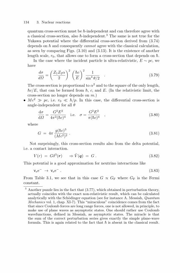
134 3. Nuclear reactions
quantum cross-section must be h-independent and can therefore agree witha classical cross-section, also h-independent.3 The same is not true for theYukawa potential where the differential cross-section derived from (3.74)depends on h and consequently cannot agree with the classical calculation,as seen by comparing Figs. (3.10) and (3.13). It is the existence of anotherlength scale, r0, that allows one to form a cross-section that depends on h.
In the case where the incident particle is ultra-relativistic, E ∼ pc, wehave
dσ
dΩ=(
Z1Z2α
2
)2 (hc
E
)2 1sin4 θ/2
. (3.79)
The cross-section is proportional to α2 and to the square of the only length,hc/E, that can be formed from h, c, and E. (In the relativistic limit, thecross-section no longer depends on m.)
• Mc2 pc, i.e. r0 h/p. In this case, the differential cross-section isangle-independent for all θ
dσ
dΩ=
G2E2
4π2(hc)4i.e. σ =
G2E2
π(hc)4, (3.80)
where
G = 4πg(hc)3
(Mc2)2. (3.81)
Not surprisingly, this cross-section results also from the delta potential,i.e. a contact interaction.
V (r) = Gδ3(r) ⇒ V (q) = G . (3.82)
This potential is a good approximation for neutrino interactions like
νee− → νee− . (3.83)
From Table 3.1, we see that in this case G ∝ GF where GF is the Fermiconstant.3 Another puzzle lies in the fact that (3.77), which obtained in perturbation theory,
actually coincides with the exact non-relativistic result, which can be calculatedanalytically with the Schodinger equation (see for instance A. Messiah, QuantumMechanics vol. 1, chap. XI-7). This “miraculous” coincidence comes from the factthat since Coulomb forces are long range forces, one is not allowed, in principle, tomake use of plane waves as asymptotic states. One should rather use Coulombwavefunctions, defined in Messiah, as asymptotic states. The miracle is thatthe sum of the correct perturbation series gives exactly the simple plane-waveformula. This is again related to the fact that h is absent in the classical result.

3.3 Quantum mechanical scattering on a fixed potential 135
3.3.4 Quasi-elastic scattering
Potential scattering most naturally applies to elastic scattering because ofthe classical limit of a light particle moving through the force field of a fixedheavy particle. However, in the quantum treatment, we saw that the potentialsimply serves to calculate a matrix element between initial and final states. Itis not surprising therefore that the same formalism applies to “quasi-elastic”scattering where the light particle changes its nature (i.e. its mass) when itinteracts with a fixed particle. Obvious candidates are the weak interactionsof leptons scattering on nucleons, e.g.
νe p ↔ e+ n . (3.84)
We note that the reaction going to the right is endothermic and the reactiongoing to the left is exothermic. Since these two reactions are due to theexchange of W bosons, we can use a delta-potential of the form (3.82) andrely on the fundamental theory of weak interactions (Table 3.1) to provideus with the effective G for each reaction.
The rate calculation proceeds as in the elastic case up to (3.70) at whichpoint we have to take into account the fact the the initial and final statemomenta are not equal. Since we will want to factor out the initial statevelocity, we write the rate as
λ(dΩ) =v
L3
v′
v
(E′)2
4π2h4c4|V (q)|2 dΩ , (3.85)
corresponding to a cross-section
dσ
dΩ=
v′
v
(E′)2
4π2h4c4|V (q)|2 . (3.86)
For the delta-potential, the angular distribution is isotropic and the cross-section is
σ =v′
v
(E′)2
πh4c4G2 . (3.87)
At sufficiently high energy, the initial and final state velocities approach cso the factor v′/v is of no importance. At low energy, this factor generates avery different behavior for the two reactions.
The endothermic reaction νep → e+n has a threshold neutrino energy ofEth = (mn + me − mp)c2 = 1.8 MeV. Near threshold, the final state positronhas an energy E′ ∼ mec
2 and a velocity v′ ∼√2(Eν − Eth)/me. The initialvelocity for the nearly massless neutrino is v ∼ c so the cross-section is
σ =(
2(Eν − Eth)mec2
)1/2 (mec2)2
πh4c4G2 Eν > Eth . (3.88)
The situation for the exothermic reaction e+n → νep is quite different.As the velocity v of the positron approaches zero, the energy E′ of the final

136 3. Nuclear reactions
state neutrino approaches (mn + me − mp)c2 = 1.8 MeV so the cross-sectionapproaches
σ =c
v
(mn + me − mp)2c4
πh4c4G2 . (3.89)
The cross-section is proportional to the inverse of the velocity, as anticipatedin Sect. 3.1.5. The reaction rate, proportional to the product of the velocityand the cross-section is therefore velocity independent.
3.3.5 Scattering of quantum wave packets
The calculations of the last section were very efficient in yielding reactionrates and cross-sections in cases where perturbation theory applies. However,they are not able to elicit various physical properties of interest. In thissection, we will provide a more physical description using wave packets, whichwe shall use later on.
In quantum mechanics, particles are represented by wavefunctions, ψ(r)giving the probability |ψ(r)|2d3r to find the particle in a volume d3r near r.If the particle interacts only via a potential V (r), the wavefunction satisfiesthe Schrodinger equation
ih∂ψ
∂t=
−h2
2m∇2ψ + V (r)ψ . (3.90)
As illustrated in Fig. 3.14, a scattering experiment on a single target parti-cle with a short range potential corresponds to the situation where V (r) ∼ 0except in a small region r < R near the target particle. Initially, the wavefunc-tion is a broad wave packet, ψin, that propagates freely in the z direction farfrom the target. The transverse width of the wave packet is taken to be muchgreater than R so that the entire potential is “sampled” by the wavefunction.When the wave packet reaches the target (t = 0), the interaction with thepotential generates a scattered wave packet ψsc which now accompanies thetransmitted wave packet.
The essential result of the calculation that follows is that the scatteredwave is found by summing spherical waves emanating from each point in theregion where V = 0. This is illustrated in Fig. 3.15. It will turn out that thescattered wave from each point is proportional to the product of the potentialand the incident wave at that point. This is physically reasonable since thescattered wave must vanish when either the potential or the incident wavevanishes. When one integrates the waves over the region of non-vanishingpotential, the result (3.113) that the scattered wave is proportional to theFourier transform of the potential will emerge in a natural way. Physically,this comes about since, as illustrated in Fig. 3.15, the waves add coherentlyin the forward direction but with increasingly random phases away from theforward direction. This leads to a decreasing cross-section with increasing

3.3 Quantum mechanical scattering on a fixed potential 137
θ
ο
ψsc
z
x
inψ
wavetransmitted
θrd
Fig. 3.14. A wave packet that impinges upon a region with V (r) = 0 will interactin a way that will produce a scattered wave packet and a transmitted wave packet.The probability to find the particle in the box in the scattered wave is proportionalto the differential scattering cross-section, dσ/dΩ.
angle. Mathematically, this is just what the Fourier transform does since itis maximized at q = 0 (θ = 0).
We now start the wave packet calculation of the differential cross-section.This cross-section is related to the rate of particles counted by a detectorplaced at an angle θ with respect to the beam shown in Fig. 3.14. The rateis given by
dNdet
dt= NT F
dσ
dΩdΩ , (3.91)
where NT is the number of target particles and F is the incident particleflux. We average the flux over some arbitrary time T much greater than thetime of passage of the wave packet. The mean incident flux is given by theprobability to find the incident particle near the z-axis:

138 3. Nuclear reactions
r1
r2ar rb
out of phase
in phase
Fig. 3.15. In the Born approximation, the scattered wave at any point far fromthe region of V = 0 is the sum of spherical waves emitted at each point r′ in thescattering region. The figure shows who such waves, one emitted at ra and oneat rb. The phase of the scattered wave at the point r is k(z′ + |r − r′|). Onlyin the forward direction is this phase independent of r′. In other directions, thephase depends on r′ so the spherical waves do not sum coherently. This results ina diminishing of the cross-section for angles satisfying |p′ − p|R > h.
F (x = y = 0, z) =1T
∫ ∞
−∞dz|ψin(x = y = 0, z, t < 0)|2 . (3.92)
We use a wave packet that is sufficiently broad that this flux is constant overthe entire extent of the region with V = 0.
The detection rate is proportional to the probability to find the particlein the box shown in Fig. 3.14:
dNdet
dt=
1T
(dθ)2∫ ∞
0dr r2|ψsc(r, θ, t 0)|2 . (3.93)
Using (3.91), we find
dσ
dΩ=
∫dr |ψsc(r, θ, t 0)|2r2∫
dz |ψin(x = y = 0, z, t < 0|2 (3.94)
To calculate the differential cross-section we need only calculate ψsc for agiven ψin. To do this, it is useful to express the wavefunction as a superposi-tion of the energy eigenfunctions ψE(r) satisfying the eigenvalue equation
− h2
2m∇2ψE(r) + V (r, t)ψE(r) = EψE(r) . (3.95)

3.3 Quantum mechanical scattering on a fixed potential 139
For V = 0 the eigenfunctions are just the familiar plane waves, exp(ip · r/h)and a superposition makes a wave packet of the form
ψ(r, t) =1
(2π)3/2
∫d3k φ(k) ei(k·r−ω(k)t) , (3.96)
where k = p/h and ω(k) = E(p)/h. With V = V (r) = 0, far from thetarget, r R, the eigenfunctions are sums of plane waves and radial wavesemanating from the target:
ψ(r, t) =1
(2π)3/2
∫d3k φ(k)
[eik·r +
f(θ)r
eikr
]e−iω(k)t . (3.97)
The first term in the integral represents the initial and transmitted wavepacket and the second term is the scattered wave. (We will see that thesecond term integrates to zero for t 0 so it does not contribute to theinitial wave packet.) The “scattering amplitude” f(θ) is a function of theangle between the momentum p and the position vector r:
cos θ(k, r) =k · r
|k||r| . (3.98)
Since f(θ) has the dimensions of length, we can anticipate that
dσ
dΩ= |f(θ)|2 . (3.99)
To describe a particle impinging on the target along the z direction wetake φ(k) to be strongly peaked at k0 = (kx = 0, ky = 0, kz = k0 = p0/h).Therefore only the values of k near k0 will contribute. We therefore expandω(k)
hω(k) = E(p0) + ∇E(p) · (p − p0) + . . .
= E(p0) + v0(pz − p0) + . . . , (3.100)
where v0 is the group velocity. For a wave packet representing a massiveparticle, the group velocity is the classical velocity v0 = p0/m. Keeping onlythe first two terms in the expansion, the first term of (3.97) is
ψin(r, t) =1
(2π)3/2 ei(k0z−ω0t)ψenv(r − v0t) , (3.101)
where the “envelope” function is
ψenv(r − v0t) =∫
d3k φ(k) ei(k−k0)·(r−v0t) . (3.102)
We see that ψin is the product of a plane wave and an envelope that is afunction only of r − v0t, i.e. the envelope moves with the group velocity.For example, if φ(k) is a real Gaussian function peaked at k − k0 = 0, thenthe envelope will be a Gaussian peaked at r − v0t = 0, i.e. at r = v0t, withthe variances of the Gaussians satisfying the Heisenberg uncertainty relations

140 3. Nuclear reactions
σxσpx= σyσpy
= σzσpz∼ h. Including higher-order terms in the expansion
(3.100) leads to spreading of the wave packet at large times.The scattered wavefunction has a similar structure:
ψsc(r, θ, t) =f(θ)
rei(k0r−ω0t)
∫d3k φ(k) ei(kz−k0)(r−v0t) (3.103)
where we have dropped a factor exp(i(k2x +k2
y)r/k0) which is near unity for asufficiently wide wave packet. We have also taken f(θ) out of the integral sinceφ(k) is strongly peaked around k0 and therefore (3.98) is well approximatedby
cos θ ∼ k0 · r
|k0||r| . (3.104)
Comparing (3.102) and (3.103), we see that
|ψsc(r − v0t, θ, t)|2 =|f(θ)|2
r2 |ψin(x = y = 0, z = r − v0t)|2 . (3.105)
This tells us the scattered wavefunction is simply a replica of ψin that is scaleddown by a factor f(θ)/r. Note also that (3.105) implies that the scatteredwave vanishes for t 0 since it is proportional to the incident wave at(t 0, z 0) which vanishes.
Substituting (3.105) into (3.94) we find the required identification of thedifferential scattering cross-section and the square of the scattering amplitude(3.99).
We now need to find the relation between f(θ) and the potential V (r).This is easy to do if the potential is sufficiently weak that the wave packetis only slightly perturbed as it passes through the potential. We rewrite theeigenvalue equation (3.95) as
(∇2 − k2)ψk(r) = 2mV (r)ψk(r)/h2 (3.106)
where k =√
2mE/h. We will look for solutions of the form
ψk = eikz + ψk sc , (3.107)
where the first term is a solution of the eigenvalue equation with V = 0and the second term is a particular solution to the equation with V = 0.Since the effect of the potential is assumed to be small, it should be a goodapproximation to replace the wavefunction of the right-hand side of (3.106)with the incident plane wave:
(∇2 − k2)ψk(r) = 4πS(r) , (3.108)
where
S(r) =2mV (r) exp(ik · r)
4πh. (3.109)
For k = 0 this is the Poisson equation of electrostatics with the electrostaticpotential replaced by ψk(r) and the charge density replaced by S(r). Thesolution is well-known:

3.3 Quantum mechanical scattering on a fixed potential 141
ψk sc(r) =14π
∫d3r′ 1
|r − r′|S(r′) (k = 0) . (3.110)
For k = 0, the solution is only slightly more complicated:
ψk sc(r) =14π
∫d3r′ exp(ik|r − r′|)
|r − r′| S(r′) . (3.111)
This formula has a simple physical interpretation: the scattered wave is asum of spherical waves generated at each point r′ in the potential well andhaving an amplitude proportional to S(r′) ∝ V (r′).
Equation (3.111) can be written as
ψk sc(r) =2m
4πh2
∫d3r′ exp(ik|r − r′|) exp(ikz′)
|r − r′| V (r) . (3.112)
We are interested in ψsc far from the scattering center in which case wecan approximate r′ = 0 (in the denominator) and |r − r′| ∼ r − r · r′/r(in the numerator). A particle observed at r will be interpreted as havinga momentum p′ = p0r/r implying |r − r′| ∼ r − k′ · r′/k0 so the scatteredwavefunction is
ψk(r) =2meikr
4πr
∫d3r′V (r′) exp(iq · r′/h) , (3.113)
where q = p−p′ is the momentum transfer of magnitude |q|2 = 2p20(1−cos θ).
We see that the scattered wave is proportional to the Fourier transform ofthe potential.
V (q) =∫
eiq·r/hV (r)d3r . (3.114)
The differential cross section is thendσ
dΩ=
m2
4π2h4 |V (p − p′)|2 (3.115)
as found in the previous section.Equation, (3.115) tells us that the cross-section takes an especially simple
form if q = 0
dσ
dΩ(q = 0) =
m2
4π2h4
∣∣∣∣(∫
V (r)d3r
)∣∣∣∣2
. (3.116)
Since q2 = 2p2(1−cos θ), this condition is met either in the forward direction,θ = 0, or in the low-energy limit where the de Broglie wavelength is muchgreater than the range of the potential, h/p R. For q2 = 0, the exponentialin the integrand is an oscillating function of r′ so the integral is suppressed.This can be intuitively understood by saying that far from the region whereV = 0, the spherical waves generated at different positions are not entirelyin phase and therefore partially cancel. As seen in (3.112) and in Fig. 3.15,only for θ = 0 or for h/p R is the phase independent of r′ so the sphericalwaves are entirely in phase at the observer’s position r.

142 3. Nuclear reactions
v= o
k
r
r
r−r
θo
Fig. 3.16. A wave packet of central momentum p0 = hk0 that impinges upona region with V (r) = 0. The scattered wave packet at r is the superposition ofspherical waves generated at each point r′. A particle observed at r will be inter-preted as having a momentum p′ = p0r/r implying a momentum transfer squaredof |q|2 = |p′ − p|2 = 2p2
0(1 − cos θ).
The suppression of the cross-section for θ = 0 because of destructiveinterference is quite different from the classical case. Here, the large anglecross-section is suppressed simply because the particle trajectory must passnear the center of the potential in order to produce a wide-angle scatter.
While the decline of the cross-section with increasing scattering anglehas different origins in quantum and classical mechanics, we saw previouslythat the classical and quantum calculations may give identical answers aslong as q2 = 0. In fact, what distinguishes quantum scattering from classicalscattering is that in quantum scattering the cross-section must be isotropicfor qR 1. This condition is met at all scattering angles if the de Brogliewavelength of the incident particle is much greater than the range R of thepotential. This is equivalent to the condition
p2
2m<
(hc)2
8R2mc2 = 5 MeV1 GeVmc2
(1 fmR
)2
. (3.117)
For incident energies below this limit, the scattering must be isotropic. Forincident energies above this limit, the scattering will still be isotropic at smallangles:

3.4 Particle–particle scattering 143
θ <hc√
2(p2/2m)mc2R= 2
(5 MeVp2/2m
)1/2 (1 GeVmc2
)1/2 1 fmR
,(3.118)
where we have taken the small-angle limit (1−cos θ) = θ2/2. For angles largerthan this values, the cross-section decreases, as seen in Fig. 3.6.
3.4 Particle–particle scattering
We now return to the treatment of scattering using time-dependent perturba-tion theory as in Sect. 3.3.2. In this section, we complicate slightly the scat-tering problem by taking into account the recoil of the target particle. Theimmediate result will be that the translation invariance of the Hamiltonianenforces momentum conservation, a fact that was ignored in fixed-potentialscattering.
3.4.1 Scattering of two free particles
We consider now the scattering to two particles, 1 and 2, with initial momentap1 and p2, and final momenta p′
1 and p′2. We take the potential energy to be
V (r1−r2), i.e. a function only of the relative coordinates of the two particles.The conservation of momentum will be a consequence of the assumption thatthe interaction potential V (r1 − r2) is translation invariant.
d Ω
p
p’
1
2
1p’
Fig. 3.17. Scattering of two particles with recoil.
The treatment of this problem follows the treatment of scattering on fixedpotential starting with the transition rate given by (3.56). The initial and finalstate wavefunctions are now
ψi(r1, r2) =eip1·r1
L3/2
eip2·r2
L3/2 ψf (r1, r2) =eip′
1·r1
L3/2
eip′2·r2
L3/2 . (3.119)

144 3. Nuclear reactions
The matrix element between initial and final states is
〈f |V |i〉 =1L6
∫ei(p1−p′
1)·r1/hei(p2−p′2)·r2/hV (r1 − r2)d3r1d3r2
=1L6
∫ei(p1−p′
1)·(r1−r2)/hei(p1+p2−p′1−p′
2)·r2/hV (r1 − r2)d3r1d3r2 .
Replacing the integration variable r1 by r = r1 − r2, we find
〈f |V |i〉 =V (p1 − p′
1)L6 (2πh)3∆3
L(p1 + p2 − p′1 − p′
2) , (3.120)
where
∆3L(p) =
∏i=x,y,z
(1π
sin piL/2h
pi
)(3.121)
is a limiting form of the three-dimensional delta function (see AppendixC.0.2). The matrix element is the product of the Fourier transform of thepotential introduced previously and an oscillating function (3.121) whoserole, when squared, is to force momentum conservation:
[∆3L(p)]2 =
L3δ3(p)(2πh)3
. (3.122)
Substituting into (3.56), the transition rate to the final state is
λi→f =2π
h
|V (p1 − p′1)|2
L12 δ(Ef − Ei)L3(2πh)3δ3(p1 + p2 − p′1 − p′
2) .
The number of states within the momentum volume d3p′1d
3p′2 is
dN =L3d3p′
1
(2πh)3L3d3p′
2
(2πh)3. (3.123)
The total transition rate into these states is then
λ(d3p′1, d
3p′2) = (3.124)(
L
2πh
)3
d3p′1d
3p′22π
h
|V (p1 − p′1)|2
L6 δ(E′ − E)δ3(p1 + p2 − p′1 − p′
2) .
Integrating over d3p′2, we find the transition rate
λ(d3p′1) = (3.125)(
L
2πh
)3
d3p′12π
h
|V (p1 − p′1)|2
L6 δ(E′1 + E′
2 − E1 − E2) ,
where E′2 = E2(p1 + p2 − p′
1) is determined by momentum conservation.This is the same transition rate as in the fixed potential case (3.68) exceptthat the energy-conservation delta function now includes the effect of nuclearrecoil. If the nuclear recoil is negligible, the reaction rate is identical to that

3.4 Particle–particle scattering 145
calculated for a fixed potential. In particular, for a heavy target at rest, wehave E2 = m2c
2 and E′2 = m2c
2 + (p′2)
2/2m2 and
λ(d3p′1) =
(L
2πh
)3
d3p′12π
h
|V (p1 − p′1)|2
L6 δ(E′1 − E1 + (p′
2)2/2m2) ,
which reduces to the fixed potential result when m2 → ∞.Another interesting limit is the collision of two ultra-relativistic particles.
We treat the problem in the center-of-mass so that E1 = E2 = Ecm/2. Thetransition rate is
λ(d3p′1) =
(L
2πh
)3
d3p′12π
h
|V (p1 − p′1)|2
L6 δ(2E′1 − 2E1) , (3.126)
or
λ(dΩ, dE′1) = (3.127)
2c
L3
(1
2πh
)3
dΩp′1E
′1dE′
1π
hc|V (p1 − p′
1)|2δ(2E′1 − 2E1) .
Dividing by the factor 2c/L3 gives the cross-section (where L cancels offidentically).
A simple example is high-energy neutrino–electron elastic scattering inwhich case V ∝ GF. This gives isotropic scattering in the center-of-mass
dσ
dΩ∝ G2
FE2cm
4π2 , (3.128)
with a total cross-section of
σ ∝ G2FE2
cm
π. (3.129)
The correct numerical factors are given in Table 3.1.By taking into account the recoil of the target, we have introduced that
added constraint of momentum conservation into the cross-section. Since mo-mentum conservation is the result of the translation invariance of the Hamil-tonian, we can anticipate that it will hold in more general reactions betweentwo (or more) free particles. Consider a reaction
a1 + a2 → b1 + b2 + . . . + bn . (3.130)
The initial momenta are p1 and p2 with p = p1 +p2 being the total momen-tum and E = E1 +E2 the total energy. The final state momenta and energiesare qi, i = 1, . . . , n and E′
i.We can anticipate that the cross-section will be of the form
dσ =2π
hv0G(p1, p2; q1, . . . , qn)(2πh)3
× δ(p − Σqi)δ(E − ΣE′i)
d3q1
(2πh)3. . .
d3qn
(2πh)3, (3.131)

146 3. Nuclear reactions
where G is the square of the relevant transition amplitude. This expressiononly has meaning after we integrate it over four independent variables (for in-stance one momentum and one energy) in order to remove the delta functionscoming from the conservation of energy and momentum.
Finally, we note that, in general, the relative velocity v0 of the initialparticles is
v0 =((v1 − v2)2 − (v1 ∧ v2)2/c2)1/2
(3.132)
This expression must be used if the initial particles are not collinear.
3.4.2 Scattering of a free particle on a bound particle
It is often the case that free particles are scattered on particles that are notfree but rather bound in potential wells as illustrated in Fig. 3.18. Considera particle a of mass ma that can scatter on a particle b of mass mb that isbound near the origin by a potential U(rb) (acting only on particle b). Theinteraction between a and b is described by another potential V (ra − rb).The possible wavefunctions of b in the potential U are called ψn(rb).
ε0
εn
p’
ε0
εn
p’
p’b
pa a a ap
Fig. 3.18. Scattering of particle a on particle b in a bound state. Particle b can beleft in bound state (left) or ejected from the potential (right).
An example of such a process is the scattering of electrons on deuterons.The deuteron is a bound state of a proton and neutron interacting throughthe nucleon–nucleon potential. The electron interacts with the proton via theCoulomb potential. Another example is νe-deuteron scattering. In this casethe νe interacts with the neutron, i.e. νen → e−p.
We assume that initially b is in its ground state ψ0(rb). The initial statewavefunction is then the product of a plane wave and a bound-state wave-function, L−3/2eip·r/hψ0(rb). In the final state, b can either stay in its groundstate or be placed in an excited state ψn(rb):
|f〉 → L−3/2 eip′·r/hψn(rb) . (3.133)
Energy conservation implies

3.4 Particle–particle scattering 147
E(p′) = E(p) − (εn − ε0) . (3.134)
In the Born approximation, the scattering matrix element is
〈f |T |i〉 =1L3
∫ei(p−p′)r/hψ∗
n(rb)ψ0(rb)V (r − rb)d3rd3rb . (3.135)
After changing integration variables (ra, rb) → (ra − rb, rb) this becomes
〈f |T |i〉 = L−3 V (p − p′) Fn(p − p′) (3.136)
where V is the previously defined Fourier transform
V (q) =∫
eiq·r/hV (r)d3r (3.137)
and where Fn is defined as
Fn(q) =∫
eiq·rb/hψ∗n(rb)ψ0(rb)d3rb . (3.138)
The amplitude is then the product of the Fourier transforms of the potentialV (ra − rb) and the Fourier transform of the product of the initial and finalstate wavefunctions of b. This leads to a factorization of the cross-section forthe excitation of the final state n:
dσn
dΩ=
dσf
dΩ|Fn(p − p′)|2 (3.139)
where dσf/dΩ is the cross-section on a free particle b. It is given by (3.72) forelastic scattering (n = 0) and, in general, by (3.86). The function |Fn(p−p′)|2is called the form factor for excitation of the state n.
The target particle can also be ejected from its potential well into a freestate of momentum p′
b. In this case, the final state is
|f〉 → eip′·r/heip1·rb/h/L3 . (3.140)
Energy conservation now implies
E(p′) + E(p′b) = E(p) + ε0 . (3.141)
We introduce the Fourier transform of the initial wavefunction:
ψ0(pb) =1
(2πh)3/2
∫e−ipb.rb/hψ0(rb)d3rb , (3.142)
which gives the amplitude for the initial bound particle to have a momen-tum pb. We then obtain, after a straightforward calculation, the scatteringamplitude
〈p′bp
′|T |p〉 = L−3V (p − p′)(
2πh
L
)3/2
ψ0(pb = p′ + p′b − p) . (3.143)
We see that the scattering amplitude is a product of the amplitude for scat-tering on free particle, p → p′, and the amplitude for the initial bound

148 3. Nuclear reactions
particle to have the correct momentum to give momentum conservation. Thecross-section for dissociation then factorizes:
dσ
d3p′d3p′b
=dσ
d3p′ (ppb → p′p′b) |ψ0(pb)|2 . (3.144)
In other words, the cross-section is the product of the cross-section on a freeparticle of momentum pb times the probability |ψ0(pb)|2 that the ejectedparticle had the momentum pb before the collision.
The three types of scattering considered here give complementary infor-mation on the target.
• Elastic scattering where b is left in its ground state. The form-factor is justthe Fourier transform of the square of the ground-state wavefunction
F0(q) =∫
eiq·r/h|φ0(r)|2d3r . (3.145)
We see that if we know the elementary cross-section, dσf/dΩ, a measure-ment of the cross section on bound b’s yields the (modulus squared of the)Fourier transform of the square of the ground-state wavefunction. Sincethe ground-state wavefunction has no zeroes and can be taken to be real,this can be inverted to give the wavefunction itself. We will see in the nextsection how this allows us to determine the charge distribution of nuclei.
• Production of an excited state. This reaction gives information on thewavefunction, quantum numbers and lifetime of the excited state. In fact,the so-called Coulomb excitation of nuclear states due to the passage of acharged particle is one of the important methods of deducing lifetimes oflow-lying states. Unfortunately, the formalism we have given here is notgeneral enough to completely explain this effect. It is better described as atwo-step process: the emission of a virtual photon by the incident particleand the absorption of the photon by the target.
• Dissociation of the bound state. This reaction allows us to deduce themomentum distribution of the target particle in its initial ground state.We will see that this will allow us to deduce the momentum distributionof quarks within nucleons from inelastic electron–nucleon scattering.
We note that |F0(q = 0)|2 = 1 and that |F0(q = 0)|2 < 1, i.e. thatthe form factor acts to suppress the elastic cross section at large q2. This isunderstandable intuitively because we saw in Sect. 3.3.5 that the decline ofthe cross-section with increasing q2 is due, in the Born approximation, to thefact that the spherical waves emanating from different points in the region ofV = 0 will not be in phase with each other except in the forward direction. If,in addition, the center of the potential is “smeared out” by the wavefunctionof b, the phases of the emanating waves are further randomized, leading to astronger decrease with q2.
Three examples of wavefunctions and their form factors are shown inTable 3.2.

3.4 Particle–particle scattering 149
Table 3.2. Three squared wavefunctions and their Fourier transforms. The commonmean square radius is r2 = 4π
∫r4|ψ(r)|2dr.
|ψ(r)|2 F (q2)
r−3(33/2/π) exp(−2√
3r/r) (1 + r2q2/12h2)−2
r−3(3/2π)3/2 exp(−3r2/2r2) exp(−r2q2/6h2)
r−3(3/5)3/2(3/4π) r <√
5/3r 3α−3(sin α − α cos α) α =√
5/3|q|r/h
0 r >√
5/3r
Some care must be taken with regards to the validity and the generaliza-tion of these results. For more details, see for instance Mott and Massey Thetheory of atomic collisions, Chap. XII.
These results can be generalized to the case of a bound state of n particleswith a wavefunction ψ(r1, . . . , rn). Taking the case of elastic scattering, wecall 〈T i
f 〉 the scattering amplitude on the particle i. The contribution to theelastic amplitude of the particle i is
〈T ib〉 = 〈T i
f 〉F i0(q) (3.146)
with q = p−p′, 〈Tb〉 and 〈Tf〉 are respectively the matrix elements on boundand free particles and
F i0(q) =
∫eiq·ri/h|ψ0(r1, . . . ri, . . . , rn)|2d3r1 . . .d3rn . (3.147)
In the Born approximation, we can ignore multiple scattering so the totalamplitude is simply the sum
〈p′|T |p〉 =n∑
i=1
〈p′|T ib|p〉 . (3.148)
The cross section is then proportional to |〈p′|T |p〉|2.
3.4.3 Scattering on a charge distribution
Suppose that ψ0(r1, . . . rn) is the wavefunction of a set of bound point chargesZ1, . . . Zn, and consider the elastic scattering of a charge Z on the boundstate. The elementary scattering amplitude is simply the Rutherford ampli-tude that we write as
〈p′|T |p〉 = ZZiαhcT i(p, p′) (3.149)
by factoring out the coupling ZZiαhc. The quantity

150 3. Nuclear reactions
q / ( h / r ) 0 2 0
0 10r / r−4
02
log
|F|2ρ
Fig. 3.19. Three charge distributions, exponential, Gaussian, and square (i.e. con-stant within r ≤ r and zero otherwise), and their form factors. The three distri-butions shown on the left all have the same total charge, 4π
∫r2ρ(r)dr = 1 and
the same mean square radius 〈r2〉 = 4π∫
r4ρ(r)dr. with r ≡ 〈r2〉1/2. The equal-ity of their 〈r2〉 requires that at low q2 their form factors, on the right are allequal, F ∼ 1 − (1/6)q2〈r2〉/h2. Only for q2 > 4h2/〈r2〉 do the form factors differsignificantly.
Pi(r) =∫
|ψ0(r1, . . . , ri = r, rn)|2d3r1 . . .d3ri−1d3ri+1 . . .d3rn
is the probability density to find the particle i in the volume d3r at r, andρi(r), defined by
ρi(r) = Zi
√αhcPi(r) , (3.150)
is the contribution of the charge i to the total charge density ρ(r) of thebound state
ρ(r) =√
αhc
n∑i=1
ZiPi(r) =√
αhcρ(r) (3.151)
with ∫ρ(r)d3r =
n∑i=1
Zi = Ztot (3.152)
where Ztot is the total charge of the system.In these conditions, the cross-section is

3.4 Particle–particle scattering 151
dσ0
dΩ=
dσRuth
dΩ(Zαhc)|FZtot
0 (q)|2 , (3.153)
where dσRuth
dΩ (Zαhc) is the Rutherford cross-section and
FZtot0 (q) =
∫eiq·R/hρ(r)d3r (3.154)
is the Fourier transform of the charge density (divided by e). Clearly
FZtot0 (0) = Ztot (3.155)
so for small momentum transfer (3.153) is reduced to the Rutherford cross-section of a particle of charge Z on a point particle of charge Ztote. One saysthat at low momentum transfer, there is coherent scattering on the boundstate. The cross-section is proportional to the total charge (Ztot)2 of thecomposite system.
3.4.4 Electron–nucleus scattering
The nucleus is not a point particle so we can expect the elastic scatter-ing will be suppressed for momentum transfers greater than h/R whereR ∼ 1.2A1/3 fm is the radius of the nucleus. The most efficient way to see thiseffect is in electron–nucleus scattering. Electrons are insensitive to the nuclearforce so the elementary cross-section (the Mott cross-section, the relativisticgeneralization of the Rutherford cross-section) is known very precisely andthe deviations at large scattering angle can give information of the chargedistribution, i.e. the distribution of protons in the nucleus. For relativisticelectrons E = pc, the non-vanishing size causes deviations from the Ruther-ford cross section for
θ >hc
ER∼ 200 MeV
EA−1/3 , (3.156)
where we use the small angle approximation q = pθ. For electrons of energyE = 400 MeV scattering on calcium, A1/3 ∼ 4 so we expect a suppression ofthe cross-section for θ > .1, i.e. θ > 7 deg.
Figure 3.20 shows the cross-section as a function of angle for electronsscattering on calcium [32]. The deviations from the Mott formula are clear andallow one to derive the nuclear charge distribution. The oscillating pattern ofthe cross-section indicates clearly that this nucleus has a relatively flat chargedistribution with a relatively well-defined edge (Fig. 3.19). This behavior isseen on all nuclei with A > 10 except strongly deformed nuclei where theaveraging over nuclear orientations leads to a “fuzzier” edge. Light nuclei,A < 10 have a more Gaussian charge distribution as indicated by the absenceof oscillations in their differential cross-sections.
As emphasized in Sect. 3.4.2, the scattering of an electron on a nucleus canleave the nucleus in one of its discrete excited states. This is illustrated in Fig.3.21 which shows the energy distribution distribution of electrons scattered

152 3. Nuclear reactions
−1030 40 60 80 100
−2
10
10
(degrees)θ
/dσ
d(b
arn/
ster
adia
n)Ω
point nucleus
10−6
10−4
−810
Fig. 3.20. Elastic scattering of electrons on calcium nuclei [32]. The dashed curveshows the Mott scattering cross-section for electrons on a heavy spinless nucleus.
at a fixed angle on 12C. Electrons that leave the nucleus in an excited statemust lose energy in order to conserve energy. Peaks corresponding to the 12Cground state (elastic scattering) and to the first three excited states are seen.
Finally, the scattering of an electron on a nucleus can also lead to theejection of a nucleon and this is also reflected in the energy distribution of thefinal-state electron. This distribution is shown for electron–2H scattering inFig. 3.22. Their are no excited states of the deuteron so the distribution showstwo peaks, one for elastic scattering and a broader peak at lower energy fornucleon ejection. The second peak is at lower energy because the electron losesenergy to eject a nucleon and, more importantly, the electron here scatters ona quasi-free nucleon of smaller mass than the nucleus. The nucleon thereforerecoils with more energy than would the nucleus as a whole (Exercise 3.6).
Generally speaking, electron–nucleon scattering dominates over elasticscattering at high q2. This is because the form-factor suppresses the elasticcross-section at high q2 and this suppression compensates the fact that theelastic cross-section is proportional to Z2 while the sum of the cross-sectionson individual nucleons if proportion only to Z. Nucleon-ejection then dom-inates for q2 greater than the value defined by |F (q2)|2 < Z−1. From Fig.3.19 we see that for Z ∼ 30, the required suppression by a factor ∼ 30 occursfor q2〈r2〉/h2 > 10, i.e. pcθ > 600 MeV.

3.4 Particle–particle scattering 153
12.
C
4.438
7.654
9.641
0.12
6.
E (
MeV
)
172 176 180 184 188electron energy (MeV)
Carbon187 MeV80 degrees
400
coun
ts
200
100
300
9.641 7.654
ground state
4.438
Fig. 3.21. The spectrum of excited states of 12C (left) and the final-state energyspectrum of 187 MeV electrons scattering at 80 deg on 12C (right). The peak at185MeV corresponds to elastic scattering. (2MeV is taken by the recoiling nucleus.)The other peaks correspond to inelastic scattering leaving the 12C nucleus in anexcited state. The three lowest excitations are clearly visible.
3.4.5 Electron–nucleon scattering
Electron scattering on nucleons is very similar to electron scattering on nu-clei. At low values of q2 one observes only elastic scattering. The angulardistribution is well described by Rutherford scattering modified by two ef-fects:
• The nucleon and electron spins must be taken into account since they leadto magnetic forces that modify the angular distribution.
• As in the case of nuclei, nucleons are not point particles so both the chargeand magnetic moments have spatial distributions leading to electric andmagnetic form factors.
The first indications of the internal structure of the proton and neutroncame from the values of their magnetic moments. According to Dirac’s the-ory, a point like elementary particle of spin 1/2 and charge q should have amagnetic moment
µp =eh
2mp, and µn = 0 (qn = 0) , (3.157)

154 3. Nuclear reactions
460420340 380
(arb
itrar
y un
its)
dEΩ
/dσ
d
500 MeV 45 degreeselectron−deuteron
E’ (MeV)Fig. 3.22. The final-state energy spectrum of 500 MeV electrons scattering at45 deg on 2H. The peak at 460 MeV corresponds to elastic scattering. (40 MeVis taken by the recoiling nucleus.) The broader peak at 425MeV corresponds todissociation of the deuteron. This can be considered as elastic scattering of theelectron on either the proton or neutron. The peak is at lower energy becauseB(2, 1) = 2.2MeV must be provided to break the nucleus and because the recoilingnucleon, because of its lower mass, takes more energy than a recoiling deuteron.The width of the inelastic peak reflects the momentum distribution of the nucleonsin the nucleus.
i.e. a gyromagnetic ratio of γ = q/m. The observed values of the proton andneutron moments based on magnetic resonance experiments are
µp = 2.7928444eh
2mpµn = −1.91304308
eh
2mp. (3.158)
These results suggests that the proton and neutron are not “elementary”particles but have an internal structure. Today, we attribute this structureto the quarks and gluons that form the nucleons and all other hadrons.
The conclusion based on the proton magnetic moment was confirmed bythe electron–proton scattering experiments of Hofstadter. Figure 3.23 showsthe angular distribution and that expected for a structureless particle. Unlikethe case for nuclei (Fig. 3.20) no diffraction minima are seen. This indicatesthat the proton has a more or less exponential density profile, as indicatedin Fig. 3.19. Figure 3.24 shows the proton form factor deduced from thecross-sections for the scattering of electrons of energies between 200 and 500MeV.

3.4 Particle–particle scattering 155
20 60 100 140laboratory scattering angle (degrees)
10−33
−3210
−3110
−3010
−2910
400 MeV
r=0
r=0.8 fm
2/s
tera
dian
)Ω
/dσ
d(c
m
Fig. 3.23. The measured angular distribution of 400 MeV electrons scattered fromprotons. The two lines show the expected distribution for scattering from a point-like proton and from an exponential charge distribution of mean radius 0.8 fm.
The experimental points can be fitted to a simple empirical charge distri-bution:
ρp(r) = ρ0e−r/a1 (3.159)
which gives a form factor
Fp(q) = (1 + q2a21/h2)−2 (3.160)
where a1 is the mean square (charge) radius of the proton
a = (〈r2〉)1/2 =√
12a1 . (3.161)
The results give a ∼ 0.8 fm which can be taken as a definition of the “size”of the proton.
The determination of the neutron charge density is more difficult because,being unstable, dense targets cannot be made of neutrons. In practice, onestudies electron–deuteron scattering and subtracts off the contribution of theprotons.

156 3. Nuclear reactions
The charge and magnetic moment densities of protons and neutrons areshown in Fig. 3.24. We note that the neutron has a positively charged coreof radius ∼ 0.3 fm surrounded by compensating negative charge between 0.3and 2 fm.
Charge MagneticMoment
proton
neutronneutron
proton
0 1 2 0 1 2
r (fm)
0
4πr2
ρ
4πr2
ρ
0
2 4 6 8 12
/ h22q (fm−2)
10
300 MeV400 MeV
200 MeV
550 MeV500 MeV
0.1
0.3
0.5
1.0
2F
Fig. 3.24. Top panel: the experimental values of the proton form factor |F (q2)|2[8]. The curve is the predicted form factor for an exponential charge distributionwith a mean charge radius of 0.8 fm. Bottom panel: the derived charge and magneticmoment densities of the proton and neutron [33].

3.5 Resonances 157
Just as in electron–nucleus scattering, inelastic scattering dominates athigh q2. In electron–nucleus scattering, one see the excitation of excited nu-clear states and scattering on individual nucleons followed by their ejection.In electron–nucleon scattering the same sequence is seen. The excited statesof nucleons correspond to hadronic resonances. The scattering on constituentscorresponds to scattering on individual quarks. The momentum distributionof quarks in the nucleon can be deduced from the energy distribution of scat-tered electrons just as the momentum distribution of nucleons in nuclei canbe deduced (Fig. 3.22).
The difference from electron–nucleus scattering is that while nucleons canbe ejected from nuclei and observed, individual quarks are never observed infinal states. Rather, one sees events with a multitude of hadrons in additionto a nucleon. The situation is visualized in Fig. 3.25. When the struck quarkleaves the nucleon, a quark–antiquark pair is produced which recombines withthe spectator quarks so that the final state consists of a nucleon and a pion.The historical sequence of seeing ever more fundamental particles seems tobe broken since the fundamental particle in this case is not observed.
du
uu
uud
u
e
e
Fig. 3.25. Electron–proton “deep-inelastic scattering.” The proton is a bound stateuud of three quarks. The electron scatters on an individual quark by exchange of avirtual photon. As the quark leaves the proton, a quark–antiquark pair is created.The pair recombines with the initial quarks to make a final state proton (uud) andπ0 (uu).
3.5 Resonances
It is common, especially at low energy, for cross-sections to exhibit resonantbehavior with energy dependences of the form
σ ∼ A
(E − E0)2 + (Γ/2)2, (3.162)

158 3. Nuclear reactions
where E0 and Γ/2 are the energy and width (at half-maximum) of the reso-nance. In nuclear physics, these resonances are excited states of nuclei thatdecay rapidly (Γ = h/τ) by dissociation or photon-emission. An example isthe fourth excited state of 7Li (Fig. 3.5) that leads to a resonance in then−6 Li cross-section (Fig. 3.4). More spectacular examples are the multitudeof highly excited states of heavy nuclei that have sufficient energies to decayby dissociation. The cases of 236U and 239U are shown in Fig. 3.26 wherethese states appear as resonances in the scattering of neutrons on 235U and238U. At the hadronic level, almost all the “elementary particles” discoveredin the 60’s were resonances seen, not as tracks, but simply as maxima incross-sections or in invariant-mass distributions.
In order to see how resonances come about in quantum mechanics, weexamine a simple model due to Wigner and Weisskopf. Consider a discretestate |a〉 of energy Ea and a set of continuum states |α〉. The discrete stateis coupled to the continuum by a Hamiltonian, H with matrix elements
〈a|H|α〉 = 〈α|H|a〉∗ = H(α) (3.163)
and
〈a|H|a〉 = 〈α|H|α〉 = 0 . (3.164)
Because of this coupling, the state |a〉 is unstable with a lifetime given by theFermi golden rule (C.15)
1τ
=2π
h|H(α ; Eα = E0)|2ρα(E0) (3.165)
where ρα(E0) is the number of states |α〉 per energy interval evaluated atEα = E0.
We now calculate the evolution of a system that is initially in a continuumstate |α〉. The most general evolution is
|ψ(t)〉 = γa(t)e−iE0t/h|a〉 +∑
β
γβ(t)e−iEβt/h|β〉 . (3.166)
We define
ωβ = (E0 − Eβ)/h , (3.167)
The Schrodinger equation is now two equations
ihγa =∑
β
γβ(t)eiωβtH(β) (3.168)
and
ihγβ = γa(t)e−iωβtH∗(β) . (3.169)
The initial conditions are
γa(t = 0) = 0 , γβ = δαβ ⇐⇒ |ψ(0)〉 = |α〉 . (3.170)

3.5 Resonances 159
Integrating (3.169) we get
γβ(t) = δαβ +1ih
∫ t
0γa(t′)e−iωβt′
H∗(β) . (3.171)
Substituting this into (3.168) we get
ihγa = eiωαtH(α) +1ih
∑β
|H(β)|2∫ t
0eiωβ(t−t′)γa(t′)dt′ . (3.172)
The Wigner–Weisskopf approximation is to replace γa(t′) in the integralby γ(t). This can be justified a posteriori. If this is done, the integral can beevaluated exactly. The sum then yields the inverse lifetime of the state (aswe will see in Chap. 4). We then have
γa(t) =1ih
eiωαtH(α) − γa(t)2τ
, (3.173)
τ is defined by (3.165).4 We can now integrate this equation to find
γa(t) =H(α)[ei(E0−Eα)t/h − e−t/2τ ]
(Eα − E0) + iΓ/2(3.174)
with
Γ = h/τ . (3.175)
For t τ this becomes
γa(t) H(α)ei(E0−Eα)t/h
(Eα − E0) + iΓ/2(3.176)
giving a steady-state probability to find the system in the state |a〉
P (a) =|H(α)|2
(Eα − E0)2 + Γ 2/4. (3.177)
Supposing that |H(α)|2 is a slowly varying function of the energy Eα, thisprobability has a peak of width Γ centered at E0.
Substituting (3.176) into (3.171 we find
γβ(t) = δαβ +1ih
H(α)H∗(β)(Eα − E0) + iΓ/2
∫ t
0ei(Eβ−Eα)t′/hdt′ . (3.178)
For β = α this is
γβ(t) =2π
i
H(α)H∗(β)(Eα − E0) + iΓ/2
ei(Eβ−Eα)t/2h∆t(Eβ − Eα) . (3.179)
The transition probability per unit time is then4 To simplify things, we neglect the principal value in the integral. This corresponds
to the energy-shift of the level in second order perturbation theory.

160 3. Nuclear reactions
d
dtPα→β =
2π
h
|H(α)|2|H(β)|2(Eα − E0)2 + Γ 2/4
δt(Eβ − Eα) . (3.180)
We see that the probability is proportional to the square of the amplitude toform the resonance from the initial state and to the square of the amplitudefor the decay of the resonance to the final state. The delta function conservesenergy in the transition between the initial and final states. The energy de-pendence of the probability reflect the parameters (width and mean energy)of the resonance.
The total cross-section is found by summing over final states in the usualway. The factor |H(β)|2δt(Eβ − Eα) when summed gives a factor Γ from(3.165). Equation (3.165) can also be used to replace |H(α)|2 ∝ Γ/ρ(E).The density of states is ρ ∝ V pE for a normalization volume V and center-of-mass momentum and energy p and E. After dividing by the flux density(pc2/E)/V , one finds
σ(E) = 4π(
h
p
)2 (Γ/2)2
(E − E0)2 + Γ 2/4, (3.181)
where p is the center of mass momentum. While we have found this formulausing perturbation theory, it turns out that it holds even when perturba-tion doesn’t apply. Note that the cross-section for E = E0 is the so-called“geometrical” cross-section 4π(h/p)2.
The calculation can be generalized to include the effects of spin and toallow for the existence of several different continuums |α1〉, . . . , |αn〉 corre-sponding to different particles coupled to the same unstable state. Let Γ bethe total width of the resonance and the Γi, i = 1, . . . , n, the “partial widths”for the channel i defined by
Γ = ΣΓi , Γi = BiΓ , (3.182)
where Bi is the branching ratio to the channel i We then have a spin averagedcross-section
σi→f (E) =(2J + 1)
(2S1 + 1)(2S2 + 1)4π
(h
p
)2 (Γi/2)(Γf/2)(E − E0)2 + Γ 2/4
, (3.183)
where J is the spin of the resonance and S1 and S2 are the spins of the twoinitial state particles. The factor (2J + 1) is then due to the sum over thepossible intermediate resonant states while the factors (2Si + 1) take intoaccount the fact that the widths Γi are due to disintegration to all possiblespin states.
An example of a cross-section exhibiting resonance behavior is shown inFig. 3.26, showing cross-sections for neutrons on 235U and 238U. The peakscorrespond to excited states of 236U and 239U. The states of 239U can onlydecay by neutron or photon emission and therefore contribute to the elasticand (n, γ) cross-sections. The states of 236U can also decay by fission. Thedips in the elastic cross-section at energies just below some of the peaks are

3.6 Nucleon–nucleus and nucleon–nucleon scattering 161
due to interference between the resonant amplitude and the non-resonantamplitude.
3.6 Nucleon–nucleus and nucleon–nucleon scattering
Up to now, our analysis of scattering has been based on perturbation theory.Here, we develop a method that is useful in calculating the elastic cross-sections on potentials that strongly affect the incoming wavefunction. It willbe most easily applied to neutron–nucleus scattering in cases where the deBroglie wavelength, 2πh/p of the incident neutron of momentum p is muchlarger than the range R of the potential. This is equivalent to
kR 1 (3.184)
where k = p/h. For neutron–nucleus scattering, this requirement is satisfiedif
p2
2mn (hc)2
2mnc2R2 ∼ 13 MeVA2/3 (3.185)
where we used R = 1.2A1/3 for the nuclear radius.
3.6.1 Elastic scattering
We return to the problem first considered in Sect. 3.3.5 of finding the eigen-functions of the Schrodinger equation(
h2
2m∇2 + V (r)
)ψk(r) =
h2k2
2mψk(r) , (3.186)
where m is the reduced mass of the neutron–nucleus system.5 We will lookfor solutions of the form
ψk(r) = eikz +feikr
rr > R (3.187)
where f is a constant independent of θ. This solution corresponds to a particleincident in the positive z direction followed by isotropic scattering. We willsee that such a solution exists as long as (3.184) is satisfied. To do this, wewrite (3.187) as the sum of a function that vanishes for kr 1 and a functionthat depends only on r:
ψk(r) =[eikz − sin kr
kr
]+[sin kr
kr+
feikr
r
]r > R . (3.188)
5 Again, we intentionally focus on aspects which seem particularly relevant forour discussion. The general discussion can be found in standard textbooks suchas M. L. Goldberger and K. M. Watson, Collision Theory, John Wiley & Sons,1964.

162 3. Nuclear reactions
10 elastic
elastic (x10)
(n4 )
(n,γ) (/100)
(n,fission) (/10
10
2 3
E (eV)
,γ)
(/10
−210
1
210U235
U238
1 10 10 10
−4
−2
−4 )510
cros
s−se
ctio
n (b
arn)
1
2
10
Fig. 3.26. The elastic and inelastic neutron cross-sections on 235U (top) and 238U(bottom). The peaks correspond to excited states of 236U and 239U. The excitedstates can contribute to the elastic cross-sections by decaying through neutronemission. They contribute to the (n, γ) cross-section by decaying by photon emissionto the ground states of 236U and 239U. In the case of 236U the states can also decayby fission so they contribute to the neutron-induced fission cross-section on 235U.

3.6 Nucleon–nucleus and nucleon–nucleon scattering 163
It can readily be verified that the first bracketed term is a solution of (3.186)if V (r) = 0. Furthermore, the first bracketed term vanishes in the regionr < R where its two terms cancel as long as (3.184) is satisfied. It is thereforea solution of (3.186) even if V = 0.
The second bracketed function depends only on r:
φ(r) =sin kr
kr+
feikr
r=
i2kr
[e−ikr − (1 + 2ikf)eikr
]. (3.189)
This function corresponds to a spherically symmetric wave directed towardthe origin (the term ∝ exp(−ikr)) and reflected with an amplitude propor-tional to (1 + 2ikf). We want to find f such that it is a solution of (3.186)for r > R. This can be done by matching the solution for r < R with thatfor r > R at r = R, i.e. by requiring that the function and its derivative becontinuous at r = R.
Finding a solution of the form (3.189) is simpler task than finding a moregeneral solution to (3.186) because the wavefunction now depends only onthe radial coordinate r. Defining
uk(r) = rψk(r)
= e−ikr − (1 + 2ikf)eikr r > R , (3.190)
(3.186) becomes(h2
2m
d2uk
dr2 + V (r))
uk(r) =h2k2
2muk(r) , (3.191)
which is just the one-dimensional Schrodinger eigenvalue equation. This equa-tion can always be solved, numerically if need be.
As a simple example, we consider the spherical square-well potential
V (r) = +∞ r < R V (r) = 0 r > R , (3.192)
corresponding to an impenetrable sphere. In this case, the boundary condi-tion is that the wavefunction vanish at the surface of the sphere, u(R) = 0.Equation (3.190) then tells us that
(1 + 2ikf)eikr = e−ikr ⇒ f = −R (1 − ikR + . . .) , (3.193)
where we have expanded in the small parameter kR 1. This gives for k → 0
dσ
dΩ= R2 ⇒ σ = 4πR2 . (3.194)
The cross-section is 4 times the naive expectation, πR2.A more realistic example that can be applied to neutron–nucleus scatter-
ing is the potential that we used to analyze the deuteron in Sect. 1.4.1:
V (r) = −V0 r < R V (r) = 0 r > R , (3.195)
where V0 > 0. There are two interesting potentials, one for spin-alignednucleons (s = 1) and one for spin-anti-aligned nucleons (s = 0).
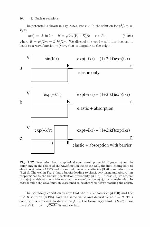
164 3. Nuclear reactions
The potential is shown in Fig. 3.27a. For r < R, the solution for p2/2m V0 is
u(r) = A sin k′r k′ =√
2m(V0 + E)/h r < R , (3.196)
where E = p2/2m = h2k2/2m. We discard the cos k′r solution because itleads to a wavefunction, u(r)/r, that is singular at the origin.
exp(−ikr) − (1+2ikf)exp(ikr)
exp(−k’r) exp(−ikr) − (1+2ikf)exp(ikr)
elastic only
elastic + absorption
exp(−ikr) − (1+2ikf)exp(ikr)
exp(−k’r)
sin(k’r)
R
R
R
r
r
r
V
V
V
elastic + absorption with barrier1r
a
b
c
Fig. 3.27. Scattering from a spherical square-well potential. Figures a) and b)differ only in the choice of the wavefunction inside the well, the first leading only toelastic scattering (3.197) and the second to elastic scattering (3.208) and absorption(3.211). The well in Fig. c) has a barrier leading to elastic scattering and absorptionproportional to the barrier penetration probability (3.216). In case (a) we requirethe u(r) vanish at the origin so that the wavefunction u(r)/r is non-singular. Incases b and c the wavefunction is assumed to be absorbed before reaching the origin.
The boundary condition is now that the r > R solution (3.190) and ther < R solution (3.196) have the same value and derivative at r = R. Thiscondition is sufficient to determine f . In the low-energy limit, kR 1, wehave k′(E = 0) =
√2mV0/h and we find

3.6 Nucleon–nucleus and nucleon–nucleon scattering 165
f(k = 0) = −R
[tan(
√2mV0R2/h)√
2mV0R2/h− 1]
. (3.197)
The pre-factor (−R) would, by itself, give a total cross-section of 4πR2. It ismultiplied by a factor that depends on the number of neutron wavelengths,√
2mV0R2/h that fit inside the potential well. As we emphasized in Sect.1.4.1, the two neutron–proton effective potentials have approximately 1/4 ofa wavelength inside the well, i.e.
√2mV0R2
h∼ π/2 ⇒ V0R
2 ∼ 109 MeV fm2 . (3.198)
For the s = 1 np system, V0R2 is slightly greater than 109 MeV fm2 so
the deuteron is bound. For the s = 0 system, V0R2 is slightly less than
109 MeV fm2 so there is no bound state. In the scattering problem consid-ered here, the quarter wavelength leads to a scattering cross-section that ismuch larger than 4πR2 since the tangent in (3.197) is large.
Table 3.3. The low-energy nucleon–nucleon scattering amplitudes and effectiveranges taken from the compilation [34]. The last two columns give the potentialparameters derived from the deuteron binding energy and the scattering formula(3.197). Note that f R for the s = 0 amplitudes.
f R V0 V0R2
(fm) (fm) (MeV) (MeV fm2)
n–p (s=1, T=0) +5.423 ± 0.005 1.73 ± 0.02 46.7 139.6
n–p (s=0, T=1) −23.715 ± 0.015 2.73 ± 0.03 12.55 93.5
p–p (s=0, T=1) −17.1 ± 0.2 2.794 ± 0.015 11.6 90.5
n–n (s=0, T=1) −16.6 ± 0.6 2.84 ± 0.03 11.1 89.5
The cross-section for the scattering on unpolarized neutrons on unpolar-ized protons is the weighted sum of the cross-section in the (s = 0) and (s = 1)state. Since there are three spin-aligned states and only one anti-aligned statewe have
σn−p = (3/4)4π|fs=1|2 + (1/4)4π|fs=0|2 = 20.47 b . (3.199)
This corresponds to the low-energy limit of the neutron–proton cross-sectionshown in Fig. 3.4. The contributions from the (s = 0) and (s = 1) amplitudescan be separated by a variety of methods. For instance, the neutron indexof refraction (Sect. 3.7) depends on the weighted sum of the amplitudesrather than of the on the weighted sum of the squares of the amplitudes. A

166 3. Nuclear reactions
measurement of the index of refraction combined with the unpolarized cross-section therefore allows one to deduce the amplitudes in the (s = 1) and(s = 0) states.
The measured amplitudes are listed in the first column of Table 3.3. Alsolisted are the effective ranges R of the potentials. These can be found byconsidering the energy dependence of the cross-section. One finds
σ(k) =4π|f(k = 0)|2∣∣ 1 − 1
2f(k = 0)Rk2∣∣2 + |f(k = 0)|2k2
(3.200)
The cross-section slowly declines with increasing energy, as can be seen inFig. 3.4. The ranges deduced from the energy dependence are listed in thesecond column of Table 3.3.
Quite generally, in strong interactions, one calls the quantity
a = −f(k = 0) (3.201)
the scattering length. The total low energy cross-section is therefore
σ(k 0) = 4πa2 . (3.202)
We have seen in equation (3.116) that, in Born approximation, the scatteringlength is related to the potential by
a =m
2πh2
∫V (r) d3r . (3.203)
Here, it is the more complicated relation (3.197)It should be emphasized that (3.200) applies only to the isotropic compo-
nent of the elastic cross-section. At energies where one no longer has kR 1,our treatment based on isotropic scattering must be modified. When the po-tential is central (or better the interaction is rotation invariant) the completetreatment of the angular dependence of scattering amplitudes is done byprojecting the Schrodinger equation on spherical harmonics. This results inincluding higher “partial wave amplitudes,” each of which corresponds toa given value of the angular momentum so that the scattering amplitudebecomes
f(θ) =∞∑
=0
a P(cos θ) (3.204)
where P(cos θ) is a Legendre polynomial and where the amplitudes of the“th” partial wave is given in terms of the “phase shifts” δ
a = (2 + 1)e2iδ − 1
2ik. (3.205)
The a can be found by solving the partial wave Schrodinger equation for thepotential in question. Our original treatment based on (3.187) supposed thatf was independent of angle and therefore corresponds to keeping only the = 0 part of the wavefunction. The inclusion of = 0 partial waves leads to

3.6 Nucleon–nucleus and nucleon–nucleon scattering 167
a peaking of the cross-section in the forward direction once the assumptionkR < 1 breaks down. This energy evolution of the differential cross-sectionis illustrated in Fig. 3.6.
Table 3.3 also shows the amplitudes of proton–proton and neutron–neutron scattering in the s = 0 state. (The s = 1 state is forbidden by thePauli principle at low energy.) The proton–proton amplitude can be derivedfrom large-angle scattering where Coulomb scattering is unimportant (Exer-cise 3.7). Since neutron–neutron scattering is difficult to observe directly, itsamplitude must be derived indirectly from other reactions.
We note the similarity in Table 3.3 of the amplitudes and ranges of thethree s = 0 amplitudes, n–p, p–p, and n–n. This similarity is indicative ofthe isospin symmetry of the strong interactions. The three s = 0 systemsform an isospin triplet whose interactions must be identical in the limit ofisospin symmetry. There is however a large difference between the iso-tripletpotential and the iso-singlet (s = 1) potential.
3.6.2 Absorption
While our analysis was intended only for potential scattering, we can includephenomenologically the effects of absorption of the incident particle (e.g. byradiative capture) by appropriately choosing the wavefunction for r < R. Forexample, if a incoming spherical wave is completely absorbed once it entersthe nucleus, we can use (Fig. 3.27b)
u(r) = Ae−ik′r r < R . (3.206)
This corresponds to an ingoing wave and no outgoing wave. (One can thinkof the ingoing wave as being absorbed near the origin.) Requiring continuityof the wavefunction and its derivative at r = R gives
f = −R
(1 − 2k
k′
)+ i(
1k′ + kR2 − k
k′2
), (3.207)
giving an elastic cross-section of
σel(k = 0) = 4π(
R2 +1
k′2
)k′ =
√2mV0/h . (3.208)
The total (elastic + absorption) cross-section can be found from the opticaltheorem to be derived in Sect. 3.7:
σtot =4π Im(f)
k(3.209)
which gives in this case
σtot =4π
kk′ + 4π
(R2 − 1
k′2
). (3.210)
Subtracting off the elastic cross-section we get the absorption cross-section:

168 3. Nuclear reactions
σabs(k → 0) =4π
kk′ . (3.211)
The cross section is proportional to the inverse of the velocity of the incidentparticle. This 1/v behavior is seen if there is a barrier-free exothermic inelasticchannel, e.g. radiative absorption (n, γ). Examples are given in Fig. 3.4.
Exothermic reactions between charged particles can only take place ifthe two particles penetrate their mutual Coulomb barriers. An example isthe (p, γ) reaction in 6Li whose cross-section is shown in Fig. 3.4. For suchreactions, the cross-section vanishes as k → 0 because the barrier penetrationprobability vanishes for k → 0.
To see how the barrier penetration factor enters, we treat the third sit-uation in Fig. 3.27c. There is a square potential barrier of height V0 forr1 < r < R. The solution in this region is
u(r) = Aeκr + Be−κr κ =√
2m(V0 − E)/h . (3.212)
Imposing the matching conditions at r = r1 and r = R one finds a scatteringamplitude
f(k → 0) = −R
(1 − 1
κR
)[1 − ikR
(1 − 1
κR
)+
2ε
κR
], (3.213)
where the small parameter ε is proportional to the barrier penetration prob-ability
ε =k′ + ik1
k′ − ik1exp(−2κ(R − r1)) . (3.214)
The elastic and absorption cross-sections are
σel(k = 0) = 4πR2(
1 − 1κR
)2
(3.215)
σabs =4πR
k
(1 − 1
κR
)Im(ε)
=4πR
k
(1 − 1
κR
)2k1k
′
k21 + k′2 exp(−2κ(R − r1)) . (3.216)
The absorption cross-section is proportional to the exponential barrier pen-etration probability, as expected.
The dimensional factor in the absorption cross-section is R/k ∝ Rλ. whereλ is the de Broglie wavelength. In the more realistic case of a Coulomb bar-rier, there is no dimensional parameter R so the cross-section must be, bydimensional analysis, proportional to λ2. The cross-section is generally writ-ten as
σabs =(
λ
2π
)2
S(E) exp(−2πZ1Z2α/β) , (3.217)

3.7 Coherent scattering and the refractive index 169
where S(E) is a slowly varying function of the energy and β = v/c for a rela-tive velocity v. The exponential barrier penetration factor, derived previouslyin Sec. 2.6 vanishes as the velocity approaches zero.
3.7 Coherent scattering and the refractive index
Up to now we have supposed that, in calculating the probability for an in-teraction in a target, the scattering probability on individual target particlescan be added. This implies that the probability for an interaction after pas-sage through a slice of matter of thickness dz is given by dP = nσdz. Asemphasized in Sect. 3.1, this is only justified if the waves emanating from thedifferent target particles have random phases. Let Ai = |Ai|eiθi be the ampli-tude for scattering from particle i. The square of the sum of the amplitudesis ∣∣∣∣∣
∑i
Ai
∣∣∣∣∣2
=∑
i
|Ai|2 +∑i =j
|Ai||Aj |ei(θi−θj) (3.218)
For random phases, the second term vanishes and we are left with the sumof the squared amplitudes. We will see that in the forward direction it is notjustified to assume random phases, so it is necessary to add amplitudes toget correct results. By doing this, we will derive an expression for the indexof refraction and for the total cross-section in terms of the forward scatteringamplitude (the optical theorem).
As shown in Fig. 3.28, we consider particles incident upon a then sliceof material of thickness dz containing a density n of scatterers. Beyond theslice, the wavefunction is the sum of the incident wave, ψ = exp(ikz) and thescattered wave found by summing the contributions of all scatterers:
ψ(z > 0) = exp(ikz) +
ndz
∫dx
∫dyf(θ)
exp(ik√
x2 + y2 + z2)(x2 + y2 + z2)1/2 , (3.219)
where the scattering angle is
θ(x, y) = tan−1
√x2 + y2
z. (3.220)
The exponential in (3.219) is a rapidly oscillating function of the integra-tion variables x, y except at the “stationary point” (x = 0, y = 0) where thephase’s partial derivatives with respect to x and y vanish. We can anticipatethat the integral will be dominated by the region near x = y = 0, corre-sponding to θ = 0. This is just the mathematical equivalent of the physicalstatement that scattering is generally only coherent in the forward direction.We therefore replace f(θ) with f(θ = 0), set x = y = 0 in the denominator,and expand the exponential, obtaining:

170 3. Nuclear reactions
x
dz
x 2 +y2+z2
ndz
ψ= eikz (1+ 2πif(0)
k
z
ndz)eikzψ=
Fig. 3.28. A plane wave, ψ = exp(ikz) is incident from the left on a thin slice ofmaterial of thickness dz containing a density n of scatterers. Beyond the slice, thewave is the sum of the incident wave and the scattered waves from all scatterersin the slice. As shown in the text, the wavefunction takes the form of Equation(3.222).
ψ(z > 0) = exp(ikz)
×[1 +
nf(0)dz
z
∫dx
∫dy exp
(ik(x2 + y2)
2z
)](3.221)
Using∫∞
∞ eiu2du =
√2πe−iπ/4, we find
ψ(z > 0) = exp(ikz)(
1 +2πif(θ = 0)
kndz
)(3.222)
The magnitude of ψ is
|ψ(z > 0)|2 = 1 − 4πIm(f(0))k
ndz . (3.223)
The total cross-section is defined by the probability dP = σtotndz so wededuce the so-called optical theorem:
σtot =4πIm(f(0))
k. (3.224)

Exercises for Chapter 3 171
The effect of the real part of f can be seen by writing the wavefunction(3.222) just after the slice:
ψ(dz) =(
1 − 2πIm(f(0))k
)exp[ik(
1 +2πnRef(0)
k2
)dz
].(3.225)
This implies that the index of refraction is
index of refraction = 1 +λ2nRe(f(0))
2π, (3.226)
where λ = 2π/k is the neutron wavelength. Note that for solids n ∼ a−30
so, if f ∼ fm then the index differs significantly from unity for λ ∼ 100a0corresponding to neutrons with E ∼ 10−5eV.
The fact that low-energy neutron refraction index is significantly differ-ent from unity is due to the fact that the scattering amplitude on nucleiapproaches a constant for k → 0. This is unlike the case of photons wherethe amplitude approaches zero for k → 0 and, consequently, the refractionindex approaches a constant, often near unity.
The neutron refraction index can be sufficiently important to permit theconstruction of neutron guides that use total internal reflection. At sufficientlylow energies, it is even possible to construct neutron containers that totalreflect neutrons of all scattering angles. While this may seem surprising, it isjust equivalent to the mean kinetic energy of the neutrons being less than itsmean potential energy within the wall of the container.
Figure 3.29 gives a example of how neutrons can be captured and thenstored for study. We will see in Chap. 4 how such stored neutrons can beused to measure the neutron lifetime.
3.8 Bibliography
1. Collision Theory M. L. Goldberger and K. M. Watson, John Wiley &Sons, 1964
2. Electron Scattering and Nuclear and Nucleon structure, R. Hofstadter,W.A. Benjamin, New-York (1963)
Exercises
3.1 Using the data in Fig. 3.4 and neglecting scattering on oxygen, calculatethe mean free path of thermal neutrons (p2/2m ∼ kT ) in normal water andin heavy water (where the 1H is replaced with 2H. On average, how manyelastic collisions will the neutron suffer before being absorbed by the (n, γ)reaction? How much time will this typically take?

172 3. Nuclear reactions
turbinegravitational trap
absorber
neutron guide
20K
D2
H2O
300K
fuel elementsUranium
Fig. 3.29. A schematic of the system at the Institute Laue-Langevin for producingultra-cold neutrons [35]. Neutrons produced by Uranium fission diffuse into thewater moderator where they are thermalized to a temperature of ∼ 300 K by elasticscattering on the protons in water molecules. Some of the neutrons diffuse into acold deuterium flask where they are further thermalized to ∼ 20K. (Deuterium isused because of its low radiative capture cross-section; see Fig. 3.4.) Neutrons thenescape from the reactor through a neutron guide that uses total internal reflection.They then impinge on a counter rotating turbine, causing them to further looseenergy by reflection. The neutrons are then guided to a gravitational trap consistinga container that is reflecting on the bottom and side surfaces but absorbing on thetop surface. Neutrons that are trapped must then have energies < mngz ∼ 10−7 eVwhere z ∼ 1 m is the vertical size of the container.

Exercises for Chapter 3 173
3.2 The explosion of the supernova SN1987A, on Feb. 23 1987, released N ∼1057 antineutrinos, some of which were detected by the Japanese detector ofKamiokande. The star that had exploded, was located at a distance of R 140, 000 light-years from Earth. The detector contained 2000 tons of water.The particles recorded were positrons produced in the reaction νep → ne+,of antineutrinos on the protons of the hydrogen atoms of H2O. The cross-section of this reaction at the mean energy of 15 MeV of the neutrinos, isσ = 2 10−45 m2. How many events would be expected to be recorded ?
3.3 From the level diagram in Fig. 3.5 and the data in Appendix G. calculatethe neutron energy necessary to excite the 7.459 MeV level of 7Li in a collisionwith 6Li.
3.4 The sun has a mean density of 1.4 g cm−3. The Thomson cross-sectionof photons, produced in the solar core, on the electrons of the solar plasma isσT(γ e− → γ e−) 0.665 10−28 m2. Calculate the mean free path of photons.In their random walk across the Sun it takes the photons a time of the orderof τ (R/l)2(l/c) 104 years to escape and reach us (the radius of the sunis R 700.000 km). Actually, the escape time is larger 105–106 years dueto the higher density by a factor of roughly ∼ 200 in the solar core.
3.5 Verify that if (3.37) is satisfied, the maximum target recoil energy ismuch less than the kinetic energy of the beam particle.
3.6 Verify that the two peak energies in Fig. 3.22 correspond to elasticscattering on protons and on 2H nuclei.
3.7 By comparing the Rutherford Scattering cross-section with that ofnucleon–nucleon scattering (Table 3.3), find the scattering angular rangewhere the nucleon–nucleon amplitude is larger than the Coulomb amplitudefor ∼ 2 MeV proton–proton scattering.

4. Nuclear decays and fundamentalinteractions
This chapter is primarily concerned with nuclear instability. Generally speak-ing, there are two types of decays of nuclear species: A- and Z-conserving “dis-sociative” decays like α-decay and spontaneous fission; and β-decays whichtransform neutrons to protons or vice versa. Additionally, nuclear excitedstates decay by emission of photons (γ-decay) or atomic electrons (internalconversion). If their energy is sufficiently high, the excited states can alsodecay by dissociation, especially nucleon emission.
Our first goal in this chapter is to describe γ- and β-decay of nuclei. Theinteresting point is that in both cases these decays are due to fundamen-tal interactions. The interactions are sufficiently weak that the decays canbe treated with standard time-dependent perturbation theory, Appendix C.This is quite different from dissociative decays which are generally viewed astunneling processes. α-decay is treated in this way in Chap. 2 and sponta-neous fission in Chap. 6.
The information gleaned from weak nuclear decays was instrumental inthe formulation of the Standard Model of fundamental constituents of matter,the families of quarks and leptons, and their interactions. We will end thischapter with a brief introduction to this model.
4.1 Decay rates, generalities
4.1.1 Natural width, branching ratios
Decay rates and mean lifetimes can be defined by the same considerationsas lead us to the definition of cross-sections in Chap. 3. An unstable particlehas a probability dP to decay in a time interval dt that is proportional to dt:
dP =dt
τ, (4.1)
where τ clearly has dimensions of time and is called the “mean lifetime” ofthe particle. This law governs the time dependence of the number N(t) of anunstable state surviving after a time t:
N(t + dt) − N(t) = −N(t)dP ⇒ dN
dt= −N(t)
τ, (4.2)
176 4. Nuclear decays and fundamental interactions
which has the solution
N(t) = N(t = 0)e−t/τ . (4.3)
The mean survival time is τ , justifying its name.The inverse of the mean lifetime is the “decay rate”
λ =1τ
. (4.4)
We saw in Sect. 3.5 that an unstable particle (or more precisely an un-stable quantum state) has a rest energy uncertainty or “width” of
Γ = hλ =h
τ=
6.58 × 10⁻²² MeV secτ
. (4.5)
Since nuclear states are typically separated by energies in the MeV range,the width is small compared to state separations if the lifetime is greaterthan ∼ 10−22 sec. This is generally the case for states decaying through theweak or electromagnetic interactions. For decays involving the dissociationof a nucleus, the width can be quite large. Examples are the excited statesof 7Li (Fig. 3.5) that decay via neutron emission or dissociation into 3H4He.From the cross-section shown in Fig. 3.4, we see that the fourth excited state(7.459 MeV) has a decay width of Γ ∼ 100 keV.
It is often the case that an unstable state has more than one “decaychannel,” each channel k having its own “branching ratio” Bk. For examplethe fourth excited state of 7Li has
Bn6Li = 0.72 B3H4He = 0.28 Bγ 7Li ∼ 0.0 , (4.6)
where the third mode is the unlikely radiative decay to the ground state. Ingeneral we have∑
k
Bk = 1 , (4.7)
the sum of the “partial decay rates,” λk = Bkλ∑k
λk = λ , (4.8)
and the sum of the “partial widths,” Γk = BkΓ∑k
Γk = Γ . (4.9)
4.1.2 Measurement of decay rates
Lifetimes of observed nuclear transitions range from ∼ 10−22 sec7Li (7.459 MeV) → n 6Li, 3H 4He τ = 6 × 10⁻²¹ sec (4.10)
to 1021 yr

4.1 Decay rates, generalities 177
76Ge → 76Se 2e− 2νe t1/2 = 1.6 × 10²¹ yr (4.11)
It is not surprising that the techniques for lifetime measurements vary con-siderably from one end of the scale to the other. Here, we summarize somebasic techniques, illustrated in Figs. 4.1- 4.4.
• τ > 108 yr (mostly α- and 2β-decay). The nuclei are still present on Earth(whose nuclei were formed about 5 × 10⁹ year ago) and can be chemicallyand isotopically isolated in macroscopic quantities and their decays de-tected. The lifetime can then by determined from (4.3) and knowledge ofthe quantity N in the sample. An illustration of this technique is shown inFig. 4.1.
• 10 min < τ < 108 yr (mostly α- and β-decay). The nuclei are no longerpresent on Earth in significant quantities and must be produced in nuclearreactions, either artificially or naturally (cosmic rays and natural radioac-tivity sequences). The lifetimes are long enough for chemical and (withmore difficulty) isotopic purification. The decays can then be observed and(4.3) applied to derive τ . The case of 170Tm is illustrated in Fig. 4.2. Ifthe observation time is comparable to τ , knowledge of N(t = 0) is notnecessary because τ can be derived from the time variation of the countingrate.
• 10−10s < τ < 103s (mostly β-, γ- and α-decay). While chemical and isotopicpurification is not possible for such short lifetimes, particles produced innuclear reactions can be slowed down and stopped in a small amount ofmaterial (Sect. 5.3). Decays can be counted and (4.3) applied to derive τ .Examples are shown in Figs. 2.18 and 2.19. The case of the first excitedstate of 170Yb produced in the β-decay of 170Tm is illustrated in Fig. 4.2.
• 10−15s < τ < 10−10s. (mostly γ-decay). The time interval between produc-tion and decay is too short to be measured by standard timing techniquesbut a variety of ingenious techniques have been devised that apply to thisrange that covers most of the radiative nuclear decays. One technique usesthe fact that the time for a particle to slow down in a material after havingbeen produced in a nuclear reaction can be reliably calculated (Sect. 5.3).For particles with 10−15s < τ < 10−10s, the disposition of material can bechosen so that some particles decay “in flight” and some after coming torest. For the former, the energies of the decay particles are Doppler shiftedand can be distinguished from those due to decays at rest. Measurement ofthe proportion of the two types and knowledge of the slowing-down timeallows one to derive τ . The technique is illustrated in Fig. 4.3.
Another indirect technique for radiative transitions is the Coulomb ex-citation method. The cross-section for the production of an excited statein collisions with a charged particle is measured. As mentioned in Sect.3.4.2, the cross-section involves the same matrix element between ground-and excited-nuclear states as that involved in the decay of the excited- toground-state. In fact, the incident charged particle can be considered to be

178 4. Nuclear decays and fundamental interactions
a source of virtual photons that can induce the transition. Knowledge ofthe cross-section allows one to deduce the radiative lifetime of the state.
• τ < 10−12s i.e. Γ > 6 × 10⁻¹⁰ MeV. (mostly γ-decay and dissociation). Inthis range where direct timing is impossible, the width of the state can bemeasured and (4.5) applied to derive τ . An example is shown in Fig. 3.4where the energy dependence of the neutron cross-section on 6Li can beused to derive the widths of excited states. In this example, the state isvery wide because it decays by breakup to n6Li or 3H4He. Widths of statesthat decay radiatively can only be measured with special techniques. Anexample is the use of the Mossbauer effect, as illustrated in Fig. 4.4.
4.1.3 Calculation of decay rates
Consider a decay
a → b1 + b2 + . . . + bN . (4.12)
Particle a, assumed to be at rest, has a mass M and an energy E = Mc2. Asin scattering theory, we can calculate decay rates by using time-dependentperturbation theory (Appendix C). We suppose that the Hamiltonian consistsof two parts. The first, H0, represents the energies of the initial and final stateparticles, while the second, H1, has matrix elements connecting initial andfinal states. The decay rate, i.e. the probability per unit time that a decaysinto a state |f〉 of final particles is
λa→f =2π
h|〈f |T |a〉|2 δt
(Mc2 −
∑Ej
)(4.13)
where Ej is the energy of particle bj . In first order perturbation theory, thetransition operator T is just the Hamiltonian responsible for the decay, H1.
As in the case of nuclear reactions, quantum field theory is the appropri-ate language to determine which decays are possible and the form of theirmatrix elements. Lacking this technology, we will usually just give the ma-trix elements for each process under consideration. However, as in reactiontheory where the classical limit of particles moving in a potential was a guidefor determining the matrix elements for elastic scattering, certain decay pro-cesses have classical analogs that can guide us. This is the case for radiativedecays which have the classical limit of a charge distribution generating anoscillating electromagnetic field.
Despite the fact that we will not generally be able to derive rigorouslythe matrix elements, we can expect that the interaction Hamiltonian istranslation invariant. Therefore, the square of the transition matrix element|〈f |T |i〉|2 will be, as in scattering theory, proportional to a momentum con-serving delta function. We therefore define the “reduced” transition matrixelement T by
|〈f |T |i〉|2 = |T (p1...pN )|2V −(N+1) V (2πh)3δ3L(Σpj) , (4.14)

4.1 Decay rates, generalities 179
−e −e
helium gas
Mo foil100sc
intil
lato
rs
scin
tilla
tors
160
120
80
40
even
ts/0
.1 M
eV
0 1 2 32 electron energy sum (MeV)
4
1433 events
(background subtracted)
Fig. 4.1. The measurement of the double-β decay of 100Mo → 100Ru 2e−2νe [36].The upper figure shows a simplified version of the experiment The source is a 40µmthick foil consisting of 172 g of isotopically enriched 100Mo (98.4% compared tothe natural abundance of 9.6%). After a decay, the daughter nucleus stays in thefoil but the decay electrons leave the foil (Exercise 4.2) and traverse a volume con-taining helium gas. The gas is instrumented with high voltage wires that sense theionization trail left by the passing electrons so as to determine the e− trajectories.The electrons then stop in plastic scintillators which generate light in proportion tothe electron kinetic energy. The bottom figure show the summed kinetic energy ofelectron pairs measured in this manner. A total of 1433 events were observed overa period of 6140 h, corresponding to a half-life of 100Mo of (0.95 ± 0.11) × 1019yr.

180 4. Nuclear decays and fundamental interactions
170
170Tm
Yb
128.6 d1
=0.9679 MeVβQ
24%
76%
Tm source
shielding
scintillator
focusingcoil
vacuumchamber
10
100
coin
cide
nce
coun
ting
rate
−8 0 8 16
promptcoincidences
84 keV γ
t 1/2=1.57x10−9s
time delay (ns)
0.084 MeV2+1.6ns
0+
_
Fig. 4.2. Observation of the decay of 170Tm and measurement of the lifetime of thefirst excited state of 170Yb [37]. The radioactive isotope 170Tm (t1/2 = 128.6day) isproduced by irradiating a thin foil of stable 169Tm with reactor neutrons. 170Tm isproduced through radiative neutron capture, 169Tm(n, γ)170Tm. After irradiation,the foil is placed at a focus of a double-armed magnetic spectrometer. The decay170Tm → 170Yb e−νe proceeds as indicated in the diagram with a 76% branchingratio to the ground state of 170Yb and with at 24% branching ratio to the 84 keVfirst excited state. The excited state subsequently decays either through γ-emissionor by internal conversion where the γ-ray ejects an atomic electron of the Yb.Electrons emerging from the foil are momentum-selected by the magnetic field andfocused onto two scintillators. Events with counts in both scintillators are due to aβ-electron in one scintillator and to an internal conversion electron in the other. Thedistribution of time-delay between one count and the other is shown and indicatesthat the exited state has a lifetime of ∼ 1.57 ns.
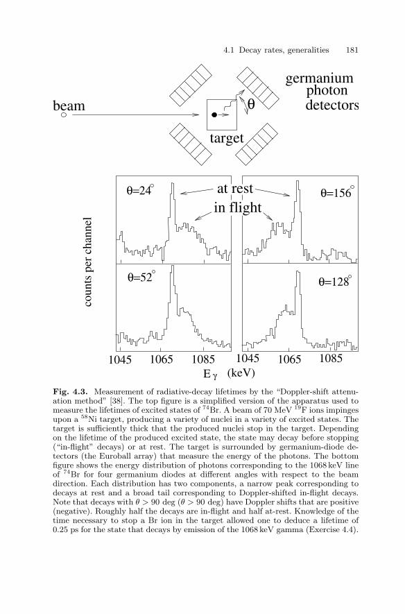
4.1 Decay rates, generalities 181
target
beam θ detectorsphoton
germanium
1065 10851045 1045 1065 1085
coun
ts p
er c
hann
el
θ=128
θ=24
θ=52
θ=156
E γ (keV)
at restin flight
Fig. 4.3. Measurement of radiative-decay lifetimes by the “Doppler-shift attenu-ation method” [38]. The top figure is a simplified version of the apparatus used tomeasure the lifetimes of excited states of 74Br. A beam of 70 MeV 19F ions impingesupon a 58Ni target, producing a variety of nuclei in a variety of excited states. Thetarget is sufficiently thick that the produced nuclei stop in the target. Dependingon the lifetime of the produced excited state, the state may decay before stopping(“in-flight” decays) or at rest. The target is surrounded by germanium-diode de-tectors (the Euroball array) that measure the energy of the photons. The bottomfigure shows the energy distribution of photons corresponding to the 1068 keV lineof 74Br for four germanium diodes at different angles with respect to the beamdirection. Each distribution has two components, a narrow peak corresponding todecays at rest and a broad tail corresponding to Doppler-shifted in-flight decays.Note that decays with θ > 90 deg (θ > 90 deg) have Doppler shifts that are positive(negative). Roughly half the decays are in-flight and half at-rest. Knowledge of thetime necessary to stop a Br ion in the target allowed one to deduce a lifetime of0.25 ps for the state that decays by emission of the 1068 keV gamma (Exercise 4.4).

182 4. Nuclear decays and fundamental interactions
E (µ eV)∆
0.0417
0.129
191Os%
abs
orpt
ion
−4 0 4 8 12v(cm/sec)
20−20 0 40
1.0
0.8
0.6
0.4
0.2
γγ
Ir191
v
absorber
191Ir γ−
detectorsourceOs191
Fig. 4.4. Measurement of the width of the first excited state of 191Ir throughMossbauer spectroscopy [39]. The excited state is produced by the β-decay of 191Os.De-excitation photons can be absorbed by the inverse transition in a 191Ir absorber.This resonant absorption can be prevented by moving the absorber with respect tothe source with velocity v so that the photons are Doppler shifted out of the reso-nance. Scanning in energy then amounts to scanning in velocity with ∆Eγ/Eγ = v/c.It should be noted that photons from the decay of free 191Ir have insufficient en-ergy to excite 191Ir because nuclear recoil takes some of the energy (4.42). Resonantabsorption is possible with v = 0 only if the 191Ir nuclei is “locked” at a crystallattice site so the crystal as a whole recoils. The nuclear kinetic energy p2/2mA in(4.42) is modified by replacing the mass of the nucleus with the mass of the crystal.The photon then takes all the energy and has sufficient energy to excite the originalstate. This “Mossbauer effect” is not present for photons with E > 200 keV becausenuclear recoil is sufficient to excite phonon modes in the crystal which take someof the energy and momentum.

4.1 Decay rates, generalities 183
T represents the dynamics of the decay, as opposed to the kinematics (energy-momentum conservation and state-counting). The factors of the wavefunctionnormalization volume V = L3 have been added for convenience so that T isV -independent. The factor V −(N+1) comes from the (N + 1) wavefunctionsin the matrix element (exp(ipr)/
√V ) while the factor V (2πh)3 comes for the
square of the integration over the wavefunctions leading to the delta function(C.24). The resulting factor of V −N will be canceled in the sum over finalstates, as demonstrated explicitly below.
We note that the dimensionality of T depends on the number N of finalstate particles:
[T ] = energy × length3(N−1)/2 (4.15)
For N = 3, as in β-decay, it has dimensions of energy×volume and we cananticipate that T ∼ GF.
The reaction rate (4.12) is obtained by summing over all possible acces-sible final states. Just like for cross sections, one first normalizes asymptoticfinal states in a finite volume V = L3, and one replaces the sum by integralsover the momenta of final particles by making use of the density of states.The normalization volume cancels off and one ends up with the general form
λa→b1+b2...+bN(4.16)
=(2πh)4
h2
∫|T (p1...pN )|2δ3(Σpj)δ(E − ΣEj)
N∏j=1
d3pj
(2πh)3,
where T (p1...pN ) is the reduced transition matrix element.In the form (4.16), the transition rate appears as the square of the tran-
sition matrix element (divided by h2) integrated over the phase space ofthe accessible final states, i.e. the set of final momenta allowed by energy-momentum conservation. The quantity
F =∫
(2πh)4δ3(Σpj)δ(E − ΣEj)N∏
j=1
d3pj
(2πh)3(4.17)
is called the volume of phase space. The larger this volume, the greater is thedecay rate (if all other factors are assumed to be equal).
If one is interested in angular distributions, or in energy distributions offinal particles, one restricts the integration in (4.16) to the appropriate partof phase space.
4.1.4 Phase space and two-body decays
A simple example is that of two-body decays. Consider the decay of a, ofmass m, into a1 and a2 of masses m1 and m2 respectively. We place ourselvesin the rest frame of a, the final momenta are opposite p1 = −p2 and we setp ≡ p1. The energy of the final state is

184 4. Nuclear decays and fundamental interactions
E = E1 + E2 =√
p2c2 + m21c
4 +√
p2c2 + m22c
4 (4.18)
from which follows that
pdp
dE=
E1E2
Ec2 . (4.19)
The decay rate is
λ =1
4π2h4
∫|T |2d3p1d3p2 δ3(p1 + p2)δ(E − E1 − E2) . (4.20)
The integration over p2 fixes p2 = −p1. Equation (4.19) gives p1dp1 =(E1E2/Ec2)d(E1 + E2) which allows a direct integration using the δ(E −E1 − E2) function. If we define the average over angles
〈|T |2〉 =14π
∫dΩ |T |2
we obtain
λ =1h
pc E1E2
π(hc)3E〈|T |2〉 (4.21)
where p is the magnitude of the momentum of each final particle.
4.1.5 Detailed balance and thermal equilibrium
In this chapter we mostly concerned with the irreversible decays of unstableparticles. However, in certain situations it is necessary to consider the inverseof the decay. For instance, in Chap. 8 we will consider the production of 8Beby fusion of two 4He. The 8Be then decays back to the original 4He pairwith a lifetime of ∼ 10−16s (Q = 92 keV), so we are led to consider the twodirections of the reaction
8Be ↔ 4He 4He . (4.22)
If Q is comparable to the temperature of the medium, the inverse decay ispossible since typical 4He nuclei have enough kinetic energy to fuse to 8Be.This can be the case in stars.
In situations like this, the relative concentration of the nuclei on the twosides of the reaction may be determined by considerations of chemical equi-librium. For instance, if there is no 8Be originally present, its concentrationis built up through fusion until the rate of 8Be decay balances the rate of 8Befusion. It will turn out that the relative concentrations of nuclear species willbe given by a formula (4.32) that is independent of the decay and formationrates.
We consider a two-body decay a → bc. The decay rate per particle intothe momentum interval d3pbd3pc is given by (4.13) multiplied by the numberof states in d3pbd3pc

4.1 Decay rates, generalities 185
λ(pa → pb, pc) =2π
h|T (pa → pb, pc)|2
× δ(Ea − Eb − Ec)V d3pb
(2πh)3V d3pc
(2πh)3(4.23)
In the functions λ and T we have not written explicitly the spin variables, sa,sb and sc. To get the decay rate within the volume V from the momentuminterval d3pa, we must multiply λ by the number of particles in this phasespace element:
Λ(pa → pb, pc) = λ(pa → pb, pc) naV fa(pa) d3pa , (4.24)
where na is the number density and fa(pa) is the normalized spin-momentumdistribution:∑
s
∫d3pfa(p) = 1 . (4.25)
Once again, we do not write explicitly the spin variable s in the function f .We want to compare this decay rate to the formation rate. Per particle
pair, this is also given by (4.13)
λ(pb, pc → pa) =2π
h|T (pb, pc → pa)|2δ(Ea − Eb − Ec)
V d3pa
(2πh)3. (4.26)
To get the formation rate in the volume V from the momentum intervald3pbd3pc, we must multiply λ by the number of particles in this phase spaceelement:
Λ(pb, pc → pa) = λ(pb, pc → pa)
× nbV fb(pb) d3pb ncV fc(pc) d3pc , (4.27)
where na and nb are the number densities and fb(pb) and fc(pc) are thenormalized momentum distributions.
To find the equilibrium number densities, we need only equate the for-mation rate (4.27) with the decay rate (4.24). Their equality at equilibriumis due to the principle of detailed balance meaning that the rate is balancedwith the inverse rate at each point in phase space, not just globally. This ispossible if the interaction involved respects time-reversal invariance, in whichcase the |T |2 is the same for both directions of the reaction. We then get
nbfb(pb) ncfc(pc) = nafa(pa) (2πh)−3 , (4.28)
for all energy conserving combinations of Ea, Eb and Ec. The densities andmomentum distributions are then constrained by
na
nbnc= (2πh)3
fb(pb) fc(pc)fa(pa)
. (4.29)
A simple situation occurs when the three species have Maxwell–Boltzmannmomentum distributions

186 4. Nuclear decays and fundamental interactions
fi(pi) =1
2si + 11
(2πmikT )3/2 exp[−p2i /(2mikT )] . (4.30)
Using energy conservation
mac2 +
p2a
2ma= mbc2 +
p2b
2mb+ mcc
2 +p2c
2mc, (4.31)
we find that (4.29) becomes a simple relation between the densities as afunction of temperature:
na
nbnc=
(2sa + 1)(2sa + 1)(2sa + 1)
× (2πh)3(
ma
2πmbmckT
)3/2
exp(−∆mc2/kT ) , (4.32)
where ∆m = ma − mb − mc. As could be expected, na vanishes for kT ∆mc2.
Another simple situation occurs when particle c is a photon. In thermalequilibrium, the photon phase-space density is the Planck distribution:
nγfγ(pγ) =1
(2πh)31
exp(Eγ/kT ) − 1. (4.33)
Substituting this into the formation rate (4.27) it appears that thermal equi-librium is not possible since, if we equate it with the decay rate (4.24), theBoltzmann factors no longer cancel as they did with the Boltzmann distri-bution. We are saved since for radiative transitions, the formation and decaymatrix elements are no longer equal because the latter is enhanced by stim-ulated emission. This means that the decay matrix element to a given stateis multiplied by (1 + N(pγ), where N(pγ) is the number of photons alreadypresent in the photon state:
|T (pa → pb, pγ)|2 = |T (pb, pγ → pa)|2[1 +
1exp(Eγ/kT ) − 1
].
Substituting this into (4.24) and equating with the formation rate (4.27) wesee that the factors |T |2/(exp(Eγ/kT ) − 1) nicely cancel. We then imposeenergy conservation
mac2 +
p2a
2ma= mbc2 +
p2b
2mb+ Eγ , (4.34)
to find a simple expression for the ratio of the densities
na
nb=
2sa + 12sb + 1
exp(−∆mc2/kT ) , (4.35)
where ∆m = ma−mb. Once again, na vanishes for kT ∆mc2. This explainswhy excited nuclear states are not seen on Earth where kT ∼ 0.025 eV.

4.2 Radiative decays 187
Thermal photons can not only excite nuclei through γ(A, Z) → (A, Z)∗,but also dissociate them. An example that will turn out to be very importantin cosmology is the dissociation of 2H so we consider equilibrium
dγ ↔ pn . (4.36)
Following the same reasoning as above, the dissociation rate is
Λ(pdpγ → pp, pn) =2π
h|T (pdpγ → pp, pn)|2δ(Ed + Eγ − Ep − En)
× V d3pp
(2πh)3V d3pn
(2πh)3ndV fd(pd) d3pdnγV fγ(pγ) d3pγ . (4.37)
We must then equate this with the rate for the inverse process. Taking intoaccount stimulated emission
|T (pppn → pd, pγ)|2 = |T (pdpγ → pppn)|2[1 +
1exp(Eγ/kT ) − 1
],
and using the Planck relation (4.33), we find the Saha equation:
nd
npnn=
sd + 1(sp + 1)(sn + 1)
×(2πh)3(
md
2πmpmnkT
)3/2
exp(−∆B/kT ) , (4.38)
where B = 2.2 MeV is the deuteron binding energy. This is basically the sameequation as (4.32) except that here the two-body state has higher energy thanthe one-body state.
4.2 Radiative decays
We now consider the dynamics of radiative decays. Radiative decays of atoms,nuclei or elementary particles are those in which photons are emitted. Mostcommon are the decays of excited states
A∗ → A + γ . (4.39)
This process is also called the spontaneous emission of a photon by A∗. Inradiative decays of nuclei or atoms, the radiator is always much heavier thanthe mass difference
mA∗ − mA
mA 1 (4.40)
in which case it is simple to check that practically all the decay energy istaken by the photon. In general we have
Eγ = (mA∗ − mA)c2 − p2
2mA. (4.41)

188 4. Nuclear decays and fundamental interactions
In nuclear decays, Eγ = pc ∼ MeV and mc2 ∼ A GeV giving a nuclear recoilof p2/2m ∼ 0.5 keV/A, which is indeed much less than Eγ implying
Eγ ∼ (mA∗ − mA)c2 . (4.42)
4.2.1 Electric-dipole transitions
The quantum field theory of photons, i.e. quantum electrodynamics, is nec-essary to derive the matrix element T for radiative transitions. Fortunately,these transitions have the classical analog of an oscillating charge distributionradiating a classical electromagnetic field and the formula for the radiatedpower will lead us to the correct formula for the transition rate. The simplestcase is that of a single charge q moving in a 1-dimensional harmonic poten-tial so that its position is x(t) = a cos ωt. This corresponds to an oscillatingelectric dipole Dx(t) = qa cos ωt. Classical electrodynamics can be used tocalculate the radiated power associated with the oscillating electromagneticfield created by the oscillating dipole. The time averaged (classical) power isgiven by the Larmor formula
P =23
〈D2〉t
4πε0c3 =13
q2
4πε0
a2ω4
c3 , (4.43)
where the 〈 〉t indicates time averaging, replacing the factor cos2 ωt by 1/2. Ifthe motion is circular, the power is doubled since this corresponds to linearharmonic motion in two dimensions.
A quantum harmonic oscillator in a state n of energy En = hω(n + 1/2)can decay to the state n − 1 by emitting a photon of energy hω. The timeaveraged power due to this transition is
P = hω λ(n → n − 1) , (4.44)
where λ(n → n − 1) is the decay rate of the state n. Equating this with theclassical power (4.43) we get
λ(n → n − 1) ∼ 1hω
13
q2
4πε0
2〈x2〉n ω4
c3 , (4.45)
where we have equated the mean of x2 in the state n with its classical valuea2/2. We have written ∼ instead of = because we expect the classical formulato apply only in the limit n → ∞. Introducing the fine-structure constantα = e2/4πε0hc we get a more elegant formula
λ(n → n − 1) ∼ 23
q2
e2 α〈x2〉nω3
c2 =23
q2
e2 α〈E〉n
mc2 ω , (4.46)
where in the second form we use 〈x2〉n = En/(mω2). We see that for anon-relativistic elementary particle (q = e), a state lives for many oscillationperiods, of order α−1mc2/En.
While (4.46) turns out to be (nearly) the correct rate as calculated us-ing quantum electrodynamics, it is not in a form that can be generalized to

4.2 Radiative decays 189
other problems. Since classically the radiation is due to the oscillating po-sition of the particle, we would expect that the decay rate is related to thematrix element of x taken between initial and final states, rather than thethe expectation value of x2 in the initial state. This suggests replacing 〈x2〉n
with
2|〈n − 1|x|n〉|2 =hn
mω= 〈n|x2|n〉 n
n + 1/2, (4.47)
which has the same large n limit but makes sense quantum mechanically.Substituting this into (4.46) we get
λ(n → n − 1) =43
q2
e2 αω3
c2 |〈n − 1|x|n〉|2 . (4.48)
This turns out to be correct and generalizable to any transition involving asingle charged particle:
λi→f =4α
3q2
e2
1h
E3γ
(hc)2〈f |r|i〉 · 〈i|r|f〉 . (4.49)
If we drop the assumption of a single charged particle involved in the tran-sition, we simply replace the position vector r with D/q where D is an ap-propriate dipole operator. Transitions governed by (4.49) are called electric-dipole transitions or “E1” transitions for short.
Equation (4.49) is used in atomic and nuclear physics when transitionsinvolve, to good approximation, a single particle in which case we have q = e.This is the case in hydrogen and alkali atoms where excited states correspondto excitations of the valence electron that moves in the field of an inert corethat remains unaffected by the transition. In nuclear physics, the formulaapplies best to even–odd nuclei where the single unpaired nucleon moves inthe potential of the paired nucleons. This is an especially good picture whenthe paired nucleons form a closed shell corresponding to a magic number ofprotons or neutrons.
In these cases, we need only take into account the wavefunctions, ψ(r) ofthe initial and final state valence particles
〈f |r|i〉 =∫
d3rψ∗f (r)rψ∗
i (r) . (4.50)
Equation (4.49) is not very useful for precise calculations because thenuclear matrix element of r is not easily calculable. However, it can be usedto estimate the lifetimes of atomic and nuclear excited states. We note thepresence of the fine structure constant α = e2/4πε0hc, which represents thesquare of the coupling constant of the electromagnetic field with the (chargeof the) electron. Note also the fact that the decay rate varies as the third powerof the photon energy, and as the square of the size of the system. For atomictransitions, hω ∼ eV and 〈r〉 ∼ 10−10 m which gives rates of the order of107 to 109s−1, i.e. lifetimes of the order of 10−7 to 10−9s. The corresponding

190 4. Nuclear decays and fundamental interactions
width, Γ = h/τ ∼ 10−7eV is much less than the photon energy (∼ eV) butmuch greater than the atomic recoil energy E2
γ /2mAc2 ∼ 10−9eV.For nuclear transitions, 〈r〉 ∼ A1/310−15 m so
λ(E1) ∼ h−1αE3γ
(A1/3fm
hc
)2
. (4.51)
For Eγ ∼ MeV, this gives rates of the order of 1015 to 1017s−1, i.e. lifetimesof the order of 10−17 to 10−15s. The corresponding width, Γ = h/τ ∼ 10 eVis much less than the photon energy.
The width is also much less than the the nuclear recoil energy E2γ /2mAc2 ∼
103 eV. This has the interesting consequence that, unlike photons emitted byatoms, photons emitted in a nuclear transition do not generally have sufficientenergy to re-excite another nucleus through the inverse transition:
Eγ = (m∗ − mA)c2 − p2/2mA < (m∗ − mA)c2 − h/τ . (4.52)
The inverse transition can only be induced in special cases where nuclearrecoil is suppressed in a crystal by the Mossbauer effect (Fig. 4.4) or whenthe excited nucleus decays in flight with the Doppler effect compensating thenuclear recoil (Fig. 4.19).
4.2.2 Higher multi-pole transitions
It is often the case that electric-dipole decay of an excited state is forbiddenbecause there are no lower-lying states for which the matrix element 〈f |r|i〉is non-zero. A famous example of this is the n = 2, l = 0 state of atomichydrogen that cannot decay to the n = 1 state
〈2 0 0|r|1 0 0〉 =∫
d3rψ∗1(r)rψ2(r) = 0 . (4.53)
The integral vanishes because the two wavefunctions are spherically sym-metric whereas r averages to zero when integrated over all directions. Thisillustrates a selection rule requiring that for E1 transitions, the parity of theinitial and final wavefunctions be different and that the angular momentumdiffer by ≤ one unit.
If an E1 transition is forbidden, a state may still decay radiatively by theaction of operators that are the quantum analogs of the higher order classicalradiation processes: oscillating magnetic dipoles (M1), electric quadrupoles(E2), etc. Each type of radiation has its own selection rules that are given inTable 4.1. Classically, the radiated power for an oscillating l-pole is propor-tional to ω2l+1 so we expect the quantum transition rates to be proportionalto E2l+1
γ . Conventionally, one therefore writes the transition rate in the form
λ(l) =8π(l + 1)
l[(2l + 1)!!]21h
E2l+1γ
(hc)2lα B(l) , (4.54)

4.2 Radiative decays 191
where (2l+1)!! = (2l+1)(2l−1)(2l−3) . . . . The reduced transition rate B(l)contains all the (difficult) nuclear physics and has dimension of length2l. From(4.49) we see that for E1 transitions we have
B(E1) = (〈f |r|i〉 · 〈i|r|f〉) ∼ R2 . (4.55)
Dimensional analysis suggest that higher order elements are of order
B(El) ∼ R2l . (4.56)
It turns out that this formula generally overestimates transition rates, withthe exception of electric quadrupole transitions (E2) as discussed below.
Just as higher classical multi-poles are less efficient radiators than classicalelectric dipoles, the quantum radiative rates decrease with increasing polenumber:
λ(El)λ(E1)
∼(
EγR
hc
)2l
∼(
Eγ(MeV)A1/3
200
)2l
, (4.57)
i.e. about 2 orders of magnitude per pole.Magnetic l-pole radiation is weaker than the corresponding electric l-pole
radiation because fields generated by oscillating currents are smaller thanfields generated by oscillating charges by a factor v/c where v is the velocityof the radiating charge. The uncertainty principle suggests that the velocityof nucleons in nuclei is of order h/(Rmp) so we expect
B(Ml) ∼(
hc
mpc2R
)2
B(El) =(
15A1/3
)2
B(El) . (4.58)
This implies that Ml transitions have rates between those of El and E(l + 1)transitions.
Table 4.1. Selection rules for radiative transitions
angulartype symbol momentum parity
change |∆J | ≤ change
electric dipole E1 1 yesmagnetic dipole M1 1 noelectric quadrupole E2 2 nomagnetic quadrupole M2 2 yeselectric octopole E3 3 yesmagnetic octopole M3 3 noelectric 16-pole E4 4 nomagnetic 16-pole M4 4 yes

192 4. Nuclear decays and fundamental interactions
M2
M4
M3
M1
E1
E2
E3
E4
E5
E(MeV)E(MeV)
τ(s
ec)
1
10
1210
6
10−6
10−12
0.10.01 0.1 11 0.01 10
Fig. 4.5. Lifetimes of excited nuclear states as a function of Eγ for various electricand magnetic multipoles.. The various multipoles separate relatively well exceptfor the E1 (open circles) and E2 (crosses) transitions that have similar lifetimes.(For clarity, only 10% of the available E1 and E2 transitions appear in the plot.)The surprising strength of the E2 transitions is because they are generally due tocollective quadrupole motions of several nucleons, whereas E1 transitions can oftenbe viewed as single nucleon transitions.

4.2 Radiative decays 193
Figure 4.5 shows the lifetimes of radiative transitions as a function of Eγand of multipole. The expected rate decrease with increasing multipole anddecreasing Eγ is evident. The longest lived states appearing in the plot arethe M4 transition
108Ag(6+ 109.44 keV) → 108Ag(2− 79.13 keV) t1/2 = 418 yr ,
and the E5 transition192Ir(11− 168.14 keV) → 192Ir(6+ 12.98 keV) t1/2 = 241 yr .
The existence of such long-lived isomeric states is only possible because thenucleus is isolated from its environment by its atomic electrons. Long-livedatomic states are not possible because they de-excite during frequent colli-sions with other atoms.
There also exist a few exceptionally short-lived nuclear states. An exampleis the E1 transition
11B(1/2− 320 keV) → 11Be(1/2+) γ (320 keV) τ = 166 fs . (4.59)
The lifetime is much shorter than those shown in Fig. 4.5. This is explainedby the fact the 11B is a halo nucleus consisting of a single neutron orbitingfar from a 10Be core [7]. This loosely bound nucleus has only two states, theground state and the 320 keV state. The short lifetime is due to the largeradius of the nucleus [see eq. (4.56)] and to the large matrix element for thesimple one-particle wavefunctions.
Except for the case of E2 transitions, (4.56) tends to overestimate therates. E2 transition rates are underestimated because these transitions areoften due to the collective motions of deformed nuclei with permanentquadrupole moments, so the effective charge involved in the transition islarge, q > e. In this case, the reduced matrix element for an E2 transition fora state of angular momentum j to a state j − 2 is
α B(E2) =158π
Q20
j(j − 1)(2j − 1)(2j + 1)
, (4.60)
where Q0 is the permanent electric quadrupole moment. This relation com-bined with lifetime measurements can be used to estimate nuclear deforma-tions (Fig. 1.8).
4.2.3 Internal conversion
Whereas an isolated excited nucleus decays by photon emission, an excitednucleus surrounded by atomic electrons can also decay by transferring energyto an atomic electron which is ejected from the atom. This process, calledinternal conversion, can be thought of as the two-step process illustrated inFig. 4.6 where the photon emitted by the excited nucleus is absorbed byan atomic electron which is subsequently ejected. The energy of the ejectedelectron is the photon energy minus the binding energy of the electron. One

194 4. Nuclear decays and fundamental interactions
e−
l mmlk
Fig. 4.6. An excited nucleus can transfer its energy to an atomic electron which issubsequently ejected from the atom. The process is called “internal conversion.” Theejected electron can come from any of the atomic orbitals. In the figure, an electronfrom the deepest orbital is ejected, so-called K-conversion. Ejection of electrons inhigher orbitals (L-, M- . . . conversion) are generally less probable.
denotes K-, L-, or M -conversion as ejection of an electron from orbital 1,2,or 3 (beginning with the inner most). Generally speaking K conversion is themost likely.
While it is intuitive to think of internal conversion as a two-step process,it must be remembered that it is, in fact, a single quantum process whoseamplitude can be calculated by standard perturbation theory.
The amplitude for internal conversion is proportional to the same nuclearmatrix element responsible for radiative decay. The factor of proportionalitydepends on the multipolarity of the transition. An approximate expressionfor the probability for K-conversion compared to that for γ-emission is
αK ∼ Z3α4 l
l + 1
(2mec
2
Eγ
)l+5/2
. (4.61)
This formula applies in the limit αK 1 and only if the atomic-electronbinding energy is negligible compared to Eγ. It implies that internal conver-sion dominates over γ-emission for low-energy transitions:
Eγ < (Z3α4)1/(l+5/2) mec2 . (4.62)
Since we always have Z3α4 < 1 this means that internal conversions is negli-gible for Eγ > mec
2. For E1 transitions, internal conversion is almost alwayssmall but for large l it becomes increasingly dominant for Eγ < mec
2. Inall circumstances, numerical values αK can be derived. These estimates aresufficiently accurate that the multipolarity of a transition can usually be de-termined if the conversion factor is measured. This is an important elementin the assignment of spins and parities to nuclear states .

4.3 Weak interactions 195
137Ba
Cs1377/2
11/2
3/2
+
_
+γ (90%)internal conversion (10%)
beta spectrumk
lm
Cs137
electron momentum
137Ba internalconversion
Fig. 4.7. The β-spectrum of 137Cs and the internal conversion lines from the decayof the first excited state of 137Ba [40]. Captures from the K, L and M orbitals areseen.
4.3 Weak interactions
Whereas the electromagnetic interactions responsible for the radiative decaysconserve the number of protons and the number of neutrons, the weak inter-actions transform protons to neutrons or vice versa as well as the numbersof charged leptons and numbers of neutrinos. The archetype of a weak decayis nuclear β-decay
(A, Z) → (A, Z ± 1) e−(e+) νe(νe) . (4.63)
Fermi gave a remarkably efficient theory of this process as soon as 1933. Thestructure of this theory became more profound in 1968 with the advent of

196 4. Nuclear decays and fundamental interactions
the unified theory of weak and electromagnetic interactions due to Glashow,Salam and Weinberg.
4.3.1 Neutron decay
In the Fermi theory, neutron decay n → pe−νe is a point-like process. Thisis similar to what we discussed in Chap. 3, concerning the small range ofweak interactions owing to the large masses of intermediate bosons. Here,the neutron transforms into a proton and a virtual W− boson, which itselfdecays into e−νe. This process is shown schematically in Fig. 4.8.
eW
n
p
νe
Fig. 4.8. Neutron decay.
To find the matrix element for neutron decay we first recall the matrixelement for scattering of two free particles, as discussed in Sect. 3.4.1. If thetwo particles 1 and 2 interact via a potential V (r1 − r2), then the scatteringelement is
〈f |V |i〉 =1L6
∫ei(p1−p′
1)·r1/hei(p2−p′2)·r2/hV (r1 − r2)d3r1d3r2 ,
where p1 and p′1 are the initial and final momenta for particle 1, and likewise
for particle 2. The weak interactions can be described by a delta-functionpotential V ∼ Gδ(r1 − r2) so the matrix element is
〈f |V |i〉 =G
L6
∫ei(p1−p′
1)·r/h ei(p2−p′2)·r/hd3r . (4.64)
There is a factor exp(ip·r) for each initial-state particle and a factor exp(−ip·r) for each final-state particle. This suggests that for neutron decay we usethe matrix element
〈pe−νe|H1|n〉 =2.4GF
L6
∫d3r exp[i(pn − pp − pe − pν) · r/h] . (4.65)
The factor 2.4GF is the effective G for neutron decay and will be discussedbelow. Since we will not always want to use plane waves, we also write themore general matrix element as

4.3 Weak interactions 197
〈pe−νe|H1|n〉 = 2.4GF
∫d3rψ∗
n(r)ψp(r)ψe(r)ψν(r) . (4.66)
The integral in (4.65) will give a momentum conserving delta function sowe find that the transition amplitude defined by (4.14) is constant
|T |2 = (2.4GF)2 . (4.67)
The fact that T is constant means that the Hamiltonian has no preferencefor particular final states as long as they conserve energy and momentum.Using (4.16), the differential decay rate of the neutron is
dλ =(2.4GF)2
8π5h7 d3ppd3ped3pνδ(pp + pe + pν)δ(mnc2 − Ep − Ee − Eν) .
We integrate over the proton momentum which eliminates the momentum-conserving delta function
dλ =c6
8π5h
(2.4GF
(hc)3
)2
d3ped3pνδ((mn − mp)c2 − pνc − Ee
). (4.68)
Here, we have neglected the recoil of the proton, i.e. Ep ∼ mpc2. The mo-menta pe and pν can have all values compatible with energy conservation.
We now use spherical coordinates
d3pe = p2edpedΩe d3pν = p2
νdpνdΩν , (4.69)
where the angles refer to the direction of the electron and neutrino momenta.The integration over angles is straightforward and it gives a factor (4π)2.Integration over the neutrino momentum eliminates the final delta functionand introduces a factor p2
ν = ((mn + mp)c2 − Ee)2/c2. We therefore obtain
dλ =2
π3h
(2.4GF
(hc)3
)2
((mn − mp)c2 − E)2√
E2 − m2ec
4 E dE (4.70)
where E is the electron energy.The energy distribution of the electron is then
dλ
dE∝ E((mn − mp)c2 − E)2
√E2 − m2
ec4 (4.71)
which reproduces the experimental data as shown in Fig. 4.9.It is the existence of such an energy spectrum which led Pauli in 1930
to the idea of the neutrino. Indeed, the β decays could not be two-bodydecays into, e.g. p e−, otherwise the electron would be mono-energetic. Athird particle had to be present in the final state in order to account for theenergy balance. This idea was taken up and formalized by Fermi.
The neutron lifetime is obtained by calculating the integral (4.70). theresult is
λ =1
2π3h
(2.4GF
(hc)3
)2
(mec2)5

198 4. Nuclear decays and fundamental interactions
backgroundbeta spectrum
0electron kinetic energy (keV)
200 400 600 800
−e
B
neutrons
scintillators
polarizing foil
Fig. 4.9. Measurement of the energy spectrum of electrons from neutron β-decay,n → pe−νe. The top figure shows the apparatus of [41]. Cold neutrons for theInstitut Laue-Langevin nuclear reactor enter the apparatus from the left (see Fig.3.29). The neutrons pass through a magnetized foil that reflect neutrons with spinaligned in the direction of the magnetization. The polarized neutrons then entera region containing a magnetic field where a certain fraction decay. The decayelectrons spiral in the field until stopping in a plastic scintillator. The light outputof the scintillator gives a measurement of the electron kinetic energy. Spectrumof the measured electron kinetic energy is shown in the bottom panel. The curveshows the theoretical spectrum.

4.3 Weak interactions 199
×[
115
(2x4 − 9x2 − 8)√
x2 − 1 + x log(x +√
x2 − 1]
(4.72)
x = (mn − mp)/me (4.73)
this gives a lifetime in agreement with the experimental lifetime τexp =886.7 ± 1.9 s. The good agreement should not be considered a triumph: thefactor 2.4 was, in fact, derived from the neutron lifetime.
The neutron lifetime is best most accurately measured with ultra-coldneutrons [42] as illustrated in Fig. 3.29. The ultra-cold neutrons are storedin a box for a time T after which they are released through a shutter into apipe that leads them to a neutron counter. The count rate as a function ofstorage time allows one to deduce the neutron lifetime after small correctionsfor absorption losses on the walls of the containing vessels.
We notice that a quick order of magnitude of (4.70) can be obtained byneglecting me compared to ∆m = mn − mp (a rather crude approximation).One then obtains
λ 2c5
π3h
(2.4GF
(hc)3
)∫ pmax
0(∆mc − p)2p2dp (4.74)
with pmax =√
∆m2c2 − m2ec
2. By replacing in this expression ∆mc by pmax,we obtain
λ ∼ 115π3h
(pmaxc)5(
2.4GF
(hc)3
)2
i.e. τ ∼ 951 s. (4.75)
The interesting thing about this approximate formula is to show that it isthe volume of phase space and the fifth power of the maximum momentum ofthe electron which is the decisive factor. This is a direct consequence of thedimensionality of the Fermi constant.
Our simple treatment has lead to a transition matrix T (4.67) that is“democratic,” i.e. it is independent of the final state as long a momentumand energy are conserved. More realistic Hamiltonians introduce non-trivialdynamics that induce correlations between particles.
The first complication that we would like to introduce is by taking intoaccount the spins of the particles. A non-relativistic neutron is described bytwo wavefunctions
|n〉 =(
ψ+n(r)ψ−n(r)
), (4.76)
and
〈n| =(ψ∗
+n(r) , ψ∗−n(r)
), (4.77)
where ψ+n(r) and ψ−n(r) gives the amplitude to find the neutron at r withspin up or down. The analogous definitions hold for non-relativistic protons,electrons and neutrinos.

200 4. Nuclear decays and fundamental interactions
It turns out that the Hamiltonian appropriate for neutron β-decay inthe (unrealistic) limit where all participating particles are non-relativistic isapproximately
〈pe−νe|H1|n〉 =
GF
∫d3r[ 〈p|I|n〉〈e|I|νe〉 + gA 〈p|σ|n〉 · 〈eT|σ|νe〉
], (4.78)
where I is the unit matrix and σ are the Pauli spin matrices. The constantgA ∼ 1.25 has a value that can be derived in principle from the underlyingtheory of quark decay. In practice, it is fixed empirically by the value of theneutron lifetime. The transposed spinor for the electron is
〈eT| =(ψ∗
−e(r) , ψ∗+e(r)
). (4.79)
The matrix element (4.78) contains no surprises. It is the sum of fourterms. The first two, I · I and σzσz, yield a proton with the same spin as theneutron and opposite spins for the e− and νe. The last two, σxσx and σyσy,flip the nucleon spin and yield e− and νe with the same spin. We see thatall four terms guarantee angular momentum conservation in the zero-velocitylimit for all particles where there is no orbital angular momentum. In fact,the conservation of angular momentum is forced by the rotational invarianceof each term, II and the scalar product σ · σ.
While the non-relativistic limit (4.78) gives no new physics, the relativis-tic generalization does. Such matrix elements use 4-component Dirac spinorsrather than 2-component Pauli spinors to describe the two spin states of par-ticles in addition to the two spin states of their antiparticles. The formalismhas sufficient flexibility to reproduce the following correlations observed inβ-decay:
• The directions of the e− and νe momenta are correlated. For an angleθ between the two momenta, the distribution of cos θ is proportional to1 + a cos θ where a = (1 + g2
A)/(1 + 3g2A) ∼ 0.5.
• A correlation of the same form exists between the spin of the neutron andthe direction of the e− and νe momenta. The measured correlation for elec-trons is shown in Fig. 4.10. We see that of order 5% more electrons areemitted in the direction of the neutron spin than opposed to the neutronspin. This is of profound importance because in indicates that parity con-servation is violated in β-decay since the correlation would be opposite ifthe experiment were observed in a mirror (Fig. 4.10).
• The νe is always emitted with its spin aligned with its momentum, i.e. ithas positive helicity :
p · s
|p| = +h/2 (νe) (4.80)

4.3 Weak interactions 201
e−
neutron
0 200 400 600 800electron kinetic energy (keV)
(N−
N)
/ (N
+N
)
0.06
0.04
0.02
0.00
Fig. 4.10. The neutron β decay asymmetry for polarized neutrons. About 5%more neutrons are emitted in the direction of the neutron spin than opposite thedirection of the neutron spin. This indicates that parity is violated in β-decay. Thisis demonstrated in the bottom figure where a spinning neutron decays with theelectron emitted in the direction of the neutron (spin) angular momentum. Viewedin the mirror, the spin is reversed but the direction of the electron is not. Theexcess of electrons emitted in the direction of the neutron spin becomes, viewedin the mirror, an excess of electrons emitted opposite the direction of the neutronspin. What is viewed in the mirror does not correspond to the real world, indicatingthat physics in the real world does not respect parity symmetry.

202 4. Nuclear decays and fundamental interactions
This is, again, an indication of parity violation since helicity is reversed ifviewed in a mirror. It turns out that νe emitted in β+−decay or electron-capture have negative helicity. The experimental demonstration of this willbe discussed in Sect. 4.3.4.
Finally, we mention the origin of the factor 2.4:
2.4GF ∼ cos θcGF(1 + 3gA)/2 . (4.81)
This formula can only be understood within the framework of the completerelativistic theory but we see that the constant gA ∼ 1.25 comes from thespin-dependent couplings. Its non-integer value can be understood from theunderlying theory of quark decay. The Cabibbo angle, cos θc = 0.975 ± 0.001,comes from the mixing of quarks as discussed in Sect. 4.4.3.
4.3.2 β-decay of nuclei
As we already emphasized, β-radioactivity of nuclei stems from the funda-mental processes
n → p e− νe, p → n e+ νe . (4.82)
As illustrated in Fig. 4.11, it is useful to think of nuclear β-decay as neutronor proton β-decay to empty orbitals. The decaying nucleons are consideredas moving in a fixed nuclear potential due to the other nucleons. If thereis only one Pauli-unblocked nucleon that is in a position to decay (e.g. 13Nin Fig. 4.11), the matrix element is the same as (4.66) except that the nu-cleon wavefunctions are not plane waves but rather normalized bound statewavefunctions:
〈(A, Z + 1)e−νe|H1|(A, Z)〉 =
2.4GF
L3
∫d3r ψ∗
p(r)ψn(r) exp[−i(pe + pν) · r/h] . (4.83)
As in neutron decay, we write 2.4GF to simulate a more complicated spin-dependent matrix element that can be calculated from the underlying rela-tivistic theory.
The matrix element (4.83) involves the Fourier transform of the productof the initial and final nucleon wavefunctions. A useful approximation comesabout by noting that the typical lepton wavelengths, 2πhc/1 MeV ∼ 103 fmare much greater than nuclear sizes, A1/3 fm, i.e. much greater than the extentof the nucleon wavefunctions in (4.83). We can therefore replace the leptonwavefunctions by their value at r = 0 and we have
〈(A, Z + 1)e−νe|H1|(A, Z)〉 =2.4GF
L3
∫d3r ψ∗
p(r)ψn(r) . (4.84)
The matrix element is proportional to the overlap of the initial and final statenucleons.

4.3 Weak interactions 203
e+ ν
e+ ν
0+14
O 14N N14
0+
1+γ
13N 1/2+ 13
C 1/2+
Fig. 4.11. Independent particle picture of nuclear β-decay. The top panel showsthe decay 13N → 13Ce+νe. The decay can be considered to be the β-decay of thevalence proton that moves in the field of an inert 12C core. The decay is shownwith no spin-flip but both flip and non-flip processes are possible. The bottompanel shows the decay 14O →14 N e+νe. This decay is predominantly to the firstexcited state (0+) of 14N followed by the radiative decay to the ground state (1+)(see Fig. 4.12) . For the decay of 14O, there are two valence protons, either of whichcan decay to a neutron.
The calculation of the decay rate then proceeds in the same manner as forfree neutron decay except that momentum conservation no longer holds. Thisis because the initial and final nuclei are represented by a fixed potential inwhich the decaying nucleon is confined. The fixed nuclear potential thereforehas effectively an infinite mass. This is just as in single-particle scatteringin a fixed potential where there was also no momentum conservation. Thedifferential decay rate is
dλ =c6
8π5h
(2.4GF
(hc)3
)2
|M |2δ(∆mc2 − Eν − Ee)d3pνd3pe , (4.85)
where ∆m is the difference in nuclear masses and the matrix element M is
M =∫
ψ∗n(r)ψp(r)d3r . (4.86)
The differential rate (4.85) is the same as the neutron rate (4.68) except themn −mp is replaced with mA,Z −mA,Z±1 = ∆m and a factor |M |2 is added.

204 4. Nuclear decays and fundamental interactions
N Mg S
100%
24%
28%
47%
100%
97%
3%
0.06%
99.3%
0.6%
O
Al
Cl
14 26 34
14
26
34
70.6 s
0.72 My6.36 s
32.0 m
1.5 s
E (
MeV
)
6
0
E (
MeV
)
6
0
0+
0+ 0+
2+
2+
5+
0+
2+
2+
1+
0+
1+
3+
0+
Fig. 4.12. The β-decays 14O →14 Ne+νe, 26Al →26 Mge+νe, and 34Cl →34 Se+νe.14O has three allowed decays, to the ground state (Qec = 5.14 MeV) and to the2.31 MeV and 3.95MeV excited states. The highest branching fraction is for thesuper-allowed decay to the 0+ excited state. 26Al has two β-decaying states, the5+ ground state and the 0+ (E = 0.228 MeV) isomeric state. The later decaysvia a super-allowed decay to the ground state of 26Mg (Qec = 4.233 MeV). Theground state has no allowed decays, explaining its long lifetime, t1/2 = 7.2 ×10⁵ yr.For 34Cl, the roles of the isomer (E = 0.146 MeV) and ground states are reversedwith the ground state decaying through the super-allowed mode (Qec = 5.49 MeV).The isomer has two allowed β-modes to the 2+ excited states of 34S. The radiativetransition to the ground state of 34Cl has a 47% branching fraction making this amixed β-radiative-decay.
Integrating over the neutrino momenta, we find the electron energy spec-trum
dλ
dEe=
2π3h
(2.4GF
(hc)3
)2
|M |2(∆mc2 − E)2√
E2 − m2ec
4E . (4.87)
The spectrum is the same as that in neutron decay with the replacementmn − mp → ∆m.
By integrating over the electron energy we get the total decay rate.
λ =2
π3h
(2.4GF
(hc)3
)2
|M |2
×∫ ∆mc2
mec2(∆mc2 − E)2
√E2 − m2
ec4EdE . (4.88)

4.3 Weak interactions 205
Σ nΞ Λ
−4
n p 14 O
π+ π0
Ne1926mAlAl
34Cl
54Fe
Σ + ΛΣ Λ
Λ p
101 100Q(MeV)
10
1
104
810λ
(sec
−1)
5Q
Fig. 4.13. β transition rates for super-allowed β-decays as a function of the max-imum kinetic energy of the final electron. The decays include elementary particlesas well has nuclei where symmetry requires the integral (4.86) to be unity. Thesolid line shows the phase-space integral with the dashed line corresponding to thehigh-energy value Q5
β . The super-allowed β+ emitters, 14O, 26mAl, 34Cl, 38mK, 42Sc,46V, 50Mn, and 54Fe fall slightly below the line because Coulomb corrections re-duce the rate. The strangeness-changing decays like Λ → p fall rather far below theextrapolation because these decays are suppressed by the Cabibbo factor sin2 θc,as discussed in Sect. 4.4.3.
The rate as a function of Qβ = (∆m − me)c2 is shown in is shown in Fig.4.13 in the case |M |2 ∼ 1. For Qβ mec
2, the rate goes like the fifth powerof the decay energy:
λ ∼ |M |2 G2FQ5
β . (4.89)
Generally, one has |M |2 1, reducing considerably the rate below therate calculated by extrapolating from free-neutron decay. However, in certaincircumstances, isospin symmetry requires that the initial and final wavefunc-tion overlap nearly perfectly so that |M |2 ∼ 1. Such decays are called super-allowed decays. Three examples are shown in Fig. 4.12 and their rates areshown in Fig. 4.13. Note that for β+ (β−) decays, the Coulomb modificationsdiscussed below make the |M |2 = 1 rates a bit below (above) that expectedby extrapolating from neutron decay.
In order to calculate more reliable decay rates, it is necessary to modify(4.84) to take into account the spin of the nucleons and leptons. As in the caseof neutron decay, there are two important terms, the Fermi term proportional

206 4. Nuclear decays and fundamental interactions
to the overlap integral (4.84), and the Gamow–Teller term proportional tothe matrix element of σ between initial and final state nuclei.
Just as in radiative decays, there are selection rules governing which com-binations of initial Ji and final Jf spins are possible. The Fermi term willvanishes if the angular dependences of the initial and final wavefunctions areorthogonal so we require
Fermi : Ji = Jf . (4.90)
The Gamow–Teller term can change the spin but vanishes if the initial andfinal angular momenta are zero:
GT : Ji = Jf , Jf ± 1 Ji = Jf = 0 forbidden . (4.91)
Additionally, in both cases, the parity of the initial and final nuclei must bethe same. Transitions that respect the selection rules are called “Allowed”decays. “Forbidden” decays are possible only if one takes into account thespatial dependence of the lepton wavefunctions, i.e. using (4.83) instead of(4.84) The examples of forbidden decays in Fig. 4.12 illustrate the muchlonger lifetimes for such transitions.
β β_ +
p (MeV/c)p (MeV/c)
0.2 0.2 0.6 1.0 1.4 1.81.81.41.00.6
Fig. 4.14. The β− and β+ spectra of 64Cu [44]. The suppression the of the β+
spectrum and enhancement of the β− at low energy due to the Coulomb effect isseen.

4.3 Weak interactions 207
Finally, it is necessary to take into account the fact that in the presenceof a charged nucleus, the energy eigenfunctions of the final state e± are notplane waves but are suppressed (enhanced) near the nucleus for e+ (e−).This has the effect of suppressing β+ decays at low positron energy and ofenhancing β− decays at low electron energy. This effect is clearly seen in Figs.4.13 and 4.14. The spectrum (4.87) is modified as
dλ
dEe∝ F (Z ′, Ee) Ee
√E2
e − m2ec
4(∆mc2 − Ee)2 , (4.92)
where F (Z ′, Ee) the “Coulomb correction.” Tabulated values can be foundin [43].
4.3.3 Electron-capture
All atomic nuclei that can decay by β+ emission can also capture an atomicelectron thereby decaying via
(A, Z) e− → (A, Z − 1) νe . (4.93)
This process is illustrated in Fig. 4.15. The neutrino energy is
Qec = (m(A, Z) − m(A, Z − 1)]c2 + 2mec2 = Qβ+ + 2mec
2 . (4.94)
Electron capture is the only decay mode possible if Qβ+ < 0 and Qβ− < 0,i.e. if the nuclear masses of neighboring isobars differ by less the the electronmass.
The effective Hamiltonian is
〈(A, Z − 1)νe|H1|(A, Z)e−〉 =
2.4GF
L3/2
∫d3r ψ∗
p(r)ψn(r)ψe(r) exp i[pν · r/h] . (4.95)
As in the case of nuclear β-decay, we can usually make the approximationthat the neutrino and electron wavefunctions are constant over the nucleusso that
〈(A, Z + 1)νe|H1|(A, Z)e−〉 =2.4GF
L3/2 ψe(r = 0)∫
d3r ψ∗p(r)ψn(r) .
This gives a decay rate
λ =c
π(hc)4(2.4GF)2|ψe(0)|2|M |2Q2
ec . (4.96)
The inner-most atomic electrons experience only the nuclear electric field sotheir wavefunctions are hydrogen-like except that the potential is ∼ Ze2/r in-stead of ∼ e2/r. The effective Bohr radius is then a factor Z smaller implyingthat the wavefunction at the origin is a factor Z3 larger:
|ψe(0)|2 ∼ Z3
a30
. (4.97)

208 4. Nuclear decays and fundamental interactions
l mmlk
(A,Z)
νe
(A,Z−1)
(A,Z−1)
a) b)
c)
γ
Fig. 4.15. Electron capture. After the nuclear transformation, the atom is leftwith an unfilled orbital, which is subsequently filled by another electron with theemission of photons (X-rays). As in the case of nuclear radiative decay, the X-raycan transfer its energy to another atomic electron which is then ejected from theatom. Such an electron is called an Auger electron.
The decay rate is then
λ =c
π(hc)4(2.4GF)2Z3
a30
|M |2Q2ec . (4.98)
Compared with nuclear β-decay, the Q dependence is weak, Q2ec rather than
Q5β. This means that for small Qβ, electron-capture dominates over β+ decay,
as can be seen in Fig. 2.13. The strong Z dependence coming from the de-creasing electron orbital radius with increasing Z means that electron-capturebecomes more and more important with increasing Z.
Finally, we note that nuclear decay by electron capture leaves the atomwith an unfilled atomic orbital. This orbital is filled by other atomic electronsfalling into it and radiating photons. The photons are in the keV (X-ray)range since the binding energy of the inner most electron of an atom ofatomic number Z is
E ∼ 0.5Z2α2mec2 = 0.01 Z2 keV . (4.99)

4.3 Weak interactions 209
2 4 6 8 10 12 14
10
20
30−
40
50
60
70
coun
ts
E (keV)
t > 50 days
t < 50 daysl−capture
k−capture
Fig. 4.16. The spectrum of Auger electrons from the electron-capture decayof 71Ge as measured by the Gallium Neutrino Observatory (continuation of theGALLEX project). The spectrum is measured with a small gas-proportional counterfilled with a Xe − GeH4 mixture. A small number of the germanium nuclei are ra-dioactive 71Ge nuclei (t1/2 = 11.4day) produced by solar neutrinos as described inSect. 8.4.1. Two peaks, corresponding to K- and L-capture, are observed in the first50 days of counting. After 50 days, most of the 71Ge has decayed and the countsare due to ambient radioactivity due to impurities in the counter.
As in the case of nuclear radiative decays, these photons can transfer theirenergy to another atomic electron that is then ejected from the atom. Suchan electron is called an “Auger electron.” Since the only high-energy particleemitted in electron capture is a neutrino, X-rays and Auger electrons aregenerally the only sure way to signal a decay be electron capture. A typicalspectrum is shown in Fig. 4.16
4.3.4 Neutrino mass and helicity
Studies of nuclear β-decay have revealed two interesting properties of neu-trinos. The most obvious is its small mass. This is seen in the fact the theenergy spectrum of electrons is consistent with (4.87) which was calculatedassuming mν = 0. A non-zero neutrino mass modifies this distribution in twoways. First, the maximum electron energy is lowered
Ee(max) = (mA,Z − mA,Z+1 − mν)c2 . (4.100)

210 4. Nuclear decays and fundamental interactions
Second, the shape of the electron energy spectrum (4.92) is modified, espe-cially near the “end point,” i.e. the maximum electron energy:
1FEe
√E2
e − m2ec
4
dλ
dEe∝ (E0 − Ee)
√(E0 − Ee)2 − m2
νc4 , (4.101)
where E0 = (m(A, Z) − m(A, Z ′))c2 is the maximum electron energy in thecase mν = 0. A plot of the square root of the left-hand side vs. Ee is, formν = 0, a straight line intersecting zero at Ee = E0. Such a plot is called aKurie plot. As shown in Fig. 4.17, this causes the Kurie plot to curve downnear the endpoint.
pEd
λ/ d
E1/
2
mνc2 E
Fig. 4.17. The Kurie plot near the electron maximum energy in the case of mν = 0(dashed line) and mν = 0 (solid line).
Very precise measurements of the electron energy spectrum have beenmade for tritium β-decay
3H → 3He e−νe Qβ = 18.54 keV . (4.102)
Tritium is chosen since the low value of Qβ facilitates accurate measurementsof Ee near the end point.
The most precise experiment to date [45] is shown in Fig. 4.18 which mea-sures the electron spectrum with an electrostatic spectrometer. The agree-ment of the observed spectrum with that expected for massless neutrinos,

4.3 Weak interactions 211
RV
R R R R R
detectortritiumsource
solenoidcoils
solenoidcoils
B field lines
electrodes
_e
18.55retarding energy (keV)
coun
ts p
er s
econ
d 0.04
0.03
0.02
0.0118.56 18.57 18.58
fit for m=0
Fig. 4.18. The Mainz tritium β-decay spectrometer [45]. Electrons emerging froma thin tritium source enter a region with an electric and magnetic field. Electronsspiral around the magnetic field lines and the electric field reflects all but the mostenergetic ones. Those passing this barrier then pass through a symmetric electricfield to recover their initial kinetic energy before being detected. The counting ratea a function of the retarding potential reflects the neutrino energy spectrum nearthe end-point. The curve shows the prediction for vanishing neutrino mass (aftercorrection for experimental resolution).

212 4. Nuclear decays and fundamental interactions
appropriately corrected for experimental resolution, results in an upper limiton the mass of the νe of
mνec2 < 3 eV . (4.103)
Note that the limit is comparable to atomic binding energies so to correctlyanalyze the experiment, it is necessary to consider the spectrum of the pro-duced helium atom.
A second important characteristic of neutrinos (antineutrinos) is that theyare produced in β-decay with negative (positive) helicity:
s · p
|p| = +h/2 (ν) = −h/2 (ν) , (4.104)
where s is the neutrino spin. This is a manifestation of parity violation inthe weak interactions.
There is only one experiment where one has been able to deduce theneutrino helicity, essentially by creating a situation where the neutrino helic-ity is correlated with a photon helicity and then measuring the latter. Theexperiment [46] uses the electron-capture decay of 152mEu shown in Fig. 4.19
e− 152mEu(0−) →152 Sm∗(1−) νe Qec = 840 keV
152Sm∗(1−) → 152Sm(0+) γ (961 keV) . (4.105)
As shown in the figure, if the neutrino and photon are emitted in oppositedirections, conservation of angular momentum requires that the photon spinhave the opposite sign of that of the neutrino spin. Since they go in oppo-site directions, the photon helicity must have the same sign as the neutrinohelicity.
Because the directions of the photon and neutrino momenta are nearlyuncorrelated, the problem is to select only those photons that happen to beemitted opposite to the neutrino. This is done by scattering the photons ina sample of 152Sm before they enter the detector. Only photons emitted op-posite to the direction of the neutrino have sufficient energy to be resonantlyscattered
γ 152Sm(0+) → 152Sm∗ (1−) → γ 152Sm(0+) . (4.106)
The fact that they were emitted opposite to the neutrino nearly compensatesfor the energy taken by the 152Sm in the radiative decay (4.105) (Exercise4.9). Photons of energy 961 keV detected in the NaI scintillator must thenhave been emitted opposite to the neutrino. (All photons can Compton scat-ter but this lowers their energy below 961 keV.)
Once one has selected the photons emitted opposite to the neutrinos,it is only necessary to measure their helicity. This can be done by placingmagnetized iron in their path. Because the Compton cross-section dependson the relative orientations of the photon and electron spins, photons arescattered out of their initial direction at rates that depend on the relative

4.3 Weak interactions 213
NaI
γ961 keV
ν 840 keV
Eu152
Sm152
152Sm
152Eu
1
2
−
961 keV837 keV
30−−
13 y9.3 h
j=0 j=1 j=0
ν
γ
ν
−e
Pbshield
+
0+
Fig. 4.19. Experiment used to measure the helicity of the neutrino [46]. The ex-periment uses the electron capture decay of the 0− isomer of 152Eu decaying witha half-life of 9.3 h to the 1− excited state of 152Sm. In the experimental apparatusshown on the upper right, the 961 keV de-excitation photons can be scattered in152Sm and be detected in a NaI scintillator. The de-excitation photons are emittedin directions that are uncorrelated with the neutrino direction, but only photonsemitted opposite to the neutrinos have sufficient energy to excite the 1− state of152Sm and therefore be resonantly scattered into the NaI. This is because in thiscase, the recoil energy of the 1− nucleus compensates for the recoil of the 0+ nucleusso the photon has the entire 961 keV transition energy (Exercise 4.9). As shown onthe bottom of the figure, in order to conserve angular momentum, photons emittedopposite to the neutrino must have the same helicity as the neutrino. The neutrinohelicity can therefore be deduced by measuring the helicity of the photon.

214 4. Nuclear decays and fundamental interactions
orientation of their spins and the magnetization vector. Measurement of thephoton counting rate for two magnetizations then allows one to deduce thephoton polarization.
4.3.5 Neutrino detection
Because of their tiny cross-sections, neutrino detection presents the challengeof using detectors that are large enough to have a sufficient counting rate yetintelligent enough to distinguish neutrino events from much more commonbackgrounds coming from cosmic-rays and natural radioactivity. These diffi-culties explain the long delay between Pauli’s neutrino hypothesis in 1934 andtheir experimental detection by Reines and Cowan in 1956. Since their pio-neering experiment, observations of solar neutrinos (Sect. 8.4.1), supernovaneutrinos (Sect. 8.4.2) and of “artificial” neutrinos from reactors and particleaccelerators have lead not only to important advances in astrophysics butalso the surprising observation of “neutrino oscillations” caused by neutrinomasses (Sect. 4.4).
The reaction used by Reines and Cowan was
νe p → e+ n . (4.107)
This reaction was chosen for several reasons. First, nuclear-fission reactors areintense sources of νe because most fission products are short-lived β−-emitters(Chap. 6). Second, massive targets can be made since ordinary organic com-pounds contain large numbers of protons. Finally, the reaction gives a distinct“signature” of a positron produced in the neutrino reactions followed, sometime later, by the capture of the thermalized neutron. (The neutron is ther-malized by elastic scatters on nuclei, especially hydrogen nuclei.)
The νe production rate of a nuclear reactor is easily estimated since eachfission yields about 200 MeV of thermal energy and, on average, 5 νe comingfrom the cascade of β-decays of the two fission products. The neutrino pro-duction rate rate is therefore simply related to the thermal power P of thereactor
dNνe
dt=
5P
200 MeV∼ 1.5 × 10²⁰s−1
(P
1 GW
). (4.108)
The mean νe energy is ∼ 4 MeV so the mean νe cross-section, from Table3.1 is σ ∼ 10−47 m2. At a distance R from the reactor, this gives a rate perproton of
λ(νep → e+n) =σ
4πR2
dNνe
dt= 10−30 sec−1
(R
10m
)2
. (4.109)
To get a rate of 1 event per hour at a distance of 10 m, we need about 2×1026
protons corresponding to about 2 kg of organic material (CH).A typical realization of such a detector is shown schematically in Fig.
4.20. The organic target is in the form of a liquid scintillator that emits light

4.3 Weak interactions 215
γγ
n
neutron−protonelastic scatters
neutron capture compton scatter
ν p n e+ γγ
e
photo−electric absorption
ν
ν
photomultipliers
liquid scintillator
e+
ephotoelectricabsorption e
e
annihilatione
pair production
e+
γγ
Fig. 4.20. A schematic of the standard method of detecting νe through the re-action νe p → e+ n. The detector consists of liquid scintillator instrumented withphotomultipliers. The νe scatters on a proton contained in the scintillator, an or-ganic compound. The positron stops through ionization loss (Sect. 5.3) and thenannihilates, e+e− → γγ. The neutron thermalizes though elastic scatters on pro-tons and is eventually captured on a nucleus, n(A, Z) → γγ(A + 1, Z). The photonsproduced in the capture and in the annihilation either convert to e+e− pairs orlose energy through Compton scattering, eventually being absorbed photoelectri-cally. Scintillation light is produced by the electrons and positrons slowing down inthe scintillator. The scintillation light is detected by the photomultipliers. The lightcomes in two flashes, the first from the positron produced in the original interaction,and the second from the Compton and photo-electrons after the thermalization andcapture of the neutron.

216 4. Nuclear decays and fundamental interactions
E (MeV)
0
reactor onreactor off
Eve
nts
100
200
300
0 2 4 6 8
Fig. 4.21. Spectrum of positrons created by the reaction νe p → n e+ as observedby the Chooz neutrino experiment [47].
in response to the passage of charged particles. A flash of light is then pro-duced by the positron created in the νe interaction. A certain fraction of thislight is detected by photomultipliers deployed in the liquid. The neutron isthermalized by elastic collisions with the protons in the scintillator (Exer-cise 4.10). It is eventually captured, either by a proton or a nucleus with ahigh capture cross-section that is added to the scintillator. The photons pro-duced in the capture then interact in the scintillator via Compton scattering,electron–positron pair production, and photoelectric absorption (Sect. 5.3.4,Exercise 4.11). Each of these processes create electrons and their total effectis to create a second pulse of scintillation light. The time between the firstand second pulse is determined by the neutron-capture rate and is gener-ally ∼ 1 ms. The double pulse then distinguishes neutrino events from morecommon events due to natural radioactivity.
Figure 4.21 shows the positron energy spectrum deduced from the quan-tity of scintillation light produced in the initial pulse. The positron en-

4.3 Weak interactions 217
ergy is just equal to the neutrino energy minus the reaction threshold,(mn + me − mp)c2 = 1.8 MeV. The distribution of neutrino energies agreeswith that expected from the β-decays of the fission products.
The detection of νe from β+-decay is more difficult than detection of νebecause the analogous reaction νen → e−p requires a target consisting of freeneutrons. A good approximation to a free neutron target uses deuterons:
νe2H → e− p p . (4.110)
Sufficiently massive neutrino detectors can be constructed from heavy waterand have been used to detect solar neutrinos (Sect. 8.4.1). In these detectors,the final-state electron is seen through its emission of “Cherenkov” light thatis detected by photomultipliers. Because there are no neutrons produced inthe event, there is no distinctive double pulse to signal a neutrino interac-tion so the reaction can only be used for Eν > 5 MeV where there is littlebackground coming from radioactivity.
The SNO experiment using heavy water also observes the deuteronbreakup reaction
ν 2H → ν p n . (4.111)
This reaction has a rather nondistinctive signature, the liberation of a neutronand its subsequent capture. It has the advantage of being a neutral currentreaction so it is equally sensitive to all neutrino species, νe, νµ and ντ.
Heavy water (and light water) detectors are also sensitive to neutrino-electron elastic scattering
ν e− → ν e− . (4.112)
This is a mixed neutral-current/charged reaction so it is sensitive to all speciesbut with a larger cross-section for νe.
Low-energy neutrinos can be also detected through capture reactions
νe (A, Z) → e− (A, Z + 1) . (4.113)
Important examples that have been used for solar neutrino detection are
νe37Cl → e− 37Ar Q = −0.81569 MeV , (4.114)
and
νe71Ga → e− 71Ge Q = −0.22194 MeV . (4.115)
The magnitudes of the (negative) Q values give the threshold neutrino energy.In both cases radiochemical techniques are used where the final state nucleusis extracted from a multi-ton target and then observed to decay in a smallcounter.
Finally, we mention that high-energy neutrinos are copiously producedat high-energy accelerators and by cosmic rays in the Earth’s atmosphere.The most important production mechanism is the decay of pions producedin nucleon-nucleon interactions

218 4. Nuclear decays and fundamental interactions
π± → µ±νµ(νµ) . (4.116)
Mostly νµ are produced in pion decay but some νe and ντ are produced bythe decays of heavier particles. While still requiring massive detectors, theirobservation is simplified by the fact that their energy is much higher thanthat of natural radioactivity.
4.3.6 Muon decay
We have already presented the µ lepton, or muon, in Sect. 1.8, when westudied muonic atoms.
The muon is elementary in the same sense as the electron. It has the samecharge, the same spin, but it is 200 times heavier, mµ = 206.8me, and it isunstable. It decays into an electron and two neutrinos : µ− → e−νeνµ with alifetime τ = 2 × 10⁻⁶ s.
The existence of the muon was an enigma for nearly 40 years. When itwas discovered, Rabi said “Who ordered that?” Why a heavy electron? Allthe matter we know around us can be built with protons, neutrons, electronsand neutrinos, or, in terms of fundamental constituents, with the family ofquarks and leptons u, d, e, ν. Why should there be a heavy electron, withwhich one can achieve the dreams of Gulliver? Because the size of atomicsystems are inversely proportional to the system’s reduced mass, one couldimagine atoms, molecules, a chemistry, a biology 200 times smaller but 200more energetic than the beings we know! We have found many applicationsof the muon as probes of nuclei, of crystal structure, and of pyramids,1 butwhy does it exist? What is its use in nature?
νµ
W
e
νe
µ
Fig. 4.22. Decay process of the muon.
A first clue comes from the calculation of the muon lifetime µ → eνν (wedo not specify the charges or lepton numbers since one of them determinesall the others). This is also a weak decay governed by the Fermi constant!For the first time, we are facing the universality of weak interactions.1 Muons are by far the most penetrating charged particles since they have no
strong interactions and, because of their large mass, radiate (bremsstrahlung)much less efficiently than electrons.

4.3 Weak interactions 219
This reaction is represented on Fig. 4.22. It occurs via the virtual pro-duction of a W boson, i.e. to a very good approximation it is a point-likeinteraction.
We denote as pµ, pνµ , pe, pνe the four-momenta of the 4 particles. Thesquare of the matrix element for this reaction is
|T |2 = 4G2F c4 (pµ · pνe)(pνµ · pe)
Eµ Eνe Eνµ Ee. (4.117)
We can make a few comments on this result:
• By inserting this into (4.16) we notice that the decay rate is written in anexplicitly Lorentz invariant form: besides scalar products of four-vectorsthere is a factor d3p/E for each final-state particle. It is readily shown thatthis factor is Lorentz invariant. This leaves only the factor 1/E for theinitial state particle which simply reflects the fact that the mean lifetimeis affected by relativistic time dilation.
• One can check that with the same notations, if we change the muon into aneutron and the νµ into a proton, and if we neglect the recoil of the finalproton, this expression boils down to the same as in (4.67) for neutrondecay except that the factor 2 becomes 2.4. This factor is due to the factthat the neutron is not an elementary particle (as opposed to a muon).
To simplify the calculation, we shall neglect the electron mass (it is easyto take it into account, which is necessary in an accurate calculation) so thatEe pec where pe is the electron momentum.
In order to simplify the notations, we set:
p1 ≡ pe , p2 ≡ pνe , p3 ≡ pνµ ,
and we place ourselves in the rest frame of the muon. By energy-momentumconservation, we have pµ = pνµ + pe + pνe , i.e. pµ − pνe = pνµ + pe, and, bysquaring
pνµ · pe =12(pµ − pνe)
2 =12mµc (mµc − 2pνe)
always in the approximation me 0.Altogether, the muon decay rate is
λµ =2G2
F mµ
h2(2πh)5I (4.118)
with
I =∫
p2(mµc − 2p2)p1p2p3
δ(p1 + p2 + p3)
× δ(mµc2 − p1c − p2c − p3c)d3p1d3p2d3p3 (4.119)
We use the momentum conservation δ function to integrate over p3 (p3 =−(p1 + p2)).

220 4. Nuclear decays and fundamental interactions
Transforming to spherical coordinates for p1 and p2, we obtain (d3p =p2dpdΩ)
I =∫
p2(mµc − 2p2)p3
δ(mµc2 − p1c − p2c − p3c)p1p2dΩ1dΩ2dp1dp2 .
Let θ be the angle between p1 and p2, the integration on the other anglesgives a factor of 4π×2π = 8π2. We now use the energy conservation δ functionδ(mµc
2 − p1c − p2c − p3c) = (1/c)δ(mµc − p1 − p2 − p3) in order to integrateover cos θ, thanks to the relation δ(f(x)) = 1
|f ′(x0)|δ(x − x0) , f(x0) = 0 .
We have p3(cos θ) = (p21 + p2
2 + 2p1p2 cos θ)1/2 therefore∣∣∣∣ dp3
d cos θ
∣∣∣∣ =p1p2
p3
i.e.
I =8π2
c
∫p2(mµc − 2p2)dp2dp1 . (4.120)
The integration bounds are obtained by noticing that in a three-bodysystem of zero mass particles of zero total momentum and of total energyMc2 :
• the maximum and minimum values of the energy of any of these particlesare obtained when the three momenta are aligned along the same axis;
• the maximum energy of one of the particles is Mc2/2 ;• the minimum invariant mass m12 of a two-body subsystem (m2
12 = (p1 +p2)2/c2) is M/2.
For a fixed value of p1, which therefore varies between 0 and mµc/2, theintegration bounds in p2 are mµc/2 − p1 and mµc/2. A simple calculationleads to
I =8π2
6c(mµc
2)4 , (4.121)
and to a decay rate
λµ =1τµ
=(
GF
(hc)3
)2 (mµc2)5
192π3h. (4.122)
Numerically, this gives a lifetime τµ = 2.187 10−6 s, in excellent agreementwith the experimental value τµ = 2.197 10−6 s. Note that we recover in thisformula the fifth power of the maximum energy of the final electron.
Actually, muon decay is the cleanest way to determine the value of theFermi constant. The muon and electron are both point-like particles, so thatthere are no wavefunction corrections to care about, and there are no finalstate interactions. The further corrections to the matrix element and to theabove result are well understood.

4.4 Families of quarks and leptons 221
The importance of this result is that it is a first indication of the universal-ity of weak interactions of leptons. The pair (e, νe) couples to the intermediatebosons of weak interactions in strictly the same way as the couple (µ, νµ).
If we compare with the calculation of the neutron lifetime, we are temptedto think that universality extends to protons and neutrons. However, protonsand neutrons are not elementary point-like particles and we must reconsiderthe problem from the point of view of quarks.
4.4 Families of quarks and leptons
The electromagnetic interactions of observed elementary particles are uni-versal in the sense that all charges are multiples of the fundamental chargee of the electron. At the quark level, this universality persists though thefundamental charge is e/3.
Universality of the weak interactions is more subtle. First, the Fermi con-stant governing weak decays, GF, is not a fundamental coupling constantbut rather an effective coupling proportional to m−2
W . Second, the fact thatneutrons and protons are not fundamental particles means that fundamentalconstants are renormalized by non-trivial factors when going from the quarklevel to the nucleon level. This is the origin of the strange factor gA ∼ 1.25 inthe effective Fermi constant in β-decay (4.81). Finally, will see that even atthe quark level the fundamental couplings are not to quarks and leptons ofdefinite mass but rather to mixtures of quarks defined by a unitary matrix.This effect is the origin of the Cabibbo angle in the effective Fermi constant(4.81).
In this section, we will go into some of the details of these problems.
4.4.1 Neutrino mixing and weak interactions
For many years, it was believed that there where three conserved “Leptonnumbers,” i.e. electron-number, muon-number, and tauon-number. The ap-parent conservation of these three numbers meant that it was useful to classifyleptons in three generations:(
νee−
) (νµµ−
) (νττ−
). (4.123)
These three groups (and their antiparticles) are ordered in increasingmasses of the charged lepton:
me(0.511 MeV/c2) mµ(105.6 MeV/c2) mτ(1777.0MeV/c2) .
It was believed that the weak interactions do not mix these families, so thatfor instance, in β-decay a e− (e+) must be created in coincidence with a νe(νe) so as to conserve electron number.

222 4. Nuclear decays and fundamental interactions
In this simple picture, the weak interactions of leptons are universal. Thedecay rates of the µ and τ can be calculated in a analogous manner as that ofthe neutron, in terms of the Fermi constant. The decay rate of the τ leptoncan be deduced from (4.122). By changing the values of masses, we obtain therates for τ− → e−νeντ and for τ− → µ−νµντ. These reactions are interpretedas originating in the universal coupling of the intermediate bosons W± toleptons in the processes W− → e−νe, W− → µ−νµ, W− → τ−ντ and allcorresponding crossed processes.
While this picture is consistent with most experimental results, it is nowgenerally believed that the νe, νµ and ντ are in fact mixtures of three leptonsν1, ν2 and ν3 of masses m1, m2 and m3:⎛
⎝ νeνµντ
⎞⎠ =
⎛⎝Ue1 Ue2 Ue3
Uµ1 Uµ2 Uµ3Uτ1 Uτ2 Uτ3
⎞⎠⎛⎝ν1
ν2ν3
⎞⎠ . (4.124)
This fancy notation means only that the amplitude to produce a ν1 pairedwith a e+ is proportional to Ue1, the amplitude to produce a ν2 paired witha µ+ is proportional to Uµ2, etc. Generally, it is supposed that the U matrixis unitary∑
l=e,µ,τ
UliU∗lk = δik . (4.125)
A 3 × 3 unitary matrix can be parameterized by 3 mixing angles, θij , i =j = 1, 2, 3 and one phase angle δ [1]:⎛
⎝ c12c23 s12c13 s13e−iδ
−s12c23 − c12s23s13eiδ c12c23 − s12s23s13 eiδ s23c13s12s23 − c12c23s13eiδ −c12s23 − s12c23s13 eiδ c23c13
⎞⎠ (4.126)
where cij = cos θij and sij = sin θij .To simplify things, we will first consider the mixing of only two neutrino
species, e.g.(νeνµ
)=(
cos θ sin θ− sin θ cos θ
)(ν1ν2
). (4.127)
The unitary mixing matrix is now a function of a single parameter, the mixingangle θ.
In the case of muon and electron coupling to two neutrinos, the one muondecay mode in Fig. 4.22 becomes the four modes shown in Fig. 4.23
µ− → νie−νj i = 1, 2 j = 1, 2
The mixing angle enters into the four amplitudes as indicated in the fig-ure. For example, the amplitude for µ → eν2ν2 is proportional to cos θ sin θ.Strangely enough, as long as all neutrino masses are much less than thecharged lepton masses so that phase-space factors for all modes are equal,the total decay rate of the muon is unaffected:

4.4 Families of quarks and leptons 223
cos θ sinθ
cos θ
sinθ
cos θ
cos θ
ν
e
ν2
1
µ
W
ν
e
ν1
2
µ
W
ν
e
ν2
2
µ
W
−sin
ν
e
ν1
1
µ
W
−sinθ
θ
Fig. 4.23. The four decay modes of the muon in the case of mixing of the νµ andνe. If the neutrinos all have masses that are negligible compared to the mµ, thetotal decay rate is unchanged from the case of no mixing shown in Fig. 4.22.
τ−1 ∝ (cos2 θ)2 + (cos θ sin θ)2 + (cos θ sin θ)2 + (sin2 θ)2 = 1 .
The unitarity of the mixing matrix guarantees that this is the case for anynumber of neutrinos.
In the case of the mixing of two neutrinos, the neutron now has two decaymodes shown in Fig. 4.24
n → pe−νi i = 1, 2 .
As with the muon, the neutron lifetime is unaffected
τ−1 ∝ cos2 θ + sin2 θ = 1 .
In order to see the effect of the existence of multiple neutrinos, it is neces-sary to observe the neutrinos themselves. A neutrino or antineutrino sourceusing nuclear β-decay produces a ν1 (ν2) flux proportional to cos2 θ (sin2 θ).The ν1 (ν2) then interact as in Fig. 4.24 with a cross-section proportional thesame factor cos2 θ (sin2 θ). The total neutrino interaction rate is then
Rate ∝ cos4 θ + sin4 θ = 1 − 12
sin2 2θ . (4.128)
This is less than the rate that would be observed if there were only oneneutrino species produced in β-decay.
If this were the whole story, the existence of neutrino mixing would havebeen discovered long ago. In fact, the situation is much more interesting be-cause the neutrino masses are so small that an argument based on the uncer-tainty principle shows that it is generally impossible to determine whether

224 4. Nuclear decays and fundamental interactions
cos θ
cos θsinθν1
e e
ν2
sinθW W
n
p p
n
W W
p n
e+
ν1ν2
p
e+
n
Fig. 4.24. The two decay modes of the neutron in the case of mixing of the νµ andνe. The total decay rate is unchanged from the case of no mixing. The ν1 and ν2produced in the decay can later interact with a proton target through the reactionνp → ne+. The total scattering rate per decay is proportional to cos4 θ +sin4 θ, i.e.different from the case of no mixing.
it was a ν1 or a ν2 that interacted. In this case, one should not sum theinteraction rates but rather the interaction amplitudes.
The situation is illustrated in Fig. 4.25. A nucleus (A, Z) confined to aregion of size ∆x decays producing an electron of energy Ee− , a recoilingdaughter nucleus of energy E(A,Z+1) and a neutrino of energy Eν = E(A,Z) −E(A,Z+1) − Ee− . The neutrino momentum for mνc
2 Eν is
pνc ∼ Eν − m2νc
4
2Eν. (4.129)
The two neutrino species have different momenta but this is allowed as longas the difference in momenta is less than the uncertainty in the momentumof the initial nucleus
(m2i − m2
j )c4
2Eν< c∆p ∼ hc
∆x. (4.130)
If this condition is respected, both ν1 and ν2 emission is possible with theidentical energies for all final-state particles. For ∆x ∼ 105 fm (correspondingto the size of an atom) and E ∼ 1 MeV, (4.130) is respected if all neutrinoshave masses 60 keV, which is the case.
The neutrino then interacts on a proton producing a neutron of energyEn and a positron of energy Ee+ . Once again, if (4.130) is respected, ν1 andν2 scattering can lead to final state particles of identical energies. Since the

4.4 Families of quarks and leptons 225
ν1or ν2
h /∆ ∆pxe
E
E
e(A,Z)
pn
e
e+
+
_
_
En
~
exp(ipr / νmν
2 c4
2Eνpc = Eh)
Z+1E
Fig. 4.25. Neutrino production and interaction. A nucleus confined to a region ofsize ∆x ∼ h/∆p β-decays to one of two neutrinos, ν1 or ν2. If the mass differenceis sufficiently small, (m2
1 − m22)/2Eν < ∆p, then either neutrino can be produced
with the same energies for the decay products, EZ+1 and Ee−. The two neutrinoscan later interact and produce the same energy neutron and positron. The globalfinal state, i.e. of particles produced in the decay and scatter, are identical and theamplitudes of ν1 scattering and ν2 scattering must be added.
two neutrinos scatter into identical final states, we must add the scatteringamplitudes before squaring. The amplitude for ν1 is
M1 ∝ cos θ exp(ipνr/h) cos θ . (4.131)
The first cos θ comes from the amplitude for the production of a ν1 whilethe second comes from the absorption. The propagation factor exp(ipr/h)comes from the fact that the neutrino wavefunction enters into the absorptionamplitude. The amplitude for ν2 is the same except that cos θ is replaced bysin θ and that the neutrino momentum (4.129) is different because of thedifferent mass. The total rate is found be summing amplitudes and squaring:
λ(ν → e+) ∝∣∣∣∣cos2 θ exp
(−i
m21c
3r2Eνh
)+ sin2 θ exp
(−i
m22c
3r2Eνh
)∣∣∣∣2
= 1 − sin2 2θ sin2(
(m21 − m2
2)c4r
4Eνhc
). (4.132)
As a function of the distance between the decay and scatter, the rate os-cillates about the “incoherent rate” given by (4.128). The oscillation lengthcorresponding to the distance between rate maxima or minima is

226 4. Nuclear decays and fundamental interactions
Losc =4πEνhc
(m21 − m2
2)c4 = 2.5 mEν
1 MeV(m2
1 − m22)c
4
1 eV2 . (4.133)
For r → 0 the rate reduces to the one neutrino case
λ(ν → e+) ∝ 1 r Losc . (4.134)
In order to see the effect of multiple neutrinos, it is necessary to observe themsufficiently far from the decay, which explains why the effect is difficult tosee.
On the other hand, sufficiently far from the neutrino source, the oscilla-tions are washed out because one must average over neutrino energies (corre-sponding to different oscillation phases). This averaging is necessary becauseof the experimental uncertainty in the energies of the final state particles,En and Ee+ , in Fig. 4.25. This uncertainty generates an uncertainty in Eνand therefore in the oscillation phase φ = ∆m2c4r/2Eνhc. If one averagesover a neutrino energy interval ∆Eν, φ is averaged over more than 2π forr > 4πhcE2
ν /∆Eν∆m2c4. This then implies that the incoherent rate is ob-served after Eν/∆Eν oscillations periods:
〈λ(ν → e+)〉 ∝ 1 − 12
sin2 2θ r 〈Eν〉∆Eν
Losc . (4.135)
It is also interesting to consider the production of muons by the β-decayneutrinos:
(A, Z) → (A, Z + 1)e−ν followed by ν p → n µ+ . (4.136)
[This sequence would require the acceleration of the (A, Z) to an energysufficiently high to produce ν of sufficient energy to produce muons, mµc
2 =105 MeV.] The ν1 → µ+ amplitude has a factor − sin θ and the ν2 → µ+
amplitude a factor + cos θ so we get
λ(ν → µ+) ∝∣∣∣∣− cos θ sin θ exp(
−im2
1c3r
2Eνh
)+ sin θ cos θ exp
(−i
m22c
3r
2Eνh
)∣∣∣∣2
= sin2 2θ sin2(
(m21 − m2
2)c4r
4Eνhc
)(4.137)
For r → 0, the rate vanishes because the amplitudes for the two neutrinoscancel. This explains the “myth” of separate conservation of electron numberand muon number. Near the decay point, antineutrinos produced in decayswith electrons can only produce positrons in subsequent interactions. It wasthus natural to call these antineutrinos “νe.” Further from the decay point,the antineutrinos can also produce muons. One says that the original νe havepartially “oscillated” to νµ.
Equation (4.132) can be used to determine sin2 2θ and m22 − m2
1 by mea-suring the rate as a function of the distance from the neutrino source. Exper-iments using reactor ν found results consistent with no mixing for r < 1 km

4.4 Families of quarks and leptons 227
1 3 51010
41010
210
Distance to Reactor (m)
N(o
bser
ved)
/ N
(exp
ecte
d)
0.0
1.2
1.0
0.8
0.6
0.4
0.2
Savannah RiverBugey
Krasnoyarsk
KamlandChoozPalo Verde
GoesgenRovno
ILL
Fig. 4.26. The νe detection rate vs. distance from nuclear reactors.
while the Kamland experiment [48] at r ∼ 180 km gave a rate of about0.6 ± 0.1 times the no-mixing rate with an average antineutrino energy of∼ 5 MeV (Fig. 4.26). Interpreting this result as a mixing between two neu-trinos suggests
sin2 2θ12 > 0.5 10−3 eV2 > (m22 − m2
1)c4 > 10−5 eV2 , (4.138)
where θ12 parametrizes the mixing between νe and νµ. Much more preciseconstraints come from experiments using solar neutrinos (Chap. 8). In orderto correctly interpret these results, one needs to include the effects on theneutrino phase of the index of refraction of the solar medium. The totalityof the results imply [48]
sin2 2θ12 = 0.84 ±0.06 (m22−m2
1)c4 = (7 ±2) × 10−5 eV2 .(4.139)
Evidence for mixing between νµ and ντ has been found using neutrinosfrom the decays of pions produced by cosmic rays in the Earth’s atmosphere(Fig. 5.4). The dominant decay mode is π± → µ±ν(ν) so, in the absenceof mixing, these neutrinos would be expected to produce muons throughsequences like
π− → µ−ν followed by νp → nµ+ . (4.140)
The muons produced by these neutrinos scattering on protons have beenobserved by the Kamiokande experiment consisting of 30 kton water instru-mented by photomultipliers. An example of a similar detector is illustrated

228 4. Nuclear decays and fundamental interactions
in Fig. 8.14. The muons produced Cherenkov light in the water which isdetected by the photomultipliers.
The Superkamiokande experiment [49] observes that neutrinos producedby cosmic rays in the atmosphere above the detector produce muons at therate expected for no mixing. On the other hand, neutrinos produced in theatmosphere on the far side of the Earth interact at about half the expectedrate indicating maximal mixing, θ ∼ π/4. The rate deficit is not compensatedby an increased production of electrons so this result is believed to indicatemixing of νµ and ντ between ν2 and ν3. The mixing angles and masses are
sin2 2θ23 > 0.86 (m23 − m2
2)c4 = (3 ± 1) × 10−3 eV2 , (4.141)
where θ23 parametrizes the mixing between νµ and ντ.The two mixing angles θ12 and θ23 are both nearly 45 deg indicating that
the mixing matrix (4.126) is approximately
U ∼⎛⎝1/
√2 1/
√2 s13e−iδ
−1/2 1/2 1/√
21/2 −1/2 1/
√2
⎞⎠ , (4.142)
where the third mixing angle is small: s13 1 and c13 ∼ 1. It can bemeasured by observing νµ → νe oscillations. A non-vanishing phase δ wouldinduce CP violation so that νµ → νe oscillations would not have the samerate as νµ → νe oscillations. Efforts are underway to determine these last twoparameters of the neutrino mixing matrix.
4.4.2 Quarks
The quark model. The quark model was imagined by Gell-Mann [51] in1964. Since then, it has received considerable experimental confirmation. Thismodel consists in constructing the hundreds of hadrons which were discoveredin the years 1960–1980 with a simple set of point-like fermions, the quarks.
Just as for leptons, there exist two series of three quarks which can beclassified by the mass hierarchy. For leptons we have
q = −1 : e− µ− τ− q = +1 : e+ µ+ τ+
q = 0 : νe νµ ντ q = 0 : νe νµ ντ
where νe, νµ and ντ are actually mixtures of ν1, ν2 and ν3. For quarks wehave
q = −1/3 : d s b q = +1/3 : d s bq = +2/3 : u c t q = −2/3 : u c t
For the moment, we ignore the possibility of quark mixing so that we pairthe d-quark with only the u-quark, etc.
Two types of hadrons have been observed2:2 Recently, evidence has been presented for the production of a particle consisting
of three quarks and a quark–antiquark pair [50].

4.4 Families of quarks and leptons 229
• The baryons, are fermions composed of three quarks,• The mesons are bosons composed of a quark and an antiquark.
For example, the proton and the neutron are bound states of “ordinary,”or light quarks of the type:
|p〉 = |uud〉, |n〉 = |udd〉 . (4.143)
The π± mesons, of spin zero and mass mπc2 140 MeV, are states :
|π+〉 = |ud〉 |π0〉 =1√2
[|uu〉 + |dd〉] |π−〉 = |du〉 . (4.144)
“Strange ” particles are obtained by substituting a strange quark s for au or d quark in an ordinary hadron. For instance the Λ0 hyperon, of massmΛ = 1115 MeV/c2 is a state |Λ0〉 = |uds〉, to be compared with the neutron|n〉 = |udd〉; the strange K− meson is a state |K−〉 = |su〉 to be comparedwith |π−〉 = |du〉. Similarly, one constructs charm particles by substitutinga charm quark c to the quark u. One observes, for instance, particles whichhave both charm and strangeness such as |D+
s 〉 = |cs〉, and so on.Quarks at first appeared simply to provide a handy classification scheme
for the observed hadrons. The experimental indication of the actual “exis-tence” of quarks was given in 1969. In “deep inelastic scattering ” of electronson nucleons, we saw in Sect. 3.4.2 that the scattering cross-section is directlyrelated to the elementary cross-section on the constituent particles, i.e. thequarks. As it turns out, the observed electron–quark scattering cross-sectioncorresponds to that of scattering on point-like spin 1/2 particles of charges2/3 and −1/3.
With our present methods of investigation, quarks present neither aninternal structure nor excited states. The charm quark was discovered in1974. The bottom quark b was discovered shortly after in 1976. The topquark t was only discovered in 1995, because of its high mass.
The original idea of Gell-Mann was to put some order in the hundreds ofhadrons that were continually discovered. It is remarkable that this is possiblewith such a minimal set of elementary constituents.
Basic Structure of the Model.
1. Quarks have spin 1/2. This is necessary since some hadrons have half-integer spins. One cannot construct a half-integer spin starting from in-teger spins, but the reverse is possible.
2. Baryons are bound states of three quarks |q1q2q3〉 (antibaryons of threeantiquarks). Therefore, the baryon number of quarks is B = 1/3 (thebaryon number of antiquarks is -1/3). Baryonic spectra correspond tothe three-body spectra of (q1q2q3) systems.
3. Mesons are quark–antiquark states |q1q2〉. The meson spectrum is thetwo-body spectrum of (q1q2) systems.
4. Quark electric charges are fractional: +2/3 or -1/3 (antiquarks: -2/3 or+1/3).

230 4. Nuclear decays and fundamental interactions
5. In addition to electric charge and baryon number, other additive quantumnumbers are conserved in strong interactions: strangeness s, charm c,beauty b and top t. One therefore attributes a flavor to each quark. Thisis an additive quantum number which is conserved in strong interactions(an antiquark has the opposite flavor). The flavor of a hadron is the sumof flavors of its constituent quarks.
6. The u and d quarks are called “usual ” quarks. They are the constituentsof the protons and neutrons and are therefore the only quarks present inmatter surrounding us. One can convince oneself that the conservation ofthe u and d flavors amounts simply to the conservation of electric charge.
7. Quarks are confined in hadrons. The observable free (asymptotic) statesare baryons (3 quarks states) and mesons (quark–antiquark states). Infact, the interaction that binds quarks corresponds to a potential whichincreases linearly at large distances. If one attempts to extract a quarkfrom a hadron, it is necessary to provide an amount of energy which, at acertain point, will be transformed into quark–antiquark pairs. These pairsrearrange themselves with the initial quarks to materialize the energy inthe form of new hadrons. (In some sense, this phenomenon is similar towhat happens if one tries to separate the north and south poles of amagnet.)
8. “Bare ” masses 3 of quarks are
md 7.5 MeV ∼ mu 4.2 MeV ms 150 MeV
mc 1.5 GeV mb 4.2 GeV mt 175 GeV.
Color . Among the excited states of the proton and neutron, a “resonance”has been known since the 1950’s. it is called the ∆ of mass m = 1232 MeVand spin-parity Jp = 3/2+. It is an isospin quadruplet T = 3/2, the ∆++,the ∆+, the ∆0 and the ∆− of similar masses (between 1230 and 1234 MeV).
In the quark model, the quark content of these particles is simple:
|∆++〉 = |uuu〉, |∆+〉 = |uud〉 |∆0〉 = |udd〉 |∆−〉 = |ddd〉 .
But this is a catastrophe! In this construction, the Pauli principle is violated.In fact, the states ∆ are spin excitations of the nucleons. They are the
ground states of three u or d quarks in the total spin state Jp = 3/2+.Unless a serious pathology occurs in the dynamics, the ground state of a threeparticle system has a zero total orbital angular momentum, and, likewise, allthe relative two-body orbital angular momenta are zero. Therefore, the spatialwavefunction of the three quarks is symmetric, and in order to ensure thatthe spin of the three quark system be Jp = 3/2+, the three spins must bealigned, i.e. the total spin state must be symmetric.3 Since quarks are permanently confined in hadrons, it is not possible to observe
the mass of a free quark. We use a terminology of solid-state physics whichcorresponds to the fact that the particles are permanently interacting with theirenvironment.
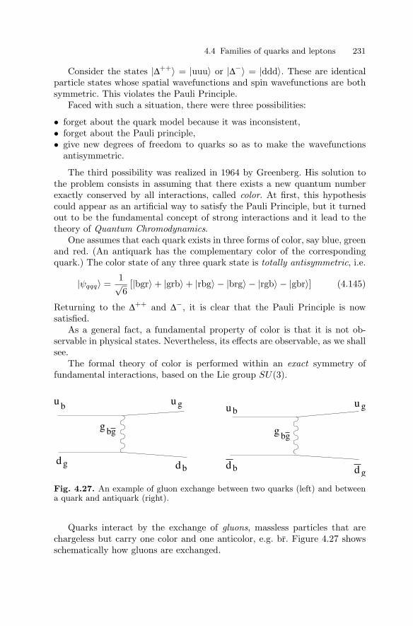
4.4 Families of quarks and leptons 231
Consider the states |∆++〉 = |uuu〉 or |∆−〉 = |ddd〉. These are identicalparticle states whose spatial wavefunctions and spin wavefunctions are bothsymmetric. This violates the Pauli Principle.
Faced with such a situation, there were three possibilities:
• forget about the quark model because it was inconsistent,• forget about the Pauli principle,• give new degrees of freedom to quarks so as to make the wavefunctions
antisymmetric.
The third possibility was realized in 1964 by Greenberg. His solution tothe problem consists in assuming that there exists a new quantum numberexactly conserved by all interactions, called color. At first, this hypothesiscould appear as an artificial way to satisfy the Pauli Principle, but it turnedout to be the fundamental concept of strong interactions and it lead to thetheory of Quantum Chromodynamics.
One assumes that each quark exists in three forms of color, say blue, greenand red. (An antiquark has the complementary color of the correspondingquark.) The color state of any three quark state is totally antisymmetric, i.e.
|ψqqq〉 =1√6
[|bgr〉 + |grb〉 + |rbg〉 − |brg〉 − |rgb〉 − |gbr〉] (4.145)
Returning to the ∆++ and ∆−, it is clear that the Pauli Principle is nowsatisfied.
As a general fact, a fundamental property of color is that it is not ob-servable in physical states. Nevertheless, its effects are observable, as we shallsee.
The formal theory of color is performed within an exact symmetry offundamental interactions, based on the Lie group SU(3).
u
d
b
g
u
d b
g
gb
u b
d b
g g bg
u
d
g
g
Fig. 4.27. An example of gluon exchange between two quarks (left) and betweena quark and antiquark (right).
Quarks interact by the exchange of gluons, massless particles that arechargeless but carry one color and one anticolor, e.g. br. Figure 4.27 showsschematically how gluons are exchanged.

232 4. Nuclear decays and fundamental interactions
In quantum field theory, it is possible to show that it is the fact that thegluons carry a charge, i.e. color, that leads to confinement, i.e. to a long-range force that that grows linearly with separation. In electromagnetism,the exchanged photons do not themselves carry charge and the force is notconfining. It is this confinement that prevents a free quark from emerging inelectron deep-inelastic scattering as shown in Fig. 3.25.
4.4.3 Quark mixing and weak interactions
It is tempting to think that the classifications of leptons and of quarks areparallel from the point of view of weak interactions. One observes a similarmass hierarchy with two sequences of three fermions separated by one unitof charge. In analogy with the lepton families (4.123), we then write threequark families as(
ud′
) (cs′
) (tb′
)(4.146)
In the absence of mixing, we would just have d′ = d, s′ = s and b′ = b. TheW could induce only the transmutations u ↔ d, c ↔ s or t ↔ b. But then,strange particles would be stable, since no s → u would exist. Unlike leptonmixing which is manifested only in subtle effects in neutrino oscillations,quark mixing is responsible for the instability of otherwise stable particles.
If the strange and/or charm particles were stable, then we would be facingseveral coexisting nuclear worlds. In addition to usual nuclei, we would see awhole series of other nuclear species, similar but heavier. For instance, in anynucleus, one could replace the neutron by the Λ0 hyperon, which is a (u, d, s)state of mass mΛ0 = 1116 MeV/c2. Furthermore, since the Pauli principledoes not constrain the neutron and the Λ0, the usual nuclei would possess alarger number of heavy isotopes, since the Λ0’s can sit on the same shells asthe neutrons (in a shell model for instance).
In order to destabilize strange particles, we must have quark mixing suchthat d′, s′ and b′ are linear combinations of d, s and b. Generally, it issupposed that the transformation is unitary (like the corresponding neutrinotransformation) so we write in analogy with (4.124)⎛
⎝d′
s′
b′
⎞⎠ =
⎛⎝Udd Uds Udb
Usd Uss UsbUbd Ubs Ubb
⎞⎠⎛⎝d
sb
⎞⎠ ,
where the unitary matrix can be put in the form (4.126). (The three quarkmixing angles and phase have, a priori, nothing to do with the neutrinomixing angles.)
The elements of the mixing matrix can be determined from decay rates.Consider the decays
n → p e− νi (i = 1, 2, 3) λ = 1.1 × 10⁻³ s−1 , (4.147)
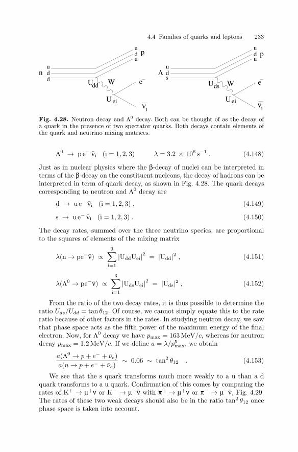
4.4 Families of quarks and leptons 233
e e
νiνi
nddu
du
s
u
ud p p
u
ud
Uei Uei
W Wdd U
ΛU ds
Fig. 4.28. Neutron decay and Λ0 decay. Both can be thought of as the decay ofa quark in the presence of two spectator quarks. Both decays contain elements ofthe quark and neutrino mixing matrices.
Λ0 → p e− νi (i = 1, 2, 3) λ = 3.2 × 10⁶ s−1 . (4.148)
Just as in nuclear physics where the β-decay of nuclei can be interpreted interms of the β-decay on the constituent nucleons, the decay of hadrons can beinterpreted in term of quark decay, as shown in Fig. 4.28. The quark decayscorresponding to neutron and Λ0 decay are
d → u e− νi (i = 1, 2, 3) , (4.149)
s → u e− νi (i = 1, 2, 3) . (4.150)
The decay rates, summed over the three neutrino species, are proportionalto the squares of elements of the mixing matrix
λ(n → pe−ν) ∝3∑
i=1
|UddUei|2 = |Udd|2 , (4.151)
λ(Λ0 → pe−ν) ∝3∑
i=1
|UdsUei|2 = |Uds|2 , (4.152)
From the ratio of the two decay rates, it is thus possible to determine theratio Uds/Udd = tan θ12. Of course, we cannot simply equate this to the rateratio because of other factors in the rates. In studying neutron decay, we sawthat phase space acts as the fifth power of the maximum energy of the finalelectron. Now, for Λ0 decay we have pmax = 163 MeV/c, whereas for neutrondecay pmax = 1.2 MeV/c. If we define a = λ/p5
max, we obtain
a(Λ0 → p + e− + νe)a(n → p + e− + νe)
∼ 0.06 ∼ tan2 θ12 . (4.153)
We see that the s quark transforms much more weakly to a u than a dquark transforms to a u quark. Confirmation of this comes by comparing therates of K+ → µ+ν or K− → µ−ν with π+ → µ+ν or π− → µ−ν, Fig. 4.29.The rates of these two weak decays should also be in the ratio tan2 θ12 oncephase space is taken into account.

234 4. Nuclear decays and fundamental interactions
ν iW
c1 Uei
ν iW
Ueiµ µ
u
dπ
u
dK
1c2s
Fig. 4.29. The decays π− → µ−νi and K− → µ−νi. The two decays occur throughquark–antiquark annihilation by creation of a W− which then decays to µ−νi. Therate of pion decay is proportional to |Udd|2 while that of kaon decay is proportionalto |Uds|2.
The idea of quark mixing was proposed in 1964 by N. Cabibbo. At thattime, only normal and strange hadron where known to exist. Cabibbo sug-gested that the W couple the u quark to a linear combination of the d and squarks:
|d′〉 = cos θc |d〉 + sin θc |s〉 (4.154)
where the value of the angle θc, now called the Cabibbo angle, is θc 13.1.The Cabibbo theory correctly predicts the decay rates of the neutron, Λ0,pions and kaons as well as the “hyperons” like Σ+ (uus, mΣ = 1189 MeV/c2).The rates of these decays are indicated on Figs. 4.13.
With the discovery of the c, b, and t quarks, we now know that thequark mixing is a bit more complicated with the three families (4.146) mixedaccording to the Kobayashi–Maskawa–Cabibbo scheme (4.4.3).
The moduli of the coefficients of this matrix are now known to be in theranges [1]:⎛
⎝0.9742 to 0.9757 0.219 to 0.226 0.002 to 0.0050.219 to 0.225 0.9734 to 0.9749 0.037 to 0.0430.004 to 0.014 0.035 to 0.043 0.9990 to 0.9993
⎞⎠ (4.155)
Note that, unlike the case of neutrino mixing, the diagonal elements are allnear unity so the mixing angles are all small.
It is important that the non-zero value of the phase δ implies automati-cally the violation of CP symmetry (product of a charge conjugation and aparity reversal). This is not of just academic interest since we will see in Chap.9 that, in the absence of CP violation, one would expect equal amounts ofmatter and antimatter in the Universe, in conflict with the observation thatthere is very little antimatter in the observable Universe. Note that a general2-dimensional unitary mixing matrix has no complex phase that cannot beeliminated by a suitable redefinition of the base states. Only with at leastthree families is it possible to induce CP violation.
Unfortunately, it does not appear that CP violation in the quark mix-ing matrix is directly connected with the CP violation that generated thecosmological matter-antimatter asymmetry. Nevertheless, the 3-family-CP-violation connection emphasizes that important effects can come from theexistence of particles that do not normally appear in nature. To this extent,

4.4 Families of quarks and leptons 235
CP violation provides a clue to the answer to Rabi’s question about the thirdgeneration, “Who ordered that?”
The second question (and there the theory is silent at present) is why thishierarchy of masses? In each class one has mb ms md, mt mc mu,mτ mµ me. This is one of the big enigmas of present theoretical physics,as is, in general, the question of the origin of mass of particles. This is directlyrelated to the third question: why these values of the Cabibbo–Kobayashi–Maskawa angles?
4.4.4 Electro-weak unification
Nuclear β-decay is an example of a reaction due to charged-current weakinteractions, by which we mean they are due to exchange of the charged W±.We summarize the W± couplings symbolically by
|W−〉 → g (|eνe〉 + |µνµ〉 + |d′u〉 + |s′c〉) (4.156)
Each of the terms of the right-hand-side is a decay channel of the W− butthey are meant to be more general than that. For instance the W− decaysto e−νe but it can also be emitted by a e− → νe transition. The νe, νµ, d′
and s′ are the linear combinations of the physical particles defined by (4.124)and (4.4.3). (To streamline the formulas, in this section we will ignore thethird generation of leptons and quarks.) The dimensionless coupling constantg gives the strength of the coupling and is related to the W mass and to theFermi constant by(
g
mWc2
)2
= 4√
2GF
(hc)3⇒ g2
4π=
129.46
. (4.157)
Similarly for the W+ if we replace fermions by their antiparticles.In the same manner, in electromagnetic interactions, the photon is uni-
versally coupled to the electric charge and, using the same notation,
|γ〉 →√
4πα(−|e−e+〉 + (2/3)|uu〉 − (1/3)|dd〉) (4.158)
where α is the fine structure constant. We see from (4.156) that g2/4π isthe weak charged current equivalent of the electromagnetic fine-structureconstant. The fact that the two fine-structure constants are of the same orderof magnitude suggests they have something to do with each other, as indeedthey do.
Until 1973, one had only observed charged current weak interactions dueto the exchange of the massive W± and the electromagnetic interactions dueto the exchange of the massless photon. In 1973 it was discovered that therewere also neutral current weak interactions due to the exchange of the massiveZ0. As we will now see, the existence of such interactions had been expectedfrom symmetry considerations.

236 4. Nuclear decays and fundamental interactions
Weak Isospin. From the point of view of weak interactions, quarks as well asleptons appear as weak-isospin doublets that are mathematically equivalentto the strong-isospin doublet formed from the u and d quarks, seen in Chap.1. The doublets (νe, e), (u, d′), (e+, νe), (νµ, µ) etc.
Consider, for instance, the doublets (νe, e) and (e+, νe). Within this as-sumption, we can construct a weak isospin triplet |ψ1
m〉 and a singlet |ψ00〉 as
follows 4⎧⎨⎩
|ψ1+1〉 = |νee+〉
|ψ10〉 = (|νeνe〉 − |e−e+〉)/√
2|ψ1
−1〉 = |e−νe〉(4.159)
|ψ00〉 = (|νeνe〉 + |e−e+〉)/
√2 . (4.160)
Note from (4.156) that the W− couples to |ψ1−1〉 and that the W+ couples
to |ψ1+1〉. This suggests that we introduce a W0 couples to |ψ1
0〉 so that thesituation is completely symmetric:
|Wm〉 → g|ψ1m〉 m = +1, 0,−1 . (4.161)
This relation can be extended to the other weak-isospin doublets: (νµµ+),(d′u) and (s′c).
Because of the triplet of W bosons, its relativistic gauge theory is said tobe based on a non-abelian group SU(2), the weak isospin.
Weak Hypercharge. One might have thought that the photon could beidentified with the W0 but this is not possible, if only because it couples tothe chargeless neutrino. To find the photon, we must first introduce anotherneutral particle, the B0 that couples to the, as yet unused |ψ0
0〉 in (4.160).We choose to make the coupling proportional to a new universal couplingconstant g′ and to the weak hypercharge of the doublet in question:
Y = 2(Q − T3) . (4.162)
The weak-hypercharge is equal to -1 for leptons and to 2/3 for quarks (op-posite values for the antiparticles).
The B0 couplings are then
|B0〉 → g′[− 1√2(|νeνe〉 + |e−e+〉) + (2/3)
1√2(|uu〉 + |dd〉) + . . .] (4.163)
Because there is only one B0, the quantum field theory of the B0 field isa gauge theory on an abelian group U(1) analogous to electromagnetism.
4 The difference in signs of the m = 0 combinations compared to previous expres-sions comes from the fact that we are dealing with fermion–antifermion systemsinstead of fermion–fermion systems.

4.4 Families of quarks and leptons 237
The Glashow–Weinberg–Salam Mechanism. Like the W0, the B0 can-not be the photon since the coupling (4.163) is not proportional to the charge.In particular, it couples to the neutrino. It is, however, simple to find a linearcombination of the two neutral bosons that does have couplings proportionalto the charge: Let us therefore define :
|Z0〉 = cos θw|W0〉 − sin θw|B0〉|γ〉 = sin θw|W0〉 + sin θw|B0〉 (4.164)
where θw is called the weak-mixing angle or also the “Weinberg angle.”The photon’s couplings are proportional to charge if we take
sin θw =g′√
g2 + g′2cos θw =
g√g2 + g′2
. (4.165)
One can check easily, restricting to the doublet (e, νe) doublet that
|γ〉 → − gg′√g2 + g′2
(|ψ10〉 − |ψ0
0〉)/√
2 = − gg′√g2 + g′2
|e−e+〉 , (4.166)
i.e. the coupling to νeνe vanishes as expected for a neutral particle. This givesus a relation with the fine structure constant
gg′√g2 + g′2
= g sin θw =√
4πα , ⇒ g′2
4π=
1107.5
. (4.167)
It can be verified that the couplings of the photon to the quarks are propor-tional to their charges.
We also need a way to ensure that the photon mass vanishes. This can bedone by considering mass-squared matrix 5 in the basis |W0〉, |B0〉
M =(
m2W −A
−A m2B
)(4.168)
where A characterizes the W0 B0 transition which is responsible for themixing.
The diagonalization of this matrix is straightforward. If one wants thephoton mass to vanish, we need to take A = mWmB which yields by identi-fying the eigenvectors of M with the expressions (4.164):
mγ = 0 , m2Z = m2
W + m2B =
m2W
cos2 θw, cos θw =
mW
mZ.(4.169)
5 Why the masses squared and not the masses themselves? This is because bosons,such as the W and B, satisfy the Klein–Gordon equation which we mentioned inSect. 1.4 (1.63), which involves the squares of the masses and not the massesthemselves. If one incorporates an interaction, this feature will remain. Forfermions, on the contrary, the Dirac equation is of first order and it is directlyon the mass that one operates.

238 4. Nuclear decays and fundamental interactions
Bringing together all these results and using the values of the fine-structure constant and GF, we obtain the following masses as a functionof the weak-mixing angle θw
6
mWc2 =38.7 GeV
sin θwmZ0 =
mW
cos θw(4.170)
cos2 θw + 4πα/g2 = 1 . (4.171)
Originally, θw was a free parameter of the Glashow, Weinberg and Salammodel. It is now known to good precision:
sin2 θw = 0.2237 ± 0.0008 , (4.172)
mWc2 = 80.33 ± 0.15 GeV , (4.173)
mZc2 = 91.187 ± 0.007 GeV . (4.174)
We should emphasize that the question of the mass of the W and Zis very delicate. In the relativistic formulation of the theory of Glashow,Weinberg and Salam, a consistent quantum field gauge theory is constructedon a non-abelian group. This can only be done if the initial masses of thefour states |W+〉, |W0〉, |W−〉 and |B0〉 are all identically zero. They acquirenon-vanishing masses mW and mB by a spontaneous symmetry breakingmechanism where Higgs bosons play a crucial role. The fact that, in the end,the photon is a zero-mass particle is a natural automatic consequence of thetheory, and not a condition imposed on the values of parameters as we havedone above. The Higgs bosons is the last particles of the standard model thatis yet to be observed. Its couplings to the other particles are responsible forthe particle masses. An intense experimental activity is underway in order toidentify them.
We have ignored the question of helicity in our discussion of electro-weaktheory. In fact the theory is constructed so that the charged current interac-tions maximally violate parity (as required by the observation that neutrinosare 100% polarized) while the electromagnetic interactions conserve parity.
We see that the theory unifies electromagnetic and weak interactions. Itpredicts the existence of weak interactions which do not change the electriccharge. These interactions are mediated by the neutral Z0 boson. An exampleof such a reaction is
ν p → νp . (4.175)
It is illustrated in Fig. 4.30The theory of neutral currents also had a role in the prediction of the
charm quark. At the time when the electroweak theory appeared, neutralcurrents were unknown and only 3 quarks had been discovered, i.e. the u6 The first relation is obtained after taking into account various radiative correc-
tions. Otherwise one obtains mWc2 = 37.3 GeV/ sin θw.

4.4 Families of quarks and leptons 239
Z
p
ν ν
pFig. 4.30. Neutrino-proton elastic scattering mediated by the exchange of the Z0
boson.
the d and the strange quark s. In 1970, in investigating neutral current reac-tions, Glashow, Iliopoulos and Maiani were led to invent a mechanism whichpredicted the existence of charm more than 4 years before its discovery.
As we have written the theory with the weak mixing of the quarks viaa unitary matrix (4.4.3), the Z0 does not have “non-diagonal” couplings tothings like ds. In the absence of the unitary mixing, it is readily shown thatthe Z0 would have such couplings. In this case, the K0 would decay to µ+µ−
through ds → Z0 → µ+µ−. However, the upper experimental limits on therate of this reaction are so low that one is sure that it is excluded up tosecond order perturbation theory (to which the exchange of charged currentsW+ and W− contributes in principle).
One should keep in mind the following aspects of neutral current weakinteractions of quarks.
1. The couplings of the Z0 are diagonal. This boson couples to (uu), (dd),(ss), but not to (ds), etc.
2. The coupling constants have a form similar to the lepton couplings.3. The partial decay width of the Z0 into 2 fermions ff is given by
Γ (Z0 → f f) =g2ZmZc2
48π(|cV|2 + |cA|2) .
4. The constants |cV |2 and |cA|2 are such that one has– for neutrinos : |cV |2 + |cA|2 = 1/2– for e, µ, τ : |cV |2 + |cA|2 = (4 sin4 θw + (2 sin2 θw − 1)2)/2 ∼ 1/4– for u, c, t : |cV |2 + |cA|2 = 1/4 + (1/2 − 4/3 sin2 θw)2 ∼ 0.29– for d, s, b : |cV |2 + |cA|2 = 1/4 + (1/2 − 2/3 sin2 θw)2 ∼ 0.37where θw is the Weinberg angle.
This means that the branching ratio is 6% for each neutrino species , it is14% for d,s,b quarks (taking into account the color of quarks which multipliesby a factor of 3 the contribution of each quark flavor).
Altogether, one obtains the estimate
ΓZ0 ∼ 2.5 GeV . (4.176)

240 4. Nuclear decays and fundamental interactions
NN
N
E (GeV)cm
88 90 92 94
=2ν=3ν=4ν
20
30
10
(nb)
σ
Fig. 4.31. Resonance curve of the Z0 measured by the Aleph experiment at CERNin e+e− collisions at the LEP colliding ring. The three curves represent the theo-retical predictions according to the number of different neutrino species. (CourtesyAleph Collaboration.)
We note that the existence of another, new, neutrino would increase thiswidth by 167 MeV, that of a new family would increase it by a factor of 4/3,that of a neutrino and its lepton, assuming the quarks are too heavy, by 264MeV.
We therefore understand the interest of measuring the Z0 width in orderto count the number of different fermions whose masses are smaller thanmZ/2.
The answer obtained in CERN with steadily increasing accuracy since1989 is
ΓZ0 = 2.4963 ± 0.0032 GeV i.e. Nν = 2.991 ± 0.016.
In other words, there are three families of quarks and leptons and only three(neutrinos lighter that the Z0, of course).
Originally, quarks were a simple way to classify hundreds of hadrons. Theidea got enriched with the construction of quantitative dynamical models ofhadron spectroscopy.

Exercises for Chapter 4 241
With deep inelastic scattering, jets in e + e− collisions, the explanationof the magnetic moments of hadrons, i.e. by studying the electromagnetic in-teractions of quarks, these acquired a physical reality and their elementaritywas established: they are point-like particles. Then, using weak interactions,one discovers a fascinating symmetry between quarks and leptons which issuggestive of a possible underlying unification, which would be more gen-eral and more profound, of the constituents of matter and their fundamentalinteractions. It is one of the great hopes of present theoretical physics to con-struct a complete and unified theory of all interactions including gravitation.Superstring theory and the reduction of all corresponding theories to a singleunique “M -Theory ” is a very active field of research at present.
4.5 Bibliography
1. F. Halzen and A.D. Martin: Quarks and Leptons (Wiley, New York, 1984)2. W. Greiner and B. Mller:Gauge Theory of Weak Interactions (Springer,
Berlin, 2000)3. U. Mosel: Fields, Symmetries, and Quarks (Springer, Berlin, 1999)4. Q. Ho-Kim and X.-Y. Pham:Elementary Particles and Their Interactions
(Springer, Berlin, 1998)5. Introduction to Elementary Particles, D. Griffiths, (Harper & Row, New
York, 1987).
Exercises
4.1 Discuss the electron energy spectrum from the 2β-decay of 100Mo shownin Fig. 4.1. The average total energy taken by the 2 electrons in ∼ 1.2 MeV.How much energy on average is taken by the two neutrinos?
4.2 Charged particles lose energy in when traversing a material by ioniza-tion. The minimum rate of energy loss (applicable to relativistic particles) is∼ 2 MeV g−1cm2. (Multiplying by the density of the medium gives the en-ergy loss per unit distance in MeV cm−1.) Consider the experiment shown inFig. 4.1. Estimate the energy loss by the decay electrons before leaving thefoil. Does this energy loss significantly affect the energy measurement by thescintillators?
4.3 Discuss the decay scheme shown in Fig. 4.2. What factors determine thebranching ratios of β-decay to the ground and first excited states of 170Yb?Estimate the internal conversion fraction for the decay of the 84 keV state byusing (4.61). Is the use of the formula justified?

242 4. Nuclear decays and fundamental interactions
4.4 Consider the photon spectra shown in Fig. 4.3. From the maximumDoppler shift of forward going photons, estimate the velocity and energy ofthe decaying 74Br nuclei. Use the Bethe–Bloch formula (5.32) to estimatethe energy-loss rate of Br ions in nickel and the time for the nuclei to cometo rest. Estimate the lifetime of the decaying state. What are the possiblecriticisms of this estimate?
4.5 A commonly used γ-source is 60Co which β-decays to an excited state of60Ni as in Fig. 4.32. Use the indicated spins and parities to explain why 60Codoes not decay directly to the ground state of 60Ni. Explain why two photonsare emitted in the de-excitation of 60Ni. Estimate the time delay between theβ-decay and the photon emissions.
5+
0+
2+1.173 MeV
1.332 MeV
β−60
60 Ni
Co5.271 yr
4+
2+0+
Fig. 4.32. The decay of 60Co.
4.6 What energy photons are emitted after each of the five β-decays shownin Fig. 4.12?
4.7 Estimate the energy of the k-capture Auger electrons emitted after theelectron-capture decay of 71Ge (Fig. 4.16) by assuming that the inner mostelectrons occupy hydrogen-like orbitals.
4.8 Verify the β spectrum in the case of a non-zero neutrino mass (4.101).
4.9 Consider the decay scheme in Fig. 4.19. Explain the large difference int1/2 for 152Eu and the isomer 152mEu. Calculate the kinetic energy of the152Sm nucleus after the electron-capture decay. What is the energy of the

Exercises for Chapter 4 243
“961 keV” photons that happen to be emitted in the direction opposite tothat of the neutrino? Do they have sufficient energy to re-excite 152Sm nucleiin the ground state?
4.10 Consider the neutrino event illustrated in Fig. 4.20. The final-stateneutron takes only a small amount of the neutrino energy. Estimate themaximum neutron energy corresponding to positrons emitted opposite tothe direction of the neutrino. What is the cross-section for such neutrons toelastically scatter on protons (Fig. 3.4). What is the neutron mean-free pathin the scintillator (CH, ρ ∼ 1 g cm−2)? Using the fact that a neutron loseson average half of its kinetic energy in a collision with a proton, estimatethe number of collisions necessary for the neutron to be thermalized. Afterthermalization, what is the neutron capture cross-section on hydrogen (Fig.3.4)? What is the mean time be for the neutron is captured?
4.11 In Fig. 4.20, what is the mean-free path of the photons in the scintillator(CH) assuming that the photons interact mostly via Compton scattering onelectrons, σ ∼ σT.

5. Radioactivity and all that
Our galaxy’s stock of heavy elements was mostly produced in supernovaeexplosions that eject stable and unstable nuclei into the interstellar medium.The interstellar clouds containing these elements may later condense to formstellar systems. By the time this happens, most of the short-lived nuclei wouldhave decayed, so planets contain, at their birth, only nuclei with lifetimesgreater than, say, 106 yr. On Earth, ∼ 4.5 × 10⁹ yr after its formation, mostof the original unstable nuclei have decayed leaving only those with t1/2 >108 yr. There is also continuous production of unstable nuclei by cosmic-rays entering the Earth’s atmosphere. The α and β decays of these nucleiconstitute the natural radioactivity that was discovered by Becquerel at theend of the nineteenth century.
All living species have evolved in this bath of radiation. What is new onEarth is the existence of an artificial radioactivity due to the developmentof nuclear technologies, most importantly energy production by nuclear re-actors. There are now also numerous uses of radioactive nuclei, most notablyin medical treatment and dating.
With these developments, public health concerns have naturally arisenbecause of the effect of ionizing radiation on living tissue. Since natural ra-dioactivity is present everywhere, it should be emphasized that the importantquestions concern keeping the ambient radioactivity at a level not much aboveits natural level. This obviously requires confinement of the large amounts ofradioactive elements produced in nuclear reactors.
In this chapter, we will first discuss the natural sources of radioactivityand the production of radioactive elements in neutron and charged-particlebeams. We will then discuss how high-energy particles lose energy whiletraversing ordinary matter. Particle detectors based on the energy-loss mech-anisms will be briefly discussed. Finally, we discuss a few applications ofradioactivity.
5.1 Generalities
Most nuclei are inherently unstable, being capable of decaying to other nucleiby β-decay, α-decay, or by spontaneous fission. The set of all possible decaysis referred to globally as radioactivity.

246 5. Radioactivity and all that
Let τ be the (mean) lifetime of a nuclear species. The half-life t1/2 isdefined by
t1/2 ≡ τ log 2 ∼ 0.693τ . (5.1)
The name “half-life” refers to the fact that the probability that the nucleushas decayed after t1/2 is equal to 1/2. Nuclear physicists traditionally use half-lives, whereas particle physicists use (mean) lifetimes. The two definitionsdiffer by a factor of ln 2 = 0.693. (We hope that the trivial mistakes inthis book that come from forgetting this factor will disappear in the editingprocess.)
The activity of a radioactive sample is the number of decays per unit time.For a source containing N particles the activity is
A = Nλ = N/τ . (5.2)
If one knows A and τ , one can deduce the concentration N of the radioactiveproduct in the sample.
Activities are measured in Becquerel:
1 Bq = 1 (decay) s−1 . (5.3)
The previously used unit was the Curie : 1 Curie = 3.7 × 10¹⁰ Bq. Thiscorresponds to the activity of 1 g of the radium isotope 226Ra.
According to the nature of emitted particles, α particles, e±, or photons,one distinguishes three types of radioactivity: α, β and γ. They were previ-ously described theoretically in Chap. 4. The types are summarized in Table.5.1.
5.2 Sources of radioactivity
At the end of the 1930s, one made the distinction between two classes ofradioactivity, natural and artificial. Natural radioactivity was discovered ac-cidentally by Henri Becquerel in 1896 who observed that photographic plates(unexposed to light) are blackened when placed next to uranium sulfide crys-tals. After some time, the primary particles responsible for the blackeningwhere identified as 4He ions from a chain of decays starting with
238U → 234Th α t1/2 4.468 × 10⁹ yr . (5.4)
Artificial radioactivity coming from elements produced in laboratory reac-tions was discovered by Frederic and Irene Joliot-Curie in 1934 who observed
α 27Al → n 30P (5.5)
followed by30P → 30Si e+ νe t1/2 = 150.0 sec . (5.6)

5.2 Sources of radioactivity 247
Table 5.1. Main types of radioactivity. The first four, β±, electron-capture, and2β are A-conserving decays that lead to the one β-stable isobar for the given A.The next two, α and (spontaneous) fission change A. All these decays may leavethe daughter nuclei in excited states that decay (generally rapidly) to the groundstates by the last two forms of radioactivity, γ and internal conversion. Two typesof radioactivity, e−-capture and internal conversion occur only if the nucleus issurrounded by atomic electrons.
name reaction energyspectrum
β− (A, Z) → (A, Z + 1)e−νe continuousβ+ (A, Z) → (A, Z − 1)e+νe continuouse−-capture e−(A, Z) → (A, Z − 1)νe discrete
+atomic X-rays/Auger e−’s
2β (A, Z) → (A, Z ± 2)2e±2νe(2νe) continuous
α (A, Z) → (A − 4, Z − 2)4He discrete
fission (A, Z) → (A1, Z1) (A2, Z2) (+neutrons) continuous
γ (A, Z)∗ → (A, Z)γ discreteinternal conversion e−(A, Z)∗ → (A, Z)e− discrete
+atomic X-rays/Auger e−’s
One can divide natural radioactivity into “fossil” radioactivity due to ele-ments present at the formation of the Earth, and “cosmogenic” radioactivitydue to elements continually produced in the atmosphere by cosmic-rays.
Techniques for producing artificial radioactivity can be divided into thosethat use neutrons (neutron activation) and those that use charged particlebeams. An example of the latter is reaction (5.5) where the Joliot-Curies usednaturally occurring α radiation (Eα ∼ 5 MeV) to induce the transmutationof aluminum to phosphorus. Modern alchemists use artificially acceleratedions of arbitrary energies, greatly increasing the possibilities, as discussed inSect. 3.1.5.
5.2.1 Fossil radioactivity
Most elements present on Earth condensed from a interstellar cloud about4.5 × 109 yr ago. This cloud consisted mostly of “primordial” 1H and 4Hethat was produced in the first minutes after the “Big Bang” (see Chap. 9).Additionally, the cloud contained heavier elements that had been producedin earlier generations of stars and dispersed into the interstellar medium byvarious processes (see Chap. 8). Most radioactive nuclei were produced insupernovae that generate a mix of neutron-rich nuclei in a period of time of

248 5. Radioactivity and all that
order a few seconds. When, some millions of years later, the cloud condensedto form the solar system, a few radioactive nuclear species were still present.At the present epoch, only nuclei with mean lives greater than, say, 108 yr,are still present in significant numbers.
The nuclei with 108 yr < τ < 1012 yr are listed in Table 5.2. These long-lived nuclei involve either highly forbidden β decays (large spin changes) orare α-decays that happen to have Q-values that place the half-lives in thisrange.
Table 5.2. Nuclei with 108 yr < t1/2 < 1012 yr. The “isotopic abundance” is forthe terrestrial mix and the activity for the purified element corresponds to theterrestrial isotopic mix. For the activity in the Earth’s crust, the uranium andthorium activities include the activities of the daughters. Note that three nuclides,40K, 147Sm and 235U have lifetimes much less than the age of the Earth (∼ 4.5 ×10⁹ yr) and therefore have very small isotopic abundances.
decay half-life isotopic activity activity(years) abundance (Bq kg−1) (Bq kg−1)
(percent) (element) (crust)
40K → 40Ca e−νe 89% 1.28 × 10⁹ 0.0117 3.0 × 10⁴ 6.3 × 10²
→ 40Ar νe 11%
87Rb → 87Sr e−νe 4.75 × 10¹⁰ 27.83 8.8 × 10⁵ 8.0 × 101
146Sm → 142Nd α 1.03 × 10⁸ < 10−7 < 1 < 10−4
147Sm → 143Nd α 1.06 × 10¹¹ 15.1 1.3 × 10⁵ 9 × 10⁻¹
176Lu → 176Hf e− 3.78 × 10¹⁰ 2.61 5.5 × 10⁴ 4 × 10⁻²
187Re → 187Os e−νe 4.15 × 10¹⁰ 62.6 1.1 × 10⁶ 8 × 10⁻⁴
232Th → 228Ra α 1.405 × 10¹⁰ 100 4.05 × 10⁶ 3.5 × 10²
235U → 231Th α 7.038 × 10⁸ 0.72 5.7 × 10⁵ 1.7 × 101
238U → 234Th α 4.468 × 10⁹ 99.275 1.2 × 10⁷ 4.7 × 10²
Most of the nuclei in Table 5.2 are isotopes of rare elements with the ex-ception of 40K. The decay modes of this isotope, shown in Fig. 5.1, yields a β−
with Emax = 1.31 MeV (BR=89.3%) or a γ with Eγ = 1.46 MeV (BR=10.5%).Potassium has a chemistry similar to that of sodium and is plentiful in bio-logical material where it is the dominant source of radioactivity.

5.2 Sources of radioactivity 249
K
CaAr
0.00
2.00
EC(0.2%)
β (89.3%)
Eγ=1.46MeV Q=1.31MeV
EC(10.5%)Qec=0.05MeV
Qec=1.505
4040
40
42
0
0
−
+
+
+
_
Fig. 5.1. The β-decay of 40K. Being an N -odd,Z-odd nucleus, it has two modes:electron capture to 40Ar and β− to 40Ca. The long half life (1.28×10⁹yr) is explainedby the large angular momentum changes in the decays to the ground states (makingthe decays highly forbidden) and the small value of Qec to the 2+ state of 40Ar.
235 238
232
205
208206207
209
Th
Bi
Pb
Tl
Np
Pa
Po
At
Rn
Fr
Ra
Ac
U
t
mostly
mostly
1/2>108 yr
β
α
−βα
Fig. 5.2. The three chains of natural radioactivity: 238U →206 Pb; 235U →207 Pb;and 232Th →208 Pb. Each chain consists of a series of α− and β−-decays. In thecase of the 232Th chain, a branch occurs at 212Bi that has a 64% branching ratiofor β−-decay and a 36% ratio for α-decay. Similar, though less balanced, branchingsoccur throughout the chains and only the primary routes are shown. Also shown isthe recently discovered 209Bi →205 Tl chain consisting of a single α decay [52].

250 5. Radioactivity and all that
Table 5.3. Members of the three natural radioactivity chains and their half-lives.
uranium series actinium series thorium series
238U92 4.468 Gyr234Th90 24.10 d234Pa91 1.17 m234U92 245.5 kyr 235U92 0.7038 Gyr230Th90 75.38 kyr 231Th90 25.52 h 232Th90 14.05 Gyr226Ra88 1600 y 231Pa91 32760 y 228Ra88 5.75 y222Rn86 3.8235 d 227Ac89 21.773 y 228Ac89 6.15 h218Po84 3.10 m 227Th90 18.72 d 228Th90 1.9116 y214Pb82 26.8 m 223Ra88 11.435 d 224Ra88 3.66 d214Bi83 19.9 m 219Rn86 3.96 s 220Rn86 55.6 s214Po84 164.3 µs 215Po84 1.781 ms 216Po84 0.145 s210Pb82 22.3 y 211Pb82 36.1 m 212Pb82 10.64 h210Bi83 5.013 d 211Bi83 2.14 m 212Bi83 60.55 m210Po84 138.376 d 207Tl81 4.77 m 64% 212Po84 0.299µs
36% 208Tl81 3.053 m206Pb82 > 1020 yr 207Pb82 > 1020 yr 208Pb82 > 1020 yr
The three heavy nuclides, 238U, 235U and 232Th, are the origins of thethree natural radioactivity chains illustrated in Fig. 5.2 and Table 5.3. Thechains proceed through a series of α and β decays that end at three isotopesof lead
238U → 206Pb (A = 4n + 2) ,
235U → 207Pb (A = 4n + 3) ,
232Th → 208Pb (A = 4n) ,
The three chains end with an isotope of Z-magic lead. (208Pb is doublymagic, N = 126.) The fourth chain with A = 4n + 1 has no long-lived nucleiheavier than 209Bi. The chain thus consists of a single decay 209Bi → α 205Tl(t1/2 = 1.9 × 10¹⁹ yr) [52].
As seen in Table 5.3, the lifetimes of the daughter nuclei are all short ongeological timescales so in many applications the cascade can be consideredto pass “instantaneously” to the final lead isotope. The fact that 238U, 235U,and 232Th are long-lived whereas the elements with 209 < A < 232 havemuch shorter half-lives can be traced to the shell structure of the nucleuswhich makes the doubly magic nucleus 208Pb especially bound. As a result,the Q-values of α-decay are relatively large for 208 < A < 232 (Fig. 2.14)making the α rates high.
The uranium and thorium chains and 40K dominate the radioactivity in-side the Earth. The activity of the lower atmosphere is mostly due to threeisotopes of the noble gas radon that are daughters of uranium and thorium

5.2 Sources of radioactivity 251
and can diffuse out of rocks into the air. It is typically ∼ 20 Bq m−3 in-side reasonably ventilated buildings [53]. It should be also noted that theEarth’s stock of helium originates mostly in the α particles emitted in theuranium–thorium chains. (Inert primordial helium was not retained duringthe formation of the Earth.)
Minerals that contain uranium and thorium also contain their daughters.Neglecting leakage out of the mineral, all species in the chain
1 → 2 → 3 → 4 . . . n
will generate quantities of each nucleus governed by the coupled differentialequations
N1 = −N1/τ1 (5.7)
Ni = Ni−1/τi−1 − Ni/τi i = 1 . (5.8)
In the case of the three natural chains, the first nucleus is by far the longestlived τ1 τi =1,n. In this case, the solution is
N1 = N1(t = 0)e−t/τ1 (5.9)
Ni = N1τi
τ1i = 1, n (5.10)
Nn = N1(t = 0)(1 − e−t/τ1) . (5.11)
The unstable daughters thus reach an equilibrium abundance proportionalto their half-lives where the activity of each daughter is equal to the activityof the parent.
It was Marie and Pierre Curie who chemically isolated the daughter nucleipresent in uranium ore. Once uranium ore is refined only the parents 238Uand 235U and the daughter 234U remain in the chemically pure uranium.
Natural lead ore contains the natural isotopes, 204Pb, 206Pb, 207Pb and208Pb, as well as the uranium–thorium daughters due to the decay of anyuranium or thorium present in the lead ore. After refining resulting in theremoval of the uranium–thorium and non-lead daughters, the purified leadcontains the four natural isotopes as well as the the β-emitting daughters210Pb (t1/2 = 22.37 yr), 211Pb (t1/2 = 36.1 min), and 212Pb (t1/2 = 10.6 hr)(see Fig. 5.2). Ignoring the two very short-lived daughters, we see that re-cently mined lead contains a 210Pb activity that depends on the amount of238U present in the ore. It ranges from ∼ 1 Bq kg−1 to 2500 Bq kg−1 [53] Inancient lead recovered, for example, from sunken Roman galleys, the 210Pbhas mostly decayed away and activities as small as 0.02 Bq kg−1 have beenreported [53]. Such ancient lead is used as shielding in measurements wherevery low radioactivity is necessary (Exercise 9.7).

252 5. Radioactivity and all that
5.2.2 Cosmogenic radioactivity
Most interstellar matter is in the form of a thermalized gas (mostly hydrogenand helium). There exists, however a non-thermal component of cosmic-raysof similar chemical composition but with an energy spectrum (Fig. 5.3) peak-ing at a kinetic energy of ∼ 300 MeV and then falling like ∼ E−3. While theorigin of this component is not entirely established, it is believed that it re-sults from acceleration of particles by time-varying magnetic fields producedby pulsars (neutron stars) and supernova remnants.
1
10kinetic energy (MeV/nucleon)
sr s
MeV
/nuc
leon
)
He
2 3 4 5 610 10 10 10 10
C
Fe
H
flux
(m
2−
1
−2
10−4
10
10
10
−8
−6
Fig. 5.3. The flux of cosmic radiation outside the Earth’s atmosphere [54]. Mostparticles are protons or 4He nuclei with smaller numbers of heavy nuclei. Carbonand Iron are important examples.
When cosmic-rays enter the Earth’s atmosphere, they lose energy throughionization and nuclear reactions. The Earth’s atmosphere is sufficiently thickthat most of the primary cosmic-radiation stops in the atmosphere. Mostcosmic radiation that reaches the Earth’s surface consists of muons and neu-trinos from the decays of pions produced in these collisions (Fig. 5.4). A smallnuclear component consisting mostly of neutrons reaches the surface but isquickly absorbed in the first few meters of the Earth’s crust.

5.2 Sources of radioactivity 253
0 200 400 600 800 1000Atmospheric depth ( g cm
15 10 5 3 2 1 0Altitude (km)
2
−210
−110
1
10
10
103
410
srs
vert
ical
flu
x (
m−2
−1
−1 )
nuclear fragmentπ
µν µ
e
π
Earth surface
ν ν
cosmic−ray proton
νµ µ,ν
µ+−
p, n
e+−
+−π
−2 )
Fig. 5.4. An example of a “shower” induced by a cosmic-ray proton in the upperatmosphere. Two pions and a nuclear fragment are produced when the protonstrikes a nucleus. The two pions decay π → µν. and one of the muons decay µ →eνν The undecayed muon reaches the Earth’s surface where it stops because ofionization energy loss. The lower panel shows the fluxes as a function of depth inthe atmosphere [54].

254 5. Radioactivity and all that
Cosmic-rays produce radioactive nuclei via their interactions with nucleiin the atmosphere and in the Earth’s crust. In the atmosphere, the mostcommon radioactivity produced is that of 14C. This nucleus is a secondaryproduct of neutrons who are themselves produced by high-energy cosmic-rayprotons that breakup nuclei in the atmosphere. The neutrons then either de-cay or are absorbed. The most common absorption process is the exothermic(n,p) reaction on abundant atmospheric nitrogen
n 14N → 14C p t1/2(14C) = 5730 yr . (5.12)
The produced 14C is mixed throughout the atmosphere and enters the foodchain through CO2 ingesting plants. This results in a 14C abundance in liveorganic material of about 10−12 relative to non-radioactive carbon. The re-sulting activity is about 250 Bq kg−1. As we will see in Sect. 5.5.2, this allowsthe estimation of ages of dead organic material.
High energy cosmic rays also produce radioactive nuclei through “spalla-tion” reactions where one or more nucleons are removed from a nucleus (Sect.3.1.5). For example a neutron with kinetic energy greater than ∼ 20 MeV canremove two nucleons for a germanium nucleus, e.g.
n 70Ge → 3n 68Ge t1/2(68Ge) = 270.7 day . (5.13)
This reaction results in a radioactivity of 0.3 mBq kg−1 in germanium crystalsproduced at the Earth’s surface [53]. In high-purity germanium crystals usedfor detection of low-level radioactivity, it is the most important source ofintrinsic radioactivity. If the crystals are placed underground, the productionof 68Ge ceases and the activity decays away.
In rare circumstances, nucleons removed in spallation reactions can com-bine to form nuclei. For example the radioactive tritium isotope of hydrogencan be produced by cosmic rays by (for example) the reaction
n 16O → 3H 14N t1/2(3H) = 12.35 yr . (5.14)
The atmospheric tritium combines with oxygen to form water that rainsdown on the Earth. Prior to the atmospheric testing of nuclear weaponsand the Chernobyl reactor accident, this was the primary source of naturallyoccurring tritium. Because of its short half-life, tritium is absent in waterfrom deep water reserves and also in crude oil.
5.2.3 Artificial radioactivity
Radioactive nuclei can be created in the laboratory by the same reactionsthat are induced by cosmic-rays, though in the laboratory we can choosebeams and targets that maximize production rates. Two general techniquesare used, those based on charged particle beams, and those using (thermal)neutrons produced by nuclear reactors.
To produce a radioactive nucleus, it is generally necessary to take a stablenucleus and add or subtract nucleons, or to transmute protons to neutrons

5.2 Sources of radioactivity 255
ion source
ion trap/source
post accelerator
mass,charge separator
thin target
thick target
primary beam primary beam
secondary target
storage−cooler ring
ISOL In−Flight
Fig. 5.5. The two primary methods of producing beams of radioactive nuclei [31].In the ISOL method (“Isotope Separator On-Line”) a primary ion beam is incidentupon a thick target. Nuclei produced in inelastic reactions are stopped in the targetbut eventually diffuse into a system that collects, purifies, and accelerates ions.In the “In-Flight” technique, the primary ions are incident upon a target that issufficiently thin that produced nuclei are not stopped. Nuclei emerging from thetarget can then be mass selected.
or vice versa. High energy ion collisions (Sect. 3.1.5) can be used to producea wide variety of nuclides by fragmentation or fusion reactions. If a specificnuclide is desired, it is more efficient to use low-energy ions. For example, inorder to produce the radioactive germanium isotope 71Ge (t1/2 = 11.44 day),two simple reactions come immediately to mind. The first uses an acceleratedproton beam:
p 71Ga → n 71Ge . (5.15)
The proton kinetic should be about 10 MeV so that the Coulomb barrierbetween the proton and gallium nucleus is insufficient to prevent the reaction,while the energy is too small to have appreciable cross-sections for other

256 5. Radioactivity and all that
inelastic reactions involving the ejection of nucleons. A target of enriched71Ga is exposed to the proton beam and then dissolved and chemically treatedto extract any germanium. If the gallium is isotopically pure, the germaniumis nearly pure 71Ge.
A second possibility uses the (n, γ) reaction
n 70Ge → γ 71Ge . (5.16)
A sample of germanium is placed in a neutron beam. After irradiation, thesample contains a mixture of 70Ge, 71Ge and 71Ga from the decay of 71Ge.Chemical treatment can then yield a mixture of stable 70Ge and radioactive71Ge.
Both charged-particle- and neutron-activation are currently used to pro-duce radioactive nuclei. Charged particles have the disadvantage in that ionslose their energy through ionization when they enter the sample, so that theyquickly become unable to induce nuclear reactions because of the Coulombbarrier. Thermal neutrons, on the other hand, perform a random walk untilthey are absorbed. One then gets more activity per incident particle withneutrons than with ions. For this reason, large activity sources are generallyproduced in intense neutron fluxes available at nuclear reactors. For example,cobalt sources used for medical purposes and food sterilization are producedthrough the reaction
n 59Co → γ 60Co . (5.17)
Sources of activity > 1016 Bq can be made by placing the sample of cobalt ina reactor for a period of weeks (Exercise 5.2).
In nuclear research, it is often useful to produce beams of radioactivenuclei that can be accelerated to energies necessary to study their reactions.In recent years, much progress has been made in the production of radioactivebeams. The two generic methods of production are illustrated in Fig. 5.5.Examples of experiments using radioactive beams are illustrated in Figs. 1.4,1.5 and 2.18.
5.3 Passage of particles through matter
Particles produced in nuclear reactions or decays interact with matter in waysthat depend on their nature. We can distinguish the following cases:
• Charged nuclei and particles. These particles lose their energy by ionizingthe atoms in the medium and eventually come to rest. This process isdescribed in Sect. 5.3.1 for particles with masses me. The special caseof electrons and positrons is studied in Sect. 5.3.3.
• Photons. γ-rays generally lose energy in material through Compton scat-tering on atomic electrons
γ e− → γ e− . (5.18)

5.3 Passage of particles through matter 257
The secondary electrons then deposit their energy in the medium throughionization. The photon continues to Compton scatter until it is photoelec-trically absorbed,
γ atom → e−atom+ . (5.19)
Photons with energies greater than 2me can be directly absorbed by pro-duction of electron–positron pairs
γ (A, Z) → e+e− (A, Z) . (5.20)
These processes are studied in Sect. 5.3.4.• Neutrons. Neutrons lose energy by elastic scattering on nuclei until they
thermalize. They are eventually absorbed, generally by the (n, γ) reactionn(A, Z) → γ(A + 1, Z). These processes are described in Sect. 5.3.5.
In this section, we describe these physical process. Their biological effectswill be briefly described in Sect. 5.4.
5.3.1 Heavy charged particles
When a charged particle traverses a medium, it progressively loses its energyby transferring it to the electrons of the atoms of the medium. The rate ofenergy loss can be estimated by considering an ion of mass mion and chargezione that passes near a free electron, as illustrated in Fig. 5.6. To simplifythe calculation, we first suppose that the ion is non-relativistic, v c, andthat mion me. Since mion me, the ion’s movement is nearly unaffectedby the close encounter with the electron so that its trajectory is, to firstapproximation a straight line with impact parameter b.
yr = (vt,b)
b
electron
ion
x
Fig. 5.6. Passage of a charged particle in the vicinity of an atom.
The electron feels a Coulomb force due to the the presence of the ionand therefore recoils after the ion’s passage. The electron’s momentum canbe calculated by integrating the force. The integral is non-zero only in thedirection perpendicular to the trajectory:

258 5. Radioactivity and all that
pe(b, v) =∫
Fydt =zione2
4πε0
∫ ∞
−∞
b dx/v
(x2 + b2)3/2 =zione2
2πε0 vb. (5.21)
This formula is valid for values of b that are sufficiently large that during thepassage, the electron recoils through a distance that is small compared to b.The energy loss of the ion, ∆E, is the kinetic energy of the recoiling electron:
∆E(b, v) =p2e
2me=(
zione2
4πε0
)2 2v2b2me
. (5.22)
The energy loss is proportional to v−2 because the slower the ion, the longerthe time that the electron feels the electric field of the ion.
The energy loss is proportional to b−2 so we need to average over impactparameters. The procedure follows precisely what we did in Chap. 3 whenwe calculated reaction probabilities in terms of cross-sections. We consider abox of volume L3 containing one electron. The mean energy loss for randomimpact parameters is
∆E(v) =1L2
∫ bmax
bmin
2πbdb2
v2b2me
(zione2
4πε0
)2
=1L2
4π
v2me
(zione2
4πε0
)2
ln(bmax/bmin)
=(hc)2
L2mec2
4π
β2 (zionα)2 ln(bmax/bmin) , (5.23)
where β = vion/c and α is the fine structure constant. For Ne electrons in thebox, the total energy loss is found simply by multiplying by Ne. The rate ofenergy loss, dE/dx, is then found by dividing by the length L of the box
dE
dx=
(hc)2ne
mec2
4π
β2 (zionα)2 ln(bmax/bmin) , (5.24)
where ne = Ne/L3 is the density of electrons in the box.The energy-loss rate (5.24) has a logarithmic dependence on bmax/bmin
that must be estimated. The naive expectation bmin = 0 obviously won’t do.The source of the problem is that our method for calculating the energy loss∆E(v, b) gives an infinite energy loss (5.22) for b = 0. In fact, a head-oncollision gives an energy loss of only ∆Emax = 4Eion(me/mion) where Eion isthe kinetic energy of the ion. We can then take for an effective value of bminthat value of b for which (5.22) gives ∆E(v, b) = ∆Emax, i.e.
bmin ∼ zione2
4πε0
(mion
8Eionv2m2e
)1/2
= zionα2
β2 a0 (5.25)
where a0 is the Bohr radius. Since the dependence dE/dx on bmin is onlylogarithmic, we can expect that this estimate will give reasonable results.

5.3 Passage of particles through matter 259
The naive result bmax = L also is incorrect but for more subtle reasonsconcerning the fact that the electron is bound to an atom rather than free aswe have assumed. In order for the ion to lose energy, the perturbation on theelectron due to the passage of the ion must excite the electron from its groundstate to a higher energy state. This is only possible in quantum mechanics ifthe perturbation varies over a time τ that is short compared to the inverse ofthe Bohr frequency of the transition, ωf − ωi where f and i refer to the initialand final states. For atomic systems, ωf −ωi ∼ αc/a0. The characteristic timefor variations of the perturbation is V/V where V = e2/4πε0
√x2 + b2 is the
perturbing potential. The condition is most stringent by taking x = 0:
bmax
v<
a0
cα, (5.26)
i.e.
bmax ∼ β
αa0 . (5.27)
This gives our estimate of the energy-loss rate
dE
dx=
(hc)2ne
mec2
4π
β2 (zionα)2 ln[β3/(zionα3)] β > z1/3ion α . (5.28)
The condition β > z1/3ion α is just bmax > bmin. For slow ions, β < z
1/3ion α, we
expect little energy loss because the perturbation is not fast enough to exciteatoms.
For β > z1/3ion α, the energy loss is proportional to the inverse square of the
velocity and to the electron density. Eliminating the electron density in favorof the mass density ρ ∼ mp(A/Z)ne we have
dE
dx= ρ z2
ionZ
A
[4π(hc)2α2
mpmec2
]1β2 ln[β3/(zionα3)] , (5.29)
An improved treatment due to H. Bethe and F. Bloch differs only in thelogarithmic term
dE
dx= ρ z2
ionZ
A
[4π(hc)2α2
mpmec2
]1β2
[ln(
2mec2β2γ2
I
)− β2
], (5.30)
where I ∼ Zα2mec2, is the mean ionization energy of the electrons in the
atom. Compared with (5.29), the argument of the logarithm is now ∼ β2/α2.The Bethe–Bloch formula (5.30) applies as long as β > zionα. At slower
speeds, the perturbation does not excite the atoms of the medium and energy-loss is suppressed. In fact, the ion attaches electrons from the medium so thatthe effective value of zion is less than the charge of the naked ion [55].
The order of magnitude of the energy-loss rate is given by the bracketedcombination of fundamental constants in (5.30):
4π(hc)2α2
mpmec2 = 0.313 MeV (g cm−2)−1 . (5.31)
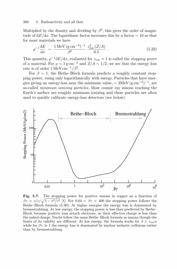
260 5. Radioactivity and all that
Multiplied by the density and dividing by β2, this gives the order of magni-tude of dE/dx. The logarithmic factor increases this by a factor ∼ 10 so thatfor most materials we have
ρ−1 dE
dx∼ 1 MeV (g cm−2)−1
β2
z2ion (Z/A)
0.5. (5.32)
This quantity, ρ−1dE/dx, evaluated for zion = 1 is called the stopping powerof a material. For ρ ∼ 1 g cm−3 and Z/A ∼ 1/2, we see that the energy lossrate is of order 1 MeV cm−1/β2.
For β ∼ 1, the Bethe–Bloch formula predicts a roughly constant stop-ping power, rising only logarithmically with energy. Particles that have ener-gies giving an energy-loss near the minimum value, ∼ 2MeV (g cm−2)−1, areso-called minimum ionizing particles. Most cosmic ray muons reaching theEarth’s surface are roughly minimum ionizing and these particles are oftenused to quickly calibrate energy-loss detectors (see below).
1 610
1
10
100
βγ0.01 10 102 4
Stop
ping
Pow
er (
MeV
/(g/
cm2) Bethe−Bloch Bremsstrahlung
Fig. 5.7. The stopping power for positive muons in copper as a function ofβγ = v/c/
√1 − v2/c2 [1]. For 0.04 < βγ < 400 the stopping power follows the
Bethe–Bloch formula (5.30). At higher energies the energy loss is dominated bybremsstrahlung. At low energy, the stopping power is less than predicted by Bethe–Bloch because positive ions attach electrons, so their effective charge is less thanthe naked charge. Nuclei follow the same Bethe–Bloch formula as muons though thelimits of its validity are different. At low energy, the formula works for β > zionαwhile for βγ 1 the energy loss is dominated by nuclear inelastic collisions ratherthan by bremsstrahlung.

5.3 Passage of particles through matter 261
Figure 5.7 shows the calculated stopping power [1]. The Bethe–Blochformula (5.30) is applicable for 0.05 < βγ < 500. The stopping power falls likeβ−2 until β ∼ 1 and then rises logarithmically. For β < αzion the formula failsbecause the slowly moving ions capture atomic electrons from the medium,lowering the effective value of zion. For γ 1, radiation (bremsstrahlung)eventually becomes important. In Fig. 5.7, this effect is calculated for positivemuons where the effect is important for γ > 1000, i.e. E > 100 GeV. Themuon is the only particle other than the electron for which bremsstrahlung isimportant. Energy loss for hadrons and nuclei with E > GeV is dominatedby discrete inelastic scatters on nuclei (Sect. 3.1.5), liberating nucleons andcreating hadrons.
The energy-loss can be integrated to give the range of a particle, i.e. thedistance traveled before stopping.
R(E) =∫ E
0
dE
dE/dx. (5.33)
For dE/dx ∝ β−2 the integral takes a simple form:
R(E) = E
(dE
dx(E))−1
∝ E2 . (5.34)
An α-particle (z2ion = 4) of E ∼ 5 MeV has β2 = 2E/mαc2 ∼ 2.5 ×
10−3 giving a stopping power of ∼ 3000 MeV (g cm−2)−1. The α-particle willtherefore penetrate only ∼ 0.03 mm of a light material like plastic.
Charged particle detectors. Detection of the ionization caused by thepassage of charged particles is the basis of most types of particle detectorsused in nuclear and high-energy physics. The simplest class consists of gas-filled ionization chambers as illustrated in Fig. 5.8. The liberated electronsand ions drift toward charged electrodes where they create an electric pulse.
Other types of energy-loss detectors are listed in Table 5.4. Semiconductorsilicon and germanium ionization detectors are very useful because, beingdenser than gasses, they can stop charged particles, yielding a measurementof their total kinetic energies. Scintillators (Fig. 5.9) where a small portionof the energy loss is transformed to visible photons are often used because oftheir simplicity and low cost.
Cherenkov radiation is created by charged particles moving at a velocitygreater than the light velocity c/n in a medium of refraction index n. Whileof great use in high-energy particle physics, they are rarely used in nuclearphysics because of most particles are non-relativistic. One of their most im-portant uses is in massive detectors constructed to detect solar neutrinos(Sect. 8.4.1).
Under special conditions, the energy loss of charged particles can createvisible tracks in a medium, as in nuclear emulsions, cloud chambers, andbubble chambers.

262 5. Radioactivity and all that
Table 5.4. Some charged-particle detectors and the signal produced for 1 keV oftotal energy loss. The largest intrinsic signal is in silicon semiconductor detectorsbut that in gas-ionization chambers can be effectively much higher since additionalelectrons will be liberated when the primary electrons collide with atoms in the highelectric fields near collection wires (proportional chambers and Geiger counters).The signal from scintillators and Cherenkov counters will be reduced because thephotons must be detected, generally by photomultiplier tubes (Figs. 5.14 and 8.14).The primary advantage of optical detectors is their excellent time resolution, asgood as 0.1 ns.
Detector yieldsilicon semiconductors ∼ 270e− keV−1
gas-ionization chambers ∼ 50 e−keV−1
organic scintillators < 15 visible photons keV−1
H2O Cherenkov counters ∼ 0.1 visible photons keV−1 (β > 1/n n = 1.33)
V pulse out
−Q
ion + + +
Q
gas
Fig. 5.8. The principle of operation of a gas-filled ionization chamber. The chargeliberated by the passage of the particle drifts in the electric field toward the elec-trodes. If the high-voltage supply is removed after charging the electrodes, thepassage of ionizing radiation would simply discharge the chamber. In the earlydays of radioactivity, this rate of discharge was a standard monitor of radioactivityand cosmic radiation. If the high-voltage supply is left in place, after the passage ofthe charged particle, the potential difference between the electrodes first drops andthen returns to its nominal value. The resulting pulse signals the passage of a singleparticle. This is the principle of proportional counters and Geiger counters. If thetime of passage of the particle is known (e.g. by an external scintillator counter),the position of the particle can be deduced from the time delay between this timeand the arrival of the ions at the electrodes. This is the principle of the operationof drift chambers.

5.3 Passage of particles through matter 263
lightphoton
dynodes (electron multipliers)
output
scintillator
photo−electron
photocathode (−V) anode
chargedparticle
photomultiplier tube (PMT)light shield
Fig. 5.9. The principle of a scintillation detector. A charged particle creates asmall amount of visible light while losing energy in the scintillating material. Thephoton may be detected by a photomultiplier tube (PMT) where it may liberatean electron on a photocathode through the photo-electric effect. The photocathodeis held at high (negative) potential so the photoelectron is directed toward a seriesof dynodes where each electron creates a certain number of further electrons. Theelectrons are finally collected at the anode.
5.3.2 Particle identification
Many nuclear species can be produced in nuclear collisions and we are now ina position to understand how the identity of individual nuclei can be deter-mined. A species is characterized by its charge, q, and mass, m, and individualnuclei are additionally characterized by their velocity, v, or equivalently bytheir momentum p or kinetic energy p2/2m. Charged particle detectors giveinformation on these quantities:
• p/q from the trajectory in a magnetic field;• v from the flight-time t between detector elements separated by a distance
d;• q2/v2 from dE/dx in a thin ionization counter;• p2/2m from the total energy deposit in a thick ionization counter.
Clearly, a single type of measurement is insufficient to identify the species.The charge-to-mass ratio q/m can be deduced by combining two measure-ments, for instance p/q from the magnetic trajectory and v from a time-of-flight measurement. With perfect precision, this would be sufficient to identifythe particle since no two species have exactly the same q/m.1 In real experi-ments, it is generally necessary to have a third type of measurement. Fig. 5.10shows how dE/dx measurements where combined with magnetic trajectoryand time-of-flight measurements to identify the doubly-magic nuclide 100Sn.1 This is effectively the case in mass-spectrometers (Fig. 1.3) where the magnetic
trajectory is combined with knowledge p2/2m determined by the acceleratingpotential. A high precision of ∆(m/q)/(m/q) ∼ 10−8 generally allows one tounambiguously identify ionic species.
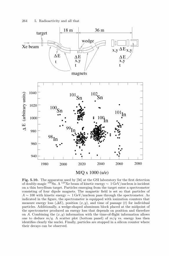
264 5. Radioactivity and all that
1980 2000 2020 2040 2060 2080
940
960
980
1020
1040
1000
E (
arbi
trar
y un
its)
∆
M/Q x 1000 (u/e)
101
In
Sn Sn
In99
101In
98
100In
102
Sn100
wedge
∆ Et x,y
t
∆ Ex,y x,y
∆ Ex,yt
∆ E
18 m 36 m
magnets
target
Xe beam
Fig. 5.10. The apparatus used by [56] at the GSI laboratory for the first detectionof doubly-magic 100Sn. A 124Xe beam of kinetic energy ∼ 1 GeV/nucleon is incidenton a thin beryllium target. Particles emerging from the target enter a spectrometerconsisting of four dipole magnets. The magnetic field is set so that particles ofA ∼ 100 with kinetic energy ∼ 1 GeV/nucleon pass through the spectrometer. Asindicated in the figure, the spectrometer is equipped with ionization counters thatmeasure energy loss (∆E), position (x, y), and time of passage (t) for individualparticles. Additionally, a wedge-shaped aluminum block placed at the midpoint ofthe spectrometer produced an energy loss that depends on position and thereforeon A. Combining the (x, y) information with the time-of-flight information allowsone to deduce m/q. A scatter plot (bottom panel) of m/q vs. energy loss thenidentifies clearly the nuclei. Finally, particles are stopped in a silicon counter wheretheir decays can be observed.

5.3 Passage of particles through matter 265
5.3.3 Electrons and positrons
1 10 100 10000
0.5
1.0
0.05
0.10
0.15
0.20
dE/d
x (
per
radi
atio
n le
ngth
)−
1E
E (MeV)(
g cm
2)−
1
Bremsstrahlung
Ionization
positrons
electrons
Moller
Bhabha
positronannihilation
Fig. 5.11. Energy loss of electrons and of positrons in lead as a function of the inci-dent energy [1]. The left scale uses the radiation length of lead (0.56 cm) as the unitof length. Ionization dominates at low energies while bremsstrahlung dominatesabove 10MeV. Subdominant contributions come from wide-angle elastic scatteringon electrons (Moller for electrons and Bhabba for positrons) and positron annihi-lation.
Our derivation of the Bethe–Bloch equation (5.30) does not apply toelectrons because we assumed that the ions were sufficiently massive thattheir trajectories are not affected by close encounters with atomic electrons.In spite of this, for Ee < 10 MeV, the stopping power for electrons is to goodapproximation given by the Bethe–Bloch equation. Electrons and positronsat low energy therefore come to rest in a manner similar to that of heavyions, though their trajectories are much less straight since they scatter atlarge angles from nuclei.
After coming to rest, positrons annihilate with atomic electrons yieldingtwo photons of energy Eγ = mec
2
e+ e− → γ γ . (5.35)

266 5. Radioactivity and all that
For Ee > 10 MeV, electrons and positrons lose most of their energy byradiation of photons (bremsstrahlung) that results from their accelerationin the electron field of nuclei. The distance over which an electron loses afraction 1/e of its energy through this process is called the radiation length,X0. . Because the effect is due to acceleration in the electric field of a nucleus,ρ−1X0 has a strong dependence on Z, ranging from 61 g cm−2 in hydrogento 6.37 g cm−2 in lead. For the low-energy electrons and positrons from β-decay, this effect is generally of secondary importance but rapidly becomes thedominant process for high-energy electrons and positrons with E > 10 MeV.This can be seen in Fig. 5.11 for lead.
5.3.4 Photons
Photons interact with matter through the following reactions whose cross-section on carbon and lead are shown in Fig. 5.12:
• Rayleigh-scattering, i.e. elastic scattering from atoms. This process has theonly cross-section that has no energy threshold.
• Compton scattering, i.e. elastic scattering from quasi-free electrons. Thisprocess has a threshold for each shell of bound electrons corresponding tothe ionization energy, I, of the shell. In the range I Eγ mec
2, thecross-section is the Thomson cross-section calculated classically in Chap.3
σT = (8π/3)r2e I Eγ mec
2 . (5.36)
In this energy range, the differential cross-section is forward and backwardpeaked
dσ
dΩ=
σT cos2 θ
2π, (5.37)
where θ is the scattering angle. For Eγ >> mec2, the cross-section falls like
E−2γ and is increasingly peaked in the forward direction θ < me/Eγ.
• Photoelectric absorption by atoms
γ atom → e− atom+ . (5.38)
The threshold for ejection of an electron of a given shell is just the ionizationenergy of the shell.
• Pair production , i.e.
γ (A, Z) → e+e− (A, Z) . (5.39)
The threshold is 2mec2. This is by far the dominant effect at high energy.
Photons also have a small probability to be absorbed by breaking upnuclei (photo-nuclear absorption) as described in Sect. 3.1.5.

5.3 Passage of particles through matter 267
10−3 3
3
1
Compton
Rayleigh
pair−production
pair−productionRayleigh
photo−electric
photo−electric
1
10photon energy (MeV)
−310 103photon energy (MeV)
610
310
1
610
10
1
cros
s−se
ctio
n (b
arn/
atom
)
carbon
lead
Compton
Fig. 5.12. Photon cross-sections on carbon and lead [1] as explained in the text.At low energy, 1 keV < E < 100 keV, photo-electric absorption dominates whileelectron–positron pair production dominates for E 2mec
2. Compton scatteringdominates at intermediate energies. Photo-nuclear absorption (Fig. 3.8) is of minorimportance.
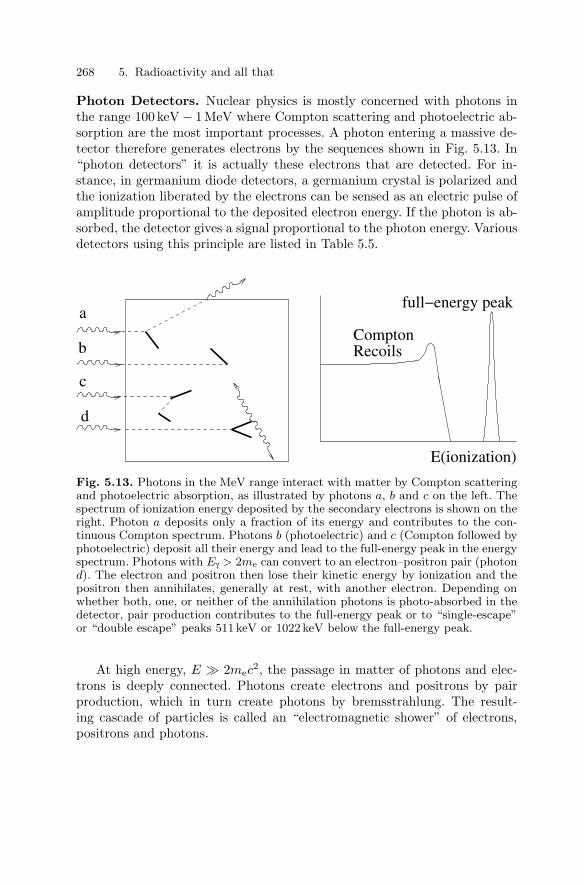
268 5. Radioactivity and all that
Photon Detectors. Nuclear physics is mostly concerned with photons inthe range 100 keV − 1 MeV where Compton scattering and photoelectric ab-sorption are the most important processes. A photon entering a massive de-tector therefore generates electrons by the sequences shown in Fig. 5.13. In“photon detectors” it is actually these electrons that are detected. For in-stance, in germanium diode detectors, a germanium crystal is polarized andthe ionization liberated by the electrons can be sensed as an electric pulse ofamplitude proportional to the deposited electron energy. If the photon is ab-sorbed, the detector gives a signal proportional to the photon energy. Variousdetectors using this principle are listed in Table 5.5.
a
b
c
d
E(ionization)
full−energy peak
RecoilsCompton
Fig. 5.13. Photons in the MeV range interact with matter by Compton scatteringand photoelectric absorption, as illustrated by photons a, b and c on the left. Thespectrum of ionization energy deposited by the secondary electrons is shown on theright. Photon a deposits only a fraction of its energy and contributes to the con-tinuous Compton spectrum. Photons b (photoelectric) and c (Compton followed byphotoelectric) deposit all their energy and lead to the full-energy peak in the energyspectrum. Photons with Eγ > 2me can convert to an electron–positron pair (photond). The electron and positron then lose their kinetic energy by ionization and thepositron then annihilates, generally at rest, with another electron. Depending onwhether both, one, or neither of the annihilation photons is photo-absorbed in thedetector, pair production contributes to the full-energy peak or to “single-escape”or “double escape” peaks 511 keV or 1022 keV below the full-energy peak.
At high energy, E 2mec2, the passage in matter of photons and elec-
trons is deeply connected. Photons create electrons and positrons by pairproduction, which in turn create photons by bremsstrahlung. The result-ing cascade of particles is called an “electromagnetic shower” of electrons,positrons and photons.

5.3 Passage of particles through matter 269
Table 5.5. Some γ- and X-ray detectors and their signal yield. Photons withE < 2mec
2 interact in the detectors mostly by photo-electric absorption and Comp-ton scattering as shown in Fig. 5.13, and the signal is generated by the secondaryelectrons. γ-detectors require the use of high-Z elements to give a high probabilityof photoelectric absorption. The effective signal from scintillators is smaller thanthat shown below by a factor of order 10 because of limited photon collection effi-ciency and quantum efficiency of photomultipliers. The intrinsic energy resolutionof scintillators is then given by Poisson statistics on the observed number N ofphotons, ∆N =
√N yielding a resolution of no better than 10 keV for a 1MeV
γ-ray. This resolution is reflected in the observed width of the full-energy peak inFigs. 5.13 and 7.2. The signal from silicon and germanium diodes is so large thatstatistical fluctuations are generally small compared to other sources, e.g. amplifiernoise. This results in γ-ray resolutions of typically ∼ 1 keV for germanium diodes,making them by far the best detectors when high resolution is required. On theother hand, scintillators are much less expensive and are therefore favored whenlarge detectors covering a large solid angle are required.
Detector yieldsilicon semiconductor diodes (x-rays) 270 e− keV−1
germanium semiconductor diodes (γ-rays) 340 e−keV−1
NaI scintillators (γ-rays) < 40 visible photons keV−1
BGO scint. ((Bi2O3)2(GeO2)3 (γ-rays) < 6 visible photons keV−1
5.3.5 Neutrons
Neutrons in the MeV range interact with matter mostly by elastic scatteringon nuclei. This results in a progressive loss of the neutron kinetic energy untilthey are thermalized with a mean energy, ∼ kT , given by the temperatureof the medium (Fig. 5.14). The neutron then continues to perform a randomwalk with velocity v ∼ 2000 m s−1 until they are absorbed, usually by a (n, γ)reactions. In a homogeneous medium containing nuclei of mass number A,the mean time for absorption after thermalization is
τ =1
n 〈σv〉 ∼ 6 µsA g cm−3
ρ
1 bσ
, (5.40)
where n and ρ are the number and mass density of nuclei and where σ is thethermally averaged cross-section at T = 300K. Note that the absorption timeis substantially sorter than the mean lifetime of a free neutron, ∼ 886.7 s.
Neutron detectors. In nuclear physics, neutrons are generally detected byfirst thermalizing them and then by observing their absorption. Some com-monly used absorption reactions are listed in Table 5.6. Absorption on 3He,6Li and 10B yielding charged particles are preferred because the final stateparticles are easily detected through their ionization. Radiative absorptionon 157Gd is sometimes used because of its enormous cross-section for thermalneutron capture, 2.55 × 10⁵ b.

270 5. Radioactivity and all that
Table 5.6. Some thermal neutron detectors.
Reaction cross-section detector typen 3He → p3H 5.33 × 10³b 3He-filled proportional chambersn 6Li → 3H 4He 9.42 × 10²b 6Li-doped scintillatorsn 10B → 4He 7Li 3.8 × 10³b BF3-filled proportional chambersn 157Gd → γγ 158Gd 2.55 × 10⁵b gadolinium-doped scintillators
n
elastic scatters
3H 4Hen 6Li
photomultiplier
Fig. 5.14. A neutron detector based on the reaction n6Li → 3H4He. The neutronenters a 6Li-doped scintillator. The neutron is thermalized by elastic scatters, afterwhich it performs a random walk through the material. Eventually, it is absorbedby a nucleus in the material, in this case by a 6Li nucleus. The final state particle3H and 4He are charged an therefore stop in the medium by depositing their kineticenergy, mostly by ionization. Scintillation light is detected by the photomultiplier.If the original neutron is sufficiently energetic for the first few nuclear recoils toproduce a significant amount of scintillation light, the event consists of two lightpulses, the first for the elastic scatters and the second for the capture.
5.4 Radiation dosimetry
We saw in the previous section that all non-thermalized particles, with thepractical exception of neutrinos, deposit their energy in the medium throughwhich the propagate. The total energy deposited per unit mass (of themedium) is called the dose. It has units of Gy (Gray)
1 Gy = 1 J kg−1 = 6.25 × 10¹² MeV kg−1 . (5.41)
The dose clearly refers to a flux of particles over a specified period of time orto a specified event (e.g. a nuclear accident).
Biological effects depend not only on the total energy deposited but alsoon the density of the energy deposit. The equivalent dose is therefore usedto have a better estimate of biological damage caused by the disruption incells due to ionization and the resultant breaking of molecular and chemicalbonds. The most important risks involve mutations that can cause cancer.The unit is the Sievert (Sv)
equivalent dose (Sv) =∑
[wR × dose (Gy)] , (5.42)
where the factor wR takes into account the long term risks in regular exposi-tions to weak doses of each type of radiation mentioned in Table 5.7 and the

5.4 Radiation dosimetry 271
sum is over the different types of radiation. Heavily ionizing radiation involv-ing particles with β < 1 have risk factors greater than unity. The fact thatwR are multiples of 5 reflects the precision of the biology, not the physics.
Table 5.7. Risk factors in various radiations
Radiation wr
X and γ rays, any energy 1Electrons and muons, any energy 1Neutrons, E < 10 keV 5Neutrons, 10 < E < 100 keV 10Neutrons, 100 keV < E < 2 MeV 20Neutrons, 2 < E < 20 MeV 10Neutrons, E > 20 MeV 5Protons, E > 20 MeV 5α particles, fission fragments, heavy nuclei 20
Table 5.8 shows the typical contribution of various sources of radiationto the mean equivalent dose we receive annually (in the absence of a localnuclear event). The primary sources are cosmic rays, 0.26 mSv at sea level,and natural radioactivity, ∼ 2 mSv. The α− and β−particles from naturalactivity are mostly confined to the material containing the radioactivity andare therefore not dangerous unless ingested. However, γ−rays from β-decaysnear the surface of materials radiate us continually. The most energetic ofthe photons are the 1460 keV 40K and 2620 keV 208Tl γ-rays. They are oftenseen in the background spectra of photon detectors (Fig. 7.2).
More important than the photon emitters is the α-emitting noble gasRadon produced in the uranium–thorium chains. It diffuses out of the groundand building materials, generating an effective dose of ∼ 1−2 mSv for buildingdwellers. This can be an order of magnitude smaller for people living outsideand an order of magnitude higher in poorly ventilated buildings or in granite-rock areas.
The effective dose derived from ingesting or inhaling radioactive materials(Table 5.9) is difficult to estimate since it depends critically on where andfor how long the body stores the particular material. The radiotoxicity, R,associated with a given nuclide is the effective dose (in Sv) resulting fromingesting or inhaling an activity A (in Bq). It can be written as
R =A wR 〈E〉 τeff
meff, (5.43)
where 〈E〉 is the mean energy per decay deposited in the body and wR isthe associated risk factor. Depending on the nucleus in question, the effectiveretention time τeff can be the nuclear mean life for short-lived nuclei, thebiological retention time for elements that are eliminated from the body (e.g.tritiated water), or the lifetime of the organism itself for long-lived nucleithat can be permanently attached to the body parts, e.g. 239Pu in bones.

272 5. Radioactivity and all that
Table 5.8. Typical annual effective doses [57].
source dose(mSv)
cosmic radiationsea level 0.262000m 0.40
air travel (per 1600 km) 0.01ground γ−rays 0.46air (radon) 2.0Weapons test fallout 0.01Dwelling (stone/brick/concrete) γ−rays 0.07Food and drink 0.3Television 0.01medical x-rays 0.40
total 3.6
Table 5.9. The whole-body effective dose (radiotoxicity) due to selected radionu-clides if taken internally [59]. Note the similar doses of the three fission products90Sr, 131I and 137Cs in spite of their very different lifetimes, indicating that theirvalues of τeff are similar, due to short biological retention times.
Isotope t1/2 〈E〉 dose principal organs(MeV) (µSv kBq−1) affected
90Sr 28.79 yr 1.3 (β−) 30 (28) bone marrow, lungs131I 8.02 day 0.5 (β−) 11 ( 22) thyroid137Cs 30.07 yr 0.8 (β−, γ) 6.7 (13) whole body
The effective mass of the organism, meff , is the body mass if one calculatesthe full-body dose or the mass of the organ in which the radioactive materialis attached if one wishes to calculate the dose received by that organ.
The radiotoxicity is mostly discussed in the context of nuclear accidentsand nuclear-waste storage. The evaluation of the expected dose from with agiven nuclide must also take into account the relative risk that the element canbe introduced into the food chain. One can also protect oneself from certainnuclides by saturating the body with non-radioactive isotopes. This is howone protects the thyroid from radioactive iodine after a nuclear incident.
The medical risks associated with radiation can be divided into short-termand long-term risks. The lethal dose defined as a 50 % risk of death within30 days is 3 Sv if it is absorbed in a short time over the whole body. Thespinal chord is the most critically affected. The long-term risks of cancer are

5.5 Applications of radiation 273
estimated to be about 0.02 Sv−1 meaning that 2% of people exposed to 1 Svwill develop a cancer due to this exposure before dying of unrelated causes.This very broad estimate can be refined to take into account the source ofradiation and the parts of the body that are exposed or contaminated. Notehowever that in the approximation that cancer rates are proportional to thedose and independent of the organ exposed, the total cancer rate does notdepend on these considerations. It should also be mentioned that there is anactive and unresolved debate about whether or not these estimates apply tovery low levels of radiation.
The recommendation for workers or medical patients exposed to radioac-tivity in a regular manner is that the equivalent dose absorbed by someoneshould be less than 20 mSv per year averaged over a period of 5 years, with amaximum of 50 mSv in a single year. For the public, the absorbed dose mustbe smaller than 5 mSv per year in addition to the natural dose and possiblemedical doses.
5.5 Applications of radioactivity
5.5.1 Medical applications
The disrupting effect on cells of ionizing radiation can be used to humanadvantage by killing unwanted, e.g. cancerous cells. The use of radiation fromexternal radioactive sources or accelerated particle beams in cancer therapyhas a long history.
It is interesting to examine the cases of protons or heavy ions. Figure5.15 shows the energy deposition in the medium in terms of the penetrationdistance. We see that practically all the energy is deposited in a very localizedregion near the stopping point. This comes from the 1/β2 factor in equation(5.30). Also shown in the figure is a comparison between the effect of ionbeams and of photons. One can see the great advantage, from the medicalpoint of view, of heavy ion beams which attack and destroy tumors in a veryaccurate and localized manner, as opposed to γ-rays which produce damageall around the point of interest.
It is also useful to sometimes inject, intravenously or orally, radioactivesubstances into the body in a chemical form that accumulates preferentiallyin particular organs or cancerous tissue. The subsequent decays can thenirradiate the tumor or betray its position by emitting externally detectableγ-rays. Pure β− emitters are preferred for tumor irradiation since all energy isdeposited within a few millimeters of the decay. Positron emitters (see below)are preferred for position measurements.
Much progress has been made in the production of radioactive tracersthat give a physical manifestation of certain biological functions in humanbodies. One can make tracers with given chemical or biological properties, sothat they become fixed in definite organs or biological functions. For example,

274 5. Radioactivity and all that
penetration distance (mm water)
dose
(G
ray)
cell
surv
ival
fra
ctio
n
0.1
0.2
0.5
1.0
0
2
3
150 50 100 15010050
1
Fig. 5.15. Energy loss of ions (left) and survival rate of cells (right) as a functionof the penetration depth. Because of the v−2 factor in the Bethe–Bloch formula(5.30), most of the energy is deposited near the stopping point. The dashed curvecorresponds to the same quantities for photons. We can see the considerable medicaladvantage to use heavy ion beams.
glucose accumulates in tumors that have a high metabolic rate. Iron is usedto study the various phases of hemoglobin, Iodine is used for the thyroidgland, rare gases (xenon and krypton) in pneumology; phosphorus for themetabolism, etc.
For position measurements, of special interest are β+-emitters which yieldpairs of 511 keV photons when the positrons annihilate. The emission of twoparticles allows one to more easily constrain the origin of the emission. Theprinciple of this “positron emission tomography” (PET) is illustrated in Fig.5.16. A commonly used positron emitter is 18F that is produced and decaysvia
p 18O → n 18F .
18F → 18O e+ νe t1/2 = 109.8 m . (5.44)
Protons of energy ∼ 15 MeV are used and the 109.8 m half-life of 18F al-lows one to chemically separate and prepare a fluorine containing compound.For instance, 18F-containing glucose can be prepared and then ingested suf-ficiently rapidly for it to accumulate in high-metabolic tumors.
5.5.2 Nuclear dating
One of the most intellectually interesting applications of radioactivity hasbeen to provide accurate estimates of ancient objects, ranging from archae-ological artifacts to stars. Important examples are the use of 14C to datearchaeological organic material and 87Rb to give an accurate age of the solarsystem.

5.5 Applications of radiation 275
annihilation
Fig. 5.16. The principle of positron-emission tomography. A β+-emitter is injectedinto a body in a chemical form such that it accumulates in the organ or tissuethat one wishes to study. Positrons from β+-decay stop in the material and thenannihilate, e+e− → γγ. The detection of the two “back-to-back” photons constrainsthe position of the decay to lie along the line connecting the two detector elements.Accumulation of many events allows one to reconstruct the geometry of the decayregion.
To understand the principle of nuclear dating, we consider a closed systemcontaining initially NA0 nuclei A and NB0 nuclei B. By closed, we mean thatthere are no exchanges of A and B nuclei with the exterior. If A decays toB, then their numbers at some time t are
NA(t) = NA0 e−t/τ (5.45)
NB(t) = NA0 (1 − e−t/τ ) + NB0
= NA(t) et/τ (1 − e−t/τ ) + NB0 , (5.46)
where τ is the (known) mean lifetime of A. If, at time t, NA and/or NB aremeasured and if NA0 and/or NB0 are known, we may be able to deduce theage t by solving one or both of the equations. We note the following cases:
1. NA is measured. We must then know NA0 to deduce t from (5.45).2. NB is measured. We must know both NA0 and NB0 to deduce t from
(5.46).3. NB and NA are measured. We need only NA0 or NB0.
Generally neither NA0 nor NB0 are known but are rather deduced fromthe measured amount of another species A′ or B′ for which the ratio NA0/NA′
or NB0/NB′ is known. Usually, A′ (B′) is another isotope of A (B). In manyapplications, A′ and B′ are stable so that NA′ and NB′ are time-independent.In this case we write (5.45) and (5.46) as

276 5. Radioactivity and all that
NA(t)NA′
=NA0
NA′e−t/τ (5.47)
NB(t)NB′
=NA0
NB′(1 − e−t/τ ) +
NB0
NB′
=NA(t)NB′
et/τ (1 − e−t/τ ) +NB0
NB′, (5.48)
14C dating uses (5.47) with A = 14C and A′ = natural carbon (12C and13C). Radioactive 14C is produced continuously in the atmosphere, mostlyvia the exothermic (n,p) reaction induced by cosmic-ray neutrons
n 14N → p 14C Q = 0.63 MeV (5.49)
The produced 14C is mixed in the atmosphere and then fixed in carbon-breathing plants. This leads to an isotopic abundance of 14C in organic ma-terial of
14C12C + 13C
= 1.2 × 10⁻¹² , (5.50)
corresponding to a specific activity of 250 Bq kg−1. There are good reasonsto believe that the cosmic-ray flux has been constant over many 14C lifetimesso that this ratio has remained constant in time, at least until atmosphericnuclear weapon testing between 1955 and 1963. The neutron flux duringthese tests resulted in a doubling of the 14C content of objects living at thattime. Since the end of the tests, the 14C content has returned to within afew percent of the pretest value, and may even have decreased due to theincreased burning of 14C-free fossil fuels.
When a living organism dies, it stops fixing carbon so the 14C containedin the organism decays with t1/2 = 5730 yr. The amount of 14C relative tonatural carbon measured in an object allows one to date the object through(5.47). The amount of 14C is generally determined by measuring the β-activityof carbon chemically extracted from the sample, though recently mass spec-trometer techniques have been become sufficiently precise to directly measurethe small amounts of 14C.
Figure 5.17 shows some early data that was used to verify the technique.The test uses objects whose age can be determined by independent means.The activity of the samples decrease with the known age of 14C. This indicatesthat the production rate of 14C has, indeed, been roughly constant over thelast few millenniums.
This method is usefully applied to objects with ages between, say, 500and 50000 years. Older objects have very little of the original 14C, makingmeasurements difficult.
The ages of minerals can sometimes be dated using potassium-argon dat-ing
e− 40K → 40Ar νe t1/2 = 1.28 × 10⁹ yr . (5.51)

5.5 Applications of radiation 277
_+
_+
_+
_+
_+
_+
_+
Perc
enta
ge o
f m
oder
n ra
dioc
arbo
n ac
ticity
100
90
80
70
60
50
Historical Age (years)0 2000 4000 6000
Tree ring 1072 A.D.
Zoser 2700
Tree ring 575 A.D.Tree ring 580 A.D.
Ptolemy 200
Redwood 979 52 B.C.Tayinat 675 50 B.C.
Dead Sea Scrolls 100 100 B.C.
Sesostris 1800 B.C.75 B.C.
75 B.C.Sneferu 2625
200 B.C.Hemaka 2950
150 B.C.
Fig. 5.17. Calibration of the 14C dating method with objects of known age [58].
In this method, (5.46) can be used directly assuming that the initial abun-dance of the noble gas argon was very small in the mineral. The age is thendeduced from the measured 40K and 40Ar abundances. It should be notedthat the measured age refers generally to the last solidification of the mineralsince melting would generally lead to loss of the argon.
In a similar technique, uranium ores can be dated by measuring the quan-tities of the descendants 206Pb (from 238U) or 207Pb (from 235U). In this case,it is not reasonable to assume that the initial abundances of the lead isotopesvanished. It is therefore necessary to use (5.48) with B′ = 204Pb which hasno radiogenic source.
The ages of meteorites have been most accurately measured using thedecay
87Rb → 87Sr e− νe . (5.52)

278 5. Radioactivity and all that
In this case, (5.48) is used with A = 87Rb, B = 87Sr and B′ = 86Sr:[ 87Sr86Sr
]t
=[ 87Rb
86Sr
]t
et/τ (1 − e−t/τ ) +[ 87Sr
86Sr
]t=0
, (5.53)
While the chemical composition, i.e. the Rb/Sr ratio, depends on the preciseconditions of the formation of an individual meteorite, the isotopic ratio87Sr/86Sr should be uniform at the formation in a well-mixed pre-solar cloud.In this case, (5.48) predicts that if all meteorites have the same age, a plot ofthe measured value of 87Sr/86Sr vs. the measured value of 87Rb/86Sr shouldbe a straight line with the slope of exp(t/τ)(1 − exp(−t/τ) ∼ t/τ . Figure5.18 [60] indicates that this is the case and that the meteorites have a commonage of ∼ 4.5 × 10⁹ yr.
0.7
0.8
0.9
1.0
0 1.0 2.0 3.0 4.0 5.087 Rb / 86 Sr
87Sr
/86
Sr
Fig. 5.18. The abundance ratio 87Sr/ 86Sr vs. the ratio 87Rb/86Sr for a collectionof meteorites [60]. The fact that the points lie on a straight line indicate that themeteorites have a common age of ∼ 4.53 × 10⁹ yr. At the epoch of formation, themeteorites had a common isotopic ratio 87Sr/ 86Sr = 0.7003.
The mean time since the formation of terrestrial heavy elements can beestimated from the abundances of two isotopes of uranium, observed to be235U/ 238U = 0.00714 ± 0.00008. One uses (5.47) with A = 235U and A′ =238U but modified to take into account the finite lifetime of 238U.

5.5 Applications of radiation 279[N235
N238
]t
=[N235
N238
]t=0
e−t/τ235et/τ238 , (5.54)
with t1/2(235) = 7.07× 10⁸ yr and t1/2(238) = 4.5× 10⁹ yr. The two isotopesare believed to have been formed in nearly equal amounts (Sect. 8.3), so (5.54)implies t ∼ 6×10⁹ yr. The age of the Earth or of meteorites is noticeably less(4.5 × 10⁹ yr) so most the the uranium on Earth had spent a considerableamount of time in interstellar space before condensing on the Earth.
The ages of very old stars have been measured by comparing their atmo-spheric abundances of uranium and thorium. One uses[
NU
NTh
]t
=[
NU
NTh
]t=0
e−t/τ238et/τ232 (5.55)
where the half-life of 232Th is 1.405 × 10¹⁰ yr and for very old stars one canassume that all the uranium is 238U. The oldest stars [61] so far found havea uranium–thorium ratio of about 0.2 implying ages of about 1.2 × 10¹⁰yr(assuming equal initial abundances). This is of the order of the estimated ageof the Universe, 1.3 × 10¹⁰ yr, indicating that stars formed within the first∼ 109 yr after the big bang (Chap. 9).
Finally, while (5.47) and (5.48) are generally used to derive the ages ofsamples using a known lifetime, they can also be used to measure the life-time of a nuclide using a sample of known age. While this may seem like astrange way to measure a nuclear lifetime, a comparison with the laboratory-measured lifetime amounts to a comparison of the present-day lifetime withthe lifetime in the past. If the two lifetimes are consistent, this verifies thehypothesis that laws and constants governing the decays have not varied.
Very restrictive bounds on such variations have been found using thedecay
187Re → 187Os e−νe t1/2 = 4.35 ×10¹⁰ yr (laboratory) .(5.56)
The age has also been measured [62] using meteorites whose age was de-termined by U-Pb or Rb-Sr dating. The 187Re half-life can then be de-termined by using 186Os as the standard in (5.48). The derived value ist1/2 = (4.16 ± 0.04) × 1010yr is in reasonable agreement with the labora-tory measurement. This indicates that the 187Re half-life has changed littleover the past 4 × 10¹⁰ yr.
The particular interest of using 187Re → 187Os is that the tiny energyrelease, Qβ = 2.64 keV, makes the decay rate extremely sensitive the thefundamental constants. For example, the value of Qβ is sensitive to the valueof the fundamental charge through its effect on the Coulomb energy in theBethe–Weisacker formula (2.13), (0.7103Z2/A1/3) MeV. The contribution ofthis term to the binding energy of 187Re is 698 MeV while that for 187Os is717 MeV for a difference of 19 MeV. A relative change in the square of thefundamental charge of only 10−4 would be sufficient to make 187Os lighterthan 187Re so that the former is stable rather than the latter. Smaller changes

280 5. Radioactivity and all that
to the electric charge would change the lifetime of 187Re through the Qβdependence of β-decay rates calculated in Chap. 4 (4.98). It is therefore simpleto transform the limit on the change in the 187Re lifetime into a limit on thetime variation of the electric charge, or equivalently on the time variationof the fine-structure constant, proportional to the square of the fundamentalcharge. Following Dyson [63] a limit |∆α/α| < 2 × 10⁻⁶ for the variation ofα over the last 187Re lifetime was recently derived [64].
5.5.3 Other uses of radioactivity
We mention here a few of the other uses of radiation and radioactivity.
• Sterilization of foodstuffsThis consists of exposing foodstuffs to ionizing radiations in order to de-stroy insects or micro-organisms and delay the deterioration without al-tering the edibility. Sources of 60Co emitting ∼ 1 MeV photons are mostcommonly used. This technique generates a loss of the germinal potential.Vegetables are treated this way, such as potatoes, fruits, onions etc. Thetreatment is simple and produces less alteration of the nutritious prop-erties and taste, compared to classical treatments such as sterilization orchemical treatments. This method has other advantages: it is efficient, non-toxic and has a low cost. It is believed to be “danger-free” and it is underconsiderable development.
• Creation of genetically modified plantsThe irradiation by γ rays of genes of certain plants (wheat, barley, rice,sugar cane, cotton, ...) gives them new properties which can be selected togive better resistance to diseases, to heat, to winter conditions, to unfavor-able soils. It also allows one to control the ripening, be it sooner or later,and to improve yields. Radioactive mutation techniques have been knownsince the 1960’s. They have been used in Europe and in the former USSRfor the culture of wheat, in the United States for the culture of barley, ofbeans and of grapefruits, in Pakistan for the culture of rice, in India forcotton and cane sugar, etc. This can be viewed as a primitive form of themore systematic genetic modification now practiced by biologists.
• Sterilization of insectsThe same method consists in exposing male insects born in a laboratoryto sufficient doses of radiation in order to sterilize them. They are thenreleased in large numbers in infected zones. Female insects who mate withthese insects have no descendants and the population of harmful insectsdecreases progressively. This method has the big advantage that it does notbring chemical pollution, unlike pesticides. It has been successfully used inJapan against the melon fly, in Mexico, in Peru, and in Egypt against thefruit fly, and in Africa against the tsetse fly.
• GammagraphyX rays which are used in radiography of the body or materials of low den-

5.6 Bibliography 281
sity, are not penetrating enough to be used for dense or thick materials. Inthat case, one can use γ rays. The principle is the same: the γ rays irradiatea sample of material and the outgoing rays are recorded on a photographicplate. this reveals possible defects coming from the manufacturing or wear-ing effects.
• Radioactive tracersIf a radio-element is introduced into a body, it is possible to follow itstrajectory through the body. By measuring the emitted radiation, tracersallow for instance to follow the displacements of products in circuits ofchemical factories, the detection of leaks in dams or in buried pipes. Thistechnique is used in particular to monitor oil pipelines.
• Fire detectorsA radioactive source (241Am) ionizes the air permanently. The ionization ismodified if smoke particles are present. This modification triggers a warn-ing signal. Such detectors are sensitive to very small amounts of smoke.They are widely used in stores, in factories and in offices.
• Nuclear batteriesRadioactive sources such as 238Pu, 60Co and 90Sr are used to constructbatteries of several hundred Watts. The heat produced by radioactivity isconverted into electricity. Such batteries are used in satellites and in distantmeteorological stations. They can function for several years without anymaintenance. For example, the Voyager spacecraft was powered by three238Pu generators. It was launched in 1977, reached Neptune in august 1989,and is now beyond the solar system. Nuclear Batteries are also used in heartpacemakers.
• Conservation of the artistic objectsThe exposition of works of art and of archaeological documents to radia-tions can destroy insects, microorganisms and mold that they contain andensures an excellent sterility. This technique has been used in particular totreat the mummy of Ramses II.The impregnation of wooden or stone objects by a polymer under gammairradiation is the principle of the “Nucleart ” process. It allows one to treatand to recover pieces of buried water-logged wood.
5.6 Bibliography
1. James E. Turner, Atoms, Radiation, and Radiation protection, John Wi-ley, New York, 1995.
2. J.E. Coggle, Biological effects of radiation, 1983.3. Edward Pochin, Nuclear radiation : risks and benefits, Oxford Science
Publication, 1983.4. R. E. Taylor, Radiocarbon Dating: An Archaeological Perspective, Aca-
demic Press, Orlando, 1987.

282 5. Radioactivity and all that
Exercises
5.1 Assume that a given radioactive nuclide has a decay rate λ1 and that itdecays into a daughter nuclide which is itself radioactive with decay rate λ2.Assume further that at time t = 0 there are N1 parent nuclei and N2 = 0daughter nuclei. Show that at time t ≥ 0 the number of daughter nuclei is
N2(t) = N1 (1 − e−(λ1−λ2)t) e−λ2t λ1
(λ1 − λ2). (5.57)
Verify that the limits t → 0, t → ∞, λ2 λ1 and λ2 λ1 are reasonable.
5.2 One gram of cobalt is placed near the core of a nuclear reactor where it isexposed to a neutron flux of 5 × 1014cm−2s−1. The cross-section for thermalneutron capture on 59Co is ∼ 40 b. Calculate the 60Co activity after 1 weekof irradiation.
5.3 About 0.3% of the mass of a human is potassium of which 0.012%is 40K (t1/2 = 1.25 × 10⁹ yr). Use the decay scheme shown in Fig 5.1 todiscuss the annual dose received by a body from the internal 40K. Argue thatalmost all of the β− kinetic energy is absorbed in the body. Use the photonabsorption cross-section in Fig. 5.12 to argue that a significant fraction ofthe 1.46 MeV γ-rays are also absorbed in the body. Estimate then the annualdose received from 40K decay.
5.4 In 1990, archaeologists found, in Pedra Furada in Brazil, human remainswhose activity in carbon 14 was 19.6 × 10⁻⁴ Bq per gram of carbon. Giventhat the lifetime of 14C is τ = 8200 years (half life t1/2 = 5700 years) and thatthe activity of 14C in living tissues and in atmospheric CO2 is 0.233 Bq (pergram of C), determine the age of these human remains. Compare the resultswith the date when the first Neanthropians (i.e. homo sapiens, the species towhich you and all other living human beings on this planet belong) appearedin Europe, about 35 000 years ago. See Bahn, Paul G.; “50,000-Year-OldAmericans of Pedra Furada,” Nature, 362:114, 1993.
5.5 The half-lives of uranium 234,235 and 238 are respectively 2.5×10⁵ years,7.1 108 years and 4.5 109 years. Their relative natural abundances are re-spectively 0.0057%, 0.72% and 99.27%. Are these data consistent with theassumption that these nuclei were formed in equal amounts at the same time?If not, can one explain the discrepancy knowing that the unstable isotopes23490 Th and 234
91 Pa exist?

Exercises for Chapter 5 283
5.6 A simple way of making a source of neutrons is to mix an α-emitter withberyllium. The α-particles can then produce neutrons via the exothermicreaction
α 9Be → n 12C + 5.7 MeV . (5.58)
The cross-section for this reactions is ∼ 0.4 b for Eα ∼ 5 MeV. For Eα <4 MeV the cross-section is much smaller because of the Coulomb barrier.
Consider a nucleus emitting 5 MeV α-particles placed in pure beryllium,(ρ ∼ 1.8g cm−3). What is the initial energy-loss rate of the α-particles? Howfar does an α-particle travel in the beryllium before losing 1 MeV of energy?What is the probability that a neutron is created by the (α, n) reaction overthis distance. What α activity is required for 1 Bq of neutron activity?

6. Fission
Fission is the spontaneous or induced breakup of a nucleus. While it is “justanother reaction” from the physics point of view, it has a special role inpublic affairs because of its enormous applications in energy production andweaponry.
In this chapter, we start with a general discussion of nuclear energy pro-duction. In Sec. 6.2 we catalog the various types of fission reactions and inSec. 6.3 we show how fission rates can be explained qualitatively by consid-ering fission as a barrier penetration process.
The remaining sections consider the basic practical problems in fissiontechnology. Section 6.4 lists the nuclei that can be used as nuclear fuel. Section6.5 presents the general conditions for setting up a fission chain reaction.Section 6.6 discusses problems associated with neutrons moderators used inthermal neutron reactors. Section 6.7 introduces the Boltzmann transportequation used to calculate the performance of reactors. Finally, in Sect. 6.8we describe the operation of the major types of fission reactors.
6.1 Nuclear energy
Nuclear energy is extracted through exothermic nuclear reactions, the twoprincipal types being fission and fusion. Of course, we should remember thatradioactivity itself liberates a large amount of energy as first recognized byPierre Curie and Henri Becquerel. For example, the decay of 238U
238U → 234Th α t1/2 = 4.468 × 10⁹yr , Qα = 4.262 MeV ,
generates a power of
P =NA
238Qα ln 2
t1/2= 8 × 10⁻⁹ W g−1 . (6.1)
This tiny amount of power is increased in nuclear reactors by ten orders ofmagnitude through neutron-induced fission of 235U. This increases Q from4.668 MeV to ∼ 200 MeV and decreases the effective lifetime to a few months.
Fission and fusion of nuclei are the main reactions which produce nuclearenergy in large amounts.

286 6. Fission
2001000
200
100
0
Q (
MeV
)
fission
fusion
AFig. 6.1. The energy release in fission and self-fusion as predicted by the Bethe–Weizsacker formula (2.13) for β-stable nuclei. Only nuclei with 40 < A < 95 arestable against both fission and self-fusion. In this figure, Qfis(A, Z) is calculated forsymmetric fission, A1 = A2 = A/2 and Z1 = Z2 = Z/2. Qfus(A, Z) is calculatedfor the production of a single nucleus of A′ = 2A and Z′ = 2Z.
A nucleus AZX can breakup, i.e. fission, in many ways. In the simplest
case, there are two fragments(A1+A2)(Z1+Z2)
X → A1Z1
X + A2Z2
X + Qfis (6.2)
The energy release is
Qfis = m(A1 + A2, Z1 + Z2)c2 − [m(A1, Z1) + m(A2, Z2)]c2
= B(A1, Z1) + B(A2, Z2) − B(A1 + A2, Z1 + Z2) . (6.3)
In the rest frame of the initial nucleus, the sum of the kinetic energies ofthe fission fragments is Qfis. The difference in binding energies B(A, Z) ofthe initial and final nuclei is thus transformed into kinetic energy which iseventually transfered to the medium, heating it up.
Symmetrically, two nuclei can undergo fusion if, by a nuclear reaction,they produce a heavier nucleus (plus a light particle y)
A1XZ1 + A2XZ2 → AXZ + y + Qfus . (6.4)
If Qfus is positive, the light particle y is necessary to conserve momentum. Inthe simplest case, y is a photon so A = A1 + A2, Z = Z1 + Z2 and
Qfus = B(A1 + A2, Z1 + Z2) − B(A1, Z1) − B(A2, Z2) . (6.5)
If Qfus > 0, the reaction can take place with the two initial nuclei at rest,in which case Qfus is the energy of the final state photon. As in fission, thedifference in binding energies of the initial and final nuclei is transformed tokinetic energy.

6.2 Fission products 287
The curve of binding energies (Fig. 1.2) shows that the binding energy ismaximum for A ∼ 56 implying
• heavy nuclei can fission ;• light nuclei can fuse.
Figure 6.1 shows Q for symmetric (A1 = A2) fusion and fission as a func-tion of A of the initial nucleus. We see that only nuclei with 40 < A < 95are intrinsically stable against both spontaneous fission and self-fusion. For-tunately for us, both fusion and fission are very slow processes under normalconditions. As we will see in Chap. 7, fusion is inhibited by the Coulombbarrier between positively charged nuclei. As we will see in the Sect. 6.3,spontaneous fission is strongly inhibited by the “fission barrier” resultingfrom the surface term in the Bethe–Weisacker formula (2.13).
In practice, we will mostly be concerned with the fission of heavy nuclei,A 240. For two fission fragments with A 120 we can estimate Qfis fromFig. 1.2. For the initial nuclei we have B/A(240) 7.6 MeV, while for thefission fragments we have B/A(120) ∼ 8.5 MeV. This gives
Qfis ∼ 240 × (8.5 − 7.6) ∼ 220 MeV . (6.6)
(This energy is somewhat greater than that shown in Fig. 6.1 because thefigure shows the Q of the initial fission while our estimate includes the energygenerated by β-decays of the fission fragments down to β-stable nuclei.) Inactual fission processes, there is always a certain number of free neutronsproduced. Let ν be the average number of such neutrons. Since, by definition,they have no binding energy, we have
Qfis ∼ 220 MeV − ν × 8.5 MeV , (6.7)
i.e. for ν ∼ 2.5, Qfis ∼ 200 MeV.
6.2 Fission products
A given nucleus can fission in many ways. For 236U, one possibility is23692 U → 137
53 I + 9639Y + 3n (6.8)
137I → 137Xe e− νe t1/2 = 24.5 s
137Xe → 137Cs e− νe t1/2 = 3.818 m
137Cs → 137Ba e− νe t1/2 = 30.07 yr
96Y → 96Zr e− νe t1/2 = 5.34 s ,
or, globally23692 U → 137
56 Ba + 9640Zr + 3n + 4e− + 4νe . (6.9)
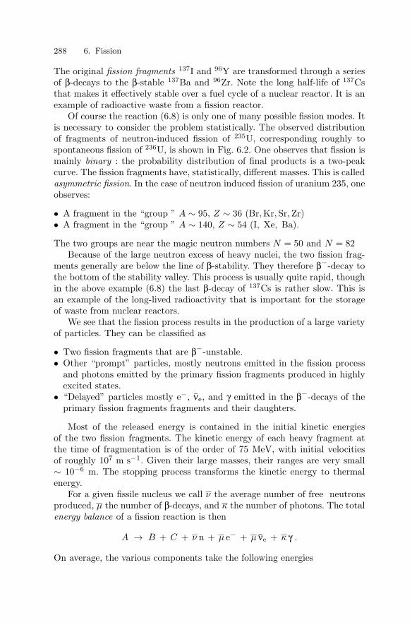
288 6. Fission
The original fission fragments 137I and 96Y are transformed through a seriesof β-decays to the β-stable 137Ba and 96Zr. Note the long half-life of 137Csthat makes it effectively stable over a fuel cycle of a nuclear reactor. It is anexample of radioactive waste from a fission reactor.
Of course the reaction (6.8) is only one of many possible fission modes. Itis necessary to consider the problem statistically. The observed distributionof fragments of neutron-induced fission of 235U, corresponding roughly tospontaneous fission of 236U, is shown in Fig. 6.2. One observes that fission ismainly binary : the probability distribution of final products is a two-peakcurve. The fission fragments have, statistically, different masses. This is calledasymmetric fission. In the case of neutron induced fission of uranium 235, oneobserves:
• A fragment in the “group ” A ∼ 95, Z ∼ 36 (Br, Kr, Sr, Zr)• A fragment in the “group ” A ∼ 140, Z ∼ 54 (I, Xe, Ba).
The two groups are near the magic neutron numbers N = 50 and N = 82Because of the large neutron excess of heavy nuclei, the two fission frag-
ments generally are below the line of β-stability. They therefore β−-decay tothe bottom of the stability valley. This process is usually quite rapid, thoughin the above example (6.8) the last β-decay of 137Cs is rather slow. This isan example of the long-lived radioactivity that is important for the storageof waste from nuclear reactors.
We see that the fission process results in the production of a large varietyof particles. They can be classified as
• Two fission fragments that are β−-unstable.• Other “prompt” particles, mostly neutrons emitted in the fission process
and photons emitted by the primary fission fragments produced in highlyexcited states.
• “Delayed” particles mostly e−, νe, and γ emitted in the β−-decays of theprimary fission fragments fragments and their daughters.
Most of the released energy is contained in the initial kinetic energiesof the two fission fragments. The kinetic energy of each heavy fragment atthe time of fragmentation is of the order of 75 MeV, with initial velocitiesof roughly 107 m s−1. Given their large masses, their ranges are very small∼ 10−6 m. The stopping process transforms the kinetic energy to thermalenergy.
For a given fissile nucleus we call ν the average number of free neutronsproduced, µ the number of β-decays, and κ the number of photons. The totalenergy balance of a fission reaction is then
A → B + C + ν n + µ e− + µ νe + κ γ .
On average, the various components take the following energies

6.2 Fission products 289
A=142
A=95
N=
82Z
N
Z
N
0.01/fission
A=140
0.0001/fissionbeta stable
0.01/fission0.0001/fissionbeta stable
U
Cf
Z=50
Z=28
N=
50
Z=50
N=
82
N=
50
A=108
235
252
Z=28
Fig. 6.2. The distribution of fission fragments for neutron induced fission of 235Uand for spontaneous fission of 252Cf. The distribution for 235U is dominated byasymmetric fission into a light nucleus (A ∼ 95) and a heavier nucleus (A ∼ 140),reasonably near the magic neutron numbers N = 50 and N = 82. The distributionfor 252Cf is broader but still dominated by asymmetric fission. Because of the largeneutron excess in nuclei with A > 230, almost all fission fragments are below theline of β-stability and therefore decay by β−-emission.

290 6. Fission
MeVKinetic energy of fragments 165 ± 5Energy of prompt photons 7 ± 1Kinetic energy of neutrons 5 ± 0.5Energy of β decay electrons 7 ± 1Energy of β decay antineutrinos 10Energy of γ decay photons 6 ± 1
Total 200 ± 6
Of the ∼ 200 MeV, only 190 ± 6 MeV are useful, since the neutrinos escapeand do not heat the medium.
The neutrons produced will maintain chain reactions in induced fissionprocesses. For 236U (i.e. for the fission of 235U induced by a neutron) themean number of produced neutrons is ν = 2.47.
The energy distribution of these neutrons is peaked around En = 0.7MeV. The mean energy is < En >∼ 2 MeV.
6.3 Fission mechanism, fission barrier
The complexity of fission seems out of reach of a detailed theoretical descrip-tion. However, as early as 1939, the liquid droplet model of Bohr and Wheelergave a good qualitative description.
We follow the potential energy of the system as the distance r betweenthe two fragments A and B varies, as illustrated on Fig. 6.3.
Initially, the two fragments are coalesced in a more or less spherical nu-cleus. As r increases, the nucleus becomes deformed, its surface area increasescompared to the initial shape. Therefore, this deformation increases the sur-face tension energy. On the other hand, the increase in the distance A − Bmeans a decrease of the Coulomb repulsion energy between A and B. Thereis a competition between the nuclear forces and the Coulomb repulsion. Atsome point, as r varies between r0 (initial shape of the nucleus) and infinity(separated fragments A and B), the potential energy of the system has amaximum value.
In other words, there is a potential barrier, called the fission barrier, thatmust be crossed in order for the process to occur. One calls activation energyEA, the difference between the maximum of the barrier and the energy of theinitial nucleus in its ground state. For nuclei with A ∼ 240, this energy turnsout to be of the order of 6 to 7 MeV.
In order for the original nucleus to decay by spontaneous fission, thebarrier must be crossed by the quantum tunnel effect. To get an idea ofthe factors that determine the difficulty of tunneling through the barrier, itis interesting to compare the surface and Coulomb energies of a sphericalnucleus as predicted by the Bethe–Weizsacker semi-empirical mass formula(2.13)

6.3 Fission mechanism, fission barrier 291
4π ε0rZ1Z2e2
EA
Ene
rgy
Fig. 6.3. Variation of the energy of a deformed nucleus as a function of the distor-tion as sketched. For small distortions, the energy increases with increasing distor-tion because of the increasing surface area. When the two fragments are separated,the energy falls with increasing separation because of the decreasing Coulomb en-ergy. An energy barrier EA must be crossed for fission to occur.
Ec
Es=
0.7103 MeV Z2A−1/3
17.804 MeV A2/3 =Z2/A
25.06. (6.10)
Nuclei with Z2/A > 25 would be expected to have small barriers because theCoulomb energy (decreasing function of separation) dominates the surfaceenergy (increasing function of separation). In fact, by calculating the surfacearea and Coulomb energies of a nucleus in the shape of an ellipsoid, it canbe shown that the surface area varies twice as fast as the Coulomb energy asthe nucleus is deformed while keeping the volume constant. This means thatwe expect fission to be instantaneous for
Ec > 2Es ⇒ Z2
A> 50 . (6.11)
Super-heavy nuclei have Z/A ∼ 1/3 implying Z > 150 for instantaneousfusion. This is an absolute upper limit on the size of nuclei.
Figure 6.4 shows the inverse of the rate of spontaneous fission of selectednuclei as a function of Z2/A. As expected, the inverse rate decreases rapidlyfor increasing Z2/A. For nuclei with Z < 92, the lifetime for spontaneous

292 6. Fission
fission becomes immeasurably large making nuclei with 100 < A < 230 effec-tively stable in spite of the fact that Qfis > 0 for these nuclei.
4535−5
5
10
15
20
25
1
10
10
10
10
10
10
−1
λ(s
ec)
/AZ2
U
258
241
Rf
Fm
Cf
Cm
40
255
249
235
250 259
257
Sg
Db
No
Fm
Cf
Am
Pu239
250
256
258
Fig. 6.4. Spontaneous fission lifetimes as a function of the fission parameter Z2/Afor selected nuclei. Circles are for even-Z nuclei, filled circles for even-even nucleiand open circles for even-odd nuclei. Squares are for odd-Z nuclei.
The fission rate can be increased by placing the nucleus in an excitedstate so as to reduce the fission barrier. This is most simply done by photonabsorption:
γ AZX → A
ZX∗ → fission , (6.12)
where AX∗ is any excited state of the nucleus AX. This process is calledphoto-fission.
Figure 6.5 shows the total photo-fission cross-section on 236U as a functionof photon energy. The cross-section is negligible for Eγ < 5 MeV, rapidlyincreases in the range 5 MeV < Eγ < 6 MeV and then slowly increases toits maximum value of 0.2 b at Eγ ∼ 14 MeV. Somewhat arbitrarily we candefine ∆ES = 5.7 MeV as the energy that must be added to the ground state

6.3 Fission mechanism, fission barrier 293
−1
−2
−4
10
10
photo−fission236U
10−3
10
cros
s−se
ctio
n (b
arns
)
0E (MeV)
2010
Fig. 6.5. Cross-section for γ 236U → fission [30].
of 236U to make the probability for fission reasonably large. This energy isexpected to be somewhat less than the height of the barrier EA
∆ES ∼ EA − 1 MeV . (6.13)
This is because it is not necessary to add enough energy to erase the barrierbut only enough to make the tunneling rapid.
Table 6.1 lists the values of ∆ES for selected nuclei in the region 230 <A < 240. They are all of the order ∆ES ∼ 6 MeV.
A second way to induce fission of a nucleus (A, Z) is through neutronabsorption by the nucleus (A − 1, Z):
n A−1XZ → AX∗Z → fission . (6.14)
The effective threshold for neutron-induced fission, i.e. the minimum neu-tron kinetic energy necessary to give a large probability for inducing fission,is
Tn(A − 1) = ∆ES(A) − Sn(A) , (6.15)
where Sn is the neutron-separation energy of the nucleus A, i.e. the energynecessary to remove a neutron. The reasoning behind this formula is illus-trated in Fig. 6.6 which shows the levels of the systems A = 236 and A = 239involved in the fission of 236U and 239U. The ground states of these two nu-clei can be transformed to a fissionable state by adding an energy (by photon

294 6. Fission
Table 6.1. Fission threshold energy ∆ES and neutron separation energy Sn forselected nuclei (A, Z). ∆ES gives the effective threshold for photo fission. Theeffective threshold for neutron-induced fission of the nucleus (A−1) is Tn = ∆ES −Sn. For the three odd-(A − 1) nuclei, Tn < 0 so fission can be induced by thermalneutrons.Fissioning ∆ES Sn Tn(threshold) neutronnucleus (MeV) (MeV) (MeV) target(A, Z) (A, Z) (A,Z) (A − 1, Z) (A − 1, Z)
23492 U 5.4 6.9 233
92 U23692 U 5.7 6.3 235
92 U24094 Pu 5.5 7.3 239
94 Pu
23390 Th 6.4 5.1 1.3 232
90 Th23592 U 5.8 5.3 0.5 234
92 U23992 U 6.0 4.8 1.2 238
92 U
235U+n
U236
U236 *
5.7MeV
fission
239U
U*239
238U+n
6.0MeV
4.8MeV6.3MeV
Fig. 6.6. Levels of the systems A = 236 and A = 239 involved in the fission of236U and 239U. The addition of a motionless (or thermal) neutron to 235U can leadto the fission of 236U. On the other hand, fission of 239U requires the addition of aneutron of kinetic energy Tn = 6.0 − 4.8 = 1.2 MeV.

6.4 Fissile materials and fertile materials 295
absorption) ∆ES equal to 5.7 MeV (236U) or 6.0 MeV (239U). A neutron canbe removed from the ground states of these two nuclei by adding an energy(by photon absorption) Sn equal to 6.3 MeV (236U) or 4.8 MeV (239U). Wesee that a 235U nucleus with a free neutron is at a higher energy than thelowest fissionable state of 236U. The addition of a motionless (or thermal)neutron to 235U can thus lead to the fission of 236U. On the other hand, a238U nucleus with a free neutron is at a lower energy than the lowest fis-sionable state of 239U, so the addition of a motionless (or thermal) neutronto 238U cannot lead to the fission of 239U but only to the radiative captureof the neutron. Fission of 239U requires the addition of a neutron of kineticenergy Tn = 6.0 − 4.8 = 1.2 MeV.
The last column of Table 6.1 gives the values of the neutron-inducedfission threshold for selected nuclei. Odd-N target nuclei are fissionable bythermal neutrons (Tn < 0), whereas even-N nuclei have a threshold for thekinetic energies of incident neutrons. As illustrated in Fig. 6.6, this is becausethe last neutron of an odd-N fissioning nucleus is less bound then the lastneutron of an even-N fissioning nucleus, as reflected in the pairing term[δ(A) = 34A−3/4] in the Bethe–Weizsacker semi-empirical mass formula.
Figure 6.7 shows the neutron-induced fission cross-sections for 235U and238U. The cross-section for 238U exhibits the expected effective threshold atE ∼ 1.2 MeV. The threshold-less cross-section on 235U exhibits the charac-teristic 1/v behavior for exothermic reactions at low energy.
6.4 Fissile materials and fertile materials
The nuclei which are most easily used as fuel in fission reactors are the threeeven-odd nuclei 233U, 235U and 239Pu which fission rapidly by thermal neu-tron capture.
Of the three fissile nuclides, only 235U exists in significant quantities onEarth, which explains its historical importance in the development of nu-clear technology. Terrestrial uranium is (at present) a mixture of isotopescontaining 0.72% 235U and 99.3% 238U.
On the other hand, 239Pu and 233U have α-decay lifetimes too short to bepresent in terrestrial ores. They are produced artificially by neutron capturestarting from the fertile materials 238U and 232Th:
n 23892 U → 239
92 U γ (6.16)
23992 U → 239
93 Np e− νe t1/2 = 23.45 m
23993 Np → 239
94 Pu e− νe t1/2 = 2.3565 day
and
n 23290 Th → 233
90 Th γ (6.17)

296 6. Fission
1 4 6 81010101010E(eV)
fission
fission
cros
s−se
ctio
n (b
arns
)
−410
10−2
1
10−4
10−2
1
10
210
(n, γ)/100
(n, γ)
235U
238U
2
2−2
Fig. 6.7. Neutron-induced fission and radiative-capture cross-sections for 235U and238U as a function of the incident neutron energy. The fission cross-section on 238Uhas an effective threshold of ∼ 1.2MeV while the cross-section on 235U is propor-tional, at low energy, to the inverse neutron velocity, as expected for exothermicreactions. Both fission and absorption cross-sections have resonances in the range1 eV < E < 10 keV.

6.5 Chain reactions 297
23390 Th → 233
91 Pa e− νe t1/2 = 22.3 m
23391 Pa → 233
92 U e− νe t1/2 = 26.967 day
In particular, a reactor which burns 239Pu and which contains 238U rods,can produce more Plutonium than it actually consumes owing to the chain(6.16). This is the principle of fast breeder reactors.
6.5 Chain reactions
The induced fission of 235U:
n 235U → A + B + νn , (6.18)
creates on average ν ∼ 2.5 neutrons. These secondary neutrons can inducethe fission of other 235U nuclei. When they are emitted in a fission reaction,the neutrons have a large kinetic energy, 2 MeV on the average. They canbe brought back to thermal energies by exchanging energy with nuclei in themedium via elastic scatters.
Since ν > 1, a multiplicative effect can occur. The number of neutronswill be multiplied from one generation to the next and the reaction rateincreases accordingly. This is called a chain reaction. In order to evaluatethe possibility for a chain reaction to occur, we must know the number k offission neutrons which will effectively induce another fission. The number kis less than ν because a certain fraction of the neutrons will be absorbed bynon-fission reactions or diffuse out of the region containing the 235U.
If k > 1, the chain reaction occurs. This case is called the supercriticalregime. If k < 1, the reaction does not develop, i.e. the sub-critical regime.The limit k = 1 is called the critical regime.
The only inherent neutron-loss mechanism is radiative capture on thenucleus constituting the fuel
n AU → γ A+1U σ ≡ σ(n,γ) . (6.19)
If this is the only loss mechanism, then the number of neutrons that inducefission will be
ν′ = νσfis
σfis + σ(n,γ). (6.20)
Table 6.2 gives the values of ν′ for pure 235U, 238U, and 239Pu underconditions where the neutrons are “fast” (En ∼ 2 MeV) and thermalized(En ∼ 0.025 eV). For fast neutrons, absorption on 235U and 239Pu is unim-portant but for 238U the large absorption cross-section reduces the numberof available neutrons from ν = 2.88 to ν′ = 0.52, i.e. sub-critical. For thermalneutrons, absorption reduces the number of available neutrons by ∼ 25% for235U and 239Pu while, as already noted, there are no fissions of 238U.

298 6. Fission
Table 6.2. Comparison of selected configurations for nuclear reactors with the lastcolumn giving the number k of fission-produced neutrons available to induce furtherfissions. It is necessary to have k ≥ 1 for a chain reaction to occur. The neutron en-ergy En ∼ 2 MeV corresponds to “fast” neutron reactors while En ∼ 0.025 eV corre-sponds to “thermal” neutron reactors. The fuels shown are pure isotopes of uraniumand plutonium as well as the natural terrestrial mixture of uranium (0.7%235U) anda commonly used enriched mixture (2.5%235U). σfis and σ(n,γ) are the cross-sections(in barns) for neutron induced fission and radiative neutron capture (appropriatelyweighted for the isotopic mixtures). ν is the mean number of neutrons produced perfission and ν′ is the mean number after correction for radiative capture on the fuelmixture. Finally, for thermal neutrons we show, in the final column, the numberof neutrons k after multiplying by δ (Table 6.3) to account for neutron losses fromradiative capture on the thermalizing medium (moderator). The three thermalizersare normal water, heavy water, and carbon.
En fuel σfis σ(n,γ) ν ν′ k
∼ 2 MeV 235U 1.27 0.10 2.46 2.28 = ν′238U 0.52 2.36 2.88 0.52 = ν′239Pu 2 0.10 2.88 2.74 = ν′
∼ 0.025 eV 233U 524 69 2.51 2.29 1.72 (1H2O)2.2 (2H2O)2.0 (C)
235U 582 108 2.47 2.08 1.56 (1H2O)2.0 (2H2O)1.8 (C)
238U 0 2.7 0 0 0
239Pu 750 300 2.91 2.08 1.56 (1H2O)2.0 (2H2O)1.8 (C)
0.7% 235U 4.07 3.5 2.47 1.33 0.99 (1H2O)1.3 (2H2O)1.16 (C)
2.5% 235U 14.5 5.4 2.47 1.8 1.37 (1H2O)1.8 (2H2O)1.6 (C)

6.6 Moderators, neutron thermalization 299
Reactors using uranium as fuel generally have mixtures of the two iso-topes 238U and 235U. It is therefore necessary to take into account fission andabsorption by both isotopes. For mixtures not to far from the natural terres-trial mixture, f235 = 0.007, fast neutron fission and absorption is dominatedby the primary isotope 238U. On the other hand, for thermal neutrons fissionis due entirely to 235U while absorption is due to both 235U and 238U so forthermal neutrons
ν′ = ν235f235σfis,235
f235(σfis,235 + σ(n,γ),235) + (1 − f235)σ(n,γ),238. (6.21)
As shown in Table 6.2, the natural mixture gives a number of availableneutrons ν′ = 1.33 while increasing f235 to 0.025 increases the number toν′ = 1.8.
At this point, the values of ν′ in Table 6.2 tell us that fast neutron reactorscan work with 239Pu or, with somewhat less efficiency, with pure 235U. Forreactors using thermal neutrons, the values of ν′ indicate that a variety offuels can yield chain reactions. However, before concluding, we must calculatethe number of neutrons lost in the thermalization process. This is done inthe next section.
6.6 Moderators, neutron thermalization
The cooling of fission neutrons is achieved through elastic collisions withnuclei of mass ∼ Amn in a moderating medium, as represented in Fig. 6.8.In such a collision, the ratio of final to initial neutron energies as a functionof center-of-mass scattering angle θ is
E′/E = (A2 + 2A cos θ + 1)/(A + 1)2 . (6.22)
Assuming isotropic scattering in the center-of-mass, a good approximationfor neutron energies less than ∼ 1 MeV, one has on the average :
〈E′/E〉 = (A2 + 1)/(A + 1)2 . (6.23)
The energy exchange is most efficient for 1H (A = 1) where half the energy islost in a collision, and becomes very inefficient for A 1. We will see shortlythat a number that is more useful than the mean of E′/E is the mean of itslogarithm:
〈log(E/E′)〉 = −12
∫ 1
−1log[E′/E]d cos θ
= 1 − (A − 1)2
2Alog
(A + 1)A − 1
. (6.24)
(For A = 1 this expression reduces to 〈log(E/E′)〉 = 1.)

300 6. Fission
nE E
E
E
0 12
n
elastic scatters
Fig. 6.8. A series of neutron–nucleus elastic scatters leading to the thermalizationof the neutron.
Consider a series of collisions as represented in Fig. (6.8). The center-of-mass scattering angles are θ1, θ2, · · · θn. After n collisions, the mean neutronenergy En is given by
En/E0 =n∏
i=1
Ei/Ei−1 ⇒ log En/E0 =n∑
i=1
log(Ei/Ei−1) , (6.25)
and, in a series of random collisions, there will be after n collisions :
〈log(En/E0)〉 = n〈log(E′/E)〉 . (6.26)
The average number of collisions Ncol which are necessary in order toreduce the energy of fission neutrons from Efis ∼ 2 MeV to the thermalenergy Eth ∼ 0.025 eV, is given by :
Ncol =log (Efis/Eth)〈log(E/E′)〉 , (6.27)
with the denominator as a function of A given by (6.24) For the three mod-erators 1H (light water 1H2O) A = 1, 2H (heavy water 2H2O) A = 2, andC (graphite or CO2) A = 12, the values of Ncol, are given in Table. 6.3.As expected, hydrogen is the most efficient thermalizer, requiring only ∼ 18collisions, while carbon requires 115.
Neutrons may be lost during the thermalization process by radiative cap-ture on the thermalizing nuclei. Per collision, the probability is
p =σ(n,γ)
σel + σ(n,γ), (6.28)
where σ(n,γ) and σel are the cross-sections for radiative capture and elasticscattering. The value of p is given for the three moderators in Table 6.3.
The probability that the neutron not be absorbed during the thermaliza-tion process,
δ = (1 − p)Ncol , (6.29)

6.7 Neutron transport in matter 301
Table 6.3. Comparison of the three most commonly used neutron moderators innuclear reactors, water, heavy water and graphite. The cross-sections per moleculefor elastic scattering and radiative absorption are σel and σ(n,γ). The probability pfor absorption per collision is given by the ratio of the elastic cross-section and thetotal cross-section. The number of elastic collisions Ncol necessary to thermalize aneutron with En ∼ 2 MeV is given by (6.27). The last column gives the probabilityof neutron survival during thermalization.
σel σ(n,γ) p = σ(n,γ)/σtot Ncol δ = (1 − p)Ncol
1H2O 44.8 0.664 1.5 × 10⁻² 18 0.76
2H2O 10.4 10−3 9.6 × 10⁻⁵ 25 0.998
C 4.7 4.5 ×10⁻³ 9.6 × 10⁻⁴ 115 0.895
is given in the last column to Table 6.3.For nuclear reactors using thermal neutrons, the final number of available
neutrons for fission is found by multiplying ν′ in Table 6.2 by δ from Table6.3 to get k as the last column in Table 6.2.
From the last column of Table 6.2, we see that there are three main typesof theoretically feasible reactors:
• Natural uranium reactors using heavy water or carbon as moderators.• Enriched uranium reactors. A 2.5% enrichment in 235U allows the use of
light water as the moderator.• Fast neutron reactors work without moderators. The most efficient fuel is
239Pu with k = 2.74. The neutron flux is sufficiently high that one oftenadds a mixture of uranium (generally depleted in 235U after previous useas nuclear fuel) that results in a production of 239Pu through neutroncapture on 238U (6.16). Such breeder reactors can actually produce morefuel (239Pu) than they consume. Breeder reactors are more complicatedthan those using thermal neutrons because, in order to avoid thermalizingthe neutrons, a liquid containing only heavy nuclei (usually sodium) mustbe used to evacuate heat from the reactor core.
6.7 Neutron transport in matter
In the previous two sections, we evaluated the possibility for creating nuclearchain reactions by considering the number of neutrons produced in a fissionevent, and the number of neutrons lost through radiative capture on fuel andmoderating nuclei. Here we will consider additional losses due to neutronsescaping outside the sides of the reactor. Roughly speaking the fuel must have

302 6. Fission
a size at least as large as the neutron mean-free path so that the neutronshave a reasonable probability of creating further fissions before escaping.
To go beyond this rough estimate requires a very detailed and complicatedanalysis. More generally, the construction and the operating of a nuclearreactor require the mastery of the distribution of neutrons both in energyand in space. This is called neutron transport in the reactor. It is a veryinvolved problem which necessitates the elaboration of complex computercodes. Several processes occur in the history of an individual neutron; itsformation in a fission, its elastic collisions with the various nuclei which arepresent inside the medium, in particular its slowing down by the nuclei ofthe moderator, its radiative capture, and finally the new fission that it caninduce. Besides that, in a finite medium, one must also consider the numberof neutrons that will be lost because they diffuse out of the region containingthe fuel. This constraint corresponds to the concept of a “critical mass” offuel, below which geometric losses necessarily lead to a sub-critical situation.A glance at Fig. 6.9, which shows an actual fuel element (which is itselfplunged into the water-moderator) illustrates why the neutron transport isa complicated problem, although all basic ingredients, i.e. the elementarycross-sections and the geometrical architecture of all materials are known.
A detailed study of neutron transport is far beyond the scope of thistext. It is both fundamental in nuclear technologies and very complicatedto solve. The transport equation is an integro-differential equation whosenumerical treatment is in itself an artistry which has been steadily developedfor decades in all nuclear research centers. Its complexity comes in part fromthe fact that it treats the behavior of neutrons both as a function of energy(they can lose energy in collisions) and in space (they scatter). All R&Dorganizations involved in this problem possess their own “secrets” to addressit. Calculations of neutron transport use the Boltzmann equation formalism.In Appendix D we give some indications about how this equation appears inthe specific case of neutron transport.
Here, we will consider the problem in a very simple approximation, inorder to exemplify why and how the concept of a “critical mass” emerges.The problem is quite simpler if we make the, not totally absurd, assumptionsthat the neutrons all have the same time-independent energy, and that themedium is homogeneous, though finite in extent.
6.7.1 The transport equation in a simple uniform sphericallysymmetric medium
We treat a simple system consisting a pure 239Pu fuel with no moderator.The lack of light nuclei in the medium allows us to make the approximationthat neutrons do not loose energy in elastic collisions, which simplifies thingsconsiderably.

6.7 Neutron transport in matter 303
The calculation will result in an estimation of the smallest sphere of 239Puthat will support a nuclear chain reaction. The calculated “critical” radius ofthis sphere turns out to be
Rc = 0.056 m , (6.30)
corresponding to a calculated critical mass
Mc = 14.7 kg . (6.31)
The parameters of the calculation and its result are shown in Table 6.4.In spheres of radius less than the critical radius, neutrons produced in
fission of 239Pu generally leave the sphere before producing a further fission,resulting in k < 1. For spheres of greater radius, the neutrons generally pro-duce further fissions (and further neutrons). The number of neutrons increasesexponentially.
The size of the critical radius is just somewhat larger than the mean freepath of neutrons in 239Pu. This is as expected since it is the mean free paththat determines whether neutron escape freely or remain to create furtherfissions.
Table 6.4. Characteristics of 239Pu needed in the calculation of the critical radiusand mass. All cross-sections are given for 2MeV neutrons.
Elastic scattering cross-section σel = 3.45 bNeutron-induced fission cross-section σfis = 1.96 bRadiative capture cross-section σn,γ = 0.080 bTotal absorption cross-section σabs = σn,γ + σfis = 2.04 bTotal cross-section σtot = σel + σabs = 5.87 bNeutrons produced per fission ν = 2.88Neutrons not radiatively absorbed k = ν′ = 2.74Density ρ239 = 19.74 × 10³ kg m−3
neutron mean free path l = (σtotρ239/m239)−1 = 0.0343 mCritical radius Rc = 0.056 mCritical mass Mc = (4/3)πR3
cρ239 = 14.7 kg
We consider neutron transport under the following assumptions.
• The medium is static (i.e. we neglect any small thermal motions); it hasa constant density, and it is spherically symmetric, centered at the originr = 0.
• Neutron–neutron scattering is negligible (since the density of neutrons ismuch smaller than the density of the medium) .
• Neutron decay is negligible, i.e. the neutron lifetime is very large comparedto the typical time differences between two interactions.

304 6. Fission
• The nuclei of the medium are of only one species, (239Pu to be specific) theyhave a much larger mass than the neutron mass. Therefore, in neutron–nucleus collisions, the neutron kinetic energy is unchanged. In such a col-lision, the direction on the neutron velocity can change, but not its mag-nitude.
The neutron distribution is characterized by their density in phase space
dN
d3pd3r= f(r, p, t) , (6.32)
where dN is the number of neutrons in the phase space element d3pd3r.The space density of neutrons and the current describing the spatial flow ofneutrons are the integrals over the momentum
n(r, t) =∫
f(r, p, t)d3p , (6.33)
J(r, t) =∫
vf(r, p, t)d3p . (6.34)
In the absence of collisions, neutron momenta are time-independent andthe flow of particles in phase space is generated by the motion of particles atvelocities v = p/m. In that case, the density ρ satisfies the Liouville equation
∂ρ
∂t+ v · ∇ρ = 0 .
In the presence of collision processes, the Liouville equation (6.7.1) be-comes
∂ρ
∂t+ v · ∇f = C(f) , (6.35)
where C(f) is the term arising from collision processes, for which we will findan explicit form shortly.
The elastic scattering and absorption rates λel and λabs are products ofthe elementary cross-sections, the density of scattering centers n239, and themean velocity v
λel = vn239σel λabs = vn239σabs . (6.36)
The absorption is due to both (n, γ) reactions and to fission
σabs = σ(n,γ) + σfis . (6.37)
The collision term is therefore
C(f(p)) = n239
∫d3p′v(p′) f(r, p′, t)
dσ
d3p′ (p′ → p) (6.38)
− [λel + λabs]f(r, p, t) + S(r, p) .
The first term accounts for neutrons coming from the elements of phasespace d3rd3p′ which enter the element of phase space d3rd3p by elastic

6.7 Neutron transport in matter 305
scattering. The second term represents the neutrons which leave the elementd3rd3p either by elastic scattering or by absorption. The last term S(r, p)is a source term, representing the production of neutrons by fission. We willwrite its explicit form shortly.
6.7.2 The Lorentz equation
We assume that all neutrons have the same velocity, v, i.e. that the functionf(r, p) is strongly peaked near values of momentum satisfying |p| = mnv.This is the case in breeders and in fission explosive devices. The homogeneityassumption is also reasonable in first approximation in these examples.
In that case, the differential elastic scattering cross-section is
dσ
d3p′ (p → p′) = p−2δ(p − p′)dσ
dΩ. (6.39)
We assume, for simplicity, that the scattering cross section is isotropic
dσel
dΩ=
σel
4π. (6.40)
Using (6.40) we find that the Boltzmann equation (6.35) and (6.38) re-duces to the Lorentz equation
∂f
∂t+ v · ∇f = λel(f − f) − λabsf + S(r, p) , (6.41)
where
f(r, p, t) =14π
∫f(r, p, t)dΩp , (6.42)
is the phase-space density averaged over momentum directions.It is useful to integrate the Lorentz equation over the direction of the
momentum (or the velocity) d3Ωp (we do not integrate on p itself since themodulus of p or v is fixed by assumption). This leads to
∂n
∂t+ ∇ · J = −λabsn + 4πS(r) , (6.43)
where 4πS(r) is the momentum integral of S(p, r).In the or local quasi-equilibrium regime which is of interest here, the
mean free path between two collisions is small compared to the size of themedium.1 We make the usual approximation of Fick’s law, where the currentis proportional to the density gradient:
J = −Dv∇n . (6.44)
The diffusion coefficient D is related to the elastic-scattering rate or to themean free path by1 A comparison of the mean free path and the critical radius in Table 6.4 indicates
that this is, admittedly, not an excellent approximation.

306 6. Fission
D =v
3λel=
l
3. (6.45)
The value of this coefficient will be justified in Appendix D. In general, thediffusion coefficient depends on the velocity and on the position r, but thisdifficulty is by-passed within our assumptions.
Inserting (6.45) into (6.44) and (6.43) leads to
∂n
∂t− Dv∇2n = −λabsn + 4πS(r) . (6.46)
In the absence of absorption and sources, we recover a Fourier diffusion equa-tion.
6.7.3 Divergence, critical mass
Consider a very simplistic fast-neutron reactor in which we assume that theneutrons have all the same velocity v, and a kinetic energy of ∼ 2 MeV.These neutrons evolve in a homogeneous fissile medium which contains n239239Pu nuclei per unit volume. The motion of the neutrons is a random walk.At each collision they can be absorbed by the nuclei of the medium, witha cross-section σabs, or they can be scattered elastically with a cross-sectionσel.
The total cross-section is σtot = σabs + σel, and the total reaction rate is
λtot = n239σtot = v/l , (6.47)
where l is the mean free path of the neutrons in the medium.The source term in (6.43) corresponds to the rate of neutron production
by fission. If σfis is the fission cross-section (σfis < σabs), and ν is the averagenumber of neutrons produced in a fission, the rate of increase of the densityn(r) due to fissions is
4πS(r) = νn239 n(r) vσfis . (6.48)
If we insert the expression (6.44) for J and this source term into (6.43),we obtain the evolution equation for n2
∇2n +(νλfis − λabs)
vDn =
1vD
∂n
∂t. (6.49)
If we set k = νσfis/σabs, as done previously, we obtain
∇2n + B2n =1
vD
∂n
∂t, (6.50)
where we have defined
B2 = (k − 1)λabs
vD. (6.51)
2 Traditionally, in neutron transport equations one works with the so-called neu-tron scalar flux φ = vn. In order to avoid introducing too many symbols, we stickto the variable n since this makes no difference in the simple case considered here.

6.7 Neutron transport in matter 307
(We assume that k ≥ 1.)Since we assume that the medium is finite, spherical, of radius R, vn
depends only on the distance r from the center. The conditions we mustimpose on vn are the following : vn ≥ 0 for r ≤ R, and vn(0, t) is finite.
However, equation (6.50) is only valid inside the medium. There are noincoming neutrons from the outside. In diffusion theory, a simple but accurateempirical way to simulate this condition is to impose that n vanishes at an“extrapolated distance ” Re :
n(Re, t) = 0 with Re = R + 0.71l , (6.52)
where l is the mean free path 1/nσtot.Of particular interest is the stationary solution (critical regime) of (6.50),
i.e. a solution for which (∂n/∂t = 0). We then have to solve ∇2n + B2n = 0or, in spherical coordinates,
1r
d2
dr2 rn + B2n = 0 . (6.53)
Setting u(r) = rn(r), this equation is readily solved:
u(r) = α sin Br + β cos Br , (6.54)
and, since vn must be regular at the origin,
n(r) = αsin Br
r. (6.55)
The limiting condition (6.52) imposes
B Re = π . (6.56)
In other words, there is only one value Rc of the radius R of the fissile spherefor which a critical regime exists (permanent or stationary regime) :
Rc = π/B − 0.71 λ . (6.57)
For plutonium
D = 1.14 10−2 m ,
B = 39 m−1 .
Therefore, there is a critical radius Rc and a critical mass Mc:
Rc = 5.63 10−2m , (6.58)
Mc = = ρ239(4π/3)R3c = 14.7 kg . (6.59)
For R = Rc, a stationary regime cannot occur. One can readily check thisby searching for solutions of the type :
n(r, t) = eγtf(r) , (6.60)
that:

308 6. Fission
– for R > Rc, necessarily γ > 0, this corresponds to a supercritical regime,the system diverges and explodes;
– for R < Rc, necessarily γ < 0, this corresponds to a sub-critical regime; theleaks (finite medium) are not compensated and the chain reaction cannottake place. The neutron density decreases exponentially in time.
The calculation leading to the plutonium critical mass is oversimplified.The actual values for critical masses of spheres of pure metals are Mc = 6 kgfor 239Pu and Mc = 50 kg for 235U. These values can be reduced if thematerial is surrounded by a non-fissile medium consisting of heavy nucleiso that neutrons have a high probability of scattering back into the fissilematerial.
6.8 Nuclear reactors
Fission was discovered in 1939 when Hahn and Strassman discovered thepresence of rare-earth elements in uranium after irradiation by neutrons.L. Meitner and O. Frisch then interpreted this production as being due toneutron-induced fission of uranium. This discovery was followed rapidly byapplications since, on December 2 1942, Enrico Fermi at the University ofChicago produced a chain reaction in a system consisting in a periodic stackof natural uranium spheres separated by graphite moderators. Fermi thusdemonstrated experimentally the notion of criticality of the size of the stackin order to ensure a chain reaction. This was achieved with a very smalltotal power of the system, ∼ 1 W. Present power reactors attain powers of∼ 3 GW. The increase in power does not present by any means the samecomplication as in fusion, as we shall see in the next chapter. Indeed, in thefission process all phenomena are more or less linear, in (great) contrast withcontrolled fusion systems.
A fission reactor core consists of the following essential elements
• Fuel elements, generally consisting of bars containing natural uranium,uranium enriched in 235U, or 239Pu. If there is to be a self-sustaining chainreaction, the amount of fuel must be greater than the critical mass definedby geometric losses.
• A heat extraction system, generally a fluid, e.g. water in thermal-neutronreactors or sodium in fast-neutron reactors. Its role is to limit the tem-perature of the core and, in power reactors, to transfer the core’s thermalenergy to electric generators.
• (Thermal-neutron reactors only) A moderating system to thermalize theneutrons. This is most simply done by bathing the fuel bars in water. Inthis case, the moderator also serves as the heat transporter.
In the following subsections, we will briefly describe three basic types offission reactors, those based on thermal neutrons, fast neutrons, and proposedschemes where reactors are driven by particle accelerators.

6.8 Nuclear reactors 309
6.8.1 Thermal reactors
Pressurized water reactors (PWRs). This is the most widely used cate-gory. In PWRs the pressurized water is both the moderator and the coolant.Typical characteristics are given in Table 6.5.
Table 6.5. Structure and operating characteristics of a typical pressurized waterreactor.
Volume V ∼ 27, m3
Initial mass of U 3 × 24 ton = 72 tonInitial mass of 235U 3 × 0.84 ton = 2.52 tonInitial number of 235U nuclei N235(t = 0) = 6.4 × 1027
Mean neutron flux φ = 5 × 1014 cm−2s−1
Mean neutron velocity v =√
3kT/mn = 2.5 × 10³ m sec−1
Mean neutron density n = φ/v = 2 × 10¹¹ m−3
Fission rate λfis = φσfisN235 = 9.4 × 10¹⁹ s−1
Thermal power P = λfis × 200 MeV = 3000 MW
Final mass of 235U 3 × 220 kg = 660 kgFinal mass of 238U 3 × 23 ton = 70 tonFinal mass of 239Pu 3 × 145 kg = 435 kgFinal mass of fission products 3 × 400 kg = 1.2 ton
The fuel rods are made with ceramic pellets of UO2, typically enriched toabout 3% in 235U. The pellets are sealed inside tubes made of zirconium, amaterial chosen for its low neutron absorption cross-section and its materialstrength. The tubes are arranged in bundles in a steel structure inside whichthe coolant circulates. The bundles are secured and are arranged verticallyin a rigid configuration called the core structure, as shown on Fig. 6.9. Thecore is inside a massive steel pressure container as shown on Fig. 6.10.
The maximum permissible power is determined by the requirement thatthe temperature in the fuel rods be less than the melting point of UO2,3100 K. Assuming the neutron flux is constant inside the tube, the emittedheat per unit volume, Q, is position independent. The integration of the heattransfer equations gives
Qa2 = 4k(Tmax − Ts) (6.61)
where a is the tube radius, Tmax is the maximal temperature inside thetube, Ts is the temperature of surface of the tube and k is the conduc-tion coefficient of the uranium oxide. Using Tmax = 1800 C, Ts = 450 C andk = 0.06 W cm−1K−1, we have Qa2 = 300 W cm−1. For a diameter of 1 cm,we obtain
Qρ = 40 W g−1 . (6.62)

310 6. Fission
Fig. 6.9. Fuel element holder for a PWR reactor. The figure shows the control rodsin place. When filled, the structure contains 264 zirconium tubes of length 4 m anddiameter 9.5 mm containing pellets of UO2.

6.8 Nuclear reactors 311
generatorturbine
coolingtower
condensorcoolingwaterpump
containmentstructure
generatorsteam
pump
control rods
core
reactorvessel
Fig. 6.10. Schematic of a pressurized water reactor.
(The density of the oxide is ∼ ρ = 10 g cm−3.) The size of the reactor istherefore fixed by the cooling conditions. For 3000 MW, we need a fuel massof
Mfuel =3000 MW40 W g−1 = 75 ton . (6.63)
This corresponds to 105 m of fuel tubes of 1 cm diameter.The neutron transport considerations (efficient thermalization, minimal
losses out the edges, etc.) imposes a moderation ratio (i.e. the ratio betweenthe volume of water and the total volume of the tubes) of roughly 3. Thereactor therefore has a diameter of at least three meters. Such large diametersand heights are necessary in order to limit the neutron leakage.
Water is used both as a moderator and as a coolant fluid. Its maximaltemperature in the vicinity of the zircalloy tubes is 300 C. In order to preventthe water from boiling, it is permanently pressurized to 150 atmospheres. Itcirculates and feeds a heat exchanger which leads to a secondary water circuitwhich generates steam to drive turbines for the production of electricity.The maximum efficiency with which the thermal energy of the steam can betransformed to work on the turbines and then to electrical energy is limitedby Carnot’s principle
ε < 1 − T1
T2, (6.64)
where T1 and T2 are the final and initial water temperatures. T1 is fixed bya cold source, generally a river or the ocean.3
3 The local temperature increase of water has an obvious ecological impact. In par-ticular it favors the development of various unwanted amebae and other micro-organisms.

312 6. Fission
At the beginning of operation, fissions are initiated with a small neutronsource and the fission rate is allowed to increase until the neutron flux reaches∼ 5 × 1014cm−2s−1. Precisely how this is done is discussed below.
After ignition, the original fuel is gradually transformed into fission prod-ucts and trans-uranium elements. The abundances of selected nuclei as afunction of time are shown in Fig. 6.11. The trans-uranium elements are pro-duced by neutron capture. The path of neutron captures is shown in Fig.6.12. By far the most common trans-uranium is 239Pu which is produced byradiative neutron capture on 238U followed by two rapid β-decays (6.16).
110 330 550 770 990Days in Reactor
5
10
15
20
Gra
m a
tom
ic w
eigh
t per
ton
of f
uel
Am x10243
90 Sr
137CsPu240
237Np
Pu239
Fig. 6.11. The buildup of selected fission products and trans-uranium elementsinside a nuclear reactor [65]. Long-lived fission-products (e.g. 137Cs) generally haveabundances that increase linearly with time. The trans-uranium nuclide 239Pu isproduced from a single neutron capture on 238U followed by two rapid β-decays andtherefore increases linearly at small time and then reaches an equilibrium whenits production rate is balanced by its destruction rate from induced fission andneutron capture. The production of 237Np requires two neutron captures (on 235U)and therefore has an abundance that varies quadratically with time.
The fuel can last 3 years before it is too contaminated by fission products.One third of the reactor fuel is renewed each year. Each recharge contains 24tons of enriched uranium.
When it leaves the reactor, the fuel still contains 23 tons of uraniumenriched to 0.95%, i.e. 220 kg of 235U and 145 kg of plutonium. 271 kg of the

6.8 Nuclear reactors 313
5.8 3.1 4.7 3.0
12.7 5.3 5.3 3.6 2.9 2.5 2.0 2.1
6.6 9.4 8.7 4.3 4.6 6.0 5.3
3.8 4.6 5.3 10.1 4.8 4.6 3.9 3.4 3.1
4.0 6.4 6.5 7.1 9.0 8.8 3.6 3.0 5.2
2.5 2.6 4.2 4.2 5.6 5.2 8.5 7.4 4.1 3.5
2.4 2.3 2.8 3.1 3.4 5.1 4.0 7.5 8.6 7.9 6.2 6.7 3.7 2.9
1.6 1.3 1.6 1.8 2.7 2.4 3.2 3.8 4.5 5.1 7.6 6.2 7.4 6.5 3.2
0.6 0.0 1.5 1.6 2.2 3.3 4.3 5.0 5.4 4.1 4.9 4.0 6.9
Cf
Es
U
Np
Pu
Am
Fm
Fm258
U235 U238
β
SF
α
n−captureβ
Bk
Cm
−3.4
16.3 14.9 17.1
13.8
11.9 11.3 13.1
11.4
15.4
11.4 11.2 14.7 13.0 11.5
10.6
10.0 10.5
−0.7 −2.5
Fig. 6.12. The production of trans-uranium elements by neutron capture on 235Uand 238U in a nuclear reactor. The production proceeds by a series of neutroncaptures and β−-decays. The figures in each box give the logarithm of the half-life in seconds (7.5 ⇒ t1/2 = 1yr) and the shape of the box gives the dominantdecay mode. Short-lived nuclei (log t1/2 < 6) generally decay while long-lived nucleicapture neutrons. The sequence ends at 258Fm that decays by spontaneous fissionwith t1/2 = 370 µ s. Elements beyond 258Fm cannot be fabricated via neutroncapture.
238U have been burnt by neutron absorption leading to the production of239Pu. Altogether, 826 kg of uranium have been consumed.
This balance shows that the efficiency is poor. One consumes 92 tons ofnatural uranium in order to recover the fission energy of 826 kg of nuclearmatter, i.e. 0.9%. This observation explains the interest for breeders, whichcan increase the energetic potential by a factor of 100.
Heavy water thermal-neutron reactors. Despite its high price, heavywater has been chosen as a moderator in the Canadian system CANDU. Insuch reactors, one can use natural uranium as a fuel (Table 6.2), which is anobvious advantage and compensates for the price of the moderator, since noenrichment is necessary.
In the CANDU system, the pellets are placed in pressurized tubes whereheavy water circulates at a temperature of 200 C (pressure of 90 atm). Heavywater is both the moderator and the coolant.
Graphite-gas thermal-neutron reactors. In these systems, the fuel isnatural metallic uranium. The moderator is graphite, and the coolant is car-bon dioxide CO2.
Among the drawbacks, there are :

314 6. Fission
• The use of metallic uranium whose low melting point limits the core tem-perature and therefore the thermal efficiency.
• The smaller moderation power which leads to larger sizes than water reac-tors for the same power.
The RMBK reactors in the former Soviet Union are slightly different.They use weakly enriched uranium (1.8%). Graphite is the moderator andboiling water is the coolant. The major drawback is that k can increasewhen the temperature increases (see below), and therefore increases whenthe density decreases due, for example, to loss of the coolant. Therefore, suchreactors are not self-regulated, as illustrated in the Chernobyl accident.
Void coefficient. A very important characteristic of the various reactors isthe variation of k with the density of the coolant. This is characterized by thevoid coefficient. This determines the behavior of the reactor if, for instance,there is a leak in the coolant system, and the temperature increases. Thisresults from the combination of two effects. The first is that if the amount ofmoderator diminishes, the neutrons have higher energies and deposit more en-ergy. However, if the neutrons are more energetic, the cross-sections decreasesas can be seen on Fig. 6.7, and this reduces the neutron flux. Altogether, inPWR reactors, the void coefficient is negative, and therefore such reactorsare self regulated against fluctuations or leak of the coolant.
In RMBK reactors, the net effect of these two opposing characteristicsvaries with the power level. At the high power level of normal operation, thetemperature effect predominates, so the global void coefficient is negative.However, at a lower power output of less than 20% the maximum, the positivevoid coefficient effect is dominant and the reactor becomes unstable and proneto sudden power surges. This was a major factor in the development of theChernobyl accident (which was above all the product of a lack of “safetyculture”).
Reactor control . The number density of neutrons obeys the equation
dn
dt= λfis(k − 1)n (6.65)
where k is the number of neutrons produced per fission, taking into accountabsorption and geometrical losses. The fission rate per neutron is given by
λfis = nfuel〈σfisv〉 (6.66)
where nfuel is the number density of fissionable nuclei and 〈σv〉 is the meanfission cross-section times velocity. The solution is
n = n0 exp(k − 1)t
τ(6.67)
where τ = 1/λfis is of the order of 0.1 ms in a thermal reactor. If k > 1, weobserve a rapid exponential increase of the flux and the reactor will become

6.8 Nuclear reactors 315
impossible to control. For instance, if k=1.1, in one tenth of a second thepower of the reactor is multiplied by 20000.
This would have been a terribly difficult problem to solve technically,if it had not been for the existence of a small number of delayed neutronsproduced in fission reactions. Most neutrons are emitted immediately in thefission reaction. However, a small number of neutrons (7.5 per thousand for235U) are emitted by highly-excited daughters of β-unstable fission fragments(Sect. 2.7). An example of a delayed neutron, due to the decay of 87Br, isshown on Fig. 6.13.
0
2
4
6
8
10
12
E (
MeV
)
87
87
87
86
Br
Kr
Rb 87Sr
Kr + n
55.6 s
76 m
stable
2.3%
48 Gyr
Fig. 6.13. Decay diagram of 87Br. 2.3% of the β-decays are to excited states of87Kr that have excitation energies greater than the neutron separation energy of87Kr, Sn = 5.518MeV. These states decay by neutron emission.
Before the reactor is ignited, control rods are in the core of the reactor.The rods are made of steel impregnated with strong neutron absorbers suchas boron or cadmium. If the control rods are deep inside the core, the chainreaction cannot occur. The rods are then slowly withdrawn to allow for asteady regime. In case the neutron flux increases too much the rods are low-ered in the core. These operations take several seconds to complete. In orderfor this process to effectively prevent an supercritical reactor from diverging,we must have
k <1
1 − β, (6.68)

316 6. Fission
where β is the fraction of fission neutrons that are delayed neutrons. If thiscondition is not satisfied, the divergence would be due to prompt neutronsand it would not be possible to control it by mechanically lowering the controlrods.
Another characteristic that is important for reactor control is that kshould decrease if the temperature increases by error or fluctuation or ifthe cooling fluid is lost. This is the case for PWRs:
• Temperature increase. In PWRs, k decreases with increasing temperaturebecause of the resonances in the neutron capture of 238U (Fig. 6.7). Theincreased thermal agitation effectively widens the resonances, resulting inincreased neutron absorption before thermalization.
• An unexpected emptying of the coolant in the core. Here, k decreases be-cause the loss of fluid increases the neutron mean-free-path thus increasinggeometric losses of neutrons. This is not necessarily the case in reactorswhere the cooling and moderating functions are separated, as in graphite-moderated reactors.
Present projects to improve reactor performance are concentrating onincreasing security. For example the European Pressurized Reactor (EPR)project, a French–German collaboration should design with more secure re-actors than the present PWRs.
There are several ingredients. One is to use more sophisticated controlsystems. In particular enriched boron carbide (B4C) control rods, sealed in-side hafnium tubes will replace soluble boron. Another improvement will bein the mechanical quality of the fuel tubes. This can lead to a 50% increasein the power delivered.
Finally, several research programs are made concerning severe accidents,in particular the risk that the “corium,” i.e. the melted core which is a magmaat 3000 K, can traverse the steel vessel.
6.8.2 Fast neutron reactors
Fast neutron reactors can be breeders that produce more nuclear fuel thanthey consume, by using an intermediate fertile nucleus such as 238U or 232Th.This is possible because more than two neutrons per fission are produced infast-neutron 239Pu reactors (Table 6.2). One of these neutrons can be usedto maintain the chain reaction and the others can create further 239Pu vianeutron absorption on 238U. If the probability for this to happen is sufficientlyclose to unity, the 239Pu destroyed by fission can be replaced by a 239Pucreated by radiative capture on 238U. The final result is that 238U is theeffective fuel of the reactor.
The following remarks are in order. Consider, for definiteness, a breederwith the fertile nucleus 238U. The fissile nucleus is 239Pu for two reasons.Firstly, it is produced in neutron absorption by 238U, which leads to a closed

6.8 Nuclear reactors 317
cycle, secondly it is produced abundantly in nuclear technologies, whereas onecan only rely on the natural resources of 235U. In order for a fertile captureof a neutron to produce an appreciable amount of the fissile 239Pu insidethe fuel, the probability for this capture must not be too small compared tothe probability that the various nuclei in the medium undergo fission. Thisprobability depends both on the amounts of 239Pu, 235U and 238U, and onthe physical design of the fuel elements. It can be calculated in terms of theamount of various nuclides and of the capture and fission cross-sections of,respectively, 238U and the pair 239Pu − 235U. We can read off from table(6.2) that for thermal neutrons one has σγ(238)/σf(239) ∼ 3.6 10−3 whereasfor fast neutrons, on the contrary, the same ration is of order 1, i.e. 300 timeslarger. The same feature appears for the 232Th − 233U pair. This is why fastneutron reactors are used in breeders.
Furthermore, this also explains why in 238U - 239Pu breeders, the designof fuel elements consists in a central core of 239Pu surrounded by a mantle of238U depleted in 235U in order to lower the amount of fission in the externalfertile region.
Consequently fast neutron reactors are used as breeders, and two fertile-fissile pairs are a priori possible, 238U −239 Pu and 232Th −233 U. Presentnuclear industry is oriented toward the first, because the thermal reactorsproduce plutonium which is separated in the fuel processing operation.
The 232Th − 233U couple is under study at present. It has many advan-tages, among which that it does not lead to appreciable amounts of danger-ous trans-uranium elements such as americium and curium. These “minoractinides” are dangerous, because they are produced in appreciable amountsand they have half-lives, and therefore activities, lying in the dangerous re-gion, neither small enough to decay sufficiently rapidly on a human scale norlong enough to be ignored, such as natural uranium and thorium. The halflives of some of these isotopes are 432 years for 241Am, 7400 years for 243Amand 8500 years for 247Cm.
The consequences of using fast neutrons. The use of fast neutrons hasseveral important consequences:
• One must avoid the slowing down of neutrons through the presence of lightnuclei. In particular, water cannot be used a coolant.
• Since fission cross-sections are much smaller than with thermal neutrons,so it is more difficult to reach the critical regime.
• Great care must be taken concerning the mechanical damage caused bythe fast neutrons to the structures and construction materials.
In order to obtain the divergence of the reactor, one must use a fuelcontaining a high proportion of 239Pu (of the order of 15 %). The mass offissile material inside a breeder is therefore larger than for a thermal neutronreactor. In the core of the Superphenix breeder in France, there was theequivalent of 4.8 tons of 239Pu for an electric power of 1200 MW, whereas

318 6. Fission
the core of a usual thermal reactor contains roughly 3.2 tons of 235U for anelectric power of 1300 MW. Therefore, the initial investment in fissile materialis larger for a fast neutron reactor. This is an economic drawback, but it hasthe advantage of having a more compact core and a larger neutron flux.
Materials. In the core of a fast-neutron reactor one must minimize the neu-tron leakage in order to ensure breeding. Therefore the core has a particularcomposition. There are three concentric shells:
• An internal shell composed of fissile fuel. In the case of Superphenix, thiswas a mixture of 15 % of plutonium oxide and of 85 % of uranium oxide.
• An intermediate shell of fertile material called the “mantle ” in which the238U is converted into 239Pu.
• An external shell contains steel elements which protect the vessel of thereactor and backscatter neutrons into the core.
A breeder produces more plutonium than it burns. It can therefore self-feed itself in fissile plutonium, provided that it is associated with a processingplant. This plant extracts from the irradiated fuel the useful plutonium nec-essary for further use.
Under these conditions, everything occurs as if the reactor consumes only238U. As an example, the yearly consumption of uranium by the reactorSuperphenix (1200 MW electric power) was one ton of 238U (an initial 4.8 tonof plutonium was provided). This is to be compared with the consumption ofa PWR of 900 MW electric power which uses 92 ton of natural uranium peryear.
This explains the interest of breeders in view of the preservation of ura-nium resources.
The use of sodium. Fast neutron reactors must use a coolant fluid withonly heavy nuclei so as to avoid neutron-energy losses. For this reason, watercannot be used, and the general choice is to use liquid sodium.
Melted sodium has very good thermal exchange properties. Furthermore,it melts at 98 C and boils at 882 C. It is used at a maximal temperature of550 C, and it does not necessitate any pressurizing, which is a favorable fea-ture for the mechanical conception and safety of the installations. Anotherfeature is that it has hydraulic properties similar to water at room tempera-ture, which is a useful coincidence for testing materials.
Another favorable feature is that sodium can be used at higher tempera-tures than water, which improves the thermal/electric conversion factor.
On the other hand, sodium has the big drawback that it burns sponta-neously in the air and in water. This is a major disadvantage for securityconsiderations. Furthermore, sodium becomes radioactive by neutron activa-tion. Therefore, two circuits are necessary. In order to prevent the primarycircuit from leaking into the secondary circuit, the latter is maintained at ahigher pressure than the former.

6.8 Nuclear reactors 319
6.8.3 Accelerator-coupled sub-critical reactors
We have made much of the fact that for a chain reaction to be self-sustaining,the number of neutrons per fission available to produce further fissions mustbe greater than unity, k > 1. Sub-critical system (k < 1) still generate energy(200 MeV per fission) but the nuclear “fire” must be continuously “re-lit”by the injection of neutrons from an external source. Such systems havethe advantage that they cannot burn out of control and can be stopped byremoving the neutron source.
The most convenient neutron source is a particle accelerator that directs abeam of charged particles on a target. This produces neutrons through (spal-lation) reactions that breakup nuclei in the target. The target is surroundedby a sub-critical mantle containing fissile material. A schematic example isshown in Fig. 6.14. Such accelerator-coupled detectors are often called hybridreactors.
The spallation target. The interaction of protons with energies Ep >100 MeV in a target sufficiently thick to stop the beam, gives rise to a copiousemission of neutrons. They are produced both in the primary proton-nucleusreaction and by further interactions of secondary particles (p,n,π...) inside thethick target. This results in a cascade contained in the target cylinder, whoselength is roughly the stopping distance of the incident beam. The diameterof the beam is optimized so that a maximum number of neutrons leave thetarget and interact with the outside material.
The mean number νp of spallation neutrons emitted per incident protonis observed to be
νp ∼ 30 × Ep (6.69)
where Ep is the incident beam energy in GeV. The high value of this numberdetermines, as we shall see, the energetic feasibility of the system. The energyspectrum of the neutrons emitted goes from a few keV to the beam energyaccording to their production mechanism (spallation, fission, evaporation).The low energy part (1–2 MeV) is favored by a thick target, compared to thehigh energy part which corresponds to direct spallation.
The sub-critical system. The thick target is surrounded by a sub-criticalsystem characterized by ν and k, the numbers of neutrons per fission beforeand after correction for absorption and geometrical losses.
The νp neutrons injected into the sub-critical system by the proton aretherefore successively multiplied by k. The total number of neutrons perincident proton is equal to:
Nt = νp(1 + k + k2 + ...) =νp
(1 − k)(6.70)
Among these Nt neutrons, Nt − νp are produced by fission. In this respect,we notice that the higher the value of k < 1, the larger the proportion offission neutrons in the sub-critical medium. Therefore, the neutron energy

320 6. Fission
proton beam tube
fuel
heat exchanger
cold lead falling
hotlead rising
Fig. 6.14. A possible design of a hybrid reactor [66]. The proton beam is directeddownward entering a region containing molten lead and surrounded by thorium fuel.The neutrons created in the lead induce fission in the thorium. The heat generatedcauses the lead to rise toward heat exchangers.
spectrum will be determined more by the sub-critical medium than by theorigin of the primary neutrons.
Since each fission produces ν neutrons, the total number of fissions perincident proton is equal to :
Nfis =(N − νp)
ν=
νp
ν
k
1 − k. (6.71)

6.8 Nuclear reactors 321
The gain of the system, i.e. the energy released in fission divided by theincident proton energy is
G =NtEfis
Ep=
Efis
Ep
νp
ν
k
1 − k, (6.72)
where Efis ∼ 200 MeV is the energy release per fission. The thermal power is:
P (MW) = Efis(MeV) I(A)νp
ν
k
1 − k(6.73)
where I(A) is the beam current. We notice that the beam intensity necessaryto reach a given power of the reactor decreases as criticality (k = 1) isapproached.
This system can achieve an energetic self-sufficiency condition providedthe power delivered by the reactor is greater than the power which is necessaryin order to make the accelerator run (neglecting all other energetic needs).In fact, given the powers under consideration, nearly all the power givento the accelerator is absorbed by the beam. The self-sufficiency condition isexpressed by:
Gε1ε2 > 1 (6.74)
where ε1 and ε2 represent respectively the thermal conversion efficiency of thereactor, and the electric efficiency of the accelerator. This condition, whichis called the “break-even ” provides a definition of a minimum value kmin fork, below which there is no longer energetic self-sufficiency :
kmin =1
1 + ε1ε2 (Efis/Ep) (νp/ν). (6.75)
The value of kmin lies between 0.61 and 0.72, depending on the values of ε1and ε2. The factor ε1 depends mainly on the temperature of the reactor; itlies between 0.3 and 0.4. The other factor is more difficult to estimate.
The high intensity accelerator. The intensity of a high energy beamfor a system whose power is equivalent to a standard reactor of 3000 MW(thermal) lies between a few mA to 360 mA. State-of-the-art acceleratorshave somewhat less power. The most powerful are either linear accelerators(linacs) working in a continuous mode, (e.g. the Los Alamos 800 MeV, 1 mAlinac) or cyclotrons, (e.g., the PSI 600 MeV, 0.8 mA cyclotron).
The technological feasibility of reaching the necessary power requiresprogress in several areas. Beam losses must be limited to very small val-ues (of the order of 10−8m−1 for a linac) in order to avoid activating thestructures of the accelerator up to a level where manual interventions be-come impossible. The efficiency of the RF system (radio frequency) must beincreased in order to obtain the best possible efficiency ε2. This efficiency ε2depends on the losses by Joule effect in the surface of the RF cavities. Thepower loss in the cavities is of the order of several times that of the beam fora hot linac and it becomes negligible for a superconducting linac.

322 6. Fission
The proposal shown in Fig. 6.14 is based on the thorium cycle with fastneutrons. The fertile material is 232Th. The fissile material is 233U. The pro-posal is called an energy amplifier because the gain which is aimed at isvery large (k = 0.98). Molten lead is used both as spallation source and ascoolant, using its natural convection. The advantages of such a system arethe following :
• The thorium cycle produces little plutonium and heavier elements. It istherefore “cleaner ” than the Uranium cycle.
• Thorium is twice as abundant as uranium and does not require isotopicseparation.
• If one masters the technology of molten lead, one avoids the drawbacks ofliquid sodium.
• The accelerator introduces a better control of the system thanks to thequickness of reactions (of the order of a microsecond) compared to themechanical handling of control bars (of the order of one second).
6.8.4 Treatment and re-treatment of nuclear fuel
Nuclear fuel requires considerable treatment before burning and careful“management” after burning because of its high radioactivity. The globalprocessing of the nuclear fuel starts with the extraction of the ore. This isfollowed by the concentration, conversion and enrichment of the uranium, themanufacturing of the fuel elements, and, finally the processing of the usedfuel, and the disposal and storage of the waste.
For thermal-neutron reactors, the production of 75 ton of fuel requires156 ton of natural uranium. The unburned natural uranium contains 1.1 tonof 235U out of which only 775 kg is retained in the enriching procedure.
The most critical step in the preparation of uranium-based fuels is isotopicseparation. The possibilities for this are
• Diffusive enrichment using the higher drift speed of gaseous 235UF6 com-pared to 238UF6 when traversing a capillary system. This is the most com-monly used system.
• Centrifugal enrichment using higher centrifugal force on 238UF6 comparedto that on 235UF6 in high-speed rotors.
• Mass-spectrometer enrichment using the differing values of Q/M of thetwo isotopes. This method is only possible for small quantities.
• Laser ionization methods, using the slight isotopic shifts in atomic spectraof the two isotopes. Isotopes are selectively ionized by photon absorptionand then collected in an electric field.
The nuclear fuel stays between three and four years in the core of thereactor. Gradually, it loses its fissile matter and is enriched in plutoniumand other trans-uranium elements, and fission fragments many of which arehighly radioactive.

6.9 The Oklo prehistoric nuclear reactor 323
In 100 kg of initial fuel, i.e. 3 kg of 235U and 97 kg of 238U, there remains,after three years of running:
• 0.9 kg of 235U (2 kg have fissioned)• 97 kg of 238U (2 kg have been transformed into 239Pu)• 0.6 kg of 239Pu (in the above 2 kg, 1 kg fissioned)• 1.7 kg of fission products.
It is necessary to renew the fuel elements periodically. The reactor isstopped each year for 3 or 4 weeks. One third or one quarter of the fuel isrenewed.
The fuel re-processing . The re-processing consists of separating, in theirradiated fuel, the uranium and the plutonium (which can be used again)from the fission products (which are essentially useless and are very radioac-tive, as shown in Fig. 6.15). The separation is basically a chemical process,using various solvents.
The storage of fission products. The volume of liquid containing the fis-sion products generated in one year by a 900 MW reactor is roughly 20 m3.The liquid is first stored in special vessels refrigerated by water in order toevacuate the residual heat. After a few years, it is possible to evaporate thesolvents and to vitrify the waste. The vitrified blocks can be stored under-ground in ventilated areas.
After several years, the problem of long term storage of the radioactivevitrified waste arises. Several methods are envisaged, in particular deep un-derground storage in salt or granite.
Accelerators coupled to fissile matter could have an interesting applicationin that they can be designed to destroy long lifetime radioactive waste. Un-der neutron irradiation, plutonium, trans-plutonium elements such as Ameri-cium and Curium, and other dangerous long-lived fission products such asTechnetium can absorb neutrons and either be transformed to short-lived orstable isotopes or fission into lighter elements. (as a general rule, the lighterthe elements, the less dangerous they are).
6.9 The Oklo prehistoric nuclear reactor
It is interesting to note that if civilization had taken 2.5 billion years to de-velop on Earth rather than 4.5 billion years, the use of nuclear reactors wouldhave been much simpler because at that time the abundance of 235U was suf-ficiently high that enrichment would have been unnecessary. In fact, on atleast one occasion, the necessary conditions for stable reactor operation wereunited apparently without intelligent intervention. These conditions includea sufficiently high concentration of uranium (> 10% by weight), a sufficientlylow concentration of nuclei with high neutron-absorption cross-sections, andsufficient water (> 50% by weight) to serve as the moderator.

324 6. Fission
−4
−2
2
4
10
10
10 10 10 10 10 102 3 4 6 7
Years after processing
137mBa90Y137Cs
243Am
239Pu99Tc
213Po
214Bi222Rn = 210Po
218Po
229Th
1
10
10
10 5
ther
mal
pow
er (
W)
original U
Fig. 6.15. Radioactivity of the fission products and trans-uranium elements in fuelthat has produced 100 Mw-yr of electrical energy [65]. It is assumed that 99.5%of the uranium and plutonium was removed for reprocessing. For comparison, alsoshown is the activity of the original uranium.
These conditions were present in a uranium-ore deposit in Oklo, Gabon[67]. As illustrated in Fig. 6.16, the uranium ore in this deposit is depletedin 235U (as little as 0.42% instead of 0.72%) and enriched in fission products.It is believed that the reactor operated ∼ 1.8 × 10⁹ years ago for a period of∼ 106yr.
One interesting result of studies of the Oklo reactor is a very stringentlimit on the time variation of the fundamental constants [68], even strongerthan those derived from the study of 187Re decay in Sect. 5.5.2. The limitcomes from the observation that the nuclide 149Sm has an Oklo abundancethat is typical of reactor wastes, i.e. about 40 times less than the naturalisotopic abundance of 13.8%. This low abundance comes about because of aresonance for thermal neutron capture (Fig. 6.17) that transforms 149Sm to150Sm in the high neutron flux.

6.9 The Oklo prehistoric nuclear reactor 325
0.72
0.62
0.52
0.42
20
40
60
U−
235
/ U−
238
(%
)
U−
238/
all
(%
by
wei
ght)
1.5 2.0
transverse postion (meters)
142 143 144 145 146 148 150
Oklo
Terrestrial
Nd
A
isot
opic
abu
ndan
ce
Fig. 6.16. The composition of a uranium deposit in Oklo, Gabon [67]. The depositcontains several layers, each about 1 meter thick, containing very rich ore, about50% uranium by weight. The top panel shows the uranium abundance profile acrossthe layer (dashed line). The solid line shows that 235U is highly depleted in thelayer, as little as 0.42% compared to the normal 0.72%. The bottom panel showsthe abundances of Nd isotopes. The fission products 143Nd −150 Nd all have largerthan normal abundances compared to that of 142Nd which cannot be produced byfission (Exercise 6.5).

326 6. Fission
nS
nS
nS
4
103
610
1
cros
s−se
ctio
n (b
arns
)
10neutron energy (eV)
10 1 102−410
−2 150 Sm
=7.987 MeV
+0.9 eV
+0.09 eV
Fig. 6.17. The radiative neutron capture cross-section on 149Sm. The absorp-tion resonances correspond to excited states of 150Sm that are above the neutron-separation energy Sn = 7.987 MeV. The diagram on the right shows the groundstate and the first two states responsible for the resonances. The first one at Sn+0.09can resonantly absorb thermal neutrons (3kT = 0.078 eV for T = 300 K).
Thermal neutron-capture on nuclide (A, Z) are due to highly excitedstates of (A + 1, Z) that can decay either by photon emission or by emis-sion of a neutron of energy En ∼ kT ∼ 0.02 eV. This means that, relativeto the ground state of (A + 1, Z), the excited state must have an energyE ∼ Sn + 0.02 eV where Sn ∼ 8 MeV is the neutron separation energy. Thefact that the thermal-neutron-capture resonance in 149Sm was still operative109 years ago means that the level has not changed by more than 0.02 eVover this period. This corresponds to a relative change < 10−8.
The positions of nuclear levels depend on the values of the fundamentalconstants, so this limit on the change in the level can be transformed into alimit on changes in the constants. About 1% of the levels energy is electro-static, so the limit of 10−8 on the level change is conservatively interpretedas a limit of 10−6 on the change in the fine-structure constant over the last2 billion years [68].
6.10 Bibliography
1. O. Hahn and F. Strassman, Naturwissenschaften, 27, 11 (1939).2. L. Meitner and O.R. Frisch, Nature, 143, 239 (1939).3. N. Bohr and J.A. Wheeler, Phys. Rev., 56, 426, (1939).

Exercises for Chapter 6 327
4. A.M. Weinberg and E.P. Wigner, The Physical Theory of Neutron ChainReactors, University of Chicago Press, Chicago, Ill., 1958.
5. L. Wilets, Theories of Nuclear Fission, Clarendon Press, Oxford, 1964.6. S. Glasstone and A. Sesonke, Nuclear Reactor Engineering, Van Nos-
trand, New York, 1967.
Exercises
6.1 Consider the typical fission process induced by thermal neutrons
n 23592 U → 140
54 Xe + 9338Sr + ν neutrons . (6.76)
What are the values of ν and Qfis for this reaction? Calculate the total fissionenergy of 1 kg of 235
92 U assuming all fissions proceed via this reaction.
6.2 Assume that the average time τ between production and absorption of aneutron in a reactor is 10−3 s. Calculate the number of free neutrons presentat any time in the core when the reactor is operating at a power level of1 GW.
6.3 A beam of neutrons of 0.1 eV is incident on 1 cm3 of natural uranium.The beam flux is 1012 neutrons s−1cm2. The fission cross section of 235U atthat energy is 250 b. The amount of 235U is 0.72%. The density of uraniumis 19 g cm−3. Each fission produces 165 MeV in the material. What is thenuclear power produced?
6.4 Consider a nuclear plant producing an electric power of 900 MW withthermal neutrons and enriched uranium at 3.32% in 235U. The total yield ofnuclear energy into electric energy is R = 1/3 (including the thermal yield).The total uranium mass is 70 tons.
1. How many 235U atoms are burnt per second?2. What mass of 235U is used per day?3. Assuming the plant works at constant full power, how long can it run
before changing the fuel?
6.5 Using the Table in Appendix G, explain why 142Nd would not be ex-pected to be abundantly produced in a nuclear reactor, unlike the other stableNd isotopes.
6.6 Estimate the amount of uranium needed to create 100 Mw-yr of electricalenergy assuming a thermal-to-electricity efficiency of 0.3. This is the amount

328 6. Fission
of uranium considered in Fig. 6.15. In this figure, translate the thermal powerto decay rate (in Bq) by assuming ∼ 5 MeV per decay. Discuss the origin ofthe nuclides shown in the figure.

7. Fusion
Fusion reactions, taking place in the Sun, have always been the main sourceof energy on Earth. Even fossil fuels like coal and petroleum were fabricatedthrough photosynthesis and should therefore be considered as stored solar en-ergy. The only exception is fission energy due to the heavy elements uraniumand thorium, which were synthesized during supernova explosions.
Since the first explosive occurrence of fusion on Earth in 1952, mankindhas had the ambition to tame that form of energy. It is cleaner than fission,creating much less long-lived radioactive waste. Its resources are unlimitedover historical time scales. In 300 liters of sea water, there is 1 g of deuterium.The fusion of two 2H nuclei yields about 10 MeV ∼ 2×10⁻¹²J. Therefore thewater in the oceans could provide sufficient energy for human needs duringtime scales of several hundred millions of years. It is particularly frustratingto see that, unlike fission which was used industrially a few years after itsdiscovery, fusion is still in a prospective stage more than 50 years after itsfirst terrestrial use.
The apparent difficulty in using fusion reactions comes from the fact that,unlike neutron-induced fission reactions, fusion reaction involve positivelycharged nuclei that, at normal temperatures and densities, are preventedfrom reacting by the Coulomb barrier. The challenge of taming fusion is tomaintain a (non-explosive) plasma that is sufficiently hot and dense to havea useful rate of fusion.
In this chapter, we will first catalog the possible fusion reactions with theconclusion that the most promising reaction for terrestrial energy reaction isdeuterium-tritium fusion
d t → 4Hen + 17.5 MeV . (7.1)
We will then calculate fusion rates in a hot plasma as a function of tem-perature and density. In Sect. 7.2 we derive performance criteria for fusionreactors, in particular the Lawson criterion for effective energy generation.The basic problem will be to maintain a plasma at a sufficiently high temper-ature and pressure for a sufficiently long time before it cools down, mostlythrough photon emission by electrons (bremsstrahlung) and atomic impu-rities. Sections 7.3 and 7.4 will then discuss the problems of the two mostwidely discussed method of maintaining the plasma, those using magneticconfinement and those using laser induced inertial implosion.

330 7. Fusion
7.1 Fusion reactions
Because the binding energy per nucleon generally increases with A for A < 50,the fusion of two light nuclei is frequently exothermic. Some examples are :
d d → 3He n + 3.25 MeV (7.2)d d → 3H p + 4 MeV (7.3)d t → 4He n + 17.5 MeV . (7.4)
Reactions like (7.4) that produce 4He are particularly exothermic owing tothe large binding energy of that nucleus. Other examples are reactions thatyield 4He from the weakly bound Li-Be-B nuclei:
n 6Li → 3H 4He + 4.8 MeV (7.5)d 6Li → 24He + 22.4 MeV (7.6)p 11B → 3 4He + 8.8 MeV . (7.7)
The above reactions are the “terrestrial ” reactions with which we areconcerned in this chapter. The basic fusion reaction in the Sun is
p p → 2H e+ νe + 0.42 MeV . (7.8)
This reaction transforms primordial hydrogen into deuterium, which sub-sequently fuses to 4He, and then to the heavier elements of which we aremade. Unlike the terrestrial fusion reactions, (7.8) is due to the weak inter-actions because of the necessity for transforming a proton into a neutron.Consequently, it has a tiny cross-section which, forgetting the Coulomb bar-rier penetration probability, is of order ∼ (GF /(hc)3)2 (hc)2 E2 ∼ 10−47cm2,with E = 0.42 MeV. This makes it impossible to observe in a laboratory.One would have to observe ∼ 1020 proton–proton collisions in order to havea chance of seeing one event of the type (7.8).
In the terrestrial reactions (7.2-7.7), the neutrons are already present inthe initial nuclei, having been produced in the primordial Universe (Chap. 9).Therefore the reactions can proceed through the strong and electromagneticinteractions.
The interest of fusion lies in two main facts. For civil uses, the mainadvantage over fission is the large amount of available fuel, i.e. hydrogenisotopes. For military uses, the advantage is the absence of any critical massconstraint. The power of a fission device is limited by the fact that the pre-ignition masses of its components cannot exceed the critical mass. This isnot the case for fusion devices since the device can explode if and only ifit is brought to sufficiently high temperatures and densities. The amountof material is irrelevant. For the same reason, a controlled fusion installationdoes not have the same risks of a nuclear accident that a critical fission systempresents.
If fusion is still not yet exploited, it is due to the fact that there aretremendous unsolved technical problems in achieving it.

7.1 Fusion reactions 331
The best fuel for terrestrial fusion is the deuterium-tritium mixture gen-erating energy through reaction (7.4). This is done in association with someamount of 6Li which absorbs neutrons and regenerates the tritium throughreaction (7.5).
Tritium itself is β-unstable,3H → 3He e− νe t1/2 = 12.33 yr , (7.9)
and is consequently not present in large quantities on Earth. It is produced byneutron irradiation of 6Li, exploiting the exothermic reaction (7.5), or by ra-diative neutron capture by deuterium. The radioactivity of tritium obviouslycreates practical problems for its manipulation.
7.1.1 The Coulomb barrier
The physical difficulty in achieving fusion reactions is due to the fact that,unlike neutron absorption in fission reactions, the nuclei which interact arecharged and, therefore, have a Coulomb repulsion. In order for the nuclei tohave strong interactions, they must approach one another at a distance of theorder of the nuclear forces, i.e. the radius of the nuclei. This is once again asituation where one must cross an electrostatic potential barrier. The barrierhas a height given by
Z1Z2e2
4πε0a=
Z1Z2αhc
a= 1.4 MeV × Z1Z2
1 fma
, (7.10)
where a is the distance within which the attractive nuclear forces becomelarger than the Coulomb force. For energies or temperatures less than ∼1 MeV the barrier is operative.
If E is the energy of the particle impinging on this barrier, the probabilityto cross the barrier by quantum tunneling is proportional to the Gamowfactor we have seen in Sect. 2.6:
P ∼ exp
⎡⎣−2
∫ b
a
√2m(V (r) − E)
h2 dr
⎤⎦ (7.11)
where m is the reduced mass m = m1m2/(m1 + m2) of the two interactingnuclei and b is the classical turning point defined by V (b) = E where V (r) isthe repulsive Coulomb potential.
The integral in the right hand side of (7.11) can be calculated easily, sincewe note that
a b =Z1Z2e
2
4πε0E=
Z1Z2αhc
E= 143 fm × Z1Z2
10 keVE
, (7.12)
and therefore the radius a can be taken equal to zero in good approxima-tion. This leads to the following expression due to Gamow (in 1934) for thetunneling probability:

332 7. Fusion
P ∼ exp(−2πZ1Z2e
2
4πε0hv
)= exp
(√−EB/E
). (7.13)
where v is the relative velocity and E = µv2/2 is the center-of-mass kineticenergy for a reduced mass µ. The barrier is characterized by the parameter
EB = 2π2Z21Z2
2α2µc2 = 1052 keV × Z21Z2
2µc2
1 GeV. (7.14)
Table 7.1. Some fusion reactions. The first three are used in terrestrial fusionreactors. The last three make up the “PPI” cycle responsible for most of the energygeneration in the Sun. Note the tiny S(E) for the weak-reaction pp → de+νe. Itcan only be calculated using weak-interaction theory.
reaction Q S(10 keV) EB EG(1 keV) EG(20 keV)(MeV) (keV b) (keV) (keV) (keV)
d d → n 3He 3.25 58.3 987. 5.1 37.5d d → p 3H 4. 57.3 987. 5.1 37.5d t → n 4He 17.5 14000. 1185 6.8 50.1
p p → d e+ νe 1.442 3.8 × 10⁻²² 526 5.1 37.5p d → 3He γ 5.493 2.5 × 10⁻⁴ 701 5.6 41.22 3He → p p 4He 12.859 5 × 10³ 25200. 18.5 136
We note that the argument of the exponential increases in absolute valuewith the product of the charges and that it decreases as the inverse of thevelocity. The higher the energy of the nuclei is, the greater the probability totunnel through the barrier. Likewise, the larger the product of charges Z1Z2is, the higher the barrier, therefore at a given energy, it is the lighter nucleiwhich can undergo fusion reactions. For particles of charge +1 (e.g. d + d)we have
E = 1keV ⇒ P ∼ 10−13 E = 10 keV ⇒ P ∼ 10−3 .
This suggests that ∼ 10 keV is the order of magnitude of the kinetic energythat the nuclei must have in order for fusion reactions to take place. (Muchbelow that energy, the cross section vanishes for all practical purposes.) Theenergy of the nuclei comes from their thermal motion, therefore from thetemperature of the medium where they are contained. Hence the name ther-monuclear reactions for fusion reactions.
We must find the factors of proportionality between the tunneling prob-ability and the reaction cross-section. In Sect. 3.6, where we treated absorp-tion reaction inhibited by potential barriers, we argued that the cross-sectionshould be of the form

7.1 Fusion reactions 333
10−12
10
10
−9
−6
−3
010
10
cros
s−se
ctio
n (b
)
0
8
12
16
4
S(E
) (M
eV b
)
10 100 1000E (keV)
ion source
Faraday cage
90 deg double−focusing magnet
1st pump gas inlet
beam calorimeter
target chamber
2nd pump
50 k
V a
ccel
erat
or
electromagnetic
to 3rd pump
steerer
aperatureaperatureaperature
10 cm
Fig. 7.1. Cross-section and S(E) for 3He 3He →4 Hepp, as measured by theLUNA underground accelerator facility [69]. The top panel shows the small (∼ 1 m2)experiment consisting of a 3He ion source, a 50 kV electrostatic accelerator, ananalyzing magnetic spectrometer, a gaseous ( 3He) target chamber, and a beamcalorimeter to measure the beam intensity. The sides of the target chamber areinstrumented with silicon ionization counters that measure dE/dx and E of protonsproduced by 3He +3 He →4 He + pp in the chamber. Because of the very smallcross-sections to be measured, the experiment is in the deep underground laboratoryLNGS, Gran Sasso, Italy, where cosmic-ray background is eliminated. The bottompanel shows the LUNA measurements as well as higher energy measurements [70].The lowest energy measurements cover the region of the solar Gamow peak for thisreaction (Fig. 7.3). Note that while the cross-section varies by more than 10 ordersof magnitude between E = 20 keV and 1 MeV, the factor S(E) varies only by afactor ∼ 2.
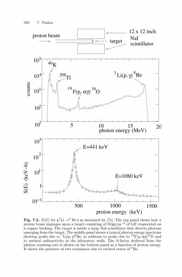
334 7. Fusion
1
−1
1
2
10
10
10
103
S(E
) (
keV
−b)
photon energy (MeV)
500 1000 1500proton energy (keV)
4
5
10
10
10
10
5 10 15 20
proton beamtarget
12 x 12 inch NaIscintillator
3
2
110
coun
ts
40K
208Tl
F(p, αγ) O1619
Li(p, γ) 8Be7
E=1080 keV
E=441 keV
Fig. 7.2. S(E) for p7Li →8 Be γ as measured by [71]. The top panel shows how aproton beam impinges upon a target consisting of 10 µg cm−2 of LiF evaporated ona copper backing. The target is inside a large NaI scintillator that detects photonsemerging from the target. The middle panel shows a typical photon energy spectrumshowing peaks due to 7Li(p, γ)8Be, in addition to peaks due to 19F(p, αγ)16O andto natural radioactivity in the laboratory walls. The S-factor deduced from thephoton counting rate is shown on the bottom panel as a function of proton energy.It shows the presence of two resonances due to excited states of 8Be.

7.1 Fusion reactions 335
σ(E) =S(E)
Eexp(−√
EB/E)
. (7.15)
where S(E) is a slowly varying function of the center-of-mass energy and EB
is given by (7.14).The experimental determination of the nuclear factors S(E) is a problem
of major interest for all calculations in astrophysical and cosmological nucle-osynthesis, as we shall see in the next chapters. Examples are shown in Figs.7.1 and 7.2. Considerable effort has been made in recent years to measure thecross-sections at energies comparable to stellar temperatures. Without suchdata it was necessary to extrapolate the S(E).
Table 7.1 lists the S(E) for some important fusion reactions. Note that thetiny cross-section for the stellar reaction pp → 2He+νe makes this reactionunobservable. The S(E) must therefore be calculated using weak-interactiontheory.
The Gamow formula (7.15) can also be obtained quite easily in the Bornapproximation. A cross-section involves, like any transition rate, the squareof a matrix element between initial and final states |〈f |M |i〉|2. When forcesare short range, the asymptotic states |i〉 and |f〉 are monochromatic planewaves.
In the presence of a Coulomb interaction, which is of infinite range, theasymptotic behavior is different. The wave function is exactly calculable (seefor instance A. Messiah, Quantum Mechanics vol. 1, chap. XI-7) and, asymp-totically, the argument of the exponential has additional terms of the form
ϕ(r) ∼ exp(i(kr + γ log kr)) with γ = Z1Z2e2/4πε0hv . (7.16)
These asymptotic wave functions are called Coulomb scattering states. Con-sider, for instance, the reaction d+ t → 4He+n. In the initial state, we mustuse Coulomb scattering states (and not the usual asymptotic states). Sincethe strong interaction is short range, we can, in good approximation, simplymultiply the usual matrix element by the value of the Coulomb scatteringwave at the origin ψcoul(0) = Γ (1 + iγ)e−πγ/2, i.e. multiply the nuclear crosssection by the factor |Γ (1 + iγ)e−πγ/2|2 = πγe−πγ/ sinhπγ. Once the kine-matic factors are taken into account, one recovers the tunnel effect factore−2πγ ∼ e−πγ/ sinhπγ introduced empirically for γ = Z1Z2e
2/4πε0hv 1.
7.1.2 Reaction rate in a medium
Consider the specific case of a mixture of deuterium and tritium. We want toevaluate the reaction rate per unit volume, i.e. the number R of reactions perunit volume and unit time, if the number densities of d and t are respectivelyn1 and n2. Knowing this rate, we can readily calculate the power emitted.
Consider a deuterium nucleus, of velocity v with respect to the tritiumnucleus. As discussed in Sect. 3.1.4, the probability per unit time λ that afusion reaction occurs is:

336 7. Fusion
1 10
1
−210
−410
−610
−810
−1010
exp(
−E
/kT
)
10
10
10
10
10
−16
−14
−12
−10
−8
P(E
)
10−18
100
(keV)cmE
EG =18.5 keV
Fig. 7.3. Factors entering the calculation of the pair reaction rate (7.22). TheBoltzmann factor exp(−E/kT ) (logarithmic scale on the left) and the barrier pen-etration probability P (E) = exp(−
√EB/E) (7.13) (logarithmic scale on the right)
are calculated for kT = 1 keV (corresponding to the center of the Sun) and for thereaction 3He 3He → 4Hepp. The product is the Gaussian-like curve in the center(shown on a linear scale). It is maximized at EG = (
√EBkT/2)2/3 ∼ 18.5 keV
and most reactions occur within ∼ 5 keV of this value. Note the small values ofexp(−EGm/kT ) ∼ 10−8 and P (EG) ∼ 10−16.
λ = n2 σ(v) v (7.17)
where σ is the fusion cross-section (7.15). The rate per unit volume is thenfound by multiplying the rate per deuterium nucleus by n1:
R = n1n2σ(v)v . (7.18)
We must average this expression over the velocity distribution in the mediumat temperature T :
R = n1n2〈σ(v)v〉 (7.19)
where 〈σ(v)v〉 is the average of the product σ(v)v, the probability of v beingdetermined by the Maxwell distribution at temperature T . Because of thedecreasing Coulomb barrier, the product σv increases rapidly with the en-ergy. In the averaging, it is however in competition with the decrease of theMaxwell distribution with increasing velocity. If only one of the two speciesis in motion, we would have

7.1 Fusion reactions 337
〈σv〉 ∼∫
d3v e−E/kT σ(v)v ∼∫
v3e−mv2/2kT σ(v)dv . (7.20)
In reality, both species are in motion so the integral is slightly more compli-cated. For nuclear of masses of m1 and m2, we have
〈σv〉 =( m1
2πkT
)3/2 ( m2
2πkT
)3/2∫
e−(m1v21+m2v2
2)/2kT σ(v)v d3v1d3v2 ,
where v = |v1 − v2| is the relative velocity. Turning to center-of-mass vari-ables, µ = m1m2/(m1 + m2) being the reduced mass, we can integrate overthe total momentum (or the velocity of the center of gravity). This leads to
〈σv〉 =
√8
πµ(kT )3
∫e−E/kT Eσ(E)dE . (7.21)
Using (7.15) this is
〈σv〉 =
√8
πµ(kT )3
∫e−
√EB/Ee−E/kT S(E)dE . (7.22)
The integrand contains the product of two exponentials shown in Fig. 7.3.Their product peaks at the Gamow energy
EG = E1/3B (kT/2)2/3 , (7.23)
where EB is given by (7.14). As long as S(E) has no resonances (e.g. asin Fig. 7.2) only the narrow region around the Gamow energy (called theGamow peak) contributes significantly to 〈σ(v)v〉. Its position determinesthe effective energy at which the reaction takes place.
In the absence of resonances, the nuclear factor S(E) varies slowly andonly the value S(EG) is relevant so it can be taken out of the integral (7.22).We can also make a Taylor expansion of the argument of the exponential inthe region EG:
√EB/E + E/kT ∼ 3
2
(EB
kT/2
)1/3
+12
(E − EG)2
∆2E
, (7.24)
where the width of the Gamow peak is
∆E =2√3EG
(kT
EG
)1/2
=2√3E
1/6B
(kT
2
)5/6
. (7.25)
[Note that the Gamow peak is relatively narrow: ∆E/EG ∼ (kT/EB)1/6.] Wethen have
〈σv〉 =8π√
µ(kT )−3/2S(EG) exp
[−(3/2)
(EB
kT/2
)1/3]
×∫
exp(
(E − EG)2
2∆2E
)dE . (7.26)

338 7. Fusion
−1 31 2
−20
−22
−24
−28
−26
−30
−32
−34
10
10
10
10
10
10
10
10 10 10 1031kT (keV)
vσ
(m3 s
d d He n4
He n3t d
−1 )
Fig. 7.4. Variation of the pair reaction rate 〈vσ〉 as a function of the temperaturefor d-d and d-t mixtures.
The Gaussian integral just gives a factor ∆E so we end up with
〈σv〉 =8π√
µ(kT )−2/3E
1/6B S(EG) exp
[−(3/2)
(EB
kT/2
)1/3]
(7.27)
Figure 7.4 shows 〈σv〉 as a function of temperature for d d → n 3Heand for d t → n 4He. The rate rises rapidly for kT < 10 keV before levelingoff. We can say that kT ∼ 10 keV , i.e. T ∼ 1.5 × 10⁸ K, defines an optimaltemperature for a fusion reactor.
7.1.3 Resonant reaction rates
If a reaction cross-section exhibits resonances, like those in Fig. 7.2, then theintegral in (7.21) may also receive an important contribution from energiesnear the resonance, in addition to the Gamow peak. Such resonances are dueto states of the compound nucleus consisting of the two interacting particles.For example, the resonance in Fig. 7.2 is due to an excited state of 8Be(Exercise 7.3). This state can decay to both the initial particles
8Be∗ → p 7Li Γp = 6 keV , (7.28)
and to the ground state of 8Be

7.2 Reactor performance criteria 339
8Be∗ → γ 8Be Γγ = 12 eV . (7.29)
Near the peak of the resonance, the cross-section for p 7Li → 8Be γ is givenby (3.183)
σi→f (E) ∼ 4π(hc)2
2µE
(Γp/2)(Γγ/2)(E − E0)2 + Γ 2/4
, (7.30)
where we have neglected the spin factors and where Γ = Γγ +Γp. The contri-bution to the integral in (7.21) coming from the resonance region is then justproportional to the cross-section on resonance, 4π(Γγ/Γ )(hc)2/(2µE) timesthe width Γ :∫
rese−E/kT Eσ(E)dE ∼ e−Eres/kT (hc)2
µc2 Γγ . (7.31)
Comparing this with the non-resonant rate (7.22) we get the ratio of thecontributions of the resonance and the Gamow peak
〈σv〉res〈σv〉Gamow
∼ e−Eres/kT
e−EG/kT
1
e−√
EB/EG
(hc)2/µc2
S(EG)Γγ
∆E. (7.32)
We have written the ratio as the product of four dimensionless factors. Thefourth favors the Gamow contribution, Γγ/∆E ∼ 10−3, while the third, ∼103 favors the resonance. The relative importance is then determined bythe strongly temperature dependent first and second terms. We leave it toExercise 7.5 to show that in the Sun (kT ∼ 1 keV) the Boltzmann factorsuppresses the resonant contribution to a negligible level.
However, for resonances near or below the Gamow peak, the resonanceis generally more important. The most important example in astrophysics isthe reaction
4He 8Be → 12C γ . (7.33)
which proceeds through an excited state of 12C corresponding to a 4He− 8Becenter-of-mass energy of Eres = 283 keV. This reaction is responsible for theproduction of carbon and takes place in stars at kT ∼ 15 keV correspondingto EG ∼ 300 keV. In this case, the Boltzmann factors in (7.32) cancel. Thefactor exp(−√EB/EG) ∼ 10−11 then ensures that the resonant contributiondominates.
7.2 Reactor performance criteria
A fusion reactor consists of three essential elements
• A confined plasma containing positively charged ions (generally 2H and3H) and electrons to maintain the neutrality.
• An energy injector to create and, if necessary, maintain a high temperature.

340 7. Fusion
• An energy recovery mechanism that collects the energy of escaping fusion-produced neutrons and thermal photons.
In practice, the confinement of the plasma is achieved by three differentmechanisms: gravitational confinement, inertial confinement and magneticconfinement. Gravitational confinement is achieved naturally in stars. Theplasma is maintained indefinitely by the self-gravitation of the star. Inertialconfinement is used in laser induced fusion. It also occurs in supernovaeexplosions (and in explosive devices). Magnetic confinement has been themain method investigated for controlled fusion before laser induced inertialconfinement was declassified.
Let V be the plasma volume, R the reaction rate as defined by (7.19) andQ the energy released in an elementary fusion reaction. The fusion-generatedpower P (before any losses are taken into account) is given by
P = R V Q . (7.34)
For a given value of the temperature, in order to increase the reaction rateR, one must increase the densities n1 and n2. For a given value of n = n1+n2,the best proportion, which maximizes the product n1n2 corresponds to n1 =n2 = n/2, i.e. equal amounts of reagents, at high densities. One thereforeseeks high temperatures (∼ 107 K, kT ∼ 1 keV) and a strong compression.
Fusion reactors are judged by how much power they create compared tohow much was used in heating the plasma. Three goals, in order of decreasingdifficulty, are defined for any fusion reactor:
• Ignition. After heating, the reaction rate is sufficiently high to maintainthe temperature without further injection of energy. In reaction (7.4), theneutron escapes so the 4He energy must be used to compensate for coolingby radiation of photons and neutrons.
• Breakeven. Power generated by fusion is equal to the input power thatmust be continually injected to compensate for energy losses (neutronsand photons).
• One-shot breakeven (Lawson Criterion). The energy generated by fusion isequal to the input energy necessary to heat the plasma. A reactor satisfyingonly this criterion is similar to the sub-critical fission reactors of Sect. 6.8.
The present goal is to satisfy the Lawson criterion which we now makemore precise. The time τ during which the plasma maintains its temperatureT and its cohesion, after its creation, is called the confinement time. Thistime is effectively infinite in stars, in the sense that confinement lasts at leastas long as there is some nuclear fuel left.
In order to heat the plasma to the temperature T , one must furnish, perunit volume, the energy 3nkT where n is the number density of nuclei. (Weassume one free electron per ion).
Let η be the efficiency to transform nuclear energy into electric energy inthe reactor, in other words the efficiency to recover the energy produced by

7.2 Reactor performance criteria 341
the plasma. The reactor will run in ignition conditions if the energy spent toheat it is smaller than the electric energy it can produce:
3nkT < (n2/4η)〈vσ〉Qτ (7.35)
where we assume that there are two species (d-t mixture) of number densitiesn1 = n2 = n/2. We must therefore have
nτ > (1η)
12kT
(Q〈vσ〉) (7.36)
where Q is the energy produced in an elementary fusion reaction. This for-mula is called the Lawson criterion.
From Fig. 7.4 we see that 〈σv〉 ∝ T 2 for kT ∼ 10 keV:
〈σv〉(dt → 4Hen) ∼ 10−22 m3s−1(
kT10 keV
)2
. (7.37)
Substituting this into (7.36) and using Q = 17.5 MeV we get the Lawsoncriterion for the d-t reaction
nτkT
10 keV> η−11.5 × 10²⁰ m−3s , (7.38)
or equivalently
nτkT > η−11.5 × 10²¹ m−3s keV , (7.39)
In gravitational confinement, τ is effectively infinite so the Lawson cri-terion is irrelevant. In magnetic confinement, confinement times achieved sofar are ∼ 1 s, limited by excess cooling due to impurities in the plasma andto various plasma instabilities. The density is planned to be of the order of1020 m−3 in the project ITER (International Thermonuclear ExperimentalReactor) and the temperature of the order of 10 to 20 keV, which is the igni-tion threshold. In laser induced inertial confinement, the confinement time ismuch shorter τ 10−11 s. However, the density is much higher 1031 m−3.The temperature is comparable, of the order of 10 keV.
Table 7.2. Comparison of the parameters in three fusion confinement schemes.
Type n(m−3) τ(s) T (keV)ITER Tokamak 1020 1 10 to 20Inertial; laser 1031 10−11 10Sun (grav) 7. 1030 1017 1.3

342 7. Fusion
7.3 Magnetic confinement
The magnetic confinement method consists in using a magnetic field to con-tain the plasma. Tokamaks are toroidal machines where the plasma is main-tained inside a tube by a strong toroidal field superimposed on a poloidalfield which maintains it in the horizontal plane.
Fig. 7.5. Diagram of a Tokamak.
In the tokamak configuration shown on Fig. 7.5, the toroidal field, createdby external currents, is rotationally symmetric around the vertical axis. The

7.3 Magnetic confinement 343
poloidal field comes from a high intensity current of several million ampereswhich runs in the tube. The design is of course quite involved since one doesnot deal with a beam of particles, as in accelerators, but with an entire large-size plasma.
Creation and heating of the plasma. The magnetic configuration is cre-ated inside a toroidal tube. The evacuated tube is filled with the hydrogen–deuterium or tritium–deuterium mixture with a pressure of 300 P, whichcorresponds to the desired density of 1014 particles per cubic centimeter. Thegas is then completely ionized in a few milliseconds.
In order to reach and to maintain a temperature of several keV, severalheating techniques are used.
• First, there is the ohmic heating, where the high intensity current in theplasma transfers heat by Joule effect. This type of heating allows one toreach temperatures of 2 to 3 keV.
• In order to reach the 10 to 20 keV necessary for fusion, fast neutral atomsare injected. One first accelerates ions of the same nature as those of theplasma (hydrogen or deuterium), outside the tokamak. These ions are neu-tralized by capturing electrons in a medium. The neutral atoms which areformed have considerably higher energies than the ions in the plasma. Theyare unaffected by the magnetic field. They cross the magnetic field, enterthe chamber and are then ionized by the plasma. Finally the whole systemthermalizes.
• The microwave heating comes from the absorption of high-frequency elec-tromagnetic waves. The modeling of this process is in itself a field ofmagneto-hydrodynamics. Waves are sent in the plasma by antennas in-side the chamber, near the walls. One can inject powers of the order of10 megawatts. The power in the European tokamak JET (Joint EuropeanTorus) is 40 megawatts.
• Finally, the α particles produced in the fusion reaction and which carry20% of the fusion energy release this energy by thermalizing with the ionsof the plasma. This should maintain the plasma temperature in the ignitionregime.
Loss mechanisms; energy balance. The plasma loses energy by radia-tion of photons. These radiation losses come mainly from the emission linesof incompletely ionized atoms. Most of these atoms are impurities of oxygen,carbon, iron and nickel. The losses due to this effect represent, at present,10 to 50% of the energy balance. They can be minimized by a proper con-ditioning of the walls of the vacuum chamber and by controlling the qualityof the plasma near the walls. Both operations are intended to prevent theproduction of impurities. Maintaining the concentration of impurities at anacceptable level is a necessary condition to have a positive fusion energybalance.

344 7. Fusion
Fig. 7.6. The interior of JET (Joint European Torus).
The energy losses by the bremsstrahlung of electrons scattering on deu-terium and tritium ions is an unavoidable source of energy loss. At a givendensity, they require a high enough plasma temperature since the fusion cross-section rises more rapidly with temperature than the bremsstrahlung cross-section. Losses by bremsstrahlung are proportional to n2T 1/2 (Exercise 7.6)whereas 〈σv〉 for fusion is proportional to T 2 in the 10 − 20 keV range. Theoverall result is that the temperature should be larger than 5 keV.
Stability of the plasma. The instability mechanisms of the plasma itselfare a field of complex fundamental research. The most dangerous instabilitiesare magneto-hydrodynamic instabilities because they are highly non-linearand they involve the plasma as a whole.
Perspectives of fusion by magnetic confinement. Since the first resultsobtained by Soviet physicists in 1968 on the tokamak T-3, about 30 machinesof that type have been constructed in the world. Much progress has been madetoward satisfying the Lawson criterion.
Three large tokamaks have been installed successively between 1982 and1985 and have attained their nominal performances : the TFTR (TokamakFusion Test Reactor) by the United States at the Princeton laboratory in NewJersey ; The JET (Joint European Torus), by the EC, located in England atCulham, near Oxford ; the JT-60 (Jaeri Tokamak), by Japan, at the Jaeri

7.3 Magnetic confinement 345
laboratory in Naka, near Kyoto. The current in the plasma ring increasedfrom 100 kA in the T-3 to 7 MA in the JET. The break-even zone wasapproached in 1991 by JET and in 1993 by the JT-60.
The performances of various machines are represented in Fig. 7.7.
6T ( 10 K)1000100101
17
18
19
20
21
22
10
10
10
10
10
10
−3 )
T4
TFR
JT−60TFTR
DIII−DTORE−SUPRA
ITER
ignition (d−t)
T3
PLTT10
ASDEXALC−A
FTALC−C
JET
break−even (d−t)
1960−70
1970−1980
1980−2000
bremsstrahlung lim
itinaccessibleregion
n kT
(ke
V s
mτ
Fig. 7.7. Performance of various Tokamaks. The ITER project is projected tostart construction in 2005. Above bremsstrahlung limit, cooling by radiation limitsthe temperature (Exercise 7.6).
The planned successor of JET is ITER (International Thermonuclear Ex-perimental Reactor), a world-wide collaboration initiated by the USA andthe Soviet Union in 1985. ITER is now a collaboration of Europe, Japan,Canada, the USA, and the Russian Federation.
The ambition is not limited to obtaining ignition conditions of thedeuterium-tritium mixture (one aims at a nuclear power of 1.5 GW). It isalso to maintain the plasma in stationary equilibrium for a period of 1000seconds.
The project is gigantic. The volume of the plasma should be 2000 m3
instead of 100 m3 in JET. ITER is supposed to deliver a power of 1500 MW.The magnetic system will be entirely superconducting.
The construction should start in 2005 and should last ten years. Theexploitation phase should last for 20 years.
The next step would be the construction of an experimental plant whichwould produce electricity, called DEMO. This plant could be exploited start-

346 7. Fusion
Fig. 7.8. Sketch of the ITER project; notice the comparative size.
ing in 2035, and the construction of the first commercial plant would onlystart after 2050.
7.4 Inertial confinement by lasers
The principle of inertial confinement by lasers is to adiabatically compress asmall (∼ 1mg) sphere containing deuterium and tritium in order to increaseits density by ∼ 104, and to obtain temperatures of ∼ 10 keV. The core ofthe sphere ignites during a time of the order of 10−10 s and then explodes(see Fig. 7.9).
One calls ignition the regime where the temperature and density condi-tions of the core allow the burning of the d-t mixture.
Initially, this method was classified, because of its military applications.Since 1993 civilian-physicists have worked in the field.
The principle is simpler than in tokamaks. Additionally, research on thismethod has been funded partly owing to its importance for the understandingof thermonuclear explosions.

7.4 Inertial confinement by lasers 347
Principle of the method. The radiation of a set of laser beams delivering avery large power (TW) for a short time (ns) is directed toward a sphere of theorder of a mm3 of a solid deuterium–tritium mixture. There is an ablation,or sudden vaporization, of the periphery of the sphere and the formation ofa corona of plasma.
laser beam laser beam
laser beam laser beam
compressed core absorption zone
Fig. 7.9. Sketch of laser induced fusion. The d-t sphere interacts with the laserbeams and it is vaporized superficially. By reaction, the corona compresses thecentral core.
The electrons of the medium which oscillate in the laser field transferenergy to the plasma by colliding with the ions. The energy is transferedto the cold regions of the center of the target by thermal conduction, byfast electrons and by UV and X radiation. A shock wave is created whichcompresses and heats the central region of the deuterium-tritium sphere,called the core.
Under that implosion, the core is compressed by a factor of 1000 to 10000,i.e. densities of ∼ 1031 m−3, and its temperature reaches ∼ 10 keV. Underthese conditions, the fusion of the d-t nuclei occurs abundantly. The coreburns for about 10−11s. Its cohesion is maintained by inertia, it explodesbecause of the thermonuclear energy release.

348 7. Fusion
The laser energy goes mainly into the compression of the d-t mixture. Theenergy necessary to heat the plasma comes mainly from the fusion energyrelease. This results in a reduction of the laser energy which is necessary tomake the target burn.
In 1992, in the United States, the Lawrence Livermore National Labora-tory (LLNL) declassified the principle of inertial confinement fusion. At AnnArbor, the KMS laboratory (named after its creator, K.M. Siegel) was thefirst, around 1973, to achieve the implosion of glass “micro-balloons” con-taining gaseous deuterium-tritium. The experiment was then performed byother laboratories. The 100 kJ Nova laser of LLNL reached a production of1013 neutrons per laser pulse.
Such experiments led to rapid development of computer-simulated explo-sions. The experimental inputs to these calculations involved the observationof X-rays and neutrons emitted by the target, the spectroscopy of tracersincorporated in the d-t mixture, such as argon and neon, and pictures ofthe α particles produced in the fusion reactions. Such measurements werecompared with the results of computer simulations, in order to validate theassumptions entering the codes, in particular the fact that neutron emissionis of thermonuclear origin.
Technical problems. An important problem is that the irradiation of thetarget must be as uniform as possible, in order for the implosion to be asspherical as possible. Several methods are used.
• One can use a direct attack by several laser beams symmetrically dis-tributed about the target.
• The indirect attack consists in sending the laser beams inside a cavity madewith a heavy element. This results in an emission of thermal X-rays. The Xrays irradiate the sphere in the center of the cavity much more uniformly.Using gold, one can reach conversion rates of laser radiation into X-rays of80%.
• Another approach consists in replacing the laser beams electron with ionbeams of ∼ 1 MeV. High power beams are easy to produce but sufficientlyaccurate focusing of the beam is difficult to achieve. The construction ofa 10 GeV heavy ion accelerator (for instance uranium) that could deliver1 MJ in 10 ns is under study.
Projects. Two important projects are underway.The NIF (National Ignition Facility) project, in the United States, consists
of 192 laser beams. It will deliver an energy of 1.8 MJ in each pulse of 1 ns.Its installation is scheduled for 2003; its cost should be 1200 million dollars.Ignition is expected in 2008-2012.
The Megajoule laser project, LMJ, in France, will consist of 240 laserbeams. It should deliver 1.8 MJ in 18 ns. Its installation is expected in 2010,for a cost of 1000 million euros. Ignition is expected in 2015.

Exercises for Chapter 7 349
7.5 Bibliography
1. James Glanz Turbulence may sink Titanic reactor, Science, 274, Decem-ber 1996.
2. M. N. Rosenbluth et A. M. Sessler et T. H. Stix, Build the Interna-tional Thermonuclear Experimental Reactor? Yes/No, Physics Today,June 1996.
3. I. Fodor, B. Coppi and J. Lawyer, Views ITERated on proposed newreactor, Ignitor, fusion power, Physics Today, December 1996.
4. M. N. Rosenbluth et A. M. Sessler et T. H. Stix, ITER debaters replyto pro and cons fusion comments from readers, Physics Today, January1997.
5. W. E. Parkins, J. A. Krumhansl et C. Starr, Insurmountable engineeringproblems seen as ruling out fusion power to the people in 21st century,Physics Today, Mach 1997.
Exercises
7.1 Calculate the nuclear energy content in joules in 1 kg of heavy water,assuming that all deuterium atoms undergo fusion into 4He.
7.2 Using the reaction rate in Fig. 7.4, calculate the fusion power in a deu-terium plasma at a temperature of kT = 10 keV and a density of 1014cm−3.
7.3 Calculate the energy of the excited state of 8Be (relative to the groundstate) that leads to the 441 keV resonance shown in Fig. 7.2.
7.4 Consider the experiment to measure the reaction 7Li(p, γ)8Be shown inFig. 7.2. Calculate the photon energy for a proton kinetic energy of 200 keV.Estimate the energy loss of the proton as it traverses the 10 µg cm−2 of LiF.How much does the cross-section vary over this energy range? Discuss howthis limits the acceptable thickness of the target.
7.5 Evaluate (7.32) for 7Li(p, γ) 8Be for solar conditions, kT ∼ keV, to showthat the resonant contribution to the rate can be ignored.
7.6 The bremsstrahlung cross-section for radiation of a photon of energy Eγby non-relativistic electrons scattering on protons is approximately
dσ
dEγ∼ α
(c2
v2
)σT
Eγ, (7.40)

350 7. Fusion
where v c is the relative electron–proton velocity and σT is the Thom-son cross-section. The rate of photon radiation (per unit time and per unitvolume) in a plasma of electron and proton density n is then
dNγ
dtdV dEγ∼ n2v
dσ
dEγ∼ c
vn2αc
σT
Eγ, (7.41)
where v is now the mean velocity. Integrate this expression up to the max-imum photon energy (∼ kT ) to show that the plasma luminosity (energyradiated per unit time and per unit volume) is
L = n2αcσT
√mec2kT . (7.42)
Argue that the characteristic time, τbrem, for the plasma to cool by photonradiation is
τbrem =nkT
L∼ 1
nαcσT
√kT
mec2 . (7.43)
Plot the quantity nkTτbrem as a function of kT and compare with thebremsstrahlung limit in Fig. 7.7. Above this line, the confinement time islonger than the cooling time so the plasma cools until the confinement timeis shorter.

8. Nuclear Astrophysics
Perhaps the most important accomplishment of nuclear physics is its expla-nation of stellar energy production and nucleosynthesis. Astrophysicists nowbelieve that they understand in some detail stellar histories from their ori-gins as diffuse clouds through their successive stages of nuclear burning untiltheir “deaths” as white dwarfs or supernovae. Through this process, nuclearphysics has allowed us to understand how the initial mix of hydrogen andhelium produced in the primordial Universe has been transformed into theinteresting mixture of heavy elements that makes terrestrial life possible.
In this brief chapter, we will first give the very minimum of stellar struc-ture theory that is necessary to understand stars. We will see how stars workas “gravitational confinement” fusion reactors where one naturally reachesa self-regulating state with a stable temperature sufficiently high to allownuclei to penetrate their mutual Coulomb barriers.
In the second section, we will describe in some detail the stages of nuclearburning where the nuclear fuels are successively hydrogen, helium, carbon,oxygen and so forth until elements in the iron group are produced.
In Sect. 8.3 we describe the estimations of the abundances of the elementsin the solar system and how the existence of elements beyond the iron-groupcan be explained by stellar neutron-capture reactions.
Finally, in Sect. 8.4 we describe observations of neutrinos and γ-rays thathave empirically confirmed that the processes discussed in this chapter doindeed take place inside stars.
8.1 Stellar Structure
Stars are gravitationally bound collections of nuclei and electrons. They alsocontain blackbody photons in thermal equilibrium with the particles. Photonscannot be gravitationally bound in stars so they diffuse through the star untilthey escape. As we will see, the role of nuclear reactions is to replace theenergy leaving the stars so as to maintain stable conditions.
In this section, we will first study classical stars, by which we mean bodiesthat are sufficiently dilute that we can neglect the quantum nature of theparticles. This is the case for stars like the Sun but fails for objects like whitedwarfs and neutron stars where fermionic particles are “degenerate,” i.e. the

352 8. Nuclear Astrophysics
phase-space density approaches the limit allowed by Pauli exclusion principle.Such stars will be treated in Sect. 8.1.2.
8.1.1 Classical stars
We would like to understand the density ρ(r), pressure P (r), and tempera-ture T (r) profiles of stars. Since stars evolved slowly, it is a good first approx-imation to take them to be time-independent. This is possible if the star isheld in quasi-hydrostatic equilibrium where the gravitational force workingfor collapse is balanced by a pressure gradient. As illustrated in Fig. 8.1, thenecessary condition for hydrostatic equilibrium is that the pressure gradientsatisfy.
dP
dr= −ρ(r)
GM(r)r2 , (8.1)
where M(r) is the mass contained within a sphere of radius r. Clearly, thepressure must decrease as r increases.
P(r+dr)
P(r)gravity
dr
T(r)
T(r+dr)
Fig. 8.1. The pressure and temperature gradients of a stable star can be qualita-tively understood by considering a thin layer of material at a distance r from thecenter of a star. The material in the layer experiences downward forces from gravityand from the pressure P (r + dr). The upward force comes only from the pressureP (r). If the pressure gradient satisfies (8.1) the upward and downward forces bal-ance. Additionally, the surfaces at r and at r + dr radiate isotropically blackbodyphotons. If the temperature gradient satisfies (8.4), the difference between the en-ergy radiated outward from the surface at r and the energy radiated inward fromthe surface r + lγ is equal to the net luminosity (lγ=photon mean free path).
Through the equation of state P = nkT , the pressure gradient (8.1) gen-erates density and temperature gradients. We then need another equationto determine one of these two gradients. For many stars, the temperaturegradient can be determined by considering energy transport by blackbodyradiation. The energy liberated by nuclear reactions is ultimately evacuatedby radiation of photons. The surface of a black body radiates an energy per

8.1 Stellar Structure 353
surface area of σT 4 where σ is the Stefan–Boltzmann constant. A sphericalblackbody of radius R must then have a luminosity given by
L(R)4πR2 = σT (R)4 , (8.2)
where T (R) is the surface temperature. Inside the star, the situation is morecomplicated since, as illustrated in Fig. 8.1, a surface at radius r both ra-diates energy and absorbs energy from layers further from the center. Wemust require that the difference between these two energies be equal to theluminosity L(r) generated inside the surface. The energy the surface receivesfrom outer layers originates about one photon absorption length (lγ) higherso we would expect that the net energy flux per unit area to be roughly thedifference between the values of σT 4 at values of r that differ by lγ:
L(r)4πr2 ∼ σ
[T 4(r) − T 4(r + lγ)
]. (8.3)
A careful treatment ( e.g. [72]) gives a factor 4/3:
L(r)4πr2 = (4/3)σ
dT 4
drlγ . (8.4)
The absorption length is usually written as (κρ)−1, where the function κis called the “Rossland mean opacity.” It is a function of the temperature,density and chemical composition.
Equation (8.4) determines the solar temperature gradient over its inner70%. The outer 30% has adiabatic convective mixing which determines thetemperature gradient by standard thermal arguments (Exercise 8.1).
To equations (8.1) and (8.4) we must add the effect of the release ofnuclear binding energy in fusion reactions. For a steady state, this energyrelease is balanced by the photon luminosity so we have
dL
dr= 4πr2ε(r) , (8.5)
where ε(r) is the total rate of energy release per unit volume. For a givenreaction, it is the Q-value times the temperature- and density-dependentreaction rates calculated in the previous chapter, (7.19) and (7.27).
The three coupled differential equations, (8.1), (8.4) and (8.5), can besolved numerically to find the internal structure of a star. The calculateddensity, temperature and pressure profiles of the Sun are shown in Fig. 8.2.The central temperature of the Sun is T (0) ∼ 1.568×10⁷K or kT ∼ 1.35 keV.
To understand the slow evolution of a star, it is useful to take a globalapproach and consider the total energy of the star. The end result of theseconsiderations will be an expression (8.20) that gives the total energy as afunction of the number particles in the star and the radius of the star.
We consider an object of mass M consisting of free massive particles(atoms and free nuclei and electrons) gravitationally bound in a sphere ofradius R. The total energy is

354 8. Nuclear Astrophysics
n γ /nb
0 1.00.5
1
−210
10−3
−4
sunr/R
10
T/ T(0)
ρ/ρ(0)10−1
Fig. 8.2. The calculated [73] solar density and temperature profiles normalized tothe central values ρ(0) = 152.4 g cm−3 and T (0) = 1.568 × 10⁷ K. The density scaleheight (i.e. the distance over which the density changes by a factor e) is ∼ 0.1R.Also shown is the photon–baryon ratio nγ/nb. This ratio is nearly constant at∼ 10−3 except for r > 0.7R where convection forces the ratio to decrease (Exercise8.1)
Etot =∑
particles
(mc2 +
p2
2m
)+ Egrav + Ephotons . (8.6)
We have used the non-relativistic form, mc2 + p2/2m, for the energy of theparticles because, as we will see, only non-relativistic particles can be boundby gravitation. The second term is the negative gravitational energy of theobject
Egrav = −∫ R
0
GM(r)r
ρ(r)4πr2dr . (8.7)
For an object of uniform density, Egrav = −(3/5)GM2/R so it is useful tointroduce the effective “gravitational ” radius of the star, Rgrav
1Rgrav
= (5/3)M−2∫ R
0
M(r)r
ρ(r)4πr2dr , (8.8)
so that Egrav is simply
Egrav = −(3/5)GM2
Rgrav. (8.9)

8.1 Stellar Structure 355
Rgrav is just the radius of the uniform sphere of matter that would have thesame gravitational energy as the star in question. For the Sun, a numericalintegration of the density profile of Fig. 8.2 gives Rgrav = 0.37R.
We can relate the kinetic and gravitational energies through the “virialtheorem.” Multiplying (8.1) by 4πr3 and integrating by parts. we find anexpression relating the mean pressure P and Egrav:
3P V = −Egrav = (3/5)GM2
Rgrav. (8.10)
If the photon pressure is negligible, we can use the ideal gas law, PV = NkT ,to estimate the mean temperature of the star
kT = (1/5)Nb
Npart
GNbm2p
Rgrav∼ (1/10)
GNbm2p
Rgrav, (8.11)
where Npart is the total number of free massive particles in the star andNb ∼ M/mp is the number of baryons (nucleons) in the star. [We neglectthe ∼ 1% difference between mp and m(A, Z)/A.] In the second form wehave assumed totally ionized hydrogen, Npart = Ne + Np = 2Nb. For theSun, Nb ∼ 1057 we find kT ∼ 500 eV in reasonable agreement with the meantemperature in solar models.
Equation (8.11) tells us that a star has a negative specific heat, i.e. as itloses energy and contracts, its temperature increases. This fact will turn outto be crucial in a star’s ability to maintain a stable nuclear-burning regime.
The kinetic energy per particle is (3/2)kT so the total kinetic energy inthe star is simply related to Egrav∑
particles
(p2
2m
)= −(1/2)Egrav . (8.12)
This is just a form of the virial theorem. Another proof that does not appealto hydrostatic equilibrium is given in Exercise 8.2.
The final term in (8.6) is the energy of the photons that must be presentif a quasi-stationary thermal equilibrium is reached:
Ephotons =∫ R
0ργ4πr2dr , (8.13)
where the photon energy density is given by the Stefan–Boltzmann law
ργ =2π2
30(kT )4
(hc)3. (8.14)
It turns out to be more interesting to work with the photon number density:
nγ =2.5π2
(kT
hc
)3
∼ ργ
3kT. (8.15)
We can use the mean temperature (8.11) to estimate the total number ofphotons in the sun Nγ ∼ nγ(T )4πR3
grav/3:

356 8. Nuclear Astrophysics
Nγ ∼ α3GN3
b1
103
4 × 2.43π
∼ 10−3α3GN3
b , (8.16)
where the “gravitational fine structure constant” is
αG =Gm2
p
hc= 6.707 × 10−39 . (8.17)
The photon–baryon ratio is then
Nγ
Nb∼ 10−3α3
G N2b . (8.18)
We see that that the photon–baryon ratio is independent of the radius andproportional to the square of the number of baryons. For the Sun, Nb =1.2 × 1057 giving α3
GN2b = 0.4 so the photon–baryon ratio is about 10−3,
in agreement with solar models (Fig. 8.2). For a star of M ∼ 30M, thephoton–baryon ratio is 302 times larger, approaching unity. It turns out thatthis makes the star unstable and the radiation pressure expels mass from thesurface until the mass falls below 30M.
The mean energy of photons in a star is of order kT so we have a totalphoton energy content of
Ephotons ∼ 10−4 α3GN3
bGm2
pNb
Rgrav. (8.19)
Since, for the Sun, the number of photons is ∼ 10−3Nb, Ephotons is of order10−3 of the total kinetic energy of the particles. This also implies that thephoton pressure is of order 10−3 the thermal pressure due to the massiveparticles.
If we neglect Ephotons we can have a compact formula for the energy of astar as a function of its radius. Substituting (8.12) into (8.6), we get
Etot =∑
particles
(mc2) − 3GM2
10Rgrav. (8.20)
We are now in a position to understand the effect of the thermal photonsdiffusing out of a star. These photons have positive energy so, as photonsleave, Etot must diminish in order to conserve energy. Equation (8.20) sug-gests that this can be done either by contraction, leading to a decrease inEgrav ∝ −1/Rgrav or by exothermic nuclear reactions which decrease themc2 term.1 The stellar luminosity, dEtot/dt, must then be
L = −dmc2
dt− 3GM2
10R2grav
dRgrav
dt. (8.21)
In fact, as illustrated in Fig. 8.3, it is generally the case that one or theother of the terms on the left side of (8.21) dominates at a given time. Stars
1 Lowering the mass would also increase slightly Egrav but, since the mc2 termdominates, this effect is negligible.

8.1 Stellar Structure 357
start their lives as diffuse clouds of gas that are too cold to initiate nuclearreactions. Photon radiation luminosity is thus supplied by the second term in(8.21). The decreasing radius increases the internal temperature of the staras required by the virial theorem (8.11). As the temperature rises, the rateof nuclear reactions increases until the photon luminosity can be providedby the nuclear reactions. At this point, the star can reach a stable regime atconstant Rgrav. After the fuel is exhausted, the contraction begins again.
time
gravitationalradius
temperature
luminosity
nuclearreaction rate
Fig. 8.3. The simplified evolution of a classical star. The star initially contracts andthe temperature rises until hydrogen fusion is initiated. The radius and temperaturethen remain constant until the fuel is exhausted, at which point another contractionphase begins. The temperature rises until another fuel (helium) can be burned.During all this time, the luminosity is constant if the mean photon cross-sectionremains constant.
The stability of a nuclear burning regime illustrated in Fig. 8.3 is due toa thermostatic effect of the negative specific heat of gravitationally boundstructures. If, for a moment, the rate of nuclear energy production increasesabove the steady state value, the local temperature increases. This causesthe pressure to increase and the star to expand. This lowers the temperatureand, as a result, the reaction rate. On the other hand, if the nuclear energygeneration rate decreases, the star starts to contract, thus increasing thetemperature and the reaction rate. A gravitationally-confined fusion reactoris thus self-regulating.
As soon as the nuclear fuel is used up, the reactions cease and the starmust resume its contraction. The contraction can stop if a new type of nuclearreaction using a different fuel reaches a rate where it can supply the star’sluminosity. Stars can then pass through a series of stable phases where thefuels are first hydrogen, then helium, and then carbon and oxygen until the

358 8. Nuclear Astrophysics
stars core consists of iron-group nuclei. The order of fuels follows a sequenceof increasing Z because the associated higher Coulomb barriers require highertemperatures to supply the necessary reaction rate. This sequence of burningstages will be discussed in more detail in Sect. 8.2. The sequence may beinterrupted if, during the contraction, the star approaches its “ground state”where fermion degeneracy prevents further contraction (Sect. 8.1.2). Thiseffect prevents all but the heaviest stars (M > 10M) from burning theirfuel all the way to the iron group. Stars with M < 0.07M reach theirground state before any nuclear reactions are ignited.
It is interesting to estimate the luminosity of a star. Very roughly speak-ing, it is given by
L =Ephotons
τγ(8.22)
where τγ is the mean time for a photon to diffuse out of the star. Photonsleave the sun as soon as their random walk takes them to the “photosphere,”beyond which their mean free paths are essentially infinite. The mean timefor this is of order
τ ∼ 3R2
λc, (8.23)
where λ is the typical photon mean free path. There are two limits where thephoton cross-section is simple. The first is at sufficiently high temperatureso that the medium is completely ionized. In this case photons can onlyThomson scatter with a mean free path given by
λ−1 ∼ σTNb/R3grav . (8.24)
This regime occurs, depending on the density, for temperatures greater than105 − 106K. The second simple case occurs when the temperature is so lowthat no atoms are ionized and few photons have enough energy to ionizethem. In this case, only Rayleigh scattering is important and the mean freepath is much longer than that given by (8.24). In between these two regimes,absorption of photons by bound electrons (photo-ionization) and on contin-uum electrons in the field of a positive ion (“free–free scattering” or inversebremsstrahlung) dominate the mean free path so the effective cross sectionwill be higher than σT.
The mean escape time is then estimated as
τ ∼ 〈σ〉Nb
Rc. (8.25)
For the Sun, the average photon cross-section 〈σ〉 is of order ∼ 10σT, givingτ ∼ 105 yr.
The luminosity (8.22) is ratio of the Ephotons given by (8.19) and thephoton escape time (8.25). We see that the factor 1/R in Ephotons (8.19) iscanceled by the factor 1/R in the mean escape time so the energy luminosityis independent of R but proportional to 〈σ〉
8.1 Stellar Structure 359
L ∼ α3GN3
bGm2
p〈σ〉c
. (8.26)
For the Sun, this gives L ∼ 1026 W compared of the observed luminosityL = 3.8× 1026 W. Given the many approximations made in this estimation,it is satisfying that we find a number of the correct order of magnitude.
Note that if the effective photon cross-section 〈σ〉 were the same in allstars, the luminosity (8.26) would simply be proportional to N3
b , i.e. to thethird power of the stars mass. This is in fact observed to be a good approx-imation for hydrogen-burning stars. Note also that if the effective photoncross-section were temperature independent so that it remained unchangedas the star contracts, the star’s luminosity would not change as the starevolves through contraction and nuclear-burning stages. This is nearly truefor very heavy stars where the medium is mostly ionized with 〈σ〉 ∼ σT. Thisidealized evolution is illustrated in Fig. 8.3 where the luminosity is indepen-dent of time.
The total time a star spends in a particular stage of its evolution is givenby T = L/∆E where L and ∆E are the mean luminosity and available energyduring the phase. The Sun is in its hydrogen burning phase which liberates∼ 6 MeV per proton. Since there is no convective mixing in the inner parts ofthe Sun, only the inner 10% of the hydrogen will actually be burned. Usingthe present luminosity, this gives a total hydrogen-burning time of ∼ 1010 yr.The Sun’s present age is ∼ 4.5 × 10⁹ yr so the Sun is a middle-aged star.
The time the Sun required to contract to its present radius before burninghydrogen can by calculated by using ∆E = (3/5)GM2
/Rgrav. Assumingthat the solar luminosity was the same during the contraction phase as inthe hydrogen-burning phase, this gives a contraction time of ∼ 107 yr. Inthe nineteenth century before nuclear energy was discovered, this was theestimated total age of the Sun, in clear conflict with the age of the Earthestimated by geologists.
Coming back to the photon–baryon ratio in a star, the fact that it isgreater than unity for M > 30M means that the pressure due to photonsis greater than that due to massive particles. This is in inherently dangeroussituation because it makes the condition (8.10) difficult to maintain becausephotons dominate the left-hand side whereas only particles contribute to theright-hand side. Detailed calculations indicate that stars greater than about30M are unstable and generally evaporate particles until their mass reachesthis value.
8.1.2 Degenerate stars
We have seen that a collection of particles must radiate photons and con-tract, with the contraction pausing whenever nuclear reactions are ignited toprovide the photon luminosity. This process must stop when the collectionreaches its quantum-mechanical “ground state.”

360 8. Nuclear Astrophysics
We want to estimate the ground-state energy of a collection of electronsand nucleons bound by gravitation. We can do this in the same way as wasdone in Chap. 1 where we estimated the ground-state energy of a collectionof nucleons bound by the strong force.
The maximum phase-space density allowed for fermions is two particlesper (∆p∆x)3 = (2πh)3. We assume that N fermions are spread uniformlyover a spatial volume V = 4πR3/3. This means that in the ground statethe single-particle orbitals are filled up to those corresponding to a Fermimomentum pF determined by
N
V × (4π/3)p3F
=1
(2πh)3(8.27)
i.e.4πp3
F
3= N
(2πh)3
21
4πR3/3. (8.28)
The mean momentum squared of this assembly is
〈p2〉 =
∫ pF
0 p2p2dp∫ pF
0 p2dp= (3/5)p2
F . (8.29)
Since, the 〈p2〉 is independent of the particle mass, the mean kinetic en-ergy, p2/2m, will be dominated by the light electrons. (This is not the casefor a classical star where thermal equilibrium requires that the mean kineticenergies of all particles be equal.) The energy of the star is then
E ∼ Ne√
〈p2〉c2 + m2ec
4 − (3/5)GM2
R.
(We do not include the rest-energy of the nucleons in this formula.) UsingM = Nbmp and equations (8.28) and (8.29) this is
E ∼ Ne
√(3/5)p2
Fc2 + m2ec
4 − 3Gm2pN2
b
5N1/3e
pF
2πh
(32π2
9
)1/3
, (8.30)
where Ne is the number of electrons and Nb is the number of baryons. Drop-ping the numerical factors for this rough estimate, and taking the derivativeof E with respect to the momentum we find that the minimum energy occursfor
pF√p2F + m2
ec2
=Gm2
p
hc
N2b
N4/3e
=(
Nb
Nc
)2/3
, (8.31)
where the “critical” number of baryons is
Nc =(
1αG
)3/2(Ne
Nb
)2
= 1.82 × 1057(
Ne
Nb
)2
, (8.32)
where αG = Gm2p/hc. This corresponds to a total mass

8.1 Stellar Structure 361
Mc = mpNc = 3.04 × 1030 kg(
Ne
Nb
)2
= 1.52M
(Ne
Nb
)2
(8.33)
Within a factor of order unity, this is just the celebrated Chandrasekhar mass,the critical mass estimated by more sophisticated reasoning:
MCh ∼ 5M
(Ne
Nb
)2
∼ 1.25M for Ne/Nb = 1/2 . (8.34)
The fate of a star depends on whether its mass is greater than or less thanthe Chandrasekhar mass. Stars with a number of baryons less than Nc havea well-defined ground state. The radius of the star in the ground state foundby substituting (8.31) into (8.28) giving
Rgs ∼ h
mecN1/3
e
(Nc
Nb
)2/3(1 − Nb
Nc
)1/2
. (8.35)
For the Sun, Nb = 1.2 × 1057 and Ne/Nb = 0.7 which gives Rgs ∼ 104 km.This is considerably less than the actual solar radius R = 6.96 × 10⁵ kmimplying that the Sun is far from its ground state. In fact, 104 km is a typicalradius for white dwarfs, believed to be degenerate stars (nearly) in theirground states.
For a very light stars, Nb → 0, Rgs → ∞ so we can anticipate that sucha star will contract to its ground state before becoming hot enough to ignitenuclear reactions. Detailed models suggest that this happens for stars withM < 0.07M. Planets are examples of such objects.
Considering stars more massive than the critical mass, we note that (8.31)has no solution if the Nb > Nc, so such stars apparently have no ground state.This suggests that after burning their nuclear fuel, they must collapse to ablackhole unless they can shed mass until Nb < Nc. We note however thatduring the final collapse, pF rises until the majority of the electrons haveenergies above the threshold for electron capture
e−(A, Z) → (A, Z − 1)νe . (8.36)
As the protons are transformed to neutrons by this reaction (neutronization),the temperature rises to the point where nuclei are dissociated to create astar made mostly of neutrons. We must then consider the ground state ofa gravitationally bound collection of neutrons. To estimate its parameters,we can repeat the previous analysis replacing me with mn and Ne/Nb withunity. This last replacement means that the critical number of baryons fora neutron star is larger than the critical number of a white dwarf meaningthat some of the stars that could not be saved from collapse by electrondegeneracy will reach a stable state as a neutron star. The radius of such astar, estimated by replacing me with mn in (8.35), is:
Rgs ∼ h
mncN
1/3b Nb Nc . (8.37)

362 8. Nuclear Astrophysics
For a solar mass this gives Rgs ∼ 3 km, comparable with the observed sizes ofneutron stars. It corresponds to a density about 10 times greater than thatof normal nuclei.
1 10
kT (
MeV
)
200
early Universe
heavy ion collisons
normal nucleineutron stars
quark−gluon plasm
nucleon/hadron gas
density of nucleons
Fig. 8.4. The expected phase diagram for nuclear matter showing the nuclear stateas a function of temperature and baryon density (minus the antibaryon density).At high temperature and density, quarks and gluons act as free particles in a quark–gluon plasma. At low temperature and density the quarks and gluons combine toform hadrons and nucleons. At vanishing temperature, the transition correspondsto a density about 10 times that of normal nuclei, i.e. nucleons in contact. Neutronstars are believed to have densities near this point. At low density, the transition isat kT ∼ 200MeV, i.e. ∼ mπc
2. Such a phase transition is believed to have occurredin the early universe (Chap. 9). High-energy (> 100GeV nucleon−1) heavy ioncollisions are believed to sometimes create quark–gluon plasmas that quickly coolback to the nucleon–hadron phase.
We emphasize that the calculated radius cannot be taken too seriouslybecause at neutron-star densities neighboring nucleons are in contact and itis necessary to take into account the nucleon–nucleon interactions. The situ-ation is further complicated by the possibility that gases of nucleons undergoa phase transition at high densities and temperatures where the constituentquarks and gluons are liberated, forming a quark–gluon plasma. The expectedphase diagram is shown in Fig. 8.4. At zero temperature, the transition isexpected to take place when the nucleons are in contact, as may be the casein neutron stars.

8.2 Nuclear burning stages in stars 363
8.2 Nuclear burning stages in stars
In this section we will give some of the details of the various stages of stellarnuclear burning. These stages are summarized in Table 8.1.
Table 8.1. The energy released in the (idealized) stages that transform 56 protonsand 56 electrons to one 56Fe nucleus and 26 electrons. Columns 2 and 3 give theavailable energy. We see that most of the energy comes in the first stage whenhydrogen is fused to helium. The fourth column gives fν, the fraction of the energyreleased that goes to neutrinos and is therefore not available for heating the medium.(For hydrogen burning, this fraction depends on the precise reaction chain thatdominates and we have taken those in the Sun.) The final two columns give theapproximate stellar ignition temperatures. It should be emphasize that the fivestages listed here do not represent distinct stages in real stars, in which manydifferent reactions may take place simultaneously but at different depths.
reaction Q/56 Q/m fν T kT(MeV) 1012 J kg−1 (109K) (keV)
14[41H → 4He] 6.683 640 0.02 0.015 1.3
2[74He → 12C 16O] 0.775 75 0 0.15 15
2[12C16O → 28Si] 0.598 57 0 0.8-2.0 100
228Si → 56Ni 0.195 19 0 3.5 300
56Ni → 56Co → 56Fe 0.120 12 0.2
total 8.371 803 .02
8.2.1 Hydrogen burning
There are four principal ways of converting 41H to 4He via exothermic re-actions.2 The first, called “PPI ” uses only 1H as the primary ingredient.The second two, “PPII” and “PPIII” use 4He as a catalyst. The fourth, the“CNO” cycle, is catalyzed by 12C and, as such, is only possible in secondgeneration stars. (The first stars created in the Universe contained essen-tially only the 1H and 4He produced in the primordial Universe.) Since twoprotons must be converted to neutrons, each chain has two reactions due toweak interactions, producing two νe.2 Only exothermic reactions are allowed because of the relatively low temperatures
of hydrogen-burning stars.

364 8. Nuclear Astrophysics
The PPI chain proceeds as follows:1H 1H → 2H e+ νe
1H 1H → 2H e+ νe (8.38)1H 2H → 3He γ 1H 2H → 3He γ . (8.39)
3He 3He → 4He 21H . (8.40)
Because of the non-existence of 2He and 2n, reaction (8.38) is the onlyreaction involving only 1H. PPI thus starts with two such reactions, trans-forming two protons to neutrons.
Once deuterium is formed by (8.38), it is in principle possible to directlyproduce 4He via the reaction 2H2H → 4Heγ. Since there is little deuteriuminitially present in the star, a much more likely possibility is that the 2Hproduced by (8.38) quickly captures one of the abundant protons in reaction(8.39) to produce 3He.
There are no non-weak exothermic reactions between 1H and 3He so,unless one uses 4He as a catalyst, the star has to wait until the quantity of3He builds to the point where 4He can be produced by reaction (8.40). Thisreaction terminates PPI. After annihilation of the positrons from (8.38) withelectrons in the medium, the complete chain is
4e− 41H [2 1H] → 2e− 4He 2νe [2 1H] . (8.41)
where the two 1H in brackets are catalysts returned in the final reaction(8.40). In this expression, we ignore the photons which, along with the kineticenergy of the charged particles, are thermalized.
To avoid waiting for the buildup of 3He, a star can make use of theabundant 4He as a catalyst. This is done in the PPII and PPIII chains asfollows:
1H 1H → 2H e+ νe (8.42)1H 2H → 3He γ (8.43)
4He 3He → 7Be γ (8.44)e− 7Be → 7Li νe (PPII) or 1H 7Be → 8B γ (PPIII) (8.45)1H 7Li → 8Be γ 8B → 8Be e+ νe (8.46)
8Be → 24He . (8.47)
In these two cycles, the 3He capture (8.40) in PPI is replaced by 4He captureproducing 7Be (8.44). PPII and PPIII then differ through the fate of the 7Be.In the PPII chain, the 7Be captures an electron to produce 7Li which thencaptures a proton to produce the α-unstable 8Be. In the PPIII chain, the7Be captures a proton to produce 8B which then β-decays to 8Be. In bothcases, the final decay 8Be → 4He 4He returns the catalyzing 4He introducedin (8.44).
The complete PPII and PPIII chains are the same as PPI (8.41) exceptthat the catalyst is 4He instead of 21H.
The final “CNO” chain uses 12C or 14N as a catalyst.

8.2 Nuclear burning stages in stars 365
1H 12C → 13N γ (8.48)13N → 13C e+ νe (8.49)1H 13C → 14N γ (8.50)1H 14N → 15O γ (8.51)
15O → 15N e+ νe (8.52)1H 15N → 12C 4He or 1H 15N → 16O γ (8.53)
1H 16O → 17F γ (8.54)17F → 17O e+ νe (8.55)
1H 17O → 14N 4He (8.56)
The cycle branches at (8.53) when the proton capture can lead to the produc-tion of 12C or, through radiative capture, of 16O. The catalyzing 12C or 14Nintroduced at (8.48) or (8.51) is returned at the terminating reaction (8.53)or (8.56).
The CNO chain avoids the use of the weak two-body reaction (8.38), theprotons being transformed to neutrons via the β-decays of 13N and 15O or of15O and 17F. Since it uses heavy nuclei as catalysts, this reaction chain wasnot possible for the first generation of stars.
The relative importance of the four hydrogen burning chains dependson the mass and chemical composition of the star. First generation starswith practically no carbon cannot use the CNO cycle. For stars with Solar-type compositions, the CNO chain avoids the initial weak interaction (8.39)but it is still estimated to be unimportant in the Sun because of the highCoulomb barrier for proton capture on carbon. The CNO cycle is importantin high-mass hydrogen-burning stars because the burning temperature is anincreasing function of the mass. This is because the luminosity is proportionalto the third power of the mass and the high reaction rate needed to providethe large luminosity requires a high burning temperature.
In stars burning with the PP chains, the (PPII+PPIII) to PPI ratio isdetermined by the relative probability for a 3He to capture another 3Heor a 4He. Capture of a 3He has a higher probability for Coulomb barrierpenetration because of the higher thermal velocity of 3He compared to 4He.Low-mass stars therefore prefer PPI. This is the case in the Sun, where 90%of the energy is produced by PPI. In low-mass stars, PPII is favored by overPPIII because of the lack of a Coulomb barrier for (8.45). In the Sun, 10%of the luminosity is generated by PPII and 0.02% by PPIII. About 1% isgenerated by the CNO cycle.

366 8. Nuclear Astrophysics
8.2.2 Helium burning
After the core of a main sequence star is transformed to 4He, it contracts3
until the temperature is sufficiently high that the star’s luminosity can beprovided by helium burning. The mechanism of 4He burning is quite differ-ent from that of hydrogen burning. There is no lack of neutrons so weakinteractions are not needed. On the other hand, helium burning is stronglyinhibited by the fact that there are no exothermic two-body reactions in-volving only 4He. In particular, the mass of 8Be is 92 keV greater than twicethe mass of 4He and therefore decays immediately (τ = 2 × 10⁻¹⁶s) back to4He4He:
4He 4He ↔ 8Be |Q| = 92 keV (8.57)
Unlike the irreversible production of 4He from 1H due to strongly exother-mic reactions, the production of 8Be is thus endothermic and reversible. Aswe showed in Sect. 4.1.5, a thermal equilibrium abundance of 8Be is built upgiven by:
n8Be
n4He=
n4He
(mkT )3/2/(4π2h3)e−92 keV/kT , (8.58)
where m is the 4He− 4He reduced mass. The typical density in a 4He-burningcore are ρ ∼ 105g cm−3 and kT ∼ 15 keV, so (8.58) gives only a tiny 8Beabundance of ∼ 10−9 of the 4He abundance.
Using this small abundances of 8Be, it is possible to produce 12C throughthe reaction
4He 8Be → 12C γ Q = 7.366 MeV (8.59)
Because of the very small quantity of 8Be, this would normally lead to avery small production rate of 12C. However, as we noted in Sect. 7.1.3, therate can be greatly increased if 12C has an excited state near the Gamowenergy for the reaction, EG ∼ 200 keV for kT ∼ 15 keV. This lead Hoyle [75]to predict the existence of such a state and subsequent measurements leadto its discovery (Fig. 8.5). This 0+ excited state of 12C is 7654 keV abovethe 12C ground state and 283 keV above 4He −8 Be. It decays mostly via αdecay, returning the original 8Be, but also has a ∼ 10−3 branching ratio tothe ground state of 12C:
4He 8Be → 12C∗ Q = −283 keV12C∗ → 8Be 4He Γ = 8.3 eV12C∗ → 12C γγ Γγ = 3 × 10⁻³ eV (8.60)
The irreversible production of 12C thus proceeds through
34He → 4He 8Be → 12C∗ →12 C γγ . (8.61)
This sequence is called the “triple-α” process.3 Only the core must contract so that the gravitational radius decreases. The
envelope of the star expands so that the stars appears as a red giant.

8.2 Nuclear burning stages in stars 367
He4
He4 He4
He4
0
Be
C
O
0+
3−
2+
1−0+
0+
0+
92keV 283keV
45keV
8
12
16
+
+3 +2
20
10
E (
MeV
)
Fig. 8.5. The energy levels of four 4He nuclei.
The energy liberated by the triple-α process can generate the star’s lumi-nosity when the central temperature reaches kT ∼ 10 keV, i.e. T ∼ 108K. Asthe 4He in the core is depleted, 12C burning is initiated via the non-resonantreaction
4He 12C → 16O γ Q = 7.162 MeV (8.62)
This reaction competes favorably with the triple-α process once the 4He isdepleted because its rate is linear in the concentration of 4He while the rateof the triple-α process is proportional to the third power of the 4He con-centration. The helium-burning stage thus generates a mixture of 12C and16O.
A peculiar characteristic of the triple-α process is that its end result de-pends critically on the details of the three remarkable energy alignments ofthe 0+ states of 8Be, 12C and the 1− state of 16O (Fig. 8.5):
4He 4He → 8Be Q4 = −0.092 MeV , (8.63)
4He 8Be → 12C∗ Q8 = −0.283 MeV , (8.64)
4He 12C → 16O∗ γ Q12 = +0.045 MeV . (8.65)
The alignment results in the three reactions being respectively slightly en-dothermic, slightly endothermic, and slightly exothermic. It turns out that

368 8. Nuclear Astrophysics
this is the only possible arrangement that leads to significant production of12C.
First, making reactions (8.63) or (8.64) more endothermic by increasingtheir Q-values would have the effect of increasing the temperature at whichthe triple-α process takes place. At this higher temperature the Coulombbarrier for the 4He −12 C reaction would be less effective so the carbon pro-duced by the triple-α process would be quickly burned to 16O, leaving littlecarbon. According to [76], an increase of 250 keV in the 12C∗ resonance leadsto negligible production of 12C.
Changing the signs of the Q-values (while keeping them small) leads tomore interesting scenarios. If (8.63) were exothermic, the hydrogen burn-ing phase would be followed be a helium burning phase producing only 8Bethrough 4He 4He → 8Beγ. This phase would then be followed at a highertemperature with a beryllium burning phase with the production of oxygenvia 28Be → 16Oγ. 12C would be largely bypassed in this scenario.
On the other hand, if reaction (8.64) were exothermic, the triple-α pro-cess would not be possible at all since the production of 12C∗ would not beresonant.
Finally, if reaction (8.65) were slightly endothermic rather than slightlyexothermic, 4He absorption by 12C would be resonant so the 12C would bequickly burned to 16O. Once again, little 12C would be produced.
Carbon is unique among low-mass elements as having a chemistry that issufficiently rich to allow for life “as we know it” on Earth. Its production instars depends upon a delicate alignment of nuclear levels. This alignment is,in turn, sensitive to the values of the fundamental parameters of physics likethe electroweak and strong interaction couplings. In particular, the aforemen-tioned increase by ∼ 200 keV in the 0+ level of 12C would require a changein the nucleon–nucleon potential of order 0.5% or in the fine-structure con-stant of order 4% [77]. Such estimates should, however, be treated with cau-tion since many correlated changes in physics might occur if the parameterschanged.
This sensitivity of stellar nucleosynthesis to nuclear levels is similar to thesensitivity of cosmological nucleosynthesis to the neutron–proton mass differ-ence and the binding energies of the A = 2 nuclei. In that case, the physicalparameters are such that they prevent hydrogen from being eliminated in theprimordial Universe, thus leaving us with a store of available free energy.
As emphasized in the introduction, these facts have inspired speculationsconcerning the possibility that the physical constants are dynamical variablesthat can take on different values in different parts of the Universe. We knowthat physics seems to be the same in other parts of the visible Universe, sothese variations must take place on scales larger than our “horizon,” i.e. thedistance to the furthest visible objects. At any rate, in such a picture, therewill be some parts of the Universe where the parameters take on values thatallow for the production of large quantities of carbon. To the extent that a

8.2 Nuclear burning stages in stars 369
large quantity of carbon increases the probability for the emergence of life, itwould then be natural that we find ourselves in such a region.
8.2.3 Advanced nuclear-burning stages
The later stages of nuclear burning are rather complicated for reasons of bothastrophysics and nuclear physics.
The nuclear reaction chains are rather complicated because of the multiplefinal states for reactions involving two nuclei. For example, in carbon burning,there are three possible exothermic reactions:
12C 12C → 24Mn γ Q = 13.93 MeV
→ 23Na p Q = 2.24 MeV
→ 20Ne 4He Q = 4.62 MeV .
These three reactions can be considered to be a single reaction consisting ofthe formation of a “compound nucleus,” i.e. an excited state of 24Mn whichthen decays by photon, proton, or α emission
12C 12C → 24Mn∗ → x y . (8.66)
Proton or α emission have larger probabilities than photon emission. Theprotons and α-particles produced in 24Mn∗ decay is are then absorbed by12C to produce 13N or 16O.
After carbon, neon and oxygen burning, the temperature becomes suffi-ciently high that some heavy nuclei are photo-dissociated by the ejection ofα’s. The abundance of 4He becomes sufficiently high that α-capture becomesthe major reaction leading up to the production of iron-peak nuclei.
The astrophysics of the later stages is complicated by several facts. First,in massive stars, an advanced nuclear stage in the hot core of a star mayalternate with “shell burning” in the outer regions of an earlier (hydrogenor helium) stage. Second, a core will be hot enough to initiate the thermalproduction of neutrinos. Because of their long mean-free paths, neutrino ra-diation is the dominant source of stellar energy loss and the total (neutrinoplus photon) luminosity given by (8.26) increases. This results in a shorten-ing of the duration of these neutrino-radiating stages. Finally, a particularcore burning stage may be reached when the electrons are degenerate. Asalready emphasized, under such circumstances, the nuclear thermostat is notoperative and the burning may be explosive.
The best examples of explosive burning are type Ia supernovae. The pro-genitor of these supernovae are believed to be carbon–oxygen white dwarfssupported by degenerate electrons. Such an object would be an star witha core that has completed it helium-burning and that has lost to a largeextent its helium–hydrogen envelope through various processes. An isolatedwhite dwarf will simply cool down but if it has a binary companion, it can

370 8. Nuclear Astrophysics
accrete matter until it reaches the Chandrasekhar mass (8.33). At this point,the star becomes unstable and will explosively burn its carbon and oxygen to56Ni. The energy liberated is enough to completely disrupt the gravitationallybound star (Exercise 8.3).
After disruption of the star, the supernova continues to produce energyvia the β-decays of 56Ni and 56Co (Fig. 8.6). The lifetimes of these two nucleidetermine the luminosity as a function of time of the supernova starting abouta week after explosion. An example of this is shown in Fig. 0.1 for Kepler’ssupernova.
Mn
Fe
NiEC
56
56
56
56CoEC81%
β+ 19%
846.7 keV
1238.3 keV
0
2
4
6
E (
MeV
)
Fig. 8.6. The A = 56 system showing the final stage of stellar burning, the β-decaysof 56Ni and 56Co.
8.2.4 Core-collapse
Stars with M > 20M will burn their cores to 56Fe. At this point, the starprofile will look something like the pre-supernova configuration shown in Fig.8.7. The various core- and shell-burning phases may have left an onion likestructure with heavy elements at the center and the original hydrogen–heliummix at the surface. Depending on mass-loss during the lifetime of the star,some of the outer layers may be missing
When the star reaches this configuration there is nothing left to burnin the core. The inert core will then accumulate mass until it reaches the

8.2 Nuclear burning stages in stars 371
Fe
Si−SM(r)=2
M(r)=5
M(r)=2.6
M(r)=6
ρ=10 O−MgC−Ne
HeH−He
ρ=10
ρ=10
M(r)=8 M=25
ρ=10
6
5
2
7
Fig. 8.7. The profile of a 25M star when its core has burned to 56Fe. For each con-centric shell, the characteristic density (in gm cm−3) and dominant nuclear speciesare shown.
Chandrasekhar mass. At this point, it will start to implode since no ther-mal pressure can balance gravitation. As the temperature rises, the nucleiwill start to evaporate to 4He and then to nucleons. At the same time, theFermi level of the electrons becomes sufficiently high that the electron aresufficiently energetic to be captured on protons to form neutrons
e− p → nνe . (8.67)
The νe will escape from the star (Exercise 8.4). That these three distinctevents, collapse, nuclear evaporation, and neutronization, all occur at roughlythe same moment is due to the “coincidence” that the electron mass, nuclearbinding energies, and the proton–neutron mass difference are all in the MeVrange.
Once the protons have been converted to neutrons, the collapse may behalted at the radius corresponding to a degenerate gas of neutrons. Theenergy change of the 1.4M core in the process of collapsing from R ∼1000 km to R ∼ 10 km is
∆E ∼ (3/5)GM2
R∼ 3 × 1046 J for M = 1.5M . (8.68)
Because of their long mean-free paths, the energy is almost entirely evac-uated in the form of thermally produced neutrinos and antineutrinos. Theνe produced in the supernova SN1987a in the neighboring galaxy the LargeMagellanic Cloud were detected (Exercise 3.2) confirming the core-collapse

372 8. Nuclear Astrophysics
mechanism for type II supernova. These observations are described in Sect.8.4.2.
The outer layers of the of the supernova are blown off into the interstellarmedium. These layers are rich in intermediate mass nuclei A = 4 to 56 andare a major source of the nuclei present on Earth. It is also believed that theproto-neutron star generates a large neutron flux that creates many heavynuclei through neutron capture, as discussed in Sect. 8.3.3.
Many of the nuclei ejected from the supernova are radioactive. Were it notfor this source of energy, the matter would quickly cool and become invisible.Figure 8.8 shows how the observed luminosity of SN1987a declined with thelifetime of 56Co indicating that this decay (Fig. 8.6) is the primary energysource for the expanding cloud. A confirming observation (Sect. 8.4.3) is thatthe γ-rays from 60Co decay were observed in the direction of SN1987a. Afterseveral 60Co lifetimes, it is believed that the supernova remnant is poweredby other, longer-lived, radioactive nuclei.
0 500 1000 1500 2000t (days)
3410
32
30
10
10
Co57
Ti44
56Co
L (
joul
e/se
c)
Fig. 8.8. The total luminosity of SN1987a as a function of time [78]. The labeledcurves show the calculated contribution to the luminosity from the β-decay of 56Co,57Co, and 44Ti.

8.3 Stellar nucleosynthesis 373
8.3 Stellar nucleosynthesis
One of the great triumphs of nuclear physics has been its ability to providesemiquantitative understanding of the observed abundances of the elementsand their isotopes. Most attention has focused on “solar-system abundances”that mostly reflect the initial composition of the pre-solar cloud that con-densed 4.5 million years ago to form the Sun, the planets, and meteorites.About 98% of the solar system mass consists of 1H and 4He and most ofthese two nuclei were produced in the primordial Universe when the cosmo-logical temperature was kT ∼ 60keV. The processes leading to the formationof these two elements will be discussed in Chap. 9. The remaining 2% of thesolar system mass consists of heavier elements that are believed to have beenproduced in stars. Prior to the formation of the solar system, these elementswere dispersed into the interstellar medium either by continuous mass loss orby supernovae-like events. This pollution of the primordial mixture of heliumand hydrogen was essential for the formation of Earth-like planets and theemergence of life.
8.3.1 Solar-system abundances
The estimated solar-system abundances are shown in Fig. 8.9 [79]. The dis-tribution falls with increasing A with peaks at the α nuclei 4He, 12C, 16O,20Ne, 24Mg, 28Si, 32S, 36Ar and 40Ca that all consist of an integer number of4He nuclei. A prominent peak is also seen at 56Fe which is believed to be theresult of the decay of the α nuclei 56Ni produced in the last stage of stellarnuclear burning.
Beyond the iron peak, the distribution continues to fall with increasing Abut shows peaks at A = 80, 87, 130, 138, 195, 208. We will see that these peaksare due to the systematics of neutron captures responsible for the productionof heavy elements.
The solar-system abundances are derived from a variety of sources. Onlythe Sun and the giant planets could be expected to have started with an en-tirely representative sample of material since gravitational attraction was thedominant factor in the formation of these bodies. The small planets and me-teorites condensed out via processes that depended on chemistry and cautionmust therefore be exercised in using elemental abundances derived from thesebodies. While chemical separation is important, the formation of small bod-ies would not have been expected to result in isotopic separation (with a fewexceptions). Therefore, isotopic abundance ratios for the Earth or meteoritescan generally be taken as representative of the Solar System.
Since most of the mass of the solar system is in the Sun, it would seembest to use “photospheric abundances” from the absorption lines that appearin the Sun’s continuous spectrum. Reliable elemental abundances can be de-rived for most elements. It should be emphasized that photosphere estimatesdepend on detailed models of the Solar atmosphere since the importance of

374 8. Nuclear Astrophysics
Ta180
Pb208
58NiFe5436
Ar
S32
O16
N14
C12
11B
B10
Be9
Li7
Li6
He4
He3
H2
H1
Rb88
Ba138
Th232
U238
U235
Log
ρL
ogρ
Fe56
40Ca
Mg24
nuclei
α−
Si28Ne20
10−100 20 30 40 50 60 70
16080 100 120 140 180 200 220 24060−14
−4
−12
−10
−8
−6
iron peak
s peaksr peaks
p−nuclei
Te,Xe
Ir,Pt
−8
−4
−2
0
A
A
−6
Fig. 8.9. The solar system abundances ρ(A, Z)/ρtot [79]. The filled circles corre-spond to even-even nuclei. For A < 70, the distribution is visually dominated bycosmogenic 1H and 4He and by “iron-peak” elements near A = 56 Between thesetwo features, the distribution is dominated by “α-nuclei” comprised of an integernumber of 4He nuclei. For A > 60, the distribution has peaks corresponding toneutron magic numbers that are produced by the s-process. The r-process producespeaks shifted to lower A after neutron-rich magic-N nuclei β-decay to the bottomof the valley of stability. Rare elements are produced by the p-process.

8.3 Stellar nucleosynthesis 375
a particular line is highly dependent on the photosphere temperature anddensity which determines the populations of atomic levels. In this regard, itshould be noted that one of the most prominent lines in the solar spectrum isdue to calcium, a rather rare element. This caused a great deal of confusionbefore the development of quantum mechanics allowed one to understand thephysics behind the creation of absorption lines. A more fundamental prob-lem with the use of photosphere abundances is that they give only elementalabundances since isotopic splittings of lines are generally narrower than thethermally determined line widths. Exceptions are the isotopic abundancesof carbon and oxygen where the vibrational and rotational lines of the COmolecule are directly determined by the atomic weights of the constituentatoms.
The most accurate elemental abundances for most elements come from theanalysis of “carbonaceous chondritic meteorites” that are thought to have arepresentative sample of elements with the important exceptions of hydro-gen, carbon, nitrogen, oxygen and the noble gases. While the formation ofmeteorites was a complicated process involving chemical separation, this typecontains three representative phases (silicate, sulfide, and metallic) that giveconsistent results. With a few exceptions, agreement with photospheric abun-dances is to within ±10%.
The most important elemental abundance that is accurately determinedneither by photosphere nor meteor abundances is that of 4He. This nuclidewas not retained in the formation of small bodies. In fact, the majority ofterrestrial 4He is believed to be due to α decay of heavy elements after theformation of the Earth. In the Sun, helium lines are seen only in the chromo-sphere where its abundance may not be entirely representative. In fact, themost reliable estimation of the helium abundance appears to be that derivedfrom solar models where the initial helium abundance is a free parameter thatis adjusted so as to predict that correct solar radius and luminosity [73, 74].The derived helium abundance is confirmed by measurements of the helio-seismological oscillation frequencies [73]. These frequencies depend directlyon the sound speed vs ∼ kT/µ where µ is the mean atomic weight. Thetemperature profile is well determined in solar models so the sound speeddetermines µ. Since the Sun is essentially made of hydrogen and helium, thisthen determines the abundance of helium.
Once the elemental abundances are determined, the nuclear abundancesare generally found by multiplying elemental abundances by the terrestrialisotopic abundance. Once again, this does not work for the noble gases. Anextreme example is argon where the atomic weight listed in the periodic tableis 39.948 reflecting the fact that 40Ar is the dominant terrestrial isotope. Inreality, most terrestrial argon comes from 40K decay (Fig. 5.1) while the αnucleus 36Ar dominates in the Sun. The isotopic abundance of this elementis therefore best determined from the solar wind.
376 8. Nuclear Astrophysics
8.3.2 Production of A < 60 nuclei
In previous sections we have seen how a succession of stellar burning stagesproduces elements from 4He up to the iron-peak. This process favors α-nucleisince their high binding energy involves them in many exothermic reactions.The distribution shown in Fig. 8.9 has peaks at these elements so it is rea-sonable to suppose that they were produced in stars and then later dispersedinto the interstellar medium.
One possible dispersion mechanism would be core-collapse supernovae. Asillustrated in Figs. 8.7, the iron core that will collapse to a neutron star issurrounded by concentric shells of the ashes of the different stages of nuclearburning. These shells will be blown off after the core-collapse.
To see whether this mechanism can account for the observed abundances,we note that about 2M of 16O would be dispersed per supernova. The ratefor core-collapse supernova explosions in Milky Way-type galaxies is about2 per century so there have been about 108 core-collapse supernova over the∼ 1010 yr life of our galaxy, about half of which occurred before the formationof the solar system. This gives about 2 × 10⁸ M of 16O or about 1% ofthe total mass of the Milky Way. This nicely matches the observed solar-system abundance of 0.9% ! While this comparison can hardly be consideredquantitative, it seems reasonable to say that a significant fraction of theobserved intermediate mass nuclei were dispersed in supernovae.
Core-collapse supernovae are not very efficient in dispersing iron-peak nu-clei since it is these nuclei that collapsed to form a neutron star. On the otherhand, we saw in Sect. 8.2.3 that type Ia supernovae lead to the destructionof a ∼ 1.4M carbon–oxygen white dwarf after its explosive burning to 56Ni.After β-decay to 56Fe there would be about 0.7 M of 56Fe dispersed intothe interstellar medium. The rate for type Ia supernovae is a about 1/4 thecore-collapse rate so the total amount of 56Fe produced is not far from the0.1% observed in the solar system.
8.3.3 A > 60: the s-, r- and p-processes
The production of elements with A > 56 is paradoxical in the sense thatthermal equilibrium requires the dominance of either iron-peak elements (atlow temperatures) or of 4He and nucleons (at high temperatures). In spite ofthis, captures of single protons or neutrons by nuclei near the stability lineare always exothermic, so it is possible to create heavy nuclei from a non-equilibrium mixture of nucleons and iron-peak nuclei. Thermal equilibriumcould then be approached by later fissioning of the heavy nuclei, though thetime scale for spontaneous fission is so long that equilibrium is reached onlyafter time scales that are enormous even for astrophysics.
The modern theory of the nucleosynthesis of elements beyond the ironpeak was spelled out in a classic paper by Burbidge, Burbidge, Fowler andHoyle [80]. These authors realized the importance of neutron captures in

8.3 Stellar nucleosynthesis 377
the production of heavy elements. While neutrons are present in only tinynumbers in most stars, neutron capture has the advantage not having theCoulomb barrier associated with proton captures. Its importance is imme-diately suggested by the fact that for values of A > 56 with more than oneβ-stable isobar, the most neutron-rich isobar is the most abundant.
Of course the problem with neutron captures is that normally very fewneutrons are present in stars. Important neutron-producing exothermic reac-tions are (α, n) reactions on the relatively rare nuclei 13C and 22Ne
4He 13C → n 16O Q = 3.00 MeV (8.69)
4He 22Ne → n 25Mn Q = 0.30 MeV . (8.70)
The slow build-up of heavy nuclei by capture of such neutrons is called the“s-process” for “slow” neutron capture.
Neutrons would also be expected to be present in large numbers in explo-sive events like supernovae or neutron-star collisions. This type of nucleosyn-thesis is called the “r-process” for “rapid” neutron capture. In fact, we willsee that the existence of both the s- and r- process is necessary to explainthe observed abundances.
The workings of the s and r processes are illustrated in Fig. 8.10 whichshows how heavy nuclei can be constructed by neutron captures on 56Fe.After first reaching the stable nuclei 57
26Fe31 and 5826Fe32, the β-unstable nu-
cleus 5926Fe33 (t1/2 = 44.5 day) is produced. If the rate of neutron captures
is slow compared to the β-decay rate, the 5926Fe33 decays “immediately” to
5927Co32. The next neutron capture produces 60
27Co33 which immediately de-cays to 60
28Ni32 and so on. This is the s-process where neutron capture isslow compared to β-decay. The s-process produces nuclei by following a well-defined path along the bottom of the valley of stability. The path sometimesbifurcates (at 64
29Cu35 in Fig. 8.10) only to quickly merge (at 6529Cu36).
On the other hand, if the rate of neutron capture is higher than typicaldecay rates, it is possible to produce nuclei far from the bottom of the valleyof stability. Referring to Fig. 8.10, starting with 56
26Fe30, the r-process cansequentially produce 57Fe, 58Fe, 59Fe 60Fe and so on until the addition of afurther neutron yields an unstable nucleus that decays by neutron emission,AFe → nA−1Fe. In fact, the r-process is expected to take place in at hightemperature in the presence of many photons so the limiting reaction is mostlikely photon dissociation γAFe → nA−1Fe. In Fig. 8.10 we show this happen-ing at 66
40Fe26, though this is uncertain because nuclei so far from the bottomof the stability valley have not been studied in the laboratory. 66Fe has avery short half-life, 0.4 s, for β-decay producing 66Co. This nucleus can thencaptures neutrons continuing the r-process.
Events producing the r-process are expected to last a very short time(about 10 sec for a type II supernova) and at the end of the event nucleiwould have been produced along the southern slope of the stability valley

378 8. Nuclear Astrophysics
Fe26
Co27
Ni28
Cu29
Zn 30
Ge32
Ga31
6.6 13.7 2.6 1.8 0.8 0.3 −0.4 −0.4 −0.3 −1.0 −0.8
7.4 6.8 8.2 3.8 2.0 1.4 −0.5 0.1 −0.6 −0.4 −0.7 −0.6 −0.8 −0.7
12.4 9.5 4.0 5.3 1.3 1.3 1.1 0.3 0.3
1.9 3.2 4.1 2.8 4.7 2.5 5.3 1.5 2.2 0.7 1.3 0.8 0.6
2.2 1.9 4.5 3.4 7.3 3.5 2.2 5.2 1.4 2.0
−0.8 −0.9 1.5 2.2 3.0 4.5 5.5 3.6 3.1 4.7 4.2 2.7 2.1
−1.0 1.8 1.5 3.9 3.1 7.4 5.1 6.0 3.7
N=30 31 32 33 34 35 36 37 38 39 40 41 42 43 44
Fig. 8.10. Nucleosynthesis by neutron capture starting at 56Fe. The decimal loga-rithm of the half-life in seconds is shown for β-unstable nuclei. If the neutron flux issmall, β-decay occurs “immediately” after neutron absorption and the path followsthe nuclei at the bottom of the stability valley indicated by the arrows. This is thes-process. On the other hand, if the neutron flux is sufficiently high, the r-processis operative where nuclei can absorb many neutrons before β-decaying so the pathmay ascend the sides of the valley until the nuclei are either photo-dissociated or βdecay. Along the Fe-line, this is shown as happening at 66
40Fe26. After the neutronflux is turned off, the nuclei on the slopes of the valley β-decay down to the bottom.Note that the neutron capture path in a nuclear reactor (Fig. 6.12) is intermediatebetween the astrophysical s- and r- processes since the time for neutron absorptionis typically a month or so.
as shown in Fig. 8.11. After the neutron flux is turned off, the nuclei thenβ-decay to the bottom of the valley.
The systematics of the s- and r-process explain the peaks in the abun-dances of A > 80 nuclei shown in Fig. 8.9. The s-process produces an ac-cumulation of nuclei with magic N where subsequent neutron captures aredifficult because of the low cross-section. The s-process peaks would occur atN = 50, 82, 126 corresponding to A = 90, 138, and 208.
On the other hand, the r-process path in Fig. 8.11 follows the lower edge ofthe valley but takes a northern direction at the neutron magic numbers 50, 82and 126. This is because the addition of a neutron to a closed shell is inhibitedboth because of a small cross-section for neutron capture and because, oncecaptured, the extra neutron is weakly bound and easily ejected by a photon.We can therefore expect that at the end of the r-process event there is anaccumulation of nuclei along the segments of the path following the magicN lines. After the subsequent β-decays, this will lead to an accumulationof nuclei at A ∼ 80, 130 and 195. Such r-process peaks are observed in thesolar-system abundances (Fig. 8.9).
We note that the details of the r-process peaks depend on the extentto which the shell structure and their magic numbers is maintained for very

8.3 Stellar nucleosynthesis 379
Z=
20
Z=
28
Z=
50
Z=
82
N=20
N=28
N=50N=50
N=82
N=126
Z
A=208
A=195
N=126
A=138
A=130
N=82
A=90
A=80
N
stab
le
Fig. 8.11. The paths for nucleosynthesis by slow and fast neutron capture. In thes-process, the prompt β-decays insure that all produced nuclei are near the bottomthe of the stability valley. In the r-process, rapid neutron absorption during anintense pulse of neutrons leads to nuclei distributed along the thick arrow on thesouthern slope of the valley. After the pulse is turned off, the nuclei β-decay downto the bottom of the valley, as indicated by the thin arrows.

380 8. Nuclear Astrophysics
neutron-rich nuclei. This is an important area of investigation in experimentalnuclear physics.
Ba56
La57
Ce58
Pr59
Nd60
Pm61
Sm62
Pd46
Ag47
Cd48
In49
Sb51
Sn50
26.5 11.7
48.2
12.5 12.8 24.1 12.2 28.7 7.5
4.3 95.7
1.0 0.6 0.3 14.5 7.7 24.2 8.6 32.6 4.6 5.8
57.4 42.6
2.4 6.6 7.9 11.2 71.7
0.1 99.9
0.2 0.2 88.5 11.1
100.
27.1 12.2 23.8 8.3 17.2 5.8 5.6
3.1 15.0 11.3 13.8 7.4 26.7 22.7
N=61
N=78
62 63 64 65 66 67 68 69 70 71 72 73 74 75
79 80 81 82 83 84 85 86 87 88 89 90 91 92
s−only
r−only
p−only
r−only
r−only
s−onlys−only
p−only
Fig. 8.12. Isotopic abundances and the s-process path for 46 ≤ Z ≤ 51 and for56 ≤ Z ≤ 62. Nuclei below the s-process path are labeled “r-only” and can onlybe produced by rapid neutron capture in, for instance, supernovae. Nuclei that areshielded from the r-process by a r-only nucleus are labeled “s-only.” Nuclei abovethe s-process path have low isotopic abundances. The can only be produced by the“p-process,” due, for instance, to (p, γ) or (γ, n) reactions.
Further indication that both s- and r-processes are needed to explain thesolar-system abundances comes from the fact that there are nuclei that canonly be produced by the s-process and also nuclei that can only be producedby the r-process. The s-process is clearly incapable of producing elementsheavier than 209Bi since the β-stable elements for A = 210, 211 are the short-lived α-emitters 210Po (t1/2 = 138.376 day) and 211Bi (t1/2 = 2.14 m). Theexistence of natural Uranium and Thorium therefore necessitates the exis-tence of the r-process.

8.4 Nuclear astronomy 381
Selected r-only and s-only nuclei are shown in Fig. 8.12. This figure showthe solar-system isotopic abundances of the stable nuclei and the s-processpath. We can see in Fig. 8.12 that 110Pd, 122Sn, and 124Sn cannot be producedby the s-process. The same is true of 148Nd, 150Nd, 152Sm, and 154Sm. On theother hand, 110Cd can only be produced by the s-process since it is “shielded”by the β-stable nucleus 110Pd from the β-decay of neutron-rich nuclei at theend of an r-process event. In Fig. 8.12, we see that 148Sm and 150Sm areshielded from the r-process by 148Nd and 150Nd.
Comparing the abundances of the s-only Sm isotopes with those of ther-only isotopes, we see that the two processes produce comparable quantitiesof nuclei. This is surprising in view of the quite different nature of the twoprocesses.
In Fig. 8.12 we also see a number of proton-rich nuclei that can beproduced neither by the s- nor the r-process. By definition, these nucleiare created by the “p-process.” These nuclei all have very low solar-systemabundances indicating that the p-process is less important than the s- andr-processes. Originally, it was thought that these nuclei would be createdby proton capture, but more recent work has indicated that (γ, n) reactions(photo-ejection of a neutron) in explosive environments may be the dominantprocess.
8.4 Nuclear astronomy
While the nuclear processes discussed in this chapter explain much about en-ergy production in stars and nuclear abundances, direct evidence for nuclearreactions in astrophysical conditions is extremely difficult to obtain. Mostreactions take place deep inside stars so the only products that escape areneutrinos produced in hydrogen burning and in stellar collapse. The cross-sections for reactions that can be used to to detect these neutrinos are, unfor-tunately, so small that astronomical neutrinos have only been observed fromthe Sun and from the nearby (∼ 50 kpc) core-collapse supernova SN1987A inthe Large Magellanic Cloud.
The other observable reaction product are γ-rays from regions of spacethat are sufficiently transparent to MeV-photons. One source is long-livedradioactive nuclei that have been dispersed into the interstellar medium bysupernovae. Much more abundant are continuous spectra of γ-rays associatedwith a variety of mechanisms, often related to the acceleration and interac-tions of cosmic-rays. All these photons have a small probability of penetratingthe Earth’s atmosphere so are better observed by γ-telescopes in orbit aboutthe Earth.

382 8. Nuclear Astrophysics
8.4.1 Solar Neutrinos
Neutrinos are necessarily produced in hydrogen burning stars by the weak-interaction processes that transform protons to neutrons. Most of the 27 MeVliberated in the hydrogen-helium transformation is thermalized in the Sunand eventually escapes from the surface as photons. (On average, only about500 keV immediately escapes with the neutrinos.) Therefore, the total neu-trino production rate is simply determined by the observed solar luminosity,L:
dNν
dt∼ 2L
27 MeV= 2 × 1038 Bq. (8.71)
(This formula assumes that the sun is in a steady state, an assumption thatis justified by detailed solar models.) At Earth, this gives a solar neutrinoflux
φν = 6 × 10⁶m−2 s−1. (8.72)
While the total neutrino flux is easy to calculate, the energy spectrumis not since it depends on the nature of the nuclear reactions that createthem. As discussed in Sect. 8.2.1, energy production in the Sun is believed tobe dominated by the PPI, PPII, and PPIII cycles, which produce neutrinosthrough the reactions:
1H 1H → 2H e+ νe Q = 420 keV PPI, II, III (8.73)
e− 7Be → 7Li νe Q = 862 keV PPII (8.74)
8B → 8Be e+ νe Q = 16 MeV PPIII (8.75)
The Q’s determine the energies of the produced neutrinos. Neutrinos fromreaction (8.73) share the Q with the final-state positron, so they have acontinuous spectrum with an endpoint of 420 keV. Neutrinos produced inthis reaction are often called “νpp.” In PPI, two νpp are produced.
In PPII, one νpp is produced along with one “νBe” in the electron capture(8.74). Being produced in a two body reaction, the νBe is monochromaticwith an energy of 861 keV (branching ratio 90 percent) or 383 keV (branchingratio 10 percent with the production of an excited state of 7Li). In PPIII,one νpp is produced along with one “νB” in the β-decay (8.75). The νB havea β-spectrum with an endpoint of 16 MeV.
Additional neutrinos come from the CNO decays13N → 13C e+νe Q = 1.20 MeV , (8.76)
15O → 15N e+νe Q = 1.73 MeV , (8.77)
17F → 17O e+νe Q = 1.74 MeV , (8.78)
and to the “pep” reaction

8.4 Nuclear astronomy 383
e− 1H 1H → 2H νe Q = 1.442 MeV . (8.79)
This reaction sometimes substitutes for (8.73). Finally, the highest energyneutrinos come from the very rare “hep” reaction
1H 3He → 4He e+νe Q = 18.8 MeV , . (8.80)
As explained in Sect. 8.2.1, the Sun is dominated by the PPI cycle so thesolar neutrino spectrum is dominated by νpp. Figure 8.13 shows the calculatedflux [73]. The fluxes of the three important neutrinos types are in the ratioνpp : νBe : νB = 1 : 0.08 : 10−4.
hep
Be
pep
pp
FO
NB
0.1 1.0 10E (MeV)
4
2
10
10
flux
610
1
10−2
Fig. 8.13. The solar-neutrino flux at Earth predicted by standard solar models [73].For the continuous components, the flux is in units of m−2s−1MeV−1. The flux ofthe line components is given in m−2s−1.
All solar neutrinos are produced as νe. As explained in Sect. 4.4, thiscorresponds to a mixture of three massive neutrinos, ν1, ν2 and ν3. Depend-ing on the neutrino masses and mixing angles, these neutrinos should reachus after being affected by vacuum oscillations and/or the MSW effect. Theoriginal νe spectrum of Fig. 8.13 is transformed into an energy-dependentcombination of νe, νµ, ντ. Solar-neutrino detectors based on neutral-currentreactions have rates that are independent of the mixture but charged-currentdetectors are only sensitive to the νe-component.
The difficulty of detecting solar neutrinos comes from their tiny interac-tion cross-sections. For solar neutrinos of energy ∼ 1MeV, a first estimate of
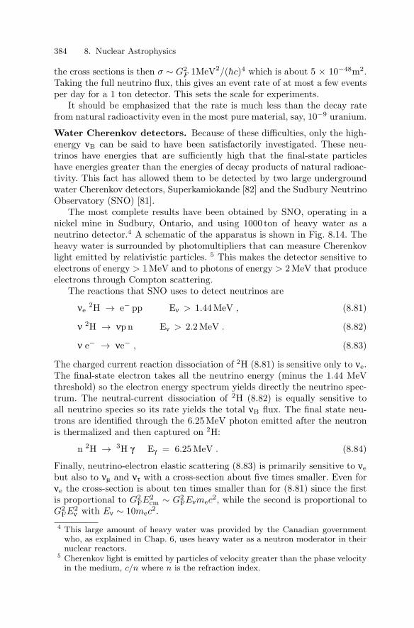
384 8. Nuclear Astrophysics
the cross sections is then σ ∼ G2F 1MeV2/(hc)4 which is about 5 × 10−48m2.
Taking the full neutrino flux, this gives an event rate of at most a few eventsper day for a 1 ton detector. This sets the scale for experiments.
It should be emphasized that the rate is much less than the decay ratefrom natural radioactivity even in the most pure material, say, 10−9 uranium.
Water Cherenkov detectors. Because of these difficulties, only the high-energy νB can be said to have been satisfactorily investigated. These neu-trinos have energies that are sufficiently high that the final-state particleshave energies greater than the energies of decay products of natural radioac-tivity. This fact has allowed them to be detected by two large undergroundwater Cherenkov detectors, Superkamiokande [82] and the Sudbury NeutrinoObservatory (SNO) [81].
The most complete results have been obtained by SNO, operating in anickel mine in Sudbury, Ontario, and using 1000 ton of heavy water as aneutrino detector.4 A schematic of the apparatus is shown in Fig. 8.14. Theheavy water is surrounded by photomultipliers that can measure Cherenkovlight emitted by relativistic particles. 5 This makes the detector sensitive toelectrons of energy > 1 MeV and to photons of energy > 2 MeV that produceelectrons through Compton scattering.
The reactions that SNO uses to detect neutrinos are
νe2H → e− pp Eν > 1.44 MeV , (8.81)
ν 2H → νp n Eν > 2.2 MeV . (8.82)
ν e− → νe− , (8.83)
The charged current reaction dissociation of 2H (8.81) is sensitive only to νe.The final-state electron takes all the neutrino energy (minus the 1.44 MeVthreshold) so the electron energy spectrum yields directly the neutrino spec-trum. The neutral-current dissociation of 2H (8.82) is equally sensitive toall neutrino species so its rate yields the total νB flux. The final state neu-trons are identified through the 6.25 MeV photon emitted after the neutronis thermalized and then captured on 2H:
n 2H → 3H γ Eγ = 6.25 MeV . (8.84)
Finally, neutrino-electron elastic scattering (8.83) is primarily sensitive to νebut also to νµ and ντ with a cross-section about five times smaller. Even forνe the cross-section is about ten times smaller than for (8.81) since the firstis proportional to G2
FE2cm ∼ G2
FEνmec2, while the second is proportional to
G2FE2
ν with Eν ∼ 10mec2.
4 This large amount of heavy water was provided by the Canadian governmentwho, as explained in Chap. 6, uses heavy water as a neutron moderator in theirnuclear reactors.
5 Cherenkov light is emitted by particles of velocity greater than the phase velocityin the medium, c/n where n is the refraction index.

8.4 Nuclear astronomy 385
heavy water
eν
ν
−Cherenkov
light
light water
photomultipliers
Fig. 8.14. A schematic of the Sudbury Neutrino Observatory (SNO) detector. Onekiloton of heavy water is observed by photomultipliers through a light-water shield.[The purpose of the shield is to prevent neutrons from entering the heavy waterand simulating the reaction (8.82).] Relativistic particles emit Cherenkov light thatis detected by the photomultipliers. The quantity of light is proportional to theenergy of the relativistic particles. The Cherenkov light is emitted in the forwarddirection so direction of the recoil electron can be determined from the pattern ofphotomultiplier hits.
The energy spectrum of SNO events is shown in Fig. 8.15 along with theexpectations for the three types of reactions. The angular distribution withrespect to the Sun in the figure shows the peaking in the forward directiondue to neutrino-electron elastic scattering. These events are forward peakedbecause the neutrino energy is much greater than the target mass so thecenter-of-mass moves forward in the laboratory. The angular distribution forcharged-current events show a small expected asymmetry due to the weak-interaction matrix element.
The rates for the three reactions allow one to deduce the flux of νB neu-trinos. The neutral-current reactions gives a total flux of [81]
φνe + φνµ + φντ = (6.42 ± 1.57 ± 0.58) × 106cm−2s−1 , (8.85)

386 8. Nuclear Astrophysics
−.5 0 .5 1.−−1.0
7 115 9 13
NC
CC
NC+CC+ES
NC+CC+ES
NCCC ES
cosθ
E(MeV)
160
120
80
40
Eve
nts
200
400
Eve
nts
Fig. 8.15. The SNO measurement of the solar-neutrino flux from 8B β-decay [81].Most events are due to the charged current (CC) reaction (8.81) and to the neutralcurrent (NC) reaction (8.82). The top figure shows the spectrum of event energyas measured by the quantity of Cherenkov light. The two solid curves show thedistributions expected for (8.81) and (8.82). The bottom figure shows the directionof recoil electrons with respect to the direction of the Sun. The peak at small anglesis due to neutrino-electron elastic scattering (ES), (8.83).

8.4 Nuclear astronomy 387
where the first and second errors are respectively statistical and systematic.This is in quite satisfactory agreement with the solar model predictions ofthe flux of νB of (5.0 ± 1.0) × 106 cm−2s−1.
The flux of νe as determined from the charged-current reaction is [81]
φνe = (1.76 ± 0.06 ± 0.09) × 106cm−2s−1 . (8.86)
As expected from the considerations of Chap. 4, the solar νe have been par-tially transformed into neutrinos of other species. The number transformedis consistent with that expected for the presently accepted neutrino massesand mixing angles (4.139).
The SNO results are consistent with those deduced using the data fromthe Super Kamiokande experiment [82]. This experiment is similar to SNObut uses only light water. As such it is sensitive to νB only through reaction(8.83) but has an enormous mass (20 kton) and thus has very small statisticalerrors.
Radiochemical detectors. Because of their low energy, the νpp and νBecannot be easily identified because electrons produced by such neutrinos can-not be distinguished from the β-decays due to natural radioactivity. Thesesolar neutrinos can, however be detected through neutrino absorption
νe (A, Z) → e− (A, Z + 1) ,
if the final-state nucleus can be identified. Generally the nucleus is chemi-cally separated from the target. For this reason, these experiments are calledradiochemical experiments.
The first such experiment was that of R. Davis and collaborators [83] whoused the reaction:
νe37Cl → e− 37Ar Q = −814 keV
The threshold for this reaction corresponding to the energy necessary toproduce the ground state of 37Ar is 814 keV. Because of this threshold, theexperiment is insensitive to νpp.
To interpret the Davis results, it is essential to remember that the 37Arnucleus can be produced in an excited state and it is necessary to knowthe cross-section for each state. The spectrum of states of 37Ar is shown inFig. 8.16. The νBe yield only the ground state of 37Ar. The cross-section forthis state can be deduced from the lifetime of 37Ar since the nuclear matrixelement is the same. The νB yield many excited states of 37Ar but luckily thenuclear matrix elements for these transitions can be accurately derived fromthe rates for the mirror decays 37Ca → 37K∗ e− νe [83].
The total absorption rate then depends on φBe, φB, and on φother (CNOand pep neutrinos). It is traditional to express the rate in “solar neutrinounits” or “SNU’s” (1 SNU = 10−36 events per target atom per second). Thecalculated rate is [73]:∫
φ(Eν)σ(Eν)dEν = [5.76 φB + 1.15 φBe + 0.7 φother ] SNU

388 8. Nuclear Astrophysics
where we have normalized the νe fluxes to those calculated by Bahcall [73]:φB ≡ φB/φB(Bahcall), etc. Since SNO has measured φB to be 0.35 ± 0.04,this gives∫
φ(Eν)σ(Eν)dEν = [2.01 + 1.15 φBe + 0.7 φother ] SNU
The rate measured with a chlorine detector can then be used to deduce theflux of νBe and the CNO/pep neutrinos. If these νe components are present,the rate should be about 4 SNU.
1/2+
5/2+
3/2+3/2+
3/2+1/2+
1/2+
5/2+3/2+3/2+3/2+3/2+
β+
(ν, e−)
K
Ca
37Cl
37Ar
37
37
3/2+
3/2+
3/2+
3/2+
20
10
0
E (
MeV
)
Fig. 8.16. The A = 37 nuclei. The states of 37Ar populated by neutrino absorp-tion on 37Cl are shown. The weak matrix elements for these transitions can bedetermined from the rates for the mirror decays of 37Ca to 37K.
The Homestake experiment in the Homestake gold mine of Lead, NorthDakota uses 600 tons of C2Cl6 as the neutrino target. It is shown schemat-ically in Fig, 8.17. It is contained in a large tank along with about 1 mg ofnon-radioactive argon “carrier.” After a three month exposure time, the car-rier and any 37Ar produced by solar neutrinos is extracted from the C2Cl6 bybubbling helium through the tank. The argon is then separated from the he-lium and trapped in a small proportional counter where the electron-capturedecays of the 37Ar (t1/2 = 37 day) are detected via their Auger electrons.
Over a 25 year period, the three month exposures have yielded, on averageabout six detected decays of 37Ar. After taking into account the detection

8.4 Nuclear astronomy 389
helium
C2Cl4
Argon trap
Fig. 8.17. The principle of the Homestake neutrino experiment. 37Ar atoms pro-duced by neutrino absorption are swept out the the C2Cl4 by bubbling helium gasthrough the liquid. The argon is then separated in a cold trap and introduced into asmall proportional counter where the electron-capture decays of 37Ar are observed
efficiency, this corresponds to 2.56±0.16 SNU [83]. Compared with the SNO-corrected standard model prediction of 4 SNU, this indicates that the νBe arealso strongly suppressed by neutrino oscillations and/or the MSW effect, asexpected for the estimated values of the neutrino masses and mixing angles(4.139).
Finally, two experiments, SAGE [85] and GALLEX [84], have observedsolar neutrinos via neutrino absorption on gallium:
νe71Ga → e− 71Ge
The threshold for this reaction is 233 keV, making the experiment sensitiveto all known sources of solar neutrinos. The νpp yield only the ground stateof 71Ge so the cross section can be calculated from the lifetime of 71Ge. TheνBe are also expected to yield primarily the ground state while the νB yielda multitude of excited states. The calculated rate is [73]∫
φ(Eν)σ(Eν)dEν =
[69.7 φpp + 34.2 φBe + 12.1 φB + 12φother ] SNU (8.87)
The coefficient in front of φB is accurate only to a factor two but this is ofno great importance in view of the small flux measured by SNO, φB = 0.35.
The gallium experiments follow rather closely the technique of the chlorineexperiment. The targets are in the form of a liquid (100 tons of GaCl3 forGALLEX and 60 tons of gallium metal for SAGE), and the volatile carrier(GeCl4) is extracted along with the produced 71Ge. The electron capture

390 8. Nuclear Astrophysics
decays of 71Ge (t1/2 = 11.43 day) are then observed in small proportionalcounters.
GALLEX and SAGE have measured rates of 75 ± 7 SNU. This suggestthat the majority of the νpp are present as νe, as expected for the presentestimates of the neutrinos masses and mixing angles (4.139).
Conclusions from solar neutrino detection. For many years, the inter-pretation of solar neutrino experiments was hampered by a lack of indepen-dent evidence for neutrino masses and oscillations. Now that the Kamlandreactor experiment [48] has seen neutrino oscillations, one has no hesitationto interpret the rates of solar experiments taking into account the MSWeffect and neutrino oscillations. This has lead to very precise tests of solarmodels. One recent paper makes the following comparison between measuredand calculated solar neutrino fluxes [86]
φ(pp)measured = (1.02 ± 0.02 ± 0.01) φ(pp)theory , (8.88)
φ(8B)measured = (0.88 ± 0.04 ± 0.23) φ(8B)theory , (8.89)
φ(7Be)measured = (0.91 +0.24−0.62 ± 0.11) φ(7Be)theory , (8.90)
where the first errors are observational and the second are theoretical. If theexcellent agreement between observation and theory survives future improvedmeasurement of neutrino oscillation parameters, it will confirm a triumph ofexperimental and theoretical nuclear astrophysics.
8.4.2 Supernova neutrinos
As explained in Sect. 8.2.3, massive stars may end their lives with a “core-collapse” supernova in which the 56Fe core collapses to a neutron star. Suchevents are powerful radiators of all species of neutrinos. The first to be cre-ated are “neutronization” νe from electron captures transforming protons toneutrons
e− (A, Z) → νe (A, Z − 1) . (8.91)
While these neutrinos are essential for the production of a neutron star,the most plentiful neutrinos come from purely thermal process that createneutrinos through reactions like
γ γ ↔ e+ e− ↔ ν ν . (8.92)
These reactions are due to the neutral currents and therefore produce allspecies of neutrinos. The proto-neutron star is so dense that the neutrinosdo not immediately escape, but rather diffuse out just like photons in normalstars, with the escape time given by (8.25)
τ ∼ 〈σ〉Nb
Rc, (8.93)

8.4 Nuclear astronomy 391
but now with σ given by the weak interactions rather than σT. Taking σ =10−45m2 and R ∼ 10 km, this gives τ ∼ 10 s.
Because their cross-section is so much smaller than that of photons im-plying a correspondingly shorter escape time, the energy evacuated duringthe collapse to a neutron star is almost entirely taken up by the neutrinos.The total energy was calculated as (8.68)
∆E ∼ (3/5)GM2
R∼ 3 × 1046 J M = 1.5 M . (8.94)
This energy is expected to be approximately equally divided among the 6types of neutrinos and antineutrinos.
The neutrinos are expected to have a roughly thermal distribution witha temperature equal to that of the “neutrinosphere,” the layer of materialwhere the neutrinos last scattered before escaping. Calculations give differenttemperatures for the different species:
kTνe ∼ 3.5 MeV kTνe ∼ 5 MeV kTν=νe,νe ∼ 8 MeV (8.95)
The mean energies are ∼ 3kT . The non-electron neutrinos and antineutri-nos have the highest temperature because they interact only through neu-tral current interactions. (Their energies are insufficient to create muons ortauons.) They therefore have the smallest cross-sections and therefore escapethe proto-neutron star from the deepest, hottest depth. The νe and νe havealso charged current interaction so they continue scatter to a greater distancefrom the center implying a smaller temperature. The νe have a higher cross-section than νe because νe charged-current scatter on the plentiful neutronswhile νe charged-current scatter on the rarer protons.
The νe from the core-collapse supernovae 1987a in the Large MagellanicCloud were observed by the Kamiokande [87] and IMB [88] experiments. Bothexperiments were kiloton-scale experiments similar to SNO (Fig. 8.14) exceptthat they contained only light water. (Kamiokande experiment was an earlierversion of Super-Kamiokande.) The supernova νe therefore scattered on thefree protons in the water through the reaction
νe p → e+ n . (8.96)
The final state positron creates Cherenkov light as in the SNO experiment.The energy of the νe is deduced from the quantity of light.
The 11 νe events observed by Kamioka and the 8 events by IMB over aperiod of 10 s on February 23, 1987 were sufficient to confirm the basic pictureof gravitational collapse with the evacuation of energy by neutrinos. Precisiontests of the scenario will require taking into account neutrino oscillations andthe MSW effect.
Further progress in the field of supernova-neutrino astronomy will be dif-ficult because the total rate of supernova in our galaxy and the nearby Mag-ellanic Clouds is believed to be about 2 per century. Present detectors arenot large enough to detect supernovae in more distant galaxies.

392 8. Nuclear Astrophysics
It would be very interesting to detect the non-νe components of the neu-trino spectrum. If SNO is still in operation, it will observe the νe componentthrough the reaction (8.81) and the other components through (8.82) and(8.83). Another recently suggested neutral-current detector [89] would use
ν p → ν p . (8.97)
The energy spectrum of the recoil protons would give information on the ντand νµ energy spectra.
8.4.3 γ-astronomy
γ-astronomy is a vast field that observes high-energy photons from a varietyof sources. Many deal with sources related to the production or propagationof cosmic rays. The recently discovered γ-ray bursts are now suspected to berelated in some way to gravitational-collapse events.
In the context of nuclear physics, the most interesting sources of γ-rays areradioactive nuclei produced in supernovae and then ejected into interstellarspace. Once the expanding cloud of matter becomes sufficiently dilute, itbecomes transparent of γ-rays so they become detectable.
Table 8.2 lists the radioactive nuclei that emit γ-rays that have a lifetimesufficiently long to be observed. Most are expected to come from supernovaebut some may be ejected in less violent “novae” that are thought to besuperficial explosions on white dwarfs acreting matter from a binary com-panion. Such novae favor the production of relatively low mass nuclei. Someradioactive nuclei are expected to be ejected through continuous mass lossby Wolf-Rayet (WR) and Asymptotic Giant Branch (AGB) stars.
The radioactive decays of the first three groups, A = 56, 57 and 44 arebelieved to be the major heating source in the expanding clouds aroundsupernovae. In fact, the luminosities of some supernovae are observed todecrease with the lifetimes of 56Co, then 57Co and the 44Ti. This is illustratedin Fig. 8.8. As long as the γ-rays are involved in heating the cloud, it cannotbe entirely transparent, so the expected flux is complicated to calculate.
As shown in Fig. 8.18, the 56Co γ-rays were observed from the remnantof SN1987a and 44Ti γ-rays from the supernova remnant Cas A. We see thatthe fluxes are just at the limit of detectability for these two nearby remnants.They nevertheless give strong evidence that radioactive nuclei are, indeed,ejected by supernovae. Another γ-ray that has been detected is that from 26Al(t1/2 = 7.17 × 10⁵ yr). Its long half-life means that its flux represents thecombined effects of many supernovae. Indeed, a diffuse flux of 26Al photonshas been detected throughout the galactic plane and gives constraints on therate of nucleosynthesis over the last 106 yr.
Gamma-ray observatories now in orbit, especially the INTEGRAL mis-sion, should greatly increase the amount of significant data available.

8.4 Nuclear astronomy 393
1000 1200 1400 1600
0
20
40
−20
E (keV)
820 840 860 880
−4
−2
2
4
6
0
E (keV)
phot
ons
cmfl
ux (
10−
5−
2 s−1 ke
V−1 )
Fig. 8.18. γ-ray spectra from supernova remnants. The top panel shows the 847 keVline (58Co) from SN1987A [90]. The bottom panel shows the 1157 keV line (44Ti)from the region Cas A [91]. This region is believed to be the remnant of a supernovathat exploded about 300 years ago.

394 8. Nuclear Astrophysics
Table 8.2. Radioactive nuclei giving rise to observable γ-rays. β-emitters with511 keV annihilation radiation are labeled with e+.
Decay t1/2 Eγ sites(keV)
56Ni → 56Co 6.077 day 158, 269, 480 supernovae56Co → 56Fe 77.27 day 847, 1238, e+ supernovae
57Ni → 57Co 35.60 hr 127, 1377, 1919 supernovae57Co → 57Fe 271.79 day 14, 122, 136 supernovae
44Ti → 44Sc 63 yr 68, 78, e+ supernovae44Sc → 44Ca 3.927 hr 1157, e+ supernovae
60Fe → 60Co 1.5 × 10⁶ yr supernovae, WR, AGB60Co → 60Ni 5.2714 yr 1173, 1332 supernovae, WR, AGB
26Al → 26Mg 7.17 × 10⁵ yr 1160 supernovae, novae,WR,AGB
7Be → 7Li 53.12 day 478 novae
22Na → 22Ne 2.6019 yr e+, 1274 novae
Bibliography
1. H. Karttunen, P. Kruger, H. Oja, M. Poutanen, K. Donner, FundamentalAstronomy, Springer, Berlin, 2003.
2. Hansen, Carl J., Kawaler, Steven D., Trimble, Virginia, Stellar Interiors,Springer, Berlin, 2004.
3. D. D. Clayton, Principles of Stellar Evolution and Nucleosynthesis, Uni-versity of Chicago Press, Chicago, 1983.
4. B. E. J. Pagel, Nucleosynthesis and Chemical Evolution of Galaxies,Cambridge University Press, Cambridge, 1997.
5. J. Audouze and S. Vauclair, An introduction to nuclear Astrophysics,Reidel, 1980.
6. D. Arnett, Supernovae and Nucleosynthesis, Princeton University Press,Princeton, 1996.
Exercises
8.1 Find a relation between the stellar temperature and density gradientsassuming that they are due to adiabatic convection of material between lower

Exercises for Chapter 8 395
and higher regions. Show that the photon–baryon density (∝ T 3/ρ) is propor-tional to ρ, consistent with Fig. 8.2 in the outer convective zone, r > 0.7R.
8.2 Poincare gave the following proof of the virial theorem, in the absenceof radiation pressure. Consider a self-gravitating system of N particles whosepotential energy is
φ = −G
N∑i=1
N∑j=i+1
mi mj
|ri − rj |where G is Newton’s constant. We denote by Ek the sum of kinetic energiesof the N particles.
The moment of inertia of this system with respect to its center of gravity,which we take as the origin of coordinates is I =
∑(mir
2i ) . Assuming that
the second derivative of I is zero, which is the case for quiet stars such as thesun, prove that one has
2Ek + φ = 0 hence E = −Ek =φ
2.
8.3 Calculate the energy liberated in the transformation of carbon andoxygen to 56Ni in a white dwarf of mass 1057mp. Compare this to the gravi-tational binding energy of the white dwarf.
8.4 Estimate the time of a neutrino of energy 10 MeV to escape from aneutron star.
8.5 The fundamental reaction in the sun can be written globally as
4p + 2e− →4 He + 2νe . (8.98)
The binding energy of 4He is −28.30 MeV. What is the energy release in thisreaction?
The total luminosity of the sun is L0 = 4 1023 kW. How many protonsare consumed per second by the reaction (1)?
In its present phase, since it was formed, the sun burns quietly with aconstant luminosity. Its mass is M = 2 1030 kg, 75% of which was initiallyhydrogen and 25% helium. Only 15% of the hydrogen can actually be burntin the reaction (1) in the solar core. For what length of time T can the sunburn before it becomes a red giant?
8.6 The binding energy of 3He is 7.72 MeV. Is the reaction pd → 3He + γexothermic? Is the inverse reaction possible in the core of a star like the sun?(The mean photon blackbody energy is ∼ 2.7kT with kT ∼ 1 keV.)

396 8. Nuclear Astrophysics
8.7 Consider a completely degenerate fermion gas. What is the equation ofstate P (n, T ) of the gas in, respectively, the non-relativistic and the rela-tivistic regimes. We call kTF the maximum energy of these fermions (TF isthe Fermi temperature), and pF their maximum momentum. What does thelimit T TF correspond to? What is the corresponding pressure? Comparethis pressure with the pressure of an ideal gas for a density n ∼ 1030cm−3
and a temperature T ∼ 107 K (for the ideal gas).We recall the virial theorem which relates the total internal energy U of a
star to its gravitational energy UG = −αGM2/R with α ∼ 1. A star is formedby gravitational contraction of a mass M of gas. How does the temperatureof an ideal gas evolve during that collapse? What happens when T ≥ 106K?(We recall that the mean temperature of the sun given by the virial theoremis 2 × 10⁶ K.)
Show that there exists a maximum temperature Tmax in the contractionif one takes into account the possibility that the electron gas becomes de-generate. Show that the electron gas becomes degenerate long before the iongas, so that the latter can be considered as an ideal gas.
If Tmax ≤ 106K, the star is called a brown dwarf. What is the peculiarityof such stars? What is the minimum mass of a star that does not become abrown dwarf?
How is the gravitational stability of a planet ensured? What is the differ-ence between a planet and a brown dwarf?
8.8 In a massive star at the end of its life, the fusion 28Si → 56Fe takes placein a shell around an iron core. The core is degenerate. What happens whenthe mass of the core increases because of the Si fusion?
What is the order of magnitude of the Fermi energy of electrons at thebeginning of the collapse? In what follows, we shall use
εF 3 MeV (ρ/109g cm−3) (8.99)
and ρ ∼ 109g cm−3) initially. If the electron capture reactions e− + (A, Z) →(A, Z− 1)+ νe are endothermic with Q ∼ a few MeV, why do these reactionstake place when ρ ≥ 1011g cm−3? Why don’t the inverse reactions take place?
Neutrinos interact with heavy nuclei in the core with a cross-section ofσ ∼ 10−42(Eν/1 MeV)2cm2.The radius of the core evolves as R ∼ 100 km (ρ/1012g cm−3)−1/3(M/M)1/3.Show that the neutrinos produced are trapped when ρ ≥ 1012g cm−3.
The diffusion time of neutrinos up to the “neutrinosphere ,” i.e. the regionwhere neutrinos cease to be coupled to matter is of the order of 1 − 10 sec.The temperature of the emitted neutrinos is T ∼ 5 MeV. Calculate thetotal energy Etot
ν carried away by the neutrinos, assuming neutronization iscomplete.
Assuming that the collapse ceases at a density of ρ ∼ 1014g cm−3, calcu-late the gravitational energy which is liberated, and compare it with Etot
ν .

9. Nuclear Cosmology
As discussed in the previous chapter, natural nuclear reactions are now mostlyconfined to stellar interiors. In the distant past, nuclear reactions are believedto have occurred throughout the Universe during the first few minutes af-ter the “Big Bang.” At this time the Universe was sufficiently hot that theCoulomb barrier could not prevent the fusion of nuclei.
We believe that the Universe went through such a hot epoch becausethe Universe is now expanding. By this we mean that the distances betweengalaxies are observed to be increasing with time. Specifically, galaxies areobserved to recede from us with a recession velocity, v, proportional to theirdistance R:
v = H0 R H0 = (70 ± 4)(km s−1) Mpc−1 , (9.1)
where we use the conventional astronomic distance unit, 1 pc = 3.085 ×10¹⁶ m. If the galactic velocities were constant in time, this would imply thatall galaxies were superimposed and the cosmological density infinite at a timein the past given by the Hubble time
tH ≡ H−10 = 1.4 × 10¹⁰ yr . (9.2)
Gravitational forces would be expected to make the galactic velocities time-dependent but the Hubble time nevertheless gives the order of magnitude ofwhat one calculates for the age of the Universe if the known laws of physics areused to extrapolate into the past. We do not know if such an extrapolation toinfinite density is justified but we can say with confidence that the expansionhas been proceeding at least since an epoch when the density was 45 ordersof magnitude greater than at present, with a temperature of kT > 1 GeV.Going backward in time, we would see stars and galaxies melt into a uniformplasma of elementary particles.
Under such conditions, reactions between elementary particles and nu-clei took place until the Universal expansion caused the temperature to dropto a level where the reactions cease because of the decreasing density andincreasing efficiency of the Coulomb barrier. It is believed the period of reac-tions lasted about 3 minutes, ending when the Universe had a temperatureof kT ∼ 40 keV and leaving a mixture of 75% 1H and 25% 4He (by mass).This mixture provided the initial conditions for stellar nucleosynthesis thatstarted once stars were formed some millions of years later.

398 9. Nuclear Cosmology
The job of primordial cosmology is to understand how this process pro-ceeded from the earliest possible moments. While we cannot say what existedat “the beginning” (if there was a beginning), we can extrapolate backward intime to temperatures of order 1 GeV when the Universe was believed to con-sist of a thermal plasma of relativistic quarks, antiquarks, gluons, neutrinosand photons. When the temperature dropped below a transition temperatureestimated to be kT ∼ 200 MeV, the quarks and antiquarks combined to formbound hadrons (mostly pions) which then, for the most part, annihilatedleaving nothing but photons and neutrinos. If there had been equal num-bers of quarks and antiquarks this would have been pretty much the end ofthe story. However, the small excess of order 10−9 of quarks over antiquarksmeant that a small number nucleons remained at T ∼ 100 MeV, of order10−9 with respect to the photons and neutrinos. This was the initial condi-tion for cosmological nucleosynthesis that came about when some nucleonslater combined (kT ∼ 40 keV) to form nuclei.
The process of cosmological nucleosynthesis differs from that of stellarnucleosynthesis in several important respects. Among them are
• The presence of neutrons. Because of the lack of neutrons in stars, stellarnucleosynthesis must start with the weak reaction 21H → 2He+νe. Cosmo-logical nucleosynthesis starts with an abundant supply of neutrons whichneed only combine with protons to form nuclei, starting with the reactionn p → 2Hγ.
• A low baryon–photon ratio. Whereas the baryon to photon ratio in starsis greater than unity (∼ 103 for the sun, Fig. 8.2), it is of order 5×10⁻⁹ inthe primordial Universe. This has the important consequence of delayingnucleosynthesis since the abundant photons quickly dissociate any nucleithat are produced until the temperature drops to ∼ 100 keV at whichpoint the probability of a thermal photon having sufficient energy to breaka nucleus becomes small enough.
• A low baryon–neutrino ratio, nearly equal to the baryon–photon ratio.This was important during the time when most nucleons were free sinceweak reactions like νen ↔ e−p can change neutrons into protons and viceversa. In fact, for kT > 800 keV it turns out that these reactions are suf-ficiently rapid that they can maintain a “chemical” equilibrium betweenthe neutrons and protons so that the neutron to proton ration takes thethermal value of exp(−(mn − mp)c2/kT ). The weak interaction rate dropsto negligible values at a temperature of around 800 keV when the neutronto proton ratio is about 0.2. Free neutron decay then lowers the ratio toabout 0.1 when nucleosynthesis starts at kT ∼ 100 keV. The proton excessresults in a large quantity of post-nucleosynthesis 1H.
• A limited amount of time. The elapsed time from the quark–gluon phasetransition to the end of cosmological nucleosynthesis is about three min-utes. Below temperatures of ∼ 60 keV, the Coulomb barrier prevents fur-

9.1 The Universe today 399
ther reactions, leaving the primordial mixture of 75% hydrogen and 25%4He.
In this chapter we provide a basic introduction to this process. Section 9.1summarizes what is believed to be the present state of the observable Universeand sec. 9.2 discusses how this state evolves as the Universe expands. Section9.3 shows how the universal expansion is governed by gravity. Section 9.5discusses the basic physics that governs the particle and nuclear reactionsin the primordial Universe and the following sections apply this physics toelectrons, neutrons, nuclei and some more speculative elementary particlesthat may have played an important role in cosmology.
9.1 The Universe today
When averaged over large volumes containing many galaxies, the observableUniverse is believed to have the following characteristics:
• A tiny density, ρ ∼ 10−26 kg m−3, and starlight output, J ∼ 10−39 W m−3;• A curious “chemical” composition (Table 9.1) with most particles being
cold photons or neutrinos and most mass being in the form of ordinary“baryonic” matter (protons and nuclei plus electrons), and not-so-ordinary“cold dark matter” (CDM). Most of the energy is in the form of an effectivevacuum energy or, equivalently, a cosmological constant.
• A non-equilibrium thermal state characterized by a deficit of highly-boundheavy nuclei.
• A hierarchy of gravitationally bound structures ranging from planets andstars to galaxies and clusters of galaxies.
In this section, we will review the major components of the Universe listedin Table 9.1. It will be convenient to express the mean densities in units ofthe “critical density”
ρc =3H2
0
8πG(9.3)
where H0 is the “Hubble constant”
H0 = (70 ± 4)km sec−1 Mpc−1 (9.4)
The physical significance of the critical density and the Hubble constant willbe discussed in the next section but here we note only the very low value ofρc:
ρc = 0.92 h270 × 10−26 kg m−3 (9.5)
= 1.4 h270 × 1011M Mpc−3 = 0.51 h2
70 × 1010 eV m−3 . (9.6)
where the reduced Hubble constant is h70 = H0/70 km sec−1 Mpc−1.

400 9. Nuclear Cosmology
Table 9.1. The known and suspected occupants of the Universe. For each species,i, the table gives estimated number density of particles, ni, and the estimatedmass or energy density, Ωi = ρi/ρc, normalized to the “critical density,” ρc =(0.92±0.08)×10−26 kg m−3. Other than the photon density taken from the COBEdata [92], the numbers are taken from the global fit of cosmological parameters bythe WMAP collaboration [94]. The lower limit on the neutrino density comes fromthe oscillation data of [49].
species ni (m−3) Ωi = ρi/ρc
γ (CBR) nγ = (4.104 ± 0.009) × 108 Ωγ = (5.06 ± 0.4) × 10−5
Tγ = (2.725 ± 0.002) K
νe, νµ, ντ nν = (3/11)nγ 0.0006 < Ων < 0.015(per species)
baryons nb ∼ 0.25 ± 0.01 Ωb = (0.044 ± 0.004)
cold dark nχ = ρCDM/mχ ΩCDM = 0.226 ± 0.04matter (mχ unknown)
“vacuum” 0 ΩΛ ∼ 0.73 ± 0.04
total ΩT ∼ 1.02 ± 0.02
9.1.1 The visible Universe
The “building blocks” of the visible Universe are galaxies which are them-selves composed of stars, interstellar gas, and unidentified dark matter.Galaxies have a wide variety of shapes (spirals, ellipticals and irregulars),masses, and luminosities. Nevertheless, most of the light in the Universe isproduced in galaxies containing 1010 to 1011 stars that generate a typicalgalactic luminosity of
〈Lgal〉 ∼ 2 × 10¹⁰L , (9.7)
where L is the solar luminosity, L = 2.4 × 1045 eV s−1. The mass of thevisible matter in a galaxy is typically
〈Mgal〉 ∼ 4 × 10¹⁰M , (9.8)
Galaxies are not uniformly distributed in space, a fact that is not sur-prising in view of their mutual gravitational attraction. Galaxies are oftengrouped in bound clusters, the largest of which contain thousands of galax-ies. In spite of this “small-scale” inhomogeneity, at large scales > 100 Mpcthe Universe appears to be uniform with a number density of visible galaxiesof
ngal ∼ 0.005 Mpc−3 (9.9)

9.1 The Universe today 401
corresponding to a typical intergalactic distance of ∼ 6 Mpc. The total massdensity ρvis associated with the “visible” parts of galaxies is
ρvis = 〈Mgal〉 ngal ∼ 3 × 10⁸ M Mpc−3 . (9.10)
The density of visible matter (9.10) divided by ρc gives
Ωvis ≡ ρvis
ρc∼ 0.002 (9.11)
9.1.2 Baryons
The total density of ordinary “baryonic matter” (protons, nuclei and elec-trons) is estimated to be an order of magnitude greater than that of visiblebaryons (9.11):
Ωb = 0.044 ± 0.004 . (9.12)
This estimate came originally from the theory of the nucleosynthesis of thelight elements which correctly predicts the relative abundances of the lightelements only if Ωb is near this value.
Since Ωb > Ωvis one can wonder where the missing “dark” baryons are.Most of them are thought to be in the intergalactic medium in the form ofan ionized gas [98]. Some fraction of them may be in dark compact objectssuch as dead stars (neutron stars or white dwarfs) or stars too light to burnhydrogen (brown dwarfs). It has also been suggested [99] that a significantfraction of the baryons are contained in cold molecular clouds.
Finally, we mention that there are apparently very few antibaryons in thevisible Universe [100]. Any antimatter consisting of antibaryons and positronswould quickly annihilate in collisions with ordinary matter. Even if the anti-matter were somehow separated from the matter, annihilations in intergalac-tic space at the boundaries between matter and antimatter domains wouldlead to a flux of high-energy annihilation photons. It thus seems probablethat the density of antimatter is extremely small within the accessible partof the Universe.
9.1.3 Cold dark matter
About 90% of the matter in galaxies and clusters of galaxies is not visible.Structure formation theories suggest that the invisible “dark matter” is “colddark matter,” i.e. non-relativistic matter that has only weak interactionswith baryonic matter and photons. Often, it is assumed to be in the form ofnonbaryonic weakly interacting massive particles called generically “wimps.”The present density of CDM is estimated to be an order of magnitude greaterthan that of baryons but still less than critical
ΩCDM = 0.226 ± 0.04 . (9.13)

402 9. Nuclear Cosmology
This dark matter is believed to make up most of the mass of galactic halosand galaxy clusters.
Unfortunately, there are no wimps in the zoo of known elementary parti-cles and their existence is a bold prediction of cosmology. Some extensions ofthe standard model of particle physics predict the existence of wimps that aresufficiently heavy that they would not yet have been produced at accelerators.For example, a class of models that predict the existence of wimps are “su-persymmetric” models. In these models, each of the known fermions (bosons)is paired with a heavy supersymmetric partner that is a boson (fermion). Thelightest of the supersymmetric partners (LSP) is expected to be stable andto have only weak interactions, making it an ideal wimp candidate. In Sect.9.8 we will see that the parameters of the supersymmetric model can be cho-sen so that the wimp has the required present-day density (9.13). The masswould be expected to be between 10 GeV and 10 TeV. Efforts are underwayto produce supersymmetric particles at accelerators and to detect them inthe Milky Way (Exercises 9.7).
9.1.4 Photons
The most abundant particles in the Universe are the photons of the “cosmic(microwave) background radiation” (CBR) (also referred to in the litera-ture as “CMB” for “Cosmic Microwave Background”). These photons havea nearly perfect thermal spectrum as shown in Fig. 9.1. The photon temper-ature is
Tγ = 2.725 K ⇒ kT = 2.35 × 10⁻⁴ eV (9.14)
corresponding to a number density of
nγ = 410.4 cm−3 . (9.15)
This is considerably greater than the number of photons that have beengenerated by stars (Exercise 9.1). Despite their great abundance, the lowtemperature of the CBR results in a small photon energy density, ργ ∼ nγkT :
Ωγ = (5.06 ± 0.4) × 10−5 . (9.16)
The present-day Universe is nearly transparent to photons (Exercise 9.2)in the sense that the photon mean free path is greater than the distance tothe most distant visible objects. The CBR photons were thermalized in theearly Universe when the temperature was > 0.26 eV and baryonic matter wascompletely ionized. At T ∼ 0.26 eV, baryonic matter “recombined” to formatoms and the resulting decrease in the photon–matter cross-section madethe Universe transparent.
The CBR temperature is not completely isotropic but is observed to varyby factors of order 10−5 according to the direction of observation. These smallvariations are believed to be due to the density inhomogeneities present atthe moment of recombination. As such, the temperature anisotropies provide

9.1 The Universe today 403
10−17
10−18
10−19
10−20
10−21
10−22
101 100 1000
10 1.0 0.1Wavelength (cm)
Frequency (GHz)
FIRAS
DMR
UBC
LBL-Italy
Princeton
Cyanogen
COBE satellite
COBE satellite
sounding rocket
White Mt. & South Pole
ground & balloon
optical
2.73 K blackbody
I ν
(W m
−2 s
r−1 H
z−1
)
Fig. 9.1. The observed spectrum of the cosmic (microwave) background radiation(CBR) [1]. The points at wavelengths < 1 cm come from ground-based experiments.At shorter wavelengths the Earth’s atmosphere is opaque and measurements mustbe made from balloons, rockets or satellites. The high precision points around thepeak of the spectrum were made by the FIRAS instrument of the COBE satellitewhich observed from 1989 to 1995 [92]. Compilation courtesy of the Particle DataGroup.
information about the “initial conditions” for structure formation. The spec-trum of anisotropies is the primary source on the values of the cosmologicaldensities in Table 9.1. In particular, it constrains ΩT to be very near unity.
9.1.5 Neutrinos
In addition to thermal photons, it is believed that the Universe is filled withneutrinos, νe, νµ and ντ and the corresponding antineutrinos.
Neutrinos interact even less than the CBR photons but they had a suffi-ciently high interaction rate at T > 1 MeV to have been thermalized. In Sect.9.6 we will see that by the time the temperature dropped below kT ∼ mec
2,relativistic neutrinos had a temperature slightly less than the photon tem-perature:
Tν = (4/11)1/3 Tγ . (9.17)
This corresponds to a neutrino (+ antineutrino) number density of

404 9. Nuclear Cosmology
nν = (3/11)nγ per species. (9.18)
corresponding to a present day value of 112 cm−3.The present-day energy density of a neutrino species depends on its mass.
For a massless species, the temperature relation (9.17) would continue tohold today and consequently the energy density would be a bit less thanthat for photons (9.16). This would be approximately true for any neutrinospecies with mass much less than the photon temperature, mνc
2 kTγ ∼2 × 10⁻⁴eV.
For a species of mass greater than the temperature, the neutrinos arecurrently non-relativistic and the summed neutrino and antineutrino massdensity is
Ων =mνnν
ρc= 0.2 h−2
70mν
10 eVif mν 10−4 eV . (9.19)
If one of the neutrinos had a mass > 0.7 eV, it would significantly distortthe observed spectrum of CBR anisotropies. Requiring mν < 0.7 eV gives theupper limit in Table 9.1, Ων < 0.015 [94].
Evidence for non-zero neutrino masses comes from searches for neutrinooscillations discussed in Sect. 4.4. In particular, oscillations of neutrinos pro-duced in the atmospheric interactions of cosmic rays [49] have given resultsthat are most easily interpreted as
(m23 − m2
2)c4 = (3 ± 1) × 10−3 eV2 ⇒ m3 > 0.04 eV , (9.20)
where m3 is the heaviest of the three neutrinos. This implies:
Ων ∼ nνm3
ρc> 0.0006 . (9.21)
It is often supposed that neutrinos have a “hierarchical” mass pattern likethat of the charged leptons, i.e. m3 m2 m1. If this is the case, the aboveinequality becomes an approximate equality, m3 ∼ 0.04 eV. It is not possible,for the moment, to directly verify this hypothesis.
Finally, we note that, because of their extremely weak interactions, thereis little hope of directly detecting the cosmic neutrino background [101].
9.1.6 The vacuum
Perhaps the most surprising recent discovery is that the Universe appears tobe dominated by an apparent “vacuum energy” or “cosmological constant”Λ:
ΩΛ ∼ Λ
3H20
∼ 0.7 . (9.22)
The observational evidence for the existence of vacuum energy involves theapparent luminosity of high redshift objects which can provide informationon whether the universal expansion is accelerating or decelerating (as would

9.2 The expansion of the Universe 405
be expected from normal gravitation). The observations indicate that theexpansion is accelerating and, as we will see in Sec. 9.3, this can be explainedby a positive vacuum energy density.
Vacuum energy is, by definition, energy that is not associated with par-ticles and is therefore not diluted by the expansion of the Universe. Unlessthe present vacuum is only metastable, this implies the the vacuum energydensity is independent of time. The value implied by ΩΛ = 0.7 is
ρΛ(t) ∼ 3 h270 × 109 eV m−3 . (9.23)
Fundamental physics cannot currently be used to calculate the value of thevacuum energy even though it is a concept used throughout modern gaugetheories of particle physics. It is expected to be a temperature-dependentquantity which changes in a calculable manner during phase transitions, e.g.the electroweak transition at T ∼ 300 GeV when the intermediate vectorbosons, W± and Z0, became massive. While the vacuum energy does notchange in particle collisions, so its existence can usually be ignored, it doeslead to certain observable effects like the Casimir force between unchargedconductors. Unfortunately, all calculable quantities involving vacuum energyconcern differences in energy densities and there are no good ideas on howto calculate the absolute value.
Despite the lack of ideas, the existence of a vacuum energy density of themagnitude given by (9.23) is especially surprising. A vacuum energy densitycan be associated with a “mass scale” M by writing
ρΛ ∼ (Mc2)4
(hc)3. (9.24)
Particle physicists are tempted to choose the Planck mass
mplc2 = (hc5/G)1/2 ∼ 1019 GeV (9.25)
as the most fundamental scale since it is the only mass that can be formedfrom the fundamental constants. This gives ρΛ ∼ 3× 10132 eV m−3, i.e about123 orders of magnitude too large making it perhaps the worst guess in thehistory of physics. In fact, the density (9.23) implies a scale of M ∼ 10−3 eVwhich is not obviously associated with any other fundamental scale in particlephysics, though it is near the estimated masses of the neutrinos.
A second problem with an energy density (9.22) is that it is comparableto the matter density ΩM ∼ 0.3. Since the matter density changes withthe expansion of the Universe while the vacuum energy does not, it appearsthat we live in a special epoch when the two energies are comparable. Thiscoincidence merits an explanation.
9.2 The expansion of the Universe
Modern cosmology started with Hubble’s discovery that galaxies are recedingfrom us with a velocity dR/dt proportional to their distance R (Fig. 9.2) :

406 9. Nuclear Cosmology
Fig. 9.2. The “Hubble diagram,” of galactic recession velocities versus distance fora set of galaxy clusters as determined by the Hubble Key Project [97]. The slopeof the line is the Hubble constant H0. The velocities are determined by the galaxyredshifts and the distances are determined by a variety of methods. For example,if a supernova of known luminosity L is observed in a galaxy or galaxy cluster, thedistance can be derived from the observed photon flux φ = L/4πR2.
dR
dt= H0 R . (9.26)
The factor of proportionality, H0, is called the Hubble constant.1 In estab-lishing Hubble’s law, the velocity dR/dt is derived from the “redshifts” of agalaxy’s photon spectrum:
1 + z ≡ λ0
λ1∼ 1 + v/c , (9.27)
where λ1 is the wavelength of photons emitted by the galaxy and λ0 is thewavelength measured later by us. The equivalence of the redshift z withv/c = (dR/dt)/c is the non-relativistic Doppler effect. As such, the formulais valid only for z << 1, which, according to Hubble’s law, corresponds toR << c/H0 ∼ 4300Mpc. A more general interpretation is given below (9.36).
1 In writing (9.26), we ignore the quasi-random “peculiar” velocities vp that aretypically of order vp ∼ 10−3c ∼ 300 km s−1. These are smaller than the Hubblevelocity H0R for R > 300 km s−1/H0 ∼ 5 Mpc.

9.2 The expansion of the Universe 407
Because photon wavelengths appear2 to increase with time, photon ener-gies (Eγ = hc/λγ) decrease with time. The energy loss between emission in agalaxy of redshift z = H0R/c and reception by us is
E1 − E0 = hc(λ−11 − λ−1
0 ) = E0[(λ0/λ1) − 1] ∼ E0z . (9.28)
Since the time to travel a distance R is R/c = z/H0, we have
dEγ
dt= −H0Eγ . (9.29)
CBR photons are not different from photons emitted by galaxies, so thesephotons must lose energy at the same rate. This implies that the cosmologicalphoton temperature decreases with time at a rate that is currently given by
dTγ
dt= −H0Tγ . (9.30)
9.2.1 The scale factor a(t)
It is useful to parameterize the expansion of the Universe by a time-dependentfunction that is proportional to the distances between galaxies. This functionis called the “scale factor,” a(t):
a(t) ∝ 〈intergalactic distances〉 . (9.31)
The normalization of a(t) can be taken to be arbitrary but we call its valuetoday
a(t0) ≡ a0 t0 ≡ today . (9.32)
Hubble’s law (9.26), R/R = H0 informs us that the logarithmic derivative ofa(t) is currently equal to H0:[
a
a
]t0
= H0 . (9.33)
Substituting this into (9.29) or (9.30) and generalizing to an arbitrary timewe get
dEγ
da= −Eγ
a
dTγ
da= −Tγ
a. (9.34)
This then says that the energies of photons or their temperature fall simplywith the scale parameters:
Eγ ∝ a−1 Tγ ∝ a−1 . (9.35)
The photon temperature can therefore be used to define the scale parameter.2 We say “appear” because the photon changes Galilean reference frames as it
travels from galaxy to galaxy. The observer that measures the original highenergy is in a different reference frame from the observer who later measures theredshifted energy.

408 9. Nuclear Cosmology
Relation (9.35) applied to photons emitted by galaxies implies a moregeneral interpretation of the galactic redshifts:
1 + z ≡ λ0
λ1=
a(t0)a(t1)
, (9.36)
where t1 is the time of emission. The redshift of photons coming from agalaxy of redshift z then gives the factor of expansion of the Universe betweenemission and detection.
The scale parameter also determines the time dependences of numberdensities of objects whose numbers are conserved. For example, the numberdensity of galaxies ngal is proportional to 〈distances〉−3 so, if the number ofgalaxies does not change with time, we have
ngal(t) = ngal(t0)(
a0
a(t)
)3
. (9.37)
While the number density of galaxies is, in fact, not conserved (there werenone in the early Universe), baryon number is conserved to good approxima-tion so we have
nb(a) = nb(a0)(
a0
a(t)
)3
. (9.38)
This dependence on a is also respected by any species of particles whosenumber does not vary with time. Hence, we expect the number density ofcold dark matter particles and photons of cosmological origin to fall like a−3.
The energy densities in the Universe as a function of time can also besimply expressed in terms of the scale factor. The energy density of non-relativistic particles like baryons and CDM particles is proportional to thenumber density of particles times their mass. It follows that
ρCDM(t) + ρb(t) ≡ ρM(t) = ρM(t0)(
a0
a(t)
)3
. (9.39)
On the other hand, the energy per photon falls like a−1 which implies anextra factor of a−1 in addition to the three factors associated with the fallingnumber density:
ργ(a) = ργ(a0)(
a0
a(t)
)4
. (9.40)
Finally, we need to know how the vacuum energy density, ρΛ, evolves withthe expansion of the Universe. The evolution of the matter density is due tothe changing density of particles as the Universe expands. Since there are,by definition, no particles associated with the vacuum energy, it seems plau-sible that the vacuum energy density will remain unchanged as the Universeevolves:
ρΛ(a) = ρΛ(a0) . (9.41)

9.2 The expansion of the Universe 409
This behavior is confirmed by an analysis using general relativity.Since the density of relativistic matter (9.40) is proportional to a−4 while
that of non-relativistic matter (9.39) is proportional to a−3, relativistic mat-ter must come to dominate for a → 0. Equating the two energy densities wefind the moment when the photon and matter densities are equal occurredwhen the scale parameter took the value
aeq
a0=
Ωγ
ΩM∼ 2 × 10⁻⁴ , (9.42)
corresponding to a temperature of
kTeq ∼ 1 eV . (9.43)
For temperatures higher than this, radiation dominates the energy of theUniverse.
Since the matter density falls like a−3, the future Universe will be increas-ingly dominated by the constant vacuum energy (if it is truly constant).
We see that the Universe passes through a succession of epochs whenthe energy density is dominated by radiation, by non-relativistic matter, andthen by vacuum energy. The energy densities as a function of temperatureare shown in Fig. 9.3.
In Table 9.2, we list some formative events in the history of the Uni-verse according to this scenario. Non-controversial physics allows us to followwith confidence the succession of events starting at, say, T ∼ 1 GeV whenthe Universe was a nearly homogeneous soup of quarks, gluons, and lep-tons. With time, the Universe cooled and a succession of bound states wereformed, hadrons, nuclei, atoms, and finally the gravitationally bound starsand galaxies. The moments of the formation of bound states are called “re-combinations.” The recombination that resulted in the formation of atomscaused the Universe to become effectively transparent to photons.
We should add that the nature of the radiation changed with temperature.Today, the radiation consists of photons and, perhaps, relativistic neutrinos.At temperatures T > me, electron–positron pairs could be produced and wewill show in Sec. 9.6 that these pairs were in thermal equilibrium with thephotons and formed a blackbody spectrum similar to that of the photonsand neutrinos. Going back in time, each time the temperature rose abovea particle-antiparticle threshold, a new blackbody component was created.During this period, the numbers of particles and antiparticles were nearlyequal. The small number of electrons and baryons present today resultedfrom the small excess (∼ 10−9) of particles over antiparticles present whenT me.
Finally, we note that the two earliest epochs in Table 9.2, those of baryo-genesis and inflation, are speculative and involve physics that is not well-understood. The existence of these epochs is postulated to solve certainmysteries in the standard scenario, e.g. the existence of the small particle-

410 9. Nuclear Cosmology
antiparticle asymmetry and the origin of the density fluctuations leading tostructure formation.
9.3 Gravitation and the Friedmann equation
While the temperature of the Universe T ∝ 1/a is simply determined by thescale parameter a(t), in order to calculate the end product of cosmologicalparticle or nuclear reactions, we will need to know how long the Universespends near a given temperature, i.e. we need to know the time dependenceof a(t).
In the absence of gravitation, the recession velocities of galaxies wouldbe constant, implying a = 0. In the presence of the attractive effects ofgravitation, we might expect that the expansion would be decelerated, a < 0.
The correct equation for a can only be found within the framework of arelativistic theory of gravitation, i.e. general relativity. The standard Newto-nian formalism is inadequate for two reasons. First, the Newtonian integrals
GUT epoch
Log
ρ(e
V m
−3)
−25
0
25
50
75
100
125
25 20 15 10
nucleosynthesis
ρ
ρΛ
R
5 0 −5 −10
LogT (eV)
recombination
today
equalitymatter−radiation
Mρ
Fig. 9.3. The energy density of matter, radiation and vacuum (assumed constant)as a function of temperature. The temperature scale starts at the expected “grandunification” scale of ∼ 1016 GeV. We suppose that the CDM particles have massesgreater than ∼ 10 GeV so the line of ρM starts at 10 GeV.

9.3 Gravitation and the Friedmann equation 411
Table 9.2. Some formative events in the past. The values of t0, trec, and teq dependon (h70, ΩM, ΩΛ) and we have used (1, 0.3, 0.7).
t kTγ (eV) event
t0 ∼ 1.5 × 10¹⁰ yr 2.349 × 10⁻⁴ today
∼ 109 yr ∼ 10−3 formation of the first structures,
trec ∼ 5 × 10⁵ yr 0.26 “recombination” (formation of atoms),Universe becomes transparent
teq ∼ 5 × 10⁴ yr 0.8 matter-radiation equality
3 min 6 × 10⁴ nucleosynthesis (formation of light nuclei,A = 2, 3, 4, 6, 7)
1 s 106 e+e− → γγ
4 × 10⁻⁶ s ∼ 4 × 10⁸ QCD phase transition (formation ofhadrons from quarks and gluons)
< 4 × 10⁻⁶ s > 109 baryogenesis (?) (generation of baryon–antibaryon asymmetry)
inflation (?)(generation of density fluctuations)
used to calculate the force on a particle or the gravitational potential at aparticular point are not defined in an infinite medium of uniform density.Second, the source of Newtonian gravitation is the mass density. We canexpect that a relativistic theory will have a more general source, just as inelectromagnetism both charge densities and charge currents can lead to fields.
General relativity treats gravitation geometrically. One way of approach-ing the problem is is illustrated in Fig. 9.4. The figure shows a small regionof a two-dimensional homogeneous Universe with a coordinate grid attachedto free test particles (galaxies). The test particles are initially equally spaced,as determined by light propagation times between galaxies. With this choice,over a small region, the distance dS between test particles separated by co-ordinate differences (dx,dy) is just
dS2 = dx2 + dy2 . (9.44)
As the Universe expands, the test particles withdraw from each other.Compared to the original situation, all intergalactic distances are multipliedby a scale factor a(t). It is convenient to keep the coordinates of the galax-ies constant during the expansion, as shown in Fig. 9.4. Such coordinates

412 9. Nuclear Cosmology
are called “comoving” coordinates. Since the coordinate separations do notchange with time, at a later time t the relation between dS and the coordinatedifferences is given by
dS2 = = a(t)2 (dx2 + dy2) . (9.45)
For this homogeneous Universe, all the effects of gravity should be stored inthe geometric scale factor a(t). The equations of general relativity will tell ushow a(t) evolves with time.
dS2=dx +dy
2 2
dS2
=a(t)2(dx2+dy2)
Fig. 9.4. A small region of a homogeneous two-dimensional Universe. A coordinategrid has lines of constant x and y that intersect at equally spaced test particles(galaxies). As the Universe expands, the distances dS between galaxies increases [bya factor a(t)], but we choose to keep the coordinates of the galaxies fixed (comovingcoordinates).
We note that the geometrization of gravitation is possible only becauseof the Principle of Equivalence which insures that gravity affects all testparticles in the same way, independent of their mass and composition. Thismeans that if, in Fig 9.4 we place two test particles at the same point withvanishing relative velocity, then in the future they will stay at the same point.If this were not the case, then the expansion of the coordinate grid would notbe unique.

9.3 Gravitation and the Friedmann equation 413
We also note that the equations of general relativity for a homogeneousUniverse will be simple because the coordinate grid can be described by onefunction a(t). In an inhomogeneous Universe, the situation is much morecomplicated, as illustrated in Fig. 9.5. In the figure we have supposed thatthere is an excess of mass in the center of the figure. The gravitational at-traction of matter to this excess will cause the test particles to expand ina non-uniform manner. Even if the coordinate system is simple at the be-ginning, it will evolve into a complicated system with distances between testparticles defined by three metric functions
dS2 = = gxx(t, x, y)dx2 + gxy(t, x, y)dxdy + gyy(t, x, y)dy2 . (9.46)
We now have 3 functions of position and time to describe the coordinatesystem. The three functions gxx, gxy and gyy define the (spatial) metric ofthe coordinate system. The equations that govern the metric can be quitecomplicated.
dS2=dx +dy
2 2
dS2=gxxdx2 2dyyy+gdxdyxy+2g
Fig. 9.5. Same as Fig. 9.4 but with a mass excess near the center of the region.The excess gravity causes the test particles to separate less rapidly near the centerthan in the homogeneous case. The resulting formula for dS is more complicated.
Fortunately for us, the metric of a homogeneous Universe is described byonly one function a(t) and we can expect the Einstein equation to be simple.It turns out to be

414 9. Nuclear Cosmology
a
a=
−4πG
3c2 (ρ + 3p) , (9.47)
where ρ is the energy density and p is the “pressure.” As expected, a positiveenergy density ρ > 0 works to decelerate the Universe. In fact, the part of ther.h.s. that is proportional to ρ can be guessed through a simple Newtonianargument, as shown in Exercise 9.4. On the other hand, the appearance ofa correction proportional to the pressure p is surprising, especially since apositive pressure also works to decelerate the Universe, out of line with ourintuition of thermal pressure encouraging the expansion of a gas. This ishowever not the role of the pressure in the gravitational context where it actsas a source of gravitation that is normally ignored in Newtonian problems.To see why it can often be ignored, we note that for a collection of particles(number density n), the pressure can be defined to be proportional to themean value of |p|2c2/3E:
p ≡ n〈|p|2c2/3E〉 . (9.48)
For instance, for a thermal collection of nonrelativistic particles of mass m,the energy density is ρ = mc2n and the pressure is given by
p = n〈(|p|c)2/3E〉 = nkT , (9.49)
where we have used 〈|p|2/2m〉 = (3/2)kT . This value of the pressure is justthat of the ideal gas law. Because kT mc2 for a non-relativistic gas, thisshows that the relativistic correction is small. On the other hand, for a rela-tivistic gas (|p|c ∼ E) we have
p = n〈(|p|c)2/3E〉 = ρ/3 . (9.50)
An example of such a gas is the cosmic (photon) background radiation. Forsuch a gas, the relativistic correction proportional to the pressure is large anddoubles the deceleration rate.
In an adiabatic expansion, the volume and energy of a gas change accord-ing to the law dE = −pdV . This suggests that in a cosmological context thepressure can be defined by the way that the energy density changes as theUniverse expands:
p = −dρa3
da3 . (9.51)
Using the laws (9.39) and (9.40) for the evolution of the energy density, wesee that (9.51) implies that, as expected, p = 0 for a non-relativistic gas andp = ρ/3 for a relativistic gas. On the other hand, the fact that the vacuumenergy density is constant (9.41) implies that for vacuum energy we have
p = −ρ vacuum . (9.52)
A negative pressure is perhaps counter intuitive but we should not forget thatour intuition for pressure is based on the pressure of collections of particleswhereas the vacuum is the absence of particles.

9.3 Gravitation and the Friedmann equation 415
The solution a(t) of (9.47)with the pressure (9.51) is
a2 =[8πGρ
3c2
]a2 + const .
To evaluate the constant we use the present values a(t0) = H0a0 and8πGρ(t0)/3c2 = H2
0ΩT to find
a2 =8πGρa2
3c2 + H20a2
0(1 − ΩT) . (9.53)
Dividing (9.53) by a2 we find the “Friedmann equation”:(a
a
)2
=8πGρ
3c2 + H20 (1 − ΩT)
(a0
a
)2. (9.54)
We note that the measurement previously discussed of the Cosmic Back-ground Radiation anisotropies indicate ΩT ∼ 1 so that the second term onthe r.h.s. nearly vanishes. At any rate, it can be ignored in the primordialUniverse since it diverges as a−2 whereas the radiation density diverges asa−4.
We will be mostly interested in the expansion rate in the primordial Uni-verse when the energy density and pressure were dominated by relativisticradiation given by the Stefan–Boltzmann law:
ρ(T ) = g(T )π2
30(kT )4
(hc)3, (9.55)
where g(T ) is the effective number of relativistic spin degrees of freedom inthermal equilibrium at the temperature T (g = 2 for a blackbody photongas). At T = 1 MeV, photons, three neutrino species and electron–positronpairs are in equilibrium corresponding to g(kT = 1 MeV) ∼ 10.75. (Notethat a fermion degree of freedom counts for only ∆g = 7/8 because the Pauliprinciples restricts the number of fermions.) When nucleosynthesis occurs atkT ∼ 50 keV, only photons and neutrinos [with Tν ∼ (4/11)1/3Tγ] are presentgiving g(kT = 50 keV) ∼ 3.36.
We then have
a
a=(
8πG
3g(T )
π2
30(kT )4
(hc)3
)1/2
∼ 0.65 s−1(
kT
1 MeV
)2(g(T )10
)1/2
. (9.56)
The Hubble time, i.e. the time for significant changes in the temperature isthe inverse of a/a. It is about 1 sec for T ∼ 1 MeV and about 100 sec forkT ∼ 100 keV when nucleosynthesis begins.

416 9. Nuclear Cosmology
9.4 High-redshift supernovae and the vacuum energy
The general relativistic equation (9.47) combined with the surprising nega-tive pressure for a positive vacuum energy (9.52) means that the expansionaccelerates in a Universe dominated by vacuum energy:
a
a= +
8πG
3c2 ρV if ρtot ∼ ρV . (9.57)
The observational evidence for acceleration involves the observed photon fluxfrom high redshift supernovae.
Understanding the relation between the measured flux of a supernova andits redshift requires the use of general relativity. However, we can understandthe relationship qualitatively through the following argument. The flux isdetermined by the present distance R to the supernova
φ ∝ 1R2 ∼ 1
c2(t0 − t1)2, (9.58)
where in the second form we replace the distance by the flight time c(t0 − t1)where t1 and t0 are the explosion and detection times.
On the other hand, the redshift, z, is defined by the emitted (λ0) andobserved (λ1) wavelengths of photons
1 + z ≡ λ1
λ0. (9.59)
For nearby objects, this redshift is most simply interpreted as a Doppler shift(9.27). However, equation (9.35) tells us that more generally the redshift isthe universal expansion factor between the time of the explosion and the timeof the observation
1 + z =a(t0)a(t1)
. (9.60)
If the expansion is accelerating (decelerating), the expansion rate in thepast was relatively slower (faster) implying a longer (shorter) time betweenthe explosion and observation. Equation (9.58) then implies that in an ac-celerating (decelerating) Universe, a fixed redshift therefore corresponds to arelatively small (large) photon flux.
Two teams [95, 96] have observed that the fluxes of supernova at z ∼ 0.5are about 40% smaller than that expected for a decelerated Universe of massdensity equal to the critical density. The effect can be explained by a vacuumenergy ΩΛ ∼ 0.7.
9.5 Reaction rates in the early Universe
These days, not much goes on in intergalactic space. There are no nuclearreactions occurring and photons and neutrinos very rarely scatter on matter.

9.5 Reaction rates in the early Universe 417
More quantitatively, the number of reactions per particle per unit time, λ,is much less than one reaction per Hubble time. For example the rate ofCompton scattering per photon is
λγe→γe = neσTc ∼ 1.4 × 10⁻³H0 , (9.61)
where the free electron density is set equal to the baryon density from Table9.1 and σT is the Thomson cross-section. The numerical value in the secondform means that only one photon out of 700 will scatter in the next Hubbletime. As long as the Universe continues to expand, reactions will becomerarer and rarer as the density decreases. In fact, we will see that the typicalphoton will never scatter again.
Things were quite different in the early Universe. Just before electronsand nuclei recombined to form atoms, the temperature was 1000 times itspresent value so the density of electrons was 109 times the present den-sity. The expansion rate, given by the Friedmann equation (9.54), was only√
ΩM10003/2 ∼ 2 × 10⁴ times the present rate:
λγe→γe(trec) ∼ ne(trec) σT c ∼ 80 H(trec) . (9.62)
At this epoch, a typical photon suffered 80 collisions per Hubble time.The thermal spectrum of photons resulted from the high reaction rate in
the early Universe. Elastic scattering, e.g.
γ e− ↔ γ e− , (9.63)
caused energy exchanges between particles and generated “kinetic” equilib-rium, i.e. a thermal momentum distribution. Inelastic collisions changed thenumber of particles and generated “chemical” equilibrium where the parti-cle densities have thermal values. For example, bremsstrahlung and photonabsorption
e−p ↔ e−pγ , (9.64)
creates and destroys photons, generating a thermal number density
nγ =2.4π2
(kT )3
(hc)3(9.65)
The elementary reactions
γ γ ↔ e+ e− ↔ νν (9.66)
generated thermal (blackbody) densities of electron–positron pairs and neu-trinos:
ne+ = ne− = nνi+ nνi
= (3/4)nγ kT mec2 . (9.67)
The factor (3/4) comes from the fact that fermions must respect the Pauliprinciple and, as such, have smaller numbers in thermal equilibrium. Alsoimportant are the neutron–proton transitions:
νen ↔ e−p νep ↔ e+n . (9.68)

418 9. Nuclear Cosmology
These reactions established chemical equilibrium between protons and neu-trons (4.35):
nn
np= exp
(−(mn − mp)c2
kT
)kT > 1 MeV . (9.69)
This determines the number of neutrons available for nucleosynthesis.The minimal requirement for the establishment of thermal equilibrium is
that the reaction rate per particle be greater than the expansion rate:
λ a
a⇒ thermal equilibrium . (9.70)
The expansion rate is the relevant parameter because its inverse, the Hubbletime tH, gives the characteristic time for temperature and density changesdue to the universal expansion. Collisions can therefore perform the necessaryreadjustments of momentum and chemical distributions only if each particlereacts at least once per Hubble time.
Because of the expansion, the collision epoch was bound to end when thereaction rate became less than the expansion rate, λ a/a. What happensto the thermal distributions once the collisions cease depends on the type ofequilibrium. For purely kinetic equilibrium, i.e. the momentum spectrum ofparticles, the thermal character of the spectrum may be maintained by theexpansion. This is the case for the CBR photons.
On the other hand, chemical thermal equilibrium is maintained only byreactions and the equilibrium is lost once the reactions cease. At the presentlow temperature, chemical equilibrium would imply that nucleons would tendto be in their most bound states near 56Fe. This is not the case because thenuclear reactions necessary to reach this state ceased when the temperaturewas much higher, kT ∼ 30 keV. Most nucleons were thus “stranded” in hydro-gen and helium. We say that the nuclear reactions “froze” at a temperatureTf ∼ 30, keV. The “freeze-out” left the Universe with a “relic” density ofhydrogen and helium nuclei that is far from the equilibrium density.
The nuclear freeze-out left the Universe with a reserve of free energy,i.e. energy that can now be degraded by entropy producing (exothermic)nuclear fusion reactions. In particular, hydrogen can be converted to heliumand helium to heavier elements once matter is gravitationally confined instars. Fusion reactions in stellar interiors transform mass into kinetic energyof the reaction products which is then degraded to thermal energy includinga multitude of thermal photons. It is this increase in the number of photonswhich is primarily responsible for the entropy increase.3
After the photons escape from a star, entropy production can continueif the photons are intercepted by a cold planetary surface. On Earth, solarphotons (T ∼ 6000 K) are multiplied into ∼ 20 thermal photons (T ∼ 300 K).The accompanying entropy increase more than compensates for the entropydecrease associated with the organization of life induced by photosynthesis.3 Entropy is always approximately proportional to the number of particles.

9.5 Reaction rates in the early Universe 419
Without the thermal gradient between the Sun and Earth photosynthesiswould not be possible because of the second law of thermodynamics. We seethat the loss of thermal nuclear equilibrium in the early Universe provides thefree energy necessary for life on Earth. Without this energy source, life woulddepend on the photons produced during the contraction phases of stars (Fig.8.3).
The explanation for the current thermal disequilibrium is one of the great-est triumphs of modern cosmology. Nineteenth century physicists were puz-zled by the disequilibrium because they knew that all isolated systems tendtoward thermal equilibrium. They also worried about the future “heat death”of the Universe when equilibrium will be reached, terminating all intelligentactivity. Modern cosmology appears to have inverted the sequence of eventssince the state of thermal equilibrium occurred in the past rather than thefuture.
It should be noted, however, that the early Universe can be said to havebeen in thermal equilibrium only if we ignore the possibility of gravitationalcollapse of inhomogeneities. Gravitational collapse results in the radiation ofphotons (Sect. 8.1.1) and this process generates entropy. The initial homo-geneous (and therefore low entropy) conditions of the Universe are therefore“special” and require an explanation as to how they were established.
In order to establish the formalism for the study of reactions in an ex-panding Universe, we consider a general two-body reaction
i j → k l (9.71)
In Sect. 3.1.4 we saw that the reaction rate per particle i is proportional tothe number of j particles present and to the cross-section times velocity:
λij→kl ≡ nj 〈σij→kl v〉 . (9.72)
We note that λij→kl = λji→kl. This is simply because the reaction rate perparticle i is proportional to the number of particles j and vice versa.
The Boltzmann equation governing the time dependence of ni was derivedin Chap. 3 for a time-independent volume (3.32). For an expanding Universe,the equation is modified to include the effect of the expansion:
dni
dt= −3
a
ani − ni λij→kl + nk λkl→ij . (9.73)
The three terms in this equation describe the three effects that change ni:the expansion of the Universe, destruction of i particles, and creation of iparticles.
While there is no analytic solution to the Boltzmann equation, there aretwo very simple limits with approximate solutions. The first is if the expansionrate is much greater than the destruction rate, a/a λij→kl, and productionrate a/a (nk/ni)λkl→ij . In this case the first term dominates
dni
dt= −3
a
ani ⇒ ni ∝ a−3 . (9.74)

420 9. Nuclear Cosmology
As expected, the number density of i particles just dilutes with the expansionof the Universe.
The second case occurs if the reaction rates are much greater than theexpansion rates, the Boltzmann equation is simply that for a gas of particlesin a fixed volume
dni
dt= − ni λij→kl + nk λkl→ij ⇒ ni ∼ ni(T ) . (9.75)
The solution in this case is the thermal equilibrium solution (principle ofdetailed balance). This comes about since if ni is greater than (less than)the equilibrium value, the first term (second term) dominates and the timederivative of ni is negative (positive). The equation then pushes ni to theequilibrium value where the two terms cancel. The slow time dependencedue to the temperature decrease with the expansion is then enforced by thefirst term of (9.73).
We can therefore get a qualitative understanding of the solution of theBoltzmann equation by simply comparing expansion and reaction rates. De-pending on which is greater, we will either have free dilution or thermalequilibrium. This will be our strategy in the following sections.
9.6 Electrons, positrons and neutrinos
As a first application of the Boltzmann equation, we will treat the case ofelectrons and positrons. These particles are created and destroyed principallyby the reaction
e+e− ↔ γγ . (9.76)
The diagram is shown in Fig. 9.6. For high center-of-mass energies, Ecm me, the annihilation cross-section is
σe+e−→γγ = (hc)22πα2
E2cm
[ 2 ln(Ecm/me) − 1 ] Ecm me . (9.77)
For low energy, v c, the cross-section is proportional to 1/v as is expectedfor barrier-free exothermic reactions:
σe+e−→γγ
(v
c
)= (hc)2
πα2
m2ec
4 v c . (9.78)
To determine if the electrons and positrons are in chemical equilibriumwith the photons, we only need to calculate the thermal equilibrium valueof the annihilation rate and compare it with the expansion rate given by theFriedmann equation (9.56). The expansion and annihilation rates are shownin Fig. 9.7. For the annihilation rate, there are two simple limits, kT mec
2
and kT mec2.
For kT mec2, we simply replace Ecm in (9.77) with its mean value ∼ kT
so 〈σv〉 ∝ T−2 (ignoring the logarithmic factor). The densities of electrons

9.6 Electrons, positrons and neutrinos 421
W
e ν
ν
γ
e
e
γ
e
e
e
e
ν
ν
Z
Fig. 9.6. The diagrams for the reactions e+ e− ↔ γ γ and ν ν ↔ e+ e−.
Γ α 2 T
H T 2
Γ e−me
f
c2
c2
/kT
10−2
10−1
Γlog (T)
110100
T
log H
kT / m e
Fig. 9.7. The annihilation rate λ(e+e− → γγ) and the expansion rate H = a/aas a function of temperature under conditions of thermal equilibrium and withne− = ne+ = ne. For T > Tf , λ > a/a and ne will take its equilibrium value. ForT < Tf , λ < a/a and the reactions are “frozen.” After the freeze-out, the numberof electrons and positrons is constant so ne decreases as 1/a3.
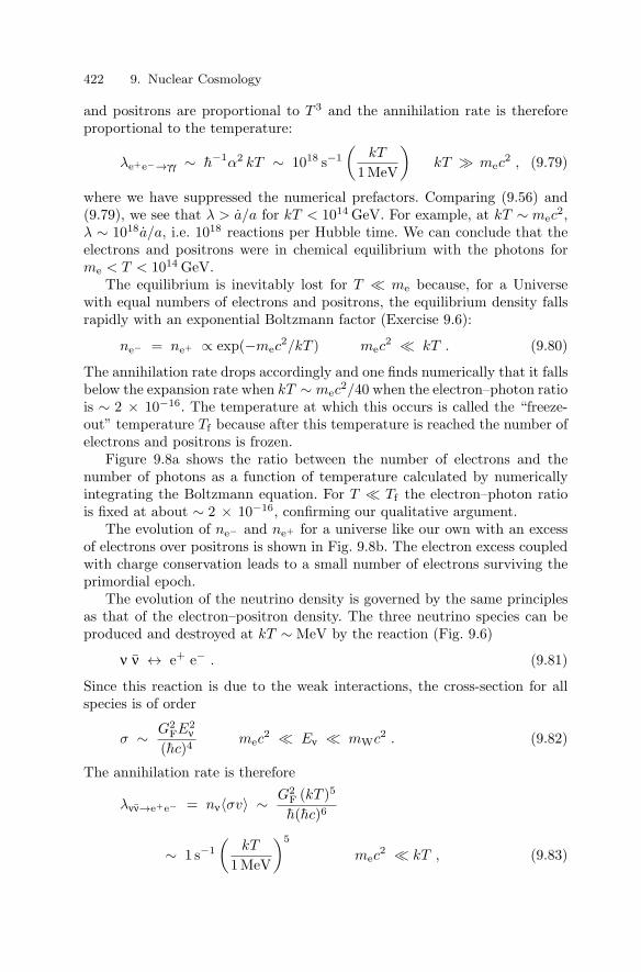
422 9. Nuclear Cosmology
and positrons are proportional to T 3 and the annihilation rate is thereforeproportional to the temperature:
λe+e−→γγ ∼ h−1α2 kT ∼ 1018 s−1(
kT
1 MeV
)kT mec
2 , (9.79)
where we have suppressed the numerical prefactors. Comparing (9.56) and(9.79), we see that λ > a/a for kT < 1014 GeV. For example, at kT ∼ mec
2,λ ∼ 1018a/a, i.e. 1018 reactions per Hubble time. We can conclude that theelectrons and positrons were in chemical equilibrium with the photons forme < T < 1014 GeV.
The equilibrium is inevitably lost for T me because, for a Universewith equal numbers of electrons and positrons, the equilibrium density fallsrapidly with an exponential Boltzmann factor (Exercise 9.6):
ne− = ne+ ∝ exp(−mec2/kT ) mec
2 kT . (9.80)
The annihilation rate drops accordingly and one finds numerically that it fallsbelow the expansion rate when kT ∼ mec
2/40 when the electron–photon ratiois ∼ 2 × 10⁻¹⁶. The temperature at which this occurs is called the “freeze-out” temperature Tf because after this temperature is reached the number ofelectrons and positrons is frozen.
Figure 9.8a shows the ratio between the number of electrons and thenumber of photons as a function of temperature calculated by numericallyintegrating the Boltzmann equation. For T Tf the electron–photon ratiois fixed at about ∼ 2 × 10⁻¹⁶, confirming our qualitative argument.
The evolution of ne− and ne+ for a universe like our own with an excessof electrons over positrons is shown in Fig. 9.8b. The electron excess coupledwith charge conservation leads to a small number of electrons surviving theprimordial epoch.
The evolution of the neutrino density is governed by the same principlesas that of the electron–positron density. The three neutrino species can beproduced and destroyed at kT ∼ MeV by the reaction (Fig. 9.6)
ν ν ↔ e+ e− . (9.81)
Since this reaction is due to the weak interactions, the cross-section for allspecies is of order
σ ∼ G2FE2
ν(hc)4
mec2 Eν mWc2 . (9.82)
The annihilation rate is therefore
λνν→e+e− = nν〈σv〉 ∼ G2F (kT )5
h(hc)6
∼ 1 s−1(
kT
1 MeV
)5
mec2 kT , (9.83)

9.6 Electrons, positrons and neutrinos 423
e/ n
nγ
e/ n
nγ
1
10
10
10
1
−15
−10
−5
10
10
10
0.1 1 10 100/ kT2cem
a) symmetric universe
b) asymmetric universe
thermal equilibrium
electrons
positrons
Fig. 9.8. log(ne/nγ) versus temperature for a symmetric universe, ne = ne− = ne+
(top panel) and for a asymmetric universe, (ne− − ne+)/nγ = 3 × 10⁻¹⁰ (bottompanel). For the symmetric universe, the dotted line shows log(ne/nγ) in the case ofthermal equilibrium.

424 9. Nuclear Cosmology
where thee factors of kT come for nν and two factors from the cross-section.Since the annihilation rate is proportional to T 5 while the expansion rate(9.56) is proportional to T 2, the reaction rate must win at high temperature.Numerically, one finds that the annihilation rate is greater than the expansionrate for kT > 1 MeV so we can conclude that for temperatures greater than 1MeV, neutrinos were in chemical equilibrium. After the annihilation reactionsfreeze-out at Tf ∼ 1 MeV, the neutrinos decouple and their number densityfalls like nν ∝ a−3.
We are now in a position to understand why the temperature for rel-ativistic neutrinos ends up being lower than the photon temperature. ForkT > 1 MeV, photons, neutrinos, and electron–positrons were in thermalequilibrium with a unique temperature, Te = Tγ = Tν. Apart from factorsdue to the Pauli principle and the small electron–positron asymmetry thenumbers of electrons, positrons, neutrinos and photons were equal.
When kTe and kTγ dropped below mec2 the e+e− pairs were transformed
into photons (by e+e− → γγ) but not into the decoupled neutrinos. After theseannihilations, the number of photons was therefore greater than the numberof neutrinos. Since the distributions are thermal with n ∝ T 3, it followsthat Tγ > Tν for kT < mec
2. One says that the photons were “reheated” beelectron–positron annihilation.
The ratio between the post-annihilation photon and neutrino tempera-tures can be calculated by using the fact that the electron–positron–photonsystem remains in thermal equilibrium until there are very few remainingelectrons and positrons which implies that the post- and pre-annihilationentropies of this system are equal. The calculation gives
Tν = (4/11)1/3 Tγ . (9.84)
This corresponds to a neutrino number density of
nν + nν = (3/11)nγ per species . (9.85)
The temperature ratio (9.84) is maintained as long as the neutrinos remainrelativistic since in this case both photon and neutrino temperatures fall asa−1. If the neutrinos have masses that are sufficiently small mνc
2 kTγ(t0),they are still relativistic and have a present temperature of
Tν(a0) = (4/11)1/3Tγ(a0) ∼ 2 K (if mνc2 10−4 eV) . (9.86)
On the other hand, the density ratio (9.85) is maintained whether or not theneutrinos remain relativistic, so today we expect
nν + nν = 1.12 × 10⁸ m−3 per species . (9.87)
9.7 Cosmological nucleosynthesis
At sufficiently high temperatures and densities, nuclear reactions can takeplace and it is important for cosmologists to understand the mix of elements

9.7 Cosmological nucleosynthesis 425
that is produced in the early Universe. The calculations were originally per-formed by Gamow and collaborators in the 1940s with the hope that therelative abundances of all elements could be explained. We now know thatnuclear reactions froze at kT ∼ 30 keV leaving most nuclei in the form of hy-drogen and helium. Nucleosynthesis started up again once stars were formedproviding “gravitational confinement” for astronomical “fusion reactors.”
In this section, we will present a very brief introduction to the theory andconfirming observations [106]. The essential theoretical result will be predic-tions for the relative abundances of the light elements (A ≤ 7, Table 9.3).Observationally, it is very difficult to determine the primordial abundancesbecause of “pollution” by stellar nucleosynthesis. The best observational es-timates are given in Table 9.3. Apart from 1H and 4He, small quantities of2H, 3He, 7Li were produced in the early Universe.
Table 9.3. The important nuclei for nucleosynthesis with their binding energiesper nucleon, B/A, their observed primordial abundances, their half-lives and decaymodes. (The half-life of 7Be by electron capture is given for atomic beryllium.) Wenote the high binding energy of 4He in comparison with the other light nuclei, whichimplies that this species will be the primary product of primordial nucleosynthesis.The absence of stable nuclei at A = 5 or A = 8 prevents the production of heavyelements by two-body reactions between 1H and 4He. Primordial nucleosynthesistherefore stops at A = 7. The production of heavy elements occurs in stars wherethe triple-α reaction 3 4He → 12C takes place.
nucleus B/A nx/nH half-life decay mode(MeV) primordial
(observed)
p 0 1 > 1032 yrn 0 0 10.24 min n → pe−νe
2H 1.11 ∼ 5 × 10⁻⁵
3H 2.83 0 12.3 yr 3H → 3He e−νe3He 2.57 ?
4He 7.07 0.08
5Li 5.27 0 3 × 10⁻²² s 5Li → p 4He
6Li 5.33 < 10−10
7Li 5.61 ∼ 3 × 10⁻¹⁰
7Be 5.37 0 53.3 d e− 7Be → νe7Li
8Be 7.06 0 6.7 × 10⁻¹⁷ s 8Be → 4He 4He

426 9. Nuclear Cosmology
We will see that the abundances are predicted as a function of the baryonto photon ratio η. The calculated values agree with the best observations for
η =nb
nγ∼ 5 × 10⁻¹⁰ ⇒ Ωb =
ηnγ(t0)mp
ρc∼ 0.04 . (9.88)
This is an extremely important result since it is significantly less than theestimates of the total matter density ΩM ∼ 0.3 implying the existence ofnonbaryonic dark matter.
Calculation of the primordial abundances are performed by numericallyintegrating the appropriate Boltzmann equations for each nuclear species.While this obviously requires a complicated computer code, we can under-stand things quantitatively because at high temperature most of the nucleonsare free and remain so to a surprisingly low temperature, kT ∼ 70 keV. Mostof the results can be understood by considering three epochs illustrated inFig. 9.9:
• kT > 800 keV. Neutrons and protons are free and in chemical equilibriumimplying
nn
np∼ exp
(− (mn − mp)c2
kT
), (9.89)
where (mn − mp)c2 = 1.29 MeV. The chemical equilibrium is possiblebecause of reactions transforming neutrons into protons and vice versa:
νen ↔ e−p νep ↔ e+n . (9.90)
The cross-sections for these weak reactions are of the same order of mag-nitude as that for νν ↔ e+e− considered in the previous section so thereaction rate per baryon is approximately given by (9.83). The equilibriumis lost when the reaction rates fall below the expansion rate (9.56). Thefreeze-out temperature turns out to be kT ∼ 800 keV, similar to that forνν ↔ e+e−. From (9.89) it follows that the neutron–proton ratio at theend of this epoch is of order
nn
np(Tf) ∼ 0.2 kTf ∼ 800 keV . (9.91)
• 800 keV > kT > 60 keV. The neutrons decay freely. The duration of thisperiod is ∆t = t(60 keV) − t(800 keV) ∼ 3 min (Exercise 9.5) so about halfthe neutrons decay leaving a neutron–proton ratio of
nn
np(60 keV) ∼ 0.2 exp(−∆t/τn) ∼ 0.1 . (9.92)
• kT ∼ 60 keV: nucleosynthesis. The remaining neutrons are rapidly incor-porated into nuclei via a series of reactions, the most important being:
n p → 2H γ (9.93)
2H 2H → 3He n 2H 2H → 3H p

9.7 Cosmological nucleosynthesis 427
Fig. 9.9. The neutron–proton ratio as a function of temperature, as explained inthe text.
3He 2H → 4Hep 3H 2H → 4Hen 2H 2H → 4He γ .
The nuclear abundances versus time are shown in Fig. 9.10. For η ∼ 5 ×10⁻¹⁰, practically all the neutrons are incorporated into 4He, the mostbound light nucleus.4 The number of available neutrons (9.92) thereforedetermines the quantity of helium:
ρHe
ρH=
2nn/np
1 − nn/np∼ 0.25 (η ∼ 5 × 10⁻¹⁰) . (9.94)
There are two obvious questions that we can ask about this scenario: whydoes nucleosynthesis start so late (kT ∼ 70 keV) and why does it stop so soon
4 The most bound nucleus is abundant not because it is easy to produce but ratherbecause it is very difficult to destroy at kT ∼ 60 keV.

428 9. Nuclear Cosmology
T (MeV)
0.1 0.01
0.0001
0.001
0.01
0.1
1
Fig. 9.10. The calculated abundances of the light elements as a function of temper-ature for η = 3 × 10⁻¹⁰ as calculated in [104]. The abundances are negligible untilkT ∼ 70 keV, after which most of the available neutrons are incorporated into 4He.After kT ∼ 30 keV, nuclear reactions are frozen and the abundances are constantin time except for the later decays of 3H and 7Be. Figure courtesy of ElisabethVangioni-Flam.
without the production of heavy elements. The first question is especiallyinteresting because the nuclear binding energies are all in the MeV rangeso it might be expected that nuclei would be produced when T ∼ MeV.The reason for the late start is the tiny baryon–photon ratio η ∼ 5 × 10⁻¹⁰
and its effect on the first step of nucleosynthesis, the formation of 2H viareaction (9.93). For η ∼ 5 × 10⁻¹⁰ and for T ∼ MeV the rate per neutron ofthis reaction is greater than the expansion rate (Exercise 9.3), from which itfollows that there is approximate chemical equilibrium between n , p and 2H.Under these conditions, the formation rate of 2H is equal to the destructionrate by photo-dissociation:
np nn〈σnpv〉T = n2 nγ〈σ2γv〉T , (9.95)
where n2 is the number density of 2H. Since nγ np, nn, (9.95) can besatisfied only if n2 np, nn to compensate for the large number of photons.This situation persists until the temperature is sufficiently low that 〈σ2γv〉T
becomes small because very few photons have energies above the thresholdfor photo-dissociation (2.2 MeV). Using the Saha equation, it can be shown(Exercise 9.3) that n2 np, nn for kT > 70 keV. Since heavier nuclei cannot

9.7 Cosmological nucleosynthesis 429
be formed until 2H is formed, it follows that nucleosynthesis cannot startuntil kT ∼ 70 keV.
The end of nucleosynthesis so soon after its start is due to two effects.The first is the absence of stable or metastable elements with A = 5 orA = 8 which makes it impossible to form anything from the two primaryspecies, 4He and 1H. The second is the increasing efficiency of the Coulombbarrier between charged nuclei which strongly suppresses the cross-sectionsfor kT < 60 keV. Nuclear reactions therefore freeze-out at a temperature ofkT ∼ 30 keV with a non-equilibrium relic abundance of nuclei characterizedby the complete lack of heavy nuclei.
As we have already mentioned, one of the great interests of the theory ofprimordial nucleosynthesis is that a comparison with observations permits usto estimate η. The predicted abundances as a function of η are shown in Fig.9.11. The abundance of 4He, the primary product of primordial nucleosyn-thesis, is an increasing function of η. The abundances of the loosely boundintermediate nuclei 2H and 3He are decreasing functions of η. The reason forthis behavior is quite simple. Nucleosynthesis can proceed only if the reac-tion rates between nuclei are greater than the expansion rate. The nuclearreaction rates are proportional to densities of initial state nuclei, which arethemselves proportional to the total baryon density. For the first reaction(9.93), it is easy to show (Exercise 9.3) that its rate per neutron is smallerthan the expansion rate for η < 10−13 implying that there is essentially nonucleosynthesis for η < 10−13. For η > 10−13, nucleosynthesis proceeds withan efficiency that increases with η. More precisely, the temperature of thenuclear freeze-out is a decreasing function of η. The later the freeze-out, themore efficient the destruction of the intermediate nuclei and the productionof 4He.
We see in Fig. 9.11 that for η ∼ 5 × 10⁻¹⁰ the abundance of 4He israther insensitive to η. This is simply because the great majority of theavailable neutrons are incorporated into this nucleus. On the other hand, theabundance of 2H is very dependent on η, so a reliable measurement of theprimordial abundance of 2H would yield a robust measurement of η.
It is in principle simple to measure the quantity of 2H in intergalac-tic clouds by measuring the relative absorption by deuterium and hydro-gen of photons from background objects. The brightest background objectsare quasars, believed to be massive black holes radiating photons as matterfalls into them. Figure 9.12 shows the spectrum of a high-redshift quasar. Thespectrum exhibits a prominent “Lyman-α” emission line corresponding to then = 2 → n = 1 states of atomic hydrogen, caused by fluorescence of materialsurrounding the black hole. The line is at λ = 121 nm but in the spectrumit is redshifted to 580 nm. Blueward of the quasar’s Lyman-α emission, wesee the forest of lines corresponding to Ly-α absorption in individual cloudsalong the line-of-sight. The formation of these absorption lines is illustratedin Fig. 9.13.

430 9. Nuclear Cosmology
0.0001 0.001 0.01 0.1 1
0.0001
0.001
0.01
0.1
1
Fig. 9.11. The abundances of the light elements as a function of the assumedbaryon–photon ratio η (Bottom Horizontal Axis) or of the assumed value of Ωbh2
(Top Horizontal Axis), as calculated in [104]. For 4He, the abundance is given asthe fraction Yp = ρHe/ρb of the total baryonic mass that is in the form of 4He,while the other elements are reported as number densities normalized to 1H. Theabundance by mass of 4He is a slowly increasing function of η. The abundancesof the loosely bound intermediate nuclei 2H and 3He are decreasing functions ofη. The form of the curve for 7Li is due to the fact that the production is mostlydirect for η < 3 × 10⁻¹⁰ and mostly indirect via production and subsequent decayof 7Be for η > 3 × 10⁻¹⁰. Observations [105] indicate that 2H/1H ∼ 3.4 × 10⁻⁵ inhigh-redshift intergalactic clouds. If this figure reflects the primordial abundance,we can conclude that η ∼ 5×10⁻¹⁰ corresponding to Ωb ∼ 0.04 (Ωb ∼ 0.04). Figurecourtesy of Elisabeth Vangioni-Flam.

9.7 Cosmological nucleosynthesis 431
Fig. 9.12. A quasar spectrum showing Ly-α emission at 580 nm and, blueward ofthis line, the “forest” of Ly-α absorption lines by intervening gas clouds [105]. Thezoom on the left shows Ly-α hydrogen and deuterium absorption by one cloud.The 2H line is shifted with respect to the hydrogen line because the atomic energylevels are proportional to the reduced electron–nucleus mass. The ratio between thehydrogen and deuterium absorption can be used to determine the two abundanceswithin the cloud. Courtesy of D. Tytler.

432 9. Nuclear Cosmology
λλ
1+zc q1+zλα αλ λα
observer z=0 cloud zc quasar zq
Fig. 9.13. The formation of absorption lines in quasar spectra by intervening cloudsof intergalactic gas. The emission at λα corresponding to the n = 2 → n = 1 lineof atomic hydrogen (right) is observed to be redshifted to λα/(1 + zq) (left). Theobserved spectrum also shows absorption in the cloud at λα/(1+ zc) correspondingto the inverse transition, n = 1 → n = 2.
The amount of absorption is determined by the quantity of hydrogen inthe cloud. The trick is to find a cloud that has an optical depth that per-mits the observation of absorption by both hydrogen and deuterium. Sucha cloud appears in the spectrum with absorption at 555.8 nm for hydrogen.The absorption is total at the center of the hydrogen line but the quantityof hydrogen in the cloud can be estimated from the width of the absorptionprofile. Also visible is the deuterium absorption line and the quantity of deu-terium can be estimated from the total absorption at this line. The spectrumshows that only clouds within a narrow range of optical depth can be used tomeasure the deuterium–hydrogen ratio. The measurement would be impos-sible for clouds with less absorption (making the deuterium line too weak tobe observed) or for clouds with more absorption (causing the hydrogen lineto widen into the deuterium line).
Only a handful of appropriate absorption systems have been found inquasar spectra. The three best examples give results that are consistent with[105]:
n2/n1 = (3.4 ± 0.3) × 10−5 . (9.96)
The quantity of heavy elements in the three high-redshift clouds is verysmall (∼ 10−3 solar abundance) which suggests that the 2H abundance mightbe unperturbed by stellar nucleosynthesis. If we suppose that (9.96) reflectsthe primordial abundance, the theory of nucleosynthesis gives a precise valueof η and Ωb:
η ∼ (5.1 ± 0.3) × 10−10 ⇒ Ωb = 0.039 ± 0.002 . (9.97)
As is often the case in astrophysics, the cited error is purely formal be-cause the real uncertainty comes from the hypotheses necessary to interpret

9.7 Cosmological nucleosynthesis 433
the data. In this case, it is necessary to suppose that the two lines in Fig. 9.12near 555.8 nm are correctly identified and to suppose that the measured abun-dances are primordial. If either hypothesis is false, the measurement must bereinterpreted. For instance, the “deuterium” line could be a hydrogen line ofa second cloud of a slightly different redshift. This would cause the observersto overestimate the deuterium and therefore underestimate Ωb. On the otherhand, if the measured deuterium is not primordial, the primordial deuteriumis underestimated since stellar processes generally destroy deuterium. Thiswould cause an overestimation of Ωb.
It is clear that the value of η derived from the 2H abundance requiresconfirmation from independent measurements. The measured abundances of4He and 7Li (Table 9.3) give qualitative confirmation though some contro-versy continues [106]. The total amount of gas in the Ly-α forest gives a lowerlimit on Ωb that is consistent with the nucleosynthesis value [107]. Finally,the spectra of CBR anisotropies [94] favors a similar value.
We end this section with some comments on how the results of cosmo-logical nucleosynthesis depends on the fundamental constants. The situationis similar to that in astrophysical nucleosynthesis where the production ofelements with A > 8 depended strongly on the alignment of states of 8Be,12C and 16O (Fig. 8.5). In the cosmological case, we have already mentionedtwo important facts
• mn > mp by 0.1%. If this mass-ordering were reversed, the now stableneutron would be more abundant than protons when the weak-interactionsfroze their ratio. Not suffering from the Coulomb barrier, these neutronswould attach themselves to 2H to form 3H which could fuse to form 4He bythe reaction 3H 3H → 4Henn. The end products of cosmological nucleosyn-thesis could then be a mixture of stable neutrons and 4He. Later, in stars,nuclear burning would start with n n → 2H e−νe. Once heavy elements areformed, the free neutrons would be rapidly absorbed by radiative capture.
• The proton–proton system is unbound by ∼ 50 keV. If it were bound,diprotons would be formed that would then β-decay to 2H. The end productof cosmological nucleosynthesis would be a mixture of 4He, 3He and any2H that failed to fuse to form helium. Later, in stars, nuclear burning wouldstart with 2H 2H → 4He γ since no weak interactions are required.
In the mn > mp scenario, very little hydrogen would be available forthe development of life based on organic chemistry. The pp-stable scenariois a bit less hopeless since organic chemistry could still be possible with thesmall amount of surviving 2H. Note that the fact that stellar nuclear burningwould not have to start with a weak interaction does not mean that starswould burn faster. Indeed, we saw in Chap. 8 that the luminosity of a stardoes not depend on the cross-section for the nuclear reactions producing theluminosity. The higher d-d cross-section compared to p-p cross-section wouldjust mean that hydrogen-burning stars would burn at a lower temperatureand be stable at a larger radius.

434 9. Nuclear Cosmology
The results of cosmological nucleosynthesis depend on another relationbetween the weak interactions and gravity. The neutron–proton ratio wasfrozen when the expansion rate, ∼ (G(kT )4/(hc)3)1/2, was equal to the weak-interaction rate, ∼ G2
F(kT )5/(h7c6). The fact that the freeze-out, ∼ 0.8 MeVis very near the neutron–proton mass difference ∼ 1.29 MeV is due to the“coincidence”
G2F(∆mc2)3√Gh11/2c9/2
∼ 1 . (9.98)
If the left side were much greater than unity, the weak interactions wouldhave maintained chemical equilibrium longer, resulting in a smaller neutron–proton ratio. Only hydrogen would have been produced. On the other hand,if the left side were much smaller than unity, chemical equilibrium would havebeen broken sooner, leading to equal numbers of neutrons and protons. Only4He would have been produced. In fact, nature finds itself just at the frontierbetween these two scenarios resulting in the production of an “interesting”mixture of hydrogen and helium.
9.8 Wimps
The three known neutrino species were relativistic when they decoupled(kTf mνc
2). The consequence of this is that today the number density ofneutrinos is of the same order of magnitude as that of photons nν = (3/11)nγ.If one of these neutrinos is sufficiently massive to be non-relativistic today,its present mass density would be ρν = mνnν. This gives ΩM ∼ 0.3 for aneutrino mass of order 10 eV/c2.
Any hypothetical stable particle with mc2 > 10 eV that decoupled whenit was relativistic would create problems for cosmology because the calculatedmass density would be overcritical. A heavy weakly interacting particle cangive an appropriate cosmological density only if it has an annihilation cross-section sufficiently large to keep it in equilibrium until the particle was non-relativistic, kTf mc2. In this case its number density would be suppressedby the Boltzmann factor and the present density might not be too large.In fact, if the cross-section is chosen correctly, the particle can give a relicdensity near critical and constitute the desired nonbaryonic dark matter.
Such a compensation between relic density and mass would seem a prioriimprobable, but stranger things have happened in cosmology. In fact, asit turns out, particles with weak interaction and masses in the GeV rangenaturally give relic densities within an order of magnitude or so of critical.Such particles are called “wimps” for “weakly interacting massive particle.”
A stable wimp is generally predicted by supersymmetric extensions of thestandard model of particle physics. The particle is called the “LSP” (lightestsupersymmetric particle) and is denoted by χ. Supersymmetric wimps are

9.8 Wimps 435
usually “Majorana” particles, i.e. they are their own antiparticle. Supersym-metric theories have many parameters that are not (yet) fixed by experimentso one can generally choose parameters that give a cross-section yielding therequired relic density. The fact that they have not been seen at acceleratorsmeans that probably mχc
2 > 30 GeV [102].As with electrons and positrons, an approximate solution of wimp Boltz-
mann equation is
nχ ∼ nχ(T ) T Tf (9.99)
nχa3 ∼ constant T Tf , (9.100)
where Tf is the freeze-out temperature corresponding to the moment whenthe annihilation rate was equal to the expansion rate:
nχ(Tf) 〈σv〉 = H(Tf) ∼(
GT 4f
(hc)3
)1/2
. (9.101)
1
−510
−1010
−1510
0.1 1 10 100
χ 2 / kTm c
χn
/ nγ
σ v/c = 10 cm2−39
−37cm
2 10
10−35
cm2
Fig. 9.14. log(nχ/nγ) versus temperature for three values of the annihilation cross-section σv/c. The wimp mass was taken to be mχc
2 = 50 GeV. The dotted lineshows log(nχ/nγ) in thermal equilibrium. Freeze-out occurs around Tf ∼ mχ/20.We see that to good approximation the relic density is inversely proportional to thecross-section.
The numerical solution is shown for three values of the cross-section inFig. 9.14. We see that, because of the exponential dependence of nχ(T ) for

436 9. Nuclear Cosmology
T < mχ, the freeze-out temperature is relatively insensitive to the cross-section, Tf ∼ mχ/20. We can therefore easily estimate the χ relic density byequating the annihilation rate and the expansion rate. This gives:
nχ(af)nγ(af)
∼ nχ(af)T 3
f∝ 1
〈σv〉 mχ. (9.102)
We see that the ratio is inversely proportional to the wimp mass and an-nihilation cross section. This ratio stays roughly constant after the freezeso today’s wimp-proton ratio is of the same order of magnitude. Using thepresent-day photon density, this gives a present-day wimp mass density of
ρχ = nχmχ ∝ 1〈σv〉 . (9.103)
It turns out that the a cross-section of 〈σv/c〉 ∼ 10−41m2 gives the observeddensity of cold dark matter. Supersymmetric models that give this cross-section can be constructed.
If it turns out that such supersymmetric models describe nature, thedark-matter mystery would be solved. Efforts are underway to detect super-symmetric particles at accelerators (LHC) . Experiments are also attemptingto observe directly Galactic wimps by detecting particles recoiling from rarewimp-nucleus scattering events (Exercise 9.7).
Bibliography
1. J. Rich, Fundamentals of Cosmology, Springer, Berlin, 2001.
Exercises
9.1 The luminosity density of the Universe (photons produced by stars)is∼ 1.2×10⁸L Mpc−3. Supposing that stellar light output has been relativelyconstant since the formation of the first stars one Hubble time ago, esti-mate the number of photons (E ∼ 2 eV) that have been produced by stars.Compare the number of stellar photons with the number of CBR photons.
Stellar energy is mostly produced by the fusion of hydrogen to helium4p → 4He+2e++2νe. This transformation occurs through a series of reactionsin stellar cores that liberate a total of ∼ 25 MeV. After thermalization, theenergy emerges from stellar surfaces in the form of starlight. Estimate thenumber of protons (per Mpc3) that have been transformed into helium overthe last Hubble time. Compare this number with the number of protonsavailable nb ∼ Ωbρc/mp.
9.2 Estimate the contribution to the universal photon mean free path of thefollowing processes:

Exercises for Chapter 9 437
• Thomson scattering of photons on free electrons of number density ne ∼ nb.• Absorption by stars of number density nstars ∼ Ωstarsρc/M, Ωstars ∼
0.003 and cross-section ∼ πR2.
• Absorption by dust in galaxies with ngal ∼ 0.005 Mpc−3 and cross-section∼ επR2
gal where Rgal ∼ 10 kpc and the fraction of visible light absorbedwhen passing through a galaxy is ε ∼ 0.1.
Compare these distances with the “Hubble distance,” dH ≡ c/H0 (∼ thedistance of the most distant visible objects). Is the Universe “transparent”?
9.3 The cross-section times velocity for the reaction np → 2H γ is
σv ∼ 7.4 × 10⁻²⁰ cm3 s−1 (v c) . (9.104)
(a) Show that the rate per neutron of this reaction is smaller than the ex-pansion rate at kT ∼ 60 keV if η < 4 × 10⁻¹². It follows that there is nonucleosynthesis if η is less than this value.
If η > 4 × 10⁻¹², 2H is in thermal equilibrium with neutrons and pro-tons. The abundances of 2H, protons and neutrons are governed by the Sahaequation:
n2
npnn= (2πhc)3
(2π
mnc2kT
2π
mpc2kT
m2c2kT
2π
)3/2
eB/T
where B = 2.2 MeV is the 2H binding energy.(b) Show that for η ∼ 5 × 10⁻¹⁰ the great majority of neutrons are freeuntil kT ∼ 60 keV. (Since the majority of baryons are protons, you canapproximate np ∼ ηnγ.)
9.4To derive (9.47) in the case of a Universe dominated by non-relativistic
matter (p ∼ 0), we can use a simple Newtonian argument. Referring to Fig.9.15, we place a galaxy of mass m at a distance R = χa(t) from the “center”of a universe of uniform density ρ. Since the mass distribution is sphericallysymmetric, Gauss’s theorem “suggests” that the galaxy is subject to a grav-itational force directed toward the origin that is proportional to the totalmass at a distance < χa(t) from the origin:
|F | =GM(χ)m
χ2a2 , (9.105)
where
M(χ) = 4π(χa)3ρ/3 . (9.106)
(We ignore the question of whether Gauss’s theorem applies in an infinitemedium.) Using |F | = mR = mχa, find the equation (9.47) for the decelera-tion of the Universe.

438 9. Nuclear Cosmology
GM( )mχ
χa
χa
χaM(χ) = ρ 4π( ) /33
T = m( ) /2
U = −GmM( χ)/
2.=F
|v| = .aχ
a(t)χ
( )2a(t)χ
Fig. 9.15. A Newtonian treatment of the universal expansion. A galaxy of massm placed in a universe of uniform density ρ at a distance χa(t) from the “center ofthe Universe.” The spherical symmetry suggests that the Newtonian force on thegalaxy will be directed toward the origin with a magnitude F = GM(χ)m/(χa(t))2,where M(χ) is the total mass at a distance < χa(t) from the origin. For a uniformmass density ρ, M(χ) = 4π(χa)3ρ/3.
9.5 Estimate the time available for neutron decay, corresponding to thetemperature range 800 keV > kT > 50 keV, by integrating (9.56) betweenthese limits and using the approximation a ∝ 1/T . Take g(T ) = 4 is anappropriate mean value over the interval.
9.6 Consider a universe with equal numbers of electrons and positrons. Ifthe universe is in thermal equilibrium at kT mec
2, use the principle ofdetailed balance (Sect. 4.1.5) applied to the reaction e+e− ↔ γγ to showthat the number density of electrons is proportional to a Boltzmann factorexp(−mec
2/kT ). For kT mec2, explain why it is a good approximation to
ignore the effects of stimulated emission.
9.7 The dark matter in Milky Way is believed to be made up of weakly-interacting massive particles (wimps). The mass density of galactic wimps atthe position of the Earth is estimated to be ρc2 ∼ 0.3 GeV cm−2. The wimpsmove around the galaxy with the same mean speed as stars, v ∼ 10−3c.Suppose that the wimps have a mass of 50 GeV/c2. What is their typicalkinetic energy? In a collision with a nucleus, would you expect a wimp to beable to excite or break the nucleus?

Exercises for Chapter 9 439
Suppose that the elastic wimp cross section is 10−35 cm2 on moderatemass nuclei. What is the mean free path of wimps in the Earth?
Experiments have attempted to detect the wimps with germanium detec-tors via the elastic scattering
χ Ge → χ Ge . (9.107)
The recoiling nucleus creates a signal in the diode. What is the scattering ratefor the assumed cross-section? Compare this rate the decay rate of cosmogenic68Ge, ∼ 0.3 mBq kg−1 (Sect. 5.2.2).
Current experiments [103] have not observed a signal that must be as-cribed to wimp scattering. This negative result places an upper limit on thewimp scattering cross-section.

A. Relativistic kinematics
In this appendix, we briefly review some facts from the special theory of rela-tivity that are useful in nuclear physics. Relativity is used in nuclear physicsprimarily through the relativistic expressions for the energy and momentumof a free particle of (rest) mass m and velocity v:
E =mc2√
1 − v2/c2p =
mv√1 − v2/c2
. (A.1)
The energy and momentum defined in this way are conserved quantities.They satisfy
E2 = m2c4 + p2c2 v
c=
pc
E. (A.2)
In nuclear physics, the non-relativistic limit v c (⇒ pc E) usuallyapplies for nuclei, in which case we have
E ∼ mc2 +p2
2mv =
p
m. (A.3)
For neutrinos and photons, the limit mc p generally applies:
E ∼ pc +m2c2
2p2 . v = c
(1 − m2c2
2p2
). (A.4)
It is customary to group energy and momentum in a single object calledthe energy-momentum 4-vector
P ≡ (E, p) . (A.5)
In a particle’s rest-frame, it takes the value (mc2, 0, 0, 0). The squared mag-nitude of the 4-vector is defined as
P 2 ≡ P · P ≡ E2 − p · p = m2c4 , (A.6)
where the last form follows from (A.1). The magnitude is clearly independentof the energy of the particle, i.e. it is invariant with respect to changes ofreference frame.
Consider the energy-momentum of a particle, P , viewed in an inertial ref-erence frame. Consider another inertial reference frame moving with velocityv in, say, the z direction with respect to the first. The energy-momentum

442 A. Relativistic kinematics
4-vector in the second is related to that in the first by a Lorentz transforma-tion: ⎛
⎜⎜⎝E′
p′xc
p′yc
p′zc
⎞⎟⎟⎠ =
⎛⎜⎜⎝
γ 0 0 −βγ0 1 0 00 0 1 0
−βγ 0 0 γ
⎞⎟⎟⎠⎛⎜⎜⎝
Epx
py
pz
⎞⎟⎟⎠ , (A.7)
where
β = v/c γ =1√
1 − β2. (A.8)
The generalizations to other directions are obvious. This relation follows triv-ially from (A.1) if one of the frames is the rest-frame. It is less obvious in thegeneral case but note that the transformation has the virtue of maintainingthe magnitude (A.6), as it must.
Energy momentum conservation can be economically expressed by using4-vectors. Consider the decay
A → B C . (A.9)
Energy-momentum conservation is
PA = PB + PC , (A.10)
which is entirely equivalent to
EA = EB + EC pA = pB + pC . (A.11)
One is often called upon to calculate the momentum of the decay productsin the rest frame of the decaying particle (pA = 0). Momentum conservationgives pB = −pC so energy conservation gives
mAc2 =√
p2c2 + m2Bc4 +
√p2c2 + m2
Cc4 , (A.12)
where p is the common momentum we would like to find. This equation isnot especially easy to solve. It is much easier to write the 4-vector equation
PC = PA − PB . (A.13)
We now take the squared magnitude of both sides of this equation:
m2Cc4 = (PA − PB)2 = P 2
A + P 2B − 2PA · PB . (A.14)
The first two terms on the right give m2Ac4 + m2
Bc4. Since the scalar productPA · PB is Lorentz invariant, we can evaluate it in the rest frame of A:
PA · PB ≡ EAEB − pA · pB = mAc2√
m2Bc4 + p2c2 . (A.15)
We thus deduce√p2c2 + m2
Bc4 =m2
Ac4 + m2Bc4 − m2
Cc4
2mAc2 , (A.16)
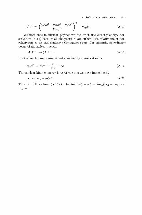
A. Relativistic kinematics 443
p2c2 =(
m2Ac4 + m2
Bc4 − m2Cc4
2mAc2
)2
− m2Bc4 . (A.17)
We note that in nuclear physics we can often use directly energy con-servation (A.12) because all the particles are either ultra-relativistic or non-relativistic so we can eliminate the square roots. For example, in radiativedecay of an excited nucleus
(A, Z)∗ → (A, Z) γ , (A.18)
the two nuclei are non-relativistic so energy conservation is
m∗c2 = mc2 +p2
2m+ pc , (A.19)
The nuclear kinetic energy is pv/2 pc so we have immediately
pc ∼ (m∗ − m)c2 . (A.20)
This also follows from (A.17) in the limit m2A − m2
C ∼ 2mA(mA − mC) andmB = 0.

B. Accelerators
The scattering experiments discussed in Chap. 3 generally required the useof beams of charged particles produced by accelerators. A notable exceptionis the original Rutherford-scattering experiments that used α-particles fromnatural radioactive decays. Neutron-scattering experiments use neutrons pro-duced at fission reactors or secondary neutrons produced by the scatteringof accelerated charged particles.
Particle accelerators require a source of charged particles and an elec-tric field to accelerate them. They can be classified as DC machines usingstatic electric fields and AC machines using oscillating fields. The second cat-egory can be divided into linear accelerators where particles are acceleratedin straight line and magnetic accelerators, i.e. cyclotrons and synchrotrons,where particles move in circular orbits.
ionsource
charging belt
evacuated beam tube
+ + + + + + + + + + + + +
hollowconductorHV charger
beam
Fig. B.1. A schematic of a simple Van de Graff accelerator. Positive charges aretransfered from ground potential to a hollow terminal. The ion source is placedinside the terminal and particles are accelerated through the electrostatic field toground potential.
In simple electrostatic systems, an ion source is placed at high voltageand extracted ions are accelerated through the electric field. Potentials of1 − 2 MV can be produced with normal rectifier circuits and potentials up

446 B. Accelerators
to 10 MV can be produced in a Van de Graff accelerator, illustrated in Fig.B.1. In this system, charge is transformed to the positive terminal by aninsulating belt. Ions are accelerated through an evacuated tube constructedfrom alternating insulators and electrodes so as to maintain a constant gra-dient. The maximum potential is limited by breakdown in the surroundinggas. Currents in the mA range can be achieved.
Tandem Van de Graff Accelerators (Fig. B.2) modify the basic design toprovide higher energy and an ion source that is at ground potential, makingit more accessible. In this case, the source provides singly-charged negativeions, e.g. O− containing an extra electron. These are accelerating to thepositive terminal where a “stripper” consisting of a thin foil or gas-containingtubes removes electrons. The resulting positive ions are then accelerated toground potential where an analyzing magnet selects a particular value ofq/m. Obtainable currents are in the µA range, smaller than simple Van deGraffs because of the difficulty in obtaining negative ions.
beam
+ + + + +
HV
stripper
sourcenegative−ion
+++ __magnet
slit
Fig. B.2. A schematic of a tandem Van de Graff accelerator. Negative ions areaccelerated to the positive potential where a “stripper” removes electrons. Theresulting positive ions are then accelerating to ground potential where a definitecharge state is selected by a magnetic field and slit.
The 10 MV limitation of DC machines can be avoided by using radio-frequency (RF) electric fields. The frequency is typically ∼ 30 MHz. The sim-plest configuration is the linear accelerator, or linac, illustrated in Fig. B.3.The RF voltage is applied to alternating conducting “drift tubes” so thatcharged particles are accelerating between tubes if they arrive at the gapsat appropriate times. The tube lengths must thus decrease in length as theparticle velocity increases down the accelerator. Linacs produce a “bunched”beam consisting of pulses of particles. The bunch structure is persists duringthe acceleration because of the “phase stability” illustrated in Fig. B.4.

B. Accelerators 447
rf supply
~ion source
beam
pulsed
drift tubes
Fig. B.3. A schematic of a drift-tube linear accelerator. Ions are accelerated in thealternating electric field between drift-tubes.
Linear accelerators are most commonly used to accelerate electrons. Thelargest is the 2-mile long accelerating SLAC at Stanford, California, thatproduces 20 GeV electrons.
acce
lera
ting
volta
ge
time
ab
cb’ optimum
voltage
a’
c’
Fig. B.4. The principle of phase stability in a linear accelerator. Particles arrivingin a gap at point b are accelerated such that they arrive at the text gap at the pointb’ with the same phase with respect to the alternating field. Particles arriving atpoint a (c) receive more (less) acceleration and therefore arrive relatively earlier(later) in the next gap, point a’ (c’). Particles in the range a-c are thus “focused”in phase-space toward the point b.
Cyclotrons are a common class of accelerators illustrated in Fig. B.5. Ionorbit in a dipole magnetic field where they are accelerated twice per orbitin a RF field. As they are accelerated, the ions spiral out with the radius ofcurvature given by

448 B. Accelerators
~
beam
deflector
rf supply
Dee
magnetic field(into page)
Dee
Fig. B.5. Schematic of a cyclotron. Particles are injected near the center of adipole magnetic field and then spiral outward as they gain energy each time theypass through the alternating electric field between two electrodes called “Dee’s.”The radio-frequency is tuned to the particle’s cyclotron frequency, ωc = qB/m.Near the maximum radius, the particles are deflected out of the cyclotron.
R =mv
qB√
1 − v2/c2, (B.1)
for a particle of velocity v, mass m and charge q. The orbital frequency isthen
fc =v
2πR=
qB
2πm
√1 − v2/c2 , (B.2)
and the RF must be tuned to this frequency to accelerate the particles.As long as the particle remains non-relativistic, v c, the frequencyis a constant, proportional to the cyclotron frequency, qB/m, equal to9.578 × 107rad s−1 T−1 × B. The energy at radius R is, for v c
12mv2 =
12m
(qB
m
)2
R2 ∼ 10 MeV(
B
1 T
)2 (R
0.5 m
)2
, (B.3)
where the numerical example is for a proton. A modest-sized cyclotron cantherefore produce particles of energies interesting for nuclear-physics experi-ments. Currents in the mA range can be produced.
The simple design of a constant-field cyclotron must be modified in prac-tical designs for a number of reasons. Most important is the necessity toprevent the particles from spiraling in the vertical direction. This can be pre-vented by introducing a small radial variation of the field, as illustrated in

B. Accelerators 449
Fig. B.6. This introduces vertical components to the force on particles thatare not in the median plane so that particles are focused in the vertical di-rection. Unfortunately, this simple scheme introduces other problems, amongthem being that the required RF frequency now depends on position. Morepopular focusing schemes use magnetic fields that vary azimuthally to obtainthe desired effect.
For energies > 1 GeV, cyclotrons become impractical because of the largerequired radius. It then becomes more practical to use synchrotron’s wherering of dipole magnets replace the one large dipole. The accelerating force isprovided by RF cavities distributed about the ring in spaces between mag-nets. Vertical and horizontal focusing is provided by quadrupole magnets.Sychrotrons are the most common accelerators in the field of high-energyparticle physics.
medianplane
north
south
Fig. B.6. Vertical focusing in a radially-decreasing dipole magnetic field. Particlesin the median plane experience a horizontal force. The force on particles above orbelow the median plane has a vertical component that pushes the particle backtoward the median.

C. Time-dependent perturbation theory
Perturbation theory is the basis for most of the calculations performed inChaps 3 and 4. Here we derive the basic equations.
C.0.1 Transition rates between two states
Consider a system described by a Hamiltonian H that is the sum of a “non-perturbed” Hamiltonian H0 and a small perturbation H1 which can inducetransitions between various eigenstates of H0. It is useful to express the stateof the system as a superposition of eigenstates of H0:
|ψ(t)〉 =∑
i
γi(t)e−iEit/h|i〉 , (C.1)
where
H0|i〉 = Ei|i〉 . (C.2)
We suppose that the system is initially in the state |i〉:γi(t = 0) = 1 γj =i(0) = 0 . (C.3)
At a later time, it has an amplitude γf (t) to be in some other state |f〉. Thisamplitude can be calculated using the Schrodinger equation
ihddt
|ψ(t)〉 = (H0 + H1)|ψ(t)〉 . (C.4)
Substituting (C.1) into this equation, multiplying on the left by 〈f | and using〈i|j〉 = δij , we find a differential equation for γf (t):
ihdγf (t)
dt=∑
k
γk(t)〈f |H1|k〉ei(Ef −Ek)t . (C.5)
This equation is exact but can only be solved numerically. A perturbativesolution for small t is found by using (C.3) to use the first approximationγi(t) = 1:
ihdγf (t)
dt= 〈f |H1|i〉ei(Ef −Ei)t . (C.6)
This equation can be directly integrated to give the first order time-dependentperturbation theory estimate of γf :
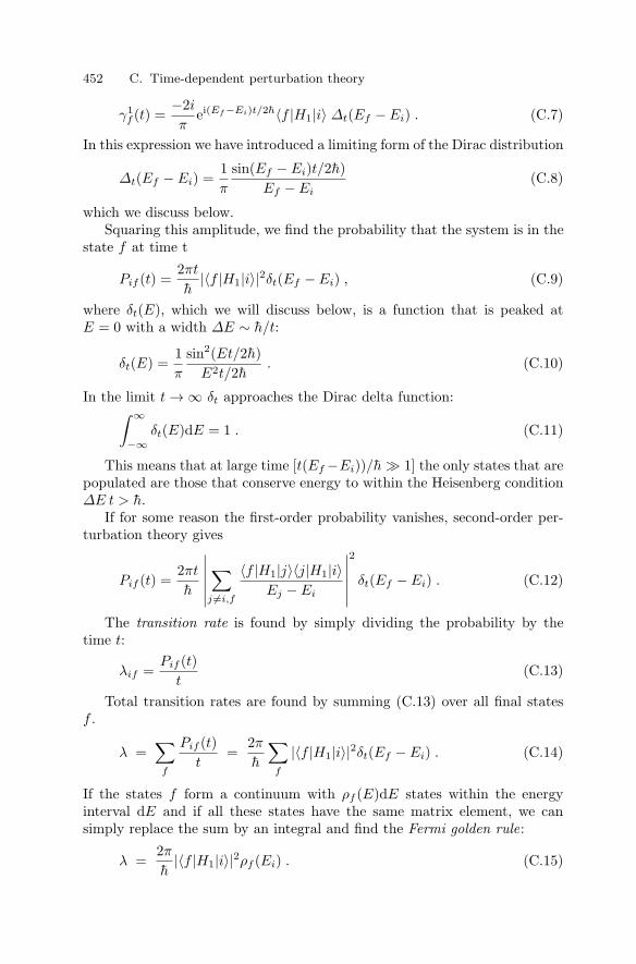
452 C. Time-dependent perturbation theory
γ1f (t) =
−2i
πei(Ef −Ei)t/2h〈f |H1|i〉 ∆t(Ef − Ei) . (C.7)
In this expression we have introduced a limiting form of the Dirac distribution
∆t(Ef − Ei) =1π
sin(Ef − Ei)t/2h)Ef − Ei
(C.8)
which we discuss below.Squaring this amplitude, we find the probability that the system is in the
state f at time t
Pif (t) =2πt
h|〈f |H1|i〉|2δt(Ef − Ei) , (C.9)
where δt(E), which we will discuss below, is a function that is peaked atE = 0 with a width ∆E ∼ h/t:
δt(E) =1π
sin2(Et/2h)E2t/2h
. (C.10)
In the limit t → ∞ δt approaches the Dirac delta function:∫ ∞
−∞δt(E)dE = 1 . (C.11)
This means that at large time [t(Ef −Ei))/h 1] the only states that arepopulated are those that conserve energy to within the Heisenberg condition∆E t > h.
If for some reason the first-order probability vanishes, second-order per-turbation theory gives
Pif (t) =2πt
h
∣∣∣∣∣∣∑
j =i,f
〈f |H1|j〉〈j|H1|i〉Ej − Ei
∣∣∣∣∣∣2
δt(Ef − Ei) . (C.12)
The transition rate is found by simply dividing the probability by thetime t:
λif =Pif (t)
t(C.13)
Total transition rates are found by summing (C.13) over all final statesf .
λ =∑
f
Pif (t)t
=2π
h
∑f
|〈f |H1|i〉|2δt(Ef − Ei) . (C.14)
If the states f form a continuum with ρf (E)dE states within the energyinterval dE and if all these states have the same matrix element, we cansimply replace the sum by an integral and find the Fermi golden rule:
λ =2π
h|〈f |H1|i〉|2ρf (Ei) . (C.15)
C. Time-dependent perturbation theory 453
C.0.2 Limiting forms of the delta function
In the above expressions, it has been useful to introduce the functions :
∆T (E) =1π
sin(ET/2h)E
(C.16)
and
δT (E) =1π
sin2(ET/2h)E2T/2h
. (C.17)
We note that∫ ∞
−∞∆T (E) = 1 , (C.18)
and ∫ ∞
−∞δt(E) = 1 . (C.19)
In the limit T → ∞, these two functions tend, in the sense of distributions,to the Dirac distribution
limT→∞
∆T (E) = limT→∞
δT (E) = δ(E) . (C.20)
They are related by :
(∆T (E))2 =T
2πhδT (E) , ∀T . (C.21)
The generalization to three variables is straightforward:
∆3L(p) =
3∏i=1
∆L(pi) , δ3L(p) =
3∏i=1
δL(pi) , (C.22)
with p = (p1, p2, p3). We have quite obviously
limL→∞
∆3L(p) = lim
L→∞δ3L(p) = δ3(p) , (C.23)
and
(∆3L(p))2 =
L3
(2πh)3δ3L(p) ∀L . (C.24)

D. Neutron transport
In this appendix, we give a few more details about neutron transport in mat-ter and the Boltzmann equation used in Sect. 6.7. We refer to the literature1
for more complete details.
D.0.3 The Boltzmann transport equation
The Boltzmann transport equation governs the behavior of neutrons in mat-ter. We shall write it under the following assumptions:
• The medium is static (neglecting small thermal motions); it is, spherical,homogeneous, and consists of 239Pu nuclei.
• Neutron–neutron scattering is negligible (since the density of neutrons ismuch smaller than the density of the medium) ;
• Neutron decay is negligible, i.e. the neutron lifetime is very large comparedto the typical time differences between two interactions.
The neutrons are described by their density in phase space
dN
d3pd3r= f(r, p, t) , (D.1)
where dN is the number of neutrons in the phase space element d3pd3r.The space density of neutrons and the current describing the spatial flow ofneutrons are the integrals over the momentum
n(r, t) =∫
f(r, p, t)d3p ,
J(r, t) =∫
vf(r, p, t)d3p .
In the absence of collisions, neutron momenta are time-independent andthe flow of particles in phase space is generated by the motion of particle atvelocities v = p/m. The density f satisfies an equation of the form
1 See for instance, E. M. Lifshitz and L. P. Pitaevskii Physical Kinetics, PergamonPress, 1981; C. Cercignani, Theory and application of the Boltzmann Equation,Scottish Academic Press, 1975.

456 D. Neutron transport
∂f
∂t+ v · ∇f = C(f) , (D.2)
where C(f) is the term arising from collision processes, for which we will findan explicit form shortly. For C(f) = 0, (D.2) is called the Liouville equation.
The elastic scattering and absorption rates λel and λabs are products ofthe elementary cross-sections, the density of scattering centers n239, and themean velocity v
λel = vn239σel λabs = vn239σabs (D.3)
The absorption is due to both (n, γ) reactions and to fission
σabs = σ(n,γ) + σfis . (D.4)
The collision term is then written as
C(f(p)) = n239
∫d3p′v(p′) f(r, p′, t)
dσ
d3p′ (p′ → p) (D.5)
− [λel + λabs]f(r, p, t) + S(r, p) .
The first term accounts for neutrons coming from the elements of phase spaced3rd3p′ which enter the element of phase space d3rd3p by elastic scattering.The second term represents the neutrons which leave the element d3rd3peither by elastic scattering or by absorption. The last term S(r, p) is a sourceterm, representing the production of neutrons by fission.
D.0.4 The Lorentz equation
We recall that we assume the neutrons all have the same time-independentenergy, and that the medium is homogeneous.
In that case, the differential elastic scattering cross-section is
dσ
d3p′ (p → p′) = p−2δ(p − p′)dσ
dΩ. (D.6)
We also assume, for simplicity, that the scattering cross section is isotropic
dσel
dΩ=
σel
4π. (D.7)
Later on, we will also make the assumption that all neutrons have the samevelocity, v, i.e. that the function f(r, p) is strongly peaked near values ofmomentum satisfying |p| = mnv.
Using (D.7) we find that the Boltzmann equation (D.2) and (D.5) reducesto the Lorentz equation
∂f
∂t+ v · ∇f = λel(f − f) − λabsf + S(r, p) , (D.8)
where
D. Neutron transport 457
f(r, p, t) =14π
∫f(r, p, t)dΩp , (D.9)
is the phase-space density averaged over momentum directions.The Lorentz equation has a large range of applications. It applies to elec-
tric conduction, to thermalization of electrons in solids, to the transfer ofradiation in stars or in the atmosphere, and to the diffusion of heat, as wellas to neutron transport.
It is useful to integrate the Lorentz equation over d3p, yielding
∂n
∂t+ ∇ · J = −λabsn + 4πS(r) , (D.10)
where 4πS(r) is the momentum integral of S(p, r). Furthermore, multiplyingthe Lorentz equation by v and integrating over d3p, we obtain :
∂J
∂t+∫
v(v · ∇f(r, p, t)) d3p = −(λel + λabs)J , (D.11)
where we have assumed that the source term S(p, r) is independent of thedirection of p.
Equations (D.10) and (D.11) are the basic equations that we want tosolve. The integral
I =∫
v(v · ∇f(r, p, t))d3p , (D.12)
in the left hand side of (D.11) contains all the physical difficulties of theproblem. There are two extreme situations.
1. The first is the ballistic regime, where the mean free path is much largerthan the size of the medium. Collisions have a weak effect and the drifttime ∝ 1/(v · ∇f(r, p, t)) controls the evolution. This is the case ofelectron movement in the base of a transistor.
2. Conversely, in the diffusive regime or local quasi-equilibrium regimewhich is of interest here, the mean free path between two collisionsis small compared to the size of the medium. In first approximation,f(r, p, t) is independent of the direction of p so f(r, p) ∼ f(r, p) and wecan write this distribution function in the form
f(r, p, t) = f(r, p, t) + f1(r, p, t) (D.13)
where f1 f contains all the anisotropy, and∫
f1(r, p, t)d3p = 0, i.e.f1 does not contribute to the density n but only to the current J .
3. There exist mixed situations, where the medium has large density variationsin the vicinity of which none of these approximations holds. This is the casefor neutrino transport in the core of supernovae during the rebound of nuclearmatter. Such situations require sophisticated numerical techniques.2
2 See for instance J-L. Basdevant, Ph.Mellor and J.-P. Chieze, “Neutrinos in Super-novae, An exact treatment of transport,” Astronomy and Astrophysics, vol.197,p 123 (1988)

458 D. Neutron transport
We place ourselves in the case (D.13). (This assumption amounts to ex-panding the distribution function in Legendre polynomials, or spherical har-monics, and in retaining only the first two terms of the expansion.) We neglectthe anisotropic part f1 in the integral (D.12). Since f is independent of thedirection of p, the integral over angles is simple
I =v2
3∇n(r, t) (D.14)
and (D.11) becomes
∂J
∂t+
v2
3∇n = −(λel + λabs)J . (D.15)
Equations (D.10) and (D.15) are now the basic equations to be solved.
Pure Diffusion. We first consider a situation where there is no absorptionand no source term, i.e. the case of pure diffusion where where there is onlyelastic scattering with the nuclei of the medium. The two equations (D.10)and D.15) reduce to
∂n
∂t+ ∇J = 0 , (D.16)
∂J
∂t+
v2
3∇n = −λelJ . (D.17)
The first relation expresses the conservation of the number of particles (onecan write energy conservation in the same manner). The second expresses thecurrent density in terms of the gradient of the density of particles
J = −D
[v∇n +
3v
∂J
∂t
], (D.18)
where the diffusion coefficient D depends on the velocity and the elastic-scattering rate
D =v
3λel=
l
3, (D.19)
where in the second form we use the fact that σtot = σel implying that themean free path is l = v/λel. Under the conditions (which occur frequently)where (3/v)∂J/∂t can be neglected, this boils down to Fick’s law, where thecurrent is proportional to the density gradient:
J = −Dv∇n . (D.20)
Inserting (D.18) into (D.16) leads to
∂n
∂t+
3D
v
∂2n
∂t2− Dv∇2n = 0 , (D.21)
which is called the telegraphy equation .

D. Neutron transport 459
This equation has the general form of a wave equation where the wavefrontpropagates with the velocity v/
√3 but the wave decreases exponentially with
the distance. If the mean free path 1/3D is small compared to the dimensionR of the system under consideration, the propagation time τ = v/R
√3 of
the wave in the system is very short compared to the time of migrationof a neutron by a random walk on the same distance. One can thereforeneglect the propagation term (3D/v)∂2n/∂t2 which amounts to consideringthe propagation velocity as infinite in the telegraphy equation.3
In this approximation, one ends up with the Fourier diffusion equation
∂n
∂t= Dv∇2n , (D.22)
which has a large range of applications and which can be solved by takingthe Fourier transformation. We set
n(r, t) =∫
eik·rg(k, t)d3k , (D.23)
and, by inserting this into (D.22), we obtain
∂g
∂t= −k2Dvg , (D.24)
i.e.
g(k, t) = f(k)e−k2Dvt , (D.25)
where f(k) is determined by the initial conditions using the inverse Fouriertransform
n(r, t = 0) =∫
eikrf(k)d3k , (D.26)
i.e.
f(k) = (2π)3∫
e−ik·rn(r, t = 0)d3r . (D.27)
If at time t = 0 the density n is concentrated at the origin, n(r, t = 0) =n0δ(r) , f(k) is then a constant f , and n(r, t) is the Fourier transform of aGaussian:
n(r, t) ∝ e−r2/4Dvt . (D.28)
The diffusion time T in a sphere of radius R is of the order of T ∼ (R2/Dv) =(R/λ)2(λ/v) where λ/v is the mean time between two elementary collisions.
The telegraphy equation (D.21) can also be treated by Fourier trans-form. One can directly check under which conditions the propagation term(3D/v)∂2n/∂t2 can be neglected.
3 We remark that the Fourier equation is a bona fide wave equation with expo-nential damping at infinity. The wavefronts have a finite velocity v/
√3, however
the propagation effects are completely negligible in the diffusion regime.

E. Solutions and Hints for Selected Exercises
Chapter 1
1.9 One has
〈E〉 = A〈 p2
2m〉 − A(A − 1)
2g2〈1
r〉 .
Therefore, owing to the Heisenberg + Pauli inequality 〈p2〉 ≥ A2/3h2(〈1/r〉)2we obtain
〈E〉 ≥ A5/3h2 12m
〈1r〉2 − A(A − 1)
2g2〈1
r〉 .
Minimizing with respect to 〈1/r〉, we obtain
〈E〉/A ∼ −mg4A4/3/8h2 and〈1/r〉 ∼ 2h2A−1/3/mg2 .
1.12 The ratio of the quadrupole and magnetic hyperfine splittings for avery elongated nucleus is of order
Z2R2/a20
α2me/mp∼ 0.3 Z2
where we use R ∼ 5 fm and a0 = hc/αmec2. For a slightly deformed nucleus,
R2 is replaced by Q ∝ R2∆R/R (Q is the mass quadrupole moment). Thislowers the quadrupole splitting by a factor of more then 10. The sign ofthis splitting is opposite for prolate and oblate nuclei whereas the magneticsplitting is shape independent.
1.13 The energy splitting is ∆E = 2 × 2.79µN = 1.76 × 10⁻⁷eV. ForkT = 0.025 eV this gives a difference in population of
e∆E/2kT − e−∆E/2kT
e∆E/2kT + e−∆E/2kT∼ ∆E/2kT ∼ 3.5 × 10⁻⁶ .
The absorption frequency is ∆E/2πh = 4.2 × 10⁷ Hz.Medical applications of MRI are confined to hydrogen since 1H is the only
common nuclide with spin.The magnetic field due to neighboring spins is of order (µ0/4π)µN/a3
0 ∼5 × 10⁻³T.

462 E. Solutions and Hints for Selected Exercises
1.16 The data indicates that the value of m/Z for 48Mn is about mid-way between the values for 46Cr and 50Fe. Using a ruler, one can findthat m/Z(Mn) ∼ f × m/Z(Fe) + (1 − f) × m/Z(Cr) with f ∼ 0.54 ± 0.01.The values of B/A for 46Cr and 50Fe imply m/Z(Cr) = 1783.624 MeV andm/Z(Fe) = 1789.497 so m/Z(Mn) = 1786.74±0.06. This gives B/A(48Mn) =(8.26±0.03) MeV. The experimenters (not obliged to use a ruler) give an un-certainty of 0.002 MeV.
1.17 The protons initially have kinetic energy Ep = 11 MeV correspondingto a momentum ppc =
√2Epmpc2 = 143 MeV. For protons recoiling from Ni
nuclei in the 1.35 MeV excited state, to first approximation, the proton energyis reduced by this amount, i.e. E′
p = 11 − 1.35 = 9.65 MeV. This correspondsto a proton momentum p′
pc = 134 MeV. Momentum conservation then allowsus to deduce the momentum components of the recoiling 64Ni nucleus if theproton scatters at an angle θ:
ptc = (134 sin θ) MeV plc = (143 − 134 cos θ) MeV ,
for the directions perpendicular to and along the beam direction. For θ =60 deg, this gives a Ni momentum of pc = 139 MeV and a kinetic energy of0.16 MeV. We can then re-estimate the energy of protons recoiling at 60 degto be 9.65 − 0.16 = 9.49 MeV.
Chapter 2
2.4 The simplest way to demonstrate the equivalence is to write down the 3-dwavefunctions in terms of products of 1-d harmonic oscillatory wavefunctionsand show that they are proportional to the appropriate spherical harmonics:Y10 ∝ cos θ and Y1 ±1 ∝ sin θe±iφ.
2.6 41Ca has one neutron outside closed shells containing 20 protons and20 neutrons. The orbital above 20 particles is 1f7/2 so J = 7/2 and l = 3implying that the parity is negative (−1l). So spinparity = 7/2− in agreementwith observation.
2.7 83Kr has an odd neutron orbiting closed shells while 93Nb has an oddproton. The odd proton contributes to the magnetic moment through bothits spin and orbital angular momentum while the neutron contributes onlyits spin. For J = 9/2, the orbital moment must dominate so we expect 93Nbto have the greater moment. For 93Nb, the Schmidt formulas give (for l = 4or l = 5):
g = (9/2 − 1/2) + 2.79 = 6.79 or (9/11)[6 − 2.79] = 2.62 .
The shell model suggests l = 4 ⇒ g = 6.79 to be compared with the experi-mental value 6.167.
For 86Kr the Schmidt formulas give:
g = −1.91 or (9/11)1.91 = 1.56 .

E. Solutions and Hints for Selected Exercises 463
The shell model suggests l = 4 ⇒ g = −1.91 to be compared with theexperimental value -0.97.
In both cases, the experimental values are between the two Schmidt valuesand somewhat closer to the value predicted by the shell model.
Chapter 3
3.2 The neutrino flux (integrated over the duration of the pulse ∼ 15 s) wasF = N/(4πR2) = 1057/(3 1043), the number of protons in the target wasNc = (4/3)1032. The number of events detected is F Nc σ 10. One canmeditate on the many elements of the observers good luck. (The Kamiokandedetector had been built 2 years before to observe a completely different phe-nomenon, the as yet unobserved proton decay).
3.6 To first approximation, the scattered electron keeps all of its energy soits momentum components perpendicular and parallel to the beam directionsare ptc ∼ 500 MeV×sin θ and plc ∼ 500 MeV×cos θ. Momentum conservationthen gives the momentum of the recoiling target particle
ptc ∼ 500 MeV × sin θ plc ∼ 500 MeV × (1 − cos θ) .
For θ = 45 deg this gives a recoil energy of 78 MeV for a nucleon and 39 MeVfor a deuteron. Subtracting this from the electron energy gives a peak at422 MeV for recoil from a proton and 461 MeV for recoil from a deuteron.The proton peak energy should be further reduced by the 2.2 MeV necessaryto break the deuteron.
3.7 The Rutherford cross-section isdσ
dΩ=
α2(hc)2
16E2sin4(θ/4).
Equating this with the strong-interaction cross-section, ∼ (10 fm)2 sr−1, givessin θ/2 ∼ 0.13, i.e. θ ∼ 16 deg. At smaller angles Rutherford scattering domi-nates while at higher angles strong-interaction scattering dominates. It shouldbe kept in mind that the amplitudes for the two interactions must be summed.This permits one to determine their relative phases.
Chapter 4
4.4 The maximum energy photons have about 15 keV excess energy out of1065 keV so the decaying nuclei initially have v/c ∼ 1.4 ×10⁻² correspondingto an energy ∼ 7 MeV. The Bethe–Bloch formula gives an energy loss of∼ 2 ×10⁶ MeV(g cm−2)−1 or about 2 ×10⁷ MeV cm−1 in nickel. The Br ionsthen would stop after ∼ 3 × 10⁻⁷ cm in a time of about 10−15 s. Since itappears that about half the nuclei decay before stopping, this would meanthat the lifetime is of order 10−15s. In fact, because at very low velocities theion attaches electrons reducing its effective charge, the Bethe–Bloch formula

464 E. Solutions and Hints for Selected Exercises
overestimates by about a factor ∼ 100 the energy loss for Br ions at v/c ∼10−2 (see L.C. Northcliffe and R.F. Schilling Nuclear Data Tables, A7 (1970)233; F.S. Goulding and B.G. Harvey, Ann. Rev. Nucl. Sci 25 (1975) 167.).The stopping time is thus a factor of ∼ 100 greater and the lifetime is ∼0.5 × 10⁻¹²s.
4.5 The decay of 60Co to the ground and first excited states of 60Ni areforbidden (∆J > 1) so the decay is primarily by the allowed transition tothe 4+ state. The 4+ state decay to the ground state is M4 so the decay isprimarily through the cascade of two E2 transitions. For Eγ ∼ 1 MeV suchtransitions have mean lives of ∼ 10−12 s.
4.9 152mEu has an allowed Gamow-Teller decay to the 1− state of 152Smwhile the decays of the 152Eu to the shown states are forbidden.
The kinetic energy of the recoiling Sm is p2c2/2mc2 = (840 keV)2/(2 ×145 GeV) = 2.4 eV corresponding to a velocity of v/c ∼ 6×10⁻⁶. The 961 keVphotons emitted in the direction of the Sm velocity are thus blue shifted toan energy of 961(1 + 6 × 10⁻⁶) keV. This gives them enough energy to excitea second Sm nuclei (taking into account the recoil of the second Sm).
4.10 To good approximation the neutrino conserves its energy ∼ 5 MeV so aneutron recoiling from a back-scattered neutrinos has an energy p2c2/2mnc2 ∼(5 MeV)2/2 GeV ∼ 12 keV. The cross-section for such neutrons on hydrogennuclei is ∼ 20 b corresponding to a mean free path of ∼ 1 cm in CH. Thisneglects the carbon, which has a smaller cross-section, ∼ 5 b. Since a neutronloses on average half its kinetic energy in a collision with a proton (isotropicscattering at low energy), about 17 collisions are necessary to reduce theenergy by five orders of magnitude to a reasonably thermal energy, 0.1 eV.
The absorption cross-section is about 0.1 b for thermal neutrons and theyhave v ∼ 4 × 105cm s−1. This gives a mean absorption time of[
10−25cm2 × 4 × 105cm s−1 × 6 × 1023/13]−1 ∼ 0.5 ms .
Chapter 5
5.4
t ∼ 8200 yr × ln(
0.23319.6 × 10−4
)∼ 3.9 × 10⁴ yr .
5.5 Assuming equal initial amounts of 235U and 238U, the elapsed time sincecreation is
7 × 10⁸ yr/ ln 21 − 0.7/4.5
ln(
99.270.72
)∼ 5.9 × 10⁹ yr .
Assuming the same for 234U and 238U, one finds 3.5 ×10⁶ yr. The discrepancyis due to the fact that most of the original 234U has decayed so the 234U nowpresent comes from the decay chain initiated by 238U. In this case, one expects234U/238U = t1/2(234)/t1/2(238) in agreement with the measured values.

E. Solutions and Hints for Selected Exercises 465
5.6 The α-particle originally has β2 ∼ 2 × 10⁻³ so the initial energy lossis ∼ 1000 MeV cm−1 for ρ = 1.8 g cm−3. The probability that it produces aneutron before losing 1 MeV is
P = (1/1000) cm × 0.4 × 10−24 cm2 × 1.8 g cm−3
× (6 × 1023/9) g−1 ∼ 5 × 10⁻⁵ ,
so to give 1 Bq neutron activity we need 2 × 10⁴ Bq of α activity.
Chapter 6
6.3 The mean free path for neutrons is dominated by fission of 235U:
l−1 = 250 × 10−24cm2 × 6 × 1023
238× 0.0072 × 19 g cm−3 ∼ 11 cm .
If the uranium is in the shape of a cube, the probability of a fission is P =1 cm/11 cm and the fission rate is
(1/11) × 1012 cm−2s−1 ∼ 1012 s−1
corresponding to ∼ 30 W. The rate is lower if the uranium is deformed sothat the dimension in the direction of the beam is comparable to or greaterthan the mean free path.6.5 Neutron-rich fission products with A = 142 will β−-decay to 142 Ce whichis a long-live 2β emitter.6.6 The nuclides with A ∼ 100 are fission products. The transuraniums243Am and 239Pu are produced by neutron captures (followed by β-decays)on 238U. The nuclides with 210 < A < 235 come from the decay chainsinitiated by the transuraniums.
Chapter 7
7.4 The photon energy is 17.49 MeV (as above). Using the Bethe–Bloch for-mula, the energy loss of the proton in the LiF is
∆E ∼ 10−5g cm−2 × 1 MeV (g cm−2)−1
β2 ∼ 20 keV
where we use β2 = 4 × 10⁻⁴ for the proton. The actual energy loss is ∼ 5times less since the Bethe–Bloch formula overestimates the energy loss at thisvelocity.
The cross-section is proportional to ∝ exp(−√EB/E) where EB ∼7.75 MeV for this reaction. This gives the variation of the cross-section asthe incident proton loses energy in the LiF:
dσ
σ= (1/2)
√EB/E
∆E
E∼ 3
∆E
E∼ 0.05 ,
so the cross-section is relatively constant over the thickness of the target.If the target were much thicker, the variation would be substantial and theevent rate would not be easily interpretable.

466 E. Solutions and Hints for Selected Exercises
7.5 The parameters entering the calculations are EB = 7.75 MeV, EG =12.45 keV, ∆EG = 0.3 keV, S(EG) = −.5 keV b, and Γγ = 12 eV. Thefactor that deviates most from unity is the Boltzmann factor giving theprobability to have a proton with enough energy to excite the resonance:exp(−441 keV/kT ). This makes the resonance contribution completely neg-ligible at kT = 1 keV.
7.6 For T = 106 K, kT = 0.086 keV we have nkTτbrem ∼ 3 × 10¹⁹ keV m−3 sin agreement with the figure. It is proportional to T 3/2, also in agreementwith the figure.
Chapter 8
8.4 The mean free path of a 10 MeV neutrino in a neutron star is of order
l =[
1057
(4π/3)(104 m)310−41 cm2
]−1
∼ 4 m ,
which is much less than the neutron star radius, R ∼ 104 m. The neutrinostherefore diffuse out of the star with a time of order R2/cl ∼ 0.1 s. In fact,the neutrino pulse from the collapse of stellar core to a neutron star lastssomewhat longer, about 10 s.
8.7 All degenerate gases have a phase space density of order h−3. The phasespace density of such a gas is the momentum space density (∼ p−3
F ) times thereal space density (n) so the Fermi momentum is p2
F ∼ n2/3h2. For pF mcand pF mc this gives a total energy for N fermions
E ∼ Np2F
2m∼ Nn2/3h2
mE ∼ NpFc ∼ Nn1/3hc .
The pressure is the derivative of the energy with respect to the volume.We find for the two limits
P ∼ n5/3 (hc)2
mc2 P ∼ n4/3hc ,
where n is the number density. (The numerical factor in the first case is(3π2)2/3/5).
For a number density of electrons n ∼ 1030 cm−3, and a temperatureT ∼ 107 K the degenerate quantum pressure ∝ n5/3 is much larger thana classical ideal gas pressure ∝ n. Between the density where the star canbe treated as an ideal gas and that where it becomes a Fermi gas, there isa transition regime. Above a critical density, and for temperatures smallerthan the Fermi temperature, the electron gas becomes degenerate. Noticethat owing to the mass effect, the gas of nuclei is still an ideal gas.
For a non-relativistic degenerate electron gas, the strong quantum pres-sure is temperature independent and it resists futher collapse, since the grav-itational inward pressure behaves as n4/3. There is no further contraction, no

E. Solutions and Hints for Selected Exercises 467
further nuclear reactions, the star cools endlessly. This situation correspondsto a white dwarf.
The order of magnitude of the temperature at which the contractinggas reaches this regime can be estimated from the virial theorem, 〈3PV 〉 ∼GM2/R. We approximate the pressure by the sum of the classical and quan-tum pressures. This gives
NkT ∼ GM2
R− N5/3h2/m
R2 . (E.1)
Minimizing with respect to R we get
R ∼ N5/3h2
GM2 kTmax =G2M2m
4N5/3h2 ,
where M is the mass of the star and m and N are the mass and number ofthe degenerate particle.
If Tmax ≤ 106 K, the star is called a brown dwarf because the temperaturehas not reached the value where nuclear reactions can take place. The differ-ence between a brown dwarf and a planet is that, in a planet, the individualatoms and molecules have not been completely dissociated in a plasma ofelectrons and nuclei, at least in the crust. The temperature is much lower,the overall cumulative gravitational forces give the object a global sphericalshape, but rocks and other non-spherical objects, whose shapes are due toelectromagnetic forces, can still exists on the surface.
8.8 The mass of the iron core of a star can increase only up to the Chan-drasekhar mass at which point it will collapse. During the collapse, the Fermienergy of the electrons increases until most electrons have sufficient energy toby captured endothermically. The neutrinos produced in the captures do notinduce the reverse reaction because they escape from the star after a periodof diffusion (Exercise 8.4).
The energy radiated by a neutrino species of temperature T is given byStefan’s law (after a minor modification taking into account the fact thatneutrinos are fermions). Taking kT = 1 MeV, a neutrinosphere radius ofR = 104 m, and a pulse duration of 10 s, one finds that the total energyradiated by three neutrino species is
5.67 × 10⁻⁸ W m−2 K−4 × 10 s × (kT )4 4πR2 ∼ 3 × 1046 J .
This agrees with the total energy liberated, (3/5)GM2/R. (The agreementis not fortuitous since the temperature and radius of the neutrino sphereare constrained by this requirement.) Note that the number of neutrinosradiated, (3 × 1046 J)/2kT ∼ 2 × 1058, is greater than the number of νeproduced by neutron capture ∼ 1057. Most of the neutrinos are thermallyproduced, γγ ↔ e+e− ↔ νν.

468 E. Solutions and Hints for Selected Exercises
Chapter 9
9.3 The density of protons when kT = 60 keV can be scaled up from thepresent density by the third power of the temperature:
np ∼ np(t0)(60 keV/kT (t0))3 = ηnγ(t0) ×(
60 keV2 × 10−4 eV
)3
.
The reaction rate per neutron is this density multiplied by σv which gives∼ 3 × 10⁻³s−1 for η ∼ 4 × 10⁻¹². This nearly the expansion rate ∼0.65s−1(60keV/1 MeV)2 ∼ 2 × 10⁻³s−1.
The deuteron-neutron ratio at this temperature isn2
nn= ηnγ
(mpc2kT )
)−3/2(2πhc)3e−B/kT ∼ η × 10−18 ,
and rises very quickly above unity as the temperature falls.
9.5 We use
a/a ∼ T /T ∼ 0.65(kT/1 MeV)2 s−1 .
Integrating, we get
∆t ∼∫ kT=60 keV
kT∼1 MeV
dT
T∼ 166 s .
9.7 The wimps have kinetic energies of order (1/2)mc2β2 ∼ 50 keV. Formost nuclear targets, this is much less than the excitation energy of the firstexcited state so we expect only elastic scattering to be possible.
The mean free path in the Earth is of order
l−1 ∼ 10−35 cm2 nucleus−1
×(6 × 1023nucleon g−1/50 nucleon/nucleus) 5 g cm−3 ∼ 1107 km
,
i.e, much greater than the radius of the Earth. The interaction rate in onekg of germanium is
λ ∼ 0.3 GeV cm−3
50 GeV/wimp× 3 × 107cm s−1 × 10⁻³⁵cm2
×6 × 1026nucleon kg−1
72nucleon/nucleus∼ 10−5s−1 ,
which is less than the rate of 68Ge decay.

F. Tables of numerical values
Table F.1. Selected physical and astronomical constants, adapted from [1].
quantity symbol value
speed of light in vacuum c 2.99 792 458 × 108 ms−1
Planck constant h 1.054 571 596(82) × 10−34J sconversion constant hc 197.326 960 2(77) MeV fmconversion constant (hc)2 389 379 292 (30) MeV2 b
(1 b ≡ 10−28 m2)e− charge magnitude e 1.602 176 462(63) × 1019 C
⇒ 1 eV = 1.602 × 10⁻¹⁹ JFine structure constant α = e2/4πε0hc [137.035 999 76(50)]−1
Bohr radius a∞ 0.529 177 208 3(39) × 10−10 mRydberg energy α2mec
2/2 13.605 691 72(53) eVThomson cross-section σT 0.665 245 854(15) × 10−28 m2
Gravitational constant GN (= G) 6.673(10) × 10−11 m3kg−1s−2
Planck mass mpl =√
hc/G 1.221 0(9) × 1019 GeV/c2
Fermi coupling constant GF/(hc)3 1.166 39(1) × 10−5GeV−2
electron mass me 0.510 998 902(21) MeV/c2
proton mass mp 938.271 998(38) MeV/c2
1.672 621 58(13) kg1836.152 667 5(39)me
neutron–proton ∆m mn − mp 1.293 318(9) MeV/c2
Avogadro constant NA 6.022 141 99(47) × 1023 mol−1
nuclear magneton µN = eh/2mp 3.152 451 238(24) 10−14MeVT−1
Boltzmann constant k 1.380 650 3(24) × 10−23J K−1
8.617 342(15) × 10−5 eV K−1
parsec pc 3.085 677 580 7(4) × 1016 m=3.262... ly
solar mass M 1.988 9(30) × 1030 kg= 1.189 × 1057mp
solar luminosity L 3.846(8) × 1026 W s−1
solar equatorial radius R 6.961 × 10⁸ m

G. Table of Nuclei
The following table lists known nuclei sorted by their mass number A. Bindingenergies are taken from [2] while decay modes, lifetimes (in seconds), andterrestrial abundances (for long-lived isotopes) are generally taken from [3].For a given A, the binding energies shown in column 2 are the parabolicfunctions of Z illustrated in Fig. 2.6. Because of the nucleon-pairing energy,their is only one parabola for odd-A and two parabolas for even-A (onefor even-even and one for odd-odd). Nuclei on the neutron-rich side of theparabola are generally β−-unstable while those on the proton-rich side areunstable to electron-capture (Qec < 2me) or to both electron-capture andβ+ decay (Qec > 2me). A few very weakly bound nuclei can also decay bynucleon emission, e.g. A = 16, Z = 5, 9, 10.
Because of the single or double parabolic structure, there is only one β-stable nucleus for odd-A and two or three β-stable nuclei for even-A. For even-A, only one nucleus is also stable against double-β decay, but the lifetime for2β decay is generally greater than 1020 yr so nuclei that are only 2β unstableare still present on Earth.
Nuclei with A > 150 (A > 100) are also usually unstable to α-decay(spontaneous fission). The lifetimes are generally greater than 1020 yr forA < 208.
Decay and reaction Q’s can be calculated from the binding energies inthis table. For example
Qβ−[(A, Z) → (A, Z + 1)] = B(Z + 1) − B(Z) + (mn − mp − me)c2
= B(Z + 1) − B(Z) + 0.782 MeV ,
Qβ+[(A, Z) → (A, Z − 1)] = B(Z − 1) − B(Z) − (mn + me − mp)c2
= B(Z − 1) − B(Z) − 1.804 MeV ,
Qα[(A, Z) → (A − 4, Z − 2)] = B(A − 4, Z − 2) − B(A, Z) + B(4, 2) ,
= B(A − 4, Z − 2) − B(A, Z) + 28.295 .

472 G. Table of Nuclei
A X Z B/A → log t1/2 A X Z B/A → log t1/2(MeV) or % (MeV) or %
1 n 0 0.0000 β− 2.79 11 Li 3 4.1499 β− -2.071 H 1 0.0000 99.99% 11 Be 4 5.9528 β− 1.14
11 B 5 6.9277 80.10%2 H 1 1.1123 0.01% 11 C 6 6.6764 β+ 3.09
11 n 7 5.3043 p -21.053 H 1 2.8273 β− 8.593 He 2 2.5727 0.00% 12 Be 4 5.7208 β− -1.63
12 B 5 6.6313 β− -1.694 H 1 1.3753 n 12 C 6 7.6801 98.90%4 He 2 7.0739 100.00% 12 N 7 6.1701 β+ -1.964 Li 3 1.1545 p 12 O 8 4.8778 p -20.78
5 H 1 0.2164 n 13 Be 4 5.1261 n -21.145 He 2 5.4811 n -20.96 13 B 5 6.4964 β− -1.765 Li 3 5.2661 p -21.36 13 C 6 7.4699 1.10%
13 N 7 7.2389 β+ 2.786 H 1 0.9636 n 13 O 8 5.8121 β+ -2.076 He 2 4.8782 β− -0.096 Li 3 5.3324 7.50% 14 Be 4 4.9991 β− -2.366 Be 4 4.4873 p -20.15 14 B 5 6.1016 β− -1.86
14 C 6 7.5203 β− 11.267 He 2 4.1178 n -20.39 14 N 7 7.4756 99.63%7 Li 3 5.6064 92.50% 14 O 8 7.0524 β+ 1.857 Be 4 5.3715 EC 6.66 14 F 9 5.1678 p7 B 5 3.5314 p -21.33
15 B 5 5.8794 β− -1.988 He 2 3.9260 β− -0.92 15 C 6 7.1002 β− 0.398 Li 3 5.1598 β− -0.08 15 N 7 7.6995 0.37%8 Be 4 7.0624 α -16.01 15 O 8 7.4637 β+ 2.098 B 5 4.7172 β+ -0.11 15 F 9 6.4834 p -21.188 C 6 3.0978 p -20.54 15 Ne 10 4.7907 ?
9 He 2 3.3621 n -20.66 16 B 5 5.5057 n -9.709 Li 3 5.0379 β− -0.75 16 C 6 6.9221 β− -0.139 Be 4 6.4628 100.00% 16 N 7 7.3739 β− 0.859 B 5 6.2571 α -17.91 16 O 8 7.9762 99.76%9 C 6 4.3371 β+ -0.90 16 F 9 6.9637 p -19.78
16 Ne 10 6.0831 p -20.2710 Li 3 4.4922 n -21.2610 Be 4 6.4977 β− 13.68 17 B 5 5.2697 β− -2.2910 B 5 6.4751 19.90% 17 C 6 6.5578 β− -0.7110 C 6 6.0320 β+ 1.29 17 N 7 7.2862 β− 0.6210 N 7 3.5538 ? 17 O 8 7.7507 0.04%
17 F 9 7.5423 β+ 1.81

G. Table of Nuclei 473
A X Z B/A → log t1/2 A X Z B/A → log t1/2(MeV) or % (MeV) or %
17 Ne 10 6.6414 β+ -0.96 22 Al 13 6.7825 β+ -1.1517 Na 11 5.4961 ? 22 Si 14 6.1115 β+ -2.22
18 B 5 4.9472 ? 23 N 7 6.1926 ?18 C 6 6.4259 β− -1.02 23 O 8 7.1637 β− -1.0918 N 7 7.0383 β− -0.20 23 F 9 7.6204 β− 0.3518 O 8 7.7671 0.20% 23 Ne 10 7.9552 β− 1.5718 F 9 7.6316 β+ 3.82 23 Na 11 8.1115 100.00%18 Ne 10 7.3412 β+ 0.22 23 Mg 12 7.9011 β+ 1.0518 Na 11 6.1867 ? 23 Al 13 7.3349 β+ -0.33
23 Si 14 6.5616 ?19 B 5 4.7410 ?19 C 6 6.0962 β− -1.34 24 N 7 5.8831 ?19 N 7 6.9483 β− -0.52 24 O 8 7.0199 β− -1.2119 O 8 7.5665 β− 1.43 24 F 9 7.4636 β− -0.4719 F 9 7.7790 100.00% 24 Ne 10 7.9932 β− 2.3119 Ne 10 7.5674 β+ 1.24 24 Na 11 8.0635 β− 4.7319 Na 11 6.9379 p 24 Mg 12 8.2607 78.99%19 Mg 12 5.8956 ? 24 Al 13 7.6498 β+ 0.31
24 Si 14 7.1668 β+ -0.9920 C 6 5.9586 β− -1.85 24 P 15 6.2492 ?20 N 7 6.7092 β− -1.0020 O 8 7.5685 β− 1.13 25 O 8 6.7352 ?20 F 9 7.7201 β− 1.04 25 F 9 7.3390 β− -1.2320 Ne 10 8.0322 90.48% 25 Ne 10 7.8407 β− -0.2220 Na 11 7.2988 β+ -0.35 25 Na 11 8.1014 β− 1.7720 Mg 12 6.7234 β+ -1.02 25 Mg 12 8.2235 10.00%
25 Al 13 8.0211 β+ 0.8621 C 6 5.6592 ? 25 Si 14 7.4802 β+ -0.6621 N 7 6.6090 β− -1.07 25 P 15 6.8470 ?21 O 8 7.3894 β− 0.5321 F 9 7.7383 β− 0.62 26 O 8 6.4782 ?21 Ne 10 7.9717 0.27% 26 F 9 7.0971 ?21 Na 11 7.7655 β+ 1.35 26 Ne 10 7.7539 β− -0.7121 Mg 12 7.1047 β+ -0.91 26 Na 11 8.0058 β− 0.0321 Al 13 6.3432 ? 26 Mg 12 8.3339 11.01%
26 Al 13 8.1498 β+ 13.3522 C 6 5.4678 ? 26 Si 14 7.9248 β+ 0.3522 N 7 6.3642 β− -1.62 26 P 15 7.1979 β+ -1.7022 O 8 7.3648 β− 0.35 26 S 16 6.5910 ?22 F 9 7.6243 β− 0.6322 Ne 10 8.0805 9.25% 27 F 9 6.8828 ?22 Na 11 7.9157 β+ 7.91 27 Ne 10 7.5188 β− -1.4922 Mg 12 7.6626 β+ 0.59 27 Na 11 7.9593 β− -0.52

474 G. Table of Nuclei
A X Z B/A → log t1/2 A X Z B/A → log t1/2(MeV) or % (MeV) or %
27 Mg 12 8.2639 β− 2.75 31 Ar 18 7.2527 β+ -1.8227 Al 13 8.3316 100.00%27 Si 14 8.1244 β+ 0.62 32 Ne 10 6.6651 ?27 P 15 7.6646 β+ -0.59 32 Na 11 7.2304 β− -1.8827 S 16 6.9593 β+ -1.68 32 Mg 12 7.8028 β− -0.92
32 Al 13 8.0992 β− -1.4828 F 9 6.6332 ? 32 Si 14 8.4816 β− 9.6728 Ne 10 7.3891 β− -1.77 32 P 15 8.4641 β− 6.0928 Na 11 7.8009 β− -1.52 32 S 16 8.4931 95.02%28 Mg 12 8.2724 β− 4.88 32 Cl 17 8.0723 β+ -0.5328 Al 13 8.3099 β− 2.13 32 Ar 18 7.6993 β+ -1.0128 Si 14 8.4477 92.23% 32 K 19 6.9687 ?28 P 15 7.9080 β+ -0.5728 S 16 7.4788 β+ -0.90 33 Na 11 7.0375 β− -2.0928 Cl 17 6.6479 ? 33 Mg 12 7.6291 β− -1.05
33 Al 13 8.0208 ?29 F 9 6.4390 ? 33 Si 14 8.3604 β− 0.7929 Ne 10 7.1801 β− -0.70 33 P 15 8.5138 β− 6.3429 Na 11 7.6843 β− -1.35 33 S 16 8.4976 0.75%29 Mg 12 8.1152 β− 0.11 33 Cl 17 8.3048 β+ 0.4029 Al 13 8.3487 β− 2.60 33 Ar 18 7.9289 β+ -0.7629 Si 14 8.4486 4.67% 33 K 19 7.4159 ?29 P 15 8.2512 β+ 0.6229 S 16 7.7486 β+ -0.73 34 Na 11 6.8621 β− -2.2629 Cl 17 7.1595 ? 34 Mg 12 7.5466 β− -1.70
34 Al 13 7.8564 β− -1.2230 Ne 10 7.0693 ? 34 Si 14 8.3361 β− 0.4430 Na 11 7.4980 β− -1.32 34 P 15 8.4484 β− 1.0930 Mg 12 8.0545 β− -0.47 34 S 16 8.5835 4.21%30 Al 13 8.2614 β− 0.56 34 Cl 17 8.3990 β+ 0.1830 Si 14 8.5207 3.10% 34 Ar 18 8.1977 β+ -0.0730 P 15 8.3535 β+ 2.18 34 K 19 7.6777 ?30 S 16 8.1228 β+ 0.07 34 Ca 20 7.2243 ?30 Cl 17 7.4799 ?30 Ar 18 6.9325 p -7.70 35 Na 11 6.6496 β− -2.82
35 Mg 12 7.3062 ?31 Ne 10 6.8241 ? 35 Al 13 7.7824 β− -0.8231 Na 11 7.3852 β− -1.77 35 Si 14 8.1687 β− -0.1131 Mg 12 7.8722 β− -0.64 35 P 15 8.4462 β− 1.6731 Al 13 8.2256 β− -0.19 35 S 16 8.5379 β− 6.8831 Si 14 8.4583 β− 3.97 35 Cl 17 8.5203 75.77%31 P 15 8.4812 100.00% 35 Ar 18 8.3275 β+ 0.2531 S 16 8.2819 β+ 0.41 35 K 19 7.9657 β+ -0.7231 Cl 17 7.8702 β+ -0.82 35 Ca 20 7.4975 β+ -1.30

G. Table of Nuclei 475
A X Z B/A → log t1/2 A X Z B/A → log t1/2(MeV) or % (MeV) or %
40 P 15 7.9864 β− -0.5936 Mg 12 7.2296 ? 40 S 16 8.3296 β− 0.9436 Al 13 7.6245 ? 40 Cl 17 8.4278 β− 1.9136 Si 14 8.1115 β− -0.35 40 Ar 18 8.5953 99.60%36 P 15 8.3079 β− 0.75 40 K 19 8.5381 β− 0.01%36 S 16 8.5754 0.02% 40 Ca 20 8.5513 ββ 96.94%36 Cl 17 8.5219 β− 12.98 40 Sc 21 8.1737 β+ -0.7436 Ar 18 8.5199 ββ 0.34% 40 Ti 22 7.8623 β+ -1.3036 K 19 8.1424 β+ -0.47 40 V 23 7.3632 ?36 Ca 20 7.8155 β+ -0.9936 Sc 21 7.2289 ? 41 Si 14 7.5156 ?
41 P 15 7.9032 β− -0.9237 Al 13 7.5369 ? 41 S 16 8.2197 ?37 Si 14 7.9516 ? 41 Cl 17 8.4137 β− 1.5837 P 15 8.2675 β− 0.36 41 Ar 18 8.5344 β− 3.8237 S 16 8.4599 β− 2.48 41 K 19 8.5761 6.73%37 Cl 17 8.5703 24.23% 41 Ca 20 8.5467 EC 12.5137 Ar 18 8.5272 EC 6.48 41 Sc 21 8.3692 β+ -0.2237 K 19 8.3398 β+ 0.09 41 Ti 22 8.0348 β+ -1.1037 Ca 20 8.0041 β+ -0.74 41 V 23 7.6383 ?37 Sc 21 7.5505 ?
42 P 15 7.7899 β− -0.9638 Al 13 7.3894 ? 42 S 16 8.1838 β− -0.2538 Si 14 7.8816 ? 42 Cl 17 8.3496 β− 0.8338 P 15 8.1432 β− -0.19 42 Ar 18 8.5556 β− 9.0238 S 16 8.4488 β− 4.01 42 K 19 8.5512 β− 4.6538 Cl 17 8.5055 β− 3.35 42 Ca 20 8.6166 0.65%38 Ar 18 8.6143 0.06% 42 Sc 21 8.4449 β+ -0.1738 K 19 8.4381 β+ 2.66 42 Ti 22 8.2596 β+ -0.7038 Ca 20 8.2401 β+ -0.36 42 V 23 7.8374 ?38 Sc 21 7.7689 ? 42 Cr 24 7.4817 ?38 Ti 22 7.3789 ?
43 P 15 7.7267 β− -1.4839 Si 14 7.7355 ? 43 S 16 8.0705 β− -0.6639 P 15 8.0948 β− -0.80 43 Cl 17 8.3208 β− 0.5239 S 16 8.3442 β− 1.06 43 Ar 18 8.4875 β− 2.5139 Cl 17 8.4944 β− 3.52 43 K 19 8.5766 β− 4.9039 Ar 18 8.5626 β− 9.93 43 Ca 20 8.6007 0.14%39 K 19 8.5570 93.26% 43 Sc 21 8.5308 β+ 4.1539 Ca 20 8.3695 β+ -0.07 43 Ti 22 8.3529 β+ -0.2939 Sc 21 8.0133 ? 43 V 23 8.0720 β+ -0.1039 Ti 22 7.5984 β+ -1.59 43 Cr 24 7.6843 β+ -1.68
40 Si 14 7.6624 ? 44 S 16 8.0341 β− -0.91

476 G. Table of Nuclei
A X Z B/A → log t1/2 A X Z B/A → log t1/2(MeV) or % (MeV) or %
44 Cl 17 8.2234 β− -0.36 48 Ar 18 8.2617 ?44 Ar 18 8.4845 β− 2.85 48 K 19 8.4309 β− 0.8344 K 19 8.5474 β− 3.12 48 Ca 20 8.6665 ββ 0.19%44 Ca 20 8.6582 2.09% 48 Sc 21 8.6560 β− 5.2044 Sc 21 8.5574 β+ 4.15 48 Ti 22 8.7229 73.80%44 Ti 22 8.5335 EC 9.30 48 V 23 8.6230 β+ 6.1444 V 23 8.2043 β+ -1.05 48 Cr 24 8.5721 β+ 4.8944 Cr 24 7.9522 β+ -1.28 48 Mn 25 8.2740 β+ -0.8044 Mn 25 7.4814 ? 48 Fe 26 8.0248 β+ -1.36
48 Co 27 7.5938 ?45 S 16 7.9004 β− -1.0945 Cl 17 8.1960 β− -0.40 49 K 19 8.3867 β− 0.1045 Ar 18 8.4188 β− 1.33 49 Ca 20 8.5947 β− 2.7245 K 19 8.5545 β− 3.02 49 Sc 21 8.6861 β− 3.5445 Ca 20 8.6306 β− 7.15 49 Ti 22 8.7110 5.50%45 Sc 21 8.6189 100.00% 49 V 23 8.6828 EC 7.4545 Ti 22 8.5557 β+ 4.05 49 Cr 24 8.6131 β+ 3.4045 V 23 8.3798 β+ -0.26 49 Mn 25 8.4397 β+ -0.4245 Cr 24 8.0854 β+ -1.30 49 Fe 26 8.1579 β+ -1.1545 Mn 25 7.7503 ? 49 Co 27 7.8419 ?45 Fe 26 7.3179 ?
50 K 19 8.2811 β− -0.3346 Cl 17 8.1038 β− -0.65 50 Ca 20 8.5498 β− 1.1446 Ar 18 8.4113 β− 0.92 50 Sc 21 8.6335 β− 2.0146 K 19 8.5182 β− 2.02 50 Ti 22 8.7556 5.40%46 Ca 20 8.6689 ββ 0.00% 50 V 23 8.6958 0.25%46 Sc 21 8.6220 β− 6.86 50 Cr 24 8.7009 ββ 4.34%46 Ti 22 8.6564 8.00% 50 Mn 25 8.5326 β+ -0.5546 V 23 8.4861 β+ -0.37 50 Fe 26 8.3539 β+ -0.8246 Cr 24 8.3038 β+ -0.59 50 Co 27 7.9989 β+ -1.3646 Mn 25 7.9150 β+ -1.39 50 Ni 28 7.7090 ?46 Fe 26 7.6127 β+ -1.70
51 Ca 20 8.4685 β− 1.0047 Cl 17 8.0272 β− 51 Sc 21 8.5966 β− 1.0947 Ar 18 8.3229 β− -0.15 51 Ti 22 8.7089 β− 2.5447 K 19 8.5146 β− 1.24 51 V 23 8.7420 99.75%47 Ca 20 8.6393 β− 5.59 51 Cr 24 8.7119 EC 6.3847 Sc 21 8.6650 β− 5.46 51 Mn 25 8.6336 β+ 3.4447 Ti 22 8.6611 7.30% 51 Fe 26 8.4611 β+ -0.5247 V 23 8.5822 β+ 3.29 51 Co 27 8.1958 ?47 Cr 24 8.4070 β+ -0.30 51 Ni 28 7.8661 ?47 Mn 25 8.1289 β+ -1.0047 Fe 26 7.7794 β+ -1.57 52 Ca 20 8.3956 β− 0.66
52 Sc 21 8.5334 β− 0.91

G. Table of Nuclei 477
A X Z B/A → log t1/2 A X Z B/A → log t1/2(MeV) or % (MeV) or %
52 Ti 22 8.6916 β− 2.01 56 Cr 24 8.7233 β− 2.5552 V 23 8.7145 β− 2.35 56 Mn 25 8.7382 β− 3.9752 Cr 24 8.7759 83.79% 56 Fe 26 8.7903 91.72%52 Mn 25 8.6702 β+ 5.68 56 Co 27 8.6947 β+ 6.8252 Fe 26 8.6096 β+ 4.47 56 Ni 28 8.6426 β+ 5.7252 Co 27 8.3250 β+ -1.74 56 Cu 29 8.3555 ?52 Ni 28 8.0857 β+ -1.42 56 Zn 30 8.1116 ?52 Cu 29 7.6855 ? 56 Ga 31 7.7229 ?
53 Ca 20 8.3025 β− -1.05 57 Ti 22 8.3528 β− -0.7453 Sc 21 8.4928 ? 57 V 23 8.5324 β− -0.4953 Ti 22 8.6301 β− 1.51 57 Cr 24 8.6611 β− 1.3253 V 23 8.7100 β− 1.98 57 Mn 25 8.7367 β− 1.9353 Cr 24 8.7601 9.50% 57 Fe 26 8.7702 2.20%53 Mn 25 8.7341 EC 14.07 57 Co 27 8.7418 EC 7.3753 Fe 26 8.6487 β+ 2.71 57 Ni 28 8.6708 β+ 5.1153 Co 27 8.4773 β+ -0.62 57 Cu 29 8.5032 β+ -0.7053 Ni 28 8.2123 β+ -1.35 57 Zn 30 8.2330 β+ -1.4053 Cu 29 7.8972 ? 57 Ga 31 7.9338 ?
54 Sc 21 8.3967 ? 58 V 23 8.4562 β− -0.7054 Ti 22 8.5972 ? 58 Cr 24 8.6423 β− 0.8554 V 23 8.6619 β− 1.70 58 Mn 25 8.6979 β− 0.4854 Cr 24 8.7778 2.37% 58 Fe 26 8.7922 0.28%54 Mn 25 8.7379 β+ 7.43 58 Co 27 8.7389 β+ 6.7954 Fe 26 8.7363 ββ 5.80% 58 Ni 28 8.7320 ββ 68.08%54 Co 27 8.5691 β+ -0.71 58 Cu 29 8.5708 β+ 0.5154 Ni 28 8.3917 β+ 58 Zn 30 8.3959 β+ -1.1954 Cu 29 8.0529 ? 58 Ga 31 8.0667 ?54 Zn 30 7.7583 ? 58 Ge 32 7.7841 ?
55 Sc 21 8.2909 ? 59 V 23 8.4089 β− -0.8955 Ti 22 8.5167 β− -0.49 59 Cr 24 8.5628 β− -0.1355 V 23 8.6378 β− 0.82 59 Mn 25 8.6800 β− 0.6655 Cr 24 8.7318 β− 2.32 59 Fe 26 8.7547 β− 6.5955 Mn 25 8.7649 100.00% 59 Co 27 8.7679 100.00%55 Fe 26 8.7465 EC 7.94 59 Ni 28 8.7365 β+ 12.3855 Co 27 8.6695 β+ 4.80 59 Cu 29 8.6419 β+ 1.9155 Ni 28 8.4972 β+ -0.67 59 Zn 30 8.4745 β+ -0.7455 Cu 29 8.2428 β+ 59 Ga 31 8.2386 ?55 Zn 30 7.9159 ? 59 Ge 32 7.9351 ?
56 Ti 22 8.4628 β− -0.80 60 V 23 8.3226 β− -0.7056 V 23 8.5742 β− -0.64 60 Cr 24 8.5388 β− -0.24

478 G. Table of Nuclei
A X Z B/A → log t1/2 A X Z B/A → log t1/2(MeV) or % (MeV) or %
60 Mn 25 8.6249 β− 1.71 64 Co 27 8.6755 β− -0.5260 Fe 26 8.7558 β− 13.67 64 Ni 28 8.7774 0.93%60 Co 27 8.7467 β− 8.22 64 Cu 29 8.7390 β+ 4.6660 Ni 28 8.7807 26.22% 64 Zn 30 8.7358 ββ 48.60%60 Cu 29 8.6655 β+ 3.15 64 Ga 31 8.6117 β+ 2.2060 Zn 30 8.5832 β+ 2.16 64 Ge 32 8.5305 β+ 1.8060 Ga 31 8.3338 ? 64 As 33 8.2875 ?60 Ge 32 8.1169 ?60 As 33 7.7477 ? 65 Mn 25 8.3995 β− -0.96
65 Fe 26 8.5474 β− -0.4061 Cr 24 8.4646 β− -0.57 65 Co 27 8.6566 β− 0.0861 Mn 25 8.5961 β− -0.15 65 Ni 28 8.7362 β− 3.9661 Fe 26 8.7037 β− 2.56 65 Cu 29 8.7570 30.83%61 Co 27 8.7561 β− 3.77 65 Zn 30 8.7242 β+ 7.3261 Ni 28 8.7649 1.14% 65 Ga 31 8.6621 β+ 2.9661 Cu 29 8.7155 β+ 4.08 65 Ge 32 8.5540 β+ 1.4961 Zn 30 8.6102 β+ 1.95 65 As 33 8.3981 β+ -0.7261 Ga 31 8.4499 β+ -0.82 65 Se 34 8.1685 β+
61 Ge 32 8.2139 β+ -1.4061 As 33 7.9440 ? 66 Fe 26 8.5255 β− -0.36
66 Co 27 8.6005 β− -0.6362 Cr 24 8.4325 β− -0.72 66 Ni 28 8.7399 β− 5.2962 Mn 25 8.5376 β− -0.06 66 Cu 29 8.7314 β− 2.4962 Fe 26 8.6932 β− 1.83 66 Zn 30 8.7596 27.90%62 Co 27 8.7214 β− 1.95 66 Ga 31 8.6693 β+ 4.5362 Ni 28 8.7945 3.63% 66 Ge 32 8.6257 β+ 3.9162 Cu 29 8.7182 β+ 2.77 66 As 33 8.4691 β+ -1.0262 Zn 30 8.6793 β+ 4.52 66 Se 34 8.3004 β+
62 Ga 31 8.5188 β+ -0.9462 Ge 32 8.3489 β+ 67 Fe 26 8.4629 β− -0.3362 As 33 8.0575 ? 67 Co 27 8.5817 β− -0.38
67 Ni 28 8.6958 β− 1.3263 Mn 25 8.5030 β− -0.60 67 Cu 29 8.7372 β− 5.3563 Fe 26 8.6296 β− 0.79 67 Zn 30 8.7341 4.10%63 Co 27 8.7176 β− 1.44 67 Ga 31 8.7075 EC 5.4563 Ni 28 8.7634 β− 9.50 67 Ge 32 8.6328 β+ 3.0563 Cu 29 8.7521 69.17% 67 As 33 8.5314 β+ 1.6363 Zn 30 8.6862 β+ 3.36 67 Se 34 8.3682 β+ -1.2263 Ga 31 8.5862 β+ 1.5163 Ge 32 8.4185 β+ -1.02 68 Fe 26 8.4227 β− -1.0063 As 33 8.1984 ? 68 Co 27 8.5229 β− -0.74
68 Ni 28 8.6828 β− 1.2864 Mn 25 8.4392 β− -0.85 68 Cu 29 8.7015 β− 1.4964 Fe 26 8.6113 β− 0.30 68 Zn 30 8.7556 18.80%

G. Table of Nuclei 479
A X Z B/A → log t1/2 A X Z B/A → log t1/2(MeV) or % (MeV) or %
68 Ga 31 8.7012 β+ 3.61 72 Se 34 8.6449 EC 5.8668 Ge 32 8.6881 EC 7.37 72 Br 35 8.5130 β+ 1.9068 As 33 8.5575 β+ 2.18 72 Kr 36 8.4321 β+ 1.2468 Se 34 8.4764 β+ 1.55 72 Rb 37 8.1987 ?68 Br 35 8.2406 p -5.82
73 Ni 28 8.4607 β− -0.1569 Co 27 8.5050 β− -0.57 73 Cu 29 8.5709 β− 0.5969 Ni 28 8.6289 β− 1.06 73 Zn 30 8.6458 β− 1.3769 Cu 29 8.6953 β− 2.23 73 Ga 31 8.6939 β− 4.2469 Zn 30 8.7227 β− 3.53 73 Ge 32 8.7050 7.73%69 Ga 31 8.7245 60.11% 73 As 33 8.6897 EC 6.8469 Ge 32 8.6809 β+ 5.15 73 Se 34 8.6414 β+ 4.4169 As 33 8.6114 β+ 2.96 73 Br 35 8.5669 β+ 2.3169 Se 34 8.5017 β+ 1.44 73 Kr 36 8.4648 β+ 1.4369 Br 35 8.3510 ? 73 Rb 37 8.3085 ?
70 Co 27 8.4374 β− -0.82 74 Ni 28 8.4338 β− -0.2770 Ni 28 8.6082 ? 74 Cu 29 8.5191 β− 0.2070 Cu 29 8.6466 β− 0.65 74 Zn 30 8.6421 β− 1.9870 Zn 30 8.7297 ββ 0.60% 74 Ga 31 8.6632 β− 2.6970 Ga 31 8.7092 β− 3.10 74 Ge 32 8.7252 35.94%70 Ge 32 8.7217 21.23% 74 As 33 8.6800 β− 6.1970 As 33 8.6217 β+ 3.50 74 Se 34 8.6877 ββ 0.89%70 Se 34 8.5762 β+ 3.39 74 Br 35 8.5838 β+ 3.1870 Br 35 8.4226 β+ -1.10 74 Kr 36 8.5308 β+ 2.8470 Kr 36 8.2543 ? 74 Rb 37 8.3791 β+ -1.19
71 Co 27 8.4071 β− -0.68 75 Ni 28 8.3681 β− -0.2271 Ni 28 8.5500 β− 0.27 75 Cu 29 8.4965 β− 0.0971 Cu 29 8.6358 β− 1.29 75 Zn 30 8.5913 β− 1.0171 Zn 30 8.6889 β− 2.17 75 Ga 31 8.6608 β− 2.1071 Ga 31 8.7175 39.89% 75 Ge 32 8.6956 β− 3.7071 Ge 32 8.7033 EC 5.99 75 As 33 8.7009 100.00%71 As 33 8.6639 β+ 5.37 75 Se 34 8.6789 EC 7.0171 Se 34 8.5905 β+ 2.45 75 Br 35 8.6281 β+ 3.7671 Br 35 8.4827 β+ 1.33 75 Kr 36 8.5523 β+ 2.4171 Kr 36 8.3239 β+ -1.19 75 Rb 37 8.4483 β+ 1.28
75 Sr 38 8.2969 β+ -1.1572 Ni 28 8.5265 β− 0.3272 Cu 29 8.5882 β− 0.82 76 Ni 28 8.3381 β− -0.6272 Zn 30 8.6915 β− 5.22 76 Cu 29 8.4404 β− -0.1972 Ga 31 8.6870 β− 4.71 76 Zn 30 8.5789 β− 0.7672 Ge 32 8.7317 27.66% 76 Ga 31 8.6233 β− 1.5172 As 33 8.6604 β+ 4.97 76 Ge 32 8.7052 ββ 7.44%

480 G. Table of Nuclei
A X Z B/A → log t1/2 A X Z B/A → log t1/2(MeV) or % (MeV) or %
76 As 33 8.6828 β− 4.9776 Se 34 8.7115 9.36% 80 Zn 30 8.4252 β− -0.2676 Br 35 8.6359 β+ 4.77 80 Ga 31 8.5065 β− 0.2376 Kr 36 8.6083 β+ 4.73 80 Ge 32 8.6265 β− 1.4776 Rb 37 8.4862 β+ 1.56 80 As 33 8.6501 β− 1.1876 Sr 38 8.3958 β+ 0.95 80 Se 34 8.7108 ββ 49.61%
80 Br 35 8.6777 β− 3.0377 Ni 28 8.2700 ? 80 Kr 36 8.6929 2.25%77 Cu 29 8.4144 β− -0.33 80 Rb 37 8.6116 β+ 1.5377 Zn 30 8.5276 β− 0.32 80 Sr 38 8.5785 β+ 3.8077 Ga 31 8.6119 β− 1.12 80 Y 39 8.4819 β+ 1.5477 Ge 32 8.6710 β− 4.61 80 Zr 40 8.3719 ?77 As 33 8.6960 β− 5.1577 Se 34 8.6947 7.63% 81 Zn 30 8.3510 β− -0.5477 Br 35 8.6668 β+ 5.31 81 Ga 31 8.4877 β− 0.0977 Kr 36 8.6168 β+ 3.65 81 Ge 32 8.5808 β− 0.8877 Rb 37 8.5373 β+ 2.35 81 As 33 8.6480 β− 1.5277 Sr 38 8.4381 β+ 0.95 81 Se 34 8.6860 β− 3.0577 Y 39 8.2845 β+ 81 Br 35 8.6959 49.31%
81 Kr 36 8.6828 EC 12.8678 Ni 28 8.2359 β− 81 Rb 37 8.6455 β+ 4.2278 Cu 29 8.3556 β− -0.47 81 Sr 38 8.5873 β+ 3.1378 Zn 30 8.5040 β− 0.17 81 Y 39 8.5096 β+ 1.8578 Ga 31 8.5766 β− 0.71 81 Zr 40 8.4116 β+ 1.1878 Ge 32 8.6717 β− 3.7278 As 33 8.6739 β− 3.74 82 Zn 30 8.2981 β−
78 Se 34 8.7178 23.78% 82 Ga 31 8.4212 β− -0.2278 Br 35 8.6620 β+ 2.59 82 Ge 32 8.5653 β− 0.6678 Kr 36 8.6610 ββ 0.35% 82 As 33 8.6130 β− 1.2878 Rb 37 8.5583 β+ 3.03 82 Se 34 8.6932 ββ 8.73%78 Sr 38 8.5001 β+ 2.18 82 Br 35 8.6825 β− 5.1078 Y 39 8.3549 ? 82 Kr 36 8.7106 11.60%
82 Rb 37 8.6474 β+ 1.8879 Cu 29 8.3247 β− -0.73 82 Sr 38 8.6357 EC 6.3479 Zn 30 8.4570 β− 0.00 82 Y 39 8.5308 β+ 0.9879 Ga 31 8.5553 β− 0.45 82 Zr 40 8.4725 β+ 1.5179 Ge 32 8.6340 β− 1.28 82 Nb 41 8.3262 ?79 As 33 8.6766 β− 2.7379 Se 34 8.6956 β− 13.55 83 Ga 31 8.3754 β− -0.5179 Br 35 8.6876 50.69% 83 Ge 32 8.5047 β− 0.2779 Kr 36 8.6571 β+ 5.10 83 As 33 8.6022 β− 1.1379 Rb 37 8.6010 β+ 3.14 83 Se 34 8.6586 β− 3.1379 Sr 38 8.5238 β+ 2.13 83 Br 35 8.6933 β− 3.9479 Y 39 8.4238 β+ 1.17 83 Kr 36 8.6956 11.50%

G. Table of Nuclei 481
A X Z B/A → log t1/2 A X Z B/A → log t1/2(MeV) or % (MeV) or %
83 Rb 37 8.6752 EC 6.87 87 As 33 8.4215 β− -0.3283 Sr 38 8.6384 β+ 5.07 87 Se 34 8.5308 β− 0.7283 Y 39 8.5751 β+ 2.63 87 Br 35 8.6055 β− 1.7583 Zr 40 8.4950 β+ 1.64 87 Kr 36 8.6752 β− 3.6683 Nb 41 8.3952 β+ 0.61 87 Rb 37 8.7109 β− 27.83%
87 Sr 38 8.7052 7.00%84 Ga 31 8.3111 β− -1.07 87 Y 39 8.6748 β+ 5.4684 Ge 32 8.4685 β− -0.02 87 Zr 40 8.6237 β+ 3.7884 As 33 8.5506 β− 0.65 87 Nb 41 8.5553 β+ 2.1984 Se 34 8.6588 β− 2.27 87 Mo 42 8.4717 β+ 1.1384 Br 35 8.6712 β− 3.28 87 Tc 43 8.3642 ?84 Kr 36 8.7173 57.00%84 Rb 37 8.6761 β− 6.45 88 As 33 8.3648 ?84 Sr 38 8.6774 ββ 0.56% 88 Se 34 8.4949 β− 0.1884 Y 39 8.5918 β+ 0.66 88 Br 35 8.5639 β− 1.2184 Zr 40 8.5499 β+ 3.19 88 Kr 36 8.6568 β− 4.0184 Nb 41 8.4261 β+ 1.08 88 Rb 37 8.6810 β− 3.0384 Mo 42 8.3445 β+ 88 Sr 38 8.7326 82.58%
88 Y 39 8.6825 β+ 6.9685 Ge 32 8.4048 β− -0.27 88 Zr 40 8.6660 EC 6.8685 As 33 8.5149 β− 0.31 88 Nb 41 8.5713 β+ 2.9485 Se 34 8.6105 β− 1.50 88 Mo 42 8.5241 β+ 2.6885 Br 35 8.6740 β− 2.24 88 Tc 43 8.4000 β+ 0.8185 Kr 36 8.6985 β− 8.5385 Rb 37 8.6974 72.17% 89 Se 34 8.4421 β− -0.3985 Sr 38 8.6757 β+ 6.75 89 Br 35 8.5340 β− 0.6485 Y 39 8.6282 β+ 3.98 89 Kr 36 8.6169 β− 2.2885 Zr 40 8.5638 β+ 2.67 89 Rb 37 8.6641 β− 2.9685 Nb 41 8.4840 β+ 1.32 89 Sr 38 8.7059 β− 6.6485 Mo 42 8.3796 ? 89 Y 39 8.7139 100.00%
89 Zr 40 8.6733 β+ 5.4586 Ge 32 8.3622 ? 89 Nb 41 8.6163 β+ 3.8486 As 33 8.4618 β− -0.02 89 Mo 42 8.5449 β+ 2.0986 Se 34 8.5822 β− 1.18 89 Tc 43 8.4517 β+ 1.1186 Br 35 8.6324 β− 1.74 89 Ru 44 8.3532 ?86 Kr 36 8.7120 ββ 17.30%86 Rb 37 8.6969 β− 6.21 90 Se 34 8.4028 ?86 Sr 38 8.7084 9.86% 90 Br 35 8.4850 β− 0.2886 Y 39 8.6384 β+ 4.73 90 Kr 36 8.5913 β− 1.5186 Zr 40 8.6122 β+ 4.77 90 Rb 37 8.6314 β− 2.2086 Nb 41 8.5103 β+ 1.94 90 Sr 38 8.6959 β− 8.9686 Mo 42 8.4453 β+ 1.29 90 Y 39 8.6933 β− 5.3686 Tc 43 8.2980 ? 90 Zr 40 8.7099 51.45%
90 Nb 41 8.6333 β+ 4.72

482 G. Table of Nuclei
A X Z B/A → log t1/2 A X Z B/A → log t1/2(MeV) or % (MeV) or %
90 Mo 42 8.5970 β+ 4.30 94 Zr 40 8.6668 ββ 17.38%90 Tc 43 8.4896 β+ 1.69 94 Nb 41 8.6489 β− 11.8190 Ru 44 8.4156 β+ 1.04 94 Mo 42 8.6623 9.25%
94 Tc 43 8.6087 β+ 4.2591 Se 34 8.3382 β− -0.57 94 Ru 44 8.5834 β+ 3.4991 Br 35 8.4468 β− -0.27 94 Rh 45 8.4727 β+ 1.8591 Kr 36 8.5459 β− 0.93 94 Pd 46 8.3943 β+ 0.9591 Rb 37 8.6080 β− 1.7791 Sr 38 8.6638 β− 4.54 95 Kr 36 8.3658 β− -0.1191 Y 39 8.6849 β− 6.70 95 Rb 37 8.4599 β− -0.4291 Zr 40 8.6933 11.22% 95 Sr 38 8.5495 β− 1.3891 Nb 41 8.6709 β+ 10.33 95 Y 39 8.6053 β− 2.7991 Mo 42 8.6136 β+ 2.97 95 Zr 40 8.6436 β− 6.7491 Tc 43 8.5366 β+ 2.27 95 Nb 41 8.6472 β− 6.4891 Ru 44 8.4467 β+ 0.95 95 Mo 42 8.6487 15.92%
95 Tc 43 8.6227 β+ 4.8692 Br 35 8.3892 β− -0.46 95 Ru 44 8.5873 β+ 3.7792 Kr 36 8.5133 β− 0.26 95 Rh 45 8.5253 β+ 2.4892 Rb 37 8.5699 β− 0.65 95 Pd 46 8.4309 β+
92 Sr 38 8.6495 β− 3.9992 Y 39 8.6617 β− 4.10 96 Kr 36 8.3328 ?92 Zr 40 8.6926 17.15% 96 Rb 37 8.4076 β− -0.7092 Nb 41 8.6623 β+ 15.04 96 Sr 38 8.5219 β− 0.0392 Mo 42 8.6577 ββ 14.84% 96 Y 39 8.5697 β− 0.7392 Tc 43 8.5637 β+ 2.40 96 Zr 40 8.6354 ββ 2.80%92 Ru 44 8.5059 β+ 2.34 96 Nb 41 8.6289 β− 4.9292 Rh 45 8.3773 ? 96 Mo 42 8.6540 16.68%
96 Tc 43 8.6148 β+ 5.5793 Br 35 8.3468 β− -0.99 96 Ru 44 8.6093 ββ 5.52%93 Kr 36 8.4577 β− 0.11 96 Rh 45 8.5340 β+ 2.7793 Rb 37 8.5418 β− 0.77 96 Pd 46 8.4899 β+ 2.0993 Sr 38 8.6136 β− 2.65 96 Ag 47 8.3609 β+ 0.7193 Y 39 8.6491 β− 4.5693 Zr 40 8.6716 β− 13.68 97 Rb 37 8.3747 β− -0.7793 Nb 41 8.6642 100.00% 97 Sr 38 8.4741 β− -0.3793 Mo 42 8.6514 EC 11.10 97 Y 39 8.5430 β− 0.5793 Tc 43 8.6086 β+ 4.00 97 Zr 40 8.6039 β− 4.7893 Ru 44 8.5320 β+ 1.78 97 Nb 41 8.6232 β− 3.6493 Rh 45 8.4366 ? 97 Mo 42 8.6351 9.55%
97 Tc 43 8.6237 EC 13.9194 Kr 36 8.4230 β− -0.70 97 Ru 44 8.6041 β+ 5.4094 Rb 37 8.4924 β− 0.43 97 Rh 45 8.5598 β+ 3.2694 Sr 38 8.5937 β− 1.88 97 Pd 46 8.5023 β+ 2.2794 Y 39 8.6228 β− 3.05 97 Ag 47 8.4221 β+ 1.28

G. Table of Nuclei 483
A X Z B/A → log t1/2 A X Z B/A → log t1/2(MeV) or % (MeV) or %
101 Sr 38 8.3256 β− -0.9398 Rb 37 8.3297 β− -0.94 101 Y 39 8.4119 β− -0.3598 Sr 38 8.4477 β− -0.19 101 Zr 40 8.4888 β− 0.3698 Y 39 8.4991 β− -0.26 101 Nb 41 8.5354 β− 0.8598 Zr 40 8.5812 β− 1.49 101 Mo 42 8.5728 β− 2.9498 Nb 41 8.5963 β− 0.46 101 Tc 43 8.5931 β− 2.9398 Mo 42 8.6351 ββ 24.13% 101 Ru 44 8.6013 17.00%98 Tc 43 8.6100 β− 14.12 101 Rh 45 8.5882 EC 8.0298 Ru 44 8.6203 1.88% 101 Pd 46 8.5608 β+ 4.4898 Rh 45 8.5607 β+ 2.72 101 Ag 47 8.5115 β+ 2.8298 Pd 46 8.5336 β+ 3.03 101 Cd 48 8.4495 β+ 1.9198 Ag 47 8.4397 β+ 1.67 101 In 49 8.3691 β+ 1.1898 Cd 48 8.3764 β+ 0.96 101 Sn 50 8.2737 β+ 0.48
99 Rb 37 8.2933 β− -1.30 102 Sr 38 8.3002 β− -1.1699 Sr 38 8.3990 β− -0.57 102 Y 39 8.3790 β− -0.4499 Y 39 8.4723 β− 0.17 102 Zr 40 8.4679 β− 0.4699 Zr 40 8.5408 β− 0.32 102 Nb 41 8.5054 β− 0.1199 Nb 41 8.5789 β− 1.18 102 Mo 42 8.5684 β− 2.8399 Mo 42 8.6078 β− 5.37 102 Tc 43 8.5706 β− 0.7299 Tc 43 8.6136 β− 12.82 102 Ru 44 8.6074 31.60%99 Ru 44 8.6086 12.70% 102 Rh 45 8.5769 β− 7.2599 Rh 45 8.5795 β+ 6.14 102 Pd 46 8.5805 ββ 1.02%99 Pd 46 8.5376 β+ 3.11 102 Ag 47 8.5148 β+ 2.8999 Ag 47 8.4748 β+ 2.09 102 Cd 48 8.4817 β+ 2.5299 Cd 48 8.3976 β+ 1.20 102 In 49 8.3868 β+ 1.3499 In 49 8.2994 ? 102 Sn 50 8.3226 β+ 0.65
100 Rb 37 8.2488 β− -1.29 103 Y 39 8.3439 β− -0.64100 Sr 38 8.3762 β− -0.69 103 Zr 40 8.4313 β− 0.11100 Y 39 8.4392 β− -0.13 103 Nb 41 8.4912 β− 0.18100 Zr 40 8.5244 β− 0.85 103 Mo 42 8.5373 β− 1.83100 Nb 41 8.5500 β− 0.18 103 Tc 43 8.5661 β− 1.73100 Mo 42 8.6046 ββ 9.63% 103 Ru 44 8.5843 β− 6.53100 Tc 43 8.5951 β− 1.20 103 Rh 45 8.5841 100.00%100 Ru 44 8.6193 12.60% 103 Pd 46 8.5712 EC 6.17100 Rh 45 8.5752 β+ 4.87 103 Ag 47 8.5375 β+ 3.60100 Pd 46 8.5637 EC 5.50 103 Cd 48 8.4897 β+ 2.64100 Ag 47 8.4851 β+ 2.08 103 In 49 8.4234 β+ 1.81100 Cd 48 8.4384 β+ 1.69 103 Sn 50 8.3415 β+ 0.85100 In 49 8.3253 β+ 0.85100 Sn 50 8.2448 β+ -0.03 104 Y 39 8.3059 ?
104 Zr 40 8.4083 β− 0.08101 Rb 37 8.2164 β− -1.49 104 Nb 41 8.4574 β− 0.68

484 G. Table of Nuclei
A X Z B/A → log t1/2 A X Z B/A → log t1/2(MeV) or % (MeV) or %
104 Mo 42 8.5278 β− 1.78 107 Ag 47 8.5539 51.84%104 Tc 43 8.5410 β− 3.04 107 Cd 48 8.5333 β+ 4.37104 Ru 44 8.5874 ββ 18.70% 107 In 49 8.4940 β+ 3.29104 Rh 45 8.5689 β− 1.63 107 Sn 50 8.4400 β+ 2.24104 Pd 46 8.5848 11.14% 107 Sb 51 8.3587 ?104 Ag 47 8.5362 β+ 3.62 107 Te 52 8.2567 α -2.51104 Cd 48 8.5177 β+ 3.54104 In 49 8.4341 β+ 2.03 108 Nb 41 8.3391 β− -0.71104 Sn 50 8.3832 β+ 1.32 108 Mo 42 8.4226 β− 0.04104 Sb 51 8.2552 β+ -0.36 108 Tc 43 8.4629 β− 0.71
108 Ru 44 8.5272 β− 2.44105 Zr 40 8.3672 β− -0.22 108 Rh 45 8.5325 β− 1.23105 Nb 41 8.4406 β− 0.47 108 Pd 46 8.5670 26.46%105 Mo 42 8.4950 β− 1.55 108 Ag 47 8.5420 β− 2.15105 Tc 43 8.5347 β− 2.66 108 Cd 48 8.5500 ββ 0.89%105 Ru 44 8.5619 β− 4.20 108 In 49 8.4951 β+ 3.54105 Rh 45 8.5727 β− 5.10 108 Sn 50 8.4685 β+ 2.79105 Pd 46 8.5706 22.33% 108 Sb 51 8.3732 β+ 0.87105 Ag 47 8.5504 β+ 6.55 108 Te 52 8.3028 β+ 0.32105 Cd 48 8.5168 β+ 3.52 108 I 53 8.1741 α -1.44105 In 49 8.4632 β+ 2.48105 Sn 50 8.3962 β+ 1.49 109 Mo 42 8.3878 β− -0.28105 Sb 51 8.3000 β+ 0.05 109 Tc 43 8.4465 β− -0.06
109 Ru 44 8.4973 β− 1.54106 Zr 40 8.3439 ? 109 Rh 45 8.5283 β− 1.90106 Nb 41 8.4006 β− 0.01 109 Pd 46 8.5449 β− 4.69106 Mo 42 8.4807 β− 0.92 109 Ag 47 8.5479 48.16%106 Tc 43 8.5066 β− 1.55 109 Cd 48 8.5388 EC 7.60106 Ru 44 8.5610 β− 7.51 109 In 49 8.5131 β+ 4.18106 Rh 45 8.5539 β− 1.47 109 Sn 50 8.4706 β+ 3.03106 Pd 46 8.5800 27.33% 109 Sb 51 8.4049 β+ 1.23106 Ag 47 8.5446 β+ 3.16 109 Te 52 8.3181 β+ 0.66106 Cd 48 8.5391 ββ 1.25% 109 I 53 8.2191 p -4.00106 In 49 8.4702 β+ 2.57106 Sn 50 8.4327 β+ 2.06 110 Mo 42 8.3696 β− -0.52106 Sb 51 8.3260 ? 110 Tc 43 8.4142 β− -0.04106 Te 52 8.2347 α -4.22 110 Ru 44 8.4869 β− 1.16
110 Rh 45 8.5054 β− 0.51107 Nb 41 8.3794 β− -0.48 110 Pd 46 8.5473 ββ 11.72%107 Mo 42 8.4459 β− 0.54 110 Ag 47 8.5321 β− 1.39107 Tc 43 8.4962 β− 1.33 110 Cd 48 8.5513 12.49%107 Ru 44 8.5339 β− 2.35 110 In 49 8.5089 β+ 4.25107 Rh 45 8.5541 β− 3.11 110 Sn 50 8.4960 EC 4.17107 Pd 46 8.5609 β− 14.31 110 Sb 51 8.4069 β+ 1.36

G. Table of Nuclei 485
A X Z B/A → log t1/2 A X Z B/A → log t1/2(MeV) or % (MeV) or %
110 Te 52 8.3586 β+ 1.27110 I 53 8.2479 β+ -0.19 114 Ru 44 8.3912 β− -0.28110 Xe 54 8.1572 β+ -6.22 114 Rh 45 8.4379 β− 0.27
114 Pd 46 8.4880 β− 2.16111 Tc 43 8.3972 β− -0.52 114 Ag 47 8.4939 β− 0.66111 Ru 44 8.4530 β− 0.33 114 Cd 48 8.5316 ββ 28.73%111 Rh 45 8.4955 β− 1.04 114 In 49 8.5120 β− 1.86111 Pd 46 8.5221 β− 3.15 114 Sn 50 8.5225 0.65%111 Ag 47 8.5348 β− 5.81 114 Sb 51 8.4641 β+ 2.32111 Cd 48 8.5371 12.80% 114 Te 52 8.4296 β+ 2.96111 In 49 8.5222 EC 5.38 114 I 53 8.3462 β+ 0.32111 Sn 50 8.4932 β+ 3.33 114 Xe 54 8.2879 β+ 1.00111 Sb 51 8.4459 β+ 1.88 114 Cs 55 8.1772 β+ -0.24111 Te 52 8.3667 β+ 1.29111 I 53 8.2829 β+ 0.40 115 Ru 44 8.3527 β− -0.40111 Xe 54 8.1806 β+ -0.13 115 Rh 45 8.4122 β− 0.00
115 Pd 46 8.4575 β− 1.40112 Tc 43 8.3595 β− -0.55 115 Ag 47 8.4906 β− 3.08112 Ru 44 8.4391 β− 0.24 115 Cd 48 8.5108 β− 5.28112 Rh 45 8.4725 β− 0.32 115 In 49 8.5165 β− 95.70%112 Pd 46 8.5209 β− 4.88 115 Sn 50 8.5141 0.34%112 Ag 47 8.5164 β− 4.05 115 Sb 51 8.4809 β+ 3.29112 Cd 48 8.5448 24.13% 115 Te 52 8.4338 β+ 2.54112 In 49 8.5147 β− 2.95 115 I 53 8.3688 β+ 1.89112 Sn 50 8.5136 ββ 0.97% 115 Xe 54 8.2955 β+ 1.26112 Sb 51 8.4437 β+ 1.71 115 Cs 55 8.2161 β+ 0.15112 Te 52 8.3979 β+ 2.08 115 Ba 56 8.1139 β+ -0.40112 I 53 8.3002 β+ 0.53112 Xe 54 8.2293 β+ 0.43 116 Ru 44 8.3363 ?112 Cs 55 8.1004 p -3.30 116 Rh 45 8.3881 β− -0.17
116 Pd 46 8.4503 β− 1.07113 Tc 43 8.3397 β− -0.89 116 Ag 47 8.4661 β− 2.21113 Ru 44 8.4052 β− -0.10 116 Cd 48 8.5124 ββ 7.49%113 Rh 45 8.4570 β− 0.45 116 In 49 8.5016 β− 1.15113 Pd 46 8.4935 β− 1.97 116 Sn 50 8.5231 14.53%113 Ag 47 8.5161 β− 4.29 116 Sb 51 8.4758 β+ 2.98113 Cd 48 8.5270 β− 12.22% 116 Te 52 8.4561 β+ 3.95113 In 49 8.5229 4.30% 116 I 53 8.3826 β+ 0.46113 Sn 50 8.5068 β+ 7.00 116 Xe 54 8.3384 β+ 1.77113 Sb 51 8.4653 β+ 2.60 116 Cs 55 8.2386 β+ 0.58113 Te 52 8.4083 β+ 2.01 116 Ba 56 8.1619 β+ -0.52113 I 53 8.3338 β+ 0.82113 Xe 54 8.2467 β+ 0.44 117 Rh 45 8.3647 β− -0.36113 Cs 55 8.1479 p -4.77 117 Pd 46 8.4178 β− 0.63

486 G. Table of Nuclei
A X Z B/A → log t1/2 A X Z B/A → log t1/2(MeV) or % (MeV) or %
117 Ag 47 8.4600 β− 1.86 120 Sb 51 8.4757 β+ 2.98117 Cd 48 8.4890 β− 3.95 120 Te 52 8.4773 ββ 0.10%117 In 49 8.5039 β− 3.41 120 I 53 8.4240 β+ 3.69117 Sn 50 8.5096 7.68% 120 Xe 54 8.4011 β+ 3.38117 Sb 51 8.4879 β+ 4.00 120 Cs 55 8.3286 β+ 1.81117 Te 52 8.4510 β+ 3.57 120 Ba 56 8.2804 β+ 1.51117 I 53 8.4045 β+ 2.12 120 La 57 8.1804 β+ 0.45117 Xe 54 8.3428 β+ 1.79117 Cs 55 8.2718 β+ 0.92 121 Pd 46 8.3268 ?117 Ba 56 8.1929 β+ 0.24 121 Ag 47 8.3835 β− -0.11
121 Cd 48 8.4300 β− 1.13118 Rh 45 8.3301 ? 121 In 49 8.4639 β− 1.36118 Pd 46 8.4065 β− 0.28 121 Sn 50 8.4852 β− 4.99118 Ag 47 8.4347 β− 0.58 121 Sb 51 8.4820 57.36%118 Cd 48 8.4879 β− 3.48 121 Te 52 8.4669 β+ 6.16118 In 49 8.4857 β− 0.70 121 I 53 8.4417 β+ 3.88118 Sn 50 8.5165 24.23% 121 Xe 54 8.4044 β+ 3.38118 Sb 51 8.4789 β+ 2.33 121 Cs 55 8.3533 β+ 2.19118 Te 52 8.4699 EC 5.71 121 Ba 56 8.2905 β+ 1.47118 I 53 8.4036 β+ 2.91 121 La 57 8.2185 β+ 0.72118 Xe 54 8.3720 β+ 2.36 121 Ce 58 8.1300 ?118 Cs 55 8.2866 β+ 1.15118 Ba 56 8.2255 β+ 0.74 122 Ag 47 8.3554 β− -0.32118 La 57 8.1158 ? 122 Cd 48 8.4240 β− 0.72
122 In 49 8.4421 β− 0.18119 Rh 45 8.3128 ? 122 Sn 50 8.4879 ββ 4.63%119 Pd 46 8.3741 β− -0.04 122 Sb 51 8.4682 β− 5.37119 Ag 47 8.4225 β− 0.32 122 Te 52 8.4780 2.60%119 Cd 48 8.4608 β− 2.21 122 I 53 8.4369 β+ 2.34119 In 49 8.4862 β− 2.16 122 Xe 54 8.4232 EC 4.86119 Sn 50 8.4995 8.59% 122 Cs 55 8.3589 β+ 1.32119 Sb 51 8.4879 EC 5.14 122 Ba 56 8.3210 β+ 2.07119 Te 52 8.4620 β+ 4.76 122 La 57 8.2348 β+ 0.94119 I 53 8.4259 β+ 3.06 122 Ce 58 8.1727 ?119 Xe 54 8.3773 β+ 2.54119 Cs 55 8.3176 β+ 1.63 123 Ag 47 8.3411 β− -0.51119 Ba 56 8.2430 β+ 0.73 123 Cd 48 8.3946 β− 0.32119 La 57 8.1572 ? 123 In 49 8.4379 β− 0.78
123 Sn 50 8.4673 β− 7.05120 Pd 46 8.3611 β− -0.30 123 Sb 51 8.4723 42.64%120 Ag 47 8.3963 β− 0.09 123 Te 52 8.4655 EC 0.91%120 Cd 48 8.4582 β− 1.71 123 I 53 8.4491 β+ 4.68120 In 49 8.4663 β− 0.49 123 Xe 54 8.4210 β+ 3.87120 Sn 50 8.5045 32.59% 123 Cs 55 8.3805 β+ 2.55

G. Table of Nuclei 487
A X Z B/A → log t1/2 A X Z B/A → log t1/2(MeV) or % (MeV) or %
123 Ba 56 8.3297 β+ 2.21 127 Cd 48 8.3152 β− -0.43123 La 57 8.2674 β+ 1.23 127 In 49 8.3757 β− 0.04123 Ce 58 8.1908 β+ 0.51 127 Sn 50 8.4209 β− 3.88
127 Sb 51 8.4399 β− 5.52124 Ag 47 8.3117 β− -0.76 127 Te 52 8.4462 β− 4.53124 Cd 48 8.3871 β− 0.10 127 I 53 8.4455 100.00%124 In 49 8.4144 β− 0.49 127 Xe 54 8.4341 EC 6.50124 Sn 50 8.4674 ββ 5.79% 127 Cs 55 8.4116 β+ 4.35124 Sb 51 8.4561 β− 6.72 127 Ba 56 8.3783 β+ 2.88124 Te 52 8.4733 4.82% 127 La 57 8.3351 β+ 2.49124 I 53 8.4415 β+ 5.56 127 Ce 58 8.2806 β+ 1.49124 Xe 54 8.4375 ββ 0.10% 127 Pr 59 8.2152 β+ 0.62124 Cs 55 8.3835 β+ 1.49 127 Nd 60 8.1381 β+ 0.26124 Ba 56 8.3559 β+ 2.82124 La 57 8.2786 β+ 1.46 128 Cd 48 8.3036 β− -0.47124 Ce 58 8.2273 β+ 0.78 128 In 49 8.3528 β− -0.08124 Pr 59 8.1267 β+ 0.08 128 Sn 50 8.4168 β− 3.55
128 Sb 51 8.4206 β− 4.51125 Cd 48 8.3575 β− -0.19 128 Te 52 8.4488 ββ 31.69%125 In 49 8.4085 β− 0.37 128 I 53 8.4329 β− 3.18125 Sn 50 8.4456 β− 5.92 128 Xe 54 8.4433 1.91%125 Sb 51 8.4582 β− 7.94 128 Cs 55 8.4065 β+ 2.34125 Te 52 8.4581 7.14% 128 Ba 56 8.3963 EC 5.32125 I 53 8.4503 EC 6.71 128 La 57 8.3382 β+ 2.48125 Xe 54 8.4309 β+ 4.78 128 Ce 58 8.3072 β+ 0.61125 Cs 55 8.3999 β+ 3.43 128 Pr 59 8.2289 β+ 0.49125 Ba 56 8.3571 β+ 2.32 128 Nd 60 8.1748 β+ 0.60125 La 57 8.3057 β+ 1.88125 Ce 58 8.2408 β+ 0.95 129 In 49 8.3398 β− -0.21125 Pr 59 8.1645 β+ 0.52 129 Sn 50 8.3931 β− 2.13
129 Sb 51 8.4180 β− 4.20126 Cd 48 8.3473 β− -0.30 129 Te 52 8.4304 β− 3.62126 In 49 8.3846 β− 0.20 129 I 53 8.4360 β− 14.69126 Sn 50 8.4436 β− 12.50 129 Xe 54 8.4314 26.40%126 Sb 51 8.4404 β− 6.03 129 Cs 55 8.4161 β+ 5.06126 Te 52 8.4633 18.95% 129 Ba 56 8.3911 β+ 3.90126 I 53 8.4400 β+ 6.05 129 La 57 8.3562 β+ 2.84126 Xe 54 8.4438 ββ 0.09% 129 Ce 58 8.3068 β+ 2.32126 Cs 55 8.3992 β+ 1.99 129 Pr 59 8.2561 β+ 1.48126 Ba 56 8.3798 β+ 3.78 129 Nd 60 8.1894 β+ 0.85126 La 57 8.3135 β+ 1.73126 Ce 58 8.2723 β+ 1.70 130 In 49 8.3148 β− -0.49126 Pr 59 8.1832 β+ 0.50 130 Sn 50 8.3877 β− 2.35
130 Sb 51 8.3982 β− 3.37

488 G. Table of Nuclei
A X Z B/A → log t1/2 A X Z B/A → log t1/2(MeV) or % (MeV) or %
130 Te 52 8.4303 ββ 33.80% 133 Cs 55 8.4100 100.00%130 I 53 8.4211 β− 4.65 133 Ba 56 8.4002 EC 8.52130 Xe 54 8.4377 4.10% 133 La 57 8.3776 β+ 4.15130 Cs 55 8.4088 β+ 3.24 133 Ce 58 8.3496 β+ 3.76130 Ba 56 8.4056 ββ 0.11% 133 Pr 59 8.3112 β+ 2.59130 La 57 8.3565 β+ 2.72 133 Nd 60 8.2632 β+ 1.85130 Ce 58 8.3335 β+ 3.18 133 Pm 61 8.2047 β+
130 Pr 59 8.2653 β+ 1.60 133 Sm 62 8.1357 β+ 0.57130 Nd 60 8.2206 β+ 1.45130 Pm 61 8.1309 β+ 0.34 134 Sn 50 8.2811 β− 0.05
134 Sb 51 8.3256 β− -0.11131 In 49 8.2993 β− -0.55 134 Te 52 8.3826 β− 3.40131 Sn 50 8.3634 β− 1.75 134 I 53 8.3884 β− 3.50131 Sb 51 8.3929 β− 3.14 134 Xe 54 8.4137 ββ 10.40%131 Te 52 8.4112 β− 3.18 134 Cs 55 8.3987 β− 7.81131 I 53 8.4223 β− 5.84 134 Ba 56 8.4082 2.42%131 Xe 54 8.4237 21.20% 134 La 57 8.3747 β+ 2.59131 Cs 55 8.4151 EC 5.92 134 Ce 58 8.3651 EC 5.44131 Ba 56 8.3987 β+ 6.00 134 Pr 59 8.3129 β+ 3.01131 La 57 8.3701 β+ 3.55 134 Nd 60 8.2864 β+ 2.71131 Ce 58 8.3334 β+ 2.79 134 Pm 61 8.2143 β+ 0.70131 Pr 59 8.2874 β+ 1.96 134 Sm 62 8.1680 β+ 1.00131 Nd 60 8.2313 β+ 1.43131 Pm 61 8.1635 ? 135 Sb 51 8.2921 β− 0.23
135 Te 52 8.3465 β− 1.28132 In 49 8.2583 β− -0.70 135 I 53 8.3848 β− 4.37132 Sn 50 8.3554 β− 1.60 135 Xe 54 8.3986 β− 4.52132 Sb 51 8.3745 β− 2.22 135 Cs 55 8.4014 β− 13.86132 Te 52 8.4086 β− 5.44 135 Ba 56 8.3976 6.59%132 I 53 8.4065 β− 3.92 135 La 57 8.3829 β+ 4.85132 Xe 54 8.4276 26.90% 135 Ce 58 8.3621 β+ 4.80132 Cs 55 8.4056 β+ 5.75 135 Pr 59 8.3287 β+ 3.16132 Ba 56 8.4094 ββ 0.10% 135 Nd 60 8.2877 β+ 2.87132 La 57 8.3678 β+ 4.24 135 Pm 61 8.2374 β+ 1.65132 Ce 58 8.3522 β+ 4.10 135 Sm 62 8.1788 β+ 1.01132 Pr 59 8.2924 β+ 1.98 135 Eu 63 8.1084 β+ 0.18132 Nd 60 8.2582 β+ 2.02132 Pm 61 8.1773 β+ 0.80 136 Sb 51 8.2565 β− -0.09
136 Te 52 8.3194 β− 1.24133 Sn 50 8.3120 β− 0.16 136 I 53 8.3510 β− 1.92133 Sb 51 8.3650 β− 2.18 136 Xe 54 8.3962 ββ 8.90%133 Te 52 8.3892 β− 2.88 136 Cs 55 8.3898 β− 6.06133 I 53 8.4053 β− 4.87 136 Ba 56 8.4028 7.85%133 Xe 54 8.4127 β− 5.66 136 La 57 8.3759 β+ 2.77

G. Table of Nuclei 489
A X Z B/A → log t1/2 A X Z B/A → log t1/2(MeV) or % (MeV) or %
136 Ce 58 8.3737 ββ 0.19% 139 Sm 62 8.2408 β+ 2.19136 Pr 59 8.3302 β+ 2.90 139 Eu 63 8.1871 β+ 1.25136 Nd 60 8.3082 β+ 3.48 139 Gd 64 8.1261 β+ 0.69136 Pm 61 8.2447 β+ 1.67 139 Tb 65 8.0537 ?136 Sm 62 8.2058 β+ 1.67136 Eu 63 8.1233 β+ 0.52 140 I 53 8.2340 β− -0.07
140 Xe 54 8.2910 β− 1.13137 Te 52 8.2821 β− 0.40 140 Cs 55 8.3144 β− 1.80137 I 53 8.3271 β− 1.39 140 Ba 56 8.3532 β− 6.04137 Xe 54 8.3643 β− 2.36 140 La 57 8.3551 β− 5.16137 Cs 55 8.3890 β− 8.98 140 Ce 58 8.3764 88.48%137 Ba 56 8.3919 11.23% 140 Pr 59 8.3466 β+ 2.31137 La 57 8.3818 EC 12.28 140 Nd 60 8.3394 EC 5.46137 Ce 58 8.3671 β+ 4.51 140 Pm 61 8.2904 β+ 0.96137 Pr 59 8.3417 β+ 3.66 140 Sm 62 8.2605 β+ 2.95137 Nd 60 8.3091 β+ 3.36 140 Eu 63 8.1949 β+ 0.18137 Pm 61 8.2626 β+ 2.16 140 Gd 64 8.1550 β+ 1.20137 Sm 62 8.2127 β+ 1.65 140 Tb 65 8.0687 β+ 0.38137 Eu 63 8.1521 β+ 1.04137 Gd 64 8.0822 β+ 0.85 141 I 53 8.2062 β− -0.37
141 Xe 54 8.2562 β− 0.24138 Te 52 8.2543 β− 0.15 141 Cs 55 8.2943 β− 1.40138 I 53 8.2948 β− 0.81 141 Ba 56 8.3260 β− 3.04138 Xe 54 8.3458 β− 2.93 141 La 57 8.3433 β− 4.15138 Cs 55 8.3602 β− 3.30 141 Ce 58 8.3555 β− 6.45138 Ba 56 8.3935 71.70% 141 Pr 59 8.3541 100.00%138 La 57 8.3752 β+ 0.09% 141 Nd 60 8.3356 β+ 3.95138 Ce 58 8.3771 ββ 0.25% 141 Pm 61 8.3037 β+ 3.10138 Pr 59 8.3393 β+ 1.94 141 Sm 62 8.2659 β+ 2.79138 Nd 60 8.3256 β+ 4.26 141 Eu 63 8.2210 β+ 1.61138 Pm 61 8.2700 β+ 1.00 141 Gd 64 8.1641 β+ 1.15138 Sm 62 8.2359 β+ 2.27 141 Tb 65 8.0994 β+ 0.54138 Eu 63 8.1634 β+ 1.08 141 Dy 66 8.0276 β+ -0.05138 Gd 64 8.1137 ?
142 Xe 54 8.2349 β− 0.09139 I 53 8.2683 β− 0.36 142 Cs 55 8.2649 β− 0.23139 Xe 54 8.3116 β− 1.60 142 Ba 56 8.3109 β− 2.80139 Cs 55 8.3424 β− 2.75 142 La 57 8.3209 β− 3.74139 Ba 56 8.3671 β− 3.70 142 Ce 58 8.3471 ββ 11.08%139 La 57 8.3781 99.91% 142 Pr 59 8.3364 β− 4.84139 Ce 58 8.3705 EC 7.08 142 Nd 60 8.3461 27.13%139 Pr 59 8.3495 β+ 4.20 142 Pm 61 8.3063 β+ 1.61139 Nd 60 8.3238 β+ 3.25 142 Sm 62 8.2860 β+ 3.64139 Pm 61 8.2857 β+ 2.40 142 Eu 63 8.2286 β+ 0.37

490 G. Table of Nuclei
A X Z B/A → log t1/2 A X Z B/A → log t1/2(MeV) or % (MeV) or %
142 Gd 64 8.1936 β+ 1.85 145 Tb 65 8.1788 ?142 Tb 65 8.1148 β+ -0.22 145 Dy 66 8.1231 β+ 1.00142 Dy 66 8.0593 β+ 0.36 145 Ho 67 8.0520 β+ 0.38
145 Er 68 7.9752 β+ -0.05143 Xe 54 8.1983 β− -0.52143 Cs 55 8.2439 β− 0.25 146 Cs 55 8.1579 β− -0.49143 Ba 56 8.2821 β− 1.16 146 Ba 56 8.2167 β− 0.35143 La 57 8.3063 β− 2.93 146 La 57 8.2396 β− 0.80143 Ce 58 8.3247 β− 5.08 146 Ce 58 8.2790 β− 2.91143 Pr 59 8.3295 β− 6.07 146 Pr 59 8.2808 β− 3.16143 Nd 60 8.3306 12.18% 146 Nd 60 8.3042 ββ 17.19%143 Pm 61 8.3178 β+ 7.36 146 Pm 61 8.2887 β+ 8.24143 Sm 62 8.2883 β+ 2.72 146 Sm 62 8.2939 α 15.51143 Eu 63 8.2466 β+ 2.20 146 Eu 63 8.2620 β+ 5.60143 Gd 64 8.1992 β+ 1.59 146 Gd 64 8.2496 β+ 6.62143 Tb 65 8.1420 β+ 1.08 146 Tb 65 8.1889 β+ 0.90143 Dy 66 8.0752 β+ 0.61 146 Dy 66 8.1482 β+ 1.46143 Ho 67 7.9996 ? 146 Ho 67 8.0697 β+ 0.56
146 Er 68 8.0135 β+ 0.23144 Xe 54 8.1755 β− 0.06 146 Tm 69 7.9128 β+ -0.63144 Cs 55 8.2122 β− 0.00144 Ba 56 8.2655 β− 1.06 147 Cs 55 8.1339 β− -0.65144 La 57 8.2818 β− 1.61 147 Ba 56 8.1915 β− -0.05144 Ce 58 8.3148 β− 7.39 147 La 57 8.2253 β− 0.60144 Pr 59 8.3116 β− 3.02 147 Ce 58 8.2537 β− 1.75144 Nd 60 8.3270 23.80% 147 Pr 59 8.2707 β− 2.91144 Pm 61 8.3054 β+ 7.50 147 Nd 60 8.2837 β− 5.98144 Sm 62 8.3037 ββ 3.10% 147 Pm 61 8.2844 β− 7.92144 Eu 63 8.2544 β+ 1.01 147 Sm 62 8.2806 15.00%144 Gd 64 8.2191 β+ 2.43 147 Eu 63 8.2636 β+ 6.32144 Tb 65 8.1556 β+ 0.00 147 Gd 64 8.2434 β+ 5.14144 Dy 66 8.1069 β+ 0.96 147 Tb 65 8.2067 β+ 3.79144 Ho 67 8.0198 β+ -0.15 147 Dy 66 8.1580 β+ 1.60
147 Ho 67 8.0973 β+ 0.76145 Cs 55 8.1895 β− -0.23 147 Er 68 8.0301 β+ 0.40145 Ba 56 8.2385 β− 0.63 147 Tm 69 7.9518 β+ -0.25145 La 57 8.2671 β− 1.39145 Ce 58 8.2901 β− 2.26 148 Cs 55 8.1017 β− -0.80145 Pr 59 8.3022 β− 4.33 148 Ba 56 8.1675 β− -0.22145 Nd 60 8.3093 8.30% 148 La 57 8.1968 β− 0.02145 Pm 61 8.3027 EC 8.75 148 Ce 58 8.2406 β− 1.75145 Sm 62 8.2931 EC 7.47 148 Pr 59 8.2492 β− 2.13145 Eu 63 8.2693 β+ 5.71 148 Nd 60 8.2772 ββ 5.76%145 Gd 64 8.2291 β+ 3.14 148 Pm 61 8.2683 β− 5.67

G. Table of Nuclei 491
A X Z B/A → log t1/2 A X Z B/A → log t1/2(MeV) or % (MeV) or %
148 Sm 62 8.2797 11.30% 151 La 57 8.1379 ?148 Eu 63 8.2534 β+ 6.67 151 Ce 58 8.1778 β− 0.01148 Gd 64 8.2484 α 9.37 151 Pr 59 8.2079 β− 1.28148 Tb 65 8.2047 β+ 3.56 151 Nd 60 8.2304 β− 2.87148 Dy 66 8.1813 β+ 2.27 151 Pm 61 8.2414 β− 5.01148 Ho 67 8.1125 β+ 0.34 151 Sm 62 8.2440 β− 9.45148 Er 68 8.0616 β+ 0.66 151 Eu 63 8.2394 47.80%148 Tm 69 7.9752 β+ -0.15 151 Gd 64 8.2311 EC 7.03148 Yb 70 7.9074 ? 151 Tb 65 8.2089 β+ 4.80
151 Dy 66 8.1847 β+ 3.03149 Cs 55 8.0792 ? 151 Ho 67 8.1456 β+ 1.55149 Ba 56 8.1394 β− -0.46 151 Er 68 8.1059 β+ 1.37149 La 57 8.1834 β− 0.02 151 Tm 69 8.0508 β+ 0.62149 Ce 58 8.2151 β− 0.72 151 Yb 70 7.9892 β+ 0.20149 Pr 59 8.2380 β− 2.13 151 Lu 71 7.9067 p -1.06149 Nd 60 8.2555 β− 3.79149 Pm 61 8.2616 β− 5.28 152 Ce 58 8.1613 β− 0.15149 Sm 62 8.2635 13.80% 152 Pr 59 8.1852 β− 0.56149 Eu 63 8.2536 EC 6.91 152 Nd 60 8.2241 β− 2.84149 Gd 64 8.2395 β+ 5.90 152 Pm 61 8.2262 β− 2.39149 Tb 65 8.2099 β+ 4.17 152 Sm 62 8.2441 26.70%149 Dy 66 8.1791 β+ 2.40 152 Eu 63 8.2267 β+ 8.63149 Ho 67 8.1334 β+ 1.32 152 Gd 64 8.2335 ββ 0.20%149 Er 68 8.0736 β+ 0.60 152 Tb 65 8.2021 β+ 4.80149 Tm 69 8.0068 β+ -0.05 152 Dy 66 8.1930 EC 3.93149 Yb 70 7.9298 ? 152 Ho 67 8.1452 β+ 2.21
152 Er 68 8.1197 α 1.01150 Ba 56 8.1173 β− -0.52 152 Tm 69 8.0575 β+ 0.90150 La 57 8.1551 β− -0.07 152 Yb 70 8.0164 β+ 0.48150 Ce 58 8.2021 β− 0.60 152 Lu 71 7.9301 β+ -0.15150 Pr 59 8.2170 β− 0.79150 Nd 60 8.2497 ββ 5.64% 153 Ce 58 8.1342 ?150 Pm 61 8.2439 β− 3.98 153 Pr 59 8.1719 β− 0.63150 Sm 62 8.2617 7.40% 153 Nd 60 8.2029 β− 1.50150 Eu 63 8.2414 β+ 9.06 153 Pm 61 8.2213 β− 2.50150 Gd 64 8.2427 α 13.75 153 Sm 62 8.2286 β− 5.22150 Tb 65 8.2064 β+ 4.10 153 Eu 63 8.2288 52.20%150 Dy 66 8.1892 β+ 2.63 153 Gd 64 8.2205 EC 7.32150 Ho 67 8.1403 β+ 1.86 153 Tb 65 8.2051 β+ 5.31150 Er 68 8.1077 β+ 1.27 153 Dy 66 8.1858 β+ 4.36150 Tm 69 8.0257 β+ 0.34 153 Ho 67 8.1537 β+ 2.08150 Yb 70 7.9663 ? 153 Er 68 8.1188 α 1.57150 Lu 71 7.8685 p -1.46 153 Tm 69 8.0714 α 0.17
153 Yb 70 8.0226 α 0.62

492 G. Table of Nuclei
A X Z B/A → log t1/2 A X Z B/A → log t1/2(MeV) or % (MeV) or %
153 Lu 71 7.9598 α -0.05 156 Hf 72 7.9536 α -1.60156 Ta 73 7.8743 p -0.84
154 Pr 59 8.1462 β− 0.36154 Nd 60 8.1926 β− 1.41 157 Nd 60 8.1294 ?154 Pm 61 8.2057 β− 2.02 157 Pm 61 8.1637 β− 1.03154 Sm 62 8.2269 ββ 22.70% 157 Sm 62 8.1877 β− 2.68154 Eu 63 8.2172 β− 8.43 157 Eu 63 8.1999 β− 4.74154 Gd 64 8.2249 2.18% 157 Gd 64 8.2036 15.65%154 Tb 65 8.1967 β+ 4.89 157 Tb 65 8.1982 EC 9.35154 Dy 66 8.1932 α 13.98 157 Dy 66 8.1847 β+ 4.47154 Ho 67 8.1507 β+ 2.85 157 Ho 67 8.1635 β+ 2.88154 Er 68 8.1325 β+ 2.35 157 Er 68 8.1364 β+ 3.05154 Tm 69 8.0795 β+ 0.91 157 Tm 69 8.1029 β+ 2.34154 Yb 70 8.0453 α -0.39 157 Yb 70 8.0627 β+ 1.59154 Lu 71 7.9701 ? 157 Lu 71 8.0136 α 0.83154 Hf 72 7.9218 β+ 0.30 157 Hf 72 7.9610 α -0.96
157 Ta 73 7.8966 α -2.00155 Pr 59 8.1306 ?155 Nd 60 8.1685 β− 0.95 158 Pm 61 8.1425 β− 0.68155 Pm 61 8.1959 β− 1.62 158 Sm 62 8.1774 β− 2.50155 Sm 62 8.2113 β− 3.13 158 Eu 63 8.1848 β− 3.44155 Eu 63 8.2167 β− 8.18 158 Gd 64 8.2019 24.84%155 Gd 64 8.2133 14.80% 158 Tb 65 8.1892 β+ 9.75155 Tb 65 8.2030 EC 5.66 158 Dy 66 8.1902 ββ 0.10%155 Dy 66 8.1844 β+ 4.55 158 Ho 67 8.1584 β+ 2.83155 Ho 67 8.1594 β+ 3.46 158 Er 68 8.1422 β+ 3.92155 Er 68 8.1295 β+ 2.50 158 Tm 69 8.0959 β+ 2.38155 Tm 69 8.0885 β+ 1.33 158 Yb 70 8.0793 β+ 1.95155 Yb 70 8.0448 α 0.26 158 Lu 71 8.0237 β+ 1.03155 Lu 71 7.9884 α -0.85 158 Hf 72 7.9865 β+ 0.45155 Hf 72 7.9317 β+ -0.05 158 Ta 73 7.9081 α -1.44
158 W 74 7.8586 α -3.05156 Nd 60 8.1557 β− 0.74156 Pm 61 8.1770 β− 1.43 159 Pm 61 8.1268 ?156 Sm 62 8.2051 β− 4.53 159 Sm 62 8.1576 β− 1.06156 Eu 63 8.2047 β− 6.12 159 Eu 63 8.1768 β− 3.04156 Gd 64 8.2154 20.47% 159 Gd 64 8.1877 β− 4.82156 Tb 65 8.1947 β+ 5.66 159 Tb 65 8.1889 100.00%156 Dy 66 8.1925 ββ 0.06% 159 Dy 66 8.1816 EC 7.10156 Ho 67 8.1593 β+ 3.53 159 Ho 67 8.1652 β+ 3.30156 Er 68 8.1435 β+ 3.07 159 Er 68 8.1428 β+ 3.33156 Tm 69 8.0899 β+ 1.92 159 Tm 69 8.1137 β+ 2.74156 Yb 70 8.0620 β+ 1.42 159 Yb 70 8.0770 β+ 1.98156 Lu 71 7.9964 α -0.70 159 Lu 71 8.0344 β+ 1.08

G. Table of Nuclei 493
A X Z B/A → log t1/2 A X Z B/A → log t1/2(MeV) or % (MeV) or %
159 Hf 72 7.9875 β+ 0.75 162 Ta 73 7.9694 β+ 0.55159 Ta 73 7.9292 α -0.24 162 W 74 7.9289 β+ 0.14159 W 74 7.8696 α -2.14 162 Re 75 7.8488 α -0.97
162 Os 76 7.7973 α -2.72160 Sm 62 8.1449 β− 0.98160 Eu 63 8.1623 β− 1.58 163 Eu 63 8.1158 ?160 Gd 64 8.1831 ββ 21.86% 163 Gd 64 8.1414 β− 1.83160 Tb 65 8.1775 β− 6.80 163 Tb 65 8.1557 β− 3.07160 Dy 66 8.1841 2.34% 163 Dy 66 8.1618 24.90%160 Ho 67 8.1587 β+ 3.19 163 Ho 67 8.1570 EC 11.16160 Er 68 8.1517 EC 5.01 163 Er 68 8.1448 β+ 3.65160 Tm 69 8.1100 β+ 2.75 163 Tm 69 8.1250 β+ 3.81160 Yb 70 8.0926 β+ 2.46 163 Yb 70 8.0996 β+ 2.82160 Lu 71 8.0421 β+ 1.56 163 Lu 71 8.0665 β+ 2.38160 Hf 72 8.0067 β+ 1.13 163 Hf 72 8.0283 β+ 1.60160 Ta 73 7.9387 β+ 0.19 163 Ta 73 7.9817 β+ 1.03160 W 74 7.8936 α -1.04 163 W 74 7.9312 β+ 0.44160 Re 75 7.8124 p -3.10 163 Re 75 7.8710 α -0.59
163 Os 76 7.8091 α161 Sm 62 8.1229 ?161 Eu 63 8.1489 β− 1.41 164 Gd 64 8.1303 β− 1.65161 Gd 64 8.1673 β− 2.34 164 Tb 65 8.1398 β− 2.26161 Tb 65 8.1745 β− 5.77 164 Dy 66 8.1588 28.20%161 Dy 66 8.1734 18.90% 164 Ho 67 8.1480 EC 3.24161 Ho 67 8.1632 EC 3.95 164 Er 68 8.1491 ββ 1.61%161 Er 68 8.1459 β+ 4.06 164 Tm 69 8.1202 β+ 2.08161 Tm 69 8.1214 β+ 3.30 164 Yb 70 8.1093 EC 3.66161 Yb 70 8.0926 β+ 2.40 164 Lu 71 8.0664 β+ 2.27161 Lu 71 8.0548 β+ 1.89 164 Hf 72 8.0435 β+ 2.05161 Hf 72 8.0088 β+ 1.23 164 Ta 73 7.9868 β+ 1.15161 Ta 73 7.9574 β+ 0.43 164 W 74 7.9517 β+ 0.78161 W 74 7.9021 α -0.39 164 Re 75 7.8815 β+ -0.42161 Re 75 7.8361 p -3.43 164 Os 76 7.8341 α -1.68
162 Eu 63 8.1291 β− 1.03 165 Gd 64 8.1101 ?162 Gd 64 8.1591 β− 2.70 165 Tb 65 8.1308 β− 2.10162 Tb 65 8.1629 β− 2.66 165 Dy 66 8.1440 β− 3.92162 Dy 66 8.1735 25.50% 165 Ho 67 8.1470 100.00%162 Ho 67 8.1555 β+ 2.95 165 Er 68 8.1400 EC 4.57162 Er 68 8.1525 ββ 0.14% 165 Tm 69 8.1256 β+ 5.03162 Tm 69 8.1180 β+ 3.11 165 Yb 70 8.1041 β+ 2.77162 Yb 70 8.1027 β+ 3.05 165 Lu 71 8.0756 β+ 2.81162 Lu 71 8.0551 β+ 1.91 165 Hf 72 8.0430 β+ 1.88162 Hf 72 8.0272 β+ 1.58 165 Ta 73 8.0028 β+ 1.49

494 G. Table of Nuclei
A X Z B/A → log t1/2 A X Z B/A → log t1/2(MeV) or % (MeV) or %
165 W 74 7.9557 β+ 0.71 168 Pt 78 7.7744 α -2.70165 Re 75 7.9017 β+ 0.38165 Os 76 7.8438 α -1.15 169 Dy 66 8.0948 β− 1.59
169 Ho 67 8.1091 β− 2.45166 Tb 65 8.1126 ? 169 Er 68 8.1171 β− 5.91166 Dy 66 8.1373 β− 5.47 169 Tm 69 8.1145 100.00%166 Ho 67 8.1356 β− 4.98 169 Yb 70 8.1045 EC 6.44166 Er 68 8.1420 33.60% 169 Lu 71 8.0863 β+ 5.09166 Tm 69 8.1190 β+ 4.44 169 Hf 72 8.0623 β+ 2.29166 Yb 70 8.1124 EC 5.31 169 Ta 73 8.0315 β+ 2.47166 Lu 71 8.0747 β+ 2.20 169 W 74 7.9947 β+ 1.88166 Hf 72 8.0560 β+ 2.61 169 Re 75 7.9510 ?166 Ta 73 8.0052 β+ 1.54 169 Os 76 7.9010 β+ 0.53166 W 74 7.9750 β+ 1.27 169 Ir 77 7.8450 α -0.40166 Re 75 7.9138 α 0.45 169 Pt 78 7.7851 α -2.30166 Os 76 7.8714 α -0.74166 Ir 77 7.7898 α -1.98 170 Ho 67 8.0939 β− 2.22
170 Er 68 8.1120 ββ 14.90%167 Tb 65 8.1012 ? 170 Tm 69 8.1056 EC 7.05167 Dy 66 8.1211 β− 2.57 170 Yb 70 8.1067 3.05%167 Ho 67 8.1305 β− 4.05 170 Lu 71 8.0817 β+ 5.24167 Er 68 8.1318 22.95% 170 Hf 72 8.0707 β+ 4.76167 Tm 69 8.1226 EC 5.90 170 Ta 73 8.0308 β+ 2.61167 Yb 70 8.1062 β+ 3.02 170 W 74 8.0131 β+ 2.16167 Lu 71 8.0828 β+ 3.49 170 Re 75 7.9554 β+ 0.96167 Hf 72 8.0542 β+ 2.09 170 Os 76 7.9212 β+ 0.86167 Ta 73 8.0158 β+ 1.92 170 Ir 77 7.8578 α 0.02167 W 74 7.9775 β+ 1.30 170 Pt 78 7.8132 α -2.22167 Re 75 7.9286 β+ 0.79167 Os 76 7.8749 α -0.08 171 Ho 67 8.0837 β− 1.72167 Ir 77 7.8127 α -2.30 171 Er 68 8.0978 β− 4.43
171 Tm 69 8.1019 β− 7.78168 Dy 66 8.1120 β− 2.72 171 Yb 70 8.0979 14.30%168 Ho 67 8.1170 β− 2.25 171 Lu 71 8.0847 β+ 5.85168 Er 68 8.1296 26.80% 171 Hf 72 8.0661 β+ 4.64168 Tm 69 8.1150 β+ 6.91 171 Ta 73 8.0399 β+ 3.15168 Yb 70 8.1119 ββ 0.13% 171 W 74 8.0086 β+ 2.16168 Lu 71 8.0806 β+ 2.52 171 Re 75 7.9708 β+ 1.18168 Hf 72 8.0652 β+ 3.19 171 Os 76 7.9249 β+ 0.90168 Ta 73 8.0209 β+ 2.08 171 Ir 77 7.8726 α 0.18168 W 74 7.9936 β+ 1.72 171 Pt 78 7.8175 α -1.60168 Re 75 7.9349 β+ 0.64168 Os 76 7.8962 β+ 0.32 172 Er 68 8.0905 β− 5.25168 Ir 77 7.8241 α -0.79 172 Tm 69 8.0911 β− 5.36

G. Table of Nuclei 495
A X Z B/A → log t1/2 A X Z B/A → log t1/2(MeV) or % (MeV) or %
172 Yb 70 8.0975 21.90% 175 Re 75 7.9948 β+ 2.55172 Lu 71 8.0783 β+ 5.76 175 Os 76 7.9603 β+ 1.92172 Hf 72 8.0717 EC 7.77 175 Ir 77 7.9182 β+ 0.95172 Ta 73 8.0385 β+ 3.34 175 Pt 78 7.8702 α 0.40172 W 74 8.0195 β+ 2.60 175 Au 79 7.8156 α -0.70172 Re 75 7.9723 β+ 1.18 175 Hg 80 7.7603 α -1.70172 Os 76 7.9418 β+ 1.28172 Ir 77 7.8801 β+ 0.64 176 Tm 69 8.0447 β− 2.06172 Pt 78 7.8395 α -1.02 176 Yb 70 8.0641 ββ 12.70%172 Au 79 7.7654 α -2.20 176 Lu 71 8.0591 2.59%
176 Hf 72 8.0614 5.21%173 Er 68 8.0740 β− 1.92 176 Ta 73 8.0393 β+ 4.46173 Tm 69 8.0845 β− 4.47 176 W 74 8.0303 EC 3.95173 Yb 70 8.0875 16.12% 176 Re 75 7.9943 β+ 2.50173 Lu 71 8.0791 EC 7.64 176 Os 76 7.9718 β+ 2.33173 Hf 72 8.0653 β+ 4.93 176 Ir 77 7.9221 β+ 0.90173 Ta 73 8.0395 β+ 4.05 176 Pt 78 7.8887 β+ 0.80173 W 74 8.0119 β+ 2.66 176 Au 79 7.8246 α 0.03173 Re 75 7.9849 β+ 2.08 176 Hg 80 7.7827 α -1.74173 Os 76 7.9441 β+ 1.20 176 Tl 81 7.7076 ?173 Ir 77 7.8970 β+ 0.95173 Pt 78 7.8451 α -0.47 177 Tm 69 8.0364 β− 1.93173 Au 79 7.7873 α -1.23 177 Yb 70 8.0500 β− 3.84
177 Lu 71 8.0535 β− 5.76174 Er 68 8.0651 β− 2.30 177 Hf 72 8.0519 18.61%174 Tm 69 8.0707 β− 2.51 177 Ta 73 8.0409 β+ 5.31174 Yb 70 8.0839 31.80% 177 W 74 8.0252 β+ 3.91174 Lu 71 8.0715 β+ 8.02 177 Re 75 8.0015 β+ 2.92174 Hf 72 8.0686 ββ 0.16% 177 Os 76 7.9718 β+ 2.23174 Ta 73 8.0420 β+ 3.58 177 Ir 77 7.9353 β+ 1.48174 W 74 8.0268 β+ 3.27 177 Pt 78 7.8926 β+ 1.04174 Re 75 7.9904 β+ 2.16 177 Au 79 7.8421 α 0.07174 Os 76 7.9635 β+ 1.64 177 Hg 80 7.7896 α -0.89174 Ir 77 7.9028 β+ 0.95 177 Tl 81 7.7297 ?174 Pt 78 7.8662 α -0.05174 Au 79 7.8008 α -0.92 178 Yb 70 8.0429 β− 3.65174 Hg 80 7.7547 ? 178 Lu 71 8.0421 β− 3.23
178 Hf 72 8.0495 27.30%175 Tm 69 8.0618 β− 2.96 178 Ta 73 8.0344 β+ 2.75175 Yb 70 8.0710 β− 5.56 178 W 74 8.0295 EC 6.27175 Lu 71 8.0692 97.41% 178 Re 75 7.9989 β+ 2.90175 Hf 72 8.0608 EC 6.78 178 Os 76 7.9814 β+ 2.48175 Ta 73 8.0449 β+ 4.58 178 Ir 77 7.9418 β+ 1.08175 W 74 8.0238 β+ 3.32 178 Pt 78 7.9122 β+ 1.32

496 G. Table of Nuclei
A X Z B/A → log t1/2 A X Z B/A → log t1/2(MeV) or % (MeV) or %
178 Au 79 7.8498 β+ 0.41178 Hg 80 7.8114 α -0.58 182 Hf 72 8.0149 β− 14.45178 Tl 81 7.7441 ? 182 Ta 73 8.0126 β− 7.00178 Pb 82 7.6954 ? 182 W 74 8.0183 26.30%
182 Re 75 7.9986 β+ 5.36179 Yb 70 8.0263 β− 2.68 182 Os 76 7.9893 EC 4.90179 Lu 71 8.0351 β− 4.22 182 Ir 77 7.9542 β+ 2.95179 Hf 72 8.0386 13.63% 182 Pt 78 7.9343 β+ 2.26179 Ta 73 8.0336 EC 7.76 182 Au 79 7.8923 β+ 1.19179 W 74 8.0233 β+ 3.35 182 Hg 80 7.8608 β+ 1.03179 Re 75 8.0038 β+ 3.07 182 Tl 81 7.7968 β+ 0.49179 Os 76 7.9789 β+ 2.59 182 Pb 82 7.7563 α -1.26179 Ir 77 7.9474 β+ 1.90179 Pt 78 7.9110 β+ 1.33 183 Hf 72 8.0000 β− 3.58179 Au 79 7.8654 β+ 0.85 183 Ta 73 8.0068 β− 5.64179 Hg 80 7.8165 α 0.04 183 W 74 8.0083 14.30%179 Tl 81 7.7607 α -0.80 183 Re 75 8.0010 EC 6.78179 Pb 82 7.7016 ? 183 Os 76 7.9851 β+ 4.67
183 Ir 77 7.9620 β+ 3.54180 Lu 71 8.0221 β− 2.53 183 Pt 78 7.9327 β+ 2.59180 Hf 72 8.0350 35.10% 183 Au 79 7.8984 β+ 1.62180 Ta 73 8.0259 0.01% 183 Hg 80 7.8597 β+ 0.97180 W 74 8.0255 ββ 0.13% 183 Tl 81 7.8136 ?180 Re 75 8.0000 β+ 2.16 183 Pb 82 7.7618 α -0.52180 Os 76 7.9875 β+ 3.11180 Ir 77 7.9475 β+ 1.95 184 Hf 72 7.9907 β− 4.17180 Pt 78 7.9227 β+ 1.72 184 Ta 73 7.9938 β− 4.50180 Au 79 7.8708 β+ 0.91 184 W 74 8.0051 30.67%180 Hg 80 7.8358 β+ 0.45 184 Re 75 7.9928 β+ 6.52180 Tl 81 7.7700 β+ -0.15 184 Os 76 7.9887 ββ 0.02%180 Pb 82 7.7256 ? 184 Ir 77 7.9596 β+ 4.05
184 Pt 78 7.9427 β+ 3.02181 Lu 71 8.0126 β− 2.32 184 Au 79 7.8997 β+ 1.72181 Hf 72 8.0221 β− 6.56 184 Hg 80 7.8734 β+ 1.49181 Ta 73 8.0234 99.99% 184 Tl 81 7.8193 β+ 1.04181 W 74 8.0181 EC 7.02 184 Pb 82 7.7824 α -0.26181 Re 75 8.0041 β+ 4.85181 Os 76 7.9836 β+ 3.80 185 Ta 73 7.9864 β− 3.47181 Ir 77 7.9568 β+ 2.47 185 W 74 7.9929 β− 6.81181 Pt 78 7.9236 β+ 1.71 185 Re 75 7.9910 37.40%181 Au 79 7.8845 β+ 1.06 185 Os 76 7.9813 β+ 6.91181 Hg 80 7.8398 β+ 0.56 185 Ir 77 7.9643 β+ 4.71181 Tl 81 7.7886 ? 185 Pt 78 7.9394 β+ 3.63181 Pb 82 7.7331 α -1.35 185 Au 79 7.9097 β+ 2.41

G. Table of Nuclei 497
A X Z B/A → log t1/2 A X Z B/A → log t1/2(MeV) or % (MeV) or %
185 Hg 80 7.8740 β+ 1.69 189 Pt 78 7.9415 β+ 4.59185 Tl 81 7.8340 β+ 1.29 189 Au 79 7.9206 β+ 3.24185 Pb 82 7.7871 α 0.61 189 Hg 80 7.8943 β+ 2.66185 Bi 83 7.7299 p -4.36 189 Tl 81 7.8627 β+ 2.14
189 Pb 82 7.8261 β+ 1.71186 Ta 73 7.9719 β− 2.80 189 Bi 83 7.7795 α -0.17186 W 74 7.9886 ββ 28.60%186 Re 75 7.9813 EC 5.51 190 W 74 7.9471 β− 3.26186 Os 76 7.9828 1.58% 190 Re 75 7.9496 β− 2.27186 Ir 77 7.9580 β+ 4.78 190 Os 76 7.9621 26.40%186 Pt 78 7.9464 β+ 3.90 190 Ir 77 7.9475 β+ 6.01186 Au 79 7.9097 β+ 2.81 190 Pt 78 7.9466 ββ 0.01%186 Hg 80 7.8878 β+ 1.92 190 Au 79 7.9191 β+ 3.41186 Tl 81 7.8431 β+ 1.44 190 Hg 80 7.9072 β+ 3.08186 Pb 82 7.8091 α 0.68 190 Tl 81 7.8663 β+ 2.19186 Bi 83 7.7398 α -1.82 190 Pb 82 7.8407 β+ 1.86
190 Bi 83 7.7907 α 0.80187 Ta 73 7.9631 ? 190 Po 84 7.7534 α -2.70187 W 74 7.9751 β− 4.93187 Re 75 7.9780 62.60% 191 Re 75 7.9440 β− 2.77187 Os 76 7.9738 1.60% 191 Os 76 7.9506 β− 6.12187 Ir 77 7.9616 β+ 4.58 191 Ir 77 7.9481 37.30%187 Pt 78 7.9408 β+ 3.93 191 Pt 78 7.9387 EC 5.38187 Au 79 7.9173 β+ 2.70 191 Au 79 7.9250 β+ 4.06187 Hg 80 7.8871 β+ 2.16 191 Hg 80 7.9043 β+ 3.47187 Tl 81 7.8511 β+ 1.71 191 Tl 81 7.8748 ?187 Pb 82 7.8087 β+ 1.26 191 Pb 82 7.8418 β+ 1.90187 Bi 83 7.7567 α -1.46 191 Bi 83 7.7994 α 1.08
191 Po 84 7.7542 α -1.81188 W 74 7.9691 β− 6.78188 Re 75 7.9668 β− 4.79 192 Re 75 7.9309 β− 1.20188 Os 76 7.9739 13.30% 192 Os 76 7.9485 ββ 41.00%188 Ir 77 7.9548 β+ 5.17 192 Ir 77 7.9390 β− 6.80188 Pt 78 7.9479 EC 5.94 192 Pt 78 7.9425 0.79%188 Au 79 7.9156 β+ 2.72 192 Au 79 7.9201 β+ 4.25188 Hg 80 7.8992 β+ 2.29 192 Hg 80 7.9137 EC 4.24188 Tl 81 7.8536 β+ 1.85 192 Tl 81 7.8764 β+ 2.76188 Pb 82 7.8239 β+ 1.38 192 Pb 82 7.8548 β+ 2.32188 Bi 83 7.7647 α -0.68 192 Bi 83 7.8041 β+ 1.57
192 Po 84 7.7702 α -1.48189 W 74 7.9527 β− 2.84189 Re 75 7.9618 β− 4.94 193 Re 75 7.9243 ?189 Os 76 7.9630 16.10% 193 Os 76 7.9363 β− 5.03189 Ir 77 7.9561 EC 6.06 193 Ir 77 7.9381 62.70%

498 G. Table of Nuclei
A X Z B/A → log t1/2 A X Z B/A → log t1/2(MeV) or % (MeV) or %
193 Pt 78 7.9338 EC 9.20 197 Hg 80 7.9087 EC 5.36193 Au 79 7.9242 β+ 4.80 197 Tl 81 7.8937 β+ 4.01193 Hg 80 7.9080 β+ 4.14 197 Pb 82 7.8715 β+ 2.68193 Tl 81 7.8851 β+ 3.11 197 Bi 83 7.8413 β+ 2.75193 Pb 82 7.8544 β+ 2.08 197 Po 84 7.8060 β+ 1.73193 Bi 83 7.8137 β+ 1.83 197 At 85 7.7626 α -0.46193 Po 84 7.7738 α -0.38
198 Ir 77 7.8975 β− 0.90194 Os 76 7.9320 β− 8.28 198 Pt 78 7.9143 ββ 7.20%194 Ir 77 7.9285 β− 4.84 198 Au 79 7.9087 β− 5.37194 Pt 78 7.9360 32.90% 198 Hg 80 7.9116 9.97%194 Au 79 7.9192 β+ 5.14 198 Tl 81 7.8902 β+ 4.28194 Hg 80 7.9149 EC 10.15 198 Pb 82 7.8791 β+ 3.94194 Tl 81 7.8837 β+ 3.30 198 Bi 83 7.8421 β+ 2.79194 Pb 82 7.8656 β+ 2.86 198 Po 84 7.8178 α 2.03194 Bi 83 7.8194 β+ 1.98 198 At 85 7.7695 α 0.62194 Po 84 7.7888 α -0.41 198 Rn 86 7.7373 α -1.19194 At 85 7.7373 α -1.40
199 Pt 78 7.9024 β− 3.27195 Os 76 7.9187 β− 2.59 199 Au 79 7.9070 β− 5.43195 Ir 77 7.9249 β− 3.95 199 Hg 80 7.9054 16.87%195 Pt 78 7.9267 33.80% 199 Tl 81 7.8942 β+ 4.43195 Au 79 7.9215 EC 7.21 199 Pb 82 7.8758 β+ 3.73195 Hg 80 7.9097 β+ 4.55 199 Bi 83 7.8500 β+ 3.21195 Tl 81 7.8913 β+ 3.62 199 Po 84 7.8111 β+ 2.52195 Pb 82 7.8574 β+ 2.95 199 At 85 7.7792 α 0.86195 Bi 83 7.8285 β+ 2.26 199 Rn 86 7.7411 α -0.21195 Po 84 7.7914 α 0.67195 At 85 7.7465 α -0.20 200 Pt 78 7.8993 β− 4.65
200 Au 79 7.8987 β− 3.46196 Os 76 7.9123 β− 3.32 200 Hg 80 7.9060 23.10%196 Ir 77 7.9142 β− 1.72 200 Tl 81 7.8898 β+ 4.97196 Pt 78 7.9266 25.30% 200 Pb 82 7.8818 EC 4.89196 Au 79 7.9150 β+ 5.73 200 Bi 83 7.8485 β+ 3.34196 Hg 80 7.9145 ββ 0.15% 200 Po 84 7.8278 β+ 2.84196 Tl 81 7.8881 β+ 3.82 200 At 85 7.7840 α 1.63196 Pb 82 7.8737 β+ 3.35 200 Rn 86 7.7551 α -0.02196 Bi 83 7.8322 β+ 2.49196 Po 84 7.8049 α 0.76 201 Pt 78 7.8859 β− 2.18196 At 85 7.7525 α -0.60 201 Au 79 7.8952 β− 3.19
201 Hg 80 7.8976 13.18%197 Ir 77 7.9091 β− 2.54 201 Tl 81 7.8914 EC 5.42197 Pt 78 7.9161 β− 4.85 201 Pb 82 7.8780 β+ 4.53197 Au 79 7.9157 100.00% 201 Bi 83 7.8550 β+ 3.81

G. Table of Nuclei 499
A X Z B/A → log t1/2 A X Z B/A → log t1/2(MeV) or % (MeV) or %
201 Po 84 7.8268 β+ 2.96 205 Ra 88 7.7073 α -0.68201 At 85 7.7938 α 1.95201 Rn 86 7.7573 α 0.85 206 Hg 80 7.8692 β− 2.69201 Fr 87 7.7114 α -1.32 206 Tl 81 7.8718 β− 2.40
206 Pb 82 7.8754 24.10%202 Au 79 7.8862 β− 1.46 206 Bi 83 7.8534 β+ 5.73202 Hg 80 7.8969 29.86% 206 Po 84 7.8406 β+ 5.88202 Tl 81 7.8863 β+ 6.03 206 At 85 7.8091 β+ 3.26202 Pb 82 7.8822 EC 12.22 206 Rn 86 7.7892 α 2.53202 Bi 83 7.8528 β+ 3.79 206 Fr 87 7.7478 α 1.20202 Po 84 7.8350 β+ 3.43 206 Ra 88 7.7200 α -0.62202 At 85 7.7954 β+ 2.26202 Rn 86 7.7695 α 1.00 207 Hg 80 7.8476 β− 2.24202 Fr 87 7.7192 α -0.47 207 Tl 81 7.8668 β− 2.46
207 Pb 82 7.8699 22.10%203 Au 79 7.8809 β− 1.72 207 Bi 83 7.8546 β+ 9.00203 Hg 80 7.8876 β− 6.61 207 Po 84 7.8367 β+ 4.32203 Tl 81 7.8861 29.52% 207 At 85 7.8141 β+ 3.81203 Pb 82 7.8775 EC 5.27 207 Rn 86 7.7880 β+ 2.74203 Bi 83 7.8576 β+ 4.63 207 Fr 87 7.7567 α 1.17203 Po 84 7.8329 β+ 3.34 207 Ra 88 7.7154 α 0.11203 At 85 7.8041 β+ 2.65203 Rn 86 7.7639 α 1.65 208 Tl 81 7.8472 β− 2.26203 Fr 87 7.7295 α -0.26 208 Pb 82 7.8675 52.40%
208 Bi 83 7.8499 β+ 13.06204 Au 79 7.8674 β− 1.60 208 Po 84 7.8394 α 7.96204 Hg 80 7.8856 ββ 6.87% 208 At 85 7.8118 β+ 3.77204 Tl 81 7.8801 β− 8.08 208 Rn 86 7.7943 α 3.16204 Pb 82 7.8800 1.40% 208 Fr 87 7.7569 α 1.77204 Bi 83 7.8544 β+ 4.61 208 Ra 88 7.7324 α 0.11204 Po 84 7.8391 β+ 4.10204 At 85 7.8035 β+ 2.74 209 Tl 81 7.8334 β− 2.12204 Rn 86 7.7809 α 1.87 209 Pb 82 7.8487 β− 4.07204 Fr 87 7.7350 α 0.23 209 Bi 83 7.8481 100.00%204 Ra 88 7.7042 α -1.23 209 Po 84 7.8353 α 9.51
209 At 85 7.8148 β+ 4.29205 Hg 80 7.8748 β− 2.49 209 Rn 86 7.7923 β+ 3.23205 Tl 81 7.8785 70.48% 209 Fr 87 7.7639 α 1.70205 Pb 82 7.8744 EC 14.68 209 Ra 88 7.7332 α 0.66205 Bi 83 7.8574 β+ 6.12 209 Ac 89 7.6955 α -1.00205 Po 84 7.8363 β+ 3.78205 At 85 7.8104 β+ 3.20 210 Tl 81 7.8136 β− 1.89205 Rn 86 7.7810 β+ 2.23 210 Pb 82 7.8360 β− 8.85205 Fr 87 7.7454 α 0.59 210 Bi 83 7.8326 β− 5.64

500 G. Table of Nuclei
A X Z B/A → log t1/2 A X Z B/A → log t1/2(MeV) or % (MeV) or %
210 Po 84 7.8344 α 7.08 214 Th 90 7.6925 α -1.00210 At 85 7.8117 β+ 4.47210 Rn 86 7.7967 α 3.94 215 Bi 83 7.7614 β− 2.66210 Fr 87 7.7632 α 2.28 215 Po 84 7.7682 α -2.75210 Ra 88 7.7415 α 0.57 215 At 85 7.7679 α -4.00210 Ac 89 7.6987 α -0.46 215 Rn 86 7.7639 α -5.64
215 Fr 87 7.7533 α -7.07211 Pb 82 7.8170 β− 3.34 215 Ra 88 7.7394 α -2.80211 Bi 83 7.8198 α 2.11 215 Ac 89 7.7195 α -0.77211 Po 84 7.8189 α -0.29 215 Th 90 7.6930 α 0.08211 At 85 7.8114 EC 4.41 215 Pa 91 7.6578 α -1.85211 Rn 86 7.7940 β+ 4.72211 Fr 87 7.7685 α 2.27 216 Bi 83 7.7440 β− 2.33211 Ra 88 7.7411 α 1.11 216 Po 84 7.7589 α -0.84211 Ac 89 7.7076 α -0.60 216 At 85 7.7531 α -3.52
216 Rn 86 7.7587 α -4.35212 Pb 82 7.8044 β− 4.58 216 Fr 87 7.7425 α -6.15212 Bi 83 7.8034 β− 3.56 216 Ra 88 7.7374 α -6.74212 Po 84 7.8103 α -6.52 216 Ac 89 7.7114 α -3.48212 At 85 7.7984 α -0.50 216 Th 90 7.6977 α -1.55212 Rn 86 7.7949 α 3.16 216 Pa 91 7.6597 α -0.70212 Fr 87 7.7670 β+ 3.08212 Ra 88 7.7475 α 1.11 217 Po 84 7.7412 α 1.00212 Ac 89 7.7086 α -0.03 217 At 85 7.7447 α -1.49212 Th 90 7.6824 α -1.52 217 Rn 86 7.7445 α -3.27
217 Fr 87 7.7378 α -4.66213 Pb 82 7.7850 β− 2.79 217 Ra 88 7.7270 α -5.80213 Bi 83 7.7911 β− 3.44 217 Ac 89 7.7104 α -7.16213 Po 84 7.7941 α -5.38 217 Th 90 7.6908 α -3.60213 At 85 7.7901 α -6.90 217 Pa 91 7.6647 α -2.31213 Rn 86 7.7823 α -1.60213 Fr 87 7.7685 α 1.54 218 Po 84 7.7316 α 2.27213 Ra 88 7.7466 α 2.21 218 At 85 7.7292 α 0.18213 Ac 89 7.7157 α -0.10 218 Rn 86 7.7388 α -1.46213 Th 90 7.6841 α -0.85 218 Fr 87 7.7268 α -3.00
218 Ra 88 7.7251 α -4.59214 Pb 82 7.7724 β− 3.21 218 Ac 89 7.7023 α -5.97214 Bi 83 7.7736 β− 3.08 218 Th 90 7.6916 α -6.96214 Po 84 7.7852 α -3.79 218 Pa 91 7.6592 α -3.92214 At 85 7.7764 α -6.25 218 U 92 7.6408 α -2.82214 Rn 86 7.7772 α -6.57214 Fr 87 7.7578 α -2.30 219 At 85 7.7196 α 1.75214 Ra 88 7.7492 α 0.39 219 Rn 86 7.7238 α 0.60214 Ac 89 7.7159 α 0.91 219 Fr 87 7.7212 α -1.70

G. Table of Nuclei 501
A X Z B/A → log t1/2 A X Z B/A → log t1/2(MeV) or % (MeV) or %
219 Ra 88 7.7142 α -2.00219 Ac 89 7.7006 α -4.93 225 Fr 87 7.6628 β− 2.38219 Th 90 7.6838 α -5.98 225 Ra 88 7.6676 β− 6.11219 Pa 91 7.6617 α -7.28 225 Ac 89 7.6657 α 5.94219 U 92 7.6365 α -4.38 225 Th 90 7.6593 α 2.72
225 Pa 91 7.6468 α 0.23220 At 85 7.7043 β− 2.35 225 U 92 7.6298 α -1.02220 Rn 86 7.7173 α 1.75 225 Np 93 7.6076 α -2.22220 Fr 87 7.7098 α 1.44220 Ra 88 7.7117 α -1.74 226 Fr 87 7.6494 β− 1.69220 Ac 89 7.6924 α -1.58 226 Ra 88 7.6620 α 10.70220 Th 90 7.6847 α -5.01 226 Ac 89 7.6557 β− 5.03220 Pa 91 7.6551 α -6.11 226 Th 90 7.6572 α 3.26220 U 92 7.6395 ? 226 Pa 91 7.6412 α 2.03
226 U 92 7.6320 α -0.46221 Rn 86 7.7013 β− 3.18 226 Np 93 7.6048 α -1.46221 Fr 87 7.7033 α 2.47221 Ra 88 7.7012 α 1.45 227 Fr 87 7.6408 β− 2.17221 Ac 89 7.6906 α -1.28 227 Ra 88 7.6483 β− 3.40221 Th 90 7.6761 α -2.77 227 Ac 89 7.6507 β− 8.84221 Pa 91 7.6570 α -5.23 227 Th 90 7.6475 α 6.21221 U 92 7.6346 ? 227 Pa 91 7.6395 α 3.36
227 U 92 7.6265 α 1.82222 Rn 86 7.6945 α 5.52 227 Np 93 7.6073 α -0.29222 Fr 87 7.6911 β− 2.93222 Ra 88 7.6967 α 1.58 228 Fr 87 7.6307 β− 1.58222 Ac 89 7.6829 α 0.70 228 Ra 88 7.6425 β− 8.26222 Th 90 7.6767 α -2.55 228 Ac 89 7.6392 β− 4.34222 Pa 91 7.6513 α -2.54 228 Th 90 7.6451 α 7.78222 U 92 7.6377 α -6.00 228 Pa 91 7.6324 β+ 4.90
228 U 92 7.6275 α 2.74223 Fr 87 7.6837 β− 3.12 228 Np 93 7.6044 β+ 1.79223 Ra 88 7.6853 α 5.99223 Ac 89 7.6792 α 2.10 229 Ra 88 7.6290 β− 2.38223 Th 90 7.6687 α -0.22 229 Ac 89 7.6333 β− 3.58223 Pa 91 7.6520 α -2.19 229 Th 90 7.6347 α 11.37223 U 92 7.6328 α -4.74 229 Pa 91 7.6299 EC 5.11
229 U 92 7.6208 β+ 3.54224 Fr 87 7.6709 β− 2.30 229 Np 93 7.6062 α 2.38224 Ra 88 7.6800 α 5.50224 Ac 89 7.6702 β+ 4.00 230 Ra 88 7.6218 β− 3.75224 Th 90 7.6677 α 0.02 230 Ac 89 7.6227 β− 2.09224 Pa 91 7.6470 α -0.10 230 Th 90 7.6310 α 12.38224 U 92 7.6353 α -3.05 230 Pa 91 7.6219 β+ 6.18

502 G. Table of Nuclei
A X Z B/A → log t1/2 A X Z B/A → log t1/2(MeV) or % (MeV) or %
230 U 92 7.6210 α 6.26 236 Am 95 7.5607 β+
230 Np 93 7.6019 α 2.44 236 Cm 96 7.5502 β+
230 Pu 94 7.5911 α237 Pa 91 7.5699 β− 2.72
231 Ac 89 7.6144 β− 2.65 237 U 92 7.5761 β− 5.77231 Th 90 7.6201 β− 4.96 237 Np 93 7.5750 α 13.83231 Pa 91 7.6184 α 12.01 237 Pu 94 7.5708 EC 6.59231 U 92 7.6135 EC 5.56 237 Am 95 7.5602 β+ 3.64231 Np 93 7.6022 β+ 3.47 237 Cm 96 7.5465 ?231 Pu 94 7.5866 ? 237 Bk 97 7.5266 ?
232 Ac 89 7.6025 β− 2.08 238 Pa 91 7.5589 β− 2.14232 Th 90 7.6151 ββ 100.00% 238 U 92 7.5701 α 99.27%232 Pa 91 7.6095 β− 5.05 238 Np 93 7.5662 β− 5.26232 U 92 7.6119 α 9.34 238 Pu 94 7.5684 α 9.44232 Np 93 7.5969 β+ 2.95 238 Am 95 7.5556 β+ 3.77232 Pu 94 7.5890 β+ 3.31 238 Cm 96 7.5483 EC 3.94
238 Bk 97 7.5242 β+ 2.16233 Th 90 7.6029 β− 3.13233 Pa 91 7.6049 β− 6.37 239 U 92 7.5586 β− 3.15233 U 92 7.6040 α 12.70 239 Np 93 7.5606 β− 5.31233 Np 93 7.5953 β+ 3.34 239 Pu 94 7.5603 α 11.88233 Pu 94 7.5838 β+ 3.10 239 Am 95 7.5537 EC 4.63233 Am 95 7.5665 ? 239 Cm 96 7.5433 β+ 4.02
239 Bk 97 7.5263 ?234 Th 90 7.5969 β− 6.32 239 Cf 98 7.5067 α 1.59234 Pa 91 7.5947 β− 4.38234 U 92 7.6007 α 0.01% 240 U 92 7.5518 β− 4.71234 Np 93 7.5897 β+ 5.58 240 Np 93 7.5502 β− 3.57234 Pu 94 7.5847 EC 4.50 240 Pu 94 7.5561 α 11.32234 Am 95 7.5635 β+ 2.14 240 Am 95 7.5471 β+ 5.26
240 Cm 96 7.5429 α 6.37235 Th 90 7.5834 β− 2.63 240 Bk 97 7.5232 β+ 2.46235 Pa 91 7.5883 β− 3.17 240 Cf 98 7.5101 α 1.80235 U 92 7.5909 α 0.72%235 Np 93 7.5871 EC 7.53 241 Np 93 7.5443 β− 2.92235 Pu 94 7.5788 β+ 3.18 241 Pu 94 7.5465 β− 8.66235 Am 95 7.5647 β+ 2.95 241 Am 95 7.5433 α 10.13235 Cm 96 7.5473 ? 241 Cm 96 7.5369 EC 6.45
241 Bk 97 7.5237 ?236 Pa 91 7.5775 β− 2.74 241 Cf 98 7.5069 β+ 2.36236 U 92 7.5865 α 14.87 241 Es 99 7.4848 α 0.95236 Np 93 7.5792 EC 12.69236 Pu 94 7.5780 α 7.96 242 Np 93 7.5334 β− 2.52

G. Table of Nuclei 503
A X Z B/A → log t1/2 A X Z B/A → log t1/2(MeV) or % (MeV) or %
242 Pu 94 7.5414 α 13.07 247 Es 99 7.4800 β+ 2.44242 Am 95 7.5350 β− 4.76 247 Fm 100 7.4650 α 1.54242 Cm 96 7.5345 α 7.15 247 Md 101 7.4433 α 0.05242 Bk 97 7.5189 β+ 2.62242 Cf 98 7.5094 α 2.32 248 Am 95 7.4874 ?242 Es 99 7.4829 α 1.60 248 Cm 96 7.4968 α 13.03
248 Bk 97 7.4907 α 8.45243 Np 93 7.5253 β− 2.03 248 Cf 98 7.4911 α 7.46243 Pu 94 7.5310 β− 4.25 248 Es 99 7.4756 β+ 3.21243 Am 95 7.5302 α 11.37 248 Fm 100 7.4660 α 1.56243 Cm 96 7.5270 α 8.96 248 Md 101 7.4416 β+ 0.85243 Bk 97 7.5175 β+ 4.21243 Cf 98 7.5052 β+ 2.81 249 Cm 96 7.4856 β− 3.59243 Es 99 7.4857 β+ 1.32 249 Bk 97 7.4861 β− 7.44243 Fm 100 7.4638 α -0.74 249 Cf 98 7.4834 α 10.05
249 Es 99 7.4744 β+ 3.79244 Pu 94 7.5248 α 15.41 249 Fm 100 7.4615 β+ 2.19244 Am 95 7.5213 β− 4.56 249 Md 101 7.4435 β+ 1.38244 Cm 96 7.5240 α 8.76244 Bk 97 7.5115 β+ 4.20 250 Cm 96 7.4790 SF 11.45244 Cf 98 7.5052 α 3.06 250 Bk 97 7.4760 β− 4.06244 Es 99 7.4833 β+ 1.57 250 Cf 98 7.4800 α 8.62244 Fm 100 7.4677 SF -2.48 250 Es 99 7.4685 β+ 4.49
250 Fm 100 7.4621 α 3.26245 Pu 94 7.5136 β− 4.58 250 Md 101 7.4405 β+ 1.72245 Am 95 7.5153 β− 3.87245 Cm 96 7.5158 α 11.43 251 Cm 96 7.4668 β− 3.00245 Bk 97 7.5093 EC 5.63 251 Bk 97 7.4693 β− 3.52245 Cf 98 7.4997 β+ 3.43 251 Cf 98 7.4705 α 10.45245 Es 99 7.4840 β+ 1.82 251 Es 99 7.4659 EC 5.08245 Fm 100 7.4654 α 0.62 251 Fm 100 7.4569 β+ 4.28
251 Md 101 7.4416 β+ 2.38246 Pu 94 7.5066 β− 5.97 251 No 102 7.4234 α -0.10246 Am 95 7.5050 β− 3.37246 Cm 96 7.5115 α 11.17 252 Bk 97 7.4586 ?246 Bk 97 7.5028 β+ 5.19 252 Cf 98 7.4654 α 7.92246 Cf 98 7.4991 α 5.11 252 Es 99 7.4573 α 7.61246 Es 99 7.4802 β+ 2.66 252 Fm 100 7.4561 α 4.96246 Fm 100 7.4682 α 0.04 252 Md 101 7.4375 β+ 2.14
252 No 102 7.4258 α 0.36247 Am 95 7.4982 β− 3.14247 Cm 96 7.5020 α 14.69 253 Bk 97 7.4520 ?247 Bk 97 7.4990 α 10.64 253 Cf 98 7.4549 β− 6.19247 Cf 98 7.4932 EC 4.05 253 Es 99 7.4529 α 6.25

504 G. Table of Nuclei
A X Z B/A → log t1/2 A X Z B/A → log t1/2(MeV) or % (MeV) or %
253 Fm 100 7.4485 EC 5.41 259 No 102 7.3998 α 3.54253 Md 101 7.4377 β+ 2.56 259 Lr 103 7.3898 α 0.80253 No 102 7.4220 α 2.01 259 Rf 104 7.3773 α 0.49253 Lr 103 7.4021 α 0.11 259 Db 105 7.3595 ?
259 Sg 106 7.3386 α -0.32254 Cf 98 7.4493 SF 6.72254 Es 99 7.4436 α 7.38 260 Md 101 7.3959 SF 6.44254 Fm 100 7.4448 α 4.07 260 No 102 7.3967 SF -0.97254 Md 101 7.4312 β+ 2.78 260 Lr 103 7.3832 α 2.26254 No 102 7.4236 α 1.74 260 Rf 104 7.3767 SF -1.70254 Lr 103 7.4003 α 1.11 260 Db 105 7.3561 α 0.18
260 Sg 106 7.3424 α -2.44255 Cf 98 7.4382 β− 3.71255 Es 99 7.4379 β− 6.54 261 Md 101 7.3916 ?255 Fm 100 7.4359 α 4.86 261 No 102 7.3882 ?255 Md 101 7.4288 β+ 3.21 261 Lr 103 7.3809 SF 3.37255 No 102 7.4178 α 2.27 261 Rf 104 7.3709 α 1.81255 Lr 103 7.4020 α 1.34 261 Db 105 7.3565 α 0.26255 Rf 104 7.3815 SF 0.18 261 Sg 106 7.3383 α -0.64
261 Bh 107 7.3159 α -1.93256 Es 99 7.4283 β− 3.18256 Fm 100 7.4318 SF 3.98 262 No 102 7.3843 SF -2.30256 Md 101 7.4204 β+ 3.67 262 Lr 103 7.3733 SF 4.11256 No 102 7.4166 α 0.46 262 Rf 104 7.3694 SF 0.32256 Lr 103 7.3972 α 1.45 262 Db 105 7.3512 α 1.53256 Rf 104 7.3853 SF -2.17 262 Sg 106 7.3403 ?
262 Bh 107 7.3141 α -0.99257 Es 99 7.4221 ?257 Fm 100 7.4222 α 6.94 263 No 102 7.3755 ?257 Md 101 7.4176 EC 4.30 263 Lr 103 7.3704 ?257 No 102 7.4098 α 1.40 263 Rf 104 7.3627 ?257 Lr 103 7.3969 α -0.19 263 Db 105 7.3506 SF 1.43257 Rf 104 7.3806 α 0.67 263 Sg 106 7.3359 SF -0.10257 Db 105 7.3608 α 0.11 263 Bh 107 7.3163 ?
258 Fm 100 7.4175 SF -3.43 264 Lr 103 7.3627 ?258 Md 101 7.4097 α 6.65 264 Rf 104 7.3605 ?258 No 102 7.4073 SF -2.92 264 Db 105 7.3449 ?258 Lr 103 7.3911 α 0.59 264 Sg 106 7.3364 ?258 Rf 104 7.3823 SF -1.92 264 Bh 107 7.3135 α -0.36258 Db 105 7.3582 α 0.64 264 Hs 108 7.2974 α -3.07
259 Fm 100 7.4075 SF 0.18 265 Lr 103 7.3589 ?259 Md 101 7.4048 SF 3.76 265 Rf 104 7.3537 ?

G. Table of Nuclei 505
A X Z B/A → log t1/2 A X Z B/A → log t1/2(MeV) or % (MeV) or %
265 Db 105 7.3436 ?265 Sg 106 7.3315 α 1.00265 Bh 107 7.3146 ?265 Hs 108 7.2935 α -3.05
266 Rf 104 7.3504 ?266 Db 105 7.3377 ?266 Sg 106 7.3309 α 1.32266 Bh 107 7.3103 ?266 Hs 108 7.2962 ?266 Mt 109 7.2681 α -3.10

References
1. Particle Data Group: Eur. Phys. J. C 15, 1 (2000)2. G. Audi and A.H. Wapstra, Nucl. Phys. A565, 1 (1993);
http://ie.lbl.gov/toimass.html.3. R. B. Firestone, V. S. Shirley, C. M. Baglin, S.Y. F. Chu, and J. Zipkin: Table
of Isotopes (Wiley, 1996); http://ie.lbl.gov/education/isotopes.htm.4. D.H. Clark and F.R. Stephenson, The Historical Supernovae, Pergamon Press,
Oxford, 1977.5. A. Pais Inward Bound, Oxford University Press, Oxford, 1986.6. E. Segre From X rays to Quarks, Freeman, San Francisco, 1980.7. P.G. Hansen, A.S. Jensen and B. Jonson, Annu. Rev. Nucl. Part. Sci. 45 (1995)
591-634.8. R. Hofstadter, Annu. Rev. Nucl. Sci. 7 (1957) 231.9. K.S. Quisenberry, T.T. Scolam and A.O. Nier, Phys. Rev. 102 (1956) 1071-1075.10. H. Hintenberger, W. Herr, and H. Voshage, Phys. Rev. 95 (1954) 1690-1691.11. J. Stadlmann et al., Phys. Lett. B 586 (2004) 27-33.12. H. Geissel et al., Nuc. Inst. Meth. Phys. Res. B70 (1992) 286-297.13. B. Franzke, Nuc. Inst. Meth. Phys. Res. B24/25 (1987) 18-25.14. G. Savard and G. Werth, Annu Rev. Nucl. Part. Sci 50 (2000) 119-52.15. J. Van Roosbroeck et al., Phys. Rev. Lett. 92 (2004) 112501.16. Th. Udem et al., Phys.Rev.Lett 79 (1997) 2646.17. P.J. Mohr and B.N. Taylor, Rev. Mod. Phys. 72 (2000) 351-495.18. E. G. Kessler et al., Phys.Lett A 255 (1999) 221.19. See e.g. P. De Bievre. et al., IEEE Trans. Instrum Meas. 46 (1997) 592-595;
and [17].20. J.K. Dickens, F.G. Percy and R.J. Silva, Phys. Rev. 132 (1963) 1190.21. J. Sharpey-Schafer, Physics World 3 (September,1990) 31-34.22. P.J. Twin et al., Phys. Rev. Lett 57 (1986) 811-814.23. M. Lacombe, B. Loiseau, J.M. Richard, R. Vinh Mau, J. Cote, P. Pires and R.
de Tourreil, Phys. Rev. C21, (1980) 861.24. G.M. Temmer, Rev. Mod. Phys. 30 (1958) 498-506.25. I. Ahmad and P.A. Butler, Annu. Rev. Nucl Part. Sci 43 (1993) 71-116.26. R.A. Carrigan et al., Phys. Rev. Lett. 20 (1968) 874-876.27. J. Giovinacco et al., Eur. Phys. J. 10 (2001) 3-84.28. C. E. Bemis et al., Phys. Rev. C 16 (1977) 1146-1158.29. Yu. Ts. Oganessian et al., Phys. Rev. C 63 (2000) 011301.30. Data from ENDF data base http://t2.lanl.gov/data/ndviewer.html.31. H.Geissel, G. Munzenberg and K. Riisager, Annu Rev. Nucl. Part. Sci 45 (1995)
163-203.32. R.F.Frosch et al., Phys. Rev. 174 (1968) 1380-1399.33. R.M. Littauer, H.F.Schopper and R.R.Wilson, Phys.Rev. Lett. 7 (1961) 144-
147.

508 References
34. Samuel S.M. Wong, Introductory Nuclear Physics Prentice Hall,EnglewoodCliffs 1990.
35. J.M. Pendlebury, Annu. Rev. Nucl. Part. Sci 43 (1993) 687-727.36. Dassie et al. Phys. Rev. D 51(1995) 2090.37. R.L. Graham et al., Can. Jour. Phys. 30 (1952) 459.38. Loritz et al. Eur.Phys. J. A6 (1999) 257-268.39. R. Mossbauer, Z. Physik 151 (1959) 126.40. C.Y. Fan, Phys.Rev. 87 ( 1952) 258.41. H. Abele et al. Phys. Lett. B 407 (1997) 212-218.42. S. Arzumanov et al. Phys. Lett. B 483 (2000) 15-22.43. H. Behrens, J. Janecke: Numerical Tables for Beta Decay and Electron Capture,
(Landolt-Bernstein, new Series, vol I/4, (Springer, Berlin, 1969).44. J.R Reitz, Phys. Rev. 77 (1950) 50.45. Weinheimer et al Phys. Lett. B 460 (1999) 219.46. M. Goldhaber, L. Grodzins and A.W. Sunyar, Phys. Rev. 109 (1958) 1015.47. M. Apollonio et al., Eur.Phys.J. C 27 (2003) 331-374.48. K. Eguchi et al., Phys.Rev.Lett. 90 (2003) 021802 ( KamLand Collaboration).49. Y. Fukuda et al.: Phys. Rev. Lett. 81, 1562 (1998)50. Physics Today 56 (2003) 19.51. M. Gell-Mann, Phys. Lett., 8 (1964) 214.52. P. de Marcillac et al. Nature 422 (2003) 876-878.53. G. Heusser, Annu. Rev. Nucl. Part. Sci 45 (1995) 543-590.54. J.A. Simpson , Annu. Rev. Nucl. and Part. Sci 33 (1983), 323.55. Energy-loss tables can be found in L.C. Northcliffe and R.F. Schilling, Nuclear
Data Tables A7 (1977) 233. See also F.S. Goulding and B.G. Harvey, Ann. Rev.Nucl. Sci. 25 (1975) 167.
56. R. Schneider et al. Zeit. Phys. A 348 (1994) 241-242.57. www.epa.gov/radiation/students/calculate.html58. W.F. Libby, in Les Prix Nobel en 1960 Stockholm, 1961.59. J. S. Lilley: Nuclear Physics (Wiley, Chichester, 2001).60. G.W. Wetherill Annu. Rev. Nuc. Sci. 25(1975) 283-328.61. R. Cayrel et al. Nature 409 (2001) 691-692.62. M. Smoliar et al., Science 271 (1996) 1099-1102.63. F. Dyson in Aspects of Quantum Thoery edited by A. Salam and E.P. Wigner
(Cambridge U. Press, Cambridge, 1972)64. K. Olive et al., Phys.Rev. D 69 (2004) 027701.65. B.L.Cohen, Rev. Mod. Phys 49 (1977) 1.66. C.D. Bowman, Annu. Rev. Nucl. Part. Sci. 48 (1998) 505-556.67. M. Maurette, “Fossil Nuclear Reactors”, Annu. Rev. Nucl. Sci 26, 319-350.68. A. I. Shlyakhter, Nature 264, 340 (1976). T. Damour and F. Dyson, Nucl.
Phys. B480 (1996) 37.69. M. Junker et al., Phys. Rev. C 57 (1998) 2700.70. A. Krauss et al., Nucl. Phys. A467 (1987) 273.71. D. Zahnow et al., Z. Phys. A 351 (1995) 229-236.72. D. D. Clayton Principles of Stellar Evolution and Nucleosynthesis (University
of Chicago Press, Chicago, 1983).73. J. N. Bahcall, M.H. Pinsonneault and S. Basu, Ap. J. 555 (2001) 990-1012.74. S. Turck-Chieze and I. Lopez, Ap. J. 408 (1993) 347.75. F. Hoyle Ap. J.Supp. 1 (1954) 121-146.76. M. Livio et al., Nat. 340 (1989) 281-284.77. H. Oberhummer, A. Csoto,.and H. Schlattl, Science 289 (2000) 88-90.78. R. Diehl and F. S. Timmes, Publ. Astron. Soc. Pac. 110 (1998) 637-659.

References 509
79. E. Anders and N. Grevess Geochimica et Cosmochimica Acta 53 (1989) 197-214.
80. E. M. Burbidge, G.R. Burbidge, W.A. Fowler and F.Hoyle, Rev. Mod. Phys.29 (1957) 547.
81. Q.R. Ahmad et al., Phys. Rev. Lett. 89 (2002) 011301; Q.R. Ahmad et al.,Phys. Rev. Lett. 89 (2002) 011302.
82. S. Fukuda et al., Phys. Rev. Lett. 86 (2001) 5651.83. B.T. Cleveland et al., Ap. J. 496 (1998) 505-526.84. W. Hampel et al., Phys. Lett. B 447 (1999) 127.85. J. N. Abdurashitov et al., Phys. Rev. C 60 (1999) 055801.86. J.N. Bahcall and M.H. Pinsonneault, Phys. Rev. Lett. 92 (2004) 121301.87. K. Hirata et al. Phys. Rev. Lett. 58 (1987) 1490-1493.88. R.M. Bionta et al. Phys. Rev. Lett. 58 (1987) 1494-1497.89. J.F. Beacom, W.M. Farr and P.Vogel, Phys.Rev. D66 (2002) 033001.90. B.J.Teegarden, Astr. J. Supp. 92 (1994) 363-368.91. A.F.Iyudin et al., Astron. Astrophys. 284 (1994) L1-L4.92. J. Mather et al.: Astrophy. J. 512 (1999) 511.93. D. Tytler et al.: Physica Scripta T85, 12 (2000).94. C.L. Bennett et al., Astrophys.J.Suppl. 148 (2003) 1.95. S. Perlmutter et al.: Astrophy. J. 517, 565 (1999)96. B. Schmidt et al.: Astrophy. J. 507, 46 (1998)97. B.F. Madore et al.: Astrophy. J. 515, 29-41 (1999)98. R. Cen and J. P. Ostriker: Astrophy. J. 514, 1 (1999)99. Combes, F. and D. Pfenniger: Astron. Astrophys. V, 453 (1997)100. A.G. Cohen, A. De Rujula and S.L. Glashow: Astrophy. J. 495, 539 (1998)101. P. Smith and J. Lewin: Phys. Rep. 187, 203 (1990)102. J. Ellis et al.: Phys.Rev. D 62, 075010 (2000)103. D.S. Akerib et al., Phys. Rev. D68 (2003) 82002; A. Benoit et al., Phys. Lett.
B 545 (2002) 43.104. E. Vangioni-Flam, A. Coc and M. Casse: Astron. Astrophys. 360, 15 (2000);
H. Reeves, J. Audouze, W. Fowler, and D. Schramm, Ap. J. 179 (1973) 909.105. S. Burles and D. Tytler: Stellar Evolution, Stellar Explosions and Galac-
tic Chemical Evolution, Second Oak Ridge Symposium on Atomic and NuclearAstrophysics (IOP,Bristol, 1998).
106. K. A. Olive, G. Steigman and T. P. Walker: Phys. Rep. 333, 389 (2000)107. M. Rauch et al.: Astrophy. J. 489, 7 (1997)

Index
α-decay 41, 94α-particle 11β-decay 42, 90, 202
absorption cross-section 167abundances 2, 18, 373accelerator-coupled reactor 319accelerators 321, 445activity 246additive quantum numbers 46, 50angular momentum 49– conservation 46anthropic principle 3antimatter 401asymmetry energy 81asymptotic states 127atom number Z 11atomic mass unit 17Auger electrons 208
barrier penetration 168baryon number 46baryon-to-photon ratio 426, 430, 432,
437– and nucleosynthesis 427, 429baryons 229becquerel (Bq) 246Becquerel, H. 1Bethe–Bloch formula 260Bethe–Weizsacker formula 74binding energy 14, 15Boltzmann equation 114, 302, 419,
455Born approximation 130Borromean nuclei 14, 89Brahe, T. 1branching ratios 175breeder reactors 301bremsstrahlung 266
Cabibbo angle 233
Cabibbo–Kobayashi–Maskawa matrix234
CANDU 313carbon-14 252CERN 22chain reactions 297Chandrasekhar mass 359charge density 150charge independence 35, 51charged currents 39, 41chemical equilibrium 417, 418, 424,
426COBE 403coherent scattering 169cold dark matter (CDM) 401, 434collective excitations 28, 120color 230compound nucleus 338, 369Compton scattering 266conservation laws 43, 48coolant fluid 311cosmic background radiation (CBR)
402, 436– anisotropies 433– temperature evolution 418cosmic-rays 120, 260cosmological constant 404Coulomb barrier 115, 117, 168, 331Coulomb excitation 177critical mass 306cross-sections 108– differential 111, 123– elastic 115– inelastic 112, 115– total 112curie (Ci) 246Curie, P. and M. 1cyclotrons 447
decay rate 175, 176, 178decays– radiative 187

512 Index
– weak 195deformed nuclei 58, 89, 90, 151delta function 453density of states 129detailed balance 184, 185, 420deuterium– cosmological 428, 429, 432, 437deuteron 11, 23, 31, 55, 56diffraction 131Doppler-shift attenuation method
177, 181drift chamber 262drip-lines 77
electric-dipole transitions 188electro-weak unification 235electromagnetic interactions 10, 39, 41electron 9– passage through matter 265electron capture 207electron-volt 17, 24energy-momentum conservation 44,
49entropy 418Euroball 181European pressurized reactor (EPR)
316
fast-neutron reactor 316Fermi gas model 77Fermi golden rule 452Fermi transitions 205fermions 9fertile materials 295Feynman diagrams 39fissile materials 295fission 119, 285– asymmetric 288– barrier 290– fragments 288– neutrons 288– photo- 292– products 287– spontaneous 42, 290flavor 230form factor 147, 156Fourier equation 306, 459fragmentation 119freeze-out 418– and free energy 418– electron–positron 421, 422– neutrino 424– neutron 426
– nuclear 429– wimps 435Friedmann equation 410, 415fundamental constants, time variation
of 279, 324fundamental interactions 175fusion 285, 329fusion–evaporation 119fusion-evaporation 100
GALLEX 209, 389gamma-ray astronomy 392gamma-ray bursts 392gammagraphy 280Gamow– factor 331– peak 337Gamow–Teller transitions 205GANIL 99gauge invariance 50Geiger counter 262germanium-diode detectors 269giant resonance 120Glashow–Iliopoulos–Maiani mechanism
238Glashow–Weinberg–Salam mechanism
237GNO 209grand unified theories (GUTs) 410graphite-gas reactors 313gray (Gy) 270GSI 19, 264
hadrons 11, 54, 120, 158half-life 246halo nuclei 14, 193hard core 36heavy water 313helicity 200helium 250, 427–429, 436– burning 366Higgs bosons 238Homestake neutrino experiment 388Hubble constant H0 405, 407Hubble diagram 406Hubble law 405hybrid reactor 319hydrogen– burning 363hypercharge 54hyperfine structure 59, 64
IMB 391impact parameter 123

Index 513
index of refraction 165, 169, 227inertial confinement 346INTEGRAL 392internal conversion 193ion traps 17ionization chamber 262ionizing radiation 257isobars 12Isolde 22Isoltrap 22isomers 25, 193, 204isospin 51, 167isotones 12isotopes 12ITER 341, 345
JET 343
Kamiokande 391Kepler, J. 1kilogram 25Klein–Gordon equation 39Kurie plot 210
Lawson criterion 339lepton number 47leptons 9, 47, 221LHC 436linear accelerators 446liquid-drop model 74Lorentz equation 305, 456Lyman-α forest 429
Mossbauer effect 182magic numbers 81, 378magnetic confinement 342magnetic moment 10, 59, 64, 104, 105– and shell model 88magnetic resonance imaging (MRI)
65mass excess 62mass formula 52, 74mass number A 11mass spectrometers 17, 18mean free path 113mean lifetime 113, 246mean potential model 69Megajoule laser project (LMJ) 348mesons 229minimum-ionizing particles 260mirror nuclei 51, 52moderator 299, 311momentum transfer 130Mott scattering 151, 152
MSW effect 223, 383, 390muon 62, 218muonic atoms 60
National Ignition Facility (NIF) 348natural width 175neutral currents 39, 41neutrinos 9, 47, 122, 134, 239– cosmological 403– detection 214– helicity 200, 212– mass 209, 223– mixing 221– oscillations 223, 383, 390, 404– solar 382neutron 9, 426–428, 437– capture resonances 324– decay 196– detectors 269– fast 301– fission 288– passage through matter 269– source 283– stars 359– transport 301, 455– mass 23neutron number N 11neutron–proton mass difference 56neutron–proton scattering 165nuclear energy 285nuclear excited states 25nuclear forces 10, 29nuclear fuel– re-processing 323– treatment 322nuclear magnetic resonance (NMR)
65nuclear masses 17nuclear radii 12, 126nuclear reactions 41nuclear reactors 308– control 314nuclear waste storage 323nucleon emission 98nucleon–nucleon potential 35, 165nucleon–nucleon scattering 161nucleons 9nucleosynthesis– p-process 381– primordial 401, 424– r-process 90, 376– s-process 376– stellar 373

514 Index
nuclide 11
Oklo prehistoric reactor 323optical theorem 170
pair production 266parity 25, 194– and shell model 86– non-conservation of 46, 200, 212partial wave amplitudes 166particle identification 263, 264particle-antiparticle asymmetry 422Pauli principle 9, 55, 70Penning traps 17, 22perturbation theory 129, 451PET scans 274phase shifts 166phase space 183photoelectric absorption 266photomultiplier tubes (PMT) 263photons 120, 266– detectors 268pions 11, 120Planck mass 405plasma 339Pressurized water reactors (PWR)
309proportional counters 262proton 9
quadrupole moment 31, 37, 58, 59, 64quantum chromodynamics 39, 41quark–gluon plasma 120, 362quarks 10, 56, 57, 157, 221, 228– mixing 232quasi-stellar objects (QSOs), quasars
431
radiative decays 187radioactive beams 256radioactivity 1, 246, 285– artificial 254– cosmogenic 252– dating 274– dosimetry 270– fossil 247– medical applications of 273radiochemistry 387radiotoxicity 271, 272radon 250range 261Rayleigh scattering 266reaction rate 114, 335, 416, 417recombination 402, 409
relativity 441resonances 115, 157, 160, 338rotation bands 28, 59Rutherford scattering 124, 133Rutherford, E. 1
SAGE 389Saha equation 187, 428, 437saturation 14, 16, 35Saxon–Woods potential 70scale factor a(t) 407scattering– neutron–nucleus 115– coherent 151– deep-inelastic 157– elastic 115– electron–nucleon 153– in quantum mechanics 126– inelastic 117– neutrino 121– of quantum wave packets 136– of two particles 143– on a bound particle 146– on a charge distribution 149– potential 121– quasi-elastic 135scattering length 166Schmidt limit 104, 105scintillators 263, 269selection rules 27– beta-decay 206– radiative-decay 190shell model 81, 378sievert (Sv) 270silicon-diode detectors 269SNO 384spallation 119, 319spherical square-well 164spin 9, 25, 194– and shell model 86spin-orbit interaction 85Standard Model of particle physics
175stars– classical 352– degenerate 359– evolution 363– neutron 359stimulated emission 186stopping power 260strong interactions 10, 29, 39, 41super-allowed decays 205super-deformed nuclei 59

Index 515
super-heavy nuclei 100, 119Superkamiokande 384supernovae 1, 416– core collapse 370, 390– SN1987A 173– type Ia 369supersymmetry 402, 434sychrotrons 449
telegraphy equation 458thermal equilibrium 184, 417thermal reactors 309thermonuclear energy 331thermonuclear reactions 332Thomson cross-section 110tokamaks 342transition rate 130
transport equation 302triton 11
vacuum energy 404, 416Van de Graff accelerators 445vibrational states 28void coefficient 314
weak hypercharge 236weak interactions 10, 39, 41, 42, 330weak isospin 236weak-mixing angle 237Weinberg angle 237white dwarfs 359wimps 401, 402, 434, 438
Yukawa potential 35, 38, 107, 132