fundamentals - math.utah.edu

Chapter 1

Fundamentals

Contents

1.1 Exponential Modeling . . . . . . . . . . . . . . 2

1.2 Exponential Application Library . . . . . . . 15

1.3 Differential Equations . . . . . . . . . . . . . . 30

1.4 Direction Fields . . . . . . . . . . . . . . . . . 38

1.5 Phase Line and Bifurcation Diagrams . . . . 49

1.6 Computing and Existence . . . . . . . . . . . 58

Introduced here are notation, definitions and background results suitablefor use in differential equations.

Prerequisites include college algebra, coordinate geometry, differentialcalculus and integral calculus. The examples and exercises include areview of some calculus topics, especially derivatives, integrals, numeri-cal integration, hand and computer graphing. A significant part of thereview is algebraic manipulation of logarithms, exponentials, sines andcosines.

New topics of an elementary nature are introduced. The chapter startsimmediately with applications to differential equations that require onlya background from pre-calculus in exponential and logarithmic functions.No differential equations background is assumed or used.

Differential equations are defined and insight is given into the notion ofanswer for differential equations in science and engineering.

Basic topics included here are direction fields, phase line diagrams andbifurcation diagrams, which require only a calculus background. Ap-plications of these ideas appear later in the text, after more solutionmethods have been introduced.

Advanced topics include existence-uniqueness theory and implicit func-tions. Included are some practical methods for employing computer al-gebra systems to assist with finding solutions, verifying equations, mod-eling, and related topics.

2 Fundamentals

1.1 Exponential Modeling

The model differential equation y′ = ky is studied through a varietyof specific applications. All applications use the exponential solutiony = y0e

kt.

Three Examples

These applications are studied:

Growth–Decay ModelsNewton CoolingVerhulst Logistic Model

It is possible to solve a variety of differential equations without readingthis book or any other differential equations text. Given in the tablebelow are three exponential models and their known solutions, all ofwhich will be derived from principles of elementary differential calculus.

Growth-DecaydA

dt= kA(t), A(0) = A0

A(t) = A0ekt

Newton Coolingdu

dt= −h(u(t)− u1), u(0) = u0

u(t) = u1 + (u0 − u1)e−ht

Verhulst LogisticdP

dt= (a− bP (t))P (t), P (0) = P0

P (t) =aP0

bP0 + (a− bP0)e−at

These models and their solution formulas form a foundation of intuitionfor all of differential equation theory. Considerable use will be made ofthe models and their solution formulas.

The physical meanings of the constants k, A0, h, u1, u0, a, b, Po andthe variable names A(t), u(t), P (t) are given below, as each example isdiscussed.

Background

Mathematical background used in exponential modeling is limited toalgebra and basic calculus. The following facts are assembled for use inapplications.

1.1 Exponential Modeling 3

ln ex = x, eln y = y In words, the exponential and the logarithmare inverses. The domains are −∞ < x <∞,0 < y <∞.

e0 = 1, ln(1) = 0 Special values, usually memorized.

ea+b = eaeb In words, the exponential of a sum of terms isthe product of the exponentials of the terms.

(ea)b = eab Negatives are allowed, e.g., (ea)−1 = e−a.(eu(t)

)′= u′(t)eu(t) The chain rule of calculus implies this formula

from the identity (ex)′ = ex.

lnAB = lnA+ lnB In words, the logarithm of a product of factorsis the sum of the logarithms of the factors.

B ln(A) = ln(AB)

Negatives are allowed, e.g., − lnA = ln1A

.

(ln |u(t)|)′ = u′(t)u(t)

The identity (ln(x))′ = 1/x implies this gen-eral version by the chain rule.

Applied topics using exponentials inevitably lead to equations involvinglogarithms. Conversion of exponential equations to logarithmic equa-tions, and the reverse, happens to be an important subtopic of differen-tial equations. The examples and exercises contain typical calculations.

Growth-Decay Equation

Growth and decay models in science are based upon the exponentialequation

y = y0ekx.(1)

The exponential ekx increases if k > 0 and decreases if k < 0. Modelsbased upon exponentials are called growth models if k > 0 and decaymodels if k < 0. Examples of growth models include population growthand compound interest. Examples of decay models include radioactivedecay, radiocarbon dating and drug elimination. Typical growth anddecay curves appear in Figure 1.

20

0

20

0

Growth Decay

0 1 0 1Figure 1. Growth anddecay curves.

Definition 1 (Growth-Decay Equation)The differential equation

dy

dx= ky(2)

4 Fundamentals

is called a growth-decay differential equation.

A solution of (2) is given by (1); see the verification on page 9. Itis possible to show directly that the differential equation has no othersolutions, hence the terminology the solution y = y0e

kx is appropriate;see the verification on page 10. The solution y = y0e

kx in (1) satisfiesthe growth-decay initial value problem :

dy

dx= ky, y(0) = y0.(3)

Recipe for Solving a Growth-Decay Equation. Numerous ap-plications to first order differential equations are based upon equationsthat have the general form y′ = ky. Whenever this form is encountered,immediately the solution is known: y = y0e

kx.

The report of the answer without solving the differential equation iscalled a recipe for the solution. The recipe for y′ = ky has an imme-diate generalization to the second order differential equations which arestudied in electrical circuits and mechanical systems.

Newton Cooling Equation

If a fluid is held at constant temperature, then the cooling of a bodyimmersed in the fluid is subject to Newton’s cooling law :

The rate of temperature change of the body is proportionalto the difference between the body’s temperature and thefluid’s constant temperature.

Translation to mathematical notation gives the differential equation

du

dt= −h(u(t)− u1)(4)

where u(t) is the temperature of the body, u1 is the constant ambienttemperature of the fluid and h > 0 is a constant of proportionality.

A typical instance is the cooling of hot chocolate in a room. Here, u1

is the wall thermometer reading and u(t) is the reading of a dial ther-mometer immersed in the chocolate drink.

Theorem 1 (Solution of Newton’s Cooling Equation)The change of variable y(t) = u(t) − u1 translates the cooling equationdu/dt = −h(u−u1) into the growth-decay equation y′(t) = −hy(t). There-fore, the cooling solution is given in terms of u0 = u(0) by the equation

u(t) = u1 + (u0 − u1)e−ht.(5)


The result is proved on page 10. It shows that a cooling model is justa translated growth-decay model. The solution formula (5) can be ex-pressed in words as follows:

The dial thermometer reading of the hot chocolate equalsthe wall thermometer reading plus an exponential decayterm.

Cooling problems have curious extra conditions, usually involving phys-ical measurements, for example the three equations

u(0) = 100, u(1) = 90 and u(∞) = 22.

The extra conditions implicitly determine the actual values of the threeundetermined parameters h, u1, u0. The logic is as follows. Equation(5) is a relation among 5 variables. Substitution of values for t and ueliminates 2 of the 5 variables and gives an equation for u1, u0, h. Thesystem of three equations in three unknowns can be solved for the actualvalues of u1, u0, h.

Stirring Effects. Exactly how to maintain a constant ambient tem-perature is not addressed by the model. One method is to stir the liquid,as in Figure 2, but the mechanical energy of the stirrer will inevitablyappear as heat in the liquid. In the simplest case, stirring effects add afixed constant temperature S0 to the ambient temperature u1. For slowstirring, S0 = 0 is assumed, which is the above model.

Figure 2. Flask Cooling with Stirring.

Populations

The human population of the world reached six billion in 1999, ac-cording to the U.S. Census Bureau.

World Population Estimate12/1999

6,033,366,287Source: U.S. Census Bureau

The term population refers to humans. In literature, it may also referto bacteria, insects, rodents, rabbits, wolves, trees, yeast and similarliving things that have birth rates and death rates.

6 Fundamentals

Malthusian Population Equation. A constant birth rate or aconstant death rate is unusual in a population, but these ideal caseshave been studied. The biological reproduction law is called Malthus’slaw :

The population flux is proportional to the population itself.

This biological law can be written in calculus terms asdP

dt= kP (t)

where P (t) is the population count at time t. The reasoning is thatpopulation flux is the expected change in population size for a unitchange in t, or in the limit, dP/dt. A careful derivation of such calculuslaws from English appears in Example 6 on page 683.

The theory of growth-decay differential equations implies that populationstudies based upon Malthus’s law employ the exponential model

P (t) = P0ek(t−t0).

The number k is the difference of the birth and death rates, or com-bined birth-death rate , t0 is the initial time and P0 is the initialpopulation size at time t = t0.

Verhulst Logistic Equation. The population model P ′ = kP wasstudied around 1840 by the Belgian demographer and mathematicianPierre-Francois Verhulst (1804–1849) in the special case when k dependson the population size P (t). Under Verhulst’s assumptions, k = a− bPfor positive constants a and b, so that k > 0 (growth) for populationssmaller than a/b and k < 0 (decay) when the population exceeds a/b.The result is called the logistic equation :

P ′ = (a− bP )P.(6)

Verhulst established the limit formula

limt→∞

P (t) = a/b,(7)

which has the interpretation that initial populations P (0), regardlessof size, will after a long time stabilize to size approximately a/b. Theconstant a/b is called the carrying capacity of the population.

Limit formula (7) follows directly from solution formula (8) below.

Theorem 2 (Verhulst Logistic Solution)The change of variable y(t) = P (t)/(a − bP (t)) transforms the logisticequation P ′(t) = (a − bP (t))P (t) into the growth-decay equation y′(t) =ay(t). Then the logistic equation solution is given by

P (t) =aP (0)

bP (0) + (a− bP (0))e−at.(8)


The derivation appears on page 11. The viewpoint of the result is thata logistic model is obtained from a growth-decay model by a fractionalchange of variable. When b = 0, the logistic model and the growth-decaymodel are the same and formula (8) reduces to the solution of growth-decay equation y′ = ay. The recipe formula for the solution remainsvalid regardless of the signs of a and b, provided the quotient is defined.

Examples

1 Example (Growth-Decay Recipe) Solve the initial value problem y′ = 2y,y(0) = 4.

Solution: This is a growth-decay equation y′ = ky, y(0) = y0 with k = 2,y0 = 4. Therefore, the solution is y = 4e2x. No method is required to solve theequation y′ = 2y, because of the theory on page 3.

2 Example (Newton Cooling Recipe) Solve the initial value problem u′ =−3(u− 72), u(0) = 190.

Solution: This is a Newton cooling equation u′ = −h(u− u1), u(0) = u0 withh = 3, u1 = 72, u0 = 190. Therefore, the solution is u(t) = 72 + 118e−3t.No method is required to solve the equation u′ = −3(u − 72), because of thetheorem on page 4.

3 Example (Verhulst Logistic Recipe) Solve the initial value problem P ′ =(1− 2P )P , P (0) = 500.

Solution: This is a Verhulst logistic equation P ′ = (a − bP )P , P (0) = P0

with a = 1, b = 2, P0 = 500. Therefore, the solution is P (t) =500

1000− 999e−t.

No method is required to solve the equation P ′ = (1 − 2P )P , because of thetheorem on page 6.

4 Example (Standing Room Only) Justify the estimate 2600 for the year inwhich each human has only one square foot of land to stand upon. Assumethe Malthus model P (t) = 3.34e0.02(t−1965), with t in years and P in billions.

Solution: The mean radius of the earth is 3965 miles or 20, 935, 200 feet. Thesurface area formula 4πr2 gives 5, 507, 622 billion square feet. About 20% ofthis is land, or 1, 101, 524 billion square feet.

The estimate 2600 is obtained by solving for t years in the equation

3.34e0.02(t−1965) = 1101524.

The college algebra details:

e0.02(t−1965) =1101524

3.34Isolate the exponential on the left.Solving for t.

8 Fundamentals

ln e0.02(t−1965) = ln 329797.6 Simplify the right side and take thelogarithm of both sides.

0.02(t− 1965) = 12.706234 On the right, compute the loga-rithm. Use ln eu = u on the left.

t = 1965 +12.706234

0.02Solve for t.

= 2600.3. About the year 2600.

5 Example (Rodent Growth) A population of two rodents in January re-produces to population sizes 20 and 110 in June and October, respectively.Determine a Malthusian law for the population and test it against the data.

Solution: However artificial this example might seem, it is almost a real exper-iment; see Braun [?], Chapter 1, and the reference to rodent Microtus ArvallisPall.

The law proposed is P = 2e2t/5, which is 40% growth, k = 2/5. For a 40% rate,P (6) ≈ 2e12/5 = 22.046353 and P (10) ≈ 2e2(10)/5 = 109.1963. The agreementwith the data is reasonable. It remains to explain how this “40% law” wasinvented.

The Malthusian model P (t) = P0ekt, with t in months, fits the three data

items P (0) = 2, P (6) = 20 and P (10) = 110 provided P0 = 2, 2e6k = 20and 2e10k = 110. The exponential equations are solved for k = ln(10)/6 andk = ln(55)/10, resulting in the two growth constants k = 0.38376418 andk = 0.40073332. The average growth rate is 39.2%, or about 40%.

6 Example (Flask Cooling) A flask of water is heated to 95C and then al-lowed to cool in ambient room temperature 21C. The water cools to 80C inthree minutes. Verify the estimate of 48 minutes to reach 23C.

Solution: Basic modeling by Newton’s law of cooling gives the temperature asu(t) = u1 + (u0−u1)e−kt where u1, u0 and k are parameters. Three conditionsare given in the English statement of the problem.

u(∞) = 21 The ambient air temperature is 21C.

u(0) = 95 The flask is heated at t = 0 to 95C.

u(3) = 80 The flask cools to 80C in three minutes.

In the details below, it will be shown that the parameter values are u1 = 21,u0 − u1 = 74, k = 0.075509216.

To find u1:

21 = u(∞) Given ambient temperature condition.

= limt→∞

u(t) Definition of u(∞).

= limt→∞

u1 + (u0 − u1)e−kt Definition of u(t).

= u1 The exponential has limit zero.

To calculate A0 = 74 from u(0) = 95:


95 = u(0) Given initial temperature condition.

= u1 + (u0 − u1)e−k(0) Definition of u(t) at t = 0.

= 21 +A0 Use e0 = 1.

Therefore, A0 = 95− 21 = 74.

Computation of k starts with the equation u(3) = 80, which reduces to 21 +74e−3k = 80. This exponential equation is solved for k as follows:

e−3k =80− 21

74Isolate the exponential factor on theleft side of the equation.

ln e−3k = ln80− 21

74Take the logarithm of both sides.

−3k = ln(59/74) Simplify the fraction. Apply ln eu = uon the left.

k =13

ln(74/59) Divide by −3, then on the right use− lnx = ln(1/x).

The estimate u(48) ≈ 23 will be verified. The time t at which u(t) = 23 is foundby solving the equation 21+74e−kt = 23 for t. A checkpoint is −kt = ln(2/74),from which t is isolated on the left. After substitution of k = 0.075509216, thevalue is t = 47.82089.

7 Example (Baking a Roast) A beef roast at room temperature 70F is putinto a 350F oven. A meat thermometer reads 100F after four minutes.Verify that the roast is done (340F) in 120 minutes.

Solution: The roast is done when the thermometer reads 340F or higher. Ifu(t) is the meat thermometer reading after t minutes, then it must be verifiedthat u(120) ≥ 340.

Even though the roast is heating instead of cooling, the beef roast temperatureu(t) after t minutes is given by the Newton cooling equation u(t) = u1 + (u0 −u1)e−kt, where u1, u0 and k are parameters. Three conditions appear in thestatement of the problem:

u(∞) = 350 The ambient oven temperature is 350F.

u(0) = 70 The beef is 70F at t = 0.

u(4) = 100 The roast heats to 100F in four minutes.

As in the flask cooling example, page 8, the first two relations above lead tou1 = 350 and u0−u1 = −280. The last relation determines k from the equation350−280e−4k = 100. Solving by the methods of the flask cooling example givesk = 1

4 ln(280/250) ≈ 0.028332171. Then u(120) = 350−280e−120k ≈ 340.65418.

Details and Proofs

Growth-Decay Equation Existence Proof. It will be verified that y = y0ekx

is a solution of y′ = ky. It suffices to expand the left side (LHS) and right side(RHS) of the differential equation and compare them for equality.

10 Fundamentals

LHS =dy

dxThe left side of

dy

dx= ky is dy/dx.

=d

dx

(y0e

kx)

Substitute y = y0ekx.

= y0kekx Apply the rule (eu)′ = u′eu.

RHS = ky The right side ofdy

dx= ky is ky.

= k(y0ekx) Substitute y = y0ekx.

Therefore, LHS = RHS. This completes the proof.

Growth-Decay Equation Uniqueness Proof. It will be shown that y =y0e

kx is the only solution of y′ = ky, y(0) = y0. The idea is to reduce thequestion to the application of a result from calculus. This is done by a cleverchange of variables, which has been traced back to Kummer.1

Assume that y is a given solution of y′ = ky, y(0) = y0. It has to be shownthat y = y0e

kx.

Define v = y(x)e−kx. This defines a change of variable from y into v. Then

v′ = (e−kxy)′ Compute v′ from v = e−kxy.

= −ke−kxy + e−kxy′ Apply the product rule (uy)′ = u′y + uy′.

= −ke−kxy + e−kx(ky) Use the differential equation y′ = ky.

= 0. The terms cancel.

In summary, v′ = 0 for all x. The calculus result to be applied is:

The only function v(x) that satisfies v′(x) = 0 on an interval is v(x) =constant.

The conclusion is v(x) = v0 for some constant v0. Then v = e−kxy givesy = v0e

kx. Setting x = 0 implies v0 = y0 and finally y = y0ekx. This completes

the verification.

Newton Cooling Solution Verification (Theorem 1). The substitutionA(t) = u(t)− u1 will be applied to find an equivalent growth-decay equation:

dA

dt=

d

dt(u(t)− u1) Definition of A = u− u1.

= u′(t)− 0 Derivative rules applied.

= −h(u(t)− u1) Cooling differential equation applied.

= −hA(t) Definition of A.

The conclusion is that A′(t) = −hA(t). Then A(t) = A0e−ht, from the theory

of growth-decay equations. The substitution gives u(t) − u1 = A0e−ht, which

is equivalent to equation (5), provided A0 = u0 − u1. The proof is complete.

1The German mathematician E. E. Kummer, in his paper in 1834, republished in1887 in J. fur die reine und angewandte Math., considered changes of variable y = wv,where w is a given function of x and v is the new variable that replaces y.


Logistic Solution Verification (Theorem 2). Given a > 0, b > 0 and thelogistic equation P ′ = (a− bP )P , the plan is to derive the solution formula

P (t) =aP (0)eat

bP (0)eat + a− bP (0).

Assume P (t) satisfies the logistic equation. Suppose it has been shown (seebelow) that the variable u = P/(a− bP ) satisfies u′ = au. By the exponentialtheory, u = u0e

at, hence

P =au

1 + buSolve u = P/(a− bP ) for P in terms of u.

=au0e

at

1 + bu0eatSubstitute u = u0e

at.

=aeat

1/u0 + beatDivide by u0.

=aeat

(a− bP (0))/P (0) + beatUse u0 = u(0) and u = P/(a− bP ).

=aP (0)eat

bP (0)eat + a− bP (0). Formula verified.

The derivation using the substitution u = P/(a− bP ) requires only differentialcalculus. The substitution was found by afterthought, already knowing thesolution; historically, integration methods have been applied.

The change of variables (t, P )→ (t, u) is used to justify the relation u′ = au asfollows.

u′ =(

P

a− bP

)′It will be shown that u′ = au.

=P ′(a− bP )− P (−bP ′)

(a− bP )2Quotient rule applied.

=a(a− bP )P(a− bP )2

Simplify and substitute the equationP ′ = (a− bP )P .

= au Substitute u = P/(a− bP ).

This completes the motivation for the formula. To verify that it works in thedifferential equation is a separate issue, which is settled in the exercises.

Exercises 1.1

Growth-decay Recipe. Solve thegiven initial value problem using thegrowth-decay recipe; see page 3 andExample 1, page 7.

1. y′ = −3y, y(0) = 20

2. y′ = 3y, y(0) = 1

3. 3A′ = A, A(0) = 1

4. 4A′ +A = 0, A(0) = 3

5. 3P ′ − P = 0, P (0) = 10

6. 4P ′ + 3P = 0, P (0) = 11

7. I ′ = 0.005I, I(t0) = I0

8. I ′ = −0.015I, I(t0) = I0

9. y′ = αy, y(t0) = 1

12 Fundamentals

10. y′ = −αy, y(t0) = y0

Growth-decay Theory.

11. Graph without a computer y =10(2x) on −3 ≤ x ≤ 3.

12. Graph without a computer y =10(2−x) on −3 ≤ x ≤ 3.

13. Find the doubling time for thegrowth model P = 100e0.015t.

14. Find the doubling time for thegrowth model P = 1000e0.0195t.

15. Find the elapsed time for the de-cay model A = 1000e−0.11237t un-til |A(t)| < 0.00001.

16. Find the elapsed time for the de-cay model A = 5000e−0.01247t un-til |A(t)| < 0.00005.

Newton Cooling Recipe. Solve thegiven cooling model. Follow Example2 on page 7.

17. u′ = −10(u− 4), u(0) = 5

18. y′ = −5(y − 2), y(0) = 10

19. u′ = 1 + u, u(0) = 100

20. y′ = −1− 2y, y(0) = 4

21. u′ = −10 + 4u, u(0) = 10

22. y′ = 10 + 3y, y(0) = 1

23. 2u′ + 3 = 6u, u(0) = 8

24. 4y′ + y = 10, y(0) = 5

25. u′ + 3(u+ 1) = 0, u(0) = −2

26. u′ + 5(u+ 2) = 0, u(0) = −1

27. α′ = −2(α− 3), α(0) = 10

28. α′ = −3(α− 4), α(0) = 12

Newton Cooling Model. The cool-ing model u(t) = u0 + A0e

−ht is ap-plied; see page 4. Methods paral-lel those in the flask cooling example,page 8, and the baking example, page9.

29. (Ingot Cooling) A metal ingotcools in the air at temperature20C from 130C to 75C in onehour. Predict the cooling time to23C.

30. (Rod Cooling) A plastic rodcools in a large vat of 12-degreeCelsius water from 75C to 20Cin 4 minutes. Predict the coolingtime to 15C.

31. (Murder Mystery) A body dis-covered at 1:00 in the afternoon,March 1, 1929, had tempera-ture 80F. Over the next hour thebody’s temperature dropped to76F. Estimate the date and timeof the murder.

32. (Time of Death) A dead personfound in a 40F river had bodytemperature 70F. The coroner re-quested that the body be left inthe river for 45 minutes, where-upon the body’s temperature was63F. Estimate the time of death,relative to the discovery of thebody.

Verhulst Recipe. Solve the given Ver-hulst logistic equation using formula(8). Follow Example 3 on page 7.

33. P ′ = P (2− P ), P (0) = 1

34. P ′ = P (4− P ), P (0) = 5

35. y′ = y(y − 1), y(0) = 2

36. y′ = y(y − 2), y(0) = 1

37. A′ = A− 2A2, A(0) = 3

38. A′ = 2A− 5A2, A(0) = 1

39. F ′ = 2F (3− F ), F (0) = 2

40. F ′ = 3F (2− F ), F (0) = 1


Inverse Modeling. Given the model,find the differential equation and ini-tial condition.

41. A = A0e4t

42. A = A0e−3t

43. P = 1000e−0.115t

44. P = 2000e−7t/5

45. u = 1 + e−3t

46. u = 10− 2e−2t

47. P =10

10− 8e−2t

48. P =5

15− 14e−t

49. P =1

5− 4e−t

50. P =2

4− 3e−t

Populations. The following exercisesuse Malthus’s population theory, page5, and the Malthusian model P (t) =P0e

kt. Methods appear in Examples 4and 5; see page 7.

51. (World Population) In June of1993, the world population of5, 500, 000, 000 people was in-creasing at a rate of 250, 000 peo-ple per day. Predict the datewhen the population reaches 10billion.

52. (World Population) Suppose theworld population at time t = 0 is5 billion. How many years beforethat was the population one bil-lion?

53. (Population Doubling) A popu-lation of rabbits increases by 10%per year. In how many years doesthe population double?

54. (Population Tripling) A popula-tion of bacteria increases by 15%per day. In how many days doesthe population triple?

55. (Population Growth) Trout in ariver are increasing by 15% in 5years. To what population sizedoes 500 trout grow in 15 years?

56. (Population Growth) A regionof 400 acres contains 1000 for-est mushrooms per acre. Thepopulation is decreasing by 150mushrooms per acre every 2 years.Find the population size for the400-acre region in 15 years.

Verhulst Equation. Write out the so-lution to the given differential equationand, when it makes sense, report thecarrying capacity

M = limt→∞

P (t).

57. P ′ = (1− P )P

58. P ′ = (2− P )P

59. P ′ = 0.1(3− 2P )P

60. P ′ = 0.1(4− 3P )P

61. P ′ = 0.1(3 + 2P )P

62. P ′ = 0.1(4 + 3P )P

63. P ′ = 0.2(5− 4P )P

64. P ′ = 0.2(6− 5P )P

65. P ′ = 11P − 17P 2

66. P ′ = 51P − 13P 2

Logistic Equation. The following ex-ercises use Verhulst’s logistic equationP ′ = (a − bP )P , page 6. Some meth-ods appear on page 11.

67. (Protozoa) Experiments on theprotozoa Paramecium determinedgrowth rate a = 2.309 and car-rying capacity a/b = 375 us-ing initial population P (0) = 5.Establish the formula P (t) =

3751 + 74e−2.309t

.

14 Fundamentals

68. (World Population) Demogra-phers incorrectly projected theworld population in the year 2000as 6.5 billion (in 1970) and 5.9 bil-lion (in 1976). Use P (1965) =3.358 × 109, a = 0.029 and car-rying capacity a/b = 1.0760668×1010 to compute the logistic equa-tion projection for year 2000.

69. (Harvesting) A fish populationsatisfying P ′ = (a − bP )P issubjected to harvesting, the newmodel being P ′ = (a− bP )P −H.Assume a = 0.04, a/b = 5000 andH = 1000. Using algebra, rewriteit as P ′ = b(α−P )(P−β) in termsof the roots α, β of ay−by2−H =0. Apply the change of variablesu = (α− P )/(P − β) to solve it.

70. (Extinction) Let an endangeredspecies satisfy P ′ = bP 2 − aP fora > 0, b > 0. The term bP 2 repre-sents births due to chance encoun-ters of males and females, whilethe term aP represents deaths.Use the change of variable u =P/(bP −a) to solve it. Show fromthe answer that population sizesbelow a/b become extinct.

71. (Logistic Solution) Let P =au/(1 + bu), u = u0e

at, u0 =P0/(a − bP0). Verify that P (t) isa solution the differential equationP ′ = (a− bP )P and P (0) = P0.

72. (Logistic Equation) Let k, α, βbe positive constants, α < β.Solve w′ = k(α − w)(β − w),w(0) = w0 by the substitutionu = (α − w)/(β − w), showingthat w = (α − βu)/(1 − u), u =u0e

(α−β)kt, u0 = (α − w0)/(β −w0). This equation is a specialcase of the harvesting equationP ′ = (a− bP )P +H.

Growth-Decay Uniqueness Proof.

73. State precisely and give a calcu-lus text reference for Rolle’s The-orem, which says that a functionvanishing at x = a and x = b musthave slope zero at some point ina < x < b.

74. Apply Rolle’s Theorem to provethat a differentiable function v(x)with v′(x) = 0 on a < x < b mustbe constant.

1.2 Exponential Application Library 15

1.2 Exponential Application Library

The model differential equation y′ = ky, and its variants via a change ofvariables, appears in various applications to biology, chemistry, finance,science and engineering. All the applications below use the exponentialmodel y = y0e

kt.

Light Intensity Chemical ReactionsElectric Circuits Drug EliminationDrug Dosage Continuous InterestRadioactive Decay Radiocarbon Dating

Light Intensity

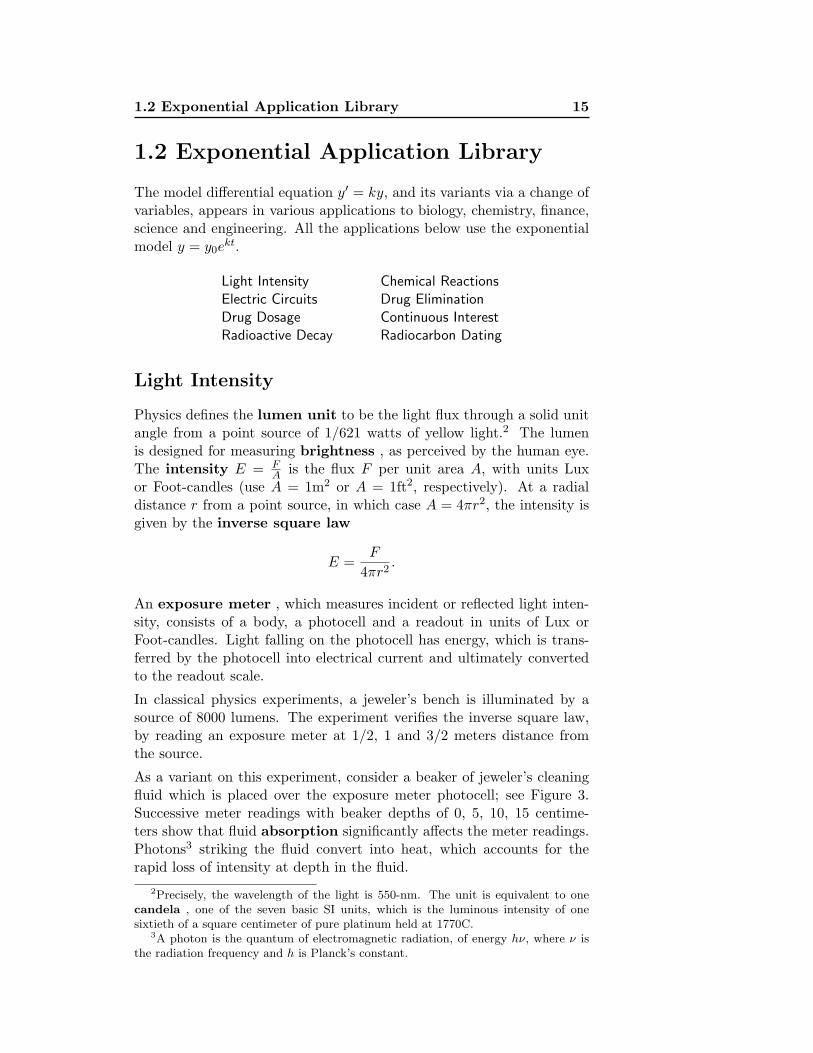
Physics defines the lumen unit to be the light flux through a solid unitangle from a point source of 1/621 watts of yellow light.2 The lumenis designed for measuring brightness , as perceived by the human eye.The intensity E = F

A is the flux F per unit area A, with units Luxor Foot-candles (use A = 1m2 or A = 1ft2, respectively). At a radialdistance r from a point source, in which case A = 4πr2, the intensity isgiven by the inverse square law

E =F

4πr2.

An exposure meter , which measures incident or reflected light inten-sity, consists of a body, a photocell and a readout in units of Lux orFoot-candles. Light falling on the photocell has energy, which is trans-ferred by the photocell into electrical current and ultimately convertedto the readout scale.

In classical physics experiments, a jeweler’s bench is illuminated by asource of 8000 lumens. The experiment verifies the inverse square law,by reading an exposure meter at 1/2, 1 and 3/2 meters distance fromthe source.

As a variant on this experiment, consider a beaker of jeweler’s cleaningfluid which is placed over the exposure meter photocell; see Figure 3.Successive meter readings with beaker depths of 0, 5, 10, 15 centime-ters show that fluid absorption significantly affects the meter readings.Photons3 striking the fluid convert into heat, which accounts for therapid loss of intensity at depth in the fluid.

2Precisely, the wavelength of the light is 550-nm. The unit is equivalent to onecandela , one of the seven basic SI units, which is the luminous intensity of onesixtieth of a square centimeter of pure platinum held at 1770C.

3A photon is the quantum of electromagnetic radiation, of energy hν, where ν isthe radiation frequency and h is Planck’s constant.

16 Fundamentals

exposure meterbeaker

8000 lumensource

1.0mFigure 3. Jeweler’s benchexperiment.The exposure meter measures lightintensity at the beaker’s base.

Empirical evidence from experiments suggests that light intensity I(x)at a depth x in the fluid changes at a rate proportional to itself, that is,

dI

dx= −kI.(9)

If I0 is the surface intensity and I(x) is the intensity at depth x me-ters, then the theory of growth-decay equations applied to (9) gives thesolution

I(x) = I0e−kx.(10)

Equation (10) says that the intensity I(x) at depth x is a percentage ofthe surface intensity I0, the percentage decreasing with depth x.

Electric Circuits

Classical physics analyzes the RC-circuit in Figure 4 and the LR-circuitin Figure 5. The physics background will be reviewed.

R

Q(t) C

Figure 4. An RC-Circuit, noemf.

R

i(t)

L

Figure 5. An LR-Circuit, noemf.

First, the charge Q(t) in coulombs and the current I(t) in amperesare related by the rate formula I(t) = Q′(t). Secondly, there are someempirical laws that are used. There is Kirchhoff’s voltage law :

The algebraic sum of the voltage drops around a closed loopis zero.

Kirchhoff’s node law is not used here, because only one loop appearsin the examples.

There are the voltage drop formulas for an inductor of L henrys, aresistor of R ohms and a capacitor of C farads:


Faraday’s law VL = LI ′

Ohm’s law VR = RI

Coulomb’s law VC = Q/C

In Figure 4, Kirchhoff’s law implies VR + VC = 0. The voltage dropformulas show that the charge Q(t) satisfies RQ′(t) + (1/C)Q(t) = 0.Let Q(0) = Q0. Growth-decay theory, page 3, gives Q(t) = Q0e

−t/(RC).

In Figure 5, Kirchhoff’s law implies that VL + VR = 0. By the voltagedrop formulas, LI ′(t) +RI(t) = 0. Let I(0) = I0. Growth-decay theorygives I(t) = I0e

−Rt/L.

In summary:

RC-CircuitQ = Q0e

−t/(RC)RQ′ + (1/C)Q = 0, Q(0) = Q0,

LR-CircuitI = I0e

−Rt/LLI ′ +RI = 0, I(0) = I0.

The ideas outlined here are illustrated in Examples 9 and 10, page 21.

Interest

The notion of simple interest is based upon the financial formula

A = (1 + r)tA0

where A0 is the initial amount, A is the final amount, t is the numberof years and r is the annual interest rate or rate per annum ( 5%means r = 5/100). The compound interest formula is

A =(

1 +r

n

)ntA0

where n is the number of times to compound interest per annum. Usen = 4 for quarterly interest and n = 360 for daily interest .

The topic of continuous interest has its origins in taking the limitas n → ∞ in the compound interest formula. The answer to the limitproblem is the continuous interest formula

A = A0ert

which by the growth-decay theory arises from the initial value problem{A′(t) = rA(t),A(0) = A0.

Shown on page 26 are the details for taking the limit as n → ∞ inthe compound interest formula. In analogy with population theory, thefollowing statement can be made about continuous interest.

18 Fundamentals

The amount accumulated by continuous interest increasesat a rate proportional to itself.

Applied often in interest calculations is the geometric sum formulafrom algebra:

1 + r + · · ·+ rn =rn+1 − 1r − 1

.

Radioactive Decay

A constant fraction of the atoms present in a ra-dioactive isotope will spontaneously decay into an-other isotope of the identical element or else intoatoms of another element. Empirical evidence givesthe following decay law:

A radioactive isotope decays at a rate proportional to theamount present.

In analogy with population models the differential equation for radioac-tive decay is

dA

dt= −kA(t),

where k > 0 is a physical constant called the decay constant , A(t) isthe number of atoms of radioactive isotope and t is measured in years.

Radiocarbon Dating. The decay constant k ≈ 0.0001245 is knownfor carbon-14 (14C). The model applies to measure the date that anorganism died, assuming it metabolized atmospheric carbon-14.

The idea of radiocarbon dating is due to Willard S. Libby4 in the late1940s. The basis of the chemistry is that radioactive carbon-14, whichhas two more electrons than stable carbon-12, gives up an electron tobecome stable nitrogen-14. Replenishment of carbon-14 by cosmic rayskeeps atmospheric carbon-14 at a nearly constant ratio with ordinarycarbon-12 (this was Libby’s assumption). After death, the radioactivedecay of carbon-14 depletes the isotope in the organism. The percentageof depletion from atmospheric levels of carbon-14 gives a measurementthat dates the organism.

Definition 2 (Half-Life)The half-life of a radioactive isotope is the time T required for half ofthe isotope to decay. In functional notation, it means A(T ) = A(0)/2,where A(t) = A(0)ekt is the amount of isotope at time t.

4Libby received the Nobel Prize for Chemistry in 1960.


For carbon-14, the half-life is 5568 years plus or minus 30 years, accordingto Libby (some texts and references give 5730 years). The decay constantk ≈ 0.0001245 for carbon-14 arises by solving for k = ln(2)/5568 inthe equation A(5568) = 1

2A(0). Experts believe that carbon-14 datingmethods tend to underestimate the age of a fossil.

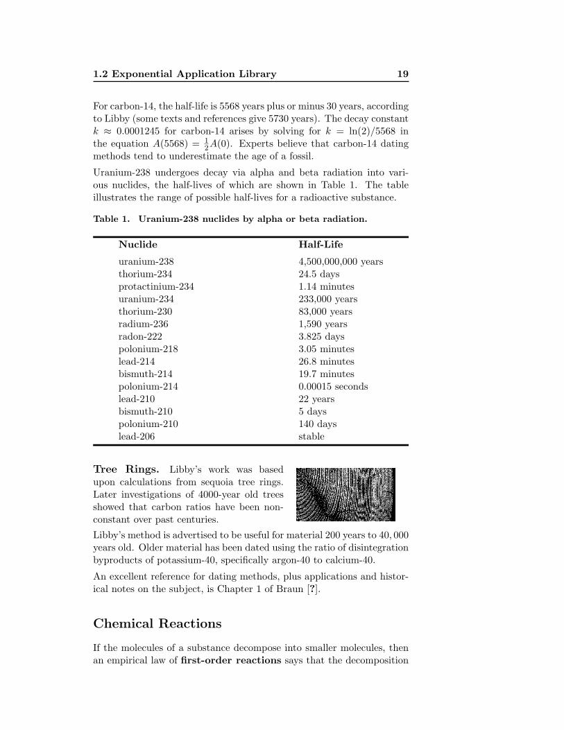
Uranium-238 undergoes decay via alpha and beta radiation into vari-ous nuclides, the half-lives of which are shown in Table 1. The tableillustrates the range of possible half-lives for a radioactive substance.

Table 1. Uranium-238 nuclides by alpha or beta radiation.

Nuclide Half-Life

uranium-238 4,500,000,000 yearsthorium-234 24.5 daysprotactinium-234 1.14 minutesuranium-234 233,000 yearsthorium-230 83,000 yearsradium-236 1,590 yearsradon-222 3.825 dayspolonium-218 3.05 minuteslead-214 26.8 minutesbismuth-214 19.7 minutespolonium-214 0.00015 secondslead-210 22 yearsbismuth-210 5 dayspolonium-210 140 dayslead-206 stable

Tree Rings. Libby’s work was basedupon calculations from sequoia tree rings.Later investigations of 4000-year old treesshowed that carbon ratios have been non-constant over past centuries.

Libby’s method is advertised to be useful for material 200 years to 40, 000years old. Older material has been dated using the ratio of disintegrationbyproducts of potassium-40, specifically argon-40 to calcium-40.

An excellent reference for dating methods, plus applications and histor-ical notes on the subject, is Chapter 1 of Braun [?].

Chemical Reactions

If the molecules of a substance decompose into smaller molecules, thenan empirical law of first-order reactions says that the decomposition

20 Fundamentals

rate is proportional to the amount of substance present. In mathematicalnotation, this means

dA

dt= −hA(t)

where A(t) is the amount of the substance present at time t and h is aphysical constant called the reaction constant .

The law of mass action is used in chemical kinetics to describe second-order reactions . The law describes the amount X(t) of chemical Cproduced by the combination of two chemicals A and B. A chemicalderivation produces a rate equation

X ′ = k(α−X)(β −X), X(0) = X0,(11)

where k, α and β are physical constants, α < β; see Zill-Cullen [Z-C],Chapter 2. The substitution u = (α−X)/(β−X) is known to transform(11) into u′ = k(α−β)u (see page 11 for the technique and the exercisesin this section). Therefore,

X(t) =α− βu(t)1− u(t)

, u(t) = u0e(α−β)kt, u0 =

α−X0

β −X0.(12)

Drug Elimination

Some drugs are eliminated from the bloodstream by an animal’s bodyin a predictable fashion. The amount D(t) in the bloodstream declinesat a rate proportional to the amount already present. Modeling drugelimination exactly parallels radioactive decay, in that the translatedmathematical model is

dD

dt= −hD(t),

where h > 0 is a physical constant, called the elimination constant ofthe drug.

Oral drugs must move through the digestive system and into the gutbefore reaching the bloodstream. The model D′(t) = −hD(t) appliesonly after the drug has reached a stable concentration in the bloodstreamand the body begins to eliminate the drug.

Examples

8 Example (Light intensity) Light intensity in a lake is decreased by 75%at depth one meter. At what depth is the intensity decreased by 95%?

Solution: The answer is 2.16 meters (7 feet, 1 116 inches). This depth will be

justified by applying the light intensity model I(x) = I0e−kx, where I0 is the

surface intensity.


At one meter the intensity is I(1) = I0e−k, but also it is given as 0.25I0. The

equation e−k = 0.25 results, to determine k = ln 4 ≈ 1.3862944. To find thedepth x when the intensity has decreased by 95%, solve I(x) = 0.05I0 for x. Thevalue I0 cancels from this equation, leaving e−kx = 1/20. The usual logarithmmethods give x ≈ 2.2 meters, as follows:

ln e−kx = ln(1/20) Take the logarithm across e−kx = 1/20.

−kx = − ln(20) Use ln eu = u and − lnu = ln(1/u).

x =ln(20)k

Divide by −k.

=ln(20)ln(4)

Use k = ln(4).

≈ 2.16 meters. Only 5% of the surface intensity remainsat 2.16 meters.

9 Example (RC-Circuit) Solve the RC-circuit equation RQ′+ (1/C)Q = 0when R = 2, C = 10−2 and the voltage drop across the capacitor at t = 0is 1.5 volts.

Solution: The solution is Q = 0.015e−50t. To justify this equation, start withthe voltage drop formula VC = Q/C, page 17. Then 1.5 = Q(0)/C impliesQ(0) = 0.015. The differential equation is Q′ + 50Q = 0; page 3 gives thesolution Q = Q(0)e−50t.

10 Example (LR-Circuit) Solve the LR-circuit equation LI ′+RI = 0 whenR = 2, L = 0.1 and the voltage drop across the resistor at t = 0 is 1.0volts.

Solution: The solution is I = 0.5e−20t. To justify this equation, start with thevoltage drop formula VR = RI, page 17. Then 1.0 = RI(0) implies I(0) = 0.5.The differential equation is I ′+20I = 0; page 3 gives the solution I = I(0)e−20t.

11 Example (Compound Interest) Compute the fixed monthly payment fora 5-year auto loan of $18, 000 at 9% per annum, using (a) daily interest and(b) continuous interest.

Solution: The payments are (a) $373.94 and (b) $373.95, which differ by onecent; details below.

Let A0 = 18000 be the initial amount. It will be assumed that the first paymentis due after 30 days and monthly thereafter. To simplify the calculation, a dayis defined to be 1/360th of a year, regardless of the number of days in thatyear, and payments are applied every 30 days. Late fees apply if the paymentis not received within the grace period , but it will be assumed here that allpayments are made on time.

Part (a). The daily interest rate is R = 0.09/360 applied for 1800 periods(5 years). Between payments P , daily interest is applied to the balance A(t)owed after t periods. The balance grows between payments and then decreaseson the day of the payment. The problem is to find P so that A(1800) = 0.

22 Fundamentals

Payments are subtracted every 30 periods making balance A(30k). Let B =(1 +R)30 and Ak = A(30k). Then

Ak = A(30k) Balance after k months.

= A0Bk − P (1 + · · ·+Bk−1) For k = 1, 2, 3, . . .

= A0Bk − P B

k − 1B − 1

Geometric sum formula applied, page18.

A0B60 = P

B60 − 1B − 1

Use A(1800) = 0, which correspondsto k = 60.

P = A0(B − 1)B60

B60 − 1Solve for P .

= 373.93857 By calculator.

Part (b). The details are the same except for the method of applying interest.Let s = 30(0.09)/360, then

Ak = A0eks − Peks−s

(1 + e−s

+ · · ·+ e−ks+s) For k = 1, 2, 3, . . ., by examination of

cases A(30) and A(60).

= A0eks − Peks−s

(e−ks − 1e−s − 1

)Apply the geometric sum formula withcommon ratio e−s.

A0e60s = Pe60s−s

e−60s − 1e−s − 1

Set k = 60 and A(1800) = 0 in theprevious formula.

P = A0−es + 1e−60s − 1

Solve for P .

= 373.94604 By calculator.

12 Example (Effective Annual Yield) A bank advertises an effective annualyield of 5.73% for a certificate of deposit with continuous interest rate 5.5%per annum. Justify the rate.

Solution: The effective annual yield is the simple annual interest rate whichgives the same account balance after one year. The issue is whether one yearmeans 365 days or 360 days, since banks do business on a 360-day cycle.

Suppose first that one year means 365 days. The model used for a savingaccount is A(t) = A0e

rt where r = 0.055 is the interest rate per annum. Forone year, A(1) = A0e

r. Then er = 1.0565406, that is, the account has increasedin one year by 5.65%. The effective annual yield is 0.0565 or 5.65%.

Suppose next that one year means 360 days. Then the bank pays 5.65% foronly 360 days to produce a balance of A1 = A0e

r. The extra 5 days make 5/360years, therefore the bank records a balance of A1e

5r/360 which is A0e365r/360.

The rate for 365 days is then 5.73%, by the calculation

365360

0.0565406 = 0.057325886.


13 Example (Retirement Funds) An engineering firm offers a starting salaryof 40 thousand per year, which is expected to increase 3% per year. Re-tirement contributions are 11% of salary, deposited monthly, growing at 6%continuous interest per annum. The company advertises a million dollars inretirement funds after 40 years. Justify the claim.

Solution: The salary is estimated to be S(t) = 40000(1.03)t after t years,because it starts with S(0) = 40000 and each year it takes a 3% increment.After 39 years of increases the salary has increased from $40, 000 to $126, 681.

Let An be the amount in the retirement account at the end of year n. Let Pn =(40000(1.03)n)(0.11)/12 be the monthly salary for year n+1. The interest ratesare r = 0.06 (annual) and s = 0.06/12 (monthly). For brevity, let R = 1.03.

During the first year, the retirement account accumulates 12 times for a total

A1 = P0 + · · ·+ P0e11s Continuous interest at rate s on amount

P0 for 1 through 11 months.

= P0er − 1es − 1

Geometric sum with common ratio es.

= 4523.3529. Retirement balance after one year.

During the second and later years the retirement account accumulates by therule

An+1 = Aner + Pn

+ Pnes + · · ·+ Pne

11sOne year’s accumulation at continuousrate r on amount An plus monthly accu-mulations on retirement contributions Pn.

= Aner + Pn

er − 1es − 1

Apply the geometric sum formula withcommon ratio es.

= Aner +RnP0

er − 1es − 1

Use Pn = P0Rn.

= Aner +RnA1. Apply A1 = P0

er − 1es − 1

.

After examining cases n = 1, 2, 3, the recursion is solved to give

An = A1

n−1∑k=0

ekrRn−1−k.

To establish this formula, induction is applied:

An+1 = Aner +RnA1 Derived above.

= A1ern−1∑k=0

ekrRn−1−k +RnA1 Apply the induction hypothesis.

= A1

n∑k=0

ekrRn−k Rewrite the sum indices.

= A1Rn (er/R)n+1 − 1

er/R− 1. Use the geometric sum formula

with common ratio er/R.

24 Fundamentals

The advertised retirement fund after 40 years should be the amount A40, whichis obtained by setting n = 39 in the last equality. Then A40 = 1102706.60.

14 Example (Half-life of Radium) A radium sample loses 1/2 percent due todisintegration in 12 years. Verify the half-life of the sample is about 1, 660years.

Solution: The decay model A(t) = A0e−kt applies. The given information

A(12) = 0.995A(0) reduces to the exponential equation e−12k = 0.995 withsolution k = ln(1000/995)/12. The half-life T satisfies A(T ) = 1

2A(0), whichreduces to e−kT = 1/2. Since k is known, the value T can be found as T =ln(2)/k ≈ 1659.3909 years.

15 Example (Radium Disintegration) The disintegration reaction

88R226 −→ 88R

224

of radium-226 into radon has a half-life of 1700 years. Compute the decayconstant k in the decay model A′ = −kA.

Solution: The half-life equation is A(1700) = 12A(0). Since A(t) = A0e

−kt,the equation reduces to e−1700k = 1/2. The latter is solved for k by logarithmmethods (see page 7), giving k = ln(2)/1700 = 0.00040773364.

16 Example (Radiocarbon Dating) The ratio of carbon-14 to carbon-12 ina dinosaur fossil is 6.34 percent of the current atmospheric ratio. Verify thedinosaur’s death was about 22, 160 years ago.

Solution: The method due to Willard Libby will be applied, using his assump-tion that the ratio of carbon-14 to carbon-12 in living animals is equal to theatmospheric ratio. Then carbon-14 depletion in the fossil satisfies the decaylaw A(t) = A0e

−kt for some parameter values k and A0.

Assume the half-life of carbon-14 is 5568 years. Then A(5568) = 12A(0) (see

page 18). This equation reduces to A0e−5568k = 1

2A0e0 or k = ln(2)/5568. In

short, k is known but A0 is unknown. It is not necessary to determine A0 inorder to do the verification.

At the time t0 in the past when the organism died, the amount A1 of carbon-14began to decay, reaching the value 6.34A1/100 at time t = 0 (the present).Therefore, A0 = 0.0634A1 and A(t0) = A1. Taking this last equation as thestarting point, the final calculation proceeds as follows.

A1 = A(t0) The amount of carbon-14 at death is A1, −t0years ago.

= A0e−kt0 Apply the decay model A = A0e

−kt at t = t0.

= 0.0634A1e−kt0 Use A0 = 6.34A1/100.

The value A1 cancels to give the new relation 1 = 0.0634e−kt0 . The valuek = ln(2)/5568 gives an exponential equation to solve for t0:


ekt0 = 0.0634 Multiply by ekt0 to isolate the exponential.

ln ekt0 = ln(0.0634) Take the logarithm of both sides.

t0 =1k

ln(0.0634) Apply ln eu = u and divide by k.

=5568ln 2

ln(0.0634) Substitute k = ln(2)/5568.

= −22157.151 years. By calculator. The fossil’s age is the negative.

17 Example (Percentage of an Isotope) A radioactive isotope disintegratesby 5% in ten years. By what percentage does it disintegrate in one hundredyears?

Solution: The answer is not 50%, as is widely reported by lay persons. Thecorrect answer is 40.13%. It remains to justify this non-intuitive answer.

The model for decay is A(t) = A0e−kt. The decay constant k is known because

of the information . . . disintegrates by 5% in ten years. Translation to equa-tions produces A(10) = 0.95A0, which reduces to e−10k = 0.95. Solving withlogarithms gives k = 0.1 ln(100/95) ≈ 0.0051293294.

After one hundred years, the isotope present is A(100), and the percentage is100A(100)

A(0) . The common factor A0 cancels to give the percentage 100e−100k ≈59.87. The reduction is 40.13%.

To reconcile the lay person’s answer, observe that the amounts present after one,two and three years are 0.95A0, (0.95)2A0, (0.95)3A0. The lay person shouldhave guessed 100 times 1− (0.95)10, which is 40.126306. The common error isto simply multiply 5% by the ten periods of ten years each. By this erroneousreasoning, the isotope would be depleted in two hundred years, whereas thedecay model says that about 36% of the isotope remains!

18 Example (Chemical Reaction) The manufacture of t-butyl alcohol fromt-butyl chloride is made by the chemical reaction

(CH3)3CCL+NaOH −→ (CH3)3COH +NaCL.

Model the production of t-butyl alcohol, when N% of the chloride remainsafter t0 minutes.

Solution: It will be justified that the model for alcohol production is A(t) =C0(1− e−kt) where k = ln(100/N)/t0, C0 is the initial amount of chloride andt is in minutes.

According to the theory of first-order reactions, the model for chloride depletionis C(t) = C0e

−kt where C0 is the initial amount of chloride and k is the reactionconstant. The alcohol production is A(t) = C0 − C(t) or A(t) = C0(1− e−kt).The reaction constant k is found from the initial data C(t0) = N

100C0, whichresults in the exponential equation e−kt0 = N/100. Solving the exponentialequation gives k = ln(100/N)/t0.

26 Fundamentals

19 Example (Drug Dosage) A veterinarian applies general anesthesia to an-imals by injection of a drug into the bloodstream. Predict the drug dosageto anesthetize a 25-pound animal for thirty minutes, given:

1. The drug requires an injection of 20 milligrams per pound of body weight inorder to work.

2. The drug eliminates from the bloodstream at a rate proportional to theamount present, with a half-life of 5 hours.

Solution: The answer is about 536 milligrams of the drug. This amount willbe justified using exponential modeling.

The drug model is D(t) = D0e−ht, where D0 is the initial dosage and h is

the elimination constant. The half-life information D(5) = 12D0 determines

h = ln(2)/5. Depletion of the drug in the bloodstream means the drug levelsare always decreasing, so it is enough to require that the level at 30 min-utes exceeds 20 times the body weight in pounds, that is, D(1/2) > (20)(25).The critical value of the initial dosage D0 then occurs when D(1/2) = 500 orD0 = 500eh/2 = 500e0.1 ln(2), which by calculator is approximately 535.88673milligrams.

Drugs like sodium pentobarbital behave somewhat like this example, althoughinjection in a single dose may not be preferable. An intravenous drip can beemployed to sustain the blood levels of the drug, keeping the level closer to thetarget 500 milligrams.

Details and Proofs

Verification of Continuous Interest by Limiting. Derived here is thecontinuous interest formula by limiting as n → ∞ in the compound interestformula.(

1 +r

n

)nt= Bnt In the exponential rule Bx = ex lnB , the base

is B = 1 + r/n.

= ent lnB Use Bx = ex lnB with x = nt.

= er ln(1+u)

u t Substitute u = r/n. Then u→ 0 as n→∞.

≈ ert Because ln(1 + u)/u ≈ 1 as u → 0, byL’Hospital’s rule.

Exercises 1.2

Light Intensity. The following ex-ercises apply the theory of light in-tensity on page 15, using the modelI(t) = I0e

−kx with x in meters. Meth-ods parallel Example 8 on page 20.

1. The light intensity is I(t) =I0e−1.4x in a certain swimming

pool. At what depth does thelight intensity fall off by 50%?


2. The light intensity in a swimmingpool falls off by 50% at a depthof 2.5 meters. Find the deple-tion constant k in the exponentialmodel.

3. Plastic film is used to cover win-dow glass, which reduces the in-terior light intensity by 10%. Bywhat percentage is the intensityreduced, if two layers are used?

4. Double-thickness colored windowglass is supposed to reduce theinterior light intensity by 20%.What is the reduction for single-thickness colored glass?

RC-Electric Circuits. In the exer-cises below, solve for Q(t) when Q0 =10 and graph Q(t) on 0 ≤ t ≤ 5.

5. R = 1, C = 0.01.

6. R = 0.05, C = 0.001.

7. R = 0.05, C = 0.01.

8. R = 5, C = 0.1.

9. R = 2, C = 0.01.

10. R = 4, C = 0.15.

11. R = 4, C = 0.02.

12. R = 50, C = 0.001.

LR-Electric Circuits. In the exer-cises below, solve for I(t) when I0 = 5and graph I(t) on 0 ≤ t ≤ 5.

13. L = 1, R = 0.5.

14. L = 0.1, R = 0.5.

15. L = 0.1, R = 0.05.

16. L = 0.01, R = 0.05.

17. L = 0.2, R = 0.01.

18. L = 0.03, R = 0.01.

19. L = 0.05, R = 0.005.

20. L = 0.04, R = 0.005.

Interest and Continuous Interest.Financial formulas which appear onpage 17 are applied below, followingthe ideas in Examples 11, 12 and 13,pages 21–23.

21. (Total Interest) Compute the to-tal daily interest and also the totalcontinuous interest for a 10-yearloan of 5, 000 dollars at 5% per an-num.

22. (Total Interest) Compute the to-tal daily interest and also the totalcontinuous interest for a 15-yearloan of 7, 000 dollars at 51

4% perannum.

23. (Monthly Payment) Find themonthly payment for a 3-yearloan of 8, 000 dollars at 7% per an-num compounded continuously.

24. (Monthly Payment) Find themonthly payment for a 4-yearloan of 7, 000 dollars at 61

3% perannum compounded continuously.

25. (Effective Yield) Determine theeffective annual yield for a cer-tificate of deposit at 7 1

4% interestper annum, compounded continu-ously.

26. (Effective Yield) Determine theeffective annual yield for a cer-tificate of deposit at 5 3

4% interestper annum, compounded continu-ously.

27. (Retirement Funds) Assume astarting salary of 35, 000 dollarsper year, which is expected toincrease 3% per year. Retire-ment contributions are 10 1

2% ofsalary, deposited monthly, grow-ing at 5 1

2% continuous interestper annum. Find the retirementamount after 30 years.

28 Fundamentals

28. (Retirement Funds) Assume astarting salary of 45, 000 dollarsper year, which is expected toincrease 3% per year. Retire-ment contributions are 9 1

2% ofsalary, deposited monthly, grow-ing at 6 1

4% continuous interestper annum. Find the retirementamount after 30 years.

29. (Actual Cost) A van is purchasedfor 18, 000 dollars with no moneydown. Monthly payments arespread over 8 years at 12 1

2% inter-est per annum, compounded con-tinuously. What is the actual costof the van?

30. (Actual Cost) Furniture is pur-chased for 15, 000 dollars with nomoney down. Monthly paymentsare spread over 5 years at 11 1

8%interest per annum, compoundedcontinuously. What is the actualcost of the furniture?

Radioactive Decay. Assume the de-cay model A′ = −kA from page 18.Below, A(T ) = 0.5A(0) defines thehalf-life T . Methods parallel Examples14– 17 on pages 24– 25.

31. 31.(Half-Life) Determine the half-life of a radium sample which de-cays by 5.5% in 13 years.

32. (Half-Life) Determine the half-life of a radium sample which de-cays by 4.5% in 10 years.

33. (Half-Life) Assume a radioac-tive isotope has half-life 1800years. Determine the percentagedecayed after 150 years.

34. (Half-Life) Assume a radioac-tive isotope has half-life 1650years. Determine the percentagedecayed after 99 years.

35. (Disintegration Constant) De-termine the constant k in the

model A′ = −kA for radioac-tive material that disintegrates by5.5% in 13 years.

36. (Disintegration Constant) De-termine the constant k in themodel A′ = −kA for radioac-tive material that disintegrates by4.5% in 10 years.

37. (Radiocarbon Dating) A fossilfound near the town of Dinosaur,Utah contains carbon-14 at a ra-tio of 6.21% to the atmosphericvalue. Determine its approximateage according to Libby’s method.

38. (Radiocarbon Dating) A fos-sil found in Colorado containscarbon-14 at a ratio of 5.73% tothe atmospheric value. Determineits approximate age according toLibby’s method.

39. (Radiocarbon Dating) In 1950,the Lascaux Cave in France con-tained charcoal with 14.52% ofthe carbon-14 present in livingwood samples nearby. Estimateby Libby’s method the age of thecharcoal sample.

40. (Radiocarbon Dating) At an ex-cavation in 1960, charcoal frombuilding material had 61% of thecarbon-14 present in living woodnearby. Estimate the age of thebuilding.

41. (Percentage of an Isotope) A ra-dioactive isotope disintegrates by5% in 12 years. By what percent-age is it reduced in 99 years?

42. (Percentage of an Isotope) A ra-dioactive isotope disintegrates by6.5% in 1, 000 years. By whatpercentage is it reduced in 5, 000years?

Chemical Reactions. Assume belowthe model A′ = kA for a first-order re-action. See page 19 and Example 18,page 25.


43. (First-Order A+B −→ C) A firstorder reaction produces productC from chemical A and catalystB. Model the production of C,given N% of A remains after t0minutes.

44. (First-Order A+B −→ C) A firstorder reaction produces productC from chemical A and catalystB. Model the production of C,given M% of A is depleted aftert0 minutes.

45. (Law of Mass-Action) Considera second-order chemical reactionX(t) with k = 0.14, α = 1, β =1.75, X(0) = 0. Find an explicitformula for X(t) and graph it ont = 0 to t = 2.

46. (Law of Mass-Action) Considera second-order chemical reactionX(t) with k = 0.015, α = 1,β = 1.35, X(0) = 0. Find an ex-plicit formula for X(t) and graphit on t = 0 to t = 10.

47. (Derive Mass-Action Solution)

Let k, α, β be positive constants,α < β. Solve X ′ = k(α−X)(β −X), X(0) = X0 by the substitu-tion u = (α−X)/(β−X), showingthat X = (α − βu)/(1 − u), u =u0e

(α−β)kt, u0 = (α − X0)/(β −X0).

48. (Verify Mass-Action Solution)

Let k, α, β be positive constants,α < β. Define X = (α−βu)/(1−u), where u = u0e

(α−β)kt andu0 = (α − X0)/(β − X0). Verifyby calculus computation that (1)X ′ = k(α − X)(β − X) and (2)X(0) = X0.

Drug Dosage. Employ the drugdosage model D(t) = D0e

−ht givenon page 20. Let h be determined bya half-life of three hours. Apply thetechniques of Example 19, page 26.

49. (Injection Dosage) Bloodstreaminjection of a drug into an ani-mal requires a minimum of 20 mil-ligrams per pound of body weight.Predict the dosage for a 12-poundanimal which will maintain a druglevel 3% higher than the minimumfor two hours.

50. (Injection Dosage) Bloodstreaminjection of an antihistamine intoan animal requires a minimum of4 milligrams per pound of bodyweight. Predict the dosage fora 40-pound animal which willmaintain an antihistamine level5% higher than the minimum fortwelve hours.

51. (Oral Dosage) An oral drug withfirst dose 250 milligrams is ab-sorbed into the bloodstream af-ter 45 minutes. Predict the num-ber of hours after the first dose atwhich to take a second dose, inorder to maintain a blood level ofat least 180 milligrams for threehours.

52. (Oral Dosage) An oral drug withfirst dose 250 milligrams is ab-sorbed into the bloodstream af-ter 45 minutes. Determine three(small) dosage amounts, and theiradministration time, which keepthe blood level above 180 mil-ligrams but below 280 milligramsover three hours.

fundamentals - math.utah.edu

Documents