fundamentals of artificial intelligence chapter 05

Fundamentals of Artificial IntelligenceChapter 05: Adversarial Search and Games

Roberto Sebastiani

DISI, Università di Trento, Italy – [email protected]://disi.unitn.it/rseba/DIDATTICA/fai_2020/

Teaching assistant: Mauro Dragoni – [email protected]://www.maurodragoni.com/teaching/fai/

M.S. Course “Artificial Intelligence Systems”, academic year 2020-2021Last update: Tuesday 8th December, 2020, 13:07

Copyright notice: Most examples and images displayed in the slides of this course are taken from[Russell & Norwig, “Artificial Intelligence, a Modern Approach”, Pearson, 3rd ed.],

including explicitly figures from the above-mentioned book, and their copyright is detained by the authors.A few other material (text, figures, examples) is authored by (in alphabetical order):

Pieter Abbeel, Bonnie J. Dorr, Anca Dragan, Dan Klein, Nikita Kitaev, Tom Lenaerts, Michela Milano, Dana Nau, MariaSimi, who detain its copyright. These slides cannot can be displayed in public without the permission of the author.

1 / 42

[email protected]

http://disi.unitn.it/rseba/DIDATTICA/fai_2020/

[email protected]

http://www.maurodragoni.com/teaching/fai/

Outline

1 Games

2 Optimal Decisions in Games

3 Alpha-Beta Pruning

4 Adversarial Search with Resource Limits

5 Stochastic Games

2 / 42

Outline

1 Games




5 Stochastic Games

3 / 42

Games and AI

Games are a form of multi-agent environmentQ.: What do other agents do and how do they affect our success?recall: cooperative vs. competitive multi-agent environmentscompetitive multi-agent environments give rise to adversarialproblems a.k.a. games

Q.: Why study games in AI?lots of fun; historically entertainingeasy to represent: agents restricted to small number of actionswith precise rulesinteresting also because computationally very hard(ex: chess has b ≈ 35, #nodes ≈ 1040)

4 / 42

Search and Games

Search (with no adversary)solution is a (heuristic) method for finding a goalheuristics techniques can find optimal solutionsevaluation function: estimate of cost from start to goal throughgiven nodeexamples: path planning, scheduling activities, ...

Games (with adversary), a.k.a adversarial searchsolution a is strategy (specifies move for every possible opponentreply)evaluation function (utility): evaluate “goodness” of game positionexamples: tic-tac-toe, chess, checkers, Othello, backgammon, ...often time limits force an approximate solution

5 / 42

Types of Games

Many different kinds of gamesRelevant features:

deterministic vs. stochastic (with chance)one, two, or more playerszero-sum vs. general gamesperfect information (can you see the state?) vs. imperfect

Most common: deterministic, turn-taking, two-player, zero-sumgames, of perfect informationWant algorithms for calculating a strategy (aka policy):

recommends a move from each state: policy : S 7→ A

6 / 42

Games: Main Concepts

We first consider games with two players: “MAX” and “MIN”MAX moves first;they take turns moving until the game is overat the end of the game, points are awarded to the winning playerand penalties are given to the loser

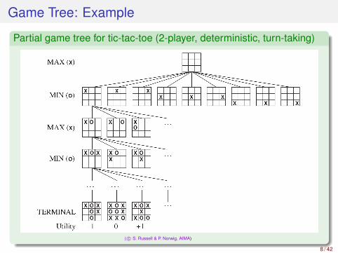
A game is a kind of search problem:initial state S0: specifies how the game is set up at the starPlayer(s): defines which player has the move in a stateActions(s): returns the set of legal moves in a stateResult(s,a): the transition model, defines the result of a moveTerminalTest(s): true iff the game is over (if so, S terminal state)Utility(s,p): (aka objective function or payoff function): defines thefinal numeric value for a game ending in state s for player p

ex: chess: 1 (win), 0 (loss), 12 (draw)

S0, Actions(s) and Result(s,a) recursively define the game treenodes are states, arcs are actionsex: tic-tac-toe: ≈105 nodes, chess: ≈1040 nodes, ...

7 / 42

Game Tree: Example

Partial game tree for tic-tac-toe (2-player, deterministic, turn-taking)

( c© S. Russell & P. Norwig, AIMA)

8 / 42

Zero-Sum Games vs. General Games

General Gamesagents have independent utilitiescooperation, indifference, competition, and more are all possible

Zero-Sum Games: the total payoff to all players is the same foreach game instance

adversarial, pure competitionagents have opposite utilities (values on outcomes)

=⇒ Idea: With two-player zero-sum games, we can use one singleutility value

one agent maximizes it, the other minimizes it=⇒ optimal adversarial search as min-max search

9 / 42

Outline

1 Games




5 Stochastic Games

10 / 42

Adversarial Search as Min-Max Search

Assume MAX and MIN are very smart and always play optimallyMAX must find a contingent strategy specifying:

MAX’s move in the initial stateMAX’s moves in the states resulting from every possible responseby MIN,MAX’s moves in the states resulting from every possible responseby MIN to those moves,...

(a single-agent move is called half-move or ply)Analogous to the AND-OR search algorithm

MAX playing the role of ORMIN playing the role of AND

Optimal strategy: for which Minimax(s) returns the highest valueMinimax(s)

def=

Utility(s) if TerminalTest(s)maxa∈Actions(s)Minimax(Result(s,a)) if Player(s) = MAXmina∈Actions(s)Minimax(Result(s,a)) if Player(s) = MIN

11 / 42

Min-Max Search: Example

A two-ply game tree

∆ nodes are “MAX nodes”, ∇ nodes are “MIN nodes”,terminal nodes show the utility values for MAXthe other nodes are labeled with their minimax value

Minimax maximizes the worst-case outcome for MAX=⇒ MAX’s root best move is a1

( c© S. Russell & P. Norwig, AIMA) 12 / 42

The Minimax Algorithm

Depth-Search Minimax Algorithm

( c© S. Russell & P. Norwig, AIMA)13 / 42

Multi-Player Games: Optimal Decisions

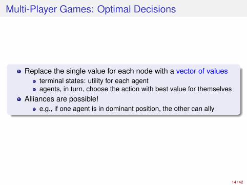
Replace the single value for each node with a vector of valuesterminal states: utility for each agentagents, in turn, choose the action with best value for themselves

Alliances are possible!e.g., if one agent is in dominant position, the other can ally

14 / 42

Multiplayer Min-Max Search: Example

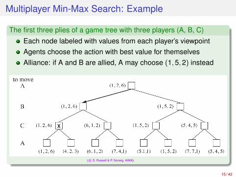
The first three plies of a game tree with three players (A, B, C)

Each node labeled with values from each player’s viewpointAgents choose the action with best value for themselvesAlliance: if A and B are allied, A may choose (1,5,2) instead


15 / 42

The Minimax Algorithm: Properties

Complete? Yes, if tree is finiteOptimal? Yes, against an optimal opponent

What about non-optimal opponent?=⇒ even better, but non optimal in this case

Time complexity? O(bm)

Space complexity? O(bm) (DFS)

For chess, b ≈ 35, m ≈ 100 =⇒ 35100 = 10154 (!)

We need to prune the tree!

16 / 42

Outline

1 Games




5 Stochastic Games

17 / 42

Pruning Min-Max Search: Example

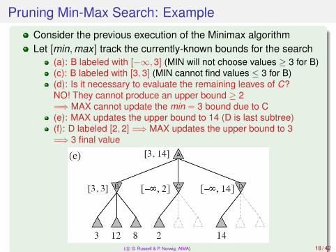
Consider the previous execution of the Minimax algorithmLet [min,max ] track the currently-known bounds for the search

(a): B labeled with [−∞,3] (MIN will not choose values ≥ 3 for B)(c): B labeled with [3,3] (MIN cannot find values ≤ 3 for B)(d): Is it necessary to evaluate the remaining leaves of C?NO! They cannot produce an upper bound ≥ 2=⇒ MAX cannot update the min = 3 bound due to C(e): MAX updates the upper bound to 14 (D is last subtree)(f): D labeled [2,2] =⇒ MAX updates the upper bound to 3=⇒ 3 final value


Alpha-Beta Pruning Technique for Min-Max Search

Idea: consider a node n (terminal or intermediate)If player has a better choice m at the parent node of n or at anychoice point further up, n will never be reached in actual play

=⇒ if we know enough of n to draw this conclusion, we can prune nAlpha-Beta Pruning: nodes labeled with [α, β] s.t.:α : best value for MAX (highest) so far off the current pathβ : best value for MIN (lowest) so far off the current path

=⇒ Prune n if its value is worse than the current α value for MAX(dual for β, MIN)


The Alpha-Beta Search Algorithm


20 / 42

Example revisited: Alpha-Beta Cuts

Notation: ≥ α; ≤ β;


21 / 42

Properties of Alpha-Beta Search

Pruning does not affect the final result =⇒ correctness preservedGood move ordering improves effectiveness of pruning

Ex: if MIN expands 3rd child of D first, the others are prunedtry to examine first the successors that are likely to be best

With “perfect” ordering, time complexity reduces to O(bm/2)

aka “killer-move heuristic”=⇒ doubles solvable depth!

With “random” ordering, time complexity reduces to O(b3m/4)

“Graph-based” version further improves performancestrack explored states via hash table

22 / 42

Exercise I

Apply alpha-beta search to the following tree

( c© D. Klein, P. Abbeel, S. Levine, S. Russell, U. Berkeley)

23 / 42

Exercise II

Apply alpha-beta search to the following tree

( c© D. Klein, P. Abbeel, S. Levine, S. Russell, U. Berkeley)

24 / 42

Outline

1 Games




5 Stochastic Games

25 / 42

Adversarial Search with Resource Limits

Problem: In realistic games, full search is impractical!

Complexity: bd (ex. chess: ≈ 35100)Idea [Shannon, 1949]: Depth-limitedsearch

cut off minimax search earlier, afterlimited depthreplace terminal utility function withevaluation for non-terminal nodes

Ex (chess): depth d = 8 (decent)=⇒ α-β: 358/2 = 105 (feasible)

26 / 42

Adversarial Search with Resource Limits [cont.]

Idea:cut off the search earlier, at limited depthsapply a heuristic evaluation function to states in the search

=⇒ effectively turning nonterminal nodes into terminal leavesModify Minimax() or Alpha-Beta search in two ways:

replace the utility function Utility(s) by a heuristic evaluationfunction Eval(s), which estimates the position’s utilityreplace the terminal test TerminalTest(s) by a cutoff testCutOffTest(s,d), that decides when to apply Eval()plus some bookkeeping to increase depth d at each recursive call

=⇒ Heuristic variant of Minimax():H-Minimax(s,d)

def= Eval(s) if CutOffTest(s,d)

maxa∈Actions(s)H-Minimax(Result(s,a),d + 1) if Player(s) = MAXmina∈Actions(s) H-Minimax(Result(s,a),d + 1) if Player(s) = MIN

=⇒ Heuristic variant of alpha-beta: substitute the terminal test withIf CutOffTest(s) then return Eval(s)

27 / 42

Evaluation FunctionsEval(s)

Should be relatively cheap to computeReturns an estimate of the expected utility from a given position

Ideal function: returns the actual minimax value of the positionShould order terminal states the same way as the utility function

e.g., wins > draws > losses

For nonterminal states, should be strongly correlated with theactual chances of winningDefines equivalence classes of positions (same Eval(s) value)

e.g. returns a value reflecting the % of states with each outcome

Typically weighted linear sum of features:Eval(s) = w1 · f1(s) + w2 · f2(s) + ...+ wn · fn(s)

ex (chess): fqueens(s) = #white queens −#black queens,wpawns = 1: wbishops = wknights = 3, wrooks = 5, wqueens = 9

May depend on depth (ex: knights vs. rooks)May be very inaccurate for some positions

28 / 42

Example

Two same-score positions (White: -8, Black: -3)(a) Black has an advantage of a knight and two pawns,

=⇒ should be enough to win the game(b) White will capture the queen,

=⇒ give it an advantage that should be strong enough to win

(Personal note: only very-stupid black player would get into (b))


29 / 42

Cutting-off the Search

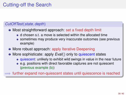
CutOffTest(state,depth)

Most straightforward approach: set a fixed depth limitd chosen s.t. a move is selected within the allocated timesometimes may produce very inaccurate outcomes (see previousexample)

More robust approach: apply Iterative DeepeningMore sophisticate: apply Eval() only to quiescent states

quiescent: unlikely to exhibit wild swings in value in the near futuree.g. positions with direct favorable captures are not quiescent(previous example (b))

=⇒ further expand non-quiescent states until quiescence is reached

30 / 42

Remark

Exact values don’t matter!Behaviour preserved under any monotonic transformation of Eval()

Only the order matters!payoff in deterministic games acts as an ordinal utility function


31 / 42

Deterministic Games in Practice

Checkers: (1994) Chinook ended 40-year-reign of worldchampion Marion Tinsley

used an endgame database defining perfect play for all positionsinvolving 8 or fewer pieces on the boarda total of 443,748,401,247 positions

Chess: (1997) Deep Blue defeated world champion GaryKasparov in a six-game match

searches 200 million positions per seconduses very sophisticated evaluation, and undisclosed methods

Othello:Human champions refuse to compete against computers, whichare too good

Go: (2016) AlphaGo beats world champion Lee Sedolnumber of possible positions > number of atoms in the universe

32 / 42

AlphaGo beats GO world champion, Lee Sedol (2016)

33 / 42

Outline

1 Games




5 Stochastic Games

34 / 42

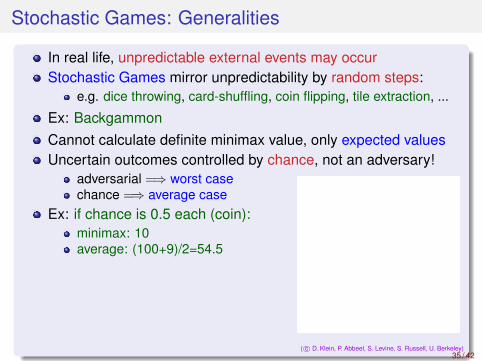
Stochastic Games: Generalities

In real life, unpredictable external events may occurStochastic Games mirror unpredictability by random steps:

e.g. dice throwing, card-shuffling, coin flipping, tile extraction, ...

Ex: BackgammonCannot calculate definite minimax value, only expected valuesUncertain outcomes controlled by chance, not an adversary!

adversarial =⇒ worst casechance =⇒ average case

Ex: if chance is 0.5 each (coin):minimax: 10average: (100+9)/2=54.5

( c© D. Klein, P. Abbeel, S. Levine, S. Russell, U. Berkeley)35 / 42

An Example: Backgammon

Rules15 pieces eachwhite moves clockwise to 25, black moves counterclockwise to 0a piece can move to a position unless ≥ 2 opponent pieces thereif there is one opponent, it is captured and must start overtermination: all whites in 25 or all blacks in 0

Ex: Possible white moves:(5-10,5-11)(5-11,19-24)(5-10,10-16)(5-11,11-16)

Combines strategy with luck=⇒ stochastic component (dice)

double rolls (1-1),...,(6-6)have 1/36 probability eachother 15 distinct rollshave a 1/18 probability each


Stochastic Games Trees

Idea: A game tree for a stochastic game includes chance nodesin addition to MAX and MIN nodes.

chance nodes above agent represent stochastic events for agent(e.g. dice roll)outcoming arcs represent stochastic event outcomeslabeled with stochastic event and relative probability


Algorithm for Stochastic Games: ExpectMinimax()

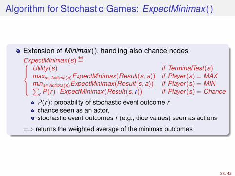
Extension of Minimax(), handling also chance nodesExpectMinimax(s)

def=

Utility(s) if TerminalTest(s)maxa∈Actions(s)ExpectMinimax(Result(s,a)) if Player(s) = MAXmina∈Actions(s)ExpectMinimax(Result(s,a)) if Player(s) = MIN∑

r P(r) · ExpectMinimax(Result(s, r)) if Player(s) = Chance

P(r): probability of stochastic event outcome rchance seen as an actor,stochastic event outcomes r (e.g., dice values) seen as actions

=⇒ returns the weighted average of the minimax outcomes

38 / 42

Simple Example with Coin-Flipping


39 / 42

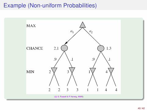
Example (Non-uniform Probabilities)


40 / 42

Remark (compare with deterministic case)

Exact values do matter!Behaviour not preserved under monotonic transformations of Utility()

preserved only by positive linear transformation of Utility()

hint: p1v1 ≥ p2v2 =⇒ p1(av1 + b) ≥ p2(av2 + b) if a ≥ 0

=⇒ Utility() should be proportional to the expected payoff


Stochastic Games in Practice

Dice rolls increase b: 21 possible rolls with 2 dice=⇒ O(bm · nm), n being the number of distinct rollEx: Backgammon has ≈ 20 moves=⇒ depth 4: 20 · (21× 20)3 ≈ 109 (!)

Alpha-beta pruning much less effective than with deterministicgames

=⇒ Unrealistic to consider high depths in most stochastic gamesHeuristic variants of ExpectMinimax() effective, low cutoff depthsEx: TD-GGAMMON uses depth-2 search + very-good Eval()

Eval() “learned” by running million training gamescompetitive with world champions

42 / 42

fundamentals of artificial intelligence chapter 05

Documents