fundamentals of radiation dosimetry and radiological physics

Fundamentals of Radiation Dosimetryand

Radiological Physics

Alex F BielajewThe University of Michigan

Department of Nuclear Engineering and Radiological Sciences2927 Cooley Building (North Campus)

2355 Bonisteel BoulevardAnn Arbor, Michigan 48109-2104

U. S. A.Tel: 734 764 6364Fax: 734 763 4540

email: [email protected]

c© 2005 Alex F Bielajew

June 21, 2005

Preface

This book arises out of a course I am teaching for a three-credit (42 hour) graduate-levelcourse Dosimetry Fundamentals being taught at the Department of Nuclear Engineering andRadiological Sciences at the University of Michigan. It is far from complete.

A formal course in dosimetry usually starts at Chapter 4, Macroscopic Radiation Physics,that describes macroscopic field quantities (primarily fluence). However, this is an approxi-mation (a good one) for rudimentary dosimetry. Underpinning this, however, is the realiza-tion that these fields are made up of discrete particles. Therefore, a discussion of microscopicradiation physics should really be the starting point. This material is given in Chapters 1and 2, couched in the language of Monte Carlo practitioner, who estimates macroscopicquantities, from microscopic calculation. Chapter 3 describes transport of particles throughmatter, again in a microscopic way.

These first three chapters should be considered pre-requisite material for the following chap-ters. Perhaps they should be combined into a single chapter with the title “Microscopicradiation physics”. Deep understanding is not required and much of the language is in aform more suitable for Monte Carlo practitioners. Nonetheless, knowledge of this materialwill aid in the assimilation of the material of the following chapters. The Monte Carlo-specificdetails should be glossed over if they are unfamiliar. However, the microscopic processes thatgovern interaction and transport must be understood, at least intuitively, before attemptingthe later chapters.

Finally, there are many missing figures. This book is far from completion. Anyone volun-teering figures for this book will be gratefully acknowledged. Chapters 4–7 were all writtenup during a very hectic week, from a collection of hand-written notes. There will be spellingand grammatical errors, some mathematics errors, and perhaps a conceptual error or two. Iwould be grateful if these were pointed out to me.

AFB, June 21, 2005

i

Contents

1 Photon Monte Carlo Simulation 1

1.1 Basic photon interaction processes . . . . . . . . . . . . . . . . . . . . . . . . 1

1.1.1 Pair production in the nuclear field . . . . . . . . . . . . . . . . . . . 2

1.1.2 The Compton interaction (incoherent scattering) . . . . . . . . . . . 5

1.1.3 Photoelectric interaction . . . . . . . . . . . . . . . . . . . . . . . . . 6

1.1.4 Rayleigh (coherent) interaction . . . . . . . . . . . . . . . . . . . . . 9

1.1.5 Relative importance of various processes . . . . . . . . . . . . . . . . 10

1.2 Photon transport logic . . . . . . . . . . . . . . . . . . . . . . . . . . . . . . 10

2 Electron Monte Carlo Simulation 21

2.1 Catastrophic interactions . . . . . . . . . . . . . . . . . . . . . . . . . . . . . 22

2.1.1 Hard bremsstrahlung production . . . . . . . . . . . . . . . . . . . . 22

2.1.2 Møller (Bhabha) scattering . . . . . . . . . . . . . . . . . . . . . . . . 22

2.1.3 Positron annihilation . . . . . . . . . . . . . . . . . . . . . . . . . . . 23

2.2 Statistically grouped interactions . . . . . . . . . . . . . . . . . . . . . . . . 23

2.2.1 “Continuous” energy loss . . . . . . . . . . . . . . . . . . . . . . . . . 23

2.2.2 Multiple scattering . . . . . . . . . . . . . . . . . . . . . . . . . . . . 24

2.3 Electron transport “mechanics” . . . . . . . . . . . . . . . . . . . . . . . . . 25

2.3.1 Typical electron tracks . . . . . . . . . . . . . . . . . . . . . . . . . . 25

2.3.2 Typical multiple scattering substeps . . . . . . . . . . . . . . . . . . . 25

2.4 Examples of electron transport . . . . . . . . . . . . . . . . . . . . . . . . . 26

2.4.1 Effect of physical modeling on a 20 MeV e− depth-dose curve . . . . 26

iii

iv CONTENTS

2.5 Electron transport logic . . . . . . . . . . . . . . . . . . . . . . . . . . . . . 38

3 Transport in media, interaction models 45

3.1 Interaction probability in an infinite medium . . . . . . . . . . . . . . . . . . 45

3.1.1 Uniform, infinite, homogeneous media . . . . . . . . . . . . . . . . . . 46

3.2 Finite media . . . . . . . . . . . . . . . . . . . . . . . . . . . . . . . . . . . . 47

3.3 Regions of different scattering characteristics . . . . . . . . . . . . . . . . . . 47

3.4 Obtaining µ from microscopic cross sections . . . . . . . . . . . . . . . . . . 50

3.5 Compounds and mixtures . . . . . . . . . . . . . . . . . . . . . . . . . . . . 53

3.6 Branching ratios . . . . . . . . . . . . . . . . . . . . . . . . . . . . . . . . . 54

3.7 Other pathlength schemes . . . . . . . . . . . . . . . . . . . . . . . . . . . . 54

3.8 Model interactions . . . . . . . . . . . . . . . . . . . . . . . . . . . . . . . . 55

3.8.1 Isotropic scattering . . . . . . . . . . . . . . . . . . . . . . . . . . . . 55

3.8.2 Semi-isotropic or P1 scattering . . . . . . . . . . . . . . . . . . . . . . 55

3.8.3 Rutherfordian scattering . . . . . . . . . . . . . . . . . . . . . . . . . 56

3.8.4 Rutherfordian scattering—small angle form . . . . . . . . . . . . . . 56

4 Macroscopic Radiation Physics 59

4.1 Fluence . . . . . . . . . . . . . . . . . . . . . . . . . . . . . . . . . . . . . . 59

4.2 Radiation equilibrium . . . . . . . . . . . . . . . . . . . . . . . . . . . . . . . 62

4.2.1 Planar fluence . . . . . . . . . . . . . . . . . . . . . . . . . . . . . . . 63

4.3 Fluence-related radiometric quantities . . . . . . . . . . . . . . . . . . . . . . 65

4.3.1 Energy fluence . . . . . . . . . . . . . . . . . . . . . . . . . . . . . . 65

4.4 Attenuation, radiological pathlength . . . . . . . . . . . . . . . . . . . . . . 66

4.4.1 Solid angle subtended by a surface . . . . . . . . . . . . . . . . . . . 67

4.4.2 Primary fluence determinations . . . . . . . . . . . . . . . . . . . . . 68

4.4.3 Volumetric symmetry . . . . . . . . . . . . . . . . . . . . . . . . . . . 68

4.5 Fano’s theorem . . . . . . . . . . . . . . . . . . . . . . . . . . . . . . . . . . 69

5 Photon dose calculation models 77

CONTENTS v

5.1 Kerma, collision kerma, and dose for photo irradiation . . . . . . . . . . . . 77

5.1.1 Kerma . . . . . . . . . . . . . . . . . . . . . . . . . . . . . . . . . . . 77

5.1.2 Collision Kerma . . . . . . . . . . . . . . . . . . . . . . . . . . . . . . 80

5.1.3 Dose . . . . . . . . . . . . . . . . . . . . . . . . . . . . . . . . . . . . 83

5.1.4 Comparison of dose deposition models . . . . . . . . . . . . . . . . . 85

5.1.5 Transient charged particle equilibrium . . . . . . . . . . . . . . . . . 87

5.1.6 Dose due to scattered photons . . . . . . . . . . . . . . . . . . . . . . 89

6 Electron dose calculation models 93

6.1 The microscopic picture of dose deposition . . . . . . . . . . . . . . . . . . . 93

6.2 Stopping power . . . . . . . . . . . . . . . . . . . . . . . . . . . . . . . . . . 94

6.2.1 Total mass stopping power . . . . . . . . . . . . . . . . . . . . . . . . 94

6.2.2 Restricted mass stopping power . . . . . . . . . . . . . . . . . . . . . 98

6.3 Electron angular scattering . . . . . . . . . . . . . . . . . . . . . . . . . . . . 99

6.4 Dose due to electrons from primary photon interaction . . . . . . . . . . . . 100

6.4.1 A practical semi-analytic dose deposition model . . . . . . . . . . . . 101

6.5 The convolution method . . . . . . . . . . . . . . . . . . . . . . . . . . . . . 105

6.6 Monte Carlo methods . . . . . . . . . . . . . . . . . . . . . . . . . . . . . . . 105

7 Ionization chamber-based air kerma standards 111

7.1 Bragg-Gray cavity theory . . . . . . . . . . . . . . . . . . . . . . . . . . . . 111

7.1.1 Exposure measurements . . . . . . . . . . . . . . . . . . . . . . . . . 112

7.2 Spencer-Attix cavity theory . . . . . . . . . . . . . . . . . . . . . . . . . . . 114

7.3 Modern cavity theory . . . . . . . . . . . . . . . . . . . . . . . . . . . . . . . 115

7.4 Interface effects . . . . . . . . . . . . . . . . . . . . . . . . . . . . . . . . . . 117

7.5 Saturation corrections . . . . . . . . . . . . . . . . . . . . . . . . . . . . . . 117

7.6 Burlin cavity theory . . . . . . . . . . . . . . . . . . . . . . . . . . . . . . . 118

7.7 The dosimetry chain . . . . . . . . . . . . . . . . . . . . . . . . . . . . . . . 118

vi CONTENTS

Chapter 1

Photon Monte Carlo Simulation

“I could have done it in a much more complicated way”said the red Queen, immensely proud.Lewis Carroll

In this chapter we discuss the basic mechanism by which the simulation of photon interactionand transport is undertaken. We start with a review of the basic interaction processesthat are involved, some common simplifications and the relative importance of the variousprocesses. We discuss when and how one goes about choosing, by random selection, whichprocess occurs. We discuss the rudimentary geometry involved in the transport and deflectionof photons. We conclude with a schematic presentation of the logic flow executed by atypical photon Monte Carlo transport algorithm. This chapter will only sketch the bareminimum required to construct a photon Monte Carlo code. A particularly good referencefor a description of basic interaction mechanisms is the excellent book [Eva55] by RobleyEvans, The Atomic Nucleus. This book should be in the bookshelf of anyone undertakinga career in the radiation sciences. Simpler descriptions of photon interaction processes areuseful as well and are included in many common textbooks [JC83, Att86, SF96].

1.1 Basic photon interaction processes

We now give a brief discussion of the photon interaction processes that should be modeledby a photon Monte Carlo code, namely:

• Pair production in the nuclear field

• The Compton interaction (incoherent scattering)

1

2 CHAPTER 1. PHOTON MONTE CARLO SIMULATION

• The photoelectric interaction

• The Rayleigh interaction (coherent scattering)

1.1.1 Pair production in the nuclear field

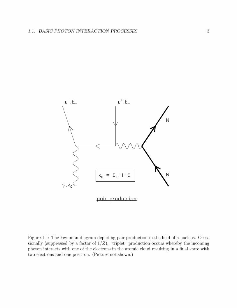
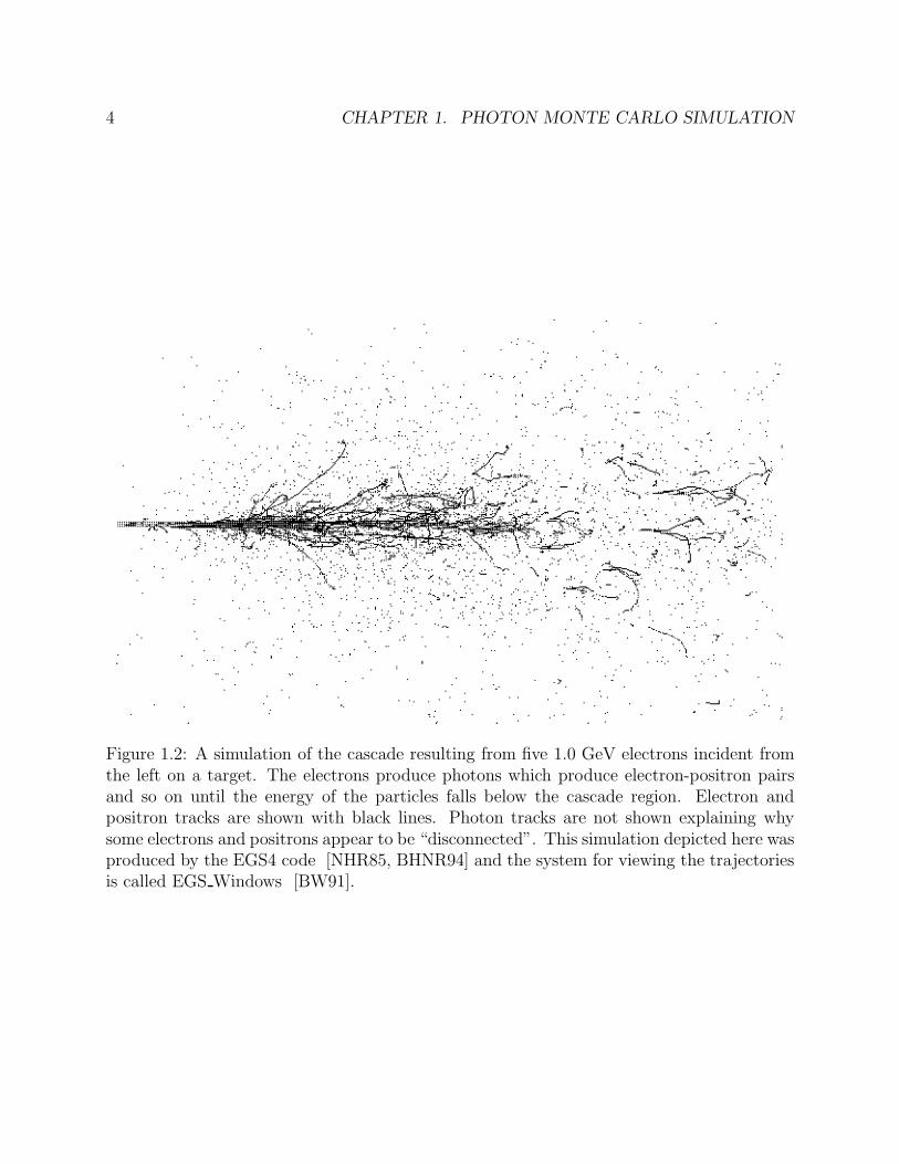
As seen in Figure 1.1, a photon can interact in the field of a nucleus, annihilate and producean electron-positron pair. A third body, usually a nucleus, is required to be present toconserve energy and momentum. This interaction scales as Z2 for different nuclei. Thus,materials containing high atomic number materials more readily convert photons into chargedparticles than do low atomic number materials. This interaction is the quantum “analog” ofthe bremsstrahlung interaction, which we will encounter in the next Chapter, Electron MonteCarlo simulation. At high energies, greater than 50 MeV or so in all materials, the pair andbremsstrahlung interactions dominate. The pair interaction gives rise to charged particlesin the form of electrons and positrons (muons at very high energy) and the bremsstrahlunginteraction of the electrons and positrons leads to more photons. Thus there is a “cascade”process that quickly converts high energy electromagnetic particles into copious amounts oflower energy electromagnetic particles. Hence, a high-energy photon or electron beam notonly has “high energy”, it is also able to deposit a lot of its energy near one place by virtueof this cascade phenomenon. A picture of this process is given in Figure 1.2.

The high-energy limit of the pair production cross section per nucleus takes the form:

limα→∞

σpp(α) = σpp0 Z2(ln(2α)− 109

42

), (1.1)

where α = Eγ/mec2, that is, the energy of the photon divided by the rest mass energy1 of

the electron (0.51099907± 0.00000015 MeV) and σpp0 = 1.80× 10−27 cm2/nucleus. We notethat the cross section grows logarithmically with incoming photon energy.

The kinetic energy distribution of the electrons and positrons is remarkably “flat” exceptnear the kinematic extremes of K± = 0 and K± = Eγ − 2mec

2. Note as well that therest-mass energy of the electron-positron pair must be created and so this interaction has athreshold at Eγ = 2mec

2. It is exactly zero below this energy.

Occasionally it is one of the electrons in the atomic cloud surrounding the nucleus thatinteracts with the incoming photon and provides the necessary third body for momentumand energy conservation. This interaction channel is suppressed by a factor of 1/Z relativeto the nucleus-participating channel as well as additional phase-space and Pauli exclusiondifferences. In this case, the atomic electron is ejected with two electrons and one positronemitted. This is called “triplet” production. It is common to include the effects of triplet pro-duction by “scaling up” the two-body reaction channel and ignoring the 3-body kinematics.This is a good approximation for all but the low-Z atoms.

1The latest information on particle data is available on the web at: http://pdg.lbl.gov/pdg.htmlThisweb page is maintained by the Particle Data Group at the Lawrence Berkeley laboratory.

1.1. BASIC PHOTON INTERACTION PROCESSES 3

Figure 1.1: The Feynman diagram depicting pair production in the field of a nucleus. Occa-sionally (suppressed by a factor of 1/Z), “triplet” production occurs whereby the incomingphoton interacts with one of the electrons in the atomic cloud resulting in a final state withtwo electrons and one positron. (Picture not shown.)


Figure 1.2: A simulation of the cascade resulting from five 1.0 GeV electrons incident fromthe left on a target. The electrons produce photons which produce electron-positron pairsand so on until the energy of the particles falls below the cascade region. Electron andpositron tracks are shown with black lines. Photon tracks are not shown explaining whysome electrons and positrons appear to be “disconnected”. This simulation depicted here wasproduced by the EGS4 code [NHR85, BHNR94] and the system for viewing the trajectoriesis called EGS Windows [BW91].


Further reading on the pair production interaction can be found in the reviews by Davies,Bethe, Maximon [DBM54], Motz, Olsen, and Koch [MOK69], and Tsai [Tsa74].

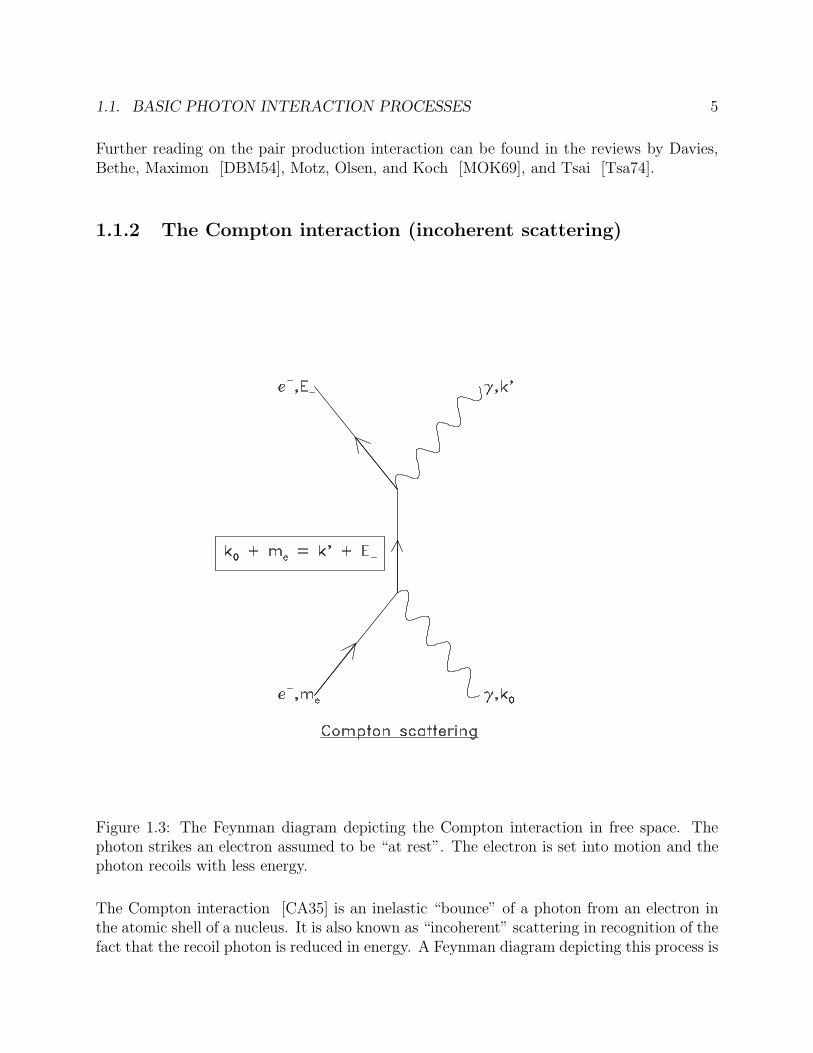
1.1.2 The Compton interaction (incoherent scattering)

Figure 1.3: The Feynman diagram depicting the Compton interaction in free space. Thephoton strikes an electron assumed to be “at rest”. The electron is set into motion and thephoton recoils with less energy.

The Compton interaction [CA35] is an inelastic “bounce” of a photon from an electron inthe atomic shell of a nucleus. It is also known as “incoherent” scattering in recognition of thefact that the recoil photon is reduced in energy. A Feynman diagram depicting this process is


given in Figure 1.3. At large energies, the Compton interaction approaches asymptotically:

limα→∞

σinc(α) = σinc0

Z

α, (1.2)

where σinc0 = 3.33 × 10−25 cm2/nucleus. It is proportional to Z (i.e. the number of elec-trons) and falls off as 1/Eγ. Thus, the Compton cross section per unit mass is nearly aconstant independent of material and the energy-weighted cross section is nearly a constantindependent of energy. Unlike the pair production cross section, the Compton cross sectiondecreases with increased energy.

At low energies, the Compton cross section becomes a constant with energy. That is,

limα→0

σinc(α) = 2σinc0 Z . (1.3)

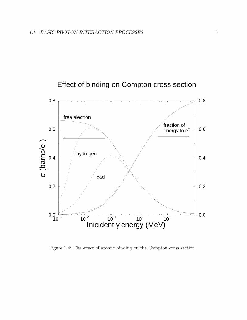
This is the classical limit and it corresponds to Thomson scattering, which describes thescattering of light from “free” (unbound) electrons. In almost all applications, the electronsare bound to atoms and this binding has a profound effect on the cross section at low energies.However, above about 100 keV on can consider these bound electrons as “free”, and ignoreatomic binding effects. As seen in Figure 1.4, this is a good approximation for photon energiesdown to 100 of keV or so, for most materials. This lower bound is defined by the K-shellenergy although the effects can have influence greatly above it, particularly for the low-Zelements. Below this energy the cross section is depressed since the K-shell electrons are tootightly bound to be liberated by the incoming photon. The unbound Compton differentialcross section is taken from the Klein-Nishina cross section [KN29], derived in lowest orderQuantum Electrodynamics, without any further approximation.

It is possible to improve the modeling of the Compton interaction. Namito and Hirayama [NH91]have considered the effect of binding for the Compton effect as well as allowing for the trans-port of polarised photons for both the Compton and Rayleigh interactions.

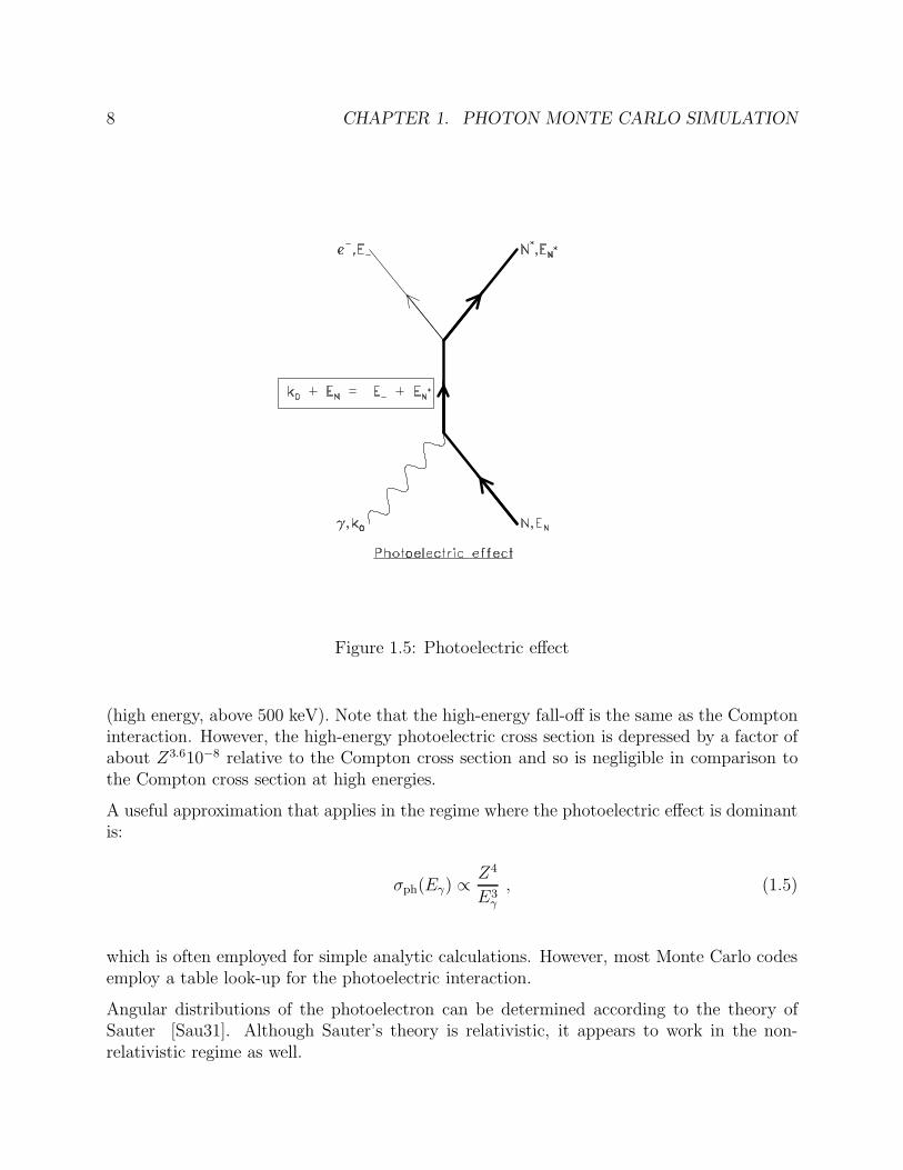
1.1.3 Photoelectric interaction

The dominant low energy photon process is the photoelectric effect. In this case the photongets absorbed by an electron of an atom resulting in escape of the electron from the atom andaccompanying small energy photons as the electron cloud of the atom settles into its groundstate. The theory concerning this phenomenon is not complete and exceedingly complicated.The cross section formulae are usually in the form of numerical fits and take the form:

σph(Eγ) ∝Zm

Enγ

, (1.4)

where the exponent on Z ranges from 4 (low energy, below 100 keV) to 4.6 (high energy,above 500 keV) and the exponent on Eγ ranges from 3 (low energy, below 100 keV) to 1


10−3

10−2

10−1

100

101

Inicident γ energy (MeV)0.0

0.2

0.4

0.6

0.8

Effect of binding on Compton cross section

10−3

10−2

10−1

100

1010.0

0.2

0.4

0.6

0.8

σ (b

arns

/e−)

free electron

hydrogen

lead

fraction ofenergy to e

−

Figure 1.4: The effect of atomic binding on the Compton cross section.


Figure 1.5: Photoelectric effect

(high energy, above 500 keV). Note that the high-energy fall-off is the same as the Comptoninteraction. However, the high-energy photoelectric cross section is depressed by a factor ofabout Z3.610−8 relative to the Compton cross section and so is negligible in comparison tothe Compton cross section at high energies.

A useful approximation that applies in the regime where the photoelectric effect is dominantis:

σph(Eγ) ∝Z4

E3γ

, (1.5)

which is often employed for simple analytic calculations. However, most Monte Carlo codesemploy a table look-up for the photoelectric interaction.

Angular distributions of the photoelectron can be determined according to the theory ofSauter [Sau31]. Although Sauter’s theory is relativistic, it appears to work in the non-relativistic regime as well.


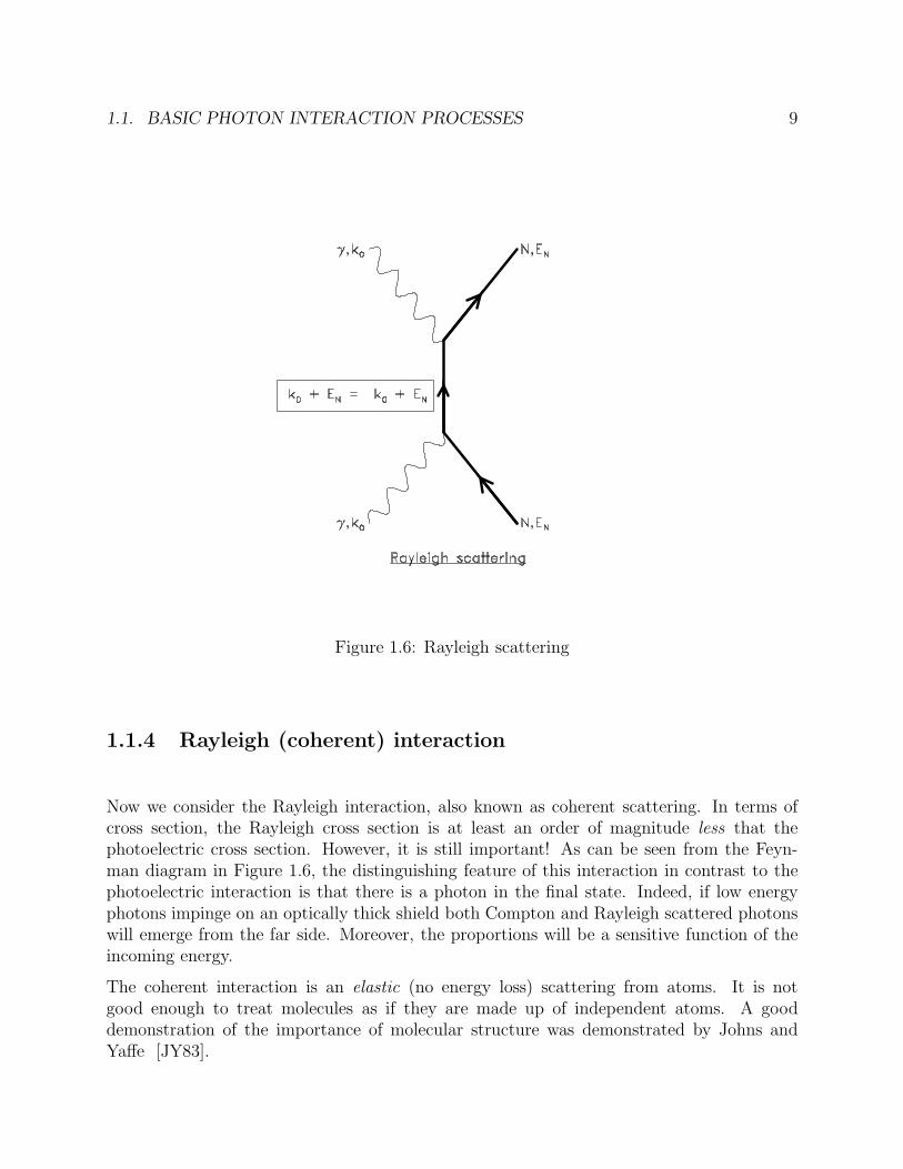
Figure 1.6: Rayleigh scattering

1.1.4 Rayleigh (coherent) interaction

Now we consider the Rayleigh interaction, also known as coherent scattering. In terms ofcross section, the Rayleigh cross section is at least an order of magnitude less that thephotoelectric cross section. However, it is still important! As can be seen from the Feyn-man diagram in Figure 1.6, the distinguishing feature of this interaction in contrast to thephotoelectric interaction is that there is a photon in the final state. Indeed, if low energyphotons impinge on an optically thick shield both Compton and Rayleigh scattered photonswill emerge from the far side. Moreover, the proportions will be a sensitive function of theincoming energy.

The coherent interaction is an elastic (no energy loss) scattering from atoms. It is notgood enough to treat molecules as if they are made up of independent atoms. A gooddemonstration of the importance of molecular structure was demonstrated by Johns andYaffe [JY83].


The Rayleigh differential cross section has the following form:

σcoh(Eγ ,Θ) =r2e2(1 + cos2Θ)[F (q, Z)]2 , (1.6)

where re is the classical electron radius (2.8179 × 10−13 cm), q is the momentum-transferparameter , q = (Eγ/hc) sin(Θ/2), and F (q, Z) is the atomic form factor. F (q, Z) approachesZ as q goes to zero either by virtue of Eγ going to zero or Θ going to zero. The atomicform factor also falls off rapidly with angle although the Z-dependence increases with angleto approximately Z3/2.

The tabulation of the form factors published by Hubbell and Øverbø [HØ79].

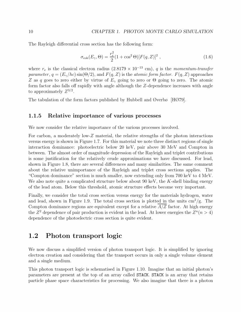
1.1.5 Relative importance of various processes

We now consider the relative importance of the various processes involved.

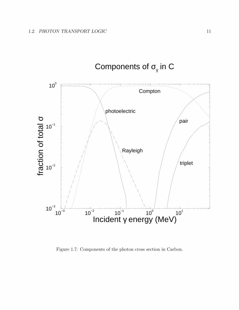
For carbon, a moderately low-Z material, the relative strengths of the photon interactionsversus energy is shown in Figure 1.7. For this material we note three distinct regions of singleinteraction dominance: photoelectric below 20 keV, pair above 30 MeV and Compton inbetween. The almost order of magnitude depression of the Rayleigh and triplet contributionsis some justification for the relatively crude approximations we have discussed. For lead,shown in Figure 1.8, there are several differences and many similarities. The same commentabout the relative unimportance of the Rayleigh and triplet cross sections applies. The“Compton dominance” section is much smaller, now extending only from 700 keV to 4 MeV.We also note quite a complicated structure below about 90 keV, the K-shell binding energyof the lead atom. Below this threshold, atomic structure effects become very important.

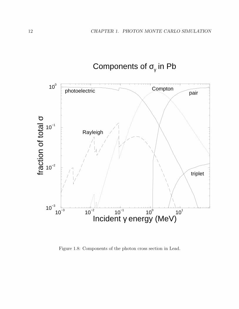
Finally, we consider the total cross section versus energy for the materials hydrogen, waterand lead, shown in Figure 1.9. The total cross section is plotted in the units cm2/g. TheCompton dominance regions are equivalent except for a relative A/Z factor. At high energythe Z2 dependence of pair production is evident in the lead. At lower energies the Zn(n > 4)dependence of the photoelectric cross section is quite evident.

1.2 Photon transport logic

We now discuss a simplified version of photon transport logic. It is simplified by ignoringelectron creation and considering that the transport occurs in only a single volume elementand a single medium.

This photon transport logic is schematised in Figure 1.10. Imagine that an initial photon’sparameters are present at the top of an array called STACK. STACK is an array that retainsparticle phase space characteristics for processing. We also imagine that there is a photon

1.2. PHOTON TRANSPORT LOGIC 11

10−3

10−2

10−1

100

101

Incident γ energy (MeV)10

−3

10−2

10−1

100

frac

tion

of to

tal σ

Components of σγ in C

Compton

photoelectric

Rayleigh

pair

triplet

Figure 1.7: Components of the photon cross section in Carbon.


10−3

10−2

10−1

100

101


−3

10−2

10−1

100

frac

tion

of to

tal σ

Components of σγ in Pb

Comptonphotoelectric

Rayleigh

pair

triplet

Figure 1.8: Components of the photon cross section in Lead.


10−2

10−1

100

101


−2

10−1

100

101

102

σ (c

m2 /g

)

Total photon σ vs γ−energy

HydrogenWaterLead

Figure 1.9: Total photon cross section vs. photon energy.


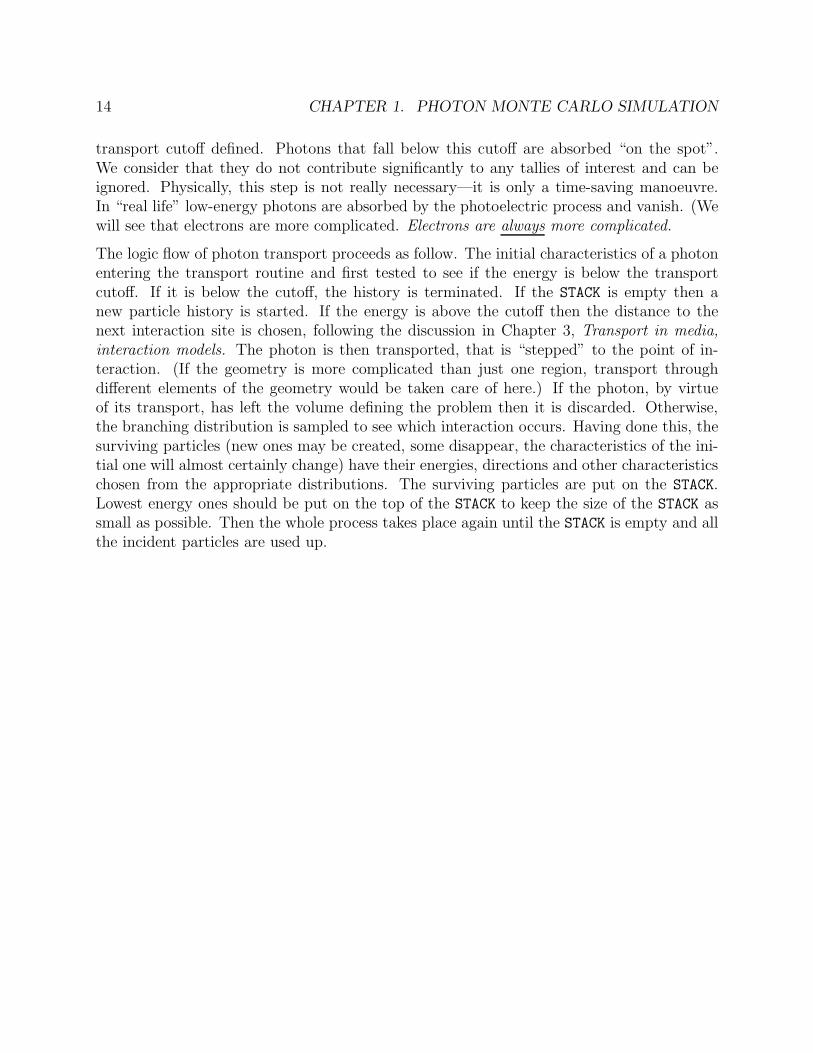
transport cutoff defined. Photons that fall below this cutoff are absorbed “on the spot”.We consider that they do not contribute significantly to any tallies of interest and can beignored. Physically, this step is not really necessary—it is only a time-saving manoeuvre.In “real life” low-energy photons are absorbed by the photoelectric process and vanish. (Wewill see that electrons are more complicated. Electrons are always more complicated.

The logic flow of photon transport proceeds as follow. The initial characteristics of a photonentering the transport routine and first tested to see if the energy is below the transportcutoff. If it is below the cutoff, the history is terminated. If the STACK is empty then anew particle history is started. If the energy is above the cutoff then the distance to thenext interaction site is chosen, following the discussion in Chapter 3, Transport in media,interaction models. The photon is then transported, that is “stepped” to the point of in-teraction. (If the geometry is more complicated than just one region, transport throughdifferent elements of the geometry would be taken care of here.) If the photon, by virtueof its transport, has left the volume defining the problem then it is discarded. Otherwise,the branching distribution is sampled to see which interaction occurs. Having done this, thesurviving particles (new ones may be created, some disappear, the characteristics of the ini-tial one will almost certainly change) have their energies, directions and other characteristicschosen from the appropriate distributions. The surviving particles are put on the STACK.Lowest energy ones should be put on the top of the STACK to keep the size of the STACK assmall as possible. Then the whole process takes place again until the STACK is empty and allthe incident particles are used up.


0.0 0.5 1.00.0

0.5

1.0

Photon Transport

Place initial photon’s parameters on stack

Pick up energy, position, direction, geometry ofcurrent particle from top of stack

Is photon energy < cutoff?

Sample distance to next interactionTransport photon taking geometry into account

Has photon left the volume of interest?

Sample the interaction channel:

Sample energies and directions of resultant particlesand store paramters on stack for future processing

- photoelectric- Compton- pair production- Rayleigh

Is stackempty?

Terminatehistory

NY

Y

N

Y

N

Figure 1.10: “Bare-bones” photon transport logic.

Bibliography

[Att86] F. H. Attix. Introduction to Radiological Physics and Radiation Dosimetry.Wiley, New York, 1986.

[BHNR94] A. F. Bielajew, H. Hirayama, W. R. Nelson, and D. W. O. Rogers. His-tory, overview and recent improvements of EGS4. National Research Councilof Canada Report PIRS-0436, 1994.

[BW91] A. F. Bielajew and P. E. Weibe. EGS-Windows - A Graphical Interface to EGS.NRCC Report: PIRS-0274, 1991.

[CA35] A. H. Compton and S. K. Allison. X-rays in theory and experiment. (D. VanNostrand Co. Inc, New York), 1935.

[DBM54] H. Davies, H. A. Bethe, and L. C. Maximon. Theory of bremsstrahlung and pairproduction. II. Integral cross sections for pair production. Phys. Rev., 93:788,1954.

[Eva55] R. D. Evans. The Atomic Nucleus. McGraw-Hill, New York, 1955.

[HØ79] J. H. Hubbell and I. Øverbø. Relativistic atomic form factors and photon co-herent scattering cross sections. J. Phys. Chem. Ref. Data, 9:69, 1979.

[JC83] H. E. Johns and J. R. Cunningham. The Physics of Radiology, Fourth Edition.Charles C. Thomas, Springfield, Illinois, 1983.

[JY83] P. C. Johns and M. J. Yaffe. Coherent scatter in diagnostic radiology. Med.Phys., 10:40, 1983.

[KN29] O. Klein and Y. Nishina. . Z. fur Physik, 52:853, 1929.

[MOK69] J. W. Motz, H. A. Olsen, and H. W. Koch. Pair production by photons. Rev.Mod. Phys., 41:581 – 639, 1969.

[NH91] Y. Namito and H. Hirayama. Improvement of low energy photon transportcalculation by EGS4 – electron bound effect in Compton scattering. Japan AtomicEnergy Society, Osaka, page 401, 1991.

17

18 BIBLIOGRAPHY

[NHR85] W. R. Nelson, H. Hirayama, and D. W. O. Rogers. The EGS4 Code System.Report SLAC–265, Stanford Linear Accelerator Center, Stanford, Calif, 1985.

[Sau31] F. Sauter. Uber den atomaren Photoeffekt in der K-Schale nach der relativis-tischen Wellenmechanik Diracs. Ann. Physik, 11:454 – 488, 1931.

[SF96] J. K. Shultis and R. E. Faw. Radiation Shielding . Prentice Hall, Upper SaddleRiver, 1996.

[Tsa74] Y. S. Tsai. Pair Production and Bremsstrahlung of Charged Leptons. Rev. Mod.Phys., 46:815, 1974.

BIBLIOGRAPHY 19

Problems

1. The Klein-Nishina differential cross section is given by:

dσKNdΩϕ

=r202

(k′

k

)2 (k′

k+

k

k′− sin2 ϕ

)

where ϕ is the angle between the scattered photon and incoming photon directions, kis the incoming photon energy and k′ is the scattered photon energy.

k′

k=

1

1 + α(1− cosϕ)

α =k

m0c2

(a) The kinematics of unbound electron scattering correlates absolutely any two ofthe four kinematic variables, k′, ϕ, T (the outgoing electron kinetic energy) andθ (the angle that the outgoing electron energy makes with the incoming photondirection, see Figure 7.2 in Attix [Att86]), as a function of k. Hence, there are 12functions of the form, k′(ϕ), ϕ(k′), k′(θ), θ(k′) and so on.

Find them all and show your calculations. You must prove relation (7.10), butyou may use (7.8) and (7.9) in Attix’s book without proof.

i. k′(ϕ) =

ii. ϕ(k′) =

iii. k′(θ) =

iv. θ(k′) =

v. k′(T ) =

vi. T (k′) =

vii. ϕ(θ) =

viii. θ(ϕ) =

ix. ϕ(T ) =

x. T (ϕ) =

xi. T (θ) =

xii. θ(T ) =

(b) Find expressions and plot vs. α (low energy and high energy limits must be seenclearly)

i. k′/k

20 BIBLIOGRAPHY

ii. (k′/k)2 − k′/k2

iii. cosϕ

iv. (cosϕ)2 − cosϕ2

v. cos θ

vi. (cos θ)2 − cos θ2

vii. Discuss the systematics of the above in the high and low energy limits.

Hint: If f(x) is an unnormalized probability distribution defined between x0 andx1, then

x =

∫ x1x0dx xf(x)∫ x1

x0dx f(x)

x2 =

∫ x1x0dx x2f(x)∫ x1

x0dx f(x)

Chapter 2

Electron Monte Carlo Simulation

In this chapter we discuss the electron and positron interactions and discuss the approxima-tions made in their implementation. We give a brief outline of the electron transport logicused in Monte Carlo simulations.

The transport of electrons (and positrons) is considerably more complicated than for pho-tons. Like photons, electrons are subject to violent interactions. The following are the“catastrophic” interactions:

• large energy-loss Møller scattering (e−e− −→ e−e−),• large energy-loss Bhabha scattering (e+e− −→ e+e−),• hard bremsstrahlung emission (e±N −→ e±γN), and• positron annihilation “in-flight” and at rest (e+e− −→ γγ).

It is possible to sample the above interactions discretely in a reasonable amount of computingtime for many practical problems. In addition to the catastrophic events, there are also “soft”events. Detailed modeling of the soft events can usually be approximated by summing theeffects of many soft events into virtual “large-effect” events. These “soft” events are:

• low-energy Møller (Bhabha) scattering (modeled as part of the collision stoppingpower),

• atomic excitation (e±N −→ e±N∗) (modeled as another part of the collision stoppingpower),

• soft bremsstrahlung (modeled as radiative stopping power), and• elastic electron (positron) multiple scattering from atoms, (e±N −→ e±N).

Strictly speaking, an elastic large angle scattering from a nucleus should really be consideredto be a “catastrophic” interaction but this is not the usual convention. (Perhaps it shouldbe.) For problems of the sort we consider, it is impractical to model all these interactions

21

22 CHAPTER 2. ELECTRON MONTE CARLO SIMULATION

discretely. Instead, well-established statistical theories are used to describe these “soft”interactions by accounting for them in a cumulative sense including the effect of many suchinteractions at the same time. These are the so-called “statistically grouped” interactions.

2.1 Catastrophic interactions

We have almost complete flexibility in defining the threshold between “catastrophic” and“statistically grouped” interactions. The location of this threshold should be chosen by thedemands of the physics of the problem and by the accuracy required in the final result.

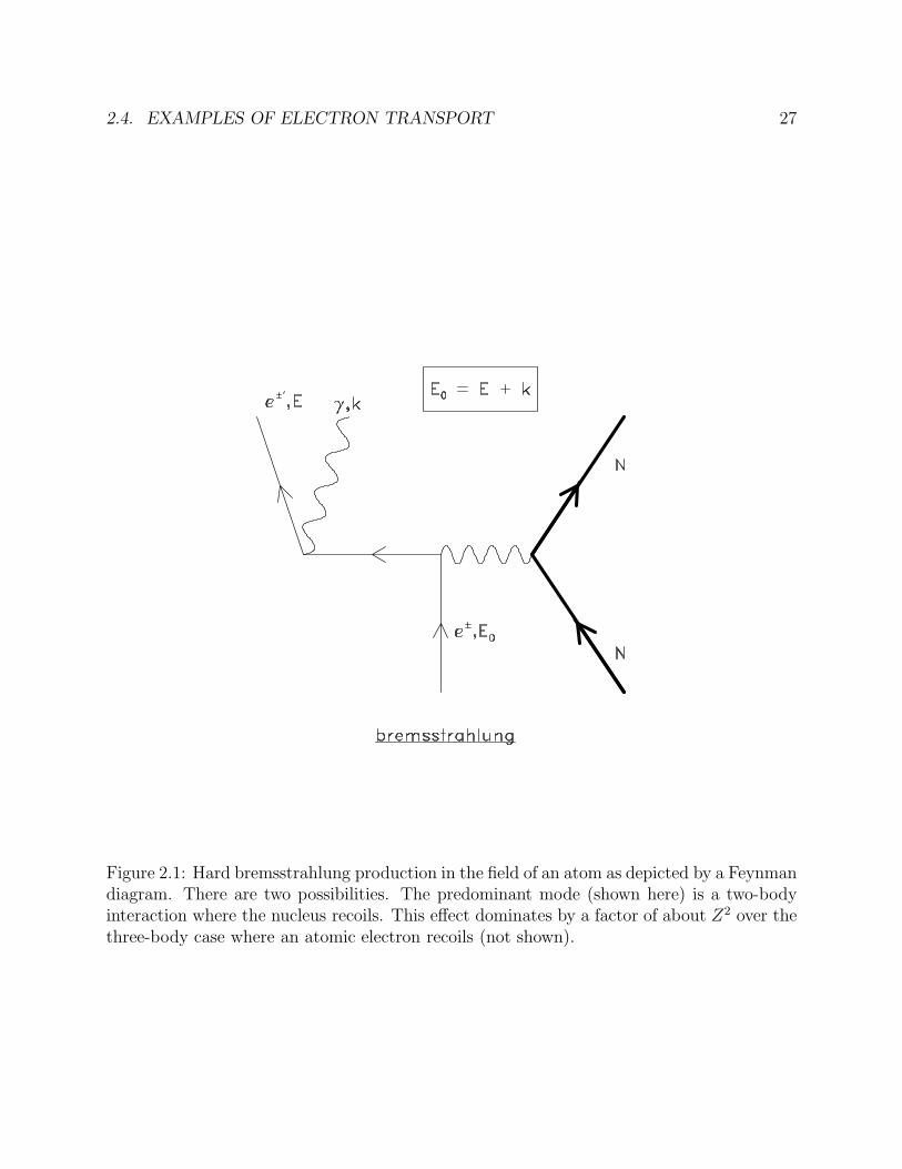
2.1.1 Hard bremsstrahlung production

As depicted by the Feynman diagram in fig. 2.1, bremsstrahlung production is the creationof photons by electrons (or positrons) in the field of an atom. There are actually twopossibilities. The predominant mode is the interaction with the atomic nucleus. This effectdominates by a factor of about Z over the three-body case where an atomic electron recoils(e±N −→ e±e−γN∗). Bremsstrahlung is the quantum analogue of synchrotron radiation, theradiation from accelerated charges predicted by Maxwell’s equations. The de-accelerationand acceleration of an electron scattering from nuclei can be quite violent, resulting in veryhigh energy quanta, up to and including the total kinetic energy of the incoming chargedparticle.

The two-body effect can be taken into account through the total cross section and angulardistribution kinematics. The three-body case is conventionally treated only by inclusion inthe total cross section of the two body-process. The two-body process can be modeled usingone of the Koch and Motz [KM59] formulae. The bremsstrahlung cross section scales withZ(Z + ξ(Z)), where ξ(Z) is the factor accounting for three-body case where the interactionis with an atomic electron. These factors comes are taken from the work of Tsai [Tsa74].The total cross section depends approximately like 1/Eγ.

2.1.2 Møller (Bhabha) scattering

Møller and Bhabha scattering are collisions of incident electrons or positrons with atomicelectrons. It is conventional to assume that these atomic electrons are “free” ignoring theiratomic binding energy. At first glance the Møller and Bhabha interactions appear to bequite similar. Referring to fig. 2.2, we see very little difference between them. In reality,however, they are, owing to the identity of the participant particles. The electrons in thee−e+ pair can annihilate and be recreated, contributing an extra interaction channel to thecross section. The thresholds for these interactions are different as well. In the e−e− case,

2.2. STATISTICALLY GROUPED INTERACTIONS 23

the “primary” electron can only give at most half its energy to the target electron if weadopt the convention that the higher energy electron is always denoted “the primary”. Thisis because the two electrons are indistinguishable. In the e+e− case the positron can give upall its energy to the atomic electron.

Møller and Bhabha cross sections scale with Z for different media. The cross sectionscales approximately as 1/v2, where v is the velocity of the scattered electron. Many morelow energy secondary particles are produced from the Møller interaction than from thebremsstrahlung interaction.

2.1.3 Positron annihilation

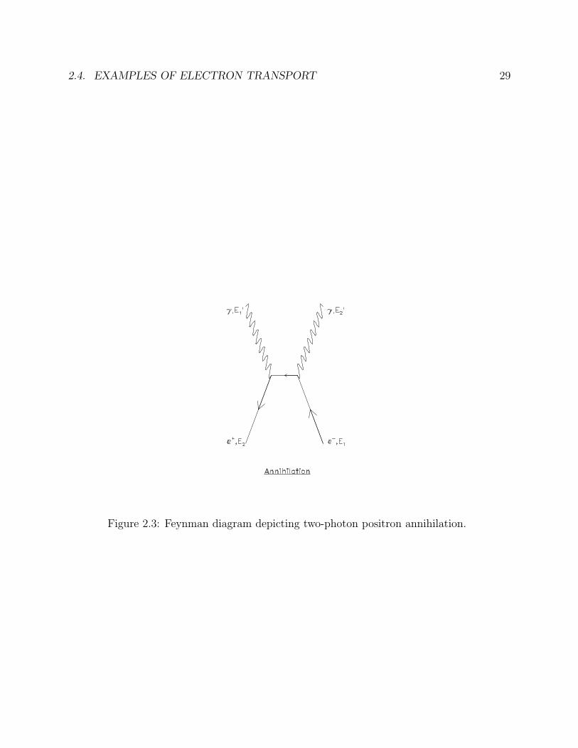
Two photon annihilation is depicted in fig. 2.3. Two-photon “in-flight” annihilation can bemodeled using the cross section formulae of Heitler [Hei54]. It is conventional to consider theatomic electrons to be free, ignoring binding effects. Three and higher-photon annihilations(e+e− −→ nγ[n > 2]) as well as one-photon annihilation which is possible in the Coulombfield of a nucleus (e+e−N −→ γN∗) can be ignored as well. The higher-order processes arevery much suppressed relative to the two-body process (by at least a factor of 1/137) whilethe one-body process competes with the two-photon process only at very high energies wherethe cross section becomes very small. If a positron survives until it reaches the transportcut-off energy it can be converted it into two photons (annihilation at rest), with or withoutmodeling the residual drift before annihilation.

2.2 Statistically grouped interactions

2.2.1 “Continuous” energy loss

One method to account for the energy loss to sub-threshold (soft bremsstrahlung and softcollisions) is to assume that the energy is lost continuously along its path. The formalism thatmay be used is the Bethe-Bloch theory of charged particle energy loss [Bet30, Bet32, Blo33]as expressed by Berger and Seltzer [BS64] and in ICRU 37 [ICR84]. This continuous energyloss scales with the Z of the medium for the collision contribution and Z2 for the radiativepart. Charged particles can also polarise the medium in which they travel. This “densityeffect” is important at high energies and for dense media. Default density effect parametersare available from a 1982 compilation by Sternheimer, Seltzer and Berger [SSB82] andstate-of-the-art compilations (as defined by the stopping-power guru Berger who distributesa PC-based stopping power program [Ber92]).

Again, atomic binding effects are treated rather crudely by the Bethe-Bloch formalism.It assumes that each electron can be treated as if it were bound by an average bindingpotential. The use of more refined theories does not seem advantageous unless one wants


to study electron transport below the K-shell binding energy of the highest atomic numberelement in the problem.

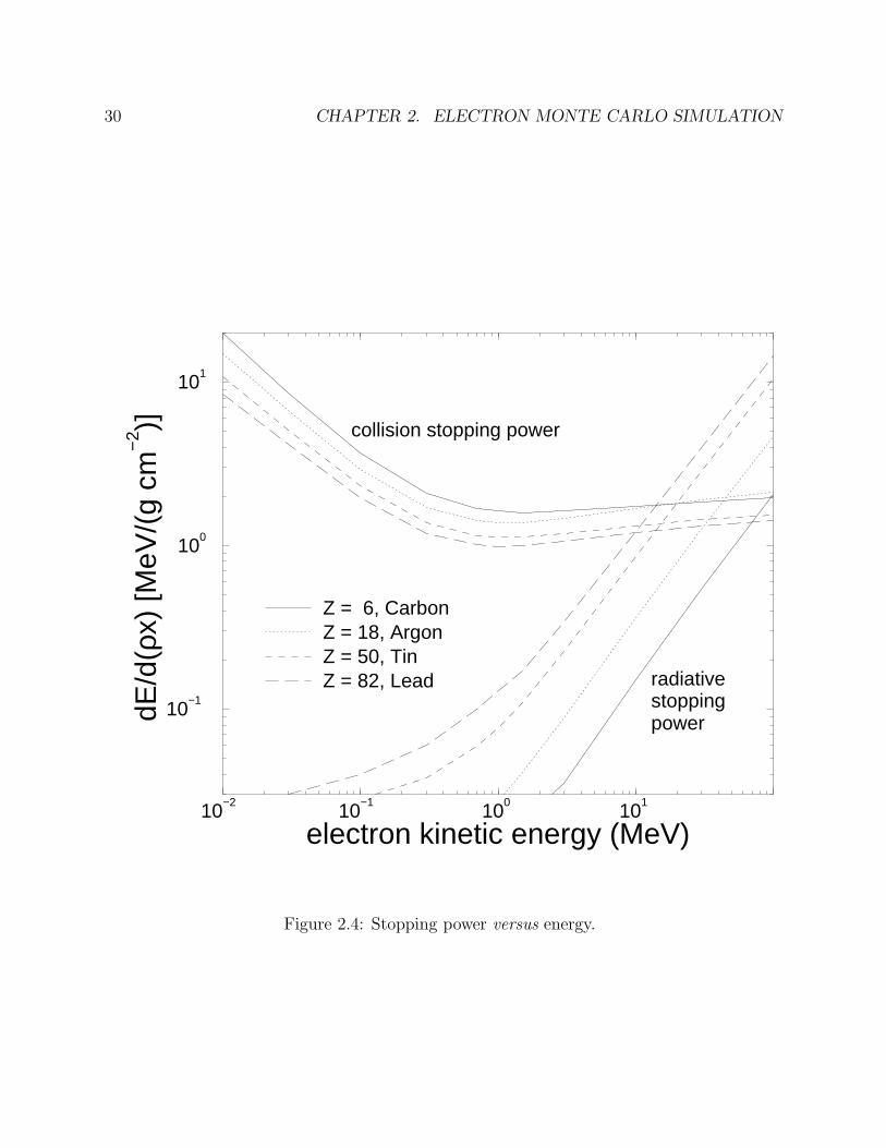
The stopping power versus energy for different materials is shown in fig. 2.4. The differencein the collision part is due mostly to the difference in ionisation potentials of the variousatoms and partly to a Z/A difference, because the vertical scale is plotted in MeV/(g/cm2),a normalisation by atomic weight rather than electron density. Note that at high energy theargon line rises above the carbon line. Argon, being a gas, is reduced less by the densityeffect at this energy. The radiative contribution reflects mostly the relative Z2 dependenceof bremsstrahlung production.

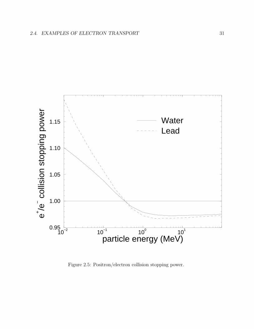
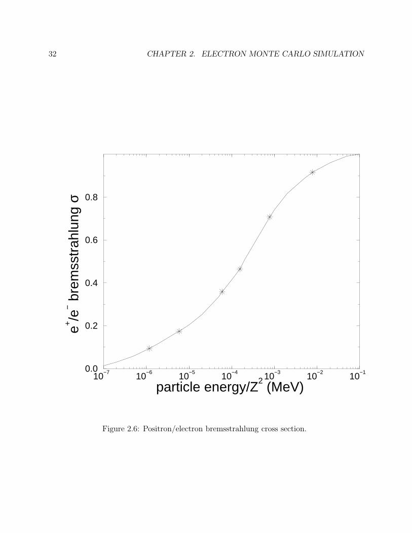
The collisional energy loss by electrons and positrons is different for the same reasons de-scribed in the “catastrophic” interaction section. Annihilation is generally not treated aspart of the positron slowing down process and is treated discretely as a “catastrophic” event.The differences are reflected in fig. 2.5, the positron/electron collision stopping power. Thepositron radiative stopping power is reduced with respect to the electron radiative stoppingpower. At 1 MeV this difference is a few percent in carbon and 60% in lead. This relativedifference is depicted in fig. 2.6.

2.2.2 Multiple scattering

Elastic scattering of electrons and positrons from nuclei is predominantly small angle withthe occasional large-angle scattering event. If it were not for screening by the atomic elec-trons, the cross section would be infinite. The cross sections are, nonetheless, very large.There are several statistical theories that deal with multiple scattering. Some of these theo-ries assume that the charged particle has interacted enough times so that these interactionsmay be grouped together. The most popular such theory is the Fermi-Eyges theory [Eyg48],a small angle theory. This theory neglects large angle scattering and is unsuitable for ac-curate electron transport unless large angle scattering is somehow included (perhaps as acatastrophic interaction). The most accurate theory is that of Goudsmit and Saunder-son [GS40a, GS40b]. This theory does not require that many atoms participate in theproduction of a multiple scattering angle. However, calculation times required to producefew-atom distributions can get very long, can have intrinsic numerical difficulties and are notefficient computationally for Monte Carlo codes such as EGS4 [NHR85, BHNR94] where thephysics and geometry adjust the electron step-length dynamically. A fixed step-size schemepermits an efficient implementation of Goudsmit-Saunderson theory and this has been donein ETRAN [Sel89, Sel91], ITS [HM84, Hal89, HKM+92] and MCNP [Bri86, Bri93, Bri97].Apart from accounting for energy-loss during the course of a step, there is no intrinsic diffi-culty with large steps either. EGS4 uses the Moliere theory [Mol47, Mol48] which producesresults as good as Goudsmit-Saunderson for many applications and is much easier to imple-ment in EGS4’s transport scheme.

The Moliere theory, although originally designed as a small angle theory has been shown

2.3. ELECTRON TRANSPORT “MECHANICS” 25

with small modifications to predict large angle scattering quite successfully [Bet53, Bie94].The Moliere theory includes the contribution of single event large angle scattering, for ex-ample, an electron backscatter from a single atom. The Moliere theory ignores differencesin the scattering of electrons and positrons, and uses the screened Rutherford cross sectionsinstead of the more accurate Mott cross sections. However, the differences are known tobe small. Owing to analytic approximations made by Moliere theory, this theory requires aminimum step-size as it breaks down numerically if less than 25 atoms or so participate inthe development of the angular distribution [Bie94, AMB93]. A recent development [KB98]has surmounted this difficulty. Apart from accounting for energy loss, there is also a largestep-size restriction because the Moliere theory is couched in a small-angle formalism. Be-yond this there are other corrections that can be applied [Bet53, Win87] related to themathematical connection between the small-angle and any-angle theories.

2.3 Electron transport “mechanics”

2.3.1 Typical electron tracks

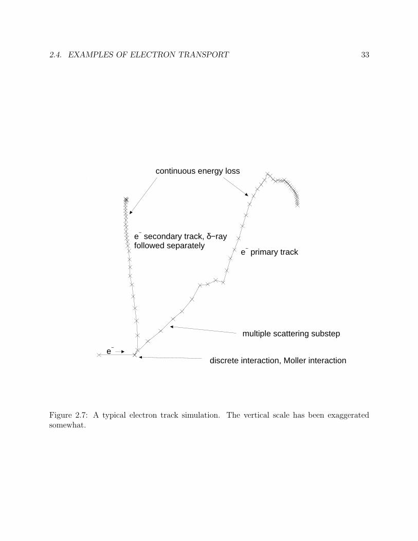
A typical Monte Carlo electron track simulation is shown in fig. 2.7. An electron is beingtransported through a medium. Along the way energy is being lost “continuously” to sub-threshold knock-on electrons and bremsstrahlung. The track is broken up into small straight-line segments called multiple scattering substeps. In this case the length of these substepswas chosen so that the electron lost 4% of its energy during each step. At the end ofeach of these steps the multiple scattering angle is selected according to some theoreticaldistribution. Catastrophic events, here a single knock-on electron, sets other particles inmotion. These particles are followed separately in the same fashion. The original particle, ifit is does not fall below the transport threshold, is also transported. In general terms, thisis exactly what the electron transport logic simulates.

2.3.2 Typical multiple scattering substeps

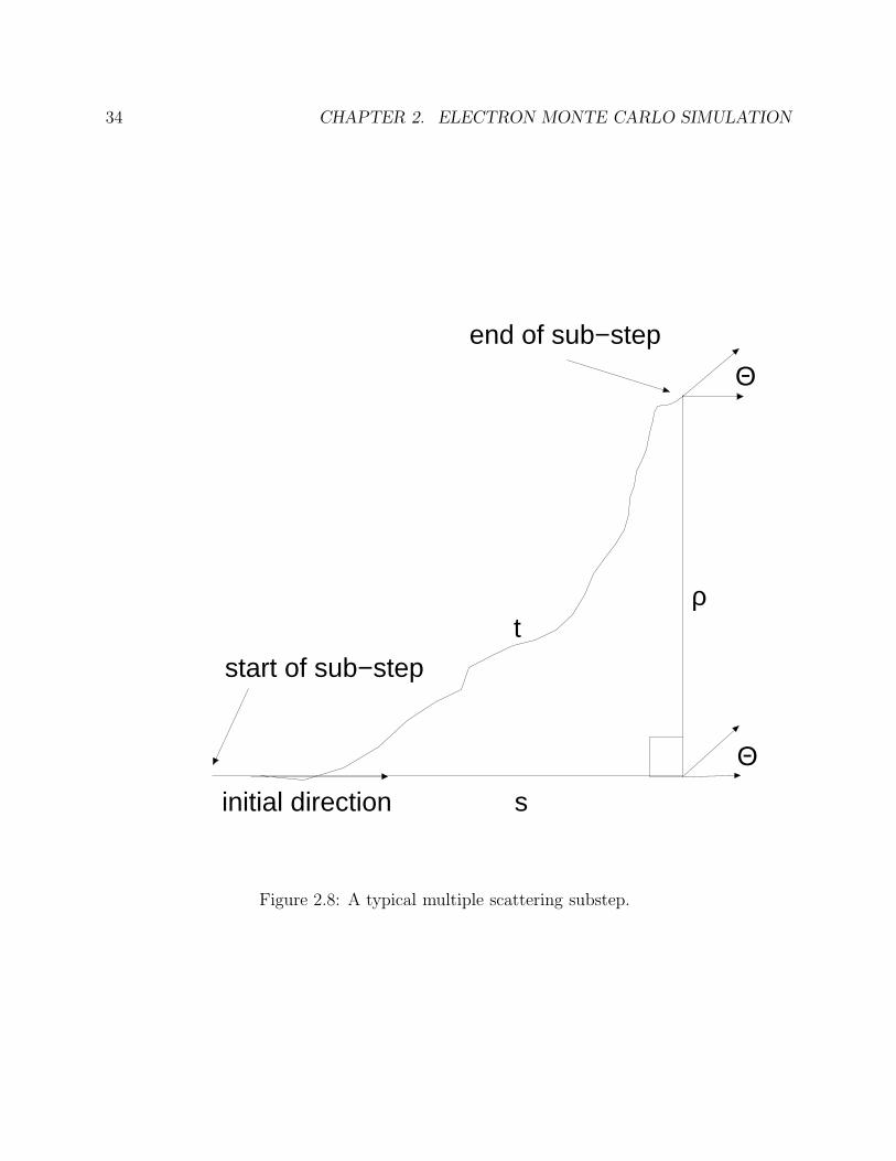
Now we demonstrate in fig. 2.8 what a multiple scattering substep should look like.

A single electron step is characterised by the length of total curved path-length to the endpoint of the step, t. (This is a reasonable parameter to use because the number of atomsencountered along the way should be proportional to t.) At the end of the step the deflectionfrom the initial direction, Θ, is sampled. Associated with the step is the average projecteddistance along the original direction of motion, s. There is no satisfactory theory for therelation between s and t! The lateral deflection, ρ, the distance transported perpendicularto the original direction of motion, is often ignored by electron Monte Carlo codes. This isnot to say that lateral transport is not modelled! Recalling fig. 2.7, we see that such lateral


deflections do occur as a result of multiple scattering. It is only the lateral deflection duringthe course of a substep which is ignored. One can guess that if the multiple scattering stepsare small enough, the electron track may be simulated more exactly.

2.4 Examples of electron transport

2.4.1 Effect of physical modeling on a 20 MeV e− depth-dose curve

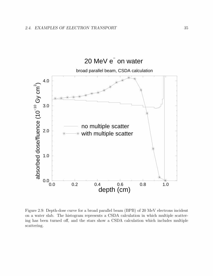
In this section we will study the effects on the depth-dose curve of turning on and offvarious physical processes. Figure 2.9 presents two CSDA calculations (i.e. no secondariesare created and energy-loss straggling is not taken into account). For the histogram, nomultiple scattering is modeled and hence there is a large peak at the end of the range ofthe particles because they all reach the same depth before being terminating and depositingtheir residual kinetic energy (189 keV in this case). Note that the size of this peak is verymuch a calculational artefact which depends on how thick the layer is in which the historiesterminate. The curve with the stars includes the effect of multiple scattering. This leads toa lateral spreading of the electrons which shortens the depth of penetration of most electronsand increases the dose at shallower depths because the fluence has increased. In this case, thedepth-straggling is entirely caused by the lateral scattering since every electron has traveledthe same distance.

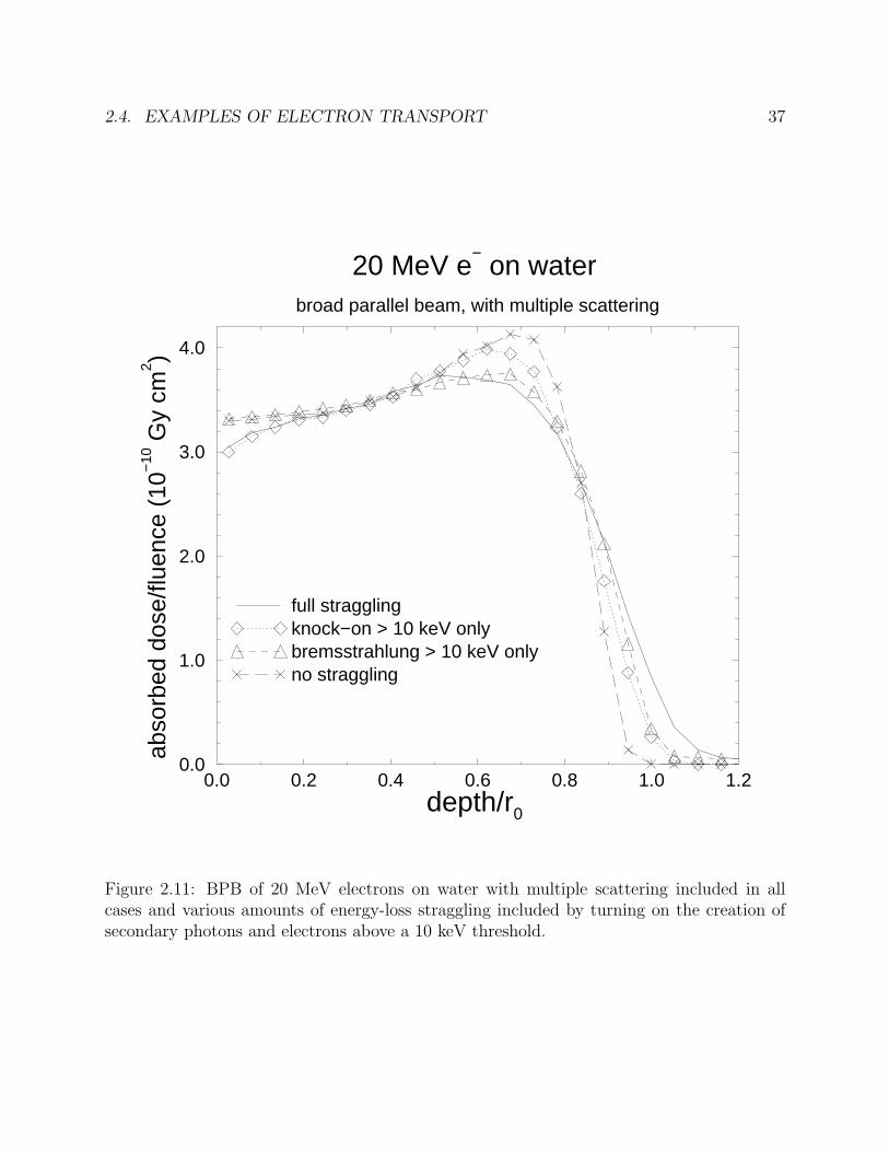
Figure 2.10 presents three depth-dose curves calculated with all multiple scattering turned off- i.e. the electrons travel in straight lines (except for some minor deflections when secondaryelectrons are created). In the cases including energy-loss straggling, a depth straggling isintroduced because the actual distance traveled by the electrons varies, depending on howmuch energy they give up to secondaries. Two features are worth noting. Firstly, theenergy-loss straggling induced by the creation of bremsstrahlung photons plays a significantrole despite the fact that far fewer secondary photons are produced than electrons. They do,however, have a larger mean energy. Secondly, the inclusion of secondary electron transportin the calculation leads to a dose buildup region near the surface. Figure 2.11 presentsa combination of the effects in the previous two figures. The extremes of no energy-lossstraggling and the full simulation are shown to bracket the results in which energy-lossstraggling from either the creation of bremsstrahlung or knock-on electrons is included. Thebremsstrahlung straggling has more of an effect, especially near the peak of the depth-dosecurve.

2.4. EXAMPLES OF ELECTRON TRANSPORT 27

Figure 2.1: Hard bremsstrahlung production in the field of an atom as depicted by a Feynmandiagram. There are two possibilities. The predominant mode (shown here) is a two-bodyinteraction where the nucleus recoils. This effect dominates by a factor of about Z2 over thethree-body case where an atomic electron recoils (not shown).


Figure 2.2: Feynman diagrams depicting the Møller and Bhabha interactions. Note the extrainteraction channel in the case of the Bhabha interaction.


Figure 2.3: Feynman diagram depicting two-photon positron annihilation.


10−2

10−1

100

101

electron kinetic energy (MeV)

10−1

100

101

dE/d

(ρx)

[MeV

/(g

cm−

2 )]

Z = 6, CarbonZ = 18, ArgonZ = 50, TinZ = 82, Lead

collision stopping power

radiativestoppingpower

Figure 2.4: Stopping power versus energy.


10−2

10−1

100

101

particle energy (MeV)0.95

1.00

1.05

1.10

1.15

e+/e

− c

ollis

ion

stop

ping

pow

er

WaterLead

Figure 2.5: Positron/electron collision stopping power.


10−7

10−6

10−5

10−4

10−3

10−2

10−1

particle energy/Z2 (MeV)

0.0

0.2

0.4

0.6

0.8

e+/e

− b

rem

sstr

ahlu

ng σ

Figure 2.6: Positron/electron bremsstrahlung cross section.


0.0000 0.0020 0.0040 0.00600.0000

0.0005

0.0010

0.0015

multiple scattering substep

discrete interaction, Moller interaction

e− primary track

e− secondary track, δ−ray

followed separately

continuous energy loss

e−

Figure 2.7: A typical electron track simulation. The vertical scale has been exaggeratedsomewhat.


0.000 0.002 0.004 0.006 0.008 0.0100.0000

0.0020

0.0040

0.0060

initial direction s

ρt

Θ

Θ

start of sub−step

end of sub−step

Figure 2.8: A typical multiple scattering substep.


0.0 0.2 0.4 0.6 0.8 1.0depth (cm)

0.0

1.0

2.0

3.0

4.0

abso

rbed

dos

e/flu

ence

(10

−10

Gy

cm2 )

20 MeV e− on water

broad parallel beam, CSDA calculation

no multiple scatterwith multiple scatter

Figure 2.9: Depth-dose curve for a broad parallel beam (BPB) of 20 MeV electrons incidenton a water slab. The histogram represents a CSDA calculation in which multiple scatter-ing has been turned off, and the stars show a CSDA calculation which includes multiplescattering.


0.0 0.2 0.4 0.6 0.8 1.0 1.2depth/r0

0.0

1.0

2.0

3.0

4.0

abso

rbed

dos

e/flu

ence

(10

−10

Gy

cm2 )


broad parallel beam, no multiple scattering

bremsstrahlung > 10 keV onlyknock−on > 10 keV onlyno straggling

Figure 2.10: Depth-dose curves for a BPB of 20 MeV electrons incident on a water slab, butwith multiple scattering turned off. The dashed histogram calculation models no stragglingand is the same simulation as given by the histogram in fig. 2.9. Note the difference causedby the different bin size. The solid histogram includes energy-loss straggling due to thecreation of bremsstrahlung photons with an energy above 10 keV. The curve denoted by thestars includes only that energy-loss straggling induced by the creation of knock-on electronswith an energy above 10 keV.


0.0 0.2 0.4 0.6 0.8 1.0 1.2depth/r0

0.0

1.0

2.0

3.0

4.0

abso

rbed

dos

e/flu

ence

(10

−10

Gy

cm2 )


broad parallel beam, with multiple scattering

full stragglingknock−on > 10 keV onlybremsstrahlung > 10 keV onlyno straggling

Figure 2.11: BPB of 20 MeV electrons on water with multiple scattering included in allcases and various amounts of energy-loss straggling included by turning on the creation ofsecondary photons and electrons above a 10 keV threshold.


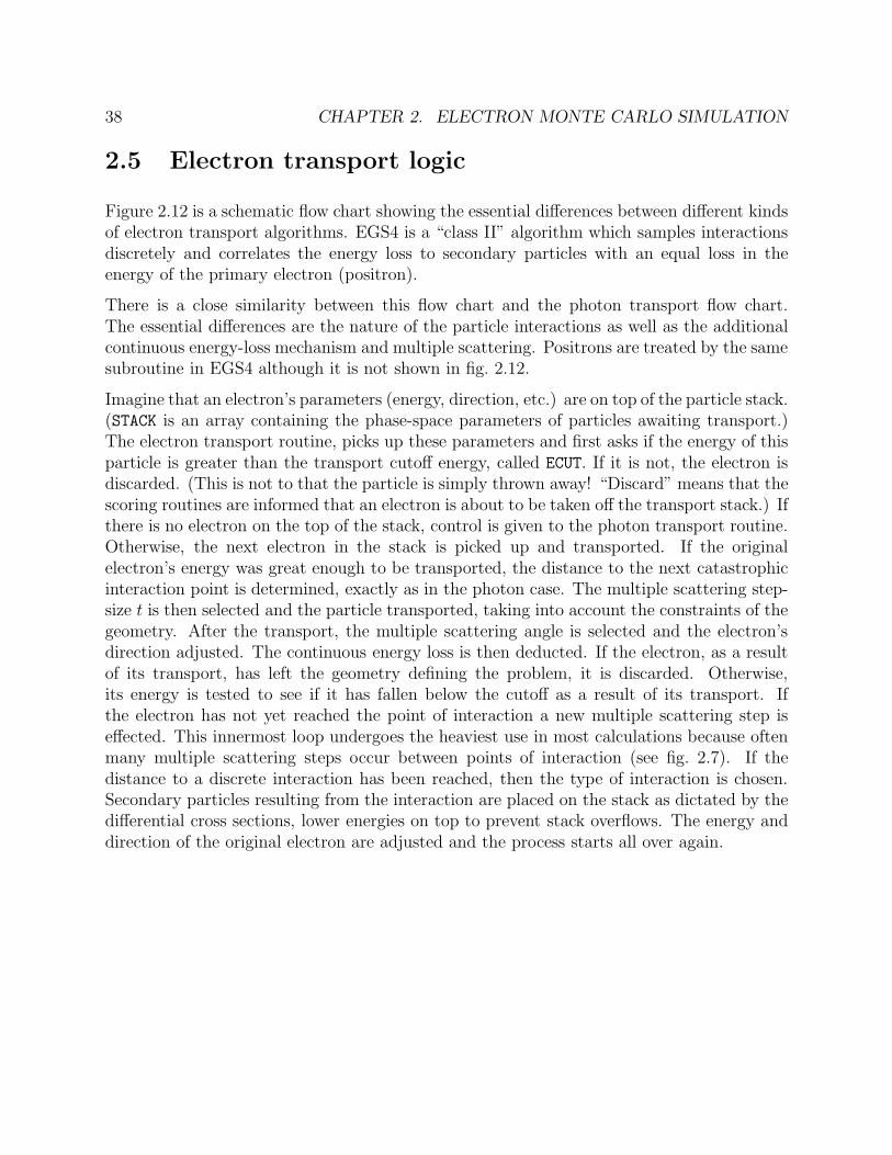
2.5 Electron transport logic

Figure 2.12 is a schematic flow chart showing the essential differences between different kindsof electron transport algorithms. EGS4 is a “class II” algorithm which samples interactionsdiscretely and correlates the energy loss to secondary particles with an equal loss in theenergy of the primary electron (positron).

There is a close similarity between this flow chart and the photon transport flow chart.The essential differences are the nature of the particle interactions as well as the additionalcontinuous energy-loss mechanism and multiple scattering. Positrons are treated by the samesubroutine in EGS4 although it is not shown in fig. 2.12.

Imagine that an electron’s parameters (energy, direction, etc.) are on top of the particle stack.(STACK is an array containing the phase-space parameters of particles awaiting transport.)The electron transport routine, picks up these parameters and first asks if the energy of thisparticle is greater than the transport cutoff energy, called ECUT. If it is not, the electron isdiscarded. (This is not to that the particle is simply thrown away! “Discard” means that thescoring routines are informed that an electron is about to be taken off the transport stack.) Ifthere is no electron on the top of the stack, control is given to the photon transport routine.Otherwise, the next electron in the stack is picked up and transported. If the originalelectron’s energy was great enough to be transported, the distance to the next catastrophicinteraction point is determined, exactly as in the photon case. The multiple scattering step-size t is then selected and the particle transported, taking into account the constraints of thegeometry. After the transport, the multiple scattering angle is selected and the electron’sdirection adjusted. The continuous energy loss is then deducted. If the electron, as a resultof its transport, has left the geometry defining the problem, it is discarded. Otherwise,its energy is tested to see if it has fallen below the cutoff as a result of its transport. Ifthe electron has not yet reached the point of interaction a new multiple scattering step iseffected. This innermost loop undergoes the heaviest use in most calculations because oftenmany multiple scattering steps occur between points of interaction (see fig. 2.7). If thedistance to a discrete interaction has been reached, then the type of interaction is chosen.Secondary particles resulting from the interaction are placed on the stack as dictated by thedifferential cross sections, lower energies on top to prevent stack overflows. The energy anddirection of the original electron are adjusted and the process starts all over again.

2.5. ELECTRON TRANSPORT LOGIC 39

0.0 0.2 0.4 0.6 0.8 1.00.0

20.0

40.0

60.0

Electron transport

PLACE INITIAL ELECTRON’SPARAMETERS ON STACK

PICK UP ENERGY, POSITION,DIRECTION, GEOMETRY OFCURRENT PARTICLE FROM

TOP OF STACK

ELECTRON ENERGY > CUTOFFAND ELECTRON IN GEOMETRY?

CLASS II CALCULATION?

SELECT MULTIPLE SCATTERSTEP SIZE AND TRANSPORT

SAMPLE DEFLECTION ANGLEAND CHANGE DIRECTION

SAMPLE ELOSSE = E - ELOSS

IS A SECONDARYCREATED DURING STEP?

ELECTRON LEFTGEOMETRY?

ELECTRON ENERGYLESS THAN CUTOFF?

SAMPLE DISTANCE TODISCRETE INTERACTION

SELECT MULTIPLE SCATTERSTEP SIZE AND TRANSPORT

SAMPLE DEFLECTIONANGLE AND CHANGE

DIRECTION

CALCULATE ELOSSE = E - ELOSS(CSDA)

HAS ELECTRONLEFT GEOMETRY?

ELECTRON ENERGYLESS THAN CUTOFF?

REACHED POINT OFDISCRETE INTERACTION?

DISCRETE INTERACTION- KNOCK-ON

- BREMSSTRAHLUNG

SAMPLE ENERGYAND DIRECTION OF

SECONDARY, STOREPARAMETERS ON STACK

CLASS II CALCULATION?

CHANGE ENERGY ANDDIRECTION OF PRIMARY

AS A RESULT OF INTERACTION

STACK EMPTY?

TERMINATEHISTORY

SAMPLE

YN

Y

N

YN

Y

NY

NY N

Y

NY

NY N

N

Y

Figure 2.12: Flow chart for electron transport. Much detail is left out.

Bibliography

[AMB93] P. Andreo, J. Medin, and A. F. Bielajew. Constraints on the multiple scatteringtheory of Moliere in Monte Carlo simulations of the transport of charged particles.Med. Phys., 20:1315 – 1325, 1993.

[Ber92] M. J. Berger. ESTAR, PSTAR and ASTAR: Computer Programs for CalculatingStopping-Power and Ranges for Electrons, Protons, and Helium Ions. NISTReport NISTIR-4999 (Washington DC), 1992.

[Bet30] H. A. Bethe. Theory of passage of swift corpuscular rays through matter. Ann.Physik, 5:325, 1930.

[Bet32] H. A. Bethe. Scattering of electrons. Z. fur Physik, 76:293, 1932.

[Bet53] H. A. Bethe. Moliere’s theory of multiple scattering. Phys. Rev., 89:1256 – 1266,1953.

[BHNR94] A. F. Bielajew, H. Hirayama, W. R. Nelson, and D. W. O. Rogers. His-tory, overview and recent improvements of EGS4. National Research Councilof Canada Report PIRS-0436, 1994.

[Bie94] A. F. Bielajew. Plural and multiple small-angle scattering from a screenedRutherford cross section. Nucl. Inst. and Meth., B86:257 – 269, 1994.

[Blo33] F. Bloch. Stopping power of atoms with several electrons. Z. fur Physik, 81:363,1933.

[Bri86] J. Briesmeister. MCNP—A general purpose Monte Carlo code for neutron andphoton transport, Version 3A. Los Alamos National Laboratory Report LA-7396-M (Los Alamos, NM), 1986.

[Bri93] J. F. Briesmeister. MCNP—A general Monte Carlo N-particle transport code.Los Alamos National Laboratory Report LA-12625-M (Los Alamos, NM), 1993.

[Bri97] J. F. Briesmeister. MCNP—A general Monte Carlo N-particle transport code.Los Alamos National Laboratory Report LA-12625-M, Version 4B (Los Alamos,NM), 1997.

41

42 BIBLIOGRAPHY

[BS64] M. J. Berger and S. M. Seltzer. Tables of energy losses and ranges of electronsand positrons. NASA Report SP-3012 (Washington DC), 1964.

[Eyg48] L. Eyges. Multiple scattering with energy loss. Phys. Rev., 74:1534, 1948.

[GS40a] S. A. Goudsmit and J. L. Saunderson. Multiple scattering of electrons. Phys.Rev., 57:24 – 29, 1940.

[GS40b] S. A. Goudsmit and J. L. Saunderson. Multiple scattering of electrons. II. Phys.Rev., 58:36 – 42, 1940.

[Hal89] J. Halbleib. Structure and Operation of the ITS code system. In T.M. Jenkins,W.R. Nelson, A. Rindi, A.E. Nahum, and D.W.O. Rogers, editors, Monte CarloTransport of Electrons and Photons, pages 249 – 262. Plenum Press, New York,1989.

[Hei54] W. Heitler. The quantum theory of radiation. (Clarendon Press, Oxford), 1954.

[HKM+92] J. A. Halbleib, R. P. Kensek, T. A. Mehlhorn, G. D. Valdez, S. M. Seltzer,and M. J. Berger. ITS Version 3.0: The Integrated TIGER Series of coupledelectron/photon Monte Carlo transport codes. Sandia report SAND91-1634,1992.

[HM84] J. A. Halbleib and T. A. Mehlhorn. ITS: The integrated TIGER series ofcoupled electron/photon Monte Carlo transport codes. Sandia Report SAND84-0573, 1984.

[ICR84] ICRU. Stopping powers for electrons and positrons. ICRU Report 37, ICRU,Washington D.C., 1984.

[KB98] I. Kawrakow and A. F. Bielajew. On the representation of electron multipleelastic-scattering distributions for Monte Carlo calculations. Nuclear Instrumentsand Methods, B134:325 – 336, 1998.

[KM59] H. W. Koch and J. W. Motz. Bremsstrahlung cross-section formulas and relateddata. Rev. Mod. Phys., 31:920 – 955, 1959.

[Mol47] G. Z. Moliere. Theorie der Streuung schneller geladener Teilchen. I. Einzelstreu-ung am abgeschirmten Coulomb-Field. Z. Naturforsch, 2a:133 – 145, 1947.

[Mol48] G. Z. Moliere. Theorie der Streuung schneller geladener Teilchen. II. Mehrfach-und Vielfachstreuung. Z. Naturforsch, 3a:78 – 97, 1948.

[NHR85] W. R. Nelson, H. Hirayama, and D. W. O. Rogers. The EGS4 Code System.Report SLAC–265, Stanford Linear Accelerator Center, Stanford, Calif, 1985.

BIBLIOGRAPHY 43

[Sel89] S. M. Seltzer. An overview of ETRAN Monte Carlo methods. In T.M. Jenkins,W.R. Nelson, A. Rindi, A.E. Nahum, and D.W.O. Rogers, editors, Monte CarloTransport of Electrons and Photons, pages 153 – 182. Plenum Press, New York,1989.

[Sel91] S. M. Seltzer. Electron-photon Monte Carlo calculations: the ETRAN code.Int’l J of Appl. Radiation and Isotopes, 42:917 – 941, 1991.

[SSB82] R. M. Sternheimer, S. M. Seltzer, and M. J. Berger. Density effect for theionization loss of charged particles in various substances. Phys. Rev., B26:6067,1982.

[Tsa74] Y. S. Tsai. Pair Production and Bremsstrahlung of Charged Leptons. Rev. Mod.Phys., 46:815, 1974.

[Win87] K. B. Winterbon. Finite-angle multiple scattering. Nuclear Instruments andMethods, B21:1 – 7, 1987.

44 BIBLIOGRAPHY

Problems

1. Basic interaction physics...

(a) Ignoring photonuclear processes, what are the 3 most important photon inter-actions to the general area of medical physics? In what energy range is eachdominant? What is the atomic number dependence of each?

(b) Ignoring electronuclear processes, what are the 2 most important electron inter-actions to the general area of medical physics? In what energy range is eachdominant? What is the atomic number dependence of each?

(c) Ignoring electronuclear processes, what are the 3 most important positron inter-actions to the general area of medical physics? In what energy range is eachdominant? What is the atomic number dependence of each?

(d) A 50 MeV photon enters a thick Pb slab. Draw a representative picture of theentire life of this photon and all of its daughter particles. Make sure that youshow all the interactions described above.

(e) Repeat (d) with a 1 MeV photon. What processes can not occur?

Chapter 3

Transport in media, interactionmodels

In the previous chapter it was stated that a simulation provides us with a set of pathlengths,(s1, s2, s3 · · ·) and an associated set of deflections, ([Θ1,Φ1], [Θ2,Φ2], [Θ3,Φ3] · · ·) that enterinto the transport and deflection machinery developed there. In this chapter we discuss howthis data is produced and give some indication as to its origins. We also present some basicinteraction models that are facsimiles of the real thing, just so that we can have somethingto model without a great deal of computational effort.

3.1 Interaction probability in an infinite medium

Imagine that a particle starts at position x0 in an arbitrary infinite scattering medium andthat the particle is directed along an axis with unit direction vector µ. The medium canhave a density or a composition that varies with position. We call the probability that aparticle exists at position x relative to x0 without having collided , ps( µ ·( x− x0)), the survivalprobability. The change in probability due to interaction is characterized by an interactioncoefficient (in units L−1) which we call µ( µ ·( x− x0)). This interaction coefficient can changealong the particle flight path. The change in survival probability is expressed mathematicallyby the following equation:

dps( µ · ( x− x0)) = −ps( µ · ( x− x0))µ( µ · ( x− x0))d( µ · ( x− x0)) . (3.1)

The minus sign on the right-hand-side indicates that the probability decreases with path-length and the proportionality with ps( µ · ( x− x0)) on the right-hand-side means the proba-bility of loss is proportional to the probability of the particle existing at the location wherethe interaction takes place.

To simplify the notation we translate and rotate so that x0 = (0, 0, 0) and µ = (0, 0, 1). (We

45

46 CHAPTER 3. TRANSPORT IN MEDIA, INTERACTION MODELS

can always rotate and translate back later if we want to.) However, the more complicatednotation reinforces the notion that the starting position and direction can be arbitrary andthat the interaction coefficient can change along the path of the particle’s direction. In thesimpler notation with a small rearrangement we have:

dps(z)

ps(z)= −µ(z)dz . (3.2)

We can integrate this from z = 0 where we assume that p(0) = 1 to z and obtain:

ps(z) = exp(−∫ z

0dz′µ(z′)

). (3.3)

The probability that a particle has interacted within a distance z is simply 1 − ps(z). Thisis also called the cumulative probability:

c(z) = 1− ps(z) = 1− exp(−∫ z

0dz′µ(z′)

). (3.4)

Since the medium is infinite, c(∞) = 1 and ps(∞) = 0.The differential (per unit length) probability for interaction at z can be obtained from thederivative of the cumulative probability c(z):

p(z) =d

dz

[1− exp

(−∫ z

0dz′µ(z′)

)]= µ(z) exp

(−∫ z

0dz′µ(z′)

)= µ(z)ps(z) . (3.5)

There is a critical assumption in the above expression! It is assumed that the existence ofa particle at z means that it has not interacted in any way. ps(z) is after all, the survivalprobability. Why is this important? The interaction coefficient µ(z) may represent a numberof possibilities. Choosing which interaction channel the particle takes is independent ofwhatever happened along the way so long as it has survived and what happens is onlydependent on the local µ(z). There will be more discussion of this subtle point later.

3.1.1 Uniform, infinite, homogeneous media

This is the usual case where it is assumed that µ is a constant, independent of positionwithin the medium. That is, the scattering characteristic of the medium is uniform. (Theinteraction can depend on the energy ofthe incoming particle, however.) In this case we havethe simplification:

ps(z) = e−µz , (3.6)

which is the well-known exponential attenuation law for the survival probability of particlesas a function of depth. The cumulative probability is:

c(z) = 1− ps(z) = 1− e−µz , (3.7)

3.2. FINITE MEDIA 47

and the differential probability for interaction z is:

p(z) =d

dz[1− e−µz] = µe−µz = µps(z) . (3.8)

The use of random numbers to sample this probability distribution was given in Chapter ??.

3.2 Finite media

In the case where the medium is finite, our notion of probability distribution seems to breakdown since:

c(∞) = 1− ps(∞) = 1− exp(−∫ ∞0dz′µ(z′)

)< 1 . (3.9)

That is, the cumulative probability at infinity is less than one because either the particleescapes a finite geometry or µ(z) is zero beyond some limit. (These are two ways of sayingthe same thing!)

We can recover our notion of probability theory by drawing a boundary at z = zb at the endof the geometry and rewrite the cumulative probability as:

c(z) = 1− ps(z) = 1− exp(−∫ z

0dz′µ(z′)

)+ exp

(−∫ zb

0dz′µ(z′)

)θ(z − zb) , (3.10)

where we assume that µ(z) = 0 for z ≥ zb. The probability distribution becomes:

p(z) = µ(z) exp(−∫ z

0dz′µ(z′)

)+ ps(zb)δ(z − zb) . (3.11)

The interpretation is that once the particle reaches the boundary, it reaches it with a cu-mulative probability equal to one minus its survival probability. Probability is conserved.In fact, this is exactly what is done in a Monte Carlo simulation. If a particle reaches thebounding box of the simulation it is absorbed at that boundary and transport discontinues.If this were not the case, an attempt at particle transport simulation would put the logicinto an infinite loop with the particle being transported elsewhere looking for more mediumto interact in. In a sense, this is exactly what happens in nature! Particles escaping theearth go off into outer space until they interact with another medium or else they transportto the end of the universe. It is simply a question of conservation of probability!

3.3 Regions of different scattering characteristics

Let us imagine that our “universe” contains regions of different scattering characteristicssuch that it is convenient to write:

µ(z) = µ1(z)θ(z)θ(b1 − z)


µ(z) = µ2(z)θ(z − b1)θ(b2 − z)

µ(z) = µ3(z)θ(z − b2)θ(b3 − z)... (3.12)

Typically, the µ’s may be constant in their own domains. However, the analysis about tobe presented is much more general. Note also that there is no fundamental restriction tolayered media. Since we have already introduced arbitrary translations and rotations, thenotation just means that along the flight path the interaction changes in some way at certaindistances that we wish to assign a particular status to.

The interaction probability for this arrangement is:

p(z) = θ(z)θ(b1 − z)µ1(z)e−∫ z

0dz′µ1(z′)

+ θ(z − b1)θ(b2 − z)µ2(z)e−∫ b10

dz′µ1(z′)e−∫ z

b1dz′µ2(z′)

+ θ(z − b2)θ(b3 − z)µ3(z)e−∫ b10

dz′µ1(z′)e−∫ b2

b1dz′µ2(z′)e

−∫ z

b2dz′µ3(z′)

... (3.13)

Another way of writing this is:

p(z) = θ(z)θ(b1 − z)µ1(z)e−∫ z

0dz′µ1(z′)

+ ps(b1)θ(z − b1)θ(b2 − z)µ2(z)e−∫ z

b1dz′µ2(z′)

+ ps(b2)θ(z − b2)θ(b3 − z)µ3(z)e−∫ z

b2dz′µ3(z′)

... (3.14)

Now consider a change of variables bi−1 ≤ zi ≤ bi and introduce the conditional survivalprobability ps(bi|bi−1) which is the probability that a particle does not interact in the regionbi−1 ≤ zi ≤ bi given that it has not interacted in a previous region either. By conservationof probability:

ps(bi) = ps(bi−1)ps(bi|bi−1) . (3.15)

Then Equation 3.14 can be rewritten:

p(z) = p(z1, z2, z3 · · ·) = p(z1) + ps(b1)[p(z2) + ps(b2|b1)[p(z3) + ps(b3|b2)[· · · (3.16)

What this means is that the variables z1, z2, z3 · · · can be treated as independent. If weconsider the interactions over z1 as independent, then from Equation 3.11 we have:

p(z1) = µ1(z1) exp(−∫ z1

0dz′µ1(z

′))+ ps(b1)δ(z − b1) . (3.17)

3.3. REGIONS OF DIFFERENT SCATTERING CHARACTERISTICS 49

If the particle makes it to z = b1 we consider z2 as an independent variable and sample from:

p(z2) = µ2(z2) exp(−∫ z2

0dz′µ2(z

′))+ ps(b2|b1)δ(z − b2) . (3.18)

If the particle makes it to z = b2 we consider z3 as an independent variable and sample from:

p(z3) = µ3(z3) exp(−∫ z3

0dz′µ3(z

′))+ ps(b3|b2)δ(z − b3) , (3.19)

and so on.

A simple example serves to illustrate the process. Consider only two regions of space oneither side of z = b with different interaction coefficients. That is:

µ(z) = µ1θ(b− z) + µ2θ(z − b) . (3.20)

The interaction probability for this example is:

p(z) = θ(b− z)µ1e−µ1z + θ(z − b)µ2e

−µ1beµ2(z−b) (3.21)

Now, treat z1 as independent, that is

p(z1) = µ1e−µ1z + e−µ1bδ(z − b) (3.22)

If the particle makes it to z = b we consider z2 as an independent variable and sample from:

p(z2) = µ2e−µ2z2 (3.23)

which is the identical probability distribution implied by Equation 3.21.

The importance of this proof is summarized as follows. The interaction of a particle is de-pendent only on the local scattering conditions. If space is divided up into regions of locallyconstant interaction coefficients, then we may sample the distance to an interaction by con-sidering the space to be uniform in the local interaction coefficient. We sample the distanceto an interaction and transport the particle. If a boundary demarcating a region of spacewith different scattering characteristics interrupts the particle transport, we may stop at thatboundary and resample using the new interaction coefficient of the region beyond the bound-ary. The alternative approach would be to invert the cumulative probability distributionimplied by Equation 3.4, ∫ z

0dz′µ(z′) = − log(1− r) , (3.24)

where r is a uniform random number between 0 and 1. The interaction distance z wouldbe determined by summing the interaction coefficient until the equality in Equation 3.24 issatisfied. In some applications it may be efficient to do the sampling directly according to theabove. In other applications it may be more efficient to resample every time the interactioncoefficient changes. It is simply a trade-off between the between the time taken to index thelook-up table for µ(z) and recalculating the logarithm in a resampling procedure.


3.4 Obtaining µ from microscopic cross sections

A microscopic cross section is the probability per unit pathlength that a particle interactswith one scattering center per unit volume. Thus,

σ =dp

n dz, (3.25)

where dp is the differential probability of “some event” happening over pathlength dz andn is the number density of scattering centers that “make the event happen”. The units ofcross section are L2. A special quantity has been defined to measure cross sections, the barn.It is equal to 10−24 cm2. This definition in terms of areas is essentially a generalization ofthe classical concept of “billiard ball” collisions.

Consider a uniform beam of particles with cross sectional area Ab impinging on a target ofthickness dz as depicted in Figure 3.1. The scattering centers all have cross sectional areaσ. The density of scattering centers is n so that there are nAbdz scattering centers in thebeam. Thus, the probability per unit area that there will be an interaction is:

dp =nAbdzσ

Ab, (3.26)

which is just the fractional area occupied by the scattering centers. Hence,

dp

dz= nσ , (3.27)

which is the same expression given in Equation 3.25. While the classical picture is useful forvisualizing the scattering process it is a little problematic in dealing with cross sections thatcan be dependent on the incoming particle energy or that can include the notion that thescattering center may be much larger or smaller than its physical size. The electromagneticscattering of charged particles (e.g. electrons) from unshielded charged centers (e.g. barenuclei) is an example where the cross section is much larger than the physical size. Muchsmaller cross sections occur when the scattering centers are transparent to the incoming par-ticles. An extreme example of this would be neutrino-nucleon scattering. On the other hand,neutron-nucleus scattering can be very “billiard ball ” in nature. Under some circumstancescontact has to be made before a scatter takes place.

Another problem arises when one can no longer treat the scattering centers as independent.Classically this would happen if the targets were squeezed so tightly together that their crosssectional areas overlapped. Another example would be where groups of targets would acttogether collectively to influence the scattering. These phenomena are treated with specialtechniques that will not be dealt with directly in this book.

The probability per unit length, dp dz is given a special symbol µ. That is,

µ =dp

dz, (3.28)

3.4. OBTAINING µ FROM MICROSCOPIC CROSS SECTIONS 51

Figure to be added later

Figure 3.1: Classical “billiard ball” scattering.


which we have been discussing in the previous sections.

The cross section, σ can also depend on the energy, E, of the incoming particle. In this casewe may write the cross section differential in energy as σ(E). The symbol σ is reserved fortotal cross section. If there is a functional dependence it is assumed to be differential in thatquantity.

Once the particle interacts, the scattered particle can have a different energy, E′ and direc-tion, Θ,Φ relative to the initial z directions. The cross section can be differential in theseparameters as well. Thus,

σ(E) =∫dE′ σ(E,E′) =

∫dΩσ(E,Θ,Φ) =

∫dE′

∫dΩσ(E,E′,Θ,Φ) , (3.29)

relates the cross section to its differential counterparts. The interaction coefficient µ canhave similar differential counterparts.

Now, consider a cross section differential both in scattered energy and angle. We may writethis as:

µ(E,E′,Θ,Φ) = µ(E)p(E,E′,Θ,Φ) , (3.30)

where p(E,E′,Θ,Φ) is a normalized probability distribution function, which describes thescattering of particle with energy E into energy E′ and angles Θ,Φ. We are now ready tospecify the final ingredients in particle transport.

Given a particle with energy E and cross section σ(E,E′,Θ,Φ):

• Form its interaction coefficient,

µ(E) = n∫dE′

∫dΩσ(E,E′,Θ,Φ) . (3.31)

• Usually the number density n is not tabulated but it can be determined from:

n =ρ

ANA . (3.32)

where ρ is the mass density, A is the atomic weight (g/mol) and NA is Avogadro’snumber, the number of atoms per mole (6.0221367(36)× 1023 mol−1) [C. 98]1.

• Assuming µ(E) does not depend on position, provide the distance to the interactionpoint employing (now familiar) sampling techniques:

s = − 1

µ(E)log(1− r) , (3.33)

where r is a uniformly distributed random number between 0 and 1. Provide this s andexecute the transport step x = xo + µs. (Do not confuse the direction cosine vector µwith the interaction coefficient µ!)

1The latest listing of physical constants and many more good things are available from the Particle DataGroup’s web page: http://pdg.lbl.gov/pdg.html

3.5. COMPOUNDS AND MIXTURES 53

• Form the marginal probability distribution function in E′:

m(E,E′) =∫dΩ p(E,E′,Θ,Φ) , (3.34)

and sample E′.

• Form the conditional probability distribution function in Θ,Φ:

p(E,Θ,Φ|E′) = p(E,E′,Θ,Φ)

m(E,E′), (3.35)

sample from it and provide [Θ,Φ] to the rotation mechanism that will obtain the newdirection after the scattering.

3.5 Compounds and mixtures

Often our scattering media are made up of compounds (e.g. water, H2O) or homogeneousmixtures (e.g. air, made up of nitrogen, oxygen, water vapor and a little bit of Argon). Howdo we form interaction coefficients for these?

We can employ Equations 3.27 and 3.28 and extend them to include partial fractions, ni ofatoms each with its own cross section σi:

µ(E) =∑i

niσi . (3.36)

Often, however, compounds are specified by fractional weights, wi, the fraction of mass dueto one atomic species compared to the total. From Equation 3.36 and 3.32:

µ(E) =∑i

ρiAi

NAσi . =∑i

ρi

(µi

ρi

)= ρ

∑i

wi

(µi

ρi

), (3.37)

orµ(E)

ρ=∑i

wi

(µi

ρi

). (3.38)

where ρi is the “normal” density of atomic component i (very often it is µi/ρi, called themass attenuation coefficient, that is provided in numerical tabulations), ρi is the “actual”mass density of the atomic species in the compound, ρ is the mass density of the compoundand the fractional weight of atomic component i in the compound is wi = ρi/ρ.


3.6 Branching ratios

Sometimes the interaction coefficient represents the compound process:

µ(E) =∑i

µi(E) . (3.39)

For example, a photon may interact through the photoelectric, coherent (Rayleigh), inco-herent (Compton) or pair production processes. Thus, from Equation 3.5 we have:

p(z) =∑i

pi(z) =∑i

µi(E)e−zµ(E) =

∑i

µi(E)ps(z) , (3.40)

where we assume (a non-essential approximation) that the µi(E)’s do not depend on position.Thus the fractional probability for interaction channel i is:

Pi =pi(z)

p(z)=

µi(E)

µ(E). (3.41)

In other words, the interaction channel is decided upon the relative attenuation coefficientsat the location of the interaction, not on how the particle arrived at that point.

This is one of the few examples of discrete probability distributions and we emphasize thisby writing an uppercase P for this probability. The sampling of the branching ratio takesthe form of the following recipe:

1. Choose a random number r. If r ≤ µ1(E)/µ(E), interact via interaction channel 1.Otherwise,

2. if r ≤ [µ1(E) + µ2(E)]/µ(E), interact via interaction channel 2. Otherwise,

3. if r ≤ [µ1(E) + µ2(E) + µ3(E)]/µ(E), interact via interaction channel 3. Other-wise...and so on.

The sampling must stop because∑

i µi(E)/µ(E) and a random number must always satisfyone of the conditions along the way.

Note that this technique can be applied directly to sampling from the individual atomicspecies in compounds and mixtures. The fractional probabilities can be calculated accordingto the discussion of the last section and the sampling procedure above adopted.

3.7 Other pathlength schemes

For complete generality it should be mentioned that there are other schemes for selectingpathlengths. We shall see this in the later chapter on electron transport. In many applica-tions, electron transport steps are provided in a pre-prescribed, non-stochastic way, such as

3.8. MODEL INTERACTIONS 55

the pathlength for which a certain average energy loss would be obtained, or a pathlengththat produces a given amount of angular deflection. Deeper discussion would invoke a longdiscussion that we will defer until later, after we have built up all the basic of the MonteCarlo technique that we will need to solve a broad class of problems.

3.8 Model interactions

In this section we will introduce several model interactions and employ them to study somebasic characteristics of Monte Carlo results.

3.8.1 Isotropic scattering

The scattering of low to medium-energy neutrons (before resonances begin to appear) isnearly isotropic in the center-of-mass. Therefore the scattering of low to medium-energyneutrons from heavy nuclei is very nearly isotropic. Isotropic scattering is sampled from thedistribution function:

p(Θ,Φ) dΘdΦ =1

4πsinΘdΘdΦ . (3.42)

The sampling procedure is:

cosΘ = 1− 2r1Φ = 2πr2 (3.43)

where the ri are uniform random numbers between 0 and 1.

3.8.2 Semi-isotropic or P1 scattering

The first order correction to isotropic scattering of low to medium-energy neutrons, a cor-rection that becomes increasingly important for scattering from lighter nuclei is the semi-isotropic cross angular distribution:

p(Θ,Φ) dΘdΦ =1

4π(1 + a cosΘ) sinΘdΘdΦ |a| ≤ 1 . (3.44)


cosΘ =2− a− 4r1

1 +√1− a(2− a− 4r1)

Φ = 2πr2 (3.45)

where the ri are uniform random numbers between 0 and 1.


3.8.3 Rutherfordian scattering

A reasonable approximation to the elastic scattering of charged particles is the Rutherfordiandistribution:

p(Θ,Φ) dΘdΦ =a(2 + a)

4π

sinΘdΘdΦ

(1− cosΘ + a)20 ≤ a < ∞ . (3.46)


cosΘ = 1− 2a 1− r1a+ 2r1

Φ = 2πr2 (3.47)

where the ri are uniform random numbers between 0 and 1. An interesting feature f theRutherfordian distribution is that it becomes the isotropic distribution in the limit a −→ ∞and the “no-scattering” distribution δ(1− cosΘ) in the limit a −→ 0.

3.8.4 Rutherfordian scattering—small angle form

One approximation that is made to the Rutherfordian distribution in the limit of small a isto make the small-angle approximation to Θ as well. The distribution then takes the form:

p(Θ,Φ) dΘdΦ =2a

π

ΘdΘdΦ

(Θ2 + 2a)20 ≤ a < ∞ , 0 ≤ Θ < ∞ . (3.48)


Θ =

√2ar

1− r

Φ = 2πr2 (3.49)

If Θ > π is sampled in the first step, it is rejected and the distribution in Θ is resampled.One also has to take care that the denominator in the √ does not become numerically zerothrough some quirk of the random number generator.

Bibliography

[C. 98] C. Caso et al. The 1998 Review of Particle Physics. European Physical Journal,C3:1, 1998.

57

58 BIBLIOGRAPHY

Problems

1. Give a derivation of the sampling procedure in Equation 3.45 for the semi-isotropicprobability distribution given in Equation 3.44 is the isotropic distribution.

2. Prove that the a −→ ∞ limit of the Rutherfordian distribution given in Equation 3.46is the isotropic distribution.

3. Prove that the a −→ 0 limit of the Rutherfordian distribution is the δ-functionδ(1− cosΘ).

4. Consider the small-angle form of the Rutherfordian distribution:

p(Θ,Φ) dΘdΦ = NΘdΘdΦ

(Θ2 + 2a)20 ≤ a < ∞ , 0 ≤ Θ < π , (3.50)

where we now exclude the non-physical regime, Θ > π. What is the normalizationfactor, N? Develop the sampling procedure for this distribution.

Chapter 4

Macroscopic Radiation Physics

In the chapter, we define the macroscopic field quantities commonly used in radiotherapyphysics and dosimetry.

4.1 Fluence

To start, we introduce the concept of radiation fluence, one of the most fundamental radio-metric1 quantity.

ϕi( x,E, t) , (4.1)

as a continuous function of 3-space, x energy, E, and time, t. Whenever the functiondependence of the fluence is necessary for clarity, we shall include it explicitly. The subscripti denotes a particular particle species, for example, we shall employ i = e− for electrons,i = e+, or i = γ for photons, but later on. Radiotherapy applications might also employsimilar notation for protons, alphas, heavy ions, or even pions.

We shall more commonly consider Φ to be ϕ integrated over all time, namely:

Φ( x,E) =∫ +∞

−∞dt ϕ( x,E, t) , (4.2)

or, when finite time limits are required,

Φ( x,E, ti, tf) =∫ tf

tidt ϕ( x, , E, t) . (4.3)

One quickly notes that complete rigor causes the notation to proliferate. Henceforth, func-tional dependence will be tacit and assume to be clear from the context, otherwise, thefunctional dependence will be shown explicitly.

1A radiometric quantity is a measurement of some aspect of the radiation field.

59

60 CHAPTER 4. MACROSCOPIC RADIATION PHYSICS

Fluence is a measure of the strength of the radiation field. It has two equivalent definitions.The ICRU definition [ICR80] is as follows. Imagine that a sphere of small (but non-vanishing)cross sectional area da is impinged upon by (strike the surface from outside the sphere fromany angle) dN particles, of type i. Then,

Φ = limda→0

dN

da. (4.4)

An objection to the definition might be raised at this point. Since the radiation field iscomprised of particles, the only mathematically sensible conclusion is that fluence is ill-defined!

The practical solution to this conundrum is realized as follows. Imagine that the sphere withcross section area is large enough so that particles do impinge upon it, and enough timeis allowed so that the number of particles impinging is large, and the variance associatedwith that measurement is negligible. Furthermore, imagine that the radiation field hassufficient spatial uniformity so that the size of the sphere does not matter. Then, thepractical realization of fluence is, dN particles, of type i. Then,

Φ =〈∆N〉∆a

. (4.5)

There are circumstances when these conditions do not hold, for very small objects, or veryweak fields, where the variances can not be ignored. This is the domain of microdosimetry,a very large topic that will not be discussed further. For this discussion, we will assumethat our concept of fluence as a function that can be evaluated at a point, and can bemanipulated with the mechanism of calculus, is valid. Unlike classical mechanics, however,we are far closer to the quantum limits, and we must always be aware of the limitations ofthe definition.

We introduced the concept of spatial uniformity of the radiation field. This will be discussedmore thoroughly later in our discussion of radiation equilibrium. One interesting point tonote, however, is that the ICRU definition, through use of a spherical detection region,works equally well in isotropic fields and directional fields, which undoubtedly was one of themotivations for that particular definition. However, it is not clear that this way of measuringfluence has anything to do with the effect of radiation on matter. How can a particle fieldimpinging on a test sphere be related, for example, to dose? Chilton’s definition below willclarify this. Note as well, that Φ has units L−2.

The alternative definition of fluence is attributed to Chilton [Chi78, Chi79],

Φ = limdV→0

∑d l

dV, (4.6)

where dV is an infinitesimal volume of any shape and∑d l is the sum of all the pathlengths

(in some units of length measure) that traverse the interior of dV . The proof of the equiva-lence for spheres is left to the student. (Problems 1 and 2 at the end of this chapter). This

4.1. FLUENCE 61

is a remarkable result! It also brings a closer connection to the effect of the radiation, asproportional to the track length of particles through a given volume.

The same mathematical conundrum besets us when taking the limit to small volumes. There-fore, using the same arguments as before to establish a practical value of fluence usingChilton’s theorem, leads us to,

Φ =

∑∆l

∆V, (4.7)

where∑∆l involves enough trajectories to make the variance associated with it negligible,

and the radiation is uniform over the volume, ∆V . It is interesting to note, that Chiltonderived his expression [4.6] based on the common estimate for variance in Monte Carlocalculations, namely,

Φ =

∑N∆Vi ∆li∆V

, (4.8)

with it’s associated estimated variance,

σ2Φ=

〈(∑N∆Vi ∆li)

2〉 − 〈∑N∆Vi ∆li〉2

(∆V )2, (4.9)

where N∆V is the number of particles that entered the volume ∆V .

The integral form of these Chilton’s expression, extended over regions of space where theirradiation is uniform, and the surfaces may be extended to surfaces of arbitrary shape are,

Φ =

∫dn

Se=

∫dl

V, (4.10)

where∫dn is the number of particles impinging on the outer surface of the volume, Se is the

cross section of the surface exposed to the source, V is the volume of the source, and∫dl is

the sum of tracklengths through the source.

In general, tracklength summations in some volume, V , may be calculated analytically using,

∫dlV =

1

4π

∫dΩ

∫Sd S · ΩΘ( S · Ω)n( xS, Ω) l( Ω, ΩS) , (4.11)

where n( xS, Ω) is the number of particles per unit area with direction Ω striking the surface

element, d S (that has its normal pointed toward the interior of the volume), Θ() is unity

when its argument is positive and zero otherwise, and l( Ω, ΩS) is the distance from theentrance point on the volume to first exit from the volume.

The total number of particle impinging a surface maybe calculated from,

∫dn =

1

4π

∫dΩ

∫Sd S · ΩΘ( S · Ω)n( xS, Ω) , (4.12)


and the cross section of the surface visible to the source, Se, from,

Se( Ω) =1

4π

∫dΩ

∫Sd S · ΩΘ( S · Ω) , (4.13)

where Ω relates to the angular distribution of the source, as emphasized above.

4.2 Radiation equilibrium

All radiometric quantities measure particle fluence in some fashion, as fluence is the mostfundamental quantity describing a radiation field, from which all others may be derived. Thestatement of radiation equilibrium is as follows, assuming we have a fluence measuring devicethat may or may not have a directional dependence in a monodirectional field, is sensitiveto only one of the particle species in the radiation field, and is sensitive to only one energycomponent, E, of the radiation field . We shall call this detector Di(E, ΩD). We may alsoconsider that there may be an externally defined constant vector (gravity, magnetic field,electric field, some aspect of the source) that provides a coordinate system orientation for

the detector’s ΩD.

A region of space, V , is considered to be in a state of radiation equilibrium with respect toparticle species i, if that radiation field is constant in time, and any measurement of Φ( x,E)is invariant with respect to translations of the detector from x to x′ within V . In this casewe conclude that Φ( x,E) = Φ(E) within V .

A second statement is required for isotropic radiation.

A region of space, V , is considered to be in a state of isotropic radiation equilibrium withrespect to particle species i, if that radiation field is constant in time, and any measurementof Φ( x,E) is invariant with respect to translations of the detector from x to x′ within V

and invariant with respect to rotations of the detector, ΩD → Ω′D in V , providing that thedetector response is uniform with respect to externally defined directions (gravity, electricand magnetic fields). In this case we conclude that Φ( x,E) = Φ(E) within V , and that thesource is isotropic.

The consequences of radiation equilibrium are central to radiation dosimetry. Consider thefirst case, where the radiation field has a direction associated with it, but the detector isinsensitive to it’s orientation within this fields. This idealization is closely approximatedby good radiation detectors. Let us imagine that we have such an ideal detector, and it isspherical in shape, clearly insensitive to direction. Moreover, the size of this detector, solong that is fits in V always measures the same fluence. Now, take an arbitrarily-shapeddetector, still that fits in V . Form this arbitrary shape from spherical detectors of smallerand smaller size, so that in the limit, the volume of this aggregation of spheres equals thevolume of the arbitrarily-shaped detector and the shape is the same in the limit of small

4.2. RADIATION EQUILIBRIUM 63

spheres. (See Figure 4.1.) Each one of these spheres measures the same fluence, and hence,so the the arbitrarily shaped one. The conclusion is that an ideal detector is independent ofits shape and orientation in a radiation field that is in equilibrium.

Remarkably, conditions of near particle equilibrium and near ideal detectors do exist in ra-diation physics and enable accurate dosimetry to be done without excessive concern aboutexact detector positioning and orientation. (They still are, however, important.) Real de-tectors are prone to positioning and orientation differences. Thankfully, they are minimizedso long as the radiation fields are near equilibrium.

Finally, sources that produce uniform fields maybe be realized by several means, first asmathematical ideals, and nearly, as physical constructs. An isotropic source may be producedat the center of a very large sphere with a uniform surface source, or uniform volume source(R ∆a). A monodirectional source may be produced by a point source moved a very longdistance away from the detector (D ∆a). A uniform source with angular dependencemay be produced by a very large plane source (D ∆a), of some uniform thickness witha source distributed through its volume. Self-shielding will cause an angular dependence inthis case.

4.2.1 Planar fluence

Planar fluence is often confused with fluence. Therefore it is important to clarify that pointnow. Planar fluence is the number of particles that strike a surface irrespective of direction.It may be calculated using the fluence from the relation,

ϕi( x,E, t) =1

4π

∫dΩ

dni( x, Ω, E, t)

| Ω · nS|

, (4.14)

where nS is the inward normal to the surface. Often, one is interested in separating theplanar fluence based on its orientation with respect to the surface. In this case, we write,

dni( x, Ω, E, t) = dn+i ( x, Ω, E, t) + dn−i ( x, Ω, E, t) , (4.15)

for the ingoing and outgoing parts.

This planar fluence is also sometimes called the total scalar flux. It is also possible to definethe net scalar flux as,

dni( x, Ω, E, t) = dn+i ( x, Ω, E, t)− dn−i ( x, Ω, E, t) . (4.16)

It is important to note that planar fluence and fluence are fundamentally different. Fluence isa point function defined as a volumetric quantity, even in the limit that this volume is madevanishingly small. The ICRU definition obscures this fact, which is probably the source of



Figure 4.1: An ideal detector of arbitrary shape may be made of up small spherical idealdetectors.

4.3. FLUENCE-RELATED RADIOMETRIC QUANTITIES 65

confusion, but Chilton’s definition makes it clear. Planar fluence is a surface-related quantity,and embeds within it, information about the source. This is best illustrated by an example.

Consider a uniform, monodirectional fluence, Φ and a right cylindrical detector with radiusa and depth d. The integrated inward flux of the detector and the fluence are related by,

Φ =n(θ)

πa(a cos θ + d| sin θ|) , (4.17)

where n(θ) is the number of particles measured with orientation θ, θ is the angle the normalthe flat face of the detector with respect to the incident fluence direction. Thus, a mea-surement of planar fluence can yield the value of the fluence. Equation (4.17) appears tobe singular in the limit d → 0, θ → π/2. However, in this limit, n → 0 as well. Φ really isa well-defined number in this context, and it is a constant in this example, independent oforientation.

4.3 Fluence-related radiometric quantities

4.3.1 Energy fluence

Just as fluence provides a sensible measure of the intensity of a radiation field, the energyfluence provides a way of measuring the ability of the radiation field to effect change, assum-ing that that change is proportional to the energy in the radiation field. The energy fluenceis defined as,

ψi( x,E, t) = Eϕi( x,E, t) . (4.18)

Generally, we will be investigating time and energy integrated energy fluences, such as,

Ψ(E, ti, tf) =∫ tf

tidt Eϕ(E, t) , (4.19)

Ψ(E) =∫ ∞−∞

dt Eϕ(E, t) , (4.20)

Ψ(Ei, Ef) =∫ Ef

Ei

dE ϕ(E) , (4.21)

Ψ =∫ ∞−∞

dE ϕ(E) . (4.22)

Note that only for the case where the field is monochromatic, may we write an expressionlike

Ψ = E0Φ(E0) . (4.23)


4.4 Attenuation, radiological pathlength

We start by considering the classical derivation of the attenuation law.

Imagine a monoenergetic, monodirectional beam of particles aligned with the z-axis, withenergy E, with infinitesimal cross sectional area dB impinging normally on a semi-infiniteplane of matter. The matter is composed homogeneously of identical “scattering centers”with cross sectional area σ(E). At some depth x, the probability of a single particle in thebeam interacting with one of the scattering centers is:

dp = ns( x)(dBdz)(

σ

dB

), (4.24)

where ns(x) is the density of scatterers (units: L−3), ns(x)dBdx is the number of scatterers

in dBdx, and σ/B is the fractional area covered by the scatterers. Assuming, for the timebeing, that the scatterers are atomic centers, we may write,

dp = ρ( x)NA

Aσdz , (4.25)

where ρ( x) is the mass density (units: ML−3), NA is Avogadro’s number (6.023×1023(mole−1)and A is the atomic mass (units: M-mole−1). Therefore, the change in primary fluence isdescribed by,

dΦ0( x) = −Φ0( x)µρ( x)dz , (4.26)

where

µ =NA

Aσ , (4.27)

µ is the mass linear attenuation coefficient (units: L2/M). It is a function of the particleenergy. It is usually a constant in space unless the atomic composition of the mediumchanges. The mass linear attenuation coefficient or macroscopic cross section is

Σ( x) = ρ( x)µ , (4.28)

is sometimes used, but is proportional to the density. We mention it here for convenience,but shall rarely use it.

The integral in expression 4.27 is elementary, yielding,

Φ0( x,E) = Φ0( x; z = 0, E) exp(−∫ z

0dz µ(E)ρ(x, y, z′)

). (4.29)

4.4. ATTENUATION, RADIOLOGICAL PATHLENGTH 67

The factor,

∫ z

0dz µ(E)ρ(x, y, z′) , (4.30)

is called the radiological path.

We often consider the case where the density of the material is a constant. In this case, theabove simplifies to:

Φ0( x,E) = Φ0( x; z = 0, E)e−µ(E)ρz , (4.31)

the most familiar form of the exponential attenuation “law”.

4.4.1 Solid angle subtended by a surface

We shall have need for this type of calculation shortly, and establish the notation now.

Consider a surface S, a surface element dS at xS, and its unit normal n( xS). The solid angleelement of that surface element

dΩ = dS|n( xS) · ( x− xS)|

| x− xS|3, (4.32)

which is just the surface element, divided by the r−2 term, times the magnitude of the cosineof the angle between n and the vector x− xS.

The total solid angle of the surface with respect to the point x is:

ΩS =∫Sv

dS|n( xS) · ( x− xS)|

| x− xS|3, (4.33)

where the integral only includes surface elements that are visible to point x.

Clearly, the solid angle of any closed surface enclosing x is 4π. Also, for closed surfaces,whether or not x is located inside the surface, we can relax the visibility criterion, andintegrate over the entire surface, as follows.

ΩS =

∣∣∣∣∣∫SdS

n( xS) · ( x− xS)

| x− xS|3

∣∣∣∣∣ . (4.34)

The absolute value is required because the direction of n is arbitrary.


4.4.2 Primary fluence determinations

Distributed volumetric source

Consider an elemental volumetric source, in vacuum, of radiation emitting particles withenergy E at a rate n( x′, Ω, E, t)d x′. A measurement of fluence at x is,

dϕi( x,E, t) =1

4π

n( x′, Ωx−x′, E, t)d x′

( x− x′)2exp

(−∫ x

x′dl µ(E, l)ρ(l)

), (4.35)

where the integral over l is the straight-line path from the source element to the point offluence measurement, and accounts for attenuation. Note that both the material compositionand the density of the medium can vary along this path.

Integrating over the source gives

ϕi( x,E, t) =1

4π

∫V

n( x′, Ωx−x′, E, t)d x′

( x− x′)2exp

(−∫ x


). (4.36)

A common example is for a fluence measurement at x = 0, due to a point, isotropic, mo-noenergetic source, constant in time, with uniform intervening medium, for which the resultis:

Φ(E) = n0e−µ(E)ρr

4πr2. (4.37)

4.4.3 Volumetric symmetry

The result of the previous section may be used to illustrate an interesting symmetry. Imaginethat a measurement, M , involves an integral over the volume of a detector, and the responsefunction of the detector R(E). The measurement is expressed as follows,

MD←S(E) =∫Dd xΦi( x,E)R(E) =

1

4π

∫Dd x∫S

n( Ω|x−x′|, E)d x′

( x− x′)2exp

(−∫ x


),

(4.38)

where the subscripts D and S refer to the detector and source regions respectfully, and thesource is homogeneous and has the symmetry, n( Ωx−x′, E) = n( Ω|x−x′|, E). This is the casefor isotropic sources, and can be arranged for directional sources.

Note that

MD←S(E) =MS←D(E) , (4.39)

4.5. FANO’S THEOREM 69

under conditions where the material making up the detector is the same as the source, andthe source has the above reflection symmetry.

Therefore, under these conditions, the response of the detector to primary fluence in volumeD due to source at S is the same as if the source occupied region D and the detector occupiedregion S.

Simpler “geometry symmetry” relations may be derived from equation 4.38 directly.

4.5 Fano’s theorem

Consider the time-independent transport equation in a uniform medium,

Ω· ∇n( x, Ω, E)+Σ( x,E)n( x, Ω, E) = S( x, Ω, E)+∫ ∞0dE′

∫4πdΩ′Σs( x,E

′ → E, Ω· Ω′)n( x, Ω′, E′) ,(4.40)

where n( x, Ω, E) is the total scalar flux, Σ( x,E) is the “out-scattering” macroscopic cross sec-

tion (“out in the sense of out from (E, Ω) to a different energy and/or direction, Σs( x,E′ →

E, Ω·) is the “in-scattering” macroscopic cross section (“in” in the sense of from (E′, Ω′)

to (E, Ω), and S( x, Ω, E) is the source. Assume that the local density, ρ( x) is everywherenon-zero, and that Σ, Σs, and S are proportional to the local ρ. That is,

Σ( x, Ω, E) = ρ( x)µ( Ω, E)

Σs( x,E′ → E, Ω · Ω′) = ρ( x)µs(E

′ → E, Ω · Ω′)S( x, Ω, E) = ρ( x)s( Ω, E) (4.41)

(The macroscopic usually are unless the atomic composition changes. We are making anassumption about the source, in this case.) Divide by the local density to give,

Ω · ∇n( x, Ω, E)

ρ( x)+µ(E)n( x, Ω, E) = s( Ω, E)+

∫ ∞0dE′

∫4πdΩ′ µs(E

′ → E, Ω · Ω′)n( x, Ω′, E′) .(4.42)

Now consider the tentative solution for the total scalar flux,

µ(E)n0( Ω, E) = s( Ω, E) +∫ ∞0dE′

∫4πdΩ′ µs(E

′ → E, Ω · Ω′)n0( Ω′, E′) , (4.43)

with the same µ(E), µs(E′ → E, Ω · Ω′), and s( Ω, E).


Since there should be a unique solution to the transport equation, this solution, independentof x is also a solution to the space-dependent equation 4.42. Therefore, invoking this propertyof uniqueness, we may identify n( x, Ω, E) in equation 4.42 with n0( Ω, E) in equation 4.43.

Therefore, under the conditions specified by expressions 4.41,

∇n( x, Ω, E) = 0 . (4.44)

In other words, if the macroscopic cross sections and the source are proportional to density,the total scalar flux is independent of x, irrespective of how the density changes. In addition,since fluence may be derived from total scalar flux via equation 4.14.

This is a powerful result and, along with the concept of radiation equilibrium has far-reachingconsequences for radiation dosimetry. It has already been argued that if radiation equilibriumexists in some volume of space, measurements become insensitive to position of the detector.Now, we find that under these conditions, the density of the medium may change arbitrarily,so long as the source and scattering physics are proportional to density. Again, we shall findthat conditions of radiation equilibrium are not uncommon in our applications. Therefore,as we shall see shortly, we we wish to determine the dose to water (for example) in a region ofnear equilibrium, we may use a detector of any density, so long as the atomic composition isthe same. Air-filled ionization chambers are such a device. It is truly remarkable that we maytake an ionization chamber measurement in water and measure the dose to within an accuracyof a few percent. The few-percent departures account for departures from equilibrium andatomic composition, and may be calculated or measured to within an accuracy of a percentor so with good confidence. (We shall discuss this topic in detail later.) Were this not thecase, the entire field of radiation dosimetry, that requires accuracy to within a percent orso for medical physics purposes, would be on very shaky ground. Fortunately, dosimetrymethods are very robust, and obtaining sufficient accuracy is always possible in the fieldwith enough care and practice.

Bibliography

[Chi78] A. B. Chilton. A note on the fluence concept. Health Physics, 34:715 – 716, 1978.

[Chi79] A. B. Chilton. Further Comments on an Alternative Definition of Fluence. HealthPhys., 35:637 – 638, 1979.

[ICR80] ICRU. Radiation Quantities and Units. ICRU Report 33, ICRU, Bethesda, MD,1980.

71

72 BIBLIOGRAPHY

Problems

1. (a) What is the definition of fluence?

(b) What is the definition of planar fluence?

(c) What does Chilton’s theorem on fluence state?

(d) A monodirectional photon beam characterized by N photons/cm2 is incident nor-mally on a cylindrical disk with radius a and depth L. Ignoring interactions inthis disk, what is the photon fluence within it? If the disk were rotated Θ degreeswith respect to the beam, what would the photon fluence within it be?

(e) If only the primary photons were allowed to interact in the disk above, qualita-tively explain what would the primary photon fluence as a function of Θ wouldbe.

2. A fluence, differential in energy E has the form

ϕ(E) =A

EEmin ≤ E ≤ Emax

and zero everywhere else.

(a) What is the total fluence? Hint: Φ =∫dE ϕ(E) over the appropriate limits.

(b) What is the energy fluence, differential in energy?

(c) What is the total energy fluence?

3. A fluence, differential in energy E has the form

ϕ(E) =A

E2Emin ≤ E ≤ Emax

and zero everywhere else. A is a constant.

(a) What is the total fluence? Hint: Φ =∫dE ϕ(E) over the appropriate limits.

(b) What is the energy fluence, differential in energy?

(c) What is the total energy fluence?

4. Assume that a fluence, Φ, is uniform in space and that the radiation is monodirectional.A perfect fluence detector (one that responds equally to all fluence at any energywith the same reading), comprised of a right circular cylinder, is employed to takemeasurements.

(a) If the detector is placed such that its axis is in the same direction as the beam,what track length per unit volume does it measure?

BIBLIOGRAPHY 73

(b) If the detector is placed such that its axis is perpendicular to the direction of thebeam, what track length per unit volume does it measure?

(c) If the detector is placed such that its axis is 45 to the direction of the beam,what track length per unit volume does it measure?

5. A perfect planar fluence detector, in the shape of a right circular cylinder, is employedto take measurements in the same radiation field as the above. A perfect planar fluencedetector counts the number of particles that strike its surface.

(a) If the detector is placed such that its axis is in the same direction of the beam,how many particles does it detect?

(b) If the detector is placed such that its axis is perpendicular to the direction of thebeam, how many particles does it detect?

(c) If the detector is placed such that its axis is 45 to the direction of the beam, howmany particles does it detect?

6. A small isotropically radiating source is situated at point A in vacuum. The rate ofparticles emanating from the source is constant per unit time. The center of a detectorwith the shape of a thin disk (diameter length) is situated at point B, a flat sidefacing the source. The detector is so thin that it perturbs negligibly the radiation field.

(a) As a function of distance, what is the relative number of source particles per unittime that strike the disk’s surface?

(b) As a function of distance, what is the relative fluence rate of source particleswithin the detector? A practical realization of fluence is “track length per unitvolume”.

(c) At large distances, what is the ratio fluence rate to the number of particles perunit time that impinge the surface of the detector.

(d) Sketch the ratio of the fluence rate to the number that strike the detector surfaceper unit time normalized to unity at large distances.

7. Consider a spherical volume in vacuum with radius R impinged upon by a monodi-rectional field of particles with incident fluence Φ0. Starting with expression [4.11]calculate explicitly

∫d l. Draw a conclusion regarding the consistency of Chilton’s

definition of fluence yields and the ICRU definition for finite volumes.

8. Consider a spherical volume in vacuum with radius R impinged upon by an isotropicfield of particles with incident fluence Φ0. Calculate Starting with expression [4.11]calculate explicitly

∫d l. Draw a conclusion regarding the consistency of Chilton’s

definition of fluence yields and the ICRU definition for finite volumes.

74 BIBLIOGRAPHY

9. (a) As a function of z, what is the fluence inside and outside an infinite plane (in thelateral sense) at z = Z, of thickness t with a uniform volume source source thathas a constant attenuation factor Σ? What happens when z → Z and t → 0?

(b) An infinitely thin uniform line source of radiation is situated at x = ([−L →L], 0, D). What is the primary fluence in vacuum at x = (0, 0, 0), with andwithout attenuation?

(c) An infinitely thin uniform disk source of radiation is situated at x = (| ρ| ≤a,D). What is the primary fluence in vacuum at x = (0, 0, 0), with and withoutattenuation?

10. A radioactive monoenergetic source of photons is sprayed uniformly on a thin sphericalshell, with an areal decay rate n0 [1/(L

2T )]. In the following, derive all your results,show your work and discuss the results.

(a) Assume the shell is infinitely thin, and is filled inside and outside with vacuum.The shell has radius R. As a function of r, the distance from the center, what isthe fluence rate ϕ(r) for 0 ≤ r < ∞?

(b) Under the assumptions stated in (a), what is ϕ(0)?

(c) Under the assumptions stated in (a), what is the leading order asymptotic behav-ior of ϕ(r) in the limit r R? From your expression, what can you conclude?

(d) Now assume that the sphere is filled with material of uniform density, rho, andatomic composition, characterized by a mass linear attenuation coefficient, µ,which attenuates the photons and does not cause any scattered radiation of anykind. Show that the fluence rate inside the sphere is given by:

ϕ(r) =n02x

∫ 1+x

1−xdν

e−εν

ν,

where x = r/R, and ε = µρR.

(e) Under conditions (d), show that the fluence rate outside the sphere may be ex-pressed as:

ϕ(r) =n02x

[1

2log

(x+ 1

x− 1

)+∫ x+1

√x2−1

dνe−εl(x,ν)

ν

],

where l(x, ν) = (1 + ν2 − x2)/ν.

(f) Take the limit ε → ∞ in (e) and discuss your result.

(g) Obtain the leading order behavior in x for (f). Interpret your result.

11. Consider an isotropically radiating source of radiation at point A. An observer is atpoint B, some distance away from A. The observer wants to make it to location Cwith as little exposure as possible to the radiation.

BIBLIOGRAPHY 75

• Points A, B, C form an equilateral triangle.

• The observer can only move at constant velocity.• The dimensions of the observer and the source are very small compared to thedistance between A and B.

The observer considers two possible paths:

Path 1 A straight-line path between B and C.

Path 2 A circular path between B and C with the center of the circle situated atpoint A.

Ignoring air scatter or scatter from the ground,

(a) Which is the better path to take?

(b) What is the ratio of the exposure of Path 1 to Path 2?

(c) It turns out that neither of the above paths is the optimum solution to thisproblem. What is the best path to take? Hint: A technique called “Calculus ofVariations” may be used to solve this problem efficiently.

12. A dirty bomb is a conventional explosive packed with radioactive material. Dirtybombs are nasty, anti-social things.

(a) The full calculation

Compute the fluence at point (x, y) = (L, 0) from a dirty bomb (you may considerit to be a point source) launched with velocity v at angle θ0 with respect the theground. v is large so that we may approximate the trajectory of the projectile asy = x tan θ0, 0 ≤ x ≤ ∞. The motion takes place entirely in the x − y plane.The activity (photons/second) of the source is N0 and is made up entirely of mo-noenergetic photons. Account for attenuation through the attenuation constantµ and scatter using a build-up factor. The buildup factor is discussed starting onpage 53 of Attix.

The resulting integral can not be performed analytically. Leave your calculationin integral form.

(b) An approximate calculation

Now, ignore attenuation and scatter. Perform the integral. You might find thefollowing expression useful:

∫ z1

z0dz

1

z2 + 1= arctan z1 − arctan z0

Discuss the following:

76 BIBLIOGRAPHY

i. v −→ 0, v −→ ∞ii. L −→ 0, L −→ ∞iii. θ0 −→ 0, θ0 = π/2

Chapter 5

Photon dose calculation models

5.1 Kerma, collision kerma, and dose for photo irradi-

ation

5.1.1 Kerma

Now we specialize to the case where the incident particle field is comprised of photons, andconsider energy deposition in a medium.

Consider a volume, V , in space comprised of some medium, where a photon with energyEγ , interacts, and transfers energy to charged particles. The interactions that cause chargedparticles to be set into motion occur via three mechanisms: 1) the Compton or incoherentinteraction, 2) pair (including triplet and higher order) production, and 3) the photoelectriceffect. Figure 5.1 illustrates this. Each of these interactions is governed by its own mi-croscopic cross section, and the individual mass attenuation coefficients are called µinc(Eγ),µpp(Eγ), and µph(Eγ), respectfully. Since Rayleigh (coherent) scattering does not set chargedparticles into motion, we ignore it in this discussion. In this figure we ignore all secondaryinteractions, except for the annihilation of the positron in the case of pair production and thecorresponding annihilation quanta. The relative proportions of the primary photon interact-ing via one of these interaction channels (branching rations) are given by µinc(Eγ)/µ(Eγ) forthe incoherent interaction, µpp(Eγ)/µ(Eγ) for pair production, and µph(Eγ)/µ(Eγ) for thephotoelectric interaction, where µ(Eγ) = µinc(Eγ) + µpp(Eγ) + µph(Eγ).

In the kerma approximation, we imagine that the volume shrinks to a point, but on itsway to collapse at this point, the primary charged particle tracks, and all their daughterparticles (δ-rays, and bremsstrahlung γ’s), except for the annihilation quanta and Comptonscattered photon from the primary interaction, are trapped within V , as depicted in Figure5.2. These charged particles have some kinetic energy associated with them, and that energy

77

78 CHAPTER 5. PHOTON DOSE CALCULATION MODELS


Figure 5.1: Idealizations of photons interacting in matter, employed to construct the Kerma.

5.1. KERMA, COLLISION KERMA, AND DOSE FOR PHOTO IRRADIATION 79


Figure 5.2: Trapping the primary charged particles within a small volume to illustrate Kerma.


is “trapped” inside V . The Kerma is defined as the ratio of the kinetic energy of the primaryelectrons trapped in this way, less the energy of the annihilation quanta that arise from theannihilation of the positrons within V , with one of the electrons in an atomic shell of one ofthe constituent atoms in V .

The mass energy transfer coefficient for each interaction channel is calculated according to,

µtr(Eγ) =µ(Eγ)

Eγ

∫ ∞0dEkin

e± Ekine± σ(Eγ, E

kine± ) , (5.1)

where σ() is the microscopic cross section that is normalized according to,

σ(Eγ , Ekine± ) = σ(Eγ , E

kine± )

/(∫ ∞0dEkin

e± σ(Eγ, Ekine± )

). (5.2)

Expression 5.1 is somewhat symbolic. However, it is meant to define the ratio of kineticenergy that goes into the primary charged particle(s) to the kinetic energy of the primaryphoton. Tables of µtr(Eγ) may be found in standard reference texts, for example, Attix’sbook [ [Att86]].

Finally, we may state the definition of Kerma,

K( x) =∫ Emax

γ

0dEγ Φ( x,Eγ)Eγµtr(Eγ) , (5.3)

An alternative microscopic form for K is,

K( x) = lim∆V→0

〈∆ε0kin〉ρ( x)∆V

, (5.4)

where 〈∆ε0kin〉 is the expectation value of the kinetic energy of primary charged particles setin motion in ∆V . Note that K has units E-M−1.

5.1.2 Collision Kerma

If one were more faithful to the physics, and allowed the primary electron to generate δ-rays, and also allowed all charged particles to create bremsstrahlung, we could imagine thisprocess to look somewhat like the idealized version shown in Figure 5.3. This time, allowV to shrink. However, the shrinking traps all charged particles, and allows all photons toescape, as seen in Figure 5.4. This concept is intended to separate local deposition of energy,ionizations and excitations by charged particles, from non-local energy transport, carriedaway by photons.



Figure 5.3: Idealizations of photons interacting in matter, employed to construct the collisionKerma.



Figure 5.4: Trapping all the charged particles within a small volume to illustrate collisionKerma.


This fraction of energy carried away by secondary photons is characterized by the massenergy absorption coefficient µen(Eγ) and allows us to define the collision Kerma,

Kc( x) =∫ Emax

γ

0dEγ Φ( x,Eγ)µen(Eγ) , (5.5)

An alternative microscopic form for K is,

Kc( x) = lim∆V→0

〈∆εkin〉ρ( x)∆V

, (5.6)

where 〈∆εkin〉 is the expectation value of the energy of ionizations and excitations caused bycharged particles set in motion in ∆V . Note that µen(Eγ) < µtr(Eγ), hence, Kc( x) < Kc( x).Tables of µen(Eγ) may be found in standard reference texts, for example, Attix’s book [[Att86]]. It should be mentioned that µen(Eγ) can be estimated analytically by integratingthe bremsstrahlung and annihilation cross sections as a function of electron or positronenergy. However, this neglects the small component of bremsstrahlung that arises from δ-rays. One can appeal to Monte Carlo calculations to provide the small corrections necessary.

5.1.3 Dose

Finally, we get to dose. Consider Figure 5.5, that illustrates the definition of dose. Dose isonly defined as follows,

D( x) = lim∆V→0

〈∆εrin −∆εrout〉ρ( x)∆V

, (5.7)

where ∆εrin is the total kinetic energy of all particles entering ∆V and ∆εrout is the total kineticenergy of all particles leaving ∆V . Thus, although the charged particles are generated within∆V , and may be transported in the vicinity of ∆V , they are allowed to leave. The energy leftbehind goes into ionizations and excitations, and these effect radiological change. Moreover,the effects of electron transport are incorporated. These are important, particularly at higherenergies where the electrons may transport a large distance (in terms of the underlyingstructures) away from their point of generation.

Thus we see how collision Kerma and Kerma are approximations to dose, the first ignoringelectron transport, and the second ignoring non-local deposition do to radiant photons.Under certain situations, collision Kerma may be a good approximation if there exists astate of charged particle equilibrium. This sometimes occurs, but never in cases where thereis a strong charged particle disequilibrium. Without getting into details of electron transport,we may illustrated some of these concepts using idealized thought experiments.



Figure 5.5: Idealizations of photons interacting in matter, employed to construct the dose.


5.1.4 Comparison of dose deposition models

Let us construct a fictitious medium that allows primary photons to interact with it, butthen by some mysterious process, regenerates the primary photon at the point of interactionwith the original energy and direction1. Given this artifice, we may sketch the behavior withdepth, of K0( ρ, z), K0

c ( ρ, z) and D0( ρ, z), due to a beam of monoenergetic (E0) photons,with intensity Φ0 incident normally at the surface (0 ≤ ρ ≤ RB), and monodirectionally

( Ω = z) on a semi-infinite plane (0 ≤ ρ < ∞, z > 0) of this fictitious material. Everywhereelse, there is vacuum. (We are only considering dose due to primary photons.)

By construction, K0 and K0c are constants inside the “tube” defined by the beam. So, in

this example,

K0( ρ, z) = Θ(RB − | ρ|)Ψ0µtr(E0)

,

and

K0c ( ρ, z) = Θ(RB − | ρ|)Ψ0µen(E0). .

To sketch D0( ρ, z) we need only introduce the barest of details of electron transport, namely,1) electrons have a finite range, that we’ll call Re, 2) because of multiple scattering, electrontransport is ergodic within a sphere of radius Re i.e. will visit the entire sphere given enoughelectrons starting at its center), and 3) the electron transport is somewhat forward directedwithin this sphere. Given this knowledge we may sketch qualitatively the 3 quantities inquestion. This is done in Figure 5.6. In this example, we have considered that Re < RB,and shown the central axis dose, and two lateral profiles, one where z < Re and one wherez > Re.

We note the following features. K0 and K0c are constants within the tube of the beam and

zero everywhere else. K0 > K0c within the tune of the beam. D(| ρ|, 0) is non-zero at the

surface of the material, because electrons can transport backwards (via multiple scattering)from their point of generation.

• D(| ρ| < RB −Re, z ≥ Re) = K0c (| ρ| < RB −Re, z ≥ Re).

• D(| ρ| < RB +Re, z > 0) is non-zero, and zero elsewhere.

• D(RB −Re ≤ | ρ| ≤ RB +Re, z ≥ Re) falls monotonically to zero at | ρ| = RB +Re andequals K0

c at | ρ| = RB −Re.

1A purist might object to out violation of physical laws to illustrate a pedagogical point at the juncture.Certainly such a material does not exist in reality. However, it is very easy to do so in a Monte Carlocalculation, or in theory. Moreover, we shall use exactly such a construct later on in our development ofionization chamber theory.



Figure 5.6: K0( ρ, z), K0c ( ρ, z) and D0( ρ, z) for our model problem.


• D(| ρ| < RB −Re, z < Re) < K0c there.

• D(RB −Re ≤ | ρ| ≤ RB +Re, z < Re) falls monotonically zero at | ρ| = RB +Re.

Thus, we see by construct, we have formed a zone of radiation equilibrium within the coor-dinates (| ρ| < RB −Re, z ≥ Re) for which we may easily predict the dose from the collisionkerma. In this zone, we may also vary the density of the medium arbitrarily and still calcu-late the same dose! Such is the power of the results of Fano’s theorem combined with theconcept of radiation equilibrium!

The zone (RB − Re ≤ | ρ| < RB − Re, z ≥ 0) is the region of strong electron disequilibrium.Without further insight we can only be qualitative. The zone (| ρ| < RB −Re, z ≥ 0) has nodose because electrons can not reach there. The zone (z < 0) has no dose because there isno material there to deposit in.

5.1.5 Transient charged particle equilibrium

The previous section bent the laws of physics to illustrate the power of radiation equilibrium.Even when we allow for primary beam attenuation, however, we are close to this idealization.Consider the same beam, but now, allow the medium to attenuate the primary photons. Now,K0 and K0

c are no longer constants inside the “tube” defined by the beam. However, wemay still calculate them easily. In this example,

K0( ρ, z) = Θ(RB − | ρ|)Ψ0µtr(E0) exp[−µ(E0)ρ( x)z] ,

and

K0c ( ρ, z) = Θ(RB − | ρ|)Ψ0µen(E0) exp[−µ(E0)ρ( x)z] .

The same considerations with respect to electron transport apply, and we may draw thefollowing conclusions:

• D(| ρ| < RB −Re, z ≥ Re) > K0c (| ρ| < RB −Re, z ≥ Re), but only slightly.

• D(| ρ| < RB +Re, z > 0) is non-zero, and zero elsewhere.

• D(RB −Re ≤ | ρ| ≤ RB +Re, z ≥ Re) falls monotonically to zero at | ρ| = RB +Re andequals it’s equilibrium value, slightly greater than K0

c at | ρ| = RB −Re.

• D(| ρ| < RB−Re, z < Re) < K0c there. (It can be slightly greater at z = Re, depending

on the model of electron transport.)



Figure 5.7: K0( ρ, z), K0c ( ρ, z) and D0( ρ, z) for our more realistic model.


• D(RB −Re ≤ | ρ| ≤ RB +Re, z < Re) falls monotonically zero at | ρ| = RB +Re.

These results are illustrated in Figure 5.7.

The region forms a zone of transient charged particle equilibrium (TCPE) within the coor-dinates (| ρ| < RB −Re, z ≥ Re) for which we may easily predict the dose from the collisionkerma, plus a small correction. In this zone, we may also vary the density of the mediumarbitrarily and still calculate nearly the same dose! Generally the perturbations by the den-sity variations is quite small owing to the fact that Re µ−1. Hence, the intensity of theprimary photon fluence varies very little over distances characteristic of electron transport.

The small correction factor arises because the electrons are produced (on average) up-stream from where they deposit dose. The attenuation is less then, hence the correctionfactor is greater than unity, but only slightly. This correction factor is often quoted asexp(µ(E0)〈zdrift〉 >, for monoenergetic beams. This is really an approximation and dependson the electron transport model. We shall have more to say on this topic after we cover thebasics of electron transport.

5.1.6 Dose due to scattered photons

We return to out general expression for dose in the collision Kerma approximation, expressedby Equation 5.5, however, we now split off the primary photon fluence from all other photonfluences, that arise from scattering process. That is,

Kc( x) = K0c ( x) +Ks

c ( x) = K0c ( x) +

∫ Emaxs

0dEsΦs( x,Es)µen(Es) . (5.8)

In order to calculate Φs( x,Es), we start with a fluence of primary photons on a surface S,Φ0( xS, Eγ). We assume that the photon fluence arising from an interaction of the primaryphoton at x′ is given generically by a function of the form,

Φs( x,Es; x′, Eγ) =

f(Eγ, Es, cos θx′,x−x′)

4π| x− x′|2 exp

(−∫ |x−x′|

0dlρ( l)µ( l, Es)

), (5.9)

in other words, a function of the distance from the interaction, the energy of the photon thatset the scattered photon into motion, and the angle between the initiating photon directionand vector from that point to x,

cos θx′,x−x′ = x′ · ( x− x′)

| x′|| x− x′| .

and the radiological path and attenuation from the interaction point.


The number of a primary photons with energy Eγ starting at xS and interacting at x′ is,

n( x′, Eγ)d x′dEγ = Φ0( xS, Eγ)ρ( x

′)µ(Eγ)d x′dEγ exp

(−∫ |x′−xS |

0dlρ( l)µ( l, Eγ)

), (5.10)

accounting for the attenuation via the radiological path, and an incident photon fluence thatis differential in energy.

Therefore,

Ks( x) =∫d x′

∫ ∞0dEγn( x

′, Eγ)∫ ∞0dEsΦe( x,Es; x

′, Eγ)Esµen(Es) , (5.11)

which also may be written,

Ks( x) =∫d x′ ρ( x′)

∫ ∞0dEγKc( x

′, Eγ)1

〈Ee(Eγ)〉

∫ ∞0dEsΦs( x,Es; x

′, Eγ)Esµen(Es) , (5.12)

where 〈Ee(Eγ)〉 is the mean energy deposited by an electron and its δ-rays set in motion bya photon with energy Eγ.

Bibliography

[Att86] F. H. Attix. Introduction to Radiological Physics and Radiation Dosimetry. Wiley,New York, 1986.

91

92 BIBLIOGRAPHY

Problems

There are no problems made up for this chapter yet.

Chapter 6

Electron dose calculation models

6.1 The microscopic picture of dose deposition

All energy deposition occurs due to electron transport, irrespective of the quality of theinitiating interaction, be it high-energy photons or elections. The high-energy photos setprimary electrons into motion and these lose energy through creating δ-rays, which makemore δ-rays, and so on. The only real difference between high-energy photons or elections assources is that high-energy electrons are a “surface” dose for subsequent electron sub-tracks,while high-energy photons are a volume dose for these subsequent electron sub-tracks.

Eventually, the bulk of the damage is done by electrons in the 10 eV range, that causeionizations directly on the DNA itself (direct effect), or by ionizing water in the surroundingsheath of the DNA molecule. These radicals may then diffuse, before de-excitation, maydiffuse to the DNA molecule, and cause further damage (indirect effect). Currently it isthought that the direct and indirect effects are about equal in their abilities to cause lesionson the DNA, and two and especially more lesions within two base pairs on the DNA chain,are thought to be lethal to the cell, in the sense that it’s reproduction can not continue.

So, a complete picture of dosimetry and radiotherapy calculation might include a precisecalculation of the electron fluences down to energies less than 10 eV and coupling those withresponse functions that measure damage. In this realm, we are still in the early stages ofpredicting damage at this level of resolution. For now, for most calculations, we are limitedto transport down to 1 keV or so, even by the best Monte Carlo codes, and rely upon “dose”as a surrogate for our lack of fine detail. Keep in mind, however, that dose, as definedpreviously, is only an approximate picture of the truth.

These approximations are buried deeply into our concept of “stopping” power, which we nowdiscuss in detail.

93

94 CHAPTER 6. ELECTRON DOSE CALCULATION MODELS

6.2 Stopping power

Consider the picture of electron slowing down in condensed matter, as depicted in Figure6.1. The macroscopic picture shows an entire electron track. For typical radiotherapy energyelectrons, in the 1 - 20 MeV range, this track, in water can be about 5mm to 10cm in totallength. These electron tracks twist and turn as they encounter nuclei that change theirdirection, usually smoothly, but occasionally by large discrete angular jumps. They alsoionize and excite atoms along the way, and lose energy in those processes. There can also bebremsstrahlung that removes energy from the electron and transports it out of the vicinity.It appears that at this level of resolution, the electron tracks can be described by continuousfunctions in space, and the loss of energy along the way described similarly.

The mesoscopic picture shows that all tracks have subtracks of δ-rays, with their own sub-tracks and so on. This level of resolution is sub-millimeter. We have turned off angularscattering to simplify the representation. The tracks look similar to a “fractal tree” althoughthe bifurcation into separate tracks can not continue forever. It also appears as if the“continuous” functional distributions persist at this level.

Finally, we arrive at the microscopic level. (Perhaps nanoscopic would have been moreapropos.) Here, we see the individual atoms, and see that the “continuous” model of energydeposition breaks down. This is the realm of microdosimetry where our definition of dose,as defined earlier in Equation 5.7 becomes problematic. Recall that definition,

D( x) = lim∆V→0

〈∆εrin −∆εrout〉ρ( x)∆V

, (6.1)

we note that our continuous model no longer applies. Energy is transferred via discreteionisation and excitation events, and the fluctuations in 〈∆εrin−∆εrout〉 are large. Moreover,since the events are discrete, the spatial and temporal correlations of the individual eventswill play a critical role in our understanding of the radiological effect of electron “dose”. Asidefrom recognizing its importance, and noting that this is the launchpad of a microdosimetricdiscussion, an interesting and rich science unto itself. For now, we step back and draw theline at the mesoscopic level, and pretend that the electron energy losses are described bycontinuous functions, and that “dose”, as defined above is well-defined.

This continuous slowing down description has several realizations.

6.2.1 Total mass stopping power

The total mass stopping power of electrons and photons is calculated from the first energymoment of the macroscopic cross section (Møller, Bhabha, and bremsstrahlung) in the fol-lowing way.

6.2. STOPPING POWER 95


Figure 6.1: Electron trajectories in condensed matter at 3 levels of resolution, macroscopic,mesoscopic, and microscopic.


For electrons,

se−(E) = se

−c (E) + se

−r (E) , (6.2)

splitting the stopping power into a collisional part, due to Møller interactions,

se−c (E) =

∫ E/2

0dEδ Eδµ

e−δ (E,Eδ) , (6.3)

and a radiative part, due to bremsstrahlung emission,

se−r (E) =

∫ E

0dEγ Eγµ

e−γ (E,Eγ) . (6.4)

Note that the upper limit integral in Equation 6.3 stops at E/2. This is because the Møllerinteraction has two electrons in the final phase space. The δ-ray is defined as that havingthe lower energy.

Similarly, for positrons,

se+

c (E) =∫ E

0dEδ Eδµ

e+

δ (E,Eδ) , (6.5)


se+

r (E) =∫ E

0dEγ Eγµ

e+

γ (E,Eγ) . (6.6)

Note that the total mass stopping power is in units E-L2-M−1.

The idea of exploiting the total stopping power is as follows. Consider a small volume ∆Vwith an electron that enters, produces a δ-ray and a bremsstrahlung photon. Both thesedaughter particles escape ∆V in this example. (See Figure 6.2.) Now, consider a model thatestimates the dose to ∆V by assuming that the daughter particles all “curl up” and depositall their energy in ∆V . If the tracklength of the primary electron in ∆V is ∆t, then, theenergy deposited in this example is,

∆E =∫ ∆t

0dt′ ρ( x, t′)s(E(t′)) ,

where we have explicitly accounted for the possibility that the stopping-power may changeover the track of the particle, and the density of the material might have a spatial variationin ∆V . Also, this integral is a path integral over the path of the electron, which accountsfor the possibility that electron paths are curved due to the underlying scattering processes.

6.2. STOPPING POWER 97


Figure 6.2: Various ways of computing the dose using total stopping power.


Therefore, the above equation is really a formal equation unless we provide some informationabout the underlying scattering processes.

However, in the limit as ∆V → 0, we note that,

∆E = lim∆V→0

∫ ∆t

0dt′ ρ( x, t′)s(E(t′)) = ∆tρ( x)s(E) .

This permits us to write the dose, in this model, for a fluence, Φ0e−( x,E) of primary electrons,

D( x) =∫ ∞0dE Φ0

e−( x,E)s(E) . (6.7)

The model expressed by Equation 6.7 tacitly assumes that all daughter particles “curl up”and deposit all their energy at the point x. If there is a substantial radiative component,and that radiation component is not in equilibrium, we may wish to consider only the dosedue to collisional processes,

D( x) =∫ ∞0dE Φ0

e−( x,E)sc(E) . (6.8)

Nonetheless, these are dose deposition models, with varying degrees of approximation.

There are similar models for positrons that extend the above in the obvious ways. Tables ofelectron and photon total mass collision stopping powers are available [ICR84], and employedfor calculations.

6.2.2 Restricted mass stopping power

Appealing again to Figure 6.2, and considering the aforementioned models, we see that evenhigh-energy δ-rays may escape the volume, ∆V . We may undo that approximation, but firstwe have to define the restricted mass stopping power, lell(E,∆Ee− ,∆Eγ), both the collisional and radiative components, as follows.

For electrons,

;e−(E,∆Ee− ,∆Eγ) = le

−c (E,∆Ee−) + le

−r (E,∆Eγ) , (6.9)

splitting the restricted stopping power into a collisional part, due to Møller interactions,

;e−c (E,∆Ee−) =

∫ min[E/2,∆Ee− ]

0dEδ Eδµ

e−δ (E,Eδ) , (6.10)

6.3. ELECTRON ANGULAR SCATTERING 99


;e−r (E,∆Eγ) =

∫ ∆Eγ

0dEγ Eγµ

e−γ (E,Eγ) . (6.11)

Note that the upper limit integral in Equation 6.3 stops at E/2. This is because the Møllerinteraction has two electrons in the final phase space. The δ-ray is defined as that havingthe lower energy.

Similarly, for positrons,

;e+

c (E,∆Ee−) =∫ min[E/2,∆Ee− ]

0dEδ Eδµ

e+

δ (E,Eδ) , (6.12)


;e+

r (E,∆Eγ) =∫ ∆Eγ

0dEγ Eγµ

e+

γ (E,Eγ) . (6.13)

Now, we have a more accurate model that estimates the dose to ∆V by assuming that onlythose daughter particles below the ∆Ee− ,∆Eγ energy thresholds, “curl up” and deposit alltheir energy in ∆V . Those above the threshold are allowed to transport out of the volume,∆V . If the tracklength of an electron in ∆V is ∆t, then, the energy deposited in this exampleis,

∆E =∫ ∆t

0dt′ ρ( x, t′);(E(t′),∆Ee−,∆Eγ) ,

As before, we now shrink ∆V , permitting us to provide the dose at a point, in this model,to a fluence of electrons.

D( x) =∫ ∞0dE Φe−( x,E);(E,∆Ee−,∆Eγ) . (6.14)

Note that if an electron in the fluence spectrum has an energy below the cutoff values, totalstopping powers should replace the restricted stopping powers in the above expression. Also,all electrons, not just primaries, are represented in the electron fluence.

The data required to tabulate ;(E,∆Ee− ,∆Eγ) is voluminous. Fortunately, there are com-puter programs available for this purpose [Ber92].

6.3 Electron angular scattering

As mentioned previously, electrons scatter into different directions predominantly from elas-tic Coulomb interactions with nuclei (Rutherford scattering), and, to a lesser extent, from


inelastic interactions with atomic electrons. The Coulomb interaction is long range, thecross sections are very large, and the deflection from each interaction is very small, exceptoccasionally, an electron makes a close approach to a nucleus and the deflection can be verylarge. A relativistic electron can undergo as many as 105 elastic electron-nuclear interactionsand 106 inelastic electron-electron interactions in the course of its entire trajectory.

Adding to this complication is the non-linear and coupled aspect of the electron-photon ofthe transport process. Electrons can set other electrons into motion, electrons can emitbremsstrahlung photons, and photons can set electrons into motion in a variety of ways.

Even if we ignored the non-linearity of the transport and transport the primary electronby modelling energy losses in using the total stopping power (this is called the CSDA,continuous slowing down approximation), a complete mathematical prescription, one withsufficient accuracy for radiotherapy and dosimetry, has not been found.

Therefore, in the following development, we describe, however briefly, Monte Carlo calcu-lations. Only Monte Carlo calculations can provide the required accuracy, but do little tobuild our intuition on the behavior of particle fields, except by the laborious process of virtualexperimentation. We do, however, introduce a simple analytic model that is too approxi-mate for quantitative results, yet has enough physical content to permit semi-quantitativeunderstanding, and intuitive fortification.

6.4 Dose due to electrons from primary photon inter-

action

Equation 6.14 provides a general form for energy deposition due to electrons. We now restrictthe discussion to those electrons that arise from primary photon interactions.

We start with a fluence of primary photons on a surface S, Φ0( xS, Eγ). We assume that theelectron fluence arising from an interaction of the primary photon at x′ is given genericallyby a function of the form,

Φe( x,Ee; x′, Eγ) = f(Eγ, Ee, | x− x′|, cos θx′,x−x′) , (6.15)

in other words, a function of the distance from the interaction, the energy of the photonthat set the electron into motion, and the angle between the initiating photon direction andvector from that point to x,

cos θx′,x−x′ = x′ · ( x− x′)

| x′|| x− x′|

The number of a primary photons with energy Eγ starting at xS and interacting at x′ is,

6.4. DOSE DUE TO ELECTRONS FROM PRIMARY PHOTON INTERACTION 101

n( x′, Eγ)d x′dEγ = Φ0( xS, Eγ)ρ( x

′)µ(Eγ)d x′dEγ exp

(−∫ |x′−xS |

0dlρ( l)µ( l, Eγ)

), (6.16)

accounting for the attenuation via the radiological path, and an incident photon fluence thatis differential in energy. Therefore,

D( x) =∫d x′

∫ ∞0dEγn( x

′, Eγ)∫ ∞0dEeΦe( x,Ee; x

′, Eγ);(E,∆Ee,∆Eγ) , (6.17)

which also may be written,

D( x) =∫d x′ρ( x′)

∫ ∞0dEγK

0c ( x′, Eγ)

1

〈Ee(Eγ)〉

∫ ∞0dEeΦe( x,Ee; x

′, Eγ);(E,∆Ee,∆Eγ) ,

(6.18)

where 〈Ee(Eγ)〉 is the mean energy deposited by an electron and its δ-rays set in motion bya photon with energy Eγ.

Energy conservation is thus implied, for in infinite media,

1

〈Ee(Eγ)〉

∫d x∫ ∞0dEeΦe( x,Ee; x

′, Eγ);(E,∆Ee,∆Eγ) = 1 . (6.19)

We can also note, if we “curl up” the electrons by letting,

Φe( x,Ee; x′, Eγ) = δ( x− x′)Φe(Ee; , Eγ) ,

we recover charged particle equilibrium, and Equation 6.18 collapses to,

DCPE( x) =∫ ∞0dEγK

0c ( x′, Eγ) = K0

c ( x) . (6.20)

6.4.1 A practical semi-analytic dose deposition model

The following model for electron transport is remarkable effective for describing electrontransport, at least in a semi-quantitative way, when those electrons are set in motion byexternal photon fields.

• Energy loss is constant. The energy of an electron at any point in its trajectory is


E(t) = E0

(1− t

Re

), (6.21)

where E0 is the initial energy, Re is it’s range, an t is the straight line distance fromthe point in space where the electron was set in motion.

• The angular distribution of is given either by the forward approximation,

Φe( x,Ee; x′, Eγ) =

1

4πΘ(z − z′)Θ(z − z′ −Re)δ(Ee − 〈Ee(Eγ)〉)δ(1− cos θ′), (6.22)

where θ is the polar angle with respect to the photon that set the electron in motion.

Another more realistic approximation is the semi-isotropic approximation,

Φe( x,Ee; x′, Eγ) =

1

4πδ(Ee − 〈Ee(Eγ)〉)Θ(| x− x′| ≤ Re)(1 + ω cos θ′) , (6.23)

where ω is an anisotropy factor. When ω = 0, the distribution is isotropic. Asω increases, the distribution gets more forward directed. The logical upper limit isω = 1, to prevent the angular distribution from becoming negative. The lower limitis ω = −1, which describes a distribution that is directed backwards, a theoreticalcuriosity, but admitted by the mathematics.

Dose due to primary photons in the straight ahead approximation

Imagine a uniform broad beam source of monoenergetic photons, E = Eγ impinging normallyon a semi-infinite volume of water.

The dose in this model is obtained by substituting Equation 6.22 into eqnref6.4.0.5, to give,

D(z) = K0c (0)

(Θ(1− x)

∫ x

0+Θ(x− 1)

∫ x

x−1

)dx′ exp(−εx′) , (6.24)

where x = z/Re and ε = µ(Eγ0 )ρRe.

The integrals are elementary, and results in,

D(z)

K0c (z)

=(Θ(1− x)

eεx − 1ε

+Θ(x− 1)eε − 1ε

). (6.25)

Note that the dose goes to zero at the surface in the build-up region, Θ(1−x), and the ratioof dose to collision Kerma is a constant in the exponential tail region Θ(x− 1). In the limitε = µ(E0)

γ)ρRe 1, the usual physical situation, we may write.

6.4. DOSE DUE TO ELECTRONS FROM PRIMARY PHOTON INTERACTION 103

D(z)

K0c (z)

= Θ(1− x)x(1 +

εx

2

)+Θ(x− 1)

(1 +

ε

2

), (6.26)

The constant offset in the exponential tail is often interpreted (perhaps mistakenly) as anaverage drift factor, for, in the same spirit of approximation, we may write,

(1 +

ε

2

)= exp(µ(Eγ

0 )ρ〈zd〉) , (6.27)

identifying the drift as,

〈zd〉 =Re

2,

in this model, as expected.

At least this model captures the concept of electron drift from an upstream interaction.However, the model is unrealistic, as a plot of the predicted curve would reveal. The build-up portion goes to zero at the surface and has a discontinuous slope at z = Re, counter tothe real situation. We shall try a more realistic model in the next section.

Dose due to primary photons in the semi-isotropic approximation

The dose in this model is obtained by substituting Equation 6.23 into Equation 6.18, to give,

D(z)

K0c (z)

= Θ(1− x)I<(x) + Θ(x− 1)I> , (6.28)

where, after some analysis it can be shown for the exponential tail, that,

I> =1

2

∫ 1

−1dy (1− ωy)

(1− e−εy

εy

), (6.29)

and, for the build-up region,

I<(x) = I> − 1

2

∫ 1

xdy (1 + ωy)

(eεy − eεx

εy

), (6.30)

expressed as integrals.


At the time of this writing, I have not found a non-integral form for I<(x), but I havefor I>(x)

1 Now, the results are more realistic. The surface dose is non-zero, and the slopecontinuous at x = 1, and the shape is more realistic.

However, the physics is further revealed by an expansion in small-ε expansion, which yields,

•

D(0)

K(0)=1

2

[1− ω

2− ε

4

(1− 2

3ω)

.],

In the case the ω = 1, the dose at the surface is about half the Kerma, less a smallportion for attenuation.

• The peak occurs slightly to the left of x = 1, at

xmax = 1−2ε

1 + ω‘,

and the dose there is,

D(xmax) = D(1)

(1 +

ε2

1 + ω

).

• The longitudinalal shift, owing to lesser attenuation upstream, in the fall-off region is,

∆x =w

6+

ε

18

(1− ω2

4

).

This identifies the average drift as

〈zd〉 =ωRe

6.

1

I> =1ε2εSi(ε) + ω[sinh(ε)− ε] ,

where

Si(ε) =∫ ε

0

dusinh(u)

u.

6.5. THE CONVOLUTION METHOD 105

6.5 The convolution method

The convolution method derives its formal basis from Equation 6.18. The basic idea is totake the conditional electron kernel,Φe( x,Ee; x

′, Eγ), and rewrite is as follows,

Φe( x,Ee; x′, Eγ) = Φ

0e( x,Ee; x

′, Eγ) + Φ1e( x,Ee; x

′, Eγ) , (6.31)

where Φ0e() contains all the electrons and their δ-rays from the primary photon interaction,

and Φ1e() that contains all other electrons, irrespective of origin, higher Compton scatter,

and those set in motion by all generations of bremsstrahlung photons. The motivation fordoing so is that these two fluences are very different. The first is tightly centered within anelectron range of the primary interaction point. The second is highly diffuse, governed bythe interaction length of the primary photons. These kernels can be calculated analyticallyor computed via Monte Carlo calculations.

Although the convolution method is approximately 20 years old, there is not much moresophistication to the method than looking up pre-computed tables of data. To my knowledge,there has been no practical exploitation of the very different natures of these kernels.

6.6 Monte Carlo methods

To be added later

Bibliography

[Ber92] M. J. Berger. ESTAR, PSTAR and ASTAR: Computer Programs for CalculatingStopping-Power and Ranges for Electrons, Protons, and Helium Ions. NIST ReportNISTIR-4999 (Washington DC), 1992.

[ICR84] ICRU. Stopping powers for electrons and positrons. ICRU Report 37, ICRU,Washington D.C., 1984.

107

108 BIBLIOGRAPHY

Problems

1. A 50 MeV beam of photons with fluence rate Φγ is incident normally on a thin slabof lead of thickness d. A 50 MeV beam of electrons with fluence rate Φe− is incidentnormally on the same slab. The incident photon fluence is 100 times that of the incidentelectron fluence. Assume that the slab is thin in the sense that any electrons the aregenerated in the slab have ranges that greatly exceed the slab thickness.

(a) Using reasonable approximations that you must justify, at least in words, estimatethe dose rate in the slab due to the incident photons.

(b) Using reasonable approximations that you must justify, at least in words, estimatethe dose rate in the slab due to the incident electrons.

(c) Using the results of the above, what thickness would the plate have to be sothat the dose due to the incident electrons and photons is the same. Provide anumerical result. Was the thin slab approximation a good one?

Hints: The photon data can be found on page 553 of Attix. The electron data canbe found on page 573 of Attix. (Use the CSDA range.) The density of lead is 11.33gm/cm3.

2. A beam of monoenergetic electrons with an energy of 30 MeV and a fluence of 10000electrons/cm2/s is normally incident on a lead foil of thickness 0.1 gm/cm2. (See thetables in Attix for physical data. You are expected to provide numerical answers. Thedensity of lead is 11.35 g/cm3.)

(a) What is the dose deposited in the foil in 1 minute?

(b) The foil is now 10 cm thick. What is the dose deposited in the foil in 1 minute?

(c) The foil is now 1 cm thick. What is the dose deposited in the foil in 1 minute?You must make some assumptions to calculate a numerical answer in this case.Assume that all the bremsstrahlung photons that are generated are generated atthe front face of the foil, are forward directed and have energy 10 MeV.

(d) Without resorting to any approximations, qualitatively sketch the dose in the foilfor thicknesses 0 to 100 cm.

3. Consider a beam of photons collimated to radius R, that is,√x2 + y2 ≤ R, impinging

on a semi-infinite medium (−∞ < x, y < ∞, 0 ≤ z < ∞) characterized by µρ(E) the

mass attenuation constant for photons of energy E, µen

ρ(E) and ρ( x).

In all the cases below, you will derive expressions for D( x) where you must specify thefull functional relationships on x and E. In all cases, you must sketch the dose on thecentral axis DCAX(x, y, z) = D(0, 0, z) and two radial profiles D(x, y, 0) and D(x, y, z1)where z1 Re,max and Re,max is the range of the maximum energy electron that can

BIBLIOGRAPHY 109

exist in the problem. You may assume, in all cases, that cylindrical symmetry holds,that is, D( x) = D(

√x2 + y2, z).

Approximation I

• The beam is monoenergetic at energy E0

• The beam is normal to the surface

• The beam at the surface is in radiation equilibrium (RE) for√x2 + y2 ≤ R

• Use the Kc approximation for dose

• Include beam attenuation

• Ignore the dose deposited by scattered photons• The medium is homogeneous

Justifying every part of your derivation, show that the solution in this case is...

DI( x) = E0Φ0 exp

[−µ

ρ(E0)ρz

] (µenρ(E0)

)Θ(R−

√x2 + y2)Θ(z)

where Φ0 is the fluence of the beam at the surface. Note that the theta functionΘ(u) is shorthand for Θ(u) = 1 ∀ u ≥ 0 ∩ Θ(u) = 0 ∀ u < 0, in other words, thestep function.

(Don’t forget to do the sketches!)

Approximation IICase I, except that the medium is no longer uniform in space. Justifying everypart of your derivation, show that the solution in this case is...

DII( x) = E0Φ0 exp

[−∫ z

0dz′

(µ

ρ(E0)

)ρ(x, y, z′)

](µenρ(E0)

)Θ(R−

√x2 + y2)Θ(z)

In your plots, assume that there is a slab of different material centered at z1.Compare with the plots of Approximation I.

Approximation IIICase I, except that the fluence has an energy distribution. ϕ(E), between 0 andE0. Justifying every part of your derivation, show that the solution in this case is...

DIII( x) =∫ E0

0dE Eϕ(E) exp

[−µ

ρ(E)ρz

] (µenρ(E)

)Θ(R−

√x2 + y2)Θ(z)

Compare your plots with those of Approximation I.

Approximation IVCase I, except that the photons arise from an isotropically radiating point sourcelocated at (0, 0,−L). Although the RE is now violated, the Kc approximation for

110 BIBLIOGRAPHY

dose still makes sense if L is large enough. Answer the question, “Large enoughcompared to what?”Compare your plots with those of Approximation I.

Approximation VCase I, except you must now account for the dose that arises from the first scat-tered photon. Only the Compton interaction is to be considered.

Approximation VICase I, except now we relax theKc approximation for dose. Assume that electronswith energy 1

2E0 are transported in the forward direction away from the interaction

point. Assume that the stopping power is a constant.

Approximation VIICase VI, except assume that the electrons are emitted isotropically.

Bonus!This is optional and worth bonus points, although the extra marks will be verytough to get! Turn off as many approximations as you can. If you wish toconsider electron transport in detail, you may assume that the electron fluencearising from an interaction at the origin directed along the z-axis has a formf(√x2 + y2, z, Eγ , E), where Eγ is the energy of the photon that set it in mo-

tion and E is the electron’s energy at x. Typically, f() is calculated by detailedMonte Carlo calculations or measured. This technique forms the basis for theconvolution/superposition dose calculation model that is the state-of-the art dosecalculation technique presently. However, in a few years, this model will be re-placed completely by ab initio Monte Carlo calculations.

4. A circular beam of monoenergetic photons is incident normally on a semi-infinite phan-tom of water, z ≥ 0, 0 ≤ ρ < ∞. (Here, ρ is the radius in cylindrical coordinates.) Theincident fluence is Φ0 for ρ ≤ a, z < 0, Φ0 exp(−µz) for ρ ≤ a, z ≥ 0, and zero else-where. Ignoring photon scattering but accounting for primary photon attenuation andelectron scattering via the 1+ω cosΘ transport model, provide an analytic expressionfor D(z, ρ, φ) for z ≥ Re. In addition, sketch Kc(z, ρ)/Kc(0, 0) and D(z, ρ)/Kc(0, 0) atsome depth z > Re, for a−Re ≤ ρ ≤ a+Re.

Chapter 7

Ionization chamber-based air kermastandards

7.1 Bragg-Gray cavity theory

Imagine an interface formed by two materials, the one on the left z < 0 wee will call(suggestively) material “w” and the one on the right z > 0, material “g”. We consider anelectron transport model in the vicinity of the interface where energy losses are computedusing total mass collision stopping powers. That is, δ-rays are not transported explicitly,but their energies are “rolled up” in the stopping powers. Now, imagine an electron beamthat crosses the interface. Since electron fluence is conserved across the interface, we cansay that,

Φ0e(Ee, x, y, 0−) = Φ0

e(Ee, x, y, 0+) = Φ0e(Ee, x, y, 0) , (7.1)

Dw(x, y, 0−) =∫ ∞0dEeΦ

0e(x, y, 0)sw(Ee) , (7.2)

and,

Dg(x, y, 0+) =∫ ∞0dΦ0

e(x, y, 0)sg(Ee) , (7.3)

from which we can infer that,Dg(x, y, 0+)

Dw(x, y, 0−)= (s)gw (7.4)

where,

111

112 CHAPTER 7. IONIZATION CHAMBER-BASED AIR KERMA STANDARDS

(s)gw ≡∫∞0 dEeΦ

0e(x, y, 0)sg(Ee)∫∞

0 dEeΦ0e(x, y, 0)sw(Ee)

. (7.5)

Now consider a volume of material “w” (wall material). We wish to measure the dose atsome point x in “w” by placing within it, a gas cavity “g” that has x within its domain.Thus, under the following assumptions:

BG-1 the size of the gas layer is so small that in any dimension it is smaller than Rwe , the

electron range in the “w” material,

BG-2 the dose in the cavity is assumed to be deposited entirely by electrons crossing it,

photon interactions in the cavity may be ignored,

then,

Dw( x) = Dg( x)(s)wg . (7.6)

That is, we can determine the dose to the wall material from a measurement of the dose tothe gas.

Note that under conditions of charged particle equilibrium, but with the proviso that theatomic composition of the gas and wall material are the same, BG-1 may be relaxed, andthe cavity allowed to assume any shape and size.

Under these conditions, we may also write,

Kwc ( x) = Kg

c ( x)(s)wg . (7.7)

7.1.1 Exposure measurements

Often, ionization chamber measurements are made in terms of exposure. Dose and “expo-sure” are related by the following relation,

Dg =(∆Q

∆m

)(W

e

)g

, (7.8)

where, ∆Q is the charge of the ions of one sign collected (assuming complete collection) fromthe “active volume” of the gas during irradiation, ∆m is the mass of the “active volume” of

the gas, and(We

)gis the average energy deposited in the gas divided by the charge of one of

7.1. BRAGG-GRAY CAVITY THEORY 113

the ion pairs, per ion pair created. The concept of “active volume” just means that volumeof the gas for which electric field lines can sweep ions toward the electrodes. There may be“guard” volumes or inactive volumes that still logically comprise the cavity volume, but donot participate in sweeping the ions toward the electrodes.

Therefore, assuming an exposure measurement has been made, we may write,

Dw =(∆Q

∆m

)(W

e

)g

(s)wg . (7.9)

Corollary 1: Same wall, different gases

Consider two exposure measurements involving the same instrument involving the samesource of radiation, but one in which the gas may be substituted. It can be shown, fromEquation 7.9, that,

∆Q2

∆Q1=

(ρ2ρ1

) (W/e

)1(

W/e)2

(s)g2g1 . (7.10)

It appears that the wall material has vanished from the above equation! However, it is stillthere, represented by the electron fluence within it, in the stopping power ratio. That thefluence is not perturbed by the gas cavity bears some emphasis here.

Corollary 2: Different walls, same gases

Consider two exposure measurements involving the similar instruments involving the samesource of radiation, but one in which the wall material may be substituted, and the gas,while remaining the same, may occupy a different volume. To start, imagine that the cavityregion is filled with wall material. Under conditions of charged particle equilibrium, we notethat the dose to any point in this location is,

DCPEw = Kc =

∫ ∞0dEγ Ψ(Eγ)µen(Eγ) , (7.11)

or,

DCPEw = Ψµen , (7.12)

where,


Ψ =∫ ∞0dEγ Ψ(Eγ) , (7.13)

and,

µen =1

Ψ

∫ ∞0dEγ Ψ(Eγ)µen(Eγ) . , (7.14)

Therefore,

Dw2

Dw1

= (µen)w2

w1, (7.15)

where,

(µen)w2

w1=

∫∞0 dEγ Ψ(Eγ)µ

w2en (Eγ)∫∞

0 dEγ Ψ(Eγ)µw1en (Eγ)

, (7.16)

from which it can be shown, from Equation 7.9, that,

∆Q2

∆Q1=(∆V2∆V1

)(µen)

w2

w1(s)w1

w2. (7.17)

It appears that the gas material has vanished from the above equation, except for the volumethey occupy. This is an interesting consequence of radiation equilibrium.

7.2 Spencer-Attix cavity theory

The substantial improvement Spencer and Attix made to Bragg-Gray cavity theory was toemploy restricted stopping powers, assuming that the high-energy δ-ray fluence spectrummight be sensitive to atomic differences as the interface. Therefore, the foregoing discussionmay be modified straightforwardly by employing restricted stopping powers.

Ignoring the contribution of bremsstrahlung to the stopping power, the dose may be calcu-lated from

D =∫ ∞0dE Φe(E);c(E,∆) , (7.18)

where ∆ is the energy above which electrons can be set in motion and contribute to theelectron fluence spectrum, Φe−(E). The choice of ∆ is an interesting one. General practiceis to set ∆ to an energy that corresponds to a an electron range, Re(∆), in the gas materialthat is characteristic of the size of the cavity. To my knowledge, this parameter has not beeneffectively tested over a range of materials and parameter-size selections.

7.3. MODERN CAVITY THEORY 115

Direct analytic calculations of Equation 7.18 are problematic, as there is no sufficientlyaccurate theory to predict Φe(E). However, as we shall soon see in “Modern Cavity Theory”that analytic calculations still have an important role to play.

7.3 Modern cavity theory

Radiation equilibrium is a mathematical fiction, yet, it is closely approximated by thick-walled ionization chambers. In this section we develop modern cavity theory and demonstratethe important role of radiation equilibrium conditions and the role of Fano’s theorem.

Consider a volume of gas material in which there exists an electron fluence of any character.The dose to that gas, obtained by integrating over the energy deposited in the gas, anddividing by it’s mass, may be written as

Dg =1

Vg

∫dEe

∫d xϕg(Ee, x)Rg(Ee, x) , (7.19)

where Vg is the volume of the gas, ϕg(Ee, x) is the electron fluence arising from all sources, andRg(Ee, x) is a response function of the gas, that has units EL2/M . We keep the discussiongeneral for now, but have in mind to use restricted stopping powers later on. Henceforth,we will employ a a compact notation for the above,

Dg =∫

ϕgRg . (7.20)

We would like to transform Equation 7.19 into a form that exhibits radiation equilibriumexplicitly. It will take many steps to get there.

First, split the electron fluence into that which arises from the primary interaction of aphoton, including all δ-rays. Bremsstrahlung and annihilation photons are considered, butif they produce an electron fluence in the cavity, that fluence goes into the “scattered” part.Therefore, we write, ϕg = ϕ0

g + ϕsg, and we rewrite the dose as,

Dg =(∫

ϕ0gRg

)Ascat , (7.21)

where

Ascat =1 +

(∫ϕsgRg

)∫ϕ0gRg

. (7.22)

Ascat is usually close to unity, for most ionization chambers, since the scattered radiationthat results in ionization in the chamber is usually overwhelmed by the primary ionization.


Now the strategy is revealed. We will keep simplifying the electron fluence until we get it intoequilibrium, and produce correction factors that are close to unity (we hope) and amenableto analytic or Monte Carlo calculations.

The primary photon fluence is not yet in equilibrium, since it is attenuating across thechamber. Therefore, assume that we can undo this this contribution to disequilibrium,thereby producing a primary electron fluence that arises from unattenuated primary photons.We call this fluence, ϕ0

g and rewrite Equation 7.21 as,

Dg =(∫

ϕ0gRg

)AscatAatt , (7.23)

where

Aatt =

∫ϕ0gRg∫

ϕ0gRg

. (7.24)

As, Ascat is close to, but greater than unity, Aatt is close to, but less than unity. To someextent they undo each other, as the action of attenuation usually leads to scattered radiation.

We still have not completely undone primary photon equilibrium, because the photon fluencearises from a geometric source, usually a near-point source, distance from the chamber.Nonetheless, 1/r2-effects and other geometric effects must be undone. We determine thephoton fluence at the center of the chamber (one may use the center-of-mass to define this)and call this the point of measurement. The source can then be converted into a broadparallel beam with the same energy spectrum. Now we rename the electron fluence obtainedin this way, ϕ0,||

g , and rewrite as,

Dg =(∫

ϕ0,||g Rg

)AscatAattApn , (7.25)

where

Apn =

∫ϕ0gRg∫

ϕ0,||g Rg

. (7.26)

A typical source configuration for a standards measurement is a small radioactive sourceabout 1 cm across at a distance of 100 cm. So, this correction is near unity as well.

Now, the primary photon fluence that set the electrons in motion is in, however, the electronfluence is not. Imagine that we have wall material in the place of the cavity, and we employthat fluence, but with the gas response function. That permits a rewrite of Equation 7.25as,

Dg =(∫

ϕ0,||w Rg

)AscatAattApnAfl , (7.27)

7.4. INTERFACE EFFECTS 117

where

Afl =

∫ϕ0gRg∫

ϕ0,||w Rg

. (7.28)

Afl is a correction that accounts for the perturbation of the electron fluence by the gas cavity.If the atomic composition of the gas and the wall is not too dissimilar, this is expected tobe a small effect.

We may also rewrite Equation 7.27 to be,

Dg =(∫

ϕ0,||w Rw

)AscatAattApnAfl (s)

gw , (7.29)

where

(s)gw =

∫ϕ0gRg∫

ϕ0,||w Rw

. (7.30)

Here we identify (s)gw as a generalized “stopping power” ratio. We can also identify the firstterm in Equation 7.29 as the dose to the wall material due to primary photons in a state ofcomplete radiation equilibrium. Thus, Equation 7.29 can also be expressed as,

Dg = Ψ0,||(µen)w (s)

gw AscatAattApnAfl , (7.31)

where,

(µen)w =1

Ψ0,||

∫ ∞0dEγ Ψ

0,||(Eγ)µen(Eγ) . (7.32)

Finally, we may rewrite Equation 7.32 as, or equivalently,

Dg = K0,||c (µen)

wq (s)

gw AscatAattApnAfl , (7.33)

which related a real measurement of dose to the gas to it’s collision Kerma under conditionsof radiation equilibrium. The connection between the two is really a ratio of factors quiteclose to unity.

7.4 Interface effects

To be written later

7.5 Saturation corrections

To be written later


7.6 Burlin cavity theory

To be written later

7.7 The dosimetry chain

We start with Equation 7.33, but expressed as a charge measurement of the primary standardinstrument in a Standards Laboratory. That is,

(∆Q

∆m

)(W

e

)g

= Dg = K0,||c,g (µen)

wq (s)

gw (∏

A)S , (7.34)

where (∏A) is the product of all the “A” correction factors.

We can can rewrite the above as,

K0,||c,g =

(∆QS

∆mS

) (We

)g

(µen)wg (s)

qw (∏A)S

. (7.35)

All the factors on the right hand side are known accurately by the Standards Laboratory,and thus, an internal calibration of the primary chamber provides a measurement of theprimary Kerma at the Standard Laboratory.

Now, consider a client’s chamber, subject to a charge measurement in the standard field ofthe Standards Laboratory, namely,

(∆Q

∆m

)C

(W

e

)g

= K0,||c,g (µen)

wg (s)

gw (∏

A)C , (7.36)

This, taken in ratio with a similar measurement of the standard chamber yields,

∆mC = ∆mS(∆Q)CS (µen)wSwC(s)wC

wS(∏

A)SC . (7.37)

All quantities on the right hand side are measured or calculable. Therefore, the measurementin the Standards Laboratory is tantamount to measuring the active mass of gas in the client’schamber.

Once the client receives their chamber, they wish to determine the dose to the air cavity ofan ion chamber in their beam. Thus, they measure,

7.7. THE DOSIMETRY CHAIN 119

Dg =(∆Q

∆m

)H

(W

e

)g

, (7.38)

back in, for example, their hospital setting. The only unknown in Equation 7.38 is themass of the gas in their standard chamber, and this is provided by the calibration from theStandards Laboratory. How one goes from dose in the gas to the dose to the medium in theclient’s laboratory is the subject of various dosimetry protocols which will not be comparedhere. However, before concluding, it it worthy to note how robust the calibration is. All thefactors on the right hand side of Equation 7.37 are very well known, typically to less thenseveral 10’ths of a percent.

Bibliography

121

122 BIBLIOGRAPHY

Problems

1. Discuss the essential differences among the Bragg-Gray, Spencer-Attix and Burlin cav-ity theories. Is Spencer-Attix theory an improvement over Bragg-Gray? When shouldBurlin cavity theory be employed.

2. Two thick-walled cavity chambers, identical in all respects except for the wall ma-terial (Lead in one case, Aluminum in the other) are placed in a spatially uniform,monoenergetic 1 MeV photon beam.

Assume that the irradiation conditions are such that you may consider there to exista state of charged-particle equilibrium (CPE) in the chambers. Two measurementsare performed and the dose to the sensitive material is measured for both chambers.What range of values should you expect for a measurement of the ratio of the dose tothe sensitive material in the Lead chamber to the dose to the sensitive material in theAluminum chamber?

You may assume that the charged particle spectrum in the sensitive material is com-prised of monoenergetic 500 keV electrons.

3. The ratio of ionization collected in an air gas cavity ionization chamber is Q1/Q2 =0.95, for V1 = 100 Volts and V2 = 200 Volts when subject to continuous ionizingradiation.

(a) Assuming you know that the chamber is in the ”initial” or ”columnar” recombi-nation regime between 100 and 200 Volts, what is the recombination correction at100 and 200 Volts, assuming the ionization in the chamber is nearly all collected?

(b) Assuming you know that the chamber is in the ”general” or ”volume” recombina-tion regime between 100 and 200 Volts, what is the recombination correction at100 and 200 Volts, assuming the ionization in the chamber is nearly all collected?

(c) What if you do not know the saturation characteristics of this chamber between100 and 200 Volts. How should you proceed?

4. The following expressions were derived for the dose to the sensitive material of a cavitytype detector.

Dg =1

Vg

∫dEe

∫d x ϕg(Eγ, Sγ, Ee, x)Rg(Ee, x)

=∫

ϕgRg (compact notational form)

=(∫

ϕ0,||w Rw

)R

gwAscatAattAflAan

= Kc,g

(µ

ρ

)w

g

RgwAscatAattAflAan

BIBLIOGRAPHY 123

(a) Explain what every symbol in the above equations means, including the domainsof the integrations.

(b) Using the compact notational form, what are the expressions in terms of ratios ofintegrals for (

µ

ρ

)w

g

, Rgw, Ascat, Aatt, Afl, Aan

(c) Under what approximations do the above equations reproduce Bragg-Gray andSpencer-Attix theories?

fundamentals of radiation dosimetry and radiological physics

Documents