fundamentals of stability theory · fundamentals of stability theory 1.1 introduction it is not...

CHAPTER ONE

FUNDAMENTALS OF STABILITY THEORY

1.1 INTRODUCTION

It is not necessary to be a structural engineer to have a sense of what itmeans for a structure to be stable. Most of us have an inherent understand-ing of the definition of instability—that a small change in load will cause alarge change in displacement. If this change in displacement is largeenough, or is in a critical member of a structure, a local or member instabil-ity may cause collapse of the entire structure. An understanding of stabilitytheory, or the mechanics of why structures or structural members becomeunstable, is a particular subset of engineering mechanics of importance toengineers whose job is to design safe structures.

The focus of this text is not to provide in-depth coverage of all stabilitytheory, but rather to demonstrate how knowledge of structural stabilitytheory assists the engineer in the design of safe steel structures. Structuralengineers are tasked by society to design and construct buildings, bridges,and a multitude of other structures. These structures provide a load-bearingskeleton that will sustain the ability of the constructed artifact to perform itsintended functions, such as providing shelter or allowing vehicles to travelover obstacles. The structure of the facility is needed to maintain its shapeand to keep the facility from falling down under the forces of nature or thosemade by humans. These important characteristics of the structure are knownas stiffness and strength.

1

COPYRIG

HTED M

ATERIAL

This book is concerned with one aspect of the strength of structures,namely their stability. More precisely, it will examine how and under whatloading condition the structure will pass from a stable state to an unstableone. The reason for this interest is that the structural engineer, knowing thecircumstances of the limit of stability, can then proportion a structuralscheme that will stay well clear of the zone of danger and will have an ad-equate margin of safety against collapse due to instability. In a well-designed structure, the user or occupant will never have to even think of thestructure’s existence. Safety should always be a given to the public.

Absolute safety, of course, is not an achievable goal, as is well known tostructural engineers. The recent tragedy of the World Trade Center collapseprovides understanding of how a design may be safe under any expectedcircumstances, but may become unstable under extreme and unforeseeablecircumstances. There is always a small chance of failure of the structure.

The term failure has many shades of meaning. Failure can be as obviousand catastrophic as a total collapse, or more subtle, such as a beam that suf-fers excessive deflection, causing floors to crack and doors to not open orclose. In the context of this book, failure is defined as the behavior of thestructure when it crosses a limit state—that is, when it is at the limit of itsstructural usefulness. There are many such limit states the structural designengineer has to consider, such as excessive deflection, large rotations atjoints, cracking of metal or concrete, corrosion, or excessive vibration underdynamic loads, to name a few. The one limit state that we will consider hereis the limit state where the structure passes from a stable to an unstablecondition.

Instability failures are often catastrophic and occur most often during erec-tion. For example, during the late 1960s and early 1970s, a number of majorsteel box-girder bridges collapsed, causing many deaths among erection per-sonnel. The two photographs in Figure 1.1 were taken by author Galambos inAugust 1970 on the site two months before the collapse of a portion of theYarra River Crossing in Melbourne, Australia. The left picture in Figure 1.1shows two halves of the multi-cell box girder before they were jacked intoplace on top of the piers (see right photo), where they were connected withhigh-strength bolts. One of the 367.5 ft. spans collapsed while the iron-workers attempted to smooth the local buckles that had formed on the topsurface of the box. Thirty-five workers and engineers perished in the disaster.

There were a number of causes for the collapse, including inexperienceand carelessness, but the Royal Commission (1971), in its report pinpointedthe main problem: ‘‘We find that [the design organization] made assump-tions about the behavior of box girders which extended beyond the range ofengineering knowledge.’’ The Royal Commission concluded ‘‘ . . . that thedesign firm ‘‘failed altogether to give proper and careful regard to the

2 FUNDAMENTALS OF STABILITY THEORY

process of structural design.’’ Subsequent extensive research in Belgium,England, the United States, and Australia proved that the conclusions of theRoyal Commission were correct. New theories were discovered, and im-proved methods of design were implemented. (See Chapter 7 in the StabilityDesign Criteria for Metal Structures (Galambos 1998)).

Structural instability is generally associated with the presence of com-pressive axial force or axial strain in a plate element that is part of a cross-section of a beam or a column. Local instability occurs in a single portion ofa member, such as local web buckling of a steel beam. Member instabilityoccurs when an isolated member becomes unstable, such as the buckling ofa diagonal brace. However, member instability may precipitate a system in-stability. System instabilities are often catastrophic.

This text examines the stability of some of these systems. The topics in-clude the behavior of columns, beams, and beam-columns, as well as thestability of frames and trusses. Plate and shell stability are beyond the scopeof the book. The presentation of the material concentrates on steel struc-tures, and for each type of structural member or system, the recommendeddesign rules will be derived and discussed. The first chapter focuses on basicstability theory and solution methods.

1.2 BASICS OF STABILITY BEHAVIOR:THE SPRING-BAR SYSTEM

A stable elastic structure will have displacements that are proportional tothe loads placed on it. A small increase in the load will result in a smallincrease of displacement.

As previously mentioned, it is intuitive that the basic idea of instability isthat a small increase in load will result in a large change in the displace-ment. It is also useful to note that, in the case of axially loaded members,

Fig. 1.1 Stability-related failures.

1.2 BASICS OF STABILITY BEHAVIOR: THE SPRING-BAR SYSTEM 3

the large displacement related to the instability is not in the same directionas the load causing the instability.

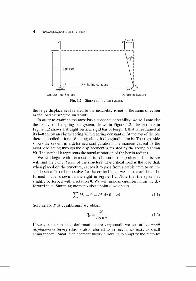
In order to examine the most basic concepts of stability, we will considerthe behavior of a spring-bar system, shown in Figure 1.2. The left side inFigure 1.2 shows a straight vertical rigid bar of length L that is restrained atits bottom by an elastic spring with a spring constant k. At the top of the barthere is applied a force P acting along its longitudinal axis. The right sideshows the system in a deformed configuration. The moment caused by theaxial load acting through the displacement is resisted by the spring reactionku. The symbol u represents the angular rotation of the bar in radians.

We will begin with the most basic solution of this problem. That is, wewill find the critical load of the structure. The critical load is the load that,when placed on the structure, causes it to pass from a stable state to an un-stable state. In order to solve for the critical load, we must consider a de-formed shape, shown on the right in Figure 1.2. Note that the system isslightly perturbed with a rotation u. We will impose equilibrium on the de-formed state. Summing moments about point A we obtain

XMA ¼ 0 ¼ PL sin u� ku (1.1)

Solving for P at equilibrium, we obtain

Pcr ¼ku

L sin u(1.2)

If we consider that the deformations are very small, we can utilize smalldisplacement theory (this is also referred to in mechanics texts as smallstrain theory). Small displacement theory allows us to simplify the math by

P L sin θP

L Rigid Bar

Undeformed System Deformed System

k = Spring constant

kθk A

θ

Fig. 1.2 Simple spring-bar system.


recognizing that for very small values of the angle, u, we can use thesimplifications that

sin u ¼ u

tan u ¼ u

cos u ¼ 1

Substituting sin u ¼ u, we determine the critical load Pcr of the spring-barmodel to be:

Pcr ¼ku

Lu¼ k

L(1.3)

The equilibrium is in a neutral position: it can exist both in the undeformedand the deformed position of the bar. The small displacement response ofthe system is shown in Figure 1.3. The load ratio PL=k ¼ 1 is variouslyreferred in the literature as the critical load, the buckling load, or the load atthe bifurcation of the equilibrium. The bifurcation point is a branch point;there are two equilibrium paths after Pcr is reached, both of which areunstable. The upper path has an increase in P with no displacement. Thisequilibrium path can only exist on a perfect system with no perturbation andis therefore not a practical solution, only a theoretical one.

Another means of solving for the critical load is through use of the prin-ciple of virtual work. Energy methods can be very powerful in describingstructural behavior, and have been described in many structural analysis

Stable Equilibrium

P

Unstable Equilibrium Bifurcation point at Pcr

θ

Fig. 1.3 Small displacement behavior of spring-bar system.

1.2 BASICS OF STABILITY BEHAVIOR: THE SPRING-BAR SYSTEM 5

and structural mechanics texts. Only a brief explanation of the methodwill be given here. The total potential P of an elastic system is defined byequation 1.4 as

P ¼ U þ Vp (1.4)

1. U is the elastic strain energy of a conservative system. In a conserva-tive system the work performed by both the internal and the externalforces is independent of the path traveled by these forces, and it de-pends only on the initial and the final positions. U is the internalwork performed by the internal forces; U ¼ Wi

2. Vp is the potential of the external forces, using the original deflectedposition as a reference. Vp is the external work; Vp ¼ �We.

Figure 1.4 shows the same spring-bar system we have considered, includ-ing the distance through which the load P will move when the bar displaces.

The strain energy is the work done by the spring,

U ¼ Wi ¼1

2ku2: (1.5)

The potential of the external forces is equal to

Vp ¼ �We ¼ �PLð1� cos uÞ (1.6)

The total potential in the system is then given by:

P ¼ U þ Vp ¼1

2ku2 � PLð1� cos uÞ (1.7)

PP

k

θ

L –

L co

s θ

L

Fig. 1.4 Simple spring-bar system used in energy approach.


According to the principle of virtual work the maxima and minima areequilibrium positions, because if there is a small change in u, there is nochange in the total potential. In the terminology of structural mechanics, thetotal potential is stationary. It is defined by the derivative

dP

du¼ 0 (1.8)

For the spring bar system, equilibrium is obtained when

dP

du¼ 0 ¼ ku� PL sin u (1.9)

To find Pcr, we once again apply small displacement theory ðsin u ¼ uÞ andobtain

Pcr ¼ k=L

as before.

Summary of Important Points

� Instability occurs when a small change in load causes a large changein displacement. This can occur on a local, member or system level.

� The critical load, or buckling load, is the load at which the systempasses from a stable to an unstable state.

� The critical load is obtained by considering equilibrium or potentialenergy of the system in a deformed configuration.

� Small displacement theory may be used to simplify the calculations ifonly the critical load is of interest.

1.3 FUNDAMENTALS OF POST-BUCKLING BEHAVIOR

In section 1.2, we used a simple example to answer a fundamental questionin the study of structural stability: At what load does the system becomeunstable, and how do we determine that load? In this section, we will con-sider some basic principles of stable and unstable behavior. We begin byreconsidering the simple spring-bar model in Figure 1.2, but we introduce adisturbing moment, Mo at the base of the structure. The new system isshown in Figure 1.5.

1.3 FUNDAMENTALS OF POST-BUCKLING BEHAVIOR 7

Similar to Figure 1.1, the left side of Figure 1.5 shows a straight, verticalrigid bar of length L that is restrained at its bottom by an infinitely elasticspring with a spring constant k. At the top of the bar there is applied a forceP acting along its longitudinal axis. The right sketch shows the deformationof the bar if a disturbing moment Mo is acting at its base. This moment isresisted by the spring reaction ku, and it is augmented by the momentcaused by the product of the axial force times the horizontal displacementof the top of the bar. The symbol u represents the angular rotation of the bar(in radians).

1.3.1 Equilibrium Solution

Taking moments about the base of the bar (point A) we obtain the followingequilibrium equation for the displaced system:

XMA ¼ 0 ¼ PL sin uþMo � ku

Letting uo ¼ Mo=k and rearranging, we can write the following equation:

PL

k¼ u� uo

sin u(1.10)

This expression is displayed graphically in various contexts in Figure 1.6.The coordinates in the graph are the load ratio PL=k as the abscissa and

the angular rotation u (radians) as the ordinate. Graphs are shown for threevalues of the disturbing action

uo ¼ 0; uo ¼ 0:01; and uo ¼ 0:05:

L sin θPP

Rigid Bar

kθA

Mo

kθ = Restoring momentMo = Disturbing momentk = S pring constant

k

L

θ

Undeformed System Deformed System

Fig. 1.5 Spring-bar system with disturbing moment.


When uo ¼ 0, that is PLk¼ u

sin u, there is no possible value of PL=k less than

unity since u is always larger than sin u. Thus no deflection is possible ifPL=k< 1:0. At PL=k> 1:0 deflection is possible in either the positive or thenegative direction of the bar rotation. As u increases or decreases the forceratio required to maintain equilibrium becomes larger than unity. However,at relatively small values of u, say, below 0.1 radians, or about 5�, the load-deformation curve is flat for all practical purposes. Approximately, it can besaid that equilibrium is possible at u ¼ 0 and at a small adjacent deformedlocation, say u< 0:1 or so. The load PL=k ¼ 1:0 is thus a special type ofload, when the system can experience two adjacent equilibrium positions:one straight and one deformed. The equilibrium is thus in a neutral position:It can exist both in the undeformed and the deformed position of the bar.The load ratio PL=k ¼ 1 is variously referred in the literature as the criticalload, the buckling load, or the load at the bifurcation of the equilibrium. Wewill come back to discuss the significance of this load after additionalfeatures of behavior are presented next.

The other two sets of solid curves in Figure 1.6 are for specific smallvalues of the disturbing action uo of 0. 01 and 0.05 radians. These curveseach have two regions: When u is positive, that is, in the right half of thedomain, the curves start at u ¼ uo when PL=k ¼ 0 and then gradually exhib-it an increasing rotation that becomes larger and larger as PL=k ¼ 1:0 isapproached, finally becoming affine to the curve for uo ¼ 0 as u becomesvery large. While this in not shown in Figure 1.6, the curve for smaller andsmaller values of uo will approach the curve of the bifurcated equilibrium.The other branches of the two curves are for negative values of u. They are

θ (radians)

–1 0 1

PL

/k

0

1

2

Stable region

Unstable region

θo = 0

θo = 0.01

θo = 0.05

Fig. 1.6 Load-deflection relations for spring-bar system with disturbing moment.


in the left half of the deformation domain and they lie above the curve foruo ¼ 0. They are in the unstable region for smaller values of �u, that is,they are above the dashed line defining the region between stable and unsta-ble behavior, and they are in the stable region for larger values of �u. (Note:The stability limit will be derived later.) The curves for �u are of little prac-tical consequence for our further discussion.

The nature of the equilibrium, that is, its stability, is examined by disturb-ing the already deformed system by an additional small rotation u�, asshown in Figure 1.7.

The equilibrium equation of the disturbed geometry isXMA ¼ 0 ¼ PL sin ðuþ u�Þ þMo � kðuþ u�Þ

After rearranging we get, noting that uo ¼ Mok

PL

k¼ uþ u� � uo

sin ðuþ u�Þ (1.11)

From trigonometry we know that sin ðuþ u�Þ ¼ sin u cos u� þ cos u sin u�.For small values of u� we can use cos u� � 1:0; sin u� � u�, and therefore

PL

k¼ uþ u� � uo

sin uþ u�cos u(1.12)

This equation can be rearranged to the following form: PLk

sin u� uþ uoþu�ðPL

kcos u� 1Þ ¼ 0. However, PL

ksin u� uþ uo ¼ 0 as per equation 1.10,

u� 6¼ 0, and thus

PL

kcos u� 1 ¼ 0 (1.13)

L sin (θ + θ*)PP

Rigid bar

k(θ + θ*)

MoAk

θ

θ*

L

Fig. 1.7 Disturbed equilibrium configuration.


Equation 1.13 is the locus of points for which u� 6¼ 0 while equilibrium isjust maintained, that is the equilibrium is neutral. The same result couldhave been obtained by setting the derivative of F ¼ PL

ksin u� uþ uo with

respect to u equal to zero:

dF

du¼ PL

kcos u� 1:

The meaning of the previous derivation is that when

1. cos u< 1PL=k

, the equilibrium is stable—that is, the bar returns to itsoriginal position when q� is removed; energy must be added.

2. cos u ¼ 1PL=k

, the equilibrium is neutral—that is, no force is requiredto move the bar a small rotation u�.

3. cos u> 1PL=k

, the equilibrium is unstable—that is, the configuration

will snap from an unstable to a stable shape; energy is released.

These derivations are very simple, yet they give us a lot of information:

1. The load-deflection path of the system that sustains an applied actionuo from the start of loading. This will be henceforth designated as animperfect system, because it has some form of deviation in eitherloading or geometry from the ideally perfect structure that is straightor unloaded before the axial force is applied.

2. It provides the critical, or buckling, load at which the equilibriumbecome neutral.

3. It identifies the character of the equilibrium path, whether it is neu-tral, stable, or unstable.

It is good to have all this information, but for more complex actual struc-tures it is often either difficult or very time-consuming to get it. We may noteven need all the data in order to design the system. Most of the time it issufficient to know the buckling load. For most practical structures, the deter-mination of this critical value requires only a reasonably modest effort, asshown in section 1.2.

In the discussion so far we have derived three hierarchies of results, eachrequiring more effort than the previous one:

1. Buckling load of a perfect system (Figure 1.2)

2. The post-buckling history of the perfect system (Figure 1.5)

3. The deformation history of the ‘‘imperfect’’ system (Figure 1.7)


In the previous derivations the equilibrium condition was established byutilizing the statical approach. Equilibrium can, however, be determined byusing the theorem of virtual work. It is sometimes more convenient to usethis method, and the following derivation will feature the development ofthis approach for the spring-bar problem.

1.3.2 Virtual Work Solution

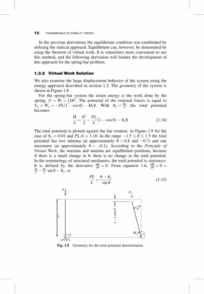
We also examine the large displacement behavior of the system using theenergy approach described in section 1.2. The geometry of the system isshown in Figure 1.8

For the spring-bar system the strain energy is the work done by thespring, U ¼ Wi ¼ 1

2ku2. The potential of the external forces is equal to

Vp ¼ We ¼ �PLð1� cos uÞ �Mou. With uo ¼ Mok

the total potentialbecomes

P

k¼ u2

2� PL

kð1� cos uÞ � uou (1.14)

The total potential is plotted against the bar rotation in Figure 1.9 for thecase of uo ¼ 0:01 and PL=k ¼ 1:10. In the range �1:5 � u � 1:5 the totalpotential has two minima (at approximately u ¼ 0:8 and �0:7) and onemaximum (at approximately u ¼ �0:1). According to the Principle ofVirtual Work, the maxima and minima are equilibrium positions, becauseif there is a small change in u, there is no change in the total potential.In the terminology of structural mechanics, the total potential is stationary.It is defined by the derivative dP

du¼ 0. From equation 1.6, dP

du¼ 0 ¼

2u2� PL

ksin u� uo, or

PL

k¼ u� uo

sin u(1.15)

PP

L

Mok

θ

L –

L co

s θ

Fig. 1.8 Geometry for the total potential determination.


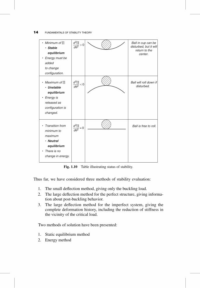
This equation is identical to equation 1.10. The status of stability isillustrated in Figure 1.10 using the analogy of the ball in the cup (stableequilibrium), the ball on the top of the upside-down cup (unstableequilibrium), and the ball on the flat surface.

The following summarizes the problem of the spring-bar model’s energycharacteristics:

P

k¼ u2

2�PL

kð1� cos uÞ � uou!Total potential

dðP=kÞdu

¼ u� uo �PL

ksin u ¼ 0! PL

k¼ u� uo

sin u!Equilibrium

d2ðP=kÞdu2

¼ 1� PL

kcos u ¼ 0! PL

k¼ 1

cos u! Stability

(1.16)

These equations represent the energy approach to the large deflectionsolution of this problem.

For the small deflection problem we set uo ¼ 0 and note that1� cos u� u2

2. The total potential is then equal to P ¼ ku2

2� PLu2

2. The deriv-

ative with respect to u gives the critical load:

dP

du¼ 0 ¼ uðk � PLÞ!Pcr ¼ k=L (1.17)

–1.5 –1.0 –0.5 0.0 0.5 1.0 1.5

Π/k

–0.04

0.00

0.04

0.08

0.12

Maximumunstable

Minimumstable

θFig. 1.9 Total potential for uo ¼ 0:01 and PL=k ¼ 1:10.


Thus far, we have considered three methods of stability evaluation:

1. The small deflection method, giving only the buckling load.

2. The large deflection method for the perfect structure, giving informa-tion about post-buckling behavior.

3. The large deflection method for the imperfect system, giving thecomplete deformation history, including the reduction of stiffness inthe vicinity of the critical load.

Two methods of solution have been presented:

1. Static equilibrium method

2. Energy method

• Minimum of ∏ • Stable

equilibrium

• Energy must be

added

to change

configuration.

d

2∏d θ2

Ball in cup can bedisturbed, but it will

return to thecenter.

• Maximum of ∏ • Unstable

equilibrium

• Energy is

released as

configuration is

changed.

Ball will roll down ifdisturbed.

• Transition from

minimum to

maximum

• Neutral

equilibrium

• There is no

change in energy.

Ball is free to roll.

> 0

< 0d

2∏dθ2

= 0d

2∏d θ2

Fig. 1.10 Table illustrating status of stability.


Such stability-checking procedures are applied to analytically exact and ap-proximate methods for real structures in the subsequent portions of this book.

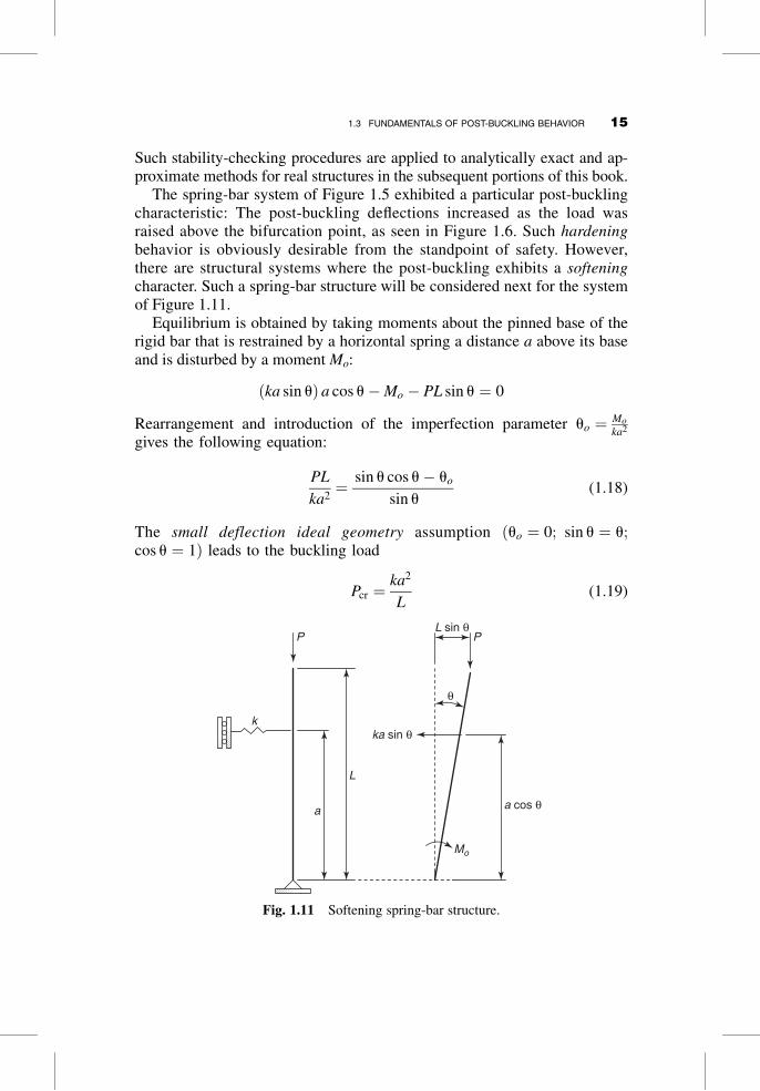
The spring-bar system of Figure 1.5 exhibited a particular post-bucklingcharacteristic: The post-buckling deflections increased as the load wasraised above the bifurcation point, as seen in Figure 1.6. Such hardeningbehavior is obviously desirable from the standpoint of safety. However,there are structural systems where the post-buckling exhibits a softeningcharacter. Such a spring-bar structure will be considered next for the systemof Figure 1.11.

Equilibrium is obtained by taking moments about the pinned base of therigid bar that is restrained by a horizontal spring a distance a above its baseand is disturbed by a moment Mo:

ðka sin uÞ a cos u�Mo � PL sin u ¼ 0

Rearrangement and introduction of the imperfection parameter uo ¼ Mo

ka2

gives the following equation:

PL

ka2¼ sin u cos u� uo

sin u(1.18)

The small deflection ideal geometry assumption ðuo ¼ 0; sin u ¼ u;cos u ¼ 1Þ leads to the buckling load

Pcr ¼ka2

L(1.19)

k

a

L

ka sin θ

L sin θ

Mo

a cos θ

PP

θ

Fig. 1.11 Softening spring-bar structure.


From the large deflection-ideal geometry assumption ðuo ¼ 0Þ we get thepost-buckling strength:

Pcr ¼ka2

Lcos u (1.20)

The load-rotation curves from equations 1.18 and 1.20 are shown in Fig-ure 1.12 for the perfect ðuo ¼ 0Þ and the imperfect ðuo ¼ 0:01Þ system. Thepost-buckling behavior is softening—that is, the load is decreased as therotation increases. The deflection of the imperfect system approaches that ofthe perfect system for large bar rotations. However, the strength of theimperfect member will never attain the value of the ideal critical load. Sincein actual structures there will always be imperfections, the theoreticalbuckling load is upper bound.

The nature of stability is determined from applying a virtual rotation to thedeformed system. The resulting equilibrium equation then becomes equal to

½ka sin ðuþ u�Þ�a cos ðuþ u�Þ �Mo � PL sin ðuþ u�Þ ¼ 0

Noting that u� is small, and so sin u� ¼ u�; cos u� ¼ 1. Also making use ofthe trigonometric relationships

sin ðuþ u�Þ ¼ sin u cos u� þ cos u sin u� ¼ sin uþ u�cos u

cos ðuþ u�Þ ¼ cos u cos u� � sin u sin u� ¼ cos u� u� sin u

we can arrive at the following equation:

½ka2 sin u cos u�Mo � PL sin u�þ u�½ka2ðcos 2u� sin 2uÞ � PLcos u�� u�½ka2cos u sin u� ¼ 0

–1.0 –0.5 0.0 0.5 1.0

PL

/ ka

2

0.0

0.5

1.0

1.5

stable

unstable

θo = 0.01

θo = 0.01

θ (radians)

θo = 0

Fig. 1.12 Load-rotation curves for a softening system.


The first line is the equilibrium equation, and it equals zero, as demonstratedabove. The bracket in the third line is multiplied by the square of a smallquantity ðu� u2Þ and so it can be neglected. From the second linewe obtain the stability condition that is shown in Figure 1.12 as a dashedline:

PL

ka2¼ cos2u� sin2u

cos u

¼ 2 cos2u� 1

cos u

(1.21)

This problem is solved also by the energy method, as follows:

Total potential: P ¼ kða sin uÞ2

2�Mou� PLð1� cos uÞ

Equilibrium:qP

qu¼ ka2 sin u cos u�Mo � PL sin u ¼ 0! PL

ka2

¼ sin u cos u

sin u

The two spring-bar problems just discussed illustrate three post-bucklingsituations that occur in real structures: hardening post-buckling behavior,softening post-buckling behavior, and the transitional case where the post-buckling curve is flat for all practical purposes. These cases are discussedin various contexts in subsequent chapters of this book. The drawings inFigure 1.13 summarize the different post-buckling relationships, and indi-cate the applicable real structural problems. Plates are insensitive to initialimperfections, exhibiting reliable additional strength beyond the bucklingload. Shells and columns that buckle after some parts of their cross sectionhave yielded are imperfection sensitive. Elastic buckling of columns, beams,and frames have little post-buckling strength, but they are not softening, norare they hardening after buckling.

Before leaving the topic of spring-bar stability, we will consider twomore topics: the snap-through buckling and the multidegree of freedomcolumn.

Stability:qP

qu¼ ka2½cos2u� sin2u� � PL cos u ¼ 0! PL

ka2¼ 2 cos2u� 1

cos u


1.4 SNAP-THROUGH BUCKLING

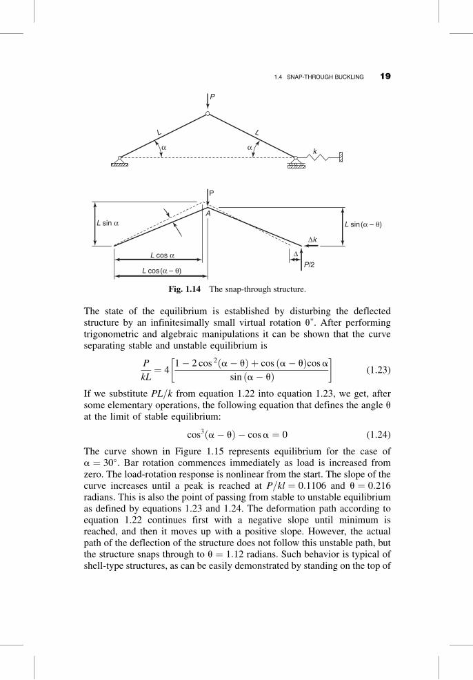
Figure 1.14 shows a two-bar structure where the two rigid bars are at anangle to each other. One end of the right bar is on rollers that are restrainedby an elastic spring. The top Figure 1.14 shows the loading and geometry,and the bottom features the deformed shape after the load is applied. Equili-brium is determined by taking moments of the right half of the deformedstructure about point A.

XMA ¼ 0 ¼ P

2½L cos ða� uÞ� � DkL sin ða� uÞ

From the deformed geometry of Figure 1.14 it can be shown that

D ¼ 2L cos ða� uÞ � 2L cos u

The equilibrium equation thus is determined to be

P

kL¼ 4½ sin ða� uÞ � tan ða� uÞcos a� (1.22)

LoadLoadLoad

000

Deflection

Imperfectioninsensitive

(plates)

Imperfectionsensitive

(shells,inelastic columns)

(elastic beamscolumnsframes)

straight

initial curvature

Pcr

Fig. 1.13 Illustration of post-buckling behavior.


The state of the equilibrium is established by disturbing the deflectedstructure by an infinitesimally small virtual rotation u�. After performingtrigonometric and algebraic manipulations it can be shown that the curveseparating stable and unstable equilibrium is

P

kL¼ 4

1� 2 cos 2ða� uÞ þ cos ða� uÞcos a

sin ða� uÞ

� �(1.23)

If we substitute PL=k from equation 1.22 into equation 1.23, we get, aftersome elementary operations, the following equation that defines the angle u

at the limit of stable equilibrium:

cos3ða� uÞ � cos a ¼ 0 (1.24)

The curve shown in Figure 1.15 represents equilibrium for the case ofa ¼ 30�. Bar rotation commences immediately as load is increased fromzero. The load-rotation response is nonlinear from the start. The slope of thecurve increases until a peak is reached at P=kl ¼ 0:1106 and u ¼ 0:216radians. This is also the point of passing from stable to unstable equilibriumas defined by equations 1.23 and 1.24. The deformation path according toequation 1.22 continues first with a negative slope until minimum isreached, and then it moves up with a positive slope. However, the actualpath of the deflection of the structure does not follow this unstable path, butthe structure snaps through to u ¼ 1:12 radians. Such behavior is typical ofshell-type structures, as can be easily demonstrated by standing on the top of

α

LL

k

P

α

A

L cos α

L cos(α – θ)

L sin α L sin(α – θ)

Δ

Δk

P

P/2

Fig. 1.14 The snap-through structure.

1.4 SNAP-THROUGH BUCKLING 19

an empty aluminum beverage can and having someone touch the side of thecan. A similar event takes place any time a keyboard of a computer ispushed. Snap-through is sudden, and in a large shell structure it can havecatastrophic consequences.

Similarly to the problems in the previous section, the energy approach can bealso used to arrive at the equilibrium equation of equation 1.22 and the stabilitylimit of equation 1.23 by taking, respectively, the first and second derivative ofthe total potential with respect to u. The total potential of this system is

P ¼ 1

2kf2L½cos ða� uÞ � cos a�g2 � PL½ sin a� sin ða� uÞ� (1.25)

The reader can complete to differentiations to verify the results.

1.5 MULTI-DEGREE-OF-FREEDOM SYSTEMS

The last problem to be considered in this chapter is a structure made up ofthree rigid bars placed between a roller at one end and a pin at the other end.The center bar is connected to the two edge bars with pins. Each interiorpinned joint is restrained laterally by an elastic spring with a spring constantk. The structure is shown in Figure 1.16a. The deflected shape at buckling ispresented as Figure 1.16b. The following buckling analysis is performed byassuming small deflections and an initially perfect geometry. Thus, the onlyinformation to be gained is the critical load at which a straight and a buckledconfiguration are possible under the same force.

θ (radians)

0.0 0.2 0.4 0.6 0.8 1.0 1.2

PL

/ k

–0.15

–0.10

–0.05

0.00

0.05

0.10

0.15snap-throughA

B

Fig. 1.15 Load-rotation curve for snap-through structure for a ¼ 30�.


Equilibrium equations for this system are obtained as follows:

Sum of moments about Point 1:P

M1 ¼ 0 ¼ kD1Lþ kD2ð2LÞ � R2ð3LÞSum of vertical forces:

PFy ¼ 0 ¼ R1 þ R2 � kD1 � kD2

Sum of moments about point 3, to the left:P

M3 ¼ 0 ¼ PD1 � R1L

Sum of moments about point 4, to the right:P

M4 ¼ 0 ¼ PD2 � R2L

Elimination of R1 and R2 from these four equations leads to the followingtwo homogeneous simultaneous equations:

P� 2kL

3� kL

3

� kL

3P� 2kL

3

264

375 D1

D2

� �¼ 0 (1.26)

The deflections D1 and D2 can have a nonzero value only if the determinantof their coefficients becomes zero:

P� 2kL

3� kL

3

� kL

3P� 2kL

3

��

��¼ 0 (1.27)

Decomposition of the determinant leads to the following quadratic equation:

3P

kL

� �2

�4P

kLþ 1 ¼ 0 (1.28)

This equation has two roots, giving the following two critical loads:

Pcr1 ¼ kL

Pcr2 ¼kL

3

(1.29)

PinRigid bar

k k

P P

R1 R2

PP1 2

3 4

(a)

(b)

L L L

kΔ1 kΔ2

Δ1 Δ2

Fig. 1.16 Three-bar structure with intermediate spring supports.

1.5 MULTI-DEGREE-OF-FREEDOM SYSTEMS 21

The smaller of the two critical loads is then the buckling load of interest tothe structural engineer. Substitution each of the critical loads into equation1.26 results in the mode shapes of the buckled configurations, as illustratedin Figure 1.17.

Finally then, Pcr ¼ kL3

is the governing buckling load, based on the smalldeflection approach.

The energy method can also be used for arriving at a solution to this prob-lem. The necessary geometric relationships are illustrated in Figure 1.18, andthe small-deflection angular and linear deformations are given as follows:

D1 ¼ c L and D2 ¼ uL

D1 � D2

L¼ g ¼ c� u

e3 ¼ L� L cos u� Lu2

2

e2 ¼ e3 þ L½1� cos ðc� uÞ� ¼ L

22u2 þ c2 � 2cu� �

e3 ¼ e2 þLc2

2¼ L u2 þ c2 � cu

� �

The strain energy equals UP ¼ k2ðD2

1 þ D22Þ ¼ kL2

2ðc2 þ u2Þ.

k k

Pcr 1 = kL

Pcr 2 =

(a)

(b)

k k

3

kL

Δ1 = Δ2

Δ1 = –Δ2

Fig. 1.17 Shapes of the buckled modes.

θ

ε1 ε2 ε3

L L L

Δ1Δ2ψ

γ

Fig. 1.18 Deflections for determining the energy solution.


The potential of the external forces equals VP ¼ �Pe1 ¼�PLðu2 þ c2 � cuÞ

The total potential is then

P ¼ U þ VP ¼kL2

2ðc2 þ u2Þ � PLðu2 þ c2 � cuÞ (1.30)

For equilibrium, we take the derivatives with respect to the two angularrotations:

qP

qc¼ 0 ¼ kL2

2ð2cÞ � 2PLcþ PLu

qP

qu¼ 0 ¼ kL2

2ð2uÞ � 2PLuþ PLc

Rearranging, we get

ðkL2 � 2PLÞ PL

PL ðkL2 � 2PLÞ

� �u

c

� �¼ 0

Setting the determinant of the coefficients equal to zero results in thesame two critical loads that were already obtained.

1.6 SUMMARY

This chapter presented an introduction to the subject of structural stability.Structural engineers are tasked with designing and building structures thatare safe under the expected loads throughout their intended life. Stability isparticularly important during the erection phase in the life of the structure,before it is fully braced by its final cladding. The engineer is especially in-terested in that critical load magnitude where the structure passes from astable to an unstable configuration. The structure must be proportioned sothat the expected loads are smaller than this critical value by a safe margin.

The following basic concepts of stability analysis are illustrated in thischapter by several simple spring-bar mechanisms:

� The critical, or buckling load, of geometrically perfect systems

� The behavior of structures with initial geometric or staticalimperfections

� The amount of information obtained by small deflection and large de-flection analyses

� The equivalence of the geometrical and energy approach to stabilityanalysis

1.6 SUMMARY 23

� The meaning of the results obtained by a bifurcation analysis, a compu-tation of the post-buckling behavior, and by a snap-through investigation

� The hardening and the softening post-buckling deformations

� The stability analysis of multi-degree-of-freedom systems

We encounter each of these concepts in the subsequent parts of this text,as much more complex structures such as columns, beams, beam-columns,and frames are studied.

PROBLEMS

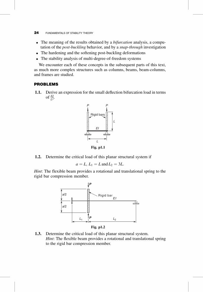
1.1. Derive an expression for the small deflection bifurcation load in termsof EI

L2.

1.2. Determine the critical load of this planar structural system if

a ¼ L; L1 ¼ L and L2 ¼ 3L:

Hint: The flexible beam provides a rotational and translational spring to therigid bar compression member.

1.3. Determine the critical load of this planar structural system.Hint: The flexible beam provides a rotational and translational springto the rigid bar compression member.

P P

L

L

EI

Rigid bars

Fig. p1.1

a/2

a/2

L2L1

P

P

Rigid barEI

Fig. p1.2


1.4. In the mechanism a weightless infinitely stiff bar is pinned at the pointshown. The load P remains vertical during deformation. The weight Wdoes not change during buckling. The spring is unstretched when thebar is vertical. The system is disturbed by a moment Mo at the pin.

a. Determine the critical load P according to small deflectiontheory.

b. Calculate and plot the equilibrium path p� u for 0 � u � p2

when uo ¼ 0 and

uo ¼ 0:01; p ¼ PL�Wb

ka2and uo ¼

Mo

ka2; a ¼ 0:75L and b ¼ 1:5L:

a

a

P

P

Rigid bars

EI

P

PL L L

Fig. p1.3

P

k

L

1.5L

0.75L

Mo

W

θ

Fig. p1.4

PROBLEMS 25

c. Investigate the stability of the equilibrium path.

d. Discuss the problem.

Note: This problem was adapted from Chapter 2, Simitses ‘‘An intro-duction to the elastic stability of structures’’ (see end of Chapter 2 forreference details).

1.5. Develop an expression for the critical load using the small-deflectionassumption. Employ both the equilibrium and the energy method.Note: that the units of K1 are inch-kip/radian, and the units of K2 arekip/inch

1.6. Develop an expression for the critical load using the small-deflectionassumption. The structure is made up of rigid bars and elastic springs.Employ both the equilibrium and the energy method.

P

L / 2

L / 2

K1K2

Fig. p1.5

P

K K

2h

h

2h

Fig. p1.6


1.7. The length of the bar is L, and it is in an initially rotated condition fi

from the vertical. The spring is undistorted in this initial configuration.A vertical load P is applied to the system, causing it to deflect an anglef from the vertical. The load P remains vertical at all times. Deriveequations for equilibrium and stability, using the equilibrium and theenergy methods. Plot P versus f for fi ¼ 0:05 radians.

KP

Deformed position

Initial position:Spring is undeformed

φi

φ

Fig. p1.7

PROBLEMS 27

fundamentals of stability theory · fundamentals of stability theory 1.1 introduction it is not...

Documents