MSH4

Fundamentals of Statistical

Consulting

Week 10 Comparison of two time series

Jean Yang and Jennifer Chan

Important points

1. Difference in sampling frequencies.

Erase the connecting lines and display only the points corresponding to actual data.

2. Difference in length.

3. What to compare?

Process or model (time series generator)?

Values, trends, patterns or periodicity?

Observed or forecast?

Some basic graphical comparison

Charissia data

Two time series: pre and post

Compare differences and ratios

More positive than negative differences in the first graph.

Ratios are much higher above 1.

Compares two cumulative time series.

The post time series has higher values in general.

Compare models

Time series models

Fix ARMA or regime switching or other nonlinear models and construct an F test to test the hypothesis of a common set of parameters for a common data set but not here.

These do not compare mean and variance but just the autocorrelation structure, acf.

The noises are smoothed out.

The three plots are acfs and cross correlation. These may not be the comparison Charissia wants!

Running ARMA models

arima(x = z4, order = c(1, 0, 1)) #pre Coefficients: ar1 ma1 intercept 0.5545 -0.3909 24.8376 s.e. 0.2109 0.2356 0.5058 sigma^2 estimated as 78.2: log likelihood = -2051.22, aic = 4110.43 arima(x = y3, order = c(1, 0, 1)) #post Coefficients: ar1 ma1 intercept 0.5976 -0.2983 26.1752 s.e. 0.1648 0.2059 0.6783 sigma^2 estimated as 86.87: log likelihood = -2088.53, aic = 4185.07 The parameter estimates are similar but there is no test of significance of the difference

on two different data!!

Compare forecast

Granger test is usually used to see if the values of one series at time t can predict the values of the other series at time t+1, that is, to test if one time series is useful in forecasting another.

The R code is grangertest() in the lmtest library.

> grangertest(z4,y3[1:570],1) #make two data the same length Granger causality test

Model 1: y3[1:570] ~ Lags(y3[1:570], 1:1) + Lags(z4, 1:1) Model 2: y3[1:570] ~ Lags(y3[1:570], 1:1) Res.Df Df F Pr(>F) 1 566 2 567 -1 14.377 0.0001657 *** --- Signif. codes: 0 ‘***’ 0.001 ‘**’ 0.01 ‘*’ 0.05 ‘.’ 0.1 ‘ ’ 1

Significant! But again, it may not be suitable as the time (hence lag) pair may differ. We

have removed repeats and NA!!!

Compare process in data mining

Distance function is suggested to compare two series in signal processing.

Distance functions:

L-p distance function D(x,y) = ( ∑|xi – yi |p )1/p

L-2 distance function D(x,y) = ( ∑(xi - yi )2 )1/2 (Most popular and efficient)

Why prefer L2 distance?

L2 distance is preserved under “orthonormal transforms”

For L-p norm, only p=2 satisfy this property.

Optimal distance measure for estimation if signals are corrupted by Gaussian,

additive noise

Widely used

Euclidean distance

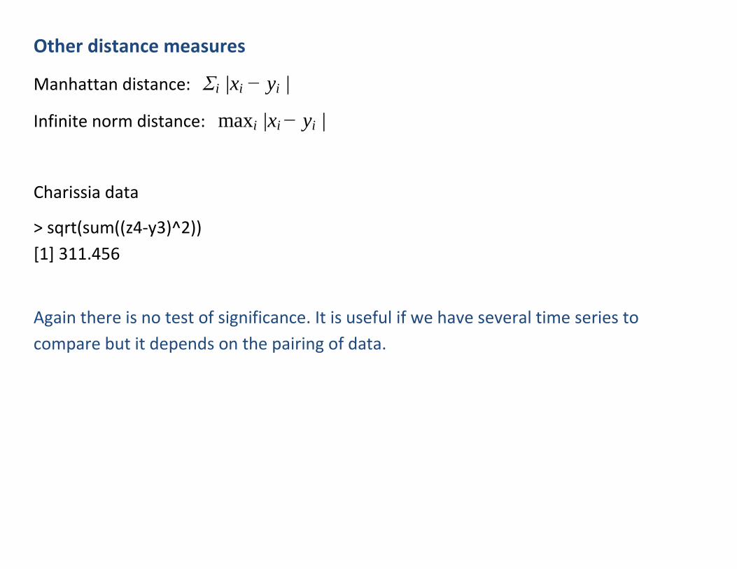
Other distance measures

Manhattan distance: Σi |xi − yi |

Infinite norm distance: maxi |xi − yi |

Charissia data

> sqrt(sum((z4-y3)^2))

[1] 311.456

Again there is no test of significance. It is useful if we have several time series to

compare but it depends on the pairing of data.

What constitutes differences?

Difference in time in the first graph?

Align the time series with the same starting point.

Difference in levels in the second graph?

Normalized or standardized the time series.

There are not the issues as the levels of pre and post are similar. The difference in levels

is what we want to study.

Elastic dissimilarity measure

What if the time series differ in length? With different sizes M and N!

Dynamic time warping (DTW)

where can be ( ∑(xi - yi )2 )1/2 .

The unit window can change to any in general,

,

where

and [ ] is to round to the nearest integer.

If and M = N, corresponds to the Euclidean distance. The window

allows reduction in computational cost.

Minimum jump costs (MJC)

where

and

Have jump from y5 to x4 (hence tx = 5 and ty = 6) and jump back to y again at minimal

cost. Evaluate all possible ty + ∆, for ∆ = 0,1,...,14 (time 6 to 20) and the best jump is y7.

There are many different distance measures but a paper said the most efficient one is L2,

DTW and MJC. However to calculate such distance measures, there is no package or

packages are not working.