fuqua investment analytics stefan d. gertsch brian wachob building blocks for a long/short strategy...
TRANSCRIPT

Fuqua Investment Analytics
Stefan D. Gertsch
Brian Wachob
Building Blocks for a Long/Short Strategy Driven by Quantitative Stock Selection

April 27, 2005 © Gertsch & Wachob 2
Purpose of Study
Build a quantitative stock selection model to guide portfolio management at a long/short hedge fund. Adopted perspective of a fund with $100M in assets
under management• This fund size estimate guided investable universe definition.
Assumed goal of maximizing returns with negligible correlation to other asset classes
• In practice, we did consider variance as well, but it is of much lesser importance if correlations with other asset classes are indeed negligible.

April 27, 2005 © Gertsch & Wachob 3
Overview
Definitions: Universe, Methodology, Conventions Cross-Sectional (Time Invariant) Factor Research
Identification and Evaluation Factor Refinement
• Negative Factor Values and Counter-Intuitive Resultant Rankings• These concerns are often overlooked by others and arise among very
common factor definitions (such as forward earnings yield)• Industry Normalization
Optimal Fractile Resolution and Clustering/Groupings/Aggregation Integration of Factor Portfolios into a Multivariate Model
Based on Mean-Variance Portfolio Optimization with the Imposition of Custom Constraints
Multivariate Model’s Out-of-Sample Performance Forecasting Factor Portfolio Returns
Demonstration of dynamic factor weightings based on factor performance forecasts

April 27, 2005 © Gertsch & Wachob 4
Universe Definition
U.S. stocks only
Time-scaled min. market cap threshold $54M in 1987, rises by 7% annually to $200M in 2005
Time-scaled min. estimated mean daily dollar volume threshold $84K in 1987, rises by 10.4% annually to $500K in 2005
Excluded ETFs and other investment funds trading as stocks
Excluded 3 instances of likely erroneous Compustat returns data
Number of stocks in universe grows with time 998 on 1/31/1987
2,649 on 11/31/2001
≈3,336 today (4/27/2005)
April 27, 2005 © Gertsch & Wachob 5
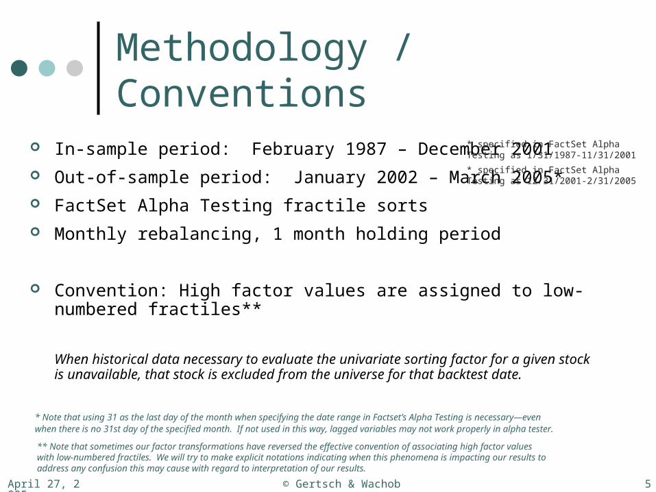
Methodology / Conventions
In-sample period: February 1987 – December 2001
Out-of-sample period: January 2002 – March 2005*
FactSet Alpha Testing fractile sorts
Monthly rebalancing, 1 month holding period
Convention: High factor values are assigned to low-numbered fractiles**
When historical data necessary to evaluate the univariate sorting factor for a given stock is unavailable, that stock is excluded from the universe for that backtest date.
** Note that sometimes our factor transformations have reversed the effective convention of associating high factor values with low-numbered fractiles. We will try to make explicit notations indicating when this phenomena is impacting our results to address any confusion this may cause with regard to interpretation of our results.
* Note that using 31 as the last day of the month when specifying the date range in Factset’s Alpha Testing is necessary—even when there is no 31st day of the specified month. If not used in this way, lagged variables may not work properly in alpha tester.
* specified in FactSet Alpha Testing as 1/31/1987-11/31/2001
* specified in FactSet Alpha Testing as 12/31/2001-2/31/2005

April 27, 2005 © Gertsch & Wachob 6
Factor Identification
Factor CategoriesValuationAccounting/Earnings QualitySentimentTechnicalUnclassified

April 27, 2005 © Gertsch & Wachob 7
Factor Refinement
Address negative factor values and counter-intuitive resultant rankings
Empirically evaluate different technical factor definitions Identify optimal evaluation window Identify best source database (e.g. Compustat? I/B/E/S?) Standardization? Absolute change? % change? Address NAs in data set
Industry normalization Factor portfolio returns: predictive forecasts Isolate factor performance within sub-universes (e.g. small cap
momentum versus large cap momentum) Optimal fractile resolution and fractile groupings/partitioning towards
multivariate integration

April 27, 2005 © Gertsch & Wachob 8
Valuation Factors
Evaluated in a previous studyhttp://faculty.fuqua.duke.edu/~charvey/Teaching/BA453_2005/DIA/DIA%20Final%20Project_007.ppt#1 Dividend Yield Book to Market Historical (Trailing) Earnings Yield (Crude) Implied Cost of Capital
Candidates for future studies Cash Flow Yield (or FCF/TEV) Reinvestment Rate ROE Sales to Market Comprehensive Implied Cost of Capital
Chosen for implementation in this study Forward Earnings Yield
April 27, 2005 © Gertsch & Wachob 9
Accounting/Earnings Quality Factors
Change in Net Accruals scaled by Assets
There are many ways to isolate different elements of accounting accruals– experimentation with factors based on these different elements of accruals is a recommended area of future research
Other measures of earnings quality also constitute an area for recommended future research
April 27, 2005 © Gertsch & Wachob 10
Sentiment Factors
Revision Ratio We experimented with various ways of defining this
metric Ultimately chose to use a three-month trailing window
and aggregate the number of up versus down earnings revisions, scaling by the total number of estimates
Candidates for future studies Aggregated consensus analyst buy/sell
recommendations (or changes) Debt or equity ratings (or changes) Change in mean or median consensus earnings
estimate

April 27, 2005 © Gertsch & Wachob 11
Technical Factors
Price Momentum We only looked at the classic momentum definition: percentage price
change over the month -13 to month -2 window Reversal (Last month’s return)
Candidates for future studies Other known quant. models separately consider 6-month price
momentum and 20-month price momentum We examined reversals (1-month price change), but found no significant
signal; perhaps more study is warranted Perhaps momentum should be considered on a beta-adjusted basis (i.e.
rank stocks on estimated alphas rather than on raw % return). As presently constructed, this factor may effectively sort on beta during periods of strong market directional moves.
MACD On-balance volume Gap-related technical factors Myriad other quantifiable technical factors
April 27, 2005 © Gertsch & Wachob 12
Unclassified Factors
Percentage Change in Shares Outstanding Standardized Unexpected Earnings Abnormal Dollar Volume or Abnormal Turnover Size
Incorporated only with regard to potential for forecasting periods of small cap outperformance versus periods of large cap outperformance
Candidates for future studies Institutional ownership: % level or
accumulation/distribution Insider purchases/sales

April 27, 2005 © Gertsch & Wachob 13
Factor Evaluation
Required painstaking data inspection in FactSetParameter codes and syntax must be very
carefully selected• Avoid or work around data sets with erroneous or
misaligned data (can impose look-ahead bias or present stale data)
• Avoid survivorship bias that can easily taint a universe via certain parameter specifications
Universe definition must also be very carefully specified and coded to avoid biases

April 27, 2005 © Gertsch & Wachob 14
Factor Evaluation
All analysis pertains to Equal-Weighting fractile constituents. As a small hedge fund (per our assumed perspective), our
universe definition is considered sufficient to limit our strategies to tradable (sufficiently liquid) stocks.
Our method of combining independently evaluated factors into an ultimate multivariate strategy is congruous with this equal-weighting
S&P500 Index is used throughout as a benchmark A future analysis should consider a different benchmark (perhaps
the equal-weighted mean return of all stocks entering our universe in any given month)
The S&P500 represents performance of very large capitalization companies– our universe equally weights a broad cross-section of large cap and small cap firms (more like an equal-weighted Russell 3000)

April 27, 2005 © Gertsch & Wachob 15
Forward Earnings YieldFactor Refinement– Technical Definition
Examined various measures of forward earnings Mean and median forecasts Weighted and unweighted forecasts Next Twelve Months, Second Twelve Months, FY1,
FY2, and FY3 forecasts Various combinations and substitution schemes for
NAs among these earnings forecast parameters
Selected FactSet codeAVAIL(IH_MED_EPS_NTMA(0), IH_MEDIAN_NTM(0), G_IBES_FY1_MED_USD(0))/MP(0) We suspect that further experimentation can identify an even better FactSet-based
definition for Forward Earnings Yield.

April 27, 2005 © Gertsch & Wachob 16
Forward Earnings YieldFactor Refinement– Data Cleaning
Excluded firms with forward earnings yield estimates of dubious accuracy from dataset (i.e. forward earnings yield universe). Forward earnings yield estimates consistently
exceeded 1 for a few firms early in the in-sample data set. One firm (SEIBELS BRUCE GROUP INC) even surpassed 100.
Set criteria for exclusion to FEY>1.

April 27, 2005 © Gertsch & Wachob 17
Forward Earnings YieldFactor Refinement– Negative Values
For negative earnings forecasts, consistent value-based sorting on forward earnings yield is unclear.
Example Company A: E = 1, P = 10 E/P = .10 Company B: E = 1, P = 100 E/P = .01 Company C: E = -1, P = 100 E/P = -.01 Company D: E = -10, P = 100 E/P = -.10 Company Y: E = -10, P = 1000 E/P = -.01 Company Z: E = -100, P = 1000 E/P = -.10
Problem: Sort on Forward Earnings Yield gives A, B, C/Y (tie), D/Z (tie) Desired result: A, B, C, D, Y, Z
All else being equal, we prefer earnings that are less negative and we prefer lesser prices, but a rational tradeoff assessing a preferred price paid per unit of negative earnings is unclear
April 27, 2005 © Gertsch & Wachob 18
Forward Earnings YieldFactor Refinement– Negative Values
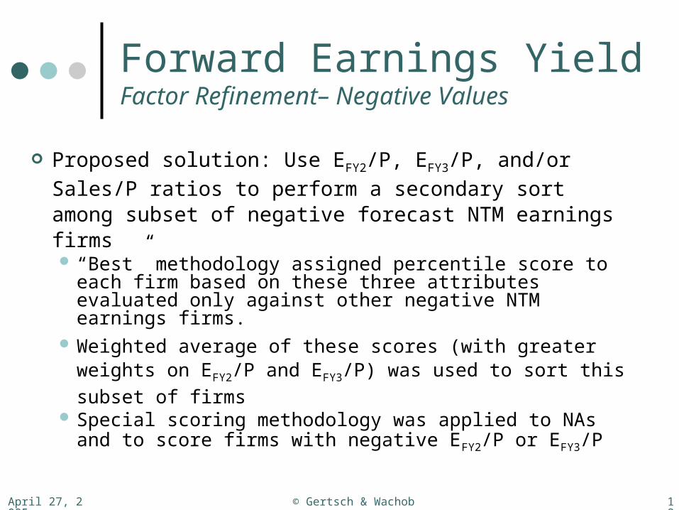
Proposed solution: Use EFY2/P, EFY3/P, and/or Sales/P
ratios to perform a secondary sort among subset of negative forecast NTM earnings firms “Best” methodology assigned percentile score to each
firm based on these three attributes evaluated only against other negative NTM earnings firms.
Weighted average of these scores (with greater weights on EFY2/P and EFY3/P) was used to sort this
subset of firms Special scoring methodology was applied to NAs and
to score firms with negative EFY2/P or EFY3/P
April 27, 2005 © Gertsch & Wachob 19
Forward Earnings YieldFactor Refinement– Negative Values
Disappointing resultsIf anything, we observe lesser separation among lowest fractiles
with our negative value adjustment scheme.
Alpha (vs. S&P500), Monthly % -- FEY
-1.20
-1.00
-0.80
-0.60
-0.40
-0.20
0.00
0.20
0.40
0.60
0.80
-1- -2- -3- -4- -5- -6- -7- -8- -9- -10- -11- -12- -13- -14- -15- -16- -17- -18- -19- -20- -21- -22- -23- -24- -25-
Fractile
Alpha (vs. S&P500), Monthly % -- FEY (w/Neg.Val.Adj.)
-1.20
-1.00
-0.80
-0.60
-0.40
-0.20
0.00
0.20
0.40
0.60
0.80
-1- -2- -3- -4- -5- -6- -7- -8- -9- -10- -11- -12- -13- -14- -15- -16- -17- -18- -19- -20- -21- -22- -23- -24- -25-
Fractile
April 27, 2005 © Gertsch & Wachob 20
Forward Earnings YieldFactor Refinement– Negative Values
Abandoned effort to improve negative value treatment in forward earnings yield factor. Our proposed methods were not found to be
empirically superior. We still believe that better treatment of these negative
values (by some other method) can improve factor performance.
• We leave such efforts to future research.
• With proper assumptions applied, an implied cost of capital metric seems like a potentially far superior valuation factor.

April 27, 2005 © Gertsch & Wachob 21
Industry Normalization
Perhaps relative assessments of factors against only a firm’s industry peers lends additional information that is obscured by universal sorts.
Proposed methods of industry-normalization Industry-specific factor standardization (by demeaning
or z-scores)• How to handle negative industry means?• How to handle outlier firms that might disproportionately affect
estimated industry factor means and standard deviations? How to treat non-normal intra-industry factor distributions?
Industry-specific factor sorts and percentile binning

April 27, 2005 © Gertsch & Wachob 22
Industry Normalization
Firms change industries over time. Most FactSet industry classification codes only retrieve present-
day industry classification data. Using these might introduce biases into our backtests.
Solution: Historically updating Industry Codes• Compustat’s historically updated SIC Codes
How to define and partition firms into industries? Group firms with similar risk of underlying assets (cost of capital) Group firms with similar overall risk profiles– such as sensitivities
to macroeconomic environment Group firms for which our factors have similar predictive power E/P, leverage, and forecast growth rates are some specific
metrics we examined to evaluate appropriate grouping schemes To enable historically accurate industry classifications in FactSet,
we must define our industries based on SIC Codes
April 27, 2005 © Gertsch & Wachob 23
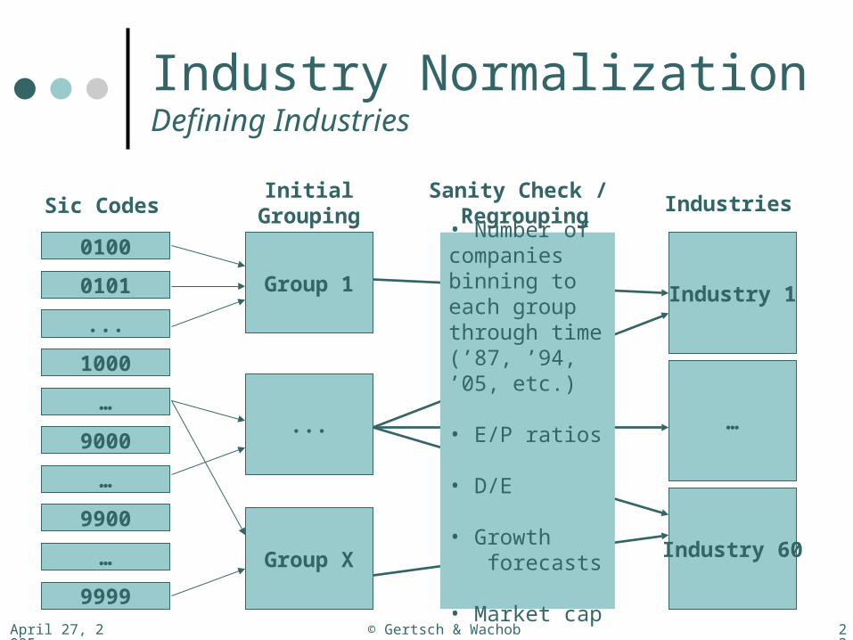
Industry NormalizationDefining Industries
0100
Sic CodesInitial
GroupingSanity Check /
Regrouping
0101
...
1000
…
9000
9999
9900
…
…
Group 1
Group X
...
• Number of companies binning to each group through time (’87, ’94, ’05, etc.)
• E/P ratios
• D/E
• Growth forecasts
• Market cap
Industries
Industry 1
…
Industry 60
April 27, 2005 © Gertsch & Wachob 24
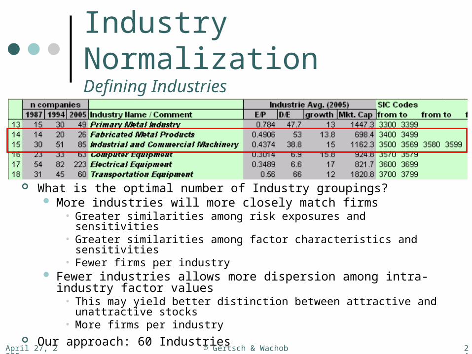
Industry NormalizationDefining Industries
What is the optimal number of Industry groupings? More industries will more closely match firms
• Greater similarities among risk exposures and sensitivities• Greater similarities among factor characteristics and sensitivities• Fewer firms per industry
Fewer industries allows more dispersion among intra-industry factor values
• This may yield better distinction between attractive and unattractive stocks
• More firms per industry Our approach: 60 Industries

April 27, 2005 © Gertsch & Wachob 25
Industry Normalization
Intra-industry factor sorts and percentile binningFinal universe-wide sort is performed on these
intra-industry percentile scoresFinal fractiles that result are industry-neutral
(i.e. same number of firms from each industry are binned to each of the final fractiles)
Intra-industry factor information is isolated; Inter-industry factor information is discarded

April 27, 2005 © Gertsch & Wachob 26
Industry NormalizationIntra-industry factor sorts and percentile binning
Group By Industry
Industry 1
…
Industry 60
Factor
high
…
low
Rank within Industry
high
high
…
low
…………
low
Percentile
F1
F2
F3
F4
F5
Fractiles
April 27, 2005 © Gertsch & Wachob 27
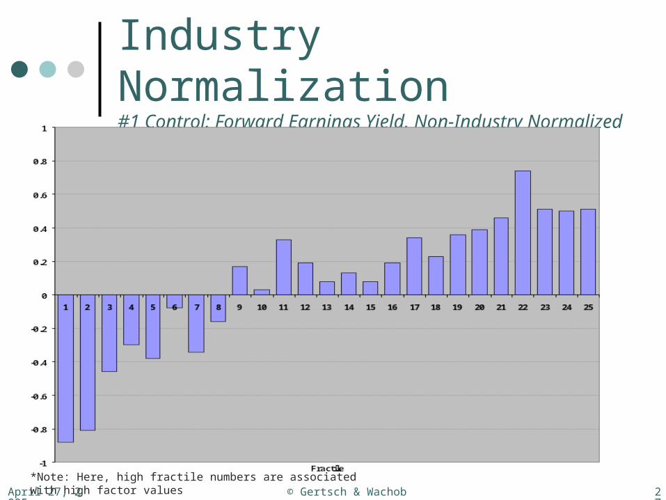
Industry Normalization#1 Control: Forward Earnings Yield, Non-Industry Normalized
*Note: Here, high fractile numbers are associated with high factor values

April 27, 2005 © Gertsch & Wachob 28
Industry Normalization#2 Forward Earnings Yield, Industry Normalized
*Note: Here, high fractile numbers are associated with high factor values

April 27, 2005 © Gertsch & Wachob 29
Industry Normalization
Fractile alphas look very similar between industry-normalized forward earnings yield and non-industry normalized forward earnings yield
Next investigation: Does a secondary sequential sort on industry-normalized forward earnings yield within standard FEY quintiles add any informational benefit over merely sorting again (with finer fractile resolution) on standard FEY?

April 27, 2005 © Gertsch & Wachob 30
Industry NormalizationCombining intra-industry signals with meta-signal
F1
F2
F3
F4
F5
Industry Normalized
Sub-Fractiles
F1F2F3F4F5F1F2F3F4F5
F1F2F3F4F5
F1F2F3F4F5
F1F2F3F4F5
Universal Standard Factor Fractiles
F1
…
F25
25 Fractiles Derived from
Sequential Sorting
April 27, 2005 © Gertsch & Wachob 31
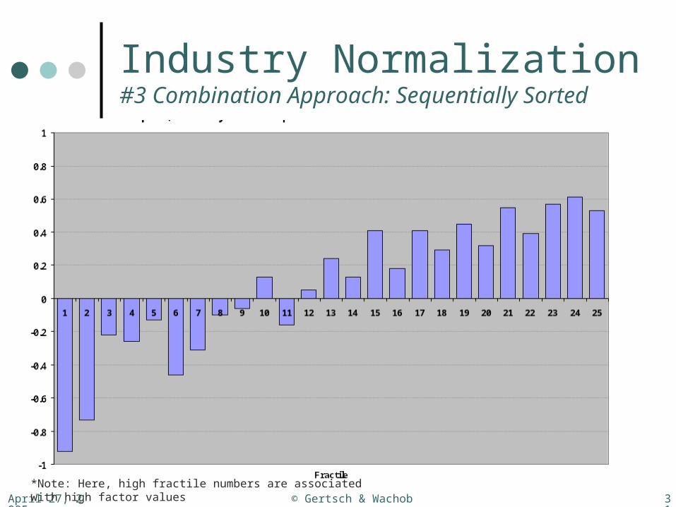
Industry Normalization#3 Combination Approach: Sequentially Sorted
*Note: Here, high fractile numbers are associated with high factor values
April 27, 2005 © Gertsch & Wachob 32
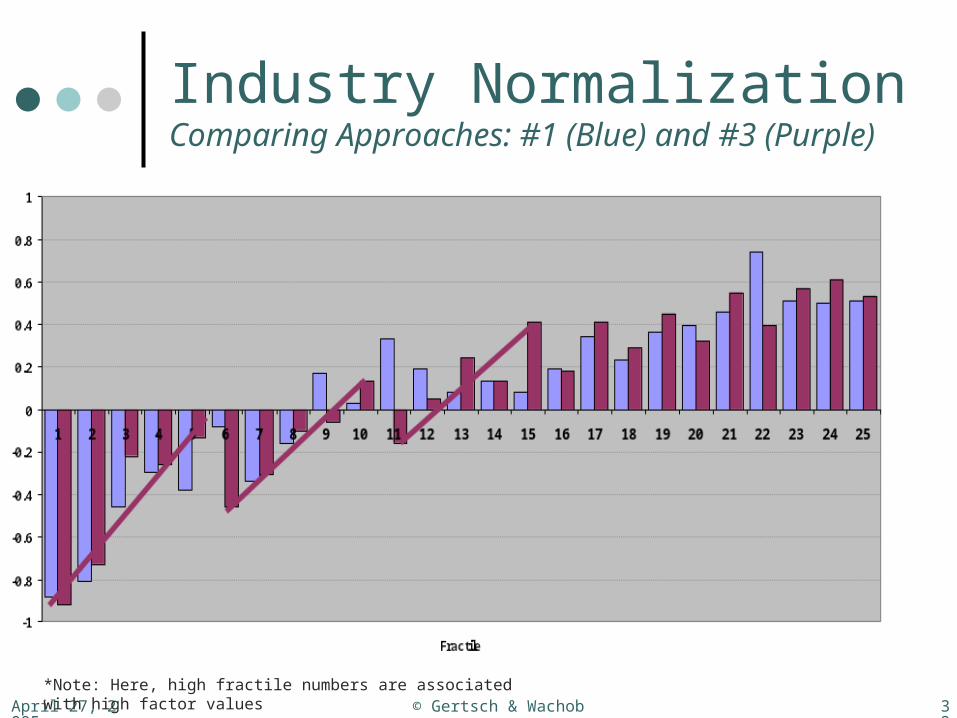
Industry NormalizationComparing Approaches: #1 (Blue) and #3 (Purple)
*Note: Here, high fractile numbers are associated with high factor values

April 27, 2005 © Gertsch & Wachob 33
Industry Normalization
ConclusionThe steeper intra-quintile alpha slopes in the
sequentially sorted plot indicate that intra-industry normalization does add informational benefit– at least in the lower FEY quintiles.

April 27, 2005 © Gertsch & Wachob 34
Industry NormalizationNext Steps in a Future Analysis
At this point, we cut off our investigation of industry normalization, but we believe that further study would reveal substantial opportunities to improve our overall model.
Areas of Future Study Further study and experimentation with industry groupings– seeking optimal
partitioning strategy for a given universe Examine impact of industry normalization for all factors (not just FEY as
studied here) For any factor, identify the industries in which the factor works well– only
model that factor in those industries. Explore other ways to combine inter-industry and intra-industry signals
• Perhaps isolate industry-to-market signal and consider separately from firm-to-industry signal
Integrate industry-normalized signals into final comprehensive stock selection model

April 27, 2005 © Gertsch & Wachob 35
Univariate Factor Diagnostics
We sought to identify factors that distinguished most dramatically between high and low alpha stocks.
Among the many factors that we studied, we present only those for which the strongest apparent signals were observed along with the lowest inter-factor correlations between factor returns.
Aggregated factor portfolios are defined that group multiple fractiles (25-tiles) together based on similarity in alphas across adjacent 25-tiles. We have defined between 3 and 6 aggregated factor portfolios for
each significant factor. Returns series from these aggregated factor portfolios will be
input to a portfolio optimization algorithm to determine desired weightings in an integrated multivariate stock selection model.

April 27, 2005 © Gertsch & Wachob 36
Forward Earnings Yield (FEY)Selected Definition and FactSet Code Excerpt
I/B/E/S weighted median analyst EPS forecast for next twelve months (div. by price) If NA, revert to I/B/E/S unweighted median analyst
EPS forecast for next twelve months (div. by price) If both are NA, revert to “G_” I/B/E/S median analyst
forecast for the current fiscal year (div. by price)
Selected FactSet codeAVAIL(IH_MED_EPS_NTMA(0), IH_MEDIAN_NTM(0), G_IBES_FY1_MED_USD(0))/MP(0)
Note that we experimented with many definitions of forward earnings yield. Refer to previous slides for further commentary.
April 27, 2005 © Gertsch & Wachob 37
Forward Earnings Yield (FEY)Alpha (vs. S&P500), Monthly % -- FEY
-1.20
-1.00
-0.80
-0.60
-0.40
-0.20
0.00
0.20
0.40
0.60
0.80
-1- -2- -3- -4- -5- -6- -7- -8- -9- -10- -11- -12- -13- -14- -15- -16- -17- -18- -19- -20- -21- -22- -23- -24- -25-
Fractile
Monthly Return, % -- FEY Univariate Factor Performance
0.00
0.20
0.40
0.60
0.80
1.00
1.20
1.40
1.60
-1- -2- -3- -4- -5- -6- -7- -8- -9- -10- -11- -12- -13- -14- -15- -16- -17- -18- -19- -20- -21- -22- -23- -24- -25-Fractile
Beta, on Market (S&P 500) -- FEY
0.00
0.20
0.40
0.60
0.80
1.00
1.20
1.40
1.60
-1- -2- -3- -4- -5- -6- -7- -8- -9- -10- -11- -12- -13- -14- -15- -16- -17- -18- -19- -20- -21- -22- -23- -24- -25-Fractile
Std. Dev. of Monthly Returns -- FEY
0.00
1.00
2.00
3.00
4.00
5.00
6.00
7.00
8.00
9.00
10.00
11.00
-1- -2- -3- -4- -5- -6- -7- -8- -9- -10- -11- -12- -13- -14- -15- -16- -17- -18- -19- -20- -21- -22- -23- -24- -25-Fractile
April 27, 2005 © Gertsch & Wachob 38
Forward Earnings Yield (FEY)Defining Aggregated Factor Portfolios
Alpha (vs. S&P500), Monthly % -- FEY
-1.20
-1.00
-0.80
-0.60
-0.40
-0.20
0.00
0.20
0.40
0.60
0.80
-1- -2- -3- -4- -5- -6- -7- -8- -9- -10- -11- -12- -13- -14- -15- -16- -17- -18- -19- -20- -21- -22- -23- -24- -25-
Fractile
FEY1 FEY2
FEY3 FEY4 FEY5
April 27, 2005 © Gertsch & Wachob 39
Forward Earnings Yield (FEY)Aggregated Factor PortfoliosAlpha (vs. S&P500), Monthly % -- FEY
-1.20
-1.00
-0.80
-0.60
-0.40
-0.20
0.00
0.20
0.40
0.60
-1- -2- -3- -4- -5-
Aggregated Factor Portfolio #
Monthly Return, % -- FEY
0.00
0.20
0.40
0.60
0.80
1.00
1.20
1.40
-1- -2- -3- -4- -5-Aggregated Factor Portfolio #
Beta, on Market (S&P 500) -- FEY
0.00
0.20
0.40
0.60
0.80
1.00
1.20
1.40
1.60
-1- -2- -3- -4- -5-
Aggregated Factor Portfolio #
Std. Dev. of Monthly Returns -- FEY
0.00
1.00
2.00
3.00
4.00
5.00
6.00
7.00
8.00
9.00
10.00
11.00
-1- -2- -3- -4- -5-Aggregated Factor Portfolio #

April 27, 2005 © Gertsch & Wachob 40
Forward Earnings Yield (FEY)Year-By-Year Returns in Excess of Benchmark -- FEY
-60%
-40%
-20%
0%
20%
40%
60%
80%
100%
120%
1988 1989 1990 1991 1992 1993 1994 1995 1996 1997 1998 1999 2000 2001
Co
mp
ute
d b
y M
ult
iplic
ativ
ely
Ag
gre
gat
ing
Mo
nth
ly R
etu
rns
Ove
r 12
-Mo
. W
ind
ow
s
FEY1
FEY2
FEY3
FEY4
FEY5

April 27, 2005 © Gertsch & Wachob 41
Forward Earnings Yield (FEY)Fractile Returns, Trailing 12 Mos. -- FEY
-75%
-50%
-25%
0%
25%
50%
75%
100%
125%
150%
175%
200%
225%
1/31/1
988
1/31/1
989
1/31/1
990
1/31/1
991
1/31/1
992
1/31/1
993
1/31/1
994
1/31/1
995
1/31/1
996
1/31/1
997
1/31/1
998
1/31/1
999
1/31/2
000
1/31/2
001
Com
pute
d by
Mul
tiplic
ativ
ely
Agg
rega
ting
Mon
thly
Ret
urns
Ove
r a T
raili
ng 1
2-M
o. W
indo
w F1-Bmark
F2-Bmark
F3-Bmark
F4-Bmark
F5-Bmark
F1-F5
Portfolios F1 through F5 are portfolios FEY1 through FEY5

April 27, 2005 © Gertsch & Wachob 42
Forward Earnings Yield (FEY)FEY -- Time Series, Cumulative Performance
-0.6
0
0.6
1.2
1.8
2.4
3
3.6
1/31
/198
7
1/31
/198
8
1/31
/198
9
1/31
/199
0
1/31
/199
1
1/31
/199
2
1/31
/199
3
1/31
/199
4
1/31
/199
5
1/31
/199
6
1/31
/199
7
1/31
/199
8
1/31
/199
9
1/31
/200
0
1/31
/200
1
log
2 C
um
Ret
urn
FEY1FEY2FEY3FEY4FEY5Bmark
April 27, 2005 © Gertsch & Wachob 43
Momentum (MOM)Selected Definition and FactSet Code Excerpt
% Return over the 12-month period leading up to the previous month (i.e. months -13 through -2)
Selected FactSet code(CM_P(-1)-CM_P(-13))/CM_P(-13)
Note that there are many other ways to quantify “momentum” For example, 6-month or 20-month trailing returns There are many other ways (besides simple trailing returns) to
measure price trends or other relevant price patterns (generally considered to fall within the realm of “technical analysis”)

April 27, 2005 © Gertsch & Wachob 44
Momentum (MOM)Alpha (vs. S&P500), Monthly % -- MOM
-1.20
-1.00
-0.80
-0.60
-0.40
-0.20
0.00
0.20
0.40
0.60
-1- -2- -3- -4- -5- -6- -7- -8- -9- -10- -11- -12- -13- -14- -15- -16- -17- -18- -19- -20- -21- -22- -23- -24- -25-
Fractile
Monthly Return, % -- MOM
-0.20
0.00
0.20
0.40
0.60
0.80
1.00
1.20
1.40
1.60
-1- -2- -3- -4- -5- -6- -7- -8- -9- -10- -11- -12- -13- -14- -15- -16- -17- -18- -19- -20- -21- -22- -23- -24- -25-
Fractile
Beta, on Market (S&P 500) -- MOM
0.00
0.10
0.20
0.30
0.40
0.50
0.60
0.70
0.80
0.90
1.00
1.10
1.20
1.30
1.40
1.50
-1- -2- -3- -4- -5- -6- -7- -8- -9- -10- -11- -12- -13- -14- -15- -16- -17- -18- -19- -20- -21- -22- -23- -24- -25-Fractile
Std. Dev. of Monthly Returns -- MOM
0.00
1.00
2.00
3.00
4.00
5.00
6.00
7.00
8.00
9.00
10.00
11.00
-1- -2- -3- -4- -5- -6- -7- -8- -9- -10- -11- -12- -13- -14- -15- -16- -17- -18- -19- -20- -21- -22- -23- -24- -25-Fractile

April 27, 2005 © Gertsch & Wachob 45
Alpha (vs. S&P500), Monthly % -- MOM
-1.20
-1.00
-0.80
-0.60
-0.40
-0.20
0.00
0.20
0.40
0.60
-1- -2- -3- -4- -5- -6- -7- -8- -9- -10- -11- -12- -13- -14- -15- -16- -17- -18- -19- -20- -21- -22- -23- -24- -25-
Fractile
Momentum (MOM)Defining Aggregated Factor Portfolios
MOM1 MOM2
MOM3 MOM4 MOM5

April 27, 2005 © Gertsch & Wachob 46
Momentum (MOM) Aggregated Factor PortfoliosAlpha (vs. S&P500), Monthly % -- MOM
-1.20
-1.00
-0.80
-0.60
-0.40
-0.20
0.00
0.20
0.40
0.60
-1- -2- -3- -4- -5-
Aggregated Factor Portfolio #
Monthly Return, % -- MOM
-0.20
0.00
0.20
0.40
0.60
0.80
1.00
1.20
1.40
1.60
-1- -2- -3- -4- -5-
Aggregated Factor Portfolio #
Beta, on Market (S&P 500) -- MOM
0.00
0.20
0.40
0.60
0.80
1.00
1.20
1.40
-1- -2- -3- -4- -5-
Aggregated Factor Portfolio #
Std. Dev. of Monthly Returns -- MOM
0.00
1.00
2.00
3.00
4.00
5.00
6.00
7.00
8.00
9.00
10.00
-1- -2- -3- -4- -5-Aggregated Factor Portfolio #
April 27, 2005 © Gertsch & Wachob 47
Momentum (MOM)Year-By-Year Returns in Excess of Benchmark -- MOM
-50%
-40%
-30%
-20%
-10%
0%
10%
20%
30%
40%
50%
60%
70%
1988 1989 1990 1991 1992 1993 1994 1995 1996 1997 1998 1999 2000 2001
Co
mp
ute
d b
y M
ult
iplic
ativ
ely
Ag
gre
gat
ing
Mo
nth
ly R
etu
rns
Ove
r 12
-Mo
. W
ind
ow
s
MOM1
MOM2
MOM3
MOM4
MOM5

April 27, 2005 © Gertsch & Wachob 48
Momentum (MOM)Fractile Returns, Trailing 12 Mos. -- MOM
-60%
-30%
0%
30%
60%
90%
120%
150%
180%
1/31/1
988
1/31/1
989
1/31/1
990
1/31/1
991
1/31/1
992
1/31/1
993
1/31/1
994
1/31/1
995
1/31/1
996
1/31/1
997
1/31/1
998
1/31/1
999
1/31/2
000
1/31/2
001
Com
pute
d by
Mul
tiplic
ativ
ely
Agg
rega
ting
Mon
thly
Ret
urns
Ove
r a T
raili
ng 1
2-M
o. W
indo
w F1-Bmark
F2-Bmark
F3-Bmark
F4-Bmark
F5-Bmark
F1-F5
Portfolios F1 through F5 are portfolios MOM1 through MOM5

April 27, 2005 © Gertsch & Wachob 49
Momentum (MOM)MOM -- Time Series, Cumulative Performance
-2
-1
0
1
2
3
4
5
6
1/31
/198
7
1/31
/198
8
1/31
/198
9
1/31
/199
0
1/31
/199
1
1/31
/199
2
1/31
/199
3
1/31
/199
4
1/31
/199
5
1/31
/199
6
1/31
/199
7
1/31
/199
8
1/31
/199
9
1/31
/200
0
1/31
/200
1
log
2 C
um
Ret
urn
MOM1MOM2MOM3MOM4MOM5Bmark

April 27, 2005 © Gertsch & Wachob 50
Abnormal Dollar Volume in Biggest 30% of Universe (ADB)Selected Definition
1. Estimate daily dollar volume over each month going 65 months into the past (any stocks without sufficient historical data are excluded from the universe)
2. Exclude the lowest 70% of market caps (among remaining firms) from the universe
3. For each of the past 6 months, compute the arithmetic average of estimated dollar volumes over a trailing 60-month window
4. For each of the past 6 months, compute the log difference in dollar volume relative to the 60-month trailing average
5. Sum these log differences of the past 6 months
• Note that we examined many definitions for this metric along with measures of abnormal turnover– we believe there may be more signal available to be harnessed with regard to a stock’s variation in trading volume.
April 27, 2005 © Gertsch & Wachob 51
Abnormal Dollar Volume in Biggest 30% of Universe (ADB)FactSet Code Excerpt
7. CM_VOL(0)/(VALUE(GM,OFDB(CLIENT:FIA,TRADING_DAYS,0)))*((CM_PH(0)+CM_PL(0))/2)8. CM_VOL(-1)/(VALUE(GM,OFDB(CLIENT:FIA,TRADING_DAYS,-1)))*((CM_PH(-1)+CM_PL(-1))/2)9. CM_VOL(-2)/(VALUE(GM,OFDB(CLIENT:FIA,TRADING_DAYS,-2)))*((CM_PH(-2)+CM_PL(-2))/2)10. CM_VOL(-3)/(VALUE(GM,OFDB(CLIENT:FIA,TRADING_DAYS,-3)))*((CM_PH(-3)+CM_PL(-3))/2)11. CM_VOL(-4)/(VALUE(GM,OFDB(CLIENT:FIA,TRADING_DAYS,-4)))*((CM_PH(-4)+CM_PL(-4))/2)12. CM_VOL(-5)/(VALUE(GM,OFDB(CLIENT:FIA,TRADING_DAYS,-5)))*((CM_PH(-5)+CM_PL(-5))/2)13. CM_VOL(-6)/(VALUE(GM,OFDB(CLIENT:FIA,TRADING_DAYS,-6)))*((CM_PH(-6)+CM_PL(-6))/2)14. CM_VOL(-7)/(VALUE(GM,OFDB(CLIENT:FIA,TRADING_DAYS,-7)))*((CM_PH(-7)+CM_PL(-7))/2)15. CM_VOL(-8)/(VALUE(GM,OFDB(CLIENT:FIA,TRADING_DAYS,-8)))*((CM_PH(-8)+CM_PL(-8))/2)16. CM_VOL(-9)/(VALUE(GM,OFDB(CLIENT:FIA,TRADING_DAYS,-9)))*((CM_PH(-9)+CM_PL(-9))/2)17. CM_VOL(-10)/(VALUE(GM,OFDB(CLIENT:FIA,TRADING_DAYS,-10)))*((CM_PH(-10)+CM_PL(-10))/2)18. CM_VOL(-11)/(VALUE(GM,OFDB(CLIENT:FIA,TRADING_DAYS,-11)))*((CM_PH(-11)+CM_PL(-11))/2)19. CM_VOL(-12)/(VALUE(GM,OFDB(CLIENT:FIA,TRADING_DAYS,-12)))*((CM_PH(-12)+CM_PL(-12))/2)20. CM_VOL(-13)/(VALUE(GM,OFDB(CLIENT:FIA,TRADING_DAYS,-13)))*((CM_PH(-13)+CM_PL(-13))/2)21. CM_VOL(-14)/(VALUE(GM,OFDB(CLIENT:FIA,TRADING_DAYS,-14)))*((CM_PH(-14)+CM_PL(-14))/2)22. CM_VOL(-15)/(VALUE(GM,OFDB(CLIENT:FIA,TRADING_DAYS,-15)))*((CM_PH(-15)+CM_PL(-15))/2)23. CM_VOL(-16)/(VALUE(GM,OFDB(CLIENT:FIA,TRADING_DAYS,-16)))*((CM_PH(-16)+CM_PL(-16))/2)24. CM_VOL(-17)/(VALUE(GM,OFDB(CLIENT:FIA,TRADING_DAYS,-17)))*((CM_PH(-17)+CM_PL(-17))/2)25. CM_VOL(-18)/(VALUE(GM,OFDB(CLIENT:FIA,TRADING_DAYS,-18)))*((CM_PH(-18)+CM_PL(-18))/2)26. CM_VOL(-19)/(VALUE(GM,OFDB(CLIENT:FIA,TRADING_DAYS,-19)))*((CM_PH(-19)+CM_PL(-19))/2)27. CM_VOL(-20)/(VALUE(GM,OFDB(CLIENT:FIA,TRADING_DAYS,-20)))*((CM_PH(-20)+CM_PL(-20))/2)28. CM_VOL(-21)/(VALUE(GM,OFDB(CLIENT:FIA,TRADING_DAYS,-21)))*((CM_PH(-21)+CM_PL(-21))/2)29. CM_VOL(-22)/(VALUE(GM,OFDB(CLIENT:FIA,TRADING_DAYS,-22)))*((CM_PH(-22)+CM_PL(-22))/2)30. CM_VOL(-23)/(VALUE(GM,OFDB(CLIENT:FIA,TRADING_DAYS,-23)))*((CM_PH(-23)+CM_PL(-23))/2)31. CM_VOL(-24)/(VALUE(GM,OFDB(CLIENT:FIA,TRADING_DAYS,-24)))*((CM_PH(-24)+CM_PL(-24))/2)32. CM_VOL(-25)/(VALUE(GM,OFDB(CLIENT:FIA,TRADING_DAYS,-25)))*((CM_PH(-25)+CM_PL(-25))/2)33. CM_VOL(-26)/(VALUE(GM,OFDB(CLIENT:FIA,TRADING_DAYS,-26)))*((CM_PH(-26)+CM_PL(-26))/2)34. CM_VOL(-27)/(VALUE(GM,OFDB(CLIENT:FIA,TRADING_DAYS,-27)))*((CM_PH(-27)+CM_PL(-27))/2)35. CM_VOL(-28)/(VALUE(GM,OFDB(CLIENT:FIA,TRADING_DAYS,-28)))*((CM_PH(-28)+CM_PL(-28))/2)36. CM_VOL(-29)/(VALUE(GM,OFDB(CLIENT:FIA,TRADING_DAYS,-29)))*((CM_PH(-29)+CM_PL(-29))/2)37. CM_VOL(-30)/(VALUE(GM,OFDB(CLIENT:FIA,TRADING_DAYS,-30)))*((CM_PH(-30)+CM_PL(-30))/2)38. CM_VOL(-31)/(VALUE(GM,OFDB(CLIENT:FIA,TRADING_DAYS,-31)))*((CM_PH(-31)+CM_PL(-31))/2)39. CM_VOL(-32)/(VALUE(GM,OFDB(CLIENT:FIA,TRADING_DAYS,-32)))*((CM_PH(-32)+CM_PL(-32))/2)40. CM_VOL(-33)/(VALUE(GM,OFDB(CLIENT:FIA,TRADING_DAYS,-33)))*((CM_PH(-33)+CM_PL(-33))/2)41. CM_VOL(-34)/(VALUE(GM,OFDB(CLIENT:FIA,TRADING_DAYS,-34)))*((CM_PH(-34)+CM_PL(-34))/2)42. CM_VOL(-35)/(VALUE(GM,OFDB(CLIENT:FIA,TRADING_DAYS,-35)))*((CM_PH(-35)+CM_PL(-35))/2)43. CM_VOL(-36)/(VALUE(GM,OFDB(CLIENT:FIA,TRADING_DAYS,-36)))*((CM_PH(-36)+CM_PL(-36))/2)44. CM_VOL(-37)/(VALUE(GM,OFDB(CLIENT:FIA,TRADING_DAYS,-37)))*((CM_PH(-37)+CM_PL(-37))/2)45. CM_VOL(-38)/(VALUE(GM,OFDB(CLIENT:FIA,TRADING_DAYS,-38)))*((CM_PH(-38)+CM_PL(-38))/2)46. CM_VOL(-39)/(VALUE(GM,OFDB(CLIENT:FIA,TRADING_DAYS,-39)))*((CM_PH(-39)+CM_PL(-39))/2)47. CM_VOL(-40)/(VALUE(GM,OFDB(CLIENT:FIA,TRADING_DAYS,-40)))*((CM_PH(-40)+CM_PL(-40))/2)48. CM_VOL(-41)/(VALUE(GM,OFDB(CLIENT:FIA,TRADING_DAYS,-41)))*((CM_PH(-41)+CM_PL(-41))/2)49. CM_VOL(-42)/(VALUE(GM,OFDB(CLIENT:FIA,TRADING_DAYS,-42)))*((CM_PH(-42)+CM_PL(-42))/2)50. CM_VOL(-43)/(VALUE(GM,OFDB(CLIENT:FIA,TRADING_DAYS,-43)))*((CM_PH(-43)+CM_PL(-43))/2)51. CM_VOL(-44)/(VALUE(GM,OFDB(CLIENT:FIA,TRADING_DAYS,-44)))*((CM_PH(-44)+CM_PL(-44))/2)52. CM_VOL(-45)/(VALUE(GM,OFDB(CLIENT:FIA,TRADING_DAYS,-45)))*((CM_PH(-45)+CM_PL(-45))/2)53. CM_VOL(-46)/(VALUE(GM,OFDB(CLIENT:FIA,TRADING_DAYS,-46)))*((CM_PH(-46)+CM_PL(-46))/2)54. CM_VOL(-47)/(VALUE(GM,OFDB(CLIENT:FIA,TRADING_DAYS,-47)))*((CM_PH(-47)+CM_PL(-47))/2)55. CM_VOL(-48)/(VALUE(GM,OFDB(CLIENT:FIA,TRADING_DAYS,-48)))*((CM_PH(-48)+CM_PL(-48))/2)56. CM_VOL(-49)/(VALUE(GM,OFDB(CLIENT:FIA,TRADING_DAYS,-49)))*((CM_PH(-49)+CM_PL(-49))/2)57. CM_VOL(-50)/(VALUE(GM,OFDB(CLIENT:FIA,TRADING_DAYS,-50)))*((CM_PH(-50)+CM_PL(-50))/2)58. CM_VOL(-51)/(VALUE(GM,OFDB(CLIENT:FIA,TRADING_DAYS,-51)))*((CM_PH(-51)+CM_PL(-51))/2)59. CM_VOL(-52)/(VALUE(GM,OFDB(CLIENT:FIA,TRADING_DAYS,-52)))*((CM_PH(-52)+CM_PL(-52))/2)
60. CM_VOL(-53)/(VALUE(GM,OFDB(CLIENT:FIA,TRADING_DAYS,-53)))*((CM_PH(-53)+CM_PL(-53))/2)61. CM_VOL(-54)/(VALUE(GM,OFDB(CLIENT:FIA,TRADING_DAYS,-54)))*((CM_PH(-54)+CM_PL(-54))/2)62. CM_VOL(-55)/(VALUE(GM,OFDB(CLIENT:FIA,TRADING_DAYS,-55)))*((CM_PH(-55)+CM_PL(-55))/2)63. CM_VOL(-56)/(VALUE(GM,OFDB(CLIENT:FIA,TRADING_DAYS,-56)))*((CM_PH(-56)+CM_PL(-56))/2)64. CM_VOL(-57)/(VALUE(GM,OFDB(CLIENT:FIA,TRADING_DAYS,-57)))*((CM_PH(-57)+CM_PL(-57))/2)65. CM_VOL(-58)/(VALUE(GM,OFDB(CLIENT:FIA,TRADING_DAYS,-58)))*((CM_PH(-58)+CM_PL(-58))/2)66. CM_VOL(-59)/(VALUE(GM,OFDB(CLIENT:FIA,TRADING_DAYS,-59)))*((CM_PH(-59)+CM_PL(-59))/2)67. CM_VOL(-60)/(VALUE(GM,OFDB(CLIENT:FIA,TRADING_DAYS,-60)))*((CM_PH(-60)+CM_PL(-60))/2)68. CM_VOL(-61)/(VALUE(GM,OFDB(CLIENT:FIA,TRADING_DAYS,-61)))*((CM_PH(-61)+CM_PL(-61))/2)69. CM_VOL(-62)/(VALUE(GM,OFDB(CLIENT:FIA,TRADING_DAYS,-62)))*((CM_PH(-62)+CM_PL(-62))/2)70. CM_VOL(-63)/(VALUE(GM,OFDB(CLIENT:FIA,TRADING_DAYS,-63)))*((CM_PH(-63)+CM_PL(-63))/2)71. CM_VOL(-64)/(VALUE(GM,OFDB(CLIENT:FIA,TRADING_DAYS,-64)))*((CM_PH(-64)+CM_PL(-64))/2)72. CM_VOL(-65)/(VALUE(GM,OFDB(CLIENT:FIA,TRADING_DAYS,-65)))*((CM_PH(-65)+CM_PL(-65))/2)73.(ROW8+ROW9+ROW10+ROW11+ROW12+ROW13+ROW14+ROW15+ROW16+ROW17+ROW18+ROW19+ROW20+ROW21+ROW22+ROW23+ROW24+ROW25+ROW26+ROW27+ROW28+ROW29+ROW30+ROW31+ROW32+ROW33+ROW34+ROW35+ROW36+ROW37+ROW38+ROW39+ROW40+ROW41+ROW42+ROW43+ROW44+ROW45+ROW46+ROW47+ROW48+ROW49+ROW50+ROW51+ROW52+ROW53+ROW54+ROW55+ROW56+ROW57+ROW58+ROW59+ROW60+ROW61+ROW62+ROW63+ROW64+ROW65+ROW66+ROW67)/60 /* ARITH AVG60 TO -1 */74.(ROW9+ROW10+ROW11+ROW12+ROW13+ROW14+ROW15+ROW16+ROW17+ROW18+ROW19+ROW20+ROW21+ROW22+ROW23+ROW24+ROW25+ROW26+ROW27+ROW28+ROW29+ROW30+ROW31+ROW32+ROW33+ROW34+ROW35+ROW36+ROW37+ROW38+ROW39+ROW40+ROW41+ROW42+ROW43+ROW44+ROW45+ROW46+ROW47+ROW48+ROW49+ROW50+ROW51+ROW52+ROW53+ROW54+ROW55+ROW56+ROW57+ROW58+ROW59+ROW60+ROW61+ROW62+ROW63+ROW64+ROW65+ROW66+ROW67+ROW68)/60 /* ARITH AVG60 TO -2 */75.(ROW10+ROW11+ROW12+ROW13+ROW14+ROW15+ROW16+ROW17+ROW18+ROW19+ROW20+ROW21+ROW22+ROW23+ROW24+ROW25+ROW26+ROW27+ROW28+ROW29+ROW30+ROW31+ROW32+ROW33+ROW34+ROW35+ROW36+ROW37+ROW38+ROW39+ROW40+ROW41+ROW42+ROW43+ROW44+ROW45+ROW46+ROW47+ROW48+ROW49+ROW50+ROW51+ROW52+ROW53+ROW54+ROW55+ROW56+ROW57+ROW58+ROW59+ROW60+ROW61+ROW62+ROW63+ROW64+ROW65+ROW66+ROW67+ROW68+ROW69)/60 /* ARITH AVG60 TO -3 */76.(ROW11+ROW12+ROW13+ROW14+ROW15+ROW16+ROW17+ROW18+ROW19+ROW20+ROW21+ROW22+ROW23+ROW24+ROW25+ROW26+ROW27+ROW28+ROW29+ROW30+ROW31+ROW32+ROW33+ROW34+ROW35+ROW36+ROW37+ROW38+ROW39+ROW40+ROW41+ROW42+ROW43+ROW44+ROW45+ROW46+ROW47+ROW48+ROW49+ROW50+ROW51+ROW52+ROW53+ROW54+ROW55+ROW56+ROW57+ROW58+ROW59+ROW60+ROW61+ROW62+ROW63+ROW64+ROW65+ROW66+ROW67+ROW68+ROW69+ROW70)/60 /* ARITH AVG60 TO -4 */77.(ROW12+ROW13+ROW14+ROW15+ROW16+ROW17+ROW18+ROW19+ROW20+ROW21+ROW22+ROW23+ROW24+ROW25+ROW26+ROW27+ROW28+ROW29+ROW30+ROW31+ROW32+ROW33+ROW34+ROW35+ROW36+ROW37+ROW38+ROW39+ROW40+ROW41+ROW42+ROW43+ROW44+ROW45+ROW46+ROW47+ROW48+ROW49+ROW50+ROW51+ROW52+ROW53+ROW54+ROW55+ROW56+ROW57+ROW58+ROW59+ROW60+ROW61+ROW62+ROW63+ROW64+ROW65+ROW66+ROW67+ROW68+ROW69+ROW70+ROW71)/60 /* ARITH AVG60 TO -5 */78.(ROW13+ROW14+ROW15+ROW16+ROW17+ROW18+ROW19+ROW20+ROW21+ROW22+ROW23+ROW24+ROW25+ROW26+ROW27+ROW28+ROW29+ROW30+ROW31+ROW32+ROW33+ROW34+ROW35+ROW36+ROW37+ROW38+ROW39+ROW40+ROW41+ROW42+ROW43+ROW44+ROW45+ROW46+ROW47+ROW48+ROW49+ROW50+ROW51+ROW52+ROW53+ROW54+ROW55+ROW56+ROW57+ROW58+ROW59+ROW60+ROW61+ROW62+ROW63+ROW64+ROW65+ROW66+ROW67+ROW68+ROW69+ROW70+ROW71+ROW72)/60 /* ARITH AVG60 TO -6 */79. LN(ROW7/ROW73)80. LN(ROW8/ROW74)81. LN(ROW9/ROW75)82. LN(ROW10/ROW76)83. LN(ROW11/ROW77)84. LN(ROW12/ROW78)85. ROW79+ROW80+ROW81+ROW82+ROW83+ROW84 /* SUM6M LNRDDV */
April 27, 2005 © Gertsch & Wachob 52
Abnormal Dollar Volume in Biggest 30% of Universe (ADB)Alpha (vs. S&P500), Monthly % -- ADB
-0.80
-0.60
-0.40
-0.20
0.00
0.20
0.40
0.60
-1- -2- -3- -4- -5- -6- -7- -8- -9- -10- -11- -12- -13- -14- -15- -16- -17- -18- -19- -20- -21- -22- -23- -24- -25-
Fractile
Monthly Return, % -- ADB
0.00
0.10
0.20
0.30
0.40
0.50
0.60
0.70
0.80
0.90
1.00
1.10
1.20
1.30
1.40
1.50
-1- -2- -3- -4- -5- -6- -7- -8- -9- -10- -11- -12- -13- -14- -15- -16- -17- -18- -19- -20- -21- -22- -23- -24- -25-Fractile
Beta, on Market (S&P 500) -- ADB
0.00
0.10
0.20
0.30
0.40
0.50
0.60
0.70
0.80
0.90
1.00
1.10
1.20
1.30
-1- -2- -3- -4- -5- -6- -7- -8- -9- -10- -11- -12- -13- -14- -15- -16- -17- -18- -19- -20- -21- -22- -23- -24- -25-Fractile
Std. Dev. of Monthly Returns -- ADB
0.00
1.00
2.00
3.00
4.00
5.00
6.00
7.00
8.00
9.00
-1- -2- -3- -4- -5- -6- -7- -8- -9- -10- -11- -12- -13- -14- -15- -16- -17- -18- -19- -20- -21- -22- -23- -24- -25-Fractile

April 27, 2005 © Gertsch & Wachob 53
Alpha (vs. S&P500), Monthly % -- ADB
-0.80
-0.60
-0.40
-0.20
0.00
0.20
0.40
0.60
-1- -2- -3- -4- -5- -6- -7- -8- -9- -10- -11- -12- -13- -14- -15- -16- -17- -18- -19- -20- -21- -22- -23- -24- -25-
Fractile
Abn. $Vol. in Big 30% (ADB)Defining Aggregated Factor Portfolios
ADB1
ADB5ADB2
ADB3ADB4
April 27, 2005 © Gertsch & Wachob 54
Abnormal Dollar Volume in Biggest 30% of Universe (ADB)Aggregated Factor PortfoliosAlpha (vs. S&P500), Monthly % -- ADB
-0.50
-0.40
-0.30
-0.20
-0.10
0.00
0.10
0.20
0.30
0.40
0.50
-1- -2- -3- -4- -5-
Aggregated Factor Portfolio #
Monthly Return, % -- ADB
0.00
0.10
0.20
0.30
0.40
0.50
0.60
0.70
0.80
0.90
1.00
1.10
1.20
1.30
-1- -2- -3- -4- -5-Aggregated Factor Portfolio #
Beta, on Market (S&P 500) -- ADB
0.00
0.10
0.20
0.30
0.40
0.50
0.60
0.70
0.80
0.90
1.00
1.10
1.20
-1- -2- -3- -4- -5-
Aggregated Factor Portfolio #
Std. Dev. of Monthly Returns -- ADB
0.00
1.00
2.00
3.00
4.00
5.00
6.00
-1- -2- -3- -4- -5-Aggregated Factor Portfolio #
April 27, 2005 © Gertsch & Wachob 55
Abnormal Dollar Volume in Biggest 30% of Universe (ADB)
Year-By-Year Returns in Excess of Benchmark -- ADB
-30%
-20%
-10%
0%
10%
20%
30%
1988 1989 1990 1991 1992 1993 1994 1995 1996 1997 1998 1999 2000 2001
Co
mp
ute
d b
y M
ult
iplic
ativ
ely
Ag
gre
gat
ing
Mo
nth
ly R
etu
rns
Ove
r 12
-Mo
. W
ind
ow
s
ADB1
ADB2
ADB3
ADB4
ADB5

April 27, 2005 © Gertsch & Wachob 56
Abnormal Dollar Volume in Biggest 30% of Universe (ADB)
Fractile Returns, Trailing 12 Mos. -- ADB
-30%
-20%
-10%
0%
10%
20%
30%
40%
1/31/1
988
1/31/1
989
1/31/1
990
1/31/1
991
1/31/1
992
1/31/1
993
1/31/1
994
1/31/1
995
1/31/1
996
1/31/1
997
1/31/1
998
1/31/1
999
1/31/2
000
1/31/2
001
Com
pute
d by
Mul
tiplic
ativ
ely
Agg
rega
ting
Mon
thly
Ret
urns
Ove
r a T
raili
ng 1
2-M
o. W
indo
w
F1-Bmark
F2-Bmark
F3-Bmark
F4-Bmark
F5-Bmark
Portfolios F1 through F5 are portfolios ADB1 through ADB5
April 27, 2005 © Gertsch & Wachob 57
Abnormal Dollar Volume in Biggest 30% of Universe (ADB)
ADB -- Time Series, Cumulative Performance
-0.4
0
0.4
0.8
1.2
1.6
2
2.4
2.8
3.2
1/31
/198
7
1/31
/198
8
1/31
/198
9
1/31
/199
0
1/31
/199
1
1/31
/199
2
1/31
/199
3
1/31
/199
4
1/31
/199
5
1/31
/199
6
1/31
/199
7
1/31
/199
8
1/31
/199
9
1/31
/200
0
1/31
/200
1
log
2 C
um
Ret
urn
ADB1ADB2ADB3ADB4ADB5Bmark
April 27, 2005 © Gertsch & Wachob 58
Abnormal Dollar Volume in Biggest 30% of Universe (ADB) Upon Further Review
Note that most (and perhaps all) of this factor’s signal (performance) is derived from the turbulent market periods of 1987, 2000, and 2001
Further analysis is warranted with regard to the implications of this factor’s varied (inconsistent) performance through time

April 27, 2005 © Gertsch & Wachob 59
Abnormal Dollar Volume in Next Biggest (Mid) 20% of Universe (ADM) Selected Definition
We used the same definition for this mid-market-cap sub-universe as for our large-cap subset.
Close examination of factor performance revealed that abnormal dollar volume carried the most signal in a large-cap sub-universe, a weaker signal in a mid-cap sub-universe, and little to no signal in a small-cap sub-universe. Thus, in our final analysis, we do not give any
consideration to this factor for small-cap stocks.
April 27, 2005 © Gertsch & Wachob 60
Abnormal Dollar Volume in Next Biggest (Mid) 20% of Universe (ADM)
Alpha (vs. S&P500), Monthly % -- ADM
-0.15
-0.10
-0.05
0.00
0.05
0.10
0.15
0.20
0.25
0.30
0.35
0.40
0.45
0.50
0.55
0.60
-1- -2- -3- -4- -5- -6- -7- -8- -9- -10- -11- -12- -13- -14- -15- -16- -17- -18- -19- -20- -21- -22- -23- -24- -25-
Fractile
Monthly Return, % -- ADM
0.00
0.10
0.20
0.30
0.40
0.50
0.60
0.70
0.80
0.90
1.00
1.10
1.20
1.30
1.40
1.50
-1- -2- -3- -4- -5- -6- -7- -8- -9- -10- -11- -12- -13- -14- -15- -16- -17- -18- -19- -20- -21- -22- -23- -24- -25-Fractile
Beta, on Market (S&P 500) -- ADM
0.00
0.20
0.40
0.60
0.80
1.00
1.20
1.40
-1- -2- -3- -4- -5- -6- -7- -8- -9- -10- -11- -12- -13- -14- -15- -16- -17- -18- -19- -20- -21- -22- -23- -24- -25-Fractile
Std. Dev. of Monthly Returns -- ADM
0.00
1.00
2.00
3.00
4.00
5.00
6.00
7.00
8.00
9.00
10.00
11.00
-1- -2- -3- -4- -5- -6- -7- -8- -9- -10- -11- -12- -13- -14- -15- -16- -17- -18- -19- -20- -21- -22- -23- -24- -25-Fractile
April 27, 2005 © Gertsch & Wachob 61
Abn. $Vol. in “Mid” 20% (ADM)Defining Aggregated Factor Portfolios
Alpha (vs. S&P500), Monthly % -- ADM
-0.15
-0.10
-0.05
0.00
0.05
0.10
0.15
0.20
0.25
0.30
0.35
0.40
0.45
0.50
0.55
0.60
-1- -2- -3- -4- -5- -6- -7- -8- -9- -10- -11- -12- -13- -14- -15- -16- -17- -18- -19- -20- -21- -22- -23- -24- -25-
Fractile
ADM3
ADM2ADM1
April 27, 2005 © Gertsch & Wachob 62
Abnormal Dollar Volume in Next Biggest (Mid) 20% of Universe (ADM) Aggregated Factor Portfolios
Alpha (vs. S&P500), Monthly % -- ADM
0.00
0.05
0.10
0.15
0.20
0.25
-1- -2- -3-Aggregated Factor Portfolio #
Monthly Return, % -- ADM
0.00
0.10
0.20
0.30
0.40
0.50
0.60
0.70
0.80
0.90
1.00
1.10
1.20
-1- -2- -3-Aggregated Factor Portfolio #
Beta, on Market (S&P 500) -- ADM
0.00
0.10
0.20
0.30
0.40
0.50
0.60
0.70
0.80
0.90
1.00
1.10
1.20
-1- -2- -3-
Aggregated Factor Portfolio #
Std. Dev. of Monthly Returns -- ADM
0.00
0.50
1.00
1.50
2.00
2.50
3.00
3.50
4.00
4.50
5.00
5.50
6.00
6.50
7.00
-1- -2- -3-Aggregated Factor Portfolio #

April 27, 2005 © Gertsch & Wachob 63
Abnormal Dollar Volume in Next Biggest (Mid) 20% of Universe (ADM)
Year-By-Year Returns in Excess of Benchmark -- ADM
-32%
-24%
-16%
-8%
0%
8%
16%
24%
32%
40%
1988 1989 1990 1991 1992 1993 1994 1995 1996 1997 1998 1999 2000 2001
Co
mp
ute
d b
y M
ult
iplic
ativ
ely
Ag
gre
ga
tin
g M
on
thly
Ret
urn
s O
ver
12-M
o.
Win
do
ws
ADM1
ADM2
ADM3
April 27, 2005 © Gertsch & Wachob 64
Abnormal Dollar Volume in Next Biggest (Mid) 20% of Universe (ADM)
Fractile Returns, Trailing 12 Mos. -- ADM
-60%
-40%
-20%
0%
20%
40%
60%
1/31/1
988
1/31/1
989
1/31/1
990
1/31/1
991
1/31/1
992
1/31/1
993
1/31/1
994
1/31/1
995
1/31/1
996
1/31/1
997
1/31/1
998
1/31/1
999
1/31/2
000
1/31/2
001
Com
pute
d by
Mul
tiplic
ativ
ely
Agg
rega
ting
Mon
thly
Ret
urns
Ove
r a T
raili
ng 1
2-M
o. W
indo
w ADM1-Bmark
ADM2-Bmark
ADM3-Bmark
ADM1-ADM3
April 27, 2005 © Gertsch & Wachob 65
Abnormal Dollar Volume in Next Biggest (Mid) 20% of Universe (ADM)
ADM -- Time Series, Cumulative Performance
-0.4
0
0.4
0.8
1.2
1.6
2
2.4
2.8
3.2
1/31
/198
7
1/31
/198
8
1/31
/198
9
1/31
/199
0
1/31
/199
1
1/31
/199
2
1/31
/199
3
1/31
/199
4
1/31
/199
5
1/31
/199
6
1/31
/199
7
1/31
/199
8
1/31
/199
9
1/31
/200
0
1/31
/200
1
log
2 C
um
Ret
urn
ADM1
ADM2
ADM3
Bmark

April 27, 2005 © Gertsch & Wachob 66
Abnormal Dollar Volume in Next Biggest (Mid) 20% of Universe (ADM) Upon Further Review
In retrospect, we would discard this factor from our model.
Closer examination of this factor’s performance over time reveals that all of its apparent signal came from its behavior in the very last two years of our sample.
In fact, a directionally opposite signal is observed in the first 12 years of our sample.
More analysis is needed to determine whether there is more signal that can be extracted from patterns in the trading volume of a stock
April 27, 2005 © Gertsch & Wachob 67
Change in Net Accruals, scaled by Assets (CNA) Selected Definition
We used a very loose definition of net accruals: EPS minus CFO per share
We used the most recently reported data for the last twelve months and evaluated net accruals as a fraction of total assets
We also evaluated this metric as of one year earlier and took the difference between the present data and that of one year ago
We tried to take great care in properly handling NAs– more detail can be found in the code on the following slide
We believe that with more research towards a better-refined definition, this factor could be a very powerful predictor of alpha. Disappointingly, our implementation yielded a relatively weak signal.
April 27, 2005 © Gertsch & Wachob 68
Change in Net Accruals, scaled by Assets (CNA) FactSet Code Excerpt
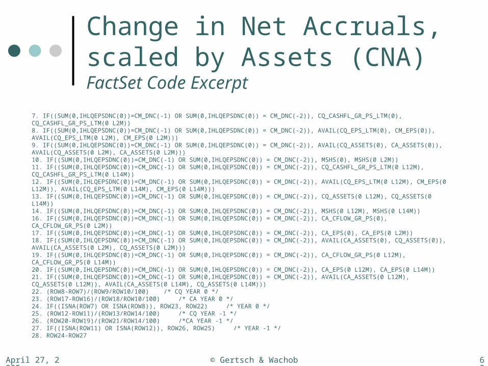
7. IF((SUM(0,IHLQEPSDNC(0))=CM_DNC(-1) OR SUM(0,IHLQEPSDNC(0)) = CM_DNC(-2)), CQ_CASHFL_GR_PS_LTM(0), CQ_CASHFL_GR_PS_LTM(0 L2M))8. IF((SUM(0,IHLQEPSDNC(0))=CM_DNC(-1) OR SUM(0,IHLQEPSDNC(0)) = CM_DNC(-2)), AVAIL(CQ_EPS_LTM(0), CM_EPS(0)), AVAIL(CQ_EPS_LTM(0 L2M), CM_EPS(0 L2M)))9. IF((SUM(0,IHLQEPSDNC(0))=CM_DNC(-1) OR SUM(0,IHLQEPSDNC(0)) = CM_DNC(-2)), AVAIL(CQ_ASSETS(0), CA_ASSETS(0)), AVAIL(CQ_ASSETS(0 L2M), CA_ASSETS(0 L2M)))10. IF((SUM(0,IHLQEPSDNC(0))=CM_DNC(-1) OR SUM(0,IHLQEPSDNC(0)) = CM_DNC(-2)), MSHS(0), MSHS(0 L2M))11. IF((SUM(0,IHLQEPSDNC(0))=CM_DNC(-1) OR SUM(0,IHLQEPSDNC(0)) = CM_DNC(-2)), CQ_CASHFL_GR_PS_LTM(0 L12M), CQ_CASHFL_GR_PS_LTM(0 L14M))12. IF((SUM(0,IHLQEPSDNC(0))=CM_DNC(-1) OR SUM(0,IHLQEPSDNC(0)) = CM_DNC(-2)), AVAIL(CQ_EPS_LTM(0 L12M), CM_EPS(0 L12M)), AVAIL(CQ_EPS_LTM(0 L14M), CM_EPS(0 L14M)))13. IF((SUM(0,IHLQEPSDNC(0))=CM_DNC(-1) OR SUM(0,IHLQEPSDNC(0)) = CM_DNC(-2)), CQ_ASSETS(0 L12M), CQ_ASSETS(0 L14M))14. IF((SUM(0,IHLQEPSDNC(0))=CM_DNC(-1) OR SUM(0,IHLQEPSDNC(0)) = CM_DNC(-2)), MSHS(0 L12M), MSHS(0 L14M))16. IF((SUM(0,IHLQEPSDNC(0))=CM_DNC(-1) OR SUM(0,IHLQEPSDNC(0)) = CM_DNC(-2)), CA_CFLOW_GR_PS(0), CA_CFLOW_GR_PS(0 L2M))17. IF((SUM(0,IHLQEPSDNC(0))=CM_DNC(-1) OR SUM(0,IHLQEPSDNC(0)) = CM_DNC(-2)), CA_EPS(0), CA_EPS(0 L2M))18. IF((SUM(0,IHLQEPSDNC(0))=CM_DNC(-1) OR SUM(0,IHLQEPSDNC(0)) = CM_DNC(-2)), AVAIL(CA_ASSETS(0), CQ_ASSETS(0)), AVAIL(CA_ASSETS(0 L2M), CQ_ASSETS(0 L2M)))19. IF((SUM(0,IHLQEPSDNC(0))=CM_DNC(-1) OR SUM(0,IHLQEPSDNC(0)) = CM_DNC(-2)), CA_CFLOW_GR_PS(0 L12M), CA_CFLOW_GR_PS(0 L14M))20. IF((SUM(0,IHLQEPSDNC(0))=CM_DNC(-1) OR SUM(0,IHLQEPSDNC(0)) = CM_DNC(-2)), CA_EPS(0 L12M), CA_EPS(0 L14M))21. IF((SUM(0,IHLQEPSDNC(0))=CM_DNC(-1) OR SUM(0,IHLQEPSDNC(0)) = CM_DNC(-2)), AVAIL(CA_ASSETS(0 L12M), CQ_ASSETS(0 L12M)), AVAIL(CA_ASSETS(0 L14M), CQ_ASSETS(0 L14M)))22. (ROW8-ROW7)/(ROW9/ROW10/100) /* CQ YEAR 0 */23. (ROW17-ROW16)/(ROW18/ROW10/100) /* CA YEAR 0 */24. IF((ISNA(ROW7) OR ISNA(ROW8)), ROW23, ROW22) /* YEAR 0 */25. (ROW12-ROW11)/(ROW13/ROW14/100) /* CQ YEAR -1 */26. (ROW20-ROW19)/(ROW21/ROW14/100) /*CA YEAR -1 */27. IF((ISNA(ROW11) OR ISNA(ROW12)), ROW26, ROW25) /* YEAR -1 */28. ROW24-ROW27
April 27, 2005 © Gertsch & Wachob 69
Change in Net Accruals, scaled by Assets (CNA)Alpha (vs. S&P500), Monthly % -- CAN
-0.60
-0.50
-0.40
-0.30
-0.20
-0.10
0.00
0.10
0.20
0.30
0.40
-1- -2- -3- -4- -5- -6- -7- -8- -9- -10- -11- -12- -13- -14- -15- -16- -17- -18- -19- -20- -21- -22- -23- -24- -25-
Fractile
Monthly Return, % -- CAN
0.00
0.10
0.20
0.30
0.40
0.50
0.60
0.70
0.80
0.90
1.00
1.10
1.20
1.30
-1- -2- -3- -4- -5- -6- -7- -8- -9- -10- -11- -12- -13- -14- -15- -16- -17- -18- -19- -20- -21- -22- -23- -24- -25-Fractile
Beta, on Market (S&P 500) -- CAN
0.00
0.20
0.40
0.60
0.80
1.00
1.20
1.40
-1- -2- -3- -4- -5- -6- -7- -8- -9- -10- -11- -12- -13- -14- -15- -16- -17- -18- -19- -20- -21- -22- -23- -24- -25-Fractile
Std. Dev. of Monthly Returns -- CAN
0.00
1.00
2.00
3.00
4.00
5.00
6.00
7.00
8.00
9.00
-1- -2- -3- -4- -5- -6- -7- -8- -9- -10- -11- -12- -13- -14- -15- -16- -17- -18- -19- -20- -21- -22- -23- -24- -25-Fractile
CNA CNA
CNACNA

April 27, 2005 © Gertsch & Wachob 70
Alpha (vs. S&P500), Monthly % -- CAN
-0.60
-0.50
-0.40
-0.30
-0.20
-0.10
0.00
0.10
0.20
0.30
0.40
-1- -2- -3- -4- -5- -6- -7- -8- -9- -10- -11- -12- -13- -14- -15- -16- -17- -18- -19- -20- -21- -22- -23- -24- -25-
Fractile
Chg. in Net Accruals (CNA)Defining Aggregated Factor Portfolios
CNA1
CNA3 CNA5CNA4
CNA6
CNA
CNA2
April 27, 2005 © Gertsch & Wachob 71
Change in Net Accruals, scaled by Assets (CNA) Aggregated Factor Portfolios
Alpha (vs. S&P500), Monthly % -- CNA
-0.60
-0.50
-0.40
-0.30
-0.20
-0.10
0.00
0.10
0.20
0.30
0.40
-1- -2- -3- -4- -5- -6-
Aggregated Factor Portfolio #
Monthly Return, % -- CNA
0.00
0.20
0.40
0.60
0.80
1.00
1.20
-1- -2- -3- -4- -5- -6-Aggregated Factor Portfolio #
Beta, on Market (S&P 500) -- CNA
0.00
0.20
0.40
0.60
0.80
1.00
1.20
1.40
-1- -2- -3- -4- -5- -6-
Aggregated Factor Portfolio #
Std. Dev. of Monthly Returns -- CNA
0.00
1.00
2.00
3.00
4.00
5.00
6.00
7.00
8.00
9.00
-1- -2- -3- -4- -5- -6-Aggregated Factor Portfolio #
April 27, 2005 © Gertsch & Wachob 72
Change in Net Accruals, scaled by Assets (CNA)
Year-By-Year Returns in Excess of Benchmark -- CNA
-36%
-24%
-12%
0%
12%
24%
36%
48%
60%
1988 1989 1990 1991 1992 1993 1994 1995 1996 1997 1998 1999 2000 2001
Co
mp
ute
d b
y M
ult
iplic
ativ
ely
Ag
gre
gat
ing
Mo
nth
ly R
etu
rns
Ove
r 12
-Mo
. W
ind
ow
s
CNA1
CNA2
CNA3
CNA4
CNA5
CNA6
April 27, 2005 © Gertsch & Wachob 73
Change in Net Accruals, scaled by Assets (CNA)
Fractile Returns, Trailing 12 Mos. -- CNA
-50%
-25%
0%
25%
50%
75%
100%
125%
150%
175%
1/31/1
988
1/31/1
989
1/31/1
990
1/31/1
991
1/31/1
992
1/31/1
993
1/31/1
994
1/31/1
995
1/31/1
996
1/31/1
997
1/31/1
998
1/31/1
999
1/31/2
000
1/31/2
001
Com
pute
d by
Mul
tiplic
ativ
ely
Agg
rega
ting
Mon
thly
Ret
urns
Ove
r a T
raili
ng 1
2-M
o. W
indo
w
F1-Bmark
F2-Bmark
F3-Bmark
F4-Bmark
F5-Bmark
F6-Bmark
Portfolios F1 through F6 are portfolios CNA1 through CNA6

April 27, 2005 © Gertsch & Wachob 74
Change in Net Accruals, scaled by Assets (CNA)
CNA -- Time Series, Cumulative Performance
-0.6
-0.3
0
0.3
0.6
0.9
1.2
1.5
1.8
2.1
2.4
2.7
3
3.3
1/31
/198
7
1/31
/198
8
1/31
/198
9
1/31
/199
0
1/31
/199
1
1/31
/199
2
1/31
/199
3
1/31
/199
4
1/31
/199
5
1/31
/199
6
1/31
/199
7
1/31
/199
8
1/31
/199
9
1/31
/200
0
1/31
/200
1
log
2 C
um
Ret
urn
CNA1CNA2CNA3CNA4CNA5CNA6Bmark
April 27, 2005 © Gertsch & Wachob 75
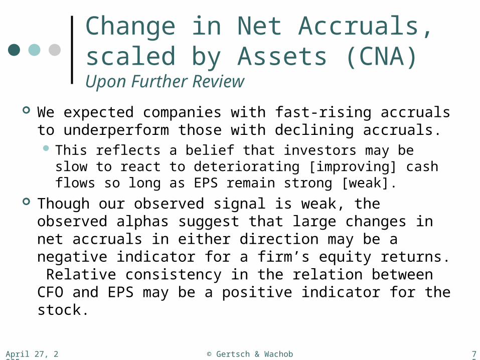
Change in Net Accruals, scaled by Assets (CNA) Upon Further Review
We expected companies with fast-rising accruals to underperform those with declining accruals. This reflects a belief that investors may be slow to
react to deteriorating [improving] cash flows so long as EPS remain strong [weak].
Though our observed signal is weak, the observed alphas suggest that large changes in net accruals in either direction may be a negative indicator for a firm’s equity returns. Relative consistency in the relation between CFO and EPS may be a positive indicator for the stock.
April 27, 2005 © Gertsch & Wachob 76
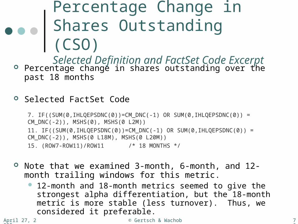
Percentage Change in Shares Outstanding (CSO) Selected Definition and FactSet Code Excerpt
Percentage change in shares outstanding over the past 18 months
Selected FactSet Code
Note that we examined 3-month, 6-month, and 12-month trailing windows for this metric. 12-month and 18-month metrics seemed to give the strongest
alpha differentiation, but the 18-month metric is more stable (less turnover). Thus, we considered it preferable.
7. IF((SUM(0,IHLQEPSDNC(0))=CM_DNC(-1) OR SUM(0,IHLQEPSDNC(0)) = CM_DNC(-2)), MSHS(0), MSHS(0 L2M))
11. IF((SUM(0,IHLQEPSDNC(0))=CM_DNC(-1) OR SUM(0,IHLQEPSDNC(0)) = CM_DNC(-2)), MSHS(0 L18M), MSHS(0 L20M))
15. (ROW7-ROW11)/ROW11 /* 18 MONTHS */

April 27, 2005 © Gertsch & Wachob 77
Percentage Change in Shares Outstanding (CSO)Alpha (vs. S&P500), Monthly % -- CSO
-0.90
-0.80
-0.70
-0.60
-0.50
-0.40
-0.30
-0.20
-0.10
0.00
0.10
0.20
0.30
0.40
0.50
0.60
-1- -2- -3- -4- -5- -6- -7- -8- -9- -10- -11- -12- -13- -14- -15- -16- -17- -18- -19- -20- -21- -22- -23- -24- -25-
Fractile
Monthly Return, % -- CSO
0.00
0.10
0.20
0.30
0.40
0.50
0.60
0.70
0.80
0.90
1.00
1.10
1.20
1.30
1.40
1.50
-1- -2- -3- -4- -5- -6- -7- -8- -9- -10- -11- -12- -13- -14- -15- -16- -17- -18- -19- -20- -21- -22- -23- -24- -25-Fractile
Beta, on Market (S&P 500) -- CSO
0.00
0.10
0.20
0.30
0.40
0.50
0.60
0.70
0.80
0.90
1.00
1.10
1.20
1.30
-1- -2- -3- -4- -5- -6- -7- -8- -9- -10- -11- -12- -13- -14- -15- -16- -17- -18- -19- -20- -21- -22- -23- -24- -25-Fractile
Std. Dev. of Monthly Returns -- CSO
0.00
1.00
2.00
3.00
4.00
5.00
6.00
7.00
-1- -2- -3- -4- -5- -6- -7- -8- -9- -10- -11- -12- -13- -14- -15- -16- -17- -18- -19- -20- -21- -22- -23- -24- -25-Fractile

April 27, 2005 © Gertsch & Wachob 78
Alpha (vs. S&P500), Monthly % -- CSO
-0.90
-0.80
-0.70
-0.60
-0.50
-0.40
-0.30
-0.20
-0.10
0.00
0.10
0.20
0.30
0.40
0.50
0.60
-1- -2- -3- -4- -5- -6- -7- -8- -9- -10- -11- -12- -13- -14- -15- -16- -17- -18- -19- -20- -21- -22- -23- -24- -25-
Fractile
% Chg. in Shs. Outstndg. (CSO)Defining Aggregated Factor Portfolios
CSO1 CSO2
CSO3 CSO4 CSO5

April 27, 2005 © Gertsch & Wachob 79
Percentage Change in Shares Outstanding (CSO) Aggregated Factor PortfoliosAlpha (vs. S&P500), Monthly % -- CSO
-0.90
-0.75
-0.60
-0.45
-0.30
-0.15
0.00
0.15
0.30
0.45
-1- -2- -3- -4- -5-
Aggregated Factor Portfolio #
Monthly Return, % -- CSO
0.00
0.20
0.40
0.60
0.80
1.00
1.20
1.40
-1- -2- -3- -4- -5-Aggregated Factor Portfolio #
Beta, on Market (S&P 500) -- CSO
0.00
0.20
0.40
0.60
0.80
1.00
1.20
-1- -2- -3- -4- -5-
Aggregated Factor Portfolio #
Std. Dev. of Monthly Returns -- CSO
0.00
1.00
2.00
3.00
4.00
5.00
6.00
7.00
-1- -2- -3- -4- -5-Aggregated Factor Portfolio #

April 27, 2005 © Gertsch & Wachob 80
Percentage Change in Shares Outstanding (CSO)
Year-By-Year Returns in Excess of Benchmark -- CSO
-45%
-40%
-35%
-30%
-25%
-20%
-15%
-10%
-5%
0%
5%
10%
15%
20%
25%
30%
35%
1988 1989 1990 1991 1992 1993 1994 1995 1996 1997 1998 1999 2000 2001
Co
mp
ute
d b
y M
ult
iplic
ativ
ely
Ag
gre
gat
ing
Mo
nth
ly R
etu
rns
Ove
r 12
-Mo
. W
ind
ow
s
CSO1
CSO2
CSO3
CSO4
CSO5

April 27, 2005 © Gertsch & Wachob 81
Percentage Change in Shares Outstanding (CSO)
Fractile Returns, Trailing 12 Mos. -- CSO
-80%
-60%
-40%
-20%
0%
20%
40%
60%
80%
1/31/1
988
1/31/1
989
1/31/1
990
1/31/1
991
1/31/1
992
1/31/1
993
1/31/1
994
1/31/1
995
1/31/1
996
1/31/1
997
1/31/1
998
1/31/1
999
1/31/2
000
1/31/2
001
Com
pute
d by
Mul
tiplic
ativ
ely
Agg
rega
ting
Mon
thly
Ret
urns
Ove
r a T
raili
ng 1
2-M
o. W
indo
w F1-Bmark
F2-Bmark
F3-Bmark
F4-Bmark
F5-Bmark
F1-F5
Portfolios F1 through F5 are portfolios CSO1 through CSO5
April 27, 2005 © Gertsch & Wachob 82
Percentage Change in Shares Outstanding (CSO)
CSO -- Time Series, Cumulative Performance
-0.6
0
0.6
1.2
1.8
2.4
3
1/31
/198
7
1/31
/198
8
1/31
/198
9
1/31
/199
0
1/31
/199
1
1/31
/199
2
1/31
/199
3
1/31
/199
4
1/31
/199
5
1/31
/199
6
1/31
/199
7
1/31
/199
8
1/31
/199
9
1/31
/200
0
1/31
/200
1
log
2 C
um
Ret
urn
CSO1CSO2CSO3CSO4CSO5Bmark
April 27, 2005 © Gertsch & Wachob 83
Revision Ratio (RRA) Selected Definition
1. For each of the past three months, subtract the I/B/E/S number of analysts who downwardly revised their EPS forecast from the I/B/E/S number of analysts who upwardly revised their EPS forecast.
2. Calculate the “net revisions over the trailing three months” as the sum of these three numbers.
3. Calculate the number of “forecast-months” as the sum of the three I/B/E/S number of existing analyst forecasts corresponding to each of the past three months.
4. Divide the “net revisions over the trailing three months” by the total number of “forecast-months.”
• We experimented with alternate ways to define this metric, but leave an exhaustive revision ratio factor refinement exercise to future research.

April 27, 2005 © Gertsch & Wachob 84
Revision Ratio (RRA) FactSet Code Excerpt
(SUM(IH_UP_FY1(0),IH_UP_FY1(-1),IH_UP_FY1(-2))
-SUM(IH_DOWN_FY1(0),IH_DOWN_FY1(-1),IH_DOWN_FY1(-2)))
/SUM(IH_NEST_FY1(0),IH_NEST_FY1(-1),IH_NEST_FY1(-2))

April 27, 2005 © Gertsch & Wachob 85
Revision Ratio (RRA)Alpha (vs. S&P500), Monthly % -- RRA
-0.80
-0.60
-0.40
-0.20
0.00
0.20
0.40
0.60
0.80
1.00
-1- -2- -3- -4- -5- -6- -7- -8- -9- -10- -11- -12- -13- -14- -15- -16- -17- -18- -19- -20- -21- -22- -23- -24- -25-
Fractile
Monthly Return, % -- RRA
0.00
0.20
0.40
0.60
0.80
1.00
1.20
1.40
1.60
1.80
2.00
-1- -2- -3- -4- -5- -6- -7- -8- -9- -10- -11- -12- -13- -14- -15- -16- -17- -18- -19- -20- -21- -22- -23- -24- -25-Fractile
Beta, on Market (S&P 500) -- RRA
0.00
0.10
0.20
0.30
0.40
0.50
0.60
0.70
0.80
0.90
1.00
1.10
1.20
1.30
-1- -2- -3- -4- -5- -6- -7- -8- -9- -10- -11- -12- -13- -14- -15- -16- -17- -18- -19- -20- -21- -22- -23- -24- -25-Fractile
Std. Dev. of Monthly Returns -- RRA
0.00
1.00
2.00
3.00
4.00
5.00
6.00
7.00
-1- -2- -3- -4- -5- -6- -7- -8- -9- -10- -11- -12- -13- -14- -15- -16- -17- -18- -19- -20- -21- -22- -23- -24- -25-Fractile

April 27, 2005 © Gertsch & Wachob 86
Alpha (vs. S&P500), Monthly % -- RRA
-0.80
-0.60
-0.40
-0.20
0.00
0.20
0.40
0.60
0.80
1.00
-1- -2- -3- -4- -5- -6- -7- -8- -9- -10- -11- -12- -13- -14- -15- -16- -17- -18- -19- -20- -21- -22- -23- -24- -25-
Fractile
Revision Ratio (RRA)Defining Aggregated Factor Portfolios
RRA1 RRA2 RRA3 RRA4
RRA5 RRA6
April 27, 2005 © Gertsch & Wachob 87
Revision Ratio (RRA) Aggregated Factor PortfoliosAlpha (vs. S&P500), Monthly % -- RRA
-0.80
-0.60
-0.40
-0.20
0.00
0.20
0.40
0.60
0.80
1.00
-1- -2- -3- -4- -5- -6-
Aggregated Factor Portfolio #
Monthly Return, % -- RRA
0.00
0.20
0.40
0.60
0.80
1.00
1.20
1.40
1.60
1.80
2.00
2.20
-1- -2- -3- -4- -5- -6-Aggregated Factor Portfolio #
Beta, on Market (S&P 500) -- RRA
0.00
0.20
0.40
0.60
0.80
1.00
1.20
-1- -2- -3- -4- -5- -6-
Aggregated Factor Portfolio #
Std. Dev. of Monthly Returns -- RRA
0.00
1.00
2.00
3.00
4.00
5.00
6.00
7.00
-1- -2- -3- -4- -5- -6-Aggregated Factor Portfolio #
April 27, 2005 © Gertsch & Wachob 88
Revision Ratio (RRA)Year-By-Year Returns in Excess of Benchmark -- RRA
-50%
-40%
-30%
-20%
-10%
0%
10%
20%
30%
40%
1988 1989 1990 1991 1992 1993 1994 1995 1996 1997 1998 1999 2000 2001
Co
mp
ute
d b
y M
ult
iplic
ativ
ely
Ag
gre
gat
ing
Mo
nth
ly R
etu
rns
Ove
r 12
-Mo
. W
ind
ow
s
RRA1
RRA2
RRA3
RRA4
RRA5
RRA6

April 27, 2005 © Gertsch & Wachob 89
Revision Ratio (RRA)Fractile Returns, Trailing 12 Mos. -- RRA
-60%
-40%
-20%
0%
20%
40%
60%
80%
1/31/1
988
1/31/1
989
1/31/1
990
1/31/1
991
1/31/1
992
1/31/1
993
1/31/1
994
1/31/1
995
1/31/1
996
1/31/1
997
1/31/1
998
1/31/1
999
1/31/2
000
1/31/2
001
Com
pute
d by
Mul
tiplic
ativ
ely
Agg
rega
ting
Mon
thly
Ret
urns
Ove
r a T
raili
ng 1
2-M
o. W
indo
w F1-Bmark
F2-Bmark
F3-Bmark
F4-Bmark
F5-Bmark
F6-Bmark
F1-F6
Portfolios F1 through F6 are portfolios RRA1 through RRA6
April 27, 2005 © Gertsch & Wachob 90
Revision Ratio (RRA)RRA -- Time Series, Cumulative Performance
-1
-0.5
0
0.5
1
1.5
2
2.5
3
3.5
4
4.5
5
5.5
1/31
/198
7
1/31
/198
8
1/31
/198
9
1/31
/199
0
1/31
/199
1
1/31
/199
2
1/31
/199
3
1/31
/199
4
1/31
/199
5
1/31
/199
6
1/31
/199
7
1/31
/199
8
1/31
/199
9
1/31
/200
0
1/31
/200
1
log
2 C
um
Ret
urn
RRA1RRA2RRA3RRA4RRA5RRA6Bmark
April 27, 2005 © Gertsch & Wachob 91
Standardized Unexpected Earnings in Non-Reporting Companies (SUN) Selected Definition
“Standardized Unexpected Earnings” is commonly calculated as the difference between the firm’s most recently (quarterly) reported EPS and the analyst consensus forecast EPS at the time of the report, divided by the standard deviation of the analyst EPS forecasts at the time of the earnings report.
The I/B/E/S database provides a parameter (which we used) that is defined as holding precisely this data set. We audited the historical time-alignment of this data series for a
few companies and found no errors or inconsistencies. Various observations (such as an apparent prevalence of values
equal to precisely 1.0 or -1.0) have led us to question the accuracy/precision of the reported values themselves. We have not yet thoroughly audited this element of the data series, but intend to do so in future research.

April 27, 2005 © Gertsch & Wachob 92
Standardized Unexpected Earnings in Non-Reporting Companies (SUN) Unique Sub-Universe Definition
We divided our universe between companies expected to report quarterly earnings in the coming month and companies not expected to report in the coming month. Accounting research suggests that the SUE
differentiation of stock returns is stronger in the period immediately surrounding a subsequent earnings report.
We did observe an apparent difference in the alphas of firms across these two sub-universes. Surprisingly, the difference ran contrary to our expectations.
• One item that we question is the reliability of our data source for expected reporting dates. Perhaps this affected our results. Further research may be warranted.
April 27, 2005 © Gertsch & Wachob 93
Standardized Unexpected Earnings in Non-Reporting Companies (SUN) FactSet Code Excerpts
Universe LimitationSUM(0,((IHLQEPSDNC(-11)-IHLQEPSDNC(-12))<>0))<>1
ParameterIH_SUE_Q(0)
** Also note that for this parameter, the data history extended back only to 8/31/1989. This limited our in-sample period for SUE.
April 27, 2005 © Gertsch & Wachob 94
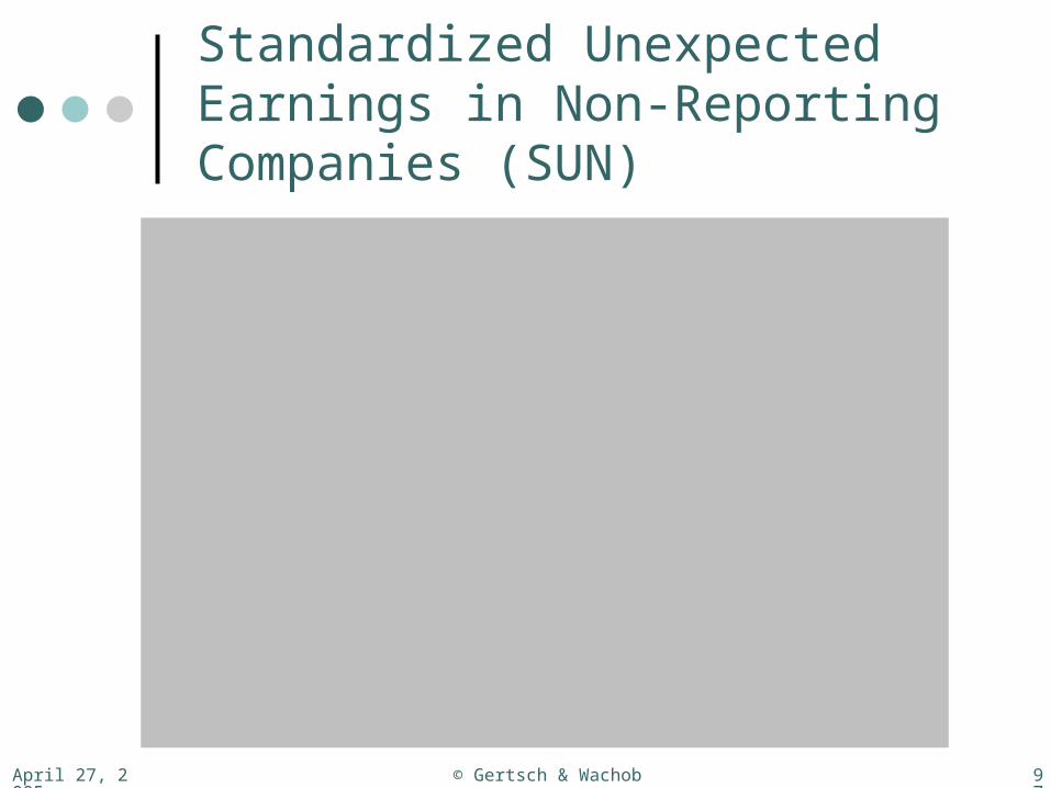
Standardized Unexpected Earnings in Non-Reporting Companies (SUN)Alpha (vs. S&P500), Monthly % -- SUN
-0.80
-0.60
-0.40
-0.20
0.00
0.20
0.40
0.60
0.80
-1- -2- -3- -4- -5- -6- -7- -8- -9- -10- -11- -12- -13- -14- -15- -16- -17- -18- -19- -20- -21- -22- -23- -24- -25-
Fractile
Monthly Return, % -- SUN
0.00
0.20
0.40
0.60
0.80
1.00
1.20
1.40
1.60
1.80
-1- -2- -3- -4- -5- -6- -7- -8- -9- -10- -11- -12- -13- -14- -15- -16- -17- -18- -19- -20- -21- -22- -23- -24- -25-Fractile
Beta, on Market (S&P 500) -- SUN
0.00
0.20
0.40
0.60
0.80
1.00
1.20
1.40
-1- -2- -3- -4- -5- -6- -7- -8- -9- -10- -11- -12- -13- -14- -15- -16- -17- -18- -19- -20- -21- -22- -23- -24- -25-Fractile
Std. Dev. of Monthly Returns -- SUN
0.00
1.00
2.00
3.00
4.00
5.00
6.00
7.00
-1- -2- -3- -4- -5- -6- -7- -8- -9- -10- -11- -12- -13- -14- -15- -16- -17- -18- -19- -20- -21- -22- -23- -24- -25-Fractile

April 27, 2005 © Gertsch & Wachob 95
Alpha (vs. S&P500), Monthly % -- SUN
-0.80
-0.60
-0.40
-0.20
0.00
0.20
0.40
0.60
0.80
-1- -2- -3- -4- -5- -6- -7- -8- -9- -10- -11- -12- -13- -14- -15- -16- -17- -18- -19- -20- -21- -22- -23- -24- -25-
Fractile
SUE in Non-Reporting Cos. (SUN)Defining Aggregated Factor Portfolios
SUN1
SUN2
SUN3
SUN4
April 27, 2005 © Gertsch & Wachob 96
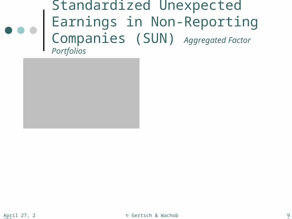
Standardized Unexpected Earnings in Non-Reporting Companies (SUN) Aggregated Factor PortfoliosAlpha (vs. S&P500), Monthly % -- SUN
-0.36
-0.24
-0.12
0.00
0.12
0.24
0.36
0.48
-1- -2- -3- -4-
Aggregated Factor Portfolio #
Monthly Return, % -- SUN
0.00
0.20
0.40
0.60
0.80
1.00
1.20
1.40
1.60
-1- -2- -3- -4-Aggregated Factor Portfolio #
Beta, on Market (S&P 500) -- SUN
0.00
0.20
0.40
0.60
0.80
1.00
1.20
-1- -2- -3- -4-
Aggregated Factor Portfolio #
Std. Dev. of Monthly Returns -- SUN
0.00
0.50
1.00
1.50
2.00
2.50
3.00
3.50
4.00
4.50
5.00
5.50
6.00
6.50
-1- -2- -3- -4-Aggregated Factor Portfolio #
April 27, 2005 © Gertsch & Wachob 97
Standardized Unexpected Earnings in Non-Reporting Companies (SUN)
Year-By-Year Returns in Excess of Benchmark -- SUN
-40%
-30%
-20%
-10%
0%
10%
20%
30%
1990 1991 1992 1993 1994 1995 1996 1997 1998 1999 2000 2001
Co
mp
ute
d b
y M
ult
iplic
ativ
ely
Ag
gre
gat
ing
Mo
nth
ly R
etu
rns
Ove
r 12
-Mo
. W
ind
ow
s
SUN1
SUN2
SUN3
SUN4

April 27, 2005 © Gertsch & Wachob 98
Standardized Unexpected Earnings in Non-Reporting Companies (SUN)
Fractile Returns, Trailing 12 Mos. -- SUN
-40%
-30%
-20%
-10%
0%
10%
20%
30%
40%
50%
60%
8/31/1990 8/31/1991 8/31/1992 8/31/1993 8/31/1994 8/31/1995 8/31/1996 8/31/1997 8/31/1998 8/31/1999 8/31/2000 8/31/2001
Com
pute
d by
Mul
tiplic
ativ
ely
Agg
rega
ting
Mon
thly
Ret
urns
Ove
r a T
raili
ng 1
2-M
o. W
indo
w
F1-Bmark
F2-Bmark
F3-Bmark
F4-Bmark
F1-F4
Portfolios F1 through F4 are portfolios SUN1 through SUN4
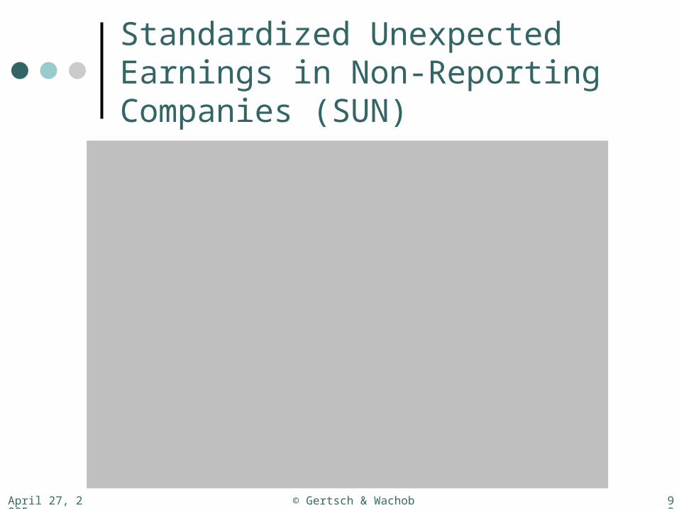
April 27, 2005 © Gertsch & Wachob 99
Standardized Unexpected Earnings in Non-Reporting Companies (SUN)
SUN -- Time Series, Cumulative Performance
-0.6
0
0.6
1.2
1.8
2.4
3
3.6
8/31
/198
9
8/31
/199
0
8/31
/199
1
8/31
/199
2
8/31
/199
3
8/31
/199
4
8/31
/199
5
8/31
/199
6
8/31
/199
7
8/31
/199
8
8/31
/199
9
8/31
/200
0
8/31
/200
1
log
2 C
um
Ret
urn
SUN1
SUN2
SUN3
SUN4
Bmark

April 27, 2005 © Gertsch & Wachob 100
Standardized Unexpected Earnings in Reporting Companies (SUR) Selected Definition and FactSet Code Excerpts
SUE factor definition is as previously described.
The universe is limited by the following FactSet code(IHLQEPSDNC(-11)-IHLQEPSDNC(-12))<>0
ParameterIH_SUE_Q(0)
** Again note that for this parameter, the data history extended back only to 8/31/1989. This limited our in-sample period for SUE.
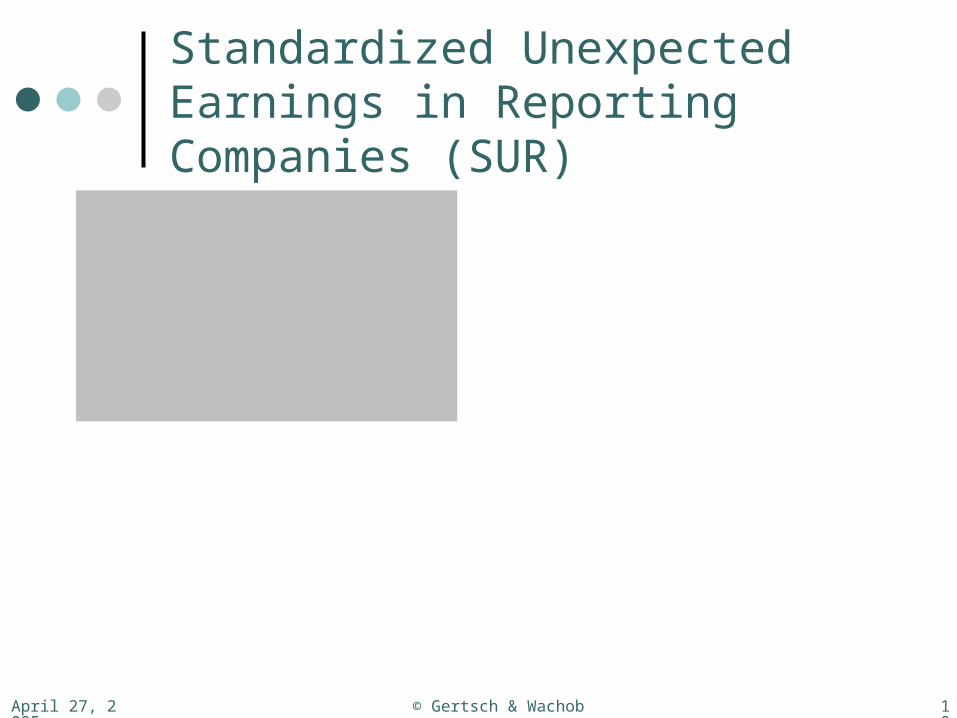
April 27, 2005 © Gertsch & Wachob 101
Standardized Unexpected Earnings in Reporting Companies (SUR)Alpha (vs. S&P500), Monthly % -- SUR
-0.10
0.00
0.10
0.20
0.30
0.40
0.50
0.60
0.70
0.80
0.90
1.00
1.10
1.20
1.30
1.40
1.50
1.60
1.70
-1- -2- -3- -4- -5- -6- -7- -8- -9- -10- -11- -12- -13- -14- -15- -16- -17- -18- -19- -20- -21- -22- -23- -24- -25-
Fractile
Monthly Return, % -- SUR
0.00
0.20
0.40
0.60
0.80
1.00
1.20
1.40
1.60
1.80
2.00
2.20
2.40
2.60
2.80
-1- -2- -3- -4- -5- -6- -7- -8- -9- -10- -11- -12- -13- -14- -15- -16- -17- -18- -19- -20- -21- -22- -23- -24- -25-Fractile
Beta, on Market (S&P 500) -- SUR
0.00
0.20
0.40
0.60
0.80
1.00
1.20
1.40
-1- -2- -3- -4- -5- -6- -7- -8- -9- -10- -11- -12- -13- -14- -15- -16- -17- -18- -19- -20- -21- -22- -23- -24- -25-Fractile
Std. Dev. of Monthly Returns -- SUR
0.00
1.00
2.00
3.00
4.00
5.00
6.00
7.00
8.00
-1- -2- -3- -4- -5- -6- -7- -8- -9- -10- -11- -12- -13- -14- -15- -16- -17- -18- -19- -20- -21- -22- -23- -24- -25-Fractile

April 27, 2005 © Gertsch & Wachob 102
Alpha (vs. S&P500), Monthly % -- SUR
-0.30
-0.15
0.00
0.15
0.30
0.45
0.60
0.75
0.90
1.05
1.20
1.35
1.50
1.65
-1- -2- -3- -4- -5- -6- -7- -8- -9- -10- -11- -12- -13- -14- -15- -16- -17- -18- -19- -20- -21- -22- -23- -24- -25-
Fractile
SUE in Reporting Cos. (SUR)Defining Aggregated Factor Portfolios
SUR1 SUR2 SUR3 SUR4

April 27, 2005 © Gertsch & Wachob 103
Standardized Unexpected Earnings in Reporting Companies (SUR) Aggregated Factor PortfoliosAlpha (vs. S&P500), Monthly % -- SUR
0.00
0.20
0.40
0.60
0.80
1.00
1.20
-1- -2- -3- -4-Aggregated Factor Portfolio #
Monthly Return, % -- SUR
0.00
0.20
0.40
0.60
0.80
1.00
1.20
1.40
1.60
1.80
2.00
2.20
-1- -2- -3- -4-Aggregated Factor Portfolio #
Beta, on Market (S&P 500) -- SUR
0.00
0.10
0.20
0.30
0.40
0.50
0.60
0.70
0.80
0.90
1.00
1.10
1.20
-1- -2- -3- -4-
Aggregated Factor Portfolio #
Std. Dev. of Monthly Returns -- SUR
0.00
1.00
2.00
3.00
4.00
5.00
6.00
7.00
8.00
-1- -2- -3- -4-Aggregated Factor Portfolio #

April 27, 2005 © Gertsch & Wachob 104
Standardized Unexpected Earnings in Reporting Companies (SUR)
Year-By-Year Returns in Excess of Benchmark -- SUR
-30%
-20%
-10%
0%
10%
20%
30%
40%
50%
1990 1991 1992 1993 1994 1995 1996 1997 1998 1999 2000 2001
Co
mp
ute
d b
y M
ult
iplic
ativ
ely
Ag
gre
gat
ing
Mo
nth
ly R
etu
rns
Ove
r 12
-Mo
. W
ind
ow
s
SUR1
SUR2
SUR3
SUR4
April 27, 2005 © Gertsch & Wachob 105
Standardized Unexpected Earnings in Reporting Companies (SUR)
Fractile Returns, Trailing 12 Mos. -- SUR
-35%
-30%
-25%
-20%
-15%
-10%
-5%
0%
5%
10%
15%
20%
25%
30%
35%
40%
45%
50%
55%
60%
65%
70%
75%
8/31/1990 8/31/1991 8/31/1992 8/31/1993 8/31/1994 8/31/1995 8/31/1996 8/31/1997 8/31/1998 8/31/1999 8/31/2000 8/31/2001
Com
pute
d by
Mul
tiplic
ativ
ely
Agg
rega
ting
Mon
thly
Ret
urns
Ove
r a T
raili
ng 1
2-M
o. W
indo
w SUR1-Bmark
SUR2-Bmark
SUR3-Bmark
SUR4-Bmark

April 27, 2005 © Gertsch & Wachob 106
Standardized Unexpected Earnings in Reporting Companies (SUR)
SUR -- Time Series, Cumulative Performance
-1
-0.5
0
0.5
1
1.5
2
2.5
3
3.5
4
8/31
/198
9
8/31
/199
0
8/31
/199
1
8/31
/199
2
8/31
/199
3
8/31
/199
4
8/31
/199
5
8/31
/199
6
8/31
/199
7
8/31
/199
8
8/31
/199
9
8/31
/200
0
8/31
/200
1
log
2 C
um
Ret
urn
SUR1
SUR2
SUR3
SUR4
Bmark
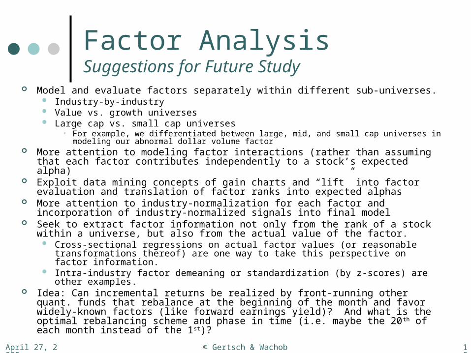
April 27, 2005 © Gertsch & Wachob 107
Factor AnalysisSuggestions for Future Study
Model and evaluate factors separately within different sub-universes. Industry-by-industry Value vs. growth universes Large cap vs. small cap universes
• For example, we differentiated between large, mid, and small cap universes in modeling our abnormal dollar volume factor
More attention to modeling factor interactions (rather than assuming that each factor contributes independently to a stock’s expected alpha)
Exploit data mining concepts of gain charts and “lift” into factor evaluation and translation of factor ranks into expected alphas
More attention to industry-normalization for each factor and incorporation of industry-normalized signals into final model
Seek to extract factor information not only from the rank of a stock within a universe, but also from the actual value of the factor.
Cross-sectional regressions on actual factor values (or reasonable transformations thereof) are one way to take this perspective on factor information.
Intra-industry factor demeaning or standardization (by z-scores) are other examples.
Idea: Can incremental returns be realized by front-running other quant. funds that rebalance at the beginning of the month and favor widely-known factors (like forward earnings yield)? And what is the optimal rebalancing scheme and phase in time (i.e. maybe the 20th of each month instead of the 1st)?
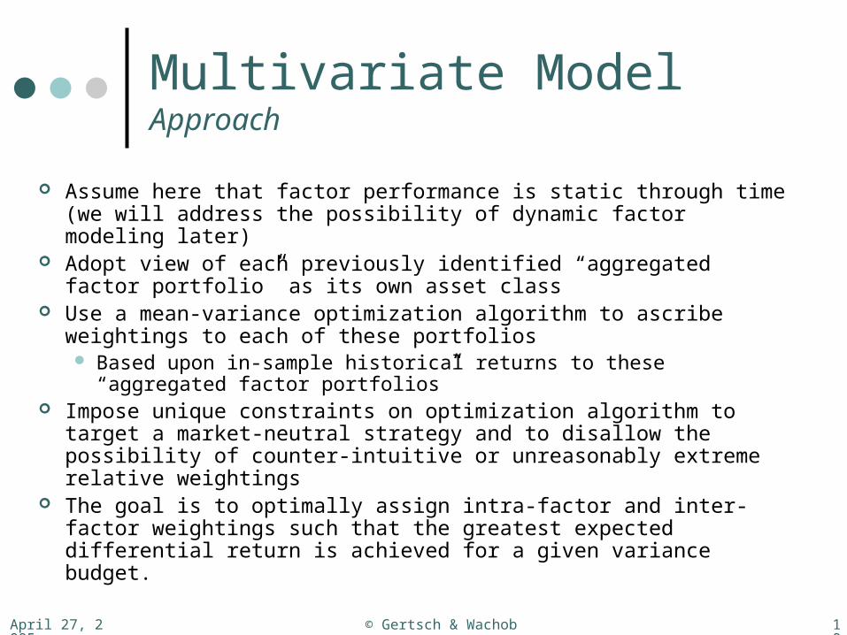
April 27, 2005 © Gertsch & Wachob 108
Multivariate ModelApproach
Assume here that factor performance is static through time (we will address the possibility of dynamic factor modeling later)
Adopt view of each previously identified “aggregated factor portfolio” as its own asset class
Use a mean-variance optimization algorithm to ascribe weightings to each of these portfolios Based upon in-sample historical returns to these “aggregated
factor portfolios” Impose unique constraints on optimization algorithm to target a
market-neutral strategy and to disallow the possibility of counter-intuitive or unreasonably extreme relative weightings
The goal is to optimally assign intra-factor and inter-factor weightings such that the greatest expected differential return is achieved for a given variance budget.
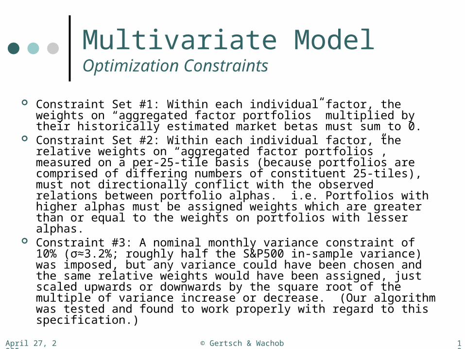
April 27, 2005 © Gertsch & Wachob 109
Multivariate ModelOptimization Constraints
Constraint Set #1: Within each individual factor, the weights on “aggregated factor portfolios” multiplied by their historically estimated market betas must sum to 0.
Constraint Set #2: Within each individual factor, the relative weights on “aggregated factor portfolios”, measured on a per-25-tile basis (because portfolios are comprised of differing numbers of constituent 25-tiles), must not directionally conflict with the observed relations between portfolio alphas. i.e. Portfolios with higher alphas must be assigned weights which are greater than or equal to the weights on portfolios with lesser alphas.
Constraint #3: A nominal monthly variance constraint of 10% (σ≈3.2%; roughly half the S&P500 in-sample variance) was imposed, but any variance could have been chosen and the same relative weights would have been assigned, just scaled upwards or downwards by the square root of the multiple of variance increase or decrease. (Our algorithm was tested and found to work properly with regard to this specification.)

April 27, 2005 © Gertsch & Wachob 110
Multivariate ModelNote
Note that we also included portfolios based on Abnormal Turnover in the smallest 50% by market cap sub-universe. These aggregated factor portfolios were assigned 0 weighting by the optimizer. This factor’s signal does look rather weak– thus, analysis of an abnormal turnover factor is not presented in this slide deck.
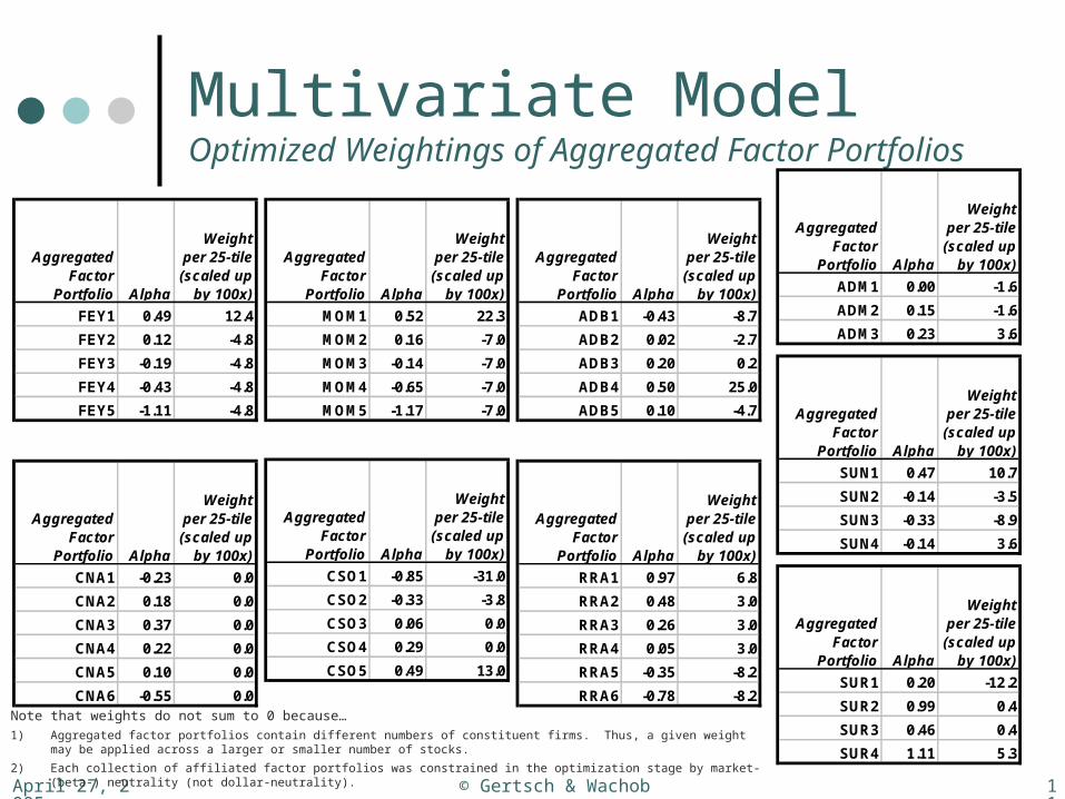
April 27, 2005 © Gertsch & Wachob 111
Multivariate ModelOptimized Weightings of Aggregated Factor Portfolios
Aggregated Factor
Portfolio Alpha
Weight per 25-tile (scaled up
by 100x)
ADB1 -0.43 -8.7
ADB2 0.02 -2.7
ADB3 0.20 0.2
ADB4 0.50 25.0
ADB5 0.10 -4.7
Aggregated Factor
Portfolio Alpha
Weight per 25-tile (scaled up
by 100x)
CSO1 -0.85 -31.0
CSO2 -0.33 -3.8
CSO3 0.06 0.0
CSO4 0.29 0.0
CSO5 0.49 13.0
Aggregated Factor
Portfolio Alpha
Weight per 25-tile (scaled up
by 100x)
FEY1 0.49 12.4
FEY2 0.12 -4.8
FEY3 -0.19 -4.8
FEY4 -0.43 -4.8
FEY5 -1.11 -4.8
Aggregated Factor
Portfolio Alpha
Weight per 25-tile (scaled up
by 100x)
MOM1 0.52 22.3
MOM2 0.16 -7.0
MOM3 -0.14 -7.0
MOM4 -0.65 -7.0
MOM5 -1.17 -7.0
Aggregated Factor
Portfolio Alpha
Weight per 25-tile (scaled up
by 100x)
CNA1 -0.23 0.0
CNA2 0.18 0.0
CNA3 0.37 0.0
CNA4 0.22 0.0
CNA5 0.10 0.0
CNA6 -0.55 0.0
Aggregated Factor
Portfolio Alpha
Weight per 25-tile (scaled up
by 100x)
RRA1 0.97 6.8
RRA2 0.48 3.0
RRA3 0.26 3.0
RRA4 0.05 3.0
RRA5 -0.35 -8.2
RRA6 -0.78 -8.2
Aggregated Factor
Portfolio Alpha
Weight per 25-tile (scaled up
by 100x)
SUN1 0.47 10.7
SUN2 -0.14 -3.5
SUN3 -0.33 -8.9
SUN4 -0.14 3.6
Aggregated Factor
Portfolio Alpha
Weight per 25-tile (scaled up
by 100x)
SUR1 0.20 -12.2
SUR2 0.99 0.4
SUR3 0.46 0.4
SUR4 1.11 5.3
Aggregated Factor
Portfolio Alpha
Weight per 25-tile (scaled up
by 100x)
ADM1 0.00 -1.6
ADM2 0.15 -1.6
ADM3 0.23 3.6
Note that weights do not sum to 0 because…
1) Aggregated factor portfolios contain different numbers of constituent firms. Thus, a given weight may be applied across a larger or smaller number of stocks.
2) Each collection of affiliated factor portfolios was constrained in the optimization stage by market- (beta-) neutrality (not dollar-neutrality).

April 27, 2005 © Gertsch & Wachob 112
Multivariate ModelUse Weightings As Scores for Quintile Sorting
Because portfolio weightings correspond to a relative overweighting or underweighting of constituent stocks, it is fair to ascribe a weighting of 0 to any stock not in a given portfolio.
To estimate the precise weighting for a given security prescribed by this strategy, the weights associated with all the portfolios with which a stock is affiliated can be summed.
Instead of going long or short every stock in the universe according to these prescribed weights, one might choose to transact only in those stocks which are receiving the heaviest weights (both long and short) per the model.
For simplicity of analysis, we have chosen to simulate a strategy that goes long the top 20% per these weights/scores and short the bottom 20%, equally-weighting the resultant portfolio constituents.

April 27, 2005 © Gertsch & Wachob 113
Multivariate ModelFactSet Code Excerpt
7.CM_VOL(0)/(VALUE(GM,OFDB(CLIENT:FIA,TRADING_DAYS,0)))*((CM_PH(0)+CM_PL(0))/2)8.CM_VOL(-1)/(VALUE(GM,OFDB(CLIENT:FIA,TRADING_DAYS,-1)))*((CM_PH(-1)+CM_PL(-1))/2)9.CM_VOL(-2)/(VALUE(GM,OFDB(CLIENT:FIA,TRADING_DAYS,-2)))*((CM_PH(-2)+CM_PL(-2))/2)10.CM_VOL(-3)/(VALUE(GM,OFDB(CLIENT:FIA,TRADING_DAYS,-3)))*((CM_PH(-3)+CM_PL(-3))/2)11.CM_VOL(-4)/(VALUE(GM,OFDB(CLIENT:FIA,TRADING_DAYS,-4)))*((CM_PH(-4)+CM_PL(-4))/2)12.CM_VOL(-5)/(VALUE(GM,OFDB(CLIENT:FIA,TRADING_DAYS,-5)))*((CM_PH(-5)+CM_PL(-5))/2)13.CM_VOL(-6)/(VALUE(GM,OFDB(CLIENT:FIA,TRADING_DAYS,-6)))*((CM_PH(-6)+CM_PL(-6))/2)14.CM_VOL(-7)/(VALUE(GM,OFDB(CLIENT:FIA,TRADING_DAYS,-7)))*((CM_PH(-7)+CM_PL(-7))/2)15.CM_VOL(-8)/(VALUE(GM,OFDB(CLIENT:FIA,TRADING_DAYS,-8)))*((CM_PH(-8)+CM_PL(-8))/2)16.CM_VOL(-9)/(VALUE(GM,OFDB(CLIENT:FIA,TRADING_DAYS,-9)))*((CM_PH(-9)+CM_PL(-9))/2)17.CM_VOL(-10)/(VALUE(GM,OFDB(CLIENT:FIA,TRADING_DAYS,-10)))*((CM_PH(-10)+CM_PL(-10))/2)18.CM_VOL(-11)/(VALUE(GM,OFDB(CLIENT:FIA,TRADING_DAYS,-11)))*((CM_PH(-11)+CM_PL(-11))/2)19.CM_VOL(-12)/(VALUE(GM,OFDB(CLIENT:FIA,TRADING_DAYS,-12)))*((CM_PH(-12)+CM_PL(-12))/2)20.CM_VOL(-13)/(VALUE(GM,OFDB(CLIENT:FIA,TRADING_DAYS,-13)))*((CM_PH(-13)+CM_PL(-13))/2)21.CM_VOL(-14)/(VALUE(GM,OFDB(CLIENT:FIA,TRADING_DAYS,-14)))*((CM_PH(-14)+CM_PL(-14))/2)22.CM_VOL(-15)/(VALUE(GM,OFDB(CLIENT:FIA,TRADING_DAYS,-15)))*((CM_PH(-15)+CM_PL(-15))/2)23.CM_VOL(-16)/(VALUE(GM,OFDB(CLIENT:FIA,TRADING_DAYS,-16)))*((CM_PH(-16)+CM_PL(-16))/2)24.CM_VOL(-17)/(VALUE(GM,OFDB(CLIENT:FIA,TRADING_DAYS,-17)))*((CM_PH(-17)+CM_PL(-17))/2)25.CM_VOL(-18)/(VALUE(GM,OFDB(CLIENT:FIA,TRADING_DAYS,-18)))*((CM_PH(-18)+CM_PL(-18))/2)26.CM_VOL(-19)/(VALUE(GM,OFDB(CLIENT:FIA,TRADING_DAYS,-19)))*((CM_PH(-19)+CM_PL(-19))/2)27.CM_VOL(-20)/(VALUE(GM,OFDB(CLIENT:FIA,TRADING_DAYS,-20)))*((CM_PH(-20)+CM_PL(-20))/2)28.CM_VOL(-21)/(VALUE(GM,OFDB(CLIENT:FIA,TRADING_DAYS,-21)))*((CM_PH(-21)+CM_PL(-21))/2)29.CM_VOL(-22)/(VALUE(GM,OFDB(CLIENT:FIA,TRADING_DAYS,-22)))*((CM_PH(-22)+CM_PL(-22))/2)30.CM_VOL(-23)/(VALUE(GM,OFDB(CLIENT:FIA,TRADING_DAYS,-23)))*((CM_PH(-23)+CM_PL(-23))/2)31.CM_VOL(-24)/(VALUE(GM,OFDB(CLIENT:FIA,TRADING_DAYS,-24)))*((CM_PH(-24)+CM_PL(-24))/2)32.CM_VOL(-25)/(VALUE(GM,OFDB(CLIENT:FIA,TRADING_DAYS,-25)))*((CM_PH(-25)+CM_PL(-25))/2)33.CM_VOL(-26)/(VALUE(GM,OFDB(CLIENT:FIA,TRADING_DAYS,-26)))*((CM_PH(-26)+CM_PL(-26))/2)34.CM_VOL(-27)/(VALUE(GM,OFDB(CLIENT:FIA,TRADING_DAYS,-27)))*((CM_PH(-27)+CM_PL(-27))/2)35.CM_VOL(-28)/(VALUE(GM,OFDB(CLIENT:FIA,TRADING_DAYS,-28)))*((CM_PH(-28)+CM_PL(-28))/2)36.CM_VOL(-29)/(VALUE(GM,OFDB(CLIENT:FIA,TRADING_DAYS,-29)))*((CM_PH(-29)+CM_PL(-29))/2)37.CM_VOL(-30)/(VALUE(GM,OFDB(CLIENT:FIA,TRADING_DAYS,-30)))*((CM_PH(-30)+CM_PL(-30))/2)38.CM_VOL(-31)/(VALUE(GM,OFDB(CLIENT:FIA,TRADING_DAYS,-31)))*((CM_PH(-31)+CM_PL(-31))/2)39.CM_VOL(-32)/(VALUE(GM,OFDB(CLIENT:FIA,TRADING_DAYS,-32)))*((CM_PH(-32)+CM_PL(-32))/2)40.CM_VOL(-33)/(VALUE(GM,OFDB(CLIENT:FIA,TRADING_DAYS,-33)))*((CM_PH(-33)+CM_PL(-33))/2)41.CM_VOL(-34)/(VALUE(GM,OFDB(CLIENT:FIA,TRADING_DAYS,-34)))*((CM_PH(-34)+CM_PL(-34))/2)42.CM_VOL(-35)/(VALUE(GM,OFDB(CLIENT:FIA,TRADING_DAYS,-35)))*((CM_PH(-35)+CM_PL(-35))/2)43.CM_VOL(-36)/(VALUE(GM,OFDB(CLIENT:FIA,TRADING_DAYS,-36)))*((CM_PH(-36)+CM_PL(-36))/2)44.CM_VOL(-37)/(VALUE(GM,OFDB(CLIENT:FIA,TRADING_DAYS,-37)))*((CM_PH(-37)+CM_PL(-37))/2)45.CM_VOL(-38)/(VALUE(GM,OFDB(CLIENT:FIA,TRADING_DAYS,-38)))*((CM_PH(-38)+CM_PL(-38))/2)46.CM_VOL(-39)/(VALUE(GM,OFDB(CLIENT:FIA,TRADING_DAYS,-39)))*((CM_PH(-39)+CM_PL(-39))/2)47.CM_VOL(-40)/(VALUE(GM,OFDB(CLIENT:FIA,TRADING_DAYS,-40)))*((CM_PH(-40)+CM_PL(-40))/2)48.CM_VOL(-41)/(VALUE(GM,OFDB(CLIENT:FIA,TRADING_DAYS,-41)))*((CM_PH(-41)+CM_PL(-41))/2)49.CM_VOL(-42)/(VALUE(GM,OFDB(CLIENT:FIA,TRADING_DAYS,-42)))*((CM_PH(-42)+CM_PL(-42))/2)50.CM_VOL(-43)/(VALUE(GM,OFDB(CLIENT:FIA,TRADING_DAYS,-43)))*((CM_PH(-43)+CM_PL(-43))/2)51.CM_VOL(-44)/(VALUE(GM,OFDB(CLIENT:FIA,TRADING_DAYS,-44)))*((CM_PH(-44)+CM_PL(-44))/2)52.CM_VOL(-45)/(VALUE(GM,OFDB(CLIENT:FIA,TRADING_DAYS,-45)))*((CM_PH(-45)+CM_PL(-45))/2)53.CM_VOL(-46)/(VALUE(GM,OFDB(CLIENT:FIA,TRADING_DAYS,-46)))*((CM_PH(-46)+CM_PL(-46))/2)54.CM_VOL(-47)/(VALUE(GM,OFDB(CLIENT:FIA,TRADING_DAYS,-47)))*((CM_PH(-47)+CM_PL(-47))/2)55.CM_VOL(-48)/(VALUE(GM,OFDB(CLIENT:FIA,TRADING_DAYS,-48)))*((CM_PH(-48)+CM_PL(-48))/2)56.CM_VOL(-49)/(VALUE(GM,OFDB(CLIENT:FIA,TRADING_DAYS,-49)))*((CM_PH(-49)+CM_PL(-49))/2)57.CM_VOL(-50)/(VALUE(GM,OFDB(CLIENT:FIA,TRADING_DAYS,-50)))*((CM_PH(-50)+CM_PL(-50))/2)58.CM_VOL(-51)/(VALUE(GM,OFDB(CLIENT:FIA,TRADING_DAYS,-51)))*((CM_PH(-51)+CM_PL(-51))/2)59.CM_VOL(-52)/(VALUE(GM,OFDB(CLIENT:FIA,TRADING_DAYS,-52)))*((CM_PH(-52)+CM_PL(-52))/2)60.CM_VOL(-53)/(VALUE(GM,OFDB(CLIENT:FIA,TRADING_DAYS,-53)))*((CM_PH(-53)+CM_PL(-53))/2)61.CM_VOL(-54)/(VALUE(GM,OFDB(CLIENT:FIA,TRADING_DAYS,-54)))*((CM_PH(-54)+CM_PL(-54))/2)62.CM_VOL(-55)/(VALUE(GM,OFDB(CLIENT:FIA,TRADING_DAYS,-55)))*((CM_PH(-55)+CM_PL(-55))/2)63.CM_VOL(-56)/(VALUE(GM,OFDB(CLIENT:FIA,TRADING_DAYS,-56)))*((CM_PH(-56)+CM_PL(-56))/2)64.CM_VOL(-57)/(VALUE(GM,OFDB(CLIENT:FIA,TRADING_DAYS,-57)))*((CM_PH(-57)+CM_PL(-57))/2)65.CM_VOL(-58)/(VALUE(GM,OFDB(CLIENT:FIA,TRADING_DAYS,-58)))*((CM_PH(-58)+CM_PL(-58))/2)66.CM_VOL(-59)/(VALUE(GM,OFDB(CLIENT:FIA,TRADING_DAYS,-59)))*((CM_PH(-59)+CM_PL(-59))/2)67.CM_VOL(-60)/(VALUE(GM,OFDB(CLIENT:FIA,TRADING_DAYS,-60)))*((CM_PH(-60)+CM_PL(-60))/2)68.CM_VOL(-61)/(VALUE(GM,OFDB(CLIENT:FIA,TRADING_DAYS,-61)))*((CM_PH(-61)+CM_PL(-61))/2)69.CM_VOL(-62)/(VALUE(GM,OFDB(CLIENT:FIA,TRADING_DAYS,-62)))*((CM_PH(-62)+CM_PL(-62))/2)70.CM_VOL(-63)/(VALUE(GM,OFDB(CLIENT:FIA,TRADING_DAYS,-63)))*((CM_PH(-63)+CM_PL(-63))/2)71.CM_VOL(-64)/(VALUE(GM,OFDB(CLIENT:FIA,TRADING_DAYS,-64)))*((CM_PH(-64)+CM_PL(-64))/2)72.CM_VOL(-65)/(VALUE(GM,OFDB(CLIENT:FIA,TRADING_DAYS,-65)))*((CM_PH(-65)+CM_PL(-65))/2)
73.(ROW8+ROW9+ROW10+ROW11+ROW12+ROW13+ROW14+ROW15+ROW16+ROW17+ROW18+ROW19+ROW20+ROW21+ROW22+ROW23+ROW24+ROW25+ROW26+ROW27+ROW28+ROW29+ROW30+ROW31+ROW32+ROW33+ROW34+ROW35+ROW36+ROW37+ROW38+ROW39+ROW40+ROW41+ROW42+ROW43+ROW44+ROW45+ROW46+ROW47+ROW48+ROW49+ROW50+ROW51+ROW52+ROW53+ROW54+ROW55+ROW56+ROW57+ROW58+ROW59+ROW60+ROW61+ROW62+ROW63+ROW64+ROW65+ROW66+ROW67)/60 /* ARITH AVG60 TO -1 */74.(ROW9+ROW10+ROW11+ROW12+ROW13+ROW14+ROW15+ROW16+ROW17+ROW18+ROW19+ROW20+ROW21+ROW22+ROW23+ROW24+ROW25+ROW26+ROW27+ROW28+ROW29+ROW30+ROW31+ROW32+ROW33+ROW34+ROW35+ROW36+ROW37+ROW38+ROW39+ROW40+ROW41+ROW42+ROW43+ROW44+ROW45+ROW46+ROW47+ROW48+ROW49+ROW50+ROW51+ROW52+ROW53+ROW54+ROW55+ROW56+ROW57+ROW58+ROW59+ROW60+ROW61+ROW62+ROW63+ROW64+ROW65+ROW66+ROW67+ROW68)/60 /* ARITH AVG60 TO -2 */75.(ROW10+ROW11+ROW12+ROW13+ROW14+ROW15+ROW16+ROW17+ROW18+ROW19+ROW20+ROW21+ROW22+ROW23+ROW24+ROW25+ROW26+ROW27+ROW28+ROW29+ROW30+ROW31+ROW32+ROW33+ROW34+ROW35+ROW36+ROW37+ROW38+ROW39+ROW40+ROW41+ROW42+ROW43+ROW44+ROW45+ROW46+ROW47+ROW48+ROW49+ROW50+ROW51+ROW52+ROW53+ROW54+ROW55+ROW56+ROW57+ROW58+ROW59+ROW60+ROW61+ROW62+ROW63+ROW64+ROW65+ROW66+ROW67+ROW68+ROW69)/60 /* ARITH AVG60 TO -3 */76.(ROW11+ROW12+ROW13+ROW14+ROW15+ROW16+ROW17+ROW18+ROW19+ROW20+ROW21+ROW22+ROW23+ROW24+ROW25+ROW26+ROW27+ROW28+ROW29+ROW30+ROW31+ROW32+ROW33+ROW34+ROW35+ROW36+ROW37+ROW38+ROW39+ROW40+ROW41+ROW42+ROW43+ROW44+ROW45+ROW46+ROW47+ROW48+ROW49+ROW50+ROW51+ROW52+ROW53+ROW54+ROW55+ROW56+ROW57+ROW58+ROW59+ROW60+ROW61+ROW62+ROW63+ROW64+ROW65+ROW66+ROW67+ROW68+ROW69+ROW70)/60 /* ARITH AVG60 TO -4 */77.(ROW12+ROW13+ROW14+ROW15+ROW16+ROW17+ROW18+ROW19+ROW20+ROW21+ROW22+ROW23+ROW24+ROW25+ROW26+ROW27+ROW28+ROW29+ROW30+ROW31+ROW32+ROW33+ROW34+ROW35+ROW36+ROW37+ROW38+ROW39+ROW40+ROW41+ROW42+ROW43+ROW44+ROW45+ROW46+ROW47+ROW48+ROW49+ROW50+ROW51+ROW52+ROW53+ROW54+ROW55+ROW56+ROW57+ROW58+ROW59+ROW60+ROW61+ROW62+ROW63+ROW64+ROW65+ROW66+ROW67+ROW68+ROW69+ROW70+ROW71)/60 /* ARITH AVG60 TO -5 */78.(ROW13+ROW14+ROW15+ROW16+ROW17+ROW18+ROW19+ROW20+ROW21+ROW22+ROW23+ROW24+ROW25+ROW26+ROW27+ROW28+ROW29+ROW30+ROW31+ROW32+ROW33+ROW34+ROW35+ROW36+ROW37+ROW38+ROW39+ROW40+ROW41+ROW42+ROW43+ROW44+ROW45+ROW46+ROW47+ROW48+ROW49+ROW50+ROW51+ROW52+ROW53+ROW54+ROW55+ROW56+ROW57+ROW58+ROW59+ROW60+ROW61+ROW62+ROW63+ROW64+ROW65+ROW66+ROW67+ROW68+ROW69+ROW70+ROW71+ROW72)/60 /* ARITH AVG60 TO -6 */79.LN(ROW7/ROW73)80.LN(ROW8/ROW74)81.LN(ROW9/ROW75)82.LN(ROW10/ROW76)83.LN(ROW11/ROW77)84.LN(ROW12/ROW78)85.ROW79+ROW80+ROW81+ROW82+ROW83+ROW84 /* SUM6M LNRDDV */86.IF((UDECILEX((UROW1=1 AND ISNA(ROW85)=0)=1, ROW3) < 3.5)=1, 1, 0)87.UPERCENTILEX((UROW1=1 AND ROW86=1)=1, ROW85)/488.IF(ROW87<4.1, 5, IF(ROW87<8.1, 4, IF(ROW87<20.1, 3, IF(ROW87<23.1, 2, IF(ROW87<25.1, 1, NA))))) /* ADB */89.IF(((UDECILEX((UROW1=1 AND ISNA(ROW85)=0)=1, ROW3) < 5.5) AND ROW86=0)=1, 1, 0)90.UPERCENTILEX((UROW1=1 AND ROW89=1)=1, ROW85)/491.IF(ROW90<5.1, 3, IF(ROW90<17.1, 2, IF(ROW90<25.1, 1, NA))) /* ADM */92.IF((SUM(0,IHLQEPSDNC(0))=CM_DNC(-1) OR SUM(0,IHLQEPSDNC(0)) = CM_DNC(-2)), MSHS(0), MSHS(0 L2M))93.IF((SUM(0,IHLQEPSDNC(0))=CM_DNC(-1) OR SUM(0,IHLQEPSDNC(0)) = CM_DNC(-2)), MSHS(0 L18M), MSHS(0 L20M))94.(ROW92-ROW93)/ROW93 /* 18 MONTHS */95.UPERCENTILEX(UROW1=1, ROW94)/496.IF(ROW95<1.1, 5, IF(ROW95<5.1, 4, IF(ROW95<11.1, 3, IF(ROW95<20.1, 2, IF(ROW95<25.1, 1, NA))))) /* CSO */97.AVAIL(IH_MED_EPS_NTMA(0), IH_MEDIAN_NTM(0), G_IBES_FY1_MED_USD(0))/MP(0)98.IF(ROW97>=1, NA, ROW97)99.UPERCENTILEX(UROW1=1, ROW98)/4100.IF(ROW99<8.1, 5, IF(ROW99<17.1, 4, IF(ROW99<21.1, 3, IF(ROW99<24.1, 2, IF(ROW99<25.1, 1, NA))))) /* FEY */101.(CM_P(-1)-CM_P(-13))/CM_P(-13)102.UPERCENTILEX(UROW1=1, ROW101)/4103.IF(ROW102<5.1, 5, IF(ROW102<18.1, 4, IF(ROW102<23.1, 3, IF(ROW102<24.1, 2, IF(ROW102<25.1, 1, NA))))) /* MOM */104.(SUM(IH_UP_FY1(0),IH_UP_FY1(-1),IH_UP_FY1(-2))-SUM(IH_DOWN_FY1(0),IH_DOWN_FY1(-1),IH_DOWN_FY1(-2)))/SUM(IH_NEST_FY1(0),IH_NEST_FY1(-1),IH_NEST_FY1(-2))105.UPERCENTILEX(UROW1=1, ROW104)/4106.IF(ROW105<1.1, 6, IF(ROW105<4.1, 5, IF(ROW105<10.1, 4, IF(ROW105<18.1, 3, IF(ROW105<24.1, 2, IF(ROW105<25.1, 1, NA)))))) /* RRA */107.IF((SUM(0,((IHLQEPSDNC(-11)-IHLQEPSDNC(-12))<>0))<>1)=1, 1, 0)108.IH_SUE_Q(0)109.UPERCENTILEX((UROW1=1 AND ROW107=1)=1, ROW108)/4110.IF(ROW109<5.1, 4, IF(ROW109<15.1, 3, IF(ROW109<20.1, 2, IF(ROW109<25.1, 1, NA)))) /* SUN */111.IF(((IHLQEPSDNC(-11)-IHLQEPSDNC(-12))<>0)=1, 1, 0)112.UPERCENTILEX((UROW1=1 AND ROW111=1)=1, ROW108)/4113.UCOUNT((UROW1=1 AND ROW111=1)=1, ROW108)114.IF(ROW113<100, (100*((ROW112*4/ROW113)-(0.5/ROW113))+0.5)/4,ROW112)115.IF(ROW114<1.001, 4, IF(ROW114<7.001, 3, IF(ROW114<24.001, 2, IF(ROW114<25.999, 1, NA)))) /* SUR */116.IF(ROW91=1, 3.60168, -1.5608) /**** ADM ****/117.IF(ROW88=1, -4.6901, IF(ROW88=2, 25.0052, IF(ROW88=3, 0.24877, IF(ROW88=4, -2.7161, -8.7251)))) /**** ADB ****/118.IF(ROW100<4.5, -4.8191, 12.3527) /**** FEY ****/119.IF(ROW96=1, 12.9797, IF(ROW96=2, 0.04123, IF(ROW96=3, 0.04123, IF(ROW96=4, -3.8275, -30.979)))) /**** CSO ****/120.IF(ROW106<2.5, -8.2051, IF(ROW106<5.5, 2.97009, 6.84939)) /**** RRA ****/121.IF(ROW103<4.5, -7.0059, 22.3312) /**** MOM ****/122.IF(ROW110=1, 3.57791, IF(ROW110=2, -8.9465, IF(ROW110=3, -3.5074, 10.6632))) /**** SUN ****/123.IF(ROW115=1, 5.29132, IF(ROW115=2, 0.38049, IF(ROW115=3, 0.38049, -12.245))) /**** SUR ****/124.SUM(ROW116, ROW117, ROW118, ROW119, ROW120, ROW121, ROW122, ROW123)
April 27, 2005 © Gertsch & Wachob 114
Multivariate Strategy (MV)In-Sample Performance
Alpha (vs. S&P500), Monthly % -- MV
-0.80
-0.60
-0.40
-0.20
0.00
0.20
0.40
0.60
0.80
-1- -2- -3- -4- -5-
Fractile
Monthly Return, % -- MV
0.00
0.20
0.40
0.60
0.80
1.00
1.20
1.40
1.60
1.80
-1- -2- -3- -4- -5-Fractile
Beta, on Market (S&P 500) -- MV
0.00
0.10
0.20
0.30
0.40
0.50
0.60
0.70
0.80
0.90
1.00
1.10
-1- -2- -3- -4- -5-
Fractile
Std. Dev. of Monthly Returns -- MV
0.00
0.50
1.00
1.50
2.00
2.50
3.00
3.50
4.00
4.50
5.00
5.50
6.00
6.50
-1- -2- -3- -4- -5-Fractile

April 27, 2005 © Gertsch & Wachob 115
Multivariate Strategy (MV)In-Sample Performance
Year-By-Year Returns in Excess of Benchmark -- MV
-40%
-30%
-20%
-10%
0%
10%
20%
30%
40%
1988 1989 1990 1991 1992 1993 1994 1995 1996 1997 1998 1999 2000 2001
Co
mp
ute
d b
y M
ult
iplic
ativ
ely
Ag
gre
ga
tin
g M
on
thly
Ret
urn
s O
ver
12-M
o.
Win
do
ws
MV1
MV2
MV3
MV4
MV5
April 27, 2005 © Gertsch & Wachob 116
Multivariate Strategy (MV)In-Sample Performance
Fractile Returns, Trailing 12 Mos. -- MV
-45%
-30%
-15%
0%
15%
30%
45%
60%
75%
1/31/1
988
1/31/1
989
1/31/1
990
1/31/1
991
1/31/1
992
1/31/1
993
1/31/1
994
1/31/1
995
1/31/1
996
1/31/1
997
1/31/1
998
1/31/1
999
1/31/2
000
1/31/2
001
Com
pute
d by
Mul
tiplic
ativ
ely
Agg
rega
ting
Mon
thly
Ret
urns
Ove
r a T
raili
ng 1
2-M
o. W
indo
w MV1-Bmark
MV2-Bmark
MV3-Bmark
MV4-Bmark
MV5-Bmark
MV1-MV5
April 27, 2005 © Gertsch & Wachob 117
Multivariate Strategy (MV)In-Sample Performance
MV -- Time Series, Cumulative Performance
-0.5
0
0.5
1
1.5
2
2.5
3
3.5
4
4.5
1/31
/198
7
1/31
/198
8
1/31
/198
9
1/31
/199
0
1/31
/199
1
1/31
/199
2
1/31
/199
3
1/31
/199
4
1/31
/199
5
1/31
/199
6
1/31
/199
7
1/31
/199
8
1/31
/199
9
1/31
/200
0
1/31
/200
1
log
2 C
um
Ret
urn
MV1MV2MV3MV4MV5Bmark

April 27, 2005 © Gertsch & Wachob 118
Multivariate Strategy (MV)In-Sample Performance
MV -- F1-F5 Portfolio: Monthly Returns Distribution
0
5
10
15
20
25
30
-0.0
85
-0.0
8-0
.07
5-0
.07
-0.0
65
-0.0
6-0
.05
5-0
.05
-0.0
45
-0.0
4-0
.03
5-0
.03
-0.0
25
-0.0
2-0
.01
5-0
.01
-0.0
05 0
0.0
05
0.0
10
.01
50
.02
0.0
25
0.0
30
.03
50
.04
0.0
45
0.0
50
.05
50
.06
0.0
65
0.0
70
.07
50
.08
0.0
85
0.0
90
.09
50
.10
.10
50
.11
0.1
15
0.1
2In
f
Monthly Return, Bin Upper Limit
Incr
emen
tal S
har
e o
f A
ll R
etu
rns
Per
Un
it X
(D
ensi
ty)
0%
10%
20%
30%
40%
50%
60%
70%
80%
90%
100%
Cu
mu
lati
ve
Sh
are
of
All
Re
turn
s
Incremental
Cumulative

April 27, 2005 © Gertsch & Wachob 119
Multivariate Strategy (MV)In-Sample Performance
MV -- F1-F5 Portfolio: ln Monthly Returns Distribution
0
5
10
15
20
25
30
-0.0
85
-0.0
8-0
.07
5-0
.07
-0.0
65
-0.0
6-0
.05
5-0
.05
-0.0
45
-0.0
4-0
.03
5-0
.03
-0.0
25
-0.0
2-0
.01
5-0
.01
-0.0
05 0
0.0
05
0.0
10
.01
50
.02
0.0
25
0.0
30
.03
50
.04
0.0
45
0.0
50
.05
50
.06
0.0
65
0.0
70
.07
50
.08
0.0
85
0.0
90
.09
50
.10
.10
50
.11
0.1
15
0.1
2In
f
ln Monthly Return, Bin Upper Limit
Incr
emen
tal S
har
e o
f A
ll R
etu
rns
Per
Un
it X
(D
ensi
ty)
0%
10%
20%
30%
40%
50%
60%
70%
80%
90%
100%
Cu
mu
lati
ve
Sh
are
of
All
Re
turn
s
Incremental
Cumulative
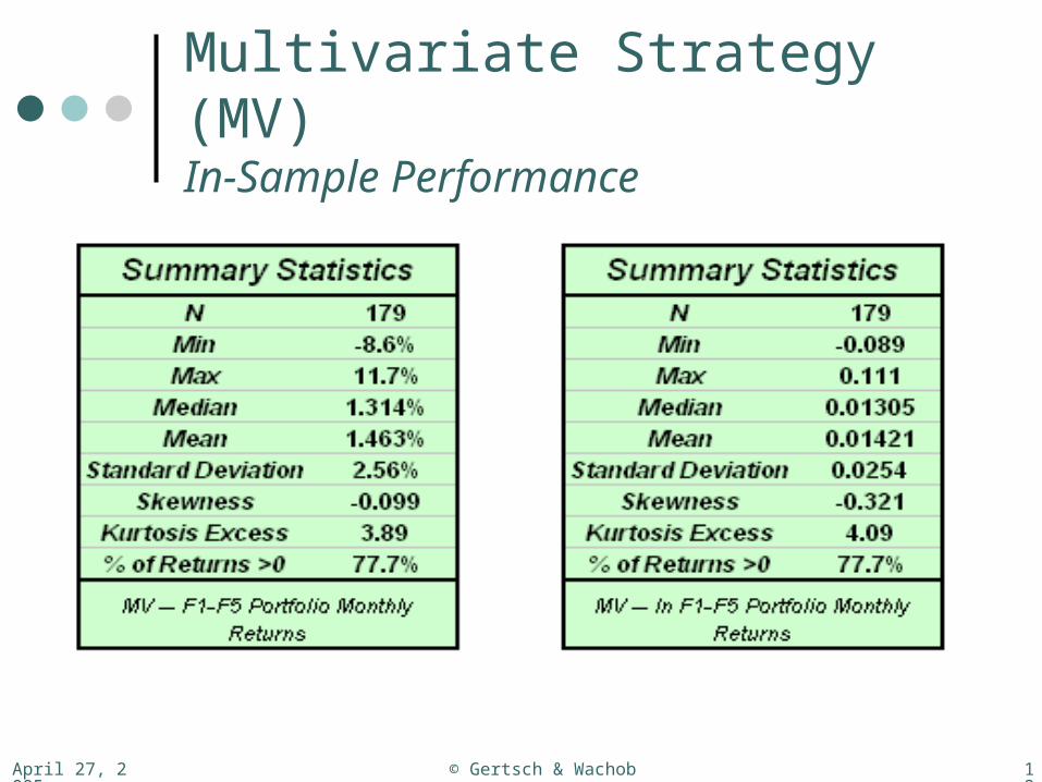
April 27, 2005 © Gertsch & Wachob 120
Multivariate Strategy (MV)In-Sample Performance
April 27, 2005 © Gertsch & Wachob 121
Multivariate Strategy (MV)In-Sample Performance
Note that there is no contiguous 12-month period for which this multivariate strategy’s quintile 1 underperformed quintile 5.
For 7 of the 14 complete in-sample years, this multivariate strategy’s quintiles exhibit a perfectly-ordered monotonic signal pattern
In-sample CAGR– Quintile 1: 23.2% Quintile 2: 17.6% Quintile 3: 14.1% Quintile 4: 9.3% Quintile 5: 3.5%

April 27, 2005 © Gertsch & Wachob 122
Multivariate Strategy (MV)Out-of-Sample PerformanceAlpha (vs. S&P500), Monthly % -- MV
-0.10
0.00
0.10
0.20
0.30
0.40
0.50
0.60
0.70
0.80
0.90
1.00
1.10
1.20
1.30
-1- -2- -3- -4- -5-
Fractile
Monthly Return, % -- MV
0.00
0.20
0.40
0.60
0.80
1.00
1.20
1.40
-1- -2- -3- -4- -5-Fractile
Beta, on Market (S&P 500) -- MV
0.00
0.20
0.40
0.60
0.80
1.00
1.20
1.40
-1- -2- -3- -4- -5-
Fractile
Std. Dev. of Monthly Returns -- MV
0.00
1.00
2.00
3.00
4.00
5.00
6.00
7.00
-1- -2- -3- -4- -5-Fractile

April 27, 2005 © Gertsch & Wachob 123
Multivariate Strategy (MV)Out-of-Sample Performance
Note that the quintile portfolio alphas are, on average, much greater than 0. This is likely because the small-cap universe had a strong run of outperformance during this out-of-sample period (Jan. 2002 – Mar. 2005). Because our benchmark (S&P500) is a large-cap index, while our universe spans small-cap to large-cap firms (excluding micro-cap), the average stock in our universe will appear to have a positive alpha against the S&P in this out-of-sample window. Though in a future analysis we would choose a different benchmark that is more reflective of our universe, we do not believe that our inter-quintile differentials are tainted.
Alpha (vs. S&P500), Monthly % -- MV
-0.10
0.00
0.10
0.20
0.30
0.40
0.50
0.60
0.70
0.80
0.90
1.00
1.10
1.20
1.30
-1- -2- -3- -4- -5-
Fractile
April 27, 2005 © Gertsch & Wachob 124
Multivariate Strategy (MV)Out-of-Sample Performance
Year-By-Year Returns in Excess of Benchmark -- MV
-12%
-6%
0%
6%
12%
18%
24%
30%
2002 2003 2004
Co
mp
ute
d b
y M
ult
iplic
ativ
ely
Ag
gre
gat
ing
Mo
nth
ly R
etu
rns
Ove
r 12
-Mo
. W
ind
ow
s
MV1
MV2
MV3
MV4
MV5
April 27, 2005 © Gertsch & Wachob 125
Multivariate Strategy (MV)Out-of-Sample Performance
Fractile Returns, Trailing 12 Mos. -- MV
-15%
-10%
-5%
0%
5%
10%
15%
20%
25%
30%
35%
40%
45%
50%
12/31/2002 4/30/2003 8/31/2003 12/31/2003 4/30/2004 8/31/2004 12/31/2004
Com
pute
d by
Mul
tiplic
ativ
ely
Agg
rega
ting
Mon
thly
Ret
urns
Ove
r a T
raili
ng 1
2-M
o. W
indo
w
MV1-Bmark
MV2-Bmark
MV3-Bmark
MV4-Bmark
MV5-Bmark
MV1-MV5
April 27, 2005 © Gertsch & Wachob 126
Multivariate Strategy (MV)Out-of-Sample Performance
MV -- Time Series, Cumulative Performance
-0.8
-0.6
-0.4
-0.2
0
0.2
0.4
0.6
0.8
1
12/31/2001 12/31/2002 12/31/2003 12/31/2004log
2 C
um
Re
turn
MV1MV2MV3MV4MV5Bmark
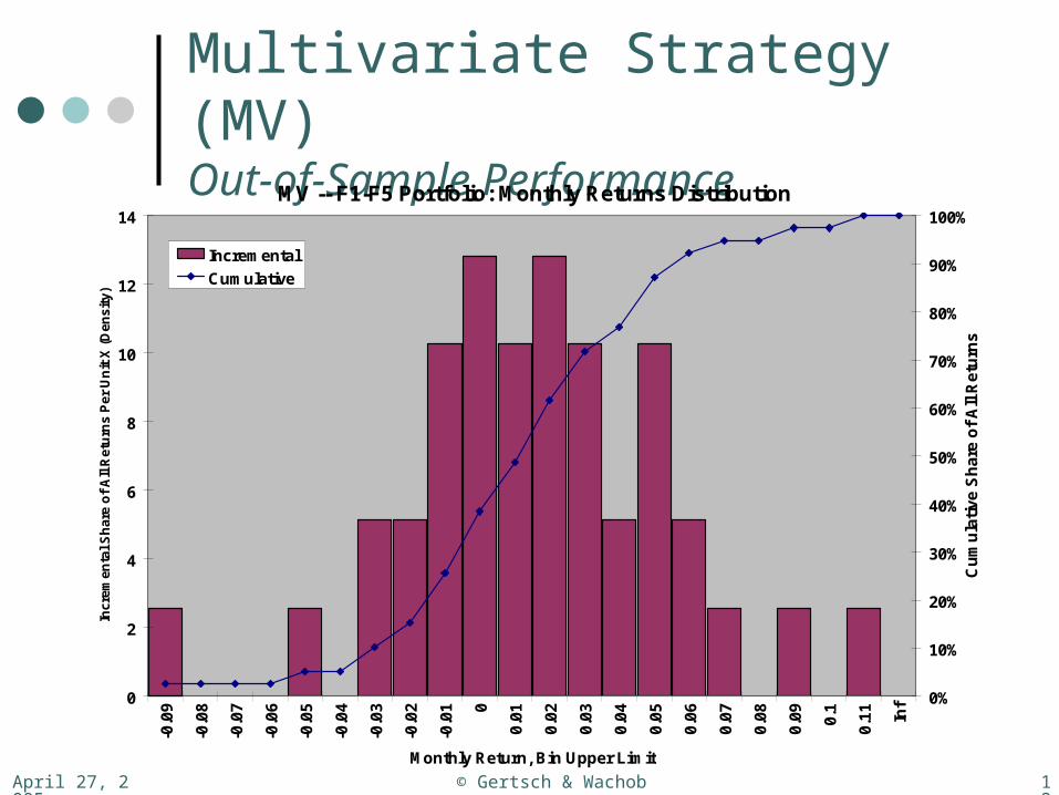
April 27, 2005 © Gertsch & Wachob 127
Multivariate Strategy (MV)Out-of-Sample Performance
MV -- F1-F5 Portfolio: Monthly Returns Distribution
0
2
4
6
8
10
12
14
-0.0
9
-0.0
8
-0.0
7
-0.0
6
-0.0
5
-0.0
4
-0.0
3
-0.0
2
-0.0
1 0
0.0
1
0.0
2
0.0
3
0.0
4
0.0
5
0.0
6
0.0
7
0.0
8
0.0
9
0.1
0.1
1
Inf
Monthly Return, Bin Upper Limit
Incr
emen
tal S
har
e o
f A
ll R
etu
rns
Per
Un
it X
(D
ensi
ty)
0%
10%
20%
30%
40%
50%
60%
70%
80%
90%
100%
Cu
mu
lati
ve
Sh
are
of
All
Re
turn
s
Incremental
Cumulative

April 27, 2005 © Gertsch & Wachob 128
Multivariate Strategy (MV)Out-of-Sample Performance
MV -- F1-F5 Portfolio: ln Monthly Returns Distribution
0
2
4
6
8
10
12
14
-0.1
-0.0
9
-0.0
8
-0.0
7
-0.0
6
-0.0
5
-0.0
4
-0.0
3
-0.0
2
-0.0
1 0
0.0
1
0.0
2
0.0
3
0.0
4
0.0
5
0.0
6
0.0
7
0.0
8
0.0
9
0.1 Inf
ln Monthly Return, Bin Upper Limit
Incr
emen
tal S
har
e o
f A
ll R
etu
rns
Per
Un
it X
(D
ensi
ty)
0%
10%
20%
30%
40%
50%
60%
70%
80%
90%
100%
Cu
mu
lati
ve
Sh
are
of
All
Re
turn
s
Incremental
Cumulative
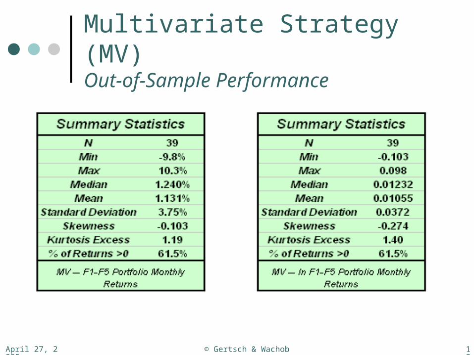
April 27, 2005 © Gertsch & Wachob 129
Multivariate Strategy (MV)Out-of-Sample Performance
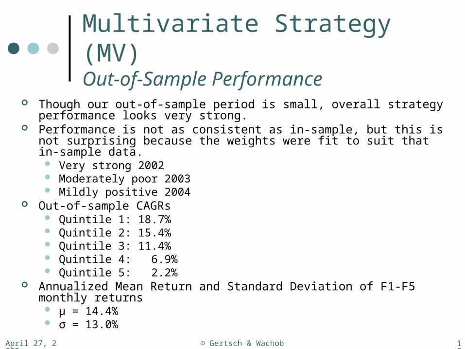
April 27, 2005 © Gertsch & Wachob 130
Multivariate Strategy (MV)Out-of-Sample Performance
Though our out-of-sample period is small, overall strategy performance looks very strong.
Performance is not as consistent as in-sample, but this is not surprising because the weights were fit to suit that in-sample data. Very strong 2002 Moderately poor 2003 Mildly positive 2004
Out-of-sample CAGRs Quintile 1: 18.7% Quintile 2: 15.4% Quintile 3: 11.4% Quintile 4: 6.9% Quintile 5: 2.2%
Annualized Mean Return and Standard Deviation of F1-F5 monthly returns μ = 14.4% σ = 13.0%

April 27, 2005 © Gertsch & Wachob 131
Multivariate Strategy (MV)Future Study
An informative follow-up analysis would explore out-of-sample performance-attribution for this multivariate strategy.
We know that value-based strategies (such as those based on a forward earnings yield factor) performed very strongly in these out-of-sample years.
How did our other component strategies perform in this out-of-sample period? Anecdotal evidence suggests that SUE and revision ratio screens may have
performed poorly. The robustness of our multivariate strategy could be questioned if all performance
was attributable to a single component factor (i.e. forward earnings yield). Future analysis should seek answers to these questions.

April 27, 2005 © Gertsch & Wachob 132
Multivariate Strategy (MV)Future Study
Transaction cost modeling demands greater attention in future revisions of this quantitative stock selection strategy.
Imprecisely, we could underweight factors that tend to generate high turnover. At each rebalancing interval, we could only choose to make adjustments to existing
portfolio positions in which expected returns (or alphas) are somehow deemed to justify the expected transaction cost.
Many other modeling options are conceivable. Scores/weights should probably be assigned in a more graduated fashion. i.e.
the last stock in aggregated factor portfolio 1 should probably not be assigned a drastically different weight/score than the first stock in aggregated factor portfolio 2 (as their actual factor values are likely to be barely distinguishable). …though it may be reasonable for the average stock within aggregated factor
portfolio 1 to receive a drastically different weight/score than the average stock within aggregated factor portfolio 2 (as prescribed by the antecedent optimization to determine aggregated factor portfolio weightings/scores).
Casting the model in a multivariate regression framework offers another means of integrating per-firm alpha forecasts based upon multiple factors (and could help smooth weights/scores as a function of underlying factor values or percentiles/ranks).

April 27, 2005 © Gertsch & Wachob 133
Dynamic Factor Weights
If we could find any predictability in factor returns, we could abandon the static weights of this initial multivariate strategy in favor of more powerful dynamic weights.
Thus, we sought predictability in factor returns.

April 27, 2005 © Gertsch & Wachob 134
Factor ForecastingOne-Period Factor Performance
For each factor, we evaluated the monthly time series of returns to an equal-weighted F1-F5 portfolio. We define this as monthly factor return. F1 is top factor quintile: firms with highest factor values. F5 is bottom factor quintile: firms with lowest factor values.
We searched for predictability in these factor returns by regressing on theoretically pertinent data series, including relevant (lagged) macroeconomic variables. We call these “candidate variables.”
A k-fold cross validation algorithm was coded and used to evaluate candidate variables based upon sum of squared errors across all subsets of “out-of-sample” data.
Best candidate variables for forecasting each factor returns series were included in a regression on all in-sample time series data to specify potential factor return forecasting models.
Sometimes reasonable transforms/combinations of candidate variables were used in regression models when data analysis revealed potentially significant statistical relations.

April 27, 2005 © Gertsch & Wachob 135
Factor ForecastingCandidate Variables
Interest Rate Term Structure US Gov't Treasuries Term Structure: 5YR-3MO US Gov't Treasuries Term Structure: 10 YR - 1YR US Gov't Treasuries Term Structure: 5YR-3MO, change over the last month US Gov't Treasuries Term Structure: 10 YR - 1YR, change over the last month US Gov't Treasuries Term Structure: 5YR-3MO, difference from a 6-mo. trailing avg. US Gov't Treasuries Term Structure: 10 YR - 1YR, difference from a 6-mo. trailing avg. US Gov't Treasuries Term Structure: 5YR-3MO, change over last 12 months US Gov't Treasuries Term Structure: 10 YR - 1YR, change over last 12 months
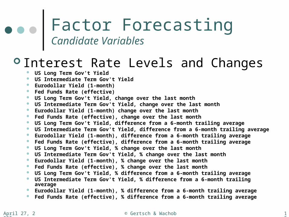
April 27, 2005 © Gertsch & Wachob 136
Factor ForecastingCandidate Variables
Interest Rate Levels and Changes US Long Term Gov't Yield US Intermediate Term Gov't Yield Eurodollar Yield (1-month) Fed Funds Rate (effective) US Long Term Gov't Yield, change over the last month US Intermediate Term Gov't Yield, change over the last month Eurodollar Yield (1-month) change over the last month Fed Funds Rate (effective), change over the last month US Long Term Gov't Yield, difference from a 6-month trailing average US Intermediate Term Gov't Yield, difference from a 6-month trailing average Eurodollar Yield (1-month), difference from a 6-month trailing average Fed Funds Rate (effective), difference from a 6-month trailing average US Long Term Gov't Yield, % change over the last month US Intermediate Term Gov't Yield, % change over the last month Eurodollar Yield (1-month), % change over the last month Fed Funds Rate (effective), % change over the last month US Long Term Gov't Yield, % difference from a 6-month trailing average US Intermediate Term Gov't Yield, % difference from a 6-month trailing average Eurodollar Yield (1-month), % difference from a 6-month trailing average Fed Funds Rate (effective), % difference from a 6-month trailing average

April 27, 2005 © Gertsch & Wachob 137
Factor ForecastingCandidate Variables
Valuation Multiples Price to Earnings: US Price to Book: US Price to Cash Earnings: US Dividend Yield: US Earnings to Price: US Book to Price: US Cash Earnings to Price: US

April 27, 2005 © Gertsch & Wachob 138
Factor ForecastingCandidate Variables
Credit Spread Credit Spread: Baa-Aaa Credit Spread: Baa-Aaa, change over the last month Credit Spread: Baa-Aaa, difference from a 6-month trailing average Credit Spread: Baa-Aaa, change over the last 12 months Credit Spread: Baa-Aaa, % change over the last month Baa-Aaa spread, % change over the last 12 months
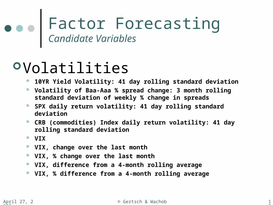
April 27, 2005 © Gertsch & Wachob 139
Factor ForecastingCandidate Variables
Volatilities 10YR Yield Volatility: 41 day rolling standard deviation Volatility of Baa-Aaa % spread change: 3 month rolling standard deviation of
weekly % change in spreads SPX daily return volatility: 41 day rolling standard deviation CRB (commodities) Index daily return volatility: 41 day rolling standard
deviation VIX VIX, change over the last month VIX, % change over the last month VIX, difference from a 4-month rolling average VIX, % difference from a 4-month rolling average
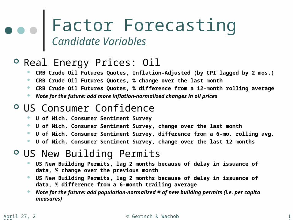
April 27, 2005 © Gertsch & Wachob 140
Factor ForecastingCandidate Variables
Real Energy Prices: Oil CRB Crude Oil Futures Quotes, Inflation-Adjusted (by CPI lagged by 2 mos.) CRB Crude Oil Futures Quotes, % change over the last month CRB Crude Oil Futures Quotes, % difference from a 12-month rolling average Note for the future: add more inflation-normalized changes in oil prices
US Consumer Confidence U of Mich. Consumer Sentiment Survey U of Mich. Consumer Sentiment Survey, change over the last month U of Mich. Consumer Sentiment Survey, difference from a 6-mo. rolling avg. U of Mich. Consumer Sentiment Survey, change over the last 12 months
US New Building Permits US New Building Permits, lag 2 months because of delay in issuance of data, % change
over the previous month US New Building Permits, lag 2 months because of delay in issuance of data, %
difference from a 6-month trailing average Note for the future: add population-normalized # of new building permits (i.e. per capita
measures)
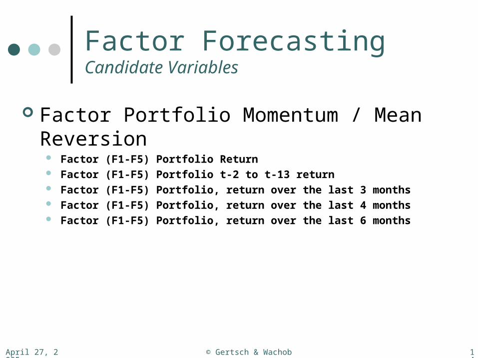
April 27, 2005 © Gertsch & Wachob 141
Factor ForecastingCandidate Variables
Factor Portfolio Momentum / Mean Reversion Factor (F1-F5) Portfolio Return Factor (F1-F5) Portfolio t-2 to t-13 return Factor (F1-F5) Portfolio, return over the last 3 months Factor (F1-F5) Portfolio, return over the last 4 months Factor (F1-F5) Portfolio, return over the last 6 months
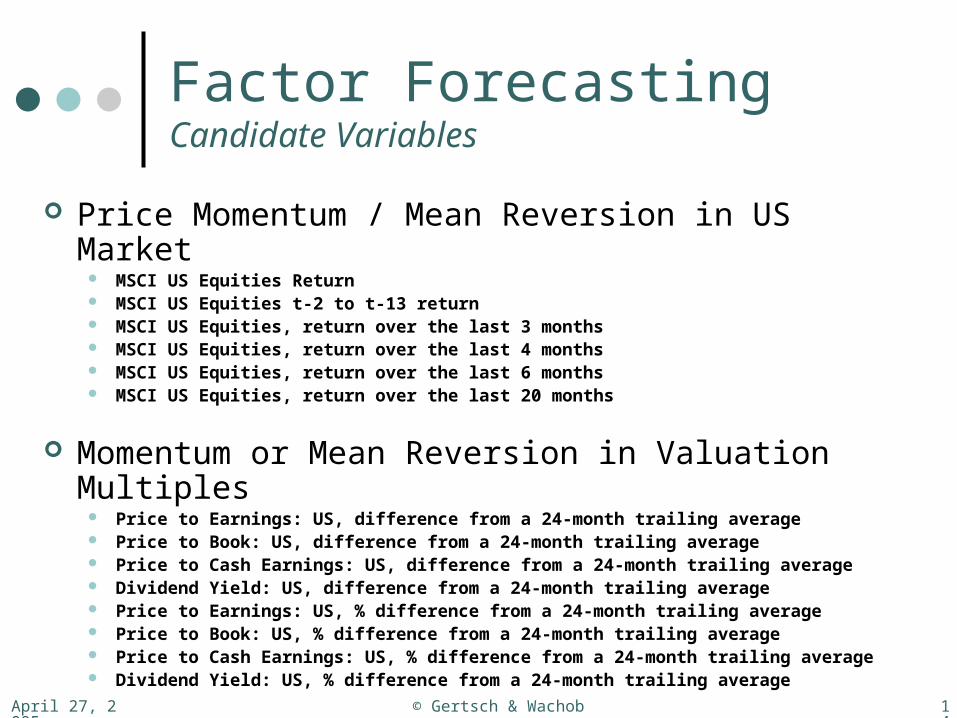
April 27, 2005 © Gertsch & Wachob 142
Factor ForecastingCandidate Variables
Price Momentum / Mean Reversion in US Market MSCI US Equities Return MSCI US Equities t-2 to t-13 return MSCI US Equities, return over the last 3 months MSCI US Equities, return over the last 4 months MSCI US Equities, return over the last 6 months MSCI US Equities, return over the last 20 months
Momentum or Mean Reversion in Valuation Multiples Price to Earnings: US, difference from a 24-month trailing average Price to Book: US, difference from a 24-month trailing average Price to Cash Earnings: US, difference from a 24-month trailing average Dividend Yield: US, difference from a 24-month trailing average Price to Earnings: US, % difference from a 24-month trailing average Price to Book: US, % difference from a 24-month trailing average Price to Cash Earnings: US, % difference from a 24-month trailing average Dividend Yield: US, % difference from a 24-month trailing average
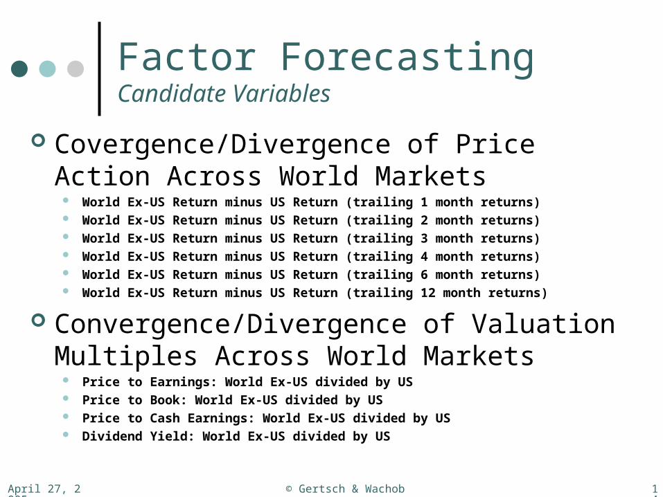
April 27, 2005 © Gertsch & Wachob 143
Factor ForecastingCandidate Variables
Covergence/Divergence of Price Action Across World Markets
World Ex-US Return minus US Return (trailing 1 month returns) World Ex-US Return minus US Return (trailing 2 month returns) World Ex-US Return minus US Return (trailing 3 month returns) World Ex-US Return minus US Return (trailing 4 month returns) World Ex-US Return minus US Return (trailing 6 month returns) World Ex-US Return minus US Return (trailing 12 month returns)
Convergence/Divergence of Valuation Multiples Across World Markets
Price to Earnings: World Ex-US divided by US Price to Book: World Ex-US divided by US Price to Cash Earnings: World Ex-US divided by US Dividend Yield: World Ex-US divided by US
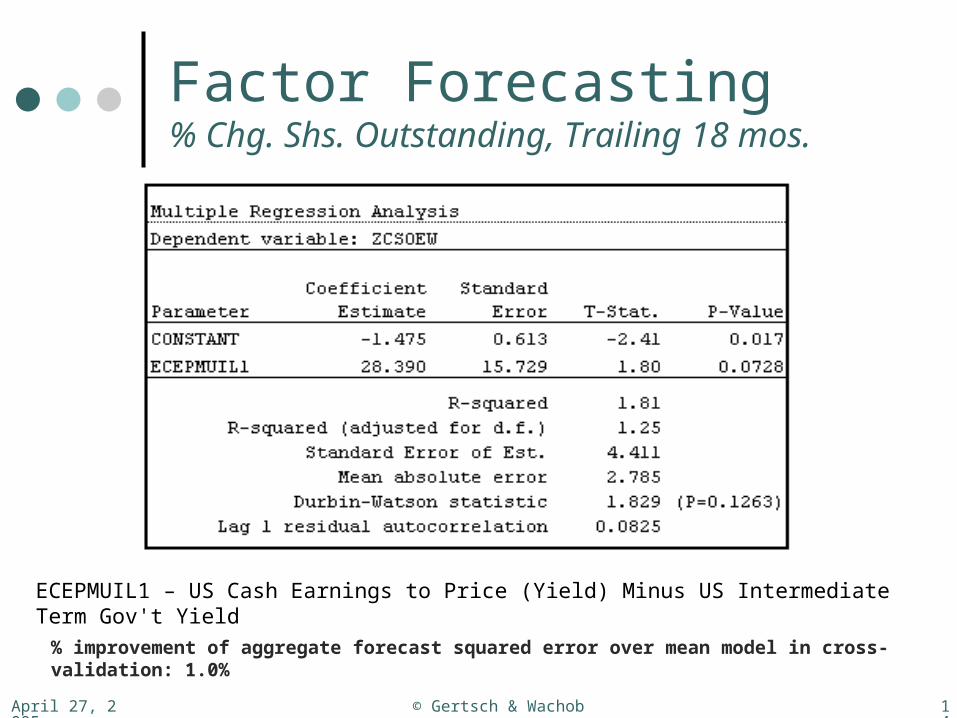
April 27, 2005 © Gertsch & Wachob 144
Factor Forecasting% Chg. Shs. Outstanding, Trailing 18 mos.
ECEPMUIL1 – US Cash Earnings to Price (Yield) Minus US Intermediate Term Gov't Yield
% improvement of aggregate forecast squared error over mean model in cross-validation: 1.0%
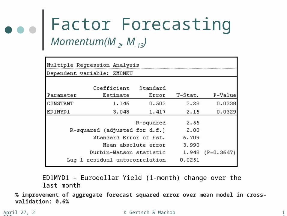
April 27, 2005 © Gertsch & Wachob 145
Factor ForecastingMomentum(M-2, M-13)
ED1MYD1 – Eurodollar Yield (1-month) change over the last month
% improvement of aggregate forecast squared error over mean model in cross-validation: 0.6%

April 27, 2005 © Gertsch & Wachob 146
Factor ForecastingReversal (% Return, Previous Month)
UITGYP1 – US Intermediate Term Gov't Yield, % change over the last month
% improvement of aggregate forecast squared error over mean model in cross-validation: 0.6%
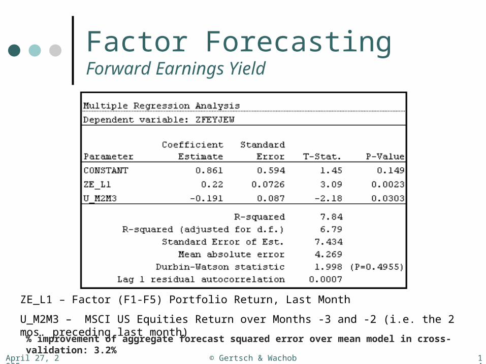
April 27, 2005 © Gertsch & Wachob 147
Factor ForecastingForward Earnings Yield
ZE_L1 – Factor (F1-F5) Portfolio Return, Last Month
U_M2M3 – MSCI US Equities Return over Months -3 and -2 (i.e. the 2 mos. preceding last month)
% improvement of aggregate forecast squared error over mean model in cross-validation: 3.2%
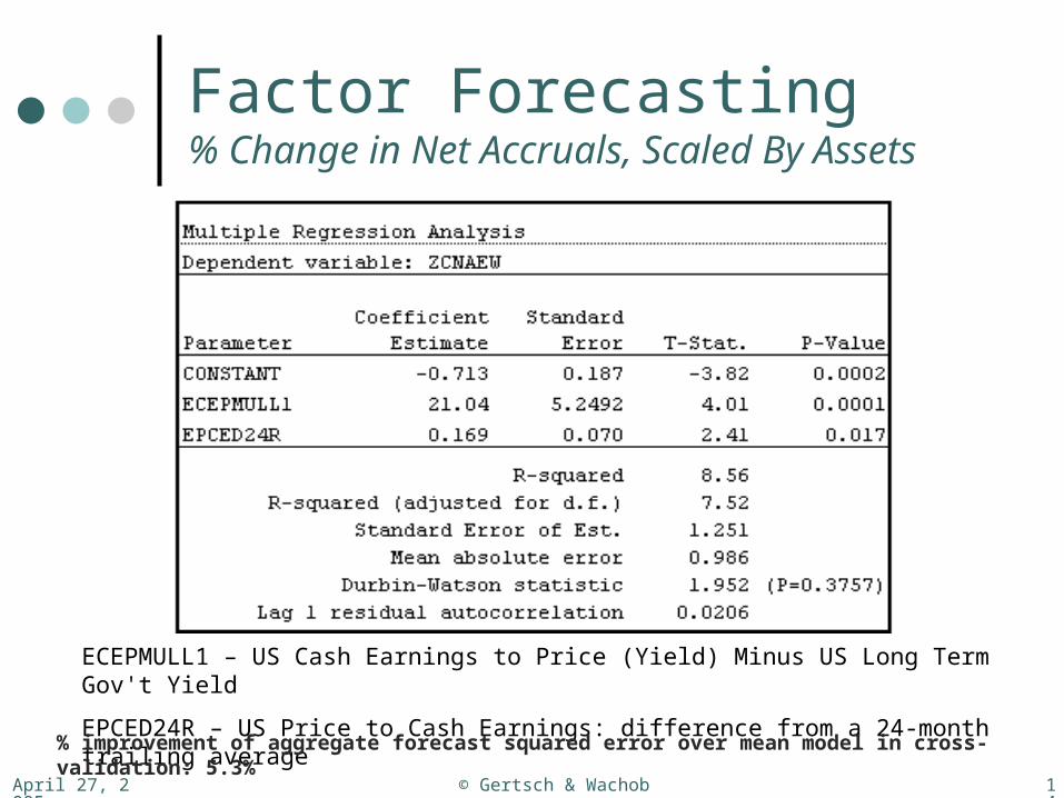
April 27, 2005 © Gertsch & Wachob 148
Factor Forecasting% Change in Net Accruals, Scaled By Assets
ECEPMULL1 – US Cash Earnings to Price (Yield) Minus US Long Term Gov't Yield
EPCED24R – US Price to Cash Earnings: difference from a 24-month trailing average
% improvement of aggregate forecast squared error over mean model in cross-validation: 5.3%
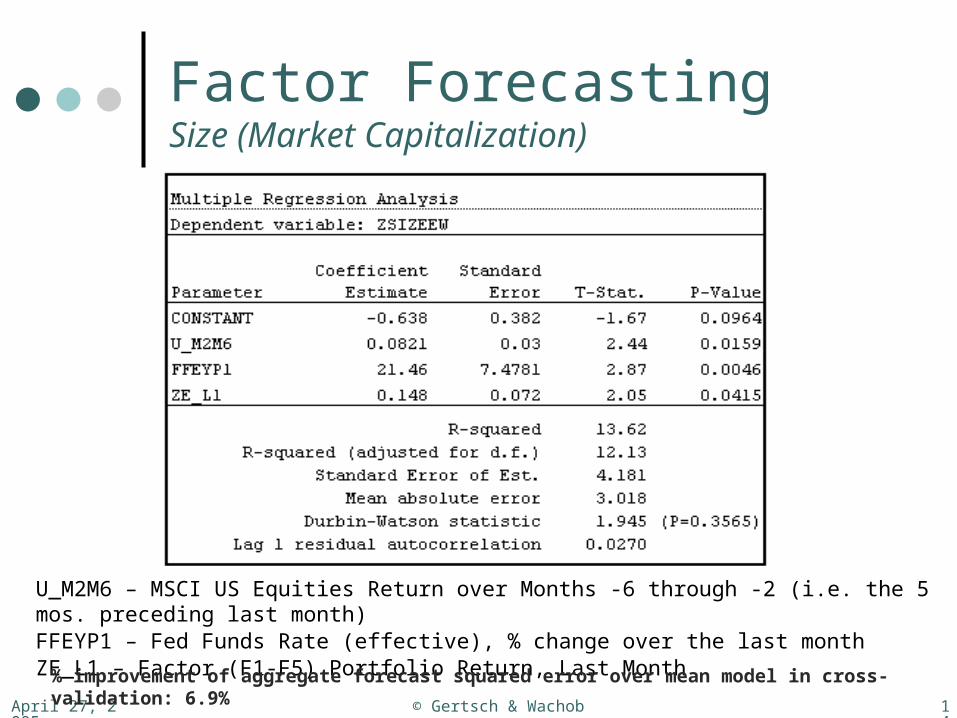
April 27, 2005 © Gertsch & Wachob 149
Factor ForecastingSize (Market Capitalization)
U_M2M6 – MSCI US Equities Return over Months -6 through -2 (i.e. the 5 mos. preceding last month)FFEYP1 – Fed Funds Rate (effective), % change over the last monthZE_L1 – Factor (F1-F5) Portfolio Return, Last Month
% improvement of aggregate forecast squared error over mean model in cross-validation: 6.9%

April 27, 2005 © Gertsch & Wachob 150
Factor ForecastingRevision Ratio (of Analysts’ EPS Estimates)
ED1MYD1 – Eurodollar Yield (1-month) change over the last month
U_M2M13 – MSCI US Equities Return over Months -13 through -2 (i.e. the 12 mos. preceding last month)
% improvement of aggregate forecast squared error over mean model in cross-validation: 5.8%
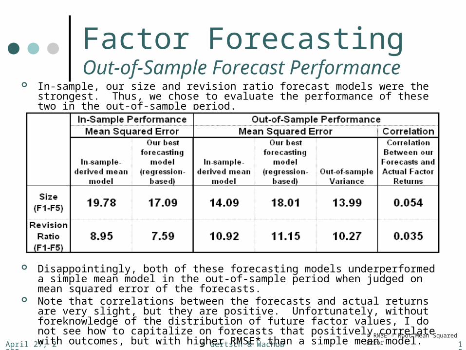
April 27, 2005 © Gertsch & Wachob 151
Factor ForecastingOut-of-Sample Forecast Performance
In-sample, our size and revision ratio forecast models were the strongest. Thus, we chose to evaluate the performance of these two in the out-of-sample period.
Disappointingly, both of these forecasting models underperformed a simple mean model in the out-of-sample period when judged on mean squared error of the forecasts.
Note that correlations between the forecasts and actual returns are very slight, but they are positive. Unfortunately, without foreknowledge of the distribution of future factor values, I do not see how to capitalize on forecasts that positively correlate with outcomes, but with higher RMSE* than a simple mean model. * RMSE – Root Mean Squared Error
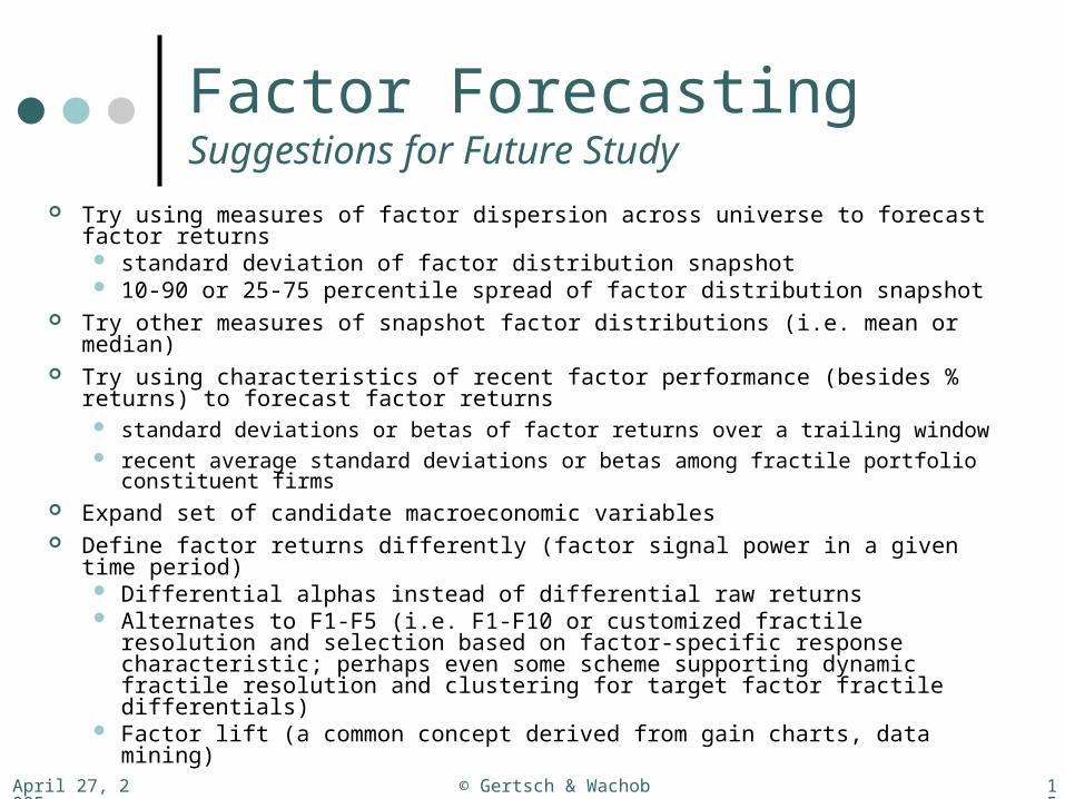
April 27, 2005 © Gertsch & Wachob 152
Factor ForecastingSuggestions for Future Study
Try using measures of factor dispersion across universe to forecast factor returns standard deviation of factor distribution snapshot 10-90 or 25-75 percentile spread of factor distribution snapshot
Try other measures of snapshot factor distributions (i.e. mean or median) Try using characteristics of recent factor performance (besides % returns) to
forecast factor returns standard deviations or betas of factor returns over a trailing window recent average standard deviations or betas among fractile portfolio
constituent firms Expand set of candidate macroeconomic variables Define factor returns differently (factor signal power in a given time period)
Differential alphas instead of differential raw returns Alternates to F1-F5 (i.e. F1-F10 or customized fractile resolution and
selection based on factor-specific response characteristic; perhaps even some scheme supporting dynamic fractile resolution and clustering for target factor fractile differentials)
Factor lift (a common concept derived from gain charts, data mining)

April 27, 2005 © Gertsch & Wachob 153
Dynamic Factor WeightsImplementation
We recognize that because our models to forecast factor returns underperformed a simple mean model out-of-sample, trying to modulate factor weightings based on these forecasts will result in degradation of long/short model performance out-of-sample.
Still, we proceed with an implementation of dynamic factor weights in order to demonstrate a proposed modeling framework (for use in future research when/if we do identify credible predictability of factor returns).
Because our model for the F1-F5 Size factor returns series appeared to have relatively high predictive power in-sample, we elected to use this size factor returns series to demonstrate our methodology Thus, our model will shift through time between favoring small
caps versus favoring large caps

April 27, 2005 © Gertsch & Wachob 154
Dynamic Factor WeightsImplementation
We integrated dynamic factor weights into our previously detailed multivariate approach grounded in mean-variance portfolio optimization.
We demeaned our forecasts for the F1-F5 Size factor returns series.
A new historical “forecast-interaction” series was generated by computing the product of each demeaned forecast and the actual factor return.
We added this “forecast-interaction” series along with the basic F1-F5 Size factor returns series as simulated “assets” to the optimization scheme as previously defined. No new constraints were required– the optimizer is limited only by
the overall variance constraint in terms of how heavily it will load up on F1-F5 size factor and its dynamic element.
Here, the optimizer’s assigned weighting will indicate the degree to which we desire to lever up a $-balanced long F1, short F5 position (a negative weighting would imply a short F1, long F5 position).

April 27, 2005 © Gertsch & Wachob 155
Dynamic Factor WeightsImplementation
The optimizer will ascribe a static weighting element to this F1-F5 Size portfolio.
It will also ascribe a dynamic weighting element. To implement the strategy, this weight is multiplied by the demeaned forecast F1-F5 Size portfolio return. The static weighting element is added to the result. This gives the desired long weighting for F1, which is also the desired short weighting for F5. Note that for consistency with the previous analysis, these
weights will have to be expressed on a per-25-tile basis. Since there are 5 25-tiles in each of the Size fractiles (quintiles: F1, F5), the optimizer-specified weights are simply divided by 5 to scale them appropriately for comparison and integration with other “aggregated factor portfolio” weights.

April 27, 2005 © Gertsch & Wachob 156
Dynamic Multivariate ModelOptimized Weightings of Aggregated Factor Portfolios
Aggregated Factor
Portfolio Alpha
Weight per 25-tile (scaled up
by 100x)
CNA1 -0.23 0.0
CNA2 0.18 0.0
CNA3 0.37 0.0
CNA4 0.22 0.0CNA5 0.10 0.0
CNA6 -0.55 0.0
Aggregated Factor
Portfolio Alpha
Weight per 25-tile (scaled up
by 100x)
RRA1 0.97 2.6
RRA2 0.48 2.6
RRA3 0.26 2.6
RRA4 0.05 2.6RRA5 -0.35 -6.3
RRA6 -0.78 -9.2
Aggregated Factor
Portfolio Alpha
Weight per 25-tile (scaled up
by 100x)
ADB1 -0.43 -10.1
ADB2 0.02 -3.4
ADB3 0.20 0.8
ADB4 0.50 20.4
ADB5 0.10 3.7
Aggregated Factor
Portfolio Alpha
Weight per 25-tile (scaled up
by 100x)
CSO1 -0.85 -36.5
CSO2 -0.33 -1.2
CSO3 0.06 -1.2
CSO4 0.29 -1.2
CSO5 0.49 16.0
Aggregated Factor
Portfolio Alpha
Weight per 25-tile (scaled up
by 100x)
FEY1 0.49 6.9
FEY2 0.12 -1.9
FEY3 -0.19 -1.9
FEY4 -0.43 -1.9
FEY5 -1.11 -11.3
Aggregated Factor
Portfolio Alpha
Weight per 25-tile (scaled up
by 100x)
MOM1 0.52 14.8
MOM2 0.16 -4.6
MOM3 -0.14 -4.6
MOM4 -0.65 -4.6
MOM5 -1.17 -4.6Aggregated
Factor Portfolio Alpha
Weight per 25-tile (scaled up
by 100x)
SUN1 0.47 12.6
SUN2 -0.14 -0.6
SUN3 -0.33 -11.8
SUN4 -0.14 -2.1
Aggregated Factor
Portfolio Alpha
Weight per 25-tile (scaled up
by 100x)
SUR1 0.20 -19.0
SUR2 0.99 0.9
SUR3 0.46 0.9
SUR4 1.11 0.9
Aggregated Factor
Portfolio Alpha
Weight per 25-tile (scaled up
by 100x)
ADM1 0.00 -0.9
ADM2 0.15 -0.9
ADM3 0.23 2.1
These are the weightings on the previously-defined aggregated factor portfolios that result from mean-variance optimization with inclusion of the F1-F5 Size Portfolio and its dynamic element.
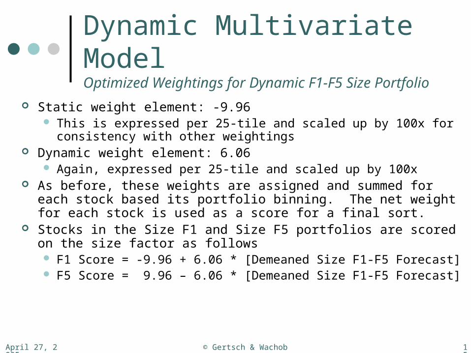
April 27, 2005 © Gertsch & Wachob 157
Dynamic Multivariate ModelOptimized Weightings for Dynamic F1-F5 Size Portfolio
Static weight element: -9.96 This is expressed per 25-tile and scaled up by 100x for consistency
with other weightings Dynamic weight element: 6.06
Again, expressed per 25-tile and scaled up by 100x As before, these weights are assigned and summed for each stock
based its portfolio binning. The net weight for each stock is used as a score for a final sort.
Stocks in the Size F1 and Size F5 portfolios are scored on the size factor as follows F1 Score = -9.96 + 6.06 * [Demeaned Size F1-F5 Forecast] F5 Score = 9.96 – 6.06 * [Demeaned Size F1-F5 Forecast]
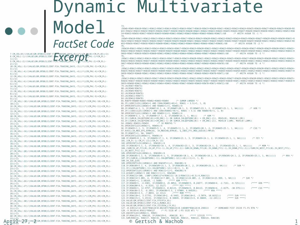
April 27, 2005 © Gertsch & Wachob 158
Dynamic Multivariate ModelFactSet CodeExcerpt
7.CM_VOL(0)/(VALUE(GM,OFDB(CLIENT:FIA,TRADING_DAYS,0)))*((CM_PH(0)+CM_PL(0))/2)8.CM_VOL(-1)/(VALUE(GM,OFDB(CLIENT:FIA,TRADING_DAYS,-1)))*((CM_PH(-1)+CM_PL(-1))/2)9.CM_VOL(-2)/(VALUE(GM,OFDB(CLIENT:FIA,TRADING_DAYS,-2)))*((CM_PH(-2)+CM_PL(-2))/2)10.CM_VOL(-3)/(VALUE(GM,OFDB(CLIENT:FIA,TRADING_DAYS,-3)))*((CM_PH(-3)+CM_PL(-3))/2)11.CM_VOL(-4)/(VALUE(GM,OFDB(CLIENT:FIA,TRADING_DAYS,-4)))*((CM_PH(-4)+CM_PL(-4))/2)12.CM_VOL(-5)/(VALUE(GM,OFDB(CLIENT:FIA,TRADING_DAYS,-5)))*((CM_PH(-5)+CM_PL(-5))/2)13.CM_VOL(-6)/(VALUE(GM,OFDB(CLIENT:FIA,TRADING_DAYS,-6)))*((CM_PH(-6)+CM_PL(-6))/2)14.CM_VOL(-7)/(VALUE(GM,OFDB(CLIENT:FIA,TRADING_DAYS,-7)))*((CM_PH(-7)+CM_PL(-7))/2)15.CM_VOL(-8)/(VALUE(GM,OFDB(CLIENT:FIA,TRADING_DAYS,-8)))*((CM_PH(-8)+CM_PL(-8))/2)16.CM_VOL(-9)/(VALUE(GM,OFDB(CLIENT:FIA,TRADING_DAYS,-9)))*((CM_PH(-9)+CM_PL(-9))/2)17.CM_VOL(-10)/(VALUE(GM,OFDB(CLIENT:FIA,TRADING_DAYS,-10)))*((CM_PH(-10)+CM_PL(-10))/2)18.CM_VOL(-11)/(VALUE(GM,OFDB(CLIENT:FIA,TRADING_DAYS,-11)))*((CM_PH(-11)+CM_PL(-11))/2)19.CM_VOL(-12)/(VALUE(GM,OFDB(CLIENT:FIA,TRADING_DAYS,-12)))*((CM_PH(-12)+CM_PL(-12))/2)20.CM_VOL(-13)/(VALUE(GM,OFDB(CLIENT:FIA,TRADING_DAYS,-13)))*((CM_PH(-13)+CM_PL(-13))/2)21.CM_VOL(-14)/(VALUE(GM,OFDB(CLIENT:FIA,TRADING_DAYS,-14)))*((CM_PH(-14)+CM_PL(-14))/2)22.CM_VOL(-15)/(VALUE(GM,OFDB(CLIENT:FIA,TRADING_DAYS,-15)))*((CM_PH(-15)+CM_PL(-15))/2)23.CM_VOL(-16)/(VALUE(GM,OFDB(CLIENT:FIA,TRADING_DAYS,-16)))*((CM_PH(-16)+CM_PL(-16))/2)24.CM_VOL(-17)/(VALUE(GM,OFDB(CLIENT:FIA,TRADING_DAYS,-17)))*((CM_PH(-17)+CM_PL(-17))/2)25.CM_VOL(-18)/(VALUE(GM,OFDB(CLIENT:FIA,TRADING_DAYS,-18)))*((CM_PH(-18)+CM_PL(-18))/2)26.CM_VOL(-19)/(VALUE(GM,OFDB(CLIENT:FIA,TRADING_DAYS,-19)))*((CM_PH(-19)+CM_PL(-19))/2)27.CM_VOL(-20)/(VALUE(GM,OFDB(CLIENT:FIA,TRADING_DAYS,-20)))*((CM_PH(-20)+CM_PL(-20))/2)28.CM_VOL(-21)/(VALUE(GM,OFDB(CLIENT:FIA,TRADING_DAYS,-21)))*((CM_PH(-21)+CM_PL(-21))/2)29.CM_VOL(-22)/(VALUE(GM,OFDB(CLIENT:FIA,TRADING_DAYS,-22)))*((CM_PH(-22)+CM_PL(-22))/2)30.CM_VOL(-23)/(VALUE(GM,OFDB(CLIENT:FIA,TRADING_DAYS,-23)))*((CM_PH(-23)+CM_PL(-23))/2)31.CM_VOL(-24)/(VALUE(GM,OFDB(CLIENT:FIA,TRADING_DAYS,-24)))*((CM_PH(-24)+CM_PL(-24))/2)32.CM_VOL(-25)/(VALUE(GM,OFDB(CLIENT:FIA,TRADING_DAYS,-25)))*((CM_PH(-25)+CM_PL(-25))/2)33.CM_VOL(-26)/(VALUE(GM,OFDB(CLIENT:FIA,TRADING_DAYS,-26)))*((CM_PH(-26)+CM_PL(-26))/2)34.CM_VOL(-27)/(VALUE(GM,OFDB(CLIENT:FIA,TRADING_DAYS,-27)))*((CM_PH(-27)+CM_PL(-27))/2)35.CM_VOL(-28)/(VALUE(GM,OFDB(CLIENT:FIA,TRADING_DAYS,-28)))*((CM_PH(-28)+CM_PL(-28))/2)36.CM_VOL(-29)/(VALUE(GM,OFDB(CLIENT:FIA,TRADING_DAYS,-29)))*((CM_PH(-29)+CM_PL(-29))/2)37.CM_VOL(-30)/(VALUE(GM,OFDB(CLIENT:FIA,TRADING_DAYS,-30)))*((CM_PH(-30)+CM_PL(-30))/2)38.CM_VOL(-31)/(VALUE(GM,OFDB(CLIENT:FIA,TRADING_DAYS,-31)))*((CM_PH(-31)+CM_PL(-31))/2)39.CM_VOL(-32)/(VALUE(GM,OFDB(CLIENT:FIA,TRADING_DAYS,-32)))*((CM_PH(-32)+CM_PL(-32))/2)40.CM_VOL(-33)/(VALUE(GM,OFDB(CLIENT:FIA,TRADING_DAYS,-33)))*((CM_PH(-33)+CM_PL(-33))/2)41.CM_VOL(-34)/(VALUE(GM,OFDB(CLIENT:FIA,TRADING_DAYS,-34)))*((CM_PH(-34)+CM_PL(-34))/2)42.CM_VOL(-35)/(VALUE(GM,OFDB(CLIENT:FIA,TRADING_DAYS,-35)))*((CM_PH(-35)+CM_PL(-35))/2)43.CM_VOL(-36)/(VALUE(GM,OFDB(CLIENT:FIA,TRADING_DAYS,-36)))*((CM_PH(-36)+CM_PL(-36))/2)44.CM_VOL(-37)/(VALUE(GM,OFDB(CLIENT:FIA,TRADING_DAYS,-37)))*((CM_PH(-37)+CM_PL(-37))/2)45.CM_VOL(-38)/(VALUE(GM,OFDB(CLIENT:FIA,TRADING_DAYS,-38)))*((CM_PH(-38)+CM_PL(-38))/2)46.CM_VOL(-39)/(VALUE(GM,OFDB(CLIENT:FIA,TRADING_DAYS,-39)))*((CM_PH(-39)+CM_PL(-39))/2)47.CM_VOL(-40)/(VALUE(GM,OFDB(CLIENT:FIA,TRADING_DAYS,-40)))*((CM_PH(-40)+CM_PL(-40))/2)48.CM_VOL(-41)/(VALUE(GM,OFDB(CLIENT:FIA,TRADING_DAYS,-41)))*((CM_PH(-41)+CM_PL(-41))/2)49.CM_VOL(-42)/(VALUE(GM,OFDB(CLIENT:FIA,TRADING_DAYS,-42)))*((CM_PH(-42)+CM_PL(-42))/2)50.CM_VOL(-43)/(VALUE(GM,OFDB(CLIENT:FIA,TRADING_DAYS,-43)))*((CM_PH(-43)+CM_PL(-43))/2)51.CM_VOL(-44)/(VALUE(GM,OFDB(CLIENT:FIA,TRADING_DAYS,-44)))*((CM_PH(-44)+CM_PL(-44))/2)52.CM_VOL(-45)/(VALUE(GM,OFDB(CLIENT:FIA,TRADING_DAYS,-45)))*((CM_PH(-45)+CM_PL(-45))/2)53.CM_VOL(-46)/(VALUE(GM,OFDB(CLIENT:FIA,TRADING_DAYS,-46)))*((CM_PH(-46)+CM_PL(-46))/2)54.CM_VOL(-47)/(VALUE(GM,OFDB(CLIENT:FIA,TRADING_DAYS,-47)))*((CM_PH(-47)+CM_PL(-47))/2)55.CM_VOL(-48)/(VALUE(GM,OFDB(CLIENT:FIA,TRADING_DAYS,-48)))*((CM_PH(-48)+CM_PL(-48))/2)56.CM_VOL(-49)/(VALUE(GM,OFDB(CLIENT:FIA,TRADING_DAYS,-49)))*((CM_PH(-49)+CM_PL(-49))/2)57.CM_VOL(-50)/(VALUE(GM,OFDB(CLIENT:FIA,TRADING_DAYS,-50)))*((CM_PH(-50)+CM_PL(-50))/2)58.CM_VOL(-51)/(VALUE(GM,OFDB(CLIENT:FIA,TRADING_DAYS,-51)))*((CM_PH(-51)+CM_PL(-51))/2)59.CM_VOL(-52)/(VALUE(GM,OFDB(CLIENT:FIA,TRADING_DAYS,-52)))*((CM_PH(-52)+CM_PL(-52))/2)60.CM_VOL(-53)/(VALUE(GM,OFDB(CLIENT:FIA,TRADING_DAYS,-53)))*((CM_PH(-53)+CM_PL(-53))/2)61.CM_VOL(-54)/(VALUE(GM,OFDB(CLIENT:FIA,TRADING_DAYS,-54)))*((CM_PH(-54)+CM_PL(-54))/2)62.CM_VOL(-55)/(VALUE(GM,OFDB(CLIENT:FIA,TRADING_DAYS,-55)))*((CM_PH(-55)+CM_PL(-55))/2)63.CM_VOL(-56)/(VALUE(GM,OFDB(CLIENT:FIA,TRADING_DAYS,-56)))*((CM_PH(-56)+CM_PL(-56))/2)64.CM_VOL(-57)/(VALUE(GM,OFDB(CLIENT:FIA,TRADING_DAYS,-57)))*((CM_PH(-57)+CM_PL(-57))/2)65.CM_VOL(-58)/(VALUE(GM,OFDB(CLIENT:FIA,TRADING_DAYS,-58)))*((CM_PH(-58)+CM_PL(-58))/2)66.CM_VOL(-59)/(VALUE(GM,OFDB(CLIENT:FIA,TRADING_DAYS,-59)))*((CM_PH(-59)+CM_PL(-59))/2)67.CM_VOL(-60)/(VALUE(GM,OFDB(CLIENT:FIA,TRADING_DAYS,-60)))*((CM_PH(-60)+CM_PL(-60))/2)68.CM_VOL(-61)/(VALUE(GM,OFDB(CLIENT:FIA,TRADING_DAYS,-61)))*((CM_PH(-61)+CM_PL(-61))/2)69.CM_VOL(-62)/(VALUE(GM,OFDB(CLIENT:FIA,TRADING_DAYS,-62)))*((CM_PH(-62)+CM_PL(-62))/2)70.CM_VOL(-63)/(VALUE(GM,OFDB(CLIENT:FIA,TRADING_DAYS,-63)))*((CM_PH(-63)+CM_PL(-63))/2)71.CM_VOL(-64)/(VALUE(GM,OFDB(CLIENT:FIA,TRADING_DAYS,-64)))*((CM_PH(-64)+CM_PL(-64))/2)72.CM_VOL(-65)/(VALUE(GM,OFDB(CLIENT:FIA,TRADING_DAYS,-65)))*((CM_PH(-65)+CM_PL(-65))/2)
73.(ROW8+ROW9+ROW10+ROW11+ROW12+ROW13+ROW14+ROW15+ROW16+ROW17+ROW18+ROW19+ROW20+ROW21+ROW22+ROW23+ROW24+ROW25+ROW26+ROW27+ROW28+ROW29+ROW30+ROW31+ROW32+ROW33+ROW34+ROW35+ROW36+ROW37+ROW38+ROW39+ROW40+ROW41+ROW42+ROW43+ROW44+ROW45+ROW46+ROW47+ROW48+ROW49+ROW50+ROW51+ROW52+ROW53+ROW54+ROW55+ROW56+ROW57+ROW58+ROW59+ROW60+ROW61+ROW62+ROW63+ROW64+ROW65+ROW66+ROW67)/60 /* ARITH AVG60 TO -1 */74.(ROW9+ROW10+ROW11+ROW12+ROW13+ROW14+ROW15+ROW16+ROW17+ROW18+ROW19+ROW20+ROW21+ROW22+ROW23+ROW24+ROW25+ROW26+ROW27+ROW28+ROW29+ROW30+ROW31+ROW32+ROW33+ROW34+ROW35+ROW36+ROW37+ROW38+ROW39+ROW40+ROW41+ROW42+ROW43+ROW44+ROW45+ROW46+ROW47+ROW48+ROW49+ROW50+ROW51+ROW52+ROW53+ROW54+ROW55+ROW56+ROW57+ROW58+ROW59+ROW60+ROW61+ROW62+ROW63+ROW64+ROW65+ROW66+ROW67+ROW68)/60 /* ARITH AVG60 TO -2 */75.(ROW10+ROW11+ROW12+ROW13+ROW14+ROW15+ROW16+ROW17+ROW18+ROW19+ROW20+ROW21+ROW22+ROW23+ROW24+ROW25+ROW26+ROW27+ROW28+ROW29+ROW30+ROW31+ROW32+ROW33+ROW34+ROW35+ROW36+ROW37+ROW38+ROW39+ROW40+ROW41+ROW42+ROW43+ROW44+ROW45+ROW46+ROW47+ROW48+ROW49+ROW50+ROW51+ROW52+ROW53+ROW54+ROW55+ROW56+ROW57+ROW58+ROW59+ROW60+ROW61+ROW62+ROW63+ROW64+ROW65+ROW66+ROW67+ROW68+ROW69)/60 /* ARITH AVG60 TO -3 */76.(ROW11+ROW12+ROW13+ROW14+ROW15+ROW16+ROW17+ROW18+ROW19+ROW20+ROW21+ROW22+ROW23+ROW24+ROW25+ROW26+ROW27+ROW28+ROW29+ROW30+ROW31+ROW32+ROW33+ROW34+ROW35+ROW36+ROW37+ROW38+ROW39+ROW40+ROW41+ROW42+ROW43+ROW44+ROW45+ROW46+ROW47+ROW48+ROW49+ROW50+ROW51+ROW52+ROW53+ROW54+ROW55+ROW56+ROW57+ROW58+ROW59+ROW60+ROW61+ROW62+ROW63+ROW64+ROW65+ROW66+ROW67+ROW68+ROW69+ROW70)/60 /* ARITH AVG60 TO -4 */77.(ROW12+ROW13+ROW14+ROW15+ROW16+ROW17+ROW18+ROW19+ROW20+ROW21+ROW22+ROW23+ROW24+ROW25+ROW26+ROW27+ROW28+ROW29+ROW30+ROW31+ROW32+ROW33+ROW34+ROW35+ROW36+ROW37+ROW38+ROW39+ROW40+ROW41+ROW42+ROW43+ROW44+ROW45+ROW46+ROW47+ROW48+ROW49+ROW50+ROW51+ROW52+ROW53+ROW54+ROW55+ROW56+ROW57+ROW58+ROW59+ROW60+ROW61+ROW62+ROW63+ROW64+ROW65+ROW66+ROW67+ROW68+ROW69+ROW70+ROW71)/60 /* ARITH AVG60 TO -5 */78.(ROW13+ROW14+ROW15+ROW16+ROW17+ROW18+ROW19+ROW20+ROW21+ROW22+ROW23+ROW24+ROW25+ROW26+ROW27+ROW28+ROW29+ROW30+ROW31+ROW32+ROW33+ROW34+ROW35+ROW36+ROW37+ROW38+ROW39+ROW40+ROW41+ROW42+ROW43+ROW44+ROW45+ROW46+ROW47+ROW48+ROW49+ROW50+ROW51+ROW52+ROW53+ROW54+ROW55+ROW56+ROW57+ROW58+ROW59+ROW60+ROW61+ROW62+ROW63+ROW64+ROW65+ROW66+ROW67+ROW68+ROW69+ROW70+ROW71+ROW72)/60 /* ARITH AVG60 TO -6 */79.LN(ROW7/ROW73)80.LN(ROW8/ROW74)81.LN(ROW9/ROW75)82.LN(ROW10/ROW76)83.LN(ROW11/ROW77)84.LN(ROW12/ROW78)85.ROW79+ROW80+ROW81+ROW82+ROW83+ROW84 /* SUM6M LNRDDV */86.IF((UDECILEX((UROW1=1 AND ISNA(ROW85)=0)=1, ROW3) < 3.5)=1, 1, 0)87.UPERCENTILEX((UROW1=1 AND ROW86=1)=1, ROW85)/488.IF(ROW87<4.1, 5, IF(ROW87<8.1, 4, IF(ROW87<20.1, 3, IF(ROW87<23.1, 2, IF(ROW87<25.1, 1, NA))))) /* ADB */89.IF(((UDECILEX((UROW1=1 AND ISNA(ROW85)=0)=1, ROW3) < 5.5) AND ROW86=0)=1, 1, 0)90.UPERCENTILEX((UROW1=1 AND ROW89=1)=1, ROW85)/491.IF(ROW90<5.1, 3, IF(ROW90<17.1, 2, IF(ROW90<25.1, 1, NA))) /* ADM */92.IF((SUM(0,IHLQEPSDNC(0))=CM_DNC(-1) OR SUM(0,IHLQEPSDNC(0)) = CM_DNC(-2)), MSHS(0), MSHS(0 L2M))93.IF((SUM(0,IHLQEPSDNC(0))=CM_DNC(-1) OR SUM(0,IHLQEPSDNC(0)) = CM_DNC(-2)), MSHS(0 L18M), MSHS(0 L20M))94.(ROW92-ROW93)/ROW93 /* 18 MONTHS */95.UPERCENTILEX(UROW1=1, ROW94)/496.IF(ROW95<1.1, 5, IF(ROW95<5.1, 4, IF(ROW95<11.1, 3, IF(ROW95<20.1, 2, IF(ROW95<25.1, 1, NA))))) /* CSO */97.AVAIL(IH_MED_EPS_NTMA(0), IH_MEDIAN_NTM(0), G_IBES_FY1_MED_USD(0))/MP(0)98.IF(ROW97>=1, NA, ROW97)99.UPERCENTILEX(UROW1=1, ROW98)/4100.IF(ROW99<8.1, 5, IF(ROW99<17.1, 4, IF(ROW99<21.1, 3, IF(ROW99<24.1, 2, IF(ROW99<25.1, 1, NA))))) /* FEY */101.(CM_P(-1)-CM_P(-13))/CM_P(-13)102.UPERCENTILEX(UROW1=1, ROW101)/4103.IF(ROW102<5.1, 5, IF(ROW102<18.1, 4, IF(ROW102<23.1, 3, IF(ROW102<24.1, 2, IF(ROW102<25.1, 1, NA))))) /* MOM */104.(SUM(IH_UP_FY1(0),IH_UP_FY1(-1),IH_UP_FY1(-2))-SUM(IH_DOWN_FY1(0),IH_DOWN_FY1(-1),IH_DOWN_FY1(-2)))/SUM(IH_NEST_FY1(0),IH_NEST_FY1(-1),IH_NEST_FY1(-2))105.UPERCENTILEX(UROW1=1, ROW104)/4106.IF(ROW105<1.1, 6, IF(ROW105<4.1, 5, IF(ROW105<10.1, 4, IF(ROW105<18.1, 3, IF(ROW105<24.1, 2, IF(ROW105<25.1, 1, NA)))))) /* RRA */107.IF((SUM(0,((IHLQEPSDNC(-11)-IHLQEPSDNC(-12))<>0))<>1)=1, 1, 0)108.IH_SUE_Q(0)109.UPERCENTILEX((UROW1=1 AND ROW107=1)=1, ROW108)/4110.IF(ROW109<5.1, 4, IF(ROW109<15.1, 3, IF(ROW109<20.1, 2, IF(ROW109<25.1, 1, NA)))) /* SUN */111.IF(((IHLQEPSDNC(-11)-IHLQEPSDNC(-12))<>0)=1, 1, 0)112.UPERCENTILEX((UROW1=1 AND ROW111=1)=1, ROW108)/4113.UCOUNT((UROW1=1 AND ROW111=1)=1, ROW108)114.IF(ROW113<100, (100*((ROW112*4/ROW113)-(0.5/ROW113))+0.5)/4,ROW112)115.IF(ROW114<1.001, 4, IF(ROW114<7.001, 3, IF(ROW114<24.001, 2, IF(ROW114<25.999, 1, NA)))) /* SUR */116.IF(ROW91=1, 3.60168, -1.5608) /**** ADM ****/117.IF(ROW88=1, -4.6901, IF(ROW88=2, 25.0052, IF(ROW88=3, 0.24877, IF(ROW88=4, -2.7161, -8.7251)))) /**** ADB ****/118.IF(ROW100<4.5, -4.8191, 12.3527) /**** FEY ****/119.IF(ROW96=1, 12.9797, IF(ROW96=2, 0.04123, IF(ROW96=3, 0.04123, IF(ROW96=4, -3.8275, -30.979)))) /**** CSO ****/120.IF(ROW106<2.5, -8.2051, IF(ROW106<5.5, 2.97009, 6.84939)) /**** RRA ****/121.IF(ROW103<4.5, -7.0059, 22.3312) /**** MOM ****/122.IF(ROW110=1, 3.57791, IF(ROW110=2, -8.9465, IF(ROW110=3, -3.5074, 10.6632))) /**** SUN ****/123.IF(ROW115=1, 5.29132, IF(ROW115=2, 0.38049, IF(ROW115=3, 0.38049, -12.245))) /**** SUR ****/124.VALUE(GM,OFDB(CLIENT:FIA,FFEYP1X,0))125.VALUE(GM,OFDB(CLIENT:FIA,U_M2M6X,0))126.VALUE(GM,OFDB(CLIENT:FIA,ZSIZEEW_L1X,0))127.-0.638112+21.4635*ROW124+0.0821071*ROW125+0.148409*ROW126+0.298513 /* DEMEANED FCST ZSIZE F1-F5 RTN */128.-9.96185+6.05811*ROW127 /* F1 SIZE WT (-F5 SIZE WT) */129.UQUINTILEX(UROW1=1, ROW3)130.IF(ROW129=1, ROW128, IF(ROW129=5, -ROW128, 0)) /**** IZSIZE ****/131.SUM(ROW116, ROW117, ROW118, ROW119, ROW120, ROW121, ROW122, ROW123, ROW130)
April 27, 2005 © Gertsch & Wachob 159
Dynamic Multivariate Strategy (DMV)In-Sample Performance
Alpha (vs. S&P500), Monthly % -- DMV
-0.90
-0.60
-0.30
0.00
0.30
0.60
0.90
-1- -2- -3- -4- -5-
Fractile
Monthly Return, % -- DMV
0.00
0.20
0.40
0.60
0.80
1.00
1.20
1.40
1.60
1.80
2.00
-1- -2- -3- -4- -5-Fractile
Beta, on Market (S&P 500) -- DMV
0.00
0.10
0.20
0.30
0.40
0.50
0.60
0.70
0.80
0.90
1.00
1.10
1.20
-1- -2- -3- -4- -5-
Fractile
Std. Dev. of Monthly Returns -- DMV
0.00
0.50
1.00
1.50
2.00
2.50
3.00
3.50
4.00
4.50
5.00
5.50
6.00
-1- -2- -3- -4- -5-
Fractile

April 27, 2005 © Gertsch & Wachob 160
Dynamic Multivariate Strategy (DMV)In-Sample Performance
Year-By-Year Returns in Excess of Benchmark -- DMV
-40%
-30%
-20%
-10%
0%
10%
20%
30%
40%
50%
1988 1989 1990 1991 1992 1993 1994 1995 1996 1997 1998 1999 2000 2001
Co
mp
ute
d b
y M
ult
iplic
ativ
ely
Ag
gre
ga
tin
g M
on
thly
Ret
urn
s O
ver
12-M
o.
Win
do
ws
DMV1
DMV2
DMV3
DMV4
DMV5
April 27, 2005 © Gertsch & Wachob 161
Dynamic Multivariate Strategy (DMV)In-Sample Performance
Fractile Returns, Trailing 12 Mos. -- DMV
-45%
-30%
-15%
0%
15%
30%
45%
60%
1/31/1
988
1/31/1
989
1/31/1
990
1/31/1
991
1/31/1
992
1/31/1
993
1/31/1
994
1/31/1
995
1/31/1
996
1/31/1
997
1/31/1
998
1/31/1
999
1/31/2
000
1/31/2
001
Com
pute
d by
Mul
tiplic
ativ
ely
Agg
rega
ting
Mon
thly
Ret
urns
Ove
r a T
raili
ng 1
2-M
o. W
indo
w DMV1-Bmark
DMV2-Bmark
DMV3-Bmark
DMV4-Bmark
DMV5-Bmark
DMV1-DMV5
April 27, 2005 © Gertsch & Wachob 162
Dynamic Multivariate Strategy (DMV)In-Sample Performance
DMV -- Time Series, Cumulative Performance
-0.5
0
0.5
1
1.5
2
2.5
3
3.5
4
4.5
5
1/31
/198
7
1/31
/198
8
1/31
/198
9
1/31
/199
0
1/31
/199
1
1/31
/199
2
1/31
/199
3
1/31
/199
4
1/31
/199
5
1/31
/199
6
1/31
/199
7
1/31
/199
8
1/31
/199
9
1/31
/200
0
1/31
/200
1
log
2 C
um
Ret
urn
DMV1DMV2DMV3DMV4DMV5Bmark
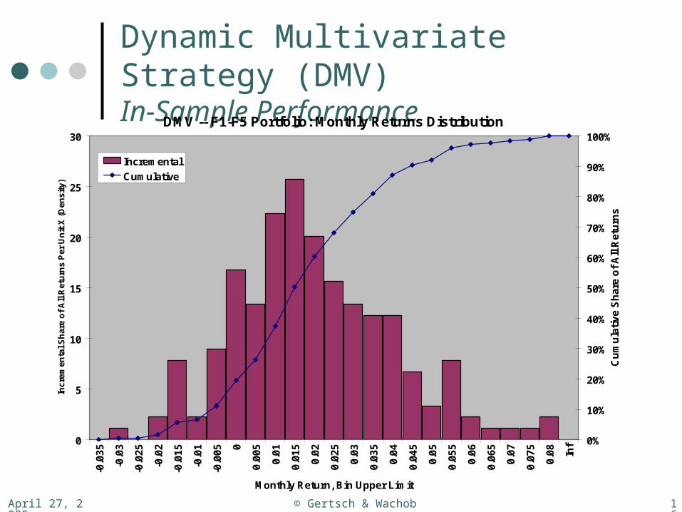
April 27, 2005 © Gertsch & Wachob 163
Dynamic Multivariate Strategy (DMV)In-Sample Performance
DMV -- F1-F5 Portfolio: Monthly Returns Distribution
0
5
10
15
20
25
30
-0.0
35
-0.0
3
-0.0
25
-0.0
2
-0.0
15
-0.0
1
-0.0
05 0
0.0
05
0.0
1
0.0
15
0.0
2
0.0
25
0.0
3
0.0
35
0.0
4
0.0
45
0.0
5
0.0
55
0.0
6
0.0
65
0.0
7
0.0
75
0.0
8
Inf
Monthly Return, Bin Upper Limit
Incr
emen
tal S
har
e o
f A
ll R
etu
rns
Per
Un
it X
(D
ensi
ty)
0%
10%
20%
30%
40%
50%
60%
70%
80%
90%
100%
Cu
mu
lati
ve
Sh
are
of
All
Re
turn
s
Incremental
Cumulative
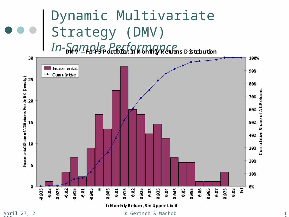
April 27, 2005 © Gertsch & Wachob 164
Dynamic Multivariate Strategy (DMV)In-Sample Performance
DMV -- F1-F5 Portfolio: ln Monthly Returns Distribution
0
5
10
15
20
25
30
-0.0
35
-0.0
3
-0.0
25
-0.0
2
-0.0
15
-0.0
1
-0.0
05 0
0.0
05
0.0
1
0.0
15
0.0
2
0.0
25
0.0
3
0.0
35
0.0
4
0.0
45
0.0
5
0.0
55
0.0
6
0.0
65
0.0
7
0.0
75
0.0
8
Inf
ln Monthly Return, Bin Upper Limit
Incr
emen
tal S
har
e o
f A
ll R
etu
rns
Per
Un
it X
(D
ensi
ty)
0%
10%
20%
30%
40%
50%
60%
70%
80%
90%
100%
Cu
mu
lati
ve
Sh
are
of
All
Re
turn
s
Incremental
Cumulative
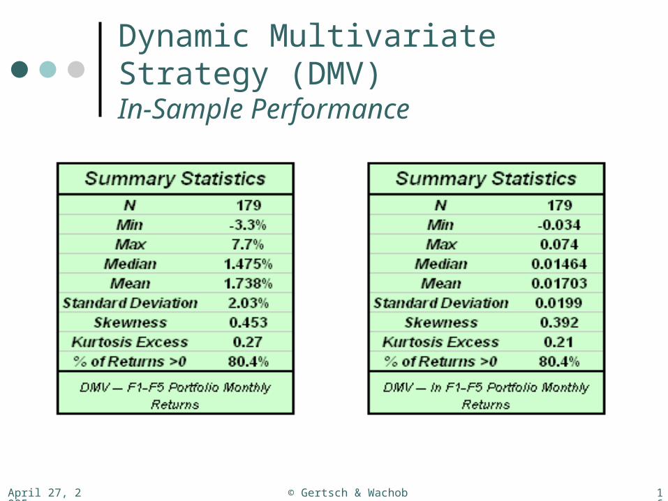
April 27, 2005 © Gertsch & Wachob 165
Dynamic Multivariate Strategy (DMV)In-Sample Performance

April 27, 2005 © Gertsch & Wachob 166
Dynamic Multivariate Strategy (DMV)In-Sample Performance
These in-sample results illustrate the potential power of dynamic factor weighting if a factor returns forecasting model with genuine predictive power is discovered.
Returns to F1-F5 portfolio Mean— DMV: 1.74% MV: 1.46% Std. Dev— DMV: 2.03% MV: 2.56% Min.— DMV: -3.3% MV: -8.6% Max.— DMV: 7.7% MV: 11.7%
The volatility decline is especially impressive. For the same volatility as the static-weighted strategy, we could have levered up another 25% and realized mean monthly returns of 2.18% (compared to only 1.46% for MV)
Note that this impressive in-sample performance enhancement is partially attributable to the addition of a new static factor (Size) as well as to the introduction of dynamic factor weighting on size. We should compare the performance between two model strategies that differ only by the addition of dynamic weighting of a factor that was already included in the static model. This would constitute a fairer apples-to-apples comparison. We leave this study to future research.

April 27, 2005 © Gertsch & Wachob 167
Dynamic Multivariate Strategy (DMV)Out-of-Sample Performance
Alpha (vs. S&P500), Monthly % -- DMV
0.00
0.20
0.40
0.60
0.80
1.00
1.20
-1- -2- -3- -4- -5-Fractile
Monthly Return, % -- DMV
0.00
0.20
0.40
0.60
0.80
1.00
1.20
1.40
-1- -2- -3- -4- -5-Fractile
Beta, on Market (S&P 500) -- DMV
0.00
0.10
0.20
0.30
0.40
0.50
0.60
0.70
0.80
0.90
1.00
1.10
1.20
1.30
-1- -2- -3- -4- -5-
Fractile
Std. Dev. of Monthly Returns -- DMV
0.00
1.00
2.00
3.00
4.00
5.00
6.00
-1- -2- -3- -4- -5-Fractile

April 27, 2005 © Gertsch & Wachob 168
Dynamic Multivariate Strategy (DMV)Out-of-Sample Performance
Year-By-Year Returns in Excess of Benchmark -- DMV
-8%
-4%
0%
4%
8%
12%
16%
20%
24%
28%
2002 2003 2004
Co
mp
ute
d b
y M
ult
iplic
ativ
ely
Ag
gre
gat
ing
Mo
nth
ly R
etu
rns
Ove
r 12
-Mo
. W
ind
ow
s
DMV1
DMV2
DMV3
DMV4
DMV5

April 27, 2005 © Gertsch & Wachob 169
Dynamic Multivariate Strategy (DMV)Out-of-Sample Performance
Fractile Returns, Trailing 12 Mos. -- DMV
-10%
-5%
0%
5%
10%
15%
20%
25%
30%
35%
40%
12/31/2002 4/30/2003 8/31/2003 12/31/2003 4/30/2004 8/31/2004 12/31/2004
Com
pute
d by
Mul
tiplic
ativ
ely
Agg
rega
ting
Mon
thly
Ret
urns
Ove
r a T
raili
ng 1
2-M
o. W
indo
w DMV1-Bmark
DMV2-Bmark
DMV3-Bmark
DMV4-Bmark
DMV5-Bmark
DMV1-DMV5

April 27, 2005 © Gertsch & Wachob 170
Dynamic Multivariate Strategy (DMV)Out-of-Sample Performance
DMV -- Time Series, Cumulative Performance
-0.7
-0.6
-0.5
-0.4
-0.3
-0.2
-0.1
0
0.1
0.2
0.3
0.4
0.5
0.6
0.7
0.8
12/31/2001 12/31/2002 12/31/2003 12/31/2004
log
2 C
um
Re
turn
DMV1DMV2DMV3DMV4DMV5Bmark
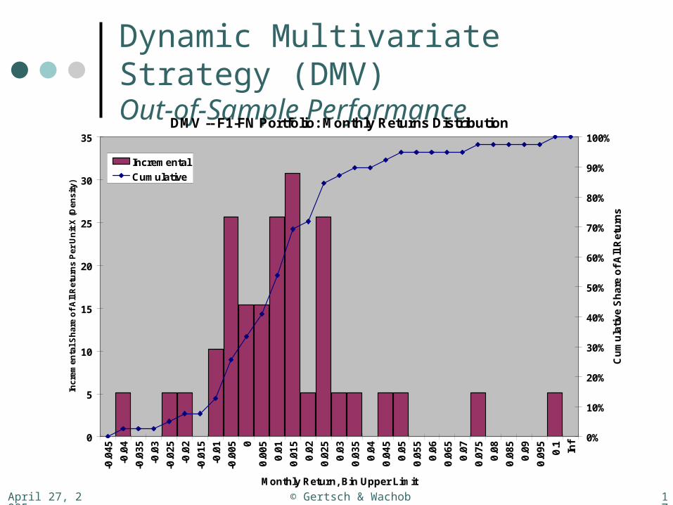
April 27, 2005 © Gertsch & Wachob 171
Dynamic Multivariate Strategy (DMV)Out-of-Sample Performance
DMV -- F1-FN Portfolio: Monthly Returns Distribution
0
5
10
15
20
25
30
35
-0.0
45
-0.0
4
-0.0
35
-0.0
3
-0.0
25
-0.0
2
-0.0
15
-0.0
1
-0.0
05 0
0.0
05
0.0
1
0.0
15
0.0
2
0.0
25
0.0
3
0.0
35
0.0
4
0.0
45
0.0
5
0.0
55
0.0
6
0.0
65
0.0
7
0.0
75
0.0
8
0.0
85
0.0
9
0.0
95
0.1 Inf
Monthly Return, Bin Upper Limit
Incr
emen
tal S
har
e o
f A
ll R
etu
rns
Per
Un
it X
(D
ensi
ty)
0%
10%
20%
30%
40%
50%
60%
70%
80%
90%
100%
Cu
mu
lati
ve
Sh
are
of
All
Re
turn
s
Incremental
Cumulative

April 27, 2005 © Gertsch & Wachob 172
Dynamic Multivariate Strategy (DMV)Out-of-Sample Performance
DMV -- F1-F5 Portfolio: ln Monthly Returns Distribution
0
5
10
15
20
25
30
35
-0.0
45
-0.0
4
-0.0
35
-0.0
3
-0.0
25
-0.0
2
-0.0
15
-0.0
1
-0.0
05 0
0.0
05
0.0
1
0.0
15
0.0
2
0.0
25
0.0
3
0.0
35
0.0
4
0.0
45
0.0
5
0.0
55
0.0
6
0.0
65
0.0
7
0.0
75
0.0
8
0.0
85
0.0
9
0.0
95
0.1 Inf
ln Monthly Return, Bin Upper Limit
Incr
emen
tal S
har
e o
f A
ll R
etu
rns
Per
Un
it X
(D
ensi
ty)
0%
10%
20%
30%
40%
50%
60%
70%
80%
90%
100%
Cu
mu
lati
ve
Sh
are
of
All
Re
turn
s
Incremental
Cumulative
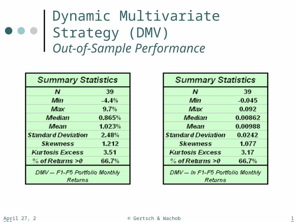
April 27, 2005 © Gertsch & Wachob 173
Dynamic Multivariate Strategy (DMV)Out-of-Sample Performance
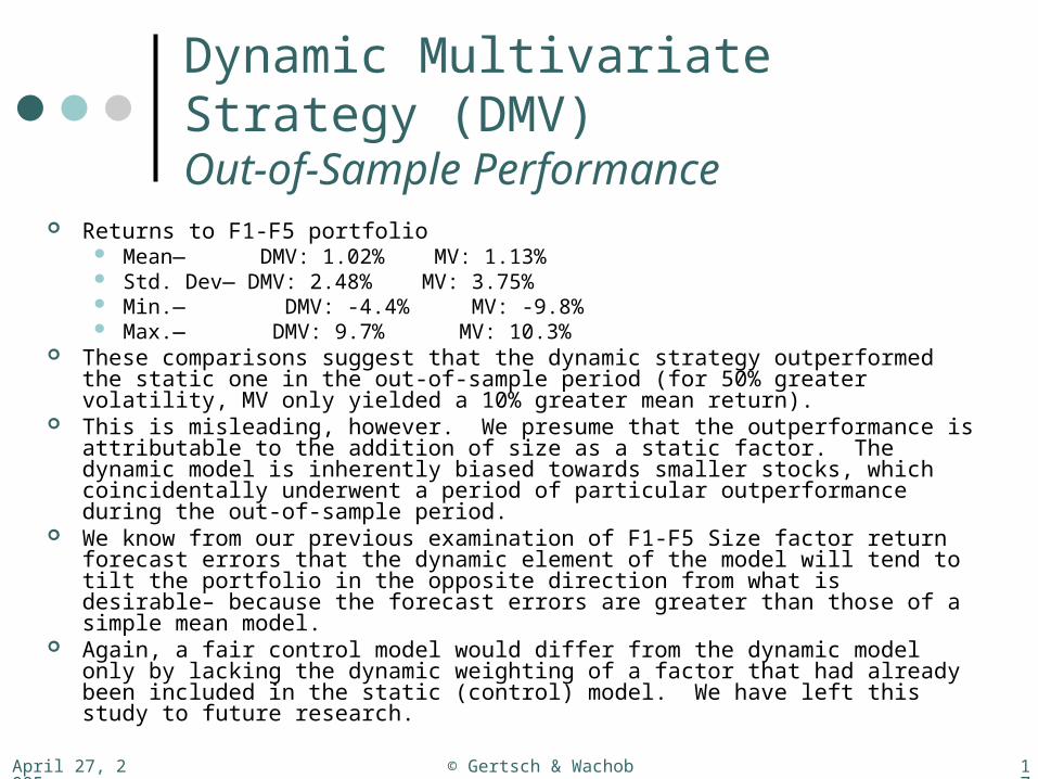
April 27, 2005 © Gertsch & Wachob 174
Dynamic Multivariate Strategy (DMV)Out-of-Sample Performance
Returns to F1-F5 portfolio Mean— DMV: 1.02% MV: 1.13% Std. Dev— DMV: 2.48% MV: 3.75% Min.— DMV: -4.4% MV: -9.8% Max.— DMV: 9.7% MV: 10.3%
These comparisons suggest that the dynamic strategy outperformed the static one in the out-of-sample period (for 50% greater volatility, MV only yielded a 10% greater mean return).
This is misleading, however. We presume that the outperformance is attributable to the addition of size as a static factor. The dynamic model is inherently biased towards smaller stocks, which coincidentally underwent a period of particular outperformance during the out-of-sample period.
We know from our previous examination of F1-F5 Size factor return forecast errors that the dynamic element of the model will tend to tilt the portfolio in the opposite direction from what is desirable– because the forecast errors are greater than those of a simple mean model.
Again, a fair control model would differ from the dynamic model only by lacking the dynamic weighting of a factor that had already been included in the static (control) model. We have left this study to future research.

April 27, 2005 © Gertsch & Wachob 175
Conclusions Our static model (and the methodology used to specify this model) does look
promising based on the strategy’s out-of-sample performance. Still, with more time, there remains obvious room for improvement to the
factor definitions and with regard to capturing all of the observed signal.• Industry-normalization, sub-universe factor specifications, factor interactions,
and more! Our efforts towards predicting factor returns to support a dynamic factor
weighting scheme were unsuccessful in out-of-sample testing Study of the change through time of dispersion of factor values is one new
area of suggested research towards forecasting factor returns. There may also be a preferable measurement of factor returns that is more
predicable than the basic quintile 1 minus quintile 5 returns series. There may be factors other than the ones we examined that exhibit more
predictability. Still, we believe in the validity of the framework we presented for
incorporating dynamic factor weighting into our model. The search continues for real predictability in factor returns.