NASATechnicalMemorandum110425

Further Developments of theFringe-Imaging Skin FrictionTechnique

Gregory G. Zilliac, Ames Research Center, Moffett Field, California

December 1996

National Aeronautics andSpace Administration

Ames Research CenterMoffett Field, California 94035-1000

" _ _ ii ......i¸ : i_ i_( i_ _i _

• _ :, :_i ", • -_ / i _.i_i _

https://ntrs.nasa.gov/search.jsp?R=19970010467 2018-06-10T22:30:51+00:00Z

il_

FURTHER DEVELOPMENTS OF THE FRINGE-IMAGING SKIN

FRICTION TECHNIQUE

Gregory G. Zilliac

Ames Research Center

SUMMARY

Various aspects and extensions of the Fringe-Imaging Skin Friction technique (FISF) have been

explored through the use of several benchtop experiments and modeling. The technique has been

extended to handle three-dimensional flow fields with mild shear gradients. The optical and imaging

system has been refined and a PC-based application has been written that has made it possible to obtain

high resolution skin friction field measurements in a resonable period of time. The improved method was

tested on a wingtip and compared with Navier-Stokes computations. Additionally, a general approach

to interferogram-fringe spacing analysis has been developed that should have applications in other areas

of interferometry. A detailed error analysis of the FISF technique is also included.

NOMENCLATURE

A

a

B,P,E

C

d

h

I

K

n

p

qRe

T

8

t

T

Uoo

U_ V_ W

W

X_ y_ Z

Oz

interferogram amplitude

wave amplitude or polynomial coefficient

low order polynomial coefficients

viscosity regression coefficients

diameter

oil film thickness

intensity

lens distortion coefficient

index of refraction, same as n D (n at A =2.320 × 10 -5 in. or 589.2 nm)

pressure

dynamic pressure

Reynolds numberradial distance measured from lens center

distance perpendicular to fringe bands (s = 0 at oil leading edge)

time

temperature

freestream velocity

velocity componentsdistance between streamlines

surface coordinate system

oil coefficient of expansion or angle of attack

specific gravity

phase difference

.................................... ............................:i i?'7: .....

As

0

A

#

/J

P

¢7-

fringe spacing (distance between peaks of destructive interference)

circumferential direction

illumination wavelength

absolute viscosity

kinematic viscosity or fringe visibility

density

angle of cf vector with z - z planeskin friction

Subscripts

a air

c chord

cal calibration

D sodium spectral line

h hydraulic

nora nominal quantity

o oil

p-p peak to peak

T temperature

w wall

oo freestream

1,2, ... fringe number (1 at first destructive interference, 2 at second .... etc.)

INTRODUCTION

Skin friction can account for half the drag (or more) of a flight vehicle. Attempts have been made

to minimize this source of drag by increasing the laminar run on wings, using flush rivets and through

the use of various boundary layer control devices. Only a small percentage of drag reduction attempts

ultimately succeed. The failures often come at great expense. One of the reasons for this is that,

until recently, no accurate methods existed to measure skin friction directly. To date, an accurate field

measurement of a three-dimensional skin friction distribution, on a surface of aerodynamic interest, has

not been achieved. In addition, turbulence modelers have a great need for skin friction data, particularly

for off-cruise conditions where, typically, Reynolds-averaged Navier-Stokes (RANS) predictions of drag

are 10% accurate at best.

Winter's extensive review paper (ref. 1) on skin friction measurement techniques quotes accuracies

of 1.4%-1 0% for the most reliable and commonly used two-dimensional technique reviewed (the Preston

tube). In a three-dimensional flow with a pressure gradient, even greater inaccuracies are to be expected

using Preston tubes and most other skin friction measurement techniques.

The fringe-imaging skin friction technique (FISF) was developed by Monson and Mateer (ref. 2)

and was inspired by the work of Tanner and Blows (ref. 3). Monson and Mateer measured the skin

friction on a two-dimensional transonic airfoil and achieved a reasonable comparison with a Navier-

Stokes solution.

2

• • -: • ,, , !/_ .i I • :

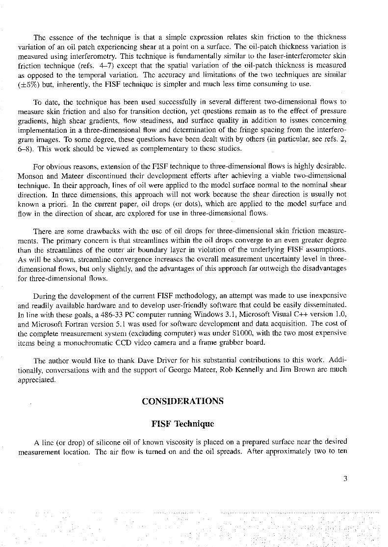
The essence of the technique is that a simple expression relates skin friction to the thickness

variation of an oil patch experiencing shear at a point on a surface. The oil-patch thickness variation is

measured using interferometry. This technique is fundamentally similar to the laser-interferometer skin

friction technique (refs. 4-7) except that the spatial variation of the oil-patch thickness is measured

as opposed to the temporal variation. The accuracy and limitations of the two techniques are similar

(+5%) but, inherently, the FISF technique is simpler and much less time consuming to use.

To date, the technique has been used successfully in several different two-dimensional flows to

measure skin friction and also for transition dection, yet questions remain as to the effect of pressure

gradients, high shear gradients, flow steadiness, and surface quality in addition to issues concerning

implementation in a three-dimensional flow and determination of the fringe spacing from the interfero-

gram images. To some degree, these questions have been dealt with by others (in particular, see refs. 2,

6-8). This work should be viewed as complementary to these studies.

For obvious reasons, extension of the FISF technique to three-dimensional flows is highly desirable.

Monson and Mateer discontinued their development efforts after achieving a viable two-dimensional

technique. In their approach, lines of oil were applied to the model surface normal to the nominal shear

direction. In three dimensions, this approach will not work because the shear direction is usually not

known a priori. In the current paper, oil drops (or dots), which are applied to the model surface and

flow in the direction of shear, are explored for use in three-dimensional flows.

There are some drawbacks with the use of oil drops for three-dimensional skin friction measure-

ments. The primary concern is that streamlines within the oil drops converge to an even greater degree

than the streamlines of the outer air boundary layer in violation of the underlying FISF assumptions.

As will be shown, streamline convergence increases the overall measurement uncertainty level in three-

dimensional flows, but only slightly, and the advantages of this approach far outweigh the disadvantages

for three-dimensional flows.

During the development of the current FISF methodology, an attempt was made to use inexpensive

and readily available hardware and to develop user-friendly software that could be easily disseminated.

In line with these goals, a 486-33 PC computer running Windows 3.1, Microsoft Visual C++ version 1.0,

and Microsoft Fortran version 5.1 was used for software development and data acquisition. The cost of

the complete measurement system (excluding computer) was under $1000, with the two most expensive

items being a monochromatic CCD video camera and a frame grabber board.

The author would like to thank Dave Driver for his substantial contributions to this work. Addi-

tionally, conversations with and the support of George Mateer, Rob Kennelly and Jim Brown are much

appreciated.

CONSIDERATIONS

FISF Technique

A line (or drop) of silicone oil of known viscosity is placed on a prepared surface near the desired

measurement location. The air flow is turned on and the oil spreads. After approximately two to ten

3

minutes,the oil forms a wedgewith a nearly linearprofile. The flow is turnedoff. At this point, anextendedquasi-monochromaticlight source,orientednearlyperpendicularto the surface,will createaninterferencepatterncausedby the reflectionof light from the top surfaceof the oil interfering withlight reflectedfrom the preparedtest surfaceat the oil-surfaceinterface. This patterncan be imagedusing monochromevideo camera.The distanceAs between the destructive interference bands of the

interferogram is proportional to the thickness of the oil and, in turn, proportional to the skin friction (by

lubrication theory) as follows:

"rw 2no#oAscf -- -- (1)

q_ qc_t

for near normal illumination, and zero pressure and shear stress gradients.

The FISF approach and measurement procedure of the current study differ from reference 2 in

several key areas. It was felt that, as suggested in reference 2, the technique should "stand alone" and

not require a known reference skin friction value. Secondly, the light source, optics, and CCD camera

have been built into a reasonably small box that approaches "point and shoot" ease of use. Thirdly, a

fringe spacing identification algorithm has been developed, based on a firm theoretical foundation, that

does not involve explicit image filtering or enhancement. Additionally, the current technique is fully

three-dimensional and applicable to flows with moderate shear gradients. Finally, to maximize the data

throughput, a PC-based Windows application has been written that integrates all of the required image

acquisition and processing into one piece of software.

Numerical Modeling

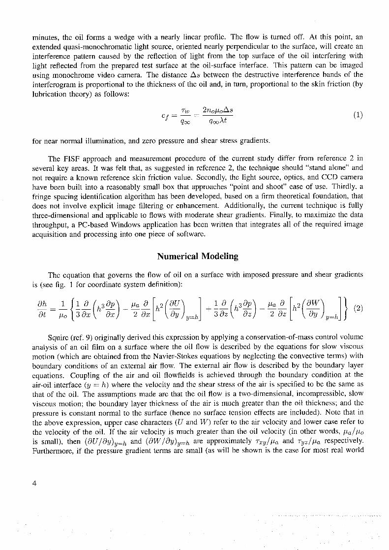
The equation that governs the flow of oil on a surface with imposed pressure and shear gradients

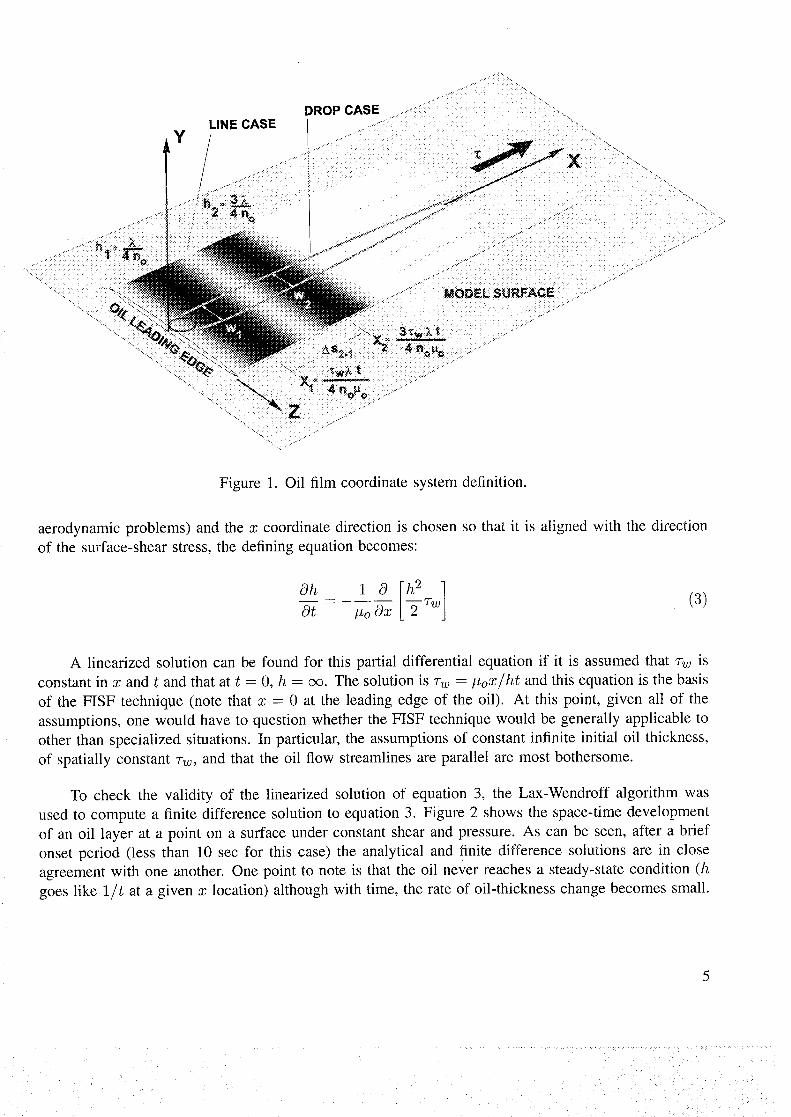
is (see fig. 1 for coordinate system definition):

{ [()] a [h2( w/ 1},2,Oh 1 1 0 /, 3 0P ) Pa 0 h20U + -3--_z _ tt -_z ] 20z _ y:hat .o 2 ox -Cv y=h

Squire (ref. 9) originally derived this expression by applying a conservation-of-mass control volume

analysis of an oil film on a surface where the oil flow is described by the equations for slow viscous

motion (which are obtained from the Navier-Stokes equations by neglecting the convective terms) with

boundary conditions of an external air flow. The external air flow is described by the boundary layer

equations. Coupling of the air and oil flowfields is achieved through the boundary condition at the

air-oil interface (y = h) where the velocity and the shear stress of the air is specified to be the same as

that of the oil. The assumptions made are that the oil flow is a two-dimensional, incompressible, slow

viscous motion; the boundary layer thickness of the air is much greater than the oil thickness; and the

pressure is constant normal to the surface (hence no surface tension effects are included). Note that in

the above expression, upper case characters (U and W) refer to the air velocity and lower case refer to

the velocity of the oil. If the air velocity is much greater than the oil velocity (in other words, #a/#o

is small), then (OU/Oy)y= h and (OW/Oy)y= h are approximately "rxy/Pa and "ryz/#a respectively.

Furthermore, if the pressure gradient terms are small (as will be shown is the case for most real world

..>

Figure 1. Oil film coordinate system definition.

aerodynamic problems) and the x coordinate direction is chosen so that it is aligned with the direction

of the surface-shear stress, the defining equation becomes:

10I 21Ot - Ox -2 (3)

A linearized solution can be found for this partial differential equation if it is assumed that _-w is

constant in x and t and that at t = 0, h = oo. The solution is _-w = #ox/ht and this equation is the basis

of the FISF technique (note that x = 0 at the leading edge of the oil). At this point, given all of the

assumptions, one would have to question whether the FISF technique would be generally applicable to

other than specialized situations. In particular, the assumptions of constant infinite initial oil thickness,

of spatially constant _-w, and that the oil flow streamlines are parallel are most bothersome.

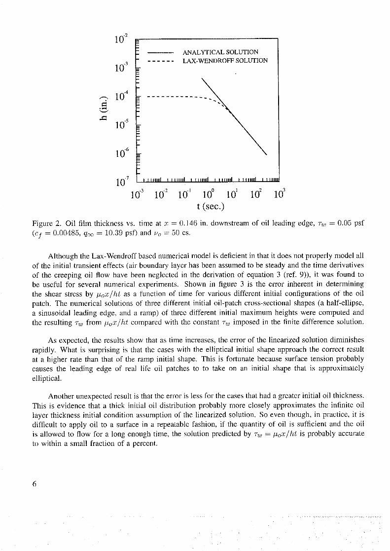
To check the validity of the linearized solution of equation 3, the Lax-Wendroff algorithm was

used to compute a finite difference solution to equation 3. Figure 2 shows the space-time development

of an oil layer at a point on a surface under constant shear and pressure. As can be seen, after a brief

onset period (less than 10 sec for this case) the analytical and finite difference solutions are in close

agreement with one another. One point to note is that the oil never reaches a steady-state condition (h

goes like lit at a given x location) although with time, the rate of oil-thickness change becomes small.

10 -2

10.3

-= 10-5

10

10.7

ANALYTICAL SOLUTION

LAX-WENDROFF SOLUTION

I IIIIIIII I Illlllll I III1|111 a | IIlIIll I IllIIIl] 1 II1111

lo 3 lO 2 lo' 10° 101 102 103

t (sec.)

Figure 2. Oil film thickness vs. time at z = 0.146 in. downstream of oil leading edge, 7-w = 0.05 psf

(cf = 0.00485, qoo = 10.39 psf) and Uo = 50 cs.

Although the Lax-Wendroff based numerical model is deficient in that it does not properly model all

of the initial transient effects (air boundary layer has been assumed to be steady and the time derivatives

of the creeping oil flow have been neglected in the derivation of equation 3 (ref. 9)), it was found to

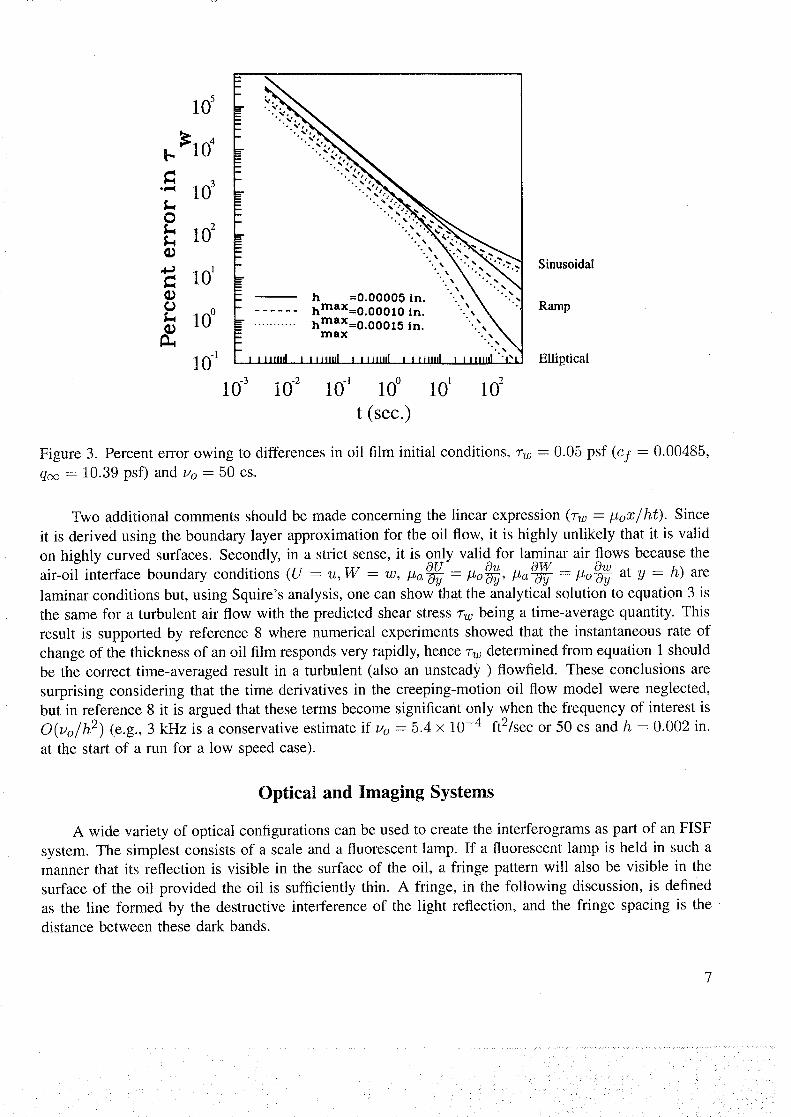
be useful for several numerical experiments. Shown in figure 3 is the error inherent in determining

the shear stress by #oz/ht as a function of time for various different initial configurations of the oil

patch. The numerical solutions of three different initial oil-patch cross-sectional shapes (a half-ellipse,

a sinusoidal leading edge, and a ramp) of three different initial maximum heights were computed and

the resulting Tw from #oz/ht compared with the constant _-w imposed in the finite difference solution.

As expected, the results show that as time increases, the error of the linearized solution diminishes

rapidly. What is surprising is that the cases with the elliptical initial shape approach the correct result

at a higher rate than that of the ramp initial shape. This is fortunate because surface tension probably

causes the leading edge of real life oil patches to to take on an initial shape that is approximately

elliptical.

Another unexpected result is that the error is less for the cases that had a greater initial oil thickness.

This is evidence that a thick initial oil distribution probably more closely approximates the infinite oil

layer thickness initial condition assumption of the linearized solution. So even though, in practice, it is

difficult to apply oil to a surface in a repeatable fashion, if the quantity of oil is sufficient and the oil

is allowed to flow for a long enough time, the solution predicted by 7-w = #oX/ht is probably accurate

to within a small fraction of a percent.

10 5

b_104

•,-, 10 3

O10 2

tl)

• " 0'1

¢)10 °

ID

10-'

•.°

°.

• • %'

-• %'

°••%•

•..

• °. %

..%

-•%

•.%

h =0.00005 in....... hmax=o,o0010 in.

........... hmax=0.00015 In.msx

°.'_

•..%%

• ° %

10- 3 10 .2 10.' 10 ° 10' 10:

t (sec.)

Sinusoidal

Ramp

Elliptical

Figure 3. Percent error owing to differencesin oil film initialconditions, vw = 0.05 psf(cf =0.00485,

qec= 10.39 psD and uo= 50 cs.

Two additional comments should be made concerning the linear expression (rw = #oX/ht). Since

it is derived using the boundary layer approximation for the oil flow, it is highly unlikely that it is valid

on highly curved surfaces. Secondly, in a strict sense, it is only valid for laminar air flows because theOU Ou OW Ow

air-oil interface boundary conditions (U = u, W = w, #a-0-_ = #o9-_, #a W = #o-8_ at y = h) are

laminar conditions but, using Squire's analysis, one can show that the analytical solution to equation 3 is

the same for a turbulent air flow with the predicted shear stress rw being a time-average quantity. This

result is supported by reference 8 where numerical experiments showed that the instantaneous rate of

change of the thickness of an oil film responds very rapidly, hence rw determined from equation 1 should

be the correct time-averaged result in a turbulent (also an unsteady ) flowfield. These conclusions are

surprising considering that the time derivatives in the creeping-motion oil flow model were neglected,

but in reference 8 it is argued that these terms become significant only when the frequency of interest is

O(uo/h 2) (e.g., 3 kHz is a conservative estimate if Uo = 5.4 x 10 -4 ft2/sec or 50 cs and h = 0.002 in.

at the start of a run for a low speed case).

Optical and Imaging Systems

A wide variety of optical configurations can be used to create the interferograms as part of an FISF

system• The simplest consists of a scale and a fluorescent lamp. If a fluorescent lamp is held in such a

manner that its reflection is visible in the surface of the oil, a fringe pattern will also be visible in the

surface of the oil provided the oil is sufficiently thin. A fringe, in the following discussion, is defined

as the line formed by the destructive interference of the light reflection, and the fringe spacing is the

distance between these dark bands.

Since a fluorescent lamp is not a monochromatic light source, the fringes will be made up of several

different colored bands but a rough measurement using a scale can still be made between bands of the

same color. If an interference filter (a narrow bandpass filter) is placed between the light source and the

oil, only the spectral components near the center wavelength of the filter will be transmitted resulting

in a quasi-monochromatic fringe pattern.

A relatively inexpensive yet accurate and highly portable optical system can be made by substituting

an HeNe laser diode and a spherical lens for the light bulb in a lighted reticle (all necessary components

available through Edmund Scientific, Barrington, N J). A note of caution: Some lasers (particularly laser

diodes) can have significant wavelength dependencies on ambient temperature.

In an attempt to improve upon the optical system used in reference 2, several different types

of light sources in combination with lens, filters, diffuser sheets, and test surfaces were tried. The

various optical system configurations were investigated by using the FISF technique to evaluate the

interferometric image created by a channel-flow shear field.

The 0.25 × 2.0 in. channel flow facility is a shop-air powered rectangular channel that is 48 in.

long with inlet flow conditioning and interchangeable test surfaces. Under normal operating conditions

(q_ = 2.1 in, water, d h = 0.44 in., and Redh = 2.3 × 104), a fully developed channel flow with a

uniform shear field and a nominal constant cf of 0.00485 is created. The reference test surface was a

piece of 0.25 in. thick SF11 Schott glass polished to better than 60/40 scratch and dig, and coated on the

back side with 1/4 wave MgF1 to minimize reflections of the light from the back-side glass-air interface

back through the oil. This particular glass has an index of refraction of 1.78 giving a theoretical fringe

visibility of u = 0.94 (for n = 1.3, silicone oil).

Initially, it was thought that a laser would be the best light source choice because lasers are highly

monochromatic and have the desirable characteristic of a coherence length that is many times the oil

layer thickness (measured in inches to feet for gas lasers and typically less than 0.040 in. for HeNe diode

lasers). This proved not to be the case because of difficulties with speckle. The peak-to-peak intensity

variation of the first fringe on SFll glass was 121 intensity levels (using an 8-bit camera which has

256 levels in total) with the speckle causing a 20 intensity-level variation superimposed on that of the

interferogram. Unfortunately, short of applying exotic techniques (e.g., a rotating ground glass piece in

the light path), there is no easy way to avoid the speckle that will be present in systems with highly

coherent light sources and diffusing optical components.

Another approach attempted was to use a thermal source (Philips Halogen spot lamp model

PAR16/H/NSR Philips Lighting Company, Somerset, NJ) combined with a bandpass interference filter.

The OCLI (Santa Rosa, CA) Green Dichroic filter had an FWHM (full width measured at half trans-

mittance) of 2.76 × 10 -6 in. (70 nm) centered on a wavelength of 2.13 × 10 -5 in. (540 nm). The

peak-to-peak intensity variation of this combination was quite poor, being less than 30 intensity levels.

In addition, the amount of heat generated by this source was potentially damaging to the interference

filter and the pellicle beam splitter.

The light source finally settled on was a green 9-watt compact fluorescent lamp (Osram Corp. model

F9TT/Green, Montgomery, NY). This lamp has a sharp spectral peak at 2.13 × 10 -5 in. (542 rim) and

several much smaller peaks approximately 1.58 to 1.97 × 10 -6 in. (40-50 rim) to either side of the main

. : .......... : ......... !

peak and farther away. These additional peaks were effectively blocked by the OCLI green interference

filter. The Osram lamp has a coherence length of 5.9 x 10 -5 in. (15 #m), nearly 30 times the path

difference at the first fringe. The first-fringe peak-to-peak intensity variation was 124 intensity levels

on SFll glass and additionally, the lamp runs fairly cool.

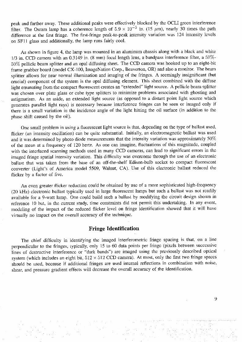
As shown in figure 4, the lamp was mounted in an aluminum chassis along with a black and white

1/3 in. CCD camera with an 0.3149 in. (8 mm) focal length lens, a bandpass interference filter, a 5(?%-

50% pellicle beam splitter and an opal diffusing sheet. The CCD camera was hooked up to an eight-bit

frame grabber board (model CX-100, ImageNation Corp., Beaverton, OR) and also a monitor. The beam

splitter allows for near normal illumination and imaging of the fringes. A seemingly insignificant (but

crucial) component of the system is the opal diffusing element. This sheet combined with the diffuse

light emanating from the compact fluorescent creates an "extended" light source. A pellicle beam splitter

was chosen over plate glass or cube type splitters to minimize problems associated with ghosting and

astigmatism. As an aside, an extended light source (as opposed to a distant point light source which

generates parallel light rays) is necessary because interference fringes can be seen or imaged only if

there is a small variation in the incidence angle of the light hitting the oil surface (in addition to the

phase shift caused by the oil).

One small problem in using a fluorescent light source is that, depending on the type of ballast used,

flicker (an intensity oscillation) can be quite substantial. Initially, an electromagnetic ballast was used

and it was determined by photo diode measurements that the intensity variation was approximately 50%

of the mean at a frequency of 120 hertz. As one can imagine, fluctuations of this magnitude, coupled

with the interlaced scanning methods used in many CCD cameras, can lead to significant errors in the

imaged fringe spatial intensity variation. This difficulty was overcome through the use of an electronic

ballast that was taken from the base of an off-the-shelf Edison-bulb socket to compact fluorescent

converter (Light's of America model 5509, Walnut, CA). Use of this electronic ballast reduced the

flicker by a factor of five.

An even greater flicker reduction could be obtained by use of a more sophisticated high-frequency

(20 kHz) electronic ballast typically used in large fluorescent lamps but such a ballast was not readily

available for a 9-watt lamp. One could build such a ballast by modifying the circuit design shown in

reference 10 but, in the current study, time constraints did not permit this undertaking. In any event,

modeling of the impact of the reduced flicker level on fringe identification showed that it will have

virtually no impact on the overall accuracy of the technique.

Fringe Identification

The chief difficulty in identifying the imaged interferometric fringe spacing is that, on a line

perpendicular to the fringes, typically, only 15 to 60 data points per fringe (pixels between successivelines of destructive interference or "dark bands") are imaged using the previously described optical

system (which includes an eight bit, 512 × 512 CCD camera). At most, only the first two fringe spaces

should be used, because if additional fringes are used internal reflections in combination with noise,

shear, and pressure gradient effects will decrease the overall accuracy of the identification.

9

? ) • •

CHASSIS

FRAME GRABBER TRIGGER

8-BIT CCD CAMERA

BAFFLE

CAMERA LENS

COMPACT FLUORESCENT

LIGHT SOURCE

50/50 PELLICLEBEAMSPLITTER

INTERFERENCE FILTER ANDOPAL DIFFUSING ELEMENT

............."...... /• i,: •:-_- _ _iiiiiiii;iiiiiiii_!;i;_i_;i;i_ii_ii!ii_:i_i_ii:iiii!_:Iiiii_iiii_iiiiiiiiiiiiiIiiii_iiiii_iiiii;i:i;__" i ¸¸ _ _ i:iiiiiiii::::iiiii:::iii:i:i::::iiii:iiiiiii_i::_::ii:::::::i

;' _.. i;iiiiiiii illiiiii!iiii:::;!iii_i;:_:_:iii_i!ii

,, _:iiiiii_:iiiii_i_iii:_iiiiiiiiiii_iiiiiiiii_i!iiiiiiii!iii_ii_ii!iii!iIiiii_iiiiiiiii_iii!iiiiiiii!!i_iiiiiii_i_ii!i

Figure 4. The FISF instrument box

i_i::::_:::::!i:!:!!::i_i!!!_i!::::::i:::::',::i:!i:::::1::!:1_:ii_:_::::::::::::::::::::::::::::::::::::::::::::::::::::::::::::::::::::::::::::::::::::::::::::::::::::::::::::::::::::

iiiii!i!iiiiiiiiiiiiiiiUiiiiiiiiiiiiiiiiiiiiiiiiiiiiiiiiiiiiiiiiiiiiiiiiiii!iiii_!:i::::i::: :::::::::::::::::::::::::::::::::::::::::::::::::::::::::::::::::::::::::::::::::

:i::i!:: :::::::::::::::::::::::::::::::::::::::::::::::::::::::::::::::::::::::::::::::::::::::::::::::::::::::::::::::::::::::::::::::

i:il1iiii;:':'j::iii:;iil;:i:;;iiii;:i;i:ii;iiiiiiiiiiiii;;;iiii:i?iiiiii)ii)iiiii;i:g

'cover removed).

10

Several approaches to identification of the fringe spacing were attempted in the current study,

namely, techniques that involved fast Fourier transforms, linear least-squares curve fitting, correlation of

trigonometric fl fions, maximum entropy determination (ref. 11) and nonlinear least-squares regression.

With the exe ,n of the nonlinear least-squares regression approach, the other approaches were found

to be inade .::::::::::::::

:::: i)

In the cases of the fast Fourier transform and maximum entropy methods, the record length (number

of pixels imaged) was too few to achieve sufficient resolution of the spectral peaks. Additionally, with

short records, FFTs shift the spectral maximums. In fact, it has been shown that when the record length

of a truncated sinusoid is less than 0.58 times the period, the spectral peak is found at zero (ref. 11).

The piecewise polynomials approach--where polynomials were fitted to the fringe-pattern crests

and troughs and fringe spacings determined--failed because the local effect of "noise" (undesirable

effects arising from background irregularities, the CCD camera, and lighting nonuniformities) over-

whelmed the local data fits.

A slightly more successful but not wholly satisfactory approach involved maximizing the product of

a cosine function (with wavelength and phase as variable parameters) and the imaged signal. The basis

of this approach is that, theoretically, the spatial intensity variation of an interferogram is describable

by trigometric functions. The downfall of this "correlation" approach is that a simple cosine variation

does not include the effect of intensity variations arising from curved surfaces and nonuniform lighting.

Consequently, in these cases correlation maximums were found for fringe spacings that were obviously

erroneous.

The marginal success of the "correlation" approach led to the development of a general fringe-

intensity-variation model. The intensity distribution of simple interferogram (Young's fringes) created by

the interference of two beams of monochromatic light of equal intensity and initially in phase with each

other is I _ A 2 = 2a2(1 + cos(5). Based on this expression, one can imagine that the intensity variation

of an interferogram of greater complexity, such as that generated on a surface with mild curvature,

illuminated with slightly nonuniform light, could be represented by a nonlinear function constructed

using quadratics as follows:

I=B 1 q-B2sq-B3s2-t - [El-l-E2,sq-E3s2]eos[Plq-P28+r382] (4)

This model, which is similar to that used in reference 12, has nine parameters, each of which has

physical significance. The trick is to determine the unknown t3, E, and P coefficients so that equation 4

best represents the digitized intensity variation. For this task, the quasi-Newton method was used as

described in reference 13. In short, the numerical technique uses an initial "best guess" for/3, E; and P

of the intensity variation and then iterates until the difference between the discrete input data points and

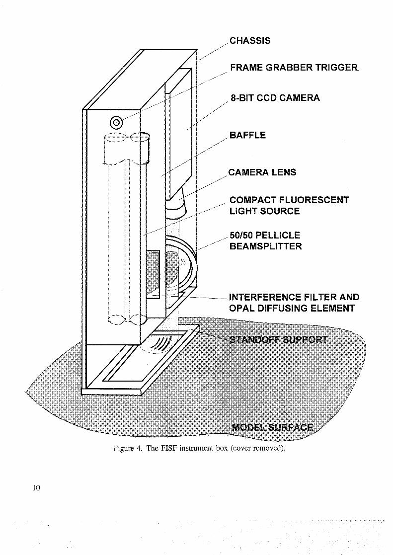
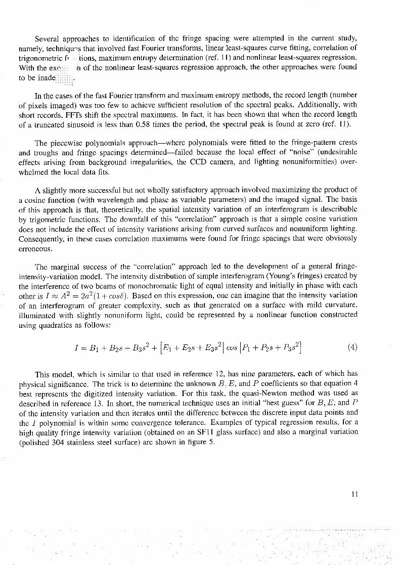
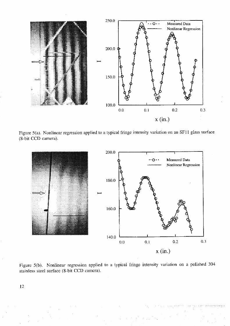
the I polynomial is within some convergence tolerance. Examples of typical regression results, for a

high quality fringe intensity variation (obtained on an SFll glass surface) and also a marginal variation

(polished 304 stainless steel surface) are shown in figure 5.

11

....... • ....... ....... • ..:> J ¸¸.%.¸• ........... ._ :> • •

250.0

200.0

150.0

100.0

!

Measured Data

Nonlinear Regression

I I

0.0 0.1 0.2 0.3

x (in.)

Figure 5(a). Nonlinear regression applied to a typical fringe intensity variation on an SF11 glass surface

(8-bit CCD camera).

i!iiii!iiiiiiii_!iii!__

iiiiiiiiiiiiiiii!_i_

200.0 [ _

•" O" • Measured Data

Nonlinear Regression

180.0

160.0 "__

140.0

0.0 0.1 0.2 0.3

x (in.)

Figure 5(b). Nonlinear regression applied to a typical fringe intensity variation on a polished 304

stainless steel surface (8-bit CCD camera).

12

There are a couple of difficulties. If the initial guess is not a reasonable one, the convergence

process can get trapped in a local minimum. Also, extremely noisy input data can cause convergence

problems. In most cases, the method is reliable and, as will be shown, fairly accurate.

In the current approach, a weighting function has been implemented in the quasi-Newton method so

that the error between the output polynomial and the input data is minimized when dI/ds is high. High

dI/ds occurs midway between the destructive and constructive interference bands. The justification for

use of weighting is that the effect of noise in the signal of the CCD based imaging system has the least

impact where the intensity variations are large.

Fringe Visibility

As stated in the Introduction, obtaining good fringe visibility when using the FISF technique under

less than ideal conditions can be difficult. Fringe visibility can be defined as u = (Imam- Imin)/

(Imaz + Imin) (where Imaz and Irain are the fringe intensity maximums and minimums) and is ameasure of the contrast between the bands of constructive and destructive interference.

Theoretically, for the FISF technique, the maximum fringe visibility (u = 1.0) is achieved on a

surface of n = 2.0 (for n = 1.4 silicone oil) observed at infinity with an extended monochromatic

source. The constraints in most real life measurement situations usually result in fringe visibilities of

0.5 or less. For instance, wind tunnel models are usually made of less than optimal interferometry

surface materials such as steel or aluminum, and these models must be polished to near mirror-quality

finish or be coated by a material with more desirable optical properties.

The ideal FISF surface has the properties of being very smooth (60/40 scratch and dig, or better),

has optical properties that remain constant (does not haze or corrode over time), can be cleaned and

reused, and is scratch resistant. As part of the current study, many different kinds of coatings were

tried, and although nothing approaching the quality of a dense flint glass was identified, a few acceptable

coatings were found.

Shown in table 1 are the results of an investigation into several candidate surface materials. The

data were obtained using the FISF system (shown in fig. 4) and channel test facility previously described.

A line of Uo = 5.4 × 10 -4 ft2/sec (50 cs) oil was placed on a candidate surface in the channel, and

fringes were generated under constant shear conditions. The resulting cf measurements were within

5°/o of each other (better than the FISF uncertainty quoted in ref. 2) for all of the surfaces studied. This

is additional evidence that surface tension effects have a minimal impact on FISF measurements. Each

datapoint in table 1 is an average over ten trials of first fringe data. In evaluating a candidate surface

material, the most useful data is the peak-to-peak first fringe intensity measurement Up-p) since the

overall accuracy of an FISF measurement is directly related to this quantity. Also presented are values

for I(p_p)r,_s, which can be considered to be a measure of the quality of the fringes, and Iavg, which

is average intensity of the imaged fringe.

A couple of disclaimers are in order. It was found that the index of refraction of the surface material

can vary by a significant amount depending on the surface preparation, the material batch, oxidation, and

other factors. In addition, the automatic electronic shuttering capability of the CCD camera determines

13

_ i/_i: ii:ii _ _ _i!iii _ i ilill i

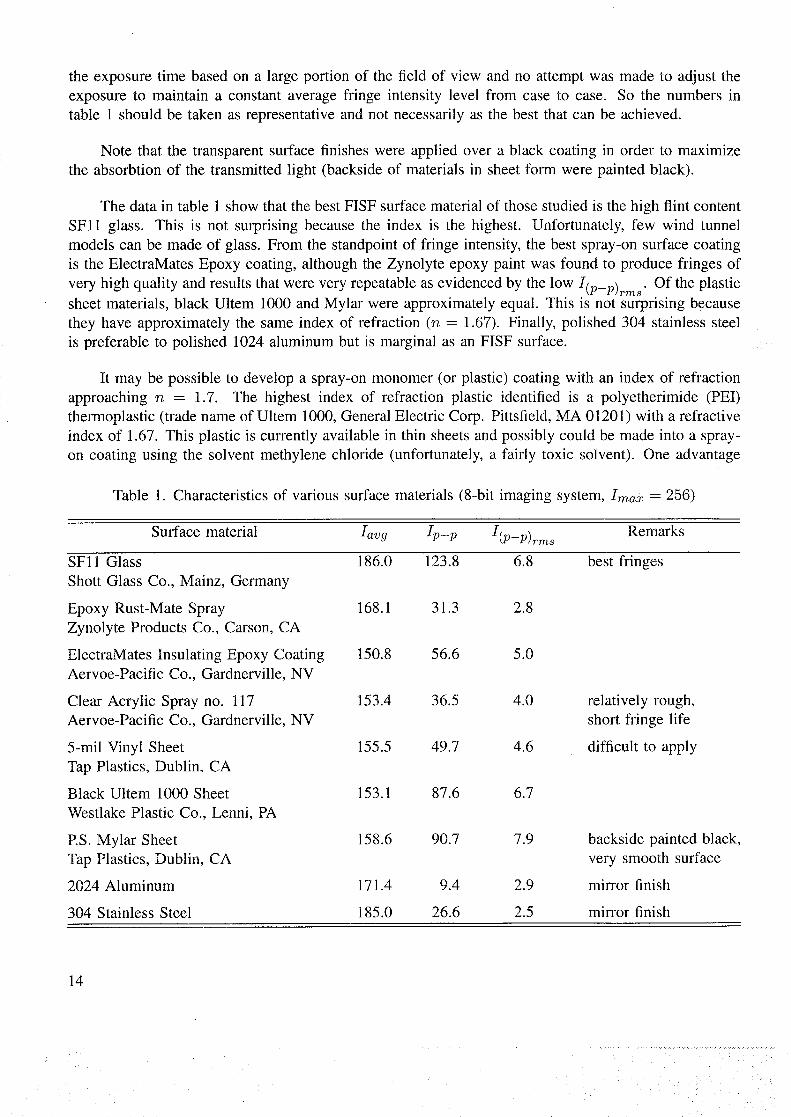
theexposuretime basedon a largeportion of thefield of view andno attemptwasmadeto adjusttheexposureto maintain a constantaveragefringe intensity level from caseto case. So the numbersintable 1 shouldbe takenasrepresentativeandnot necessarilyasthebest that canbe achieved.

Note that the transparentsurfacefinisheswereappliedover a black coating in order to maximizethe absorbtionof the transmittedlight (backsideof materialsin sheetform werepaintedblack).

Thedatain table 1showthatthebestFISFsurfacematerialof thosestudiedis thehigh flint contentSFll glass. This is not surprisingbecausethe index is the highest. Unfortunately,few wind tunnelmodelscanbemadeof glass.From thestandpointof fringe intensity,thebestspray-onsurfacecoatingis theElectraMatesEpoxy coating,althoughthe Zynolyteepoxypaint wasfound to producefringesofveryhigh quality andresultsthatwereveryrepeatableasevidencedby the low I(p_p)rm s. Of the plastic

sheet materials, black Ultem 1000 and Mylar were approximately equal. This is not surprising because

they have approximately the same index of refraction (n = 1.67). Finally, polished 304 stainless steel

is preferable to polished 1024 aluminum but is marginal as an FISF surface.

It may be possible to develop a spray-on monomer (or plastic) coating with an index of refraction

approaching n = 1.7. The highest index of refraction plastic identified is a polyetherimide (PEI)

thermoplastic (trade name of Ultem 1000, General Electric Corp. Pittsfield, MA 01201) with a refractive

index of 1.67. This plastic is currently available in thin sheets and possibly could be made into a spray-

on coating using the solvent methylene chloride (unfortunately, a fairly toxic solvent). One advantage

Table 1. Characteristics of various surface materials '8-bit imaging system, Imaz = 256)

Surface material Iav9 Ip-p I(p_p)rm s Remarks

SFll Glass 186.0 123.8

Shott Glass Co., Mainz, Germany

Epoxy Rust-Mate Spray 168.1 31.3

Zynolyte Products Co., Carson, CA

ElectraMates Insulating Epoxy Coating 150.8 56.6

Aervoe-Pacific Co., Gardnerville, NV

Clear Acrylic Spray no. 117 153.4 36.5

Aervoe-Pacific Co., Gardnerville, NV

5-mil Vinyl Sheet 155.5 49.7

Tap Plastics, Dublin, CA

Black Ultem 1000 Sheet 153.1 87.6

Westlake Plastic Co., Lenni, PA

RS. Mylar Sheet 158.6 90.7

Tap Plastics, Dublin, CA

2024 Aluminum 171.4 9.4

304 Stainless Steel 185.0 26.6

6.8 best fringes

2.8

5.0

4.0 relatively rough,

short fringe life

4.6 difficult to apply

6.7

7.9 backside painted black,

very smooth surface

2.9 mirror finish

2.5 mirror finish

14

of this plastic is that it can be flame polished (approximately 650_F melting point) to remove small

surface imperfections. Application of the FISF technique on an Ultem 1000 surface should result in a

theoretical fringe visibility of 0.82.

Pressure Gradient Effects

The effect of pressure gradients on FISF measurements is very small and can be ignored in virtually

all cases. By examining the order of magnitude of the terms in equation 2, it can be seen that the pressure

gradient terms are at least two orders of magnitude smaller than the shear stress terms for most flows

of aerodynamic interest.

Direct evidence of the insignificance of pressure gradient effects was obtained through numerical

experiments using the Lax-Wendroff code discussed previously with the streamwise pressure gradient

term included. Cases of high shear and high pressure gradient, similar to that found on the leading edge

of a wing (cf = 0.01 and dCp/dz = -0.42/in.), and also cases of low shear and moderate pressure

gradient (cf = 0.0005 and dCp/dx = -0.05/in.) were computed. For the worst case studied, the

impact of pressure gradients was only 0.14% of cf.

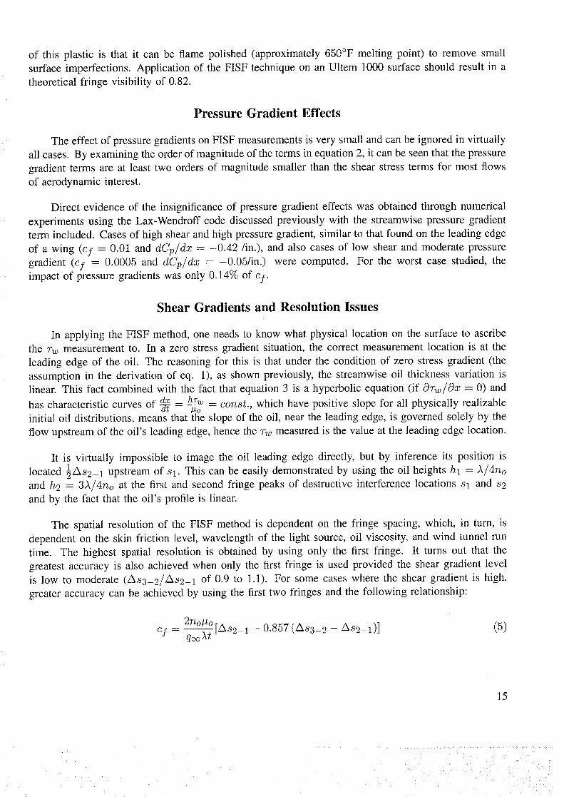
Shear Gradients and Resolution Issues

In applying the FISF method, one needs to know wha physical location on the surface to ascribe

the _w measurement to. In a zero stress gradient situation, the correct measurement location is at the

leading edge of the oil. The reasoning for this is that under the condition of zero stress gradient (the

assumption in the derivation of eq. 1), as shown previously, the streamwise oil thickness variation is

linear. This fact combined with the fact that equation 3 is a hyperbolic equation (if OTw/Ox = 0) and

has characteristic curves of @ = _ = const., which have positive slope for all physically realizablea_: _o

initial oil distributions, means that the slope of the oil, near the leading edge, is governed solely by the

flow upstream of the oil's leading edge, hence the "rw measured is the value at the leading edge location.

It is virtually impossible to image the oil leading edge directly, but by inference its position is

located ½As2-1 upstream of Sl. This can be easily demonstrated by using the oil heights hi = A/4no

and h2 = 3A/4no at the first and second fringe peaks of destructive interference locations sl and s2

and by the fact that the oil's profile is linear.

The spatial resolution of the FISF method is dependent on the fringe spacing, which, in turn, is

dependent on the skin friction level, wavelength of the light source, oil viscosity, and wind tunnel run

time. The highest spatial resolution is obtained by using only the first fringe. It turns out that the

greatest accuracy is also achieved when only the first fringe is used provided the shear gradient level

is low to moderate (/ks3_2//k82_l of 0.9 to 1.1). For some cases where the shear gradient is high,

greater accuracy can be achieved by using the first two fringes and the following relationship:

2nopo [As2_1 - o.s57 (As3_2 - As2_1)]Cf- qocAt

(5)

15

• /

........................... ..... : . :7 ¸¸ - - : -: i ¸

_ _ ,: _ : _i V_ _ • _ :

• • _ • , • • i ii_: i__I_I_ i_i

This expression was arrived at through a minimization process wherein the constant (0.857, above)

was varied until the difference between the cf predicted from the above equation and the value prescribed

at the leading edge of the oil in a numerical solution of equation 3 was a minimum over a range of

shear and shear gradient levels (-0.015 < dcf/dx >_ 0.015 /in., which are the maximum gradient

levels typically encountered on wings and 0.002 _< cf > 0.01). Note that equation 1 is recovered when

A83_ 2 = As2_ 1 (zero shear gradient).

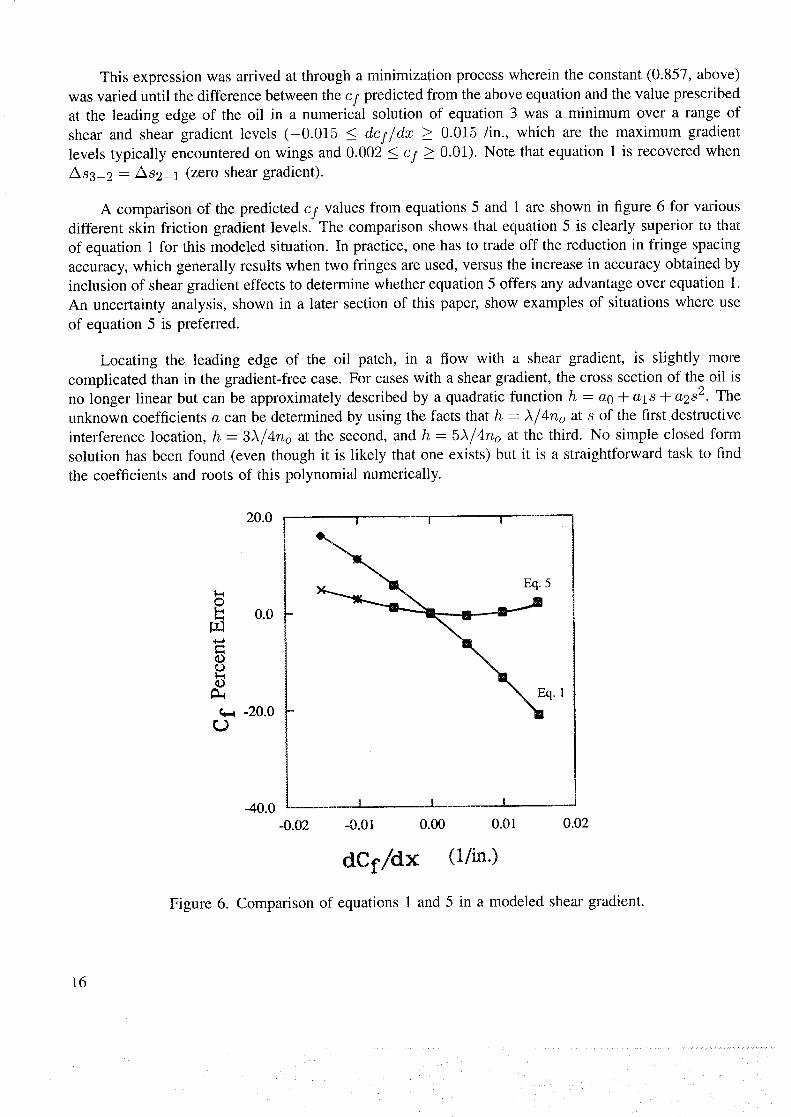
A comparison of the predicted cf values from equations 5 and 1 are shown in figure 6 for various

different skin friction gradient levels. The comparison shows that equation 5 is clearly superior to that

of equation 1 for this modeled situation. In practice, one has to trade off the reduction in fringe spacing

accuracy, which generally results when two fringes are used, versus the increase in accuracy obtained by

inclusion of shear gradient effects to determine whether equation 5 offers any advantage over equation 1.

An uncertainty analysis, shown in a later section of this paper, show examples of situations where use

of equation 5 is preferred.

Locating the leading edge of the oil patch, in a flow with a shear gradient, is slightly more

complicated than in the gradient-free case. For cases with a shear gradient, the cross section of the oil is

no longer linear but can be approximately described by a quadratic function h = a0 + alS + a2 s2. The

unknown coefficients a can be determined by using the facts that h = ,_/4no at s of the first destructive

interference location, h = 3,k/4no at the second, and h = 5,_/4no at the third. No simple closed form

solution has been found (even though it is likely that one exists) but it is a straightforward task to find

the coefficients and roots of this polynomial numerically.

20.0 | ! I

Eq. 5

I I

0.00 0.01 0.02

dCf/dx (1/in.)

Figure 6. Comparison of equations 1 and 5 in a modeled shear gradient.

16

Often, it is desirable to be able to quote a numerical spatial resolution value for a measurement. In

a three-dimensional flow, such a number for the FISF technique must have a component in the surface

that is perpendicular to the skin friction direction (measurement volume width). Since one of the key

assumptions in the derivation of equation 1 is that the oil flow is locally two-dimensional, it stands to

reason that the measurement volume width must be at least 50 times the thickness of the oil for a locally

two-dimensional approximation to be reasonably accurate. For a one-fringe space measurement, taking

into account the way the fringe spacing algorithm functions, the measurement volume length would3A

be approximately _As2-1 and the width would be 50 × (2-g-go) (if A -- 2.13 × 10 .5 in. or 542 nm,

no = 1.4, As2_1 = 0.12 in., then measurement volume length = 0.105 in. and width = 0.0012 in.) Note

that for most CCD based imaging systems, the measurement volume width is sub pixel. Additional

numerical experiments should be performed to confirm this spatial resolution analysis.

Extension to Three Dimensions

The FISF method developed in reference 2 is a two-dimensional technique that can readily be

extended to three dimensions if a drop of oil is used as opposed to a line of oil. The skin friction

magnitude is determined, as before, by measuring the fringe spacing. The direction of the skin friction

vector is found by determining the orientation of the oil pathline measured in the vicinity of the leading

edge of the oil relative to a fixed coordinate system. The essence of this idea was originally proposed

in reference 5, and comparisons of "rw from interferograms of oil lines and drops in a two-dimensional

flow were made, but the potential of this approach was not further developed.

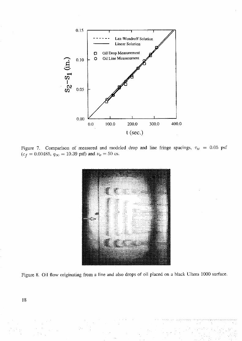
The main issue concerning the use of a drop is whether the assumptions used in deriving equation 1

are valid. This appears to be the case, as shown in figure 7 where a comparison of the fringe-spacing

time histories of a line and drop are presented (note that in fig. 7 the Lax-Wendroff and linear solution

results are for the oil-line case and are indistinguishable from each other). These data were measured

in the two-dimensional channel facility. One can see that the measured fringe spacing is the same for

a drop and a line within the accuracy limits of the FISF technique. This should not be a total surprise

because the high initial oil thinning rate quickly drives even a very small drop to within the bounds of

the underlying assumption of a two-dimensional flow (on the symmetry plane of the drop).

As will be shown later, in the case of two-dimensional flow, the total cf measurement uncertainty

is less for the oil-line case in comparison to oil drops, but in a three-dimensional flow the uncertainty

is approximately the same. The use of oil drops has the added advantage of allowing one to determine

the cf vector direction.

To maximize the directional accuracy, the size of the drop should be made as small as the imaging

system will allow. To maintain the assumption of a locally two-dimensional oil flow, the drop-diameter

lower limit is quite small (roughly 50 x _ or 0.0012 in.).

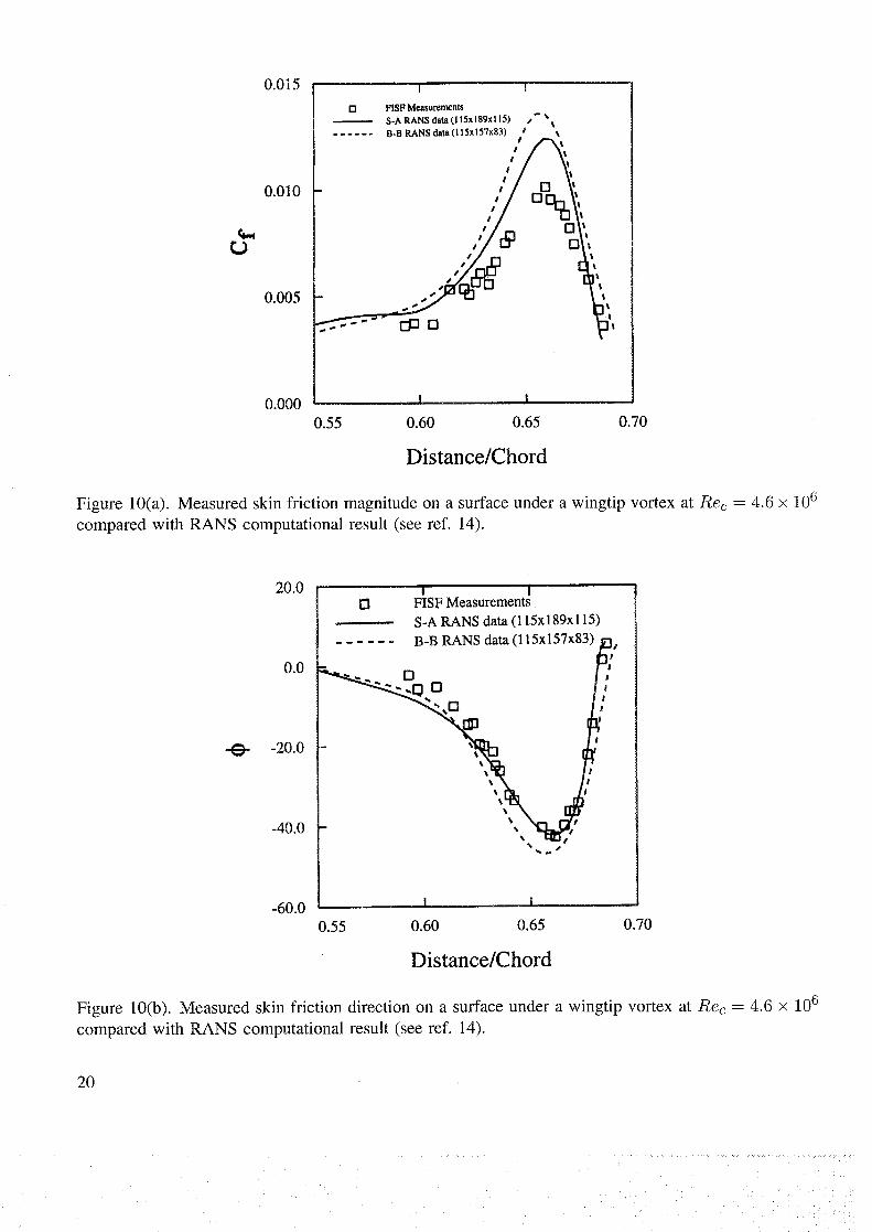
Shown in figure 8 is a comparison of fringe patterns for a drop and line taken in the channel flow

facility on an Ultem 1000 surface. The fringes created by the drops are curved but the fringe spacing is

relatively constant across the drop. At the extreme edges of the drop, the curvature of the fringe pattern

is the greatest, giving a visual indication of where oil thickness variation violates the assumptions of

the FISF technique.

17

0.15

"'2", 0.10

turk 0.05

0.00

I I I

...... Lax-Wendroff Solution

Linear Solution j

1:3 Oil Drop Measurement _"

0.0 100.0 200.0 300.0 400.0

t (sec.)

Figure 7. Comparison of measured and modeled drop and line fringe spacings, "rw = 0.05 psf

(cf = 0.00485, qec = 10.39 psf) and Uo = 50 cs.

Figure 8. Oil flow originating from a line and also drops of oil placed on a black Ultem 1000 surface.

18

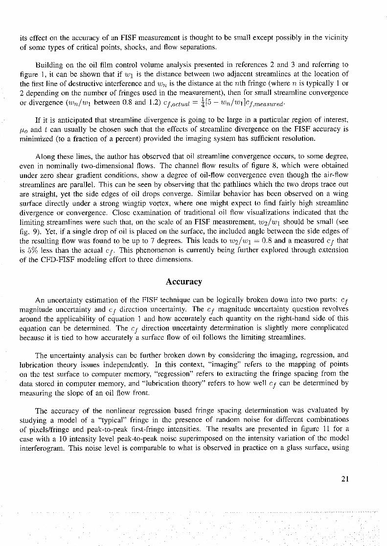
To demonstrate the capability of this approach to a greater degree, the skin friction distribution

(magnitude and direction) along a spanwise oriented line on the surface of a wingtip (directly under the

streamwise wingtip vortex) was measured and compared to Reynolds-averaged Navier-Stokes (RANS)

predictions. The Reynolds number was 4.6 million, o_ = 10 °, and the boundary layer was tripped near

the naturally ocurring transition location of 2% chord. In the RANS computations, the Baldwin-Barth

(B-B) and the Spalart-Allmaras (S-A) turbulence models were used on grids of 115 x 157 x 83 and

115 x 189 × 115 points respectively. For further information on the computational approach and also

for the complete computed wingtip-vortex surface cf distribution, see reference 14.

Figure 9 shows a typical image of the wingtip oil-drop fringes, and the the cf comparison is

shown in figure 10. The agreement with these state-of-the-art computations is poor, In a sense, this

is a welcome result because the discrepancy can mostly be attributed to the inability of turbulence

models to function correctly in highly three-dimensional flows and underscores the need for accurate

Tw measurements in such flows.

In preparation for these measurements, a flat-bed pen plotter was used to draw and label a 12 x 16

fiducial grid (0.62 in. square cells) on 8 1/2 in. by 11 in. sheets of 2 mil black Ultem 1000. These sheets

were then adhered to the suction side of the the wing surface using 3M General Purpose Spray Adhesive

201 (3M Adhesive Systems, St. Paul MN). The edges were further bonded using cyanoacrylate.

There is one small complication with the extension of the FISF approach to three dimensions, that

being the effects of surface streamline convergence or divergence in the air and oil flows. The main

difficulty is that equation 1 was derived based on the assumption of parallel limiting streamlines. In

virtually all three-dimensional flows, streamline divergence is present to some degree but, fortunately,

Figure 9. Oil flow originating from drops of oil on a black Ultem 1000 film under a wingtip vortex.

19

0.015 i ' e

0.010

0.005

0.000

D HSF Measurements

S.A RANS dsta (I 15xlg9x115) i" %_

...... B-B RANS dam (I 15x 157x83) t ,_

I I

1 I

,8 t

- I 1

I

//s 5LI

I I

0.55 0.60 0.65 0.70

Distance/Chord

Figure 10(a). Measured skin friction magnitude on a surface under a wingtip vortex at Rec = 4.6 × 10 6

compared with RANS computational result (see ref. 14).

20.0

0.0

"e" -20.0

-40.0

i iO FISF Measurements

S-A RANS data (115x189x115)

...... B-B RANS data (115x157x83) Lo/u,

-"_-_-o o !,r,

-60.0 I i0.55 0.60 0.65 0.70

Distance/Chord

Figure 10(b). Measured skin friction direction on a surface under a wingtip vortex at Rec = 4.6 x 10 6

compared with RANS computational result (see ref. 14).

20

its effect on the accuracy of an FISF measurement is thought to be small except possibly in the vicinity

of some types of critical points, shocks, and flow separations.

Building on the oil film control volume analysis presented in references 2 and 3 and referring to

figure 1, it can be shown that if Wl is the distance between two adjacent streamlines at the location of

the first line of destructive interference and Wn is the distance at the nth fringe (where n is typically 1 or

2 depending on the number of fringes used in the measurement), then for small streamline convergence

115- Wn/Wl]Cf,measured.or divergence (Wn/Wl between 0.8 and 1.2) Cf,ac_ual = 7_

If it is anticipated that streamline divergence is going to be large in a particular region of interest,

#o and t can usually be chosen such that the effects of streamline divergence on the FISF accuracy is

minimized (to a fraction of a percent) provided the imaging system has sufficient resolution.

Along these lines, the author has observed that oil streamline convergence occurs, to some degree,

even in nominally two-dimensional flows. The channel flow results of figure 8, which were obtained

under zero shear gradient conditions, show a degree of oil-flow convergence even though the air-flow

streamlines are parallel. This can be seen by observing that the pathlines which the two drops trace out

are straight, yet the side edges of oil drops converge. Similar behavior has been observed on a wing

surface directly under a strong wingtip vortex, where one might expect to find fairly high streamline

divergence or convergence. Close examination of traditional oil flow visualizations indicated that the

limiting streamlines were such that, on the scale of an FISF measurement, wS/wl should be small (see

fig. 9). Yet, if a single drop of oil is placed on the surface, the included angle between the side edges of

the resulting flow was found to be up to 7 degrees. This leads to ws/wl = 0.8 and a measured cf that

is 5% less than the actual cf. This phenomenon is currently being further explored through extension

of the CFD-FISF modeling effort to three dimensions.

Accuracy

An uncertainty estimation of the FISF technique can be logically broken down into two parts: cf

magnitude uncertainty and cf direction uncertainty. The c/ magnitude uncertainty question revolves

around the applicability of equation 1 and how accurately each quantity on the right-hand side of this

equation can be determined. The cf direction uncertainty determination is slightly more complicated

because it is tied to how accurately a surface flow of oil follows the limiting streamlines.

The uncertainty analysis can be further broken down by considering the imaging, regression, and

lubrication theory issues independently. In this context, "imaging" refers to the mapping of points

on the test surface to computer memory, "regression" refers to extracting the fringe spacing from the

data stored in computer memory, and "lubrication theory" refers to how well cf can be determined by

measuring the slope of an oil flow front.

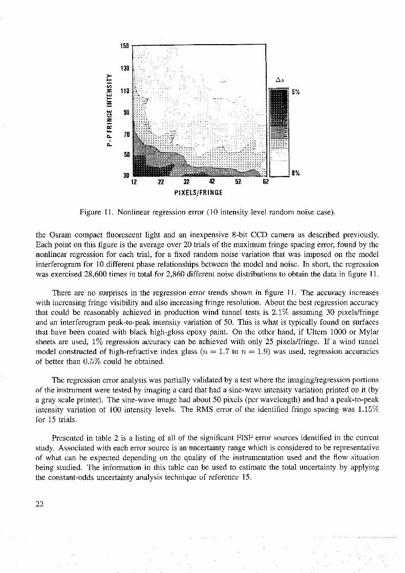
The accuracy of the nonlinear regression based fringe spacing determination was evaluated by

studying a model of a "typical" fringe in the presence of random noise for different combinations

of pixels/fringe and peak-to-peak first-fringe intensities. The results are presented in figure 11 for a

case with a 10 intensity level peak-to-peak noise superimposed on the intensity variation of the model

interferogram. This noise level is comparable to what is observed in practice on a glass surface, using

21

I--

ZI../.I

Z

t.ld

¢_Z

ta_

Iet_

119

9O

30

150

13o-l, "

70

50

12

_8

22 32 42 52 62

5%

0%

PIXELS/FRIHGE

Figure 11. Nonlinear regression error (10 intensity level random noise case).

the Osram compact fluorescent light and an inexpensive 8-bit CCD camera as described previously.

Each point on this figure is the average over 20 trials of the maximum fringe spacing error, found by the

nonlinear regression for each trial, for a fixed random noise variation that was imposed on the model

interferogram for 10 different phase relationships between the model and noise. In short, the regression

was exercised 28,600 times in total for 2,860 different noise distributions to obtain the data in figure 11.

There are no surprises in the regression error trends shown in figure 11. The accuracy increases

with increasing fringe visibility and also increasing fringe resolution. About the best regression accuracy

that could be reasonably achieved in production wind tunnel tests is 2.i.% assuming 30 pixels/fringe

and an interferogram peak-to-peak intensity variation of 50. This is what is typically found on surfaces

that have been coated with black high-gloss epoxy paint. On the other hand, if Ultem 1000 or Mylar

sheets are used, 1% regression accuracy can be achieved with only 25 pixels/fringe. If a wind tunnel

model constructed of high-refractive index glass (n = 1.7 to n = 1.9) was used, regression accuracies

of better than 0.5% could be obtained.

The regression error analysis was partially validated by a test where the imaging/regression portions

of the instrument were tested by imaging a card that had a sine-wave intensity variation printed on it (by

a gray scale printer). The sine-wave image had about 50 pixels (per wavelength) and had a peak-to-peak

intensity variation of 100 intensity levels. The RMS error of the identified fringe spacing was 1.15%

for 15 trials.

Presented in table 2 is a listing of all of the significant FISF error sources identified in the current

study. Associated with each error source is an uncertainty range which is considered to be representative

of what can be expected depending on the quality of the instrumentation used and the flow situation

being studied. The information in this table can be used to estimate the total uncertainty by applying

the constant-odds uncertainty analysis technique of reference 15.

22

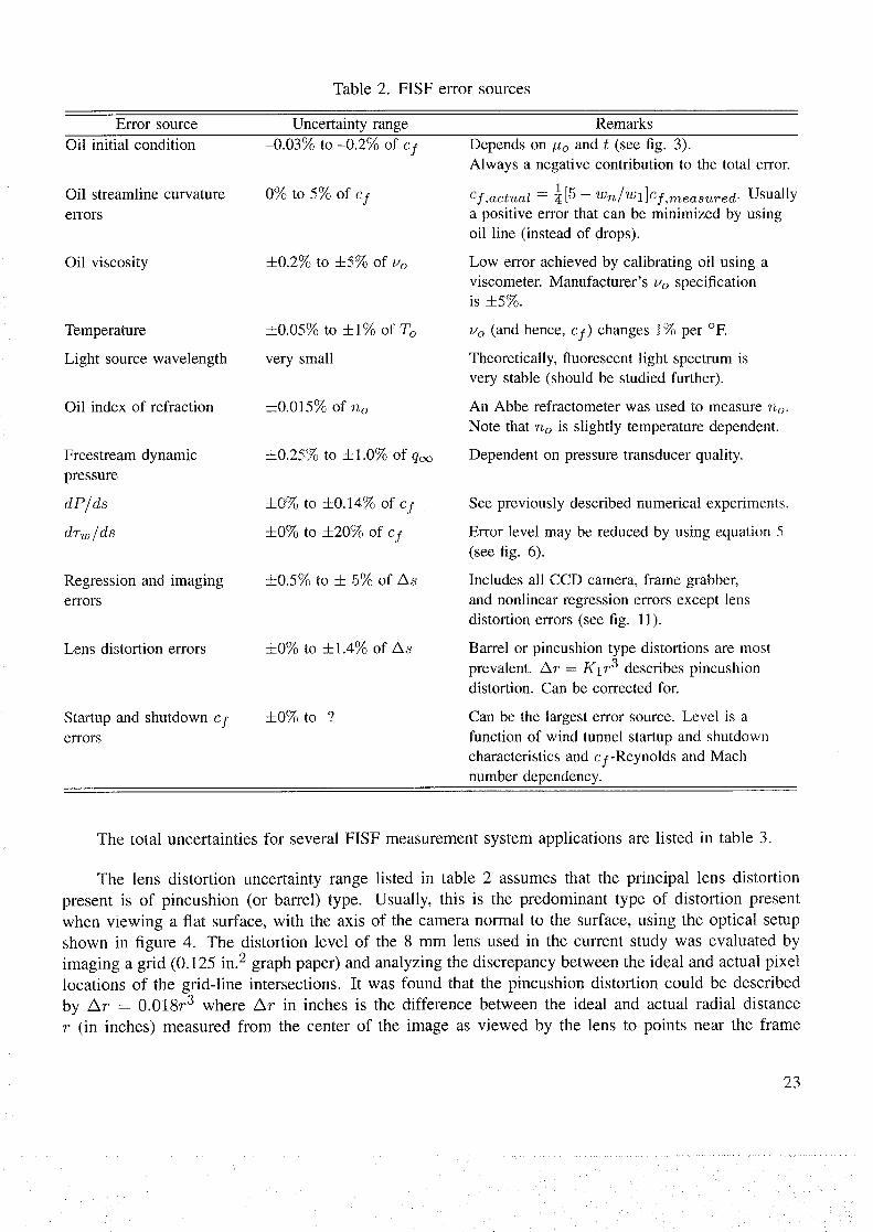
Table2. FISF error sources

Errorsource Uncertaintyrange RemarksOil initial condition

Oil streamlinecurvatureerrors

Oil viscosity

Temperature

Light sourcewavelength

Oil indexof refraction

Freestreamdynamicpressure

dP/ds

dr_/ds

Regression and imaging

errors

Lens distortion errors

Startup and shutdown cferrors

-0.03% to -0.2% of cf

0% to 5% ofcf

4-0.2% to -t-5% of Uo

4-0.05% to 4-1% of To

very small

4-0.015% of no

-4-0.25% to 4-1.0% of qoo

4-0% to -I-0.14% of Cf

4-0% to 4-20% of cf

4-0.5% to 4- 5% of As

4-0% to 4-1.4% of As

4-0% to ?

Depends on #o and t (see fig. 3).

Always a negative contribution to the total error.

Cf,actual = ¼[5 - Wn/Wl]Cf,raeasure d. Usually

a positive error that can be minimized by using

oil line (instead of drops).

Low error achieved by calibrating oil using a

viscometer. Manufacturer's Uo specificationis 4-5%.

Uo (and hence, c f) changes IYo per °E

Theoretically, fluorescent light spectrum is

very stable (should be studied further).

An Abbe refractometer was used to measure no.

Note that no is slightly temperature dependent.

Dependent on pressure transducer quality.

See previously described numerical experiments.

Error level may be reduced by using equation 5

(see fig. 6).

Includes all CCD camera, frame grabber,

and nonlinear regression errors except lens

distortion errors (see fig. 11).

Barrel or pincushion type distortions are most

prevalent. Ar = K1 r3 describes pincushion

distortion. Can be corrected for.

Can be the largest error source. Level is a

function of wind tunnel startup and shutdown

characteristics and c f-Reynolds and Machnumber dependency.

The total uncertainties for several FISF measurement system applications are listed in table 3.

The lens distortion uncertainty range listed in table 2 assumes that the principal lens distortion

present is of pincushion (or barrel) type. Usually, this is the predominant type of distortion present

when viewing a flat surface, with the axis of the camera normal to the surface, using the optical setup

shown in figure 4. The distortion level of the 8 mm lens used in the current study was evaluated by

imaging a grid (0.125 in. 9, graph paper) and analyzing the discrepancy between the ideal and actual pixel

locations of the grid-line intersections. It was found that the pincushion distortion could be described

by Ar = 0.018r a where Ar in inches is the difference between the ideal and actual radial distance

r (in inches) measured from the center of the image as viewed by the lens to points near the frame

23

u j

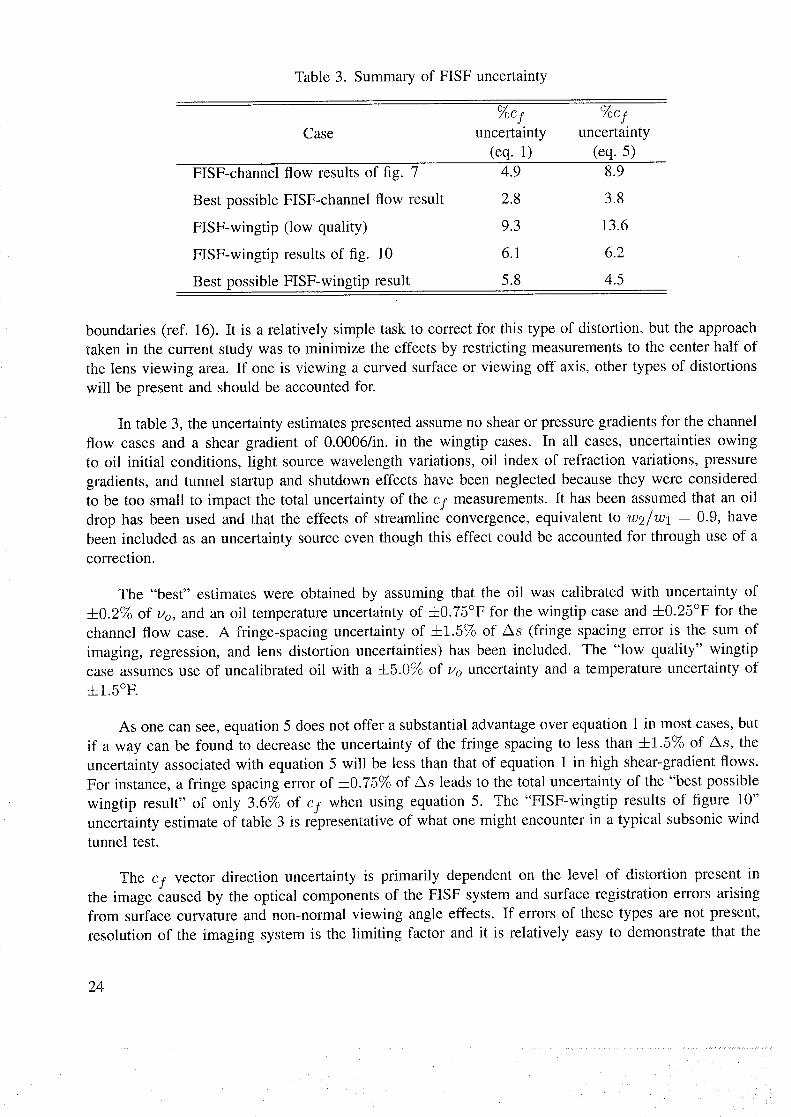
Table 3. Summary of FISF uncertainty

Case%cf %cy

uncertainty uncertainty

(eq. 1) (eq. 5)

FISF-channel flow results of fig. 7 4.9 8.9

Best possible FISF-channel flow result 2.8 3.8

FISF-wingtip (low quality) 9.3 13.6

FISF-wingtip results of fig. 10 6.1 6.2

Best possible FISF-wingtip result 5.8 4.5

boundaries (ref. 16). It is a relatively simple task to correct for this type of distortion, but the approach

taken in the current study was to minimize the effects by restricting measurements to the center half of

the lens viewing area. If one is viewing a curved surface or viewing off axis, other types of distortions

will be present and should be accounted for.

In table 3, the uncertainty estimates presented assume no shear or pressure gradients for the channel

flow cases and a shear gradient of 0.0006/in. in the wingtip cases. In all cases, uncertainties owing

to oil initial conditions, light source wavelength variations, oil index of refraction variations, pressure

gradients, and tunnel startup and shutdown effects have been neglected because they were considered

to be too small to impact the total uncertainty of the cf measurements. It has been assumed that an oil

drop has been used and that the effects of streamline convergence, equivalent to w2/w 1 = 0.9, have

been included as an uncertainty source even though this effect could be accounted for through use of a

correction.

The "best" estimates were obtained by assuming that the oil was calibrated with uncertainty of

+0.2% of Uo, and an oil temperature uncertainty of +0.75°F for the wingtip case and +0.25°F for the

channel flow case. A fringe-spacing uncertainty of +1.5% of As (fringe spacing error is the sum of

imaging, regression, and lens distortion uncertainties) has been included. The "low quality" wingtip

case assumes use of uncalibrated oil with a +5.0% of Uo uncertainty and a temperature uncertainty of

+l.5°K

As one can see, equation 5 does not offer a substantial advantage over equation 1 in most cases, but

if a way can be found to decrease the uncertainty of the fringe spacing to less than 4-1.5% of As, the

uncertainty associated with equation 5 will be less than that of equation 1 in high shear-gradient flows.

For instance, a fringe spacing error of 4-0.75% of 2xs leads to the total uncertainty of the "best possible

wingtip result" of only 3.6% of cf when using equation 5. The "FISF-wingtip results of figure 10"

uncertainty estimate of table 3 is representative of what one might encounter in a typical subsonic wind

tunnel test.

The cf vector direction uncertainty is primarily dependent on the level of distortion present in

the image caused by the optical components of the FISF system and surface registration errors arising

from surface curvature and non-normal viewing angle effects. If errors of these types are not present,

resolution of the imaging system is the limiting factor and it is relatively easy to demonstrate that the

24

vectordirection canbe determinedto within 4-0.2 degree for an imaging system with 230 pixels/in.

and a fringe spacing of 0.1 in. This uncertainty limit is nearly achieved when performing an FISF

measurement on a flat surface with a normal viewing angle and using the center of the lens field of

view as was done for the channel flow cases.

When performing measurements of greater complexity (e.g., wingtip case), it is often necessary

to use as much of the lens field of view as possible. Pincushion distortion, if not corrected for, can

cause relatively large cf directional inaccuracies. For the 8 mm Computar model T0812FICS lens

(Computar Inc., Japan) used in the current study, A0 = 0.98r 3 (0 in degrees and r in inches) describes

the maximum angle error which approaches 2 degrees at the extreme edges of the lens field of view.

If measurements are limited to the center half of the viewing area, the maximum angle error is about

0.5 degree, These numbers underscore the point that money spent on a good lens is not wasted.

A second cf vector direction issue concerns the degree to which the oil flow deviates from thedirection of the shear stress vector. Squire (ref. 9) performed an analysis which shows that the thinner the

initial oil thickness (or drop maximum height) the closer the oil follows the actual surface skin friction

direction. His analysis shows that the viscosity of the oil has no effect on the directional accuracy. This

issue needs further study but it seems clear that if the characteristic length of the wind tunnel model

being studied is large in comparison to the drop size, the oil pathline error is negligible in comparison

to other directional errors.

Practical Aspects

There are several subtle points to the FISF technique that one learns from experience. If the test

surface is a high-gloss painted surface, allow the paint to dry for at least 48 hours--but not too long,

because eventually the gloss surface will dull. Virtually any cleaning (or polishing) agent will change

the optical properties of a painted or plastic surface. Ideally, the best painted surface is an untouched one

although, in practice, it is occasionally necessary to redo a case. The author has found that non-abrasive

wipes such as those used in clean-room applications (Hydroentangled 100% polyester, Tech Spray Inc.

Amarillo, TX 79105) work very well at removing oil without damaging the surface. It is important that

as much of the oil be removed as possible if additional measurements are going to be made at the same

spot. Another good practice is to start oil application at the downstream locations and work upstream

in subsequent wind tunnel runs thereby reducing or possibly eliminating model cleaning.

The author has run into difficulties with dust, water vapor condensation, and lubricating oil from

associated wind tunnel machinery. In one case, dust from the environment was entrained into a jet and

deposited on the top of the silicone oil layer which, in the process, obliterated the fringes. In another

case, FISF measurements on a cone in supersonic flow failed owing to condensation when the wind

tunnel wall was removed. During the run, the model surface temperature decreased to nearly 0°E Upon

opening the test section, the water vapor in the air immediately condensed on the surface of the cold

model destroying any possibility of obtaining a measurement. Lubricating oil from compressors and

moving machinery in the flow can also cause problems. In most cases, these types of problems can be

worked around. For instance, a telescope mounted on a traverse stage was used to measure the fringe

spacing through the glass of the test section wall in the case of the supersonic cone experiment.

25

L

Wind tunnel startup and shutdown (off condition) time can be quite long in some large facilities.

As pointed out in reference 2, this effect can be partially accounted for by replacing the product qec_

in equations 5 or 1 with ft_n qoodt and using an average surface temperature when obtaining the

oil properties. This modification has no effect on the physical fact that the Reynolds number and

consequently, in most cases, the skin friction varies when off condition, but it does normalize the "rw

data so that consistent results may be obtained from wind tunnel run to run. It should be noted that for

cases where cf is not dependent on Reynolds or Mach number (i.e., incompressible tripped flows), windtunnel transient effects do not impact on FISF measurements provided the integral approach is used.

Alternatively, the effects of the startup and shutdown can be avoided by measuring the time variation

of the fringe pattern as in reference 17 provided the measurement locations can be viewed during a run.

Note that the other extreme (a too rapid startup of a tunnel) should also be avoided in order to prevent

waves on the surface of the oil. These waves were studied in reference 8 but their origin remains

unknown.

Application of an array of oil drops was accomplished by dipping a hard plastic hair comb into a

plastic tray containing the oil and then touching the comb to the surface being studied. For surfaces

with curvature, this technique does not work well and an alternative approach of placing individual

drops using a glass rod with a round tip was used. The size of the drops can be roughly controlled by

varying the size of the applicator and the depth of the oil in the tray.

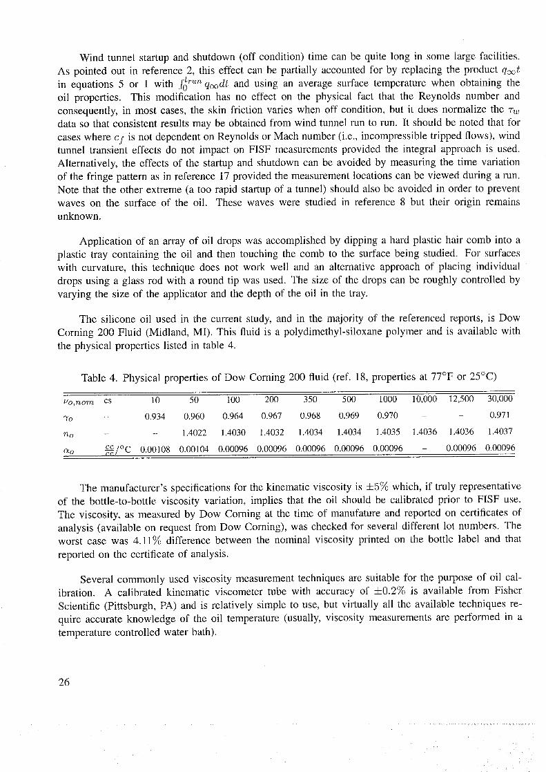
The silicone oil used in the current study, and in the majority of the referenced reports, is Dow

Corning 200 Fluid (Midland, MI). This fluid is a polydimethyl-siloxane polymer and is available with

the physical properties listed in table 4.

Table 4. Physical properties of Dow Corning 200 fluid (ref. 18, properties at 77°F or 25°C)

Uo,nom cs 10 50 100 200 350 500 1000 10,000 12,500 30,000

3'0 - 0.934 0.960 0.964 0.967 0.968 0.969 0.970 - - 0.971

no - - 1.4022 1.4030 1.4032 1.4034 1.4034 1.4035 1.4036 1.4036 1.4037

cc/oC 0.00108 0.00104 0.00096 0.00096 0.00096 0.00096 0.00096 - 0.00096 0.00096O_° C,-'-d,_

The manufacturer's specifications for the kinematic viscosity is -t-5% which, if truly representative

of the bottle-to-bottle viscosity variation, implies that the oil should be calibrated prior to FISF use.

The viscosity, as measured by Dow Coming at the time of manufature and reported on certificates of

analysis (available on request from Dow Coming), was checked for several different lot numbers. The

worst case was 4.11% difference between the nominal viscosity printed on the bottle label and that

reported on the certificate of analysis.

Several commonly used viscosity measurement techniques are suitable for the purpose of oil cal-

ibration. A calibrated kinematic viscometer tube with accuracy of +0.2% is available from Fisher

Scientific (Pittsburgh, PA) and is relatively simple to use, but virtually all the available techniques re-

quire accurate knowledge of the oil temperature (usually, viscosity measurements are performed in a

temperature controlled water bath).

26

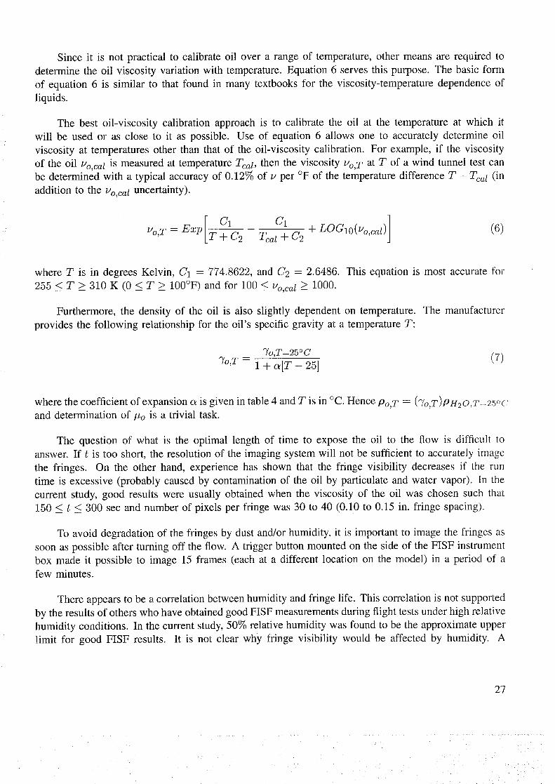
Sinceit is not practical to calibrateoil over a rangeof temperature,othermeansarerequiredtodeterminethe oil viscosityvariationwith temperature.Equation6 servesthis purpose.Thebasicformof equation6 is similar to that found in many textbooksfor the viscosity-temperaturedependenceofliquids.

The best oil-viscosity calibrationapproachis to calibratethe oil at the temperatureat which itwill be usedor as closeto it as possible. Useof equation6 allowsone to accuratelydetermineoilviscosityat temperaturesother than that of the oil-viscosity calibration. For example,if the viscosityof the oil Yo,calis measuredat temperatureTea l, then the viscosity Uo,T at T of a wind tunnel test canbe determined with a typical accuracy of 0.12% of u per °F of the temperature difference T - rca l (in

addition to the Uo,ca l uncertainty).

C1Uo,T = Exp T _-C2

C1

Tca I -4- C 2 + LOGlO(go,cal)](6)

where T is in degrees Kelvin, C1 = 774.8622, and C2 = 2.6486. This equation is most accurate for

255 < T _> 310 K (0 _< T > 100°F) and for 100 _< r'o,ca l > 1000.

Furthermore, the density of the oil is also slightly dependent on temperature. The manufacturer

provides the following relationship for the oil's specific gravity at a temperature T:

o,T=25oc (7)"Yo,T = 1 + a[T - 25]

where the coefficient of expansion a is given in table 4 and T is in °C. Hence Po,T = ('7o,T)PH20,T=25°C

and determination of/Zo is a trivial task.

The question of what is the optimal length of time to expose the oil to the flow is difficult to

answer. If t is too short, the resolution of the imaging system will not be sufficient to accurately image

the fringes. On the other hand, experience has shown that the fringe visibility decreases if the run

time is excessive (probably caused by contamination of the oil by particulate and water vapor). In the

current study, good results were usually obtained when the viscosity of the oil was chosen such that

150 < t < 300 sec and number of pixels per fringe was 30 to 40 (0.10 to 0.15 in. fringe spacing).

To avoid degradation of the fringes by dust and/or humidity, it is important to image the fringes as

soon as possible after turning off the flow. A trigger button mounted on the side of the FISF instrument

box made it possible to image 15 frames (each at a different location on the model) in a period of a

few minutes.

There appears to be a correlation between humidity and fringe life. This correlation is not supported

by the results of others who have obtained good FISF measurements during flight tests under high relative

humidity conditions. In the current study, 50% relative humidity was found to be the approximate upper

limit for good FISF results. It is not clear why fringe visibility would be affected by humidity. A

27

.... ! •

/

possibility is that water vapor in the air, under high humidity conditions, gets deposited on the surface

of the oil causing speckle and therefore, reduced fringe visibility.

CONCLUSIONS

In an effort to obtain an accurate, reliable, and easy to use skin friction measurement technique

for three-dimensional flows, several enhancements have been made to the fringe-imaging skin friction

technique of reference 2. Most important is the extension of the FISF technique to three dimensions,

which was achieved by using drops of oil (as opposed to the line of oil used in the original approach).

Additional noteworthy improvements include a new skin friction data reduction formula for flows with

shear gradients, development of a nonlinear regression approach to fringe analysis, and the development

of a PC-based application for FISF measurements. The hardware developed is relatively inexpensive

and the software has been made available.

Extensive use of modeling and benchtop tests have verified the new FISF approach. The overall

accuracy range was found to be 4-2.8% to +13.6% of cf and 4-1 degree directional accuracy depending

on the instrumentation used and flow being studied. A comparison of cf measured on a wingtip with

computed Reynolds-averaged Navier-Stokes results showed large differences. This disagreement, which

is thought to be a turbulence modeling deficiency, serves to reaffirm the importance of skin friction

measurements.

28

_ / i ,_ i:'

APPENDIX

A personal computer application (cxwinlg) has been written that automates several aspects of

the FISF technique, including image acquisition, nonlinear regression fringe analysis and skin friction

computation. Use of this application in conjunction with a frame grabber and the FISF-CCD based

imaging system (or equivalent) will allow one to rapidly obtain accurate skin friction data.

The source code, an executable, and some utility programs are currently in the process of being

released by COSMIC. This application was developed on a 486-33 machine running Windows 3.1 andhas been tested on several other machines. The minimum RAM memory requirement is 8 megabytes.

Either a VGA, super VGA, or EGA video card is required. The application has a built_in capability

to grab and display images provided that the ImageNation (Beaverton, OR) CX100 board has been

installed. For systems where this board is not present, the Fileit utility can be used to convert several

commonly used image file formats to the ".bin" format which cxwinlg reads or one can modify the

source code to work with other frame grabbers. To use Fileit, type "Fileit infile.tif outfile,bin" at the

command line prompt. Fileit converts gif, tif, tga, tif, wpg, pic, and pcx files.

The Microsoft Windows application is a mixed language application that was developed using

Microsoft Visual C++ version 1.00 and MicrosoftFortran version 5,1. The main program and most of

the image processing related routines are coded in ANSI C, and the nonlinear regression related routines

are coded in Fortran and called by the C main program. In the event that recompilation of any of the

cxwinlg C modules becomes necessary, it may be possible to link the recompiled C modules with the

Fortran object modules provided on the disk, hence no Fortran compiler would be required. The .mak

file included on the floppy disk shows the necessary C compiler options required to recompile and link

the application.

To install the application, simply create the directories c:\expskin and c:\expskin\data and copy

the .exe file to c:\expskin and the default.dat and default.bas files to c:\expskin\data. A double click on

the cxwinlg icon should start the application and the screen shown in figure 12 should appear (except

with no fringe pattern visible).

If one is going to analyze an existing FISF fringe image, the corresponding binary image file should

be placed in the c:\expskin\data subdirectory and it should have a file name of XXXXXXX.bin (whereXXXXXXX are seven user defined characters that can be used to designate a run number or some

other distinguishing characteristic subsequently referred to as the "Append characters"). The sequence

of steps to obtain a skin friction result is as follows:

1. Click on the "Read File" button and the "Data" window will appear as shown in figure 13o

Enter the appropriate quantities as required. Three freestream property data input options are available.

One can enter q_ and T; or Ptotal, M_ and T; or f_)r_n q_dt and T. The choice is made by clicking

on the desired radiobutton in the "Freestream Properties" section of the "Data"window. Only data for

the user's choice need be entered. Units are cs for u, nM for the light source wavelength, sec for t, in.

H20 for qc_, °F for T, psi for Ptotal, and in. H20 sec for f_fun q_dt. The oil viscosity termed "Nora

Kin Visc" is the oil kinematic viscosity at 77°F (25°C) in centistokes. If this value is not known, then

equation 6 should be used to determine Uo at 77°E

29

/

_ _ _: i_ii17_

Figure 12. Main window of skin friction application.

!_!::!|::::_ !i_!::i::ii::.!_:.!!!!|!::!:!:.!::_l::!!_!__ Fo" Prope,*es--- _]| /.om.K,n.V,so._ fill| I.o'-'ndo__llll

Wavelength

Run Time

X Pixelslln.

Y Pixels/In.

-Freestream Properties--

Q) q,t O PLM,t _> qdtt

Integral qdt

Temperature

Dyn. Press.

Ptotal

Mini

"110 1

Dir. [c:_axpskint, data ]

Appended char.

[] Read data from disk

3O

Figure 13. Data entry dialog box of skin friction application.

If a spatialcalibration is going to be performedand the type of the calibration is type 1, no "XPixels/In." or "Y Pixels/ln." entry is requiredasthesevalueswill bedeterminedduring thecalibrationprocess.Alternately,if a type 2 calibrationis to beperformed,"X Pixels/In." and"Y Pixels/In." mustbeentered.Thesevaluesarein termsof windowcoordinateswhereX is measured across top of screen

and Y is down. Upon hitting the "Ok" button, cxwinlg will create a log file (filename XXXXXXX.log)

in the c:\expskin\ data directory and a popup dialog box will appear that allows you to select and open

the XXXXXXX.bin file. The desired image should appear in the main portion of the screen.

2. A spatial calibration can be performed using the "Calibrate " feature. In order to achieve a

proper spatial calibration of the imaging system, an x-y reference axes system target must appear in the

image's field of view. A draftsman's target or some other marking that denotes a known x-y position

on the surface, the +x and +y axes directions, and, for calibration type 1, Ax and Ay may be used

The simplest possible marking consists of three dots, the first located at a known surface location and

the other two located at tax, 0 and 0, Ay respectively. All spatial dimension related quantities have

units of inches.

Obviously, if the surface being imaged is highly curved, there is no way to obtain a proper

registration of the surface using a one-camera system. Under this condition, an alternative method

should be used to determine the measurement location on the surface and the magnification of the

imaging system. The spatial calibration function does not have to be invoked. One can enter the

number of pixels/inch in screen coordinates directly in the "Data" window if that information is already

known although, without a spatial calibration, the reference system used to compute the skin-friction

direction is based on the "screen coordinates" (which depend on the orientation of the CCD camera

relative to the model).

To invoke the calibration, click on the "Calibrate" button. The calibration window will pop up

as shown in figure 14. One of two calibration processes may be chosen. Calibration type 1 should

be chosen if the magnification (pixels/inch in screen coordinates) of the imaging system is not known.

Calibration type 2 is simpler and is most useful when processing a number of images where the distance

from the lens to the model surface remains constant.

If calibration type 1 is chosen, enter the x, y position of the reference location and +Ax, ray

in the calibration dialog box. Next, position the crosshair over the reference position and click. Fine

positioning of the crosshair can be accomplished using the arrows after the left mouse button has been

depressed. Move the crosshair to the tax position and click twice. Return the crosshair to the reference

position and click. Finally, position the crosshair at the ray location and click twice. Cxwinlg uses

the information entered in the calibration dialog box along with the information entered via the mouse

to determine the pixels/inch in the x and y directions and also the orientation of the surface coordinate

system relative to the current camera or screen based coordinate system.

If calibration type 2 is chosen, enter the x, y position of the reference location in the calibration

dialog box ("X Pixels/In." and "Y Pixels/In." should have been previously entered) and click on "Ok."

Next, position the crosshair over the reference position and click. Move the crosshair to some point on

the +x axis and click twice. Return the crosshair to the reference position and click. Finally, position

the crosshair at some point on the ty axis and click twice.

31

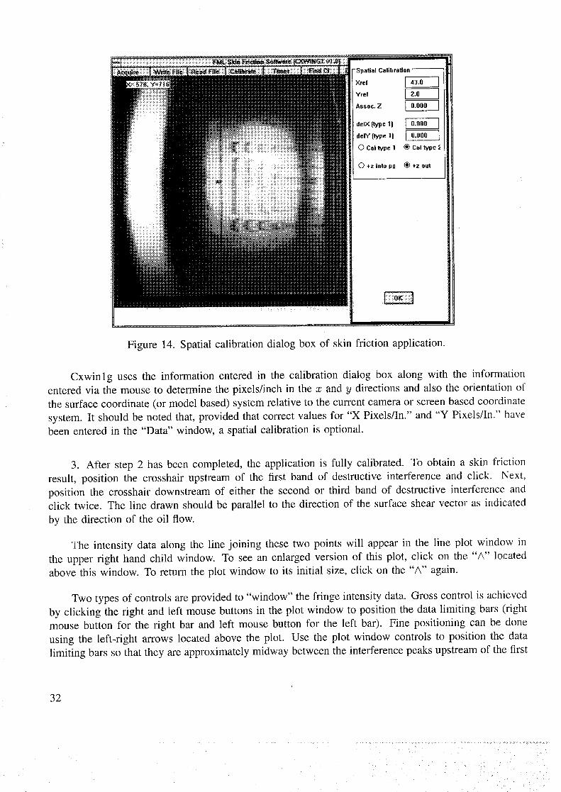
Figure 14. Spatialcalibrationdialog box of skin friction application.

Cxwinlg usesthe informationenteredin the calibrationdialog box alongwith the informationenteredvia the mouseto determinethepixels/inchin the x and y directions and also the orientation of

the surface coordinate (or model based) system relative to the current camera or screen based coordinate

system. It should be noted that, provided that correct values for "X Pixels/In." and "Y Pixels/In." have

been entered in the "Data" window, a spatial calibration is optional.

3. After step 2 has been completed, the application is fully calibrated. To obtain a skin friction

result, position the crosshair upstream of the first band of destructive interference and click. Next,

position the crosshair downstream of either the second or third band of destructive interference and

click twice. The line drawn should be parallel to the direction of the surface shear vector as indicated

by the direction of the oil flow.

The intensity data along the line joining these two points will appear in the line plot window in

the upper right hand child window. To see an enlarged version of this plot, click on the "A" located

above this window. To return the plot window to its initial size, click on the "A" again.

Two types of controls are provided to "window" the fringe intensity data. Gross control is achieved

by clicking the right and left mouse buttons in the plot window to position the data limiting bars (right

mouse button for the right bar and left mouse button for the left bar). Fine positioning can be done

using the left-right arrows located above the plot. Use the plot window controls to position the data

limiting bars so that they are approximately midway between the interference peaks upstream of the first

32

destructiveinterferencebandanddownstreamof thesecondor third destructiveinterferenceband. Thiswindowingprocesswill be indicatedon theimageandin the plot window by a color changeto green.The purposeof windowing is to obtainthe greatestaccuracyby restrictingthe regressionanalysistothe first oneor two fringes.

4. Click on "Get Cf" and,after a few seconds,a blue line (thenonlinearregressionresults)willappearin the line-plot child window andthe cf result will appear in the lower right-hand text window.

5. The results of the skin friction measurement can be saved in the ASCII database file c:\expskin

\data\default.bas by hitting the "Db" button.

33

5! • •i i

REFERENCES

1. Winter, K. (3.: An Outline of the Techniques Available for the Measurement of Skin Friction in

Turbulent Boundary Layers. Prog. Aerospace Sci., vol. 18, no. 1, 1977, pp. 1-57.

2. Monson, D. J.; and Mateer, (3. G.: Boundary-Layer Transition and Global Skin Friction Measure-

ments with an Oil-Fringe Imaging Technique. SAE 932550, Aerotech '93, Costa Mesa, CA,

Sept. 27-30, 1993.

3. Tanner, L. H.; and Blows, L. (3.: A Study of the Motion of Oil Films on Surfaces in Air Flow, with

Application to the Measurement of Skin Friction. J. Physics E, vol. 9, 1976, pp. 194-202:

4. Tanner, L. H.: A Skin Friction Meter, Using the Viscosity Balance Principle, Suitable for Use with

Flat or Curved Metal Surfaces. J. Physics E, vol. 10, 1977, pp. 278-284.

5. Tanner, L. H.; and Kulkarni, V. (3.: The Viscosity Balance Method of Skin Friction Measurement:

Further Developments Including Applications to Three-Dimensional Flow. J. Physics E, vol. 9,

1976, pp. 1114-1121.

6. Monson, D. J.; and Higuchi, H.: Skin Friction Measurements by a New Nonintrusive Double Laser

Beam-Oil Viscosity Balance Technique. AIAA J., vol. 19, no. 6, 1980, pp. 739-744.

7. Westphal, R. V.; Bachalo, W. D.; and Houser, M. H.: Improved Skin Friction Interferometer. NASA

TM-88216, 1986o

8. Murphy, J. D.; and Westphal, R. V.: The Laser-Interferometer Skin-Friction Meter: A Numerical

and Experimental Study. J. Physics E, vol. 19, 1986, pp. 744-751.

9. Squire, L. C.: The Motion of a Thin Oil Sheet under the Steady, Boundary Layer on a Body. JFM,

vol. 11, 1961, pp. 161-179.

10. Haver, R. J.: The Verdict is In: Solid-State Fluorescent Ballasts are Here. Electronic Design News,

Nov. 5, 1976, pp. 65-69.

11. Chen, W. Y.; and Stegen, G. R.: Experiments with Maximum Entropy Power Spectra of Sinusoids.

J. Geophys. Res., vol. 79, no. 20, 1974, pp. 3019-3022.

12. Schemm, J. B.; and Vest, C. M.: Fringe Pattern Recognition and Interpolation Using Nonlinear

Regression Analysis. Applied Optics, vol. 22, no. 18, 1983, pp. 2850-2853.

13. Saunders, D. A.; Kennelly, R. A.; and Kennelly, L. C.: "Aerodynamics Division Software Library.

NASA RP-1276, June 1992.

14. Dacles-Mariani, J.; Zilliac, G. G.; and Bradshaw, P.: Numerical/Experimental Study of a Wingtip

Vortex in the Near Field. AIAA J., vol. 33, no. 9, 1995, pp. 1561-1568.

15. Kline, S. J.; and McClintock, F. A.: Describing Uncertainties in Single-Sample Experiments. Mech.

Eng., Jan. 1953, p. 3.

16. Born, M.; and Wolf, E.: Principle of Optics. 3rd ed., Pergamon Press, Oxford, U.K., 1965.

34

............... •• • . • • • • •• • • •• • .• • ••i¸,..•.•, •.•:••••,HH.••.••:>•:••<:•+.:

• i

17. Naughton, J. W.; and Brown, J. L.: Surface Interferometric Skin-Friction Technique. AIAA

Paper 96-2183, New Orleans, LA, June 17-20, 1996.

18. Information About Dow Corning Silicone Fluids. Dow Coming Corp., Midland, MI, 1994.

35

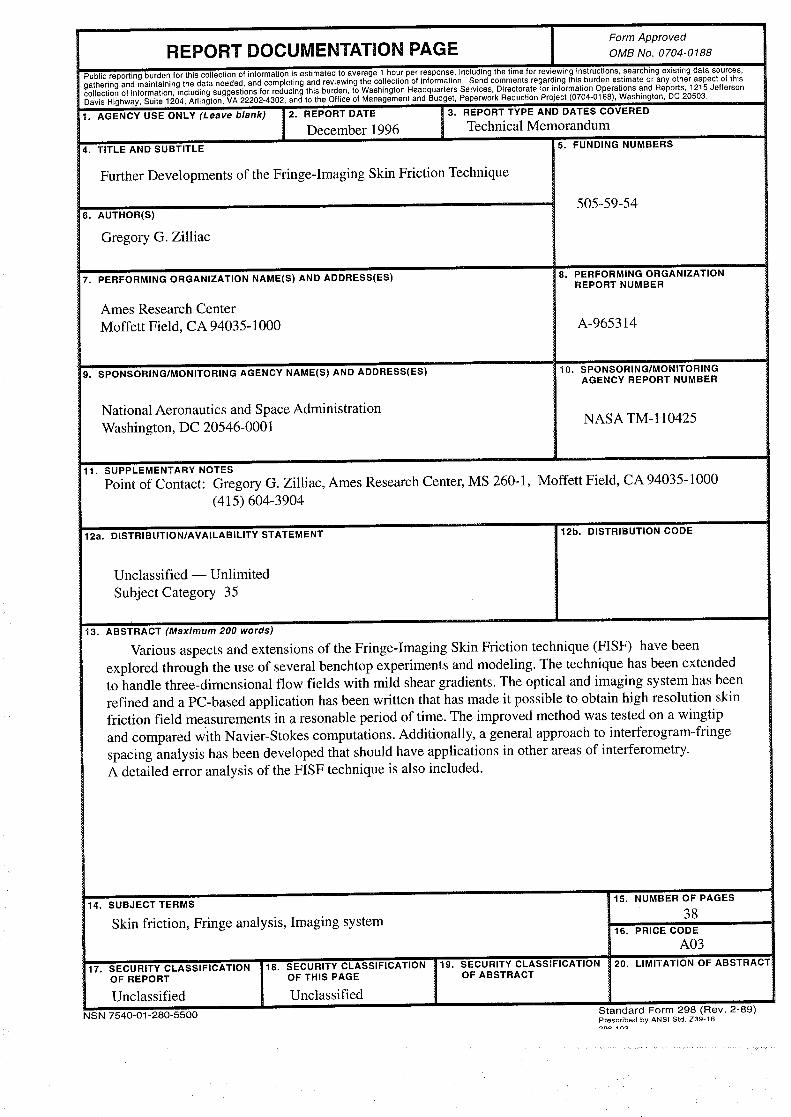
Form Approved

REPORT DOCUMENTATION PAGE OMBNo.o7o4-o188

Public reporting burden for this collection of information is estimated to average 1 hour per response, including the time for reviewing instructions, searching existing data sources,gathering and maintaining the data needed, and completing and reviewing the co lection of information. Send comments regarding this burden estimate or any other aspect of thiscollection of information, including suggestions for reducing this burden, to Washington Headquarters Services, Directorate :?orinformation Operations and Reports, 1215 Jef ersonDavis Highway, Suite 1204, Arlington, VA 22202-4302, and to the Office of Management and Budget, Paperwork Reduction Project (0704-0188), Washington, DC 20503.

1. AGENCY USE ONLY (Leave blank) 2. REPORT DATE 3. REPORT TYPE AND DATES COVERED

December 1996 Technical Memorandum

4. TITLE AND SUBTITLE 5. FUNDING NUMBERS

Further Developments of the Fringe-Imaging Skin Friction Technique

6. AUTHOR(S)

Gregory G. Zilliac

7. PERFORMING ORGANIZATION NAME(S) AND ADDRESS(ES)

Ames Research Center

Moffett Field, CA 94035-1000

9. SPONSORING/MONITORING AGENCY NAME(S) AND ADDRESS(ES)

National Aeronautics and Space Administration

Washington, DC 20546-0001

505-59-54

8. PERFORMING ORGANIZATIONREPORT NUMBER

A-965314

10. SPONSORING/MONITORINGAGENCY REPORT NUMBER

NASA TM-110425

11. SUPPLEMENTARY NOTES

Point of Contact: Gregory G. Zilliac, Ames Research Center, MS 260-1, Moffett Field, CA 94035-1000

(415) 604-3904

12a. DISTRIBUTION/AVAILABILITY STATEMENT

Unclassified -- Unlimited

Subject Category 35

12b. DISTRIBUTION CODE

I

13. ABSTRACT (Maximum 200 words)

Various aspects and extensions of the Fringe-Imaging Skin Friction technique (FISF) have been

explored through the use of several benchtop experiments and modeling. The technique has been extendedto handle three-dimensional flow fields with mild shear gradients. The optical and imaging system has been

refined and a PC-based application has been written that has made it possible to obtain high resolution skinfriction field measurements in a resonable period of time. The improved method was tested on a wingtip

and compared with Navier-Stokes computations. Additionally, a general approach to interferogram-fringe

spacing analysis has been developed that should have applications in other areas of interferometry.

A detailed error analysis of the FISF technique is also included.

14. SUBJECTTERMS

Skin friction, Fringe analysis, Imaging system

17. SECURITY CLASSIFICATION 18. SECURITY CLASSIFICATIONOF REPORT OF THIS PAGE

Unclassified Unclassified

NSN 7540-01-280-5500

19. SECURITY CLASSIFICATIONOF ABSTRACT

"15. NUMBER OF PAGES

3816. PRICE CODE

A03

20. LIMITATION OF ABSTRACI

Standard Form 298 (Rev. 2-89)Prescribed by ANSI Std. zsg-1a

i_ iiiiiiiiiiiiii_i

i _i ii!