further results related to power supply design and analysis in the undergraduate curriculum

262 IEEE TRANSACTIONS ON EDUCATION, VOL. 44, NO. 3, AUGUST 2001

Further Results Related to Power Supply Design andAnalysis in the Undergraduate Curriculum

Kenneth V. Cartwright, Member, IEEE

Abstract—The power supply analysis and design results ofSherman and Hamacher are extended to include approximate so-lutions to the nonlinear equations that define the rectifier turn-onangles. Additionally, peak rectifier current solely as a functionof ripple factor, as well as the inverse relationship, i.e., ripplefactor as a function of peak rectifier current, are also provided.Simplified exact equations and also new approximations are givenfor rms transformer current. These new approximations allow theripple factor to be determined as a function of rms transformercurrent. These results are for both the constant current andresistive load supplies.

Index Terms—Nonlinear equation approximation, power sup-plies, power supply design.

I. INTRODUCTION

RECENTLY, Sherman and Hamacher [1] have presentednew results for the design and analysis of power supplies,

both for the resistive load power supply (RLP) and for the con-stant current load power supply (CCLP). Their paper goes a longway in enabling more meaningful design and analysis of powersupplies in the undergraduate curriculum, especially when theripple is not small. Notwithstanding the substantial contributionof their paper, there remains opportunity to extend the resultspresented.

The purpose of this paper is to extend the results of Shermanand Hamacher by providing the following, for both types ofsupply:

1) Approximate solutions to the nonlinear equations de-rived by Sherman and Hamacher that define the rectifierturn-on angles. (Sherman and Hamacher provided ap-proximate solutions only for the turn-off angles.) Thismeans that students will not need a programmablecalculator to solve the nonlinear equations, but moreimportantly, students will be able to see explicit relation-ships between variables.

2) The peak rectifier current is given solely in terms of theripple factor, so that the role of the ripple factor is clearlyseen. Additionally, for RLP, the peak rectifier current isdetermined for ripple factors greater than 0.57. (Shermanand Hamacher [1] provided results only for ripple factorsless than 0.57.)

3) The ripple factor is determined as a function of peak rec-tifier current and root mean square (rms) transformer cur-rent. This is of value when one has in mind a particular

Manuscript received July 9, 1998; revised May 25, 2001.The author is with the School of Technology, College of The Bahamas,

Nassau, Bahamas; (e-mail: [email protected]).Publisher Item Identifier S 0018-9359(01)06991-6.

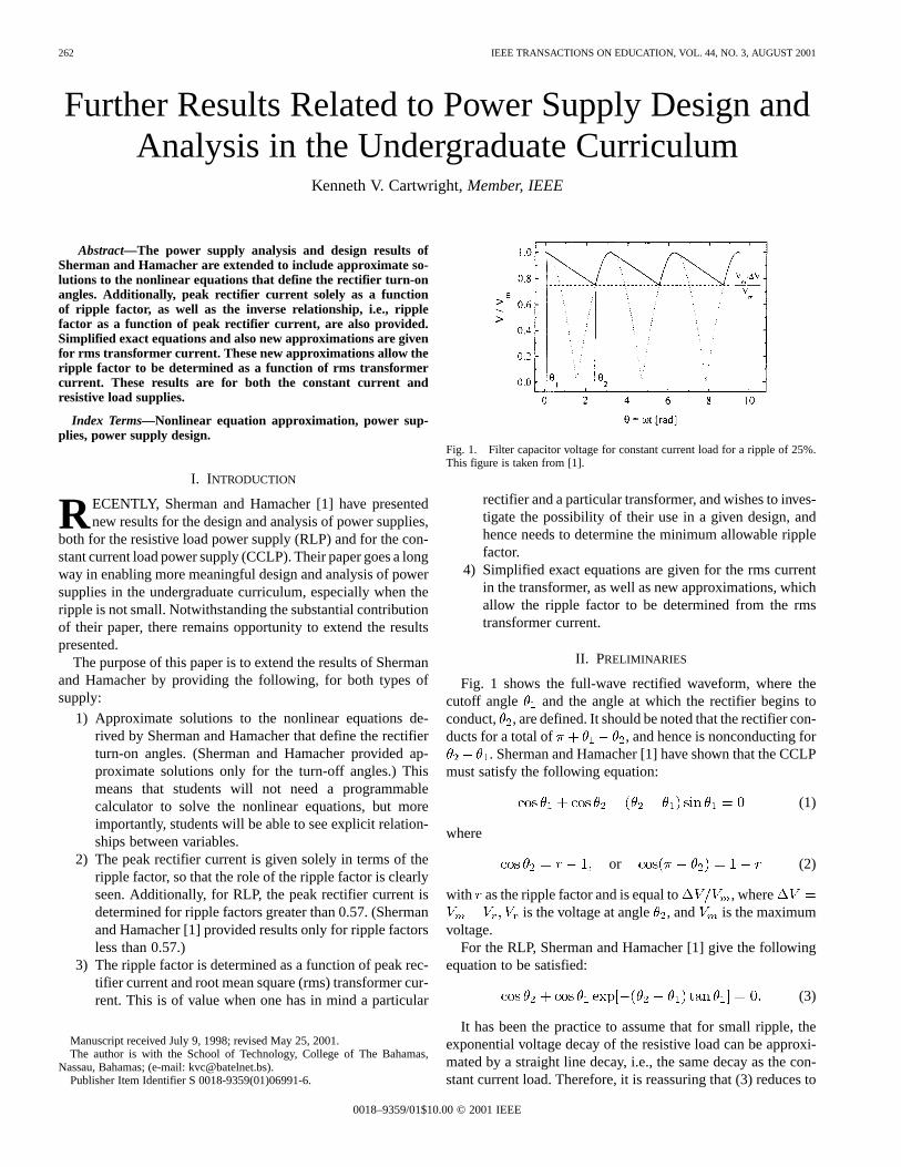
Fig. 1. Filter capacitor voltage for constant current load for a ripple of 25%.This figure is taken from [1].

rectifier and a particular transformer, and wishes to inves-tigate the possibility of their use in a given design, andhence needs to determine the minimum allowable ripplefactor.

4) Simplified exact equations are given for the rms currentin the transformer, as well as new approximations, whichallow the ripple factor to be determined from the rmstransformer current.

II. PRELIMINARIES

Fig. 1 shows the full-wave rectified waveform, where thecutoff angle and the angle at which the rectifier begins toconduct, , are defined. It should be noted that the rectifier con-ducts for a total of , and hence is nonconducting for

. Sherman and Hamacher [1] have shown that the CCLPmust satisfy the following equation:

(1)

where

or (2)

with as the ripple factor and is equal to , whereis the voltage at angle , and is the maximum

voltage.For the RLP, Sherman and Hamacher [1] give the following

equation to be satisfied:

(3)

It has been the practice to assume that for small ripple, theexponential voltage decay of the resistive load can be approxi-mated by a straight line decay, i.e., the same decay as the con-stant current load. Therefore, it is reassuring that (3) reduces to

0018–9359/01$10.00 © 2001 IEEE

CARTWRIGHT: FURTHER RESULTS RELATED TO POWER SUPPLY DESIGN 263

Fig. 2. Percentage error of approximations for the turn-on angle� , of the constant current supply, (6A)-[i.e., (6) withk = 1; k = 1], and (6B)-[i.e., (6) withk = 1:6114; k = 1:2893], and for the resistive load supply, (6C)-[i.e., (6) withk = 1:0095; k = 0:83515].

(1) for small ripple. This is easily demonstrated by replacing theexponential function in (3) by the first two terms of its Taylorseries expansion. As a consequence of the above, the solutionfor (1) and (3) must coincide for the small ripple case.

III. A PPROXIMATESOLUTIONS OF THEDEFINING EQUATIONS

A. Approximate Solutions of the Defining Equation for for theConstant Current Load Power Supply (CCLP)

In the design phase, a required ripple factor is usually given,and hence the solution of (1) will give in terms and ,which of course are related by (2). Indeed, [1, eq. (12)] providesan excellent approximation (accurate to 0.5% for )that can be written as

(4)

Knowing from (4) allows the capacitor value to be de-termined from (5) of [1], i.e.,

(5)

where is the constant discharge current of the filter capacitor(which is also assumed to be the value of the load current),

and is the radian frequency of the applied ac voltage.After the power supply has been designed, it is sometimes

necessary to analyze its performance, i.e., to determine for ex-ample what ripple level has been achieved. In order to do this,(1) has to be solved for as is now known from (5).

There are many ways of deriving an approximate solutionto (1), given the value of . The best approximation that theauthor has found is derived by first noting that a solution to

(1) is given by , for small . This can be seen byapproximating by 1 and using . Furthermore,from (2), . Hence, . Solvingthis equation for gives the desired result

(6)

where and .The percentage error performance for (6) with and

, is shown in the curve (6A) of Fig. 2, which clearlyshows that (6) is indeed an excellent approximation to the turnon angle for .

However, an approximation that is valid for all values ofcan be obtained if one sets ,and is optimized to give near minimax percentage error per-formance. Indeed, gives percentage errors within

%, as shown in the curve (6B) of Fig. 2.The relationship between and is established by noting

that for , and these are then substitutedinto (6).

After is found, the level of ripple can then be determinedfrom (2).

B. Approximate Solutions of the Defining Equation for theResistive Load Power Supply (RLP)

For the design phase for the RLP, (3) has to be solved forinterms of or . In fact, [1, eq. (20)] can be used as it providesan excellent approximation (accurate to 0.5% for )and can be written as

(7)


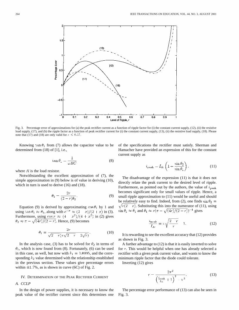
Fig. 3. Percentage error of approximations for (a) the peak rectifier current as a function of ripple factor for (i) the constant current supply, (12),(ii) the resistiveload supply, (17), and (b) the ripple factor as a function of peak rectifier current for (i) the constant current supply, (13), (ii) the resistive load supply, (18). Pleasenote that (17) and (18) are only valid forr � 0:57.

Knowing from (7) allows the capacitor value to bedetermined from (18) of [1], i.e.,

(8)

where is the load resistor.Notwithstanding the excellent approximation of (7), the

simple approximation in (9) below is of value in deriving (10),which in turn is used to derive (16) and (18).

(9)

Equation (9) is derived by approximating by 1 andusing , along with in (3).Furthermore, using in (2) gives

. Hence, (9) becomes

(10)

In the analysis case, (3) has to be solved forin terms of, which is now found from (8). Fortunately, (6) can be used

in this case, as well, but now with , and the corre-sponding value determined with the relationship establishedin the previous section. These values give percentage errorswithin %, as is shown in curve (6C) of Fig. 2.

IV. DETERMINATION OF THEPEAK RECTIFIERCURRENT

A. CCLP

In the design of power supplies, it is necessary to know thepeak value of the rectifier current since this determines one

of the specifications the rectifier must satisfy. Sherman andHamacher have provided an expression of this for the constantcurrent supply as

(11)

The disadvantage of the expression (11) is that it does notdirectly relate the peak current to the desired level of ripple.Furthermore, as pointed out by the authors, the value ofbecomes significant only for small values of ripple. Hence, asmall ripple approximation to (11) would be useful and shouldbe relatively easy to find. Indeed, from (2), one finds

. Substituting this into the numerator of (11), usingand gives

(12)

It is rewarding to see the excellent accuracy that (12) providesas shown in Fig. 3.

A further advantage to (12) is that it is easily inverted to solvefor . This would be helpful when one has already selected arectifier with a given peak current value, and wants to know theminimum ripple factor that the diode could tolerate.

Inverting (12) gives

(13)

The percentage error performance of (13) can also be seen inFig. 3.


B. Resistive Load (RLP)

In the resistive load power supply, Sherman and Hamachergives the rectifier current in [1, eq. (21)]. However, this can bewritten as

for (14)

where .The upper limit is valid because of the periodicity of

the current.It is further stated that the peak current will occur at ,

for values less than 0.57, but no statement is made concerningthe peak value for values greater than 0.57. However, it is nowpossible to show that this peak value is given by

(15)

To see this, note that (14) is a maximum when the numeratoris a maximum, i.e., when , which results in (15).However, must be greater than (since the current is zerofor ). Hence, the maximum occurs at when

.To find the peak current in terms of, set in (14), ex-

pand the compound angle, and then substitute (2) and. Furthermore, substitute (10) for and use the ap-

proximation to give:

(16)

However, recall that (16) is only valid for values less than0.57, and for this range, the author has found that a better ap-proximation is given by

(17)

The percentage error of (17) is shown in Fig. 3, where it isclear that (17) is an excellent approximation.

To find the peak rectifier current in terms ofsolely, forgreater than 0.57, solve (2) for, then use this to solve (7) for

and substitute into (15).Unfortunately, (17) is not easily inverted in closed form, if it

is desired to find in terms of the peak rectifier current. Nev-ertheless, Appendix I shows how this expression can be found,and is given in (18) below.

(18)

where .Please note that (18) is valid forvalues less than 0.571 28,

or .

To determine values for , (15) could besolved for , and determined from (10).

C. Designing for Peak Rectifier Current

Given a desired peak rectifier current for CCLP, (13) [(18) forRLP] can be used to find the ripple factor, which can then besubstituted into (2) to obtain , and these in turn can be used in(4) and (5) [(7) and (8) for RLP] to obtain the values of[ for RLP] and the value of the capacitor, respectively.Of course, the closest commercial value ofwill have to beused, and hence (5) [(8) for RLP] can be used to determine theactual value of , (6) is then used to find , and hence with(2). Finally, (11) [(14) or (15) for RLP] is used to verify thedesired peak rectifier current has been achieved.

V. DETERMINATION OF THERMS TRANSFORMERCURRENT

A. CCLP

Sherman and Hamacher have extended our understanding ofpower supply design by deriving an expression for the rms cur-rent in the transformer, which is given in [1, eq. (14)]. However,this expression can be simplified as will now be demonstrated.From (1), can be found and substituted into the first termunder the radical of [1, eq. (14)], thereby making that term equalto . Hence, the rms currentin the transformer willsimplify to

(19)

Sherman and Hamacher also gives a very good approximationto (19) as

(20)

If one wanted to find the minimum ripple factor that couldbe tolerated by a given transformer, it would be necessary tohave an expression ofas a function of . This is not easilyaccommodated by (20). However, (19) can be approximated by(21) below

(21)

Fig. 4 shows the percentage error of (21), which clearly showsthat it is quite competitive to that of (20). In fact, (21) has lowerpercentage error than (20) for . For ,the percentage error of (21) is only slightly higher than that of(20), becoming equal asgoes to zero.

Inverting (21) produces

(22)


Fig. 4. Percentage error of approximations for the rms transformer current as a function of ripple factor, (20) and (21), and ripple factor as a function of rmstransformer current, (22), for the constant current supply.

where , the positive sign is for , and thenegative sign is needed for .

Figure 4 also shows the percentage error of (22), where itcan be seen that it is excellent (less than 1%) for

. Furthermore, on inspection of Fig. 4, the steepness of thepercentage error of (22) asgoes to zero might appear to bea problem. However, the percentage error at is lessthan 11%, and therefore (22) can be used with confidence forpractical values of .

B. Resistive Load (RLP)

For the RLP, the rms current in the secondary winding ofthe transformer is a bit more involved than that of the constantcurrent load. It is determined by the authors of [1] as

, where the ratio of is given by [1, eq.(25)], and a very good approximation of this by [1, eq. (26)], andthe ratio of by a complicated [1, eq. (27)]. Fortunately, thisexpression can be simplified to

(23)

This follows by simply substituting (14) into the rms formulabelow

(24)

Sherman and Hamacher also gives a very good approximationto the rms current as

(25)

As before, it is not easy to invert (25). However, (26) belowcan be used instead of (25). The advantage to (26) is that it iseasily inverted

(26)

Fig. 5 shows the percentage error of (26), which clearly showsthat it is also quite competitive to that of (25), and therefore canbe used in place of (25), without cause for concern.

Inverting (26) produces

(27)

where the positive sign is for , and the negative signis needed for .

Fig. 5 also shows the percentage error of (27), where it can beseen that quite accurate estimates of the ripple factor as a func-tion of rms transformer current can be achieved for all values of

less than about .95.

C. Designing for RMS Transformer Current

Given a desired rms transformer current for the CCLP, use(22) [(27) for RLP] to obtain , then (2) for , followed by (4)and (5) [(7) and (8) for RLP] to obtain the value of. Again theclosest commercial value of will have to be used, and thus(5) [(8) for RLP] can be used to determine the actual value of

achieved, (6) is then used to find, and hence with (2).Finally, (20) [(25) for RLP] is used to verify the desired rmstransformer current has been achieved.


Fig. 5. Percentage error of approximations for the rms transformer current as a function of ripple factor, (25) and (26), and ripple factor as a function of rmstransformer current, (27), for the resistive load supply.

VI. CONCLUSION

In this paper, new results have been derived which furtherextend knowledge of resistive load and constant current powersupply design and analysis. Specifically, excellent approximatesolutions were found to the nonlinear equations which allow theturn-on angles to be found in closed form. Furthermore, peakrectifier currents were determined in terms of ripple factor, andvice versa. Additionally, rms transformer currents were foundin terms of ripple factor, and vice versa.

APPENDIX I

In this Appendix, (18) will be derived.Recall that . Substitute this into (14) (setting

) and use to get .Furthermore, substitute (10) into the previous equation, and use

to produce , an estimate for , where

. Unfortunately, has poorpercentage error. In fact, the percentage error varies almost lin-early with respect to the true value of, and can be written as

, where is a constant. Letand solve to produce .Optimizing to give minimax error performance for all valuesof less than 0.57 produces (18).

ACKNOWLEDGMENT

The author would like to thank the reviewers for their help inimproving the quality of this paper and the administration of

The College of The Bahamas for allowing the opportunity topursue this research project.

REFERENCES

[1] B. W. Sherman and K. A. Hamacher, “Power supply design in the un-dergraduate curriculum,”IEEE Trans. Educ., vol. 40, pp. 278–282, Nov.1997.

Kenneth V. Cartwright (S’77–M’78) was born in Nassau, N. P., Bahamas, onNov. 13, 1953. He received the B.E.Sc, M.S., and Ph.D. degrees in electrical en-gineering from the University of Western Ontario, Canada, in 1978, and TulaneUniversity, New Orleans, LA, in 1987 and 1990, respectively.

From 1978 to 1983, he was the Service Manager for a consumer electronicsfirm. He joined The College of The Bahamas in 1983 as an Assistant Lecturerand was promoted to Lecturer in 1986. From 1985 to 1990, he was awardedstudy leave to pursue graduate work at Tulane University, where he was alsoan instructor in the Electrical Engineering Department for the 1988–1989 aca-demic year. Presently, he is a Senior Lecturer in the School of Technology andthe Coordinator for the Electrical Engineering Department. His research inter-ests include digital signal processing, analog and digital communication sys-tems, and analog electronics. Some of this research is published in IEEE SIGNAL

PROCESSINGLETTERS, IEEE COMMUNICATION LETTERS, IEEE TRANSACTIONS

ON COMMUNICATIONS, and conferences proceedings.Dr. Cartwright was awarded the Seto Award for Outstanding Graduate Stu-

dent (1989–1990) while at Tulane, . He returned to The College of The Bahamasin 1990, where he received awards for Outstanding Performance for the aca-demic years 1992–1993 and 1993–1994. He is a member of Eta Kappa Nu, TauBeta Pi, numerous IEEE societies, and the American Society for EngineeringEducation (ASEE).

further results related to power supply design and analysis in the undergraduate curriculum

Documents