further titles in this series: 1. g. sanglerat - the
TRANSCRIPT
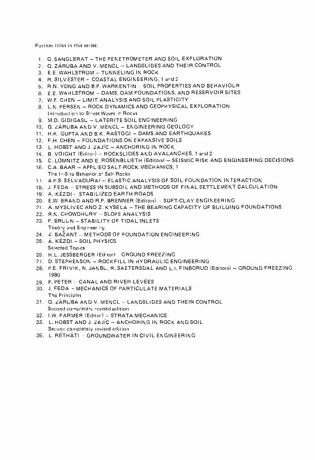
Further titles in this series:
1. G. SANGLERAT - THE PENETROMETER AND SOIL EXPLORATION 2. Q. ZARUBA AND V. MENCL - LANDSLIDES AND THEIR CONTROL 3. E.E. WAHLSTROM - TUNNELING IN ROCK 4. R. SILVESTER - COASTAL ENGINEERING, 1 and 2 5. R.N. YONG AND B.P. WARKENTIN - SOIL PROPERTIES AND BEHAVIOUR 6. E.E. WAHLSTROM - DAMS, DAM FOUNDATIONS, A N D RESERVOIR SITES 7. W.F. CHEN - LIMIT ANALYSIS AND SOIL PLASTICITY 8. L.N. PERSEN - ROCK DYNAMICS AND GEOPHYSICAL EXPLORATION
Introduction to Stress Waves in Rocks
9. M.D. GIDIGASU - LATERITE SOIL ENGINEERING 10. Q. ZARUBA AND V. MENCL - ENGINEERING GEOLOGY 11. H.K. GUPTA AND B.K. RASTOGI - DAMS AND EARTHQUAKES 12. F.H. CHEN - FOUNDATIONS ON EXPANSIVE SOILS 13. L. HOBST AND J. ZAJIC - ANCHORING IN ROCK 14. B. VOIGHT (Editor) - ROCKSLIDES A N D AVALANCHES, 1 and 2 15. C. LOMNITZ AND E. ROSENBLUETH (Editors) - SEISMIC RISK AND ENGINEERING DECISIONS 16. C.A. BAAR - APPLIED SALT-ROCK MECHANICS, 1
The In-Situ Behavior of Salt Rocks 17. A.P.S. SELVADURAI - ELASTIC ANALYSIS OF SOIL -FOUNDATION INTERACTION 18. J. FEDA - STRESS IN SUBSOIL AND METHODS OF F INAL SETTLEMENT CALCULATION 19. A. KEZDI - STABILIZED EARTH ROADS 20. E.W. BRAND AND R.P. BRENNER (Editors) - SOFT-CLAY ENGINEERING 21. A. MYSLIVEC AND Z. KYSELA - THE BEARING CAPACITY OF BUILDING FOUNDATIONS 22. R.N. CHOWDHURY - SLOPE ANALYSIS 23. P. BRUUN - STABILITY OF T I D A L INLETS
Theory and Engineering 24. Ζ. BAZANT - METHODS OF FOUNDATION ENGINEERING 25. A. KEZDI - SOIL PHYSICS
Selected Topics 26. H.L. JESSBERGER (Editor) - G R O U N D FREEZING 27. D. STEPHENSON - ROCKFILL IN H Y D R A U L I C ENGINEERING 28. P.E. FRIVIK, N. JANBU, R. SAETERSDAL AND L.I. F INBORUD (Editors) - GROUND FREEZING
1980
29. P. PETER - CANAL AND RIVER LEVEES 30. J. FEDA - MECHANICS OF PARTICULATE MATERIALS
The Principles 31. Q. ZARUBA AND V. MENCL - LANDSLIDES AND THEIR CONTROL
Second completely revised edition 32. I.W. FARMER (Editor) - STRATA MECHANICS 33. L. HOBST AND J. ZAJIC - ANCHORING IN ROCK AND SOIL
Second completely revised edition 35. L. RETHATI - GROUNDWATER IN CIVIL ENGINEERING

DEVELOPMENTS IN GEOTECHNICAL ENGINEERING 34A
GUY SANG LE RAT GILBERT OLIVARI BERNARD CAM BO U
ELSEVIER Amsterdam — Oxford — New York — Tokyo 1984
PRACTICAL PROBLEMS IN SOIL MECHANICS AND FOUNDATION ENGINEERING, 1 PHYSICAL CHARACTERISTICS OF SOILS, PLASTICITY,
SETTLEMENT CALCULATIONS, INTERPRETATION OF IN-S/TU TESTS
Translated by G. GENDARME

ELSEVIER SCIENCE PUBLISHERS B.V. Molenwerf 1 P.O. Box 211 , 1000 AE Amsterdam, The Netherlands
Distributors for the United States and Canada:
ELSEVIER SCIENCE PUBLISHING COMPANY INC. 52, Vanderbilt Avenue New York, N.Y. 10017
Library of Congress Cataloging in Publicatio n Data
Sanglerat, Guy, 1921*-Practical problems in soil mechanics and foundation
engineering.
(Developments in geotechnical engineering ; ) Translation of: Problemes practiques de mecanique des
sols et de fondations. Bibliography: v. 1 , p. Includes index. Contents: 1 . Physical characteristics of soils,
plasticity, settlement calculations, interpretation of in-situ tests.
1 . Soil mechanics. 2 . Foundations. I. Olivari, Gilbert. II. Cambou, Bernard. III. Title. IV. Series: Developments in geotechnical engineering ; 3k. T A 7 1 0 . S 2 1 + 6 13 1 9 8 * 1 6 2 À * . 1 ' 5 1 3â 8 4 - 1 0 2 5 0
ISBN 0 - 4 4 4 - 4 2 1 0 9 - 2 (U.S. : set) ISBN 0 - 4 4 4 - 4 2 1 0 8 - 4 (U.S. : v. l)
ISBN 0-444-42108-4 (Vol. 34A) ISBN 0-444-41662-5 (Series) ISBN 0-444-42109-2 (Set)
© Elsevier Science Publishers B.V., 1984
All rights reserved. No part of this publication may be reproduced, stored in a retrieval system or transmitted in any form or by any means, electronic, mechanical, photo-copying, recording or otherwise, without the prior written permission of the publisher, Elsevier Science Publishers B.V./Science & Technology Division, P.O. Box 330, 1000 AH Amsterdam, The Netherlands.
Special regulations for readers in the USA — This publication has been registered with the Copyright Clearance Center Inc. (CCC), Salem, Massachusetts. Information can be ob-tained from the CCC about conditions under which photocopies of parts of this publica-tion may be made in the USA. All other copyright questions, including photocopying outside of the USA, should be referred to the publishers.
í
P R E F A C E
by PROF. Dr. VICTOR F.B. De MELLO
President International Society for Soil Mechanics and Foundation Engineering 1981—1985
In the cont inuum of persistent change which characterizes the professional quest for scientific and engineering solut ions , there is an absolute need for pauses and movement by steps. Such a need is felt all the more intensely as all social and technological factors have m a d e the cont inuum of change more and more accelerated.
Man, and especially the Engineer, cannot shy away from the discontinuity imposed by a yes vs. no decis ion: maybe does not exist , because its imple-mentat ion would be as maybe-yes or maybe-no. Bo th right and wrong, however arbitrary and nominal , mus t be allowed to s tand long enough to permit the experience cycle to c lose , starting with a given set of data, hypo-theses, calculations and decisions, and reaching a certain set of observations on the constructed product under operat ional condit ions .
Far t o o much of the modern product ion of technical literature is con-ditioned by the eureka complex , especially in the respected advanced tech-nological centers . Yet , Man's and Soc ie ty ' s t ime cycle of experience is still deeply condit ioned by an animal life cycle , even if somewhat altered by physiological and social evolutions. A house is intended to be a h o m e , and its life cycle should respect a span roughly between twenty and eighty years ; public works should serve a couple of generations. It is not only materially but also socially that f rom the solutions of one generation or period arise the plagues of a following generation.
T h e appropriately named book , Practical Problems in Soil Mechanics and Foundation Engineering by Sanglerat , Olivari and C a m b o u , c o m e s to fulfill a very important need of thousands of practicing engineers in the geotech-nical profess ion. It sets a modern , practical milestone for reference, and is a lmost unique in doing this with its emphasis on calculations, the principal working tool of engineers. The analysis and calculation procedures presented, which encompass the great propor t ion of geotechnical problems , are simul-taneously both the indication of accepted practice and the reminder that such accepted pract ice is based on hypotheses : both the hypotheses and the rules developed from them must a lways be clearly s tated, not only so that except ions m a y be distinguished, but also so that the consequences of a given pract ice may be used to establish a m o d i c u m statistical universe of
VI PREFACE
case histories for judging the results achieved and for subsequent iterative adjustment.
Solutions in engineering are immediately recognized to be wrong if a patent or catastrophic failure ensues. Time, however, reveals the other extreme of the histogram of failures of engineering solutions, when they conceal a condition of being too safe and relatively less economical than desirable or acceptable. The authors are to be thanked for having offered a good up-to-date reference for appraising both ends of the spectrum. Engin-eers should be enjoined to state clearly the design procedures according to which their projects of a given period were calculated. This book augurs well to stand as a guide for many, many such calculations.

VII
I N T R O D U C T I O N
G u y Sanglerat has taught geotechnical engineering at the " E c o l e Centrale de L y o n " since 1 9 6 7 . This discipline was introduced there by J e a n Costet . S ince 1 9 6 8 and 1 9 7 0 , respectively, Gilbert Olivari and Bernard C a m b o u actively assisted in this responsibil i ty. They directed laboratory work, outs ide studies and led special s tudy groups .
In order to master any scientific discipline, it is necessary to apply its theoretical principles to pract ice and to readily solve its problems . This holds true also for theoretical soil mechanics when applied to geotechnical engin-eering.
F r o m Costet ' s and Sanglerat ' s experiences with their previously published t e x t b o o k s in geotechnical engineering, which contain example-problems and answers, it b e c a m e evident that one element was still missing in conveying the understanding of the subject matter to the solution of practical prob lems : problems apparently needed detai led, step-by-step solutions.
F o r this reason and at the request of many of their s tudents , Sanglerat , Olivari and C a m b o u decided to publish problems . Over the years since 1 9 6 7 the problems in this t ex t have been given to students o f the " E c o l e Centrale de L y o n " and since 1 9 7 6 to special geotechnical engineering s tudy groups of the Public Works Depar tment of the Nat ional School at Vaulx-en-Velin, where Gilbert Olivari was assigned to teach soil mechanics .
In order to assist the reader of these volumes , it was decided to categorize problems by degrees of solution diff iculty. Therefore , easy problems are preceded by one star ( * ) , those considered mos t difficult by 4 stars ( * * * * ) . Depending on his degree of interest, the reader may choose the types of problems he wishes to solve.
T h e authors direct the prob lems not only to s tudents but also to the practicing Civil Engineer and to others who, on occas ion, need to solve geo-technical engineering problems . T o all, this work offers an easy reference, provided that similarities of actual condit ions can be found in one or more of the solut ions prescribed herein.
Mainly, the S .I . (Systfeme International) units have been used. But , since practice cannot be ignored, it was deemed necessary to incorporate other widely accepted units . Thus the C.G.S . and English units (inch, foo t , pounds per cubic foo t , etc . ) have been included because a large quant i ty of literature is based on these units .
The authors are grateful to Mr. J e a n Kerisel , past president of the Inter-national Soc iety for Soil Mechanics and Founda t ion Engineering, for having

VIII INTRODUCTION
written the Preface to the French edition and allowing the authors to include one of the problems given his s tudents while Professor of Soil Mechanics at the " E c o l e Nationale de Ponts et Chaus see s " in Paris. Their gratitude also goes to Victor F . B . de Mello, President of the International Society for Soil Mechanics, who had the kindness to preface the English edit ion.
The first problems were originally prepared by J e a n Costet for the course in soil mechanics which he introduced in L y o n .
Thanks are also due to Jean-Claude Rouaul t of " A i r L i q u i d e " and Henri Vidal of "Re in forced E a r t h " and also to our Brazilian friend Lucien Decourt for contributing problems, and to Thierry Sanglerat for proofreading manu-scripts and printed proofs .
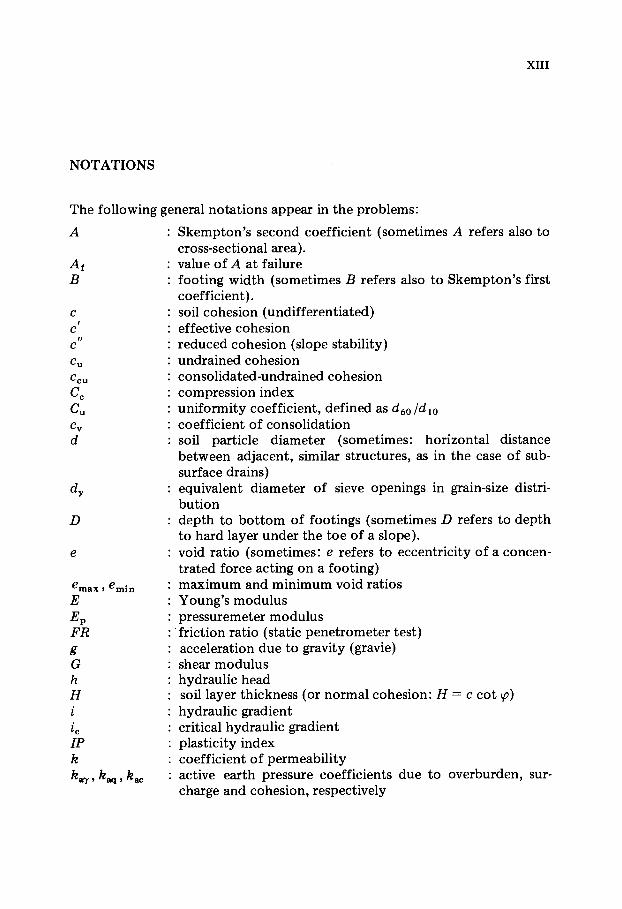
XIII
N O T A T I O N S
Β
c t
c ft
c
cc
d
The following general notat ions appear in the prob lems :
A : S k e m p t o n ' s second coefficient ( somet imes A refers also to cross-sectional area) , value o f A a t failure foot ing width ( somet imes Β refers also to S k e m p t o n ' s first coeff ic ient) . soil cohesion (undifferentiated) effective cohes ion reduced cohesion (s lope stabil i ty) undrained cohes ion consol idated-undrained cohesion compress ion index uniformity coeff icient, defined as d60/dl0
coefficient of consol idat ion soil particle diameter ( somet imes : horizontal distance between adjacent , similar structures , as in the case of sub-surface drains) equivalent diameter of sieve openings in grain-size distri-but ion depth to b o t t o m of foot ings ( somet imes D refers to depth to hard layer under the t o e o f a s lope) , void ratio ( somet imes : e refers to eccentricity of a concen-trated force acting on a foot ing) m a x i m u m and min imum void rat ios Young ' s m o d u l u s pressuremeter m o d u l u s friction ratio (static penetrometer test ) acceleration due to gravity (gravie) shear m o d u l u s hydraulic head soil layer thickness (or normal cohes ion: Ç = c cot ö) hydraulic gradient critical hydraulic gradient plasticity index coefficient of permeabi l i ty active earth pressure coefficients due to overburden, sur-charge and cohes ion, respectively
D
^ m a x > ^ m i n
Ε
£P
FR
g G h Ç
'c
IP k k ay > , va q > , va c

XIV NOTATIONS
, fepq, fepc : passive earth pressure coefficients K*Y > ^ aq > ^ ac : active earth pressures perpendicular to a given plane K ^ y , pq , ifpc : passive earth pressures perpendicular to a given plane fes : soil react ion modu lus Κ : bulk modulus ( X s of soil s tructure , KW of water) K0 : coefficient of earth pressure at rest I : width of an excavat ion L : length of an excavat ion m v : coefficient of compressibi l i ty Mm : driving m o m e n t MR : resisting m o m e n t Ì : bending m o m e n t ç : poros i ty ç¼ : stability coefficient ( s lope stability prob lems) Ny, , iVc : bearing capacity factors for foundat ion design Ρ : concentrated (point) load ñ Õ : l imit pressure (pressuremeter tes t ) Pf : creep pressure (pressuremeter test) q : uniformly distr ibuted load (or percolat ion discharge) Q : discharge (or load acting upon a foot ing) Qf : friction force of pile shaft ( total skin friction force) Qp : end-bearing force of pile ( tota l ) qd : u l t imate bearing capaci ty of soil under a foot ing or pile Qad : a l lowable bearing capaci ty of a foot ing or pile R : radius of a circular foot ing (or radius of drawdown of a
well) RD : relative density ( e m ax - e ) / ( e m ax - emin) r : well radius (or polar radius in polar coordinate sys tem) i ? p or qc : end-bearing on the area of a static penetrometer (cone
resistance) s : curvilinear abscissa (or cross-sectional area of a thin wall
tube , or sett lement) S : cross-sectional area of a mold or a sample S. G. : specific gravity S t : degree of saturat ion t : t ime Ô : shear Tv : t ime factor u : porewater pressure U : degree of consol idat ion (or resultant of pore-water pressure
forces) í : rate of percolat ion V : vo lume W : weight of a given soil vo lume

NOTATIONS XV
w : water content or sett lement w u w p : l iquid limit, plastic limit x,y,z : Cartesian coordinates , with Oz usually considered the verti-
cal, downward axis a : angle between orientat ions, usually reserved for the angle
between two crystal faces. Also used to classify soils for the purpose of their compressibi l i ty f rom static cone penetro-meter test da ta C.P.T.
â : s lope of the surface of backfill behind a retaining wall (angle of s lope)
7 : unit weight of soil (unspecif ied) 7S : soil particles unit weight (specific gravity) 7 s at : saturated unit weight of soil 7 h : wet unit weight of soil 7 W : unit weight of water = 9 .81 k N / m 3 . 7 d : dry unit weight of soil 7' : effective unit weight of soil T x y , 7yZ 5 Tz x · shear strain, twice the angular deformat ion in a rectangular,
3-dimensional system δ : angle of friction between soil and retaining wall surface in
passive or active earth pressure problems , or the angle of inclination of a point load acting on a foot ing
77 : dynamic viscosity of water e x , e y , e z : axial strains in a rectangular, 3-dimensional system 6 j , e 2 , e 3 : principal stress e v : volumetric strain θ : angle of radius in polar coordinates system ( somet imes :
temperature) í : Poisson's ratio σ' : effective normal stress ï : tota l normal stress σ χ , oy, σ ζ : normal stresses in a rectangular, 3-dimensional system σ ι ? σ2 » σ3 : ma jor principal stresses om : average stress r : shear stress
: average shear stress : shear stresses in a rectangular, 3-dimensional system
ö : angle of internal friction (undefined) ö : effective angle of internal friction ö" : reduced , effective angle of internal friction (slope-stability
analyses) <pcu : angle o f internal fr ict ion, consol idated, undrained λ : s lope of a wall f rom the vertical ùâ, ùä : auxiliary angles defined by sin ùâ = sin β/sin ö and
sin co δ = sin δ/sin ö
' m
NOTATIONS
3 .1416 distance f rom origin to a point in polar coordinate sys tem angle of major principal stress with radius vector (plasticity problems)
XVI
ð
Ρ
Ö
XVII
E N G I N E E R I N G U N I T S
It is presently required that all scientific and technical publ icat ions resort to the S .I . units ( Sys t&ne International) and their multipliers (deca , hecta , ki lo, Mega, Giga) . Geotechnical engineering units fol low this requirement and mos t of the problems treated here are in the S . I . sy s tem.
Fundamental S.I. units:
length : meter (m) mass : ki logram (kg) t ime : second (s)
S.I. Units derived from the above
surface vo lume specific mass velocity (permeabi l i ty) acceleration discharge force (weight) unit weight pressure, stress work (energy) viscosity
square meter ( m 2 ) cubic meter ( m 3 ) ki logram per cubic meter ( k g / m 3) meter per second (m/s ) meter per second per second ( m / s 2 ) cubic meter per second ( m 3 /s) N e w t o n (N) N e w t o n per cubic meter ( N / m 3 ) Pascal (Pa) 1 Pa = 1 N / m 2
J o u l e ( J ) 1 J = 1 Ν χ m Pasca l - second* Pa χ s
However, in pract ice , other units are encountered frequently. Table A presents correlations between the S .I . and two other unit sys tems encoun-tered worldwide. This is t o familiarize the readers of any publ icat ion with the units used therein. F o r that purpose also , British units have been a d o p t e d for s o m e of the presented prob lems .
Force (pressure) conversions
Force units : see Tab le Β Pressure units : see Tab le C Weight unit : 1 k N / m 3 = 0 . 1 0 2 t f / m 3
*This unit used to be called the "poiseuille", but it has not been officially adopted.
XVIII ENGINEERING UNITS
TABLE A Correlations between most common unit systems
Systeme International Meter-Kilogram system Centimeter-Gram-(S.I.) (M.K.) Second system
(C.G.S.)
units common units common units common multiples multiples multiples
Length meter (m) km meter (m) km cm m Mass kilogram (kg) tonne (t) gravie* — g — Time second (s) — second (s) — s — Force Newton (N) kN kilogram force
(kgf) tf dyne —
Pressure Pascal (Pa) kPa kilogram force ( t / m 2 barye bar (stress) MPa per square
meter ( k g f / m 2) I kg/cm ( 1 0 6 baryes)
Work Joule (J) kJ kilogram meter t f . m erg Joule (energy) (kgm) ( 1 0 7 ergs)
*Note that 1 gravie = 9.81 kg (in most problems rounded off to 10).
The unit weight of water is: 7 W = 9 .81 k N / m 3 but it is often rounded off t o : 7 W = 10 k N / m 3.
Energy units:
1 J o u l e = 0 . 1 0 2 k g . m = 1.02 χ 1 0 " 4 t . m 1 k g f . m = 9 .81 Jou le s 1 t f . m = 9 .81 χ 1 0 3 J ou le s
Dynamic viscosity units:
1 Pascal-second ( P a . s ) = 10 poises (Po) .
British units:
1 inch 1 foo t 1 square inch 1 square foo t l m 2
1 cubic inch 1 cubic foo t l m 3
1 p o u n d (lb) 1 Newton
1 lb/cu. in.
= 0 . 0 2 5 4 m = 0 . 3 0 4 8 m = 6 . 4 5 1 6 c m 2
= 1 4 4 sq. in. = 0 . 0 9 2 9 m 2
= 1 0 . 7 6 4 s q . f t . = 1 6 . 3 8 7 c m 3
= 1 7 2 8 cu. in. = 0 . 0 2 8 3 1 7 m 3
= 3 5 . 3 1 4 cu. ft. = 4 . 4 4 9 7 Newton = 0 . 4 5 3 5 9 kgf = 0 . 2 2 5 lb = 0 . 1 1 2 4 χ 1 0 - 3 sh. t on = 1 .003 x l O " 4 ton . = 2 7 0 . 2 7 k N / m 3
l m = 3 9 . 3 7 0 in. l m
l c m 2
= 3 . 280 8 foo t = 0 . 1 5 5 sq. in.
l c m 3 = 0 . 0 6 1 Ocu. in.
(1 sh. ton . = 2 kip)

ENGINEERING UNITS XIX
1 lb/cu. ft. 1 k N / m 3
1 lb/sq . in. (p.s . i .) 1 Pascal 1 0 0 kPa
0 . 1 5 6 9 9 k N / m 3
3.7 χ 1 0 - 3 lb /cu . in. = 6 . 37 lb /cu . ft. 6 . 8 9 6 5 5 χ 1 0 3 Pa 1 4 . 5 0 χ 1 0 " s p.s . i . 1 bar = 1 4 . 5 0 p.s . i .

TABLE Β
Force units conversions
Value of / \ ^ ' e x p r e s s e d / in
Newton Decanewton Kilonewton Kilogram force
Tonne Dyne force
Newton Decanewton Kilonewton Kilogram
force Tonne force Dyne
1 10 1 0 3
9.81
9.81 × 1 0 3
IO"5
1 0 " 1
1 1 0 2
9 .81 X 10 1
9 .81 × 1 0 2
10 6
1 0 " 3
IO"2
1 9.81 × 1 0 " 3
9 .81 10 8
1.02 × 1 0 " 1
1.02 1.02 × 1 0 2
1
1 0 3
1.02 X 10 6
1.02 × 1 0 " 4 1 0 s
1.02 X 10 3 1 0 6
1.02 X 10 1 1 0 8
1 0 " 3 9 .81 × 1 0 5
1 9 .81 × 1 0 8
1.02 × 1 0 " 9 1
T A B L E C
Pressure units conversions
Value y/ of / Pa i ./expressed
in -*•
kPa bar hbar barye kg/cm2 kg /mm2 t / m 2 cm of water atm.
Pascal 1 10"3
Kilopascal 103 1
Bar 10s 102
Hectobar ΙΟ7 104
Barye 0.1 10 4
kg/cm2 9.81 × 10⁴ 9.81 χ 101
kg /mm2 9.81 x 10⁶ 9.81 χ 10"3
t / m 2 9.81 x 10³ 9.81 cm o i water 9.81 × 101 9.81 × 10"2
Atmosphere 1.013 3 X 10s 1.013 3 ÷ 102
10"5
I O ' 2
1 102
10"6
0.981 9.81 × 101
9.81 × 10"2
9.81 X 10 4
1.013 3
IO"7
10"4
I O ' 2
1 10 8
9.81 × 10³
0.981 9.81 X 10 4
9.81 X 10 6
1.013 3 X 10'
10 104
106
108
1 9.81 x 10s
9.81 × 10⁷
9.81 × 10⁴
9.81 × 10²
"2 1.013 3 × 10⁶
1.02 x 10"5 1.02 × I O -7
1.02 x I O -2 1.02 X 10 4
1.02 1.02 x 10 2
1.02 x 10² 1.02 1.02 × 10"6 1.02 X 10 8
1 10 2
102 1 0.1 10 3
10"3 10 5
1.033 1.033 X 10 2
1.02 x 10"4 1.02 × 10"2
1.02 x I O -1 10.2 10.2 1.02 x 10³
1.02 x 10³ 1.02 X 10s
1.02 x 10"~5 1.02 x 10 3
10 i o 3
i o 3 i o 5
1 102
ιο~2 1 1.033 × 101 1.033 χ 103
9.869 × 10"6
9.869 X 10 3
0.986 9 9.869 x 101
9.869 x 10 7
0.968 1 9.681 × 101
9.681 X 10 2
9.681 × 10"4
1
XX

1
Chapter 1
P H Y S I C A L C H A R A C T E R I S T I C S O F S O I L
if Pro blem 1.1 Water content
A saturated clay sample has a mass of 1526 g. After drying, its mass is 1053g. The solid constituant (soilparticles) has a specific gravity of 2.7. Find: — water content, w — void ratio, e — porosity, ç — wet unit weight, yh
— wet density, 7 h / T w · Takeg = 9.81 m/s2.
Solut ion The weight o f the clay sample is : 1 .526 χ 9 . 8 1 = 1 4 . 9 7 Ν. The dry weight is : 1 .053 χ 9 .81 = 1 0 . 3 3 Ν. The weight of water conta ined in the sample i s : 1 4 . 9 7 — 1 0 . 3 3 = 4 .64 N . The water content : w = weight o f water/weight of dry soil = 4 . 6 4 / 1 0 . 3 3 = 0 . 4 5 .
The void ratio is : e = vo lume of water /volume of soil particles. S ince the soil is sa turated , the voids between soil particles are filled with
water and the volume of voids is equal to the volume of water (F ig . 1 .1) .
à Wate r
Grains 7 W = 9 . 8 1 · 1 0 3 N / m 3
Fig. 1.1.
The volume of water is :
weight of water _ 4 .64
yl " 9 . 81 χ 1 0 3 = 0 . 4 7 3 x l 0 _ 3m 3 = 4 7 3 c m 3 .
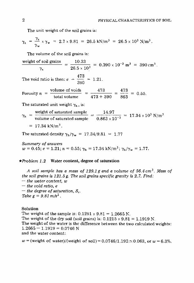
2 PHYSICAL CHARACTERISTICS OF SOIL
The unit weight of the soil grains is :
= — X 7 w = 2 . 7 x 9 . 8 1 = 2 6 . 5 k N / m 3 = 2 6 . 5 χ 1 0 3 N / m 3 . Tw
The volume of the soil grains is :
weight of soil grains 1 0 . 3 3
Ts 2 6 . 5 χ 1 0 3 0 . 3 9 0 x l 0 ~ 3 m 3 = 3 9 0 c m 3 .
4 7 3 The void ratio is then: e = = 1 .21 .
3 9 0
volume of voids 4 7 3 4 7 3 Porosity ç = = = = 0 . 5 5 .
total vo lume 4 7 3 + 3 9 0 8 6 3
The saturated unit weight 7 h , is :
weight of saturated sample 14 .97 7h = — : : — = ~ = 1 7 . 3 4 x l O 3 N / m 3
volume of saturated sample 0 .863 χ 10 3
= 17 .34 k N / m 3 .
The saturated density 7 h / 7 w = 1 7 . 3 4 / 9 . 8 1 = 1.77
Summary of answers w = 0 . 4 5 ; e = 1 . 2 1 ; ç = 0 . 5 5 ; jh = 1 7 . 3 4 k N / m 3 ; 7 h / 7 w = 1.77.
if Problem 1.2 Water content , degree o f saturat ion
A soil sample has a mass of 129.1 g and a volume of 56.4 cm3. Mass of the soil grains is 121.5g. The soil grains specific gravity is 2.7. Find: — the water content, w — the void ratio, e — the degree of saturation, SY. Takeg = 9.81 m/s2.
Solut ion The weight of the sample is : 0 . 1 2 9 1 χ 9 .81 = 1 .2665 Ν. The weight of the dry soil (soil grains) i s : 0 . 1 2 1 5 χ 9 . 8 1 = 1 .1919 Ν. The weight of the water is the difference between the two calculated weights : 1 .2665 - 1 .1919 = 0 . 0 7 4 6 Ν and the water content :
w = (weight o f water)/(weight of soil) = 0 . 0 7 4 6 / 1 . 1 9 2 ^ 0 . 0 6 3 , or w = 6 .3%.

PROBLEM 1.2
The void rat io is :
e = vo lume of voids (water 4- a ir ) /volume of soil grains
e
1
Air Wate r -=~z
7
j . · - · . . - ·'
Grains ·" *
Fig. 1.2.
The volume of voids is equal t o the total vo lume less the volume of grains. The total vo lume is k n o w n : 56 .4 c m 3 .
weight of grains The volume of the grains is :
unit weight (ys)
Since specific gravity
S .G . = 7 s / 7 w = 2.7
where 7 W = pg = 9 .81 k N / m 3 and 7 S = 2.7 χ 9 .81 χ 1 0 3 N / m 3 .
The volume of grains Vs is :
V s = 1 .1919 /2 .7 χ 9 . 8 1 x l O 3 = 4 . 5 x l 0 " 5 m 3 = 4 5 c m 3
and the volume of voids is :
Vv = 5 6 . 4 - 4 5 = 11 .4 c m 3 .
The void ra t io : e = 1 1 . 4 / 4 5 = 0 . 2 5 3 , say e = 0 . 2 5 . The degree o f saturat ion S r is given b y :
vo lume of water/volume of voids
The vo lume of water : Vw = weight of water/density of water = 0 . 0 7 4 6 / 9 . 8 1 χ 1 0 3 = 7.6 χ 1 0 " 6 m 3 or V w = 7.6 c m 3 . The degree o f saturat ion is : S r = 7 . 6 / 1 1 . 4 = 0 . 6 6 6 , say 6 7 % .
Summary of answers: w = 6 .3%; e = 0 . 2 5 ; S r = 6 7 % .
3
= VJVS (F ig . 1.2)
4 PHYSICAL CHARACTERISTICS OF SOIL
^Problem 1.3 Unit weight and density
A quartzitic sand weighs, in a dry condition, 15.4 kN/m 3. What is its wet unit weight (yh) and its wet density 7 h / 7 w when it is saturated? Assume: specific gravity of sand: S.G. = 2.66, acceleration due to gravity: g = 9.81 m/s2, unit mass of water: ñ = 103 kg/m3.
Solut ion The unit weight of the sand grains is :
7 S = S .G . χ 7 W = S .G . χ ρ x g = 2 .66 Ί 0 3 · 9 . 8 1 N / m 3 = 2 6 . 1 0 k N / m 3 .
A cubic meter of dry sand contains 1 5 . 4 0 / 2 6 . 1 0 = 0 .59 m 3 of grains and, consequent ly , 1 — 0 .59 = 0 .41 m 3 of voids. When this sand is saturated, the voids are complete ly filled with water. The weight of the void water is then:
0 .41 X 7 W = 0 . 4 1 x 9 . 8 1 = 4 . 0 2 k N .
The weight of a cubic meter of saturated sand is thus 15 .4 4- 4 . 0 2 = 1 9 . 4 2 kN or 7 h = 1 9 . 4 2 k N / m 3 . The density of sand 7 hA y w = 1 9 . 4 2 / 9 . 8 1 = 1.98.
Summary of answers:
7 h = 1 9 . 4 2 k N / m 3 ; T h/ 7 w = 1.98.
*Problem 1.4 Unit weight and densi ty ; saturat ion and water content
A clay sample is placed in a glass container. Total mass of clay sample and container is 72.49g. After drying in an oven, the dry mass of the clay and container is 61.28g. The mass of the container is 32.54 g. A specific gravity test by the picnometer method has determined that S.G. of the soil constitu-ant is 2.69.
(a) Assume the sample to be saturated, find: — the water content, w — the porosity, ç — the void ratio, e — the wet density (jh/Jw) — the dry density (ya/y w) — the buoyant density (y'/y w).
(b) Before drying the sample, its volume V was determined by immersing the soil in mercury (V = 22.31 cm3). What is the actual degree of saturation and what are the new values of the densities determined in (a)?
Solut ion (a) The mass of water contained in the sample is : 7 2 . 4 9 — 6 1 . 2 8 = 1 1 . 2 1 g .

PROBLEM 1.4 5
The mass of dry soil particles is : 6 1 . 2 8 — 3 2 . 5 4 = 2 8 . 7 4 # . The water content w = weight of water/weight of dry soil = mass of water/ mass of dry soil = 1 1 . 2 1 / 2 8 . 7 4 = 0 . 3 9 , w = 39%.
Porosity ç = vo lume of voids / tota l vo lume.
Since the sample is a s sumed to be saturated, the vo lume of voids is equal to the volume of water or 1 1 . 2 1 c m 3 ( the unit mass of water is ρ = lg/cm3).
Vg = mass of dry soil grains/specific gravity of soil = 2 8 . 7 4 / 2 . 6 9 ~ 1 0 . 6 8 c m 3 .
Therefore , ç = ( 1 1 . 2 1 ) / ( 1 1 . 2 1 4 - 1 0 . 6 8 ) ~ 0 . 5 1 2 , say ç = 0 . 5 1 . The void ratio is e = volume of voids /volume of soil grains = 1 1 . 2 1 / 1 0 . 6 8 = 1 .049, say e~ 1 .05.
S ince the unit mass of water is 1 g/cm3, densities are of the same numerical values as the unit masses . The mass of the wet sample is, therefore : 7 2 . 4 9 — 3 2 . 5 4 = 3 9 . 9 5 g .
The total volume of the clay sample is : 1 1 . 2 1 + 1 0 . 6 8 = 2 1 . 8 9 c m 3 . The wet unit mass is : 3 9 . 9 5 / 2 1 . 8 9 = 1 . 8 2 5 g / c m 3, say 1.83 £ / c m 3 , and the
wet density 7 h / T w thus 1.83. The mass of the dry soil is 2 8 . 7 4 # . Its dry unit mass is : 2 8 . 7 4 / 2 1 . 8 9 =
1 . 3 1 3 g / c m 3, say 1 . 3 1 g / c m 3, the dry density yd/y w = 1 . 31 . In order to obtain the b u o y a n t density , the weight of water displaced by
the submerged mass of the soil grains mus t be subtracted f rom the soil weight. The volume of the grains is 1 0 . 6 8 c m 3 . Their mass in water will then b e : 2 8 . 7 4 - 1 0 . 6 8 = 1 8 . 0 6 g , and the buoyant unit mass is : 1 8 . 0 6 / 2 1 . 8 9 = 0 . 8 2 5 ^ / c m 3 ; say 0 . 8 3 # / c m 3 . (Another , mos t c o m m o n l y used way of determining buoyant unit mass , is f rom the relat ion: buoyant unit mass = saturated unit mass — unit mass of water ) .
(b) The volume of the samples being 2 2 . 3 1 c m 3 proves that the clay is not saturated. Part of the voids is filled with air. The air vo lume is: 2 2 . 3 1 — 2 1 . 8 9 = 0 .42 c m 3 . The degree of saturat ion, Sr = volume of water/ tota l void vo lume.
The vo lume of water calculated in (a) is 1 1 . 2 1 c m 3 , the volume of void = 1 1 . 2 1 + 0 . 4 2 = 1 1 . 6 3 c m 3 then S r = 1 1 . 2 1 / 1 1 . 6 3 = 0 . 9 6 3 , say Sr = 0 . 9 6 .
The total soil sample volume is 2 2 . 3 1 c m 3 . The corrected densities are thus : for the wet densi ty : yh/y w = 3 9 . 9 5 / 2 2 . 3 1 = 1.79 and for the dry den-si ty : T d / 7 w = 2 8 . 7 4 / 2 2 . 3 1 = 1.29.
Since the concept of b u o y a n t mass is appl icable to saturated soils only, it should not be calculated in this instance.
Summary of answers
(a) w = 3 9 % ; ç — 0 . 5 1 ; e = 1 . 0 5 ; T h/ T w = 1 . 8 3 ;7d / T w = 1 . 3 1 ; T ' /TW = 0 .83 . ( b ) S r = 9 6 % ; 7 h / 7 w = 1-79; ydlyw = 1 .29. (y'/y w has no meaning in the second part of the prob lem because the soil is n o t saturated. )

6 PHYSICAL CHARACTERISTICS OF SOIL
irProblem 1.5 Grain-size dis tr ibution : effectiv e diamete r and Hazen's coefficien t
A grain-size analysis is performed on 3500g of dry sand from the Saone valley. No soil is retained on the 12.5-mm openings sieve. A nest of six sieves is subsequently used to separate the various sand sizes. The openings of the sieve meshes are, from top to bottom; 5,2,1, 0.5, 0.2 and 0.1 mm. The soil masses remaining on each of the six sieves are 217g, 868g, 1095g, 809g, 444 g, 39 g, and the amount of soil in the bottom pan is 28 g.
Draw the grain-size distribution curve and find the effective diameter and the uniformity coefficient (Hazen's coefficient) of this sand.
Solu t ion Drawing the grain-size distr ibution curve consists of connect ing the points
on a graph which represent the cumulat ive mass percentages passing down to the sieves size.
As shown in Fig . 1.3, the soil passing sieve ç = soil passing sieve (ç — 1) minus the soil retained on sieve n, or Tn =Tn-x — Rn, where Tn is the weight passing sieve n.
Siev e ç
Nes t of sieve s
Fig. 1.3. A nest of sieves.
Since the initial sieve (12 .5-mm openings) retained no soil, Tx = 3 5 0 0 g. The soil retained on the top sieve of the nest is 2 1 7 g, therefore T2 =
3 5 0 0 - 2 1 7 g = 3 2 8 3 g, T 3 = 3 2 8 3 - 8 6 8 g = 2 4 1 5 , and so on. A table , such as the one shown below, is constructed to give the calculated
values of the percents passing. The values in the last co lumn are p lot ted on a semi-log grid (see Fig. 1.4).

Fig. 1.4. Grain-size distribution curve.
6U
ISS
PCJ
;ua
oja
d
7
8 PHYSICAL CHARACTERISTICS OF SOIL
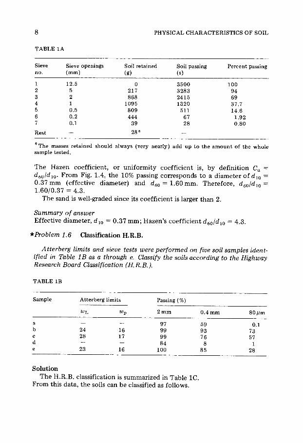
TABLE 1A
Sieve Sieve openings Soil retained Soil passing Percent passing no. (mm) (*) (s)
1 12.5 0 3500 100 2 5 217 3283 94 3 2 868 2415 69 4 1 1095 1320 37.7 5 0.5 809 511 14.6 6 0.2 444 67 1.92 7 0.1 39 28 0.80
Rest — 28* —
The masses retained should always (very nearly) add up to the amount of the whole sample tested.
The Hazen coefficient, or uniformity coefficient is, by definition C u = d60/dlQ. F r o m Fig. 1.4, the 10% passing corresponds to a diameter of d 1 0 = 0 .37 m m (effective diameter) and d 6 0 = 1.60 m m . Therefore , d 6 0/ d 1 0 = 1 .60/0 .37 = 4 .3 .
The sand is well-graded since its coefficient is larger than 2.
Summary of answer
Effective diameter , dl0 = 0 .37 m m ; Hazen's coefficient d60/dx0 = 4 .3 .
^Problem 1.6 Classification H.R .B.
Atterberg limits and sieve tests were performed on five soil samples ident-ified in Table IB as a through e. Classify the soils according to the Highway Research Board Classification (H.R.B.).
TABLE I B
Sample Atterberg limits Passing (%) Sample
2 mm 0.4 mm 80 μιη
a — — 97 59 0.1 b 24 16 99 93 73 c 28 17 99 76 57 d — — 84 8 1 e 23 16 100 85 28
Solut ion The H .R .B . classification is summarized in Table 1C .
F r o m this data , the soils can be classified as fol lows.

TABLE 1C
Summarized H.R.B-classification
Less than 35% passing 80-μ sieve More than 35% passing 80-μ sieve
Aia A i b A 3 A 2-4 A 2- s A 2- 6 A 2- 7 A 4 A 5 A 6 A7-5 A7-6
Percent passing: 2-mm sieve 0.4-mm sieve 80-μηι sieve
< 5 0 < 3 0 < 5 0 < 1 5 < 2 5
> 5 1 < 1 0 < 3 5 < 3 5 < 3 5 < 3 5 >S6 > 3 6 > 3 6 > 3 6 > 3 6
Characteristics of portions passing the 2-mm sieve: — plasticity index — liquid limit
< 5 no test
no test < 1 0 < 4 0
< 1 0 > 4 1
> 1 1 < 4 0
> 1 1 > 4 1
< 1 0 < 4 0
< 1 0 > 4 1
> 1 1 < 4 0
>11 > 4 1
> 1 1 > 4 1
— group index 0 0 0 < 4 < 8 < 1 2 < 1 6 < 2 0 < 2 0
— general name cobbles gravels sands
fine sand
mixture of silty gravel or clayey gravel with silty or clayey sand
silty soils clayey soils
PR
OB
LE
M 1.6
9

10 PHYSICAL CHARACTERISTICS OF SOIL
Sample a. (1) The percent passing the 8 0 μ π ι = 0 . 1 % , the soil must be classified as granular soil. (2 ) The percent passing 0.4 m m is more than half, it is 59%. The soil is a fine sand of t y p e A 3 (non plast ic) .
Sample b. (1) The percent passing the 80 Mm: 73% > 3 5 % ; it is therefore a fine-grained soil. (2 ) The plasticity index Ip = w h — w p = 2 4 — 16 = 8 < 10%: the soil is silty. (3 ) The liquid limit w h = 2 4 < 4 0 % : the classifi-cat ion is type A 4 : a silt.
Sample c. (1 ) Percent passing 80 Mm: 57% > 3 5 % : a fine-grained soil. (2 ) plasticity index : J p = w h — w p = 2 8 — 17 = 1 1 % : a clayey soil. (3 ) w L = 28 < 4 0 % ; this soil is o f type A 6 , clay.
Sample d. (1 ) Percent passing 80 μπι : 1 % < 3 5 % : a coarse-grained soil. (2 ) Percent passing the 0.4 m m : 8% < 30%. (3 ) Percent passing the 2 m m : 84% > 50%: this is the type A l b soil, a gravelly sand.
Sample e. (1) Percent passing 8 0 Mm: 2 8 % < 3 5 % : a coarse-grained soil ; (2 ) Plasticity index J p = w h~wp = 23 - 16 = 7 < 10%. (3 ) L iqu id limit u ; L = 23 < 4 0 % : this is a type A 2 - 4 soil, a silty sand.
Summary of answers Samples a: type A 3 , b : type A 4 , c : type A 6 , d : t y p e A l b, e : type A 2 - 4 .
**Problem 1.7 Atterberg limits
An Atterberg limits test on soil samples gave the results shown in Tables ID and IE.
TABLE I D
Liquid limits (masses in grams)
Number of blows 17 21 26 30 34
Test nr. l a 16 2a 26 3a 36 4a 46 5a 56
Total wet mass 9.35 9.68 13.69 12 .16 10 .11 9.27 10 .31 11 .08 11 .50 9.59 (soil + tare) Total dry mass 8.79 9.20 11.35 10 .19 8.67 8 .02 8.84 9.42 9.78 8.31 (soil + tare) Tare mass 7.11 7.77 4.05 4.05 4.10 4.07 4 .10 4.10 4.07 4 .05
TABLE IE
Plastic limits (masses in grams)
1st test 2nd test
Container nr. A Β Ε F Total wet mass 6.32 6.56 6.54 6.36 Total dry mass 5.94 6.15 6.12 5.97 Tare mass 4.06 4.10 4.07 4.05

PROBLEM 1.7 11
Calculate the liquid limit w h and the plastic limit w p of the soil. What is the plasticity index? Compare the results of w h with those given by the following (approximate) mathematical relation: w L = w(N/25) 0A21.
Classify the soil in accordance with Casagrande's A-line.
Solut ion By definit ion,
weight of water mass of water w = =
weight of dry soil mass of dry soil
The mass of water = total wet mass — total dry m a s s ; the mass of dry soil = total dry mass — tare mass .
The average of two values in each co lumn is taken to make a new tabu-lation as shown in Table I F .
TABLE I F
Liquid limits (w^)
Number of blows 17 21 26 30 34
Test nr. l a l b 2a 2b 3a 3b 4a 4b 5a 5b
Mass of water 0.56 0.48 2.34 1.97 1.44 1.25 1.47 1.66 1.72 1.28 Mass of soil 1.68 1.43 7.30 6.14 4.57 3.95 4.74 5.32 5.71 4.26 Water content 33 .30 33 .60 32 .10 32 .10 31 .50 31 .60 31.00 31 .2 30 .10 30 .00
Averages 33.5 32 .10 31.6 31 .1 30.1
The average values of the water contents are p lot ted against their corre-sponding numbers of blows on the graph of Fig . 1.5. By definit ion, the liquid limit w L is the water content corresponding to 2 5 blows. S o w L = 31 .6%, say 3 2 % .
Ö 32 •Ç» c ï õ
Ö 31
1—
< >
í
J é < >
—
15 20 25 30 35 N u m b e r o f b l o w s
Fig. 1.5. Average water contents plotted against number of blows.

12
PH
YS
ICA
L C
HA
RA
CT
ER
IST
ICS
OF
SO
IL
Fig. 1.6. Casagrande's graph.

PROBLEM 1.7 13
Table 1 G compares the values of w h obta ined from the laboratory test versus those obta ined by the use of the empirical formula w h = w(N/25)° ·121.
The laboratory determinat ion o f w L entails an error est imated t o be half a point of the value of w\ or : 0 . 5 / 3 1 . 6 = 1.6%.
The empirical m e t h o d yields an average value of 31 .6 with a m a x i m u m error of 0 .4 point . The two methods are acceptable to the same degree of accuracy for this particular soil .
F o r the plastic l imits, w p, Table 1H, similar to the previous one , can be m a d e u p .
TABLE 1G
Ν N/25 (ΛΓ/25) 0· 1 21 w
17 0.68 0 .954 33.5 ^ 3 2 21 0.84 0 .979 32.1 31.4 26 1.04 1.005 31.6 31.7 30 1.20 1.022 31.1 31.8 34 1.36 1.038 30.1 31.2
TABLE 1H
Plastic limits (wp)
1st test 2nd test
Container i.d. A Β Ε F
Mass of water (g) 0.38 0.41 0.42 0.39 Mass of dry soil (g) 1.88 2.05 2.05 1.92 Water content (%) 20.2 20.0 20.5 20.3
Averages (%) 20.1 20.4
The plastic limit is 20%, the nearest whole number of the experimental results. Therefore : w L = 3 2 % , w p = 20%, Ip = w h — w p = 1 2 % .
Casagrande's Α-line graph shown in Fig . 1.6 with the results p lo t ted on it indicates that the soil is an inorganic clay of med ium plasticity.
***Problem 1.8 Correct ion o f a grain-size distr ibution curve: scalping and mixing of soils
The sieve analysis of an alluvial gravelly soil sample gave the following size
distribution:
d100 = 1 0 0 d 7 5 = 50 d 4 5 = 20 d 3 8 = 10 d 3 4 = 5
d 3 0 = 2 d29 = 1 d 2 5 = 0 .5 d 1 0 = 0 .2 d 3 = 0 .08
14
Bu
jssed
lu
ao
jed
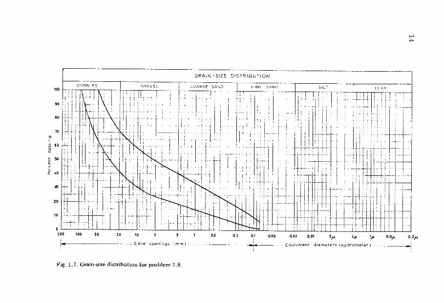
Fig. 1.7. Grain-size distribution for problem 1.8.
PROBLEM 1.8 15
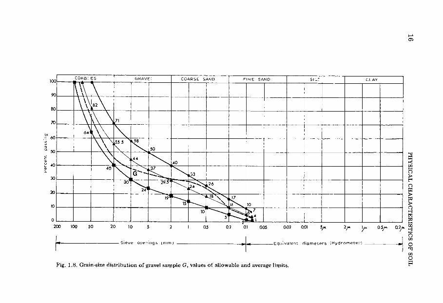
(1) Determine whether this material would meet the gradation require-ment of an acceptable foundation soil as defined by the limit curves shown in Fig. 1.7.
(2) It is desirable to reduce the sand content by 5% between 0.2 and 0.5, which is, in its present quantity, considered detrimental for achieving proper compaction. However, the percentages of sizes over 10 mm should not be changed. Recommend a procedure to correct the grain-size distribution. All values of dy are in millimeters.
Solut ion (1) The grain-size distribution curves for the upper and lower limits as well
as the averages between them and for the soil sample are shown in Fig. 1.8. The curve for the sample is contained entirely within the specified limits.
The soil is an acceptable material for the foundat ion. It is not iced how-ever, that its grain-size distribution deviates substantially from the average between the upper and lower limits and shows a ' h u m p ' in the sand range between d = 0 .2 and d = 2 . This hump is also evident in the histogram plot ted in Fig . 1.9, which shows the individual (as o p p o s e d to the cumu-lative) percentages for each consecutive sieve-size opening range. The average-curve histogram is also shown. The ' h u m p ' in the sand fraction is seen to occur more precisely between sieve sizes 0.2 and 0 .5 .
(2 ) To reduce the a m o u n t of sand in the range 0.2—0.5 by 5% may be interpreted to mean that the quant i ty of the size corresponding to 1 5 % must be lowered to 10%. Furthermore , there is the requirement not to change the percentages of sizes equal to or greater than 10 m m . In order to achieve this, an amount ρ of a soil of an as ye t undetermined grain-size distribution must be mixed with the alluvial gravelly soil to bring the 0.2—0.5 range of the mixture down to 10%.
For , let us say, 1 0 0 kg of gravel G, the weight ñ to be added , is:
15 = 1 0 / 1 0 0 ( 1 0 0 + p) or ñ = 50 kg.
Since all sizes equal to or greater than 10 m m amount to 2 5 4- 30 4- 7 = 6 2 % of the weight of the original sample , it is necessary to add a pro-port ionate part , or 0 .62 χ 50 kg = 3 1 kg of material scalped from the gravel retained on sieves 10 m m and above . This only leaves 50 — 3 1 = 19 kg to add a material that has the gradation of 'fine gravelly sand ' ( m a x i m u m diameter smaller than 10 m m ) but is coarse enough not to have sizes less than 0 .5 m m .
F r o m the histogram of Fig . 1.9, it is evident that the a m o u n t of gravelly sand in the range 0.5—5.0 m m is below the average gradation of the two allowable limits. One possible solution to lower d 1 5 would be to add 19 kg of gravelly sand with a gradation between 0.5 and 5 . Such a sand (with a distribution d100 = 5 m m , d90 = 2 m m and d30 = 1 m m ) is p lot ted in Fig . 1.10 as sand S. Hence Table I I is obta ined .
PH
YS
ICA
L C
HA
RA
CT
ER
IST
ICS
OF
SO
IL Fig. 1.8. Grain-size distribution of gravel sample G, values of allowable and average limits.
16
PROBLEM 1.8 17
100 50 20 5 2 1 0.5 0.2 0.1 0.08
S iev e opening s i z e s ( m m )
COARSE SAND FINE SAND
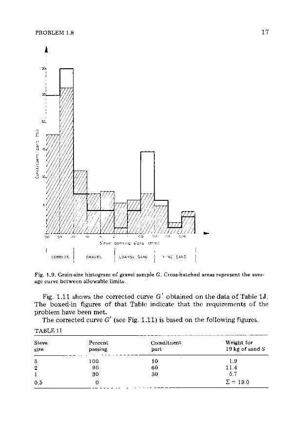
Fig. 1.9. Grain-size histogram of gravel sample G. Cross-hatched areas represent the aver-age curve between allowable limits.
Fig. 1.11 shows the corrected curve Gf obta ined on the data o f Table 1 J . The boxed-in figures of that Table indicate that the requirements of the problem have been met .
The corrected curve G' (see Fig. 1.11) is based on the following figures.
TABLE II
Sieve Percent Constituent Weight for size passing part 19 kg of sand S
5 100 10 1.9 2 90 60 11.4 1 30 30 5.7
0.5 0 Σ = 19.0

18 PHYSICAL CHARACTERISTICS OF SOIL
2 1 0.5 0.2 S i e ve o p e n i n gs ( m m)
Fig. 1.10. Grain-size distribution of sand S.
TABLE 1J
Sieve sizes
Weight in kg at various constituents for 150 kg of G'
Constituent parts (%) passing
100
50
20
10
5
2
1
0.5
0.2
0.1
0.08
25 XI .5 =
30 X 1.5 =
7 X 1 . 5 =
4 + 1.9 =
1 + 11.4 =
4 + 5.7 =
100 37 .50 25%
100
45 .00 30% 75
10.50 7% 45
4.00 2.6% 38
5.90 3.9% 35.4
12 .40 8.3% 31.5
9.70 6.5% 23.2
16.7
6.7 15 .00 10%
16.7
6.7 6.00 4%
16.7
6.7
1.00 0.7% 2.7
3.00 2% 2
0
The values in Table 1J show that the imposed conditions are verified: % of dy > 10 unchanged % of 0.2 < dy < 0.5 decrease to 10%

Fig. 1.11. Grain-size distribution of corrected material.
19
20 PHYSICAL CHARACTERISTICS OF SOIL
Conclusions. The natural gravel sample has to be scalped on a 10-mm size screen. Retained material must be mixed with a gravelly sand soil meeting the gradation of material S.
For each ton of gravel G, 3 1 0 kg of the scalped material and 190 kg of sand S will have to be added, to meet requirements . In actual practice the solution of the problem could read: add 3 0 0 kg of scalped material for each ton of gravel and add 2 0 0 kg of sand S for each ton of gravel G.
irk+Problem 1.9 Compac t ion , Proctor diagram and saturat ion curve
(a) A modified Proctor-test yielded the following values for water content and densities of a clayey gravel.
w(%): 3.00 4.45 5.85 6.95 8.05 9.46 9.90
7 d/ 7 w: 1.94 2.01 2.06 2.09 2.08 2.06 2.05
Draw the Proctor compaction curve and determine values at optimum condition. Calculate the degree of saturation corresponding to the optimum condition, assuming the soil specific gravity to be 2.65.
(b) Calculate the percentage of air for a given porosity ç and degree of saturation Sr. On the dry density—moisture content graph, find the equation of the curve connecting points of equal degree of saturation (or equal per-centage of air voids). From this, determine the equation of the curve for 100% saturation. What are the characteristics of this curve?
(c) Consider an equilateral triangle ASW whose height is Aa or Ss or Ww. Show that the conditions of a soil regarding the volumes of air, of soil grains and of water can be represented by a point Ì located inside the triangle in such a manner that the perpendicular distances from point Ì to each of the triangle sides are proportional to three volumes, Va, Vs and Vw. — draw in the triangle curves of equal air- void percentage; — what does the saturation curve of the Proctor-diagram represent? — show that the set of straight lines from point S correspond to the lines showing the state of soils for a constant degree of saturation; — draw in this diagram the Modified Proctor-compaction curve of question (a) above; — on a random curve C, analogous to the test curve, consider two points M1
and Ì2 so that MXM2 is parallel to AW. What can be said about the state of soils at points Mx and M2 ?
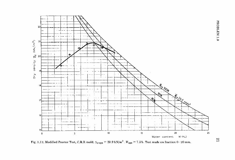
Solut ion (a) The test results may be plot ted directly on a graph such as that of
Fig. 1.12. With the dry density as ordinate and water content as abscissa. The coordinates at m a x i m u m dry density correspond to the o p t i m u m dry density and o p t i m u m water content (the so-called modif ied Proctor l ine) , are : (7d/7w)oPt = 2 . 0 9 , w opt = 7 .5%
PR
OB
LE
M 1
.9
21
Fig. 1.12. Modified Proctor Test, C.B.R mold. 7dopt = 20·9 kN/m3. W opt = 7.5%. Test made on fraction 0—20 mm.
22 PHYSICAL CHARACTERISTICS OF SOIL
and e = (Ys/Yd) - 1.
Therefore: - = ~ ~ / ( r ~ -yd). 1 e
At optimum condition the degree of saturation will be:
= 74%
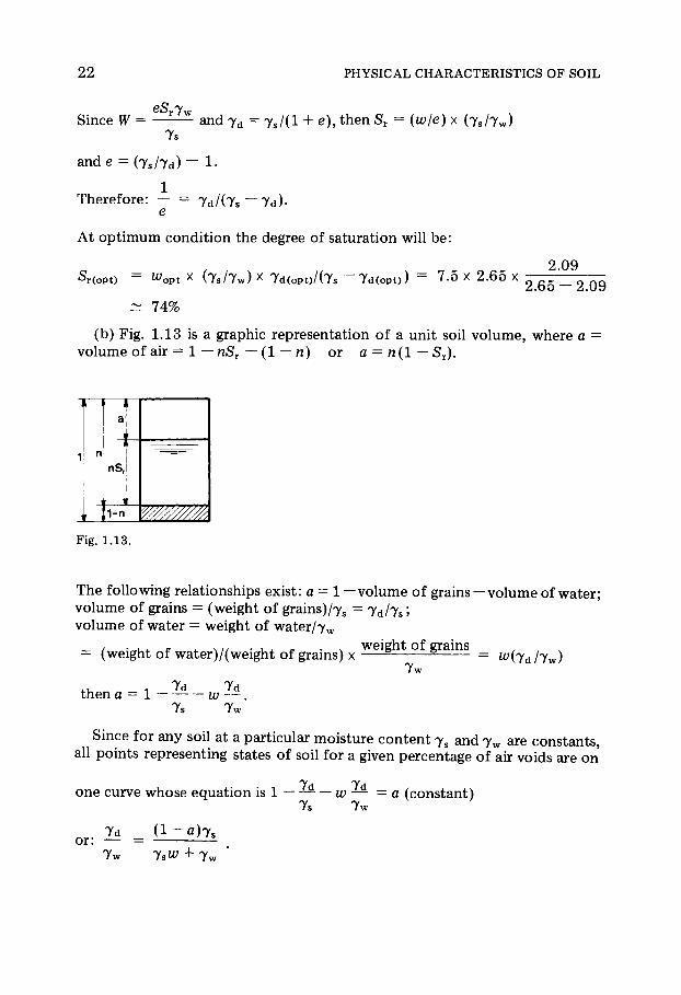
(b) Fig. 1.13 is a graphic representation of a unit soil volume, where a = volume of air = 1 - nS, - (1 - n ) or a = n (1 - S r ) .
Fig. 1.13.
The following relationships exist: a = 1 -volume of grains -volume of water; volume of grains = (weight of grains)/y, = Yd/Ys;
volume of water = weight of water/y, weight of grains
Yw = (weight of water)/(weight of grains) x = w ( Y d / Y w )
Y d Yd t henu= 1 - - - - w - - . Ys Y W
Since for any soil at a particular moisture content ys and yw are constants, all points representing states of soil for a given percentage of air voids are on
one curve whose equation is 1 - - - w rd = a (constant) Yd
Y S Yw
Yd - ( l - - a ) Y s or: - - Yw YSW + Yw -

PROBLEM 1.9 23
This is a port ion of a hyperbola with w>0, whose a s y m p t o t e is the w-axis, passing through w = 0 , such that 7 d = ( 1 — a)ys (see Fig . 1 . 1 4 ) .
If a = 0 , the volume of air is zero and the soil is saturated. The saturation
curve then is represented by the equat ion : 7 s Td
Tw 7 s w + 7v
Note: The same result is obta ined by determining the equat ion of a family o f curves of equal saturat ion ST:
volume of water
volume of air + vo lume of water
or, for a unit vo lume :
volume of water w ( 7 d / 7 w )
volume of soil grains ( 7 d / 7 s )
(w Sr
or: 7 d — + — \7 w 7 s
= Sr
Id
7w
S r 7 s
wjs+ S r 7 w
The curves are also hyperbolas with the w-axis as an a s y m p t o t e . Only the sections corresponding to w > 0 have a physical meaning.
If w — 0 , all the curves pass through point ys (see Fig. 1 . 1 5 ) . If Sr = 1 in
Figs. 1.14 and 1.15
2 4 PHYSICAL CHARACTERISTICS OF SOIL
the above formula , the full saturation equat ion is obtained which is identical to the first one.
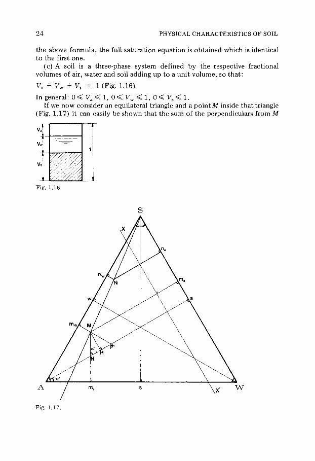
(c) A soil is a three-phase system defined by the respective fractional volumes of air, water and soil adding up to a unit vo lume, so that :
Va + Vw + Vs = 1 (Fig . 1.16)
In general: 0 < V a < 1, 0 < Vw < 1, 0 < Vs < 1. If we now consider an equilateral triangle and a point Μ inside that triangle
(Fig . 1.17) it can easily be shown that the sum of the perpendiculars f rom Ì
Fig. 1.16
Fig. 1.17.
PROBLEM 1.9 2 5
to the three sides is equal to the height of the triangle. F r o m Fig. 1 .17 :
Ha — Mma
Kms = %AK
PMW — PM + M m w = KM 4- M m w = £A P
KMS + KM + Mmw = Mms+Mmw = ^ ( A # + A P ) = A i /
hence : Mms + M m w + Afm a = AH + Ha - Aa = 1.
If the height o f the equilateral triangle is uni ty , the perpendiculars f rom Ì represent the volumes o f the three phases (soil , water and air) . — The curves of equal air void vo lume ( V a = constant) are straight lines parallel t o the side SW ( for e x a m p l e ×1 X). — The saturat ion line of the Proctor-diagram is given by side SW ( V a = 0 ) . — L e t Ν be any po int on line SM where the project ions on SW and SA are na and nw, respectively, then the similarity of the triangles SMmw and S'Nn^ gives:
VW _ SM V* _ SM
y ; " SN 3X1 Vi ~ SN'
B y d e f i n i t i o n s , = V w/ ( V a + ^ w ) . The degree of saturat ion represented by point Ν i s :
, = Κ = (SM/SN)VW =
Vi + V^ (SM/SN)(Va + Vw)
The straight lines f rom S are therefore lines of equal degree of saturat ion and we have : Vs = yd/y s, Vw = (yd/y w)w, V& = 1 ~ (V. + Vw).
Going back to the Modif ied Proctor-test results , Table I K can be m a d e u p :
TABLE IK
w% 3.00 7d/Tw 1-94 Vs 0.732 Vw 0.058 í¢ 0.210
4.45 5.85 2.01 2.06 0.758 0.777 0.089 0.121 0.153 0.102
6.95 8.05 2.09 2.08 0.789 0.785 0.145 0.167 0.066 0.048
9.46 9.90 2.06 2.05 0.777 0.774 0.195 0.203 0.028 0.023
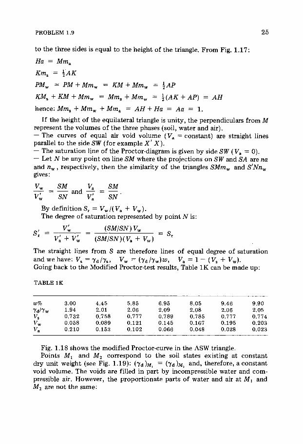
Fig. 1.18 shows the modif ied Proctor-curve in the ASW triangle. Points Ì÷ and M2 correspond to the soil states existing at constant
dry unit weight (see F ig . 1 .19 ) : (yd)M{ ~ ( T d ) M 2 and, therefore, a constant void vo lume. The voids are filled in part by incompressible water and com-pressible air. However, the proport ionate parts of water and air at Ìl and Ì2 are not the s ame :

2 6 PHYSICAL CHARACTERISTICS OF SOIL
S
1
Air
Wate r
Air
Water 1 1
W/k '/////
1
M1 M2
Fig. 1.19.
— in order to improve the mechanical propert ies of the soil in condit ion Ìë
its water content will have to be increased to within a close range around the o p t i m u m moisture content , then the soil will have to be c o m p a c t e d to in-crease its dry unit weight;
- on the other hand, in order to increase the mechanical propert ies of the same soil at point M2, the moisture content should be decreased to a value beneath w opt (by drying) and the soil then c o m p a c t e d .
It will be noticed that the water content at M2 is near 1 0 0 % saturat ion. Compact ing this soil at that moisture content would tend to bring the soil close to complete saturat ion and would likely lead to pumping , causing excessive deformat ions of the soil. It would not be possible to use the com-pacted material, for instance, for a stable pavement subgrade.

PROBLEM 1.10 27
**Problem 1.10 Void rat io of an organic soil
Let us assume that the unit weights of the soil, ysm ,and organic matters, Tso are known. Then:
(1) What is the unit weight of the combined dry organic soil whose organic content is M0(*)?
(2) What is the void ratio of this soil, if it is known that its water content is w and its degree of saturation is Sr?
Solut ion
We use the following definitions (F ig . 1 .20 ) :
vo lume of voids for void rat io : e =
for degree of saturat ion: Sr =
for water content : w =
for organic content : M0
volume of soil grains '
vo lume of water
vo lume of voids
weight of water
weight of dry soil
_ dry organic matter weight
total dry sample weight
(1)
(2)
( 3 )
( 4 )
for a unit weight of dry soil we have: M0 = weight of organic matter , 1 — M0 = weight of mineral matter , M0 /7go = vo lume of organic matter , (1 ~ M 0 ) / 7 s m = vo lume of mineral matter .
i é Air
e
Wate r
mmrnm 1
Organic part
Soil part
Fig. 1.20.
• N o t e : The organic content is the percentage by weight, of the dry organic constituent of the total dry weight of sample for a given volume.

2 8 PHYSICAL CHARACTERISTICS OF SOIL
The total unit weight, 7 S , of the dry soil is the weight of a unit v o l u m e :
( M 0 / 7 s o ) + l(l-M0)/y m]
7so X 7sm or: 7 S =
M0(jsm — 7 s o) + ^ so
7 S is a function of the form Y= a/(bx + c ) , meaning that the curve rep-resenting Y as a function of M0 is a part of a hyperbola (see Fig . 1 . 2 1 ) . S ince 7 s m( = 2 6 . 5 k N / m 3) is always a greater value than 7 s o, the curve, which is only real for value where 0 < M 0 < 1 0 0 % , decreases and varies between the limit values 7 s m , for M0 = 0 , and 7 s o, for M 0 = 1 0 0 % (see Fig. 1 . 2 1 ) .
1 7s =
k
ï 100 Mo(%)
Fig. 1.21.
The expression for S r can be transformed to give:
volume of water volume of voids =
but we know also that :
volume of water weight of water (weight of dry matter)
= w χ 7'
From ( 1 ) :
w 1 e =
S r7 w ( M o/ 7 s o ) + [ ( l - M 0 ) / 7 sm J
PROBLEM 1.11 29
or:
Tso Tsm
e — ·
S r7 w Mo ( T s m ~ T s o ) + Tso
Summary of answers
Tso * Tsm Ts =
e =
Tsc
Tso Tsm
S r Tw M0 ( 7 s m - Tso) + Tso
+*Pro blem 1.11 Hydrometer analysis
A hydrometer analysis is performed on a 2000 cm3 solution containing 50g of dry soil. The solution concentration at a depth of 5 cm is 5g/l after a sedimentation time of 80 minutes. Find:
(a) the maximum diameter dy of the particles at that depth and time; (b) the percentage of dry soil of particles having a diameter equal to or
smaller than dy.
Assume ç = 1 cPo (dynamic viscosity of water at 20°C) and ys/y w = 2.65.
Solut ion
(a) The m a x i m u m diameter dy is that of the soil particles which at t ime zero were at the surface of the solut ion and at t ime t = 8 0 min. , have trav-elled 5 cm.
/18 ç Ç dy = V 7
Ts ~ Tw t
In the C .G.S . sy s t em:
t = 8 0 χ 6 0 = 4 8 0 0 s
Ç — 5 c m
ç = 1 cPo = 1 · 1 0 " 2 Po
ys = 2 . 6 5 χ 9 . 8 1 d y n e s / c m 3
7 W = 1 χ 9 . 8 1 d y n e s / c m 3
/ 1 8 - 1 0 - 2 χ 5 v = J r = 3.4 · 1 0 ~ 3 c m (or 34 Mm). y ^ 9 . 8 1 ( 2 . 6 5 - 1 . 0 0 ) χ 4 . 8 · 1 0 3
(b) The density of the solution at 5 c m after 8 0 min. is :
30 PHYSICAL CHARACTERISTICS OF SOIL
5 + 1 1 0 0 0 - - ^ - ) x l 7 \ 2 . 6 5 /
r = — = - L = 1.003
7 W 1 0 0 0 χ 1 The percentage of weight is:
V 7 S 7 W 2 0 0 0 2 .65 χ 1.00 y = ^ H r - 1 ) = χ ( 1 . 0 0 3 - 1) = 0 .19
ñ 7 ~ 7 w 50 2 . 6 5 - 1 . 0 0 y = 19% where V is the volume of the solution and ñ the weight o f the soil.
Summary of answers dy = 3 . 4 - 1 0 " 3 c m ; y = 19%.
* * P r o blem 1.12 Relative density (English units)
Determine the relative density of a calcareous sand (ysl = 146.3 Ib/cu. ft) and that of a quartzitic sand (ys2 = 165.6 Ib/cu. ft) whose void ratios are:
— for the calcareous sand: e m ax = 0.89, emin — 0.62; — for the quartzitic sand: e m ax = 0.98, emin = 0.53.
The measurement of the above void ratios was made in a Proctor-mold (ö = 4 in., Ç = 4.59 in.) filled with following weights: Px = 2.868 lb of dry calcareous sand, P2 — 3.254 lb of dry quartzitic sand.
Solut ion
^ m a í e Relative density is : Dt — IA =
em a x ^min
The void ratio of the calcareous sand is :
ðÇö 2/4 - PJysl ( 3 . 1 4 χ 4 . 5 9 x 4 2/ 4 ) - ( 2 . 8 6 8 / 1 4 6 . 3 ) χ 1 2 3
= 0 .70 Pi/y,i 2 . 8 6 8 x l 2 3 / 1 4 6 . 3
and that of the quartzit ic sand i s :
_ t t # 0 2 / 4 - P 2 / 7 s 2 _ ( 3 . 1 4 χ 4 .59 χ 4 2/ 4 ) - ( 3 . 2 5 4 χ 1 2 3/ 1 6 5 . 6 ) _ â À ~ Pjhs2 ~ 3 . 254 x l 2 3 / 1 6 5 . 6
It will be noticed that e1 — e2.
The relative density for each of the sands is :
0 .89 - 0 . 7 0 £ ) , . = - 0 .70 calcareous sand
0 . 8 9 - 0 . 6 2
0 . 9 8 - 0 . 7 0 Dt2 — = 0 .62 quartzitic sand.
0 . 9 8 - 0 . 5 3
PROBLEM 1.13 3 1
The two sands, even though they have the same in place void rat io , have different relative densities, which indicates that the grains o f the calcareous sand are more tightly packed than those o f the quartzit ic sand. This cannot be concluded either from the void ratio or from the dry unit weights.
It is t o be n o t e d that the dry unit weight is greater for the soil with lower relative densi ty :
7 . i 1 4 6 . 3 (7d)i = = = 8 6 . 1 1 b / c u . f t φ Γ ΐ = 0 . 7 0 ) W 1 1 + ex 1 + 0.7 K 11 }
7 s 2 165 .6 ( T d ) 2 = = = 9 7 . 4 1 b / c u . f t (Dr2 = 0 . 6 2 ) .
1 + e 2 1 + 0.7 V r2 '
Summary of answers
(ÉΏ)Ι = Φ ã ) é = 0 . 7 0 ; ( / D ) 2 = (Dx)2 = 0 . 6 2 .
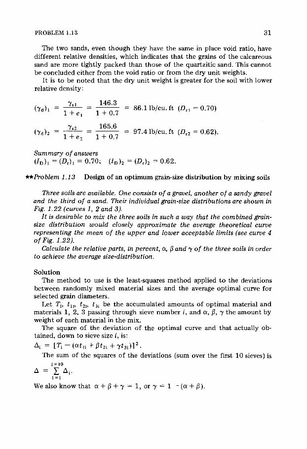
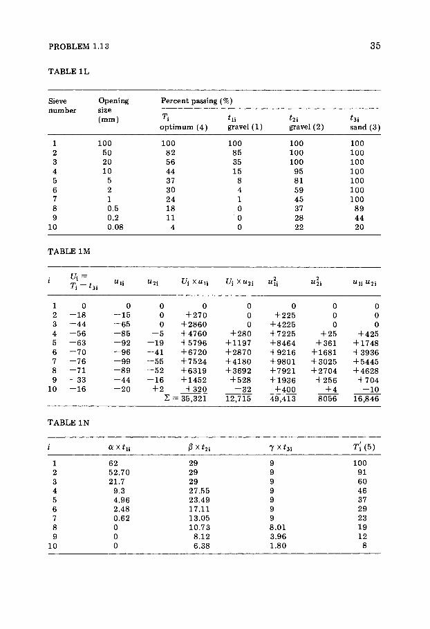
**Problem 1.13 Design of an o p t i m u m grain-size distr ibution by mixing soils
Three soils are available. One consists of a gravel, another of a sandy gravel and the third of a sand. Their individual grain-size distributions are shown in Fig. 1.22 (curves 1, 2 and 3).
It is desirable to mix the three soils in such a way that the combined grain-size distribution would closely approximate the average theoretical curve representing the mean of the upper and lower acceptable limits (see curve 4 of Fig. 1.22).
Calculate the relative parts, in percent, á, â and y of the three soils in order to achieve the average size-distribution.
Solut ion The m e t h o d to use is the least-squares m e t h o d appl ied to the deviations
between randomly mixed material sizes and the average opt imal curve for selected grain diameters .
Le t T{, tn, t2i, t3i be the accumula ted amount s of opt imal material and materials 1 , 2 , 3 passing through sieve number i, and á, â, y the a m o u n t by weight of each material in the mix .
The square of the deviation of the opt imal curve and that actual ly ob-tained, down to sieve size /, is :
Δ . = [τß-(ïá ç+âß2ß + 7ΐ 3 ί) ] 2 .
T h e sum of the squares of the deviations ( sum over the first 1 0 sieves) is i = 10
Δ = Ó Δ,. i = 1
We also know that α + β + 7 = 1 , or 7 = 1 — (α + β ) .
32 P
HY
SIC
AL
CH
AR
AC
TE
RIS
TIC
S O
F S
OIL
Fig. 1.22. Grain-size distribution curves.

PROBLEM 1.13 33
10 Hence: Δ = Ó [2 \ - (octn 4- 0 t 2 i) - {1 - (α + 0 ) } f 3 i] 2
ι
10
Δ - Ó — i 3i ) — ^ ( ί ΐ ί — ^3i) — β ( ί 2ί — ^3i )] 2 . 1
If we let : U{ = 2\ — f3 i, un = i 14 - f 3 i, w 2i = £ 2i - i 3 i,
10
we have : Δ = Ó t ^ i a wi i ~~ £ w 2 i] 2 . ι
The sum Δ mus t be a min imum, or its partial derivative with respect to α and β, mus t be zero :
3 Δ J2 — = Ó 2([/i - a u u — &u2i) x = 0 3α ι
3 Δ " — = L 2 ( [ / i - a u l i- j 3 u 2 i) x u 2 i = 0 σρ ι
or:
10 10 10
a I M i i + 0 Z w i i " 2i = Ó r ji wi i ι ι ι
ßï 10 10
α Ó " ΐ ί " 2À + ί3 Ó " 2ß = Ó UiU2i 1 1 1
This is a linear set of equat ions for which α, β, and y m a y be determined knowing that : y = 1 — (α 4- â).
Tables 1 L and 1M summarize the percentages and sizes of the curves o f Fig . 1 .22 and the coefficients o f the linear set o f equat ions . F r o m these the following equat ions are obta ined : 4 9 , 4 1 3 a + 1 6 , 8 4 6 0 = 3 5 , 3 2 1 ; 1 6 , 8 4 6 a + 8,056j3 = 1 2 , 7 1 5 , resulting in a = 6 2 % , â = 2 9 % , y = 9%. Hence the a m o u n t o f m i x e d soil pass ing through sieve number i i s :
Tl = cxi2i + 0 f 2 i + yt 3i.
Table I N summarizes the calculat ion for different percentages of soil retained in order to construct the grain-size distr ibution curve of the mixed soil, curve 5 of Fig . 1 .23.
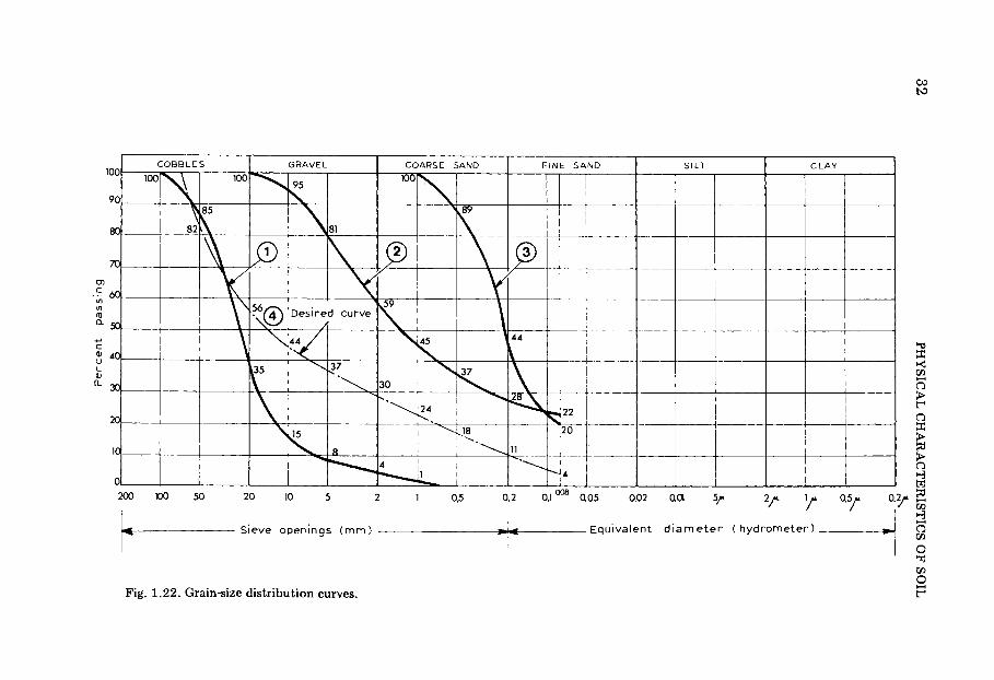
If the three soils are m i x e d in the propor t ions shown above , the grain-size distribution (curve 5 o f Fig . 1 .23) is obta ined , which corresponds to the first ten sieve-sizes.
34
PH
YS
ICA
L C
HA
RA
CT
ER
IST
ICS
OF
SO
IL Fig. 1.23. Grain-size distribution curve of the mixture.
PROBLEM 1.13 35
TABLE 1L
Sieve Opening Percent passing (%)
number size Ά (mm) Ά hi (mm)
optimum (4) gravel (1) gravel (2) sand (3)
1 100 100 100 100 100 2 50 82 85 100 100 3 20 56 35 100 100 4 10 44 15 95 100 5 5 37 8 81 100 6 2 30 4 59 100 7 1 24 1 45 100 8 0.5 18 0 37 89 9 0.2 11 0 28 44
10 0.08 4 0 22 20
TABLE 1M
i Ui = Ά - t 31 " U
Ui X u2i
1 0 0 0 0 0 0 0 0 2 - 1 8 - 1 5 0 4-270 0 + 225 0 0 3 - 4 4 - 6 5 0 4-2860 0 + 4225 0 0 4 - 5 6 - 8 5 - 5 + 4 7 6 0 + 280 + 7225 + 25 + 425 5 - 6 3 - 9 2 - 1 9 + 5796 + 1197 + 8 4 6 4 + 361 + 1748 6 - 7 0 - 9 6 - 4 1 + 6 7 2 0 + 2 8 7 0 + 9216 + 1681 + 3936 7 - 7 6 - 9 9 - 5 5 + 7 5 2 4 + 4 1 8 0 + 9 8 0 1 + 3025 + 5445 8 - 7 1 - 8 9 - 5 2 + 6 3 1 9 + 3692 + 7 9 2 1 + 2704 + 4628 9 - 3 3 - 4 4 - 1 6 + 1452 + 528 + 1936 + 256 + 704
10 - 1 6 - 2 0 + 2 + 320 - 3 2 + 4 0 0 + 4 - 1 0 Σ = 35 ,321 12 ,715 4 9 , 4 1 3 8 0 5 6 16 ,846
TABLE I N
i a x f a 7 X * 3i Ti (5)
1 62 29 9 100 2 52 .70 29 9 91 3 21.7 29 9 60 4 9.3 27 .55 9 46 5 4 .96 23 .49 9 37 6 2.48 17 .11 9 29 7 0.62 13.05 9 23 8 0 10 .73 8.01 19 9 0 8 .12 3.96 12
10 0 6.38 1.80 8

36 PHYSICAL CHARACTERISTICS OF SOIL
**Problem 1.14 S t u d y of a soil structure by means of two-dimensional theoretical packing (small-cylinder analogy)
Let us consider an analogical model of a soil medium formed by an as-sembly of thin cylinders. The problems to be solved, are:
(1) What regular, stable packing may be made if all the thin cylinders have the same diameter D? Determine the void ratio and the dry unit weight for these different assemblies (ys = 27 kN/m 3).
(2) What is the maximum diameter d of other cylinders which could be introduced in the voids of the D-size packing?
For each of the original packing, determine the grain-size distribution of D- and d-sizes leading to maximum densities. Calculate also the void ratios and the dry unit weights of the mixtures at maximum compactness.
Which combination leads to maximum packing? In order to draw the grain-size curves, assume D = 5 mm.
Solut ion (1 ) The two stable , regular packing arrangements correspond to square
(2-dimensional) and equilateral triangle configurations as shown in Fig . 1.24. Hexagonal packing is very improbable because it is very unstable .
Square Equilateral triangle
Fig. 1.24.
The void ratio for the square arrangement i s :
£ 2 ( 1 - π / 4 ) 4 - π = ~ = = 0 . 2 7 3 .
π£>2/4 π If we assume the unit weight of the cylinders to be ys = 27 k N / m 3, we have:
(π Ι ) 2/ 4 ) × 7 s π 7 d = ô—- = 27 χ - = 21 .2 k N / m 3 .
Dz 4 F o r the triangular arrangement, the values of e and 7 d a re :

PROBLEM 1.14
(y/3 D2I4) - (ITD2/8) lJZ~-n = U£ ' — = = 0 . 1 0 2
7TD 2/8 7Ã
(vD2/8)ys π 7 d = . _ * = 27 χ — = 2 4 . 5 k N / m 3 .
( V 3 / 4 ) D 2 2 ^ 3
(2) Arrangement for the square packing: the size o f a cylinder that could be introduced in the void will have a diameter d = D(sf2 — 1 ) .
In order to obta in m a x i m u m packing with cylinders D and d, all the elements o f the mass should have the shape o f that shown in Fig . 1 .25 , a.
Fig. 1.25. a. Square element of mass. b. Triangular element of mass.
In each element there is one cylinder of d iameter D and one o f d iameter d. This corresponds to weight percentages of:
D2 D2 1 = 0 . 8 5
D2+d2 D2[(l + ( v ^ - l ) 2 ] l + i v ^ - l ) 2
for particle of d iameter D and
d2 _ ( V 2 - 1 ) 2
D2 +d2 ~ 1 + (χ/2 - l ) 2 0 . 1 5
for the d-size particles. The mix ture , therefore , will have the grain-size distribution curve as
shown in Fig . 1.26. At m a x i m u m c o m p a c t i o n , the mix ture will l o o k exact ly like the element of F ig . 1 .25 , a. There fore :
D 2 ( l - π/4) - D2(s/2 - 1 ) 2( π / 4 )
— [ ( 1 + ( V 2 - 1 ) 2 ) ]
38 P
HY
SIC
AL C
HA
RA
CT
ER
IST
ICS OF
SO
IL
1 C LAY 1 1 C LAY 1 1 C LAY 1 1 SILT 1 SILT 1 SILT
1 element )
FINE SAND
1 element )
FINE SAND
r gular
FINE SAND
e element)
r c L (-»
COARSE SAND
e element)
r Ì
<
Ε
COARSE SAND
( squar
—
COARSE SAND
MIX 1 \ \
GRAVEL 1
ω COBB Lf ο
ο 3k
Ε
cr LU
c c <b
á Ï
<b
>
6u
iss
ed
;ua
oja
d
Fig. 1.26. Grain-size distribution.
PROBLEM 1.14 39
s = 2 4 . 8 k N / m 3 . 7 d =
D2
F o r the arrangement of triangular packing, the distance between the center of particles D and d is equal t o : (2D/3)(y/li/2) = DjyfS. The size o f the cylinder that can be introduced in the central void will have a m a x i m u m diameter of d = 2(D/y/%-D/2) = £ > ( 2 A / 3 ~ - 1 ) .
In order to obtain m a x i m u m packing of rods D- and d-sizes, each element of mass will have to look like Fig . 1 .25 , b . In each e lement of mass , there will be half a particle of size D and one of size d.
The percentage of weights of the size-D particle is :
The percentage by weight of the size-d particles is 0 . 0 4 4 . S o : 9 5 . 6 % of £)-size and 4 .4% of d-size particles m a k e up the mass . The mix will have a grain-size distr ibution as shown by the curve of Fig. 1.26. The mixture will have m a x i m u m compactnes s when its mass will have elemental sect ions identical to that of Fig . 1 .25 , b and
D2
D2 + 2 d 2 l + 2 ( 2 / v ^ 3 - l ) 2 = 0 . 9 5 6 .
e = (y/3D 2/4) - (ðΡ2/8) - ðΡ2/4(2/^ - l ) 2
( π ΰ 2 / 4 ) [ 1 / 2 + ( 2 / χ / 3 - 1 ) 2 ] = 0 . 0 5 2
Td =
The m a x i m u m packing arrangement is that of the equilateral configurat ion.

4 1
Chapter 2
W A T E R IN T H E S O I L
^Problem 2.1 Permeabil ity of sand
A coarse-sand sample is 15 cm high and has 5.5 cm diameter. It is placed in a constant-head permeameter. Water passes through the sample under a con-stant head of 40 cm and after 6 sec, 40g of water has been collected. What is the coefficient of permeability of the sand?
Solut ion T h e flow of water through a soil is governed by Darcy ' s law
í = ki (1 )
The a m o u n t o f water percolated is q = í χ s , the rate percolat ion is :
v - 9 L _ l2_ _ 4 χ 4 0 _ Q 2 g c m/ S
s nd2 6 χ π χ 5 . 5 2
T h e hydraulic gradient i = h/l = 4 0 / 1 5 = 2 . 6 6 F r o m equat ion ( 1 ) : k = v/i = 0 . 2 8 / 2 . 6 6 = 0 . 1 0 5 , say 0 . 1 1 cm/sec .
Answer
k = 0 .11 cm/sec .
itProblem 2.2 Permeabil i ty of clay
A clay sample is 2.5 cm high and has a diameter of 6.5 cm. It is placed in an oedometer with a variable-head permeameter. The water percolation through the sample is measured in a standpipe whose inner diameter is 1.7 mm. The tube is graduated in centimeters from the top to the bottom. The top graduation is zero and is located 35 cm above the base of the oedometer. The overflow in the oedometer is 3 cm above its base. At the start of the test, the water level in the tube is at zero; 6 mins and 35 sees later, the water level has dropped to graduation 2. What is the coefficient of permeability of the clay?
Solut ion It is a s sumed that after achieving saturat ion of the sample , the f low of
water is sufficiently s low to apply Darcy ' s law for each t ime increment during which the water flows (t, t + dt).
The hydraulic gradient (see Fig . 2 .1 ) is i = h/l

4 2 WATER IN THE SOIL
P o r o u s stone :
S e c t i o n A ^
Fig. 2 .1 .
S e c t i o n a
Since í = ki (Darcy's l aw) , the quanti ty of water is q = Akh/l , where Λ = cross-sectional area of the clay sample . S ince the volume of water permeating through the sample is equal to the vo lume of water which left the s tandpipe , we have:
qdt = (Akh/l) = dt = — adh
where a = the cross-sectional area of the s tandpipe . Then:
a dh kdt = É-
Á h
Integrating this value between height h ë and h2 o f the s tandpipe gives:
kT = ~^llog(h2)/h
l or :
2 .3 — — log J j-11, but α = — and A = — A Ô
therefore, k = 2.3(d/D)2 — log (hl/h2).
Numerical application: d = 0 .17 c m , D = 6 . 5 c m , / = 2 . 5 c m , Ô = 6 min 3 5 s = 3 9 5 s, ht = 3 5 - 3 = 3 2 c m , Λ2 = 3 2 — 2 = 3 0 c m ,
s o : fe = 2.3 χ Ό . 17 \ 2 2 .5 , 6 .5 / X 3 9 5
32 log — = 2 .8 · 1 0 " 7 cm/s .
oU
PROBLEM 2.3 43
Answer
k = 2 .8 · 1 0 " 7 cm/s .
^Problem 2.3 Permeabil i ty of sand
A well graded sand sample containing well-rounded grains has a void ratio of 0.62 and a coefficient of permeability of 2.5 · J O " 2 cm/s. Estimate the coefficient of permeability for the same sand with a void ratio of 0.73, using the Casagrande and Terzaghi formulas.
Solut ion Casagrande's formula is k = 1.4 k0S5 (e)2 ,
therefore : k062 = 1 . 4 f e 0 > 85 0 . 6 2 2 and fc0>73 = 1 . 4 f e 0 # 85 0 . 7 3 2
0 7 3 2
Therefore , ^ = ^ „ = 2 . 5 · 1 ( Γ 2 χ ( 1 . 1 8 ) 2
= 3 .48 · 1 ( Γ 2 - 3 .5 · 1 0 - 2 c m / s .
Terzaghi's formula i s :
* - c - filial d W
ç $1 - n 10
For specific test condit ions , the ratio k0.73/&ï.62 m a Y be calculated because the value of viscosity, 7? would be the same in both instances.
fco.73 = fop.73 ~ 0 - 1 3 ) 2 χ \/l - n 0 M
feo.62 (^0.62 ~ 0 - 1 3 ) 2 s / l - M0.7 3
where n = e/(l + e ) , hence e = 0 . 6 2 corresponds t o n = 0 . 6 2 / 1 . 6 2 ~ 0 . 3 8 , e = 0 .73 corresponds t o n = 0 . 7 3 / 1 . 7 3 ~ 0 . 4 2
k0 7 3 = 2 .5 · Ι Ο " 2 χ j ° — ) · ^ — = 2.5 · Ι Ο " 2 χ 1 . 3 4 6 χ 1 .022 0 , 73 , 0 .25 / v0 . 5 8
&0.73 = 3 .44 · 1 0 " 2 - 3.4 · 1 0 " 2 c m / s .
Terzaghi 's formula gives a value of permeabi l i ty slightly lower than that of Casagrande.
Summary of answers
Casagrande's formula fc0.73 = 3.5 · 1 0 " 2 cm/s , Terzaghi 's formula k 0 1 3 =
3.4 · 1 0 " 2 cm/ s , then 3.4 · 1 0 " 2 cm/ s < fc0.73 < 3 .5 · 1 0 " 2 c m / s .

44 WATER IN THE SOIL
irkProblem 2.4 Average coefficient o f permeabil i ty of a layered sys tem
A sand deposit contains three distinct horizontal layers of equal thick-nesses. The coefficient of permeability of the upper and lower sand is 10~3
cm/s. That of the middle layer is 10~2 cm/s. What are the horizontal and vertical coefficients of permeability of the
three-layered system, and what is their ratio.
Fig. 2.2.
Solut ion Let us consider first an horizontal flow. It is parallel to the layers. We
assume that all three layers have the same hydraulic gradient, i, (see Fig . 2 .2 ) , then : v{ = k1i, v2 — k2i, v3 = k3i.
Let us consider the a m o u n t o f water passing through an imaginary vertical p lane through the three layers, o f unit width; it could be seen that the average value o f the rate of seepage is :
í = ~ ( * > ι # ι + v2H2 +v3H3) = ^ ( f e i # i +k2H2 +k3H3).
By definit ion;
õ = kHi, and feH = τ ; ( & ι # ι + k2H2 + k3H3).
For this particular problem H1 = H2 = H3 = - and kx =k3, therefore : ï
= 7 r ( 2 f ei + f e2 ) o r: feH = 7Γ(2 ' 1 0 ~ 3 + 1 0 " 2 ) = 0 . 0 0 4 , or : 3 ï
4 · 1 0 " 3 cm/s .
For the vertical f low of water, in the perpendicular direction to the three beds , the principle of continuity requires that the rate of discharge at each layer boundary be the same .
PROBLEM 2.5 4 5
Summary of answers
kH = 4 - 1 0 _ 3c m / s ; kv = 1.4 · 1 0 "3 cm/s ; kH/kv = 2 .9 .
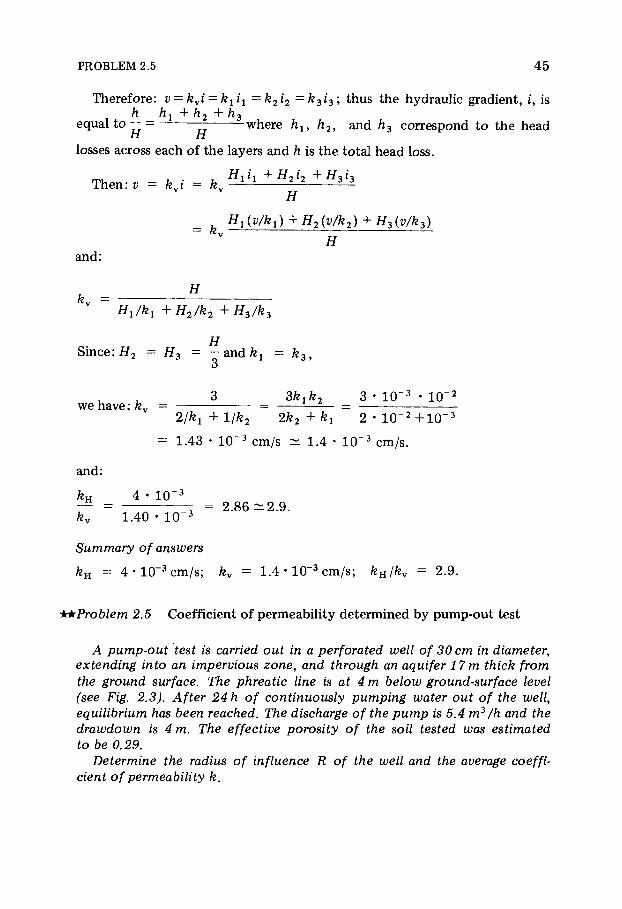
**Problem 2.5 Coefficien t o f permeabi l i t y de termine d b y pump-ou t tes t
A pump-out test is carried out in a perforated well of 30 cm in diameter, extending into an impervious zone, and through an aquifer 17 m thick from the ground surface. The phreatic line is at 4 m below ground-surface level (see Fig. 2.3). After 24 h of continuously pumping water out of the well, equilibrium has been reached. The discharge of the pump is 5.4 m3/h and the drawdown is 4 m. The effective porosity of the soil tested was estimated to be 0.29.
Determine the radius of influence R of the well and the average coeffi-cient of permeability k.
Therefore : v = kvi = k1il =k2i2 =k3i3; thus the hydraulic gradient, i, is
equal to ~ - — where hu h2i and h3 correspond to the head
losses across each of the layers and h is the total head loss .
T h e n : õ
and :
S ince : H2 = H3 = - a n d ^ = k3, 3
we have : kv
and:

46 WATER IN THE SOIL
Fig. 2.3.
Solut ion Once flow equilibrium is reached, after 24 h o f pumping , Dupui t ' s equat ion
becomes appl icable :
q = irk Ç 2 -h2
In (R/r) (1)
or :
1.365fe H2 h2
log (R/r) d')
coefficient of permeabil i ty of soil mass , height of water in the well, R = radius
where q = discharge at p u m p , fe Ç = thickness of the aquifer, h of influence, and r = well radius.
Equat ion (1) contains two unknowns , namely R and fe. It is valid only for t>24h. For £ < 2 4 h there is another formula for the radius R which is applicable only to non-equilibrium condit ion. It i s :
R - l.byJ{kH/n)t (2)
where: R — the radius of influence at t ime £, fe = coefficient of permeabil ity of the soil mass , Ç = aquifer thickness , and ç = effective porosi ty of soil.
For t = 24 h both eqs . 1 and 2 are appl icable (see Fig . 2 .4 ) and we dispose now of two equat ions with two unknown factors , R and fe.
PROBLEM 2.5 4 7
E q u i l i b r i um c o n d i t i o n
24H
Fig. 2.4.
The solution may be either solved graphically or by numerical i teration, since one of the equat ions is transcendental . F o r this example , a graphic solution has been chosen and is accurate for the purpose .
Equat ion (2) can be written a s :
nR2
k = 2 .25 tH
and eqn. ( ΐ ' ) a s :
log Λ - l o g r = 1.365& H2 -h2
from which:
ãé(υ2 fa,2) log R = 0 .607 — R2 + l o g r (3)
qtH
The intersection of the two p lot ted curves (Fig . 2 . 5 ) , one the function log R and the other a parabola with an Oy axis , yields the solut ion.
Numerical application (see Fig. 2 . 5 ) ; ç = 0 . 2 9 , Ç — 17 — 4 = 13 m, h — 13 - 4 = 9 m, q = 5 . 4 m 3 / h , t = 2 4 h, r = 0 . 1 5 m, log r = 1 .176 = 0 . 8 2 4 . Equat ion (3) may be written a s : log R — 0 . 0 0 9 19R2 - 0 . 8 2 4 . The only realistic solution i s : R - 1 5 m . Transposing this value of R to calculate k:
q log (R/r) 5.4 log 1 0 0 ; ~ - = 9 · 1 0 ' 2 m/h = 2 .5x 1 0 - 3 cm/s .
1 . 3 6 5 ( # 2 -h2) 1 .365x 88 k =

4 8 WATER IN THE SOIL
Summary of answers
R = 1 5 m ; k = 2 .5 · 1 0 " 3 cm/s .
Remarks (a) R should be expected to fall within the range of 1 0 0 r to 3 0 0 r or
15—45 m, which is the case.
Fig. 2.5.
(b) The Sichardt formula for R is : R = 3 0 0 0 ( i / — h\/k
and would yie ld :
J? = 3 · 1 0 3 x ( 1 3 - 9 ) > / 2 . 5 · 1 0 " 5 = 1 2 x \ / 2 . 5 · 1 0 6 · 1 0 " 5 = 6 0 m .
The radius is 4 t imes greater. The large differences can be accounted for when considering that the formula R = 1.5y/(kH/n)t is only valid for the logarithmic approx imat ion of the solution of the equat ion . This assumes a relatively small drawdown, which is not the case here (drawdown is 4 m for a height of 1 3 m, or 3 0 % ) . In pract ice , the radius of influence would be much greater than found in the problem.
^Problem 2.6 Effective stress in sand
The ground-water level in a thick, very fine sand deposit is located 1.20 m below ground surface. Above the free ground-water line, the sand is saturated by capillary action. The unit weight of the saturated sand is 20.3 kN/m 3.
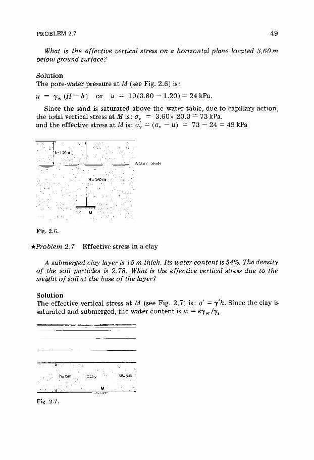
PROBLEM 2.7 4 9
What is the effective vertical stress on a horizontal plane located 3.60 m below ground surface?
Solut ion The pore-water pressure at Ì (see Fig . 2 .6) i s :
u = 7 w ( H - f t ) or u = 1 0 ( 3 . 6 0 - 1 . 2 0 ) = 24 kPa.
Since the sand is saturated above the water table , due to capillary act ion, the total vertical stress at Μ i s : σ ν = 3 .60χ 20 .3 — 73 kPa. and the effective stress at Ì i s : σ ν = (σ ν — ý) = 73 — 24 = 49 kPa
h z 1.20m ' .
Wate r leve l
H= a 6 om
Fig. 2.6.
if Problem 2.7 Effective stress in a clay
A submerged clay layer is 15 m thick. Its water content is 54%. The density of the soil particles is 2.78. What is the effective vertical stress due to the weight of soil at the base of the layer?
Solut ion The effective vertical stress a t Ì (see Fig . 2 .7 ) i s : a = y'h. S ince the clay is saturated and submerged, the water content is w = eyw/y s
h = l 5 m . .' Clay W = 5 4 * ;
Fig. 2.7.

50 WATER IN THE SOIL
from which e — w — = 0 .54 χ — = 1.50 7 w 1
We also know that :
Ί = ( 7 s " 7 w ) ( 1 _ n) = 7 s - 7 .
1 4 - e a n d 7 s / 7 w = 2 .78 is given,
therefore ys = 27 .8 k N / m 3 and 7 W = 10 k N / m 3 .
Subst i tut ing: yf = 27 .8 - 1 0
= 7 .12 k N / m 3 . 1 + 1.50
For the total thickness : a = 7 .12 χ 1 5 = 1 0 7 kPa
Answer
a ~ 107 kPa.
^Problem 2.8 Critical hydraulic gradient of sands at various densities
The specific gravity of sand particles is 26.6 kN/m 3. The porosity of the sand mass in both its least and maximum compactness is 45% and 37%, respectively. What are the critical hydraulic gradients in these two cases?
The critical hydraulic gradient, / c r i t, corresponds to a condit ion wherein the effective vertical stress is zero.
' ' 7 o' = ( 7 ' ~ * 7 w) < z , therefore / c r it = — .
We know that 7' = (1 -~ ç) (γ 8 — 7 W ). F o r the loose sand nx = 0 . 4 5 , y\ =
(1 ~ 0 .45) (26 .6 - 10) - 9 .13 - 9.1 k N / m 3. For the dense sand: n2 = 0 .37 , yf2 = (1 - 0 .37) (26 .6 - 10 ) = 1 0 . 4 5 -10 .5 k N / m 3.
Since 7 W = 10 k N / m 3 , we have i l c r it = 0 . 9 1 , i 2 c r it = 1 .05 .
ick+Problem 2.9 Blow out and piping
A large-sized excavation is made in a stiff clay whose saturated density is 1.76. When the depth of the excavation reaches 7.5 m, cracks appear and water begins to flow upward to bring up sand to the surface. Subsequent borings indicate that the clay is underlain by sand at a depth of 11 m below the original ground surface.
What is the depth to the water table outside the excavation below the original ground level?
Solut ion

PROBLEM 2.9 51
Solut ion Making an excavat ion in the clay, creates a hydraulic gradient between the
t o p of the sand layer and the b o t t o m of the excavat ion. As a consequence, water starts seeping in a vertical, upward direction from the sand layer towards the excavat ion floor. Because the clay has a very low permeabil i ty , f low equilibrium can only be reached after a long t ime per iod.
The solution mus t be considered over a short t ime interval. T w o phases appear successively.
( J ) First phase: clay fissuration The floor of the excavat ion is stable only if the water pressure p , at the
t o p of the sand layer (see Fig. 2 .8) is counterbalanced by the weight Ρ of the clay above it , disregarding shear strength of the clay. Stabil i ty condit ion therefore i s :
yh(H-f) > yw(H-d)
or:
( 7 ' + 7 w ) ( H - f l > T w ( H - d )
or:
y'(H-f) > yw(f-d)
When incipient failure condit ions occur , then:
y'{H-f) = yw(f-d)
from which:
d =
or:
d = 7 . 5 0 x 1 - ( 1 1 . 0 0 - 7 . 5 0 ) χ 0 .76 = 4 . 8 4 m .
Fig. 2.8.

52 WATER IN THE SOIL
(2) Second phase: uplift of sand (quick sand) A steady flow of water rising vertically through the cracks has been reached,
the top of the sand layer and the b o t t o m of the excavation being equi-potential lines (see Fig. 2 .8 ) . Depending on the value of the hydraulic gradient, piping may occur. The head at point A (Fig. 2 .9) i s :
w a , (H -d)y w
hA = — 4 - zA = = H — d 7 w T w
and at point Β:
uB
hB = h zB - Ç — f, because uB = 0 T w
with reference to the t o p of the sand layer. The hydraulic gradient is constant from A to Β and is : hA ~hB = f-d
AB ~ H-f
Its critical value is i c r it = T ' / T W and a b lowout would occur when
f """ _ 7 s a t ~ 7 w
H-f ~ ' T w
( 7 s at is the unit weight of sand, assumed to be 20 k N / m 3) . or :
7 .50 - d - 1, therefore d = 7 .50 - 3 .50 χ 1 = 4 .00 m. 1 1 . 0 0 - 7 . 5 0
In order to bring up sand through the cracks , the depth , d t o the water table must be d = 4.0 m.
Notes
(1) In either case the results are the same if the unit weights of the clay and the sand are identical. ~ for the first phase , the shear strength of the clay was not taken into account ; — for the second phase , shear strength of clay was also implicitly neglected and it was assumed that the cracks in the clay would permit passage of the sand grains. (2) Neglecting the shear strength of clay is reasonable if the width of excava-tion is large enough with respect to the thickness of the clay layer at the b o t t o m of the excavat ion. This layer acts like a slab with a uni form load acting upward from beneath and it is in tension, which results in fissures through the clay. The fissures eliminate shear-strength considerat ion, (see Fig. 2 .9 and 2 . 1 0 ) .
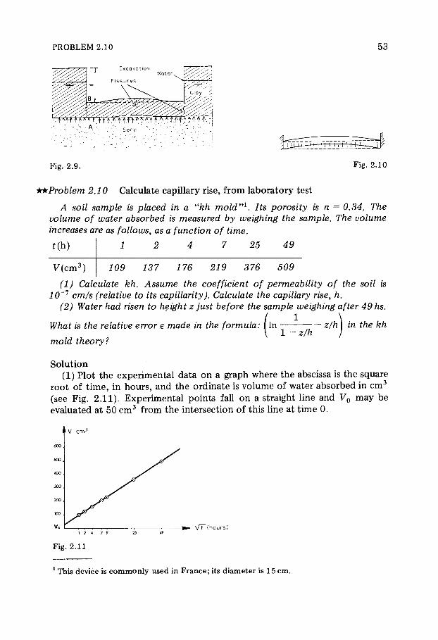
PROBLEM 2.10 53
irkProblem 2.10 Calculate capillary rise, f rom laboratory test
A soil sample is placed in a "kh mold"1. Its porosity is ç — 0.34. The volume of water absorbed is measured by weighing the sample. The volume increases are as follows, as a function of time.
t (h ) 1 2 4 7 25 49
y ( c m 3 ) 109 137 176 219 376 509
(1) Calculate kh. Assume the coefficient of permeability of the soil is 10~Ί cm/s (relative to its capillarity). Calculate the capillary rise, h.
(2) Water had risen to height æ just before the sample weighing after 49 hs.
What is the relative error e made in the formula,
mold theory?
( i n — ! — -\ l-z/h
z/h in the kh
Solut ion (1) Plot the experimental data on a graph where the abscissa is the square
root of t ime , in hours , and the ordinate is volume of water absorbed in c m 3
(see Fig. 2 . 1 1 ) . Exper imenta l points fall on a straight line and V0 may be evaluated at 50 c m 3 from the intersection of this line at t ime 0.
lV cm 3
\ / T (hours)
1 This device is commonly used in France; its diameter is 15 cm.

5 4 WATER IN THE SOIL
T o obta in a more accurate value, we may write, since the product kh remains constant :
( V 7 - V 0 ) 2 1 (V, - ν0γ 1 •x = ÷
A2 2ntn A2 2ntx
or:
γ_ — í j
— ~ = v ^ 7 * 7 = V 4 9 / 1 = 7
or :
V , - V 0 = 7 ( ^ - ^ 0 )
then:
7 V , - V 7
6
m, ô, 7 x 1 09 _ 5 0 9 Therefore : V 0 = = 4 2 . 3 # 4 2 c m 3 .
6 Since the diameter o f the m o l d is 1 5 c m :
π ÷ Ϊ 5 2" A =
4
f rom which:
2 ni. 7
/ 4 6 7 x 4 \ 2 1 ë ï1 2„
feft = x = 0 . 2 1 c m 2 / h . U x T 5 2 / 2 x 0 . 3 4 x 4 9
and therefore : 0 . 1 < kh < 1
This value of feft shows that we have, in this case , a soil with an average capillary rise.
If the coefficient o f permeabi l i ty , relative to capillarity, is 1 0 ~ 7 cm/ s , we then have :
0 . 2 1 h = = 5 . 8 · 1 0 2 c m
3 6 0 0 ÷ 1 0 "7
or: h = 5 . 8 0 m.

PROBLEM 2.11 55
(2) Let A be equal t o : In æ
h' 1—z/h
We are seeking the relative error e = AA/A m a d e in the kh mold theory. This theory assumes z/h is small and a niperian logarithm series is developed in which terms over 2 are not taken into considerat ion. Therefore , the error is of the order of the first term not considered of (z/h)3. Say t h a t : z/h = ÷
1/(1 ~ ÷) = l + x + x 2 + x 3 + 0(x4)
f rom which:
1 l o g ;
± -
with:
R3(x)
= ÷ + — + Rs(x)
— + — + 0(x5) = x3
3 4
1 ÷ - + - + 0 ( * 2 ) 3 4 ;
therefore: R3(x)<x3 [l+x + 0(x2)] or : R3 (x) < x3/(l - x).
On the other hand, we have : R3 (x) > x3 / 3 , and AA = R3 (x) and A — x2 /2
therefore : 2 / 3 * < AA/A < 2x/(l - x).
In the present example we have :
- / / 2 x 0 .21 V η OA
x 4 9 — 7 .8 cm 2kh
t = J-n v
0 .34
therefore : ÷ = z/h 7 . 8 / 5 8 0 ^ 1 .35x 1 0 " 2 ; 0 .9% < AA/A < 2 .74%
or, rounding off : 1% < e < 3%.
Summary of answers:
kh = 0 .21 c m 2 A ; h = 5 .80 m; 1% < e < 3%.
^Problem 2.11 Hydraulic gradient and discharge of a subsurface toe drain
A homogenous slope of infinite length, making an angle â with the hori-zontal is composed of a soil with a permeability k. Water seeps through the soil in uniform, rectilinear flow inclined at an angle a to the horizontal near the drainage blanket. The face of the slope intersects the water-free surface at point Ï ÷ , which corresponds to a height Ç above the toe of the slope. A drainage system consists of a sloped drainage blanket and a subsurface drain located at the toe and parallel to the slope face (see Fig. 2.12).
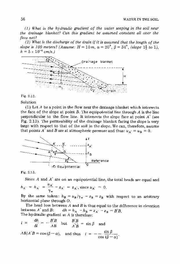
5 6 WATER IN THE SOIL
(1) What is the hydraulic gradient of the water seeping in the soil near the drainage blanket? Can this gradient be assumed constant all over the flow net?
(2) What is the discharge of the drain if it is assumed that the length of the
slope is 100 meters? (Assume: Ç = 10 m, a k = 5x 1 0 - 4 cm/s.)
2 0 ° , â = 3 4 ° , (slope l\ to 1 ) ,
D r a i n a g e blanke t
Drain' :
Fig . 2.12 .
Solut ion (1) Let A be a point in the flow near the drainage blanket which intersects
the face of the s lope at point B. The equipotential line through A is the line perpendicular to the flow line. It intersects the s lope face at point A' (see Fig. 2 . 1 3 ) . The permeabil ity of the drainage blanket facing the s lope is very large with respect to that of the soil in the s lope. We can, therefore, assume that points A' and Β are at atmospheric pressure and thus : uA> = uB = 0 .
R e f e r e n c e
— r ~ —
(€ ) E q u i p o t e n t i a l
Fig . 2.13 .
Since A and A ' are on an equipotential line, the total heads are equal and UA'
hA> = h zA' = zA>, since uA' = 0 . hA' — nA' --r ÝÁ' T w
By the same t o k e n : hB = uB/y w 4- zB = zB with respect to an arbitrary horizontal plane through O.
The head loss between A and Β is thus equal to the difference in elevation between A' and B: dh = hA — hB = zA> — zB = BfB.
The hydraulic gradient at A is therefore : dh BB B'B . n
1 = ~~dT= ~AB b Ut A"B= * É ¿â a nd
AB/A'B = cos (â — a), and thus i = ^tt-—.
cos (ρ — a )
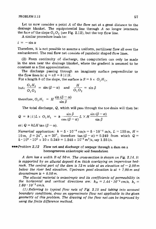
PROBLEM 2.12 57
Let us now consider a point A of the f low net at a great distance to the drainage blanket . The equipotentia l line through A no longer intersects the face o f the s lope Ïë 0 2 (see Fig . 2 . 1 2 ) , but the t o p flow line.
A similar procedure leads t o :
i — — sin a
Therefore , it is not poss ible to as sume a uni form, rectilinear f low all over the embankment . The real f low net consists o f parabol ic shaped flow lines.
( 2 ) F r o m continuity of discharge, the computa t ion can only be m a d e in the area near the drainage blanket , where the gradient is a s sumed to be constant as a first approx imat ion .
The discharge passing through an imaginary surface perpendicular to the flow lines i s : q — vS = k | ί | S. F o r a length b of the s lope , the surface is S = b χ OlHlJ
b u t :
therefore, Oxi
The total discharge, Q, which will pass through the toe drain will then b e :
o r : Q = kLHten (â-a).
Numerical application: k = 5 · 1 0 4 cm/s = 5 * 10 6 m/s , L = 1 0 0 m, Ç = 10 m, j3 = 3 4 ° , a = 2 0 ° , therefore tan (â - a) = 0 . 2 4 9 from which Q = 5 · 1 0 6 · Ι Ο 2 χ 10 χ 0 . 2 4 9 = 1 .245 χ 1 0 " 3 m 3/ s , say 1.251/s.
***Problem 2.12 F l o w net and discharge of seepage through a dam on a homogeneous anisotropic soil foundat ion
A dam has a width Β of 50 m. The cross-section is shown on Fig. 2.14. It is supported by an alluvial deposit 6 m thick overlaying on impervious bed-rock. The central part of the dam is 12 m wide at an elevation of — 2.00 m below the river bed elevation. Upstream pool elevation is at + 7.00 m and downstream is + 0.50 m.
The alluvial material is anisotropic and its coefficients of permeability in the horizontal and vertical directions are: kH = 1.44 · 10~2 cm/s, kv = 1.60 · 10~3cm/s.
(1) Referring to typical flow nets of Fig. 2.15 and taking into account boundary conditions, draw an approximate flow net applicable to the given geometry of this problem. The drawing of the flow net can be improved by using the finite difference method.
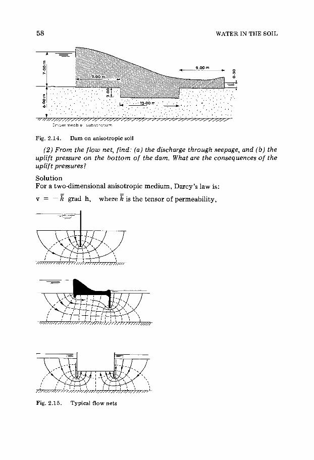
58 WATER IN THE SOIL
Impermeabl e substratu m
Fig. 2.14. Dam on anisotropic soil
(2) From the flow net, find: (a) the discharge through seepage, and (b) the uplift pressure on the bottom of the dam. What are the consequences of the uplift pressures?
Solut ion
For a two-dimensional anisotropic med ium, Darcy ' s law is :
ν = — k grad h, where k is the tensor of permeabi l i ty ,
Fig. 2.15. Typical flow nets
PROBLEM 2.12 59
dh
dx therefore / ( 1 )
3 h dz
The requirement of the principle of continuity for a two-dimensional system is:
dy* dv7
— + — = 0 (2) dx dz
therefore, f rom eqn. (1 ) and for an anisotropic soil , we have :
It is important to note that the latter equat ion is no t similar to a Laplace equat ion . The f low net is no longer m a d e up of orthogonal curves. In order to solve the prob lem, we must resort to a t ransformed section which is obta ined by assuming that the foundat ion alluvium is i sotropic but of a different geometry . In order to accomplish this, the ÷ and y directions must be t ransformed to new values in accordance with the following relat ionships :
(x = x^K/K
[Z = z.
Therefore :
dX _
dx feh'
w u d 2h fev d2h d2h d2h i t e m w h i c h : — ; = - ~ 2 and - T = ~ ~ 2
Equa t ion (3 ) then b e c o m e s :
d2h b2h — , + — ; = 0 (3 ' ) dX2 dZ2

6 0 WATER IN THE SOIL
Anisotropi c medi a (scal e 1 : 40 0 )
Transforme d sectio n ( r =- j ) Isotropi c mediu m
Fig. 2.16.
Conclusion
The transformed section allows one to consider an isotropic condit ion with the ratio V f e v/ f e h. In this case , where fev = 1.6χ 1 0 " 3 c m / s , kh = 1 4 . 4 χ 1 0 " 3 cm/s and r =\Jkv/k^ =\/l/9 = 1 /3 , F ig . 2 .16 shows the anisotropic section at a scale of 1 : 4 0 0 (axes x, z) and the transformed section with a ratio of 1 : 3 (axes X , Z ) .
Drawing the flow net
Since the transformed section represents a f ictit ious isotropic condit ion as far as permeabil i ty is concerned, the orthogonal net exists with equipotential and flow lines.
The net m a y be drawn by reference to the typical nets given in the prob-lem and by observing the fol lowing:
(a) The geometry of the soil foundat ion is symmetr ica l with respect to axis OOf. Therefore only half of the need be drawn, say to the left o f OO' (see Fig. 2 . 1 7 ) .
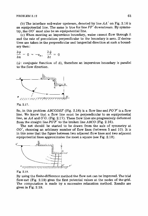
PROBLEM 2.12 6 1
(b) The interface soil-water ups t ream, denoted by line AA ' on Fig. 2 .16 is an equipotential l ine. The same is true for line FFr downstream. By symme-try , the O O ' must also b e an equipotent ia l l ine.
(c) When meeting an impervious boundary , water cannot f low through it and the rate of percolat ion perpendicular to the boundary is zero. If deriva-tives are taken in the perpendicular and tangential direction at such a bound-ary then :
= 0 = - * n , - f = 0 on ot
(ö: conjugate function of 0 ) , therefore an impervious boundary is parallel t o the f low direct ion.
/ / / / / / / / / / / / / / / / / / / / / / / I
Fig. 2.17.
S o , in this prob lem ABCODEF (F ig . 2 . 1 6 ) is a f low line and PO'P' is a f low line. We know that a f low line mus t be perpendicular to an equipotentia l l ine, as AA and O'O. (F ig . 2 . 1 7 ) . These f low lines are progressively de formed from the straight line PO'P' to the broken line ABCO (F ig . 2 . 1 6 ) .
The net should be started to be drawn f rom the axis of symmetry at O O ' , choosing an arbitrary number o f f low lines (between 5 and 1 0 ) . It is in this zone that the figure between t w o ad jacent f low lines and two adjacent equipotentia l lines approx imate s the mos t a square (see Fig. 2 . 1 8 ) .
'//////}////
o' r/////////// //////// ///////////////
Fig. 2 .18.
By using the finite-difference m e t h o d the f low net can be improved. The trial flow-net (F ig . 2 .19 ) gives the first potent ia l values at the nodes of the grid. The computa t ion is m a d e by a successive relaxat ion m e t h o d . Results are given in Fig . 2 . 1 9 .

6 2 WATER IN THE SOIL
Fig. 2 .19. Flow net and grid used for the finite difference method. Note: The potential has been arbitrarily chosen equal to 100 along ËÁ! and to zero along OO'.
Percolation discharge. At any one point of the anisotropic sect ion, we have
dq = vx dz dy + vz dx dy
In the plane of symmetry OO' we have vz = 0 , then:
, dh dq = -\/k hkv — · dz χ 1
oX
and the equivalent permeabil i ty k is obta ined : k = y/k hkv
Earlier, it was shown that feh = 9 fev or k = 3 fev, or k = 4 .8 · 1 0 " 3 c m / s .
The discharge is given by the formula : q = k χ AH χ ATx/iVH , where AH = tota l head loss between the upstream and downstream equi-potential lines, NT = number of f low channels, Nu = number of equipo-tential intervals f rom which:
q = 4 .8 χ 1 0 ~ 5 χ 6 .5 χ ( 6 / 2 0 ) χ 3.6 χ Ι Ο 3 = 3 .37 χ 1 0 " 1 m 3 / h
or q = 0 .34 m 3 /h for a 1 meter wide slice through the d a m . The d a m width is 5 0 m ; therefore , the total percolat ion loss is Q = 17 m 3 /h .
dh dX

PROBLEM 2.12 63
Remark. Considering a horizontal plane (at the beginning or the end of the net ) , we have vx = 0 .
ö , , 7 dh dh dh Then: dg = - 4 , ^ x 1 , ^ = ^
and after changing the variable:
dx fev
d X , then d<? = — k dh fk^ dh
Uplift pressures. L e t the t o p of the foundat ion soil layer be the reference plane of F ig . 2 . 2 0 . The head a t any r a n d o m point is ft = u/yw + æ where æ is the elevation of the r andom point with respect to the reference plane. There are 20 equipotentia l drops . The tota l head loss is :
AH =hA-hF = 7 . 0 0 - 0 . 5 0 = 6 .50 m
The head drop between any two consecutive equipotent ia l lines i s :
Ah = AH/N = 6 . 5 0 / 2 0 = 0 . 3 2 5 m.
4.30m , 4.70
Fig. 2.20. Schematic representation of uplift pressures
At point A:
uA 7 .00 Λ A = — +zA = + 6 .00 = 1 3 . 0 0 m , uA = 7 0 k P a .
Tw 1 At point Ì (equipotential line number 5 , see Figs . 2 . 1 9 and 2 . 2 0 ) :
hM = — + z M = — + 6 = hA - 4Ah Tw Tv
= 13 — 4 χ 0 . 3 2 5 = 1 1 . 7 0 m
"M = 1 1 . 7 0 - 6 . 0 0 = 5 .70 m, 57 kPa.

64 WATER IN THE SOIL
for length CD:
Ι Ο 2 χ I 1 2 . 0 0 χ 1.00 χ Q' 7 1 + ° ' 4 3^ ^ 6 8 0 k N
for length EF:
0 / 0 .16 + 0 .14 0 .14 \ Ι Ο 2 χ 6 .40 χ 1.00 χ + 2 .60 χ 1.00 χ ^ 1 1 0 k N
Tota l = 1 3 2 0 k N
Since the length of dam is 2 χ 9 .00 4- 1 2 = 30 m and assuming a unit 1 3 2 0
weight of concrete of 23 k N / m 3 , an average height of at least 2 3 x 1.00 x 30
= 1.9 m of concrete is needed t o balance the uplift pressure.
**Problem 2.13 Ear th d a m : quick-sand condi t ion ; drainage b lanket ; discharge by percolat ion
Consider an earth fill dam supported on a stratified, heterogeneous foun-
At M' (equipotential line number 6 ) : ι r
hM> = — + * M = — + 5 .00 = hA-5Ah = 1 1 . 3 7 5 m Tw Tw
— = 1 1 . 3 7 5 - 5 . 0 0 = 6 . 3 7 5 m , u'M = 6 4 k P a . 7w
At point Ï (equipotential line number 1 1 ) :
hQ = — + z 0 = — + 4 . 0 0 = hA — 1 0 Ah = 1 3 . 0 0 - 3 . 2 5 = 9 . 7 5 m Tw Tw
— = 9 . 7 5 - 4 . 0 0 = 5 .75 m, uQ = 57 .5 kPa. Tw
The uplift pressure (see F ig . 2 .20 ) m a y be c o m p u t e d in this manner for each equipotential l ine. Planes BC and ED of the d a m foundat ion are under horizontal pressures of oppos i te directions. The resultant of these horizontal pressures is a net pressure-acting downstream.
The vertical uplift pressure resultant for a i m slice of the d a m i s : for length AB:
, . 0 .70 + 0 .57 0 .57 + 0 . 5 4 \ 1 0 2 x 4 .30 χ 1.00 χ + 4 . 7 0 χ 1.00 χ ^ 5 3 0 k N
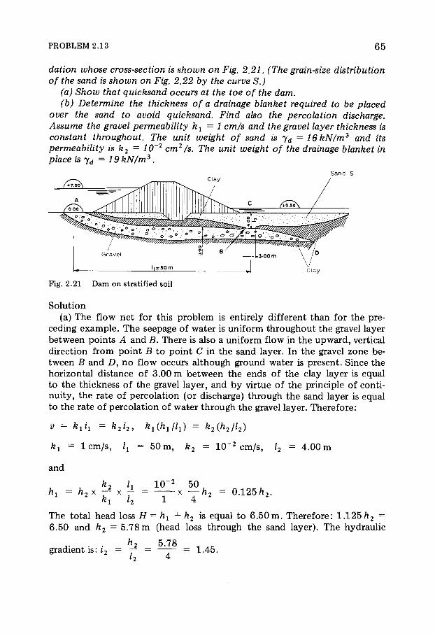
PROBLEM 2.13 6 5
dation whose cross-section is shown on Fig. 2.21. (The grain-size distribution of the sand is shown on Fig. 2.22 by the curve S.)
(a) Show that quicksand occurs at the toe of the dam. (b) Determine the thickness of a drainage blanket required to be placed
over the sand to avoid quicksand. Find also the percolation discharge. Assume the gravel permeability k1 = 1 cm/s and the gravel layer thickness is constant throughout. The unit weight of sand is yd = 16kN/m 3 and its permeability is k2 = 10~2 cm1 Is. The unit weight of the drainage blanket in place is yd = 19 kN/m 3.
San d S
Fig. 2.21 Dam on stratified soil
Solut ion (a) The flow net for this problem is entirely different than for the pre-
ceding e x a m p l e . The seepage of water is uniform throughout the gravel layer between points A and J5. There is also a uni form flow in the upward , vertical direction f rom point Β to point C in the sand layer. In the gravel zone be-tween Β and D, n o flow occurs a l though ground water is present . S ince the horizontal distance of 3 .00 m between the ends of the clay layer is equal to the thickness of the gravel layer, and by virtue of the principle of conti-nuity, the rate of percolat ion (or discharge) through the sand layer is equal to the rate o f percolat ion of water through the gravel layer. Therefore :
Ό = k1i1 = k2i2, kl{h1/ll) = k2(h2/l2)
kx = l c m / s , lx = 50 m, k2 = 1 0 " 2 c m / s , l2 = 4 .00 m
and
k2 lx 1 0 " 2 50 hl = h2 χ — χ — = χ — h 2 = 0 . 1 2 5 h 2.
kx l2 1 4
The total head loss Ç = h1 + h2 is equal to 6 . 5 0 m . There fore : 1 . 1 2 5 h 2 = 6.50 and h2 = 5 .78 m (head loss through the sand layer) . The hydraulic
h2 5 .78 gradient is : i2 = — = — - - = 1 .45 .
l2 4
WA
TE
R IN
TH
E
SO
IL
66
Fig. 2.22 Grain-size distribution curves

PROBLEM 2.13 6 7
Quicksand condit ion in the sand would b e :
ß > icrit = — = ~—— — , b u t : Td = 1 6 k N / m 3 , and Tw Ts Tw
7 S = 2 7 k N / m 3 , hence i c r it ~ 1 . 0 1 , so i2 = 1.45 > 1 .01 ,
i.e. quicksand would occur.
(b) Consider the sand column element d S of height Æ in F ig . 2 . 2 3 . This e lement is being ac ted u p o n , downwardly by its b u o y a n t weight W' = y'ZdS and upwardly b y the percolat ion water force F = i.ywZdS. We have shown that quicksand occurs , therefore we know that F> W R. In order to avoid quicksand, a weight acting downward must be added to the sand in order to have q'dS + W' + F> 0 so that the resultant is acting downward (positive direct ion) . There fore :
q'dS + y'ZdS - iywZdS > 0 , or q > (iyw - y')Z.
•:'f F 1 Æ 1 • W 1 •
ds Fig. 2.23
The m a x i m u m value of Æ mus t be selected, i .e . : Æ = l2 = 4 m, yd s a nd = 16 k N / m 3 or 7 s a nd = 1 0 . 1 k N / m 3 . We need q' > ( 1 4 . 5 - 1 0 . 1 ) ÷ 4 . 00 or q' > 17 .6 k N / m 3 .
Water will rise u p into the filter b lanket to level + 0 . 5 0 . Therefore : q' = y'mter ÷ 0 .50 + ( T d W r x Ç = 1 7 . 6 k N / m 2 .
(Td)filte r = 1 9 k N / m 3 ,
f rom which: 7; m er = ^ — ^ Td = hlxl9 = 12kPa
Ts ^· ·
a n d ? = 12 ÷ 0 .50 + 1 9 ÷ Ç = 1 7 . 6 k N / m 3 . Final ly:
1 7 . 6 - 6 Ç = = 0 . 6 1 c m .
1 9 In view of the simplifying, conservative a s sumpt ions m a d e (constant hy-draulic gradient in the sand) , a lower safety factor m a y be accepted and the value of Ç = 80 cm a d o p t e d .
The drainage blanket would be c o m p o s e d o f t w o layers in accordance with the design criteria for filters.
6 8 WATER IN THE SOIL
4 . 5 d 1 5 s u b g r a de ^ disfater ^ 4 .5 d 8 5 s u b g r a de
The layer immediate ly on t o p of the sand (material Gx on grain-size curves of Fig. 2 .22 ) would be 50 cm thick, layer G2 would be 80 cm thick.
F r o m the grain-size curves of the sand we ge t : d15 = 0 .2 m m and d 8 5 = 1 m m , giving, for instance, for material Gx: ( < 3 1 5) Fi = 2 m m , ( d 8 5) F l =
20 m m and for G 2 : 9 m m < ( d 1 5) F2 < 9 0 m m . The larger sizes should be placed on the upper s ide of G 2 material (on
t o p of the filter b lanket ) .
Percolation discharge: q = vS = k2(h2/l2)S. The cross-sectional area of the gravel layer S = 3 .00 χ 1.00 = 3 m 2 per linear meter of d a m length, and q = 0 . 4 4 1/s per linear meter of length, but Β = 50 m, hence Q = 50 χ 4 . 3 5 · Ι Ο " 4 χ 3 . 6 - 1 0 3 ~ 7 8 . 5 m 3 / h .
+*Problem 2.14 Capillary rise in a h o m o g e n e o u s soil, effective stresses
A dense silt layer has the following properties: void ratio e — 0.40, effective diameter d10 = 10 ìm, capillary constant C — 0.20 cm2.
Free ground-water level is 8.00 m below surface. Find: (1) the height of capillary rise in the silt; (2) the vertical effective stress at depths of 5 m and 10 m. Assume ys = 26.5 kN/m 3 and that the soil above the capillary rise and ground surface is partially saturated at 50%.
Solut ion (1) The capillary rise is calculated f rom the formula h — C/edl0
where h and d are in cm and C in c m 2 .
Therefore : d10 = 1 0 Mm = 1 0 " 3 cm, and h = ^ β · 2 β = q 5 χ 1 Q3 0 .40 χ 10 0
or h = 5 m. (2 ) F o r the vertical effective stress at any depth above the free ground
water (see Fig . 2 . 2 4 ) , consider a unit area water co lumn. It is in static equilibrium, hence : u = ~ywZ.
We t soi l ·.·.'•; •
Capillar y ;.v / r i s e
3m (oh
5m 10m
Saturate d soi l
5m
. Fre e wate r -leve l
Fig. 2.24.

PROBLEM 2.15 6 9
Pore-water pressure is negative above the free ground water table , in the capillary rise area. Hence Terzaghi 's equat ion ï — ï + u, can be written as : 0 = 0 — \u\ or σ'= σ + \u\.
At a depth of 5 m, the total vertical stress i s : ( σ ν ) 5 = hxyh + (h2 ~~<z)7sat> b u t u = —z.7w, f rom which: ( σ ν ) 5 = hxy^ + (h2 -z)y sat + zy w .
Let us calculate 7 s a t: 7 s at = ys e = 2 . 6 5 w
( 2 . 6 5 + 0 .40 ) and 7 s at = 2 6 . 5 χ - = 2 1 . 8 k N / m 3 .
2 .65 χ 1.40
Le t us now calculate 7 h . Above ground water, S r = 50%, so
S r7 w 0 .40 χ 0 .50 χ 10 w = e — - = = 7 .5%
7s 2 6 . 5 from which:
1 + w 1 .075 7h = 7s T — = 2 6 . 5 χ — — = 2 0 . 4 k N / m 3
1 + e 1.40
a n d : ( a ; ) 5 = 3 .00 x 2 0 . 4 + 2 .00 x 2 1 . 8 + 3 x 1 0 = 1 3 4 . 8 kPa,
say 1 3 5 kPa.
At a depth of 1 0 m , the effective stress ( σ í ) 1 0 = h1yh + h2ysat + \z\y = 3.00 χ 20 .4 + 5 .00 χ 2 1 . 8 + 2 .00 χ 1 1 . 8 = 1 9 3 . 8 kPa.
Summary of answers
h = 5 . 0 0 m ; ( σ ^ ) 5 ^ 1 3 5 k P a ; (σν) ιο - 1 9 4 k P a .
k**Problem 2.15 Capillary rise in an analogous soil mode l
A poorly graded sand may be idealized by stacking of spheres of identical diameters. Find the capillary rise in this theoretical model assuming that the spheres are stacked in the loosest packing arrangement (n = 0.48). The surface tension of water is 75 dynes/cm and assumed acceleration due to gravity is g — 1000 cm/s2. Compare the result with the result of the em-pirical formula h = C/ed10.
So lut ion In its loosest s tate , a stacking of spheres looks like the diagram of Fig .
2 . 2 5 . L e t us s tudy the static forces acting on a co lumn o f capillary water as shown in Fig . 2 .26 . L e t us first find the m a x i m u m capillary tension due to surface tension at the contact between water and a sphere (at the meniscus) ,

70 WATER IN THE SOIL
as shown in Fig . 2 . 27 . This figure makes clear that the contact curve is m a d e up of four J circles of radius r. B u t r = R cos â where R is the radius o f one of the spheres.
Fig. 2.26.
Let a be the wetting angle (between the two tangents of the meniscus and of the surface particle s at the point of contac t ) , then the vertical com-ponent of the capillary force is : T v = 2nrT cos (a 4- â) = 2kRT cos â cos (α + â)-
The m a x i m u m value will occur when â = —a/2:
T r a ax = 2 7 L R T c o s 2a / 2 .
Plan v i ew Deta il of c o n t a c t c i r c le
Fig. 2.27.
Plan v i e w E l e v a t i on AA'
Fig. 2 .25.
C a p i l l a ry w a t e r
C o n t a c t c u r ve of m e n i s c u s
Contact c irc le of m e n i s c us
V
PROBLEM 2.16 7 1
Le t us now assume a = 0 . In this ease the capillary m a x i m u m force will occur when the meniscus contacts a row o f spheres along a plane through the center of these spheres. The vertical force due t o capillary act ion will be balanced by the weight of a water co lumn of height h, whose cross-sectional area, Sm, is yet to be determined. L e t us consider one row of spheres of height d = 2R. The void rat io , for one element of mass (4 spheres) is calcu-lated f rom:
4 , nd3
volume of vo ids : Vv = Sm χ d, volume of grains: Vs = — KR = , 3 6
d3 ôôÜ2
and : e = Vv/Vg, f rom which: d χ Sm = âð — or S m = e ——
The weight of the water co lumn of height h and of section S m is then : W = en(d2/6)/i7w . This weight is suppor ted by the capillary force which is,
d2
for a = 0 : T v = ðÜÔ. Therefore : ðÜÔ = eir — hyw or h = 6T/edy w . 6 If we take Ô = 7 5 d y n e s / c m and £ = 1 0 0 0 c m / s 2 , which gives Y W =
1 0 0 0 dynes , then :
6 χ 7 5 0 . 4 5 h = = .
1 0 0 0 ed ed
Since all the spheres have the same diameter , d = d 1 0, the empirical formula is proven: h = C/edl0 (h and d 1 0 are in cm) in which C varies be-tween 0 .1 and 0 .5 c m 2 , depending on the soil t y p e .
Remark: In reality the wetting of the grain is far f rom ideal , therefore angle α is different f rom zero , which y ie lds :
6 Ô c o s 2 ( a / 2 ) h = .
ed
The corresponding value of C is lower bu t remains in the range 0.1—0.5 c m 2 .
irkirProblem 2.16 Water table drawdown b y vertical drains
(1) Assuming that DupuiVs hypothesis is applicable to the problem, find the discharge and the equation of the free ground-water surface of a drainage trench of infinite length excavated to an impervious substratum through a soil of permeability k (assumed to be isotropic) and in which the static, free ground-water height is Ç above the substratum. Let R be the horizontal dis-tance from the side of the trench to a location where the drawdown is zero, (analogous to the radius of influence of a pump-out well). Assume that the ground-water table is replenished by two infinite sources on each side of the trench whose horizontal distance from the trench is larger than R.
(2) Vertical drains consist of tubes of small diameter (from 5 to 8 cm) perforated at the base. They are usually installed by jetting, when spaced

72 WATER IN THE SOIL
about lm on center. Assume that one row of drains is equivalent to a drainage trench. The vertical drains are connected at the surface by a collector pipe attached to a pump.
In order to install a sewerline, it is necessary to excavate a 4m deep trench through a silty sand of permeability k = 2x 10~3cm/s. The axis of the trench is located parallel to a river bank at 55 m distance. The impervious substratum is at 7 m below the existing ground surface. A row of vertical drain is installed 5 m away from the axis of the sewer. The free ground-water, prior to excavation of pumping is at 0.50 m below ground surface. See Fig. 2.28.
The vertical drains are jetted to the depth of the substratum. The length of the trench is 150 m. Find the discharge required to draw the water table down to a depth of 0.5 m below the bottom of the trench. Assume R = 50 m.
Trench of inf ini te length
Fig. 2.28
(3) The silty sand through which the water table is drawn has e = 0 . 6 0 , d10 =z15ìm, ysat = 20.4 kN/m 3. Its wet unit weight, above the capillary rise is estimated to be yh = 17.6 kN/m 3. Find the change in effective stress during the drawdown, acting on a horizontal surface element located 10 m horizontally from the trench at a depth of 5 m. What is to be concluded? Assume C = 0.3 cm2 for the capillary rise empirical formula.
Solut ion (1 ) L e t Μ be a point on the free ground-water surface along the drawdown
curve. The hydraulic gradient at that point is i = — Ah/AL Since Ì is at the free water surface, the pore pressure is zero and if M' is
located an incremental distance away f rom Ì on the free surface , then :
dz Ah = hM —hM> = —dz and i =
ds

PROBLEM 2.16 73
where s is the abscissa a long the curved line of the free surface oriented f rom Ì towards Mf. If the direction of orientat ion of the curvilinear abscissa is changed towards O x' then i = dz/ds.
The rate of discharge, according to Darcy ' s L a w is í = k (dz/ds). The hori-zontal c o m p o n e n t of this velocity is (see Fig . 2 . 2 9 )
dx dz dx dz /J A 2
vx = í cos a = í — , vx = k — — = ft — d s d s d s dx
Since the s lope of the free water surface is low, Dupui t ' s hypothes i s is appl icable . S o :
dx a2 1 ldz\ 2 , ldx\2 ldz\ 2
— = cos a ^ 1 ^ 1 — and — ^ 1 — — d s 2 2 \dx) \ds) \dx)
(dz\ 21 d * 1 - — c± k —
\dx] J dx
if we neglect the third order t e rm. Assuming that the water flow is laminar (Dupui t ) vx is the average value
of the discharge rate across a vertical p lane located a t a d i s t a n c e s . The dis-charge across that plane passing b y point M, parallel to the trench axis over a length b of the trench i s :
dz q = vx. S = vxbz = kbz — .
d x
Since water is incompress ible and a s teady f low is ult imately obta ined , this unit discharge is half tha t f lowing f rom both sides of the trench. There-fore we have the differential equa t ion : qdx = kbzdz, and, integrating it between points Ï and R, we have :
dz f rom which: vx = k —
dx
2

74 WATER IN THE SOIL
The discharge p u m p e d out for a unit length of trench (b = 1 ) is:
(H2 -hl\
Q = 2q = (1 )
Integrating between Ο and ÷ y ie lds :
<?x = fe6 and f rom eqn. ( 1 ) : = — n n w
\ 2 / ' k 2qR
f rom which: ζ 2 — / ι ^ = (for b = 1 ) k
t h e n : * 2 = + (H2 -hi) (2 )
(2 ) Numerical application: vertical drains:
R = 5 0 m , f c = 2 χ 1 0 " 3 cm/s = 2 χ 1 ( Γ 5 m/s , i f = 7 - 0 . 5 0 = 6 .50 m.
and along the axis of the sewer t rench:
÷ = 5 .00 m, æ = 7 . 0 0 - 4 . 5 0 = 2 .50 m.
Equat ion (2 ) gives: 2L502 = hi + ^ - ( 6 J 5 0 2 - hi). 50
f rom which ftw ~ 1.50 m. Equat ion (1) yields then:
. 6 ΐ 5 0 2 - Γ 5 0 2 . , Q = 2 χ Ι Ο " 5 χ = 1.6 χ 1 0 - 5 m 3 / s
50
per meter length of trench. For a 1 5 0 m long trench,
QT = 1.6 χ Ι Ο " 5 χ 1 5 0 χ 3.6 χ 1 0 3 = 8 .64 m 3 /h (or 2.4 1/s).
(3 ) The capillary rise in the sand, in cm, is calculated f rom h = C/ed10
for : e = 0 . 6 0 , C = 0.3 c m 2 and d 1 0 = 50 Mm = 5 0 χ 1 0 " 3 m m =
0 3 5 ÷ 1 0 " 3 cm, we get : h = ———i——τ = 1 0 0 cm.
0 .60 χ 5 χ 10 0
The capillary height above the free ground-water level is 1.00 m. The unit weight of soil t o b e applicable to this capillary zone is the saturated unit

PROBLEM 2.17 7 5
z\ = ( 1 . 5 0 2) + — ( 6 . 5 0 2 - 1 . 5 0 2 ) f rom which zx = 3 .20 m.
The tota l stress at 5 m depth and 1 0 m f rom the trench, before the draw-d o w n , w a s : (σ ν) ΐ = 5 7 s at = 2 0 . 4 χ 5 = 1 0 2 k P a and the pore-water pressure was : (u){ = 4 . 5 7 w = 4 5 k P a . The effective stress, prior to drawdown was : (σΙ\ = 1 0 2 — 4 5 = 5 7 k P a . After equil ibrium has been reached with full d rawdown:
(ov)f = 7 s a t( 4 . 2 0 - 2 ) + 7 h ( 7 - 4 . 2 0 ) = 2 0 . 4 x 2 .20 + 17 .6 x 2 .8 =
94 .2 kPa. (u)f = 7 w( 3 . 2 - 2 ) = 1 2 k P a ,
from which (a'v)f = 9 4 . 2 — 1 2 ~ 8 2 k P a .
Drawing the water down causes an increase in effective stresses Áσ'í = 2 5 kPa. This is a considerable a m o u n t as it is greater b y :
Δ σ ; 2 5 - ~ = — ~ 4 4 % . (σ'í)é 57
This increase in stress is sufficiently large that considerat ion would have to be given to sett lements resulting f rom a dewatering operat ion occurring in compress ible soils.
**Problem 2.17 Piping condit ions in a fractured rock mass
Consider the dam whose cross-section is shown on Fig. 2.30. An unlined drainage gallery was excavated in the rock downstream of the dam. The gallery intersects a fracture filled with pervious soil. The thickness of rock above the center line of the gallery is x, at the location of the fracture. The level difference between the reservoir pool and the grade where the fissure intersects the ground surface is Z. If we know that the unit weight of the fracture fill material is ys = 26.5 kN/m 3, determine what values of ÷ and æ and of porosity n, would cause piping in the fracture. Calculate ÷ in terms of z, for ç = 40%.
weight 7 Sat = 2 0 . 4 k N / m 3 . Above the capillary rise, 7 h = 1 7 . 6 k N / m 3 as given in the prob lem.
L e t us calculate the level of the drawdown at equil ibrium 1 0 m away from the t rench :
7 6 WATER IN THE SOIL
Fig. 2 .30. Piping in fractured rocks.
Solut ion Piping occurs where soil is carried away by water flowing upward and
exerting a force greater than the buoyant weight of the soil particles . The consequence of piping is excessive loss of water and partial caving of foun-dat ion materials and possibly disastrous damage to the dam structure. In the case of rock, as in this prob lem, the only probable consequence would be excessive leakage through the foundat ion.
Piping would occur when at a point in the fracture, the weight of the soil is balanced by an upward force of the-water f low. If it is a s sumed that the head gradient is constant throughout the length of the fracture, piping will occur when the pressure at the b o t t o m of the fracture is u = (z + x)yw , and equal to the tota l stress which is σ = xy&u therefore when u — (z + x)yw
= xJsat = x ( 7 + Tw ) or when zy w = xy'.
T o avoid piping we mus t maintain the condit ion zy w <xy'. We know that the buoyant unit weight of the soil material in the fracture is : y1 — (7s " 7 w ) ( l - n) f rom which: x/z > yj(y s -y w)(l~n). Condit ions for piping are realized then, when x/z > 1 0 / 1 6 . 5 ( 1 — 0 . 4 0 ) or x/z> 1 / 0 . 9 9 - 1 .
T o avoid piping, the rock thickness above the gallery would have to be greater than z.
**Problem 2.18 Permeabil ity
A test is set up as shown in Fig. 2.31. A cylindrical mold of 4 in. in diameter (D = 4 in.) is filled to height h2 = 0.2 ft with silt whose perme-ability is k2 = 5.3 * i 0 "4 ft/min.
A second coaxial mold is placed on top of the first mold whose inside diameter is d = 1.5in. and whose height is hx =0.3 ft. Its thickness is negligible. The inside of this second mold is filled with the same silt, but the anular ring outside the small tube and outer tube is filled with sand whose permeability iskx =2 * i 0 "3 ft/min.
The test set-up is a permeameter of constant head. Water is placed in the

PROBLEM 2.18 77
mold and maintained at a level Æ = 1.25 ft above the level of the outlet. It may be considered that altogether the system consists of a fictitious soil of thickness Ç = hx + h2 and of permeability kf. (1) Find the value of kf. (2) Determine the volume of water which perco-lated after 30 min.
Wate r
Ç Q Ç
k
Sil t
. S a n d
Ç
i *
* Wate r
P o r o u s s t o n e
Fig. 2 .31 .
Solut ion (1 ) The radius of frozen soil R1 a round a liquid pipe can be calculated,
through the anular space qx and through the inner mold q2. The hydraulic gradient in both instances is Z/H. F ind q2 f rom Darcy ' s law, where í = ki:
k2i Æ Æ d2
k7 ôæ f rom which q2 — V2S2 = k2—n — , 2 Ç Ç 4
Æ D2-d2
The same applies t o : qx = kv— π Ç 4
(1)
but here, kv is the equivalent permeabi l i ty corresponding to the 2-layer
Ç hx h2
sys tem, therefore: — = ~ Η — , kv ki k2
f rom which: kv
klk2H and qx =
kxk2H
kxh2 + k2hx~ *l klh2+k2hl Ç
The total discharge at the outlet is q = qx + q>i.
Æ D2
We also have: q = kf— χ π — . Ç 4
Æ D2-d2
χ — χ π . (2)
(3)
(4 )
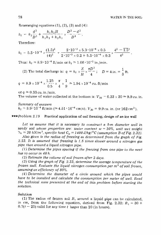
78 WATER IN THE SOIL
Rearranging equations (l), (2) , (3) and (4): D 2 - d 2
x--. d 2 k I k 2 H k f = k 2 1 +
D k l h 2 + k ? ; h , D 2
Therefore:
2 5.3 x 0.5 42 - 1.52 + x -- (1.5)'
2 ~ l O - ~ x 0.2 + 5.3*10-4 x 0.3 42 k f = 5 . 3 ~ 1 0 - ~
Thus: k f = 8.9 ftimin or k f 1.06 *lod2 in./min.
Z .rrD2 1 (2 ) The total discharge is: q = k f x - x - ; D = 4 in. = .---ft. H 4 3
or q 2 0.33 cu. in./min. The volume of water collected at the bottom is: V30 = 0.33 x 30 'v 9.9 cu. in.
Summary o f answers k f = 8.9 - ftimin (% 4.51 * lob4 cm/s); V30 = 9.9 cu. in. (or 162 cm3 ).
*++Problem 2.19 Practical application of soil freezing; design of an ice wall
Let us assume that it is necessary t o construct a 5-m diameter well in sandy soil whose properties are: water content w = 3076, unit wet weight Y h = 20 k N / m 3 , specific heat C, = 1400 J/kg/'C (assumption B o f Fig. 2.32).
Also given is the radius of freezing as determined from the graph o f Fig. 2.23. It is assumed that freezing is 1.5 times slower around a nitrogen gas pipe than around a liquid nitrogen pipe.
(1) Determine the pipes spacing i f the freezing f rom one pipe t o the nex t has to occur in 48 h.
( 2 ) Estimate the volume o f soil frozen after 3 days. ( 3 ) Using the graph o f Fig. 2.33, determine the average temperature o f the
frozen wall. Evaluate the liquid nitrogen consumption per m3 o f soil frozen, assuming an efficiency of 80%.
(4 ) Determine the diameter of a circle around which the pipes would have to be installed and calculate the consumption per meter of well. Read the technical note presented a t the end o f this problem before starting the solution.
Solution (1) The radius of frozen soil R , around a liquid pipe can be calculated,
in cm, from the following equation, derived from Fig. 2.32: R 1 = 30 + 0.7(t - 20) valid for any time t larger than 20 (in hours).

PROBLEM 2.19 79
Liqui d pip e
A s s u m p t i o n A on soil ë - 2 - w . m - l _ ° k - 1
0 s q u a re p ipe , 115 mm s i de W 3 2 0 %
t e m p e r a t u r e SL 140 Ê C ï P = 1 8 0 0 k g . m~ 3
SG 1 30 Ê 1 0 0 0 J- k g - 1. ° k
0 10 20 30 4 0 50 60 70 80 Time (hours)
Fig. 2.32. Isotherm 0°C evolution with time along an axis perpendicular to the pipe alignment.
The freezing radius R2 a round a nitrogen gas pipe will be R2 = 20 + 0.47(£ — 20) and at the end of 4 8 hours : R1 4- R2 = 49 .6 + 33 .2 = 82 .8 cm.
This distance corresponds to the theoretical spacing because at the end of this t ime the two radii would touch and the freezing circles would be tangent.
(2) A t the end of 72 h, the respective frozen soil radii will be R x = 6 6 . 4 cm (circle area = 1 . 3 8 m 2 ) , R2 = 4 4 . 6 c m (circle area = 0 . 6 2 m 2 ) . If the excess

80 WATER IN THE SOIL
freezing, occurring due to the overlap of the two circles, is neglected, the total soil volume frozen is 2 .00 m 3 /2 = 1 m 3 for a length of travel of 0 .83 m and for a depth of p ipe of l m . The average thickness o f frozen wall is therefore 1.2 m.
(3) With assumption B , from Fig. 2 . 3 3 , at the end of 72 h, the average wall temperature is 2 4 0 ° Κ or — 3 3 ° C . The amount of l iquid nitrogen needed to lower the soil to that temperature can be calculated: the energy required
°ê t
285
Fig. 2 .33. Average wall temperature (°C = 273° K).

PROBLEM 2.19 81
to cool 1 m 3 of soil (water exc luded) from + 1 2 ° C to - 3 3 ° C (AT = 4 5 ° C ) is : 2 0 0 0 kg ÷ 1 4 0 0 J ° C _ 1 k g " 1 ÷ 4 5 = 1 2 6 , 0 0 0 , 0 0 0 J .
One m 3 of soil with a water content of 30% contains 4 6 0 1 of water. In order to freeze the water, the energy required will be 80 ÷ 4 .18 ÷ 4 6 0 , 0 0 0 = 1 5 3 , 8 2 4 , 0 0 0 J , and the total energy need for both soil and water is: 2 7 9 , 8 2 4 , 0 0 0 J .
But 1 1 o f liquid nitrogen has a mass of 8 0 0 g and l g provides 4 0 0 J / g when changing phase (vaporizing) to raise its temperature to the ambient one . If the efficiency of this process is 80%, then 1 1 of l iquid nitrogen provides 2 5 6 , 0 0 0 J . Therefore , the liquid nitrogen demand is:
(4 ) It was shown that the radius of the frozen ground around the liquid pipe is 6 6 . 4 cm after 72 h. The minimum radius of a circular layout of pipes would then be 5 .00 m Η- 2 ÷ 0 . 6 6 4 = 6 .33 m , giving a perimeter of 19 .87 m and a number of pipes of 1 9 . 8 7 / 0 . 8 3 = 2 3 . 9 , say 24 pipes .
These pipes will be placed along the perimeter of a circle whose diameter is 6 .35 m. The frozen ground volume will be , per lineal meter of p ipe : 6 .35 ÷ 3 .14 ÷ 1.20 = 2 3 . 9 m 3 (thickness of 1.20 m is average frozen thick-ness already c o m p u t e d ) .
The construct ion of the frozen wall will require: 23 .9 ÷ 1 0 9 3 = 2 6 , 1 2 3 1 of liquid nitrogen per meter of well.
Appendix of Chapter 2
Technical no te a b o u t freezing o f soils
1. Principle of computation
Usually, the placement of pipes carrying the cooling agent is determined by the geometry of the area to be excavated. It is necessary to determine the spacing between the pipes. The diameters of the pipes are standard for this type of ground preparation and usually consider the following: — for large excavations pipe lengths greater than 10 m, the outside pipe diameter is of the order of 3 inches; — for smaller works, such as in localized areas and for short lengths of pipe, the pipes may be of the order of 2 inches (50 to 60 mm).
The following assumptions can be made: the pipe temperature is fixed at say 0 S, only slightly warmer than the temperature of liquid nitrogen along the liquid pipes. It is variable along the length of the pipe when nitrogen gas is used.
If thermal losses through the pipe walls are omitted, the following equations apply:
2 7 9 , 8 2 4 , 0 0 0
2 5 6 , 0 0 0 = 1 0 9 3 1 liquid nitrogen per m 3 of ground to freeze.
(heat transfer in frozen ground)

8 2 WATER IN THE SOIL
b0\ / . 30 \ a dr c λ — I — — λ — = * p · L · — (freezing at isothermal 0 C)
br \ br a + 1 0 0 at
30 _ l ^ l 1_ 90
bt ~ a n f\ b r 2 + 2 bar — = anf ( ^ - γ + — ) (heat transfer in unfrozen ground)
where: 0 = temperature, f = time, r = radius, r c = freezing radius, λ = conductivity, a = X/p c = diffusion, ñ = unit mass, c = specific heat, f = frozen, nf = not frozen, L = phase change heat of water (freezing). The limit conditions are:
0 0 = 0 S (for r — pipe radius)
0 = 0o initial temperature of the ground (for r > pipe radius)
r = rc 0 f = O°C
r = oo θ=θ0.
A graphic interpretation is best used for the solution of the equations (method of Binder-Schmidt) or by computer.
(a) The following simplifying assumptions may be made:
tj ^ . 4 . È~θ* l n r/ r s Heat flows according to: ^ In r 0/ r s
where s — pipe subscript; r 0 = radius beyond which temperature changes are negligible;
r0 = rs exp — l n ( r c/ r s) .
Instead of mental calculation which would imply too crude an assumption, the previous hypothesis allows us to calculate the average temperature of a frozen block as a function of two parameters: pipe temperature and freezing radius. From there on it is easy to determine the amount of liquid nitrogen which is needed to reach this freezing radius.
Example Consider a 3-in. outside-diameter pipe (D = 88 .9 mm) at a temperature of —133 C
(140° K). For a 45-cm freezing radius (rc/rs = 10) the average temperature will be —42 C (see Fig. 2 .34) . If the soil has the following properties: θ0 = + 1 2 ° C , w = 30%, then L =
3 0 · 1 0 3
334 X = 77 ,000 Jou le s /dm 3, ρ = 1.8 k g / d m 3 , C = 1400 J · kg"1 · Κ"1 , the energy
required to lower the temperature of the ground from + 1 2 to 0°C to freeze it and to decrease the temperature from 0°C to —42°C will be: 1 .8 [77 ,000 + 1400(42 + 12 ) ] = 274 ,000 J per m 3 of ground; this corresponds to a nitrogen demand, at 80% efficiency (0-outlet = —70°C) of 1.07 liters per m 3 of ground. (See Fig. 2 .35) . If the nitrogen gas pipe, next in line after a liquid nitrogen pipe, has an average between outlet and inlet temperature of —100°C, the average temperature of the frozen ground bloc of 45 cm of radius will be —32°C (see Fig. 2 .33) . The amount of energy required then is: 1 .8[77 ,000 + 1 4 0 0 ( 3 2 + 1 2 ) ] = 249 ,000 J per m 3 of ground, or 0.97 liters of nitrogen per m 3 of ground.
By and large, it is seen that nitrogen consumption will be about 1 m 3 of liquid nitrogen per m 3 of ground to freeze.

APPENDIX gg
Fig. 2.35.
Fig. 2.34. Average temperature of frozen block (assuming a logarithmic distribution of temperatures) as a function of r c/ r s, where r c is the freezing radius and rs is the pipe radius.

84 WATER IN THE SOIL
The simplifying assumptions neglect: (1) Cooling of the ground beyond the frozen radius, which in fact reduces consumption by 3 to 5%; (2) the effect of alternating liquid and gaseous nitrogen pipes which increase nitrogen consumption by about 10% (the average temperature is, in fact, higher).
(b) Soil information. Heat conductivity: Heat conductivity of the soil depends primarily on the following
factors: water content (first of all); grain-size distribution, compactness. The value of λ is different for a frozen and a thawed soil (see Fig. 2.36 for this and for
thermal conductivities). Specific heat: We know that C w a t er = 1 cal-g"1 · KT1 = 4 . 1 8 J ' g _1 · K"1 and C i ce =
0 . 5 c a l * g _1 · KT1 = 2.09 J-g" 1 · K"1. It can be assumed that:
Cgrain = 0.17 cal · g"1, K"1 = 0.76 J · g"1 · K"1 (average value for any type of soil grains).
7 S
The specific heat for unfrozen soil is: C u = 7 d( 0 . 1 7 + w) = (0.17 4- w) Ts «> + Tw
Fig. 2.36. Thermal conductivity of soils (after Kersten). 7 d( l b / c u . ft = 0 .016 g k m 3) ; Κ = λ = conductivity ( B T U / f f 1 h"1 OF"1 = 1.73 w m - 1/ 0 ^ 1 ; Ku = conductivity of non-frozen soil; Kf = conductivity of frozen soil.
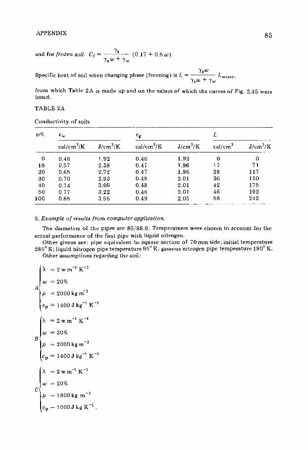
APPENDIX
and for frozen soil: Cf = — (0.17 + 0.5 w). Ts + Tw
T s ^ Specific heat of soil when changing phase (freezing) is L — ^water,
T s + Tw from which Table 2A is made up and on the values of which the curves of Fig. 2.35 were based.
TABLE 2A
Conductivity of soils
U)% cu cg L U)%
cal /cm 3/K J /cm 3/K cal /cm 3/K J / cm 3/K ca l / cm 3 J /cm 3/K
0 0.46 1.92 0.46 1.92 0 0 10 0.57 2.38 0.47 1.96 17 71 20 0.65 2.72 0.47 1.96 28 117 30 0.70 2.93 0.48 2.01 36 150 40 0.74 3.09 0.48 2.01 42 175 50 0.77 3.22 0.48 2.01 46 192
100 0.85 3.55 0.49 2.05 58 242
2. Example of results from computer application.
The diameters of the pipes are 80 /88 .9 . Temperatures were chosen to account for the
actual performance of the first pipe with liquid nitrogen. Other givens are: pipe equivalent to square section of 70 mm side; initial temperature
285° K; liquid nitrogen pipe temperature 95° K; gaseous nitrogen pipe temperature 180° K. Other assumptions regarding the soil:
λ = 2 w m " 1 K"1
w = 20%
ρ = 2000 kg m 3
c p = 1400 J kg"1 K"1
λ = 2 w m " 1 K"1
w = 30% B{
ñ = 2000 kg m 3
c p = 1400 J kg"1 K"1
λ = 2 w m _ 1 K"1
w = 20%
C -3
ρ = 1800 kg m 3
c p = 1000 J kg K " 1.
86 WATER IN THE SOIL
Results are presented on the graphs of Figs. 2 .32, 2.33 and 2.35. Fig. 2.32 gives the frozen radius along an axis through a liquid nitrogen pipe and perpendicular to the line of pipes. Not only have the curves the same shape, but it will be noticed that they appear closely grouped. This means that the rate of freezing does not change much for different soil conditions. Also the order of magnitude of R (in cm) is 30 + 0.71 (£— 20) for t in hours greater than 20.
Fig. 2.33 shows the average frozen-wall temperature. This result is in good agreement with the curve giving the freezing radius. It should be noted that the average temperature varies little in different soil types. The order of magnitude is from —20°C to —28°C after 60 hours.

87
Chapter 3
P R A C T I C A L S E T T L E M E N T C A L C U L A T I O N S - C O M P R E S S I B I L I T Y A N D T H E O R Y O F C O N S O L I D A T I O N
**Problem 3.1 Oedometer test on sand
An oedometer test performed on a sand sample gave the following results:
loading (in kg) in frame 0 24.52 73.56 171.70 36 7.90 settlement (in mm) 0 0.04 0.12 0.25 0.41
The oedometer ring area is 38.5 cm2, the sample has an initial height of
24 mm. (a) Draw the compression curve and find the consolidation moduli (in (daN/cm) corresponding to the load intervals. (b) Calculate the slope of the compression curve for the last two load in-crements and compare it to the compression moduli.
Solut ion
The compress ion curve for the sand is p lot ted from the strain values
Ah -— = (h0 — h)/h0 and corresponding load stresses. (F ig . 3 .1 ) . These are h0
presented on Table 3 A . The oedometr ic modulus for a load increment Δ σ = o2 ~ ox by definition
is:
Ah/h
TABLE 3A
h - h 0 Masses (kg) σ ( d a N / c m 2) h — h0 (mm) Masses (kg) σ ( d a N / c m 2)
h0
0 0 0 0 24 .52 0.64 0.04 0.167
73 .56 1.91 0.12 0.50 171 .70 4.46 0.25 1.04 367 .90 9 .53 0.41 1.71

88
PR
AC
TIC
AL
SE
TT
LE
ME
NT
C
AL
CU
LA
TIO
NS Fig. 3.1. Consolidation test for sand.
PROBLEM 3.1 89
where h is the sample height for σ = σ ΐ 5 Ah is the sett lement of the sample under a load of Δ σ . Table 3 B summarizes the oedometr ic modul i for each load increment
TABLE 3B
σ ( d a N / c m 2) Δ σ ( d a N / c m 2) h (mm) Ah Ah/h (%) E' (daN/cm 2)
9 0.64 24 .00 0 Q4 Q 1 67 3 83
™ * 1.27 ll'll 0.08 0 .334 380
ë ëÉ 2· 5 5 Hit °·13 0545 469
t S 5· ° 7 23 59 ° · 1 6 ° · 6 75 7 52
The s lope o f the compress ion curve is :
Δ σ Δ α _ Δ σ
h2 —h0 _ h x —hp h2 — hx Ah
ho hp hp ~J[~o
and since h0>h, the value of this s lope is slightly greater than the oedo-metric modulus .
For the last t w o load increments we have:
(a) 1.91 < σ < 4 . 4 6 , Δ σ = 2 . 5 5 ,
f rom Table 3 A :
h2 ~h0 hy —he,
— = 1.04%, and ~ — - = 0 .50% hp hp
and the s lope is : Δ σ 2 .55 2 5 5 0
= = = 4 7 2 instead of 4 6 9 for Ε Ah/hp 0 . 5 4 / 1 0 0 5.4
(b) 4 .46 < a < 9 . 5 3 , Δ σ = 5 .07 .
h2 — hp hx — hp Similarly: — = 1 .71% and — - = 1.04%
hp ho
f rom which the s lope is: 5 0 7 0 / 6 . 7 = 7 5 7 , instead of 7 5 2 for E'. It will be not iced that the two values are very close and the difference is less than inaccuracies d u e t o test errors.

90 PRACTICAL SETTLEMENT CALCULATIONS
irk Problem 3.2 Consol idat ion test on clay
A clay sample is tested in an oedometer with the following results:
stress (daN/cm2) settlement (mm)
0 0 0.1 0.2 0.2 0.03 0.4 0.05 0.8 0.10 1.6 0.19 3.2 0.43 6.4 1.09
12.8 1.78 1.6 1.58 0.4 1.43 0.1 1.22
At the start of the test, the sample height was 25mm and its void ratio was 1.01. Draw the compression curve (e vs 1 g o) and calculate the com-pression index Cc and the oedometric modulus corresponding to the load increment 6.4 daN/cm2 to 12.8 daN/cm2 (loading). Compare this modulus with the secant modulus for point load at 6.4 daN/cm2.
The consolidation pressure oc may be determined from the classical method on the e — log ï curve and the ln(l +e) — log ï diagram as rec-ommended by Butterfield (Fig. 3.2b).
Solut ion Since the volume of soil grains remains constant throughout the test , we
have:
Ah_ _ Ae
h0 l + e0
for hQ = 2 5 m m and e0 = 1 .01 , and calculating Δ β , if Ah is in m m :
l + e 0 2 .01 Ae = Ah = Ah = 8 .04 ÷ Ι Ο " 2 ÷ Ah.
h0 2 5
The values of void ratio e change, corresponding to the sett lements ob-served during the test , and are given in Table 3 C .
The compress ion index C c is the s lope of the straight line port ion of the compress ion curve for σ > oc (see Figs . 3 .2a and 3 .2b) (oc = consol idat ion stress)
c = c Δ log σ '
The diagram may be approx imated to a straight line for the interval
PROBLEM 3.2 91
TABLE 3C
a ( d a N / c m 2) Ah (mm) Ae e
0 0 0 1.010 0.1 0.02 16.1 X 1 0 "4 1.008 4 0.2 0.03 24.1 × 1 0 " 4 1.007 6 0.4 0.05 40 .2 X 1 0 "4
1.006 0.8 0.10 80 .4 X 1 0 "4 1.002 1.6 0.19 152.8 X 1 0 " 4 0.995 3.2 0.43 345.7 X 1 0 " 4 0.975 6.4 1.09 876 .4 X l O "4 0.922
12.8 1.78 1431.1 X 1 0 " 4 0.867 1.6 1.58 1270 .3 × 1 0 " 4 0 .883 0.4 1.43 1149.7 X l O "4 0.895 0.1 1.22 980 .9 × 1 0 " 4 0 .912
3 . 2 < σ < 12 .8 d a N / c m 2, and :
0 . 8 6 7 - 0 . 9 7 5 0 . 1 0 8 0 . 1 0 8
c = = =
log 1 2 . 8 - l o g 3.2 log 4 0 . 6 0 2
0 .18 .
The oedometr ic modu lus E' corresponding to the stress interval 6.4 to
Δ σ 12 .8 d a N / c m 2 is given b y : E'
Ah/h
where h is the height of the sample when a = 6.4 d a N / c m 2 and Ah rep-resents the set t lement occurring when the load is increased from 6 .4 to 12 .8 d a N / c m 2. h = 2 5 . 0 0 - 1.09 = 2 3 . 9 1 m m , Ah = - ( 1 . 7 8 - 1 . 0 9 ) = - 0 . 6 9 m m , Δ σ = 1 2 . 8 - 6 . 4 - 6 .4 d a N / c m 2
Δ/ζ 0 .69 , 6 .4 from whzch: - = - — = - 0 . 0 2 8 8 , Ε = — ^ 2 2 2 d a N / c m .
The secant modulus at any one point is : Es = Ah/h 0
where /z 0 is the initial height of sample , Ah is the sett lement under σ and therefore :
6 .4 6 4 0 E' = = = 1 4 7 d a N / c m 2 .
- ( 1 . 0 9 / 2 5 ) 4 .36
In this instance, the difference between the two modul i is substantial . The consol idat ion pressure of a b o u t 2.4 d a N / c m 2 is obtained by simply

92 PRACTICAL SETTLEMENT CALCULATIONS
0.1 0.5 Vertical stress ( da Ν / c m 2)
5 10 5 0 100
6* ( log scale)
Fig. 3.2a. Curve of compression in clay.

PROBLEM 3.3 93
drawing the intersection of the tangents to the consol idat ion curve on the e - log σ graph, as indicated on Fig . 3 .2a . On the other hand, if we use the Butterfield construct ion (see Geotechnique, 2 9 : 4 6 9 — 4 7 9 ) , we find a consol idat ion pressure of 2 .5 d a N / c m 2 (see Fig . 3 .2b ) . Butterf ield 's con-struction appears to be simpler and avoids errors of est imating from the graphical construct ion.
Summary of answers
Cc = 0 . 1 8 , oc ~ 2 .5 d a N / c m 2
and
E' = 2 2 2 d a N / c m 2 for 6 .4 < σ < 12 .8 d a N / c m 2
E' = 147 d a N / c m 2 for σ = 6 .4 d a N / c m 2.
**Problem 3.3 A p p r o x i m a t e evaluation o f the compress ion index C c and of the set t lement o f a normal ly consol idated clay
Borings were made for a construction project. They showed that sub-surface soils consist of a layer of fine sand 10.60 m thick, overlaying a soft clay layer 7.60 m thick. The free ground-water table is at 4.60 m below the ground surface (see Fig. 3.3).
The buoyant unit weight is 1.04. The wet sand density is 1.76 above the water table. The water content of the normally consolidated clay is w =40%,
94 PRACTICAL SETTLEMENT CALCULATIONS
its liquid limit w h = 45% and the soil particles unit weight of the soil con-stituent is 2.78 kN/m 3. The proposed construction will impart a net stress of 1.2 daN/cm2.
Find the average settlement of the clay layer (determine the compression index Cc by Skempton's formula and start from the initial vertical stress in the middle of the clay layer).
Solut ion S k e m p t o n ' s formula for the compress ion index is C c = 0 . 0 0 9 ( u ; L — 1 0 ) ,
and for this problem, it is: C c = 9 x l 0 " 3 ( 4 5 — 10) = 9 χ 35 χ Ι Ο " 3 = 3 1 5 χ 1 0 ~ 3 = 0 . 3 2 .
The sett lement is given by the formula :
Ah
h 1 + e log 1 +
o'J '
Since the clay is saturated, its initial void ratio is :
e = w— = 0 . 4 0 x 2 . 7 8 = 1 . 1 1 . 7w
(This value corresponds to a soft clay.) The vertical stress acting at mid-height in the clay layer is :
7 .60 , a = 4 . 6 0 χ 17 .6 + 6 . 0 0 χ 10 .4 + χ y'
2
Water table-
Fine sand #=10-4 kN/m 3 ."•
Ë
ôç
N o r m a l l y c o n s o l i d a t e d ] c l a y
/ / /
Fig. 3 .3.
where y' is the buoyant weight of the c lay :
7h = 7 s + eyv
1 + e
2 7 . 8 + 1 1 . 1
2 1 . 1 1 8 . 4 4 ~ 1 8 . 4 , so γ ' = 8 . 4 k N / m 3 .
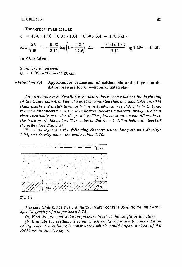
PROBLEM 3.4 9 5
The vertical stress then is :
d = 4 .60 x 1 7 . 6 + 6 . 0 0 x 1 0 . 4 + 3 .80 x 8.4 = 1 7 5 . 3 kPa
Ah 0 .32 / 12 \ 7 . 6 0 x 0 . 3 2 and — — = - — — log 1 + — — , Ah = log 1 .686 = 0 . 2 6 1
7 .60 2 .11 \ 1 7 . 5 / 2 .11
or Ah ~ 26 c m .
Summary of answers Cc = 0 . 3 2 ; set t lement : 26 c m .
**Problem 3.4 A p p r o x i m a t e evaluation o f set t lements and o f preconsoli-dat ion pressure for an overconsol idated clay
An area under consideration is known to have been a lake at the beginning of the Quaternary era. The lake bottom consisted then of a sand layer 55.70 m thick overlaying a clay layer of 7.6 m in thickness (see Fig. 3.4). With time, the lake disappeared and the lake bottom became a plateau through which a river eventually carved a deep valley. The plateau is now some 45 m above the bottom of this valley. The water in the river is 1.5 m below the level of the valley (see Fig. 3.5).
The sand layer has the following characteristics: buoyant unit density: 1.04, wet density above the water table: 1.76.
Lake
5S70m , 4 ' * · . * / • " . Sand
1 '"V///// 7 6 0 m / / / / / / /
////// Sss/ / / / / / / / / c l ay / / / / / / / / / , - / /
Fig. 3.4.
The clay layer properties are: natural water content 35%, liquid limit 45%, specific gravity of soil particles 2.78.
(a) Find the pre-consolidation pressure (neglect the weight of the clay). (b) Evaluate the settlement range which could occur due to consolidation
of the clay if a building is constructed which would impart a stress of 0.9 daN/cm2 to the clay layer.

96 PRACTICAL SETTLEMENT CALCULATIONS
Fig. 3.5 .
Solut ion (a) B y definition, the pre-consolidation pressure is the largest effective
vertical stress ever experienced by the soil during its geological history. A t the t ime when the lake exis ted, the effective overburden pressure was, a t the t o p of the clay layer: σ' = 5 5 . 7 0 χ 10 .4 = 5 7 9 kPa.
If the water level remained at the ground surface during the erosional process , the largest overburden pressure was the one calculated above , therefore : oc = 5 8 0 k P a , or oc = 5 . 8 d a N / c m 2.
Remarks
F o r the case corresponding to the condit ions summarized in Fig. 3 .6, which would correspond to a long dry per iod before the erosional process started, the stress a t the t o p of the clay layer would b e : σ' = ( 5 5 . 7 0 —Ç, )yh
+ ( t f 2 - # i ) 7 « t + # i V .
If we as sume the following values: H2 = 4 5 . 7 0 m, Hx = 4 5 . 0 0 m , then σ' = (55 .7 - 45 .7 ) χ 17 .6 + 0 .70 χ 20 .4 + 4 5 . 0 0 χ 10 .4 = 176 + 14 .3 4- 4 6 8 =
PROBLEM 3.5 97
6 5 8 . 3 k P a = 6 . 6 d a N / c m 2, which is considerably larger than the preconsoli-dat ion pressure.
(b) L e t us calculate the vertical in-situ stress σό at the mid-height of the clay layer before construct ion of the building. We must first know the unit weight of the clay.
•We k n o w :
1 + w 7h = 7s T — " , e = w(7s/7w) = 0 .35 χ 2 .78 = 0 . 9 7 3 .
1 + e
Because the clay is sa turated : yh = 2 7 . 8 ( 1 . 3 5 / 1 . 9 7 3 ) ~ 1 9 k N / m 3 , then 7'/7w = 0 .9 .
The unit weight of the saturated sand in the capillary rise zone is 2 0 . 4 k N / m 3 . The thickness of this layer is 1.5 m. We then have: σό = 1 . 5 0 x 20 .4 + ( 5 5 . 7 0 - 4 6 . 5 0 ) χ 10 .4 + 3 .80 χ 9 = 1 6 0 . 5 kPa or σό = 1.6 d a N / c m 2 .
This stress is smaller than the pre-consolidation pressure (σό < a c ) , so the clay is overconsol idated.
The weight of the structure will increase the stress on the clay layer by an a m o u n t o f Δ σ = 0 .9 d a N / c m 2 , but oe — σ'0 = 5.7 —1.6 = 4 .1 d a N / c m 2 , there-fore : Δ σ = 0 . 9 d a N / c m 2 <\{oc — σό) . If we let Ah be the set t lement of a normally consol idated clay layer of equal thickness and equal l iquid l imit, we would approx imate ly have, for the set t lement , s , of the overconsol idated c lay : Ah/10 <s < Ah/4 and for a normally consol idated clay, S k e m p t o n ' s formula for the compress ion index gives: C c = 0 . 0 0 9 ( k ; l - 1 0 ) = 0 . 0 0 9 χ 3 5 = 0 . 3 1 5 ~ 0 . 3 2 .
If the clay were normally consol idated , the sett lement would b e :
Ah Cr 1 Ao\ 0 .32 / 0.9 \ 0 . 3 2 , log 1 + — = - — l o g 1 + — U — l o g l . 5 8 h 1+e "°\~ σ ό / 1 .973 ~ ~ ° \ ~ 1 .56/ 1.97
~ 3 .21 χ 1 0 " 2
Ah = 7 6 0 χ 3 .21 χ 1 0 " 2 = 24 .4 c m .
F o r the overconsol idated clay then : Δ / ι / 1 0 ~ 2 .4 c m , Ah/4 = 6 c m hence 2 . 4 < s < 6 c m .
Summary of answers oc ~ 580 kPa; 2 . 4 < s < 6 c m .
irk Problem 3.5 S tresses at depth be low shallow foot ings
A shallow footing is 12 m square and 20 cm thick. It supports a load whose intensity is 0.78 daN/cm2. Assume concrete unit weight to be 2.5.
Determine the vertical stresses due to the footing and its load, at a depth of 24 m below the ground surface and on verticals from points A, C, Ε and F as shown in Fig. 3.7. Compare these values to those obtained if it were asssumed that all loads are concentrated at point C.
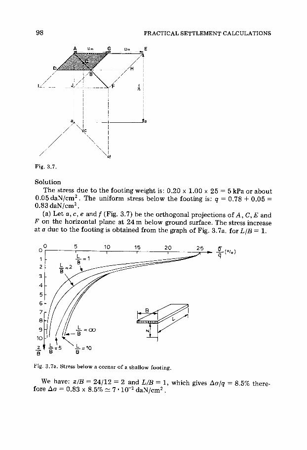
98 PRACTICAL SETTLEMENT CALCULATIONS
Fig. 3.7.
Solut ion The stress due to the foot ing weight is : 0 .20 χ 1.00 χ 2 5 = 5 kPa or about
0 .05 d a N / c m 2. The uniform stress below the foot ing is : q = 0 . 7 8 4- 0 . 0 5 = 0 .83 d a N / c m 2.
(a) L e t a , c , e and f (Fig . 3.7) be the orthogonal project ions of A , C , Ε and F on the horizontal plane at 2 4 m below ground surface. The stress increase at a due to the foot ing is obta ined f rom the graph of Fig . 3 .7a. for L/B= 1 .
Fig. 3.7a. Stress below a corner of a shallow footing.
We have: z/B = 2 4 / 1 2 = 2 and L/B = 1 , which gives Áσ/q = 8 .5% there-fore Δ σ = 0 .83 χ 8 .5% ~ 7 · 1 0 " 2 d a N / c m 2 .
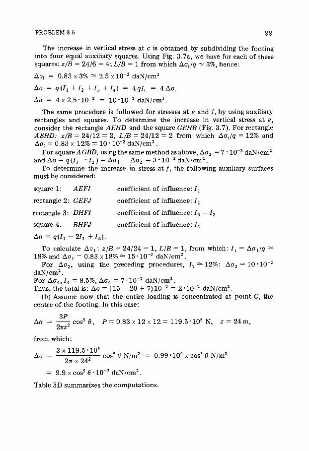
PROBLEM 3.5 9 9
The increase in vertical stress at c is obta ined by subdividing the foot ing into four equal auxil iary squares . Using Fig . 3 .7a , we have for each of these squares : z/B = 2 4 / 6 = 4 ; LIB = 1 f rom which Aojq ~ 3%, hence :
Áσ { = 0 .83 χ 3% ^ 2 .5 χ 1 0 " 2 d a N / c m 2
Δ σ = q(Ix +I2 + J 3 + J 4 ) = Aqlx = AAo{
Áσ = 4 χ 2 . 5 · 1 0 " 2 = 1 0 · 1 0 " 2 d a N / c m 2.
The same procedure is fo l lowed for stresses at e and f, by using auxiliary rectangles and squares . T o determine the increase in vertical stress a t e , consider the rectangle AEHD and the square GEHB (Fig . 3 .7 ) . F o r rectangle AEHD: z/B = 2 4 / 1 2 = 2 , LIB = 2 4 / 1 2 = 2 f rom which Aajq = 1 2 % and Áσ { = 0 .83 χ 12% = 10 · 1 0 " 2 d a N / c m 2 .
F o r square AGBD, using the same m e t h o d as above , Δ σ 2 = 7 · 1 0 " 2 d a N / c m 2
and Áσ = q(Ix —12 ) = Áσ ë — Áσ 2 = 3 · 1 0 " 2 d a N / c m 2 . T o determine the increase in stress at f, the following auxiliary surfaces
must be considered:
square 1 : AEFI coefficient of influence: Ix
rectangle 2 : GEFJ coeff icient of influence: I2
rectangle 3 : DHFI coeff icient of inf luence: J 3 = I2
square 4 : BHFJ coeff icient of inf luence: I4
Ao = q(I1-2I2 +/4).
T o calculate Áσ ë: z/B = 2 4 / 2 4 = 1 , L/B = 1 , f rom which: Ix = Aojq ^ 18% and Aox = 0 .83 χ 18% ~ 1 5 Ί Ο " 2 d a N / c m 2 .
F o r Δ σ 2 , using the preceding procedures , I2 — 1 2 % : Δ σ 2 = 1 0 · 1 0 ~ 2
d a N / c m 2. F o r Δ σ 4 , / 4 = 8 .5%, Δ σ 4 = 7 - 1 0 ' 2 d a N / c m 2. Thus , the total is : Δ σ = ( 1 5 - 2 0 + 7 ) 1 0 " 2 = 2 - 1 0 " 2 d a N / c m 2.
(b) A s s u m e now that the entire loading is concentrated at po int C , the centre of the foot ing. In this ca se :
3 P Δ σ = r c o s 5 θ , Ρ = 0 .83 χ 12 χ 12 = 1 1 9 . 5 · 1 0 5 Ν, æ = 24 m,
2ðæ2
f rom which:
3 χ 1 1 9 5 · 1 0 s
Δ σ = — : — c o s 5 θ N / m 2 = 0 .99 Ί Ο 4 χ c o s 5 θ N / m 2
2π χ 2 4 2
= 9 .9 χ c o s 5 θ · Ι Ο " 2 d a N / c m 2.
Table 3 D summarizes the computa t ions .

1 0 0 PRACTICAL SETTLEMENT CALCULATIONS
TABLE 3D
Point r cos θ = z/r c o s 5 (9 Δ σ ( 1 0 2 d a N / c m 2)
A 25.46 0 .943 0.745 7.4 C 24 1 1 9.9 Ε 30.6 0.784 0.296 2.9 F 35 0.686 0 .152 1.5
Summary of answers
TABLE 3E
Vertical stress increase (in 10" ~2 d a N / c m 2)
Points Surface loads Concentrated load
A 7.0 7.4 C 10.0 9.9 Ε 3.0 2.9 F 2.0 1.5
It is clear that the differences are small. This is due mainly to the fact that the depth at which the stresses are calculated is twice the width of the foot-ing. Had the depth been smaller, the differences would be more significant.
irk Problem 3.6 Set t lement under a point load in a clay layer
A load of 3200 kN bears upon a thick sand layer (assumed incompressible) in which there is a compressible clay layer at a depth of 8 m from the surface (see Fig. 3.8). This clay layer is 4.80 m thick. The oedometric modulus of
Fig. 3.8.

PROBLEM 3.6 1 0 1
the clay is estimated to be 23 daN/cm2 in the upper half of the clay layer and 29 daN/cm2 in the lower half. Determine the vertical settlements of the load assumed to be concentrated at one point.
Solut ion Assume that the load of 3 2 0 0 kN is t ransmitted to the foundat ion soil
through an isolated foot ing at the surface of the soil mass . T h e stress distri-but ion in the soil may then be compared to that of a point load at Ρ acting on a semi-infinite elastic and h o m o g e n o u s mass .
Under these condit ions , at depth æ (F ig . 3 .9) on a vertical f rom P , the vertical stress on the horizontal plane is determined by Bouss inesq ' s formula : σ = (3Ρ/2ðæ 2) c o s 5 θ in which: 0 = 0, therefore : ï = 3 Ρ / 2 π ζ 2 .
T o determine the sett lement , the clay layer may be divided into two sub-layers of equal thicknesses. A t mid-height of the upper clay layer, σ is :
3 χ 3 2 0 0 (σ) , = = 1 8 . 1 kPa, or 0 .18 d a N / c m 2 . 1 11 2 π χ ( 8 + 1 . 2 0 ) 2
A t mid-height of the lower clay layer, σ is :
= 3 x 3 2 00 = H . 4 k P a , or 0 . 1 1 d a N / c m 2 . n 2 π χ ( 8 + 3 . 6 0 ) 2
L e t 2 h be the thickness of the clay layer, then the set t lement directly under point Ρ will b e :
h , v 2h
E[ I E2 E[ E'2
or: 0 .18 χ 2 4 0 0 . 1 1 χ 2 4 0
s = + = 2 .79 cm ~ 2 .8 c m . 23 29
Remarks (1 ) T h e Bouss inesq formula corresponds to a concentrat ion factor of ç = 3.
Frohlich's formula , with a concentrat ion factor of ç = 4, gives:
σ = 4 Ρ / 2 π ζ 2 , or: ( σ ) 1 £ = | ( σ ) 1 , (σ)2ß = f ( σ ) 2
and
s f = § χ s = 3.7 cm.
(2) In order to evaluate the accuracy of the hypothes i s ( load a s sumed to be concentrated at one po in t ) , it is necessary t o a s sume certain values as shown below. Let γ = 17 k N / m 3 and ö = 3 0 ° be the propert ies of the sand. If the

1 0 2 PRACTICAL SETTLEMENT CALCULATIONS
Fig. 3.9.
foot ing is square , and its side is B , the bearing capacity will b e :
Β Β Qd = 0 . 8 γ - Ν Ύ + γΖλ/Vq + 1 . 2 d V c = 0.8 7 — N 7 , b e c a u s e ! ) = 0 a n d c = 0.
2 2
Therefore, Ρ = qdB2/3 with a safety factor o f 3 or: 9 6 0 0 = 0.4 ÷ 17 ÷ 2 1 . 8 ÷ jB 3 , since Ny = 2 1 . 8 for ö = 3 0 ° , from which B ~ 4 m , and g a d ~ 2 d a N / c m 2 .
A t mid-height of the upper clay layer, σ will b e , f rom Fig. 3 .7a :
6 .5 I æ 9 .20 ( σ ) ! - <?ad = 0 .13 d a N / c m 2 - = = 2.3 1 1 0 0 ad \B 4 . 00
At mid-height of the lower clay layer :
5 „ (z 1 1 . 6 0 (ah— ^ad = 0 .10 d a N / c m 2 — = = 2.9
1 0 0 ad \B 4 . 00
The total sett lement will be :
0 .13 ÷ 2 4 0 0 .10 ÷ 2 4 0
= + 23 29
2 . 1 8 cm ~ 2 .2 c m .
In this particular instance, the sett lement is overest imated if the load is a s sumed to be concentrated rather than acting as a footing. The overest imate is As/s = ( 2 .8 - 2 .2 ) /2 .2 ^ 27%.
Since the sett lement is overest imated, it is on the safe s ide.
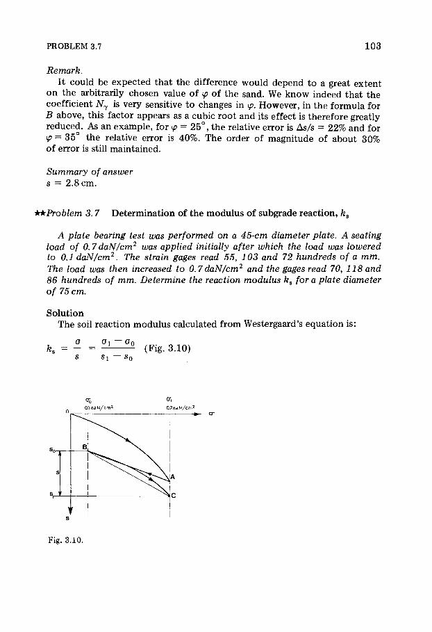
PROBLEM 3.7 1 0 3
Remark.
It could be expec ted that the difference would depend to a great extent on the arbitrarily chosen value of ö o f the sand. We know indeed that the coefficient Ny is very sensitive to changes in ö. However, in the formula for Β above , this factor appears as a cubic roo t and its effect is therefore greatly reduced. As an example , for ö = 2 5 ° , the relative error is As/s = 2 2 % and for ö = 3 5 ° the relative error is 40%. The order of magnitude of about 30% of error is still maintained.
Summary of answer s = 2.8 cm.
irk Problem 3.7 Determinat ion of the m o d u l u s of subgrade react ion, fes
A plate bearing test was performed on a 45-cm diameter plate. A seating load of 0.7 daN/cm2 was applied initially after which the load was lowered to 0.1 daN/cm2. The strain gages read 55, 103 and 72 hundreds of a mm. The load was then increased to 0.7daN/cm2 and the gages read 70, 118 and 86 hundreds of mm. Determine the reaction modulus ks for a plate diameter of 75 cm.
So lut ion The soil reaction modu lus calculated f rom Westergaard's equat ion is :
Fig. 3 .10.

1 0 4 PRACTICAL SETTLEMENT CALCULATIONS
ks is inversely proport ional to the radius R of the plate . F o r the 75-cm radius p late , and expressing σ in d a N / c m 2 , we get :
0.6 4 5 0 .36 tfs(075) - Ã 7 ( -
in which s x and s 0 are in cm and ks in d a N / c m 3. After the first loading cycle , the average o f three gage readings is :
55 + 1 0 3 + 7 2 (so)av = = 76 .7 hundreds of m m .
3 After the second load increment, this average is:
7 0 + 118 + 86 (si)av = ~ 91 .3 hundreds of m m .
3 The permanent sett lement is therefore : 91 .3 — 76 .7 = 14 .6 hundreds of
m m and the modulus is :
0 .36 feS(075) = = 24 .6 d a N / c m 3, say 2 4 d a N / c m 2.
— ÷ 1 0 " 1
100 Answer ks = 24 d a N / c m 2 .
*Problem 3.8 T ime of consol idat ion of a clay layer with double drainage
An 8 m thick clay layer, which has two drainage boundaries is being consolidated. The coefficient of permeability of the clay is 3 ' 10~9 cm/s. Its oedometric modulus is 400 daN/cm2. What is the time required to achieve a degree of consolidation of 40%, and of 80%?
So lut ion F r o m the Terzaghi and Frohlich theories , the degree of consol idat ion is
dependent on the t ime factor T v :
T v = (cv/h2)t.
TABLE 3F: U(TV)
T v U T v U T v U
0.02 0.160 0.3 0 .613 0.8 0.887 0.06 0 .276 0.4 0.697 0.9 0 .912 0.10 0.356 0.5 0 .764 1 0 .931 0.15 0.437 0.6 0 .816 2 0 .994 0 .20 0 .504 0.7 0 .856 00 1.000

PROBLEM 3.9 1 0 5
u 10% 20% 30% 40% 60%
0.008 0 .031 0 .071 0.127 0.289
The functions U = f(Tv) and T v = ö(û) are given in Tables 3 F and 3 G . F r o m these tables we get T v = 0 . 1 2 7 for U = 4 0 % , bu t Tab le 3G does not show a value for U = 80%. We only know that T v for 8 0 % consol idat ion is between 0.5 and 0.6. T h e approx imate relationship of Brinch Hansen gives:
V * u - é m l U6 0· 8 6
- — — from which: = = = - = 0 . 1 7 8 Τ 3 + 0 .5 v 2 ( 1 - U 6 ) 2 ( l - 0 . 8 6 ) '
and T v ^ 0 .56 .
h2 kE' h2y Therefore : i 4 0% = 0 . 1 2 7 — and because c v = , i 4 0% = 0 .127 — —
Cy T w kE
h2y B y the same token , tso% = 0 .56 w
kE'
Numerical application:
h = half thickness of clay layer (open layer) = 4 m k = 3 χ 1 0 " 9 c m / s = 3 χ 1 0 " 1 1 m/s E' = 4 χ 1 0 2 d a N / c m 2 = 4 χ 1 0 7 Pa 7 W = 9 .81 x l O 3 N / m 3
0 . 1 2 7 χ 16 χ 9 .81 x l O 3
i 4 0% = ~ = 0 . 1 2 7 χ 1 3 . 0 8 x l O 7 sec 4 0% 3 x l 0 _ 1 1x 4 x l O 7
1 3 . 0 8 ^40% = 0 . 1 2 7 χ χ 1 0 2 days = 1 9 2 days = 6 months and 1 1 days
0 . 8 6 4
1 3 . 0 8 ^80% - 0 .56 χ χ 1 0 2 days = 8 4 8 days = 2 years , 3 months , 27 days .
0 . 8 6 4
Summary of answers
6 months , 1 1 days ; 2 years , 3 months , 27 days .
*Problem 3.9 Coeff icient of permeabi l i ty The void ratio of clay A decreases from 0.581 to 0.512 when the applied
stress is changed from 1.1 to 1.7daN/cm2. That of clay Β decreases from
TABLE 3G: TV(U)

106 PRACTICAL SETTLEMENT CALCULATIONS
0.609 to 0.596 under the same load transfer. The thickness of sample A is 50% greater than that of B. Nevertheless, sample Β requires 3 times the amount of time needed for A to reach 50% consolidation under identical boundary drainage conditions. What is the ratio of coefficients of permea-bility of the two clays?
Solut ion F r o m Terzaghi and Frohlich's theory , the coefficient of consol idat ion of a
clay is :
c v = kE'/yw (1 )
the t ime factor is:
T v = (cJH2)t. (2 )
For a given degree of consol idat ion, the t ime factor is the s ame for both samples , therefore :
7 71 ^50 A = 7 77 ^50 Β ^ B
27
4
or:
( \ 2 2
^VA fe A Ε A
F r o m eqn. ( 1 ) , we have: = — c v B kBEB
The oedometr ic modu lus is a function of void ra t io :
Δ σ Ae , Δ σ ( 1 + β ) —- = or Ε = . Ε' 1+e Ae
For a given stress increase, Δ σ , of 1.1 to 1.7 d a N / c m 2 we have :
J?b _ Δ β Α ( 1 + β Β ) _ 0 . 0 6 9 χ 1 .609
EA ~ AeB(l+eA) " 0 . 0 1 3 x 1 . 5 8 1 " 5' 4
kA cVA e b 27 f rom which: — = — χ — = — χ 5.4 = 36 .4 or kA/kB = 3 6 .
fee c V R EA 4
Remark
The given of U = 50% is redundant . Sample Β t akes 3 t imes as much t ime to consol idate than A regardless the value of U.

PROBLEM 3.10 1 0 7
if Problem 3.10 T ime o f consol idat ion
An oedometer test is performed on a 2-cm thick clay sample. After 5 minutes, 50% of consolidation is reached. After how long a time would the same degree of consolidation be achieved in the field where the clay layer is 3.70 m thick?
Assume the sample and the clay layer have the same drainage boundary conditions.
Solut ion The t ime factor function is: T v = c v · t/h 2 where c v = kE'/yw . For double drainage condi t ions , h represents half the thickness of the
layer (drainage path length) . In single drainage condit ion, h would represent the total clay layer thickness , (see Fig . 3 . 1 1 ) . L e t h' be the length corre-sponding to the field condit ion and t' the t ime required for the layer to reach U degree of consol idat ion. Since the clay and drainage condit ions are the same as those of the laboratory test , the t ime factor for bo th is the s ame as is the coefficient of consol idat ion c v . Therefore :
Cyt SO t =
Fig. 3 .11 .
Numerical application t = 5 minutes = 5 ÷ 6 0 seconds , h' = 3 7 0 c m , h = 2 cm
/ 3 7 0 \ 2 / 1 1 day = 8 6 , 4 0 0 seconds and t = 5 ÷ 6 0 ÷ ÷
J \ 2 / \ 8 6 4 0 0
t = 1 1 8 . 8 , say 1 1 9 days or 4 months .
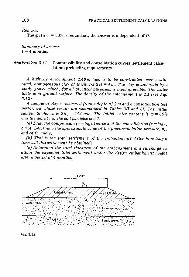
1 0 8 PRACTICAL SETTLEMENT CALCULATIONS
Remark: The given U = 50% is redundant , the answer is independent of U.
Summary of answer t = 4 months .
+*+Problem 3.11 Compressibi l i ty and consol idat ion curves; set t lement calcu-lat ion; preloading requirements
A highway embankment 2.40 m high is to be constructed over a satu-rated, homogeneous clay of thickness 2H — 4 m. The clay is underlain by a sandy gravel which, for all practical purposes, is incompressible. The water table is at ground surface. The density of the embankment is 2.1 (see Fig. 3.12).
A sample of clay is recovered from a depth of 2 m and a consolidation test performed whose results are summarized in Tables 3H and 31. The initial sample thickness is 2h0 = 24.0 mm. The initial water content is w = 69% and the density of the soil particles is 2.7.
(a) Draw the compression (e — log a) curve and the consolidation (e — logt) curve. Determine the approximate value of the preconsolidation pressure, oc, and of Cc and c v.
(b) What is the total settlement of the embankment? After how long a time will this settlement be obtained?
(c) Determine the total thickness of the embankment and surcharge to attain the expected total settlement under the design embankment height after a period of 4 months.
L>20m.
Fig. 3 .12.

PROBLEM 3.11 1 0 9
TABLE 3H: Consolidation TABLE 31: Compression (each load is maintained for 2 4 h ) (from 0.4 to 0.8 d a N / c m 2)
Stress Void Time Void ( d a N / c m 2) ratio (min) ratio
0.05 1.82 0.1 1.700 0.2 1.690
0.1 1.81 0.3 1.683 0.5 1.675
0.2 1.80 1 1.650 2.5 1.600
0.4 1.74 5 1.550 10 1.504
0.8 1.40 20 1.451 50 1.432
1.6 0.80 100 1.421 200 1.418
3.2 0.16 500 1.409 1400 1.400
Solut ion (a) Tables 3 H and 31 provide the data to construct the curves. The com-
pression curve is shown on Fig . 3 .13 . The initial void ratio for a saturated soil is : e0 = w(yjy w) or e0 = 0 . 69 χ 2.7 = 1.86.
Table 31 gives the data needed to p lot the compress ion curve as a function of t ime (e — l o g i ) for a constant stress of 0 . 8 d a N / c m 2 , after the sample has consol idated under the stress of 0 .4 d a N / c m 2. This curve is p lot ted on Fig. 3 .14 .
The preconsol idat ion stress is the m a x i m u m effective overburden stress to which the clay was ever submit ted . It can be evaluated from the con-struction shown on the curve of Fig. 3 . 1 3 ; it is ofc ~ 0 .50 d a N / c m 2 . The compress ion index, C c , is the s lope of the straight line BC in Fig. 3 .13 and corresponds (after Casagrande's construct ion) t o :
-Ae
Cc = 7
A l o g a We have :
o[ = 0 . 8 0 d a N / c m 2, ex = 1 .40, o2 = 3 . 2 0 d a N / c m 2, e2 = 0 . 1 6 .
Ae = 0 .16 - 1 . 4 0 = ~ 1 . 2 4 ,
Δ log σ' = log d2 — log o\ = log 0jj
from which: C c = - ( — 1 . 2 4 / 0 . 6 0 2 )
é 3· 2 1 Ë
l o g — = log 4
2 .06 , C c = 2 . 1 .

110 PRACTICAL SETTLEMENT CALCULATIONS
0.01 0.02 0.05 0.1 0.2
Fig. 3 .13.
Stres s ( d a N / c m 2) ( log scale)
Consolidation coefficient
The coefficient of consol idat ion, c v , is determined by the following method :
(1) Determination of the void ratio at 100% consol idat ion. The inter-section of the two tangents determines e100 corresponding to the end of the primary consol idat ion (Fig . 3 . 14 ) .
(2) Determination of the initial void ratio eQ. The following procedure is used (see Fig. 3 . 1 5 ) : Choose a t ime near the origin, in the example tl = 0.1 min, and another t ime 4 t imes longer so that t2 = 4tl9 = 0 .4 min (in the example ) .

PROBLEM 3.11 1 1 1
The consol idat ion curve is drawn on a t-e graph of arithmetic scale for the time axis . We have then: ex = 1 .700 for t = tx (direct reading) , e2 = 1 .678 for t = t2
( interpolated reading) . By approx imat ing the curve to a parabola with a horizontal axis near
the origin and from the geometric propert ies of a parabola , the following relationships exis t : e0c — ex — ex — e2 f rom which e0c = 1 . 7 2 1 .
Fig. 3 .14 gives: exoo = 1 .430, txoo ~ 3 2 . 5 min from which:
e0c + eioo 1-721 + 1 .430 _ ~ o 7 m in eso = = - 1 .576 , i 5 0 — 3.7 min.
The height of the sample at the start of consol idat ion under the 0.8 d a N / c m 2
load is 2h and we have:
2h 2hn
1 + e0c 1 + e0
f rom which:
1 + e0c 2 . 7 2 1 h = h0 = 1 2 . 0 ÷ = 11 .4 m m .
1 +e0 2 . 8 6 0
The coefficient of consol idat ion c v i s : 0 .197 h2/t 50,
s o : c v = 0 .197 ÷ ( 1 . 1 4 ) 2/ ( 3 . 7 ÷ 6 0 ) - 1 . 1 5 ÷ 1 0 " 3 c m 2 / s .
Total settlement of embankment Because the thickness of the compress ib le clay layer is rather small com-
pared to the width of the embankment (for highways, this width is se ldom less than 2 5 m ) , it m a y be a s sumed that the stress distribution in the clay due to the load imposed by the e m b a n k m e n t is uniform (Fig . 3 . 1 6 ) . We thus have: Δ σ ' = 2 .40 χ 2 1 = 5 0 k P a « 0 . 5 0 d a N / c m 2.
The vertical, initial stress at point M, at mid-height in the clay layer is : σό = Ç X Tclay ·
T o find 7 c i a y> we proceed as fo l lows:
ι Ts Tw Ts τ = ÷ T d , Td = 77— ·
Ts l + ^ o
Earlier it was found that e0 = 1 . 8 6 , therefore y'/y w — (ys — 7 W) / ( 1 + eo) =
(2 .70 - 1 . 0 0 ) / 2 . 8 6 = 0 . 5 9 4 and σ'0 = 2 . 0 0 ÷ 5 .94 = 1 1 . 9 k P a # 0 . 1 2 d a N / c m 2. We found, in the previous sect ion, that the preconsol idat ion pressure is

112 P
RA
CT
ICA
L SE
TT
LE
ME
NT
CA
LC
UL
AT
ION
S Fig. 3.15.

PROBLEM 3.11 113
Fig. 3.16.
o'c = 0 . 5 0 d a N / c m 2 . The existing effective vertical stress at the mid-height of the clay layer is less than the preconsol idat ion pressure: the clay is over-consol idated.
After construct ion of the e m b a n k m e n t , the effective vertical stress at the mid-height of the layer will be (see Fig. 3 . 1 7 ) : σό + Δ σ ' = 0 .12 4- 0 .50 = 0 .62 d a N / c m 2 which leads t o : σό + Δ σ ' > a'c.
F r o m the compress ion curve of Fig. 3 .13 , we have for : σό = 0 .12 d a N / c m 2 , e = 1.80 and : σό = 0 .62 d a N / c m 2 , e = 1.56 and f rom: Ah/h = Ae/(1 4- e) we get :
1 . 8 0 - 1 . 5 6 Ah = 4 0 0 ÷ = 34 .3 cm, say 34 cm.
2 .80
It would be necessary, in this case , to check the stability of the embank-ment for foundat ion failure. The stability is satisfactory if in this case , c u = 4 0 kPa.
Thickness of embankment surcharge to reach the total settlement in 4 months
What would be the t ime required for the clay layer to consol idate 34 c m ?
Fig. 3.17.

114 PRACTICAL SETTLEMENT CALCULATIONS
Theoretically, this t ime is infinite, but in pract ice , it is considered that 1 0 0 percent of the sett lement is obta ined when T v = 2 , which corresponds to U = 99 .4%.
Since T v = (cv/h2)t and since the drainage of the clay layer is in both direct ions: h = H/2
2 χ ( 2 0 0 ) 2
hence: t = ———rrr^ 1.15 χ 10 0
8 . 1 and : t = χ Ι Ο 7 χ - = 8 0 5 days
1.15 8 .64 χ 1 0 4
or 2 years , 2 months , 1 5 days . T o decrease the sett lement t ime to 4 months , ( 1 2 0 d a y s ) , the t ime factor
T v must b e :
1.15 χ Ι Ο " 3 χ 1 2 0 χ 8 .64 χ 1 0 4 ΟΛ
Τ = = 0 . 2 9 8 ^ 0 . 3 0 ( 2 0 0 ) 2
The corresponding U value is U = 0 . 6 1 3 (see Table 3 F ) . This means that the sett lement of 34 cm corresponds to 6 1 . 3 % of the sett lement S that would be obta ined under a heavier surcharge, which sett lement would b e : 0 . 3 4 / 0 . 6 1 3 — 0 .55 m.
The following equat ion for S gives the surcharge needed :
Cc (σï + Δ σ ' *
l + e 0 \ oc
σ'ñ + Δ σ ; * 5 5 χ 2 .86 If we let ë: = ; , then: log χ = = 0 .187,
σβ' 4 0 0 x 2 . 1 and χ = 1 .54 , f rom which
Δ σ ' * = 1.54 x 0 . 5 0 - 0 . 1 2 ^ 0 . 6 5 d a N / c m 2
Δ σ ' * = 6 5 k P a ( * ) .
The corresponding embankment height is : Hf = 6 5 / 2 1 = 3 .10 m, and the surcharge needed would b e : AH = 3 .10 — 2 .40 = 0 .70 m.
This example shows that it is poss ible to quickly stabilize an embank-ment , if the t ime needed for preconsol idat ion by surcharge is p rogrammed . A surcharge of 70 cm, left in place for 4 months and then removed would eliminate any significant embankment sett lement thereafter.
*This value could also have been obtained from the e — log σ' graph.

PROBLEM 3.12 1 1 5
Summary of answers (a) see Figs . 3 .13 and 3 . 1 4 : o'c = 0 .5 d a N / c m 2 ; C c = 2 . 1 ; c v = 1.15 χ 1 0 " 3
c m 2/ s ; (b) s = 34 cm after 2 years , 2 months and 15 days ; (c) about 3 1 0 c m .
irk Problem 3.12 Oedometr ic modul i : behavior of an overconsol idated clay
From the givens of problem 3.11: (a) Calculate the oedometric modulus Er of the clay in the section BC of
the compression curve corresponding to the stress increase due to the em-bankment load (Fig. 3.12), at mid-height in the clay layer. Compare the result with the modulus obtained by the approximate formula:
1 +e Ε = 2.3 σ
(b) Find the compression index C'c of the linear portion AB of the com-pression curve corresponding to a stress level less than 0.20 daN/cm2 (Figs. 3.13 and 3.19). Find the corresponding oedometric modulus.
(c) What can be inferred about the clay from this? What are some practical conclusions?
So lut ion (a) F r o m the answer of problem 3 . 1 1 , the initial effective stress at mid-
height in the clay layer is : σ^ = 0 .12 d a N / c m 2. The increase in stress due to the weight of the e m b a n k m e n t is : Δ σ ' = 0 .92 d a N / c m 2. The pre-consolidation stress of the clay was found to be o'c = 0 .5 d a N / c m 2.
In order to calculate E\ the initial point on the compress ion curve, to start f rom, is the pre-consolidation stress σ<!. Therefore :
Δ σ ' = 0 . 9 2 - 0 . 5 0 = 0 .42 d a N / c m 2
' - 1 + e Δ σ '
E ~ C c l o g ( l + (Áσ'Ê))
where e is the void ratio at σ', or e = 1.68 (read on the compress ion curve) , a n d :
1 + 1.68 Ε = x 0 . 4 2 / [ l o g ( l + ( 0 . 4 2 / 0 . 5 0 ) ] = 1.84
2 .1
log 1.84 = 0 . 2 6 5
E'= ( 2 . 6 8 / 2 . 1 ) χ ( 0 . 4 2 / 0 . 2 6 5 ) = 2 . 0 2 d a N / c m 2 ( * ) or : 2 . 0 0 d a N / c m 2.
*E' could also be calculated from the compression curve by writing: AH/H = AE/(1 +E) a n d E ' = Δσ'/(Δή//ι).

116 PRACTICAL SETTLEMENT CALCULATIONS
The approx imate formula gives: E' = 2.3 ÷ 0 .5 ÷ ( 2 . 6 8 / 2 . 1 ) = 1.47 d a N / c m 2. This approximat ion is not very good because Δ σ ' is t o o large in comparison to σ^. The value of Ef = 2 . 0 0 d a N / c m 2 corresponds to that of a soft clay.
(b) The compress ion index Cc is found from the relat ion: C'c = —Ae/ A log σ', where: ex = 1 .82, σί = 0 . 0 5 d a N / c m 2 , log a[ = 2 . 6 9 9 = - 1 . 3 0 1 ; e2 = 1.80, o2 = 0 . 2 0 d a N / c m 2 , log σ2 = 1 .301 = - 0 . 6 9 9 from which:
- ( 1 . 8 0 - 1 . 8 2 ) 0 .02 Co = — = ^ 0 . 0 3 3 .
- 0 . 6 9 9 + 1 .301 0 .602
E'
The oedometr ic modulus is:
- 1 + e Δ σ ' C c 1 ï8(1 + ( Δ σ 7 σ ^ ) ) '
As an example , we can take Δ σ ' = 0 .10 d a N / c m 2 in order to remain on the AB port ion of the curve (Fig . 3 . 18 ) , which corresponds t o stresses less than o2.
a'Q = 0 .10 d a N / c m 2, e0 = 1.81 ( from the given)
2 .81 0 .10 0 .281 Ε = ÷ = = 28 .3 d a N / c m 2.
0 . 0 3 3 log 2 0 . 0 3 3 x 0 . 3 0 1
This value corresponds with that of a stiff c lay. (c) The results show that for small increases in stress Δ σ ' , the clay is stiff
(see Fig. 3 .18 ) .
7 \ c
t . 1>
Fig . 3.18 .
On the other hand for larger stress increases (o'c + Δ σ ' > o'c) the over-consol idated clay initially behaves as a stiff clay (as long as the stress is smaller than o'c), and as a soft clay as soon as the stress level increases beyond the value of o'c.
The clay behavior in consol idat ion therefore depends on the level of stresses. The qualifications ' soft ' or ' s t i f f must be viewed with respect to

PROBLEM 3.13 117
the imposed loads and cannot be based only on visual inspection in an open pit .
ictckProblem 3.13 Consol idat ion with vertical sand drains
Referring once again to the geometry of problem 3.11, it is now desired to decrease the settlement time by accelerating the clay consolidation with vertical sand drains, going through the compressible layer to the underlaying gravel (shown in Fig. 3.19).
Fig. 3.19. Plan view.
The center to center distance between the two adjacent drains is 2 R, the drain diameter, 2r. The drains have equal diameters. Under these conditions, it can be assumed that the clay drainage during the consolidation consists of the superposition of a vertical drainage, characterized by c v z, kv, Uz and T v and of a horizontal, radial drainage characterized by c v r, kh, Ux and Tx
with: T v = (cvJh2)tand T r = [cJ(2R)2] t.
The coefficient of radial consolidation c v r is further defined by the equation: c^/c = kh/kv. Under these conditions the degree of consolidation U is given by: 1 — U =
The degree of radial consolidation Ur, function of Tx and of the geometry of the drains, is presented in Table 3J.
Assuming that we have a condition where kh = 5kv, recommend drain spacing and drain diameter to obtain all settlements in 4 months, taking into account current practice i.e. drain diameters vary from 0.3 to 0.8 m and spacing goes from 2.5 to 7.5 m.
Since kh = 5 f c v, we can determine immediate ly : c v r = 5 χ 1.15 · 10 3 — 5 .75 Ί Ο " 3 c m 2/ s .
F r o m the previous solution of prob lem 3 .11 we know that Uz = 6 1 . 3 % . Since we must realise the set t lement in a period of 4 months , we also know U = 99 .4%.
Therefore :
D ra ß ð
(1 - Uz)(l - Ut).
So lut ion
1 -1 -
1 -
0 . 9 9 4
0 . 6 1 3 ~- 0 . 0 1 6 , then Ut = 1 — 0 .016
0 . 9 8 4 ~ 0.99.·

TABLE 3J
Radial drainage, equal vertical strains (after Leonards)
Degree of consolidation
Time factor Degree of consolidation
u,(%) R - = 5 r
10 15 20 25 30 40 50 60 8 0 100
5 0.006 0.010 0 .013 0 .014 0 .016 0.017 0 .019 0 .020 0 .021 0 .023 0 .025 10 0.012 0.021 0.026 0 .030 0 .032 0 .035 0 .039 0 .042 0 .044 0 .048 0 .051 15 0 .019 0.032 0 .040 0 .046 0 .050 0 .054 0 .060 0 .064 0.068 0 .074 0 .079 20 0.026 0.044 0.055 0 .063 0 .069 0 .074 0 .082 0.088 0 .092 0 .101 0 .107 25 0.034 0.057 0 .071 0 .081 0 .089 0 .096 0 .106 0 .114 0 .120 0 .131 0 .139
30 0 .042 0.070 0.088 0 .101 0 .110 0 .118 0 .131 0 .141 0 .149 0 .162 0 .172 35 0 .050 0.085 0 .106 0 .121 0 .133 0 .143 0.158 0 .170 0 .180 0 .196 0 .208 40 0 .060 0.101 0.125 0 .144 0 .158 0 .170 0.188 0 .202 0 .214 0 .232 0 .246 45 0 .070 0.118 0.147 0 .169 0 .185 0.198 0 .220 0 .236 0 .250 0 .291 0 .288 50 0.081 0.137 0 .170 0 .195 0 .214 0 .230 0 .255 0 .274 0 .290 0 .315 0 .334
55 0.094 0.157 0.197 0 .225 0.247 0 .265 0 .294 0 .316 0 .334 0 .363 0 .385 60 0.107 0.180 0 .226 0.258 0 .283 0 .304 0 .337 0 .362 0 .383 0 .416 0 .441 65 0 .123 0.207 0 .259 0 .296 0 .325 0.348 0 .386 0.415 0 .439 0.477 0 .506 70 0.137 0.231 0 .289 0 .330 0 .362 0 .389 0 .431 0 .463 0 .490 0 .532 0 .564 75 0.162 0 .273 0 .342 0 .391 0 .429 0 .460 0 .510 0.548 0 .579 0 .629 0 .668
8 0 0.188 0.317 0.397 0 .453 0.498 0 .534 0 .592 0.636 0 .673 0 .730 0 .775 85 0.222 0 .373 0.467 0 .534 0 .587 0 .629 0.697 0 .750 0 .793 0 .861 0 .914 90 0.270 0.455 0.567 0 .649 0 .712 0 .764 0.847 0.911 0 .963 1.046 1.110 95 0.351 0.590 0.738 0 .844 0 .926 0 .994 1.102 1.185 1.253 1.360 1.444 99 0 .539 0.907 1.135 1.298 1.423 1.528 1.693 1.821 1.925 2 .091 2 .219
118 P
RA
CT
ICA
L S
ET
TL
EM
EN
T C
AL
CU
LA
TIO
NS
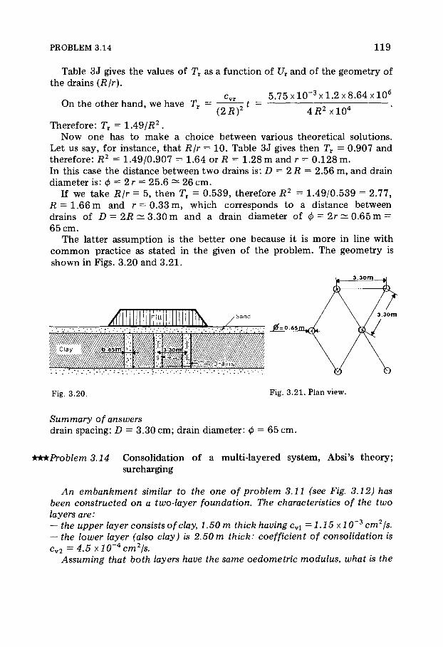
PROBLEM 3.14 1 1 9
Table 3 J gives the values of T r as a function of C/r and of the geometry of the drains (R/r).
c v r 5 .75 χ 1 0 ~ 3 χ 1.2 χ 8 .64 χ 1 0 6
On the other hand, we have Tr = - t = : : . (2R)2 4R2xl04
Therefore : T r = 1 . 4 9 / E 2 . N o w one has to m a k e a choice between various theoretical solut ions .
L e t us say , for instance, that R/r = 1 0 . Table 3 J gives then T r = 0 .907 and therefore : R2 = 1 . 49 /0 .907 = 1.64 or R = 1 .28 m and r = 0 . 1 2 8 m. In this case the distance between t w o drains i s : D = 2 R = 2 .56 m, and drain diameter is : ö = 2 r = 2 5 . 6 — 2 6 c m .
If we take R/r = 5 , then T r = 0 . 5 3 9 , therefore R2 = 1 . 49 /0 .539 = 2 .77 , R = 1.66 m and r = 0 .33 m, which corresponds to a distance between drains of D = 2R — 3 .30 m and a drain diameter of 0 = 2 r ~ 0 .65 m = 6 5 cm.
The latter a s sumpt ion is the better one because it is more in line with c o m m o n practice as s tated in the given of the prob lem. The geometry is shown in Figs . 3 .20 and 3 . 2 1 .
Fig. 3 .20. Fig. 3 .21 . Plan view.
Summary of answers
drain spacing: D = 3 .30 cm; drain d iameter : ö = 6 5 c m .
+**Problem 3.14 Consol idat ion o f a multi-layered sys tem, Abs i ' s theory ; surcharging
An embankment similar to the one of problem 3.11 (see Fig. 3.12) has been constructed on a two-layer foundation. The characteristics of the two layers are: — the upper layer consists of clay, 1.50 m thick having c v l =1.15x10~3 cm2/s. — the lower layer (also clay) is 2.50 m thick: coefficient of consolidation is c v 2 = 4.5 χ 1 0 " 4 cm2/s.
Assuming that both layers have the same oedometric modulus, what is the
120 PRACTICAL SETTLEMENT CALCULATIONS
difference between this condition and that of problem 3.13. Refer to Absi's theory [1].
Solut ion If the oedometr ic modul i and densities are the same, the tota l sett lement
is the same as that of problem 3 . 1 1 , s = 0 .34 m. But because of the two-layer system, the t ime of consol idat ion will be different.
According to the theory of Absi , the two-layer sys tem may be equated to a system of a single layer of thickness H' = 4 . 0 0 m (Ç' = 2h') and with an apparent coefficient of consol idat ion c v a such that :
= H l - H l
, ft, J cv l V Cv 2
( 4 x l 0 2 ) 2 1.6 c v a = ; " : — ÃÃ % x l°
/ 1.50 x l O 2 2 .50 x l O 2 \ 2 1.5 2 .5 + —===— —— + Wl . 1 5 x l O " 3 " ë / 4 . 5 0 x l O " 4 / 3 .39 ' 2 .12
1.6 , , , c v a = χ 1 0 " 3 ^ 0 .99 x l 0 " 3 c m 2 / s .
0 . 4 4 2 + 1 .179
finally: H' = 2h' = 4 . 00 m, c v a ~ 9.9 χ 1 0 " 4 c m 2 /s .
T o decrease the sett lement t ime to 4 months , a larger surcharge than placed in the case of problem 3.11 will have to be considered here, because :
c v a 9.9 x l 0 " 4 x l . 2 x 8 .64 x l O 6 Λ ftr/, Tv = -^t = = 0 .256 ~ 0 .26
ft'2 4 - 1 0 4
T v = 0 .26 which gives, after Terzaghi's approx imat ion ,
£ 7 - 1 .128 V ^ 2 6 = 0 . 5 7 5 .
Therefore : S = Soo ÷ 1 /0 .575 = 0 . 3 4 / 0 . 5 7 5 = 0 .59 m
59 χ 2 .86 l o g x = = 0 . 2 0 1 , from which ÷ = 1 .59;
4 0 0 χ 2.1 Δ σ ' = 0 .50 x 1 . 5 9 - 0 . 1 2 = 0 .68 d a N / c m 2 .
Thus , the total embankment height is : 6 8 / 2 1 = 3 .24 m. A temporary surcharge, left in place for 4 months , of wet density equal
to 7 h = 2 1 k N / m 3 will have a height of 3 .24 - 2 .40 m = 0 .84 m. Note. The theory of Absi is only an approx imat ion . It does no t t ake into
account the continuity across the two-layer faces. A more accurate but also more t ime-consuming solut ion would be the use of the finite-difference method (see problem 3 . 1 9 ) .
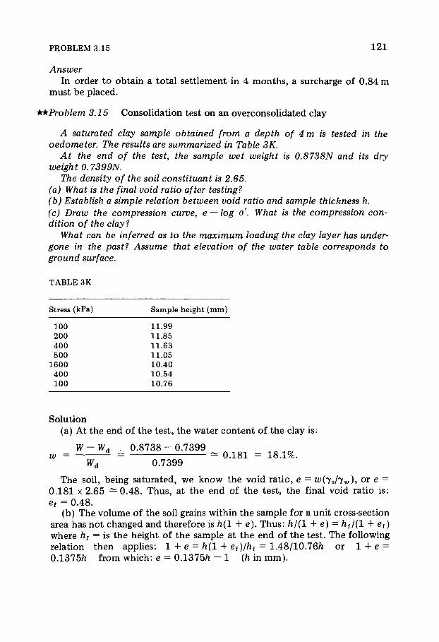
PROBLEM 3.15 1 2 1
Answer In order t o obta in a tota l set t lement in 4 months , a surcharge of 0 .84 m
must be placed.
irk Problem 3.15 Consol idat ion test on an overconsol idated clay
A saturated clay sample obtained from a depth of 4 m is tested in the oedometer. The results are summarized in Table 3K.
At the end of the test, the sample wet weight is 0.8738N and its dry weight 0.7399N.
The density of the soil constituant is 2.65. (a) What is the final void ratio after testing? (b) Establish a simple relation between void ratio and sample thickness h. (c) Draw the compression curve, e — log σ'. What is the compression con-dition of the clay ?
What can be inferred as to the maximum loading the clay layer has under-gone in the past? Assume that elevation of the water table corresponds to ground surface.
TABLE 3K
Stress (kPa) Sample height (mm)
100 11 .99 200 11.85 400 11 .63 800 11.05
1 6 0 0 10 .40 4 0 0 10 .54 100 10 .76
Solut ion (a) At the end of the tes t , the water content of the clay is :
W-W d . 0 . 8 7 3 8 - 0 . 7 3 9 9 w = = ^ 0 . 1 8 1 = 1 8 . 1 % .
W d 0 . 7 3 9 9
The soil , being saturated , we know the void ra t io , e = w(yjy w), or e = 0 . 1 8 1 χ 2 . 6 5 — 0 . 4 8 . Thus , a t the end of the test , the final void rat io is : ef = 0 . 4 8 .
(b) The volume of the soil grains within the sample for a unit cross-section area has not changed and therefore is ft(l + e). T h u s : h/(l + e) = ftf/(l + e f ) where hf = is the height of the sample at the end of the test . The following relation then appl ies : 1 + e = h(l + e f )/ftf = 1 .48/10.76ft or 1 + e = 0.1375ft f rom which: e = 0.1375ft - 1 (ft in m m ) .
122 PRACTICAL SETTLEMENT CALCULATIONS
(c) This relation is the basis for Table 3 L which presents void rat ios as a function of the vertical stress applied to the sample . F r o m the data in that Table , it is possible to draw the compress ion curve (e — log σ ' ) as presented in Fig. 3 .22 . The preconsol idat ion pressure σ 0, est imated from this figure, is about 3 0 0 kPa.
Now, we have to calculate the effective vertical stress to which the soil sample was submit ted in situ.
0.5 5
0-50
0.4 5
0.40
" ^ - ^ 0-6 5 \
\ \
0 . 6 ^ \
\ ° ' >0
J
\ y Loi. 3d<
J
?° 52
J
I
0.4 8
J n l o a d ec 0.4 5
J \o.4 - J
10 lo o 2 0 0 50 0 loo o 2 0 0 0 lo g cr
P r e s s u re ( k P a)
Fig. 3 .22.
TABLE 3L
σ (kPa) e
100 0.65 200 0.63 400 0.60 800 0.52
1600 0.43 400 0.45 100 0.48

PROBLEM 3.16 123
We have : o'0=y'xh with y = 7 s at - yw ; 7 s at = γ β ( 1 + w/1 + e), and e = 2 . 6 5
The in-situ saturated unit weight can be es t imated from 7 s at a t the start of the test , and therefore :
2 .65 + e 2 . 6 5 + 0 . 6 5 7 s at = Ts Q „ n , , = 10 ÷ — = 2 0 k N / m 3
2 . 6 5 ( 1 + e) 1.65 and finally: y = 20 - 10 = 10 k N / m 3 . Then σό = 10 ÷ 4 = 4 0 kPa. This stress is considerably less than oc: the clay is overconsol idated.
S ince the preconsol idat ion pressure corresponds to the highest effective stress ever applied to the clay throughout its geologic history, this weight m a y have been caused by an overburden since then eroded, or a glacier.
Because the actual pressure is σό, the difference, o'c — σό, = 3 0 0 — 4 0 = 2 6 0 kPa is the weight of that pas t overburden. In this case , where soil buoy-ant density y = 10 k N / m 3 and that of ice, yi = 9 .17 k N / m 3 , the stress differ-ence may mean a soil erosion thickness of 2 6 0 / 1 0 = 26 m or a glacier ice thickness of 2 6 0 / 9 . 1 7 = 2 8 m.
irk Problem 3.16 Determinat ion o f C c and m v and the sett lements o f a satu-rated c lay ; degree o f consol idat ion
An undisturbed clay sample of 20 mm thickness is tested in an oedometer and the following results are obtained:
effective stresses applied (kN/m 2): 50, 100, 200
sample thicknesses, h(mm): 20, 19.62, 19.24
The initial water content is 40%, the density of soil grains is 2.7. (a) What is the compression index Cc and the coefficient of volumetric
compressibility rav for each of the stress increments? (b) The sample was recovered from a clay layer 4 m thick located over an
impervious rock base and overlain by a sand layer. The average vertical effective stress in the clay layer is 75 kN/m 2. This stress is ultimately in-creased to 150 kN/m 2 as a consequence of a surface load placed at the ground surface. Calculate the total settlement of the clay layer due to this new condition, using the appropriate Cc value.
(c) In practice, some engineers prefer using mv rather than Cc to calculate the settlements. This is because in reality the e—log σ curve may not be straight. Can you give another reason?
(d) During the consolidation test, 90% of the primary consolidation was obtained after one hour for the stress interval of 100 to 200 kN/m 2. After what time would a degree of 50% consolidation be obtained?
Solut ion (a) F r o m the consol idat ion test it is observed that the 50 k N / m 2 stress did

1 2 4 PRACTICAL SETTLEMENT CALCULATIONS
not result in a significant decrease in sample height. Therefore , one m a y expect that e0 ~ e50.
Since the soil is saturated, e0 = w(yjy w) and e0 = e50 = 0 .40 χ 2.7 = 1 .08. The variation of void ratio Δ β is proport ional to the sample height change Ah. The relation is: Ae/(1 + eQ) = Ah/h 0, f rom which: Ae = [ ( 1 + e)/ h0 ] Ah or Ae = [ 2 . 0 8 / 2 0 ] Ah = 0 . 1 0 4 Δ/ζ, where Ah is in mill imeters.
The compress ion index C c is given b y : C c = — Ae/A log σ'. S ince the load is doubled for each increment, we have : Δ log σ' = l o g ( 1 0 0 / 5 0 ) = l o g ( 2 0 0 / 1 0 0 ) = log 2 = 0 . 3 0 1 0 3 .
Since the sample height change is the same for both load increments , Ah = 1 9 . 6 2 — 20 = 1 9 . 2 4 — 1 9 . 6 2 = — 0 .38 m m . The compress ion index is the same in both cases and is : C c = - ( 0 . 1 0 4 χ 0 . 3 8 ) / 0 . 3 0 1 0 3 = 0 . 1 3 1 .
The coefficient of volumetric compressibi l i ty i s : m v = — ( Δ ή / ή ) / Δ σ . In the first load increment, then: m v = — ( 0 . 3 8 / 2 0 ) / ( 1 0 0 — 50 ) = 3.8 χ 1 0 " 4 m 2/ k N = 3.8 x l O " 2 c m 2/ d a N and in the second : m v = - ( 0 . 3 8 / 1 9 . 6 2 ) / ( 2 0 0 - 1 0 0 ) = 1.9 χ 1 0 ' 4 m 2/ k N = 1.9 χ 1 0 " 2 c m 2/ d a N .
(b) The effective vertical stress is within the range 50—200 k N / m 2 for which we have C c = 0 . 1 3 3 . This value may be used t o calculate the clay layer set t lement .
For σ' = 7 5 k N / m 2, the value of the void rat io is : Ae = Cc l o g [ ( a ' + Áσ)/σ'] therefore : e15 — e50 = — 0 . 1 3 1 log ( 7 5 / 5 0 ) = - 0 . 0 2 3 and e 7 5 = 1.08 — 0 .023 = 1 .057.
F o r the increase in stress f rom 7 5 t o 1 5 0 k N / m 2 , we have :
Ae = elS0 -els = — 0 . 1 3 1 log ( 1 5 0 / 7 5 ) = - 0 . 0 3 9 4 and
Ah/h = Ae/(1 + e15) = - 0 . 0 3 9 4 / ( 1 + 1 .057) .
The sett lement due to the consol idat ion of the 4-m thick layer will b e : Ah = ( 0 . 0 3 9 4 χ 4 χ 1 0 3) / 2 . 0 5 2 = 7 6 . 7 , or 77 m m .
(c) If the sett lement is ca lcuated f rom rav, it is not necessary to calculate the void rat io .
(d) F r o m the Terzaghi and Frohlich theories , we have : T v = (cv/h2)t. The functions U = f(Ty) and Tv = ö(û) are given in Tables 3 F and 3 G [ 8 ] .
During the laboratory consol idat ion test , the sample is drained both a t the upper and lower faces . The height to consider is that corresponding to the shortest drainage path , or half the sample height. Therefore h l = 1 0 m m .
A degree of consol idat ion U1 = 9 0 % , gives by interpolation (see Table 3 F ) a t ime factor T v l ~ 0 . 8 5 :
Tvi = Μ ι / δ ι = 0 . 8 5 . (1 )
However, the clay layer in situ is only drained through the t o p surface , the drainage path therefore corresponds to the clay layer thickness and h2 = 4 m. For a degree of consol idat ion of 50%, the same source [ 8 ] gives a t ime factor T v 2 = 0 .20 and therefore :
T v 2 = cvt2/h22 = 0 .20 . (2 )
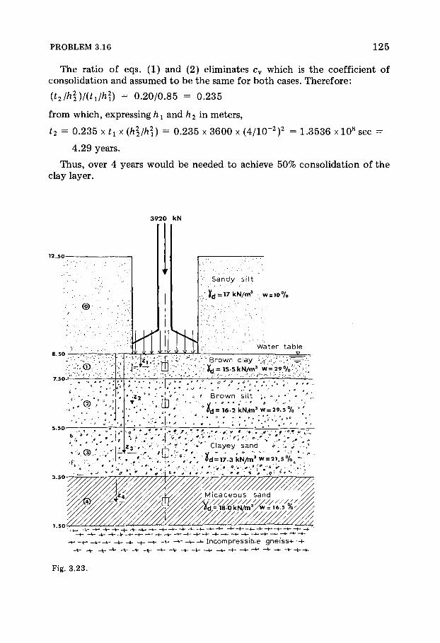
PROBLEM 3.16 1 2 5
The rat io of eqs . (1 ) and (2) el iminates c v which is the coefficient of consol idat ion and a s sumed t o b e the same for bo th cases . There fore :
(t2lh\)l{tllh\) = 0 . 2 0 / 0 . 8 5 = 0 . 2 3 5
from which, express ing h x and h2 in meters ,
t2 = 0 . 2 3 5 χ tx χ (hl/h\) = 0 . 2 3 5 χ 3 6 0 0 χ ( 4 / 1 0 " 2 ) 2 = 1 .3536 χ 1 0 8 sec =
4 . 2 9 years .
Thus , over 4 years would be needed to achieve 50% consol idat ion of the clay layer.
3920 kN
•
I
I
i í / \'
•
I
I
i ' \' \f \C
•·". Sandy silt
!fd = 17 kN/m 3 w = io%
; . . ; ' Water table
':: ' ; :rri * * ' B r o wn c l ay '-'ß-'· •··"
v.^ , -•^•lQ O'V v" J f d =1 5 ,5 k N/ " ?3v w = 2 9 > í :· ; .'
- " - * . ; Ú ' - " '
; / ® v ··;,; '• z 2 * ' J- ' B r o w n silt ;.-.·*'
r— Ë [Π -"•·"··' . y - * · · . ' · ' < - * _ V \ . Τ Γ ' •· d d = 16-2 kN/tn 3w = 29.5%
·';,-·-··'.':
«
*,
*r *. 4 ν · - yV . / :' - <•-''<'-• <•-'<·•.-1-.*-.-
z 3-,'·•>'.'· ì:Ë * ' * ·' Clayey sand c ./
• :- · / ' · . , . ! ; ° ; , V i d = 17.3kN/An3 w = 2i . 5 % f t- ;
mm. *4////////rW^ M icaceous sand / / / .
v/////////^ =16·5 /o////
—^ -i 1- - v - Incompressible gneiss-*- —v-
-V- -± V -t - -ë V- -» l ^_ t - - 4 ì - Ç - ^ - ^ - ^ - é
Fig. 3 .23 .

126 PRACTICAL SETTLEMENT CALCULATIONS
**•Problem 3.17 Set t lemen t o f shal low foot ing s
During the preliminary foundation studies for a proposed steel mill plant, it was found necessary to determine the settlement of a typical column of the laminating plant expected to be loaded up to 3920 kN. From the soil investi-gation, it is known that sound, gneiss bedrock is at an average depth of 11 m. The alluvial soil profile above the rock consists of, from the surface to the gneiss: sandy silt, clay, silt, clayey and micaceous sand layers.
10 20 30 40 SO 100 200 300 400 500
g . ________ _
ã _____________^
__ù_
-®_
0
1 Vertica l stres s (kPa) 5 10 20 30 40 50 100 200 300 400 500
( l o g s c a l e ) Fig. 3 .24.

PROBLEM 3.17 1 2 7
The average ground surface elevation is +12.5 m. The bottom of a square footing, 4 by 4 m in plan dimension, is proposed at an elevation of 8.50 m. The cross-section and the properties of the soil layers are shown on Fig. 3.23. The ground water table is at the footing level. Four soil layers have been identified which are: Dx = 1.00m, Zx = 0.50m; D2 = 2.00m, Z2 = 2.00m; D3 = 2.00m, Z3 = 4.00m;Dt = 2.00m, Z 4 = 6.00m.
Four samples were recovered from depths Zx, Z2, Z 3 and Z 4 and were tested by means of a consolidometer and a triaxial settlement test.
(1) From the compression curves of the four samples (see Fig. 3.24) define the state of consolidation of the various layers.
(2) To what laboratory load stresses should the samples be reconsoli-dated before being tested in the triaxial load frame?
(3) Determine the stress increase caused by the column at elevation +8.50, assumed that the footing is flexible. Then, determine the additional stress increases Áσ ÷, and Áσ 3, which will have to be applied in the triaxial test, to reproduce the in situ condition, when the column load is applied. Assume í = 0.25.
(4) With the triaxial test under additional stress tensor (Fig. 3.25) curves giving settlement as a function of load stress were obtained. Determine the total settlement of the column. What can be said about the fact that the footing is well below ground surface? According to the shape of the curves in Fig 3.25 compute the instantaneous (at 10 sec), primary and secondary settlements. Express each settlement as a percentage of the total settle-ment.
(5) Determine the settlement of the column from the oedometer test results. Do not apply Skempton's correction.
Now go through Skempton's correction for the settlement calculated by the oedometric method. What are the conclusions? Tlme (, scale)
10" 30" Ã 2' 5' 10' 30' lh 8h 24h 48h
®
Initial height h = 80 mm
Fig. 3 .25.
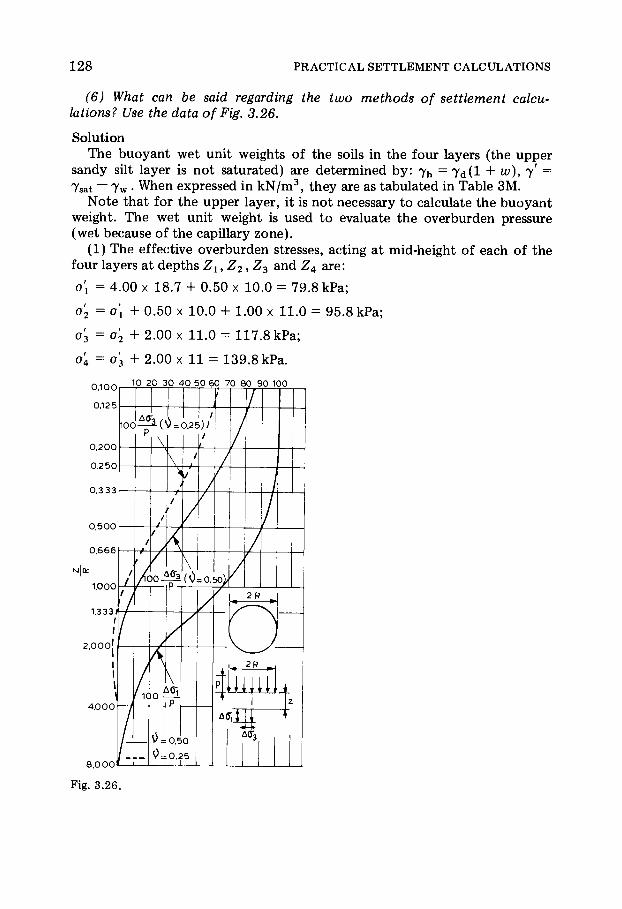
1 2 8 PRACTICAL SETTLEMENT CALCULATIONS
(6) What can be said regarding the two methods of settlement calcu-lations? Use the data of Fig. 3.26.
Solut ion The buoyant wet unit weights of the soils in the four layers (the upper
sandy silt layer is no t saturated) are determined b y : 7 h = γ ά ( 1 + w), γ ' = Tsat ~~ Tw · When expressed in k N / m 3 , they are as tabula ted in Table 3M.
N o t e that for the upper layer, it is not necessary to calculate the b u o y a n t weight. The wet unit weight is used to evaluate the overburden pressure (wet because of the capillary z o n e ) .
(1 ) The effective overburden stresses, act ing a t mid-height of each o f the four layers at depths Z1, Z2, Z 3 and Z 4 a re :
o\ = 4 . 0 0 χ 18 .7 + 0 .50 χ 10 .0 = 79 .8 kPa;
o2 = o\ + 0 .50 χ 10 .0 + 1.00 χ 11 .0 = 9 5 . 8 kPa;
σ'3 = σ'2 + 2 .00 χ 11 .0 = 1 1 7 . 8 kPa ;
o\ = σ'3 4- 2 .00 χ 11 = 1 3 9 . 8 kPa.
Fig. 3 .26.
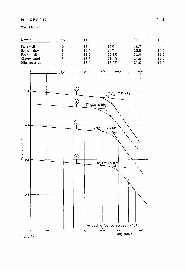
PROBLEM 3.17
TABLE 3M
1 2 9
Layers No. 7d w 7h 1
Ί
Sandy silt 0 17 10% 18.7 —
Brown clay 1 15.5 29% 20.0 10.0 Brown silt 2 16,2 29.5% 21.0 11.0 Clayey sand 3 17 .3 21.5% 21.0 11.0 Micaceous sand 4 18 .0 16.5% 21 .0 11.0
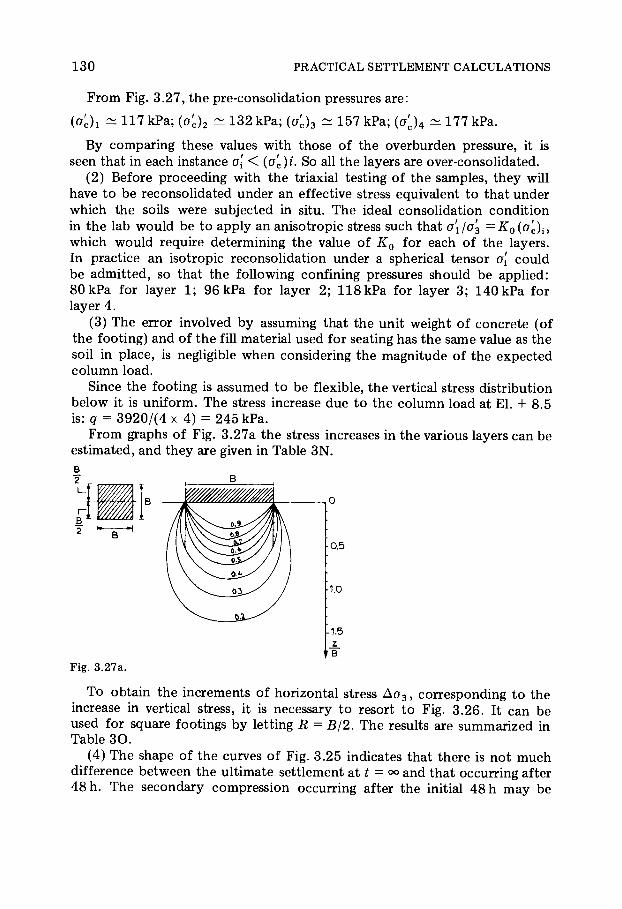
1 3 0 PRACTICAL SETTLEMENT CALCULATIONS
F r o m Fig. 3 .27 , the pre-consolidation pressures a re :
(σ;)_ ^ 1 1 7 kPa; (o'c)2 ~ 1 3 2 kPa; ( σ ^ 1 5 7 kPa ; (σ^)4 ^ 1 7 7 kPa.
By comparing these values with those of the overburden pressure, it is seen that in each instance o[ < {o'c)i. S o all the layers are over-consolidated.
( 2 ) Before proceeding with the triaxial testing o f the samples , they will have to be reconsol idated under an effective stress equivalent to that under which the soils were subjected in situ. The ideal consol idat ion condit ion in the lab would be t o apply an anisotropic stress such that ï\/σ' 3 =Ê0(σ'€){ß
which would require determining the value of K0 for each of the layers. In practice an isotropic reconsol idat ion under a spherical tensor o[ could be admit ted , so that the following confining pressures should be appl ied : 8 0 k P a for layer 1 ; 9 6 k P a for layer 2 ; 1 1 8 kPa for layer 3 ; 1 4 0 kPa for layer 4 .
(3 ) The error involved by assuming that the unit weight of concrete (of the foot ing) and of the fill material used for seating has the s ame value as the soil in p lace , is negligible when considering the magni tude of the expec ted co lumn load.
Since the foot ing is a s sumed to be f lexible, the vertical stress distr ibution below it is uni form. The stress increase due to the co lumn load at EL + 8 .5 is: q = 3 9 2 0 / ( 4 χ 4) = 2 4 5 kPa.
F r o m graphs of Fig . 3 .27a the stress increases in the various layers can be est imated, and they are given in Table 3 N . Β
Fig. 3.27a.
T o obtain the increments o f horizontal stress Δ σ 3 , corresponding to the increase in vertical stress, it is necessary to resort to Fig. 3 .26 . It can be used for square footings by letting R = B/2. The results are summarized in Table 3 0 .
(4 ) The shape of the curves of Fig . 3 .25 indicates that there is no t much difference between the ul t imate sett lement at t = 00 and that occurring after 4 8 h. The secondary compress ion occurring after the initial 48 h m a y be

PROBLEM 3.17 1 3 1
TABLE 3N
Æ Z/B Aojq Aox (kPa)
0.50 0.125 0 .995 244 2 .00 0.50 0.70 171 4 .00 1.00 0 .33 81 6.00 1.50 0.18 44
TABLE 3 0
Æ Z/R Ao3/q (v = 0 .25) Ao3 (kPa)
0.50 0 .250 0.45 110 2.00 1.00 0.05 12 4 .00 2.00 —0.02 (tension) 0 6.00 3.00 —0.02 (tension) 0
over looked. S ince the sample height in the triaxial is 8 0 m m , the change in sample thickness for each test is:
sample no . 1
sample no . 2
sample no . 3
sample no . 4
Ahtoo ~ 1 2 / 1 0 m m ;
Ahtoo ~ 1 8 / 1 0 m m ;
Ahtoo ~ 1 3 / 1 0 m m ;
Ahtoo ~ 8 . 3 /10 m m .
Thus the tota l sett lement under the foot ing will b e :
AH 1 2 1 0 0 1 8 2 0 0 13 2 0 0 8 .3 2 0 0 — X h — χ 1 χ 1 χ
1 0 8 1 0 8 1 0 8 1 0 8
1 1 3
AH ~ 1 1 3 m m .
The fact that the foot ing is 4 m below grade does no t greatly influence the a m o u n t of total sett lement. Contrary to the outda ted m e t h o d o f determining the stresses in a semi-infinite b o d y by the Mindlin theory , the m o r e accurate solution t o d a y m a k e s use o f finite e lement m e t h o d which is based more on the real condi t ions (F ig . 3 . 2 8 , 3 . 2 9 ) . B y Mindlin's m e t h o d , tensil stresses are
Fig. 3 .28. Fig. 3 .29.
developed in the shaded area of F ig . 3 .29 which, we know, cannot exist in soils . The calculated set t lement should not be considered conservative and therefore the value of AH = 1 1 3 m m should b e repor ted .
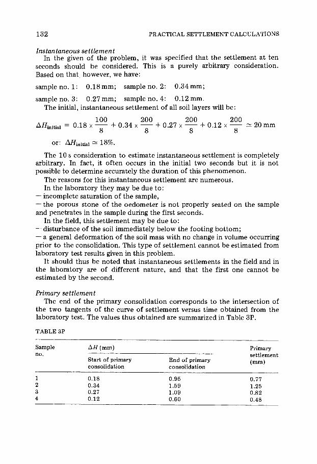
1 3 2 PRACTICAL SETTLEMENT CALCULATIONS
Instantaneous settlement In the given of the problem, it was specified that the sett lement at ten
seconds should be considered. This is a purely arbitrary considerat ion. Based on that , however, we have :
sample no . 1 : 0 . 1 8 m m ; sample no . 2 : 0 . 3 4 m m ;
sample no. 3 : 0 . 2 7 m m ; sample no . 4 : 0 . 1 2 m m . The initial, instantaneous sett lement of all soil layers will b e :
1 0 0 2 0 0 2 0 0 2 0 0 Ä/Zinitia i = 0 . 1 8 ÷ + 0 . 3 4 ÷ + 0 . 2 7 ÷ + 0 . 1 2 ÷ ~ 2 0 m m
initial 8 8 8 8
or: Ä / ϊ ω ί ω ^ 1 8 % .
The 1 0 s considerat ion to es t imate instantaneous set t lement is complete ly arbitrary. In fact , it often occurs in the initial two seconds but it is not poss ible to determine accurately the durat ion of this phenomenon .
The reasons for this instantaneous sett lement are numerous . In the laboratory they m a y be due t o :
— incomplete saturat ion of the sample , — the porous s tone of the oedometer is not properly seated on the sample and penetrates in the sample during the first seconds .
In the field, this sett lement m a y be due t o : — disturbance of the soil immediate ly below the foot ing b o t t o m ; — a general de format ion of the soil mass with no change in volume occurring prior to the consol idat ion. This t y p e of set t lement cannot be es t imated f rom laboratory test results given in this prob lem.
It should thus be noted that instantaneous sett lements in the field and in the laboratory are of different nature , and that the first one cannot be es t imated by the second .
Primary settlement
The end of the pr imary consol idat ion corresponds to the intersection of the two tangents of the curve of sett lement versus t ime obta ined f rom the laboratory test . The values thus obta ined are summarized in Table 3 P .
TABLE 3P
Sample no.
Δ Η (mm) Primary settlement (mm)
Sample no.
Start of primary consolidation
End of primary consolidation
Primary settlement (mm)
1 0.18 0.95 0.77 2 0.34 1.59 1.25 3 0.27 1.09 0.82 4 0.12 0.60 0.48

PROBLEM 3.17 1 3 3
The primary set t lement , corresponding to the pr imary consol idat ion of all the layers is thus :
1 0 0 2 0 0 2 0 0 2 0 0 0 .77 χ + 1.25 χ 4- 0 .82 χ 4- 0 .48 χ = 73 m m
8 8 8 8
say ~ 6 5 % of the total set t lement .
(5 ) Oedometer method
We must now refer to the oedometer diagrams and the oedometr ic equat ion : AH/H = Ae/(1 4- e ) , on which is based Table 3Q (stresses in kPA) .
TABLE 3Q
σ' σ' + Δσ' e(o) e(o' 4 Δσ') Ae Ae
1 4 e AH
78 323 0.749 0.657 0 .092 0 .0526 5.26 94 265 0 .782 0 .710 0 .072 0 .0404 8.08
115 198 0.681 0.658 0 .023 0 .0137 2.74 136 180 0 .580 0 .572 0.008 0.005 1.00
Therefore • A w
• oedomete r = 17 cm. Σ - 17.08 cm
F r o m experimental triaxial curves (Fig . 3 .25 ) the following correlations can be ant ic ipated for the oedometer te s t :
-primar y QI=i% ât o t a l ^ atZQr c2 4 h °oedomete r — o o / o a oedomete r — y j u / o ï oedomete r
On the other hand, the soils are slightly overconsol idated. We can est imate A t o be 0 .4 . With Ç = 7 m and B = 4 m w e get : Ç IB = 1 .75 , and S k e m p t o n and Bjerrum's graph gives: μ = 0 . 5 5 to 0 .60 or :
0 .55 χ (0 .65 χ 1 7 0 ) ^ 6 0 m m
and :
s2 4 h = 60 + ο 35 χ 1 70 = H9.5 or ~ 120 m m
We then have:
Ah = 113 m m (triaxial test m e t h o d ) ,
Ah = 170 m m (original oedometer m e t h o d ) ,
Ah = 1 2 0 m m ( S k e m p t o n corrected oedometer m e t h o d ) . The agreement between the two methods is acceptable , provided S k e m p t o n ' s correction is m a d e .

1 3 4 PRACTICAL SETTLEMENT CALCULATIONS
(6 ) The oedometer m e t h o d leaves something to be desired. It does n o t account for the horizontal strains. When calculating the sett lements of a relatively thin clay layer that is loaded by a large area fill or a wide embank-ment , this method gives much more sat is factory results .
In this example , however, where the thicknesses of the layers are large with respect t o the loaded area (thickness wider than foot ing dimension) the oedometer m e t h o d lacks accuracy. Theoret ical ly , the triaxial test method is preferable because it reproduces more realistic the in-situ stress condit ions . But the Poisson's ratio of the soil m u s t be known and it is difficult t o deter-mine this value accurately. Because of this l imitat ion and the complex i ty of performing triaxial tests , the theoretical advantage of the m e t h o d is doubt fu l .
irk Problem 3.18 Set t lement calculat ion with Newmark ' s chart , ef fect o f ad jacent foot ings
A square footing Sx is 2 m wide and located 2 m below the ground surface in a sandy gravel layer assumed to be incompressible. This layer is 5.5 m
F o o t i n g ST
1 2
4 m .
J.00 ,1.00
n o t o n n e s
° ï -Ï ¼ Ï ï ï .á
2.00ÃÔΊ
. Ï Sandy g r a v e l
ßÃ=19 kN/m 3
>ι
ï . ο - Ï
C l ay
)f= 17.2 kN/ma
Rock / /
5 . 5 0 m
Ρ
ï .
Fig. 3 .30.

PROBLEM 3.18 1 3 5
thick. Below it is a clay layer 3 m thick which overlays a sound bedrock (see Fig. 3.30). The footing supports a column loaded to 1200kN. The in-place density of the sandy gravel is 1.9 and that of the clay is 1.72.
The preconsolidation pressure of the clay was found to be oc = 1.29 daN/ cm2 from laboratory tests. The oedometric modulus is E' = 30daN/cm2
for stresses less than 10 daN/cm2. (1) Calculate the settlement at the center of the footing.
(2) This footing is surrounded by other footings, S 2 , ^3 and ^4 as shown on the plan of Fig. 3.31. All are at the same level and carry loads of 580, 435 and 1085 kN, respectively.
Calculate the settlement of Sx under the influence of adjacent loads. Assume that the unit weights of concrete and the surrounding soil are the same and that the excavation is filled up after construction. Use Newmarks chart of Fig. 3.32.
Solut ion
(1) The sett lement beneath the center o f the square foot ing is :
Ah/h = -Áσ/Ε'. (1)
r 2 00 " ι
Fig. 3 .31 .
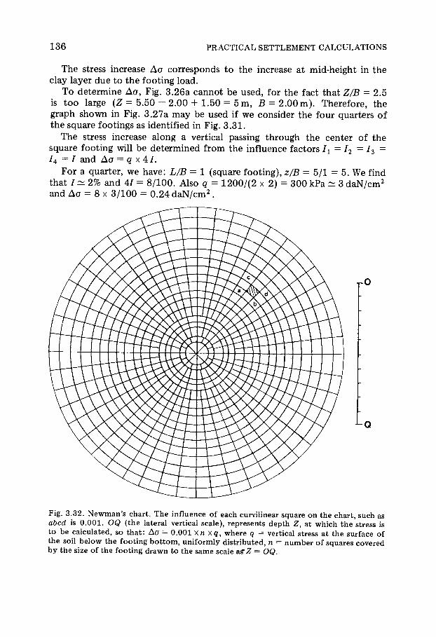
1 3 6 PRACTICAL SETTLEMENT CALCULATIONS
The stress increase Δ σ corresponds to the increase at mid-height in the clay layer due to the foot ing load .
T o determine Δ σ , Fig. 3 .26a cannot be used, for the fact that Z/B = 2 .5 is t o o large (Z = 5 .50 - 2 .00 + 1.50 = 5 m, B = 2 .00 m ) . Therefore , the graph shown in Fig. 3 . 2 7 a m a y be used if we consider the four quarters o f the square footings as identified in Fig . 3 . 3 1 .
The stress increase along a vertical passing through the center of the square foot ing will b e determined f rom the influence factors Ix = I2 — 13 — I4 = I and Δ σ = q χ 4 / .
F o r a quarter, we have: L/B = 1 (square foot ing) , z/B = 5 /1 = 5 . We find that / ~ 2% and 4 / = 8 / 1 0 0 . Also q = 1 2 0 0 / ( 2 χ 2 ) = 3 0 0 kPa ~ 3 d a N / c m 2
and Δ σ = 8 χ 3 / 1 0 0 = 0 .24 d a N / c m 2 .
Fig. 3 .32. Newman's chart. The influence of each curvilinear square on the chart, such as abed is 0 .001 . OQ (the lateral vertical scale), represents depth Z, at which the stress is to be calculated, so that: Δ σ = 0.001 XnXq, where q = vertical stress at the surface of the soil below the footing bottom, uniformly distributed, ç = number of squares covered by the size of the footing drawn to the same scale a_f Ζ = OQ.

PROBLEM 3.18 1 3 7
The overburden pressure at mid-height in the clay, prior t o the start of construct ion, was : σ 0 = 5 .50 χ 1 9 + 1.50 χ 1 7 . 2 = 1 3 0 . 3 kPa ^ 1 . 3 d a N / c m 2 .
We know that the preconsol idat ion pressure is oc = 1 . 2 9 d a N / c m 2, there-fore we can say that the clay is normally consol idated . F o r m u l a (1 ) m a y be used with E' = 3 0 d a N / c m 2 which we were to ld is valid up to a stress level of 1 0 d a N / c m 2 . Therefore : Ah = -h(Ao/E')9 \Ah\ = 3 0 0 χ 0 . 2 4 / 3 0 = 2 . 4 c m .
(2 ) Addit ional sett lement will occur under the square foot ing d u e to the loads imposed by ad jacent foot ings S 2 , S 3 , S 4 (F ig . 3 . 3 1 ) . Newmark ' s chart is used for calculating these set t lements . The size of the foot ing is drawn on the chart and the squares within the foot ing are counted . Here we have OQ — 6 .5 cm which corresponds to Æ = 5 .00 m.
F o r the number of squares (see Fig . 3 . 3 3 ) we have:
foot ing Sx: n1 = 74 squares foot ing S2 - n2 = 1 1 . 5 squares loot ing à2 : n2 = ii.o squares foot ing S3 : n3 = 8 .5 squares foot ing S 4 : n 4 = 2 2 squares .

1 3 8 PRACTICAL SETTLEMENT CALCULATIONS
The respective foot ing areas are : S i : 4 .00 m 2 , S2 : 2 .00 m 2 , S3 : 1.50 m 2 , S 4 : 3 .50 m 2 , f rom which:
qx = 1 2 0 0 / 4 = 3 0 0 kPa = 3 d a N / c m 2 ,
q2 = 5 8 0 / 2 = 2 9 0 kPa = 2 .9 d a N / c m 2 ,
q3 = 4 3 5 / 1 . 5 = 2 9 0 kPa = 2 .9 d a N / c m 2 ,
q4 = 1 0 8 5 / 3 . 5 = 3 1 0 kPa = 3 .1 d a N / c m 2 .
The total i s : Δ σ ' = 0 . 0 0 1 [ 7 4 x 3 + 1 1 . 5 χ 2 .9 + 8 .5 χ 2.9 + 2 2 χ 3 .1 ] = 0 . 3 4 8 ~ 0 . 3 5 d a N / c m 2 .
The sett lement below the center of the square foot ing will therefore b e :
Ah = 3 0 0 χ 0 . 3 5 / 3 0 = 3.5 cm.
The adjacent foot ings increase the sett lement of the square foot ing by a factor of about 46%.
Remark
Newman' s chart may of course also be used to determine the stress for the isolated foot ing Sx. If used, it gives a value of Δ σ " = 0 . 0 0 1 χ 7 4 χ 3 = 0 .22 d a N / c m 2 as o p p o s e d to 0 .24 d a N / c m 2 found in our so lut ion.
*+rkProblem 3.19 So lut ion o f Terzaghi 's consol idat ion equat ion by the finite-difference m e t h o d : appl icat ion to a two-layered sys tem
In order to obtain an approximate numerical solution to Terzaghi's consolidation equation, increments to time t and depth Æ will be given finite values At and AZ. Let us adopt the indexes i for depth and j for time; the pore pressure is noted with two indices: uu, and Ì_+_,ß-é means the pore pressure at depth Æ + AZ at time t — At.
D r a i n a g e
.—^ ·) ·)
"é ß D r a i n a g e
Fig. 3 .34 .

PROBLEM 3.19 139
(1) By incremental changes the two elements of Terzaghi's formula, show that this equation consists of a linear recurrence relation between
" i +u and Mi-i,s - L et A = cv(At/AZ 2). For which value of A is the relation very simple?
(2) Consider a two-layered system of compressible soils located between pervious boundaries (Fig. 3.34). To solve Terzaghi's equation, layer 1 is divided into nx sub-layers, each of thickness AZX and layer 2 is divided in n2
sublayers of thickness AZ2. Show that AZ1 and AZ2 are not independent and determine what the
relation is between n2 and nx.
(3) Find the initial and limit conditions on the upper and lower faces of the two-layered system which indicate that drainage is ideal.
Assume that the initial excess pore-water pressure is 1 over the entire height of the layers, except at the boundaries where u(0, 0) = u(H, 0) = 0.5. At the boundaries in fact, at t = 0, the excess pore pressure is 1 and become zero at t = t + e.
Give an equation of continuity at the interface between the two layers using the principle of continuity of the flow.
(4) For the rest of the problem, assume A = 1/2 to simplify the compu-tations.
Remark We could also assume Á Ö 1/2; the accuracy of the method depends on its
value. The smaller the elements, the longer is the computation but the better is the accuracy.
For computer use, it is generally assumed that A = 1/6. Given are:
h2 = 2.5ft x ; c v l = 1 . 8 x l ( T 4 c m 2 / s ; c v 2 = 1.62 χ l ( r 3 c m 2 / s ;
kx = 1.1 χ 10"4 c m / s ; k2 = 2.2 χ Ι Ο " 4 c m / s ; Ç = 7.00 m.
Based on the equations obtained above, show that it is possible to con-struct, point by point, an isochrone net. Show the computation in the form of tables to the 10th increment of At. Take the minimum whole values for nx and n2. Draw the net corresponding to t = 0, tx = 5 At, and t2 = 10 At.
If we call the degree of consolidation at time t for depth Æ by u(t, Z) = 1 ~u(t, Z)/u0 (u0 = initial excess pore-water pressure) give the formula for the degree of consolidation of the two-layered system and find its value for t = t2 and t = tx.
Solut ion
(1) F o r a function f (x) the formula for finite increments is :
f(a + h) = f{a)Jrhf{a + dh) with O < 0 < 1 . (1)
Porewater pressure is a function of Æ and t: u(Z,t). Le t ' s fix Æ = Z0,

1 4 0 PRACTICAL SETTLEMENT CALCULATIONS
u(Z,t) then becomes a function of t ime a lone :
u(t) = u(Z0,t),
u(t +At) = u(t) +At.u'(t + d At) O < 0 < 1 .
If Δ ί is sufficiently small , then u'(t + θ At) u'(t) u'(t + At) and
du u(t + At)-u(t) u (t) — — —
9 ί Δ ί x , · 3 " ui i+i ~~ "i i or, using the indices : — — — - — (2)
dt At K '
b z ~ AZ ' az^
(3)
Similarly, for ί = ί 0:
AZ AZ \ I d2u u i +1 j — 2ui ι + U i - j j
or — '• '• — . 3 Z 2 AZ2
du d2u The consol idat ion equat ion — = c v — - m a y be written as :
ot oZ
Ui,) + l ~~ ui , j _ + j ~ ^ Ui j + UJ-! j
Δ ί " ° v AZ2
letting A = cv(At/AZ 2 ) we get :
u i J + 1 = (1 — 2 A ) u i fj + A ( u i + 1J + M i - U ) (4 )
which is the relation asked for .
This relation m a y be simplified if A = 1/2, it then b e c o m e s :
Wij+ i = + " i - l j ) (5 )
(2 ) We have A = cvl{AtjAZ\) = cy2{AtlAZ\) s ince the same t ime incre-ment must be chosen for the two layers. Therefore : AZl/AZ2 = V cv i / < ?V2 ·
Therefore we have: Δ Ζ Χ = hl/n1 and Δ Ζ 2 = h2/n27 and
^ i / c v 2
= — /— -n2. (6)
(3a ) The boundary condit ions are :
(w(0, f ) = 0 for i ^ O (7)

PROBLEM 3.19 1 4 1
which implies that drainage at the surfaces of the sys tem is ideal. (b) The initial condit ions m a y be written:
i °
(u(Z90) = 1 íÆÖ{ [Ç (8 )
L ( 0 , 0 ) = u(H90) = 0 .5
(c) Le t us write the condit ion of continuity of flow at the interface between the two compress ible layers . L e t us start by determining the head ft at a point Ì at elevation Z . S a y H0 is the distance to the water table from an arbitrarily chosen reference level (see Fig . 3 . 3 5 ) .
W a t e r t a b l e
R e f e r e n c e
p l a n e
Ì
Fig. 3 .35.
The pore-water pressure at Ì at t ime t is equal t o the sum of the excess pore pressure u (Z , t) and of the hydrostat ic pressure (H0 4- Z)yw
existing at Ì prior to the increase u ( Z , t). The head ft is usually expressed by Λ = ( w / 7 w) + Z .
The posit ive vertical direction is downward and u = (H0 4- Z)yw. Therefore :
ft = (t f 0 + Z)7w + M( 2 > 0
Ζ = H 0 + u(Z,t). (9 )
The continuity of f low at the interface m a y be expressed by the con-tinuity of rate of percolat ion vx = v2 or kxix = k2i2 or also by taking into account eqn. ( 9 ) : k1 (Au/AZ) x = k2(Au/AZ) 2
t h e r e f o r e b y k x(uKJ — M k _ l f j) = ft2(wk + 1 J - w k > j) ( A Z 1 / A Z 2 ) ( 10 )
where index k corresponds the value of index i a t the interface, and if we as sume that index i increases f rom b o t t o m to t o p of the compress ible layers .
(4 ) The numerical appl icat ions give:
c v 2 1 .62 x l O " 3
1.8 x l O " 4

142 PRACTICAL SETTLEMENT CALCULATIONS
from which:
AZX/AZ2 =y/Tj9 = 1/3 from which H= 7 . 0 0 m , h2 = 2 . 5 h x, h x = 2 . 0 0 m ,
h2 = 5 . 0 0 m ,
hx [c 1
ft2 V C vl 2 2 .5 2
or Ì2 = 5 , ç\ = 6 , finally k2/kx = 2 .
We then have the following relations:
" i j + i = + W i - i j ) (5 )
" k j ~ " k - i j = 2 x i ( w k - i j ~ W k j ) - ( lObis )
The interface between the two layers corresponds to the value 6 of index k and since equat ion (10 bis) is valid regardless of i , i n d e x ; is no longer necess-ary. Therefore, eqn. (10 bis) may be rewritten a s :
u 6 ~ u s = i(ui -ue) ( lOte r )
or u6 = ^(3u5 + 2u7).
Finally, increment At is given b y : cvAt/AZ 2 = 1/2. For instance, if values applicable to layer 1 are subst i tuted , we have :
2 x l 0 2 1 / 2 x l 0 2 \ 2 1
AZX = — - — cm from which Δ ί = — ÷ | — : — I x 6 2 \ 6 / 1.8 x l O " 4
Δ ί — 3.09 · 1 0 6 seconds or a b o u t 36 days . The initial and boundary condit ions are : u 0 0 = 0 . 5 , w 0 j = 0 , u l l t 0 = 0 . 5 ,
u\i,i = 0? which allow us to calculate by successive approx imat ions with eqn. (5 ) . When the value o f 6 is reached for index /, equat ion ( l O t e r ) must then be used.
Calculations are m a d e easier if tabulated with double entry. For instance, each column may be made to correspond to a specific index value corre-sponding to the locat ion of a point in the two-layered sys tem, (i = 0 , 1 , 2 , . . . 1 1 ) and each line corresponds to a t ime increment 0, Δ ί , 2 Δ ί , . . . , η Δ ί (j = 0, 1, 2 , . . . ç). As specified in the given of the prob lem, the limit of ; is 1 0 .
The first line of the table may be filled in immediate ly since it is a s sumed that u = 1 , except at the end surfaces (i = 0 and ι = 1 1 ) at which u = 0 . 5 .
Columns 0 and 1 can also be filled in immediately since u o j = 0 and un j = 0 , regardless of L ine 2 is easily filled in for u0 j = 0 and ux x =
+ 0 .5 ) = 0 . 7 5 . The same procedure is used for u 1 0 1, at the right end of the table line 1 .

PROBLEM 3.19 143
For l i n e ; = 4, we would have:
*6, 4
*6, 4
i ( 3 w 5 )4 + 2u1A) = H ( 3 x l ) + (2 x 0 . 9 6 8 ) ]
0 . 9 8 7 .
1 Excess of pore wate r Β Bj p r e s s u re
Fig. 3 .36.
Table 3Q is filled in f rom the extremities of each line and to be terminated in column 6 with equat ion ( l O t e r ) . Each line of the table thus represents a point-by-point construct ion of the net .
The isochrons corresponding to t = 0 , t{ = 5 At and t2 = 10 At are pre-sented in Fig. 3 .36 .
The degree of consol idat ion at t ime t and depth Æ are defined b y :
U(t Zj _ ! _ U Z (u0 = initial excess pore-water pressure) .
The degree of consol idat ion of the two-layered system is Ç ,
'L ""dZ. é -
u(t,Z)
which is the ratio o f the cross-hatched area (.<•) shown in Fig. 3 .37 and the rectangle AMNB, oxHu0:
U(t) = sSIHu0.

1 4 4 PRACTICAL SETTLEMENT CALCULATIONS
A Ì
Ç
Β Fig. 3 .37.
The area m a y be c o m p u t e d by numerical method (trapezoid m e t h o d ) or by planimeter.
We f ind: U(t1) ~ 0 .34 and U(t2 ) ^ 0 . 49 .
Fig. 3 .38. Different settlement below a 16th century old building in Lyons, France.

1 4 5
Chapter 4
P L A S T I C I T Y A N D S H E A R S T R E N G T H
^Problem 4.1 Triaxial test on sand
A dry sample of sand is tested in triaxial compression. It is assumed that the internal angle of friction is ö = 36°. If the minor principal stress, σ3, is 300 kPa, at which value of maximum principal stress, ox will the sample
Fai lure , or plastic deformat ion of the sample , will occur when Mohr's circle becomes tangent to the failure envelope. The failure envelope consists of two straight lines which, in this case, make an angle of 3 6 ° above and below the principal stress axis Οσ. At the beginning of the test, the sample is subjected to a confining isotropic stress, σ 3 . For this condit ion, Mohr's circle reduces to a single point , which abscissa is σ 3 .
When the major principal stress ox is appl ied, the diameter of Mohr's circle increases by a distance of ox — σ 3 while σ 3 remains constant (see Fig. 4-1) . The diameter continues to increase until the circle becomes tan-gent to the two straight lines.
fail?
Solut ion
0
cr
Fig. 4 .1 .

146 PLASTICITY AND SHEAR STRENGTH
Let d be the abscissa of the center, and R the radius of Mohr's circle at failure (see Fig. 4 . 2 ) , then:
R , R „ „ 1 ~ sin ö — = sm ö\ σ 3 = α — R = --R = R ; d sin ö sin ö
and:
o 1 R = d + R= — + R = R 1 + S i n Therefore : sm <p sm ö
O+R _ 1 + sin ι _ (ð_ ö_ = t a n 2 - +
σ 3 1 — sin ^ 14 2
Numerical application With σ 3 = 3 0 0 kPa, ^ = 3 6 ° . We have: π/4 + <p/2 = 4 5 4- 18 = 6 3 ° ; t a n 6 3 c
1.96; alR = 3 0 0 χ 1 .96 2 = 1 1 5 5 , say 1 1 6 0 kPa.
Answer olR = 1 1 6 0 kPa.
^Problem 4.2 Triaxial test on sand with cohes ion
Using the data of problem 4.1, solve for o1R assuming that the sand has a cohesion of 12 kPa.
Solut ion The failure envelope, as in problem 4 . 1 , consists of two lines inclined at-3 6 ° above and below the principal stresses axis . However, the two straight lines now no longer cross the axis at the origin but to the left of it at a point whose coordinates are σ = 0, r = ± c (see Fig. 4 . 3 ) .
ζ
/ 1 R \
Χ* ( \ 1 <
0 -— - ^ · \ . \ d
Fig. 4.2.

PROBLEM 4.2 147
Ç 0 cr
Fig. 4 .3 .
A computa t ion similar to that o f example problem 4 .1 gives: Ç = c cot ö (F ig . 4 . 4 ) , σ ι κ + Ç = ( σ 3 + Ç) t a n 2 (π/4 4- ö/2), σ ι κ = ( σ 3 + Ç) t a n 2 (ð/4 + ö/2)-Ç.
Numerical application σ 3 = 3 0 0 kPa, ^ = 3 6 ° , cot ö = 1 .376 , t a n 2 (π/4 4- <ρ/2) = 3 . 8 5 , c = 1 2 kPa, i f = c co t ö = 1 6 . 5 , say 17 kPa f rom which σ ι κ = ( 3 0 0 + 1 7 ) χ 3 .85 - 17 = 1 2 0 3 , say 1 2 0 0 kPa.
Answer a 1 R = 1 2 0 0 kPa.
Fig. 4.4.
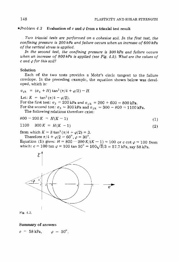
1 4 8 PLASTICITY AND SHEAR STRENGTH
^Problem 4.3 Evaluat ion o f c and ö f rom a triaxial test result
Two triaxial tests are performed on a cohesive soil. In the first test, the confining pressure is 200 kPa and failure occurs when an increase of 600 kPa of the vertical stress is applied.
In the second test, the confining pressure is 300 kPa and failure occurs when an increase of 800 kPa is applied (see Fig. 4.5). What are the values of c and ö for this soil?
Solut ion Each of the two tests provides a Mohr's circle tangent to the failure
envelope. In the preceding example , the equat ion shown below was devel-oped , which is :
°IR = (°s + H) tan2 (ð/4 + ö/2)-H.
Let : Ê = t a n 2 (π/4 + ö/2).
For the first tes t : σ 3 = 2 0 0 kPa and σ ι κ = 2 0 0 + 6 0 0 = 8 0 0 kPa. For the second tes t : σ 3 = 3 0 0 kPa and σ ι κ = 3 0 0 4- 8 0 0 = 1 1 0 0 kPa.
The following relations therefore exist :
8 0 0 - 2 0 0 # = H(K-l) (1 )
1 1 0 0 - 3 0 0 Κ = H(K - 1) (2 )
from which Ê = 3 t a n 2 (π/4 + ö/2) = 3. Therefore π/4 4- ö/2 = 6 0 ° , ö = 3 0 ° .
Equat ion (1) gives: Ç = 8 0 0 - 200Ê/(Ê - 1) = 1 0 0 or c cot ö = 1 0 0 from which: c = 100 tan ö = 100 tan 3 0 ° = 1 0 0 ^ / 3 = 57 .7 kPa, say 58 kPa.
Fig . 4.5 .
S u m m a r y o f answers
c = 5 8 k P a , ö -ö = 3 0 ° .
PROBLEM 4.4 149
Remark
Answers can also be obta ined graphically from the diagram of Fig. 4 .5 showing the t w o Mohr's circles tangent to the failure envelope.
Problem 4.4. Triaxial compress ion tests per formed under different draining condi t ions ; Mohr ' s circles and failure envelopes
A 40 mm diameter saturated sample is 80 mm high and weighs 1.85N. It is tested in a triaxial compession test. Specific gravity of the soil constitu-ants is 2.75.
(a) The sample is subjected to a confining pressure of 85kPa without allowing any drainage to occur. The pore-water pressure is measured at 69kPa. What was the value of the initial pore-water pressure u0 after the sample was removed from the borehole but before it was subjected to the confining pressure in the laboratory? Why is the initial pore pressure, u0 not equal to zero?
(b) The sample is now allowed to drain until the pore-water pressure is zero, indicating that the sample has been fully consolidated. If the volume of the sample has decreased by 10%, what is the compression index Cc of the clay ?
(c) The same sample, after consolidation in the triaxial cell, is submitted to an undrained compression test, the confining pressure being 85kPa. At failure, the pore pressure is 35kPa and the load on the sample is 123 Ν (applied to the piston). The height of the resulting sample is 3.6 mm shorter. Assuming that during the test the sample retained the shape of a right cylinder, calculate the deviator stress (σé —σ3) and from the calculated value, the principal effective stresses o\ and σ 3.
(d) Another identical sample is tested in a drained condition with a con-fining pressure of 85 kPa. At failure, the major effective principal stress o\ is 255 kPa. Draw the Mohr's circles for the two tests at failure with effective stresses and draw the failure envelope. What are the c and ö values?
So lut ion (a) During sample recovery, a stress relief occurs since the soil sample is
no longer subjected to the overburden pressure. Assuming that the labora-tory tests are per formed a short t ime after sample recovery, the water losses are negligible. S ince water is incompress ible with respect to the soil struc-ture , the observed volume change will be nil. Fur thermore , the effective stresses remain constant since they are linked to the deformat ion of soil s tructure, therefore to volume change.
Under isotropic stress condit ions in the triaxial device we have thus °3 = °3 ~u- At atmospheric pressure, just before the test , ( σ ' 3) 0 = ( σ 3 ) 0 — u0. Since atmospheric condit ions correspond to the zero total stress con-dit ion: ( σ 3 ) 0 = 0 , therefore : ( σ 3 ) 0 = — u0.
The effective stresses are constant , so ( σ 3 ) 0 = σ 3 and : — u0 = σ 3 — u

1 5 0 PLASTICITY AND SHEAR STRENGTH
u0 = - (σ 3 - u) = - ( 8 5 - 6 9 ) = - 1 6 k P a
u0 = - 1 6 k P a
(b) First , let us calculate the wet unit weight of the clay sample . The weight is Ρ = 1.85 Ν, its vo lume is V = nR2h = π χ 2 2 χ 8 c m 3 ^ 1 0 0 . 5 c m 3 . The unit weight isP/V = 1 . 85 /100 = 0 . 0 1 8 5 N / c m 3 = 1 8 . 4 k N / m 3 .
F r o m the relations between 7 h , γ 8 , 7 W and e:
(1 + e)yh = 7 s + * 7w
e = ( 7 s - 7 h ) / ( 7 h - 7 w ) . 7 w = 1 0 k N / m 3 .
Therefore : e = (27 .5 - 1 8 . 4 ) / ( 1 8 . 4 - 1 0 ) ~ 1 .08. This is the initial void ratio corresponding to an effective initial stress due
to overburden pressure of σ 0 = 1 6 kPa. After applying the confining pressure of 8 5 k N / m 2 until the pore pressure is zero , the effective stress is equal t o σ' = 8 5 k N / m 2 .
If V is the total volume of the sample and if Vg is the vo lume of soil particles as sumed to be constant (soil grains are as sumed incompress ible) , it is possible to write :
initial s tate : V = Vg(l + e ) ,
final s tate : V + AV = V g ( l + e + Ae)
f rom which: AV = VgAe, or : AV = V ( l + e)Ae.
AVIV = Ae/(1 + e) and \Ae\ = 0 .10 χ (1 + 1.08) ~ 0 .21 So Δ β = - 0 . 2 1 .
Stress paths fol lowed during an isotropic triaxial test and that of an oedometer test are very similar. It can, therefore, be as sumed that volume changes during the test will be control led by the same equat ion :
-Ae -Ae 0 . 21 C c = , = — — . S o : Cc = = 0 . 2 9 0
A l o g a log(aVao) log ( 8 5 / 1 6 )
Remark. The compress ion index, as defined by an oedometer test was evaluated in
this example f rom a triaxial test . S ince the stress paths for the two tests are not identical (only similar) it m a y be that the calculated value of C c m a y vary f rom that obta ined f rom an oedometer test .
(c) At each point during compress ion, the deviator stress σ1— σ 3 is given b y : σ1 — σ 3 = F/S in which S is the actual cross-sectional area of the sample . If the sample remained a right cylinder during testing, the following relation-ship is true since no volume changes occur in an undrained tes t : HQSQ = HfSf, where subscripts ο and f represent initial and final values, respectively, from which:

PROBLEM 4.5 1 5 1
At failure we have: (σ÷ - σ 3 ) £ = ( 123 ÷ 1 0 ~ 3) / ( 1 3 . 8 1 ÷ 1 0 ' 4 ) ^ 8 9 . 1 kPa. The minor effective principal stress i s :
°3 ~ °3 ~ u = 8 5 — 3 5 = 50 kPa. But o\ — o3 = ox ~ σ3.
Then the major effective principal stress is: o\ = 8 9 . 1 + 50 = 1 3 9 . 1 kPa
Summary
a\ = 1 3 9 . 1 kPa ; o'3 = 5 0 k P a .
(d) In the drained condi t ion, u = 0 and we have: o'3 = o3 = 8 5 k N / m 2 , σΊ = 2 5 5 k N / m 2 .
With this set of values and that obta ined in the preceding paragraph it is possible to draw the Mohr's circle for the two samples (see Fig . 4 . 6 ) . The failure enevelope of these circles passes through the origin. The mechanical properties of the soil, in terms of effective stresses, are : cohesion c = 0 , angle of internal friction ö = 3 0 ° .
irkProblem 4.5 Shear strength o f a c lay ; effective stresses
A clay layer is 20 ft thick and covered by a sandy gravel layer whose porosity ç = 0.30 and which is 40 ft thick. The water table is at 13 ft below ground surface (see Fig. 4.7). Triaxial tests are performed on the clay samples. These tests are undrained with pore-water pressure measurements. The following results were obtained: cohesion c = 2.9 lb/in2, angle of internal friction ö = 24°.
The dry unit weight of the sandy gravel is 103 lb/ft 3 and the saturated unit weight of the clay is 112 lb/ft 3. Find: (1) the soil shear strength at mid-

1 5 2 PLASTICITY AND SHEAR STRENGTH
height of the clay layer, and (2) the effective and total stresses acting on a vertical face of a soil element at mid-height of the clay layer.
Solut ion
(1) At mid-height in the clay layer, the vertical total stress is (see Fig . 4 . 7 ) : ox = dy a + (Hx ~d)ygt + ( t f 2/ 2 ) 7 sAa t .
H2
- W a t e r table
Sandy gravel 'G d = 10 3 lb/ft 3
Clay
$sa t =11 2 lb/ft 3
Fig. 4.7.
The saturated unit weight of the sandy gravel is :
7sGat = 7 d + " 7 w , 7 w = 10 k N / m 3 = 6 2 . 5 l b / f t 3,
7sGat = 103 + 0 .30 x 6 2 . 5 = 1 2 1 . 7 5 l b / f t 3,
from which:
σ÷ = 13 χ 103 + (40 - 1 3 ) χ 1 2 1 . 7 5 + 10 χ 1 1 2 = 5 7 4 6 . 2 5 lb / f t 3 = 38 lb / in 2 .
The corresponding effective stress is :
o\ = a x - u = σë -y w(H2/2 +HX ~ d) = 5 7 4 6 . 2 5 - 6 2 . 5 (10 + 2 7 )
= 3 4 3 3 . 7 5 lb / f t 2 = 2 4 l b / i n 2.
The shear strength in the middle of the clay layer (Fig . 4 .8 ) will b e :
s = c +o\ tan ö = 2 .9 + 24 tan 2 4 ° = 2 .9 + 2 4 x 0 . 4 4 5 = 1 3 . 5 8 lb / in 2
S o s - 1 3 . 6 l b / i n 2. Æ
Fig. 4.8.

PROBLEM 4.6 1 5 3
(2) S ince the clay is sa turated , the coeff icient of earth pressure at rest , K0, is 0 . 5 0 . The effective stress acting on a vertical face of a soil e lement at mid-height in the clay will b e : σ3 = Ê0σ\ = 0 .50 χ 2 4 = 1 2 l b / i n 2 .
The tota l stress corresponding to this value i s :
6 2 . 5 χ 37 o3 = o3+u = 1 2 + ^ 2 8 l b / i n 2 ( * ) .
1 4 4
Summary of solutions
s = 13 .6 l b / i n 2 or 9 4 k P a , σ 3 = 1 2 lb / in 2 or 8 3 k P a , σ 3 = 2 8 lb / in 2 or
1 9 3 . 5 kPa.
+***Problem 4.6 Interpretat ion o f various types o f triaxial tests (drained, un-drained, conso l idated , unconsol idated)
Several triaxial tests have been performed on identical clay samples. The variation in test procedures for samples X and Y only varied by one factor.
In each of the following tests, draw the Mohr's circles and failure envel-opes for both total and effective stresses.
For each of the conditions below, which sample was subjected to the highest value of shear stress?
(1) Consolidated drained test (CD. test): consolidation pressure σ 3 ; for sample X, rate of strain is 1 mm/min; for sample Y, rate of strain is 0.005 mm/min.
(2) Consolidated drained test (CD. test): consolidation pressure: σ3 = 0.3MPa; sample X was subjected to a pre-consolidation pressure of 0.2MPa (rate of strain = 0.005mm/min.); sample Y was subjected to a pre-consoli-dation pressure of 0.4 MPa (rate of strain = 0.005 mm/min).
(3) For sample Y the test was a consolidated drained (CD.) test, but for sample X the test was a consolidated, then undrained (CU.) test. The consolidation pressure o3 is the same for both samples.
(4) Both samples are overconsolidated to 0.6MPa: sample X was drained and consolidated to 0.2MPa; sample Y was undrained and consolidated to a pressure o3 such that the effective stress σ3 at failure is equal to σ3 = 0.2 MPa.
(5) Consolidated undrained test (CU. test): the consolidation stress was σ3, sample Y was not remolded, sample X was remolded and recompacted to the same density as that of Y. The clay was a sensitive clay.
So lut ion
F o r all types of triaxial tests of certain states of stresses, the Mohr's circle for effective stresses is obta ined f rom that for tota l stresses by s imply
*Note: 1 lb / in 2 = 144 l b / f t 2, 1 lb / f t 2 = 48 Pa, 1 lb / in 2 = 6.897 Pa.

154 PLASTICITY AND SHEAR STRENGTH
translating the circle by a value of u (pore-water pressure) . If pore-water pressure is zero in all locations in the sample (drained test condi t ion) the circles for both effective and total stresses are super imposed. We also know the m a x i m u m shear stress (shear strength) that can be applied to a soil, corresponds to the radius of the Mohr's circle at failure.
(1 ) In the first condit ion, a rate of strain of 1 m m / m i n is considered t o o fast to represent a drained test condit ion. Because clays have a very low coefficient of permeabil i ty, pore-water pressure would increase during this test. Let that pressure be u at failure at mid-height of the sample . The test on sample X can be assumed to represent drained condit ion. The higher shear stress will be applied to sample Y because its effective confining pressure will be higher than that of sample X (see Fig. 4 . 9 ) .
X
ï
Fig. 4.9.
Then the diameter of the Mohr's circle, representing the stress condit ion at failure, for sample Y will be larger than that of sample X (see Fig. 4 .9 ) .
(2) Since sample Y was subjected to a pre-consolidation pressure greater than that of sample X, its shear strength is greater (see Fig. 4 . 1 0 ) .
X
E f f e c t i ve and tota l s t r e s s e s
E f f e c t i ve and tota l s t r e s s e s
o cr 3 σ Fig. 4.10.
(3) This is the same test condit ion as in case (1 ) . The solut ion is the same . (4) We agree with Wroth, R o s c o e and Schofield [Ref . 3 3 ] who have stated
that the limit state condit ions are the same in their e , ñ (average stresses) and

PROBLEM 4.7 155
q (deviator) space , regardless of the type of test . Sample Y is undrained, its void rat io remains constant at e0 during testing. S ince sample X is drained, its void ratio increases during shearing (the clay is overconsol idated) and its final condit ion is ef > e0.
In the space diagram p, q, e, for a constant value of p, q decreases with e [Ref . 3 3 ] . The radius of Mohr's circle at failure will therefore be smaller for sample X than for sample Y (see Fig . 4 . 1 1 ) .
Fig. 4 .11 .
(5) If the clay is sensitive, its shear strength decreases immediately after it has been remolded . The m a x i m u m shear stress for sample Y will be higher than that for sample X (see Fig . 4 . 1 2 ) .
Undraine d tes t tota l stresse s
Fig. 4 .12.
irk Problem 4.7 Unconf ined compress ive strength f rom a consol idated un-drained triaxial test
A consolidated, undrained (C. U.) triaxial test is performed on a clay sample of low plasticity whose dry unit weight is yd = 1.7 ÷ 10* N/m3. The sample was recovered from a depth of 8.15 m. The porosity of the clay is

1 5 6 PLASTICITY AND SHEAR STRENGTH
ç = 0.35. The triaxial test results yielded the following values: ö0×1 = 14 ,
ccu =4xl04Pa. Determine the unconfined compressive strength of a saturated sample of
this clay from the same depth (assume that 100% saturation was maintained after sample recovery and during handling).
Solut ion The unconfined compress ion shear strength of the saturated clay sample is
given by Rc = 2 c u . It is necessary to determine c u f rom the parameters ö0×1
and c c u. L e t us draw Mohr's circle for tota l stress condit ions (see Fig. 4 . 1 3 ) of the consol idated undrained test . The consol idat ion pressure σ 0 is the s ame during the test . At the end of consol idat ion, u = 0 since the drainage occurs then. S o σ 0 = σ 3 is one of the effective stresses at the start of the test . At the end of the test , however, since after consol idat ion of the sample no more drainage was al lowed, u Ö 0 and σ 3 = σ 0 is a tota l stress.
It will be noticed that line O'T (see F ig . 4 . 1 3 ) is not a failure envelope during testing, because then two different phases exist , namely a l iquid and a solid one .
Le t r be the radius of Mohr's circle, then :
Fig. 4 .13.
cu = (ox — σ 0) / 2 = r and Ω Τ / Ο ' Ω = s i n ^ c u,
r therefore: = sinv?cu o0 + r + c c u co t ö0
or : c u = ( σ 0 + c u) sin ö0×1 + c c u cos öïç
and thus : c u ( l — sin <pc u) = σ 0 sin <pcu + c c u cos <£ c u.
, ï . Ί1 sin ö0×1 cos <£cu
and finally: c u = σ 0 P ^ — + c c u r ^ — 1 — sin ö0ë× 1 — sm ö0×1
The consol idat ion pressure σ 0 corresponding t o the effective overburden pressure σν at depth Ç of the sample has ye t t o be determined. It is f ound as fol lows:
PROBLEM 4.8 157
°o = ffv = y'H; i = 7 s at - 7 W
7sat = 7 d + ^ 7w = 1.7 + 0 . 3 5 x l x l O 4 = 2 . 0 5 χ 1 0 4 N / m 3
a'y = 1.05 x l O 4 x 8 . 1 5 = 8 .56 χ 1 0 4 Pa.
f rom which: c u = 8 .56 χ 1 0 4 8 1 11 1 4 Q + 4 χ 1 0 4 C° S 14
1 - sin 1 4 ° 1 - sin 1 4 °
= 7 . 8 5 x l 0 4 P a
o r : i 2 c ^ 1 . 5 7 x l 0 5 Pa.
It can be noted that the soil is a stiff clay.
**Problem 4.8 Re la t ion between Young ' s m o d u l u s , oedometr ic m o d u l u s and Poisson's rat io
(1) Consider a linearly elastic soil. Find the change in volume of this material when subjected to isotropic stress loading. What can be said about the Poisson's ratio of this soil. For what condition is í = 0.5?
(2) In an oedometric test, assume that for an increase in stress Δ σ ν verti-cally applied to the sample, the soil shows a linear, elastic behavior. Deter-mine then the relation between the oedometric modulusEf, Young's modulus Ε and the Poisson ratio v. What is the relation for í = 0.33 (usual assumption made for soils in general).
So lu t ion (1) L e t σ{ be the i sotropic stress appl ied to the soil with Young ' s modulus
Ε and Poisson's ratio v. Adopt ing the sign convention usually a d o p t e d in soil mechanics , linear elasticity is expressed b y :
1 a i d -2v) €i = --(o i~2voi) = .
The vo lume change is equal to the first invariant of the strain tensor :
_ 3 ^ ( 1 - 2 * 0
V Ε
If the i sotropic stress is compress ion (σ{ > 0 ) the vo lume change corre-sponds to a vo lume decrease AV/V< 0 . Therefore , the fol lowing condit ion mus t ex i s t :
l - 2 i > > 0 or : v<l/2.
T h e case when í = 0 .5 corresponds to AV/V = 0 , that is t o say , t o a material that is incompress ible .
(2 ) The oedometr ic m o d u l u s is def ined b y :
Ε' = — Δ σ ν/ ( Δ Λ / Λ ) or Δ σ ν = - £ ' e v . (1 )
1 5 8 PLASTICITY AND SHEAR STRENGTH
The symbol Δ σ ν means that the linear elastic behavior is only valid for a small range of stress change. In the oedometer , the vertical load corresponds to a ma jor principal stress and ax i symmetry implies σ 2 = σ 3 . Therefore , (1 ) we can write :
Áσ ÷ = —Ere1. (2 )
S ince the elastic deformat ions o f the metal mold holding the sample m a y be considered negligible compared with those o f the soil , we can formula te : e 2 = e 3 = 0 . Linear elasticity condit ion then means t h a t :
- - [ Δ α , -í(Áσ 2 + Δ σ 3 ) ] = - - [ Δ σ χ — 2íÁσ 3]
e2 = e 3 = - - [ Δ σ 3 í{Áï ÷ + Δ σ 3 ) ] = 0
(3 )
(4)
F r o m eqn. ( 4 ) , we have: σ 3 — í{Áσ é + Δ σ 3 ) = 0 or Δ σ 3 = Δ σ !
{íÖÉ f rom eqn. 1 ) . B y replacing the value of Δ σ 3 in eqn . 3 , we obta in :
2v2
e , = Δ σ χ
Ε 1 -
and by compar ing eqn. (2 ) and ( 5 ) , we have :
2v2
Ε = Ε'
(5)
1-v
In the particular instance of í = 0 .33 or 1/3, we have Ε = 2/3Ef. The soil appears t o be less compress ible than it is in reality.
irkProblem 4.9 Evaluat ion o f Poisson's rat io f rom triaxial tes t
A soil sample is tested in a triaxial compression test at small increments of principal stresses: Áσ ÷ and Ao2 = Δ σ 3 .
Assume that the soil behaves in a linearly elastic manner. Axial strain (Ah/h = el) and volumetric changes AV/V, corresponding to the drainage of pore water during testing, are measured, (see drained test set up Fig. 4.14).
Derive the formula for Poisson's ratio of this soil under the test conditions. For a numerical application, consider the soil to be a loose sand in one case and a normally consolidated clay in another. The test results for both are presented in the graphs of Fig. 4.15.
So lu t ion In the triaxial cell ax i symmetry implies, Δ σ 2 = Δ σ 3 and from the elasticity

PROBLEM 4.9 159
Fig. 4 .14.
| -<rr ßï5 p a
Loose sand
n = 0-46
( £ = 2 - 1 . 1 0 5 P a
Normally consolidate d c lay
Q~r= 2 . 1 0 5 P a
A x i a l d e f o r m a t i o n
Loose sand
ç = 0-4 6 (ÃÃ = 2 · 1 . 1 0 5 P a
Normally consol ida te d clay
Q"r= 2 . 1 0 5 P a
Fig. 4.15. Drained triaxial test results on saturated samples.
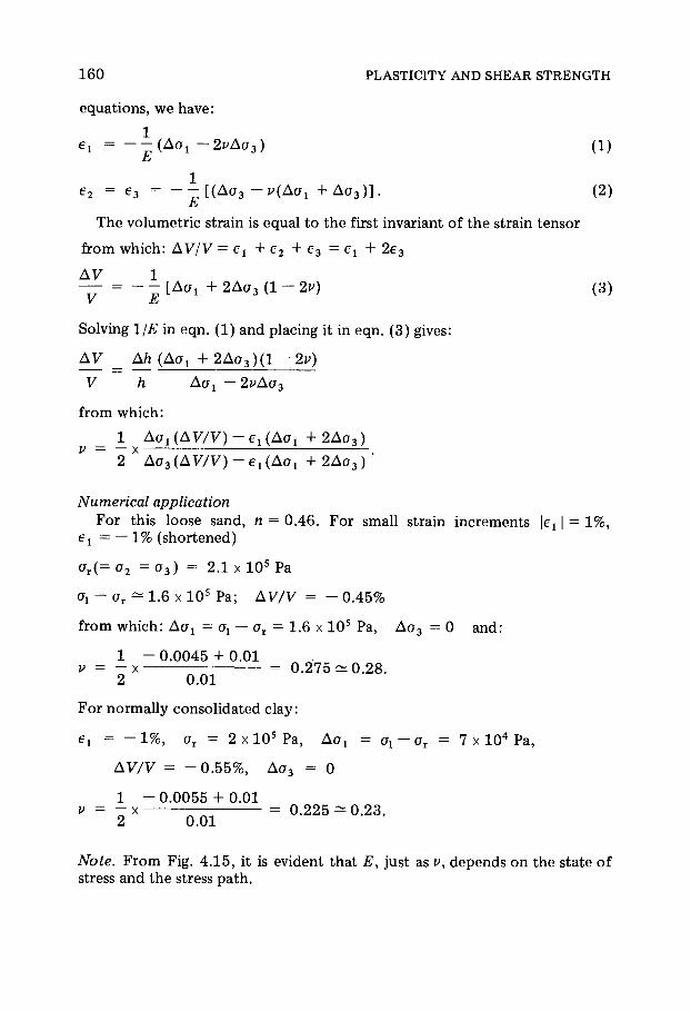
1 6 0 PLASTICITY AND SHEAR STRENGTH
2 Ao3(AV/V)-e 1(Ao1 + 2 Δ σ 3 ) '
Numerical application
F o r this loose sand, ç = 0 . 46 . F o r small strain increments |€χ | = 1%, e1 = — 1% ( shortened)
σ Γ ( = σ 2 = σ 3 ) = 2 .1 χ 1 0 5 Pa
σ÷ - σΓ ^ 1.6 χ 1 0 5 Pa; Ä V / V = - 0 . 4 5 %
from which: Áσ 1 = σë — σΓ = 1.6 χ Ι Ο 5 Pa, Δ σ 3 = 0 and :
1 - 0 . 0 0 4 5 + 0 .01 í = - χ = 0 . 2 7 5 ~ 0 . 2 8 .
2 0 .01 F o r normally consol idated c lay :
ex = - 1 % , σΓ = 2 χ 1 0 s Pa, Δ σ ! = ïë~ï÷ = 7 χ 1 0 4 Pa,
AV/V = - 0 . 5 5 % , Δ σ 3 = 0
1 - 0 . 0 0 5 5 + 0 .01 í = - χ = 0 . 2 2 5 — 0 . 2 3 .
2 0 .01
Note. F r o m Fig. 4 . 1 5 , it is evident that E, jus t as v9 depends on the state of stress and the stress pa th .
equat ions , we have:
ex = - ^ ( Ä σ é ~2pAo3) (1 ) Ε
e 2 = 6 3 = [ ( Δ σ 3 -v(Ao x + Δ σ 3 ) ] . ( 2 ) Ε
The volumetric strain is equal to the first invariant of the strain tensor
f rom which: AV/V = e x + e 2 + e 3 = e x + 2 e 3
^ = ~ ^ [ Δ σ ι + 2 Δ σ 3 ( 1 - 2 ^ ) (3 )
Solving 1/E in eqn. (1 ) and placing it in eqn. (3 ) gives:
AV _ Ah (Áσ ÷ + 2 Δ σ 3 ) ( 1 -2v)
V h Aox —2vAo 3
f rom which:
1 Áσ ÷ (AV/V) - e t (Áσ ÷ + 2 Δ σ 3 ) í — — χ
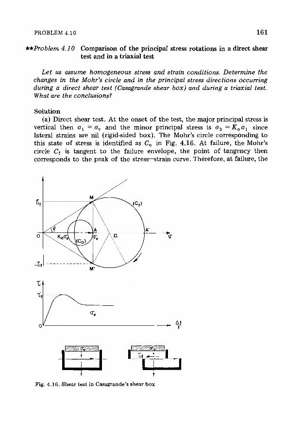
PROBLEM 4.10 1 6 1
itkProblem 4.10 Compar i son o f the principal stress rota t ions in a direct shear test and in a triaxial test
Let us assume homogeneous stress and strain conditions. Determine the changes in the Mohr's circle and in the principal stress directions occurring during a direct shear test (Casagrande shear box) and during a triaxial test. What are the conclusions?
(a) Direct shear test . A t the onset o f the test , the major principal stress is vertical then σé = σ ν and the minor principal stress is σ 3 =Ê0σ1 since lateral strains are nil (rigid-sided b o x ) . The Mohr's circle corresponding to this state of stress is identified as C G in Fig . 4 . 1 6 . At failure, the Mohr's circle C f is tangent to the failure envelope, the point of tangency then corresponds to the peak of the stress—strain curve. Therefore , at failure, the
So lu t ion
-it -
ο or
ο Ä É
Fig. 4 .16. Shear test in Casagrande's shear box

1 6 2 PLASTICITY AND SHEAR STRENGTH
stress vector acting on the horizontal shear plane is OM ( σ ν, of) whereas initially it was figured by O A .
Let Ω be the center of Mohr's circle ( C f) . The end of OM rotated clock-wise at an angle of π/2 4- ö since (ΩΑ' , Ω Μ ' ) = (π/2) + ö. Therefore the face on which the major principal stress OA' acts at failure makes an angle of 4- (π/4 4 ö 12) with the horizontal .
(b) Triaxial compress ion test . During the triaxial test , the vertical stress acting on a horizontal plane through the sample center remains the major principal stress throughout . S ince the sample is cylindrical, any direction perpendicular to the vertical is also a principal stress direction.
In conclusion then, the shear p lane direction in the direct shear device is predetermined by the geometry of the test setup. As a consequence , the orientation of the major principal stresses undergoes a rotat ion of π/4 4- ö/2 during the shearing process . In the case of the triaxial test , however, the orientation of the principal stresses remains the s ame , the angle o f the shear plane is a = π/4 4 ö/2 with the horizontal (Fig . 4 . 1 7 ) .
I t
(D (2)
Fig. 4.17. Triaxial test.
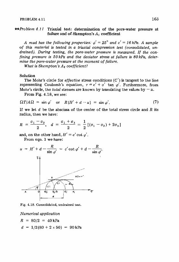
P R 0 B L E M 4 . i l 163
trkProblem 4.11 Triaxial tes t : determinat ion o f the pore-water pressure a t failure and o f S k e m p t o n ' s ^ l f coefficient
A mud has the following properties: ö = 25° and c = 16kPa. A sample of this material is tested in a triaxial compression test (consolidated, un-drained). During testing, the pore-water pressure is measured. If the con-fining pressure is 50kPa and the deviator stress at failure is 80kPa, deter-mine the pore-water pressure at the moment of failure.
What is Skempton 's Af coefficient?
The Mohr's circle for effective stress condi t ions ( C ' ) is tangent to the line representing Coulomb ' s equat ion , r = c + σ' tan ö . Fur thermore , f rom Mohr's circle, the total stresses are known b y translating the values by — u.
F r o m Fig. 4 . 1 8 , we see :
If we let d be the abscissa of the center of the tota l stress circle and R its radius , then we have :
So lu t ion
ÙÔ/ÁÙ, = sin ö or R (Hf + d - u) = sin ö. ( Ό
and, on the other hand, Hr = c cot ö . F r o m eqn. 1 we have:
= ~ [ ( σ ι - σ 3 ) + 2 σ 3 ]
u — Ç' + d : , = c co t ö + d : sm ö sm ö
Æ
d
Fig. 4 .18. Consolidated, undrained test.
Numerical application
R = 8 0 / 2 = 4 0 k P a
d = 1 / 2 ( 8 0 + 2 x 5 0 ) = 9 0 k P a

1 6 4 PLASTICITY AND SHEAR STRENGTH
sin 2 5 ° = 0 . 4 2 3 , cot 2 5 ° 2 . 1 4 5
f rom which: u = 16 χ 2 . 1 4 5 + 9 0 - 4 0 / 0 . 4 2 3 = 2 9 . 7 kPa or : u - 3 0 k P a .
F o r a saturated sample , Β = 19 and S k e m p t o n ' s relation b e c o m e s :
Au = Aor + Á (Áσ 1 — Δ σ Γ ) .
In the s tandard triaxial t e s t :
AoY = 0 ( σ 3 = constant) and : Af = (Au/Ao x)f.
Before starting the compress ion , the soil sample is consol idated under a confining pressure of 50 kPa (Fig . 4 . 1 9 ) .
°3 = °3 = (<*i)o = (σ'ι)ο = 5 0 k P a ; u = 0 .
Consolidation stag e Compress ion s tag e
j(a,)o=<r3=50kPa |o"i-(o;)0+Aq
Draining
u =0
Fig. 4 .19.
Non - d r a i n i ng
u^O
Then the drainage tube is closed and the compress ion stage starts by applying a load , whereas σ 3 = 50 kPa remains constant . Therefore , we have:
Au = ut - 0 = 30 kPa
Aox = (ox )f - (ox ) 0 = (σ÷ - σ 3 ) 4- σ 3 - (σ÷ ) 0 = 8 0 + 50 - 50 = 8 0 kPa.
and finally: Af = 3 0 / 8 0 ^ 0 . 3 8 .
Note
This value for A{ corresponds to a saturated clay which is slightly over-consol idated (0 .3 < Af < 0 .7 after Leonards ) . This is a reasonable conclusion for a c = 16 kPa (for normally consol idated clay, c = 0 ) .
Summary of answers
u = 3 0 k P a ; At = 0 . 3 8 .
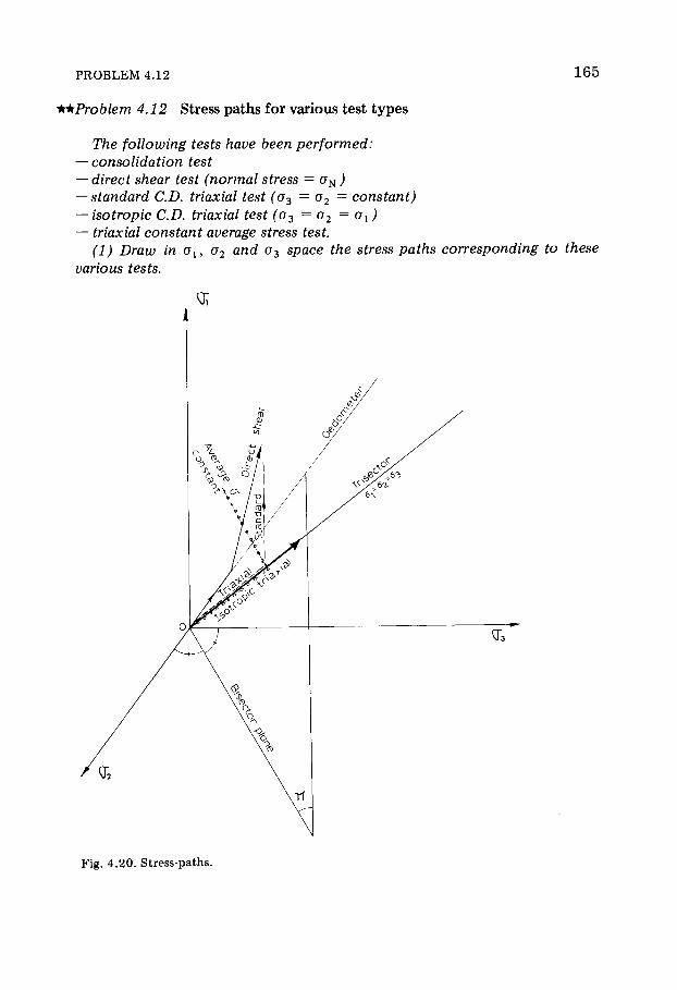
PROBLEM 4.12 1 6 5
irk Problem 4.12 Stress pa ths for various test t y p e s
The following tests have been performed: — consolidation test — direct shear test (normal stress = oN) — standard CD. triaxial test (o3 — o2 = constant) — isotropic CD. triaxial test (σ3 = σ2 = o1) — triaxial constant average stress test.
(1) Draw in σÚ9 σ2 and σ3 space the stress paths corresponding to these
various tests.
Fig. 4 .20. Stress-paths.

166 PLASTICITY AND SHEAR STRENGTH
(2) Draw in the p , q plane the stress paths of the tests. Let ñ and q be defined by: ñ = 1/3(ïë + σ 2 + o3), q = ï ÷ — σ2 = σ1 — σ 3 .
(3) Draw on the Mohr-diagram, the circles representing the states of stress at the beginning and end of each test. Determine for each condition, if the direction of the principal stress remains constant during the test.
So lut ion (1) Fig . 4 .20 gives the answer to part 1 , and in F ig . 4 . 2 1 each of the test
stress paths is shown in the bisector p lane π. (2 ) In the plane p , q the stress paths Eire: ñ = 1/3(σ1 4- σ 2 + σ 3 ) and q =
ox — σ 2 — Οχ — Οχ, f rom which Fig . 4 . 2 2 has been drawn. The only test wherein principal stresses undergo a rotat ion of orientat ion
during the test is the direct shear test (see Problem 4 . 1 0 ) . Figs . 4 . 2 3 , 4 .24
Fig. 4 .21 . Stress paths in bisector plane π.
Fig. 4 .22. Stress paths in plane p, q.

PROBLEM 4.12 167
S t a r t
Fig. 4 .23 . Mohr's circles for the start and the end of the direct shear test.
S t a r t
Fig. 4 .24. Mohr's circle for the start and end conditions of the consolidation test.
and 4 . 2 5 present the Mohr's circles at the start and end of the direct-shear test 5 the oedometer test and the various triaxial compress ion tests .
I s o t r o p ic t r i a x i al
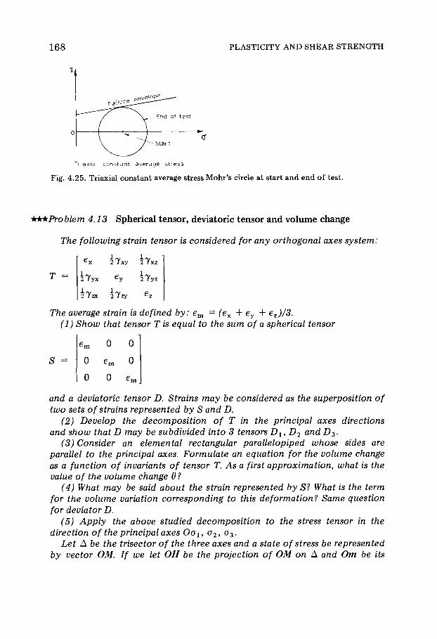
1 6 8 PLASTICITY AND SHEAR STRENGTH
Tr iax ial c o n s t a n t a v e r a g e s t r e s s
Fig. 4 .25. Triaxial constant average stress Mohr's circle at start and end of test.
+rkrkProblem 4.13 Spherical tensor , deviatoric tensor and volume change
The following strain tensor is considered for any orthogonal axes system:
Ô =
2 T x y
2 7 y x
2 Tz x 2 Tz y
2 ¾÷ æ
2 7 y z
The average strain is defined by: em = (ex + e y 4- ez)/3. (1) Show that tensor Ô is equal to the sum of a spherical tensor
m 0 0
0 e m 0
0 0
and a deviatoric tensor D. Strains may be considered as the superposition of two sets of strains represented by S and D.
(2) Develop the decomposition of Ô in the principal axes directions and show thatD may be subdivided into 3 tensorsDlt D2 andD3.
(3) Consider an elemental rectangular parallelopiped whose sides are parallel to the principal axes. Formulate an equation for the volume change as a function of invariants of tensor T. As a first approximation, what is the value of the volume change θ ?
(4) What may be said about the strain represented by S? What is the term for the volume variation corresponding to this deformation? Same question for deviator D.
(5) Apply the above studied decomposition to the stress tensor in the direction of the principal axes Oox, σ 2, σ 3.
Let Δ be the trisector of the three axes and a state of stress be represented by vector OM. If we let OH be the projection of OM on Δ and Om be its

PROBLEM 4.13 1 6 9
projection on plane (II), perpendicular to Δ at 0, analyze the decomposition
OM = OH+Om.
So lut ion (1 ) We get immediate ly :
D =
2 e x e y e z
2Ty x
2Tx y
2 e y e x e z
έΎζχ
Ô = S + D
(2 ) F o r the principal a x e s :
2 e j - e 2 - e 3
2 7z y
D =
3
0 2 e ,
3
0
S =
e j + e 2 + e 3
3
0
0
ei + e 2 + e 3
3
0
2 Txz
2 7y z
2 β Ζ â ÷ 6y
0
ο
2 e ,
Fur thermore , it can be s ta ted that : D — D1 + D2 + D3
with:
r e i - e 2
3
0
0
0 0
e , — e , 0
3
0 0

1 7 0 PLASTICITY AND SHEAR STRENGTH
0 0
o — — -
3
0 0
0
0
3
0
0
0
0
0
(3 ) The elemental rectangular paral lelopiped has sides AX, AY and AZ which coincide with the principal axes (see F ig . 4 . 2 6 ) . After strains occur , the volume remains rectangular. Then , its sides have the following dimen-s ions : AX(1 + e t ) , AY(1 + e2), AZ(1 + e3) and its vo lume b e c o m e s : V2 = AXAYAZ(1 + εΟίΙ + e2)(l + e3).
The relative volume change θ, i s :
θ AV = V2 - Vt = AXAYAZjl + ex)(l + e2)(l + e3)
AXAYAZ V Vi
or, by simplifying the equat ion :
θ = ex + e2 + e 3 + 6 ^ 2 + e 2 e 3 + e3e1 + e1e2e3
the quantit ies 1ã = ex + e2 + e 3 , I2 = e1e2 + e2e3 + e3el, I3 = e , e 2 e 3 are the invariants o f the strain tensor.
As a first-order approx imat ion , we have:
θ = AV/V^Ii = ej + e 2 + e 3 - e x + e y + e z .
(4) F r o m the above results , it can b e seen that the deformat ion represented by the tensor :
S =
0
corresponds t o a volume change of AV/V — 3 e m = e x + e y + e z , which is the volume change expression represented by tensor T . It is charac-terized by three equal axial strains and no shear strains. The L a m e quadrat ic is a sphere and is the reason why the tensor S is called spherical tensor.
The deviator D corresponds to a deformat ion where shear strains are
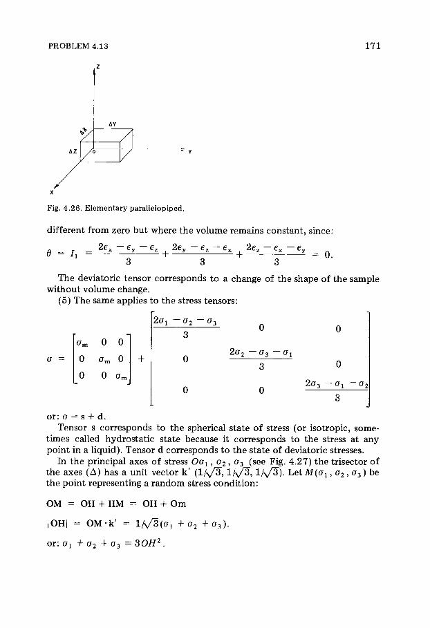
PROBLEM 4.13 1 7 1
ζ
ÄÆ
Fig. 4 .26. Elementary parallelopiped.
different f rom zero but where the vo lume remains constant , s ince:
θ = I, 2 e x - e y
+ 2 e v e7 —
+ 2e7
Z JL = 0 .
The deviatoric tensor corresponds to a change of the shape o f the sample without vo lume change.
(5 ) The same applies to the stress tensors :
Cm 0 0
a = 0 0 + 0 0
2σι — σï
3
0
0
0
2 σ 9
3
0 2 σ ,
0
or : σ = s + d. Tensor s corresponds to the spherical s tate of stress (or i sotropic , some-
t imes called hydrostat ic s tate because it corresponds to the stress at any point in a l iquid) . Tensor d corresponds to the state of deviatoric stresses.
In the principal axes of stress Ïïë ,_σ2» 03_ ( s e e Fig. 4 . 2 7 ) the trisector of the axes ( Δ ) has a unit vector k ' ( l / \ / 3 > 1 Α / 3> ^ / V3) - L e t Af ( a j , σ 2 , σ 3 ) be the point representing a r a n d o m stress condi t ion :
OM = OH + HM = OH + O m
|OH| = O M - k ' = lS/3(a1 + σ2 + σ 3 ) .
or : σ! + σ 2 + σ 3 = 30H2.
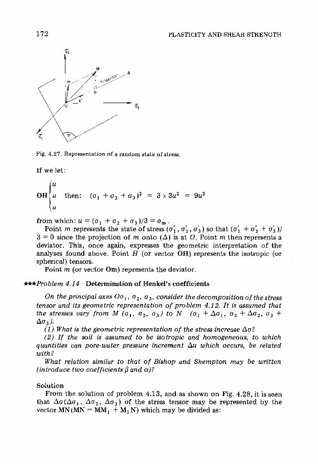
1 7 2 PLASTICITY AND SHEAR STRENGTH
<r3
Fig. 4.27. Representation of a random state of stress.
If we let :
u then : (σ! + σ 2 + σ 3 ) 2 = 3 χ 3u2 = 9u2
u
f rom which: u = (σ 2 + σ 2 + o3 )/3 = om . Point m represents the state of stress (σ[, σ 2 , σ'3) so that ( a i 4- σ 2 + σ 3 ) /
3 = 0 since the project ion of m onto ( Δ ) is at O. Point m then represents a deviator. This , once again, expresses the geometric interpretation of the analyses found above . Point Ç (or vector OH) represents the isotropic (or spherical) tensors .
Point m (or vector O m ) represents the deviator.
+**Problem 4.14 Determinat ion o f Henkel ' s coefficients
On the principal axes Ο σ 1 ? σ 2, σ 3, consider the decomposition of the stress tensor and its geometric representation of problem 4.12. It is assumed that the stresses vary from Ì (σë, σ 2, σ3) to Ν (σé + Áσ À9 σ2 + Δ σ 2 , σ 3 + Δσ3Λ
(1) What is the geometric representation of the stress increase Ao? (2) If the soil is assumed to be isotropic and homogeneous, to which
quantities can pore-water pressure increment Au which occurs, be related with?
What relation similar to that of Bishop and Skempton may be written (introduce two coefficients â and a)?
Solut ion F r o m the solution of problem 4 . 1 3 , and as shown on Fig . 4 . 2 8 , it is seen
that Δ σ ( Δ σ ΐ 5 Δ σ 2 , Δ σ 3 ) of the stress tensor m a y be represented by the vector M N ( M N = M M j + M x N ) which may be divided as :

PROBLEM 4.14 173
Fig. 4.28.
Δσΐ = variation of the isotropic part (vector MM1)
Δ σ ά = variation of the magni tude of the deviator Δ Φ = variation of the direction of the deviator j vector ( M N j ) .
(2 ) The soil is a s sumed to be isotropic and homogeneous . S o there are no reasons for Δ Φ to affect the variation in pore-water pressure Au that appears when stress increase Δ σ is appl ied t o the soil. Therefore , Au is related to Δσ^ and Áσ Ü. B y analogy to the formula of B i shop and S k e m p t o n , we may write :
Au = âÁσ { + áÁσ Ü, and Áσ { = (Áσ ÷ + Δ σ 2 + Δ σ 3 ) / 3 ,
we then have: â = Β.
L e t us n o w express Aod :
If we let the increases Δ σ 1 2 3 be sufficiently small, Áö is low and the variation of the deviator magni tude Δ σ ά m a y be as sumed to coincide with MXN.
The general express ion of the deviator magnitude may be derived then as shown below.
F o r the stress tensor ( σ , , σ 2 , σ 3 ) represented by Μ, we have:
σ÷ +σ2 + σ3 OH = χ / 3
The magni tude of the deviator is then :
HP 2 — OP2 - OH2 σ2+σ22+ o\ {σú + σ 2 + σ 3 ) 2
= \[o\ + a\ +a23 -{0^2 +σ2σ3 +0^^)}

1 7 4 PLASTICITY AND SHEAR STRENGTH
but :
(o2 -σ3)2 + (σ 3 - σ÷ )2 + (ot - σ 2 ) 2
= 2[σ\ 4- ï\ 4- σ | — - σ 2 σ 3 — a 3 a j
f rom which:
HP = W(°2 -O3)2 + ( σ 3 -oxY +(σ÷ ~o2f.
Let us apply the results to the stress increment vector M N :
M i N = W ( A a 2 ~Ao3y 4- ( Δ σ 3 - Δ σ ^ 2 + ( Δ σ ! ~ Δ σ 2 ) 2 .
if the increments Δ σ 1 } 2, 3 a r e small, then we can write :
Au = âÁσ ß 4- W(&°2 ~ Δ σ 3 ) 2 + ( Δ σ 3 - Δ σ ^ 2 + ( Δ σ χ ~ Δ σ 2 ) 2 .
This is the Henkel relation, which is a generalized form of that o f Bishop and S k e m p t o n .
+rk*Problem 4.15 Coefficients of Henkel. Compar i son o f two triaxial tests
A saturated clay is tested in two triaxial compression devices. Both tests are undrained and have the following characteristics: — in one test, the confining pressure is constant throughout the test and the axial load is increased until failure occurs (standard triaxial test); — in the other test, the axial stress is kept constant and the confining press-ure is increased until failure occurs.
Compare the variations of pore-water pressure occurring during the two types of testing. Use the Henkel coefficients. What is the conclusion?
So lut ion : In the first test , we have: Δ σ 2 = Δ σ 3 = 0, Áσ ÷ = oL — σ Γ.
Henkel 's equat ion (see problem 4 .14 ) gives:
Δ σ ι + Δ σ 2 4- Δ σ 3 Au = â - - - - -
H 3
4- a í ( Δ σ χ - Δ σ 2 ) 2 + ( Δ σ 2 - Δ σ 3 ) 2 + ( Δ σ 3 - Δ σ ! ) 2
from which ( 0 = 1 , for saturated c l ay ) : oh — a r
Au = h a \ / 2 ( a L — σ Γ)
3
or:
Au = (0,-0^(1/3 +ay/2). (1)
In the second test : Δ σ ! = Δ σ 2 = a L — σ Γ, Δ σ 3 = 0 .
Henkel 's equat ion here gives:
PROBLEM 4.16 1 7 5
Au = 2 ( a L - a r )
+ ay/2 ( a L - σΓ) 3
or: Au = ( a L - a r ) ( 2 / 3 -hay/2).
F o r the triaxial compress ion test at constant axial stress the confining pressure increases result in a higher pore-water pressure than in the standard triaxial test .
***Problem 4.16 Influence of loading condi t ion on the behavior of a soil. B i shop and S k e m p t o n ' s coefficients
Consider an elemental volume AV of a saturated soil in situ. Assume that the loading conditions are such that the soil is in a plane strain state (usual assumption made in soil mechanics). Within the range of deformations being considered here, the soil structure may be assumed to behave elastically with a Young's modulus of Ε and Poisson's ratio v.
(1) Find the relation between the principal stresses σ 1 ? σ 2, and o3 which express the plane-strain condition.
(2) Find the "pseudo" bulk modulus which relates the volume change to the variation of the average stress of σ1 and o3.
(3) What may be concluded about Bishop and Skempton's parameters?
(1) F r o m elasticity theory , disregarding the second-order terms, we can write:
AV/V=e 1 + e2 + e 3 .
For plane-strain condit ion, we have e 2 = 0 .
F r o m the generalized Hooke ' s equat ion , we have:
e 2 = σ2/Ε-(í/Ε)(σ1 + σ 3 ) .
But since the plane-strain condit ion is that e 2 = 0 we can write:
o2 = ñ(σ÷ + σ 3 ) (1)
(2 ) AV/V = et + e 2 + e 3 = ex + e 3 since e 2 = 0. Fur thermore :
So lut ion
AV/V = (σ÷ -ôσ3)/Ε-(í/Ε)(2σ2+σ1 + σ 3 )
from which:
AV/V = (2σðé/Ε)-(í/Ε)[σ1 +2u(0l + σ 3 ) + σ 3 ]
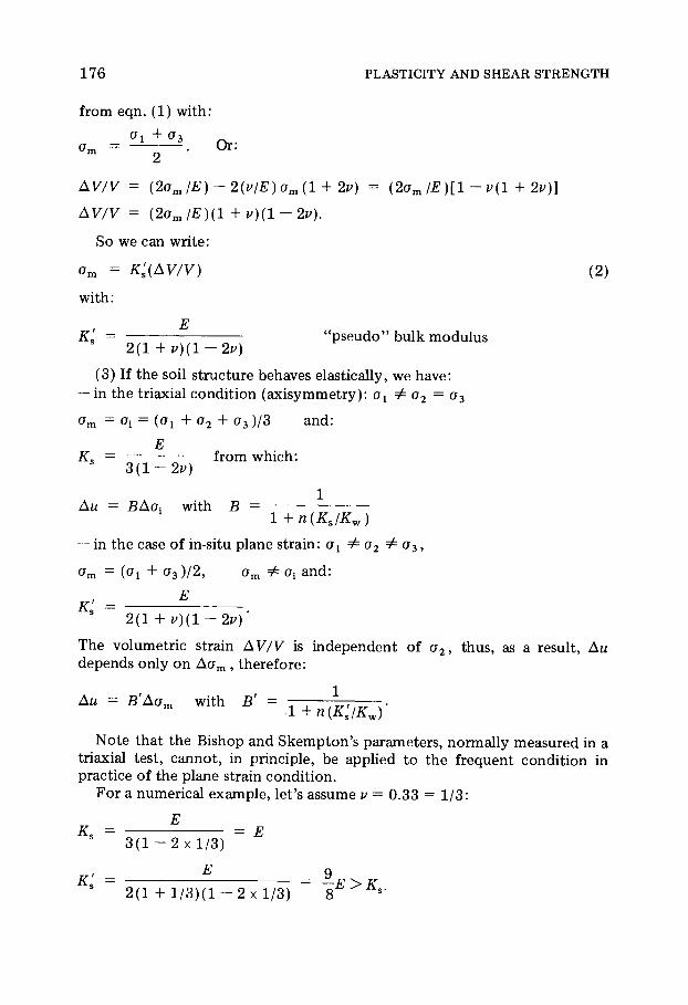
176 PLASTICITY AND SHEAR STRENGTH
from eqn. (1) with:
om = - ã - · Or.
AV/V = (2om/E)-2(v/E)om(l + 2v) = (2om /E)[l - v(l + 2v)}
AV/V = (2amIE)(l + p)(l-2v).
S o we can write:
om = K'S{AV/V) (2 )
with:
Ε
Kl = " p s e u d o " bulk modulus 2 ( 1 + ι > ) ( 1 - 2 ι ; )
(3 ) If the soil structure behaves elastically, we have: — in the triaxial condit ion ( ax i symmetry ) : σ1 Ö σ2 = o3
°m = °i = (°i + °2 + °3 )/3 and :
Ε Ê\ = f rom which:
3 ( 1 ~2v)
ι Au = ΒÁσ÷ with Β l + n(KJKw)
— in the case of in-situ plane strain: σ÷ Ö σ2 Ö σ 3 ,
m = (σ1 4- σ 3) / 2 , om Ö σ{ and :
2 ( 1 + í)(1 ~2í)'
The volumetric strain AV/V is independent of σ 2 , thus, as a result, Au depends only on Aom , therefore :
Au = BrAom with B' = l + n « / X w )
Note that the Bishop and S k e m p t o n ' s parameters , normally measured in a triaxial test, cannot , in principle, be applied to the frequent condit ion in practice of the plane strain condit ion.
F o r a numerical example , let 's a s sume í = 0 .33 = 1/3:
Ε Kc = = Ε

PROBLEM 4.17 177
Thus for the plane strain condit ion, usually found in-situ, the soil would deform less than it does in the triaxial test . On the other hand, the values of Ks and Ê are relatively close for the usual values of v. This justifies the use of Bi shop and Skempton ' s coefficients in plane strain problems and besides, the a s sumpt ion that the soil structure behaves elastically, is only an approxi-mat ion of real condit ions .
+++Problem 4.17 Measurement of the coefficient of earth pressure at rest K0
using a triaxial device
A saturated clay sample is recovered from a depth of 12 m. Its unit weight is 19kN/m 3. The pore-water pressure measured with a piezometer at that depth was 110kPa. The Atterberg limits of the clay are: w h = 52%, w p = 17%.
The sample is tested in a triaxial compression test. Drainage is allowed during compression and zero radial deformation conditions are maintained by adjusting the confining pressure ox and the axial load σë. When or reaches a value of 50kPa, the deviator stress is 68kPa. Calculate the coefficient of earth pressure at rest, K0. Does this value appear acceptable, knowing that the clay is normally consolidated and that a consolidated drained test yielded values of ö =20° and Af = 1.1.? What is your estimate of the apparent cohesion for this soil?
Solut ion Since no radial deformat ion is al lowed during testing, the sample is in
the same condit ion in the lab and in situ, provided that the same stresses are applied. The test is a drained one , then u = 0. Therefore o\ = ox and ofT = ot.
F o r a ; = 5 0 k P a , we have a l - a i = 6 8 k P a or o\ = 6 8 4- 50 = 1 1 8 kPa.
The effective vertical stress in situ is :
tfv = JsatH-u = 1 9 x 1 2 - 1 1 0 = 1 1 8 kPa. S ince the stress condit ions in the test and in situ are the s ame : o'r — K0o[, f rom which K0 = σ'ô/σ\ = 0 . 5 0 / 1 . 1 8 ~ 0 . 4 2 .
We know that for a normally consol idated clay (c = 0) the parameters c u , oc, ö , KQ and Af are not independent , but are related by the following equat ion :
c_± = sin y[Kn+At(l-K0)]
σ ; l + sin<p'(2A,
Therefore :
c u _ sin 2 0 ° ( 0 . 4 2 + 1.1 ÷ 0 .58 ) _
σÀ ~ 1 + sin 2 0 ° ( 2 x 1 . 1 - 1 ) ~
1 7 8 PLASTICITY AND SHEAR STRENGTH
Skerxipton has given a good correlation between the ratio cu/o'v and the plasticity index of a clay, Ip :
^7 = 0 .11 + 0 .37 J p
σ ν
For this p rob lem: Ip = w h — w p = 0 .52 — 0 .17 = 0 . 3 5 . Therefore : cv/o'y = 0 .11 + 0 .37 χ 0 .35 - 0 .24 .
The agreement between the two results is good . Taking the average of the two values, 0 . 2 5 , we have: c u = 0 .25 χ 1 1 8 — 3 0 kPa.
Summary of answers
K0 = 0 . 4 2 ; c u = 3 0 k P a .
irkrkProblem 4.18 Stress paths applied on a soil e lement during the construct ion of an earth dam
It is necessary for the design of a clay core earth dam to specify tests on soil samples which would give representative values for the behavior of the clay core not only during construction but also during filling of the reser-voir and under rapid drawdown conditions. The clay core would be com-pacted in place at a moisture content close to the optimum moisture as determined by the Proctor test where the effective vertical compaction pressure is 400 kPa. At optimum, the clay exhibits yh = 18 kN/m 3 and, when saturated, yS3Lt = 20 kN/m 3.
When the reservoir is filled, pore-water pressures at two locations (1 and 2) are measured: ux — 30 kPa and u2 — 340 kPa.
(1) Determine the stress history at points 1 and 2 (Fig. 4.29). Draw the stress path in the principal effective stress σ\, o2, o'3 space. Draw the stress path in the plane p, q. Find in each case if the clay is overconsolidated or normally consolidated.
(2) Determine also the test procedures to subject the clay sample in the lab to a stress path similar to that it would undergo in the dam.
Fig. 4 .29

PROBLEM 4.18 1 7 9
Solut ion (1) Stress history (a) During compaction o\ = o\c = 4 0 0 kPa.
If KQ is the coefficient of earth pressure at rest, we have σ 2 — K0o'lc = o3. The stress tensor is complete ly defined by σ 2 , σ'3 in the horizontal plane, o\ being vertical. Therefore : P = h(o\ + o'2 + o'3)=l3o\{l + 2K0),
t t t t * i t ôô- \
q = σ÷ — σ2 = σë — σ3 = σë(1 —Ê0). (b) At the end of construction. Assume that construction progress was
sufficiently slow to allow for the full diss ipation o f pore-water pressures : o'i = 7hZ,
o\ = o3 = K0yhz, where æ is the depth from the crest of the d a m .
ñ = ^(1 + 2K0) = 2 | - ( 1 + 2 K 0 ) ,
q = o\ -o2 = o\ -o'3 = yhz(l-K 0).
The soil e lement at locat ion 1 is overconsol idated because at the end of construct ion, the vertical stress is o\ = 1 8 0 kPa and it was previously sub-jected to a compact ion pressure of 4 0 0 kPa. The soil e lement at locat ion 2 is normally consol idated since at the end of construct ion, it would experi-ence an overburden pressure of = 1 4 4 0 kPa.
(c) Filling of the reservoir. Seepage occurs through the core . At each of the two locations there will be saturation condit ion and pore-water pres-sure u.
We have: o\ = ysat (æ ~ u) and σ 2 = σ3 = K0ysat (æ - u). At locat ion 1, the clay will be overconsol idated because o\ = 2 0 0 — 30 =
1 7 0 kPa. At locat ion 2, the clay is still overconsol idated because the overburden
effective stress is o\ = 1 6 0 0 — 3 4 0 = 1 2 6 0 kPa whereas at the end of con-struction, σ\ = 1 4 4 0 kPa.
(d) Rapid drawdown. The seepage in the core reverses its direction after drawdown. The pore-water pressure decreases slowly with t ime. At the start of the rapid drawdown, the stress condit ions are the same as those of the filling of the reservoir, then, as the pore-water pressure decreases , the ef-fective stress increases and when u = 0, then: o'i = Tsa t* = 2 0 0 kPa, o2 =o3 =K0ysat-z = 1 6 0 0 kPa.
At locat ion 1, the clay is overconsol idated and at locat ion 2 it is normally consol idated. The various stress paths are presented in Figs . 4 .30 and 4 . 3 1 .
(2) Test procedures to be used in the laboratory. The mos t versatile equipment to reproduce the stress condit ions is that of the triaxial com-pression test .
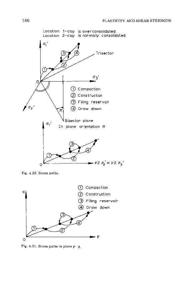
1 8 0 PLASTICITY AND SHEAR STRENGTH
(Ô) Compaction
(?) Construction
(3) Filling reservoir
(4) Draw down
Fig. 4 .31 . Stress paths in plane p—q.
Location 1-clay is over consolidated Location 2-clay is normally consolidated
(?) Compaction (2) Construction (5) Filling reservoir (4) Draw down
Bisector plane plane orientation
Fig. 4.30. Stress paths.
Trisector

PROBLEM 4.18 1 8 1
(a) For compaction conditions. The sample should be anisotropically consol idated (open drainage) under the effective load of o\ = 4 0 0 kPa, σ2 = σ3 = K0ol.
(b) During construction. The stress tensor of consol idat ion should be increased to the following values:
σ'é = 7hZ
°2 = o'3 = K0yhz
Depending on the locat ion of the sample , there will either be an increase or a decrease o f stress. All variation is done with drainage.
(c) Filling of the reservoir. Then drainage is no more allowed and pore-water pressure u is applied. Seepage is caused to occur in the sample in order to saturate it completely (this is very difficult to do in practice and very t ime consuming) . F o r the filling condit ion, the reproduct ion in the lab of the field condit ion leaves something to be desired, because in the dam core seepage is not interrupted.
(d) Drawdown. The drainage is once again open and the pore-water pressure al lowed to dissipate s lowly.
Note
The various stress paths a s sume that the relation o'3 = K0o\ is always true and that K0 remains constant . This is an approx imat ion which is mos t likely not fully representative of the complex actual field condit ions .

1 8 3
Chapter 5
P L A S T I C E Q U I L I B R I U M
**Problem 5.1 T h e po le o f Mohr ' s circle
In a two-dimensional space,
(l)show that Mohr's circle does not sufficiently define the stress con-ditions at a point in a continuous mass;
(2) assume that the stress tensor at a point A in a continuous mass is known and defined by the following data: Mohr's circle and a stress vector f acting on a small faceRR* in direction Δ . Let Ì be the point on Mohr's circle representing f, and m be the symmetrical point of Ì with respect to the principal stress axis, Oo. From m, a parallel line to the Δ direction is drawn which crosses Mohr's circle at a point P. Show that when the face RRr
rotates about A, point Ρ remains fixed. This point is called the pole of the Mohr's circle.
(3) Show that, knowing the pole location enables the determination of the orientation of a face for a given stress vector, and, inversely, the stress vector for a given orientation of the face. Apply this method to find the orientation of the principal stresses.
(1) T h e Mohr's circle only gives the magnitude of the principal stresses, but does not define their orientation in space . F o r any given Mohr's circle, several equal L a m e ' s ellipses of various orientations (Fig . 5 .2 ) .
(2 ) L e t the small face RRf (F ig . 5 .3) be rota ted counter-clockwise through an angle a. When it reaches the orientation QQ', the stress f', represented by M' on Mohr's circle, is known to act . F r o m the propert ies of Mohr's circle,
(Ä)
Fig. 5 .1 .
So lut ion
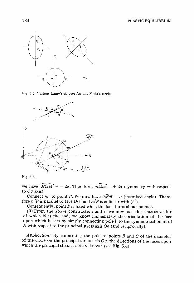
184 PLASTIC EQUILIBRIUM
Fig. 5.2. Various Lame's ellipses for one Mohr's circle.
Fig. 5.3.
we have: Μ Ω Μ ' = — 2a. Therefore : rafZm' = 4- 2a ( symmetry with respect to Ï ï ax i s ) .
Connect m to point P. We now have fnPm' = a ( inscribed angle). There-fore m'P is parallel to face QQ' and m'P is colinear with (δ ' ) .
Consequently , point Ρ is f ixed when the face turns about point A. ( 3 ) F r o m the above construct ion and if we now consider a stress vector
of which Ν is the end, we know immediately the orientation of the face upon which it acts by simply connecting pole Ρ to the symmetrical point of Ν with respect to the principal stress axis Oo (and reciprocal ly) .
Application: By connecting the pole to points Β and C of the diameter of the circle on the principal stress axis Οσ, the directions of the faces upon which the principal stresses act are known (see Fig. 5 . 4 ) .

PROBLEM 5.2 1 8 5
D i r e c t i o n o f m a j o r p r i n c i p a l s t r e s s
D i r e c t i o n o f m i n o r p r i n c i p a l s t r e s s
( o r d i r e c t i o n of f a ce u p o n w h i c h t h e m a j o r s t r e s s a c t s )
Fig. 5.4.
**Problem 5.2 L imi t equil ibriu m of a granular, semi-infinit e b o d y
Let us assume a point in a granular, semi-infinite mass in a state of limit equilibrium. Show that if a stress vector is known for the face of a given orientation, two Mohr's circles may be constructed. What conditions do these two circles represent? Find also the orientation of the faces upon which the stress is the least favorable (corresponding to the limit stress vectors).
The propert ies of every circle meeting the above condit ions are : — the center is on the axis Oo; — it mus t go through point M; — it mus t be tangent to the failure envelope (therefore to two lines D and D' which are symmetr ica l with respect to Oo) (see Fig. 5 .5 ) .
The geometric solut ion shows that there are two circles which satisfy the above condit ions .
The construction of the circles is done in the following manner (see Figs. 5 .5 . and 5 .6 ) .
Solut ion
D
Ï
D'
Fig. 5.5.
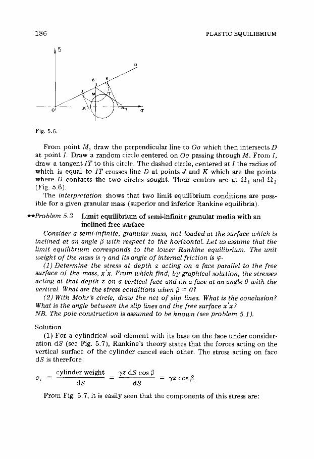
186 PLASTIC EQUILIBRIUM
Fig . 5.6 .
From point M, draw the perpendicular line to Oo which then intersects D at point / . Draw a random circle centered on Oo passing through M. F r o m / , draw a tangent IT to this circle. The dashed circle, centered at J the radius of which is equal to IT crosses line D at points J and Ê which are the points where D contacts the two circles sought. Their centers are at Ù÷ and Ω 2
(Fig . 5 .6) . The interpretation shows that two limit equilibrium condit ions are poss-
ible for a given granular mass (superior and inferior Rankine equilibria) .
++Problem 5.3 L imit equilibrium of semi-infinite granular media with an inclined free surface
Consider a semi-infinite, granular mass, not loaded at the surface which is inclined at an angle â with respect to the horizontal. Let us assume that the limit equilibrium corresponds to the lower Rankine equilibrium. The unit weight of the mass is y and its angle of internal friction is ö.
(1) Determine the stress at depth æ acting on a face parallel to the free surface of the mass, x'x. From which find, by graphical solution, the stresses acting at that depth æ on a vertical face and on a face at an angle θ with the vertical. What are the stress conditions when â = 0?
(2) With Mohr's circle, draw the net of slip lines. What is the conclusion? What is the angle between the slip lines and the free surface x'x? NB. The pole construction is assumed to be known (see problem 5.1).
Solution (1) For a cylindrical soil e lement with its base on the face under consider-
ation dS (see Fig. 5 .7 ) , Rankine 's theory states that the forces acting on the vertical surface of the cylinder cancel each other. The stress acting on face dS is therefore:
cylinder weight yz dS cos â oy = = = yz cos β.
dS dS
F r o m Fig. 5 .7, it is easily seen that the component s of this stress are :

PROBLEM 5.3 187
c = o
ζ
Fig. 5.7.
j σ = yz c o s 2 â
{ ô = yz cos â sin â.
Mohr's circle corresponding to this condit ion is drawn in Fig. 5 .8 . It goes through point M, which is the end of the stress vector σ ν and it is tangent to the failure envelope (Coulomb' s lines) since the soil mass is at limit equi-l ibrium.
It was shown in problem 5 .2 . that two circles satisfy the condit ions . Since it is a s sumed that the soil mass is at the lower Rankine limit equilib-rium, the circle representing the stresses is the smaller of the two. F r o m the pole construct ion (see problem 5 .1) we know the stress vectors acting on the vertical face OM' and on the face making an angle θ with the vertical O M " . Note that the point M' is the same as the pole of Mohr's circle.
ο cr
Fig. 5.8.
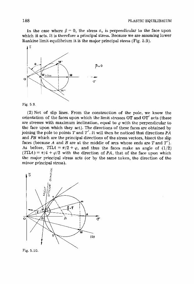
1 8 8 PLASTIC EQUILIBRIUM
In the ease where â = 0, the stress σ ν is perpendicular to the face u p o n which it acts . It is therefore a principal stress. Because we are assuming lower Rankine limit equilibrium it is the major principal stress (Fig. 5 .9 ) .
é Ε
θ >
M'(POLE)
Ì"
" × Ρ
)
I ^
= 0
Fig. 5.9.
(2) Net of slip lines. F r o m the construct ion of the po le , we know the orientation of the faces upon which the limit stresses O T and O T ' acts (these are stresses with m a x i m u m inclination, equal to ö with the perpendicular to the face upon which they ac t ) . The directions of these faces are obta ined by joining the pole to points Τ and T ' . It will then be not iced that directions PA and PB which are the principal directions of the stress vectors , bisect the slip faces (because A and Β are at the middle of arcs whose ends are Γ and Ô'). As before , ÔÙÁ = ð/2 + ö, and thus the faces m a k e an angle of ( 1 /2 ) ( Τ Ω Α ) = π/4 4- ö/2 with the direction of PA, that of the face u p o n which the major principal stress acts (or by the same token, the direction of the minor principal stress) .
c Ï
Fig. 5.10.

PROBLEM 5.3 1 8 9
When considering the effect of depth 2 , po int Ì describes a straight line D inclined at â on Οσ, since this angle remains constant . The Mohr 's circle remains homothet ica l and the direction of the slip faces remains the same. Therefore the slip lines, which are the envelops of slip faces , are straight lines with an angle of ± (π/4 4- ö/2) with the direction of the minor principal stress.
It should be not iced that it is not poss ible to have a condit ion wherein â > ö because an equilibrium may not exist in such condit ions .
L e t us now find the angle between the vertical and the direction of the minor principal stress. Consider angles ΟΡΩ a n d P Ω A (Fig . 5 . 1 1 ) . In triangle Ο Ρ Ω , we have : ùâ = â + 2 γ , and in triangle Ρ Ω Α , we have: a = ð — 2 γ , f rom which a = ð — (ùâ — â).
T o define angle ω^ , we have: sin ùâ = but sin â = Ω / / / Ο Ω and sin ö = Λ / Ο Ω . Therefore : sin ùâ = sin |3/sin ö, ùâ = arcsin (sin j3/sin<£>).
4 *
Fig. 5.12.
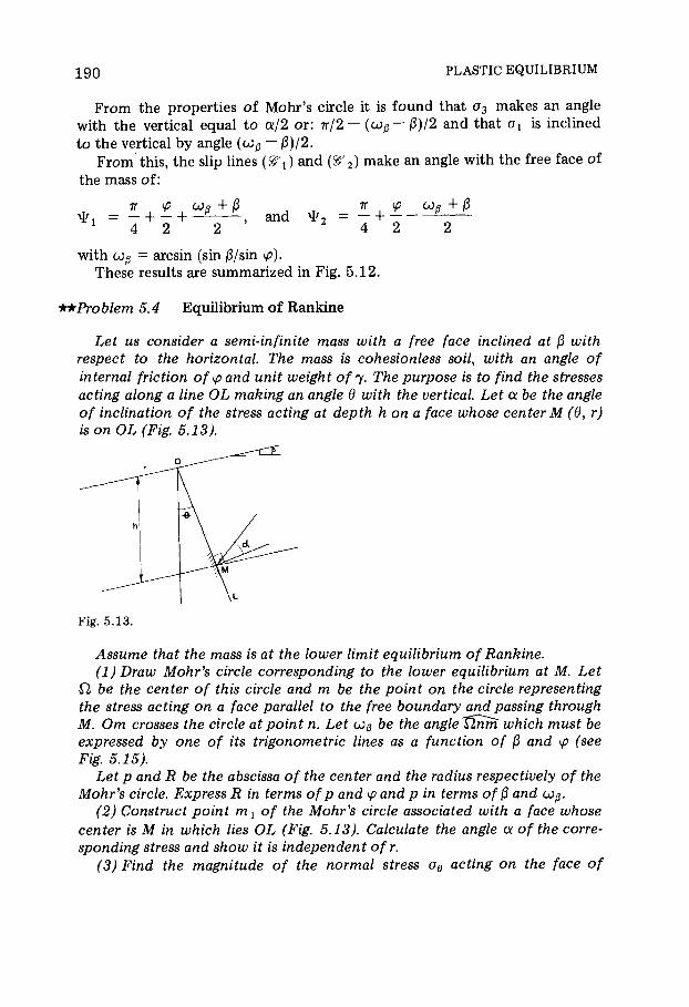
1 9 0 PLASTIC EQUILIBRIUM
F r o m the propert ies of Mohr's circle it is found that σ 3 makes an angle with the vertical equal to a/2 or : π/2 — (ω^ — j3)/2 and that σ1 is inclined to the vertical by angle (ùâ — â)/2.
F r o m this, the slip lines and ( & 2 ) m a k e an angle with the free face of the mass of :
ð ö ùâ +â ð ö ùâ + â ψ = — + — + — , and Ψ 2 = — 4-
1 4 2 2 2 4 2 2 with ùâ = arcsin (sin â/sin ö).
These results are summarized in Fig. 5 .12 .
**Problem 5.4 Equi l ibr ium o f Rank ine
Let us consider a semi-infinite mass with a free face inclined at â with respect to the horizontal. The mass is cohesionless soil, with an angle of internal friction of ö and unit weight of y. The purpose is to find the stresses acting along a line OL making an angle θ with the vertical. Let a be the angle of inclination of the stress acting at depth h on a face whose center Ì (θ, r) is on OL (Fig. 5.13).
Assume that the mass is at the lower limit equilibrium of Rankine. (1) Draw Mohr's circle corresponding to the lower equilibrium at M. Let
Ω be the center of this circle and m be the point on the circle representing the stress acting on a face parallel to the free boundary and passing through M. Om crosses the circle at point n. Let ùâ be the angleXlnrn which must be expressed by one of its trigonometric lines as a function of â and ö (see Fig. 5.15).
Let ñ and R be the abscissa of the center and the radius respectively of the Mohr's circle. Express R in terms of ñ and ö and ñ in terms of â and ùâ.
(2) Construct point m± of the Mohr's circle associated with a face whose center is Ì in which lies OL (Fig. 5.13). Calculate the angle a of the corre-sponding stress and show it is independent of r.
(3) Find the magnitude of the normal stress oQ acting on the face of
Fig . 5.13 .

PROBLEM 5.4 1 9 1
center Ì and direction OL. Show it is proportional to y and to r and that the equation σ0 = Kyr exists.
Write Ê as a function of 0, ft ö and of angle ùâ. What can be said about the stress distribution on segment OL?
So lut ion (1 ) T h e stress on face dS at Ì has a value o f (Fig . 5 . 1 4 ) :
df = weight o f cylinder yh ds cos â
ds ds yh cos â.
Fig. 5 .14.
Hence Mohr's circle passes through po int m , the coordinates of which are :
j yh c o s 2 â m
[yh cos]3 sin]3 (Fig. 5 .15 )
ô
I Lowe r Rankin e limi t / equ i libriu m
SI
Fig. 5.15
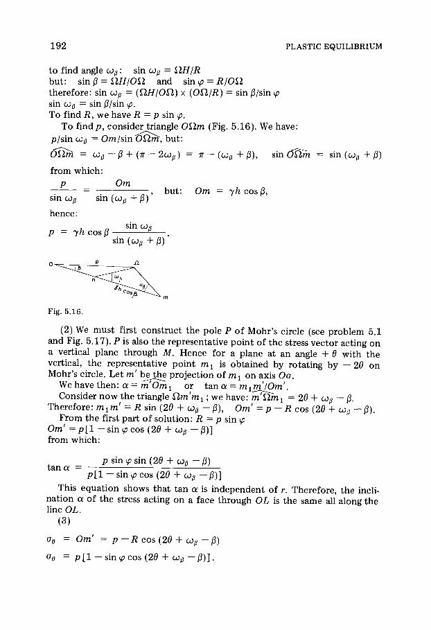
1 9 2 PLASTIC EQUILIBRIUM
to find angle ùâ: sin ùâ = ¿,Ç/R but : sin â = Ω ίΓ /ΟΩ and sin ö = i i / Ο Ω therefore : sin = (Ωϋί /ΟΩ) χ (ÏÙ,/R) = sin j3/sin γ? sin = sin â/sin ö.
To find R, we have Λ = ρ sin <£. T o find p , consider triangle ÏÙ,ôç (Fig . 5 . 1 6 ) . We have:
p / s in = Om/sint)£lm:, but :
Of2m = — â 4- (π — 2ùâ) = ð ~ (ùâ 4- â), sin üÙôç = sin(ùâ+â)
from which: ρ Om
- — _ —, but : Om = yh cos â, sm sin (ω^ 4- â) hence :
sin (JUR
ñ = yh cos ]3 sin (ùâ 4- 0)
Fig. 5.16.
(2) We mus t first construct the pole Ρ of Mohr's circle (see problem 5 .1 and Fig. 5 .17 ) . Ρ is also the representative po int o f the stress vector acting on a vertical plane through M. Hence for a plane at an angle 4- 0 with the vertical, the representative po int m1 is obta ined by rotating by — 2È on Mohr's circle. L e t m bej the project ion o f m t on axis Οσ.
We have then : a — m'Om1 or t an a = m1mJOmt. Consider now the triangle Q,m'ml; we have : mfilm1 = 2È + ùâ — β.
Therefore : mxm' = R sin (20 4- ùâ — â), Om' = ñ — R cos (2È 4- ùâ — â). F r o m the first part of so lut ion: R = ρ sin ö
Om' = p [ l — sin ö cos (20 4- ùâ — β) ] from which:
ρ sin sin (20 4- co^ —18 ) fall Q{ — "
p [ l — sin ö cos (20 4- — â)]
This equat ion shows that tan a is independent of r. Therefore, the incli-nat ion a o f the stress acting on a face through OL is the same all along the line O L .
(3)
oQ = Om' = ñ — R cos (20 4- ùâ — â)
ïθ = ρ [ 1 — sin ö cos (20 4- ùâ — â)].

PROBLEM 5.4
20/ rrv ι SI
Fig. 5.17.
Then, f rom the first part of the so lut ion :
sin ùâ
ñ = yh cos â — . s m (ω^ + â)
and from triangle ONM (Fig . 5 .18 ) we also have
r = h
sin (π/2 - â) sin [π - θ - (π/2 - â)]
r _ h
cos â cos (â —θ)
Fig. 5.18. Fig. 5 .19.

1 9 4 PLASTIC EQUILIBRIUM
from which:
h = r cos (â — θ)
COS â
Therefore we have: oi È = K*yr with:
Ê = cos (θ — â) sin ù â
sin (ùâ -f â) [1 — sin <p cos (20 + ùâ — â)].
The stress distr ibution along OL is linear (Fig . 5 .19 ) and t o summar ize : Rankine ' s equil ibrium is characterized b y :
— slip lines which are straight l ines ; — triangular stress distribution with constant inclination along a straight line through the mass .
+*+Problem 5.5 Plast icity; limit equil ibrium o f a weightless mass loaded a t the surface ; Prandtl corner
(See pole construct ion of problem 5.1)
(1) Study the limit equilibrium of a semi-infinite cohesionless mass having an angle of internal friction of ö, whose free surface is inclined at an angle â with the horizontal. It is subjected to a uniform vertical load of q (Fig. 5.20). What can be said about the stress tensor? Draw the slip lines. What happens when â = 0?
(2) Consider the same mass with a horizontal free surface and a point A at the surface. Assume that a uniform load p0 is applied to the surface along a line to the right of point A and a uniform load p2 is applied along the same line but to the left of point A. Assume that the mass is at limit equilibrium.
(a) Show that it could be assumed that there coexist two limit equilibria zones. What are they and what are the limit equilibria which could exist there? What relation must exist between p2 and p0 for these equilibria to exist? Show, considering the slip lines net, that this solution is not kine-matically possible.
mas s
ds
Fig. 5 .20.
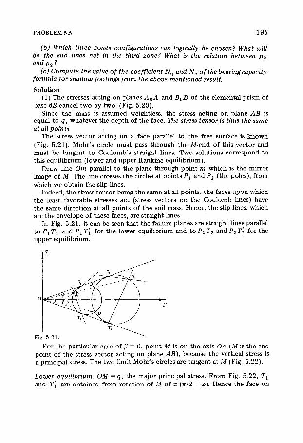
PROBLEM 5.5 1 9 5
(b) Which three zones configurations can logically be chosen? What will be the slip lines net in the third zone? What is the relation between p0
and p2 ? (c) Compute the value of the coefficient AT q and Nc of the bearing capacity
formula for shallow footings from the above mentioned result.
So lut ion (1) The stresses acting on planes A0A and B0B of the elemental prism of
base dS cancel two by two . (Fig . 5 . 2 0 ) . Since the mass is a s sumed weightless, the stress acting on plane AB is
equal to q, whatever the depth o f the face . The stress tensor is thus the same at all points.
The stress vector acting on a face parallel to the free surface is known (Fig. 5 . 2 1 ) . Mohr's circle mus t pass through the M-end of this vector and m u s t be tangent to Cou lomb ' s straight lines. T w o solut ions correspond to this equil ibrium (lower and upper Rankine equil ibrium).
Draw line Om parallel t o the plane through po int m which is the mirror image o f M. The line crosses the circles at points Pl and P2 ( the po le s ) , f rom which we obta in the slip lines.
Indeed, the stress tensor being the same at all po ints , the faces u p o n which the least favorable stresses act (stress vectors on the C o u l o m b lines) have the same direction at all points of the soil mass . Hence, the slip lines, which are the envelope o f these faces , are straight lines.
In Fig. 5 . 2 1 , it can be seen that the failure planes are straight lines parallel to Px T1 and Px T[ for the lower equilibrium and to P 2 T2 and P 2 T 2 for the upper equil ibrium.
F o r the particular case of â = 0 , po int Ì is on the axis Ïσ (M is the end point of the stress vector acting on plane AB), because the vertical stress is a principal stress. The two limit Mohr ' s circles are tangent at Ì (Fig . 5 . 2 2 ) .
Lower equilibrium. OM = q, the ma jor principal stress. F r o m Fig. 5 . 2 2 , T1
and T[ are obta ined f rom rotat ion of Ì o f ± (π/2 4- ö). Hence the face on
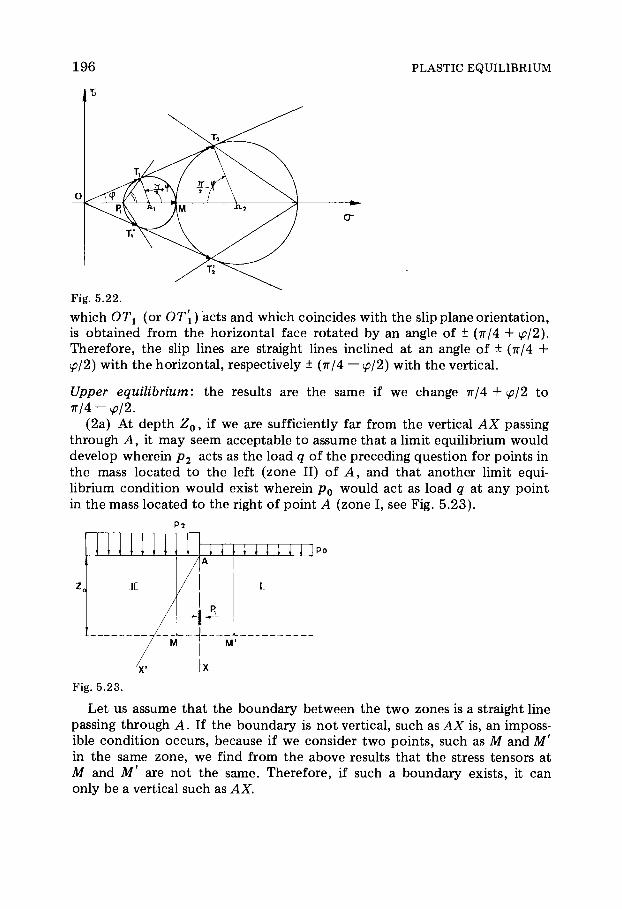
196 PLASTIC EQUILIBRIUM
Fig. 5.22.
which 0Ôë (or OT\) acts and which coincides with the slip plane orientat ion, is obta ined from the horizontal face rota ted by an angle of ± (π/4 4- ö/2). Therefore, the slip lines are straight lines inclined at an angle of ± (π/4 4-ö/2) with the horizontal , respectively ± (π/4 — ö/2) with the vertical.
Upper equilibrium: the results are the same if we change ð/4 + ö/2 to π/4 - ö/2.
(2a) At depth Z0, if we are sufficiently far f rom the vertical AX passing through A, it m a y seem acceptable to a s sume that a limit equilibrium would develop wherein p2 acts as the load q o f the preceding quest ion for points in the mass located to the left (zone II) of A, and that another limit equi-librium condit ion would exist wherein p0 would act as load q at any point in the mass located to the right o f point A (zone I, see Fig . 5 . 2 3 ) .
P2
t \ m i n i
i t
A
JL
X' X
Fig. 5 .23.
L e t us as sume that the boundary between the two zones is a straight line passing through A. If the boundary is not vertical, such as AX is, an imposs-ible condit ion occurs , because if we consider two points , such as Ì a n d M ' in the same zone, we find from the above results that the stress tensors at Ì and Mf are not the same . Therefore , if such a boundary exists , it can only be a vertical such as AX.

PROBLEM 5.5 1 9 7
In order for equilibrium to be realized, however, the stress acting on a vertical face through AX mus t be the same in the two zones . L e t px be that value. It is clear, that we mus t necessarily have p2 > P i > p 0 and that the two equil ibrium states are represented by two tangent circles (Fig . 5 . 2 4 ) .
Fig. 5.24.
We have already seen that for a limit equilibrium we have:
o3/o1 = t a n 2 (π/4 — ö/2) and σ1/σ3 = t a n 2 (π/4 4- ö/2).
That means in this case :
p2/Pl = úæç2(ð/4 + ö/2)
Po/Ρé = t a n 2 (π/4 -ö/2)
and, therefore :
p2/p0 = t a n 4 (π/4 + ö/2) (1)
Thus , for such a s tate to exist , p2 and p0 cannot have any value but mus t satisfy the relation (1 ) .
This scheme mus t also be kinematical ly acceptable , that is t o say, it mus t be compat ib le with the continuity of mass and its boundary condit ions .
P2 11111II Po
P 0 < P , < P 2
ZONE I
Pi < P2
Lowe r lin e e q u i l i b r i u m
Uppe r lin e equ'il i b r i u m
Fig. 5.25.

1 9 8 PLASTIC EQUILIBRIUM
F o r the case under considerat ion (see Fig. 5 . 2 5 ) , it is obvious that the failure planes do not have the same inclination with respect to the vertical. Line AX is a line of kinematic d i scont inui ty . * Besides , this line does not coincide with a slip line, then this scheme is not kinematical ly acceptable . We must therefore consider a three-zone sys tem.
(b) The simple solution which comes to mind in this context , is to intro-duce a third zone b o u n d e d by two straight lines passing through A which are slip lines, respectively AY and AZ, for each o f the limit equilibrium states . The second set of slip lines in the third zone must m a k e at any point M, an angle of (π/2 — ö) with the slip line of the first family, that is with the straight line AM (see Fig. 5 . 2 6 ) . But we know that the logarithmic spiral is a curve the tangent of which at any point makes a constant angle with the radius. Therefore , the two zones m a y be linked by a third zone containing logarithmic spirals with a pole at A and whose tangent makes an angle o f π/2 — ö with the radius .
This 3rd zone is called Prandtl 's corner. The slip lines are : —log spirals with a po le at A, — straight lines issuing from A.
P2
Fig. 5.26.
The 3-zone condit ion is kinematical ly acceptable . N o w , we mus t determine the relation between p0 and p2 with respect to stresses q2 and q1 acting on the faces through AZ and AY. For this purpose , we write that the prism ABD o f Fig. 5 .27 is in equil ibrium, by equating to zero the sum of the moment s acting on faces AB, BD and AD. The stresses on the port ion BD of the spiral act along the straight slip lines and pas s through point A. Their m o m e n t arm is zero. Stress q2 acts on face AB. Stress qa acts on face AD which makes an angle a with AY. S ince the mass is weightless, the stress distribution is uniform along AB and AD. The m o m e n t equilibrium with
•Along AX a segment stretches if in Zone I or shrinks if in Zone II.

PROBLEM 5.5 1 9 9
respect t o point A gives:
AB2
q2 cos ö = qa cos ö AD2
2 * 2
from which:
q* _ A& __ p g e 2 ( - g Q > t a n^
q2 ~ AD2 ~ p2 e 2 < ^ - e 0 ) t a n ^
If we let θ2 and θá be the polar angles corresponding to the radii o f AB and AD with respect to an arbitrary origin corresponding to a value p 0
o f the radius then : qa = ^ 2 e 2 (^ - ^ ) t a n = â 2 θ- 2 < * t a n *e
Fig. 5.27.
For the relation between q2 a n d p 2 , we have t o show that ρ 2 = p 2 tan ( π / 4 - ^ / 2 ) .
Let us draw Mohr's circle for point Β (F ig . 5 . 2 8 )
Fig. 5.28.
p2 = d + R R = d sin <p
q2 — d cos <p

2 0 0 PLASTIC EQUILIBRIUM
cos ö
1 4- sin ö
cos ö
1 + sin ö
sin ö 12
sin — h sin ^ 2
/π γ? 2 sin I cos
4 2
/ π <p 2 sin I — I — I cos
y4 2
sin ' π
sin I — 4
cos π / π <p
2 14 2 cos
= tan I
We finally get : qa = p2 tan (π/4 - öâ)^2á çö
By drawing Mohr's circle for po int C (Fig. 5 .29 ) a similar calculation as above gives: q1 = p0 tan (π/4 + ö/2). B u t : qx = q(a) = p2 t an (π/4 - ö/2) for a = π /2 . Hence p2 and p 0 are related by :
tan (π/4 + ö/2)âð%*çö
P 2 = P° tan (π/4 - ö/2) °* P* = P° tan (π/4 + ^ / 2 ) e — .
Fig. 5 .29.
fc^ Coefficients NQ and Nc of the bearing capacity formula for shallow footings. The above calculations E i re applicable to determine the depth factor Ë/q in the formula referred t o . The as sumpt ion is made that the foot ing does not alter the inclination of the failure lines. Under this condit ion the stress condit ion under a foot ing is as shown in Fig. 5 .30 .
The distr ibution p0 corresponds to the weight of the overburden above the level of the base of the foot ing x'x, therefore t o p 0 = yD.
We therefore have:
from which:
p2 = d/(l + sin ö) and
but :

PROBLEM 5. 5 2 0 1
F o r a cohesive soil with cohesion c, the uniform vertical f ictitious stress Ç = c cot ö is a s sumed to act at the free face of the weightless mass . The fictitious bearing capaci ty would b e : (q<x)' = qa+H and we will also have: (qd)f = Nq(H + yD) or : qd + c co t ö — iVq (yD + c cot ö) o r: Qd — jDNq + c cot ö(Ν^ — 1 ) and : qd = yDN^ + cNc with: Nc = cot ö(Ν(é — 1 ) .
Nc is the coefficient corresponding to the cohesion factor in the bearing capacity formula . The coefficient Ny can o f course not be calculated by this method since it mus t consider the weight o f the mass .
Note on the stress vector of zone III (Prandtl 's corner ) : When the radius
Fig . 5.31 .
from which:

2 0 2 PLASTIC EQUILIBRIUM
rotates through an angle a f rom AB, the direction of the stress q rotates through angle a, but since q makes an angle ö — which remains constant — with the radius, the principal directions also rotate by a. But at B, the major principal stress direction is vertical. Therefore, at D the direction of the major principal stress makes an angle a with the vertical. Lamp's ellipse rotates and the size of the axes decreases to go from ellipse 1 to ellipse 2 (see Fig. 5 .31 ) .
***Problem 5.6 L imi t equil ibrium o f a semi-infinite cohesive mas s with an inclined free surface
Refer to problem 5.3 and assume that the soil has a cohesion c. Two cases are then considered in analyzing slip lines, depending on the value of â. The inclination angle of the slip lines with the free surface x'x and the orientation of the asymptotes, if any, will be determined. (Refer to problem 5.1 for the construction to determine the pole of the Mohr's circle).
Solut ion (1) This problem is similar to problem 5 .3 , but a dist inction must be
made between real and fictitious stresses. Real stress at depth æ is : σ ν = yz cos â (Fig . 5 .7 ) . It is represented by vector OM of Mohr's diagram (Fig . 5 .32) and its com-
ponents are:
ï = yz c o s 2 â.
r — yz cos â sin â.
The fictitious stress, represented by vector O'M is:
σ' = Ç + yz c o s 2 â = c cot ö 4- yz c o s 2 â
ô = yz cos â sin â
therefore: \o'v\ = \Jo'2 4- r ' 2.
The pole is determined as above (see problem 5 .1 ) , f rom which the real and fictitious stresses (ΟΜ', O M " and O'M', O 'M" , respectively) , acting on a vertical face and an inclined face at angle θ, are determined (Fig . 5 .32 ) .
At the free surface, we have: real stress : σ ν = 0 , fictitious stress:
( f r
ï = σ ν
The fictitious stress is perpendicular to the free surface. The condit ion â = 0 , is represented in Fig. 5 .33 . In this case , the pole o f Mohr's circle is located on Oo. (2) Slip lines.
Mohr's diagram (Fig . 5 .34 ) shows that two condit ions exist depending on the value o f â:

PROBLEM 5.6 2 0 3
Fig. 5 .33 .
condit ion 1 : if â < ö, drawing Mohr 's circle corresponding t o the limit lower equilibrium o f Rankine is a lways poss ib le , condit ion 2 : if â > ö9 Mohr's circle can only be drawn if |σν | < ÏÔ'.
Therefore , the magnitude of the stress vector cannot exceed the limit value o f O T , otherwise the equil ibrium is not poss ib le . Hence there is a limit depth , æã, for which equilibrium exists (see Fig . 5 . 3 4 ) .
(a) Condition of â<ö (Fig. 5.35) T o determine the orientation o f the faces upon which the limit stresses
OT and O T ' act , the procedure is identical to the one in problem 5.3 . It will be noted however, that as æ varies, the Mohr's circles are n o longer similar because vector OM does not originate f rom the intersection of O' of Cou lomb ' s l ines. The orientation of the faces u p o n which the limit stresses act , varies with depth z. Therefore the slip envelopes are no longer straight lines. The net of the slip lines will then consist of two families of curves crossing at an angle π/2 + ö, because we have :
( Ω Τ ' , Ω Τ ) = 2(PT',PT)
( Ω Τ ' , Ω Τ ) = 2 ( Ω Α , Ω Τ ) = 2(ð/2 + ö).

2 0 4 PLASTIC EQUILIBRIUM
F r o m which: (ΡΤ' , PT) = π/2 + ö.
Asymptotic direction: whenever depth æ becomes infinite, Fig. 5 .35 shows that Ì tends toward infinite on line D. But , O'M = Η + OM and Ç remains finite, therefore OM O'M when æ - > ©ï . The a sympto te s t o the slip lines in the case o f a cohesive soil are the straight slip lines o f the cohesionless mass . When point Ì is at the surface, Mohr's circle is tangent at Ο to OT (Fig . 5 .36 ) . We then have:
(ΩΟ, Ω Τ ) = π(2 + ö)
(ΩΟ, Ω Τ ' ) = - ( π / 2 + ö).
Point Ο corresponds to the end of the stress vector O'O acting on the free surface. Therefore, f rom the classic property of Mohr's circle, the planes on which OT and O T ' act , are inclined to the s lope surface by angles of ± (π/4 + ö/2).
Summary: In the case of â < ö the failure lines belong t o t w o families of
a
b Fig. 5.34.
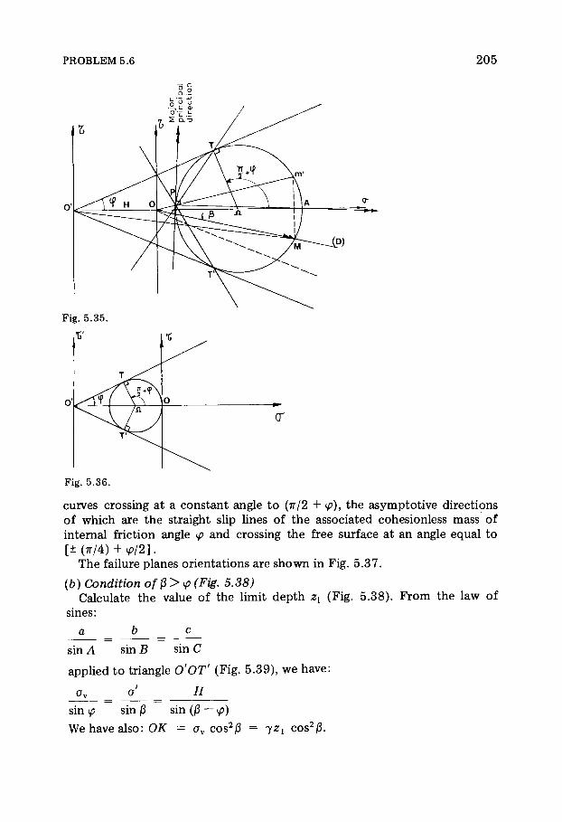
PROBLEM 5.6 2 0 5
Fig. 5.35.
0
σ
Fig. 5.36.
curves crossing at a constant angle to (π/2 + ö), the asymptot ive directions of which are the straight slip lines of the associated cohesionless mass of internal friction angle ö and crossing the free surface at an angle equal to [± (ð/4) + ö/2].
T h e failure planes orientat ions are shown in Fig . 5 .37 .
(6 ) Condition ïßâ>ö (Fig. 5.38)
Calculate the value of the limit depth zx (F ig . 5 . 3 8 ) . F r o m the law of sines:
a _ b _ c
sin A sin Β sin C
applied to triangle Ï'ÏÔ' (Fig . 5 . 3 9 ) , we have:
σ ν σ' Ç sin ö sin â sin (â — ö)
We have a l so : OK = σ ν cos2â = yz x cos2â.

2 0 6 PLASTIC EQUILIBRIUM
Fig . 5.38 .
Fig . 5.37 .
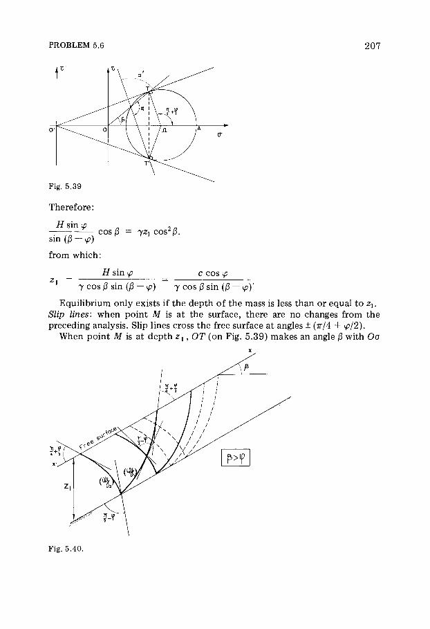
PROBLEM 5.6 207
r'
0' 0
TV
III 1a cr
Fig. 5.39
Therefore :
Ç sin ö n 0 _ — — c o s j 3 = yz x cos2 â. s i n (â - ö)
from which:
Ç sin ö c cos ö
z — = γ cos â sin (â —ö) y cos â sin (β — ö)'
Equil ibrium only exists if the depth of the mass is less than or equal to zY. Slip lines: when point Ì is at the surface, there are no changes from the preceding analysis . Slip lines cross the free surface at angles ± (π/4 + ö/2).
When point Ì is at depth zx, OT (on Fig. 5 .39) makes an angle â with Oo X
Fig. 5.40.

2 0 8 PLASTIC EQUILIBRIUM
and one of the two families of curves representing the slip lines is tangent to a line parallel t o the free surface at depth zx.
We also have : (ΩΓ, Ω Τ ' ) = 2a = 2 (π /2 + ö) = π + 2ö from which: a = π/2 4- ö and ïß = π — (π/2 + ö) = π/2 — <ρ.
The second family of curves is tangent to the line making an angle of π/2 — ö with the free surface. This result is readily observed since as before , the slip lines cross each other at an angle o f π/(2 — ö).
The shape of the net o f slip lines for the case â > ö is shown in Fig . 5 .40 .
**Problem 5.7 M a x i m u m height o f an excavat ion in cohesive soil
Find the maximum height of an unsupported vertical cut in a cohesive soil with a horizontal surface which supports no load. Let y, c and ö be the unit weight, cohesion and angle of internal friction respectively. For a numerical application, assume 7 = 20 k N / m 3 , c = 1 0 4 Pa, ö = 1 0 ° .
A t a point Ì at depth æ in the cut , the total vertical stress is equal to the weight of the overburden on a horizontal face through Ì (Fig. 5 . 4 1 ) . The total horizontal stress acting on the vertical face through Ì is zero since Ì is a t the free face of the cut.
L e t us find at what depth zl9 Mohr's circle becomes tangent to the failure envelope at the lower Rankine limit equilibrium (Fig . 5 .42 ) .
So lut ion
crv = £z
c
O '
cr
Fig. 5 .41 . Fig. 5 .42.
L e t R be the radius o f the circle, then:
from which: R(l — sin ö) = Ç sin ö = c · cot ø sin ö = c · cos ö but : R = o1/2 = yz x/2 f rom which:
PROBLEM 5.8 2 0 9
Therefore :
2c zx = — tan (π/4 4- ö/2). (1)
7 Be low depth zx the soil becomes in a plastic s tate . However, because of
stress relaxat ion, the stresses will redistribute themselves in part to adjacent upper zones which are in elastic s tate . It is therefore possible that the maxi-m u m height m a y be somewhat greater than the calculated value of æë by the above formula (1 ) . Terzaghi has p r o p o s e d : z[ = 2 .67 (c/y) tan (π/4 + ö/2).
Numerical application:
y = 2 0 k N / m 3 ö = 1 0 ° , c = 1 0 4 Pa = 1 0 k N / m 2
tan (π/4 4- ö/2) = tan 5 0 ° - 1.192·· æë = 1 . 1 9 m and z[ = 1 . 5 9 m .
*** Problem 5.8 Superpos i t ion o f two limit equilibrium states
Assume a two-dimensional configuration. Consider two limit equilibria at point Ì in a soil mass with an internal angle of ö. The two equilibrium states are defined by the Lame's ellipses at M.
(1) Show that the superposition of the two-limit states is generally not one limit equilibrium state. Consider the Mohr's circles Cx and C2 cor-responding to the two limit equilibrium states and Mohr's circle C corre-sponding to the stresses after superposition.
(2) Evaluate the ratio ñ of the radius of Mohr's circle C to that of Mohr's circle at failure centered at the same point Ω (let λ be the ratio of the radii of the circles Cx and C2). What conclusion may be drawn?
(3) Are there particular cases wherein the superposition leads to an incipi-ent failure condition? What other notable conclusions can be drawn?
So lut ion (1) A s s u m e a cohesionless soil. The case of a cohesive soil is solved in the
same manner but with fictit ious stresses. We may consider the minor principal direction of the first equilibrium
state as vertical without changing the generalized solut ion. The minor princi-pal direction of the second equil ibrium state is as sumed then to be at an angle a with the vertical. A face o f a given orientation Δ will then have an angle ax and a2 with the two minor principal directions (Fig. 5 .43 ) .
Consider the Mohr diagram of Fig. 5 .44 . F o r equilibrium state 1, the stress acting on the plane oriented in Δ is O M j so that ÷ý^Ìë = — 2al. The equil ibrium state 2 , O M 2 is such that x£l^M2 — — 2a2 to conform to the propert ies of Mohr's circle.
Whatever the direction of the plane may be , we always have áë — a2 =

2 1 0 PLASTIC EQUILIBRIUM
Fig. 5.44 .
á = constant (for one given locat ion M) because the angle á is the angle of the principal stresses of the two states at M.
T o super impose the limit equilibrium condit ions at Ì, we add vectorial stresses acting on each plane. The result is: OM = Ï Ì ÷ + O M 2 = Ï Ù ! + Ï Ù 2 + Ù1Ìé 4- Ù 2 Ì 2 = Ï Ù + ÙÌ . When the orientation of plane Δ changes, we have: Ï Ù ! 4- Ï Ù 2 = Ï Ù = constant and : Ù,1Ì1 + Ù 2 Ì 2 = Ù Ì with |ÙÌ | = constant , since á is constant .
Therefore, the locus of Μ is a circle C. B u t this circle is no t tangent to the failure envelopes. Therefore : the superposi t ion of the two equilibrium states is generally not an incipient failure condit ion.
(2) F r o m Fig. 5 .44 , we see :
2 = Ù Ì 2 = Ù μ Γ + Ù Ì 22 4- 2 Ù Ì ; · Ù Ì 2 cos 2á Ρ Ù Ô 2 (ÙÌ Ί + ÙÌ' 2) 2
but :
Fig. 5.43 .
PROBLEM 5.8 2 1 1
λ -Ο Ω ι _ ¿.Ì[
Ο Ω 2 ~ ¿,Ì2' f rom which:
Ρ 2 = λ 2 + 1 + 2λ cos 2á
(λ + I ) 2
We always have ρ < 1 ; hence Mohr's circle is always inside the failure envelope.
The superposi t ion of the t w o limit equilibria results in a stress condit ion which can actual ly exist but is generally on the safe side because ρ < 1.
(3 ) If a = 0 , we have ñ = 1. The directions of the principal stresses are the same. We then have Ω Τ = Ω Τ ' and the superposi t ion of the two limit states is still a condit ion of limit equil ibrium. In this case , the slip lines net can be super imposed .
If a = π /2 :
Ω Τ ' _ Ù,1Ì1 - Ω 2 Μ 2 _ ñ2 —Pi
Ρ " Ω Τ ÙéÌ1 + Ω Μ 2 ñ2 4- ñ ÷ '
Furthermore , if ñ2 =ñ÷ (see Fig . 5 . 4 4 ) , then ρ = 0 and the Mohr's circle reduces to a point .
Hence by superimposing two equal stress condit ions whose principal directions are at right angle , an isotropic stress condit ion is obta ined.

213
Chapter 6
I N T E R P R E T A T I O N O F IN-SITU T E S T S
*Problem 6.1 Interpretat ion of static penetrat ion tests
A soil investigation was performed by the static penetrometer along the Rhone river. Test results were very uniform and are summarized by the diagram of Fig. 6.1.
Determine what the possible types of foundation are and the allowable bearing capacities for a four-storey building with basement requiring a 2m deep excavation (the sand layer will therefore be excavated).
The building will be 10 by 20 m in plan dimensions. Columns will be 4 m on center. The total weight of the structure will impart an average stress over its plan dimensions equivalent to 40kPa. The ground-water table is 1.5 m below the surface.
Soil unit densities: Jh/Jw = 1-8 above the water table, y' /y w = 1 below the water table.
Solut ion F r o m the penetrat ion diagram of Fig . 6 .1 it can be concluded that the soil
condit ions consist of a shallow surface sand layer, some 2 m thick, underlain by a thick clay layer.
In fact the ratio oiRf/qc called friction ratio [ 1 9 ] , [ 2 2 ] , [ 2 3 ] for each of the layers is less than 2% and over 4%.
It is not poss ible , however, to determine the foundat ion dimensions because one important given for the problem is missing, namely , the type of penetrometer used in the investigation. It is not known if the cone of the penetrometer is of the Delft type or a s imple cone type [ 2 2 ] , [ 2 3 ] , [ 2 9 ] , [ 3 0 ]
Without addit ional information, a dangerously erroneous interpretation could be m a d e due to the low shear strength of the clay.
irk Problem 6.2 Interpretat ion of a dynamic penetrat ion test
A dynamic penetration test was performed at a construction site. The test result is shown in Fig. 6.2 in the form of the number of blows counted for 20 cm penetration at the respective depth increments.
The solutions to this problem are given in problems 6.3 and 6.4.

2 1 4 INTERPRETATION OF IN-SITU TESTS
Fig. 6 .1 . Static penetration test.
What is the allowable bearing capacity of shallow footings at a depth of 3 m for a three-storey structure with basement?
Solut ion It is not possible to m a k e a valid evaluation of the diagram of Fig . 6 .2
because the following needed information is missing to characterize N2o [ 2 3 ] , [ 2 9 ] :
— t y p e of penetrometer and height Ç of fall of the hammer (is the fall height cons t an t ? ) ;
-- weight of the hammer and of the rods ; — diameter of the rods , and cross sectional area o f the po int ;

PROBLEM 6.3 2 1 5
— was the hole cased with hol low rods of outer diameter equal to the point diameter to eliminate parasitic side fr ict ion?
— was drilling m u d used t o stabilize the hole? — t y p e of soil tes ted; — locat ion of the ground water table . On the other hand, one test only has no t much meaning. It is necessary to
perform several tests at various locat ions within a site in order to appreciate eventual variat ions. Final ly, it is a lways preferable , for u l t imate users of the diagrams of dynamic penetrat ion tests , to draw the p lot values of Rd vs. depth , where the resistance value Rd is c o m p u t e d by the Dutch formula and a safety factor of 1, shown as Rd = M2H/(M + P)eA where e is defined as the average penetrat ion by blow.
Q
1 5 f
Fig. 6.2.
irk Problem 6.3 Interpretat ion of a Delft-type static cone penetrometer test in clay
The givens are similar to those of problem 6.1, with the added information that the cone penetrometer test was performed with a Delft-type cone pushed at a rate of 2 cm/s penetration [19, 22, 23, 29].

2 1 6 INTERPRETATION OF IN-SITU TESTS
Determine the type of foundation and allowable bearing capacity of the soil to support an apartment building, 4 storeys high with basement located 2 m below finished exterior grade. Refer to problem 6.1 for the geometry of the building.
The clay layer is very thick (qc = 4 0 0 kPa, Rf = 2 0 k P a , friction ratio FR > 4%) and contains lenses of sand (2A<qc < 7 .2 MPa and FR < 2%) [ 2 9 , 3 0 ] .
The penetration diagrams of Fig. 6 .1 shows that it would not be practical to recommend a semi-deep pier-type foundat ion or a pile foundat ion bearing on a very dense layer. The diagram shows no g o o d bearing layer at depths down to 20 m. A pile foundat ion would have to be designed with friction piles whose performance is sensitive to local soil variations and to differential sett lements. The only other solution is to r ecommend a shallow foundat ion.
For clays, the apparent cohesion of the soil may be evaluated f rom the penetrat ion diagram. F r o m this value then, the al lowable bearing capaci ty of the soil may be calculated for different types of foot ings .
For a Delft-cone, the correlation between cone resistance and cohesion is c u = <?c/15.
F r o m the average value of the end bearing qc = 4 0 0 k P a = 4 d a N / c m 2 , we have c u = 4 0 0 / 1 5 = 26 .7 kPa.
Let us now first look at strip footings embedded 1 m below grade. For a purely cohesive soil (ö = 0) the allowable bearing capacity of the soil is : <7ad =JD + 5 .14 c u / 3 .
For short-term stability, and therefore considering total stresses, and for 7 = 18 k N / m 3 and D = 1 m, we have g a d = 18 χ 1 + (5 .14 χ 2 6 . 7 ) / 3 ~ 6 4 kPa.
It must be remembered that in mos t cases, the long-term stability of bearing capacity is higher than that of short-term.
The foundat ion load imposed by the building of 4 stories is, for a spacing of footings of 4 m, a b o u t : Q = 4 0 k P a χ 4 = 1 6 0 k N ~ 1 6 1 (per m width) . 'The width of the strip footing would then b e : Β = Q/q&d = 1 6 0 / 6 4 = 2 . 5 0 m .
Once the width of a foot ing is larger than half the spacing dis tance, it is generally admit ted that a mat-type foundat ion is more economica l . The formula to use then for this type of foundat ion is :
where yD corresponds to the overall embedment (2 m ) , yD = 18 χ 2 = 36 kPa, Β = 10 m, L = 20 m.
Solut ion
<?ad = yD + 5 .14 (1 + Q.2BIL)c,
3 u
We get: q a d - 3 6 + 5 . 1 4 [ 1 + (0 .2 χ 1 0 / 2 0 ) ] χ 26 .7
3 = 86 .3
~ 8 6 k P a .

PROBLEM 6.4 217
But the pressure imparted by the tota l weight of the building is 4 0 kPa; furthermore, 2 m of soil were excavated which represent a vertical stress o f 36 kPa. The net pressure o f the building is only 4 kPa. The raft foundat ion is the preferred one for this case . (The buoyant force of the ground water is generally not counted upon since the level o f the water m a y vary.)
An additional advantage of the mat-type foundat ion resides in the ease with which the basement f loors m a y be m a d e impervious.
It should be noted that certain authors use slightly different correlations to est imate c u f rom the penetrometer test , such as qc/18 < c u < qc/15 when measured with the Delft-type cone pushed at 2 cm/s .
**Problem 6.4 Interpretat ion o f a stat ic penetrometer test with s imple cone point in the clay
Once again consider the givens of problem 6.1 but assume that the pen-etration diagram of Fig. 6.1 pertains to a test done with a simple cone (a simple cone is one with a constant cross-sectional circular area above the cone, as opposed to the Delft-cone). Recommend the foundation type and allowable bearing capacity of the clay, for the building under consideration.
Solut ion The initial reasoning presented in problem 6.2 is valid here. Therefore
only shallow foundat ions are considered. The apparent cohes ion, c u is determined to calculate the bearing capaci ty .
Instead o f using the correlation qc/15, it is now necessary to use c u = qc/10. For an average value of qc = 4 d a N / c m 2 , this gives c u = 4 / 1 0 = 0 . 4 d a N /
c m 2 = 40 kPa. The importance of knowing the type of penetrometer used is well illus-
trated here if this result is compared with that of problem 6 .3 . L e t us consider the strip foot ing with 1 m embedment . F r o m the same
formula of problem 6 .3 , we have :
5 .14 χ 4 0 <?ad = 18 x l + = 8 7 k P a .
3
The load carried by interior part it ion is Q = 1 6 0 k N (per meter width) . The m a x i m u m width of the strip foot ing would then b e :
Β = Q/qad = 1 6 0 / 8 7 = 1.84 m.
In this instance, the width of foot ing is less than half the spacing between line loads and this t y p e of foot ing is more economica l than would be a raft foundat ion .
In conclus ion, it is seen that depending on the t y p e of penetrometer used , for a given diagram one m a y r e c o m m e n d differing types of foundat ion . This illustrates the importance of knowing the type of static-cone penetrometer

2 1 8 INTERPRETATION OF IN-SITU TESTS
utilized. The test specification should always be included in the test results [ 2 2 , 2 3 , 2 9 , 3 0 ] .
* Problem 6.5 Interpretation of a dynamic penetrat ion diagram
On a fairly horizontal site, dynamic penetration tests were performed. The results were very closely grouped. The least resistance was encountered at one test location whose diagram is shown in Fig. 6.3.
To develop the site, about 1 m of the upper soil will have to be excavated. Under these conditions, determine the allowable bearing capacity for foun-dations of an industrial building whose footings bottoms will be 1 m below finish grade (that is 2 m below the 0-level of the penetration diagram). The building will be supported by steel columns, 10 m on center each way and each supporting an axial load of 1000 kN.
3 5 ΊÏ . . so lo o 2 0 0 Rd in d a N / c m 2 ^
-fHsl 1 1
1 i
! I
I 1
1
•
i
! ! ! ate à tabl e
1
é é 1 !
1
1 i
1
I
1
Fig. 6.3. Dynamic penetration test.
Solut ion As was the case in problems 6 .1 and 6 .2 , it is not truly poss ible to solve
the problem. F r o m an examinat ion of the diagram, one could conclude that no resistance is expected below a low value of 1 8 d a N / c m 2 and f rom the usual formula , one would conc lude : qad = Ra/20 (for cohesionless soils) or 9 0 kPa would be an al lowable bearing pressure. F o r a net load of 6 3 0 k N at

PROBLEM 6.5 2 1 9
the surface, a 7 m 2 foot ing would support the load (or square footings of 2.6 χ 2.6 m ) . Note that the 1 0 0 0 k N load is not obtained. But it must be remembered that it is not possible to interpret a penetrat ion diagram with-out knowing the t y p e of equipment used in testing, and the soil type . The givens of problem 6.5 are not sufficient to be of value. If this conclusion appears t o o critical, consider the diagram of Fig . 6.4 on which, in addit ion to the dynamic penetrometer diagram, a static-cone diagram obtained with the Andina penetrometer has been drawn for compar i son purpose . The dynamic penetrat ion da ta were in fact obta ined with a Durmeyer device.
q c and Rd in d a N / c m 2
Fig. 6.4. Comparison between static Andina and dynamic Durmeyer penetration tests.
For a foundat ion level p roposed at 2 m , the point bearing resistance of the static-cone penetrometer test is a lmos t zero and the bearing of 9 0 kPa would not have been acceptable .
The main conclusion to be drawn f rom this problem is that it is not poss ible to correctly interpret dynamic penetrat ion tests in soft c lays , nor in any clay below the water table [ 1 3 , 1 5 ] .
2 2 0 INTERPRETATION OF IN-SITU TESTS
*Problem 6.6 Interpretat ion of a dynamic penetrat ion test of the Sermes type
Several Sermes-type dynamic penetration tests were performed at a site in Salies-de-Bearn (France). Assume that the results obtained are represented by the diagram of Fig. 6.5, which show conventional resistance, Rd, as a function of depth.
Can this test be interpreted? What would be the allowable bearing pressure for pier foundations located 4 m deep, having a diameter of 1 m and spaced 10 m on center?
Fig. 6.5. Dynamic penetration test (Sermes).
Solut ion It really is not possible to interpret the diagram because we do not know
the soil t y p e and there are n o indications as t o whether the test was per-formed with or without drilling m u d . The solution to this problem is pre-sented in problem 6.7 where all da ta are provided in the givens.
irk Problem 6.7 Interpretat ion of a dynamic penetrat ion test o f the Sermes-type in submerged clay soil
The conditions are similar to those of problem 6.6. We know the standard procedures for the Sermes-type test were followed, that is, without the use
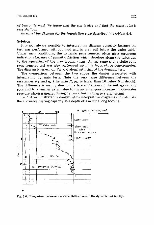
PROBLEM 6.7 2 2 1
of bentonite mud. We know that the soil is clay and that the water table is very shallow.
Interpret the diagram for the foundation type described in problem 6.6.
Solut ion It is no t a lways poss ible to interpret the diagram correctly because the
test was per formed without m u d and in clay soil below the water table . Under such condit ions , the dynamic penetrometer often gives erroneous indications because of parasit ic friction which develops a long the tubes due to the squeezing of the clay around them. At the same site, a static-cone penetrometer test was also per formed with the Gouda- type penetrometer . The diagram is shown on Fig . 6.6 along with that o f the dynamic test .
The compar i son between the two shows the danger associated with interpreting dynamic tests . Note the very large difference between the resistances Rd and qc ( the ratio Rd/qc is larger than 1 0 below 5 m depth) . The difference is mainly due to the lateral friction of the soil against the rods and to a smaller extent due to the instantaneous increase in pore-water pressure which is greater during dynamic test ing than in static testing.
T o further il lustrate the danger, let us interpret the diagrams and calculate the a l lowable bearing capaci ty at a depth of 4 m for a long foot ing .
50 100 R<j and q c in d a N / c m 2
\ i i
Ã
t_
Silty clay
Silty clay with
thin sand len
Plast ic clay
i
Ã
t_
Silty clay
Silty clay with
thin sand len
Plast ic clay
=- Wate r t a b l e 2.3θ]
i
Ã
t_
Silty clay
Silty clay with
thin sand len
Plast ic clay
; ">
i
Ã
t_
Silty clay
Silty clay with
thin sand len
Plast ic clay — -
i
Ã
t_
Silty clay
Silty clay with
thin sand len
Plast ic clay
/ — - 5.10^
i
Ã
t_
Silty clay
Silty clay with
thin sand len
Plast ic clay
I q (static GOUC Ä ) "Ν 1
V /
) f ?d (dynamic S E R Iv 1ES) — ^
C] ( 1
á ö
10
Fig. 6.6. Comparison between the static Delft-cone and the dynamic test in clay.

2 2 2 INTERPRETATION OF IN-SITU TESTS
Dynamic penetration test. A general rule often used to determine al lowable bearing pressure for shallow foot ings or semi-deep foundat ion i s : i ? d / 2 0 . At 4 m, i ? d > 6 0 0 0 kPa (60 d a N / c m 2 ) from which: qad = 6 0 0 0 / 2 0 = 3 0 0 kPa (3 d a N / c m 2) .
Static penetrometer test. The Dutch-type penetrometer ( G o u d a ) has a Delft-t y p e cone . qc is practically constant and equal to 8 0 0 k P a (or 8 d a N / c m 2 ) . Cohesion of the clay m a y be est imated a t :
c u = qjlb = 8 0 0 / 1 5 = 53 kPa (0 .53 d a N / c m 2)
and the al lowable bearing pressure would then b e :
5 . 1 4 c u 5 . 1 4 x 5 3 ( ? ad = = = 9 0 k P a ( 0 . 9 d a N / c m 2)
3 3 neglecting the depth term yD.
The al lowable bearing pressure calculated f rom the dynamic penetrometer is about equal t o the ult imate bearing capaci ty calculated by the static penetrometer . These results speak for themselves.
if Problem 6.8 Interpretat ion o f a Bevac-type dynamic penetrat ion test in submerged clay soil
The Bevac-type penetrometer was used at a site near Nantua (France), in a very thick layer of soft clay and a water table at about 1 m depth. The results of the test are presented in Fig. 6.7.
Can this diagram be interpreted? If so, give the allowable bearing capacity of a strip footing of 1 m width constructed at 2.5 m depth.
10 2 0 30 5 0
R d in d a N / c m 2
100 2 0 0
-=Water table
c 1
é ç
Rd ( d y n a m i c B E V A C) bfp
?-c
i r 3
7
N A N T U A: S o f t c l a y
Fig. 6.7. Dynamic penetration test (Bevac).

PROBLEM 6.8 2 2 3
Solut ion This t y p e of dynamic test in clay below the water table cannot be inter-
preted for the same reasons as cited in prob lem 6.7 [ 1 3 , 1 5 ] . T o confirm this conclusion, two static penetrometer tests were per-
formed at the same site, one with the Gouda- and the other with the Andina-penetrometers , very near to the dynamic penetrometer test . The results are shown in the diagram of Fig . 6 .8 . Once again a large difference between Rd and qc is not iceable . The t w o static-cone tes t s , however, agree quite well with each other. The difference is due to the same causes as expla ined in problem 6 .7 .
0 10 2 0 30 50
-cd a n d q c in d a N / c m 2
100 2 0 0
a.
Q
/ Wate ?r table ~ - 1_
> ¾ . — é I
\ — q c ( s t a t i c A N D I N A) I
, ι I
Rd ( d y n a m i c ç r \ /ä r \ *-Rd ( d y n a m i c Ï t VM J ø.
c J—
- t c -? N A N T U A: S o f t c l a y
Fig. 6.8. Comparison between static-cone penetrometer and dynamic penetration test.
If we t o o k i ? d / 2 0 (as for cohesionless soils) to calculate the allowable bearing pressure at 2 .5 m depth , we would get : <?ad = 2 5 0 kPa (2 .5 d a N / c m 2 ) . On the other hand, for the static-cone penetrometer te s t : qc = 1 8 0 k P a (simple cone) or qc = 3 0 0 kPa (Delft-cone) .
The Andina penetrometer has a s imple point , therefore :
c u = qc/10 = 1 8 0 / 1 0 = 1 8 k P a (0 .18 d a N / c m 2)
and the al lowable bearing pressure for a s m o o t h strip foot ing at 2 .5 m is :
5 . 1 4 c u 5 .14 χ 18 <?ad = = 30 kPa ( 0 . 3 d a N / c m 2)
The al lowable bearing pressure is 8 t imes less with the static penetrometer than with the dynamic penetrometer . It should be noted that at this s ite, a raft-type foundat ion designed for 3 0 kPa underwent substantial set t lements . See problem 6 .16 and Ref . [ 1 4 ] .
It should be remembered that when < ? c < 1 2 0 0 k P a , it is absolutely necessary to recover undis turbed samples for laboratory testing.
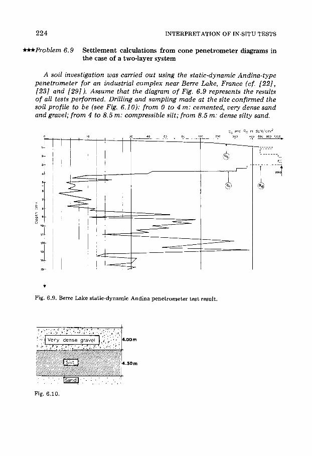
2 2 4 INTERPRETATION OF IN-SITU TESTS
***Problem 6.9 Set t lemen t calculations from con e penetromete r diagrams in th e case of a two-laye r sys te m
A soil investigation was carried out using the static-dynamic Andina-type penetrometer for an industrial complex near Berre Lake, France (cf. [22], [23] and [29]). Assume that the diagram of Fig. 6.9 represents the results of all tests performed. Drilling and sampling made at the site confirmed the soil profile to be (see Fig. 6.10): from 0 to 4 m: cemented, very dense sand and gravel; from 4 to 8.5 m: compressible silt; from 8.5 m: dense silty sand.
q c and R<j in daN/crrr
Fig. 6.9. Berre Lake static-dynamic Andina penetrometer test result.
Fig. 6.10.

PROBLEM 6.9 2 2 5
Consolidation tests were performed on undisturbed samples of the compres-sible silt recovered at locations very near to those of cone-penetrometer tests.
The observed correlation between the point resistance qc and oedometric modulus Er indicates that the coefficient a. is equal to 3 and is valid for the whole site (mv = l/ocqc).
Assuming that the upper sand and gravel and lower sand layers are incom-pressible, calculate the settlement of a strip footing, 2 m wide, imparting a pressure of 400 kPa and located at 0.5 m below existing grade.
Could the settlement be reduced, assuming the same total load if the width of the footing was increased to 4 m, therefore reducing the pressure to 200 kPa?
N o t e : It m a y appear n o t logical t o correlate an 'e last ic ' characterist ic , such as the modu lus of consol idat ion t o an u l t imate strength of the penetrometer . In fact , the soil behavior is a very c o m p l e x p h e n o m e n a which a lways consists of s o m e reversible and other irreversible mechanisms . Perfect elasticity and plasticity are only approx imat ions . During the two types of tests , bo th phenomena occur, which m a y account for the possibi l i ty of empirical correlat ion observed between Ef and qc. It should be remembered that the various correlations established are only valid for well defined soil t ype s .
So lut ion First method. Settlement calculations from the Giroud-tables. The tables
for the calculat ion of set t lement of J . P. Giroud , give formulas which permit direct calculat ion of set t lements for various foot ing types bearing on homo-geneous soils of finite thickness and whose deformat ion m o d u l u s is known and bearing on an unyielding substra tum ( [ 1 0 ] ) .
Formulas have been developed for the case of foot ings bearing directly on the compress ib le layer. However, a t the Berre L a k e s ite , there exists a sand and gravel layer overlaying the compress ible layer. The analysis , therefore , m a y be as fo l lows. Because the sand and gravel layer is very dense and very rigid, the soil stress a t the t o p of the silt layer m a y be calculated by assuming a stress distr ibution of 4 5 ° through the cemented sand and gravel layer as shown in Fig . 6 . 1 1 . Normal ly , such a distr ibution is a s sumed t o spread over a 3 0 ° angle according t o the pressure bulb of Bouss inesq .
By utilizing the notat ions o f Giroud t a b l e s * , the spread at the t o p of the silt layer is: 2a = 2 + 3.5 χ 2 = 9 m and the stress is : ñ = 4 0 0 χ 2 /9 = 8 9 k P a (0 .89 d a N / c m 2 ) with Ç la = 4 . 5 0 / 4 . 5 0 = 1 and í = 1/3. F r o m the Giroud tab le , p . 3 9 9 * we get : p H = 0 . 3 1 .
2a _ The sett lement is given by the formula w = ñ —pn-
•Printed by Dunod, Paris in 1 9 7 2 and 1973 [ 1 0 ] .

2 2 6 INTERPRETATION OF IN-SITU TESTS
2a = 9m
2m
i0.5Om
Ç = 4.50m
3.50m
Fig. 6 .11 .
The oedometr ic modulus is obta ined from the static penetrometer tes t : E' = aqc =3qc.
The average value of qc in the silt layer is calculated f rom depth 4—8.5 m, and it is qc — 8 0 0 kPa, f rom which:
Ef = 3 x 8 0 0 = 2 4 0 0 kPa (24 d a N / c m 2)
and for í = 1/3, Young ' s modu lus is Ε = 2/3 Ε' = 16 d a N / c m 2 . Finally, the sett lement is w = ( 0 . 89 χ 9 0 0 / 1 6 ) χ 0 . 3 1 = 1 5 . 5 cm or w =
16 cm. Let us now consider the case of the 4 m wide foot ing , imparting a pressure
of 2 0 0 kPa. We have 2a = 4 + 2 χ 3 .50 = 1 1 m, f rom which a = 5 .50 m . Therefore ,
H/a = 4 . 5 0 / 5 . 5 0 = 0 . 8 2 a n d : p H = 0 . 2 5 , ñ = 2 0 0 χ 4 / 1 1 = 73 kPa (0 .73 d a N / c m 2 ) and the sett lement is : w = ( 0 . 73 χ 1 . 1 0 0 / 1 6 ) χ 0 . 2 5 = 12 .5 cm say w ~ 13 cm.
The sett lement is decreased very little by doubl ing the width of the footing. This is accounted for by the rigidity of the upper layer. It would therefore not be advisable to r ecommend an increase of the foot ing width. The cemented sand and gravel layer acts like a m a t foundat ion .
Second method. A more classical m e t h o d is to determine the stresses and then calculate the sett lement layer by layer, using the formula Ah/h = -Áσ/Ε'.
Let us first consider the stress distribution at depth for a f lexible foot ing and calculate the stress at mid-height in the silt layer as well as at the upper and lower boundar ies of this layer.
Once again, the Giroud table can be used, and Table 6 A is compi led (results along the foot ing ax i s ) .
The silt layer is divided into two equally thick layers of 2 . 2 5 m. The average stress in the upper half-layer is :
Aox = ( 1 4 0 + 8 8 ) / 2 = 1 1 4 kPa (1 .14 d a N / c m 2)
PROBLEM 6.9 2 2 7
TABLE 6A
z Averag e æ la k0 Δ σ (kPa)
3.50 3 .50 0.35 140 5.75 5.75 0.22 88 8 8 0 .16 64
and in the lower half-layer i s :
Δ σ 2 = (88 + 6 4 ) / 2 = 7 6 k P a (0 .76 d a N / c m 2) .
Assuming that the m o d u l u s E' is the s ame for bo th half layers ; the settle-
ment is : ÓÁÕé = — j ( A o 1 + A o 2 ) = ( 1 1 4 + 7 6 ) = 1 7 . 8 c m . Ε 2 4 0 0
If we now a s sume the foot ing t o be rigid, and using Giroud ' s table (Vol . I I , p . 3 6 5 ) we can m a k e u p Table 6 B .
The same results are obta ined for all practical purposes in assuming the foot ing to be rigid. This is unders tandable because for rat ios of æ /a over 3 the stress distr ibution for strip foot ings is practically the s ame , regardless of the a s sumpt ion on the rigidity of the foot ing .
TABLE 6B
z Averag e æ la k0 Δ σ
3.50 3 .50 0.34 136 5.75 5.75 0.22 88 8 8 0.16 64
The conclus ion would n o t have been the s ame had the foot ing been resting directly on the silt layer.
Comparison between the two methods. Se t t lements c o m p u t e d by the second m e t h o d are somewhat higher than those of the first m e t h o d . This is be-cause in the second m e t h o d stress condit ions are a s sumed which corre-spond to a homogeneous soil and no account is taken of the high rigidity o f the cemented sand and gravel layer. The first m e t h o d therefore is con-sidered more representative o f reality.
A third m e t h o d could be used , by referring to the tables o f Bo t te ro and T o u z o t for sett lements on a two-layer sys tem. Assuming a value of 1 2 0 0 d a N / c m 2 for the modu lus of the cemented sand and gravel layer, a sett lement o f 10 .3 cm would be obta ined for the 2 m wide foot ing. This is c lose t o the result of the first m e t h o d .

2 2 8 INTERPRETATION OF IN-SITU TESTS
**Problem 6.10 Se t t lement calculations based on Schmertmann ' s m e t h o d and static penetrometer tests in gravels and sands
The city hall of Lyons consists mainly of an administration block sup-ported by 4 concrete columns of 10 by 10 m (see Fig. 6.12) containing stair wells, elevators and utility shafts. Spacing between the columns is 20 m. Each column rests on a square footing bearing a net load of 70 MN after considering an excavation of 10 m of soil from ground level.
Over the site of this building, the soil profile is: — fill, 1 to 2 m thick; — clayey silt, 1 to 2 m thick; — sandy gravels to a maximum thickness of 20 m; — sandstone substratum; — water table at about 5 m below natural grade.
A penetration test was performed at the location of one of the columns with an Andina static-dynamic penetrometer after excavation. The test results are shown in Fig. 6.13.
Over a depth of about 10 m, dense gravels were encountered which are underlain by incompressible sandstone whose characteristics are well known in the area.
Assuming a coefficient a = 3, calculate the settlement of a column from the test result, using Schmertmann's method (cf [35]).
We have: y/y w — 2 for the soil above the water table, and y'/y w — 1 for the soil below the water table.
Schmertmann' s m e t h o d is valid only for cohesionless soils . It consists of drawing a very simple vertical stress diagram at depths due to a rigid foot ing.
The stress distribution is a s sumed to be triangular and the m a x i m u m stress occurs at depth B/2, where Β is the width of the foot ing, and that below B/2, no appreciable vertical stresses exist in the soil. (F ig . 6 . 1 4 ) . If Ap is the stress increase due to the foot ing , according to Schmer tmann, at depth B/2, the stress is 0.6 Ap. Correction factors are needed as indicated below.
A A
Solut ion
Sectio n A - A
o l
Fig. 6 .12. City Hall of Lyons: plan and section.
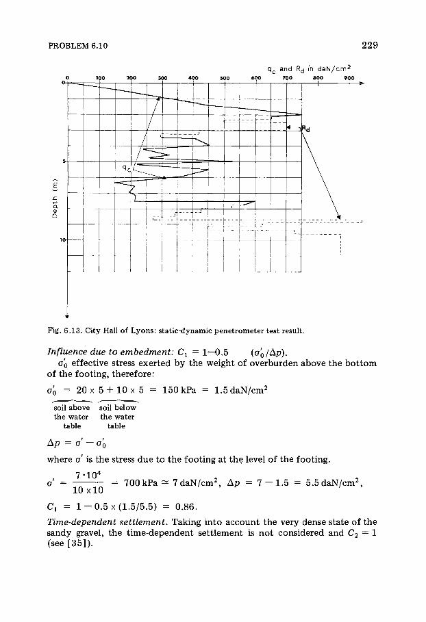
PROBLEM 6.10 2 2 9
Fig. 6 .13 . City Hall of Lyons: static-dynamic penetrometer test result.
Influence due to embedment: C1 — 1—0.5 (σ'0/Áñ). σ'0 effective stress exer ted b y the weight of overburden above the b o t t o m
of the foot ing, therefore :
σο = 20 χ 5 + 10 χ 5 = 1 5 0 kPa = 1.5 d a N / c m 2
soil above soil below the water the water
table table
Ap = σ' — σ'0
where σ' is the stress due to the foot ing at the level of the foot ing .
7 - 1 0 4
σ' = = 7 0 0 kPa ^ 7 d a N / c m 2, Ap = 7 - 1 . 5 = 5 .5 d a N / c m 2, 1 0 x 1 0
Cy = 1 - 0 . 5 χ ( 1 . 5 / 5 . 5 ) = 0 . 8 6 . Time-dependent settlement. Taking into account the very dense s ta te of the sandy gravel, the t ime-dependent sett lement is not considered and C 2 = 1 (see [ 3 5 ] ) .

2 3 0 INTERPRETATION OF IN-SITU TESTS
Interaction between columns. F o r two identical foot ings , each 1 0 m wide, Β é = Β 2 = 10 m and the distance between the foot ing is known to be 2 0 m.
We have : 0.6(Β× + B2) = 0 .6 χ 2 0 = 1 2 m , so L> 0.6(Bl + £ 2 ) , and the footings behave as isolated foot ings .
Stress diagrams. The m a x i m u m stress i s : a = Cx χ 0 .6 Δ ρ or σ = 0 .86 χ 0.6 χ 5.5 — 2 .84 d a N / c m 2 , and the stress diagram is shown on Fig. 6 . 1 4 .
1 2 3
Fig. 6.14.
Settlement calculation A rigid soil layer is encountered at 10 m below the b o t t o m of the foot ing,
that is at a depth inferior to 2B = 2 0 m. The same triangular distr ibution is a s sumed down to the level of the rigid soil layer, but sett lements are only c o m p u t e d to a depth of 10 m (Fig . 6 . 1 4 ) . The sandy gravel layer of 1 0 m m a y be divided into 10 layers each 1 m thick. The σ-value is determined for each layer as well as the average cone resistance qc. Table 6 C is then made u p . The total sett lement is c o m p u t e d t o be 17 m m .
Actual sett lement measurements m a d e on the structure showed :
5—7 m m for a load of 4 0 MN, 8—10 m m for a load of 6 0 MN.
This example confirms the validity of sett lement est imates based on cone penetrometer test data .
Level of incompressible substratum

P R 0 B L E M 6 . il 2 3 1
TABLE 6C
Depth (m) ° z 2 ( d a N / c m 2)
q° 2 ( d a N / c m 2) OL oz/Sqc
0-1 0.28 160 3 0 .00058 1-2 0.85 550 3 0 .00052 2-3 1.42 6 5 0 3 0 .00073 3-4 1.99 4 0 0 3 0 .00166 4-5 2.56 340 3 0 .00251 5-6 2.75 330 3 0 .00278 6-7 2.56 200 3 0 .00427 7-8 2.37 390 3 0 .00203 8 -9 , 2.18 500 3 0 .00145 9-10 1.99 740 3 0 .00090
0 .01743 m w — 11 mm
t * *Proble m 6.11 Se t t lemen t calculat ions of a compress ib l e s lopin g layer , based on stati c pene tromete r tes t da t a
The city of Annecy (France) is built in part on thick lake deposits consist-ing mainly of compressible silts overlaying a limestone substratum which in places is overlain by dense morraine deposits. The soil profile shown on Fig. 6.15 was established from numerous static-dynamic Andina penetrometer tests performed at a particular site in Annecy. Construction consisted of erecting 2 buildings. Building A was to be constructed over a sloping rock substratum while building Β was planned over the horizontal portion of the bedrock.
Bui ld Β Bui ld A
Fig. 6 .15. Longitudinal soil sections.

2 3 2 INTERPRETATION OF IN-SITU TESTS
Two test results obtained by the Andina-penetrometer are shown in Figures 6.16 and 6.17. Test 2 is assumed to be representative of the soil con-ditions throughout the site of building B. The water table is at a depth of 1.5 m. All the buildings have a cellar, excavated to 2.5 m and have 5 stories. The stress may be assumed at 70 kPa. The width of the cellar is 22 m and each building is 80 m in length.
Give recommendations for the foundation of each building. Calculate the settlement of shallow footings at the locations of the penetrometer tests, assuming a in the silt to be 5 < α < 10 and a = 3 in the gravel layer. We also have: y/y w = 2 above the water table, y'/y w = 1 below the water table. What solution can be chosen for each building?
Solut ion (1) Deep footings. Because of the sloping bedrock for building A, and the low consistency of the silt, the first solut ion that comes to mind is to sup-port the buildings on piles driven to the l imestone or to the dense moraine . (qc > 1 0 4 kPa or 1 0 0 d a N / c m 2 ) .
F r o m the technical s tandpoint , this would be the safest solut ion because tota l and differential sett lement problems would be virtually non-existent [ 3 0 ] . (2) Shallow footings. The deep foundat ion scheme is very cost ly because of the great lengths of piles required. It is therefore worthwhile to investigate the possibil ity of support ing the structures on shallow foot ings . The allow-able bearing capaci ty of the silt i s : taking qc = 3 0 0 k P a ( 3 d a N / c m 2 ) , c u = qc/10 = 3 0 0 / 1 0 = 3 0 k P a , f rom which g a d = 5 . 1 4 c u/ 3 = (5 .14 χ 3 0 / 3 ) = 5 1 . 4 k P a (0 .5 d a N / c m 2) .
F rom the total building weight, the only poss ible shallow foot ing t y p e would be a raft-type foundat ion , as should have been expec ted . The problem associated with the raft-foundation is that of evaluating set t lements .
The net pressure due to the new structure at the foundat ion level a t the b o t t o m of the raft a t a depth of 2 .5 m is the total building pressure less the weight of the soil excavated to a depth o f 2 .5 m, or : 2 0 χ 1.50 + 1 0 χ 1 = 4 0 k P a
soil above soil below the water the water
table table
The net pressure at the b o t t o m of the raft is Δ σ = 70 — 4 0 = 30 kPa — 0.3 d a N / c m 2 .
For each penetrometer test , an idealized soil cross section may be drawn into a number o f layers which also accounts for the gravel layer encountered in C.P.T. no . 1, as shown in Fig. 6 . 1 5 .
The vertical stress due to the net building load a t mid-height of each layer is calculated. Because of the plan dimensions of the buildings, the stresses

PROBLEM 6.11 2 3 3
Fig. 6 .16. Static-dynamic Andina penetrometer test 1.
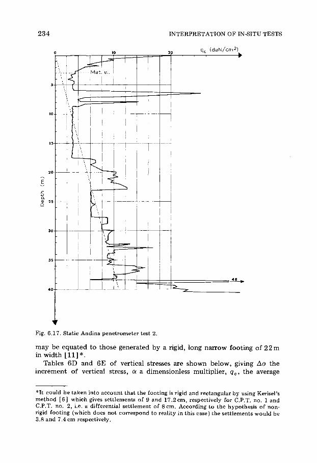
2 3 4 INTERPRETATION OF IN-SITU TESTS
4 8
Fig. 6.17. Static Andina penetrometer test 2.
m a y be equated to those generated by a rigid, long narrow footing of 2 2 m in width [ 1 1 ] * .
Tables 6 D and 6 E of vertical stresses are shown below, giving Δ σ the increment of vertical stress, oc a dimensionless multiplier, <?c, the average
*It could be taken into account that the footing is rigid and rectangular by using Kerisel's method [ 6 ] which gives settlements of 9 and 1 7 . 2 c m , respectively for C.P.T. no. 1 and C.P.T. no. 2, i.e. a differential settlement of 8 cm. According to the hypothesis of non-rigid footing (which does not correspond to reality in this case) the settlements would be 3.8 and 7.4 cm respectively.
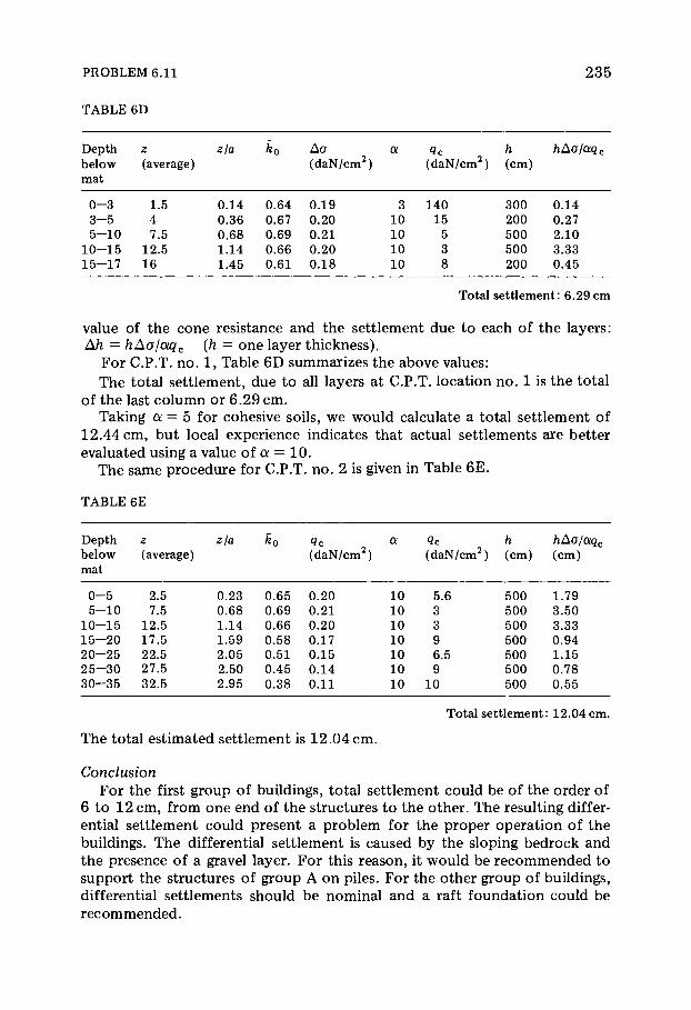
PROBLEM 6.11 2 3 5
TABLE 6D
Depth below mat
æ (average)
æ la Δ σ ( d a N / c m 2)
a ( d a N / c m 2)
h (cm)
hAo/aqc
0 - 3 1.5 0.14 0.64 0.19 3 140 300 0.14 3 - 5 4 0.36 0.67 0.20 10 15 200 0.27 5 - 1 0 7.5 0.68 0.69 0.21 10 5 500 2.10
1 0 - 1 5 12.5 1.14 0.66 0.20 10 3 500 3 .33 15—17 16 1.45 0.61 0.18 10 8 200 0.45
Total settlement: 6 . 2 9 c m
value of the cone resistance and the set t lement due t o each of the layers : Ah = hAo/aqc (h = one layer thickness ) .
F o r C.P.T. no . 1 , Table 6 D summarizes the above values: The tota l set t lement , d u e t o all layers a t C.P.T. locat ion n o . 1 is the to ta l
of the last co lumn or 6 .29 cm. Taking α = 5 for cohesive soils , we would calculate a tota l set t lement of
1 2 . 4 4 cm, but local experience indicates that actual set t lements are better evaluated using a value of a: = 1 0 .
The same procedure for C.P.T. n o . 2 is given in Table 6 E .
TABLE 6E
Depth below mat
æ (average)
æ/a ko q° 2 ( d a N / c m 2) a
( d a N / c m 2) h (cm)
hAo/aqc
(cm)
0 - 5 2.5 0.23 0.65 0 .20 10 5.6 500 1.79 5 - 1 0 7.5 0.68 0.69 0.21 10 3 500 3.50
1 0 - 1 5 12.5 1.14 0.66 0.20 10 3 500 3 .33 1 5 - 2 0 17.5 1.59 0.58 0.17 10 9 500 0.94 2 0 - 2 5 22.5 2.05 0.51 0.15 10 6.5 500 1.15 2 5 - 3 0 27.5 2.50 0.45 0.14 10 9 500 0.78 3 0 - 3 5 32.5 2.95 0.38 0.11 10 10 500 0.55
Total settlement: 12 .04 cm.
The tota l es t imated set t lement is 1 2 . 0 4 c m .
Conclusion
F o r the first group of buildings, to ta l set t lement could be o f the order o f 6 to 12 cm, f rom one end o f the structures t o the other. The resulting differ-ential set t lement could present a prob lem for the proper operat ion of the buildings. The differential set t lement is caused by the s loping bedrock and the presence of a gravel layer. For this reason, it would be r e c o m m e n d e d to suppor t the structures of g roup A on piles. For the other group of buildings, differential sett lements should be nominal and a raft foundat ion could be r e c o m m e n d e d .

2 3 6 INTERPRETATION OF IN-SITU TESTS
***Problem 6.12 Pile foundat ion calculat ion f rom static cone test in atr i- layer sys tem
Cone penetrometer test data were performed in the Annecy (France) area at a swampy site, with static-dynamic Andina penetrometer. The penetration record of Fig. 6.18 is representative of the subsurface soil conditions. The cone point used in the test has a diameter of 8 cm.
The soil cross-section is: — 0 to 8 m, peat and soft clay; — 8 to 11.5 m, sand and gravel layer; — from 11.5 m, soft clay.
To support the proposed structures, the obvious solution is to resort to driven pile foundation, penetrating to the upper part of the sand and gravel layer.
Estimate the bearing capacity of 0.6 m and 1.0 m diameter piles whose
q c ( d a N / c m 2 )
80 90 10
Fig. 6.18. Tri-layer system Andina static penetrometer test.
PROBLEM 6.12 2 3 7
tips would be driven to a depth of 8 .5 m, using the following 3 methods: the Dutch method, Geuze's rule, Meyerhofs method [22, 25].
Compare the results. In addition, for the 0.6-m diameter pile, estimate the load capacity if the pile is driven one additional meter (to —9.50 m).
Solut ion (1) The Dutch method. This method consists of calculating the average
cone bearing over a depth increment of 8 diameters above the pile tip (qCi) and the average cone bearing resistance to 4 diameters depth below the pile t ip cjC2 (tip being at —8.5 m ) .
The ul t imate bearing pressure at the pile tip is then : qd = ( q Ci 4- qC2)/2 and the al lowable bearing pressure is qaa = qd/2 = (qCx + QC2 )/4 for the safety factor of 2 .
If a layer of low cone bearing is encountered, with a minimum value of <?mini o v er a depth of 4 diameters below the pile t ip , and if ç cone bearing readings were m a d e in this soft layer, the value of qP2 is then:
q » = Vn ·
(a) For the 0.6-m diameter pile ( 80 = 4 .8 m and 4 0 = 2 . 4 m ) the calculated average cone bearing values from 3.7 to 8 . 5 m , is qCi ~ 6 d a N / c m 2 ; for values f rom 8 .5 to 1 0 . 9 m qC2 ~ 8 0 d a N / c m 2 , and the al lowable bearing pressure at the tip of the pile is qad = (6 4- 8 0 ) / 4 = 2 1 . 5 d a N / c m 2, say 20 d a N / c m 2 .
(b) For the 1-m diameter pile (80 = 8 m and 4 0 = 4 m ) the average value of qCx, between 0 .5 and 8.5 m is qCi — 4 .6 d a N / c m 2.
For the depth 4 0 below the proposed pile tip elevation the presence of a soft layer is encountered. The bearing capaci ty of the soil for the 1 m 0 pile will have to be decreased to take this into account . The Andina-type penetrometer measures qc every 0 .25 m ; over 4 m there are 16 readings. The average value of qCi f rom 8.5 to 1 2 . 5 m is equal to 56 d a N / c m 2 and the minimal value of qCi is 8 .5 d a N / c m 2. We therefore have:
56 ÷ 16 + 8 .5 ÷ 16 qc = 3 2 d a N / c m 2 .
2 x 1 6
Hence the al lowable bearing pressure is : <7ad = (4 .6 + 3 2 . 2 ) / 4 = 9.2 d a N / c m 2 , say 10 d a N / c m 2 .
Remark Piles of 1 m in diameter have an al lowable tip bearing pressure consider-
ably lower than that of the 0.6-m diameter pile (not quite half) . N o t e : The pressure bulb at the t ip of the large-diameter pile is larger than that for the small-diameter pile and the bulb extends therefore into the soft underlaying clay. Thus it is advantageous to use smaller-diameter piles. However, it does
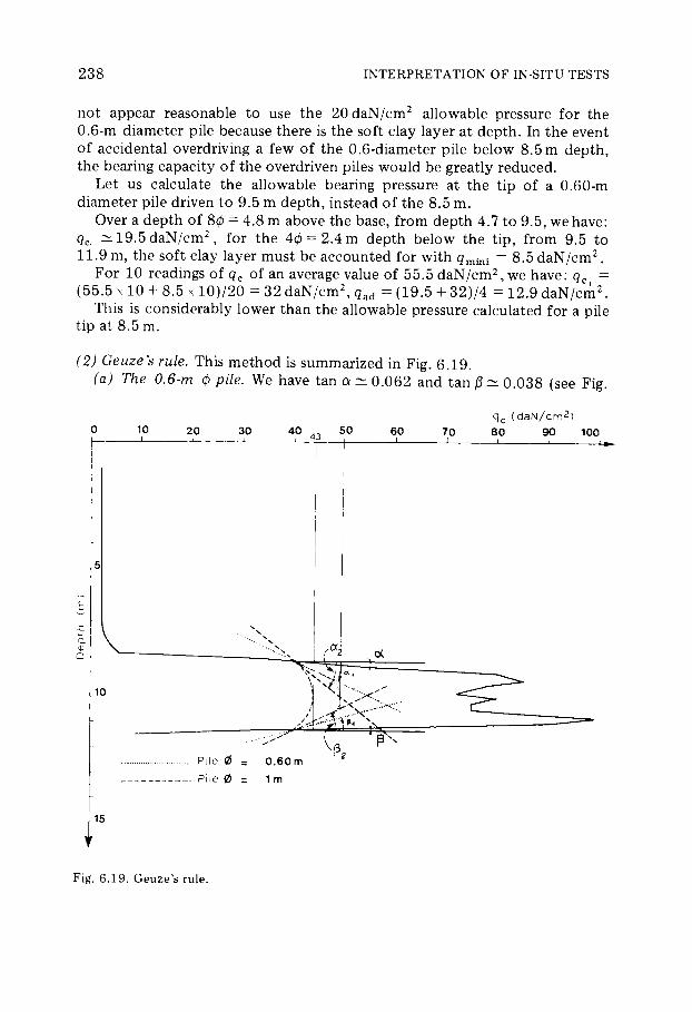
2 3 8 INTERPRETATION OF IN-SITU TESTS
not appear reasonable to use the 20 d a N / c m 2 allowable pressure for the 0.6-m diameter pile because there is the soft clay layer at depth . In the event of accidental overdriving a few of the 0.6-diameter pile below 8 . 5 m depth , the bearing capacity of the overdriven piles would be greatly reduced.
Let us calculate the allowable bearing pressure at the tip of a 0.60-m diameter pile driven to 9.5 m depth, instead of the 8.5 m.
Over a depth of 8 0 = 4 . 8 m above the base , from depth 4 . 7 to 9 . 5 , we have: qc ^ 19 .5 d a N / c m 2, for the 4 0 = 2 . 4 m depth below the t ip, from 9.5 to 11 .9 m, the soft clay layer must be accounted for with q m i ni = 8 .5 d a N / c m 2.
For 10 readings of qc of an average value of 55 .5 d a N / c m 2, we have: qc — ( 5 5 . 5 ÷ 10 + 8 . 5 ÷ 1 0 ) / 2 0 = 3 2 d a N / c m 2, qad = ( 1 9 . 5 + 3 2 ) / 4 = 12 .9 d a N / c m 2.
This is considerably lower than the allowable pressure calculated for a pile tip at 8 . 5 m.
(2) Geuze's rule. This method is summarized in Fig. 6 .19 . (a) The 0.6-m ö pile. We have tan a 0 . 0 6 2 and tan â* 0 . 0 3 8 (see Fig.
q c ( d a N / c m ^ )
0 10 20 30 40 50 60 70 80 90 100
Fig. 6.19. Geuze's rule.

PROBLEM 6.13 2 3 9
6 . 1 9 ) . The diameter of the Andina penetrometer cone is 6 = 8 c m , and that of the pile Β = 6 0 cm.
Geuze 's law s tates : tan <xx = B/b tan a = ( 6 0 / 8 ) χ 0 . 0 6 2 = 0 .47 and tan ft = B/b tan â = ( 6 0 / 8 ) χ 0 . 0 3 8 = 0 . 2 9 .
The actual cone resistance o f Fig. 6 .19 is deduced graphically to qc = 50 d a N / c m 2 and, using a safety factor of 4 , qad = 5 0 / 4 = 12 .5 d a N / c m 2 .
(b) The 1.0-m ö pile. The same procedure is used for Β = 1 0 0 cm from which tan ax = 0 . 0 6 2 χ 1 0 0 / 8 = 0 . 7 8 and tan â÷ = 0 . 0 3 8 χ 1 0 0 / 8 = 0 .48 . The corrected cone bearing value is qc 2 1 4 3 d a N / c m 2 and qad = 4 3 / 4 ~ 1 1 d a N / c m 2 . The allowable bearing pressures for the 2 pile sizes are very near the same in this instance.
(3) Meyerhofs method. (a) The 0.6-m ö pile. The tip of the piles at 8.5 m depth is located at a
distance i f of 3 m above the soft underlaying layer. This is less than the critical distance 10J3 = 6 m . The approx imate cone bearing value of the soft layer is q~ ~ 10 d a N / c m 2 and that of the sand and gravel layer is qc ~ 7 5 d a N / c n r .
According to Meyerhof, the ul t imate bearing capaci ty of the soil i s :
(Qc —Qc)H 6 5 χ 3 Qd = Qc +— £sJ— = 10 + = 4 2 . 5 d a N / c m 2.
d c° 1 0 5 6
and for a safety factor of 3 (because the method is a little pess imist ic) , we have: qad = 4 2 . 5 / 3 = 14 d a N / c m 2 .
(b) The 1.0-m ö pile. Ç = 3 m < 10B = 1 0 m , = 1 0 d a N / c m 2 and qc ~ 7 5 d a N / c m 2 , from which qd = 10 + ( 6 5 χ 3 ) / 1 0 = 2 9 . 5 d a N / c m 2 and <7ad =<7d/3 = 10 d a N / c m 2 .
Conclusion
The three methods yield closely related results , except for the 0.6-m diameter pile at 8 .5 m depth ; however, for practical reasons, it was pointed out that the high value of al lowable pressure for this instance was not to be recommended .
An average a l lowable pressure of all the methods may be r ecommended at 8 .5 m. This would be a b o u t 13 d a N / c m 2 for the 0.6-m diameter pile. N o fill should be placed on the ground surface and all ground floors should also be suppor ted on piles to avoid differential sett lements between columns , walls and f loors .
irkrkProblem 6.13 Se t t lement est imates of a surcharge fill, f rom static-cone penetrometer test data
In the Cannes region (France), it is not uncommon to have recent alluvial deposits of clays and silts over depths of 40 m above the marly bedrock. Cone-penetrometer tests performed with the Gouda 100 kN device have
2 4 0 INTERPRETATION OF IN-SITU TESTS
shown that in such soils the cone-bearing value is very constant and of about 1000 kPa for these alluvial deposits. The project consists of the construction of several relatively low buildings one of which of five storeys.
In order to reduce the total and differential settlements of the structures, it was decided to surcharge the sites and consequently, a 5m high fill was placed over a plan dimension of about 40 ÷ 130 m. The vertical cross-section of the fill has a trapezoidal shape with a top horizontal dimension of 30 m. The soil density is 1.8.
Calculate the settlement caused by the surcharge fill along its central axis, assuming the following values of a: 3<a<5 and mv = l/aqc [23, 27, 28].
Solut ion The mos t direct m e t h o d of est imating sett lements is t o resort to vertical
stress distribution and tables of Giroud (vol. II , 6 . 1 1 , p . 4 3 6 ) , formula 2 :
w = ^-^[(^-(a/aYri)], y = 1 8 k N / m 3 , h = 5 m , Ε a—a
Ε = 2/3 Ε' = 2 /3 aqc with í = 0 . 3 3 , a = 2 0 m , a = 15 m.
Here, for 3 < a < 6, we get 3 0 0 0 < Ε < 6 0 0 0 kPa and we have :
H/a' = 4 0 / 1 5 = 2 .67 from which r'n = 1 .142 ,
H/a = 4 0 / 2 0 = 2 from which r h = 0 .983
with: Ε' = 3 0 0 0 kPa, Ε = 2 0 0 0 kPa, we get :
18 x 5 4 0 0 / 1 5 \ 1
w = χ ( 0 . 9 8 3 - — x 1 .142) = 1.23 m, 2 0 0 0 5 \ 2 0 /
with Ε' = 6 0 0 0 kPa, Ε = 4 0 0 0 kPa, we get : w = 0 . 6 2 m. Thus , the sett lement would be between 6 2 and 1 2 3 cm [ 3 2 ] . Remark
The actual sett lement measured at the end of 4 months of preloading was between 30 and 4 2 cm at different observation stat ions . These settle-ments are smaller than the range predicted f rom penetrometer tests . This m a y be due t o :
— the ul t imate sett lements have not yet occurred at the end of 4 months ; — no account was taken of the slight increase in cone-bearing value of the
silt starting at a depth of 20 m, nor of the presence of a few sand lenses. The actual sett lements , however, val idate the m e t h o d of est imating
sett lements f rom static-penetrometer test da ta .
**•Problem 6.14 Set t lement calculation o f a surcharge fill f rom the results of an Andina penetrometer test
Two cooling structures were constructed near Lyons for the development of a nuclear power plant. Each structure is 127m high and has a diameter of
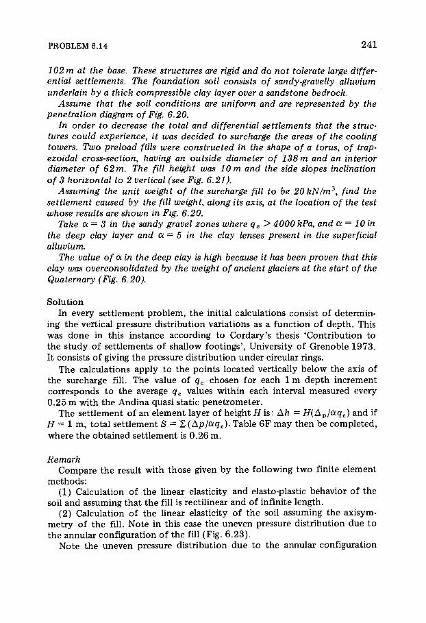
PROBLEM 6.14 2 4 1
102 m at the base. These structures are rigid and do not tolerate large differ-ential settlements. The foundation soil consists of sandy-gravelly alluvium underlain by a thick compressible clay layer over a sandstone bedrock.
Assume that the soil conditions are uniform and are represented by the penetration diagram of Fig. 6.20.
In order to decrease the total and differential settlements that the struc-tures could experience, it was decided to surcharge the areas of the cooling towers. Two preload fills were constructed in the shape of a torus, of trap-ezoidal cross-section, having an outside diameter of 138 m and an interior diameter of 62 m. The fill height was 10 m and the side slopes inclination of 3 horizontal to 2 vertical (see Fig. 6.21).
Assuming the unit weight of the surcharge fill to be 20 kN/m 3, find the settlement caused by the fill weight, along its axis, at the location of the test whose results are shown in Fig. 6.20.
Take a = 3 in the sandy gravel zones where qc > 4000 kPa, and a = 10 in the deep clay layer and a = 5 in the clay lenses present in the superficial alluvium.
The value of a in the deep clay is high because it has been proven that this clay was overconsolidated by the weight of ancient glaciers at the start of the Quaternary (Fig. 6.20).
Solut ion In every sett lement prob lem, the initial calculations consist o f determin-
ing the vertical pressure distr ibution variations as a function o f depth. This was done in this instance according to Cordary ' s thesis 'Contribution to the s tudy o f sett lements of shallow foot ings ' , University of Grenoble 1 9 7 3 . It consists o f giving the pressure distr ibution under circular rings.
The calculations apply to the points located vertically below the axis of the surcharge fill. The value of qc chosen for each 1 m depth increment corresponds to the average qc values within each interval measured every 0 . 2 5 m with the Andina quasi static penetrometer .
The set t lement of an e lement layer of height Ç is: Ah = H(Ap/aqc) and if Ç = 1 m, tota l set t lement S = Σ (Ap/aqc). Table 6 F may then be comple ted , where the obta ined sett lement is 0 .26 m.
Remark
Compare the result with those given by the following two finite element methods :
(1 ) Calculation of the linear elasticity and elasto-plastic behavior of the soil and assuming that the fill is rectilinear and of infinite length.
(2 ) Calculation of the linear elasticity of the soil assuming the axisym-metry of the fill. N o t e in this case the uneven pressure distribution due to the annular configuration o f the fill (F ig . 6 . 2 3 ) .
N o t e the uneven pressure distr ibution due to the annular configuration

2 4 2 INTERPRETATION OF IN-SITU TESTS
Fig. 6.20. Andina static penetrometer test.
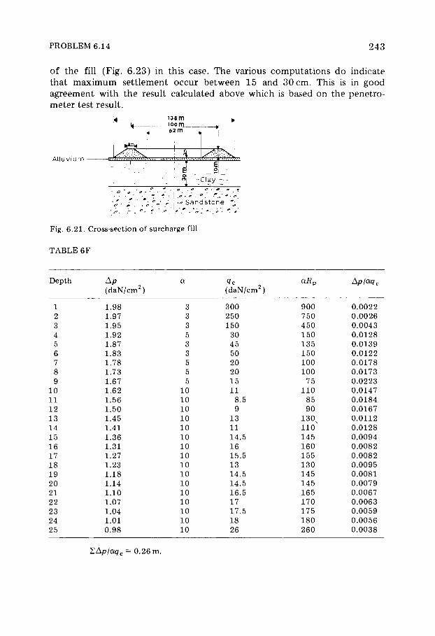
PROBLEM 6.14 243
of the fill (F ig . 6 . 23 ) in this case. The various computat ions do indicate that m a x i m u m sett lement occur between 15 and 30 cm. This is in good agreement with the result calculated above which is based on the penetro-meter test result .
A l l u v i u m
Fig. 6 .21. Cross-section of surcharge fill.
TABLE 6F
Depth Ap ( d a N / c m 2)
a Qc ( d a N / c m 2)
Ap/aqc
1 1.98 3 300 900 0 .0022 2 1.97 3 250 750 0 .0026 3 1.95 3 150 450 0 .0043 4 1.92 5 30 150 0 .0128 5 1.87 3 45 135 0 .0139 6 1.83 3 50 150 0 .0122 7 1.78 5 20 100 0 .0178 8 1.73 5 20 100 0 .0173 9 1.67 5 15 75 0 .0223
10 1.62 10 11 110 0.0147 11 1.56 10 8.5 85 0 .0184 12 1.50 10 9 90 0.0167 13 1.45 10 13 1 3 0 χ 0 .0112 14 1.41 10 11 110 0 .0128 15 1.36 10 14.5 145 0 .0094 16 1.31 10 16 160 0 .0082 17 1.27 10 15.5 155 0 .0082 18 1.23 10 13 130 0 .0095 19 1.18 10 14.5 145 0 .0081 20 1.14 10 14.5 145 0 .0079 21 1.10 10 16.5 165 0.0067 22 1.07 10 17 170 0 .0063 23 1.04 10 17.5 175 0 .0059 24 1.01 10 18 180 0 .0056 25 0.98 10 26 260 0 .0038
ÓÁñ/aqc = 0.26 m.

244 INTERPRETATION OF IN-SITU TESTS
T r i a x i al
O e d o m e t e r
ø (2) Rigidi ty of f i l l, sand and gravel n e g t e c t e d
Fig. 6.22. Settlement under surcharge fill if length is unlimited. Curves 1 and 2 corre-spond to linear elastic behavior and curve 3 to elastoplastic behavior.
r = 50 m
Fig. 6.23. Settlement under surcharge fill in annular configuration (axisymmetry). Curve 2: rigidity of fill, sand and gravel neglected.
***Problem 6.15 Set t lement computa t ions based on static penetrometer test results
Static penetrometer tests of the Parez-type penetrometer [23, 29, 30] were performed at the location of a proposed building. Fig. 6.24 shows a representative penetration record of the tests. The building plan dimensions will be 20 by 20 m.
The substratum, consisting of Plaisancien mams, is overlain by a silty clay alluvium of about 30 m in thickness [31, 37]. This layer is very compressible. It was resolved to proceed in the following manner to support the building: — excavate the soil to a depth of 2 m; — backfill with a compacted selected fill and overfill laterally by 2 m in all directions; — design the shallow footings for an allowable bearing pressure on the engin-eered fill of 150kPa.
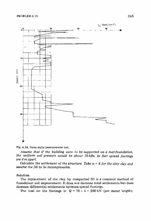
PROBLEM 6.15 2 4 5
q c ( d a N / c m 2)
Ε
Fig. 6.24. Parez static penetrometer test.
Assume that if the building were to be supported on a mat-foundation, the uniform soil pressure would be about 70kPa. In fact spread footings are 4 m apart.
Calculate the settlement of the structure. Take a — 6 for the silty clay and assume the fill to be incompressible.
Solut ion The replacement of the clay by c o m p a c t e d fill is a c o m m o n m e t h o d of
foundat ion soil improvement . It does not decrease total set t lements but does decrease differential sett lements between spread foot ings .
The load o n the foot ings is: Q = 70 χ 4 = 2 8 0 kN (per meter length) .
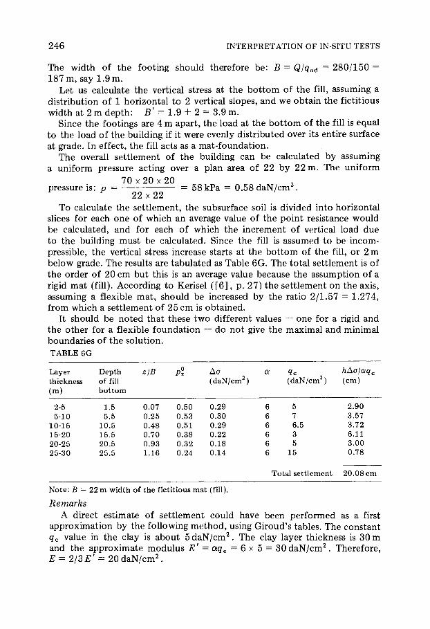
2 4 6 INTERPRETATION OF IN-SITU TESTS
The width of the foot ing should therefore be : Β = Q/qad = 2 8 0 / 1 5 0 = 187 m, say 1.9 m.
Let us calculate the vertical stress at the b o t t o m of the fill, assuming a distribution of 1 horizontal to 2 vertical s lopes , and we obtain the fictitious width at 2 m depth : B' = 1.9 + 2 = 3.9 m.
Since the footings are 4 m apart , the load at the b o t t o m of the fill is equal to the load of the building if it were evenly distr ibuted over its entire surface at grade. In effect, the fill acts as a mat- foundat ion.
The overall sett lement of the building can be calculated by assuming a uni form pressure acting over a plan area of 2 2 by 2 2 m. The uni form
70 ÷ 20 ÷ 2 0 pressure is : ñ = = 5 8 k P a = 0 .58 d a N / c m 2.
2 2 ÷ 2 2 T o calculate the sett lement , the subsurface soil is divided into horizontal
slices for each one of which an average value of the point resistance would be calculated, and for each of which the increment of vertical load due to the building must be calculated. Since the fill is a s sumed to be incom-pressible, the vertical stress increase starts at the b o t t o m of the fill, or 2 m below grade. The results are tabulated as Table 6 G . The total sett lement is of the order of 20 cm but this is an average value because the a s sumpt ion of a rigid mat (fill). According to Kerisel ( [ 6 ] , p . 2 7 ) the sett lement on the axis , assuming a flexible mat , should be increased by the ratio 2 / 1 . 5 7 = 1 .274, from which a sett lement of 2 5 cm is obta ined.
It should be noted that these two different values — one for a rigid and the other for a flexible foundat ion — do not give the maximal and minimal boundaries of the solut ion. TABLE 6G
Layer Depth z/B P°z Δ σ a hAo/aqc
thickness of fill ( d a N / c m 2) ( d a N / c m 2) (cm) (m) bot tom
2-5 1.5 0.07 0.50 0.29 6 5 2.90 5-10 5.5 0.25 0.53 0.30 6 7 3.57
10-15 10.5 0.48 0.51 0.29 6 6.5 3.72 15-20 15.5 0.70 0.38 0.22 6 3 6.11 20-25 20.5 0.93 0.32 0.18 6 5 3.00 25-30 25.5 1.16 0.24 0.14 6 15 0.78
Total settlement 20 .08 cm
Note: Β = 22 m width of the fictitious mat (fill).
Remarks
A direct est imate of sett lement could have been per formed as a first approx imat ion by the following m e t h o d , using Giroud ' s tables . The constant qc value in the clay is about 5 d a N / c m 2. The clay layer thickness is 30 m and the approx imate modulus E' = aqc = 6 x 5 = 3 0 d a N / c m 2 . Therefore , £ = 2 / 3 £ ' = 2 0 d a N / c m 2.
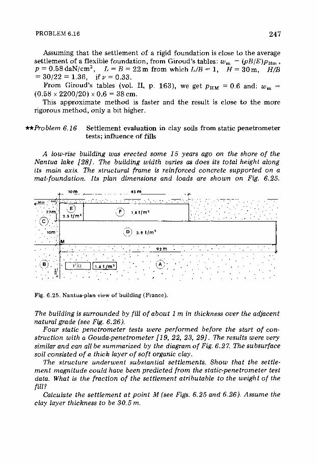
PROBLEM 6.16 2 4 7
Assuming that the set t lement of a rigid foundat ion is close to the average sett lement of a f lexible foundat ion , f rom Giroud ' s tab les : w m = (pB/E)pUm , ñ = 0 . 5 8 d a N / c m 2, L = Β = 2 2 m from which LIB = 1 , Ç = 3 0 m , H/B = 3 0 / 2 2 = 1.36, if = 0 . 3 3 .
F r o m Giroud ' s tables (vol. II , p . 1 6 3 ) , we get pHM = 0.6 and : w m = ( 0 .58 χ 2 2 0 0 / 2 0 ) χ 0.6 = 38 cm.
This a p p r o x i m a t e m e t h o d is faster and the result is c lose to the more r igorous m e t h o d , only a bit higher.
**Problem 6.16 Se t t lement evaluation in clay soils f rom stat ic penetrometer te s t s ; influence of fills
A low-rise building was erected some 15 years ago on the shore of the Nantua lake [28]. The building width varies as does its total height along its main axis. The structural frame is reinforced concrete supported on a mat-foundation. Its plan dimensions and loads are shown on Fig. 6.25.
2.5 t / m 2 ( ? ) i .et / r
O) 3 . 9 t / m 2
Fi l l | h . 8 t / m 2|
Fig. 6.25. Nantua-plan view of building (France).
The building is surrounded by fill of about 1 m in thickness over the adjacent natural grade (see Fig. 6.26).
Four static penetrometer tests were performed before the start of con-struction with a Gouda-penetrometer [19, 22, 23, 29]. The results were very similar and can all be summarized by the diagram of Fig. 6.27. The subsurface soil consisted of a thick layer of soft organic clay.
The structure underwent substantial settlements. Show that the settle-ment magnitude could have been predicted from the static-penetrometer test data. What is the fraction of the settlement atributable to the weight of the fill?
Calculate the settlement at point Ì (see Figs. 6.25 and 6.26). Assume the clay layer thickness to be 30.5 m.
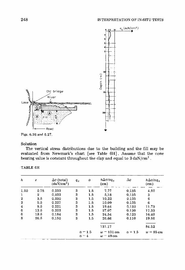
2 4 8 INTERPRETATION OF IN-SITU TESTS
R o a d
Figs. 6.26 and 6.27.
Solut ion The vertical stress distributions due to the building and the fill may be
evaluated from Newmark ' s chart [see Table 6 H ] . Assume that the cone bearing value is constant throughout the clay and equal to 3 d a N / c m 2 .
TABLE 6H
h æ Δ σ (total) ( d a N / c m 2)
Qc a hAo/aqc
(cm) Δ σ hAo/aqc
(cm)
1.50 0.75 0 .233 3 1.5 7.77 0.135 4 .50 1 2 0 .233 3 1.5 5.18 0 .135 3 2 3.5 0 .230 3 1.5 10 .22 0.135 6 2 5.5 0.227 3 1.5 10 .09 0 .135 6 4 8.5 0 .221 3 1.5 19 .64 0 .132 11.73 6 13.5 0 .203 3 1.5 27.07 0 .130 17 .33 6 19.5 0 .184 3 1.5 24.54 0 .123 16.40 8 26.5 0 .150 3 1.5 26 .66 0 .110 19 .56
131 .17 84 .52
a = 1.5 w = 131 cm a = 1.5 w = 85 cm a = 4 w = 49 cm
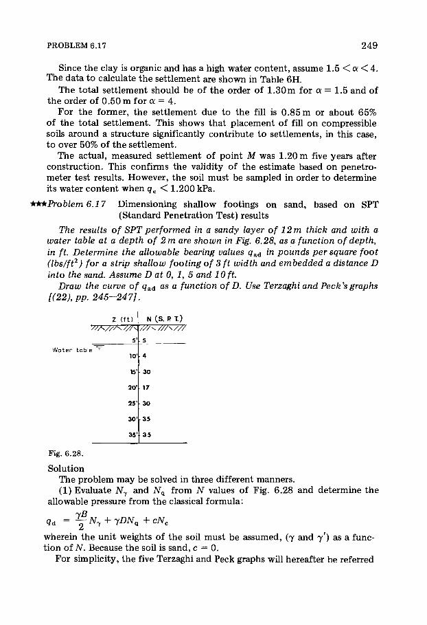
PROBLEM 6.17 2 4 9
Since the clay is organic and has a high water content , a s sume 1.5 < α < 4 . The da ta to calculate the set t lement are shown in Table 6 H .
The tota l set t lement should be of the order of 1.30 m for a = 1.5 and of the order of 0 .50 m for a = 4 .
F o r the former, the sett lement due t o the fill is 0 . 8 5 m or about 6 5 % of the tota l sett lement. This shows that p lacement o f fill on compress ible soils around a structure significantly contr ibute to sett lements , in this case , t o over 50% of the sett lement.
The actual , measured sett lement o f po int Ì was 1.20 m five years after construct ion. This confirms the validity o f the est imate based on penetro-meter test results . However, the soil m u s t be sampled in order t o determine its water content when qc < 1 .200 kPa.
Problem 6.17 Dimensioning shal low foot ings on sand, based o n S P T (S tandard Penetrat ion Tes t ) results
The results of SPT performed in a sandy layer of 12 m thick and with a water table at a depth of 2 m are shown in Fig. 6.28, as a function of depth, in ft. Determine the allowable bearing values c?ad in pounds per square foot (lbs/ft2) for a strip shallow footing of 3 ft width and embedded a distance D into the sand. Assume D at 0, 1, 5 and 10 ft.
Draw the curve of qad as a function of D. Use Terzaghi and Peck's graphs [(22), pp. 245-247]
Z ( f t ) Ν (S. R T.)
5' / / / v / / A / / / 5
W a t e r t a b l e ^
10' 4
15' 30
20' 17
25' 30
30' 35
35' 35
Fig. 6.28.
Solut ion The prob lem m a y be solved in three different manners . (1 ) Evaluate N7 and Nq f rom Ν values of Fig . 6 .28 and determine the
al lowable pressure f rom the classical fo rmula :
<7d = ^Ny + yDN^ +cNc
wherein the unit weights of the soil m u s t be a s sumed, (7 and 7') as a func-t ion of N. Because the soil is sand, c = 0 .
F o r s implicity, the five Terzaghi and Peck graphs will hereafter be referred

2 5 0 INTERPRETATION OF IN-SITU TESTS
to as A, B, C, D and E , to correspond to the order in which they were published [ 2 2 ] .
(a) D = 0 , Ν = 5 . For this value of N, the sand is very loose . Because of the proximity of the water table , a s sume the sand to be saturated by capil-larity. We can then a s s u m e :
7 d = 90 lb / f t 3 and 7 h = 1 0 0 l b / f t 3.
Graph A of Terzaghi and Peck gives, for Ν = 5 ; Ny = 5 and Nq = 8 f rom which, with Β = 3 ft : qd = ( 1 0 0 χ 3 χ 5 ) / 2 = 7 5 0 lb / f t 2 . F o r a safety factor of 3, <?ad = 2 5 0 lb / f t 2 or 1 2 kPa.
(b) D = 1 ft , Ν = 5 , we have Ny = 5 and 7Vq = 8 f rom which: qd = 7 5 0 + 1 0 0 ÷ 1 ÷ 8 = 1 5 5 0 lb / f t 2 and qad = 517 lb / f t 2 = 2 5 kPa.
(c) D — 5 ft. Because we are now very close to the water table (at 6 ft) its influence on the value of Ν mus t be taken into account and corrected b y : Ν = 1 5 4- ^(Ν' —15) where Ν' = 4 , no correction is necessary and N7 — 4 and iVq = 7.N' being the S P T value below water table .
T o calculate yNy the buoyant weight must be used ; we have: yr = yh — 7w = ( 1 0 0 - 6 2 . 4 ) = 37 .6 say 3 8 l b / f t 3.
For the overburden weight, the saturated weight of soil must be cons idered :
38 ÷ 3 ÷ 4 qd = + 1 0 0 x 5 x 7 = 2 2 8 + 3 5 0 0 = 3 7 2 8 l b / f t 2,
2
<7ad = 1 2 4 2 lb / f t 2 = 0.6 d a N / c m 2.
(d) D = 1 0 ft. The average value of N' must be calculated from the value at the level of the b o t t o m of the foot ing and 5 ft below that . In this case it is : N' = (4 + 3 0 ) / 2 = 17 from which: Ν = 1 5 + £ ( 1 7 - 1 5 ) = 16 .
Table A then gives: Ny = 1 4 , Nq = 1 6 . Ν increases between 10 and 1 5 ft, therefore ya and yh increase. S o it can
be a s sumed that : 7 d = 1 0 0 l b / f t 3, yh = 1 1 5 l b / f t 3 and y' = 53 l b / f t 3. F o r embedment the effective stress must be calculated at the foot ing level
according to the water table (6 f t . ) . F r o m which: yD = 6 χ 1 0 0 + 4 χ 53 = 8 1 2 lb / f t 2
53 χ 3 χ 14 and<? d = + 8 1 2 x 16 = 1.113 + 1 2 . 9 9 2 = 1 4 . 1 0 5 l b / f t 2,
qad = 4 . 7 0 0 lb / f t 2 = 2 2 5 kPa.
Fig. 6 .29 shows the variations of the al lowable soil bearing pressure as a function of depth D.
(2) Evaluation of qad f rom graphs. (a) D = 0. Graph Β gives directly qad for D = 0 and for a safety factor of
3: qad - 0 .1 t o n / f t 2 = 11 kPa. The two methods give identical results. (b) D = 1 , Ν = 5 . Graph C gives the increase in bearing pressure as a func-
tion of depth D: qad = 0 .1 + 0 .13 = 0 .23 tons / f t 2 = 2 5 kPa. The two methods give identical results.

PROBLEM 6.17 2 5 1
Fig. 6.29.
(c) D = 5 . If there were no water table , we would have qad = 0 .1 4- 0 .52 = 0 .62 t o n / f t 2 = 6 6 k P a . Because of the presence of the water-table 1 ft below the foot ing b o t t o m , the first term must be divided by (1 + 2 / 3 ) = 1.66. T h e n < ? a d = 0 .06 + 0 .52 = 0 .58 t o n / f t 2 = 6 2 k P a .
(d) Β = 10 ft. F o r N' = 1 7 , it was shown that Ν = 16 . The al lowable bearing pressure is, according to graph B : qad = 1 t o n / f t 2, but this pressure must be divided by 2 to account for the water table . The increase of the stress due to e m b e d m e n t is 2.3 t o n s / f t 2 (see graph C ) .
Since the e m b e d m e n t is 4 ft below the water table , this increase must be divided by (1 + 4 / 1 0 ) = 1.4 or : qad = 1/2 + 2 .3 /1 .4 = 0 .5 + 1.64 = 2 .14 tons / f t 2 = 2 2 9 kPa.
A good accordance between the two methods can also be noted .
Remark
The al lowable bearing pressures are l imited further to account for settle-ments . All the above calculated al lowable bearing pressures have a safety factor with respect to the ul t imate failure pressure. They must be further reduced to account for the sett lements that they could generate. For that reason, graph D mus t be used which gives qad for a m a x i m u m sett lement of 1 inch , assuming the water table at depth Β below the foot ing. If the water table is close to the foot ing, qad given by graph D mus t be divided by 2 .
For Β = 3 ft, graph D gives f o r i V = 5 : qad = 0 .5 t o n s / f t 2 = 5 4 k P a , for Ν — 1 6 : qad = 1.9 t o n s / f t 2 = 2 0 3 kPa.
2 5 2 INTERPRETATION OF IN-SITU TESTS
(3) Al lowable bearing pressures f rom Meyerhof ' s formula [ 2 2 ] .
q a d = NB(1+D/B)(H30) (1 )
for B, expressed in feet , qad in t o n s / f t 2 . The above formula is valid only for cohesionless soils above the water table . For c layey sands and submerged sands , qad mus t be divided by 2 .
Meyerhof also p r o p o s e d : qd = N(B 4- D)/C where C = 10 for fine sand, 6 < C < 8 for coarse sand and gravelly sand, 1 5 < C < 2 0 for silty sand and non-plastic silts.
Equat ion (1) gives respectively: (a) D = 0, Ν = 5 : qad = (5 χ 3 ) / 3 0 = 0 .5 t o n s / f t 2 = 53 kPa. (b) D = l, Ν = 5 : qad = (5 χ 3 ) ( 1 + 1/3) χ 1/30 = 0 .667 t o n s / f t 2 =
71 kPa. (c) D = 5 , Ν = 4 , if there were no water tab le : qad = 4 χ 3 ( 1 4- 5 /3 ) χ
1/30 = 1.07 t o n s / f t 2 but because of the water table , the result must be divided by 2 and qad = 0 .54 t o n s / f t 2 = 58 kPa.
(d) £> = 1 0 , Ë Ã = 1 6 : qad = ? [ 1 6 x 3 ( l + 1 0 / 3 ) x 1 /30] = 3 .47 t o n s / f t 2 = 3 7 0 kPa.
For cases (a) and (b ) , Meyerhof ' s formula gives al lowable bearing pressures considerably higher than the other two methods . F o r cases (c) and (d) it gives about the same or slightly higher results . These values should also be decreased to limit the foot ing sett lements to 1 inch or less.
Meyerhof es imates that for Β < 4 ft , qad must be l imited by N/8 or for each of the preceding cases :
case a qad < 0 .62 t o n / f t 2 = 66 kPa (D = 0 )
case b qad < 0 .62 t o n / f t 2 = 66 kPa (D = l ' )
case c qad < 0 .5 t o n / f t 2 = 54 kPa (D = 5')
case d qad<2 t o n / f t 2 = 2 1 4 kPa (D = 1 0 ' )
Finally, it can be concluded that all the methods give close results , except for case a , which is hardly ever encountered in pract ice anyway .
** Problem 6.18 Pile capaci ty determinat ion in sand f rom S P T
Assume the same givens as in the preceding problem, and assume that the sand layer overlies bedrock. Determine the ultimate bearing capacity, in tons, of a driven pile of 1 ft diameter at a depth of 25 ft.
Solut ion The ul t imate pile bearing capaci ty is c o m p o s e d of t w o component s ,
namely end-bearing and skin frictions: Qd = Qa + Qf. L e t A be the end area of the pile of diameter B, f rom Meyerhof and for
the case of s ands :
ð Β xD -Qd = ANA 4- — — — xJV (average over pile shaf t ) . (Qd in tons )
ou

PROBLEM 6.19 2 5 3
Solut ion Soil investigation A: (1) Pressuremeter te s t s :
The corrected values of Ν because of the water table must first be deter-mined
N' 5 4 3 0 17 30 3 5 3 5
Ν 5 4 2 2 . 5 16 2 2 . 5 2 5 2 5
The Ν average value for lateral friction along the pile shaft i s :
- 5 + 4 + 2 2 . 5 + 16 + 2 2 . 5 ^average = = 7 0 / 5 = 14 from which:
5
Qd = 4 χ 2 2 . 5 χ (π/4) χ 1 2 + π χ 1 χ 2 5 χ ( 1 4 / 5 0 ) = 70 .7 4- 2 2 = 9 2 . 7 t o n s .
For a safety factor of 2 , we have : Qad = 46 tons = 4 0 9 k N
*Problem 6.19 Cost compar i son of soil investigations based on different types o f in-situ tests
Determine from the unit prices given below in U.S. dollars 1984 the total costs of soil investigations using different types of in-situ tests, such as pressuremeter tests, static-electric cone-penetrometer tests and S.P.T. Assume sites are readily accessible.
Soil investigation A: for the control of vibroflotation or dynamic com-paction (Menard-method) of a fill, it is proposed to perform 10 tests to 3 m depth and 2 to 7m depth.
Soil investigation B: three tests must be performed to a 20 m depth at the site of a proposed building. Assume that both sites are 150 km from con-tractor office. The unit rates are given below:
For the pressuremeter:
Mobilization and demobilization US $ 80/hr Drilling to 20 m, by linear meter, with a
pressuremeter test, each meter US $ 100/hr
For the static cone-penetrometer:
Mobilization (C.P.T.) demobilization and penetration US $ 120/hr
For the S.P.T:
Mobilization and demobilization US $ 80/hr Drilling from 0 to 20 m, with a test performed every
1.50 meter US $ 80/hr

254 INTERPRETATION OF IN-SITU TESTS
These tests should be performed every meter , therefore :
Mobilization and demobil izat ion, 6 hrs at $ 80 U S $ 4 8 0 Drilling and pressuremeter test (44 m) in, say, 44 hrs at $ 1 0 0 U S $ 4 4 0 0
Total U S $ 4 8 8 0
(2) Cone-penetrometer tests :
Mobilization and demobil izat ion, 6 hrs at $ 1 2 0 U S $ 7 2 0 Static penetrat ion, assume 12 hrs at $ 80 us $ 1 4 40
Total U S $ 2 1 6 0
(3) S .P.T. :
Mobilization and demobil izat ion, 6 hrs at $ 80 U S $ 4 8 0 Drilling, 4 4 m in, say, 2 8 hrs at S 80 U S $ 2 2 4 0
Total U S $ 2 7 2 0
To summarize , for soil investigation A: (1) cone-penetrometer U S $ 2 1 6 0 (2) pressuremeter tests U S $ 4 8 8 0 (3) S .P.T. U S $ 2 7 2 0
Because the nature of the fill is known, it is not necessary in this case to include drilling and sampling in the cost es t imate .
Soil investigation Β Three tests to 20 m are p roposed :
(1) Pressuremeter tests :
Mobilization and demobil izat ion, 6 hrs at $ 8 0 U S $ 4 8 0 Drilling with pressuremeter test , every m, 6 0 hrs at $ 1 0 0 U S $ 6 0 0 0
Total U S $ 6 4 8 0
(2) Cone-penetrometer test :
Mobilization and demobil izat ion, 6 hrs at $ 120 U S $ 7 2 0 8 hrs of penetrat ion at $ 120 U S $ 9 6 0
Total U S $ 1 6 8 0
PROBLEM 6.20 2 5 5
(3) S .P.T. :
Mobilization and demobi l izat ion, 6 hrs at $ 8 0 Drilling, 4 8 hrs (with a test every 1.50 m ) at $ 8 0
U S $ 4 8 0 U S $ 3 8 4 0
Total U S $ 4 3 2 0
For this example , the summary is : (1 ) Cone-penetrometer (2) Pressuremeter (3) S .P .T.
U S $ 1 6 8 0 U S $ 6 4 8 0 U S $ 4 3 2 0
However, it should be noted that , unless the site is in a very well known geologic and geotechnic area, it would be necessary to include one bore hole with soil sampling to the stat ic-penetrometer investigation. The cost of this bore hole and sampling must be added to the cost of the cone-penetration and this addit ional cost would still m a k e that investigation the cheapest . Its added cost would be about one-third of the tota l .
Often, in pressuremeter investigations, for the purpose of reducing costs , tests are m a d e only every 2 , 3, 4 , or even 5 m depth intervals, to the detri-ment of profile definition.
It is important to underl ine the fact that the cost of the cone-penetrometer investigation is not high, when considering that it is the only one yielding cont inuous information throughout the depth of penetrat ion. The more expensive alternate of the pressuremeter investigation yields information at best every meter . More data is m a d e available at a lower total cost with the penetrometer . However, in addit ion to the pf and ñë l imits obta ined by the pressuremeter, the pressuremeter modulus Ep is also determined.
It should also be ment ioned that laboratory testing of soils would be more expensive than SPT or pressuremeter measurements because of the cost of recovering undis turbed samples ( about U S $ 3 0 each) and the added costs of the tests themselves. F o r each sample , the addit ional laboratory testing cost would be approx imate ly U S $ 6 0 0 , depending on per formed tests .
As a general rule, both technical and financial considerations must be evaluated because each t y p e of soil investigation has advantages that the other two do not present. No single method is a lways the best for all pro-jects .
ick+Problem 6.20 Compar i son o f set t lement calculat ion based on static pen-etrometer tests and consol idometer tests da ta ; determinat ion of the value of the coeff icient a
The following profile was determined at a site along the Saone River near Lyons (France) with the Andina, static-dynamic penetrometer:
Remarks

2 5 6 INTERPRETATION OF IN-SITU TESTS
— from 0 to 3 m: old sandy gravel fill; — from 3 to 6.5 m: clayey silt; — below 6.5: sandy-gravelly alluvium.
The penetration diagram of Fig. 6.30 is representative of the soil resist-ances at the site. It is proposed to erect a light building consisting of 2
S c a l e c h a n g e -Ï 1 2 3 4 5 6 7 8 9 1 0 11 12 13 14 15 16 17 1È 19 2 0 2 5
Sca l e c h a n g e 3 5 4 5 5 5 6 5 7 5 8 5
q c ( d a N / c m 2)
9510 0 12 5 17 5 22 5 2 7 5 325 _
> ^—'
——-
r
Fig. 6.30. Andina static-dynamic penetrometer result.
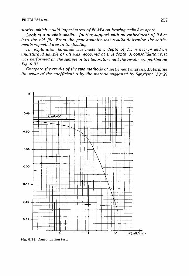
PROBLEM 6.20 2 5 7
stories, which would impart stress of 20 kPa on bearing walls 3 m apart. Look at a possible shallow footing support with an embedment of 0.5 m
into the old fill. From the penetrometer test results determine the settle-ments expected due to the loading.
An exploration borehole was made to a depth of 4.5 m nearby and an undisturbed sample of silt was recovered at that depth. A consolidation test was performed on the sample in the laboratory and the results are plotted on Fig. 6.31.
Compare the results of the two methods of settlement analysis. Determine the value of the coefficient a by the method suggested by Sanglerat (1972)
0.65
0.60
0.55
0.50
0.45
0.40
0.35
10 <T(daN/cm2)
Fig. 6 .31 . Consolidation test.

2 5 8 INTERPRETATION OF IN-SITU TESTS
[27]. Assume the old fill density and that of the silt to be 1.8. The water
table is located at over 6 m depth.
Solut ion F r o m the penetrometer test data , it m a y be concluded that the old fill is
quite dense (50 <qc < 1 5 0 d a N / c m 2) . Because the building loads are light, the fill is adequate t o suppor t the loads . Foot ings separat ion, f rom center to center would be 3 m (that of the bearing walls) . The fill thickness below the footings would be 2 .5 m. If we as sume a load distribution of 2 to 1 through the fill, the stress would be a lmost uni form at the base of the fill and equal to 20 kPa or 0.2 d a N / c m 2. The fill layer acts as a mat-type foundat ion .
(a) Settlement calculations based on the Andina penetrometer test data. Sett lements would occur in the silt layer. The average cone-bearing value
in that layer is qc = 5 d a N / c m 2. If we as sume the silt t o have a low plasticity, α will be in the range 3 < a < 6. Ef = aqc or 15 <Ef < 30 d a N / c m 2 .
The stress increase at the surface of the silt layer is : Δ σ = 0.2 d a N / c m 2
and over the thickness of the silt layer (H = 3 .5 m ) the sett lement would be Ah = HAo/aqc = 3 5 0 χ 0 . 2 / 1 5 = 4.7 cm for a = 3 or : Ah = 3 5 0 χ 0 . 2 / 3 0 = 2.3 cm for a = 6.
The expected sett lement would be between 2 c m < Ah < 5 c m . It was implicitly a s sumed that the fill and underlying sand-gravel sub-
stratum are incompressible because of their density and the light surface building loads . An accurate calculation f rom the static penetrometer would give, for a = 3 and qc = 1 0 0 d a N / c m 2 (average value) , in the fill a sett lement of about w = 0 .2 c m , which is minimal compared t o that caused by the silt layer.
(b) Settlement calculation from the consolidation test result. The effective overburden pressure at the depth where the sample was
recovered must be computed . It is at depth 4.5 m, or jus t at mid-height of the compress ible silt layer.
We have: oc> = 18 χ 4 .5 = 8 1 kPa ^ 0.8 d a N / c m 2. The compress ion curve of Fig . 6 .31 indicates that the void ratio at that
stress level is e0 = 0 . 5 8 6 . The load increment due to the building weight over the thickness of the
silt layer is about Δ σ = 0 .2 d a N / c m 2 . The stress at mid-height would then b e : σ = σό + Δ σ = 0 .8 + 0.2 = 1 d a N / c m 2. The corresponding void rat io for that stress level i s : e = 0 .576 .
The void ratio has decreased by Ae = 0 .586 — 0 .576 = 0 . 0 1 0 . Thus the consol idat ion of the sample of thickness h is Ah/h = Ae/(1 + e0)
0 . 0 1 0 from which the sett lement of the silt layer is : Ah = 3 5 0 χ „ , „ „ ^ = 2 . 2 c m .
* 1 + 0 .586
PROBLEM 6.20 2 5 9
(c) Comparison of the results of the two methods.
The sett lement c o m p u t e d on the basis o f the consol idat ion test is practi-cally equal to that c o m p u t e d on the basis of the static penetrometer for a value o f a = 6 .
(d) Evaluation of the a coefficient
T h e compress ion curve shows that the preconsol idat ion stress oc is equal to about 0 . 8 d a N / c m 2 . Since this corresponds to the effective overburden stress, it is indicative that the silt layer is normally consol idated. It also shows that the consol idat ion due to the old fill is comple ted for all practical purposes .
Therefore , the fol lowing formula is appl icable :
a = 2 .3 — , C e o Qc
where σ'0 = effective overburden stress ;
eco = void rat io corresponding to σ'0; _ gc gc o
c o ~ logd + l/ai) e
x = void rat io corresponding t o o'
0 + 1 ( d a N / c m 2) ;
qc — cone bearing value f rom the penetrometer test at the depth where the sample was recovered, that is f rom 4 .5 to 4 .8 m.
In this case we get qc = 4 d a N / c m 2 at that depth .
F r o m the compress ion curve we have: for o'0 = 0 .8 d a N / c m 2 , eco = 0 . 586 for σ'0+1 = 1.8 d a N / c m 2 , et = 0 . 5 3 6
Then:
0 . 5 8 6 - 0 . 5 3 6 1 + 0 . 5 8 6 0 .8 C c o = ,„ , Λ ιΛ ox = 0 . 1 4 2 and a = 2 .3 χ χ — = 5 .14
log (1 + 1/0 .8) 0 . 1 4 2 4
or, say , a: = 5 .
Remark
This value of α is within the range 3 < a < 6 . However, the quest ion arises why the value of a = 6 was no t obta ined since the sett lement calculations giving an answer of 2 .2 were based on that value.
The difference is due mainly t o the fol lowing reasons : t o calculate a , an increase o f stress o f Δ σ = 1 d a N / c m 2 f rom σ 0 was considered. On the com-pression curve, it can be seen that for this increment, the s lope o f the curve is steeper than that caused by the building load Δ σ = 0 .2 d a N / c m 2. In other words , a value of a: = 5 would overest imate the sett lement .
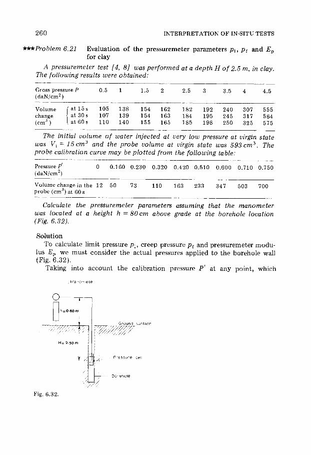
2 6 0 INTERPRETATION OF IN-SITU TESTS
***Problem 6.21 Evaluation of the pressuremeter parameters pu pt and Ep
for clay
A pressuremeter test [4, 8] was performed at a depth Ç of 2.5 ra, in clay. The following results were obtained:
Gross pressure Ρ (daN/cm 2)
0.5 1 1.5 2 2.5 3 3.5 4 4.5
Volume ( at 15 s change at 30 s ( c m 3) ( a t 6 0 s
105 138 154 162 182 192 240 307 107 139 154 163 184 195 245 317 110 140 155 165 185 198 250 325
555 564 575
The initial volume of water injected at very low pressure at virgin state was V{ = 15 cm3 and the probe volume at virgin state was 593 cm3. The probe calibration curve may be plotted from the following table-
Pressure Ρ (daN/cm 2)
0 0.160 0.230 0 .320 0 .420 0.510 0.600 0.710 0.750
Volume change in the probe ( cm 3) at 6 0 s
12 50 73 110 163 233 347 503 700
Calculate the pressuremeter parameters assuming that the manometer was located at a height h —80cm above grade at the borehole location (Fig 6.32).
Solut ion To calculate limit pressure pu creep pressure pf and pressuremeter modu-
lus Ep we must consider the actual pressures appl ied to the borehole wall (Fig. 6 . 3 2 ) .
Taking into account the calibration pressure P' at any point , which
/ M a n o m e t e r
Ground surface
P r e s s u re cell
Fig. 6.32.

PROBLEM 6.21 2 6 1
gives the same volume change as the gross pressure Ρ and the level h of the manometer above the ground, the actual pressure to the soil is given by :
P r = P-P' + (H + h)yw = Ρ — P' + 0 .33 d a N / c m 2
(a) Limit pressure. The gross limit pressure is the a symptote ' s abscissa of the pressiometric curve (ρ, V), i .e. : (pl )r = 4 .6 d a N / c m 2 .
But for practical purposes the limit pressure is conventially the point at which the initial borehole vo lume (at the beginning of the elastic phase) has doubled , i .e. :
AV = 593 + 1 5 4 - 1 4 0 - 7 5 0 c m 3
Therefore :
V= 593 + 2 ( 1 5 + 1 4 0 ) ~ 9 0 3 c m 3 .
At V = 9 0 3 c m 3 , the corresponding value of P' is about 0 .76 d a N / c m 2 on the cal ibration curve (Fig . 6 . 3 4 ) .
F r o m this, the limit pressure is : px = 4 .6 — 0 . 7 6 0 + 0 .33 = 4 .17 d a N / c m 2.
(b) Creep pressure p f . The pressure at the creep point can be determined f rom either: - Fig. 6 . 3 5 , which gives (pf)h ~ 2 . 8 d a N / c m 2 ;
Fig. 6 .33. Limit-pressure curve.
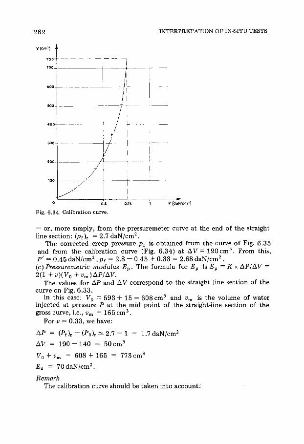
2 6 2 INTERPRETATION OF IN-SITU TESTS
V(cm3)
Ï 0. 5 0.7 6
Fig. 6.34. Calibration curve.
1 Ρ (daN/cm2
— or, more s imply, f rom the pressuremeter curve at the end of the straight line sect ion: (Pf) r. = 2 . 7 d a N / c m 2.
The corrected creep pressure pt is obta ined from the curve of Fig . 6 . 3 5 and from the calibration curve (Fig . 6 .34 ) at A V = 1 9 0 c m 3 . F r o m this, P' = 0 .45 d a N / c m 2 , pf = 2.8 - 0 . 4 5 + 0 .33 = 2 .68 d a N / c m 2 . (c) Pressuremetric modulus Ep. The formula for Ep is Ep = Ê χ AP/AV = 2(1+ p){V0 + vm) AP/AV.
The values for AP and AV correspond to the straight line section of the curve on Fig. 6 . 3 3 .
In this case : VQ = 593 + 15 = 6 0 8 c m 3 and vm is the volume of water injected at pressure Ρ at the mid point of the straight-line section of the gross curve, i.e., vm = 1 6 5 c m 3 .
For í — 0 . 33 , we have:
AP = (Pf), ~ ( P 0) r ^ 2 . 7 - 1 = 1.7 d a N / c m 2
AV = 1 9 0 - 1 4 0 = 50 c m 3
V0 + vm = 6 0 8 4- 1 6 5 = 7 7 3 c m 3
£ p = 70 d a N / c m 2.
Remark The calibration curve should be taken into account :

PROBLEM 6.22 2 6 3
20
15
10
5
0 1 2 Ô 3 4 Ρ (daN/cm*) Mr
Fig. 6 .35. Creep diagram [ Δ ν ] * ™ £ .
AP = ( 2 . 7 - 0 . 4 4 ) - ( 1 - 0 . 3 8 ) = 1.64 d a N / c m 2
which yields the very close result for Ep = 6 7 . 5 d a N / c m 2. It should be noted that the above method is only correct for the Menard
pressuremeter and cannot be used for the self-boring pressuremeter. For this kind of device, the interpretation p r o p o s e d by Baguelin et al. [ 2 , 3 ] should be a d o p t e d .
++*Problem 6.22 Determinat ion o f a bridge foundat ion based on pressure-meter test results
It is proposed to construct a 15 m road bridge across a river. The soil on either bank of the river was investigated by means of boreholes and pressure-meter testing. The results are presented in Fig. 6.36.
Design the foundations scheme using the following criteria road level: 248 m a.s.l.; dead load: 200 kN per meter width; live load: 100 kN per meter width;
A cross-section of the project is shown in Fig. 6.37.
Solut ion The retaining walls will be suppor ted on spread foot ings at the level of the
gravelly clay layer. This will el iminate set t lements which would occur if the foot ing was placed on the compress ib le organic silt (see Fig. 6 . 3 7 ) .
The access fills o f s o m e 3 m in thickness will settle differentially with re-spect to the retaining wall since they will cause consol idat ion of the organic silt layer. It would be advantageous , in this case , t o preload the banks . This would require taking undis turbed samples of the silt t o determine the o p t i m u m t ime for the appl icat ion of a pre load. The fol lowing planning may be a d o p t e d :
ÄV (cm3) ë

2 6 4 INTERPRETATION OF IN-SITU TESTS
Soil p r o f i le 2 4 5 Q.S.I.
Bor ing P r e s s u r e m e t r i c modulus
E p- ( d a N / c m2)
p t- L i m it p re s sure — ( ä )—
p f~ C r e ep l i m it 3 — (daN/cm 2)
0 5 0 10 0 2 0 0 4 0 0 80 0 0 5 1 0 2 0 4 0 8 0
Fig. 6.36.
— construct the footings and the deck co lumns ; — place a preload fill and allow sett lements to occur on the banks ; — build the roadway.
(A) Bearing capacity. T o evaluate the allowable soil-bearing pressure, only the vertical loads given will be considered, since the horizontal loads will be nominal because of the construct ion method (deck co lumns) . The maxi-m u m load will be of the order o f 3 0 0 k N per meter width. The limit pressure is of the order of (4 .5 + 6 .5 ) /2 = 5.5 d a N / c m 2 at the proposed foundat ion level. A foundat ion whose width will distribute the load so that qad — P i /3 ~ 2 0 0 k N / m 2 must be considered. As a preliminary evaluation, Β = 3 0 0 / 2 0 0 = 1.50 m. The vertical ult imate bearing pressure, qr, is then:
Qr = Qo + fe(Pi -Po)
where:

PROBLEM 6.22 2 6 5
Figs. 6.37 and 6.38.
• Po — total horizontal earth pressure (on a vertical plane) at the t ime of the test . Assuming a coefficient of earth pressure at rest of K0 = 0 .5 and Tsat — Th = 20 k N / m 3 we have :
Po = 2 .5 χ 2 0 χ 0 .5 + 1 χ 10 χ 0 .5 + 10 χ 1 = 4 0 k N / m 2 = 0.4 d a N / c m 2 .
• Qo = total vertical overburden stress (on a horizontal plane) at the p roposed foundat ion level after construct ion of the fill, or :
q0 = 3 x 2 0 + 2 .5 x 2 0 + 10 x 2 = 1 3 0 k N / m 2 = 1.3 d a N / c m 2
(access fill) (backfil l)
• P i ~ equivalent l imit pressure (the soil at the foundat ion level is hetero-geneous , see F ig . 6 . 3 8 ) .
Pie = yPi(-3R)xpl(-2R)xpl(-R)xpl(0)xpi(+R)xpl(+2R)xpl(+3R)
or: p l e — \/4 ÷ 6 .5 χ 4 .5 χ 5 .5 χ 6 .5 χ 1 1 χ 9
= ^ 4 1 4 , 0 9 2 . 5 = 6 .4 d a N / c m 2 .
This value should not be reduced to account for decompress ion of the soil which will occur due to excavat ion and groundwater f low, because the proposed m e t h o d of construct ion is going t o impose a load to reconsol idate the material prior to finalizing the s tructure .
• k = bearing factor , f rom Menard's curves (Fig . 6 . 3 9 ) which is a function of e m b e d m e n t , soil t y p e and the foot ing geometry .
• The e m b e d m e n t ra t io : he/R where R = foundat ion radius = 0 . 7 5 m , ,fte = e m b e d m e n t :

266 INTERPRETATION OF IN-SITU TESTS
For a preliminary evaluation, embedment is only considered in the existing soils :
4 ÷ 1 + 6 .5 ÷ 1 + 0 .5 ÷ 4 .5 2 he = = 2 m and hJR = = 2 . 7 .
6.4 0 .75
• Soil category The foundat ion soil type is a clay, for which the limit pressure is less than 12 d a N / c m 2, therefore the soil category is I (see Table 61).
• Foot ing geometry The length of the foot ing may be as sumed equal to the proposed width of the road , or L = 1 5 m, hence : L/2R = 1 0 .
The k value is calculated from the graph of Fig. 6 . 3 9 for the given example hJR = 2.7 and L/2R = 1 0 ; k is found as fo l lows: Set off k vertical line f rom hJR = 2 .7 , cutt ing the category / lines for strip and square footings at A and B, respectively. Draw lines A0A and B0B t o intersect at C. Draw the line L/2R = 10 to C which cuts he/2R = 2 .7 at M, then the k value, ordinate of Af, is 1.26. The ult imate vertical bearing pres-sure will then be :
qt = 1.3 + 1.26 χ ( 6 . 4 - 0 . 4 ) = 8 . 9 d a N / c m 2
and the allowable bearing pressure then is:
qad = 1.3 + 1 . 2 6 / 3 ( 6 . 4 - 0 . 4 ) = 3 . 8 d a N / c m 2 .
TABLE 61
Soil type Nature Limit pressure pl
(daN/cm 2)
I clay 0—12 loam 0 - 7
II stiff clay and marl 1 8 - 4 0 loam 1 2 - 3 0 loose sand 4 - 8 weak soil 1 0 - 3 0
III sand and gravel 1 0 - 2 0 rock 4 0 - 1 0 0
Illb very dense sand and gravel 3 0 - 6 0
(After L. Menard)

PROBLEM 6.22 267
Fig. 6.39. -values for shallow footings (after Menard).
The allowable load, per meter length of footing, would then be 3.8 χ 1 5 0 = 5 7 0 kN, which is appreciably higher than the expected load of 3 0 0 k N per meter length.
Remarks (a) The analysis of the consol idat ion results of the preload on the silt layer
would eventually conclude that the bridge foot ing could bear on the com-pacted access fill. This could be checked by a complementary in situ testing investigation with penetrometer tests per formed after unloading.
(b) Another construct ion method would be to remove the organic silt
TABLE 6J
k values (for homogeneous layer)
D Square footing Strip footing
Β I II III I l lb I II III I l lb
0 0.8 0.8 0.8 0.8 0.8 0.8 0.8 0.8 0.5 1.3 1.5 1.9 2.1 1.0 1.1 1.2 1.3 1.0 1.6 1.8 2.5 2.8 1.2 1.3 1.4 1.6 1.5 1.8 2.1 3.0 3.3 1.2 1.4 1.6 1.8
(After L. Menard).
' I I I I I I I ' s c a le L/2R is a nomograp h to g ive k for a r e c t a n g u l ar f o o t i n g by i n t e r p o l a t i o n betwee n a s q u a re footing and a s tr ip foot ing _ . E x a m p l e: Find k f or Ae/ / ? = 1.5 , 1 / 2 / ?= 2 and so il t y p e I E. D r aw t he hne h / /? = 15 c r o s s i ng c u r v e s JZT and 4 - 8 . Find t h e o r d i n a t e k, and Ì so t h a t Ì d i v i d e s t h e s e g m e n t AB in t he s a m e p r o p o r t i o n as MQ and Ë 08 0 · D r aw A QA and 8 0 8 w h i ch c r o ss C, and f r om t h e s e points d r aw a l i ne t o M 0. A- is t h e o r d i n a te of Ì and is equal to 1.75 | (
' i ' 2 Ã 3 *~ R 2.7
INTERPRETATION OF IN-SITU TESTS
and replace it by compac ted select material to also allow for the construct ion of shallow footings on the fill.
This method leads to conservatism because : (1) a surcharge fill would increase the characteristics of the organic silt
therefore the value of he. This would m a k e us to t ake this layer into account ; (2) the compac ted fill would have a px > 1 5 d a N / c m 2 which would also
lead to a larger he; (b) the allowable bearing capacity will in fact be higher because of the
consol idat ion of the clay due to the surcharge; (c) it was a s sumed that the access fills would not impart horizontal
pressures. (B) Settlement evaluations. The final sett lement of the footing will be at most equal to the sum of the sett lements caused by the fill weight and structural dead loads . Live loads applied only for short durat ions can be ignored.
(a) Set t lement due to fills. The following formula m a y b e u sed :
where: • P z = vertical stress increment at depth æ due to the fill. Because of the large width o f the fill a t its base ( about 2 5 m ) and the
thickness of the soil layers ( 1 0 . 2 5 m ) susceptible to consol idat ion, P z may be a s sumed constant with æ and equal t o :
Ρ = h r χ 7 r ,
where hx = fill thickness or 3 m, yx = unit weight of wet soil of the com-pacted fill or 7 h = 2 2 k N / m 3 . So Ρ = 6 6 k N / m 2 .
• E(z) = pressuremeter modulus at depth z. • a(z) = rheologic coefficient depending on soil t y p e at depth æ (see
Table 6 K ) : for the organic silt a = 1/2, for the gravelly clay α = 1/2. • â (Ã) = 1 if Γ > 2 ( Γ is the ratio of the limit pressure of the soil to the
actual stress at depth z). F o r the silt: limit stress is ~ 0.8pu actual stress is = 6 6 k N / m 2 = 0 .66
d a N / c m 2 and Γ = 4 / 0 . 6 6 = 6 . For the clay, which is stiffer: â(Ã) = 2 /3 χ Γ / ( Γ - 1 ) = 0 .8 . Final ly :
h
w T = á÷Ρ÷â(Ã) Σ i E(z)
1 1 1 1 — + — + — + — +
\ 6 0 8 5 70 4 2 1 0 2
1 1 + — +
70
0 .75
1 8 0
PROBLEM 6.22 2 6 9
1 0 0
0 .27
1 0 0
TABLE 6K
x (1 .7 + 1.17 + 1.43 + 2 .4 + 1 + 1.43 + 0 . 4 2 )
( 9 . 5 5 ) , w t = 2 .6 c m .
Soil type Peat Clay Silt Sand
Sand and gravel
Type Rock
a E/Pi a ElPi a E/Pi a ΕÉΡ÷ α a
Over-consolidated
— > 1 6 1 > 1 4 2/3 > 1 2 1/2 > 1 0 1/3 slightly fractured
2/3
Normally consolidated
1 9.16 2/3 8.14 1/2 7 .12 1/3 6.10 1/4 normal 1/2
Under-consolidated very loose
7.9 1/2 5.8 1/2 5.7 1/3 highly fractured highly weathered
1/3
2 /3
(b) Settlements due to structural dead loads. Menard proposes the follow-ing formula : W = W x 4- W 2 + W 3, where W x = immedia te set t lement , not usual ly cons idered :
1.33 / R\a . W 2 = -Ã7Ã x p x i ? o x ^ 2 X 7 T (sett lement d u e to deviatoric stress)
3EB \ R0j
W3 = ( α / 4 . 5 EA) ÷ ñ ÷ λ 3 χ R ( sett lement due to isotropic stress) .
where : • R = half width of a rectangular foot ing or radius of a circular foot ing,
R = 75 c m ; • R0 = 3 0 cm (reference d imens ion) ; • ñ — average increase in stress due to the foot ing, with respect to the
natural stress condit ion, calculated under the permanent structural loads : ñ = 2 0 0 / 1 . 5 0 = 1 3 3 kPa = 1.3 d a N / c m 2 ;
TABLE 6L
λ 2 and λ 3 coefficients in function of L/2 R
L/2R I 2 3 5 10 20
circle square
λ 2 1 1.12 1.53 1.78 2.14 2.40 2.65 λ 3 1 1.1 1.2 1.3 1.4 1.46 1.5
0 .27

2 7 0 INTERPRETATION OF IN-SITU TESTS
• λ 2 and λ 3 = shape factors depending on foot ing dimensions . F o r L/2R = 1 5 / 1 . 5 = 1 0 . Table 6 L gives: λ 2 = 2 .40 and λ 3 = 1 . 4 6 .
• EA and EB are the pressiometric modul i corresponding to the spherical and deviatoric stresses calculated as shown below.
• a = rheologic coefficient of the soil : a = 1/2 (Table 6 K ) .
Determination of EA:
EA = E1 harmonic mean of the pressuremeter modul i to a depth R beneath the foot ing :
I = i f l + - i _ El 2 \E0 E(-R)
In this ca se :
A _ I [/J. + i ) + i . Ei 3 [ \ 2 5 6 0 / 6 0
0 . 0 2 4
Ei — EA = 4 1 d a N / c m 2.
Determination of EB:
Ex 0 . 85 E2 + •
E,
^3 /4 / 5 2 . 5 i J 6 / 7/ 8 2.5E9toi6
harmonic mean of the modul i at depths — R and — 2R (Fig . 6 . 4 0 ) :
_1^
E2
_1^ _1
2 160 8 5 0 . 0 1 4 .
E2 Ε 3/4/5
Ε 6/7/8
" _ R j 2R= 1.50m J El
_ 2 R
_ 3 R
- 4 R
- 5 R - 6 R
- 7 R - 8 R - 9R
- 10R
- 11 R
- 12 R Ε 9ft 16
- 1 3 R
- 1 4 R
- 1 5 R
—16 R
Fig. 6 .40.

PROBLEM 6.22 2 7 1
1 1 / 1 1 \ 1 — + — + — + — + — 8 5 7 0 1 7 0 4 2 / 4 2
= 0 . 0 1 8 .
£ 3 / 4 / 5 = harmonic mean of modul i in layers 3 t o 5 (Fig . 6 . 4 0 ) :
1 _ 1_
£ 3 / 4 / 5 5
•2-6/7/8 — harmonic mean of modul i o f layers 6 t o 8.
1 _ 1
5
1 1 1 / 1 1 — + + — + 1 — +
4 2 1 0 2 7 0 1 7 0 1 8 0 £6/7 / 8
£ 9 t o 16 = harmonic mean of modul i of layers 9—16:
1 1
= 0 . 0 1 4 .
£ 9tol 6 1 1
1 1 \ 1 1 1 / 1 1 \ — + — + — + — + — + — + — + \ 7 0 1 8 0 / 1 8 0 3 5 0 5 0 0 \ 5 0 0 7 5 0 /
1 1 1 1
+ + + + 7 5 0 1 0 0 0 1 0 0 0 1 0 0 0 = 0 . 0 0 3 5
and :
EB = 1 1 1
0 . 0 2 4 + — — χ 0 . 0 1 4 + 0 . 0 1 8 + — ( 0 . 0 1 4 ) + — ( 0 . 0 0 3 ) 0 .85 z .o 2.Ό
or EB = 6 1 . 3 d a N / c m 2.
1.33 W, = _ 0 χ 1.3 χ 30 χ 2 .40 χ —
3 χ 6 1 . 3 \ 3 0
7 5 1/2
~ 0.7 cm
χ 1.3 χ 1.46 χ 7 5 ^ 0 .4 c m . 2 χ 4 .5 χ 4 1
Final ly : W f = W 2 + W 3 = 1 . 1 c m .
N o t e the soft clay layer between 6 .5 m and 7.5 m of which the pressure-meter modulus is : Ec = 4 2 d a N / c m 2 .
In this case , Menard's m e t h o d increases the set t lement W' by a. value W" to account for that of the soft layer:
W" = ac(l/Ec -l/Em)ApcH.
where: • <xc = rheologic coefficient o f the soft layer a c = 1/2, • Ec = 4 2 d a N / c m 2. • Em = mean modulus of deviatoric s tate calculated without accounting
for the presence of the soft layer ( subst i tute to Ec the modulus values E'c
as fo l lows:
2 7 2 INTERPRETATION OF IN-SITU TESTS
J _ - 1 / j L JL JL J _ J l_ 1
E'c ~ 6 \ 6 0 8 5 7 0 1 0 2 70 1 8 0
and E'c = 8 3 d a N / c m 2 .
= 0 . 0 1 2
Going back to the calculations of the pressuremeter modul i in the devi-atoric s tate , as explained for E, we have:
1/El = 0 . 0 2 4 , 1/E2 = 0 . 0 1 4
Ε 3/4/5
1
Ε, 6 / 7 / 8
1 1 1 1 1 — + — + — + — + — 8 5 7 0 7 0 83 83
JL + ^ L +J L + J L + J L 83 1 0 2 70 70 1 8 0
= 0 . 0 1 3
= 0 . 0 1 1
E, = 0 . 0 0 4
9 t o 16
and E„
0 . 0 2 4 + ^ + 0 . 0 1 3 + 2 ^ 1 + 0 0 0 4
6 7 d a N / c m 2 .
0 . 8 5 2 .5 2 .5
• Apc increment o f the vertical stress in the middle o f the soft layer. The Bouss inesq formula est imates this va lue : Apc ~ 0.3 Ap = 0 .3 χ 1.3 = 0.4 d a N / c m 2.
• Ç = thickness o f the soft layer : Ç = 1 0 0 cm.
Final ly : W" = 1 / 1
2 \ 4 2
_ 1 ^
6 7 x 0 . 4 χ 1 0 0 = 0 .2 c m .
The expected total set t lement o f the foot ing would b e : W t = 2.6 + 1.1 + 0 .2 = 3.9 cm.
T o take into account the m e t h o d of construct ion, the residual foot ing sett lements after complet ion of construct ion would be reduced t o those caused by the dead loads , or : residual W = 1.3 c m . This is tolerable for m o s t bridge structures .
Remark The tota l set t lement of the fill m a y be es t imated by m e t h o d Β-a.
W = - χ 0 .66 χ 1 2
1.5 1 1 1 1 1 1 + — + — + —+ — + — + — 2 5 3 5 2 5 6 0 8 5 7 0 4 2
6.4 cm
W = 6 .4 cm which m a y be divided into that port ion occurring below the foot ing (2 .6 c m ) and that occurring above the foot ing (4 .8 c m ) .

PROBLEM 6.23 2 7 3
The preloading of foundat ion soil by p lacement of the fill will have to be of sufficient t ime durat ion to al low for the set t lement of 6 .4 cm to occur . This m a y be control led by field measurement .
**•Problem 6.23 Es t imat ion of ins tantaneous set t lement f rom pressuremeter test results
Assume the pressuremeter modulus of a thick saturated clay layer to be Ep = 42 daN/cm2. Estimate the immediate settlement of a circular footing of diameter 2R=2m supported on the clay and imposing a stress σ = 1.5 daN/cm2.
Solut ion The instantaneous sett lement corresponds to the initial deformat ion of
the soil and occurs at ' constant vo lume ' . T h e Poisson's ratio for the un-drained condit ion is í = 0 . 5 .
The sett lement evaluation, taking into account Bouss inesq ' s formula is:
Si = — χ χ ï χ R. 2 Eu
A pressuremeter test per formed in a saturated clay m a y be considered to an undrained test on the soil. Young ' s modu lus must be considered as the constant-volume elastic modulus in the formula for Ep, if the value of vu = 0 . 5 . However, Ep = 2 ( 1 + v)V(AP/AV) is normally calculated for υ = 0 . 3 3 .
If we t a k e vu = 0 . 5 , the corresponding value o f Eu i s :
_ Ep(l + vu) = 4 2 ( 1 + 0 .5 )
1 + í 1 + 0 .33
or Eu = 4 7 . 4 d a N / c m 2 , and the instantaneous sett lement is :
3 .14 1 - ( 0 . 5 ) 2
S i = χ * - x 1 . 5 x 1 0 0 = 3.7 c m . 2 4 7 . 5
Problem 6.24 Design a foundat ion f r o m static and dynamic penetrometer data and f rom results o f pressuremeter tests
Various other problems covering the interpretation of in situ tests are to be found in Volume II, in particular:
Problems 10.14, 10.15, 10.16: Shallow footings designed from pressure-
meter tests. Problem 11.10: Bearing capacity of a pile from static or dynamic pen-
etrometer or S.P.T. tests. Problem 11.11: Bearing capacity of a pile from pressuremeter test.
2 7 5
B I B L I O G R A P H Y
[ 1 ] Absi , Ε . , 1 9 6 5 . General isat ion d e la theorie d e consol idat ion d e Terzaghi au cas d 'un mul t icouche . Ann. Inst. Tech. Batim. Trav. Publics, 5 1 : 1 0 1 3 .
[ 2 ] Baguelin, F . and Jezeque l , J . F . , 1 9 7 3 . L e press iometre autoforeur . Ann. Inst. Tech. Batim. Trav. Publics, 3 0 7 — 3 0 8 : 1 3 4 —1 6 0 .
[ 3 ] Baguelin, F. , J ezeque l , J . F . and L e Mehaute , Α., 1 9 7 9 . L e press iometre autoforeur et le calcul des fondat ions . Congr. Eur. Mec. Sols, Brighton, 1979.
[ 4 ] Baguelin, F . , J ezeque l , J . F . and Shields , T .H. , 1 9 7 8 . T h e press iometer and foundat ions engineering. Trans. Tech. Publ. Clausthal.
[ 5 ] Butterf ields , R., 1 9 7 9 . A natural compress ion law for soils (an advance o n e-log p). Geotechnique , 2 9 : 4 6 9 — 4 8 0 .
[ 6 ] Caquot , A . and Kerisel , J . , 1 9 6 6 . Traite de Mecanique des Sols. Gauthier-Villars, Paris, 4 th ed. , 5 0 9 p p .
[ 7 ] C h e l l i s , R., 1 9 5 1 . Pile Foundations. McGraw-Hill, New Y o r k , N.Y. , 7 0 4 p p .
[ 8 ] Costet , J . and Sanglerat , G., 1 9 8 1 / 1 9 8 3 . Cours Pratique de Mecanique des Sols, 3rd ed . — Vol . 1 . Plasticite et Calculs des Tassements. D u n o d , Paris, ( 1 9 8 1 ) , 3 1 2 p p . — Vol . 2 . Calculs des Ouvrages. D u n o d , Paris, ( 1 9 8 3 ) , 4 6 4 p p .
[ 9 ] Decour t , L. , 1 9 8 2 . Prediction of the bearing capaci ty o f piles based exclusively on Ν values of the S .P.T. ESOPT II, Amsterdam, 1982, 1 : 2 9 - 3 4 .
[ 1 0 ] Gielly, J . , Lareal , P. and Sanglerat , G., 1 9 6 9 . Correlation between in situ penetrometer tes t s and the compress ibi l i ty characteristics o f soils . Proc. Conf. In Situ Invest. Soils Rock, London, 1969, 1 6 7 — 1 7 2 .
[ 1 1 ] Gi roud , J . P . , 1 9 7 2 / 1 9 7 3 . Tables pour le Calcul des Fondations. — Vol . 1 . Tassement. D u n o d , Paris, 1 9 7 2 , 3 6 0 p p . — Vol . 2 . Tassement. D u n o d , Paris, 1 9 7 3 , 5 0 5 p p .
[ 1 2 ] Giroud, J . P . , Tran V o Nhiem and Obin, J . P . , 1 9 7 4 . Tables pour le Calcul des Fondations. — Vol . 3 . Force Portante. D u n o d , Paris, 4 4 5 p p .
[ 1 3 ] Lareal , P., Sanglerat , G. and Gielly, J . , 1 9 7 4 . Compar i son o f penetrat ion test da ta obta ined b y different static or dynamic penetrometers . Proc. Eur. Symp. Penetration Test. Stockholm, 2.2: 229—236 .

2 7 6 BIBLIOGRAPHY
[ 1 4 ] Lareal , P., Sanglerat , G. and Gielly, J . , 1 9 7 4 . Set t lements of two build-ings supported on rafts . Compar i son with predicted sett lements calculated f rom static cone penetrometer da ta . Conf. Settlements Struct, Cambridge (G.B.), 37—43.
[ 1 5 ] Lareal , P., Sanglerat , G. and Gielly, J . , 1 9 7 6 . Compara i son des essais de penetrat ion effectues avec differents penetrometres s tat iques ou dynamiques . Ann. Inst. Tech. Batim. Trav. Publics, 3 4 0 : 15—24.
[ 1 6 ] Marche, R., 1 9 7 4 . Sollicitations en flexion des pieux par les couches quHls traversent. Thesis , Ecole Polytechnique Federate de Lausanne .
[ 1 7 ] Menard, L . , 1 9 7 1 . L e tassement des fondat ions et les techniques pressio-metr iques . Ann. Inst. Tech. Batim. Trav. Publics.
[ 1 8 ] Pilot, G. and Moreau, M., 1 9 7 3 . La stabilite des Remblais Sols Mous. Eyrol les , 1 5 1 p p .
[ 1 9 ] De Ruiter , J . , 1 9 7 1 . Electric penetrometer for site investigation. Proc. A.S.C.E., J. SoilMech. Found. Div., 9 7 ( 2 ) : 4 5 7 - 4 7 2 .
[ 2 0 ] Sanglerat, G., 1 9 6 5 . Le Penetrometre et la Reconnaissance des Sols. D u n o d , Paris, 2 3 0 p p . Transl . in Spanish ( 1 9 6 7 ) , in Russian ( 1 9 7 1 ) , English ( 1 9 7 2 , see ref. [ 1 9 ] ) and J a p a n e s e ( 1 9 7 6 ) .
[ 2 1 ] Sanglerat , G., 1 9 7 1 . Massifs de Terre Armee . Technica — Eco le Centrale de L y o n , 20—27.
[ 2 2 ] Sanglerat, G. , 1 9 7 2 . The Penetrometer and Soil Exploration. Elsevier, Amsterdam, 4 6 4 p p . (2nd ed. in 1 9 7 9 ; transl . in J apanese in 1 9 7 6 ) .
[ 2 3 ] Sanglerat , G., 1 9 7 4 . Penetration test ing in France — Sta te o f the art report . Proc. Eur. Symp. Penetration Test., Stockholm, 1974, 1 : 47— 5 8 .
[ 2 4 ] Sanglerat , G., 1 9 7 6 . Regies de l'art des essais de penetrat ion en France . Ann. Inst. Tech. Batim. Trav. Publics, 3 4 0 : 5—14.
[ 2 5 ] Sanglerat , G., 1 9 7 7 . Le penetrometre statique-dynamique et ses diverses applications pratiques. Lec t . held at L i sbon , T o k y o , F u k u o k a , Taipeh. Imprimerie du Bat iment , L y o n , 32 p p .
[ 2 6 ] Sanglerat, G., 1 9 7 8 . Pathologie des Fondations et Reprises en Sous-oeuvre. C A S T I .N.S .A. , L y o n .
[ 2 7 ] Sanglerat , G., Gielly, G. and Lareal , P., 1 9 7 2 . L e penetrometre s tat ique et la compressibi l i tes des sols . Ann. Inst. Batim. Tech. Publics, 2 9 8 , Ser. S F / 9 2 .
[ 2 8 ] Sanglerat , G. Girousse , L . and Gielly, J . , 1 9 7 4 . Unusual sett lements of a building at Nantua . Conf. Settlements Struct., Cambridge (G.B.), p p . 1 2 3 - 1 3 2 .
[ 2 9 ] Sanglerat , G., Tran V o Nhiem, Se journe , M. and Andina, R., 1 9 7 4 . Direct soil classification by static penetrometer with local side friction measuring device. Proc. Eur. Symp. Penetration Test., Stockholm, 1 9 7 4 , 2 : 3 3 7 - 3 4 4 .
[ 3 0 ] Sanglerat , G., Tran V o Nhiem, Se journe , M. and Andina, R., 1 9 7 6 . Classification des sols a l 'aide du penetrometre s tat ique avec manchon

BIBLIOGRAPHY 277
de mesure du f rot tement lateral. Ann. Inst. Batim. Tech. Publics, 3 4 0 : 2 5 - 3 0 .
[ 3 1 ] Sanglerat , G., Girousse , L . and B a r d o t , F. , 1 9 7 7 . Set t lement predict ion o f building based on static penetrometer da ta . Southeast Asian Conf., 5th, Bankok, p p . 27—40.
[ 3 2 ] Sanglerat , G., Girousse , L . and Bardot , F. , 1 9 7 9 . Controle in situ des previsions d e tas sements basees sur les essais d e penetrat ion stat ique pour 79 ouvrages sur 1 7 sites differents. Ann. Inst. Tech. Batim. Publics, 3 6 9 : 3 0 - 4 0 .
[ 3 3 ] Sanglerat , G., Mlynarek, Z. and Sanglerat , T .R . , 1 9 8 2 . The statistical analysis o f certain factors influencing cone resistance during static sounding o f cohesive soils . ESOPTII, Amsterdam, 1982,1: 827—834 .
[ 3 4 ] Sanglerat , G. and Sanglerat , T .R . , 1 9 8 2 . Pitfalls of the S .P.T. ESOPT II, Amsterdam, 1982,1: 1 4 5 p p .
[ 3 5 ] Sanglerat , G. and Sanglerat , T .R . , 1 9 8 3 . Quand et p o u r q u o i faire intervenir un geotechnicien lors d 'une expert i se bat iment ou travaux publ ics? Cah. Expert. Judiciaire, L y o n s , N o . 4.
[ 3 6 ] Schmertmann, J . H . , 1 9 7 0 . Stat ic cone to c o m p u t e static sett lement over sand. Proc. A.S.C.E., J. Soil Mech. Found. Div., S M 3 , Pap. 7 3 0 2 .
[ 3 7 ] Soulier, F . , Dous so t , M., Sanglerat , G. and Bardot , F. , 1 9 7 6 . Previsions et mesures in situ des ta s sements des remblais d e prechargement a l ' emplacement de deux refrigerants pour la centrale nucleaire de Bugey . Technica, 3 9 0 : 30—34.
[ 3 8 ] Tran V o Nhiem, 1 9 7 6 . Stabi l i te des murs de soutenement . Technica, 1 9 7 6 : 2 8 - 2 9 .
[ 3 9 ] Winterkorn, H .F . and Fang , H.Y. , 1 9 7 5 . Foundation Engineering Hand-book. 7 5 0 p p .
[ 4 0 ] Wroth, C P . , R o s c o e , K .H. and Schof ie ld , A .N. , 1 9 5 8 . On the yielding o f soils. Geotechnique , 8 ( 1 ) : 22—53.
2 7 9
I N D E X
References beginning with numbers 1 to 6 = V o l u m e 1 . References beginning with numbers 7 to 12 = V o l u m e 2 . References correspond to the prob lem numbers .
Abs i , Gamier , G i roud , 6 . 1 5 Absi ' s theory , 3 .14 Allowable load , 1 1 . 5 ; 1 1 . 6 Allowable stress, under a foot ing,
6 . 3 ; 6 .4 ; 6 . 5 ; 6 . 7 ; 6 . 8 ; 6 . 1 1 ; 6 . 1 2 ; 6 . 1 7 ; 1 0 . 1 ; 1 0 . 3 ; 1 0 . 4 ; 1 0 . 5 ; 1 0 . 6 ; 1 0 . 7 ; 1 0 . 1 0 ; 1 1 . 1 ; 1 1 . 2 ; 1 1 . 3 ; 1 1 . 8
Anchors , 7 . 9 ; 8 . 1 ; 8 . 2 ; 9 .2 —, for retaining walls , 7.9 Anchor wall, 8 .2 Anchored wall, 9 .4 Andina , penetrometer , 6 . 5 ; 6 . 8 ; 6 . 9 ;
6 . 1 0 ; 6 . 1 1 ; 6 . 1 2 ; 6 . 1 4 Angle of internal friction, 4 . 1 ; 4 . 2 ;
4 . 3 ; 4 . 4 ; 4 .5 Ani so t ropy , f low through, 2 . 1 2 Apparent cohes ion, 4 .17 Atterberg l imits , 1.6; 1.7; 6 . 1 9
Bearing capaci ty , 1 0 . 1 ; 1 0 . 2 ; 1 0 . 3 ; 1 0 . 4 ; 1 0 . 5 ; 1 0 . 6 ; 1 0 . 7 ; 1 0 . 9 ; 1 0 . 1 0 ; 1 0 . 1 4 ; 1 0 . 1 5
factor , 5 . 5 ; 6 . 1 7 ; 11 .6 Bending m o m e n t d iagram, 8 . 1 ; 8 . 3 ;
8 . 5 ; 9 . 2 ; 9 . 3 ; 9 .4 Bentoni te , trench with, 9 .1 Bevac, dynamic penetrometer , 6 .8 B i shop , coefficients of, 4 . 16 B lum, m e t h o d of, 8 . 3 ; 9 .2 B o t t o m heave, 8.6 Bouss inesq , equil ibrium, 7 . 3 ; 7 .5 —, formula of, 10 .9 B r o m s , coeff icients of, 1 1 . 5
Capillary rise, 2 . 1 0 ; 2 . 1 4 ; 2 . 1 5 Caquot and Kerisel (method o f ) ,
3 . 1 7 ; 1 1 . 5 Casagrande, chart of, 1.7 —, device , 4 . 1 0 —, formula of, 2 .3 Circular foot ing, 1 0 . 1 ; 1 1 . 8 ; 6 .23 Circular m a t , 1 0 . 1 2 Coefficient of compress ibi l i ty , 3 .16 Coefficient of consol idat ion, 3 .8 ;
3 .9 ; 3 . 1 0 ; 3 . 1 1 ; 3 . 1 3 ; 3 .14 Coefficient of earth pressure at rest ,
4 . 1 7 ; 7 .1 Coefficient o f permeabi l i ty , 2 . 1 ; 2 . 2 ;
2 . 3 ; 2 . 4 ; 2 . 1 8 ; 3.9 Cohes ion, 4 . 2 ; 4 . 3 ; 4 . 4 ; 4 . 5 ; 6 . 3 ; 6 .4 C o m p a c t i o n , 1.9 —, m a x i m u m , 1.14 Compress ion curve, 3 . 1 ; 3 .2 ; 3 .11 — index, 3 . 2 ; 3 . 1 1 ; 3 . 1 2 ; 3 . 1 6 ; 4 .4 Cone penetrometer , 6 . 3 ; 6 . 4 ; 6 .11 Consol idat ion, 3 . 8 ; 3 . 1 0 ; 3 . 1 1 ; 3 . 1 3 ;
3 . 1 4 ; 3 .19 — curve, 3 .11 — pressure, 3 .4 ; 3 . 1 1 ; 3 . 1 5 ; 3 .17 — tes t , oedometr ic , 3 . 1 ; 3 .2 ; 3 . 1 1 ;
3 . 1 2 ; 3 . 1 5 ; 4 . 1 2 ; 6 . 1 9 ; 6 .20 Cordary , m e t h o d of, 6 .14 Correct ion of a grain-size distribution,
1.8 C o u l o m b ' s criteria, 10 .9 — m e t h o d , 7 .10 — wedge , 7 .10
2 8 0 INDEX
Cubic di latat ion, 4 .13 Cullman's m e t h o d , 7 .5 Cut in clay, 8.6
D a m , homogeneous , 1 2 . 3 ; 12 .4 —, seepage under, 2 .12 — with core , 1 2 . 5 ; 4 .18 Deformat ion tensor , 4 .13 Deformat ions , of a wall, 8 . 1 ; 8 . 5 ;
9 . 2 ; 9 . 3 ; 9 .4 Degree of consol idat ion, 3 .8 ; 3 . 1 3 ;
3 . 1 6 ; 3 .19 Delft (penetrometer c o n e ) , 6 . 3 ; 6 .4 ;
6.7 Density , 1 .1 ; 1.3; 1.4; 6 .19 —, relative, 1.12 Deviator, 4 . 1 3 ; 4 .14 Differential uplift , 1 0 . 1 3 Dike , 1 2 . 3 ; 1 2 . 4 ; 12 .5 Drain, sand, 3 .13 —, t o e , 2 . 1 1 Drainage, behind a wall, 7.8 —, blanket , 2 .11 Drains, vertical, 2 .16 Drawdown, 2 .16 Durmeyer (penetrometer) , 6 .5 Dynamic penetrat ion test , 6 . 5 ; 6 . 6 ;
6 .7 ; 6 .8 Dynamic penetrometer , 1 1 . 1 0
Earth pressures, 7 . 1 ; 7 .2 ; 7 .3 ; 7 .4 ; 7 . 5 ; 7 .6 ; 7 . 7 ; 7 .8 ; 7 .9 ; 7 . 1 0 ; 7 . 1 1 ; 8 . 1 ; 8 . 2 ; 8 . 3 ; 8 .4 ; 9 . 2 ; 9 . 3 ; 9 .4
Effective diameter , 1.5 Effective stresses, 2 . 6 ; 2 . 7 ; 2 . 1 4 ;
2 . 1 6 ; 4 . 5 ; 4.6 Elasto-plasticity, 8 . 1 ; 8 . 5 ; 9 . 2 ; 9.4 Elements , o f reinforced earth, 7 .11 E m b a n k m e n t stability, 12 .7 E m b e d m e n t , 9 .2 —, critical, piles, 11 .5 —, o f sheet piles, 8 . 1 ; 8 . 3 ; 8 .4 Excavat ion , limit height of, 5 .7 ; 9 . 1 ;
12 .1
— piping into , 2 .9
Failure envelope, 4 .4 - l i n e s , 5 .4 ; 5 . 5 ; 5 .6 ; 5 .13 — plane, 1 2 . 1 ; 12 .2 Fai lures , 7 . 6 ; 7 .9 ; 11 .8 Fender pi le , 8 .5 Fill , preloading, 3 . 1 1 ; 3 .14 ; 6 .13 — sett lement, 3 . 1 1 ; 3 . 1 3 ; 6 . 1 3 ;
6 . 1 4 ; 6 .16 Filter b lanket , 2 .13 Filters , 2 .13 Finite e lements , 2 . 1 2 ; 3 . 19 ; 8 .5 F low, 2 . 5 ; 2 . 1 1 ; 2 .16 - n e t , 2 . 1 2 ; 7 . 1 8 ; 12 .3 - , o f a l e a k , 2 . 1 2 ; 2 .13 - , p lane , 2 . 9 ; 2 . 1 1 ; 2 . 1 2 ; 2 . 1 3 ;
7 .8 ; 12 .2 Foundat ions , deep , 11 .1—11.9 ; 6 . 1 1 ;
6 . 1 2 ; 6 .19 - , shallow, 3 . 5 ; 3 .6 ; 3 . 1 7 ; 3 . 1 8 ;
3 . 2 0 ; 6 . 3 ; 6 .4 ; 6 . 7 ; 6 . 8 ; 6 .9 ; 6 . 1 0 ; 6 . 1 1 ; 6 . 1 3 ; 6 .14 ; 6 . 1 5 ; 6 . 1 7 ; 1 0 . 1 - 1 0 . 1 3
Freezing p r o b e , 2 .19 — o f soils , 2 .19 Frict ion, lateral, 1 1 . 5 ; 11 .6 — rat io , 6 . 1 ; 6.3 Frohlich's formula , 10 .9 Fugro , penetrometer , 6 .4
Geuze , rule of, 6 .12 Giroud , diagrams of, 6 . 9 ; 6 . 1 1 ;
6 . 1 3 ; 6 . 1 5 ; 1 0 . 7 ; 1 0 . 1 1 Global m e t h o d , 12 .3 G o u d a (penetrometer ) , 6 . 3 ; 6 . 7 ;
6 . 8 ; 6 . 1 3 ; 6 .16 Grain size, 1.5; 1 .13 ; 1 .14; 2 . 1 2 ;
6 .19 — distr ibution, 1.5
curve, 1.5
Hazen's coeff icient, 1.5 Heave, of the b o t t o m of a cut in
c lay, 8.6

INDEX 2 8 1
Height, limit o f excavat ion, 5.7 Henkel 's coeff icient, 4 . 1 4 ; 4 . 1 5 H . R . B . classif ication, 1.6 Hydraulic gradient, 2 .11
, critical, 2 .8
Ice wall ( freezing), 2 .19 Inclined and eccentric load , 7 . 3 ;
1 0 . 1 2 Influence coeff icient, 3 .5 In-situ loading tes t , 1 1 . 1 0 Interaction o f neighbouring foot ings ,
3 . 5 ; 3 . 1 8 ; 6 . 10 Isochrones , 3 . 1 9 ; 6 .16 Isolated foot ing , 6 . 2 2 ; 6 . 2 3 ; 1 0 . 2 ;
1 0 . 6 ; 1 0 . 7 ; 1 0 . 8 ; 1 0 . 1 3 Isotropic tensor , 4 . 1 3 ; 4 . 1 4
Limit equil ibrium, 5 . 2 ; 5 . 3 ; 5 . 5 ; 5.8 Long-term calculat ions, 1 0 . 1 0 ; 1 1 . 8
Mandel and Sa lencon, m e t h o d of, 1 0 . 1 1
Mat foundat ion , 6 . 3 ; 6 . 1 1 ; 1 0 . 6 ; 1 0 . 7 ; 1 0 . 8 ; 1 0 . 1 0 ; 1 0 . 1 1
Menard's graphs, 11 .6 Meyerhof ' s formula , 6 .17 - m e t h o d , 6 . 1 2 ; 7 .3 ; 7 . 1 0 ; 7 .11 Mixture , grain size of, 1.13 Mohr's circle, 4 . 1 ; 4 . 2 ; 4 . 3 ; 4 . 4 ; 4 . 6 ;
4 . 1 2 ; 5 . 1 ; 5 . 2 ; 5 . 3 ; 5 . 4 ; 5 . 5 ; 5 . 6 ; 5 . 8 ; 10 .9
Newmark ' s chart , 3 . 1 8 ; 6 .16 Normal ly consol idated c lay, 3 . 3 ;
6 .20
Oedometr ic diagram, 3 . 1 ; 3 . 2 ; 3 . 1 1 ; 3 . 1 2 ; 3 . 1 5 ; 3 . 1 7 ; 6 . 20
Oedometr ic m o d u l u s , 3 . 1 ; 3 . 2 ; 3 . 1 2 ; 4 .8
O p t i m u m (Proctor ) , 1.9 Organic matter content , 1.10 Organic, soils, 1.10
Overconsol idated clay, 3 .4 ; 3 . 1 1 ; 3 . 1 2 ; 3 .15
Parez, penetrometer , 6 .15 Passive earth pressure, 8 . 1 ; 8 . 2 ; 8 . 3 ;
8 . 4 ; 9 . 2 ; 9 . 3 ; 9 .4 Penetrometer , with m u d , 6.6 —, Andina , 6 .4 ; 6 . 5 ; 6 . 8 ; 6 . 9 ; 6 . 1 0 ;
6 . 1 1 ; 6 . 1 2 ; 6 . 1 4 ; 6 .20 —, Bevac , 6 . 8 ; 6 .9 —, Durmeyer , 6 .5 - , G o u d a , 6 . 3 ; 6 . 7 ; 6 . 8 ; 6 . 1 3 ; 6 .16 —, Sermes , 6 . 6 ; 6.7 Penetrometer , dynamic , 6 . 2 ; 6 . 5 ;
6 . 6 ; 6 . 7 ; 6 . 8 ; 6 .9 —, stat ic , 6 . 1 ; 6 .4 ; 6 . 7 ; 6 . 8 ; 6 . 9 ;
6 . 1 0 ; 6 . 1 1 ; 6 . 1 2 ; 6 . 1 3 ; 6 . 1 4 ; 6 . 1 5 ; 6 . 1 6 ; 6 . 2 0 ; 1 1 . 1 ; 11 .2
—, stat ic-dynamic, 6 . 1 9 , 1 1 . 3 Permeabil i ty , coeff icient, 2 . 1 ; 2 . 2 ;
2 . 3 ; 2 . 4 ; 2 . 1 8 ; 3.9 Permeameter , constant head, 2 . 1 ;
2 .18 —, variable head, 2 .29 Phase construct ion o f fill, 12 .7 — excavat ion, 9 . 2 ; 9 .4 Pier (dril led), 11 .7 Pile bearing capaci ty , 1 1 . 1 0 ; 1 1 . 1 1 Piles, 6 . 1 2 ; 6 .19 - , dril led, 1 1 . 3 ; 1 1 . 6 ; 11 .7 - , driven, 1 1 . 1 ; 1 1 . 2 ; 1 1 . 5 —, enlarged base , 11 .8 Piping, 2 . 9 ; 2 .17 — condi t ion , 2 .17 Plane strain, 4 .16 Plasticity chart , Casagrande graph,
1.17 — index, 1.6 Plate bearing tes t , 3.7 Poisson's ra t io , 4 . 8 ; 4 .9 Pole , o f Mohr's circle, 5 .1 Poros i ty , 1 .1 ; 1.4; 1.9 Prandtl 's wedge , 5 .5 Prefabricated wall, 9 .2
2 8 2 INDEX
Preloading, 3 . 1 1 ; 3 . 1 4 ; 6 .13 Pressure ( l imit) , 6 . 2 1 ; 11 .6 Pressuremeter, 6 . 1 9 ; 6 . 2 1 ; 6 . 2 2 ;
6 . 2 3 ; 11 .6 , — modulus , 6 . 2 1 ; 6 . 2 2 ; 6 .23 — tes t , 6 . 1 9 ; 6 . 2 1 ; 6 . 2 2 ; 1 0 . 1 4 ;
1 0 . 1 5 ; 1 1 . 1 1 Prestressed anchors , slurry wall, 9 .2
, sheet piles, 8 . 1 ; 8 . 2 ; 8 .3 ; 8 .4 Principal direct ions , 4 . 1 0 ; 5 .1 Principal stresses, 4 . 1 0 ; 4 . 1 2 ; 4 .18 Proctor diagram, 1.9 - t e s t , 1.9 Pumping test , 5 .5
Radius of influence, 2.5 — of freezing, 2 .19 Raf t , 10 .16 Rankine equil ibrium, 5 . 2 ; 5 . 3 ; 5 .4 ;
5 . 5 ; 7 . 1 ; 7 .9 ; 7 .11 Rapid drawdown, 12 .5 React ion modulus , 8 .5 Regular grain arrangement, 1 .14;
2 . 1 5 Reinforced earth, 7 . 1 0 ; 7 .11 Retaining wall, 7 . 1 ; 7 . 2 ; 7 . 3 ; 7 .4 ;
7 . 5 ; 7 .6 ; 7 .7 ; 7.8 , gravity, 7 .3 ; 7 .4 ; 7 .6 ; 7.7 , reinforced earth, 7 . 1 0 ; 7 .11
Rido program, 8 .1 Rigidity of foot ings , 6 .11
Safety factor of reinforcement, reinforced earth, 7 . 1 0 ; 7 .11
, wall sliding, 7 . 3 ; 7 .9 ; 7 . 1 0 ; 1 2 . 1 ; 1 2 . 2 ; 1 2 . 3 ; 1 2 . 4 ; 12 .5
Sand l iquefact ion, 2 . 9 ; 2 .13 Saturat ion curve, 1.9 - , degree of, 1.2; 1.9; 1.10 Schmertmann' s m e t h o d , 6 .10 Schneebeli ' s rods , 1.14 Sed imentometry , 1.11 Sermes penetrometer , 6 .6 ; 6.7
Set t lements , 3 .3 ; 3 .4 ; 3 .6 ; 3 . 1 1 ; 3 . 1 6 ; 3 . 1 7 ; 3 . 1 8 ; 3 .20 ; 6 . 9 ; 6 . 1 0 ; 6 . 1 1 ; 6 . 1 3 ; 6 . 1 4 ; 6 . 1 5 ; 6 . 1 6 ; 6 . 1 7 ; 6 . 2 0 ; 6 . 2 3 ; 1 0 . 7 ; 1 0 . 8 ; 12 .7
Shallow foot ing, 1 0 . 1 4 Shear, resistance, 4 .5 — strength tes t , Casagrande b o x ,
4 . 1 0 ; 4 . 1 2 ; 6 .19 — stress, d iagrams, 8 . 1 ; 9 . 2 ; 9 . 3 ; 9 .4 Sheet pile wall, 8.1—8.4 — piles, 8.1—8.4 Short t e rm, calculat ions for, 6 .3 ;
1 0 . 1 0 ; 11 .8 Sieving, 1.5 S imple point , penetrometer , 6 .4 ;
6 .11 S k e m p t o n ' s coefficient Af, 4 . 11 — (Bishop and) coeff icients , 4 .16 - f o r m u l a , 3 .3 ; 3 .4 ; 10 .7 Slice m e t h o d , 12 .4 Slip circle, 1 2 . 1 ; 1 2 . 3 ; 1 2 . 4 ; 12 .5 S lope , drainage in, 2 . 1 1 - , failure of, 1 2 . 2 ; 1 2 . 3 ; 1 2 . 4 ; 12 .5 — stabil ity, 1 2 . 2 ; 1 2 . 3 ; 1 2 . 4 ; 12 .5 Slurry wall, 9 . 1 ; 9 . 2 ; 9.3 S.P.T. , 6 . 1 7 ; 6 . 1 8 ; 6 . 1 9 ; 1 1 . 1 0 Square foot ing, 3 . 5 ; 3 . 1 8 ; 1 0 . 5 ;
1 0 . 6 ; 1 0 . 7 ; 10 .8 Stabi l i ty against overturning (of a
wal l ) , 7 . 3 ; 7 .9 ; 7 .10 —, internal, reinforced earth, 7 .10 Stat ic penetrat ion test , 6 . 1 ; 6 . 2 ;
6 . 3 ; 6 .4 ; 6 . 1 0 ; 6 . 1 1 ; 6 . 1 2 ; 6 . 1 4 ; 6 . 1 5 ; 6 . 1 6 ; 6 . 1 9 ; 6 .20
— penetrometer , 1 1 . 1 0 Stiffness coeff icient, 3.7 Stratif ied soil, 7.7 Stress pa th , 4 . 1 2 ; 4 .18 — tensors , 4 . 1 8 ; 5 . 1 ; 5 . 2 ; 5 . 3 ; 5 .4 ;
5 . 5 ; 5.6 Stresses under foot ings , 3 . 5 ; 3 .18 Swelling, of c lays , 1 0 . 1 3 ; 1 1 . 7 ; 11 .8 Strip foot ing, 6 .4 ; 6 . 7 ; 6 . 1 0 ; 6 . 1 1 ;
6 . 1 3 ; 6 . 1 5 ; 6 . 1 9 ; 1 0 . 1 ; 1 0 . 3 ;
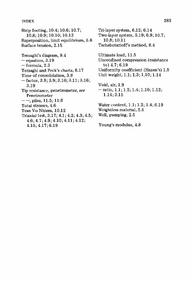
INDEX 2 8 3
Strip foot ing, 1 0 . 4 ; 1 0 . 6 ; 1 0 . 7 ; 1 0 . 8 ; 1 0 . 9 ; 1 0 . 1 0 ; 1 0 . 1 3
Superpos i t ion, limit equil ibrium, 5.8 Surface tens ion, 2 .15
Terzaghi 's d iagram, 9.4 — equat ion, 3 .19 — formula , 2 .3 Terzaghi and Peck's charts , 6 .17 T ime of consol idat ion, 3.8 — factor , 3 .8 ; 3 . 9 ; 3 . 1 0 ; 3 . 1 1 ; 3 . 1 6 ;
3 .19 Tip resistance, penetrometer , see
Penetrometer , piles, 1 1 . 5 ; 11 .6
Tota l stresses, 4 .6 Tran V o Nhiem, 1 0 . 1 2 Triaxial tes t , 3 . 1 7 ; 4 . 1 ; 4 . 2 ; 4 . 3 ; 4 . 5 ;
4 . 6 ; 4 . 7 ; 4 . 9 ; 4 . 1 0 ; 4 . 1 1 ; 4 . 1 2 ; 4 . 1 5 ; 4 . 1 7 ; 6 .19
Tri-layer sys tem, 6 . 1 2 ; 6 . 1 4 Two-layer sys tem, 3 . 1 9 ; 6 . 9 ; 1 0 . 7 ;
1 0 . 8 ; 1 0 . 1 1 Tschebotar io f f ' s m e t h o d , 8 .4
Ul t imate load , 11 .5 Unconf ined compress ion (resistance
t o ) 4 . 7 ; 6 .19 Uniformity coefficient (Hazen's ) 1.5 Unit weight, 1 . 1 ; 1.3; 1 .10 ; 1.14
V o i d , air, 1.9 - rat io , 1 .1 ; 1 .2 ; 1.4; 1 .10 ; 1 .12 ;
1 .14 ; 3 .15
Water content , 1 .1 ; 1.2; 1.4; 6 .19 Weightless material , 5 .5 Well, pumping , 2 .5
Young ' s m o d u l u s , 4 .8
SP
CD
1 ï c
I â"
« S3
ñ >
CO
·Λ
c Ï
1°
; á>
é Ï
.Ï
42
Ç)
GG
Ï
ö
ö
•8 Ï)
3 Ο
é Ο
00
ú§ ö
Ό ï C
O
Ö
α
ö
«2 -S3 •Β
>>
õ ! Ö
Ö
Ö
ö
Ö
ç
5 «2 JS
s ï ï
×
× 5
×