fusion 2017 multi object estimation tutorial lecture notes

Basic concepts for multi-object estimation

Lecture notes

Daniel Clark, Emmanuel Delande1, Jeremie HoussineauHeriot-Watt University

D.E.Clark, E.D.Delande, [email protected]

v.1 (July 5, 2016)

1Corresponding author, email: [email protected]

2

Motivation

These lecture notes present fundamental concepts in point process theory for multi-object es-timation problems, and includes practical derivation tools for the derivation of multi-targetdetection and tracking filters. Even though these notes aims at being as self-contained as possi-ble, the reader is expected to have basic knowledge in probability theory. Some parts, notably inChap. 3, may require additional knowledge in measure theory. In order to keep a natural flow inthe development of the arguments exposed in these notes, simplicity is sometimes favoured overstrict mathematical rigour in the presentation of some advanced concepts, notably pertaining tomeasure theory. Fortunately, the available literature on point processes propose some excellentbooks covering the topic in deeper details; some of them are provided in the next section.

A few useful references

A comprehensive study on point processes is given by Daley and Vere-Jones in [6, 7], diggingdeep in measure theory to present all the fundamental concepts related to point processes andmany useful applications. Stoyan, Kendall, and Mecke follow a different approach in [14], cast-ing the point processes in a more intuitive but perhaps less mathematically-involved framework,and provide an excellent complement to [6, 7]. Fundamental concepts in measure theory canbe found in Bogachev’s [2, 3], and their exploitation in the context of multi-object filtering iscovered in more details in the authors’ notes from the First International School on Finite SetStatistics [10], from which these lecture notes are inspired.

The exploitation of point processes for practical target tracking applications is to the credit ofGoodman, Mahler, and Nguyen in [9], and Mahler in [13], where the Finite Set Statistics (FISST)framework is presented in detail. Mahler’s seminal papers on the Probability Hypothesis Density(PHD) [11] and Cardinalized Probability Hypothesis Density (CPHD) [12] filters paved the wayfor most of the subsequent developments in multi-object filtering.

Introduction

In the context of multi-target tracking, multi-object estimation problems are the study of apopulation of objects or targets, whose number and individual states (e.g. position, velocity co-ordinates) are unknown. Cast in a Bayesian framework, the multi-object filters aim at describingthe uncertainty on this population through a probabilistic description, and update that descrip-tion across time whenever additional information on the population of targets are available –typically, through observations collected from some sensor system observing the surveillancescene.

A point process is a random variable whose realizations are sequences whose size and elements areboth random; it is thus particularily adapted to the description of a multi-object configuration,i.e., a number of objects and their respective states. To a certain extent, a point process canbe seen as the extension of an integer-valued random variable, describing the size of a popula-tion of objects, to a random variable describing the size and the states of a population of objects.

3

This key remark motivated the two-step pedagogical approach followed by these lecture notes,presenting first integer-valued random variables in Chap 1, and then point processes in Chap 2.The concepts pertaining to integer-valued random variables have (almost) always a counterpartfor point processes, and the structures of Chaps 1, 2 present many remarkable similarities.

Organization of the lecture notes

The lecture notes are organized in three main chapters of increasing complexity:

• Chap. 1 serves as an introduction, and describes the study of a integer-valued random vari-able through its probability generating function (p.g.f.). The exploitation of integer-valuedrandom variables is illustrated through the modelling and derivation of the “cardinalityonly” PHD filter.

• Chap. 2 contains the core notions presented in the lecture notes, and describes the study ofa point process through its probability generating functional (p.g.fl.). The exploitation ofpoint processes is illustrated through the modelling and derivation of the PHD filter [11].

• Chap. 3 explores the construction and exploitation of higher-order moments for pointprocesses, and illustrates the concept for the Poisson point process.

Finally, a few exercises relating to the three chapters above are proposed in Chap. 4.

Note

Most of the recent developments in multi-object filtering, following the terminology proposedin the FISST methodology [12] pertaining to Random Finite Sets (RFSs), make use of sets ofpoints, multi-object densities, and set integrals. The general terminology pertaining to pointprocesses, on the other hand, make use of sequences of points, probability measures, probabilitydensities, and measure-theoretical integrals.

These notions are largely equivalent, as a RFS can be seen as a (simple) point process (seeChap. 2). However the expression of higher-order moments for point processes, presented inChap. 3, requires the construction of quantities described with measures but admitting no den-sities, and more easily described with measure-theoretical integrals than set integrals. For thisreason, these lectures notes follow the general terminology of point processes.

Chapter 1

Integer-valued random variables

In this chapter, we shall focus on the estimation of the number of targets in the surveillancescene, and not their individual states.

1.1 Integer-valued random variables: basic concepts

The number of targets in the scene is obviously an integer, but it is unknown; thus, it is aptlydescribed by an integer-valued random variable X.

The random variable X is a mapping from someprobability space (Ω,F ,P) to the set of non-negative integers N.

Depending on the construction of the randomvariable X, several outcomes ωi may be associ-ated to the same realization k.

The quantity X−1(n) represents the collectionof all the possible outcomes ωi leading to therealization n. The probability space is endowedwith a probability measure P which allows usto measure the “size” of X−1(n). The “larger”X−1(n) is, the more likely is the value n to bedrawn when sampling from X.

5

6 CHAPTER 1. INTEGER-VALUED RANDOM VARIABLES

The quantitypX(n) = P(X−1(n)) (1.1)

denotes the likelihood that n is drawn when sampling from X, which we shall describe as theevent X = n. The structure of the probability space is such that∑

n≥0

pX(n) =∑n≥0

P(X−1(n)) (1.2a)

= 1, (1.2b)

which ensures that the elements pX(n) can be readily intepreted as cardinality probabilities, andthe family pX(n)n≥0 as a cardinality distribution. In our context, pX(n) is the probabilitythat the population described by X has exactly n objects.

The cardinality distribution pX(n)n≥0 fully characterizes the random variable X, but its fullknowledge is seldom available in practical problems as it may be intractable to estimate andpropagate across time. Random variables can also be described by their moments, which pro-vide a limited but meaningful description of the behaviour of X. Given an integer k ≥ 0, the

kth order non factorial (respectively (resp.) factorial) moment µ(k)X (resp. α

(k)X ) of X are defined

as

µ(k)X = E

[Xk]

=∑n≥0

pX(n)nk, (1.3)

α(k)X = E [X(X − 1) . . . (X − k + 1)] =

∑n≥k

pX(n)n(n− 1) . . . (n− k + 1). (1.4)

The non factorial moments are useful for the construction of the central moments such as thevariance

varX = µ(2)X −

(µ

(1)X

)2

, (1.5)

a well-known statistic which describes the spread of the values taken by X around its mean

value µ(1)X . Also, the correlation between two random variables X, Y can be studied through the

covariancecovX,Y = µ

(1)XY − µ

(1)X µ

(1)Y . (1.6)

The factorial moments have no easy physical interpretation and are seldomly used to producemeaningful statistics on random variables. The exception is the first-order factorial moment,

which equals the first-order non factorial moment µ(1)X and provides the mean value of X, usually

noted µX :

µX =∑n≥0

pX(n)n(= µ(1)X = α

(1)X ). (1.7)

The cardinality distribution is a convenient tool to study a single given random variable. In themulti-object Bayesian framework, however, different random variables are used to describe theevolution of our knowledge of the same concept across time – for example, our knowledge on thenumber of targets in the scene is enriched when the sensor system produces new measurements,and the random variable describing the number of targets is updated accordingly. It turns out

1.2. DEFINITIONS 7

that the transition between these random variables is difficult to describe through their cardi-nality distributions, and that another representation of the random variable is necessary to beable to produce the filtering equations effectively.

For example, suppose that the random variables X1 and X2 are fully known through theirrespective cardinality distributions pX1

(n)n≥0, pX2(n)n≥0, and that the random variable X

is defined as the sum

X = X1 +X2. (1.8)

What is the cardinality distribution pX(n)n≥0 of X? One way to find out is to enumerateevery possible realization n of X and consider all the possible joint realizations of X1, X2 whosesum equals n:

pX(0) = pX1(0)pX2

(0), (1.9)

pX(1) = pX1(1)pX2

(0) + pX1(0)pX2

(1), (1.10)

pX(2) = pX1(2)pX2

(0) + pX1(1)pX2

(1) + pX1(0)pX2

(2), (1.11)

· · ·

We see on the example above that a simple operation on random variables - the sum - does nottranslate into a simple operation on the cardinality probabilities.

Just as the Fourier transform allows us to shift the study of time-varying signals from thetime to the frequency domain in which simple operations on signals are easily transcribed, onewould like to shift the study of random variables from the cardinality probabilities to a moreadequate domain.

1.2 Probability generating function: definitions

A generating function is a function G : R+ → R which is built upon (or “generated by”) a(possibly infinite) sequence of real numbers1. Given a sequence of real numbers (un)n≥0, itsgenerating function G is defined as

G(s) =∑n≥0

unsn (1.12)

for any s ∈ R+ such that the sum on the right hand side of (1.12) is finite.

Applied to a random variable X, one can substitute the cardinality probabilities pX(n)n≥0 in(1.12) to produce the p.g.f. GX of X, defined as the expectation

GX(s) = E[sX]

(1.13a)

=∑n≥0

pX(n)sn. (1.13b)

1R+ is the set of non negative real numbers. More general definitions of the generating function exist, but itis out of the scope of this lecture.


Note that using the cardinality probabibilities as the generating sequence imposes some re-strictions on the range of admissible values for the test variable s, and the p.g.f. is defined for0 ≤ s ≤ 1. From (1.13) it is easy to see that:

GX(0) =∑n≥0

pX(n)0n = pX(0) (1.14)

GX(1) =∑n≥0

pX(n)1n =∑n≥0

pX(n) = 1, (1.15)

Setting s to 0 in (1.13) allowed us to extract the cardinality probability pX(0) from the p.g.f.;we will see in Section 1.3 that other cardinality probabilities can be extracted through differen-tiation of the p.g.f..

In multi-object filtering applications it will be necessary to study the joint behaviour of sev-eral random variables; for example, to describe the number of measurements produced by thesensor system given the number of targets in the scene. The joint p.g.f. GZ,X of two (possiblydependent) random variables Z, X is defined as the expectation

GZ,X(t, s) = E[tZsX

](1.16a)

=∑m,n≥0

pZ,X(m,n)tmsn, (1.16b)

where pZ,X(m,n) is the joint probability that Z = m and X = n. Note that, if Z and X areindependent variables, then by definition pZ,X(m,n) = pZ(m)pX(n) and the joint p.g.f. becomes:

GZ,X(t, s) =∑m,n≥0

pZ(m)pX(n)tmsn (1.17a)

=

∑m≥0

pZ(m)tm

∑n≥0

pX(n)sn

(1.17b)

= GZ(t)GX(s). (1.17c)

We now need to introduce the notion of derivative to further exploit the p.g.f..

1.3 Ordinary differentiation

1.3.1 Definition and basic rules

As p.g.f.s are real-valued functions taking a real number as argument, the “classic” derivativecan be applied to the p.g.f.s. Suppose that f : R → R is some function, we call “the derivativeof f (evaluated) at x ∈ R”, and denote it by f ′(x), the limit

f ′(x) = limε→0

f(x+ ε)− f(x)

ε, (1.18)

1.4. P.G.F.S AND DIFFERENTIATION 9

where ε ∈ R, if it exists. The ordinary derivative comes with a few calculus rules that will beuseful for the differentiation of p.g.f.s. Suppose that f and g are admissible functions, then:

sum: (f + g)′(x) = f ′(x) + g′(x) (1.19)

product: (f · g)′(x) = f ′(x)g(x) + f(x)g′(x) (1.20)

power: (fm)′(x) = mfm−1(x)f ′(x) (1.21)

chain (or composition): (f g)′(x) = g′(x)f ′(g(x)) (1.22)

1.3.2 A few advanced rules

A very important function that is used extensively in the construction of filter is the exponentialfunction. Indeed, a common approximation in the design of multi-object filters is to assume thatsome p.g.f. can be written as an exponential as it often leads to tractable and easily implementablefiltering equations. The following “tricks” involving the exponential function will be used lateron:

ordinary differentiation: exp′(x) = exp(x) (1.23)

composition: (exp f)′(x) = f ′(x)(exp f)(x) (1.24)

Taylor expansion: exp(x) =∑n≥0

exp(n)(0)

n!xn =

∑n≥0

xn

n!(1.25)

1.4 p.g.f.s and differentiation

We shall now apply the ordinary differentiation to the p.g.f. to see what kind of informationcan be extracted from it. Suppose that X is a random variable with known p.g.f. GX and onewish to determine the cardinality distribution pX(n)n≥0. Let us have a look at the successivederivatives of GX :

GX(s) =∑n≥0

pX(n)sn, (1.26)

G′X(s) =∑n≥0

pX(n)(sn)′ =∑n≥1

pX(n)nsn−1, (1.27)

G(2)X (s) =

∑n≥1

pX(n)n(sn−1)′ =∑n≥2

pX(n)n(n− 1)sn−2, (1.28)

· · ·

G(k)X (s) =

∑n≥k

pX(n)n(n− 1) · · · (n− k + 1)︸︷︷︸=n(n−1)···(n−k+1)(n−k)···1

(n−k)···1= n!

(n−k)!

sn−k. (1.29)


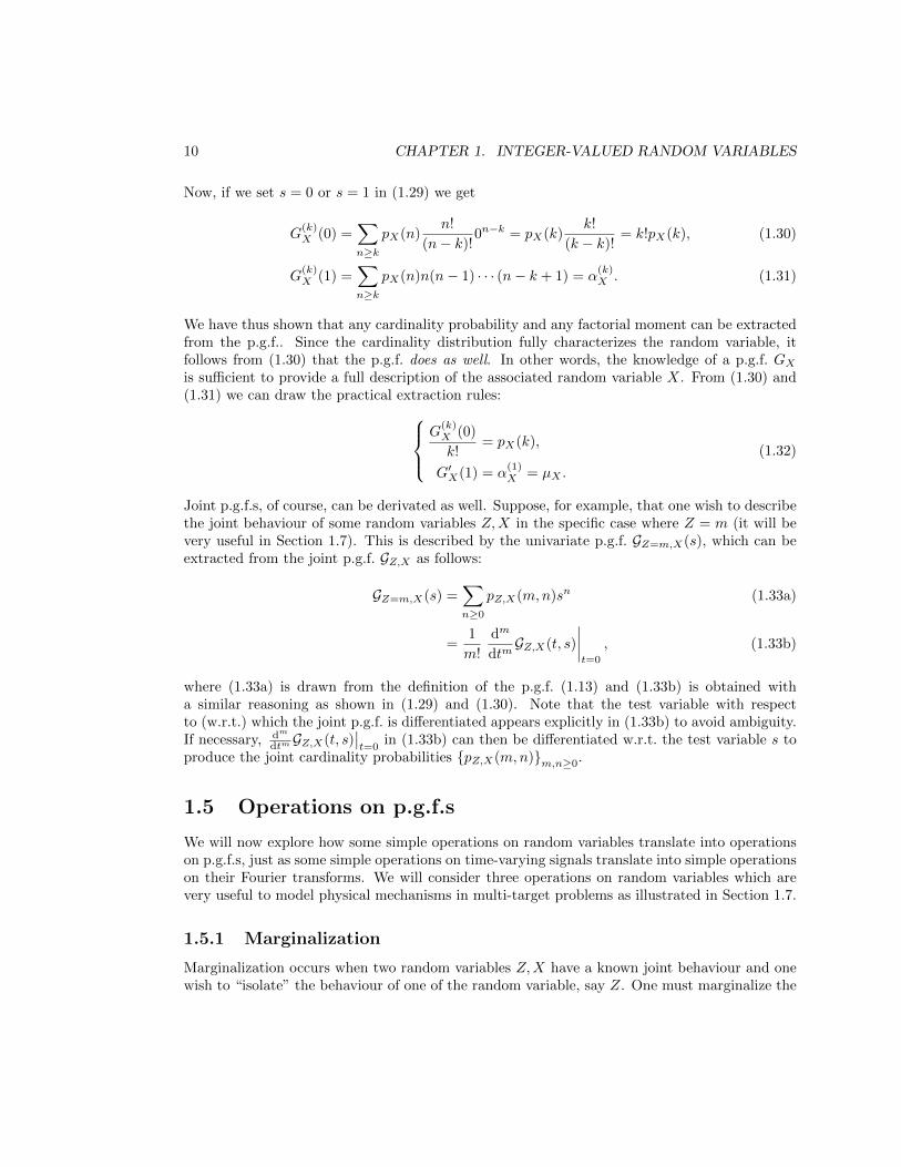
Now, if we set s = 0 or s = 1 in (1.29) we get

G(k)X (0) =

∑n≥k

pX(n)n!

(n− k)!0n−k = pX(k)

k!

(k − k)!= k!pX(k), (1.30)

G(k)X (1) =

∑n≥k

pX(n)n(n− 1) · · · (n− k + 1) = α(k)X . (1.31)

We have thus shown that any cardinality probability and any factorial moment can be extractedfrom the p.g.f.. Since the cardinality distribution fully characterizes the random variable, itfollows from (1.30) that the p.g.f. does as well. In other words, the knowledge of a p.g.f. GXis sufficient to provide a full description of the associated random variable X. From (1.30) and(1.31) we can draw the practical extraction rules:

G(k)X (0)

k!= pX(k),

G′X(1) = α(1)X = µX .

(1.32)

Joint p.g.f.s, of course, can be derivated as well. Suppose, for example, that one wish to describethe joint behaviour of some random variables Z,X in the specific case where Z = m (it will bevery useful in Section 1.7). This is described by the univariate p.g.f. GZ=m,X(s), which can beextracted from the joint p.g.f. GZ,X as follows:

GZ=m,X(s) =∑n≥0

pZ,X(m,n)sn (1.33a)

=1

m!

dm

dtmGZ,X(t, s)

∣∣∣∣t=0

, (1.33b)

where (1.33a) is drawn from the definition of the p.g.f. (1.13) and (1.33b) is obtained witha similar reasoning as shown in (1.29) and (1.30). Note that the test variable with respectto (w.r.t.) which the joint p.g.f. is differentiated appears explicitly in (1.33b) to avoid ambiguity.If necessary, dm

dtmGZ,X(t, s)∣∣t=0

in (1.33b) can then be differentiated w.r.t. the test variable s toproduce the joint cardinality probabilities pZ,X(m,n)m,n≥0.

1.5 Operations on p.g.f.s

We will now explore how some simple operations on random variables translate into operationson p.g.f.s, just as some simple operations on time-varying signals translate into simple operationson their Fourier transforms. We will consider three operations on random variables which arevery useful to model physical mechanisms in multi-target problems as illustrated in Section 1.7.

1.5.1 Marginalization

Marginalization occurs when two random variables Z,X have a known joint behaviour and onewish to “isolate” the behaviour of one of the random variable, say Z. One must marginalize the

1.5. OPERATIONS ON P.G.F.S 11

joint behaviour over X, i.e. “integrate” the joint cardinality probabilities over all the possiblerealizations of X since

∀m ∈ N, pZ(m) =∑n≥0

pZ,X(m,n). (1.34)

Suppose that the joint behaviour is known through the joint p.g.f. GZ,X . Using the definition ofthe joint p.g.f. (1.16) we can write:

GZ,X(t, 1) =∑m,n≥0

pZ,X(m,n)tm1n (1.35a)

=∑m≥0

∑n≥0

pZ,X(m,n)

tm (1.35b)

=∑m≥0

pZ(m)tm (1.35c)

= GZ(t). (1.35d)

That is, the marginalization of a random variable easily translates into a very simple operationon the joint p.g.f.:

GZ(t) = GZ,X(t, 1). (1.36)

1.5.2 Sum (or superposition)

Superposition occurs when one is not interested in the individual realizations of two independentrandom variables X and Y , but only in the sum of the two realizations. If we denote by Z thesum of random variables X, Y with known p.g.f.s GX , GY , then Z is also a random variable;using the definition of the p.g.f. (1.13) yields

GZ(s) = E[sZ]

(1.37a)

= E[sX+Y

](1.37b)

= E[sXsY

](1.37c)

= E[sX]E[sY]

(1.37d)

= GX(s)GY (s), (1.37e)

where (1.37c) is equivalent to (1.37d) because X and Y are independent.

In other words, the sum of two independent random variables easily translates into the productof the associated p.g.f.s:

GX+Y (s) = GX(s)GY (s). (1.38)

1.5.3 Branching

Branching is a special kind of dependence between two random variables Y,X. Upon any realiza-tionm of the parent random variable Y , the daughter random variable X will be the superpositionof m identical but independent random variables T , as if any object in the parent population


was “spawning” a number of objects in the daughter population following a common transitionmechanism described by T .

Suppose that the parent random variable Y and the transition random variable T are knownthrough the p.g.f.s GY , GT , and that one wish to describe the daughter random variable X. Thep.g.fl. describing the joint behaviour of the parent Y and daughter X random variables can bewritten as follows:

GY,X(t, s) =∑m,n≥0

pY,X(m,n)tmsn (1.39a)

=∑m,n≥0

pY (m)pX|Y (n|m)tmsn (1.39b)

=∑m≥0

pY (m)

∑n≥0

pX|Y (n|m)sn

tm (1.39c)

=∑m≥0

pY (m)GX|Y (s|m)tm, (1.39d)

where GX|Y (s|m) is the p.g.f. describing the daughter random variable X conditioned on therealization Y = k. If Y = m, then X|Y is the superposition of m independent “copies” of thetransition random variable T . Thus from (1.38) we have

GX|Y (s|m) = (GT (s))m. (1.40)

Substituting (1.40) in (1.39d) gives

GY,X(t, s) =∑m≥0

pY (m)(GT (s))mtm (1.41a)

=∑m≥0

pY (m)(tGT (s))m (1.41b)

= GY (tGT (s)). (1.41c)

The result (1.41c) above is an important result which describes the joint behaviour of the parentand daughter random variables and that we shall use in Section 1.7. For now, since we areinterested in the description of the daughter random variable X alone, we can simply marginalizethis result over the parent random variable Y using (1.36) and we get

GX(s) = GY,X(1, s) (1.42a)

= GY (GT (s)). (1.42b)

In other words, the branching of a parent random variable following a mechanism described bya transition random variable translates into the composition of the associated p.g.f.s.

1.6. EXAMPLES OF P.G.F.S 13

1.6 A few examples of random variables and their p.g.f.s

We shall now present two specific classes of random variables which are often used in multi-objectfiltering and for which it is useful to learn beforehand the structure of the associated p.g.f.s.

1.6.1 Bernoulli random variable

A Bernoulli random variable X with parameter 0 ≤ p ≤ 1 is a very simple integer-valued randomvariable defined as follows:

X =

0, with probability 1− p,1, with probability p.

(1.43)

The construction of the p.g.f. GX is straightforward using definition (1.13):

GX(s) =∑n≥0

pX(n)sn (1.44a)

= pX(0)︸︷︷︸=1−p

+ pX(1)︸︷︷︸=p

s+∑n≥2

pX(n)︸︷︷︸=0

sn (1.44b)

= 1− p+ ps. (1.44c)

The Bernoulli random variable is a “basic component” in the modelling of multi-object filtersbecause it depicts the physical mechanisms of target survival and target detection (see Section 1.7for more details).

1.6.2 Poisson random variable

A Poisson random variable X with rate λX ≥ 0 is defined as follows:

∀n ≥ 0, X = n with probability exp(λX)λnXn!. (1.45)

The construction of the p.g.f. GX using definition (1.13) gives:

GX(s) =∑n≥0

pX(n)sn (1.46a)

=∑n≥0

exp(−λX)λnXn!sn (1.46b)

= exp(−λX)∑n≥0

(λXs)n

n!(1.46c)

That is, using the Taylor expansion of the exponential (1.25):

GX(s) = exp(−λX) exp(λXs) (1.46d)

= exp(λX(s− 1)). (1.46e)


It is formative to extract the mean value of a Poisson random variable using the differentiationof the p.g.f. (1.31):

µX = G′X(s)|s=1 (1.47a)

= (exp(λX(s− 1)))′|s=1 (1.47b)

= (λX(s− 1))′ exp(λX(s− 1))|s=1 (1.47c)

= λX exp(λX(s− 1))|s=1 (1.47d)

= λX exp(λX(1− 1)) (1.47e)

= λX . (1.47f)

In other words, the mean value of Poisson random variable X equals its rate; since λX fullycharacterizes X through the definition (1.45), so does the mean value µX . Another importantproperty of a Poisson random variable, left as exercise in Ex. 4.1.2, is that its variance varXequals its mean µX .

Despite the simplicity of their structure, Poisson random variables provide a rather accuratedescription of a various number of natural phenomena (e.g. customer arrivals in queue lines). Inmulti-object filtering, Poisson random variables are appealing because of the exponential formof their p.g.f. (1.46e), easily differentiable; assuming some random variables to be Poisson allowsthe production of tractable and easily implementable filtering equations.

1.7 Application: the “cardinality only” PHD filter

We shall now apply the results we have seen in the previous sections to construct the “cardi-nality only” PHD filter. The purpose of this Bayesian filter is to estimate and propagate themean number of target in the scene observed by some sensor with known characteristics. Themodelling and filtering assumptions are identical to Mahler’s PHD filter [11] – hence its name– and shall be detailed later. In other words, the “cardinality only” PHD filter can be seen asthe reduction of the PHD filter to its cardinality component – we are interested in the numberof targets only, not their state. A similar application for the “full” PHD filter will be the topicof Chap. 2.

The data flow of one iteration of the “cardinality only” PHD filter can be represented as follows:

where the random variables provide a description of the size of the following populations:

1.7. APPLICATION 15

• Y : the targets before the prediction (prior knowledge from past iterations);

• X: the targets after the prediction;

• Z: the current measurements;

• X|Z: the targets after the data update (i.e. conditioned on some realization Z = m).

The construction of a filter follows two steps:

1. The modelling phase: we translate the physical phenomena of the tracking problem intorelations between the random variables describing the populations of interest. In our case,we have to describe how to get X from Y , then how to get X|Z from X. We have seenin Section 1.5 that operations on random variables are easily transcribed into operationson their p.g.f.s: for this reason, we will describe how to get GX from GY , then how to getGX|Z from GX .

2. The differentiation phase: we extract the information that we wish to propagate from theappropriate differentiation of the p.g.f.s produced in the modelling phase. In our case, wehave to describe how to get µX from µY , and how to get µX|Z from µX .

The modelling phase relies on modelling assumptions, constituting a description of the physicalphenomena that we wish to take into account and that we can afford to include in the designof the filter: it might be so, for example, that there is very slight chance that pairs of targetsmove in a correlated manner, but we may have to discard the modelling of correlated targetsif the increasing complexity of the designed filter is not worth it and/or is unaffordable. Oncecompleted, the modelling phase provides a full description of the sizes of the population of inter-est since random variables are completely described by their p.g.f.s (see Section 1.4). In otherwords, the modelling phase gives us exactly what we are looking for and the differentiation phaseis, in theory at least, superfluous.

The differentiation phase aims at extracting a reduced information from the p.g.f.s producedby the modelling phase. It is of course necessary in the construction of a practical filter, as thestorage of a p.g.f. requires, in the most general case, an infinite amount of memory (see definition(1.13)). The challenge of the differentiation phase is to extract the right amount of information,i.e. meaningful enough to the operator for tracking purposes, and resulting in filtering equationsthat are tractable enough. In our present case, for example, we aim at reducing the propagatedinformation to the mean target number in the scene. In order to produce the filtering equations,it is often necessary to make filtering approximations on top of the modelling assumptions; itis the combination of both that characterizes the resulting filter - in our case, the “cardinalityonly” PHD filter.

1.7.1 Modelling phase

Prediction step

The modelling assumptions are as follows:

1. The targets are independent;


2. A target survives with probability ps, dies (i.e. vanishes from the scene) otherwise;

3. A number of newborn targets enter the scene, independently of the number survivingtargets, following a birth mechanism described by a random variable Xbirth with knowncharacteristics (p.g.f. Gbirth).

The prediction step can be represented as follows:

Exploiting the results established in sections 1.5 and 1.6, we can then say that:

1. Since each target survives with probability ps, the “survival” random variable Xs in thefigure above is Bernoulli with parameter ps:

Gs(s) = 1− ps + pss. (1.48)

2. The number of surviving targets is described by a random variable Xsur. which is the resultof a branching with parent random variable Y and transition random variable Xs:

Gsur.(s) = GY (Gs(s)). (1.49)

3. The predicted number of targets, described by X, is the sum of the surviving targets and thenewborn targets:

GX(s) = Gsur.(s)Gbirth(s). (1.50)

In consequence, the p.g.f. form of the prediction step of the “cardinality only” PHD filter is givenby:

GX(s) = GY (1− ps + pss)Gbirth(s). (1.51)

Note that using the p.g.f.s allowed us to produce a full description of the predicted number oftargets X without enumerating and computing each cardinality probability pX(n) for every targetnumber n ∈ N.

Data update step


1. The measurements are produced independently;

2. A target is detected and produces a single measurement with probability pd, is undetectedotherwise;

3. A number of clutter measurements are produced, independently from the target measure-ments, following a clutter mechanism described by a random variable Zclutter with knowncharacteristics (p.g.f. Gclutter).

1.7. APPLICATION 17

The update step can be represented as follows:


1. Since each target is detected with probability pd, the “observation” random variable Zobs. inthe figure above is Bernoulli with parameter pd:

Gobs.(t) = 1− pd + pdt. (1.52)

2. The number of target measurements is described by a random variable Ztarget which is theresult of a branching with parent random variable X and transition random variable Zobs.:

GZtarget,X(t, s) = GX(sGobs.(t)). (1.53)

3. The number of measurement, described by Z, is the sum of the target measurements and theclutter measurements:

GZ,X(t, s) = GZtarget,X(t, s)Gclutter(t). (1.54)

In consequence, the joint p.g.f. of the number of measurements and targets is given by:

GZ,X(t, s) = GX(s(1− pd + pdt))Gclutter(t). (1.55)

So far, the structures of the prediction and update steps have been remarkably similar and haveled to identical results. The main difference is that we are not interested, at least as a final re-sult, in marginalizing (1.55) over the predicted number of targets X in the same way as (1.51) is(implicitly) marginalized over the prior number of targets Y . Nor are we interested in marginal-izing (1.55) over the number of measurements Z; we know with certainty that the sensor systemproduced m measurements and we wish to estimate the number of targets conditioned on therealization Z = m.

In order to do this, we will use the classic Bayes’ rule for conditional probabilities which statesthat

pX|Z(n|m) =pZ,X(m,n)

pZ(m), (1.56)

that is, the probability that there are X = n targets in the scene, given that there Z = mmeasurements, is the joint probability that there are X = n targets and Z = m measurementsover the probability that there are Z = m measurements.

If we multiply both sides of (1.56) by sn and sum over all possible realizations of X we get

∑n≥0

pX|Z(n|m)sn =

∑n≥0 pZ,X(m,n)sn

pZ(m). (1.57a)


Using (1.13) and (1.33a), (1.57a) is equivalent to

GX|Z(s|m) =GZ=m,X(s)

pZ(m), (1.57b)

where (1.33b) and (1.32) yield

GX|Z(s|m) =1m!

dm


1m!G

(m)Z (0)

. (1.57c)

Finally, the denominator of Bayes’ rule being the probability that there are Z = m measurements

marginalized over all the possible target numbers, GZ(t) = GZ,X(t, 1) and thus 1m!G

(m)Z (0) =

1m!

dm

dtmGZ,X(t, 1)∣∣t=0

. Thus (1.57c) becomes

GX|Z(s|m) =dm


dm


. (1.57d)

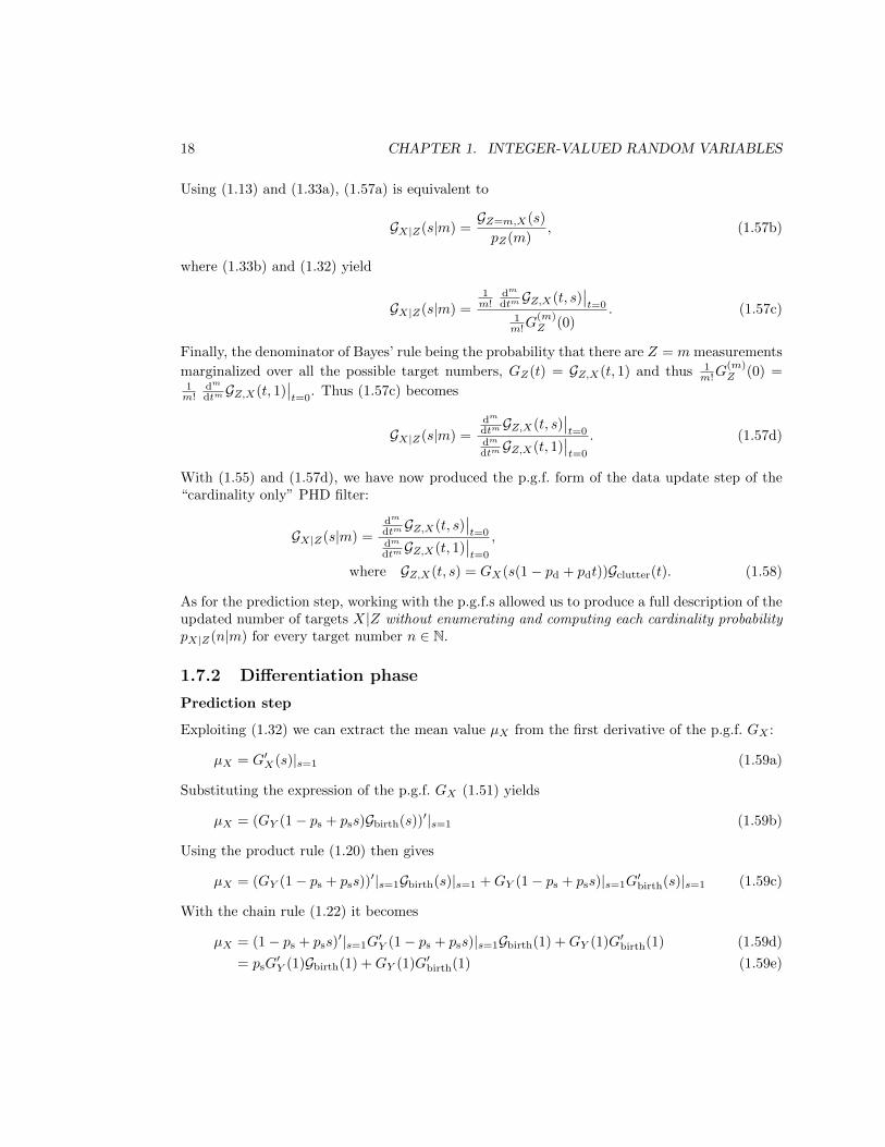
With (1.55) and (1.57d), we have now produced the p.g.f. form of the data update step of the“cardinality only” PHD filter:

GX|Z(s|m) =dm


dm


,

where GZ,X(t, s) = GX(s(1− pd + pdt))Gclutter(t). (1.58)

As for the prediction step, working with the p.g.f.s allowed us to produce a full description of theupdated number of targets X|Z without enumerating and computing each cardinality probabilitypX|Z(n|m) for every target number n ∈ N.

1.7.2 Differentiation phase

Prediction step

Exploiting (1.32) we can extract the mean value µX from the first derivative of the p.g.f. GX :

µX = G′X(s)|s=1 (1.59a)

Substituting the expression of the p.g.f. GX (1.51) yields

µX = (GY (1− ps + pss)Gbirth(s))′|s=1 (1.59b)

Using the product rule (1.20) then gives

µX = (GY (1− ps + pss))′|s=1Gbirth(s)|s=1 +GY (1− ps + pss)|s=1G

′birth(s)|s=1 (1.59c)

With the chain rule (1.22) it becomes

µX = (1− ps + pss)′|s=1G

′Y (1− ps + pss)|s=1Gbirth(1) +GY (1)G′birth(1) (1.59d)

= psG′Y (1)Gbirth(1) +GY (1)G′birth(1) (1.59e)

1.7. APPLICATION 19

Recall from (1.15) that the p.g.f.s evaluated at s = 1 always yield 1, that is:

µX = psG′Y (1) +G′birth(1) (1.59f)

And finally, exploiting again the relation between the mean value and the first differentiation ofthe p.g.f. (1.32) yields the result

µX = psµY + µbirth. (1.59g)

Note that no filtering approximations were necessary to produce this result, which means thatthe validity of the prediction step is not limited to a particular model for the prior cardinalityY and/or the newborn cardinality Xbirth.

Update step

Again, it is straightforward to write their expression of the posterior number of targets µX|Z=m,given that the sensor system produced m observations, as the first order derivative of the p.g.f.GX|Z(·|m):

µX|Z=m = G′X|Z(s|m)|s=1 (1.60a)

Substituting the expression of the p.g.f. GX|Z(·|m) (1.58) yields

µX|Z=m =

dm+1

dsdtmGZ,X(t, s)∣∣∣t=0,s=1

dm


(1.60b)

The previous result (1.58) provides an expression of the joint p.g.f. GZ,X w.r.t. the predictedp.g.f. GX and the clutter p.g.f. Gclutter, but at this point we have not made any assumptions onthe predicted cardinality X or the clutter cardinality and their respective p.g.f.s. If we attemptto proceed with the derivation in (1.60b) without assuming any particular forms for the p.g.f.sGX and Gclutter, we will end up with a very general but intractable result. We will thus assumethat:

1. The predicted number of targets X is Poisson;

2. The number of false alarms Zclutter is Poisson.

Using the expression of a Poisson random variable w.r.t. its mean value (1.46e), we can rewritethe joint p.g.f. GZ,X (1.55) as follows:

GZ,X(t, s) = GX(s(1− pd + pdt))Gclutter(t) (1.61a)

= eµX(s(1−pd+pdt)−1)eµclutter(t−1) (1.61b)

= eµX(s(1−pd+pdt)−1)+µclutter(t−1). (1.61c)

We can now proceed to the derivation of the joint p.g.f. in its new form (1.61c), for its exponentialform makes the derivation easier exploiting the composition rule (1.24). Indeed, resolving the


first-order derivative yields immediately:

d

dtGZ,X(t, s) =

d

dteµX(s(1−pd+pdt)−1)+µclutter(t−1) (1.62a)

=d

dt(µX(s(1− pd + pdt)− 1) + µclutter(t− 1)) eµX(s(1−pd+pdt)−1)+µclutter(t−1)

(1.62b)

= (µXspd + µclutter) eµX(s(1−pd+pdt)−1)+µclutter(t−1). (1.62c)

Since the multiplicative term in front of the exponential is independent of t, it is straightforwardto write the m-th order derivative of the joint p.g.f. w.r.t. t:

dm

dtmGZ,X(t, s) = (µXspd + µclutter)

meµX(s(1−pd+pdt)−1)+µclutter(t−1). (1.63)

For the numerator in (1.58), we need to differentiate (1.63) once w.r.t. s. This is a simple taskusing first the product rule (1.20):

dm+1

dsdtmGZ,X(t, s) =

d

ds((µXspd + µclutter)

m) eµX(s(1−pd+pdt)−1)+µclutter(t−1)

+ (µXspd + µclutter)m d

dseµX(s(1−pd+pdt)−1)+µclutter(t−1) (1.64a)

We then resolve the first differentiation using the power rule (1.21), and the second one usingthe composition rule (1.24):

dm+1

dsdtmGZ,X(t, s) = m (µXspd + µclutter)

m−1µXpde

µX(s(1−pd+pdt)−1)+µclutter(t−1)

+ (µXspd + µclutter)mµX(1− pd + pdt)e

µX(s(1−pd+pdt)−1)+µclutter(t−1) (1.64b)

Dividing (1.64b) by (1.63) then yields:

dm+1

dsdtmGZ,X(t, s)dm

dtmGZ,X(t, 1)= m

µXpd

µXspd + µclutter+ µX(1− pd + pdt) (1.64c)

At this point we just have to set s = 1 and t = 0 to produce the desired result (recall the generalexpression (1.60b)):

µX|Z=m = mµXpd

µXpd + µclutter+ µX(1− pd). (1.65)

1.7.3 Filtering equations

We have now succeeded in producing the filtering equations of the “cardinality only” PHD filterwith equations (1.59g) and (1.65), repeated here: µX = µY ps + µbirth,

µX|Z=m = µX(1− pd) +mµXpd

µXpd + µclutter.

(1.66)

Chapter 2

Point processes

Here we extend the estimation problem exposed in Chap. 1 to the full scope of multi-objectfiltering: we are now interested in the number and the spatial distribution of the objects. Forthis reason, we cover the description of the size and the spatial configuration of a populationwith point processes and their exploitation through p.g.fl.s.

We will see that results in Chaps. 1 and 2, and notably the exploitation of p.g.f.s and p.g.fl.s,are remarkably similar. In a broad sense, considering the spatial distribution of the objects inaddition to the object number means that a lot of the quantities we defined in the previouschapter will appear in a similar form except that a dependency upon a particular multi-objectconfiguration – a sequence of object states (x1, x2, . . . , xn) – will be added. Whenever a newresult is provided in this chapter, we shall reference the equivalent result in the previous chapterfor pedagogical purpose.

2.1 Point processes: basic concepts

The number of targets in the scene is obviously an integer but it is unknown; besides, we supposethat each target has a state x in some target state space X ⊆ Rdx (e.g., position and velocitycoordinates), but it is unkwown as well. For this reason, the description of a multi-target con-figuration is naturally provided by a point process Φ, a random variable whose realization is asequence whose size and elements are both random.

Remark 1. The target state space X is continuous, and we must proceed with care when definingrandom variables on X describing the state of a single target. Events of the form “the targethas a state equal to some value x ∈ X” have little practical interest, because they will occurwith probability zero; rather, we wish to assess events of the form “the target has a state withinsome neighborhood dx of x ∈ X”. Intuitively speaking, if X is one dimensional and describesthe target’s coordinate on some axis, we wish to be able to determine the probability that thecoordinate of the target lies within some “suitable” range of values dx (say, 5 m with a toleranceof 2 mm) rather than a value x (say, exactly 5 m). We shall call the set of all these “suitable”regions the Borel σ-algebra B(X) of X, and whenever we shall select a (suitable) region B ⊆ X

21

22 CHAPTER 2. POINT PROCESSES

throughout the chapter it is to be understood that B ∈ B(X). The same concept shall apply toother continuous spaces on which probabilites are defined.

Likewise, the number of measurements produced by the sensor system between two time stepsis an integer, and we suppose that each measurement has a state z in some state space Z ⊆ Rdz(e.g. polar and radial velocity coordinates).

A point process Φ on the state space X is amapping from some probability space (Ω,F ,P)to the space X of all the sequences of points inX, i.e. X =

⋃k≥0 X

k.

Depending on the construction of the point pro-cess Φ, several outcomes ωi may be associatedto “close” realizations ϕ,ϕ′.

The quantity Φ−1(dϕ) represents the collectionof all the possible outcomes ωi leading to arealization within the neighborhood dϕ aroundϕ. The probability space is endowed witha probability measure P which allows us tomeasure the “size” of Φ−1(dϕ). The “larger”Φ−1(dϕ) is, the more likely is a realization tobe drawn within dϕ when sampling from Φ.

The probability distribution of the point process Φ, given by

PΦ(dϕ) = P(Φ−1(dϕ)) (2.1)

denotes the likelihood that a realization is drawn within dϕ when sampling from Φ. The structureof the probability space is such that∫

XPΦ(dϕ) =

∫XP(Φ−1(dϕ)) (2.2a)

= 1, (2.2b)

which ensures that PΦ can be readily interpreted as a probability measure. In our context,PΦ(d(x1, . . . , xk)) is the probability that the population described by Φ has exactly n objectsand that the ith object is localized in the neighbourhood dxi, 1 ≤ i ≤ n.

2.1. POINT PROCESSES 23

An important property of point processes is that their probability distributions are always definedas symmetric functions, so that permutations of a given realization occur with equal probability– e.g., PΦ(d(x1, x2)) = PΦ(d(x2, x1)). In addition, if the realizations of a point process aresequences of points that are always pairwise distinct, then the point process is called simple. Inthe context of multi-target tracking problems, the point processes are (almost) always consideredsimple, and this will be the case throughout this lecture.

Remark 2. An alternative construction of simple point processes as random objects whose real-izations are sets of points ϕ = x1, . . . , xn, in which the elements are by construction unordered,is more common in the literature relating to the FISST framework [13]. In this context, a pointprocess is called a RFS.

The probability distribution PΦ is characterized by its projection measures P(n)Φ , for any n ≥ 0.

The nth-order projection measure P(n)Φ , for any n ≥ 1, is defined on Xn; it gives the probability

for the point process to be composed of n points, and the probability distribution of these points.

By extension, P(0)Φ is the probability for the point process to be empty. It is important to note

that the projection measures P(n)Φ are not probability measures as they do not integrate to one.

For any n ≥ 0, we indeed have ∫Xn

P(n)Φ (d(x1, . . . , xn)) = ρΦ(n), (2.3)

where ρΦ is the cardinality distribution of the point process, describing the size of its realizations:that is, ρΦ(n) is the probability that a realization ϕ of the point process Φ is a sequence of npoints.

Since the probability distribution PΦ is symmetrical, so are the projection measures P(n)Φ . For

this reason, point processes are often described through their Janossy measures, for they “aggre-gate” the information provided by the projection measures over all the possible permutations of

points. More precisely, for any n ≥ 0, J(n)Φ denotes the nth-order Janossy measure of the point

process Φ and is defined as

J(n)Φ (B1 × . . .×Bn) =

∑σ(n)

P(n)Φ (Bσ1

× . . .×Bσn) (2.4a)

= n!P(n)Φ (B1 × . . .×Bn), (2.4b)

where Bi, 1 ≤ i ≤ n, is a region of X, and σ(n) denotes the set of all permutations (σ1, . . . , σn)of (1, . . . , n).

In many practical multi-object estimation problems, the probability distribution PΦ admits adensity pΦ, which quantifies the rate of change of the probability measure PΦ per unit volume of

the state space. The quantity p(n)Φ (x1, . . . , xn) is thus the density of probability, per unit volume,

of the point process Φ evaluated at the sequence (x1, . . . , xn); loosely speaking, we may describe

it as the “probability that Φ = (x1, . . . , xn)”. The projection measures P(n)Φ and the Janossy

measures J(n)Φ admit densities as well, denoted p

(n)Φ and j

(n)Φ , respectively.


We have now several tools allowing for an equivalent description of a point process: assum-ing that f is suitable function on X , then the integral of f w.r.t. to the measure PΦ can bewritten

PΦ(f) =

∫Xf(ϕ)PΦ(dϕ) (2.5a)

=

∫Xf(ϕ)pΦ(ϕ)dϕ (2.5b)

=∑n≥0

∫Xn

f(x1, . . . , xn)P(n)Φ (d(x1, . . . , xn)) (2.5c)

=∑n≥0

∫Xn

f(x1, . . . , xn)p(n)Φ (x1, . . . , xn)dx1 . . . dxn (2.5d)

=∑n≥0

1

n!

∫Xn

f(x1, . . . , xn)J(n)Φ (d(x1, . . . , xn)) (2.5e)

=∑n≥0

1

n!

∫Xn

f(x1, . . . , xn)j(n)Φ (x1, . . . , xn)dx1 . . . dxn. (2.5f)

A measure-theoretical formulation provides a more general framework that is required to con-struct certain statistical properties on point processes that can be exploited for practical appli-cations, such as seen in Chap. 3, but is not necessary to obtain the more common results of thischapter. Throughout this chapter we shall favour expression exploiting densities rather thanmeasures, as they are probably more common to the reader, but keep in mind that equivalentresults can be obtained with a measure-theoretic formulation as well. We shall also favour prob-ability densities over Janossy densities, as the former spare the handling of factorial terms of theform 1

n! are a more convenient tools in the context of functional differentiation.

Remark 3. Recall that in the FISST litterature, point processes are RFSs whose realizationsare sets of points [13]. It is common to define the set integral, for any suitable function f andregion B ⊆ X, as ∫

B

f(X)δX =∑n≥0

1

n!

∫Bn

f(x1, . . . , xn)dx1 . . . dxn (2.6)

Set integrals are practical tools in the derivation of multi-object filtering solutions such as thePHD filter, and are convenient because of their compact expression. They are not, however,measure-theoretic integrals; for example, they are non additive as∫

B∪B′f(X)δX 6=

∫B

f(X)δX +

∫B′f(X)δX, (2.7)

in the general case, even if B and B′ are disjoint regions of the target state space X.

Similarly to random variables (see Chap. 1), the full knowledge of the multi-object density isseldom available in practical problems and a limited description of a point process Φ is provided

2.2. DEFINITIONS 25

by its moment measures or its moment densities. Factorial and non factorial moment measurescan be defined for any order, but their construction is more involved than for random variablesand their will be the topic of a specific chapter (see Chap. 3). In this chapter we shall focus onthe first-order moment density or intensity or Probability Hypothesis Density µΦ, the equivalentof the mean value of a random variable µX defined in Chap. 1.

The quantity µΦ(x) is the density, per unit volume, of the average number of objects evaluatedat x or, loosely speaking, the “average number of objects with state x”. In order to compute it,one must count all the possible realizations ϕ of Φ with an object with state x, i.e.

µΦ(x) =

∫X

(∑xi∈ϕ

δx(xi)

)pΦ(ϕ)dϕ (2.8a)

=∑n≥1

∫Xn

(n∑i=1

δx(xi)

)p

(n)Φ (x1, . . . , xn)dx1 . . . dxn, (2.8b)

where δx(·) = δ(· − x) is the Dirac delta function. Thus (2.8b) equals to:

µΦ(x) =∑k≥1

∫Xk−1

(n∑i=1

p(n)Φ (x1, . . . , x, . . . , xn−1︸︷︷︸

x as ith variable

)

)dx1 . . . dxn−1 (2.8c)

=∑n≥1

∫Xn−1

np(n)Φ (x, x1, . . . , xn−1)dx1 . . . dxn−1 (2.8d)

=∑n≥0

(n+ 1)

∫Xn

p(n+1)Φ (x, x1, . . . , xn)dx1 . . . dxn (2.8e)

The last result (2.8e) shows explicitly that the first moment density is constructed by consider-ing all the possible realizations of Φ which contains x, and marginalizing over all the possiblecardinalities and over all the possible states of the remaining elements.

Just as for the integer-valued random variables, the probability and the multi-object densitiesare not convenient to deal with when one wish to describe simple operations on point processes(see discussion in Section 1.1). We thus need to shift the study of the point processes from theprobability density to another domain.

2.2 Probability generating functional: definitions

A generating functional on X is a mapping G from the functions h : X→ R+ to R; it is built upon(or “generated by”) a (possibly infinite) sequence of functions (un)n≥0, where un : Xn → R+.The generating functional G of the sequence (un)n≥0 is defined as

G(h) =∑n≥0

∫Xn

(n∏i=1

h(xi)

)uk(x1, . . . , xn)dx1 . . . dxn, (2.9)


for any h : X→ R+ such that the right hand side of (2.9) is finite.

Applied to a point process Φ, one can substitute the probability density in (2.9) in order toproduce the p.g.fl. GΦ of Φ, defined as

GΦ(h) = E

[∏x∈Φ

h(x)

](2.10a)

=

∫X

(∏x∈ϕ

h(x)

)pΦ(ϕ)dϕ (2.10b)

=∑n≥0

∫Xn

(n∏i=1

h(xi)

)p

(n)Φ (x1, . . . , xn)dx1 . . . dxn. (2.10c)

Note that using the probability density as the generating sequence imposes some restrictions onthe range of admissible values for the test function h, and the p.g.fl. is defined for h : X→ [0 1].

Note the similarities between the p.g.f. of a random variable (1.13) and the p.g.fl. of a pointprocess (2.10). The test variable s of a p.g.f. is a real number in [0 1], while the test function of ap.g.fl. is a mapping from the target space X into [0 1]: the p.g.fl. “adds” the spatial componentto the p.g.f., and the sum over all the possible cardinalities in the p.g.f. (1.13) becomes a sumover all the possible cardinalities and, for a given cardinality, an integral over all the possibleobject states in the p.g.fl. (2.10). From (2.10) it is easy to see that

GΦ(0) =∑n≥0

∫Xn

(n∏i=1

0

)p

(n)Φ (x1, . . . , xn)dx1 . . . dxn = ρΦ(0), (2.11)

GΦ(1) =∑n≥0

∫Xn

(n∏i=1

1

)p

(n)Φ (x1, . . . , xn)dx1 . . . dxn = 1. (2.12)

Setting h to the mapping h : x ∈ X 7→ 0 in (2.10) allowed us to extract the scalar ρΦ(0) fromthe p.g.fl., i.e. the probability that there are no objects in the scene; we will see in Section 2.3that the probability density evaluated in any number of points can be extracted through differ-entiation of the p.g.fl..

In multi-object filtering applications it will be necessary to study the joint behaviour of sev-eral point processes; for example, to describe the multi-measurement configuration produced bythe sensor system given the multi-target configuration in the scene. The joint p.g.fl. GΞ,Φ of two(possibly dependent) point processes Ξ (on Z), Φ (on X) is defined as the expectation

GΞ,Φ(g, h) = E

[(∏z∈Ξ

g(z)

)(∏x∈Φ

h(x)

)](2.13a)

=

∫Z

∫X

∏z∈ξ

g(z)

(∏x∈ϕ

h(x)

)pΞ,Φ(ξ, ϕ)dξdϕ, (2.13b)

2.3. DIFFERENTIATION 27

where pΞ,Φ(ξ, ϕ) is the joint probability density, per unit volume, evaluated at ξ and ϕ or, looselyspeaking, the “probability that Ξ = ξ and Φ = ϕ”. Note that, if Ξ and Φ are independentprocesses, then by definition pΞ,Φ(ξ, ϕ) = pΞ(ξ)pΦ(ϕ) and the joint p.g.fl. becomes:

GΞ,Φ(g, h) =

∫Z

∫X

∏z∈ξ

g(z)

(∏x∈ϕ

h(x)

)pΞ(ξ)pΦ(ϕ)dξdϕ (2.14a)

=

∫Z

∏z∈ξ

g(z)

pΞ(ξ)dξ

(∫X

(∏x∈ϕ

h(x)

)pΦ(ϕ)dϕ

)(2.14b)

= GΞ(g)GΦ(h). (2.14c)

We now need to introduce the notion of functional derivative to further exploit the p.g.fl..

2.3 Functional differentiation

2.3.1 Definition and basic rules

The first step is to check if the “classic” derivative can be applied to functionals as well asfunctions (see Section 1.3 in Chap. 1). Following the definition (1.18), the ordinary derivative ofsome functional F evaluated at h would look like:

F ′(h) = limη→0

F (h+ η)− F (h)

η, (2.15)

where η would be some function of the same nature as h, i.e. η : X→ [0 1]. Two problems arisein the definition (2.15), as neither the convergence η → 0 nor the division by a function η arewell defined – recall that the argument of a functional F is a function h – and so is η in (2.15)– not a real number h(x).

Fortunately, other differentiation tools adapted to functionals do exist: the functional derivatives.Different functional derivatives have been defined by different authors for different applications,the most popular being perhaps the Frechet and the Gateaux derivatives. The Frechet derivativeis more restrictive, but comes with calculus rules similar to the ordinary derivative ; the Gateauxis more general, but does not a admit a chain rule similar to the ordinary derivative given in(1.22). Quite recently, the chain derivative has been proposed as an intermediary between Frechetand Gateaux for which a chain rule is available; since the chain rule will be important for thederivation of filtering equations, we will use the chain derivative.

Given a functional F and two functions h, η : X → R+, we call “the (chain) derivative of F(evaluated) at h in the direction (or increment) η”, and denote it by δF (h; η), the limit

δF (h; η) = limn→∞

F (h+ εnηn)− F (h)

εn, (2.16)

where ηnn≥0 is a sequence of functions ηn : X→ R+ converging (pointwise) to η and εnn≥0

is a sequence of positive real numbers converging to zero, if it exists and is identical for any


admissible sequences ηnn≥0 and εnn≥0. Note that the derivative δF (h; η) is a function onthe object space X; the variation of F around h in direction η being still dependent on the pointx where η is evaluated, the direction appears explicitly in the functional derivative while this isnot the case in the notation f ′(x) of the ordinary derivative.

It is formative to see how the functional derivative can be interpreted as an “extension” ofthe ordinary derivative. If we consider in definition (2.16) the special case where h is the con-stant function equal to some point x ∈ X, η another constant function equal to some point tobe specified later, and f is a functional on constant functions on X, and therefore can be seenas a function on X, we can write

δf(x; η) = limn→∞

f(x+ εnηn)− f(x)

εn(2.17a)

= limn→∞

ηnf(x+ εnηn)− f(x)

εnηn(2.17b)

= η limε→0

f(x+ ε)− f(x)

ε(2.17c)

= ηf ′(x) (2.17d)

And thus, by setting η to the constant function equal to 1:

δf(x; 1) = f ′(x) (2.17e)

The functional derivative comes with a few calculus rules that will be useful for the differentiationof p.g.fl.s. Suppose that F and G are admissible functionals, then:

sum: δ(F +G)(h; η) = δF (h; η) + δG(h; η), (2.18)

product: δ(F ·G)(h; η) = δF (h; η)G(h) + F (h)δG(h; η), (2.19)

chain (or composition): δ(F G)(h; η) = δF (G(h); δG(h; η)). (2.20)

Note that the sum and product rules (2.18), (2.19) are similar to those pertaining to the ordinarydifferentiation (1.19), (1.20).

The chain rule (2.20), on the other hand, is no longer a product as in the ordinary case (1.22).Higher-order derivations of composite functionals can be established through the Faa di Bruno’sformula for chain differentials [4, 5]. The 2nd order shall be used in the next chapter, it statesthat

δ2(F G)(h; η1, η2) = δF(G(h); δ2G(h; η1, η2)

)+ δ2F (G(h); δG(h; η1), δG(h; η2)) . (2.21)

2.3.2 A few advanced rules

The derivation of filtering equations for multi-object filters will involve the differentiation of anumber of p.g.fl.s or more general functionals of various forms. Some functionals with an identi-cal structure need to be derivated in the design of a specific filter; for this reason, it is interestingto detail here the differentiation of the most common functionals and consider the results as


“advanced rules” later on.

Let us consider a functional F such that F (h) = h(x) for some fixed point x in the statespace X. F could be the p.g.fl. of a point process Φ that describes the trivial situation wherethere is single target in the state, and that this target has state x, with probability one. Thenfrom the definition (2.16) we draw



εn(2.22a)

= limn→∞

h(x) + εnηn(x)− h(x)

εn(2.22b)

= limn→∞

ηn(x) (2.22c)

= η(x) (2.22d)

That is:

δ(h(x); η) = η(x). (2.23)

It is important to note that while “δ(h(x); η)” is a very convenient notation to use, it is improperbecause the functional w.r.t. which we differentiate, namely F , does not appear. It can be writtenwith the more rigorous but cumbersome form

δ (· → ·(x)) (h; η) = η(x). (2.24)

You will probably favour the more cumbersome form (2.24) when you start dealing with ratherintricate functionals, because it helps you remembering the three basic elements of the diffenti-ation process: the functional, the function where it is evaluated, and the direction in which it isdifferentiated. With a little experience, you will probably switch to the lighter notation (2.26).Exploiting the definition of the differentiation (2.16) we can expand (2.23) to the more generalresult:

δ((h(x))k; η) = kη(x)(h(x))k−1, (2.25)

or, in the more exact form:

δ(· → (·(x))k

)(h; η) = kη(x)(h(x))k−1. (2.26)

Let us now consider a functional F such that F (h) =∫h(x)f(x)dx for some function f on the

state space X. If∫f(x)dx = 1, F could be the p.g.fl. of a point process Φ that describes the

trivial situation where there is single target in the state with probability one, and that the target


is distributed in space according to f . Then from the definition (2.16) we draw



εn(2.27a)

= limn→∞

∫(h(x) + εnηn(x))f(x)dx−

∫h(x)f(x)dx

εn(2.27b)

= limn→∞

∫h(x)f(x)dx+ εn

∫ηn(x)f(x)dx−

∫h(x)f(x)dx

εn(2.27c)

= limn→∞

∫ηn(x)f(x)dx (2.27d)

=

∫η(x)f(x)dx (2.27e)

That is:

δ

(∫h(x)f(x)dx; η

)=

∫η(x)f(x)dx (2.28)

Similarly to (2.23), the result above uses a lighter notation where the functional does not appearexlicitly. We need to be even more cautious in this case, for h and f seem to play the same roleand there is an ambiguity regarding the function in which the functional is evaluated. The moreexact but cumbersome notation would be

δ

(· →

∫·(x)f(x)dx

)(h; η) =

∫η(x)f(x)dx, (2.29)

where the functional to be differentiated, i.e. F : h 7→∫h(x)f(x)dx, appears explicitly.

Let us now consider a functional F such that F (h) =∫G(h|x)f(x)dx for some function f

on the state space X and some functional G. If∫f(x)dx = 1, G could be the p.g.fl. of a point

process Φ whose behaviour depends on the state of some target, and the F the p.g.fl. of the pointprocess marginalized over all the possible values x of the said target (this will be encountered inthe branching for point processes discussed in Section 2.5). Then from the definition (2.16) wedraw



εn(2.30a)

= limn→∞

∫G(h+ εnηn|x)f(x)dx−

∫G(h|x)f(x)dx

εn(2.30b)

=

∫limn→∞

G(h+ εnηn|x)−G(h|x)

εnf(x)dx (2.30c)

=

∫δG(h|x; η)f(x)dx (2.30d)

= F (δG(h|·; η)) (2.30e)

That is:

δ

(∫G(h|x)f(x)dx; η

)=

∫δG(h|x; η)f(x)dx, (2.31)


or, with the more exact notation where the functional F appears explicitly in the left-hand side:

δ

(· →

∫G(·|x)f(x)dx

)(h; η) =

∫δG(h|x; η)f(x)dx, (2.32)

Loosely speaking, we can “swap” the integral and the derivative in (2.31) or (2.32) because thefunctional G(h|.) is encapsulated in an integral which does not depend on the test function hwhere the differentiation takes place. This result is easily expendable to integrals over a arbitrarynumber of variables xi ∈ X:

δ

(∫XG(h|ϕ)f(ϕ)dϕ; η

)=

∫XδG(h|ϕ; η)f(ϕ)dϕ, (2.33)

or, with the more exact notation where the outer functional F appears explicitly in the left-handside:

δ

(· →

∫XG(·|ϕ)f(ϕ)dϕ

)(h; η) =

∫XδG(h|ϕ; η)f(ϕ)dϕ. (2.34)

As you may imagine, the ability to swap integrals and derivatives will be extremely handy inpractical derivations. The key element that led us to the general result (2.33) is that the integralis a linear continuous operator that allowed us to proceed from (2.30b) to (2.30c). This resultcan be extended to other functionals than the integral, as seen in Ex. 4.2.1.

Finally, as explained in Section 1.3, the exponential form will be used extensively in the derivationof multi-object filters because the derivative of the exponential functional are easy to produce.The following results will be particularly important in the scope of this lecture. First of all,the ordinary differentiation rule (1.23) tells us that exp′(x) = exp(x); therefore if we exploit therelationship between ordinary and functional differentiations (2.17d) we get

δ exp(x; η) = η exp(x). (2.35)

This result is extremely simple, but it might seem of little use in the context of point processessince we shall be dealing primarily with functionals – recall that in this context the exponentialis evaluated in x and differentiated in the direction η, which are real-valued numbers. It will be,in fact, very useful in the resolution of composition of functionals where the outer functional isan exponential (more on that in Chap. 3).

Let us move on to the chain rule (2.20). When the outer functional is the exponential, it simplifiesas follows:

δ(exp F )(h; η) = δF (h; η)(exp F )(h). (2.36)

Establishing this result is left as exercise (see Ex. 4.2.2). Note that the chain rule for exponen-tials for ordinary (1.24) and functional (2.36) derivatives are remarkably close.

Another useful result can be drawn from (2.36). Suppose that F is the functional F (h) = h(x)for some fixed point x ∈ X (i.e., the functional F evaluates the test function h at some point ofthe target state space). Then, using (2.36) we can write

δ exp(h(x); η) = δ(exp F )(h; η) (2.37)

= δF (h; η)(exp F )(h) (2.38)

= η(x) exp(h(x)), (2.39)


where we have used the property (2.24) to proceed from (2.38) to the final result (2.39). Thedevelopment above is very formative, because it follows a typical derivation process when dealingwith functional differentiation. We start from an initial expression that is a slight abuse ofnotation, but is convenient to write: the differentiation in the left-hand side is made in thedirection of the function η and evaluated at the function h, not at the real-valued number h(x)(the cases (2.35) and (2.37) are very different!). We then rewrite the initial in its “cumbersome”but rigorous expression, then we apply previously established derivation rules (2.36), (2.24), andthen we revert back to a lighter and more convenient expression (2.39). Of course, with someexperience, one might go straight from the left-hand side of (2.37) to the final result (2.39),having in mind the elementary rules involved in the derivation process.

2.4 p.g.fl.s and differentiation

We shall now apply the functional differentiation to the p.g.fl. to see what kind of informationcan be extracted from it. Suppose that Φ is a point process with known p.g.fl. GΦ and one wishto determine the probability density pΦ(x), i.e. the probability that 1) there is a single targetin the state space, and 2) that target has state x. Suppose that one wish to determine the firstmoment density µΦ(x) as well. The results (1.32) we obtained for the p.g.f.s provide some insighton the method to produce the desired result: we should differentiate the p.g.fl. once. Since thespatial component is now relevant and we want to evaluate the probability density and the firstmoment density in a given point x ∈ X, we shall differentiate GΦ in the direction δx:

δGΦ(h; δx) = δ

∑n≥0

∫Xn

(n∏i=1

h(xi)

)p

(n)Φ (x1, . . . , xn)dx1 . . . dxn; δx

. (2.40a)

This is a typical example where we can apply the swapping rule (2.33) and we get

δGΦ(h; δx) =∑n≥1

∫Xn

δ

((n∏i=1

h(xi)

); δx

)p

(n)Φ (x1, . . . , xn)dx1 . . . dxn, (2.40b)

where proceeding with the product rule (2.19) yields


∫Xn

n∑i=1

δ(h(xi); δx)

∏j 6=i

h(xj)

p(n)Φ (x1, . . . , xn)dx1 . . . dxn, (2.40c)

2.4. PGFL!s (PGFL!s) AND DIFFERENTIATION 33

which simplifies with the advanced rule (2.23) and gives


∫Xn

n∑i=1

δx(xi)

∏j 6=i

h(xj)

p(n)Φ (x1, . . . , xn)dx1 . . . dxn (2.40d)

=∑n≥1

∫Xn−1

n∑i=1

∏j 6=i

h(xj)

p(n)Φ (x1, . . . , x, . . . , xn︸︷︷︸

x as ith variable

)dx1 . . . dxi−1dxi+1 . . . dxn

(2.40e)

=∑n≥1

∫Xn−1

n

(n−1∏i=1

h(xi)

)p

(n)Φ (x, x1, . . . , xn−1)dx1 . . . dxn−1 (2.40f)

=∑n≥1

n

∫Xn−1

(n−1∏i=1

h(xi)

)p

(n)Φ (x, x1, . . . , xn−1)dx1 . . . dxn−1 (2.40g)

=∑n≥0

(n+ 1)

∫Xn

(n∏i=1

h(xi)

)p

(n+1)Φ (x, x1, . . . , xn)dx1 . . . dxn (2.40h)

Now, if we set h = 0 or h = 1 in (2.40h) we get

δGΦ(h; δx)|h=0 =∑n≥0

(n+ 1)

∫Xn

(n∏i=1

0

)p

(n)Φ (x, x1, . . . , xn)dx1 . . . dxn

= p(1)Φ (x), (2.41)

δGΦ(h; δx)|h=1 =∑n≥0

(n+ 1)

∫Xn

(n∏i=1

1

)p

(n+1)Φ (x, x1, . . . , xn)dx1 . . . dxn

=∑n≥0

(n+ 1)

∫Xn

p(n+1)Φ (x, x1, . . . , xn)dx1 . . . dxn

= µΦ(x). (2.42)

Further differentiating (2.40h) before setting h = 0 produces the probability density evaluatedat a set of any desired size. Alternatively, further differentiating (2.40h) before setting h = 1produces higher order factorial moment densities, which are out of the scope of this lecture.From (2.41) and (2.42) we can draw the practical extraction rules:

1

k!δkGΦ(h; δx1

, . . . , δxk)∣∣h=0

= p(k)Φ (x1, . . . , xk)

(=j

(k)Φ (x1, . . . , xn)

k!

),

δGΦ(h; δx)|h=1 = µΦ(x).

(2.43)

Again, the extraction rules for p.g.f.s (1.32) and p.g.fl.s (2.43) are very similar. Since its prob-ability density fully characterizes a point process, it follows from (2.43) that its p.g.fl. does aswell. In other words. the knowledge of a p.g.fl. GΦ is sufficient to provide a full description ofthe associated point process Φ.


Before moving on to joint p.g.fl.s, we shall write a “technical result” that is known as Campbell’stheorem in point process theory. Assume that one wish to evaluate some real-valued functionf , defined on the state space X, on each point x ∈ ϕ, where ϕ takes all the possible realizationsof some point process Φ; in other words, one wish to compute the expected value of f w.r.t. toΦ – for example, f could be a function such that f(x) evaluates the level of threat of a targetwith state x ∈ X, and one wish to evaluate the average global level of threat of the populationof targets described by Φ. Then we have:

E

[∑x∈ϕ

f(x)

]=∑n≥1

∫Xn

(n∑i=1

f(xi)

)p

(n)Φ (x1, . . . , xn)dx1 . . . dxn (2.44a)

=∑n≥1

(n∑i=1

∫Xn

f(xi)p(n)Φ (x1, . . . , xn)dx1 . . . dxn

)(2.44b)

But, since the probability density pΦ is symmetrical:

E

[∑x∈ϕ

f(x)

]=∑n≥1

n

∫Xn

f(x1)p(n)Φ (x1, . . . , xn)dx1 . . . dxn (2.44c)

=

∫f(x)

∑n≥1

n

∫Xn−1

p(n)Φ (x, x1, . . . , xn−1)dx1 . . . dxn−1

dx (2.44d)

=

∫f(x)

∑n≥0

(n+ 1)

∫Xn

p(n+1)Φ (x, x1, . . . , xn)dx1 . . . dxn

dx (2.44e)

And finally, using the expression of the first-order moment density (2.8e):

E

[∑x∈ϕ

f(x)

]=

∫f(x)µΦ(x)dx. (2.44f)

In other words, rather than evaluating f at each object x ∈ ϕ averaged over all the possiblemulti-object realizations ϕ of Φ, it is equivalent to evaluate f at each point x of the statespace X, weighted by the scalar µΦ(x), i.e. the “average number of objects with state x”. Itis a very important result, because it shifts the study of f from the space X of all the finitesequences of points of X to the “much smaller” space X. Furthermore, it is valid regardless ofthe point process Φ, since we have assumed no particular form to produce the result (2.44f).The Campbell’s theorem will be very handy in the derivation of the PHD filter in Section 2.7.We can rewrite Campbell’s theorem (2.44) under the equivalent form∫

X

(∑x∈ϕ

f(x)

)pΦ(ϕ)dϕ =

∫f(x)µΦ(x)dx. (2.45)

Joint p.g.fl.s, of course, can be differentiated as well. Suppose, for example, that one wish todescribe the joint behaviour of some point processes Ξ,Φ in the specific case where Ξ yields the

2.5. OPERATIONS ON P.G.FL.S 35

realization ξ = (z1, . . . , zm). This is described by the single variate p.g.fl. GΞ=ξ,Φ(h), which canbe extracted from the joint p.g.fl. GΞ,Φ as follows:

GΞ=ξ,Φ(h) =

∫X

(∏x∈ϕ

h(x)

)pΞ,Φ(ξ, ϕ)dϕ (2.46a)

=1

m!δmGΞ,Φ(g, h; δz1 , . . . , δzm)|g=0 , (2.46b)

where (2.46a) is drawn from the definition of the p.g.fl. (2.10) and (2.46b) is obtained with asimilar reasoning as shown in (2.40) and (2.41). Note that one must keep track of test functionw.r.t. which the joint p.g.fl. is differentiated in (2.46b) as it does not appear explicitly. Othernotations can be adopted to avoid ambiguity, for example

δmGΞ,Φ(g, h; δz1 , . . . , δzm ; ∅), (2.47)

which means that the directions δz1 , . . . , δzm pertain to a differentiation w.r.t the first function(i.e. g), while ∅ means that no differentiation has taken place (yet) w.r.t. the second function(i.e. h). For the remainder of this lecture, points z will relate to the g function defined on theobservation space Z, while points x, y will relate to the h function defined on the target statespace X. For this reason, there will be no ambiguity on the function to which the directionsrelate in the various differentials, and we will use the lighter notation (2.46b) rather than themore cumbersome (2.47).

If necessary, δmGΞ,Φ(g, h; δz1 , . . . , δzm)|g=0 in (2.46b) can then be differentiated w.r.t. the test

function h to produce the joint probability density pΞ,Φ(ξ, ϕ) for any desired realization ϕ.

2.5 Operations on p.g.fl.s

We will now explore how some simple operations on point processes translate into operationson p.g.fl.s, just as some simple operations on random variables translate into simple operationson their p.g.f.s. We will consider three operations on point processes which are very useful tomodel physical mechanisms in multi-target filtering problems.

2.5.1 Marginalization

Marginalization occurs when two point processes Ξ,Φ have a known joint behaviour and one wishto “isolate” the behaviour of one of the point process, say Ξ. One must marginalize the jointbehaviour over Φ, i.e. “integrate” the joint probability density over all the possible realizationsof Φ since

∀ξ ∈ Z, pΞ(ξ) =

∫XpΞ,Φ(ξ, ϕ)dϕ. (2.48)


Suppose that the joint behaviour is known through the joint p.g.fl. GΞ,Φ. Using the definition ofa joint p.g.fl. (2.13) we can write:

GΞ,Φ(g, 1) =

∫Z

∫X

∏z∈ξ

g(z)

(∏x∈ϕ

1

)pΞ,Φ(ξ, ϕ)dξdϕ (2.49a)

=

∫Z

∏z∈ξ

g(z)

(∫XpΞ,Φ(ξ, ϕ)dϕ

)dξ (2.49b)

=

∫Z

∏z∈ξ

g(z)

pΞ(ξ)dξ (2.49c)

= GΞ(g) (2.49d)

Exactly as for the random variables (1.36), the marginalization of a point process easily translatesinto a very simple operation on the joint p.g.fl.:

GΞ(g) = GΞ,Φ(g, 1). (2.50)

2.5.2 Superposition

Superposition occurs when one is not interested in the individual realizations of two independentpoint processes Φ1 and Φ2, but only in the union of the two realizations. If we denote by Ξ theunion of two point processes Φ1, Φ2 with known p.g.f.s GΦ1 , GΦ2 , then Ξ is also a point process;using the definition of the p.g.f. (2.10) yields

GΞ(h) = E

[∏x∈Ξ

h(x)

](2.51a)

= E

[ ∏x∈Φ1∪Φ2

h(x)

](2.51b)

= E

[ ∏x1∈Φ1

h(x)∏

x2∈Φ2

h(x)

](2.51c)

= E

[ ∏x1∈Φ1

h(x)

]E

[ ∏x2∈Φ2

h(x)

](2.51d)

= GΦ1(h)GΦ2(h), (2.51e)

where (2.51c) is equivalent to (2.51d) because Φ1 and Φ2 are independent.

Similarly to the random variables (1.38), the superposition of two independent point processesseasily translates into the product of the associated p.g.fl.s:

GΦ1∪Φ2(s) = GΦ1

(s)GΦ2(s). (2.52)

2.5. OPERATIONS ON P.G.FL.S 37

2.5.3 Branching

Branching is a special kind of dependence between two point processes Ξ,Φ. Upon any realizationξ = (z1, . . . , zm) of the parent process Ξ, the daughter process Φ will be the superposition of mindependent point processes Υ|zi, each one depending on the state of a different element zi, asif any object zi in the parent population was “spawning” a number of objects in the daughterpopulation.

Suppose that the parent process Φ and the transition process Υ|· are known through their p.g.fl.s,and that one wish to describe the daughter process Φ. The p.g.fl. describing the joint behaviourof the parent Ξ and daughter Φ processes can be written as follows:

GΞ,Φ(g, h) =

∫Z

∫X

∏z∈ξ

g(z)

(∏x∈ϕ

h(x)

)pΞ,Φ(ξ, ϕ)dξdϕ (2.53a)

=

∫Z

∫X

∏z∈ξ

g(z)

(∏x∈ϕ

h(x)

)pΞ(ξ)pΦ|Ξ(ϕ|ξ)dξdϕ (2.53b)

=

∫Z

∏z∈ξ

g(z)

(∫X

(∏x∈ϕ

h(x)

)pΦ|Ξ(ϕ|ξ)dϕ

)pΞ(ξ)dξ (2.53c)

=

∫Z

∏z∈ξ

g(z)

GΦ|Ξ(h|ξ)pΞ(ξ)dξ, (2.53d)

where GΦ|Ξ(h|ξ) is the p.g.fl. describing the daughter process Φ conditioned on the realizationΞ = ξ. If Ξ = ξ, then Φ|Ξ is the superposition of |ξ| independent transition processes Υ|zi,where zi ∈ ξ. Thus from (2.52) we have

GΦ|Ξ(h|ξ) =∏z∈ξ

GΥ(h|z). (2.54)

Substituting (2.54) in (2.53d) gives

GΞ,Φ(g, h) =

∫Z

∏z∈ξ

g(z)

∏z∈ξ

GΥ(h|z)

pΞ(ξ)dξ (2.55a)

=

∫Z

∏z∈ξ

g(z)GΥ(h|z)

pΞ(ξ)dξ (2.55b)

= GΞ(gGΥ(h|·)). (2.55c)


The result (2.55c) above describes the joint behaviour of the parent and daughter processes andis used in the construction of the data update equation of the multi-object Bayes filter. As before,the result is very close to its p.g.f. counterpart (1.41c). The notable difference is that the innerp.g.fl. in (2.55c) depends on the states of the elements in the parent population, which appearsexplicitly in the notation GΥ(h|·), while the inner p.g.f. in (1.41c) does not. For now, since we areinterested in the description of the daughter process Φ alone, we can simply marginalize (2.55c)over the parent process Ξ using (2.50) and we get

GΦ(h) = GΞ,Φ(1, h) (2.56a)

= GΞ(GΥ(h|·)). (2.56b)

In other words, the branching of a parent point process following a mechanism described by atransition point process translates into the composition of the associated p.g.fl.s.

2.6 A few examples of point processes and their p.g.fl.s

We shall now present two specific classes of point processes which are often used in multi-objectfiltering and for which it is useful to learn beforehand the structure of the associated p.g.fl.s.

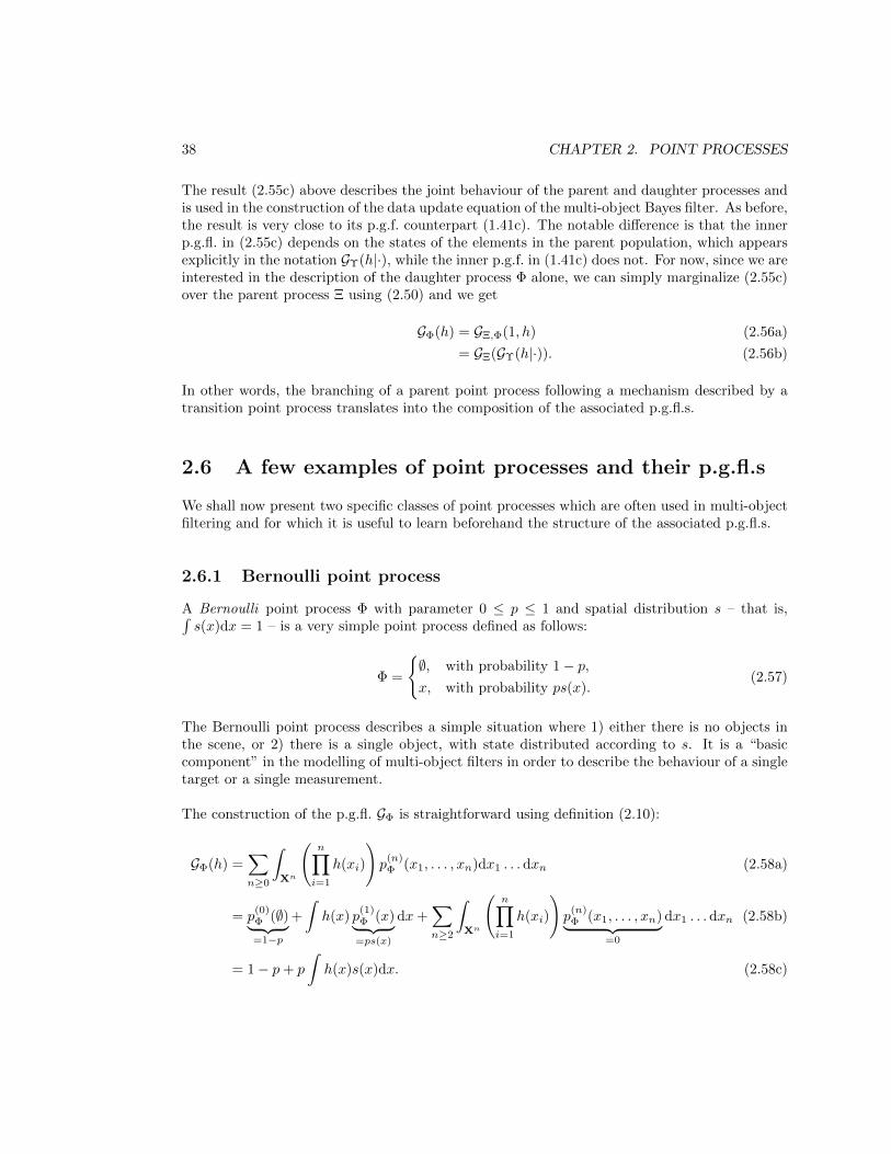
2.6.1 Bernoulli point process

A Bernoulli point process Φ with parameter 0 ≤ p ≤ 1 and spatial distribution s – that is,∫s(x)dx = 1 – is a very simple point process defined as follows:

Φ =

∅, with probability 1− p,x, with probability ps(x).

(2.57)

The Bernoulli point process describes a simple situation where 1) either there is no objects inthe scene, or 2) there is a single object, with state distributed according to s. It is a “basiccomponent” in the modelling of multi-object filters in order to describe the behaviour of a singletarget or a single measurement.

The construction of the p.g.fl. GΦ is straightforward using definition (2.10):

GΦ(h) =∑n≥0

∫Xn

(n∏i=1

h(xi)

)p

(n)Φ (x1, . . . , xn)dx1 . . . dxn (2.58a)

= p(0)Φ (∅)︸︷︷︸=1−p

+

∫h(x) p

(1)Φ (x)︸︷︷︸

=ps(x)

dx+∑n≥2

∫Xn

(n∏i=1

h(xi)

)p

(n)Φ (x1, . . . , xn)︸︷︷︸

=0

dx1 . . . dxn (2.58b)

= 1− p+ p

∫h(x)s(x)dx. (2.58c)

2.6. EXAMPLES OF P.G.FLS 39

2.6.2 Poisson point process

A Poisson point process Φ with rate λ ≥ 0 and spatial distribution s is defined as follows:∀n ≥ 0, |Φ| = n with probability e−λλn

n!,

The object states are i.i.d. according to s.(2.59)

A Poisson point process describes a population whose number of element follows a Poisson distri-bution, and whose element states are independently identically distributed (i.i.d.) in space. Thepoint patterns produced by a Poisson process, especially when the spatial distribution s is cho-sen as uniform over the state space, epitomize the notion of spatial randomness. It can be usedto describe some natural phenomena, such as the distribution of a certain tree species in a forest.

The construction of the p.g.fl. GΦ using definition (2.10) gives:

GΦ(h) =

∫X

(∏x∈ϕ

h(x)

)pΦ(ϕ)dϕ (2.60a)

=∑n≥0

∫Xn

(n∏i=1

h(xi)

)e−λ

λn

n!

(n∏i=1

s(xi)

)dx1 . . . dxn (2.60b)

= e−λ∑n≥0

λn

n!

∫Xn

(n∏i=1

h(xi)s(xi)

)dx1 . . . dxn (2.60c)

= e−λ∑n≥0

λn

n!

(∫h(x)s(x)dx

)n(2.60d)

= e−λ∑n≥0

(λ∫h(x)s(x)dx

)nn!

. (2.60e)

That is, using the Taylor expansion of the exponential (1.25):

GΦ(h) = e−λeλ∫h(x)s(x)dx (2.60f)

= eλ(∫h(x)s(x)dx−1). (2.60g)

In multi-object filtering, Poisson random variables are appealing because of the exponential formof their p.g.fl. (2.60g), easily differentiable; assuming some point processes to be Poisson allowsthe production of tractable and easily implementable filtering equations. It is, in essence, theprinciple behind the derivation of the PHD filter (see Section 2.7).

It is formative to extract the first moment density of a Poisson point process in some point,say y ∈ X, using the differentiation of the p.g.fl. (2.42):

µΦ(y) = δGΦ(h; δy)|h=1 (2.61a)

= δ(eλ(∫h(x)s(x)dx−1); δy)

∣∣∣h=1

, (2.61b)


where using the derivation rule for exponential functionals (2.36) yields

(2.61c)

µΦ(y) = δ

(λ

(∫h(x)s(x)dx− 1

); δy

)eλ(

∫h(x)s(x)dx−1)

∣∣∣∣h=1

(2.61d)

= λδ

(∫h(x)s(x)dx; δy

)∣∣∣∣h=1

eλ(∫s(x)dx−1)︸︷︷︸

=eλ(1−1)=e0=1

, (2.61e)

where using the derivation rule (2.28) gives

µΦ(y) = λ

∫δy(x)s(x)dx (2.61f)

= λs(y) (2.61g)

In other words, the first moment density of a Poisson process Φ equals its rate multiplied by itsspatial distribution; since λ and s fully characterize Φ through the definition (2.59), so does thefirst moment density µΦ. It is indeed customary to describe a Poisson process through its firstmoment density µΦ from which the rate λ and the spatial distribution s are easily retrieved: λ =

∫µΦ(x)dx

s(·) = λ−1µΦ(·)(2.62)

From (2.60g) and (2.62) we can write another expression of the p.g.fl. of a Poisson process Φthat is common in the point process litterature:

GΦ(h) = e∫

(h(x)−1)µΦ(x)dx. (2.63)

Since it allows the expression of the p.g.fl. w.r.t. a single quantity µΦ which is propagated bythe PHD filter, we will favour this last expression in the construction of the filter in Section 2.7.

2.7 Application: equations of the PHD filter

We shall now apply the results we have seen in the previous sections to derive the filtering equa-tions, in their p.g.fl. form, of the PHD filter. The purpose of this Bayesian filter is to estimateand propagate the mean number of target in any subregion of the scene, observed by some sensorwith known characteristics. Roughly speaking, the PHD filter adds a spatial component to the“cardinality only” PHD filter presented in Chap. 1, i.e., we are now interested in the number oftargets and their state. It is formative to compare the current section to the corresponding onein the previous chapter (Section 1.7), because the construction of the filtering equations shareremarkable similarities.

The data flow of one iteration of the PHD filter can be represented as follows:

2.7. APPLICATION 41

where the point processes provide a description of the configuration of the following populations:

• Ψ: the targets before the prediction (prior knowledge from past iterations);

• Φ: the targets after the prediction;

• Ξ: the current measurements;

• Φ|Ξ: the targets after the data update (i.e. conditioned on some realization Ξ = (z1, ..., zm)).

2.7.1 Modelling phase

Prediction step


1. The targets are independent;

2. A target with state x ∈ X survives with probability ps(x) and moves to some new statey ∈ X distributed acc. to m(y|x), dies (i.e. vanishes from the scene) otherwise;

3. A number of newborn targets enter the scene, independently of the number survivingtargets, following a birth mechanism described by a point process Φbirth with known char-acteristics (p.g.fl. Gbirth).

The prediction step can be represented as follows:


1. Since a target with state x ∈ X survives with probability ps(x) and moves to some statey ∈ X distributed acc. to m(y|x),, the “survival” point process Φs|x in the figure above isBernoulli with parameter ps(x) and spatial distribution m(·|x):

Gs(h|·) = 1− ps(·) + ps(·)∫h(y)m(y|·)dy. (2.64)


Note the difference between the p.g.f. (1.48) and the p.g.fl. above (2.64). The p.g.fl. is essen-tially in “augmented version” of the p.g.f. in which the spatial component is taken into account,because the state y of the (eventually) surviving target does matter and does depend on theprevious state x of the target. This dependency upon the prior state is important, because itmeans that the different survival point processes Gs will be dependent on different prior states,and will behave differently. This is the reason why we mark the dependency clearly and write“Gs(h|·)” rather than “Gs(h)”.

2. The surviving targets are described by a point process Φsur. which is the result of a branchingwith parent point process Ψ and transition point process Φs:

Gsur.(h) = GΨ(Gs(h|·)). (2.65)

3. The predicted targets, described by Φ, is the superposition of the surviving targets and thenewborn targets:

GΦ(h) = Gsur.(h)Gbirth(h). (2.66)

In consequence, the p.g.fl. form of the prediction step of the PHD filter is given by:

GΦ(h) = GΨ

(1− ps(·) + ps(·)

∫h(y)m(y|·)dy

)Gbirth(h). (2.67)

Similarly the “cardinality only” PHD, the p.g.fl.s allowed us to produce a full description of thepredicted targets Φ without computing its probability density pΦ(ϕ) for every possible sequenceϕ ∈ X .

Data update step


1. The measurements are produced independently;

2. A target with state x ∈ X is detected with probability pd(x) and produces a single mea-surement z ∈ Z distributed acc. to `(z|x), is undetected otherwise;

3. A number of clutter measurements “enter the scene”, independently from the target mea-surements, following a clutter mechanism described by a point process Ξclutter with knowncharacteristics (p.g.fl. Gclutter).

The update step can be represented as follows:


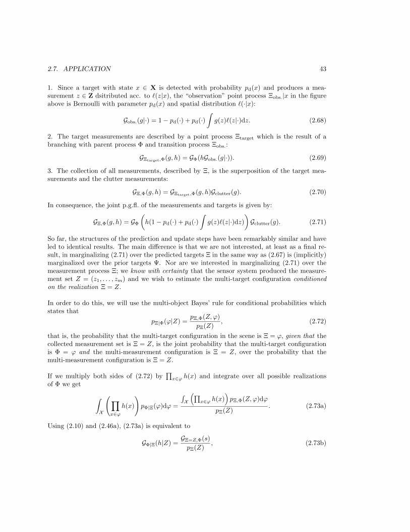
2.7. APPLICATION 43

1. Since a target with state x ∈ X is detected with probability pd(x) and produces a mea-surement z ∈ Z dsitributed acc. to `(z|x), the “observation” point process Ξobs.|x in the figureabove is Bernoulli with parameter pd(x) and spatial distribution `(·|x):

Gobs.(g|·) = 1− pd(·) + pd(·)∫g(z)`(z|·)dz. (2.68)

2. The target measurements are described by a point process Ξtarget which is the result of abranching with parent process Φ and transition process Ξobs.:

GΞtarget,Φ(g, h) = GΦ(hGobs.(g|·)). (2.69)

3. The collection of all measurements, described by Ξ, is the superposition of the target mea-surements and the clutter measurements:

GΞ,Φ(g, h) = GΞtarget,Φ(g, h)Gclutter(g). (2.70)

In consequence, the joint p.g.fl. of the measurements and targets is given by:

GΞ,Φ(g, h) = GΦ

(h(1− pd(·) + pd(·)

∫g(z)`(z|·)dz)

)Gclutter(g). (2.71)

So far, the structures of the prediction and update steps have been remarkably similar and haveled to identical results. The main difference is that we are not interested, at least as a final re-sult, in marginalizing (2.71) over the predicted targets Ξ in the same way as (2.67) is (implicitly)marginalized over the prior targets Ψ. Nor are we interested in marginalizing (2.71) over themeasurement process Ξ; we know with certainty that the sensor system produced the measure-ment set Z = (z1, . . . , zm) and we wish to estimate the multi-target configuration conditionedon the realization Ξ = Z.

In order to do this, we will use the multi-object Bayes’ rule for conditional probabilities whichstates that

pΞ|Φ(ϕ|Z) =pΞ,Φ(Z,ϕ)

pΞ(Z), (2.72)

that is, the probability that the multi-target configuration in the scene is Ξ = ϕ, given that thecollected measurement set is Ξ = Z, is the joint probability that the multi-target configurationis Φ = ϕ and the multi-measurement configuration is Ξ = Z, over the probability that themulti-measurement configuration is Ξ = Z.

If we multiply both sides of (2.72) by∏x∈ϕ h(x) and integrate over all possible realizations

of Φ we get

∫X

(∏x∈ϕ

h(x)

)pΦ|Ξ(ϕ)dϕ =

∫X

(∏x∈ϕ h(x)

)pΞ,Φ(Z,ϕ)dϕ

pΞ(Z). (2.73a)

Using (2.10) and (2.46a), (2.73a) is equivalent to

GΦ|Ξ(h|Z) =GΞ=Z,Φ(s)

pΞ(Z), (2.73b)


where (2.46b) and (2.43) yield

GΦ|Ξ(h|Z) =

1m!δ

m GΞ,Φ(g, h; δz1 , . . . , δzm)|g=01m!δ

m GΞ(g; δz1 , . . . , δzm)|g=0

. (2.73c)

Finally, the denominator of Bayes’ rule being the probability that the collected measurementsare Ξ = Z marginalized over all the possible multi-target configurations, GΞ(g) = GΞ,Φ(g, 1) andthus 1

m!δm GΞ(g; δz1 , . . . , δzm)|g=0 = 1

m!δm GΞ,Φ(g, 1; δz1 , . . . , δzm)|g=0. Thus (2.73c) becomes

GΦ|Ξ(h|Z) =δm GΞ,Φ(g, h; δz1 , . . . , δzm)|g=0

δm GΞ,Φ(g, 1; δz1 , . . . , δzm)|g=0

. (2.73d)

With (2.71) and (2.73d), we have now produced the p.g.fl. form of the data update step of thePHD filter:

GΦ|Ξ(h|Z) =δm GΞ,Φ(g, h; δz1 , . . . , δzm)|g=0

δm GΞ,Φ(g, 1; δz1 , . . . , δzm)|g=0

,

where GΞ,Φ(g, h) = GΦ

(h(1− pd(·) + pd(·)

∫g(z)`(z|·)dz)

)Gclutter(g). (2.74)

As for the prediction step, working with the p.g.fl.s allowed us to produce a full description ofthe updated targets Φ|Ξ without computing the probability density pΦ|Ξ(ϕ|Z) for every possiblesequence ϕ ∈ X .

2.7.2 Differentiation phase

Prediction step

Exploiting (2.43) we can extract the first-order moment density µΦ from the first derivative ofthe p.g.fl. GΦ:

µΦ(x) = δGΦ(h; δx)|h=1 (2.75a)

Substituting the expression of the p.g.fl. GΦ (2.67) yields

µΦ(x) = δ (GΨ(Gs(h|·))Gbirth(h); δx)|h=1 (2.75b)

Using the product rule (2.19) then gives

µΦ(x) = δ (GΨ(Gs(h|·)) ; δx)|h=1 Gbirth(h)|h=1︸︷︷︸=Gbirth(1)=1

+ GΨ(Gs(h|·))|h=1︸︷︷︸=GΨ(Gs(1|·))=GΨ(1)=1

δGbirth(h; δx)|h=1 (2.75c)

Exploiting again the relation between the first-order moment density and the first differentiationof the p.g.fl. (2.43) then yields

µΦ(x) = δ (GΨ(Gs(h|·)) ; δx)|h=1 + µbirth(x). (2.75d)

We now have to solve the composition δ (GΨ(Gs(h|·)) ; δx)|h=1 in (2.75d). This is the challengingpart, because we have not assumed any particular form for the prior process Ψ. If we were to

2.7. APPLICATION 45

assume that Ψ was Poisson, for example, we could exploit the special composition rule (2.36);however, the PHD filter does not assume such thing and we have to resolve the composition inthe general case. Quite fortunately, Campbell’s theorem (2.45) will help us in this task. Startingfrom the definition of the p.g.fl. (2.10) we can write down explicitly the outer functional:

δ (GΨ(Gs(h|·)) ; δx)|h=1 = δ

(∫X

(∏x∈ϕGs(h|x)

)pΦ(ϕ)dϕ; δx

)∣∣∣∣∣h=1

(2.76a)

Using (2.33) we can swap the differentiation and integral:

δ (GΨ(Gs(h|·)) ; δx)|h=1 =

∫Xδ

(∏x∈ϕGs(h|x); δx

)∣∣∣∣∣h=1

pΦ(ϕ)dϕ (2.76b)

The derivative can now be expanded using the product rule:

δ (GΨ(Gs(h|·)) ; δx)|h=1 =

∫X

∑x∈ϕ

δGs(h|x; δx)|h=1

∏¯x∈ϕ\x

Gs(h|¯x)|h=1︸︷︷︸=Gs(1|¯x)=1

pΦ(ϕ)dϕ (2.76c)

=

∫X

(∑x∈ϕ

δGs(h|x; δx)|h=1

)pΦ(ϕ)dϕ (2.76d)

Given the simple structure (2.64) of the inner functional Gs, the derivation in (2.76d) can nowbe solved:

δGs(h|x; δx)|h=1 = δ

(1− ps(x) + ps(x)

∫h(y)m(y|x)dy; δx

)∣∣∣∣h=1

(2.76e)

= ps(x) δ

(∫h(y)m(y|x)dy; δx

)∣∣∣∣h=1

(2.76f)

Where (2.28) gives

δGs(h|x; δx)|h=1 = ps(x)

∫δx(y)m(y|x)dy (2.76g)

= ps(x)m(x|x). (2.76h)

Substituting (2.76h) into (2.76d) gives

δ (GΨ(Gs(h|·)) ; δx)|h=1 =

∫X

(∑x∈ϕ

ps(x)m(x|x)

)pΨ(ϕ)dϕ (2.76i)

And, finally, Campbell’s theorem (2.45) yields the desired result

δ (GΨ(Gs(h|·)) ; δx)|h=1 =

∫ps(x)m(x|x)µΨ(x)dx. (2.76j)


Substituting (2.76j) into (2.75d) yields the final result for the predictions step:

µΦ(x) =

∫ps(x)m(x|x)µΨ(x)dx+ µbirth(x). (2.77)

Similarly to the “cardinality only” PHD filter, no filtering approximations were necessary toproduce this result, which means that the validity of the prediction step is not limited to aparticular model for the prior targets Ψ and/or the newborn targets Φbirth. We have seen thatthe general expression had a cost as the construction of the prediction equation (2.77) wassignificantly more involved than its “cardinality only” counterpart (1.59g). On the other hand,we will see in the next section that the construction of the update equation for the PHD filter isalmost identical to its “cardinality only” counterpart.

Update step

Again, it is straightforward to write the first-order moment of the posterior targets µΦ|Ξ=Z ,given that the sensor system produced the observation set Z = z1, . . . , zm, as the first orderderivative of the p.g.fl. GΦ|Ξ(·|Z):

µΦ|Ξ(x|Z) = δGΦ|Ξ(h|Z)|h=1 (2.78a)

Substituting the expression of the p.g.fl. GΦ|Ξ(h|Z) (2.74) yields

µΦ|Ξ(x|Z) =δm+1GΞ,Φ(g, h; δz1 , . . . , δzm , δx)

∣∣g=0,h=1

δmGΞ,Φ(g, 1; δz1 , . . . , δzm)|g=0

(2.78b)

The previous result (2.74) provides an expression of the joint p.g.f. GΞ,Φ w.r.t. the predictedp.g.fl. GΦ and the clutter p.g.fl. Gclutter, but at this point we have not made any assumptions onthe predicted targets Φ or the clutter process Ξclutter and their respective p.g.fl.s. If we attemptto proceed with the derivation in (2.78b) without assuming any particular forms for the p.g.fl.sGΞ and Gclutter, we will end up with a very general but intractable result. We will thus assumethat:

1. The predicted targets Φ is a Poisson process;

2. The clutter Ξclutter is a Poisson process.

Using the expression of a Poisson process w.r.t. its first-order moment density (2.63), we canrewrite the joint p.g.fl. GΞ,Φ (2.71) as follows:

GΞ,Φ(g, h) = GΦ

(h(1− pd(·) + pd(·)

∫g(z)`(z|·)dz)

)Gclutter(g) (2.79a)

= e∫

(h(y)(1−pd(y)+pd(y)∫g(z)`(z|y)dz)−1)µΦ(y)dye

∫(g(z)−1)µclutter(z)dz (2.79b)

= e∫

[h(x)(1−pd(y)+pd(y)∫g(z)`(z|y)dz)−1]µΦ(x)dx+

∫[g(z)−1]µclutter(z)dz (2.79c)

= eF (g,h), (2.79d)

where we defined the inner bivariate functional

F (g, h) =

∫ [h(y)(1− pd(y) + pd(y)

∫g(z)`(z|y)dz)− 1

]µΦ(y)dy +

∫[g(z)− 1]µclutter(z)dz.

2.7. APPLICATION 47

We can now proceed to the derivation of the joint p.g.fl. in its new form (2.79d), for its exponentialform makes the derivation easier exploiting the composition rule (2.36). Indeed, resolving thefirst-order derivative yields immediately:

δGΞ,Φ(g, h; δz1) = δ(eF (g,h); δz1) (2.80a)

= δF (g, h; δz1)eF (g,h). (2.80b)

Now, the resolution of δF (g, h; δz1) is straightforward if we first swap the integral and the dif-ferentation using (2.31), then resolve the differentiation using (2.28):

δF (g, h; δz1) =

∫h(y)pd(y)δ

(∫g(z)`(z|y)dz; δz1

)µΦ(y)dy + δ

(∫g(z)µclutter(z)dz; δz1

)(2.81a)

=

∫h(y)pd(y)

(∫δz1(z)`(z|y)dz

)µΦ(y)dy +

∫δz1(z)µclutter(z)dz (2.81b)

=

∫h(y)pd(y)`(z1|y)µΦ(y)dy + µclutter(z1). (2.81c)

And thus the first-order derivative (2.80b) reads:

δGΞ,Φ(g, h; δz1) =

[∫h(y)pd(y)`(z1|y)µΦ(y)dy + µclutter(z1)

]eF (g,h). (2.82a)

Since the multiplicative term in front of the exponential is independent of g, it is straightforwardto write the m-th order derivative of the joint p.g.fl. w.r.t. the function g:

δmGΞ,Φ(g, h; δz1 , . . . , δzm) =

m∏i=1

[∫h(y)pd(y)`(zi|y)µΦ(y)dy + µclutter(zi)

]eF (g,h). (2.82b)

For the numerator in (2.74), we need to differentiate (2.82b) once w.r.t. h. This is a simple taskusing first the product rule (2.19):

δm+1GΞ,Φ(g, h; δz1 , . . . , δzm , δx)

=

m∑i=1

[δ

(∫h(y)pd(y)`(zi|y)µΦ(y)dy + µclutter(zi); δx

) m∏j=1j 6=i

[ ∫h(y)pd(y)`(zj |y)µΦ(y)dy + µclutter(zj)

]]eF (g,h)

+

m∏i=1


]δ(eF (g,h); δx) (2.83a)


Where (2.28) in the first summand and the composition rule (2.36) in the second summand give

δm+1GΞ,Φ(g, h; δz1 , . . . , δzm , δx)

=

m∑i=1

[∫δx(y)pd(y)`(zi|y)µΦ(y)dy

m∏j=1j 6=i


]]eF (g,h)

+

m∏i=1


]δF (g, h; δx)eF (g,h) (2.83b)

=

m∑i=1

[pd(x)`(zi|x)µΦ(x)

m∏j=1j 6=i


]]eF (g,h)

+

m∏i=1


]δF (g, h; δx)eF (g,h) (2.83c)

Again, the resolution of δF (g, h; δx) is straightforward using (2.28):

δF (g, h; δx) =

∫δx(y)

(1− pd(y) + pd(y)

∫g(z)`(z|y)dz

)µΦ(y)dy (2.84a)

=

(1− pd(x) + pd(x)

∫g(z)`(z|x)dz

)µΦ(x). (2.84b)

Substituting (2.84b) in (2.83c) yields the desired numerator

δm+1GΞ,Φ(g, h; δz1 , . . . , δzm , δx)

=

m∑i=1

[pd(x)`(zi|x)µΦ(x)

m∏j=1j 6=i


]]eF (g,h)

+

m∏i=1


](1− pd(x) + pd(x)

∫g(z)`(z|x)dz

)µΦ(x)eF (g,h)

(2.85)

Dividing the numerator (2.85) by the denominator (2.82b) finally yields:

δm+1GΞ,Φ(g, h; δz1 , . . . , δzm , δx)

δmGΞ,Φ(g, h; δz1 , . . . , δzm)=

n∑i=1

pd(x)`(zi|x)µΦ(x)∫h(y)pd(y)`(zi|y)µΦ(y)dy + µclutter(zi)

+

(1− pd(x) + pd(x)

∫g(z)`(z|x)dz

)µΦ(x) (2.86a)

At this point we just have to set h = 1 and g = 0 to produce the desired result (recall the generalexpression (2.78b)):

µΦ|Ξ(x|Z) =∑z∈Z

pd(x)`(z|x)µΦ(x)∫pd(y)`(z|y)µΦ(y)dy + µclutter(z)

+ (1− pd(x))µΦ(x).

(2.86b)

2.7. APPLICATION 49

2.7.3 Filtering equations

We have now succeeded in producing the filtering equations of the PHD filter [11] with equations(2.77) and (2.86b), repeated here:

µΦ(x) =

∫ps(y)m(x|y)µΨ(y)dy + µbirth(x),

µΦ|Ξ(x|Z) = (1− pd(x))µΦ(x) +∑z∈Z

pd(x)`(z|x)µΦ(x)∫pd(y)`(z|y)µΦ(y)dy + µclutter(z)

.(2.87)

If we compare the equations of the “cardinality only” PHD filter (1.66) with those above, wecan remark that they have a remarkably similar structure.

Chapter 3

Point processes and higher ordermoments

This chapter explores the concept of higher-order moments for point processes, and providesthe tools for their practical derivation using the functional derivatives introduced in Chap. 2.The construction of the PHD filter with variance in target number, an example of application ofhigher-order moments for target detection and tracking problems, is introduced. A more detailedconstruction is given for the PHD and the CPHD filters in [8].

3.1 Defining moments for point processes: first attempt

We have seen in Chap. 1 that statistical moments are readily available for integer-valued randomvariables. Inspired by the expression of the kth order moment in (1.3), we may be want to produce

the kth order moment µ(k)Φ of a point process Φ as

µ(k)Φ = E

[Φk]

=

∫XpΦ(ϕ)ϕkdϕ. (3.1)

Then, what is wrong with the result above? Suppose, for example, that Φ is a very simple point

process on X such that p(2)Φ (x1, x2) = p

(2)Φ (x2, x1) = p

(1)Φ (x3) = 1

3 , where x1, x2, x3 ∈ X. If weexploit (3.1) then the 1th order moment µΦ is

µ(1)Φ =

1

3(x1, x2) +

1

3(x1, x2) +

1

3(x3). (3.2)

Does the result above denote some kind of “average behaviour” of the point process, as we wouldexpect from the 1st order moment of a random variable? We may say that “on average, the popu-lation of targets has a size of 5

3”, but what can we say about the “average state” of those targets?

In turns out that summing sequences of points makes little sense, neither would multliplyingthem if we were to consider higher-order moments through our first attempt of definition (3.1).Integer-valued random variables take, by definition, values in the set of non-negative integers N;

51

52 CHAPTER 3. POINT PROCESSES AND HIGHER-ORDER MOMENTS

this a very convenient space as the operations of sum and multiplication are well-defined and wecan thus produce expressions for statistical moments (1.3), (1.4). The point process Φ, however,is a random variable with values in the space X of finite sequences of points on X; this spacehas a much more complicated structure on which the operations of sum and multiplication makelittle sense. In order to define statstical moments on a point process, then, we shall try first tocharacterize a point process with integer-valued random variables, then produce the moments ofthe said random variables.

3.2 Point processes and counting measures

Statistical moments are readily available forinteger-valued random variables. In our case,we need to build an integer-valued randomvariable, providing a description of the targetpopulation, from a point process Φ.

Point processes are random variables whoserealizations are sequences of points in the targetstate space X . A point process is not a real (orcomplex) valued random variable and momentscannot be directly defined from point processes– the expression E [Φ] has no mathematicalsense, since realizations can be sequences of dif-ferent sizes for which no sum operator is defined.

Let us fix a suitable region B ⊆ X 1. One canmap any realization ϕ of the point process to thenumber of elements in ϕ belonging to B, that is:

Nϕ(B) =∑x∈ϕ

1B(x), (3.3)

where 1B is the indicator function on B, i.e.

1B(x) =

1, x ∈ B0, otherwise.

(3.4)

1Recall from Chap. 2 that B belongs to B(X), the Borel σ-algebra on the target space X.

3.3. MOMENTS: SECOND ATTEMPT 53

If we compose the point process with the map-ping defined above in (3.3), we get the integer-valued random variable

NΦ(B) =∑x∈Φ

1B(x), (3.5)

which provides a description of the number oftargets within B acc. to the point process Φ.

Let us have a look at the nature of the different mathematical objects involved in the constructionwe have just illustrated.

1. Nϕ(B) is the number of elements of the realization ϕ belonging to the fixed region B; it isan integer ;

2. NΦ(B) maps an outcome ω ∈ Ω to the number of elements of the realization Φ(ω) belongingto the fixed region B; it is an integer-valued random variable;

3. Nϕ(·) maps a suitable region B ⊆ X to the number of elements of the realization ϕ thatit contains; it is an integer-valued measure called a counting measure;

4. NΦ(·) maps an outcome ω ∈ Ω to the counting measure NΦ(ω)(·); it is a integer-valuedrandom measure.

We have now built a integer-valued random variable NΦ(B) for any suitable region B ⊆ X,and it can be shown that these random variables characterize the point process Φ when all thesuitable regions of the target state space are considered. We can now focus on the constructionof the moments of these random variables.

3.3 Defining moments for point processes: second attempt

Since NΦ(B) is a random variable for any suitable region B ⊆ X, inspired from (1.3), we canbuild the kth order non factorial moment of the point process Φ as the joint expectation

µ(k)Φ (B1 × . . .×Bk) = E [NΦ(B1) · · ·NΦ(Bk)] (3.6a)

= E

[∑x∈Φ

1B1(x) · · ·∑x∈Φ

1Bk(x)

](3.6b)

= E

∑x1,...,xk∈Φ

1B1(x1) · · · 1Bk(xk)

, (3.6c)

for any suitable regions Bi ⊆ X, 1 ≤ i ≤ k. We can make two important remarks about

the structure of the kth order non factorial moment µ(k)Φ above. First, we see that it takes as

argument a suitable region of Xk; it is actually a measure on Xk and its full name is the kth order


non factorial moment measure of the point process Φ. Second, equation (3.6b) provides someinsight on the physical meaning on the non factorial moment measure: it assesses the number oftargets falling jointly in regions Bi of the state space, and includes events where a single targetbelongs to several of these regions. If we wish to exclude the latter possibility, we obtain thekth order factorial moment measure of the point process Φ, defined as the joint expectation

α(k)Φ (B1 × . . .×Bk) = E

∑ 6=

x1,...,xk∈Φ

1B1(x1) · · · 1Bk(xk)

, (3.7)

where the 6= sign indicates that the selected points in the sequence are all distinct. We maysee from (3.6) and (3.7) that the 1st order moment measures, factorial and non factorial, areequal; the 1st order moment measure is also called the intensity measure of the point processand simply denoted by µΦ.

Remark 4. For the sake of simplicity, we have adopted the same notation for the momentmeasures in this chapter and the moment densities in Chap. 2. In particular, we use the notationµΦ for both the intensity measure of Φ and the density of the intensity measure, also called theProbability Hypothesis Density or intensity of the point process Φ.

Similarly as we have seen in (1.5) for integer-valued random variables, it is interesting to definethe central second moment or variance of the point process Φ as

varΦ(B) = µ(2)Φ (B ×B)− [µΦ(B)]

2, (3.8)

for any suitable region B ⊆ X. The regional statistics (µΦ(B), varΦ(B)) of the point process Φcan then be interpreted as follows [8]

• µΦ(B) is the mean value of the random variable NΦ(B), i.e., the average number of targetswithin B;

• varΦ(B) quantifies the spread of the random variable NΦ(B) around its mean value, i.e.,the spread of the estimated number of targets within B around its mean value.

In detection and tracking problems, these statistics allow us to estimate the average number oftarget in any suitable region B ⊆ X of the state space, with associated uncertainty. They can beused, for example, in a sensor scheduling policy focussing on the regions where the uncertaintyin the target number is the highest [1].

Remark 5. Even if the variance is a function defined on the Borel σ-algebra B(X) associated tothe state space X, it is not a measure on X. In particular, it can be shown that the variance isnot additive, i.e. B1 ⊆ B2 does not imply that varΦ(B1) ≤ varΦ(B2) (this will be the topic of anexercise in Ex 4.3.3). An important consequence is that the variance does not admit a density,in the general case; i.e., there does not exist a density vΦ on X, such that

varΦ(B) =

∫B

vΦ(x)dx, (3.9)

for any suitable region B ⊆ X.

3.4. COMPUTING THE MOMENT MEASURES 55

Other meaningful statistical quantities about a point process can be defined from its momentmeasures, though they are out of the scope of this lecture. Suppose that one wish to study thecorrelation between the number of targets in suitable regions B1, B2 ⊆ X according to somepoint process, then similarly to (3.8) one can define the covariance

covΦ(B1, B2) = µ(2)Φ (B1 ×B2)− µΦ(B1)µΦ(B2). (3.10)

3.4 Computing the moment measures

At this stage, we can make two important remarks regarding the moment measures for pointprocesses, through a direct analogy with the moments for integer-valued random variables stud-ied in Chap. 1. First, the central moments are the most interesting to us as we can provide ameaningful physical interpretation for them – at least for the lower orders! – and exploit themto study the point process, as we have just seen with the variance in (3.8). Second, the centralmoments can be easily written through the non factorial moment measures – again, we havejust illutrated this point with the variance in (3.8).

Our next task, then, it to find a convenient way to produce the kth order moment measure µ(k)Φ

of a point process Φ. We have already seen in Chap. 2 that the 1th order moment density µΦ canbe retrieved in any x ∈ X with one functional differentation in (2.43); in fact, all the derivationrules presented for densities in Chap. 2 extend naturally to measures when indicator functionsare substituted to Dirac delta functions, i.e.

1

k!δkGΦ(h; 1B1

, . . . , 1Bk)∣∣h=0

= P(k)Φ (B1 × · · · ×Bk)

(=J

(k)Φ (B1 × · · · ×Bk)

k!

),

δGΦ(h; 1B)|h=1 = µΦ(B).

(3.11)

The question is, can we differentiate k times the p.g.fl. GΦ to produce the kth order moment

measures µ(k)Φ ? Unfortunately for us, as suggested by the similar result for integer-valued random

variables in (1.31), this operation yields the factorial moment measure α(k)Φ , i.e.

δkGΦ(h; 1B1, . . . , 1Bk)

∣∣h=1

= α(k)Φ (B1 × . . .×Bk). (3.12)

Can we, then, find a simple expression of the non factorial moment measures exploiting thefactorial ones? Let us have a look at the case k = 2. Starting from the definition (3.6) we canwrite:

µ(2)Φ (B1 ×B2) = E [NΦ(B1)NΦ(B2)] (3.13a)

= E

∑x1,x2∈Φ

1B1(x1)1B2

(x2)

(3.13b)

= E

∑6=

x1,x2∈Φ

1B1(x1)1B2

(x2)

︸︷︷︸

=α(2)Φ (B1×B2)

+E

[∑x∈Φ

1B1(x)1B2

(x)

]︸︷︷︸

=µΦ(B1∩B2)

(3.13c)


That is, the 2nd order moment measure µ(2)Φ can be retrieved from the 2nd order factorial moment

measure α(2)Φ and the intensity µΦ. Since α

(2)Φ can be computed with a second-order derivative

of the p.g.fl. with (3.12), µ(2)Φ can be expressed as a combination of differentiated p.g.fl.s. While

a relation between factorial and non factorial moments such as (3.13c) exists for higher orders,it becomes increasingly complicated and tedious to write in order to produce the expression ofnon factorial moment measures of increasing order.

So why can’t we write µ(2)Φ (B1 ×B2) directly as the derivative of a single p.g.fl.? Since we need

to consider the occurrence of a single point of the point process falling in the intersection of thetwo regions, the quantity

1B1(x)1B2(x), (3.14)

among others, must appear somewhere during the derivation process. Let us differentiate twicethe p.g.fl. in the directions 1B1

and 1B2and see what we get. Recall from the previous chapter

in (2.10) that the p.g.fl. of a process Φ is given by

GΦ(h) =∑n≥0

∫Xn

(n∏i=1

h(xi)

)P

(n)Φ (d(x1, . . . , xn)). (3.15)

Thus, the differentiated p.g.fl. reads

δ2GΦ(h; 1B1, 1B2

)∣∣h=1

= δ2

∑n≥0

∫Xn

(n∏i=1

h(xi)

)P

(n)Φ (d(x1, . . . , xn)); 1B1

, 1B2

∣∣∣∣∣∣h=1

. (3.16a)

=∑n≥0

∫Xn

δ2

(n∏i=1

h(xi); 1B1, 1B2

)∣∣∣∣∣h=1

P(n)Φ (d(x1, . . . , xn)). (3.16b)

Let us expand a derivation term in (3.16b), say n = 3. If we differentiate h(x1)h(x2)h(x3) oncein the direction 1B1 using the product rule (2.19) we get:

δ(h(x1)h(x2)h(x3); 1B1)

= δ(h(x1); 1B1)h(x2)h(x3) + h(x1)δ(h(x2); 1B1)h(x3) + h(x1)h(x2)δ(h(x3); 1B1) (3.17a)

= 1B1(x1)h(x2)h(x3) + h(x1)1B1(x2)h(x3) + h(x1)h(x2)1B1(x3) (3.17b)

We see in (3.17b) that h is not “available” at a given point xi once it has been differentiated –for example, the first term does not contain h(x1) anymore. If we differentiate a second time inthe direction 1B2

, then set h = 1, we get:

δ2(h(x1)h(x2)h(x3); 1B1, 1B2

)∣∣h=1

= 1B1(x1)1B2

(x2) + 1B1(x1)1B2

(x3) + 1B2(x1)1B1

(x2)

+ 1B1(x2)1B2

(x3) + 1B2(x1)1B1

(x3) + 1B2(x2)1B1

(x3) (3.18)

Because the test function h “disappeared” in the simple derivation terms such as δ(h(x1); 1B1),

the desired products such as 1B1(x1)1B2

(x1) do not appear in (3.18): in other words, the p.g.fl.is not adapted to the production of non factorial moment measures.

3.4. COMPUTING THE MOMENT MEASURES 57

Let us consider the transformation h→ e−f and consider f as the new test function. Using theproperty (2.36), one can show that

δ(e−f(x1); 1B1) = −1B1

(x1)e−f(x1). (3.19)

This result is left as an exercise in Ex. 4.3.1.

Remark 6. The result above may look familiar to the reader; indeed, if we consider functionsrather than functional, we have the well-known result(

e−f(x1))′

= −f ′(x1)e−f(x1). (3.20)

This time, the test function f did not disappear in the derivation process (3.19); differentiatinga second time in direction 1B2 yields

δ2(e−f(x1); 1B1, 1B2

) = −1B1(x1)δ(e−f(x1); 1B2

) (3.21a)

= 1B1(x1)1B2(x1)e−f(x1), (3.21b)

and the desired product 1B1(x1)1B2(x1) do appear.

The transformation h→ e−f is a promising lead to solve our problem at hand; if we apply it tothe p.g.fl., we obtain the Laplace functional

LΦ(f) = GΦ(e−f ) (3.22a)

= E

[∏x∈Φ

e−f(x)

](3.22b)

=

∫X

(∏x∈ϕ

e−f(x)

)PΦ(dϕ) (3.22c)

=∑n≥0

∫Xn

(n∏i=1

e−f(xi)

)P

(n)Φ (d(x1, . . . , xn)). (3.22d)

As the developments above suggest, the Laplace functional is well-adapted to the production ofnon factorial moment measures; one can show that

(−1)k δkLΦ(f ; 1B1 , . . . , 1Bk)∣∣f=0

= µ(k)Φ (B1 × . . .×Bk). (3.23)

In particular, the quantity µ(2)Φ (B × B) in the expression of the variance (3.8) is given by the

second-order derivative δ2LΦ(f ; 1B , 1B)∣∣f=0

.

We now have all the tools to produce the various statistical quantities of a point process, repeatedhere:

P(k)Φ (B1 × · · · ×Bk) =

1

k!δkGΦ(h; 1B1

, . . . , 1Bk)∣∣h=0

,

α(k)Φ (B1 × · · · ×Bk) = δkGΦ(h; 1B1 , . . . , 1Bk)

∣∣h=1

,

µ(k)Φ (B1 × · · · ×Bk) = (−1)k δkLΦ(f ; 1B1

, . . . , 1Bk)∣∣f=0

.

(3.24)


We know from the definition of the moment measures in Sec. 3.3, that the intensity measure µΦ

is the 1st order non factorial moment measure µ(1)Φ by definition, but it also equals the 1st order

factorial moment measure α(1)Φ by construction. From the result above, it follows that we should

find be able to find the intensity measure µΦ from the 1st order derivative of either the p.g.fl. orthe Laplace functional; this is left as exercise in Ex. 4.3.2.

3.5 Example: Poisson process and regional statistics

We have seen in Chap. 2 that Poisson point processes are very important in the modellingand derivation of multi-object filters, because their p.g.fl. has a very simple structure that isparticularily easy to differentiate (see Section 2.6.2). Let us recall the definition (2.59) of aPoisson point process with rate λΦ ≥ 0 and spatial distribution sΦ:∀n ≥ 0, |Φ| = n with probability e−λΦ

λnΦn!,

The object states are i.i.d. according to sΦ.(3.25)

We have also established in (2.61g) that µΦ(x) = λΦsΦ(x); as all the results expressed withdensities in Chap. 2 it extends to the corresponding measures, i.e.

µΦ(B) = λΦsΦ(B), (3.26)

for any suitable region B ⊆ X. Likewise, the p.g.fl. of Φ that we obtained for densities in (2.63)becomes

GΦ(h) = exp

[∫(h(x)− 1)µΦ(dx)

]. (3.27)

As seen in (3.25), a key element in the construction of a Poisson point process is to assumethat the cardinality distribution of the process is itself distributed according to a scalar Poissondistribution, i.e.

ρΦ(n) = e−λΦλnΦn!. (3.28)

As you may know, the variance of a Poisson variable equals its mean (left as exercise in Ex. 4.1.2).It suggests that a Poisson random variable is “flexible” and allows a great variability along itsmean – the greater the estimated mean is, though, the greater is the uncertainty associated tothe estimation.

Assume that the information we maintain about the population of targets in the scene is de-scribed by a Poisson point process Φ. Since the size of the population is described by a Poissondistribution (3.28), we conclude that the estimated target number in the whole surveillancescene has a mean µΦ(X) equal to its variance varΦ(X). We may wonder, however, whether thisproperty holds locally, i.e., whether

µΦ(B) = varΦ(B), (3.29)

for any suitable region B ⊆ X. The fact that the targets’ states are i.i.d. suggests that theproperty (3.29) might be true, and we shall now proceed to compute the regional statistics

3.5. EXAMPLE: POISSON PROCESS AND REGIONAL STATISTICS 59

(µΦ(B), varΦ(B)) in order to check if it is the case.

Since our goal is to find the expression of the variance varΦ, following the definition (1.5) we

need to find the expression of the 2nd order moment measure µ(2)Φ first, and we have just seen

(Section 3.4) that we can compute this quantity from the Laplace functional LΦ of the pointprocess. From the general expression of the Laplace functional (3.22) and the p.g.fl. of a Poissonpoint process (3.27) we get

LΦ(f) = exp

[∫(e−f(x) − 1)µΦ(dx)

]. (3.30)

Let us fix some suitable region B ⊆ X. Using the relation between moment measures andderivatives of the Laplace functional (3.23) we can write:

µ(2)Φ (B ×B) = δ2LΦ(f ; 1B , 1B)

∣∣f=0

(3.31a)

= δ2

(exp

[∫(e−f(x) − 1)µΦ(dx)

]; 1B , 1B

)∣∣∣∣f=0

(3.31b)

= δ2 (exp F ) (f ; 1B , 1B)∣∣f=0

, (3.31c)

where the inner functional F is defined as F (f) =∫

(e−f(x)−1)µΦ(dx). The derivation in (3.31c)can be easily expanded with Faa di Bruno’s formula (2.21), and it yields

µ(2)Φ (B ×B) = δ2 exp(F (f); δF (f ; 1B), δF (f ; 1B))

∣∣f=0

+ δ exp(F (f); δ2F (f ; 1B , 1B))∣∣f=0

.

(3.31d)

Let us have a look at the increment δF (f ; 1B) in (3.31d). We can write

δF (f ; 1B) = δ

(∫(e−f(x) − 1)µΦ(dx); 1B

)(3.32a)

=

∫δ(e−f(x) − 1; 1B)µΦ(dx) (3.32b)

=

∫δ(e−f(x); 1B)µΦ(dx) (3.32c)

Then, using the previously established rule (3.19):

δF (f ; 1B) =

∫(−1B(x))e−f(x)µΦ(dx). (3.33)

As expected, the test function f has not “disappeared” and thus δF (f ; 1B) can be differentiatedanother time without vanishing. Following the same reasoning that led to (3.33), we can writethe expression of the second-order derivative of the inner function F :

δ2F (f ; 1B , 1B) =

∫(−1B(x))2e−f(x)µΦ(dx) (3.34a)

=

∫1B(x)e−f(x)µΦ(dx). (3.34b)


Now that the increments δF (f ; 1B) and δ2F (f ; 1B , 1B) are known, let us resolve the outerdifferentiation in (3.31d). At this stage, the expression (3.31d) looks rather involved; however, theonly derivatives left involve exponentials differentiated in the directions δF (f ; 1B), δ2F (f ; 1B , 1B)which are real-valued numbers, and evaluated at the real-valued number F (f). Resolving thistype of differentiation is particularly easy, as we have seen in Chap. 2; using (2.35), the expression(3.31d) then becomes

µ(2)Φ (B ×B) = (δF (f ; 1B))

2exp(F (f))

∣∣∣f=0

+ δ2F (f ; 1B , 1B)) exp(F (f))∣∣f=0

. (3.35)

We can then substitute in (3.35) the values of the increments which have been determined in(3.33) and (3.34b):

µ(2)Φ (B ×B)

=

(∫(−1B(x))e−f(x)µΦ(dx)

)2∣∣∣∣∣f=0

exp(F (f))|f=0 +

(∫1B(x)e−f(x)µΦ(dx)

)∣∣∣∣f=0

exp(F (f))|f=0

(3.36a)

= (−µΦ(B))2 × 1 + (µΦ(B))× 1 (3.36b)

= (µΦ(B))2

+ µΦ(B). (3.36c)

Now that the second moment measure has been determined in (3.36c), we can produce thevariance varΦ of the Poisson process Φ from the definition (1.5):

varΦ(B) = µ(2)Φ (B ×B)− (µΦ(B))

2(3.37a)

= (µΦ(B))2

+ µΦ(B)− (µΦ(B))2

(3.37b)

= µΦ(B). (3.37c)

We have thus proved that property (3.29) holds: the mean and the variance in the number oftargets in any suitable region B ⊆ X of the state space are always equal when the populationof targets is estimated with a Poisson point process. This result, of course, does not hold in thegeneral case!

An interesting consequence to (3.37c) is that the variance of a Poisson process in any region Bis bounded by the mean target number in the state space since

varΦ(B) = µΦ(B) ≤ µΦ(X). (3.38)

This means that the local behaviour of a Poisson process with “reasonable global average be-haviour” – i.e. with a finite mean target number in the whole state space µΦ(X) – can beestimated in any region B with “some accuracy” since the variance of the target number in Bis finite as well according to (3.38). We will see in an exercise 4.3.5 that this is not necessarilytrue for other point processes.

Chapter 4

Exercises

4.1 Integer-valued random variables

4.1.1 Chain rule for ordinary differentiation

Prove the chain rule when the outer function is the exponential (1.24), i.e.

(exp f)′(x) = f ′(x)(exp f)(x). (4.1)

(Hint) Use the Taylor expansion of the exponential (1.25) and the power rule (1.21).

4.1.2 Poisson random variable

Assume X is a Poisson random variable with parameter λX , i.e.

pX(n) = exp(−λX)λnXn!. (4.2)

Prove that its variance varX equals its mean µX .

(Hint) Use the differentiation rule (1.31) to extract the factorial moment α(2)X from the p.g.f.

GX , then use the definitions (1.3), (1.4) to find the expression of the non factorial moment µ(2)X

w.r.t. to α(2)X and µX . Conclude using the definition of the variance (1.5).

Remark 7. Alternatively, cecause a Poisson random variable has a simple structure, the non

factorial moment µ(2)X can be computed directly from its definition (1.3).

61

62 CHAPTER 4. EXERCISES

4.2 Point processes

4.2.1 Functional differentiation of linear functionals

A linear functional is a functional L such that for any functions f , g, and for any scalars α, β:

L(αf + βg) = αL(f) + βL(g). (4.3)

Let L be a continuous linear functional. Prove that, for any functional F , any test function hand any admissible direction η:

δ(L F )(h; η) = L(δF (h; η)). (4.4)

(Hint) Use the definition of the chain differential (2.16).

This result tells us, loosely speaking, that we can “swap” a linear continuous functional anda derivative. It is very useful for practical derivations, and we sometimes apply the rule onexpressions where the linear continuous functional does not appear explicity. The most commonexample is perhaps the rule (2.33) allowing us to swap the integral and derivative, which is aparticular case of the rule (4.4) above.

4.2.2 Functional differentiation of exponential

Prove the chain rule when the outer function is the exponential (2.36), i.e.

δ(exp F )(h; η) = δF (h; η)(exp F )(h). (4.5)

(Hint) Use the chain rule (2.20), then write the outer differentation using the definition of thechain differential (2.16). Use the Taylor expansion of the exponential (1.25) to conclude.

4.3 Higher-order moments for point processes

4.3.1 Functional differentiation of exponential (cont.)

Let f be some suitable function on X, and B some suitable region of X, and x some point of X.Prove the equality (3.19), i.e.

δ (exp(−f(x)); 1B) = −1B(x) exp(−f(x)). (4.6)

(Hint) Find the“cumbersome” expression of the left-hand side, i.e., find the functional F suchthat δ(exp(−f(x)); 1B) = δ(exp F )(f ; 1B). Then, use the result (2.36) (repeated in (4.5) inEx. 4.2.2) to resolve the composition. Use the definition of the chain differential (2.16) onδF (f ; 1B) to conclude.

4.3. CHAPTER 3 63

4.3.2 p.g.fl. and Laplace functional

Let Φ be a point process with p.g.fl. GΦ and Laplace functional LΦ. Prove that:

δGΦ(h; 1B)|h=1 = − δLΦ(f ; 1B)|f=0 , (4.7)

for any suitable region B ⊆ X.

What can we conclude on the first moment µ(1)Φ and first factorial moment α

(1)Φ of Φ?

4.3.3 Variance and additivity

Let B1, B2 ⊆ X be two suitable regions of the state space such that B1 ∩ B2 = ∅. Let Φ be apoint process whose target number is decribed by the cardinality distribution

ρΦ(n) =

1, n = 1,

0, otherwise,(4.8)

and whose targets’ states are i.i.d. according to some spatial distribution sΦ such that sΦ(B1) =sΦ(B2) = 1

2 . The point process Φ describes a very simple situation where the number of targetis the scene is 1 with certainty, and this target is within B1 or B2 with equal probability.

a) Prove that µΦ(B1) = µΦ(B2) = 12 , and µΦ(B1 ∪B2) = 1.

b) Prove that varΦ(B1) = varΦ(B2) = 14 , and varΦ(B1 ∪B2) = 0.

Since, according to Φ, there is one and only one target in the scene, and it is either in B1 or B2,the results above make sense. There is uncertainty whether the target is in B1 or B2, and thusboth varΦ(B1) and varΦ(B2) are non-zero. However the target is in B1 ∪B2 with certainty, andthus µΦ(B1 ∪B2) = 1 and varΦ(B1 ∪B2) = 0.

This simple example, however, show that the variance is not additive, since varΦ(B1 ∪ B2) ≤varΦ(B1) and yet B1 ⊂ B1 ∪ B2. Therefore, the variance is not a measure, and does not admita density.

4.3.4 PHD filter and variance

We have seen in Chap. 2 that the intensity measure of the updated process Φ|Ξ, propagated bythe PHD filter, is given by (see (2.87)):

µΦ|Ξ(B|Z) =

∫B

(1− pd(x))µΦ(dx) +∑z∈Z

∫Bpd(x)`(z|x)µΦ(dx)∫

Xpd(y)`(z|y)µΦ(dy) + µclutter(z)

. (4.9)


Show that the variance of the updated process is given by

varΦ|Ξ(B|Z) =

∫B

(1− pd(x))µΦ(dx)

+∑z∈Z



(1−



). (4.10)

We know that the predicted process Φ is assumed Poisson in the case of the PHD filter, and thusµΦ(B) = varΦ(B). What does the comparaison of (4.9) and (4.10) tell us about the updatedprocess Φ|Ξ?

4.3.5 i.i.d. cluster processes

A i.i.d. (cluster) process Φ is a generalization of a Poisson process which plays an importantrole in the construction of the CPHD filter [12], characterized by a spatial distribution sΦ and acardinality distribution ρΦ. It is defined as follows:

∀n ≥ 0, |Φ| = n with probability ρΦ(n)

The object states are i.i.d. according to sΦ.(4.11)

Just as for the Poisson point process, the spatial distribution is the normalized intensity measure

sΦ(·) = µΦ(·)µΦ(X) . Also, it holds that

∑n≥0 nρΦ(n) = µΦ(X).

Let Φ be a i.i.d. process, with intensity measure µΦ and cardinality distribution ρΦ.

a) Find the expression of the p.g.fl. of the point process.(Hint) You should find

GΦ(h) =∑n≥0

ρΦ(n)

(∫h(x)µΦ(dx)

µΦ(X)

)n. (4.12)

b) In the special case where the cardinality distribution is a Poisson random variable with rateλΦ = µΦ(X), prove that Φ is a Poisson process.

(Hint) Show that if ρΦ(n) = exp(−λΦ) (λΦ)n

n! , then the p.g.fl. (4.12) reduces to the p.g.fl. of aPoisson process (2.60).

c) Show that the variance of Φ in any suitable region B ⊆ X is equal to

varΦ(B) = µΦ(B) + (µΦ(B))2

∑n≥2 n(n− 1)ρΦ(n)[∑n≥1 nρΦ(n)

]2 − 1

. (4.13)

4.3. CHAPTER 3 65

What happens if the cardinality distribution is Poisson?

d) (Advanced) i.i.d. cluster processes have a less intuitive behaviour than Poisson processes andcan yield surprising results. Prove that, for any mean target number 0 < µ < ∞, any constant0 < C <∞, there exists a i.i.d. point process ΦC such that:

•∫µΦC (dx) = µ;

• ∀B ∈ B(X), B 6= ∅, varΦC (B) > µΦC (B) + C[λ(B)]2;

where λ is the dimensionless Lebesgue measure on X.

(Hint) Produce a sequence of i.i.d. point processes Φmm≥0 such that:

• ∀m ∈ N,∫µΦm(dx) = µ;

• ∀B ∈ B(X), limm→∞varΦm (B)−µΦm (B)

λ(B)2 =∞.

That is, contrary to a Poisson process (see Section 3.5), one can always find a i.i.d. processΦ with a “reasonable average behaviour” – i.e. a finite global mean target number µΦ(X) – andyet an arbitrary high variance in any non-empty region B – the information on the local targetnumber in B is “completely unreliable”.

Bibliography

[1] M. Andrecki, E. D. Delande, J. Houssineau, and D. E. Clark. Sensor management withregional statistics for the PHD filter. In Sensor Signal Processing for Defence (SSPD),September 2015.

[2] V. I. Bogachev. Measure Theory, volume 1. Springer, 2007.

[3] V. I. Bogachev. Measure Theory, volume 2. Springer, 2007.

[4] D. E. Clark and J. Houssineau. Faa di Bruno’s formula for chain differentials.arXiv:1310.2833, 2013.

[5] D. E. Clark, J. Houssineau, and E. D. Delande. A few calculus rules for chain differentials.arXiv:1506.08626, 2015.

[6] D. J. Daley and D. Vere-Jones. An Introduction to the Theory of Point Processes, volume 1of Statistical Theory and Methods. Springer Series in Statistics, 2 edition, 2003.

[7] D. J. Daley and D. Vere-Jones. An Introduction to the Theory of Point Processes, volume 2of Statistical Theory and Methods. Springer Series in Statistics, 2 edition, 2008.

[8] E. D. Delande, M. Uney, J. Houssineau, and D. E. Clark. Regional Variance for Multi-ObjectFiltering. Signal Processing, IEEE Transactions on, 13(62):3415–3428, 2014.

[9] I. R. Goodman, R. P. S. Mahler, and H.-T. Nguyen. Mathematics of Data Fusion. KluwerAcademic Publishers, 1997.

[10] J. Houssineau, E. D. Delande, and D. E. Clark. Notes of the Summer School on Finite SetStatistics. Technical report, Heriot-Watt University, 2013. arXiv:1308.2586.

[11] R. P. S. Mahler. Multitarget Bayes Filtering via First-Order Multitarget Moments.Aerospace and Electronic Systems, IEEE Transactions on, 39(4):1152–1178, 2003.

[12] R. P. S. Mahler. PHD Filters of Higher Order in Target Number. Aerospace and ElectronicSystems, IEEE Transactions on, 43(4):1523–1543, 2007.

[13] R. P. S. Mahler. Statistical Multisource-Multitarget Information Fusion. Artech House,2007.

[14] D. Stoyan, W. S. Kendall, and J. Mecke. Stochastic geometry and its applications. Wiley,2 edition, 1995.

67

fusion 2017 multi object estimation tutorial lecture notes

Documents