future changes in climate, ocean circulation, ecosystems...

Future changes in climate, ocean circulation, ecosystems, and

biogeochemical cycling simulated for a business-as-usual

CO2 emission scenario until year 4000 AD

Andreas Schmittner,1 Andreas Oschlies,2 H. Damon Matthews,3 and Eric D. Galbraith4

Received 5 February 2007; revised 22 June 2007; accepted 6 September 2007; published 14 February 2008.

[1] A new model of global climate, ocean circulation, ecosystems, andbiogeochemical cycling, including a fully coupled carbon cycle, is presented andevaluated. The model is consistent with multiple observational data sets from the past50 years as well as with the observed warming of global surface air and seatemperatures during the last 150 years. It is applied to a simulation of the coming twomillennia following a business-as-usual scenario of anthropogenic CO2 emissions(SRES A2 until year 2100 and subsequent linear decrease to zero until year 2300,corresponding to a total release of 5100 GtC). Atmospheric CO2 increases to a peak ofmore than 2000 ppmv near year 2300 (that is an airborne fraction of 72% of theemissions) followed by a gradual decline to �1700 ppmv at year 4000 (airbornefraction of 56%). Forty-four percent of the additional atmospheric CO2 at year 4000 isdue to positive carbon cycle–climate feedbacks. Global surface air warms by �10�C,sea ice melts back to 10% of its current area, and the circulation of the abyssal oceancollapses. Subsurface oxygen concentrations decrease, tripling the volume of suboxicwater and quadrupling the global water column denitrification. We estimate 60 ppbincrease in atmospheric N2O concentrations owing to doubling of its oceanicproduction, leading to a weak positive feedback and contributing about 0.24�Cwarming at year 4000. Global ocean primary production almost doubles by year 4000.Planktonic biomass increases at high latitudes and in the subtropics whereas itdecreases at midlatitudes and in the tropics. In our model, which does not account forpossible direct impacts of acidification on ocean biology, production of calciumcarbonate in the surface ocean doubles, further increasing surface ocean andatmospheric pCO2. This represents a new positive feedback mechanism and leads to astrengthening of the positive interaction between climate change and the carbon cycleon a multicentennial to millennial timescale. Changes in ocean biology becomeimportant for the ocean carbon uptake after year 2600, and at year 4000 they accountfor 320 ppmv or 22% of the atmospheric CO2 increase since the preindustrial era.

Citation: Schmittner, A., A. Oschlies, H. D. Matthews, and E. D. Galbraith (2008), Future changes in climate, ocean circulation,

ecosystems, and biogeochemical cycling simulated for a business-as-usual CO2 emission scenario until year 4000 AD, Global

Biogeochem. Cycles, 22, GB1013, doi:10.1029/2007GB002953.

1. Introduction

[2] During the last decades the global climate researchcommunity has established the growing influence of humangreenhouse gas emissions on Earth’s climate. This research

has culminated every 6 years in the publication of theassessment reports (ARs) of the Intergovernmental Panelon Climate Change (IPCC). Each time a new AR has beenpublished the impact of burning fossil fuel has become moreevident as reflected in the following two statements fromthe three most recent successive reports. ‘‘The balance ofevidence suggests a discernible human influence on globalclimate’’ (2nd AR [IPCC, 1995]). ‘‘There is new andstronger evidence that most of the warming observed overthe last 50 years is attributable to human activities’’ (3rd AR[IPCC, 2001]). ‘‘Most of the observed increase in globallyaveraged temperatures since the mid-20th century is verylikely due to the observed increase in anthropogenic green-house gas concentrations’’ (AR4, [IPCC, 2007]). The in-creasing knowledge about global warming has not yet been

GLOBAL BIOGEOCHEMICAL CYCLES, VOL. 22, GB1013, doi:10.1029/2007GB002953, 2008ClickHere

for

FullArticle

1College of Oceanic and Atmospheric Sciences, Oregon StateUniversity, Corvallis, Oregon, USA.

2Leibniz Institute of Marine Sciences at the Christian-AlbrechtsUniversity of Kiel (IFM-GEOMAR), Kiel, Germany.

3Planning and Environment, Concordia University, Montreal, Quebec,Canada.

4Atmospheric and Oceanic Sciences, Princeton University, Princeton,New Jersey, USA.

Copyright 2008 by the American Geophysical Union.0886-6236/08/2007GB002953$12.00

GB1013 1 of 21

http://dx.doi.org/10.1029/2007GB002953

paralleled with increasing action to prevent ‘‘dangerousanthropogenic interference with the climate system’’ asrequired by Article 2 of the United Nations FrameworkConvention on Climate Change. Instead anthropogeniccarbon emissions have been increasing faster than everduring the last years [Marland et al., 2006] (see alsohttp://www.newscientist.com/article/dn10507-carbon-emis-sions-rising-faster-than-ever.html) and have been closelytracking business-as-usual scenarios rather than scenariosof CO2 stabilization at levels below 650 ppmv. The long-term response of the global climate system to a continuationof the present emission trends, in which most readilyavailable fossil fuel resources are burned and released tothe atmosphere, is a matter of concern. Here we explore thisscenario through simulations with a coupled intermediatecomplexity model of climate, ecosystems and biogeochem-ical cycles.[3] Most projections of climate change, including the

fully coupled ocean-atmosphere general circulation modelsimulations performed for the 3rd AR [IPCC, 2001] andAR4, have been limited to the 21st century, in some casesthe next few centuries. This is also true for estimates offuture climate–carbon cycle feedbacks [Maier-Reimer etal., 1996; Sarmiento et al., 1998; Matear and Hirst, 1999;Cox et al., 2000; Joos et al., 2001; Dufresne et al., 2002;Friedlingstein et al., 2003; Jones et al., 2003; Zeng et al.,2004; Govindasamy et al., 2005; Friedlingstein et al., 2006]and changes in ocean ecosystems [Sarmiento et al., 2004].However, it is clear that anthropogenic carbon will remainmuch longer in the climate system causing climate changesfor many millennia to come [Archer et al., 1998; Loutre andBerger, 2000; Archer and Ganopolski, 2005]. Hence herewe present climate change projections for 2000 years intothe future. Such multimillennial timescale simulations havepreviously been only possible with highly simplified models[Archer et al., 1998; Joos et al., 1999; Knutti et al., 2003;Lenton et al., 2006], but are now feasible with more detailedmodels because of increased computer power. The modelwe use here is much improved relative to those of previousstudies with respect to the simulation of ocean circulationand ventilation, as well as the representation of the marineecosystem and biogeochemical cycles. We will focus ourdiscussion on these aspects of the model simulation. Adetailed description of the terrestrial ecosystem and carboncycle model response to global warming can be found in thework of Matthews et al. [2005b]. We provide the firstestimate of the future climate–carbon cycle feedback onmultimillennial timescales.

2. Model Description

[4] The UVic Earth System Climate Model [Weaver et al.,2001] version 2.7 used here consists of a coarse resolution(1.8 � 3.6�, 19 vertical layers) three-dimensional generalcirculation model of the ocean (Modular Ocean Model 2)with state-of-the-art physical parameterizations such asdiffusive mixing along and across isopycnals, eddy inducedtracer advection [Gent and McWilliams, 1990] and a schemefor the computation of tidally induced diapycnal mixingover rough topography [Simmons et al., 2004]. This scheme

leads to low diapycnal mixing in the pycnocline with dif-fusivities in the open ocean of around 2 � 10�5 m2 s�1.The along isopycnal diffusivity is 2000 m2 s�1 and thethickness diffusivity is 1000 m2 s�1. A simple one-layeratmospheric energy-moisture balance model interactivelycalculates heat and water fluxes to ocean, land and sea ice.Wind velocities are prescribed from the NCAR/NCEPmonthly climatology to calculate the momentum transfer tothe ocean and to a dynamic-thermodynamic sea ice model,surface heat and water fluxes, and the advection of watervapor in the atmosphere. In order to improve the simulationof precipitation over topography the atmospheric lapse rate isreduced to 30% in the calculation of the elevated saturationspecific humidity. The terrestrial vegetation and carboncycle component [Meissner et al., 2003] is based on theHadley Center model TRIFFID. Continental ice sheets areassumed to remain constant. The simulation of sea ice hasbeen evaluated previously and found to be in good agreementwith observations [Bitz et al., 2001; Saenko et al., 2002].The annual mean sea ice area in the current model versionis 24 � 106 km2 (12 � 106 km2 in the Southern Hemisphereand 11 � 106 km2 in the Northern Hemisphere) consistentwith observations [Cavalieri et al., 1997]. Radiocarbon(D14C) and chlorofluorocarbons (CFC11 and CFC12) areincluded to track the ocean’s ventilation on decadal tomillennial timescales. The climate sensitivity expressed asthe equilibrium warming for a doubling of atmospheric CO2

is 4�C. Note that the model version we use here (which welabel 2.7B, B for Biology), is different from the defaultversion 2.7 which was used for the upcoming IPCC AR4runs which will be published shortly and which did notcontain ocean biology.

2.1. Marine Ecosystem Model

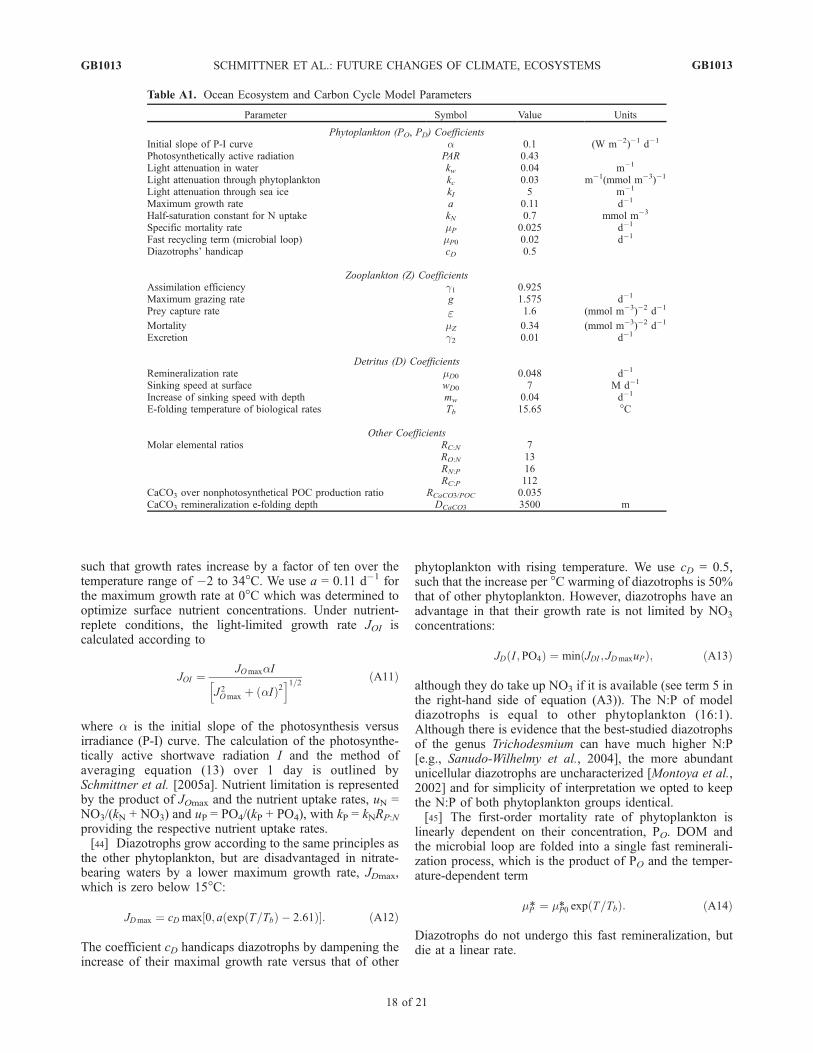
[5] The ocean ecosystem/biogeochemical model is animproved NPZD (nutrient, phytoplankton, zooplankton,detritus) ecosystem model of Schmittner et al. [2005a] witha parameterization of fast nutrient recycling due to micro-bial activity after Schartau and Oschlies [2003]. It includestwo phytoplankton classes (nitrogen fixers and other phy-toplankton), nitrate (NO3) and phosphate (PO4) as nutrients,as well as oxygen (O2), dissolved inorganic carbon (DIC)and alkalinity (ALK) as tracers. A complete description ofthe ecosystem model is given in Appendix A, and parametervalues are listed in Table A1 in Appendix A.

2.2. Marine Carbon Cycle

[6] Formulations of air-sea gas exchange and carbonchemistry follow protocols from the Ocean Carbon-CycleModel Intercomparison Project (OCMIP) [Orr et al., 1999]as described by Ewen et al. [2004]. Biological uptake andrelease occurs in fixed elemental ratios of carbon, phospho-rus, nitrogen and oxygen (see Table A1 in Appendix A forvalues). Production of DIC and ALK is controlled bychanges in inorganic nutrients and calcium carbonate(CaCO3), in molar numbers according to

S DICð Þ ¼ S PO4ð ÞRC:P � S CaCO3ð Þ ð1Þ

S ALKð Þ ¼ �S NO3ð Þ � 10�3 � 2S CaCO3ð Þ: ð2Þ

GB1013 SCHMITTNER ET AL.: FUTURE CHANGES OF CLIMATE, ECOSYSTEMS

2 of 21

GB1013

S(X) denotes the source minus sink term for tracer X andRC:P is the carbon to phosphorus ratio (see Table A1 inAppendix A) The sources minus sink term of calciumcarbonate S(CaCO3) = Pr(CaCO3) � Di(CaCO3) isdetermined by its production

Pr CaCO3ð Þ ¼ 1� g1ð ÞG POð ÞZþ mP2P2O þ mZZ

2� �

RCaCO3=POCRC:P;

ð3Þ

which is parameterized as a fixed ratio (RCaCO3/POC) of theproduction of nondiazotrophic detritus. In our model, noneof the above processes explicitly depends on temperature.However, maximum phytoplankton growth and microbialremineralization rates are assumed to increase withtemperature according to Eppley [1972] (see equations(A10), (A14), and (A16) in Appendix A), and as a result theproduction of CaCO3 tends to increase with temperature aswell. A similar temperature dependence is expected forother ecosystem models that parameterize calcium carbo-nate production as a function of primary production [e.g.,Moore et al., 2002]. The dissolution of calcium carbonate,

Di CaCO3ð Þ ¼Z

Pr CaCO3ð Þdz � ddz

e�z=DCaCO3

� �; ð4Þ

is computed by assuming instantaneous sinking with ane-folding depth DCaCO3 = 3500 m of the vertically integ-rated production. The strength of the calcium carbonatepump and hence the vertical alkalinity distribution is

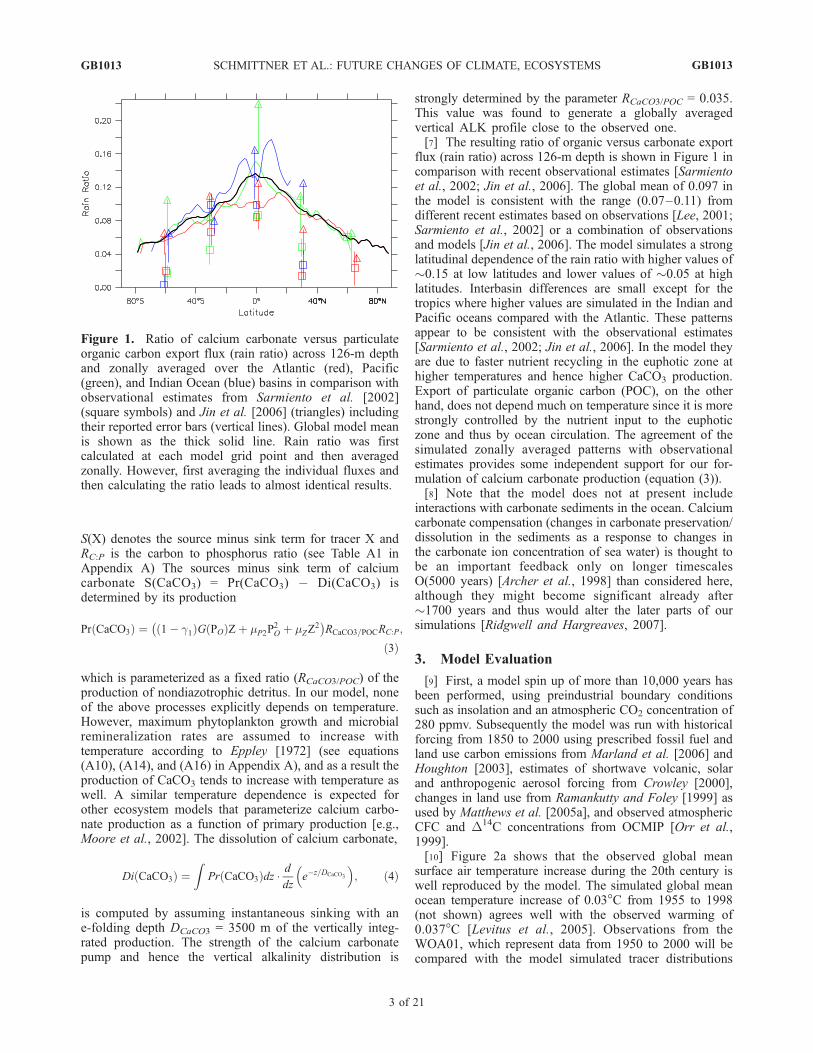
strongly determined by the parameter RCaCO3/POC = 0.035.This value was found to generate a globally averagedvertical ALK profile close to the observed one.[7] The resulting ratio of organic versus carbonate export

flux (rain ratio) across 126-m depth is shown in Figure 1 incomparison with recent observational estimates [Sarmientoet al., 2002; Jin et al., 2006]. The global mean of 0.097 inthe model is consistent with the range (0.07–0.11) fromdifferent recent estimates based on observations [Lee, 2001;Sarmiento et al., 2002] or a combination of observationsand models [Jin et al., 2006]. The model simulates a stronglatitudinal dependence of the rain ratio with higher values of�0.15 at low latitudes and lower values of �0.05 at highlatitudes. Interbasin differences are small except for thetropics where higher values are simulated in the Indian andPacific oceans compared with the Atlantic. These patternsappear to be consistent with the observational estimates[Sarmiento et al., 2002; Jin et al., 2006]. In the model theyare due to faster nutrient recycling in the euphotic zone athigher temperatures and hence higher CaCO3 production.Export of particulate organic carbon (POC), on the otherhand, does not depend much on temperature since it is morestrongly controlled by the nutrient input to the euphoticzone and thus by ocean circulation. The agreement of thesimulated zonally averaged patterns with observationalestimates provides some independent support for our for-mulation of calcium carbonate production (equation (3)).[8] Note that the model does not at present include

interactions with carbonate sediments in the ocean. Calciumcarbonate compensation (changes in carbonate preservation/dissolution in the sediments as a response to changes inthe carbonate ion concentration of sea water) is thought tobe an important feedback only on longer timescalesO(5000 years) [Archer et al., 1998] than considered here,although they might become significant already after�1700 years and thus would alter the later parts of oursimulations [Ridgwell and Hargreaves, 2007].

3. Model Evaluation

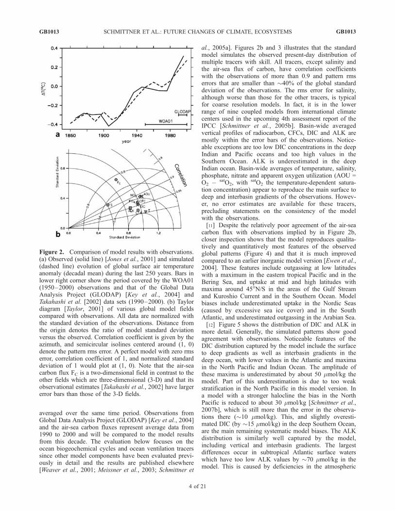
[9] First, a model spin up of more than 10,000 years hasbeen performed, using preindustrial boundary conditionssuch as insolation and an atmospheric CO2 concentration of280 ppmv. Subsequently the model was run with historicalforcing from 1850 to 2000 using prescribed fossil fuel andland use carbon emissions from Marland et al. [2006] andHoughton [2003], estimates of shortwave volcanic, solarand anthropogenic aerosol forcing from Crowley [2000],changes in land use from Ramankutty and Foley [1999] asused by Matthews et al. [2005a], and observed atmosphericCFC and D14C concentrations from OCMIP [Orr et al.,1999].[10] Figure 2a shows that the observed global mean

surface air temperature increase during the 20th century iswell reproduced by the model. The simulated global meanocean temperature increase of 0.03�C from 1955 to 1998(not shown) agrees well with the observed warming of0.037�C [Levitus et al., 2005]. Observations from theWOA01, which represent data from 1950 to 2000 will becompared with the model simulated tracer distributions

Figure 1. Ratio of calcium carbonate versus particulateorganic carbon export flux (rain ratio) across 126-m depthand zonally averaged over the Atlantic (red), Pacific(green), and Indian Ocean (blue) basins in comparison withobservational estimates from Sarmiento et al. [2002](square symbols) and Jin et al. [2006] (triangles) includingtheir reported error bars (vertical lines). Global model meanis shown as the thick solid line. Rain ratio was firstcalculated at each model grid point and then averagedzonally. However, first averaging the individual fluxes andthen calculating the ratio leads to almost identical results.


3 of 21

GB1013

averaged over the same time period. Observations fromGlobal Data Analysis Project (GLODAP) [Key et al., 2004]and the air-sea carbon fluxes represent average data from1990 to 2000 and will be compared to the model resultsfrom this decade. The evaluation below focuses on theocean biogeochemical cycles and ocean ventilation tracerssince other model components have been evaluated previ-ously in detail and the results are published elsewhere[Weaver et al., 2001; Meissner et al., 2003; Schmittner et

al., 2005a]. Figures 2b and 3 illustrates that the standardmodel simulates the observed present-day distribution ofmultiple tracers with skill. All tracers, except salinity andthe air-sea flux of carbon, have correlation coefficientswith the observations of more than 0.9 and pattern rmserrors that are smaller than �40% of the global standarddeviation of the observations. The rms error for salinity,although worse than those for the other tracers, is typicalfor coarse resolution models. In fact, it is in the lowerrange of nine coupled models from international climatecenters used in the upcoming 4th assessment report of theIPCC [Schmittner et al., 2005b]. Basin-wide averagedvertical profiles of radiocarbon, CFCs, DIC and ALK aremostly within the error bars of the observations. Notice-able exceptions are too low DIC concentrations in the deepIndian and Pacific oceans and too high values in theSouthern Ocean. ALK is underestimated in the deepIndian ocean. Basin-wide averages of temperature, salinity,phosphate, nitrate and apparent oxygen utilization (AOU =O2 � satO2, with

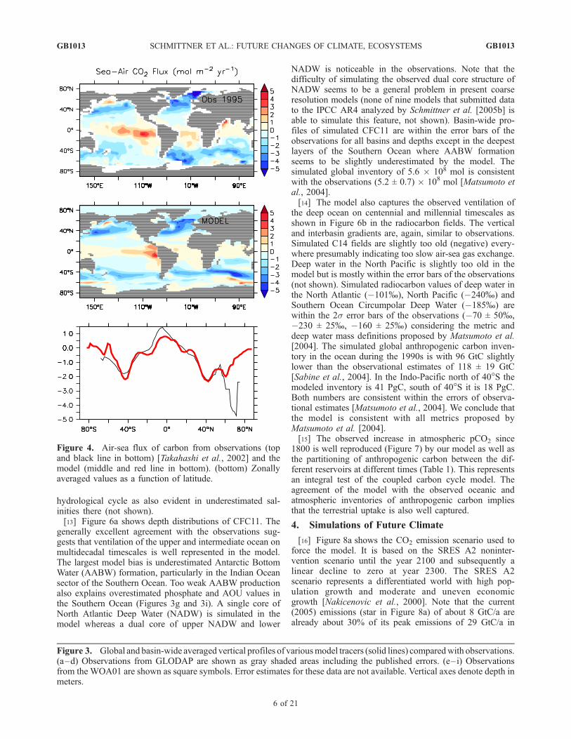
satO2 the temperature-dependent satura-tion concentration) appear to reproduce the main surface todeep and interbasin gradients of the observations. Howev-er, no error estimates are available for these tracers,precluding statements on the consistency of the modelwith the observations.[11] Despite the relatively poor agreement of the air-sea

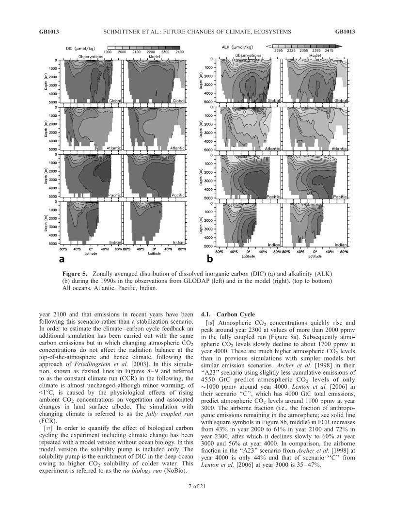
carbon flux with observations implied by in Figure 2b,closer inspection shows that the model reproduces qualita-tively and quantitatively most features of the observedglobal patterns (Figure 4) and that it is much improvedcompared to an earlier inorganic model version [Ewen et al.,2004]. These features include outgassing at low latitudeswith a maximum in the eastern tropical Pacific and in theBering Sea, and uptake at mid and high latitudes withmaxima around 45�N/S in the areas of the Gulf Streamand Kuroshio Current and in the Southern Ocean. Modelbiases include underestimated uptake in the Nordic Seas(caused by excessive sea ice cover) and in the SouthAtlantic, and underestimated outgassing in the Arabian Sea.[12] Figure 5 shows the distribution of DIC and ALK in

more detail. Generally, the simulated patterns show goodagreement with observations. Noticeable features of theDIC distribution captured by the model include the surfaceto deep gradients as well as interbasin gradients in thedeep ocean, with lower values in the Atlantic and maximain the North Pacific and Indian Ocean. The amplitude ofthese maxima is underestimated by about 50 mmol/kg themodel. Part of this underestimation is due to too weakstratification in the North Pacific in this model version. Ina model with a stronger halocline the bias in the NorthPacific is reduced to about 30 mmol/kg [Schmittner et al.,2007b], which is still more than the error in the observa-tions there (�10 mmol/kg). This, and slightly overesti-mated DIC (by �15 mmol/kg) in the deep Southern Ocean,are the main remaining systematic model biases. The ALKdistribution is similarly well captured by the model,including vertical and interbasin gradients. The largestdifferences occur in subtropical Atlantic surface waterswhich have too low ALK values by �70 mmol/kg in themodel. This is caused by deficiencies in the atmospheric

Figure 2. Comparison of model results with observations.(a) Observed (solid line) [Jones et al., 2001] and simulated(dashed line) evolution of global surface air temperatureanomaly (decadal mean) during the last 250 years. Bars inlower right corner show the period covered by the WOA01(1950–2000) observations and that of the Global DataAnalysis Project (GLODAP) [Key et al., 2004] andTakahashi et al. [2002] data sets (1990–2000). (b) Taylordiagram [Taylor, 2001] of various global model fieldscompared with observations. All data are normalized withthe standard deviation of the observations. Distance fromthe origin denotes the ratio of model standard deviationversus the observed. Correlation coefficient is given by theazimuth, and semicircular isolines centered around (1, 0)denote the pattern rms error. A perfect model with zero rmserror, correlation coefficient of 1, and normalized standarddeviation of 1 would plot at (1, 0). Note that the air-seacarbon flux FC is a two-dimensional field in contrast to theother fields which are three-dimensional (3-D) and that itsobservational estimates [Takahashi et al., 2002] have largererror bars than those of the 3-D fields.


4 of 21

GB1013

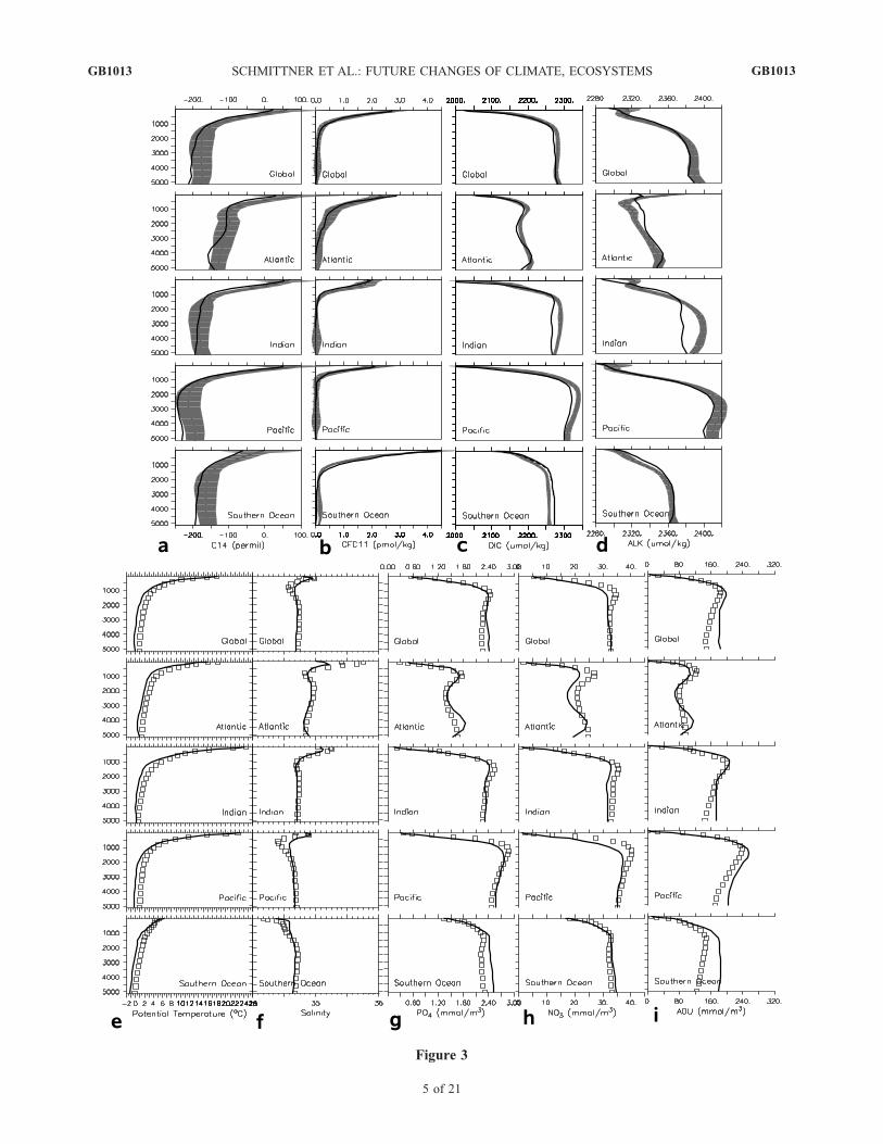
Figure 3


5 of 21

GB1013

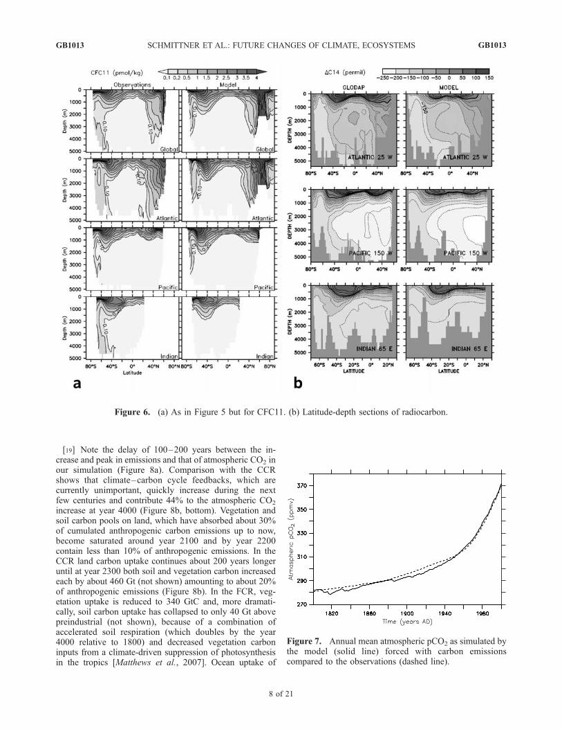
hydrological cycle as also evident in underestimated sal-inities there (not shown).[13] Figure 6a shows depth distributions of CFC11. The

generally excellent agreement with the observations sug-gests that ventilation of the upper and intermediate ocean onmultidecadal timescales is well represented in the model.The largest model bias is underestimated Antarctic BottomWater (AABW) formation, particularly in the Indian Oceansector of the Southern Ocean. Too weak AABW productionalso explains overestimated phosphate and AOU values inthe Southern Ocean (Figures 3g and 3i). A single core ofNorth Atlantic Deep Water (NADW) is simulated in themodel whereas a dual core of upper NADW and lower

NADW is noticeable in the observations. Note that thedifficulty of simulating the observed dual core structure ofNADW seems to be a general problem in present coarseresolution models (none of nine models that submitted datato the IPCC AR4 analyzed by Schmittner et al. [2005b] isable to simulate this feature, not shown). Basin-wide pro-files of simulated CFC11 are within the error bars of theobservations for all basins and depths except in the deepestlayers of the Southern Ocean where AABW formationseems to be slightly underestimated by the model. Thesimulated global inventory of 5.6 � 108 mol is consistentwith the observations (5.2 ± 0.7) � 108 mol [Matsumoto etal., 2004].[14] The model also captures the observed ventilation of

the deep ocean on centennial and millennial timescales asshown in Figure 6b in the radiocarbon fields. The verticaland interbasin gradients are, again, similar to observations.Simulated C14 fields are slightly too old (negative) every-where presumably indicating too slow air-sea gas exchange.Deep water in the North Pacific is slightly too old in themodel but is mostly within the error bars of the observations(not shown). Simulated radiocarbon values of deep water inthe North Atlantic (�101%), North Pacific (�240%) andSouthern Ocean Circumpolar Deep Water (�185%) arewithin the 2s error bars of the observations (�70 ± 50%,�230 ± 25%, �160 ± 25%) considering the metric anddeep water mass definitions proposed by Matsumoto et al.[2004]. The simulated global anthropogenic carbon inven-tory in the ocean during the 1990s is with 96 GtC slightlylower than the observational estimates of 118 ± 19 GtC[Sabine et al., 2004]. In the Indo-Pacific north of 40�S themodeled inventory is 41 PgC, south of 40�S it is 18 PgC.Both numbers are consistent within the errors of observa-tional estimates [Matsumoto et al., 2004]. We conclude thatthe model is consistent with all metrics proposed byMatsumoto et al. [2004].[15] The observed increase in atmospheric pCO2 since

1800 is well reproduced (Figure 7) by our model as well asthe partitioning of anthropogenic carbon between the dif-ferent reservoirs at different times (Table 1). This representsan integral test of the coupled carbon cycle model. Theagreement of the model with the observed oceanic andatmospheric inventories of anthropogenic carbon impliesthat the terrestrial uptake is also well captured.

4. Simulations of Future Climate

[16] Figure 8a shows the CO2 emission scenario used toforce the model. It is based on the SRES A2 noninter-vention scenario until the year 2100 and subsequently alinear decline to zero at year 2300. The SRES A2scenario represents a differentiated world with high pop-ulation growth and moderate and uneven economicgrowth [Nakicenovic et al., 2000]. Note that the current(2005) emissions (star in Figure 8a) of about 8 GtC/a arealready about 30% of its peak emissions of 29 GtC/a in

Figure 4. Air-sea flux of carbon from observations (topand black line in bottom) [Takahashi et al., 2002] and themodel (middle and red line in bottom). (bottom) Zonallyaveraged values as a function of latitude.

Figure 3. Global and basin-wide averaged vertical profiles of variousmodel tracers (solid lines) comparedwith observations.(a–d) Observations from GLODAP are shown as gray shaded areas including the published errors. (e–i) Observationsfrom the WOA01 are shown as square symbols. Error estimates for these data are not available. Vertical axes denote depth inmeters.


6 of 21

GB1013

year 2100 and that emissions in recent years have beenfollowing this scenario rather than a stabilization scenario.In order to estimate the climate–carbon cycle feedback anadditional simulation has been carried out with the samecarbon emissions but in which changing atmospheric CO2

concentrations do not affect the radiation balance at thetop-of-the-atmosphere and hence climate, following theapproach of Friedlingstein et al. [2003]. In this simula-tion, shown as dashed lines in Figures 8–9 and referredto as the constant climate run (CCR) in the following, theclimate is almost unchanged although minor warming, of<1�C, is caused by the physiological effects of risingambient CO2 concentrations on vegetation and associatedchanges in land surface albedo. The simulation withchanging climate is referred to as the fully coupled run(FCR).[17] In order to quantify the effect of biological carbon

cycling the experiment including climate change has beenrepeated with a model version without ocean biology. In thismodel version the solubility pump is included only. Thesolubility pump is the enrichment of DIC in the deep oceanowing to higher CO2 solubility of colder water. Thisexperiment is referred to as the no biology run (NoBio).

4.1. Carbon Cycle

[18] Atmospheric CO2 concentrations quickly rise andpeak around year 2300 at values of more than 2000 ppmvin the fully coupled run (Figure 8a). Subsequently atmo-spheric CO2 levels slowly decline to about 1700 ppmv atyear 4000. These are much higher atmospheric CO2 levelsthan in previous simulations with simpler models butsimilar emission scenarios. Archer et al. [1998] in their‘‘A23’’ scenario using slightly less cumulative emissions of4550 GtC predict atmospheric CO2 levels of only�1000 ppmv around year 4000. Lenton et al. [2006] intheir scenario ‘‘C’’, which has 4000 GtC total emissions,predict atmospheric CO2 levels around 1100 ppmv at year3000. The airborne fraction (i.e., the fraction of anthropo-genic emissions remaining in the atmosphere; see solid linewith square symbols in Figure 8b, middle) in FCR increasesfrom 43% in year 2000 to 61% in year 2100 and 72% inyear 2300, after which it declines slowly to 60% at year3000 and 56% at year 4000. In comparison, the airbornefraction in the ‘‘A23’’ scenario from Archer et al. [1998] atyear 4000 is only 44% and that of scenario ‘‘C’’ fromLenton et al. [2006] at year 3000 is 35–47%.

Figure 5. Zonally averaged distribution of dissolved inorganic carbon (DIC) (a) and alkalinity (ALK)(b) during the 1990s in the observations from GLODAP (left) and in the model (right). (top to bottom)All oceans, Atlantic, Pacific, Indian.


7 of 21

GB1013

[19] Note the delay of 100–200 years between the in-crease and peak in emissions and that of atmospheric CO2 inour simulation (Figure 8a). Comparison with the CCRshows that climate–carbon cycle feedbacks, which arecurrently unimportant, quickly increase during the nextfew centuries and contribute 44% to the atmospheric CO2

increase at year 4000 (Figure 8b, bottom). Vegetation andsoil carbon pools on land, which have absorbed about 30%of cumulated anthropogenic carbon emissions up to now,become saturated around year 2100 and by year 2200contain less than 10% of anthropogenic emissions. In theCCR land carbon uptake continues about 200 years longeruntil at year 2300 both soil and vegetation carbon increasedeach by about 460 Gt (not shown) amounting to about 20%of anthropogenic emissions (Figure 8b). In the FCR, veg-etation uptake is reduced to 340 GtC and, more dramati-cally, soil carbon uptake has collapsed to only 40 Gt abovepreindustrial (not shown), because of a combination ofaccelerated soil respiration (which doubles by the year4000 relative to 1800) and decreased vegetation carboninputs from a climate-driven suppression of photosynthesisin the tropics [Matthews et al., 2007]. Ocean uptake of

Figure 6. (a) As in Figure 5 but for CFC11. (b) Latitude-depth sections of radiocarbon.

Figure 7. Annual mean atmospheric pCO2 as simulated bythe model (solid line) forced with carbon emissionscompared to the observations (dashed line).


8 of 21

GB1013

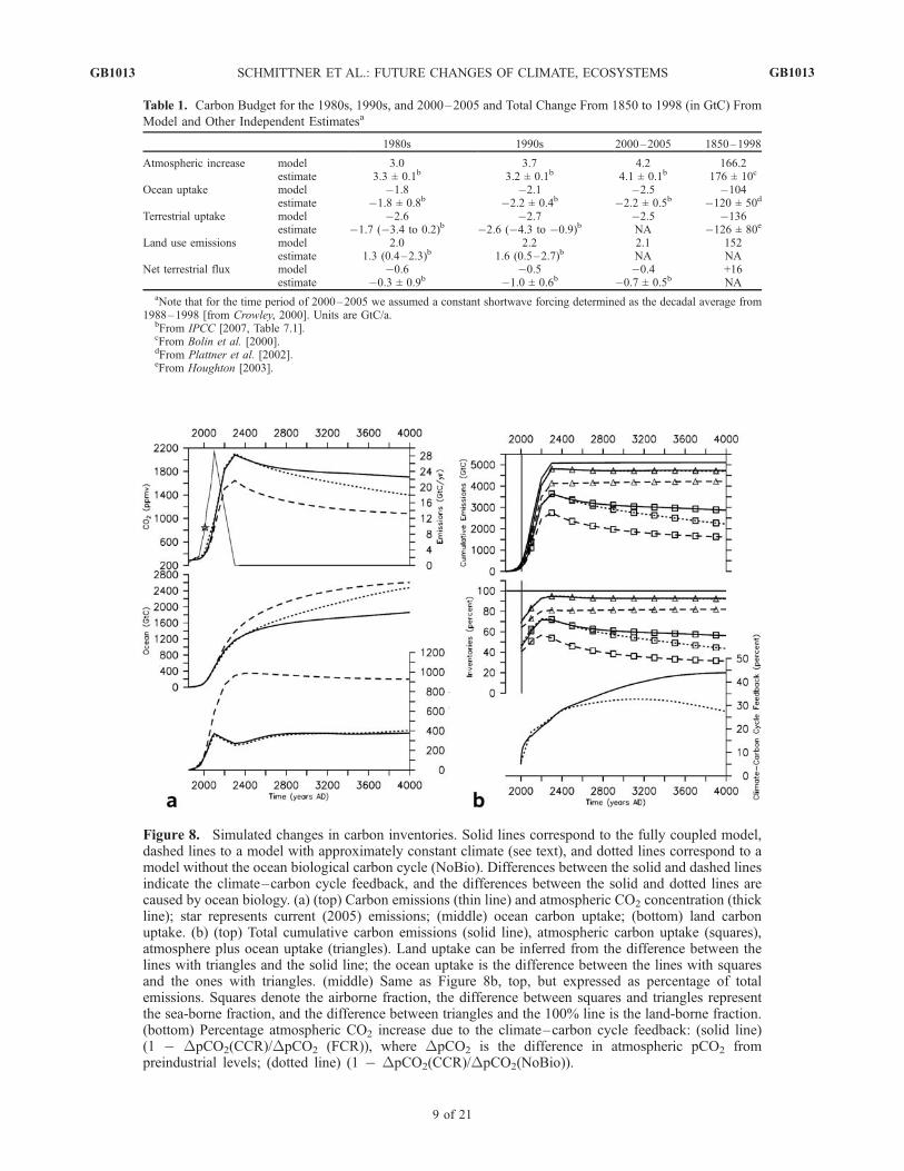
Table 1. Carbon Budget for the 1980s, 1990s, and 2000–2005 and Total Change From 1850 to 1998 (in GtC) From

Model and Other Independent Estimatesa

1980s 1990s 2000–2005 1850–1998

Atmospheric increase model 3.0 3.7 4.2 166.2estimate 3.3 ± 0.1b 3.2 ± 0.1b 4.1 ± 0.1b 176 ± 10c

Ocean uptake model �1.8 �2.1 �2.5 �104estimate �1.8 ± 0.8b �2.2 ± 0.4b �2.2 ± 0.5b �120 ± 50d

Terrestrial uptake model �2.6 �2.7 �2.5 �136estimate �1.7 (�3.4 to 0.2)b �2.6 (�4.3 to �0.9)b NA �126 ± 80e

Land use emissions model 2.0 2.2 2.1 152estimate 1.3 (0.4–2.3)b 1.6 (0.5–2.7)b NA NA

Net terrestrial flux model �0.6 �0.5 �0.4 +16estimate �0.3 ± 0.9b �1.0 ± 0.6b �0.7 ± 0.5b NA

aNote that for the time period of 2000–2005 we assumed a constant shortwave forcing determined as the decadal average from1988–1998 [from Crowley, 2000]. Units are GtC/a.

bFrom IPCC [2007, Table 7.1].cFrom Bolin et al. [2000].dFrom Plattner et al. [2002].eFrom Houghton [2003].

Figure 8. Simulated changes in carbon inventories. Solid lines correspond to the fully coupled model,dashed lines to a model with approximately constant climate (see text), and dotted lines correspond to amodel without the ocean biological carbon cycle (NoBio). Differences between the solid and dashed linesindicate the climate–carbon cycle feedback, and the differences between the solid and dotted lines arecaused by ocean biology. (a) (top) Carbon emissions (thin line) and atmospheric CO2 concentration (thickline); star represents current (2005) emissions; (middle) ocean carbon uptake; (bottom) land carbonuptake. (b) (top) Total cumulative carbon emissions (solid line), atmospheric carbon uptake (squares),atmosphere plus ocean uptake (triangles). Land uptake can be inferred from the difference between thelines with triangles and the solid line; the ocean uptake is the difference between the lines with squaresand the ones with triangles. (middle) Same as Figure 8b, top, but expressed as percentage of totalemissions. Squares denote the airborne fraction, the difference between squares and triangles representthe sea-borne fraction, and the difference between triangles and the 100% line is the land-borne fraction.(bottom) Percentage atmospheric CO2 increase due to the climate–carbon cycle feedback: (solid line)(1 � DpCO2(CCR)/DpCO2 (FCR)), where DpCO2 is the difference in atmospheric pCO2 frompreindustrial levels; (dotted line) (1 � DpCO2(CCR)/DpCO2(NoBio)).


9 of 21

GB1013

anthropogenic carbon continues much longer than that onland, but is strongly reduced by climate change (by about30% at year 4000, from 2606 Gt in the CCR to 1859 Gt inthe FCR; Figure 8a, middle). Changes in the biologicalpump become important after year 2500 and are responsiblefor most of this reduction at year 4000.[20] Our estimate of the climate–carbon cycle feedback

(i.e., the change in atmospheric CO2 from preindustriallevels in the fully coupled model divided by the change inthe constant climate model) increases on a multicentennial tomillennial timescale. At year 2100 only 17% (111 ppmv =225 GtC) of the CO2 increase is due to climate–carbon cyclefeedbacks, within the range of previous estimates of 10–30% [Cox et al., 2000; Friedlingstein et al., 2003, 2006], butat year 2300 it is already 24% (438 ppmv = 886 GtC) and atyear 3000 it is 38% (576 ppmv = 1164 GtC). This slowincrease is due to changes in ocean biological carbon cyclingwhich, in our model, are negligible before year 2500 butincrease in importance until year 4000 at which they accountfor 37% of the total climate–carbon cycle feedback.

4.2. Climate and Ocean Circulation

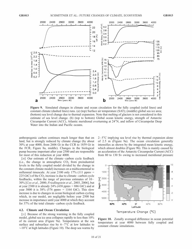
[21] Because of the strong warming in the fully coupledmodel, global sea ice area collapses rapidly to less than 10%of its current area (Figure 9a). Temperatures at the seasurface and subsurface rise by 6–7�C at low latitudes to�10�C at high latitudes (Figure 10). The deep sea warms by

2–5�C implying sea level rise by thermal expansion aloneof 2.5 m (Figure 9a). The ocean circulation generallyintensifies as shown by the integrated mean kinetic energy,which almost doubles (Figure 9b). This is mainly caused byan acceleration of the Antarctic Circumpolar Current (ACC)from 80 to 130 Sv owing to increased meridional pressure

Figure 9. Simulated changes in climate and ocean circulation for the fully coupled (solid lines) andconstant climate (dashed lines) runs. (a) (top) Surface air temperature (SAT); (middle) global sea ice area;(bottom) sea level change due to thermal expansion. Note that melting of glaciers is not considered in thisestimate of sea level change. (b) (top to bottom) Global ocean kinetic energy, strength of AntarcticCircumpolar Current (ACC), Atlantic meridional overturning at 24�N, and inflow of Circumpolar DeepWater into the Indian and Pacific oceans.

Figure 10. Zonally averaged difference in ocean potentialtemperature at year 4000 between fully coupled andconstant climate simulations.


10 of 21

GB1013

gradients across the Southern Ocean that arise from greaterwarming at middle to low latitudes than in high-latitudewaters around Antarctica (Figure 10). A strengthening ofthe ACC has recently been observed and attributed, at leastin part, to human induced global warming and an associatedsouthward shift and acceleration of zonal winds over theSouthern Ocean [Fyfe and Saenko, 2005]. Russell et al.[2006] also find a strengthening of the ACC in globalwarming scenarios until year 2300, which they also attributeto a strengthening and southward shift in Southern Hemi-sphere westerly winds. In our simulation wind stress is heldconstant. Thus the accelerated ACC is not caused by windstress changes but rather by an increase in the meridionaldensity and pressure differences. Together these resultsimply that both wind and buoyancy forcing lead to astrengthening of the ACC in a warmer climate. It istherefore possible that part of the ACC increase found inthe multicentennial simulations by Russell et al. [2006] isalso caused by buoyancy forcing. The increase of the ACCsimulated here (Figure 9b) has to be regarded as a lowerlimit because of the neglect of wind changes.[22] The modeled deep overturning circulation slows

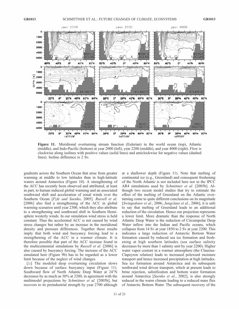
down because of surface buoyancy input (Figure 11).Southward flow of North Atlantic Deep Water at 24�Ndecreases by as much as 30% at 2200, in agreement with themultimodel projections by Schmittner et al. [2005b], butrecovers to its preindustrial strength by year 2700 although

at a shallower depth (Figure 11). Note that melting ofcontinental ice (e.g., Greenland) and consequent fresheningof the North Atlantic is not included here nor in the IPCCAR4 simulations used by Schmittner et al. [2005b]. Al-though two recent model studies that try to estimate theeffect of the melting of Greenland on the Atlantic over-turning come to quite different conclusions on its magnitude[Swingedouw et al., 2006; Jungclaus et al., 2006], it is safeto say that melting of Greenland leads to an additionalreduction of the circulation. Hence our projection representsa lower limit. More dramatic than the response of NorthAtlantic Deep Water is the reduction of Circumpolar DeepWater inflow into the Indian and Pacific oceans, whichcollapses from 14 Sv at year 1850 to 2 Sv at year 2200. Thisindicates a large reduction of Antarctic Bottom Waterformation caused by reduced sea ice formation and fresh-ening at high southern latitudes (sea surface salinitydecreases by more than 1 salinity unit by year 2200). Higherwater vapor content in a warmer atmosphere (the Clausius-Clapeyron relation) leads to increased poleward moisturetransport and hence increased precipitation at high latitudes.Sea ice formation around Antarctica and its subsequentnorthward wind driven transport, which at present leads tobrine rejection, salinification and bottom water formationaround Antarctica [Saenko et al., 2002], is also stronglyreduced in the warm climate leading to a reduced mass fluxof Antarctic Bottom Water. The subsequent recovery of the

Figure 11. Meridional overturning stream function (Eulerian) in the world ocean (top), Atlantic(middle), and Indo-Pacific (bottom) at year 2000 (left), year 2200 (middle), and year 4000 (right). Flow isclockwise along isolines with positive values (solid lines) and anticlockwise for negative values (dashedlines). Isoline difference is 2 Sv.


11 of 21

GB1013

deep circulation in the Indian and Pacific oceans is muchslower than that of North Atlantic Deep Water and notcomplete by year 4000.[23] Increased isolation of the deep sea from the atmo-

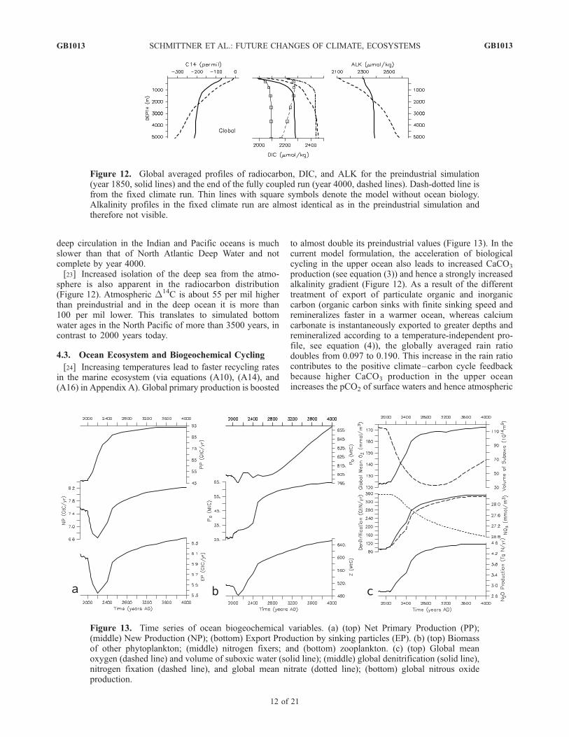
sphere is also apparent in the radiocarbon distribution(Figure 12). Atmospheric D14C is about 55 per mil higherthan preindustrial and in the deep ocean it is more than100 per mil lower. This translates to simulated bottomwater ages in the North Pacific of more than 3500 years, incontrast to 2000 years today.

4.3. Ocean Ecosystem and Biogeochemical Cycling

[24] Increasing temperatures lead to faster recycling ratesin the marine ecosystem (via equations (A10), (A14), and(A16) in Appendix A). Global primary production is boosted

to almost double its preindustrial values (Figure 13). In thecurrent model formulation, the acceleration of biologicalcycling in the upper ocean also leads to increased CaCO3

production (see equation (3)) and hence a strongly increasedalkalinity gradient (Figure 12). As a result of the differenttreatment of export of particulate organic and inorganiccarbon (organic carbon sinks with finite sinking speed andremineralizes faster in a warmer ocean, whereas calciumcarbonate is instantaneously exported to greater depths andremineralized according to a temperature-independent pro-file, see equation (4)), the globally averaged rain ratiodoubles from 0.097 to 0.190. This increase in the rain ratiocontributes to the positive climate–carbon cycle feedbackbecause higher CaCO3 production in the upper oceanincreases the pCO2 of surface waters and hence atmospheric

Figure 12. Global averaged profiles of radiocarbon, DIC, and ALK for the preindustrial simulation(year 1850, solid lines) and the end of the fully coupled run (year 4000, dashed lines). Dash-dotted line isfrom the fixed climate run. Thin lines with square symbols denote the model without ocean biology.Alkalinity profiles in the fixed climate run are almost identical as in the preindustrial simulation andtherefore not visible.

Figure 13. Time series of ocean biogeochemical variables. (a) (top) Net Primary Production (PP);(middle) New Production (NP); (bottom) Export Production by sinking particles (EP). (b) (top) Biomassof other phytoplankton; (middle) nitrogen fixers; and (bottom) zooplankton. (c) (top) Global meanoxygen (dashed line) and volume of suboxic water (solid line); (middle) global denitrification (solid line),nitrogen fixation (dashed line), and global mean nitrate (dotted line); (bottom) global nitrous oxideproduction.


12 of 21

GB1013

CO2. To our knowledge this effect has not been suggested,described or considered before. We speculate, however, thatcommon parameterizations of calcium carbonate productionas a function of temperature-dependent primary productionwill yield similar results in other models. The comparison inTable 2 also confirms the important role alkalinity changesplay in determining ocean surface and atmospheric pCO2 inthe FCR.[25] The large increase of simulated primary production

and CaCO3 production is in sharp contrast to the response ofnew and export production (Figure 13), which both declineduring the 21st and 22nd centuries by about 15% and recoverafterward to values slightly higher than preindustrial. Thetransient decline is caused by the reduction in the over-turning circulation during the same period, which impedesnutrient supply from upwelling as described by Schmittner[2005].[26] Global phytoplankton stocks show surprisingly little

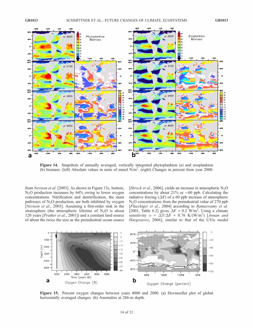
response until about year 2800 after which they begin toincrease gradually and reach about 5% higher values thanpreindustrial at year 4000. Zooplankton stocks increasemore strongly by about 30% following the temperature rise.Both phytoplankton and zooplankton biomass show muchlarger changes regionally (Figure 14). They increase at highlatitudes because of reduced sea ice cover and a longergrowing season in agreement with earlier findings by Boppet al. [2001]. North of about 55�N, plankton abundanceincreases in the North Atlantic because of deeper mixedlayers and a northward shift in convections sites. In thenorthern Nordic Seas and Arctic ocean as well as aroundAntarctica stocks more than double by year 2400. Largerelative increases in plankton mass are also simulated in theoligotrophic subtropical gyres. Faster nutrient recycling inthe upper ocean allows more lateral advection of nutrientsinto these areas leading to a strong reduction in the area ofoligotrophic oceans by year 4000. At mid latitudes bothphytoplankton and zooplankton biomass decrease owing toincreased stratification and reduced nutrient delivery intothe photic zone. At year 2100 large reductions in phyto-plankton stocks occur in the North Atlantic. In the Labradorand Irminger Seas as well as in the northeastern part of thesubtropical gyre, in a broad band along the Iberian andnorthwest African margins biomass decreases by up to 50%.This is a response to the shoaling of mixed layers caused bythe slow down of the Atlantic overturning circulation as

shown earlier [Schmittner, 2005]. The ecosystem recoversthere after year 2400. In the North Pacific plankton stocksdecrease by about 20%. Nitrogen fixers migrate form thecentral tropical Pacific toward the east and move more than15� poleward in both hemispheres owing to increaseddenitrification and warmer SSTs. Plankton abundance inthe tropics shifts upward (not shown) from the subsurfacelevel (80 m) to the surface (20 m) presumably due to morenitrate input from above (by nitrogen fixation) and less frombelow (enhanced denitrification).[27] Warmer ocean temperatures lead to lower solubility

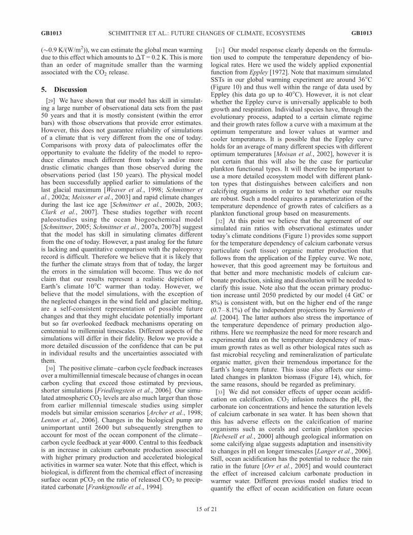
of oxygen, which together with slower ventilation of thedeep ocean lead to a �30% decrease of global mean oxygenconcentrations by year 3000 (Figure 13c). The oxygenchanges are consistent with earlier 600-year model simula-tion using a simpler biogeochemical model [Matear andHirst, 2002]. After year 3000, oxygen below 1 km depthslowly increases again because of the recovering deep oceancirculation (Figures 9b and 15a). Locally much largerreductions in oxygen concentrations are simulated. In theshallow subsurface ocean, for example (Figure 15b), oxy-gen concentrations decrease by more than 80% in theeastern equatorial Pacific and Atlantic. Along the WestCoast of North America reductions of 40–80% occur. Suchstrong reductions in oxygen concentrations will very likelyincrease the frequency of hypoxic events on the shelvessuch as the ‘‘dead zones’’ on the Oregon shelf observedduring the last few years [Grantham et al., 2004]. Thesimulated volume of suboxic water triples by year 2500 andthen remains constant (Figure 13c). This is accompanied byincreased denitrification and, in turn, higher simulatednitrogen fixation since the ecological niche of nitrogen-fixing organisms (low-nitrate, high-phosphate waters)expands. Global stocks of nitrogen fixers more than double.The global average NO3 concentration declines in oursimulation by �1.5 uM, or �5%, although the magnitudeof this decline is dependent on the ecological disadvantagethat nitrogen fixers experience in the presence of nitrate,which is poorly quantified.[28] It is well known that the oxygen minimum zones

present an important source of nitrous oxide in the modernocean [Law and Owens, 1990; Yamagishi et al., 2005]. Weestimate the effect of the simulated changes in oxygenconcentrations and remineralization rates on the marineproduction of this potent greenhouse gas using equation (8)

Table 2. Changes Between Years 4000 and 1850 in Atmospheric pCO2 (DpCO2A), Surface Ocean pCO2 (DpCO2

O), and Approximate

Contributions to DpCO2O From Projected Changes in Temperature (T), Salinity (S), DIC (D), and ALK (A)a

Experiment DpCO2A DpCO2

O T, S D, A T S D A

Fully coupled 1420 1428 137 976 136 18 158 466Fixed climate 798 754 9 729 9 2 702 7

aThe contribution of a given variable is calculated by comparing the DpCO2O using the surface ocean output for that variable at year 4000 and other

state variables from year 1850 to the DpCO2O at year 1850. For example, the effect of temperature is calculated as pCO2

O(T(t = 4000), S(t = 1850),DIC(t = 1850), ALK(t = 1850)) � pCO2

O(T(t = 1850), S(t = 1850), DIC(t = 1850), ALK(t = 1850)). Changes in both temperature and salinity (T, S)and both DIC and ALK (D, A) are also shown. Note that because of nonlinearities in the pCO2

O dependency the contributions of individual variablesdo not sum to the total change. Thus the numbers in this table are only useful to get an idea of the order of magnitude and importance of certainprocesses. For example, it can be concluded that salinity changes (S) have a negligible impact and that solubility effects alone (T) have a smaller effectthan changes in dissolved inorganic carbon (DIC) and ALK. It is also clear that changes in alkalinity (ALK) are important in determining the fullycoupled atmospheric CO2 response, whereas in the fixed climate run they are negligible.


13 of 21

GB1013

from Nevison et al. [2003]. As shown in Figure 13c, bottom,N2O production increases by 64% owing to lower oxygenconcentrations. Nitrification and denitrification, the mainpathways of N2O production, are both inhibited by oxygen[Nevison et al., 2003]. Assuming a first-order sink in thestratosphere (the atmospheric lifetime of N2O is about120 years [Prather et al., 2001]) and a constant land sourceof about the twice the size as the preindustrial ocean source

[Hirsch et al., 2006], yields an increase in atmospheric N2Oconcentrations by about 21% or �60 ppb. Calculating theradiative forcing (DF) of a 60 ppb increase of atmosphericN2O concentrations from the preindustrial value of 270 ppb[Flueckiger et al., 2004] according to Ramaswamy et al.[2001, Table 6.2] gives DF = 0.2 W/m2. Using a climatesensitivity a = DT/DF = 0.76 K/(W/m2) [Annan andHargreaves, 2006], similar to that of the UVic model

Figure 14. Snapshots of annually averaged, vertically integrated phytoplankton (a) and zooplankton(b) biomass. (left) Absolute values in units of mmol N/m2. (right) Changes in percent from year 2000.

Figure 15. Percent oxygen changes between years 4000 and 2000. (a) Hovmoeller plot of globalhorizontally averaged changes. (b) Anomalies at 286-m depth.


14 of 21

GB1013

(�0.9 K/(W/m2)), we can estimate the global mean warmingdue to this effect which amounts toDT = 0.2 K. This is morethan an order of magnitude smaller than the warmingassociated with the CO2 release.

5. Discussion

[29] We have shown that our model has skill in simulat-ing a large number of observational data sets from the past50 years and that it is mostly consistent (within the errorbars) with those observations that provide error estimates.However, this does not guarantee reliability of simulationsof a climate that is very different from the one of today.Comparisons with proxy data of paleoclimates offer theopportunity to evaluate the fidelity of the model to repro-duce climates much different from today’s and/or moredrastic climatic changes than those observed during theobservations period (last 150 years). The physical modelhas been successfully applied earlier to simulations of thelast glacial maximum [Weaver et al., 1998; Schmittner etal., 2002a; Meissner et al., 2003] and rapid climate changesduring the last ice age [Schmittner et al., 2002b, 2003;Clark et al., 2007]. These studies together with recentpaleostudies using the ocean biogeochemical model[Schmittner, 2005; Schmittner et al., 2007a, 2007b] suggestthat the model has skill in simulating climates differentfrom the one of today. However, a past analog for the futureis lacking and quantitative comparison with the paleoproxyrecord is difficult. Therefore we believe that it is likely thatthe further the climate strays from that of today, the largerthe errors in the simulation will become. Thus we do notclaim that our results represent a realistic depiction ofEarth’s climate 10�C warmer than today. However, webelieve that the model simulations, with the exception ofthe neglected changes in the wind field and glacier melting,are a self-consistent representation of possible futurechanges and that they might elucidate potentially importantbut so far overlooked feedback mechanisms operating oncentennial to millennial timescales. Different aspects of thesimulations will differ in their fidelity. Below we provide amore detailed discussion of the confidence that can be putin individual results and the uncertainties associated withthem.[30] The positive climate–carbon cycle feedback increases

over a multimillennial timescale because of changes in oceancarbon cycling that exceed those estimated by previous,shorter simulations [Friedlingstein et al., 2006]. Our simu-lated atmospheric CO2 levels are also much larger than thosefrom earlier millennial timescale studies using simplermodels but similar emission scenarios [Archer et al., 1998;Lenton et al., 2006]. Changes in the biological pump areunimportant until 2600 but subsequently strengthen toaccount for most of the ocean component of the climate–carbon cycle feedback at year 4000. Central to this feedbackis an increase in calcium carbonate production associatedwith higher primary production and accelerated biologicalactivities in warmer sea water. Note that this effect, which isbiological, is different from the chemical effect of increasingsurface ocean pCO2 on the ratio of released CO2 to precip-itated carbonate [Frankignoulle et al., 1994].

[31] Our model response clearly depends on the formula-tion used to compute the temperature dependency of bio-logical rates. Here we used the widely applied exponentialfunction from Eppley [1972]. Note that maximum simulatedSSTs in our global warming experiment are around 36�C(Figure 10) and thus well within the range of data used byEppley (his data go up to 40�C). However, it is not clearwhether the Eppley curve is universally applicable to bothgrowth and respiration. Individual species have, through theevolutionary process, adapted to a certain climate regimeand their growth rates follow a curve with a maximum at theoptimum temperature and lower values at warmer andcooler temperatures. It is possible that the Eppley curveholds for an average of many different species with differentoptimum temperatures [Moisan et al., 2002], however it isnot certain that this will also be the case for particularplankton functional types. It will therefore be important touse a more detailed ecosystem model with different plank-ton types that distinguishes between calcifiers and noncalcifying organisms in order to test whether our resultsare robust. Such a model requires a parameterization of thetemperature dependence of growth rates of calcifiers as aplankton functional group based on measurements.[32] At this point we believe that the agreement of our

simulated rain ratios with observational estimates undertoday’s climate conditions (Figure 1) provides some supportfor the temperature dependency of calcium carbonate versusparticulate (soft tissue) organic matter production thatfollows from the application of the Eppley curve. We note,however, that this good agreement may be fortuitous andthat better and more mechanistic models of calcium car-bonate production, sinking and dissolution will be needed toclarify this issue. Note also that the ocean primary produc-tion increase until 2050 predicted by our model (4 GtC or8%) is consistent with, but on the higher end of the range(0.7–8.1%) of the independent projections by Sarmiento etal. [2004]. The latter authors also stress the importance ofthe temperature dependence of primary production algo-rithms. Here we reemphasize the need for more research andexperimental data on the temperature dependency of max-imum growth rates as well as other biological rates such asfast microbial recycling and remineralization of particulateorganic matter, given their tremendous importance for theEarth’s long-term future. This issue also affects our simu-lated changes in plankton biomass (Figure 14), which, forthe same reasons, should be regarded as preliminary.[33] We did not consider effects of upper ocean acidifi-

cation on calcification. CO2 infusion reduces the pH, thecarbonate ion concentrations and hence the saturation levelsof calcium carbonate in sea water. It has been shown thatthis has adverse effects on the calcification of marineorganisms such as corals and certain plankton species[Riebesell et al., 2000] although geological information onsome calcifying algae suggests adaptation and insensitivityto changes in pH on longer timescales [Langer et al., 2006].Still, ocean acidification has the potential to reduce the rainratio in the future [Orr et al., 2005] and would counteractthe effect of increased calcium carbonate production inwarmer water. Different previous model studies tried toquantify the effect of ocean acidification on future ocean


15 of 21

GB1013

carbon uptake and atmospheric CO2 concentrations. Heinze[2004] isolated the effect of acidification by keeping climateconstant in a scenario in which atmospheric CO2 increasedto 1400 ppmv until year 2250. He finds a reduction of theCaCO3 production by one half but a decrease of atmosphericCO2 by year 2250 of only 10 ppmv.[34] An improved quantification of this effect including

uncertainties in its parameterization [Ridgwell et al., 2006]suggest higher future uptake of anthropogenic CO2 andreduced atmospheric CO2 levels at year 3000 of 30–100 ppmv. This amplitude is smaller but similar to thebiological effects in our simulation (108 ppmv) at that time.Since both effects lead to changes with different signs, thenet effect might be much smaller than our projections or theones of Ridgwell et al. [2006].[35] Note that our formulation of CaCO3 production is

different from the one used by Ridgwell et al. [2006], whoassume it proportional to the export production of POM witha proportionality factor that considers the saturation state ofsurface waters with respect to CaCO3. Their scheme alsoproduces a latitudinal distribution with lower values at highlatitudes and higher values at low latitudes in qualitativeagreement with the observations. However, their rain ratios[Ridgwell et al., 2006, Figure 5c] show maxima of 0.17 inthe subtropics and local minima along the equator, appar-ently in conflict with the observational patterns (Figure 1).This, together with the better agreement of our simulatedrain ratios with observations, suggests that at least part of theobserved latitudinal distribution is explained by a tempera-ture effect (that is not considered by Ridgwell et al. [2006]).[36] In the as yet most complete parameterization, includ-

ing effects of increased dissolution, Gehlen et al. [2007]using a 4 � CO2 scenario, also show a large decrease inCaCO3 production by 27%, but only a negligible effect onoceanic carbon uptake (6 GtC) and hence atmospheric CO2.The reason(s) for the different effects of acidification onfuture oceanic carbon uptake in these three studies [Heinze,2004; Ridgwell et al., 2006; Gehlen et al., 2007] are notclear. The small effect by Heinze [2004] and Gehlen et al.[2007] may be in part be due to the short integration time.As discussed in more detail by Gehlen et al. [2007],considerable uncertainties are associated with the parame-terizations. Nevertheless, all three studies report consistent-ly a decrease in the CaCO3 production which wouldcounteract the temperature effect described in this paper.The effect of ocean acidification on atmospheric CO2 onlong (longer than a few centuries) timescales, however,remains to be quantified.[37] In our global warming simulations oxygen concen-

trations strongly decrease leading to accelerated watercolumn denitrification. Whereas the global patterns ofocean oxygen concentrations are well captured in themodel, difficulties remain in the simulation of suboxiczones. This is discussed in more detail by Schmittner et al.[2007a]. Briefly, low resolution and high meridionalviscosities lead to an underestimation of zonal currentsin the tropics such as the Equatorial Under Current [Largeet al., 2001]. Consequently, oxygen delivery to the easternequatorial Pacific is too small and suboxic zones are toolarge in the model. This suggests that the simulation of

denitrification and nitrogen fixation is less reliable than thegeneral decrease in oxygen concentrations, which seems tobe robust in different models [Matear and Hirst, 2002].Furthermore, changes in wind driven ocean circulation,which is neglected in our simulations, will certainly leadto regional differences in the simulated oxygen changes[Schmittner et al., 2007a]. Changes in wind driven circu-lation might also affect the climate–carbon cycle feed-back, e.g., through changes in Southern Ocean ventilation[Russell et al., 2006]. These effects remain to be quanti-fied on multimillennial timescales.

6. Conclusions

[38] Our simulations suggest the positive feedback be-tween climate change and the carbon cycle will continue toincrease on a multicentennial to millennial timescale andthat it may become larger than previous shorter modelsimulations suggested. A previously unconsidered feedbackmechanism between temperatures and calcium carbonateproduction in the surface ocean strengthens the verticalalkalinity gradient, leading to reduced carbon uptake in awarmer sea. Changes in biological carbon cycling in theocean have negligible impact on atmospheric CO2 untilabout 2600. This suggests that shorter (century-scale) sim-ulations can be carried out without ocean biology. Onmillennial timescales, however, changes in the biologicalpump contribute to a large fraction (37%) of the totalclimate–carbon cycle feedback and need to be taken intoaccount. These estimates need to be taken with cautionsince they rely on the simulated changes in calcium car-bonate production and do not take into account acidificationand attendant changes in the carbonate chemistry. Ourresults demonstrate the importance that changes in CaCO3

cycling can have on projected levels of future atmosphericCO2 and climate. Improved, process based models ofCaCO3 production and dissolution are urgently needed inorder to improve estimates of the effects of anthropogenicCO2 emissions on millennial timescales.[39] Warming and ventilation changes lead to lower

oxygen concentrations and a large increase of denitrificationin the water column in our simulations (Figure 13c).Production rates of nitrous oxide (N2O), an important andpotent greenhouse gas increase by 60%. This representsanother positive feedback mechanism which we quantify forthe first time. We estimate a radiative forcing of 0.32 W/m2

which suggests that the amplitude of this feedback (DT =0.24 K) is more than an order of magnitude smaller than thewarming associated with CO2.[40] Taken together these results suggest that, unless

action is taken soon in order to reduce the uncontrolledburning of fossil fuels, future generations will live in a verydifferent world from the one we experience today. Even thecomplete elimination of fossil fuel use by year 2300 will notresult in a return to the preanthropogenic state within thenext several millennia, but Earth’s climate will stabilize inan alternate mode, the nature of which is determined by thecumulative carbon emissions.[41] The delay of more than 100 years between the

emissions peak and the resulting peak of atmospheric CO2


16 of 21

GB1013

(Figures 8a and 9a) is a critical feature of our results. Byyear 2100 the year of peak emissions, atmospheric CO2 willhave increased by 580 ppmv above preindustrial levels andsurface air temperatures will be 4�C warmer. Two hundredyears later, when emissions have decreased to zero, atmo-spheric CO2 is reaching its peak value of 1800 ppmv abovepreindustrial values and the climate is 8.4�C warmer. Thisdelayed response of the climate system and carbon cycleindicates that CO2 concentrations and temperatures willcontinue to rise for a long time after emission reductionsare implemented. It follows that humans may commit theplanet to dangerous climate change through emissionsgenerated while the observed climate change remains stillrelatively mild [Wigley, 2005]. This is a treacherous situa-tion and suggests that we cannot wait until climatic changesare so large that they strongly and directly affect our lives.Early action on emission reductions is needed in order toavoid dangerous climate change for future generations.

Appendix A: Description of Marine EcosystemModel Component

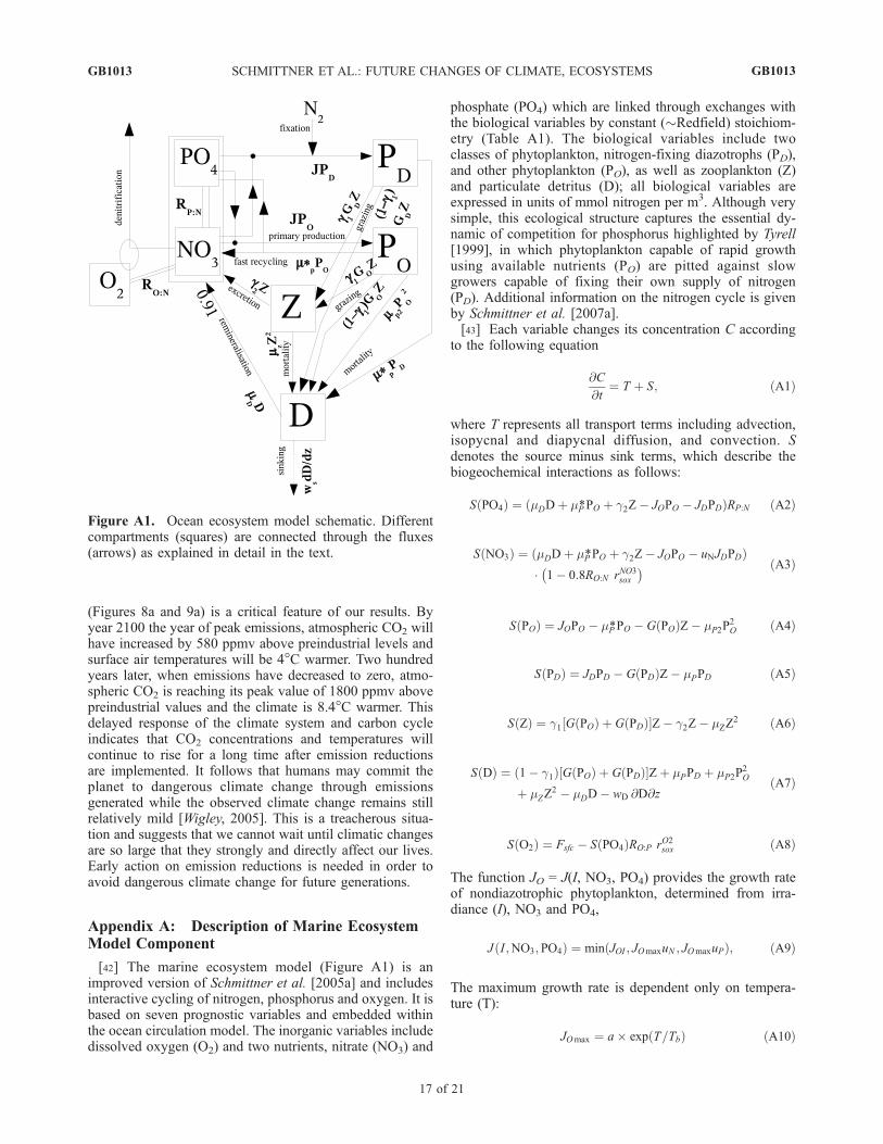
[42] The marine ecosystem model (Figure A1) is animproved version of Schmittner et al. [2005a] and includesinteractive cycling of nitrogen, phosphorus and oxygen. It isbased on seven prognostic variables and embedded withinthe ocean circulation model. The inorganic variables includedissolved oxygen (O2) and two nutrients, nitrate (NO3) and

phosphate (PO4) which are linked through exchanges withthe biological variables by constant (�Redfield) stoichiom-etry (Table A1). The biological variables include twoclasses of phytoplankton, nitrogen-fixing diazotrophs (PD),and other phytoplankton (PO), as well as zooplankton (Z)and particulate detritus (D); all biological variables areexpressed in units of mmol nitrogen per m3. Although verysimple, this ecological structure captures the essential dy-namic of competition for phosphorus highlighted by Tyrell[1999], in which phytoplankton capable of rapid growthusing available nutrients (PO) are pitted against slowgrowers capable of fixing their own supply of nitrogen(PD). Additional information on the nitrogen cycle is givenby Schmittner et al. [2007a].[43] Each variable changes its concentration C according

to the following equation

@C

@t¼ T þ S; ðA1Þ

where T represents all transport terms including advection,isopycnal and diapycnal diffusion, and convection. Sdenotes the source minus sink terms, which describe thebiogeochemical interactions as follows:

S PO4ð Þ ¼ mDDþ mP*PO þ g2Z� JOPO � JDPDð ÞRP:N ðA2Þ

S NO3ð Þ ¼ mDDþ mP*PO þ g2Z� JOPO � uNJDPDð Þ� 1� 0:8RO:N rNO3sox

� � ðA3Þ

S POð Þ ¼ JOPO � mP*PO � G POð ÞZ� mP2P2O ðA4Þ

S PDð Þ ¼ JDPD � G PDð ÞZ� mPPD ðA5Þ

S Zð Þ ¼ g1 G POð Þ þ G PDð Þ½ Z� g2Z� mZZ2 ðA6Þ

S Dð Þ ¼ 1� g1ð Þ G POð Þ þ G PDð Þ½ Zþ mPPD þ mP2P2O

þ mZZ2 � mDD� wD @D@z

ðA7Þ

S O2ð Þ ¼ Fsfc � S PO4ð ÞRO:P rO2sox ðA8Þ

The function JO = J(I, NO3, PO4) provides the growth rateof nondiazotrophic phytoplankton, determined from irra-diance (I), NO3 and PO4,

J I ;NO3; PO4ð Þ ¼ min JOI ; JOmaxuN ; JOmaxuPð Þ; ðA9Þ

The maximum growth rate is dependent only on tempera-ture (T):

JOmax ¼ a� exp T=Tbð Þ ðA10Þ

Figure A1. Ocean ecosystem model schematic. Differentcompartments (squares) are connected through the fluxes(arrows) as explained in detail in the text.


17 of 21

GB1013

such that growth rates increase by a factor of ten over thetemperature range of �2 to 34�C. We use a = 0.11 d�1 forthe maximum growth rate at 0�C which was determined tooptimize surface nutrient concentrations. Under nutrient-replete conditions, the light-limited growth rate JOI iscalculated according to

JOI ¼JOmaxaI

J 2Omax þ aIð Þ2h i1=2 ðA11Þ

where a is the initial slope of the photosynthesis versusirradiance (P-I) curve. The calculation of the photosynthe-tically active shortwave radiation I and the method ofaveraging equation (13) over 1 day is outlined bySchmittner et al. [2005a]. Nutrient limitation is representedby the product of JOmax and the nutrient uptake rates, uN =NO3/(kN + NO3) and uP = PO4/(kP + PO4), with kP = kNRP:N

providing the respective nutrient uptake rates.[44] Diazotrophs grow according to the same principles as

the other phytoplankton, but are disadvantaged in nitrate-bearing waters by a lower maximum growth rate, JDmax,which is zero below 15�C:

JDmax ¼ cD max 0; a exp T=Tbð Þ � 2:61ð Þ½ : ðA12Þ

The coefficient cD handicaps diazotrophs by dampening theincrease of their maximal growth rate versus that of other

phytoplankton with rising temperature. We use cD = 0.5,such that the increase per �C warming of diazotrophs is 50%that of other phytoplankton. However, diazotrophs have anadvantage in that their growth rate is not limited by NO3

concentrations:

JD I ; PO4ð Þ ¼ min JDI ; JDmaxuPð Þ; ðA13Þ

although they do take up NO3 if it is available (see term 5 inthe right-hand side of equation (A3)). The N:P of modeldiazotrophs is equal to other phytoplankton (16:1).Although there is evidence that the best-studied diazotrophsof the genus Trichodesmium can have much higher N:P[e.g., Sanudo-Wilhelmy et al., 2004], the more abundantunicellular diazotrophs are uncharacterized [Montoya et al.,2002] and for simplicity of interpretation we opted to keepthe N:P of both phytoplankton groups identical.[45] The first-order mortality rate of phytoplankton is

linearly dependent on their concentration, PO. DOM andthe microbial loop are folded into a single fast reminerali-zation process, which is the product of PO and the temper-ature-dependent term

mP* ¼ mP0* exp T=Tbð Þ: ðA14Þ

Diazotrophs do not undergo this fast remineralization, butdie at a linear rate.

Table A1. Ocean Ecosystem and Carbon Cycle Model Parameters

Parameter Symbol Value Units

Phytoplankton (PO, PD) CoefficientsInitial slope of P-I curve a 0.1 (W m�2)�1 d�1

Photosynthetically active radiation PAR 0.43Light attenuation in water kw 0.04 m�1

Light attenuation through phytoplankton kc 0.03 m�1(mmol m�3)�1

Light attenuation through sea ice kI 5 m�1

Maximum growth rate a 0.11 d�1

Half-saturation constant for N uptake kN 0.7 mmol m�3

Specific mortality rate mP 0.025 d�1

Fast recycling term (microbial loop) mP0 0.02 d�1

Diazotrophs’ handicap cD 0.5

Zooplankton (Z) CoefficientsAssimilation efficiency g1 0.925Maximum grazing rate g 1.575 d�1

Prey capture rate " 1.6 (mmol m�3)�2 d�1

Mortality mZ 0.34 (mmol m�3)�2 d�1

Excretion g2 0.01 d�1

Detritus (D) CoefficientsRemineralization rate mD0 0.048 d�1

Sinking speed at surface wD0 7 M d�1

Increase of sinking speed with depth mw 0.04 d�1

E-folding temperature of biological rates Tb 15.65 �C

Other CoefficientsMolar elemental ratios RC:N 7

RO:N 13RN:P 16RC:P 112

CaCO3 over nonphotosynthetical POC production ratio RCaCO3/POC 0.035CaCO3 remineralization e-folding depth DCaCO3 3500 m


18 of 21

GB1013

[46] Grazing of phytoplankton by zooplankton is un-changed from Schmittner et al. [2005a]. Detritus is gener-ated from sloppy zooplankton feeding and mortality amongthe three classes of plankton, and is the only component ofthe ecosystem model to sink. It does so at a speed of

wD ¼ wD0 þ mwz; z � 1000m

wD0 þ mw1000m; z > 1000m

� ; ðA15Þ

increasing linearly with depth z from wD0 = 7 m d�1 at thesurface to 40 m d�1 at 1 km depth and constant below that,consistent with observations [Berelson, 2002]. The reminer-alization rate of detritus is temperature dependent anddecreases by a factor of 5 in suboxic waters, as O2 decreasesfrom 5 mM to 0 mM:

mD ¼ mD0 exp T=Tbð Þ 0:65þ 0:35 tanh O2 � 6ð Þ½ : ðA16Þ

Remineralization returns the N and P content of detritus toNO3 and PO4. Photosynthesis produces oxygen, whilerespiration consumes oxygen, at rates equal to theconsumption and remineralization rates of PO4, respec-tively, multiplied by the constant ratio RO:P. Dissolvedoxygen exchanges with the atmosphere in the surface layer(Fsfc) according to the OCMIP protocol.[47] Oxygen consumption in suboxic waters (<5 mM) is

inhibited, according to

rO2sox ¼ 0:5 tanh O2 � 5ð Þ þ 1½ ðA17Þ

but is replaced by the oxygen-equivalent oxidation ofnitrate,

rNO3sox ¼ 0:5 1� tanh O2 � 5ð Þ½ : ðA18Þ

Denitrification consumes nitrate at a rate of 80% of theoxygen equivalent rate, as NO3 is a more efficient oxidanton a mol per mol basis (i.e., 1 mol of NO3 can accept 5e�

while 1 mol of O2 can accept only 4 e�). Note that themodel does not include sedimentary denitrification, whichwould provide a large and less time-variant sink for fixednitrogen. Because sedimentary denitrification would notchange the qualitative dynamics of the model’s behavior,but would slow the integration time, it is not included in theversion presented here.

[48] Acknowledgments. Thanks toT.Westberry, T. Lenton,K.Kohfeld.and C. Le Quere for helpful comments. AS is supported by the Paleoclimateprogram of the National Science Foundation (ATM-0602395).

ReferencesAnnan, J. D., and J. C. Hargreaves (2006), Using multiple observationally-based constraints to estimate climate sensitivity, Geophys. Res. Lett., 33,L06704, doi:10.1029/2005GL025259.

Archer, D., and A. Ganopolski (2005), A movable trigger: Fossil fuel CO2

and the onset of the next glaciation, Geochem. Geophys. Geosyst., 6,Q05003, doi:10.1029/2004GC000891.

Archer, D., H. Kheshi, and E. Maier-Reimer (1998), Dynamics of fossil fuelCO2 neutralization by marine CaCO3, Global Biogeochem. Cycles, 12,259–276.

Berelson, W. M. (2002), Particle settling rates increase with depth in theocean, Deep Sea Res., Part II, 49, 237–251.

Bitz, C. M., M. M. Holland, A. J. Weaver, and M. Eby (2001), Simulatingthe ice-thickness distribution in a coupled climate model, J. Geophys.Res., 106, 2441–2463.

Bolin, B., et al. (2000), Global perspective, in Land Use, Land-UseChange, and Forestry: A Special Report of the Intergovernmental Panelon Climate Change, edited by R. T. Watson et al., pp. 23–51, CambridgeUniv. Press, New York.

Bopp, L., P. Monfray, O. Aumont, J.-L. Dufresne, H. Le Treut, G. Madec,L. Terray, and J. C. Orr, (2001), Potential impact of climate change onmarine export production, Global Biogeochem. Cycles, 15, 81–100.

Cavalieri, D. J., P. Gloersen, C. L. Parkinson, J. C. Comiso, and H. J.Zwally (1997), Observed asymmetry in global sea ice changes, Science,278, 1104–1106.

Clark, P. U., S. W. Hostetler, N. G. Pisias, A. Schmittner, and K. J. Meissner(2007), Mechanisms for a �7-kyr climate and sea-level oscillation duringMarine Isotope Stage 3, in Ocean Circulation: Mechanisms and Impacts,Geophys. Monogr. Ser., vol. 173, edited by A. Schmittner, J. Chiang, andS. Hemming, pp. 207–246, AGU, Washington, D. C.

Cox, P. M., R. A. Betts, C. D. Jones, S. A. Spall, and I. J. Totterdell (2000),Acceleration of global warming due to carbon-cycle feedbacks in acoupled climate model, Nature, 408, 184–187.

Crowley, T. J. (2000), Causes of climate change over the past 1000 years,Science, 289, 270–277.

Dufresne, J.-L., L. Fairhead, H. Le Treut, M. Berthelot, L. Bopp, P. Ciais,P. Friedlingstein, and P. Monfray (2002), On the magnitude of positivefeedback between future climate change and the carbon cycle, Geophys.Res. Lett., 29(10), 1405, doi:10.1029/2001GL013777.

Eppley, R. W. (1972), Temperature and phytoplankton growth in the sea,Fish. Bull., 70, 1063–1085.

Ewen, T. L., A. J. Weaver, and M. Eby (2004), Sensitivity of the inorganicocean carbon cycle to future climate warming in the UVic coupled model,Atmos. Ocean, 42, 23–42.

Flueckiger, J., T. Blunier, B. Stauffer, J. Chappellaz, R. Spahni,K. Kawamura, J. Schwander, T. F. Stocker, and D. Dahl-Jensen (2004),N2O and CH4 variations during the last glacial epoch: Insight into globalprocesses, Global Biogeochem. Cycles, 18, GB1020, doi:10.1029/2003GB002122.

Frankignoulle, M., C. Canon, and J.-P. Gattuso (1994), Marine calcificationas a source of carbon dioxide: Positive feedback of increasing atmo-spheric CO2, Limnol. Oceanogr., 39, 458–462.

Friedlingstein, P., J.-L. Dufresne, P. M. Cox, and P. Rayner (2003), Howpositive is the feedback between climate change and the carbon cycle?,Tellus, Ser. B, 55, 692–700.

Friedlingstein, P., et al. (2006), Climate-carbon cycle feedback analysis:Results from the C4MIP model intercomparison, J. Clim., 19, 3337–3353.

Fyfe, J. C., and O. A. Saenko (2005), Human-induced change in the Ant-arctic Circumpolar Current, J. Clim., 18, 3068–3073.

Gehlen, M., R. Gangsto, B. Schneider, L. Bopp, O. Aumont, and C. Ethe(2007), The fate of pelagic CaCO3 production in a high CO2 ocean:A model study, Biogeosci. Disc., 4, 534–560.

Gent, P. R., and J. C. McWilliams (1990), Isopycnal mixing in oceancirculation models, J. Phys. Oceanogr., 20, 150–155.

Govindasamy, B., S. Thompson, A. Mirin, M. Wickett, K. Caldeira,C. Delire, and P. B. Duffy (2005), Increase of carbon cycle feedbackwith climate sensitivity: Results from a coupled climate and carboncycle model, Tellus, Ser. B, 57, 153–163.

Grantham, B. A., F. Chan, K. J. Nielsen, D. S. Fox, J. A. Barth,A. Huyer, J. Lubchenco, and B. A. Menge (2004), Nearshore upwel-ling-driven hypoxia signals ecosystem and oceanographic changes inthe NE Pacific, Nature, 429, 749–754.

Heinze, C. (2004), Simulating oceanic CaCO3 export production inthe greenhouse, Geophys. Res. Lett., 31, L16308, doi:10.1029/2004GL020613.

Hirsch, A. I., A. M. Michalak, L. M. Bruhwiler, W. Peters, E. J.Dlugokencky, and P. P. Tans (2006), Inverse modeling estimates of theglobal nitrous oxide surface flux from 1998–2001, Global Biogeochem.Cycles, 20, GB1008, doi:10.1029/2004GB002443.

Houghton, R. (2003), Revised estimates of the annual net flux of carbonto the atmosphere from changes in land use and land management1850–2000, Tellus, Ser. B, 55, 378–390.

IPCC (1995), Climate Change 1995: The Science of Climate Change.Contribution of Working Group I to the Second Assessment Report ofthe Intergovernmental Panel on Climate Change, edited by J. T. Houghtonet al., 572 pp., Cambridge Univ. Press, New York.

IPCC (2001), Climate Change 2001: The Scientific Basis. Contribution ofWorking Group I to the Third Assessment Report of the Intergovernmen-


19 of 21

GB1013

tal Panel on Climate Change, edited by J. T. Houghton et al., 881 pp.,Cambridge Univ. Press, New York.

IPCC (2007), Climate Change 2007: The Physical Science Basis. Contri-bution of Working Group I to the Fourth Assessment Report of the Inter-governmental Panel on Climate Change, edited by S. Solomon et al.,996 pp., Cambridge Univ. Press, New York.

Jin, X., N. Gruber, J. P. Dunne, J. L. Sarmiento, and R. A. Armstrong(2006), Diagnosing the contribution of phytoplankton functional groupsto the production and export of particulate organic carbon, CaCO3, andopal from global nutrient and alkalinity distributions, Global Biogeo-chem. Cycles, 20, GB2015, doi:10.1029/2005GB002532.

Jones, C. D., P. M. Cox, R. L. H. Essery, D. L. Roberts, and M. J. Woodage(2003), Strong carbon cycle feedbacks in a climate model with interactiveCO2 and sulphate aerosols, Geophys. Res. Lett., 30(9), 1479,doi:10.1029/2003GL016867.

Jones, P. D., T. J. Osborn, K. R. Briffa, C. K. Folland, B. Horton, L. V.Alexander, D. E. Parker, and N. Rayner (2001), Accounting for sam-pling density in grid-box land and ocean surface temperature timeseries, J. Geophys. Res., 106, 3371–3380.

Joos, F., G.-K. Plattner, T. F. Stocker, O. Marchal, and A. Schmittner(1999), Global warming and marine carbon cycle feedbacks on futureatmospheric CO2, Science, 284, 464–467.

Joos, F., I. C. Prentice, S. Sitch, R. Meyer, G. Hooss, G.-K. Plattner,S. Gerber, and K. Hasselmann (2001), Global warming feedbacks onterrestrial carbon uptake under the Intergovernmental Panel on ClimateChange (IPCC) emission scenarios, Global Biogeochem. Cycles, 15,891–908.

Jungclaus, J. H., H. Haak, M. Esch, E. Roeckner, and J. Marotzke (2006),Will Greenland melting halt the thermohaline circulation?, Geophys. Res.Lett., 33, L17708, doi:10.1029/2006GL026815.

Key, R. M., A. Kozyr, C. L. Sabine, K. Lee, R. Wanninkhof, J. L. Bullister,R. A. Feely, F. J. Millero, C. Mordy, and T.-H. Peng (2004), A globalocean carbon climatology: Results from Global Data Analysis Project(GLODAP), Global Biogeochem. Cycles, 18, GB4031, doi:10.1029/2004GB002247.

Knutti, R., T. F. Stocker, F. Joos, and G.-K. Plattner (2003), Probabilisticclimate change projections using neural networks, Clim. Dyn., 21, 257–272.

Langer, G., M. Geisen, K.-H. Baumann, J. Klas, U. Riebesell, S. Thoms,and J. R. Young (2006), Species-specific responses of calcifying algae tochanging seawater carbonate chemistry, Geochem. Geophys. Geosyst., 7,Q09006, doi:10.1029/2005GC001227.

Large, W. G., G. Danabasoglu, J. C. McWilliams, P. R. Gent, and F. O.Bryan (2001), Equatorial circulation of a global ocean climate model withanisotropic horizontal viscosity, J. Phys. Oceanogr., 31, 518–536.

Law, C. S., and N. J. P. Owens (1990), Significant flux of atmosphericnitrous oxide from the northwest Indian Ocean, Nature, 348, 826–828.

Lee, K. (2001), Global net community production estimated from the an-nual cycle of surface water total dissolved inorganic carbon, Limnol.Oceanogr., 46, 1287–1297.

Lenton, T. M., et al. (2006), Millennial timescale carbon cycle and climatechange in an efficient Earth system model, Clim. Dyn., 26, 687–711.

Levitus, S., J. Antonov, and T. Boyer (2005), Warming of the world ocean,1955 – 2003, Geophys. Res. Lett., 32 , L02604, doi:10.1029/2004GL021592.

Loutre, M. F., and A. Berger (2000), Future climatic changes: Are weentering an exceptional long interglacial?, Clim. Change, 46, 61–90.

Maier-Reimer, E., U. Mikolajewicz, and A. Winguth (1996), Future oceanuptake of CO2: Interaction between ocean circulation and biology, Clim.Dyn., 12, 711–722.

Marland, G., T. A. Boden, and R. J. Andres (2006), In Trends: A Compen-dium of Data on Global Change, Carbon Dioxide Information AnalysisCenter, Oak Ridge Natl. Lab., U. S. Dep. of Energy, Oak Ridge, Tenn.

Matear, R. J., and A. C. Hirst (1999), Climate change feedback on thefuture oceanic CO2 uptake, Tellus, Ser. B, 51, 722–733.

Matear, R. J., and A. C. Hirst (2002), Long-term changes in dissolvedoxygen concentrations in the ocean caused by protracted global warming,Global Biogeochem. Cycles, 17(4), 1125, doi:10.1029/2002GB001997.

Matsumoto, K., et al. (2004), Evaluation of ocean carbon cycle models withdata-based metrics, Geophys. Res. Lett., 31, L07303, doi:10.1029/2003GL018970.

Matthews, H. D., A. J. Weaver, K. J. Meissner, N. P. Gillett, and M. Eby(2005a), Natural and anthropogenic climate change: Incorporating histor-ical land cover change, vegetation dynamics and the global carbon cycle,Clim. Dyn., 22, 461–479.

Matthews, H. D., A. J. Weaver, and K. J. Meissner (2005b), Terrestrialcarbon cycle dynamics under recent and future climate change, J. Clim.,18, 1609–1628.

Matthews, H. D., M. Eby, T. Ewen, P. Friedlingstein, and B. J. Hawkins(2007), What determines the magnitude of carbon cycle-climate feed-backs?, Global Biogeochem. Cycles, 21, GB2012, doi:10.1029/2006GB002733.

Meissner, K. J., A. J. Weaver, H. D. Matthews, and P. M. Cox (2003), Therole of land surface dynamics in glacial inception: A study with the UVicEarth System Model, Clim. Dyn., 21, 515–537.

Moisan, J. R., T. A. Moisan, and M. R. Abbott (2002), Modelling the effectof temperature on the maximum growth rates of phytoplankton popula-tions, Ecol. Modell., 153, 197–215.

Montoya, J. P., E. J. Carpenter, and D. G. Capone (2002), Nitrogen fixationand nitrogen isotope abundances in zooplankton of the oligotrophicNorth Atlantic, Limnol. Oceanogr., 47, 1617–1628.

Moore, J. K., S. C. Doney, J. A. Kleypas, D. M. Glover, and I. Y. Fung(2002), An intermediate complexity marine ecosystem model, Deep SeaRes., Part II, 49, 403–462.

Nakicenovic, N., et al. (2000), IPCC Special Report on Emissions Scenar-ios, edited by N. Nakicenovic and R. Swart, 570 pp., Cambridge Univ.Press, New York.

Nevison, C., J. H. Butler, and J. W. Elkins (2003), Global distribution ofN2O and the delta N2O-AOU yield in the subsurface ocean, GlobalBiogeochem. Cycles, 17(4), 1119, doi:10.1029/2003GB002068.

Orr, J. C., R. Najjar, C. L. Sabine, and F. Joos (1999), Abiotic-HOWTO,internal OCMIP report, LSCE/CEA Saclay, 25 pp., Gif-sur-Yvette,France.

Orr, J. C., et al. (2005), Anthropogenic ocean acidification over the twenty-first century and its impact on calcifying organisms, Nature, 437, 681–686.

Plattner, G.-K., F. Joos, and T. F. Stocker (2002), Revision of the globalcarbon budget due to changing air-sea oxygen fluxes, Global Biogeo-chem. Cycles, 16(4), 1096, doi:10.1029/2001GB001746.

Prather, M., et al. (2001), Atmospheric chemistry and greenhouse gases, inClimate Change 2001: The Scientific Basis. Contribution of WorkingGroup I to the Third Assessment Report of the Intergovernmental Panelon Climate Change, edited by J. R. Houghton et al., 881 pp., CambridgeUniv. Press, New York.

Ramankutty, N., and J. A. Foley (1999), Estimating historical changes inland cover: Croplands from 1700 to 1992, Global Biogeochem. Cycles,13, 997–1027.

Ramaswamy, V., O. Boucher, J. Haigh, D. Hauglustaine, J. Haywood,G. Myhre, T. Nakajima, G. Y. Shi, and S. Solomon (2001), Radiativeforcing of climate change, in Climate Change 2001: The Scientific Basis.Contribution of Working Group I to the Third Assessment Report of theIntergovernmental Panel on Climate Change, edited by J. R. Houghtonet al., 881 pp., Cambridge Univ. Press, New York.

Ridgwell, A., and J. C. Hargreaves (2007), Regulation of atmospheric CO2

by deep-sea sediments in an Earth system model, Global Biogeochem.Cycles, 21, GB2008, doi:10.1029/2006GB002764.

Ridgwell, A., I. Zondervan, J. C. Hargreaves, J. Bijma, and T. M. Lenton(2006), Significant long-term increase of fossil fuel CO2 uptake fromreduced marine calcification, Biogeosci. Disc., 3, 1763–1780.

Riebesell, U., I. Zondervan, B. Rost, P. D. Tortell, R. E. Zeebe, and F. M.Morel (2000), Reduced calcification of marine plankton in response toincreased atmospheric CO2, Nature, 407, 311–313.

Russell, J. L., K. W. Dixon, A. Gnanadesikan, R. J. Stouffer, and J. R.Toggweiler (2006), The Southern Hemisphere westerlies in a warmingworld: Propping open the door to the deep ocean, J. Clim., 19, 6382–6390.

Sabine, C. L., et al. (2004), The oceanic sink for anthropogenic CO2,Science, 305, 367–371.

Saenko, O. A., A. Schmittner, and A. J. Weaver (2002), On the role of winddriven sea ice motion on ocean ventilation, J. Phys. Oceanogr., 32,3376–3395.

Sanudo-Wilhelmy, S. A., A. Tovar-Sanchez, F.-X. Fu, D. G. Capone, E. J.Carpenter, and D. A. Hutchins (2004), The impact of surface-adsorbedphosphorus on phytoplankton Redfield stoichiometry, Nature, 432, 897–901.

Sarmiento, J. L., T. M. C. Hughes, R. J. Stouffer, and S. Manabe (1998),Simulated response of the ocean carbon cycle to anthropogenic climatewarming, Nature, 393, 245–249.

Sarmiento, J. L., J. Dunne, A. Gnanadesikan, R. M. Key, K. Matsumoto,and R. Slater (2002), A new estimate of the CaCO3 to organic carbonexport ratio, Global Biogeochem. Cycles, 16(4), 1107, doi:10.1029/2002GB001919.

Sarmiento, J. L., et al. (2004), Response of ocean ecosystems to climatewarming, Global Biogeochem. Cycles, 18, GB3003, doi:10.1029/2003GB002134.


20 of 21

GB1013

Schartau, M., and A. Oschlies (2003), Simultaneous data-based optimiza-tion of a 1D-ecosystem model at three locations in the North Atlantic.part I: Method and parameter estimates, J. Mar. Res., 61, 765–793.

Schmittner, A. (2005), Decline of the marine ecosystem caused by a reduc-tion in the Atlantic overturning circulation, Nature, 443, 628–633.

Schmittner, A., K. J. Meissner, M. Eby, and A. J. Weaver (2002a), Forcingof the deep ocean circulation in simulations of the Last Glacial Max-imum, Paleoceanography, 17(2), 1015, doi:10.1029/2001PA000633.

Schmittner, A., M. Yoshimori, and A. J. Weaver (2002b), Instability ofglacial climate in a model of the ocean-atmosphere-cryosphere system,Science, 295, 1489–1493.

Schmittner, A., O. A. Saenko, and A. J. Weaver (2003), Coupling of thehemispheres in observations and simulations of glacial climate change,Quat. Sci. Rev., 22, 659–671.

Schmittner, A., A. Oschlies, X. Giraud, M. Eby, and H. L. Simmons(2005a), A global model of the marine ecosystem for long term simula-tions: Sensitivity to ocean mixing, buoyancy forcing, particle sinking anddissolved organic matter cycling, Global Biogeochem. Cycles, 19,GB3004, doi:10.1029/2004GB002283.

Schmittner, A., M. Latif, and B. Schneider (2005b), Model projections ofthe North Atlantic thermohaline circulation for the 21st century assessedby observations, Geophys. Res. Lett., 32, L23710, doi:10.1029/2005GL024368.

Schmittner, A., E. D. Galbraith, S. Hostetler, T. F. Pedersen, and R. Zhang(2007a), Large fluctuations of dissolved oxygen in the Indian and Pacificoceans during Dansgaard-Oeschger oscillations caused by variations ofNorth Atlantic Deep Water subduction, Paleoceanography, 22, PA3207,doi:10.1029/2006PA001384.

Schmittner, A., E. J. Brook, and J. Ahn (2007b), Impact of the ocean’soverturning circulation on atmospheric CO2, in Ocean Circulation:Mechanisms and Impacts, Geophys. Monogr. Ser., vol. 173, edited byA. Schmittner, J. Chiang, and S. Hemming, pp. 315–334, AGU,Washington, D. C.

Simmons, H. L., S. R. Jayne, L. C. St. Laurent, and A. J. Weaver (2004),Tidally driven mixing in a numerical model of the ocean general circula-tion, Ocean Modell., 6, 245–263.

Swingedouw, D., P. Braconnot, and O. Marti (2006), Sensitivity of theAtlantic Meridional Overturning Circulation to the melting from northern

glaciers in climate change experiments, Geophys. Res. Lett., 33, L07711,doi:10.1029/2006GL025765.

Takahashi, T., et al. (2002), Global sea-air CO2 flux based on climatologicalsurface ocean pCO2, and seasonal biological and temperature effects,Deep Sea Res., Part II, 49, 1601–1622.

Taylor, K. E. (2001), Summarizing multiple aspects of model performancein a single diagram, Geophys. Res. Lett., 106, 7183–7192.

Tyrell, T. (1999), The relative influence of nitrogen and phosphorus onoceanic primary production, Nature, 400, 525–531.

Weaver, A. J., M. Eby, A. F. Fanning, and E. C. Wiebe (1998), Simulatedinfluence of carbon dioxide, orbital forcing and ice sheets on the climateof the Last Glacial Maximum, Nature, 394, 847–853.

Weaver, A. J., et al. (2001), The UVic Earth system climate model: Modeldescription, climatology and applications to past, present and future cli-mates, Atmos. Ocean, 4, 361–428.

Wigley, T. M. L. (2005), The climate change commitment, Science, 307,1766–1769.

Yamagishi, H., N. Yoshida, S. Toyoda, B. N. Popp, M. B. Westley, and S.Watanabe (2005), Contributions of denitrification and mixing on thedistribution of nitrous oxide in the North Pacific, Geophys. Res. Lett.,32, L04603, doi:10.1029/2004GL021458.

Zeng, N., H. Qian, E. Munoz, and R. Iacono (2004), How strong is carboncycle-climate feedback under global warming?, Geophys. Res. Lett., 31,L20203, doi:10.1029/2004GL020904.

��E. D. Galbraith, Atmospheric and Oceanic Sciences, Princeton

University, 300 Forrestal Road, Princeton, NJ 08540, USA.H. D. Matthews, Planning and Environment, Concordia University, 1455

de Maisonneuve Boulevard West, Montreal, Quebec, H3G 1M8, Canada.A. Oschlies, Leibniz Institute of Marine Sciences at the Christian-

Albrechts University of Kiel (IFM-GEOMAR), Dusternbrooker Weg 20,24105 Kiel, Germany.A. Schmittner, College of Oceanic and Atmospheric Sciences, Oregon

State University, 104 COAS Admin Building, Corvallis, OR 97331-5503,USA.


21 of 21

GB1013

future changes in climate, ocean circulation, ecosystems...

Documents