Future Supply of Oil and Gas From the Gulf of MexicoU.S. GEOLOGICAL SUltyEY PROFESSIONAL PAPER 1294

Future Supply of Oil and Gas From the Gulf of MexicoBy E. D. Attanasi and]. L. Haynes

U.S. GEOLOGICAL SURVEY PROFESSIONAL PAPER 1294

An engineering-economic costing algorithm combined with a discovery process model to forecast long-run incremental costs of undiscovered oil and gas

UNITED STATES GOVERNMENT PRINTING OFFICE, WASHINGTON : 1983

UNITED STATES DEPARTMENT OF THE INTERIOR

JAMES G. WATT, Secretary

GEOLOGICAL SURVEY

Dallas L. Peck, Director

Library of Congress Cataloging in Publication DataAttanasi, E. D.Future supply of oil and gas from the Gulf of Mexico.

(U.S. Geological Survey professional paper ; 1294)Bibliography: p.1. Petroleum in submerged lands Mexico, Gulf of. 2. Gas, Natural, in submerged lands Mexico, Gulf of.

I. Haynes, J. (John), 1954- . II. Title. III. Series: Geological Survey professional paper ; 1294. TN872.A5A87 1983 553.2'8'0916364 83-600030 ____ ____________

For sale by the Superintendent of Documents, U.S. Government Printing OfficeWashington, D.C. 20402

CONTENTS

PageAbstract 1Introduction 1Engineering-economic model 3

Methodology 3Engineering data and assumptions 5

Field classification 5Field design 6Production schedules of oil and nonassociated gas wells 7

Economic assumptions and variables 8Field development costs 8Production costs and production related taxes 9Assumptions for after-tax net present value calculations 10Exploration costs 10

Industry behavior and market conditions 10Forecasting future discoveries 11

Discovery process model 11Estimated marginal cost functions for undiscovered recoverable oil

and gas resources in the Gulf of Mexico 12 Conclusions and implications 16 References cited 16 Appendix A 17 Appendix B 20

ILLUSTRATIONS

FIGURE 1. Map showing location of study area in the Gulf of Mexico 22. Graph showing wildcat well discovery rate for oil and gas in the Gulf of Mexico to the end of 1975 33. Map showing geographic locations of the offshore geologic trend areas in study area in the Gulf of Mexico 44. Schematic diagram of the structure of the engineering-economic cost algorithm 5

5-9. Graphs showing:5. Production curves for oil wells in the Gulf of Mexico 76. Production curves for nonassociated gas wells in the Gulf of Mexico 87. Marginal costs of recoverable oil and gas resources, by form of hydrocarbon, from undiscovered fields

(as of January 1,1977) in the Gulf of Mexico 158. Wildcat wells projected to be drilled in the Gulf of Mexico as a function of marginal finding and

development costs and various assumed in situ costs of resources 159. Marginal cost of recoverable oil and gas resources from undiscovered fields (as of January 1, 1977)

in the Gulf of Mexico as a function of various assumed in situ costs of resources 15

in

IV CONTENTS

TABLES

TABLE 1. Distribution of exploratory wells in the Gulf of Mexico by geologic trend and Federal lease sale 32. Expected nominal crude oil and nonassociated gas recovery per well and field 63. Percentages of prospective areas in each water depth interval 64. Cost estimates for fabrication and installation of oil and gas production platforms in the Gulf of Mexico 95. Gulf of Mexico oil and gas processing equipment capacities and costs 96. Exploration efficiencies, areal extent, and expected remaining number of fields for various field size classes

7. Fields predicted to be found by 3 groups of 20 successive increments of 200 wildcat wells in the Miocene-Pliocene trend

8. Potential recoverable oil and gas resources from future discoveries in the Gulf of Mexico as a function of output price, marginal finding cost, marginal production costs, exploratory wells, and return on investment

A2. Development well, platform, and processing equipment configurations for new nonassociated gas fields in the

A5 . Drilling costs and completion costs for the Gulf of Mexico

A7. Development strategies: Drilling and production stages Bl. Oil production schedule constants for Texas and Louisiana offshore oil fields by size class R2 NVinassnrviafWl eras nrnrhirtinn enimtirm nnrntnofora

17

171710

10

10

19 2091

FUTURE SUPPLY OF OIL AND GAS FROM THE GULF OF MEXICO

By E. D. ATTANASI and J. L. HAYNES*

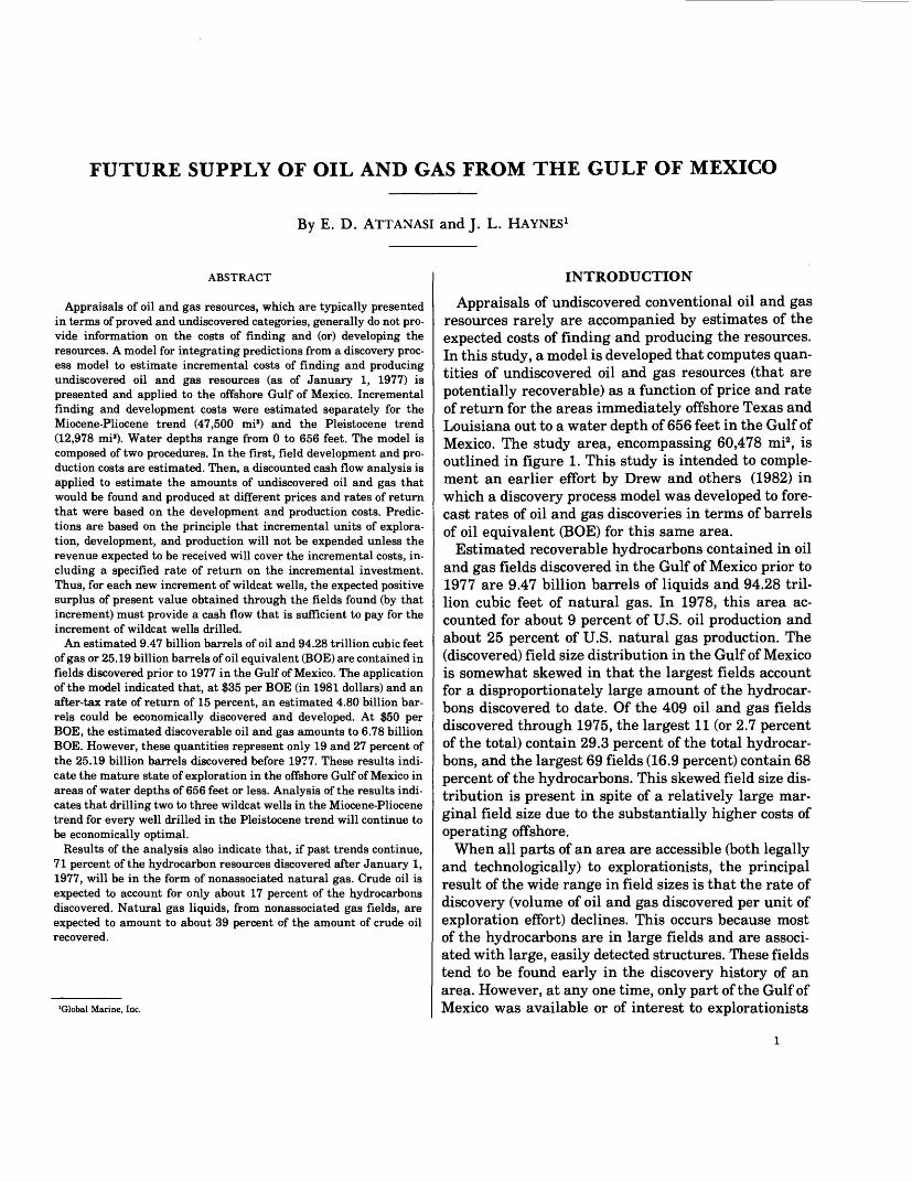
ABSTRACT

Appraisals of oil and gas resources, which are typically presented in terms of proved and undiscovered categories, generally do not pro­ vide information on the costs of finding and (or) developing the resources. A model for integrating predictions from a discovery proc­ ess model to estimate incremental costs of finding and producing undiscovered oil and gas resources (as of January 1, 1977) is presented and applied to the offshore Gulf of Mexico. Incremental finding and development costs were estimated separately for the Miocene-Pliocene trend (47,500 mi2) and the Pleistocene trend (12,978 mi2). Water depths range from 0 to 656 feet. The model is composed of two procedures. In the first, field development and pro­ duction costs are estimated. Then, a discounted cash flow analysis is applied to estimate the amounts of undiscovered oil and gas that would be found and produced at different prices and rates of return that were based on the development and production costs. Predic­ tions are based on the principle that incremental units of explora­ tion, development, and production will not be expended unless the revenue expected to be received will cover the incremental costs, in­ cluding a specified rate of return on the incremental investment. Thus, for each new increment of wildcat wells, the expected positive surplus of present value obtained through the fields found (by that increment) must provide a cash flow that is sufficient to pay for the increment of wildcat wells drilled.

An estimated 9.47 billion barrels of oil and 94.28 trillion cubic feet of gas or 25.19 billion barrels of oil equivalent (BOE) are contained in fields discovered prior to 1977 in the Gulf of Mexico. The application of the model indicated that, at $35 per BOE (in 1981 dollars) and an after-tax rate of return of 15 percent, an estimated 4.80 billion bar­ rels could be economically discovered and developed. At $50 per BOE, the estimated discoverable oil and gas amounts to 6.78 billion BOE. However, these quantities represent only 19 and 27 percent of the 25.19 billion barrels discovered before 1977. These results indi­ cate the mature state of exploration in the offshore Gulf of Mexico in areas of water depths of 656 feet or less. Analysis of the results indi­ cates that drilling two to three wildcat wells in the Miocene-Pliocene trend for every well drilled in the Pleistocene trend will continue to be economically optimal.

Results of the analysis also indicate that, if past trends continue, 71 percent of the hydrocarbon resources discovered after January 1, 1977, will be in the form of nonassociated natural gas. Crude oil is expected to account for only about 17 percent of the hydrocarbons discovered. Natural gas liquids, from nonassociated gas fields, are expected to amount to about 39 percent of the amount of crude oil recovered.

'Global Marine, Inc.

INTRODUCTION

Appraisals of undiscovered conventional oil and gas resources rarely are accompanied by estimates of the expected costs of finding and producing the resources. In this study, a model is developed that computes quan­ tities of undiscovered oil and gas resources (that are potentially recoverable) as a function of price and rate of return for the areas immediately offshore Texas and Louisiana out to a water depth of 656 feet in the Gulf of Mexico. The study area, encompassing 60,478 mi2 , is outlined in figure 1. This study is intended to comple­ ment an earlier effort by Drew and others (1982) in which a discovery process model was developed to fore­ cast rates of oil and gas discoveries in terms of barrels of oil equivalent (BOE) for this same area.

Estimated recoverable hydrocarbons contained in oil and gas fields discovered in the Gulf of Mexico prior to 1977 are 9.47 billion barrels of liquids and 94.28 tril­ lion cubic feet of natural gas. In 1978, this area ac­ counted for about 9 percent of U.S. oil production and about 25 percent of U.S. natural gas production. The (discovered) field size distribution in the Gulf of Mexico is somewhat skewed in that the largest fields account for a disproportionately large amount of the hydrocar­ bons discovered to date. Of the 409 oil and gas fields discovered through 1975, the largest 11 (or 2.7 percent of the total) contain 29.3 percent of the total hydrocar­ bons, and the largest 69 fields (16.9 percent) contain 68 percent of the hydrocarbons. This skewed field size dis­ tribution is present in spite of a relatively large mar­ ginal field size due to the substantially higher costs of operating offshore.

When all parts of an area are accessible (both legally and technologically) to explorationists, the principal result of the wide range in field sizes is that the rate of discovery (volume of oil and gas discovered per unit of exploration effort) declines. This occurs because most of the hydrocarbons are in large fields and are associ­ ated with large, easily detected structures. These fields tend to be found early in the discovery history of an area. However, at any one time, only part of the Gulf of Mexico was available or of interest to explorationists

FUTURE SUPPLY OF OIL AND GAS FROM THE GULF OF MEXICO

32N, 96W

TEXAS

GULF OF MEXICO

100 KILOMETERS

FIGURE 1. Location of study area in the Gulf of Mexico (L. J. Drew, written commun., 1982).

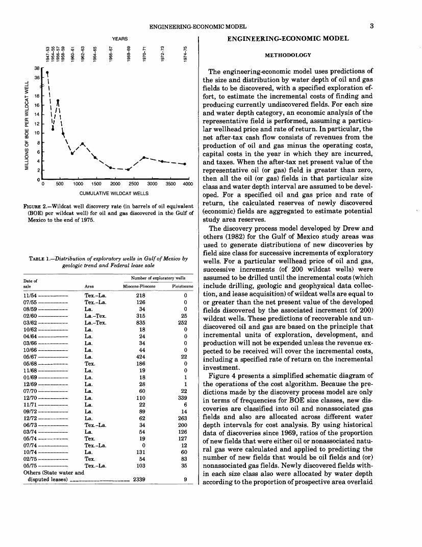
because new technology had to be developed for certain phases of offshore operations and because the State and Federal Governments had only partially leased the area. The graph of the overall discovery rate for the Gulf of Mexico (see fig. 2) exhibits some degree of regu­ larity. The irregularities in the Gulf of Mexico dis­ covery rate are probably the result of restricted access that explorationists had to areas of interest and to the substantial increase in natural gas prices in the early 1970's, which made many moderately large natural gas fields profitable to develop.

In modeling the Gulf of Mexico discovery process, Drew and others (1982) divided the area by general geologic trend. The areas, the combined Miocene- Pliocene and the Pleistocene trends, are presented in figure 3. More wildcat wells have been drilled in the Miocene-Pliocene trend than in the Pleistocene trend. In table 1, data are presented that show the wildcat wells grouped by trend and by the lease sale date of the

tract upon which they were drilled. Drew and others (1982) estimated parameters of a discovery process model by using historical data from the Miocene-Plio­ cene trend and by using an assumption about the func­ tional form of the underlying field size distribution. Because the Pleistocene trend has only recently been intensively explored (see table 1), Drew and others (1982) used the Miocene-Pliocene trend as an analog for the Pleistocene trend. They adapted the model to discovery data of the Pleistocene trend to forecast rates of discoveries in BOE's.

In the following sections, the engineering-economic model is developed, along with its supporting assump­ tions. After briefly discussing the discovery process model and its linkage with the economic model, the in­ cremental costs of finding and developing currently un­ discovered oil and gas fields in the Gulf of Mexico are estimated. Results of the analysis and their implica­ tions are considered in the final section of the study.

ENGINEERING-ECONOMIC MODEL

MILLIONS OF BOE PER WILDCAT WELL

>f\j.^O>OOOfO-^O>00 O) 00

___ - 1947-53 C"^""" 1954-55 !T-=»« 1956-57 J+ """" 1958-59

«^" 1960-61

\

^ 1962-63

/

ff 1964-65

/

9 1966-67

i rn >' 3)

^ 1968-69 W

\

\ 1970-71

/

R 15 di 4 1 fe

0 500 1000 1500 2000 2500 3000 3500 4000

CUMULATIVE WILDCAT WELLS

FIGURE 2. Wildcat well discovery rate (in barrels of oil equivalent (BOE) per wildcat well) for oil and gas discovered in the Gulf of Mexico to the end of 1975.

TABLE I. Distribution of exploratory wells in Gulf of Mexico by geologic trend and Federal lease sale

_ Number of exploratory wells Date ofsale Area Miocene-Pliocene

11/54 Tex. La. 21807/55 Tex. La. 12608/59 La. 34 02/60 La. Tex. 31503/62 La. Tex. 83510/62 La. 18(\A/RA T a 94.

03/66 La. 34 10/66 La. 44 05/67 La. 424 05/68 Tex. 186 11/68 La. 19 01/69 La. 18 12/69 La. 2807/70 La. 6012/70 - La. 11011/71 La. 22OQ/79 T a RQ

12/72 La. 62 06/73 Tex. La. 340^/74. T ,a ^4.0^/74. TW 1 Q

07/74 Tex.-La. 0 10/74 La. 13109/7^ TW ^4.

05/75 Tex.-La. 103 Others (State water and

disputed leases) ______________ 2339

Pleistocene

0 0 0

25 252

0 0 0 0

22 0 0 1 1

22 339

6 14

263 200 126 127

12 60 83 35

9

ENGINEERING-ECONOMIC MODEL

METHODOLOGY

The engineering-economic model uses predictions of the size and distribution by water depth of oil and gas fields to be discovered, with a specified exploration ef­ fort, to estimate the incremental costs of finding and producing currently undiscovered fields. For each size and water depth category, an economic analysis of the representative field is performed, assuming a particu­ lar wellhead price and rate of return. In particular, the net after-tax cash flow consists of revenues from the production of oil and gas minus the operating costs, capital costs in the year in which they are incurred, and taxes. When the after-tax net present value of the representative oil (or gas) field is greater than zero, then all the oil (or gas) fields in that particular size class and water depth interval are assumed to be devel­ oped. For a specified oil and gas price and rate of return, the calculated reserves of newly discovered (economic) fields are aggregated to estimate potential study area reserves.

The discovery process model developed by Drew and others (1982) for the Gulf of Mexico study areas was used to generate distributions of new discoveries by field size class for successive increments of exploratory wells. For a particular wellhead price of oil and gas, successive increments (of 200 wildcat wells) were assumed to be drilled until the incremental costs (which include drilling, geologic and geophysical data collec­ tion, and lease acquisition) of wildcat wells are equal to or greater than the net present value of the developed fields discovered by the associated increment (of 200) wildcat wells. These predictions of recoverable and un­ discovered oil and gas are based on the principle that incremental units of exploration, development, and production will not be expended unless the revenue ex­ pected to be received will cover the incremental costs, including a specified rate of return on the incremental investment.

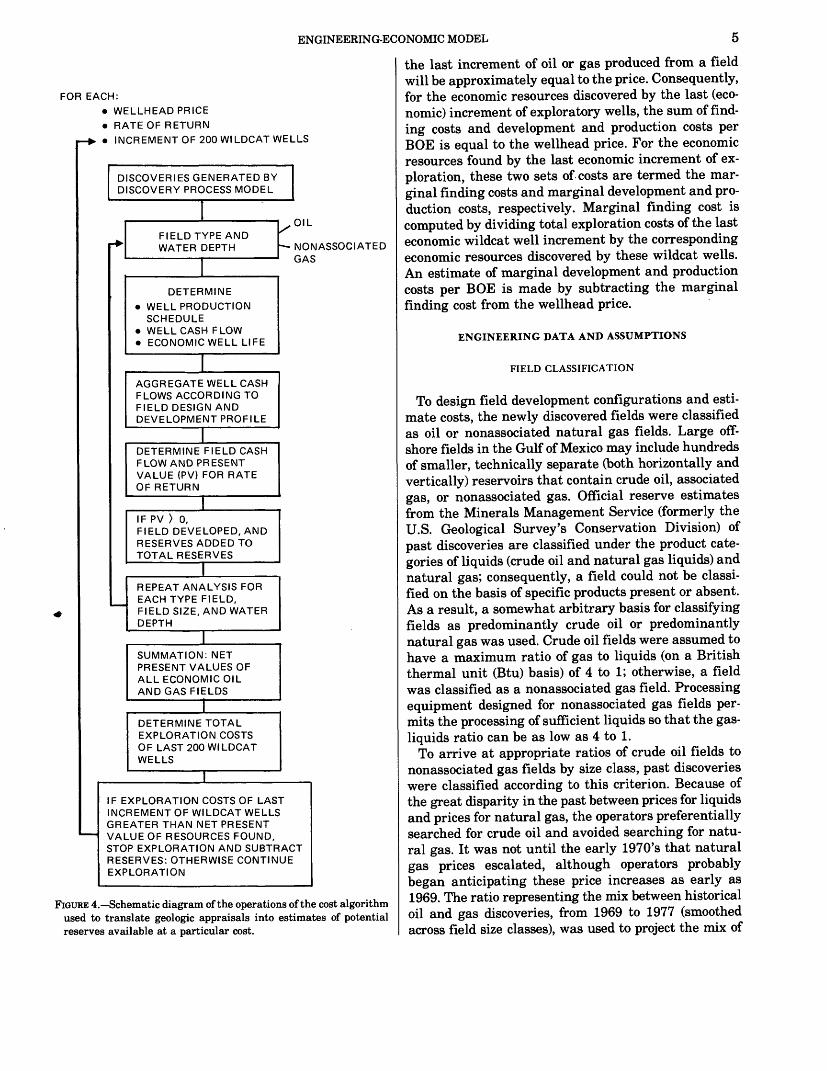
Figure 4 presents a simplified schematic diagram of the operations of the cost algorithm. Because the pre­ dictions made by the discovery process model are only in terms of frequencies for BOE size classes, new dis­ coveries are classified into oil and nonassociated gas fields and also are allocated across different water depth intervals for cost analysis. By using historical data of discoveries since 1969, ratios of the proportion of new fields that were either oil or nonassociated natu­ ral gas were calculated and applied to predicting the number of new fields that would be oil fields and (or) nonassociated gas fields. Newly discovered fields with­ in each size class also were allocated by water depth according to the proportion of prospective area overlaid

FUTURE SUPPLY OF OIL AND GAS FROM THE GULF OF MEXICO

32N, 96W 32N, 92W

TEXAS

GULF OF MEXICO

100 KILOMETERS

FIGURE 3. Geographic locations of the offshore geologic trend areas in the study area in the Gulf of Mexico (from an unpublished map of the Gulf of Mexico prepared by the U.S. Geological Survey for Federal OCS Lease Sale 38 held in 1975).

by each water depth interval.Production schedules for oil and nonassociated gas

wells were generated with formulations originally developed by the Dallas Field Office of the U.S. Depart­ ment of Energy (John Wood, written commun., 1979). By using the production schedule and the associated nominal reserves per well, the number of wells per field were estimated, and a development design (num­ ber of wells, platform size, processing equipment size, and development time profile) for each field size class and water depth interval was specified. With the pro­ duction schedule, the individual well cash flow was computed for a given set of oil and gas prices and costs. Economic well life was terminated after the well cash flow equaled the economic limit rate; that is, the year when operator income was equal to the sum of direct operating expenses and production-related taxes. For each individual well representative of a specific field size class, the net after-tax cash flow stream was com­ puted. The net after-tax cash flow stream is the produc­ tion revenue minus operating costs, capital costs in the

year they are incurred, and taxes. Individual well net after-tax cash flow streams are adjusted and aggre­ gated to be consistent with the field development time profiles that are presented in detail in Appendix A. If the sum of the annual components of the after-tax dis­ counted cash flow stream for the representative oil or gas field (for each size class and water depth interval) is greater than zero, then all the newly discovered fields of that size and water depth category are assumed to be developed and are added to total potential reserves.

This study does not consider the rate of exploratory drilling in the time dimension, and so a full supply analysis, that is, quantity of hydrocarbons produced per unit time, is not performed. Moreover, operators are assumed to drill nonpreferentially for oil or gas fields. Exploration continues until the exploration costs (drilling, geologic and geophysical data collection costs, and lease acquisition costs) of the next 200 wildcat wells exceed the after-tax net present value of the resources found by that increment of wells. Assuming that production continues to the economic limit rate,

ENGINEERING-ECONOMIC MODEL

FOR EACH:

WELLHEAD PRICE

RATE OF RETURN

. INCREMENT OF 200 WILDCAT WELLS

DISCOVERIES GENERATED BY DISCOVERY PROCESS MODEL

FIELD TYPE AND WATER DEPTH

XOIL

NONASSOCIATED GAS

DETERMINE

WELL PRODUCTION SCHEDULE WELL CASH FLOW ECONOMIC WELL LIFE

AGGREGATE WELL CASH FLOWS ACCORDING TO FIELD DESIGN AND DEVELOPMENT PROFILE

DETERMINE FIELD CASH FLOW AND PRESENT VALUE (PV) FOR RATE OF RETURN

IF PV ) 0,FIELD DEVELOPED, AND RESERVES ADDED TO TOTAL RESERVES

1REPEAT ANALYSIS FOR EACH TYPE FIELD, FIELD SIZE, AND WATER DEPTH

SUMMATION: NET PRESENT VALUES OF ALL ECONOMIC OIL AND GAS FIELDS

DETERMINE TOTAL EXPLORATION COSTS OF LAST 200 Wl LDCAT WELLS

IF EXPLORATION COSTS OF LAST INCREMENT OF WILDCAT WELLS GREATER THAN NET PRESENT VALUE OF RESOURCES FOUND, STOP EXPLORATION AND SUBTRACT RESERVES: OTHERWISE CONTINUE EXPLORATION

FIGURE 4. Schematic diagram of the operations of the cost algorithm used to translate geologic appraisals into estimates of potential reserves available at a particular cost.

the last increment of oil or gas produced from a field will be approximately equal to the price. Consequently, for the economic resources discovered by the last (eco­ nomic) increment of exploratory wells, the sum of find­ ing costs and development and production costs per BOE is equal to the wellhead price. For the economic resources found by the last economic increment of ex­ ploration, these two sets of costs are termed the mar­ ginal finding costs and marginal development and pro­ duction costs, respectively. Marginal finding cost is computed by dividing total exploration costs of the last economic wildcat well increment by the corresponding economic resources discovered by these wildcat wells. An estimate of marginal development and production costs per BOE is made by subtracting the marginal finding cost from the wellhead price.

ENGINEERING DATA AND ASSUMPTIONS

FIELD CLASSIFICATION

To design field development configurations and esti­ mate costs, the newly discovered fields were classified as oil or nonassociated natural gas fields. Large off­ shore fields in the Gulf of Mexico may include hundreds of smaller, technically separate (both horizontally and vertically) reservoirs that contain crude oil, associated gas, or nonassociated gas. Official reserve estimates from the Minerals Management Service (formerly the U.S. Geological Survey's Conservation Division) of past discoveries are classified under the product cate­ gories of liquids (crude oil and natural gas liquids) and natural gas; consequently, a field could not be classi­ fied on the basis of specific products present or absent. As a result, a somewhat arbitrary basis for classifying fields as predominantly crude oil or predominantly natural gas was used. Crude oil fields were assumed to have a maximum ratio of gas to liquids (on a British thermal unit (Btu) basis) of 4 to 1; otherwise, a field was classified as a nonassociated gas field. Processing equipment designed for nonassociated gas fields per­ mits the processing of sufficient liquids so that the gas- liquids ratio can be as low as 4 to 1.

To arrive at appropriate ratios of crude oil fields to nonassociated gas fields by size class, past discoveries were classified according to this criterion. Because of the great disparity in the past between prices for liquids and prices for natural gas, the operators preferentially searched for crude oil and avoided searching for natu­ ral gas. It was not until the early 1970's that natural gas prices escalated, although operators probably began anticipating these price increases as early as 1969. The ratio representing the mix between historical oil and gas discoveries, from 1969 to 1977 (smoothed across field size classes), was used to project the mix of

FUTURE SUPPLY OF OIL AND GAS FROM THE GULF OF MEXICO

future discoveries. The ratio of crude oil to natural gas fields also is assumed independent of water depth. For the intensively explored Miocene-Pliocene trend, 25 per­ cent of the future discoveries in each size class are pro­ jected to be crude oil fields according to the definition discussed above. Similarly, for the Pleistocene trend, 36 percent of future discoveries in size classes 7 through 11 and 22 percent of the future discoveries in size classes 12 through 16 are expected to be crude oil fields. The BOE size class ranges are presented in table 2.

Because development costs vary substantially with water depths, future discoveries also should be classified by water depth. Areas bounded by the water depth contours of 60, 240, 393, and 656 feet were measured by planimeter. Estimates of the proportion of area accounted for by the areas within each contour are presented in table 3 (L. J. Drew, written commun., 1981). The proportion of future discoveries by water depth are assumed to correspond to the proportion of the prospective area within the water depth contours for each of the two trend areas. For purposes of cost estimation, fields that fall in the 0 to 60, 60 to 240, 240 to 393, and 393 to 656 feet intervals are considered to lie at water depths of 40,150, 317, and 525 feet, respec­ tively.

TABLE 2. Expected nominal crude oil and nonassociated gasrecovery per well and field

[BOE, barrel of oil equivalent; bbl, barrels; mcf, million cubic feet]

Size class

7g9

1011 12

13

15

1617 1 Q

19 °0~"

BOE size class

range (10" BOE)

A 1Q f\ QQ

r\ QQ f\ "7C

0.76-1.52 1 52 3 04

3.04-6.076 07 12 14

12 14 24 30

97 ° 194 3

194.3 -388.6

Crude oil recovery

per oil well (10s bbl)1

111.0 178.0 270.0 387.0 466.0 545.0 637.0 744.0 870.0

1,020.0 1,190.0 1,390.0 1,620.0 1,900.0

Nominal oil recovery per

crude oil field (10s bbl)

220.5 447.0 894.0

1,814.0 3,628.8 7,257.6

14,726.4 29,452.8 58,905.6

119,500.8 239,001.6 478,003.2 970,752.0

1,941,514.0

Nominal nonassociated gas recovery per gas well

(10* ft')1 -2

0.8 1.5 2.5 3.5 5.1 7.2

10.8 14.5 20.3 24.4 29.6 39.2 39.7 42.7

Nominal gas recovery per

nonassociated gas per field

(10" ft'y

1.58 3.16 6.32

12.65 25.30 50.59

101.18 202.37 404.74 809.47

1,618.94 3,237.89 6,475.78

12,951.55

'Farmer and Zaffarano (in press) and John Wood, written commun. (1979). "Natural gas field reserves and well reserves are for wet gas where 1 bbl of oil =5.27 mcf

gas.

TABLE 3. Percentages of prospective areas in each water depth interval1

Water depth in meters

Trend area

Miocene-Pliocene - Pleistocene Total prospective area

I0-60

39.4 0.0 30.9

n60-240

52.6 53.9 52.9

in240-393

6.7 38.3 13.5

IV 393-656

1.3

7.8

2.7

'L. J. Drew, written commun., 1981.

FIELD DESIGN

New field discoveries have the following characteris­ tics: size class, water depth interval, and type (either crude oil or nonassociated natural gas). When deter­ mining the field configuration (number of wells per field), nominal values (as opposed to price sensitive actual values) of reserves per field and well were ap­ plied. The required number of development wells was estimated by dividing the nominal reserves per well by the nominal recovery per field (see table 3). To be con­ sistent with the data upon which the well production schedules used in the cashflow analysis are based, the nominal recovery per field was taken as the midpoint of the field size classes used in Farmer and Zaffarano (in press), which were at most 10 percent greater than the midpoints of the field intervals shown in the second column of table 2. In the case of oil fields, the midpoint was adjusted to compensate for the expected recovery of associated gas that accounts for 25 to 30 percent of the total hydrocarbons on a Btu basis. The nominal recovery per well for crude oil wells and natural non- associated gas wells was obtained either from published sources (Farmer and Zaffarano, in press) or by calculat­ ing reserves per well by using the well production schedule and a nominal price and operating cost. Re­ serves per well for each size class are presented in table 2.

Configurations of development wells, production platforms, and processing equipment were devised to estimate investment and operating costs for the repre­ sentative field. For any particular offshore oil or gas field, many combinations of different platform sizes and processing equipment configurations may be used in actual practice in the Gulf of Mexico. Site character­ istics such as slope or sea floor conditions may dictate certain development designs. Alternatively, the opera­ tor may stage or time field development to maximize profits according to special economic or regulatory con­ ditions that prevail at the time of discovery. The ap­ proach taken in this study in constructing the field development scenarios was to minimize overall devel­ opment costs subject to the degree of excess capacity (in terms of extra platform slots and processing equipment capacity) that is frequently observed in the Gulf of Mexico. The configurations also were subject to a degree of standardization necessary for handling by a computer-based cost algorithm.

Tables Al through A4 in Appendix A present equip­ ment configurations and time profiles of development for each representative field. The field development pro­ files reflect the assumptions that, for the larger fields (larger than class-13 oil and class-14 gas), approxi­ mately 10 percent of the wells in the field are drilled with mobile drilling rigs (prior to the platform implace-

ENGINEERING-ECONOMIC MODEL

ment) and the remainder of the wells are drilled by us­ ing platform drilling rigs. It is also assumed that, for every 100 successful productive wells, 20 dry develop­ ment wells will be drilled. These implied development well success rates approximate experience for offshore Louisiana for the years 1976 through 1979.

PRODUCTION SCHEDULES OF OIL AND NONASSOCIATED GAS WELLS

Oil and nonassociated gas well production schedules for the Gulf of Mexico were developed by the Dallas Field Office of the U.S. Department of Energy (John Wood, written commun., 1979). Their basic mathemati­ cal description is presented in Appendix B. Production schedules were derived by using data from offshore Louisiana and Texas fields. The schedules are assumed to represent a typical well for an average field within each field size class. The production schedules for the class 11 and larger oil fields indicated that the repre­ sentative wells will produce at a constant initial pro­

duction rate for a period and then begin to decline exponentially. Production rates for smaller fields begin their decline immediately. For oil fields, associated gas production was calculated by using estimated ratios of gas to oil for each size field class. These gas-oil ratios are presented in appendix table A8. Figure 5 presents several oil well production profiles.

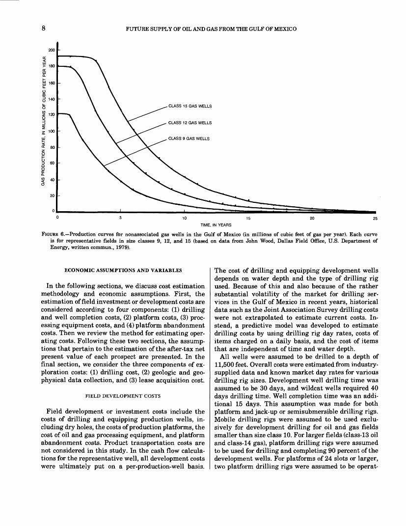
Nonassociated gas well production schedules also in­ dicate a constant initial production rate for a period followed by a decline in production according to a hyperbolic function. To estimate quantities of natural gas liquids expected to be produced by gas wells, the gas well production schedules were supplemented with information from a geologic resource appraisal of un­ discovered prospects in the Gulf of Mexico prepared for the U.S. Department of Energy (Richard Farmer, writ­ ten commun., 1982). The estimated natural gas liquid yield for the Miocene-Pliocene trend is 17.52 barrels of liquid per million cubic feet of gas produced, and, for the Pleistocene trend, the yield is 14.74 barrels of liquid per million cubic feet of gas. Figure 6 presents several nonassociated gas production profiles.

7 8 9 10 11 12 13 14 15 16 17 18 19 20 21 22 23 24 25

40

30

01 2345

FIGURE 5. Production curves for oil wells in the Gulf of Mexico (in thousands of barrels per year). Each curve is based on an average well for a representative field in size classes 9,12, and 15 (based on data from John Wood, Dallas Field Office, U.S. Department of Energy, written commun., 1979).

FUTURE SUPPLY OF OIL AND GAS FROM THE GULF OF MEXICO

TIME, IN YEARS

FIGURK 6. Production curves for nonassociated gas wells in the Gulf of Mexico (in millions of cubic feet of gas per year). Each curve is for representative fields in size classes 9, 12, and 15 (based on data from John Wood, Dallas Field Office, U.S. Department of Energy, written commun., 1979).

ECONOMIC ASSUMPTIONS AND VARIABLES

In the following sections, we discuss cost estimation methodology and economic assumptions. First, the estimation of field investment or development costs are considered according to four components: (1) drilling and well completion costs, (2) platform costs, (3) proc­ essing equipment costs, and (4) platform abandonment costs. Then we review the method for estimating oper­ ating costs. Following these two sections, the assump­ tions that pertain to the estimation of the after-tax net present value of each prospect are presented. In the final section, we consider the three components of ex­ ploration costs: (1) drilling cost, (2) geologic and geo­ physical data collection, and (3) lease acquisition cost.

FIELD DEVELOPMENT COSTS

Field development or investment costs include the costs of drilling and equipping production wells, in­ cluding dry holes, the costs of production platforms, the cost of oil and gas processing equipment, and platform abandonment costs. Product transportation costs are not considered in this study. In the cash flow calcula­ tions for the representative well, all development costs were ultimately put on a per-production-well basis.

The cost of drilling and equipping development wells depends on water depth and the type of drilling rig used. Because of this and also because of the rather substantial volatility of the market for drilling ser­ vices in the Gulf of Mexico in recent years, historical data such as the Joint Association Survey drilling costs were not extrapolated to estimate current costs. In­ stead, a predictive model was developed to estimate drilling costs by using drilling rig day rates, costs of items charged on a daily basis, and the cost of items that are independent of time and water depth.

All wells were assumed to be drilled to a depth of 11,500 feet. Overall costs were estimated from industry- supplied data and known market day rates for various drilling rig sizes. Development well drilling time was assumed to be 30 days, and wildcat wells required 40 days drilling time. Well completion time was an addi­ tional 15 days. This assumption was made for both platform and jack-up or semisubmersible drilling rigs. Mobile drilling rigs were assumed to be used exclu­ sively for development drilling for oil and gas fields smaller than size class 10. For larger fields (class-13 oil and class-14 gas), platform drilling rigs were assumed to be used for drilling and completing 90 percent of the development wells. For platforms of 24 slots or larger, two platform drilling rigs were assumed to be operat-

ENGINEERING-ECONOMIC MODEL

ing. A detailed accounting of the fixed and time-sensi­ tive costs is provided in Appendix A.

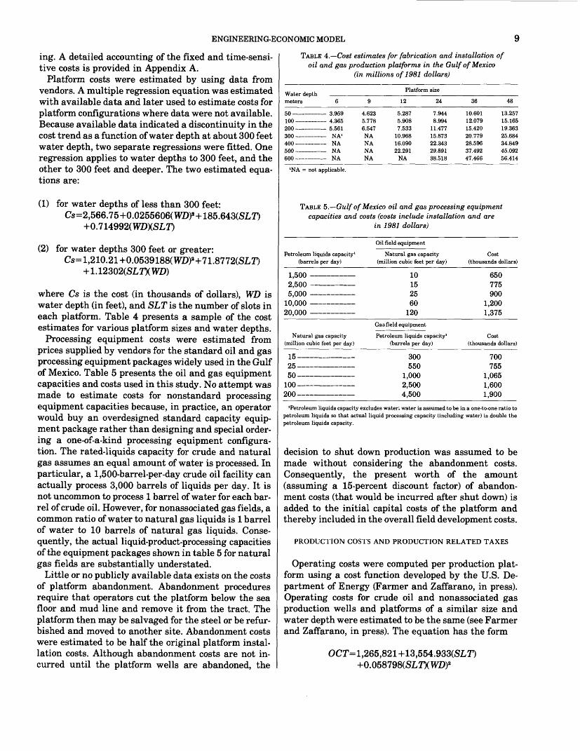
Platform costs were estimated by using data from vendors. A multiple regression equation was estimated with available data and later used to estimate costs for platform configurations where data were not available. Because available data indicated a discontinuity in the cost trend as a function of water depth at about 300 feet water depth, two separate regressions were fitted. One regression applies to water depths to 300 feet, and the other to 300 feet and deeper. The two estimated equa­ tions are:

(1) for water depths of less than 300 feet:Cs=2,566.75+0.0255606(WZ»2 -r-185.643(SLr)

+0.714992(WDXSL!T)

(2) for water depths 300 feet or greater:Cs=l,210.21+0.0539188(WD)2 +71.8772(SLr)

+1.12302(SLTXWD)

where Cs is the cost (in thousands of dollars), WD is water depth (in feet), and SLT is the number of slots in each platform. Table 4 presents a sample of the cost estimates for various platform sizes and water depths.

Processing equipment costs were estimated from prices supplied by vendors for the standard oil and gas processing equipment packages widely used in the Gulf of Mexico. Table 5 presents the oil and gas equipment capacities and costs used in this study. No attempt was made to estimate costs for nonstandard processing equipment capacities because, in practice, an operator would buy an overdesigned standard capacity equip­ ment package rather than designing and special order­ ing a one-of-a-kind processing equipment configura­ tion. The rated-liquids capacity for crude and natural gas assumes an equal amount of water is processed. In particular, a 1,500-barrel-per-day crude oil facility can actually process 3,000 barrels of liquids per day. It is not uncommon to process 1 barrel of water for each bar­ rel of crude oil. However, for nonassociated gas fields, a common ratio of water to natural gas liquids is 1 barrel of water to 10 barrels of natural gas liquids. Conse­ quently, the actual liquid-product-processing capacities of the equipment packages shown in table 5 for natural gas fields are substantially understated.

Little or no publicly available data exists on the costs of platform abandonment. Abandonment procedures require that operators cut the platform below the sea floor and mud line and remove it from the tract. The platform then may be salvaged for the steel or be refur­ bished and moved to another site. Abandonment costs were estimated to be half the original platform instal­ lation costs. Although abandonment costs are not in­ curred until the platform wells are abandoned, the

TABLE 4. Cost estimates for fabrication and installation ofoil and gas production platforms in the Gulf of Mexico

(in millions of 1981 dollars)

Water depth meters

Platform size

12 24 36 48

50 ________100 200

300400500 Cf\f\

3.9594.3655.561NA*

NANANA

4.6235.7786.547NANANANA

5.2875.9087.533

1ft Qfift

16.09022.291

NA

7.9448.994

11.4771 1; QTQ

99 ^A.^

29.891

10.60112.07915.42020 7799ft SQfi

37.49247.466

13.25715.16519.363

45.09256.414

'NA = not applicable.

TABLE 5. Gulf of Mexico oil and gas processing equipmentcapacities and costs (costs include installation and are

in 1981 dollars)

Petroleum liquids capacity1 (barrels per day)

Oil field equipment

Natural gas capacity (million cubic feet per day)

Cost (thousands dollars)

1,500 2,500 __*> 000

10,000 20,000

1015oc

60120

650775QOO

1,2001,375

Natural gas capacity (million cubic feet per day)

Gas field equipment

Petroleum liquids capacity* (barrels per day)

Cost (thousands dollars)

15 .25 -50 -100 -200 -

300550

1,0002,5004,500

700755

1,0651,6001,900

'Petroleum liquids capacity excludes water; water is assumed to be in a one-to-one ratio to petroleum liquids so that actual liquid processing capacity (including water) is double the petroleum liquids capacity.

decision to shut down production was assumed to be made without considering the abandonment costs. Consequently, the present worth of the amount (assuming a 15-percent discount factor) of abandon­ ment costs (that would be incurred after shut down) is added to the initial capital costs of the platform and thereby included in the overall field development costs.

PRODUCTION COSTS AND PRODUCTION RELATED TAXES

Operating costs were computed per production plat­ form using a cost function developed by the U.S. De­ partment of Energy (Farmer and Zaffarano, in press). Operating costs for crude oil and nonassociated gas production wells and platforms of a similar size and water depth were estimated to be the same (see Farmer and Zaffarano, in press). The equation has the form

OCT=1,265,821+13,554.933(SLT)+0.058798(SL7WZ»2

10 FUTURE SUPPLY OF OIL AND GAS FROM THE GULF OF MEXICO

where OCT is the operating costs per platform, SLT is the number of slots in the platform, and WD is the water depth in feet. The costs generated from this func­ tion are in 1977 dollars and were inflated by 1.736 to account for cost increases prior to 1981 (Funk and Anderson, 1982). Operating costs include overhead, insurance, transportation of personnel and other per­ sonnel services, well workovers, and maintenance.

Because most significant new fields are expected to be in Federal offshore waters, the only production taxes assumed for this study were Federal royalties at a rate of 16.7 percent. No other severance or State taxes were assumed to be imposed directly on field production.

ASSUMPTIONS FOR AFTER-TAX NET PRESENT VALUE CALCULATION

1. Estimated costs were based on those prevailing in 1981, so that the entire analysis assumed con­ stant 1981 dollars.

2. Operators have 100-percent working interest in the lease.

3. The Federal royalty rate of 16.7 percent on all pro­ duction applied (except where otherwise explicit­ ly stated), and no other State or local production taxes were assumed.

4. Federal income tax rate was assumed to be 46 per­ cent of taxable income.

5. No limit on the carry over of losses for income taxes was assumed.

6. Depreciation was calculated by the unit-of-produc- tion method.

7. The investment tax credit was computed as 10 per­ cent of all depreciable investment costs.

8. Cost depletion was applied when determining the depletion allowance for Federal income taxes. The basis for cost depletion included geologic and geophysical data collection costs and lease ac­ quisition costs. In 1979, the estimated expen­ diture on geophysical data collection was $196.5 million (U.S. Census Bureau, 1981). The Gulf of Mexico accounted for approximately 74 percent of the total 1979 geophysical crew months in the off­ shore conterminous 48 States (American Associa­ tion of Petroleum Geologists, 1980). There were 280 wildcat wells drilled in the Gulf of Mexico in 1979, so the geophysical cost per well was about $519,000 per well. These costs were inflated to $732,000 per wildcat well to 1981 dollars by us­ ing the general drilling cost inflation of 18.7 per­ cent experienced from 1979 to 1980 (American Petroleum Institute, 1982). Estimates of lease ac­ quisition costs were computed by multiplying the nominal field reserve by an assumed per BOE in

situ value. The assumed in situ values were ad­ justed for water depth to compensate for extra risks and costs of operating in the deep areas. The adjustment scheme is discussed in the presenta­ tion of specific results pertaining to alternate assumed lease acquisition costs (see p. 00). The computation of depletable cost per unit output is the sum of expenditures on lease acquisition and geologic and geophysical data collection divided by the initial estimated reserves (or proportion of working interest in reserves). For both cost deple­ tion and unit-of-production depreciation, cal­ culated reserves for each well or field were deter­ mined by assuming that production stops when the economic limit rate is reached. The economic limit rate is the production rate at which operating costs plus production-related taxes equal operators revenues.

9. We assumed that 70 percent of the drilling costs of successful wells along with costs of all dry wells were expensed and that all well completion costs, platform costs, and processing equipment costs were capitalized.

EXPLORATION COSTS

1. All wildcat wells are drilled to a target depth of 11,500 feet.

2. Expenditures for geologic and geophysical data col­ lection are set at $732,000 per wildcat well.

3. Explorationists were assumed to search nonprefer- entially for either oil or gas.

4. Newly drilled wildcat wells are allocated according to water depths in the same proportion as the per­ cent of total prospective area in each water depth interval.

5. Exploration costs associated with each increment of wildcat wells also include expenditures associ­ ated with lease acquisition. Total lease acquisi­ tion costs were estimated by multiplying the quantity of economic resources discovered with each wildcat well increment by an assumed in situ value of the resource. In this scheme, the in situ values are adjusted for cost differences and risks of operating at various water depths.

INDUSTRY BEHAVIOR AND MARKET CONDITIONS

Several assumptions associated with industry behav­ ior are reiterated here. First, it is assumed that field development design, along with development timing, are independent of current prices or operator price ex­ pectations. In practice, field design and development

FORECASTING FUTURE DISCOVERIES 11

staging are influenced by operators' cash flow needs and expectations about oil and gas prices. The result is a slight increase in actual development costs. It is also implicitly assumed that there will be sufficient excess capacity in the contract drilling industry and among equipment and platform suppliers to accommodate without substantial delays any change in industry activity.

This analysis assumes that lease selection practices will not be a constraint to explorationists. Further, it is also assumed that development of oil and gas resources in the Gulf of Mexico will not affect the price of oil or natural gas. Whereas this assumption is probably true for crude oil, it may not be realistic for natural gas, because in 1978 the Gulf accounted for 25 percent of U.S. natural gas production.

Lease acquisition costs were determined outside the model. Theoretically, the payments the petroleum in­ dustry makes to acquire prospective undeveloped oil and gas acreage is related to the in situ value of the resource. Uncertainty about the quantities of hydro­ carbons accounts for the deviation of expected discov­ ery costs (or resource replacement) from the in situ value of identified resources. Operators are risk averse, and the penalties associated with overestimating un­ discovered resources are much greater than for under­ estimating the resources. As a result, lease bids should understate the in situ value of the resources. Individual tracts also have qualities that influence the price that operators are willing to pay. For example, for offshore tracts, water depth significantly influences costs of development and therefore will affect the price that operators are willing to pay for the tract. Moreover, at any specific time, the willingness of the petroleum in­ dustry to acquire and explore in any given basin or area depends on the quality of exploration opportuni­ ties and discovery costs for other areas.

Because of these complicating factors, it was not sur­ prising that an analysis of long-term trends in bids for Federal offshore areas failed to yield a workable model that could be applied in this study to predict lease ac­ quisition costs. In view of this, lease costs are assumed and set on the basis of per unit of oil and gas reserves that were discovered. Computations of the future costs of finding and developing oil and gas in the Gulf of Mexico were made assuming a suite of values for lease acquisition costs. Lease acquisition costs do not influ­ ence the decision as to whether to develop a particular identified field. For an increment of 200 wildcat wells, however, all lease costs must be recovered through the industry's activities. Consequently, the lease costs are added to exploration costs and will determine, in part, when total exploration costs will exceed the returns from fields discovered by an increment of exploratory wells.

FORECASTING FUTURE DISCOVERIES

DISCOVERY PROCESS MODEL

The discovery process model applied here was devel­ oped by Drew and others (1982). They used the ana­ lytical structure devised by Arps and Roberts (1958) who assumed that, for any size class field, the probabil­ ity of discovery is directly proportional to the number of undiscovered fields and the ratio of their average areas to the effective basin area. A consequence of this assumption is that the largest fields in the basin tend to be found and developed early in the area's explora­ tion history.

The analytical form of the Arps-Roberts model sug­ gests that the proportion of undiscovered fields in a given size class declines exponentially as drilling con­ tinues. The cumulative number of discoveries expected to be made of fields for a given size class after drilling w cumulative wildcat wells is predicted with the equation:

where Ft(w) is the cumulative number of fields ex­ pected to be discovered in size class i by drilling w wild­ cat wells, Fj(oo) is the ultimate number of fields in size class i, B is the basin area, A; is the (average) area of fields in size class i, and Ct is the efficiency of discovery of fields in size class i. For random drilling, C;=l; if drilling is twice as efficient as random drilling, Ct =2. Arps and Roberts, in their initial application of the model, assumed a constant exploration efficiency across size classes.

In the application of the model to the Gulf of Mexico, Drew and others (1982) estimated the efficiency sepa­ rately for each size class. For most classes in the Miocene-Pliocene trend, the number of discoveries for equal increments of exploratory effort by size class had declined by January 1977. However, for the classes smaller than class 12, discovery rates had remained relatively constant through 1976. Substantial increases in new oil and natural gas prices that occurred in the early 1970's resulted in many more reported discov­ eries of fields that were formerly reported as only shows of hydrocarbons because they had not been com­ mercial. For size classes where the discovery data were thought to be influenced by economic truncation, C, and Fj(oo) were estimated by another method. Drew and others (1982) assumed that the ultimate underlying field size distribution is approximately log geometric in form. For example, for size class 12, the ultimate number of fields was estimated by multiplying the esti­ mated ultimate number for class 13 by 1.65; that is, /J_2=1.65 -ft where fi is the ultimate number of fields in

12 FUTURE SUPPLY OF OIL AND GAS FROM THE GULF OF MEXICO

size class i. This scheme was applied to size classes 9 through 12 for the Miocene-Pliocene trend.

For the sparsely explored Pleistocene trend, Drew and others (1982) used the Miocene-Pliocene trend as an analog. In particular, they assumed that the explo­ ration efficiencies estimated for the Miocene-Pliocene trend by size classes would prevail in the Pleistocene trend. These assumed class efficiencies, together with the number of discoveries for each size class, permitted the estimation of the ultimate number of fields by size class. For field size classes less than class 13 that ap­ pear to be affected by economic truncation, the same procedure used in the Miocene-Pliocene trend was ap­ plied to the estimation of the ultimate number of fields by size class. In particular, for fields in size class 12 or smaller, the ultimate number of fields was estimated by using the relation /|_; = 1.65 /-.

In table 6, parameters of the model used for estimat­ ing the rate of future discoveries are presented. The values for FX°°) are obtained by adding the number of fields discovered to the number remaining to be found. Forecasts of future discoveries were made for 60 incre­ ments of 200 wildcat wells. Of course, for any given price and discount rate, not all of these 60 increments of 200 wells were economical. The discovery process model predictions are aggregated into 3 groups of 20 successive increments of 200 wildcat wells for each trend and presented in table 7.

ESTIMATED MARGINAL COST FUNCTIONS FORUNDISCOVERED RECOVERABLE OIL AND GAS IN THE

GULF OF MEXICO

Table 8 presents estimates of marginal finding and production costs exclusive of the cost of lease acquisi­

tion. Because no lease acquisition costs are included, the costs underestimate the actual costs that firms will incur or, alternatively, the estimates of potential recoverable reserves are optimistic. However, these estimates indicate that even at $50 per BOE and a 5-percent after-tax rate of return, economic undiscov­ ered hydrocarbons in the Gulf of Mexico are about 33 percent of total discoveries to January 1977 (of 25.19 billion BOE). Furthermore, 13,600 wildcat wells (or well over 3 times the wildcat wells drilled through 1977) are needed to identify these resources.

The results presented in table 8 provide information to answer two questions: What price and rate of return are required to stimulate a certain level of exploration to find a given amount of oil and gas? What amount of oil and gas can be anticipated from the Gulf of Mexico at present or some future price and rate of return? According to table 8, at a 15-percent required rate of return, raising the wellhead price from $35 per BOE to $50 per BOE increases the number of economic wildcat wells from 5,600 to 9,600, or 71 percent. As a result, the total potential recoverable oil and gas resources in­ crease from 4.80 billion BOE to 6.78 billion BOE, or 41 percent. Thus, in this example, by raising the price 43 percent, from $35 to $50, an additional 70 percent more wildcat wells were economic and could be drilled, resulting in a 41-percent increase in hydrocarbon dis­ coveries. However, this additional quantity of hydro­ carbons amounts to only 8 percent of the amount of oil and gas discovered to January 1977.

The Miocene-Pliocene trend currently has about three times as many wildcat wells drilled in it as the Pleistocene trend. The analysis suggests that explora- tionists should optimally continue to drill the Miocene-

TABLE 6. Exploration efficiencies, areal extent, and expected remaining number of fields for various size classes in the Gulf of Mexico (from Drew and others, 1982, and J. H. Schuenemeyer, written commun., 1981)

Miocene-Pliocene trend1

Size class

9

1112131415 _____________ lg _____________ 17 _____________ 181Q90

Size range 10" BOE

0.19-0.38 0.38-0.76 0.76-1.52 1.52-3.04 3.04-6.07 6.07-12.14

1914 94 324.3 -48.6 48.6 -97.2 97.2 -194.3

194.3 -388.6 388.6 -777.2777 9 1 *\*\4. 9

1554.2 3108.4

Exploration efficiency

1.83 2.24 2.65 2.65 2.65 2.65 2.65 3.40 4.15 4.89 5.64

-

Area(mi2 )

0.61 .74 .92

1.18 1.58 2.17 3.09 4.55 6.93

10.91 17.17

_

Fields discoveredby 1/1/77

24 27 27 35 50 42 43 25 17

5 2

Number Cj of fields Exploration

remaining efficiency

2421.0 - 1468.0 - 864.4512.2 - 299.7 - 163.0 - 70.3 - 23.9 - 7.7 -

.8 - 0 - 00 -

Pleistocene trend2

Area (mi2)

0.61 .74 .92

1.18 1.58 1.66 2.58 4.03 4.28 9.79

15.26

-

Fields discovered by 1/1/77

9 11 20 17 21 26

9 8 3 1

Number of fields

remaining

976.6 591.9 349.7 206.4 111.8 62.9 30.3 13.9

1.4 .2

0 0

'Basin area (B) for the Miocene-Pliocene trend was 47,251 mi2.

2Basin area (B) for the Pleistocene trend was 12,983 mi*.

FORECASTING FUTURE DISCOVERIES 13

TABLE 7. Fields predicted to be found by 3 groups of 20 successive increments of 200 wildcat wells in the Miocene-Pliocene trend and in the Pleistocene trend (each group represents 4,000 wildcat wells in each trend)

Size class

Miocene-Pliocene trend

Wildcat well group I II III

Pleistocene trend

Wildcat well group I II III

7 -8-9 10-11 12 -13 -14 15 -16 -

202.90172.37141.33102.1274.0652.3335.1317.467.000.77

184.58149.79114.9978.3851.9632.1617.594.700.650.00

167.95116.4893.5360.1536.4729.428.761.190.030.00

178.51132.3099.0980.7261.7942.2426.6113.621.390.20

144.11100.6369.1646.2725.7410.913.250.220.000.00

116.3176.5648.2526.3510.722.810.400.000.000.00

Pliocene trend at about that same ratio. This result, which is somewhat unexpected, probably occurs for two reasons. First, according to table 2, none of the prospec­ tive target areas for the Pleistocene trend are in the shallowest water depth interval. Almost half (46 per­ cent) of the prospective area associated with the Pleistocene trend is located in water depths of greater than 240 feet, whereas 92 percent of the prospective area in the Miocene-Pliocene trend is located in water depths shallower than 240 feet. On the average, then, finding and development costs for Miocene-Pliocene trend areas will be much less than for comparably sized fields in the Pleistocene trend. Another reason for the larger number of wells in the Miocene-Pliocene trend is that it includes about 3.7 times the area of the Pleisto­ cene trend. This result is also independent of the lease costs when they are introduced.

Figure 7 indicates the hydrocarbon mix associated with the results presented in table 7. Most of the future hydrocarbons from the Gulf of Mexico will come pre­ dominately from what we have defined as nonassoci- ated natural gas fields. At a price of $35 per BOE (assuming a 15-percent rate of return), all liquids ac­ count for about 24 percent of the hydrocarbons on a BTu basis, whereas crude accounts for about 72 per­ cent of liquids or about 17 percent of all hydrocarbons discovered. Associated gas accounts for about 5 percent of the total hydrocarbons, and nonassociated gas ac­ counts for the remaining 71 percent of hydrocarbons. This mix of hydrocarbons holds for a wide range of prices and costs.

We might also compare the amount of resources dis­ covered with the ultimate amount of resources remain­ ing to be discovered. In this report, we have assumed an estimate of the nominal ultimate recovery for each field size class that is different from the historical average size of fields found in each size class. If the

assumptions used here were applied to the frequencies of remaining deposits (see table 6, size classes 8 to 16) that were estimated by Drew and others (1982), there would be 12.72 billion BOE of hydrocarbon resources remaining. Consequently, even at $50 per BOE (at a 5-percent required return), only 63 percent of the total resources would be found and developed. The remain­ ing resources beyond that amount would be very costly to find and develop without a significant technological breakthrough. Using the historical average for class size instead of the nominal recoveries used here, Drew and others (1982) estimated total remaining hydrocar­ bons to be 10.65 billion BOE or about 93 percent of the amount (11.48 billion BOE) that would have been ob­ tained using our nominal field sizes for classes 9 through 16. Because the data used for estimating the historical field size classes are based on proved reserves, the averages might be expected to increase as infield drilling results in larger estimates of reserves of the fields used in estimating the discovery process model. However, if the ultimate recovery of future dis­ coveries only matches the proved reserves of past dis­ coveries, then the overall results presented in table 8 should be reduced accordingly, to perhaps 93 percent of the values presented.

The results presented in table 8 are compared in figures 8 and 9 to cases where various lease acquisition costs were assumed. Introduction of positive lease costs in this analysis will not affect the decision to develop an already identified field. However, lease costs are added to exploration costs and therefore influence the number of wildcat wells that are determined to be eco­ nomic. Lease acquisition costs were introduced by assuming an in situ value per BOE adjusted for water depth for the resource. The amount of the required adjustment was estimated by running the economic model where lease costs were excluded and determin­ ing cost differences (reductions in after-tax present values) due to water depth costs. Analysis of the differ­ ences in the after-tax present values of marginal fields across the four water depth intervals used in this study indicate that, on the average (for a variety of prices and discount rates), the after-tax net present values of mar­ ginal fields at depth intervals of 60 to 240 feet, 240 to 393 feet, and 393 to 656 feet were 90 percent, 70 per­ cent, and 35 percent, respectively, of the values for the shallowest interval (0 to 60 feet) of water depth. These factors were used to scale the assumed in situ values of the resource.

Gruy and others (1982) recently reviewed prices paid for oil and gas reserves in merger and reserve acquisi­ tion transactions from 1979 to 1981. The prices ranged from $3.44 to $12.65 per BOE, with the most recent (February 1981) at $8.63. However, reserve estimates used in their study corresponded to currently recover-

TABL

E 8.

Pot

enti

al r

ecov

erab

le o

il a

nd g

as r

esou

rces

fro

m f

utu

re d

isco

veri

es i

n th

e G

ulf

of M

exic

o as

a f

unct

ion

of o

utpu

t pri

ce,

mar

gina

l fi

ndin

g

cost

, m

argi

nal p

rodu

ctio

n co

sts,

exp

lora

tory

wel

ls,

and

retu

rn o

n in

vest

men

t (R

OI)

(ex

clus

ive

of l

ease

cos

t)[B

OE

, bar

rels

of

oil

equi

vale

nt;

Tcf

, tr

illi

ons

of s

tand

ard

cubi

c fe

et o

f nat

ura

l ga

s]

Mio

cene

-Pli

ocen

e

Out

put

pric

e ($

/BO

E)

15

on oc 30 QC 40 -

45 50

Cum

ulat

ive

RO

I w

ildc

at

(per

cent

) w

ells

1

5 15

25 5 15

25

5 15

25 5 15

25

5 15

25 5 15

25 5 15

25

- -

- 5 15

25

800

2400

60

0

3800

18

00

200

5200

28

00

1200

6600

40

00

2000

8000

50

00

3000

9200

62

00

4000

1020

0 72

00

5000

Mar

gina

l co

sts2

Fin

ding

($

/BO

E)

3.06

4.41

2.

69

5.86

3.

71

2.17

7.55

4.

67

3.10

9.05

5.

99

3.80

10.5

7 7.

00

4.70

12.1

0 8.

18

5.60

13.5

3 9.

37

6.70

Pro

duct

ion

($/B

OE

)

11.9

4

15.5

9 17

.31

19.1

4 21

.29

22.8

3

22.4

5 25

.33

26.9

0

25.9

5 29

.01

31.2

0

29.4

3 33

.00

35.3

0

32.9

0 36

.82

39.4

0

36.4

7 40

.63

43.3

0

Tot

al

liqu

ids

(10"

)

.219

.563

.1

78

.797

.4

63

.067

.958

.6

61

.339

1.09

8 .8

34

.527

1.21

1 .9

56

.703

1.33

4 1.

079

.847

1.39

3 1.

176

.966

Tot

al g

as

Tcf

B

OE

(1

0")

4.34

4

11.0

28

3.48

6

15.0

96

8.99

4 1.

290

18.2

46

12.4

44

6.55

2

20.9

82

15.7

38

9.87

0

23.4

72

18.1

62

13.2

72

25.2

18

20.7

96

16.2

00

26.4

12

22.5

12

18.5

40

.724

1.83

8 .5

81

2.51

6 1.

499

.215

3.04

1 2.

074

1.09

2

3.49

7 2.

623

1.64

5

3.91

2 3.

027

2.21

2

4.20

3 3.

466

2.70

0

4.40

2 3.

752

3.09

0

Tot

al

BO

E

.943

2.40

1 .7

59

3.31

3 1.

962

.282

3.99

9 2.

735

1.43

1

4.59

5 3.

457

2.17

2

5.12

3 3.

983

2.91

5

5.53

7 4.

545

3.54

7

5.79

5 4.

928

4.05

6

Cum

ulat

ive

wil

dcat

w

ells

1

200

800

200

1200

60

0

1800

10

00

400

2200

14

00

600

2600

16

00

1000

3000

20

00

1200

3400

24

00

1600

Ple

isto

cene

Mar

gina

l co

sts*

Fin

ding

($

/BO

E)

2.65

4.30

2.

61

5.35

3.

53

7.30

4.

64

2.97

8.72

5.

85

3.45

10.0

8 6.

43

4.49

11.5

0 7.

66

5.02

13.2

8 9.

08

6.23

Pro

duct

ion

($/B

OE

)

12.3

5

15.7

0 17

.39

19.6

5 21

.47

22.7

0 25

.36

27.0

3

26.2

8 29

.16

31.5

5

29.9

2 33

.57

35.5

1

33.5

0 37

.34

39.9

8

36.7

2 40

.90

43.7

7

Tot

al

liqu

ids

(10'

)

.057

.194

.0

58

.268

.1

60

.343

.2

38

.113

.393

.2

99

.166

.431

.3

32

.243

.470

.3

78

.275

.497

.4

16

.335

Tot

al g

as

Tcf

B

OE

(1

09)

1.27

8

4.11

0 1.

296

5.57

4 3.

402

7.20

6 4.

968

2.47

2

8.05

2 6.

264

3.43

8

8.86

2 6.

804

5.06

4

9.53

4 7.

800

5.77

2

10.0

62

8.59

2 6.

900

.213

.685

.2

16

.929

.5

67

1.20

1 .8

28

.412

1.34

2 1.

044

.573

1.47

7 1.

134

.844

1.58

9 1.

300

.962

1.67

7 1.

432

1.15

0

Tot

al

BO

E(1

09)

.270

.879

.2

74

1.19

7.7

27

1.54

4 1.

066

.525

1.73

5 1.

343

.739

1.90

8 1.

466

1.08

7

2.05

9 1.

678

1.23

7

2.17

4 1.

848

1.48

5

Tot

al

liqu

ids

(bbl

)

.276

.757

.2

36

1.06

5 .6

23

.067

1.30

1 .8

99

.452

1.49

1 1.

133

.693

1.64

2 1.

288

.946

1.80

4 1.

457

1.12

2

1.89

0 1.

592

1.30

1

Tot

als

Tot

al g

as

Tcf

(1

0")

(BO

E)

5.62

2

15.1

38

4.78

2

20.6

70

12.3

96

1.29

0

25.4

52

17.4

12

9.02

4

29.0

34

22.0

02

13.3

08

32.3

34

25.2

66

18.3

36

34.7

52

28.5

96

21.9

72

36.4

74

31.1

04

25.4

40

.937

2.52

3 .7

97

3.44

5 2.

066

.215

4.24

2 2.

902

1.50

4

4.83

9 3.

667

2.21

8

5.38

9 4.

211

3.05

6

5.79

2 4.

766

3.66

2

6.07

9 5.

184

4.24

0

Tot

al

BO

E

(109

) (B

OE

)

1.21

3

3.28

0 1.

033

4.51

0 2.

689

.282

5.54

3 3.

801

1.95

6

6.33

0 4.

800

2.91

1

7.03

1 5.

449

4.00

2

7.59

6 6.

223

4.78

4

7.96

9 6.

776

5.54

1

02 O

*1 O 1 i s = W

O a o

O

'Exp

lora

tory

wel

ls a

ssum

ed to

be

dril

led

sinc

e D

ecem

ber

31,1

976.

The

sto

ppin

g ru

le fo

r exp

lora

tory

wel

ls d

oes

not t

ake

into

acc

ount

the

tax

bene

fit o

f cha

rgin

g th

e co

st o

f exp

lora

tory

wel

ls a

gain

st

curr

ent

inco

me.

The

refo

re,

thes

e fi

gure

s ov

eres

tim

ate

the

effe

ctiv

e co

st o

f ex

plor

ator

y dr

illi

ng.

'At

the

mar

gin,

th

e su

m o

f th

e m

argi

nal

find

ing

cost

and

th

e m

argi

nal

prod

ucti

on c

ost

is e

qual

to

the

outp

ut p

rice

(co

lum

n 1)

.

FORECASTING FUTURE DISCOVERIES 15

CO

81-

LJJ

Q. O 111

LU CC O LU

is

is

50

45

40

35

30

2 25ODC

20

/ / 11CO<

h O Q

£ <O ,

SiCO i< '

1 ' J* I

I / /M /

ILL

ol tu ,

/

*

/

01 234 56 7

UNDISCOVERED PETROLEUM, IN BILLIONS OF BOE

FIGURE 7. Marginal costs of recoverable oil and gas resources (in dollars per barrel of oil equivalent (BOE)), by form of hydrocarbon, from undiscovered fields (as of January 1, 1977) in the Gulf of Mexico (15 percent discounted cash flow return and zero lease cost assumed).

able reserves with production facilities already in place. Consequently, we performed the economic anal­ ysis using $1.50 and $3.00 per BOE as in situ values of the resource.

In figure 8, the number of economic wildcat wells is shown as a function of marginal finding and produc­ tion costs for cases where assumed in situ resource values were zero, $1.50 per BOE, and $3.00 per BOE. Figure 9 shows the relation between potential recover-

IN SITU VALUE OFRESOURCE PER BOE

$3.00 $1.50 $0.0

PCO

81-

UJ

O. LUQ ou m> DC LU LU Q Q- Q CO^ DC<5

li-z. -z. C ~ _i1

gi

45

40

35

30

25

20

I 1 1 I I 1 1 J 1 X" 'X

x x X x XX

x' / S' / ,'

/ / '.' .' .'XX'

X x x X / ^

/ / "X * ' X

x x xX X X

X / X X"* '"

X X

/ 'X , x

XX

X-X , i ,,,,,,

01 23456789 10

WILDCAT WELLS, IN THOUSANDS

FIGURE 8. Wildcat wells projected to be drilled in the Gulf of Mexico as a function of marginal finding and development costs of oil and gas (in dollars per barrel of oil equivalent (BOE)) and in situ per barrel of oil equivalent costs of resources (15-percent discounted cash flow return assumed).

able undiscovered reserves as a function of marginal finding and production costs for these same assumed in situ resource values. Figures 8 and 9 assume a 15-per­ cent return on investments. At $35 per BOE, figure 7 indicates recoverable resources for the $3.00 per BOE

IN SITU VALUE OF RESOURCE PER BOE

$3.00 $1.50 $0.0

co 50to O" 45

O § 40^JLU EC> LULU Q.

0 8 35 z. << 3o oi Q 30

9c25

20

J* .' / /

/

/

/ s

01234567

UNDISCOVERED PETROLEUM, IN BILLIONS OF BOE

FIGURE 9. Marginal cost of recoverable oil and gas resources (in dollars per barrel of oil equivalent (BOE)) from undiscovered fields (as of January 1,1977) in the Gulf of Mexico as a function of in situ per barrel of oil equivalent costs of resources (15-percent discounted cash flow return assumed ).

16 FUTURE SUPPLY OF OIL AND GAS FROM THE GULF OF MEXICO

in situ costs at about 68 percent of the zero lease cost estimate, and for $1.50 per BOE recoverable resources are about 85 percent of the zero lease cost estimate. At $50 per BOE, the estimate at $3.00 per BOE in situ costs is almost 90 percent of the zero lease cost esti­ mate, whereas the estimate assuming $1.50 per BOE in situ value was 91 percent of the zero lease cost esti­ mate. As price and prevailing marginal costs are per­ mitted to increase, relative differences in these poten­ tial discoveries diminish because the discovery rates are continually declining. In particular, although the higher prices (and lower in situ values) permit more wildcat wells to be drilled, the economic resources per wildcat well increment diminishes with the cumula­ tive number of wildcat wells.

CONCLUSIONS AND IMPLICATIONS

The analysis shows that, at $35 per BOE and at a 15-percent rate of return (without lease acquisition costs), the potential recoverable oil and gas discovered after January 1, 1977, is estimated to be 4.80 billion BOE. This amount is less than 19 percent of the esti­ mated combined oil and gas discovered through 1976. Even at $50 per barrel (and a 15-percent return), the expected discoveries yield only 6.78 billion BOE from new fields, which is still only 27 percent of past discov­ eries. Without technological breakthroughs, additional oil and gas beyond this amount is likely to be very cost­ ly to find and develop.

The economic analysis indicates that, for every wild­ cat well drilled in the Pleistocene trend, there probably will be two or three wildcat wells drilled in the Mio­ cene-Pliocene trend. Higher costs due to greater water depths for fields in the Pleistocene trend and the larger prospective area in the Miocene-Pliocene trend con­ tribute to this result.

In all cases studied, if trends of the past 10 to 12 years continue, over 71 percent of resources in future

discoveries will be in the form of nonassociated gas, and less than 17 percent of these resources will be in the form of crude oil.

Future oil and gas exploration in the Gulf of Mexico can still be profitable. At a 15-percent return and $35 per BOE with lease costs corresponding to $3.00 per BOE for the in situ resources, an additional 3,000 wild­ cat wells (after January 1, 1977) can be commercially drilled. However, these wells are expected to yield only 3.26 billion BOE of new reserves, which is less than 3 years of production at the 1977 level of 1.1 billion BOE per year. Moreover, because these fields will generally be smaller and in deeper water depths, the oil and gas from the new discoveries will be more difficult and costly to produce.

REFERENCES CITED

American Petroleum Institute, 1982, American Petroleum Institute Basic Petroleum Data Book: v. 11, no. 2, Washington, D.C.

American Association of Petroleum Geologists, 1980, North American Developments Issue: Bulletin of the American Association of Petroleum Geologists, v. 64, no. 9, p. 1291-1570.

Arps, J. J., and Roberts, T. G., 1958, Economics of Cretaceous oil on the east flank of the Denver-Julesburg basin: Bulletin of American Association of Petroleum Geologists, v. 42, no. 11, p. 2549-2566.

Drew, L. J., Schuenemeyer, J. H., and Bawiec, W. J., 1982, Estima­ tion of the future rates of oil and gas discoveries in the western Gulf of Mexico: U.S. Geological Survey Professional Paper 1252, 26 p.

Farmer, Richard, and Zaffarano, Richard, OCS oil and gas supply model Data description, v. 3: U.S. Department of Energy tin press].

Funk, V. T., and Anderson, T. C., 1982, Cost indexes for domestic oil and gas field equipment and production operations, 1981: U.S. Department of Energy, Energy Information Administration, Washington, D.C., 158 p.

Gruy, H. J., Garb, F. A., and Wood, J. W., 1982, Determining the value of oil and gas in the ground: World Oil, March, p. 105-108.

U.S. Bureau of the Census, 1981, Current Industrial Reports, Series MA-13K(79)-1, Annual Survey of Oil and Gas, 1979: U.S. Govern­ ment Printing Office, Washington, D.C., 74 p.

APPENDIX A. FIELD EQUIPMENTCONFIGURATION, COSTS, AND

DEVELOPMENT PROFILES

This section presents assumptions and data relating to offshore field development equipment configurations and practices. Although one might find various opera­ tors using many different configurations to develop fields of similar sizes and at similar water depths, we felt that the particular configurations used in this study are representative of current practices in the Gulf of Mexico.

Development well, platform, and processing equipment configurations for newly discovered oil fields and for newly discovered nonassociated gas fields are presented in tables Al and A2, respectively. The configurations were designed to allow for a degree of expected excess capacity (in terms of platform slots and processing equipment capacity) that generally prevails in Gulf of Mexico production practices. As indicated by these tables, in cases where water depths were greater than 300 feet, the minimum platform costs were the same as costs associated with a 12-slot platform at that particular water depth, even though a platform of less than 12 slots would actually be constructed. The mini­ mum amount of steel and the number of pilings re­ quired for operation of the smaller platforms at these water depths would be approximately equal to the amounts used in fabrication of a 12-slot platform.

TABLE Al. Development well, platform, and processing equipment configurations for new oil fields in the Gulf of Mexico

Field Platform size Number of size classes wells (slots)

7 _____

9 _______1011 _______1913 _____14 _______15 _____16 ____1718 19 _____20

0

0

34579

142033KK

82163303

12 1 , 412l,4121 , 41O1 A

121, 6191 Q

1218121219

121212

Processing equipment capacity

Gas (106 ftfVd)

151515OK

50en

100100100100100100100100

Liquids Number of platforms (bbl/d) and equipment package

300300300KKf\

1,0001,0002,5002,5002,5002,5002,5002,5002,5002,500

1111111123

81632

TABLE A2. Development well, platform, and processingequipment configurations for new nonassociated gas fields

in the Gulf of Mexico

1 For water depths greater than 300 feet, 12-slot platform costs were used.

Table A3 presents the particular platform fabrication and installation costs that were used in this study. Estimates of platform operating costs (also used in this study) are presented in table A4.

The cost of drilling exploratory and development wells offshore was estimated with data supplied by industry sources. Components of drilling and well- completion costs were classified as either a time-sensi­

Field size classes

7 _______

8 ______

-LV/

1112 ______ 13 _____

1*i1617 _____ 18 1Q90

"For water dep

Number of wells

2 3 3 5 8

13 23 40 68

117 201 343 599

1,022

Platform size

(slots)

12 1 , 4 12l , 4 121 , 4 121 , 6 121 , 9

18 24 24 24 24 42 40 42 36

Processing equipment capacity

Liquids (bbVd)

1,500 1,500 2,500 2,500 2,500 5,000

10,000 10,000 10,000 10,000 20,000 20,000 20,000 20,000

ths greater than 300 feet, 12-slot

Associated gas (106 ftVd)

10 10 15 15

25 60 60 60 60

120 120 120 120

Number of platforms and equipment package

1

1

1

1

1

1

1

2 3 5 5 9

15 30

platform costs were used.

tive cost or a cost fixed for a given drilling depth. Costs for all wildcat wells and dry development wells did not

TABLE A3. Estimates of platform fabrication and installation costs (size vs. water depth) for the Gulf of Mexico (in millions of dollars, costs as of 1981)

Platform size

4-slot 6-slot 9-slot

12-slot 18-slot 24-slot 36-slot

4.9 «lnt

Water depths (feet)

40 150 317 525

3.645 4.313 NA NA 3.893 4.900 NA NA 4.536 5.778 NA NA 5.179 6.657 11.763 24.009 6.464 8.414 14.330 27.978 7.749 10.171 16.897 31.947

10.320 13.686 22.032 39.884 11.177 14.858 23.743 42.530 11.606 15.443 24.599 43.853

'NA = not applicable.

17

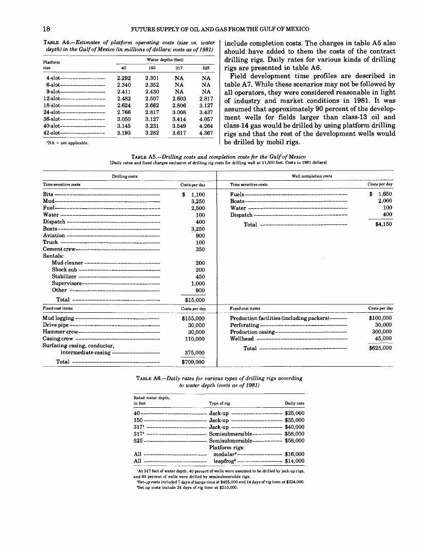
18 FUTURE SUPPLY OF OIL AND GAS FROM THE GULF OF MEXICO

TABLE A4. Estimates of platform operating costs (size vs. water depth) in the Gulf of Mexico (in millions of dollars; costs as of 1981)

_. _ Water depths (feet) Platformsize 40 150 317 525

4-slot 2.292 2.301 NA NA 6-slot 2.340 2.352 NA NA9-slot 2.411 2.430 NA NA

12-Qlnt 9 4ft9 9^07 9 fiO3 9 ftl 7

18-slot 2.624 2.662 2.806 3.12794 csl/vf O 1RR O Q1 7 Q DDQ Q A Q7

36-slot 3.050 3.127 3.414 4.057 40-slot 3.145 3.231 3.549 4.26442-slot 3.193 3.282 3.617 4.367

include completion costs. The charges in table A5 also should have added to them the costs of the contract drilling rigs. Daily rates for various kinds of drilling rigs are presented in table A6.

Field development time profiles are described in table A7. While these scenarios may not be followed by all operators, they were considered reasonable in light of industry and market conditions in 1981. It was assumed that approximately 90 percent of the develop­ ment wells for fields larger than class- 13 oil and class- 14 gas would be drilled by using platform drilling rigs and that the rest of the development wells would

>NA = not applicable. be drilled by mobil rigs.

TABLE A5. Drilling costs and completion costs for the Gulf of Mexico[Daily rates and fixed charges exclusive of drilling rig costs for drilling well at 11,500 feet. Costs in 1981 dollars]

Drilling costs

Time sensitive costs Costs per day

MuH 3 9 c>fl

Wat6r 100Dispatch 400Rrtafo Q OCfi

Truck 100fl^TTi^nl" r»tVMJi7 QP\fi

Rentals: Mud cleaner 200 Shock sub 200 Stabilizer 450

Othpr * Qfin

Total $15,000

Fixed cost items Costs per day

Mud logging $155,000 Drive pipe 30 ,000

Surfacing casing, conductor, intermediate casing 375,000

Total $700,000

Well completion costs

Time sensitive costs Costs per day

TTiiolc $ 1 650

Boats 2 000Water 100rti cnn trVi 400

Total $4,150

Fixed cost items Costs per day

Production facilities (including packers) $100,000 Perforating 30,000PrnHiir>tinn rasincr 300 000

WollVioarl _ AK. 000

Total $625,000

TABLE A6. Daily rates for various types of drilling rigs according to water depth (costs as of 1981)

Rated water depth, in feet Type of rig Daily rate

40 .Tnrlr nn $25 000

150 Jack-up $35,000317 1 Jack-up $40,000 317 1 Semisubmersible $58,000 525 Semisubmersible $58,000

Platform rigs: All modular2 $16,000All Ipnnfrncr3 $14000

'At 317 feet of water depth, 40 percent of wells were assumed to be drilled by jack-up rigs, and 60 percent of wells were drilled by Semisubmersible rigs.

'Set-up costs included 7 days of barge time at $455,000 and 14 days of rig time at $224,000. 3Set-up costs include 24 days of rig time at $210,000.

APPENDIX A

TABLE A7. Development strategies: Drilling and production schedules

19

I. Classes 5-9: Smaller than class 10 for both oil and gas; it is assumed that the development takes place within 1 year and, for accounting purposes, drilling and production are almost instantaneous. Some of early project costs are adjusted to correct for this assumption.

II. Classes 10 and 11 (oil) and classes 10,11,12 (gas): All drilling and platform expenditures occur during year 1, and production begins in year 2 (class 12 gas same as above).

III. Classes 12, 13, and 14 (oil) and classes 13, 14, 15, and 16 (gas):

Expenditures

% cost item

Drilling

Platform

Processing equipment

Revenue stream% of total wells coming into production

Year

1

50

50

50

0

2

50

50

50

50

3

50

IV. Classes 15 and 16 (oil); and classes 17, 18, and 19 (gas):

Expenditures:

% cost item

Drilling

Platform

Processing equipment

Revenue stream% of total wells coming into production

V. Class 17 (oil) and class 20 (gas):

Expenditures

% cost item

Drilling

Platform

Processing equipment

Revenue stream% of total wells coming into production

VI. Classes 18, 19, and 20 (oil):

Expenditures

% cost item

Drilling

Platform

Processing equipment

Revenue stream% of total wells coming into production

Year

1

40

40

40

0

2

35

35

35

30

3

25

25

25

45

4

25

Year

1

35

35

35

0

2

35

35

35

20

3

20

20

20

30

4

10

10

10

40

5

10

Year

1

20

20

20

0

2

30

30

30

15

3

30

30

30

25

4

15

15

15

25

5

5

5

5

25

6

10

'Exploratory wells assumed to be drilled since December 31,1976. The stopping rule for exploratory wells does not take into account the tax benefit of charging the cost of exploratory wells against current income. Therefore, these figures overestimate the effective cost of exploratory drilling.

'At the margin, the sum of the marginal finding cost and the marginal production cost is equal to the output price (column 1).

APPENDIX B. OIL AND NONASSOCIATED GAS WELL PRODUCTION SCHEDULES

Oil and nonassociated gas well production schedules were developed by the Dallas Field Office of the U.S. Department of Energy for another study. The following is a description of the equations used in the generation of the production schedules (John Wood, U.S. Depart­ ment of Energy, written commun., 1979).

Oil well schedules. Wells that represent field size classes of larger than 10 are assumed to produce at a constant rate for a period of time. Wells representing size classes of fields smaller than class 11 are assumed to decline immediately according to a hyperbolic func­ tion. The following variables are defined:

t = current time period,q0 = initial well production rate,Np(t) = cumulative oil production to time t in

barrels, Gp(t) = cumulative associated gas production in

thousands of cubic feet, Nu = expected ultimate per well oil recovery in

barrels,D = exponential decline rate, td = deliverability life in years, qa = nominal 1978 offshore abandonment rate of

9,125 barrels per year or 25 barrels perday,

g = gas-to-oil ratio in thousands of cubic feetper barrel,

ap(t) = annual oil production, ag(f) = annual associated gas production.

For fields in size classes 7 through 20:

Nu+qa"° fc+Cl/D)

Ift<td, then Np(f)=t(q0l Otherwise

D

Annual oil production is ap(t)=Np(t)-Np(t-l), and an­ nual gas production is ag(t)=g ap(t).

Values of parameters associated with each size class field are presented in Table Bl.

Nonassociated gas production schedules. Gas deliv­ erability was computed on a well basis by number of wells per field using the computer program developed by J. N. Hicks (Dallas Field Office, Department of Energy, 1976). Initial gas rates were based on 25 per­ cent of initial open flow production, except in class 20 where 24 percent was used. The predictive equation for generating future nonassociated gas production prior to the production decline is Gp(t)=tdqg. With the onset of decline, the predictive equation is

where Gp(f) is cumulative gas production to time t in million cubic feet, td is the period of constant produc­ tion, qc is the initial constant gas production rate in millions of cubic feet per year, qg is the initial gas pro­ duction rate in millions of cubic feet per year for the decline curve, a is the initial loss ratio, and b is the first derivative (with respect to time) of the loss ratio (b is dimensionless). Values for the parameters associated with each size class field are presented in Table B2.

TABLE Bl. Oil production schedule constants for Texas and Louisiana offshore oil fields by size class

[Nu is expected ultimate per well oil recovery in barrels; D is the exponential decline rate; td is deliverability life in years]

Size class

7

gg ___________

10 ___________11 ___________

1213 14 ___________15 ___________16 17lg ___________19 ___________20 _______

N

111,0001 rjo AAA

270,000387,000466,000545,000637,000744,000870,000

1,020,0001 1 on nnn

1,390,0001,620,0001,900,000

D

0.3400.3100.2860.2660.251A OOQ

0.2270.2170.2090.2020.1950.1900.1850.180

td

00000.51.01.52.02.53.0q c

4.04.55.0

Gas/oil ratio

(bbl/mcfl

1 q1 R

1.81.71.71.71.61.61.61.51.51.51.41.4

20

FUTURE SUPPLY OF OIL AND GAS FROM THE GULF OF MEXICO

TABLE B2. Nonassociated gas production equation parameters[trf is the period of constant production, in years; qc is the initial constant gas production

rate, in millions of cubic feet per year; <?~ is the initial gas production rate, in millions of cubic feet per year, for the decline curve; a is the initial loss ratio; 6 is the first derivative of the loss ratio]

21

Size class

7

g

9101112 ___________13 ___________14 ___________15 ___________lg ___________17 ___________lg ___________19 ___________20

*d

0.43f\ CO

0 Qi 07

1.712.252.863.524.174.765.255.575.706.04

1c

coo A etc

1 1 70 qc1 O£C 1

1551.251 7^,9 ft

1956.42168.12383.452606.12839.73076.953321.53569.73686.5

igCQQ An

1 1Q9. Q

1QQO C

000*7 Q£

1QCA 7C

1790.692118.772441.62487.962937.583129.783353.543593.253710.69

a

0.748033A rr A OAOO

0 7/1 ftAOO

0 74QAOO

1 9°.7ft°.

1.835602.611382.624744.623213.905494.673995.340456.027736.27156

6

0 1 OAQC

0 1 OAQC

0 1 OAQC

0 1 OAQC

0 1 ee£*£*

-0.15641-0.20523-0.0485-0.21428-0.05787-0.08371-0.10133-0.11818-0.23789

6U.S. GOVERNMENT PRINTING OFFICE: 1983-381-419/115