fuzzy clustering and data analysis toolbox

Fuzzy Clustering and DataAnalysis Toolbox

For Use with Matlab

Balazs Balasko, Janos Abonyi and Balazs Feil

Preface

About the Toolbox

The Fuzzy Clustering and Data Analysis Toolbox is a collection of Matlabfunctions. Its propose is to divide a given data set into subsets (calledclusters), hard and fuzzy partitioning mean, that these transitions betweenthe subsets are crisp or gradual.The toolbox provides four categories of functions:

• Clustering algorithms. These functions group the given data setinto clusters by different approaches: functions Kmeans and Kmedoidare hard partitioning methods, FCMclust, GKclust, GGclust are fuzzypartitioning methods with different distance norms that are defined inSection 1.2.

• Evaluation with cluster prototypes. On the score of the cluster-ing results of a data set there is a possibility to calculate membershipfor ”unseen” data sets with these set of functions. In 2-dimensionalcase the functions draw a contour-map in the data space to visualizethe results.

• Validation. The validity function provides cluster validity measuresfor each partition. It is useful, when the number of cluster is un-known apriori. The optimal partition can be determined by the pointof the extrema of the validation indexes in dependence of the numberof clusters. The indexes calculated are:Partition Coefficient(PC), Clas-sification Entropy(CE),Partition Index(SC), Separation Index(S), Xie andBeni’s Index(XB), Dunn’s Index(DI) and Alternative Dunn Index(DII).

• Visualization The Visualization part of this toolbox provides themodified Sammon mapping of the data. This mapping method is a

i

multidimensional scaling method described by Sammon. The originalmethod is computationally expensive when a new data point has tobe mapped, so a modified method described by Abonyi got into thistoolbox.

• Example. An example based on industrial data set to present theusefulness of the purpose of these algorithms.

Installation

The installation is straightforward and it does not require any changes toyour system settings. If you would like to use these functions, just copy thedirectory ”FUZZCLUST” within its files where the directory ”toolbox” issituated (...\ MATLAB\ TOOLBOX \ ...).

Contact

Janos Abonyi or Balazs Feil:Department of Process Engineering University of VeszpremP.O.Box 158 H-8200, Veszprem, HungaryPhone: +36-88-422-022/4209 Fax: +36-88-421-709E-mail: [email protected], [email protected]: (www.fmt.vein.hu/softcomp)

Fuzzy Clustering and Data Analysis Toolbox ii

Contents

1 Theoretical introduction 3

1.1 Cluster analysis . . . . . . . . . . . . . . . . . . . . . . . . . . 3

1.1.1 The data . . . . . . . . . . . . . . . . . . . . . . . . . . 4

1.1.2 The clusters . . . . . . . . . . . . . . . . . . . . . . . . 4

1.1.3 Cluster partition . . . . . . . . . . . . . . . . . . . . . . 5

1.2 Clustering algorithms . . . . . . . . . . . . . . . . . . . . . . . 8

1.2.1 K-means and K-medoid algorithms . . . . . . . . . . . . 8

1.2.2 Fuzzy C-means algorithm . . . . . . . . . . . . . . . . . 8

1.2.3 The Gustafson–Kessel algorithm . . . . . . . . . . . . . 10

1.2.4 The Gath–Geva algorithm . . . . . . . . . . . . . . . . . 11

1.3 Validation . . . . . . . . . . . . . . . . . . . . . . . . . . . . . 13

1.4 Visualization . . . . . . . . . . . . . . . . . . . . . . . . . . . . 15

1.4.1 Principal Component Analysis (PCA) . . . . . . . . . . 16

1.4.2 Sammon mapping . . . . . . . . . . . . . . . . . . . . . 17

1.4.3 Fuzzy Sammon mapping . . . . . . . . . . . . . . . . . 18

2 Reference 19

Function Arguments . . . . . . . . . . . . . . . . . . . . . . . . 21

Kmeans . . . . . . . . . . . . . . . . . . . . . . . . . . . . . . 24

Kmedoid . . . . . . . . . . . . . . . . . . . . . . . . . . . . . . 28

1

FCMclust . . . . . . . . . . . . . . . . . . . . . . . . . . . . . 31

GKclust . . . . . . . . . . . . . . . . . . . . . . . . . . . . . . 35

GGclust . . . . . . . . . . . . . . . . . . . . . . . . . . . . . . 39

clusteval . . . . . . . . . . . . . . . . . . . . . . . . . . . . . . 43

validity . . . . . . . . . . . . . . . . . . . . . . . . . . . . . . . 45

clustnormalize and clustdenormalize . . . . . . . . . . . . . . . 46

PCA . . . . . . . . . . . . . . . . . . . . . . . . . . . . . . . . 48

Sammon . . . . . . . . . . . . . . . . . . . . . . . . . . . . . . 50

FuzSam . . . . . . . . . . . . . . . . . . . . . . . . . . . . . . 51

projeval . . . . . . . . . . . . . . . . . . . . . . . . . . . . . . 53

samstr . . . . . . . . . . . . . . . . . . . . . . . . . . . . . . . 54

3 Case Studies 55

3.1 Comparing the clustering methods . . . . . . . . . . . . . . . . 56

3.2 Optimal number of clusters . . . . . . . . . . . . . . . . . . . . 60

3.3 Multidimensional data sets . . . . . . . . . . . . . . . . . . . . 63

3.3.1 Iris data set . . . . . . . . . . . . . . . . . . . . . . . . 65

3.3.2 Wine data set . . . . . . . . . . . . . . . . . . . . . . . 67

3.3.3 Breast Cancer data set . . . . . . . . . . . . . . . . . . 69

3.3.4 Conclusions . . . . . . . . . . . . . . . . . . . . . . . . 71

Fuzzy Clustering and Data Analysis Toolbox 2

Chapter 1

Theoretical introduction

The aim of this chapter is to introduce the theories in the fuzzy clustering sothat one can understand the subsequent chapter of this thesis at a necessarylevel. Fuzzy clustering can be used as a tool to obtain the partitioning of data.Section 1.1 gives the basic notions about the data, clusters and different typesof partitioning. Section 1.2 presents the description of the algorithms used inthis toolbox. The validation of these algorithms is described in Section 1.3.Each discussed algorithm has a demonstrating example in Chapter 2 at thedescription of the Matlab functions.For a more detailed treatment of this subject see the classical monograph byBezdek [1] or Hoppner’s book [2]. The notations and the descriptions of thealgorithms closely follow the structure used by [3].

1.1 Cluster analysis

The objective of cluster analysis is the classification of objects according to sim-ilarities among them, and organizing of data into groups. Clustering techniquesare among the unsupervised methods, they do not use prior class identifiers.The main potential of clustering is to detect the underlying structure in data,not only for classification and pattern recognition, but for model reduction andoptimization.Different classifications can be related to the algorithmic approach of the cluster-ing techniques. Partitioning, hierarchical, graph-theoretic methods and meth-ods based on objective function can be distinguished. In this work we haveworked out a toolbox for the partitioning methods, especially for hard and fuzzypartition methods.

3

1.1. CLUSTER ANALYSIS

1.1.1 The data

Clustering techniques can be applied to data that is quantitative (numerical),qualitative (categoric), or a mixture of both. In this thesis, the clustering ofquantitative data is considered. The data are typically observations of somephysical process. Each observation consists of n measured variables, groupedinto an n-dimensional row vector xk = [xk1, xk2, . . . , xkn]T ,xk ∈ Rn. A set ofN observations is denoted by X = {xk|k = 1, 2, . . . , N}, and is represented asan N × n matrix:

X =

x11 x12 · · · x1n

x21 x22 · · · x2n...

.... . .

...xN1 xN2 · · · xNn

. (1.1)

In pattern recognition terminology, the rows of X are called patterns or objects,the columns are called the features or attributes, and X is called the patternmatrix. In this thesis, X is often referred to simply as the data matrix.The meaning of the columns and rows of X with respect to reality dependson the context. In medical diagnosis, for instance, the rows of X may repre-sent patients, and the columns are then symptoms, or laboratory measurementsfor the patients. When clustering is applied to the modeling and identificationof dynamic systems, the rows of X contain samples of time signals, and thecolumns are, for instance, physical variables observed in the system (position,velocity, temperature, etc.). In order to represent the system’s dynamics, pastvalues of the variables are typically included in X as well.In system identification, the purpose of clustering is to find relationships be-tween independent system variables, called the regressors, and future values ofdependent variables, called the regressands. One should, however, realize thatthe relations revealed by clustering are just causal associations among the datavectors, and as such do not yet constitute a prediction model of the given sys-tem. To obtain such a model, additional steps are needed.

1.1.2 The clusters

Various definitions of a cluster can be formulated, depending on the objective ofclustering. Generally, one may accept the view that a cluster is a group of objectsthat are more similar to one another than to members of other clusters. Theterm ”similarity” should be understood as mathematical similarity, measuredin some well-defined sense. In metric spaces, similarity is often defined by



means of a distance norm. Distance can be measured among the data vectorsthemselves, or as a distance form a data vector to some prototypical object ofthe cluster. The prototypes are usually not known beforehand, and are soughtby the clustering algorithms simultaneously with the partitioning of the data.The prototypes may be vectors of the same dimension as the data objects, butthey can also be defined as ”higher-level” geometrical objects, such as linear ornonlinear subspaces or functions.

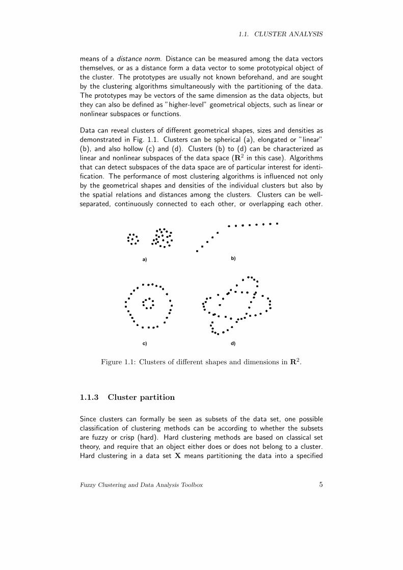
Data can reveal clusters of different geometrical shapes, sizes and densities asdemonstrated in Fig. 1.1. Clusters can be spherical (a), elongated or ”linear”(b), and also hollow (c) and (d). Clusters (b) to (d) can be characterized aslinear and nonlinear subspaces of the data space (R2 in this case). Algorithmsthat can detect subspaces of the data space are of particular interest for identi-fication. The performance of most clustering algorithms is influenced not onlyby the geometrical shapes and densities of the individual clusters but also bythe spatial relations and distances among the clusters. Clusters can be well-separated, continuously connected to each other, or overlapping each other.

Figure 1.1: Clusters of different shapes and dimensions in R2.

1.1.3 Cluster partition

Since clusters can formally be seen as subsets of the data set, one possibleclassification of clustering methods can be according to whether the subsetsare fuzzy or crisp (hard). Hard clustering methods are based on classical settheory, and require that an object either does or does not belong to a cluster.Hard clustering in a data set X means partitioning the data into a specified



number of mutually exclusive subsets of X. The number of subsets (clusters)is denoted by c. Fuzzy clustering methods allow objects to belong to sev-eral clusters simultaneously, with different degrees of membership. The dataset X is thus partitioned into c fuzzy subsets. In many real situations, fuzzyclustering is more natural than hard clustering, as objects on the boundariesbetween several classes are not forced to fully belong to one of the classes, butrather are assigned membership degrees between 0 and 1 indicating their partialmemberships. The discrete nature of hard partitioning also causes analyticaland algorithmic intractability of algorithms based on analytic functionals, sincethese functionals are not differentiable.The structure of the partition matrix U = [µik]:

U=

µ1,1 µ1,2 · · · µ1,c

µ2,1 µ2,2 · · · µ2,c...

.... . .

...µN,1 µN,2 · · · µN,c

.

Hard partition

The objective of clustering is to partition the data set X into c clusters. Forthe time being, assume that c is known, based on prior knowledge, for instance,or it is a trial value, of witch partition results must be validated[1].Using classical sets, a hard partition can be defined as a family of subsets{Ai|1 ≤ i ≤ c ⊂ P (X)}, its properties are as follows:

⋃ci=1 Ai = X, (1.2)

Ai ∩Aj , 1 ≤ i 6= j ≤ c, (1.3)Ø ⊂ Ai ⊂ X, 1 ≤ i ≤ c. (1.4)

These conditions mean that the subsets Ai contain all the data in X, they mustbe disjoint and none of them is empty nor contains all the data in X. Expressedin the terms of membership functions:

∨ci=1 µAi = 1, (1.5)

µAi ∨ µAj , 1 ≤ i 6= j ≤ c, (1.6)0 < µAi < 1, 1 ≤ i ≤ c. (1.7)

Here µAi is the characteristic function of the subset Ai and its value can bezero or one.To simplify the notations, we use µi instead of µAi , and denoting µi(xk) byµik, partitions can be represented in a matrix notation.



A N×c matrix U = [µik] represents the hard partition if and only if its elementssatisfy:

µij ∈ 0, 1, 1 ≤ i ≤ N, 1 ≤ k ≤ c, (1.8)c∑

k=1µik = 1, 1 ≤ i ≤ N, (1.9)

0 <N∑

i=1µik < N, 1 ≤ k ≤ c. (1.10)

Definition: Hard partitioning space Let X = [x1,x2, . . . ,xN ] be a finite setand let 2 ≤ c < N be an integer. The hard partitioning space for X is the set

Mhc = {U ∈ RN×c|µik ∈ 0, 1,∀i, k;c∑

k=1

µik = 1,∀i; 0 <N∑

i=1

µik < N,∀k}.(1.11)

Fuzzy partition

Fuzzy partition can be seen as a generalization of hard partition, it allows µik

to attain real values in [0,1].A N × c matrix U = [µik] represents the fuzzy partitions, its conditions aregiven by:

µij ∈ [0, 1], 1 ≤ i ≤ N, 1 ≤ k ≤ c, (1.12)c∑

k=1µik = 1, 1 ≤ i ≤ N, (1.13)

0 <N∑

i=1µik < N, 1 ≤ k ≤ c. (1.14)

Definition: Fuzzy partitioning space Let X = [x1,x2, . . . ,xN ] be a finite setand let 2 ≤ c < N be an integer. The fuzzy partitioning space for X is the set

Mfc = {U ∈ RN×c|µik ∈ [0, 1], ∀i, k;c∑

k=1

µik = 1, ∀i; 0 <N∑

i=1

µik < N,∀k}.(1.15)

The i-th column of U contains values of the membership function of the i-thfuzzy subset of X.(1.13) constrains the sum of each column to 1, and thus thetotal membership of each xk in X equals one. The distribution of memberships


1.2. CLUSTERING ALGORITHMS

among the c fuzzy subsets is not constrained.We do not discuss the possibilistic partition in this work, but we mention, thatin case of probabilistic partition the sum of the membership degrees for a datapoint must not be equal to one .

1.2 Clustering algorithms

1.2.1 K-means and K-medoid algorithms

The hard partitioning methods are simple and popular, though its results are notalways reliable and these algorithms have numerical problems as well. From anN × n dimensional data set K-means and K-medoid algorithms allocates eachdata point to one of c clusters to minimize the within-cluster sum of squares:

c∑

i=1

∑

k∈Ai

||xk − vi||2 (1.16)

where Ai is a set of objects (data points) in the i-th cluster and vi is themean for that points over cluster i. (1.16) denotes actually a distance norm. InK-means clustering vi is called the cluster prototypes, i.e. the cluster centers:

vi =∑Ni

k=1 xk

Ni, xk ∈ Ai, (1.17)

where Ni is the number of objects in Ai.In K-medoid clustering the cluster centers are the nearest objects to the meanof data in one cluster V = {vi ∈ X|1 ≤ i ≤ c}. It is useful for example, wheneach data point denotes a position of a system, so there is no continuity in thedata space. In these ways the mean of the points in one set does not exist. Theconcrete algorithms are described on page 27 and 29 in Chapter 2.

1.2.2 Fuzzy C-means algorithm

The Fuzzy C-means clustering algorithm is based on the minimization of anobjective function called C-means functional. It is defined by Dunn as:

J(X;U,V) =c∑

i=1

N∑

k=1

(µik)m‖xk − vi‖2A (1.18)

whereV = [v1,v2, . . . ,vc], vi ∈ Rn (1.19)



is a vector of cluster prototypes (centers), which have to be determined, and

D2ikA = ‖xk − vi‖2

A = (xk − vi)T A(xk − vi) (1.20)

is a squared inner-product distance norm.Statistically, (1.18) can be seen as a measure of the total variance of xk fromvi. The minimization of the c-means functional (1.18) represents a nonlinearoptimization problem that can be solved by using a variety of available methods,ranging from grouped coordinate minimization, over simulated annealing togenetic algorithms. The most popular method, however, is a simple Picarditeration through the first-order conditions for stationary points of (1.18), knownas the fuzzy c-means (FCM) algorithm.

The stationary points of the objective function (1.18) can be found by adjoiningthe constraint (1.13) to J by means of Lagrange multipliers:

J(X;U,V, λ) =c∑

i=1

N∑

k=1

(µik)mD2ikA +

N∑

k=1

λk

(c∑

i=1

µik − 1

), (1.21)

and by setting the gradients of (J) with respect to U,V and λ to zero. IfD2

ikA > 0, ∀i, k and m > 1, then (U,V) ∈ Mfc ×Rn×c may minimize (1.18)only if

µik =1

∑cj=1 (DikA/DjkA)2/(m−1)

, 1 ≤ i ≤ c, 1 ≤ k ≤ N, (1.22)

and

vi =

N∑k=1

µmikxk

N∑k=1

µmi,k

, 1 ≤ i ≤ c. (1.23)

This solution also satisfies the remaining constraints (1.12) and (1.14). Notethat equation (1.23) gives vi as the weighted mean of the data items thatbelong to a cluster, where the weights are the membership degrees. That iswhy the algorithm is called ”c-means”. One can see that the FCM algorithm isa simple iteration through (1.22) and (1.23).The FCM algorithm computes with the standard Euclidean distance norm, whichinduces hyperspherical clusters. Hence it can only detect clusters with the sameshape and orientation, because the common choice of norm inducing matrixis: A = I or it can be chosen as an n × n diagonal matrix that accounts fordifferent variances in the directions in the directions of the coordinate axes ofX:

AD=

(1/σ1)2 0 · · · 00 (1/σ2)2 · · · 0...

......

...0 0 · · · (1/σn)2

, (1.24)



or A can be defined as the inverse of the n × n covariance matrix:A = F−1,with

F =1N

N∑

k=1

(xk − x)(xk − x)T . (1.25)

Here x denotes the sample mean of the data. In this case, A induces theMahalanobis norm on Rn. The concrete algorithm is described on page 33 inChapter 2.

1.2.3 The Gustafson–Kessel algorithm

Gustafson and Kessel extended the standard fuzzy c-means algorithm by employ-ing an adaptive distance norm, in order to detect clusters of different geometricalshapes in one data set [4]. Each cluster has its own norm-inducing matrix Ai,which yields the following inner-product norm:

D2ikA = (xk − vi)T Ai(xk − vi), 1 ≤ i ≤ c, 1 ≤ k ≤ N. (1.26)

The matrices Ai are used as optimization variables in the c-means functional,thus allowing each cluster to adapt the distance norm to the local topologicalstructure of the data. Let A denote a c-tuple of the norm-inducing matrices:A = (A1, A2, ..., Ac). The objective functional of the GK algorithm is definedby:

J(X;U,V,A) =c∑

i=1

N∑

k=1

(µik)mD2ikAi

. (1.27)

For a fixed A, conditions (1.12), (1.13) and (1.14) can be directly applied.However, the objective function (1.27) cannot be directly minimized with respectto Ai, since it is linear in Ai. This means that J can be made as small as desiredby simply making Ai less positive definite. To obtain a feasible solution, Ai mustbe constrained in some way. The usual way of accomplishing this is to constrainthe determinant of Ai. Allowing the matrix Ai to vary with its determinantfixed corresponds to optimizing the cluster’s shape while its volume remainsconstant:

‖Ai‖ = ρi, ρ > 0, (1.28)

where ρi is fixed for each cluster. Using the Lagrange multiplier method, thefollowing expression for Ai is obtained:

Ai = [ρidet(F i)]1/nF−1i , (1.29)

where F i is the fuzzy covariance matrix of the i-th cluster defined by:

F i =

N∑k=1

(µik)m(xk − vi)(xk − vi)T

N∑k=1

(µik)m

. (1.30)



Note that the substitution of (1.29) and (1.30) into (1.26) gives a generalizedsquared Mahalanobis distance norm between xk and the cluster mean vi, wherethe covariance is weighted by the membership degrees in U. The concretealgorithm is described on page 37 in Chapter 2.The numerically robust GK algorithm described by R. Babuska, P.J. van derVeen, and U. Kaymak [5] is used in this toolbox.

1.2.4 The Gath–Geva algorithm

The fuzzy maximum likelihood estimates (FMLE) clustering algorithm employsa distance norm based on the fuzzy maximum likelihood estimates, proposed byBezdek and Dunn [6]:

Dik(xk,vi) =√

det(F wi)αi

exp

(12

(xk − v(l)

i

)TF−1

wi

(xk − v(l)

i

))(1.31)

Note that, contrary to the GK algorithm, this distance norm involves an ex-ponential term and thus decreases faster than the inner-product norm. F wi

denotes the fuzzy covariance matrix of the i-the cluster, given by:

F wi =

N∑k=1

(µik)w (xk − vi) (xk − vi)T

N∑k=1

(µik)w

, 1 ≤ i ≤ c (1.32)

where w = 1 in the original FMLE algorithm, but we use the w = 2 weightingexponent, so that the partition becomes more fuzzy to compensate the expo-nential term of the distance norm. The difference between the matrix F i in GKalgoritm and the F wi define above is that the latter does not involve the weight-ing exponent m, instead of this it consists of w = 1. (The reason for using thisw exponent is to enable to generalize this expression.) This is because the twoweighted covariance matrices arise as generalizations of the classical covariancefrom two different concepts. The αi is the prior probability of selecting clusteri, given by:

αi =1N

N∑

k=1

µik. (1.33)

The membership degrees µik are interpreted as the posterior probabilities of se-lecting the i-th cluster given the data point xk. Gath and Geva [7] reported thatthe fuzzy maximum likelihood estimates clustering algorithm is able to detectclusters of varying shapes, sizes and densities. The cluster covariance matrixis used in conjunction with an ”exponential” distance, and the clusters are notconstrained in volume. However, this algorithm is less robust in the sense thatit needs a good initialization, since due to the exponential distance norm, it



converges to a near local optimum. The concrete algorithm is described onpage 41 in Chapter 2.


1.3. VALIDATION

1.3 Validation

Cluster validity refers to the problem whether a given fuzzy partition fits to thedata all. The clustering algorithm always tries to find the best fit for a fixednumber of clusters and the parameterized cluster shapes. However this does notmean that even the best fit is meaningful at all. Either the number of clustersmight be wrong or the cluster shapes might not correspond to the groups inthe data, if the data can be grouped in a meaningful way at all. Two mainapproaches to determining the appropriate number of clusters in data can bedistinguished:

• Starting with a sufficiently large number of clusters, and successively re-ducing this number by merging clusters that are similar (compatible) withrespect to some predefined criteria. This approach is called compatiblecluster merging.

• Clustering data for different values of c, and using validity measures toassess the goodness of the obtained partitions. This can be done in twoways:

– The first approach is to define a validity function which evaluatesa complete partition. An upper bound for the number of clustersmust be estimated (cmax), and the algorithms have to be run witheach c ∈ {2, 3, . . . , cmax}. for each partition, the validity functionprovides a value such that the results of the analysis can be comparedindirectly.

– The second approach consists of the definition of a validity functionthat evaluates individual clusters of a cluster partition. Again, cmax

has to be estimated and the cluster analysis has to be carried outfor cmax. The resulting clusters are compared to each other on thebasis of the validity function. Similar clusters are collected in onecluster, very bad clusters are eliminated, so the number of clusters isreduced. The procedure can be repeated until there are bad clusters.

Different scalar validity measures have been proposed in the literature, noneof them is perfect by oneself, therefor we used several indexes in our Toolbox,which are described below:

1. Partition Coefficient (PC): measures the amount of ”overlapping” be-tween cluster. It is defined by Bezdek[1] as follows:

PC(c) =1N

c∑

i=1

N∑

j=1

(µij)2 (1.34)


1.3. VALIDATION

where µij is the membership of data point j in cluster i.The disadvantageof PC is lack of direct connection to some property of the data themselves.The optimal number of cluster is at the maximum value.

2. Classification Entropy (CE):it measures the fuzzyness of the clusterpartition only, which is similar to the Partition Coefficient.

CE(c) = − 1N

c∑

i=1

N∑

j=1

µijlog(µij) , (1.35)

3. Partition Index (SC): is the ratio of the sum of compactness and sep-aration of the clusters. It is a sum of individual cluster validity measuresnormalized through division by the fuzzy cardinality of each cluster[8].

SC(c) =c∑

i=1

∑Nj=1(µij)m||xj − vi||2Ni

∑ck=1 ||vk − vi||2 (1.36)

SC is useful when comparing different partitions having equal number ofclusters. A lower value of SC indicates a better partition.

4. Separation Index (S): on the contrary of partition index (SC), the sepa-ration index uses a minimum-distance separation for partition validity[8].

S(c) =∑c

i=1

∑Nj=1(µij)2||xj − vi||2

Nmini,k||vk − vi||2 (1.37)

5. Xie and Beni’s Index (XB):it aims to quantify the ratio of the totalvariation within clusters and the separation of clusters[9].

XB(c) =∑c

i=1

∑Nj=1(µij)m||xj − vi||2

Nmini,j ||xj − vi||2 (1.38)

The optimal number of clusters should minimize the value of the index.

6. Dunn’s Index (DI): this index is originally proposed to use at the iden-tification of ”compact and well separated clusters”. So the result of theclustering has to be recalculated as it was a hard partition algorithm.

DI(c) = mini∈c{minj∈c,i6=j{minx∈Ci,y∈Cjd(x, y)

maxk∈c{maxx,y∈Cd(x, y)}}} (1.39)

The main drawback of Dunn’s index is computational since calculatingbecomes computationally very expansive as c and N increase.

7. Alternative Dunn Index (ADI):the aim of modifying the original Dunn’sindex was that the calculation becomes more simple, when the dissimilarity


1.4. VISUALIZATION

function between two clusters(minx∈Ci,y∈Cjd(x, y)) is rated in value frombeneath by the triangle-nonequality:

d(x, y) ≥ |d(y, vj)− d(x, vj)| (1.40)

where vj is the cluster center of the j-th cluster.

ADI(c) = mini∈c{minj∈c,i6=j{minxi∈Ci,xj∈Cj |d(y, vj)− d(xi, vj)|

maxk∈c{maxx,y∈Cd(x, y)} }}(1.41)

Note, that the only difference of SC, S and XB is the approach of the separationof clusters. In the case of overlapped clusters the values of DI and ADI arenot really reliable because of re-partitioning the results with the hard partitionmethod.

1.4 Visualization

The clustering-based data mining tools are getting popular, since they are able to”learn” the mapping of functions and systems or explore structures and classesin the data.The Principal Component Analysis maps the data points into a lower dimen-sional space, which is useful in the analysis and visualization of the correlatedhigh-dimensional data.We focused on the Sammon mapping method for the visualization of the clus-tering results,which preserves interpattern distances. This kind of mapping ofdistances is much closer to the proposition of clustering than simply preservingthe variances. Two problems with the Sammon mapping application are:

• The prototypes of clusters are usually not known apriori, and they arecalculated along with the partitioning of the data. These prototypes canbe vectors dimensionally equal to the examined data points, but they alsocan be defined as geometrical objects, i.e. linear or non.linear subspaces,functions. Sammon mapping is a projection method, which is based onthe preservation of the Euclidian interpoint distance norm, so it can beonly used by clustering algorithms calculating with this type of distancenorm[10],[11].

• The Sammon mapping algorithm forces to find in a high n-dimensionalspace N points in a – lower – q-dimensional subspace, such these inter-point distances correspond to the distances measured in the n-dimensionalspace. This effects a computationally expensive algorithm, since in everyiteration step it requires computation of N(N − 1)/2 distances.


1.4. VISUALIZATION

To avoid these problems a modified Sammon mapping algorithm is used in thiswork, described in Section 1.4.3. The functions PCA and Sammon were takenfrom SOM Toolbox described by Vesanto[12].

1.4.1 Principal Component Analysis (PCA)

Principal component analysis (PCA) involves a mathematical procedure thattransforms a number of (possibly) correlated variables into a (smaller) num-ber of uncorrelated variables called principal components. The first principalcomponent accounts for as much of the variability in the data as possible, andeach succeeding component accounts for as much of the remaining variabilityas possible. The main objectives of PCA are:

• 1. identify new meaningful underlying variables;

• 2. discover or to reduce the dimensionality of the data set.

The mathematical background lies in ”eigen analysis”: The eigenvector asso-ciated with the largest eigenvalue has the same direction as the first principalcomponent. The eigenvector associated with the second largest eigenvalue de-termines the direction of the second principal component.In this work we used the second objective, in that case the covariance matrix ofthe data set (also called the ”data dispersion matrix”)is defined as follows:

F =1N

(xk − v) (xk − v)T , (1.42)

where v = xk, the mean of the data (N equals the number of objects in thedata set). Principal Component Analysis (PCA) is based on the projection ofcorrelated high-dimensional data onto a hyperplane[13]. This mapping uses onlythe first few q nonzero eigenvalues and the corresponding eigenvectors of theF i = U iΛiU

Ti , covariance matrix, decomposed to the Λi matrix that includes

the eigenvalues λi,j of F i in its diagonal in decreasing order, and to the U i

matrix that includes the eigenvectors corresponding to the eigenvalues in itscolumns. The vector yi,k = W−1

i (xk) = W Ti (xk) is a q-dimensional reduced

representation of the observed vector xk, where the W i weight matrix contains

the q principal orthonormal axes in its column W i = U i,qΛ12i,q.


1.4. VISUALIZATION

1.4.2 Sammon mapping

As mentioned, the Sammon mapping method for finding N points in a q-dimensional data space, where the original data are from a higher n-dimensionalspace. The dij = d(xi,xj) interpoint distances measured in the n-dimensionalspace approximate the corresponding d∗ij = d∗(yi,yj) interpoint distances inthe q-dimensional space. This is achieved by minimizing an error criterion, E(called Sammon’s stress)[10]:

E =1λ

N−1∑

i=1

N∑

j=i+1

(dij − d∗ij

)2

dij(1.43)

where λ =∑

i<j dij =N−1∑i=1

N∑j=i+1

dij , but there is no need to maintain λ for a

successful solution of the optimization problem, since as a constant, it does notchanges the optimization result.

The minimization of E is an optimization problem in the N ∗ q variables yil,i = 1, 2, . . . , N l = 1, 2, . . . , q, as yi = [yi1, . . . , yiq]T . At the t-th iteration letto be the rating of yil ,

yil(t + 1) = yil(t)− α

∂E(t)∂yil(t)

∂2E(t)∂y2

il(t)

(1.44)

where α is a nonnegative scalar constant (recommended α ' 0.3− 0.4), this isthe step size for gradient search in the direction of

∂E(t)∂yil(t)

= − 2λ

N∑

k=1,k 6=i

[dki − d∗ki

dkid∗ki

](yil − ykl)

∂2E(t)∂y2

il(t)= − 2

λ

N∑

k=1,k 6=i

1dkid

∗ki

[(dki − d∗ki)

−(

(yil − ykl)2

d∗ki

) (1 +

dki − d∗ki

dki

)](1.45)

A drawback of this gradient-descent method is a possibility to reach a localminimum in the error surface, while searching for the minimum of E, so experi-ments with different random initializations are necessary. The initialization canbe estimated based on information which is obtained from the data .


1.4. VISUALIZATION

1.4.3 Fuzzy Sammon mapping

Avoiding the drawbacks of Sammon’s mapping (see the introduction of thisSection) the modified mapping method uses the basic properties of fuzzy clus-tering algorithms where only the distance between the data points and the clus-ter centers are considered to be important[14]. The modified algorithm takesinto account only N × c distances, where c represents the number of clusters,weighted by the membership values similarly to (1.18):

Efuzz =c∑

i=1

N∑

k=1

(µki)m (d(xk,vi)− d∗ki)2 (1.46)

where d(xk,vi) represents the distance between the xk datapoint and thevi cluster center measured in the original n-dimensional space, while d∗ki =d∗(yk, zi) represents the Euclidian distance between the projected cluster cen-ter zi and the projected data yk.

This means, in the projected two dimensional space every cluster is representedby a single point, independently to the form of the original cluster prototype,vi.

The resulted algorithm is similar to the original Sammon mapping, but in thiscase in every iteration after the adaptation of the projected data points, theprojected cluster centers are recalculated based on the weighted mean formulaof the fuzzy clustering algorithms described in Chapter 2 on Page 51.

The distances between the projected data and the projected cluster centers arebased on the normal Euclidian distance measures. The membership values ofthe projected data can be also plotted based on the classical formula of thecalculation of the membership values:

µ∗ki =1

c∑j=1

(d∗(xk,ηi)d∗(xk,vj)

) 2m−1

(1.47)

and U∗ = [µ∗ki] is the partition matrix containing the recalculated memberships.The resulted plot will only be an approximation of the original high dimensionalclustering in two dimension. The quality of the this rating can be evaluated bydetermining the maximal value of the mean square error between the originaland the re-calculated membership values:

P = ‖U−U∗‖ (1.48)

Examples are shown in Section 3.3.


Chapter 2

Reference

The Reference chapter provides the descriptions of the functions included intothis toolbox. At each description one can find the syntax, the algorithm andtwo uncomplicated example are considered: a generated disjoint data set in R2

and a motorcycle real data set: head acceleration of a human ”post mortemtest object” was plotted in time.(it can be found on the web: http://www.ece.pdx.edu/∼mcnames/DataSets/).The figures are discussed, and several notes are mentioned as well. The lines ofthe contour maps mean the level curves of the same values of the membershipdegree (for details see the description of clusteval on Page 43).The used input and output arguments are shown in Tab. 2.3 and Tab. 2.4in the ”Function Arguments” section, so one can more easily find out, whichfunction uses which parameter, and what are the output matrix structures. Inthe following Tab. 2.1 the implemented functions are listed and grouped byproposition.

19

Table 2.1: ReferenceHard and Fuzzy clustering algorithms Page

Kmeans Crisp clustering method 24with standard Euclidean distance norm

Kmedoid Crisp clustering method with standard 28standard Euclidean distance normand centers chosen from the data

FCMclust Fuzzy C-means clustering method 31with standard Euclidean distance norm

GKclust Fuzzy Gustafson–Kessel clustering method 35with squared Mahalanobis distance norm

GGclust Fuzzy Gath–Geva clustering method 39with a distance norm based on thefuzzy maximum likelihood estimates

Evaluation of clustering results Page

clusteval calculates the membership values of fuzzy clusteringalgorithms (C-means, Gustafson-Kessel, Gath-Geva)for ”unseen” data

43

Validation of the clustering results Page

validity Validity measure by calculating different types of 43validation indexes.

Data normalization Page

clustnormalize data normalization with two possible method. 46clustdenormalize denormalization of data with the method used 46

through the normalization.

Visualization Page

PCA Principal Component Analysis of n-dimensional data. 48sammon Sammon Mapping for visualization. 50FuzSam Modified Sammon Mapping for visualization of n- 51

dimensional data.


Function Arguments

The base syntax of calling a clustering function of this toolbox is:

[result] = function(data,param) (2.1)

[result] = function(result,data,param) (2.2)

This means, the input arguments must be given in structure arrays, asone gets the output matrices in them as well. Some functions use theoutput matrices as inputs, these are described at their description.

The input data matrixdata.X denotes the matrix of the N × n dimensional data set X, whereN is the number of data points, and n is the number of observations,

X =

X1,1 X1,2 · · · X1,n

X1,2 X2,2 · · · X2,n...

.... . .

...XN,1 XN,2 · · · XN,n

.

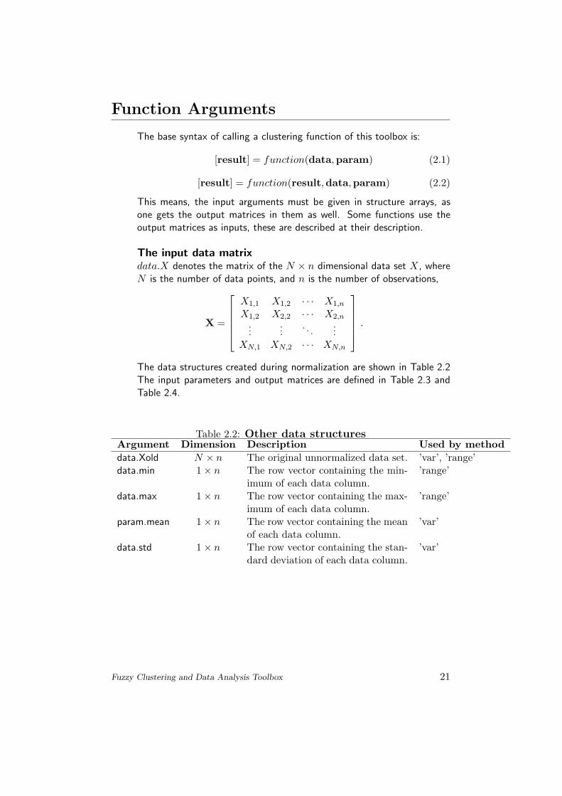
The data structures created during normalization are shown in Table 2.2The input parameters and output matrices are defined in Table 2.3 andTable 2.4.

Table 2.2: Other data structuresArgument Dimension Description Used by methoddata.Xold N × n The original unnormalized data set. ’var’, ’range’data.min 1× n The row vector containing the min-

imum of each data column.’range’

data.max 1× n The row vector containing the max-imum of each data column.

’range’

param.mean 1× n The row vector containing the meanof each data column.

’var’

data.std 1× n The row vector containing the stan-dard deviation of each data column.

’var’


Table 2.3: The input parameter structuresArgument Notation Description Used byparam.c c The number of clusters or the ini-

tial partition matrix. If previous, itmust be given as a round scalar witha value greater than one.

kmeans, kmedoid,FCMclust, GKclustGGclust

param.m m The weighting exponent which de-termines the fuzziness of the clus-ters. It must be given as a scalargreater or equal to one. The defaultvalue of m is 2.

FCMclust, GK-clust, GGclust

param.e ε The termination tolerance of theclustering method. The default set-ting is 0.001.


param.ro ρ The ρ parameter is a row vector,which consists of the determinantsi.e. the cluster volumes of the clus-ters.The default value is one for eachcluster.

GKclust

param.vis - Visualization parameter for K-means and K-medoid clusteringmethods. Its value can be zero orone.

kmeans,kmedoid

param.beta β A predefined threshold: the max-imal ratio between the maximumand minimum eigenvalue of the co-variance matrix, with the defaultvalue of 1015

GKclust

param.gamma γ Weighting parameter, a scaled iden-tity matrix can be added to the co-variance matrix in the ratio of γ. Itsdefault value is 0, the maximum isone.

GKclust

param.val – It determines, which validity mea-sures will be calculated. It can bechosen 1, 2 or 3.

validity

param.max – Maximal number of iteration with adefault value of 100.

Sammon, FuzSam

param.alpha α Gradient step size, its default valueis 0.4.

Sammon, FuzSam


Table 2.4: The result structuresArgument Notation Dimension Description Output ofresult.data.f U N × c The structure matrix

represents the partitionmatrix U

Kmeans,Kmedoid,FCMclust, GK-clust, GGclust

result.data.d D2ik N × c The distance matrix

containing the squaredistances between datapoints and clustercenters.

Kmeans,Kmedoid,FCMclust, GK-clust,GGclust

result.cluster.v V c× n Contains the vi clustercenters.


result.cluster.P P n× n× c Contains the n × ndimensional covariancematrices for each clus-ter.

GKclust, GGclust

result.cluster.M M n× n× c Contains the n × ndimensional norm-inducing matrices foreach cluster.

GKclust

result.cluster.V V c× n Contains the eigenvec-tors of each cluster.

GKclust, GGclust

result.cluster.D D c× n contains the eigenvaluesof each cluster.

GKclust, GGclust

result.cluster.Pi αi 1× 1× c The prior probabilityfor each cluster.

GGclust

result.iter - 1× 1 The number of iterationduring the calculation.


result.cost J 1× iter The value of the fuzzyC-means functional foreach iteration step.


result.eval.f U* N ′ × n Partition matrix for theevaluated data set.

clusteval

result.eval.d D2∗ik N ′ × c Distance matrix with

the distances betweenthe evaluated datapoints and the clustercenters.

clusteval

result.proj.P Y N × q Projected data matrix. PCA, Sammon,FuzSam

result.proj.vp Z c× q Matrix of the projectedcluster centers.

PCA, Sammon,FuzSam

result.proj.e E c× q Value of Sammon’sstress.

samstr


Kmeans

PurposeHard partition of the given data matrix, described inSection 1.2.1.

Syntax[result]=Kmeans(data,param)

DescriptionThe objective function Kmeans algorithm is to partition the dataset X into c clusters. Calling the algorithm with the syntax above,first the param.c and data.X must be given, and the output ma-trices of the function are saved in result.data.f , result.data.d andresult.cluster.v. The number of iteration and the cost functionare also saved in the result structure. The calculated cluster centervi (i ∈ {1, 2, . . . , c}) is the mean of the data points in cluster i.The difference from the latter discussed algorithms are that it gener-ates random cluster centers, not partition matrix for initialization,so param.c can be given as an initializing matrix containing thecluster centers too.

ExampleThe examples were generated with the Kmeanscall function locatedin ..\Demos\clusteringexamples\synthetic\ and..\Demos\clusteringexamples\motorcycle\ directories, where the nDex-ample function and motorcycle.txt are situated.


0 0.1 0.2 0.3 0.4 0.5 0.6 0.7 0.8 0.9 10

0.1

0.2

0.3

0.4

0.5

0.6

0.7

0.8

0.9

1

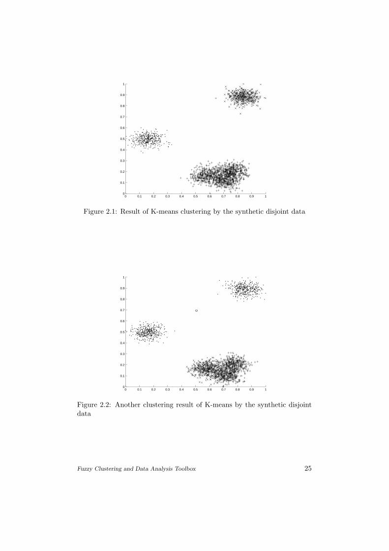
Figure 2.1: Result of K-means clustering by the synthetic disjoint data

0 0.1 0.2 0.3 0.4 0.5 0.6 0.7 0.8 0.9 10

0.1

0.2

0.3

0.4

0.5

0.6

0.7

0.8

0.9

1

Figure 2.2: Another clustering result of K-means by the synthetic disjointdata


0 0.1 0.2 0.3 0.4 0.5 0.6 0.7 0.8 0.9 10

0.1

0.2

0.3

0.4

0.5

0.6

0.7

0.8

0.9

1

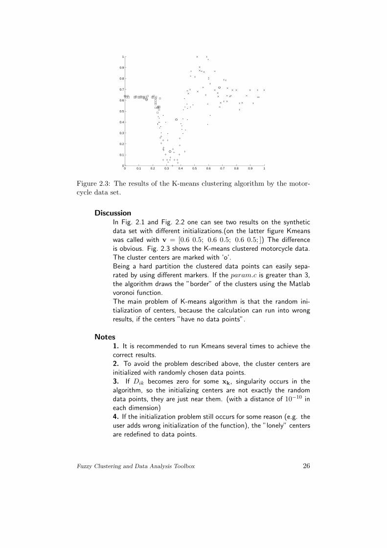
Figure 2.3: The results of the K-means clustering algorithm by the motor-cycle data set.

DiscussionIn Fig. 2.1 and Fig. 2.2 one can see two results on the syntheticdata set with different initializations.(on the latter figure Kmeanswas called with v = [0.6 0.5; 0.6 0.5; 0.6 0.5; ]) The differenceis obvious. Fig. 2.3 shows the K-means clustered motorcycle data.The cluster centers are marked with ’o’.Being a hard partition the clustered data points can easily sepa-rated by using different markers. If the param.c is greater than 3,the algorithm draws the ”border” of the clusters using the Matlabvoronoi function.The main problem of K-means algorithm is that the random ini-tialization of centers, because the calculation can run into wrongresults, if the centers ”have no data points”.

Notes1. It is recommended to run Kmeans several times to achieve thecorrect results.2. To avoid the problem described above, the cluster centers areinitialized with randomly chosen data points.3. If Dik becomes zero for some xk, singularity occurs in thealgorithm, so the initializing centers are not exactly the randomdata points, they are just near them. (with a distance of 10−10 ineach dimension)4. If the initialization problem still occurs for some reason (e.g. theuser adds wrong initialization of the function), the ”lonely” centersare redefined to data points.


Algorithm[K-means algorithm] For corresponding theory see Section 1.2.1.Given the data set X, choose the number of clusters 1 < c < N .

Initialize with random cluster centers chosen from the data set.

Repeat for l = 1, 2, . . .

Step 1 Compute the distances

D2ik = (xk − vi)T (xk − vi), 1 ≤ i ≤ c, 1 ≤ k ≤ N. (2.3)

Step 2 Select the points for a cluster with the minimal distances,they belong to that cluster.

Step 3 Calculate cluster centers

v(l)i =

∑Nij=1 xi

Ni(2.4)

untiln∏

k=1max|v(l) − v(l−1)| 6= 0.

Ending Calculate the partition matrix

See AlsoKmedoid, clusteval, validity


Kmedoid

PurposeHard partition of the given data matrix, where cluster centers mustbe data points (described inSection 1.2.1).

Syntax[result]=Kmedoid(data,param)

DescriptionThe objective function Kmedoid algorithm is to partition the dataset X into c clusters. The input and output arguments are thesame what K-means uses. The main difference between Kmeansand Kmedoid stands in calculating the cluster centers: the newcluster center is the nearest data point to the mean of the clusterpoints.The function generates random cluster centers, not partition matrixfor initialization, so param.c can be given as an initializing matrixcontaining the cluster centers too, not only a scalar (the number ofclusters)

ExampleThe examples were generated with the Kmedoidcall function lo-cated in ..\Demos\clusteringexamples\synthetic\ and..\Demos\clusteringexamples\motorcycle\ directories, where the nDex-ample function and motorcycle.txt are situated.


0 0.1 0.2 0.3 0.4 0.5 0.6 0.7 0.8 0.9 10

0.1

0.2

0.3

0.4

0.5

0.6

0.7

0.8

0.9

1

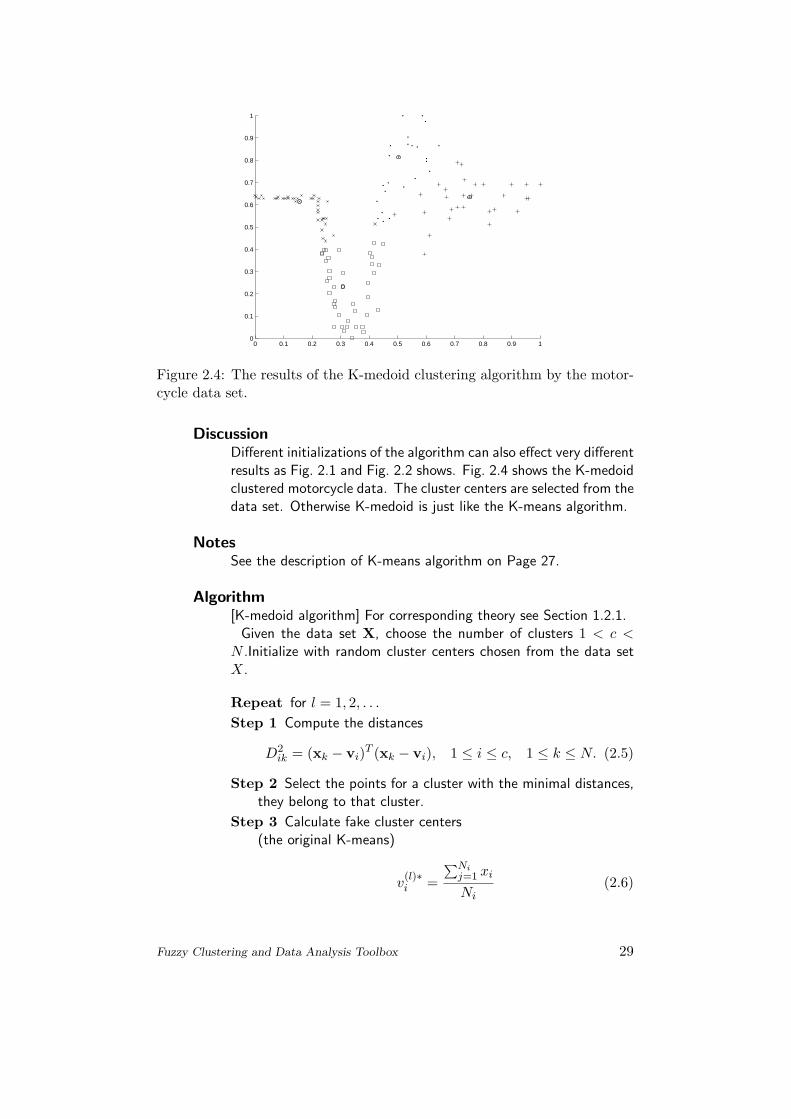
Figure 2.4: The results of the K-medoid clustering algorithm by the motor-cycle data set.

DiscussionDifferent initializations of the algorithm can also effect very differentresults as Fig. 2.1 and Fig. 2.2 shows. Fig. 2.4 shows the K-medoidclustered motorcycle data. The cluster centers are selected from thedata set. Otherwise K-medoid is just like the K-means algorithm.

NotesSee the description of K-means algorithm on Page 27.

Algorithm[K-medoid algorithm] For corresponding theory see Section 1.2.1.

Given the data set X, choose the number of clusters 1 < c <N .Initialize with random cluster centers chosen from the data setX.

Repeat for l = 1, 2, . . .

Step 1 Compute the distances

D2ik = (xk − vi)T (xk − vi), 1 ≤ i ≤ c, 1 ≤ k ≤ N. (2.5)

Step 2 Select the points for a cluster with the minimal distances,they belong to that cluster.

Step 3 Calculate fake cluster centers(the original K-means)

v(l)∗i =

∑Nij=1 xi

Ni(2.6)


Step 4 Choose the nearest data point to be the cluster center

D2∗ik = (xk − v∗i)T (xk − v∗i), (2.7)

andx∗i = argmini(D2∗

ik ) ; v(l)i = x∗i . (2.8)

untiln∏

k=1max|v(l) − v(l−1)| 6= 0.

Ending Calculate the partition matrix

See AlsoKmeans, clusteval, validity


FCMclust

PurposeFuzzy C-means clustering of a given data set (described in Sec-tion 1.2.2).

Syntax[result]=FCMclust(data,param)

DescriptionThe Fuzzy C-means clustering algorithm uses the minimization ofthe fuzzy C-means functional (1.18). There are three input pa-rameter needed to run this function: param.c, as the number ofclusters or initializing partition matrix; param.m, as the fuzzinessweighting exponent; and param.e, as the maximum terminationtolerance. The two latter parameter have their default value, ifthey are not given by the user.The function calculates with the standard Euclidean distance norm,the norm inducing matrix is an n×n identity matrix. The result ofthe partition is collected in structure arrays. One can get the par-tition matrix cluster centers, the square distances, the number ofiteration and the values of the C-means functional at each iterationstep.


ExampleThe examples were generated with the FCMcall function located in..\Demos\clusteringexamples\synthetic\ and..\Demos\clusteringexamples\motorcycle\ directories, where the nDex-ample function and motorcycle.txt are situated.

0 0.1 0.2 0.3 0.4 0.5 0.6 0.7 0.8 0.9 10

0.1

0.2

0.3

0.4

0.5

0.6

0.7

0.8

0.9

1

Figure 2.5: The results of the Fuzzy C-means clustering algorithm by asynthetic data set

0 0.1 0.2 0.3 0.4 0.5 0.6 0.7 0.8 0.9 10

0.1

0.2

0.3

0.4

0.5

0.6

0.7

0.8

0.9

1

x1

x2

Figure 2.6: The results of the Fuzzy C-means clustering algorithm by themotorcycle data set.


DiscussionIn Fig. 2.5 and Fig. 2.6 the ’.’ remark the data points, the ’o’the cluster centers, which are the weighted mean of the data. Thealgorithm can only detect clusters with circle shape, that is whyit cannot really discover the orientation and shape of the cluster”right below” in Fig. 2.5. In Fig. 2.6 the circles in the contour-mapare a little elongated, since the clusters have effect on each other.However the Fuzzy C-means algorithm is a very good initializationtool for more sensitive methods (e.g. Gath-Geva algorithm on page39).

Notes1. If DikA becomes zero for some xk, singularity occurs in thealgorithm: the membership degree cannot be computed.2. The correct choice of the weighting parameter (m) is important:as m approaches one from above, the partition becomes hard, if itapproaches to infinity, the partition becomes maximally fuzzy, i.e.µik = 1/c.3. There is no possibility to use different AA for the clusters,although in most cases it would be needed.

Algorithm[FCM algorithm] For corresponding theory see Section 1.2.2.Given the data set X, choose the number of clusters 1 < c < N ,

the weighting exponent m > 1, the termination tolerance ε > 0and the norm-inducing matrix A. Initialize the partition matrixrandomly, such that U(0) ∈ Mfc.

Repeat for l = 1, 2, . . .

Step 1 Compute the cluster prototypes (means):

v(l)i =

N∑k=1

(µ(l−1)ik )mxk

N∑k=1

(µ(l−1)i,k )m

, 1 ≤ i ≤ c. (2.9)

Step 2 Compute the distances:

D2ikA = (xk − vi)T A(xk − vi), 1 ≤ i ≤ c, 1 ≤ k ≤ N.

(2.10)Step 3 Update the partition matrix:

µ(l)i,k =

1∑c

j=1 (DikA/DjkA)2/(m−1). (2.11)


until ||U(l) −U(l−1)|| < ε.

See AlsoKmeans, GKclust, GGclust

ReferencesJ. C. Bezdek, Pattern Recognition with Fuzzy Objective FunctionAlgorithms, Plenum Press, 1981


GKclust

PurposeGustafson-Kessel clustering algorithm extends the Fuzzy C-meansalgorithm by employing an adaptive distance norm, in order to de-tect clusters with different geometrical shapes in the data set.

Syntax[result]=GKclust(data,param)

DescriptionThe GKclust function forces, that each cluster has its own norminducing matrix Ai, so they are allowed to adapt the distance normto the local topological structure of the data points. The algorithmuses the Mahalanobis distance norm. The parameters are extendedwith param.ro, it is set to one for each cluster by default value.There are two numerical problems with GK algorithm, which aredescribed in Notes.


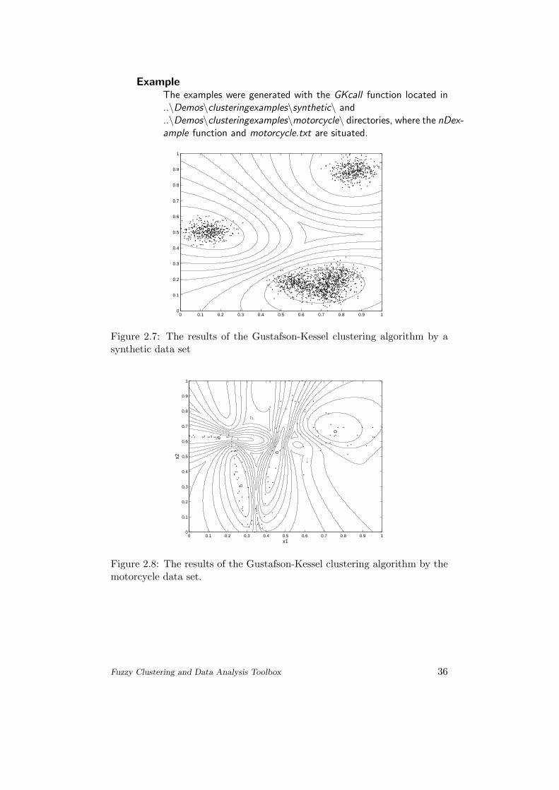
ExampleThe examples were generated with the GKcall function located in..\Demos\clusteringexamples\synthetic\ and..\Demos\clusteringexamples\motorcycle\ directories, where the nDex-ample function and motorcycle.txt are situated.

0 0.1 0.2 0.3 0.4 0.5 0.6 0.7 0.8 0.9 10

0.1

0.2

0.3

0.4

0.5

0.6

0.7

0.8

0.9

1

Figure 2.7: The results of the Gustafson-Kessel clustering algorithm by asynthetic data set

0 0.1 0.2 0.3 0.4 0.5 0.6 0.7 0.8 0.9 10

0.1

0.2

0.3

0.4

0.5

0.6

0.7

0.8

0.9

1

x2

x1

Figure 2.8: The results of the Gustafson-Kessel clustering algorithm by themotorcycle data set.


DiscussionIn Fig. 2.7 and Fig. 2.8 the ’.’ remark the data points, the ’o’the cluster centers. Since this algorithm is an extension of theC-means algorithm (uses adaptive distance norm), it detects theelongated clusters. The orientation and shape can be ”mined”from the eigenstructure of the covariance matrix: the direction ofthe axes are given by the eigenvectors. In Fig. 2.8 the contour-mapshows the superposition of the four ellipsoidal clusters.

Notes1. If there is no prior knowledge, ρi is 1 for each cluster, so the GKalgorithm can find only clusters with approximately equal volumes.2. A numerical drawback of GK is: When an eigenvalue is zero orwhen the ratio between the maximal and the minimal eigenvalue,i.e. the condition number of the covariance matrix is very large, thematrix is nearly singular. Also the normalization to a fixed volumefails, as the determinant becomes zero. In this case it is useful toconstrain the ratio between the maximal and minimal eigenvalue,this ratio should be smaller than some predefined threshold, that isin the β parameter.3. In case of clusters extremely extended in the direction of thelargest eigenvalues the computed covariance matrix cannot estimatethe underlaying data distribution, so a scaled identity matrix canbe added to the covariance matrix by changing the value of γ fromzero (as default)to a scalar: 0 ≤ γ ≤ 1.

Algorithm[Modified Gustafson-Kessel algorithm] For corresponding theory seeSection 1.2.3.Given the data set X, choose the number of clusters 1 < c < N ,

the weighting exponent m > 1, the termination tolerance ε > 0and the norm-inducing matrix A. Initialize the partition matrixrandomly, such that U(0) ∈ Mfc.

Repeat for l = 1, 2, . . .

Step 1 Calculate the cluster centers.

v(l)i =

N∑k=1

(µ(l−1)ik )mxk

N∑k=1

(µ(l−1)ik )m

, 1 ≤ i ≤ c (2.12)


Step 2 Compute the cluster covariance matrices.

F(l)i =

N∑k=1

(µ(l−1)ik )m

(xk − v(l)

i

) (xk − v(l)

i

)T

N∑k=1

(µ(l−1)ik )m

, 1 ≤ i ≤ c

(2.13)Add a scaled identity matrix:

F i := (1− γ)F i + γ(F 0)1/nI (2.14)

Extract eigenvalues λij and eigenvectors φij ,find λi,max = maxjλij and set:

λi,max = λij/β, ∀j for which λi,max/λij ≥ β (2.15)

Reconstruct F i by:

F i = [φi,1 . . . φi,n]diag(λi,1 . . . λi,n)[φi,1 . . . φi,n]−1 (2.16)

Step 3 Compute the distances.

D2ikAi

(xk,vi) =(xk − v(l)

i

)T [(ρidet(Fi))1/nF−1

i

] (xk − v(l)

i

)

(2.17)Step 4 Update the partition matrix

µ(l)ik =

1∑c

j=1 (DikAi(xk,vi)/Djk(xk,vj))2/(m−1)

, 1 ≤ i ≤ c, 1 ≤ k ≤ N .

(2.18)until ||U (l) −U (l−1)|| < ε.

See AlsoKmeans, FCMclust, GGclust

ReferencesR. Babuska, P.J. van der Veen, and U. Kaymak. Improved co-variance estimation for GustafsonKessel clustering. In Proceedingsof 2002 IEEE International Conference on Fuzzy Systems, pages10811085, Honolulu, Hawaii, May 2002.


GGclust

PurposeGath-Geva clustering algorithm uses a distance norm based on thefuzzy maximum likelihood estimates.

Syntax[result]=GGclust(data,param)

DescriptionThe Gath-Geva clustering algorithm has the same outputs definedat the description of Kmeans and GKclust, but it has less inputparameters (only the weighting exponenet and the termination tol-erance), because the used distance norm involving the exponentialterm cannot run into numerical problems.Note that the original fuzzy maximum likelihood estimates does notinvolve the value of param.m, it is constant 1.The parameter param.c can be given as an initializing partitionmatrix or as the number of clusters. For other attributes of thefunction see Notes.


ExampleThe examples were generated with the Kmeanscall function locatedin ..\Demos\clusteringexamples\synthetic\ and..\Demos\clusteringexamples\motorcycle\ directories, where the nDex-ample function and motorcycle.txt are situated.

0 0.1 0.2 0.3 0.4 0.5 0.6 0.7 0.8 0.9 10

0.1

0.2

0.3

0.4

0.5

0.6

0.7

0.8

0.9

1

Figure 2.9: The results of the Gath-Geva clustering algorithm by a syntheticdata set

0 0.1 0.2 0.3 0.4 0.5 0.6 0.7 0.8 0.9 10

0.1

0.2

0.3

0.4

0.5

0.6

0.7

0.8

0.9

1

x2

x1

Figure 2.10: The results of the Gath-Geva clustering algorithm by the mo-torcycle data set.


DiscussionIn the figures the ’.’ remark the data points, the ’o’ the clustercenters. Cause of the exponential term in the distance norm (1.31),which decreases faster by increasing |xk − vi| distance, the GGalgorithm divides the data space into disjoint subspaces shown inFig. 2.9. In Fig. 2.10 the effects of the other ”cluster-borders”distort this disjointness, but the clusters can be easily figured out.

Notes1. The GG algorithm can overflow at large c values (which indicatesmall distances) because of invertation problems in (1.31).2. The fuzzy maximum likelihood estimates clustering algorithm isable to detect clusters of varying shapes, sizes and densities.3. The cluster covariance matrix is used in conjunction with an”exponential” distance, and the clusters are not constrained in vol-ume.4. This algorithm is less robust in the sense that it needs a goodinitialization, since due to the exponential distance norm, it con-verges to a near local optimum. So it is recommended to use theresulting partition matrix of e.g. FCM to initialize this algorithm.

Algorithm[Gath-Geva algorithm] For corresponding theory see Section 1.2.4.

Given a set of data X specify c, choose a weighting exponentm > 1 and a termination tolerance ε > 0. Initialize the partitionmatrix with a more robust method.

Repeat for l = 1, 2, . . .

Step 1 Calculate the cluster centers:

v(l)i =

N∑k=1

(µ(l−1)ik )wxk

N∑k=1

(µ(l−1)ik

)w

, 1 ≤ i ≤ c

Step 2 Compute the distance measure D2ik.

The distance to the prototype is calculated based the fuzzycovariance matrices of the cluster

F(l)i =

N∑k=1

(µ(l−1)ik )w

(xk − v(l)

i

) (xk − v(l)

i

)T

N∑k=1

(µ(l−1)ik )w

, 1 ≤ i ≤ c

(2.19)


The distance function is chosen as

D2ik(xk,vi) =

(2π)(n2 )√det(Fi)

αiexp

(12

(xk − v(l)

i

)TF−1

i

(xk − v(l)

i

))

(2.20)with the a priori probability

αi = 1N

∑Nk=1 µik

Step 3 Update the partition matrix

µ(l)ik =

1∑c

j=1 (Dik(xk,vi)/Djk(xk,vj))2/(m−1)

, 1 ≤ i ≤ c, 1 ≤ k ≤ N .

(2.21)until ||U(l) −U(l−1)|| < ε.

See AlsoKmeans, FCMclust, GKclust

ReferencesI. Gath and A.B. Geva, Unsupervised Optimal Fuzzy Clustering,IEEE Transactions on Pattern Analysis and Machine Intelligence,7:773–781, 1989


clusteval

PurposeThe purpose of the function is to evaluate ”unseen” data withthe cluster centers calculated by the selected function of clusteringmethod.

Syntax[eval] = clusteval(new,result,param)

DescriptionThe clusteval function uses the results and the parameters of FCM-clust, GKclust, GGclust clustering functions: It recognizes the usedclustering algorithm to evaluate the unseen data sets, on the groundsof the results of clustering.The new data points to be evaluated must be given in the N ′ × nstructure array new.X, i.e. only the dimensions must be equal forboth data sets. The results are collected in eval.f and eval.d, asthe partition matrix and the distances from cluster prototypes ofthis data set.In 2-dimensional case it generates pair-coordinate points in the dataspace, calculates the partition matrix, and draws a contour-map byselecting the points with the same partitioning values and drawingdefault number of colored lines in the data field (the density,i.e.number of lines can be changed with the parameter of the contourfunction). If the user wants to see this contour-map for a simpleclustering, new.X = data.X should be used. The lines of thecontour map denotes the position of points with equal membershipdegrees.

AlgorithmThe clusteval function uses the algorithms of the clustering func-tions, i.e. it can be comprehended as a clustering method with onlyone iteration step.


ExampleThe example was generated with the evalexample function locatedin ..\Demos\clustevalexample\ directory, where data2.txt is situ-ated.

0 0.1 0.2 0.3 0.4 0.5 0.6 0.7 0.8 0.9 10

0.1

0.2

0.3

0.4

0.5

0.6

0.7

0.8

0.9

1

x1

x2

Figure 2.11: The results of the Gustafson-Kessel clustering algorithm.

DiscussionTo present the evaluation, a 2-D data set (data2.txt) wasselected and the GK-clustering was executed. During thefirst running new.Xwas equal to data.X, so the contour mapcould be plotted (see Fig. 2.11). After that a new data pointwas chosen to be evaluated: new.X = [0.5 0.5] and theresult is in eval.f .

Ueval = [0.0406 0.5971 0.3623], (2.22)

As Fig. 2.11 also shows the new data point rather belongs tothe clusters in the ”upper left” corner of the normalized dataspace.

See AlsoFCMclust, GKclust, GGclust


validity

PurposeCalculating validity measure indexes to estimate the goodness ofan algorithm or to help to find the optimal number of clusters fora data set.

Syntax[result] = validity(result,data,param)

DescriptionDepending on the value of param.val the validity function calcu-lates different cluster validity measures.

• param.val = 1: the function calculates Partition Coefficient(PC)and Classification Entropy(CE),

• param.val = 2: the function calculates Partition Index(SC),Separation Index(S) and Xie and Beni’s Index(XB),

• param.val = 3: the function calculates Dunn’s Index(DI) andAlternative Dunn Index(ADI).

If this parameter is not given by the user or it has another value, theprogram calculates only PC and CE, as default validity measures.For validation of hard partitioning methods it is recommended tocalculate DI and ADI.The calculation of these indexes is described in Section 1.3.

ExampleExamples of the validation indexes are shown in the experimentalchapter in Section 3.1 and Section 3.2.

ReferencesJ.C. Bezdek, Pattern Recognition with Fuzzy Objective FunctionAlgorithms, Plenum Press, 1981, NY.A.M. Bensaid, L.O. Hall, J.C. Bezdek, L.P. Clarke, M.L. Silbiger,J.A. Arrington, R.F. Murtagh, Validity-guided (re)clustering withapplications to image segmentation, IEEE Transactions on on FuzzySystems, 4:112 -123, 1996.X.L. Xie and G.A. Beni, Validity measure for fuzzy clustering, IEEETrans. PAMI, 3(8):841–846, 1991.


clustnormalize and clustdenormalize

PurposeNormalization and denormalization of the wanted data set.

Syntax[data] = clustnormalize(data,method)

Syntax[data] = clustdenormalize(data,method)

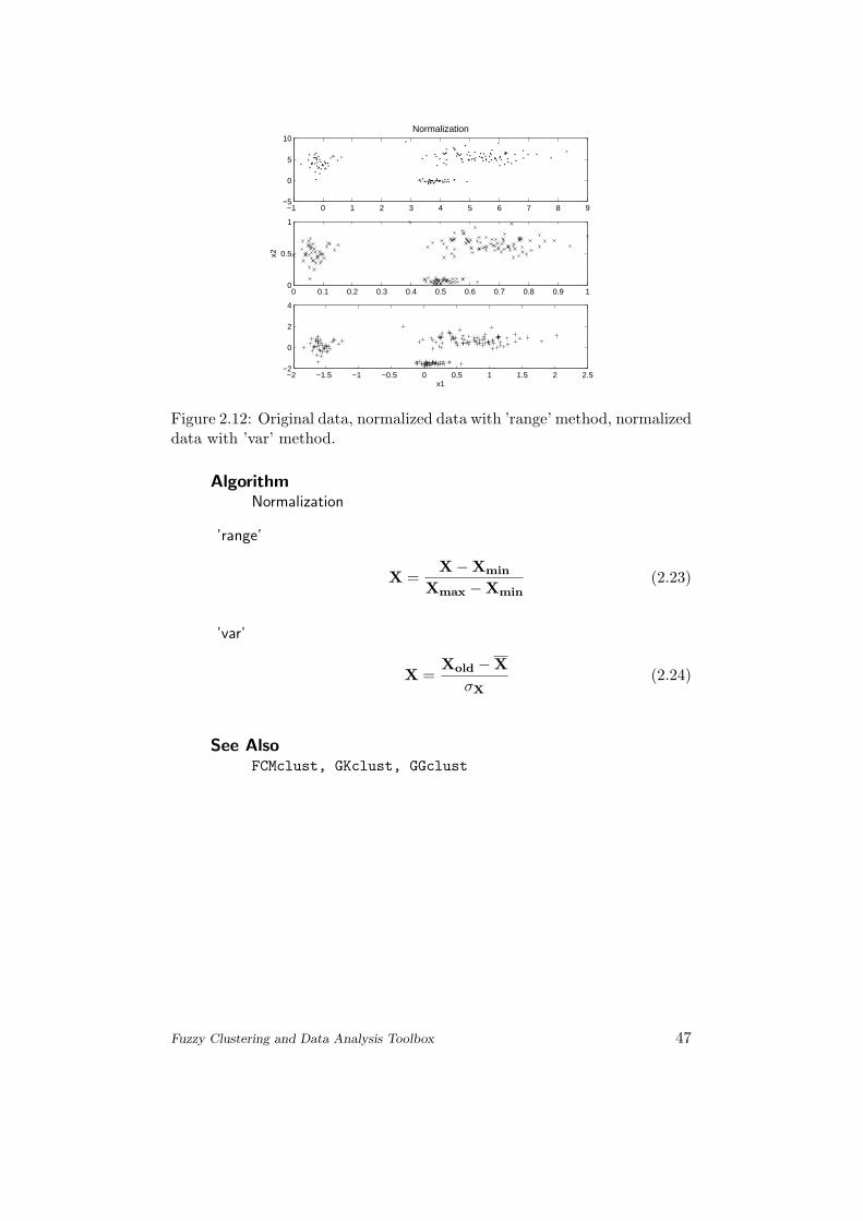
Descriptionclustnormalize uses two method to data normalization. If methodis:range - Values are normalized between [0,1] (linear operation).var - Variance is normalized to one (linear operation).The original data is saved in data.Xold, and the function also saves:1. in case of ’range’ the row vectors containing the minimumand the maximum elements of each column from the original data(data.min and data.max)2. in case of ’var’ the row vectors containing the mean and standarddeviation of the data (data.mean and data.std)

clustdenormalize is the inverse of the normalization function: itrecognizes, which method was used during the normalization andforms it back.

ExampleThe example was generated with the normexample function locatedin ..\Demos\normexample\ directory, where data3.txt is situated.


−1 0 1 2 3 4 5 6 7 8 9−5

0

5

10Normalization

0 0.1 0.2 0.3 0.4 0.5 0.6 0.7 0.8 0.9 10

0.5

1

x2

−2 −1.5 −1 −0.5 0 0.5 1 1.5 2 2.5−2

0

2

4

x1

Figure 2.12: Original data, normalized data with ’range’ method, normalizeddata with ’var’ method.

AlgorithmNormalization

’range’

X =X−Xmin

Xmax −Xmin(2.23)

’var’

X =Xold −X

σX(2.24)

See AlsoFCMclust, GKclust, GGclust


PCA

PurposePrincipal Component Analysis. Projection of the n-dimensionaldata into a lower q-dimensional data (Section 1.4.1).

Syntax[result] = PCA(result,data,param)

DescriptionThe inputs of the PCA function are the multidimensional data.Xand the param.q projection dimension parameter (with a commonvalue of 2). The function calculates the autocorrelation matrix ofthe data and its eigenvectors, sort them according to eigenvalues,and they are normalized. Only the first eigenvector of q-dimension isselected, it will be the direction of the plane to which the data pointsare projected. The output matrices are saved in result.PCAprojstructure, one can get the projected data (P), the projected clus-ter centers(vp), the eigenvectors (V) and the eigenvalues (D). Theresults are evaluated with projeval function.

ExampleThe example was generated with the PCAexample function locatedin ..\Demos\PCAexample\ directory, where the nDexample func-tion is situated, which generated the random 3-D data.

3

4

5

6

7

−2−101234562

3

4

5

6

7

8

9

x1

Synthetic 3−D data

x2

x3

Figure 2.13: Random generated 3-dimensional data set.


−3 −2 −1 0 1 2 3−3

−2

−1

0

1

2

3

y1

y2

Projected data

Figure 2.14: The into 2-dimension projected data by Principal ComponentAnalysis.

DiscussionA simple example is presented: random generated 3-D data is clus-tered with Fuzzy C-means algorithm, and through PCA projectionthe results are plotted. The original and the projected data is shownin Fig. 2.13 and Fig. 2.14. The error (defined at the description ofthe projeval function on page 53) is P = 0.0039.

NotesThe PCA Matlab function is taken from the SOM Toolbox, whichis obtainable on the web:http://www.cis.hut.fi/projects/somtoolbox/.

See Alsoprojeval, samstr

ReferencesJuha Vesanto, Neural Network Tool for Data Mining: SOM Tool-box,Proceedings of Symposium on Tool Environments and Develop-ment Methods for Intelligent Systems (TOOLMET2000), 184-196,2000.


Sammon

PurposeSammon’s Mapping. Projection of the n-dimensional data into alower q-dimensional data (described in Section 1.4.2).

Syntax[result] = Sammon(result,data,param)

DescriptionThe Sammon function calculates the original Sammon’s Mapping.It uses result.data.d of the clustering as input and two parame-ters: the maximum iteration number (param.max, default valueis 500.) and the step size of the gradient method (param.alpha,default value is 0.4.). The proj.P can be given either an initializingprojected data matrix or the projection dimension. In latter case thefunction calculates with random initialized projected data matrix,hence it needs normalized clustering results. During calculation theSammon function uses online drawing, where the projected datapoints are marked with ’o’, and the projected cluster centers with’*’. The online plotting can be disengaged by editing the code, iffaster calculation wanted. The results are evaluated with projevalfunction.

ExampleThe examples would be like the one shown in Fig. 2.14 on page 49.

NotesThe Sammon Matlab function is is taken from the SOM Toolbox,which is obtainable on the web:http://www.cis.hut.fi/projects/somtoolbox/.


ReferencesJuha Vesanto, Neural Network Tool for Data Mining: SOM Tool-box,Proceedings of Symposium on Tool Environments and Develop-ment Methods for Intelligent Systems (TOOLMET2000), 184-196,2000.


FuzSam

PurposeFuzzy Sammon Mapping. Projection of the n-dimensional data intoa lower q-dimensional data (described Section 1.4.3).

Syntax[result] = FuzSam(proj,result,param)

DescriptionThe FuzSam function modifies the Sammon Mapping, so it becomescomputationally cheaper. It uses result.data.f and result.data.dof the clustering as input.It has two parameters, the maximum it-eration number (param.max, default value is 500.) and the stepsize of the gradient method (param.alpha, default value is 0.4.).The proj.P can be given either an initializing projected data matrixor the projection dimension. In latter case the function calculateswith random initialized projected data matrix, hence it needs nor-malized clustering results. During calculation FuzSam uses onlinedrawing, where the projected data points are marked with ’o’, andthe projected cluster centers with ’*’. The online plotting can bedisengaged by editing the code. The results are evaluated withprojeval function.

ExampleThe examples would be like the one shown in Fig. 2.14 on page 49.

Algorithm

• [Input] : Desired dimension of the projection, usually q = 2,the original dataset, X; and the results of fuzzy clustering:cluster prototypes, vi, membership values, U = [µki], and thedistances D = [dki = d(xk,vi)]N×c.

• [Initialize] the projected datapoints by yk PCA based projec-tion of xk, and compute the projected cluster centers by

zi =∑N

k=1(µki)myk∑Nk=1(µki)m

(2.25)

and compute the distances with the use of these projectedpoints D∗ = [d∗ki = d(yk, zi)]N×c


• [While] (Efuzz > ε) and (t≤ maxstep){for (i = 1 : i ≤ c : i + +{for (j = 1 : j ≤ N : j + +

{Compute ∂E(t)∂yil(t)

, ∂2E(t)∂2yil(t)

, ∆yil = ∆yil +

[∂E(t)∂yil(t)

∂2E(t)

∂2yil(t)

]}

}yil = yil + ∆yil∀i = 1, . . . , N, l = 1, . . . , qCompute zi =

∑Nk=1(µki)myk/

∑Nk=1(µki)m

D∗ = [d∗ki = d(yk, zi)]N×c}Compute Efuzz by (1.46).

where the derivatives are defined in (1.45).


ReferencesA. Kovacs - J. Abonyi, Vizualization of Fuzzy Clustering Resultsby Modified Sammon Mapping, Proceedings of the 3rd Interna-tional Symposium of Hungarian Researchers on Computational In-telligence, 177-188, 2002.


projeval

PurposeEvaluation for projected data.

Syntax[perf] = projeval(result,param)

DescriptionThe projeval function uses the results and the parameters of theclustering and the visualization functions. It is analog to the clus-teval function, but it evaluates the projected data. The distancesbetween projected data and projected cluster centers are based onthe Euclidean norm, so the function calculates only with a 2-by-2identity matrix, generates the pair-coordinate points, calculates thenew partition matrix, and draws a contour-map by selecting thepoints with the same partitioning values.A subfunction of projeval is to calculate relation-indexes defined onthe ground of (1.48):

P = ‖U−U∗‖,N∑

k=1

µ2k,

N∑

k=1

µ2∗k . (2.26)

See Alsoclusteval, PCA, Sammon, FuzSam, samstr


samstr

PurposeCalculation of Sammon’s stress for projection methods.

Syntax[result] = samstr(data,result)

DescriptionThe simple function calculates Sammon’s stress defined in (1.43).It uses data.X and result.proj.P as input, and the only output isthe result.proj.e containing the value of this validation constant.

See AlsoPCA,Sammon, FuzSam


Chapter 3

Case Studies

The aim of this chapter is present the differences, the usefulness and effective-ness of the partitioning clustering algorithms by partitioning different data sets.In Section 3.1 the five presented algorithms are compared based on numericalresults (validity measures). Section 3.2 deals with the problem of finding theoptimal number of clusters, because this information is rarely known apriori. Areal partitioning problem is presented in Section 3.3 with three real data sets:different types of wine, iris flowers and breast cancer symptoms are partitioned.

55

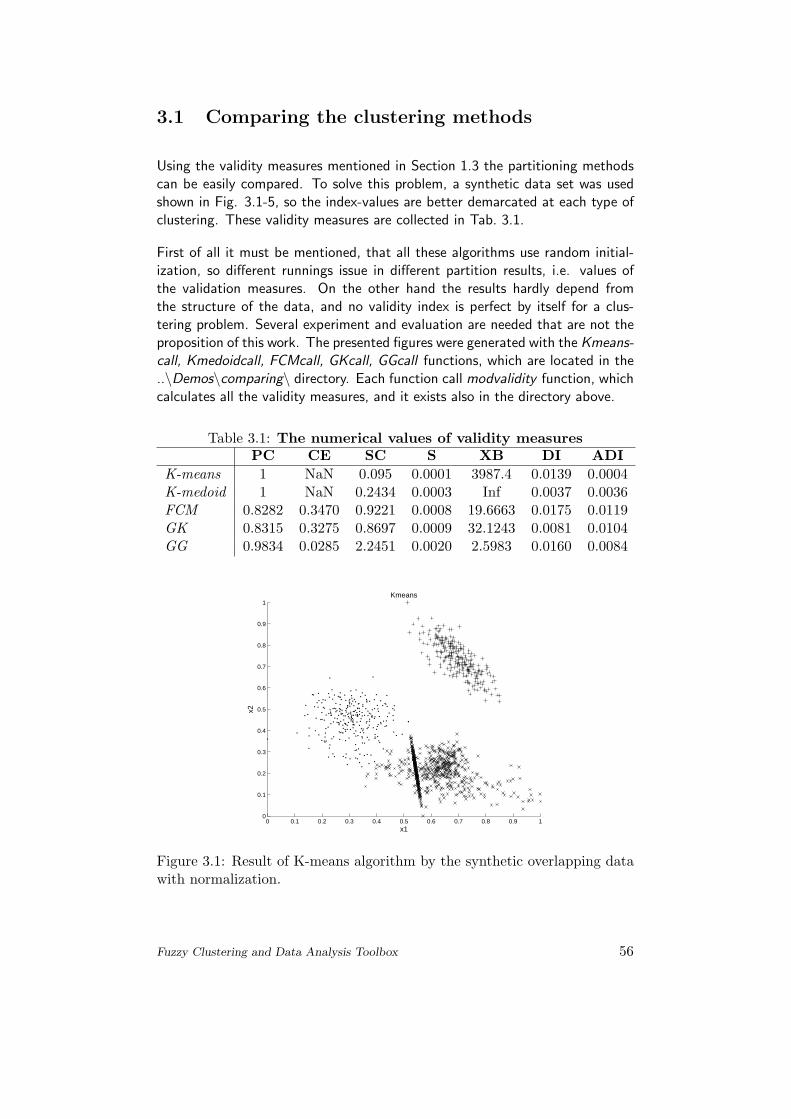
3.1 Comparing the clustering methods

Using the validity measures mentioned in Section 1.3 the partitioning methodscan be easily compared. To solve this problem, a synthetic data set was usedshown in Fig. 3.1-5, so the index-values are better demarcated at each type ofclustering. These validity measures are collected in Tab. 3.1.

First of all it must be mentioned, that all these algorithms use random initial-ization, so different runnings issue in different partition results, i.e. values ofthe validation measures. On the other hand the results hardly depend fromthe structure of the data, and no validity index is perfect by itself for a clus-tering problem. Several experiment and evaluation are needed that are not theproposition of this work. The presented figures were generated with the Kmeans-call, Kmedoidcall, FCMcall, GKcall, GGcall functions, which are located in the..\Demos\comparing\ directory. Each function call modvalidity function, whichcalculates all the validity measures, and it exists also in the directory above.

Table 3.1: The numerical values of validity measuresPC CE SC S XB DI ADI

K-means 1 NaN 0.095 0.0001 3987.4 0.0139 0.0004K-medoid 1 NaN 0.2434 0.0003 Inf 0.0037 0.0036FCM 0.8282 0.3470 0.9221 0.0008 19.6663 0.0175 0.0119GK 0.8315 0.3275 0.8697 0.0009 32.1243 0.0081 0.0104GG 0.9834 0.0285 2.2451 0.0020 2.5983 0.0160 0.0084

0 0.1 0.2 0.3 0.4 0.5 0.6 0.7 0.8 0.9 10

0.1

0.2

0.3

0.4

0.5

0.6

0.7

0.8

0.9

1Kmeans

x1

x2

Figure 3.1: Result of K-means algorithm by the synthetic overlapping datawith normalization.


0 0.1 0.2 0.3 0.4 0.5 0.6 0.7 0.8 0.9 10

0.1

0.2

0.3

0.4

0.5

0.6

0.7

0.8

0.9

1Kmedoid

x1

x2

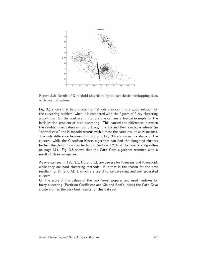
Figure 3.2: Result of K-medoid alogrithm by the synthetic overlapping datawith normalization.

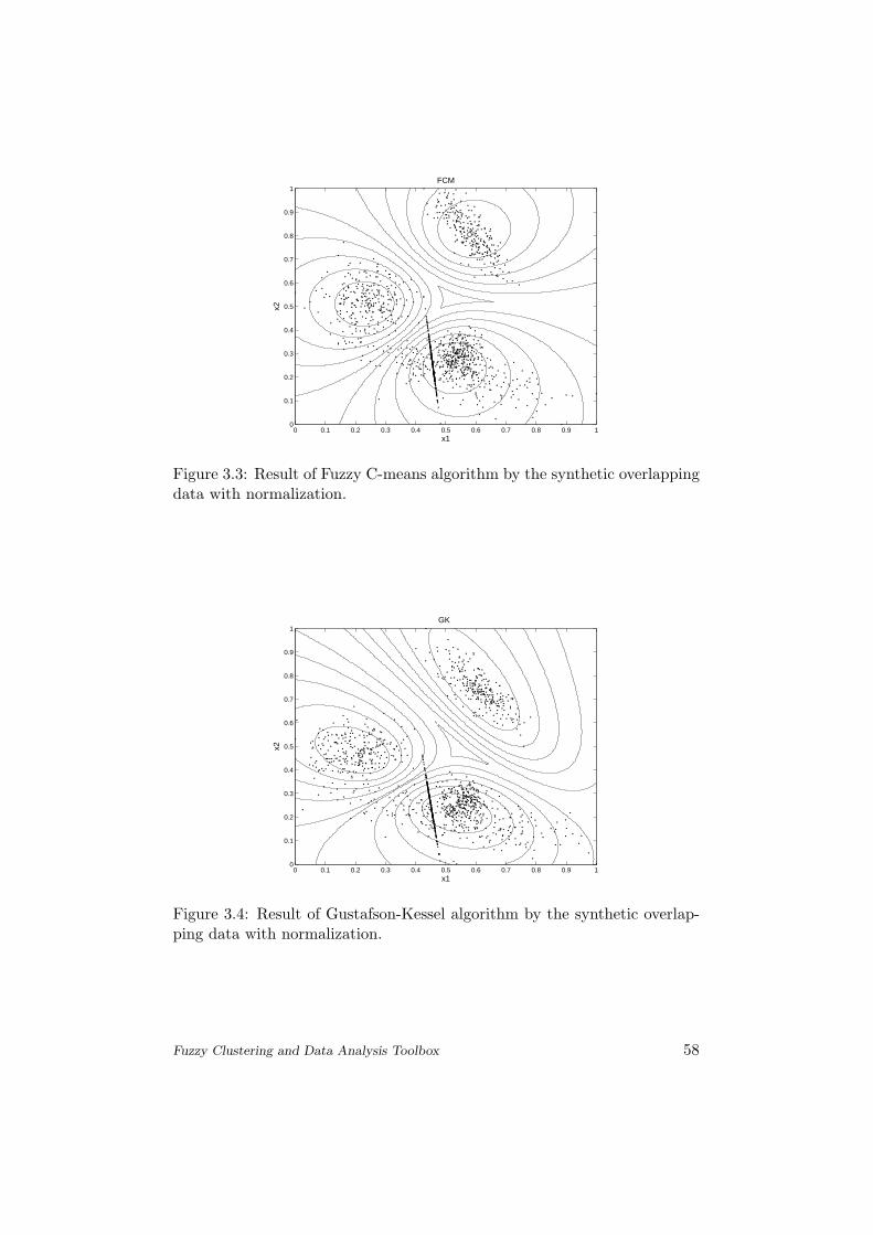
Fig. 3.1 shows that hard clustering methods also can find a good solution forthe clustering problem, when it is compared with the figures of fuzzy clusteringalgorithms. On the contrary in Fig. 3.2 one can see a typical example for theinitialization problem of hard clustering. This caused the differences betweenthe validity index values in Tab. 3.1, e.g. the Xie and Beni’s index is infinity (in”normal case” the K-medoid returns with almost the same results as K-means).The only difference between Fig. 3.3 and Fig. 3.4 stands in the shape of theclusters, while the Gustafson-Kessel algorithm can find the elongated clustersbetter (the description can be find in Section 1.2.3and the concrete algorithmon page 37). Fig. 3.5 shows that the Gath–Geva algorithm returned with aresult of three subspaces.

As one can see in Tab. 3.1, PC and CE are useless for K-means and K-medoid,while they are hard clustering methods. But that is the reason for the bestresults in S, DI (and ADI), which are useful to validate crisp and well separatedclusters.On the score of the values of the two ”most popular and used” indexes forfuzzy clustering (Partition Coefficient and Xie and Beni’s Index) the Gath-Gevaclustering has the very best results for this data set.


0 0.1 0.2 0.3 0.4 0.5 0.6 0.7 0.8 0.9 10

0.1

0.2

0.3

0.4

0.5

0.6

0.7

0.8

0.9

1FCM

x2

x1

Figure 3.3: Result of Fuzzy C-means algorithm by the synthetic overlappingdata with normalization.

0 0.1 0.2 0.3 0.4 0.5 0.6 0.7 0.8 0.9 10

0.1

0.2

0.3

0.4

0.5

0.6

0.7

0.8

0.9

1GK

x2

x1

Figure 3.4: Result of Gustafson-Kessel algorithm by the synthetic overlap-ping data with normalization.


0 0.1 0.2 0.3 0.4 0.5 0.6 0.7 0.8 0.9 10

0.1

0.2

0.3

0.4

0.5

0.6

0.7

0.8

0.9

1GG

x2

x1

Figure 3.5: Result of Gath-Geva algorithm by the synthetic overlappingdata with normalization.


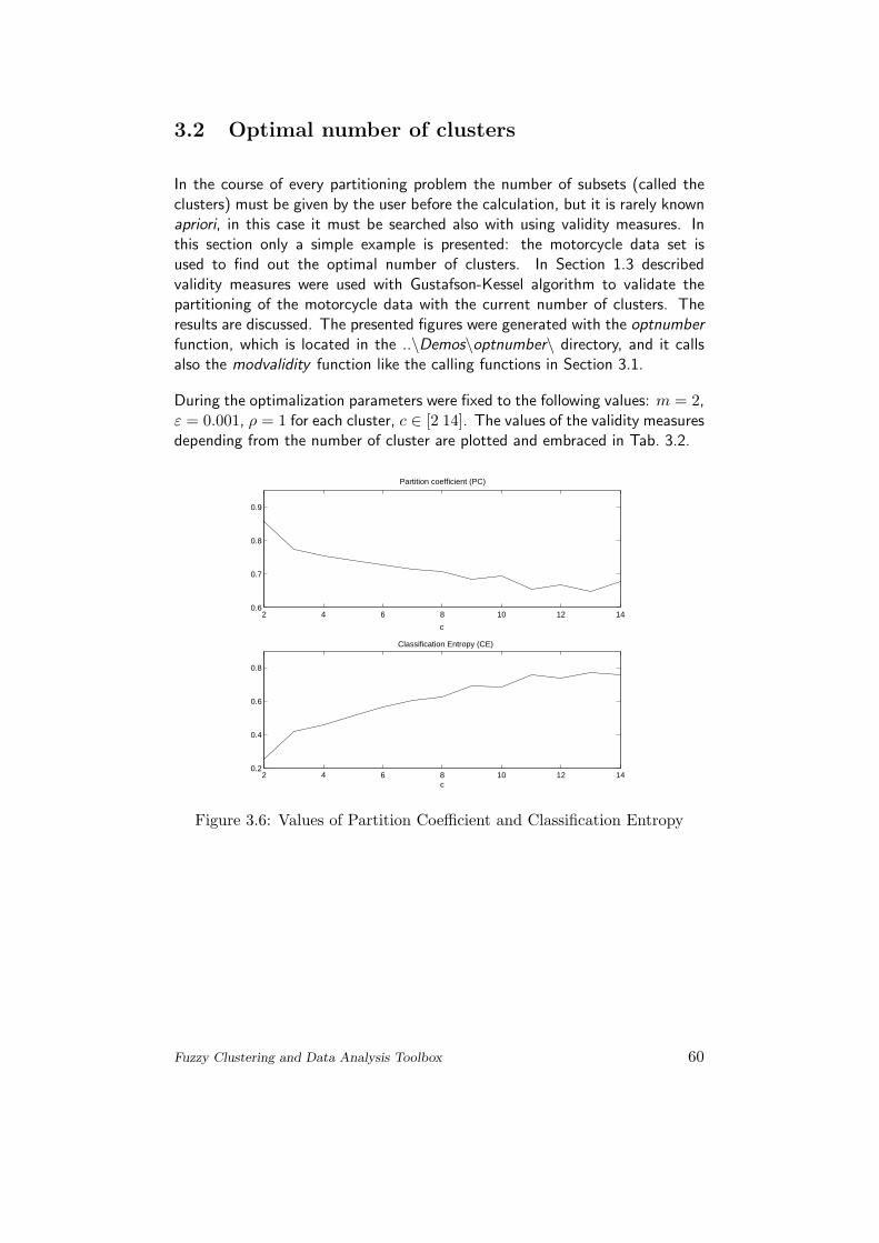
3.2 Optimal number of clusters

In the course of every partitioning problem the number of subsets (called theclusters) must be given by the user before the calculation, but it is rarely knownapriori, in this case it must be searched also with using validity measures. Inthis section only a simple example is presented: the motorcycle data set isused to find out the optimal number of clusters. In Section 1.3 describedvalidity measures were used with Gustafson-Kessel algorithm to validate thepartitioning of the motorcycle data with the current number of clusters. Theresults are discussed. The presented figures were generated with the optnumberfunction, which is located in the ..\Demos\optnumber\ directory, and it callsalso the modvalidity function like the calling functions in Section 3.1.

During the optimalization parameters were fixed to the following values: m = 2,ε = 0.001, ρ = 1 for each cluster, c ∈ [2 14]. The values of the validity measuresdepending from the number of cluster are plotted and embraced in Tab. 3.2.

2 4 6 8 10 12 140.6

0.7

0.8

0.9

c

Partition coefficient (PC)

2 4 6 8 10 12 140.2

0.4

0.6

0.8

c

Classification Entropy (CE)

Figure 3.6: Values of Partition Coefficient and Classification Entropy


2 4 6 8 10 12 140

0.5

1

1.5

2Partition index (SC)

2 4 6 8 10 12 140.005

0.01

0.015

0.02Separation index (S)

2 4 6 8 10 12 140

10

20

30Xie and Beni index (XB)

c

Figure 3.7: Values of Partition Index and Separation Index and Xie andBeni’s Index

We must mention again, that no validation index is reliable only by itself, thatis why all the programmed indexes are shown, and the optimum can be onlydetected with the comparison of all the results. We consider that partitions withless clusters are better, when the differences between the values of a validationindex are minor.The main drawback of PC is the monotonic decreasing with c and the lack ofdirect connection to the data. CE has the same problems: monotonic increasingwith c and hardly detectable connection to the data structure. On the score ofFig. 3.6, the number of clusters can be only rated to 3.In Fig. 3.7 there are more informative diagrams are shown: SC and S hardlydecreases at the c = 5 point. The XB index reaches this local minimum atc = 4. Considering that SC and S are more useful, when comparing differentclustering methods with the same c, we chose the optimal number of clustersto 4, which is confirmed by the Dunn’s index too in Fig. 3.8. (The AlternativeDunn Index is not tested enough to know how reliable its results are.)


2 4 6 8 10 12 140

0.02

0.04

0.06

0.08

0.1

0.12Dunn index (DI)

2 4 6 8 10 12 140

0.5

1

1.5

2

2.5x 10

−3 Alternative Dunn index (ADI)

Figure 3.8: Values of Dunn’s Index and the Alternative Dunn Index

Table 3.2: The numerical values of validity measuresc 2 3 4 5 6 7 8

PC 0.8569 0.7743 0.7550 0.7422 0.7291 0.7139 0.7075CE 0.2531 0.4168 0.4588 0.5110 0.5679 0.6055 0.6246SC 1.6465 1.4591 1.0646 0.6593 0.6055 0.5126 0.5181S 0.0124 0.0160 0.0133 0.0067 0.0057 0.0069 0.0064

XB 28.5271 4.8294 3.3545 4.4216 6.0929 5.1619 5.1688DI 0.1154 0.0317 0.0192 0.0230 0.0270 0.0183 0.0203

ADI 0.0023 0.0017 0.0008 0.0003 0.0005 0.0004 0.0000c 9 10 11 12 13 14

PC 0.6833 0.6957 0.6554 0.6682 0.6464 0.6771CE 0.6882 0.6820 0.7590 0.7404 0.7689 0.7572SC 0.5565 0.4868 0.5032 0.4354 0.4427 0.4079S 0.0072 0.0062 0.0065 0.0055 0.0057 0.0054

XB 5.2679 3.4507 2.3316 5.0879 2.8510 3.9492DI 0.0276 0.0196 0.0160 0.0144 0.0120 0.0132

ADI 0.0001 0.0003 0.0001 0.0001 0.0001 0.0000


3.3 Multidimensional data sets

In order to examine the performance of the proposed clustering methods threewell-known multidimensional classification benchmark problems are presentedin this section.

• Iris data

• Wine data

• Wisconsin Breast Cancer data

These data sets come from the UCI Repository of Machine Learning Databases,and they are downloadable from:ftp://ftp.ics.uci.edu/pub/machine-learning-databases/ , but they also exist inthe ..\Demos\projection\ directory. Cause of the too many data points thereis no use to show the partition matrixes in tables, so the results of the n-dimensional clustering was projected into 2-dimension, and the 2-D results wereplotted. Considering that projected figures are only approximations of the realpartitioning results, the difference between the original and the projected par-tition matrix is also represented, and on the other hand one can observe thedifference between the PCA, Sammon’s mapping and the Modified SammonMapping too, when these values are comprehended. These relation-indexes aredefined in (2.26).

Because of using real data sets the classes are known, so the misclassed objectscan be plotted. These items are signed with an ’o’ accessory-marker. Thegoodness of the classification is also can be defined by the percental error ofthese misclassed data points (a data point is misclassed when on the groundsof its largest membership degree it is not in the cluster which it belongs to):

Err =Nmisscl

N· 100. (3.1)

Note that calculating Err indicates only the goodness of the classification notthe clustering, hence we must take its results under protest. This error value isindependent from the visualization method, so they are stated below in Tab. 3.3.For the comparison five independent run were estimated with each algorithm.Fuzzy C-means, Gustafson-Kessel and Gath-Geva returned always with the sameminimum, while the results of K-means and K-medoid hardly depend from theinitialization as shown in Tab. 3.3, so in the case of these algorithms the mini-mum, mean and maximum were also represented.The difference between the minimal and maximal value shows the sensitivity ofthe algorithm to the initialization (as one can see K-medoid is the most sensitive


Kmeans Kmedoid FCM GK GG- min mean max min mean max - - -

Iris 10.667 10.933 11.333 9.333 25.199 34.667 10.667 10 20Wine 5.056 5.505 6.742 7.865 24.494 39.887 5.056 38.202 24.719Wisc 3.806 3.923 3.9531 2.635 3.982 4.8316 3.367 9.809 11.420

Table 3.3: Percental values of the misclassed objects with different clusteringmethods.

algorithm). The minimal value denotes the flexibility of the model, the meandenotes the estimation of the expected error. One can see that the best stableresults has the Fuzzy C-means clustering for these data sets, so its resultingfigures are shown in the following subsections, which are generated with thevisualcall function (situated in the same directory as the data sets).


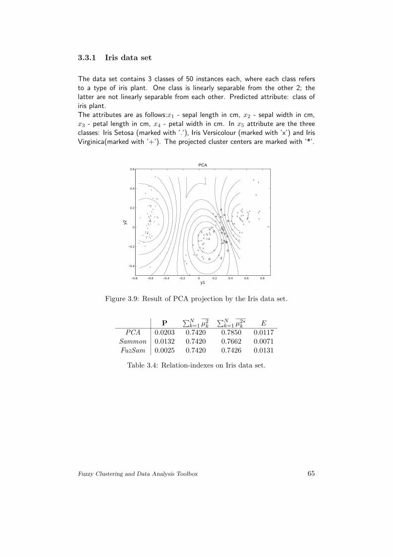
3.3.1 Iris data set

The data set contains 3 classes of 50 instances each, where each class refersto a type of iris plant. One class is linearly separable from the other 2; thelatter are not linearly separable from each other. Predicted attribute: class ofiris plant.The attributes are as follows:x1 - sepal length in cm, x2 - sepal width in cm,x3 - petal length in cm, x4 - petal width in cm. In x5 attribute are the threeclasses: Iris Setosa (marked with ’.’), Iris Versicolour (marked with ’x’) and IrisVirginica(marked with ’+’). The projected cluster centers are marked with ’*’.

−0.8 −0.6 −0.4 −0.2 0 0.2 0.4 0.6 0.8

−0.4

−0.2

0

0.2

0.4

0.6PCA

y2

y1

Figure 3.9: Result of PCA projection by the Iris data set.

P∑N

k=1 µ2k

∑Nk=1 µ2∗

k E

PCA 0.0203 0.7420 0.7850 0.0117Sammon 0.0132 0.7420 0.7662 0.0071FuzSam 0.0025 0.7420 0.7426 0.0131

Table 3.4: Relation-indexes on Iris data set.


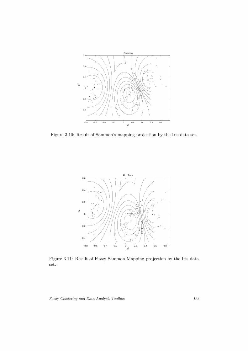
−0.8 −0.6 −0.4 −0.2 0 0.2 0.4 0.6 0.8 1

−0.4

−0.2

0

0.2

0.4

0.6

y1

y2

Sammon

Figure 3.10: Result of Sammon’s mapping projection by the Iris data set.

−0.8 −0.6 −0.4 −0.2 0 0.2 0.4 0.6 0.8

−0.4

−0.2

0

0.2

0.4

0.6FuzSam

y1

y2

Figure 3.11: Result of Fuzzy Sammon Mapping projection by the Iris dataset.


3.3.2 Wine data set

The Wine data contains the chemical analysis of 178 wines grown in the sameregion in Italy but derived from three different cultivars (marked with ’.’,’x’and ’+’). The problem is to distinguish the three different types based on 13continuous attributes derived from chemical analysis.

−0.8 −0.6 −0.4 −0.2 0 0.2 0.4 0.6 0.8−0.8

−0.6

−0.4

−0.2

0

0.2

0.4

0.6

PCA

y1

y2

Figure 3.12: Result of PCA projection by the Wine data set.

−1 −0.8 −0.6 −0.4 −0.2 0 0.2 0.4 0.6 0.8 1

−1

−0.8

−0.6

−0.4

−0.2

0

0.2

0.4

0.6

0.8

1

y1

y2

Sammon

Figure 3.13: Result of Sammon’s mapping projection by the Wine data set.


−1 −0.8 −0.6 −0.4 −0.2 0 0.2 0.4 0.6 0.8 1−1

−0.8

−0.6

−0.4

−0.2

0

0.2

0.4

0.6

0.8

1

FuzSam

y2

y1

Figure 3.14: Result of Fuzzy Sammon Mapping projection by the Wine dataset.

P∑N

k=1 µ2k

∑Nk=1 µ2∗

k E


Table 3.5: Relation-indexes on Wine data set.


3.3.3 Breast Cancer data set

The Wisconsin breast cancer data is widely used to test the effectiveness ofclassification and rule extraction algorithms. The aim of the classification is todistinguish between benign and malignant cancers based on the available ninemeasurements: x1 clump thickness, x2 uniformity of cell size, x3 uniformity ofcell shape, x4 marginal adhesion, x5 single epithelial cell size, x6 bare nuclei, x7

bland chromatin, x8 normal nuclei, and x9 mitosis. The attributes have integervalue in the range [1,10]. The original database contains 699 instances however16 of these are omitted because these are incomplete, which is common withother studies. The class distribution is 65.5% benign and 34.5% malignant,respectively.

−0.5 0 0.5 1 1.5 2

−1

−0.8

−0.6

−0.4

−0.2

0

0.2

0.4

0.6

PCA

y1

y2

Figure 3.15: Result of PCA projection by the Wisconsin Breast Cancer dataset.

P∑N

k=1 µ2k

∑Nk=1 µ2∗

k E


Table 3.6: Relation-indexes on Wisconsin Breast cancer data set.


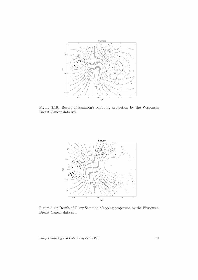
−1.5

−1

−0.5

0

0.5

1

−2−1.5−1−0.500.51

y2

y1

Sammon

Figure 3.16: Result of Sammon’s Mapping projection by the WisconsinBreast Cancer data set.

−0.5 0 0.5 1 1.5 2

−1

−0.5

0

0.5

1

FuzSam

y1

y2

Figure 3.17: Result of Fuzzy Sammon Mapping projection by the WisconsinBreast Cancer data set.


3.3.4 Conclusions

As Tab. 3.4, Tab. 3.5 and Tab. 3.6 show, Fuzzy Sammon Mapping has muchbetter projection results by the value of P than Principal component Analy-sis, and it is computationally cheaper than the original Sammon Mapping. Soduring the evaluation of the partition the figures created with this projectionmethod were considered. We calculated the original Sammon’s stress for all thethree techniques to be able to compare them.Tab. 3.3 shows that the ”advanced” algorithms does not have always the best

−0.6 −0.4 −0.2 0 0.2 0.4 0.6 0.8

−0.6

−0.4

−0.2

0

0.2

0.4

0.6

0.8

y2

y1

GK algorithm − FuzSam

Figure 3.18: Result of Fuzzy Sammon projection by the wine data set withGustafson-Kessel algorithm.

results. It depends on the underlying structure of the data. The Gustafson-Kessel and the Gath-Geva algorithm cannot detect correctly the wine species,as it is shown in Fig. 3.18. On the contrary the Fuzzy C-means provides de-pendable results for all data sets. By far the best results are in the case of theWisconsin Breast Cancer data, where from 683, 9-dimensional points ”only” 23are misclustered, and the 96.6 % secure result is very reliable, considering thatthe clustering techniques do not use prior class identifiers, the are among theunsupervised methods.


Summary

To meet the growing demands of systematizing the nascent data, a flexible, pow-erful tool is needed. The Fuzzy Clustering and Data Analysis Toolbox providesseveral approaches to cluster, classify and evaluate wether industrial or exper-imental data sets. The software for these operations has been developed withMatlab, which is very powerful for matrix-based calculations. The Toolboxprovides five different types of clustering algorithms, which can be validated byseven validity measures. High-dimensional data sets can be also visualized witha 2-dimension projection, hence the toolbox contains three different method forvisualization.With all these useful tools the work is not finished yet: many more clusteringalgorithms, validation indices, visualization methods exist or will come up thenext day. They could take place in this work too, hence the author knows ”it isnot the end. . . it is the beginning. . . ”

72

Bibliography

[1] J. C. Bezdek. Pattern Recognition with Fuzzy Objective Function Algo-rithms. Plenum Press, 1981.

[2] F. Hoppner, F. Klawonn, R. Kruse, and T. Runkler. Fuzzy Cluster Analysis.Wiley, Chichester, 1999.

[3] R. Babuska. Fuzzy Modeling for Control. Kluwer Academic Publishers,Boston, 1998.

[4] D.E. Gustafson and W.C. Kessel. Fuzzy clustering with fuzzy covariancematrix. In Proceedings of the IEEE CDC, San Diego, pages 761–766. 1979.

[5] R. Babuska, P. J. van der Veen, and U. Kaymak. Improved covarianceestimation for Gustafson-Kessel clustering. IEEE International Conferenceon Fuzzy Systems, pages 1081–1085, 2002.

[6] J.C. Bezdek and J.C. Dunn. Optimal fuzzy partitions: A heuristic forestimating the parameters in a mixture of normal dustrubutions. IEEETransactions on Computers, pages 835–838, 1975.

[7] I. Gath and A.B. Geva. Unsupervised optimal fuzzy clustering. IEEE Trans-actions on Pattern Analysis and Machine Intelligence, 7:773–781, 1989.

[8] A.M. Bensaid, L.O. Hall, J.C. Bezdek, L.P. Clarke, M.L. Silbiger, J.A.Arrington, and R.F. Murtagh. Validity-guided (Re)Clustering with applica-tions to imige segmentation. IEEE Transactions on Fuzzy Systems, 4:112–123, 1996.

[9] X. L. Xie and G. A. Beni. Validity measure for fuzzy clustering. IEEETrans. PAMI, 3(8):841–846, 1991.

[10] Sammon JW Jr. A nonlinear mapping for data structure analysis. IEEETransactions on Computers, 18:401–409, 1969.

[11] M. Aladjem I. Dinstein B. Lerner, H. Guterman and Y. Romem. On patternclassification with sammon’s nonlinear mapping - an experimental study.Pattern Recognition Letters, 31(4):371–381, 1998.

73

[12] Juha Vesanto. Neural network tool for data mining: Som toolbox. In Pro-ceedings of Symposium on Tool Environments and Development Methodsfor Intelligent Systems (TOOLMET2000), pages 184–196. 2000.

[13] M. E. Tipping and C. M. Bishop. Mixtures of probabilistic principal com-ponents analysis. Neural Computation, 11:443–482, 1999.

[14] Kovacs A.-Abonyi J. Vizualization of fuzzy clustering results by modifiedsammon mapping. In Proceedings of the 3rd International Symposiumof Hungarian Researchers on Computational Intelligence, pages 177–188.2002.


fuzzy clustering and data analysis toolbox

Documents